Citation: Tran, H.P.; Jung, W.-S.; Yoo,

D.-S.; Oh, H. Design and

Implementation of a Multi-Hop

Real-Time LoRa Protocol for

Dynamic LoRa Networks. Sensors

2022, 22, 3518. https://doi.org/

10.3390/s22093518

Academic Editor: Carles Gomez

Received: 14 March 2022

Accepted: 3 May 2022

Published: 5 May 2022

Publisher’s Note: MDPI stays neutral

with regard to jurisdictional claims in

published maps and institutional affil-

iations.

Copyright: © 2022 by the authors.

Licensee MDPI, Basel, Switzerland.

This article is an open access article

distributed under the terms and

conditions of the Creative Commons

Attribution (CC BY) license (https://

creativecommons.org/licenses/by/

4.0/).

sensors

Article

Design and Implementation of a Multi-Hop Real-Time LoRaProtocol for Dynamic LoRa NetworksHuu Phi Tran 1 , Woo-Sung Jung 2 , Dae-Seung Yoo 2 and Hoon Oh 1,*

1 Department of Electrical, Electronic and Computer Engineering, University of Ulsan, Ulsan 680-749, Korea;huuphi.tran88@gmail.com

2 Electronics and Telecommunications Research Institute, Daejeon 305-350, Korea; woosung@etri.re.kr (W.-S.J.);ooseyds@etri.re.kr (D.-S.Y.)

* Correspondence: hoonoh@ulsan.ac.kr

Abstract: Recently, LoRa (Long Range) technology has been drawing attention in various applicationsdue to its long communication range and high link reliability. However, in industrial environments,these advantages are often compromised by factors such as node mobility, signal attenuation due tovarious obstacles, and link instability due to external signal interference. In this paper, we propose anew multi-hop LoRa protocol that can provide high reliability for data transmission by overcomingthose factors in dynamic LoRa networks. This study extends the previously proposed two-hop real-time LoRa (Two-Hop RT-LoRa) protocol to address technical aspects of dynamic multi-hop networks,such as automatic configuration of multi-hop LoRa networks, dynamic topology management,and updating of real-time slot schedules. It is shown by simulation that the proposed protocolachieves high reliability of over 97% for mobile nodes and generates low control overhead in topologymanagement and schedule updates. The protocol was also evaluated in various campus deploymentscenarios. According to experiments, it could achieve high packet delivery rates of over 97% and95%, respectively, for 1-hop nodes and 2-hop nodes against node mobility.

Keywords: multi-hop LoRa protocol; dynamic network; mobility; real-time scheduling; reliabletransmission

1. Introduction

Recently, interest in LoRa networks has been increasing due to the absence of anindustrial IoT network capable of reliable data transmission at a low price. In keepingwith this need, remarkable research progress has been made on industrial multi-hop LoRanetworks by enabling reliable real-time data transmission and supporting a wide area withmany nodes with the use of a slot scheduling-based data transmission method [1]. However,in industrial applications supporting worker safety, real-time machine management, etc.,LoRa terminals (nodes) can be attached to mobile equipment or carried by workers. Thisrequires a data transmission protocol for dynamic multi-hop LoRa networks. However,designing a reliable and real-time data transmission protocol in a dynamic multi-hop LoRanetwork is a challenge because it involves topology maintenance in a slot scheduling-basedapproach. This problem gets worse in LoRa networks with a low data rate and a highprobability of message collisions.

So far, many studies designed to deal with reliable data transmission in dynamicwireless networks have been conducted under three areas of communication technology:cellular networks, wireless sensor networks (WSNs), and low-power wide-area networks(LPWANs). The cellular network has the advantage of reliably collecting data while cover-ing a wide area and can easily support node mobility because it uses a simple star topologyand operates at high bandwidth. However, when a node enters a wireless communicationshadow area, it suffers from reduced reliability of data transmission and high energy con-

Sensors 2022, 22, 3518. https://doi.org/10.3390/s22093518 https://www.mdpi.com/journal/sensors

Sensors 2022, 22, 3518 2 of 21

sumption. Moreover, cellular networks are seldom used for monitoring applications exceptfor special cases because every node has to pay an expensive communication fee.

Meanwhile, there have been many studies on industrial WSNs based on the IEEE802.15.4 standard [2] for low-cost data collection over the past decade. In WSNs, nodesthat are typically considered stationary send data to a sink via multiple radio hops. Sev-eral protocols using a slot scheduling have been proposed to transmit data reliably inWSNs [3–6]. However, in industrial sites, even though nodes send data according to a slotschedule, the reliability of data transmission may not be secured due to various communi-cation obstacles and external interferences. Furthermore, node mobility not only increasescontrol overhead but also causes data loss temporarily due to link failure and frequentupdates of a slot schedule, making it more difficult to secure data transmission reliability.Recently, the slotted sense multiple access (SSMA) protocol [7] using a tree topology andsharable slots addressed the issue of data transmission reliability under various signalinterferences in industrial environments and node mobility. In this method, instead ofallocating a tiny slot to each link, a shareable slot is allocated to each tree level of the treetopology, and nodes at each tree level send data to nodes one tree level below them throughcontention using CSMA/CA within a sharable slot allocated to their tree level. In this way,data transmission is progressively performed level by level from the highest tree level to thelowest tree level to which a sink node belongs. This method eliminates scheduling overheadby making slot scheduling topology-independent and greatly improves the reliability ofdata transmission by limiting channel contention to nodes in the same tree level. However,since this approach still allows channel contention, it is not free from data collision. Tofurther improve the reliability, the authors in [8] proposed a smart multi-channel SSMA(SMC-SSMA) protocol. In this approach, in the process of acquiring a common channel forsecure data transmission, each node includes “delay time before sending its own controlmessage” in the control message it transmits. Then, every node learns the delay times of itsneighboring nodes and hidden nodes by overhearing the control messages and then sets itsown delay time before sending a control message so that its control messages can nevercollide with those transmitted by its neighboring and hidden nodes. After acquiring thecommon channel, a node transmits data using a data channel not used by its neighbors,enabling parallel transmission.

Despite remarkable progress in these dynamic WSNs, WSNs in industrial fields stillhave difficulties in securing data transmission reliability due to obstacles and/or externalinterference and have limitations in covering a wide area or supporting densely deployednodes. Some studies [9–14] on the use of LoRa technology [15] to overcome those difficultiesand limitations have been conducted. It is said in the LoRa specification [16] that a LoRatransceiver can cover up to 2 km even with the smallest spreading factor; however, itstransmission range can be reduced to within hundreds or tens of meters due to signalattenuation by obstructions and the installations of nodes inside wireless unfriendly zones(WUZs) such as underground tunnels and enclosed spaces. Furthermore, in industrialmonitoring and control applications, a server may collect data from each node every tensof seconds or even every few seconds. Therefore, a LoRa protocol must address how toachieve high reliability of data transmission against signal attenuation and heavy traffic.

Some LoRa protocols have been proposed to tackle the problem of reliability and/ornetwork coverage. In [13], the authors proposed the real-time LoRa (RT-LoRa) protocolthat enables real-time and reliable data transmission by using a distributed slot schedulingmethod. Another slot scheduling-based protocol, TS-LoRa [14], allows nodes to determinea slot in a frame autonomously in order to reduce slot scheduling overhead. However, theseprotocols suffer from the limitation of network coverage in industrial fields. To resolvecoverage limitation, some studies focused on multi-hop LoRa networks [17–22]. In [17], theprotocol extends network coverage by having the end node transmit data using a routeestablished by a simplified Destination-Sequenced Distance Vector (DSDV) protocol [23].This protocol suffers from high energy consumption by routing data via multiple radiohops, and also from data collision due to the nature of contention-based data transmission

Sensors 2022, 22, 3518 3 of 21

in high traffic. The authors in [18] proposed CT-LoRa, a multi-hop LoRa protocol based onthe Glossy protocol [24], that takes advantage of concurrent transmission (CT) to improvenetwork reliability. This approach relies on flooding for data transmission while removingthe overhead of constructing and maintaining a multi-hop topology. However, the floodingis not free from the viewpoint of network overhead and energy consumption. The studiesof the same category include the LoRa-Mesh protocol [19] in which a GW constructs andmaintains a tree path to every node in the network by selecting a path that has the smallesthop count and provides a good link quality. In order to get data from a specified node,GW sends a query message to the node along the tree path. This approach improves thereliability of data transmission significantly; it incurs a high control overhead. According toexperiment results, the above-mentioned multi-hop LoRa protocols effectively extend thenetwork coverage as well as provide high reliability on data transmissions. However, theseprotocols may not be suitable for monitoring applications because they have difficulty indealing with high traffic networks.

Recently, the authors in [1] proposed the Two-Hop RT-LoRa protocol to extend networkcoverage in which nodes send data periodically, while some nodes make use of relay nodesto send data to GW. The protocol uses a real-time slot schedule for a two-hop tree topologyto remove data collision while it satisfies the time constraint of every data transmission.According to the experimental results, the two-hop protocol using the lowest spreadingfactor SF7 showed a high packet delivery rate of more than 95% in the rough networkdeployment scenario where the one-hop protocol using the relatively high spreading factorSF10 mostly fails to transmit data. In addition, according to the analysis results, the two-hop protocol could improve energy consumption by almost 60% compared to the one-hopprotocol. However, the protocol did not deal with the change of topology. In wirelessnetworks with a relatively high bandwidth such as WiFi and IEEE 802.15.4, the change oftopology may be easily handled by exchanging control messages. However, in a dynamicLoRa network, a method is required to quickly detect link failures and update slot schedulesefficiently in response to topology changes while using a small number of control messagesto reduce message collisions. To the best of our knowledge, no one has ever conductedresearch on a multi-hop LoRa protocol that can deal with node mobility.

This paper presents a reliable and real-time data transmission protocol for dynamicmulti-hop LoRa networks. This study basically extends the slot scheduling-based Two-HopRT-LoRa protocol proposed in the previous study [1], further covering the technical aspectsof the implementation and operation of a dynamic multi-hop LoRa network such as auto-configuration of a multi-hop LoRa network, slot scheduling, topology maintenance, andupdating of a slot schedule. First, in autonomously configuring a two-hop network, it isimportant to ensure that the tree topology can be gradually and stably built in the processof individual node registration. Therefore, a GW includes the list of registered nodes inthe tree construction message before broadcasting so that a node can confirm whether it isregistered or not. Considering that the one-hop relay nodes play an important role in thestability of tree topology, a node decides whether it can become a relay by itself based onits link quality. As a server generates and broadcasts slot scheduling information based onthe tree topology, each node can easily and autonomously create a slot schedule that doesnot conflict with the slot schedules of other nodes. In this process, the server provides theretransmission slot schedule for relay nodes so that all relay nodes can safely rebroadcast theslot scheduling information to their children without collision. During data transmission,when a node detects link failure, it immediately reports the change of link state to theGW using an unscheduled slot to prevent collision with other data transmissions. Uponreceiving this, the GW completes topology maintenance by transmitting only updated slotscheduling information using the DL message.

The rest of this paper is organized as follows. Section 2 describes the research back-ground. Section 3 gives a detailed design of the proposed protocol and is followed by thediscussion of simulation and experimental results in Section 4. Finally, the conclusion isdrawn in Section 5.

Sensors 2022, 22, 3518 4 of 21

2. Background2.1. Network Model

A considered LoRa network consists of one server, multiple gateways (GWs) and anumber of end devices or nodes. A server and GWs are interconnected by a wired high-speedbackhaul network. End nodes are mobile and battery-powered. A server (or a GW) collectssensor data from end nodes via GWs periodically and provides services based on theanalysis of the collected data. Nodes may be installed in a WUZ, such as an undergroundtunnel and an enclosed space. Some nodes may not have a direct connection to the GW dueto signal attenuation. Every node can act as a relay that forwards data to a GW. Nodes canform a two-hop tree originating from a GW in which an internal node acts as a relay node,and a leaf node can be either a 1-hop node that connects to GW directly or a 2-hop node thatconnects to a relay node. A node that does not belong to a tree is said to be an orphan node.For time synchronization and/or command transmission, a GW broadcasts a downlinkmessage periodically to all end nodes. Thus, all relay nodes are to rebroadcast the receiveddownlink message towards 2-hop nodes.

Figure 1 shows a simple LoRa network with two GWs and six end nodes. Two nodes,B and E, are deployed in WUZ-1 and WUZ-2, respectively. Nodes A, B, C form Tree-1originated from GW1, and nodes D, E, F form Tree-2 originated from GW2 where nodes Aand D are relay nodes. The figure also illustrates the movement of node B connecting toGW2 after disconnecting from node A.

Sensors 2022, 22, x FOR PEER REVIEW 4 of 21

discussion of simulation and experimental results in Section 4. Finally, the conclusion is

drawn in Section 5.

2. Background

2.1. Network Model

A considered LoRa network consists of one server, multiple gateways (GWs) and a

number of end devices or nodes. A server and GWs are interconnected by a wired high-

speed backhaul network. End nodes are mobile and battery-powered. A server (or a GW)

collects sensor data from end nodes via GWs periodically and provides services based on

the analysis of the collected data. Nodes may be installed in a WUZ, such as an under-

ground tunnel and an enclosed space. Some nodes may not have a direct connection to

the GW due to signal attenuation. Every node can act as a relay that forwards data to a

GW. Nodes can form a two-hop tree originating from a GW in which an internal node acts

as a relay node, and a leaf node can be either a 1-hop node that connects to GW directly or a

2-hop node that connects to a relay node. A node that does not belong to a tree is said to be

an orphan node. For time synchronization and/or command transmission, a GW broadcasts

a downlink message periodically to all end nodes. Thus, all relay nodes are to rebroadcast

the received downlink message towards 2-hop nodes.

Figure 1 shows a simple LoRa network with two GWs and six end nodes. Two nodes,

B and E, are deployed in WUZ-1 and WUZ-2, respectively. Nodes A, B, C form Tree-1

originated from GW1, and nodes D, E, F form Tree-2 originated from GW2 where nodes

A and D are relay nodes. The figure also illustrates the movement of node B connecting to

GW2 after disconnecting from node A.

Figure 1. A LoRa network model with two-hop tree topology.

2.2. Problem Identification

Recently, the authors in [1] proposed a Two-Hop Real-Time LoRa protocol that uses

a two-hop tree topology for extension of network coverage and a two-hop slot scheduling

for reliable data transmission. Based on the slot scheduling information transmitted by a

GW, every node generates its own slot schedule in a distributed manner such that it sat-

isfies its own transmission period if it transmits data according to the slot schedule, and

does not cause any collision in data transmission with other nodes. However, this ap-

proach does not respond to the change of topology.

There are some issues to consider in designing a real-time protocol for dynamic two-

hop LoRa networks. First, the protocol should be able to detect the uplink or downlink

failure of a node quickly. A node, either a GW or a relay node, can detect its downlink

failure by counting the amount of missing data from its child. Furthermore, a 1-hop (relay)

node can detect its uplink failure easily by counting the number of missing downlink mes-

sages from a GW. However, it is not possible for a 2-hop node to use a downlink message

to detect uplink failure. The reason is that all relay nodes rebroadcast an identical down-

link message. Therefore, this requires a different method to using downlink messages.

Figure 1. A LoRa network model with two-hop tree topology.

2.2. Problem Identification

Recently, the authors in [1] proposed a Two-Hop Real-Time LoRa protocol that uses atwo-hop tree topology for extension of network coverage and a two-hop slot scheduling forreliable data transmission. Based on the slot scheduling information transmitted by a GW,every node generates its own slot schedule in a distributed manner such that it satisfies itsown transmission period if it transmits data according to the slot schedule, and does notcause any collision in data transmission with other nodes. However, this approach doesnot respond to the change of topology.

There are some issues to consider in designing a real-time protocol for dynamic two-hop LoRa networks. First, the protocol should be able to detect the uplink or downlinkfailure of a node quickly. A node, either a GW or a relay node, can detect its downlink failureby counting the amount of missing data from its child. Furthermore, a 1-hop (relay) nodecan detect its uplink failure easily by counting the number of missing downlink messagesfrom a GW. However, it is not possible for a 2-hop node to use a downlink message to detectuplink failure. The reason is that all relay nodes rebroadcast an identical downlink message.Therefore, this requires a different method using downlink messages. One way is that a2-hop node can detect its uplink failure by using the downlink failure information of itsparent. For example, consider a simple two-hop network topology in Figure 2a that consists

Sensors 2022, 22, 3518 5 of 21

of relay node a and 2-hop nodes b and c. Let a downlink state of node x with k children,x1, x2, . . . , and xk, be represented as (x(x1, x2, . . . , xk)). Suppose that node a detected thefailure of its downlink (a, b) and reported its changed downlink state (a(c)) to GW. If the GWbroadcasts (a(c)), node b will know of the failure of uplink (b, a) if it has already connected toGW.

1

Figure 2. Link failure and inconsistency of slot schedule due to node mobility. (a) The change oftopology by node movement; (b) Slot schedule before node b moves away; (c) Slot schedule afternode b moves away.

Second, the protocol should be able to update a slot schedule quickly for the changeof topology. If GW detects the downlink failure of a 1-hop relay or leaf node, the GWsimply releases the slots allocated to that node and its children, and then broadcasts adownlink message to request the relevant nodes to switch to orphan nodes. Then, eachorphan node needs to individually rejoin the tree and be allocated slots. However, when arelay node detects a downlink failure for a child, the slot rescheduling becomes a bit morecomplicated. In this case, the relay node will first report its changed downlink state to GWso that the GW can generate a new slot schedule for the relay node. The child can knowits uplink failure if it receives the changed link state of its parent from GW. For example,referring to Figure 2, suppose that GW has a slot schedule (SS) for the downlink state(a(b, c)) of node a, as SS(a) = (a = (1), b = (2, 3), c = (4, 5)) as shown in Figure 2b. Note thatevery 2-hop node need two slots, one for its own transmission and another for its parent toforward the received data. If node a detects its downlink failure due to the movement ofnode b and reports a changed downlink state (a(c)) to GW, the new slot schedule becomesSS(a) = (a = (1), c = (2, 3)) as in Figure 2c.

Third, the protocol has to handle a slot schedule conflict problem that occurs whenmultiple nodes use the same slot temporarily. Suppose that node a has a new slot scheduleshown in Figure 2c after it detects the failure of its downlink (a, b). The problem is thatnode b may still use its previous slot number 2 until it finds a new parent.

Fourth, as GWs and relay nodes form the mobile backbone of the LoRa network, itis of great importance to build and maintain the network topology in such a way thatthe relay nodes have stable uplink. If a one-hop relay node loses an uplink, a significantamount of overhead may occur in the process of topology change and slot rescheduling.

Finally, one important question is whether it is or is not appropriate to have three ormore radio hops in a low data rate LoRa network, even at the cost of the increased controloverhead and the increased likelihood of collisions due to increased traffic. For example, if k-hop is allowed in multi-hop LoRa networks, the data generated at the (k + 1)th tree level mustbe transmitted k times before reaching a GW. This may increase interference severely due tothe long transmission distance of LoRa. However, even though k is limited to 2, the use of

Sensors 2022, 22, 3518 6 of 21

two GWs can extend the coverage of a LoRa network up to eight hops such that two GWscover three nodes arranged linearly between them, and each GW additionally covers twonodes arranged linearly on opposite sides as (x1 − x2 − G1 − x3 − x4 − x5 − G2 − x6 − x7)where G1 and G2 are gateways and xi, i = 1 . . . 7, indicates an end node.

In conclusion, this paper aims at designing a multi-hop LoRa protocol in considerationof the issues discussed so far.

2.3. Notations and Messages

A node can be modelled as a task, an active entity that receives command and transmitsdata. In this paper, we assume that each node has only one task. Thus, task and node areused interchangeably. A task belongs to a specific task class based on its data transmissioninterval (TI) such that for a frame with 2N uplink slots, where N is defined as a frame factor(N ≥ 0), a task belongs to class c (0 ≤ c ≤ N) if it transmits one data per TI = 2N/2c. Thisimplies that a task of class c has a slot demand (SD) of 2c slots and transmits 2c packetsduring one frame period. Task x can be expressed by its profile PF(x) as follows:

PF(x) = (x, class(x)) (1)

where x and class(x) indicate node address and the class of node x, respectively.Some notations used in this paper are summarized as follows:

Notation MeaningRNL indicates a registered node list in which every node has registered

with a server.

P(x) indicates the parent of node x.

TCRInt indicates the interval that GW uses to broadcast a tree constructionrequest (TCR) message during initialization period.

MaxChildren indicates the maximum number of children that a 1-hop relay nodecan have.

uPF(x indicates the updated profile that node x generates if it detects linkbreakage to any of its children.

uSSI(x) indicates an updated slot scheduling information that a servergenerates for node x that has reported uPF(x)

Some messages used in this paper are summarized as follows:

Message DescriptionTCR = (level, RNL) is a tree construction request (TCR) message that a server broadcasts

at the intervals of TCRInt during initialization period and levelindicates the tree level of the node that broadcasts this message.

RR(x) = (x,P(x),PF(x)) is the registration request (RR) message that node x sends to itsparent P(x) to register with a server.

2.4. Overview of Slot Scheduling for Two-Hop LoRa Networks

The Two-hop RT-LoRa protocol uses a frame as a data collection cycle that is dividedinto a downlink (DL) period and an uplink (UL) period that GW uses to broadcast a DLmessage and end nodes use to send data, respectively. The DL period is further dividedinto two DL slots: DL#1 for GW to broadcast a DL message and DL#2 for 1-hop relay nodesto rebroadcast the DL message, and the UL period is sliced into 2N data slots.

Given a set of tasks, the protocol performs slot scheduling by relying on the logical slotindexing (LSI) algorithm [13], that assigns a logical slot index to each of 2N data slots suchthat if a task of class c selects 2c logical slots sequentially starting with any logical slot indexand transmits data in each logical slot, it can meet the transmission period of 2N/2c. Thelogical slot indices for 16 data slots are given in Figure 3a.

Sensors 2022, 22, 3518 7 of 21Sensors 2022, 22, x FOR PEER REVIEW 7 of 21

Figure 3. Two-hop tree slot scheduling using logical slot indices. (a) Logical slot indexing with 16

slots; (b) Slot scheduling for Tree-1 in Figure 1.

For slot scheduling, every node is required to report its profile to a server. A 1-hop

relay collects the profiles of its children and merges them with its own task profile before

reporting. Suppose that a network has a list of k 1-hop nodes as (n1, n2, …, ni, …, nk). Then,

the integrated profile PF(ni) is expressed as follows:

1 2( ) ( , ( ) , ( ) , ( ) , . . . , ( ) , . . . , ( ) )ii i i i i i j icP F n n c la s s n P F n P F n P F n P F n (2)

where PF(nij) indicates the profile of the jth child of node ni, and ci is the number of ni’s

children. Let SD(x) and TSD(x) denote the slot demand of node x and the total slot demand

of x and x’s children, respectively. Then, TSD(ni) is expressed as follows:

1( ) ( ) ( )ic

i i ijjTSD n SD n SD n

(3)

where ( )( ) 2 iclass niSD n and ( )

( ) 2*2 ijclass n

ijSD n since 2-hop node needs twice as

many slots as it demands. Then, every 1-hop node ni reports PF(ni) to a server so that the

server can manage the task profile (PF) for all nodes in the network as follows:

1 2( ( ), ( ),..., ( ))kPF PF n PF n PF n (4)

If tasks are scheduled in the order of the elements in PF, the start logical slot index of

node ni, startLSI(ni), in slot schedule is calculated as follows:

1

1( ) ( ) 1

i

i jjstartLSI n TSD n

(5)

A sever calculates total slot demands for all 1-hop nodes according to (3), and distrib-

utes the network slot scheduling information (NSSI) using a DL message:

1 1 2 2( ( , ( ) ) , ( , ( ) ) , . . . , ( , ( ) ) )k kN S S I n T SD n n T S D n n T S D n (6)

Upon receiving NSSI, every 1-hop node x gets its startLSI(x) according to (5) and gen-

erates a local slot schedule, LSS(x), using Algorithm 1 with startLSI(x) and TSD(x). The

LSS(x) consists of its receiving slots, RxSlots(x), used to receive data from its children and

its transmitting slots, TxSlots(x), used to transmit its own data and relay data received from

its children.

Algorithm 1. Slot scheduling of 1-hop relay node

1: At node x that receives NSSI:

2: calculates startLSI(x) using (5);

3: Alloc(x) = a list of SD(x) sequential logical slot numbers starting with startLSI(x)

according to the LSI algorithm;

//The ascending sorted list of physical slot numbers corresponding to Alloc(x)

4: TxSlots(x) = ascSort {psi(y)| y ∈ Alloc(x)};

5: startLSI = startLSI(x) + SD(x);

Figure 3. Two-hop tree slot scheduling using logical slot indices. (a) Logical slot indexing with16 slots; (b) Slot scheduling for Tree-1 in Figure 1.

For slot scheduling, every node is required to report its profile to a server. A 1-hoprelay collects the profiles of its children and merges them with its own task profile beforereporting. Suppose that a network has a list of k 1-hop nodes as (n1, n2, . . . , ni, . . . , nk).Then, the integrated profile PF(ni) is expressed as follows:

PF(ni) = (ni, class(ni), PF(ni1), PF(ni2), . . . , PF(nij), . . . , PF(nici )) (2)

where PF(nij) indicates the profile of the jth child of node ni, and ci is the number of ni’schildren. Let SD(x) and TSD(x) denote the slot demand of node x and the total slot demandof x and x’s children, respectively. Then, TSD(ni) is expressed as follows:

TSD(ni) = SD(ni) + ∑cij=1 SD(nij) (3)

where SD(ni) = 2class(ni) and SD(nij) = 2 ∗ 2class(nij) since 2-hop node needs twice as manyslots as it demands. Then, every 1-hop node ni reports PF(ni) to a server so that the servercan manage the task profile (PF) for all nodes in the network as follows:

PF = (PF(n1), PF(n2), . . . , PF(nk)) (4)

If tasks are scheduled in the order of the elements in PF, the start logical slot index ofnode ni, startLSI(ni), in slot schedule is calculated as follows:

startLSI(ni) = ∑i−1j=1 TSD(nj) + 1 (5)

A sever calculates total slot demands for all 1-hop nodes according to (3), and distributesthe network slot scheduling information (NSSI) using a DL message:

NSSI = ((n1, TSD(n1)), (n2, TSD(n2)), . . . , (nk, TSD(nk))) (6)

Upon receiving NSSI, every 1-hop node x gets its startLSI(x) according to (5) andgenerates a local slot schedule, LSS(x), using Algorithm 1 with startLSI(x) and TSD(x). TheLSS(x) consists of its receiving slots, RxSlots(x), used to receive data from its children andits transmitting slots, TxSlots(x), used to transmit its own data and relay data received fromits children.

Sensors 2022, 22, 3518 8 of 21

Algorithm 1. Slot scheduling of 1-hop relay node

1: At node x that receives NSSI:2: calculates startLSI(x) using (5);3: Alloc(x) = a list of SD(x) sequential logical slot numbers starting with startLSI(x) accordingto the LSI algorithm;

//The ascending sorted list of physical slot numbers corresponding to Alloc(x)4: TxSlots(x) = ascSort {psi(y)| y ∈ Alloc(x)};5: startLSI = startLSI(x) + SD(x);6: RxSlots(x) = { };7: for each y ∈ CS(x)8: Alloc(y) = a list of SD(y) sequential logical slot numbers starting with startLSI;9: psiAlloc(y) = ascSort {psi(v)| v ∈ Alloc(y)}10: RxSlots(x) = RxSlots(x) ∪ {v| v ∈ psiAlloc(y), v is in odd position};11: TxSlots(x) = TxSlots(x) ∪ {v| v ∈ psiAlloc(y), v is in even position};12: startLSI = startLSI + SD(y);13: endFor

Furthermore, 1-hop relay node x generates its local slot scheduling information, LSSI(x),that is required for its children to perform slot scheduling:

LSSI(x) = (startLSI, PF(x1), PF(x2), . . . , PF(xkx )) (7)

where startLSI = startLSI(x) + SD(x), and kx indicates the number of node x’s children. Then,node x broadcasts LSSI(x), and its child generates a slot schedule that includes TxSlotsusing Algorithm 2.

Algorithm 2. Slot scheduling of 2-hop node

1: At node xi that receives LSSI(x):2: startLSI = startLSI + ∑i−1

j=1 SD(xj);3: get Alloc(xi) starting with startLSI;4: psiAlloc(xi) = ascSort {psi(v)| v ∈ Alloc(xi)};5: TxSlots(xi) = {x| x ∈ psiAlloc(xi), x is in odd position};

Let us give an example to generate LSS(A) in Figure 1. Suppose that PF(A) = (A, 1, (B, 1),(C, 0)) and startLSI(A) = 1. Then, TSD(A) = 8 and Alloc(A) = (1, 2), Alloc(B) = (3, 4, 5, 6), andAlloc(C) = (7, 8). Then, we get the ascending-sorted physical slot indices: psiAlloc(A) = (1, 9),psiAlloc(B) = (3, 5, 11, 13), and psiAlloc(C) = (7, 15). The underlined numbers in even positionsare transmission slot numbers: TxSlots(A) = (1, 5, 9, 13, 15), and RxSlots(A) = (3, 7, 11) thatcorresponds to TxSlots(B) ∪ TxSlots(C) from Algorithm 2. The slot schedule is illustrated inFigure 3b.

3. Protocol Design3.1. Protocol Structure

The protocol operation starts with network initialization (NI). As each node is installed, itstarts registering with a server via GWs immediately, and the installed nodes progressivelyform a two-hop tree originating from a GW. When a specified percentage of end nodesare registered, the server starts a slot scheduling (SCH) period. Unregistered nodes areregistered later during the data collection (DC) period. The SCH period is divided into twosubperiods, SCH1 and SCH2, for the slot scheduling of 1-hop nodes and that of 2-hopnodes, respectively. Then, the server initiates a data collection period that repeats a frame ordata collection cycle. The maintenance of network topology is made continuously duringdata collection. The operational structure of the proposed protocol for dynamic LoRanetworks is illustrated in Figure 4.

Sensors 2022, 22, 3518 9 of 21Sensors 2022, 22, x FOR PEER REVIEW 9 of 21

Figure 4. The operational structure of the proposed protocol.

3.2. Frame-Slot Architecture

With m channels, m overlapping frames can be defined during one frame period. A

frame using channel Chi is denoted by Chi-frame. A GW broadcasts a DL message during

DL#1, and 1-hop relay node rebroadcasts the received DL message during DL#2 while all

nodes listen to the common channel. Upon receiving the DL message, every node syn-

chronizes the start time of the UL period.

The UL period is further sliced into 2N data slots where N as a frame factor is an integer

constant, and each data slot is sufficiently large to send one data packet. The data slots in

the UL period are identified by physical slot indices, numbered sequentially from 1 to 2N. A

frame-slot architecture using m channels is illustrated in Figure 5.

Figure 5. Multi-channel frame-slot architecture.

3.3. Network Initialization

During the NI period, nodes register with a server and form a two-hop tree topology

by considering link quality. A server starts constructing a tree by having a GW broadcast

a tree construction request (TCR) message at regular intervals. The TCR includes a current

registered node list (RNL), which is empty at the beginning and is updated whenever a

server receives a registration request (RR) message from a new node.

A node determines its node type (nodeType) using a received signal strength indicator

(RSSI) and a signal-to-noise ratio (SNR) after receiving multiple TCRs and comparing them

with the specified threshold values, RSSI_Th1, RSSI_Th2, SNR_Th1, and SNR_Th2 such

that RSSI_Th1 > RSSI_Th2 and SNR_Th1 > SNR_Th2. An orphan (Orphan) node turns into

a 1-hop (1Hop) node or a 1-hop relay (1HopR) node if the uplink quality is good; otherwise,

it remains a 2-hop candidate (2HopCan) node temporarily, as detailed in Algorithm 3. If a

2HopCan node determines its parent, it becomes a 2-hop (2Hop) node. Since a 1HopR node

determines the stability of the network, its uplink has to be highly robust.

Algorithm 3. Node type determination

//avg_rssi indicates the average of RSSIs

//avr_snr indicates the average of SNRs

1: At an Orphan node that receives k TCRs, k > 1:

2: calculate avg_rssi and avg_snr with multiple TCRs;

Figure 4. The operational structure of the proposed protocol.

3.2. Frame-Slot Architecture

With m channels, m overlapping frames can be defined during one frame period. Aframe using channel Chi is denoted by Chi-frame. A GW broadcasts a DL message duringDL#1, and 1-hop relay node rebroadcasts the received DL message during DL#2 whileall nodes listen to the common channel. Upon receiving the DL message, every nodesynchronizes the start time of the UL period.

The UL period is further sliced into 2N data slots where N as a frame factor is an integerconstant, and each data slot is sufficiently large to send one data packet. The data slots inthe UL period are identified by physical slot indices, numbered sequentially from 1 to 2N. Aframe-slot architecture using m channels is illustrated in Figure 5.

Sensors 2022, 22, x FOR PEER REVIEW 9 of 21

Figure 4. The operational structure of the proposed protocol.

3.2. Frame-Slot Architecture

With m channels, m overlapping frames can be defined during one frame period. A

frame using channel Chi is denoted by Chi-frame. A GW broadcasts a DL message during

DL#1, and 1-hop relay node rebroadcasts the received DL message during DL#2 while all

nodes listen to the common channel. Upon receiving the DL message, every node syn-

chronizes the start time of the UL period.

The UL period is further sliced into 2N data slots where N as a frame factor is an integer

constant, and each data slot is sufficiently large to send one data packet. The data slots in

the UL period are identified by physical slot indices, numbered sequentially from 1 to 2N. A

frame-slot architecture using m channels is illustrated in Figure 5.

Figure 5. Multi-channel frame-slot architecture.

3.3. Network Initialization

During the NI period, nodes register with a server and form a two-hop tree topology

by considering link quality. A server starts constructing a tree by having a GW broadcast

a tree construction request (TCR) message at regular intervals. The TCR includes a current

registered node list (RNL), which is empty at the beginning and is updated whenever a

server receives a registration request (RR) message from a new node.

A node determines its node type (nodeType) using a received signal strength indicator

(RSSI) and a signal-to-noise ratio (SNR) after receiving multiple TCRs and comparing them

with the specified threshold values, RSSI_Th1, RSSI_Th2, SNR_Th1, and SNR_Th2 such

that RSSI_Th1 > RSSI_Th2 and SNR_Th1 > SNR_Th2. An orphan (Orphan) node turns into

a 1-hop (1Hop) node or a 1-hop relay (1HopR) node if the uplink quality is good; otherwise,

it remains a 2-hop candidate (2HopCan) node temporarily, as detailed in Algorithm 3. If a

2HopCan node determines its parent, it becomes a 2-hop (2Hop) node. Since a 1HopR node

determines the stability of the network, its uplink has to be highly robust.

Algorithm 3. Node type determination

//avg_rssi indicates the average of RSSIs

//avr_snr indicates the average of SNRs

1: At an Orphan node that receives k TCRs, k > 1:

2: calculate avg_rssi and avg_snr with multiple TCRs;

Figure 5. Multi-channel frame-slot architecture.

3.3. Network Initialization

During the NI period, nodes register with a server and form a two-hop tree topologyby considering link quality. A server starts constructing a tree by having a GW broadcasta tree construction request (TCR) message at regular intervals. The TCR includes a currentregistered node list (RNL), which is empty at the beginning and is updated whenever a serverreceives a registration request (RR) message from a new node.

A node determines its node type (nodeType) using a received signal strength indicator(RSSI) and a signal-to-noise ratio (SNR) after receiving multiple TCRs and comparing themwith the specified threshold values, RSSI_Th1, RSSI_Th2, SNR_Th1, and SNR_Th2 such thatRSSI_Th1 > RSSI_Th2 and SNR_Th1 > SNR_Th2. An orphan (Orphan) node turns into a1-hop (1Hop) node or a 1-hop relay (1HopR) node if the uplink quality is good; otherwise, itremains a 2-hop candidate (2HopCan) node temporarily, as detailed in Algorithm 3. If a2HopCan node determines its parent, it becomes a 2-hop (2Hop) node. Since a 1HopR nodedetermines the stability of the network, its uplink has to be highly robust.

Sensors 2022, 22, 3518 10 of 21

Algorithm 3. Node type determination

//avg_rssi indicates the average of RSSIs//avr_snr indicates the average of SNRs1: At an Orphan node that receives k TCRs, k > 1:2: calculate avg_rssi and avg_snr with multiple TCRs;3: determine nodeType using avg_rssi and avg_snr as follows:4: if avg_rssi ≥ RSSI_Th1 and avg_snr ≥ SNR_Th1 then5: nodeType = 1HopR;6: else if avg_rssi ≥ RSSI_Th2 and avg_snr ≥ RSSI_Th2 then7: nodeType = 1Hop;8: else9: nodeType = 2HopCan;

A 2HopCan node turns to a 2Hop node only if it can join any 1HopR node. The joiningprocess is as follows. A 2HopCan node waits to receive more TCRs to find a good 1HopRnode. Suppose that it received TCRs from multiple 1HopR nodes. Then, it first selectsall 1HopR nodes with RSSI and SNR greater than and equal to RSSI_Th2 and SNR_Th2,respectively. Then, a 2HopCan node turns to a 2Hop node if it can connect to any 2HopRnode with the minimum link quality that can maintain connectivity. This is quite reasonablein LoRa networks since the data transmitted from any 2Hop node can reach GW directly orindirectly via 1HopR node, thereby increasing the probability of data delivery to GW. Theeffect of increasing the reliability of transmission due to data being transmitted additionallyalong another path without wasting spectrum is referred to as an augmented transmissioneffect. The 2HopCan node x selects a 1HopR node with the largest RSSI value as a candidateparent, say y, among the selected 1HopR nodes to send RR. Upon receiving RR, node yforwards RR to GW only if it has children less than or equal to MaxChidren. In this process,since node x can register with the server without 1HopR node y’s knowledge, the GW mustdiscard the RR sent directly by node x. When node x finds itself in RNL the next time itreceives TCR, it becomes a 2Hop node. Otherwise, node x must hold off joining the networkuntil the start of the DC period. Tree construction and node registration process of a 1HopRnode x and a 2Hop node y with GW g is illustrated in Figure 6.

Sensors 2022, 22, x FOR PEER REVIEW 10 of 21

3: determine nodeType using avg_rssi and avg_snr as follows:

4: if avg_rssi ≥ RSSI_Th1 and avg_snr ≥ SNR_Th1 then

5: nodeType = 1HopR;

6: else if avg_rssi ≥ RSSI_Th2 and avg_snr ≥ RSSI_Th2 then

7: nodeType = 1Hop;

8: else

9: nodeType = 2HopCan;

A 2HopCan node turns to a 2Hop node only if it can join any 1HopR node. The joining

process is as follows. A 2HopCan node waits to receive more TCRs to find a good 1HopR

node. Suppose that it received TCRs from multiple 1HopR nodes. Then, it first selects all

1HopR nodes with RSSI and SNR greater than and equal to RSSI_Th2 and SNR_Th2, re-

spectively. Then, a 2HopCan node turns to a 2Hop node if it can connect to any 2HopR node

with the minimum link quality that can maintain connectivity. This is quite reasonable in

LoRa networks since the data transmitted from any 2Hop node can reach GW directly or

indirectly via 1HopR node, thereby increasing the probability of data delivery to GW. The

effect of increasing the reliability of transmission due to data being transmitted addition-

ally along another path without wasting spectrum is referred to as an augmented trans-

mission effect. The 2HopCan node x selects a 1HopR node with the largest RSSI value as a

candidate parent, say y, among the selected 1HopR nodes to send RR. Upon receiving RR,

node y forwards RR to GW only if it has children less than or equal to MaxChidren. In this

process, since node x can register with the server without 1HopR node y’s knowledge, the

GW must discard the RR sent directly by node x. When node x finds itself in RNL the next

time it receives TCR, it becomes a 2Hop node. Otherwise, node x must hold off joining the

network until the start of the DC period. Tree construction and node registration process

of a 1HopR node x and a 2Hop node y with GW g is illustrated in Figure 6.

Figure 6. Node registration and tree construction process.

In this process, every node, say x, maintains a node information table, NodeIT(x), as

follows: ( ) ( ( ), ( ), ( ( )), ( ( )), ( ))NodeIT x P x level x RSSI P x SNR P x CS x (8)

where P(x) is the parent of node x, level(x) is the tree level of node x, RSSI(P(x)) and

SNR(P(x)) indicate RSSI and SNR for a link (x, P(x)), respectively, and CS(x) indicates the

set of node x’s children.

If a server finds a specified portion of nodes registered, it initiates SCH period by

broadcasting slot scheduling information.

3.4. Scheduling Information Dissemination and Slot Scheduling

Figure 6. Node registration and tree construction process.

In this process, every node, say x, maintains a node information table, NodeIT(x), asfollows:

NodeIT(x) = (P(x), level(x), RSSI(P(x)), SNR(P(x)), CS(x)) (8)

where P(x) is the parent of node x, level(x) is the tree level of node x, RSSI(P(x)) andSNR(P(x)) indicate RSSI and SNR for a link (x, P(x)), respectively, and CS(x) indicates theset of node x’s children.

Sensors 2022, 22, 3518 11 of 21

If a server finds a specified portion of nodes registered, it initiates SCH period bybroadcasting slot scheduling information.

3.4. Scheduling Information Dissemination and Slot Scheduling

During the NI period, a server manages the full tree topology and the profile of allnodes with the received RRs. For the convenience of management, it divides all nodes intom groups corresponding to m channels and distributes scheduling information in groups.

Suppose that group i has a list of ki 1-hop nodes as (ni1, ni2, . . . , niki). Then, a server

generates group slot scheduling information, GSSI(i) for group i as follows:

GSSI(i) = (i, (ni1, TSD(ni1)), (ni2, TSD(ni2)), . . . , (niki, TSD(niki

))) (9)

where ki is the number of 1-hop nodes in group i, and nij indicates the jth 1-hop node. Then,the network slot scheduling information (NSSI) can be represented in terms of groups asfollows:

NSSI = (GSSI(1), GSSI(2), . . . , GSSI(m)) (10)

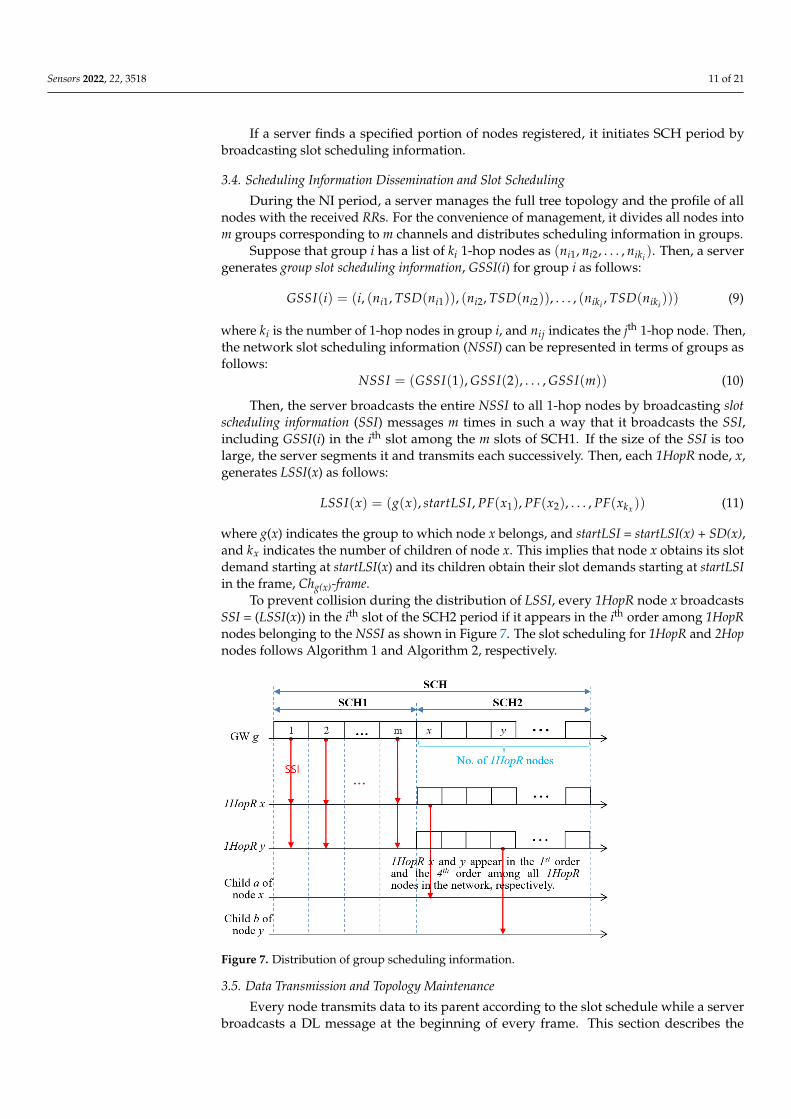
Then, the server broadcasts the entire NSSI to all 1-hop nodes by broadcasting slotscheduling information (SSI) messages m times in such a way that it broadcasts the SSI,including GSSI(i) in the ith slot among the m slots of SCH1. If the size of the SSI is toolarge, the server segments it and transmits each successively. Then, each 1HopR node, x,generates LSSI(x) as follows:

LSSI(x) = (g(x), startLSI, PF(x1), PF(x2), . . . , PF(xkx )) (11)

where g(x) indicates the group to which node x belongs, and startLSI = startLSI(x) + SD(x),and kx indicates the number of children of node x. This implies that node x obtains its slotdemand starting at startLSI(x) and its children obtain their slot demands starting at startLSIin the frame, Chg(x)-frame.

To prevent collision during the distribution of LSSI, every 1HopR node x broadcastsSSI = (LSSI(x)) in the ith slot of the SCH2 period if it appears in the ith order among 1HopRnodes belonging to the NSSI as shown in Figure 7. The slot scheduling for 1HopR and 2Hopnodes follows Algorithm 1 and Algorithm 2, respectively.

Sensors 2022, 22, x FOR PEER REVIEW 11 of 21

During the NI period, a server manages the full tree topology and the profile of all

nodes with the received RRs. For the convenience of management, it divides all nodes into

m groups corresponding to m channels and distributes scheduling information in groups.

Suppose that group i has a list of ki 1-hop nodes as 1 1( , ,..., )ii i ikn n n . Then, a server gen-

erates group slot scheduling information, GSSI(i) for group i as follows:

1 1 2 2( ) ( ,( , ( )),( , ( )),...,( , ( )))i ii i i i ik ikGSSI i i n TSD n n TSD n n TSD n (9)

where �� is the number of 1-hop nodes in group i, and ��� indicates the jth 1-hop node.

Then, the network slot scheduling information (NSSI) can be represented in terms of

groups as follows: ( (1), (2), ..., ( ))NSSI GSSI GSSI GSSI m (10)

Then, the server broadcasts the entire NSSI to all 1-hop nodes by broadcasting slot

scheduling information (SSI) messages m times in such a way that it broadcasts the SSI, in-

cluding GSSI(i) in the ith slot among the m slots of SCH1. If the size of the SSI is too large,

the server segments it and transmits each successively. Then, each 1HopR node, x, gener-

ates LSSI(x) as follows:

1 2( ) ( ( ), , ( ), ( ),..., ( ))xk

LSSI x g x startLSI PF x PF x PF x (11)

where g(x) indicates the group to which node x belongs, and startLSI = startLSI(x) + SD(x),

and �� indicates the number of children of node x. This implies that node x obtains its

slot demand starting at startLSI(x) and its children obtain their slot demands starting at

startLSI in the frame, Chg(x)-frame.

To prevent collision during the distribution of LSSI, every 1HopR node x broadcasts

SSI = (LSSI(x)) in the ith slot of the SCH2 period if it appears in the ith order among 1HopR

nodes belonging to the NSSI as shown in Figure 7. The slot scheduling for 1HopR and

2Hop nodes follows Algorithm 1 and Algorithm 2, respectively.

Figure 7. Distribution of group scheduling information.

3.5. Data Transmission and Topology Maintenance

Every node transmits data to its parent according to the slot schedule while a server

broadcasts a DL message at the beginning of every frame. This section describes the meth-

ods to deal with link failure against node mobility, node joining and leaving, and the up-

date of a slot schedule during data transmission.

Figure 7. Distribution of group scheduling information.

3.5. Data Transmission and Topology Maintenance

Every node transmits data to its parent according to the slot schedule while a serverbroadcasts a DL message at the beginning of every frame. This section describes the

Sensors 2022, 22, 3518 12 of 21

methods to deal with link failure against node mobility, node joining and leaving, and theupdate of a slot schedule during data transmission.

3.5.1. Link Failure

A link has a time-varying condition due to node movement, signal interference, or theintervention of obstacles. Thus, a node and its parent should be able to detect and repairlink failure and update a slot schedule accordingly.

A node detects downlink failure by making use of data transmission. If node x hasnot received data from any child y for three consecutive frames, it decides that link (x, y) isbroken and updates NodeIT(x) with CS(x) = CS(x) − y. If node x is GW, it releases the slotsallocated to node y. If node x is of 1HopR, it creates an updated profile uPF(x) for its newlink state as follows:

uPF(x) = (x, class(x), {PF(c)|c ∈ CS(x)}) (12)

Then, 1HopR node x sends RR = (x, P(x), uPF(x)) to GW.To avoid collision, a node transmits RR using an unscheduled slot in its frame. Upon

receiving RR, a server generates an updated slot scheduling information, uSSI(x), for 1HopRnode x as follows:

uSSI(x) = (g(x), startLSI(x), uPF(x)) (13)

Then, the server includes uSSI(x) in the next DL message so that node x and node x’schildren can update their slot schedules.

However, it is not possible for a 2-hop node to detect that the uplink to its parent isdown using a DL message. The reason is that since all 1HopR nodes broadcast the same DLmessage at the same time, the node does not always receive a DL message its parent nodebroadcasts. In fact, a 2Hop node can receive a DL message through various routes, such asa GW, its parent 1HopR node, or other 1HopR nodes. Therefore, very conservatively, if anode does not receive a DL message for three consecutive frame periods, it determines thatthe uplink is down and changes its type to Orphan. An additional way for 2Hop node x todetect uplink failure is to analyze uSSI(P(x)) in the DL message. If 2Hop node x finds itselfremoved from uSSI(P(x)), it decides that its uplink (x, P(x)) is down and changes its typeto Orphan.

3.5.2. Node Joining

To maintain the reliability of data transmission, an Orphan node should be able tojoin a GW or 1HopR node without interfering with other data transmissions. Therefore,every 1HopR node r always includes two parameters: jFlag and jSlotNo before sending dataas follows:

DATA = (r, P(r), jFlag, jSlotNo, payload) (14)

An orphan node, say x, that overhears DATA judges the quality of link (x, r), uses jFlagto determine whether it is possible to join node r, and if possible, sends a join message usingan unscheduled slot, jSlotNo, to node r to avoid collision. In this case, jFlag = 1 indicatesthat node r can have a new child, and jSlotNo is an unscheduled slot number in the framethat node r uses for slot scheduling. The joining process of an Orphan node is very similarto the node registration process, except that it uses a collision avoidance technique and hasto explore a channel or group to join because they do not use a common channel.

Considering that there are multiple groups using different channels, an Orphan nodeshuffles m channels to have a channel explore list (ChXpList) and tries to overhear DATA tofind a 1HopR node with good link quality and jFlag = 1 during k frame periods, sequentiallyselecting a channel from ChXpList every UL frame period. Note that ChXpList helpsdistribute Orphan nodes evenly into different groups. An Orphan node also receives DLmessages using a common channel at the beginning of every frame period for the same kframe periods. An Orphan node, z, after receiving DL messages, calculates link quality anddecides whether or not it can become a 1Hop node. If node z can become 1Hop or 1HopR

Sensors 2022, 22, 3518 13 of 21

node, it transmits RR including uPF(z) to GW using a randomly selected channel and waitsfor uSSI(z) in the next DL message. Otherwise, node z checks to see if it can be a 2Hopnode based on the DATA that it has overheard. Based on the overheard DATA, it selectsan 1HopR node with the best link quality and jFlag = 1, and joins the selected 1HopR nodeby sending RR using jSlotNo on the channel that the 1HopR node uses. Upon receivingRR, 1HopR node x updates CS(x) = CS(x) ∪ {z}, generates uPF(x), and sends RR = (x, P(x),uPF(x)) to GW. Then, a server registers a new node z, generates uSSI(x), and broadcasts theDL message, including uSSI(x).

3.5.3. Slot Scheduling Information Management

Given a list of k 1-hop nodes for group i as (ni1, ni2, . . . , nik), a server maintains anetwork information table, NIT(i), as follows:

NIT(i) = (nij, TSD(nij), PF(nij), valid) (15)

where valid indicates whether the corresponding entry is valid or not. Then, the startlogical slot index startLSI(nij) of node nij in group i can be calculated easily by (5).

A server updates the table whenever it receives an updated profile from any 1-hopnode during the data collection period. As mentioned in the subsection of problem identifi-cation, the update of the schedule can cause a slot schedule conflict problem. Two solutionsto this problem can be considered. First, upon receiving uPF(x) from a 1HopR node x, aserver can produce uSSI(x) using a list of slots that do not include the slots allocated previ-ously to node x. In this case, even though any child, say y, disconnected from node x sendsdata continuously, its transmission slot will never conflict with the new slot schedule ofnode x. As another method, upon receiving uPF(x), a server includes Removed(y) in the nextDL message to indicate that node x has removed its child y. If node y receives it, fortunately,it changes its state to Orphan and attempts to join GW or any of relay nodes. In this case, theserver may have to broadcast Removed(y) continuously until it receives uPF(y) or uPF(P(y))from node y or node P(y) (if node y found a new parent), respectively. Upon receivinguPF(y) or uPF(P(y)), the server generates and broadcasts uSSI(x) for y’s previous parentx. This implies that the new scheduling of node x waits until node y finds its new parent,GW or P(y). The first method may not work well unless node x finds a sufficient numberof unscheduled slots except for the slots allocated to itself previously. If this happens, itmay have to migrate to another group. In the second method, if node y does not receive theDL message, it may have to wait long by broadcasting the Removed(y) continuously. Onesolution is to let node y change its type to Orphan if it misses DL messages for the specifiednumber of frame periods.

In this paper, the first solution was implemented as follows. A 1HopR node reports anupdated profile to a server if it has a new child joined or loses any of its children, and thenturns to a virtual node immediately. Upon receiving the updated profile, the server setsthe validity of the corresponding entry to zero and changes the node to a virtual node (v)immediately in the NIT. Then, the 1HopR node remains a virtual node, waiting for a newslot scheduling information from the server.

Suppose that a server receives RR = (nij, P(nij), uPF(nij)) from node nij. The serverchanges node nij to a virtual node in NIT(i) and schedules TSD(nij) either using the slotsoccupied by the other virtual nodes that have a sufficient number of slots or starting withnextLSI(i) as follows:

nextLSI(i) = ∑x∈G(i)+ TSD(x) + 1 (16)

where G(i)+ is a set of all nodes and virtual nodes that belong to group i.For example, consider Table 1 in which NIT(i) has one virtual node v1. Suppose that

ni2 has reported uPF(ni2) with TSD(ni2) = 3 after losing one child. Then, the server allocatesTSD(ni2) to a new virtual node v2 immediately. Then, node ni2 obtains 3 slots from theslots occupied by v1, instead of its previous slots that are now occupied by v2. Then, the

Sensors 2022, 22, 3518 14 of 21

remaining 2 slots out of 5 slots are given to a new virtual node v3. A server broadcastsuSSI(ni2) as follows:

uSSI(ni2) = (i, startLSI(ni2), uPF(ni2)) (17)

Table 1. Network information table, NIT(i).

(a) Before the Update of ni2 (b) After the Update of ni21Hop TSD PF Valid 1Hop TSD PF Valid

ni1 3 PF(ni1) 1 ni1 3 PF(ni1) 1ni2 5 PF(ni2) 1 ni2 → v2 5 - 0. . . . . .

ni(j−1) 1 PF(ni(j−1)) 1 ni(j−1) 1 PF(ni(j−1)) 1nij → ni2 3 PF(ni2) 1nij → v1 5 - 0 nij → v3 2 - 0

ni(j + 1) 1 PF(ni(j + 1)) ni(j + 1) 1 PF(ni(j + 1)). . . . . .nik 1 PF(nik) 1 nik 1 PF(nik) 1. . . . . .

4. Evaluation4.1. Simulation4.1.1. Channel Model

The simulation uses the log-distance path loss model with shadowing [25], which iswidely used to model wireless channels in built-up and densely populated areas. Usingthis model, the path loss at communication distance d is described as follows:

PL(d) = PL(d0) + 10γ log10dd0

+ Xσ (18)

where PL(d0) is the path loss at reference distance d0, γ is the pass loss exponent, d is thetransmission distance (d > d0), and Xσ is the zero-mean Gaussian distributed variable withstandard deviation σ.

p(Xσ) =1

σ√

2πexp(−Xσ

2

2σ2 ) (19)

The received power at distance d, Pr(d), is calculated based on transmission power Ptand path loss at distance d as follows:

Pr(d) = Pt − PL(d) (20)

Assuming that the LoRa signal can be demodulated if the received power is greaterthan or equal to receiving sensitivity of the receiver, Pmin. The probability of receiving apacket at distance d, preceiving(d), can be calculated as follows:

preceiving(d) = p(Pr(d) ≥ Pmin) (21)

Refer to Section 2.7.2 in [25]:

preceiving(d) = Q(Pmin − Pr(d)

σ) (22)

where the Q function is defined as the probability that a Gaussian random variable x withmean zero variance one is greater than z:

Q(z) = p(x > z) =∫ ∞

z

1√2π

e−y22 dy (23)

Sensors 2022, 22, 3518 15 of 21

4.1.2. Simulation Setup

For simulation, 500 nodes and 20 additional mobile nodes are randomly distributedin a square area of 800 × 800 m2, and one gateway denoted by a red circle is placed at thecenter, as illustrated in Figure 8. The big cyan-colored circle indicates the transmissionrange of GW and the small yellow-circle shows one example of a mobile node that movesalong the arrows.

Sensors 2022, 22, x FOR PEER REVIEW 15 of 21

For simulation, 500 nodes and 20 additional mobile nodes are randomly distributed

in a square area of 800 × 800 m2, and one gateway denoted by a red circle is placed at the

center, as illustrated in Figure 8. The big cyan-colored circle indicates the transmission

range of GW and the small yellow-circle shows one example of a mobile node that moves

along the arrows.

Figure 8. Example of spatial distribution with 500 end nodes in an area of 800 × 800 (m2).

The two-hop LoRa network is constructed under the assumption that the connectiv-

ity between two nodes exists only if the link provides a receiving probability greater than

95%. For the values of the channel parameters, refer to the experimental results in [26]

where d0 = 1 m, PL(d0) = 40.7 dB, γ = 3.54, and σ = 5.34. Every mobile node moves arbitrarily

at the speed of 2 m/s that models the movement of workers carrying sensor nodes, and

takes the pausing time that follows a Poisson process with an expected pausing time λ in

minutes. The key parameters and values are listed in Table 2.

Table 2. Simulation parameters.

Parameter Value Parameter Value

No. GWs 1 Data rate (SF, BW) 7, 125

No. static nodes 500 No. UL slots 128

No. mobile nodes 20 UL slot size 100 (ms)

UL payload size 50 (bytes) DL slot size 200 (ms)

Data transmission interval 13.2 (s) Frame size 13.2 (s)

Expected pausing time (λ) 5, 10, 15, 20, 25 No. Data channels 8

4.1.3. Simulation Results

Some performance evaluation metrics are used as follows. The packet delivery rate

(PDR) is the ratio of the number of packets received successfully by GW to the number of

packets generated by all end nodes during simulation. Additionally, it may be meaningful

to evaluate the quality of links. Thus, the packet delivery rate for the nodes except orphan

nodes is evaluated under the premise that Orphan nodes do not transmit data, referred to

as PDR_NoOrphan that is defined as the ratio of the number of packets received success-

fully at GW to the number of packets transmitted by all end nodes.

Simulations were performed over a period of 10,000 frames (=132,000 s), changing

the value of λ from 5 to 25 min. Figure 9 shows the average PDR and PDR_NoOrphan of

20 mobile nodes. It is seen that the average PDR_NoOrphan remains high above 97% for

all values of λ, while the average PDR increases from 91.2 to 95.9% as the value of λ in-

creases from 5 to 25. The gap between two graphs implies that packet loss caused by the

transmission of orphan nodes cannot be ignored.

Figure 8. Example of spatial distribution with 500 end nodes in an area of 800 × 800 (m2).

The two-hop LoRa network is constructed under the assumption that the connectivitybetween two nodes exists only if the link provides a receiving probability greater than 95%.For the values of the channel parameters, refer to the experimental results in [26] where d0= 1 m, PL(d0) = 40.7 dB, γ = 3.54, and σ = 5.34. Every mobile node moves arbitrarily at thespeed of 2 m/s that models the movement of workers carrying sensor nodes, and takes thepausing time that follows a Poisson process with an expected pausing time λ in minutes.The key parameters and values are listed in Table 2.

Table 2. Simulation parameters.

Parameter Value Parameter ValueNo. GWs 1 Data rate (SF, BW) 7, 125

No. static nodes 500 No. UL slots 128

No. mobile nodes 20 UL slot size 100 (ms)

UL payload size 50 (bytes) DL slot size 200 (ms)

Data transmissioninterval 13.2 (s) Frame size 13.2 (s)

Expected pausingtime (λ) 5, 10, 15, 20, 25 No. Data channels 8

4.1.3. Simulation Results

Some performance evaluation metrics are used as follows. The packet delivery rate(PDR) is the ratio of the number of packets received successfully by GW to the number ofpackets generated by all end nodes during simulation. Additionally, it may be meaningfulto evaluate the quality of links. Thus, the packet delivery rate for the nodes except orphannodes is evaluated under the premise that Orphan nodes do not transmit data, referred to asPDR_NoOrphan that is defined as the ratio of the number of packets received successfullyat GW to the number of packets transmitted by all end nodes.

Sensors 2022, 22, 3518 16 of 21

Simulations were performed over a period of 10,000 frames (=132,000 s), changingthe value of λ from 5 to 25 min. Figure 9 shows the average PDR and PDR_NoOrphanof 20 mobile nodes. It is seen that the average PDR_NoOrphan remains high above 97%for all values of λ, while the average PDR increases from 91.2 to 95.9% as the value of λincreases from 5 to 25. The gap between two graphs implies that packet loss caused by thetransmission of orphan nodes cannot be ignored.

Sensors 2022, 22, x FOR PEER REVIEW 16 of 21

Figure 9. The average PDR and PDR_NoOrphan with different λ.

Additionally, control overheads of the mobile node (MobileOH), which is defined as

the number of control packets transmitted by the mobile node and its parent, was meas-

ured during simulation. Figure 10 shows the average MobileOH of 20 mobile nodes for

different λ values. It is shown that MobileOH decreases sharply as λ increases up to 25.

When λ = 5, the mobile node needs more than 500 control packets during simulation,

which is 5% of the number of packets generated.

Figure 10. The average MobileOH with different λ.

4.2. Experiment

4.2.1. Experiment I with Static Node Scenario

For the experiment, GW and node (in fact, weather device with an ultra-sound wind

detector and a LoRa end node) were developed as shown in Figure 11. The GW consists

of Raspberry PI 3 Model B+ and SX1301 LoRa transceiver, and the LoRa node consist of

STM32L151xx and SX1276 LoRa transceiver. In this static node scenario, 1 GW and 40

nodes were deployed on a 500 × 350 (m2) area of a university campus. Each node receives

GPS data, wind speed, wind direction, temperature and humidity from the weather de-

tection system and sends those data to the GW periodically. Since some nodes were in-

stalled in communication shadow areas such as valleys on campus, inside buildings, and

behind buildings, many nodes could not be directly connected to the GW. As shown in

the upper left photo of Figure 11, the GW was installed in the lecture room on the 6th floor

of the computer science building, with the antenna exposed to the outside. The key exper-

iment parameters and values are summarized in Table 3.

Figure 9. The average PDR and PDR_NoOrphan with different λ.

Additionally, control overheads of the mobile node (MobileOH), which is defined asthe number of control packets transmitted by the mobile node and its parent, was measuredduring simulation. Figure 10 shows the average MobileOH of 20 mobile nodes for differentλ values. It is shown that MobileOH decreases sharply as λ increases up to 25. When λ = 5,the mobile node needs more than 500 control packets during simulation, which is 5% of thenumber of packets generated.

Sensors 2022, 22, x FOR PEER REVIEW 16 of 21

Figure 9. The average PDR and PDR_NoOrphan with different λ.

Additionally, control overheads of the mobile node (MobileOH), which is defined as

the number of control packets transmitted by the mobile node and its parent, was meas-

ured during simulation. Figure 10 shows the average MobileOH of 20 mobile nodes for

different λ values. It is shown that MobileOH decreases sharply as λ increases up to 25.

When λ = 5, the mobile node needs more than 500 control packets during simulation,

which is 5% of the number of packets generated.

Figure 10. The average MobileOH with different λ.

4.2. Experiment

4.2.1. Experiment I with Static Node Scenario

For the experiment, GW and node (in fact, weather device with an ultra-sound wind

detector and a LoRa end node) were developed as shown in Figure 11. The GW consists

of Raspberry PI 3 Model B+ and SX1301 LoRa transceiver, and the LoRa node consist of

STM32L151xx and SX1276 LoRa transceiver. In this static node scenario, 1 GW and 40

nodes were deployed on a 500 × 350 (m2) area of a university campus. Each node receives

GPS data, wind speed, wind direction, temperature and humidity from the weather de-

tection system and sends those data to the GW periodically. Since some nodes were in-

stalled in communication shadow areas such as valleys on campus, inside buildings, and

behind buildings, many nodes could not be directly connected to the GW. As shown in

the upper left photo of Figure 11, the GW was installed in the lecture room on the 6th floor

of the computer science building, with the antenna exposed to the outside. The key exper-

iment parameters and values are summarized in Table 3.

Figure 10. The average MobileOH with different λ.

4.2. Experiment4.2.1. Experiment I with Static Node Scenario

For the experiment, GW and node (in fact, weather device with an ultra-sound winddetector and a LoRa end node) were developed as shown in Figure 11. The GW consistsof Raspberry PI 3 Model B+ and SX1301 LoRa transceiver, and the LoRa node consist ofSTM32L151xx and SX1276 LoRa transceiver. In this static node scenario, 1 GW and 40 nodeswere deployed on a 500 × 350 (m2) area of a university campus. Each node receives GPSdata, wind speed, wind direction, temperature and humidity from the weather detectionsystem and sends those data to the GW periodically. Since some nodes were installed incommunication shadow areas such as valleys on campus, inside buildings, and behindbuildings, many nodes could not be directly connected to the GW. As shown in the upper

Sensors 2022, 22, 3518 17 of 21

left photo of Figure 11, the GW was installed in the lecture room on the 6th floor of thecomputer science building, with the antenna exposed to the outside. The key experimentparameters and values are summarized in Table 3.

Sensors 2022, 22, x FOR PEER REVIEW 17 of 21

Figure 11. Photos of GW and some nodes installed in a university campus.

Table 3. Experiment parameters and values.

Parameter Value Parameter Value

UL slot size 100 ms Data rate (SF, BW) 7, 125

DL slot size 200 ms Frame Size 13.2 s

No. UL slot 128 Data transmission interval 13.2 s

No. UL channel 1 Payload size 24 bytes

Figure 12a shows the two-hop topology constructed with (RSSI_Th1, SNR_Th1) =

(−110 dBm, −3.5 dB) and (RSSI_Th2, SNR_Th2) = (−115 dBm, −5.5 dB) immediately after

network construction. The blue colored, brown-colored, and red-colored circles indicate

1HopR, 1Hop, and 2Hop nodes, respectively.

The experiment was conducted for several days, recording network connection sta-

tus every 8 h as shown in Figure 12b–d. As shown in the figures, nodes 4, 5, 7, 15, and 20

change connections frequently due to their link instability. The reason is that node 20 was

placed low behind the Chemical Engineering Building that blocks the building having the

GW, and nodes 4, 5, and 15 were placed quite far from the GW and intercepted by several

buildings and trees. Node 7 was placed in an open area but blocked by the hills because

it is placed low. Nodes 20 and 7 started out as 1HopR nodes and turned into 2Hop nodes

after 8 and 16 h, respectively, and then node 20 turned into 1Hop nodes after 24 h.

(a) (b)

Figure 11. Photos of GW and some nodes installed in a university campus.

Table 3. Experiment parameters and values.

Parameter Value Parameter ValueUL slot size 100 ms Data rate (SF, BW) 7, 125DL slot size 200 ms Frame Size 13.2 s

No. UL slot 128 Data transmissioninterval 13.2 s

No. UL channel 1 Payload size 24 bytes

Figure 12a shows the two-hop topology constructed with (RSSI_Th1, SNR_Th1) =(−110 dBm, −3.5 dB) and (RSSI_Th2, SNR_Th2) = (−115 dBm, −5.5 dB) immediately afternetwork construction. The blue colored, brown-colored, and red-colored circles indicate1HopR, 1Hop, and 2Hop nodes, respectively.

The experiment was conducted for several days, recording network connection statusevery 8 h as shown in Figure 12b–d. As shown in the figures, nodes 4, 5, 7, 15, and 20 changeconnections frequently due to their link instability. The reason is that node 20 was placedlow behind the Chemical Engineering Building that blocks the building having the GW, andnodes 4, 5, and 15 were placed quite far from the GW and intercepted by several buildingsand trees. Node 7 was placed in an open area but blocked by the hills because it is placedlow. Nodes 20 and 7 started out as 1HopR nodes and turned into 2Hop nodes after 8 and16 h, respectively, and then node 20 turned into 1Hop nodes after 24 h.

Table 4 summarizes the number of 1-hop nodes, the number of 2-hop nodes, and thelowest and average PDR_NoOrphan values among the PDR_NoOrphans of 1-hop and 2-hopnodes. The proposed protocol achieves a high PDR_NoOrphan of over 99% on average for1-hop nodes and over 97% for 2-hop nodes. Node 15 had a low PDR_NoOrphan of 92.2%because its one-hop connection was unstable during the first 8 h. However, it can be seenthat the PDR_NoOrphan continued to increase after node 15 became a 2-hop node or a 1-hopnode with a stable connection. A similar situation occurred on node 7. After 8 h, node 7connected to node 8 to become a 2Hop node. After 24 h, it is shown that all 1-hop or 2-hopnodes could achieve a high PDR_NoOrphan of 95% or more.

Sensors 2022, 22, 3518 18 of 21

Sensors 2022, 22, x FOR PEER REVIEW 17 of 21

Figure 11. Photos of GW and some nodes installed in a university campus.

Table 3. Experiment parameters and values.

Parameter Value Parameter Value

UL slot size 100 ms Data rate (SF, BW) 7, 125

DL slot size 200 ms Frame Size 13.2 s

No. UL slot 128 Data transmission interval 13.2 s

No. UL channel 1 Payload size 24 bytes

Figure 12a shows the two-hop topology constructed with (RSSI_Th1, SNR_Th1) =

(−110 dBm, −3.5 dB) and (RSSI_Th2, SNR_Th2) = (−115 dBm, −5.5 dB) immediately after

network construction. The blue colored, brown-colored, and red-colored circles indicate

1HopR, 1Hop, and 2Hop nodes, respectively.

The experiment was conducted for several days, recording network connection sta-

tus every 8 h as shown in Figure 12b–d. As shown in the figures, nodes 4, 5, 7, 15, and 20

change connections frequently due to their link instability. The reason is that node 20 was

placed low behind the Chemical Engineering Building that blocks the building having the

GW, and nodes 4, 5, and 15 were placed quite far from the GW and intercepted by several

buildings and trees. Node 7 was placed in an open area but blocked by the hills because

it is placed low. Nodes 20 and 7 started out as 1HopR nodes and turned into 2Hop nodes

after 8 and 16 h, respectively, and then node 20 turned into 1Hop nodes after 24 h.

(a) (b)

Sensors 2022, 22, x FOR PEER REVIEW 18 of 21

(c) (d)

Figure 12. Static node deployment scenario and the change of topology. (a) Node connections after

network initialization; (b) Node connections after 8 hours of operation; (c) Node connections after

16 hours of operation; (d) Node connections after 24 hours of operation.

Table 4 summarizes the number of 1-hop nodes, the number of 2-hop nodes, and the

lowest and average PDR_NoOrphan values among the PDR_NoOrphans of 1-hop and 2-

hop nodes. The proposed protocol achieves a high PDR_NoOrphan of over 99% on average

for 1-hop nodes and over 97% for 2-hop nodes. Node 15 had a low PDR_NoOrphan of

92.2% because its one-hop connection was unstable during the first 8 h. However, it can

be seen that the PDR_NoOrphan continued to increase after node 15 became a 2-hop node

or a 1-hop node with a stable connection. A similar situation occurred on node 7. After 8

h, node 7 connected to node 8 to become a 2Hop node. After 24 h, it is shown that all 1-

hop or 2-hop nodes could achieve a high PDR_NoOrphan of 95% or more.

Table 4. Experiment results.

After

Initialization After 8 h After 16 h After 24 h

No. 1-hop nodes 33 28 25 26

No. 2-hop nodes 7 12 15 14

AVG. PDR_NoOrphan

(1-hop) N.A. 99.4% 99.4% 99.2%

Worst PDR_NoOrphan

(1-hop) N.A. 97.9% 97.7% 95.9%

AVG. PDR_NoOrphan

(2-hop) N.A. 97.5% 97.7% 98.5%

Worst PDR_NoOrphan

(2-hop) N.A. 92.2% 93.4% 95.2%

Figure 12. Static node deployment scenario and the change of topology. (a) Node connections afternetwork initialization; (b) Node connections after 8 h of operation; (c) Node connections after 16 h ofoperation; (d) Node connections after 24 h of operation.

Table 4. Experiment results.

AfterInitialization After 8 h After 16 h After 24 h

No. 1-hop nodes 33 28 25 26No. 2-hop nodes 7 12 15 14

AVG. PDR_NoOrphan(1-hop) N.A. 99.4% 99.4% 99.2%

Worst PDR_NoOrphan(1-hop) N.A. 97.9% 97.7% 95.9%

AVG. PDR_NoOrphan(2-hop) N.A. 97.5% 97.7% 98.5%

Worst PDR_NoOrphan(2-hop) N.A. 92.2% 93.4% 95.2%

4.2.2. Experiment II with Mobile Node Scenario

In this experiment, two additional mobile nodes, 41 and 42, were allowed to travelalong their respective predetermined paths over the previous static node scenario. At thestarting point of the experiment, node 41 is installed inside the vehicle and travels alonga green curved path starting at position L1 at a speed of 6 km/h (≈1.7 m/s) as shownin Figure 13a. After about 30 min, one of our lab members carried node 42 and movedfrom the starting point L2 along the blue curved path at about 4 km/h (≈1.1 m/s), whichcorresponds to the normal walking speed, as shown in Figure 13b.

Sensors 2022, 22, 3518 19 of 21

Sensors 2022, 22, x FOR PEER REVIEW 19 of 21

4.2.2. Experiment II with Mobile Node Scenario

In this experiment, two additional mobile nodes, 41 and 42, were allowed to travel

along their respective predetermined paths over the previous static node scenario. At the

starting point of the experiment, node 41 is installed inside the vehicle and travels along

a green curved path starting at position L1 at a speed of 6 km/h (≈1.7 m/s) as shown in

Figure 13a. After about 30 min, one of our lab members carried node 42 and moved from

the starting point L2 along the blue curved path at about 4 km/h (≈1.1 m/s), which corre-

sponds to the normal walking speed, as shown in Figure 13b.

(a) (b)

Figure 13. The change of connections according to node movement (The red-colored dashed lines

indicate the unreliable connection). (a) Moving path of node 41; (b) Moving path of node 42.

Two mobile nodes moving along their respective paths performed data transmission

while repeating the process of joining and leaving the already established and operating

fixed LoRa network as in Experiment I. Mobile nodes, 41 and 42, move 4 laps and 1 lap,

respectively, along their respective paths.

Table 5 summarizes the total experiment time, number of parent changes,

PDR_NoOrphan, and PDR for two mobile nodes. It is shown that two mobile nodes

achieve a high PDR_NoOrphan of over 90%. Taking advantage of the augmented trans-

mission effect, the PDR_NoOrphan is improved to over 95%, the value in parentheses. This

means that mobile nodes can transmit data quite reliably, even though they are constantly

on the move. Note that two mobile nodes take a large difference of nearly 10% in PDR.

The reason for this is that the slowly moving node 42 takes link disconnection time longer

than mobile node 41.

Table 5. Experiment result.

Node ID 41 42

Experiment time 1 h 25 min

Number of parent changes 1 2

PDR_NoOrphan 93.3 (97.4) 90.2 (96.5)

PDR 90.3 (94.3) 80.8 (86.4)

Referring to Figure 13a, let us explain how mobile node 41 changes its node type.

Starting as a 1Hop type at point L1, mobile node 41 maintains a 1Hop node during its first

and second laps even though it has experienced link instability temporarily during these

laps. However, in the third lap, when node 41 enters zone 2 pass zone 1 and its link be-

comes unstable, it became an orphan since it failed to receive the DL message three times

in a row. Then, it gets node 20 as a new parent to be a 2Hop type. In the fourth lap, when

node 41 enters zone 1, it keeps the link to its parent despite that it is unstable temporarily.

Then, it remains a 2Hop type by the end of experiment.

Figure 13. The change of connections according to node movement (The red-colored dashed linesindicate the unreliable connection). (a) Moving path of node 41; (b) Moving path of node 42.

Two mobile nodes moving along their respective paths performed data transmissionwhile repeating the process of joining and leaving the already established and operatingfixed LoRa network as in Experiment I. Mobile nodes, 41 and 42, move 4 laps and 1 lap,respectively, along their respective paths.

Table 5 summarizes the total experiment time, number of parent changes, PDR_NoOrphan,and PDR for two mobile nodes. It is shown that two mobile nodes achieve a highPDR_NoOrphan of over 90%. Taking advantage of the augmented transmission effect,the PDR_NoOrphan is improved to over 95%, the value in parentheses. This means thatmobile nodes can transmit data quite reliably, even though they are constantly on the move.Note that two mobile nodes take a large difference of nearly 10% in PDR. The reason forthis is that the slowly moving node 42 takes link disconnection time longer than mobilenode 41.

Table 5. Experiment result.

Node ID 41 42Experiment time 1 h 25 min

Number of parent changes 1 2PDR_NoOrphan 93.3 (97.4) 90.2 (96.5)

PDR 90.3 (94.3) 80.8 (86.4)

Referring to Figure 13a, let us explain how mobile node 41 changes its node type.Starting as a 1Hop type at point L1, mobile node 41 maintains a 1Hop node during itsfirst and second laps even though it has experienced link instability temporarily duringthese laps. However, in the third lap, when node 41 enters zone 2 pass zone 1 and its linkbecomes unstable, it became an orphan since it failed to receive the DL message three timesin a row. Then, it gets node 20 as a new parent to be a 2Hop type. In the fourth lap, whennode 41 enters zone 1, it keeps the link to its parent despite that it is unstable temporarily.Then, it remains a 2Hop type by the end of experiment.

Take a look at Figure 13b in which node 42 takes only one lap at a walking speed.Node 42 starts as an 1Hop type at point L2. When it enters zone 1, its link becomes unstable,but remains same. Upon entering zone 2, node 42 changed its parent to node 24 since itfailed to receive the DL message three times in a row. However, when it enters zone 3, itchanges its parent back to GW due to its link instability. It is natural that node 42 changesits parent more since it maintains the state of link disconnection longer by moving moreslowly than node 41.

Sensors 2022, 22, 3518 20 of 21

5. Conclusions

A new multi-hop LoRa protocol for dynamic LoRa networks was presented by extend-ing the previously proposed two-hop real-time LoRa protocol. It addressed the technicalaspects of dynamic multi-hop networks, such as automatic configuration of multi-hopLoRa networks, dynamic topology management, and updating of real-time slot sched-ules and dealt with some technical issues related to node mobility. By resorting to bothsimulation and experiment, it was verified that the proposed protocol could achieve highreliability against signal attenuation and node mobility, but with low control overheadin topology management and schedule updates. According to experimental results withuniversity campus deployment scenarios with forty nodes, the proposed protocol couldachieve packet delivery rates of over 95% against node mobility.

Author Contributions: Conceptualization, H.O. and H.P.T.; methodology, H.P.T. and H.O.; software,H.P.T.; validation, W.-S.J., D.-S.Y. and H.O.; data curation, W.-S.J. and D.-S.Y.; writing originaldraft preparation, H.P.T.; writing review and editing, H.O., W.-S.J. and D.-S.Y.; visualization, H.P.T.;supervision, H.O.; funding acquisition, H.O. All authors have read and agreed to the publishedversion of the manuscript.

Funding: This work was supported by Institute of Information & communication Technology Plan-ning & Evaluation (IITP) grant funded by the Korea government (MSIT) (2020-0-00869, Developmentof 5G-based Shipbuilding & Marine Smart Communication Platform and Convergence Service).

Conflicts of Interest: The authors declare no conflict of interest.

References1. Tran, H.P.; Jung, W.; Yoon, T.; Yoo, D.; Oh, H. A Two-Hop Real-Time LoRa Protocol for Industrial Monitoring and Control Systems.

IEEE Access 2020, 8, 126239–126252. [CrossRef]2. IEEE Std 802.15.4-2020 (Revision of IEEE Std 802.15.4-2015); IEEE Standard for Low-Rate Wireless Networks. The IEEE Standards

Association: Piscataway, NJ, USA, 2020; pp. 1–800.3. Song, J.; Han, S.; Mok, A.; Chen, D.; Lucas, M.; Nixon, M.; Pratt, W. WirelessHART: Applying Wireless Technology in Real-Time

Industrial Process Control. In Proceedings of the 2008 IEEE Real-Time and Embedded Technology and Applications Symposium,St. Louis, MO, USA, 22–24 April 2008; pp. 377–386.

4. ISA100.11a Standard; Wireless Systems for Industrial Automation: Process and Related Applications. Standards Committees—ISA:Research Triangle Park, NC, USA, 2009.

5. Song, W.; Huang, R.; Shirazi, B.; LaHusen, R. TreeMAC: Localized TDMA MAC protocol for real-time high-data-rate sensornetworks. In Proceedings of the 2009 IEEE International Conference on Pervasive Computing and Communications, Galveston,TX, USA, 9–13 March 2009; pp. 1–10.

6. Oh, H.; van Vinh, P. Design and implementation of a MAC protocol for timely and reliable delivery of command and data indynamic wireless sensor networks. Sensors 2013, 13, 13228–13257. (In English) [CrossRef] [PubMed]

7. Oh, H.; Ngo, C.T. A Slotted Sense Multiple Access Protocol for Timely and Reliable Data Transmission in Dynamic WirelessSensor Networks. IEEE Sens. J. 2018, 18, 2184–2194. [CrossRef]

8. Nguyen, T.; Oh, H. A Smart Multi-Channel Slotted Sense Multiple Access Protocol for Industrial Wireless Sensor Networks. IEEEInternet Things J. 2021, 1. [CrossRef]

9. Reynders, B.; Wang, Q.; Tuset-Peiro, P.; Vilajosana, X.; Pollin, S. Improving Reliability and Scalability of LoRaWANs throughLightweight Scheduling. IEEE Internet Things J. 2018, 5, 1830–1842. [CrossRef]

10. Haxhibeqiri, J.; Moerman, I.; Hoebeke, J. Low Overhead Scheduling of LoRa Transmissions for Improved Scalability. IEEE InternetThings J. 2019, 6, 3097–3109. [CrossRef]

11. Leonardi, L.; Battaglia, F.; Bello, L.L. RT-LoRa: A Medium Access Strategy to Support Real-Time Flows over LoRa-Based Networksfor Industrial IoT Applications. IEEE Internet Things J. 2019, 6, 10812–10823. [CrossRef]

12. Polonelli, T.; Brunelli, D.; Marzocchi, A.; Benini, L. Slotted ALOHA on LoRaWAN-Design, Analysis, and Deployment. Sensors2019, 19, 838. [CrossRef] [PubMed]

13. Hoang, Q.L.; Jung, W.; Yoon, T.; Yoo, D.; Oh, H. A Real-Time LoRa Protocol for Industrial Monitoring and Control Systems. IEEEAccess 2020, 8, 44727–44738. [CrossRef]

14. Zorbas, D.; Abdelfadeel, K.; Kotzanikolaou, P.; Pesch, D. TS-LoRa: Time-slotted LoRaWAN for the Industrial Internet of Things.Comput. Commun. 2020, 153, 1–10. [CrossRef]

15. Augustin, A.; Yi, J.; Clausen, T.H.; Townsley, W. A Study of LoRa: Long Range & Low Power Networks for the Internet of Things.Sensors 2016, 16, 1466.

16. Semtech Corp. AN1200.22 LoRa Modulation Bacics; Semtech Corp.: Camarillo, CA, USA, 2015.17. Dias, J.; Grilo, A. LoRaWAN multi-hop uplink extension. Procedia Comput. Sci. 2018, 130, 424–431. [CrossRef]

Sensors 2022, 22, 3518 21 of 21

18. Liao, C.; Zhu, G.; Kuwabara, D.; Suzuki, M.; Morikawa, H. Multi-Hop LoRa Networks Enabled by Concurrent Transmission.IEEE Access 2017, 5, 21430–21446. [CrossRef]

19. Lee, H.; Ke, K. Monitoring of Large-Area IoT Sensors Using a LoRa Wireless Mesh Network System: Design and Evaluation.IEEE Trans. Instrum. Meas. 2018, 67, 2177–2187. [CrossRef]

20. Farooq, M.O. Clustering-Based Layering Approach for Uplink Multi-Hop Communication in LoRa Networks. IEEE Netw. Lett.2020, 2, 132–135. [CrossRef]

21. Bor, M.; Vidler, J.; Roedig, U. LoRa for the Internet of Things. In Proceedings of the International Conference on EmbeddedWireless Systems and Networks (EWSN), Graz, Austria, 15–17 February 2016; pp. 361–366.

22. Ebi, C.; Schaltegger, F.; Rust, A.; Blumensaat, F. Synchronous LoRa Mesh Network to Monitor Processes in UndergroundInfrastructure. IEEE Access 2019, 7, 57663–57677. [CrossRef]

23. Perkins, C.E.; Bhagwat, P. Highly dynamic Destination-Sequenced Distance-Vector routing (DSDV) for mobile computers. In Proceedingsof the Conference on Communications Architectures, Protocols and Applications, London, UK, 31 August–2 September 1994. [CrossRef]

24. Ferrari, F.; Zimmerling, M.; Thiele, L.; Saukh, O. Efficient network flooding and time synchronization with Glossy. In Proceedings ofthe 10th ACM/IEEE International Conference on Information Processing in Sensor Networks, Chicago, IL, USA, 12–14 April 2011;pp. 73–84.

25. Goldsmith, A. Wireless Communications; Cambridge University Press: Cambridge, UK, 2005.26. Xu, W.; Kim, J.Y.; Huang, W.; Kanhere, S.S.; Jha, S.K.; Hu, W. Measurement, Characterization, and Modeling of LoRa Technology

in Multifloor Buildings. IEEE Internet Things J. 2020, 7, 298–310. [CrossRef]