On the Error Rate of the LoRa Modulation with Interference

arX

iv:1

905.

1125

2v2

[ee

ss.S

P] 3

Dec

201

91

On the Error Rate of the LoRa Modulation

with InterferenceOrion Afisiadis, Student Member, IEEE, Matthieu Cotting,

Andreas Burg, Member, IEEE, and Alexios Balatsoukas-Stimming, Member, IEEE

Abstract—LoRa is a chirp spread-spectrum modulation de-veloped for the Internet of Things. In this work, we examinethe performance of LoRa in the presence of both additive whiteGaussian noise and interference from another LoRa user. To thisend, we extend an existing interference model, which assumesperfect alignment of the signal of interest and the interference,to the more realistic case where the interfering user is neitherchip- nor phase-aligned with the signal of interest and we derivean expression for the error rate. We show that the existing alignedinterference model overestimates the effect of interference on theerror rate. Moreover, we prove two symmetries in the interferingsignal and we derive low-complexity approximate formulas thatcan significantly reduce the complexity of computing the symboland frame error rates compared to the complete expression.Finally, we provide numerical simulations to corroborate thetheoretical analysis and to verify the accuracy of our proposedapproximations.

I. INTRODUCTION

The Internet of Things (IoT) will consist of billions of

connected devices that have a large number of applications,

such as smart metering, logistics [1], and localization and

tracking [2]. Other potential uses of IoT devices include health

monitoring [3] and massive sensor networks for smart farming

and environmental monitoring [4]. Since these devices will

mostly be low-power and they are expected to connect wire-

lessly with each other (or with centralized gateways), several

specialized communications protocols have been proposed for

IoT applications. Some examples include Sigfox, Weightless,

NB-IoT, and LoRa [5], [6].

LoRa specifically is a low-rate, low-power, and high-range

modulation that uses chirp spread-spectrum for its physical

layer [7]. LoRa supports multiple spreading factors, coding

rates, and packet lengths, to support a very wide range of

operating signal-to-noise ratios (SNRs). The LoRa physical

layer is proprietary [8], but reverse engineering attempts [9],

[10] have led to detailed mathematical descriptions [11]. The

effect of carrier- and sampling frequency offset on LoRa

digital receivers has been modeled and analyzed in [12].

Since LoRa uses the ISM band, interference from other

technologies using the same band is a potential problem.

More importantly, LoRa relies on LoRaWAN for the MAC

Orion Afisiadis, Matthieu Cotting, and Andreas Burg are withthe Telecommunication Circuits Laboratory, Ecole polytechniquefederale de Lausanne, Switzerland (e-mail: [email protected],[email protected], [email protected]). AlexiosBalatsoukas-Stimming was with the Telecommunication Circuits Laboratory,Ecole polytechnique federale de Lausanne, Switzerland, and is currentlywith the Department of Electrical Engineering, Eindhoven University ofTechnology, Netherlands (e-mail: [email protected]).

layer, which uses an ALOHA-based channel access scheme in

which collisions are not explicitly avoided. These collisions

lead to same-technology inter-user interference which may

ultimately become the capacity-limiting factor in massive IoT

scenarios [13]. For this reason, it is of great interest and

importance to study the performance of LoRa under same-

technology interference.

The authors of [14] present a mathematical network model

for LoRa that includes the capture effect, i.e., the fact that a

LoRa packet can be correctly decoded even under interference

from another LoRa packet. A stochastic geometry framework

for modeling the performance of a single gateway LoRa

network is used in [15]. An investigation of the latency,

collision rate, and throughput for LoRaWAN under duty-cycle

restrictions is performed in [16]. Several real-world deploy-

ments of LoRa have been tested, but in order to assess the

network scalability of LoRaWAN to future network densities

that are expected to be orders of magnitude larger, evaluations

through network simulators need to be performed. For this

reason, the works of [17], [18] added LoRa functionality to the

well-known ns-3 network simulator. A simpler Python-based

network simulator for the LoRa uplink was first described

in [19], and later extended for the LoRa downlink in [20].

The impact of the downlink feedback on LoRa capacity was

also studied in [21]. A general overview and performance

evaluations of LoRaWAN can be found in [13], [22].

The impact of interference coming from different technolo-

gies on the performance of the LoRa modulation has received

some attention in the literature. Specifically, [23] studies the

co-existence of LoRa with IEEE 802.15.4g, while [24] studies

the co-existence of LoRa with ultra-narrowband technologies,

such as Sigfox. The impact of interference coming from other

LoRa nodes has also received some attention. Specifically,

the work of [25] extended the simulator of [19] in order to

study the impact of imperfect orthogonality between different

LoRa spreading factors. The work of [26] also examines the

effect of imperfect orthogonality by examining the signal-

to-interference ratio (SIR) threshold for receiving a packet

correctly for all combinations of spreading factors. The SIR

thresholds are derived both by simulations and experimental

results and rectify the values found in [6]. Interference is

particularly detrimental when users with the same spreading

factor collide since the spreading can no longer mitigate the

interference. The authors of [27] perform an experimental

assessment of the link-level characteristics of the LoRa system,

followed by a system-level simulation to assess the capacity

of a LoRaWAN network.

http://arxiv.org/abs/1905.11252v2

2

Convenient approximations for the bit-error rate (BER) of

the LoRa modulation when transmission takes place over

additive white Gaussian noise (AWGN) and Rayleigh fading

channels are given in [28], but collisions are not considered.

Finally, the work of [29], which is most closely related to our

work, provides an approximation for the BER of the LoRa

modulation under AWGN and interference from a single LoRa

interferer with the same spreading factor (same-SF). Capacity

planning for LoRa with the aforementioned interference model

is addressed in [30]. The work in [30] is the first work that,

to the best of our knowledge, analyzes the coverage of LoRa

under a unified noise and interference framework.

Contributions: The work of [29] made a significant first

step toward understanding the behavior of LoRa under same-

SF interference. In this paper, based on our own previous work

of [31], we extend the interference model of [29] to the more

general (and more realistic) case where the interference is

neither chip- nor phase-aligned with the signal-of-interest. We

derive an expression for the symbol error rate (SER) under

this new complete interference model. Moreover, we derive

an approximation for the SER under the new interference

model and we show that non-integer chip duration time-

misalignment in particular has a significant effect on the SER.

Specifically, we show that the interference model of [29] is

pessimistic in the sense that it consistently over-estimates the

actual SER. We also prove two properties of same-SF LoRa-

induced interference that enable a significant reduction of the

complexity of calculating both the exact and the approximated

SER. Similar properties which were stated (without proof)

in [29] are shown to be special cases of our results. Finally, we

derive an approximation for the frame error rate (FER), which

is generally of greater practical interest for network simulators

such as the ones presented in [17]–[20].

Outline: The remainder of this paper is organized as

follows. In Section II, we provide a detailed description of

the LoRa modulation and demodulation processes. In Sec-

tion III, we derive an expression and we review existing

approximations for the SER of the LoRa modulation under

AWGN. In Section IV, we model the behavior of LoRa under

same-SF interference with neither chip- nor phase-alignment

assumptions and we derive a corresponding expression for

the SER. In Section V, we explore and prove the existence

of equivalent interference patterns that can be exploited to

reduce the complexity of computing the SER and we derive

a low-complexity approximation for the SER. In Section VI

we also derive an approximation for the FER, which is of

greater practical interest than the SER in network simulators.

Finally, Section VII contains numerical SER and FER results

and Section VIII concludes this paper.

Notation: Bold lowercase letters (e.g., a) denote vectors,

while bold uppercase letters (e.g., A) denote the discrete

Fourier transform (DFT) of a, i.e., A = DFT(a). We define

[x]y = x mod y. We denote the normal and complex normal

(with i.i.d. components) probability density functions (PDFs)

with mean µ and variance σ2 as N (µ, σ2) and CN (µ, σ2),respectively. Moreover, we denote the PDF and the cumulative

density function (CDF) of the Rayleigh and Rice distributions

by fRa(y;σ), fRi(y; v, σ) and FRa(y;σ), FRi(y; v, σ), respec-

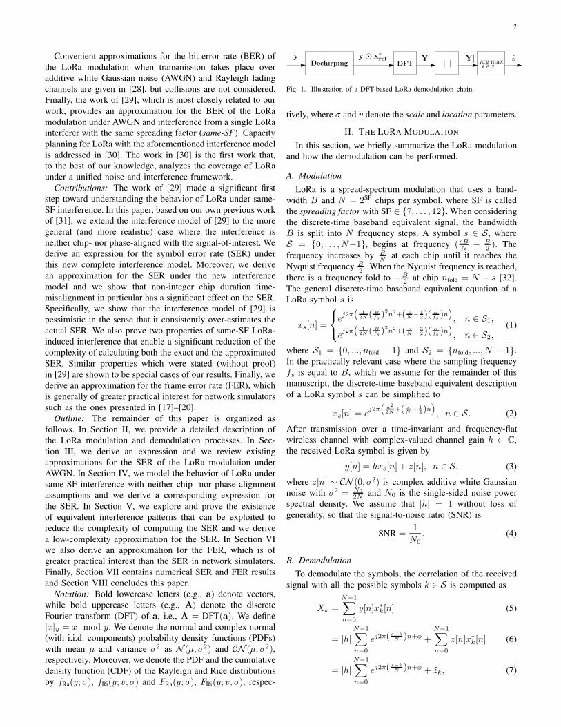
Dechirpingy

DFT argmaxy ⊙ x∗

refj j

Y jYj s

k 2 S

Fig. 1. Illustration of a DFT-based LoRa demodulation chain.

tively, where σ and v denote the scale and location parameters.

II. THE LORA MODULATION

In this section, we briefly summarize the LoRa modulation

and how the demodulation can be performed.

A. Modulation

LoRa is a spread-spectrum modulation that uses a band-

width B and N = 2SF chips per symbol, where SF is called

the spreading factor with SF ∈ {7, . . . , 12}. When considering

the discrete-time baseband equivalent signal, the bandwidth

B is split into N frequency steps. A symbol s ∈ S, where

S = {0, . . . , N−1}, begins at frequency ( sBN − B2 ). The

frequency increases by BN at each chip until it reaches the

Nyquist frequency B2 . When the Nyquist frequency is reached,

there is a frequency fold to −B2 at chip nfold = N − s [32].

The general discrete-time baseband equivalent equation of a

LoRa symbol s is

xs[n] =

ej2π

(

12N ( B

fs)2n2+( s

N − 12 )(

Bfs)n

)

, n ∈ S1,

ej2π

(

12N ( B

fs)2n2+( s

N − 32 )(

Bfs)n

)

, n ∈ S2,(1)

where S1 = {0, ..., nfold − 1} and S2 = {nfold, ..., N − 1}.

In the practically relevant case where the sampling frequency

fs is equal to B, which we assume for the remainder of this

manuscript, the discrete-time baseband equivalent description

of a LoRa symbol s can be simplified to

xs[n] = ej2π

(

n2

2N +( sN − 1

2 )n)

, n ∈ S. (2)

After transmission over a time-invariant and frequency-flat

wireless channel with complex-valued channel gain h ∈ C,

the received LoRa symbol is given by

y[n] = hxs[n] + z[n], n ∈ S, (3)

where z[n] ∼ CN (0, σ2) is complex additive white Gaussian

noise with σ2 = N0

2N and N0 is the single-sided noise power

spectral density. We assume that |h| = 1 without loss of

generality, so that the signal-to-noise ratio (SNR) is

SNR =1

N0. (4)

B. Demodulation

To demodulate the symbols, the correlation of the received

signal with all the possible symbols k ∈ S is computed as

Xk =

N−1∑

n=0

y[n]x∗k[n] (5)

= |h|N−1∑

n=0

ej2π(s−kN )n+φ +

N−1∑

n=0

z[n]x∗k[n] (6)

= |h|N−1∑

n=0

ej2π(s−kN )n+φ + zk, (7)

3

where φ = h denotes a phase shift introduced by the

transmission channel h that is fixed for each transmitted

packet but generally uniformly distributed in [0, 2π), and

zk ∼ CN (0, Nσ2). In a non-coherent receiver a symbol

estimate s is obtained as

s = argmaxk∈S

(|Xk|) . (8)

The complexity of computing (8) is O(N2). The following

equivalent and low-complexity method can also be used to

perform the demodulation. First, a dechirping is performed,

where the received signal is multiplied by the complex con-

jugate of a reference signal xref. A convenient choice for this

reference signal is an upchirp, i.e., the LoRa symbol for s = 0

xref[n] = ej2π

(

n2

2N −n2

)

, n ∈ S. (9)

Then, the non-normalized discrete Fourier transform (DFT)

is applied to the dechirped signal in order to obtain

Y = DFT (y ⊙ x∗ref), where ⊙ denotes the Hadamard

product and y =[

y[0] . . . y[N − 1]]

and xref =[

xref[0] . . . xref[N − 1]]

. Demodulation can be performed

by selecting the frequency bin index with the maximum

magnitude

s = argmaxk∈S

(|Yk|) . (10)

Using the fast Fourier transform (FFT), the complexity of

computing (10) is O(N logN). These demodulation steps are

illustrated in Fig. 1.

III. SYMBOL ERROR RATE UNDER AWGN

In this section, we first derive the expression for the LoRa

SER under additive white Gaussian noise (AWGN), which is

useful for later explaining how the SER and the FER can be

calculated in the presence of both AWGN and interference.

A. Distribution of the Decision Metric

In the absence of noise, and with perfect synchronization,

the DFT of the dechirped signal Y has a single frequency bin

that contains all the signal energy (i.e., a bin with magnitude

N ) and all remaining N − 1 bins have zero energy. On the

other hand, when AWGN is present, all frequency bins will

contain some energy. The distribution of the frequency bin

values Yk for k ∈ S is

Yk ∼{

CN(

0, 2σ2)

, k ∈ S/s,CN

(

N(cosφ+ j sinφ), 2σ2)

, k = s,(11)

where s is the transmitted symbol.

Let us define Y ′k = Yk

σ for k ∈ S. The values Y ′k can be

used in (10) instead of Yk without changing the result and

their distribution is

Y ′k ∼

{

CN (0, 2) , k ∈ S/s,CN

(

N cosφσ + jN sinφ

σ , 2)

, k = s.(12)

Thus, using basic properties of the complex normal distribu-

tion, we can show that the demodulation metric |Y ′k| follows a

−25 −20 −15 −1010−5

10−4

10−3

10−2

10−1

100

SNR (dB)

Sym

bol

Err

or

Rat

e

MC: SF=7 SF=8 SF=9 SF=10 SF=11 SF=12

Approx.: SF=7 SF=8 SF=9 SF=10 SF=11 SF=12

Fig. 2. Symbol error rate of the LoRa modulation under AWGN for allsupported spreading factors SF ∈ {7, . . . , 12}. Results for Monte Carlosimulations and the approximation in (17) are shown.

Rayleigh distribution for k ∈ S/s and a Rice distribution for

k = s, i.e.,

|Y ′k| ∼

{

fRa(y; 1), k ∈ S/s,fRi

(

y; Nσ , 1

)

, k = s.(13)

B. Symbol Error Rate

A symbol error occurs if and only if any of the |Y ′k| values

for k ∈ S/s exceeds the value of |Y ′s |, or, equivalently, if and

only if |Y ′max| > |Y ′

s |, where |Y ′max| = maxk∈S/s |Y ′

k|. Using

order statistics [33] and the fact that all |Y ′k| for k ∈ S/s are

i.i.d., the PDF of |Y ′max| can be obtained as

f|Y ′

max|(y) = (N − 1) fRa(y; 1)FRa (y; 1)

(N−2)(14)

Using f|Y ′

max|(y), the conditional SER when symbol s is

transmitted can be calculated as

P (s 6= s|s) =∫ +∞

y=0

∫ y

x=0

fRi (x; v, 1) f|Y ′

max|(y)dxdy (15)

=

∫ +∞

y=0

FRi (y; v, 1) f|Y ′

max|(y)dy, (16)

with v = Nσ . The SER for all symbols s is identical, meaning

that (16) is in fact equal to the average SER and, if we

assume that all symbols are equiprobable, it is also equal to

the expected SER.

C. Symbol Error Rate Approximations

While the evaluation of (16) is in principle straightfor-

ward, in practice the values of N in the LoRa modulation

are very large so that numerical problems arise. For this

reason, two approximations that can be used to efficiently

evaluate (16) were derived in [28]. Specifically, [28] used

a Gaussian approximation so that |Y ′s | ∼ N

(

Nσ , 1

)

and

|Y ′max| ∼ N

(

µβ , σ2β

)

and where appropriate expressions are

4

User

Interfering

User

Gateway

τ

sI1 sI2

Fig. 3. Illustration of LoRa uplink transmission with one interfering userhaving an arbitrary τ .

given to calculate µβ and σ2β . With our definition of the SNR

in (4), the SER can be approximated as

P (s 6= s) ≈ Q

√SNR −

(

(HN−1)2 − π2

12

)1/4

√

HN−1 −√

(HN−1)2 − π2

12 + 0.5

,

(17)

where Hn =∑n

k=11k denotes the nth harmonic number and

Q(·) denotes the Q-function. Using several additional approx-

imations [28], the following more concise version of (17) is

obtained

P (s 6= s) ≈ Q(√

2SNR −√

2 (log(2)SF + γEM))

, (18)

where γEM ≈ 0.57722 is the Euler–Mascheroni constant. We

note that it is also possible to directly arrive at (18) using the

methodology of [28] by skipping the intermediate result (17)

and the required additional approximations. It is sufficient to

observe that the distribution of the random variable γ defined

in [28, Section II-B] converges to a Gumbel distribution with

µγ = 2σ2 (log(2)SF + γEM) and σ2γ = 4σ2 π2

6 for large N due

to the Fisher–Tippett–Gnedenko extremal value theorem [33].

The SER of the LoRa modulation under AWGN for all

supported spreading factors SF ∈ {7, . . . , 12} is provided

in Fig. 2. We show results obtained from both Monte Carlo

simulations and the approximation given in (17).

IV. SYMBOL ERROR RATE UNDER AWGN AND

SAME-SF LORA INTERFERENCE

In this section, we analyze the case of a gateway trying to

decode the message of a user in the presence of an interfering

LoRa device, as depicted in Fig. 3. This scenario becomes

particularly relevant in future deployments with a high density

of nodes due to the uncoordinated ALOHA-based random

channel access of LoRaWAN [15]. We assume that the LoRa

gateway is perfectly synchronized to the user whose message

is decoded. Various synchronization techniques for LoRa have

been explained in the literature [10]. It has been shown in [26]

that interferers with different spreading factors have an average

rejection SIR threshold of −16 dB while the SIR threshold for

same-SF interference is 0 dB. As such, even though the inter-

SF interference has a non-negligible effect on the error rate,

it is the same-SF interference that has a dominant impact and

needs to be modeled first. Therefore, in this work we limit our

model to interference signals with the same spreading factor as

the one employed by the user of interest. Finally, for simplicity,

in this work we only consider one interfering user. In this case,

the signal model is

y[n] = hx[n] + hIxI [n] + z[n], n ∈ S, (19)

where h is the channel gain between the user of interest and the

LoRa gateway, x[n] is the signal of interest, hI is the channel

gain between the interferer and the LoRa gateway, xI [n] is

the interfering signal, and z[n] ∼ N (0, σ2) is additive white

Gaussian noise. Since we assume that |h| = 1, the signal-to-

interference ratio (SIR) can be defined as

SIR =1

|hI |2=

1

PI, (20)

where we use PI to denote the power of the interfering

user. Since LoRa uses the (non-slotted) ALOHA protocol for

medium access control, the interfering signal yI [n] = hIxI [n]is not synchronized in any way to the user of interest or

the gateway. Due to the lack of synchronization, each LoRa

symbol of the user of interest is generally affected by a

combination of parts of two distinct interfering LoRa symbols,

which we denote by sI1 and sI2 , as shown in Fig. 3.

Let τ denote the relative time-offset between the first chip

of the symbol of interest s and the first chip of the interfering

symbol sI2 (i.e., the first chip of the interfering symbol sI2starts τ chip durations after the first chip of s). Due to

the complete lack of synchronization, we assume that τ is

uniformly distributed in [0, N). We note that in [29], the offset

τ is constrained to integer chip durations, which is not partic-

ularly realistic since it effectively assumes that the interferer

is chip-aligned with the user. Let NL1 = {0, . . . , ⌈τ⌉ − 1}and NL2 = {⌈τ⌉, . . . , N − 1}. The discrete-time baseband

equivalent equation of xI [n] can be found using (2) for sI1and sI2 , appropriately adjusted to include the offset τ

xI [n] =

ej2π

(

(n+N−τ)2

2N +(n+N−τ)( sI1

N − 12

)

)

, n ∈ NL1 ,

ej2π

(

(n−τ)2

2N +(n−τ)( sI2

N − 12

)

)

, n ∈ NL2 .

(21)

The demodulation of y[n] at the receiver yields

Y = DFT (y ⊙ x∗ref) (22)

= DFT (hx⊙ x∗ref) + DFT (hIxI ⊙ x∗

ref) + DFT (z⊙ x∗ref) .(23)

We call DFT (xI ⊙ x∗ref) and DFT (hIxI ⊙ x∗

ref) = DFT(yI ⊙x∗

ref) the transmitted and received interference patterns, re-

spectively. It is clear that the interference pattern depends on

the time-domain interference signal yI , which is in turn a

function of the interfering symbols sI1 , sI2 , the channel hI ,

and the interferer time-offset τ .

A. Distribution of the Decision Metric

Let Rk denote the value of the transmitted interference

pattern at frequency bin k, i.e.,

Rk = DFT (xI ⊙ x∗ref) [k], k ∈ S. (25)

5

P (s 6= s) = 1− 1

2πN4

N−1∑

s=0

N−1∑

sI1=0

N−1∑

sI2=0

∫ N

τ=0

∫ 2π

ω=0

∫ +∞

y=0

fRi (y; vs, 1)

N∏

k=1k 6=s

FRi(y; vk, 1)dydωdτ. (24)

!

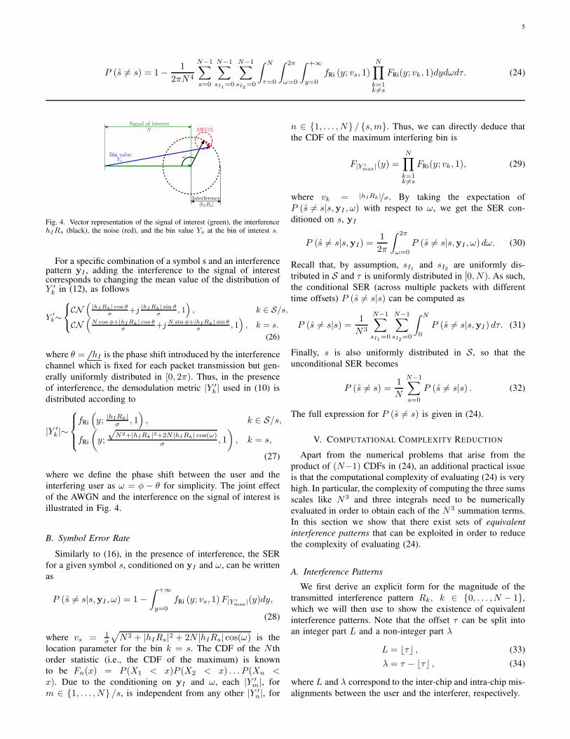
jhIRsj

N

Signal of interest

Interference

AWGN

Bin valueYs

Fig. 4. Vector representation of the signal of interest (green), the interferencehIRs (black), the noise (red), and the bin value Ys at the bin of interest s.

For a specific combination of a symbol s and an interferencepattern yI , adding the interference to the signal of interestcorresponds to changing the mean value of the distribution ofY ′k in (12), as follows

Y ′k∼

CN(

|hIRk| cos θσ

+j |hIRk| sin θ

σ, 1)

, k ∈ S/s,

CN(

N cos φ+|hIRk| cos θσ

+j N sinφ+|hIRk| sin θ

σ, 1)

, k = s.

(26)

where θ = hI is the phase shift introduced by the interference

channel which is fixed for each packet transmission but gen-

erally uniformly distributed in [0, 2π). Thus, in the presence

of interference, the demodulation metric |Y ′k| used in (10) is

distributed according to

|Y ′k|∼

fRi

(

y; |hIRk|σ , 1

)

, k ∈ S/s,

fRi

(

y;

√N2+|hIRk|2+2N |hIRk| cos(ω)

σ , 1

)

, k = s,

(27)

where we define the phase shift between the user and the

interfering user as ω = φ − θ for simplicity. The joint effect

of the AWGN and the interference on the signal of interest is

illustrated in Fig. 4.


Similarly to (16), in the presence of interference, the SER

for a given symbol s, conditioned on yI and ω, can be written

as

P (s 6= s|s,yI , ω) = 1−∫ +∞

y=0

fRi (y; vs, 1)F|Y ′

max|(y)dy,

(28)

where vs = 1σ

√

N2 + |hIRs|2 + 2N |hIRs| cos(ω) is the

location parameter for the bin k = s. The CDF of the N th

order statistic (i.e., the CDF of the maximum) is known

to be Fn(x) = P (X1 < x)P (X2 < x) . . . P (Xn <x). Due to the conditioning on yI and ω, each |Y ′

m|, for

m ∈ {1, . . . , N} /s, is independent from any other |Y ′n|, for

n ∈ {1, . . . , N} / {s,m}. Thus, we can directly deduce that

the CDF of the maximum interfering bin is

F|Y ′

max|(y) =

N∏

k=1k 6=s

FRi(y; vk, 1), (29)

where vk = |hIRk|/σ. By taking the expectation of

P (s 6= s|s,yI , ω) with respect to ω, we get the SER con-

ditioned on s, yI

P (s 6= s|s,yI) =1

2π

∫ 2π

ω=0

P (s 6= s|s,yI , ω)dω. (30)

Recall that, by assumption, sI1 and sI2 are uniformly dis-

tributed in S and τ is uniformly distributed in [0, N). As such,

the conditional SER (across multiple packets with different

time offsets) P (s 6= s|s) can be computed as

P (s 6= s|s) = 1

N3

N−1∑

sI1=0

N−1∑

sI2=0

∫ N

0

P (s 6= s|s,yI) dτ. (31)

Finally, s is also uniformly distributed in S, so that the

unconditional SER becomes

P (s 6= s) =1

N

N−1∑

s=0

P (s 6= s|s) . (32)

The full expression for P (s 6= s) is given in (24).

V. COMPUTATIONAL COMPLEXITY REDUCTION

Apart from the numerical problems that arise from the

product of (N−1) CDFs in (24), an additional practical issue

is that the computational complexity of evaluating (24) is very

high. In particular, the complexity of computing the three sums

scales like N3 and three integrals need to be numerically

evaluated in order to obtain each of the N3 summation terms.

In this section we show that there exist sets of equivalent

interference patterns that can be exploited in order to reduce

the complexity of evaluating (24).

A. Interference Patterns

We first derive an explicit form for the magnitude of the

transmitted interference pattern Rk, k ∈ {0, . . . , N − 1},

which we will then use to show the existence of equivalent

interference patterns. Note that the offset τ can be split into

an integer part L and a non-integer part λ

L = ⌊τ⌋ , (33)

λ = τ − ⌊τ⌋ , (34)

where L and λ correspond to the inter-chip and intra-chip mis-

alignments between the user and the interferer, respectively.

6

Using the definition of the DFT and after some algebraic

transformations, we have

Rk =

N−1∑

n=0

Zk,n, (35)

where Zk,n is defined as

Zk,n =

{

T1ej 2π

N n(sI1−k−τ)e−j2πλ, n ∈ NL1 ,

T2ej 2π

N n(sI2−k−τ), n ∈ NL2 ,(36)

and Ti are terms that are independent of the summation

variable n which are given by

Ti = ej2πτ2

2N ej2πτ2 e−j2π

sIiτ

N . (37)

Using the geometric series sum formula and after some

relatively straightforward operations, Rk can be written as

Rk = Ak,1e−jθk,1 +Ak,2e

−jθk,2 , (38)

where

Ak,1 =sin(

πN (sI1 − k − τ)⌈τ⌉

)

sin(

πN (sI1 − k − τ)

) , (39)

Ak,2 =sin(

πN (sI2 − k − τ)(N − ⌈τ⌉)

)

sin(

πN (sI2 − k − τ)

) , (40)

and

θk,1 =π

N

(

−τ2 + (λ−L)N + sI1(2τ − ⌈τ⌉+ 1)+

+ k(⌈τ⌉ − 1)+τ(⌈τ⌉ − 1)) , (41)

θk,2 =π

N

(

−τ2 + sI2(2τ − ⌈τ⌉+ 1−N)+

+ k(⌈τ⌉ − 1 +N) + τ(⌈τ⌉ − 1)) . (42)

For the special case where τ is an integer and k = [sI1 − τ ]Nand k = [sI2 − τ ]N , (39) and (40), respectively, are of the

indeterminate form 00 . Using L’Hopital’s rule, it can be shown

that in these cases we have Ak,1 = ⌈τ⌉, and Ak,2 = N −⌈τ⌉.

Using Euler’s formula, and for all k ∈ S, the magnitude of

Rk in (38) can be written as

|Rk| =√

A2k,1 +A2

k,2 + 2Ak,1Ak,2 cos(θk,1 − θk,2). (43)

B. Equivalent Interference Patterns

We first give a definition for the equivalent interference

patterns. Then, we show two equivalent interference pattern

properties and we explain how they can be used in order to

reduce the computational complexity of evaluating (24).

Definition 1. An interference pattern yI1 is said to be equiv-

alent with respect to some other interference pattern yI2 if

it contains exactly the same set of frequency bin magnitudes

|Rk|, k ∈ S, irrespective of the order of these magnitudes

within the set.

We note that the ordering of the magnitudes |Rk| does

not change the distribution of |Y ′max|, thus the probability

of |Y ′max| > |Y ′

s | is not affected. Therefore, equivalent in-

terference patterns result in exactly the same conditional SER

P (s 6= s|s,yI), meaning that it is sufficient to compute each

distinct interference pattern once for the evaluation of the

unconditional SER P (s 6= s) given in (24). Naturally, care has

to be taken so that the contribution of each distinct interference

pattern is weighted according to how many other equivalent

interference patterns exist.

Proposition 1. Let δ ∈ {0, 1, ..., N−1} and sI1 ≥ sI2 without

loss of generality and let τ be fixed. Moreover, let s′I1 = [sI1+δ]N and s′I2 = [sI2 + δ]N . Then there exist the following two

sets of equivalent interference patterns

YI1 ={

yI(s′I1 , s

′I2 , τ) : s

′I1 ≥ s′I2

}

, (44)

YI2 ={

yI(s′I1 , s

′I2 , τ) : s

′I1 < s′I2

}

, (45)

where the interference patterns in YI1 are generally not

equivalent versions of the patterns in YI2 . Furthermore, the

cardinalities of the two sets are

|YI1 | = N − (sI1 − sI2), (46)

|YI2 | = (sI1 − sI2). (47)

In the special case where λ = 0 (i.e., when τ is an integer),

all interference patterns in both YI1 and YI2 are equivalent.

Proof: A detailed proof is given in the Appendix.

Proposition 2. Let τ ∈ [0, N − 1) and let τ ′ be

τ ′ = (N − 1)− τ. (48)

Then, the interference patterns yI(sI1 , sI2 , τ) and

yI(sI1 , sI2 , τ′) are equivalent.

Proof: A detailed proof is given in the Appendix.

C. Complexity Reduction

The essence of Proposition 1 is that there are only two

sets of distinct interference patterns for each value of sI =[sI1−sI2 ]N . Let Pe(YIi ) = P (s 6= s|s,yIi(sI , τ)), where

yIi(sI , τ) denotes any (equivalent) element of YIi . Then, the

double sum in (31) can be simplified to

P (s 6= s|s) = 1

N3

N−1∑

sI1=0

N−1∑

sI2=0

∫ N

0

P (s 6= s|s,yI) dτ (49)

=1

N2

N−1∑

sI=0

∫ N

0

(

1

N

2∑

i=1

|YIi |Pe(YIi )

)

dτ,

(50)

which reduces the complexity of evaluating (24) by a factor of

N/2. In the special case of integer offsets τ (i.e., λ = 0 and

τ = L) the above integral can be simplified to a sum over all

the integer offsets L. Moreover, in such a case, the sets YIi

are equivalent, meaning that there is only one set of equivalent

interference patterns YI . Therefore, the above expression can

be further simplified to the expression found in [29]

P (s 6= s|s) = 1

N2

N−1∑

sI=0

N−1∑

L=0

Pe(YI). (51)

Proposition 2 essentially means that any interference pattern

with τ ∈ ((N−1)/2, N−1] is equivalent with exactly one inter-

ference pattern with τ ∈ [0, (N−1)/2). It is important to note

7

that we have not shown any property about the interference

patterns in the region τ ∈ (N − 1, N), so we consider this

region separately.1 If we let Pe =(

1N

∑2i=1 |YIi |Pe(YIi )

)

,

the expression in (50) can be re-written as

P (s 6= s|s) = 1

N2

N−1∑

sI=0

(

2

∫N−1

2

0

Pedτ +

∫ N

N−1

Pedτ

)

,

(52)

which reduces the complexity of evaluating (24) by an ad-

ditional factor of approximately 2. In the special case of

integer offsets τ (i.e., λ = 0 and τ = L) any interference

pattern with τ ∈ {N/2, N−1} is equivalent with exactly one

interference pattern with τ ∈ {0,N/2−1}. Therefore, the above

two integrals can be simplified to a summation over all the

integer offsets L. In this integer-offset case we have

P (s 6= s|s) = 1

N(

N2

)

N−1∑

sI=0

N2 −1∑

L=0

Pe(YI). (53)

We note that the corresponding simplification that is used

in [29], corresponding to the special chip-aligned case, is

different than the simplification we gave in (53). Specifically,

in [29] the upper limit of the sum over L is N/2 and,

consequently, the normalization is done with(

N2 + 1

)

instead

of N2 . However, the interference pattern resulting from τ = N

2is equivalent with the interference pattern resulting from

τ = N2 −1, which has already been considered in the sum.

D. Symbol Error Rate Approximation

Since, even with the above simplifications, the complexity

of evaluating (24) is very high, we derive a low-complexity

approximation for (24). Using the triangle inequality, we can

simplify (43) to

|Rk| ≈ |Ak,1|+ |Ak,2|. (54)

With this simplification, the Ak,1Ak,2 cos(θk,1−θk,2) term that

leads to the existence of two sets of interference patterns YI1

and YI2 (cf. proof of Proposition 1) disappears. Thus, there is

only a single set of interference patterns YI and (50) can be

simplified to

P (s 6= s|s) ≈ 1

N2

N−1∑

sI=0

∫ N

0

Pe(YI)dτ. (55)

Moreover, we also approximate (52) by ignoring the second

integral for τ ∈ (N − 1, N) so that

P (s 6= s|s) ≈ 2

N2

N−1∑

sI=0

∫N−1

2

0

Pe(YI)dτ, (56)

We now follow a procedure that is similar to the procedure

in [29] in order to derive a simple approximation for Pe(YI).

1It is relatively simple to verify that the region τ ∈ (N − 1, N) contains

equivalent interference patterns around the point τ = N − 12

following thesyllogism of the proof of Property 2. However, this property only marginallyreduces the computational complexity and we thus neither use it nor prove itexplicitly.

First, we assume that the interference-induced SER is dom-

inated by the maximum of |Rk|. Thus, we are interested in

evaluating

|Rkmax | = maxk

(|Ak,1|+ |Ak,2|) . (57)

Without loss of generality, we assume that sI2 = 0, so that

sI = sI1 . Since τ ∈ [0, (N−1)/2) and due to (39) and (40)

it holds that maxk (|Ak,2|) > maxk (|Ak,1|). Based on this

observation, we choose

kmax ≈ argmaxk

(|Ak,2|) = ⌊τ⌉, (58)

so that we can easily approximate |Rkmax | as

|Rkmax | ≈ |A⌊τ⌉,1 +A⌊τ⌉,2|. (59)

The probability of the event that the (maximum) interference

bin ⌊τ⌉ coincides with the bin of the signal-of-interest sis 1

N . Since in LoRa N is relatively large (N > 27),

the impact of the aforementioned event on the total error

probability is negligible, and therefore, for the approximation

of the SER, we only consider the cases where ⌊τ⌉ 6= s.

The aforementioned fact, combined with (59) which says that

all bins except s and ⌊τ⌉ are zero-valued, means that the

approximation of the SER does not depend on the value of

s. As such, P (s 6= s|s) = P (s 6= s) and calculating the

expectation over s can be avoided. Only considering ⌊τ⌉ 6= salso has the convenient side-effect that we ignore the only

case of (27) which contains ω, meaning that we can entirely

avoid the integration over ω in the computation of Pe(YI). Let

P (I)(s 6= s) denote the interference-dominated SER resulting

from the approximation in (59). As explained in Section IV-A,

|Y ′kmax

| follows a Rice distribution, which can be approximated

by a Gaussian distribution for large location parameters [29]

so that

|Y ′kmax

| ∼ N( |hI ||Rkmax |

σ, 1

)

. (60)

Using the Gaussian approximation, the interference-dominated

SER P (I)(s 6=s) can be computed as

P (I)(s 6=s) =1

N(

N2

)

N−1∑

sI=0

∫N−1

2

0

Q

(

N − |hI ||Rkmax |√2σ2

)

dτ,

(61)

where Q(·) denotes the Q-function and the integral can be

evaluated numerically by discretizing the interval [0, (N−1)/2)with a step size ǫ as

P (I)(s 6=s) ≈ ǫ

N(

N2

)

N−1∑

sI=0

∑

τ∈T

Q

(


)

,

(62)

where T ={

0, ǫ, 2ǫ, . . . , N−12 − ǫ

}

.

We note that, in the low SNR (i.e., AWGN-limited) regime,

the above approximation becomes inaccurate, since all bins

have similar values and no single bin dominates the error rate.

Let P (N)(s 6= s) denote the SER under AWGN given in (16)

(which can be evaluated efficiently using the approximation

8

in (17)). Then, a final estimate of the SER that is more accurate

also in the low SNR regime [29] can be obtained as

P (s 6=s) ≈ P (N)(s 6=s)+(

1−P (N)(s 6=s))

P (I)(s 6=s). (63)

VI. FRAME ERROR RATE UNDER AWGN AND

SAME-SF INTERFERENCE

Since network simulators, such as the ones presented

in [17]–[20], typically operate on a frame level, the frame error

rate (FER) is generally of greater practical relevance than the

SER. The expression for the SER derived in Section IV can

not be used directly to evaluate the FER because it includes

an expectation over τ and an expectation over ω, while all

symbols in a frame would experience the same τ and ω.

For this reason, in this section we derive an expression to

approximate the FER. We note that we are considering the

FER of an uncoded system. Thus, the expression we derive can

be used for the LoRa mode that uses a channel code of rate 4/5,which has error-detection but no error-correction capabilities.

We first make the following simplifying assumptions. We

assume that perfect frame synchronization for the user of

interest is achieved even in the presence of interference. Then,

we also assume that the interfering frame has the same length

as the frame of interest. The latter assumption is taken only

for clarity of the presentation and does not restrict our results

from being easily generalized to any interfering frame length.

Due to the time offset between the frames, only part of the

frame of interest is affected by interference.

Let the vector s denote a frame of F LoRa symbols and

let the vector s denote the estimated frame at the receiver.

The FER can then be defined as P (s 6= s). Moreover, let Fi,

where i ∈ {1, . . . , F}, denote the number of symbols in the

frame that are affected by the interfering frame. The value

of Fi depends on the relative position of the two frames.

As mentioned in [26], the random relative position of the

two frames plays an important role on the final FER. We

consider the final FER as the expectation over all the possible

relative positions of the two frames. We note that, except in

the case of perfect alignment between the frame of interest

and the interference, there always exists one symbol that

is only partially affected by interference. For simplicity, we

approximate this situation by considering the partially-affected

symbol as fully-affected by interference, thus including it in

Fi. The number of symbols in the frame that are affected

only by AWGN is F − Fi. Since the frame of interest and

the interfering frame have the same length, the number Fi

of interfered symbols in a frame is uniformly distributed in

{1, . . . , F}.

Since all symbols of the interfering frame have the same

offset τ , the probability, for a given Fi, that all Fi symbols

under interference and all F − Fi symbols under AWGN are

correct is

P (s = s|Fi, τ) = (1− P (s 6= s|τ))Fi

(

1− P (N)(s 6= s))F−Fi

,

(64)

−22 −20 −18 −16 −14 −12 −10 −8 −610−5

10−4

10−3

10−2

10−1

100

1/ǫ 1 2 3 4

SF= 9:

SF= 10:

SF= 11:

SNR (dB)

Sym

bol

Err

or

Rat

e

Fig. 5. Symbol error rate approximation of the LoRa modulation underAWGN and same-SF interference for SF ∈ {9, 10, 11} and PI = −3 dB,for various values of the oversampling factor 1/ǫ.

where P (s 6= s|τ) can be approximated as

P (s 6= s|τ) = 1

N

N−1∑

sI=0

Q

(


)

. (65)

By using a similar simplification to (56), the conditional frame

error rate P (s 6= s|Fi) can be approximated as

P (s 6= s|Fi) ≈2

N

∫N−1

2

0

(1− P (s = s|Fi, τ)) dτ. (66)

Finally, we take the expectation over all possible values of Fi

and we obtain the final expression for the FER

P (s 6= s) ≈ 1

F

F∑

Fi=1

P (s 6= s|Fi). (67)

VII. RESULTS

In this section, we provide numerical results for the SER

and the FER of a LoRa user with same-SF interference.

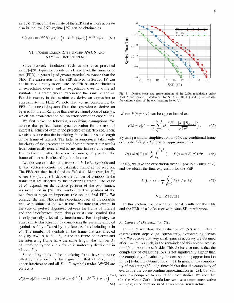
A. Choice of Discretization Step

In Fig. 5 we show the evaluation of (62) with different

discretization steps ǫ (or, equivalently, oversampling factors1/ǫ). We observe that very small gains in accuracy are obtained

after ǫ = 1/3. As such, in the remainder of this section we use

ǫ = 1/5 to be on the safe side. This choice also means that the

complexity of evaluating (62) is not significantly higher than

the complexity of evaluating the corresponding approximation

in [29] (which is obtained for ǫ = 1). In general, the complex-

ity of evaluating (62) is 1/ǫ times higher than the complexity of

evaluating the corresponding approximation in [29], but still

very low compared to simulation-based studies. We note that

for the Monte Carlo simulations we use a more conservative

ǫ = 1/10, since they are used as a comparison baseline.

9

−25 −20 −15 −10 −5 010−5

10−4

10−3

10−2

10−1

100

SNR (dB)

Sym

bol

Err

or

Rat

e

PO: SF=7 SF=8 SF=9 SF=10 SF=11 SF=12

Non-PO: SF=7 SF=8 SF=9 SF=10 SF=11 SF=12

Fig. 6. Symbol error rate of the LoRa modulation under AWGN and same-SFinterference for SF ∈ {7, . . . , 12} and PI = −3 dB. Black dotted lines showthe SER when ignoring the phase offset ω and thick transparent lines showthe SER when there is only AWGN for comparison (taken from Fig. 2).

−22 −20 −18 −16 −14 −12 −10 −8 −610−5

10−4

10−3

10−2

10−1

100

Non-aligned (this work)

MC Approx.

SF=9:

SF=10:

SF=11:

Aligned [29]

MC Approx.

SF=9:

SF=10:

SF=11:

SNR (dB)

Sym

bol

Err

or

Rat

e

Fig. 7. Symbol error rate of the LoRa modulation under AWGN and same-SF interference for SF ∈ {9, 10, 11} and PI = −3 dB. The approximationsof [29] and (63) are shown with black dotted lines.


In Fig. 6, we show the results of a Monte Carlo simulation

for the SER of a LoRa user for all possible spreading factors

SF ∈ {7, . . . , 12}, under the effect of same-SF interference

with an SIR of 3 dB (i.e., PI = −3 dB) and AWGN. The

SER when there is only AWGN is also included in the figure

with thick transparent lines (taken from Fig. 2). We can clearly

observe the strong impact of the interference on the SER when

comparing to the case where there is only AWGN. The black

dotted lines in the figure depict the SER when the relative

phase offset ω between the interferer and the user is not taken

into account in the Monte Carlo simulation. It is interesting to

observe that ω does not seem to play an important role for the

SER, which further justifies ignoring ω in the approximation

of Section V-D.


0 1 2 3 4 5 6 7 8 9 10

−20

−15

−10

−5

0

5

10

15Non-aligned (this work)

Approx.

SF=7:

SF=12:

Aligned [29]

Approx.

SF=7:

SF=12:

SIR (dB)

SN

R(d

B)

Fig. 8. Required SNR for a target symbol error rate of 2 ·10−5 as a functionof the SIR for SF = 7 and SF = 12.

for the SER of a LoRa user with SF ∈ {9, 10, 11} using the

chip-aligned model of [29] and the model we described in

this work, as well as the corresponding approximations in (61)

and [29], respectively. We observe that there exists a significant

difference of approximately 1 dB between the two models,

meaning that the chip-aligned model of [29] is pessimistic in

the computation of the SER. This can be intuitively explained

as follows. When the offset τ is an integer, the maximum

value of the interference magnitudes Ak,1 and Ak,2 with

respect to the index k is always larger than when τ is not an

integer. As such, considering only chip-aligned interference is

a worst-case scenario. Finally, we can clearly observe that the

low-complexity computation of (24) using the approximation

derived in Section V-D is very accurate.

In Fig. 8, we show the required SNR for a target SER

performance of 2 · 10−5, for different SIR levels and for the

two extremal spreading factors, i.e., SF = 7 and SF = 12.

The target SER performance of 2 · 10−5 is chosen similarly

to [29] and in accordance with the sensitivity thresholds for a

bandwidth of B = 125 kHz and a coding rate of R = 4/5, as

provided by Semtech [7]. The SNR vs SIR plot is important

for every framework that considers AWGN and interference

jointly and was introduced in [29]. It is obvious that as the

interference power increases, there is a significant increase in

the required SNR to obtain the same performance. We can

observe that the chip-aligned model of [29] overestimates the

required SNR increase for both the extremal spreading factors.

Moreover, the overestimation is slightly more pronounced for

higher levels of interference, since in the interference-limited

regime, the impact of the overestimation of the chip-aligned

model is higher than in the noise-limited regime.

It is important to note that the framework that treats the

signal and the interference in a unified fashion, which is used

both in [29], [30] and in this work, does not contradict, but

rather enhances the view of the non-unified framework of [6],

[15], [19]. In particular, in the non-unified framework, the

SNR and the SIR are considered independently, and a LoRa

message is received successfully only if both of the following

two assumptions hold

10

1) SNR > SNR(SF)thr , where SNR

(SF)thr is the SF-specific SNR

threshold for a given target error probability, and

2) SIR > 6 dB

In the unified SINR framework, a message can potentially

survive even if SIR < 6 dB if in turn the SNR is high enough.

This SNR-SIR trade-off is in essence the information that

Fig. 8 provides. Therefore, the unified SINR framework allows

for a softer decision threshold on the successful reception of

a LoRa message, rather than the hard 6 dB SIR threshold that

is commonly used in the literature. On the other hand, the

effect of multiple same-SF interferers can easily be handled

under the non-unified framework. As explained in [15], the

analysis for multiple same-SF interferers can be simplified by

considering only the most powerful interferer in the SIR value;

the larger the number of same-SF users in the network, the

higher the probability that the most powerful interferer will

lead to a critical SIR (e.g., < 6 dB). The effect of multiple

same-SF interferers on the error rate under the unified SINR

framework is a field that needs to be explored further.

C. Frame Error Rate


for the FER of a LoRa user with SF ∈ {9, 10, 11} using the

chip-aligned model of [29] and the model we described in this

work, as well as the corresponding approximation described

in Section VI. The frame contains F = 10 LoRa symbols,

which is a valid data payload length for LoRa. We observe

the same difference of approximately 1 dB between the two

models. Moreover, we can see that the approximation for the

FER described in Section VI is very accurate.

In Fig. 10, we show the required SNR for a target FER

performance of 10−1, for different SIR levels, and for the

two extremal spreading factors, i.e., SF = 7 and SF = 12.

Similarly to Fig. 8, as the interference power increases, there

is an increase in the required SNR to obtain the same per-

formance. For the chosen target FER performance of 10−1

we can observe that the overestimation of the chip-aligned

model of [29] is clearly more pronounced for higher levels of

interference.

Finally, in Fig. 11, we show the required SNR for two

different target FERs and three different frame lengths, for

different SIR levels and for SF = 7. Specifically, we choose

both a typical target FER performance of 10−1 and a stricter

target FER of 10−2 [26], and we choose frames of length

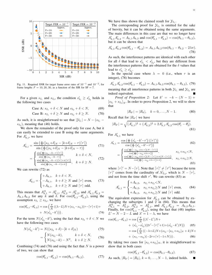
F = 10, F = 20, and F = 30 LoRa symbols. We observe that

longer frames require a larger increase in the required SNR

for successful reception under the same interference power.

Moreover, the performance requirement plays an important

role, since the increase in the required SNR values for a packet

to survive under a stricter target FER performance is very

pronounced.

VIII. CONCLUSION

In this work, we introduced a LoRa interference model

where the interference is neither chip- nor phase-aligned with

the LoRa signal-of-interest and we derived a corresponding

expression for the SER and the FER. Moreover, we proved

−22 −20 −18 −16 −14 −12 −10 −8 −610−4

10−3

10−2

10−1

100

Non-aligned (this work)

MC Approx.

SF=9:

SF=10:

SF=11:

Aligned [29]

MC Approx.

SF=9:

SF=10:

SF=11:

SNR (dB)

Fra

me

Err

or

Rat

e

Fig. 9. Frame error rate of the LoRa modulation for a frame length F = 10under AWGN and same-SF interference for SF ∈ {9, 10, 11} and PI = −3dB. The approximations of [29] and (63) are shown with black dotted lines.

0 1 2 3 4 5 6 7 8 9 10

−20

−15

−10

−5

0

5Non-aligned (this work)

Approx.

SF=7:

SF=12:

Aligned [29]

Approx.

SF=7:

SF=12:

SIR (dB)

SN

R(d

B)

Fig. 10. Required SNR for a target frame error rate of 10−1 as a functionof the SIR for SF = 7 and SF = 12.

two properties of same-SF LoRa-induced interference that

enabled us to reduce the complexity of calculating the SER

and the FER by a factor that is approximately equal to the

LoRa symbol length N . Finally, we derived a low-complexity

approximation for both the SER and the FER and we showed

that ignoring the non-integer time offsets overestimates the

error rate by 1 dB.

APPENDIX

Proof of Proposition 1: We will first show that YI1 indeed

contains N−(sI1−sI2) equivalent interference patterns for a

given sI1 and sI2 , which can be obtained by setting s′I1 =[sI1 + δ]N , s′I2 = [sI2 + δ]N , and k′ = [k + δ]N . Recall that

for |Rk′ | we have

|Rk′ | =√

(A′k,1)

2 + (A′k,2)

2 + 2A′k,1A

′k,2 cos(θ

′k,1 − θ′k,2).

(68)

Then, our goal essentially is to show that |Rk′ | = |Rk| for all

δ such that s′I1 ≥ s′I2 , and for all k.

11

0 1 2 3 4 5 6 7 8 9 10−10

−5

0

5

10Target FER = 10−1

Approx.

F=10:

F=20:

F=30:

Target FER = 10−2

Approx.

F=10:

F=20:

F=30:

SIR (dB)

SN

R(d

B)

Fig. 11. Required SNR for target frame error rates of 10−1 and 10−2, forframe lengths F = 10, 20, 30, as a function of the SIR for SF = 7.

For a given sI1 and sI2 , the condition s′I1 ≥ s′I2 holds in

the following two cases

Case A: sI1 + δ < N and sI2 + δ < N, (69)

Case B: sI1 + δ ≥ N and sI2 + δ ≥ N. (70)

As such, it is straightforward to see that |YI1 | = N − (sI1 −sI2), meaning that (46) holds.

We show the remainder of the proof only for case A, but it

can easily be extended to case B using the same arguments.

For A′k,i, we have

A′k,i =

sin(

πN ([sIi+δ]N − [k+δ]N − τ)⌈τ⌉

)

sin(

πN ([sIi+δ]N − [k+δ]N − τ)

) (71)

=

sin( πN (sIi−k−τ)⌈τ⌉)

sin( πN (sIi−k−τ))

, k + δ < N,

sin( πN (sIi−k−τ)⌈τ⌉+π⌈τ⌉)sin( π

N (sIi−k−τ)+π), k + δ ≥ N.

(72)

We can rewrite (72) as

A′k,i =

+Ak,i, k + δ < N,

−Ak,i, k + δ ≥ N and ⌈τ⌉ even,

+Ak,i, k + δ ≥ N and ⌈τ⌉ odd.

(73)

This means that A′2k,1 = A2

k,1, A′2k,2 = A2

k,2, and A′k,1A

′k,2 =

Ak,1Ak,2 for any k and δ. For cos(θ′k,1−θ′k,2), using theassumption sI1 ≥ sI2 , we have

cos(θ′k,1−θ′k,2) = cos( π

N((λ−L)N+(sI1−sI2)(τ−⌈τ⌉+1)+

+ N(s′I2−k′)))

. (74)

For the term N(s′I2−k′), using the fact that sI2 + δ < N we

have the following two cases

N(s′I2−k′) = N((sI2 + δ)−[k + δ]N ) (75)

=

{

N(sI2−k), k + δ < N,

N(sI2−k)−N2, k + δ ≥ N.(76)

Combining (74) and (76) and using the fact that N is a power

of two, we can show that

cos(θ′k,1−θ′k,2) = cos(θk,1−θk,2). (77)

We have thus shown the claimed result for YI1 .

The corresponding proof for YI2 is omitted for the sake

of brevity, but it can be obtained using the same arguments.

The main differences in this case are that we no longer have

A′k,1A

′k,2 = Ak,1Ak,2 and cos(θ′k,1−θ′k,2) = cos(θk,1−θk,2),

but it can be shown that

A′k,1A

′k,2 cos(θ

′k,1 − θ′k,2) = Ak,1Ak,2 cos(θk,1 − θk,2 − 2λπ).

(78)

As such, the interference patterns are identical with each other

for all δ that lead to s′I1 < s′I2 , but they are different from

the interference patterns that are obtained for the δ values that

lead to s′I1 ≥ s′I2 .

In the special case where λ = 0 (i.e., when τ is an

integer), (78) becomes

A′k,1A

′k,2 cos(θ

′k,1 − θ′k,2) = Ak,1Ak,2 cos(θk,1 − θk,2), (79)

meaning that all interference patterns in both YI1 and YI2 are

indeed equivalent.

Proof of Proposition 2: Let k′ = −k − (N − 1) +[sI1 + sI2 ]N . In order to prove Proposition 2, we will to show

that

|Rk′ | = |Rk|, k = 0, . . . , N − 1. (80)

Recall that for |Rk′ | we have

|Rk′ | =√

(A′k,1)

2 + (A′k,2)

2 + 2A′k,1A

′k,2 cos(θ

′1 − θ′2).

(81)

For A′k,1 we have

A′k,1 =

cos(

πN

(

s′I1−k′−τ ′)

(⌈τ⌉′))

cos(

πN

(

s′I1−k′−τ ′)) (82)

=

cos( πN (−sI2

+k+τ)(N−⌈τ⌉))cos( π

N (−sI2+k+τ))

, sI1+sI2<N,

cos( πN (−sI2

+k+τ)(N−⌈τ⌉)+π(N−⌈τ⌉))cos( π

N (−sI2+k+τ)+π)

, sI1+sI2≥N,

(83)

where ⌈τ⌉′ = N−⌈τ⌉. Note that ⌈τ⌉′ 6= ⌈τ ′⌉ because the term

⌈τ⌉′ comes from the cardinality of NL2 , which is N − ⌈τ⌉,

and not from the time shift τ ′. We can rewrite (83) as

A′k,1 =

+Ak,2, sI1+sI2<N,

−Ak,2, sI1+sI2≥N and ⌈τ⌉ even,

+Ak,2, sI1+sI2≥N and ⌈τ⌉ odd.

(84)

The equivalent expression for A′k,2 can be obtained by ex-

changing the subscripts 1 and 2 in (84). This means thatA′2

k,1 = A2k,2, A′2

k,2 = A2k,1, and A′

k,1A′k,2 = Ak,2Ak,1.

Finally, for cos(θ′k,1 − θ′k,2), using the fact that (48) implies

L′ = N − 2− L and λ′ = 1− λ, we have

cos(θ′k,1−θ′k,2) = cos( π

N

(

(λ′−L′)N+

+ (s′I1−s′I2)(2τ′−⌈τ⌉′+1)+(s′I2−k′)N

))

(85)

= cos( π

N((−λ+L)N+(sI2−[sI1+sI2 ]N + k)N+

+ (sI1−sI2)(−2τ+⌈τ⌉−1+N))) . (86)

By taking two cases for [sI1+sI2 ]N , it is straightforward to

show that in both cases

cos(θ′k,1−θ′k,2) = cos(θk,1−θk,2). (87)

As such, |Rk′ | = |Rk|, k = 0, . . . , N − 1, indeed holds.

12

REFERENCES

[1] F. Adelantado, X. Vilajosana, P. Tuset-Peiro, B. Martinez, J. Melia-Segui, and T. Watteyne, “Understanding the limits of LoRaWAN,” IEEECommunications Magazine, vol. 55, no. 9, pp. 34–40, Sep. 2017.

[2] W. Bakkali, M. Kieffer, M. Lalam, and T. Lestable, “Kalman filter-based localization for internet of things LoRaWAN end points,” in IEEEAnnual International Symposium on Personal, Indoor, and Mobile Radio

Communications (PIMRC), Oct. 2017, pp. 1–6.[3] P. A. Catherwood, D. Steele, M. Little, S. Mccomb, and J. McLaughlin,

“A community-based IoT personalized wireless healthcare solution trial,”IEEE Journal of Translational Engineering in Health and Medicine,vol. 6, pp. 1–13, May 2018.

[4] H. M. Jawad, R. Nordin, S. K. Gharghan, A. M. Jawad, and M. Ismail,“Energy-efficient wireless sensor networks for precision agriculture: Areview,” Sensors, vol. 17, no. 8, 2017.

[5] U. Raza, P. Kulkarni, and M. Sooriyabandara, “Low power wide areanetworks: An overview,” IEEE Communications Surveys & Tutorials,vol. 19, no. 2, pp. 855–873, Secondquarter 2017.

[6] C. Goursaud and J.-M. Gorce, “Dedicated networks for IoT : PHY /MAC state of the art and challenges,” EAI Endorsed Transactions onInternet of Things, Oct. 2015.

[7] Semtech Corporation, “SX1272/73–860 MHz to 1020 MHzlow power long range transceiver.” [Online]. Available:https://www.semtech.com/uploads/documents/sx1272.pdf

[8] O. B. Seller and N. Sornin, “Low power long range transmitter,” USPatent 9,252,834, Feb., 2016.

[9] M. Knight and B. Seeber, “Decoding LoRa: Realizing a modern LPWANwith SDR,” in GNU Radio Conference, Sep. 2016.

[10] P. Robyns, P. Quax, W. Lamotte, and W. Thenaers, “A multi-channelsoftware decoder for the LoRa modulation scheme,” in International

Conference on Internet of Things, Big Data and Security (IoTBDS),Mar. 2018, pp. 41–51.

[11] L. Vangelista, “Frequency shift chirp modulation: The LoRa modula-tion,” IEEE Signal Processing Letters, vol. 24, no. 12, pp. 1818–1821,Dec. 2017.

[12] R. Ghanaatian, O. Afisiadis, M. Cotting, and A. Burg, “LoRa digitalreceiver analysis and implementation,” in IEEE International Conference

on Acoustics, Speech and Signal Processing (ICASSP), May 2019.[13] J. Haxhibeqiri, E. De Poorter, I. Moerman, and J. Hoebeke, “A survey of

LoRaWAN for IoT: From technology to application,” Sensors, vol. 18,no. 11, 2018.

[14] D. Bankov, E. Khorov, and A. Lyakhov, “Mathematical model ofLoRaWAN channel access with capture effect,” in IEEE Annual Inter-

national Symposium on Personal, Indoor, and Mobile Radio Communi-

cations (PIMRC), Oct. 2017, pp. 1–5.[15] O. Georgiou and U. Raza, “Low power wide area network analysis: Can

LoRa scale?” IEEE Wireless Communications Letters, vol. 6, no. 2, pp.162–165, Apr. 2017.

[16] R. B. Sørensen, D. M. Kim, J. J. Nielsen, and P. Popovski, “Analysisof latency and MAC-layer performance for class A LoRaWAN,” IEEE

Wireless Communications Letters, vol. 6, no. 5, pp. 566–569, Oct. 2017.[17] F. Van den Abeele, J. Haxhibeqiri, I. Moerman, and J. Hoebeke,

“Scalability analysis of large-scale LoRaWAN networks in ns-3,” IEEEInternet of Things Journal, vol. 4, no. 6, pp. 2186–2198, Dec. 2017.

[18] B. Reynders, Q. Wang, and S. Pollin, “A LoRaWAN module for ns-3:Implementation and evaluation,” in Workshop on ns-3, ser. WNS3 ’18.New York, NY, USA: ACM, 2018, pp. 61–68.

[19] M. C. Bor, U. Roedig, T. Voigt, and J. M. Alonso, “Do LoRa low-power wide-area networks scale?” in ACM International Conference on

Modeling, Analysis and Simulation of Wireless and Mobile Systems, ser.MSWiM ’16. New York, NY, USA: ACM, 2016, pp. 59–67.

[20] A. Pop, U. Raza, P. Kulkarni, and M. Sooriyabandara, “Does bidirec-tional traffic do more harm than good in LoRaWAN based LPWA net-works?” in IEEE Global Communications Conference (GLOBECOM),Dec. 2017, pp. 1–6.

[21] M. Centenaro, L. Vangelista, and R. Kohno, “On the impact of downlinkfeedback on LoRa performance,” in IEEE Annual International Sympo-sium on Personal, Indoor, and Mobile Radio Communications (PIMRC),Oct. 2017, pp. 1–6.

[22] A. J. Wixted, P. Kinnaird, H. Larijani, A. Tait, A. Ahmadinia, andN. Strachan, “Evaluation of LoRa and LoRaWAN for wireless sensornetworks,” in IEEE SENSORS, Oct. 2016, pp. 1–3.

[23] C. Orfanidis, L. M. Feeney, M. Jacobsson, and P. Gunningberg, “In-vestigating interference between LoRa and IEEE 802.15.4g networks,”in IEEE International Conference on Wireless and Mobile Computing,

Networking and Communications (WiMob), Oct. 2017, pp. 1–8.[24] B. Reynders, W. Meert, and S. Pollin, “Range and coexistence analysis

of long range unlicensed communication,” in International Conference

on Telecommunications (ICT), May 2016, pp. 1–6.[25] D. Croce, M. Gucciardo, I. Tinnirello, D. Garlisi, and S. Mangione,

“Impact of spreading factor imperfect orthogonality in LoRa communi-cations,” in Digital Communication. Towards a Smart and Secure Future

Internet, A. Piva, I. Tinnirello, and S. Morosi, Eds. Cham: SpringerInternational Publishing, 2017, pp. 165–179.

[26] D. Croce, M. Gucciardo, S. Mangione, G. Santaromita, and I. Tinnirello,“Impact of LoRa imperfect orthogonality: Analysis of link-level perfor-mance,” IEEE Communications Letters, vol. 22, no. 4, pp. 796–799,Apr. 2018.

[27] L. Feltrin, C. Buratti, E. Vinciarelli, R. De Bonis, and R. Verdone,“LoRaWAN: Evaluation of link- and system-level performance,” IEEE

Internet of Things Journal, vol. 5, no. 3, pp. 2249–2258, Jun. 2018.[28] T. Elshabrawy and J. Robert, “Closed-form approximation of LoRa

modulation BER performance,” IEEE Communications Letters, vol. 22,no. 9, pp. 1778–1781, Sep. 2018.

[29] T. Elshabrawy and J. Robert, “Analysis of BER and coverage perfor-mance of LoRa modulation under same spreading factor interference,” inIEEE International Symposium on Personal, Indoor and Mobile Radio

Communications (PIMRC), Sep. 2018.[30] T. Elshabrawy and J. Robert, “Capacity planning of LoRa networks with

joint noise-limited and interference-limited coverage considerations,”IEEE Sensors Journal, pp. 1–1, Feb. 2019.

[31] O. Afisiadis, M. Cotting, A. Burg, and A. Balatsoukas-Stimming,“LoRa symbol error rate under non-aligned interference,” in Asilomar

Conference on Signals, Systems, and Computers, Nov. 2019.[32] M. Chiani and A. Elzanaty, “On the LoRa modulation for IoT: Wave-

form properties and spectral analysis,” IEEE Internet of Things Journal,May 2019 (early access).

[33] H. A. David and H. N. Nagaraja, Order Statistics. Wiley, 2003.

https://www.semtech.com/uploads/documents/sx1272.pdf

On the Error Rate of the LoRa Modulation with Interference

Documents

Transcript of On the Error Rate of the LoRa Modulation with Interference