
Implementation of a Fuzzy Logic Based Set-Point ... - MSpace
Upload
khangminh22Category
view
0download
0
DESIGN AND IMPLEMENTATION OF A FUZZY
LOGIC BASED MAXIMUM POWER POINT
TRACKER FOR A PHOTOVOLTAIC SYSTEM
LAWRENCE KIPRONO LETTING
MASTER OF SCIENCE
(Electrical Engineering)
JOMO KENYATTA UNIVERSITY OF
AGRICULTURE AND TECHNOLOGY
2008

- i -
Design and Implementation of a Fuzzy Logic Based Maximum
Power Point Tracker for a Photovoltaic System
Lawrence Kiprono Letting
A thesis submitted in partial fulfillment for the degree of Master of
Science in Electrical Engineering in the Jomo Kenyatta University
of Agriculture and Technology
2008

- ii -
DECLARATION
This thesis is my original work and has not been presented for a degree in any other
university.
Signature ………………….. Date …………………
Lawrence Kiprono Letting
This thesis has been submitted for examination with our approval as university
supervisors:
Signature ………………….. Date …………………
Dr. George N. Nyakoe
JKUAT, Kenya.
Signature ………………….. Date …………………
Dr. Cyrus W. Wekesa
UoN, Kenya.

- iii -
DEDICATION
I would like to dedicate this thesis to my mother for her constant and endless
support.

- iv -
ACKNOWLEDGEMENTS
First, I would like to take this opportunity to thank my supervisors Dr. G.N. Nyakoe
and Dr. C.W. Wekesa for their valuable guidance and support throughout my
research project. Their patience and encouragement were invaluable in the course of
this research.
I would also like to thank my postgraduate colleagues including Kipyegon Edwin,
Kibet Philip, Omae Oteri, Manene Franklin, and Irungu George for their support. In
addition, I would like to thank the Chairman of the EEE department Dr. L.M. Ngoo
for introducing us into the world of fuzzy logic. I would also like to thank
D’Oketch and Kibunja at Electronics laboratory for their support. I will also not
forget Barnabas Togom of Maryland, USA for his assistance in acquiring the data
acquisition card. For that, I am extremely grateful.
Finally, I would like to thank my family and friends for their encouragement and
support throughout my studies. Last but by no means the least, I would like to thank
God for having seen me through all the challenges in my academic work.

- v -
TABLE OF CONTENTS
Declaration.................................................................................................................. ii
Dedication .................................................................................................................. iii
Acknowledgements ................................................................................................... iv
List of Tables ............................................................................................................. xi
List of Figures........................................................................................................... xii
List of Appendices.................................................................................................... xv
List of Abbreviations .............................................................................................. xvi
List of Symbols ...................................................................................................... xviii
Abstract .................................................................................................................. xxiii
CHAPTER ONE ........................................................................................................ 1
1 INTRODUCTION........................................................................................... 1
1.1 Background...................................................................................................... 1
1.2 Statement of the Problem ................................................................................ 3
1.3 Objectives ........................................................................................................ 3
1.4 An Overview on MPPT Algorithms ............................................................... 4
1.5 Fundamentals of Fuzzy Logic Controllers ..................................................... 6
1.5.1 What is Fuzzy Logic? ......................................................................... 6
1.5.2 Fuzzy Sets and Membership Functions.............................................. 7

- vi -
1.5.3 Fuzzy Rules and Inferencing .............................................................. 8
1.5.4 Fuzzy Controller Structure.................................................................. 8
1.6 Application of Fuzzy Logic in MPPT Control ............................................. 10
1.7 Thesis Organization....................................................................................... 12
CHAPTER TWO ..................................................................................................... 14
2 MODELING OF A PHOTOVOLTAIC MODULE .................................... 14
2.1 Model Theory ................................................................................................ 14
2.1.1 Model Inputs ..................................................................................... 15
2.1.2 Model Outputs................................................................................... 15
2.1.3 Modifying Parameters....................................................................... 15
2.1.4 Solar Cell Model ............................................................................... 16
2.2 Modeling of the PV module.......................................................................... 18
2.2.1 PV Module Structure ........................................................................ 18
2.2.2 Model Parameters ............................................................................. 18
2.2.3 Determination of Model Parameters ................................................ 20
2.2.4 PV Array Structure............................................................................ 23
2.3 Simulink Models............................................................................................ 24
2.3.1 PV Array Model................................................................................ 25
2.3.2 PV Module Model............................................................................. 27
2.4 Model Validation........................................................................................... 28
2.5 Conclusion ..................................................................................................... 31

- vii -
CHAPTER THREE................................................................................................. 32
3 DC-DC CONVERTERS AND MAXIMUM POWER POINT
TRACKING…..………………………………………………………………….32
3.1 DC-DC Converters ........................................................................................ 32
3.2 Maximum Power Point Tracking.................................................................. 34
3.3 Identification of a Suitable Converter Topology for Maximum Power Point
Tracking ............................................................................................................... 36
3.3.1 Buck Converter ................................................................................. 36
3.3.2 Boost Converter ................................................................................ 37
3.3.3 Buck-Boost Converter ...................................................................... 37
3.3.4 Conclusion......................................................................................... 38
3.4 Buck-Boost Converter Model ....................................................................... 38
3.4.1 Mode 1............................................................................................... 39
3.4.2 Mode 2............................................................................................... 41
3.4.3 Mode 3............................................................................................... 43
3.5 Averaged Buck-Boost Converter Model ...................................................... 45
3.5.1 Method of State Space Averaging.................................................... 45
3.5.2 Converter Averaged Model .............................................................. 47
3.6 Buck-Boost Converter Simulink Model ....................................................... 49
3.7 Simulation Results......................................................................................... 50
3.8 Conclusion ..................................................................................................... 53

- viii -
CHAPTER FOUR.................................................................................................... 54
4 FUZZY LOGIC CONTROLLER DESIGN AND HARDWARE
IMPLEMENTATION................................................................................................ 54
4.1 Design of Fuzzy Logic Controller Parameters ............................................. 54
4.1.1 Controller Structure........................................................................... 54
4.1.2 Membership Functions ..................................................................... 56
4.1.3 Scaling Factors .................................................................................. 58
4.1.4 Derivation of Control Rules.............................................................. 58
4.1.5 Tuning of Control Rules ................................................................... 63
4.1.6 Decision Making ............................................................................... 63
4.1.7 Defuzzification.................................................................................. 65
4.2 Simulation Model .......................................................................................... 67
4.2.1 PV Source.......................................................................................... 68
4.2.2 Fuzzy Logic Controller ..................................................................... 69
4.2.3 Buck-Boost Converter ...................................................................... 69
4.3 Hardware Design Overview.......................................................................... 70
4.4 Buck-Boost Converter Operation.................................................................. 71
4.4.1 Continuous Inductor Current ............................................................ 72
4.4.2 Discontinuous Inductor Current ....................................................... 74
4.5 Buck-Boost Converter Design ...................................................................... 76
4.5.1 Inductor Selection ............................................................................. 77
4.5.2 Input Capacitor Selection.................................................................. 79

- ix -
4.5.3 Output Capacitor Selection............................................................... 80
4.5.4 Diode Selection ................................................................................. 81
4.5.5 Switching Transistor Selection ......................................................... 81
4.6 Pulse Width Modulation................................................................................ 82
4.6.1 SG3525A PWM IC Operation.......................................................... 82
4.6.2 Design Procedure .............................................................................. 84
4.7 Data Acquisition System............................................................................... 87
4.7.1 USB-1208FS Data Acquisition Card ............................................... 88
4.7.2 Sensing Circuitry............................................................................... 89
4.8 Features of the Software................................................................................ 90
4.9 Conclusion ..................................................................................................... 92
CHAPTER FIVE ..................................................................................................... 93
5 RESULTS AND DISCUSSION................................................................... 93
5.1 Simulation Results......................................................................................... 93
5.2 Experimental Results................................................................................... 101
5.3 Conclusion ................................................................................................... 104
CHAPTER SIX ...................................................................................................... 105
6 CONCLUSION AND FUTURE WORK................................................... 105
6.1 Conclusion ................................................................................................... 105
6.2 Future Work................................................................................................. 107

- x -
REFERENCES....................................................................................................... 109
APPENDICES ........................................................................................................ 114

- xi -
LIST OF TABLES
Table 2-1 Characteristics of BP SX 75TU PV module ........................................................30
Table 4-1 Fuzzy controller rule base .....................................................................................60
Table 5-1 Electrical specifications for Kenital 14W PV module ......................................102
- xii -
LIST OF FIGURES
Figure 1-1 Illustration of membership functions for a set of tall people (a) crisp set
(b) fuzzy set ..................................................................................................... 8
Figure 1-2 Basic configuration of a fuzzy logic controller........................................ 9
Figure 2-1 Equivalent Circuit of a Solar Cell .......................................................... 17
Figure 2-2 Model structure of a PV module ............................................................ 19
Figure 2-3 Model structure of a PV array ................................................................ 24
Figure 2-4 PV array Simulink model structure ........................................................ 26
Figure 2-5 Simulink block diagram mask of a PV array - external structure ......... 26
Figure 2-6 Simulink block diagram mask of a PV array - internal structure .......... 27
Figure 2-7 Simulink PV array model mask dialog box ........................................... 27
Figure 2-8 Simulink PV module model mask dialog box ....................................... 29
Figure 2-9 BP Solar SX75TU PV Module I-V Curves (a) Manufacturer Supplied
(b) Simulated ................................................................................................. 30
Figure 2-10 PV module Power-Voltage curves under (a) varying temperature and
(b) varying solar radiation ............................................................................. 31
Figure 3-1 Structure of a dc-dc converter ................................................................ 33
Figure 3-2 Transistor control signal, ( )tδ ............................................................... 33
Figure 3-3 Tracking the maximum power point of a PV module ........................... 35
Figure 3-4 Circuit of a buck-boost converter ........................................................... 39

- xiii -
Figure 3-5 Circuit of the boost converter during ton................................................. 40
Figure 3-6 Circuit of the buck-boost converter during off
t (CCM) ......................... 42
Figure 3-7 Circuit of the buck-boost converter during off
t (DCM)......................... 43
Figure 3-8 Buck-boost converter Simulink model................................................... 50
Figure 3-9 Buck-boost converter model mask dialog box....................................... 50
Figure 3-10 Effect of inductor resistance on buck-boost converter output voltage 52
Figure 3-11 Effect of inductor resistance on buck-boost converter efficiency....... 53
Figure 4-1 Fuzzy control scheme for a maximum power point tracker .................. 55
Figure 4-2 Functional block of the fuzzy controller ................................................ 56
Figure 4-3 Membership functions for (a) change in power (b) change in duty
cycle ............................................................................................................... 57
Figure 4-4 Quantization effect during maximum power search.............................. 62
Figure 4-5 Graphical representation of Table 4-1.................................................... 62
Figure 4-6 Fuzzy inferencing and defuzzification using Mamdani method ........... 66
Figure 4-7 Fuzzy MPPT Simulink Simulation Model............................................. 68
Figure 4-8 Schematic diagram of a PC-based MPPT using fuzzy logic ................. 71
Figure 4-9 Buck-boost converter circuit .................................................................. 72
Figure 4-10 Buck-boost converter waveforms for continuous inductor current and
discontinuous inductor current waveforms................................................... 73
Figure 4-11 Input capacitor ripple current ............................................................... 79
Figure 4-12 SG3525A pin configuration ................................................................. 83

- xiv -
Figure 4-13 SG3525A output waveforms ................................................................ 84
Figure 4-14 SG3525A biasing circuit ...................................................................... 85
Figure 4-15 SG3525A PWM IC test outputs ........................................................... 87
Figure 4-16 USB-1208FS data acquisition card ...................................................... 88
Figure 4-17 Sensing circuitry ................................................................................... 89
Figure 4-18 Flowchart describing operation of the software................................... 91
Figure 4-19 Control software user interface ............................................................ 91
Figure 5-1 Maximum power point tracking under 50% sinusoidal variation of solar
radiation ......................................................................................................... 95
Figure 5-2 Maximum power point tracking under 50% sinusoidal variation of solar
radiation and step changes in load ................................................................ 97
Figure 5-3 Maximum power point tracking under time-invariant solar radiation and
step changes in load....................................................................................... 97
Figure 5-4 Controller mask dialog box .................................................................. 100
Figure 5-5 Maximum power point tracking under time-varying solar radiation in the
presence of noise ......................................................................................... 100
Figure 5-6 Fuzzy controller test interface dialog box ............................................ 101
Figure 5-7 Measured results under high solar radiation on a clear sunny day at
12.30pm ....................................................................................................... 103

- xv -
LIST OF APPENDICES
A-1 S-functions ................................................................................................... 114
A-2 Fuzzy Logic Controller C++ files ............................................................... 118
A-3 MPPT Circuit Diagram ............................................................................... 132

- xvi -
LIST OF ABBREVIATIONS
A/D Analogue/Digital
CCM Continuous Conduction Mode
D/A Digital/Analogue
DAQ Data Acquisition Card
DCM Discontinuous Conduction Mode
I/O Input/Output
I-V Current-Voltage
MPP Maximum Power Point
MPPT Maximum Power Point Tracker
NB Negative Big
NM Negative Medium
NMM Negative Medium Medium
NOCT Nominal Cell Operating Temperature
NS Negative Small
NSS Negative Small Small
PB Positive Big
PM Positive Medium
PMM Positive Medium Medium

- xvii -
PS Positive Small
PSS Positive Small Small
PV Photovoltaic
P-V Power-Voltage
PWM Pulse Width Modulation
TTL Transistor Transistor Logic
ZE Zero

- xviii -
LIST OF SYMBOLS
oI Averaged converter output current
mI Averaged PV module output current
mV Averaged PV module output voltage
kD∆ Change in duty cycle at -k th sampling instant
kP∆ Change in PV module power at -k th sampling instant
tϑ Duration in which inductor current is zero in a converter-switching period
mpptη Efficiency of maximum power point tracking
A Curve-fitting parameter
a Subscript indicates parameter refers to PV array
c Subscript indicates parameter refers to solar cell
cD Change in duty cycle
cP Change in power
CSS Soft-start capacitor
CT Oscillator capacitor
D Converter averaged duty cycle
d Converter duty cycle
0D Initial value of duty cycle

- xix -
Dk Duty cycle at -k th sampling instant
fs Converter switching frequency
G Solar radiation current-generator
Ga Solar radiation
iC Capacitor current
Ic Solar cell output current
Ig Converter averaged input current
IG Light-generated current
IG,m PV module light-generated current
iL Inductor current
iLmax Maximum inductor current
iLmin Minimum inductor current
Im PV module output current
Imp PV module current at maximum power
Io Converter averaged output current
Io Diode or cell reverse saturation current
Isc Short circuit current
Isc Short-circuit current
Ish Current through shunt resistance
IT Diode current
k Boltzmann’s gas constant (1.381 x 10⁻²³
J/K)
kd Duty cycle scale factor

- xx -
kp Power scale factor
Lcrit Critical inductance
m Idealizing factor
m Subscript indicates parameter refers to PV module
Mp Number of solar cells in parallel in a PV array
Ms Number of solar cells in series in a PV array
Np Number of solar cells in parallel in a PV module
Ns Number of solar cells in series in a PV module
Pachieved Maximum power attained during maximum power point tracking
Pk PV module power at -k th sampling instant
Pmp PV module maximum power
Pmpp Power at a maximum power point
q Electronic charge (1.602 x 10⁻¹⁹
C)
Q Transistor
R Load resistance
R’ Load resistance referred to the PV module output terminals
RC Capacitor equivalent series resistance (esr)
RD Dead-time resistor
ref Subscript indicates the parameter at reference conditions
RL Inductor winding resistance
Rpvm PV module internal resistance at maximum power
Rs Series resistance

- xxi -
Rsh Shunt resistance
RT Oscillator resistor
S Switch
T Diode
t Time
Ta Ambient temperature
Tc Absolute cell temperature
toff Transistor off-time
ton Transistor on-time
Ts Converter switching period
VC Averaged capacitor voltage
Vc Solar cell output voltage
VCC Dc supply voltage
VCTRL Control voltage
vg DC-DC converter input voltage
gV Converter averaged input voltage
Vm PV module output voltage
Vmp PV module voltage at maximum power
vo DC-DC converter output voltage
oV Converter averaged output voltage
Voc PV module open-circuit voltage

- xxii -
VQ Voltage across the transistor
VT Diode forward voltage voltage
Z-1
Unit time delay
δ Transistor control signal
ε Band-gap energy
µG Solar cell temperature coefficient of solar radiation
µI,sc Coefficient of short-circuit current
µV,oc Coefficient of open-circuit voltage

- xxiii -
ABSTRACT
This thesis presents a method used to optimize the energy extraction in a
photovoltaic (PV) power system. The maximum power of a PV module changes
with temperature, solar radiation, and load. To increase efficiency, PV systems use
a Maximum Power Point Tracker (MPPT) to continuously extract the highest
possible power and deliver it to the load. An MPPT consists of a dc-dc converter
and a controller. The MPPT finds and maintains operation at the maximum power
point using a tracking algorithm. Many such algorithms have been proposed.
However, the existing methods have drawbacks in terms of efficiency, accuracy,
and flexibility. Due to the nonlinear behaviour of PV module current-voltage
characteristics and the nonlinearity of converters due to switching, conventional
controllers are unable to give a good response in the presence of wide parameter
variations and line transients.
The objective of this research was to design and implement an MPPT that
uses a fuzzy logic control algorithm. Fuzzy logic, by dealing naturally with
nonlinearities, offers a superior controller for this type of application. The
technique also benefits from the heuristic approach to the problem that overcomes
the complexity in modeling nonlinear systems. In order to achieve this goal, an
MPPT model consisting of a PV module, a dc-dc converter, and a fuzzy logic
controller was developed. Analysis of buck, boost, and buck-boost converter

- xxiv -
characteristics was carried out in order to identify the most suitable topology. An
integrated model of the PV module and the identified converter was simulated and
the results used to derive the expert knowledge needed to formulate and tune the
fuzzy logic controller. The controller was coded as a real-time control program and
the MPPT implemented using a dc-dc converter controlled by a microcomputer.
The proposed method shows improved performance in terms of oscillations
about the maximum power point, speed, and sensitivity to parameter variation. The
results indicate that a significant amount of additional energy can be extracted from
a photovoltaic module by using a fuzzy logic based maximum power point tracker.
This results in improved efficiency for the operation of a photovoltaic power system
since batteries can be sufficiently charged and used during periods of low solar
radiation. The improved efficiency is expected to lead to significant cost savings in
the long run.

- 1 -
CHAPTER ONE
1 INTRODUCTION
This thesis presents the design and implementation of a fuzzy logic based
Maximum Power Point Tracker (MPPT) for a photovoltaic power supply. In this
chapter, the background of the problem is described and the motivation for the
work is presented. An overview of existing MPPT algorithms is then carried out
and the need for application of fuzzy logic in maximum power point tracking is
discussed. The last part gives the organization of the remainder of the thesis.
1.1 Background
There is an ever-increasing energy demand, owing to industrial development
and population growth. This has led to greater interest in research and technological
investments related to improved energy efficiency and use of alternative and
renewable energy sources. Fossil fuels used in the production of power are also
dwindling and becoming more expensive. The main challenge in replacing
conventional energy sources with newer more environmentally friendly alternatives,
such as solar and wind energy, is how to capture the maximum energy and deliver
the maximum power at a minimum cost for a given load. A combination of two or
more types of energy sources might offer the best chance of optimizing power
generation by varying the contribution from each energy source depending on the

- 2 -
load demand. The goal is to develop and optimize maximum power tracking and
control of a multi-source renewable distributed energy generation system consisting
photovoltaic (PV) modules, wind generators and other sources.
At a subsystem level, photovoltaic (PV) power is a renewable energy source
that is currently attracting attention and might in future replace fossil fuel dependent
energy sources. However, for that to happen, PV power cost per kilowatt-hour has to
be competitive in comparison to fossil fuel energy sources. The efficiency of PV
modules depends on the material used in solar cells and the technology used in
arranging the solar cells to form a module. Currently, PV modules have very low
efficiencies with only about 12 29%− efficiency in their ability to convert sunlight
to electrical power [1]. Gallium Arsenide solar cells have a high efficiency of 29%,
while Silicon solar cells have an efficiency of about 12-14%. The efficiency can
drop further due to other factors such as PV module temperature and load
conditions. In order to maximize the power derived from the PV module it is
important to operate the module at its optimal power point. To achieve this, a
controller called a Maximum Power Point Tracker is required.
A PV module is a non-linear power source and its output power depends on
the terminal operating voltage. The Maximum Power Point Tracker compensates for
the varying current-voltage characteristics of the solar cell. The MPPT varies the
output voltage and current from the PV module and determines the operating point
that will deliver the most power. The MPPT must be able to accurately track the

- 3 -
constantly varying operating point where the maximum power is delivered in order
to increase the efficiency of the PV module.
1.2 Statement of the Problem
Photovoltaic power is a relatively untapped source of energy due to low
efficiency and relatively high cost per watt compared to fossil fuels. Thus, there still
remains a lot of work to be done to make PV systems as efficient and reliable as
possible. One approach to understanding and improving PV module efficiency is
through modeling and simulation. After successfully modeling and simulating a PV
module, it is possible to develop methods for optimizing the system operation.
Various methods of maximum power tracking in PV power applications
have been reported in literature. The existing methods have drawbacks in terms of
efficiency, accuracy and flexibility. This research explored ways of improving
maximum power point tracking using fuzzy logic. The control algorithm uses the
excellent knowledge representation and deduction capabilities of fuzzy logic to
address the drawbacks of existing methods.
1.3 Objectives
The main objective of this research was to design and implement a fuzzy
logic based maximum power point tracker for a photovoltaic power supply. In order
to achieve this goal, an MPPT model consisting of a PV module, a dc-dc converter,

- 4 -
and a fuzzy logic controller was developed. Analysis of buck, boost, and buck-boost
converter characteristics was then carried out in order to identify the most suitable
topology. An integrated model of the PV module and the identified converter was
simulated and the results used to obtain the expert knowledge needed to formulate
and tune the fuzzy logic control algorithm for tracking the maximum power. The
fuzzy logic controller was coded as a real-time control program and the MPPT
implemented using a dc-dc converter controlled by a microcomputer.
1.4 An Overview on MPPT Algorithms
Many MPPT algorithms have been proposed and are generally categorized
into the following groups: 1) perturbation and observation methods [4]–[6]; 2)
incremental conductance methods [7], [8]; 3) fuzzy logic [9] and neural network
based methods [10].
The “perturbation and observation” method, also known as the “hill-
climbing method,” is widely applied because of its ease of implementation. This
method tracks the maximum power point (MPP) by repeatedly increasing or
decreasing (perturbing) the module voltage and comparing the output power with
that at the previous perturbing cycle. Various problems occur in this method when
acquiring the maximum power. It cannot track the MPP during low solar radiation
levels and when radiation changes rapidly. It also oscillates around MPP instead of
directly tracking it [10], [11]. As oscillations always appear in the method, the
power loss may be increased. Several improvements of the perturb and observe

- 5 -
algorithm have been proposed. One approach involves the use of the short-circuit
current or the open-circuit voltage to determine the direction in which to perturb
the module voltage. Methods based on this approach can be considered as
variations of the standard perturb and observe algorithm since instead of observing
the change in PV module power, change in either module short-circuit current or
open-circuit voltage is used.
The “short-circuit current method” [12] performs MPPT control while a
short circuit current flows for measurements in the circuit. Although this method
does not have oscillations like those appearing in the standard perturb and observe
method, the power loss may increase since the short circuit current flows
whenever MPPT control is performed. Furthermore, it becomes difficult to
perform MPPT control during periods of low solar radiation because short-circuit
current decreases with solar radiation.
The “open-circuit voltage method” [13] utilizes the fact that the operating
voltage is almost linearly proportional to open-circuit voltage of the PV module at
MPP. It is simple, cost-effective, and avoids power loss associated with the short-
circuit current method. A limitation of this method is the fact that the reference
voltage does not change between samplings [10].
The “incremental conductance method”, is a technique used to reduce the
oscillation around the MPP. This method calculates the direction in which to
perturb the module’s operating point and it can determine when it has actually
reached the MPP [11]. It is however, computationally intensive and the speed at

- 6 -
which it approaches the MPP depends on a fixed perturbation step. The
perturbation step is difficult to choose when dealing with tradeoff between steady-
state performance and fast dynamic response. The control circuit is also complex
resulting in a higher system cost [5].
Application of fuzzy logic and artificial neural networks in MPPT control
is an ongoing research field. These modern algorithms based on artificial
intelligence are capable of improving the tracking performance as compared to
existing conventional methods [10]. With the neural network based method, the
solar radiation, temperature, module voltage and current are measured and used to
identify the maximum power point of the PV module [10], [14]. Although this
method can predict the maximum power point, the data acquisition and memory
space requirements are very intensive and greatly affects the performance of the
algorithm. This research explores ways of improving maximum power tracking
using fuzzy logic.
1.5 Fundamentals of Fuzzy Logic Controllers
1.5.1 What is Fuzzy Logic?
Fuzzy Logic is a branch of Artificial Intelligence. It owes its origin to Lofti
Zadeh, a professor at the University of California, Berkley, who developed fuzzy set
theory in 1965 [15]. The basic concept underlying fuzzy logic is that of a linguistic
variable, that is, a variable whose values are words rather than numbers (such as

- 7 -
small and large). Fuzzy logic uses fuzzy sets to relate classes of objects with
unclearly defined boundaries in which membership is a matter of degree.
1.5.2 Fuzzy Sets and Membership Functions
A fuzzy set is an extension of a crisp set where an element can only belong
to a set (full membership) or not belong at all (no membership). Fuzzy sets allow
partial membership which means that an element may partially belong to more than
one set. A fuzzy set A is characterized by a membership function A
µ that assigns
to each object in a given class a grade of membership to the set. The grade of
membership ranges from 0 (no membership) to 1 (full membership) written as,
: [0,1]A
Uµ → (1-1)
which means that the fuzzy set A belongs to the universal set U (called the
universe of discourse) defined in a specific problem. A membership function
defines how each point in the input space is mapped to a degree of membership.
For example, consider the set of membership functions for a set of tall
people shown in Figure 1-1. If the set is given the crisp boundary of a classical set,
it can be considered that all people taller than six feet are considered tall, while
those less than six feet are short. But, such a distinction is not fully realistic. If one
would however consider a smooth curve from “short” to “tall”, then the transition
would make more sense. A person may be both tall and short to some degree. The
output axis would be a number between 0 and 1, known as the degree of
membership in a fuzzy set of height.

- 8 -
(a) (b)
mem
ber
shi p
()
µD
egre
e of
Short Tall Short Tall
Height (ft) Height (ft)
Figure 1-1 Illustration of membership functions for a set of tall people (a) crisp set (b) fuzzy set
1.5.3 Fuzzy Rules and Inferencing
The use of fuzzy sets allows the characterization of the system behaviour
through fuzzy rules between linguistic variables. A fuzzy rule is a conditional
statement i
R based on expert knowledge expressed in the form:
:i
R IF x is small THEN y is large (1-2)
where x and y are fuzzy variables and small and large are labels of the fuzzy sets.
If there are n rules, the rule set is represented by the union of these rules i.e.,
1R R= else
2R else …..
nR . (1-3)
A fuzzy controller is based on a collection R , of control rules. The execution of
these rules is governed by the compositional rule of inference [17] [18].
1.5.4 Fuzzy Controller Structure
The general structure of a fuzzy logic controller is presented in Figure 1-2
and comprises of four principal components:

- 9 -
• Fuzzification interface: - It converts input data into suitable linguistic
values using a membership function.
• Knowledge base: - Consists of a database with the necessary linguistic
definitions and the control rule set.
• Inference engine: - It simulates a human decision making process in order
to infer the fuzzy control action from the knowledge of the control rules
and the linguistic variable definitions.
• Defuzzification interface: - Converts an inferred fuzzy controller output into
a non-fuzzy control action.
1u
Inputs
Fuzzification InterfaceInference Engine
(decision making logic)
Defuzzification
Output
N Z
N
Z
P
PB PS
PS
Z NS
Z
2u
Interface
Knowledge Base
2u
1u
Figure 1-2 Basic configuration of a fuzzy logic controller

- 10 -
1.6 Application of Fuzzy Logic in MPPT Control
Dc-dc converter systems are becoming strong candidates for modern fuzzy
control techniques due to their complex, nonlinear behavior, particularly for large
load and line variations [16]. The highly nonlinear behavior of these power circuits
is caused by the presence of a switch, which can be any electronic switch such as a
transistor, a thyristor, or any other switching device. Depending on the state of the
switch (ON/OFF) the plant structure exhibits very different functioning modes,
resulting in a severe nonlinearity. PV modules also have nonlinear current-voltage
(I-V) characteristics that are dependent on solar radiation, temperature, and
degradation due to environmental effects. Therefore, their operating point that
corresponds to the maximum output power varies with the environmental and load
conditions.
MPPT control is therefore an intriguing subject from the control point of
view, due to the intrinsic nonlinearity of dc-dc converters and PV modules. This is
because an accurate model of the plant and the controller is necessary while
formulating the control algorithm. There are two possible ways of overcoming
this. One method is to develop more accurate nonlinear models for controllers, but
the discouraging fact about taking this route is that complex mathematical
derivations are involved. Even when developed, the complicated control
algorithms may not be suitable for practical implementations. The other method is
to employ heuristic reasoning based on human experience of the plant. Such

- 11 -
experience is usually collected in the form of linguistic statements and rules. In
this case, no modeling is required, and the whole business of controller design
reduces to the "conversion" of a set of linguistic rules into an automatic control
algorithm. Here, fuzzy logic comes into play as it provides the essential machinery
for performing the said conversion. Such a completely different approach is
offered by fuzzy logic, which does not require a precise mathematical modeling of
the system nor complex computations [17], [18]. This control technique relies on
the human capability to understand the system's behavior and is based on
qualitative control rules. Thus, controller design is simple, since it is only based on
linguistic rules of the type: “IF the change in output power is positive AND the
change in duty cycle is negative THEN reduce slightly the duty cycle" and so on.
Fuzzy logic control relies on basic physical properties of the system, and it
is potentially able to extend control capability even to those operating conditions
where linear control techniques fail, i.e., large signal dynamics and large
parameter variations. As fuzzy logic control is based on heuristic rules, application
of nonlinear control laws to overcome the nonlinear nature of dc-dc converters is
easy. Fuzzy logic offers several unique features that make it a particularly good
choice for these types of control problems because:
• It is inherently robust as it does not require precise, noise-free inputs. The
output control is a smooth control function despite a wide range of input
variations.

- 12 -
• It can be easily modified to improve system performance by generating
appropriate governing rules.
• Any sensor data that provides some indication of a system's actions and
reactions is sufficient. This allows the sensors to be inexpensive and
imprecise thus keeping the overall system cost and complexity low.
• Its rule-based operation enables any reasonable number of inputs to be
processed and numerous outputs generated. The control system can be
broken into smaller units that use several smaller fuzzy logic controllers
distributed on the system, each with more limited responsibilities.
1.7 Thesis Organization
This thesis consists of six chapters. In Chapter 1, recent opportunities and
challenges to photovoltaic energy generation have been highlighted. The
motivation for conducting the research is discussed as well as the expected
outcome. The chapter introduces the fundamentals of fuzzy logic control, gives an
overview of existing MPPT algorithms and compares possible advantages of one
over the other.
Chapter 2 introduces the operation and modeling framework for PV
modules. It includes a literature review on the photovoltaic modules, the solar cell
characteristics and cell operation. A PV module model is developed and

- 13 -
simulation results are compared with those provided in the manufacturer’s data
sheets.
Chapter 3 covers the identification of a suitable dc-dc converter topology
for maximum power tracking considering the buck, boost and buck-boost
topologies. State-space averaging is used to derive a model of the identified
converter. The simulation results are used to develop the control strategies and to
choose the converter components in subsequent chapters.
In chapter 4, the PV module and converter models developed are combined
to form a complete MPPT model. The design and implementation of the fuzzy
logic-based MPPT in a microcomputer is then carried out.
The simulated and experimental results are presented in Chapter 5.
Discussion of the results is also carried out.
Chapter 6 gives the thesis conclusions and the suggestions for future work.

- 14 -
CHAPTER TWO
2 MODELING OF A PHOTOVOLTAIC MODULE
This chapter introduces the modeling framework for a photovoltaic module.
A model is developed and validated using manufacturer supplied data for a specific
module. The model is used to study PV module operation characteristics with the
view of formulating a suitable control strategy for extraction of maximum power.
The model theory in this chapter is adapted from the Hybrid2 theory manual [19].
Hybrid2 is a computer simulation model for hybrid power systems developed by
the University of Massachusetts. The model in Hybrid2 can calculate the expected
cost savings when maximum power point trackers are included in photovoltaic
systems but has no provision for formulating or testing control strategies.
2.1 Model Theory
A PV module is composed of individual solar cells connected in series and
parallel and mounted on a single panel. The goal is to calculate the power output
from a PV module based on an analytical model that defines the current-voltage
relationships based on the electrical characteristics of the module. As described in
the following theory section, a one diode model forms the basic circuit model used
to establish the current-voltage curve specific to a PV module. The theory is used to
formulate a PV module model using Simulink software. This model is able to

- 15 -
include the effects of solar radiation level and cell temperature on the output power.
The performance of PV arrays that consist of several modules connected in series or
parallel is also discussed.
2.1.1 Model Inputs
The primary inputs that affect the PV module output are the parameters
that define the basic module current-voltage (I-V) relationship. These parameters
are determined from information supplied by the manufacturer and include the
open circuit voltage and short circuit current of the module. The model inputs
during simulation are the solar radiation and ambient temperature.
2.1.2 Model Outputs
The model outputs at the beginning of the simulation are 1) the light-
generated current, 2) the diode (or cell) reverse saturation current, 3) the series
resistance, and 4) a curve fitting parameter. The output of the model at each time
step is the generated module current and voltage.
2.1.3 Modifying Parameters
These parameters affect the calculations performed in the PV module
model. They relate to the module behavior under various ambient and load
conditions. Modules are rated at various standard conditions. Ratings or
specifications at other conditions are considered using the modifying parameters.

- 16 -
These parameters include the number of cells in series (s
N ), solar radiation (a
G )
and cell temperature (c
T ) at normal operating conditions ( NOCT ).
2.1.4 Solar Cell Model
Solar cells are solid-state semiconductor devices that convert incident
sunlight energy into an electrical current. Currently, Silicon and Gallium Arsenide
are the most commonly used materials in the manufacture of solar cells. The
equivalent circuit of a solar cell is based on the well-known single-diode
representation as shown in Figure 2-1 [19]. The model contains a current source G ,
one diode T , a shunt resistance sh
R , and a series resistance s
R . sh
R models the
surface leakage along the edges of the cell or the crystal defects along the junction
depletion region, while s
R models the resistance of the diffused layer that is in
series with the junction as well as the resistance of the ohmic contacts [20].
The net current I is the difference between the light-generated current G
I ,
the normal diode current T
I , and current through sh
R .
G T shI I I I= − − (2-1)
The diode current T
I and the current through the shunt resistance sh
I are given by
Equations (2-2) and (2-3) respectively [19].

- 17 -
Rsh R
RsIG I
VSolar
irradiation
IT Ish
T
G
Figure 2-1 Equivalent Circuit of a Solar Cell
exp ( ) 1T o s
c
qI I V IR
mkT
= + −
(2-2)
sh
s
shR
IRVI
+= (2-3)
where, m is the idealizing factor, k is Boltzmann’s gas constant, c
T is the absolute
cell temperature, q is the electronic charge, V is the voltage imposed across the
cell, and o
I is the cell reverse saturation current.
Using Equations (2-2) and (2-3), Equation (2-1) is expressed as shown in
Equation (2-4).
exp ( ) 1 sG o s
c sh
V IRqI I I V IR
mkT R
+ = − + − −
(2-4)
Normally the shunt resistance, sh
R , in most modern cells is very large [19]; thus
( ) /s sh
V IR R+ in Equation (2-4) can be ignored. Hence,

- 18 -
( )exp 1s
G o
V IRI I I
A
+ = − −
(2-5)
where A is the curve fitting parameter given by,
q
mkTA c= (2-6)
2.2 Modeling of the PV module
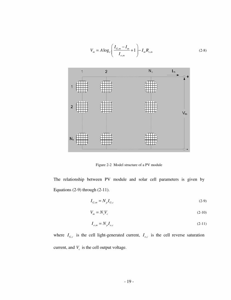
2.2.1 PV Module Structure
A PV module consists of p
N parallel branches, each with s
N solar cells in
series as shown in Figure 2-2 [21]. A model for the PV module is obtained by
replacing each cell in Figure 2-2 by its individual solar cell model. For clarity, the
following notation is used: the parameters with subscript “m” refer to the PV
module, while the parameters with subscript “c” refer to the solar cell.
2.2.2 Model Parameters
Using Equation (2-5), the module current m
I , under arbitrary operating
conditions is given by:
,
, ,
( )exp 1
m m s m
m G m o m
V I RI I I
A
+ = − −
(2-7)
where, ,G mI is the module light generated current, ,o m
I is the module reverse
saturation current, m
V is the module voltage, and ,s mR is the module series
resistance. The module voltage is obtained from Equation (2-7) as,
- 19 -
,
,
,
log 1G m m
m e m s m
o m
I IV A I R
I
−= + −
(2-8)
Figure 2-2 Model structure of a PV module
The relationship between PV module and solar cell parameters is given by
Equations (2-9) through (2-11).
, ,G m p G cI N I= (2-9)
m s cV N V= (2-10)
, ,o m p o cI N I= (2-11)
where ,G cI is the cell light-generated current, ,o c
I is the cell reverse saturation
current, and c
V is the cell output voltage.

- 20 -
2.2.3 Determination of Model Parameters
Reference values for the three parameters in this model, namely, the light-
generated current G
I , reverse saturation current o
I , and absolute cell temperature
cT , can be obtained indirectly using measurements of the current and voltage
characteristics of a solar module at reference conditions. Measurements of current
and voltage at these or other known reference conditions are often available at
open circuit conditions, short circuit conditions, and maximum power conditions
from manufacturer’s data sheets. All quantities with the subscript ‘ref’ are
obtained from measurements taken at reference conditions. Traditionally,
measurements of PV electrical characteristics are made at reference incident
radiation of 21 /kW m and an ambient temperature of 25 oC . These are the
standard conditions used by manufacturers to test PV modules.
Light Current at Reference Conditions
At short circuit conditions, the diode current is very small and the light-
generated current is equal to the short circuit current measured at the reference
conditions, i.e.,
, ,G ref sc refI I= (2-12)
Diode Reverse Saturation Current
At open circuit conditions there is no current, the exponential term in
Equation (2-5) is much greater than unity.

- 21 -
exp oco G
VI I
A
− =
(2-13)
where, Voc is the open circuit voltage. At reference conditions,
,
, , expoc ref
o ref G ref
ref
VI I
A
−=
(2-14)
Series Resistance
The series resistance is derived using the -I V curve at maximum power
conditions and is given by [19]:
,
, ,
,
,
.log 1mp ref
ref e mp ref oc ref
G ref
s
mp ref
IA V V
IR
I
− − +
= (2-15)
where, mp
I and mp
V are the current and voltage at maximum power point
respectively. If both s
R and ref
A are to be positive, the maximum value of s
R
occurs when A tends to zero and the maximum value of ref
A occurs when s
R tends
zero.
Temperature Coefficients
The temperature coefficient of the short circuit current ,I scµ , is obtained
from measurements at the reference solar radiation using,
12
12
,
)()(
TT
TITI
dT
dI scsc
c
sc
scI−
−==µ (2-16)

- 22 -
where 2T and 1T are two temperatures above and below the reference temperature.
Similarly, the temperature coefficient of the open circuit voltage, ,V ocµ can be
obtained from measurements using:
12
12
,
)()(
TT
TVTV
dT
dV ococ
c
oc
ocV−
−==µ (2-17)
Curve Fitting Parameter at Reference Conditions
This value can be derived by equating the experimental value of ,V ocµ with
the value determined from an analytical expression for the derivative, /oc
dV dT to
give:
, , ,
, ,
,
. .
.3
c ref V oc oc ref s
refI sc c ref
G ref
T V NA
T
I
µ ε
µ
− +=
−
(2-18)
where ε is the material bandgap energy in electron-volts (eV). The bandgap energy
depends on the material used in the manufacture of solar cells. The derivation of
Equation (2-18) is given in [19].
Cell Temperature
The working temperature of the cells c
T , depends exclusively on the solar
radiation a
G , and on the ambient temperature a
T according to the empirical linear
relation: [21]
aGac GTT µ+= (2-19)

- 23 -
where the constant G
µ is the temperature coefficient of solar radiation is computed
as:
refa
refarefc
GG
TT
,
,, −=µ (2-20)
The open circuit voltage depends exclusively on the temperature of the solar cells
and is given by,
, , , ,( )c oc c ref V oc c c ref
V V T Tµ= + − (2-21)
where ,c ocV is the solar cell open circuit voltage.
2.2.4 PV Array Structure
Large PV systems consist of modules connected in arrays. Figure 2-3 shows
an array of modules with p
M parallel branches each with s
M modules in series. a
V
denotes the output voltage at the array’s terminals, while a
I denotes the total
generated current. If all the modules are identical and operating under uniform solar
radiation, the PV array’s current and voltage is given by Equations (2-22) and (2-23)
respectively.
a P mI M I= (2-22)
a s mV M V= (2-23)

- 24 -
Figure 2-3 Model structure of a PV array
2.3 Simulink Models
Matlab-Simulink® is a software package that provides a graphical user
interface for modeling, simulating, and analyzing dynamic systems. It offers the
advantage of building hierarchical models, i.e. the system can be designed using
both top-down, and bottom-up approaches. Modeling of linear and nonlinear
systems in continuous time, sampled time, or a hybrid of the two is also supported
[22].

- 25 -
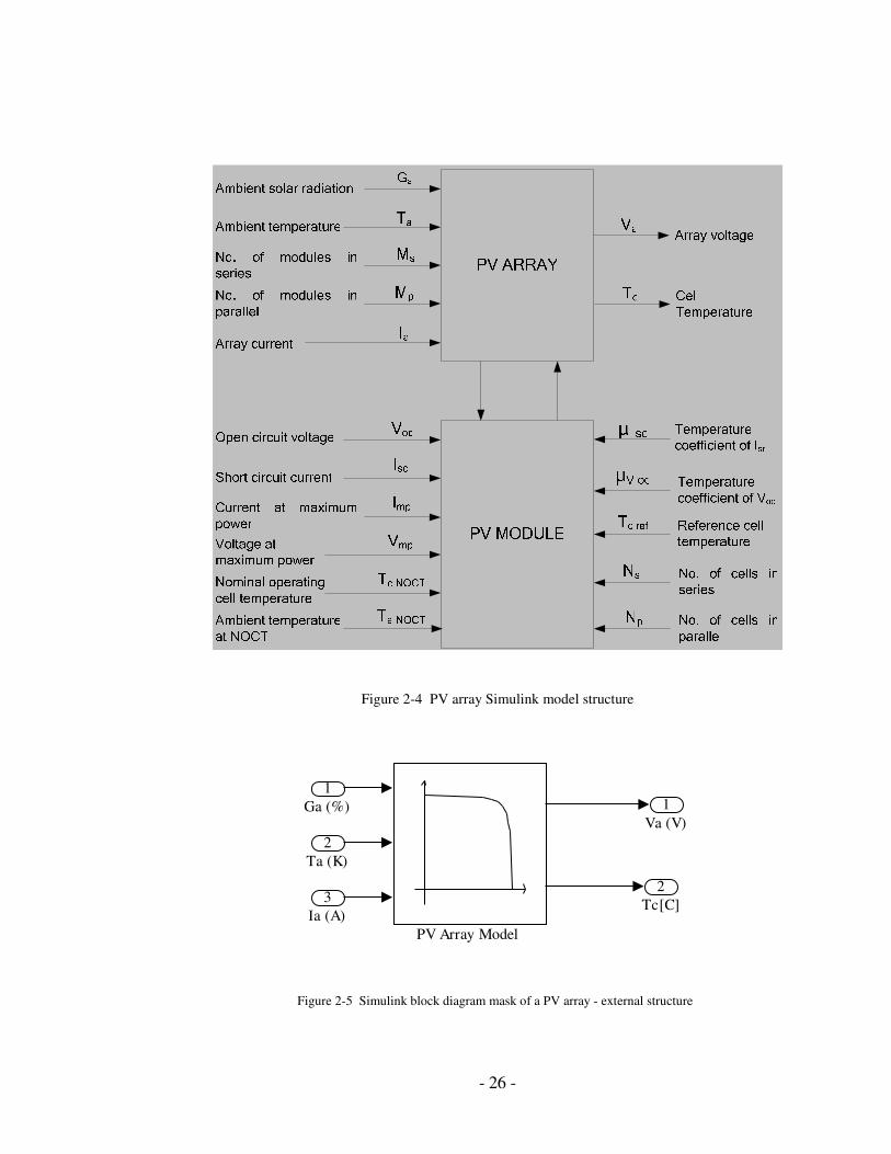
2.3.1 PV Array Model
The PV array Simulink model is structured in a hierarchical manner as
shown in Figure 2-4. Arrows entering the model are inputs while those leaving are
the outputs. The model allows the user to define the number of modules and their
connection. The array current and voltage is computed using Equations (2-22) and
(2-23) respectively.
The Simulink model mask for the PV array external and internal structure is
shown in Figure 2-5 and Figure 2-6 respectively. The external inputs are the solar
radiation a
G (expressed as a percentage of the reference value), ambient
temperature a
T , and the array current a
I from the previous time step. The model’s
output is the array voltage a
V , and the cell temperature c
T . The array output is solely
dependent on the operation of the individual PV modules, which are assumed to be
identical in this model. The parameters of the model can be set using the dialogue
box shown in Figure 2-7.
- 26 -
Figure 2-4 PV array Simulink model structure
2
Tc[C]
1
Va (V)
PV Array Model
3
Ia (A)
2
Ta (K)
1
Ga (%)
Figure 2-5 Simulink block diagram mask of a PV array - external structure

- 27 -
2
Tc [C]
1
Va [V]PV Module Model
u/Mp
Fcn2
u*Ms
Fcn1
3
Ia [A]
2
Ta [C]
1
Ga [ % ]
Im
Figure 2-6 Simulink block diagram mask of a PV array - internal structure
Figure 2-7 Simulink PV array model mask dialog box
2.3.2 PV Module Model
The Simulink model of a PV module is shown in the internal structure of the
array model in Figure 2-6. The model is implemented using an s-function coded
using the governing equations developed in section 2.3. An s-function is a computer
language description of a Simulink block coded in MATLAB®, C++, Fortran or
other supported programming languages. S-functions use a special calling syntax
that enables direct interaction with Simulink equation solvers. A listing of the

- 28 -
module voltage s-function, which is an implementation of Equation (2-8), is given in
the Appendix. The model modifying parameters are set using the dialogue box
shown in Figure 2-8.
2.4 Model Validation
The model was validated using manufacturer supplied data for BP solar SX
75TU PV module. The electrical characteristics for this module are given in Table 1
[23]. The I-V characteristics of the model match the supplied data as shown in
Figure 2-9. The power-voltage (P-V) curves under varying ambient temperature and
solar radiation are shown in Figure 2-10. It is observed that the model provides
sufficient accuracy for simulations.

- 29 -
Figure 2-8 Simulink PV module model mask dialog box

- 30 -
Table 2-1 Characteristics of BP SX 75TU PV module
BP SX 75TU Photovoltaic Module
Type: Silicon Multicrystalline
Number of Cells in series 36
Number of Cells in parallel 1
Maximum Power (Pmax) 75 W
Voltage at Pmax (Vmp) 17.3 V
Current at Pmax (Imp) 4.35 A
Short-circuit current (Isc) 4.75 A
Open-circuit voltage (Voc) 21.8 V
Temperature co-efficient of Isc (0.065 0.015)% / oC±
Temperature co-efficient of voltage (80 10) / omV C− ±
Nominal Operating Cell Temperature (NOCT) 47 2 oC±
0 5 10 15 20 25 300
0.5
1
1.5
2
2.5
3
3.5
4
4.5
5
5.5
Voltage (V)
T=0 oC
T=25 oC
T=50 oC
T=75 oC
(a) (b)
Figure 2-9 BP Solar SX75TU PV Module I-V Curves (a) Manufacturer Supplied (b) Simulated

- 31 -
0 5 10 15 20 250
10
20
30
40
50
60
70
80
90
Voltage (V)
Po
wer
(W)
T= 0 oC
T= 25 oC
T= 50 oC
T= 75 oC
Ga=100%
0 5 10 15 20 250
10
20
30
40
50
60
70
80
Voltage
Ga= 100%
Ta=25 oC
Ga= 75%
Ga= 50%
Ga= 25%
(a) (b)
Figure 2-10 PV module Power-Voltage curves under (a) varying temperature and (b) varying solar
radiation
2.5 Conclusion
The photovoltaic module was modeled in Matlab/Simulink. The results of
the simulation were compared to manufacturer supplied data and both results were
found to be very close. The model is detailed enough and can be used to model any
solar panel using information available in manufacturer’s data sheet. The model is
used in Chapter 4 to formulate a complete MPPT model.

- 32 -
CHAPTER THREE
3 DC-DC CONVERTERS AND MAXIMUM POWER
POINT TRACKING
In this chapter the characteristics of the three basic dc-dc converter
topologies; buck, boost, and buck-boost, are analyzed to determine the best topology
for performing PV module maximum power point tracking. A model of the
identified topology is then formulated. The model is used to carry out simulations to
determine the effect of component non-idealities on converter efficiency and output
voltage. The simulation results are used as the basis for developing control strategies
and selecting converter components. The converter model forms the main part in the
complete MPPT model used for tuning the fuzzy logic controller.
3.1 DC-DC Converters
The schematic diagram of a dc-dc converter is shown in Figure 3-1. It
converts a dc input voltage ( )gv t , to a dc output voltage ( )ov t , at a different voltage
level from the input [24]. It is desirable that the conversion be made with low losses
in the converter. Therefore, the transistor is operated as a switch using the control
signal ( )tδ , which is held high for a time on
t , and low for a time off
t as shown in
Figure 3-2.

- 33 -
( )gv t ( )ov t
( )oi t
( )tδ
g ( )i t
DC-DC
POWER
CONVERTER
Load
Figure 3-1 Structure of a dc-dc converter
While the transistor is on, the voltage across it is low which means that the
power loss in the transistor is low. While the transistor is off, the current through it
is low and the power loss is also low. The average output voltage is controlled by
changing the width of the pulses while the switching period s
T is held constant. The
duty cycle, d(t), is a real value in the interval 0 to 1 and it is equal to the ratio of the
width of a pulse to the switching period i.e. ( ) /on s
d t t T= .
( )tδ
0 ( ) sd t T sT
t
ont offt
Figure 3-2 Transistor control signal, ( )tδ

- 34 -
To obtain low losses, resistors are avoided in dc-dc converters.
Capacitors and inductors are used instead since ideally they have no losses. The
electrical components can be combined and connected to each other in different
ways, called topologies, each one having different properties. The buck, boost, and
buck-boost converters are three basic converter topologies. The buck converter has
an output voltage that is lower than the input voltage; the boost converter has an
output voltage that is higher than the input voltage, and the buck-boost converter is
able to produce an output voltage magnitude that is higher or lower than the input
voltage magnitude.
3.2 Maximum Power Point Tracking
As observed in Figure 2-10, the power produced from a photovoltaic module
depends strongly on the operating voltage of the load to which it is connected, as
well as to the solar radiation level and cell temperature. If a variable load resistance
R, is connected across the module’s terminals, the operating point is determined by
the intersection of module I-V curve and the load I-V characteristic. Figure 3-3
illustrates the operating characteristic of a PV module. It consists of two regions:
Zone I is the current source region, and Zone II is the voltage source region. In Zone
I, the internal impedance of the module is high, while in Zone II the internal
impedance is low. The maximum power point mpP , is located at the knee of the
power curve. Increase in solar radiation at constant temperature causes a decrease in

- 35 -
internal impedance as it causes an increase in short-circuit current. An increase in
temperature at constant solar radiation causes a decrease in internal impedance since
it causes a decrease in open circuit voltage.
According to the maximum power transfer theory, the power delivered to the
load is maximum when the source internal impedance matches the load impedance.
The load characteristic is a straight line with a slope of RVI /1/ = . If R is small, the
module operates in the region AB only and behaves like a constant current source at
a value close to sc
I . If R is large, the module operates in the region CD behaving
like a constant voltage source, at a value almost equal to oc
V .
Figure 3-3 Tracking the maximum power point of a PV module

- 36 -
Maximum power point tracking is based on load line adjustment under
varying atmospheric and load conditions by searching for an optimal equivalent
output resistance optR . A dc-dc converter is used to perform load-line adjustment by
varying the converter duty cycle using a controller.
3.3 Identification of a Suitable Converter Topology for Maximum
Power Point Tracking
The different converter topologies are analyzed in this section in order to
ascertain their performance and identify the most suitable topology for maximum
power point tracking.
3.3.1 Buck Converter
For an ideal buck converter, averaged input voltage gV , output voltage oV ,
input current gI , and output current oI are related as follows [25]:
o gV V D= (3-1)
g
o
II
D= (3-2)
where D is the equilibrium duty cycle of the converter. The dc load R connected to
the converter can be expressed using Ohm’s law as:
o
o
VR
I= (3-3)
The load resistance 'R referred to the input terminals of the converter can be derived
from Equations (3-1) and (3-2) as:

- 37 -
'
2
LRR
D= (3-4)
Since 0 1D< < , varying D can only increase the load seen by the source. A
buck converter is therefore, only able to extract maximum power if the original load
draws a higher current than the maximum power point current mpI , of the PV
module ( Zone I of Figure 3-3).
3.3.2 Boost Converter
For an ideal boost converter, the averaged input and output values of current
and voltage are related as follows [25]:
1
g
o
VV
D=
− (3-5)
(1 )o gI I D= − (3-6)
The load resistance 'R referred to the input side is given by:
' 2(1 )R R D= − (3-7)
Since 0 1D< < , varying D can only decrease the load seen by the source. It
is therefore noted that a tracker based on the boost converter is only able to extract
maximum power if the original load draws lower current than maximum power
point current mpI , of the PV module (Zone II of Figure 3-3).
3.3.3 Buck-Boost Converter
For an ideal buck-boost converter, the averaged input and output values of
current and voltage are related as follows [25]:

- 38 -
1o g
DV V
D
=
− (3-8)
1o g
DI I
D
− =
(3-9)
The load resistance 'R referred to the input side is given by:
2
' 1 DR R
D
− =
(3-10)
Since 0 1D< < , varying D can increase or decrease the load seen by the
source. The buck-boost converter is therefore able to operate both in Zones I and II.
3.3.4 Conclusion
It is noted from the analysis carried out in the preceding sub-sections that the
buck-boost converter has the best performance since it is able to perform maximum
power tracking in both zones I and II of Figure 3-3. A state space model of the
converter is developed in the next section.
3.4 Buck-Boost Converter Model
The circuit of a buck-boost converter is shown in Figure 3-4. It consists of
four basic components; transistor Q , diode T , inductor L , and capacitor C . These
components are not ideal and some of the non-idealities are considered when
modeling. The inductor is modeled as an ideal inductor in series with a resistance
LR . The capacitor is modeled as an ideal capacitor in series with a resistance CR .
LR and CR are used to model the power losses in the inductor and capacitor

- 39 -
respectively. The transistor has an on-state resistance, tR while the diode has a
forward voltage drop TV . A converter can operate in two or three modes. The state
space description of each mode is derived in this subsection.
T
( )L
i t
( )Lv t
+
−
LR
L
Q( )gi t
( )gv tDriver
( )tδ
( )Cv t
+
−
CR
R( )ov t
+
−
( )Ci t
( )oi t
Figure 3-4 Circuit of a buck-boost converter
3.4.1 Mode 1
This mode is valid for the time interval (0 )ont t< < when the control signal
( )tδ is high. When the transistor is on, the diode is reverse biased and is not
conducting. The circuit in Figure 3-5 shows the model of the buck-boost converter
during on
t .

- 40 -
)(tiC
CR
C −
+
)(tvo
−
+
)(tvC
−+ )(tvL
LR
tR
)(tiL
)(tvg
Figure 3-5 Circuit of the boost converter during ton
Applying Kirchhoff’s laws, the following equations are obtained from the model:
))(()()(
)( LtLg
L
L RRtitvdt
tdiLtv +−== (3-11)
( ) ( )( ) C C
C
C
dv t v ti t C
dt R R= = −
+ (3-12)
( ) ( )o C
C
Rv t v t
R R= −
+ (3-13)
)()( titi Lg = (3-14)
Re-arranging Equations (3-11) and (3-12) gives,
( ) 1( ) ( )
( ) 1( )
( )
t LLL g
cC
C
R Rdi ti t v t
dt L L
dv tv t
dt C R R
+= − +
= −+
(3-15)
Equations (3-13), (3-14), and (3-15) are of the form:
)()()(
)()()(
11
11
ttt
ttt
uExCy
uBxAx
+=
+=
(3-16)
Where,

- 41 -
,)(
)()(
=
tv
tit
C
Lx (3-17)
( )( ) ,
g
T
v tt
V
=
u (3-18)
,)(
)()(
=
ti
tvt
g
oy (3-19)
1
0
,1
0( )
t L
C
R R
L
C R R
+ − = +
A (3-20)
,
00
01
1
= LB (3-21)
1
0,
1 0
C
R
R R
− +=
C (3-22)
[ ].01 =E (3-23)
3.4.2 Mode 2
This mode is valid for the time interval ( )on on tt t t ϑ< < + , where on t st Tϑ+ ≤ ,
and t
ϑ is the time during which the inductor current is zero. During this mode, the
transistor is OFF and the diode is ON (provided ( ) 0Li t > ). The mode is valid for
( )on st t T< < if ( )Li t does not vanish. When the transistor is OFF, the voltage across
the diode is the forward voltage drop T
V . The circuit in Figure 3-6 can therefore be

- 42 -
used as a model of the buck-boost converter during off
t , for the continuous
conduction mode (CCM).
( )L
v t
+
−
LR
L
TV
( )L
i t
CR
C( )C
v t
+
−
( )o
v t
+
−
( )Ci t
R
( )oi t
Figure 3-6 Circuit of the buck-boost converter during off
t (CCM)
Applying Kirchhoff’s laws, the following equations are obtained from the model:
( )( ) ( ) ( ) ( )L
L L L C C C T
di tv t L R i t R i t v t V
dt= = − + + − (3-24)
1( ) ( ) ( )
C L C
C C
Ri t i t v t
R R R R= − −
+ + (3-25)
( ) ( ) ( )o C C C
v t v t i t R= − − (3-26)
( ) 0g
i t = . (3-27)
From Equations (3-24) to (3-27), the following state space model is obtained,
)()()(
)()()(
22
22
ttt
ttt
uExCy
uBxAx
+=
+=
(3-28)
where,

- 43 -
2
1
( ) ( ),
1
( ) ( )
CL
C C
C C
RR RR
L R R L R R
R
C R R C R R
− +
+ + =
− − + +
A (3-29)
,
00
10
2
−
= LB (3-30)
2 ,
0 0
C
C C
RR R
R R R R
− + +=
C (3-31)
.12 EE = (3-32)
3.4.3 Mode 3
This mode is valid for the time interval on t st t Tϑ+ < ≤ , whenever it exists.
During this mode the transistor is OFF and the diode is not in conduction (i.e.
( ) 0Li t = ). The circuit in Figure 3-7 can therefore be used as a model of the buck-
boost converter during off
t , for the discontinuous conduction mode (DCM).
( )C
v t
+
−
( )o
v t
+
−
CR
C
R
( )Ci t
Figure 3-7 Circuit of the buck-boost converter during off
t (DCM)

- 44 -
The functioning of the circuit in this mode is given by:
0)( =tiL (3-33)
( ) 1( ) ( )C
C C
C
dv ti t C v t
dt R R= =
+ (3-34)
( ) ( )o C
C
Rv t v t
R R= −
+ (3-35)
0)( =tig (3-36)
The corresponding standard state space model derived from Equations (3-33) to (3-
36) is given by,
)()()(
)()()(
33
33
ttt
ttt
uExCy
uBxAx
+=
+=
(3-37)
Where,
3
0 0
,10
( )CC R R
=
+
A (3-38)
[ ],03 =B (3-39)
3
0,
0 0
C
R
R R
− +=
C (3-40)
.13 EE = (3-41)

- 45 -
3.5 Averaged Buck-Boost Converter Model
The averaged converter model is a representation of the converter as linear
time invariant system that ignores all the switching dynamics. The model is obtained
by applying the method of state space averaging to the state space model.
3.5.1 Method of State Space Averaging
A converter can be considered to switch between two different linear time-
invariant systems during a switching period. This is valid if the natural frequencies
of the converter, and the variations of the converter inputs are much slower than the
switching frequency. The converter acts as a time-invariant system while the
transistor is on. While the transistor is off the converter acts as another time-
invariant system and if the inductor current reaches zero, the converter acts as yet
another time-invariant system. Converters therefore, switch between different time-
invariant systems during each switching period. Consequently, the converter can be
modeled as a time-varying system. State-space averaging [26] is one method to
approximate this time-varying system with a linear continuous-time time-invariant
system. This method uses the state-space description of each time-invariant system
as a starting point. These state-space descriptions are then averaged with respect to
their duration in the switching period. The averaged model is nonlinear and time-
invariant and has the duty cycle ( )d t , as the control signal instead of ( )tδ .

- 46 -
The state-space averaged model that describes a converter in equilibrium is
given by:
EUCXY
BUAX0
+=
+= (3-42)
where the averaged matrices are given by,
321
321
321
321
EEEE
CCCC
BBBB
AAAA
321
321
321
321
DDD
DDD
DDD
DDD
++=
++=
++=
++=
(3-43)
D1, D2 and D3 are the fraction of the switching period in which the converter
operates in modes 1, 2, and 3 respectively. The equilibrium dc components are,
=
C
L
V
IX (3-44)
g
T
V
V
=
U (3-45)
=
g
o
I
VY (3-46)
Quantities in Equation (3-44) to (3-46) represent the equilibrium values of the
averaged vectors; LI is the inductor current, CV is the capacitor voltage, gV is the
input voltage, T
V is the diode forward conduction voltage drop, oV is the output
voltage, and gI is the input current. Equation (3-42) can be solved to find the
equilibrium state and output vectors as:

- 47 -
UEBCAY
BUAX
1
1
)( +−=
=−
−
(3-47)
Equation (3-47) gives the converter averaged dc model.
The principle of state-space averaging is applied to the buck-boost converter
model to obtain the averaged dc model. The converter is assumed to operate in the
continuous conduction mode and the notations for the duty cycle are then redefined
as,
.0
'1
,
3
2
1
=
=−=
=
D
DDD
DD
(3-48)
3.5.2 Converter Averaged Model
Applying Equations (3-43) and (3-48) to the model equations in sections
3.4.1 and 3.4.2 gives:
'1 '
( ) ( ),
' 1
( ) ( )
CL
C C
C C
D RR D RR DRt
L R R L R R
D R
C R R C R R
− + +
+ + =
− − + +
A (3-49)
,
00
'
−
= L
D
L
D
B (3-50)
'
,
0
C
C C
D RR R
R R R R
D
− + +=
C (3-51)
.0=E (3-52)

- 48 -
The dc equations are derived by expanding Equation (3-42) to obtain:
DgC
C
L
C
C
Lt VL
DV
L
DV
RRL
RDI
RR
RRDRDR
L
'
)(
''10 −+
++
+++−= (3-53)
C
C
L
C
VRRC
IRRC
RD
)(
1
)(
'0
+−
+−= (3-54)
' Co L C
C C
D RR RV I V
R R R R= −
+ + (3-55)
Lg DII = (3-56)
Equation (3-54) is simplified to:
'C LV D I R= − (3-57)
Substituting Equation (3-57) into (3-55) and simplifying, gives:
o CV V= − (3-58)
Substituting Equations (3-57) and (3-58) into (3-53) and rearranging gives:
+
+
+
+
+
−
−=
R
R
R
RD
RD
DRR
V
V
D
D
D
D
V
V
C
C
tL
g
D
g
o
1
1
1'
1
'
'1
'
2
2
(3-59)
Assuming all components are ideal, i.e. 0t L T
R R V= = = , Equation (3-59) reduces
to:
+
−=
RD
RD
D
V
V
Lg
o
2'1
1
' (3-60)
The converter efficiency considering the average power is given by:

- 49 -
+
+
+
+
+
−
==
R
R
R
RD
RD
DRR
V
V
D
D
IV
IV
C
C
tL
g
D
gg
oo
1
1
1'
1
'
'1
2
2
η (3-61)
Assuming 0t L T
R R V= = = , Equation (3-61) reduces to:
2
1
1'
LR
D R
η =
+
(3-62)
3.6 Buck-Boost Converter Simulink Model
The averaged converter model is implemented using the Simulink block
shown in Figure 3-8. The state space averaged model given by Equations (3-49) to
(3-52) is coded as an s-function whose parameters are modified using the mask
dialog box shown in Figure 3-9. The model inputs are the input voltage g
V , load
resistance R , and the duty cycle D , while the outputs are the load voltage o
V ,
inductor current L
I , input current g
I , input power in
P , and output power o
P .
Scope
buck_boost_dc_sfun
S-Function
Demux
D
R
Vg
Vo
I_L
Ig
Pin
Po

- 50 -
Figure 3-8 Buck-boost converter Simulink model
Figure 3-9 Buck-boost converter model mask dialog box
3.7 Simulation Results
Equation (3-60) is plotted in Figure 3-10 for several values of /L
R R to
show the effect of inductor resistance on the output voltage. It can be seen that
Equation (3-60) contains two terms. The first term, '/D D− , is the ideal conversion
ratio with 0L
R = . The second term, '21/(1 / )L
R D R+ , describes the effect of the

- 51 -
inductor winding resistance. If L
R is much less than ' 2D R , then the second term
tends to unity and the conversion ratio is approximately equal to the ideal value
'/D D− . However, increase in L
R in relation to ' 2D R leads to decrease in the
second term which decreases /o g
V V as well.
As the duty cycle D approaches unity, the inductor winding resistance
causes a significant effect in the /o g
V V curve. Rather than approaching infinity at
1D = , the curve tends to zero. This condition is expected since at 1D = the
inductor is never connected to the output, hence no energy is transferred to the
output and the output voltage tends to zero. The inductor current increases rapidly,
limited only by the inductor resistance L
R . A large amount of power is lost in the
inductor winding resistance while no power is delivered to the load. The converter
efficiency therefore tends to zero as D approaches unity.
Equation (3-62) is plotted in Figure 3-11 for several values of /L
R R to
illustrate the effect of inductor resistance on converter efficiency. It can be seen
from Equation (3-62) that to obtain high efficiency, L
R should be much smaller than
' 2D R . This is easier to attain at low duty cycle, where 'D is close to unity, than at
high duty cycle where 'D approaches zero. It is observed in Figure 3-11 that the
efficiency is high at low duty cycles, but decreases rapidly towards zero near 1D = .

- 52 -
0 0.1 0.2 0.3 0.4 0.5 0.6 0.7 0.8 0.9 10
1
2
3
4
5
6
Duty Cycle, D
- V
o /
Vg
RL/R = 0
RL/R = 0.01
RL/R = 0.02
RL/R = 0.05
RL/R = 0.1
Figure 3-10 Effect of inductor resistance on buck-boost converter output voltage

- 53 -
0 0.1 0.2 0.3 0.4 0.5 0.6 0.7 0.8 0.9 10
0.1
0.2
0.3
0.4
0.5
0.6
0.7
0.8
0.9
1
Duty cycle, D
Eff
icie
ncy,
n
R / R = 0.01
RL / R = 0.02
RL / R = 0.05
RL / R = 0.1
Figure 3-11 Effect of inductor resistance on buck-boost converter efficiency
3.8 Conclusion
The application of dc-dc converters in PV module maximum power point
tracking has been studied in this chapter. The buck-boost converter was identified as
the most suitable converter topology for maximum power tracking and a model of
the converter developed. The effects of non-idealities on converter efficiency is
considered in choosing converter components and setting duty cycle limits for the
controller. The model is used in the next chapter to tune and test the performance of
the fuzzy logic algorithm.

- 54 -
CHAPTER FOUR
4 FUZZY LOGIC CONTROLLER DESIGN AND
HARDWARE IMPLEMENTATION
This chapter presents a study on the application of fuzzy logic to formulate a
control algorithm for a maximum power point tracker. The design of the fuzzy logic
controller structure and formulation of the control rules is presented. A hardware
implementation of the maximum power point tracker is also carried out.
4.1 Design of Fuzzy Logic Controller Parameters
4.1.1 Controller Structure
The basic scheme of a fuzzy logic based maximum power point tracker is
shown in Figure 4-1. The dc-dc converter is represented by a “black box” from
which only the terminals corresponding to input voltage m
V , input current m
I
from the PV module, and the controlled switch S are extracted. As observed, only
two state variables are sensed; the input voltage and input current. The two values
are used to calculate the input power. From these measurements, the fuzzy logic
controller provides a signal proportional to the converter duty cycle which is then
applied to the converter through a pulse width modulator. The modulator uses the
value of D to perform Pulse Width Modulation (PWM), which generates the

- 55 -
control signals for the converter switch. The fuzzy logic controller scheme is a
closed loop system.
mV
+
−o
V
+
−
Fuzzy
Controller
S
R
+
−
PWM Modulator
Dm
V
mI
PV
Mo
du
le
Figure 4-1 Fuzzy control scheme for a maximum power point tracker
A functional block diagram representation of the fuzzy controller is shown
in Figure 4-2. The inputs to the controller are the scaled change of power, p k
k P∆
and the previous change of duty, 1kD −∆ , where
pk is a power scale factor, and k is
the sampling instant. The output of the fuzzy controller is the duty cycle k
D at the
k -th sampling instant, and is defined as
1k k d kD D k D−= + ∆ (4-1)

- 56 -
where k
D∆ is the inferred change of duty cycle by the fuzzy controller at the -k th
sampling instant, and d
k is a duty-cycle scale factor. The block containing the
term 1Z − in Figure 4-2 indicates a unit time delay.
kD∆
kD
kP
1kP −
kP∆
1Z
−
+
+
Defuzzification
Decision
MakingFuzzification
1Z
−
+
−
1Z −
mi
mv
Output1kD −
1kD −∆
dk
kp
Figure 4-2 Functional block of the fuzzy controller
4.1.2 Membership Functions
Fuzzy sets for each input and output variable are defined as shown in Figure
4-3. Five fuzzy subsets Negative Big (NB), Negative Small (NS), Zero (ZE),
Positive Small (PS), and Positive Big (PB) are chosen for the input variable k
P∆ .
Eleven subsets are used for the input and output variable 1kD −∆ . The subsets are NB,

- 57 -
Negative Medium (NM), Negative Medium Medium (NMM), NS, Negative Small
Small (NSS), ZE, Positive Small Small (PSS), PS, Positive Medium Medium
(PMM), Positive Medium (PM), and PB. Eleven fuzzy subsets were chosen for
1kD −∆ in order to smooth the control action. As shown in Figure 4-3, triangular and
trapezoidal shapes have been adopted for the membership functions; the value of
each input and output variable is normalized. The same membership function is used
for the output value k
D∆ and the input value 1kD −∆ .
P∆
k
1− 0.25− 0 0.25 1
NB NS ZE PS PB
1D
−∆
k
1− 10.2 0.4 0.70.2−0.4−0.7−
PBNB
NS PS
NM PMNSS
NMM
PSS
PMM
0
11
(a) (b)
Figure 4-3 Membership functions for (a) change in power (b) change in duty cycle
The membership functions for k
P∆ and 1kD −∆ are made more dense at the
centre in order to provide more sensitivity as the variation of power approaches zero.
The duty cycle is internally limited to a maximum value of 90% to prevent
operation at low efficiencies. It is also limited to a minimum value of 10% to
ensure that the converter switching process does not stop as operation at 0D = will
indicate a false maximum power point.

- 58 -
4.1.3 Scaling Factors
For simplicity, the universe of discourse for each fuzzy variable was
normalized to be in the range [-1 1] ; this procedure involves scale mapping for the
input and output data. The choice of the scale factors p
k and d
k greatly affects the
bandwidth and the overall performance of the controller. The factor p
k determines
the sensitivity of the controller to changes in power, and d
k determines the
sensitivity to change in duty cycle. Suitable values of p
k and d
k were chosen based
on simulation results.
4.1.4 Derivation of Control Rules
Fuzzy control rules are obtained from the analysis of the system behaviour.
The different operating conditions are considered in order to improve tracking
performance in terms of dynamic response and robustness.
The algorithm can be explained as follows: the tracking process is started
with an initial duty cycle, 0D . The converter input current m
I , and voltage m
V , are
then measured and used to compute the module power k
P . Then, the duty cycle is
increased by the controller based on the initial changes in power and duty cycle. At
stage two, m
I and m
V are measured and used to compute 1kP + . After gathering the
past and present information of the module power, the controller makes a decision
on whether to increase or decrease the duty cycle. This tracking process repeats

- 59 -
itself continuously until the peak power point is reached. The control rules are
divided into four categories.
Category I
These rules are used to guide the controller under constant operating
conditions i.e. when there are no variations in solar radiation, temperature, or load.
Operation is based on the meta-rule:
“IF the last change in the duty cycle has caused the power to increase, keep
moving the duty cycle in the same direction; otherwise if it has caused power to
decrease, move it in the opposite direction.”
The duty cycle is changed in adaptive steps which depend on the change in
power to ensure the maximum power point is approached at a fast speed and to
prevent oscillations around it. There are forty rules in this category and they are
shown in Table 4-1 with a degree of support of 1. These rules are given the
strongest degree of support since the task they represent describes the normal system
operation. The rules are read as,
• IF k
P∆ is NB AND 1kD −∆ is NB THEN
kD∆ is PM
• IF k
P∆ is NB AND 1kD −∆ is NM THEN
kD∆ is PMM
• IF k
P∆ is NB AND 1kD −∆ is NS THEN
kD∆ is PSS
• …………………………………………………………..
• IF k
P∆ is PB AND 1kD −∆ is PB THEN
kD∆ is PM.

- 60 -
Table 4-1 Fuzzy controller rule base
k-1∆D
k∆
P
Key:
Category II
The rules in this category guide the controller when there are sudden
changes in solar radiation, temperature, or load leading to an overall shift in the
optimum point. There are four rules in this category and are found in the vertical
column of Table 4-1 corresponding to 1 0k
D −∆ = , and a degree of support of 0.5 .
This condition is rare and the rules are used to return the system to normal operation
where category I rules are activated to search for the new optimum operating point.
Category III
The rules in this group are used to ensure that the maximum power transfer
search only stops when the true maxima has been reached. Several false maxima are

- 61 -
introduced due to the quantization effect shown in Figure 4-4. Since the input
signals are digitized, the continuous curve is broken into a series of plateaus (points
with constant power). It is observed from Figure 4-4 that the steeper the curve, the
shorter the plateau. Since the optimum point satisfies the condition / 0P D∂ ∂ = , the
controller might recognize any large plateau as a maximum power point and stop.
There are ten rules in this category and are found in the horizontal column of Table
4-1 corresponding to 0k
P∆ = . The rules are given a degree of support of 0.5 since
the condition is rare.
Category IV
There is only one rule in this category. The rule is activated when the system
reaches the optimum point and it is used to stabilize operation at the maximum
power point. It is given a weight of 0.25 as shown in Table 4-1. The rule is read as,
• IFk
P∆ is ZE AND 1kD −∆ is ZE THEN
kD∆ is ZE
Figure 4-5 shows the fuzzy controller rule surface. It is a graphical
representation of the rule base. In this figure, ( 1)cD k − is the previous change in
duty cycle, ( )cP k is the current change in module power, and ( )cD k is the
corresponding change in duty cycle.

- 62 -
kplateaus where∆P = 0k
PV
mod
ule
po
wer
(P)
kDuty cycle(D )
Figure 4-4 Quantization effect during maximum power search
Figure 4-5 Graphical representation of Table 4-1

- 63 -
4.1.5 Tuning of Control Rules
A system model of the block diagram shown in Figure 4-1 was formulated in
the Simulink/Matlab environment using the models of the PV module and the buck-
boost converter formulated in Chapters 2 and 3 respectively. The fuzzy logic
algorithm was formulated using the fuzzy logic toolbox and the rules were fine
tuned by simulations. This involved the choice of the number of rules, setting
membership function boundaries, and determining suitable values for the scale
factors p
k and d
k .
4.1.6 Decision Making
From the membership functions in Figure 4-3, it is observed that every
input and output belongs to at most two fuzzy sets. A maximum of four rules are
therefore activated at any sampling instant during which the input signals k
P∆ and
1kD =∆ are processed. For instance, let 0.2
kP∆ = and 1 0.35
kD −∆ = − . From Figure
4-5, change in power k
P∆ belongs to the fuzzy set PS and PB with a degree of
membership ( ) 0.33PS k
Pµ ∆ = , and ( ) 0.71PB k
Pµ ∆ = . Change in duty cycle 1kD −∆
belongs to the fuzzy set NMM and NM with 1( ) 0.5NMM k
Dµ −∆ = , and
1( ) 0.25NM k
Dµ −∆ = . The degree of membership for the other membership
functions is zero. Therefore, the following four rules are activated,
• Rule 1: IF k
P∆ is PS AND 1kD −∆ is NM THEN
kD∆ is NMM

- 64 -
• Rule 2: IF k
P∆ is PS AND 1kD −∆ is NMM THEN
kD∆ is NS
• Rule 3: IF k
P∆ is PB AND 1kD −∆ is NM THEN
kD∆ is NMM
• Rule 4: IF k
P∆ is PB AND 1kD −∆ is NMM THEN
kD∆ is NS.
The inference result of each rule consists of two parts, the degree of fulfillment,
iDOF of the individual rule, and the weighting factor
iw , according to the rule. The
degree of fulfillment (DOF) is obtained by means of Mamdani’s min-fuzzy
implication [15] and i
w is retrieved from the control rule table. The degree of
fulfillment of each rule using Mamdani’s min fuzzy implication is given by,
1 1min ( ), ( )ki P k D k
DOF P Dµ µ−∆ ∆ −= ∆ ∆ (4-2)
and the output of each rule is given by,
( )i i i
z DOF w= (4-3)
where i
z denotes the fuzzy representation of change in duty cycle inferred from the
-i th rule. Since the inferred output is fuzzy, the defuzzification operation is
performed to obtain a crisp output.
The fuzzy inference system with the Mamdani’s min fuzzy implication
method for inputs 0.2k
P∆ = and 1 0.35k
D −∆ = − , is illustrated in Figure 4-6. The
degree of fulfillment of 1Rule is given by:
1 1( ) ( ) 0.33 0.25 0.25PS k NM k
DOF P Dµ µ −= ∆ ∧ ∆ = ∧ = (4-4)

- 65 -
where ∧ = minimum (AND) operator. The rule output 1z , is given by the truncated
membership function NMM . Similarly, degrees of fulfillment for 2, 3Rules and
4 are evaluated using Equation 4-5 to give:
2 0.33DOF = (4-5)
3 0.25DOF = (4-6)
4 0.5DOF = (4-7)
The corresponding outputs for 2, 3Rules and 4 are the truncated membership
functions NS , NMM and NS respectively, as shown in Figure 4-6. The total fuzzy
output is the union of all the component membership functions and is given by,
( ) ( ) ( ) ( ) ( )out NMM NS NMM NS
Z Z Z Z Zµ µ µ µ µ= ∨ ∨ ∨ (4-8)
where ∨ = maximum (OR) operator. The fuzzy output ( )out
Zµ is shown in Figure
4-6.
4.1.7 Defuzzification
The output of an inference process is a fuzzy set specifying a distribution
space of fuzzy control actions defined over an output universe of discourse.
Defuzzification is the conversion of this fuzzy output to crisp output suitable for a
control action. A defuzzification strategy is aimed at producing a non-fuzzy
control action that best represents the possibility distribution of an inferred fuzzy
control action. Unfortunately, there is no systematic procedure for choosing a
defuzzification strategy [18]. This process involves the operation:

- 66 -
0 ( )Z defuzzifier Z= (4-9)
0 0.25 1
PS1
1− 0.3−0.7−
NM
0 0.25 1
PS1
0.4−
NMM
0.05 1
PB1
1
PB1
1− 0.7−
NM1
0.4−
NMM
0.2−0.4−
NMM
0.2−
NS
0.1−
0.2−0.4−
NMM
0.2−
NS
0.1−
1
1
1 1
0.05
0.2−
0.3−
0.2−
0.2kP∆ =1 0.35kD −∆ = −
0.33 0.25
0.50.33
0.71
0.25
0.710.5
0.4− 0
0.22Z = −o
1
Centroid
( )Zµout
1Rule
2Rule
3Rule
4Rule
Z
Figure 4-6 Fuzzy inferencing and defuzzification using Mamdani method

- 67 -
The term 0Z in Equation (4-9) is the non-fuzzy control output and
defuzzifier is the defuzzification operator. There are various defuzzification methods
which include, centre of area (COA), bisector, mean of maxima, sum of maxima,
etc. The COA method commonly known as centre of gravity (or centroid) is used
in this work. The method is computationally intensive but more accurate than
other methods. In this method, the crisp output 0Z of the Z variable is taken to be the
geometric centre of the output fuzzy value ( )out
Zµ , where ( )out
Zµ is formed by
taking the union of all the contributions of rules whose 0DOF > [15] as shown in
Figure 4-6. The general expression for the COA method in the case of a discretized
universe of discourse is given by,
10
1
( )
( )
n
i out i
i
n
out i
i
Z Z
Z
Z
µ
µ
=
=
=∑
∑. (4-10)
A crisp value for the change in duty cycle is calculated by applying Equation (4-10)
to the output fuzzy value ( )out
Zµ in Figure 4-6.
4.2 Simulation Model
The fuzzy MPPT algorithm was simulated by implementing a complete
system model in Matlab/Simulink as shown in Figure 4-7. The system is
composed of a PV source, buck-boost converter, and a fuzzy logic controller
block.

- 68 -
4.2.1 PV Source
This block simulates the nonlinear I-V characteristic of a PV module using
the model developed in Chapter 2. BP solar SX 75TU PV module was used for the
simulation. This solar panel has a rated power of 75W . The inputs for this block are
the ambient solar radiation a
G , ambient temperature a
T , and the module current m
I .
The outputs are the cell temperature c
T and module voltage m
V which are recorded
using scope 2.
Figure 4-7 Fuzzy MPPT Simulink Simulation Model

- 69 -
4.2.2 Fuzzy Logic Controller
This model simulates the fuzzy MPPT algorithm. It computes the desired
duty cycle of the buck-boost converter using the procedure shown in Figure 4-2.
This block performs the fuzzification, decision making and defuzzification
processes. The inputs are the PV module voltage and current, while the output is
the converter duty cycle. All controller parameters i.e. the current change in power
( )cP k , previous change in duty cycle ( 1)cD k − , current change in duty cycle
( )cD k , and the current value of duty cycle ( )D k are recorded by scope 1. ( )cP k
and ( 1)cD k − are used by the controller to determine ( )cD k . The duty cycle
( )D k used to drive the converter is determined by updating the previous value
using ( )cD k .
4.2.3 Buck-Boost Converter
This block simulates the buck-boost converter characteristics using a
Simulink s-function, buck_ boost_dc_ sfun. The s-function was coded using the
model equations of the buck-boost converter developed in Chapter 3. The Matlab
code for the buck_ boost_dc_ sfun is listed in the Appendix. The use of an s-
function greatly improves simulation speed compared to a converter model
developed using discrete components available in the Simulink SimPowerSystems
toolbox. The s-function model also allows simulations of step changes in load
which cannot be easily achieved in a discrete component model. The inputs for

- 70 -
this block are; the module voltage m
V , duty cycle k
D , and load resistance R . The
outputs are the input current m
I , input power in
P , inductor current L
I , output
voltage o
V , and output power o
P . All the output parameters are recorded using
scope 2.
4.3 Hardware Design Overview
Maximum Power Point Tracker design involves the selection of dc-dc
converter components and implementation of the control algorithm. In this design,
the buck-boost converter topology is chosen in order to maximize the efficiency of
the PV array. The selection of the converter topology was carried out in Chapter 3.
A schematic diagram of the maximum power point tracker is shown in Figure 4-8.
Implementation of the control algorithm involves the design of current and voltage
sensing circuits and formulation of the control software. The controller senses
analogue voltages and currents proportional to measured quantities. The inputs are
digitized and processed in a micro-controller in order to determine, and output a
suitable duty cycle that ensures the system operates at its maximum power point.
USB-1208FS data acquisition (DAQ) card manufactured by Measurement
Computing Corporation is used.

- 71 -
PV
Mo
du
leLoad
m mSampling V and I
PWM Signal
Personal Computer
USBCable
USB-1208FS DAQ Card
Buck-Boost Converter
Figure 4-8 Schematic diagram of a PC-based MPPT using fuzzy logic
4.4 Buck-Boost Converter Operation
The buck-boost converter circuit is shown in Figure 4-9. When the transistor
Q , is on, energy is transferred to the inductor L. When the transistor turns off,
inductor current flows through the diode T . Energy stored in L is transferred to the
capacitor C and the load R. This transfer action results in an output voltage of
opposite polarity to that of the input. Neither the input current nor the output current
is continuous, although the inductor current may be continuous or discontinuous.

- 72 -
LmV
oC
R
Ti
mi
QT
oV
−
+
Lv
+
−
Tv− +L
i
sT
ont
Figure 4-9 Buck-boost converter circuit
4.4.1 Continuous Inductor Current
The circuit voltage and current waveforms for the buck-boost converter
operating in continuous conduction mode are shown in Figure 4-10. The voltage
drop across the inductor Lv is given by:
L
div L
dt= (4-11)
Assuming a constant input and output voltage, the change in inductor current L
i∆ is
derived from Equation (4-11) with L m L, ,on
v V di i dt t= = ∆ = . m
V is the input
voltage, and on
t is the transistor on-time. L
i∆ is therefore given by,
( )m oL on s on
V Vi t T t
L L∆ = = − − (4-12)

- 73 -
Li
Qi
Ti
LI
Li∆
QV
TVm oV V+
m oV V+
mV
oV
offt
ont
sT
mV
t
t
0
0
0
0
0
sT
ont
offtxt
( )Continuous Conduction Mode CCM ( )DiscontinuousConduction Mode DCM
Figure 4-10 Buck-boost converter waveforms for continuous inductor current and discontinuous
inductor current waveforms

- 74 -
thus,
1
o m
m o
V I D
V I D= = −
− (4-13)
where s
T is the transistor switching period, /on s
D t T= , o
V is the output voltage, m
I
is the average input current, and o
I is the average output current. For 0.5D < , the
output voltage magnitude is less than the input voltage while 0.5D > ,the output is
greater in magnitude than the input. Using Equations (4-12) and (4-13) the
maximum change in inductor current maxLi∆ , is given by,
max2
m sL
DV Ti
L∆ = (4-14)
The maximum inductor current maxLi∆ ,and the minimum inductor current minL
i∆ , are
given by,
max2
LL L
ii I
∆= + (4-15)
min2
LL L
ii I
∆= − (4-16)
where L
I is the average inductor current.
4.4.2 Discontinuous Inductor Current
The change from continuous to discontinuous inductor current conduction
occurs when the average inductor current LI , is given by,
max
2
LL L
iI i= = ∆ (4-17)

- 75 -
where from Equation (4-12),
max ( )oL s on
Vi T t
L= − (4-18)
The output voltage for discontinuous conduction is evaluated from
max ( )m oL s on x
V Vi t T t t
L L= = − − − (4-19)
which gives,
1
o
xm
s
V D
tVD
T
= −
− −
(4-20)
Using Equation (4-19) and
max
1
2L L
I Di= (4-21)
yields
2
m sL
V T DI
L= (4-22)
It is observed from Figure 4-10 that the input and output currents are proportional to
the inductor current. The inductor current depends on the duty cycle and at the
boundary between continuous and discontinuous conduction:
max
max
2
(1 )
2
Lm
Lo
DiI
D iI
=
−=
(4-23)
where,
max2
LL L
Ii i= ∆ = (4-24)

- 76 -
Using m LI DI= , Equation (4-24) becomes
2
2
m sm
V T DI
L= (4-25)
Assuming the converter is lossless, that is m m o oV I V I=
2 2
2 2 2
o m m s o s s
m o o m
V I V T D V T D T RD
V I LI LI L= = = = (4-26)
At the boundary between continuous and discontinuous conduction, Equation (4-25)
can be modified using Equation (4-13) to give
(1 )2
mo s
VI T D D
L= − (4-27)
The critical (or minimum) inductance required to ensure continuous conduction is
derived from Equation (4-27) and is given by,
20.5 (1 )crit s
L RT D= − (4-28)
At a low output current or low input voltage there is a likelihood of discontinuous
conduction. To avoid this condition, a larger inductance value is needed, which
worsen transient response.
4.5 Buck-Boost Converter Design
Converter design involves the choice of suitable component values that meet
the desired operating conditions. The component values that need to be determined
are the input capacitor, inductor, and the output capacitor. The input capacitor is
required because the input current of the buck-boost converter is discontinuous. The

- 77 -
main goal of this design is to ensure that the converter operates in the continuous
conduction mode since it lowers the peak current flowing through the inductor, and
consequently reduces the losses in the converter.
The buck-boost converter conduction mode changes when it is used in PV
applications, since the input voltage and current change continuously with the
atmospheric conditions. In addition, the converter duty cycle D , is changed
continuously in order to track the maximum power point of the PV module. The
choice of the converter switching frequency and the inductor value is a compromise
between converter efficiency, cost, power capability and weight. For example, the
higher the switching frequency, the lower the inductor core size, but the power
switch losses are higher. Also, by using a large inductor value, the peak to peak
current ripple L
i∆ , is smaller, requiring lower current rating power switches, but the
converter size is increased substantially because a larger inductor core is required
[25][27].
4.5.1 Inductor Selection
The inductor value L , required to operate the converter in the continuous
conduction mode is calculated using Equation (4-28). In order to determine the
values of R and D to be used in calculating crit
L , the worst case condition has to be
considered. This occurs when the PV array operates at its maximum capacity at
minimum load. It can be assumed that the load is constant at 1 Ω , the converter is

- 78 -
lossless and operates in CCM. The PV module internal resistance at maximum
power pvm
R is given by,
mp
pvm
mp
VR
I= (4-29)
where mp
V and mp
I are the voltage and current at maximum power respectively. A
14W solar panel with 14.5mp
V V= , and 0.97mp
I A= was selected for use in the
experiment. pvm
R for this panel is obtained using Equation (4-29) as 17.01 Ω . For
operation at the maximum power point the load resistance R , must be equal to pvm
R .
The value of D required for operation at maximum power is obtained from
Equation (3-10) by setting '
pvmR R= and rearranging to give,
1
1pvm
DR
R
=
+
(4-30)
Using Equation (4-29) with 17.01pvm
R = Ω and ' 1R = Ω , gives the required value
of D as 0.195 . Choosing a switching frequency 40s
f kHz= and using Equation
(5-18), gives 81.0crit
L Hµ= . It is however noted that pvm
R increases with decrease
in solar radiation. A more suitable value of crit
L is therefore determined with the
limiting case of 0D = . This gives 125crit
L Hµ= . However, a larger inductance
than crit
L is chosen to ensure continuous inductor current during periods of low solar
radiation and in the presence of large loads. A 270 Hµ PCV-2-274-10L series

- 79 -
Bobbin inductor from Coilcraft Incorporation was chosen for the converter. It has a
10 A r.m.s. current rating and a maximum resistance of 0.060Ω [28].
4.5.2 Input Capacitor Selection
An input capacitor is needed in order to limit the input voltage ripple due the
switching action. Since the short circuit current of the PV module is 1.2 A , the
maximum current ripple to be handled by the input capacitor is approximately 1 A .
Figure 4-11 shows the capacitor current ripple due to variations in input current. The
charge stored in the capacitor Q∆ is given by,
2 2
m si T
Q i dt∆
∆ = ⋅ = ⋅∫ (4-31)
Using 1m
i A∆ = and 61/ 25 10s s
T f s−= = × , Equation (4-31) gives
66.25 10Q C−∆ = × .
Q∆ 2
mi∆
2
sT
mI
mi
t0
Figure 4-11 Input capacitor ripple current

- 80 -
With an input voltage of 14.5 V at maximum power, the minimum capacitor size
required to regulate the input voltage ripple to 1% is given by,
6(6.25 10 )43.10
(0.01)(14.5 )
Q CC F
V Vµ
−∆ ×= = =
∆ (4-32)
A 50 ,30F Vµ electrolytic capacitor was selected for the input.
4.5.3 Output Capacitor Selection
A suitable value of capacitance is required in order to attain the desired
output voltage ripple. The output voltage ripple is the capacitor ripple voltage. The
output current o
I is provided solely from the capacitor during the period on
t when
the switch is conducting, thus
1 1o on o
V i dt t IC C
∆ = ⋅ =∫ (4-33)
Substituting for /o o
I V R= gives
on oo
t VV
CR∆ = (4-34)
Rearranging gives the fractional peak-to-peak voltage ripple in the output voltage as,
1o son
o
V DTt
V CR CR
∆= = (4-35)
Considering the extreme case where, 0.9D = ( D is limited to maximum value of
0.9 to reduce power loss) and 1R = Ω , the minimum capacitor size required to
regulate the output voltage ripple to 1% is obtained by rearranging Equation (4-35)
as,

- 81 -
( / )
s
o o
DTC
V V R=
∆ (4-36)
Using 0.9D = , 625 10s
T s−= × , 1R = Ω , and / 0.01
o oV V∆ = A Equation (4-36)
gives 2250C Fµ= . A 2700 , 50F Vµ electrolytic capacitor was selected for the
output.
4.5.4 Diode Selection
Diode choice is a trade off between breakdown voltage, speed, and forward
voltage. A higher forward voltage drop increases the converter power loss.
However, a fast switching diode is needed to act as a switch for the energy in the
inductor. If the diode is slow to react, the efficiency of the converter is low and
damaging high voltage transients will develop. In case of these transients and the
possibility of large output voltages if the load is suddenly disconnected, the diode
must have a high breakdown voltage. The best combination of these features could
be found in SB530 Schottky diode from RS Components, which has a reverse
breakdown voltage of 30 V and a forward voltage drop of 0.57V at a rated current
of 5A [29].
4.5.5 Switching Transistor Selection
An n-channel enhancement mode power MOSFET IRFZ24N from Fairchild
Semiconductor Corporation was selected as a high speed-switching device for the
buck-boost converter. The rating of this device is 55V and 17A, well above
maximum operating voltage and current which are 21 V and 1.2 A of the converter.

- 82 -
It has a maximum gate leakage current of only 100nA and a low on state resistance
of 0.07Ω [30]. The low on-state resistance leads to small conduction loss hence
higher converter efficiency.
4.6 Pulse Width Modulation
Pulse Width Modulation (PWM), is a method of controlling the amount of
power to a load by switching the load on and off. The amount of power delivered to
the load is proportional to the percentage of time that the load is switched on. PWM
signals can be generated in a number of ways namely: analogue circuitry, PWM
chips, digital counters, and using timers on microcontrollers. The SG3525A PWM
controller from ST Microelectronics was chosen for this purpose because it can be
operated to give a duty cycle of 0 100%− .
4.6.1 SG3525A PWM IC Operation
The pin configuration of the IC is shown in Figure 4-12 [31]. The PWM
controller has two complementary outputs called Output A (pin 11) and Output B
(pin 14). Both outputs have a duty cycle limited to less than 50% and they are never
high at the same time. If the frequency of each output is F , then the frequency of
the sum of the outputs is 2F . Example waveforms are shown in Figure 4-13 where
the frequency of each output is 20 kHz . When both outputs are used in parallel, the
switching waveform in the circuit will have a frequency of 40 kHz as shown in
Figure 4-13.

- 83 -
The SG3525A PWM IC allows control of a parameter called the dead time
which is a fixed length of time where both outputs are off. This feature is useful
when two MOSFETs are used, one switched by each output, in order to attain
100% duty cycle. The negative feedback can easily force the PWM portion of the
controller to go to 100% duty cycle, which means that the switches will never turn
off. If the switches never turn off, the inductor will never discharge and the inductor
current becomes very large. The dead time is used to ensure that both MOSFET
switches have a guaranteed amount of off time, preventing this problem.
1
2
3
5
4
6
7
8 9
10
11
12
13
14
15
16 refV
i+ V
OUTPUT B
CV
GROUND
OUTPUT A
SHUTDOWN
COMP.SOFT-START
DISCHARGE
TR
TC
OSC. OUTPUT
SYNC.
N.I. INPUT
INV. INPUT
SG
35
25
A
Figure 4-12 SG3525A pin configuration

- 84 -
Output A (20 kHz)
Output B (20 kHz)
Output A + Output B (40kHz)
0 125 250 375 500 625 750 1000
Time (µS)
0 V
20 V
0 V
0 V
20 V
20 V
Figure 4-13 SG3525A output waveforms
4.6.2 Design Procedure
The biasing circuit for the PWM IC is shown in Figure 4-14 [31]. The design
process involves choosing the values for the oscillator resistorT
R , dead-time resistor
DR , and oscillator capacitor
TC , in order to produce the desired switching
frequency and a dead time that limits the maximum duty cycle. The switching
frequency is given by [31],
1
(0.7 3 )T T D
fC R R
=+
(4-37)

- 85 -
TC
DR
TR
SSC
CCV
TC
DISC
TR
SD
V−
COMP
SS
GN
D
OUTB
OUTA
V+
SYNC
REFV
OSC
CV5
7
6
10
1
9
2
3
16
4
13
11
14
128
15
CCV
CTRLV
GATE1
GATE 2
Figure 4-14 SG3525A biasing circuit
A switching frequency of 40 kHz was selected for the circuit. Choosing
0.01T
C Fµ= and 0D
R = , T
R is calculated using Equation (4-37) to give
3.6T
R k= Ω . The dead time resistor D
R was set to zero so that the maximum duty
cycle could be software controlled using the control voltage CTRL
V , supplied to pin 2.
The minimum and maximum duty cycle is attained with an input voltage of 0.7V
and 3.6V respectively [31]. The output drivers, Pins 11 and 14, can each sink or

- 86 -
source a maximum current of 100 mA . The output voltage waveform has a
maximum value of CC
V+ and a minimum of zero. With 12CC
V V= , the output
drivers meet the IRFZ24N MOSFET requirements which has a rated a gate current
of 100 nA and a minimum gate threshold voltage of 4V .
The rate at which the pulse-width is allowed to increase during start-up is
determined by the soft-start capacitor SS
C , connected to pin 8. This capacitor is
charged by a 50 Aµ current source in the IC. When the capacitor reaches
approximately 2.5 volts, the soft-start is complete. This feature prevents high duty
cycles at start up which cause large inductor currents. Choosing a soft-start that
takes 1 second, SS
C is calculated using the equation:
SS
Q ItC
V V
∆= =
∆ ∆ (4-38)
Using 50I Aµ= , 1t s= , and 5V V∆ = , Equation (4-38) gives 20SS
C Fµ= .
The SG3525A PWM IC outputs with 0.02 , 37T T
C F R kµ= = Ω and
2.5CTRL
V V= are shown in Figure 4-15.

- 87 -
Figure 4-15 SG3525A PWM IC test outputs
4.7 Data Acquisition System
The data acquisition system consists of voltage and current sensing circuitry
and USB-1208FS data acquisition (DAQ) card. The DAQ card acquires the PV
module current and voltage, which is used by the maximum power point tracking
software to determine the converter duty cycle. A control voltage ( )CTRL
V
corresponding to the desired duty cycle is passed through the DAQ card, which
feeds it to PWM IC.

- 88 -
4.7.1 USB-1208FS Data Acquisition Card
The USB-1208FS is a USB 2.0 full-speed device supported under
Microsoft® Windows®. It features eight analog inputs, two 12-bit analog outputs,
16 digital I/O connections, and one 32-bit external event counter [32]. The device
appears as shown in Figure 4-16. The analog inputs are software configurable for
either eight 11-bit single-ended inputs, or four 12-bit differential inputs. The
input/output (I/O) ports are Transistor Transistor Logic (TTL) compatible with a
programmable sampling rate of up to 50 kHz . I/O connections are made to the
screw terminals located along each side of the DAQ card.
Figure 4-16 USB-1208FS data acquisition card

- 89 -
4.7.2 Sensing Circuitry
The PV module voltage is sensed directly by the microcontroller through a
voltage divider network while a 0.1Ω current sensing resistor is used to measure the
current. The sensing circuitry is shown in Figure 4-17.
+−
+ −
VCC
GND
USB CABLE
12V
PV
MO
DU
LE
0.1Ω
33k
11k
2k
2k
120k
120k
3R
1R
2R
4R
LM 358
USB-1208FS
DAQ CARD
VoltageSense
Current Sense
Figure 4-17 Sensing circuitry
For a maximum current of 1.2 A the current sensing resistor produces a
voltage drop of 0.12V . A non-inverting differential amplifier was used to increase
this voltage to a level where the microcontroller was easily able to read. The low
cost LM358 IC was chosen for the differential amplifier. The amplification of the

- 90 -
amplifier is directly proportional to 1 2
/R R . With 2
120R k= Ω and 1
2R k= Ω it
gives an amplification of 60 . This amplifies the 0.12V at 1.2 A over the current
sensing resistor to 7.2V . The features of LM358 IC are given in reference [33].
4.8 Features of the Software
The control software was coded in C++ using Microsoft Visual Studio 6.0.
A flowchart of the software is shown in Figure 4-18. The software acquires the PV
module voltage and current periodically from the DAQ card and uses the fuzzy
algorithm to determine the required change in duty cycle in the search for maximum
power. The duty cycle is changed by modifying the control voltage signal supplied
to pin 2 of SG3525A PWM controller using the DAQ card. A control voltage of
0.9V corresponds to zero duty cycle while 3.3V corresponds to 100% duty cycle.
The output ports of the DAQ card are latched which ensures that the system operates
at constant duty cycle until the next update. An initial duty cycle of 10% is used
with initial values of change in power P∆ and change in duty D∆ set to zero. All the
input values and controller parameters are logged to a data file and displayed on the
screen using the user interface shown in Figure 4-19. The inputs are sampled at
10 Hz and the duty cycle is also updated at the same rate. A listing of the software is
given in the Appendix.

- 91 -
Load setpoint data
D=0.1, P=0, D=0∆ ∆
Read ModuleCurrent
and Voltage
Fuzzy Logic Control
Algorithm
Output
DutyWritedata
to file
Start
return
Periodic interrupt
Figure 4-18 Flowchart describing operation of the software
Figure 4-19 Control software user interface

- 92 -
4.9 Conclusion
A complete fuzzy logic based maximum power point tracker for a PV
system was successfully designed and implemented. The design of the fuzzy logic
controller structure and formulation of the algorithm has been presented. The
power circuit is based on a buck-boost converter, while the controller used a
microcomputer with a fuzzy logic control algorithm that searches for the optimum
duty cycle and transfers the peak power from the solar panel to a resistive load. The
system is ready to be implemented in a dedicated microcontroller and fitted to a
larger installation.

- 93 -
CHAPTER FIVE
5 RESULTS AND DISCUSSION
This chapter presents a simulation and experimental results of the fuzzy
logic based maximum power point tracker. It consists of a PV module, buck-boost
dc-dc converter, data acquisition card, and a resistive load. The fuzzy logic control
algorithm developed in Chapter 4 is used to search for the optimal operating point
under different operating conditions. A computer was used for data acquisition,
running the control algorithm, data storage, as well as data display and analysis.
5.1 Simulation Results
In order to investigate the performance and accuracy of the proposed fuzzy
MPPT technique simulations were performed under time-invariant and time
varying conditions. The model in Figure 4-7 was first simulated in open loop mode
without the fuzzy controller in order to determine a data set consisting of the
expected maximum power under different values of solar radiation. The data was
generated by varying the module input current from zero to short-circuit current
for each value of solar radiation and recording the output power. The maximum
power point for each value of solar radiation was then obtained from the data. The
achieved maximum power during the simulation at each time step k
t was recorded
for comparison with the expected maximum power. At the end of the simulation,

- 94 -
the data was used to determine the efficiency of the maximum power point
tracking algorithm using the formula,
( , )
( )( )
achieved k kmppt k
mpp k
P D tt
P tη = (5-1)
where, ( , )achieved k k
P D t is the power achieved by the algorithm at duty cycle k
D , and
( )mpp k
P t is the actual maximum power possible. The average of mppt
η over all t
gives a good measure of the effectiveness of the algorithm. In general, the fuzzy
logic algorithm, operating at sampling frequencies between 1kHz and 10 kHz ,
achieved an average tracking effectiveness of over 95% . This means that over
95% of the available power was captured by the tracking algorithm.
For comparison purposes, the maximum power achieved by the algorithm
was plotted with the expected actual maximum power under different operating
conditions. Figure 5-1 shows the power track when the solar radiation varies at
0.3 Hz between 50% and 100% . This fast and wide variation of solar radiation
was used to test the effectiveness of the algorithm under rapidly changing
conditions. The tracking effectiveness of the simulation of Figure 5-1 was 98.6% .
Without the MPPT less than 20% of the available power could be delivered to the
load of 100Ω used in the simulation.
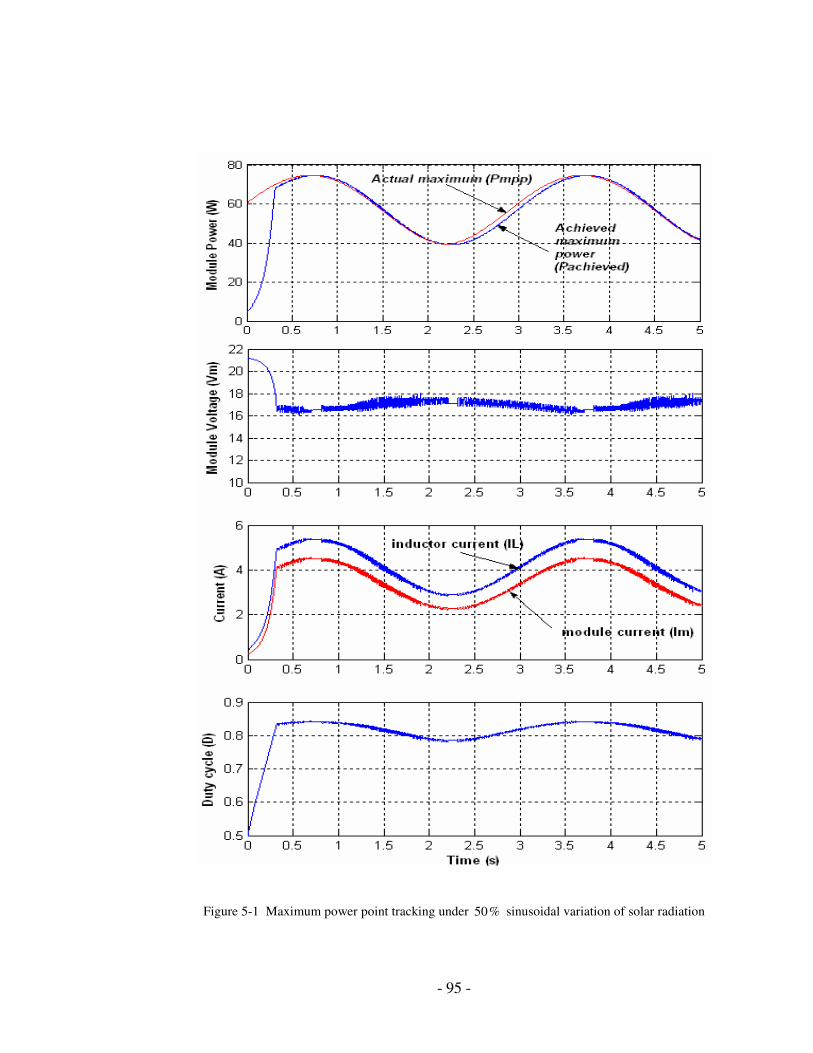
- 95 -
Figure 5-1 Maximum power point tracking under 50% sinusoidal variation of solar radiation

- 96 -
However, it was observed that the maximum power delivered without the
tracker depends on the size of the load. The variation of module voltage, module
current, inductor current, and the duty cycle are also shown in Figure 5-1. The
inductor current and the module current have no overshoots due to the smooth
variation of the duty cycle.
As a further test on the performance of the algorithm, step changes of load
by 50% were introduced in addition to the time variation of solar radiation. The
simulation results are shown in Figure 5-2. The algorithm exhibits a recovery time
of less than 0.1s . This is the time taken to return the system back to operation at
maximum power after the step change in load. There is no appreciable change in the
efficiency of the algorithm under step changes in load. Figure 5-2 also shows how
the algorithm moves the duty cycle while tracking the maximum power. The
variation in duty cycle is fast but smooth which avoids oscillations around the
maximum power.
Having proven the effectiveness of the algorithm under time-varying
conditions, it was also applied to the time-invariant case. This is a situation where
the solar radiation and temperature of the PV module are held constant in time. In
this static case, the algorithm attained an efficiency of over 99% . The track of this
simulation is shown in Figure 5-3. Under this static case, the algorithm is also able
to reach the maximum power point in under 0.1s when there are step changes in
load.

- 97 -
Figure 5-2 Maximum power point tracking under 50% sinusoidal variation of solar radiation and
step changes in load
Figure 5-3 Maximum power point tracking under time-invariant solar radiation
and step changes in load

- 98 -
The performance of the algorithm considered so far assume that the
system has perfect knowledge of the power that results from a particular duty
cycle ( )D k . In reality, however, the algorithm will not have such perfect
measurements. Due to the limitations of the analog-to-digital converter and the
current and voltage sensing circuits, the measurements of the PV module’s
voltage and current, and hence the module power is subjected to noise. Therefore,
to test the robustness of the algorithm in the presence of measurement noise, the
simulation was extended. Gaussian noise was added to the power measurements
before the algorithm used them. The Matlab awgn() function was used to add
white Gaussian noise to the measured power signal. The signal-to-noise ratio is
specified in decibels. A noise power value of 7 dB , which represents a signal-to-
noise ratio of 5 was used. This represents an absolute worst case noise level of
15W when the PV module is operating at its maximum power rating of 75W .
Although the algorithm did not perform effectively in the presence of
measurement noise as in the noise-less case, the results of the simulations were
satisfactory. For the case where the solar radiation varied in time, the tracking
efficiency of the algorithm (averaged over a single run) was generally in the range of
90 95%− . It was observed that the efficiency improved by decreasing the change in
power scale factor p
k and increasing the change in duty scale factor d
k . The
simulation was run with 0.1p
k = and 0.01d
k = . The control parameters were
entered using the controller dialog box shown in Figure 5-4. Due to the stochastic

- 99 -
nature of the noise in the simulation, the performance varied from one simulation
run to the next. The track of one such run is given in Figure 5-5.
The simulation in Matlab proved essential for developing and fine tuning the
control rules and membership functions of the maximum power point tracking
algorithm. The simulation results show that the algorithm is robust and is able to
handle variations in the operating conditions of a PV module. However, for the
hardware implementation, the fuzzy logic algorithm was coded in C++ using
Microsoft Visual Studio 6.0. This became necessary because the drivers for the data
acquisition card were not available in Matlab. The C++ control software was tested,
and debugged using the Matlab simulation as a benchmark. A set of test points
was selected randomly from the design space, representing several of the possible
input conditions that would be encountered by the maximum power point tracker.
Each test point was input into the Matlab model as well as the C++ controller
code. Utilizing the output of the Matlab model, the controller code was debugged
until the controller code output matched the output of the Matlab model. The
program dialog box for testing the fuzzy controller outputs is shown in Figure 5-6.
It displays the inferred output for the given inputs as well as identifying the
activated rules and their firing strengths.

- 100 -
Figure 5-4 Controller mask dialog box
Figure 5-5 Maximum power point tracking under time-varying solar radiation in
the presence of noise

- 101 -
Figure 5-6 Fuzzy controller test interface dialog box
5.2 Experimental Results
The system shown in Figure 4-8 was implemented as explained in the
preceding sections and used to supply power to a resistive load. The main goal was
to transfer as much power as possible to a 100Ω resistor. A PV module used for the
collection of the experimental data is Kenital 14 W solar panel. The module has a
maximum power output of 14W and a 22.5V open-circuit voltage at an irradiation
of 21000 /W m at 25oC . The PV module specifications provided by the
manufacturer are shown in Table 5-1 [34].
The performance of the MPPT system was first tested using a dc power
supply with different current settings. The MPPT was able to vary the output voltage
until the maximum current set was drawn from the power supply which corresponds

- 102 -
to transfer of maximum available power to the load. The MPPT was then connected
to a PV module and tested during a clear sunny day. A clear sunny day was chosen
to ensure a constant solar radiation was available since the circuit does not include
ways of measuring the solar radiation level. Figure 5-7 shows the maximum power
attained with the MPPT and the normal operating power (without MPPT) in one of
the test runs. The system with MPPT was found to attain an average maximum
power of 12.5W . It is clear that the module power is maintained at an optimum
value with slight variations due to noise in current and voltage measurements.
Figure 5-7 also shows that the attained power for the same load without MPPT is
only 4 W . These results indicate an increase of about 200% in PV output power in
the presence of the fuzzy MPPT.
Table 5-1 Electrical specifications for Kenital 14W PV module
Maximum power, m
P (W) 14
Short circuit current, sc
I (A) 1.20
Open circuit voltage, oc
V (V) 22.5
Voltage at maximum power point, mp
V (V) 14.5
Current at maximum power point, mp
I (A) 0.97
Size ( mm mm mm× × ) 430x406x22

- 103 -
0 50 100 150 200 250 3000
5
10
15
Mo
du
le P
ow
er
(W)
0 50 100 150 200 250 3000
0.5
1
Mo
du
le C
urr
en
t (A
)
0 50 100 150 200 250 3000
0.2
0.4
0.6
0.8
Du
ty C
ycle
(D
)
Time (s)
Without MPPT
With MPPT
Figure 5-7 Measured results under high solar radiation on a clear sunny day at 12.30pm
Extensive measurements indicate that the amount of increase in PV module
output power highly depends on the environmental conditions and the load level.
This shows the importance of using MPPT to get a good matching between the load

- 104 -
and the PV module. It was however noted that the system could not track the
maximum power under very cloudy conditions. Under low solar radiations the solar
panel generates very low currents due to its low power rating and the system could
not be able to sense the low currents and track the power adequately. It is however
expected that the system will give good performance when fitted in PV systems with
high power ratings.
5.3 Conclusion
The simulation results have shown that the controller is inherently robust
with an efficiency of over 95% under wide input variations. The experimental
results also show that system reliably stabilizes the maximum power transfer under
time invariant input conditions. Further experimental tests are required in order to
determine the stability of the algorithm under rapidly changing atmospheric and load
conditions.

- 105 -
CHAPTER SIX
6 CONCLUSION AND FUTURE WORK
6.1 Conclusion
The aim of this thesis was to develop a method to optimize the energy
extraction in a photovoltaic power system. The concept of PV module maximum
power point tracking has been presented and various methods of addressing existing
challenges are explored. A fuzzy logic based algorithm for tracking the maximum
power is proposed in this work. In order to formulate and implement the algorithm,
a system model is needed. The various components and subsystems are analyzed,
modeled, validated, and combined together to produce a complete maximum power
point tracker model. A hardware implementation was then carried out to determine
the performance of the algorithm in a practical setup.
Analysis of different dc-dc converter topologies showed that the buck-boost
topology is the most suitable for a maximum power tracker. The PV module and the
buck-boost converter were modeled and validated in Simulink while the fuzzy logic
algorithm was formulated using the Fuzzy Logic Toolbox in Matlab. The complete
Maximum Power Point Tracker model was formed by combining the PV module
and the converter model with the fuzzy logic controller. The MPPT model was used
to tune the fuzzy logic controller rules and membership functions. The PV module

- 106 -
model was found to be sufficiently accurate and can model any solar panel using
information supplied in manufacturer data sheets. Simulation results show that the
proposed fuzzy logic algorithm has an average efficiency of 95% under rapidly
varying conditions and in the presence of measurement noise. The results show that
compared to other MPPT techniques, it provides improved performance in terms of
oscillations about the maximum power point, speed and sensitivity to parameter
variation. This is possible since fuzzy logic controller rules can be assigned
separately for the various regions of operation resulting in effective small-signal and
large-signal operation.
A hardware design and implementation of the MPPT was then carried out in
order to test the performance of the proposed algorithm. The design was broken
down into several smaller components, which are described in turn. For each sub-
circuit, a thorough description of the relevant design issues and decisions was
provided. Experimental results show that the proposed algorithm is able to transfer
peak power from a PV module to the load. The results indicate that a significant
amount of additional energy can be extracted from a photovoltaic module by using a
fuzzy logic based maximum power point tracker. This results in improved efficiency
for the operation of a photovoltaic power system since batteries can be sufficiently
charged and used during periods of low solar radiation. The improved efficiency is
expected to lead to significant cost savings in the long run.

- 107 -
6.2 Future Work
The overall control goal in a photovoltaic power system is not to deliver the
maximum amount of possible power to the load or batteries, but only as much as is
needed at any given time; this can be referred to as power matching. Usable power
that is not extracted from a particular solar panel (because it is not operating at its
current maximum power point) is dissipated as heat through its surface. In a
practical application like a water pump in a remote village, the MPPT circuit must
include a way to determine how much power is needed at any given time and
perform maximum power tracking only to a level where power requirements are
met. The MPPT should also include a second voltage regulation stage that maintains
a steady output regardless of variations in the load demand. These improvements
will greatly boost the functionality of the system in a practical setup.
As part of future work, ways of implementing a fuzzy logic algorithm in a
dedicated single-chip microcontroller needs to be addressed. The control algorithm
is fairly complex and modifications need to be made in order to meet the limited
memory space and speed of microcontrollers. The microcontroller must also
incorporate timers, PWM input and output, A/D and D/A interfaces, and interrupts
for timing control and communications. The overall circuit also needs to be
modified to include ways of supplying power to the control circuit using batteries
charged by the MPPT. The redesigned circuit should be implemented in a printed
circuit board.

- 108 -
On the whole, it is concluded that the overall objective of formulating and
implementing a fuzzy logic based maximum power point tracker for a photovoltaic
power system has been met. Although there is a large amount of work that can and
should still be done, the work in this thesis has created a solid foundation to allow
that work to continue.
.

- 109 -
REFERENCES
[1] Ocran, T.A. et al, Artificial Neural Network Maximum Power Point
Tracker for Solar Electric Vehicle, Tsinghua Science & Technology, Vol.
10, No. 2, pp. 204-208, 2005.
[2] Hua C., Lin J., A modified tracking algorithm for maximum power tracking
of solar array, Energy Conversion and Management 45 (2004) 911-925,
Elsevier Ltd. 2003.
[3] Salas V., et al, New algorithm using only one variable measurement
applied to a maximum power point tracker, Solar Energy Materials &
Solar Cells 87 (2005) 675-684, Elsevier B.V. 2004.
[4] C. Hua and C. Shen, Comparative study of peak power tracking
techniques for solar storage systems, in Proc. IEEE Appl. Power
Electron. Conf. and Expo., Feb. 1998, vol. 2, pp. 676–683.
[5] Koutroulis E., Kalaitzakis K., Voulgaris N.C., Development of a
Microcontroller Based Photovoltaic Maximum Power Point Tracking
Control System, IEEE Transactions on Power Electronics, Vol. 16, No. 1,
2001.
[6] J. H. R. Enslin, D. B. Snyman, Simplified feed-forward control of the
maximum power point tracker for photovoltaic applications, Proc. Int.
Conf. IEEE Power Electron. Motion Control, 1992, vol. 1, pp. 548–553.

- 110 -
[7] M. Bodur and M. Ermis, Maximum power point tracking for low power
photovoltaic solar panels, in Proc. IEEE Electro Tech. Conf., 1992, vol.
2, pp. 758–761.
[8] C. R. Sullivan and M. J. Powers, A high-efficiency maximum power point
trackers for photovoltaic array in a solar-powered race vehicle, in Proc.
IEEE PESC, 1993, pp. 574–580.
[9] M. Veerachary, T. Senjyu, and K. Uezato, Feed-forwardmaximum power
point tracking of PV systems using fuzzy controller, IEEE Trans. Aerosp.
Electron. Syst., vol. 38, no. 3, pp. 969–981, Jul. 2002.
[10] Ocran, T.A. et al, Artificial Neural Network Maximum Power Point Tracker
for Solar Electric Vehicle, Tsinghua Science & Technology, Vol. 10, No. 2,
pp. 204-208, 2005.
[11] Hohm D.P., Ropp M.E., Comparative Study of Maximum Power Point
Tracking Algorithms, Progress in Photovoltaics: Research and Applications
2003; 11:47-62 (DOI: 10.1002/pip.459).
[12] Noguchi T., Togashi S., and Nakamoto R., Short-current pulse-based
maximum power point tracking method for multiple photovoltaic-and
converter module system, IEEE Trans. Ind. Electron., vol. 49, no. 1, pp.
217–223, Feb. 2002.
[13] Enslin J.R., Wolf M.S., Snyman D.B., Sweigers W., Integrated
photovoltaic maximum power point tracking converter, IEEE Trans. Ind.
Electron., 1997, 44(6): 769-773.

- 111 -
[14] Baghat A.B.G, et al, Maximum power point tracking controller for PV
systems using neural networks, Renewable Energy 30 (2005) 1257-1268,
Elsevier Ltd. 2004.
[15] Bose B. K, Modern Power Electronics and AC Drives, University of
Tennessee, Prentice Hall, 2002, Chapter 11.
[16] B. Tomescu, H.F. VanLandingham, Improved Large Signal Performance
of Paralleled DC/DC Converters Current Sharing Using Fuzzy Logic
Control, IEEE Trans. PE, vol. 14 No. 3, May 1999, pp. 573-577.
[17] Lee C. C, Fuzzy logic in control systems: Fuzzy Logic Controller- Part I,
IEEE Transactions on Systems Man and Cybernetics Vol. 20, NO.2,
March/April 1990, pages 404-417
[18] Lee C.C, Fuzzy logic in control systems: Fuzzy Logic Controller- Part II,
IEEE Transactions on Systems, Man and Cybernetics, Volume: 20, NO.2,
March/April 1990, pages 418-435.
[19] Manwell J.F, Rogers A. Hayman G., Avelar C.T., McGowan J.G., Hybrid2 –
A Hybrid System Simulation Model - Theory Manual, Renewable Energy
Research Laboratory, Department of Mechanical Engineering, University of
Massachusetts,1998, pp 105-117.
URL:http://www.ecs.umass.edu/mie/labs/rerl/hy2/theory/pdf/complete.pdf
(date: 12th Aug. 2005)
[20] Tyagi, M.S., Introduction to Semiconductor Materials and Devices, John
Wiley & Sons, 1991.
- 112 -
[21] Anca D. Hansen et al, Models for a Stand-Alone PV system, Risø National
Laboratory, Roskilde, Norway, December 2000.
URL: http://www.risoe.dk/solenergi/rapporter/pdf/sec-r-12.pdf (date: 15th
Nov. 2005)
[22] Mathworks Corporation, Simulink Reference Manual, Matlab Release 13
documentation. URL:
http://www.mathworks.com/access/helpdesk/help/pdf_doc/simulink/slref.pdf
(date: 23rd
Sep. 2005)
[23] BP Solar Global Marketing , BP Solar SX 75TU PV module data sheet,
2002.
URL: http://ww.solardepot.com/pdf/BPSX75TU.pdf (date: 20th Oct. 2005)
[24] R.W. Erickson, D. Makasimovic, Fundamentals of Power Electronics, 2nd
edition, Kluwer Academic Publishers, 2001, page 311.
[25] Mohan N., T.M. Undeland, and W.P. Robbins, Power Electronics:
Converters, Applications, and Design, John Wiley & Sons, Inc., New
York, 1995.
[26] Middlebrook R. D., Cuk, S. (1976), A general unified approach to
modeling switching converter power stages, IEEE Power Electronics
Specialists Conference Record, pp. 18-34, 1976.
[27] Rashid Muhammad H., Power Electronics, Circuits, Devices, and
Applications, Prentice-Hall India, 3rd
Edition, pp. 186-204, 2004.
[28] Coilcraft Incorporation, PCV-2-274-10L inductor datasheet,

- 113 -
URL: http://www.coilcraft.com/pdfs/pcv.pdf (Date: 20th Jan. 2006)
[29] Vishay Semiconductors, SB530 diode datasheet,
URL: http://www.ortodoxism.ro/datasheets/vishay/sb520.pdf (Date: 20th
Jan. 2006)
[30] Fairchild Semiconductor Inc., IRFZ24N datasheet,
URL: http://www.irf.com/product-info/datasheets/data/irfz24n.pdf (Date:
20th Jan. 2006)
[31] ST Microelectronics, SG3525A datasheet,
URL: http://www.st.com/stonline/books/pdf/docs/4286.pdf. (Date: 20th Jan.
2006)
[32] Measurement Computing Corp., USB-1208FS user’s guide,
URL: http://www.measurementcomputing.com/PDFmanuals/usb-1208fs.pdf
(Date: 20th Jan. 2006)
[33] National Semiconductors, LM358 datasheet,
URL: http://www.national.com/ds/LM/LM158.pdf (Date: 20th Jan. 2006)
[34] Kenital ,14W solar panel datasheet,
URL: http://www.kenital.com/category.asp?ID=8 (Date: 20th Jan. 2006)

- 114 -
APPENDICES
A-1 S-Functions
1 Buck-Boost Converter S-function
function [sys,x0,str,ts] =buck_boost_dc_sfun(t,x,u,flag,Rind,Rc,L,C,Vd,Rd,Rt)
% Dispatch the flag. The switch function controls the calls to
% S-function routines at each simulation stage of the S-function.
%
switch flag,
% Initialization %
% Initialize the states, sample times, and state ordering strings.
case 0
[sys,x0,str,ts]=mdlInitializeSizes;
% Outputs %
% Return the outputs of the S-function block.
case 3
sys=mdlOutputs(t,x,u,Rind,Rc,L,C,Vd,Rd,Rt);
% Unhandled flags %
% There are no termination tasks (flag=9) to be handled.
% Also, there are no continuous or discrete states,
% so flags 1,4, and 9 are not used, so return an emptyu
% matrix
case 1,2,4, 9
sys=[];
% Unexpected flags (error handling)%
% Return an error message for unhandled flag values.
otherwise
error(['Unhandled flag = ',num2str(flag)]);
end
%
%=========================================================
====================
% mdlInitializeSizes
% Return the sizes, initial conditions, and sample times for the S-function.
%%========================================================
function [sys,x0,str,ts] = mdlInitializeSizes()

- 115 -
sizes = simsizes;
sizes.NumContStates = 0;
sizes.NumDiscStates = 0;
sizes.NumOutputs = 6;
sizes.NumInputs = 3;
sizes.DirFeedthrough = 1; % has direct feedthrough
sizes.NumSampleTimes = 1;
sys = simsizes(sizes);
str = [];
x0 =[];
ts =[-1 0]; % sample time
% end mdlInitializeSizes
%=========================================================
====================
% mdlOutputs
% Return the output vector for the S-function
%=========================================================
function sys = mdlOutputs(t,x,u,Rind,Rc,L,C,Vd,Rd,Rt)
D=u(2); %duty cycle
D1=1-D;
R=u(3);
U=[u(1);Vd]; %inputs
% update state space matrices
A=[-1/L*(D*Rt+Rind+D1*R*Rc/(R+Rc)) D1*R/(L*(R+Rc));-D1*R/(C*(R+Rc))
-1/(C*(R+Rc))];
B=[D/L -D1/L;0 0];
Cm=[D1*R*Rc/(R+Rc) -R/(R+Rc);D 0];
X=-inv(A)*B*U; % state vector
Y=Cm*X; % output vector
Pin=U(1)*Y(2); %input power
Po=(Y(1))^2/R; %output power
sys=[X',Y',Pin,Po];
%end
% end mdlOutputs

- 116 -
2 PV Module Voltage S-function
function [sys,x0,str,ts] = module_voltage(t,x,u,flag)
% Dispatch the flag. The switch function controls the calls to
% S-function routines at each simulation stage of the S-function.
%
switch flag,
%%%%%%%%%%%%%%%%%%
% Initialization %
%%%%%%%%%%%%%%%%%%
% Initialize the states, sample times, and state ordering strings.
case 0
[sys,x0,str,ts]=mdlInitializeSizes;
%%%%%%%%%%%
% Outputs %
%%%%%%%%%%%
% Return the outputs of the S-function block.
case 3
sys=mdlOutputs(t,x,u);
%%%%%%%%%%%%%%%%%%%
% Unhandled flags %
%%%%%%%%%%%%%%%%%%%
% There are no termination tasks (flag=9) to be handled.
% Also, there are no continuous or discrete states,
% so flags 1,2, and 4 are not used, so return an emptyu
% matrix
case 1, 2, 4, 9
sys=[];
%%%%%%%%%%%%%%%%%%%%%%%%%%%%%%%%%%%%
% Unexpected flags (error handling)%
%%%%%%%%%%%%%%%%%%%%%%%%%%%%%%%%%%%%
% Return an error message for unhandled flag values.
otherwise
error(['Unhandled flag = ',num2str(flag)]);
end
%

- 117 -
%=========================================================
====================
% mdlInitializeSizes
% Return the sizes, initial conditions, and sample times for the S-function.
%=========================================================
====================
%
function [sys,x0,str,ts] = mdlInitializeSizes()
sizes = simsizes;
sizes.NumContStates = 0;
sizes.NumDiscStates = 0;
sizes.NumOutputs = 1; % dynamically sized
sizes.NumInputs = -1; % dynamically sized
sizes.DirFeedthrough = 1; % has direct feedthrough
sizes.NumSampleTimes = 1;
sys = simsizes(sizes);
str = [];
x0 = [];
ts = [0]; % inherited sample time
% end mdlInitializeSizes
%=========================================================
% mdlOutputs
% Return the output vector for the S-function
%=========================================================
%u(1)=Rs, u(2)=A, u(3)=IG(light-generated current), u(4)=Io (reverse saturation
%current), u(5)=Im (module current)
%====================
function sys = mdlOutputs(t,x,u)
if u(3)<=(u(5)-u(4)) sys=[0];
else sys=u(2)*log((u(3)-u(5))/u(4)+1)-u(5)*u(1);
end
% end mdlOutputs

- 118 -
A-2 Fuzzy Logic Controller C++ Files
1. fuzzy.h
// fuzzy.h: interface for the fuzzy class.
//
//////////////////////////////////////////////////////////////////////
#if
!defined(AFX_FUZZY_H__BDEC3FB0_C8BC_486F_A31A_EE98F050CED0__
INCLUDED_)
#define
AFX_FUZZY_H__BDEC3FB0_C8BC_486F_A31A_EE98F050CED0__INCLU
DED_
#if _MSC_VER > 1000
#pragma once
#endif // _MSC_VER > 1000
#include "mf.h"
#include "ruleIndex.h"
const unsigned int
MAXLEN=20,NUM_INPUTS=2,NUM_OUTPUTS=1,NUM_ROW=5,NUM_CO
L=11,NUM_RULES=NUM_ROW*NUM_COL;
const float MF_RANGE_MIN=-1.0,MF_RANGE_MAX=1.0;
//char NAME[]="MPPT",TYPE[]="MAMDANI";
enum NBr=0,NSr,ZEr,PSr,PBr;//row id for rule base
enum
NBc=0,NMc,NMMc,NSc,NSSc,ZEc,PSSc,PSc,PMMc,PMc,PBc;//collumn id
for rule base
enum CP,CD;
class fuzzy
private:
char name,type;
unsigned int numInputs,numOutputs,numRules;
int fired;

- 119 -
//float ccd;//current change in duty cycle;
mf cD[NUM_COL]; // MFs for change in duty
mf cP[NUM_ROW];// MFs for change in power
mf rbMf[NUM_ROW][NUM_COL];// rule base
public:
fuzzy();
virtual ~fuzzy();
void fuzzify(float,float);
float defuzzify();
unsigned int get_numInputs();
unsigned int get_numOutputs();
unsigned int get_numRules();
int get_fired();
float get_ruleFs(int,int);
float get_ruleWt(int,int);
ruleIndex firedRule[NUM_RULES];
;
#endif //
!defined(AFX_FUZZY_H__BDEC3FB0_C8BC_486F_A31A_EE98F050CED0__
INCLUDED_)
2. mf.h
// mf.h: interface for the mf class.
//
//////////////////////////////////////////////////////////////////////
#if
!defined(AFX_MF_H__792C6BA9_4F58_4026_A780_6A22F5E9728C__INCLU
DED_)
#define
AFX_MF_H__792C6BA9_4F58_4026_A780_6A22F5E9728C__INCLUDED_
#if _MSC_VER > 1000
#pragma once
#endif // _MSC_VER > 1000
const float STEP=0.01;

- 120 -
class mf
float a,b,c,d;//boundaries
bool id;// id=1 when fired else 0
float fs; //firing strength
float wt; //rule weight if mf is used for output
public:
mf();
float get_a();
float get_b();
float get_c();
float get_d();
float get_fs();
void set_fs(float,int=0);//set firing strength
void set_wt(float);//set weight
float get_centroid();
float get_uz(float,float,float,float);
float get_area();
void set_param(float,float,float,float);
void set_param(float,float,float);
void set_id();
void reset_id();
bool get_id();
float get_wt();// return weight
void image(mf);
virtual ~mf();
;
#endif //
!defined(AFX_MF_H__792C6BA9_4F58_4026_A780_6A22F5E9728C__INCLU
DED_)
3. ruleIndex.h
// ruleIndex.h: interface for the ruleIndex class.
//
//////////////////////////////////////////////////////////////////////

- 121 -
#if
!defined(AFX_RULEINDEX_H__72487254_97C7_47AE_AAE5_284132207673
__INCLUDED_)
#define
AFX_RULEINDEX_H__72487254_97C7_47AE_AAE5_284132207673__INCL
UDED_
#if _MSC_VER > 1000
#pragma once
#endif // _MSC_VER > 1000
class ruleIndex
int i,j;
public:
ruleIndex();
void set_i(int);
void set_j(int);
int get_i()return i;;
int get_j()return j;;
virtual ~ruleIndex();
;
#endif //
!defined(AFX_RULEINDEX_H__72487254_97C7_47AE_AAE5_284132207673
__INCLUDED_)
4. fuzzy.cpp
// fuzzy.cpp: implementation of the fuzzy class.
//
//////////////////////////////////////////////////////////////////////
#include <float.h>
#include <MSVCRT.LIB>
#include "stdafx.h"
#include "FuzzyController.h"
#include "fuzzy.h"
#ifdef _DEBUG
#undef THIS_FILE

- 122 -
static char THIS_FILE[]=__FILE__;
#define new DEBUG_NEW
#endif
//////////////////////////////////////////////////////////////////////
// Construction/Destruction
//////////////////////////////////////////////////////////////////////
fuzzy::fuzzy()
numInputs=NUM_INPUTS;numOutputs=NUM_OUTPUTS;numRules=NUM_R
ULES;
//initialize MFs for change in duty (cD)
cD[PBc].set_param(0.5,0.7,1,1); // parameters for trap MF PB
cD[PMc].set_param(0.3,0.5,0.7); // parameters for tri MF PM
cD[PMMc].set_param(0.2,0.3,0.4); // parameters for tri MF PMM
cD[PSc].set_param(0.1,0.2,0.3);// parameters for tri MF PS
cD[PSSc].set_param(0.0,0.1,0.2);// parameters for tri MF PSS
cD[ZEc].set_param(-0.1,0,0.1);// parameters for tri MF ZE
cD[NBc].image(cD[PBc]);
cD[NMc].image(cD[PMc]);
cD[NMMc].image(cD[PMMc]);
cD[NSc].image(cD[PSc]);
cD[NSSc].image(cD[PSSc]);
//initialize MFs for change in power (cP)
cP[PBr].set_param(0.25,0.5,1,1); // parameters for trap MF PB
cP[PSr].set_param(0.0,0.25,0.5); // parameters for tri MF PS
cP[ZEr].set_param(-0.1,0,0.1);// parameters for tri MF ZE
cP[NSr].image(cP[PSr]);
cP[NBr].image(cP[PBr]);
//initialize rule base
rbMf[NBr][NBc]=cD[PMc];//rule no.1
rbMf[NBr][NMc]=cD[PMMc];//rule no.2
rbMf[NBr][NMMc]=cD[PSc];//rule no.3
rbMf[NBr][NSc]=cD[PSSc];//rule no.4
rbMf[NBr][NSSc]=cD[PSSc];//rule no.5
rbMf[NBr][ZEc]=cD[NBc];//rule no.6
rbMf[NBr][PSSc]=cD[NSSc];//rule no.7

- 123 -
rbMf[NBr][PSc]=cD[NSSc];//rule no.8
rbMf[NBr][PMMc]=cD[NSc];//rule no.9
rbMf[NBr][PMc]=cD[NMMc];//rule no.10
rbMf[NBr][PBc]=cD[NMc];//rule no.11
rbMf[NSr][NBc]=cD[PMc];//rule no.12
rbMf[NSr][NMc]=cD[PMMc];//rule no.13
rbMf[NSr][NMMc]=cD[PSc];//rule no.14
rbMf[NSr][NSc]=cD[PSSc];//rule no.15
rbMf[NSr][NSSc]=cD[PSSc];//rule no.16
rbMf[NSr][ZEc]=cD[NSc];//rule no.17
rbMf[NSr][PSSc]=cD[NSSc];//rule no.18
rbMf[NSr][PSc]=cD[NSSc];//rule no.19
rbMf[NSr][PMMc]=cD[NSc];//rule no.20
rbMf[NSr][PMc]=cD[NMMc];//rule no.21
rbMf[NSr][PBc]=cD[NMc];//rule no.22
rbMf[ZEr][NBc]=cD[NBc];//rule no.23
rbMf[ZEr][NMc]=cD[NMc];//rule no.24
rbMf[ZEr][NMMc]=cD[NMMc];//rule no.25
rbMf[ZEr][NSc]=cD[NSc];//rule no.26
rbMf[ZEr][NSSc]=cD[NSSc];//rule no.27
rbMf[ZEr][ZEc]=cD[ZEc];//rule no.28
rbMf[ZEr][PSSc]=cD[PSSc];//rule no.29
rbMf[ZEr][PSc]=cD[PMc];//rule no.30
rbMf[ZEr][PMMc]=cD[PMMc];//rule no.31
rbMf[ZEr][PMc]=cD[PMc];//rule no.32
rbMf[ZEr][PBc]=cD[PBc];//rule no.33
rbMf[PSr][NBc]=cD[NMc];//rule no.34
rbMf[PSr][NMc]=cD[NMMc];//rule no.35
rbMf[PSr][NMMc]=cD[NSc];//rule no.36
rbMf[PSr][NSc]=cD[NSSc];//rule no.37
rbMf[PSr][NSSc]=cD[NSSc];//rule no.38
rbMf[PSr][ZEc]=cD[PSc];//rule no.39
rbMf[PSr][PSSc]=cD[PSSc];//rule no.40
rbMf[PSr][PSc]=cD[PSSc];//rule no.41
rbMf[PSr][PMMc]=cD[PSc];//rule no.42
rbMf[PSr][PMc]=cD[PMMc];//rule no.43
rbMf[PSr][PBc]=cD[PMc];//rule no.44
rbMf[PBr][NBc]=cD[NMc];//rule no.45
rbMf[PBr][NMc]=cD[NMMc];//rule no.46

- 124 -
rbMf[PBr][NMMc]=cD[NSc];//rule no.47
rbMf[PBr][NSc]=cD[NSSc];//rule no.48
rbMf[PBr][NSSc]=cD[NSSc];//rule no.49
rbMf[PBr][ZEc]=cD[PSc];//rule no.50
rbMf[PBr][PSSc]=cD[PSSc];//rule no.51
rbMf[PBr][PSc]=cD[PSSc];//rule no.52
rbMf[PBr][PMMc]=cD[PSc];//rule no.53
rbMf[PBr][PMc]=cD[PMMc];//rule no.54
rbMf[PBr][PBc]=cD[PMc];//rule no.55
// set rule weights for rules whose weights are not equal to 1
rbMf[NBr][ZEc].set_wt(0.5);//rule no.6
rbMf[NSr][ZEc].set_wt(0.5);//rule no.17
rbMf[ZEr][NBc].set_wt(0.5);//rule no.23
rbMf[ZEr][NMc].set_wt(0.5);//rule no.24
rbMf[ZEr][NMMc].set_wt(0.5);//rule no.25
rbMf[ZEr][NSc].set_wt(0.5);//rule no.26
rbMf[ZEr][NSSc].set_wt(0.25);//rule no.27
rbMf[ZEr][ZEc].set_wt(0.25);//rule no.28
rbMf[ZEr][PSSc].set_wt(0.25);//rule no.29
rbMf[ZEr][PSc].set_wt(0.5);//rule no.30
rbMf[ZEr][PMMc].set_wt(0.5);//rule no.31
rbMf[ZEr][PMc].set_wt(0.5);//rule no.32
rbMf[ZEr][PBc].set_wt(0.5);//rule no.33
rbMf[PSr][ZEc].set_wt(0.5);//rule no.39
rbMf[PBr][ZEc].set_wt(0.5);//rule no.50
unsigned int fuzzy::get_numInputs() return numInputs; // return number of
inputs
unsigned int fuzzy::get_numOutputs() return numOutputs; // return number of
outputs
unsigned int fuzzy::get_numRules() return numRules; // return number of rules

- 125 -
void fuzzy::fuzzify(float ccP, float ccD)
int j;
//reset all MF ids
for (j=NBr;j<=PBr;j++)
cP[j].reset_id();
for (j=NBc;j<=PBc;j++)
cD[j].reset_id();
//scale inputs to MF allowed range
if (ccP<MF_RANGE_MIN) ccP=MF_RANGE_MIN;
if (ccP>MF_RANGE_MAX) ccP=MF_RANGE_MAX;
if (ccD<MF_RANGE_MIN) ccD=MF_RANGE_MIN;
if (ccD>MF_RANGE_MAX) ccD=MF_RANGE_MAX;
//test set membership for current change in power (cP) parameter
for (j=NBr; j<=PBr;j++)
if ((ccP >= cP[j].get_a())&&(ccP <= cP[j].get_d()))
cP[j].set_fs(ccP);
if (cP[j].get_fs()>0) cP[j].set_id();
//test set membership for change in duty (ccD) parameter
for (j=NBc; j<=PBc;j++)
if ((ccD >= cD[j].get_a())&&(ccD <= cD[j].get_d()))
cD[j].set_fs(ccD);
if (cD[j].get_fs()>0) cD[j].set_id();
float fuzzy::defuzzify()
int i,j;

- 126 -
fired=0;
float ccD,area,areasum=0,moment,momentsum=0,fs,fs1,fs2;
for (i=NBr;i<=PBr;i++)
for (j=NBc;j<=PBc;j++)
if ((cP[i].get_id())&&(cD[j].get_id()))
fired+=1;
firedRule[fired-1].set_i(i);
firedRule[fired-1].set_j(j);
fs1=cP[i].get_fs();
fs2=cD[j].get_fs();
if (fs1>fs2) fs=fs2;
else fs=fs1;
rbMf[i][j].set_fs(fs,1);
moment=rbMf[i][j].get_centroid();
area=rbMf[i][j].get_area()*rbMf[i][j].get_wt();
areasum+=area;
momentsum+=moment*area;
if ((areasum ==0)||(momentsum ==0))
ccD=0.0;
else ccD=momentsum/areasum;
return ccD;
int fuzzy::get_fired()
return fired;
float fuzzy::get_ruleFs(int i,int j)
return rbMf[i][j].get_fs()*rbMf[i][j].get_wt();
float fuzzy::get_ruleWt(int i,int j)
return rbMf[i][j].get_wt();

- 127 -
fuzzy::~fuzzy()
5. mf.cpp
// mf.cpp: implementation of the mf class.
//
//////////////////////////////////////////////////////////////////////
#include "stdafx.h"
#include "FuzzyController.h"
#include "mf.h"
#ifdef _DEBUG
#undef THIS_FILE
static char THIS_FILE[]=__FILE__;
#define new DEBUG_NEW
#endif
//////////////////////////////////////////////////////////////////////
// Construction/Destruction
//////////////////////////////////////////////////////////////////////
mf::mf()
a=0;
b=0;
c=0;
d=0;
fs=0;
id=0;
wt=1;
mf::~mf()
float mf::get_a()
return a;
float mf::get_b()
return b;

- 128 -
float mf::get_c()
return c;
float mf::get_d()
return d;
bool mf::get_id()
return id;
float mf::get_wt()
return wt;
void mf::set_fs(float val,int id )
if (id==0)
if ((val<a)||(val>d)) fs=0;
else if ((val < b)&&(b != a)) fs=(val-a)/(b-a);
else if ((val > c)&&(c != d)) fs=(val-d)/(c-d);
else fs=1;
else fs=val;
float mf::get_fs()
return fs;
float mf::get_uz(float z,float b1,float c1,float y)
float x;
if ((z<=a)||(z>d)) x=0;
else if ((z < b1)&&(b1 != a)) x=(z-a)/(b1-a);
else if ((z > c)&&(c != d)) x=(z-d)/(c1-d);
else x=y;
return x;

- 129 -
float mf::get_centroid()
if (fs==0)
AfxMessageBox("The firing strength of MF is zero
when calculating CENTROID ");
return 0;
float b1,c1,num=0,den=0,z=a+STEP,uz=0;
b1=a+fs*(b-a);
c1=d+fs*(c-d);
while (z<=d)
uz=get_uz(z,b1,c1,fs);
num+=z*uz;
den+=uz;
z+=STEP;
if (den==0)
AfxMessageBox("Division by zero when calculating
CENTROID");
return 0;
return num/den;
float mf::get_area()
float b1,c1,area;
b1=a+fs*(b-a);
c1=d+fs*(c-d);
area=0.5*fs*(d-a+c1-b1);
return area;
void mf::set_param(float a1,float b1,float c1,float d1)
a=a1; // trap mf

- 130 -
b=b1;
c=c1;
d=d1;
void mf::set_param(float a1,float b1,float c1)
a=a1; // tri mf
b=b1;
c=b1;
d=c1;
void mf::set_id()
id=1;
void mf::set_wt(float w)
wt=w;
void mf::reset_id()
id=0;
void mf::image(mf val)
set_param(-val.d,-val.c,-val.b,-val.a);
6. ruleIndex.cpp
// ruleIndex.cpp: implementation of the ruleIndex class.
//
//////////////////////////////////////////////////////////////////////
#include "stdafx.h"
#include "FuzzyController.h"
#include "ruleIndex.h"
#include "fuzzy.h"
#ifdef _DEBUG
#undef THIS_FILE
static char THIS_FILE[]=__FILE__;

- 131 -
#define new DEBUG_NEW
#endif
//////////////////////////////////////////////////////////////////////
// Construction/Destruction
//////////////////////////////////////////////////////////////////////
ruleIndex::ruleIndex()
i=-1;
j=-1;
void ruleIndex::set_i(int x)
i=x;
void ruleIndex::set_j(int x)
j=x;
ruleIndex::~ruleIndex()

- 132 -
A-3 MPPT Circuit Diagram
12
V+5761019
2 3 16 4
13
1114
12
8
15
G1
G2
0.1µ
F50µ
F
mD
0.1µ
F2700µ
F
Neg
ative
Input
Positiv
eIn
put
()
PV
Mo
du
le J1J2
0R
1
Q1
Q2
C1
C2
270µ
H
L
Outp
ut
Voltag
e
Gro
un
d
G1
G2
3K
6
10R
0.0
1µ
F
2K
2K
J1 J2
32
120K
120K
12
V+
84
1
J3
DA
QC
AR
D
IC1
IC2
J3
11K
33
K
13
2/3
0/1
US
BC
AB
LE
Dm
SB
530
Q1,Q
2IR
FZ
24N
IC1
SG
3525A
IC2
LM
358
LP
CV
-274-1
0L
DA
QC
AR
DU
SB
-1208F
S
KE
Y:
50µ
F
po
wer
gro
un
d
signal
gro
und

- 133 -
Copyright © 2022 FDOKUMEN