DESIGN AND FAULT ANALYSIS OF A 345KV 220 MILE ...
196
DESIGN AND FAULT ANALYSIS OF A 345KV 220 MILE OVERHEAD TRANSMISSION LINE A Project Presented to the faculty of the Department of Electrical and Electronic Engineering California State University, Sacramento Submitted in partial satisfaction of the requirements for the degree of MASTER OF SCIENCE in Electrical and Electronic Engineering and MASTER OF SCIENCE in Electrical and Electronic Engineering by Greg Clawson Mira Lopez SPRING 2012
-
Upload
khangminh22 -
Category
Documents
-
view
2 -
download
0
Transcript of DESIGN AND FAULT ANALYSIS OF A 345KV 220 MILE ...

DESIGN AND FAULT ANALYSIS OF
A 345KV 220 MILE OVERHEAD TRANSMISSION LINE
A Project
Presented to the faculty of the Department of Electrical and Electronic Engineering
California State University, Sacramento
Submitted in partial satisfaction of
the requirements for the degree of
MASTER OF SCIENCE
in
Electrical and Electronic Engineering
and
MASTER OF SCIENCE
in
Electrical and Electronic Engineering
by
Greg Clawson
Mira Lopez
SPRING
2012

ii
© 2012
Greg Clawson
Mira Lopez
ALL RIGHTS RESERVED

iii
DESIGN AND FAULT ANALYSIS OF
A 345KV 220 MILE OVERHEAD TRANSMISSION LINE
A Project
by
Greg Clawson
Mira Lopez
Approved by:
_____________________________________, Committee Chair
Turan Gönen, Ph.D.
_____________________________________, Second Reader
Salah Yousif, Ph.D.
____________________
Date

iv
Student: Greg Clawson
Mira Lopez
I certify that these students have met the requirements for the format contained in the
University format manual and that this project is suitable for shelving in the Library and
that credit is to be awarded for the project.
_____________________________, Graduate Coordinator _________________
B. Preetham. Kumar, Ph.D. Date
Department of Electrical and Electronic Engineering

v
Abstract
of
DESIGN AND FAULT ANALYSIS OF
A 345KV 220 MILE OVERHEAD TRANSMISSION LINE
by
Greg Clawson
Mira Lopez
Efficient and reliable transmission of bulk power economically benefits both the power
company and consumer. This report gives clarification to concept and procedure in
design of an overhead 345 kV long transmission line. The project will find an optimum
design alternative which meets certain criteria including transmission efficiency, voltage
regulation, power loss, line sag and tension. A MATLAB script will be developed to
assess which alternative solutions can fulfill the criteria.
Integration of protective devices is a fundamental part of achieving power system
reliability. To determine the sizing and setting of protective devices, analysis of potential
fault conditions provide the necessary current and voltage data. A fault analysis for the
final transmission line design will be simulated two ways: 1) by using a MATLAB script
that was developed for this project and 2) by using an available Aspen One Liner
program.
_____________________________________, Committee Chair
Turan Gönen, Ph.D.
_____________________
Date

vi
DEDICATION
I dedicate my work to my sister, Mandica Konjevod for inspiring me.

vii
TABLE OF CONTENTS
Page
Dedication……………………………………………………………………………...…vi
List of Tables…………………………………………………………………………….xii
List of Figures…………………………………………………………………………...xiii
Chapter
1. INTRODUCTION……………………………………………………………..…..…...1
2. LITERATURE SURVEY…………………………………………………………..…..3
2.1. Introduction……………………………………………………………….……...3
2.2. Support Structure……………………………………………………….………...3
2.3. Line Spacing and Transposition……………………………………….…………5
2.3.1. Symmetrical Spacing……………………………………………….……....6
2.3.2. Asymmetrical Spacing………………………………………………..….....7
2.3.3. Transposed Line………………………………………………………..….10
2.4. Line Constants…………………………………………………………………..11
2.5. Conductor Type and Size…………………………………………………….….12
2.6. Extra-High Voltage Limiting Factors……………………………..…………….16
2.6.1. Corona…………………………………………………………………..…16
2.6.2. Line Design Based on Corona………………………………………..…...19
2.6.3. Advantages of Corona………………………………………………….…19
2.6.4. Disadvantages of Corona……………………………………………..…...20

viii
2.6.5. Prevention of Corona……………………………………………………...20
2.6.6. Radio Noise………………………………………………………………..20
2.6.7. Audible Noise…………………………………………………………..…21
2.7. Line Modeling…………………………….……………………………….…….21
2.8. Line Loadability…………………………………………………………………24
2.9. Fault Events……………………………………………..………………………25
2.10. Fault Analysis………………………………………………………….………26
2.11. Single Line-to-Ground (SLG) Fault………...…………………………………27
2.12. Line-to-Line (L-L) Fault…………………………….…………..……………..27
2.13. Double Line-to-Ground (DLG) Fault………………………….………………28
2.14. Three-Phase Fault…………………………………….……….……………….29
2.15. The Per-Unit System…………………………………..………………….……30
3. MATHEMATICAL MODEL……………………………..……….………………….31
3.1. Introduction…………………………………………………………………...…31
3.2. Geometric Mean Distance (GMD)…………………………………………...…31
3.3. Geometric Mean Radius (GMR)………………………………………………..33
3.4. Inductance and Inductive Reactance……………………………………...……..34
3.5. Capacitance and Capacitive Reactance…………………………………….……35
3.6. Long Transmission Line Model………………………………………...….……35
3.7. Sending-End Voltage and Current……………………………………………....40
3.8. Power Loss…………………………………………………………..……….….42

ix
3.9. Transmission Line Efficiency……………………………………..…………….44
3.10. Percent Voltage Regulation…………………………………….…...…………44
3.11. Surge Impedance Loading (SIL)………………………………………………45
3.12. Sag and Tension……………………………………………………………….46
3.12.1. Catenary Method……………….………...………………………… …46
3.12.2. Parabolic Method…………………..…………………………………….50
3.13. Corona Power Loss………………………….…………………………………51
3.13.1. Critical Corona Disruptive Voltage……………………………………...51
3.13.2. Visual Corona Disruptive Voltage……………………………………….53
3.13.3. Corona Power Loss at AC Voltage………………………………………54
3.14. Method of Symmetrical Components……………………………………….....55
3.14.1. Sequence Impedance of Transposed Lines………………………………59
3.15. Fault Analysis………………………………………………………...………..61
3.16. Per Unit………………………………………………………..………….……62
3.17. Single Line-to-Ground (SLG) Fault………………………..…………….……63
3.18. Line-to-Line (L-L) Fault………………………….……...……………………66
3.19. Double Line-to-Ground (DLG) Fault…………………...……………….…….69
3.20. Three-Phase Fault……………………………………………………….……..72
4. APPLICATION OF MATHEMATICAL MODEL…………….…………….……..76
4.1. Introduction……………………………………………………..………………76
4.2. Design Criteria…………………………………………………………..……....77

x
4.3. Geometric Mean Distance (GMD)……………..……………...………………..77
4.4. Geometric Mean Radius (GMR)………………………………………….….....78
4.5. Inductance and Inductive Reactance.………………...…………………………78
4.6. Capacitance and Capacitive Reactance…………………...……...…..…………79
4.7. Long Line Characteristics……………………...……………………………......80
4.8. ABCD Constants………………………….………………………..…………...81
4.9. Sending-End Voltage and Current…………………………………..…………..83
4.10. Power Loss…………………………………….……………..…………….…..84
4.11. Percent Voltage Regulation…………………………………………................86
4.12. Transmission Line Efficiency………………………..………………………...86
4.13. Surge Impedance Loading (SIL)………………………………………………86
4.14. Sag and Tension…………………………………………………………...…...87
4.14.1. Catenary Method…………………………………………………………87
4.14.2. Parabolic Method………………………………………………...………89
4.15. Corona Power Loss ……………………………………………………….…...89
4.15.1. Critical Corona Disruptive Voltage………………………………….......89
4.15.2. Visual Corona Disruptive Voltage…………………………………...…..91
4.15.3. Corona Power Loss at AC Voltage………………………………..……..92
4.15.4. Corona Power Loss for Foul Weather Conditions.………………………94
4.16. Per Unit……………………………………………………………...….……...97
4.17. Fault Analysis Outline…………………………………………….…………...98

xi
4.18. Procedure Using Symmetrical Components……………………..…..………...99
4.19. Fault Analysis at the End of Transmission Line……………....…………..….100
4.19.1. Single Line-to-Ground (SLG) Fault………………………...……....….101
4.19.2. Line-to-Line (L-L) Fault……………….……………………………….104
4.19.3. Double Line-to-Ground (DLG) Fault……….………………………….109
4.19.4. Three Line-to-Ground (3LG) Fault…………………………….....…….113
5. CONCLUSIONS………………………..……………………………………..…….117
Appendix A. Conductor and Tower Characteristics……………….………………......119
Appendix B. Aspen Simulation Model and Analysis……….……….…………...……120
Appendix C. Aspen Fault Analysis Summary…………………..….….………………123
Appendix D. MATLAB–Aspen Fault Analysis Results..……………….……….….....131
Appendix E. MATLAB Code……………………...……………………………...…...137
Bibliography……………………………………………………………………………182

xii
LIST OF TABLES
Tables Page
1. Table 2.1 Typical conductor separation…………………………………….…………5
2. Table 2.2 Aluminum vs. copper conductor type…………………………….…….…13
3. Table 3.1 Corona Factor………………………………………………………..……55
4. Table 3.2 Power and functions of operator a………………………………………...56
5. Table 4.1 Design parameters…………………………………………………………77
6. Table 4.2 System data for power system model.…………………………...………..99
7. Table 4.3 Fault analysis of SLG fault at receiving end of line.……………….……104
8. Table 4.4 Fault analysis of L-L fault at receiving end of line.………….…….……108
9. Table 4.5 Fault analysis of DLG fault at receiving end of line……………………112
10. Table 4.6 Fault analysis of 3LG fault at receiving end of line……………………..116

xiii
LIST OF FIGURES
Figures Page
1. Figure 2.1 Three-phase line with symmetrical spacing…………………………..…...6
2. Figure 2.2 Cross section of three-phase line with horizontal tower configuration…....6
3. Figure 2.3 Three-phase line with asymmetrical spacing………………………………8
4. Figure 2.4 A transposed three-phase line…………………………………………….10
5. Figure 2.5 Equivalent circuit of short transmission line…………………….…….…22
6. Figure 2.6 Nominal-T circuit of medium transmission line……………………...….22
7. Figure 2.7 Nominal-π circuit of medium transmission line……………………….…23
8. Figure 2.8 Segment of 1-phase and neutral connection for long transmission line.…23
9. Figure 2.9 Practical Loadability for Line Length……………………………………25
10. Figure 2.10 General representation for single line-to-ground fault………………….27
11. Figure 2.11 General representation for line-to-line fault…………………………….28
12. Figure 2.12 General representation of double line-to-ground fault………………….29
13. Figure 2.13 General representation for three-phase fault………………………...….30
14. Figure 3.1 Bundled conductors configurations………………...…………………….32
15. Figure 3.2 Cross section of three-phase horizontal bundled-conductor……………..32
16. Figure 3.3 Segment of 1-phase and neutral connection for long transmission line….36
17. Figure 3.4 Parameters of catenary…………………………………...………………48
18. Figure 3.5 Parameters of parabola…………………………………………………...50
19. Figure 3.6 Sequence components……………………………..……………………..56

xiv
20. Figure 3.7 Single line-to-ground fault sequence network connection……………….64
21. Figure 3.8 Line-to-line fault sequence network connection………...……………….66
22. Figure 3.9 Double line-to-ground fault sequence network connection………………70
23. Figure 3.10 Three-phase fault sequence network connection………………………..72
24. Figure 4.1 3H1 wood H-frame type structure.…………………………………...…..76
25. Figure 4.2 One line diagram of power system model.…………………………...…..98
26. Figure 4.3 Power system model with fault at end of line.……………………….....100
27. Figure 4.4 Equivalent sequence networks.…………………………………………101
28. Figure 4.5 Sequence network connection for SLG fault…………………………...101
29. Figure 4.6 Sequence network connection for L-L fault.……………………………105
30. Figure 4.7 Sequence network connection for DLG fault.……………………..……109
31. Figure 4.8 Sequence network connection for 3LG fault ……………………..…….113

1
Chapter 1
INTRODUCTION
The purpose of this project is to design an overhead long transmission line that operates
at an extra-high voltage (EHV), and effectively supplies power to a specified load. The
line will have a length of 220 miles, and operate at 345 kV. The receiving end of the line
will be connected to a load of 100 MVA with a lagging power factor of 0.9.
Design of an overhead transmission line is an intricate process that essentially involves a
complete study of conductors, structure, and equipment [1]. The study determines the
potential effectiveness of a proposed system of components in satisfying design criteria.
The design criteria for this project are primarily focused on electrical performance
requirements. The criteria include transmission line efficiency, power loss, voltage
regulation, line sag and tension. To simplify the design process for this project, the same
support structure will be used for all design options, and for the final solution. The
options in conductor size with the predetermined structure will provide alternative
solutions. A MATLAB program will be used to determine the performance of all
alternative solutions with respect to each design criteria. Amongst the options, the ones
that meet all design criteria will be considered and compared for selecting the optimal
final solution.
A fault analysis will be completed for the final solution in order to demonstrate the
electrical behavior and performance of the transmission line system, when subjected to
fault conditions. The system model will interconnect the transmission line to a typical

2
generator source, via a step-up transformer, in order to supply power to the line. On the
receiving end of the line, the load will be connected. This fault study will be completed
twice, one time via a MATLAB program, and another time via the ASPEN One-Liner
software. Current and voltage conditions will be found during the different fault events.
The study will cover fault events occurring at the following three locations: 1) beginning
of the transmission line, 2) midpoint on the transmission line and 3) end of the
transmission line. At each location, the four classical fault types will be considered.
The last analysis for this project will use the ASPEN One-Liner software to simulate the
load flow for the final line design using the same system model as described for the fault
study. The results will indicate performance of the final line design under normal
operating conditions.
Equation Chapter (Next) Section 1
Equation Chapter (Next) Section 1
Equation Section (Next)

3
Chapter 2
LITERATURE SURVEY
2.1 INTRODUCTION
This chapter succinctly introduces and explains important fundamental concepts and
terminology involved with transmission line design and fault analysis. Some basic theory
is provided as circumstantial information that leads to general questions and issues that
must be addressed during the design and analysis processes.
2.2 SUPPORT STRUCTURE
A line design usually has structure support requirements that are very similar to
requirements of some existing lines [1]. Thus, an existing structure design can likely be
found and leveraged to accommodate the support requirements. For this reason, most of
the work associated with the structure involves defining the configuration and mechanical
load requirements that the structure must support in order to select the appropriate
existing structure design.
Many factors must be considered when defining the configuration and mechanical load of
an overhead transmission line. First, data about the environmental conditions and climate
must be gathered and reviewed. Parameters such as air temperature, wind velocity,
rainfall, snow, ice, relative humidity and solar radiation must be studied [9].
Subsequently, other factors are assessed, including conductor weight, ground shielding
needs, clearance to ground, right of way, equipment mounting needs, material

4
availability, terrain to be crossed, cost of procurement, and lifetime upgrading and
maintenance [1].
Conductor load is found by calculating sag/tension on the conductor. The amount of
tension depends on the conductor's weight, sag, and span. In addition, wind and ice
loading increases the tension and must be included in the load specifications [9]. For safe
operation of conductors, the structure must have a margin of strength under all expected
load/tension conditions. For all conditions, the structure must also provide adequate
clearance between conductors.
The three main types of structures are pole, lattice, and H-frame. The lattice and H-frame
types are stronger than the pole type, and provide more clearance between conductors.
Common materials used for structure fabrication are wood, steel, aluminum and concrete
[1]. For an extra-high or ultra-high voltage line, conductors are larger and heavier, so the
structure must be stronger than ones that are used for lower voltage lines. Steel lattice
type structures are the most reliable, having advantages in strength of structure type and
material and in additional clearance between conductors. In comparison, wood and
concrete pole type structures are suited more for lower load stresses. Wood has
advantages of less procurement cost and natural insulating qualities [1].
Since the scope of this project is primarily focused on the electrical design criteria of
transmission lines, a structure for this design will be selected from a group of existing
345kV support structures without defining specific load support requirements.

5
2.3 LINE SPACING AND TRANSPOSITION
When designing a transmission line the spacing between conductors should be taken into
consideration. There are two aspects of spacing analysis: mechanical and electrical.
Mechanical Aspect: Wing conductors usually swing synchronously. However, in cases
of small size conductors and long spans there is the likelihood that conductors might
swing non-synchronously. In order to determine correct conductor spacing the following
factors should be included into analysis: the material, the diameter and the size of the
conductor, in addition to maximum sag at the center of the span. A conductor with
smaller cross-section will swing out further than a conductor of large cross-section. There
are several formulas in use to determine right spacing [8].This is NESC, USA formula
3.6812
LD A S (2.1)
D = horizontal spacing in cm
A = 0.762 cm per kV line voltage
S = sag in cm
L = length of insulator string in cm
Voltage between
conductors
Minimum horizontal
spacing
Minimum vertical
spacing
Up to 8700V 12in 16in
8701 to 50,000V 12in, plus 0.4in for each
1000 V above 8700V* 40in
Above 50,000V 12in, plus 0.4in for each
1000 V above 8700V
40in, plus 0.4in for each
1000 V above 50,000V
*This is approximate.
Table 2.1 Typical conductor separation [11].

6
Electrical Aspect: When increasing spacing (GMDΦ = geometric mean distance between
the phase conductors in ft) Z1 (positive-sequence impedance) increases and Z0 (zero-
sequence impedance) decreases. If the neutral is placed closer to the phase conductors it
will reduce Z0 but may increase the resistive component of Z0. A small neutral with high
resistance increases the resistance part of Z0 [8].
2.3.1 SYMMETRICAL SPACING
Three-phase line with symmetrical spacing forms an equilateral triangle with a distance D
between conductors. Assuming that the currents are balanced:
0a b cI I I (2.2)
(a) (b)
Figure 2.1 Three-phase line with symmetrical spacing: a) geometry; b) phase inductance [8].
b ca
D12 D23
D31
Figure 2.2 Cross section of three-phase line with horizontal tower configuration.
La
neutral
D
D
D
Ia
IbIcr

7
The total flux linkage of phase conductor is:
7
'
1 1 12 10 ( )a a b cI ln I ln I ln
Dr D (2.3)
b c aI I I (2.4)
7
'
1 12 10 a a aI ln l
rI n
D
(2.5)
72 10'
a a lnr
DI (2.6)
Because of symmetry:
a b c (2.7)
and the three inductances are identical.
The inductance per phase per kilometer length:
0.2s
D mHL ln
D km (2.8)
r′= the geometric mean radius, GMR, and is shown by Ds
For a solid round conductor:
1
4sD r e
(2.9)
Inductance per phase for a three-phase circuit with equilateral spacing is the same as for
one conductor of a single-phase circuit.
2.3.2 ASYMMETRICAL SPACING
While constructing a transmission line it is necessary to take into account the practical
problem of how to maintain symmetrical spacing. With asymmetrical spacing between

8
the phases, the voltage drop due to line inductance will be unbalanced even when the line
currents are balanced. The distances between the phases are denoted by D12, D32 and D13.
The following flux linkages for the three phases are obtained:
D13
D23
D12
a
b
c
Figure 2.3 Three-phase line with asymmetrical spacing [8].
7
12 13
1 1 12 10 ( )
'a a b cI ln I ln I ln
r D D (2.10)
7
12 23
1 1 12 10 ( )
'b a b cI ln I ln I ln
D r D (2.11)
7
13 23
1 1 12 10 (
' )c a b cI ln I ln I ln
D D r (2.12)
In matrix form:
L I (2.13)
9
The symmetrical inductance matrix:
12 13
7
12 23
13 23
1 1 1
'
'
'
1 1 12 10
1 1 1
ln ln lnr D D
L ln ln lnD
r
r D
ln ln lnD D
(2.14)
With Ia as a reference for balanced three-phase currents:
2240b a aI I a I (2.15)
120c a aI I a I (2.16)
The operator a:
120aa I (2.17)
2 240aa I (2.18)
The phase inductances are not equal and they contain an imaginary term due to the
mutual inductance:
7
12 13
1 1 1 2 10 ( )
'
aa a b c
a
L I ln I ln I lnI r D D
(2.19)
7
12 23
1 1 1 2 10 (
')
bb a b c
b
L I ln I ln I lnI D r D
(2.20)
7
13 23
1 1 1 2 1
'0
cc a b c
c
L I ln I ln I lnI D D r
(2.21)

10
2.3.3 TRANSPOSED LINE
In most power system analysis a per-phase model of the transmission line is required.
The previously above stated inductances are unwanted because they result in an
unbalanced circuit configuration. The balanced nature of the circuit can be restored by
exchanging the positions of the conductors at consistent intervals. This is known as
transposition of line and is shown in Figure 2.4. In this example each segment of the line
is divided into three equal sub-segments. Transposition involves interchanging of the
phase configuration every one-third the length so that each conductor is moved to occupy
the next physical position in a regular sequence.
aa
aa
aa
bb
bb
bb
cc
cc
cc
1
2
3
D23D23
D12D12
S/3
Length of line, S
S/3 S/3
1
2
3
1
2
3
Section IISection I Section III
Figure 2.4 A Transposed three-phase line [7].
In a transposed line, each phase takes all the three positions. The inductance per phase
can be found as the average value of the three inductances (La, Lb and Lc) previously
calculated in (2.19) to (2.21). Consequently,
3
a b cL L LL
(2.22)

11
Since, 2 1 120 1 240 1o oa a (2.23)
The average of a b cL L L come to be
7
'
12 23 13
2 10 1 1 1 1 3
3L ln ln ln ln
r D D D
(2.24)
1
37 12 23 31( )
2 10'
D D DL ln
r
(2.25)
The inductance per phase per kilometer length:
0.2s
GMD mHL ln
D km (2.26)
Ds is the geometric mean radius, (GMR). For stranded conductor Ds is obtained from the
manufacture‟s data. However, for solid conductor:
1
4'sD r r e
(2.27)
GMD (geometric mean distance) is the equivalent conductor spacing:
312 23 31GMD D D D (2.28)
For the modeling purposes it is convenient to treat the circuit as transposed.
2.4 LINE CONSTANTS
Transmission lines have four basic constants: series resistance, series inductance, shunt
capacitance, and shunt conductance [8].
Series resistance is the most important cause of power loss in a transmission line. The ac
resistance or effective resistance of a conductor is

12
2
ΩLac
PR
I (2.29)
where the real power loss (PL) in the conductor is in watts, and the conductor's rms
current (I) is in amperes [8]. The amount of resistance in the line depends mostly upon
conductor material resistivity, conductor length, and conductor cross-sectional area.
The inductance of a transmission line is calculated as flux linkages per ampere. An
accurate measure of inductance in the line must include both flux internal to each
conductor and the external flux that is produced by the current in each conductor [5].
Both series resistance and series inductance, i.e. series impedance, bring about series
voltage drops along the line.
Shunt capacitance produces line-charging currents. Shunt capacitance in a transmission
line is due to the potential difference between conductors [1].
Shunt conductance causes, to a much lesser degree, real power losses as a result of
leakage currents between conductors or between conductors and ground. The current
leaks at insulators or to corona [8]. Shunt conductance of overhead lines is usually
ignored.
2.5 CONDUCTOR TYPE AND SIZE
A conductor consists of one or more wires appropriate for carrying electric current. Most
conductors are made of either aluminum or copper.

13
Aluminum (Al) Copper (Cu) Observation
Melting Point 660C 1083C
Annealing
starts
Most rapidly
above 100C
100C
200C and 325C
Both soften and lose
tensile strength.
Resistance to
corrosion Good Very Good
Al corrodes quickly
through electrical
contact with Cu or
steel. This galvanic
corrosion
accelerates in the
presence of salt.
Oxidation When exposed to the
atmosphere
Al thin invisible
oxidation film
protects against
most chemicals,
weather and even
acids.
Resistivity Very low
Cu conductor has
equivalent
ampacity of an
aluminum
conductor that is
two AWG sizes
larger. A larger Al
cross-sectional area
is required to obtain
the same loss as in a
Cu conductor
Usage
Al is lighter, less
expensive and so it has
been used for almost all
new overhead
installations
Cu is widely used as a
power conductor, but
rarely as an overhead
conductor. Cu is
heavier and more
expensive than Al
The supply of Al is
abundant, whereas
that of Cu is limited.
Table 2.2 Aluminum vs. copper conductor type.
Since aluminum is lighter and less expensive for a given current-carrying capability it has
been used by utilities for almost all new overhead installations. Aluminum for power

14
conductors is alloy 1350, which is 99.5% pure and has a minimum conductivity of 61.0%
IACS [10].
Different types of aluminum conductors are available:
AAC — all-aluminum conductor
Aluminum grade 1350-H19 AAC has the highest conductivity-to-weight ratio of all
overhead conductors [10].
ACSR — aluminum conductor, steel reinforced
Because of its high mechanical strength-to-weight ratio, ACSR has equivalent or higher
ampacity for the same size conductor. The steel adds extra weight, normally 11 to 18% of
the weight of the conductor. Several different strandings are available to provide different
strength levels. Common distribution sizes of ACSR have twice the breaking strength of
AAC. High strength means the conductor can withstand higher ice and wind loads.
Also, trees are less likely to break this conductor [10]. Stranded conductors are easier to
manufacture, since larger conductor sizes can be obtained by simply adding successive
layers of strands. Stranded conductors are also easier to handle and more flexible than
solid conductors, especially in larger sizes. The use of steel strands gives ACSR
conductors a high strength-to-weight ratio. For purposes of heat dissipation, overhead
transmission-line conductors are bare (no insulating cover) [8].
AAAC — all-aluminum alloy conductor
This alloy of aluminum, the 6201-T81 alloy, has high strength and equivalent ampacities
of AAC or ACSR. AAAC finds good use in coastal areas where use of ACSR is
prohibited because of excessive corrosion [10].
15
ACAR — aluminum conductor, alloy reinforced
Strands of aluminum 6201-T81 alloy are used along with standard 1350 aluminum. The
alloy strands increase the strength of the conductor. The strands of both are the same
diameter, so they can be arranged in a variety of configurations. For most urban and
suburban applications, AAC has sufficient strength and has good thermal characteristics
for a given weight. In rural areas, utilities can use smaller conductors and longer pole
spans, so ACSR or another of the higher-strength conductors is more appropriate [10].
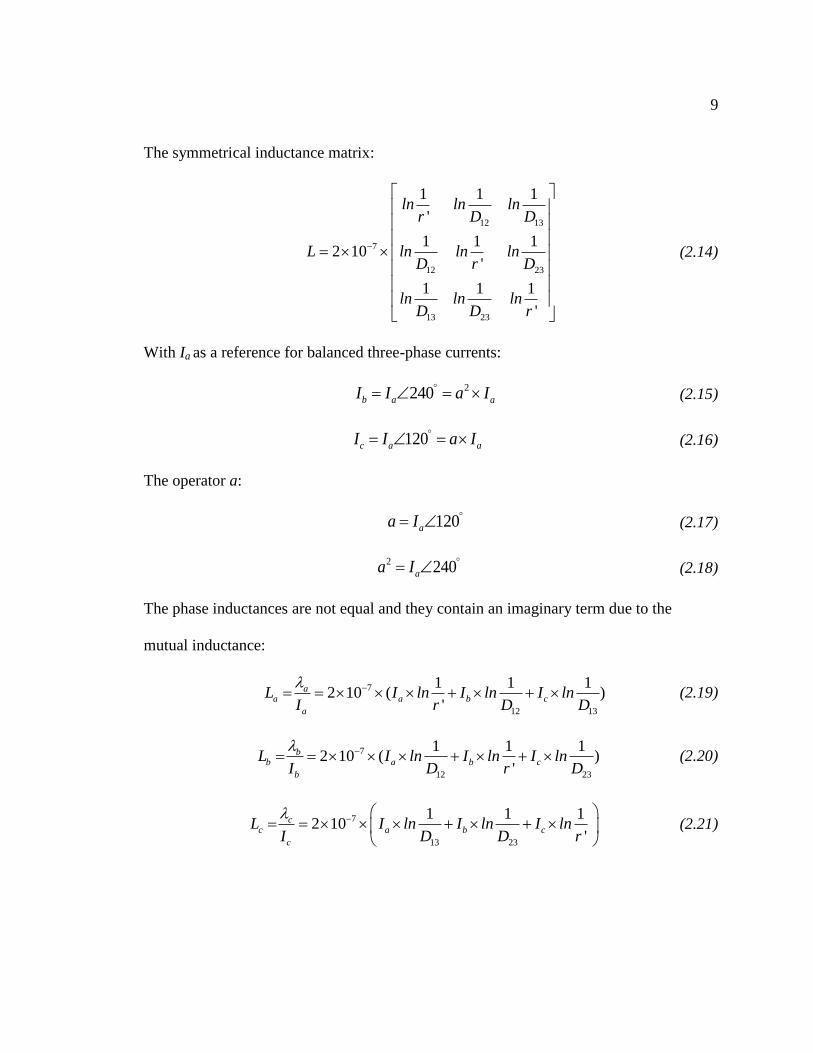
Conductor Sizes
The American Wire Gauge (AWG) is the standard generally employed in this country
and where American practices prevail. The circular mil (cmil) is usually used as the unit
of measurement for conductors. It is the area of a circle having a diameter of 0.001 in,
which works out to be 0.7854 × 10⁻⁶ in2. In the metric system, these figures are a
diameter of 0.0254 mm and an area of 506.71 × 10⁻⁶ mm2 [11]. Wire sizes are given in
gauge numbers, which, for distribution system purposes, range from a minimum of no. 12
to a maximum of no.0000 (or 4/0) for solid type conductors. Solid wire is not usually
made in sizes larger than 4/0, and stranded wire for sizes larger than no. 2 is generally
used. Above the 4/0 size, conductors are generally given in circular mils (cmil) or in
thousands of circular mils (cmil × 103); stranded conductors for distribution purposes
usually range from a minimum of no. 6 to a maximum of 1,000,000 cmil (or 1000 cmil ×
103) and may consist of two classes of strandings. Gauge numbers may be determined
from the formula:
0.3249
1.123n
Diameter in (2.30)

16
105,500
Cross sectional area 1,261n
cmil (2.31)
where n is the gauge number (no. 0 = 0; no. 00 = – 1; no. 000 = – 2; no.0000 = – 3) [11].
2.6 EXTRA HIGH VOLTAGE LIMITING FACTORS
Limiting factors for extra high voltage are:
a) Corona
b) Radio noise (RN)
c) Audible Noise (AN)
2.6.1 CORONA
Air surrounding conductors act as an insulator between them. Under certain conditions
air gets ionized and its partial breakdown occurs. Disruption of air dielectrics when the
electrical field reaches the critical surface gradient is known as corona. Corona effect
causes significant power loss and a high frequency current. Corona comes in different
forms: visual corona as violet or blue glows, audible corona as high pitched sound and
gaseous corona as ozone gas which can be identified by its specific odor. In addition
high conductor surface gradient causes the emission of radio and television interference
(RI and TVI) to the surrounding antennas known as radio corona. In order to design
corona free lines it is necessary to take into consideration following factors:
1) Electrical
2) Atmospheric

17
3) Conductor
1) Electrical Factors:
a) Frequency and waveform of the supply: Corona loss is a function of frequency.
For that reason the higher the frequency of the supply voltage the higher is corona
loss. This means that corona loss at 60 Hz is greater than at 50 Hz. As a result
direct current (DC) corona loss is less than the alternate current (AC).
b) Line Voltage: Line voltage factor is significant for voltages higher than disruptive
voltage. Corona and line voltage are directly proportional.
c) Conductor electrical field: Conductor electrical field depends on the voltage and
conductor configuration i.e., vertical, horizontal, delta etc. In horizontal
configuration the middle conductor has a larger electrical field than the outsides
ones. This means that the critical disruptive voltage is lower for the middle
conductor and therefore corona loss is larger.
2) Atmospheric Factors: Air density, humidity, wind, temperature and pressure have an
effect on the corona loss. In addition rain, snow, hail and dust can reduce the critical
disruptive voltage and hence increase the corona loss. Rain has more effect on the
corona loss than any other weather conditions. The most influential are temperature
and pressure. Atmospheric condition such as air density is directly proportional to the
air strength breakdown.
3) Conductor Factors: Several different conductor factors affect the corona loss:

18
a) Radius or size of the conductor: The larger the size of the conductor (radius) the
larger the power lower loss. For a certain voltages the larger the conductor size,
the larger the critical disruptive voltage and therefore the smaller the power loss.
2( )loss ln cP V V (2.32)
Vln = line-to-neutral (phase) operating voltage in kV
Vc = disruptive (inception) critical voltage kV (rms)
b) Spacing between conductors: The larger the spacing between conductors the
smaller the power loss. This can be observed from power loss approximation:
loss
rP
D (2.33)
r = conductor radius
D = distance (spacing) between conductors
c) Number of conductors / Phases: In case of a single conductor per phase for higher
voltages there is a significant corona loss. In order to reduce corona loss two or
more conductors are bundled together. By bundling conductors the self-
geometric mean distance (GMD) and the critical disruptive voltage are greater
than in case of a single conductor per phase which leads to reducing corona loss.
d) Profile or shape of the conductor: Conductors can have different shapes or
profiles. The profile of the conductor (cylindrical, oval, flat, etc.,) affects the
corona loss. Cylindrical shape has better field uniformity than any other shape and
hence less corona loss.

19
e) Surface conditions of the conductors: The disruptive voltage is higher for smooth
cylindrical conductors. Conductors with uneven surface have more deposit (dust,
dirt, grease, etc.,) which lowers the disruptive voltage and increases corona.
f) Clearance from ground: Electrical field is affected by the height of the conductor
from the ground. Corona loss is greater for smaller clearances.
g) Heating of the conductor by load current: Load current causes heating of the
conductor which accelerates the drying of the conductor surface after rain. This
helps to minimize the time of the wet conductor and indirectly reduces the corona
loss [12].
2.6.2 LINE DESIGN BASED ON CORONA
When designing a long transmission line (TL) it is desirable to have corona-free lines for
fair weather conditions and to minimize corona loss under wet weather conditions. The
average corona value is calculated by finding out corona loss per kilometer at various
points at long transmission line and averaging them out. For typical transmission line in
fair weather condition corona loss of 1kW per three-phase mile and foul weather loss of
20 kW per three-phase mile is acceptable [7].
2.6.3 ADVANTAGES OF CORONA
Corona reduces the magnitude of high voltage waves due to lightning by partially
dissipating as a corona loss. In this case it has a purpose of a safety valve.
20
2.6.4 DISADVANTAGES OF CORONA
a) Loss of power
b) The effective capacitance of the conductor is increased which increases the
flow of charging current.
c) Due to electromagnetic and electrostatic induction field corona interferes with
the communication lines which usually run along the same route as the power
lines [7].
2.6.5 PREVENTION OF CORONA
Corona loss can be prevented by:
a) increasing the radius of conductor
b) increasing spacing of the conductors
c) selecting proper type of the conductor
d) using bundled conductors [7].
2.6.6 RADIO NOISE
Radio noise (RN) happens due to corona and gap discharges (sparking). It is unwanted
interference within radio frequency band. RN includes radio interference (RI) and
television interference (TVI).
Radio interference (RI): It affects amplitude modulated (AM) radio waves within the
standard broadcast band (0.5 to 1.6 MHz). Frequency modulated (FM) waves are less
affected.

21
Television interference (TVI): In general TVI is caused by sparking within VHF (30-
300MHz) and UHF (300-3000MHz) bands. Two types of TVI are recognized due to
weather conditions: fair and foul [1].
2.6.7 AUDIBLE NOISE
Audible noise (AN) takes place predominantly during foul weather conditions due to
corona. AN sounds like a hiss or sizzle. In addition corona produces low-frequency
humming tones (120 - 240Hz) [1].
2.7 LINE MODELING
To understand the electrical performance of a transmission line, electrical parameters at
both ends of a line must be evaluated. When voltage and current is given at one end of a
line, an accurate calculation of voltage and current at the other end, or at some point
along the line, requires a sufficiently accurate model of a line. How a transmission line is
modeled depends on the line length. There are three classes of line lengths. For line
lengths that are classified as short, up to 50 miles, the model is simplified because shunt
capacitance and shunt admittance can be omitted because they have little effect on the
accuracy of the model. Because the line impedance is constant throughout the line, the
current will be the same from the sending end to the receiving end, so the model can be a
simple, lumped impedance value, as shown in Figure 2.5 [1].

22
Figure 2.5 Equivalent circuit of short transmission line [1].
For line lengths that are classified as medium, between 50 and 150 miles, there is enough
current leaking through the shunt capacitance that shunt admittance must be included in
order for the model to be an acceptable representation. However, a medium line is still
short enough that lumping the shunt admittance at some points along the line is a
sufficiently accurate model [1]. Typically, a medium line is modeled either as a T or π
network, as shown in Figures 2.6 and 2.7.
Figure 2.6 Nominal-T circuit of medium transmission line [1].
I S Z = R + jX LI R
+
V S
-
+
V R
-
a a ’
N ’N
S e n d in g
e n d
( s o u r c e )
R e c e iv in g
e n d
( s o u r c e )
l
I S R / 2 + j( X L / 2 ) R / 2 + j( X L / 2 ) I R
+
V S
-
+
V R
-
C G
I Y
a a ’
N ’N
V Y

23
Figure 2.7 Nominal-π circuit of medium transmission line [1].
For line lengths that are classified as long, above 150 miles, the needed accuracy from the
model requires that the series impedance and shunt admittance be represented by a
uniform distribution of the line parameters [1]. Each differential length is infinitely small
and defined as a unit length. The series impedance and shunt admittance is represented
for each unit length of line, as shown in Figure 2.8.
Figure 2.8 Segment of one phase and neutral connection for long transmission line [5].
I S R + jX LI R
+
V S
-
+
V R
-
C / 2 G / 2
I C 1
a a ’
N ’N
C / 2 G / 2
I C 2
I I

24
This model accounts for the changes in voltage and current throughout the line exactly as
the series impedance and shunt admittance affect them. In this way, the difference
between voltage and current at the sending end and receiving end can be analyzed
accurately [5]. The scope of this project will only cover the mathematical model used for
designing long line lengths. For details of the long transmission line mathematical model,
see Chapter 3.
2.8 LINE LOADABILITY
The characteristic impedance of a line, also known as surge impedance, is a function of
line inductance and capacitance. Surge impedance loading (SIL) is a measure of the
amount of power the line delivers to a purely resistive load equal to its surge impedance.
SIL provides a comparison of the capabilities of lines to carry load, and permissible
loading of a line can be expressed as a fraction of SIL.
The theoretical maximum power that can be transmitted over a line is when the angular
displacement across the line is δ = 90⁰, for the terminal voltages. However, for reasons
of system stability, the angular displacement across the line is typically between 30⁰ and
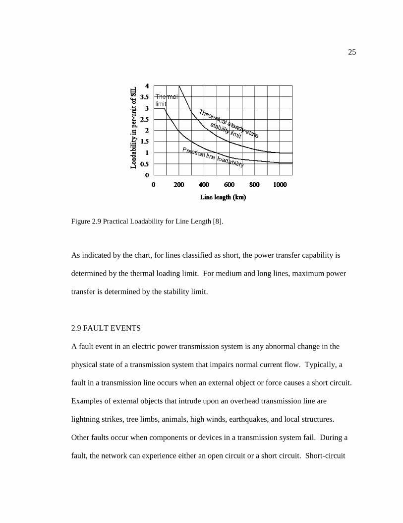
45⁰ [8]. Figure 2.9 illustrates the differences in curve plots for the theoretical steady-
state stability limit and a practical line loadability. The practical line loadability is
derived from a typical voltage-drop limit of and a maximum angular
displacement of 30⁰ to 35⁰ across the line [8]. The loadability curve is generally
applicable to overhead 60-Hz lines with no compensation.
25
Figure 2.9 Practical Loadability for Line Length [8].
As indicated by the chart, for lines classified as short, the power transfer capability is
determined by the thermal loading limit. For medium and long lines, maximum power
transfer is determined by the stability limit.
2.9 FAULT EVENTS
A fault event in an electric power transmission system is any abnormal change in the
physical state of a transmission system that impairs normal current flow. Typically, a
fault in a transmission line occurs when an external object or force causes a short circuit.
Examples of external objects that intrude upon an overhead transmission line are
lightning strikes, tree limbs, animals, high winds, earthquakes, and local structures.
Other faults occur when components or devices in a transmission system fail. During a
fault, the network can experience either an open circuit or a short circuit. Short-circuit

26
faults impose the most risk of damaging elements in a power system. Open circuit faults
are typically not a threat for causing damage to other network elements.
2.10 FAULT ANALYSIS
Important part of TL designing includes fault analysis. In order to have well protected
network typically faults are simulated at different points throughout the transmission
system. It is crucial to have precise analysis of the designed system to prevent fault‟s
interruption. In general the three phase faults can be classified as:
1. Shunt faults (short circuits)
1.1. Unsymmetrical faults (Unbalanced)
1.1.1. Single line-to-ground (SLG) fault
1.1.2. Line-to-line (L-L) fault
1.1.3. Double line-to-ground (DLG) fault
1.2. Symmetrical fault (Balanced)
1.2.1. Three-phase-fault
2. Series Faults (open conductor)
2.1. Unbalanced faults
2.1.1. One line open (OLO)
2.1.2. Two lines open (TLO)
3. Simultaneous faults

27
2.11 SINGLE LINE-TO-GROUND (SLG) FAULT
Seventy percent of all transmission line faults are attributable to when a single conductor
is physically damaged and either lands a connection to the ground or makes contact with
the neutral wire [1]. This fault type makes the system unbalanced and is called a single
line-to-ground (SLG) fault. The failed phase conductor, generally defined as phase a, is
connected to ground by an impedance value Zf. Figure 2.10 shows the general
representation of an SLG fault.
Zf
a
b
c
n
F
+Vaf
-
Ibf = 0Iaf Icf = 0
Figure 2.10 General representation for single line-to-ground fault [1].
2.12 LINE-TO-LINE (L-L) FAULT
A line-to-line fault is unsymmetrical (unbalanced) fault and it takes place when two
conductors are short-circuited. This can happen for various reasons i.e., ionization of air,

28
flashover, or bad insulation. Figure 2.11 shows the general representation of an LL fault
[1].
a
b
c
F
Ibf Iaf=0 Icf = -Ibf
Zf
Figure 2.11 General representation for line-to-line fault [1].
2.13 DOUBLE LINE-TO-GROUND (DLG) FAULT
Ten percent of all transmission line faults are attributable to when two conductors are
physically damaged and both of them land a connection through the ground or both
contact the neutral wire [1]. This fault type makes the system unbalanced and is called a
double line-to-ground (DLG) fault. The failed phase conductors, generally defined as
phases b and c, are each connected to ground by their own separate fault impedance value
Zf and a common ground impedance value Zg.

29
Figure 2.12 shows the general representation of a DLG fault.
Zf
a
b
c
n
F
Ibf Iaf = 0 Icf
Zf
Zg
N
Ibf + Icf
Figure 2.12 General representation of double line-to-ground fault [1].
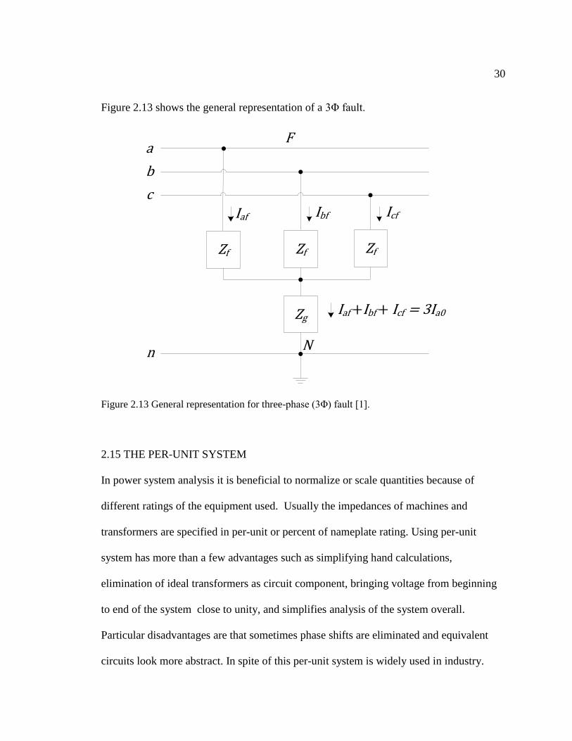
2.14 THREE-PHASE FAULT
A three-phase (3Φ) fault occurs when all three phases of a TL are short-circuited to each
other or earthed. It is a symmetrical (balanced) fault and the most severe one. Since 3Φ
fault is balanced it is sufficient to identify the positive sequence network. As all three
phases carry 120 displaced equal currents the single line diagram can be used for the
analysis. Three-phase faults make 5% of the initial faults in a power system [1].
30
Figure 2.13 shows the general representation of a 3Φ fault.
Zf
a
b
c
n
F
Ibf Iaf Icf
Zf
Zg
N
Iaf +Ibf + Icf = 3Ia0
Zf
Figure 2.13 General representation for three-phase (3Φ) fault [1].
2.15 THE PER-UNIT SYSTEM
In power system analysis it is beneficial to normalize or scale quantities because of
different ratings of the equipment used. Usually the impedances of machines and
transformers are specified in per-unit or percent of nameplate rating. Using per-unit
system has more than a few advantages such as simplifying hand calculations,
elimination of ideal transformers as circuit component, bringing voltage from beginning
to end of the system close to unity, and simplifies analysis of the system overall.
Particular disadvantages are that sometimes phase shifts are eliminated and equivalent
circuits look more abstract. In spite of this per-unit system is widely used in industry.

31
Chapter 3
MATHEMATICAL MODEL
Equation Chapter (Next) Section 1
3.1 INTRODUCTION
This chapter steps through the mathematical approach which is used for design and
analysis of an overhead extra-high voltage long transmission line. Some information
about the physical solution is included to relate the mathematical model and physical
solution.
After design requirements are established, the first step in preliminary design is to choose
a standardized support structure that can be adapted to provide the best solution for the
given job. The selection should be taken from a group of structures that have been
categorized as standard designs for the transmission voltage level that matches the design
requirement. A selected structure will define the spacing between conductor phases and
the limits on conductor size that can be supported.
The next step in preliminary design is to choose a conductor type and size that has
adequate capacity to handle the load current. With a preliminary selection of support
structure and conductor type and size, a detailed design analysis can be undertaken, as
shown in the mathematical approach from the following sections.
3.2 GEOMETRIC MEAN DISTANCE (GMD)
Bundling of conductors is used for extra-high voltage (EHV) lines instead of one large

32
conductor per phase. The bundles used at the EHV range usually have two, three, or four
subconductors [1].
(a) (b) (c)
d
d
d d
d
d d
d
Figure 3.1 Bundled conductors configurations: (a) two-conductor bundle; (b) three-conductor
bundle; (c) four-conductor bundle [1].
b'b
d
c'c
d
a'a
d
D12 D23
D31
Figure 3.2 Cross section of bundled-conductor three-phase line with horizontal tower
configuration [1].
The three-conductor bundle has its conductors on the vertices of an equilateral triangle,
and the four-conductor bundle has its conductors on the corners of a square.
For balanced three-phase operation of a completely transposed three-phase line only one
phase needs to be considered. Deq, the cube root of the product of the three-phase
spacings, is the geometric mean distance (GMD) between phases:
312 23 31 eq mD D D D D ft (3.1)

33
3.3 GEOMETRIC MEAN RADIUS (GMR)
Geometric Mean Radius (GMR) of bundled conductors for
Two-conductor bundle:
b
S SD D d ft (3.2)
Three-conductor bundle:
23 b
S SD D d ft (3.3)
Four-conductor bundle:
34 b
S SD D d ft (3.4)
where:
= GMR of subconductors
distance between two subconductors
If the phase spacings are large compared to the bundle spacing, then sufficient accuracy
for Deq is obtained by using the distances between bundle centers. If the conductors are
stranded and the bundle spacing d is large compared to the conductor outside radius, each
stranded conductor is replaced by an equivalent solid cylindrical conductor with
GMR= .
The modified GMR of bundled conductors used in capacitance calculations for
Two-conductor bundle:
b
SCD r d ft (3.5)
Three-conductor bundle:
3 2 b
SCD r d ft (3.6)

34
Four-conductor bundle:
341.09 b
SCD r d ft (3.7)
where:
= outside radius of subconductors
= distance between two subconductors.
3.4 INDUCTANCE AND INDUCTIVE REACTANCE
For three-phase transmission lines that are completely transposed, Equation (3.1) can be
used to find the equivalent equilateral spacing for the line. Thus, the average inductance
per phase is
72 10 ln
eq
a
s
D HL
D m
(3.8)
or
100.7411 log eq
a
s
D mHL
D mi
(3.9)
and the inductive reactance is found by
2L aX f L per phase (3.10)
or
0.1213 ln eq
L
s
DX
D mi
per phase (3.11)

35
3.5 CAPACITANCE AND CAPACITIVE REACTANCE
The average line-to-neutral capacitance per phase is
10
0.0388 μF to neutral
log
N
eq
CD mi
r
(3.12)
where
1
3 eq m ab bc caD D D D D ft (3.13)
radius of cylindrical conductor in feet.
The capacitive reactance is calculated by
1
2C
N
Xf C
(3.14)
or
100.06836 log .eq
C
DX M mi
r
(3.15)
3.6 LONG TRANSMISSION LINE MODEL
For lines 150 miles and longer, i.e. long lines, modeling with lumped parameters is not
sufficiently accurate for representing the effects of the parameters‟ uniform distribution
throughout the length of the line. An acceptable model provides mathematical
expressions for voltage and current at any point along the line [1]. Figure 3.3 depicts a
segment of one phase of a three-phase transmission line of length l.

36
Figure 3.3 Segment of one phase and neutral connection for long transmission line. [5]
The following derivation is given by Saadat [5]. The series impedance per unit length is
z, and the shunt admittance per phase is y, where z = r + jωL and y = g + jωC. Consider
one small segment of line Δx at a distance x from the receiving end of the line. The
phasor voltages and currents on both sides of this segment are shown as a function of
distance. From Kirchhoff‟s voltage law
( )V x x V x z xI x (3.16)
or
( )
( )V x x V x
zI xx
(3.17)

37
Taking the limit as , we have
( )
( )dV x
zI xdx
(3.18)
Also, from Kirchhoff‟s current law
I x x I x y xV x x (3.19)
or
( )
( )I x x I x
yV x xx
(3.20)
Taking the limit as , we have
( )
( )dI x
yV xdx
(3.21)
Differentiating (3.18) and substituting from (3.21), we get
2
2
( ) ( )( )
d x dI xz z x
dx
VyV
dx (3.22)
Let
2 zy (3.23)
The following second-order differential equation will result.
2
2
2
( )0
d V xV x
dx (3.24)
The solution of the above equation is
1 2
x xV x Ae A e (3.25)
where γ, known as the propagation constant, is a complex expression given by (3.23) or
( ) ( )j zy r j L g j C (3.26)

38
The real part α is known as the attenuation constant, and the imaginary component β is
known as the phase constant. β is measured in radian per unit length. From (3.18), the
current is
1 2 1 2
1 ( ) x x x xdV x yI x Ae A e Ae A e
z dx z z
(3.27)
or
1 2
1 x x
C
I x Ae A eZ
(3.28)
where Zc is known as the characteristic impedance, given by
C
zZ
y (3.29)
To find the constants and , we note that when , ( ) , and ( ) .
From (3.25) and (3.28) these constants are found to be
12
R C RV Z IA
(3.30)
22
R C RV Z IA
(3.31)
Upon substitution in (3.25) and (3.28), the general expressions for voltage and current
along a long transmission line become
2 2
x xR C R R C RV Z I V Z IV x e e
(3.32)
2 2
R RR R
x xC C
V VI I
Z ZI x e e
(3.33)

39
The equations for voltage and currents can be rearranged as follows:
2 2
x x x x
R C R
e e e eV x V Z I
(3.34)
1
2 2
x x x x
R R
C
e e e eI x V I
Z
(3.35)
Recognizing the hyperbolic functions sinh, and cosh, the above equations are written as
follows:
cosh sinhR C RV x x V Z x I (3.36)
1
sinh coshR R
C
I x x V x IZ
(3.37)
We are particularly interested in the relation between the sending-end and the receiving-
end on the line. Setting , ( ) and ( ) , the result is
cosh sinhS R C RV l V Z l I (3.38)
1
sinh coshS R R
C
I l V l IZ
(3.39)
Rewriting the above equations in terms of ABCD constants, we have
S R
S R
V VA B
I IC D
(3.40)
where
cosh cosh coshA l YZ (3.41)
sinh sinh sinhC C
ZB Z l YZ Z
Y (3.42)

40
sinh sinh sinhC C
YC Y l YZ Y
Z (3.43)
cosh cosh coshD A l YZ (3.44)
where
LZ r jx l (3.45)
is total line series impedance per phase
S Y g jb l (3.46)
is total line shunt admittance per phase.
Note that A D (3.47)
and 1AD BC . (3.48)
For a long transmission line, conductance is very small compared to susceptance, and can
be omitted for simplicity. Thus, can be reduced to the following equation:
1
C
Y jb l j lX
(3.49)
3.7 SENDING-END VOLTAGE AND CURRENT
One step in line design is analyzing what power input, i.e. voltage and current, is needed
at the sending-end in order to deliver the load power requirements. If the resulting power
input needs are within parameters that are acceptable to the overall power system, the
design is viable. However, the line design may still be adjusted to match preferred input
parameters. After the ABCD constants are determined, as shown in the previous section,
the following steps can be used to find the sending-end voltage and current.

41
Using the receiving-end design requirements for load power, voltage, and power factor,
the receiving-end line-to-neutral voltage and current magnitude are determined by the
following equations:
( )
3
R L L
R L N
VV (3.50)
and
( )3
R
R L L
S
IV
(3.51)
where:
( ) receiving-end line-to-neutral voltage (kV),
magnitude of receiving-end line current (A).
The receiving-end current phasor can be found by
(cos sin )R R R Rj I I (3.52)
where:
angle difference between ( ) and
and can be found by taking the inverse cosine of the power factor.
Using the calculated values for ABCD constants and receiving-end voltage and current,
we can use Equation (3.40) to determine the corresponding sending-end voltage and
current.
The sending-end voltage and current can be equated by
( ) ( ) ( )S L N RR L N V A V B I (3.53)

42
and
( ) ( )S RR L N I C V D I (3.54)
where:
sending-end line current (A),
( ) sending-end line-to-neutral voltage (kV).
The sending-end line-to-line voltage is
( ) 3 1 30S L L S L N V V (3.55)
where:
( ) sending-end line-to-line voltage (kV).
Note that an additional is added to the angle since the line-to-line voltage is
ahead of its line-to-neutral voltage.
3.8 POWER LOSS
Typically, referring to power loss in a transmission line means the difference in real
power between the sending- and receiving- ends. To calculate the power loss, the first
step is to determine the power factor at each end. For the receiving-end, the power factor
is normally specified per design criteria. For the sending-end, the power factor is found
by determining the angle θS between the sending-end current and voltage phasors. The
expression for sending-end power factor is
cos( os) cSS
S IV L N spf
(3.56)

43
where:
sending-end power factor,
( ) = angle of sending-end line-to-neutral voltage phasor,
angle of sending-end current phasor,
angle difference between ( ) and .
Then, using the value of , the equation for calculating real power at the sending-end is
( )33 cosS L L S SS
P V I (3.57)
where:
( ) sending-end real power in the line (MW).
A similar equation for calculating the receiving-end real power is
( )33 cosR L L R RR
P V I (3.58)
where:
( ) receiving-end real power in the line (MW).
Using the calculated values from the above equations, real power loss in the line is found
by
(3 ) (3 ) (3 )L S RP P P (3.59)
where:
( ) total real power loss in the line (MW).
The majority of power loss in a transmission line is a result of real power loss due to the
resistance of the line. A good design will minimize the total real power loss in the line.

44
3.9 TRANSMISSION LINE EFFICIENCY
Performance of transmission lines is determined by efficiency and regulation of lines.
Transmission line efficiency is:
100R
S
P
P (3.60)
where:
= transmission line efficiency
= receiving-end power
= sending end power
% 100
Power deliverd at receiving endtransmissionlineefficiency
Power sent fromthesending end (3.61)
% 100R
S
Ptransmissionlineefficiency
P (3.62)
The end of the line where source of supply is connected is called the sending end and
where load is connected is called the receiving end [1].
3.10 PERCENT VOLTAGE REGULATION
Voltage regulation of the line is a measure of the decrease in receiving-end voltage as
line current increases. In mathematical terms, percent voltage regulation is defined as the
percent change in receiving-end voltage from the no-load to the full-load condition at a
specified power factor with sending-end voltage VS held constant, that is,
, ,
,
- | |
| |
R NL R FL
R FL
V VPercentVR 100
V (3.63)

45
where:
|VR,NL|=magnitude of receiving-end voltage at no-load,
|VR,FL|=magnitude of receiving-end voltage at full-load with constant |Vs|,
|VS|=magnitude of sending-end phase (line-to-neutral) voltage at no load.
3.11 SURGE IMPEDANCE LOADING (SIL)
In power system analysis of high frequencies or surges caused by lightning, losses are
typically ignored and surge impedance becomes important. A line is lossless when its
series resistance and shunt conductance are zero [6]. The surge impedance of a lossless
line, also known as characteristic impedance, is a function of line inductance and
capacitance, and can be expressed as
C
LZ
C (3.64)
or
C C LZ X X (3.65)
where:
shunt capacitive reactance ( ),
series inductive reactance ( ),
characteristic impedance (Ω).
Surge impedance loading (SIL), a measure of the amount of power the line delivers to a
purely resistive load equal to its surge impedance [6], is found for a three-phase line by
the following equation:

46
2
( )| |Lr L
c
kVSIL MW
Z
(3.66)
where: SIL = surge impedance loading (MW).
SIL provides a comparison of the capabilities of lines to carry load, and permissible
loading of a line can be expressed as a fraction of SIL. SIL, or natural loading, is a
function of the line-to-line voltage, line inductance and line capacitance. Since the
characteristic impedance is based on the ratio of inductance and capacitance, SIL is
independent of line length. The relationship between SIL and voltage explains why an
extra-high voltage line has more power transfer capability than lower voltage lines.
3.12 SAG AND TENSION
3.12.1 CATENARY METHOD
Sag-tension calculations predict the behavior of conductors based on recommended
tension limits under varying loading conditions. These tension limits specify certain
percentages of the conductor‟s rated breaking strength that are not to be exceeded upon
installation or during the life of the line. These conditions, along with the elastic and
permanent elongation properties of the conductor, provide the basis for defining the
amount of resulting sag during installation and long-term operation of the line.
Accurately determined initial sag limits are essential in the line design process. Final sags
and tensions depend on initial installed sags and tensions and on proper handling during
installation. The final sag shape of conductors is used to select support point heights and
span lengths so that the minimum clearances will be maintained over the life of the line.
47
If the conductor is damaged or the initial sags are incorrect, the line clearances may be
violated or the conductor may break during heavy ice or wind loadings [1].
( )maxT w c d (3.67)
( )maxT w c d (3.68)
minT w c (3.69)
H w c (3.70)
H
cw
(3.71)
minT H (3.72)
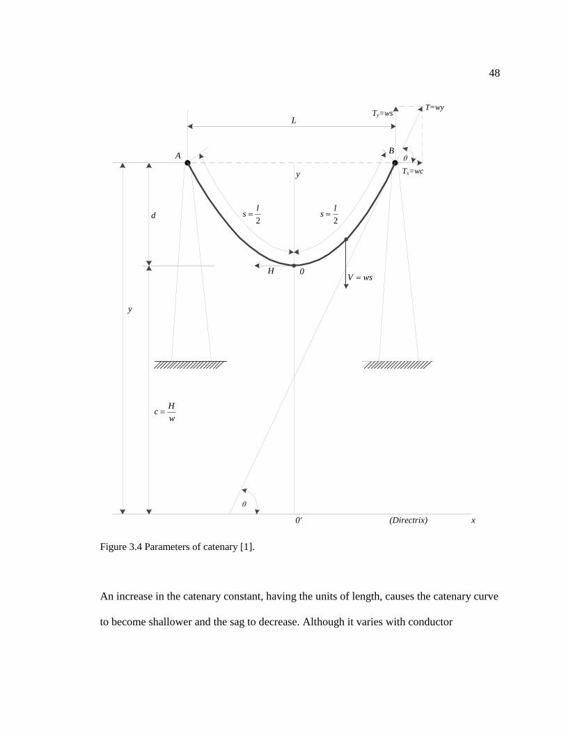
T = the tension of the conductor at any point P in the direction of the curve
w = the weight of the conductor per unit length
H = the tension at origin 0
c = catenary constant
s = the length of the curve between points 0 and P
v = that the weight of the portion s is ws
L = horizontal distance.
48
d
y
AB
L
0H
2
ls
2
ls
Hc
w
θ
θ
V ws
0' (Directrix) x
y
T=wyTy=ws
Tx=wc
Figure 3.4 Parameters of catenary [1].
An increase in the catenary constant, having the units of length, causes the catenary curve
to become shallower and the sag to decrease. Although it varies with conductor
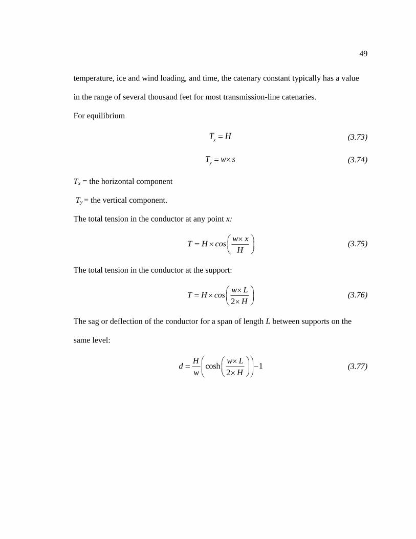
49
temperature, ice and wind loading, and time, the catenary constant typically has a value
in the range of several thousand feet for most transmission-line catenaries.
For equilibrium
xT H (3.73)
yT w s (3.74)
Tx = the horizontal component
Ty = the vertical component.
The total tension in the conductor at any point x:
w x
T H cosH
(3.75)
The total tension in the conductor at the support:
2
w LT H cos
H
(3.76)
The sag or deflection of the conductor for a span of length L between supports on the
same level:
cosh 12
H w Ld
w H
(3.77)

50
3.12.2 PARABOLIC METHOD
The conductor curve can be observed as a parabola for short spans with small sags.
x
y
A B
L
0 Hwx
d
Ty
H
θ
T Ty
Tx
P
Figure 3.5 Parameters of parabola [1].
The following assumptions can be taken into consideration when using parabolic method:
1. The tension is considered uniform throughout the span.
2. The change in length of the conductor due to stretch or temperature is the same as
the change of the length due to the horizontal distance between the towers [1].
Approximate value of tension by using parabolic method can be calculated as
2
8
w LT
d
(3.78)

51
or
2
8
w Ld
T
(3.79)
when
1
2x L (3.80)
y d . (3.81)
3.13 CORONA POWER LOSS
3.13.1 CRITICAL CORONA DISRUPTIVE VOLTAGE
The maximum stress on the surface of the conductor is given by:
ln
LNmax
V kVE
D cmm r
r
(3.82)
VLN = the phase or line-to-neutral voltage in kV
D = is equivalent spacing in cm
r = radius of the conductor in cm
mc = surface irregularity factor ( )
mc = 1 for smooth, solid, polished round conductor
mc = 0.93 – 0.98 for roughened or weathered conductor
mc = 0.80 – 0.87 for up to seven strands conductor
mc = approx. 0.90 for large conductor with more than seven strands [12]
Mean voltage gradient can be calculated from:

52
ln 3
LNmean
V kVE
D cmm r
r
(3.83)
The air density correction factor is defined as:
3.9211
273
p
t
(3.84)
where:
p = the barometric pressure in cm Hg
t = temperature in C
The critical disruptive voltage (corona inception voltage) Vc is voltage at which complete
disruption of dielectric occurs. The dielectric stress is 30δ kV/cm peak or 21.1δ rms at
NTP i.e., 25C and 76 mmHg. Vc is minimum conductor voltage with respect to earth at
which the corona is expected to start. At Vc corona is not visible [7].
30 c c
DV m r ln kV peak
r
(3.85)
21.1 c c
DV m r ln kV rms
r
(3.86)
Vc = the critical disruptive voltage in kV
The critical disruptive voltage Vc line-to-line is
( ) ( )3 c L L c rmsV V kV (3.87)
53
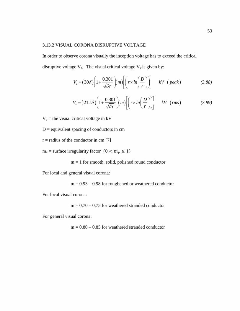
3.13.2 VISUAL CORONA DISRUPTIVE VOLTAGE
In order to observe corona visually the inception voltage has to exceed the critical
disruptive voltage Vc. The visual critical voltage Vv is given by:
0.301
30 1 v
DV m r ln kV peak
rr
(3.88)
0.301
21.1 1 v
DV m r ln kV rms
rr
(3.89)
Vv = the visual critical voltage in kV
D = equivalent spacing of conductors in cm
r = radius of the conductor in cm [7]
mv = surface irregularity factor ( )
m = 1 for smooth, solid, polished round conductor
For local and general visual corona:
m = 0.93 – 0.98 for roughened or weathered conductor
For local visual corona:
m = 0.70 – 0.75 for weathered stranded conductor
For general visual corona:
m = 0.80 – 0.85 for weathered stranded conductor

54
3.13.3 CORONA POWER LOSS AT AC VOLTAGE
For AC transmission lines empirical equations are used to determine corona loss.
According to Peek corona power loss can be determined from:
2 5241
25 10 / LN c
r kWP f V V phase peak
D km
(3.90)
P = corona loss in kW/km/phase
δ = density correction factor
VLN = the phase or line-to-neutral voltage in kV
Vc = the critical disruptive voltage in kV
f = frequency
r = radius of the conductor in cm
D = equivalent spacing of conductors in cm.
It is desirable to design transmission line with corona loss between 0.10 and 0.21
kW/km/phase for fair weather conditions. For lower loss range i.e., when
V
1 .8 LN
cV (3.91)
Peek‟s formula is not accurate [7].
According to Peterson‟s corona power loss formula:
2
5
10
2.1 10 /cV kWP f F phase
D kmlog
r
(3.92)
F = corona loss function

55
VLN / Vc 1.0 1.2 1.4 1.5 1.6 1.8 2.0
F 0.037 0.082 0.3 0.9 2.2 4.95 7.0
Table 3.1 Corona factor [7].
Above stated formulas are used for fair weather conditions. For wet weather conditions
critical disruptive voltage is approximately 0.80 of the fair weather calculated value. The
calculated disruptive critical voltage for three-phase horizontal conductor configuration
can be determined as:
3 0.96
c c fairV V
(3.93)
for the middle conductor and
3 1.06
c c fairV V
(3.94)
for the two outer conductors [1].
3.14 METHOD OF SYMMETRICAL COMPONENTS
According to Charles Fortescue, a set of three-phase voltages are resolved into the
following three sets of sequence components:
1. Zero-sequence components: consisting of three phasors with equal magnitudes and
with zero phase displacement
2. Positive-sequence components, consisting of three phasors with equal magnitudes,
±120 phase displacement
3. Negative-sequence components, consisting of three phasors with equal magnitudes,
±120 phase displacement[1].

56
Vb0 Vc0 = V0Va0
Vc2
Vb2 Va2 = V2
Va1 = V1
Vb1
Vc1
(a) (b) (c)
Figure 3.6 Sequence components: ( a) zero ( b) positive ( c) negative [8 ]
0 1 2 a a a a V V V V (3.95)
0 1 2 b b b b V V V V (3.96)
0 1 2 c c c c V V V V (3.97)
Operator a is a complex number with unit magnitude and a 120 phase angle. When any
phasor is multiplied by a, that phasor rotates by 120 (counterclockwise).
A list of some common powers, functions and identities involving a:
Power or Function In Polar Form In Rectangular Form
a 1120 -0.5+j0.866
a2 1240=1-120 -0.5-j0.866
a3 1360=10 1.0+j0.0
a4 1120 -0.5+j0.866
1+a = -a2 160 0.5+j0.866
1- a √ -30 1.5-j0.866
1+ a2= -a 1-60 0.5-j0.866
1- a2 √ 30 1.5+j0.866
a -1 √ 150 -1.5+j0.866
a + a2 1180 -1.0+j0.0
a - a2 √ 90 0.0+j1.732
a2- a √ -90 0.0-j1.732
a2- 1 √ -150 -1.5-j0.866
1 + a + a2 0 0.0+j0.0
ja 1210 -0.884+j0.468
Table 3.2 Power and functions of operator a [1].

57
1 120 a (3.98)
1 3
1 1202 2
j
a (3.99)
Similarly, when any phasor is multiplied by
2 1 120 1 240 a (3.100)
the phasor rotates by 240.
The phase voltages in terms of the sequence voltages i.e. synthesis equations:
0 1 2 0a a a a V V V V (3.101)
2
0 1 2 0b a a a V a V aV V (3.102)
2
0 1 2 0c a a a V aV a V V (3.103)
The sequence voltages in terms of phase voltages i.e. analysis equations:
0
1
3a a b c V V V V (3.104)
2
1
1
3a a b c V V aV a V (3.105)
2
2
1
3a a b c V V a V aV (3.106)
In matrix form the phase voltages can be expressed as
0
2
1
2
2
1 1 1
1
1
a a
b a
c a
V V
V a a V
V a a V
(3.107)
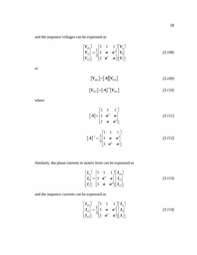
58
and the sequence voltages can be expressed as
0
2
1
2
2
1 1 11
13
1
a a
a b
a c
V V
V a a V
V a a V
(3.108)
or
012abc V A V (3.109)
1
012 abc
V A V (3.110)
where
2
2
1 1 1
1
1
A a a
a a
(3.111)
1 2
2
1 1 11
13
1
A a a
a a
(3.112)
Similarly, the phase currents in matrix form can be expressed as
0
2
1
2
2
1 1 1
1
1
a a
b a
c a
I I
I a a I
I a a I
(3.113)
and the sequence currents can be expressed as
0
2
1
2
2
1 1 11
13
1
a a
a b
a c
I I
I a a I
I a a I
(3.114)

59
or
012abc I A I (3.115)
1
012 abc
I A I (3.116)
3.14.1 SEQUENCE IMPEDANCES OF TRANSPOSED LINES
In order to attain equal mutual impedances the line should be transposed or conductors
should have equilateral spacings.
Hence, for the equal mutual impedances
ab bc ca m Z Z Z Z (3.117)
In case when the self-impedances of conductors are equal to each other
aa bb cc s Z Z Z Z . (3.118)
Therefore,
s m m
abc m s m
m m s
Z Z Z
Z Z Z Z
Z Z Z
(3.119)
where,
0.1213ln es a e
s
Dr r j l
D
Z Ω (3.120)
and
0.1213ln em e
eq
Dr j l
D
Z Ω. (3.121)
ra = resistance of a single conductor a

60
re = resistance of Carson‟s equivalent earth return conductor which is a function of
frequency
31.588 10er f
. (3.122)
At 60 Hz,
0.09528er
(3.123)
At 60 Hz frequency and for 100
average earth resistivity
2788.55eD ft. (3.124)
The equilateral spacings of the conductors can be calculated as
3eq m ab bc caD D D D D (3.125)
The Ds is geometric mean radius (GMR) of the phase conductor.
The sequence impedance matrix of a transposed transmission line can be expressed as
012
2 0 0
0 0
0 0
s m
s m
s m
Z Z
Z Z Z
Z Z
(3.126)
where, by definition,
Z0 is zero-sequence impedance at 60Hz
0 00 2s mZ Z = Z Z (3.127)
3
0 23 0.1213ln e
a e
s eq
Dr r j l
D D
Z Ω, (3.128)

61
Z1 is positive-sequence impedance at 60Hz
1 11 s m-Z Z = Z Z (3.129)
1 0.1213lneq
a
s
Dr j l
D
Z Ω, (3.130)
Z2 is negative-sequence impedance at 60Hz
2 22 s m-Z Z = Z Z (3.131)
2 0.1213lneq
a
s
Dr j l
D
Z Ω. (3.132)
Therefore, the sequence impedance matrix of a transposed transmission line can be
expressed as
0
012 1
2
0 0
0
0 0
Z
Z Z
Z
(3.133)
3.15 FAULT ANALYSIS
Three-phase faults can be balanced (i.e., symmetrical) or unbalanced (i.e.,
unsymmetrical). The unbalanced faults are more common. In order to resolve an
unbalanced system the method of symmetrical components can be applied by converting
the system into positive, negative and the zero-sequence fictitious networks. After
defining positive, negative and zero-sequence currents for specific fault phase currents,
sequence and phase voltages can calculated.

62
3.16 PER UNIT
Power, current, voltage, and impedance are often expressed in per-unit or percent of
specified base values.
The per-unit values are calculated as:
-
actual quantity
per unit quantitybasevalueof quantity
(3.134)
where actual quantity is the value of the quantity in the actual units and the base value
has the same units as the actual quantity, forcing the per-unit quantity to be
dimensionless. The actual value may be complex but the base value is always a real
number. Consequently, the angle of the per-unit value is the same as the angle of the
actual value [8] .
In a given power system two independent base values can be arbitrarily selected at one
point. Typically the base complex power Sbase1Φ and the base voltage VbaseLN are chosen
for either a single-phase circuit or for one phase of a three-phase circuit. In order to
preserve electrical laws in the per-unit system, the following equations must be used for
other base values:
1 1 1 base base baseP Q S (3.135)
11
basebase
baseLN
SI
V
(3.136)
2
1
baseLN baseLNbase base base
base base
V VR X
I SZ
(3.137)
1
base base base
base
Y G BZ
(3.138)

63
2
basebase
base
kVZ
MVA (3.139)
( )
3
basebase
base LL
MVAI
kV (3.140)
The subscripts LN and 1Φ represent “line-to-neutral” and “per-phase” respectively, for
three-phase circuits. Equations (2.35) and (2.36) are also effective for single-phase
circuits by omitting the subscripts.
By agreement, the following two rules for base quantities are assumed:
1) The value of Sbase1Φ is the same for the entire power system
2) The ratio of the voltage bases on either side of a transformer is selected to be the
same as the ratio of the transformer voltage ratings.
As a result per-unit impedance remains unchanged when referred from one side of a
transformer to the other [8].
3.17 SINGLE LINE-TO-GROUND (SLG) FAULT
An SLG fault generally occurs when one phase conductor either falls to the ground or
makes contact with the neutral wire. Figure 3.7 depicts the typical representation of an
SLG fault at a fault point F with a fault impedance Zf. It is customary to show the fault
occurring on phase a. If the fault actually takes place on another phase, the phases of the
system can simply be relabeled in the appropriate sequence.

64
(a)
(b)
Figure 3.7 Single line-to-ground fault: (a) general representation; (b) sequence network
connection [1]
From inspection of Figure 3.7a, the currents for phases b and c are
0bf cf I I (3.141)
Zf
a
b
c
n
F
+Vaf
-
Ibf = 0Iaf Icf = 0
F0Z0 N0
+ VA0 -
F1Z1 N1
+ VA1 -
F2Z2 N2
+ VA2 -
1.0 + -
0o
3ZfIa1
Ia1Ia0 Ia2
Zero-sequencenetwork
Positive-sequencenetwork
Negative-sequencenetwork

65
Substituting values into Equation (3.114), the symmetrical components for
the currents are given as
0
2
1
2
2
1 1 11
1 03
1 0
a af
a
a
a a
a a
I I
I
I
(3.142)
Using the above equation, the sequence currents for phase a are
0 1 2
1
3a a a af I I I I (3.143)
and can be rewritten as
0 1 23 3 3 af a a a I I I I (3.144)
By inspection of Figure 3.7b, the zero-, positive-, and negative-sequence currents are
equal and can be determined by
0 1 2
0 1 2
1.0 0
3a a a
f
I I I
Z Z Z Z (3.145)
Substituting (3.145) into Equation (3.144) gives
0 1 2
1.0 03
3af
f
IZ Z Z Z
(3.146)
With the sequence current values, Equation (3.155) can be used to find the sequence
voltages, and then Equation (3.107) can be used to find the phase voltages.

66
3.18 LINE-TO-LINE (L-L) FAULT
A line-to-line (L-L) fault occurs when two conductors are short-circuited. Figure 3.8a
represents the characteristic representation of a L-L fault at a fault point F with a fault
impedance Zf. Figure 3.8b indicates the interconnection of resulting sequence networks.
It is presumed that L-L fault is between phases b and c.
(a)
(b)
Figure 3.8 Line-to-line fault: (a) general representation; (b) sequence network connection [1].
a
b
c
F
Ibf Iaf=0 Icf = -Ibf
Zf
F0
Z0
N0
+VA0 = 0
-
F1
Z1
N1
+VA1
-
F2
Z2
N2
+VA2
-+
1.0-
0o
Ia1Ia0=0 Ia2
Zf
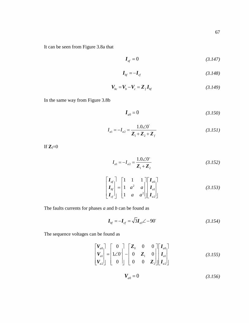
67
It can be seen from Figure 3.8a that
0af I (3.147)
bf cf I I (3.148)
bc b c f bf V V V Z I (3.149)
In the same way from Figure 3.8b
0 0a I (3.150)
1 2
1 2
1.0 0a a
f
I I
Z Z Z
(3.151)
If Zf=0
1 2
1 2
1.0 0a aI I
Z Z (3.152)
0
2
1
2
2
1 1 1
1
1
af a
b a
a
f
cf
a a
a a
I I
I I
I I
(3.153)
The faults currents for phases a and b can be found as
13 90bf cf a I I I (3.154)
The sequence voltages can be found as
0 0 0
1 1 1
2 2 2
0 0 0
1 0 0 0
0 0 0
a a
a a
a a
V Z I
V Z I
V Z I
(3.155)
0 0a V (3.156)

68
1 1 11 0a a V Z I (3.157)
2 2 2 2 1a a a V Z I Z I (3.158)
0
2
1
2
2
1 1 1
1
1
af a
bf a
cf a
V V
V a a V
V a a V
(3.159)
1 2af a a V V V (3.160)
2 2 11.0af a V I Z Z (3.161)
2
1 2bf a a V a V aV (3.162)
2 2
1 2 1bf a V a I aZ a Z (3.163)
2
1 2cf a a V aV a V (3.164)
2
1 2 1cf a V a I a Z aZ (3.165)
Thus, the L-L voltages can be specified as
ab af bf-V V V (3.166)
1 23 30 30ab a a V V V (3.167)
bc bf cf-V V V (3.168)
1 23 90 90bc a a V V V (3.169)
ca cf af-V V V (3.170)
1 23 150 150ca a a V V V (3.171)

69
3.19 DOUBLE LINE-TO-GROUND (DLG) FAULT
This fault is similar to an SLG fault, but involves two phase conductors. A double line-
to-ground fault takes place when two phase conductors either fall to the ground or make
contact with the neutral wire. The fault is represented as being on phases b and c. Figure
3.9 depicts the typical DLG fault at a fault point F with a fault impedance Zf and the
impedance from line to ground Zg.
From inspection of the circuit in Figure 3.9a, current and voltage equations can be written
as
0a I (3.172)
bf f g bf g cfV Z Z I Z I (3.173)
cf f g cf g bf V Z Z I Z I (3.174)

70
(a)
(b)
Figure 3.9 Double line-to-ground fault: (a) general representation; (b) sequence network
connection [1].
Zf
a
b
c
n
F
Ibf Iaf = 0 Icf
Zf
Zg
N
Ibf + Icf
F0
Z0
N0
+VA0
-
F1
Z1
N1
+VA1
-
F2
Z2
N2
+VA2
-+
1.0-
0o
Zf
Ia1Ia0Ia2
Zf +3Zg Zf

71
From Figure 3.9b, the positive-sequence current is found first by
1
2 0
1
2 0
2 0
1
0 2
1.0 0
3
3
1.0 0
3
2 3
a
f f g
f
f f g
f f g
f
f gZ
IZ Z Z Z Z
Z ZZ Z Z Z Z
Z Z Z Z ZZ Z
Z Z Z
(3.175)
Multiplying the positive-sequence current by the appropriate impedance ratios is the
direct method for dividing current between the two current paths. Thus, the zero- and
negative-sequence currents are given by
2
0 1
2 0 3
f
a a
f f g
I I
Z Z
Z Z Z Z Z (3.176)
and
0
2 1
2 0
3
3
f g
a a
f f g
I I
Z Z Z
Z Z Z Z Z (3.177)
With the sequence current values, Equation (3.113) can be used to find and phase
currents, Equation (3.155) can be used to find the sequence voltages, and then Equation
(3.107) can be used to find the phase voltages.

72
3.20 THREE-PHASE FAULT
The three-phase fault is a balanced fault that can be analyzed using symmetrical
components. The sequence networks are short-circuited and isolated from each other.
Only the positive-sequence network is considered to have internal voltage source. Figure
3.10b shows that resulting sequence networks are disconnected.
(a)
(b)
Figure 3.10 Three-phase fault: (a) general representation; (b) sequence network [1].
Zf
a
b
c
n
F
Ibf Iaf Icf
Zf
Zg
N
Iaf +Ibf + Icf = 3Ia0
Zf
F0
Z0
N0
F1
Z1
N1
+VA1
-
F2
Z2
N2
+VA2
-+
1.0-
0o
Zf
Ia1Ia0Ia2
Zf +3Zg Zf

73
The positive-, negative-, and zero-sequence currents can be specified as
0 0a I (3.178)
2 0a I (3.179)
1
1
1.0 0a
f
I
Z Z (3.180)
If the fault impedance Zf =0
1
1
1.0 0a
I
Z (3.181)
2
1
2
1 1 1
1
1
0
0
af
a
c
b
f
f
I
I a a I
I a a
(3.182)
1
1
1.0 0af a
f
I = I
Z Z (3.183)
2
1
1
1.0 240bf a
f
I = a I
Z Z (3.184)
1
1
1.0 120cf a
f
I = aI
Z Z (3.185)
Since the sequence networks are short-circuited over their own fault impedances,
0 0a V (3.186)
1 1a f aV Z I (3.187)
2 0a V (3.188)

74
2
1
2
1 1 1
1
0
1 0
bf
af
a
cf
a a
a
V
a
V
V
V
(3.189)
1 1af a f a V V Z I (3.190)
2
1 1 240bf a f a V a V Z I (3.191)
1 1 120cf a f a V aV Z I (3.192)
Hence, the L-L voltages become
2
1 11 3 30ab af bf a f a V V V =V a Z I (3.193)
2
1 13 90bc bf cf a f a V V V =V a a Z I (3.194)
1 11 3 150ca cf af a f a V V V =V a Z I (3.195)
If Zf=0
1
1.0 0af
I =
Z (3.196)
1
1.0 240bf
I =
Z (3.197)
1
1.0 120cf
I =
Z (3.198)
0af V (3.199)
0bf V (3.200)
0cf V (3.201)

75
0 0a V (3.202)
1 0a V (3.203)
2 0a V (3.204)

76
Chapter 4
APPLICATION OF THE MATHEMATICAL MODEL
Equation Chapter (Next) Section 1
4.1 INTRODUCTION
This chapter uses the mathematical model from Chapter 3 to step through important
design calculations which validate a solution meets prescribed design criteria and enables
the selection of an optimal solution from a group of varying solutions. As mentioned in
Chapter 1, the scope of this project is to find an optimal solution from varying conductor
sizes that are configured and supported by a 3H1 wood H-frame-type structure. Figure
4.1 shows a 3H1 structure with important dimensions noted.
Figure 4.1 3H1 wood H-frame type structure [1].
Prior to writing this chapter, the optimal solution was selected by using the E.1
MATLAB program in Appendix E to expeditiously repeat the process of calculation for
3 H 1
2 6 '
2 4 ' 6 "
13
'6
0 '

77
each variation of solution. The intent of this chapter is to show one example of the
process of calculation for a solution. The given example is for the optimal solution that
was selected from the MATLAB results as the final design. The calculated results for this
example were done by calculator using the equations from Chapter 3. Due to calculator
rounding and precision, the results are not exactly the same as the MATLAB results, but
are close enough for practical purposes.
4.2 DESIGN CRITERIA
Design Parameters
Parameters Specifications Description
VLL 345 kV Line-to-line voltage
l 220 mi Transmission line length
f 60 Hz Frequency
S 100 MVA Load
p.f. 0.9 lagging Power factor
3H1 horizontal Tower
VD ≤ 5% Voltage drop
VReg ≤ 5% Voltage regulation
η ≥ 95% Efficiency
PL ≤ 5% Power loss
s ≥8.5m Vertical clearance
Table 4.1 Design parameters.
4.3 GEOMETRIC MEAN DISTANCE (GMD)
The equivalent spacing between the conductors or GMD is calculated by using Equation
(3.1) as:
312 23 31 eq mD D D D D ft Equation Section (Next)

78
3 26 26 52 eq mD D ft (4.1)
32.7579 eq mD D ft
4.4 GEOMETRIC MEAN RADIUS (GMR)
Bundled conductors were not used in the design.
4.5 INDUCTANCE AND INDUCTIVE REACTANCE
Using Equation (3.9), the average inductance per phase is
100.7411 logeq
a
s
D mHL
D mi
10
32.75790.7411 log
0.0304
(4.2)
2.2473mH
mi
Equation (3.11) is used to find the inductive reactance, as follows,
0.1213 lneq
L
s
DX
D
32.7579
0.1213 ln0.0304
(4.3)
0.8470 perphasemi

79
Using the inductive reactance value, the line impedance per mile is found by
Lz r jx
0.216 0.847 0j perphasemi
(4.4)
Therefore, the total impedance of the line per phase is calculated as
0.216 0.8470 (220 )zl j mimi
Z
47.52 186.34 j (4.5)
o=192.3038 75.69
4.6 CAPACITANCE AND CAPACITIVE REACTANCE
Given Equation (3.12), the average line-to-neutral capacitance per phase is found as
10
0.0388
log
N
eq
CD
r
10
0.0388
32.7579log
0.883
2 1
2
(4.6)
0.0132 F
mi
to neutral.
The capacitive reactance is found by applying Equation (3.15), as follows,
100.06836 logeq
C
DX
r

80
10
32.7579 0.06836 log
0.883
2 12
(4.7)
0.2016 M mi (4.8)
Using the capacitive reactance, the line admittance is determined as
1
C
C
y jb jx
6
1
0.2016 10j
(4.9)
64.9603 10S
mij
Multiplying by the 220 mile line length gives the total line impedance as
64.9603 10 (220 )S
Y j mimi
0.0010927j S (4.10)
0.0010927 90 S
4.7 LONG LINE CHARACTERISTICS
Per Equation (3.29), the characteristic impedance of the line is
C
zZ
y
6
0.216 0.8470
4.9603 10
j
j
(4.11)

81
416.52 52.27j
419.79 7.15
The characteristic admittance is
C
yY
z
64.9603 10
0.216 0.8470
j
j
(4.12)
0.0023636 0.0002966j
0.0023636 7.15
Using Equation (3.26), the propagation constant is found by
zy
60.216 0.8470 4.9603 10 j j (4.13)
0.00025929 0.0020 606 6j per mile
4.8 ABCD CONSTANTS
Multiplying γ by the line length gives
0.00025929 0.00206606 220l j (4.14)
0.057044 0.454533j
From Equations (3.41) through (3.44), the ABCD constants are determined by
coshA l

82
cosh 0.057044 0.454533j (4.15)
0.8999 0.0251j
0.9003 1.60
sinhCB Z l
(416.52 52.27) sinh 0.057044 0.454533j j (4.16)
44.3453 180.4874j
185.8554 76.20
sinhCC Y l
(0.00236 0.000297) sinh 0.057044 0.454533j j (4.17)
6 9.2266 10 0.0011j
0.00105466 90.50
and
coshD A l
0.8999 0.0251j (4.18)
0.9003 1.60

83
4.9 SENDING-END VOLTAGE AND CURRENT
To find the sending-end voltage and current, Equation (3.40) can be used once the
receiving end line-to-neutral voltage and current is determined. From Equation (3.50),
the receiving end line-to-neutral voltage is calculated by
( )
3
R L L
R L N
VV
3345 10 0
3
(4.19)
199.186 0 kV
Using Equation (3.51), the receiving end current is
( )3
R
R L L
S
IV
6
3
100 10
3(345 10 )
(4.20)
167 9 .347 A
Since the design criteria defines the receiving end power factor as 0.9, and the magnitude
of receiving end current was just found, Equation (3.52) gives the receiving end current
phasor as
(cos sin )R R R Rj I I
167.3479(cos25.84 sin 25.84 )j (4.21)
150.6132 72. 4 9 02j A
167.346 25.84 A

84
The sending end voltage is found from Equation (3.53) as
( ) ( ) ( )S L N RR L N V A V B I
(0.9003 1.60 199186 0 ) (185.8554 76.20 167.346 25.84 ) (4.22)
201.194 8.28 kV
The sending end current is found from Equation (3.54) as
( ) ( )S RR L N I C V D I
(0.00105466 90.50 199186 0 ) (0.9003 1.60 167.346 25.84 ) (4.23)
200.845 47.56
From Equation (3.55), the conversion to sending end line-to-line voltage is
( ) 3 1 30S L L S L N V V
3(201.194 8.28 ) 1 30 (4.24)
348.487 38.28 kV (4.25)
Given the calculated voltages at both the sending and receiving ends, the voltage drop
satisfies the requirement of 5% or less.
4.10 POWER LOSS
For the sending-end, the power factor is determined from Equation (3.56) as
cos( ) cos SS
S I SV L Npf
cos(8.28 47.56 ) cos( 39.28 ) (4.26)
0.7741 lagging.

85
Then, using the value of , equation (3.57) gives the real power at the sending-end as
( )33 cosS L L S SS
P V I
33(348.487 10 )(200.845)(0.7741) (4.27)
93.83904 MW
Similarly, Equation (3.58) gives the receiving-end real power as
( )33 cosR L L R RR
P V I
33(345 10 )(167.346)(0.9) (4.28)
89.99898 MW
Using the calculated values from the above equations, and Equation (3.59), real power
loss in the line is found by
(3 ) (3 ) (3 )L S RP P P
93.83904 89. 8 9989 (4.29)
3.84006 MW (4.30)
The percent power loss can be found by
(3 )
(3 )
(3 )
% 100L
L
S
PP
P
3.84006
10093.83904
(4.31)
4.09%
Calculated power loss satisfies the requirement of 5% or less.

86
4.11 PERCENT VOLTAGE REGULATION
Using Equation (3.63), the voltage regulation of the line is
R,NL R,FL
R,FL
| |Percent VR 1 00
| |
V V
V
3 3
3
201.194 10 199.186 10 1 00
199.186 10
(4.32)
1.008%
Calculated percent voltage regulation satisfies the requirement of 5% or less.
4.12 TRANSMISSION LINE EFFICIENCY
Transmission line efficiency is calculated by using Equation (3.60):
100 %R
S
P
P
7
7
9.0000 10100
9.3818 10
(4.33)
95.9309%
95.93% 95.00%calc req (4.34)
Calculated transmission line efficiency satisfies the requirement of 95% and above.

87
4.13 SURGE IMPEDANCE LOADING (SIL)
Using the calculated values for and in Equation (3.65), the characteristic
impedance is
C C LZ X X
60.2016 10 0.8470 (4.35)
413.23 Ω
Using the characteristic impedance value above with Equation (3.66), the surge
impedance loading (SIL) is
2
r(L L)
c
| kV |SIL
Z
2(345)
413.23
(4.36)
288.04 MW
4.14 SAG AND TENSION
4.14.1 CATENARY METHOD
Due to diverse ground relief of the TL the value of the approximate span between two
towers at the maximum sagging point is assumed to be:
700 spanL ft
Similarly, the minimum tension at the maximum sag point is assumed as:
3000 H lb

88
The weight of the ACSR 477 000 kcmil 30 strand conductor from Appendix A.1 is:
3933 0.74489lb lb
wmi ft
The catenary constant is calculated from Equation. (3.71)
H
cw
3000 3000
4027.5
3933 0.74489
lb lbc ft
lb lb
mi ft
(4.37)
cosh 12
spLd c
c
700
4027.5 cosh 12 4027.5
ftd ft
ft
(4.38)
15.218 d ft
Since a 3H1 wood H-frame-type structure has been used the distance from the ground to
the insulator is approximated as 60 ft. The phase to ground clearance can be calculated as
follows:
PhasetoGround Clearance Tower hight sag (4.39)
60 15.218 PhasetoGround Clearance ft ft
44.782 ft
Conductor tension by using catenary method from Equation (3.67) is:
( )maxT w c d
0.74489 (4027.5 0.74489 )max
lb lbT ft
ft ft (4.40)

89
3011.3 lb
From Equation (3.69):
minT w c
0.74489 4027.5 min
lbT ft
ft (4.41)
3000.0 lb
4.14.2 PARABOLIC METHOD
Approximate value of tension by using parabolic method:
2
8
sp
app
w LT lb
d
2 0.74489 700
8 15.218 app
lbft
ftT
ft
(4.42)
2998.1 lb
4.15 CORONA POWER LOSS
4.15.1 CRITICAL CORONA DISRUPTIVE VOLTAGE
The maximum stress on the surface of the conductor is given by Equation (3.78)
ln
LNmax
V kVE
D cmm r
r

90
3199.1858 10
998.462
0.9 1.1214 ln1.1214
2max
kVE
c
V
cm
cm
mcm
(4.43)
29.0590maxE kV
cm (4.44)
Mean voltage gradient can be calculated from Equation 3.79:
ln 3
LNmean
V kVE
D cmm r
r
3199.1858 10
998.4622
0.9 1.1214 ln 31.1214
mean
V
cm
cm
kVE
cmcm
(4.45)
16. 77 7 2mean
kVE
cm
The air density correction factor is calculated from Equation (3.80) as
3.9211
273
p
t
3.9211 76
273 25
cmHg
C
(4.46)
1.00
The critical disruptive voltage (corona inception voltage) Vc is calculated from Equations
(3.81) and (3.82) as
30 c c
DV m r ln kV peak
r
998.4622
0.91.121
30 1.00 1.1214 4
cV ln kV peak
(4.47)
91
205.6359 cV kV peak
21.1 c c
DV m r ln kV rms
r
998.4622
0.91.1214
21.1 1.00 1.1214 cV ln kV rms
(4.48)
14 4.63 06cV kV rms
The critical disruptive voltage Vc line-to-line is found from Equation (3.83) as
( ) ( )3 c L L c rmsV V kV
( ) 3 1 44.6306 c L LV kV (4.49)
( ) 250.5075 c L LV kV
4.15.2 VISUAL CORONA DISRUPTIVE VOLTAGE
The visual critical voltage Vv can be calculated from Equations (3.83) and (3.84)
0.301
30 1 v
DV m r ln kV peak
rr
0.9
998.4
0.30130 1.
622
1.1214
00 11.00 1.1214
1.1214
vV
ln kV peak
(4.50)
264.0859 vV kV peak
0.301
21.1 1 v
DV m r ln kV rms
rr

92
0.30121.1 1.00 1
1.00 1.1214
1.1214
0.9
998.4622
1.1 14
2
vV
ln kV rms
(4.51)
185.7404 vV kV rms
4.15.3 CORONA POWER LOSS AT AC VOLTAGE
According to Peek corona power loss can be determined from Equation (3.85)
2 5241
25 10 / LN c
r kWP f V V phase peak
D km
2 5
24160 25
199.1858 144.6306 10 /
1.1214
1.00 998.4622P
kWphase peak
km
(4.52)
20.4330 / kW
P phase peakkm
Corona power loss for 3-phase is
3 3P P (4.53)
3 3 20.4330P
kWpeak
km (4.54)
3 61.2990P
kWpeak
km
Total loss for 220 mi or 354.0557 km long TL is
3 3totalP l P kW peak (4.55)
93
3 354.0557 61.2990totalP kW peak (4.56)
3
3 21.703 10totalP kW peak
According to Peterson‟s corona power loss can be found from Equation (3.87) as
2
5
10
2.1 10 /cV kWP f F phase
D kmlog
r
2
5
10
144
998.4622
1.121
.63062.1 60 0.4566 10
4
/kW
P phasekm
log
(4.57)
1.3833 /kW
P phasekm
From Equation (4.53) corona power loss for 3-phase is
3 3P P
3 1.3833 3km
PkW
(4.58)
3 4.1498 PkW
km
According to Peterson‟s total loss for 220 mi or 354.0557 km long TL using Equation
(4.55) is
3 3totalP l P kW peak
3 354.0557 4.1498totalP kW peak (4.59)
3
3 1.4693 10totalP kW peak

94
4.15.4 CORONA POWER LOSS FOR FOUL WEATHER CONDITIONS
On the occasion of foul weather conditions for three-phase horizontal line a middle
conductor disruptive critical voltage value should be multiplied by 90% of fair weather
disruptive critical voltage and two outside conductors by 106%.
14 4.63 06cV kV rms
( ) 0.96 c cmiddle VV kV rms (4.60)
( ) 0.96 144. 630 6c middleV kV rms
( ) 138.850 0 c middleV kV rms
( ) 1. 06 cc outerV kV msV r (4.61)
( ) 1.06 144.6 306 c outerV kV rms
( ) 153.310 0 c outerV kV rms
Using Peeks‟ formula Equation (3.85)
2 5
24160 25
199.1858 138.8500 10 /
1.1214
1.00 998.4622middleP
kWphase peak
km
(4.62)
24.9960 / middle
kWP phase peak
km
2 5
24160 25
199.1858 153.3100 10 /
1
.1214
1.00 998.4622outerP
kWphase peak
km
(4.63)

95
14.4490 / outer
kWP phase peak
km
3 2 middle outer
kWP P P peak
km (4.64)
3 24.9960 2 14.4490 kW
P peakkm
(4.65)
3 53.8950 kW
P peakkm
3 ( ) 3 line
kWP l P peak
km (4.66)
3 ( ) 354.0557 53.8950 line
kWP peak
km (4.67)
3
3 ( ) 1 9.0820 10 line
kWP peak
km
It can be confirmed from the above obtained results that Peek‟s formula provides
inaccurate results. For that reason it is not valid for lower loss range when
1.8ph
c
V
V (4.68)
For wet weather conditions using Peterson‟s formula Equation (3.87)
critical disruptive voltage is taken as approximately 80% of the fair weather value.
0.8 0 ccV kV sV rm (4.69)
0.80 144.6306 cV kV rms (4.70)
11 5.70 00cV kV rms

96
199.1858
1.7215115.7000
LN
c
V
V (4.71)
For this ratio using Table 3.1 by interpolation F is found to be 4.7107. Hence,
2
5
10
998.4622
1.121
144.59282.1 60 4.7107 10 /
4
kWP phase
kmlog
(4.72)
14.2640 /kW
P phasekm
From Equation (4.53) corona power loss for 3-phase is
3 3P P
3 14.2640 3km
PkW
(4.73)
3 42.7910 PkW
km
According to Peterson‟s total loss for 220 mi or 354.0557 km long TL using Equation
(4.55) is
3 3totalP l P kW peak
3 354.0557 42.7910totalP kW peak (4.74)
3
3 15.1500 10totalP kW peak

97
4.16 PER UNIT
In this case per-unit system will be used for TL fault analysis.
Voltage base is nominated as
345baseV kV (4.75)
Apparent power base is selected to be
100baseS MVA (4.76)
Using Equation (3.134)
2
basebase
base
kVZ
MVA
2345
00 1
baseZ (4.77)
31 .1903 10baseZ Ω
The total impedance of the line per phase is from Equation (4.5) is
47.52 186.34 j Z
Applying Equation (3.129) impedance of the TL in per-unit can be found as
( )
( ) 3
( )
47.52 186.34
1.1903 10
TL actual
TL pu
TL base
j
ZZ
Z (4.78)
3 3
( ) 39.924 10 156.56 10TL pu j Z pu

98
4.17 FAULT ANALYSIS OUTLINE
An analysis of fault scenarios will be performed for three different locations on the line.
The three selected locations are the beginning of the line, the midpoint on the line, and
the end of the line. At each location, the four classical shunt fault scenarios will be
studied. In this chapter, as an explicit example, the fault analysis for the four fault type
scenarios occurring at the end of line location are calculated using the equations from
Chapter 3 and a calculator.
As part of this project, a MATLAB program was written for performing the fault studies.
In addition, ASPEN One-Liner was learned and used to simulate and verify the same
fault studies. In Appendix D, results from MATLAB and ASPEN One-Liner programs
for all fault scenarios at all three locations are provided.
Figure 4.2 shows the model which is used for the fault studies. All three fault locations
are marked with an „X‟.
Figure 4.2 One line diagram of power system model.
For the generator and transformer, typical values for their parameters were selected. The
synchronous generator was chosen to be a two pole turbine type. The transmission line
F F F
G 1
T 1
G e n B u s
(2 2 k V )
S e n d B u s
(3 4 5 k V )
L o a d B u s
(3 4 5 k V )
T L 1

99
parameters are the values from the final design of the transmission line, which uses a 477
kcmil conductor for each phase of the line. Table 4.2 lists the system data for the
model‟s network components.
Network
Component
MVA
Rating
Voltage
Rating
(kV)
Z 1 (pu) Z 2 (pu) Z 0 (pu) X d' Xd
G1 100 22 j0.09 j0.09 j0.03 0.15 1.2
T1 100 22/345 j0.07 j0.07 j0.07
TL1 100 345 0.0399 +
j0.1566
0.0399 +
j0.1566
0.1198 +
j0.4699
Table 4.2 System data for power system model.
Refer to the following sections for the explicit example of all fault scenarios occurring at
the end of the designed transmission line.
4.18 PROCEDURE USING SYMMETRICAL COMPONENTS
Symmetrical component method is generally used for analysis of the unbalanced systems.
Three-phase unbalanced systems can be separated into three balanced phasor systems:
1) Positive –sequence system
2) Negative – sequence system
3) Zero–sequence system
When applying symmetrical component concise procedure can be itemized as follows
1) Phase a is chosen to be the reference phase
2) Using synthesis (3.102) and analysis (3.103) equations find phase and sequence
voltages
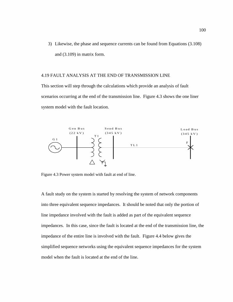
100
3) Likewise, the phase and sequence currents can be found from Equations (3.108)
and (3.109) in matrix form.
4.19 FAULT ANALYSIS AT THE END OF TRANSMISSION LINE
This section will step through the calculations which provide an analysis of fault
scenarios occurring at the end of the transmission line. Figure 4.3 shows the one liner
system model with the fault location.
Figure 4.3 Power system model with fault at end of line.
A fault study on the system is started by resolving the system of network components
into three equivalent sequence impedances. It should be noted that only the portion of
line impedance involved with the fault is added as part of the equivalent sequence
impedances. In this case, since the fault is located at the end of the transmission line, the
impedance of the entire line is involved with the fault. Figure 4.4 below gives the
simplified sequence networks using the equivalent sequence impedances for the system
model when the fault is located at the end of the line.
F
G 1
T 1
G e n B u s
(2 2 k V )
S e n d B u s
(3 4 5 k V )
L o a d B u s
(3 4 5 k V )
T L 1

101
Figure 4.4 Equivalent sequence networks: (a) positive; (b) negative; (c) zero.
4.19.1 SINGLE LINE-TO-GROUND (SLG) FAULT
For a single line-to-ground fault at the receiving end of the line, the sequence network for
the fault occurring on phase a is shown in Figure 4.5 below.
F0Z0 N0
+ VA0 -
F1Z1 N1
+ VA1 -
F2Z2 N2
+ VA2 -
1.0 + -
0o
Ia1
Ia1Ia0 Ia2
0.1198 + j0.5399 pu 0.0399 + j0.3166 pu 0.0399 + j0.3166 pu
Figure 4.5 Sequence network connection for SLG fault at receiving end of line [1].
Note that and is not included in the circuit above.
0 .0 3 9 9
+ j0 .3 1 6 6 p u
F 1
N 1
+
1 .0 0 °
a ) F 2
N 2
b ) F 0
N 0
c )
Z 1 Z 2 Z 00 .0 3 9 9
+ j0 .3 1 6 6 p u
0 .1 1 9 8
+ j0 .5 3 9 9 p u

102
From Equation (3.145), the positive, negative, and zero sequence currents are equal and
found by
0 1 2
0 1 2
1.0 0
3a a a
f
I I I
Z Z Z Z
1.0 0
0.1198 0.5399 0.0399 0.3166 0.0399 0.3166 (3 0)j j j
(4.79)
0.840 80.3 pu A
From Equation (3.144), the fault current on phase a is equal to three times the positive
sequence current, and is equated by
13af aI I
3 0.840 80.3 (4.80)
2.521 80.3 pu A
Since phases b and c are not involved with the fault, as shown in figure 3.7a,
and .
With the sequence current values, Equation (3.155) can be used to find the sequence
voltages as
0 0 0
1 1 1
2 2 2
0 0 0
0 0
0 0 0
a a
a f a
a a
V Z I
V V Z I
V Z I

103
0 0.1198 0.5399 0 0
1.0 0 0 0.0399 0.3166 0
0 0 0 0.0399 0.3166
0.840 80.3
0.840 80.3
0.840 80.3
j
j
j
(4.81)
0.4645 177.19
0.7323 0.92
0.2680 177.48
pu V
With the sequence voltage values, Equation (3.107) can be used to find the phase
voltages as
0
2
1
2
2
1 1 1
1
1
af a
bf a
cf a
V V
V a a V
V a a V
1 1 1 0.4645 177.19
1 1 240 1 120 0.7323 0.92
1 1 120 1 240 0.2680 177.48
(4.82)
0.000 60.36
1.0845 129.94
1.1383 127.71
pu V
The SLG results above were verified using both MATLAB and Aspen programs to
calculate values for the same variables.

104
Table 4.3 below lists the results from both programs
SLG Fault at Load Bus
Variable Value
Matlab Aspen
Ia0 (pu) 0.840 -80.3 0.840 -80.3
Ia1 (pu) 0.840 -80.3 0.840 -80.3
Ia2 (pu) 0.840 -80.3 0.840 -80.3
Iaf (pu) 2.521 -80.3 2.520 -80.3
Ibf (pu) 0.000 0.000
Icf (pu) 0.000 0.000
Va0 (pu) 0.465 177.1 0.465 177.1
Va1 (pu) 0.732 -0.9 0.732 -0.9
Va2 (pu) 0.268 177.5 0.268 -177.5
Vaf (pu) 0.000 0.000
Vbf (pu) 1.084 -129.9 1.084 -130.0
Vcf (pu) 1.138 127.7 1.139 127.7
Table 4.3 Fault Analysis of SLG fault at receiving end of line.
4.19.2 LINE-TO-LINE (L-L) FAULT
Typically line-to-line (L-L) fault occurs when two conductors are short circuited. It is
assumed for the symmetric perseverance that L-L fault occurs between phases b and c.

105
Since the fault impedance is not shown in the circuit Figure 4.6 below.
F0
Z0
N0
+VA0 = 0
-
F1
Z1
N1
+VA1
-
F2
Z2
N2
+VA2
-+
1.0-
0o
Ia1Ia0=0 Ia2
Zf
0.1198+j0.5399 pu
0.0399+j0.3166 pu
0.0399+j0.3166 pu
Figure 4.6 Sequence network connection for L-L fault at receiving end of line [1]
From Equations (3.146) and (3.147) the sequence currents at the receiving end of the line
are
0 0a I
1 2
1 2
1.0 0a a
f
I I
Z Z Z
0 0a I pu (4.83)
10.0399 0.3166 0.03
1.0 0
99 0.3166 (3 0)a
j j
I (4.84)
1 1.5669 82.8171a I

106
2 1.5669 97.1829a I (4.85)
Using above calculated values and Equation (3.149) the phase currents are
0
2
1
2
2
1 1 1
1
1
af a
b a
a
f
cf
a a
a a
I I
I I
I I
01 1 1
1 1 240 1 120
1 1 120 1 240
0
1.5669 82.8171
1.5669 97.1829
af
f
bf
c
I
I
I
(4.86)
0
2.7139 172.8171
2.7139 7.1 9
0
82
bf
af
cf
I
I
I
pu A (4.87)
Furthermore using the sequence currents and impedance values the sequence voltages can
be found from Equation (3.151) as
0 0 0
1 1 1
2 2 2
0 0 0
1 0 0 0
0 0 0
a a
a a
a a
V Z I
V Z I
V Z I
0
1
2
0 0.1198 0.5399 0 0
1 0 0 0
0 0 0
0.0399 0.3166
0.0399 0.3166
0 0
1.5669 82.8171
1.5669 97.1829
a
a
a
j
j
j
V
V
V
(4.88)
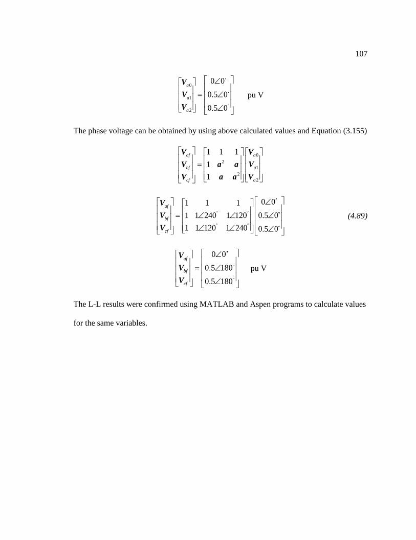
107
0
1
2
0 0
0.5 0
0.5 0
a
a
a
V
V
V
pu V
The phase voltage can be obtained by using above calculated values and Equation (3.155)
0
2
1
2
2
1 1 1
1
1
af a
bf a
cf a
V V
V a a V
V a a V
01 1 1
1 1 240 1 120
1 1 120 1 2
0
0.5 0
0.540 0
af
bf
cf
V
V
V
(4.89)
0
0.5 180
0.
0
5 180
af
bf
cf
V
V
V
pu V
The L-L results were confirmed using MATLAB and Aspen programs to calculate values
for the same variables.

108
Table 4.4 below lists the results obtained by these programs
L-L Fault at Load Bus
Variable Value
Matlab Aspen
Ia0 (pu) 0.000 0.000
Ia1 (pu) 1.567 -82.8 1.566 -82.8
Ia2 (pu) 1.567 97.2 1.566 97.2
Iaf (pu) 0.000 0.000
Ibf (pu) 2.714 -172.8 2.713 -172.8
Icf (pu) 2.714 7.2 2.713 7.2
Va0 (pu) 0.000 0.000
Va1 (pu) 0.500 0.0 0.500 0.0
Va2 (pu) 0.500 0.0 0.500 0.0
Vaf (pu) 1.000 0.0 1.000 0.0
Vbf (pu) 0.500 180.0 0.500 180.0
Vcf (pu) 0.500 180.0 0.500 180.0
Table 4.4 Fault Analysis of L-L fault at receiving end of line.

109
4.19.3 DOUBLE LINE-TO-GROUND (DLG) FAULT
For a double line-to-ground fault at the receiving end of the line, the sequence network
for the fault occurring on phases b and c is shown in Figure 4.7 below.
F0
Z0
N0
F1
Z1
N1
+VA1
-
F2
Z2
N2
+VA2
-+
1.0-
0o
Ia1Ia0Ia2
0.1198+j0.5399 pu
0.0399+j0.3166 pu
0.0399+j0.3166 pu
Figure 4.7 Sequence network connection for DLG fault at receiving end of line [1]
Because the fault impedance , and the impedance from line to ground ,
neither is shown in the circuit above.
From Equation (3.175), the positive sequence current is found by
1
2 0
1
0 2
1.0 0
3
2 3
a
f f g
f
f gZ
IZ Z Z Z Z
Z ZZ Z Z
1
1.0 0
(0.0399 0.3166) 0 (0.1198 0.5399) 0 (3 0)(0.0399 0.3166) 0
(0.1198 0.5399) (0.0399 0.3166) (2 0) (3 0)
aj j
jj j
I
1 1.9172 82.06a I pu A (4.90)

110
Using Equations (3.176) and (3.177) to multiply the positive-sequence current by the
appropriate impedance ratios is the direct method for dividing current between the two
current paths. Thus, the zero- and negative-sequence currents are given by
2
0 1
2 0 3
f
a a
f f g
Z ZI I
Z Z Z Z Z
0
(0.0399 0.3166) 0
(0.0399 0.3166) 0 (0.1198 0.5399) 0 (3 0)
(1.9172 82.06 )
a
j
j j
I
(4.91)
0 0.7022 101 .32a I pu A
and
0
2 1
2 0
3
3
f g
a a
f f g
Z Z ZI I
Z Z Z Z Z
2
(0.1198 0.5399) 0 (3 0)
(0.0399 0.3166) 0 (0.1198 0.5399) 0 (3 0)
(1.9172 82.06 )
a
j
j j
I (4.92)
2 1.2170 95 9 .9a I pu A
From Equation (3.113), the fault currents are equated by
0
2
1
2
2
1 1 1
1
1
af a
bf a
cf a
I I
I a a I
I a a I
1 1 1 0.7022 101.32
1 1 240 1 120 1.9172 82.06
1 1 120 1 240 1.2170 95.99
af
bf
cf
I
I
I
(4.93)

111
0.000 89.43
2.9811 166.55
2.8394 28.90
af
bf
cf
I
I
I
pu A
With the sequence current values, Equation (3.155) can be used to find the sequence
voltages as
0 0 0
1 1 1
2 2 2
0 0 0
0 0
0 0 0
a a
a f a
a a
V Z I
V V Z I
V Z I
0
1
2
0 0.1198 0.5399 0 0
1.0 0 0 0.0399 0.3166 0
0 0 0 0.0399 0.3166
0.7022 101.32
1.9172 82.06
1.2170 95.99
a
a
a
j
j
j
V
V
V(4.94)
0
1
2
0.3883 1.19
0.3884 1.19
0.3883 1.19
a
a
a
V
V
V
pu V
With the sequence voltage values, Equation (3.107) can be used to find the phase
voltages as
0
2
1
2
2
1 1 1
1
1
af a
bf a
cf a
V V
V a a V
V a a V
1 1 1 0.3883 1.19
1 1 240 1 120 0.3884 1.19
1 1 120 1 240 0.3883 1.19
af
bf
cf
V
V
V
(4.95)

112
1.1650 1.19
0.0000 127.58
0.0000 130.72
af
bf
cf
V
V
V
pu V
The DLG results above were verified using both MATLAB and Aspen programs to
calculate values for the same variables. Table 4.5 below lists the results from both
programs.
DLG Fault at Load Bus
Variable Value
Matlab Aspen
Ia0 (pu) 0.702 101.3 0.702 101.3
Ia1 (pu) 1.917 -82.1 1.916 -82.1
Ia2 (pu) 1.217 96.0 1.216 96.0
Iaf (pu) 0.000 0.000
Ibf (pu) 2.981 166.5 2.980 166.6
Icf (pu) 2.839 28.9 2.838 28.9
Va0 (pu) 0.388 -1.2 0.388 -1.2
Va1 (pu) 0.388 -1.2 0.388 -1.2
Va2 (pu) 0.388 -1.2 0.388 -1.2
Vaf (pu) 1.165 -1.2 1.165 -1.2
Vbf (pu) 0.000 0.000
Vcf (pu) 0.000 0.000
Table 4.5 Fault Analysis of DLG fault at receiving end of line.

113
4.19.4 THREE LINE-TO-GROUND (3LG) FAULT
Three-phase fault is a balanced fault. The sequence networks are isolated from each other
because they are short-circuited through their individual fault impedances.
F0
Z0
N0
+VA0
-
F1
Z1
N1
+VA1
-
F2
Z2
N2
+VA2
-+
1.0-
0o
Zf
Ia1Ia0Ia2
Zf +3Zg Zf
0.1198+j0.5399 pu
0.0399+j0.3166 pu
0.0399+j0.3166 pu
Figure 4.8 Sequence network connection for 3LG fault at receiving end of line [1].
The negative - and zero-sequence networks do not have internal voltage sources therefore
they do not generate any currents. Hence, Equations (3.174)-(3.177) can be applied
0 0a I
0 0a I pu A (4.96)
2 0a I
2 0a I pu A (4.97)
1
1
1.0 0a
f
I
Z Z
Since the fault impedance Zf =0 the 3LG fault current is calculated from

114
1
1
1.0 0a
I
Z.
1
1.0 0
0.399 0.3166a
j
I (4.98)
1 3.1338 82.8171a I pu A
Using above calculated values and Equation (3.149) the phase currents are
0
2
1
2
2
1 1 1
1
1
af a
b a
a
f
cf
a a
a a
I I
I I
I I
01 1 1
1 1 240 1 120
1 1 120 1 240 0
0
3.1338 82.8171
0
af
c
bf
f
I
I
I
(4.99)
3.1338 82.8171
3.1338 157.1829
3.1338 37.1829
af
f
bf
c
I
I
I
pu A
Additionally using the above calculated results for sequence currents and impedance the
sequence voltages can be found from Equation (3.151) as
0 0 0
1 1 1
2 2 2
0 0 0
1 0 0 0
0 0 0
a a
a a
a a
V Z I
V Z I
V Z I

115
0
1
2
0.0399 0.3166
0.03
0 0.1198 0.5399 0 0
1 0 0
99 0
0
0 0 0
0
3.1338 82.8
.31
0
1 1
0
6
7
6
0
a
a
a
j
j
j
V
V
V
(4.100)
0
1
2
0
0 0
0 0
0a
a
a
V
V
V
pu V
The phase voltage can be found by using above calculated outcomes and Equation
(3.155)
0
2
1
2
2
1 1 1
1
1
af a
bf a
cf a
V V
V a a V
V a a V
01 1 1
1 1 240 1 120
1 1 120 1 24
0
0 0
00 0
af
bf
cf
V
V
V
(4.101)
0
0 0
0
0
0
af
bf
cf
V
V
V
pu V
The 3LG results were confirmed by using MATLAB and Aspen programs for the same
variables.

116
Table 4.6 below lists the results obtained by these programs.
3LG Fault at Load Bus
Variable Value
Matlab Aspen
Ia0 (pu) 0.000 0.000
Ia1 (pu) 3.134 -82.8 3.132 -82.8
Ia2 (pu) 0.000 0.000
Iaf (pu) 3.134 -82.8 3.132 -82.8
Ibf (pu) 3.134 157.2 3.132 157.2
Icf (pu) 3.134 37.2 3.132 37.2
Va0 (pu) 0.000 0.000
Va1 (pu) 0.000 0.000
Va2 (pu) 0.000 0.000
Vaf (pu) 0.000 0.000
Vbf (pu) 0.000 0.000
Vcf (pu) 0.000 0.000
Table 4.6 Fault Analysis of 3LG fault at receiving end of line.

117
Chapter 5
CONCLUSIONS
The goal of this project was to design an overhead transmission line that fulfills the
prescribed design criteria. To simplify the exercise, a line configuration for spacing
between phase conductors was predefined by selecting a standard support structure that
would be used throughout the design process, and for the final solution. A 3H1 wood H-
frame-type structure was selected. Only ACSR conductors were considered for the
design. ACSR conductors are one of the most commonly used types, providing good
strength for a 220-mile long transmission line. The design options included different
ACSR conductor sizes supported by the 3H1 structure. The process of design analysis
was developed to determine and compare the performance of each design option. The
design calculations are based on the requirement of the transmission line being
completely transposed. A MATLAB program was written to efficiently and accurately
perform the many calculations for analysis of all options considered. Fourteen different
design options were analyzed. The results from the analysis of each design option are
given in Appendix E.2. From the group of design options that met the design criteria, a
final design was selected based primarily on tradeoffs between the following factors: cost
of conductor size, capacity for future load growth, and margin to maintain performance
criteria if the load decreases slightly due to load fluctuations. The final design used the
predefined 3H1 wood H-frame-type structure with ACSR 477 kcmil conductors. The
electrical performance of this solution met the design requirements for transmission line

118
efficiency, power loss, and voltage regulation. The mechanical performance of this
solution met the design requirements for sag and tension. Per the calculated SIL, the
design can easily handle the load criteria of 90 MW, which is significantly less than the
practical loadability limit of the line. Power loss due to corona at fair and foul weather
conditions is satisfactory. A fault study was done for the final solution to show the
system exposure to voltage and current during typical fault events. A MATLAB program
was written to efficiently and accurately perform the many calculations required for fault
analysis. In addition, ASPEN One-Liner software was used to simulate the same fault
conditions. Twelve combinations of fault conditions, between four fault types and three
fault locations, were evaluated. The results from the fault study are given in Chapter 4
and Appendices C and D.

119
APPENDIX A
Conductor and Tower Characteristics
A.1 ACSR CHARACTERISTICS
Circular
Mills
Aluminum Steel
Frequency
[Hz]
Outside
Diameter
[in]
Weight
[lb/mi] Strands Layers
Strand
Diameter
[in]
Strands
Strand
Diameter
[in]
477000 30 2 0.1261 7 0.1261 60 0.883 3933
Geometric
Mean
Radius Ds
[ft]
Resistance
r
[Ω/mi]
at 50C
Inductive
Reactance xa
at 1ft spacings
[Ω/cond./mi]
Shunt Capacitive
Reactance
at 1ft spacings
[MΩmi/cond.]
Inductive
Reactance
Spacing Factor
Xd
[Ω/cond./mi]
Shunt
Capacitive
Reactance
Spacing Factor
[MΩ/cond.
mi]
0.0304 0.216 0.424 0.0980 0.42337 0.1035
A.2 STRUCTURE CHARACTERISTICS
Material Type
Average
Number
per mile
Average
Weight per
structure
[lb]
Height
[ft]
Base
Width
[ft]
Conductor
Spacing
Style
Conductor
Spacing
[ft]
Steel 3H1 8 16000 73 36 Horizontal
D12=26
D23=26
D31=52

120
APPENDIX B
Aspen Simulation Model and Analysis
B.1.1 SYSTEM MODEL ONE LINE DIAGRAM
B.1.2 GENERATOR DATA

121
B.1.3 TRANSFORMER DATA
B.1.4 TRANSMISSION LINE DATA FOR FAULT ANALYSIS

122
B.1.5 TRANSMISSION LINE DATA FOR POWER FLOW ANALYSIS
B.1.6 LOAD DATA
B.2 POWER FLOW BY NEWTON-RAPHSON METHOD

123
Appendix C
Aspen Fault Analysis Summary
C.1 477kcmil SE FAULTS
===================================================================================================================================
5. Interm. Fault on: 2 Send Bus 345.kV - 3 Load Bus 345.kV 1L 3LG 0.50%( 0.01%)
with end opened
FAULT CURRENT (PU @ DEG)
+ SEQ - SEQ 0 SEQ A PHASE B PHASE C PHASE
6.216@ -89.9 0.000@ 0.0 0.000@ 0.0 6.216@ -89.9 6.216@ 150.1 6.216@ 30.1
THEVENIN IMPEDANCE (PU)
0.0002+j0.16084 0.0002+j0.16084 0.0006+j0.07236
SHORT CIRCUIT MVA= 621.6 X/R RATIO= 805.617 R0/X1= 0.00373 X0/X1= 0.44989
-----------------------------------------------------------------------------------------------------------------------------------
BUS 3 Load Bus 345.KV AREA 1 ZONE 1 TIER 0 (PREFAULT V=1.000@ 0.0 PU)
+ SEQ - SEQ 0 SEQ A PHASE B PHASE C PHASE
VOLTAGE (PU) > 0.000@ 0.0 0.000@ 0.0 0.000@ 0.0 0.000@ 0.0 0.000@ 0.0 0.000@ 0.0
SHUNT CURRENTS (PU) >
TO LOAD 0.000@ 0.0 0.000@ 0.0 0.000@ 0.0 0.000@ 0.0 0.000@ 0.0 0.000@ 0.0
FROM FICT. CURR. SOURCE 1.000@ -25.8 0.000@ 0.0 0.000@ 0.0 1.000@ -25.8 [email protected] 1.000@ 94.2
CURRENT TO FAULT (PU) > 1.000@ -25.8 0.000@ 0.0 0.000@ 0.0 1.000@ -25.8 [email protected] 1.000@ 94.2
THEVENIN IMPEDANCE (PU) > 1.@ 25.8 1.@ 25.8 1.@ 25.8
-----------------------------------------------------------------------------------------------------------------------------------
BUS -3 #Load Bus 345.KV AREA 1 ZONE 1 TIER 0 (PREFAULT V=1.000@ 0.0 PU)
+ SEQ - SEQ 0 SEQ A PHASE B PHASE C PHASE
VOLTAGE (PU) > 0.000@ 0.0 0.000@ 0.0 0.000@ 0.0 0.000@ 0.0 0.000@ 0.0 0.000@ 0.0
BRANCH CURRENT (PU) TO >
-2 Send$1 $#Loa 345. 1L 0.000@ 0.0 0.000@ 0.0 0.000@ 0.0 0.000@ 0.0 0.000@ 0.0 0.000@ 0.0
CURRENT TO FAULT (PU) > 0.000@ 0.0 0.000@ 0.0 0.000@ 0.0 0.000@ 0.0 0.000@ 0.0 0.000@ 0.0
THEVENIN IMPEDANCE (PU) > 0.31925@ 82.8 0.31925@ 82.8 0.55339@ 77.5
-----------------------------------------------------------------------------------------------------------------------------------
BUS -2 Send$1 $#Loa 345.KV AREA 1 ZONE 1 TIER 0 (PREFAULT V=1.000@ 0.0 PU)
+ SEQ - SEQ 0 SEQ A PHASE B PHASE C PHASE
VOLTAGE (PU) > 0.000@ 0.0 0.000@ 0.0 0.000@ 0.0 0.000@ 0.0 0.000@ 0.0 0.000@ 0.0
BRANCH CURRENT (PU) TO >
2 Send Bus 345. 1L 6.218@ 90.1 0.000@ 0.0 0.000@ 0.0 6.218@ 90.1 6.218@ -29.9 [email protected]
-3 #Load Bus 345. 1L 0.002@ -90.0 0.000@ 0.0 0.000@ 0.0 0.002@ -90.0 0.002@ 150.0 0.002@ 30.0
CURRENT TO FAULT (PU) > 6.216@ -89.9 0.000@ 0.0 0.000@ 0.0 6.216@ -89.9 6.216@ 150.1 6.216@ 30.1
THEVENIN IMPEDANCE (PU) > 0.16084@ 89.9 0.16084@ 89.9 0.07236@ 89.5
-----------------------------------------------------------------------------------------------------------------------------------
BUS 2 Send Bus 345.KV AREA 1 ZONE 1 TIER 0 (PREFAULT V=1.000@ 0.0 PU)
+ SEQ - SEQ 0 SEQ A PHASE B PHASE C PHASE
VOLTAGE (PU) > 0.005@ -14.2 0.000@ 0.0 0.000@ 0.0 0.005@ -14.2 [email protected] 0.005@ 105.8
BRANCH CURRENT (PU) TO >
-2 Send$1 $#Loa 345. 1L 6.218@ -89.9 0.000@ 0.0 0.000@ 0.0 6.218@ -89.9 6.218@ 150.1 6.218@ 30.1
1 Gen Bus 22. T1T 6.220@ 90.1 0.000@ 0.0 0.000@ 0.0 6.220@ 90.1 6.220@ -29.9 [email protected]
-----------------------------------------------------------------------------------------------------------------------------------
MONITORED BRANCH: 2 Send Bus 345.KV -> -2 Send$1 $#Loa 345.KV 1L
+ SEQ - SEQ 0 SEQ A PHASE B PHASE C PHASE
RELAY CURRENT (PU) 6.218@ -89.9 0.000@ 0.0 0.000@ 0.0 6.218@ -89.9 6.218@ 150.1 6.218@ 30.1
BUS VOLTAGES (PU)
2 Send Bus 345.kV 0.005@ -14.2 0.000@ 0.0 0.000@ 0.0 0.005@ -14.2 [email protected] 0.005@ 105.8
-2 Send$1 $#Loa 345.kV 0.000@ 0.0 0.000@ 0.0 0.000@ 0.0 0.000@ 0.0 0.000@ 0.0 0.000@ 0.0
3Io= 0.0@ 12.2 A Va/Ia= 0.962@ 75.7 Ohm (Va-Vb)/(Ia-Ib)= 0.962@ 75.7 Ohm
(Zo-Z1)/3Z1 = 0.6669 @ -0.0
-----------------------------------------------------------------------------------------------------------------------------------
===================================================================================================================================
6. Interm. Fault on: 2 Send Bus 345.kV - 3 Load Bus 345.kV 1L 2LG 0.50%( 0.01%) Type=B-C
with end opened
FAULT CURRENT (PU @ DEG)
+ SEQ - SEQ 0 SEQ A PHASE B PHASE C PHASE
4.744@ -89.9 1.472@ 89.9 3.272@ 90.3 0.000@ 0.0 7.297@ 137.8 7.273@ 42.5
THEVENIN IMPEDANCE (PU)
0.0002+j0.16084 0.0002+j0.16084 0.0006+j0.07236
SHORT CIRCUIT MVA= 729.7 X/R RATIO= 418.232 R0/X1= 0.00373 X0/X1= 0.44989
-----------------------------------------------------------------------------------------------------------------------------------
BUS 3 Load Bus 345.KV AREA 1 ZONE 1 TIER 0 (PREFAULT V=1.000@ 0.0 PU)
+ SEQ - SEQ 0 SEQ A PHASE B PHASE C PHASE
VOLTAGE (PU) > 0.000@ 0.0 0.000@ 0.0 0.000@ 0.0 0.000@ 0.0 0.000@ 0.0 0.000@ 0.0
SHUNT CURRENTS (PU) >
TO LOAD 0.000@ 0.0 0.000@ 0.0 0.000@ 0.0 0.000@ 0.0 0.000@ 0.0 0.000@ 0.0
FROM FICT. CURR. SOURCE 1.000@ -25.8 0.000@ 0.0 0.000@ 0.0 1.000@ -25.8 [email protected] 1.000@ 94.2
CURRENT TO FAULT (PU) > 1.000@ -25.8 0.000@ 0.0 0.000@ 0.0 1.000@ -25.8 [email protected] 1.000@ 94.2
THEVENIN IMPEDANCE (PU) > 1.@ 25.8 1.@ 25.8 1.@ 25.8
-----------------------------------------------------------------------------------------------------------------------------------
BUS -3 #Load Bus 345.KV AREA 1 ZONE 1 TIER 0 (PREFAULT V=1.000@ 0.0 PU)
+ SEQ - SEQ 0 SEQ A PHASE B PHASE C PHASE
VOLTAGE (PU) > 0.237@ -0.2 0.237@ -0.2 0.237@ -0.2 0.710@ -0.2 0.000@ 0.0 0.000@ 0.0
BRANCH CURRENT (PU) TO >

124
-2 Send$1 $#Loa 345. 1L 0.000@ 0.0 0.000@ 0.0 0.000@ 0.0 0.000@ 0.0 0.000@ 0.0 0.000@ 0.0
CURRENT TO FAULT (PU) > 0.000@ 0.0 0.000@ 0.0 0.000@ 0.0 0.000@ 0.0 0.000@ 0.0 0.000@ 0.0
THEVENIN IMPEDANCE (PU) > 0.31925@ 82.8 0.31925@ 82.8 0.55339@ 77.5
-----------------------------------------------------------------------------------------------------------------------------------
BUS -2 Send$1 $#Loa 345.KV AREA 1 ZONE 1 TIER 0 (PREFAULT V=1.000@ 0.0 PU)
+ SEQ - SEQ 0 SEQ A PHASE B PHASE C PHASE
VOLTAGE (PU) > 0.237@ -0.2 0.237@ -0.2 0.237@ -0.2 0.710@ -0.2 0.000@ 0.0 0.000@ 0.0
BRANCH CURRENT (PU) TO >
2 Send Bus 345. 1L 4.746@ 90.1 1.473@ -90.1 3.272@ -89.7 0.001@ 90.5 7.299@ -42.2 [email protected]
-3 #Load Bus 345. 1L 0.002@ -89.9 0.001@ 89.8 0.001@ 89.8 0.001@ -89.5 0.002@ 150.0 0.002@ 30.0
CURRENT TO FAULT (PU) > 4.744@ -89.9 1.472@ 89.9 3.272@ 90.3 0.000@ 0.0 7.297@ 137.8 7.273@ 42.5
THEVENIN IMPEDANCE (PU) > 0.16084@ 89.9 0.16084@ 89.9 0.07236@ 89.5
-----------------------------------------------------------------------------------------------------------------------------------
BUS 2 Send Bus 345.KV AREA 1 ZONE 1 TIER 0 (PREFAULT V=1.000@ 0.0 PU)
+ SEQ - SEQ 0 SEQ A PHASE B PHASE C PHASE
VOLTAGE (PU) > 0.240@ -0.4 0.236@ -0.1 0.229@ 0.3 0.705@ -0.1 [email protected] 0.010@ 140.8
BRANCH CURRENT (PU) TO >
-2 Send$1 $#Loa 345. 1L 4.746@ -89.9 1.473@ 89.9 3.272@ 90.3 0.001@ -89.5 7.299@ 137.8 7.275@ 42.5
1 Gen Bus 22. T1T 4.747@ 90.1 1.473@ -90.1 3.272@ -89.7 0.002@ 90.2 7.300@ -42.2 [email protected]
-----------------------------------------------------------------------------------------------------------------------------------
MONITORED BRANCH: 2 Send Bus 345.KV -> -2 Send$1 $#Loa 345.KV 1L
+ SEQ - SEQ 0 SEQ A PHASE B PHASE C PHASE
RELAY CURRENT (PU) 4.746@ -89.9 1.473@ 89.9 3.272@ 90.3 0.001@ -89.5 7.299@ 137.8 7.275@ 42.5
BUS VOLTAGES (PU)
2 Send Bus 345.kV 0.240@ -0.4 0.236@ -0.1 0.229@ 0.3 0.705@ -0.1 [email protected] 0.010@ 140.8
-2 Send$1 $#Loa 345.kV 0.237@ -0.2 0.237@ -0.2 0.237@ -0.2 0.710@ -0.2 0.000@ 0.0 0.000@ 0.0
3Io= 1642.9@ 90.3 A Va/Ia= 1.21e+006@ 89.4 Ohm (Va-Vb)/(Ia-Ib)= 117@ 42.2 Ohm
(Zo-Z1)/3Z1 = 0.6669 @ -0.0
-----------------------------------------------------------------------------------------------------------------------------------
===================================================================================================================================
7. Interm. Fault on: 2 Send Bus 345.kV - 3 Load Bus 345.kV 1L 1LG 0.50%( 0.01%) Type=A
with end opened
FAULT CURRENT (PU @ DEG)
+ SEQ - SEQ 0 SEQ A PHASE B PHASE C PHASE
2.537@ -89.9 2.537@ -89.9 2.537@ -89.9 7.612@ -89.9 0.000@ 0.0 0.000@ 0.0
THEVENIN IMPEDANCE (PU)
0.0002+j0.16084 0.0002+j0.16084 0.0006+j0.07236
SHORT CIRCUIT MVA= 761.2 X/R RATIO= 394.638 R0/X1= 0.00373 X0/X1= 0.44989
-----------------------------------------------------------------------------------------------------------------------------------
BUS 3 Load Bus 345.KV AREA 1 ZONE 1 TIER 0 (PREFAULT V=1.000@ 0.0 PU)
+ SEQ - SEQ 0 SEQ A PHASE B PHASE C PHASE
VOLTAGE (PU) > 0.000@ 0.0 0.000@ 0.0 0.000@ 0.0 0.000@ 0.0 0.000@ 0.0 0.000@ 0.0
SHUNT CURRENTS (PU) >
TO LOAD 0.000@ 0.0 0.000@ 0.0 0.000@ 0.0 0.000@ 0.0 0.000@ 0.0 0.000@ 0.0
FROM FICT. CURR. SOURCE 1.000@ -25.8 0.000@ 0.0 0.000@ 0.0 1.000@ -25.8 [email protected] 1.000@ 94.2
CURRENT TO FAULT (PU) > 1.000@ -25.8 0.000@ 0.0 0.000@ 0.0 1.000@ -25.8 [email protected] 1.000@ 94.2
THEVENIN IMPEDANCE (PU) > 1.@ 25.8 1.@ 25.8 1.@ 25.8
-----------------------------------------------------------------------------------------------------------------------------------
BUS -3 #Load Bus 345.KV AREA 1 ZONE 1 TIER 0 (PREFAULT V=1.000@ 0.0 PU)
+ SEQ - SEQ 0 SEQ A PHASE B PHASE C PHASE
VOLTAGE (PU) > 0.592@ -0.0 [email protected] 0.184@ 179.7 0.000@ 0.0 [email protected] 0.910@ 107.6
BRANCH CURRENT (PU) TO >
-2 Send$1 $#Loa 345. 1L 0.000@ 0.0 0.000@ 0.0 0.000@ 0.0 0.000@ 0.0 0.000@ 0.0 0.000@ 0.0
CURRENT TO FAULT (PU) > 0.000@ 0.0 0.000@ 0.0 0.000@ 0.0 0.000@ 0.0 0.000@ 0.0 0.000@ 0.0
THEVENIN IMPEDANCE (PU) > 0.31925@ 82.8 0.31925@ 82.8 0.55339@ 77.5
-----------------------------------------------------------------------------------------------------------------------------------
BUS -2 Send$1 $#Loa 345.KV AREA 1 ZONE 1 TIER 0 (PREFAULT V=1.000@ 0.0 PU)
+ SEQ - SEQ 0 SEQ A PHASE B PHASE C PHASE
VOLTAGE (PU) > 0.592@ -0.1 [email protected] 0.184@ 179.7 0.000@ 0.0 [email protected] 0.910@ 107.6
BRANCH CURRENT (PU) TO >
2 Send Bus 345. 1L 2.538@ 90.1 2.538@ 90.1 2.538@ 90.1 7.614@ 90.1 0.001@ -89.0 0.001@ -90.2
-3 #Load Bus 345. 1L 0.001@ -89.9 0.001@ -89.9 0.000@ 0.0 0.002@ -90.0 0.001@ 91.0 0.001@ 89.8
CURRENT TO FAULT (PU) > 2.537@ -89.9 2.537@ -89.9 2.537@ -89.9 7.612@ -89.9 0.000@ 0.0 0.000@ 0.0
THEVENIN IMPEDANCE (PU) > 0.16084@ 89.9 0.16084@ 89.9 0.07236@ 89.5
-----------------------------------------------------------------------------------------------------------------------------------
BUS 2 Send Bus 345.KV AREA 1 ZONE 1 TIER 0 (PREFAULT V=1.000@ 0.0 PU)
+ SEQ - SEQ 0 SEQ A PHASE B PHASE C PHASE
VOLTAGE (PU) > 0.594@ -0.1 [email protected] [email protected] 0.010@ -14.2 [email protected] 0.908@ 107.4
BRANCH CURRENT (PU) TO >
-2 Send$1 $#Loa 345. 1L 2.538@ -89.9 2.538@ -89.9 2.538@ -89.9 7.614@ -89.9 0.001@ 91.0 0.001@ 89.8
1 Gen Bus 22. T1T 2.539@ 90.1 2.538@ 90.1 2.538@ 90.1 7.615@ 90.1 0.002@ -47.6 [email protected]
-----------------------------------------------------------------------------------------------------------------------------------
MONITORED BRANCH: 2 Send Bus 345.KV -> -2 Send$1 $#Loa 345.KV 1L
+ SEQ - SEQ 0 SEQ A PHASE B PHASE C PHASE
RELAY CURRENT (PU) 2.538@ -89.9 2.538@ -89.9 2.538@ -89.9 7.614@ -89.9 0.001@ 91.0 0.001@ 89.8
BUS VOLTAGES (PU)
2 Send Bus 345.kV 0.594@ -0.1 [email protected] [email protected] 0.010@ -14.2 [email protected] 0.908@ 107.4
-2 Send$1 $#Loa 345.kV 0.592@ -0.1 [email protected] 0.184@ 179.7 0.000@ 0.0 [email protected] 0.910@ 107.6
3Io= 1274.0@ -89.9 A Va/Ia= 1.6@ 75.7 Ohm (Va-Vb)/(Ia-Ib)= 142@ 161.8 Ohm
(Zo-Z1)/3Z1 = 0.6669 @ -0.0
-----------------------------------------------------------------------------------------------------------------------------------
===================================================================================================================================
8. Interm. Fault on: 2 Send Bus 345.kV - 3 Load Bus 345.kV 1L LL 0.50%( 0.01%) Type=B-C
with end opened
FAULT CURRENT (PU @ DEG)
+ SEQ - SEQ 0 SEQ A PHASE B PHASE C PHASE
3.108@ -89.9 3.108@ 90.1 0.000@ 0.0 0.000@ 0.0 [email protected] 5.383@ 0.1
THEVENIN IMPEDANCE (PU)
0.0002+j0.16084 0.0002+j0.16084 0.0006+j0.07236
SHORT CIRCUIT MVA= 538.3 X/R RATIO= 805.617 R0/X1= 0.00373 X0/X1= 0.44989
-----------------------------------------------------------------------------------------------------------------------------------
BUS 3 Load Bus 345.KV AREA 1 ZONE 1 TIER 0 (PREFAULT V=1.000@ 0.0 PU)
+ SEQ - SEQ 0 SEQ A PHASE B PHASE C PHASE
VOLTAGE (PU) > 0.000@ 0.0 0.000@ 0.0 0.000@ 0.0 0.000@ 0.0 0.000@ 0.0 0.000@ 0.0

125
SHUNT CURRENTS (PU) >
TO LOAD 0.000@ 0.0 0.000@ 0.0 0.000@ 0.0 0.000@ 0.0 0.000@ 0.0 0.000@ 0.0
FROM FICT. CURR. SOURCE 1.000@ -25.8 0.000@ 0.0 0.000@ 0.0 1.000@ -25.8 [email protected] 1.000@ 94.2
CURRENT TO FAULT (PU) > 1.000@ -25.8 0.000@ 0.0 0.000@ 0.0 1.000@ -25.8 [email protected] 1.000@ 94.2
THEVENIN IMPEDANCE (PU) > 1.@ 25.8 1.@ 25.8 1.@ 25.8
-----------------------------------------------------------------------------------------------------------------------------------
BUS -3 #Load Bus 345.KV AREA 1 ZONE 1 TIER 0 (PREFAULT V=1.000@ 0.0 PU)
+ SEQ - SEQ 0 SEQ A PHASE B PHASE C PHASE
VOLTAGE (PU) > 0.500@ 0.0 0.500@ -0.0 0.000@ 0.0 1.000@ 0.0 0.500@ 180.0 [email protected]
BRANCH CURRENT (PU) TO >
-2 Send$1 $#Loa 345. 1L 0.000@ 0.0 0.000@ 0.0 0.000@ 0.0 0.000@ 0.0 0.000@ 0.0 0.000@ 0.0
CURRENT TO FAULT (PU) > 0.000@ 0.0 0.000@ 0.0 0.000@ 0.0 0.000@ 0.0 0.000@ 0.0 0.000@ 0.0
THEVENIN IMPEDANCE (PU) > 0.31925@ 82.8 0.31925@ 82.8 0.55339@ 77.5
-----------------------------------------------------------------------------------------------------------------------------------
BUS -2 Send$1 $#Loa 345.KV AREA 1 ZONE 1 TIER 0 (PREFAULT V=1.000@ 0.0 PU)
+ SEQ - SEQ 0 SEQ A PHASE B PHASE C PHASE
VOLTAGE (PU) > 0.500@ 0.0 0.500@ 0.0 0.000@ 0.0 1.000@ 0.0 [email protected] [email protected]
BRANCH CURRENT (PU) TO >
2 Send Bus 345. 1L 3.109@ 90.1 3.109@ -89.9 0.000@ 0.0 0.000@ 0.0 5.385@ 0.1 [email protected]
-3 #Load Bus 345. 1L 0.001@ -90.0 0.001@ 90.0 0.000@ 0.0 0.000@ 0.0 0.002@ 179.9 0.002@ 0.1
CURRENT TO FAULT (PU) > 3.108@ -89.9 3.108@ 90.1 0.000@ 0.0 0.000@ 0.0 [email protected] 5.383@ 0.1
THEVENIN IMPEDANCE (PU) > 0.16084@ 89.9 0.16084@ 89.9 0.07236@ 89.5
-----------------------------------------------------------------------------------------------------------------------------------
BUS 2 Send Bus 345.KV AREA 1 ZONE 1 TIER 0 (PREFAULT V=1.000@ 0.0 PU)
+ SEQ - SEQ 0 SEQ A PHASE B PHASE C PHASE
VOLTAGE (PU) > 0.502@ -0.1 0.497@ 0.1 0.000@ 0.0 1.000@ 0.0 [email protected] 0.499@ 179.5
BRANCH CURRENT (PU) TO >
-2 Send$1 $#Loa 345. 1L 3.109@ -89.9 3.109@ 90.1 0.000@ 0.0 0.000@ 0.0 [email protected] 5.385@ 0.1
1 Gen Bus 22. T1T 3.110@ 90.1 3.109@ -89.9 0.000@ 0.0 0.001@ 90.0 5.386@ 0.1 [email protected]
-----------------------------------------------------------------------------------------------------------------------------------
MONITORED BRANCH: 2 Send Bus 345.KV -> -2 Send$1 $#Loa 345.KV 1L
+ SEQ - SEQ 0 SEQ A PHASE B PHASE C PHASE
RELAY CURRENT (PU) 3.109@ -89.9 3.109@ 90.1 0.000@ 0.0 0.000@ 0.0 [email protected] 5.385@ 0.1
BUS VOLTAGES (PU)
2 Send Bus 345.kV 0.502@ -0.1 0.497@ 0.1 0.000@ 0.0 1.000@ 0.0 [email protected] 0.499@ 179.5
-2 Send$1 $#Loa 345.kV 0.500@ 0.0 0.500@ 0.0 0.000@ 0.0 1.000@ 0.0 [email protected] [email protected]
3Io= 0.0@ 0.5 A Va/Ia= 1.86e+008@ 90.0 Ohm (Va-Vb)/(Ia-Ib)= 332@ 0.1 Ohm
(Zo-Z1)/3Z1 = 0.6669 @ -0.0
-----------------------------------------------------------------------------------------------------------------------------------

126
C.2 477kcmil MID FAULTS
===================================================================================================================================
5. Interm. Fault on: 2 Send Bus 345.kV - 3 Load Bus 345.kV 1L 3LG 50.00%
with end opened
FAULT CURRENT (PU @ DEG)
+ SEQ - SEQ 0 SEQ A PHASE B PHASE C PHASE
4.179@ -85.2 0.000@ 0.0 0.000@ 0.0 4.179@ -85.2 4.179@ 154.8 4.179@ 34.8
THEVENIN IMPEDANCE (PU)
0.01997+j0.23842 0.01997+j0.23842 0.05997+j0.30511
SHORT CIRCUIT MVA= 417.9 X/R RATIO= 11.9388 R0/X1= 0.25152 X0/X1= 1.27975
-----------------------------------------------------------------------------------------------------------------------------------
BUS 3 Load Bus 345.KV AREA 1 ZONE 1 TIER 0 (PREFAULT V=1.000@ 0.0 PU)
+ SEQ - SEQ 0 SEQ A PHASE B PHASE C PHASE
VOLTAGE (PU) > 0.000@ 0.0 0.000@ 0.0 0.000@ 0.0 0.000@ 0.0 0.000@ 0.0 0.000@ 0.0
SHUNT CURRENTS (PU) >
TO LOAD 0.000@ 0.0 0.000@ 0.0 0.000@ 0.0 0.000@ 0.0 0.000@ 0.0 0.000@ 0.0
FROM FICT. CURR. SOURCE 1.000@ -25.8 0.000@ 0.0 0.000@ 0.0 1.000@ -25.8 [email protected] 1.000@ 94.2
CURRENT TO FAULT (PU) > 1.000@ -25.8 0.000@ 0.0 0.000@ 0.0 1.000@ -25.8 [email protected] 1.000@ 94.2
THEVENIN IMPEDANCE (PU) > 1.@ 25.8 1.@ 25.8 1.@ 25.8
-----------------------------------------------------------------------------------------------------------------------------------
BUS -3 #Load Bus 345.KV AREA 1 ZONE 1 TIER 0 (PREFAULT V=1.000@ 0.0 PU)
+ SEQ - SEQ 0 SEQ A PHASE B PHASE C PHASE
VOLTAGE (PU) > 0.000@ 0.0 0.000@ 0.0 0.000@ 0.0 0.000@ 0.0 0.000@ 0.0 0.000@ 0.0
BRANCH CURRENT (PU) TO >
-2 Send$1 $#Loa 345. 1L 0.001@ 90.0 0.000@ 0.0 0.000@ 0.0 0.001@ 90.0 0.001@ -30.0 [email protected]
CURRENT TO FAULT (PU) > 0.001@ -90.0 0.000@ 0.0 0.000@ 0.0 0.001@ -90.0 0.001@ 150.0 0.001@ 30.0
THEVENIN IMPEDANCE (PU) > 0.31925@ 82.8 0.31925@ 82.8 0.55333@ 77.5
-----------------------------------------------------------------------------------------------------------------------------------
BUS -2 Send$1 $#Loa 345.KV AREA 1 ZONE 1 TIER 0 (PREFAULT V=1.000@ 0.0 PU)
+ SEQ - SEQ 0 SEQ A PHASE B PHASE C PHASE
VOLTAGE (PU) > 0.000@ 0.0 0.000@ 0.0 0.000@ 0.0 0.000@ 0.0 0.000@ 0.0 0.000@ 0.0
BRANCH CURRENT (PU) TO >
2 Send Bus 345. 1L 4.181@ 94.8 0.000@ 0.0 0.000@ 0.0 4.181@ 94.8 4.181@ -25.2 [email protected]
-3 #Load Bus 345. 1L 0.002@ -90.0 0.000@ 0.0 0.000@ 0.0 0.002@ -90.0 0.002@ 150.0 0.002@ 30.0
CURRENT TO FAULT (PU) > 4.179@ -85.2 0.000@ 0.0 0.000@ 0.0 4.179@ -85.2 4.179@ 154.8 4.179@ 34.8
THEVENIN IMPEDANCE (PU) > 0.23925@ 85.2 0.23925@ 85.2 0.31095@ 78.9
-----------------------------------------------------------------------------------------------------------------------------------
BUS 2 Send Bus 345.KV AREA 1 ZONE 1 TIER 0 (PREFAULT V=1.000@ 0.0 PU)
+ SEQ - SEQ 0 SEQ A PHASE B PHASE C PHASE
VOLTAGE (PU) > 0.338@ -9.5 0.000@ 0.0 0.000@ 0.0 0.338@ -9.5 [email protected] 0.338@ 110.5
BRANCH CURRENT (PU) TO >
-2 Send$1 $#Loa 345. 1L 4.181@ -85.2 0.000@ 0.0 0.000@ 0.0 4.181@ -85.2 4.181@ 154.8 4.181@ 34.8
1 Gen Bus 22. T1T 4.182@ 94.8 0.000@ 0.0 0.000@ 0.0 4.182@ 94.8 4.182@ -25.2 [email protected]
-----------------------------------------------------------------------------------------------------------------------------------
MONITORED BRANCH: 2 Send Bus 345.KV -> -2 Send$1 $#Loa 345.KV 1L
+ SEQ - SEQ 0 SEQ A PHASE B PHASE C PHASE
RELAY CURRENT (PU) 4.181@ -85.2 0.000@ 0.0 0.000@ 0.0 4.181@ -85.2 4.181@ 154.8 4.181@ 34.8
BUS VOLTAGES (PU)
2 Send Bus 345.kV 0.338@ -9.5 0.000@ 0.0 0.000@ 0.0 0.338@ -9.5 [email protected] 0.338@ 110.5
-2 Send$1 $#Loa 345.kV 0.000@ 0.0 0.000@ 0.0 0.000@ 0.0 0.000@ 0.0 0.000@ 0.0 0.000@ 0.0
3Io= 0.0@ 0.0 A Va/Ia= 96.2@ 75.7 Ohm (Va-Vb)/(Ia-Ib)= 96.2@ 75.7 Ohm
(Zo-Z1)/3Z1 = 0.6669 @ -0.0
-----------------------------------------------------------------------------------------------------------------------------------
===================================================================================================================================
6. Interm. Fault on: 2 Send Bus 345.kV - 3 Load Bus 345.kV 1L 2LG 50.00% Type=B-C
with end opened
FAULT CURRENT (PU @ DEG)
+ SEQ - SEQ 0 SEQ A PHASE B PHASE C PHASE
2.669@ -84.2 1.511@ 93.0 1.162@ 99.4 0.000@ 0.0 4.140@ 160.0 3.890@ 31.3
THEVENIN IMPEDANCE (PU)
0.01997+j0.23842 0.01997+j0.23842 0.05997+j0.30511
SHORT CIRCUIT MVA= 414.0 X/R RATIO= 9.87422 R0/X1= 0.25152 X0/X1= 1.27975
-----------------------------------------------------------------------------------------------------------------------------------
BUS 3 Load Bus 345.KV AREA 1 ZONE 1 TIER 0 (PREFAULT V=1.000@ 0.0 PU)
+ SEQ - SEQ 0 SEQ A PHASE B PHASE C PHASE
VOLTAGE (PU) > 0.000@ 0.0 0.000@ 0.0 0.000@ 0.0 0.000@ 0.0 0.000@ 0.0 0.000@ 0.0
SHUNT CURRENTS (PU) >
TO LOAD 0.000@ 0.0 0.000@ 0.0 0.000@ 0.0 0.000@ 0.0 0.000@ 0.0 0.000@ 0.0
FROM FICT. CURR. SOURCE 1.000@ -25.8 0.000@ 0.0 0.000@ 0.0 1.000@ -25.8 [email protected] 1.000@ 94.2
CURRENT TO FAULT (PU) > 1.000@ -25.8 0.000@ 0.0 0.000@ 0.0 1.000@ -25.8 [email protected] 1.000@ 94.2
THEVENIN IMPEDANCE (PU) > 1.@ 25.8 1.@ 25.8 1.@ 25.8
-----------------------------------------------------------------------------------------------------------------------------------
BUS -3 #Load Bus 345.KV AREA 1 ZONE 1 TIER 0 (PREFAULT V=1.000@ 0.0 PU)
+ SEQ - SEQ 0 SEQ A PHASE B PHASE C PHASE
VOLTAGE (PU) > 0.361@ -1.8 0.361@ -1.8 0.361@ -1.8 1.084@ -1.8 0.000@ 0.0 0.000@ 0.0
BRANCH CURRENT (PU) TO >
-2 Send$1 $#Loa 345. 1L 0.001@ 90.0 0.000@ 0.0 0.000@ 0.0 0.001@ 90.0 0.001@ -30.0 [email protected]
CURRENT TO FAULT (PU) > 0.001@ -90.0 0.000@ 0.0 0.000@ 0.0 0.001@ -90.0 0.001@ 150.0 0.001@ 30.0
THEVENIN IMPEDANCE (PU) > 0.31925@ 82.8 0.31925@ 82.8 0.55333@ 77.5
-----------------------------------------------------------------------------------------------------------------------------------
BUS -2 Send$1 $#Loa 345.KV AREA 1 ZONE 1 TIER 0 (PREFAULT V=1.000@ 0.0 PU)
+ SEQ - SEQ 0 SEQ A PHASE B PHASE C PHASE
VOLTAGE (PU) > 0.361@ -1.8 0.361@ -1.8 0.361@ -1.8 1.084@ -1.8 0.000@ 0.0 0.000@ 0.0
BRANCH CURRENT (PU) TO >
2 Send Bus 345. 1L 2.670@ 95.8 1.511@ -87.0 1.163@ -80.6 0.000@ 0.0 4.142@ -20.0 [email protected]
-3 #Load Bus 345. 1L 0.001@ -89.4 0.000@ 0.0 0.000@ 0.0 0.000@ 0.0 0.002@ 150.0 0.002@ 30.0
CURRENT TO FAULT (PU) > 2.669@ -84.2 1.511@ 93.0 1.162@ 99.4 0.000@ 0.0 4.140@ 160.0 3.890@ 31.3
THEVENIN IMPEDANCE (PU) > 0.23925@ 85.2 0.23925@ 85.2 0.31095@ 78.9
-----------------------------------------------------------------------------------------------------------------------------------

127
BUS 2 Send Bus 345.KV AREA 1 ZONE 1 TIER 0 (PREFAULT V=1.000@ 0.0 PU)
+ SEQ - SEQ 0 SEQ A PHASE B PHASE C PHASE
VOLTAGE (PU) > 0.576@ -4.3 0.242@ 3.0 0.081@ 9.4 0.897@ -1.1 [email protected] 0.423@ 131.4
BRANCH CURRENT (PU) TO >
-2 Send$1 $#Loa 345. 1L 2.671@ -84.2 1.512@ 93.0 1.163@ 99.4 0.001@ -82.2 4.143@ 160.0 3.892@ 31.3
1 Gen Bus 22. T1T 2.672@ 95.8 1.512@ -87.0 1.163@ -80.6 0.001@ 93.6 4.144@ -20.0 [email protected]
-----------------------------------------------------------------------------------------------------------------------------------
MONITORED BRANCH: 2 Send Bus 345.KV -> -2 Send$1 $#Loa 345.KV 1L
+ SEQ - SEQ 0 SEQ A PHASE B PHASE C PHASE
RELAY CURRENT (PU) 2.671@ -84.2 1.512@ 93.0 1.163@ 99.4 0.001@ -82.2 4.143@ 160.0 3.892@ 31.3
BUS VOLTAGES (PU)
2 Send Bus 345.kV 0.576@ -4.3 0.242@ 3.0 0.081@ 9.4 0.897@ -1.1 [email protected] 0.423@ 131.4
-2 Send$1 $#Loa 345.kV 0.361@ -1.8 0.361@ -1.8 0.361@ -1.8 1.084@ -1.8 0.000@ 0.0 0.000@ 0.0
3Io= 583.9@ 99.4 A Va/Ia= 2.09e+006@ 81.1 Ohm (Va-Vb)/(Ia-Ib)= 372@ 30.9 Ohm
(Zo-Z1)/3Z1 = 0.6669 @ -0.0
-----------------------------------------------------------------------------------------------------------------------------------
===================================================================================================================================
7. Interm. Fault on: 2 Send Bus 345.kV - 3 Load Bus 345.kV 1L 1LG 50.00% Type=A
with end opened
FAULT CURRENT (PU @ DEG)
+ SEQ - SEQ 0 SEQ A PHASE B PHASE C PHASE
1.268@ -82.7 1.268@ -82.7 1.268@ -82.7 3.805@ -82.7 0.000@ 0.0 0.000@ 0.0
THEVENIN IMPEDANCE (PU)
0.01997+j0.23842 0.01997+j0.23842 0.05997+j0.30511
SHORT CIRCUIT MVA= 380.5 X/R RATIO= 7.8266 R0/X1= 0.25152 X0/X1= 1.27975
-----------------------------------------------------------------------------------------------------------------------------------
BUS 3 Load Bus 345.KV AREA 1 ZONE 1 TIER 0 (PREFAULT V=1.000@ 0.0 PU)
+ SEQ - SEQ 0 SEQ A PHASE B PHASE C PHASE
VOLTAGE (PU) > 0.000@ 0.0 0.000@ 0.0 0.000@ 0.0 0.000@ 0.0 0.000@ 0.0 0.000@ 0.0
SHUNT CURRENTS (PU) >
TO LOAD 0.000@ 0.0 0.000@ 0.0 0.000@ 0.0 0.000@ 0.0 0.000@ 0.0 0.000@ 0.0
FROM FICT. CURR. SOURCE 1.000@ -25.8 0.000@ 0.0 0.000@ 0.0 1.000@ -25.8 [email protected] 1.000@ 94.2
CURRENT TO FAULT (PU) > 1.000@ -25.8 0.000@ 0.0 0.000@ 0.0 1.000@ -25.8 [email protected] 1.000@ 94.2
THEVENIN IMPEDANCE (PU) > 1.@ 25.8 1.@ 25.8 1.@ 25.8
-----------------------------------------------------------------------------------------------------------------------------------
BUS -3 #Load Bus 345.KV AREA 1 ZONE 1 TIER 0 (PREFAULT V=1.000@ 0.0 PU)
+ SEQ - SEQ 0 SEQ A PHASE B PHASE C PHASE
VOLTAGE (PU) > 0.697@ -1.1 [email protected] 0.394@ 176.2 0.000@ 0.0 [email protected] 1.081@ 123.1
BRANCH CURRENT (PU) TO >
-2 Send$1 $#Loa 345. 1L 0.001@ 90.0 0.000@ 0.0 0.000@ 0.0 0.001@ 90.0 0.001@ -30.0 [email protected]
CURRENT TO FAULT (PU) > 0.001@ -90.0 0.000@ 0.0 0.000@ 0.0 0.001@ -90.0 0.001@ 150.0 0.001@ 30.0
THEVENIN IMPEDANCE (PU) > 0.31925@ 82.8 0.31925@ 82.8 0.55333@ 77.5
-----------------------------------------------------------------------------------------------------------------------------------
BUS -2 Send$1 $#Loa 345.KV AREA 1 ZONE 1 TIER 0 (PREFAULT V=1.000@ 0.0 PU)
+ SEQ - SEQ 0 SEQ A PHASE B PHASE C PHASE
VOLTAGE (PU) > 0.697@ -1.1 [email protected] 0.394@ 176.2 0.000@ 0.0 [email protected] 1.081@ 123.1
BRANCH CURRENT (PU) TO >
2 Send Bus 345. 1L 1.269@ 97.3 1.269@ 97.3 1.269@ 97.3 3.807@ 97.3 0.001@ -18.7 [email protected]
-3 #Load Bus 345. 1L 0.001@ -89.1 0.000@ 0.0 0.000@ 0.0 0.002@ -90.0 0.001@ 161.3 0.001@ 22.1
CURRENT TO FAULT (PU) > 1.268@ -82.7 1.268@ -82.7 1.268@ -82.7 3.805@ -82.7 0.000@ 0.0 0.000@ 0.0
THEVENIN IMPEDANCE (PU) > 0.23925@ 85.2 0.23925@ 85.2 0.31095@ 78.9
-----------------------------------------------------------------------------------------------------------------------------------
BUS 2 Send Bus 345.KV AREA 1 ZONE 1 TIER 0 (PREFAULT V=1.000@ 0.0 PU)
+ SEQ - SEQ 0 SEQ A PHASE B PHASE C PHASE
VOLTAGE (PU) > 0.799@ -1.8 [email protected] [email protected] 0.513@ -7.0 [email protected] 0.961@ 113.7
BRANCH CURRENT (PU) TO >
-2 Send$1 $#Loa 345. 1L 1.270@ -82.7 1.269@ -82.7 1.269@ -82.7 3.807@ -82.7 0.001@ 161.1 0.000@ 0.0
1 Gen Bus 22. T1T 1.270@ 97.3 1.269@ 97.3 1.269@ 97.3 3.808@ 97.3 0.001@ -24.4 [email protected]
-----------------------------------------------------------------------------------------------------------------------------------
MONITORED BRANCH: 2 Send Bus 345.KV -> -2 Send$1 $#Loa 345.KV 1L
+ SEQ - SEQ 0 SEQ A PHASE B PHASE C PHASE
RELAY CURRENT (PU) 1.270@ -82.7 1.269@ -82.7 1.269@ -82.7 3.807@ -82.7 0.001@ 161.1 0.000@ 0.0
BUS VOLTAGES (PU)
2 Send Bus 345.kV 0.799@ -1.8 [email protected] [email protected] 0.513@ -7.0 [email protected] 0.961@ 113.7
-2 Send$1 $#Loa 345.kV 0.697@ -1.1 [email protected] 0.394@ 176.2 0.000@ 0.0 [email protected] 1.081@ 123.1
3Io= 637.1@ -82.7 A Va/Ia= 160@ 75.7 Ohm (Va-Vb)/(Ia-Ib)= 373@ 124.1 Ohm
(Zo-Z1)/3Z1 = 0.6669 @ -0.0
-----------------------------------------------------------------------------------------------------------------------------------
===================================================================================================================================
8. Interm. Fault on: 2 Send Bus 345.kV - 3 Load Bus 345.kV 1L LL 50.00% Type=B-C
with end opened
FAULT CURRENT (PU @ DEG)
+ SEQ - SEQ 0 SEQ A PHASE B PHASE C PHASE
2.089@ -85.2 2.089@ 94.8 0.000@ 0.0 0.000@ 0.0 [email protected] 3.619@ 4.8
THEVENIN IMPEDANCE (PU)
0.01997+j0.23842 0.01997+j0.23842 0.05997+j0.30511
SHORT CIRCUIT MVA= 361.9 X/R RATIO= 11.9388 R0/X1= 0.25152 X0/X1= 1.27975
-----------------------------------------------------------------------------------------------------------------------------------
BUS 3 Load Bus 345.KV AREA 1 ZONE 1 TIER 0 (PREFAULT V=1.000@ 0.0 PU)
+ SEQ - SEQ 0 SEQ A PHASE B PHASE C PHASE
VOLTAGE (PU) > 0.000@ 0.0 0.000@ 0.0 0.000@ 0.0 0.000@ 0.0 0.000@ 0.0 0.000@ 0.0
SHUNT CURRENTS (PU) >
TO LOAD 0.000@ 0.0 0.000@ 0.0 0.000@ 0.0 0.000@ 0.0 0.000@ 0.0 0.000@ 0.0
FROM FICT. CURR. SOURCE 1.000@ -25.8 0.000@ 0.0 0.000@ 0.0 1.000@ -25.8 [email protected] 1.000@ 94.2
CURRENT TO FAULT (PU) > 1.000@ -25.8 0.000@ 0.0 0.000@ 0.0 1.000@ -25.8 [email protected] 1.000@ 94.2
THEVENIN IMPEDANCE (PU) > 1.@ 25.8 1.@ 25.8 1.@ 25.8
-----------------------------------------------------------------------------------------------------------------------------------
BUS -3 #Load Bus 345.KV AREA 1 ZONE 1 TIER 0 (PREFAULT V=1.000@ 0.0 PU)
+ SEQ - SEQ 0 SEQ A PHASE B PHASE C PHASE
VOLTAGE (PU) > 0.500@ 0.0 0.500@ 0.0 0.000@ 0.0 1.000@ 0.0 0.500@ 180.0 [email protected]
BRANCH CURRENT (PU) TO >
-2 Send$1 $#Loa 345. 1L 0.001@ 90.0 0.000@ 0.0 0.000@ 0.0 0.001@ 90.0 0.001@ -30.0 [email protected]
CURRENT TO FAULT (PU) > 0.001@ -90.0 0.000@ 0.0 0.000@ 0.0 0.001@ -90.0 0.001@ 150.0 0.001@ 30.0

128
THEVENIN IMPEDANCE (PU) > 0.31925@ 82.8 0.31925@ 82.8 0.55333@ 77.5
-----------------------------------------------------------------------------------------------------------------------------------
BUS -2 Send$1 $#Loa 345.KV AREA 1 ZONE 1 TIER 0 (PREFAULT V=1.000@ 0.0 PU)
+ SEQ - SEQ 0 SEQ A PHASE B PHASE C PHASE
VOLTAGE (PU) > 0.500@ 0.0 0.500@ 0.0 0.000@ 0.0 1.000@ 0.0 [email protected] [email protected]
BRANCH CURRENT (PU) TO >
2 Send Bus 345. 1L 2.091@ 94.8 2.090@ -85.2 0.000@ 0.0 0.001@ 90.0 3.620@ 4.8 [email protected]
-3 #Load Bus 345. 1L 0.001@ -90.0 0.001@ 90.0 0.000@ 0.0 0.001@ -90.0 0.002@ 169.1 0.002@ 10.9
CURRENT TO FAULT (PU) > 2.089@ -85.2 2.089@ 94.8 0.000@ 0.0 0.000@ 0.0 [email protected] 3.619@ 4.8
THEVENIN IMPEDANCE (PU) > 0.23925@ 85.2 0.23925@ 85.2 0.31095@ 78.9
-----------------------------------------------------------------------------------------------------------------------------------
BUS 2 Send Bus 345.KV AREA 1 ZONE 1 TIER 0 (PREFAULT V=1.000@ 0.0 PU)
+ SEQ - SEQ 0 SEQ A PHASE B PHASE C PHASE
VOLTAGE (PU) > 0.667@ -2.4 0.334@ 4.8 0.000@ 0.0 1.000@ 0.0 [email protected] 0.536@ 147.4
BRANCH CURRENT (PU) TO >
-2 Send$1 $#Loa 345. 1L 2.091@ -85.2 2.090@ 94.8 0.000@ 0.0 0.001@ -90.0 [email protected] 3.621@ 4.8
1 Gen Bus 22. T1T 2.092@ 94.8 2.090@ -85.2 0.000@ 0.0 0.001@ 90.0 3.622@ 4.8 [email protected]
-----------------------------------------------------------------------------------------------------------------------------------
MONITORED BRANCH: 2 Send Bus 345.KV -> -2 Send$1 $#Loa 345.KV 1L
+ SEQ - SEQ 0 SEQ A PHASE B PHASE C PHASE
RELAY CURRENT (PU) 2.091@ -85.2 2.090@ 94.8 0.000@ 0.0 0.001@ -90.0 [email protected] 3.621@ 4.8
BUS VOLTAGES (PU)
2 Send Bus 345.kV 0.667@ -2.4 0.334@ 4.8 0.000@ 0.0 1.000@ 0.0 [email protected] 0.536@ 147.4
-2 Send$1 $#Loa 345.kV 0.500@ 0.0 0.500@ 0.0 0.000@ 0.0 1.000@ 0.0 [email protected] [email protected]
3Io= 0.0@ 80.6 A Va/Ia= 2e+006@ 90.0 Ohm (Va-Vb)/(Ia-Ib)= 518@ 5.8 Ohm
(Zo-Z1)/3Z1 = 0.6669 @ -0.0
-----------------------------------------------------------------------------------------------------------------------------------

129
C.3 477kcmil RE FAULTS
===================================================================================================================================
1. Line-End Fault on: 2 Send Bus 345.kV - 3 Load Bus 345.kV 1L 3LG
FAULT CURRENT (PU @ DEG)
+ SEQ - SEQ 0 SEQ A PHASE B PHASE C PHASE
3.132@ -82.8 0.000@ 0.0 0.000@ 0.0 3.132@ -82.8 3.132@ 157.2 3.132@ 37.2
THEVENIN IMPEDANCE (PU)
0.03993+j0.31675 0.03993+j0.31675 0.11995+j0.54024
SHORT CIRCUIT MVA= 313.2 X/R RATIO= 7.93257 R0/X1= 0.37871 X0/X1= 1.70557
-----------------------------------------------------------------------------------------------------------------------------------
BUS -3 #Load Bus 345.KV AREA 1 ZONE 1 TIER 0 (PREFAULT V=1.000@ 0.0 PU)
+ SEQ - SEQ 0 SEQ A PHASE B PHASE C PHASE
VOLTAGE (PU) > 0.000@ 0.0 0.000@ 0.0 0.000@ 0.0 0.000@ 0.0 0.000@ 0.0 0.000@ 0.0
BRANCH CURRENT (PU) TO >
2 Send Bus 345. 1L 3.132@ 97.2 0.000@ 0.0 0.000@ 0.0 3.132@ 97.2 3.132@ -22.8 [email protected]
CURRENT TO FAULT (PU) > 3.132@ -82.8 0.000@ 0.0 0.000@ 0.0 3.132@ -82.8 3.132@ 157.2 3.132@ 37.2
THEVENIN IMPEDANCE (PU) > 0.31926@ 82.8 0.31926@ 82.8 0.55339@ 77.5
-----------------------------------------------------------------------------------------------------------------------------------
BUS 3 Load Bus 345.KV AREA 1 ZONE 1 TIER 0 (PREFAULT V=1.000@ 0.0 PU)
+ SEQ - SEQ 0 SEQ A PHASE B PHASE C PHASE
VOLTAGE (PU) > 0.000@ 0.0 0.000@ 0.0 0.000@ 0.0 0.000@ 0.0 0.000@ 0.0 0.000@ 0.0
SHUNT CURRENTS (PU) >
TO LOAD 0.000@ 0.0 0.000@ 0.0 0.000@ 0.0 0.000@ 0.0 0.000@ 0.0 0.000@ 0.0
FROM FICT. CURR. SOURCE 1.000@ -25.8 0.000@ 0.0 0.000@ 0.0 1.000@ -25.8 [email protected] 1.000@ 94.2
-----------------------------------------------------------------------------------------------------------------------------------
BUS 2 Send Bus 345.KV AREA 1 ZONE 1 TIER 0 (PREFAULT V=1.000@ 0.0 PU)
+ SEQ - SEQ 0 SEQ A PHASE B PHASE C PHASE
VOLTAGE (PU) > 0.506@ -7.1 0.000@ 0.0 0.000@ 0.0 0.506@ -7.1 [email protected] 0.506@ 112.9
BRANCH CURRENT (PU) TO >
-3 #Load Bus 345. 1L 3.134@ -82.8 0.000@ 0.0 0.000@ 0.0 3.134@ -82.8 3.134@ 157.2 3.134@ 37.2
1 Gen Bus 22. T1T 3.134@ 97.2 0.000@ 0.0 0.000@ 0.0 3.134@ 97.2 3.134@ -22.8 [email protected]
-----------------------------------------------------------------------------------------------------------------------------------
MONITORED BRANCH: 2 Send Bus 345.KV -> -3 #Load Bus 345.KV 1L
+ SEQ - SEQ 0 SEQ A PHASE B PHASE C PHASE
RELAY CURRENT (PU) 3.134@ -82.8 0.000@ 0.0 0.000@ 0.0 3.134@ -82.8 3.134@ 157.2 3.134@ 37.2
BUS VOLTAGES (PU)
2 Send Bus 345.kV 0.506@ -7.1 0.000@ 0.0 0.000@ 0.0 0.506@ -7.1 [email protected] 0.506@ 112.9
-3 #Load Bus 345.kV 0.000@ 0.0 0.000@ 0.0 0.000@ 0.0 0.000@ 0.0 0.000@ 0.0 0.000@ 0.0
3Io= 0.0@ 0.0 A Va/Ia= 192@ 75.7 Ohm (Va-Vb)/(Ia-Ib)= 192@ 75.7 Ohm
(Zo-Z1)/3Z1 = 0.6669 @ -0.0
-----------------------------------------------------------------------------------------------------------------------------------
===================================================================================================================================
2. Line-End Fault on: 2 Send Bus 345.kV - 3 Load Bus 345.kV 1L 2LG Type=B-C
FAULT CURRENT (PU @ DEG)
+ SEQ - SEQ 0 SEQ A PHASE B PHASE C PHASE
1.916@ -82.1 1.216@ 96.0 0.702@ 101.3 0.000@ 0.0 2.980@ 166.6 2.838@ 28.9
THEVENIN IMPEDANCE (PU)
0.03993+j0.31675 0.03993+j0.31675 0.11995+j0.54024
SHORT CIRCUIT MVA= 298.0 X/R RATIO= 7.16758 R0/X1= 0.37871 X0/X1= 1.70557
-----------------------------------------------------------------------------------------------------------------------------------
BUS -3 #Load Bus 345.KV AREA 1 ZONE 1 TIER 0 (PREFAULT V=1.000@ 0.0 PU)
+ SEQ - SEQ 0 SEQ A PHASE B PHASE C PHASE
VOLTAGE (PU) > 0.388@ -1.2 0.388@ -1.2 0.388@ -1.2 1.165@ -1.2 0.000@ 0.0 0.000@ 0.0
BRANCH CURRENT (PU) TO >
2 Send Bus 345. 1L 1.916@ 97.9 1.216@ -84.0 0.702@ -78.7 0.000@ 0.0 2.980@ -13.4 [email protected]
CURRENT TO FAULT (PU) > 1.916@ -82.1 1.216@ 96.0 0.702@ 101.3 0.000@ 0.0 2.980@ 166.6 2.838@ 28.9
THEVENIN IMPEDANCE (PU) > 0.31926@ 82.8 0.31926@ 82.8 0.55339@ 77.5
-----------------------------------------------------------------------------------------------------------------------------------
BUS 3 Load Bus 345.KV AREA 1 ZONE 1 TIER 0 (PREFAULT V=1.000@ 0.0 PU)
+ SEQ - SEQ 0 SEQ A PHASE B PHASE C PHASE
VOLTAGE (PU) > 0.000@ 0.0 0.000@ 0.0 0.000@ 0.0 0.000@ 0.0 0.000@ 0.0 0.000@ 0.0
SHUNT CURRENTS (PU) >
TO LOAD 0.000@ 0.0 0.000@ 0.0 0.000@ 0.0 0.000@ 0.0 0.000@ 0.0 0.000@ 0.0
FROM FICT. CURR. SOURCE 1.000@ -25.8 0.000@ 0.0 0.000@ 0.0 1.000@ -25.8 [email protected] 1.000@ 94.2
-----------------------------------------------------------------------------------------------------------------------------------
BUS 2 Send Bus 345.KV AREA 1 ZONE 1 TIER 0 (PREFAULT V=1.000@ 0.0 PU)
+ SEQ - SEQ 0 SEQ A PHASE B PHASE C PHASE
VOLTAGE (PU) > 0.697@ -3.5 0.195@ 6.0 0.049@ 11.3 0.938@ -0.8 [email protected] 0.570@ 126.9
BRANCH CURRENT (PU) TO >
-3 #Load Bus 345. 1L 1.917@ -82.1 1.217@ 96.0 0.702@ 101.3 0.000@ 0.0 2.981@ 166.5 2.840@ 28.9
1 Gen Bus 22. T1T 1.917@ 97.9 1.217@ -84.0 0.702@ -78.7 0.000@ 0.0 2.981@ -13.5 [email protected]
-----------------------------------------------------------------------------------------------------------------------------------
MONITORED BRANCH: 2 Send Bus 345.KV -> -3 #Load Bus 345.KV 1L
+ SEQ - SEQ 0 SEQ A PHASE B PHASE C PHASE
RELAY CURRENT (PU) 1.917@ -82.1 1.217@ 96.0 0.702@ 101.3 0.000@ 0.0 2.981@ 166.5 2.840@ 28.9
BUS VOLTAGES (PU)
2 Send Bus 345.kV 0.697@ -3.5 0.195@ 6.0 0.049@ 11.3 0.938@ -0.8 [email protected] 0.570@ 126.9
-3 #Load Bus 345.kV 0.388@ -1.2 0.388@ -1.2 0.388@ -1.2 1.165@ -1.2 0.000@ 0.0 0.000@ 0.0
3Io= 352.6@ 101.3 A Va/Ia= 8.59e+006@ -71.1 Ohm (Va-Vb)/(Ia-Ib)= 577@ 29.6 Ohm
(Zo-Z1)/3Z1 = 0.6669 @ -0.0
-----------------------------------------------------------------------------------------------------------------------------------
===================================================================================================================================
3. Line-End Fault on: 2 Send Bus 345.kV - 3 Load Bus 345.kV 1L 1LG Type=A
FAULT CURRENT (PU @ DEG)
+ SEQ - SEQ 0 SEQ A PHASE B PHASE C PHASE
0.840@ -80.3 0.840@ -80.3 0.840@ -80.3 2.520@ -80.3 0.000@ 0.0 0.000@ 0.0
THEVENIN IMPEDANCE (PU)
0.03993+j0.31675 0.03993+j0.31675 0.11995+j0.54024

130
SHORT CIRCUIT MVA= 252.0 X/R RATIO= 5.87412 R0/X1= 0.37871 X0/X1= 1.70557
-----------------------------------------------------------------------------------------------------------------------------------
BUS -3 #Load Bus 345.KV AREA 1 ZONE 1 TIER 0 (PREFAULT V=1.000@ 0.0 PU)
+ SEQ - SEQ 0 SEQ A PHASE B PHASE C PHASE
VOLTAGE (PU) > 0.732@ -0.9 [email protected] 0.465@ 177.1 0.000@ 0.0 [email protected] 1.139@ 127.7
BRANCH CURRENT (PU) TO >
2 Send Bus 345. 1L 0.840@ 99.7 0.840@ 99.7 0.840@ 99.7 2.520@ 99.7 0.000@ 0.0 0.000@ 0.0
CURRENT TO FAULT (PU) > 0.840@ -80.3 0.840@ -80.3 0.840@ -80.3 2.520@ -80.3 0.000@ 0.0 0.000@ 0.0
THEVENIN IMPEDANCE (PU) > 0.31926@ 82.8 0.31926@ 82.8 0.55339@ 77.5
-----------------------------------------------------------------------------------------------------------------------------------
BUS 3 Load Bus 345.KV AREA 1 ZONE 1 TIER 0 (PREFAULT V=1.000@ 0.0 PU)
+ SEQ - SEQ 0 SEQ A PHASE B PHASE C PHASE
VOLTAGE (PU) > 0.000@ 0.0 0.000@ 0.0 0.000@ 0.0 0.000@ 0.0 0.000@ 0.0 0.000@ 0.0
SHUNT CURRENTS (PU) >
TO LOAD 0.000@ 0.0 0.000@ 0.0 0.000@ 0.0 0.000@ 0.0 0.000@ 0.0 0.000@ 0.0
FROM FICT. CURR. SOURCE 1.000@ -25.8 0.000@ 0.0 0.000@ 0.0 1.000@ -25.8 [email protected] 1.000@ 94.2
-----------------------------------------------------------------------------------------------------------------------------------
BUS 2 Send Bus 345.KV AREA 1 ZONE 1 TIER 0 (PREFAULT V=1.000@ 0.0 PU)
+ SEQ - SEQ 0 SEQ A PHASE B PHASE C PHASE
VOLTAGE (PU) > 0.868@ -1.5 [email protected] [email protected] 0.679@ -4.6 [email protected] 0.976@ 115.8
BRANCH CURRENT (PU) TO >
-3 #Load Bus 345. 1L 0.840@ -80.3 0.840@ -80.3 0.841@ -80.3 2.521@ -80.3 0.000@ 0.0 0.000@ 0.0
1 Gen Bus 22. T1T 0.840@ 99.7 0.840@ 99.7 0.841@ 99.7 2.521@ 99.7 0.000@ 0.0 0.000@ 0.0
-----------------------------------------------------------------------------------------------------------------------------------
MONITORED BRANCH: 2 Send Bus 345.KV -> -3 #Load Bus 345.KV 1L
+ SEQ - SEQ 0 SEQ A PHASE B PHASE C PHASE
RELAY CURRENT (PU) 0.840@ -80.3 0.840@ -80.3 0.841@ -80.3 2.521@ -80.3 0.000@ 0.0 0.000@ 0.0
BUS VOLTAGES (PU)
2 Send Bus 345.kV 0.868@ -1.5 [email protected] [email protected] 0.679@ -4.6 [email protected] 0.976@ 115.8
-3 #Load Bus 345.kV 0.732@ -0.9 [email protected] 0.465@ 177.1 0.000@ 0.0 [email protected] 1.139@ 127.7
3Io= 422.0@ -80.3 A Va/Ia= 321@ 75.7 Ohm (Va-Vb)/(Ia-Ib)= 643@ 116.3 Ohm
(Zo-Z1)/3Z1 = 0.6669 @ -0.0
-----------------------------------------------------------------------------------------------------------------------------------
===================================================================================================================================
4. Line-End Fault on: 2 Send Bus 345.kV - 3 Load Bus 345.kV 1L LL Type=B-C
FAULT CURRENT (PU @ DEG)
+ SEQ - SEQ 0 SEQ A PHASE B PHASE C PHASE
1.566@ -82.8 1.566@ 97.2 0.000@ 0.0 0.000@ 0.0 [email protected] 2.713@ 7.2
THEVENIN IMPEDANCE (PU)
0.03993+j0.31675 0.03993+j0.31675 0.11995+j0.54024
SHORT CIRCUIT MVA= 271.3 X/R RATIO= 7.93257 R0/X1= 0.37871 X0/X1= 1.70557
-----------------------------------------------------------------------------------------------------------------------------------
BUS -3 #Load Bus 345.KV AREA 1 ZONE 1 TIER 0 (PREFAULT V=1.000@ 0.0 PU)
+ SEQ - SEQ 0 SEQ A PHASE B PHASE C PHASE
VOLTAGE (PU) > 0.500@ -0.0 0.500@ -0.0 0.000@ 0.0 1.000@ -0.0 0.500@ 180.0 0.500@ 180.0
BRANCH CURRENT (PU) TO >
2 Send Bus 345. 1L 1.566@ 97.2 1.566@ -82.8 0.000@ 0.0 0.000@ 0.0 2.713@ 7.2 [email protected]
CURRENT TO FAULT (PU) > 1.566@ -82.8 1.566@ 97.2 0.000@ 0.0 0.000@ 0.0 [email protected] 2.713@ 7.2
THEVENIN IMPEDANCE (PU) > 0.31926@ 82.8 0.31926@ 82.8 0.55339@ 77.5
-----------------------------------------------------------------------------------------------------------------------------------
BUS 3 Load Bus 345.KV AREA 1 ZONE 1 TIER 0 (PREFAULT V=1.000@ 0.0 PU)
+ SEQ - SEQ 0 SEQ A PHASE B PHASE C PHASE
VOLTAGE (PU) > 0.000@ 0.0 0.000@ 0.0 0.000@ 0.0 0.000@ 0.0 0.000@ 0.0 0.000@ 0.0
SHUNT CURRENTS (PU) >
TO LOAD 0.000@ 0.0 0.000@ 0.0 0.000@ 0.0 0.000@ 0.0 0.000@ 0.0 0.000@ 0.0
FROM FICT. CURR. SOURCE 1.000@ -25.8 0.000@ 0.0 0.000@ 0.0 1.000@ -25.8 [email protected] 1.000@ 94.2
-----------------------------------------------------------------------------------------------------------------------------------
BUS 2 Send Bus 345.KV AREA 1 ZONE 1 TIER 0 (PREFAULT V=1.000@ 0.0 PU)
+ SEQ - SEQ 0 SEQ A PHASE B PHASE C PHASE
VOLTAGE (PU) > 0.752@ -2.4 0.251@ 7.2 0.000@ 0.0 1.000@ -0.0 [email protected] 0.623@ 135.7
BRANCH CURRENT (PU) TO >
-3 #Load Bus 345. 1L 1.567@ -82.8 1.567@ 97.2 0.000@ 0.0 0.000@ 0.0 [email protected] 2.714@ 7.2
1 Gen Bus 22. T1T 1.567@ 97.2 1.567@ -82.8 0.000@ 0.0 0.000@ 0.0 2.714@ 7.2 [email protected]
-----------------------------------------------------------------------------------------------------------------------------------
MONITORED BRANCH: 2 Send Bus 345.KV -> -3 #Load Bus 345.KV 1L
+ SEQ - SEQ 0 SEQ A PHASE B PHASE C PHASE
RELAY CURRENT (PU) 1.567@ -82.8 1.567@ 97.2 0.000@ 0.0 0.000@ 0.0 [email protected] 2.714@ 7.2
BUS VOLTAGES (PU)
2 Send Bus 345.kV 0.752@ -2.4 0.251@ 7.2 0.000@ 0.0 1.000@ -0.0 [email protected] 0.623@ 135.7
-3 #Load Bus 345.kV 0.500@ -0.0 0.500@ -0.0 0.000@ 0.0 1.000@ -0.0 0.500@ 180.0 0.500@ 180.0
3Io= 0.0@ -45.5 A Va/Ia= 1.02e+018@ 39.3 Ohm (Va-Vb)/(Ia-Ib)= 708@ 8.5 Ohm
(Zo-Z1)/3Z1 = 0.6669 @ -0.0
-----------------------------------------------------------------------------------------------------------------------------------

131
Appendix D
MATLAB – Aspen Fault Analysis Results
D.1 SLG FAULT AT LOAD BUS
SLG Fault at Load Bus
Variable Value
Matlab Aspen
Ia0 (pu) 0.840 -80.3 0.840 -80.3
Ia1 (pu) 0.840 -80.3 0.840 -80.3
Ia2 (pu) 0.840 -80.3 0.840 -80.3
Iaf (pu) 2.521 -80.3 2.520 -80.3
Ibf (pu) 0.000 0.000
Icf (pu) 0.000 0.000
Va0 (pu) 0.465 177.1 0.465 177.1
Va1 (pu) 0.732 -0.9 0.732 -0.9
Va2 (pu) 0.268 177.5 0.268 -177.5
Vaf (pu) 0.000 0.000
Vbf (pu) 1.084 -129.9 1.084 -130.0
Vcf (pu) 1.138 127.7 1.139 127.7
D.2 DLG FAULT AT LOAD BUS
DLG Fault at Load Bus
Variable Value
Matlab Aspen
Ia0 (pu) 0.702 101.3 0.702 101.3
Ia1 (pu) 1.917 -82.1 1.916 -82.1
Ia2 (pu) 1.217 96.0 1.216 96.0
Iaf (pu) 0.000 0.000
Ibf (pu) 2.981 166.5 2.980 166.6
Icf (pu) 2.839 28.9 2.838 28.9
Va0 (pu) 0.388 -1.2 0.388 -1.2
Va1 (pu) 0.388 -1.2 0.388 -1.2
Va2 (pu) 0.388 -1.2 0.388 -1.2
Vaf (pu) 1.165 -1.2 1.165 -1.2
Vbf (pu) 0.000 0.000
Vcf (pu) 0.000 0.000

132
D.3 L-L FAULT AT LOAD BUS
D.4 3LG FAULT AT LOAD BUS
3LG Fault at Load Bus
Variable Value
Matlab Aspen
Ia0 (pu) 0.000 0.000
Ia1 (pu) 3.134 -82.8 3.132 -82.8
Ia2 (pu) 0.000 0.000
Iaf (pu) 3.134 -82.8 3.132 -82.8
Ibf (pu) 3.134 157.2 3.132 157.2
Icf (pu) 3.134 37.2 3.132 37.2
Va0 (pu) 0.000 0.000
Va1 (pu) 0.000 0.000
Va2 (pu) 0.000 0.000
Vaf (pu) 0.000 0.000
Vbf (pu) 0.000 0.000
Vcf (pu) 0.000 0.000
L-L Fault at Load Bus
Variable Value
Matlab Aspen
Ia0 (pu) 0.000 0.000
Ia1 (pu) 1.567 -82.8 1.566 -82.8
Ia2 (pu) 1.567 97.2 1.566 97.2
Iaf (pu) 0.000 0.000
Ibf (pu) 2.714 -172.8 2.713 -172.8
Icf (pu) 2.714 7.2 2.713 7.2
Va0 (pu) 0.000 0.000
Va1 (pu) 0.500 0.0 0.500 0.0
Va2 (pu) 0.500 0.0 0.500 0.0
Vaf (pu) 1.000 0.0 1.000 0.0
Vbf (pu) 0.500 180.0 0.500 180.0
Vcf (pu) 0.500 180.0 0.500 180.0

133
D.5 SLG FAULT AT MIDPOINT OF LINE
SLG Fault at Midpoint of Line
Variable Value
Matlab Aspen
Ia0 (pu) 1.269 -82.7 1.268 -82.7
Ia1 (pu) 1.269 -82.7 1.268 -82.7
Ia2 (pu) 1.269 -82.7 1.268 -82.7
Iaf (pu) 3.808 -82.7 3.805 -82.7
Ibf (pu) 0.000 0.000
Icf (pu) 0.000 0.000
Va0 (pu) 0.394 176.2 0.394 176.2
Va1 (pu) 0.697 -1.1 0.697 -1.1
Va2 (pu) 0.304 -177.5 0.303 -177.5
Vaf (pu) 0.000 0.000
Vbf (pu) 1.016 -125.5 1.015 -125.5
Vcf (pu) 1.081 123.1 1.081 123.1
D.6 DLG FAULT AT MIDPOINT OF LINE
DLG Fault at Midpoint of Line
Variable Value
Matlab Aspen
Ia0 (pu) 1.163 99.4 1.162 99.4
Ia1 (pu) 2.671 -84.2 2.669 -84.2
Ia2 (pu) 1.512 93.0 1.511 93.0
Iaf (pu) 0.000 0.000
Ibf (pu) 4.143 160.0 4.140 160.0
Icf (pu) 3.893 31.3 3.890 31.3
Va0 (pu) 0.362 -1.8 0.361 -1.8
Va1 (pu) 0.362 -1.8 0.361 -1.8
Va2 (pu) 0.362 -1.8 0.361 -1.8
Vaf (pu) 1.085 -1.8 1.084 -1.8
Vbf (pu) 0.000 0.000
Vcf (pu) 0.000 0.000

134
D.7 L-L FAULT AT MIDPOINT OF LINE
D.8 3LG FAULT AT MIDPOINT OF LINE
3LG Fault at Midpoint of Line
Variable Value
Matlab Aspen
Ia0 (pu) 0.000 0.000
Ia1 (pu) 4.182 -85.2 4.179 -85.2
Ia2 (pu) 0.000 0.000
Iaf (pu) 4.182 -85.2 4.179 -85.2
Ibf (pu) 4.182 154.8 4.179 154.8
Icf (pu) 4.182 34.8 4.179 34.8
Va0 (pu) 0.000 0.000
Va1 (pu) 0.000 0.000
Va2 (pu) 0.000 0.000
Vaf (pu) 0.000 0.000
Vbf (pu) 0.000 0.000
Vcf (pu) 0.000 0.000
L-L Fault at Midpoint of Line
Variable Value
Matlab Aspen
Ia0 (pu) 0.000 0.000
Ia1 (pu) 2.091 -85.2 2.089 -85.2
Ia2 (pu) 2.091 94.8 2.089 94.8
Iaf (pu) 0.000 0.000
Ibf (pu) 3.621 -175.2 3.619 -175.2
Icf (pu) 3.621 4.8 3.619 4.8
Va0 (pu) 0.000 0.000
Va1 (pu) 0.500 0.0 0.500 0.0
Va2 (pu) 0.500 0.0 0.500 0.0
Vaf (pu) 1.000 0.0 1.000 0.0
Vbf (pu) 0.500 180.0 0.500 180.0
Vcf (pu) 0.500 180.0 0.500 -180.0

135
D.9 SLG FAULT AT SEND BUS
D.10 DLG FAULT AT SEND BUS
SLG Fault at Send Bus
Variable Value
Matlab Aspen
Ia0 (pu) 2.564 -90.0 2.537 -89.9
Ia1 (pu) 2.564 -90.0 2.537 -89.9
Ia2 (pu) 2.564 -90.0 2.537 -89.9
Iaf (pu) 7.692 -90.0 7.612 -89.9
Ibf (pu) 0.000 0.000
Icf (pu) 0.000 0.000
Va0 (pu) 0.180 180.0 0.184 179.7
Va1 (pu) 0.590 0.0 0.592 0.0
Va2 (pu) 0.410 180.0 0.408 -179.9
Vaf (pu) 0.000 0.000
Vbf (pu) 0.907 -107.3 0.907 -107.7
Vcf (pu) 0.907 107.3 0.910 107.6
DLG Fault at Send Bus
Variable Value
Matlab Aspen
Ia0 (pu) 3.333 90.0 3.272 90.3
Ia1 (pu) 4.792 -90.0 4.744 -89.9
Ia2 (pu) 1.458 90.0 1.472 89.9
Iaf (pu) 0.000 0.000
Ibf (pu) 7.369 137.3 7.297 137.8
Icf (pu) 7.369 42.7 7.273 42.5
Va0 (pu) 0.233 0.0 0.237 -0.2
Va1 (pu) 0.233 0.0 0.237 -0.2
Va2 (pu) 0.233 0.0 0.237 -0.2
Vaf (pu) 0.700 0.0 0.710 -0.2
Vbf (pu) 0.000 0.000
Vcf (pu) 0.000 0.000

136
D.11 L-L FAULT AT SEND BUS
D.12 3LG FAULT AT SEND BUS
L-L Fault at Send Bus
Variable Value
Matlab Aspen
Ia0 (pu) 0.000 0.000
Ia1 (pu) 3.125 -90.0 3.108 -89.9
Ia2 (pu) 3.125 90.0 3.108 90.1
Iaf (pu) 0.000 0.000
Ibf (pu) 5.413 180.0 5.383 -179.9
Icf (pu) 5.413 0.0 5.383 0.1
Va0 (pu) 0.000 0.000
Va1 (pu) 0.500 0.0 0.500 0.0
Va2 (pu) 0.500 0.0 0.500 0.0
Vaf (pu) 1.000 0.0 1.000 0.0
Vbf (pu) 0.500 180.0 0.500 180.0
Vcf (pu) 0.500 180.0 0.500 -180.0
3LG Fault at Send Bus
Variable Value
Matlab Aspen
Ia0 (pu) 0.000 0.000
Ia1 (pu) 6.250 -90.0 6.216 -89.9
Ia2 (pu) 0.000 0.000
Iaf (pu) 6.250 -90.0 6.216 -89.9
Ibf (pu) 6.250 150.0 6.216 150.1
Icf (pu) 6.250 30.0 6.216 30.1
Va0 (pu) 0.000 0.000
Va1 (pu) 0.000 0.000
Va2 (pu) 0.000 0.000
Vaf (pu) 0.000 0.000
Vbf (pu) 0.000 0.000
Vcf (pu) 0.000 0.000

137
Appendix E
MATLAB Code
E.1. LONG TRANSMISSION LINE DESIGN PROGRAM
%Parameters %Power in MVA %l=220mi %VLL=345kV=345*10^3 V %pf=0.90 lagging % %Cable Characteristics %ACSR %f=60Hz cycles %t=50 C Temperature % %Cable Parameters %ra ohm/mi Resistance %xa ohm/mi Inductive Reactance %xa' Mohm*mi/cond or (*10^6 ohm/mi) % %Tower Parameters %Using 3H1 tower type %Spacings 26ft 26ft 52ft %Deq=nthroot(26*26*52,3)=32.7579ft %From Table 8 for 32.7579ft: %xd=0.42333737 ohm/mi by interpolation % %From Table 9 for 32.7579ft: %xd'= 0.1035*10^6 Mohm*mi/cond=0.1035*10^6 ohm/mi %Note: all necessary data for the code are from the book reference [1] % % clc clear all format short
%Data Input disp('<a href="">Results for Optimum Conductor </a>')
%Distance between conductors in ft Dab=26; Dbc=Dab; Dca=Dab*2; Deq=(Dab*Dbc *Dca)^(1/3); %Equivalent spacing (GMD) %The Line Length in [mi] l=220; %The Line Voltage in [V] VLL=345e3; %P=input('Enter Power in [MVA]:'

138
Power=[40;50;60;70;80;90;100]; for n=1:7 P=(Power(n,1))*10^6;
% pf power factor pf=0.9; % %Cable Parameters From Table 3
%ra in [ohm/mi]
%xa in [ohm/mi]
%xa_prime in [Mohm*mi/cond] %xap=xap*10^6;
%Cable Parameters From Table 3 % Size(CMIL) Strands ra(ohm/cond) xa(ohm/mi)
xap(Mohm*mi/cond)) Cond_param= [266800 26 0.385 0.465 0.1074; 300000 30 0.342 0.452 0.1049; 397500 26 0.259 0.441 0.1015; 397500 30 0.259 0.435 0.1006; 477000 30 0.216 0.424 0.0980; 500000 30 0.206 0.421 0.0973; 556500 30 0.1859 0.415 0.0957; 605000 26 0.1720 0.415 0.0953; 636000 30 0.1618 0.406 0.0937; 636000 54 0.1688 0.414 0.0950; 666600 54 0.1601 0.412 0.0943; 715500 30 0.1442 0.399 0.0920; 715500 54 0.1482 0.407 0.0932; 900000 54 0.1185 0.393 0.0898; 1192500 54 0.0906 0.376 0.0857; 1590000 54 0.0684 0.359 0.0814];
for k=1:16 Cond_Size_cmil=Cond_param(k,1); Strands=Cond_param(k,2); ra=Cond_param(k,3); xa=Cond_param(k,4); xap=10^6*Cond_param(k,5);
%Cable Parameters From Table 8 % xd(ohm/mi) xdp(Mohm*mi/cond) %From Table A.8 for xd y1=0.4232; %Lower value y2=0.4235; %Upper value x=32.7579; %Value x1=32.7; %Lower Value x2=32.8; %Upper value

139
y=y1+((x-x1)/(x2-x1))*(y2-y1);
xd=y; %From table A.8 by linear interpolation
%From Table 9 for 32.8ft xdp=0.1035
%xd_prime in [Mohm*mi/cond] %xdp=xdp*10^6; xdp=0.1035*10^6;
%Series Impedance z=ra+1i*(xa+xd); real1=abs(z); angle1=angle(z); Zpolar=real1,angle1*(180/pi);
%Shunt Admittance xc=xap+xdp; y=(1i/xc); real2=abs(y); angle2=angle(y); Ypolar=real2,angle2*(180/pi);
%gamma - Propagation Constant per Unit Length gamma=sqrt(z*y); gammapolar=abs(gamma),angle(gamma)*(180/pi);
%gamma*length of the line: for l=200mi yl=gamma*l; ylpolar=abs(yl),angle(yl)*(180/pi);
%Characteristic Impedance of the Line Per Unit Length zc=sqrt(z/y); zcpolar=abs(zc),angle(zc)*(180/pi);
%Characteristic Admittance of the Line Per Unit Length yc=1/zc; ycpolar=abs(yc),angle(yc)*(180/pi);
%The Receiving-end Line to Neutral Voltage Vrln=VLL/(sqrt(3)); Vrlnrad=Vrln + 1i*0; Vrlnpolar=abs(Vrln),angle(Vrln)*(180/pi);
%Using the Receiving-end Voltage as the Reference The Receiving-end
Current angle3=-acos(pf); real3=(P/((sqrt(3)*VLL)))*(cos(angle3)+1i*sin(angle3)); Ir=[real3 angle3]; Ir=real3; angle3deg=angle3*(180/pi);

140
%Irpolar = real3 angle3deg Ir_abs=abs(Ir); Irpolar = Ir_abs angle3deg;
%ABCD Constants %A Constant A=cosh(yl); Apolar=abs(A),angle(A)*(180/pi);
%B Constant B=zc*sinh(yl); Bpolar=abs(B),angle(B)*(180/pi);
%C Constant C=yc*sinh(yl); Cpolar=abs(C),angle(C)*(180/pi);
%D Constant D=A; Dpolar=Apolar; % %Constant Matrix format short g ConstMatrx = [A B;C D]; %ConstMatrx = [[Apolar] [Bpolar];[Cpolar] [Dpolar]];
%Sending-end Voltage and Current %Irrad=real3+i*angle3 VrlnIr = [Vrlnrad; Ir]; %Receving-end Voltage and Current Matrix %VrlnIr = Vrlnpolar Irpolar VslnIs = ConstMatrx*VrlnIr; %Sending-end Voltage and Current Matrix
Vsln=VslnIs(1,1); % Gives 1st row of the VslnIs Matrix % Is = VslnIs(2,1); % Gives 2nd row of the VslnIs Matrix
Vslnreal=real(Vsln); %Real part Vslnimag=imag(Vsln); %Imaginary Part
Isreal=real(Is); %Real part Isimag=imag(Is); %Imaginary Part
Vslnpolar=[abs(Vsln),angle(Vsln)*(180/pi)]; %Sending-end Line-to-
Neutral Voltage in Polar Form
Ispolar=[abs(Is),angle(Is)*(180/pi)]; %Sending-end Current in
Polar Form
Vsll=sqrt(3)* Vsln; %Sending-end Line-to-Line
Voltage %Note: An additional 30deg is added to the angle since a line-to-line

141
%voltage is 30deg ahead of its line-to neutral voltage Vsllnpolar=abs(Vsll),angle(Vsll)*(180/pi)+30; %Sending-end Line-to-
Line Voltage in Polar Form
%The Sending End PF thetas=Vslnpolar-Ispolar; %Theta angle sending (subtracts Is angle
from Vs line-to-neutral angle) thetas_=thetas(1,2);
pf_=cos(thetas_/180*pi); % The Sending-end Power Factor
%The Sending End Power ps=sqrt(3)*abs(Vsll)*abs(Is)*pf_;
%The Receiving End Power Pr=sqrt(3)*VLL*abs(Ir)*pf; % %The Power Loss in the Line Pl=ps-Pr;
%The TL Efficiency format short eng %disp('<a href="">Outputs</a>') %fprintf(2,'Optimal TL >= 95% ') etha=(Pr/ps)*100; TL_efficiency_percent=etha; TLeff=TL_efficiency_percent;
%The % of Voltage Regulation %fprintf(2,'Optimal Voltage Drop <= 5% ') VoltReg_percent=((abs(Vsln)-abs(Vrln))/(Vrln))*100; Vreg=VoltReg_percent;
%Power Loss Percentage %fprintf(2,'Optimal Power Loss <= 5% ') Power_loss_percent=(Pl/ps)*100; PL=Power_loss_percent;
%disp('Optimal TL >= 95%___________Optimal Voltage Drop <=
5%__________Optimal Power Loss <= 5') %disp('................................................................
.......................') %Results within the specs: %if TL_efficiency_percent>95 && 0<VoltReg_percent && VoltReg_percent<5
&& Power_loss_percent<5
%Loose results just for comparison and check: if TL_efficiency_percent>95 && VoltReg_percent<5 &&
Power_loss_percent<5 disp([' Power: Cond_cmil: Strands_#: TL_eff_%:
VoltReg_%: Power_loss_%:'])

142
disp([P, Cond_Size_cmil, Strands, TLeff, Vreg, PL])
k=k+1; n=n+1; end end end disp('_____________________________________________________________')

143
E.2. LONG TRANSMISSION LINE DESIGN OUTPUT
Results for Optimum Conductor
Power: Cond_cmil: Strands_#: TL_eff_%: VoltReg_%: Power_loss_%:
40.0000e+006 500.0000e+003 30.0000e+000 95.1183e+000 -5.8234e+000 4.8817e+000
Power: Cond_cmil: Strands_#: TL_eff_%: VoltReg_%: Power_loss_%:
40.0000e+006 556.5000e+003 30.0000e+000 95.5148e+000 -5.9893e+000 4.4852e+000
Power: Cond_cmil: Strands_#: TL_eff_%: VoltReg_%: Power_loss_%:
40.0000e+006 605.0000e+003 26.0000e+000 95.8240e+000 -6.1037e+000 4.1760e+000
Power: Cond_cmil: Strands_#: TL_eff_%: VoltReg_%: Power_loss_%:
40.0000e+006 636.0000e+003 30.0000e+000 96.0066e+000 -6.1770e+000 3.9934e+000
Power: Cond_cmil: Strands_#: TL_eff_%: VoltReg_%: Power_loss_%:
40.0000e+006 636.0000e+003 54.0000e+000 95.8881e+000 -6.1320e+000 4.1119e+000
Power: Cond_cmil: Strands_#: TL_eff_%: VoltReg_%: Power_loss_%:
40.0000e+006 666.6000e+003 54.0000e+000 96.0688e+000 -6.2093e+000 3.9312e+000
Power: Cond_cmil: Strands_#: TL_eff_%: VoltReg_%: Power_loss_%:
40.0000e+006 715.5000e+003 30.0000e+000 96.3726e+000 -6.3224e+000 3.6274e+000
Power: Cond_cmil: Strands_#: TL_eff_%: VoltReg_%: Power_loss_%:
40.0000e+006 715.5000e+003 54.0000e+000 96.3158e+000 -6.3030e+000 3.6842e+000
Power: Cond_cmil: Strands_#: TL_eff_%: VoltReg_%: Power_loss_%:
40.0000e+006 900.0000e+003 54.0000e+000 96.9417e+000 -6.5569e+000 3.0583e+000
Power: Cond_cmil: Strands_#: TL_eff_%: VoltReg_%: Power_loss_%:
40.0000e+006 1.1925e+006 54.0000e+000 97.5541e+000 -6.8083e+000 2.4459e+000
Power: Cond_cmil: Strands_#: TL_eff_%: VoltReg_%: Power_loss_%:
40.0000e+006 1.5900e+006 54.0000e+000 98.0640e+000 -7.0319e+000 1.9360e+000
Power: Cond_cmil: Strands_#: TL_eff_%: VoltReg_%: Power_loss_%:
50.0000e+006 477.0000e+003 30.0000e+000 95.6339e+000 -4.6521e+000 4.3661e+000
Power: Cond_cmil: Strands_#: TL_eff_%: VoltReg_%: Power_loss_%:
50.0000e+006 500.0000e+003 30.0000e+000 95.8070e+000 -4.7486e+000 4.1930e+000
Power: Cond_cmil: Strands_#: TL_eff_%: VoltReg_%: Power_loss_%:
50.0000e+006 556.5000e+003 30.0000e+000 96.1565e+000 -4.9523e+000 3.8435e+000
Power: Cond_cmil: Strands_#: TL_eff_%: VoltReg_%: Power_loss_%:
50.0000e+006 605.0000e+003 26.0000e+000 96.4249e+000 -5.0889e+000 3.5751e+000
Power: Cond_cmil: Strands_#: TL_eff_%: VoltReg_%: Power_loss_%:
50.0000e+006 636.0000e+003 30.0000e+000 96.5879e+000 -5.1871e+000 3.4121e+000
Power: Cond_cmil: Strands_#: TL_eff_%: VoltReg_%: Power_loss_%:
50.0000e+006 636.0000e+003 54.0000e+000 96.4813e+000 -5.1233e+000 3.5187e+000
Power: Cond_cmil: Strands_#: TL_eff_%: VoltReg_%: Power_loss_%:
50.0000e+006 666.6000e+003 54.0000e+000 96.6394e+000 -5.2164e+000 3.3606e+000
Power: Cond_cmil: Strands_#: TL_eff_%: VoltReg_%: Power_loss_%:
50.0000e+006 715.5000e+003 30.0000e+000 96.9080e+000 -5.3673e+000 3.0920e+000
Power: Cond_cmil: Strands_#: TL_eff_%: VoltReg_%: Power_loss_%:
50.0000e+006 715.5000e+003 54.0000e+000 96.8554e+000 -5.3339e+000 3.1446e+000
Power: Cond_cmil: Strands_#: TL_eff_%: VoltReg_%: Power_loss_%:
50.0000e+006 900.0000e+003 54.0000e+000 97.4016e+000 -5.6487e+000 2.5984e+000
Power: Cond_cmil: Strands_#: TL_eff_%: VoltReg_%: Power_loss_%:
50.0000e+006 1.1925e+006 54.0000e+000 97.9327e+000 -5.9612e+000 2.0673e+000
Power: Cond_cmil: Strands_#: TL_eff_%: VoltReg_%: Power_loss_%:
50.0000e+006 1.5900e+006 54.0000e+000 98.3721e+000 -6.2368e+000 1.6279e+000

144
Power: Cond_cmil: Strands_#: TL_eff_%: VoltReg_%: Power_loss_%:
60.0000e+006 397.5000e+003 26.0000e+000 95.3225e+000 -3.0521e+000 4.6775e+000
Power: Cond_cmil: Strands_#: TL_eff_%: VoltReg_%: Power_loss_%:
60.0000e+006 397.5000e+003 30.0000e+000 95.2954e+000 -3.0587e+000 4.7046e+000
Power: Cond_cmil: Strands_#: TL_eff_%: VoltReg_%: Power_loss_%:
60.0000e+006 477.0000e+003 30.0000e+000 95.9868e+000 -3.5457e+000 4.0132e+000
Power: Cond_cmil: Strands_#: TL_eff_%: VoltReg_%: Power_loss_%:
60.0000e+006 500.0000e+003 30.0000e+000 96.1496e+000 -3.6608e+000 3.8504e+000
Power: Cond_cmil: Strands_#: TL_eff_%: VoltReg_%: Power_loss_%:
60.0000e+006 556.5000e+003 30.0000e+000 96.4783e+000 -3.9020e+000 3.5217e+000
Power: Cond_cmil: Strands_#: TL_eff_%: VoltReg_%: Power_loss_%:
60.0000e+006 605.0000e+003 26.0000e+000 96.7266e+000 -4.0605e+000 3.2734e+000
Power: Cond_cmil: Strands_#: TL_eff_%: VoltReg_%: Power_loss_%:
60.0000e+006 636.0000e+003 30.0000e+000 96.8820e+000 -4.1836e+000 3.1180e+000
Power: Cond_cmil: Strands_#: TL_eff_%: VoltReg_%: Power_loss_%:
60.0000e+006 636.0000e+003 54.0000e+000 96.7795e+000 -4.1009e+000 3.2205e+000
Power: Cond_cmil: Strands_#: TL_eff_%: VoltReg_%: Power_loss_%:
60.0000e+006 666.6000e+003 54.0000e+000 96.9272e+000 -4.2096e+000 3.0728e+000
Power: Cond_cmil: Strands_#: TL_eff_%: VoltReg_%: Power_loss_%:
60.0000e+006 715.5000e+003 30.0000e+000 97.1810e+000 -4.3984e+000 2.8190e+000
Power: Cond_cmil: Strands_#: TL_eff_%: VoltReg_%: Power_loss_%:
60.0000e+006 715.5000e+003 54.0000e+000 97.1290e+000 -4.3509e+000 2.8710e+000
Power: Cond_cmil: Strands_#: TL_eff_%: VoltReg_%: Power_loss_%:
60.0000e+006 900.0000e+003 54.0000e+000 97.6382e+000 -4.7265e+000 2.3618e+000
Power: Cond_cmil: Strands_#: TL_eff_%: VoltReg_%: Power_loss_%:
60.0000e+006 1.1925e+006 54.0000e+000 98.1309e+000 -5.1000e+000 1.8691e+000
Power: Cond_cmil: Strands_#: TL_eff_%: VoltReg_%: Power_loss_%:
60.0000e+006 1.5900e+006 54.0000e+000 98.5361e+000 -5.4277e+000 1.4639e+000
Power: Cond_cmil: Strands_#: TL_eff_%: VoltReg_%: Power_loss_%:
70.0000e+006 397.5000e+003 26.0000e+000 95.4717e+000 -1.8495e+000 4.5283e+000
Power: Cond_cmil: Strands_#: TL_eff_%: VoltReg_%: Power_loss_%:
70.0000e+006 397.5000e+003 30.0000e+000 95.4499e+000 -1.8622e+000 4.5501e+000
Power: Cond_cmil: Strands_#: TL_eff_%: VoltReg_%: Power_loss_%:
70.0000e+006 477.0000e+003 30.0000e+000 96.1308e+000 -2.4268e+000 3.8692e+000
Power: Cond_cmil: Strands_#: TL_eff_%: VoltReg_%: Power_loss_%:
70.0000e+006 500.0000e+003 30.0000e+000 96.2909e+000 -2.5604e+000 3.7091e+000
Power: Cond_cmil: Strands_#: TL_eff_%: VoltReg_%: Power_loss_%:
70.0000e+006 556.5000e+003 30.0000e+000 96.6141e+000 -2.8388e+000 3.3859e+000
Power: Cond_cmil: Strands_#: TL_eff_%: VoltReg_%: Power_loss_%:
70.0000e+006 605.0000e+003 26.0000e+000 96.8547e+000 -3.0188e+000 3.1453e+000
Power: Cond_cmil: Strands_#: TL_eff_%: VoltReg_%: Power_loss_%:
70.0000e+006 636.0000e+003 30.0000e+000 97.0097e+000 -3.1670e+000 2.9903e+000
Power: Cond_cmil: Strands_#: TL_eff_%: VoltReg_%: Power_loss_%:
70.0000e+006 636.0000e+003 54.0000e+000 96.9067e+000 -3.0652e+000 3.0933e+000
Power: Cond_cmil: Strands_#: TL_eff_%: VoltReg_%: Power_loss_%:
70.0000e+006 666.6000e+003 54.0000e+000 97.0511e+000 -3.1895e+000 2.9489e+000
Power: Cond_cmil: Strands_#: TL_eff_%: VoltReg_%: Power_loss_%:
70.0000e+006 715.5000e+003 30.0000e+000 97.3020e+000 -3.4163e+000 2.6980e+000
Power: Cond_cmil: Strands_#: TL_eff_%: VoltReg_%: Power_loss_%:
70.0000e+006 715.5000e+003 54.0000e+000 97.2485e+000 -3.3544e+000 2.7515e+000
Power: Cond_cmil: Strands_#: TL_eff_%: VoltReg_%: Power_loss_%:
70.0000e+006 900.0000e+003 54.0000e+000 97.7459e+000 -3.7904e+000 2.2541e+000

145
Power: Cond_cmil: Strands_#: TL_eff_%: VoltReg_%: Power_loss_%:
70.0000e+006 1.1925e+006 54.0000e+000 98.2250e+000 -4.2249e+000 1.7750e+000
Power: Cond_cmil: Strands_#: TL_eff_%: VoltReg_%: Power_loss_%:
70.0000e+006 1.5900e+006 54.0000e+000 98.6171e+000 -4.6048e+000 1.3829e+000
Power: Cond_cmil: Strands_#: TL_eff_%: VoltReg_%: Power_loss_%:
80.0000e+006 397.5000e+003 26.0000e+000 95.4705e+000 -635.4097e-003 4.5295e+000
Power: Cond_cmil: Strands_#: TL_eff_%: VoltReg_%: Power_loss_%:
80.0000e+006 397.5000e+003 30.0000e+000 95.4527e+000 -654.3706e-003 4.5473e+000
Power: Cond_cmil: Strands_#: TL_eff_%: VoltReg_%: Power_loss_%:
80.0000e+006 477.0000e+003 30.0000e+000 96.1432e+000 -1.2958e+000 3.8568e+000
Power: Cond_cmil: Strands_#: TL_eff_%: VoltReg_%: Power_loss_%:
80.0000e+006 500.0000e+003 30.0000e+000 96.3054e+000 -1.4479e+000 3.6946e+000
Power: Cond_cmil: Strands_#: TL_eff_%: VoltReg_%: Power_loss_%:
80.0000e+006 556.5000e+003 30.0000e+000 96.6329e+000 -1.7632e+000 3.3671e+000
Power: Cond_cmil: Strands_#: TL_eff_%: VoltReg_%: Power_loss_%:
80.0000e+006 605.0000e+003 26.0000e+000 96.8735e+000 -1.9645e+000 3.1265e+000
Power: Cond_cmil: Strands_#: TL_eff_%: VoltReg_%: Power_loss_%:
80.0000e+006 636.0000e+003 30.0000e+000 97.0324e+000 -2.1376e+000 2.9676e+000
Power: Cond_cmil: Strands_#: TL_eff_%: VoltReg_%: Power_loss_%:
80.0000e+006 636.0000e+003 54.0000e+000 96.9261e+000 -2.0168e+000 3.0739e+000
Power: Cond_cmil: Strands_#: TL_eff_%: VoltReg_%: Power_loss_%:
80.0000e+006 666.6000e+003 54.0000e+000 97.0718e+000 -2.1565e+000 2.9282e+000
Power: Cond_cmil: Strands_#: TL_eff_%: VoltReg_%: Power_loss_%:
80.0000e+006 715.5000e+003 30.0000e+000 97.3273e+000 -2.4212e+000 2.6727e+000
Power: Cond_cmil: Strands_#: TL_eff_%: VoltReg_%: Power_loss_%:
80.0000e+006 715.5000e+003 54.0000e+000 97.2709e+000 -2.3448e+000 2.7291e+000
Power: Cond_cmil: Strands_#: TL_eff_%: VoltReg_%: Power_loss_%:
80.0000e+006 900.0000e+003 54.0000e+000 97.7724e+000 -2.8411e+000 2.2276e+000
Power: Cond_cmil: Strands_#: TL_eff_%: VoltReg_%: Power_loss_%:
80.0000e+006 1.1925e+006 54.0000e+000 98.2537e+000 -3.3364e+000 1.7463e+000
Power: Cond_cmil: Strands_#: TL_eff_%: VoltReg_%: Power_loss_%:
80.0000e+006 1.5900e+006 54.0000e+000 98.6460e+000 -3.7685e+000 1.3540e+000
Power: Cond_cmil: Strands_#: TL_eff_%: VoltReg_%: Power_loss_%:
90.0000e+006 397.5000e+003 26.0000e+000 95.3690e+000 589.8914e-003 4.6310e+000
Power: Cond_cmil: Strands_#: TL_eff_%: VoltReg_%: Power_loss_%:
90.0000e+006 397.5000e+003 30.0000e+000 95.3542e+000 564.5055e-003 4.6458e+000
Power: Cond_cmil: Strands_#: TL_eff_%: VoltReg_%: Power_loss_%:
90.0000e+006 477.0000e+003 30.0000e+000 96.0676e+000 -153.2770e-003 3.9324e+000
Power: Cond_cmil: Strands_#: TL_eff_%: VoltReg_%: Power_loss_%:
90.0000e+006 500.0000e+003 30.0000e+000 96.2352e+000 -323.5469e-003 3.7648e+000
Power: Cond_cmil: Strands_#: TL_eff_%: VoltReg_%: Power_loss_%:
90.0000e+006 556.5000e+003 30.0000e+000 96.5734e+000 -675.5677e-003 3.4266e+000
Power: Cond_cmil: Strands_#: TL_eff_%: VoltReg_%: Power_loss_%:
90.0000e+006 605.0000e+003 26.0000e+000 96.8192e+000 -897.7055e-003 3.1808e+000
Power: Cond_cmil: Strands_#: TL_eff_%: VoltReg_%: Power_loss_%:
90.0000e+006 636.0000e+003 30.0000e+000 96.9851e+000 -1.0960e+000 3.0149e+000
Power: Cond_cmil: Strands_#: TL_eff_%: VoltReg_%: Power_loss_%:
90.0000e+006 636.0000e+003 54.0000e+000 96.8736e+000 -955.9301e-003 3.1264e+000
Power: Cond_cmil: Strands_#: TL_eff_%: VoltReg_%: Power_loss_%:
90.0000e+006 666.6000e+003 54.0000e+000 97.0235e+000 -1.1109e+000 2.9765e+000
Power: Cond_cmil: Strands_#: TL_eff_%: VoltReg_%: Power_loss_%:

146
90.0000e+006 715.5000e+003 30.0000e+000 97.2888e+000 -1.4137e+000 2.7112e+000
Power: Cond_cmil: Strands_#: TL_eff_%: VoltReg_%: Power_loss_%:
90.0000e+006 715.5000e+003 54.0000e+000 97.2286e+000 -1.3225e+000 2.7714e+000
Power: Cond_cmil: Strands_#: TL_eff_%: VoltReg_%: Power_loss_%:
90.0000e+006 900.0000e+003 54.0000e+000 97.7447e+000 -1.8788e+000 2.2553e+000
Power: Cond_cmil: Strands_#: TL_eff_%: VoltReg_%: Power_loss_%:
90.0000e+006 1.1925e+006 54.0000e+000 98.2388e+000 -2.4348e+000 1.7612e+000
Power: Cond_cmil: Strands_#: TL_eff_%: VoltReg_%: Power_loss_%:
90.0000e+006 1.5900e+006 54.0000e+000 98.6401e+000 -2.9191e+000 1.3599e+000
Power: Cond_cmil: Strands_#: TL_eff_%: VoltReg_%: Power_loss_%:
100.0000e+006 397.5000e+003 26.0000e+000 95.1977e+000 1.8260e+000 4.8023e+000
Power: Cond_cmil: Strands_#: TL_eff_%: VoltReg_%: Power_loss_%:
100.0000e+006 397.5000e+003 30.0000e+000 95.1854e+000 1.7940e+000 4.8146e+000
Power: Cond_cmil: Strands_#: TL_eff_%: VoltReg_%: Power_loss_%:
100.0000e+006 477.0000e+003 30.0000e+000 95.9309e+000 1.0005e+000 4.0691e+000
Power: Cond_cmil: Strands_#: TL_eff_%: VoltReg_%: Power_loss_%:
100.0000e+006 500.0000e+003 30.0000e+000 96.1060e+000 812.1515e-003 3.8940e+000
Power: Cond_cmil: Strands_#: TL_eff_%: VoltReg_%: Power_loss_%:
100.0000e+006 556.5000e+003 30.0000e+000 96.4595e+000 423.7291e-003 3.5405e+000
Power: Cond_cmil: Strands_#: TL_eff_%: VoltReg_%: Power_loss_%:
100.0000e+006 605.0000e+003 26.0000e+000 96.7141e+000 181.0093e-003 3.2859e+000
Power: Cond_cmil: Strands_#: TL_eff_%: VoltReg_%: Power_loss_%:
100.0000e+006 636.0000e+003 30.0000e+000 96.8890e+000 -42.3493e-003 3.1110e+000
Power: Cond_cmil: Strands_#: TL_eff_%: VoltReg_%: Power_loss_%:
100.0000e+006 636.0000e+003 54.0000e+000 96.7709e+000 116.9316e-003 3.2291e+000
Power: Cond_cmil: Strands_#: TL_eff_%: VoltReg_%: Power_loss_%:
100.0000e+006 666.6000e+003 54.0000e+000 96.9272e+000 -53.1645e-003 3.0728e+000
Power: Cond_cmil: Strands_#: TL_eff_%: VoltReg_%: Power_loss_%:
100.0000e+006 715.5000e+003 30.0000e+000 97.2056e+000 -393.9519e-003 2.7944e+000
Power: Cond_cmil: Strands_#: TL_eff_%: VoltReg_%: Power_loss_%:
100.0000e+006 715.5000e+003 54.0000e+000 97.1410e+000 -287.9565e-003 2.8590e+000
Power: Cond_cmil: Strands_#: TL_eff_%: VoltReg_%: Power_loss_%:
100.0000e+006 900.0000e+003 54.0000e+000 97.6791e+000 -904.0125e-003 2.3209e+000
Power: Cond_cmil: Strands_#: TL_eff_%: VoltReg_%: Power_loss_%:
100.0000e+006 1.1925e+006 54.0000e+000 98.1932e+000 -1.5205e+000 1.8068e+000
Power: Cond_cmil: Strands_#: TL_eff_%: VoltReg_%: Power_loss_%:
100.0000e+006 1.5900e+006 54.0000e+000 98.6098e+000 -2.0570e+000 1.3902e+000
_________________________________________________________________________________________

147
E.3. CONDUCTOR'S SAG AND TENSION USING CATENARY AND PARABOLIC
METHOD PROGRAM
%Calculation of conductor's tension using catenary and parabolic method
%
%Assumptions:
% - A transmission line conductor has been suspended freely from two
% towers in catenary shape.
% - The span between two towers is 700ft.
% - Horizontal tension is 3000lb.
clc
clear all
format short g
% Cable Parameters
Lspan=900; %Assuming the span between two towers is 700ft
w_lb_mi=3933; %Weight of the conductor 477000 30 strand is
3933lb/mi
mi=5280; %1mi=5280ft
w_lb_ft=w_lb_mi/mi; %lb/mi to lb/ft conversion
w=w_lb_ft; %Weight of the conductor
H=3000; %Assuming horizontal tension is 3000lb.
%Length of the conductor:
l=((2*H)/w)*sinh((w*Lspan)/(2*H));
%or
c=H/w;
l=2*c*(sinh(Lspan/(2*c)));
%Sag
d_sag=c*(cosh((Lspan)/(2*c))-1);
% Conductor tension using catenary method:
Tmax=w*(c+d_sag); %Maximum value of conductor tension [lb]
Tmin=w*c; %Minimum values of conductor tension [lb]
%Approximate value of tension by using parabolic method:
Tapp=(w*Lspan^2)/(8*d_sag);
%Phase to Ground Clearance :
Thight=60; %Tower hight [ft]
Clr=Thight-d_sag; %Phase to Ground Clearence
%Results Display
disp('<a href="">Results for Sag and Tension </a>')
disp('Sag Value [ft]')
disp([d_sag])
disp('..............................................')
disp('Conductor tension using catenary method:')
disp('Maximum value of the conductor tension [lb]:')

148
disp([Tmax])
disp('Minimum value of the conductor tension [lb]:')
disp([Tmin])
disp('..............................................')
disp('Conductor tension using parabolic method:')
disp('Minimum value of the conductor tension [lb]:')
disp([Tapp])
disp('_______________________________________________')
disp('<a href="">Results for Phase to Ground Clearance </a>')
disp('Phase to Ground Clearance [ft]:')
disp([Clr])

149
E.4. CONDUCTOR'S SAG AND TENSION USING CATENARY AND PARABOLIC
METHOD OUTPUT
Results for Sag and Tension
Sag Value [ft]
15.21
..............................................
Conductor tension using catenary method:
Maximum value of the conductor tension [lb]:
3011.3
Minimum value of the conductor tension [lb]:
3000
..............................................
Conductor tension using parabolic method:
Minimum value of the conductor tension [lb]:
2998.1
_______________________________________________
Results for Phase to Ground Clearance
Phase to Ground Clearance [ft]:
44.782

150
E.5. CORONA POWER LOSS PROGRAM
clc
clear all
format short eng
%Line Parameters
VLL=345e3; % line voltage in [V]
Vln=VLL/sqrt(3); % line-to-neutral operating voltage in [kV]
Vln=Vln/10^3; % adjusted for formula usage
f=60; % frequency in [Hz]
%Distance between conductors in [ft]
Dab=26;
Dbc=Dab;
Dca=Dab*2;
Deq=(Dab*Dbc *Dca)^(1/3); %Equivalent spacing (GMD)
%Conductor Parameters
l=220; % line length in [mi]
km=1.6093; % [mi] to [km] conversion factor
l_km=l*km; % line length in [km]
D=Deq; % distance between conductors in [ft]
ft=30.48; % [ft] to [cm] conversion factor
D=Deq*ft; % equivalent spacing between conductors [ft] to
[cm]
d=0.883; % conductor diameter - Outside diameter [in]
in=2.54; % [in] to [cm] conversion factor
d=in*d; % [in] to [cm] conversion
r=d/2; % radius of the conductor [cm]
%*******************************************************************
%For fair weather conditions
%*******************************************************************
%
%Maximum electric stress on the surface of the conductor:
m=0.9; %Surface irregularity factor (0<m=<1,0.87-0.90
for
%weathered conductors with more than seven
strands)
Emax=Vln/(m*r*log(D/r)); % max voltage gradient
[kV/cm]
Emean=Vln/(m*r*log(D/r)*(sqrt(3))); % mean voltage
gradient[kV/cm]
%For fair weather conditions 25C and 760 mmHg:
%The breakdown field strength of air is 30kV/cm
%For any other temperature in [C] and pressure p in [mmHg]
t=25;
p=760;
delta=(0.392*p)/(273+t); %The air-density factor

151
%The disruptive (inception)critical voltage
Vc_peak=30*delta*m*r*log(D/r); %kV (peak)
Vc_rms=21.1*delta*m*r*log(D/r); %kV (rms)/phase
Vc_LL=sqrt(3)*Vc_rms; %kV
%Visual corona inception voltage
Vv_peak=30*delta*(1+0.301/(sqrt(delta*r)))*m*r*log(D/r); %kV (peak)
Vv_rms=21.1*delta*(1+0.301/(sqrt(delta*r)))*m*r*log(D/r); %kV (rms)
%Peek's Formula:
P_Peek_phase=(241/(delta))*(f+25)*sqrt(r/D)*(Vln-Vc_rms)^2*10^-5;
%[kW/km/phase]
P_Peek_3_phase=3*P_Peek_phase; %[kW/km]
P_Peek_Line=l_km*P_Peek_3_phase; %Total loss for all three lines [kW]
%Peterson's Formula:
Vln_per_Vc_rms=Vln/Vc_rms;
%By Linear Interpolation
x=Vln_per_Vc_rms;
y1=0.3; %Lower value
y2=0.9; %Upper value
x=1.4261; %Value of Vln_per_Vc_rms
x1=1.4; %Lower Value
x2=1.5; %Upper value
y=y1+((x-x1)/(x2-x1))*(y2-y1);
F=y; %Corona factor: ratio of Vln/Vc
P_Peterson_phase=2.1*f*F*(Vc_rms/log10(D/r))^2*10^-5;
%[kW/km/phase]
P_Peterson_3_phase=3*P_Peterson_phase; %[kW/km]
P_Peterson_Line=l_km*P_Peterson_3_phase; %Total loss for all three
%lines [kW]
%*******************************************************************
%For foul weather conditions
%*******************************************************************
%
%Peek's Formula:
Vc_rms_foul_middle=0.96*Vc_rms; %Disruptive voltage is taken as
%0.9*fair weather value for a middle conductor
Vc_rms_foul_outer=1.06*Vc_rms; %Disruptive voltage is taken as
%1.06*fair weather value for a outer conductor
%Vc_rms_foul_outer=2*Vc_rms_foul_outer %Disruptive voltage for two
%outside conductors
P_Peek_phase_foul_middle=(241/(delta))*(f+25)*sqrt(r/D)*(Vln-
Vc_rms_foul_middle)^2*10^-5; Power loss for middle
%conductor[kW/km/phase]
P_Peek_phase_foul_outer=(241/(delta))*(f+25)*sqrt(r/D)*(Vln-
Vc_rms_foul_outer)^2*10^-5; %[kW/km/phase]
P_Peek_phase_foul_two_outer=2*P_Peek_phase_foul_outer; %Power loss
%for two outside conductors

152
P_Peek_3_phase_foul_total=P_Peek_phase_foul_middle+P_Peek_phase_foul_tw
o_outer; %Total power loss for all three conductors[kW/km]
P_Peek_3_phase_foul_total_TL=l_km*P_Peek_3_phase_foul_total; %Total
%loss for all three lines [kW]
%Peterson's Formula:
%For rain Vc is approx. 80% of the fair weather calculated value
Vln_per_Vc_rms_foul=Vln/(0.8*Vc_rms);
%By Linear Interpolation
x_f=Vln_per_Vc_rms_foul;
y1_f=2.2; %Lower value
y2_f=4.95; %Upper value
x_f=1.7826; %Value of Vln_per_Vc_rms_foul
x1_f=1.6; %Lower Value
x2_f=1.8; %Upper value
y_f=y1_f+((x_f-x1_f)/(x2_f-x1_f))*(y2_f-y1_f);
F_f=y_f; %Corona factor: ratio of Vln/Vc
P_Peterson_phase_foul=2.1*f*F_f*(Vc_rms/log10(D/r))^2*10^-5;
%[kW/km/phase]
P_Peterson_3_phase_foul=3*P_Peterson_phase_foul; %[kW/km]
P_Peterson_Line_foul=l_km*P_Peterson_3_phase_foul; %Total loss
%for all three lines [kW]
disp('<a href=""> Voltage Gradient</a>')
disp(' Emax[kV/cm] Emean[kV/cm] ')
disp([Emax Emean ])
disp('<a href=""> Corona Loss for Fair Weather Conditions</a>')
disp('According to Peek`s Formula:')
disp('P_Peek_phase[kW/km/phase]=')
disp([P_Peek_phase ])
disp('P_Peek_3_phase[kW/km]=')
disp([P_Peek_3_phase ])
disp('P_Peek_Line[kW]=')
disp([P_Peek_Line ])
disp('________________________________________________________')
disp('According to Peterson`s Formula:')
disp('P_Peterson_phase [kW/km/phase]=')
disp([P_Peterson_phase ])
disp(' P_Peterson_3_phase [kW/km]= ')
disp([ P_Peterson_3_phase ])
disp(' P_Peterson_Line[kW]]=')
disp([ P_Peterson_Line ])
disp('________________________________________________________')
disp('<a href=""> Corona Loss for Foul Weather Conditions</a>')
disp('According to Peek`s Formula:')
disp('P_Peek_3_phase_foul[kW/km]=')
disp([P_Peek_3_phase_foul_total ])
disp('P_Peek_Line_foul[kW]=')
disp([P_Peek_3_phase_foul_total_TL ])
disp('________________________________________________________')
disp('According to Peterson`s Formula:')
disp('P_Peterson_phase_foul [kW/km/phase]=')

153
disp([P_Peterson_phase_foul ])
disp(' P_Peterson_3_phase_foul [kW/km]= ')
disp([ P_Peterson_3_phase_foul ])
disp(' P_Peterson_Line_foul[kW]]=')
disp([ P_Peterson_Line_foul ])

154
E.6. CORONA POWER LOSS OUTPUT
Voltage Gradient
Emax[kV/cm] Emean[kV/cm]
29.0588e+000 16.7771e+000
Corona Loss for Fair Weather Conditions
According to Peek`s Formula:
P_Peek_phase[kW/km/phase]=
20.4665e+000
P_Peek_3_phase[kW/km]=
61.3994e+000
P_Peek_Line[kW]=
21.7382e+003
________________________________________________________
According to Peterson`s Formula:
P_Peterson_phase [kW/km/phase]=
1.3826e+000
P_Peterson_3_phase [kW/km]=
4.1477e+000
P_Peterson_Line[kW]]=
1.4685e+003
________________________________________________________
Corona Loss for Foul Weather Conditions
According to Peek`s Formula:
P_Peek_3_phase_foul[kW/km]=
53.9898e+000
P_Peek_Line_foul[kW]=
19.1149e+003
________________________________________________________
According to Peterson`s Formula:
P_Peterson_phase_foul [kW/km/phase]=
14.2639e+000
P_Peterson_3_phase_foul [kW/km]=
42.7916e+000
P_Peterson_Line_foul[kW]]=
15.1502e+003

155
E.7 CALCULATIONS OF THE FOUR SHUNT FAULT TYPES
% Matlab program for calculations of the 4 shunt fault types.
% Model: 22kV generator, 22/345-kV transformer connected delta-Y
grounded,
% and 345kV overhead transmission line.
% Pre-set parameters: Sbase, Gen_Xd_subtran, Z0gen, Z2gen, Z0trf,
ZL_ohms, Zf, Zg
%
clear all
clc
format short
%Setting 'a' operator value to use as element in A matrix
j=sqrt(-1);
a=cosd(120)+j*sind(120);
%System base parameter
Sbase=100e6;
%Generator assigned values
SBgen=100e6;
VBgen=22e3;
Gen_Xd_subtran=j*0.09; %Average subtransient reactance for two-pole
turbine generator
Z0gen=j*0.03; %Average zero sequence impedance for two-pole turbine
generator
Z1gen=Gen_Xd_subtran; %Average pos-sequence impedance for two-pole
turbine generator
Z2gen=j*0.09; %Average neg-sequence impedance for two-pole turbine
generator
%Transformer assigned values; common practice to set Z0=Z1=Z2 for a
transformer
Z0trf=j*0.07;
Z1trf=Z0trf;
Z2trf=Z0trf;
%Transmission line assigned values
SBL=100e6;
VBL=345e3;
ZBL=VBL^2/SBL
ZL_ohms = 47.52+j*186.4280;
%Sequence impedances of line in per-unit
Z1L=ZL_ohms/ZBL;
Z2L=Z1L;
Z0L=3*Z1L;
%Choosing shunt fault type for calculations
Fault_type = input('\nEnter fault type(1=SLG,2=DLG,3=LL,4=3LG): \n');
%Getting fault location on line to calculate actual portion of line
impedance involved with fault
fpoint = input('\nEnter percentage of line from sending-end that is
involved with fault(e.g.0,50,100): \n');
fpoint = fpoint/100;
%System equivalent sequence impedance values
Z0=Z0trf+fpoint*Z0L;
Z1=Z1gen+Z1trf+fpoint*Z1L;

156
Z2=Z2gen+Z2trf+fpoint*Z2L;
Zseq=[Z0;Z1;Z2]
%Setting fault impedance values;
Zf=0;
Zg=0;
%Base values for per-unit fault calculations
Sbase=100e6;
Vbase=345e3;
Ibase=Sbase/(sqrt(3)*Vbase);
%Calculating sequence currents in p.u.
if Fault_type == 1 %Case for calculating SLG fault sequence currents
Ia0=(1+j*0)/(Z0+Z1+Z2+3*Zf);
Ia1=Ia0;
Ia2=Ia0;
disp('+++++++++++++SLG Fault Analysis+++++++++++++');
elseif Fault_type == 2 %Case for calculating DLG fault sequence
currents
Ia1=(1+j*0)/[(Z1+Zf)+((Z2+Zf)*(Z0+Zf+3*Zg))/((Z2+Zf)+(Z0+Zf+3*Zg))];
Ia2=-[(Z0+Zf+3*Zg)/((Z2+Zf)+(Z0+Zf+3*Zg))]*Ia1;
Ia0=-[(Z2+Zf)/((Z2+Zf)+(Z0+Zf+3*Zg))]*Ia1;
disp('+++++++++++++DLG Fault Analysis+++++++++++++');
elseif Fault_type == 3 %Case for calculating LL fault sequence
currents
Ia0=0+j*0;
Ia1=(1.0+j*0)/(Z1+Z2+Zf);
Ia2=-Ia1;
disp('+++++++++++++LL Fault Analysis+++++++++++++');
else %Case for calculating 3LG fault sequence currents
Ia0=0+j*0;
Ia1=(1.0+j*0)/(Z1+Zf);
Ia2=0+j*0;
disp('+++++++++++++3-Phase Fault Analysis+++++++++++++');
end
disp('Sequence Currents in Per-Unit:');
Iaseq_pu_rect=[Ia0;Ia1;Ia2]; %Array of p.u. current values in
rectangular form
Iaseq_pu_polar=polar(Iaseq_pu_rect) %Converting to polar form
for i=1:3 %Setting sequence current angle to zero if sequence current
magnitude is zero
if abs(Iaseq_pu_polar(i)) == 0
Iaseq_pu_rect(i)=0;
end
end
disp('Sequence Currents in Amps:');
Iaseq_amps_rect=Iaseq_pu_rect*Ibase; %Converting sequence currents
from p.u. to amps
Iaseq_amps_polar=polar(Iaseq_amps_rect) %Converting to polar form
Amatrix=[1 1 1;1 a^2 a;1 a a^2]; %Defining A matrix for calculations
disp('Phase Currents in Per-Unit:');
Iabcf_pu_rect=Amatrix*Iaseq_pu_rect; %Calculating phase currents in
p.u.
Iabcf_pu_polar=polar(Iabcf_pu_rect) %Converting to polar form
disp('Phase Currents in Amps');

157
Iabcf_amps_rect=Iabcf_pu_rect*Ibase; %Converting phase currents from
p.u. to amps
Iabcf_amps_polar=polar(Iabcf_amps_rect) %Converting to polar form
disp('Sequence Voltages in Per-Unit(L-N):');
Eseq=[0;1+j*0;0];
Zmatrix=[Z0 0 0;0 Z1 0;0 0 Z2];
Vaseq_pu_rect=Eseq-Zmatrix*Iaseq_pu_rect; %Calculating sequence
voltages in p.u.
Vaseq_pu_polar=polar(Vaseq_pu_rect) %Converting to polar form
disp('Sequence Voltages in Volts(L-N)');
Vaseq_volts_rect=Vaseq_pu_rect*Vbase; %Converting sequence voltages
from p.u. to volts
Vaseq_volts_polar=polar(Vaseq_volts_rect) %Converting to polar form
for i=1:3 %Setting sequence voltage angle to zero if sequence voltage
magnitude is zero
if abs(Vaseq_pu_polar(i)) == 0
Vaseq_pu_rect(i)=0;
end
end
disp('Phase Voltages in Per-Unit(L-N):');
Vabcf_pu_rect=Amatrix*Vaseq_pu_rect; %Calculating phase voltages(L-N)
in p.u.
Vabcf_pu_polar=polar(Vabcf_pu_rect) %Converting to polar form
disp('Phase Voltages in Volts(L-N):');
Vabcf_volts_rect=Vabcf_pu_rect*Vbase; %Converting phase voltages from
p.u. to volts
Vabcf_volts_polar=polar(Vabcf_volts_rect) %Converting to polar form
disp('Phase Voltages in Per-Unit(L-L):');
%Calculating phase voltages(L-L) in p.u.
Vabf_pu_rect=Vabcf_pu_rect(1)-Vabcf_pu_rect(2);
Vbcf_pu_rect=Vabcf_pu_rect(2)-Vabcf_pu_rect(3);
Vcaf_pu_rect=Vabcf_pu_rect(3)-Vabcf_pu_rect(1);
%Converting to polar form
Vabf_pu_polar=polar(Vabf_pu_rect)
Vbcf_pu_polar=polar(Vbcf_pu_rect)
Vcaf_pu_polar=polar(Vcaf_pu_rect)
disp('Phase Voltages in Volts(L-L)');
%Converting phase voltages from p.u. to volts
Vabf_volts_rect=Vabf_pu_rect*Vbase;
Vbcf_volts_rect=Vbcf_pu_rect*Vbase;
Vcaf_volts_rect=Vcaf_pu_rect*Vbase;
%Converting to polar form
Vabf_volts_polar=polar(Vabf_volts_rect)
Vbcf_volts_polar=polar(Vbcf_volts_rect)
Vcaf_volts_polar=polar(Vcaf_volts_rect)

158
E.8 OUTPUTS OF THE FOUR SHUNT FAULT TYPES
E8.1 477kcmil SLG SE
SBgen =
100000000
VBgen =
22000
ZBL =
1.1903e+003
Enter fault type(1=SLG,2=DLG,3=LL,4=3LG):
1
Enter percentage of line from sending-end that is involved with
fault(e.g.0,50,100):
0
Zseq =
0 + 0.0700i
0 + 0.1600i
0 + 0.1600i
+++++++++++++SLG Fault Analysis+++++++++++++
Sequence Currents in Per-Unit:
Iaseq_pu_polar =
2.5641 -90.0000
2.5641 -90.0000
2.5641 -90.0000
Sequence Currents in Amps:
Iaseq_amps_polar =
429.0972 -90.0000
429.0972 -90.0000
429.0972 -90.0000
Phase Currents in Per-Unit:
Iabcf_pu_polar =
7.6923 -90.0000
0.0000 45.0000
0.0000 45.0000
Phase Currents in Amps
Iabcf_amps_polar =
1.0e+003 *
1.2873 -0.0900
0.0000 0.0450
0.0000 0.0450
Sequence Voltages in Per-Unit(L-N):
Vaseq_pu_polar =
0.1795 180.0000
0.5897 0
0.4103 180.0000
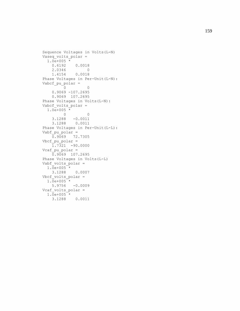
159
Sequence Voltages in Volts(L-N)
Vaseq_volts_polar =
1.0e+005 *
0.6192 0.0018
2.0346 0
1.4154 0.0018
Phase Voltages in Per-Unit(L-N):
Vabcf_pu_polar =
0 0
0.9069 -107.2695
0.9069 107.2695
Phase Voltages in Volts(L-N):
Vabcf_volts_polar =
1.0e+005 *
0 0
3.1288 -0.0011
3.1288 0.0011
Phase Voltages in Per-Unit(L-L):
Vabf_pu_polar =
0.9069 72.7305
Vbcf_pu_polar =
1.7321 -90.0000
Vcaf_pu_polar =
0.9069 107.2695
Phase Voltages in Volts(L-L)
Vabf_volts_polar =
1.0e+005 *
3.1288 0.0007
Vbcf_volts_polar =
1.0e+005 *
5.9756 -0.0009
Vcaf_volts_polar =
1.0e+005 *
3.1288 0.0011

160
E8.2 477kcmil SLG MID
SBgen =
100000000
VBgen =
22000
ZBL =
1.1903e+003
Enter fault type(1=SLG,2=DLG,3=LL,4=3LG):
1
Enter percentage of line from sending-end that is involved with
fault(e.g.0,50,100):
50
Zseq =
0.0599 + 0.3049i
0.0200 + 0.2383i
0.0200 + 0.2383i
+++++++++++++SLG Fault Analysis+++++++++++++
Sequence Currents in Per-Unit:
Iaseq_pu_polar =
1.2692 -82.7224
1.2692 -82.7224
1.2692 -82.7224
Sequence Currents in Amps:
Iaseq_amps_polar =
212.3918 -82.7224
212.3918 -82.7224
212.3918 -82.7224
Phase Currents in Per-Unit:
Iabcf_pu_polar =
3.8075 -82.7224
0.0000 48.3665
0.0000 48.3665
Phase Currents in Amps
Iabcf_amps_polar =
637.1755 -82.7224
0.0000 48.3665
0.0000 48.3665
Sequence Voltages in Per-Unit(L-N):
Vaseq_pu_polar =
0.3944 176.1669
0.6969 -1.0840
0.3035 -177.5106
Sequence Voltages in Volts(L-N)
Vaseq_volts_polar =
1.0e+005 *
1.3607 0.0018
2.4043 -0.0000
1.0471 -0.0018
Phase Voltages in Per-Unit(L-N):
Vabcf_pu_polar =

161
0.0000 1.7899
1.0156 -125.5359
1.0810 123.0984
Phase Voltages in Volts(L-N):
Vabcf_volts_polar =
1.0e+005 *
0.0000 0.0000
3.5039 -0.0013
3.7294 0.0012
Phase Voltages in Per-Unit(L-L):
Vabf_pu_polar =
1.0156 54.4641
Vbcf_pu_polar =
1.7321 -90.0000
Vcaf_pu_polar =
1.0810 123.0984
Phase Voltages in Volts(L-L)
Vabf_volts_polar =
1.0e+005 *
3.5039 0.0005
Vbcf_volts_polar =
1.0e+005 *
5.9756 -0.0009
Vcaf_volts_polar =
1.0e+005 *
3.7294 0.0012

162
E8.3 477kcmil SLG RE
ZBL =
1.1903e+003
Enter fault type(1=SLG,2=DLG,3=LL,4=3LG):
1
Enter percentage of line from sending-end that is involved with
fault(e.g.0,50,100):
100
Zseq =
0.1198 + 0.5399i
0.0399 + 0.3166i
0.0399 + 0.3166i
+++++++++++++SLG Fault Analysis+++++++++++++
Sequence Currents in Per-Unit:
Iaseq_pu_polar =
0.8403 -80.3431
0.8403 -80.3431
0.8403 -80.3431
Sequence Currents in Amps:
Iaseq_amps_polar =
140.6274 -80.3431
140.6274 -80.3431
140.6274 -80.3431
Phase Currents in Per-Unit:
Iabcf_pu_polar =
2.5210 -80.3431
0.0000 90.0000
0.0000 90.0000
Phase Currents in Amps
Iabcf_amps_polar =
421.8823 -80.3431
0.0000 90.0000
0.0000 90.0000
Sequence Voltages in Per-Unit(L-N):
Vaseq_pu_polar =
0.4647 177.1485
0.7322 -0.9046
0.2682 -177.5297
Sequence Voltages in Volts(L-N)
Vaseq_volts_polar =
1.0e+005 *
1.6033 0.0018
2.5260 -0.0000
0.9252 -0.0018
Phase Voltages in Per-Unit(L-N):
Vabcf_pu_polar =
0.0000 -165.9638
1.0844 -129.9443
1.1384 127.7026

163
Phase Voltages in Volts(L-N):
Vabcf_volts_polar =
1.0e+005 *
0.0000 -0.0017
3.7411 -0.0013
3.9275 0.0013
Phase Voltages in Per-Unit(L-L):
Vabf_pu_polar =
1.0844 50.0557
Vbcf_pu_polar =
1.7321 -90.0000
Vcaf_pu_polar =
1.1384 127.7026
Phase Voltages in Volts(L-L)
Vabf_volts_polar =
1.0e+005 *
3.7411 0.0005
Vbcf_volts_polar =
1.0e+005 *
5.9756 -0.0009
Vcaf_volts_polar =
1.0e+005 *
3.9275 0.0013

164
E8.4 477kcmil LL SE
SBgen =
100000000
VBgen =
22000
ZBL =
1.1903e+003
Enter fault type(1=SLG,2=DLG,3=LL,4=3LG):
3
Enter percentage of line from sending-end that is involved with
fault(e.g.0,50,100):
0
Zseq =
0 + 0.0700i
0 + 0.1600i
0 + 0.1600i
+++++++++++++LL Fault Analysis+++++++++++++
Sequence Currents in Per-Unit:
Iaseq_pu_polar =
0 0
3.1250 -90.0000
3.1250 90.0000
Sequence Currents in Amps:
Iaseq_amps_polar =
0 0
522.9622 -90.0000
522.9622 90.0000
Phase Currents in Per-Unit:
Iabcf_pu_polar =
0 0
5.4127 180.0000
5.4127 -0.0000
Phase Currents in Amps
Iabcf_amps_polar =
0 0
905.7971 180.0000
905.7971 -0.0000
Sequence Voltages in Per-Unit(L-N):
Vaseq_pu_polar =
0 0
0.5000 0
0.5000 0
Sequence Voltages in Volts(L-N)
Vaseq_volts_polar =
0 0
172500 0
172500 0

165
Phase Voltages in Per-Unit(L-N):
Vabcf_pu_polar =
1.0000 0
0.5000 180.0000
0.5000 180.0000
Phase Voltages in Volts(L-N):
Vabcf_volts_polar =
1.0e+005 *
3.4500 0
1.7250 0.0018
1.7250 0.0018
Phase Voltages in Per-Unit(L-L):
Vabf_pu_polar =
1.5000 -0.0000
Vbcf_pu_polar =
0 0
Vcaf_pu_polar =
1.5000 180.0000
Phase Voltages in Volts(L-L)
Vabf_volts_polar =
1.0e+005 *
5.1750 -0.0000
Vbcf_volts_polar =
0 0
Vcaf_volts_polar =
517500 180

166
E8.5 477kcmil LL MID
SBgen =
100000000
VBgen =
22000
ZBL =
1.1903e+003
Enter fault type(1=SLG,2=DLG,3=LL,4=3LG):
3
Enter percentage of line from sending-end that is involved with
fault(e.g.0,50,100):
50
Zseq =
0.0599 + 0.3049i
0.0200 + 0.2383i
0.0200 + 0.2383i
+++++++++++++LL Fault Analysis+++++++++++++
Sequence Currents in Per-Unit:
Iaseq_pu_polar =
0 0
2.0907 -85.2119
2.0907 94.7881
Sequence Currents in Amps:
Iaseq_amps_polar =
0 0
349.8817 -85.2119
349.8817 94.7881
Phase Currents in Per-Unit:
Iabcf_pu_polar =
0 0
3.6213 -175.2119
3.6213 4.7881
Phase Currents in Amps
Iabcf_amps_polar =
0 0
606.0130 -175.2119
606.0130 4.7881
Sequence Voltages in Per-Unit(L-N):
Vaseq_pu_polar =
0 0
0.5000 0
0.5000 0
Sequence Voltages in Volts(L-N)
Vaseq_volts_polar =
1.0e+005 *
0 0
1.7250 0
1.7250 0

167
Phase Voltages in Per-Unit(L-N):
Vabcf_pu_polar =
1.0000 0
0.5000 180.0000
0.5000 180.0000
Phase Voltages in Volts(L-N):
Vabcf_volts_polar =
345000 0
172500 180
172500 180
Phase Voltages in Per-Unit(L-L):
Vabf_pu_polar =
1.5000 0
Vbcf_pu_polar =
0.0000 -90.0000
Vcaf_pu_polar =
1.5000 180.0000
Phase Voltages in Volts(L-L)
Vabf_volts_polar =
517500 0
Vbcf_volts_polar =
0.0000 -90.0000
Vcaf_volts_polar =
517500 180

168
E8.6 477kcmil LL RE
SBgen =
100000000
VBgen =
22000
ZBL =
1.1903e+003
Enter fault type(1=SLG,2=DLG,3=LL,4=3LG):
3
Enter percentage of line from sending-end that is involved with
fault(e.g.0,50,100):
100
Zseq =
0.1198 + 0.5399i
0.0399 + 0.3166i
0.0399 + 0.3166i
+++++++++++++LL Fault Analysis+++++++++++++
Sequence Currents in Per-Unit:
Iaseq_pu_polar =
0 0
1.5667 -82.8134
1.5667 97.1866
Sequence Currents in Amps:
Iaseq_amps_polar =
0 0
262.1887 -82.8134
262.1887 97.1866
Phase Currents in Per-Unit:
Iabcf_pu_polar =
0 0
2.7137 -172.8134
2.7137 7.1866
Phase Currents in Amps
Iabcf_amps_polar =
0 0
454.1241 -172.8134
454.1241 7.1866
Sequence Voltages in Per-Unit(L-N):
Vaseq_pu_polar =
0 0
0.5000 -0.0000
0.5000 0.0000
Sequence Voltages in Volts(L-N)
Vaseq_volts_polar =
1.0e+005 *
0 0
1.7250 -0.0000
1.7250 0.0000

169
Phase Voltages in Per-Unit(L-N):
Vabcf_pu_polar =
1.0000 0
0.5000 180.0000
0.5000 180.0000
Phase Voltages in Volts(L-N):
Vabcf_volts_polar =
345000 0
172500 180
172500 180
Phase Voltages in Per-Unit(L-L):
Vabf_pu_polar =
1.5000 0
Vbcf_pu_polar =
0.0000 -90.0000
Vcaf_pu_polar =
1.5000 180.0000
Phase Voltages in Volts(L-L)
Vabf_volts_polar =
517500 0
Vbcf_volts_polar =
0.0000 -90.0000
Vcaf_volts_polar =
517500 180

170
E8.7 477kcmil DLG SE
SBgen =
100000000
VBgen =
22000
ZBL =
1.1903e+003
Enter fault type(1=SLG,2=DLG,3=LL,4=3LG):
2
Enter percentage of line from sending-end that is involved with
fault(e.g.0,50,100):
0
Zseq =
0 + 0.0700i
0 + 0.1600i
0 + 0.1600i
+++++++++++++DLG Fault Analysis+++++++++++++
Sequence Currents in Per-Unit:
Iaseq_pu_polar =
3.3333 90.0000
4.7917 -90.0000
1.4583 90.0000
Sequence Currents in Amps:
Iaseq_amps_polar =
557.8263 90.0000
801.8754 -90.0000
244.0490 90.0000
Phase Currents in Per-Unit:
Iabcf_pu_polar =
0.0000 90.0000
7.3686 137.2695
7.3686 42.7305
Phase Currents in Amps
Iabcf_amps_polar =
1.0e+003 *
0.0000 0.0900
1.2331 0.1373
1.2331 0.0427
Sequence Voltages in Per-Unit(L-N):
Vaseq_pu_polar =
0.2333 0
0.2333 0
0.2333 0
Sequence Voltages in Volts(L-N)
Vaseq_volts_polar =
1.0e+004 *
8.0500 0
8.0500 0
8.0500 0

171
Phase Voltages in Per-Unit(L-N):
Vabcf_pu_polar =
0.7000 0
0.0000 -158.1986
0.0000 129.8056
Phase Voltages in Volts(L-N):
Vabcf_volts_polar =
1.0e+005 *
2.4150 0
0.0000 -0.0016
0.0000 0.0013
Phase Voltages in Per-Unit(L-L):
Vabf_pu_polar =
0.7000 0.0000
Vbcf_pu_polar =
0.0000 -90.0000
Vcaf_pu_polar =
0.7000 180.0000
Phase Voltages in Volts(L-L)
Vabf_volts_polar =
1.0e+005 *
2.4150 0.0000
Vbcf_volts_polar =
0.0000 -90.0000
Vcaf_volts_polar =
1.0e+005 *
2.4150 0.0018
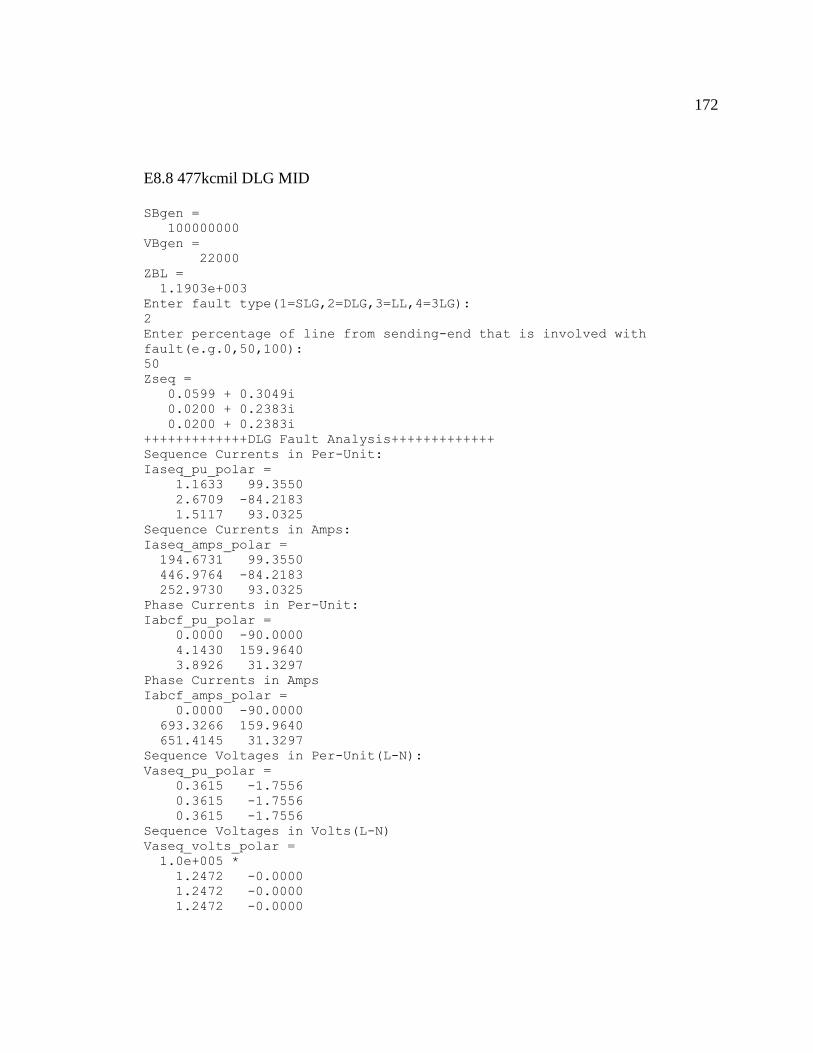
172
E8.8 477kcmil DLG MID
SBgen =
100000000
VBgen =
22000
ZBL =
1.1903e+003
Enter fault type(1=SLG,2=DLG,3=LL,4=3LG):
2
Enter percentage of line from sending-end that is involved with
fault(e.g.0,50,100):
50
Zseq =
0.0599 + 0.3049i
0.0200 + 0.2383i
0.0200 + 0.2383i
+++++++++++++DLG Fault Analysis+++++++++++++
Sequence Currents in Per-Unit:
Iaseq_pu_polar =
1.1633 99.3550
2.6709 -84.2183
1.5117 93.0325
Sequence Currents in Amps:
Iaseq_amps_polar =
194.6731 99.3550
446.9764 -84.2183
252.9730 93.0325
Phase Currents in Per-Unit:
Iabcf_pu_polar =
0.0000 -90.0000
4.1430 159.9640
3.8926 31.3297
Phase Currents in Amps
Iabcf_amps_polar =
0.0000 -90.0000
693.3266 159.9640
651.4145 31.3297
Sequence Voltages in Per-Unit(L-N):
Vaseq_pu_polar =
0.3615 -1.7556
0.3615 -1.7556
0.3615 -1.7556
Sequence Voltages in Volts(L-N)
Vaseq_volts_polar =
1.0e+005 *
1.2472 -0.0000
1.2472 -0.0000
1.2472 -0.0000

173
Phase Voltages in Per-Unit(L-N):
Vabcf_pu_polar =
1.0845 -1.7556
0.0000 180.0000
0.0000 131.1859
Phase Voltages in Volts(L-N):
Vabcf_volts_polar =
1.0e+005 *
3.7417 -0.0000
0.0000 0.0018
0.0000 0.0013
Phase Voltages in Per-Unit(L-L):
Vabf_pu_polar =
1.0845 -1.7556
Vbcf_pu_polar =
0.0000 -74.2914
Vcaf_pu_polar =
1.0845 178.2444
Phase Voltages in Volts(L-L)
Vabf_volts_polar =
1.0e+005 *
3.7417 -0.0000
Vbcf_volts_polar =
0.0000 -74.2914
Vcaf_volts_polar =
1.0e+005 *
3.7417 0.0018

174
E8.9 477kcmil DLG RE
SBgen =
100000000
VBgen =
22000
ZBL =
1.1903e+003
Enter fault type(1=SLG,2=DLG,3=LL,4=3LG):
2
Enter percentage of line from sending-end that is involved with
fault(e.g.0,50,100):
100
Zseq =
0.1198 + 0.5399i
0.0399 + 0.3166i
0.0399 + 0.3166i
+++++++++++++DLG Fault Analysis+++++++++++++
Sequence Currents in Per-Unit:
Iaseq_pu_polar =
0.7022 101.3174
1.9171 -82.0575
1.2168 95.9956
Sequence Currents in Amps:
Iaseq_amps_polar =
117.5116 101.3174
320.8198 -82.0575
203.6295 95.9956
Phase Currents in Per-Unit:
Iabcf_pu_polar =
0.0000 110.5560
2.9808 166.5497
2.8393 28.9028
Phase Currents in Amps
Iabcf_amps_polar =
0.0000 110.5560
498.8298 166.5497
475.1491 28.9028
Sequence Voltages in Per-Unit(L-N):
Vaseq_pu_polar =
0.3883 -1.1910
0.3883 -1.1910
0.3883 -1.1910
Sequence Voltages in Volts(L-N)
Vaseq_volts_polar =
1.0e+005 *
1.3397 -0.0000
1.3397 -0.0000
1.3397 -0.0000
Phase Voltages in Per-Unit(L-N):

175
Vabcf_pu_polar =
1.1650 -1.1910
0.0000 180.0000
0.0000 134.7753
Phase Voltages in Volts(L-N):
Vabcf_volts_polar =
1.0e+005 *
4.0192 -0.0000
0.0000 0.0018
0.0000 0.0013
Phase Voltages in Per-Unit(L-L):
Vabf_pu_polar =
1.1650 -1.1910
Vbcf_pu_polar =
0.0000 -90.0000
Vcaf_pu_polar =
1.1650 178.8090
Phase Voltages in Volts(L-L)
Vabf_volts_polar =
1.0e+005 *
4.0192 -0.0000
Vbcf_volts_polar =
0.0000 -90.0000
Vcaf_volts_polar =
1.0e+005 *
4.0192 0.0018

176
E8.10 477kcmil 3LG SE
SBgen =
100000000
VBgen =
22000
ZBL =
1.1903e+003
Enter fault type(1=SLG,2=DLG,3=LL,4=3LG):
4
Enter percentage of line from sending-end that is involved with
fault(e.g.0,50,100):
0
Zseq =
0 + 0.0700i
0 + 0.1600i
0 + 0.1600i
+++++++++++++3-Phase Fault Analysis+++++++++++++
Sequence Currents in Per-Unit:
Iaseq_pu_polar =
0 0
6.2500 -90.0000
0 0
Sequence Currents in Amps:
Iaseq_amps_polar =
1.0e+003 *
0 0
1.0459 -0.0900
0 0
Phase Currents in Per-Unit:
Iabcf_pu_polar =
6.2500 -90.0000
6.2500 150.0000
6.2500 30.0000
Phase Currents in Amps
Iabcf_amps_polar =
1.0e+003 *
1.0459 -0.0900
1.0459 0.1500
1.0459 0.0300
Sequence Voltages in Per-Unit(L-N):
Vaseq_pu_polar =
0 0
0 0
0 0
Sequence Voltages in Volts(L-N)
Vaseq_volts_polar =
0 0
0 0
0 0

177
Phase Voltages in Per-Unit(L-N):
Vabcf_pu_polar =
0 0
0 0
0 0
Phase Voltages in Volts(L-N):
Vabcf_volts_polar =
0 0
0 0
0 0
Phase Voltages in Per-Unit(L-L):
Vabf_pu_polar =
0 0
Vbcf_pu_polar =
0 0
Vcaf_pu_polar =
0 0
Phase Voltages in Volts(L-L)
Vabf_volts_polar =
0 0
Vbcf_volts_polar =
0 0
Vcaf_volts_polar =
0 0

178
E8.11 477kcmil 3LG MID
SBgen =
100000000
VBgen =
22000
ZBL =
1.1903e+003
Enter fault type(1=SLG,2=DLG,3=LL,4=3LG):
4
Enter percentage of line from sending-end that is involved with
fault(e.g.0,50,100):
50
Zseq =
0.0599 + 0.3049i
0.0200 + 0.2383i
0.0200 + 0.2383i
+++++++++++++3-Phase Fault Analysis+++++++++++++
Sequence Currents in Per-Unit:
Iaseq_pu_polar =
0 0
4.1815 -85.2119
0 0
Sequence Currents in Amps:
Iaseq_amps_polar =
0 0
699.7635 -85.2119
0 0
Phase Currents in Per-Unit:
Iabcf_pu_polar =
4.1815 -85.2119
4.1815 154.7881
4.1815 34.7881
Phase Currents in Amps
Iabcf_amps_polar =
699.7635 -85.2119
699.7635 154.7881
699.7635 34.7881
Sequence Voltages in Per-Unit(L-N):
Vaseq_pu_polar =
1.0e-015 *
0 0
0.1110 0
0 0
Sequence Voltages in Volts(L-N)
Vaseq_volts_polar =
1.0e-010 *
0 0
0.3830 0
0 0
Phase Voltages in Per-Unit(L-N):

179
Vabcf_pu_polar =
0.0000 0
0.0000 -120.0000
0.0000 120.0000
Phase Voltages in Volts(L-N):
Vabcf_volts_polar =
0.0000 0
0.0000 -120.0000
0.0000 120.0000
Phase Voltages in Per-Unit(L-L):
Vabf_pu_polar =
0.0000 30.0000
Vbcf_pu_polar =
0.0000 -90.0000
Vcaf_pu_polar =
0.0000 150.0000
Phase Voltages in Volts(L-L)
Vabf_volts_polar =
0.0000 30.0000
Vbcf_volts_polar =
0.0000 -90.0000
Vcaf_volts_polar =
0.0000 150.0000

180
E8.12 477kcmil 3LG RE
SBgen =
100000000
VBgen =
22000
ZBL =
1.1903e+003
Enter fault type(1=SLG,2=DLG,3=LL,4=3LG):
4
Enter percentage of line from sending-end that is involved with
fault(e.g.0,50,100):
100
Zseq =
0.1198 + 0.5399i
0.0399 + 0.3166i
0.0399 + 0.3166i
+++++++++++++3-Phase Fault Analysis+++++++++++++
Sequence Currents in Per-Unit:
Iaseq_pu_polar =
0 0
3.1335 -82.8134
0 0
Sequence Currents in Amps:
Iaseq_amps_polar =
0 0
524.3773 -82.8134
0 0
Phase Currents in Per-Unit:
Iabcf_pu_polar =
3.1335 -82.8134
3.1335 157.1866
3.1335 37.1866
Phase Currents in Amps
Iabcf_amps_polar =
524.3773 -82.8134
524.3773 157.1866
524.3773 37.1866
Sequence Voltages in Per-Unit(L-N):
Vaseq_pu_polar =
0 0
0.0000 -7.1250
0 0
Sequence Voltages in Volts(L-N)
Vaseq_volts_polar =
0 0
0.0000 -7.1250
0 0

181
Phase Voltages in Per-Unit(L-N):
Vabcf_pu_polar =
0.0000 -7.1250
0.0000 -127.1250
0.0000 112.8750
Phase Voltages in Volts(L-N):
Vabcf_volts_polar =
0.0000 -7.1250
0.0000 -127.1250
0.0000 112.8750
Phase Voltages in Per-Unit(L-L):
Vabf_pu_polar =
0.0000 22.8750
Vbcf_pu_polar =
0.0000 -97.1250
Vcaf_pu_polar =
0.0000 142.8750
Phase Voltages in Volts(L-L)
Vabf_volts_polar =
0.0000 22.8750
Vbcf_volts_polar =
0.0000 -97.1250
Vcaf_volts_polar =
0.0000 142.8750

182
BIBLIOGRAPHY
[1] Gonen, T. 2009. Electrical power transmission system engineering analysis and
design, 2nd
ed. Florida: CRC Press.
[2] Electrical Power Research Institute. 1979. Transmission line reference book 345
kV and above. Palo Alto, CA: EPRI.
[3] Kiessling, F., Nefzger, P., Nolasco, J.F., and Kaintzyk, U. 2003. Overhead power
lines. New York: Springer.
[4] Gonen, T. 2008. Electrical power distribution system engineering, 2nd
ed. Florida:
CRC Press.
[5] Sadaat, H. 2002. Power system analysis. New York: McGraw-Hill.
[6] Granger, J. J. and W. D. Stevenson. 1994. Power system analysis. New York:
McGraw-Hill.
[7] Ray, S. 2012. Electrical power systems: concepts, theory and practice, 4th
ed. New
Delhi: PHI Learning Private Limited.
[8] Glover, J. D., Sarma M. S., Overbye T. J. 2010. Power system analysis and design,
5th
ed. Stamford, CT: Cengage Learning
[9] Bayliss, C., Hardy, B. 2007. Transmission and distribution electrical engineering,
3rd
ed. Burlington, MA: Elsevier Ltd.
[10] Short, T.A. 2004. Electric power distribution handbook. New York: CRC Press.
[11] Pansini, A.J. 2006. Electrical distribution engineering, 3rd
ed. Florida: CRC Press.
[12] Wadhwa, C.L. 2009. Electric power systems, 2nd
ed. Tunbridge Wells: New
Academic Science Ltd.