Simulation of Radiant Cooling Performance with Evaporative ...
Upload
khangminh22Category
view
0download
0
Design and Control of High Thermal Mass Radiant Systems
By
Carlos Duarte Roa
A dissertation submitted in partial satisfaction of the
requirements for the degree of
Doctor of Philosophy
in
Architecture
in the
Graduate Division
of the
University of California, Berkeley
Committee in charge:
Professor Stefano Schiavon, Chair Professor Gail Brager
Professor Francesco Borrelli
Summer 2020

Design and Control of High Thermal Mass Radiant Systems © By Carlos Duarte Roa

1
Abstract
Design and Control of High Thermal Mass Radiant Systems
by
Carlos Duarte Roa
Doctor of Philosophy in Architecture
University of California, Berkeley
Professor Stefano Schiavon, Chair
Heating, ventilation, and air-conditioning (HVAC) systems play a key role in providing healthy, productive, and thermally comfortable built environment for the occupants. Improper HVAC design will degrade occupants’ satisfaction with the built environment, potentially affecting their performance which can be valued up to 200 times the building’s energy costs. In the top two energy consuming countries, the US and China, over 40% of the energy use in buildings with HVAC systems can be attributed to those systems. Moreover, 13% of total greenhouse gas emissions in the US can also be ascribed to HVAC systems. On a global scale, electricity demand for space cooling could increase by up to 210% by 2050 from 2016 levels. This rapid growth prediction is driven by the fact that most of the world’s population and wealth growth is happening in the tropics and in middle-income countries where air-conditioning has relatively small penetration in buildings. There are serious implications to electrical grid systems and most importantly, to our ecosystems if HVAC design is left unchecked.
Therefore, in this dissertation we investigate high thermal mass radiant systems (HTMR) as a promising strategy to address the challenges and strain imposed by HVAC systems, with the focus on space cooling. HTMR, and other radiant systems in general, deliver 50% or more of the design heat transfer through thermal radiation, have large heat transfer areas, and have high heat transport efficiency. The “high thermal mass” in HTMR comes from the fact that there is a significant time delay, measured in hours, between a control action and the temperature response observed in the zone as a result of the thermal inertia in the concrete. This property has presented obstacles to the adoption rate of HTMR in the building stock in the US. In general, building designers are unfamiliar with how to design and control HTMR without adversely affecting occupants’ thermal satisfaction while also balancing other performance objectives such as capital and operational costs. Yet, because of the thermal response delay property, HTMR presents building designers and other stakeholders with innovative and beneficial design and control options that are difficult to implement in the more typical all-air systems to reduce equipment and electricity costs while maintaining acceptable indoor temperatures.
https://escholarship.org/uc/item/82t6n3xrPhD Dissertation, Dept. of Architecture, UC Berkeley 2020

2
The development of most building standards, guidelines, and tools have focused on all-air HVAC systems. One example is the standard design procedure for sizing cooling systems. The standard design procedure includes a definition of space cooling load which serves as the basis to size HVAC components from the zone level to the central cooling plant. However, that space cooling load definition is too narrowly constrained and omits fundamental principles that are essential to the operation of various cooling systems, including HTMR. We provide a critical review of the standard design procedure for sizing cooling systems to identify fundamental flaws, explain how it has influenced building energy modeling, system sizing and operation in practice, and propose a new definition for space cooling load along with an associated cooling system design procedure that better suits a variety of systems and control strategies. We conduct whole building energy simulations with the focus on HTMR to demonstrate the consequences of the standard procedure and compare it to our recommended procedure. The results show that following the standard design approach for HTMR can lead designers to underestimate the peak space cooling load by 100%, yet also select cooling plant equipment that is 100% larger than necessary due to its large thermal inertia. The standard design obscures considerable opportunities to reduce costs and improve energy efficiency and thermal comfort.
For example, large heat transfer areas allow HTMR to take advantage of high-temperature cooling, i.e. using higher than typical supply water temperature to perform space cooling, and potentially eliminating the use of the vapor-compression refrigeration cycle. In lieu of this energy- and cost-intensive cycle, more sustainable cooling plants that use adiabatic cooling with cooling towers or fluid coolers can provide cool water production for HTMR. We used whole building energy simulation to determine the warmest supply water temperature that is able to still maintain comfortable temperatures for various building, HTMR, and control strategy designs. We used single zone models that represent ASHRAE 90.1-2016 and Title 24-2016 code-compliant buildings in 14 US and 16 Californian representative climates during the climates’ cooling design day. We found the warmest supply water temperature to be 18.2, 21.4, 23.4 °C for the first quartile, median, and third quartile, respectively, among all test cases. Cooling towers can generate these required supply water temperatures during nighttime periods when their performance is at their highest. There is great potential to avoid installing a compressor-based refrigeration system in most climates, while only a few will require more than code-compliant designed buildings.
A key determinant to the successful implementation of HTMR is the control system. Improved HVAC control can improve energy, cost, and thermal comfort performance over typical control strategies, but improper control and faults can penalize them on a similar scale. We developed and experimentally tested a new HTMR control strategy that independently adapts to each radiant zone’s observed indoor temperatures in two California buildings located in distinct, contrasting climates. The results show that the new HTMR control strategy reduces the number of hours that zone dry-bulb temperatures exceed predefined thermal comfort limits from 9.1% to 1.6% as a proportion of total occupied hours when compared to the buildings’ existing
https://escholarship.org/uc/item/82t6n3xrPhD Dissertation, Dept. of Architecture, UC Berkeley 2020

3
controls. We verified that the new control strategy did not have adverse effects on occupant thermal comfort satisfaction through a detailed “right-now” satisfaction survey. The new strategy also reduces the number of average daily minutes HTMR manifold valves open for water flow through the slab, a proxy for energy consumption, by up to 93%.
Finally, we created an interactive web-based tool for the early design of HTMR. The primary aim of this design tool is to provide an interface for estimating the performance of HTMR under steady-state and transient conditions. It allows users to estimate the impact of innovative control strategies such as nighttime pre-cooling on indoor temperature response. The tool website not only contains resources and lessons learned through the investigations presented in this dissertation but also from the overarching investigations on radiant systems undertaken by the Center for the Built Environment, which this Ph.D. study was part of.
In this dissertation, we contributed on revising the fundamental cooling load definition and associated design procedure for applicability to a broader range of systems and applications, demonstrated the potential of using HTMR coupled with more sustainable cooling plants in a diverse set of US climate zones, developed and tested adaptive control strategies that take advantage of HTMR’s high thermal inertia to shift the building’s cooling load to more beneficial periods, and facilitate mechanical designers’ decision making with respect to HTMR systems through our early design web-based tool. These innovations will help achieve reductions in energy and greenhouse gas emissions attributed to HVAC systems and therefore support our global shift towards a more sustainable built environment.
https://escholarship.org/uc/item/82t6n3xrPhD Dissertation, Dept. of Architecture, UC Berkeley 2020

i
Table of Contents
List of Figures ................................................................................................................................ v
List of Tables .............................................................................................................................. xiv
List of Abbreviations .................................................................................................................. xvi
List of Symbols .......................................................................................................................... xviii
Acknowledgements ..................................................................................................................... xix
1. Introduction ........................................................................................................................... 1
1.1. Energy and demand requirements for HVAC systems .................................................... 1
1.2. Greenhouse gas emissions ............................................................................................. 4
1.3. Typical HVAC systems ..................................................................................................... 4
1.4. Proposed Solution: Compressor-less cooling with high thermal mass radiant systems . 5
1.5. Research objectives ........................................................................................................ 7
1.6. Summary of contributions and relevant publications ..................................................... 7
1.6.1. Chapter summaries ................................................................................................. 7
1.6.2. Related publications list .......................................................................................... 9
2. Background .......................................................................................................................... 11
2.1. High thermal mass radiant systems .............................................................................. 11
2.1.1. Radiant system descriptions .................................................................................. 12
2.1.2. Advantage, limitations, and implications ............................................................... 14
2.2. Conclusion .................................................................................................................... 20
3. A critical review – and proposed redefinition – of the industry standard definition of “cooling and heating loads” and the associated system design sizing procedure, with focus on high thermal mass radiant cooling systems ................................................................................ 21
3.1. Background ................................................................................................................... 21
3.2. Shortcomings with the standard definition of “cooling (heating) load” and the associated system design procedure ....................................................................................... 25
3.2.1. The standard definition of “space cooling (heating) load” does not fully reflect all aspects of standards that address thermal comfort ............................................................ 25
3.2.2. The standard definition of “space cooling load” only facilitates design of systems for basic applications ........................................................................................................... 27
3.2.3. The standard definition of “space cooling load” does not account for the way that cooling system type impacts space cooling requirements ................................................... 28
https://escholarship.org/uc/item/82t6n3xrPhD Dissertation, Dept. of Architecture, UC Berkeley 2020
ii
3.2.4. The standard definition of “cooling load” does not account for the way that system control strategies impact space cooling requirements ............................................ 30
3.2.5. The standard definition of “space cooling load” does not provide sufficient guidance on the selection of design periods ........................................................................ 31
3.2.6. The standard design procedure does not facilitate design for any performance metric other than indoor dry-bulb air temperature. ............................................................ 32
3.2.7. The standard design procedure is not satisfactory for systems with long response time 33
3.3. Proposed redefinition of cooling load and system design procedure ........................... 34
3.4. Practical impact of our proposed design procedure ..................................................... 38
3.4.1. Example of the standard cooling load calculation and system design procedure: 40
3.4.2. Example of our proposed cooling load calculation and system design procedure: 43
3.4.3. Comparison of performance for systems designed according to each procedure . 48
3.5. Conclusions ................................................................................................................... 57
4. Determining the warmest supply water temperature for high thermal mass radiant cooling systems under thermal comfort constrains ................................................................................ 78
4.1. Background ................................................................................................................... 78
4.2. Methods ....................................................................................................................... 80
4.2.1. Envelope ................................................................................................................ 80
4.2.2. Internal heat gains ................................................................................................. 81
4.2.3. Radiant system ...................................................................................................... 82
4.2.4. Sampling method .................................................................................................. 84
4.2.5. Supply water temperature determination ............................................................ 85
4.2.6. Simulation test case exclusion criteria ................................................................... 86
4.2.7. Outdoor wet-bulb temperature analysis ............................................................... 87
4.2.8. Simplified model development.............................................................................. 88
4.3. Results .......................................................................................................................... 89
4.3.1. Data cleaning ......................................................................................................... 89
4.3.2. Supply water temperature analysis ....................................................................... 92
4.3.3. Simplified model development............................................................................ 103
4.4. Discussion ................................................................................................................... 106
4.5. Future work ................................................................................................................ 109
https://escholarship.org/uc/item/82t6n3xrPhD Dissertation, Dept. of Architecture, UC Berkeley 2020

iii
4.6. Conclusions ................................................................................................................. 109
4.7. Acknowledgment ........................................................................................................ 110
5. Energy and thermal comfort assessment of a new control strategy for high thermal mass radiant systems ......................................................................................................................... 111
5.1. Background ................................................................................................................. 111
5.2. Methods ..................................................................................................................... 113
5.2.1. Field study building descriptions ......................................................................... 113
5.2.2. Intervention control strategy .............................................................................. 124
5.2.3. Occupant satisfaction surveys ............................................................................. 129
5.2.4. HTMR control strategy performance analysis ..................................................... 131
5.2.5. Statistical metrics ................................................................................................ 133
5.3. Results ........................................................................................................................ 134
5.3.1. Building site weather ........................................................................................... 134
5.3.2. Example cooling days for control strategies ........................................................ 135
5.3.3. Thermal comfort performance ............................................................................ 139
5.3.4. Energy consumption performance ...................................................................... 160
5.3.5. Resilience in HTMR buildings ............................................................................... 164
5.4. Discussion ................................................................................................................... 167
5.5. Conclusion .................................................................................................................. 170
5.6. Acknowledgments ...................................................................................................... 170
6. Interactive web-based tool for the early design of high thermal mass radiant systems .... 172
6.1. Background ................................................................................................................. 172
6.2. Structure of the website ............................................................................................. 173
6.2.1. Steady-state analysis ........................................................................................... 173
6.2.2. Resources ............................................................................................................ 175
6.2.3. In the resources section of the website, we gathered useful information for HTMR designers. These include documentation to both the steady-state and transient HTMR tools, the adaptive radiant control sequences we used and analyzed in Chapters 3 and 5, and links to an interactive map for buildings with radiant systems (Karmann, Schiavon, and Bauman 2014) and to other research pertaining to radiant systems. The radiant control sequences come in language that can be handed directly to controls contractors, as part of a single zone model example where advanced users can modify for their case studies, and as a so-called OpenStudio measure. The OpenStudio measure facilitates the transferring of
https://escholarship.org/uc/item/82t6n3xrPhD Dissertation, Dept. of Architecture, UC Berkeley 2020

iv
the adaptive control sequences to a custom EnergyPlus model including multizone models (Goldwasser et al. 2016). We make the control sequences available in several formats since it is an important factor in implementing a successful HTMR project. .............................. 175
7. Conclusion ......................................................................................................................... 177
8. References ......................................................................................................................... 179
https://escholarship.org/uc/item/82t6n3xrPhD Dissertation, Dept. of Architecture, UC Berkeley 2020

v
List of Figures
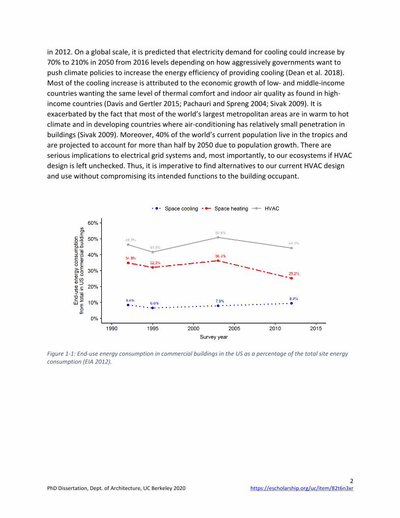
Figure 1-1: End-use energy consumption in commercial buildings in the US as a percentage of the total site energy consumption (EIA 2012). .............................................................................. 2
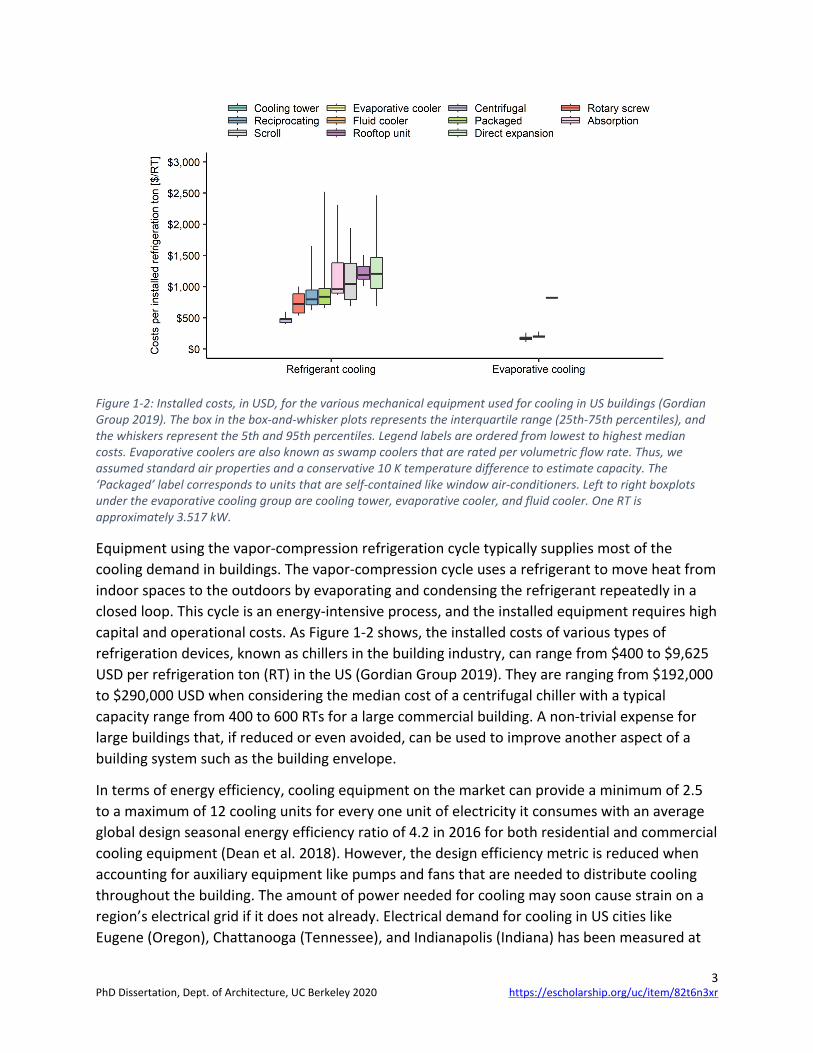
Figure 1-2: Installed costs, in USD, for the various mechanical equipment used for cooling in US buildings (Gordian Group 2019). The box in the box-and-whisker plots represents the interquartile range (25th-75th percentiles), and the whiskers represent the 5th and 95th percentiles. Legend labels are ordered from lowest to highest median costs. Evaporative coolers are also known as swamp coolers that are rated per volumetric flow rate. Thus, we assumed standard air properties and a conservative 10 K temperature difference to estimate capacity. The ‘Packaged’ label corresponds to units that are self-contained like window air-conditioners. Left to right boxplots under the evaporative cooling group are cooling tower, evaporative cooler, and fluid cooler. One RT is approximately 3.517 kW. ........................................................ 3
Figure 2-1: From left, schematic of radiant panels (RP), embedded surface system (ESS), and thermally activated building systems (TABS). The radiant layer in ESS can be composed of a concrete or screed topping slab, gypsum board, or plaster depending on the building structure base, e.g. floor, ceiling, or wall. TABS can also be found ‘bare’ with no floor construction layer or floor covering. Graphic source: (Karmann 2013). ........................................................................ 12
Figure 2-2: High thermal mass radiant (HTMR) buildings under construction. Top two images) Correspond to the same project where HTMR is constructed using a cast-in-place method. Photo courtesy of David Brower Center. Bottom left) HTMR is constructed through a precast method. The red ellipse shows tubing leads that will eventually connect to a manifold. Communication and coordination are crucial for the two HTMR construction methods. Bottom right) If the tubing is punctured after the concrete has set, then the leakage must be identified, and concrete needs to be chiseled out for repair. ...................................................................... 17
Figure 3-1: Conceptual illustration of the dynamic space cooling load for a cooling design day, and its relationship to outdoor temperature, indoor dry-bulb air temperature, and space heat gain rates. (Left): Outdoor temperature and indoor dry-bulb air temperature. (Right): Space heat extraction rate (space cooling load) and space heat gain rate (the sum of: internal heat gains, infiltration heat gain (loss), and solar heat gains). The red circle indicates the peak space cooling load used for sizing cooling systems. The gray hatched areas illustrate the rate at which space heat gains are absorbed by masses, and the rate at which heat stored in masses is released to the space. A portion of the space heat gains absorbed by masses may also be released to the environment (not indicated), and a portion of the heat released to the space from masses may have originated from the environment (not indicated). ................................. 21
Figure 3-2: Isometric and cross-section illustrations of the zone used to demonstrate each system design procedure. ........................................................................................................... 39
https://escholarship.org/uc/item/82t6n3xrPhD Dissertation, Dept. of Architecture, UC Berkeley 2020

vi
Figure 3-3: Standard cooling load calculation for the cooling design day. (Left): Outdoor dry-bulb air temperature and indoor temperatures. (Right): Sum of internal, solar, and infiltration heat gain (loss) rates, and the required space heat extraction rate (space cooling load). .................. 40
Figure 3-4: Steady-state space cooling capacity for an internally cooled 23.26 cm thick medium-weight concrete-slab floor and ceiling, with a thin covering on the floor surface, 8 parallel 104.2 m tubing loops, with tube spacing = 22.86 cm, tube inside diameter = 17 mm, tube depth = 57.15 mm. (Left): Steady-state space cooling capacity as a function of supply water temperature and supply water flow rate. (Right): Steady-state space cooling capacity as a function of supply water temperature and indoor operative temperature (ISO 2012; Raftery et al. 2019). ............ 42
Figure 3-5: (Left): Steady-state cooling capacity for an air-cooled chiller as a function of return water temperature and outdoor dry-bulb air temperature. (Right): Steady-state supply water temperature for an air-cooled chiller as a function of return water temperature and outdoor dry-bulb air temperature. ........................................................................................................... 43
Figure 3-6: Inputs to and results from design day simulations for four example design variants. (Left): Outdoor dry-bulb air temperature and indoor temperatures. (Right): Sum of internal, solar, and infiltration heat gain (loss) rates, space heat extraction rate (space cooling load), and hydronic heat extraction rate (plant cooling load). ..................................................................... 47
Figure 3-7: Comparison of the standard cooling load calculation to cooling design day simulation of the system designed according to the standard system design procedure. (Left): Outdoor dry-bulb air temperature and indoor temperatures. (Right): Sum of internal, solar, and infiltration heat gain (loss) rates, space heat extraction rate (space cooling load), and hydronic heat extraction rate (plant cooling load). .................................................................................... 50
Figure 3-8: Annual simulation results for each example of system design and control. (Left): Indoor operative temperature. (Right): Space heat extraction rate (space cooling load). .......... 57
Figure 4-1: Supply water temperature (SWT) used in previous laboratory, field, and simulation studies with radiant ceiling panels (RCP), embedded surface systems (ESS), and thermally activated building systems (TABS). Each dot represents one experiment in which multiple experiments may be contained within one journal manuscript. The reported SWT is rounded to the nearest 0.5 °C (Feustel 1993; Meierhans 1993; 1996; Niu, Kooi, and Rhee 1995; Olesen 1997; Sodec 1999; Stetiu 1999; Conroy and Mumma 2001; De Carli and Olesen 2001; Niu, Zhang, and Zuo 2002; Chantrasrisalai et al. 2003; Sprecher and Tillenkamp 2003; Weber et al. 2005; Beat Lehmann, Dorer, and Koschenz 2007; Song et al. 2008; Wang, Niu, and van Paassen 2008; Catalina, Virgone, and Kuznik 2009; Tian and Love 2009; Rijksen, Wisse, and van Schijndel 2010; B. Lehmann et al. 2011; Raftery et al. 2012; Odyjas and Górka 2013; Lim, Song, and Song 2014; C. Zhang et al. 2015; Schiavon et al. 2015; Zhao, Liu, and Jiang 2016; Jia, Pang, and Haves 2018; Woolley et al. 2019). ......................................................................................................... 79
Figure 4-2: Schematics of left) exclusive use of adiabatic cooling for cooled water production and right) chiller with an integrated waterside economizer. ...................................................... 79
https://escholarship.org/uc/item/82t6n3xrPhD Dissertation, Dept. of Architecture, UC Berkeley 2020

vii
Figure 4-3: Construction layers of high thermal mass radiant systems. Embedded surface systems (ESS) have an insulating layer that thermally decouples the floor and ceiling surfaces. Thermally activated building systems (TABS) have the tubing embedded directly in the floor/ceiling structural slab. ........................................................................................................ 80
Figure 4-4: Comparison between design hydronic extraction energy and simulated instantaneous heat gains by using the ratio ΔRX − G which is calculated with Equation 4-4. A negative number suggests that the hydronic cooling plant might be undersized, heat gains in the space are too high, or a combination of both. The thick black line in the boxplot and the number below it indicates the median of the distribution. N indicates the number of total test cases in each distribution. Distributions do not include test cases with reported condensation problems. .................................................................................................................................... 91
Figure 4-5: Simulation test cases where condensation occurred for at least one hour. A) hour at which the first condensation occurred in the simulation as a function of the average zone dew point temperature for all hours of condensation and B) total condensation hours in each simulation as a function of design day outdoor wet-bulb temperature. ..................................... 92
Figure 4-6: Final outcome of the iterative process to find the warmest SWT that will maintain comfortable temperatures in the zone. This test case represents one good practical example of a building with TABS in Albuquerque, NM. The resulting SWT for this test case is 20.1 °C. A) shows the instantaneous total (sensible plus latent) heat gain (HG) rate and B) heat extraction (HX) rates of various zone components, and C) the coincident outdoor dry-bulb air (OAT) and dewpoint (ODT) and resulting indoor operative (IOT), dry-bulb air (IAT), mean radiant (IMRT), dewpoint (IDT), ceiling and floor surface, and supply water (SWT) temperatures with a D) closeup of indoor temperatures during the cooling design day. ................................................. 94
Figure 4-7: Supply water temperature (SWT) as a function of A) instantaneous simulated peak (red) and 24-hour mean (pink) heat gain (HG) rate in zone expected to be extracted by the radiant system, B) solar radiation and convection HG through the window, C) window-to-wall ratio (WWR), and D) radiant system operation duration. A) and B) is binned up in 10-unit intervals, C) 5 units, and D) 2 units. Each boxplot shows the number of simulations in the distribution above or below it. .................................................................................................... 98
Figure 4-8: The effects of various building and high thermal mass radiant system design parameters on supply water temperature (SWT). .................................................................... 100
Figure 4-9: Range of supply water temperatures (SWT) to maintain occupant thermal comfort for each climate tested. We compared the models’ final SWT to their respective climates’ May to end of October wet-bulb temperature (WBT). We used the difference, median SWT minus median WBT, to rank the climates. Thus, the climate in Cal-16 has a higher potential to do low energy cooling and climate in Miami the lowest. The red boxplots represent all the results and the green boxplot further subset the data to only simulated test cases with instantaneous sensible heat gains (HG) entering or generated in the zone at 60 W·m-2 or less and WBT and radiant system operation that are between 22:00 and 10:100. The solid and dashed lines are 4
https://escholarship.org/uc/item/82t6n3xrPhD Dissertation, Dept. of Architecture, UC Berkeley 2020
viii
°C above the respective climate’s WBT 75th percentile representing the approach temperature in the cooling tower with a heat exchanger or fluid cooler. ...................................................... 101
Figure 4-10: Supply water temperature (SWT) as a function of instantaneous simulated peak (red) and 24-hour mean (pink) heat gain (HG) rate in zone expected to be extracted by the radiant system. A) Contains all simulation test cases where 24-hour mean HG is equal to or less than 25 W·m-2. B) Contains all simulation test cases where peak HG is equal or less than 60 W·m-2. Each boxplot shows the number of simulations in the distribution above or below it .. 102
Figure 4-11: Comparison of initial and final supply water temperature (SWT) in test cases for thermally activated building system (TABS) (dark) and embedded surface systems (ESS) (light). The HG are the HG entering or generated in the zone that is expected to be extracted by the radiant system. However, we estimated the initial SWT using Duarte et al. (2018)'s random forest model using the estimated instantaneous HG before any simulation was performed. The blue dashed line indicated where the estimated SWT and SWT found in this study are equal, i.e. the final minus initial SWT is zero. The solid red lines indicate ± 5 °C. ...................................... 104
Figure 4-12: A) Goodness-of-fit and B) residuals of the five simplified models to predict supply water temperature (SWT). We tested the models with data that was not used to develop the models. The solid line indicates where the simplified model prediction is equal the simulated SWT. The dashed lines indicates ±2.5 °C offset from the ideal prediction. ............................... 106
Figure 5-1: David Brower Center Building's east and south façades. Image credit Tim Griffith. 113
Figure 5-2: Radiant zone and space layout for third floor in DBC. The radiant zones are outlined with black dashed lines. There is one thermostat per radiant zone. The space layouts are designated with color. The radiant zones are the same on floors two and four. However, the space layouts on the other two floors are different. We applied the new control strategy to all radiant zones of DBC during the intervention time frame. ....................................................... 115
Figure 5-3: Cross-section illustrations of left) a typical zone found in DBC and right) thermally activated building system (TABS) with an underfloor air distribution (UFAD) system. In DBC, the ceiling surface is the active surface that does most of the radiant heat transfer in the zones. 116
Figure 5-4: Radiant zone manifolds for zones left) 2-3 and right) 4-4. Radiant zone 4-4 is part of a two-manifold system. Each of the radiant zones is controlled through a single open/close valve on the return side of the manifold. .................................................................................. 116
Figure 5-5: Schematic of the water loops at the plant system level in DBC. Solid lines represent supply side water loops while dashed lines represent the return side in each subsystem of the HVAC system. Colored lines represent different water loops: hot water in red, cool water in blue, condenser in purple, and radiant system in green. Note: schematics are based on design documentation which may differ from as built. One example discrepancy is that the schematic shows the water flow valve on the supply side whereas it is actually on the return side as shown in Figure 5-4. ............................................................................................................................. 117
https://escholarship.org/uc/item/82t6n3xrPhD Dissertation, Dept. of Architecture, UC Berkeley 2020

ix
Figure 5-6: HVAC system level temperature setpoints in DBC. The design temperature setpoints represent the setpoints as originally designed. The as-found temperature setpoints represent the setpoints at the time when this field study started. ........................................................... 118
Figure 5-7: Sacramento Municipal Utility District East Campus Office Building’s north and west façades. Image credit HRGA Architecture. ................................................................................ 119
Figure 5-8: Radiant zone and space layout for SMUD floors top) two and bottom) three; the only two floors we applied the new control strategy for this field study. The space color designates the type of HVAC system installed in the two floors. Thermally activated building systems (TABS) are installed in the north and south perimeter and core zones, embedded surface systems (ESS) in the floors’ corners, and active chilled beams in conference rooms. TABS core radiant zones only provide cooling to the spaces. The orange and purple outline designates the type of lockouts we used in SMUD for the new control strategy which is described further in Section 5.2.2.1.2. ...................................................................................................................... 121
Figure 5-9: Typical open plan office space with TABS radiant ceiling, ventilation ducts, acoustical baffles, and ceiling fans. ............................................................................................................ 122
Figure 5-10: Schematic diagram of controller tested in DBC and SMUD buildings in cooling mode. The same approach applies in heating mode but using the minimum instead of the maximum zone indoor dry-bulb air temperature and using the heating instead of the cooling comfort setpoint. DBC uses an on/off controller in the primary control loop and SMUD uses a pulse flow modulation controller (Tang et al. 2018). ................................................................ 125
Figure 5-11: Small custom-made sensor kit used in our pilot study. We placed one sensor kit on the subject’s desk as shown within the white circle in the image on the right. ........................ 131
Figure 5-12: Outdoor dry-bulb air temperature (OAT) at top) Berkeley and bottom) Sacramento, California during the baseline and intervention time frames. The weather data was measured through each building’s energy management system. The time frame for DBC-baseline is August 20 through October 31, 2016, August 20 through October 31, 2018 for DBC-intervention, June 4 through November 9, 2017 for SMUD-baseline, and June 4 through November 9, 2018 for SMUD-intervention. The OAT between the two periods was similar. ....................................... 135
Figure 5-13: Example HTMR data in cooling mode with the top) baseline control strategy from Sunday, September 25 to Friday, September 30, 2016 and bottom) the intervention control strategy Sunday, September 8 to Friday, September 14, 2018, in DBC. Zones 3-2 and 3-4 are on the north and south facing façades, respectively. The gray dashed lines represent the defined comfort limits used during the intervention control strategy. The shaded gray areas designate the typically occupied hours (8:00 to 18:00). The green shaded area designates a triggered pre-cooling event in the baseline control when outdoor dry-bulb air temperature exceeded the designed threshold (28.9 °C). In the intervention time frame, the green shaded area designates our defined HTMR availability period (22:00-10:00). We set the upper slab temperature
https://escholarship.org/uc/item/82t6n3xrPhD Dissertation, Dept. of Architecture, UC Berkeley 2020

x
setpoint limits in the intervention control strategy to 23.9 °C. The intervention control strategy maintained better indoor temperature control. ....................................................................... 137
Figure 5-14: Example HTMR data in cooling mode with the top) baseline control strategy from Sunday, September 3 to Friday, September 8, 2017 and bottom) the intervention control strategy Sunday, September 23 to Friday, September 28, 2018 in SMUD. Zone F2-West north and F2-West south is on the north and south facing façades, respectively. The gray dashed lines represent the defined comfort limits used during the intervention control strategy. The shaded gray areas designate the typically occupied hours (5:00 to 17:00). The green shaded area designates the HTMR availability period. The baseline control strategy intends to shift most of the cooling to nighttime hours and manifold valve control is based on a fixed zone dry-bulb temperature setpoint schedule. Building operators tuned the fixed setpoint schedules from the improved setpoints modified through a previous CBE field study (Bauman et al. 2015). We were unable to obtain the tuned setpoint schedules. We set the upper slab temperature setpoint limits in the intervention control strategy to 23.9 °C. The intervention control strategy maintained better indoor temperature control. ....................................................................... 138
Figure 5-15: Thermal discomfort evaluation during the baseline and intervention field study time frames. A) Both the exceedance percentage of total occupied hours and B) average degree Celsius exceedance have statistically significant (p < 0.025) lower values during the intervention time frames and the effect size is small to medium, as shown through Cohen’s d. The intervention control strategy maintained indoor temperatures within acceptable temperatures for more of the occupied hours. ............................................................................................... 139
Figure 5-16: Daily zones’ dry-bulb air temperature profiles showing the interday and intraday variations with the left) baseline and right) intervention control strategies in DBC. The date interval for DBC-baseline is from August 20 through October 31, 2016 and August 20 through October 31, 2018 for DBC-intervention. The thick red or light green line represents the local polynomial regression (LOESS) fit for the daily temperature profiles in each zone. The gold dashed lines show our defined thermal comfort range implemented in the intervention control strategy (21.1 and 25.6 °C) and grey dashed lines represent the typical start and end of occupancy (8:00 to 18:00). The dry-bulb temperatures are more consistent with the intervention control strategy. ................................................................................................... 143
Figure 5-17: Daily zones’ slab temperature profiles showing the interday and intraday variations with the left) baseline and right) intervention control strategies in DBC. The slab temperature sensor is embedded within the floor slab. The date interval for DBC-baseline is from August 20 through October 31, 2016 and August 20 through October 31, 2018 for DBC-intervention. The thick red or light green line represents the local polynomial regression (LOESS) fit for the daily temperature profiles in each zone. The gold dashed lines show our defined thermal comfort range implemented in the intervention control strategy (21.1 and 25.6 °C) and grey dashed lines represent the typical start and end of occupancy (8:00 to 18:00). The slab temperatures are more consistent with the intervention control strategy. .......................................................... 144
https://escholarship.org/uc/item/82t6n3xrPhD Dissertation, Dept. of Architecture, UC Berkeley 2020
xi
Figure 5-18: Daily zones’ dry-bulb air temperature profiles showing the interday and intraday variations with the left) baseline and right) intervention control strategies in SMUD. The date interval for SMUD-baseline is from June 4 through November 9, 2017 and June 4 through November 9, 2018 for SMUD-intervention. The thick red or light green line represents the local polynomial regression (LOESS) fit for the daily temperature profiles in each zone. The gold dashed lines show our defined thermal comfort range implemented in the intervention control strategy (21.1 and 24.4 °C) and grey dashed lines represent the typical start and end of occupancy (5:00 to 17:00). Purple colored labels represent the zones where we implemented a daytime lockout in the intervention control strategy. The dry-bulb temperatures are more consistent with the intervention control strategy. .................................................................... 145
Figure 5-19: Daily zones’ slab temperature profiles showing the interday and intraday variations with the left) baseline and right) intervention control strategies in SMUD. The slab temperature sensor is embedded within the floor slab. The date interval for SMUD-baseline is from June 4 through November 9, 2017 and June 4 through November 9, 2018 for SMUD-intervention. The thick red or light green line represents the local polynomial regression (LOESS) fit for the daily temperature profiles in each zone. The gold dashed lines show our defined thermal comfort range implemented in the intervention control strategy (21.1 and 24.4 °C) and grey dashed lines represent the typical start and end of occupancy (5:00 to 17:00). Purple colored labels represent the zones where we implemented a daytime lockout in the intervention control strategy. The slab temperatures are more consistent with the intervention control strategy. 146
Figure 5-20: Boxplots of daily dry-bulb air and slab temperature drifts at periods 0.25, 0.5, 1, 2, 4 h for top) in DBC and bottom) SMUD with the baseline and intervention control strategies. We also separated boxplots into ascending (Asc.) and descending (Desc.) drifts. Comfort standards impose limits on the rate of change in operative temperatures to 1.1, 1.7, 2.2, 2.8, and 3.3 °C at periods of 0.25, 0.5, 1, 2, and 4 h, respectively (ASHRAE 2017). None of the drifts exceed thresholds imposed by comfort standards during occupied hours. .............................. 147
Figure 5-21: Boxplots of daily dry-bulb air and slab temperature drifts in SMUD core zones during the intervention time frame to compare afternoon and daytime lockouts in the intervention control strategy. We separated boxplots into ascending (Asc.) and descending (Desc.) drifts for typical occupied hours only (5:00 to 17:00). The afternoon lockout produced larger temperature drifts than the daytime lockout during occupied hours but smaller slab temperature drifts. ................................................................................................................... 150
Figure 5-22: Boxplot of daily dry-bulb air and slab temperature ranges during the typical occupied hours in DBC and SMUD for the baseline and intervention time frames. The temperature ranges have a statistically significant difference (p < 0.025) with the baseline and intervention control strategies and small effect size, as shown with Cohen’s d. The intervention control strategy most likely did not have a noticeable effect to the occupants. ....................... 151
Figure 5-23: Boxplot of daily dry-bulb air and slab temperature range in SMUD core zones for typical occupied hours (5:00 to 17:00) during the intervention time frame to compare afternoon
https://escholarship.org/uc/item/82t6n3xrPhD Dissertation, Dept. of Architecture, UC Berkeley 2020

xii
and daytime lockouts in the intervention control strategy. There are statistically significant differences (p < 0.025) between the two lockouts and the effect size is large for dry-bulb temperature range and medium for the slab temperature range. The afternoon lockout produced a larger dry-bulb temperature range than the daytime lockout during occupied hours but a smaller slab temperature range. ...................................................................................... 151
Figure 5-24: Boxplots of A) interday variability and B) absolute interday variability in DBC and SMUD with the baseline and intervention control strategies. There is a statistically significant difference (p < 0.025) in absolute interday variability with the baseline and intervention control strategies and the effect size is small to medium, as shown with Cohen’s d. The interday variability narrows around the mean temperatures with the intervention control strategy. ... 152
Figure 5-25: Boxplots plots grouped by the building’s heating, ventilation, and air-conditioning (HVAC) mode of A) various indoor temperatures collected through our sensor kits placed on subjects’ desk and the building’s energy management system and B) outdoor air temperature (OAT) during the detailed right-now occupant survey study period (October 20 through December 10, 2019). The whiskers represent the 5th and 95th percentiles. ........................... 157
Figure 5-26: Occupant thermal satisfaction results from eight subjects in the detailed right-now occupant survey study (October 20 through December 10, 2019). Thermal A) preference, B) acceptability, and C) whole body sensation. Daily radiant slab surface measurements collected with our sensor kits on all subjects’ workplace desks and represented as gray lines and the gold dashed lines show our defined thermal comfort range implemented in the intervention control strategy (21.1 and 25.6 °C) in A). The solid black line in B) and C) is the local polynomial regression (LOESS) fit with 95% confidence interval in the shaded area. Point color and shape in all scatter plots indicate thermal preference and acceptability votes, respectively. ................. 159
Figure 5-27: A) Vote distribution as a proportion of total votes in the bin and B) multinomial logistic regression model showing the probability of subjects’ preference as a function of slab surface temperature measured through an infrared temperature sensor................................ 160
Figure 5-28: Daily number of minutes that HTMR system is opening radiant zones' manifold valves for water circulation through the slab in DBC and SMUD with the baseline and new control strategies. We grouped zone manifold data in two ways 1) all days in the time frames (All days) and 2) only for days when the manifold valve opened (Operation days). The intervention control strategy reduced the number of minutes that manifold valves opened which is a proxy for energy consumption. ................................................................................ 161
Figure 5-29: Daily number of minutes that HTMR system is opening radiant zones' manifold valves for water circulation through the slab in DBC and SMUD with the baseline and intervention control strategies. We first grouped building manifold data by 1) all days in the time frames (All days) and 2) only for days when manifold valve opened (Operation days). Then within the two main groupings, we grouped the data in SMUD by 1) using data from all zones (SMUD-All zones), 2) using data from zones that had the afternoon lockout implemented in the new control strategy, and 3) using data from zones that had the daytime lockout (SMUD-
https://escholarship.org/uc/item/82t6n3xrPhD Dissertation, Dept. of Architecture, UC Berkeley 2020

xiii
Daytime). There was a statistically significant difference between baseline and new control strategy daily average number of minutes zone manifold is open between the baseline and intervention time frame groups. The effect size varies between small to large between the groups, as shown through Cohen’s d. ....................................................................................... 163
Figure 5-30: Cumulative gas consumption in DBC with the baseline and new control strategies for time frames from different years. The time frames are from August 20 through October 31. The baseline control strategy is implemented for the years 2012, 2013, 2014, and 2016. The new control strategy is implemented for the year 2018 and 2019. The dashed and dashed lines represent the best fit linear regression line for the gas consumption with the baseline and new control strategy, respectively. ................................................................................................... 164
Figure 5-31: Indoor temperature response after a software issue caused the new control sequences to fail during the intervention time frame in DBC for a top) single zone and bottom) for all zones in DBC except for zone 2-3 which was vacant. The shaded gray areas designate the typically occupied hours (8:00 to 18:00). The green shaded area designates the HTMR availability period. The pink shaded area designates the time period that no manifold valves were opening due to the issue (October 7 to October 10, 2018). ............................................. 165
Figure 5-32: Indoor temperature response after a software issue caused a variable frequency drive for the pump to fail during the intervention time frame in SMUD for a top) single zone and bottom) for all zones on the south loop. The shaded gray areas designate the typically occupied hours (5:00 to 17:00). The green shaded area designates the HTMR availability period. The pink shaded area designates the time period that no water circulation was going through the slabs even though manifold valves opened (June 30 to July 11, 2018). ............................................. 166
Figure 6-1: Screenshot of the CBE Rad Tool in steady-state analysis mode. ............................. 174
Figure 6-2: Screenshot of the CBE Rad Tool in transient analysis mode. ................................... 175
https://escholarship.org/uc/item/82t6n3xrPhD Dissertation, Dept. of Architecture, UC Berkeley 2020

xiv
List of Tables
Table 3-1: Design variable values for four example design variants tested in our recommended system design procedure, and for the preceding example design developed according to the standard system design procedure. ............................................................................................ 45
Table 3-2: Summary of the design variable values selected and consequential results from simulation on design day for: (A) high thermal mass radiant systems sized with the standard system design procedure, and controlled with constant indoor dry-bulb air temperature setpoints; and (B) high thermal mass radiant systems sized with our recommended system design procedure, and controlled with an adaptive demand-shifting control sequence. ........... 52
Table 3-3: Summary of results from annual simulations. (A) High thermal mass radiant systems sized with the standard system design procedure, and controlled with constant indoor dry-bulb air temperature setpoints. (B) High thermal mass radiant systems sized with our recommended system design procedure, and controlled with an adaptive demand-shifting control sequence developed by Raftery et al. (2017) and demonstrated in field studies in Chapter 5. .................. 55
Table 4-1: Exterior wall construction layers with thermophysical properties. ............................ 81
Table 4-2: Lower and upper limits in which continuous design parameters for each of the models could be sampled. .......................................................................................................... 85
Table 4-3: Summary of design parameters for full factorial design. ............................................ 85
Table 4-4: Summary statistics on select results for all the simulated test cases after the cleaning process. ....................................................................................................................................... 95
Table 4-5: Median of key metrics for each peak (red) boxplot distribution in Figure 4-10 for test cases where A) 24-hour mean heat gains (HG) is equal or less than 25 W·m-2 and B) peak HG is equal or less than 60 W·m-2. The HG are the HG entering or generated in the zone that is expected to be extracted by the radiant system. The key metrics are supply water temperature (SWT), radiant system operation duration (Operation), 24-hour mean HG (24h HG), 24-hour mean hydronic cooling plant heat extraction rate (24h plant), mean hydronic cooling plant heat extraction rate when the plant is in operation only (Operation plant), and window-to-wall ratio (WWR)....................................................................................................................................... 103
Table 4-6: Room mean squared error (RMSE) and mean absolute error (MAE) for training and testing of three linear and six nonlinear models. ...................................................................... 105
Table 5-1: Number of loops (B) and manifolds (C) for each radiant zone (A) in DBC. The mechanical plans specify 5/8 in (0.0159 m) nominal PEX tubing diameter with a maximum loop length of 114.3 m. We were unable to verify actual specifications for tubing diameter and loop length. ....................................................................................................................................... 115
Table 5-2: Initialization values of relevant parameters of the intervention HTMR control strategy in DBC. Please refer to the sequences of operations (SOO)
https://escholarship.org/uc/item/82t6n3xrPhD Dissertation, Dept. of Architecture, UC Berkeley 2020

xv
(http://radiant.cbe.berkeley.edu/resources/rad_control_sequences) for a more detailed description and intent of the variables. .................................................................................... 127
Table 5-3: Initialization values of relevant parameters of the intervention HTMR control strategy in SMUD. Please refer to the sequences of operations (SOO) (http://radiant.cbe.berkeley.edu/resources/rad_control_sequences) for a more detailed description and intent of the variables. .................................................................................... 129
Table 5-4: Thermal comfort performance assessment for DBC and SMUD during the baseline time frames. DBC-baseline period is from August 20 through October 31, 2016 and June 4 through November 9, 2017 for SMUD-baseline. Failures of zone control strategies were also not included in the summary statistics. The purple colored rows represent the zones where we implemented a daytime lockout in the intervention control strategy. ..................................... 140
Table 5-5: Thermal comfort performance assessment for DBC and SMUD during the intervention time frames. DBC-intervention period is from August 20 through October 31, 2018 and June 4 through November 9, 2018 for SMUD-intervention. Failures of zone control strategies were also not included in the summary statistics. The purple colored rows represent the zones where we implemented a daytime lockout in the intervention control strategy. .... 141
Table 5-6: Effect size of the various period drifts with the baseline and intervention control strategies in DBC and SMUD. The negative sign represents the descending drift while the positive the ascending. The number defines the period of the drift. We performed the Wilcoxon signed ranked test on occupancy hours and hours when the zone manifold valve is open data subsets. ..................................................................................................................................... 149
Table 5-7: The median for the various dry-bulb air temperature variation metrics at the building, zone, and lockout level for DBC and SMUD with the baseline and intervention control strategies. DBC-intervention time frame is from August 20 through October 31, 2018 and June 4 through November 9, 2018 for SMUD-intervention. Failures of zone control strategies were also not included in the summary statistics. The purple colored rows represent the zones where we implemented a daytime lockout in the intervention control strategy. ..................................... 154
Table 5-8: The median for the various slab temperature variation metrics at the building, zone, and lockout level for DBC and SMUD with the baseline and intervention control strategies. DBC-intervention time frame is from August 20 through October 31, 2018 and June 4 through November 9, 2018 for SMUD-intervention. Failures of zone control strategies were also not included in the summary statistics. The purple colored rows represent the zones where we implemented a daytime lockout in the intervention control strategy. ..................................... 155
https://escholarship.org/uc/item/82t6n3xrPhD Dissertation, Dept. of Architecture, UC Berkeley 2020
xvi
List of Abbreviations
AC ...................................................................................................................... Air-conditioning AHU .................................................................................................................. Air handling unit DBC ............................................................................................... David Brower Center Building DOAS ............................................................................................ Dedicated outdoor air system DOE ..................................................................................................... US Department of Energy EMS .............................................................................................. Energy management systems ESS ................................................................................................... Embedded surface systems GHG ................................................................................................................... Greenhouse gas HB ............................................................................................................. Heat balance method HG ............................................................................................................................... Heat gains HTMR ..................................................................................... High thermal mass radiant system HVAC ......................................................................... Heating, ventilation, and air-conditioning IQR ................................................................................................................. Interquartile range ISO ..................................................................... International Organization for Standardization LPD .......................................................................................................... Lighting power density MAE ............................................................................................................ Mean absolute error MPC ..................................................................................................... Model predictive control MSE ............................................................................................................. Mean squared error OD ................................................................................................................... Occupant density PEX ..................................................................................................... Cross-linked polyethylene PFM ......................................................................................................... Pulse flow modulation PI ................................................................................................................ Proportional integral PID .................................................................... Proportional-integral-derivative control system PLPD ...................................................................................................... Plug load power density POE .................................................................................................. Post-occupancy evaluations PPLC ........................................................................................ Powers process control language RCP ........................................................................................................... Radiant ceiling panels RELU ............................................................................................................. Rectified linear unit RMSE ................................................................................................... Root mean squared error RMSprop .................................................................................... Root mean square propagation RP ........................................................................................................................ Radiant panels RT ..................................................................................................................... Refrigeration ton RTS ................................................................................................................ Radiant time series RWT ................................................................................................... Return water temperature SHGC .................................................................................................. Solar heat gain coefficient sMAP ...................................................................... Simple Measurement and Actuation Profile SMUD .................................. Sacramento Municipal Utility District East Campus Office Building SWT .................................................................................................... Supply water temperatue TABS ................................................................................. Thermally activated building systems
https://escholarship.org/uc/item/82t6n3xrPhD Dissertation, Dept. of Architecture, UC Berkeley 2020

xvii
USD ............................................................................................................... United States dollar VAV ............................................................................................................... Variable air volume VFD ....................................................................................................... Variable frequency drive WBT ......................................................................................................... Wet-bulb temperature WWR ......................................................................................................... Window-to-wall ratio
https://escholarship.org/uc/item/82t6n3xrPhD Dissertation, Dept. of Architecture, UC Berkeley 2020
xviii
List of Symbols
V̇tlt ......................................................................................................Total volumetric flow rate HGsimzn
sen ..................................... Simulated sensible heat gain energy introduced into the zone ΔRX-G Difference between design hydronic extraction energy in 24-hours and simulated heat
gain energy Δthyd ................................................................................ Number of operation hours in HTMR ΔTr-s .................................................................... Design supply/return temperature difference Qhyd ................................................................... Design hydronic extraction energy in 24-hours qISO .......................................................................................... ISO 11855-2012 design capacity TRW .................................................................................................... Return water temperature TSW .................................................................................................... Supply water temperature T�air ........................................................................... Daily mean zone dry-bulb air temperature Tcomfortupperlimit ...................................................................... Upper comfort temperature limit Tcomfortlowerlimit ...................................................................... Lower comfort temperature limit Ihot .......... Total exceedance degree hours when zone dry-bulb air temperature is above upper
comfort limit Icold ........ Total exceedance degree hours when zone dry-bulb air temperature is below lower
comfort limit specific heat cp .................................................................................................................... Fluid specific heat ρ .............................................................................................................................. Fluid density ϵ .................. Error between SWT and maximum operative temperature during occupied hours η ....................................................................... Tolerance for stopping iteration of finding SWT
https://escholarship.org/uc/item/82t6n3xrPhD Dissertation, Dept. of Architecture, UC Berkeley 2020

xix
Acknowledgements
It is not the circumstances that I wanted to finalize and celebrate this accomplishment. We are in the midst of a global pandemic and still witnessing racial injustices that disproportionately affect the black community and other people of color. I would not have been able to reach this incredible milestone if it was not for all the people that simply opened their doors to give me an opportunity to prove myself, looking beyond color, appearances, or how a name sounded when they looked at credentials. I know that many individuals do not get this opportunity despite them knocking on door after door. Thus, I want to dedicate this great achievement to the people that spark the curiosity of young minds, push their capabilities, and support them to become better individuals. To them, I say thank you.
I am thankful for the wonderful group of people at the Center for the Built Environment for their support, advice, feedback, and making this journey feel like it passed in less time than what it actually took. I enjoyed the celebrations, happy hours, trail runs, excursions that made this group feel like a second family. I want to especially thank Stefano Schiavon, my faculty adviser, and Paul Raftery, my direct supervisor, that helped me develop research ideas and being the go-to persons throughout my Ph.D. experience. I am grateful for the advice, feedback, and optimism that Stefano offered in our weekly or bi-weekly meetings. He not only offered advice that helps me grow professionally but also on a personal level. Paul consistently offered insights that grounded my research into practical outcomes that directly benefit building designers and their buildings. I am impressed with how knowledgeable he is across various subject matters and how they connect.
I would like to thank my committee members Stefano, Gail Brager, Francesco Borrelli, Ed Arens, and Scott Moura for helping me develop research ideas, critique them, and offering valuable feedback to improve the overall quality of my work.
I would like to thank Ricardo Hernandez, chief building engineer at the David Brower Building, for letting me shadow him numerous times as he diagnosed and fixed heating, ventilation, and air conditioning issues in the building. He provided valuable insight into how a building is operated and maintained on a daily basis. He was also an integral part of having a successful implementation of new radiant system control strategies in his building, which were part of the investigations in this dissertation.
I would like to thank all the students of the Building Science Group that were there to guide me in the beginning and support throughout the program. I am grateful to Priya Gandhi, Kit Elsworth, and Soazig Kaam for guiding me through the logistics of the program and navigation of the campus at the beginning of this journey. I enjoyed Luis Santos’s and Won Hee Ko’s company and conversations as we worked on our research late into the night. I enjoyed the drinks with Antony Kim and Jonathon Woolley as we all prepared for our qualification exams. I enjoyed the experience and learned a lot from working with Jonathon on a mutual dissertation chapter.
https://escholarship.org/uc/item/82t6n3xrPhD Dissertation, Dept. of Architecture, UC Berkeley 2020

xx
I would like to thank my parents for their hard work and sacrifices they made when they left their families and country to seek a better life, which had a direct positive impact on mine and my siblings. They always instilled in us the importance of getting an education. They can see that their efforts did not go to waste.
Finally, I would like to thank Elí for her support, patience, and love since we embarked together on this new and exciting journey. I’m glad she was there to pick me up in the downs as well as celebrate the ups with me. Elí and I are delighted to have an additional family member, Sebas, whom we can celebrate this great accomplishment.
This research was supported by the California Energy Commission (CEC) Electric Program Investment Charge (EPIC) (EPC-14-009) “Optimizing Radiant Systems for Energy Efficiency and Comfort”, and the Center for the Built Environment, UC Berkeley, California.
https://escholarship.org/uc/item/82t6n3xrPhD Dissertation, Dept. of Architecture, UC Berkeley 2020

1
1. Introduction
Cooling for comfort went from a luxury in the early 1900s to a necessity in contemporary commercial buildings (Cooper 1998). Contemporary buildings moved away from H-, T-, and L-shaped floor plans that allowed higher proportions of building occupants exposed to natural daylight and ventilation. Now, the default floor plan is a block shape with core zones deep within the building such that the zone’s interactions with the exterior environment is minimized. This requires the installation of artificial lighting and mechanical systems to illuminate the occupants’ working surfaces, provide outside air to dilute the concentration of pollutants, and extract heat generated by lighting systems and occupants and their equipment to provide an adequate working environment. At the same time, owners, developers and designers desire large glazing areas for better views to the outside, increased daylighting, better building aesthetics, or a combination, but with the side-effects of introducing more heat during the cooling season or increasing the loss of heat during the heating season inside perimeter zones of the building. Buildings like the Seagram and the Lever House in New York City would not have been inhabitable with advancements for cooling for comfort or, more generally, heating, ventilation, and air-conditioning (HVAC) systems. While there is a need for better overall building design to manage these objectives and provide more climate-responsive strategies where feasible, the need for better performing HVAC systems in commercial buildings still remains.
1.1. Energy and demand requirements for HVAC systems
In occupant comfort applications, mechanical designers design HVAC systems to provide a healthy, productive, and thermally comfortable indoor built environment. An improper design will degrade indoor conditions and building occupants’ satisfaction with the built environment, potentially affecting their productivity. Productivity can be valued up to 200 times the energy costs in buildings used for commercial reasons (Evans et al. 2004; Leaman and Bordass 1999). Thus, it makes sense in a commercial setting to create an indoor environment that leads to improved comfort and lower productivity losses, irrespective of building energy consumption. However, HVAC systems currently make up a significant portion of the energy consumption in buildings that have these systems installed, so this remains an important performance objective. In the US, HVAC systems account for 44% of the total site energy consumed in commercial buildings (EIA 2012). In China, the largest consumer of primary energy (IEA 2019), 40% of total site energy consumed is to provide space heating and cooling for their buildings with HVAC systems in 2017 (Yan 2018). Most HVAC site energy consumption currently goes to space heating, but shifts in economic and population growth, building design and use, and climate change is expected to lead to decreased heating and increased cooling needs in the US and on a global scale (Dean et al. 2018; Isaac and van Vuuren 2009; Zhou et al. 2013, 2014). The US commercial building stock already experiences these trends. Figure 1-1 shows that heating represents about 25% of the total site energy used in commercial buildings and 9.4% for cooling
https://escholarship.org/uc/item/82t6n3xrPhD Dissertation, Dept. of Architecture, UC Berkeley 2020
2
in 2012. On a global scale, it is predicted that electricity demand for cooling could increase by 70% to 210% in 2050 from 2016 levels depending on how aggressively governments want to push climate policies to increase the energy efficiency of providing cooling (Dean et al. 2018). Most of the cooling increase is attributed to the economic growth of low- and middle-income countries wanting the same level of thermal comfort and indoor air quality as found in high-income countries (Davis and Gertler 2015; Pachauri and Spreng 2004; Sivak 2009). It is exacerbated by the fact that most of the world’s largest metropolitan areas are in warm to hot climate and in developing countries where air-conditioning has relatively small penetration in buildings (Sivak 2009). Moreover, 40% of the world’s current population live in the tropics and are projected to account for more than half by 2050 due to population growth. There are serious implications to electrical grid systems and, most importantly, to our ecosystems if HVAC design is left unchecked. Thus, it is imperative to find alternatives to our current HVAC design and use without compromising its intended functions to the building occupant.
Figure 1-1: End-use energy consumption in commercial buildings in the US as a percentage of the total site energy consumption (EIA 2012).
https://escholarship.org/uc/item/82t6n3xrPhD Dissertation, Dept. of Architecture, UC Berkeley 2020
3
Figure 1-2: Installed costs, in USD, for the various mechanical equipment used for cooling in US buildings (Gordian Group 2019). The box in the box-and-whisker plots represents the interquartile range (25th-75th percentiles), and the whiskers represent the 5th and 95th percentiles. Legend labels are ordered from lowest to highest median costs. Evaporative coolers are also known as swamp coolers that are rated per volumetric flow rate. Thus, we assumed standard air properties and a conservative 10 K temperature difference to estimate capacity. The ‘Packaged’ label corresponds to units that are self-contained like window air-conditioners. Left to right boxplots under the evaporative cooling group are cooling tower, evaporative cooler, and fluid cooler. One RT is approximately 3.517 kW.
Equipment using the vapor-compression refrigeration cycle typically supplies most of the cooling demand in buildings. The vapor-compression cycle uses a refrigerant to move heat from indoor spaces to the outdoors by evaporating and condensing the refrigerant repeatedly in a closed loop. This cycle is an energy-intensive process, and the installed equipment requires high capital and operational costs. As Figure 1-2 shows, the installed costs of various types of refrigeration devices, known as chillers in the building industry, can range from $400 to $9,625 USD per refrigeration ton (RT) in the US (Gordian Group 2019). They are ranging from $192,000 to $290,000 USD when considering the median cost of a centrifugal chiller with a typical capacity range from 400 to 600 RTs for a large commercial building. A non-trivial expense for large buildings that, if reduced or even avoided, can be used to improve another aspect of a building system such as the building envelope.
In terms of energy efficiency, cooling equipment on the market can provide a minimum of 2.5 to a maximum of 12 cooling units for every one unit of electricity it consumes with an average global design seasonal energy efficiency ratio of 4.2 in 2016 for both residential and commercial cooling equipment (Dean et al. 2018). However, the design efficiency metric is reduced when accounting for auxiliary equipment like pumps and fans that are needed to distribute cooling throughout the building. The amount of power needed for cooling may soon cause strain on a region’s electrical grid if it does not already. Electrical demand for cooling in US cities like Eugene (Oregon), Chattanooga (Tennessee), and Indianapolis (Indiana) has been measured at
https://escholarship.org/uc/item/82t6n3xrPhD Dissertation, Dept. of Architecture, UC Berkeley 2020

4
58%, 59%, and 62%, respectively, of their total electrical grid demand during high ambient temperatures (Waite et al. 2017). Utility companies mitigate the strain on their networks by implementing pricing schemes, which causes electricity charges to fluctuate through the time of day and throughout the year. Electricity costs can be twice as much in the daytime when compared to nighttime or when comparing demand charges in the summer to winter charges (Berger 2015). Pricing structures will continue to evolve as the proportion of renewable generation on the grid increases (Dillig et al. 2016; Kyritsis et al. 2017). Other possible solutions to alleviate stress on the grid due to cooling is to add costly infrastructure to increase grid capacity, find innovative solutions to increase the energy efficiency of providing cooling in buildings, reduce or shift the cooling needs to non-peak hours through various architecture and mechanical designs, or a combination of these elements.
1.2. Greenhouse gas emissions
Energy consumption is only one side of the story. As implied above, cooling is mostly produced with electricity, and most of the electricity is produced with power plants using fossil fuels. The combustion of fossil fuels is the primary source of total greenhouse gas (GHG) emissions (EPA 2017). On average, the US’s electricity grid produced 0.458 kg of CO2 per kWh of electricity generated, which does not differ much with the world’s average electricity production carbon intensity of 0.505 kg CO2 per kWh (Dean et al. 2018; EIA 2012). Although, high-income countries generate more than two times the GHG emissions per capita when compared to middle or low income countries: 13,800 kg of equivalent CO2 per person for high-income versus 5,980 and 5,130 kg per person for middle- and low-income countries, respectively, in 2012 (The World Bank 2019). As such, buildings in the US contribute about 29% of the total US GHG emissions and 38% of the CO2 emissions from the fuel combustion. This roughly translates to about 13% of total US GHG emissions attributed to HVAC systems. The proportion of GHG emissions attributed to buildings can even be higher in densely populated cities (NYC 2012). These statistics do not take into consideration the direct GHG emissions from refrigerants used in air-conditioning (AC) units, which can have thousands of times greater global warming potential than carbon dioxide. Refrigerants contribute to the total GHG emissions during production, filling, service, leakages, and disposal but over 90% of the refrigerants’ direct contributions occur during the disposal process (L. Zhao et al. 2015). There is about two billion AC units in circulation today, and the number continues to increase so rapidly that properly containing, managing, and/or destroying the refrigerants in them has been identified as the number one impact that can help reverse global warming (Hawken 2017). Thus, it is essential to demonstrate the feasibility of new strategies and technologies that will help reduce the electrical demand for cooling in the first place.
1.3. Typical HVAC systems
Most HVAC systems found in existing buildings constructed after the 1980s use all-air systems with a large portion of the floor space using variable air volume (VAV) distribution systems
https://escholarship.org/uc/item/82t6n3xrPhD Dissertation, Dept. of Architecture, UC Berkeley 2020

5
(Winiarski et al. 2006). In VAV systems, multiple zones connect back to one central air handling unit (AHU). The AHU controls the amount of ventilation and recirculation air, and how much to heat, cool, and dehumidify the air supplied to the zones. Zones have a VAV terminal unit that modulates the volume of air required to satisfy both thermal and ventilation needs. It is a system designed to do multiple functions but not necessarily in the most optimal way (Kaam et al. 2017). All-air systems can rapidly address dynamic changes in the zone air temperature. Air has a low specific heat and density that allows its temperature to change quickly and bring indoor air temperature back into the range of occupant thermal comfort. Thus, all-air systems fall into the fast response HVAC category. Disadvantages of all-air systems include the requirement to supply large air volumes at low temperatures to maintain occupant thermal comfort by mostly using the convection heat transfer mode. Moving large volumes of air is inefficient since fan energy has a cubic relationship to the airflow velocity. The architect also needs to allot a substantial amount of physical space in ceilings to install ducts distributing conditioned air to zones of the building. It is also difficult to decouple ventilation from heating and cooling requirements. Typical design cooling supply air temperatures range from 11.1 to 13.9 °C with typically 5.6 °C colder fluid temperature running through cooling coils to provide that cold air (Hydeman et al. 2009), necessitating the use of the vapor-compression cycle. What if we can elevate (for space cooling) and reduce (for space heating) the working temperatures of HVAC systems? Not only do HVAC systems use less energy and power to supply temperatures at reduced temperature differences between nodes of the system, but it also increases the overall energy efficiency of the system as also shown theoretically through Carnot’s theorem derived from the second law of thermodynamics (P. R. Armstrong et al. 2009). This enables the use of low-grade energy sources that utilize local renewable and ambient resources.
1.4. Proposed Solution: Compressor-less cooling with high thermal mass radiant systems
Eliminating the vapor-compression cycle from the building design seems like an obvious solution to reduce energy consumption, GHG emissions, and costs. However, the design without refrigerants must continue to provide the same or better level of service that current HVAC systems provide. We propose that radiant heating and cooling systems can address these challenges, specifically high thermal mass radiant (HTMR) systems. Radiant systems deliver 50% or more of the design heat transfer through thermal radiation (ASHRAE 2016d) while providing equal or better thermal comfort (Karmann, Schiavon, and Bauman 2017; J. Niu and Kooi 1994; Olesen et al. 1980; Kulpmann 1993; Mustakallio et al. 2016; Imanari et al. 1999; Sastry and Rumsey 2014). Other advantages of radiant systems over all-air systems include higher heat transport efficiency, larger heat transfer areas for occupant comfort, and the ability to control the building’s thermal mass for thermal energy storage (Braun 1990). These benefits imply that HVAC components need less physical space in the building, reduced capacities of HVAC systems, and the ability to shift energy and power consumption of HVAC components to more
https://escholarship.org/uc/item/82t6n3xrPhD Dissertation, Dept. of Architecture, UC Berkeley 2020
6
favorable conditions or extend the operation of the HVAC to reduce electrical power demand. Hence, radiant systems have the potential to reduce total building energy and power consumption, GHG emissions, and costs without adversely affecting occupant comfort. However, radiant systems, particularly for cooling (the focus of this dissertation), are still relatively unfamiliar to US design professionals. They need guidance on correctly sizing mechanical system components, selecting the appropriate control strategy, and identifying the advantages and limitations of this technology for various climates and building types.
This research investigates high thermal mass radiant cooling systems using modeling and simulation tools and field studies to provide the needed guidelines. Similar methods and analysis can be applied to heating but cooling in the built environment is of interest for several reasons. First, as discussed above, HVAC accounts for a large portion of the building’s energy use, and heating is currently a significant component. Yet there is a gradual decline in heating and an increase in cooling energy due to the change of design and use of buildings and the increasing adoption rate of space cooling on a global scale. For example, mandatory provisions in energy codes continually improve envelope performance (Hunn et al. 2010). The effects are that a larger proportion of buildings are becoming internally load driven where cooling can be required year-round. In particular, this applies to buildings that have a low ratio of external surface to building volume such as office buildings (Ratti et al. 2003), or higher occupant densities like in the case of educational facilities. Office building and education facility types account for about 32% of the total floor space in the US, and the total floor space in the US is increasing at an average annual growth rate of 1.6% since 1979 (EIA 2012), adding thousands of new buildings each year that can benefit from this research. Second, space cooling is straining electrical grid systems making cooling costs vary significantly due to different pricing schemes throughout the day and seasons. There is an excellent opportunity for cost savings by optimizing cooling through demand peak reductions and shifting HVAC operation to off-peak hours (Rijksen et al. 2010). This aspect will become even more important if policies toward decarbonization of the electrical grid system are implemented (Meeus et al. 2010). Buildings can play a prominent role in ancillary services for the smart grid and can be facilitated through HTMR. The third reason is that the thermal dynamics of cooling in a building is more complex since outdoor temperatures can be above or below the indoor space temperature on a given day, which affects the heat flow direction and the availability of ‘free cooling’ (Taylor 2014; Yao and Wang 2010). Furthermore, the efficiency of providing cooling is typically highly dependent on outdoor conditions. Proposed control strategies need to be effective in recognizing the potential for using economizer modes of HVAC equipment and obtaining the highest efficiencies while still maintaining occupant thermal comfort. For these reasons, cooling in buildings presents research opportunities where the process can be optimized and have a significant impact to building stakeholders.
https://escholarship.org/uc/item/82t6n3xrPhD Dissertation, Dept. of Architecture, UC Berkeley 2020
7
1.5. Research objectives
High thermal mass radiant systems can be designed to accomplish performance goals without having adverse effects on occupants’ thermal comfort. These goals include HVAC capital and operational cost reductions, HVAC energy and power demand reduction, decoupling of HVAC operation from buildings’ occupancy hours , and increasing the role of buildings in grid ancillary services. The specific objectives of this dissertation are:
1. Develop and test a new cooling load definition through detailed dynamic energy simulation that applies to both air and radiant systems.
2. Investigate the feasibility of replacing vapor-compression based cooling with adiabatic cooling like cooling towers or fluid coolers in various US climate conditions that include hot-humid, hot-dry, mixed-dry, mixed-humid, marine, and cold.
3. Develop and experimentally test control strategies for HTMR that will consider the slow response time and storage of thermal energy within the building structure.
4. Develop web-based tools and guidelines to design and control HTMR that provide occupant thermal comfort, reduce electricity consumption, and reduce costs in buildings.
1.6. Summary of contributions and relevant publications
This section presents a summary of the chapters of this dissertation and associated publications.
1.6.1. Chapter summaries
Chapter 2—This chapter provides a background on radiant cooling systems, detailing the characteristics of HTMR. It includes descriptions, advantages, limitations, and implications of such systems.
Chapter 3—The standard procedure for sizing HVAC systems was conceived for overhead-mixing all-air systems and not suited for design of many other HVAC system types especially HTMR. The standard procedure is flawed for several reasons including that the definition of “space cooling load” is too narrowly constrained and omits fundamental principles that are essential to operation of various HVAC system types. The space cooling load is currently defined as the space heat extraction rate that would be required “to maintain a constant space air temperature and humidity”. In this chapter, we address several shortcomings with this definition and the standard design procedure. We focus especially on how the design procedure is applied HTMR. Our assessment reveals that the fundamental flaws with the standard definition of the space cooling load and the associated system design procedure are significant when used for design of HTMR, and can lead designers to underestimate the peak space cooling load by 100%, yet to select cooling plant equipment that is 100% larger than
https://escholarship.org/uc/item/82t6n3xrPhD Dissertation, Dept. of Architecture, UC Berkeley 2020

8
necessary. In addition, the standard approach can lead designers to control systems in a way that consumes more thermal energy during high tariff periods and causes more discomfort during occupied periods. We used our proposed design procedure to develop several example designs that reduce cooling plant equipment size by as much as 50%, reduce annual thermal energy use during high tariff periods by as much as 100%, and reduce annual occupied discomfort hours by as much as 55%.
Chapter 4—The need for cooling is a major driver of energy consumption in buildings and is mostly handled using systems based on the refrigeration cycle, an energy- and cost-intensive process as discussed above. Thus, Chapter 4 discusses the potential of eliminating the refrigeration cycle from the buildings’ primary cooling system design in 14 US and 16 Californian representative climates. We created single zone EnergyPlus models that use a HTMR as the primary cooling system and meet the climate zones’ energy code requirements. We then used Sobol sequences to perform a quasi-random sampling of building and radiant design parameters to build 168,480 test cases. Each test case was iteratively simulated on the cooling design day to determine the warmest supply water temperature (SWT) that maintains comfortable conditions in the zone. The results show that the highest SWT for the HTMR for the design parameters tested can be 18.2, 21.4, and 23.4 °C for the first quartile, median, and third quartile, respectively, indicating a great potential to couple HTMR with low- energy and -cost cooling devices like evaporative cooling towers or fluid coolers.
Chapter 5— HVAC systems rely on control sequences implemented at the individual component, subsystem, and/or whole system level to achieve building stakeholder defined performance metrics that include energy efficiency, energy cost-effectiveness, and maximize occupant comfort. Improved HVAC control strategies can yield substantial energy and cost savings but can also have the same magnitude in energy and cost penalties for poor or malfunctioning control strategies. Moreover, advances in direct digital controls (DDC) have increased the proportion of buildings that implement more sophisticated control systems such as automatic control systems that use proportional, proportional-integral (PI), and proportional-integral-derivative (PID) feedback loop control. These classical control processes are set up to take corrective action and have been proven to be adequate for HVAC systems that respond quickly to control actions such as all-air systems. However, more research is needed to identify if and how classical control processes can be implemented to HTMR systems in a generalizable format, i.e. without excessive manual tuning. In this chapter, we report on a field study assessment of the performance of two control strategies for HTMR in two buildings that can be implemented in industry practice energy management systems, can avoid peak electricity prices, and do not need excessive manual tuning. The results show that the new control strategies maintain low day-to-day zone temperature variability, within the prescribed comfort range, with no adverse effects to occupant thermal comfort acceptability.
Chapter 6—HTMR contain significant amounts of thermal mass which prevent such systems from ever operating at steady-state in typical built environment settings. The best approach is
https://escholarship.org/uc/item/82t6n3xrPhD Dissertation, Dept. of Architecture, UC Berkeley 2020

9
to use tools that can perform detailed dynamic simulations. However, building designers perceive detailed simulation as complicated, time-consuming, and high cost and often prefer to use simplified methods that do not incorporate the transient behavior of HTMR. Therefore, we developed interactive web-based tools for the early design of HTMR that incorporate the widely used steady-state methods and a simplified transient tool that is based on whole building energy simulation results. The overall website aims to serve as a repository of tools and other resources pertaining to the early design of HTMR.
Chapter 7—This chapter provides a conclusion on the state of HTMR in the US and overall summary of how the important findings of the studies presented in this dissertation improve the information available to building designers to achieve reductions in energy and greenhouse gas emissions attributed to HVAC systems.
1.6.2. Related publications list
Senel Solmaz, Aslihan, Paul Raftery, and Carlos Duarte. 2020. “Effect of Elevated Air Movement on Radiant Cooling Systems.” In Review. Energy Technology.
Duarte Roa, Carlos, Stefano Schiavon, and Thomas Parkinson. 2020. “Targeted Occupant
Surveys: A Novel Method to Effectively Relate Occupant Feedback with Environmental Conditions.” In Review. Building and Environment.
Duarte, Carlos, Paul Raftery, Stefano Schiavon, and Fred Bauman. 2018. “How High Can You
Go? Determining the Highest Supply Water Temperature for High Thermal Mass Radiant Cooling Systems in California.” In 4th International Conference on Building Energy & Environment. Melbourne, Australia. https://escholarship.org/uc/item/0s06q03g.
Pang, Xiufeng, Carlos Duarte, Philip Haves, and Frank Chuang. 2018. “Testing and
Demonstration of Model Predictive Control Applied to a Radiant Slab Cooling System in a Building Test Facility.” Energy and Buildings, May. https://doi.org/10.1016/j.enbuild.2018.05.013.
Feng, Jingjuan Dove, Hwakong Cheng, Fred Bauman, Paul Raftery, Stefano Schiavon, Jovan
Pantelic, Jonathan Woolley, and Carlos Duarte. 2018. “Codes and Standards Report,” December. https://escholarship.org/uc/item/7st6c08f.
Bauman, Fred, Paul Raftery, Stefano Schiavon, Caroline Karmann, Jovan Pantelic, Carlos Duarte,
Jonathan Woolley, et al. 2018. “Optimizing Radiant Systems for Energy Efficiency and Comfort.” EPC-14-009. Sacramento, CA: California Energy Commission. https://escholarship.org/uc/item/6qx027rh.
Raftery, Paul, Carlos Duarte, and Megan Dawe. 2018. “Final Field Study #2 Report - Sacramento
Municipal Utility (SMUD) East Campus Operations Center, Sacramento, CA.” EPC-14-009.
https://escholarship.org/uc/item/82t6n3xrPhD Dissertation, Dept. of Architecture, UC Berkeley 2020

10
Optimizing Radiant Systems for Energy Efficiency and Comfort. Sacramento, CA: California Energy Commission.
Raftery, Paul, Carlos Duarte, and Megan Dawe. 2018. “Final Field Study #3 Report - David
Brower Center, Berkeley, CA.” EPC-14-009. Optimizing Radiant Systems for Energy Efficiency and Comfort. Sacramento, CA: California Energy Commission.
Woolley, Jonathan, Fred Bauman, Carlos Duarte, Paul Raftery, and Jovan Pantelic. 2018.
“Cooling Load and Design Sizing Report.” EPC-14-009. Optimizing Radiant Systems for Energy Efficiency and Comfort. California Energy Commission. https://escholarship.org/uc/item/1x58x5gc.
Raftery, Paul, Carlos Duarte, Stefano Schiavon, and Fred Bauman. 2017. “A New Control
Strategy for High Thermal Mass Radiant Systems.” In Proceedings of Building Simulation 2017. http://escholarship.org/uc/item/5tz4n92b.
Duarte Roa, Carlos, Paul Raftery, and Stefano Schiavon. 2017. “Development of Whole Building
Energy Models for Detailed Energy Insights of a Large Office Building with Green Certification Rating in Singapore.” Energy Technology. https://doi.org/10.1002/ente.201700564.
Duarte, Carlos, Paul Raftery, and Stefano Schiavon. 2016. “SinBerBEST Technology Energy
Assessment Report.” Building Efficiency and Sustainability in the Tropics, April. http://escholarship.org/uc/item/7k1796zv.
https://escholarship.org/uc/item/82t6n3xrPhD Dissertation, Dept. of Architecture, UC Berkeley 2020

11
2. Background
In this dissertation, we focus on hydronic radiant cooling systems because of the reasons previously mentioned in Section 1.4 for focusing on cooling, and with about 68% market share, hydronic radiant systems surpass electric radiant systems (Technavio Research 2018). Hydronic radiant systems may benefit from using the needed supply water temperature generated with sustainable energy sources such as ground source and evaporative heat exchange using heat pumps and cooling towers. Hydronic radiant systems circulate water or water-based liquids through crossed-linked polyethylene (PEX) tubes to control the active surface temperature. Water can store 3,400 times more thermal energy per unit volume than air due to the higher specific heat capacity and density of water resulting in efficiency improvements on the overall HVAC system. Moreover, radiant systems decouple the cooling needs from the ventilation needs leading to reductions in fan and duct sizes, since these components would then only require the transport of the smaller volumes needed for ventilation air. The required cooling capacity flows through small diameter pipes transported using pumps. Researchers and mechanical designers tend to agree that switching from an all-air HVAC system such as variable-air-volume (VAV) to a system that distributes the cooling requirements to the zone through hydronic systems like HTMR have the effects of increasing overall HVAC pumping energy and reducing the space needed in the building to accommodate ducts that would have distributed both cooling and ventilation needs to the space. However, the impacts on total fan energy consumption are mixed. By definition, the dedicated outdoor air system (DOAS) typically installed in conjunction with HTMR supplies all of the outdoor air to satisfy the designed ventilation requirements to the building, typically at a constant airflow rate (ASHRAE 2017b). Therefore, DOAS will use more fan energy than a VAV if the VAV fans operate at part-load conditions the majority of time, i.e. supplying only minimum ventilation, benefitting from the cubic relationship of transport energy and airflow velocity (Feng and Cheng 2018; Stein and Taylor 2013). On the other hand, if the VAV is operating at design airflow rates, which can be true for the cooling season in many climates, then fan energy use in DOAS may be substantially lower (Moore 2008). DOAS can also benefit from using demand control ventilation (Crowther and Ma 2016). More research is needed to determine when and for which climates fan energy penalties occur and how to mitigate it since DOAS is an integral component for many HTMR applications.
2.1. High thermal mass radiant systems
This section provides a literature review on the HTMR. It starts with a description of the characteristics of HTMR. It then dives into the advantages and limitations of HTMR in terms of design, construction, and operation along with their implications for energy consumption, occupant thermal comfort, control, and grid services. We touched briefly on some aspects of HTMR in previous sections, but we reiterate them in more detail in the following subsections for completeness. We reference various chapters of this dissertation in the following
https://escholarship.org/uc/item/82t6n3xrPhD Dissertation, Dept. of Architecture, UC Berkeley 2020

12
subsections to direct the reader to the contributions on the subject and for further details and discussion.
2.1.1. Radiant system descriptions
There is no clear consensus on a formal definition for radiant systems in general. International standards and guidelines currently classify radiant systems based on their structure and geometry (Babiak et al. 2009; ISO 2012). The three main types of radiant systems are radiant panels (RP), embedded surface systems (ESS), and thermally activated building systems (TABS) (Babiak et al. 2009). Figure 2-1 shows a schematic of each main type. RP have tubing attached to thin metal panels, ESS have the tubing embedded in a radiant layer that is insulated from the building’s structural slab, and TABS have the tubing embedded in the structural slab. ESS and TABS in Figure 2-1 show examples of a floor construction but these systems can also be installed for ceiling or wall building structure base. The typical radiant layer for ESS can consist of a screed topping slab, gypsum board, or plaster depending on the building structure base. TABS can also be found ‘bare’ with no floor construction layer or floor covering. Another important detail to consider is the location of the system’s active surface. The active surface is the surface that is being temperature controlled through the fluid flowing in the tubing. It is the surface that is actively absorbing heat generated or entering a zone, also known as heat gains, so that the tubing with cooled fluid flowing through it ultimately extracts the heat gains from the zone. For ESS, the active surface location depends if it is a radiant ceiling or floor system, and both ceiling and floor surfaces are active surfaces for TABS. Feng et al. (2013b) provide a review of the heat transfer mechanisms for radiant systems at the active surface.
Figure 2-1: From left, schematic of radiant panels (RP), embedded surface system (ESS), and thermally activated building systems (TABS). The radiant layer in ESS can be composed of a concrete or screed topping slab, gypsum board, or plaster depending on the building structure base, e.g. floor, ceiling, or wall. TABS can also be found ‘bare’ with no floor construction layer or floor covering. Graphic source: (Karmann 2013).
A drawback to classifying radiant systems based on their structure and geometry is that it fails to provide information on the system’s thermal response. Knowing the thermal response of any HVAC system is important because it dictates the characteristics that its control strategy must have to maintain occupant thermal comfort while maximizing energy efficiency. There have been qualitative classifications where ESS and TABS are categorized as light-weight TABS and
https://escholarship.org/uc/item/82t6n3xrPhD Dissertation, Dept. of Architecture, UC Berkeley 2020

13
heavy-weight TABS, respectively (Romaní et al. 2016) and the terms low-mass and high-thermal-mass are used to describe how quickly a radiant system can switch from one operating point to another (ASHRAE 2016d). Ning et al. (2017) proposed a formal classification based on thermal response time; fast response (τ95 < 10 min), medium response (1 h < τ95 < 9 h), and slow response (9 h < τ95 < 19 h) where they define response time (τ95) as “The time it takes for the surface temperature of a radiant system to reach 95% of the difference between its final and initial values when a step change in control of the system is applied as input”. These types of classification schemes acknowledge that different quantities of thermal mass will impact the energy balance in a building in different ways that warrant different design and control strategy needs. However, Ning et al. (2017)’s classification only takes into account the radiant system itself without including the zone masses and loads that affects the overall zone response (e.g., internal thermal mass, heat gain levels, etc.).
In the building industry, thermal mass is used to describe a zone’s ability to absorb, store, and release heat and depends on the materials’ conductivity, specific heat, and density. A radiant system with high thermal mass, as in the case of TABS, implies that it has high thermal inertia and is said to be slow to respond to control actions (Feng et al. 2015) and we adopt Ning et al. (2017)’s formal definition of response time for the medium and slow response categories to group “slow to respond to control actions” radiant systems as HTMR. The two categories include TABS and ESS in our more general HTMR category with some caveats. Radiant systems towards the lower end of response times in medium category indicate less thermal inertia in the system and therefore the findings discussed throughout this dissertation may not apply. We investigate ESS where the tubing is embedded in a concrete radiant layer which, according to Ning et al. (2017), have a response time greater than 2 h. Radiant systems with low thermal mass, as in the case of RP, are quick to respond and therefore not investigated further in this dissertation.
We emphasize ‘control actions’ because building designers often have the misconception that HTMR are slow to extract heat gains. The reality is that a internally cooled slab surface like in a TABS system will extract heat gains using radiation heat exchange from the zone as soon as it is within the slab’s line-of-sight view and through convection (Feng et al. 2013a, 2014b). Moreover, Woolley et al. (2019) demonstrated that radiant systems, in general, can extract more heat gains in a controlled setting from the zone when compared to all-air systems. This fundamental difference is critical because it leaves a larger thermal battery to store heat gains for the next day. Along the same lines, the amount of thermal mass that the system can control effectively is also important to consider. That is, RP will effectively control less thermal mass than a system like TABS, where tubes are embedded within a large mass of concrete using conduction to change the temperature of the concrete slab from within. RP is limited to heat transfer through thermal radiation on the thermal mass’s surfaces. Thus, TABS can facilitate the storage of a significant portion of a zone’s heat gains within its available thermal mass.
https://escholarship.org/uc/item/82t6n3xrPhD Dissertation, Dept. of Architecture, UC Berkeley 2020
14
We go through a back of the envelope example to illustrate the potential. Let us assume typical properties of a concrete slab in a building (specific heat = 0.28 Wh·kg1·K-1, density = 2,400 kg·m-3, thickness range = 0.1016-0.2032 m), typical occupied times (8:00 to 18:00), and typical peak heat gains in the zone (30-75 W·m-2). The total energy due to heat gains is in the range of 300-750 Wh·m-2, and the thermal storage capacity of the slab itself is in the range of 68-137 Wh·m-2·K-1. These results show that the percentage between available energy storage in the slab to heat gain energy can have a range of 9-46% for every one °C the slab temperature is allowed to drift within acceptable limits (ASHRAE 2017c). Woolley et al. (2019) experimentally showed about 430 Wh·m-2 of heat gains stored in non-active surfaces during a period from 6:00 to 18:00. We further demonstrate this dynamic process of thermal energy storage and discharge in zones with different configurations in multiple climates and how this concept can reduce hydronic plant loads in HVAC systems and decouple HVAC operation from thermal comfort needs in Chapter 4.
2.1.2. Advantage, limitations, and implications
2.1.2.1. Design
Radiant systems decouple the cooling and ventilation needs of a thermal zone. Smaller fans and ducts transport ventilation air while HTMR’s embedded tubing in the building structure (TABS) or radiant layer (ESS) cover most of the floor or ceiling surface area or both. The active surface’s large area gives the advantage to use higher than typical HVAC design supply water temperatures, also known as high-temperature cooling since the area is proportional to the heat transfer to occupants and other surfaces and furnishings in the zone. On the other hand, the embedded tubing in a large amount of thermal mass increases the response time of HTMR. Combining HTMR’s slow response times with the cyclic nature of the building’s heat gains prevents it from rarely, if ever, reaching a steady-state condition. In Chapters 3, 4, and 5, we show that zone temperatures, including air, infrared, slab, and operative temperatures, never reach a constant profile within a 24-hour period using detailed simulation and field study measurements.
The operative temperature is a measure of occupant thermal comfort that directly incorporates two of the six significant parameters that affect thermal comfort (Fanger 1970). It is defined as a uniform temperature of an imaginary black enclosure in which an occupant would exchange the same amount of heat by radiation plus convection as in the actual non-uniform environment. It is calculated as a weighted sum of dry-bulb air and mean radiant temperature with convective and radiant heat transfer coefficients acting as the weights (ISO 2012). The active surface’s heat flux and the hydronic plant heat extraction rate are also always in transient mode. This leads to the limitation that mechanical design should not use conventional design and sizing methods to properly design HTMR. However, most radiant system designers use the same methods and tools that they use for all-air systems, even if not accurate (Feng et al. 2014a). Likewise, conventional methods use steady-state calculations first to determine the
https://escholarship.org/uc/item/82t6n3xrPhD Dissertation, Dept. of Architecture, UC Berkeley 2020
15
cooling capacity of HVAC components then specify a control strategy design (ISO 2012; ASHRAE 2017a; Tödtli et al. 2007). The cooling capacity calculations and control strategy must be integrated for HTMR to take full advantage of such systems. There is a gap to be bridged in this area since HTMR system designers do not agree that HTMR design and operation affect the building’s hydronic plant cooling capacity sizing (Paliaga et al. 2017). We will address the conventional cooling load calculation methods and its challenges as it pertains to HTMR and propose a redefinition of zone cooling load in Chapter 3. The redefinition will have implications on its calculation procedures in which we demonstrate in Chapter 3 as well. In Chapter 6, we dive into the details about the development of a web-based HTMR design tool that considers both the steady-state and transient cooling capacity methods. The transient method incorporates hydronic plant operation to calculate its cooling capacity.
Likewise, conventional methods may not apply for the zoning of HTMR (Paliaga et al. 2017). Zoning is usually kept to a minimum since adding valves, sensors, and extra controls add complexity and costs. Zoning can be separated by differences in external and internal heat gains and the need for different levels of comfort with a two-pipe distribution system (de Wit and Wisse 2012). A four-pipe distribution system is typically unnecessary in HTMR due to its slow response time to control actions. Without the correct control strategy, it may lead to simultaneous heating and cooling that wastes energy (Sourbron et al. 2009). Besides, each zone must have the ability to turn off flowrate independently, and an on-off valve will suffice. Modulating valves also add costs without having significant technical advantages (Tang et al. 2018).
2.1.2.2. Construction
Coordination and communication between various professional trades on a construction site are crucial for any successful building project. HTMR have its tubing embedded in the structural slab or on it through a radiant layer. Therefore, structural engineers need to coordinate with mechanical engineers to ascertain that the tubing sizing and its layout do not compromise the integrity of the building structure which might be critical in areas where multiple tube circuits, or loops, converge to connect to the main water supply line through a manifold. The trades also need to agree with the composition of the concrete where the tubing is embedded. A mismatch between design thermophysical specifications and what gets poured can result in lower expected performance from the HTMR to maintain occupant thermal comfort.
HTMR are generally built on-site with cast-in-place concrete methods, as shown in Figure 2-2. Construction workers lay down and secure tubing to rebar which can be very labor-intensive (Feng and Cheng 2018). Assembled tubing mats can be used to help reduce labor costs and installation time (Faloon 2018; Feng and Cheng 2018). With the cast-in-place method, on-site coordination is required between rebar layers, tubing layers, and concrete pourers to secure the tubing at consistent spacing and depth without puncturing it.
https://escholarship.org/uc/item/82t6n3xrPhD Dissertation, Dept. of Architecture, UC Berkeley 2020

16
Precast concrete is another construction method that has been increasing in the building industry (Elliott 2003) and has been used to construct HTMR systems (Underwood and Worley 2017). With precast concrete, building components are prefabricated offsite in a more controlled environment, potentially increasing quality and reducing costs. Figure 2-2 also shows precast structural slabs with built-in tubing for an HTMR system. Whichever construction method is used, ongoing coordination and communication are required to identify ‘drill-safe’ zones in the slabs to avoid rupturing the tubing or the concrete needs to be chiseled out to repair a leak in the tube (Sastry and Rumsey 2014).
https://escholarship.org/uc/item/82t6n3xrPhD Dissertation, Dept. of Architecture, UC Berkeley 2020
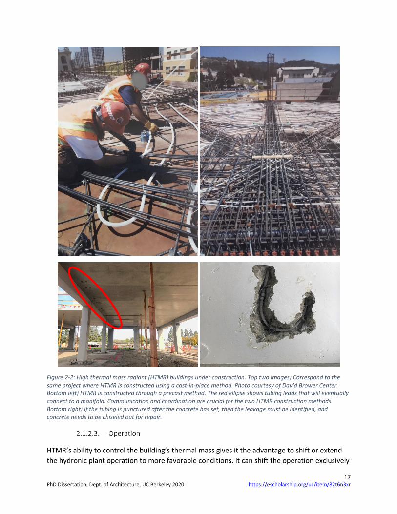
17
Figure 2-2: High thermal mass radiant (HTMR) buildings under construction. Top two images) Correspond to the same project where HTMR is constructed using a cast-in-place method. Photo courtesy of David Brower Center. Bottom left) HTMR is constructed through a precast method. The red ellipse shows tubing leads that will eventually connect to a manifold. Communication and coordination are crucial for the two HTMR construction methods. Bottom right) If the tubing is punctured after the concrete has set, then the leakage must be identified, and concrete needs to be chiseled out for repair.
2.1.2.3. Operation
HTMR’s ability to control the building’s thermal mass gives it the advantage to shift or extend the hydronic plant operation to more favorable conditions. It can shift the operation exclusively
https://escholarship.org/uc/item/82t6n3xrPhD Dissertation, Dept. of Architecture, UC Berkeley 2020

18
to nighttime hours or operate on a 24-hour schedule to lower its peak cooling demand (Rijksen et al. 2010). In either way, the selected control strategy must maintain HTMR’s active surface within acceptable temperatures. Comfort standards restrict the range of temperatures for floor surface temperature at 19-29 °C due to contact with occupant’s feet (ASHRAE 2017c; ISO 2012). This may constraint limits on the active surface cooling capacity to 40-50 W·m-2 (Beat Lehmann et al. 2007; Olesen 1997). In ceiling cooling surfaces, the range can be between 40-60 W·m-2 with mixed convection and radiation heat gains (Woolley et al. 2018). The peak capacity can increase dramatically under direct sunlight. In some cases, the floor cooling capacity can increase up to 140 W·m-2 (Causone et al. 2010; Feng 2014; K. Zhao et al. 2013, 2014; Pantelic et al. 2018).
Decoupling the hydronic plant operation from the occupancy hours when thermal comfort requirements are needed also make HTMR suitable for demand response programs. Demand response programs have the goal of changing the behavior of electricity consumers to manage supply and demand or to provide grid stability (DOE 2006). The increase in renewables has created a situation where too much electricity is available at certain times, so that consumers can get it for free or even get paid to consume it (Martin 2016; Penn 2017). HTMR, like other thermal storage systems, can operate during these and other demand response events to aid with ancillary grid services since the shutdown or start-up of the HTMR will not have an immediate impact on the thermal environment (Ning et al. 2017). Thermostatic loads such as refrigerators and electric water heaters in large numbers have shown the potential to regulate high variability renewables (Burger and Moura 2017), and the same may apply for HTMR (Arteconi et al. 2014). We discuss different operation strategies and robustness to indoor temperature changes in Chapter 5.
2.1.2.4. Practical implications of HTMR advantages and limitations
There are several implications of the advantages and limitations listed above. High-temperature cooling increases the efficiency of chillers (P. R. Armstrong et al. 2009) and allows the use of low-grade energy sources that utilize local renewable sources and favorable weather patterns (Moore 2008; Schmidt 2009; Kazanci et al. 2016). Decoupling the hydronic plant operation from the hours that require occupant thermal comfort has the potential to reduce peak cooling capacities needed from HVAC components. The cooling capacity reduction can be quantified in terms of HVAC capital and operational costs. The potential chiller capital savings can be up to $2,900 for every 1% reduction in peak cooling capacity. Researchers often cite 50% or more, from their particular baseline, as the potential reductions in peak cooling demands when using HTMR (Rijksen et al. 2010; B. Lehmann et al. 2011; K. W. Kim and Olesen 2015a). Operational cost savings are derived not only from the reduction in total energy used through higher hydronic plant efficiency and high-temperature cooling but also from the reduction in the amount paid per unit of energy and peak demand charges associated with time-of-use pricing schemes (Berger 2015; Ontario Energy Board 2007). Peak cooling reductions also allow physically smaller HVAC components that require less space and structural support in the
https://escholarship.org/uc/item/82t6n3xrPhD Dissertation, Dept. of Architecture, UC Berkeley 2020

19
building. The gain in space, along with the benefits of the embedded tubing, may increase the rentable area in commercial buildings (Schlueter et al. 2016). Overall, the cost of construction may be comparable or lower for HTMR when compared to all-air systems (Bauer 2016; Sastry and Rumsey 2014), but labor cost and its uncertainty is high (Feng and Cheng 2018).
The high thermal inertia in the system maintains HTMR in a continuous transient mode that has implications for occupant thermal comfort and control strategy. Room temperatures, including operative, air, infrared, and slab temperatures in HTMR, do not reach steady-state conditions and depart from the conventional design philosophy of uniform temperatures. However, laboratory studies suggest that occupants can be comfortable in a variety of non-uniform conditions (Hensen 1990; Mishra et al. 2016). It also have been found that intentional and controlled non-uniformity can result in more pleasurable thermal experiences (Mower 1976; de Dear 2011; Parkinson and Dear 2015). Research is ongoing to identify how pleasurable thermal experiences can apply in practice which may include HTMR. Nevertheless, HTMR control strategies must bound room temperatures within acceptable conditions. Current practices define HTMR supply water temperature curves as a function of outdoor temperature (de Wit and Wisse 2012; Sourbron and Helsen 2014; Tödtli et al. 2005), as constant values (K. W. Kim and Olesen 2015b; Chung et al. 2017), or to maintain a constant active surface or slab temperature (Paliaga et al. 2017). Control based on outdoor environments may not be the best strategy since building energy codes improve the prescriptive envelope requirements in subsequent energy code cycles which leads to buildings being relatively less sensitive to outdoor conditions. Internally load dominated buildings are better served with control strategies that account for indoor thermal conditions for HTMR control (Gwerder et al. 2008; Raftery et al. 2017). Constant supply water temperatures near the desired room setpoints rely on the concept that small differences between room and active surface temperatures will yield a substantial change in heat flux transfer rate which brings the operative temperature back to room setpoint (Schmelas et al. 2015). This avoids complexity in the control strategy and is robust, but it only applies to buildings with low and less variable heat gains. More advanced control strategies use forecasts in weather, occupancy, thermal storage, and energy price signals to improve thermal comfort and reduce energy consumption and costs (G. P. Henze et al. 2004; Y. Ma et al. 2012; Oldewurtel et al. 2012, 2013). However, these control strategies depend on the accuracy of the models that must be customized for each building (Afram and Janabi-Sharifi 2014). There is also the need for a balance between sophistication of models and computational time for optimization to be implemented in real-time scenarios (Corbin et al. 2013; Schmelas et al. 2017; Zakula et al. 2014). We provide details and performance results on a new control strategy that does not rely on advanced controlling methods and can be programmed in existing energy management systems (EMS) for buildings in Chapter 5.
Lastly, HTMR if designed like TABS, is limited to new construction since embedded tubing is required in the structural slabs. If HTMR is being designed as an ESS, then it may be used in some retrofit applications, but designers need to consider that ESS adds few centimeters of concrete or screed that may not be trivial for the building’s current structural design. Moreover,
https://escholarship.org/uc/item/82t6n3xrPhD Dissertation, Dept. of Architecture, UC Berkeley 2020

20
the embedded tubing leads to less flexibility in space arrangements, especially during tenant changeovers. A mismatch between the radiant thermal zone and the tenant space layout may cause occupant thermal discomfort but may be mitigated with personal comfort systems (J. Kim et al. 2019; Schiavon and Melikov 2008).
2.2. Conclusion
HTMR have the potential to reduce and shift electricity consumption and help reduce GHG emissions while saving on HVAC capital and operational costs. The high thermal mass and inertia associated with these systems present opportunities and challenges. Conventional design methods and control strategies will not allow HTMR to take full advantage of their benefits and, at worst, will hinder these systems from executing HVAC’s basic function of providing a healthy, productive, and thermally comfortable indoor built environment. There is a need to develop clear and simplified guidelines that integrate the transient nature of HTMR for a successful HVAC design. This dissertation aims to provide guidelines on the redefining the industry-accepted definition of the zone cooling load to make it more inclusive of non-traditional HVAC systems, high-temperature cooling without the vapor compression cycle, and new control strategies through simulation and field studies.
https://escholarship.org/uc/item/82t6n3xrPhD Dissertation, Dept. of Architecture, UC Berkeley 2020
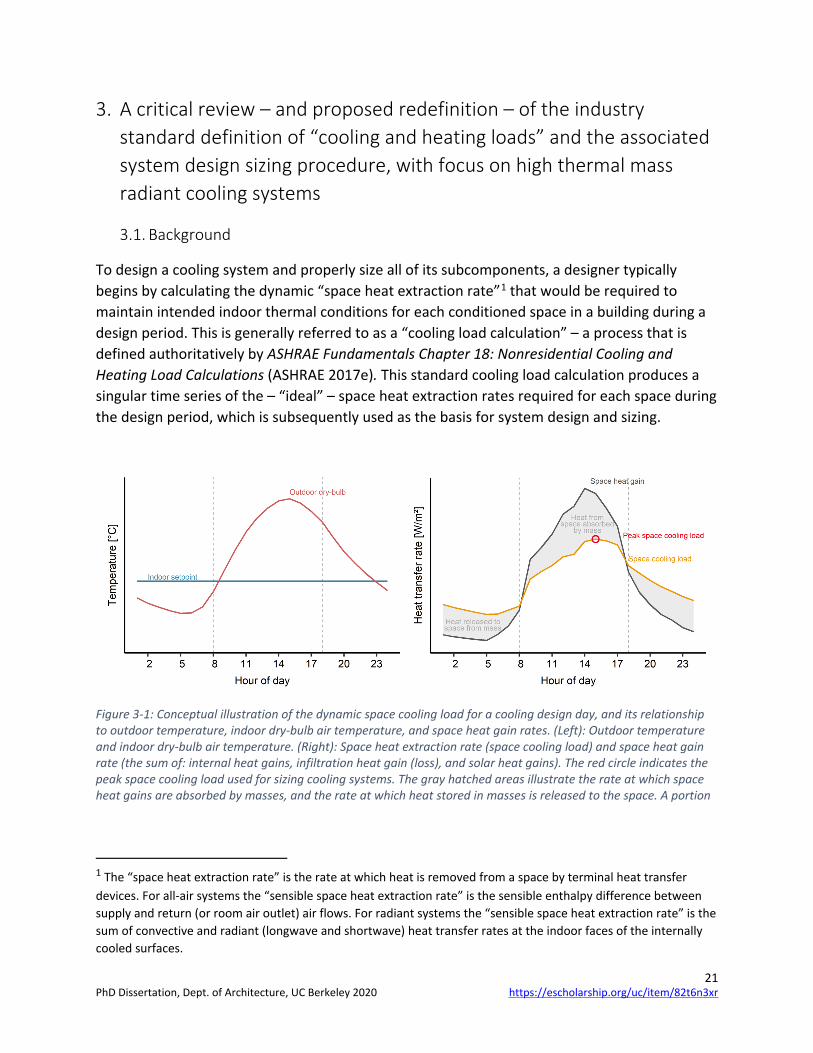
21
3. A critical review – and proposed redefinition – of the industry standard definition of “cooling and heating loads” and the associated system design sizing procedure, with focus on high thermal mass radiant cooling systems
3.1. Background
To design a cooling system and properly size all of its subcomponents, a designer typically begins by calculating the dynamic “space heat extraction rate”1 that would be required to maintain intended indoor thermal conditions for each conditioned space in a building during a design period. This is generally referred to as a “cooling load calculation” – a process that is defined authoritatively by ASHRAE Fundamentals Chapter 18: Nonresidential Cooling and Heating Load Calculations (ASHRAE 2017e). This standard cooling load calculation produces a singular time series of the – “ideal” – space heat extraction rates required for each space during the design period, which is subsequently used as the basis for system design and sizing.
Figure 3-1: Conceptual illustration of the dynamic space cooling load for a cooling design day, and its relationship to outdoor temperature, indoor dry-bulb air temperature, and space heat gain rates. (Left): Outdoor temperature and indoor dry-bulb air temperature. (Right): Space heat extraction rate (space cooling load) and space heat gain rate (the sum of: internal heat gains, infiltration heat gain (loss), and solar heat gains). The red circle indicates the peak space cooling load used for sizing cooling systems. The gray hatched areas illustrate the rate at which space heat gains are absorbed by masses, and the rate at which heat stored in masses is released to the space. A portion
1 The “space heat extraction rate” is the rate at which heat is removed from a space by terminal heat transfer devices. For all-air systems the “sensible space heat extraction rate” is the sensible enthalpy difference between supply and return (or room air outlet) air flows. For radiant systems the “sensible space heat extraction rate” is the sum of convective and radiant (longwave and shortwave) heat transfer rates at the indoor faces of the internally cooled surfaces.
https://escholarship.org/uc/item/82t6n3xrPhD Dissertation, Dept. of Architecture, UC Berkeley 2020

22
of the space heat gains absorbed by masses may also be released to the environment (not indicated), and a portion of the heat released to the space from masses may have originated from the environment (not indicated).
The rate at which heat must be extracted from a space is dynamic; it changes in time as the balance of heat gains to – and losses from – a space changes, and because surfaces within and enclosing a space absorb, store, and release heat dynamically. As a consequence of thermal storage, the space heat extraction rate required by a cooling system is generally smaller than the heat gain rate, yet it can persist after heat gains subside if heat stored in surfaces is released back to the space. Figure 3-1 illustrates the space heat extraction requirement (space cooling load) for a hypothetical design day, and its relationship to outdoor temperature, indoor dry-bulb air temperature, internal heat gain rates, solar heat gain rates, and net space heat gain (loss) rates.
Without bias toward any particular mathematical method, the standard cooling load calculation and associated system design procedure can be summarized as the following distinct steps:
1. Space cooling (heating) load calculation
a. Define site location and meteorological information for a design period, including: (i) site latitude and longitude, (ii) outdoor dry-bulb air temperature (see Figure 3-1) and humidity, (iii) wind speed and direction, and (iv) direct and global horizontal solar irradiance.
b. Define building characteristics, including: (i) building geometry, (ii) construction thermal characteristics, (iii) internal and external shading devices, and, (iv) envelope air tightness characteristics.
c. Define internal heat gains for a design period of interest, including heat gains from (i) people, (ii) lighting, and (iii) equipment – this step should account for diversity in the timing and magnitude of internal heat gains in different spaces.
d. Define other known heat gains (losses) to the space including: (i) infiltration, and (ii) direct to space ventilation.
e. Perform calculations to determine: (i) solar heat gain rates and (ii) the distribution of solar heat gains.
f. Define the constant indoor dry-bulb air temperature (see Figure 3-1) and humidity for the design period.
g. Perform cooling load calculations to determine: (i) the rates of heat transfer and storage associated with boundary surfaces, (ii) the net heat gain to (loss from) the space, and (iii) the space heat extraction rates required to maintain indoor environmental conditions during the design period – the space cooling load (see Figure 3-1).
2. Design terminal heat transfer devices
https://escholarship.org/uc/item/82t6n3xrPhD Dissertation, Dept. of Architecture, UC Berkeley 2020

23
a. Choose terminal heat transfer devices with steady-state cooling capacity to satisfy the peak space cooling load during the design period, at coincident operating conditions.
3. Design cooling plant and distribution systems
a. Aggregate space cooling loads for all spaces to determine the rates at which heat must be transferred to the distribution systems and cooling plants. This step must account for: (i) diversity in the timing and magnitude of cooling loads associated with different spaces, (ii) incidental dehumidification that occurs while generating required sensible heat transfer rates (or incidental sensible heat transfer that occurs while generated required dehumidification), and (iii) additional heat losses and gains to the system such as duct leakage, distribution losses, or ventilation that is cooled or heated by the system before it is supplied to the space.
b. Select distribution systems and cooling plants with steady-state cooling capacity to match the peak aggregate cooling loads at coincident operating conditions.
Since the net heat gain to (loss from) a space changes from day-to-day, standards guide designers to size cooling systems based on the conditions in hypothetical “cooling design days”. These design days are intended to represent the most extreme scenarios in which a cooling system should be expected to maintain the desired indoor conditions. ASHRAE Fundamentals Chapter 14: Climatic Design Information (ASHRAE 2017d) is the standard reference for definition of climatic conditions on design days. As explained therein, it may be necessary to conduct load calculations for several different design days, to separately determine different operational extremes, such as: peak sensible cooling requirements and peak dehumidification requirements. Due mainly to seasonal variation in solar heat gains, different spaces within a building may require different design days, and the maximum aggregate load for the combined system may occur on yet a different design day. Following a cooling load calculation, standards guide designers to select and size terminal cooling devices that are capable of satisfying the maximum space cooling loads, then design and size distribution systems and cooling plant equipment that are capable of satisfying the maximum sum of coincident heat transfer rates from all associated terminal cooling devices. The “cooling capacity” for a system is usually not a constant value2; rather, it depends on coincident environmental conditions and system states. For example, the cooling capacity of an air-cooled chiller depends on the outdoor dry-bulb air temperature, the chiller entering water temperature, the refrigeration circuit part-capacity state – and to some extent – the water flow rate. Standards guide designers to account for the fact that the cooling capacity of a system changes with operating conditions. To do so, designers typically use models and system performance data that quantify cooling capacity as
2 Some systems, such as resistance heaters and gas furnaces may have a nearly constant heating capacity.
https://escholarship.org/uc/item/82t6n3xrPhD Dissertation, Dept. of Architecture, UC Berkeley 2020

24
the steady-state heat extraction rate that could be produced by continuous operation with steady conditions.
For most cooling system components, it is reasonable to assume that steady-state cooling capacity data is representative of the actual cooling rates that a system will produce in dynamic circumstances. The assumption is reasonable because the time required for most cooling system components to approach steady-state following a change to the inputs – the “response time” – is small relative to the time required for either the space cooling load or environmental conditions to change. Therefore, sizing a cooling system generally entails specifying a cooling plant, distribution system, and terminal heat transfer device(s) each with the steady-state cooling capacity to match the peak aggregate space cooling load at coincident conditions. This sizing process must account for: diversity in the timing and magnitude of cooling loads from different spaces, (ii) incidental dehumidification to generate sensible space cooling (or incidental sensible heat transfer to generate dehumidification), and (iii) additional heat losses and gains to the system such as duct leakage, distribution losses, or ventilation that is cooled or heated by the system before it is supplied to the space – so-called “system heating and cooling load effects” (ASHRAE 2017e).
Although the standard approach for calculating space cooling load, and the associated system design procedure have been applied successfully for the design of many buildings, our research has revealed that because they were conceived for overhead-mixing all-air systems, they impose several assumptions and constraints that limit them from accurately representing all cooling systems types and applications. More specifically:
1. The standard definition of “space cooling load”:
a. does not fully reflect all aspects of standards that address thermal comfort
b. only facilitates design of systems for basic applications
c. does not account for the way that cooling system type impacts the space cooling requirements
d. does not account for the way that system control strategies impact space cooling requirements
e. does not provide sufficient guidance on the selection of design periods
2. The standard system design procedure:
a. does not facilitate design for any performance metric other than indoor dry-bulb air temperature
b. is based solely on steady-state heat transfer and so is inaccurate for systems with long response time
In this chapter, we explain why the standard definition of “space cooling load” is unsatisfactory, we propose a new definition for the concept, and we present simulation results to illustrate the
https://escholarship.org/uc/item/82t6n3xrPhD Dissertation, Dept. of Architecture, UC Berkeley 2020

25
practical impact of our proposed definition. In Section 3.2 we identify the specific shortcomings with the standard definition of “space cooling load”, and explain how this notion has influenced building energy simulation tools and system sizing in practice. We consider how these issues relate to various system types, but we focus especially on why they are problematic for design and control of high thermal mass radiant (HTMR) cooling systems. In Section 3.3 we propose a new definition for “space cooling load”, and a new system design procedure. In addition to the summary explanations in Section 3.3, the proposed redefinition is composed as a comprehensive revision to the explanatory sections of ASHRAE Fundamentals Chapter 18 (ASHRAE 2017e), which is included in Appendix A. Finally, in Section 3.4 we present simulation results to demonstrate the consequences of the standard procedure – compared to our recommended procedure – for the design of HTMR cooling systems.
3.2. Shortcomings with the standard definition of “cooling (heating) load” and the associated system design procedure
3.2.1. The standard definition of “space cooling (heating) load” does not fully reflect all aspects of standards that address thermal comfort
ASHRAE Fundamentals Chapter 18 (2017a) defines “space cooling load” as the space heat extraction rate that would be required “to maintain a constant space air temperature and humidity”. There are two distinct problems with this definition as it relates to thermal comfort. First, it focuses only on indoor dry-bulb air temperature and humidity, which ignores the fact that many variables influence thermal comfort. Second, it imposes constant indoor dry-bulb air temperature and humidity, which is neither necessary nor realistic – especially for certain system types.
The standard definition of “space cooling load” implicitly discourages design based on prevailing standards that address acceptable thermal environmental conditions for human occupancy. ASHRAE Standard 55 (ASHRAE 2017c) and EN 16798 (CEN 2019) present comprehensive metrics to estimate thermal comfort based on many variables including: indoor dry-bulb air temperature, indoor mean radiant temperature, indoor humidity, indoor air speed, metabolic rate, clothing, and outdoor dry-bulb air temperature. These standards do not require constant indoor environmental conditions; rather, they describe a range of acceptable conditions during occupied periods and allow for substantial variation over time.
Moreover, the standard definition of “space cooling load” excludes some systems and control strategies that do not maintain a constant air temperature, yet still maintain a thermally comfortable indoor environment. For example, HTMR cooling systems are really not capable of maintaining constant indoor dry-bulb air temperature. The response time (Ning et al. 2017) of these systems precludes them from using automated feedback control to instantaneously adjust the space heat extraction rate in a way that is required to maintain constant indoor dry-bulb air temperature. Manual commissioning, or adaptive controls (Raftery et al. 2017) can
https://escholarship.org/uc/item/82t6n3xrPhD Dissertation, Dept. of Architecture, UC Berkeley 2020

26
select dynamic temperature setpoints and operating schedules for HTMR that – together with their self-regulating characteristics – will consistently produce a comfortable indoor thermal environment; however indoor dry-bulb air temperature cannot be expected to remain constant.
Although designers familiar with radiant cooling understand that HTMR behave differently than overhead-mixing all-air systems, these systems are often sized according to standard space cooling load calculation methods, and controlled with constant dry-bulb air temperature setpoints. This practice was revealed by Feng (2014) and Feng et al. (2014a) who investigated what methods and tools designers use to size radiant cooling systems, then by Paliaga et al. (2017, 2018) and Raftery et al. (2018a, 2018b) who studied the design and control strategies commonly implemented in practice for HTMR cooling systems. Unfortunately, there are various problems with sizing and operating HTMR cooling systems in this way. First, the constant indoor dry-bulb air temperature constraint assumes an impossible behavior for HTMR cooling systems and produces an unrealistic estimate of the space heat extraction rate (space cooling load) that the system will actually produce. Second – as discussed in Section 3.2.3 – standard space cooling load calculation methods do not properly account for the heat transfer pathways associated with space heat extraction by radiant cooling systems. In Section 3.4, we present simulation results to demonstrate the practical impact of these combined problems.
Furthermore, the constant indoor dry-bulb air temperature constraint is especially peculiar because constant indoor dry-bulb air temperature does not necessarily indicate constant thermal comfort for any system type. For a typical overhead-mixing all-air system, the temperatures of surfaces within and enclosing a space change as they absorb and release heat, which causes operative temperature to change throughout the day. For example, in a space with substantial solar gains, constant air temperature may not adequately counteract the comfort impacts of insolation and increased surface temperatures (Arens et al. 2015).
The standard definition of “space cooling load” should not be constrained to a constant indoor dry-bulb air temperature. Instead, it ought to allow for dynamic thermal environments – within the limits established by consensus standards on the subject of thermal comfort. This would offer designers flexibility, and facilitate system design to reduce energy consumption, reduce equipment cost, and improve thermal comfort. For example, designers can substantially reduce energy use and equipment size if indoor temperature is allowed to drift somewhat over the course of the day (Schiavon and Melikov 2008; Schiavon, Melikov, et al. 2010; Hoyt et al. 2015). The impact is more substantial if increased air motion, or personal comfort systems, are used to extend the range of acceptable indoor temperature (Sekhar 1995; Schiavon and Melikov 2008; Huang et al. 2013; Hoyt et al. 2015; Schiavon et al. 2017; Lipczynska et al. 2018).
https://escholarship.org/uc/item/82t6n3xrPhD Dissertation, Dept. of Architecture, UC Berkeley 2020

27
3.2.2. The standard definition of “space cooling load” only facilitates design of systems for basic applications
ASHRAE Fundamentals Chapter 18 (ASHRAE 2017e) presents a narrow conception of “cooling load” that is based solely on the design of overhead-mixing all-air systems for comfort conditioning. This standard definition overlooks how the notion of “cooling load” relates to design of heating, cooling, and ventilation systems for other objectives or applications. The following paragraphs give examples that demand a broader definition of the concept.
First, the design of cooling systems for data centers requires a different approach than what is represented in ASHRAE Fundamentals Chapter 18 (ASHRAE 2017e). For this application cooling systems must be sized to maintain an appropriate air temperature and flow rate at the inlet for computer equipment, and the relationship between air distribution and heat gains in such a space can have a dramatic impact on the amount of cooling that a mechanical system must generate. For example, if heat from computer equipment is mixed into the space – as described by ASHRAE Fundamentals Chapter 18 (ASHRAE 2017e) – system cooling requirements are much larger than if heat from computer equipment is captured and exhausted or recirculated to cooling equipment and handled directly.
Second, the design of heating, cooling, and ventilation systems may have multiple objectives that compete and interact in complex ways that are not captured by standard cooling load calculations. For example, a dehumidification system designed for a particular “latent space cooling load” can impact sensible space heat extraction requirements in a way that is not accounted for by a simple cooling load calculation presented in ASHRAE Fundamentals Chapter 18 (ASHRAE 2017e). The standard approach recommends that designers calculate sensible loads and latent loads separately, when in reality sensible and latent heat transfer rates are interrelated.
Additionally, the standard definition of “space cooling load” cannot accommodate the design of natural ventilation systems because it presumes a constant indoor dry-bulb air temperature, and a predetermined constant ventilation rate. In reality, natural ventilation systems must simultaneously satisfy several distinct objectives including energy performance goals, and constraints on indoor temperature, indoor humidity, indoor air speed, and indoor air quality. These objectives interact and may compete with one another, making it impossible to maintain constant indoor temperature and humidity conditions, and impractical for a designer to specify the exact indoor thermal conditions that will occur.
Finally, the design of cooling systems for thermal comfort in outdoor spaces – such as stadiums or patio restaurants – completely eludes the standard definition of “cooling load”. Yet, these systems merit a standard basis for system sizing with the same foundations that justify the design of any cooling system. These systems have different performance expectations and operate with different heat transfer mechanisms than what is represented in ASHRAE Fundamentals Chapter 18 (ASHRAE 2017e).
https://escholarship.org/uc/item/82t6n3xrPhD Dissertation, Dept. of Architecture, UC Berkeley 2020

28
3.2.3. The standard definition of “space cooling load” does not account for the way that cooling system type impacts space cooling requirements
ASHRAE Fundamentals Chapter 18 (ASHRAE 2017e) recommends two different mathematical methods to calculate the space cooling load: a Heat Balance (HB) method, and the Radiant Time Series (RTS) method. However, neither of these methods – as currently implemented – fully account for the heat transfer pathways associated with space heat extraction by various types of terminal heat transfer devices. Most importantly, both methods assume that convection with a well-mixed air volume is the only heat transfer mechanism by which heat can be removed from a space. Consequently, these methods do not properly estimate the space heat extraction rates by radiant cooling systems (J. L. Niu et al. 1995, 1997; Feng et al. 2013a, 2014a, 2014b; Novoselac et al. 2017; Woolley et al. 2018, 2019), by underfloor air distribution systems (Schiavon, Lee, et al. 2010; Schiavon et al. 2011; Lee et al. 2012), or by displacement ventilation systems (S. Zhang, Cheng, et al. 2019; S. Zhang, Lin, et al. 2019). In addition to limitations with the mathematical methods, the definitions and explanations presented in ASHRAE Fundamentals Chapter 18 (ASHRAE 2017e) systemically fail to consider the implications of space heat extraction by any mechanisms other than convection with a well-mixed air volume. These issues are important because the presence of other heat transfer pathways – especially radiant exchange with the terminal heat transfer device – disrupts the network of heat transfer and storage and impacts the time and rate at which heat must be extracted from a space.
Computational and experimental research has proven that to maintain equal operative temperature as an overhead-mixing all-air system, a radiant cooling system must remove more heat overall, the peak space heat extraction rate must be larger, and it must occur earlier (J. L. Niu et al. 1995, 1997; Feng et al. 2013a, 2014a, 2014b; Novoselac et al. 2017; Woolley et al. 2018, 2019). The differences are mainly due to the way that heat gains are absorbed by, stored in, and released from non-active masses – a process described thoroughly by Woolley et al. (2018).
The magnitude of these differences depends on many factors. As documented by Woolley et al. (2019), Feng et al. (2013), and (Feng 2014), the differences are larger for cases with highly radiant heat gains, and larger in scenarios that benefit from passive cooling of the thermal mass in a building. For some scenarios radiant cooling may have 25% larger peak space cooling load, and the cumulative daily space cooling load may be 40% larger. Since the ASHRAE conception of “space cooling load” does not account for heat extraction by radiant heat transfer, it does not account for these differences in the heat gain (loss), and the space cooling load.
Similarly, Schiavon, Lee, et al. (2010) and Schiavon et al. (2011) and Lee et al. (2012) found that the space cooling load for underfloor air distribution systems was generally 19% higher than traditional overhead mixing systems. Researchers attributed these differences mainly to the fact that the raised floor in an underfloor air distribution system changes the interaction
https://escholarship.org/uc/item/82t6n3xrPhD Dissertation, Dept. of Architecture, UC Berkeley 2020

29
between heat gains and thermal storage from what normally happens in the absence of the raised floor (Schiavon, Lee, et al. 2010; Schiavon et al. 2011; Raftery et al. 2014).
The standard definition of “space cooling load” should account for all possible methods of heat transfer for space heat extraction so that the calculations can properly assess the space heat extraction requirements for different types of terminal heat transfer devices.
Researchers have developed and validated numerical methods that properly estimate the fundamental heat transfer mechanisms involved with HTMR (Fort 1989, 2001; C. Stetiu et al. 1995; J. L. Niu et al. 1995, 1997; R. Strand et al. 1999; R. K. Strand and Pedersen 2002; R. K. Strand and Baumgartner 2005; Laouadi 2004; Yu et al. 2014). Even though the most prominent numerical methods are direct descendants of the Heat Balance method presented in ASHRAE Fundamentals Chapter 18 (ASHRAE 2017e), the standard method has not been updated accordingly. The ASHRAE Heat Balance method was initially developed by Kusuda (1974) and implemented in the BLAST and TARP energy analysis programs (Walton et al. 1983). Later, the method was described in full by Liesen and Pedersen (1998), McClellan and Pedersen (1997), and Pedersen et al. (1998) as part of ASHRAE RP-875. Shortly afterward, Strand et al. (1999), Strand and Pedersen (2002), and Strand and Baumgartner (2005) extended the Heat Balance method to consider the heat transfer dynamics HTMR, and developed the requisite features to incorporate the methods into EnergyPlus (EnergyPlus 2018). Feng et al. (2014a, 2014b) conducted laboratory experiments which validated the predictions from the more comprehensive Heat Balance method developed by Strand et al. (1999); and simultaneously, proved that the Radiant Time Series method and the ASHRAE Heat Balance method do not accurately predict the space heat extraction rates for radiant systems.
Although the methods developed by Strand and Pedersen (2002) and Strand and Baumgartner (2005) have been incorporated into some building energy simulation software, the problematic assumption perpetuated by ASHRAE Fundamentals Chapter 18 (ASHRAE 2017e) – that all space heat extraction occurs by convection – still persists in some aspects. For each simulation timestep EnergyPlus uses the numerical methods developed by Strand and Pedersen (2002) and Strand and Baumgartner (2005) to calculate the rate at which internally cooled surfaces extract heat from a space. However, the space cooling load calculations performed to estimate space heat extraction requirements on a design day, and to autosize components of a radiant system and cooling plant still rely on the standard definition of “space cooling load”. Specifically, the EnergyPlus radiant system autosizing subroutine sets the design water flow rate to achieve a hydronic heat extraction rate that matches the space heat extraction rate determined from a standard cooling load calculation (DOE 2020). In addition to ignoring space heat extraction by radiation in the initial load calculation, this approach fails to consider whether or not this hydronic heat extraction rate will generate commensurate space heat extraction rate. Moreover, several widely-used building energy simulation tools have not addressed the problematic assumption in any way, yet researchers and practitioners often use these tools for design and simulation of radiant cooling and heating systems (Feng 2014; Feng
https://escholarship.org/uc/item/82t6n3xrPhD Dissertation, Dept. of Architecture, UC Berkeley 2020

30
et al. 2014a). In Section 3.4, we present simulation results to demonstrate the practical consequences of using the standard method for cooling load calculations to design HTMR.
ASHRAE Fundamentals Chapter 18 (ASHRAE 2017e) should be extensively revised to account for these issues, and the mathematical methods presented therein should be updated. However, the problem is more extensive than updates to this chapter. Although ASHRAE Systems & Equipment Chapter 6: Radiant Heating and Cooling (ASHRAE 2016d) clearly explains that radiant cooling transfers heat by convection and radiation, it does not recognize that the magnitude and timing of the required space heat extraction rate (space cooling load) is fundamentally different from that of overhead-mixing all-air systems. Moreover, the system design procedure presented in ASHRAE Systems & Equipment Chapter 6 (ASHRAE 2016d) specifically references the methods in ASHRAE Fundamentals Chapter 18 (ASHRAE 2017e), even though these methods do not account for the effects of space heat extraction by radiation with internally cooled surfaces.
In the widely referenced guidebook Low Temperature Heating and High Temperature Cooling, Babiak et al. (2009) and ISO 11855-2 (ISO 2012) thoroughly explain the combined radiant and convective heat transfer rates that a radiant system can be expected to produce for different steady-state conditions (space cooling capacity). However, these references do not explain how to determine the dynamic space heat extraction requirement (space cooling load) for a HTMR, do not specifically recognize that it can differ substantially from that of overhead-mixing all-air systems, do not explain how steady-state calculations ought to be used within a whole system design procedure, and do not offer any approach to adjust steady-state calculations for dynamic conditions. The guidebook does indicate that for TABS systems “dynamic simulations can be required to predict the thermal comfort in a conditioned zone”, and ISO 11855-4 (ISO 2012) provides methods to perform such dynamic simulations, but neither reference frames the need for dynamic simulations in relation to the standard concept of “space cooling load”.
Among standards focused on the topic of space cooling loads, ISO 52016 (ISO 2017) – which supersedes prEN 15255 (CEN 2007) – is the only resource we are aware of to explicitly state that the dynamic space heat extraction requirements (space cooling load) depends on the system type. In an equation for determining the space heat balance, the standard introduces a variable called the “convective fraction of the cooling system”. However, the standard currently provides no guidance on how to determine this fraction for different systems and circumstances.
3.2.4. The standard definition of “cooling load” does not account for the way that system control strategies impact space cooling requirements
ASHRAE Fundamentals Chapter 18 (ASHRAE 2017e) defines “space cooling load” as the space heat extraction rate that would be required “to maintain a constant space air temperature and humidity”, and thus entirely overlooks the fact that the sequence of operations – including temperature setpoint schedules – will impact the space heat extraction requirement. For
https://escholarship.org/uc/item/82t6n3xrPhD Dissertation, Dept. of Architecture, UC Berkeley 2020

31
example, scheduling a setback during unoccupied periods in the cooling season could cause a larger peak space cooling load than continuous setpoints, because surfaces will begin each day at a higher temperature, and so will store a smaller portion of the heat gains during the day. For the same reasons, a pre-cooling setpoint schedule would reduce the peak space cooling load (Keeney and Braun 1997; Braun 2003; G. Henze et al. 2007). Many designers account for the fact that the size for a heating system can be driven by morning warm up requirements following a setback period, yet this consideration is not accommodated by the standard definition of “cooling load”.
This aspect of the standard “space cooling load” definition is especially problematic for HTMR, for which the sequence of operations, choice of control feedback variable, temperature setpoint, the supply water temperature, and system availability schedule will substantially change the shape and magnitude of the space cooling load. It is also problematic for spaces that rely on multiple cooling systems. For example, the choice of control sequence to coordinate radiant cooling and supplemental air cooling will have a major impact on the space cooling load for each system. To this point, Chung et al. (2017) used building energy simulations to demonstrate that design and control of HTMR, and supplemental air cooling systems substantially impacts the cooling load for each system. Similarly, the choice of control sequence in mixed-mode buildings that utilize natural ventilation for pre-cooling will have a major impact on the cooling load for mechanical systems. Research by Woolley et al. (2018, 2019) clearly revealed that because radiant cooling extracts a significant amount of heat from non-active thermal masses, it can preempt some of the benefits of natural ventilation pre-cooling. For such a mixed-mode building, the sequence of operations would have a major impact on the space cooling load, as well as the cumulative mechanical cooling load.
The definitions, explanations, and mathematical methods in ASHRAE Fundamentals Chapter 18 (ASHRAE 2017e) effectively discourage design of systems that use strategic control strategies to shift electrical demand, reduce energy consumption, reduce equipment cost, and improve thermal comfort. As the expectations for dynamic control of electrical demand from buildings continue to accelerate, the dynamic control of cooling systems requires a more sophisticated approach for system design and sizing than what is promulgated by the standard definition of “space cooling load”.
3.2.5. The standard definition of “space cooling load” does not provide sufficient guidance on the selection of design periods
ASHRAE Fundamentals Chapter 18 (ASHRAE 2017e) defines the notion of cooling load and explains that cooling load calculations should be used as the basis for system design decisions. However, it provides relatively little information about what constitutes an appropriate design period. ASHRAE Fundamentals Chapter 14 (ASHRAE 2017d) provides extensive climate summary statistics for locations around the world, and defines a standard method to use these summary statistics to generate a 24 hour times series for outdoor dry-bulb and wet-bulb
https://escholarship.org/uc/item/82t6n3xrPhD Dissertation, Dept. of Architecture, UC Berkeley 2020

32
temperatures for a design day. However, although the chapter indicates that a designer should “use judgement” in choosing appropriate design conditions, it provides relatively little guidance about what constitutes an appropriate design period. In some cases, the largest heat gains to a space might occur during the spring or fall when solar gains are largest. A designer may choose to perform load calculations for various design days to find the constraining design condition, but this requires special effort, and is generally overlooked by the common practice use of a “cooling design day”. For example, weather data for EnergyPlus and other modeling tools include a set of “cooling design days” developed from the methods in ASHRAE Fundamentals Chapter 14 (ASHRAE 2017d); but these are selected on the basis of outdoor dry-bulb and wet-bulb temperatures, so may not result in appropriate design conditions when maximum space cooling loads are actually driven by other factors. An iterative simulation on these design days is typically used to autosize equipment, even if there are ultimately other days in the year with large heat gains.
Additionally, as the results of this chapter indicate, the typical design day approach may not provide a sufficient basis for design of certain systems because a simulation on a single 24-hour period:
1. Requires convergence of iterative simulations, which can result in initial thermal conditions for masses that do not represent worst case scenarios.
2. Fail to capture the effect of multi-day transient oscillations caused by large thermal mass.
3. May not be adequate to assess the impact of system controls.
For example – in regard to system controls – Raftery et al. (2017) developed a control sequence for HTMR that resets the slab temperature setpoint each day in response to indoor dry-bulb air temperature performance on the previous day. The thermal behavior that results from such a control sequence cannot be captured by a 24-hour design day simulation. An even simpler example of this issue is the impact that weekend setbacks have on temperature of thermal masses in a building. Design periods really ought to capture these effects, since they can significantly influence the heat extraction requirements.
Additional research is necessary to quantify the impact of these issues and to recommend improvements to standards and current modeling practices.
3.2.6. The standard design procedure does not facilitate design for any performance metric other than indoor dry-bulb air temperature.
System design is inherently a type of multi-objective optimization. Designers are expected to make decisions based on numerous factors including life cycle cost, greenhouse gas emissions, comfort, or indoor air quality. Unfortunately, since the standard design procedure expects that the standard space cooling load must be satisfied, it does not allow other objectives to enter
https://escholarship.org/uc/item/82t6n3xrPhD Dissertation, Dept. of Architecture, UC Berkeley 2020
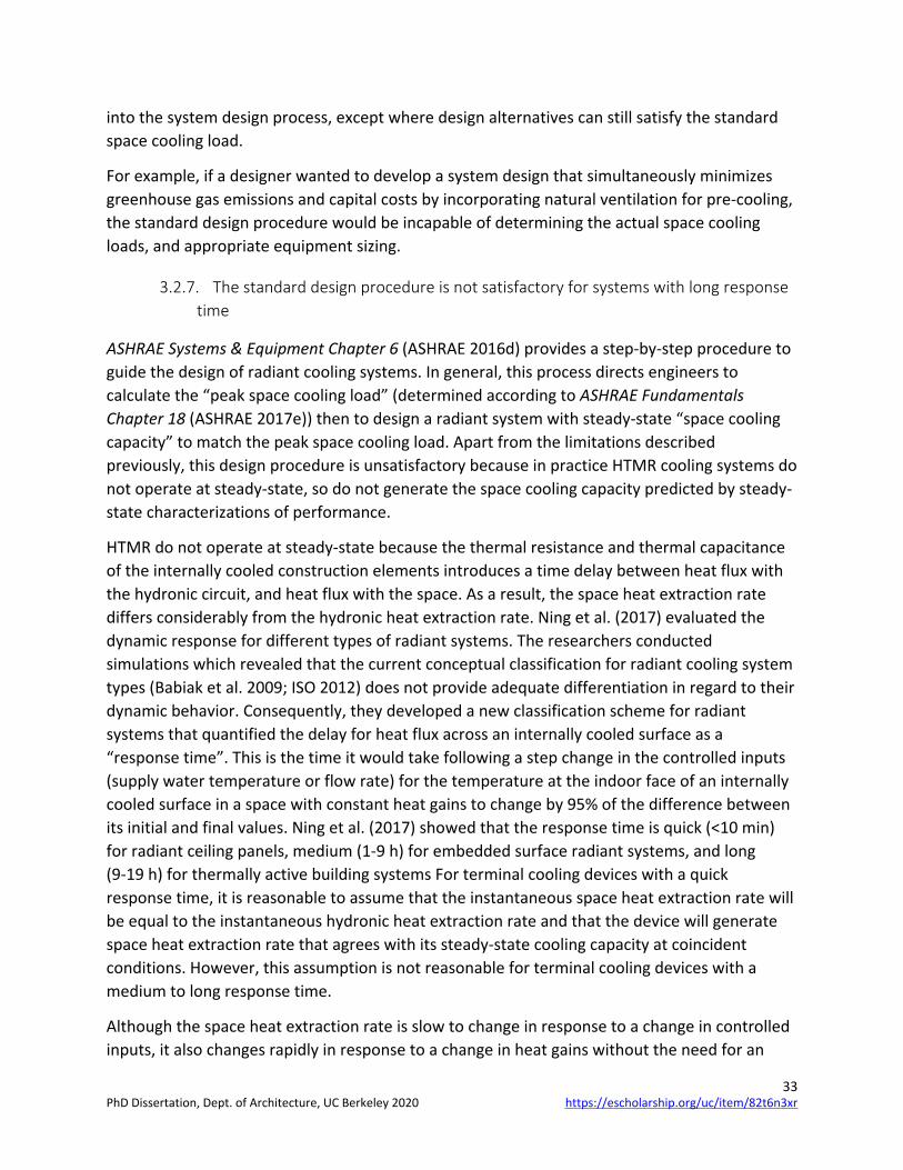
33
into the system design process, except where design alternatives can still satisfy the standard space cooling load.
For example, if a designer wanted to develop a system design that simultaneously minimizes greenhouse gas emissions and capital costs by incorporating natural ventilation for pre-cooling, the standard design procedure would be incapable of determining the actual space cooling loads, and appropriate equipment sizing.
3.2.7. The standard design procedure is not satisfactory for systems with long response time
ASHRAE Systems & Equipment Chapter 6 (ASHRAE 2016d) provides a step-by-step procedure to guide the design of radiant cooling systems. In general, this process directs engineers to calculate the “peak space cooling load” (determined according to ASHRAE Fundamentals Chapter 18 (ASHRAE 2017e)) then to design a radiant system with steady-state “space cooling capacity” to match the peak space cooling load. Apart from the limitations described previously, this design procedure is unsatisfactory because in practice HTMR cooling systems do not operate at steady-state, so do not generate the space cooling capacity predicted by steady-state characterizations of performance.
HTMR do not operate at steady-state because the thermal resistance and thermal capacitance of the internally cooled construction elements introduces a time delay between heat flux with the hydronic circuit, and heat flux with the space. As a result, the space heat extraction rate differs considerably from the hydronic heat extraction rate. Ning et al. (2017) evaluated the dynamic response for different types of radiant systems. The researchers conducted simulations which revealed that the current conceptual classification for radiant cooling system types (Babiak et al. 2009; ISO 2012) does not provide adequate differentiation in regard to their dynamic behavior. Consequently, they developed a new classification scheme for radiant systems that quantified the delay for heat flux across an internally cooled surface as a “response time”. This is the time it would take following a step change in the controlled inputs (supply water temperature or flow rate) for the temperature at the indoor face of an internally cooled surface in a space with constant heat gains to change by 95% of the difference between its initial and final values. Ning et al. (2017) showed that the response time is quick (<10 min) for radiant ceiling panels, medium (1-9 h) for embedded surface radiant systems, and long (9-19 h) for thermally active building systems For terminal cooling devices with a quick response time, it is reasonable to assume that the instantaneous space heat extraction rate will be equal to the instantaneous hydronic heat extraction rate and that the device will generate space heat extraction rate that agrees with its steady-state cooling capacity at coincident conditions. However, this assumption is not reasonable for terminal cooling devices with a medium to long response time.
Although the space heat extraction rate is slow to change in response to a change in controlled inputs, it also changes rapidly in response to a change in heat gains without the need for an
https://escholarship.org/uc/item/82t6n3xrPhD Dissertation, Dept. of Architecture, UC Berkeley 2020

34
active change in controlled inputs. This phenomenon is often referred to as “self-control” of HTMR.
As a consequence of these two behaviors, in some conditions the instantaneous space heat extraction rate for a HTMR may be smaller than predicted by steady-state assumptions, and in other conditions it may be larger. The difference depends on the initial thermal conditions of the internally cooled surface, slab, and the way conditions change at the boundaries of the surface. For example, when chilled water begins to flow through an internally cooled surface, it may take an hour or more before the space heat extraction rate begins to respond, yet such a surface can continue to extract heat from a space long after chilled water flow ends, and the space heat extraction rate will change naturally in response to changes in heat gains. We are not aware of any research that has quantified the range of response times for which steady-state capacity calculations may be acceptable, but it is clear that they are inaccurate for many radiant system configurations.
The standard design procedure for radiant cooling effectively directs engineers to assume that there is no delay or attenuation between hydronic heat extraction rate and space heat extraction rate. As a result, many designers often size hydronic systems, pumps, and cooling plants for HTMR to handle the peak space heat extraction rate predicted by standard cooling load calculation (Feng 2014; Feng et al. 2014a; Paliaga et al. 2017, 2018), even though the space heat extraction rate differs substantially from hydronic heat extraction rate. Research by Feng (2014), Feng et al. (2014a), and Paliaga et al. (2017, 2018) has revealed that some designers use detailed numerical models to predict the dynamic performance of HTMR and to size equipment, but that most do not. Researchers, manufacturers, and standards have advanced some simplified design methods that account for dynamic heat transfer behavior for HTMR (Koschenz and Lehmann 2003; Olesen and Zöllner 2007; Babiak et al. 2009; ISO 2012; Uponor 2013; Raftery et al. 2019), but our research suggests that in practice, most designers do not explicitly account for these issues and instead size systems using steady state capacity estimates. In Section 3.4, we present simulation results to demonstrate the practical consequences of using the standard method for cooling load calculations and associated system design procedure to size and operate HTMR.
3.3. Proposed redefinition of cooling load and system design procedure
To address the shortcomings described, we propose a comprehensive redefinition of “cooling load” and the associated system design procedure. Our approach expands the notion of “cooling load” so that it can accommodate the design of a variety of system types, control strategies, and performance objectives. Most significantly, our redefinition eliminates the idea of a singular – “ideal” – space cooling load as the objective for system design. Instead, we orient the system design procedure toward selecting and sizing components and their controls that best satisfy performance objectives such as thermal comfort, indoor air quality, resilience, grid-
https://escholarship.org/uc/item/82t6n3xrPhD Dissertation, Dept. of Architecture, UC Berkeley 2020

35
interactive responses, or energy cost minimization. Our approach requires that designers utilize modeling tools capable of accurately representing the systems and controls they design.
The problematic notion of “space cooling load” and the standard system design procedure is invoked by many standards and design guidelines, but it is defined authoritatively by ASHRAE Fundamentals Chapter 18 (ASHRAE 2017e). The shortcomings we’ve explained are pervasively entwined into almost every aspect of that chapter – from explanation about what input data is required for a load calculation, to definition about terms such as “heat gain”. Therefore, we have prepared an exhaustive revision to all definitions and explanatory sections within ASHRAE Fundamentals Chapter 18 (ASHRAE 2017e). The proposed revisions are included as Appendix A.
At the core of our amendments is a revision to the central problematic term:
Current definition:
Space cooling load – the rate at which sensible and latent heat must be removed from the space to maintain a constant space air temperature and constant humidity in the space.
Revised definition:
Space cooling load – the space cooling load at any point in time is the rate at which terminal heat transfer devices, with associated control sequences, must extract sensible and/or latent heat such that associated thermal environmental conditions, and/or other performance metrics, comply with desired constraints during a design period (e.g. limits on operative temperature, peak electrical demand, etc).
Our redefinition does not require that a design be based on maintaining a constant indoor dry-bulb air temperature; in fact it doesn’t even require ex ante specification of the exact indoor thermal conditions that will occur. Instead, our redefinition allows designers to specify constraints on any ex post performance metric including thermal comfort, indoor air quality, electrical demand, etc. For example, a designer could specify an allowable range for operative temperature, or for the rate of change in operative temperature; then they would reject design alternatives for which simulation results do not comply with these constraints. In our view, standards should be impartial about what mathematical methods or tools are used for system models and simulations. Some designers may use numerical building energy simulation tools, while others may use simple diagrammatic design guidelines. Any type of “model and simulation” should be acceptable – as long as it represents the systems and controls it is used to design, with accuracy that is appropriate for the design phase in which it is utilized. For example, Koschenz and Lehmann (2003) and Raftery et al. (2019) have both developed simplified design tools that account for dynamic heat transfer behaviors for HTMR.
Our proposed system design procedure includes the following steps. The first three steps align with standard system design procedure, but the rest differ:
https://escholarship.org/uc/item/82t6n3xrPhD Dissertation, Dept. of Architecture, UC Berkeley 2020

36
1. Describe all building and site characteristics and uncontrolled input values for a design period(s)
a. Define site location and meteorological information for a design period(s), including: (i) site latitude and longitude, (ii) outdoor dry-bulb air temperature (see Figure 3-1) and humidity, (iii) wind speed and direction, (iv) direct and global horizontal solar irradiance.
b. Define building characteristics, including: (i) building geometry, (ii) construction thermal characteristics, (iii) internal and external shading devices, and (iv) envelope air tightness characteristics.
c. Define site characteristics that impact building heat transfer, including: (i) shading by external objects (e.g. trees and buildings), and (ii) reflection from external surfaces (e.g. adjacent buildings, ground, water bodies).
d. Define internal heat gains for a design period(s) of interest (see Figure 3-1), including heat gains from: (i) people, (ii) lighting, and (iii) equipment – this step must account for diversity in the timing and magnitude of internal heat gains in different spaces.
e. Define other known heat gains (losses) to the space including: (i) infiltration, (ii) direct to space ventilation.
2. Describe performance objectives and constraints for the design period(s)
a. Define performance priorities for the design, which may include balancing multiple objectives such as achieving acceptable: (i) life cycle cost, (ii) energy cost, and/or (iii) life cycle greenhouse gas emissions.
b. Define constraints on performance metrics, which may include: (i) allowable range for air or operative temperature, (ii) allowable range for predicted mean vote (PMV), (iii) minimum required ventilation during occupied periods, (iv) maximum pollutant concentrations during occupied periods, (v) maximum peak electrical demand.
3. Describe system design variables, controlled input variables, and control strategy
a. Define all terminal heat transfer devices, which may include: (i) sensible cooling (heating) devices, (ii) dehumidification devices, and (iii) sources of direct-to-space ventilation (including natural ventilation systems).
b. Define all other factors and components associated with a space that may be controlled to influence performance (such as thermal comfort, or indoor air quality) which may include: (i) ceiling fans, (ii) personal comfort systems, (iii) sources of ventilation, (iv) air cleaning devices, (v) occupant adaptive behaviors.
c. Define all cooling (heating) systems within the scope of design, which may include: (i) distribution systems, (ii) air handlers, and (iii) cooling (heating) plants.
d. Define all heat gains and losses from the cooling (heating) system, which may include: (i) duct leakage, (ii) fan heat, (iii) distribution losses.
https://escholarship.org/uc/item/82t6n3xrPhD Dissertation, Dept. of Architecture, UC Berkeley 2020

37
e. Define a sequence of operations for all controlled devices in a system (and occupant behaviors), which may include: (i) system operating schedules, (ii) feedback control loops and controlled variables, (iii) temperature setpoint schedules, and (iv) adaptive occupant responses.
4. Simulation and design iteration
a. Perform simulation3 of the building and systems model for the design period(s), and output values for any metrics needed to assess performance of the systems designed. This requires that designers utilize modeling tools capable of predicting these performance metrics, for the systems and controls to be designed, with accuracy that is appropriate for the scope and phase of design.
b. Compare simulation results to the performance constraints (defined in step 4.b).
c. Iterate on design definition and simulation (steps 5-6) so as to best achieve desired performance objectives (defined in step 4.a) subject to performance constraints (defined in step 4.b). Reject design alternatives that do not satisfy performance constraints and choose among satisfactory design alternatives to best satisfy performance objectives.
Foremostly, it is important to recognize that our system design procedure does not result in a singular – “ideal” – space cooling load. Instead, it recognizes that there may be various system designs and control strategies that satisfy performance objectives and constraints – and each may have different cooling loads. Our procedure is generalized and intended to apply to any system type in a fundamental way. For design of many systems, it would likely be sufficient and expedient to abbreviate our procedure using common assumptions. However, such simplifying assumptions should not be expected to apply to design of all system types. With this in view, the standard definition of “space cooling load” is a special case that is permitted by our expanded definition. For example, if desired, a designer could use our procedure to design a cooling system with the simplifying assumptions that: (a) all space heat extraction occurs by convection with the well-mixed air volume within a space, and (b) controls adjust space heat extraction rates to maintain constant indoor air dry-bulb temperature. The resulting space heat extraction rates would correspond exactly to the standard definition of “space cooling load”.
In practice, our process may be repeated for different design periods, or different performance objectives to support final design decisions. Since the process does not result in a singular –
3 Note that this design procedure assumes that calculation of solar heat gains occurs as an integral part of the simulation step. In some cases, solar heat gains can be defined or calculated prior to simulation, but in other cases, solar heat gains can be impacted by controls and behavior – consider automated daylighting controls using blinds and dynamic electrochromic glazing, so can only be determined through simulation. If necessary, other parameters typically thought of as uncontrolled input variables (defined in step 1), could instead be determined as an integral part of the simulation step. For example, design of systems for demand response might require dynamic control of internal heat gains from lights and equipment.
https://escholarship.org/uc/item/82t6n3xrPhD Dissertation, Dept. of Architecture, UC Berkeley 2020

38
“ideal” – space cooling load, it requires that designers develop and test various design alternatives, then choose between those that satisfy performance constraints.
Designers must also be careful to select design periods that are appropriate to assess whether or not a design will satisfy performance objectives and constraints in the course of operation. Simple system sizing could be based on a single “design day”, and rule-of-thumb factors of safety, but design of systems that utilize more advanced controls might require a multi-day design period(s), and system sizing based on life cycle cost considerations generally requires an annual design period, or a multi-annual future forecast design period. Moreover, sizing of separate system components might require separate design days. Additionally, in many cases it can be difficult to make an ex ante determination what constitutes an appropriate design period. For example, because of solar gains, the maximum annual sensible space cooling loads in some spaces can occur in the autumn, and not on the “cooling design day” typically specified by standard references such as ASHRAE Fundamentals Chapter 14: Climatic Design Information (ASHRAE 2017d).
These may be challenging tasks because there are an immense number of possible designs that could be tested and because any project may have multiple competing performance objectives, such as: to minimize first cost, to minimize life cycle costs, to minimize greenhouse gas emissions, and to maximize thermal comfort. Challenging as it may be, this task is – and always has been – the charge and art of design.
Finally, it is also important to note that our proposed process focuses on the design of mechanical systems and controls. The process assumes that factors such as building physical characteristics and internal heat gains have been previously decided. However, where a building project embraces an integrated design approach, features such as façade elements, construction, and even internal heat gains may be treated as design variables, rather than as uncontrolled inputs. In this case, some variables described as parts of steps 3.b-3.d in our system design procedure would instead be defined in step 5, alongside other design variables.
3.4. Practical impact of our proposed design procedure
In this section, we articulate the practical benefits of our proposed revisions for design of a HTMR. We present a step-by-step example of each system design procedure, compare the resulting design decisions, then present results from cooling design day simulations and annual simulations to demonstrate the consequences for indoor thermal comfort and total thermal energy use. Although we discuss implications for cooling plant design and performance, we did not explicitly evaluate the performance of cooling plant equipment – we simply modeled plants with fixed maximum cooling capacity, controlled to target fixed cooling supply water temperature setpoints. We used EnergyPlus for all models and simulations (Crawley 1999).
Both examples design the internally cooled ceiling and floor surfaces for one southern exposed perimeter zone in a multi-zone multi-story office building, as illustrated in Figure 3-2. The
https://escholarship.org/uc/item/82t6n3xrPhD Dissertation, Dept. of Architecture, UC Berkeley 2020
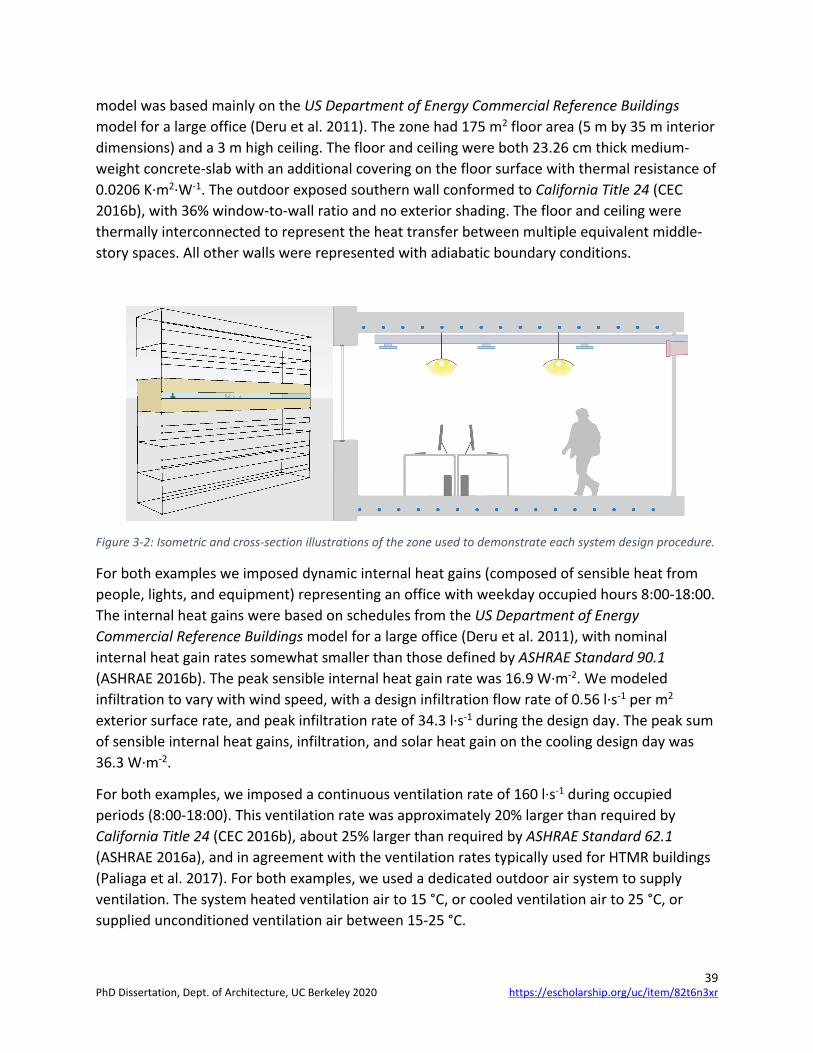
39
model was based mainly on the US Department of Energy Commercial Reference Buildings model for a large office (Deru et al. 2011). The zone had 175 m2 floor area (5 m by 35 m interior dimensions) and a 3 m high ceiling. The floor and ceiling were both 23.26 cm thick medium-weight concrete-slab with an additional covering on the floor surface with thermal resistance of 0.0206 K·m2·W-1. The outdoor exposed southern wall conformed to California Title 24 (CEC 2016b), with 36% window-to-wall ratio and no exterior shading. The floor and ceiling were thermally interconnected to represent the heat transfer between multiple equivalent middle-story spaces. All other walls were represented with adiabatic boundary conditions.
Figure 3-2: Isometric and cross-section illustrations of the zone used to demonstrate each system design procedure.
For both examples we imposed dynamic internal heat gains (composed of sensible heat from people, lights, and equipment) representing an office with weekday occupied hours 8:00-18:00. The internal heat gains were based on schedules from the US Department of Energy Commercial Reference Buildings model for a large office (Deru et al. 2011), with nominal internal heat gain rates somewhat smaller than those defined by ASHRAE Standard 90.1 (ASHRAE 2016b). The peak sensible internal heat gain rate was 16.9 W·m-2. We modeled infiltration to vary with wind speed, with a design infiltration flow rate of 0.56 l·s-1 per m2 exterior surface rate, and peak infiltration rate of 34.3 l·s-1 during the design day. The peak sum of sensible internal heat gains, infiltration, and solar heat gain on the cooling design day was 36.3 W·m-2.
For both examples, we imposed a continuous ventilation rate of 160 l·s-1 during occupied periods (8:00-18:00). This ventilation rate was approximately 20% larger than required by California Title 24 (CEC 2016b), about 25% larger than required by ASHRAE Standard 62.1 (ASHRAE 2016a), and in agreement with the ventilation rates typically used for HTMR buildings (Paliaga et al. 2017). For both examples, we used a dedicated outdoor air system to supply ventilation. The system heated ventilation air to 15 °C, or cooled ventilation air to 25 °C, or supplied unconditioned ventilation air between 15-25 °C.
https://escholarship.org/uc/item/82t6n3xrPhD Dissertation, Dept. of Architecture, UC Berkeley 2020

40
We performed system design calculations and annual simulations for the building located in Sacramento California – a climate with 0.4% cooling design condition outdoor dry-bulb temperature = 37.9 °C and mean coincident wet-bulb temperature = 21.3 °C. For simplicity, both examples only design systems for sensible cooling requirements.
3.4.1. Example of the standard cooling load calculation and system design procedure:
3.4.1.1. Step #1 Space cooling load calculation
The first steps in the standard system design procedure are to define a site, and building characteristics, then to define climate conditions and internal heat gains for a design day, and to perform a standard space cooling load calculation. This process is described with greater detail in Section 3.1 – the background to this chapter. To be clear, although we are designing a radiant system, this standard space cooling load calculation only considers space heat extraction by convection. As discussed previously, Feng (2014), Feng et al. (2014a), and Paliaga et al. (2017, 2018) showed that many designers commonly use this approach to size radiant cooling systems, and it is what standards recommend.
Figure 3-3 plots the results of the design day cooling load calculation for a constant indoor dry-bulb air temperature of 25 °C. The calculation suggests that the peak sensible space cooling load should be 26.3 W·m-2, and that it would occur at 15:00.
Figure 3-3: Standard cooling load calculation for the cooling design day. (Left): Outdoor dry-bulb air temperature and indoor temperatures. (Right): Sum of internal, solar, and infiltration heat gain (loss) rates, and the required space heat extraction rate (space cooling load).
1. Heat transfer rates are normalized by the floor area for the zone analyzed. 2. The red circle indicates the peak sensible space cooling load of 26.3 W·m-2. 3. The horizontal gray dashed lines indicate the minimum and maximum operative temperature that would
achieve |PMV| <= 0.5 during occupied hours for metabolic rate = 1.15 met, and clothing = 0.67 clo, relative humidity = 55%, and indoor air speed < 0.2 m·s-1.
4. The vertical gray dashed lines indicate the start and end hours for occupancy in the example building.
https://escholarship.org/uc/item/82t6n3xrPhD Dissertation, Dept. of Architecture, UC Berkeley 2020
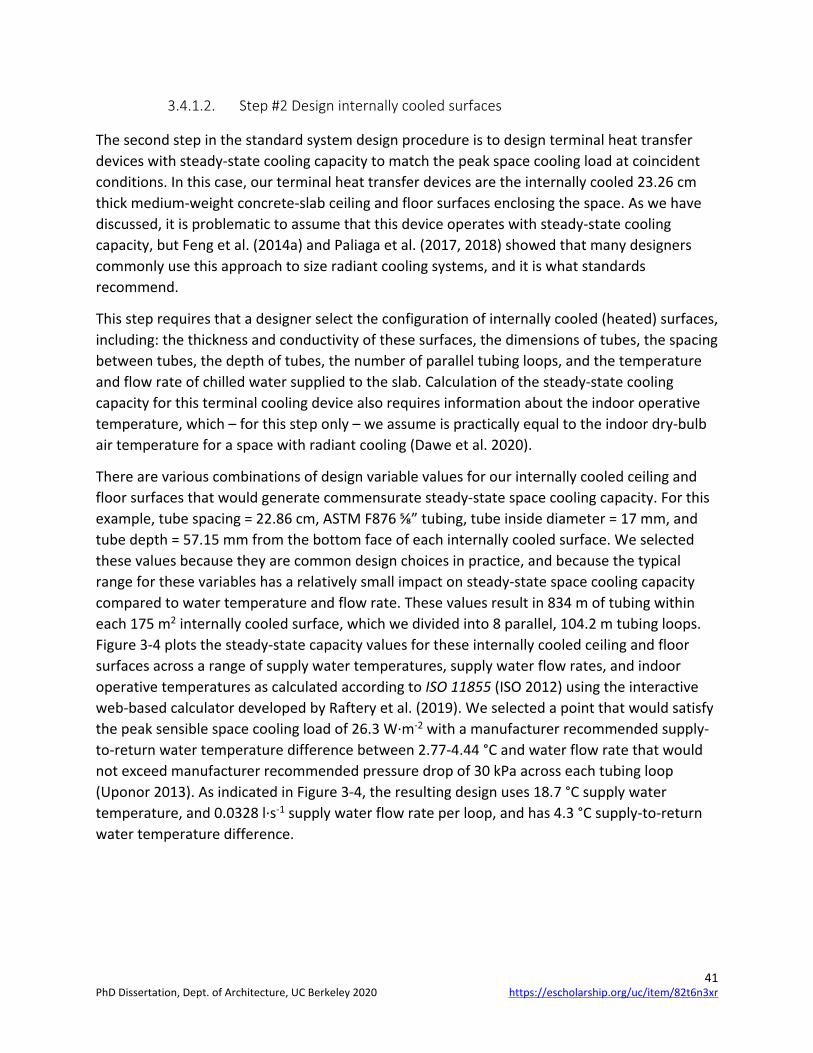
41
3.4.1.2. Step #2 Design internally cooled surfaces
The second step in the standard system design procedure is to design terminal heat transfer devices with steady-state cooling capacity to match the peak space cooling load at coincident conditions. In this case, our terminal heat transfer devices are the internally cooled 23.26 cm thick medium-weight concrete-slab ceiling and floor surfaces enclosing the space. As we have discussed, it is problematic to assume that this device operates with steady-state cooling capacity, but Feng et al. (2014a) and Paliaga et al. (2017, 2018) showed that many designers commonly use this approach to size radiant cooling systems, and it is what standards recommend.
This step requires that a designer select the configuration of internally cooled (heated) surfaces, including: the thickness and conductivity of these surfaces, the dimensions of tubes, the spacing between tubes, the depth of tubes, the number of parallel tubing loops, and the temperature and flow rate of chilled water supplied to the slab. Calculation of the steady-state cooling capacity for this terminal cooling device also requires information about the indoor operative temperature, which – for this step only – we assume is practically equal to the indoor dry-bulb air temperature for a space with radiant cooling (Dawe et al. 2020).
There are various combinations of design variable values for our internally cooled ceiling and floor surfaces that would generate commensurate steady-state space cooling capacity. For this example, tube spacing = 22.86 cm, ASTM F876 ⅝” tubing, tube inside diameter = 17 mm, and tube depth = 57.15 mm from the bottom face of each internally cooled surface. We selected these values because they are common design choices in practice, and because the typical range for these variables has a relatively small impact on steady-state space cooling capacity compared to water temperature and flow rate. These values result in 834 m of tubing within each 175 m2 internally cooled surface, which we divided into 8 parallel, 104.2 m tubing loops. Figure 3-4 plots the steady-state capacity values for these internally cooled ceiling and floor surfaces across a range of supply water temperatures, supply water flow rates, and indoor operative temperatures as calculated according to ISO 11855 (ISO 2012) using the interactive web-based calculator developed by Raftery et al. (2019). We selected a point that would satisfy the peak sensible space cooling load of 26.3 W·m-2 with a manufacturer recommended supply-to-return water temperature difference between 2.77-4.44 °C and water flow rate that would not exceed manufacturer recommended pressure drop of 30 kPa across each tubing loop (Uponor 2013). As indicated in Figure 3-4, the resulting design uses 18.7 °C supply water temperature, and 0.0328 l·s-1 supply water flow rate per loop, and has 4.3 °C supply-to-return water temperature difference.
https://escholarship.org/uc/item/82t6n3xrPhD Dissertation, Dept. of Architecture, UC Berkeley 2020
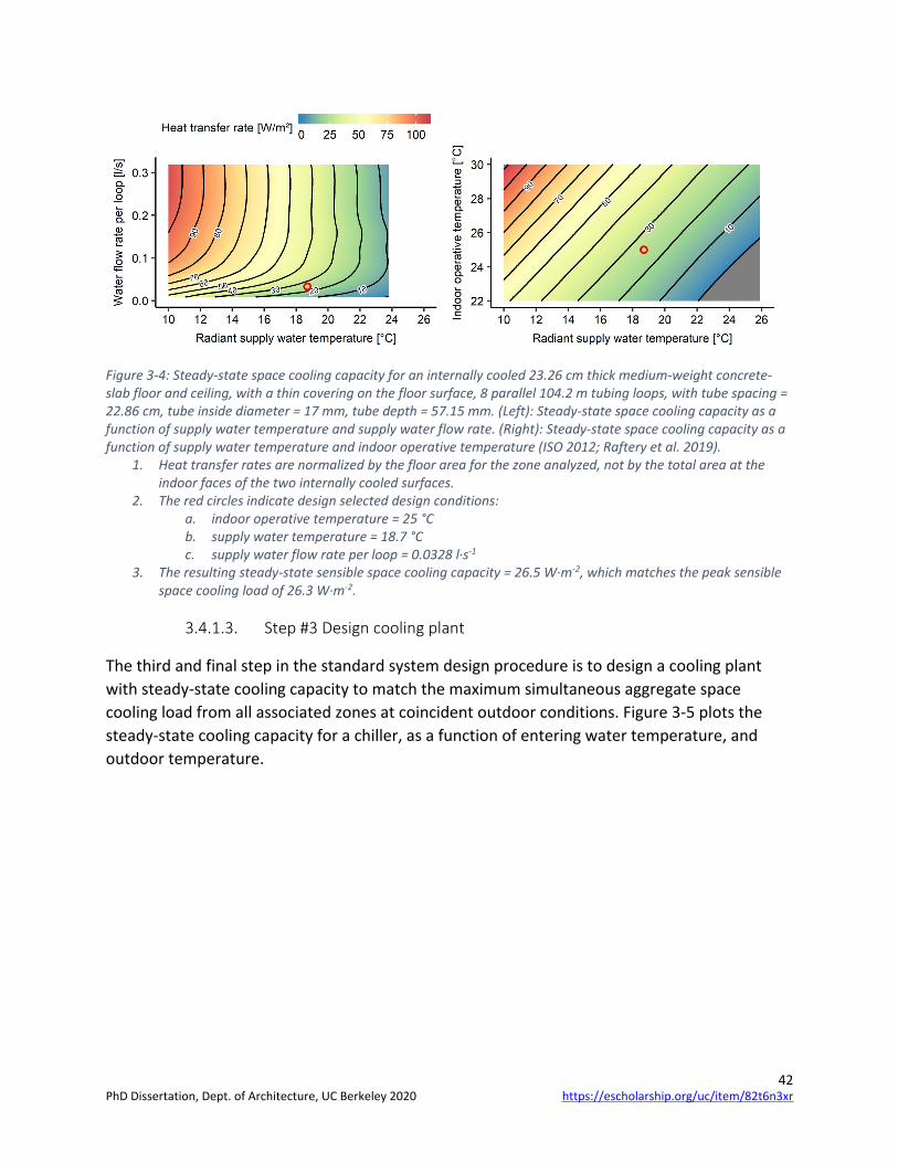
42
Figure 3-4: Steady-state space cooling capacity for an internally cooled 23.26 cm thick medium-weight concrete-slab floor and ceiling, with a thin covering on the floor surface, 8 parallel 104.2 m tubing loops, with tube spacing = 22.86 cm, tube inside diameter = 17 mm, tube depth = 57.15 mm. (Left): Steady-state space cooling capacity as a function of supply water temperature and supply water flow rate. (Right): Steady-state space cooling capacity as a function of supply water temperature and indoor operative temperature (ISO 2012; Raftery et al. 2019).
1. Heat transfer rates are normalized by the floor area for the zone analyzed, not by the total area at the indoor faces of the two internally cooled surfaces.
2. The red circles indicate design selected design conditions: a. indoor operative temperature = 25 °C b. supply water temperature = 18.7 °C c. supply water flow rate per loop = 0.0328 l·s-1
3. The resulting steady-state sensible space cooling capacity = 26.5 W·m-2, which matches the peak sensible space cooling load of 26.3 W·m-2.
3.4.1.3. Step #3 Design cooling plant
The third and final step in the standard system design procedure is to design a cooling plant with steady-state cooling capacity to match the maximum simultaneous aggregate space cooling load from all associated zones at coincident outdoor conditions. Figure 3-5 plots the steady-state cooling capacity for a chiller, as a function of entering water temperature, and outdoor temperature.
https://escholarship.org/uc/item/82t6n3xrPhD Dissertation, Dept. of Architecture, UC Berkeley 2020
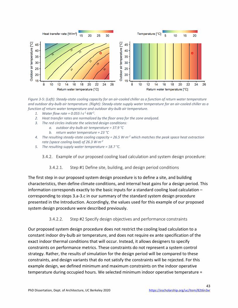
43
Figure 3-5: (Left): Steady-state cooling capacity for an air-cooled chiller as a function of return water temperature and outdoor dry-bulb air temperature. (Right): Steady-state supply water temperature for an air-cooled chiller as a function of return water temperature and outdoor dry-bulb air temperature.
1. Water flow rate = 0.055 l·s-1·kW-1. 2. Heat transfer rates are normalized by the floor area for the zone analyzed. 3. The red circles indicate the selected design conditions:
a. outdoor dry-bulb air temperature = 37.9 °C b. return water temperature = 23 °C
4. The resulting steady-state cooling capacity = 26.5 W·m-2 which matches the peak space heat extraction rate (space cooling load) of 26.3 W·m-2
5. The resulting supply water temperature = 18.7 °C.
3.4.2. Example of our proposed cooling load calculation and system design procedure:
3.4.2.1. Step #1 Define site, building, and design period conditions
The first step in our proposed system design procedure is to define a site, and building characteristics, then define climate conditions, and internal heat gains for a design period. This information corresponds exactly to the basic inputs for a standard cooling load calculation – corresponding to steps 3.a-3.c in our summary of the standard system design procedure presented in the Introduction. Accordingly, the values used for this example of our proposed system design procedure were described previously.
3.4.2.2. Step #2 Specify design objectives and performance constraints
Our proposed system design procedure does not restrict the cooling load calculation to a constant indoor dry-bulb air temperature, and does not require ex ante specification of the exact indoor thermal conditions that will occur. Instead, it allows designers to specify constraints on performance metrics. These constraints do not represent a system control strategy. Rather, the results of simulation for the design period will be compared to these constraints, and design variants that do not satisfy the constraints will be rejected. For this example design, we defined minimum and maximum constraints on the indoor operative temperature during occupied hours. We selected minimum indoor operative temperature =
https://escholarship.org/uc/item/82t6n3xrPhD Dissertation, Dept. of Architecture, UC Berkeley 2020
44
22.3 °C and maximum indoor operative temperature = 26 °C, which correspond to |PMV| <= 0.5 for metabolic rate = 1.15 met, clothing = 0.67 clo, relative humidity = 55%, and indoor air speed < 0.2 m·s-1 (ASHRAE 2017c; ISO 2005).
3.4.2.3. Step #3 Define terminal heat transfer devices, system details, and control sequence
The third step in our proposed system design procedure is to define the terminal heat transfer devices that will cool the space, the systems that will serve these devices, and a control sequence to manage these systems. This requires specification of all physical parameters and control sequences necessary to populate a mathematical model that adequately emulates the system thermodynamics. Since the proposed system design procedure requires iteration, and may allow for multiple solutions that satisfy performance constraints, we present four example design variants. In practice, a designer may test more design variants, as necessary to settle on a satisfactory design.
All four example design variants used tube spacing = 22.86 cm, tube inside diameter = 17 mm, and tube depth = 57.15 mm from the bottom face of each internally cooled surface. These values are the same as what we selected for the example of the standard system design procedure. We selected these design variable values because they are common values in practice, and because the typical range for these variables has a relatively small impact on steady-state space cooling capacity compared to supply water temperature and flow rate. All four example design variants used 8 parallel 104 m tubing loops, with total water flow rate = 0.65 l·s-1 – the maximum flow rate that would not exceed manufacturer recommended pressure drop of 30 kPa across each tubing loop.
Instead of using a feedback control loop to target an indoor dry-bulb air temperature setpoint – as is typical for most cooling and heating systems – these four example design variants use a feedback control loop that targets a floor surface temperature setpoint (measured at the top face of the floor). For calculations on the design day, we selected a floor surface temperature setpoint = 19 °C – the minimum floor surface temperature allowed by ISO 7730 (ISO 2005) and ASHRAE Standard 55 (ASHRAE 2017c). Within a designer-specified water circulation availability period, the system controls two-position valves to allow water to circulate through parallel tubing loops at a designer-specified flow rate, and with chilled water from a plant with designer-specified capacity, and designer-specified supply water temperature setpoint. Outside of the availability period, the two-position valves remain closed, and the cooling plant is off, but the internally cooled surfaces continue to extract heat from the space.
With all of these preceding design variable values, we tested four example design variants, each with a different combination of cooling plant capacity, water circulation availability period, and supply water temperature setpoint. We tested cooling plant sizes that would be smaller than or equal to the cooling plant selected by the standard design procedure. We tested two different water circulation availability periods: one that allows operation during all hours, and one that
https://escholarship.org/uc/item/82t6n3xrPhD Dissertation, Dept. of Architecture, UC Berkeley 2020

45
reduces operation during a periods with high time-of-use electricity tariffs4. Then for each example combination, we adjusted the supply water temperature setpoint and floor surface temperature setpoint to find a setting that could satisfy the constraints on operative temperature during the cooling design day. We also ensured that supply water temperature would not cause condensation, but it was not necessary to invoke this constraint for any of the design variants. Table 3-1 summarizes all of the design variable values we selected for each design variant.
Table 3-1: Design variable values for four example design variants tested in our recommended system design procedure, and for the preceding example design developed according to the standard system design procedure.
Design variable
System sized with standard
design procedure
Systems sized with our recommended design procedure
Variant 1: plant=50%, avail.=0-24
Variant 2: plant=75%, avail.=0-24
Variant 3: plant=75%, avail.=18-12
Variant 4: plant=100%, avail.=18-12
Tube depth (mm) 57.15 Tube spacing (mm) 22.86 Tube inside diameter (mm) 17 Number of parallel tubing loops 8 Length of ea. parallel loop (m) 104.2 Total length of tubing (m) 834 DOAS supply air temp. (°C) cooled to 25, heated to 15, floats from 15–25 Supply water flow rate (l·s-1) 0.262 0.65 Supply water temp. stpnt. (°C)A 18.7 20 20 18 19 Water circ. avail. Period 00:00-24:00 00:00-24:00 18:00-12:00 Indoor dry-bulb air temp. stpnt. (°CB) 25 – Floor srfc. temp. stpnt. (°C)B,C – 19 Plant capacity (W·m-2) D 26.3 13.3 19.9 19.8 26.2 Plant capacity (as % of standard) 100% 50% 75% 75% 100% A. The supply water temperature setpoints recorded here are often not satisfied with the available plant capacity. In such a
case, the supply water temperature values recorded in Table 3-2 will not match the supply water temperature setpoint values recorded here.
B. For the standard radiant system design, circulation through the internally cooled floor and ceiling is controlled by a constant indoor dry-bulb air temperature setpoint, whereas the design variants developed with our recommended procedure are controlled by a floor surface temperature setpoint.
C. The floor surface temperature setpoint recorded here is used for design day simulations, but annual simulations use an adaptive demand-shifting control sequence that adjusts the floor surface temperature setpoint each day based on feedback about the indoor dry-bulb air temperature on the previous day. In this case, the floor surface temperature setpoint recorded here is used as the minimum allowable floor surface temperature setpoint.
D. Value normalized by the floor area for the zone analyzed.
4 Time-of-use electricity tariff structures vary substantially between different utilities, and service types. We selected an availability schedule that would avoid operation from 12:00–18:00, which corresponds to the “summer peak pricing” period on PG&Es E-19 “General Demand” time of use tariff.
https://escholarship.org/uc/item/82t6n3xrPhD Dissertation, Dept. of Architecture, UC Berkeley 2020

46
3.4.2.4. Step #4 Conduct design period simulation, compare results to constraints, and iterate
The last step in our proposed system design procedure is to simulate each design variant for the design period of interest, then compare the results to performance constraints, and iterate on design variants to select a system design and control sequence that best satisfies performance objectives. As results in Section 3.4.3 demonstrate, the traditional cooling design day may not always be the most appropriate basis for system design selection, but for now we present results from cooling design day simulations for each example design variant.
Figure 3-6 presents the results from simulation of the four example design variants on the cooling design day. These results show that on the cooling design day Variant 2-4 all satisfy the designer-specified constraints on operative temperature, but Variant 1 (plant=50%, avail.=0-24) does not. These results demonstrate that multiple design variants may satisfy the performance constraints. In practice, a designer may test more variants. For example, a designer may reassess Variant 1 (plant=50%, avail.=0-24) with the addition of ceiling fans, personal comfort systems, or different controls to find a design with 50% size cooling plant that will achieve acceptable PMV on the design day. Also, a designer must be careful to select a design period that is appropriate to test performance of each design variant. In Section 3.4.3, we present results from annual simulations which reveal that Variant 1 (plant=50%, avail.=0-24) actually performs reasonably well on an annual basis, demonstrating that a single day design period may not adequately represent differences between design variants.
Additionally, these dynamic simulations on the cooling design day reveal that the peak space heat extraction rate (peak space cooling load) can be much larger than what is predicted by a standard cooling load calculation, but that the cooling plant can be much smaller. In this case, the peak space heat extraction rates (peak cooling load) for the example design variants are 10-29% larger than the peak space heat extraction rate (peak cooling load) predicted by the standard cooling load calculations. At the same time, these design variants use cooling plants that are smaller than or equal to the peak space heat extraction rate (peak cooling load) predicted by the standard cooling load calculation. Of the four design variants tested here, the largest peak space cooling capacity is generated by the system with a 00:00-24:00 availability schedule and cooling plant that is 25% smaller than what is predicted by a standard space cooling load calculation.
https://escholarship.org/uc/item/82t6n3xrPhD Dissertation, Dept. of Architecture, UC Berkeley 2020
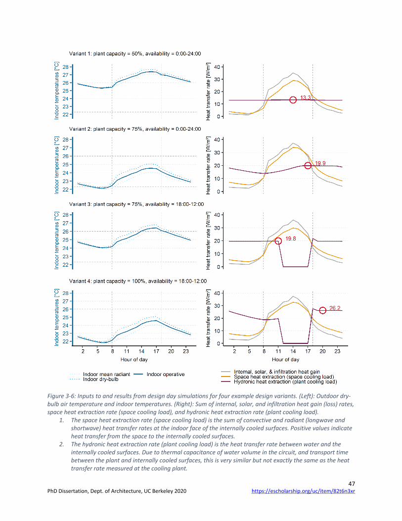
47
Figure 3-6: Inputs to and results from design day simulations for four example design variants. (Left): Outdoor dry-bulb air temperature and indoor temperatures. (Right): Sum of internal, solar, and infiltration heat gain (loss) rates, space heat extraction rate (space cooling load), and hydronic heat extraction rate (plant cooling load).
1. The space heat extraction rate (space cooling load) is the sum of convective and radiant (longwave and shortwave) heat transfer rates at the indoor face of the internally cooled surfaces. Positive values indicate heat transfer from the space to the internally cooled surfaces.
2. The hydronic heat extraction rate (plant cooling load) is the heat transfer rate between water and the internally cooled surfaces. Due to thermal capacitance of water volume in the circuit, and transport time between the plant and internally cooled surfaces, this is very similar but not exactly the same as the heat transfer rate measured at the cooling plant.
https://escholarship.org/uc/item/82t6n3xrPhD Dissertation, Dept. of Architecture, UC Berkeley 2020

48
3. Heat transfer rates are normalized by the floor area for the zone analyzed, not by the total area at the indoor faces of the two internally cooled surfaces
4. The red circles indicate the peak hydronic heat extraction rate (plant cooling load) for each design variant. 5. The horizontal gray dashed lines indicate designer-specified constraints on operative temperature.
Minimum and maximum constraints on operative temperature were selected that would achieve |PMV| <= 0.5 during occupied hours for metabolic rate = 1.15 met, clothing = 0.67 clo, relative humidity = 55%, and indoor air speed < 0.2 m·s-1.
6. The vertical gray dashed lines indicate the start and end hours for occupancy in the example building. 7. Outdoor dry-bulb air temperature for the cooling design day is shown in Figure 3-3.
3.4.3. Comparison of performance for systems designed according to each procedure
In this section, we assess and compare the systems designed in the preceding examples. First, we compare the space heat extraction rates predicted by a standard cooling load calculation to the space heat extraction rates that would actually be produced on the design day by the HTMR designed according to the standard procedure. Second, we compare the equipment size requirements, and design day system efficiency, for the systems designed according to each procedure. Third, we compare occupant thermal comfort, and thermal energy consumption for each system design predicted by annual simulation for the building in Sacramento, CA – using meteorological data representative of California Climate Zone 12 (CEC 2016b). All results are based on models developed in EnergyPlus (EnergyPlus 2018).
It is currently common to size HTMR according to standard space cooling load calculation procedures, and then to control these systems with constant indoor dry-bulb air temperature setpoints on all days, regardless of occupancy (Feng 2014; Feng et al. 2014a; Paliaga et al. 2017, 2018; Raftery et al. 2018a, 2018b). Correspondingly, our models of the system sized according to the standard design procedure used two position valves controlled by constant indoor dry-bulb air temperature setpoints on all days – heating setpoint = 22 °C, and cooling setpoint = 25 °C. Additionally, for annual simulations, we tested two common variants on this control strategy:
1. The first approach allows changeover between heating and cooling whenever the indoor dry-bulb air temperature setpoints are not met
2. The second approach uses the same indoor dry-bulb air temperature setpoints but imposes a 24-hour lockout between heating and cooling.
Our models of the four example design variants developed according to our recommended system design procedure used two position valves controlled by a floor surface temperature setpoint (measured at the top face of the floor), and only allowed to open during a water circulation availability period – as described previously in Section 3.4.2.3. Additionally, rather than operate with constant floor surface temperature setpoints for the entire year, we modeled an adaptive demand-shifting control sequence that adjusts the floor surface temperature setpoint each day based on feedback about the indoor dry-bulb air temperature
https://escholarship.org/uc/item/82t6n3xrPhD Dissertation, Dept. of Architecture, UC Berkeley 2020

49
on the previous day. The floor surface temperature setpoint is limited to 19 °C for cooling, and 29 °C for heating, in accordance with ISO 7730 (ISO 2005) and ASHRAE Standard 55 (ASHRAE 2017c). This control sequence is modeled after one described by Raftery et al. (2017) and demonstrated in practice in Chapter 5.
3.4.3.1. Comparison of the standard cooling load calculation to simulated performance of the standard system design on the design day
As discussed throughout this chapter, standard cooling load calculations do not properly estimate the space heat extraction rates that are generated by radiant systems. This inaccuracy is attributed in part to the fact that standard cooling load calculations do not consider space heat extraction by radiation, and in part to the fact that they do not account for dynamic variation in the indoor thermal conditions that typically occur with HTMR. Figure 3-7 compares the space heat extraction rates (space cooling load) predicted by a standard cooling load calculation (also shown in Figure 3-3) to the space heat extraction rates that would actually be produced on the design day by the HTMR designed according to the standard procedure and controlled with constant indoor dry-bulb air temperature setpoints. The comparison reveals that on the cooling design day the actual peak space heat extraction rate is 22% larger, even though the cumulative space heat extraction is practically equal. This reconfirms findings from simulations by Niu et al. (1995, 1997), Feng et al. (2013), and Feng (2014) and experiments by Feng (2014), Feng et al. (2014b), Novoselac et al. (2017), and Woolley et al. (2018, 2019). Additionally, whereas previous research has made this comparison whilst radiant cooling and all-air cooling maintained equal operative temperatures or equal air temperatures, these results indicate that the peak space heat extraction rate for radiant cooling is larger than for all-air cooling even when the indoor dry-bulb air temperature for HTMR drifts around the indoor dry-bulb air temperature setpoint, and the indoor dry-bulb air temperature for the all-air system remains constant.
https://escholarship.org/uc/item/82t6n3xrPhD Dissertation, Dept. of Architecture, UC Berkeley 2020
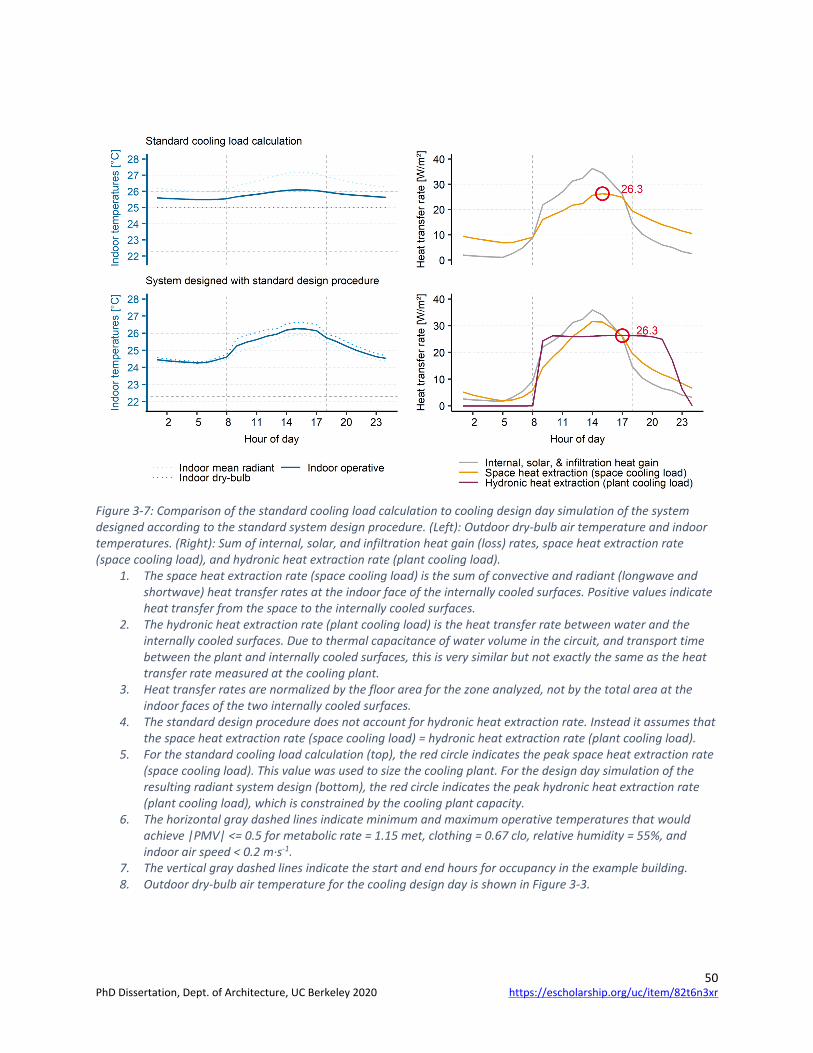
50
Figure 3-7: Comparison of the standard cooling load calculation to cooling design day simulation of the system designed according to the standard system design procedure. (Left): Outdoor dry-bulb air temperature and indoor temperatures. (Right): Sum of internal, solar, and infiltration heat gain (loss) rates, space heat extraction rate (space cooling load), and hydronic heat extraction rate (plant cooling load).
1. The space heat extraction rate (space cooling load) is the sum of convective and radiant (longwave and shortwave) heat transfer rates at the indoor face of the internally cooled surfaces. Positive values indicate heat transfer from the space to the internally cooled surfaces.
2. The hydronic heat extraction rate (plant cooling load) is the heat transfer rate between water and the internally cooled surfaces. Due to thermal capacitance of water volume in the circuit, and transport time between the plant and internally cooled surfaces, this is very similar but not exactly the same as the heat transfer rate measured at the cooling plant.
3. Heat transfer rates are normalized by the floor area for the zone analyzed, not by the total area at the indoor faces of the two internally cooled surfaces.
4. The standard design procedure does not account for hydronic heat extraction rate. Instead it assumes that the space heat extraction rate (space cooling load) = hydronic heat extraction rate (plant cooling load).
5. For the standard cooling load calculation (top), the red circle indicates the peak space heat extraction rate (space cooling load). This value was used to size the cooling plant. For the design day simulation of the resulting radiant system design (bottom), the red circle indicates the peak hydronic heat extraction rate (plant cooling load), which is constrained by the cooling plant capacity.
6. The horizontal gray dashed lines indicate minimum and maximum operative temperatures that would achieve |PMV| <= 0.5 for metabolic rate = 1.15 met, clothing = 0.67 clo, relative humidity = 55%, and indoor air speed < 0.2 m·s-1.
7. The vertical gray dashed lines indicate the start and end hours for occupancy in the example building. 8. Outdoor dry-bulb air temperature for the cooling design day is shown in Figure 3-3.
https://escholarship.org/uc/item/82t6n3xrPhD Dissertation, Dept. of Architecture, UC Berkeley 2020
51
3.4.3.2. Comparison of design variable values selected with each system design procedure, and simulation of each system on the design day
In this subsection, we compare the equipment size requirements, and design day system efficiency, for the systems designed according to each procedure. Table 3-2 summarizes some consequential differences between the designs that result from each procedure. The results demonstrate that for HTMR, the standard definition of “space cooling load” and the associated standard system design procedure can lead to equipment that is much larger than necessary, supply water temperature that is colder than necessary, and operation mainly during periods with high electricity tariffs. In particular, these examples of our recommended design procedure result in as much as 50% smaller cooling plant equipment, 5.2 °C warmer median supply water temperature on the cooling design day, and 100% reduction in chilled water consumption during periods with high electricity tariffs. Smaller cooling plant equipment translates directly to reduced capital expenses. Moreover, the warmer supply water temperatures that occur for designs with reduced sized cooling plants demonstrate that it would be possible to use very efficient cooling plant equipment, such as a cooling tower, instead of a conventional chiller. The standard design procedure indicated that the supply water temperature should be 18.7 °C, whereas Variant 1 (plant=50%, avail.=0-24) has cooling supply water temperature 23.5-24.2 °C on the cooling design day. This comparison reveals that for design of HTMR the standard design procedure can mislead designers by obscuring impactful design opportunities.
https://escholarship.org/uc/item/82t6n3xrPhD Dissertation, Dept. of Architecture, UC Berkeley 2020

52
Table 3-2: Summary of the design variable values selected and consequential results from simulation on design day for: (A) high thermal mass radiant systems sized with the standard system design procedure, and controlled with constant indoor dry-bulb air temperature setpoints; and (B) high thermal mass radiant systems sized with our recommended system design procedure, and controlled with an adaptive demand-shifting control sequence.
Design variable values Results for simulation on design day
Cooling plant capacity (as % of
standard)
Water circ. avail. period
Supply water flow rate
[l·s-1]
Supply water temperature
range [°C]A
Chilled water use in high
tariff hoursD
[kWh·m-2]C
Outdoor temp. range
for chiller operation
[°C] (A) System sized with standard design procedure, and controlled with constant indoor dry-bulb air temperature setpoint
System sized with standard design procedure
100% 00:00-24:00 0.262 18.7-18.9 0.157 23.4-37.9
(B) Systems sized with our recommended design procedure, and controlled with constant slab temperature setpoint Variant 1: plant=50%, avail=0-24
50% 00:00-24:00 0.65 23.5-24.3 0.0799 19.9-37.9
Variant 2: plant=75%, avail=0-24
75% 00:00-24:00 0.65 20-20.2 0.110 19.9-37.9
Variant 3: plant=75%, avail=18-12
75% 18:00-12:00 0.65 21.2-22.5 0 19.9-34.2
Variant 4: plant=100%, avail=18-12
100% 18:00-12:00 0.65 19-19.7 0 19.9-34.2
A. The supply water temperature setpoints recorded in Table 3-1 are not always satisfied with the available plant capacity. This table records the actual supply water temperature range that occurs during the design day simulation due to limited cooling plant capacity.
B. Value is normalized by the floor area for the zone analyzed. C. “High tariff hours” are assumed to be 12:00-18:00.
3.4.3.3. Comparison of annual simulations of the system designs that result from the alternate system design procedures
In this subsection, we compare occupant thermal comfort, and thermal energy consumption predicted for each system design over the course of a year in Sacramento, CA – using meteorological data representative of California Climate Zone 12 (CEC 2016b). We performed annual simulations of each design variant in EnergyPlus (EnergyPlus 2018). The control sequences for these annual simulations are described in the introductory paragraphs for Section 3.4.3 and in more detail in Chapter 5.
Table 3-3 summarizes the results from annual simulation of each system design.
Figure 3-8 presents the indoor operative temperature and the space heat extraction rates (space cooling load) for every work day of the year, as predicted by annual simulation of each system design. Each plot aggregates 260 daily time series traces into a composite 00:00-24:00 range. Each trace is colored to represent periods with chilled water circulation (blue), periods
https://escholarship.org/uc/item/82t6n3xrPhD Dissertation, Dept. of Architecture, UC Berkeley 2020

53
with heating water circulation (red), and periods with no water circulation (green). The comparison reveals that our proposed system design procedure and control strategy can enable substantial improvements in annual performance. Compared to the system designed according to the standard design procedure, the four example variants designed according to our proposed procedure reduced discomfort during occupied periods by as much as 55%, reduced cumulative thermal energy use for cooling by as much as 81% during periods with high electricity tariffs, increased median supply water temperature in cooling by as much as 3.3 °C, and increased the minimum supply water temperature in cooling by as much as 1.6 °C.
However, our four example design variants also increase annual thermal energy use for cooling by as much as 14% and increase the relatively small amount of heating thermal energy use. We expect that these increases in thermal energy use occur because the systems controlled to a slab temperature setpoint with an adaptive demand shifting control sequence:
1. Have lower operative temperatures which results in a larger cumulative indoor–outdoor temperature difference (i.e. larger potential for envelope heat transfer).
2. Derive less space cooling benefit from the DOAS system (a very small impact).
3. Operate for longer hours with lower hydronic heat transfer rates, which reduces the amount of heat stored in surfaces and the amount of heat released to the environment.
Additionally, the median supply water temperature in cooling was lowest for Variant 4 (plant=100%, avail.=18:00-12:00) – despite the fact that the standard system designs had a lower supply water temperature setpoint. We expect that this occurred because the 18:00-12:00 availability schedule shifts operation to periods when building masses are naturally cooler.
Awareness of performance trade-offs such as these is essential to the design process, yet the standard design procedure does not examine trade-offs because it assumes a singular – “ideal” – space cooling load and simplified heat transfer.
Some designers impose a lockout period on changeover from heating to cooling to avoid energy use associated shifting the mass temperature, while other designers suggest that rapid changeover from heating to cooling is necessary to ensure comfort and that the impact on energy use is relatively small (Paliaga et al. 2017, 2018). For the single zone scenario we simulated, allowing rapid changeover from heating to cooling – based simply on a 3 °C deadband between indoor dry-bulb air temperature setpoints – reduced discomfort hours by 5%, while increasing annual thermal energy for cooling by 1% and heating by 0%.
Finally – and most pertinent to our critique of the standard system design procedure – these annual simulation results reveal that the cooling and heating design day simulations may not represent the most extreme behavior for a system. This result can be deduced from Figure 3-8.
https://escholarship.org/uc/item/82t6n3xrPhD Dissertation, Dept. of Architecture, UC Berkeley 2020

54
Consequently, the comparison of design day simulation results for different design variants may not be indicative of differences in annual performance.
The annual peak space heat extraction rate (space cooling load) for each of the six example system designs was 60-76% larger than predicted by cooling design day simulations for each system. The discrepancy is even more significant when compared to standard cooling load calculations the annual peak space heat extraction rate (space cooling load) for each of the system designs was 93-107% larger than what was predicted by standard cooling load calculations on the cooling design day.
Furthermore, the operative temperature response predicted by cooling design day simulations is not representative of what will occur annually. This issue is not simply that design day simulations fail to capture annual variation, but rather that the design day simulations of multiple design alternatives may not represent a consistent point within the respective annual variations. Specifically, although design day simulations indicate that Variant 1 (plant=50%, avail.=0-24) would not maintain indoor operative temperature within designer specified constraints, annual simulations reveal that this design would actually perform reasonably well, with fewer discomfort hours than the system designed according to the standard design procedure. On the other extreme, the cooling design day simulation for Variant 2 (plant=75%, avail.=0-24) and Variant 4 (plant=100%, avail.=18-12) largely underpredict the range of operative temperatures that would occur annually.
We see three factors underlying this problem with design day simulations.
1. The outdoor climate conditions, internal heat gains, and solar heat gains on the designated cooling design day may not represent the most extreme heat gain scenario that will occur annually.
2. Design day simulations may not capture real control variations that occur throughout the year.
3. Design day simulations typically repeat a 0:00-24:00 design period iteratively until dynamic heat transfer behavior converges to a stable daily profile (steady-state oscillation). This approach has a substantial and unrealistic influence on the initial thermal conditions predicted at the beginning of the design day. We expect this issue is especially pronounced for buildings with large thermal mass and cooling systems with long response time.
Consider, for example, that the design day simulations for Variant 1-Variant 4 included designer specified floor surface temperature setpoints, and supply water temperature setpoints; but our annual simulations used an adaptive control sequence which reset the floor surface temperature setpoint in response to performance the previous day. Consequently, the space heat extraction rates (space cooling load) and operative temperature response predicted on the
https://escholarship.org/uc/item/82t6n3xrPhD Dissertation, Dept. of Architecture, UC Berkeley 2020

55
design day within the annual simulation differ substantially from what is predicted by the iterative design day simulation with fixed setpoints.
These final observations highlight that in some circumstances, the conditions in the cooling design day prescribed by standards may not be the appropriate basis for system design decisions, and that the typical design day simulation procedure may not represent the realistic multi-day dynamics that a system and control sequence will encounter.
Table 3-3: Summary of results from annual simulations. (A) High thermal mass radiant systems sized with the standard system design procedure, and controlled with constant indoor dry-bulb air temperature setpoints. (B) High thermal mass radiant systems sized with our recommended system design procedure, and controlled with an adaptive demand-shifting control sequence developed by Raftery et al. (2017) and demonstrated in field studies in Chapter 5.
24-hour
changeover lockoutB
Annual thermal energy use for cooling and heating plantA
Discomfort during occupied periods (hours)
Cooling [kWh·m-2]
Heating [kWh·m-2]
PMV>0.5 (too warm)
PMV<–0.5 (too cool) Total High tariff
hours Total High tariff hours
(A) Systems sized with standard design procedure and controlled with constant indoor dry-bulb air temperature setpoint System sized with standard design procedure
No 494 13 59.9 27.7 2.8 0.01
Yes 519 10 59.4 27.0 2.8 0.009 (B) Systems sized with our recommended design procedure and controlled with an adaptive floor surface temperature setpoint Variant 1: plant=50%, avail=0-24
Yes 268 72 65.3 14.5 4.5 0.46
Variant 2: plant=75%, avail=0-24
Yes 157 81 67.9 20.9 5.1 0.47
Variant 3: plant=75%, avail=18-12
Yes 225 111 65.8 0 0 0.33
Variant 4: plant=100%, avail=18-12
Yes 176 144 66.9 0 0 0.30
A. Annual thermal energy use for cooling and heating plants does not include the amount of thermal energy used by DOAS to heat ventilation air to 15 °C and cool ventilation air to 25 °C. Annually, the DOAS system uses 4.7 kWh·m-2 thermal energy for cooling and 4.8 kWh·m-2 thermal energy for heating.
B. When the standard design does not include a 24-hour lockout on changeover between heating and cooling, changeover is only governed by a 3 °C deadband between heating and cooling setpoints which results in 46 days with heating and cooling on the same day. When the standard design includes a 24-hour lockout on changeover between heating and cooling, the two modes never operate with less than 24 hours separation.
https://escholarship.org/uc/item/82t6n3xrPhD Dissertation, Dept. of Architecture, UC Berkeley 2020
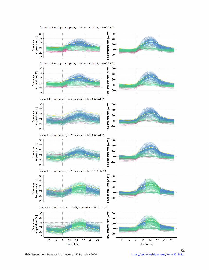
56
https://escholarship.org/uc/item/82t6n3xrPhD Dissertation, Dept. of Architecture, UC Berkeley 2020
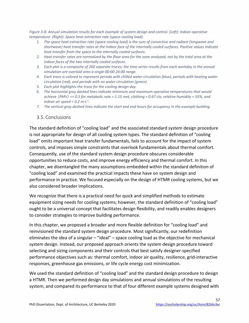
57
Figure 3-8: Annual simulation results for each example of system design and control. (Left): Indoor operative temperature. (Right): Space heat extraction rate (space cooling load).
1. The space heat extraction rate (space cooling load) is the sum of convective and radiant (longwave and shortwave) heat transfer rates at the indoor face of the internally cooled surfaces. Positive values indicate heat transfer from the space to the internally cooled surfaces.
2. Heat transfer rates are normalized by the floor area for the zone analyzed, not by the total area at the indoor faces of the two internally cooled surfaces.
3. Each plot is a composite of 260 separate traces; the time series results from each workday in the annual simulation are overlaid onto a single 00:00-24:00 range.
4. Each trace is colored to represent periods with chilled water circulation (blue), periods with heating water circulation (red), and periods with no water circulation (green).
5. Each plot highlights the trace for the cooling design day. 6. The horizontal gray dashed lines indicate minimum and maximum operative temperatures that would
achieve |PMV| <= 0.5 for metabolic rate = 1.15 met, clothing = 0.67 clo, relative humidity = 55%, and indoor air speed < 0.2 m·s-1.
7. The vertical gray dashed lines indicate the start and end hours for occupancy in the example building.
3.5. Conclusions
The standard definition of “cooling load” and the associated standard system design procedure is not appropriate for design of all cooling system types. The standard definition of “cooling load” omits important heat transfer fundamentals, fails to account for the impact of system controls, and imposes simple constraints that overlook fundamentals about thermal comfort. Consequently, use of the standard system design procedure obscures considerable opportunities to reduce costs, and improve energy efficiency and thermal comfort. In this chapter, we disentangled the many assumptions embedded within the standard definition of “cooling load” and examined the practical impacts these have on system design and performance in practice. We focused especially on the design of HTMR cooling systems, but we also considered broader implications.
We recognize that there is a practical need for quick and simplified methods to estimate equipment sizing needs for cooling systems; however, the standard definition of “cooling load” ought to be a universal concept that facilitates design flexibility, and readily enables designers to consider strategies to improve building performance.
In this chapter, we proposed a broader and more flexible definition for “cooling load” and reinvisioned the standard system design procedure. Most significantly, our redefinition eliminates the idea of a singular – “ideal” – space cooling load as the objective for mechanical system design. Instead, our proposed approach orients the system design procedure toward selecting and sizing components and their controls that best satisfy designer-specified performance objectives such as: thermal comfort, indoor air quality, resilience, grid-interactive responses, greenhouse gas emissions, or life cycle energy cost minimization.
We used the standard definition of “cooling load” and the standard design procedure to design a HTMR. Then we performed design day simulations and annual simulations of the resulting system, and compared its performance to that of four different example systems designed with
https://escholarship.org/uc/item/82t6n3xrPhD Dissertation, Dept. of Architecture, UC Berkeley 2020
58
our recommended procedure. This comparison revealed large errors associated with the standard design procedure. In particular, in our examples, standard cooling load calculations underestimated peak space cooling loads by more than 100%, yet overestimated the required cooling plant capacity by as much as 100%. The comparison also demonstrated how the standard design procedure can lead designers to overlook considerable opportunities to improve performance. For example, the standard design procedure indicated that the cooling supply water temperature should be 18.7 °C, but using our proposed procedure we developed an example system design and control strategy that would operate with cooling supply water temperature 20.3-25.1 °C – median 22.2 °C – while also reducing discomfort during occupied periods. Additionally, the four examples developed with our design procedure reduced annual thermal energy consumption for cooling by as much as 81% during periods with high electricity tariffs, and reduced discomfort during occupied periods by as much as 55%.
Furthermore, our examples demonstrate that even when a designer employs accurate models of systems and controls, using a typical “cooling design day” simulation as the basis for system design may result in suboptimal equipment sizing, and may lead designers to reject design variants that would actually perform well on an annual basis.
Many critical global challenges hinge on improving performance of heating, cooling, and ventilation systems in buildings; and achieving such improvements demands system design that is more sophisticated than what is currently designated by the standard definition of “space cooling load”. Yet, the standard definition of “cooling load” is commonly used as the basis to design a wide range of cooling systems – including HTMR. Therefore, we recommend that industry stakeholders update standards to address the shortcomings we have explained in this chapter. In Appendix A, we include a comprehensive revision to the definitions and explanatory sections in ASHRAE Fundamentals Chapter 18 (ASHRAE 2017e). Finally, we recognize that custom models for buildings and systems and annual simulations are currently beyond the reach of many designers. We therefore think that there is an urgent need to develop design guidelines and user-friendly design tools that facilitate accurate comparison and optimization of system design and control alternative
https://escholarship.org/uc/item/82t6n3xrPhD Dissertation, Dept. of Architecture, UC Berkeley 2020
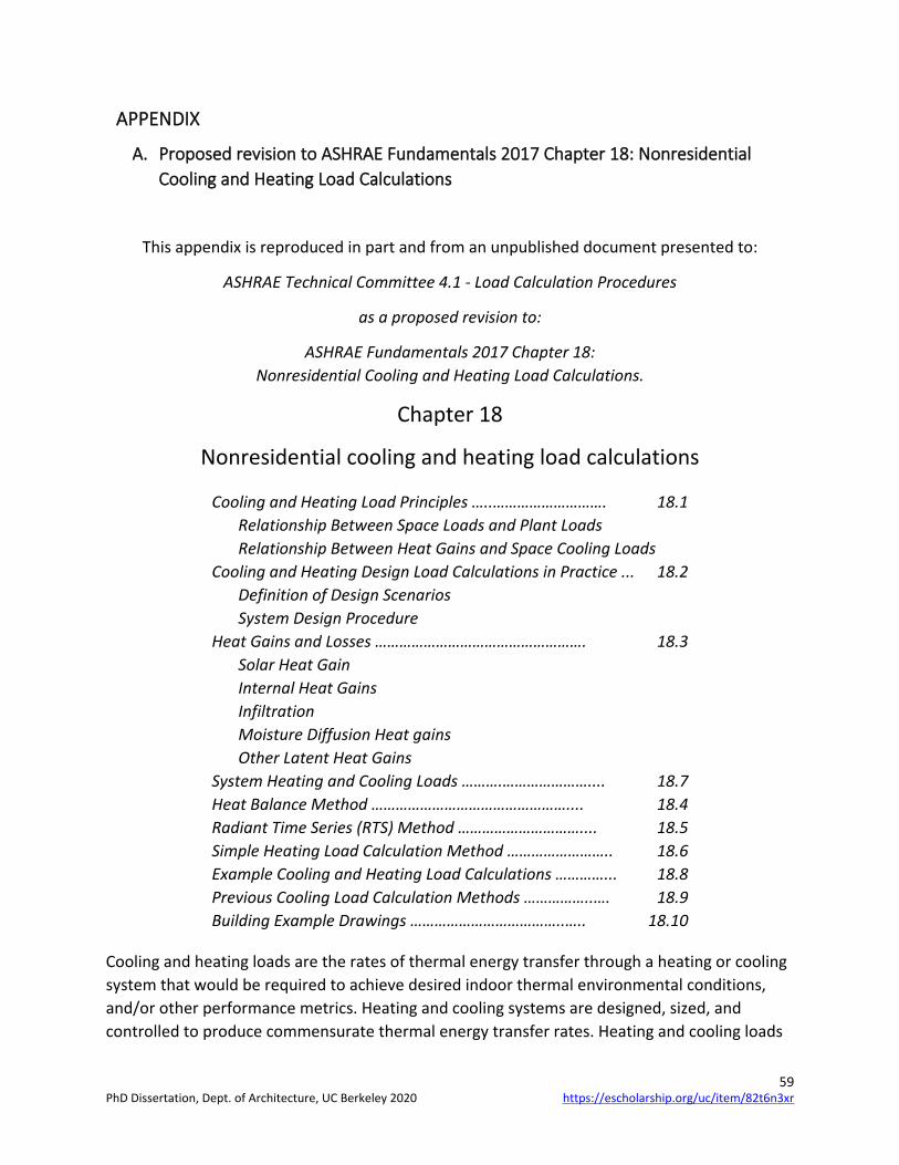
59
APPENDIX
A. Proposed revision to ASHRAE Fundamentals 2017 Chapter 18: Nonresidential Cooling and Heating Load Calculations
This appendix is reproduced in part and from an unpublished document presented to:
ASHRAE Technical Committee 4.1 - Load Calculation Procedures
as a proposed revision to:
ASHRAE Fundamentals 2017 Chapter 18: Nonresidential Cooling and Heating Load Calculations.
Chapter 18
Nonresidential cooling and heating load calculations
Cooling and Heating Load Principles …..………………………. 18.1 Relationship Between Space Loads and Plant Loads Relationship Between Heat Gains and Space Cooling Loads
Cooling and Heating Design Load Calculations in Practice ... 18.2 Definition of Design Scenarios System Design Procedure
Heat Gains and Losses ……………………………………………. 18.3 Solar Heat Gain Internal Heat Gains Infiltration Moisture Diffusion Heat gains Other Latent Heat Gains
System Heating and Cooling Loads ……….………………….... 18.7 Heat Balance Method ………………………………………….... 18.4 Radiant Time Series (RTS) Method ………………………….... 18.5 Simple Heating Load Calculation Method …………………….. 18.6 Example Cooling and Heating Load Calculations …………... 18.8 Previous Cooling Load Calculation Methods ……………..…. 18.9 Building Example Drawings ………………………………..….. 18.10
Cooling and heating loads are the rates of thermal energy transfer through a heating or cooling system that would be required to achieve desired indoor thermal environmental conditions, and/or other performance metrics. Heating and cooling systems are designed, sized, and controlled to produce commensurate thermal energy transfer rates. Heating and cooling loads
https://escholarship.org/uc/item/82t6n3xrPhD Dissertation, Dept. of Architecture, UC Berkeley 2020

60
can be determined for any point in time, but loads are inherently dynamic so should only be calculated across some period of time. Heating and cooling loads calculated, respectively, across heating and cooling design periods serve as the primary basis for selection and design of most heating and cooling systems. These design load calculations affect the size of piping, ductwork, diffusers, air handlers, boilers, chillers, coils, compressors, fans, pumps, and every other component of systems designed to condition indoor environments. Therefore, cooling and heating design load calculations can have large impacts on first cost of building construction, comfort and productivity of occupants, and operating cost and energy consumption.
The amount of heating or cooling required for a particular space is dynamic and depends on many factors including: the type of system used to provide heating and cooling, diurnal patterns of outdoor temperature and humidity, patterns and distribution of internal sensible and latent heat gain, building construction, and system controls. To produce an appropriate rate of heat transfer to or from a space, heating and cooling systems must transfer thermal energy through a series of steps. Heat is transferred to or from a space by terminal heat transfer devices, which transfer heat to or from a distribution system, which transfers heat to or from a cooling or heating plant. The heat transfer rates required at various points within the system can vary in time and magnitude. For example, thermal energy storage attenuates heat transfer through a system, and losses from ductwork and the need to heat or cool ventilation air require the plant heating or cooling load to be larger than the space heating or cooling load.
This chapter describes the principles underpinning heating and cooling loads generally, but focuses mainly on design load calculations for space heating and space cooling, which are typically intended to estimate the maximum rates at which thermal energy would ever need to be transferred to and from a space to achieve desired indoor thermal environmental conditions, and/or other performance metrics. The chapter also discusses factors that affect plant heating and cooling loads and system sizing, but whole system design is addressed with greater detail in other chapters. Similar principles can be used to estimate building energy consumption – the subject of Chapter 19. The main difference between design load calculations and building energy simulations is that the former facilitate the selection of design details (such as flow rates or supply temperature) based on conditions in a design period, whereas the latter estimate the heat transfer rates, indoor thermal conditions, energy use, and other performance metrics that a particular system would produce during a simulation period.
This chapter discusses the typical elements of heating and cooling load calculations. Section A1 provides an overview of the principles that govern the dynamics of heating and cooling loads, and provides definitions for terminology. Section A2 provides practical guidance for how to prepare cooling load calculations, and explains how the concept of heating and cooling loads fits within a recommended conceptual system design procedure. Section A3 provides reference documentation for estimating heat gains and losses (e.g., internal heat gain, ventilation and infiltration, moisture migration, and fenestration heat gain). Then, the chapter describes two
https://escholarship.org/uc/item/82t6n3xrPhD Dissertation, Dept. of Architecture, UC Berkeley 2020

61
different methods for estimating cooling loads, and one method for estimating heating loads. Section 4 describes the heat balance (HB) method for cooling load calculations, Section 5 describes the radiant time series (RTS) method for cooling load calculations, and Section 6 describes a simplified method for heating load calculations.
A1. Cooling and Heating Load Principles
Cooling and heating loads depend on many complex dynamic heat transfer processes involving the environment, the building construction, its internal contents, internal heat sources and sinks, the heating cooling and ventilation systems, and their controls. These factors impact the timing and magnitude of space heating and cooling loads in the following ways:
Outdoor environment: Outdoor environmental variables including temperature, humidity, solar irradiance, wind speed and wind direction are significant periodic inputs to the dynamic heat balance for a space. Their diurnal patterns can have large impacts on the magnitude and timing of heating or cooling loads. For example, buildings often release heat to the outdoor environment passively overnight, thereby reducing space cooling loads for the following day.
Building construction: Building geometry and thermal properties of construction impact the magnitude and timing of heat gains and losses through outdoor exposed surfaces. These characteristics influence space heat gains from solar radiation, gains and losses by conduction to outdoors, and gains and losses by infiltration. The thermal properties of surfaces within and enclosing a space (whether or not they are exposed to outdoors) also impact the extent to which heat gains are absorbed, stored, and later released to the space (or to the environment), instead of immediately impacting the space cooling or heating load.
Internal factors: The magnitude and timing of heat gains from lights, people, appliances, and equipment have distinct impacts on space heating and space cooling loads. As discussed in Section A3.2 it is important to distinguish between convective heat gains, radiative heat gains and latent heat gains, because they each impact the timing and magnitude of space heating and cooling loads differently. The physical contents of a building can also have substantial impact on heating and cooling loads, especially because of the way they absorb, store, and release heat from gains.
Systems: The type of terminal heating and cooling devices used in a space impacts the magnitude and timing of space heating and cooling loads. Different terminal heating and cooling devices interact with the complex heat transfer network for a space in different ways, changing the extent to which heat is absorbed and stored in masses, as well the rates of conductive heat transfer through outdoor exposed surfaces. As a result, to achieve equivalent operative temperature and humidity conditions, different systems require different space heat transfer rates.
System controls: The timing and magnitude of space heating and cooling loads are impacted by: the times at which heating or cooling systems are controlled to operate (i.e.: setpoint
https://escholarship.org/uc/item/82t6n3xrPhD Dissertation, Dept. of Architecture, UC Berkeley 2020

62
schedules), the way that parallel strategies are coordinated (i.e.: mechanical cooling and natural ventilation cooling), and the comfort range within which indoor operative temperature and humidity are allowed to drift over the course of a day (i.e.: ASHRAE Standard 55 specifies that systems may allow indoor thermal environmental conditions to drift and change over the course of a day, as long as they are maintained within an acceptable range and with an acceptable rate of change.).
In light of these factors, it should be noted that accurate determination of space heating and cooling loads requires definition of the system and control strategy – just as it requires definition of the environmental conditions, building construction, and heat gain characteristics. Often, design space load calculations are made without a final definition of the heating and cooling system that will be used, so it is therefore important that inputs and assumptions for design load calculations reasonably reflect the system type and control strategy that is ultimately used.
A1.1 Relationship Between Space Loads and Plant Loads
The design and control of systems also impacts the relationship between space loads and plant loads. For some systems the rate of heat transfer to or from a space translates almost immediately to equal loads for the heating or cooling plant. While for other systems, the thermal capacity of system components, transit time for thermal distribution, or active thermal storage delays the transfer of heat from one end of the system to the other, and spreads out heat transfer rates required by the heating or cooling plant. For example, when designed and controlled with these factors in mind the peak capacity of a cooling plant for a building with high thermal mass radiant cooling can be much smaller than the peak space cooling load – the plant can operate overnight, or extract heat from the slab slowly over a long period of time, while the actively cooled surfaces extract heat from the space more rapidly. Furthermore, leaks, thermal losses, and other factors cause plant heating and cooling loads to be larger than space heating cooling loads, and must be accounted for as part of design – these issues are discussed further in Section 3.7.
A1.2 Relationship Between Heat Gains and Space Cooling Loads
Surfaces within and enclosing a space (walls, floor, furniture, etc.) absorb and store a portion of the thermal energy from heat gains to a space. Consequently, peak space cooling load on a particular day is generally smaller than the corresponding peak space heat gain rate; yet, space cooling loads can be larger than space heat gains at other times, when heat gains subside, and heat stored in surfaces is released to the space. As surfaces absorb heat their temperature increases, which impacts operative temperature in a space and shifts the balance of convective and radiant heat transfer between surfaces and the indoor air. As a result, as space heat gains increase, the space cooling load increases more slowly. In an adiabatic system the space cooling load would eventually increase to match the space heat gain rate, but the time scale for this thermal response in a real building is generally so long that it does not reach steady-state.
https://escholarship.org/uc/item/82t6n3xrPhD Dissertation, Dept. of Architecture, UC Berkeley 2020
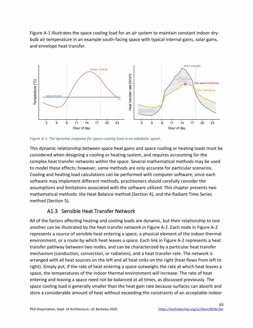
63
Figure A-1 illustrates the space cooling load for an air system to maintain constant indoor dry-bulb air temperature in an example south-facing space with typical internal gains, solar gains, and envelope heat transfer.
Figure A-1: The dynamic response for space cooling load in an adiabatic space.
This dynamic relationship between space heat gains and space cooling or heating loads must be considered when designing a cooling or heating system, and requires accounting for the complex heat transfer networks within the space. Several mathematical methods may be used to model these effects; however, some methods are only accurate for particular scenarios. Cooling and heating load calculations can be performed with computer software; since each software may implement different methods, practitioners should carefully consider the assumptions and limitations associated with the software utilized. This chapter presents two mathematical methods: the Heat Balance method (Section 4), and the Radiant Time Series method (Section 5).
A1.3 Sensible Heat Transfer Network
All of the factors affecting heating and cooling loads are dynamic, but their relationship to one another can be illustrated by the heat transfer network in Figure A-2. Each node in Figure A-2 represents a source of sensible heat entering a space, a physical element of the indoor thermal environment, or a route by which heat leaves a space. Each link in Figure A-2 represents a heat transfer pathway between two nodes, and can be characterized by a particular heat transfer mechanism (conduction, convection, or radiation), and a heat transfer rate. The network is arranged with all heat sources on the left and all heat sinks on the right (heat flows from left to right). Simply put, if the rate of heat entering a space outweighs the rate at which heat leaves a space, the temperatures of the indoor thermal environment will increase. The rate of heat entering and leaving a space need not be balanced at all times, as discussed previously. The space cooling load is generally smaller than the heat gain rate because surfaces can absorb and store a considerable amount of heat without exceeding the constraints of an acceptable indoor
https://escholarship.org/uc/item/82t6n3xrPhD Dissertation, Dept. of Architecture, UC Berkeley 2020
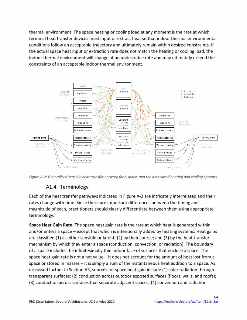
64
thermal environment. The space heating or cooling load at any moment is the rate at which terminal heat transfer devices must input or extract heat so that indoor thermal environmental conditions follow an acceptable trajectory and ultimately remain within desired constraints. If the actual space heat input or extraction rate does not match the heating or cooling load, the indoor thermal environment will change at an undesirable rate and may ultimately exceed the constraints of an acceptable indoor thermal environment.
Figure A-2: Generalized sensible heat transfer network for a space, and the associated heating and cooling systems.
A1.4 Terminology
Each of the heat transfer pathways indicated in Figure A-2 are intricately interrelated and their rates change with time. Since there are important differences between the timing and magnitude of each, practitioners should clearly differentiate between them using appropriate terminology.
Space Heat Gain Rate. The space heat gain rate is the rate at which heat is generated within and/or enters a space – except that which is intentionally added by heating systems. Heat gains are classified (1) as either sensible or latent; (2) by their source; and (3) by the heat transfer mechanism by which they enter a space (conduction, convection, or radiation). The boundary of a space includes the infinitesimally thin indoor face of surfaces that enclose a space. The space heat gain rate is not a net value – it does not account for the amount of heat lost from a space or stored in masses – it is simply a sum of the instantaneous heat addition to a space. As discussed further in Section A3, sources for space heat gain include (1) solar radiation through transparent surfaces; (2) conduction across outdoor exposed surfaces (floors, walls, and roofs); (3) conduction across surfaces that separate adjacent spaces; (4) convection and radiation
https://escholarship.org/uc/item/82t6n3xrPhD Dissertation, Dept. of Architecture, UC Berkeley 2020

65
across the boundaries that separate adjacent spaces; (5) heat generated within a space by occupants, lights, and equipment; (6) positive net heat transfer associated with direct-with-space ventilation and infiltration of outdoor dry-bulb air; and (6) miscellaneous heat gains.
Space Heating or Cooling Load:
The space cooling (heating) load at any point in time is the rate at which terminal heat transfer devices, with associated control sequences, must extract (input) sensible and/or latent heat such that associated thermal environmental conditions, and/or other performance metrics, comply with desired constraints during a design period (e.g.: limits on: operative temperature, ventilation rates, peak electrical demand, etc). ASHRAE Standard 55 defines acceptable indoor thermal environmental conditions for human occupancy, and ASHRAE Standard 62.1 defines ventilation for acceptable indoor air quality. The space heating or cooling load cannot be calculated for any point in time without context to thermal conditions at preceding times. As discussed previously, space heating or cooling loads are dynamic and depend on many factors including the system type and control strategy. Therefore, there may be more than one space heating or cooling load profile that satisfies desired constraints during a design period. Sensible and latent space heating and cooling loads must be accounted separately, yet with consideration for how they interact. For example, to generate sensible space heat extraction rates commensurate with sensible space cooling loads, a system may cause incidental latent cooling (dehumidification) that exceeds the amount of dehumidification that would otherwise be required. Consequently, the resulting total space cooling load is larger than the sum of the sensible and latent cooling requirements. This is one of many examples for how the system and control strategy influences space cooling heating loads. Importantly, the instantaneous space cooling load is not equivalent to the sum of all heat gains at the same time because surfaces within and enclosing a space absorb and store a portion of the heat gains (this is illustrated in Figure A-1).
Space Heat Input or Extraction Rate. The space heat input or extraction rate is the rate at which terminal heat transfer devices actually input or extract heat from a space. If the space heat input or extraction rate does not match the space heating or cooling load the indoor thermal environment will change at a rate different from the rate expected.
Plant (System) Heating or Cooling Load: The instantaneous plant (system) heating or cooling load is the rate at which a heating or cooling plant (or other point in the system) would need to transfer heat to or from the rest of a heating or cooling system in order to generate space heat input or extraction rates commensurate with the space heating or cooling loads. The plant heating or cooling load is not simply the sum of space heating or cooling loads. Practitioners must account for: heat gains and losses that occur outside of the space (e.g.: ventilation air, or duct leakage), diversity in timing and magnitude of aggregate space heating and cooling loads, the transit time for thermal distribution, system control sequences, and the dynamic thermal response of system components (e.g.: thermal energy storage, high thermal mass radiant
https://escholarship.org/uc/item/82t6n3xrPhD Dissertation, Dept. of Architecture, UC Berkeley 2020

66
slabs). Each of these factors decouple the timing and magnitude of space heating or cooling loads from that of the plant heating or cooling load.
Plant (System) Heat Input or Extraction Rate: The plant heat input or extraction rate is the rate at which a heating or cooling plant actually inputs or removes heat from a heating or cooling system. If the plant (system) heat input or extraction rate does not match the plant (system) heating or cooling load the space heat input or extraction rate will not match the space heating or cooling load.
Design Period (Space/System/Plant) Heating or Cooling Loads: Heating and cooling loads can be estimated for any point in time, but load calculations across heating and cooling design periods serve as the primary basis for selection and design of most heating and cooling systems. These design period heating or cooling loads usually represent the maximum rates at which thermal energy would ever need to be transferred to and from a space to achieve desired indoor thermal environmental conditions. However various design periods might be used to guide the design of systems that perform well across a variety of scenarios. The inputs used to define a design scenario – discussed further in Section A2 – may not represent regular operation; rather design period space heating and cooling loads are intended to bound the system design process. At the same time, a design scenario should represent realistic expectations, as overly conservative assumptions may lead to design and sizing of systems that are more costly than necessary or do not perform well under regular operating conditions.
Peak Design Heating or Cooling Load: While heating and cooling loads can be calculated for any point in time, and design period heating and cooling loads represent the dynamic loads during a design period, the peak design heating or cooling load is the single maximum heat input or extraction rate required during a design period. Commonly, the peak load is used as the basis for sizing the capacity of a heating or cooling system.
In summary, the terminology described here helps to differentiate between various heat flow rates that differ in time and magnitude. These terms can be combined logically to describe more detailed concepts associated with heating and cooling loads. For example, “cooling plant design period loads” are the heat transfer rates that would be required by a cooling plant during a design period to generate the space heat transfer rates commensurate with design period space heating or cooling loads. The same concepts may also be applied to intermediate points in a system. For example, the heat extraction rate for one hydronic zone in a high thermal mass radiant cooling system could be described as the “zone hydronic heat extraction rate”, and this could be different from the associated “space heat extraction rate” because thermal capacity of the slab imposes considerable delay for heat transfer through the slab, and because a controlled hydronic zone may be associated with multiple spaces.
https://escholarship.org/uc/item/82t6n3xrPhD Dissertation, Dept. of Architecture, UC Berkeley 2020
67
A2. Cooling and Heating Design Load Calculations in Practice
The affecting cooling load calculations are numerous, often difficult to define precisely, and always intricately interrelated. Many cooling load components vary widely in magnitude, and possibly direction, during a 24 h period. Because these cyclic changes in load components often are not in phase with each other, each component must be analyzed to establish the maximum cooling load for a building or zone. A zoned system (i.e., one serving several independent areas, each with its own temperature control) needs to provide no greater total cooling load capacity than the largest hourly sum of simultaneous zone loads throughout a design day; however, it must handle the peak cooling load for each zone at its individual peak hour. At sometimes of day during heating or intermediate seasons, some zones may require heating while others require cooling. The zones’ ventilation, humidification, or dehumidification needs must also be considered.
Load calculations should accurately describe the building. All load calculation inputs should be as accurate as reasonable, without using safety factors. Introducing compounding safety factors at multiple levels in the load calculation results in an unrealistic and oversized load.
Variation in heat transmission coefficients of typical building materials and composite assemblies, differing motivations and skills of those who construct the building, unknown infiltration rates, and the manner in which the building is actually operated are some of the variables that make precise calculation impossible. Even if the designer uses reasonable procedures to account for these factors, the calculation can never be more than a good estimate of the actual load. Frequently, a cooling load must be calculated before every parameter in the conditioned space can be properly or completely defined. An example is a cooling load estimate for a new building with many floors of unleased spaces for which detailed partition requirements, furnishings, lighting, and layout cannot be predefined. Potential tenant modifications once the building is occupied also must be considered. Load estimating requires proper engineering judgment that includes a thorough understanding of heat balance fundamentals.
Perimeter spaces exposed to high solar heat gain often need cooling during sunlit portions of traditional heating months, as do completely interior spaces with significant internal heat gain. These spaces can also have significant heating loads during non-sunlit hours or after periods of non-occupancy, when adjacent spaces have cooled below interior design temperatures. The heating loads involved can be estimated conventionally to offset or to compensate for them and prevent overheating, but they have no direct relationship to the spaces’ design heating loads.
Correct design and sizing of air-conditioning systems require more than calculation of the cooling load in the space to be conditioned. The type of air-conditioning system, ventilation rate, reheat, fan energy, fan location, duct heat loss and gain, duct leakage, heat extraction
https://escholarship.org/uc/item/82t6n3xrPhD Dissertation, Dept. of Architecture, UC Berkeley 2020

68
lighting systems, type of return air system, and any sensible or latent heat recovery all affect system load and component sizing. Adequate system design and component sizing require that system performance be analyzed as a series of psychrometric processes.
System design could be driven by either sensible or latent load, and both need to be checked. In a sensible-load-driven space (the most common case), the cooling supply air has surplus capacity to dehumidify, but this is usually permissible. For a space driven by latent load (e.g., an auditorium), supply airflow based on sensible load is likely not to have enough dehumidifying capability, so subcooling and reheating or some other dehumidification process is needed.
This chapter is primarily concerned with a given space or zone in a building. When estimating loads for a group of spaces (e.g., for an air-handling system that serves multiple zones), the assembled zones must be analyzed to consider (1) the simultaneous effects taking place; (2) any diversification of heat gains for occupants, lighting, or other internal load sources; (3) ventilation; and/or (4) any other unique circumstances. With large buildings that involve more than a single HVAC system, simultaneous loads and any additional diversity also must be considered when designing the central equipment that serves the systems. Methods presented in this chapter are expressed as hourly load summaries, reflecting 24 h input schedules and profiles of the individual load variables. Specific systems and applications may require different profiles.
This chapter presents two load calculation methods that vary significantly from previous methods. The technology involved, however (the principle of calculating a heat balance for a given space) is not new. The first of the two methods are the heat balance (HB) method; the second is radiant time series (RTS), which is a simplification of the HB procedure. Both methods are explained in their respective sections.
Cooling load calculation of an actual, multiple room building requires a complex computer program implementing the principles of either method.
A2.1 Definition of Design Scenarios
Regardless of the mathematical method used to calculate design heating or cooling loads, designers must specify the inputs that define a design scenario. These inputs and assumptions have substantial influence on the result of design heating and cooling load calculations; they should be defined realistically, yet may also incorporate assumptions that intentionally introduce a margin of safety to ensure that the resulting heating or cooling loads represent the maximum rates at which thermal energy would ever conceivably need to be transferred to and from a space. It is often useful to conduct load calculations for various scenarios, to guide the design of systems that perform well for maximum conceivable loads, while also performing well on typical days and at low load conditions. In addition to load calculations during design periods, annual building system simulations can also be exceedingly useful for system design,
https://escholarship.org/uc/item/82t6n3xrPhD Dissertation, Dept. of Architecture, UC Berkeley 2020

69
whether they are performed to estimate energy use – the topic of Chapter 19 – or to predict and evaluate other aspects of system performance.
Generally, the following information must be specified to define a design scenario.
Site Location Information. Most load calculation methods model solar heat gains as a dynamic interaction between climatological data, a solar position model, site characteristics, the building geometry, and building construction thermal properties. Therefore, the design scenario must include information about site latitude, longitude, altitude, and orientation, as well as the specific range of time for which load calculations will be performed. Additionally, information such as local terrain roughness, external shading, or external reflectance help to estimate local outdoor conditions based on climatological data from a meteorological station. For example, external objects such as adjacent buildings, water, or parking lots may reflect solar radiation and increase direct solar gains to a space.
Building Characteristics. Not surprisingly, design load calculations must be based on information about the building geometry and thermal properties of building construction. Each load calculation software tool may require different level of detail, but generally information is required to describe: material thermal properties, the layered configuration of materials to form construction surfaces (opaque and transparent), the geometry and arrangement of construction surfaces to form spaces, the relationship to adjacent spaces, outdoor surfaces, and the outdoors environment, as well as the thermal properties and geometry of surfaces within these spaces. Important thermal properties of materials include: spectral absorptivity, reflectivity, transmissivity and emissivity, surface roughness, thermal conductivity, specific heat capacity, and density. Additional input requirements may include information to estimate the effects of thermal bridging, or corner heat transfer effects. Some software tools are setup to allow users to input common construction ratings for particular construction surfaces, such as SHGC and U-factor; in which case it is important to ensure that surface area definitions comply with standard rating procedures (as discussed in ASHRAE Fundamentals Chapter 15: Fenestration).
System Characteristics. Calculation of space heating or cooling loads requires definition of the terminal heating or cooling devices that will provide heat transfer with the space. Different terminal heating and cooling devices interact with the complex heat transfer network for a space in different ways, and therefore impact the timing and magnitude of space heat transfer rates required to achieve desired operative temperature and humidity conditions. Many design load calculation procedures presuppose that terminal cooling devices are idealized air systems that transfer heat by convection and mix air perfectly throughout a space. This assumption is appropriate in many cases, but will not accurately represent space heating and cooling loads for other systems including: displacement systems, underfloor air distribution systems, and radiant systems. Furthermore, calculation of plant heating or cooling loads requires definition of all sources of heat transfer throughout a system, including the terminal heat transfer devices in
https://escholarship.org/uc/item/82t6n3xrPhD Dissertation, Dept. of Architecture, UC Berkeley 2020
70
multiple spaces, losses in distribution, and ventilation heating and cooling requirements that occur outside of the space.
Outdoor Conditions. Time series climatological data is required for the site location during the design period, and typically must include: outdoor dry-bulb temperature, outdoor humidity ratio, direct solar irradiance, diffuse solar irradiance, wind speed, wind direction, and opaque sky cover percentage or horizontal infrared radiation intensity. There are many resources for historical, typical, and projected future climatological data. ASHRAE Fundamentals Chapter 14: Climatic Design Information provides climatological information for many locations, and discusses other data resources. Regardless of the source, designers should conscientiously appraise the appropriateness of available data, including consideration of potential differences between conditions at the source meteorological station and conditions likely at the project site. For example, dry-bulb temperatures or wind speeds in an urban area may vary considerably from measurements by a nearby rural meteorological station.
It is essential that designers choose an appropriate period to guide design load calculations. The peak sensible space cooling load often occurs during periods of peak outdoor dry-bulb temperature, or periods of peak solar gains through fenestration – which often occur in cool months with low solar altitude. However, because of combined sensible and latent loads, the peak plant cooling load can occur during periods of peak wet-bulb temperature.
Indoor Thermal Environment and System Controls. The instantaneous space heating or cooling load is the rate at which terminal heat transfer devices would need to input or extract heat so that indoor thermal environmental conditions comply with desired constraints (ASHRAE Standard 55 defines acceptable indoor thermal environmental conditions for human occupancy). Therefore, definition of a design scenario requires specification of these desired constraints for the thermal environment. These may include minimum and maximum limits for all aspects of the thermal environment (air temperature, operative temperature, humidity ratio, etc), as well as limits on the rate of change for each, all of which might change in time as a function of other dynamic variables. Traditionally, design load calculations have specified constant indoor dry-bulb air temperature as the only constraint – an assumption that is absolutely integral to some load calculation procedures. However, modern objectives for design of high-performance building systems – such as the ability to actively shift electric demand – necessitate that design load calculations be guided by more liberal constraints.
Moreover, it is not sufficient to schedule an allowable envelope for indoor thermal conditions, a design scenario must also specify the control strategy used by a system. This is important because strategies like setback during vacant periods, or pre-cooling to avoid operation during peak electric demand periods, have substantial impact on the magnitude and timing of space cooling loads. Notice that definition of these constraints and controls are not the same as specifying the exact indoor thermal conditions that shall occur; rather they serve as inputs for a model to predict what indoor thermal conditions would occur and the corresponding space heat transfer rates that would be required by systems. For example, the design scenario for a
https://escholarship.org/uc/item/82t6n3xrPhD Dissertation, Dept. of Architecture, UC Berkeley 2020
71
system that employs pre-cooling would not specify the exact indoor thermal conditions that would occur; rather, it would specify a control strategy that precools to a particular setpoint, then load calculations would estimate how the indoor thermal conditions evolve in response to heat gains, control behaviors, and system characteristics. Often, load calculations specify very simple control strategies – such as a constant indoor dry-bulb air temperature setpoint; although this assumption is acceptable for design of many systems, it is not sufficient for some systems and controls. For example, high thermal mass radiant systems cannot be controlled to maintain constant indoor dry-bulb air temperature, and load calculations that impose such a simplifying assumption would overestimate the space heat extraction rates required by a radiant system to maintain acceptable indoor thermal comfort.
Internal Heat Gains. A design scenario must specify the magnitude, schedule, and characteristics of internal heat gains. Internal heat gains include heat from people, lights, and equipment (appliances, processes, etc), located within a space. As discussed in Section 7, these heat gains may have sensible and latent components, and the sensible part may enter the space as conduction, convection, or radiation. Some models differentiate between long-wave and short-wave radiant gains. All models must include some method to estimate the distribution of radiation between surfaces in a space – some methods simply assume uniform distribution across all surfaces. Direct-to-space ventilation should be scheduled as an internal heat gain, but heat gains from ventilation handled by central air handler should be accounted for in air handler system load calculations instead of space load calculations (as discussed in Section 7). Some load calculation methods calculate solar gains and infiltration rates as dynamic interactions with the environment, while others require these heat gains be scheduled as part of the design scenario.
A2.2 System Design Procedure
1. Describe all building and site characteristics and uncontrolled input values for a design period(s)
a. Define site location and meteorological information for a design period(s), including: (i) site latitude and longitude, (ii) outdoor dry-bulb air temperature and humidity, (iii) wind speed and direction, (iv) direct and global horizontal solar irradiance.
b. Define building characteristics, including: (i) building geometry, (ii) construction thermal characteristics, (iii) internal and external shading devices, and (iv) envelope air tightness characteristics.
c. Define site characteristics that impact building heat transfer, including: (i) shading by external objects (e.g.: trees and buildings), and (ii) reflection from external surfaces (e.g.: adjacent buildings, ground, water bodies).
d. Define internal heat gains for a design period(s) of interest, including heat gains from: (i) people, (ii) lighting, and (iii) equipment – this step must account for diversity in the timing and magnitude of internal heat gains in different spaces.
https://escholarship.org/uc/item/82t6n3xrPhD Dissertation, Dept. of Architecture, UC Berkeley 2020
72
e. Define other known heat gains (losses) to the space including: (i) infiltration, (ii) direct to space ventilation.
2. Describe performance objectives and constraints for the design period(s) a. Define performance priorities for the design, which may include balancing
multiple objectives such as achieving acceptable: (i) life cycle cost, (ii) energy cost, and/or (iii) life cycle greenhouse gas emissions.
b. Define constraints on performance metrics, which may include: (i) allowable range for air or operative temperature, (ii) allowable range for predicted mean vote (PMV), (iii) minimum required ventilation during occupied periods, (iv) maximum pollutant concentrations during occupied periods, (v) maximum peak electrical demand.
3. Describe system design variables, controlled input variables, and control strategy a. Define all terminal heat transfer devices, which may include: (i) sensible cooling
(heating) devices, (ii) dehumidification devices, and (iii) sources of direct-to-space ventilation (including natural ventilation systems).
b. Define all other factors and components associated with a space that may be controlled to influence performance (such as thermal comfort, or indoor air quality) which may include: (i) ceiling fans, (ii) personal comfort systems, (iii) sources of ventilation, (iv) air cleaning devices, (v) occupant adaptive behaviors.
c. Define all cooling (heating) systems within the scope of design, which may include: (i) distribution systems, (ii) air handlers, and (iii) cooling (heating) plants.
d. Define all heat gains and losses from the cooling (heating) system, which may include: (i) duct leakage, (ii) fan heat, (iii) distribution losses.
e. Define a sequence of operations for all controlled devices in a system (and occupant behaviors), which may include: (i) system operating schedules, (ii) feedback control loops and controlled variables, (iii) temperature setpoint schedules, and (iv) adaptive occupant responses.
4. Simulation and design iteration a. Perform simulation of the building and systems model for the design period(s),
and output values for any metrics needed to assess performance of the systems designed. This requires that designers utilize modeling tools capable of predicting these performance metrics, for the systems and controls to be designed, with accuracy that is appropriate for the scope and phase of design.
b. Compare simulation results to the performance constraints (defined in step 2.b). c. Iterate on design definition and simulation (steps 3–4) so as to best achieve
desired performance objectives (defined in step 2.a) subject to performance constraints (defined in step 2.b). Reject design alternatives that do not satisfy performance constraints, and choose among satisfactory design alternatives to best satisfy performance objectives.
A3. Heat Gains and Losses
As illustrated by Figure A-2, sources for sensible (and latent) space heat gain include: (1) solar radiation through transparent surfaces; (2) conduction (and moisture diffusion) from outdoor exposed surfaces; (3) conduction (and moisture diffusion) from interior partitions; (4)
https://escholarship.org/uc/item/82t6n3xrPhD Dissertation, Dept. of Architecture, UC Berkeley 2020
73
conduction (and moisture diffusion) from other surfaces within a space; (5) sensible heat (and moisture) generated in the space by occupants, lights, and appliances; (6) sensible heat (and moisture) associated with direct-to-space ventilation, infiltration, or transfer air from adjacent spaces; and (7) miscellaneous heat gains.
Sensible (and latent) heat losses from a space include: (1) conduction (and moisture diffusion) to outdoor exposed surfaces (floors, walls, and roofs); (2) conduction (and moisture diffusion) to interior partitions; (3) conduction (and moisture diffusion) to other surfaces within a space; (4) sensible heat (and moisture) associated with direct-to-space ventilation, infiltration, or transfer air from adjacent spaces, (5) miscellaneous losses, such as short-wave and long-wave radiative losses through transparent surfaces.
Section A3 provides standard reference information for estimating these different components of heat gain and loss – except for conduction into and out of surfaces within and enclosing a space, which is calculated differently by each of the cooling and heating load calculation methods described in this chapter. Section A3.1 provides information about the calculation of solar heat gains (a subject covered in greater detail by Chapter 15), Section A3.2 provides information about different sources of internal heat gains, Section A3.3 provides information to estimate gains and losses by infiltration (a subject covered in greater details by Chapter 16), Section 3.4 addresses latent gain from moisture diffusion through surfaces, and Section A3.5 addresses latent heat gains from other sources.
A3.1 Solar Heat Gains
See existing ASHRAE 2017 Fundamentals Chapter 18 section “Fenestration Heat Gain”
A3.2 Internal Heat Gains
Internal heat gains from people, lights, motors, appliances, and equipment can comprise the majority of the space heat gains in a modern building. While building envelopes have improved in response to more restrictive energy codes, internal heat gains have increased because of factors such as increased use of computers and the advent of dense-occupancy spaces (e.g., call centers).
A3.2.1 People
Table A-1 gives representative rates at which sensible heat and moisture are emitted by humans in different states of activity. A portion of the sensible heat emitted by people is transferred to air in the space by convection, and a portion is transferred by radiation to surfaces within and enclosing a space – both components are counted as space heat gains. In high-density spaces, such as auditoriums, these sensible and latent heat gains comprise a large fraction of the total heat gain to a space. Even for short-term occupancy, the extra sensible heat and moisture introduced by people may be significant. See ASHRAE Fundamentals Chapter 9 for detailed information; however, Table A-1 summarizes design data for common conditions.
https://escholarship.org/uc/item/82t6n3xrPhD Dissertation, Dept. of Architecture, UC Berkeley 2020

74
Table A-1: Representative Rates at Which Heat and Moisture Are Given Off by Human Beings in Different Activities and Locations
Table 1 from ASHRAE 2017 Fundamentals Chapter 18
A3.2.2 Electric Lighting
Electric lighting often comprises a major fraction of the total heat gain to a space. Most of the heat gain associated with lighting is produced by the lamps (the light-emitting elements), but a portion may be produced by ballasts and other appurtenances. A portion of the heat from each of these sources is transferred to air in the space by convection, and a portion is transferred by radiation to surfaces within and enclosing a space. The convective and radiant components from all parts of an electric lighting system are counted as space heat gains; however since electric lighting is often integrated into ceiling systems, a portion of the heat is transferred to the space, and a portion is transferred to the ceiling plenum. Therefore, the heat gain to a space from electric lighting can be calculated as:
QL-space= 3.41⋅Wnom⋅Fuse⋅Fspace (A.1)
where
QL-space = heat gain to space from lighting, Btu/hr {W} Wnom = nominal lighting power, W Fuse = lighting use factor Fspace = space fraction 3.41 = conversion factor The lighting use factor is the ratio of instantaneous lighting power consumption to the installed nominal lighting power. The factor may change in time to represent the pattern of use due to building operation, occupancy, and electric lighting needs. Design cooling load scenarios often set the lighting use factor to 1.0 to ensure cooling systems will be sized for a worst-case scenario.
The nominal lighting power is the rated electric power consumption of all lighting systems associated with a space, including lamps, ballasts, and controls. This can be estimated from values in Table A-2 – the maximum allowable lighting power densities (electric lighting power per square foot {meter}) specified by ASHRAE Standard 90.1 for different space types. Alternatively, when lighting plans and manufacturers technical information are available, the nominal lighting power can be calculated by:
Wnom= Wlamp⋅Fsa (A.2)
where
Wnom = nominal lighting power, W Wlamp = rated power of lamps, W
https://escholarship.org/uc/item/82t6n3xrPhD Dissertation, Dept. of Architecture, UC Berkeley 2020
75
Fsa = special allowance factor The rated power of lamps is obtained from manufacturer technical information for lamps, separate from their ballasts and controls. In some applications, the actual power consumed by lamps in operation may be smaller than their rated power.
The special allowance factor is the ratio of the lighting system’s total power consumption, including lamps and ballast, to the rated power of the lamps. For incandescent lights, this factor is 1. For other types of lights, the factor can be greater than 1 to account for power consumed by the ballast, power supply, or controls. For example, metal halide and high-pressure sodium vapor lighting systems may have special allowance factors from about 1.3 (for low-wattage lamps) down to 1.1 (for high-wattage lamps). The special allowance factor can be less than 1 when the ballasts used limit the power input to the lamps relative to their rated power. When available, use manufacturers’ values for the nominal power of lighting systems, rather than estimating lamps and ballasts independently.
Table A-2
Table 2 from ASHRAE 2017 Fundamentals Chapter 18
The space fraction is the portion of heat emitted by a luminaire that is transferred to the space as either convection or radiation. For luminaires that are integrated into the ceiling, this faction is less than 1, and the remaining portion of the heat is transferred to the plenum above as convection. Table A-3 – composed of data from experimental research by Fisher and Chantrasrisalai (2006) and Zhou et al. (2016) – presents the space fraction for several types of luminaires installed in drop ceilings.
In addition to determining the space heat gain from lighting it is necessary to distinguish between the portion that is emitted to the space as convection, and the portion that is emitted as radiation. Accordingly, Table A-3 presents the radiant fraction for each type of luminaire studied. The radiant fraction is the portion of the heat transferred to the space that is emitted as radiation; the remaining portion is emitted as convection.
Table A-3
Table 3 from ASHRAE 2017 Fundamentals Chapter 18
The data in Table A-3 represents space fraction and radiative fraction for typical operating conditions: supply-to-return airflow rate of 1 cfm/ft² {5 L/(s·m2)}, supply air temperature between 59 and 62 °F {15 and 16.7 °C}, and room air temperature between 72 and 75 °F {22 and 24 °C}. and lighting power density of 0.9 to 2.6 W/ft2 {9.7 to 28 W/m2}. For design power input above this range, the lower bounds of the space fraction and radiant fractions should be used; for design power input below this range, the upper bounds should be used. Using values
https://escholarship.org/uc/item/82t6n3xrPhD Dissertation, Dept. of Architecture, UC Berkeley 2020

76
in the middle of the range yields sufficiently accurate results. However, values that better suit a specific situation may be determined according to the notes for Table A-3.
For a room with a non-ducted ceiling plenum return, the heat transferred from lighting systems to the plenum above the ceiling is basically transferred into the return air stream and therefore impacts heating and cooling loads for the air handler, but not space heating and cooling loads. Conversely, for a room with a ducted return, a large portion of the heat transferred from lighting systems to the ceiling plenum would eventually be transferred to the space by conduction through the suspended ceiling. Despite the difference in how heat transferred to the plenum ultimately impacts loads, the values in Table A-3 apply to luminaires in suspended ceilings whether the room uses ducted return, or non-ducted ceiling plenum return
If the space airflow rate is different from the typical condition (i.e., about 1 cfm/ft2) {[i.e., about 5 L/(s·m2)]}, Figure A-3 can be used to estimate the lighting heat gain parameters. Data shown in Figure A-3 are only applicable for the recessed fluorescent luminaire without lens.
Figure 3 from ASHRAE 2017 Fundamentals Chapter 18
Figure A-3
Although Table A-3 and Figure A-3 would accurately represent a vented luminaire with side-slot returns, they are likely not applicable for a vented luminaire with lamp compartment returns, because in the latter case, all heat emitted by convection is likely to go directly to the ceiling plenum. This would result in a much lower space fraction, and a radiative fraction of 1.
For luminaire types not listed in Table A-3, it may be necessary to use judgment to estimate each component of the heat emitted by lighting.
When using the radiant time series (RTS) method for cooling load calculations, note that because a major portion of the radiation emitted by downlight luminaires may be absorbed by the floor, it could be more appropriate to use the solar radiant time factors (RTFs) instead of the non-solar RTFs. Solar RTFs are calculated assuming most solar radiation is absorbed by the floor, while non-solar RTFs assume uniform distribution by area over all interior surfaces. This effect may be significant for rooms where lighting heat gain is high and for which solar RTFs are significantly different from non-solar RTFs.
https://escholarship.org/uc/item/82t6n3xrPhD Dissertation, Dept. of Architecture, UC Berkeley 2020

77
This is the end of revisions drafted for ASHRAE 2017 Fundamentals Chapter 18 as of May 29, 2020. The other sections in the existing chapter also deserve revisions. In particular:
1. Although Strand et al. (1999), Strand and Pedersen (2002), and Strand and Baumgartner (2005) have extended the Heat Balance Method to consider radiation heat transfer as a pathway for heat input to and extraction from a space, the explanations and mathematical representation of the method in ASHRAE 2017 Fundamentals Chapter 18 only apply to all-air systems..
2. The existing section Heating Load Calculations outlines a simple method for sizing heating systems. It is an acceptable method, and it is used in practice, but it is only one approach that makes a lot of major assumptions. A fundamental representation of load calculations should allow the opportunity for more advanced methods, especially to facilitate design of high performance buildings. This section should remain in the chapter, but should be renamed “Simple Heating Load Calculation Method”
3. The existing section Previous Load Calculation Methods should be updated to identify the changes made in this revision. In particular, this revision introduces a flexible and forward-facing approach for load calculations that allows for a variety of solutions, whereas the existing approach is backward-facing, highly constrained, and produces a singular – “ideal” – estimate of space cooling load.
4. The existing section Example Cooling and Heating Load Calculations should be updated to reflect the flexible forward-facing approach.
Otherwise, the major content of the ASHRAE 2017 Fundamentals Chapter 18 could remain as is, with the following outline:
Infiltration Moisture Diffusion Heat gains Other Latent Heat Gains
System Heating and Cooling Loads ……….………………….... 18.7 Heat Balance Method ………………………………………….... 18.4 Radiant Time Series (RTS) Method ………………………….... 18.5 Simple Heating Load Calculation Method …………………….. 18.6 Example Cooling and Heating Load Calculations …………... 18.8 Previous Load Calculation Methods ……………..…. 18.9 Building Example Drawings ………………………………..….. 18.10
https://escholarship.org/uc/item/82t6n3xrPhD Dissertation, Dept. of Architecture, UC Berkeley 2020

78
4. Determining the warmest supply water temperature for high thermal mass radiant cooling systems under thermal comfort constrains
4.1. Background
The need for cooling is a significant driver of energy consumption in buildings and is mostly handled using systems based on the refrigeration cycle, which is energy- and cost-intensive, as discussed in Chapter 1. High-temperature cooling is one key advantage of radiant systems that can help eliminate the refrigeration cycle from a building’s cooling plant. Radiant systems’ use of large heat transfer areas compensates for the lower cooling power inherent in higher water temperatures. Figure 4-1 shows a range of 4 to 26 °C for supply water temperatures (SWT) used in investigations of radiant ceiling panels (RCP), embedded surface systems (ESS), and thermally activated building systems (TABS) in previous laboratory, field, and simulation studies. All studies maintained an upper operative temperature near 26 °C for the conditioned space. The bulk of the reported SWT are above 12 °C, with only a few low-temperature outliers. The required SWT generally depends on the heat gains (HG) generated and entering the zone and control strategy implemented in the radiant system, e.g. number of operating hours and water flow rate. High-temperature cooling has been demonstrated in mild and more extreme climates (Meierhans 1996; Corina Stetiu 1999; J. L. Niu et al. 2002). In many climates, the SWT is often high enough that the space does not require any dehumidification. Still, an additional system is needed in hot and humid climates to address dehumidification and/or supplemental cooling (L. Z. Zhang and Niu 2003).
Knowing the warmest SWT allows building designers to evaluate if sustainable cooling plant options are adequate for a specific set of building characteristics and climate (Samuel et al. 2013). One sustainable and probably cost-efficient option is the use of adiabatic cooling with cooling towers or fluid coolers. Buildings can exclusively use adiabatic cooling or chillers designed with waterside economizing to provide what is commonly referred to as free cooling and shown schematically in Figure 4-2. In an integrated waterside economizer, the heat exchanger is piped in series with the chiller to precool the return water temperature (RWT) and is considered the better waterside economizing choice (Taylor 2014). The other option is called non-integrated waterside economizing and the heat exchanger is piped as if it were an additional chiller in parallel. An integrated waterside economizer takes advantage of more economizing hours (Taylor 2014). Radiant systems that take advantage of waterside economizing have the potential for significant energy savings in the range of 8-15% (J. L. Niu et al. 1995), 10-20% (Sodec 1999), 21-23% (Raftery et al. 2012), and up to 55% (Tian and Love 2009) when compared to all-air systems. When exclusively using adiabatic cooling, designers must consider the potential impacts on occupant thermal comfort since available adiabatic cooling is highly dependent on weather conditions (J. L. Niu et al. 2002) and usually not in sync with the required cooling load profile. It is also reliant on the efficacy of the adiabatic cooling equipment to approach the wet-bulb temperature (WBT) (X. Wang et al. 2008).
https://escholarship.org/uc/item/82t6n3xrPhD Dissertation, Dept. of Architecture, UC Berkeley 2020
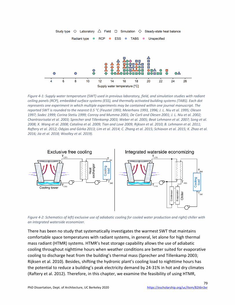
79
Figure 4-1: Supply water temperature (SWT) used in previous laboratory, field, and simulation studies with radiant ceiling panels (RCP), embedded surface systems (ESS), and thermally activated building systems (TABS). Each dot represents one experiment in which multiple experiments may be contained within one journal manuscript. The reported SWT is rounded to the nearest 0.5 °C (Feustel 1993; Meierhans 1993, 1996; J. L. Niu et al. 1995; Olesen 1997; Sodec 1999; Corina Stetiu 1999; Conroy and Mumma 2001; De Carli and Olesen 2001; J. L. Niu et al. 2002; Chantrasrisalai et al. 2003; Sprecher and Tillenkamp 2003; Weber et al. 2005; Beat Lehmann et al. 2007; Song et al. 2008; X. Wang et al. 2008; Catalina et al. 2009; Tian and Love 2009; Rijksen et al. 2010; B. Lehmann et al. 2011; Raftery et al. 2012; Odyjas and Górka 2013; Lim et al. 2014; C. Zhang et al. 2015; Schiavon et al. 2015; K. Zhao et al. 2016; Jia et al. 2018; Woolley et al. 2019).
Figure 4-2: Schematics of left) exclusive use of adiabatic cooling for cooled water production and right) chiller with an integrated waterside economizer.
There has been no study that systematically investigates the warmest SWT that maintains comfortable space temperatures with radiant systems, in general, let alone for high thermal mass radiant (HTMR) systems. HTMR’s heat storage capability allows the use of adiabatic cooling throughout nighttime hours when weather conditions are better suited for evaporative cooling to discharge heat from the building’s thermal mass (Sprecher and Tillenkamp 2003; Rijksen et al. 2010). Besides, shifting the hydronic plant’s cooling load to nighttime hours has the potential to reduce a building’s peak electricity demand by 24-31% in hot and dry climates (Raftery et al. 2012). Therefore, in this chapter, we examine the feasibility of using HTMR,
https://escholarship.org/uc/item/82t6n3xrPhD Dissertation, Dept. of Architecture, UC Berkeley 2020
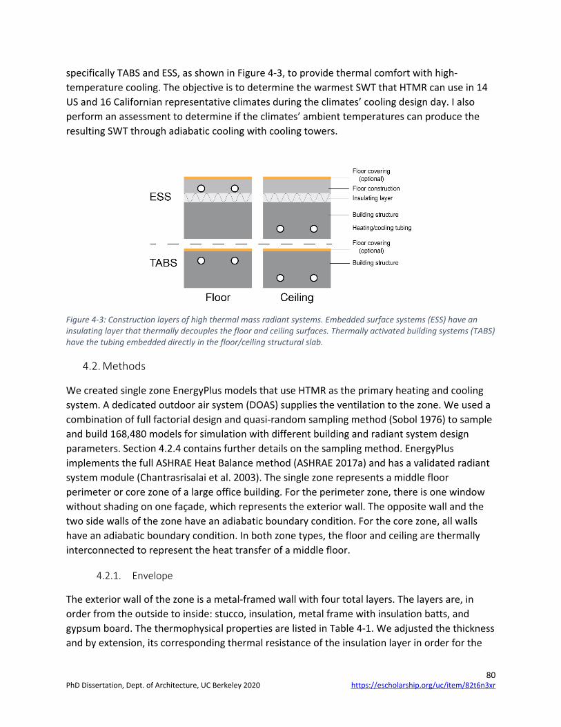
80
specifically TABS and ESS, as shown in Figure 4-3, to provide thermal comfort with high-temperature cooling. The objective is to determine the warmest SWT that HTMR can use in 14 US and 16 Californian representative climates during the climates’ cooling design day. I also perform an assessment to determine if the climates’ ambient temperatures can produce the resulting SWT through adiabatic cooling with cooling towers.
Figure 4-3: Construction layers of high thermal mass radiant systems. Embedded surface systems (ESS) have an insulating layer that thermally decouples the floor and ceiling surfaces. Thermally activated building systems (TABS) have the tubing embedded directly in the floor/ceiling structural slab.
4.2. Methods
We created single zone EnergyPlus models that use HTMR as the primary heating and cooling system. A dedicated outdoor air system (DOAS) supplies the ventilation to the zone. We used a combination of full factorial design and quasi-random sampling method (Sobol 1976) to sample and build 168,480 models for simulation with different building and radiant system design parameters. Section 4.2.4 contains further details on the sampling method. EnergyPlus implements the full ASHRAE Heat Balance method (ASHRAE 2017a) and has a validated radiant system module (Chantrasrisalai et al. 2003). The single zone represents a middle floor perimeter or core zone of a large office building. For the perimeter zone, there is one window without shading on one façade, which represents the exterior wall. The opposite wall and the two side walls of the zone have an adiabatic boundary condition. For the core zone, all walls have an adiabatic boundary condition. In both zone types, the floor and ceiling are thermally interconnected to represent the heat transfer of a middle floor.
4.2.1. Envelope
The exterior wall of the zone is a metal-framed wall with four total layers. The layers are, in order from the outside to inside: stucco, insulation, metal frame with insulation batts, and gypsum board. The thermophysical properties are listed in Table 4-1. We adjusted the thickness and by extension, its corresponding thermal resistance of the insulation layer in order for the
https://escholarship.org/uc/item/82t6n3xrPhD Dissertation, Dept. of Architecture, UC Berkeley 2020

81
whole wall assembly to meet the maximum U-factor allowed in the prescriptive requirements of the climate zone where the energy model is simulated (ASHRAE 2016b; CEC 2015). We used Title 24-2016 to find prescriptive requirements of all California climates zones and ASHRAE 90.1-2016 for the rest of the US climate zones. Similarly, the window’s maximum U-factor and minimum solar heat gain coefficient (SHGC) is based on the climates’ energy code. The maximum window-to-wall ratio (WWR) allowed in the prescriptive requirement is 40%, but in this study, we varied it from 20 to 60% for perimeter zones. High WWR without shading is not typical for radiant systems due to their limited cooling capacity. High WWR is also not desirable due to the strong adverse effects of direct solar radiation on occupant thermal comfort and visual glare (Arens et al. 2015; Tuaycharoen and Tregenza 2016). However, high WWR may be found in atriums or lobbies.
We use the quasi-random sampling method to test various zone length, width, and orientations (Sobol 1976). Table 4-2 shows the lower and upper limits of the sampling method. The zone length refers to the measurement that is parallel to the window length and zone width to the measurement going into the zone, i.e. perpendicular to the window. The height of the zone remains constant through all test cases at 3.048 m.
Table 4-1: Exterior wall construction layers with thermophysical properties.
Material Thickness [m]
Thermal conductivity [W·m-1·K-1]
Specific heat [J·kg-1·K-1]
Density [kg·m-3]
Total R-value [m2·K·W-1]
Stucco 0.0222 0.72 840 1856 0.0308 Insulation a 0.032 1680 72 a Metal frame with insulation batts
- - - - 1.3
Gypsum board 0.0127 0.16 1090 800 0.79 a. Adjusted to meet energy code U-factor wall assembly requirement.
4.2.2. Internal heat gains
We sampled lighting (LPD) and plug load power densities (PLPD), and occupant density (OD) for each model in this study. Table 4-2 shows the upper and lower limits of the sampling method. Table 4-2 also shows the radiant fraction used in the simulations. The radiant fraction for LPD corresponds to LED lighting fixtures. The radiant fraction remains constant for simplicity. The upper limit for the LPD is the minimum allowed in office building types in ASHRAE 90.1-2016. Non-regulated internal HG includes PLPD and OD. Title 24 Nonresidential ACM Reference Manual and US Department of Energy’s (DOE) large office prototype building model informs limits on non-regulated loads (CEC 2016a; Deru et al. 2011). The occupancy hours in the models is set to 8:00 to 18:00. We obtained the LPD, PLPD, and OD schedules from DOE’s large office prototype building model. However, the factors’ magnitude in these schedules are likely overestimated (Duarte et al. 2013), which will result in conservative high-temperature cooling SWT values. We modified the PLPD’s after-hour schedule (18:01 to 7:59) to test different
https://escholarship.org/uc/item/82t6n3xrPhD Dissertation, Dept. of Architecture, UC Berkeley 2020

82
nighttime base loads of the zone. The sampled diversity factors are from 0.1 to 0.5 of the design PLPD.
The ventilation rates set in the models for all California climates are the maximum of 7.08 L·s-1 per person or 0.762 L·s-1·m-2 as defined in Title 24-2016. For all other US climates zones, the ventilation rates are the sum of 2.5 L·s-1 per person and 0.3 L·s-1·m-2 per ASHRAE 60.1-2016. We then used the sampling method to vary the ventilation rate up to two times the defined minimum value. A 30% above minimum ventilation airflow is common practice for DOAS and other ventilation systems to receive credits under rating systems such as LEED (Paliaga et al. 2017; USGBC 2013). Designing DOAS systems above minimum ventilation airflow may also provide supplementary cooling. The DOAS ventilation system in the models has dual temperature setpoints at 15 and 21 °C with a design humidity ratio sampled from 0.0128 and 0.0175 kg of moisture per kg of dry air. The design humidity ratio range corresponds to a dew point temperature range of 14.7 to 22.7 °C which depends on the building site altitude. It is very important that the DOAS system must be temperature independent or completely decoupled from the cooling plant serving the radiant system to take advantage of increased SWT when applicable. The separation can be done through a separate packaged air conditioning system or small chiller with or without a recovery system (L. Z. Zhang 2006). To maintain the goal of no vapor compression in the building design, the ventilation would be addressed through a desiccant dehumidification system (J. L. Niu et al. 2002; La et al. 2010). In this study, the DOAS is a constant volume packaged air terminal unit for simplicity. We set the infiltration rate to 0.537 L·s-1·m-2 of the exterior surface which reduces to a quarter of the value when the ventilation system operates and pressurizes the building. The infiltration rate is in line with US commercial reference models (Deru et al. 2011).
4.2.3. Radiant system
We included several radiant system design parameters in the full factorial design portion of defining the test cases while sampling other parameters using the quasi-random method described below. The radiant system design parameters included in the full factorial are radiant system type (TABS or ESS), active surface (floor or ceiling), and tube spacing (0.1524, 0.2286, 0.3048 m). We treated the tube spacing as a discrete parameter because PEX tube manufacturers have standardized tube mats and other products to these three spacing lengths. We simulate all levels in the radiant system type, active surface, and tube spacing because these factors are fairly standardized options in the HTMR design and have significant effects on its performance. The rest of the parameters studied here, have considerable variation among building projects and the reason why we chose to sample among a range. We sampled floor/ceiling slab thickness, tube depth, outside tube diameter, maximum circuit, or ‘loop’, length, slab, and floor construction thermal conductivity, floor covering thermal resistance, design supply/return temperature difference, radiant system operation start time, and radiant system operation duration. Table 4-2 shows the limits used in the sampling method for each of the parameters. Since the sampling method treats slab thickness and depth as independent
https://escholarship.org/uc/item/82t6n3xrPhD Dissertation, Dept. of Architecture, UC Berkeley 2020

83
parameters, it is possible to pair them up in nonrealistic ways, e.g. a tube depth of 0.1524 m with a slab thickness of 0.1016 m. Thus, we deleted test cases where tube depth exceeded slab thickness or not within predefined bounds. The tube depth is the measurement from the active surface to the top of the tube. Tube diameters also come in discrete sizes, but we wanted to test a range of diameters without adding an extensive amount of test cases to this simulation study. Therefore, we referenced tube diameters specifications in ASTM standard F876-17 and used linear interpolation to define non-standard tube diameters (ASTM 2017). We assumed the same thermal conductivity for the slab and floor construction with constant specific heat and density of 900 J·kg-1·K-1 and 2,240 kg·m-3, respectively.
We calculated the total volumetric water flow rate through the radiant system by performing a steady-state heat balance between the hydronic heat transfer and the radiant system design capacity according to ISO standard 11855-2012, as shown in Equation 4-1. Where V̇tlt is the total volumetric flow rate, qISO is the design capacity according to ISO standard 11855-2012, ρ and cp are the density and specific heat of the fluid flowing through the radiant system, TSW and TRW are the SWT and RWT, respectively (ISO 2012). One of the inputs to the ISO design capacity calculation is the SWT. Since this is an unknown parameter in this study, we defined a reference SWT at 12.8 °C to determine the steady-state design capacity used to calculate V̇tlt. Thus, we maintained the same calculated volumetric water flow rate for each test case throughout the iteration process of finding the final SWT. For ESS, we used ISO method for Type A and C in Appendix A of ISO standard 11855-2012 and Type E in Appendix B of the standard for TABS. A web-tool is available to calculate these values (http://radiant.cbe.berkeley.edu/).
V̇tlt =qISO
ρcp(TRW-TSW) Equation 4-1
We determined the total tube length in each test case using the zone tube spacing and the total area along with the assumption of an average 10% leader length for connecting back to the radiant manifold. Then, we calculated the number of loops in each test case by dividing the total tube length by the maximum loop length and rounding up to the next whole loop. Thus, the actual loop length is lower than the sampled maximum loop length. Next, we calculated the pressure drop per loop at the steady-state design condition using the Darcy-Weisbach equation and the Swamee-Jain friction factor. If the manufacturer recommended pressure drop in any one circuit was above 30 kPa, We iteratively increased the number of loops, and repeated the pressure calculation, until the pressure drop per loop is below this threshold. We used water as the fluid through the radiant system.
We sampled radiant system operation start time and number of operating hours in a 24-hour period to test many different control strategy scenarios. Every building is unique and may require different operation times of their HVAC system due to utility price tariff structure,
https://escholarship.org/uc/item/82t6n3xrPhD Dissertation, Dept. of Architecture, UC Berkeley 2020
84
availability and time-dependent efficiency of the central cooling plant, or other constraints. We sampled the start time from the integers 0-23 representing an hour of the day from midnight to 23:00 while the operation time from the integers 8-24. The needed capacity of the cooling plant for HTMR decreases as the number of operation hours increases (Olesen and Zöllner 2007; Duarte et al. 2018). Finally, We defined the central cooling plant as a district cooling object in EnergyPlus to supply the requested water temperature to the HTMR during all its operation period, i.e. unlimited cooling plant capacity.
4.2.4. Sampling method
We used the Sobol’ quasi-random sequences to sample all the parameters listed in Table 4-2 (Sobol 1976). This sampling method is not performing a truly random sample of parameters since it has knowledge of the previously sampled points to avoid clusters and gaps (Saltelli et al. 2010). The method progressively samples the space at a given density, thus requiring a sample size of 2m points (m=1,2,…) where a higher chosen m increases the density of sample points in the space. It was found that Sobol’ sequences outperformed other Monte Carlo sampling methods when evaluating a simple building simulation model and all tested sampling techniques converged with a sample size of 256 points, i.e. an m equal to eight (Burhenne et al. 2011). Thus, we used a sample size of 256 in this study as well.
As mentioned above, we performed a full factorial design on some parameters, listed in Table 4-3 along with the levels tested. This full factorial design results in 720 test cases and factoring in the sample size for using Sobol’ sequences, we calculated a total of 184,320 test cases. We deleted 15,840 test cases where the tube depth exceeds slab thickness or not within specified bounds. In total, we created 168,480 single zone models that went through the cooling design day simulation. After the simulations, we reduced the number of test cases for the analysis according to the criteria reported in Section 4.2.6.
https://escholarship.org/uc/item/82t6n3xrPhD Dissertation, Dept. of Architecture, UC Berkeley 2020

85
Table 4-2: Lower and upper limits in which continuous design parameters for each of the models could be sampled.
Design parameter Lower limit Upper limit Additional notes Window-to-wall ratio 20 90% Only for perimeter zone Zone length 3 45 m Measurement parallel to window
length Zone width 3 9 m Measurement into zone Exterior wall orientation 0 359° South = 0° | West = 90°
North = 180° | East = 270° Lights 5 8.5 W·m-2 a0.72 Plug loads 5 14 W·m-2 a0.5 Floor area per occupant 5 20 m2·person-1 a0.4 Nighttime plug load diversity factor 0.1 0.5 - Ventilation oversize airflow factor 1 2 - Supply air design humidity ratio 0.0128 0.0175 kg·kg-1·dry air - Floor/ceiling slab thickness 0.1016 0.3048 m - Tube depth 0.0254 0.1524 m Measurement is taken from the active
surface to top of the tube Outside tube diameter 0.0127 0.02858 m Includes non-standard diameters Maximum loop length 45.7 152.4 m - Slab and floor construction thermal conductivity
1 2.5 W·m-1·K-1 -
Floor covering thermal resistance 0 0.35 m·K·W-1 - Supply/return temperature difference
1.67 8.3 °C -
Radiant operation start time 0:00 23:00 - Radiant operation duration 8 24 h - a. Radiant fraction
Table 4-3: Summary of design parameters for full factorial design.
Design parameter Levels Climate zone 1 to 30 (14 US climates and 16 California)
Zone type Perimeter, Core HTMR type TABS, ESS
Active surface Floor, Ceiling Tube spacing 0.1524, 0.2286, 0.3048 m
4.2.5. Supply water temperature determination
We calculated the comfort bounds at an operative temperature range 22.5 to 26 °C. This corresponds to -0.5 to +0.5 predicted mean vote (PMV) at an airspeed of 0.1 m·s-1, relative humidity of 50%, occupant metabolic rate of 1.2 met, and clothing insulation of 0.57 clo. We used the upper thermal comfort limit of 26 °C with a tolerance of ±0.25 °C as the stopping criteria for the search of the required SWT to the radiant system.
We initialized the SWT for each model according to Duarte et al. (2018)’s random forest model on SWT for TABS. The nonlinear model requires instantaneous peak HG rate, WWR, exterior wall orientation, slab thickness, tube depth and spacing, and HTMR start time and operation hours in a 24-hour period. We calculated the steady-state design internal, envelope, ventilation, and infiltration HG rates according to ASHRAE’s 2017 Handbook of Fundamentals
https://escholarship.org/uc/item/82t6n3xrPhD Dissertation, Dept. of Architecture, UC Berkeley 2020

86
(ASHRAE 2017a) to obtain a HG rate estimate to feed into the random forest model. We assumed an average adult’s skin surface area, DuBois area = 1.8 m2 and 1.2 met to find the instantaneous HG rate for occupants. We used the upper comfort limit as the indoor design condition for the space. For the outdoor design conditions, we used the 0.4% dry-bulb temperature and mean coincident WBT design day for each climate. We used this design day for the steady-state HG rate estimation as well as for the transient simulation in EnergyPlus. For the latent HG rate, we calculated the humidity difference between the model’s design day condition and the sampled DOAS design humidity ratio. We assumed latent heat of evaporation for water at 2,260 kJ·kg-1.WeI used the Python CoolProp package to calculate air properties at each climate’s design day, i.e. specific heat, density, and humidity ratio (Bell et al. 2014). We followed ASHRAE’s clear-sky solar calculation method to obtain the total solar radiation based on each model’s location and orientation (ASHRAE 2017a). We downloaded weather files from EnergyPlus’s website (DOE 2018). We refer to California’s climates as Cal-##, where ## signifies the climate zone number. For US climate zones, we refer to them by their representative city.
Once we obtained the initial SWT, we simulated the models and extracted the maximum operative temperature in the zone during occupied hours. If the operative temperature was not within the ±0.25 °C from the upper thermal comfort limit, then we adjusted SWT per Equation 4-2 and repeated the simulation. This step was iterated until the maximum operative temperature for each model tested was within ±0.25 °C.
TSW,n = TSW,n-1 + 1.0ϵ if ε > 3η TSW,n = TSW,n-1 + 0.8ϵ if 2η < ε ≤ 3η TSW,n = TSW,n-1 + 0.6ϵ if ε ≤ 2η
Equation 4-2
The subscripts n and n-1 in Equation 4-2 represent the new and old SWT, respectively, ϵ represents the error, and η the tolerance set at 0.25 °C. The error (ϵ) is calculated as the difference between the upper comfort bound and the maximum operative temperature during occupied hours calculated in the simulation. This is conceptually similar to a control strategy presented in (Raftery et al. 2017). The only parameter changing between each simulation iteration is the SWT to the radiant system; everything else remains constant, including the water flow rate through the radiant system tubes. We used the Python eppy package to create all the energy models with the corresponding design parameters and modify the SWT in each iteration (Philip 2016).
4.2.6. Simulation test case exclusion criteria
After the simulation, we deleted test cases where condensation issues in the zone occurred, design operative temperature is not satisfied, and SWT resulted below 7.2 °C or above 26.25 °C. In practice, chillers for all-air systems are designed to generate about 7.2 °C water
https://escholarship.org/uc/item/82t6n3xrPhD Dissertation, Dept. of Architecture, UC Berkeley 2020
87
temperatures, thus using lower SWT for HTMR is unreasonable. We report the specific number of cases deleted at each criterion in Section 4.3.1. The remaining test cases after the cleaning process are the test cases we used to perform the data analysis.
4.2.7. Outdoor wet-bulb temperature analysis
We obtained the annual weather data for each climate zone to do an analysis of the WBT and compare it to the final SWT results. However, WBT is not included in the weather file, so we calculated it using the Python module CoolProp mentioned above. We then created a subset of annual WBT to only include months May through the end of October. We arbitrarily selected this period to only cover the cooling season. It is essential to compare WBT to SWT because WBT is an important driver for cooling tower/fluid coolers to generate cooled water. The lower the WBT, the lower the temperature of the cooled water and the higher the percentage of building and radiant system designs that can provide comfortable temperatures for occupants. It is important to mention that the outgoing water temperature from conventional cooling tower/fluid coolers is not going to equal the climates’ WBT. The primary approach temperature – the difference between the WBT and the outgoing cooling tower water temperature – can be 1-2 °C and an additional 2-4 °C for the secondary approach temperature – the difference between the outgoing cooling tower water temperature and the SWT into the radiant system – due to a heat exchanger for the cooling tower in low-temperature rejection applications (Costelloe and Finn 2003). However, advances in indirect evaporative cooling systems, i.e. fluid coolers, can produce outgoing water temperatures that are lower than climates’ WBT (Mahmood et al. 2016; Sverdlin et al. 2011).The thermodynamic process known as the Maisotsenko Cycle, or M-cycle, uses a series of dry and wet channels where a fraction of the air being cooled in the dry channel is diverted to the wet channel to further evaporatively cool the air in the dry channel that approaches the ambient air dewpoint temperature (Mahmood et al. 2016). Ongoing research is addressing technical challenges to produce practical fluid coolers that use the M-cycle (Sverdlin et al. 2011).
We compare WBT to SWT by creating boxplots for each climate. The box of the boxplot represents the interquartile range (IQR) (25th-75th percentiles) with the median presented with a solid black inside the IQR. We use the same definition whenever we use boxplots to represent data results. We dropped the whiskers to increase the readability of the plot. We rank the climates by the difference between the median SWT minus median WBT. The larger the difference between these two metrics, the larger the feasibility of designing a building’s cooling plant only using adiabatic cooling for the primary cooling requirements of building’s spaces.
Also, designers can optimize parameters at the cooling plant and/or at the zone level to further increase the feasibility of using low energy cooling devices. For example, mechanical designers can design their HTMR’s cooling plant to only operate during the night and building designers can design the building to minimize the total HG rate entering and generated inside the space. With this in mind, we subsetted the WBT data to only include nighttime temperatures from
https://escholarship.org/uc/item/82t6n3xrPhD Dissertation, Dept. of Architecture, UC Berkeley 2020
88
hours 22:00 to 10:00, test cases where HG rate are 60 W·m-2 or less, and where radiant system operation hours are within the nighttime temperatures. Then, we made the same distribution comparison between SWT and WBT, as mentioned above.
4.2.8. Simplified model development
We split the results into two datasets to train (70%) and test (30%) nine simplified models to estimate the SWT for a given set of parameters for the zone and radiant system: three linear models, three nonlinear models using random forest regression algorithm, and three nonlinear models using deep learning neural networks. An estimate of the SWT is useful for designers to determine if HTMR coupled with energy-efficient cooling sources is feasible for their building design. We followed a similar approach outlined in Duarte et al. (2018) but with slight modifications. In the first linear model, we used the simulated peak and 24-hour mean instantaneous HG rates to train the model. Both HG rate metrics are normalized to the floor area of the test case model. We obtained the instantaneous HG rate from lights, plug loads, occupants, solar, conduction through the exterior wall, ventilation, and infiltration using EnergyPlus’s standard outputs. HG rates are an important metric in the cooling load calculation and are an essential metric in predicting SWT as shown in later figures (ASHRAE 2017e). In the second linear model, we took the first linear model and added HTMR type as well as the active surface type: ceiling or floor. The insulation layer may have significant effects on the model results because it reduces the useable thermal mass and the active surface area that extracts heat from the zone. The inclusion of the active surface parameter is to take into account the different heat transfer coefficients of the surfaces. In the third linear model, we used the normalized to floor area simulated peak and 24-hour mean HG rate, WWR, floor covering thermal resistance, HTMR tube depth and spacing, supply/return temperature difference, and total operation time in a 24-hour period. If the second linear model shows that there is a prediction improvement in adding HTMR and active surface type to the simplified model, then we will add both parameters to the third linear model as well.
We used almost all input parameters in the third linear model described above to build the nonlinear models. We replaced WWR parameter with the metric, solar radiation to total HG rate ratio. The ratio is the peak simulated solar radiation entering the zone to total peak simulated zone HG rate during the cooling design day. We added zone width, length, and orientation, slab thickness, HTMR type, active surface, volumetric water flow rate per loop, and operation start time, and cooling design day maximum outdoor dry-bulb air temperature and daily range. We designate this nonlinear model as XX-1, where XX is RF for random forest or NN for neural network model type. We excluded zone orientation and radiant system start time from the linear models but added it to the nonlinear model because these cyclical parameters cannot be represented in a linear model. These parameters can be handled through a random forest regression model and other nonlinear modeling methods. Having many input parameters for a model increases complexity and the number of parameters users need to define. Therefore, we tested the sensitivity of the nonlinear model with fewer input parameters. In the
https://escholarship.org/uc/item/82t6n3xrPhD Dissertation, Dept. of Architecture, UC Berkeley 2020

89
second nonlinear model (XX-2), we excluded zone width and length, tube depth, and slab thickness. In the third nonlinear model (XX-3), we further excluded the floor covering thermal resistance and operation start time.
We used the R Statistical Software package caret to train the linear models as well as the random forest regression models with three repeated, ten-fold cross-validation (Kuhn 2008). We used the ranger random forest regression algorithm with a parametric grid search for the number of variables (4 to 18) that random tree could be split at each node and the minimum node size (10 to 50) (Wright and Ziegler 2015). The maximum number of trees in the three models is 500 and no limit for the tree depth.
We used the Python packages TensorFlow and Keras to build and train the deep learning neural network models (Abadi et al. 2016; Chollet 2015). We created a sequential neural network with one input, hidden, and an output layer with input and output dimensionality of (number of input parameters, 64), (64, 64), and (64, 1), respectively. The activation function on the input and hidden layers are rectified linear unit, or RELU, which is ideal for regression models. We implemented the loss function as the mean squared error (MSE) and the root mean square propagation (RMSprop) as the optimizer with a learning rate of 0.001 (Hinton 2012). We did additional testing to the model structure by adding a second layer with the dimensionality of (64, 24) between the hidden and output layer but only report the results of the better performing model structure. We report the root mean squared error (RMSE) as well as the mean absolute error (MAE) to evaluate and compare all models developed in this study. We report multiple performance metrics since there has been debate on which performance metric better represents the average error (Willmott and Matsuura 2005; Chai and Draxler 2014).
4.3. Results
In the following sections, we first report the number of test cases deleted from the SWT analysis and offer explanations as to why they were removed. Next, we discuss the results of one good practice test case by looking at the design parameters and the resulting timeseries data in detail. Then, discuss the results in aggregate and ending the section with the results of the simplified model development.
4.3.1. Data cleaning
We created 168,480 total energy models and 152,164 models were left after completing the data cleaning process. The following list provides more details on the number of test cases deleted at each step and reasons for the deletion. The percentages are taken from the initial total number of test cases created.
1. 1,003 (0.6%) due to condensation occurrences.
2. 14,839 (8.8%) were below 7.2 °C.
https://escholarship.org/uc/item/82t6n3xrPhD Dissertation, Dept. of Architecture, UC Berkeley 2020

90
3. 474 (0.3%) were above 26.25 °C and did not need cooling at the cooling design day.
In total, we deleted about 10% of the results from the primary analysis. Most of the deleted cases were due to simulations where the iterative process reduced the SWT below 7.2 °C. Since we can extract the simulated HG rate of the zones where this occurred, we are able to compare the total 24-hour cumulative simulated HG energy to the total 24-hour cumulative design hydronic heat extraction energy (Qhyd) as calculated in Equation 4-3.
Qhyd = 3600�V̇tltρcpΔTr-sΔthyd� Equation 4-3
Where V̇tlt is the total volumetric flow rate as calculated in Equation 4-1, ΔTr-s is the sampled design supply/return temperature difference, and Δthyd is the sampled HTMR operation duration hours. Qhyd is calculated before any simulation is performed so it is not the actual hydronic heat extraction energy resulting from the design day simulation. Figure 4-4 shows the metric ΔRX-G and calculated in Equation 4-4. ΔRX-G is the difference between Qhyd and simulated sensible HG (HGsimzn
sen ) energy introduced in the zone as a percentage of Qhyd and it is used to gain information on why models requested low SWT for its radiant system. HGsimzn
sen energy is the 24-hour sum of sensible HG energy into the zone due to people, lights, plug loads, net window gain or loss, net wall gain or loss, and net gain or loss due to the introduction of conditioned ventilation air into the zone at the corresponding dry-bulb air temperature for each timestep. The assumption is that the resulting HG energy of this addition is to be extracted by the radiant system. Figure 4-4 suggests that HGsimzn
sen were too high for the cooling plant where SWT resulted below 7.2 °C in the model for the given water flow rate and the operation schedule in a given 24-hour period. SWT increases as ΔRX-G becomes positive. Designers can calculate the ΔRX-G using estimated zone sensible HG rate and expected cooling plant extraction energy in a 24-hour period for their building and HTMR designs and use Figure 4-4 to preliminary estimate the range of SWT needed. A resulting positive ΔRX-G indicates that high temperature cooling is possible for their specific HTMR and building design. A negative number suggests that the hydronic cooling plant may be undersized, HG rates in the space are too high, or a combination of both.
ΔRX-G = �Qhyd-HGsimzn
sen
Qhyd� Equation 4-4
https://escholarship.org/uc/item/82t6n3xrPhD Dissertation, Dept. of Architecture, UC Berkeley 2020
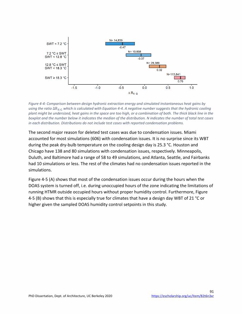
91
Figure 4-4: Comparison between design hydronic extraction energy and simulated instantaneous heat gains by using the ratio ΔRX-G which is calculated with Equation 4-4. A negative number suggests that the hydronic cooling plant might be undersized, heat gains in the space are too high, or a combination of both. The thick black line in the boxplot and the number below it indicates the median of the distribution. N indicates the number of total test cases in each distribution. Distributions do not include test cases with reported condensation problems.
The second major reason for deleted test cases was due to condensation issues. Miami accounted for most simulations (606) with condensation issues. It is no surprise since its WBT during the peak dry-bulb temperature on the cooling design day is 25.3 °C. Houston and Chicago have 138 and 80 simulations with condensation issues, respectively. Minneapolis, Duluth, and Baltimore had a range of 58 to 49 simulations, and Atlanta, Seattle, and Fairbanks had 10 simulations or less. The rest of the climates had no condensation issues reported in the simulations.
Figure 4-5 (A) shows that most of the condensation issues occur during the hours when the DOAS system is turned off, i.e. during unoccupied hours of the zone indicating the limitations of running HTMR outside occupied hours without proper humidity control. Furthermore, Figure 4-5 (B) shows that this is especially true for climates that have a design day WBT of 21 °C or higher given the sampled DOAS humidity control setpoints in this study.
https://escholarship.org/uc/item/82t6n3xrPhD Dissertation, Dept. of Architecture, UC Berkeley 2020

92
Figure 4-5: Simulation test cases where condensation occurred for at least one hour. A) hour at which the first condensation occurred in the simulation as a function of the average zone dew point temperature for all hours of condensation and B) total condensation hours in each simulation as a function of design day outdoor wet-bulb temperature.
4.3.2. Supply water temperature analysis
4.3.2.1. Details of a single simulation
Figure 4-6 illustrates the timeseries results of the final outcome of the iterative process to find the warmest SWT for one good practice test case that meets the given constraints. Figure 4-6 A) shows the instantaneous sensible plus latent HG rate and B) heat extraction rates of various zone components and C) the coincident outdoor and resulting indoor temperatures with a D) closeup of indoor temperatures during the cooling design day in Albuquerque, NM. The thermal zone is 5 m x 35 m with the exterior wall orientation angle of 13°, which is a slight offset from the south and has a WWR of 35.8%. The zone has a TABS ceiling radiant system with a slab thickness of 0.2326 m with a thin floor covering represented with a thermal resistance of 0.0206 K·m2·W-1, 0.2286 m tube spacing, 33.8 mm tube depth, 19.2 mm inside diameter tube, eight parallel tube circuits with each measuring 104.3 m. Each circuit has a design water flow rate of 0.081 l·s-1 and a design temperature difference of 5.1 °C. The radiant system operates from 2:00-13:00, which is 11 h of operation. The resulting SWT for this test case is 20.1 °C.
A
B
https://escholarship.org/uc/item/82t6n3xrPhD Dissertation, Dept. of Architecture, UC Berkeley 2020
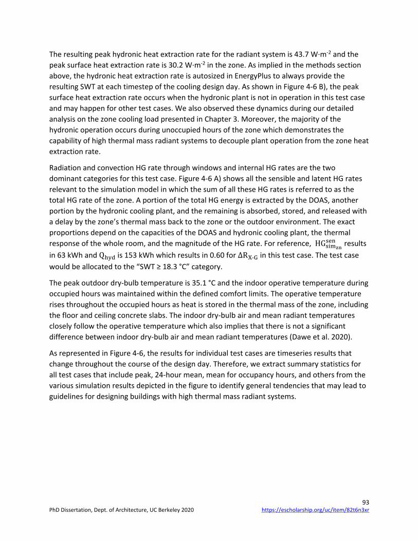
93
The resulting peak hydronic heat extraction rate for the radiant system is 43.7 W·m-2 and the peak surface heat extraction rate is 30.2 W·m-2 in the zone. As implied in the methods section above, the hydronic heat extraction rate is autosized in EnergyPlus to always provide the resulting SWT at each timestep of the cooling design day. As shown in Figure 4-6 B), the peak surface heat extraction rate occurs when the hydronic plant is not in operation in this test case and may happen for other test cases. We also observed these dynamics during our detailed analysis on the zone cooling load presented in Chapter 3. Moreover, the majority of the hydronic operation occurs during unoccupied hours of the zone which demonstrates the capability of high thermal mass radiant systems to decouple plant operation from the zone heat extraction rate.
Radiation and convection HG rate through windows and internal HG rates are the two dominant categories for this test case. Figure 4-6 A) shows all the sensible and latent HG rates relevant to the simulation model in which the sum of all these HG rates is referred to as the total HG rate of the zone. A portion of the total HG energy is extracted by the DOAS, another portion by the hydronic cooling plant, and the remaining is absorbed, stored, and released with a delay by the zone’s thermal mass back to the zone or the outdoor environment. The exact proportions depend on the capacities of the DOAS and hydronic cooling plant, the thermal response of the whole room, and the magnitude of the HG rate. For reference, HGsimzn
sen results in 63 kWh and Qhyd is 153 kWh which results in 0.60 for ΔRX-G in this test case. The test case would be allocated to the “SWT ≥ 18.3 °C” category.
The peak outdoor dry-bulb temperature is 35.1 °C and the indoor operative temperature during occupied hours was maintained within the defined comfort limits. The operative temperature rises throughout the occupied hours as heat is stored in the thermal mass of the zone, including the floor and ceiling concrete slabs. The indoor dry-bulb air and mean radiant temperatures closely follow the operative temperature which also implies that there is not a significant difference between indoor dry-bulb air and mean radiant temperatures (Dawe et al. 2020).
As represented in Figure 4-6, the results for individual test cases are timeseries results that change throughout the course of the design day. Therefore, we extract summary statistics for all test cases that include peak, 24-hour mean, mean for occupancy hours, and others from the various simulation results depicted in the figure to identify general tendencies that may lead to guidelines for designing buildings with high thermal mass radiant systems.
https://escholarship.org/uc/item/82t6n3xrPhD Dissertation, Dept. of Architecture, UC Berkeley 2020

94
Figure 4-6: Final outcome of the iterative process to find the warmest SWT that will maintain comfortable temperatures in the zone. This test case represents one good practical example of a building with TABS in Albuquerque, NM. The resulting SWT for this test case is 20.1 °C. A) shows the instantaneous total (sensible plus latent) heat gain (HG) rate and B) heat extraction (HX) rates of various zone components, and C) the coincident outdoor dry-bulb air (OAT) and dewpoint (ODT) and resulting indoor operative (IOT), dry-bulb air (IAT), mean
https://escholarship.org/uc/item/82t6n3xrPhD Dissertation, Dept. of Architecture, UC Berkeley 2020

95
radiant (IMRT), dewpoint (IDT), ceiling and floor surface, and supply water (SWT) temperatures with a D) closeup of indoor temperatures during the cooling design day.
4.3.2.2. Aggregated simulation results
At an aggregated level, the resulting SWT for the remaining simulations after the data cleaning ranges from 7.2 to 26 °C with a median of 21.4 °C. The resulting instantaneous simulated peak sensible HG rate entering or generated in the zone that is expected to be removed by the radiant system ranges from 3.5 to 161.7 W·m-2 with a median of 14.9 W·m-2. The actual peak surface heat extraction in the zone ranges from 1.6 to 139.4 W·m-2 and the actual peak hydronic pant heat extraction rate from 0 to 196.8 W·m-2 with a median of 13.8 W·m-2. The DOAS system mostly aides with extracting the sensible and latent heat gains associated with ventilation. In some test cases, the DOAS is oversized to simulate cases when above minimum ventilation is designed into the building to achieve certification points for indoor air quality. In other cases, it is oversized due to the sampled humidity controls. In these two cases, the DOAS system will provide some supplemental cooling. Table 4-4 shows additional summary statistics on select simulation results for the aggregated test cases. The summary statistics are the minimum, first quartile, median, mean, third quartile, maximum.
Table 4-4: Summary statistics on select results for all the simulated test cases after the cleaning process.
Min 1st quartile Median Mean 3rd
quartile Max
SWT [°C] 7.2 18.2 21.4 20.3 23.4 26 Peak total HG rate [W·m-2] 10.3 31.7 42.2 47.8 59.1 172.5 24 h mean total HG rate [W·m-2] 3.6 14.4 18.5 20.1 24.7 62.5 Peak sensible HG rate in zone [W·m-2] 3.5 9.1 14.9 24.1 33.9 161.7 24 h mean sensible HG rate in zone [W·m-2] -1.7 5.3 8.2 10.3 14.1 54.8 Peak surface HX rate [W·m-2] 1.6 8.8 13.8 20.1 27.4 139.4 24 h mean surface HX rate [W·m-2] -0.5 5.6 8.2 10.2 13.4 53.5 Peak total ventilation HX rate [W·m-2] 0 28.2 37.1 40.0 48.3 196.8 24 h mean total ventilation HX rate [W·m-2] 0 14.1 17.9 19.5 23.7 62.5 Occupied h mean total ventilation HX rate [W·m-2] 0 21.7 29.4 30.9 38.3 108.3 Peak sensible ventilation HX rate [W·m-2] 0 10.2 16.8 19.6 26.8 87.3 24 h mean sensible ventilation HX rate [W·m-2] 0 3.9 6.4 7.3 9.9 34.1 Occupied h mean sensible ventilation HX rate [W·m-2] 0 8.9 14.6 16.7 22.7 77.2 Peak cooling plant HX rate [W·m-2] 0 10.3 16.6 21.2 27.1 196.8 24 h mean cooling plant HX rate [W·m-2] 0 5.9 8.6 10.6 13.9 54.2 Operation h mean cooling plant HX rate [W·m-2] 0 8.8 13.6 17.1 21.8 126.7 A negative number means there was a net heat loss in the zone instead of a heat gain (HG), or there was heat input instead of heat extraction (HX) in the zone.
As expected and shown in Figure 4-7 A), the more HG introduced or generated inside the space, the lower the SWT to the HTMR needed to maintain a thermally comfortable temperature for the occupant. The trend is similar when plotting the SWT as a function of solar radiation and convection HG rate through the window, as shown in Figure 4-7 B). The downward trend is not
https://escholarship.org/uc/item/82t6n3xrPhD Dissertation, Dept. of Architecture, UC Berkeley 2020

96
as pronounced when plotting the SWT as a function of WWR, as shown in Figure 4-7 C). The reason is that the distributions contain a range of different orientations and levels of internal HG rate due to people, lights, and plug loads that result in a moderate overall HG rate for the distribution. On the other hand, the more hours that the HTMR can operate during a 24-hour period, the higher the SWT, as shown in Figure 4-7 D). That is, the hydronic cooling plant can be designed to lower capacity values when the operation can be extended.
Figure 4-8 shows the effects of various building and HTMR design parameters on SWT. The plots are arranged to start from site location effects to whole building design choices such as B) orientation to HTMR design choices such as G) tube spacing and ending with control parameters such as N) water flow rate through each tubing loop. On an aggregate level, some of the design parameters do not have a significant effect, such as E) slab thickness or H) tube depth. For other design parameters, there is a discernable trend such as in the N) water flow rate per loop, B) exterior wall orientation or temperature difference between M) simulated supply and return water temperature. Also, it is counterintuitive to see that the resulting SWT is lower for the east orientated zone when compared to the west. One would expect that a lower SWT to result in a west orientated zone since solar HG are hard to control and HG have been accumulating in the zone’s thermal mass for most of the day. The reason is that radiant operation duration in the east distribution has a median of 12 h of operation while the west has 19. This discrepancy results from the sampling method used is this study and this specific subsetting combination. All other parameters between the two distributions remain comparable.
https://escholarship.org/uc/item/82t6n3xrPhD Dissertation, Dept. of Architecture, UC Berkeley 2020
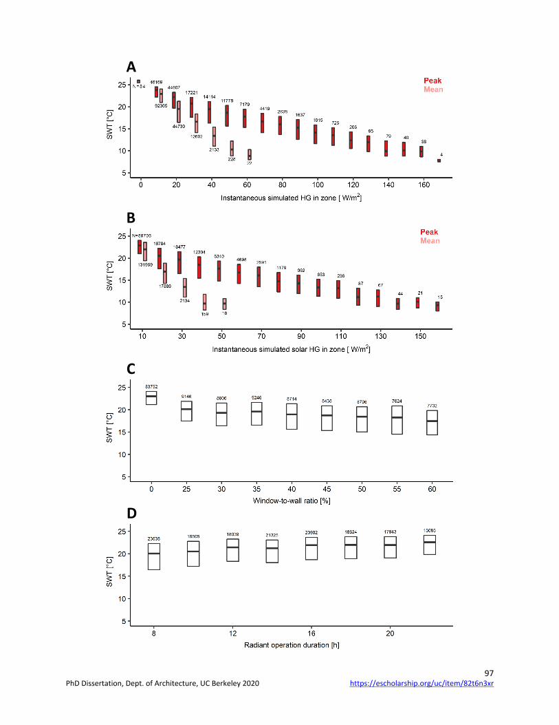
97
A
B
C
D
https://escholarship.org/uc/item/82t6n3xrPhD Dissertation, Dept. of Architecture, UC Berkeley 2020

98
Figure 4-7: Supply water temperature (SWT) as a function of A) instantaneous simulated peak (red) and 24-hour mean (pink) heat gain (HG) rate in zone expected to be extracted by the radiant system, B) solar radiation and convection HG through the window, C) window-to-wall ratio (WWR), and D) radiant system operation duration. A) and B) is binned up in 10-unit intervals, C) 5 units, and D) 2 units. Each boxplot shows the number of simulations in the distribution above or below it.
A
C
E
B
D
F
https://escholarship.org/uc/item/82t6n3xrPhD Dissertation, Dept. of Architecture, UC Berkeley 2020

99
G H
M N
K L
I J
https://escholarship.org/uc/item/82t6n3xrPhD Dissertation, Dept. of Architecture, UC Berkeley 2020

100
Figure 4-8: The effects of various building and high thermal mass radiant system design parameters on supply water temperature (SWT).
Figure 4-9 shows that for most climates, the median SWT for each simulated test case is above the median WBT of the climate on the cooling design day, indicating that there is a large overall potential to design buildings without the energy and cost-intensive refrigeration cycle. The results show that cooling towers or fluid coolers coupled to HTMR have the ability to provide cooling to maintain comfortable temperatures in the space. This is true even when accounting for an approach temperature for the cooling tower with a heat exchanger or fluid cooling of 4 °C. The potential increases if designers focus on utilizing the coldest WBT of the climate for cooled water production and improve the design of the building to reduce HGs in the space. It is no surprise that Houston and Miami have the lowest potential given the high humidity. However, these climates still benefit by using HTMR since, for most of the test cases, SWT above the typical 7.2 °C can be used which will improve the efficiency of the central chiller plant. In fact, 90.3% of the initially created test cases can have SWT at or above 7.2 °C, 84% above 12.8 °C, our steady-state reference temperature, and 67.2% above 18.3 °C which have the greatest compatibility with using a cooling tower for cold water production.
Figure 4-10 shows visualizations and Table 4-5 gives more details on the median of key metrics for simulation test cases with low HG. There are two different ways to define simulated test cases with low HG. Each method has its implications on the design of the building and its radiant system. The first is to limit the 24-hour HG mean. Figure 4-10 A) shows the results of using this method with a limit of 25 W·m-2. The second method is to limit the peak HG. Figure 4-10 B) shows the results of using the alternative approach with a limit of 60 W·m-2. Figure 4-10 and Table 4-5 shows that there is a tradeoff between internal HG and HG rate due to solar radiation that will still accomplish high-temperature cooling. That is, limiting the 24-hour mean allows up to 58% WWR (more solar radiation HG) but with lower internal HG since the 24-hour mean needs to stay at or below the 25 W·m-2 limit. On the other hand, limiting the peak HG to 60 W·m-2 allows for WWR up to about 43% but with the possibility of higher internal HG or for higher SWT through the radiant system.
https://escholarship.org/uc/item/82t6n3xrPhD Dissertation, Dept. of Architecture, UC Berkeley 2020

101
Figure 4-9: Range of supply water temperatures (SWT) to maintain occupant thermal comfort for each climate tested. We compared the models’ final SWT to their respective climates’ May to end of October wet-bulb temperature (WBT). We used the difference, median SWT minus median WBT, to rank the climates. Thus, the climate in Cal-16 has a higher potential to do low energy cooling and climate in Miami the lowest. The red boxplots represent all the results and the green boxplot further subset the data to only simulated test cases with
https://escholarship.org/uc/item/82t6n3xrPhD Dissertation, Dept. of Architecture, UC Berkeley 2020

102
instantaneous sensible heat gains (HG) entering or generated in the zone at 60 W·m-2 or less and WBT and radiant system operation that are between 22:00 and 10:100. The solid and dashed lines are 4 °C above the respective climate’s WBT 75th percentile representing the approach temperature in the cooling tower with a heat exchanger or fluid cooler.
Figure 4-10: Supply water temperature (SWT) as a function of instantaneous simulated peak (red) and 24-hour mean (pink) heat gain (HG) rate in zone expected to be extracted by the radiant system. A) Contains all simulation test cases where 24-hour mean HG is equal to or less than 25 W·m-2. B) Contains all simulation test cases where peak HG is equal or less than 60 W·m-2. Each boxplot shows the number of simulations in the distribution above or below it
A B
https://escholarship.org/uc/item/82t6n3xrPhD Dissertation, Dept. of Architecture, UC Berkeley 2020

103
Table 4-5: Median of key metrics for each peak (red) boxplot distribution in Figure 4-10 for test cases where A) 24-hour mean heat gains (HG) is equal or less than 25 W·m-2 and B) peak HG is equal or less than 60 W·m-2. The HG are the HG entering or generated in the zone that is expected to be extracted by the radiant system. The key metrics are supply water temperature (SWT), radiant system operation duration (Operation), 24-hour mean HG (24h HG), 24-hour mean hydronic cooling plant heat extraction rate (24h plant), mean hydronic cooling plant heat extraction rate when the plant is in operation only (Operation plant), and window-to-wall ratio (WWR).
HG bin | Key metric median
SWT [°C]
Operation [h]
24h HG [W/m2]
24h plant [W/m2]
Operation plant [W/m2]
WWR [%]
A) Test cases with low heat gains where 24-mean HG is equal or less than 25 W·m-2. 10 23.7 16 7.3 5.0 7.5 0 20 22.2 16 13.9 8.0 12.0 0 30 20.7 16 25.3 11.3 17.0 33.1 40 19.5 16 34.7 14.2 21.9 38.3 50 18.7 16 44.6 16.4 24.7 41.4 60 17.9 16 54.6 19.2 28.7 43.4 70 17.1 17 64.8 21.6 31.0 45.0 80 16.7 18 73.4 23.2 31.3 49.2 90 16.6 19 82.7 23.5 28.3 50.6
100 15.4 10 93.3 24.9 59.8 58.4 B) Test cases with low heat gains where peak HG is equal or less than 60 W·m-2.
10 23.8 16 7.3 5.0 7.5 0 20 22.2 16 13.5 8.0 12.0 0 30 20.7 16 25.6 11.3 17.1 33.1 40 19.5 16 34.6 14.2 21.9 38.3 50 18.7 16 44.3 16.4 24.8 41.4 60 17.8 16 54.6 19.3 29.4 43.4
4.3.3. Simplified model development
Duarte et al. (2018) offered simplified models to estimate the SWT for HTMR. We used their random forest model to obtain the starting SWT for each test case model. The dataset in this study provides for a validation exercise of their model. Figure 4-11 shows that Duarte et al. (2018)’s random forest model for predicting SWT are within ± 5 °C for the test cases with TABS and ESS with HG rate up to about 90 W·m-2. The random forest model is conservative for TABS with HG rate up to about 70 W·m-2. The model predicted higher initial SWT than the final SWT for TABS greater than 100 W·m-2 and ESS at all HG rate levels. These trends are not surprising since Duarte et al. (2018)’s models did not use ESS and the maximum HG rate used to train the models was 90 W·m-2. Furthermore, TABS has two active surfaces that extract HG from the zone. It was expected that the model’s SWT estimate for ESS, with only one active surface, resulted in a higher SWT than the lower final SWT found through this study.
https://escholarship.org/uc/item/82t6n3xrPhD Dissertation, Dept. of Architecture, UC Berkeley 2020
104
Figure 4-11: Comparison of initial and final supply water temperature (SWT) in test cases for thermally activated building system (TABS) (dark) and embedded surface systems (ESS) (light). The HG are the HG entering or generated in the zone that is expected to be extracted by the radiant system. However, we estimated the initial SWT using Duarte et al. (2018)'s random forest model using the estimated instantaneous HG before any simulation was performed. The blue dashed line indicated where the estimated SWT and SWT found in this study are equal, i.e. the final minus initial SWT is zero. The solid red lines indicate ± 5 °C.
We developed new linear and nonlinear models that incorporate ESS and the resulting larger range of HG simulated in this study. Equation 4-5, Equation 4-6, Equation 4-7, Equation 4-8, and Equation 4-9 show the training results of the five linear models. We added two more linear models to separate the SWT prediction for TABS (Equation 4-8) and ESS (Equation 4-9) because Equation 4-7 results in low prediction power when incorporating both HTMR types. Where HGmean is the simulated 24-hour mean HG (W·m-2), TD is tube depth (m), TS is tube spacing (m), and FC is the floor covering thermal resistance (m2·K·W-2). The models are for use in SI units. HG are the HG entering or generated in the zone that is expected to be extracted by the radiant system. The simulated peak HG is not a significant variable to predict SWT in the linear models and removing it to develop the linear models did not have adverse performance impacts on the predictions. All other parameters in their respective linear equations were significant, as indicated by a p value of 0.05 or less. The remaining variables used in the linear models also have a low risk of collinearity. The variance inflation factor, or VIF, for each predictor in each of the linear models is less than five, which indicates a low problematic risk of collinearity (James et al. 2013), and most are closer to one. Table 4-6 shows the RMSE and MAE for training and test datasets of the linear and nonlinear models. The similarity of these two metrics between the training and testing datasets indicate a low risk of model overfitting. Figure 4-12 shows visualizations of the prediction performance for the best performing model in each model category. Figure 4-12 A) shows the goodness-of-fit between the simplified model predicted SWT and detailed simulation SWT for data that was not used to develop the models and B) a histogram of the models’ residuals.
https://escholarship.org/uc/item/82t6n3xrPhD Dissertation, Dept. of Architecture, UC Berkeley 2020
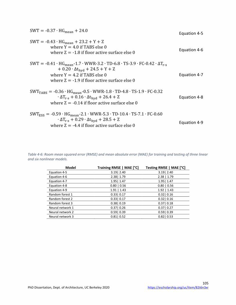
105
SWT = -0.37 ∙ HGmean + 24.0 Equation 4-5
SWT = -0.43 ∙ HGmean + 23.2 + Y + Z where Y = 4.0 if TABS else 0 where Z = -1.8 if floor active surface else 0
Equation 4-6
SWT = -0.41 ∙ HGmean-1.7 ∙ WWR-3.2 ∙ TD-6.8 ∙ TS-3.9 ∙ FC-0.42 ∙ ΔTr-s+ 0.20 ∙ ∆thyd + 24.5 + Y + Z
where Y = 4.2 if TABS else 0 where Z = -1.9 if floor active surface else 0
Equation 4-7
SWTTABS = -0.36 ∙ HGmean-0.5 ∙ WWR-1.8 ∙ TD-4.8 ∙ TS-1.9 ∙ FC-0.32∙ ∆Tr-s + 0.16 ∙ ∆thyd + 26.4 + Z
where Z = -0.14 if floor active surface else 0
Equation 4-8
SWTESS = -0.59 ∙ HGmean-2.1 ∙ WWR-5.3 ∙ TD-10.4 ∙ TS-7.1 ∙ FC-0.60∙ ∆Tr-s + 0.29 ∙ ∆thyd + 28.5 + Z
where Z = -4.4 if floor active surface else 0
Equation 4-9
Table 4-6: Room mean squared error (RMSE) and mean absolute error (MAE) for training and testing of three linear and six nonlinear models.
Model Training RMSE | MAE [°C] Testing RMSE | MAE [°C] Equation 4-5 3.19| 2.40 3.19| 2.40 Equation 4-6 2.38| 1.79 2.38 | 1.79 Equation 4-7 1.95| 1.47 1.95| 1.47 Equation 4-8 0.80 | 0.56 0.80 | 0.56 Equation 4-9 1.91 | 1.43 1.92 | 1.43 Random forest 1 0.33| 0.17 0.32| 0.16 Random forest 2 0.33| 0.17 0.32| 0.16 Random forest 3 0.38| 0.19 0.37| 0.18 Neural network 1 0.37| 0.26 0.37| 0.27 Neural network 2 0.59| 0.39 0.59| 0.39 Neural network 3 0.81| 0.52 0.82| 0.53
https://escholarship.org/uc/item/82t6n3xrPhD Dissertation, Dept. of Architecture, UC Berkeley 2020
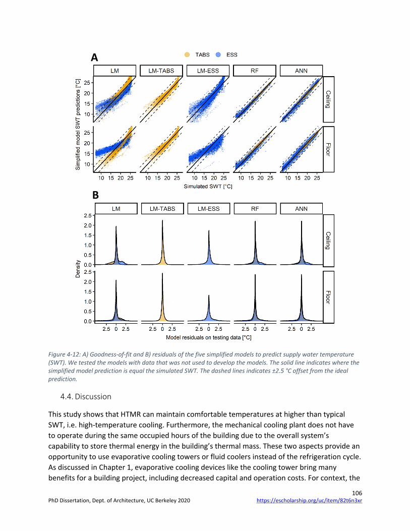
106
Figure 4-12: A) Goodness-of-fit and B) residuals of the five simplified models to predict supply water temperature (SWT). We tested the models with data that was not used to develop the models. The solid line indicates where the simplified model prediction is equal the simulated SWT. The dashed lines indicates ±2.5 °C offset from the ideal prediction.
4.4. Discussion
This study shows that HTMR can maintain comfortable temperatures at higher than typical SWT, i.e. high-temperature cooling. Furthermore, the mechanical cooling plant does not have to operate during the same occupied hours of the building due to the overall system’s capability to store thermal energy in the building’s thermal mass. These two aspects provide an opportunity to use evaporative cooling towers or fluid coolers instead of the refrigeration cycle. As discussed in Chapter 1, evaporative cooling devices like the cooling tower bring many benefits for a building project, including decreased capital and operation costs. For context, the
A
B
https://escholarship.org/uc/item/82t6n3xrPhD Dissertation, Dept. of Architecture, UC Berkeley 2020

107
chiller cost is between $5 and $126 per square meter at a cooling load density of 50 W·m-2. This is sufficiently high that avoiding that initial cost by using a cooling tower plus radiant design is likely a much lower over initial cost option that other more conventional radiant designs.
However, the feasibility of this design option is highly dependent on climate and peak design HG. Miami and Houston climates, where the WBT is too high and in general for climates where WBT is above 21 °C, cooling towers are not going to be very effective at producing the required SWT for cooling on the cooling design day even if designers choose to operate them at night. Yet, these climates benefit from using HTMR since the results in this study show that higher than typical SWT in the central cooling plant can be used, but designers would need to properly control humidity levels during times when the ventilation system is typically turned off in more conventional HVAC systems. One option would be to integrate an air recirculation mode into the DOAS system to avoid condensation in the space. Higher SWT also means more opportunity for waterside economizing throughout much of the year, even in climates like Miami and Houston.
There are other approaches to address cases where it is not feasible to reduce peak design HG rate further. High airspeeds can provide occupant thermal comfort at higher indoor temperatures (Lipczynska et al. 2018; Schiavon and Melikov 2008), which would increase the highest SWT that will still provide a comfortable environment. The elevated airspeeds can also be beneficial in delivering higher convection heat transfer with the surface in the zone during unoccupied hours (Karmann, Bauman, et al. 2018; Pantelic et al. 2018). This will accelerate the cooling of the building’s thermal mass in preparation for the occupied period of the building. The other alternative for challenging weather conditions is to provide a supplemental chiller that can operate alongside the cooling tower (i.e. a waterside economizer) during extreme conditions to further reduce SWT to a value that will meet comfort criteria in the zone.
For most of the climates, the WBT looks favorable to consider an HTMR coupled to a cooling tower or fluid cooler. This is especially true for all core zones, as seen in Figure 4-7 C). The SWT 25th percentile for core zones is greater than 21 °C. This result presents building designers with new hydronic plant design possibilities. For example, core zones can be connected on a separate water loop that only use cooled water produced through cooling towers or connect to the return water from air handling units or the radiant system of the perimeter zones where cooler SWT need to be used due to solar HG. The cooling tower feasibility increase for all test cases, as shown in Figure 4-9, if designers can make two optimizations: 1) design their cooling plant in such a way so that the HTMR can operate during the night, and 2) design their building accordingly to reduce HG generated or entering into the space. In this study, no specific design measures have been taken to minimize cooling loads such as shading, increased insulation, improved glazing, and reduced internal HG rate. More challenging climates will require design strategies that go beyond code requirements to use this approach successfully.
Another important aspect to consider is the control of the system during off-design periods. This paper performed simulations for only the cooling design day of each climate tested. The
https://escholarship.org/uc/item/82t6n3xrPhD Dissertation, Dept. of Architecture, UC Berkeley 2020

108
takeaways from Chapter 3 indicate that the design day performance does not necessarily translate to similar performance for an annual simulation. However, Chapter 3 also indicates that high-temperature cooling performs well in annual simulations. The annual simulation will have different results because the radiant system will not operate the total number of hours designed for an extreme day. Raftery et al. (2017) presented a control strategy for HTMR that can account for different SWT and hours of operation and can adapt to daily HG rate variations. Raftery et al. (2017) is the same adaptive control strategy we used in the model variants to step through the proposed design procedure discussed in Chapter 3. We further discuss the adaptive control’s performance in two existing buildings in Chapter 5.
We developed several simplified linear and nonlinear models to predict SWT using different combinations of parameters. Using more parameters, including the HTMR and active surface type for the linear model training, reduce the RMSE by about 1.2 °C for both training and testing datasets when compared to only using the mean 24-hour HG. As shown visually in Figure 4-12, the linear model incorporating both TABS and ESS types into one model (Equation 4-7) does not perform well. The model has more non-constant variance as lower HTMR SWT is needed. The SWT prediction improves when using separate model for each system type and the variation between the simplified model prediction and simulation is reduced at lower SWT. In general, predicting the SWT for ESS using linear models is more difficult because there is one active surface that behaves differently depending on its construction. TABS uses both surface faces for heat transfer and its average performance is better captured through linear models. The RMSE improves at least another 54% for the testing dataset when using random forest or neural networks nonlinear regression models. All three random forest nonlinear model iterations with a different number of parameters resulted in similar RMSE. On the other hand, using more parameters in the neural network models did not improve the prediction power. A two hidden layer structure for the neural network models did not improve or only slightly improved the accuracy of the predictions. Therefore, we report the models with one hidden layer since the models are less complex. Designers can easily use any of the linear models to estimate SWT requirements to the HTMR early in the design phase of the building. The random forest and neural network models are best used within a tool. The nonlinear models can be downloaded through the following weblink.
Nonetheless, in the early design phase, mechanical designers can use the simplified linear models developed in this chapter to estimate the potential of providing cooling using only a cooling tower in radiant buildings. We recommend designers use Equation 4-8 for TABS and Equation 4-9 for ESS. The models have a 99% and 94% prediction within ±2.5 °C from our testing simulation data for TABS and ESS, respectively, and 95% and 80% prediction within ±1 °C. However, it is important to keep in mind those limitations and to consider the inputs and assumptions that went into creating such models. The input parameter values are reasonable for the detailed energy models that we created to simulate during the design day, but some parameters need further investigation for use during an annual simulation such as the HG schedules. Building occupants play a passive and active role in the energy use of buildings.
https://escholarship.org/uc/item/82t6n3xrPhD Dissertation, Dept. of Architecture, UC Berkeley 2020
109
Deterministic schedules are one way to model occupants’ behavior in energy simulations that affect the HG rate that needs to be removed by the cooling plant. In this study, we used HG schedules that came from the DOE’s large office prototype building model. These HG schedules may be higher than real buildings (Duarte et al. 2013). Thus, it leads to lower SWT estimates in the detailed simulation results and, ultimately, a conservative overall prediction for the SWT in our simplified models.
Moreover, there are only a few parameters that are vaguely linear to the SWT, as shown visually in Figure 4-7 and Figure 4-8, and there are limitations in addressing categorical or cyclical parameters, e.g. zone orientation and radiant system start time. Nevertheless, simplified linear models are easy to develop and report results, and thus the reason we used them in this study. A better approach is to create a nonlinear model that can easily consider the nonlinearities that exist between the data. We used random forests and neural network regression models in this study and the RMSE in the training and testing data was reduced significantly when compared to the linear models. The nonlinear model will need to be implemented into a tool to simplify its use. Regardless of which model designers use, the predicted SWT will need to be compared to the climate’s respective WBT to assess the feasibility of using alternatives to the refrigeration cycle.
4.5. Future work
Future work of this study will investigate the performance of cooling towers in more detail. This study did not directly connect the performance of a cooling tower to the radiant system needs. The results will be different since the cooling tower’s performance limitations are not considered, such as the cooling tower design approach temperature, the difference between SWT and WBT, which is rarely lower than 2 °C, or the potential need for a heat exchanger and the associated difference in temperature incurred. We only used WBT data plus an assumed design approach temperature as a proxy to the potential of using these devices in conjunction with the HTMR for cooling in buildings.
4.6. Conclusions
This study investigates the highest supply water temperature (SWT) provided to high thermal mass radiant system (HTMR) for cooling that maintains comfortable temperatures in a single zone model. The models represent ASHRAE 90.1-2016 and Title 24-2016 code-compliant buildings in 14 US and 16 Californian representative climates during the climates’ cooling design day. We found that the highest SWT to be 18.2, 21.4, 23.4 °C for the first quartile, median, and third quartile, respectively, among all test cases. These higher than typical SWT open the possibility to use cooling towers or fluid coolers in combination with high thermal mass radiant systems to eliminate the refrigeration cycle from the primary cooling system. Cooling towers can generate the required SWT during nighttime periods when wet-bulb temperatures are generally at their lowest. There is great potential to avoid installing a compressor-based
https://escholarship.org/uc/item/82t6n3xrPhD Dissertation, Dept. of Architecture, UC Berkeley 2020

110
refrigeration system, while only a few climates will require more than code compliant and standard design. Building designers can increase the feasibility by limiting heat gains entering or generated inside the space, allowing the HTMR to operate for a more significant fraction in a 24-hour period, designing a thermal activated building system (TABS) for their zones, and using ceiling instead of floor cooling systems.
We developed simple and advanced predictive models that can help designers assess the potential of coupling cooling towers to HTMR. We recommend designers to predict HTMR with Equation 4-8 for TABS and Equation 4-9 for ESS if all the model parameters are known in the early design. Equation 4-5 and Equation 4-6 may be used for TABS is limited parameters are known but should be avoided for ESS systems. Linear models are the easiest to interpret. However, building data contains nonlinearities and alternative models need to be created to improve SWT prediction. The successful implementation of this HVAC system will lower energy needs and greenhouse gas emissions significantly.
4.7. Acknowledgment
This work was supported by the California Energy Commission (CEC) Electric Program Investment Charge (EPIC) (EPC-14-009) “Optimizing Radiant Systems for Energy Efficiency and Comfort”, and the Center for the Built Environment, UC Berkeley, California.
https://escholarship.org/uc/item/82t6n3xrPhD Dissertation, Dept. of Architecture, UC Berkeley 2020
111
5. Energy and thermal comfort assessment of a new control strategy for high thermal mass radiant systems
5.1. Background
Heating, ventilation, and air-conditioning (HVAC) systems rely on control sequences implemented at the individual component, subsystem, and whole system level to achieve building stakeholder defined performance metrics that include energy efficiency, energy cost-effectiveness, and maximized occupant comfort. Improved HVAC control can yield energy savings of 7 to 35% and cost savings of 2 to 40% (S. Wang and Ma 2008; Alajmi 2012; Raftery et al. 2017; Pang et al. 2018). On the other hand, improper control and other control related faults can have an energy penalty up to 21.8%, depending on the severity of the malfunction (Z. Ma and Wang 2011). The majority of buildings incorporate the basic on-off control functionality into its HVAC systems but advances in direct digital controls (DDC) have increased the proportion of buildings that implement more sophisticated control systems such as automatic control systems that use proportional, proportional-integral (PI), and proportional-integral-derivative (PID) feedback loop control (Roth et al. 2005). However, the PID feedback control scheme increases complexity and commissioning efforts and it often does not improve HVAC control rendering it useful to limited HVAC applications (Sellers 2001, 2003; Ang et al. 2005). These classical control processes are set up to take corrective action and have been proven to be adequate for HVAC systems that respond quickly to control actions such as all-air systems and metal ceiling radiant panels. More research is needed to identify if and how classical controls process can be implemented in high thermal mass radiant (HTMR) systems in a generalizable format, i.e. without excessive manual tuning.
Model predictive control (MPC) is the current state of the art control methodology that can systematically estimate future disturbances while providing a mechanism to prevent violations in system constraints (Y. Ma 2012; Afram and Janabi-Sharifi 2014). Thus, it takes preventive action instead of correcting deviations from setpoints and is suitable for slow-moving HVAC processes with time delays such as those found in HTMR (Afram and Janabi-Sharifi 2014; Pang et al. 2018). The challenge then becomes in developing simple, yet representative models since the decision space grows exponentially with each additional state variable (Váňa et al. 2014; Zakula et al. 2015; Feng et al. 2015). Hence significantly increasing the computational time for complex models with the possibility of rendering them intractable for finding optimal control solutions. In addition, current industry practice building energy management systems (EMS) do not have the functionality to implement MPC and building control contractors and operators, in general, do not have the expertise to program and maintain such control systems. For these reasons, MPC has mainly stayed confined to the research phase within the building industry.
As mentioned in Chapter 2, HTMR has high thermal inertia where the effects of running chilled water through the slab will take several hours before there is a noticeable effect to the
https://escholarship.org/uc/item/82t6n3xrPhD Dissertation, Dept. of Architecture, UC Berkeley 2020

112
occupants (Babiak et al. 2009; Ning et al. 2017). Thus, it is important to consider the thermal inertia when determining HTMR’s control settings to extract the necessary heat gains of the building at the correct time to achieve acceptable thermal comfort. Building operators need to strike a balance in HTMR operation to avoid overcooling or undercooling the slab which will cause occupant thermal discomfort and any immediate control actions to the HTMR to correct such deviations will prove futile. Researchers have studied various model-free and rule-based control methods for HTMR for easy implementation in current building industry EMS that include the following (Weitzmann 2004; Tödtli et al. 2005; Romaní et al. 2016):
• Control of the supply or average water temperature based on indoor or outdoor temperature dependent cooling curves (Olesen 2007; Lim et al. 2014; Sourbron and Helsen 2014)
• Control of the supply or average water temperature to a constant value (Olesen et al. 2002; Chung et al. 2017)
• Control based on indoor temperature feedback (Olesen 1997; Cho and Zaheer-uddin 1999; Sourbron et al. 2009; Raftery et al. 2017)
• Cooling plant on during the night and off during the day to pre-cool the radiant slab before occupancy (Rijksen et al. 2010; Raftery et al. 2012)
• Intermittent (pulse) control (Gwerder et al. 2009; Tang et al. 2018)
The water flow rate is typically maintained at a constant value in the various control methods mentioned above. Variable flow rate control methods using proportional valves are also used in radiant system controls but have limited cooling capacity control, low control precision at low flows, and modulating valves have higher costs (Tang et al. 2018). Other limitations on current radiant system controls include excessive manual tuning for each building may be necessary for control schemes that rely on a cooling curve that is dependent on indoor and/or outdoor environmental conditions. Not only does occupant behavior change on a short term basis (Duarte et al. 2013; Gunay et al. 2016), but it also changes on a long term basis with tenant turnover, work schedule, equipment needs, and equipment energy efficiency. Also, not all buildings respond to outdoor conditions in the same way. Proponents of controlling HTMR to a constant supply water temperature, usually water temperature close to acceptable indoor air conditions, indicate that this method results in a high degree of self-control, or self-regulation, since a small change in the temperature difference between the zone and the active surface temperatures will significantly influence the heat transfer in the radiant system (Olesen et al. 2002; Chung et al. 2017). Although this method limits the overall heat extraction capacity of HTMR and cannot handle large heat gain variations (de Wit and Wisse 2012). Thus, it is necessary to continue the research for effective HTMR control that does not burden the current building industry EMS and operators and control contractors’ skill set.
https://escholarship.org/uc/item/82t6n3xrPhD Dissertation, Dept. of Architecture, UC Berkeley 2020

113
In this chapter, we discuss the development, implementation, and analysis of a new control strategy for HTMR that is model-free and can easily be implemented in the current building industry EMS. We implemented the new control strategy in two HTMR buildings located in two different climates in California. We also performed a general thermal comfort evaluation in both buildings and a more detailed evaluation with a limited number of occupants in one of the buildings of the field study.
5.2. Methods
5.2.1. Field study building descriptions
5.2.1.1. David Brower Center Building
The David Brower Center (DBC) Building, shown in Figure 5-1, is a LEED Platinum, four-story mixed-use building located in downtown Berkeley, California. DBC’s program consists of private and open plan offices, conference rooms, an auditorium, a restaurant, and a gallery with 3,590 m2 and 307 m2 of conditioned and unconditioned area, respectively. The restaurant, auditorium, and gallery are located on the first floor and office spaces are mainly on floors two through four. The building’s main tenants are nonprofit environmental organizations with a current total building occupancy of about 150 people.
Figure 5-1: David Brower Center Building's east and south façades. Image credit Tim Griffith.
https://escholarship.org/uc/item/82t6n3xrPhD Dissertation, Dept. of Architecture, UC Berkeley 2020

114
5.2.1.1.1. DBC site climate
Berkeley, California is located in California Climate Zone 3 and ASHRAE climate 3C. It is characterized by moderate temperatures year-round with dry summers and wet winters. Average high temperatures throughout the year range from 14.7 to 23.9 °C and the average low temperatures range from 5.6 to 12.2 °C. The 99% winter design day has an outdoor dry-bulb air temperature of 1.1 °C and 1% summer design day of 29.4 °C with relative humidity of 64%.
5.2.1.1.2. Building envelope
DBC has its longest façades oriented towards the north-south with a window-to-wall ratio (WWR) average of 42%. The highest WWR percentage is on the north façade with 54% and the lowest on the west façade with 6%. Skylights make up about 2% of the gross roof area. The external glazing includes operable windows at both low and high levels to allow occupants direct control of thermal conditions as well as fresh air. The external glazing has an area-weighted average U-factor of 3.18 W·m-2·K, area-weighted average solar heat gain coefficient (SHGC) of 0.37, fixed external shading devices, and adjustable indoor blinds to control solar heat gains. The exterior surfaces have an area-weighted average U-factor of 1.08, 0.182, and 0.352 W·m-2·K for the walls, roof, and ground floor, respectively. The roof includes a photovoltaic array for electricity production.
5.2.1.1.3. Heating, ventilation, and air-conditioning system
5.2.1.1.3.1. Zone level
The heating, ventilation, and air-conditioning (HVAC) system includes a thermally activated building (TABS) radiant system for the primary heating and cooling in the office spaces. A 100% outdoor air underfloor air distribution (UFAD) system, as well as natural ventilation through operable windows provides ventilation to the building. Carbon dioxide (CO2) sensors are used to provide demand-controlled ventilation to the occupied spaces. The first floor heating and cooling requirements are met with seven water-to-air heat pumps. The first floor does not use a radiant system. An eighth heat pump located on the second floor is used to provide heating and cooling to a large conference meeting room, which also does not use a radiant system.
There are three perimeter and two core radiant zones on each floor for a total of 15 radiant zones in DBC. The smallest zone is about 135 m2 while 232 m2 for the largest. Figure 5-2 shows a typical floor plan with the radiant zones outlined with black dashed lines. The ventilation zones are separated into two zones per floor: east and west zones split at the elevator shaft. Floors two through four have the same radiant and ventilation zone layouts. The radiant zones use a ceiling TABS system where the ceiling surface provides most of the thermal heat transfer to occupants and the zones’ contents. Figure 5-3 shows a cross-section of a typical zone in DBC and the TABS system construction. Radiant zone X-2 is on the north side perimeter, X-4 on the south side perimeter, X-5 on the east side perimeter, X-3 on the west side core, and X-6 on the
https://escholarship.org/uc/item/82t6n3xrPhD Dissertation, Dept. of Architecture, UC Berkeley 2020

115
east side core. The “X” designates the floor number. Each radiant zone has a single thermostat and a slab temperature sensor embedded within the slab structure. Figure 5-2 shows the locations of the thermostats on the second floor. Each floor has different thermostat locations within its zone. We were not able to confirm the locations of the slab temperature sensors. Figure 5-2 also shows tenant-occupied space layout and each suite is designated with a different color. Refer to Figure B-1 in Appendix B to see the floor layouts of floors two and three. We use the same color scheme in the other floor layouts but do not represent the same tenant.
A single two-position (open/close) valve to one or two manifolds controls the water flow to each radiant zone. The number of loops for each zone ranges from four to nine loops (Table 5-1). The perimeter south radiant zones have the highest number of loops (9 loops). Figure 5-4 shows a pair of manifolds for radiant zones 2-3 and 4-4. The valve controlling the water flow is located on the return side of the manifold.
Figure 5-2: Radiant zone and space layout for third floor in DBC. The radiant zones are outlined with black dashed lines. There is one thermostat per radiant zone. The space layouts are designated with color. The radiant zones are the same on floors two and four. However, the space layouts on the other two floors are different. We applied the new control strategy to all radiant zones of DBC during the intervention time frame.
Table 5-1: Number of loops (B) and manifolds (C) for each radiant zone (A) in DBC. The mechanical plans specify 5/8 in (0.0159 m) nominal PEX tubing diameter with a maximum loop length of 114.3 m. We were unable to verify actual specifications for tubing diameter and loop length.
A 2-2 2-3 2-4 2-5 2-6 3-2 3-3 3-4 3-5 3-6 4-2 4-3 4-4 4-5 4-6 B 8 7 9 4 5 8 5 9 4 5 8 5 9 4 5 C 1 1 2 1 1 1 1 2 1 1 1 1 2 1 1
https://escholarship.org/uc/item/82t6n3xrPhD Dissertation, Dept. of Architecture, UC Berkeley 2020
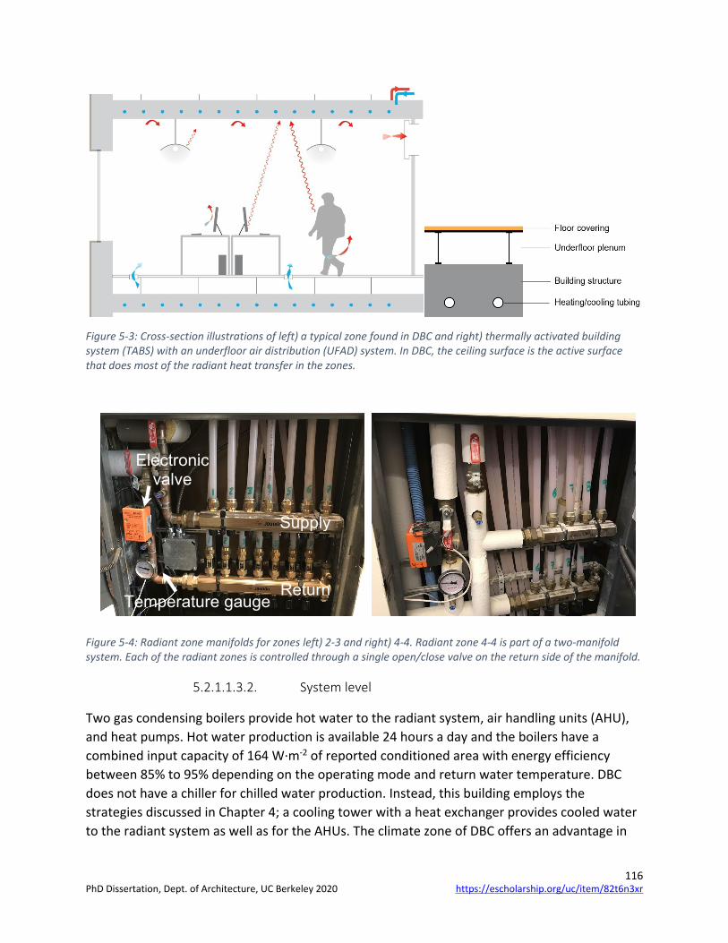
116
Figure 5-3: Cross-section illustrations of left) a typical zone found in DBC and right) thermally activated building system (TABS) with an underfloor air distribution (UFAD) system. In DBC, the ceiling surface is the active surface that does most of the radiant heat transfer in the zones.
Figure 5-4: Radiant zone manifolds for zones left) 2-3 and right) 4-4. Radiant zone 4-4 is part of a two-manifold system. Each of the radiant zones is controlled through a single open/close valve on the return side of the manifold.
5.2.1.1.3.2. System level
Two gas condensing boilers provide hot water to the radiant system, air handling units (AHU), and heat pumps. Hot water production is available 24 hours a day and the boilers have a combined input capacity of 164 W·m-2 of reported conditioned area with energy efficiency between 85% to 95% depending on the operating mode and return water temperature. DBC does not have a chiller for chilled water production. Instead, this building employs the strategies discussed in Chapter 4; a cooling tower with a heat exchanger provides cooled water to the radiant system as well as for the AHUs. The climate zone of DBC offers an advantage in
2 4
Supply
Return
Electronic valve
Temperature gauge
https://escholarship.org/uc/item/82t6n3xrPhD Dissertation, Dept. of Architecture, UC Berkeley 2020
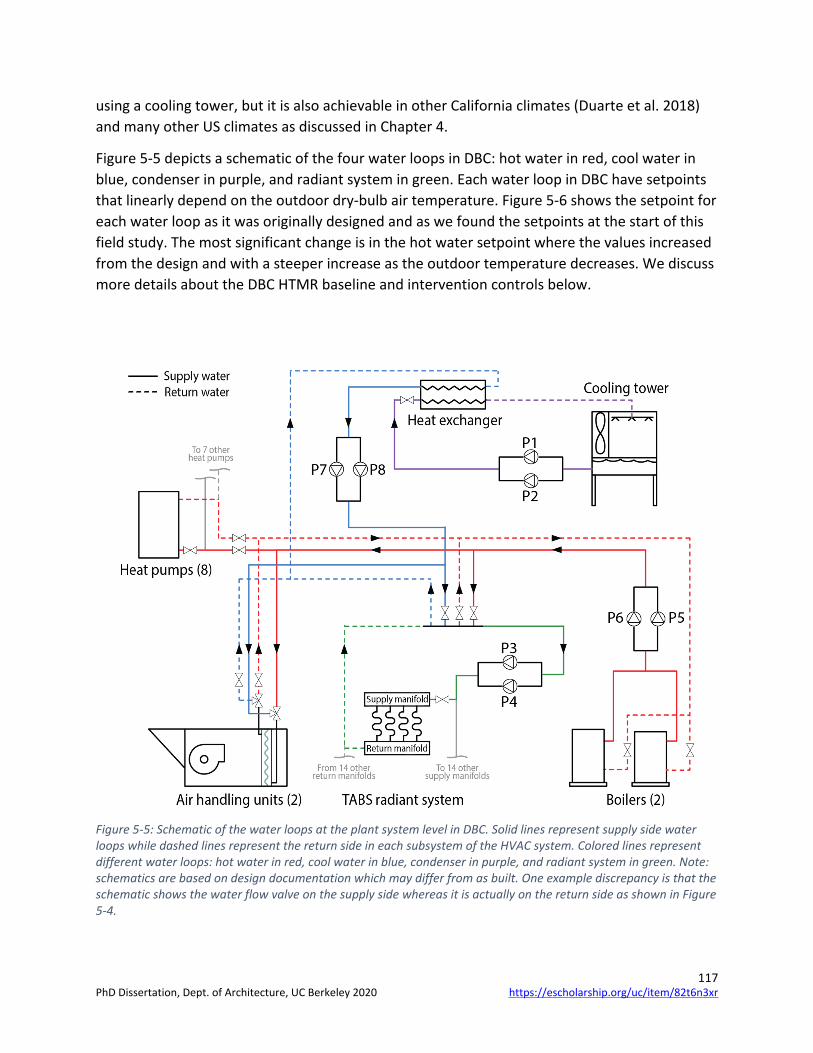
117
using a cooling tower, but it is also achievable in other California climates (Duarte et al. 2018) and many other US climates as discussed in Chapter 4.
Figure 5-5 depicts a schematic of the four water loops in DBC: hot water in red, cool water in blue, condenser in purple, and radiant system in green. Each water loop in DBC have setpoints that linearly depend on the outdoor dry-bulb air temperature. Figure 5-6 shows the setpoint for each water loop as it was originally designed and as we found the setpoints at the start of this field study. The most significant change is in the hot water setpoint where the values increased from the design and with a steeper increase as the outdoor temperature decreases. We discuss more details about the DBC HTMR baseline and intervention controls below.
Figure 5-5: Schematic of the water loops at the plant system level in DBC. Solid lines represent supply side water loops while dashed lines represent the return side in each subsystem of the HVAC system. Colored lines represent different water loops: hot water in red, cool water in blue, condenser in purple, and radiant system in green. Note: schematics are based on design documentation which may differ from as built. One example discrepancy is that the schematic shows the water flow valve on the supply side whereas it is actually on the return side as shown in Figure 5-4.
https://escholarship.org/uc/item/82t6n3xrPhD Dissertation, Dept. of Architecture, UC Berkeley 2020
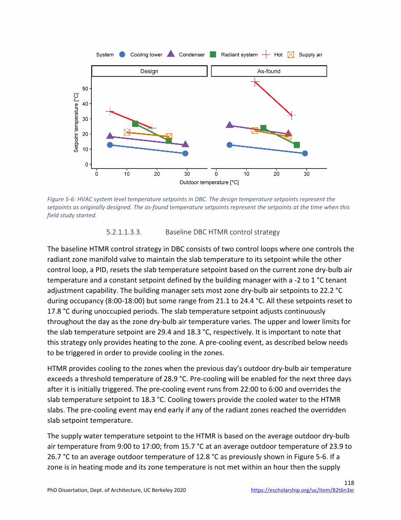
118
Figure 5-6: HVAC system level temperature setpoints in DBC. The design temperature setpoints represent the setpoints as originally designed. The as-found temperature setpoints represent the setpoints at the time when this field study started.
5.2.1.1.3.3. Baseline DBC HTMR control strategy
The baseline HTMR control strategy in DBC consists of two control loops where one controls the radiant zone manifold valve to maintain the slab temperature to its setpoint while the other control loop, a PID, resets the slab temperature setpoint based on the current zone dry-bulb air temperature and a constant setpoint defined by the building manager with a -2 to 1 °C tenant adjustment capability. The building manager sets most zone dry-bulb air setpoints to 22.2 °C during occupancy (8:00-18:00) but some range from 21.1 to 24.4 °C. All these setpoints reset to 17.8 °C during unoccupied periods. The slab temperature setpoint adjusts continuously throughout the day as the zone dry-bulb air temperature varies. The upper and lower limits for the slab temperature setpoint are 29.4 and 18.3 °C, respectively. It is important to note that this strategy only provides heating to the zone. A pre-cooling event, as described below needs to be triggered in order to provide cooling in the zones.
HTMR provides cooling to the zones when the previous day’s outdoor dry-bulb air temperature exceeds a threshold temperature of 28.9 °C. Pre-cooling will be enabled for the next three days after it is initially triggered. The pre-cooling event runs from 22:00 to 6:00 and overrides the slab temperature setpoint to 18.3 °C. Cooling towers provide the cooled water to the HTMR slabs. The pre-cooling event may end early if any of the radiant zones reached the overridden slab setpoint temperature.
The supply water temperature setpoint to the HTMR is based on the average outdoor dry-bulb air temperature from 9:00 to 17:00; from 15.7 °C at an average outdoor temperature of 23.9 to 26.7 °C to an average outdoor temperature of 12.8 °C as previously shown in Figure 5-6. If a zone is in heating mode and its zone temperature is not met within an hour then the supply
https://escholarship.org/uc/item/82t6n3xrPhD Dissertation, Dept. of Architecture, UC Berkeley 2020

119
water temperature setpoint is overridden to 32.2 °C for an hour. This condition might be too aggressive since HTMR contains a substantial amount of thermal mass that needs to be heated up. The rate at which the thermal mass heats up is typically between 0.56 to 1.1 °C per hour. During a pre-cooling event, the supply water temperature setpoint is overridden to 15.6 °C.
We collected data on the baseline control strategy from August 20, 2016 through October 31, 2016. We refer to this time frame as the “DBC-baseline” period throughout this chapter.
5.2.1.2. Sacramento Municipal Utility District East Campus Office Building
The Sacramento Municipal Utility District (SMUD) East Campus Office Building, shown in Figure 5-7, is an 18,600 m2 LEED Platinum, single tenant office building located in Sacramento, California. SMUD is part of a 51-acre campus that includes a diverse set of building types and uses. It has five above-ground floors and one underground. Its program consists of private and open plan offices, conference rooms, a cafeteria, a gym, an assembly space for trainings, and a large unconditioned storage space for utility vehicles. The building houses 750 employees with a capacity of up to 900 occupants.
Figure 5-7: Sacramento Municipal Utility District East Campus Office Building’s north and west façades. Image credit HRGA Architecture.
5.2.1.2.1. SMUD site climate
Sacramento, California is located in California Climate Zone 12 and ASHRAE climate 3B. It is characterized by warm and dry summers and cool and dry winters. Sacramento is located near a junction of two major rivers which help maintain moderate temperatures year-round. The average high temperatures throughout the year range from 12.1 to 33.4 °C and average low
https://escholarship.org/uc/item/82t6n3xrPhD Dissertation, Dept. of Architecture, UC Berkeley 2020
120
temperature range from 3.8 to 14.7 °C. The 99% winter design day has an outdoor dry-bulb temperature of 0.94 °C and 1% summer design day of 36.6 °C with relative humidity of 23.6%.
5.2.1.2.2. Building envelope
SMUD has its longest façades oriented towards the north-south with an overall WWR of less than 25%. The building’s envelope is a high thermal mass envelope composed of light-reflecting concrete. Thus, the envelope reduces heat gains through two mechanisms: 1) the high heat storage capacity of the concrete absorbs heat with a slow rate of change in its temperature and 2) the light-reflecting property reflects incoming shortwave solar radiation. The north and south walls are constructed of thermally massive sandwich panels with a thermal break: 0.0762 m concrete, 0.0508 m insulation, and 0.1016 m concrete, listed from outside to inside. The east and west walls do not include the insulation layer. The roof is also highly insulated and includes a reflective surface to manage solar radiation. The south glazing includes a shading device divided into a lower part with a fixed direction grid to allow the view to the outdoors while blocking solar heat gains and an upper section with fixed louvers that bounces daylight onto the ceiling for distribution deep within the space. The building does not include operable blinds or operable windows, and the north glazing does not include shading devices.
5.2.1.2.3. Heating, ventilation, and air-conditioning system
5.2.1.2.3.1. Zone level
SMUD also uses a TABS system for its primary heating and cooling system on the majority of its floor area but also contains embedded surface systems (ESS) in each of the floor’s corners. A dedicated outdoor air system (DOAS) with overhead mixing diffusers provides demand-controlled ventilation. The building’s conference rooms contain active chilled beams that simultaneously provide cooling and ventilation needs. The active chilled beams are well suited for the intermittent and potential high-density occupancy patterns observed in conference rooms. Figure 5-8 shows the radiant and space layout and the type of HVAC system used on the two floors we implemented the new control strategy interventions during our field study. The radiant zones where we implemented the intervention control strategy are between 74 and 124 m2 and grouped by orientation using a 2-pipe system which requires all radiant zones on one orientation to be in the same heating or cooling mode. North and south perimeter zones use TABS with heating and cooling, but the TABS core zones only provide cooling to the zones i.e. does not contain changeover piping. In addition, the open plan office spaces incorporate ceiling fans to aid with thermal comfort (Tanabe et al. 1993). The HTMR system uses 5/8 in (0.0159 m) or 1/2 in (0.127 m) nominal PEX tubing diameter installed 0.0508 m from the ceiling surface in a 0.254 m concrete slab. There are temperature sensors embedded in the concrete slab, but we were unable to identify their depth. The ceiling surface is almost fully exposed with no drop ceiling or acoustical clouds. However, acoustical panels that are mounted vertically provide little obstruction to radiant exchange. Dominguez et al. (2017) and Karmann et al.
https://escholarship.org/uc/item/82t6n3xrPhD Dissertation, Dept. of Architecture, UC Berkeley 2020

121
(2017) discuss the impact of vertical and horizontal acoustical panels on radiant system heat transfer. Figure 5-9 shows the typical open plan office layout in SMUD with the different features as discussed above.
Figure 5-8: Radiant zone and space layout for SMUD floors top) two and bottom) three; the only two floors we applied the new control strategy for this field study. The space color designates the type of HVAC system installed in the two floors. Thermally activated building systems (TABS) are installed in the north and south perimeter and core zones, embedded surface systems (ESS) in the floors’ corners, and active chilled beams in conference rooms. TABS core radiant zones only provide cooling to the spaces. The orange and purple outline designates the type of lockouts we used in SMUD for the new control strategy which is described further in Section 5.2.2.1.2.
https://escholarship.org/uc/item/82t6n3xrPhD Dissertation, Dept. of Architecture, UC Berkeley 2020

122
Figure 5-9: Typical open plan office space with TABS radiant ceiling, ventilation ducts, acoustical baffles, and ceiling fans.
5.2.1.2.3.2. System level
A central plant with gas boilers and chillers provides hot and cold water production, respectively, for the HTMR, DOAS, and chilled beam systems in SMUD. The central plant also serves other buildings of the campus that contain traditional all-air variable air volume (VAV) HVAC terminal systems. Thus, the outgoing water temperatures from the central plant must remain high (~43.3 °C) for heating and low (~7.2 °C) for cooling. Therefore, the central plant’s supply water is mixed with return water to supply more moderate temperatures to the HTMR with resulting mixed temperatures of 35 °C for heating and 16.7 °C for cooling. The mixing reduces most of the energy efficiency from having a high-temperature cooling and low-temperature heating system installed at the zone level. The central plant also incorporates horizontal geothermal ground heat exchange and thermal energy storage (TES) systems. The geothermal system can directly provide cool water to the HTMR, but it only works well from November to December for heating and during April for cooling. The TES system uses a 75,700 L water storage tank. The water for the tanks is chilled during off-peak hours and stored at 7.8 °C. The TES system is mainly used for the active chilled beams and other HVAC terminal systems on the campus that generally require the use of low supply water temperatures.
As stated above, the HTMR in SMUD uses a 2-pipe system grouped by orientation i.e. all zones in one orientation on all floors must be in the same mode. Mixing valves and variable frequency drive (VFD) controlled pumps with a differential pressure setpoint regulate supply water temperatures to each group. There are three control groups for the HTMR: north, south, and core. Thus, simultaneous heating and cooling on the same floor is possible. Net cooling or heating calls determine the mode of the group in the baseline control strategy. We discuss more details about the SMUD HTMR baseline and intervention controls below.
https://escholarship.org/uc/item/82t6n3xrPhD Dissertation, Dept. of Architecture, UC Berkeley 2020

123
5.2.1.2.3.3. Baseline SMUD HTMR control strategy
5.2.1.2.3.3.1. As designed control strategy
The existing HTMR control strategy at the start of this field study reflects changes that occurred in a previous Center for the Built Environment (CBE) field study in 2014 (Bauman et al. 2015). The originally designed control strategy implemented a variable water flow, constant supply water temperature scheme. The supply water temperature was set at 14.4 °C with adjustment to avoid condensation. The water flow is linearly dependent on the zone dry-bulb air temperature where the water flow is 100% of the design flow at the defined setpoint and 0% at a 1.1 °C offset from the setpoint. The cooling setpoint was set at 23.9 °C and 20.6 °C for heating. Thus, water flow is 0% between 21.7 and 22.8 °C which is a quite narrow band within which the radiant system is free-floating. The narrow free-floating band frequently led to heating in the morning followed by cooling in the afternoon on the same day causing significant energy waste and comfort issues. In most cases, only cooling would have been necessary or no water flow to maintain zones within comfort temperatures during occupancy (5:30-17:30). The embedded slab temperature sensors are not used in the baseline control strategy. In current industry practice, most designers reported to measure slab temperature but only half reported to explicitly use slab temperature sensors to reset the slab temperature setpoints in their HTMR control strategies (Paliaga et al. 2017).
5.2.1.2.3.3.2. First control intervention in 2014
The previous field study made modifications to the original control strategy to resolve deficiencies. The modifications below were the starting point for this field study on HTMR control sequences. The research team were constrained by the onsite Siemens expertise to only make changes to dry-bulb air temperature setpoints or to the schedule, with or without an outside dry-bulb air dependent reset. The building operators may have tuned the modifications for each zone as needed. The three primary modifications were the following:
1. Water flow now started at the zone dry-bulb air temperature setpoint and linearly increases as more extreme temperatures are measured in zones. For example, in cooling, the water flow is 0% at 23.9 °C and 100% of the design water flow at 25 °C. The same 1.1 °C offset remained. The modification resolved issues with same-day heating and cooling.
2. Implementation of a 2.8 °C setback from 17:00 to 2:00 to the temperature setpoints based on indoor dry-bulb temperature to control when HTMR operation should occur. For example, in cooling, the 2.8 °C setback would help prevent overcooling and shift chiller plant operation to avoid high electricity costs while also increasing the plant’s efficiency.
3. Implementation of a more aggressive pre-cooling event triggered by lower daily average outdoor dry-bulb air temperature the previous day. If the event is triggered,
https://escholarship.org/uc/item/82t6n3xrPhD Dissertation, Dept. of Architecture, UC Berkeley 2020

124
the nighttime slab temperature setpoints decrease linearly from 26.8 to 22.9 °C between 19:00 to 2:00 and returning to normal 23.9 °C setpoint at 9:00.
Please refer to the report for more details on the control strategy modifications (Bauman et al. 2015). We used the resulting control strategy after the modifications as the baseline control strategy, which is already significantly improved from the original operation, to compare against the new control strategy interventions in this field study. We collected data on the baseline control strategy from June 4, 2017 through November 9, 2017. We refer to this time frame as the “SMUD-baseline” period throughout this chapter.
5.2.2. Intervention control strategy
The intervention control strategy implemented in both DBC and SMUD in these field studies consists of two control loops, as shown schematically in Figure 5-10. The primary control loop controls the water flow rate to maintain the slab temperature at its setpoint. A secondary cascading control loop uses a proportional controller to reset the slab temperature setpoint on a daily basis. One important difference between the baseline and the intervention control strategies is that the slab temperature setpoint is reset only once per day at the end of occupancy of the building for the new control strategy whereas the slab temperature setpoint is adjusted continuously in the baseline control strategies of both field study buildings through the day to meet the required zone dry-bulb air temperature setpoints. The secondary control loop of the intervention strategy resets the slab temperature setpoint using the error between the maximum/minimum zone dry-bulb air temperature during the preceding occupied hours and the comfort setpoint for cooling/heating. The intervention HTMR control strategy intends to slowly adjust slab temperature setpoints based on information from the radiant zone, e.g. zone air and slab temperature. While also accounting for the expected daily zone temperature variation, as opposed to controlling the radiant system to a constant temperature setpoint as initially designed for DBC. For this field study, there was no control differences between holidays and weekend days.
We implemented two variations of the controller of the primary control loop, outlined in green in Figure 5-10, in each of the field study buildings. DBC uses a simple on/off controller and SMUD uses a pulse flow modulating (PFM) controller (Tang et al. 2018). The on/off controller opens the zone manifold valve when the current zone slab temperature is above the setpoint in cooling mode or the current zone slab temperature is below the setpoint in heating mode. The PFM controller fully opens the manifold valve for five minutes (approximately the length of time required to flush all the water in a PEX circuit loop at the design flow rate) and then closes for a period determined by a proportional band. The water flow pulses increase as the current slab temperature deviates further from the slab temperature setpoint. This approach allows for better control at low flow conditions than modulation valves and reduces pumping power (Tang
https://escholarship.org/uc/item/82t6n3xrPhD Dissertation, Dept. of Architecture, UC Berkeley 2020

125
et al. 2018). It also allows for reduced installation costs for valve and wiring a new construction project.
Figure 5-10: Schematic diagram of controller tested in DBC and SMUD buildings in cooling mode. The same approach applies in heating mode but using the minimum instead of the maximum zone indoor dry-bulb air temperature and using the heating instead of the cooling comfort setpoint. DBC uses an on/off controller in the primary control loop and SMUD uses a pulse flow modulation controller (Tang et al. 2018).
The intervention HTMR control strategy also allows the building operator to select a time interval to remove heat from the slab. The strategy constrains the radiant system to take advantage of the thermal inertia inherent in these types of systems and operate the water flow within the slab only during certain predetermined periods of the day. The building operator (or designer) can select from several options:
• More efficient operating hours e.g. nighttime hours in cooling mode
• Lower energy cost hours e.g. nighttime or other off-peak hours for electric heating/cooling systems
• Hours that avoid affecting the building’s peak electricity demand e.g. radiant system is off from 10:00 to 19:00
• Longer operating hours to reduce the chiller or other plant heating/cooling design capacity or maximum load e.g. greater than 12 hours
• Stagger the timing of available periods for different zones in the building throughout the 24-hour period to reduce plant design capacity e.g. zones A, B, C operate from 0:00 to 12:00, zones D, E, F operate from 6:00 to 18:00, zone G, H, I from 12:00 to 0:00, and zones J, K, L from 18:00 to 6:00. This could also be coordinated with the heating/cooling requirements of other systems served by the same plant e.g. the DOAS system.
• Provide a more uniform daily range of comfort conditions by timing the conditioning of the slab such that it approximately coincides with the peak space heating/cooling loads, with a lead time of approximately 3-4 hours (Raftery et al. 2017).
https://escholarship.org/uc/item/82t6n3xrPhD Dissertation, Dept. of Architecture, UC Berkeley 2020

126
We evaluated an early iteration of the intervention control strategy with the on/off controller in the primary control loop using detailed whole building energy simulation (Raftery et al. 2017). We varied the supply water temperature and operation period for TABS and ESS systems. The results show that the intervention control strategy can reduce electricity cost and energy consumption by up to 40% and 35%, respectively, when compared to typical on/off controller based on fixed zone dry-bulb air temperature setpoints. We also used the intervention control strategy in Chapter 3 to evaluate the implications of calculating the cooling load through the industry standard procedure and our proposed revisions. Building designers can also download the sequences of operation used in this field study for control contractor’s use or to evaluate its performance in custom EnergyPlus building models (http://radiant.cbe.berkeley.edu/resources).
5.2.2.1. Implementation and initialization
5.2.2.1.1. DBC building
In DBC, we selected to operate the HTMR with a pre-cooling strategy during nighttime hours (22:00 to 10:00) since DBC’s cooling plant is a cooling tower. The cooling tower is more effective at producing cool water during the night when the outdoor wet-bulb temperatures are the lowest, as described in Chapter 4. The supply water temperature setpoint to the HTMR is overridden to 15.6 °C during a cooling call in the radiant zone. However, the actual supply water temperature will highly depend on the weather conditions at the time when zones call for cooling. For heating, the supply water temperature maintains the same linear relationship to the outdoor dry-bulb air temperature as in the baseline control strategy described above.
We connected a small fanless PC to DBC’s network infrastructure that allowed us to communicate with the building’s EMS. DBC’s EMS system uses the BACnet communications protocol (Bushby 1997; ASHRAE 2016c). We used the Simple Measurement and Actuation Profile (sMAP) along with BACpypes software to develop a polling program that collects EMS data points at three-minute intervals through BACnet and archives it for future data analysis. sMAP is an open source software program developed by UC Berkeley’s Electrical Engineering and Computer Sciences department to store and access time series data (Dawson-Haggerty et al. 2010). BACpypes provides the BACnet application and network layer to communicate with the building’s EMS (Bender 2018).
We also used the software tools mentioned above to implement the intervention HTMR control strategy. We slowly began rolling out the intervention control to three zones with no manifold valve actuation to test the control calculations and sequences and reveal any issues. Then, we enabled manifold valve control to only one zone to decrease the risk of causing discomfort that may arise from problems in the intervention control strategy. We rolled out to more zones as we determined that the intervention control strategy performed as expected. The intervention control strategy had full control of all zones’ manifold valves by August 9, 2018.
https://escholarship.org/uc/item/82t6n3xrPhD Dissertation, Dept. of Architecture, UC Berkeley 2020

127
We use the time frame from August 20, 2018 through October 31, 2018 to evaluate the performance of the intervention against the DBC-baseline control strategy. We refer to the intervention time frame for DBC as “DBC-intervention” throughout this chapter. We use a later date than the actual start of the intervention control to remove data during initialization. We also remove data where the new control strategy's program suddenly stopped functioning. The typical occupied hours for DBC are from 8:00 to 18:00. The building operator implements a hot water system lockout when the 24-hour average outdoor dry-bulb air temperature is 18.3 °C or above during the intervention time frame. We initialized the slab temperature setpoints in all DBC radiant zones to 21.1 °C, the lower thermal comfort limit. We limit the slab temperature setpoint to vary between 18.8 to 23.9 °C. Table 5-2 lists all relevant parameters for the intervention HTMR control strategy implemented in DBC. We described some of the variables previously while others were not. Please refer to the HTMR sequences of operations (SOO) (http://radiant.cbe.berkeley.edu/resources/rad_control_sequences) for a more detailed description and intent of the variables.
Table 5-2: Initialization values of relevant parameters of the intervention HTMR control strategy in DBC. Please refer to the sequences of operations (SOO) (http://radiant.cbe.berkeley.edu/resources/rad_control_sequences) for a more detailed description and intent of the variables.
SOO variable Description Value T_comf_upper_limit Upper occupant comfort limit 25.6 °C T_comf_lower_limit Lower occupant comfort limit 21.1 °C T_slab_stpt_upper_limit Upper slab temperature setpoint limit 23.9 °C T_slab_stpt_upper_limit Lower slab temperature setpoint limit 18.3 °C T_offset Safety factor to the occupant comfort limits 0.56 °C O_start | O_end Start | end hour of occupancy 8:00 | 18:00 L_start_clg | L_end_clg Start | end hour of cooling lockout period 10:00 | 22:00 K Proportional gain coefficient for slab setpoint reset 0.3 Switchover delay Time delay for cooling/heating switchover 24 hours1
1. Note that this means there is a minimum of 24 hours in which the radiant zone manifold valve does not open for that zone as it switches between heating and cooling operation, or vice versa. Depending on the available hours for heating and cooling for that zone, this is typically closer to 36 hours minimum, and could potentially be longer.
https://escholarship.org/uc/item/82t6n3xrPhD Dissertation, Dept. of Architecture, UC Berkeley 2020

128
5.2.2.1.2. SMUD building
In SMUD, we chose to test and demonstrate two different operating hours strategies. Figure 5-8 shows the two floors where we implemented either of the two options listed below.
• Daytime lockout:
- Allow the HTMR to operate only during nighttime hours from 20:00 to 6:00 with the system locked out entirely during occupied hours. This is a full pre-cooling and pre-heating strategy. The HTMR operation is decoupled from the occupied hours and thus, it does not operate at the same time as the DOAS system.
• Afternoon lockout:
- Allow the HTMR to operate only during the early morning and afternoon, from 4:00 to 14:00. This will shift cooling use away from hot afternoons and peak periods. We expect it to provide a slightly more uniform comfort condition during the day. That is, the range between the minimum and maximum zone dry-bulb air temperature should be slightly smaller than with the existing baseline controls and significantly smaller than with the daytime lockout.
SMUD has a Siemens APOGEE EMS system that required us to program the intervention HTMR control in Siemen’s Powers Process Control Language (PPCLC) for SMUD’s zone controllers. This shows that the intervention HTMR controls can be implemented into existing EMS control software and hardware. In the same way, as in DBC, we applied the intervention control strategy in phases to determine the proper functionality and expected performance without increasing the risk of causing occupant discomfort. We implemented the daytime lockout in six zones (564 m2) and the afternoon lockout in seven zones (704 m2). The intervention HTMR control strategy began on May 18, 2018 but we use June 4, 2018 as the starting date to evaluate the performance of the intervention against the SMUD-baseline control strategy. We refer to the intervention time frame for SMUD as “SMUD-intervention” throughout this chapter. We used a later date than the actual start of the intervention control to remove data during initialization. We also removed data where the intervention program suddenly stopped functioning. The typical occupied hours of SMUD are from 5:30 to 17:30 but defined as 5:00 to 17:00 in the intervention control strategy program at the direction of the building operators. The building operators have a hot water system lockout during the testing of the new control strategy at 15.6 °C or above. We initialized the slab temperature setpoints in all SMUD radiant zones to 21.1 °C, the lower thermal comfort limit. We limit the slab temperature setpoint to vary between 18.8 to 23.9 °C. Table 5-3 lists all relevant parameters for the intervention HTMR control strategy implemented in SMUD. We described some of the variables previously while others were not. Please refer to the sequences of operations (SOO) (http://radiant.cbe.berkeley.edu/resources/rad_control_sequences) for a more detailed description and intent of the variables.
https://escholarship.org/uc/item/82t6n3xrPhD Dissertation, Dept. of Architecture, UC Berkeley 2020

129
Table 5-3: Initialization values of relevant parameters of the intervention HTMR control strategy in SMUD. Please refer to the sequences of operations (SOO) (http://radiant.cbe.berkeley.edu/resources/rad_control_sequences) for a more detailed description and intent of the variables.
SOO variable Description Value T_comf_upper_limit Upper occupant comfort limit 24.4 °C T_comf_lower_limit Lower occupant comfort limit 21.1 °C T_slab_stpt_upper_limit Upper slab temperature setpoint limit 23.9 °C T_slab_stpt_upper_limit Lower slab temperature setpoint limit 18.3 °C T_offset Safety factor to the occupant comfort limits 0.56 °C O_start | O_end Start | end hour of occupancy 5:00 | 17:00
L_start_clg | L_end_clg Start | end hour of cooling lockout period Daytime: 6:00 | 20:00 Afternoon: 14:00 | 4:00
K Proportional gain coefficient for slab setpoint reset 0.3 P_open Duration of the open pulse 5 minutes P_closed_max Maximum duration of the closed pulse 120 minutes PB Proportional band 1.1 °C Switchover delay Time delay for cooling/heating switchover 24 hours1
1. Note that this means there is a minimum of 24 hours in which the radiant zone manifold valve does not open for that zone as it switches between heating and cooling operation, or vice versa. Depending on the available hours for heating and cooling for that zone, this is typically closer to 36 hours minimum, and could potentially be longer.
5.2.3. Occupant satisfaction surveys
Occupant surveys are one of the main method used in post-occupancy evaluations (POE) to obtain feedback about a building’s performance such as occupant comfort and satisfaction with the built environment (Humphreys 1976; Li et al. 2018; ASHRAE/CIBSE/USGBC 2010). We used two types of occupant surveys in this field study presented in this chapter; general and comprehensive assessments (aka ‘long-term survey’), and ‘right-now’ surveys that are known in other research fields as ecological momentary assessments (Shiffman et al. 2008). General POE surveys are designed to gather an overall description of the building, assess occupants’ long-term satisfaction and comfort, and collect occupant characteristics (Schiller et al. 1988; Frontczak et al. 2012). In contrast, the right-now surveys are designed to provide a snapshot of how occupants perceive their indoor environment at the moment in time they are completing the survey e.g. ‘Right now I feel …’, ‘Right now I prefer …’, etc (Benton et al. 1990). Right-now surveys are typically coupled with IEQ measurements, such as temperature, air velocity, sound pressure level, illuminance, and CO2 concentration.
We indirectly distributed the CBE Occupant Survey web-based general occupant survey (CBE 2014; Zagreus et al. 2004; Graham et al. 2020) to building occupants that are affected by the HTMR in DBC and SMUD during baseline control operation. Each of the building’s management team distributed the survey via email. We conducted the survey between April 24 to May 24, 2018 in DBC and from February 27 to March 14, 2017 in SMUD. We did a follow-up CBE Occupant Survey and a more granular ‘right-now’ survey in DBC only after the main field study period but with the intervention HTMR control strategy still in use from October 20 through December 10, 2019. We were unable to perform follow-up surveys in SMUD for the
https://escholarship.org/uc/item/82t6n3xrPhD Dissertation, Dept. of Architecture, UC Berkeley 2020

130
intervention control strategy. Instead, we infer occupant thermal comfort through zone temperature measurements.
The CBE Occupant Survey quantifies occupant satisfaction for seven indoor environment categories: thermal comfort, air quality, lighting, acoustics, cleanliness and maintenance, office layout, and office furnishing. It also contains two questions for overall satisfaction with the building and personal workspace. Occupants marked their responses on a continuous scale with 7-points ranging from very dissatisfied (-3) to very satisfied (3) to rate their satisfaction with the seven categories and overall satisfaction. We compare the average scores for each of the seven core categories and overall satisfaction to the CBE Occupant Survey benchmark.
For the right-now survey, we used a continuous scale with 7-points (the ASHRAE scale: -3 -cold; 0 -neutral; +3 -hot) to evaluate occupants’ thermal sensation (ASHRAE 2017c). For thermal acceptability, occupants marked their responses on a continuous scale with 7-points ranging from clearly not acceptable (-3) to just unacceptable (-0.1), and from just acceptable (+0.1) to clearly acceptable (+3); occupants were required to distinguish between acceptable and unacceptable. Occupants were asked to rate their thermal preference by selecting if they prefer to be cooler, warmer, or no change. Self-reported productivity questions used a 5-point discrete scale. We also asked occupants about their level of activity in the past 15-20 minutes, clothing ensemble, and their use of fans and windows. All of the questions in the right-now survey were optional.
We also collected indoor dry-bulb air temperature, relative humidity, operative temperature, and surface (infrared) temperature measurements through a custom-built sensor kit placed on occupants’ desks shown in Figure 5-11 to pair with right-now survey occupant responses. The air temperature (0.3 °C uncertainty) and relative humidity (2% uncertainty) sensors were integrated into a Senseware node (Senseware 2019). We measured operative temperature using a small globe sensor, which has a HOBOware TMC1-HD temperature probe (0.25 °C uncertainty and 2 min response rate) placed in the center of a 40 mm ping pong ball painted grey with 95% emissivity (Humphreys 1977). We used a Melexis MLX90614 sensor to measure infrared temperature (0.5 °C uncertainty). This infrared sensor has a 90° field of view and it points directly to the ceiling surface which does most of the heat exchange for the radiant system. It was inevitable that we only capture the ceiling surface. The sensor’s field of view may also capture window and monitor surfaces, but the sensor’s sensitivity drops dramatically after 40° from its center reducing its impact on the reported average temperature. The infrared sensor also contains an optical filter that filters out most of the shortwave radiation i.e. direct sunlight and lights. We calibrated the temperature probe sensors using a recirculating oil bath (PD7LR-20, Polyscience, U.S.). We also calibrated the infrared sensors using a thin metal pan coated with black matte paint submerged in the oil bath. We performed a four-point calibration from 15 to 30 °C for both sensor types.
We recruited eight occupants from DBC to respond to the right-now survey from October 20 through December 10, 2019. We used the targeted occupant survey (TOS) distribution method
https://escholarship.org/uc/item/82t6n3xrPhD Dissertation, Dept. of Architecture, UC Berkeley 2020

131
to send right-now surveys at our predefined infrared temperature measurements (Duarte Roa et al. 2020). We set up the TOS platform to send surveys at every whole temperature between 15 to 30 °C with the goal of collecting a maximum of two or four surveys per temperature bin per occupant. We required a maximum of two surveys between infrared temperature 23-25 °C since the indoor temperatures around these infrared temperatures are most likely acceptable to occupants. We require a maximum of four surveys for the other temperature bins. UC Berkeley’s Committee for the Protection of Human Subjects approved the IRB protocol (IRB-2011-04-3163).
Figure 5-11: Small custom-made sensor kit used in our pilot study. We placed one sensor kit on the subject’s desk as shown within the white circle in the image on the right.
5.2.4. HTMR control strategy performance analysis
We analyzed the baseline and intervention HTMR control strategies using four primary performance criteria:
1. The ability to maintain indoor dry-bulb air temperatures within the defined comfort temperatures of each building.
2. The rate of temperature change of indoor dry-bulb air and slab temperatures during occupied hours and HTMR operation.
3. The range between the minimum and maximum indoor dry-bulb air temperatures during occupied hours.
4. The ability to produce predictable interday indoor temperatures in zones.
We chose these performance criteria because the main objective of any HVAC system within a building that accommodates people is to provide a healthy and thermally acceptable indoor built environment where its occupants can be productive. To quantify criterion one, we calculated two metrics: 1) exceedance hours and 2) the exceedance degree hours. Exceedance hours are the number of hours that zone dry-bulb air temperatures during occupied hours
https://escholarship.org/uc/item/82t6n3xrPhD Dissertation, Dept. of Architecture, UC Berkeley 2020
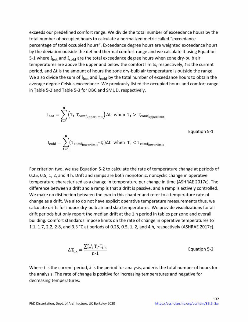
132
exceeds our predefined comfort range. We divide the total number of exceedance hours by the total number of occupied hours to calculate a normalized metric called “exceedance percentage of total occupied hours”. Exceedance degree hours are weighted exceedance hours by the deviation outside the defined thermal comfort range and we calculate it using Equation 5-1 where Ihot and Icold are the total exceedance degree hours when zone dry-bulb air temperatures are above the upper and below the comfort limits, respectively, t is the current period, and ∆t is the amount of hours the zone dry-bulb air temperature is outside the range. We also divide the sum of Ihot and Icold by the total number of exceedance hours to obtain the average degree Celsius exceedance. We previously listed the occupied hours and comfort range in Table 5-2 and Table 5-3 for DBC and SMUD, respectively.
Ihot = ��Tt-Tcomfupperlimit� ∆tn
t=1
when Tt > Tcomfupperlimit
Equation 5-1
Icold = ��Tcomflowerlimit-Tt�∆tn
t=1
when Tt < Tcomflowerlimit
For criterion two, we use Equation 5-2 to calculate the rate of temperature change at periods of 0.25, 0.5, 1, 2, and 4 h. Drift and ramps are both monotonic, noncyclic change in operative temperature characterized as a change in temperature per change in time (ASHRAE 2017c). The difference between a drift and a ramp is that a drift is passive, and a ramp is actively controlled. We make no distinction between the two in this chapter and refer to a temperature rate of change as a drift. We also do not have explicit operative temperature measurements thus, we calculate drifts for indoor dry-bulb air and slab temperatures. We provide visualizations for all drift periods but only report the median drift at the 1 h period in tables per zone and overall building. Comfort standards impose limits on the rate of change in operative temperatures to 1.1, 1.7, 2.2, 2.8, and 3.3 °C at periods of 0.25, 0.5, 1, 2, and 4 h, respectively (ASHRAE 2017c).
∆Tt,k =∑ Tt-Tt-kn-1t=1
n-1 Equation 5-2
Where t is the current period, k is the period for analysis, and n is the total number of hours for the analysis. The rate of change is positive for increasing temperatures and negative for decreasing temperatures.
https://escholarship.org/uc/item/82t6n3xrPhD Dissertation, Dept. of Architecture, UC Berkeley 2020

133
We subtract the minimum from the maximum indoor dry-bulb air temperature during occupied hours to quantify criterion three.
To quantify criterion four, we first calculate each study period daily mean zone dry-bulb air temperature (T�air) and then calculate the first difference between consecutive T�air. For example, the first difference of T�tair at period t is equal to T�tair-T�t-1air. We calculated the median of all consecutive first differences to report the metric called “interday variability” per zone and at the building level. Occupants may prefer indoor temperatures that do not significantly deviate from the previous day’s indoor temperatures making it easier for them to select their clothing layers and set expectations.
We use zone dry-bulb air temperature as measured through each zone’s thermostats to calculate each metric. We use the temperature sensor embedded within the slab to calculate the slab’s temperature rate of change. We expect that the designs of DBC and SMUD provide operative temperatures close to indoor dry-bulb air temperature and thus the reason we use the air temperature for our calculations (Dawe et al. 2020). We report metrics for individual zones and overall building. We do not include days when the control strategies failed or when a zone was vacant during any of the studied periods in which we did observed and discuss further in sections below.
The four performance criteria can have a significant impact on occupant thermal comfort. However, thermal comfort requires several variables for an accurate assessment but it is ultimately “that condition of mind that expresses satisfaction with the thermal environment” and large variations exist from person to person (ASHRAE 2017c). Thus, our approach taken here simplifies the occupant thermal comfort assessment, but we can easily gather the required data in both buildings for this approach. We conduct granular occupant surveys in DBC, as discussed in Section 5.2.3, to gain more information about occupants’ thermal comfort with the intervention HTMR control strategy.
We also use secondary performance metrics to evaluate the energy consumption for the baseline and intervention control strategies. We calculate the daily average number of minutes that each zone’s manifold valve is open for comparisons at the zone and building level. We use this metric as a proxy for energy consumption since we do not have direct measurements for all HVAC systems in DBC or SMUD. We only have gas consumption in DBC and report in the results as well. We do not have any HVAC energy consumption for SMUD since it is part of a centralized HVAC plant that supplies other buildings and it is not sub-metered.
5.2.5. Statistical metrics
We performed statistical comparisons of the various performance metrics discussed in Section 5.2.4 using the Wilcoxon signed ranked test to evaluate the statistical significance between the baseline and intervention control strategies. We also use Cohen’s d to assess the effect size between the distribution groups and used Cohen (1988)’s effect size interpretations i.e. 0.2,
https://escholarship.org/uc/item/82t6n3xrPhD Dissertation, Dept. of Architecture, UC Berkeley 2020
134
0.5, and 0.8 for small, medium, and large effect size, respectively. We used p < 0.025 to deem statistical significance which includes the Bonferroni correction since we are performing two statistical tests (R. A. Armstrong 2014; Napierala 2012).
5.3. Results
5.3.1. Building site weather
Figure 5-12 shows the outdoor dry-bulb air temperature measured through each of the building’s EMS sensors during the baseline and intervention time frames. The 24-hour boxplots show that there are no significant discrepancies in the weather during the two periods. However, the baseline time frames in both Berkeley and Sacramento seem to have slightly higher extreme temperatures than the intervention time frame as seen from the longer whiskers in the hourly distributions. The measured outdoor dry-bulb air temperature for Berkeley observed a minimum, maximum, and mean daily range of 9.9, 34.2, and 6.9 °C, respectively, using data from both time frames. In general, the weather in Berkeley during the two time frames was mild and occasionally surpassed the upper comfort limit we defined in the intervention controls for DBC. In contrast, the weather in Sacramento was rarely within the thermal comfort limits we defined in the intervention controls for SMUD. We observed an outdoor dry-bulb air temperature minimum, maximum, and mean daily range of 4.7, 44.1, and 17.8 °C, respectively, using data from both time frames.
https://escholarship.org/uc/item/82t6n3xrPhD Dissertation, Dept. of Architecture, UC Berkeley 2020

135
Figure 5-12: Outdoor dry-bulb air temperature (OAT) at top) Berkeley and bottom) Sacramento, California during the baseline and intervention time frames. The weather data was measured through each building’s energy management system. The time frame for DBC-baseline is August 20 through October 31, 2016, August 20 through October 31, 2018 for DBC-intervention, June 4 through November 9, 2017 for SMUD-baseline, and June 4 through November 9, 2018 for SMUD-intervention. The OAT between the two periods was similar.
5.3.2. Example cooling days for control strategies
Figure 5-13 and Figure 5-14 show example HTMR operation and performance data for DBC and SMUD, respectively, during the baseline and intervention time frames. The zones' names can be mapped back to floor plans shown in Figure 5-2 and Figure 5-8 for DBC and SMUD, respectively. The figures show how the manifold valve is controlled to maintain zone dry-bulb air temperature within acceptable temperatures. In DBC-baseline, the manifold valve operation is based on the slab setpoint which changes based on the deviation of the current indoor dry-bulb air temperature and a constant zone air temperature setpoint (24.4 °C) defined by the building operator. The slab temperature setpoint changes continuously, as shown in Figure 5-13 A), which causes instability in the control of zone temperatures. The baseline control strategy in DBC also has a high potential to waste heating/cooling energy as hot and then cooled water, or vice-versa, flows through the HTMR within a short time period (Sourbron et al. 2009). The concrete slabs can store substantial amounts of thermal energy. Thus, when there is ongoing heating and then it switches over to cooling mode within 24 hours, the HTMR needs to first extract a portion of the heat that was actively supplied plus the additional heat to cool the slab to the desired setpoint. It also happens when starting from cooling and switching over to heating. Figure 5-13 A) for zone 3-2 shows wasted energy from September 25 to 29 due to
https://escholarship.org/uc/item/82t6n3xrPhD Dissertation, Dept. of Architecture, UC Berkeley 2020
136
rapid switchovers. We and others recommend to restrict heating/cooling mode switchovers to no less than 24 hours, or preferably longer (Sourbron and Helsen 2014; Raftery et al. 2017).
The baseline control strategy for SMUD is an improvement from the originally designed control strategy. In SMUD-baseline, the modulating manifold valve operates on the deviation between the current zone dry-bulb air temperature and a fixed zone dry-bulb air temperature setpoint schedule. The fixed setpoint schedule intends to shift most of the heat extraction from the zone during nighttime hours when electricity prices are the lowest and the cooling plant can operate at higher efficiency due to lower outdoor air temperatures. The building operators may have tuned the fixed setpoint schedule for each zone which is a limitation of having fixed operating setpoint schedules. There are no automatic adjustments to the setpoints as heating and cooling requirements change in the zones which may cause discomfort issues due to overcooling or overheating and increases energy consumption and electricity costs.
The intervention control strategy may overcome the issues present in the baseline control strategies. It improves zone temperature control by limiting the times the slab setpoint is adjusted, reduces energy consumption and electricity costs by shifting the heat extraction in the zones when electricity is less expensive or HVAC equipment is more efficient to operate. The new control strategy also tunes itself as the heat gains entering and generated inside the space change (Raftery et al. 2017). These changes lead to significant reductions in the amount of time that manifold valves are open which is proportional to the amount of energy used while also maintaining comfortable temperatures in the zones. These trends are not only limited to the zones and time periods shown in Figure 5-13 and Figure 5-14 but for all zones in both buildings that used the intervention control strategy.
https://escholarship.org/uc/item/82t6n3xrPhD Dissertation, Dept. of Architecture, UC Berkeley 2020

137
Figure 5-13: Example HTMR data in cooling mode with the top) baseline control strategy from Sunday, September 25 to Friday, September 30, 2016 and bottom) the intervention control strategy Sunday, September 8 to Friday, September 14, 2018, in DBC. Zones 3-2 and 3-4 are on the north and south facing façades, respectively. The gray dashed lines represent the defined comfort limits used during the intervention control strategy. The shaded gray areas designate the typically occupied hours (8:00 to 18:00). The green shaded area designates a triggered pre-cooling event in the baseline control when outdoor dry-bulb air temperature exceeded the designed threshold (28.9 °C). In the intervention time frame, the green shaded area designates our defined HTMR availability period (22:00-10:00). We set the upper slab temperature setpoint limits in the intervention control strategy to 23.9 °C. The intervention control strategy maintained better indoor temperature control.
DBC-Baseline
DBC-Intervention
https://escholarship.org/uc/item/82t6n3xrPhD Dissertation, Dept. of Architecture, UC Berkeley 2020

138
Figure 5-14: Example HTMR data in cooling mode with the top) baseline control strategy from Sunday, September 3 to Friday, September 8, 2017 and bottom) the intervention control strategy Sunday, September 23 to Friday, September 28, 2018 in SMUD. Zone F2-West north and F2-West south is on the north and south facing façades, respectively. The gray dashed lines represent the defined comfort limits used during the intervention control strategy. The shaded gray areas designate the typically occupied hours (5:00 to 17:00). The green shaded area designates the HTMR availability period. The baseline control strategy intends to shift most of the cooling to nighttime hours and manifold valve control is based on a fixed zone dry-bulb temperature setpoint schedule. Building operators tuned the fixed setpoint schedules from the improved setpoints modified through a previous CBE field study (Bauman et al. 2015). We were unable to obtain the tuned setpoint schedules. We set the upper slab temperature setpoint limits in the intervention control strategy to 23.9 °C. The intervention control strategy maintained better indoor temperature control.
SMUD-Baseline
SMUD-Intervention
https://escholarship.org/uc/item/82t6n3xrPhD Dissertation, Dept. of Architecture, UC Berkeley 2020
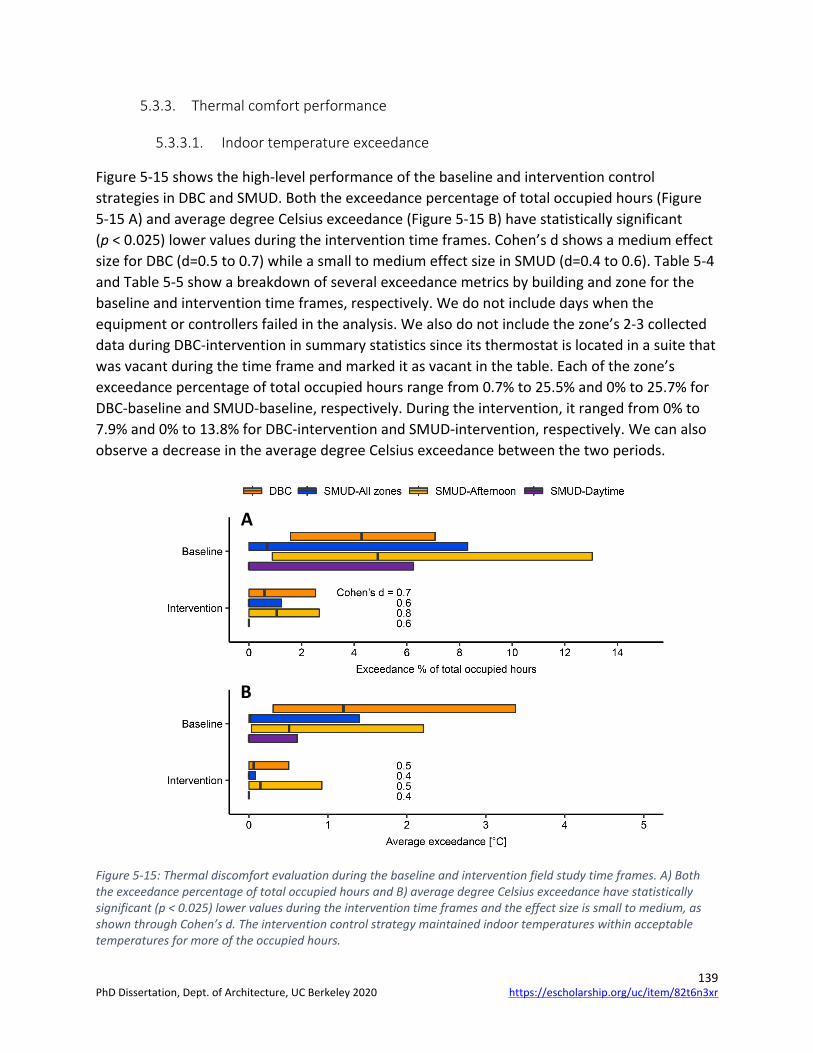
139
5.3.3. Thermal comfort performance
5.3.3.1. Indoor temperature exceedance
Figure 5-15 shows the high-level performance of the baseline and intervention control strategies in DBC and SMUD. Both the exceedance percentage of total occupied hours (Figure 5-15 A) and average degree Celsius exceedance (Figure 5-15 B) have statistically significant (p < 0.025) lower values during the intervention time frames. Cohen’s d shows a medium effect size for DBC (d=0.5 to 0.7) while a small to medium effect size in SMUD (d=0.4 to 0.6). Table 5-4 and Table 5-5 show a breakdown of several exceedance metrics by building and zone for the baseline and intervention time frames, respectively. We do not include days when the equipment or controllers failed in the analysis. We also do not include the zone’s 2-3 collected data during DBC-intervention in summary statistics since its thermostat is located in a suite that was vacant during the time frame and marked it as vacant in the table. Each of the zone’s exceedance percentage of total occupied hours range from 0.7% to 25.5% and 0% to 25.7% for DBC-baseline and SMUD-baseline, respectively. During the intervention, it ranged from 0% to 7.9% and 0% to 13.8% for DBC-intervention and SMUD-intervention, respectively. We can also observe a decrease in the average degree Celsius exceedance between the two periods.
Figure 5-15: Thermal discomfort evaluation during the baseline and intervention field study time frames. A) Both the exceedance percentage of total occupied hours and B) average degree Celsius exceedance have statistically significant (p < 0.025) lower values during the intervention time frames and the effect size is small to medium, as shown through Cohen’s d. The intervention control strategy maintained indoor temperatures within acceptable temperatures for more of the occupied hours.
A
B
https://escholarship.org/uc/item/82t6n3xrPhD Dissertation, Dept. of Architecture, UC Berkeley 2020
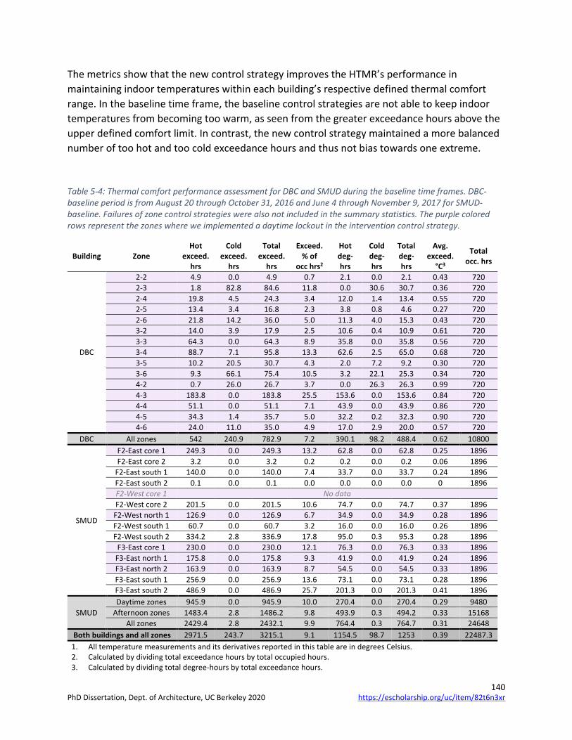
140
The metrics show that the new control strategy improves the HTMR’s performance in maintaining indoor temperatures within each building’s respective defined thermal comfort range. In the baseline time frame, the baseline control strategies are not able to keep indoor temperatures from becoming too warm, as seen from the greater exceedance hours above the upper defined comfort limit. In contrast, the new control strategy maintained a more balanced number of too hot and too cold exceedance hours and thus not bias towards one extreme.
Table 5-4: Thermal comfort performance assessment for DBC and SMUD during the baseline time frames. DBC-baseline period is from August 20 through October 31, 2016 and June 4 through November 9, 2017 for SMUD-baseline. Failures of zone control strategies were also not included in the summary statistics. The purple colored rows represent the zones where we implemented a daytime lockout in the intervention control strategy.
Building Zone Hot
exceed. hrs
Cold exceed.
hrs
Total exceed.
hrs
Exceed. % of
occ hrs2
Hot deg-hrs
Cold deg-hrs
Total deg-hrs
Avg. exceed.
°C3
Total occ. hrs
DBC
2-2 4.9 0.0 4.9 0.7 2.1 0.0 2.1 0.43 720 2-3 1.8 82.8 84.6 11.8 0.0 30.6 30.7 0.36 720 2-4 19.8 4.5 24.3 3.4 12.0 1.4 13.4 0.55 720 2-5 13.4 3.4 16.8 2.3 3.8 0.8 4.6 0.27 720 2-6 21.8 14.2 36.0 5.0 11.3 4.0 15.3 0.43 720 3-2 14.0 3.9 17.9 2.5 10.6 0.4 10.9 0.61 720 3-3 64.3 0.0 64.3 8.9 35.8 0.0 35.8 0.56 720 3-4 88.7 7.1 95.8 13.3 62.6 2.5 65.0 0.68 720 3-5 10.2 20.5 30.7 4.3 2.0 7.2 9.2 0.30 720 3-6 9.3 66.1 75.4 10.5 3.2 22.1 25.3 0.34 720 4-2 0.7 26.0 26.7 3.7 0.0 26.3 26.3 0.99 720 4-3 183.8 0.0 183.8 25.5 153.6 0.0 153.6 0.84 720 4-4 51.1 0.0 51.1 7.1 43.9 0.0 43.9 0.86 720 4-5 34.3 1.4 35.7 5.0 32.2 0.2 32.3 0.90 720 4-6 24.0 11.0 35.0 4.9 17.0 2.9 20.0 0.57 720
DBC All zones 542 240.9 782.9 7.2 390.1 98.2 488.4 0.62 10800
SMUD
F2-East core 1 249.3 0.0 249.3 13.2 62.8 0.0 62.8 0.25 1896 F2-East core 2 3.2 0.0 3.2 0.2 0.2 0.0 0.2 0.06 1896
F2-East south 1 140.0 0.0 140.0 7.4 33.7 0.0 33.7 0.24 1896 F2-East south 2 0.1 0.0 0.1 0.0 0.0 0.0 0.0 0 1896 F2-West core 1 No data F2-West core 2 201.5 0.0 201.5 10.6 74.7 0.0 74.7 0.37 1896
F2-West north 1 126.9 0.0 126.9 6.7 34.9 0.0 34.9 0.28 1896 F2-West south 1 60.7 0.0 60.7 3.2 16.0 0.0 16.0 0.26 1896 F2-West south 2 334.2 2.8 336.9 17.8 95.0 0.3 95.3 0.28 1896
F3-East core 1 230.0 0.0 230.0 12.1 76.3 0.0 76.3 0.33 1896 F3-East north 1 175.8 0.0 175.8 9.3 41.9 0.0 41.9 0.24 1896 F3-East north 2 163.9 0.0 163.9 8.7 54.5 0.0 54.5 0.33 1896 F3-East south 1 256.9 0.0 256.9 13.6 73.1 0.0 73.1 0.28 1896 F3-East south 2 486.9 0.0 486.9 25.7 201.3 0.0 201.3 0.41 1896
SMUD Daytime zones 945.9 0.0 945.9 10.0 270.4 0.0 270.4 0.29 9480
Afternoon zones 1483.4 2.8 1486.2 9.8 493.9 0.3 494.2 0.33 15168 All zones 2429.4 2.8 2432.1 9.9 764.4 0.3 764.7 0.31 24648
Both buildings and all zones 2971.5 243.7 3215.1 9.1 1154.5 98.7 1253 0.39 22487.3 1. All temperature measurements and its derivatives reported in this table are in degrees Celsius. 2. Calculated by dividing total exceedance hours by total occupied hours. 3. Calculated by dividing total degree-hours by total exceedance hours.
https://escholarship.org/uc/item/82t6n3xrPhD Dissertation, Dept. of Architecture, UC Berkeley 2020
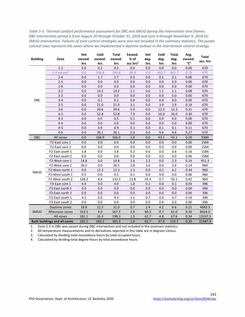
141
Table 5-5: Thermal comfort performance assessment for DBC and SMUD during the intervention time frames. DBC-intervention period is from August 20 through October 31, 2018 and June 4 through November 9, 2018 for SMUD-intervention. Failures of zone control strategies were also not included in the summary statistics. The purple colored rows represent the zones where we implemented a daytime lockout in the intervention control strategy.
Building Zone Hot
exceed. hrs
Cold exceed.
hrs
Total exceed.
hrs
Exceed. % of
occ hrs3
Hot deg-hrs
Cold deg-hrs
Total deg-hrs
Avg. exceed.
°C4
Total occ. hrs
DBC
2-2 0.0 0.2 0.2 0.0 0.0 0.0 0.0 0.00 670 2-3-vacant1 0.0 594.8 594.8 88.8 0.0 463.7 463.7 0.78 670
2-4 0.0 1.7 1.7 0.3 0.0 0.1 0.1 0.06 670 2-5 0.0 0.0 0.0 0.0 0.0 0.0 0.0 0.00 670 2-6 0.0 0.0 0.0 0.0 0.0 0.0 0.0 0.00 670 3-2 0.0 14.2 14.2 2.1 0.0 1.1 1.1 0.08 670 3-3 0.0 0.0 0.0 0.0 0.0 0.0 0.0 0.00 670 3-4 0.0 0.1 0.1 0.0 0.0 0.0 0.0 0.00 670 3-5 0.0 21.0 21.0 3.1 0.0 3.9 3.9 0.19 670 3-6 0.0 39.6 39.6 5.9 0.0 12.3 12.3 0.31 670 4-2 0.0 52.8 52.8 7.9 0.0 16.0 16.0 0.30 670 4-3 0.0 0.5 0.5 0.1 0.0 0.0 0.0 0.00 670 4-4 0.0 0.0 0.0 0.0 0.0 0.0 0.0 0.00 670 4-5 0.0 0.9 0.9 0.1 0.0 0.1 0.1 0.11 670 4-6 0.0 36.1 36.1 5.4 0.0 9.6 9.6 0.27 670
DBC All zones 0.0 166.9 166.9 1.8 0.0 43.1 43.1 0.26 9380
SMUD
F2-East core 1 0.0 0.0 0.0 0.0 0.0 0.0 0.0 0.00 1584 F2-East core 2 0.0 0.0 0.0 0.0 0.0 0.0 0.0 0.00 1584
F2-East south 1 3.8 0.0 3.8 0.2 0.6 0.0 0.6 0.16 1584 F2-East south 2 0.0 0.0 0.0 0.0 0.0 0.0 0.0 0.00 1584 F2-West core 1 14.8 0.0 14.8 1.6 2.3 0.0 2.3 0.16 951.3 F2-West core 2 26.5 0.0 26.5 2.8 3.6 0.0 3.6 0.14 960
F2-West north 1 0.0 12.3 12.3 1.3 0.0 4.2 4.2 0.34 960 F2-West south 1 0.5 0.0 0.5 0.1 0.0 0.0 0.0 0.00 960 F2-West south 2 128.3 4.0 132.3 13.8 55.4 0.7 56.1 0.42 960
F3-East core 1 4.0 0.0 4.0 1.0 0.1 0.0 0.1 0.03 396 F3-East north 1 0.0 0.0 0.0 0.0 0.0 0.0 0.0 0.00 396 F3-East north 2 0.0 0.0 0.0 0.0 0.0 0.0 0.0 0.00 396 F3-East south 1 4.3 0.0 4.3 1.1 0.7 0.0 0.7 0.16 396 F3-East south 2 0.0 0.0 0.0 0.0 0.0 0.0 0.0 0.00 396
SMUD Daytime zones 18.8 12.3 31.0 0.7 2.4 4.2 6.6 0.21 4683.3
Afternoon zones 163.3 4.0 167.3 2.0 60.3 0.7 61.0 0.36 8424.0 All zones 182.1 16.3 198.3 1.5 62.7 4.8 67.6 0.34 13107.3
Both buildings and all zones 182.1 183.2 365.3 1.6 62.7 47.9 110.7 0.30 22487.3 1. Zone 2-3 in DBC was vacant during DBC-intervention and not included in the summary statistics. 2. All temperature measurements and its derivatives reported in this table are in degrees Celsius. 3. Calculated by dividing total exceedance hours by total occupied hours. 4. Calculated by dividing total degree-hours by total exceedance hours.
https://escholarship.org/uc/item/82t6n3xrPhD Dissertation, Dept. of Architecture, UC Berkeley 2020
142
5.3.3.2. Indoor temperature intraday and interday variations
The next series of figures show the daily profiles for each zone’s dry-bulb air and slab temperatures for both DBC and SMUD during the baseline and intervention time frames. These figures show intraday and interday variations of the two temperatures. We also calculated the local polynomial regression (LOESS) fit for the daily temperature profiles in each zone. The figures show the intervention control strategy’s marked improvement in stabilizing the zones’ temperature and maintaining them within the defined setpoints.
https://escholarship.org/uc/item/82t6n3xrPhD Dissertation, Dept. of Architecture, UC Berkeley 2020

143
Figure 5-16: Daily zones’ dry-bulb air temperature profiles showing the interday and intraday variations with the left) baseline and right) intervention control strategies in DBC. The date interval for DBC-baseline is from August 20 through October 31, 2016 and August 20 through October 31, 2018 for DBC-intervention. The thick red or light green line represents the local polynomial regression (LOESS) fit for the daily temperature profiles in each zone. The gold dashed lines show our defined thermal comfort range implemented in the intervention control strategy (21.1 and 25.6 °C) and grey dashed lines represent the typical start and end of occupancy (8:00 to 18:00). The dry-bulb temperatures are more consistent with the intervention control strategy.
DBC-Baseline: Air DBC-Intervention: Air
https://escholarship.org/uc/item/82t6n3xrPhD Dissertation, Dept. of Architecture, UC Berkeley 2020

144
Figure 5-17: Daily zones’ slab temperature profiles showing the interday and intraday variations with the left) baseline and right) intervention control strategies in DBC. The slab temperature sensor is embedded within the floor slab. The date interval for DBC-baseline is from August 20 through October 31, 2016 and August 20 through October 31, 2018 for DBC-intervention. The thick red or light green line represents the local polynomial regression (LOESS) fit for the daily temperature profiles in each zone. The gold dashed lines show our defined thermal comfort range implemented in the intervention control strategy (21.1 and 25.6 °C) and grey dashed lines represent the typical start and end of occupancy (8:00 to 18:00). The slab temperatures are more consistent with the intervention control strategy.
DBC-Baseline: Slab DBC-Intervention: Slab
https://escholarship.org/uc/item/82t6n3xrPhD Dissertation, Dept. of Architecture, UC Berkeley 2020

145
Figure 5-18: Daily zones’ dry-bulb air temperature profiles showing the interday and intraday variations with the left) baseline and right) intervention control strategies in SMUD. The date interval for SMUD-baseline is from June 4 through November 9, 2017 and June 4 through November 9, 2018 for SMUD-intervention. The thick red or light green line represents the local polynomial regression (LOESS) fit for the daily temperature profiles in each zone. The gold dashed lines show our defined thermal comfort range implemented in the intervention control strategy (21.1 and 24.4 °C) and grey dashed lines represent the typical start and end of occupancy (5:00 to 17:00). Purple colored labels represent the zones where we implemented a daytime lockout in the intervention control strategy. The dry-bulb temperatures are more consistent with the intervention control strategy.
SMUD-Baseline: Air SMUD-Intervention: Air
https://escholarship.org/uc/item/82t6n3xrPhD Dissertation, Dept. of Architecture, UC Berkeley 2020

146
Figure 5-19: Daily zones’ slab temperature profiles showing the interday and intraday variations with the left) baseline and right) intervention control strategies in SMUD. The slab temperature sensor is embedded within the floor slab. The date interval for SMUD-baseline is from June 4 through November 9, 2017 and June 4 through November 9, 2018 for SMUD-intervention. The thick red or light green line represents the local polynomial regression (LOESS) fit for the daily temperature profiles in each zone. The gold dashed lines show our defined thermal comfort range implemented in the intervention control strategy (21.1 and 24.4 °C) and grey dashed lines represent the typical start and end of occupancy (5:00 to 17:00). Purple colored labels represent the zones where
SMUD-Baseline: Slab SMUD-Intervention: Slab
https://escholarship.org/uc/item/82t6n3xrPhD Dissertation, Dept. of Architecture, UC Berkeley 2020
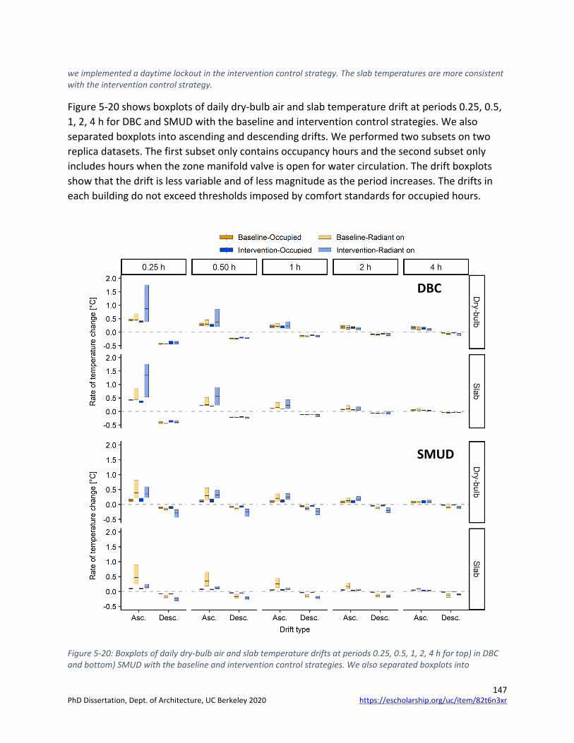
147
we implemented a daytime lockout in the intervention control strategy. The slab temperatures are more consistent with the intervention control strategy.
Figure 5-20 shows boxplots of daily dry-bulb air and slab temperature drift at periods 0.25, 0.5, 1, 2, 4 h for DBC and SMUD with the baseline and intervention control strategies. We also separated boxplots into ascending and descending drifts. We performed two subsets on two replica datasets. The first subset only contains occupancy hours and the second subset only includes hours when the zone manifold valve is open for water circulation. The drift boxplots show that the drift is less variable and of less magnitude as the period increases. The drifts in each building do not exceed thresholds imposed by comfort standards for occupied hours.
Figure 5-20: Boxplots of daily dry-bulb air and slab temperature drifts at periods 0.25, 0.5, 1, 2, 4 h for top) in DBC and bottom) SMUD with the baseline and intervention control strategies. We also separated boxplots into
SMUD
DBC
https://escholarship.org/uc/item/82t6n3xrPhD Dissertation, Dept. of Architecture, UC Berkeley 2020
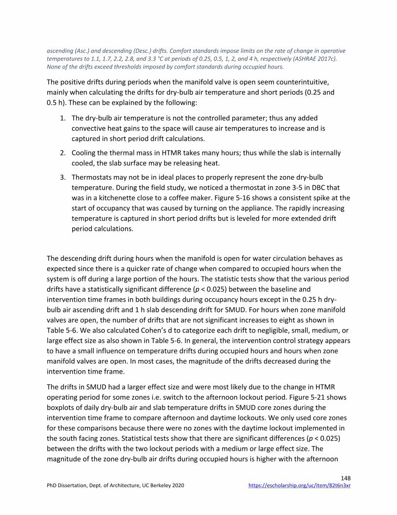
148
ascending (Asc.) and descending (Desc.) drifts. Comfort standards impose limits on the rate of change in operative temperatures to 1.1, 1.7, 2.2, 2.8, and 3.3 °C at periods of 0.25, 0.5, 1, 2, and 4 h, respectively (ASHRAE 2017c). None of the drifts exceed thresholds imposed by comfort standards during occupied hours.
The positive drifts during periods when the manifold valve is open seem counterintuitive, mainly when calculating the drifts for dry-bulb air temperature and short periods (0.25 and 0.5 h). These can be explained by the following:
1. The dry-bulb air temperature is not the controlled parameter; thus any added convective heat gains to the space will cause air temperatures to increase and is captured in short period drift calculations.
2. Cooling the thermal mass in HTMR takes many hours; thus while the slab is internally cooled, the slab surface may be releasing heat.
3. Thermostats may not be in ideal places to properly represent the zone dry-bulb temperature. During the field study, we noticed a thermostat in zone 3-5 in DBC that was in a kitchenette close to a coffee maker. Figure 5-16 shows a consistent spike at the start of occupancy that was caused by turning on the appliance. The rapidly increasing temperature is captured in short period drifts but is leveled for more extended drift period calculations.
The descending drift during hours when the manifold is open for water circulation behaves as expected since there is a quicker rate of change when compared to occupied hours when the system is off during a large portion of the hours. The statistic tests show that the various period drifts have a statistically significant difference (p < 0.025) between the baseline and intervention time frames in both buildings during occupancy hours except in the 0.25 h dry-bulb air ascending drift and 1 h slab descending drift for SMUD. For hours when zone manifold valves are open, the number of drifts that are not significant increases to eight as shown in Table 5-6. We also calculated Cohen’s d to categorize each drift to negligible, small, medium, or large effect size as also shown in Table 5-6. In general, the intervention control strategy appears to have a small influence on temperature drifts during occupied hours and hours when zone manifold valves are open. In most cases, the magnitude of the drifts decreased during the intervention time frame.
The drifts in SMUD had a larger effect size and were most likely due to the change in HTMR operating period for some zones i.e. switch to the afternoon lockout period. Figure 5-21 shows boxplots of daily dry-bulb air and slab temperature drifts in SMUD core zones during the intervention time frame to compare afternoon and daytime lockouts. We only used core zones for these comparisons because there were no zones with the daytime lockout implemented in the south facing zones. Statistical tests show that there are significant differences (p < 0.025) between the drifts with the two lockout periods with a medium or large effect size. The magnitude of the zone dry-bulb air drifts during occupied hours is higher with the afternoon
https://escholarship.org/uc/item/82t6n3xrPhD Dissertation, Dept. of Architecture, UC Berkeley 2020
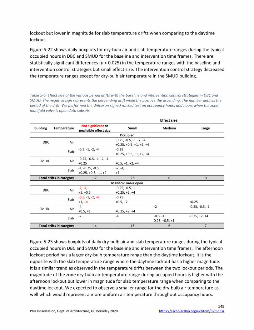
149
lockout but lower in magnitude for slab temperature drifts when comparing to the daytime lockout.
Figure 5-22 shows daily boxplots for dry-bulb air and slab temperature ranges during the typical occupied hours in DBC and SMUD for the baseline and intervention time frames. There are statistically significant differences (p < 0.025) in the temperature ranges with the baseline and intervention control strategies but small effect size. The intervention control strategy decreased the temperature ranges except for dry-bulb air temperature in the SMUD building.
Table 5-6: Effect size of the various period drifts with the baseline and intervention control strategies in DBC and SMUD. The negative sign represents the descending drift while the positive the ascending. The number defines the period of the drift. We performed the Wilcoxon signed ranked test on occupancy hours and hours when the zone manifold valve is open data subsets.
Effect size
Building Temperature Not significant or negligible effect size Small Medium Large
Occupied
DBC Air -0.25, -0.5, -1, -2, -4 +0.25, +0.5, +1, +2, +4
Slab -0.5, -1, -2, -4 -0.25 +0.25, +0.5, +1, +2, +4
SMUD Air -0.25, -0.5, -1, -2, -4 +0.25
+0.5, +1, +2, +4
Slab -1, -0.25, -0.5 +0.25, +0.5, +1, +2
-2, -4, +4
Total drifts in category 17 23 0 0 Manifold valve open
DBC Air -2, -4, +1, +0.5
-0.25, -0.5, -1 +0.25, +2, +4
Slab -0.5, -1, -2, -4 +1, +4
-0.25 +0.5, +2
+0.25
SMUD Air -4 +0.5, +1
+0.25, +2, +4
-2 -0.25, -0.5, -1
Slab -2 -4 -0.5, -1 0.25, +0.5, +1
-0.25, +2, +4
Total drifts in category 14 13 6 7
Figure 5-23 shows boxplots of daily dry-bulb air and slab temperature ranges during the typical occupied hours in DBC and SMUD for the baseline and intervention time frames. The afternoon lockout period has a larger dry-bulb temperature range than the daytime lockout. It is the opposite with the slab temperature range where the daytime lockout has a higher magnitude. It is a similar trend as observed in the temperature drifts between the two lockout periods. The magnitude of the zone dry-bulb air temperature range during occupied hours is higher with the afternoon lockout but lower in magnitude for slab temperature range when comparing to the daytime lockout. We expected to observe a smaller range for the dry-bulb air temperature as well which would represent a more uniform air temperature throughout occupancy hours.
https://escholarship.org/uc/item/82t6n3xrPhD Dissertation, Dept. of Architecture, UC Berkeley 2020
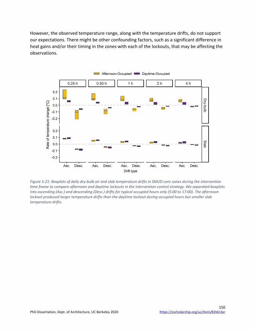
150
However, the observed temperature range, along with the temperature drifts, do not support our expectations. There might be other confounding factors, such as a significant difference in heat gains and/or their timing in the zones with each of the lockouts, that may be affecting the observations.
Figure 5-21: Boxplots of daily dry-bulb air and slab temperature drifts in SMUD core zones during the intervention time frame to compare afternoon and daytime lockouts in the intervention control strategy. We separated boxplots into ascending (Asc.) and descending (Desc.) drifts for typical occupied hours only (5:00 to 17:00). The afternoon lockout produced larger temperature drifts than the daytime lockout during occupied hours but smaller slab temperature drifts.
https://escholarship.org/uc/item/82t6n3xrPhD Dissertation, Dept. of Architecture, UC Berkeley 2020

151
Figure 5-22: Boxplot of daily dry-bulb air and slab temperature ranges during the typical occupied hours in DBC and SMUD for the baseline and intervention time frames. The temperature ranges have a statistically significant difference (p < 0.025) with the baseline and intervention control strategies and small effect size, as shown with Cohen’s d. The intervention control strategy most likely did not have a noticeable effect to the occupants.
Figure 5-23: Boxplot of daily dry-bulb air and slab temperature range in SMUD core zones for typical occupied hours (5:00 to 17:00) during the intervention time frame to compare afternoon and daytime lockouts in the intervention control strategy. There are statistically significant differences (p < 0.025) between the two lockouts and the effect size is large for dry-bulb temperature range and medium for the slab temperature range. The afternoon lockout produced a larger dry-bulb temperature range than the daytime lockout during occupied hours but a smaller slab temperature range.
https://escholarship.org/uc/item/82t6n3xrPhD Dissertation, Dept. of Architecture, UC Berkeley 2020
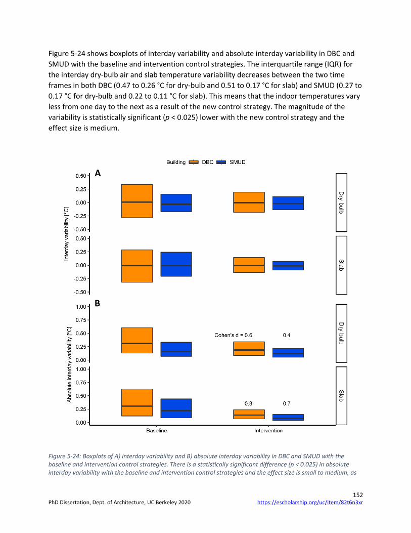
152
Figure 5-24 shows boxplots of interday variability and absolute interday variability in DBC and SMUD with the baseline and intervention control strategies. The interquartile range (IQR) for the interday dry-bulb air and slab temperature variability decreases between the two time frames in both DBC (0.47 to 0.26 °C for dry-bulb and 0.51 to 0.17 °C for slab) and SMUD (0.27 to 0.17 °C for dry-bulb and 0.22 to 0.11 °C for slab). This means that the indoor temperatures vary less from one day to the next as a result of the new control strategy. The magnitude of the variability is statistically significant (p < 0.025) lower with the new control strategy and the effect size is medium.
Figure 5-24: Boxplots of A) interday variability and B) absolute interday variability in DBC and SMUD with the baseline and intervention control strategies. There is a statistically significant difference (p < 0.025) in absolute interday variability with the baseline and intervention control strategies and the effect size is small to medium, as
A
B
https://escholarship.org/uc/item/82t6n3xrPhD Dissertation, Dept. of Architecture, UC Berkeley 2020

153
shown with Cohen’s d. The interday variability narrows around the mean temperatures with the intervention control strategy.
Table 5-7 and Table 5-8 contains the median for the various dry-bulb air and slab temperature variation metrics at the building, zone, and lockout levels for DBC and SMUD with the baseline and intervention control strategies. The tables provide more detailed information to supplement the visualizations of the different variation metrics shown in previous figures.
https://escholarship.org/uc/item/82t6n3xrPhD Dissertation, Dept. of Architecture, UC Berkeley 2020

154
Table 5-7: The median for the various dry-bulb air temperature variation metrics at the building, zone, and lockout level for DBC and SMUD with the baseline and intervention control strategies. DBC-intervention time frame is from August 20 through October 31, 2018 and June 4 through November 9, 2018 for SMUD-intervention. Failures of zone control strategies were also not included in the summary statistics. The purple colored rows represent the zones where we implemented a daytime lockout in the intervention control strategy.
Dry-bulb air1,2 Baseline Intervention
Building Zone - | + drift3
Intra. range
Inter. var.4 Min | Max - | +
drift3 Intra. range
Inter. var.4 Min | Max
DBC
2-2 -0.16 | 0.20 1.24 0.24 22.4 | 23.6 -0.11 | 0.20 1.27 0.16 21.8 | 23.0 2-3 -0.09 | 0.19 1.44 0.39 21.2 | 22.5 Vacant 2-4 -0.08 | 0.22 1.54 0.29 22.1 | 23.7 -0.1 | 0.21 1.49 0.20 22.0 | 23.6 2-5 -0.11 | 0.20 1.12 0.19 22.7 | 23.8 -0.11 | 0.18 0.90 0.14 22.2 | 23.1 2-6 -0.11 | 0.20 1.23 0.32 22.2 | 23.5 -0.11 | 0.17 1.22 0.21 22.1 | 23.4 3-2 -0.14 | 0.22 1.37 0.25 22.9 | 24.1 -0.11 | 0.16 0.89 0.19 21.7 | 22.7 3-3 -0.12 | 0.21 1.24 0.29 23.5 | 24.7 -0.11 | 0.18 1.13 0.15 23.0 | 24.2 3-4 -0.19 | 0.36 2.35 0.39 22.7 | 24.6 -0.15 | 0.26 1.81 0.21 22.2 | 24.1 3-5 -0.11 | 0.19 1.24 0.30 22.8 | 24.0 -0.11 | 0.18 1.13 0.15 21.7 | 22.8 3-6 -0.11 | 0.17 1.01 0.30 22.6 | 23.5 -0.11 | 0.16 1.00 0.19 21.6 | 22.5 4-2 -0.11 | 0.17 1.01 0.33 22.3 | 23.6 -0.11 | 0.17 1.00 0.21 21.8 | 22.7 4-3 -0.17 | 0.32 1.92 0.35 23.9 | 25.9 -0.11 | 0.22 1.48 0.28 22.5 | 24.1 4-4 -0.15 | 0.25 1.62 0.35 23.0 | 24.7 -0.11 | 0.17 1.12 0.15 22.3 | 23.3 4-5 -0.11 | 0.30 1.69 0.31 22.1 | 23.8 -0.11 | 0.28 1.57 0.20 22.1 | 23.5 4-6 -0.12 | 0.19 1.23 0.31 22.7 | 24.0 -0.11 | 0.17 1.12 0.22 21.5 | 22.6
DBC All zones -0.12 | 0.21 1.37 0.31 22.5 | 23.9 -0.11 | 0.19 1.23 0.19 22.0 | 23.2
SMUD
F2-East core 1 -0.02 | 0.02 0.18 0.16 23.8 | 24.0 -0.02 | 0.02 0.14 0.12 23.6 | 23.7 F2-East core 2 -0.04 | 0.06 0.35 0.16 23.1 | 23.4 -0.05 | 0.07 0.50 0.10 23.0 | 23.5
F2-East south 1 -0.05 | 0.11 0.84 0.18 23.3 | 24.2 -0.04 | 0.13 1.12 0.11 22.9 | 23.9 F2-East south 2 -0.06 | 0.09 0.52 0.18 22.6 | 23.1 -0.07 | 0.10 0.68 0.11 22.3 | 23.0 F2-West core 1 No data -0.01 | 0.05 0.43 0.18 22.7 | 23.2 F2-West core 2 -0.08 | 0.13 0.99 0.19 22.9 | 24.0 -0.08 | 0.15 1.14 0.14 22.9 | 24.2
F2-West north 1 -0.04 | 0.07 0.54 0.11 23.6 | 24.0 -0.03 | 0.08 0.64 0.14 22.7 | 23.4 F2-West south 1 -0.07 | 0.16 1.04 0.18 22.7 | 23.7 -0.04 | 0.24 2.09 0.11 21.9 | 24.0 F2-West south 2 -0.14 | 0.21 1.52 0.20 23.0 | 24.6 -0.04 | 0.36 3.32 0.18 21.8 | 25.1
F3-East core 1 -0.07 | 0.06 0.35 0.16 23.7 | 24.0 -0.10 | 0.06 0.43 0.08 23.4 | 23.8 F3-East north 1 -0.04 | 0.07 0.54 0.12 23.6 | 24.2 -0.04 | 0.08 0.50 0.10 23.1 | 23.6 F3-East north 2 -0.07 | 0.09 0.64 0.14 23.5 | 24.1 -0.07 | 0.11 0.59 0.15 22.7 | 23.4 F3-East south 1 -0.08 | 0.14 1.04 0.19 23.4 | 24.4 -0.12 | 0.20 1.54 0.07 22.5 | 24.0 F3-East south 2 -0.04 | 0.09 0.71 0.19 23.8 | 24.4 -0.05 | 0.12 1.02 0.15 22.8 | 23.9
SMUD Daytime zones -0.04 | 0.07 0.42 0.14 23.6 | 24.0 -0.03 | 0.05 0.40 0.13 23.2 | 23.6
Afternoon zones -0.06 | 0.12 0.84 0.18 23.1 | 24.1 -0.05 | 0.13 1.00 0.12 22.7 | 23.8 All zones -0.06 | 0.09 0.63 0.16 23.3 | 24.1 -0.05 | 0.10 0.70 0.12 22.8 | 23.7
Both buildings and all zones -0.07 | 0.13 0.84 0.20 23.1 | 24.0 -0.07 | 0.15 0.96 0.15 22.5 | 23.6 1. We calculated the median of the metrics only using measurements within each building’s respective typical occupancy
hours except for the interday variation (inter. var.) metric. 2. All values are in degrees Celsius. 3. These are descending (-) and ascending (+) drift at the 1 h period. 4. These are the absolute interday variation calculated using 24-hour temperature measurements.
https://escholarship.org/uc/item/82t6n3xrPhD Dissertation, Dept. of Architecture, UC Berkeley 2020

155
Table 5-8: The median for the various slab temperature variation metrics at the building, zone, and lockout level for DBC and SMUD with the baseline and intervention control strategies. DBC-intervention time frame is from August 20 through October 31, 2018 and June 4 through November 9, 2018 for SMUD-intervention. Failures of zone control strategies were also not included in the summary statistics. The purple colored rows represent the zones where we implemented a daytime lockout in the intervention control strategy.
Slab1,2 Baseline Intervention
Building Zone - | + drift3
Intra. range
Inter. var.4 Min | Max - | +
drift3 Intra. range
Inter. var.4 Min | Max
DBC
2-2 -0.11 | 0.11 0.22 0.24 23.4 | 23.6 -0.1 | 0.11 0.11 0.14 22.4 | 22.6 2-3 -0.06 | 0.05 0.44 0.42 24.1 | 24.5 Vacant 2-4 -0.04 | 0.07 0.35 0.20 23.0 | 23.4 -0.03 | 0.09 0.40 0.12 22.7 | 23.0 2-5 -0.11 | 0.11 0.22 0.26 24.0 | 24.2 -0.11 | 0.11 0.22 0.11 22.4 | 22.6 2-6 -0.11 | 0.11 0.33 0.21 23.8 | 24.2 -0.14 | 0.11 0.45 0.24 23.0 | 23.5 3-2 -0.11 | 0.11 0.44 0.47 24.4 | 24.7 -0.11 | 0.11 0.11 0.11 21.7 | 21.9 3-3 -0.11 | 0.11 0.22 0.28 25.3 | 25.5 -0.11 | 0.11 0.22 0.21 23.3 | 23.6 3-4 -0.11 | 0.11 0.44 0.40 25.2 | 25.7 -0.11 | 0.11 0.45 0.14 23.4 | 23.9 3-5 -0.11 | 0.11 0.44 0.40 24.8 | 25.3 -0.11 | 0.11 0.22 0.12 22.7 | 23.0 3-6 -0.11 | 0.11 0.44 0.49 25.1 | 25.9 -0.11 | 0.10 0.22 0.19 22.8 | 23.1 4-2 -0.11 | 0.11 0.11 0.37 24.0 | 24.2 -0.10 | 0.10 0.11 0.12 22.4 | 22.5 4-3 -0.11 | 0.11 0.11 0.17 24.8 | 25.0 -0.10 | 0.11 0.11 0.10 23.4 | 23.5 4-4 -0.11 | 0.11 0.33 0.31 23.7 | 24.1 -0.11 | 0.11 0.33 0.15 22.4 | 22.8 4-5 -0.11 | 0.11 0.33 0.24 23.5 | 24.0 -0.03 | 0.09 0.33 0.12 23.2 | 23.5 4-6 -0.11 | 0.12 0.22 0.43 24.2 | 24.4 -0.11 | 0.11 0.11 0.12 22.5 | 22.6
DBC All zones -0.11 | 0.11 0.33 0.31 24.0 | 24.4 -0.1 | 0.11 0.22 0.14 22.8 | 23.1
SMUD
F2-East core 1 -0.04 | 0.04 0.34 0.19 23.5 | 23.8 -0.04 | 0.04 0.26 0.15 23.5 | 23.8 F2-East core 2 -0.02 | 0.03 0.18 0.17 23.0 | 23.1 -0.03 | 0.03 0.12 0.07 23.0 | 23.2
F2-East south 1 -0.03 | 0.07 0.53 0.25 22.8 | 23.3 -0.05 | 0.07 0.45 0.04 22.1 | 22.6 F2-East south 2 -0.03 | 0.05 0.34 0.18 21.7 | 22.0 -0.03 | 0.06 0.40 0.08 21.3 | 21.7 F2-West core 1 No data -0.03 | 0.03 0.18 0.11 22.9 | 23.1 F2-West core 2 -0.03 | 0.05 0.40 0.20 23.9 | 24.3 -0.03 | 0.05 0.32 0.06 23.6 | 23.9
F2-West north 1 -0.02 | 0.03 0.26 0.21 24.0 | 24.3 -0.02 | 0.03 0.12 0.05 24.1 | 24.3 F2-West south 1 -0.02 | 0.05 0.38 0.21 23.3 | 23.7 -0.03 | 0.05 0.38 0.19 22.6 | 23.0 F2-West south 2 -0.05 | 0.07 0.44 0.24 24.0 | 24.4 -0.05 | 0.10 0.66 0.34 23.3 | 24.0
F3-East core 1 -0.02 | 0.06 0.53 0.29 22.3 | 22.9 -0.01 | 0.05 0.46 0.05 22.1 | 22.5 F3-East north 1 -0.03 | 0.06 0.38 0.22 23.2 | 23.6 -0.03 | 0.04 0.23 0.07 23.7 | 23.9 F3-East north 2 -0.03 | 0.04 0.30 0.17 23.1 | 23.3 -0.03 | 0.03 0.18 0.10 23.1 | 23.4 F3-East south 1 -0.08 | 0.09 0.58 0.30 22.3 | 22.9 -0.10 | 0.13 0.74 0.07 21.1 | 21.9 F3-East south 2 -0.05 | 0.10 0.60 0.43 21.4 | 22.2 -0.03 | 0.09 0.62 0.10 21.8 | 22.4
SMUD Daytime zones -0.03 | 0.04 0.34 0.21 23.2 | 23.6 -0.03 | 0.03 0.20 0.09 23.4 | 23.7
Afternoon zones -0.03 | 0.06 0.42 0.23 23.0 | 23.3 -0.03 | 0.06 0.38 0.08 22.4 | 22.9 All zones -0.03 | 0.05 0.40 0.22 23.1 | 23.4 -0.03 | 0.05 0.30 0.08 23.0 | 23.2
Both buildings and all zones -0.04 | 0.06 0.36 0.25 23.3 | 23.7 -0.04 | 0.07 0.28 0.10 22.9 | 23.2 1. We calculated the median of the metrics only using measurements within each building’s respective typical occupancy
hours except for the interday variation (inter. var.) metric. 2. All values are in degrees Celsius. 3. These are descending (-) and ascending (+) drift at the 1 h period. 4. These are the absolute interday variation calculated using 24-hour temperature measurements.
https://escholarship.org/uc/item/82t6n3xrPhD Dissertation, Dept. of Architecture, UC Berkeley 2020
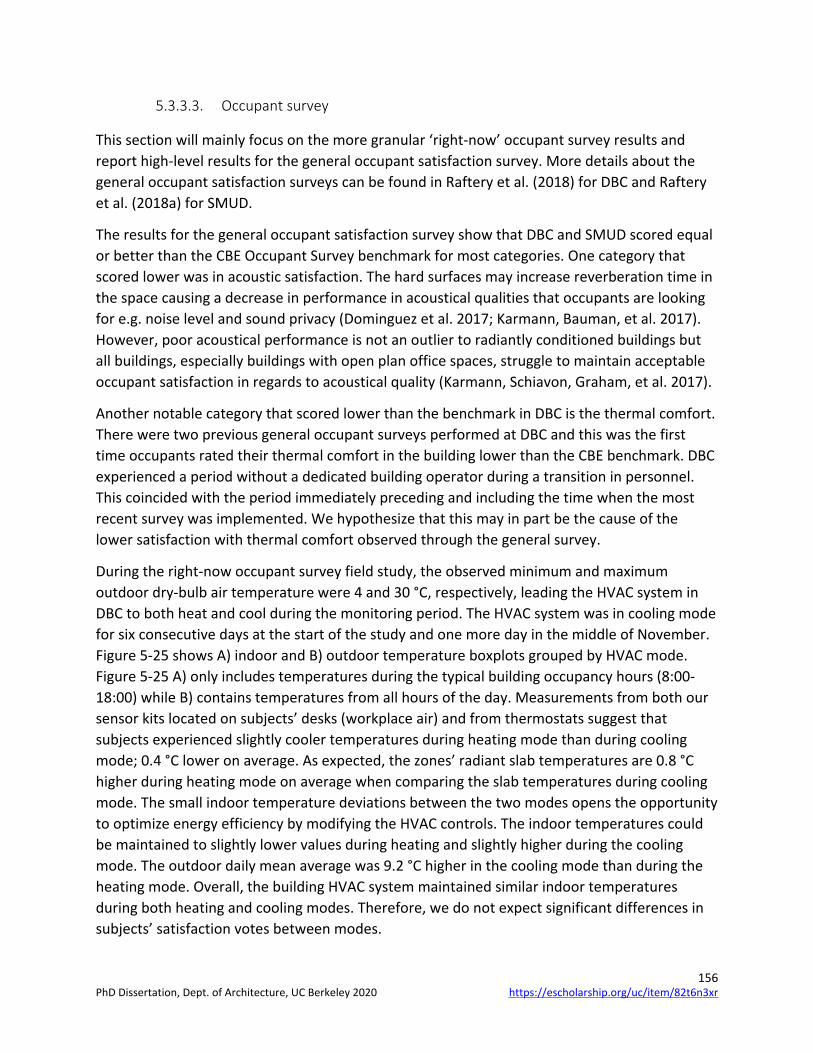
156
5.3.3.3. Occupant survey
This section will mainly focus on the more granular ‘right-now’ occupant survey results and report high-level results for the general occupant satisfaction survey. More details about the general occupant satisfaction surveys can be found in Raftery et al. (2018) for DBC and Raftery et al. (2018a) for SMUD.
The results for the general occupant satisfaction survey show that DBC and SMUD scored equal or better than the CBE Occupant Survey benchmark for most categories. One category that scored lower was in acoustic satisfaction. The hard surfaces may increase reverberation time in the space causing a decrease in performance in acoustical qualities that occupants are looking for e.g. noise level and sound privacy (Dominguez et al. 2017; Karmann, Bauman, et al. 2017). However, poor acoustical performance is not an outlier to radiantly conditioned buildings but all buildings, especially buildings with open plan office spaces, struggle to maintain acceptable occupant satisfaction in regards to acoustical quality (Karmann, Schiavon, Graham, et al. 2017).
Another notable category that scored lower than the benchmark in DBC is the thermal comfort. There were two previous general occupant surveys performed at DBC and this was the first time occupants rated their thermal comfort in the building lower than the CBE benchmark. DBC experienced a period without a dedicated building operator during a transition in personnel. This coincided with the period immediately preceding and including the time when the most recent survey was implemented. We hypothesize that this may in part be the cause of the lower satisfaction with thermal comfort observed through the general survey.
During the right-now occupant survey field study, the observed minimum and maximum outdoor dry-bulb air temperature were 4 and 30 °C, respectively, leading the HVAC system in DBC to both heat and cool during the monitoring period. The HVAC system was in cooling mode for six consecutive days at the start of the study and one more day in the middle of November. Figure 5-25 shows A) indoor and B) outdoor temperature boxplots grouped by HVAC mode. Figure 5-25 A) only includes temperatures during the typical building occupancy hours (8:00-18:00) while B) contains temperatures from all hours of the day. Measurements from both our sensor kits located on subjects’ desks (workplace air) and from thermostats suggest that subjects experienced slightly cooler temperatures during heating mode than during cooling mode; 0.4 °C lower on average. As expected, the zones’ radiant slab temperatures are 0.8 °C higher during heating mode on average when comparing the slab temperatures during cooling mode. The small indoor temperature deviations between the two modes opens the opportunity to optimize energy efficiency by modifying the HVAC controls. The indoor temperatures could be maintained to slightly lower values during heating and slightly higher during the cooling mode. The outdoor daily mean average was 9.2 °C higher in the cooling mode than during the heating mode. Overall, the building HVAC system maintained similar indoor temperatures during both heating and cooling modes. Therefore, we do not expect significant differences in subjects’ satisfaction votes between modes.
https://escholarship.org/uc/item/82t6n3xrPhD Dissertation, Dept. of Architecture, UC Berkeley 2020
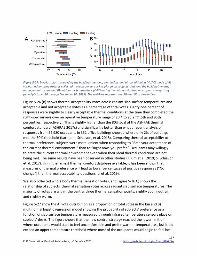
157
Figure 5-25: Boxplots plots grouped by the building’s heating, ventilation, and air-conditioning (HVAC) mode of A) various indoor temperatures collected through our sensor kits placed on subjects’ desk and the building’s energy management system and B) outdoor air temperature (OAT) during the detailed right-now occupant survey study period (October 20 through December 10, 2019). The whiskers represent the 5th and 95th percentiles.
Figure 5-26 (B) shows thermal acceptability votes across radiant slab surface temperatures and acceptable and not acceptable votes as a percentage of total votes. Eighty-one percent of responses were slightly to clearly acceptable thermal conditions at the time they completed the right-now surveys over an operative temperature range of 20.4 to 25.2 °C (5th and 95th percentiles, respectively). This is slightly higher than the 80% goal of the ASHRAE thermal comfort standard (ASHRAE 2017c) and significantly better than what a recent analysis of responses from 52,980 occupants in 351 office buildings showed where only 2% of buildings met the 80% threshold (Karmann, Schiavon, et al. 2018). Comparing thermal acceptability to thermal preference, subjects were more lenient when responding to “Rate your acceptance of the current thermal environment.” than to “Right now, you prefer.” Occupants may willingly tolerate the current thermal environment even when their ideal thermal conditions are not being met. The same results have been observed in other studies (J. Kim et al. 2019; S. Schiavon et al. 2017). Using the largest thermal comfort database available, it has been shown that measures of thermal preference will lead to lower percentages of positive responses (“No change”) than thermal acceptability questions (Li et al. 2019).
We also collected whole body thermal sensation votes, and Figure 5-26 C) shows the relationship of subjects’ thermal sensation votes across radiant slab surface temperatures. The majority of votes are within the central three thermal sensation points: slightly cool, neutral, and slightly warm.
Figure 5-27 show the A) vote distribution as a proportion of total votes in the bin and B) multinomial logistic regression model showing the probability of subjects’ preference as a function of slab surface temperature measured through infrared temperature sensors place on subjects’ desks. The figure shows that the new control strategy reached the lower limit of where occupants would start to feel uncomfortable and prefer warmer temperatures, but it did exceed an upper temperature threshold where most of the occupants would begin to feel hot
https://escholarship.org/uc/item/82t6n3xrPhD Dissertation, Dept. of Architecture, UC Berkeley 2020

158
and prefer cooler temperatures. Both the collected occupant preference votes and the logistic regression model indicate that the HTMR may be controlled to warmer temperatures i.e. raising the defined upper comfort limit parameter in the control strategy. The crossover temperature where occupants go from preferring warmer temperatures to no change is 21.4 °C using the actual votes and 20.8 °C using the logistic regression model. Furthermore, the model predicts that 50% of the responses above 20.8 °C will be a “No change” vote which reiterates that HVAC controls can be optimized to let indoor temperatures float towards warmer temperatures.
https://escholarship.org/uc/item/82t6n3xrPhD Dissertation, Dept. of Architecture, UC Berkeley 2020

159
Figure 5-26: Occupant thermal satisfaction results from eight subjects in the detailed right-now occupant survey study (October 20 through December 10, 2019). Thermal A) preference, B) acceptability, and C) whole body sensation. Daily radiant slab surface measurements collected with our sensor kits on all subjects’ workplace desks and represented as gray lines and the gold dashed lines show our defined thermal comfort range implemented in the intervention control strategy (21.1 and 25.6 °C) in A). The solid black line in B) and C) is the local polynomial regression (LOESS) fit with 95% confidence interval in the shaded area. Point color and shape in all scatter plots indicate thermal preference and acceptability votes, respectively.
https://escholarship.org/uc/item/82t6n3xrPhD Dissertation, Dept. of Architecture, UC Berkeley 2020
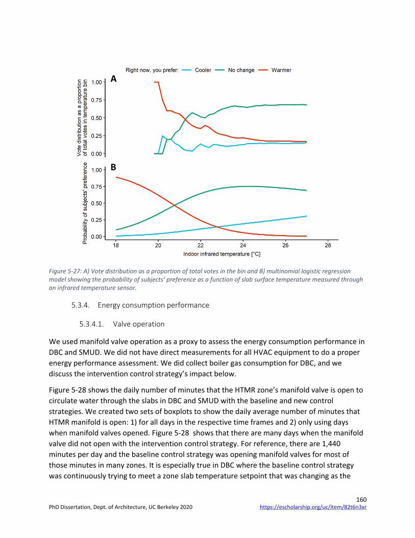
160
Figure 5-27: A) Vote distribution as a proportion of total votes in the bin and B) multinomial logistic regression model showing the probability of subjects’ preference as a function of slab surface temperature measured through an infrared temperature sensor.
5.3.4. Energy consumption performance
5.3.4.1. Valve operation
We used manifold valve operation as a proxy to assess the energy consumption performance in DBC and SMUD. We did not have direct measurements for all HVAC equipment to do a proper energy performance assessment. We did collect boiler gas consumption for DBC, and we discuss the intervention control strategy’s impact below.
Figure 5-28 shows the daily number of minutes that the HTMR zone’s manifold valve is open to circulate water through the slabs in DBC and SMUD with the baseline and new control strategies. We created two sets of boxplots to show the daily average number of minutes that HTMR manifold is open: 1) for all days in the respective time frames and 2) only using days when manifold valves opened. Figure 5-28 shows that there are many days when the manifold valve did not open with the intervention control strategy. For reference, there are 1,440 minutes per day and the baseline control strategy was opening manifold valves for most of those minutes in many zones. It is especially true in DBC where the baseline control strategy was continuously trying to meet a zone slab temperature setpoint that was changing as the
A
B
https://escholarship.org/uc/item/82t6n3xrPhD Dissertation, Dept. of Architecture, UC Berkeley 2020
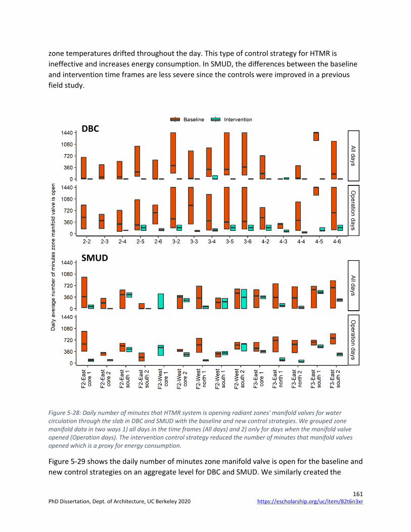
161
zone temperatures drifted throughout the day. This type of control strategy for HTMR is ineffective and increases energy consumption. In SMUD, the differences between the baseline and intervention time frames are less severe since the controls were improved in a previous field study.
Figure 5-28: Daily number of minutes that HTMR system is opening radiant zones' manifold valves for water circulation through the slab in DBC and SMUD with the baseline and new control strategies. We grouped zone manifold data in two ways 1) all days in the time frames (All days) and 2) only for days when the manifold valve opened (Operation days). The intervention control strategy reduced the number of minutes that manifold valves opened which is a proxy for energy consumption.
Figure 5-29 shows the daily number of minutes zone manifold valve is open for the baseline and new control strategies on an aggregate level for DBC and SMUD. We similarly created the
SMUD
DBC
https://escholarship.org/uc/item/82t6n3xrPhD Dissertation, Dept. of Architecture, UC Berkeley 2020

162
boxplots as in the previous figure showing the daily average number of minutes per zone where we used all days in the time frames and only days when HTMR opened zone manifold valves. We created other groups for SMUD, where we used all zones and then grouped by lockout period. There is a drastic change in the daily number of minutes that the zone manifold valves opened between the baseline and new control strategies. For example, using the data from all days, the median number of minutes in DBC-baseline is 190 minutes and fell to 14 minutes in DBC-intervention, a 93% reduction. The reduction in the number of opened minutes directly translates to energy savings since cooled water is not being used to extract heat from the zones or added as in the case with the baseline controls. In SMUD, the new control strategy reduced the number of minutes from 345 to 80, a 77% reduction. Statistic tests show that the decrease in the daily average number of minutes is statistically significant and the effect size is small to large with DBC having the largest effect size.
https://escholarship.org/uc/item/82t6n3xrPhD Dissertation, Dept. of Architecture, UC Berkeley 2020

163
Figure 5-29: Daily number of minutes that HTMR system is opening radiant zones' manifold valves for water circulation through the slab in DBC and SMUD with the baseline and intervention control strategies. We first grouped building manifold data by 1) all days in the time frames (All days) and 2) only for days when manifold valve opened (Operation days). Then within the two main groupings, we grouped the data in SMUD by 1) using data from all zones (SMUD-All zones), 2) using data from zones that had the afternoon lockout implemented in the new control strategy, and 3) using data from zones that had the daytime lockout (SMUD-Daytime). There was a statistically significant difference between baseline and new control strategy daily average number of minutes zone manifold is open between the baseline and intervention time frame groups. The effect size varies between small to large between the groups, as shown through Cohen’s d.
5.3.4.2. DBC gas consumption
Figure 5-30 shows the cumulative boiler gas consumption for DBC during the DBC-baseline and DBC-intervention as well as for previous periods with the baseline control strategy and the subsequent year after we implemented the new control strategy in DBC. The different years’
https://escholarship.org/uc/item/82t6n3xrPhD Dissertation, Dept. of Architecture, UC Berkeley 2020

164
time frames are also from August 20 through October 31. DBC’s HTMR is not the only hot water consumer in DBC, but it is the major end-use component. Water-source heat pumps located on the first floor also use boilers’ hot water when net heating is required by that combined system. As mentioned previously, hot water is circulated through the HTMR because the baseline control strategy is attempting to continuously meet a slab setpoint that is always changing. Sometimes the slab temperature setpoint is higher than the current slab temperature, but not necessarily outside the occupant thermal comfort limits, which drives the gas consumption. The new control strategy allows for the zone temperature to float within limits, thus significantly reducing gas consumption and in line with the reduction in the number of minutes the manifold valves are open. We developed the best fit linear regression lines for the baseline (dashed line in Figure 5-30) and new (dotted line in Figure 5-30) control strategy and calculated an 87% reduction between the two control strategies. The gas consumption reduction represents about $1,240 USD in gas cost savings for the time period shown in Figure 5-30 based on mean 2018 and 2019 natural gas rates. The constant heating calls for heating with the baseline control strategy caused boiler short-cycling, which likely contributed to such a large gas consumption difference most likely contributing.
Figure 5-30: Cumulative gas consumption in DBC with the baseline and new control strategies for time frames from different years. The time frames are from August 20 through October 31. The baseline control strategy is implemented for the years 2012, 2013, 2014, and 2016. The new control strategy is implemented for the year 2018 and 2019. The dashed and dashed lines represent the best fit linear regression line for the gas consumption with the baseline and new control strategy, respectively.
5.3.5. Resilience in HTMR buildings
Figure 5-31 (DBC) and Figure 5-32 (SMUD) show the indoor temperature response after issues (e.g. a VFD failure) that prevented water from circulating through the HTMR slabs even though zones called for cooling. The figures show the detailed response for one zone of each building and the dry-bulb air temperature response of the zones affected by the failures. As expected,
https://escholarship.org/uc/item/82t6n3xrPhD Dissertation, Dept. of Architecture, UC Berkeley 2020

165
indoor temperatures rise after there is no cooled water to extract heat from the zones. However, the rise in zone temperatures was substantially lower than one would expect in a typical building with an all-air HVAC system. The maximum dry-bulb air temperatures slightly exceeded 26 °C. The issue in SMUD lasted for 11 days that affected eight zones on the south water loop of the building, some of which were not under the new control strategy. There was no increase in thermal comfort complaints from the occupants and the building managers were not aware of the issue until we noticed that the new control strategy was not performing as expected. In DBC, the failure lasted for three days but the failure affected all radiant zones in the building. The indoor temperatures started to decrease after we resolved the issues.
Figure 5-31: Indoor temperature response after a software issue caused the new control sequences to fail during the intervention time frame in DBC for a top) single zone and bottom) for all zones in DBC except for zone 2-3 which
https://escholarship.org/uc/item/82t6n3xrPhD Dissertation, Dept. of Architecture, UC Berkeley 2020
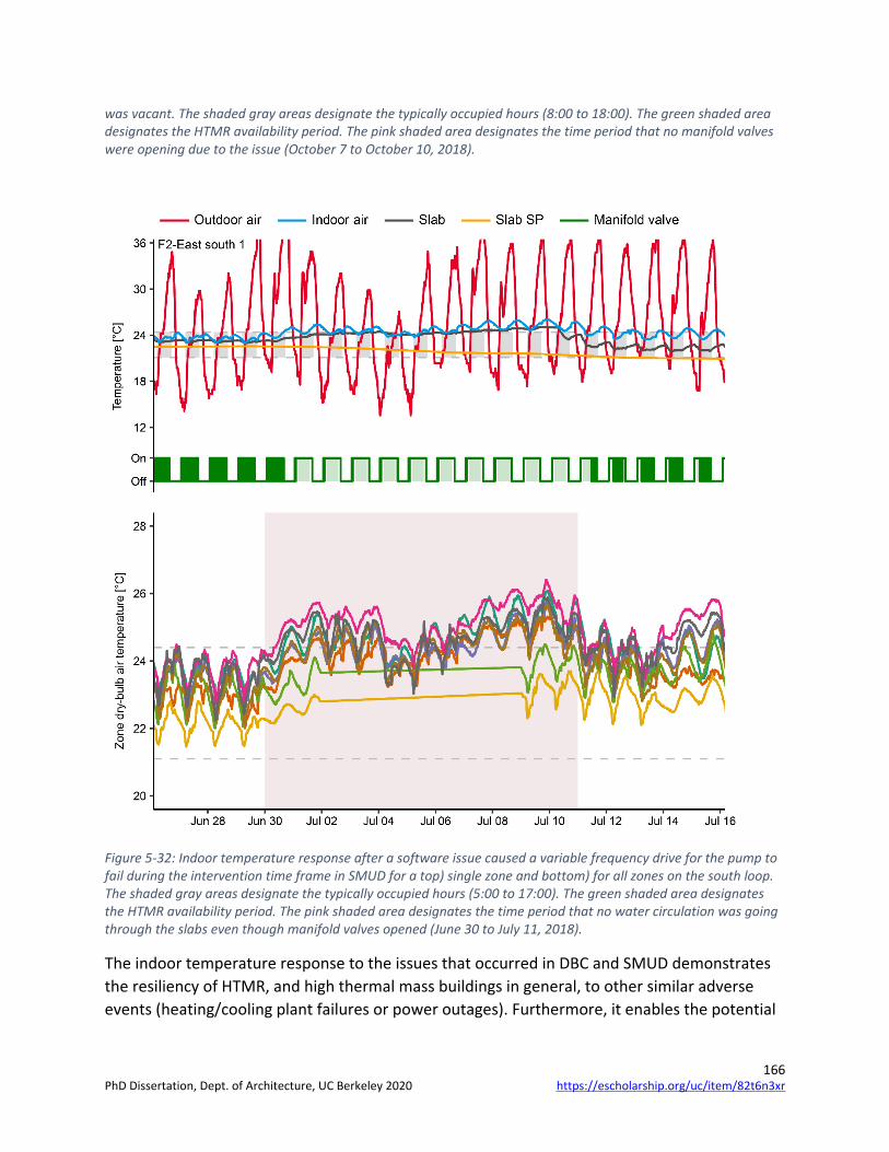
166
was vacant. The shaded gray areas designate the typically occupied hours (8:00 to 18:00). The green shaded area designates the HTMR availability period. The pink shaded area designates the time period that no manifold valves were opening due to the issue (October 7 to October 10, 2018).
Figure 5-32: Indoor temperature response after a software issue caused a variable frequency drive for the pump to fail during the intervention time frame in SMUD for a top) single zone and bottom) for all zones on the south loop. The shaded gray areas designate the typically occupied hours (5:00 to 17:00). The green shaded area designates the HTMR availability period. The pink shaded area designates the time period that no water circulation was going through the slabs even though manifold valves opened (June 30 to July 11, 2018).
The indoor temperature response to the issues that occurred in DBC and SMUD demonstrates the resiliency of HTMR, and high thermal mass buildings in general, to other similar adverse events (heating/cooling plant failures or power outages). Furthermore, it enables the potential
https://escholarship.org/uc/item/82t6n3xrPhD Dissertation, Dept. of Architecture, UC Berkeley 2020

167
of these systems to participate in demand response programs or aid with ancillary grid services (Arteconi et al. 2014; Burger and Moura 2017).
5.4. Discussion
Control strategies have a significant influence over the energy and thermal comfort performance of HVAC systems. Therefore, it is important to consider the capabilities and limitations of HVAC systems when selecting the control strategy for them. HTMR contains and controls a significant amount of thermal mass, so typical control sequences which take a reactive approach in regulating the indoor temperatures are ineffective in maintaining proper thermal comfort or operating efficiently.
In DBC, we saw that the baseline control strategy was in a constant pursuit to meet the zones’ slab temperature setpoint which was changing throughout the day as the zone dry-bulb air temperature changed. These sequences resulted in the HTMR calling for heating during the cool mornings and then switched over to cooling in the afternoons as the zones warmed during the cooling season. The baseline control strategy caused a huge amount of energy wasted because it needed to heat the high thermal inertia concrete to then extract a portion of the HVAC added heat on the same day. The wasted energy is apparent in the increased number of minutes that the manifold valves opened for water circulation observed during the baseline time frame and ultimately increasing the boilers’ gas consumption and cooling towers’ electricity and water usage. We recommend using a 24-hour mode switchover delay to reduce wasted energy with HTMR.
The baseline control strategy in SMUD performed better than the baseline control strategy in DBC because it already went through one iteration of improvements over its originally designed HTMR control strategy during a previous CBE field study. However, the new control strategy implemented in SMUD was still able to increase the overall performance of the HTMR system in terms of thermal comfort and manifold valve operation. The reason for the performance improvement is because the new control strategy adapts based on the extreme indoor temperatures observed in the radiant zones. Each radiant zone may experience differences in heat gains due to their occupant and equipment density and solar heat gain rates in perimeter zones. Moreover, the heat gains in zones may have different rates throughout the day e.g. an east versus west perimeter zone, and these change frequently over the life of a building The baseline control strategy in SMUD started from the same dry-bulb air temperature setpoint for all zones, but we presume that building operators performed manual tuning or adjustments as the zone required since the zones’ setpoints did not match the setpoints reported in the previous field study (Bauman et al. 2015). Further adjustments may have been needed as the seasons changed or the density of occupants or equipment change in the radiant zones. Other control strategies, such as those that implement cooling curves based on outdoor conditions, may also experience similar limitations and need manual tuning before porting to other building projects.
https://escholarship.org/uc/item/82t6n3xrPhD Dissertation, Dept. of Architecture, UC Berkeley 2020

168
Furthermore, outdoor conditions may have a weak influence on the indoor conditions as buildings’ envelopes’ performance requirements are improved with each new building energy code cycle. HVAC control strategies and rules of thumb based on the assumption that the outdoor conditions are a good predictor of indoor conditions will suffer performance degradations as the envelope assumptions used to develop the control strategy deviates from those of the current project. The baseline control strategy in DBC triggered a pre-cooling event only if the outdoor dry-bulb temperature met or exceeded a threshold of 28.9 °C. On many occasions, the outdoor dry-bulb air temperature would be close to the threshold but not enough to trigger the pre-cooling event, which negatively affected indoor thermal comfort conditions.
The new control strategy implemented in DBC and SMUD during the intervention time frames resolved many of the issues presented with the baseline control strategies. The new control strategy tunes itself independently by radiant zone as each zone’s heat gains entering and generated inside the space vary. The new control strategy only adjusts the slab temperature setpoint once per day and allows the indoor dry-bulb air temperature to float within a predefined set of temperature limits. The results show that the new control strategy enables an overall reduction of exceedance percentage of total occupied hours from 9.1% to 1.6% and average exceedance from 0.39 °C to 0.30 °C using data from both buildings and all their zones. It may be counterintuitive but allowing the zone temperatures to float within the full range of acceptable temperatures predicted by thermal comfort standards helped stabilized their interday variability. That is, the indoor temperatures between subsequent days were similar. The observed interday variability went from 0.2 °C and 0.25 °C, for zone dry-bulb air and slab temperature, respectively, during the baseline time frame to 0.15 °C and 0.10 °C, during the intervention time frame. That is, a 25% and 60% reduction in day-to-day variability, for zone dry-bulb air and slab temperature, respectively, when using data from both buildings and all their zones. Predictable indoor temperatures are important for occupants because the decreased uncertainty reduces the burden in selecting appropriate clothing and other thermal adaptation. The intraday variations also deviate from the baseline to intervention time frame but not as much as with the interday variations. The negative 1 h period drifts remain unchanged and the positive 1 h period drifts increased by 15% and 17% for zone dry-bulb air and slab temperature during occupied hours, respectively. In general, the temperature drifts rarely exceeded those imposed by thermal comfort standards during occupied hours. The zone dry-bulb air temperature range increased from 0.84 °C in the baseline time frame to 0.96 °C in the intervention time frame while the slab temperature range decreased from 0.36 °C to 0.28 °C between the two time frame, respectively.
The right-now occupant survey reiterates that occupant thermal comfort is not being adversely affected by the new control strategy. We aimed to collect survey responses at more extreme indoor temperatures to guide any modifications to the control sequences of the HTMR and add to the body of literature on thermal comfort in radiant buildings (Karmann, Schiavon, and Bauman 2017). The average difference in the five indoor temperature measurements between
https://escholarship.org/uc/item/82t6n3xrPhD Dissertation, Dept. of Architecture, UC Berkeley 2020

169
the heating and cooling modes was 0.4 °C, which is of little practical significance. It also demonstrates that the radiant system was able to maintain consistent indoor temperatures as the HVAC modes switched. In addition, the median infrared and dry-bulb temperature measured in the occupied zone by our sensor kits were 22.6 °C and 22.8 °C, respectively, indicating that there are negligible differences in air and mean radiant temperatures experienced by occupants in this building (Dawe et al. 2020). The subjective thermal satisfaction responses from the small number of subjects indicate that this radiant building exceeds the ASHRAE 80% acceptability criteria (Figure 5-26). These acceptability votes were cast at infrared temperatures ranging from 19.6 to 26.9 °C, indicating that we were able to receive votes at extreme conditions even though they did not happen often during our study period. The occupant survey also shows the new control strategy never reached an upper comfort threshold where the majority of the participants would prefer cooler temperatures—suggesting that we can increase our defined upper comfort limit for the new control strategy.
At the same time that the new control strategy is improving thermal comfort, it also reduces energy consumption. We used the number of minutes that the manifold valves as a proxy for energy consumption. The new control strategy reduces the daily average number of minutes that the zone valves are opened by 93% and 77% in DBC and SMUD, respectively. The reduction is in part because the indoor temperatures can float through a wider range of acceptable temperatures, the controls are not constantly pursuing a changing setpoint within a day for the high thermal inertia slab, and eliminating the heating/cooling mode switchover within 24 hours. The number of minutes that the manifold valves are opened correlates with the energy consumption for hot or cold water production. We obtained boiler gas consumption data for DBC and observed a reduction of 87% from using the baseline control strategy to the new control strategy. We also expect significant energy consumption reductions for cold water production used in the HTMR. The energy savings can improve if the heating and cooling plant in HTMR buildings can take advantage of high-temperature cooling and low-temperature heating, as discussed in Chapter 4. However, buildings where they are part of a campus with centralized HVAC plants, such as in SMUD, will not be able to take full advantage of the efficiency benefits of a decreased temperature difference between the zone and supply water temperatures.
Finally, HTMR buildings contain, and more importantly have the capability to control, a significant amount of thermal mass. The thermal energy storage potential for these buildings is high (68-137 Wh·m-2·K-1) as previously mentioned in Chapter 1. These types of buildings can implement demand response or ancillary grid services without having adverse effects on the indoor built environment. We experienced control failures in both buildings that prevented water from circulating through slabs in all zones (DBC) or the zones on one whole façade of the building (SMUD). The rise in temperatures was not significant during the non-operation of the HTMR even though more than a week past by before anyone noticed the failures. A controlled HTMR shutoff scenario should decrease the risks of causing discomfort to a greater level.
https://escholarship.org/uc/item/82t6n3xrPhD Dissertation, Dept. of Architecture, UC Berkeley 2020
170
5.5. Conclusion
We performed a field study to test a new control strategy for high thermal mass radiant systems (HTMR) in two office spaces located in two distinct climates in California. The new control strategy allows the indoor temperatures to float within a wider range of acceptable temperatures, adapt to changing indoor environment fluctuations, and eliminates same day heating and cooling by increasing the mode switchover delay to at least 24 hours.
The new control strategy reduced the overall exceedance percentage of total occupied hours from 9.1% to 1.6% and the average degree Celsius exceedance from 0.39 to 0.30 °C. This means that the indoor temperatures stay within the predefined thermal comfort limits for a larger fraction of the total occupied hours, reducing the risk of occupant thermal discomfort. We verified that the new control strategy is not causing adverse effects in the built environment through a ‘right-now’ occupant thermal comfort survey in one of the buildings. The subjective thermal satisfaction responses from the survey participants indicate that the radiant building exceeds the ASHRAE 80% acceptability criteria. Moreover, the survey results suggest that the new control strategy did not reach an upper limit where occupants would generally prefer cooler temperatures. An indication that we can expand the predefined thermal comfort limits in the new control strategy and allow the indoor temperatures to float in a wider range of temperatures.
The new control strategy also reduces the energy consumption for hot and cold water production that circulates through the HTMR radiant zones. We observed a reduction of 77% to 93% in the daily average number of minutes that zones valves opened for water circulation, which is a proxy for the HTMR’s energy consumption. We did not have direct energy consumption measurements, but we did obtain boiler gas consumption for one of the buildings and measured an 87% reduction in gas consumption when comparing the baseline control strategy to the new control strategy. Overall, the new control strategy performs well in both buildings. It is easy to implement in existing building’s energy management systems and does not require an increased skill set to operate and manage. Its advantages will help reduce barriers to increase the adoption of HTMR in buildings.
5.6. Acknowledgments
We would like to thank Laurie Rich, Executive Director of the David Brower Center (DBC) Building, for allowing us to study the building and support for installing our BACnet communication devices and sensor kits. We are grateful to Ricardo Hernandez, Hugh Newman, and Steven Sewell, the building managers of DBC and SMUD, for their support, availability, and patience throughout the field study.
https://escholarship.org/uc/item/82t6n3xrPhD Dissertation, Dept. of Architecture, UC Berkeley 2020
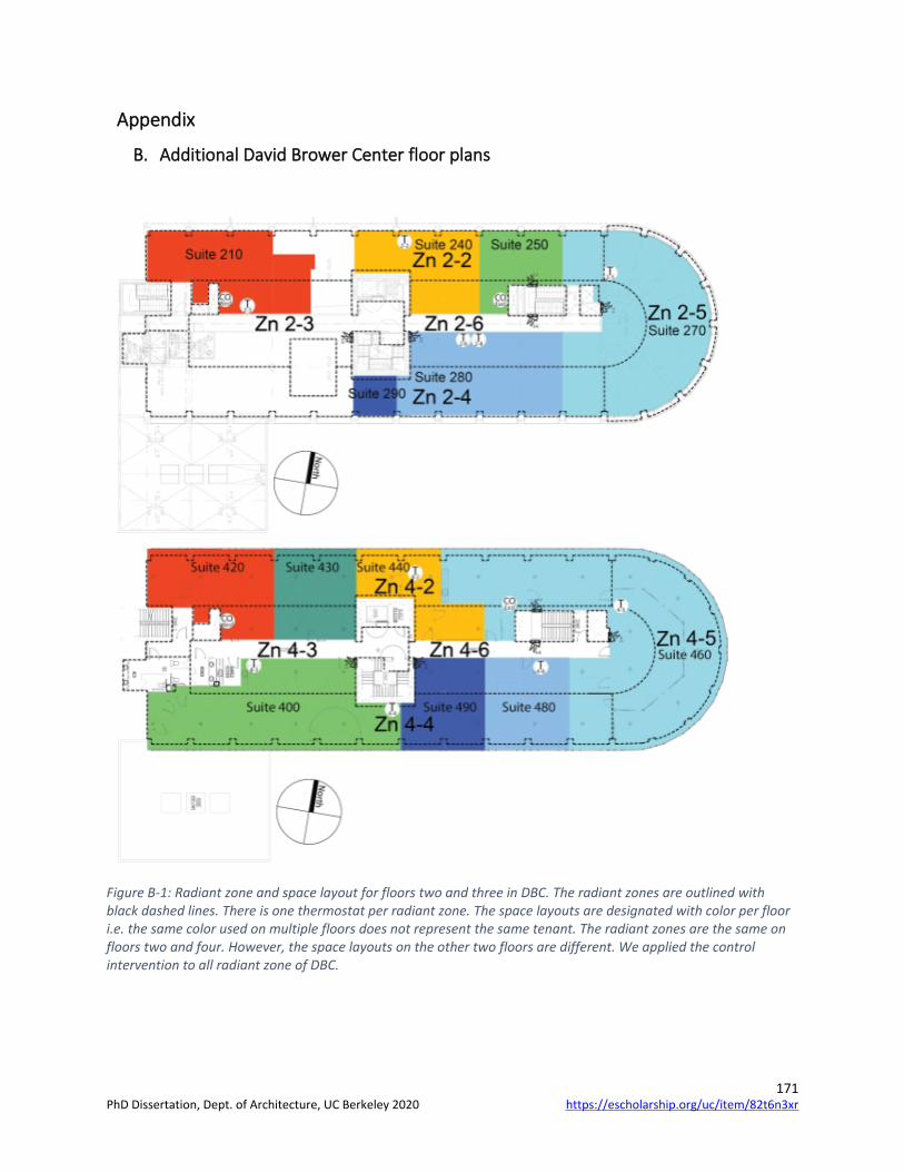
171
Appendix
B. Additional David Brower Center floor plans
Figure B-1: Radiant zone and space layout for floors two and three in DBC. The radiant zones are outlined with black dashed lines. There is one thermostat per radiant zone. The space layouts are designated with color per floor i.e. the same color used on multiple floors does not represent the same tenant. The radiant zones are the same on floors two and four. However, the space layouts on the other two floors are different. We applied the control intervention to all radiant zone of DBC.
https://escholarship.org/uc/item/82t6n3xrPhD Dissertation, Dept. of Architecture, UC Berkeley 2020

172
6. Interactive web-based tool for the early design of high thermal mass radiant systems
6.1. Background
Guidebooks from REHVA, ISO, and ASHRAE provide detailed guidelines for calculating the design radiant and convective heat transfer rates that various radiant system types can be expected to produce for different steady-state conditions (ASHRAE 2016d; Babiak et al. 2009; ISO 2012). We discussed and demonstrated throughout this dissertation that the significant amounts of thermal mass in HTMR prevent such systems from ever operating at steady-state in typical built environment settings, and hence these guidelines are unsuitable. The best approach is to use tools that perform detailed dynamic simulations such as EnergyPlus, TRNSYS, or IES-VE (Beckman et al. 1994; Behrendt et al. 2011; Crawley et al. 2008; Drury B. Crawley 1999). However, building designers often perceive detailed simulations as complicated, time-consuming, and high cost (Feng et al. 2014a; Østergård et al. 2016). As a consequence, the majority of radiant system designers who completed a survey on design tool usage reported they use steady-state and other simplified methods instead of heat balance or other advanced methods to calculate the cooling load; 59% versus 27% (Feng et al. 2014a). Yet, the HTMR steady-state cooling load calculation procedure can also be laborious. It requires designers to calculate the relationship between heat flux and the temperature difference between the supply water temperature and the zone operative temperature, also known as the characteristic curve, using a single power function based on multiple parameters (ISO 2012). It can be intimidating for HTMR designers and prone to mistakes when translating the equations from the standard to a usable format, such as in spreadsheet tools. Moreover, there does not exist a publicly available tool that incorporates the ISO equations for HTMR cooling capacity. Each designer or firm would need to repeat the process of interpreting the ISO equations and create their in-house tool.
Therefore, we developed interactive web-based tools for the early design of HTMR. The tools serve as a shared resource for the steady-state analysis that designers are already accustomed to, as well as for our latest developments in HTMR tools that incorporate transient analysis. We believe the steady-state analysis tool will serve as the attractor to the website, but we will encourage the use of simplified transient tools and provide pathways for the designer to transition to the less familiar transient analysis. The following sections briefly describe the web tools and resources currently available at the time of this publication. We will use a growth-driven design approach to incrementally improve the website and available tools as we learn more about building designers’ needs and gain new information about HTMR design, and in general, about radiant cooling and heating systems. The web tools are freely available at http://radiant.cbe.berkeley.edu/ as well as its more detailed documentation.
https://escholarship.org/uc/item/82t6n3xrPhD Dissertation, Dept. of Architecture, UC Berkeley 2020

173
6.2. Structure of the website
The overall website project aims to serve as a repository of tools and other resources pertaining to the early design of HTMR. We focus on early design because decisions made in early design phases have the greatest impact on final performance and costs (Hygh et al. 2012; Kanters and Horvat 2012). We divided the website into three sections: 1) “Steady State”, 2) “Transient”, and 3) “Resources”.
6.2.1. Steady-state analysis
The steady-state analysis provides evaluation for thermally activated building systems (TABS) and embedded surface systems (ESS) for both heating and cooling modes. By definition, a steady-state process does not change in time. This means that the method cannot be used to analyze the thermal inertia of the space and HTMR. Hence, in this method of analysis, the space heat extraction rate is equal to the hydronic plant extraction rate. The characteristic curve, or the equivalent heat transmission coefficient, depends on the tubing spacing, depth, and diameter, slab thermal conductivity, water flow rate, and other parameters (ISO 2012). The web tool users have the option to vary all these inputs to either the International System or Imperial units and obtain the following categories of outputs in the same selected units:
1. Design calculations such as equivalent heat transmission coefficient, design temperature difference, and active surface temperature.
2. Heat extraction rate at the surface and hydronic level.
3. Tubing design factors such as total design water flow rate, design water velocity in the tubing, and the number of loops for the area of the room.
There are also visual outputs as shown in Figure 6-1. The designer has access to two plots; a two- and three-dimensional plot. The plots can be used to perform ‘what-if’ scenarios. The designers can visually understand the relationship between two or three different parameters.
https://escholarship.org/uc/item/82t6n3xrPhD Dissertation, Dept. of Architecture, UC Berkeley 2020

174
Figure 6-1: Screenshot of the CBE Rad Tool in steady-state analysis mode.
6.2.2. Transient analysis
Another limitation of the steady-state analysis is that calculations are performed with the assumption of a constant zone dry-bulb air, as discussed in Chapter 3. The zone temperatures’ response is not constant and its variation depends on the heat gains generated and entering the zone, control strategy, HTMR type, and other parameters. The transient analysis provides evaluation for TABS in cooling mode. Designers have access to 12 critical inputs, including start and duration of hydronic plant operation, with various levels accessed through dropdown menus to evaluate the response of the zone heat gains, operative temperature, surface heat flux, and hydronic cooling load. The tool displays the responses in 24-hour timeseries plots, as shown in Figure 6-2. The transient tool is available for only cooling mode analysis at a standardized summer design day (Rudoy and Duran 1975; Spitler et al. 1993). The transient tool is easy to use, interactive and requires no online simulations. The transient tool is unique because it allows designers to consider the impact of innovative control strategies such as nighttime cooling plant operation.
https://escholarship.org/uc/item/82t6n3xrPhD Dissertation, Dept. of Architecture, UC Berkeley 2020

175
Figure 6-2: Screenshot of the CBE Rad Tool in transient analysis mode.
We pre-simulated over two and a half million cases of a single zone model on a summer cooling design day using EnergyPlus. Similar to the models we used in Chapter 3, the single zone in the transient tool represents a perimeter middle floor of a large office building. The detailed EnergyPlus model description can be found through the following link: http://radiant.cbe.berkeley.edu/resources/rad_tool_documentation. The documentation includes descriptions of the geometry, construction layers, heat gains, the HTMR, and other assumptions we used to create the single zone models.
6.3. Resources
In the resources section of the website, we gathered useful information for HTMR designers. These include documentation to both the steady-state and transient HTMR tools, the adaptive radiant control sequences we used and analyzed in Chapters 3 and 5, and links to an interactive map for buildings with radiant systems (Karmann et al. 2014) and to other research pertaining to radiant systems. The radiant control sequences come in language that can be handed directly to controls contractors, as part of a single zone model example where advanced users can modify for their case studies, and as a so-called OpenStudio measure. The OpenStudio
https://escholarship.org/uc/item/82t6n3xrPhD Dissertation, Dept. of Architecture, UC Berkeley 2020
176
measure facilitates the transferring of the adaptive control sequences to a custom EnergyPlus model including multizone models (Goldwasser et al. 2016). We make the control sequences available in several formats since it is an important factor in implementing a successful HTMR project.
Finally, we do not provide an analysis of the implications of using steady-state versus transient analysis in this chapter since we already provide a detailed analysis in Chapter 3. The main takeaway between using one analysis versus the other is that steady-state analysis can lead designers to overlook considerable opportunities to improve HTMR energy and thermal comfort performance.
6.4. Conclusion
Most radiant system designers use steady-state analysis for the design of HTMR despite that these systems never operate in such conditions in real buildings. We recommend that designers use transient analysis, but detailed simulations present challenges for them. We developed interactive web-based tools that facilitate the steady-state and transient analysis for the early design of HTMR. We use the more familiar steady-state analysis to attract designers to the website, and provide pathways for designers to supplement their steady-state analysis with transient analysis or fully embrace the transient analysis in early HTMR design. We will update the website and tools using a growth-driven design approach as we learn more about building designers’ needs and gain new information about HTMR design, and about radiant cooling and heating systems in general.
https://escholarship.org/uc/item/82t6n3xrPhD Dissertation, Dept. of Architecture, UC Berkeley 2020

177
7. Conclusion
In this dissertation, we investigate the design and control of high thermal mass radiant systems (HTMR) focusing on space cooling. HTMR is still relatively unfamiliar to US design professionals, who need guidance on correctly sizing mechanical system components, selecting the appropriate control strategy, and identifying the advantages and limitations of this technology for various climates, building types and programs. For these reasons, we provide a critical review of the current standard design procedure for sizing cooling systems to identify fundamental flaws; explain how it has influenced building energy modeling, system sizing and operation in practice; and propose a new definition for space cooling load, along with an associated design procedure. The current, widely used space cooling load definition is too narrowly constraint and omits fundamental principles that are essential to the operation of various cooling systems, including HTMR. Our proposed redefinition and associated design procedure enable building designers to unlock new opportunities to reduce costs and improve energy efficiency and thermal comfort. One such opportunity is to combine HTMR’s innate high thermal inertia with high-temperature cooling to replace the energy- and cost-intensive vapor-compression cycle with cooling towers or fluid coolers to produce the needed cool supply water temperatures during nighttime hours, when adiabatic cooling is the most effective. We found that the warmest supply water temperatures that can be used in HTMR is 18.2, 21.4, 23.4 °C for the first quartile, median, and third quartile, respectively, among all test cases. The production of these supply water temperatures by only using adiabatic cooling is possible within many climates in the US, particularly California. If a building design with HTMR cannot use adiabatic cooling, it still benefits by having the capability to shift the cooling plant’s operation to nighttime when the system is more energy efficient and can avoid high electricity prices during peak demand periods, or design a lower capacity plant by extending the plant’s operation.
Shifting the cooling plant’s operation to nighttime hours does not have adverse effects on occupants’ thermal comfort satisfaction. Our whole building energy simulation results show that indoor temperatures can be maintained within acceptable thermal comfort limits for a cooling design day and annual simulation. We confirmed these results by implementing an adaptive HTMR control strategy in two buildings in California located in Sacramento and Berkeley. The field study results show that the new adaptive control strategy reduces the number of hours that zone dry-bulb temperatures exceed predefined thermal comfort limits from 9.1% to 1.6% as a proportion of total occupied hours when compared to the buildings’ existing controls. We also verified that the new control strategy did not have adverse effects on occupant thermal comfort satisfaction through a detailed “right-now” satisfaction survey. The right-now surveys indicate that 81% of occupants’ responses found the thermal conditions to be slightly to clearly acceptable at the time they completed the surveys over an operative temperature range of 20.4 to 25.2 °C (5th and 95th percentiles, respectively). This is slightly higher than the 80% goal suggested in the ASHRAE thermal comfort standard. We also observed that the new adaptive control strategy reduces the number of average daily minutes
https://escholarship.org/uc/item/82t6n3xrPhD Dissertation, Dept. of Architecture, UC Berkeley 2020

178
HTMR manifold valves open for water flow through the slab, a proxy for energy consumption, by up to 93%. Finally, we created an interactive web-based tool for the early design of HTMR to increase the availability of tools to design HTMR. The tool estimates HTMR performance under steady-state and transient conditions. We recommend designers use transient analysis to design HTMR since the high thermal inertia prevents these systems from ever operating at steady-state. Improving the design of HTMR and making information available to designers will help achieve reductions in energy and greenhouse gas emissions attributed to HVAC systems.
https://escholarship.org/uc/item/82t6n3xrPhD Dissertation, Dept. of Architecture, UC Berkeley 2020

179
8. References
Abadi, M., A. Agarwal, P. Barham, E. Brevdo, Z. Chen, C. Citro, G. S. Corrado, A. Davis, J. Dean, and M. Devin. 2016. Tensorflow: Large-scale machine learning on heterogeneous distributed systems. ArXiv Preprint ArXiv:1603.04467.
Afram, A., and F. Janabi-Sharifi. 2014. Theory and applications of HVAC control systems – A review of model predictive control (MPC). Building and Environment, 72:343–355.
Alajmi, A. 2012. Energy audit of an educational building in a hot summer climate. Energy and Buildings, 47:122–130.
Ang, K. H., G. Chong, and Y. Li. 2005. PID control system analysis, design, and technology. IEEE Transactions on Control Systems Technology, 13(4):559–576.
Arens, E., T. Hoyt, X. Zhou, L. Huang, H. Zhang, and S. Schiavon. 2015. Modeling the comfort effects of short-wave solar radiation indoors. Building and Environment, 88:3–9.
Armstrong, P. R., W. Jiang, D. Winiarski, S. Katipamula, and L. K. Norford. 2009. Efficient Low-Lift Cooling with Radiant Distribution, Thermal Storage, and Variable-Speed Chiller Controls—Part II: Annual Use and Energy Savings. HVAC&R Research, 15(2):402–432.
Armstrong, R. A. 2014. When to use the Bonferroni correction. Ophthalmic and Physiological Optics, 34(5):502–508.
Arteconi, A., D. Costola, P. Hoes, and J. L. M. Hensen. 2014. Analysis of control strategies for thermally activated building systems under demand side management mechanisms. Energy and Buildings, 80(Supplement C):384–393.
ASHRAE. 2016a. ANSI/ASHRAE Standard 62.1-2016 - Ventilation for Acceptable Indoor Air Quality. Atlanta, GA: American Society of Heating, Refrigerating and Air-Conditioning Engineers.
ASHRAE. 2016b. ASHRAE Standard 90.1-Energy standard for buildings except low-rise residential buildings. Atlanta, GA: American Society of Heating, Refrigerating and Air Conditioning Engineers, Inc.
ASHRAE. 2016c. ASHRAE Standard 135 - BACnet - A data communications protocol for building automation and control networks. Atlanta, GA: American Society of Heating, Refrigerating and Air Conditioning Engineers, Inc.
ASHRAE. 2016d. Chapter 6: Radiant Heating and Cooling. In HVAC Systems and Equipment. Atlanta, GA: American Society of Heating, Refrigerating and Air Conditioning Engineers.
ASHRAE. 2017a. 2017 ASHRAE Handbook: Fundamentals. Atlanta, GA: American Society of Heating, Refrigerating and Air-Conditioning Engineers.
ASHRAE (Ed.). 2017b. ASHRAE design guide for dedicated outdoor air systems. Atlanta: ASHRAE. ASHRAE. 2017c. ASHRAE Standard 55-2017: Thermal Environmental Conditions for Human
Occupancy. Atlanta, GA: American Society of Heating, Refrigerating and Air Conditioning Engineers Inc.
ASHRAE. 2017d. Chapter 14: Climatic Design Information. In ASHRAE Handbook Fundamentals. Atlanta, GA: American Society of Heating, Refrigerating and Air Conditioning Engineers.
ASHRAE. 2017e. Chapter 18: Nonresidential cooling and heating calculations. In ASHRAE Handbook Fundamentals. Atlanta, GA: American Society of Heating, Refrigerating and Air Conditioning Engineers.
https://escholarship.org/uc/item/82t6n3xrPhD Dissertation, Dept. of Architecture, UC Berkeley 2020

180
ASHRAE/CIBSE/USGBC. 2010. Performance Measurement Protocols (PMP) for Commercial Buildings. Atlanta, GA: Atlanta: American Society of Heating, Refrigerating, and Air-Conditioning Engineers, Inc.
ASTM. 2017. ASTM F876:2017 - Standard Specification for Crosslinked Polyethylene (PEX) Tubing.
Babiak, J., B. Olesen, and D. Petras. 2009. REHVA guidebook No. 7: Low temperature heating and high temperature cooling. Brussels, Belgium: Federation of European Heating and Air-Conditioning Associations.
Bauer, K. T. 2016, January. Integrating Sustainability & Structure: A Case Study. STRUCTURE. Bauman, F., H. Zhang, E. Arens, P. Raftery, C. Karmann, J. (Dove) Feng, Y. Zhai, D. Dickerhoff, S.
Schiavon, and X. Zhou. 2015. Advanced Integrated Systems Technology Development: Personal Comfort Systems and Radiant Slab Systems.
Beckman, W. A., L. Broman, A. Fiksel, S. A. Klein, E. Lindberg, M. Schuler, and J. Thornton. 1994. TRNSYS The most complete solar energy system modeling and simulation software. Renewable Energy, 5(1):486–488.
Behrendt, B. M., D. Raimondo, Y. Zhang, S. Schwarz, J. E. Christensen, and B. W. Olesen. 2011. A System for the Comparison of Tools for the Simulation of Water-based Radiant Heating and Cooling System. In 12th Conference of International Building Performance Simulation Association (p. 8). Sydney, Australia.
Bell, I. H., J. Wronski, S. Quoilin, and V. Lemort. 2014. Pure and Pseudo-pure Fluid Thermophysical Property Evaluation and the Open-Source Thermophysical Property Library CoolProp. Industrial & Engineering Chemistry Research, 53(6):2498–2508.
Bender, J. 2018. BACpypes Documentation. Benton, C., F. Bauman, and M. Fountain. 1990. A Field Measurement System for the Study of
Thermal Comfort. ASHRAE Transactions, 96(1):623–633. Berger, E. 2015. The Hidden Daytime Price Of Electricity. ASHRAE Journal, 57(4):64. Braun, J. E. 1990. Reducing Energy Costs and Peak Electrical Demand through Optimal Control
of Building Thermal Storage. ASHRAE Transactions, 96(2):876–887. Braun, J. E. 2003. Load Control Using Building Thermal Mass. Journal of Solar Energy
Engineering, 125(3):292–301. Burger, E. M., and S. J. Moura. 2017. Generation following with thermostatically controlled
loads via alternating direction method of multipliers sharing algorithm. Electric Power Systems Research, 146(Supplement C):141–160.
Burhenne, S., D. Jacob, and G. P. Henze. 2011. Sampling based on Sobol’ sequences for Monte Carlo techniques applied to building simulations. In Proc. Int. Conf. Build. Simulat (pp. 1816–1823).
Bushby, S. T. 1997. BACnetTM: a standard communication infrastructure for intelligent buildings. Automation in Construction, 6(5–6):529–540.
Catalina, T., J. Virgone, and F. Kuznik. 2009. Evaluation of thermal comfort using combined CFD and experimentation study in a test room equipped with a cooling ceiling. Building and Environment, 44(8):1740–1750.
Causone, F., S. P. Corgnati, M. Filippi, and B. W. Olesen. 2010. Solar radiation and cooling load calculation for radiant systems: Definition and evaluation of the Direct Solar Load. Energy and Buildings, 42(3):305–314.
https://escholarship.org/uc/item/82t6n3xrPhD Dissertation, Dept. of Architecture, UC Berkeley 2020

181
CBE. 2014. Occupant indoor environmental quality (IEQ) survey. Berkeley, CA: Center for the Built Environment, University of California, Berkeley.
CEC. 2015. Title-24 2016 Part 6: Building energy efficiency standards for residential and nonresidential buildings. In Title 24 of the California Code of Regulations. Sacramento, CA: California Energy Commission.
CEC. 2016a. Nonresidential Alternative Calculation Method. California Energy Commission. CEC. 2016b. Title 24 of California Code of Regulations. Sacramento, CA: California Building
Standards Commission. CEN. 2007. EN 15255-2007 Thermal performance of buildings-Sensible room cooling load
calculation. Brussels, Belgium: European Committee for Standardization. CEN. 2019. EN 16798-1:2019 — Energy performance of buildings — Ventilation for buildings —
Part 1: Indoor environmental input parameters for design and assessment of energy performance of buildings addressing indoor air quality, thermal environment, lighting and acoustics — Module M1-6. Brussels: European Committee for Standardization.
Chai, T., and R. R. Draxler. 2014. Root mean square error (RMSE) or mean absolute error (MAE)? – Arguments against avoiding RMSE in the literature. Geoscientific Model Development, 7(3):1247–1250.
Chantrasrisalai, C., V. Ghatti, D. E. Fisher, and D. G. Scheatzle. 2003. Experimental validation of the EnergyPlus low-temperature radiant simulation. ASHRAE Transactions, 109(2):614–623.
Cho, S.-H., and M. Zaheer-uddin. 1999. An experimental study of multiple parameter switching control for radiant floor heating systems. Energy, 24(5):433–444.
Chollet, F. 2015. Keras: The Python Deep Learning library. Chung, W. J., S. H. Park, M. S. Yeo, and K. W. Kim. 2017. Control of Thermally Activated Building
System Considering Zone Load Characteristics. Sustainability, 9(4):586. Cohen, J. 1988. Statistical Power Analysis for the Behavioral Sciences. New York: Lawrence
Erlbaum Associates. Conroy, C. L., and S. A. Mumma. 2001. Ceiling radiant cooling panels as a viable distributed
parallel sensible cooling technology integrated with dedicated outdoor air systems / Discussion. ASHRAE Transactions; Atlanta, 107:578.
Cooper, G. 1998. Air-conditioning America: engineers and the controlled environment, 1900-1960. Baltimore, Md: Johns Hopkins University Press.
Corbin, C. D., G. P. Henze, and P. May-Ostendorp. 2013. A model predictive control optimization environment for real-time commercial building application. Journal of Building Performance Simulation, 6(3):159–174.
Costelloe, B., and D. Finn. 2003. Experimental energy performance of open cooling towers used under low and variable approach conditions for indirect evaporative cooling in buildings. Building Services Engineering Research and Technology, 24(3):163–177.
Crawley, D. B., J. W. Hand, M. Kummert, and B. T. Griffith. 2008. Contrasting the capabilities of building energy performance simulation programs. Building and Environment, 43(4):661–673.
Crowther, H., and Y. T. Ma. 2016. Design Considerations for Dedicated OA Systems. ASHRAE Journal.
https://escholarship.org/uc/item/82t6n3xrPhD Dissertation, Dept. of Architecture, UC Berkeley 2020

182
Davis, L. W., and P. J. Gertler. 2015. Contribution of air conditioning adoption to future energy use under global warming. Proceedings of the National Academy of Sciences of the United States of America, 112(19):5962–5967.
Dawe, M., P. Raftery, J. Woolley, S. Schiavon, and F. Bauman. 2020. Comparison of mean radiant and air temperatures in mechanically-conditioned commercial buildings from over 200,000 field and laboratory measurements. Energy and Buildings, 206:109582.
Dawson-Haggerty, S., X. Jiang, G. Tolle, J. Ortiz, and D. Culler. 2010. sMAP: a simple measurement and actuation profile for physical information. In Proceedings of the 8th ACM Conference on Embedded Networked Sensor Systems - SenSys ’10 (p. 197). Zurich, Switzerland: ACM Press.
De Carli, M., and B. W. Olesen. 2001. Field measurements of thermal comfort conditions in buildings with radiant surface cooling systems. Clima 2000, 15th–18th (2001), Naples, Italy.
de Dear, R. 2011. Revisiting an old hypothesis of human thermal perception: alliesthesia. Building Research & Information, 39(2):108–117.
de Wit, A. K., and C. J. Wisse. 2012. Hydronic circuit topologies for thermally activated building systems – design questions and case study. Energy and Buildings, 52:56–67.
Dean, B., J. Dulac, T. Morgan, and U. Remme. 2018. The Future of Cooling: Opportunities for energy efficient air conditioning (p. 92). IEA.
Deru, M., K. Field, D. Studer, K. Benne, B. Griffith, P. Torcellini, B. Liu, M. Halverson, D. Winiarski, M. Rosenberg, M. Yazadanian, J. Huang, and D. Crawley. 2011. U.S. Department of Energy commercial reference building models of the national building stock (Technical Report). National Renewable Energy Laboratory.
Dillig, M., M. Jung, and J. Karl. 2016. The impact of renewables on electricity prices in Germany – An estimation based on historic spot prices in the years 2011–2013. Renewable and Sustainable Energy Reviews, 57:7–15.
DOE. 2006. Benefits of demand response in electricity markets and recommendations for achieving them. Washington, DC: Department of Energy.
DOE. 2018. Weather Data | EnergyPlus. DOE. 2020. Input Output Reference: The encyclopedic reference to EnergyPlus input and
output. US Department of Energy. Dominguez, L. M., O. B. Kazanci, N. Rage, and B. W. Olesen. 2017. Experimental and numerical
study of the effects of acoustic sound absorbers on the cooling performance of Thermally Active Building Systems. Building and Environment, 116:108–120.
Drury B. Crawley, L. K. L. 1999. EnergyPlus: A New-Generation Building Energy Simulation. Duarte, C., P. Raftery, S. Schiavon, and F. Bauman. 2018. How High Can You Go? Determining
the Highest Supply Water Temperature for High Thermal Mass Radiant Cooling Systems in California. In 4th International Conference on Building Energy & Environment. Melbourne, Australia.
Duarte, C., K. Van Den Wymelenberg, and C. Rieger. 2013. Revealing occupancy patterns in an office building through the use of occupancy sensor data. Energy and Buildings, 67:587–595.
https://escholarship.org/uc/item/82t6n3xrPhD Dissertation, Dept. of Architecture, UC Berkeley 2020

183
Duarte Roa, C., S. Schiavon, and T. Parkinson. 2020. Targeted occupant surveys: A novel method to effectively relate occupant feedback with environmental conditions. In Review. Building and Environment.
EIA. 2012. Commercial Building Energy Consumption Survey (CBECS). Energy Information Administration, U.S. Department of Energy.
Elliott, K. 2003. Mixed options for precast concrete construction. Concrete; London, 37(7):18. EnergyPlus. 2018. (Version 9.3.0). U.S. Department of Energy Building Technologies Office. EPA. 2017. Inventory of U.S. Greenhouse Gas Emissions and Sinks: 1990-2015 (Reports and
Assessments). Washington, DC: U.S. Environmental Protection Agency. Evans, R., R. Haryott, H. Norman, and A. Jones. 2004. The Long-term costs of owning and using
buildings. In Designing Better Building: Quality and value in the built environment. Abingdon, Oxon: Routledge.
Faloon, K. 2018. Rolling out radiant. Contractor Magazine, 63(12):1–8. Fanger, P. 1970. Thermal Comfort. Analysis and applications in environmental engineering. Feng, J. (Dove). 2014. Design and Control of Hydronic Radiant Cooling Systems (Ph.D.).
University of California, Berkeley, United States -- California. Feng, J. (Dove), F. Bauman, and S. Schiavon. 2014a. Critical review of water based radiant
cooling system design methods. Feng, J. (Dove), F. Bauman, and S. Schiavon. 2014b. Experimental comparison of zone cooling
load between radiant and air systems. Energy and Buildings, 84:152–159. Feng, J. (Dove), and H. Cheng. 2018. Comparison of construction and energy costs for radiant vs.
VAV systems in the California Bay Area. California Energy Commission. Feng, J. (Dove), F. Chuang, F. Borrelli, and F. Bauman. 2015. Model predictive control of radiant
slab systems with evaporative cooling sources. Energy and Buildings, 87:199–210. Feng, J. (Dove), S. Schiavon, and F. Bauman. 2013a. Cooling load differences between radiant
and air systems. Energy and Buildings, 65:310–321. Feng, J. (Dove), S. Schiavon, and F. Bauman. 2013b. Impact of Solar Heat Gain on Radiant Floor
Cooling System Design. In Proceedings of the 11th International Conference CLIMA 2013. Prague, Czech Republic.
Feustel, H. E. 1993. Hydronic Radiant Cooling: Overview and Preliminary Performance Assessment (No. LBL-33194). Berkeley, CA: Lawrence Berkeley National Laboratory.
Fort, K. 1989. Dynamisches Verhalten von Fussbodenheizungen (Doctoral Dissertation). Eidgenossische Technische Hochschule Zurich.
Fort, K. 2001. TRYNSYS Model Type 360: Floor Heating and Hypocaust. TRANSSOLAR Energietechnik GmbH.
Frontczak, M., S. Schiavon, J. Goins, E. Arens, H. Zhang, and P. Wargocki. 2012. Quantitative relationships between occupant satisfaction and satisfaction aspects of indoor environmental quality and building design. Indoor Air, 22(2):119–131.
Goldwasser, D., D. Macumber, A. Parker, E. Lee, R. Guglielmetti, and L. Brackney. 2016. The Life Cycle of an OpenStudio Measure: Developement, Testing, Distribution, and Application. In Building Performance Modeling Conference (p. 8). Salt Lake City, UT.
Gordian Group. 2019. Mechanical Costs With RSmeans Data 2020. (J. Kelble, Ed.) (43rd Annual edition). Gordian Group Inc RSMeans.
https://escholarship.org/uc/item/82t6n3xrPhD Dissertation, Dept. of Architecture, UC Berkeley 2020

184
Graham, L. T., T. Parkinson, and S. Schiavon. 2020. Where do we go now? Lessons learned from 20 years of CBE’s Occupant Survey.
Gunay, H. B., W. O’Brien, I. Beausoleil-Morrison, and S. Gilani. 2016. Modeling plug-in equipment load patterns in private office spaces. Energy and Buildings, 121:234–249.
Gwerder, M., B. Lehmann, J. Tödtli, V. Dorer, and F. Renggli. 2008. Control of thermally-activated building systems (TABS). Applied Energy, 85(7):565–581.
Gwerder, M., J. Tödtli, B. Lehmann, V. Dorer, W. Güntensperger, and F. Renggli. 2009. Control of thermally activated building systems (TABS) in intermittent operation with pulse width modulation. Applied Energy, 86(9):1606–1616.
Hawken, P. 2017. Drawdown: The Most Comprehensive Plan Ever Proposed to Reverse Global Warming. Penguin.
Hensen, J. L. M. 1990. Literature review on thermal comfort in transient conditions. Building and Environment, 25(4):309–316.
Henze, G., M. Brandemuehl, C. Felsmann, A. Florita, and H. Cheng. 2007. Final project report for ashrae research project 1313-rp: Evaluation of building thermal mass savings. American Society of Heating, Refrigerating and Air-Conditioning Engineers, Inc., Atlanta.
Henze, G. P., C. Felsmann, and G. Knabe. 2004. Evaluation of optimal control for active and passive building thermal storage. International Journal of Thermal Sciences, 43(2):173–183.
Hinton, G. 2012. Neural Networks for Machine Learning - Lecture 6a - Overview of mini-batch gradiant descent. University of Toronto.
Hoyt, T., E. Arens, and H. Zhang. 2015. Extending air temperature setpoints: Simulated energy savings and design considerations for new and retrofit buildings. Building and Environment, 88:89–96.
Huang, L., Q. Ouyang, Y. Zhu, and L. Jiang. 2013. A study about the demand for air movement in warm environment. Building and Environment, 61:27–33.
Humphreys, M. A. 1976. Field studies of thermal comfort compared and applied. Building Services Engineer, 44:5–27.
Humphreys, M. A. 1977. The optimum diameter of a globe thermometer for use indoors. Annual of Occupational Hygiene, 20(2):135–140.
Hunn, B. D., D. R. Conover, R. E. Jarnagin, M. McBride, and M. Schwedler. 2010. 35 Years of Standard 90.1. ASHRAE Journal, 52(3):36.
Hydeman, M., S. Taylor, and J. Stein. 2009. Advanced variable air volume system design guide. Energy Design Resources.
Hygh, J. S., J. F. DeCarolis, D. B. Hill, and S. Ranji Ranjithan. 2012. Multivariate regression as an energy assessment tool in early building design. Building and Environment, 57:165–175.
IEA. 2019. World Energy Balances 2019. Paris, France: International Energy Agency. Imanari, T., T. Omori, and K. Bogaki. 1999. Thermal comfort and energy consumption of the
radiant ceiling panel system.: Comparison with the conventional all-air system. Energy and Buildings, 30(2):167–175.
Isaac, M., and D. P. van Vuuren. 2009. Modeling global residential sector energy demand for heating and air conditioning in the context of climate change. Energy Policy, 37(2):507–521.
https://escholarship.org/uc/item/82t6n3xrPhD Dissertation, Dept. of Architecture, UC Berkeley 2020

185
ISO. 2005. ISO 7730:2005-Ergonomics of the thermal environment-Analytical determination and interpretation of thermal comfort using calculation of the PMV and PPD indices and local thermal comfort criteria. Geneva, Switzerland: International Organization for Standardization.
ISO. 2012. ISO 11855:2012 - Building environment design-Design, dimensioning, installation and control of embedded radiant heating and cooling systems. Geneva, Switzerland: International Organization for Standardization.
ISO. 2017. ISO Standard 52016-1:2017 — Energy performance of buildings — Energy needs for heating and cooling, internal temperatures and sensible and latent heat loads — Part 1: Calculation procedures. International Organization for Standardization.
James, G., D. Witten, T. Hastie, and R. Tibshirani. 2013. An Introduction to Statistical Learning (Vol. 103). New York, NY: Springer New York.
Jia, H., X. Pang, and P. Haves. 2018. Experimentally-determined characteristics of radiant systems for office buildings. Applied Energy, 221:41–54.
Kaam, S., P. Raftery, H. Cheng, and G. Paliaga. 2017. Time-averaged ventilation for optimized control of variable-air-volume systems. Energy and Buildings, 139(Supplement C):465–475.
Kanters, J., and M. Horvat. 2012. The Design Process known as IDP: A Discussion. Energy Procedia, 30:1153–1162.
Karmann, C. 2013. Main hydronic system types. Karmann, C., F. Bauman, P. Raftery, S. Schiavon, and M. Koupriyanov. 2018. Effect of acoustical
clouds coverage and air movement on radiant chilled ceiling cooling capacity. Energy and Buildings, 158:939–949.
Karmann, C., F. S. Bauman, P. Raftery, S. Schiavon, W. H. Frantz, and K. P. Roy. 2017. Cooling capacity and acoustic performance of radiant slab systems with free-hanging acoustical clouds. Energy and Buildings, 138:676–686.
Karmann, C., S. Schiavon, and E. Arens. 2018. Percentage of commercial buildings showing at least 80% occupant satisfied with their thermal comfort.
Karmann, C., S. Schiavon, and F. Bauman. 2014. Online map of buildings using radiant technologies.
Karmann, C., S. Schiavon, and F. Bauman. 2017. Thermal comfort in buildings using radiant vs. all-air systems: A critical literature review. Building and Environment, 111(Supplement C):123–131.
Karmann, C., S. Schiavon, L. T. Graham, P. Raftery, and F. Bauman. 2017. Comparing temperature and acoustic satisfaction in 60 radiant and all-air buildings. Building and Environment, 126:431–441.
Kazanci, O. B., M. Shukuya, and B. W. Olesen. 2016. Theoretical analysis of the performance of different cooling strategies with the concept of cool exergy. Building and Environment, 100:102–113.
Keeney, K. R., and J. E. Braun. 1997. Application of building precooling to reduce peak cooling requirements. ASHRAE Transactions, 103(1):463–469.
Kim, J., F. Bauman, P. Raftery, E. Arens, H. Zhang, G. Fierro, M. Andersen, and D. Culler. 2019. Occupant comfort and behavior: High-resolution data from a 6-month field study of
https://escholarship.org/uc/item/82t6n3xrPhD Dissertation, Dept. of Architecture, UC Berkeley 2020
186
personal comfort systems with 37 real office workers. Building and Environment, 148:348–360.
Kim, K. W., and B. W. Olesen. 2015a. Part One: Radiant Heating and Cooling Systems. ASHRAE Journal, 57(2):28.
Kim, K. W., and B. W. Olesen. 2015b. Part Two: Radiant Heating and Cooling Systems. ASHRAE Journal, 57(3):34.
Koschenz, M., and B. Lehmann. 2003. Thermoaktive Bauteilsysteme tabs: Kühlen mit Energie aus dem Erdreich. In Energie aus dem Untergrund : Erdreichspeicher für moderne Gebäudetechnik (pp. 89–95).
Kuhn, M. 2008. Building Predictive Models in R Using the caret Package. Journal of Statistical Software, 28(5).
Kulpmann, R.-W. 1993. Thermal comfort and air quality in rooms with cooled ceilings-results of scientific investigations [Texte imprimé]. Ashrae Transactions, 99:488–502.
Kusuda, T. 1974. NBSLD, the computer program for heating and cooling loads in buildings (Technical Report No. PB-246184; NBSIR-74-574). National Bureau of Standards, Washington, D.C. (USA). Center for Building Technology.
Kyritsis, E., J. Andersson, and A. Serletis. 2017. Electricity prices, large-scale renewable integration, and policy implications. Energy Policy, 101:550–560.
La, D., Y. J. Dai, Y. Li, R. Z. Wang, and T. S. Ge. 2010. Technical development of rotary desiccant dehumidification and air conditioning: A review. Renewable and Sustainable Energy Reviews, 14(1):130–147.
Laouadi, A. 2004. Development of a radiant heating and cooling model for building energy simulation software. Building and Environment, 39(4):421–431.
Leaman, A., and B. Bordass. 1999. Productivity in buildings: the ‘killer’ variables. Building Research & Information, 27(1):4–19.
Lee, K. H., S. Schiavon, F. Bauman, and T. Webster. 2012. Thermal decay in underfloor air distribution (UFAD) systems: Fundamentals and influence on system performance. Applied Energy, 91(1):197–207.
Lehmann, B., V. Dorer, M. Gwerder, F. Renggli, and J. Tödtli. 2011. Thermally activated building systems (TABS): Energy efficiency as a function of control strategy, hydronic circuit topology and (cold) generation system. Applied Energy, 88(1):180–191.
Lehmann, Beat, V. Dorer, and M. Koschenz. 2007. Application range of thermally activated building systems tabs. Energy and Buildings, 39(5):593–598.
Li, P., T. M. Froese, and G. Brager. 2018. Post-occupancy evaluation: State-of-the-art analysis and state-of-the-practice review. Building and Environment, 133:187–202.
Li, P., T. Parkinson, G. Brager, S. Schiavon, T. C. T. Cheung, and T. Froese. 2019. A data-driven approach to defining acceptable temperature ranges in buildings. Building and Environment, 153:302–312.
Liesen, R. J., and C. O. Pedersen. 1998. An evaluation of inside surface heat balance models for cooling load calculations.
Lim, J.-H., J.-H. Song, and S.-Y. Song. 2014. Development of operational guidelines for thermally activated building system according to heating and cooling load characteristics. Applied Energy, 126:123–135.
https://escholarship.org/uc/item/82t6n3xrPhD Dissertation, Dept. of Architecture, UC Berkeley 2020

187
Lipczynska, A., S. Schiavon, and L. T. Graham. 2018. Thermal comfort and self-reported productivity in an office with ceiling fans in the tropics. Building and Environment, 135:202–212.
Ma, Y. 2012. Model predictive control for energy efficient buildings. University of California, Berkeley, Berkeley, CA.
Ma, Y., A. Kelman, A. Daly, and F. Borrelli. 2012. Predictive Control for Energy Efficient Buildings with Thermal Storage: Modeling, Stimulation, and Experiments. IEEE Control Systems, 32(1):44–64.
Ma, Z., and S. Wang. 2011. Online fault detection and robust control of condenser cooling water systems in building central chiller plants. Energy and Buildings, 43(1):153–165.
Mahmood, M. H., M. Sultan, T. Miyazaki, S. Koyama, and V. S. Maisotsenko. 2016. Overview of the Maisotsenko cycle – A way towards dew point evaporative cooling. Renewable and Sustainable Energy Reviews, 66:537–555.
Martin, R. 2016, April 7. Texas and California have a bizarre problem: too much renewable energy. MIT Technology Review.
McClellan, T. M., and C. O. Pedersen. 1997. Investigation of Outside Heat Balance Models for Use in a Heat Balance Cooling Load Calculation Procedure. ASHRAE Transactions, 103(2):469–484.
Meeus, L., M. Saguan, J.-M. Glachant, and R. Belmans. 2010. “Smart Regulation for Smart Grids” (Working Paper).
Meierhans, R. A. 1993. Slab cooling and earth coupling. ASHRAE Transactions, 99(1):511–518. Meierhans, R. A. 1996. Room air conditioning by means of overnight cooling of the concrete
ceiling. ASHRAE Transactions, 102(1):693–697. Mishra, A. K., M. G. L. C. Loomans, and J. L. M. Hensen. 2016. Thermal comfort of
heterogeneous and dynamic indoor conditions — An overview. Building and Environment, 109(Supplement C):82–100.
Moore, T. 2008. Potential and limitations for hydronic radiant slabs using waterside free cooling and dedicated outside air systems. IBPSA-USA Journal, 3(1):148–155.
Mower, G. D. 1976. Perceived intensity of peripheral thermal stimuli is independent of internal body temperature. Journal of Comparative and Physiological Psychology, 90(12):1152–1155.
Mustakallio, P., Z. Bolashikov, K. Kostov, A. Melikov, and R. Kosonen. 2016. Thermal environment in simulated offices with convective and radiant cooling systems under cooling (summer) mode of operation. Building and Environment, 100:82–91.
Napierala, M. A. 2012. What Is the Bonferroni Correction? American Academy of Orthopaedic Surgeons, 3.
Ning, B., S. Schiavon, and F. S. Bauman. 2017. A novel classification scheme for design and control of radiant system based on thermal response time. Energy and Buildings, 137:38–45.
Niu, J., and J. v. d. Kooi. 1994. Indoor climate in rooms with cooled ceiling systems. Building and Environment, 29(3):283–290.
Niu, J. L., J. V. D. Kooi, and H. V. D. Rhee. 1995. Energy saving possibilities with cooled-ceiling systems. Energy and Buildings, 23(2):147–158.
https://escholarship.org/uc/item/82t6n3xrPhD Dissertation, Dept. of Architecture, UC Berkeley 2020
188
Niu, J. L., J. V. D. Kooi, and H. V. D. Rhee. 1997. Cooling load dynamics of rooms with cooled ceilings. Building Services Engineering Research and Technology, 18(4):201–207.
Niu, J. L., L. Z. Zhang, and H. G. Zuo. 2002. Energy savings potential of chilled-ceiling combined with desiccant cooling in hot and humid climates. Energy and Buildings, 34(5):487–495.
Novoselac, A., S. Bourne, and A. Moftakhari. 2017. Experiment Verification of Cooling Load Calculations for Spaces with Non-Uniform Temperature Radiant Surface: ASHRAE 1729-TRP Project (No. 1729- TRP). Austin, TX: University of Texas at Austin.
NYC. 2012. New York City Local Law 84 Benchmarking Report (p. 36). New York, NY: Mayor’s Office.
Odyjas, A., and A. Górka. 2013. Simulations of floor cooling system capacity. Applied Thermal Engineering, 51(1–2):84–90.
Oldewurtel, F., A. Parisio, C. N. Jones, D. Gyalistras, M. Gwerder, V. Stauch, B. Lehmann, and M. Morari. 2012. Use of model predictive control and weather forecasts for energy efficient building climate control. Energy and Buildings, 45:15–27.
Oldewurtel, F., D. Sturzenegger, and M. Morari. 2013. Importance of occupancy information for building climate control. Applied Energy, 101:521–532.
Olesen, B. W. 1997. Possibilities and limitations of radiant floor cooling. ASHRAE Transactions, 103(1):42–48.
Olesen, B. W. 2007. Operation and Control of Thermally Activated Slab Heating and Cooling Systems. In Proceedings of the sixth International Conference on Indoor Air Quality, Ventilation and Energy Conservation in Buildings. Sendai, Japan.
Olesen, B. W., E. Mortensen, J. Thorshauge, and B. Berg-Munch. 1980. Thermal comfort in a room heated by different methods. ASHRAE Transactions, 86(1):34–48.
Olesen, B. W., K. Sommer, and B. Duchting. 2002. Control of slab heating and cooling systems studied by dynamic computer simulations. ASHRAE Transactions; Atlanta, 108:698.
Olesen, B. W., and G. Zöllner. 2007. New European standards for design, dimensioning and testing embedded radiant heating and cooling systems. Proceedings of Clima 2007 WellBeing Indoors.
Ontario Energy Board. 2007. Ontario Energy Board smart price pilot final report. Ontario: Ontario Energy Board.
Østergård, T., R. L. Jensen, and S. E. Maagaard. 2016. Building simulations supporting decision making in early design – A review. Renewable and Sustainable Energy Reviews, 61:187–201.
Pachauri, S., and D. Spreng. 2004. Energy Use and Energy Access in Relation to Poverty. Economic and Political Weekly, 39(3):271–278.
Paliaga, G., F. Farahmand, P. Raftery, and J. Woolley. 2017. TABS Radiant Cooling Design & Control in North America: Results from Expert Interviews. EScholarship.
Paliaga, G., F. Farahmand, and J. Woolley. 2018. Current Practice for Design and Control of High Thermal Mass Radiant Cooling Systems, and Opportunities for Future Improvements. Presented at the ACEEE Summer Study on Energy Efficiency in Buildings, American Council for an Energy-Efficient Economy.
Pang, X., C. Duarte, P. Haves, and F. Chuang. 2018. Testing and Demonstration of Model Predictive Control Applied to a Radiant Slab Cooling System in a Building Test Facility. Energy and Buildings.
https://escholarship.org/uc/item/82t6n3xrPhD Dissertation, Dept. of Architecture, UC Berkeley 2020

189
Pantelic, J., S. Schiavon, B. Ning, E. Burdakis, P. Raftery, and F. Bauman. 2018. Full scale laboratory experiment on the cooling capacity of a radiant floor system. Energy and Buildings.
Parkinson, T., and R. de Dear. 2015. Thermal pleasure in built environments: physiology of alliesthesia. Building Research & Information, 43(3):288–301.
Pedersen, C., D. Fisher, J. Spitler, and R. Liesen. 1998. Cooling and heating load calculation principles. American Society of Heating Refrigerating and Air-Conditioning Engineers, Inc.
Penn, I. 2017, June 22. California invested heavily in solar power. Now there’s so much that other states are sometimes paid to take it. Www.Latimes.Com.
Philip, S. 2016. eppy (Version 0.4.6.4a). Raftery, P., C. Duarte, and M. Dawe. 2018a. Final Field Study #2 Report - Sacramento Municipal
Utility (SMUD) East Campus Operations Center, Sacramento, CA (Optimizing radiant systems for energy efficiency and comfort No. EPC-14-009) (p. 30). Sacramento, CA: California Energy Commission.
Raftery, P., C. Duarte, and M. Dawe. 2018b. Final Field Study #3 Report - David Brower Center, Berkeley, CA (Optimizing Radiant Systems for Energy Efficiency and Comfort No. EPC-14-009). Sacramento, CA: California Energy Commission.
Raftery, P., C. Duarte, S. Schiavon, and F. Bauman. 2017. A new control strategy for high thermal mass radiant systems. In Proceedings of Building Simulation 2017.
Raftery, P., C. Duarte, S. Schiavon, and F. Bauman. 2019. CBE Rad Tool. Center for the Built Environment, University of California Berkeley.
Raftery, P., E. Lee, T. Webster, T. Hoyt, and F. Bauman. 2014. Effects of furniture and contents on peak cooling load. Energy and Buildings, 85:445–457.
Raftery, P., K. H. Lee, T. Webster, and F. Bauman. 2012. Performance analysis of an integrated UFAD and radiant hydronic slab system. Applied Energy, 90(1):250–257.
Ratti, C., D. Raydan, and K. Steemers. 2003. Building form and environmental performance: archetypes, analysis and an arid climate. Energy and Buildings, 35(1):49–59.
Rijksen, D. O., C. J. Wisse, and A. W. M. van Schijndel. 2010. Reducing peak requirements for cooling by using thermally activated building systems. Energy and Buildings, 42(3):298–304.
Romaní, J., A. de Gracia, and L. F. Cabeza. 2016. Simulation and control of thermally activated building systems (TABS). Energy and Buildings, 127:22–42.
Roth, K. W., D. Westphalen, M. Y. Feng, P. Llana, and L. Quartararo. 2005. Energy Impact of Commercial Building Controls and Performance Diagnostics: Market Characterization, Energy Impact of Building Faults and Energy Savings Potential (No. D0180) (p. 413). Washington DC: U.S. Department of Energy.
Rudoy, W., and F. Duran. 1975. Development of an improved cooling load calculation method. ASHRAE Transactions, 81(2):19–69.
Saltelli, A., P. Annoni, I. Azzini, F. Campolongo, M. Ratto, and S. Tarantola. 2010. Variance based sensitivity analysis of model output. Design and estimator for the total sensitivity index. Computer Physics Communications, 181(2):259–270.
Samuel, D. G. L., S. M. S. Nagendra, and M. P. Maiya. 2013. Passive alternatives to mechanical air conditioning of building: A review. Building and Environment, 66:54–64.
https://escholarship.org/uc/item/82t6n3xrPhD Dissertation, Dept. of Architecture, UC Berkeley 2020

190
Sastry, G., and P. Rumsey. 2014. VAV vs. Radiant: Side-by-Side Comparison. ASHRAE Journal, 56(5).
Schiavon, S., B. Yang, Y. Donner, V. W.-C. Chang, and W. W. Nazaroff. 2017. Thermal comfort, perceived air quality, and cognitive performance when personally controlled air movement is used by tropically acclimatized persons. Indoor Air, 27(3):690–702.
Schiavon, Stefano, F. S. Bauman, B. Tully, and J. Rimmer. 2015. Chilled ceiling and displacement ventilation system: Laboratory study with high cooling load. Science and Technology for the Built Environment, 21(7):944–956.
Schiavon, Stefano, K. H. Lee, F. Bauman, and T. Webster. 2010. Influence of raised floor on zone design cooling load in commercial buildings. Energy and Buildings, 42(8):1182–1191.
Schiavon, Stefano, K. H. Lee, F. Bauman, and T. Webster. 2011. Simplified calculation method for design cooling loads in underfloor air distribution (UFAD) systems. Energy and Buildings, 43(2–3):517–528.
Schiavon, Stefano, and A. K. Melikov. 2008. Energy saving and improved comfort by increased air movement. Energy and Buildings, 40(10):1954–1960.
Schiavon, Stefano, A. K. Melikov, and C. Sekhar. 2010. Energy analysis of the personalized ventilation system in hot and humid climates. Energy and Buildings, 42(5):699–707.
Schiller, G., E. Arens, F. Bauman, C. Benton, M. Fountain, and T. Doherty. 1988. A Field Study of Thermal Environments and Comfort in Office Buildings. ASHRAE Transactions, 94(2):280–208.
Schlueter, A., A. Rysanek, C. Miller, J. Pantelic, F. Meggers, M. Mast, M. Bruelisauer, and C. K. Wee. 2016. 3for2: Realizing Spatial, Material, and Energy Savings through Integrated Design. CTBUH Journal, (2).
Schmelas, M., T. Feldmann, and E. Bollin. 2015. Adaptive predictive control of thermo-active building systems (TABS) based on a multiple regression algorithm. Energy and Buildings, 103:14–28.
Schmelas, M., T. Feldmann, and E. Bollin. 2017. Savings through the use of adaptive predictive control of thermo-active building systems (TABS): A case study. Applied Energy, 199:294–309.
Schmidt, D. 2009. Low exergy systems for high-performance buildings and communities. Energy and Buildings, 41(3):331–336.
Sekhar, S. C. 1995. Higher space temperatures and better thermal comfort — a tropical analysis. Energy and Buildings, 23(1):63–70.
Sellers, D. A. 2001. An Overview of Proportional plus Integral plus Derivative Control and Suggestions for Its Successful Application and Implementation. In Proceedings of the First International Conference for Enhanced Building Operations (p. 12). Austin, TX.
Sellers, D. A. 2003. 21st-Century HVAC Controls: Progress and Paradox. Heating/Piping/Air Conditioning Engineering, 42:38–46.
Senseware. 2019. IAQ Monitoring Platform. Shiffman, S., A. A. Stone, and M. R. Hufford. 2008. Ecological Momentary Assessment. Annual
Review of Clinical Psychology, 4(1):1–32. Sivak, M. 2009. Potential energy demand for cooling in the 50 largest metropolitan areas of the
world: Implications for developing countries. Energy Policy, 37(4):1382–1384.
https://escholarship.org/uc/item/82t6n3xrPhD Dissertation, Dept. of Architecture, UC Berkeley 2020

191
Sobol, I. M. 1976. Uniformly distributed sequences with an additional uniform property. USSR Computational Mathematics and Mathematical Physics, 16(5):236–242.
Sodec, F. 1999. Economic viability of cooling ceiling systems. Energy and Buildings, 30(2):195–201.
Song, D., T. Kim, S. Song, S. Hwang, and S.-B. Leigh. 2008. Performance evaluation of a radiant floor cooling system integrated with dehumidified ventilation. Applied Thermal Engineering, 28(11):1299–1311.
Sourbron, M., R. De Herdt, T. Van Reet, W. Van Passel, M. Baelmans, and L. Helsen. 2009. Efficiently produced heat and cold is squandered by inappropriate control strategies: A case study. Energy and Buildings, 41(10):1091–1098.
Sourbron, M., and L. Helsen. 2014. Sensitivity analysis of feedback control for concrete core activation and impact on installed thermal production power. Journal of Building Performance Simulation, 7(5):309–325.
Spitler, J. D., F. C. McQuiston, and K. L. Lindsey. 1993. The CLTD/SCL/CLF cooling load calculation method. ASHRAE Transactions, 91(1):183–192.
Sprecher, P., and F. Tillenkamp. 2003. Energy saving systems in building technology based on concrete-core-cooling. International Journal of Ambient Energy, 24(1):29–34.
Stein, J., and S. Taylor. 2013. VAV Reheat Versus Active Chilled Beams and DOAS. Stetiu, C., H. E. Feustel, and F. C. Winkelmann. 1995. Development of a simulation tool to
evaluate the performance of radiant cooling ceilings (Technical Report No. LBL-37300). Lawrence Berkeley National Laboratory.
Stetiu, Corina. 1999. Energy and peak power savings potential of radiant cooling systems in US commercial buildings. Energy and Buildings, 30(2):127–138.
Strand, R., F. Buhl, F. Winkelmann, J. Huang, R. Liesen, C. Pedersen, D. Fisher, R. Taylor, D. Crawley, and L. Lawrie. 1999. Enhancing and Extending the Capabilities of the Building Heat Balance Simulation Technique for use in EnergyPlus. Presented at the The 6th International Conference of IBPSA.
Strand, R. K., and K. T. Baumgartner. 2005. Modeling radiant heating and cooling systems: integration with a whole-building simulation program. Energy and Buildings, 37(4):389–397.
Strand, R. K., and C. O. Pedersen. 2002. Modeling Radiant Systems in an Integrated Heat Balance Based Energy Simulation Program. ASHRAE Transactions, 108:979–987.
Sverdlin, B., A. Tikhonov, and R. Gelfand. 2011. Theoretical Possibility of The Maisotsenko Cycle Application to Decrease Cold Water Temperature in Cooling Towers. International Journal of Energy for a Clean Environment, 12(2–4):175–185.
Tanabe, S., Y. Hasebe, K. Kimura, and Y. Haga. 1993. Estimation of thermal sensation using PMV and SET under high air movement conditions. Journal of Thermal Biology, 18(5):551–554.
Tang, H., P. Raftery, X. Liu, S. Schiavon, J. Woolley, and F. S. Bauman. 2018. Performance analysis of pulsed flow control method for radiant slab system. Building and Environment, 127(Supplement C):107–119.
Taylor, S. T. 2014. How to design & control waterside economizers. ASHRAE Journal, 56(6):30–36.
https://escholarship.org/uc/item/82t6n3xrPhD Dissertation, Dept. of Architecture, UC Berkeley 2020
192
Technavio Research. 2018. Global Radiant Heating and Cooling Systems Market 2018-2022 | Rising Demand for Smart Homes to Drive Growth | Technavio. Business Wire (English).
The World Bank. 2019. DataBank. Washington DC: The World Bank Group. Tian, Z., and J. A. Love. 2009. Energy performance optimization of radiant slab cooling using
building simulation and field measurements. Energy and Buildings, 41(3):320–330. Tödtli, J., M. Gwerder, A. Hass, B. Lehmann, and F. Renggli. 2005. Control of Concrete Core
Conditioning Systems. In 8th REHVA World Congress for Building Technologies. Lausanne.
Tödtli, J., M. Gwerder, B. Lehmann, F. Renggli, and V. Dorer. 2007. INTEGRATED DESIGN OF THERMALLY ACTIVATED BUILDING SYSTEMS AND OF THEIR CONTROL Integrated design of thermally activated building systems and of their control. In 9th REHVA World Congress for Building Technologies. Helsinki.
Tuaycharoen, N., and P. R. Tregenza. 2016. View and discomfort glare from windows: Lighting Research & Technology.
Underwood, G. A., and J. Worley. 2017. Apple Park Precast - Integrated Architecture, Structure, and Mechanical Services in a Long Span Floor System. In 2017 SEAOC Convention Proceedings (p. 12). San Diego, CA.
Uponor. 2013. Radiant Cooling Design Manual - Embedded Systems for Commercial Applications (First Edition). Uponor.
USGBC. 2013. Leadership in Energy and Environmental Design. US Green Building Council. Váňa, Z., J. Cigler, J. Široký, E. Žáčeková, and L. Ferkl. 2014. Model-based energy efficient control
applied to an office building. Journal of Process Control, 24(6):790–797. Waite, M., E. Cohen, H. Torbey, M. Piccirilli, Y. Tian, and V. Modi. 2017. Global trends in urban
electricity demands for cooling and heating. Energy, 127:786–802. Walton, G. N., United States, National Bureau of Standards, United States, Department of
Energy, and Building Energy Sciences Branch. 1983. Thermal analysis research program reference manual. U.S. Department of Commerce, National Bureau of Standards.
Wang, S., and Z. Ma. 2008. Supervisory and Optimal Control of Building HVAC Systems: A Review. HVAC&R Research, 14(1):3–32.
Wang, X., J. Niu, and A. H. C. van Paassen. 2008. Raising evaporative cooling potentials using combined cooled ceiling and MPCM slurry storage. Energy and Buildings, 40(9):1691–1698.
Weber, T., G. Jóhannesson, M. Koschenz, B. Lehmann, and T. Baumgartner. 2005. Validation of a FEM-program (frequency-domain) and a simplified RC-model (time-domain) for thermally activated building component systems (TABS) using measurement data. Energy and Buildings, 37(7):707–724.
Weitzmann, P. 2004. Modelling building integrated heating and cooling systems. Willmott, C. J., and K. Matsuura. 2005. Advantages of the mean absolute error (MAE) over the
root mean square error (RMSE) in assessing average model performance. Climate Research, 30(1):79–82.
Winiarski, D. W., W. Jiang, and M. A. Halverson. 2006. Review of Pre-and Post-1980 Buildings in CBECS–HVAC Equipment. Richland, WA: Pacific Northwest National Laboratory.
Woolley, J., S. Schiavon, F. Bauman, and P. Raftery. 2019. Side-by-side laboratory comparison of radiant and all-air cooling: How natural ventilation cooling and heat gain characteristics
https://escholarship.org/uc/item/82t6n3xrPhD Dissertation, Dept. of Architecture, UC Berkeley 2020

193
impact space heat extraction rates and daily thermal energy use. Energy and Buildings, 200:68–85.
Woolley, J., S. Schiavon, F. Bauman, P. Raftery, and J. Pantelic. 2018. Side-by-side laboratory comparison of space heat extraction rates and thermal energy use for radiant and all-air systems. Energy and Buildings, 176:139–150.
Wright, M. N., and A. Ziegler. 2015. ranger: A Fast Implementation of Random Forests for High Dimensional Data in C++ and R. Journal of Statistical Software.
Yan, L. 2018. China Energy Efficiency Report: Protocol on Energy Efficiency and Environment Aspects. National Energy Administration of China.
Yao, Y., and L. Wang. 2010. Energy analysis on VAV system with different air-side economizers in China. Energy and Buildings, 42(8):1220–1230.
Yu, T., P. Heiselberg, B. Lei, and M. Pomianowski. 2014. Validation and modification of modeling thermally activated building systems (TABS) using EnergyPlus. Building Simulation, 7(6):615–627.
Zagreus, L., C. Huizenga, E. Arens, and D. Lehrer. 2004. Listening to the occupants: a Web-based indoor environmental quality survey. Indoor Air, 14(s8):65–74.
Zakula, T., P. R. Armstrong, and L. Norford. 2014. Modeling environment for model predictive control of buildings. Energy and Buildings, 85:549–559.
Zakula, T., P. R. Armstrong, and L. Norford. 2015. Advanced cooling technology with thermally activated building surfaces and model predictive control. Energy and Buildings, 86:640–650.
Zhang, C., P. K. Heiselberg, M. Pomianowski, T. Yu, and R. L. Jensen. 2015. Experimental study of diffuse ceiling ventilation coupled with a thermally activated building construction in an office room. Energy and Buildings, 105:60–70.
Zhang, L. Z. 2006. Energy performance of independent air dehumidification systems with energy recovery measures. Energy, 31(8):1228–1242.
Zhang, L. Z., and J. L. Niu. 2003. Indoor humidity behaviors associated with decoupled cooling in hot and humid climates. Building and Environment, 38(1):99–107.
Zhang, S., Y. Cheng, C. Huan, and Z. Lin. 2019. Equivalent room air temperature based cooling load estimation method for stratum ventilation and displacement ventilation. Building and Environment, 148:67–81.
Zhang, S., Z. Lin, P. Zhou, and Y. Cheng. 2019. Fully mixed air model based cooling load estimation method for both stratum ventilation and displacement ventilation. Energy and Buildings, 199:247–263.
Zhao, K., X.-H. Liu, and Y. Jiang. 2013. Application of radiant floor cooling in a large open space building with high-intensity solar radiation. Energy and Buildings, 66:246–257.
Zhao, K., X.-H. Liu, and Y. Jiang. 2014. On-site measured performance of a radiant floor cooling/heating system in Xi’an Xianyang International Airport. Solar Energy, 108:274–286.
Zhao, K., X.-H. Liu, and Y. Jiang. 2016. Application of radiant floor cooling in large space buildings – A review. Renewable and Sustainable Energy Reviews, 55:1083–1096.
Zhao, L., W. Zeng, and Z. Yuan. 2015. Reduction of potential greenhouse gas emissions of room air-conditioner refrigerants: a life cycle carbon footprint analysis. Journal of Cleaner Production, 100:262–268.
https://escholarship.org/uc/item/82t6n3xrPhD Dissertation, Dept. of Architecture, UC Berkeley 2020

194
Zhou, Y., L. Clarke, J. Eom, P. Kyle, P. Patel, S. H. Kim, J. Dirks, E. Jensen, Y. Liu, J. Rice, L. Schmidt, and T. Seiple. 2014. Modeling the effect of climate change on U.S. state-level buildings energy demands in an integrated assessment framework. Applied Energy, 113:1077–1088.
Zhou, Y., J. Eom, and L. Clarke. 2013. The effect of global climate change, population distribution, and climate mitigation on building energy use in the U.S. and China. Climatic Change, 119(3–4):979–992.
https://escholarship.org/uc/item/82t6n3xrPhD Dissertation, Dept. of Architecture, UC Berkeley 2020
Copyright © 2022 FDOKUMEN