Design and Assessment of Battery Electric Vehicle Powertrain ...
229
THESIS FOR THE DEGREE OF DOCTOR OF PHILOSOPHY Design and Assessment of Battery Electric Vehicle Powertrain, with Respect to Performance, Energy Consumption and Electric Motor Thermal Capability EMMA ARFA GRUNDITZ Department of Energy and Environment Division of Electric Power Engineering CHALMERS UNIVERSITY OF TECHNOLOGY Göteborg, Sweden 2016
-
Upload
khangminh22 -
Category
Documents
-
view
0 -
download
0
Transcript of Design and Assessment of Battery Electric Vehicle Powertrain ...

THESIS FOR THE DEGREE OF DOCTOR OF PHILOSOPHY
Design and Assessment of Battery Electric VehiclePowertrain, with Respect to Performance, Energy
Consumption and Electric Motor Thermal Capability
EMMA ARFA GRUNDITZ
Department of Energy and EnvironmentDivision of Electric Power Engineering
CHALMERS UNIVERSITY OF TECHNOLOGYGöteborg, Sweden 2016

Design and Assessment of Battery Electric Vehicle Powertrain, with Respect toPerformance, Energy Consumption and Electric Motor Thermal CapabilityEMMA ARFA GRUNDITZISBN 978-91-7597-412-5
© EMMA ARFA GRUNDITZ, 2016.
Doktorsavhandlingar vid Chalmers Tekniska högskolaNy serie nr. 4093ISSN 0346-718X
Department of Energy and EnvironmentDivision of Electric Power EngineeringChalmers University of TechnologySE–412 96 GöteborgSwedenTelephone +46 (0)31–772 1000
Chalmers Bibliotek, ReproserviceGöteborg, Sweden 2016

To Daryoush and Faraz . . .

iv

Design and Assessment of Battery Electric Vehicle Powertrain, with Respect toPerformance, Energy Consumption and Electric Motor Thermal CapabilityEMMA ARFA GRUNDITZDepartment of Energy and EnvironmentChalmers University of Technology
AbstractIn this thesis, various drive cycles, legislative, official real-world and measured, have
been studied and characterized based on their speed and acceleration content. Three ref-erence vehicles (a City car, a Highway car and a Sport car) were conceptualized afterperformance requirements, with data on existing battery electric cars as a frame of ref-erence. The acceleration performance, energy consumption and efficiency of the power-train, comprising a traction motor, a power electronic module and a battery, was deter-mined and analyzed for the various drive cycles. Furthermore, the consequence on ac-celeration performance, drive cycle fulfilment and energy consumption during re-scalingof the electric drive system was studied. Moreover, the electromagnetic losses for fourdifferent slot areas were compared, along with the thermal steady state and transient overload as well as temperature development during drive cycles.
Through comparison between official and measured drive cycles, it was found thateven though the measured cycles reach higher peak acceleration levels for a certain speedlevel, on an average they still spend only slightly more time at higher levels of accelera-tion compared to the official cycles. The resulting cycle average powertrain efficiencieswere fairly similar for both the official and measured cycles, and showed to be slightlyhigher for cycles that spend more time at higher speed levels.
During the powertrain sizing regarding torque and power, the acceleration require-ment turned out to dominate over other requirements such as top speed, and grade levels.It was found that a down scaling of the electric power train resulted in an energy con-sumption down to 94% of the original powertrain size.
Finally, the small slot geometry had the highest peak losses during the drive cycles,however, on a cycle average it had the lowest losses for many cycles. This fact, in combi-nation with the highest peak torque and lowest material cost, makes it a very interestingoption as an electric vehicle traction motor.
Index Terms: Battery Electric Vehicle, Drive Cycles, Electric Motor, Sizing, EnergyEfficiency, Energy Consumption, Thermal Modelling, Thermal Capacity.
v

vi

AcknowledgementsThe financial support through Chalmers Energy Initiative (CEI) is gratefully appreciated.
I would here like to take the opportunity to thank all of those that had a positiveimpact during the execution of this work.
Foremost, I want to thank my main supervisor and examiner Torbjörn Thiringer forhis endless commitment to give vital support, feedback, and encouragement, which he didthrough all these years. Furthermore, I would like to express my gratitude towards my co-supervisors: Mikael Alatalo for many fruitful discussions and for sharing his knowledgeand opinions, and Sonja Lundmark for all her help during this project, e.g. by collectingdriving data, and particularly for giving detailed feedback during the finalizing of thisthesis.
Additionally, I am very grateful for all of the friendly colleagues at the division ofElectric Power Engineering, which together contribute to a very pleasant working envi-ronment. Specifically, I would like to thank my long term room-mates over the years:Christian Du-bar, Ali Rabiei and Andreas Andersson for their professional insights, aswell as for their kindness and humor.
Finally, I give my warmest thanks to my family whose support after all is the mostessential.
Emma Arfa GrunditzGöteborg, SwedenMay, 2016
vii

viii

Contents
Abstract v
Acknowledgements vii
Contents ix
1 Introduction 11.1 Background . . . . . . . . . . . . . . . . . . . . . . . . . . . . . . . . 11.2 Previous work . . . . . . . . . . . . . . . . . . . . . . . . . . . . . . . 21.3 Purpose of the thesis and contributions . . . . . . . . . . . . . . . . . . 21.4 List of Publications . . . . . . . . . . . . . . . . . . . . . . . . . . . . 3
2 BEV Dynamics, Powertrain Component Modeling, and Heat Transfer Mod-elling 52.1 Battery electric vehicle (BEV) powertrain . . . . . . . . . . . . . . . . 52.2 Vehicle dynamics . . . . . . . . . . . . . . . . . . . . . . . . . . . . . 6
2.2.1 Aerodynamic drag . . . . . . . . . . . . . . . . . . . . . . . . 72.2.2 Rolling resistance . . . . . . . . . . . . . . . . . . . . . . . . . 82.2.3 Grading force . . . . . . . . . . . . . . . . . . . . . . . . . . . 102.2.4 Wheel force . . . . . . . . . . . . . . . . . . . . . . . . . . . . 102.2.5 Wheel power and energy . . . . . . . . . . . . . . . . . . . . . 11
2.3 Permanent Magnet Synchronous Machine (PMSM) . . . . . . . . . . . 122.3.1 Equivalent electric circuit model . . . . . . . . . . . . . . . . . 122.3.2 Mechanical output . . . . . . . . . . . . . . . . . . . . . . . . 122.3.3 PMSM power losses . . . . . . . . . . . . . . . . . . . . . . . 132.3.4 PMSM control . . . . . . . . . . . . . . . . . . . . . . . . . . 142.3.5 PMSM steady state modeling with regard to core losses . . . . 15
2.4 DC-AC Converter loss modeling . . . . . . . . . . . . . . . . . . . . . 152.5 Battery modeling . . . . . . . . . . . . . . . . . . . . . . . . . . . . . 172.6 Transmission . . . . . . . . . . . . . . . . . . . . . . . . . . . . . . . 182.7 Auxiliary loads . . . . . . . . . . . . . . . . . . . . . . . . . . . . . . 192.8 Heat transfer modeling in electric machines . . . . . . . . . . . . . . . 19
2.8.1 Heat transfer modes . . . . . . . . . . . . . . . . . . . . . . . 192.8.2 Lumped-parameter modelling . . . . . . . . . . . . . . . . . . 21
ix

Contents
3 Road Type Driving Patterns, Road Grade and Daily Driven Distances 253.1 Driving patterns . . . . . . . . . . . . . . . . . . . . . . . . . . . . . . 25
3.1.1 Legislative cycles . . . . . . . . . . . . . . . . . . . . . . . . . 263.1.2 Non-legislative cycles . . . . . . . . . . . . . . . . . . . . . . 303.1.3 Driving pattern characterization parameters . . . . . . . . . . . 31
3.2 Road type specification based on speed levels . . . . . . . . . . . . . . 323.2.1 Urban . . . . . . . . . . . . . . . . . . . . . . . . . . . . . . . 323.2.2 Rural . . . . . . . . . . . . . . . . . . . . . . . . . . . . . . . 353.2.3 Highway . . . . . . . . . . . . . . . . . . . . . . . . . . . . . 37
3.3 Acceleration distributions . . . . . . . . . . . . . . . . . . . . . . . . . 393.3.1 Urban . . . . . . . . . . . . . . . . . . . . . . . . . . . . . . . 393.3.2 Rural . . . . . . . . . . . . . . . . . . . . . . . . . . . . . . . 423.3.3 Highway driving . . . . . . . . . . . . . . . . . . . . . . . . . 45
3.4 Acceleration duration . . . . . . . . . . . . . . . . . . . . . . . . . . . 473.5 Road grade levels . . . . . . . . . . . . . . . . . . . . . . . . . . . . . 47
3.5.1 Measured road grades . . . . . . . . . . . . . . . . . . . . . . 483.6 Average daily driving/traveling distance . . . . . . . . . . . . . . . . . 50
4 Performance Requirements and Wheel Load Analysis of Studied ConceptVehicles 534.1 Performance requirements based on data of existing BEVs . . . . . . . 53
4.1.1 Speed and acceleration performance . . . . . . . . . . . . . . . 544.1.2 Gradability . . . . . . . . . . . . . . . . . . . . . . . . . . . . 554.1.3 Driving range and curb weight . . . . . . . . . . . . . . . . . . 564.1.4 Area, Cd and Cr . . . . . . . . . . . . . . . . . . . . . . . . . 564.1.5 Summary of requirements on chosen vehicle concepts . . . . . 57
4.2 Wheel load analysis of chosen concepts . . . . . . . . . . . . . . . . . 574.2.1 Road load and grade . . . . . . . . . . . . . . . . . . . . . . . 584.2.2 Acceleration . . . . . . . . . . . . . . . . . . . . . . . . . . . 60
4.3 Wheel load analysis for selected drive cycles . . . . . . . . . . . . . . . 644.3.1 Peak wheel power per cycle . . . . . . . . . . . . . . . . . . . 644.3.2 Wheel energy per distance for the Test cycles . . . . . . . . . . 654.3.3 Wheel energy per distance for the Logged cycles . . . . . . . . 684.3.4 Change in potential energy per driven distance for the Logged
cycles . . . . . . . . . . . . . . . . . . . . . . . . . . . . . . . 69
5 Powertrain Component Sizing, Modeling and Vehicle Simulation 715.1 Components used for modeling . . . . . . . . . . . . . . . . . . . . . . 71
5.1.1 Converter . . . . . . . . . . . . . . . . . . . . . . . . . . . . . 725.1.2 Battery cell . . . . . . . . . . . . . . . . . . . . . . . . . . . . 725.1.3 Electric machine . . . . . . . . . . . . . . . . . . . . . . . . . 73
5.2 Components sizing process . . . . . . . . . . . . . . . . . . . . . . . . 755.3 Implemented battery models . . . . . . . . . . . . . . . . . . . . . . . 765.4 Implemented EM models including transmissions . . . . . . . . . . . . 785.5 Implemented converter model . . . . . . . . . . . . . . . . . . . . . . 815.6 Simulator structure . . . . . . . . . . . . . . . . . . . . . . . . . . . . 82
x

Contents
5.7 Simulated time to accelerate 0− 100 km/h . . . . . . . . . . . . . . . 845.8 Simulated time to accelerate 0− 100 km/h with grade . . . . . . . . . 855.9 Fulfillment of reference cycle speed in simulation . . . . . . . . . . . . 875.10 Simulated component efficiency per cycle . . . . . . . . . . . . . . . . 895.11 Simulated energy per driven distance, per cycle . . . . . . . . . . . . . 925.12 Simulated driving range . . . . . . . . . . . . . . . . . . . . . . . . . . 96
6 V-Shaped Reference PMSMs for CityII and HighwayII Concept BEVs 996.1 CityII and HighwayII concept BEVs . . . . . . . . . . . . . . . . . . . 996.2 Design, material and mass of machine parts . . . . . . . . . . . . . . . 100
6.2.1 Frame . . . . . . . . . . . . . . . . . . . . . . . . . . . . . . . 1036.2.2 Core lamination . . . . . . . . . . . . . . . . . . . . . . . . . . 1036.2.3 Magnets . . . . . . . . . . . . . . . . . . . . . . . . . . . . . . 1036.2.4 Other machine parts and material summary . . . . . . . . . . . 1056.2.5 Mass of machine parts . . . . . . . . . . . . . . . . . . . . . . 105
6.3 FEA evaluation of performance and losses . . . . . . . . . . . . . . . . 1066.3.1 Losses and efficiency of the HighwayII motor . . . . . . . . . . 108
6.4 CityII and HighwayII motor efficiency with different dc voltage limits . 1106.5 CityII and HighwayII motor efficiency at 50%, 100% and 200% of stack
length . . . . . . . . . . . . . . . . . . . . . . . . . . . . . . . . . . . 1116.6 HighwayII motor losses at three magnet and copper temperatures . . . . 1136.7 HighwayII motor losses for four slot areas . . . . . . . . . . . . . . . . 115
7 Effects of CityII and HighwayII Motor and Inverter Re-scaling on Perfor-mance and Energy Efficiency 1217.1 Performance . . . . . . . . . . . . . . . . . . . . . . . . . . . . . . . . 1227.2 System Efficiency and Cycle Energy Consumption . . . . . . . . . . . 123
8 Lumped-Parameter Thermal Model of HighwayII V-shaped Reference PMSM1298.1 Implemented thermal network . . . . . . . . . . . . . . . . . . . . . . 129
8.1.1 Frame and cooling . . . . . . . . . . . . . . . . . . . . . . . . 1308.1.2 Stator yoke . . . . . . . . . . . . . . . . . . . . . . . . . . . . 1338.1.3 Stator teeth . . . . . . . . . . . . . . . . . . . . . . . . . . . . 1348.1.4 Stator winding . . . . . . . . . . . . . . . . . . . . . . . . . . 1358.1.5 Air gap . . . . . . . . . . . . . . . . . . . . . . . . . . . . . . 1368.1.6 Rotor core and magnets . . . . . . . . . . . . . . . . . . . . . 1388.1.7 Shaft . . . . . . . . . . . . . . . . . . . . . . . . . . . . . . . 1398.1.8 Bearings . . . . . . . . . . . . . . . . . . . . . . . . . . . . . 1408.1.9 Internal air . . . . . . . . . . . . . . . . . . . . . . . . . . . . 1418.1.10 Thermal capacitances . . . . . . . . . . . . . . . . . . . . . . . 1428.1.11 Summary of thermal network node resistances . . . . . . . . . 144
8.2 Calculation set-up of lumped-parameter thermal model . . . . . . . . . 1448.3 Steady state comparison of lumped network and FEA . . . . . . . . . . 1458.4 Steady state sensitivity analysis for selected parameters . . . . . . . . . 1478.5 Transient thermal response to load step . . . . . . . . . . . . . . . . . . 149
xi
Contents
9 Thermal Performance for HighwayII PMSM with Four Different Slot Areas1519.1 Steady state performance . . . . . . . . . . . . . . . . . . . . . . . . . 1519.2 Transient over load . . . . . . . . . . . . . . . . . . . . . . . . . . . . 1539.3 Performance during drive cycles . . . . . . . . . . . . . . . . . . . . . 155
10 Conclusions and Future Work 15910.1 Conclusions . . . . . . . . . . . . . . . . . . . . . . . . . . . . . . . . 15910.2 Future Work . . . . . . . . . . . . . . . . . . . . . . . . . . . . . . . . 161
References 163
Appendices 187
A Sales and Specification BEV data 189A.1 Top selling BEVs 2014 and 2015 . . . . . . . . . . . . . . . . . . . . . 189A.2 Specification BEV data . . . . . . . . . . . . . . . . . . . . . . . . . . 189
A.2.1 Brand, model and miscellaneous data . . . . . . . . . . . . . . 190A.2.2 Dimensional specifications . . . . . . . . . . . . . . . . . . . . 190A.2.3 Powertrain specifications . . . . . . . . . . . . . . . . . . . . . 193A.2.4 Performance specifications . . . . . . . . . . . . . . . . . . . . 193A.2.5 Terminated and coming BEV models . . . . . . . . . . . . . . 193
A.3 Comments on selected data . . . . . . . . . . . . . . . . . . . . . . . . 193A.3.1 Area and aerodynamic drag coefficient, Cd . . . . . . . . . . . 193A.3.2 Rolling resistance coefficient, (Cr) . . . . . . . . . . . . . . . . 193A.3.3 Wheel radius estimation from tire dimensions . . . . . . . . . . 198A.3.4 Traction Electric Machine data . . . . . . . . . . . . . . . . . . 199
B GPS-accelerometer Measurement System 201B.1 Description of the measurement system . . . . . . . . . . . . . . . . . 201B.2 Filtering of measurement Data . . . . . . . . . . . . . . . . . . . . . . 202B.3 Ambiguity of measurements . . . . . . . . . . . . . . . . . . . . . . . 203B.4 Logged vehicles . . . . . . . . . . . . . . . . . . . . . . . . . . . . . . 204
C Speed and Acceleration Dither 207
D Temperature Dependence of some Material Parameters 211
E Cooling Channel Modelling 215
xii

Chapter 1
Introduction
1.1 BackgroundOne of the major challenges in the global society today is to reduce the negative im-pacts that road transportation has on the environment due to toxic and green-house-gasemissions. As a consequence, these type of emissions from vehicles are legally regulatedon national and sometimes regional levels. In order to comply with expected near futuremore stringent regulations, vehicle manufacturers are forced to invest in various fuel sav-ing technologies. This has led to an increased interest in vehicle electrification, foremosthybrid electric vehicles (HEVs) which can reduce fuel consumption compared to con-ventional vehicles, but also battery electric vehicles (BEVs). BEVs offer high powertrainefficiency and no tailpipe emissions, which is why they are so far considered CO2 neu-tral in the regulations [1]. If charged with electricity that is produced by fossil free andrenewable sources, BEVs have the potential to offer an emission free use phase [2].
Today a large part of the major automotive manufacturers in the world have devel-oped their own BEV model, and BEV sales have seen increased annual growth rates, ashigh as 54%-87% during 2012-2014 [3]. Still, the battery related drawbacks of relativelyshort driving range (mainly due to prize constraints) combined with long charging time,prohibit BEVs from taking up the commercial competition with fuel energized cars on alarge scale just yet [4, 5].
In this light, it becomes important to investigate the effect on energy efficiency aswell as performance that different design choices have, both when it comes to designof the different components in the powertrain, but also regarding the design of the drivesystem as a whole. Another interesting research aspect is to investigate the possibilityto design the drive system according to a specific type of usage, and then to assess theconsequence on energy efficiency and performance. Moreover, due to the often limitedspace for drive system components in vehicles, the choice of peak torque versus thermalcapability for a certain electric machine size also becomes highly important.
1

Chapter 1. Introduction
1.2 Previous workIn order to evaluate tailpipe emissions and fuel consumption of conventional combustionvehicles, various drive cycles have been developed over the last few decades. Numerousstudies have been conducted that relate different types of cycles and their speed andacceleration characteristic to the resulting levels of fuel consumption [6], [7], [8] and [9].However, the influence of speed and acceleration measures on the energy consumptionof a BEV is lacking in available literature.
Moreover, since the often used official drive cycles were developed decades ago andvehicle performance have increased from that time, and since they have a relatively lowtime resolution compared to vehicle dynamics, there is a need for having access to up-dated cycles with a higher time resolution.
Several interesting publications report measured or simulated results regarding BEVenergy consumption per driven distance, range and efficiency during different drive cy-cles, such as [10–18]. Still, often only a few illustrative well-known official drive cyclesare used, e.g. the European NEDC or US FTP(UDDS), HWFET and US06 [10–15]. Afew publications utilize several different cycles [16, 17], however an extensive analysisof the influence of driving has not been found in literature so far. Unfortunately, the twojust mentioned references also lack in documentation and description of some or all ofthe component models, thus making them less transparent. An interesting review is givenin [18], along with the general relationship between measured battery power and mea-sured speed, acceleration and road grade, for a specially constructed BEV. Additionally,cycle average powertrain efficiencies based on measurements are reported in [10,12,15],however the resulting discrepancy is quite large (60-80%, 90% and 83-91% respectively),even though the former two are based on the same BEV model. In addition, simulatedand measured cycle average powertrain component efficiencies are found in [11], [15],but only for two different drive cycles in each.
Furthermore, numerous publications suggest lumped parameter transient thermal mod-els of the electric machine with a varying degree of complexity, e.g [19, 20]. In manycases, the modeled temperature development in a certain machine is compared with ex-perimental results in a few operating points [21,22], and sometimes even during one loadcycle [23]. However, the objective is seldom to broadly evaluate the thermal capabilityof the motor with an electrified vehicle application in mind.
To conclude, many valuable contributions have been made in the theme of relatingdrive cycles with BEV energy consumption and powertrain energy efficiency. However, abroad compilation of the topic, using transparent and traceable models has not been foundin publicly available literature. Furthermore, there is a lack of published evaluations ofelectric motor thermal capability during both steady state and transient loads for vehicularapplications.
1.3 Purpose of the thesis and contributionsThe purpose of this thesis is to investigate and quantify the relation between vehicle per-formance, component size, and energy consumption, while accounting for both a fairlyfull coverage of drive cycles as well as considering vehicles designed based on an ex-
2

1.4. List of Publications
tensive number of existing BEVs. Moreover, a target was to account for the performancerequirements in an adequate way, which brought a need to collect high frequency drivecycles where also the acceleration was determined using an accelerometer in addition tojust deriving it from a GPS speed signal. An aim was also to investigate the consequenceon acceleration performance, drive cycle fulfillment, and cycle energy consumption dueto powertrain re-scaling. A final goal was to evaluate the effect that various slot sizeshave on the steady state and transient thermal capability of an electric motor when theexternal size is unaltered.
The main contributions of this work are:
• Sorting and parameterized characterization of official drive cycles, put in relationwith own measured cycles
• BEV powertrain component sizing after three differently put performance require-ments, with numerous existing BEVs as a frame of reference
• A determination of powertrain component cycle average efficiencies, during vari-ous drive cycles using fairly highly detailed and transparent models
• Quantification of the consequence in energy consumption per distance for differentcycles, as well as acceleration performance, while the electric drive system maxoutput is varied through active length scaling
• Establishing the consequence on electric machine continuous and peak intermittenttorque for four different slot sizes
• Determination of the influence that four different slot sizes has on the total lossesand max temperatures reached during various drive cycles
1.4 List of PublicationsI E. Grunditz; T. Thiringer, "Performance Analysis of Current BEVs - Based on a
Comprehensive Review of Specifications" accepted for publication in IEEE Trans-actions on Transportation Electrification, 2016
II A. Rabiei; T. Thiringer; M. Alatalo; E. Grunditz, "Improved Maximum Torque PerAmpere Algorithm Accounting for Core Saturation, Cross Coupling Effect andTemperature for a PMSM Intended for Vehicular Applications," in IEEE Transac-tions on Transportation Electrification , vol.PP, no.99, pp.1-1, 2016
III E. Grunditz; T. Thiringer, "Characterizing BEV Powertrain Energy Consumption,Efficiency and Range during Official and Drive Cycles from Gothenburg/Sweden,"in IEEE Transactions on Vehicular Technology , vol.PP, no.99, pp.1-1, 2015
Some contributions are also made in the following publications, however, their con-tent is not directly related to the content of this thesis.
3

Chapter 1. Introduction
I B. Sandén, P. Wallgren, Editors of E-book: "Systems Perspectives on Electro-mobility", S. T. Lundmark, M. Alatalo,T. Thiringer, E. Grunditz, B-E Mellander,Chapter 3 "Vehicle Components and Configurations",
II S. Haghbin, A. Rabiei and E. Grunditz, "Switched reluctance motor in electricor hybrid vehicle applications: A status review," 2013 IEEE 8th Conference onIndustrial Electronics and Applications (ICIEA), Melbourne, VIC, 2013, pp. 1017-1022.
III S. T. Lundmark, A. Rabiei, T. Abdulahovic, S. Lundberg, T. Thiringer, M. Alat-alo, E. Grunditz, C. Du-bar, "Experiences from a distance course in electric drivesincluding on-line labs and tutorials," Electrical Machines (ICEM), 2012 XXth In-ternational Conference on, Marseille, 2012, pp. 3050-3055.
IV S. T. Lundmark, M. Alatalo, E. Grunditz, "Electric Machine Design for TractionApplications Considering Recycling aspects -Review and New Solution," IECONconference, Melbourne, November 2011
4

Chapter 2
BEV Dynamics, PowertrainComponent Modeling, and HeatTransfer Modelling
This chapter deals with basic concepts and what is considered to be necessary informa-tion for taking part of the rest of the report.
2.1 Battery electric vehicle (BEV) powertrainThe powertrain of a Battery Electric Vehicle (BEV) consists of an electric drive sys-tem with a battery serving as an energy buffer. Often there is only one electric machine,typically of three phase AC type, connected to the wheel shaft via a gearbox and a differ-ential. However some applications may utilize several electric machines, e.g. hub wheelmotors. The energy is stored chemically in a battery, which is electrically connected tothe machine via a DC/AC power electronic converter accompanied by a control system.The control system controls the frequency and magnitude of the three phase voltage thatis applied to the electric machine, and these are depending on the driver’s present request,which is communicated via the acceleration and/or brake pedal.
In vehicle applications, it is usually desirable to keep the physical volume of the elec-tric machine down. This can be done by designing it for higher speed levels. A reasonablecompromise is a maximum speed between 12 000 to 16 000rpm [24], since it serves as agood compromise between volume and performance. Still, during normal on road drivingthe speed range of a vehicle may vary between zero to about 130 km/h or even higher attimes. This means that the wheels will spin up to around 1200 rpm or higher. Thereforea reduction gear ratio towards the wheels, is inherently needed. Additionally, in order togive the left and right traction wheels a chance to spin at slightly different speeds duringturning, there is also a need for a differential to be connected between the wheels. Some-times the differential also includes a final gear ratio. A typical BEV drive system, whichis also the type of system studied in this theses, is depicted in Figure 2.1.
5

Chapter 2. BEV Dynamics, Powertrain Component Modeling, and Heat TransferModelling
M
Converter
Battery
Electricmachine
VDC
SinglespeedGear
DrivingWheel pair
Differential
Figure 2.1 Simple schematic sketch of a BEV powertrain.
2.2 Vehicle dynamicsVehicle dynamics aim to describe how a vehicle moves on a road surface while it is underthe influence of forces between the tire and the road, as well as aerodynamics and gravity.
During the powertrain design phase, basic knowledge in vehicle dynamics is essentialsince it reveals what loads and load levels that the powertrain needs to cope with duringdriving. The understanding of vehicle dynamics is equally important while evaluating thepowertrain’s impact on the vehicle’s performance (usually assessed through simulations),whether it may be time to accelerate, or average energy consumption per driven distance.
As with modeling of any object, a rolling vehicle can be modeled with various levelsof detail depending on what main phenomena that is targeted to be studied. For the typeof dynamical studies in this thesis, where powertrain load levels and energy consumptionwill be analyzed, it is reasonable to assume that the vehicle body is rigid, hence it canbe modeled as a lumped mass at the vehicle’s center of gravity [25]. Furthermore, onlydynamics in one direction, the longitudinal forward direction, is of interest while underthe assumption that vehicle stability is not under any circumstances violated.
According to Newton’s second law of mechanics, the dynamical movement of a ve-hicle in one coordinate axis is entirely determined by the sum of all the forces acting onit in that same axis of direction, as described in the translational form
ma = md
dtv(t) = Ftractive(t)− Fresistive(t) (2.1)
where m (kg) is the equivalent mass to be accelerated including possible rotating iner-tias in the powertrain, a (m/s2) and d
dtv(t) is the time rate of change of vehicle speedv(t) (m/s), i.e. acceleration a (m/s2), Ftractive(t) (Nm) is the sum of all the tractiveforces acting to increase the vehicle speed and Fresistive(t) is the sum of the resistiveforces acting to decrease the speed.
The main tractive force is the one exerted from the powertrain via the gear, differentialand the wheel shaft to the contact area between the wheels and the road. During downhilldriving gravity may also serve as a major tractive force, however during uphill driving itmay instead be a large resistive force. Other major resistive forces are aerodynamic dragand rolling resistance, as well as regenerative braking using the electric power train andbraking using conventional friction brakes.
IN short, a vehicle will accelerate when the sum of the tractive forces is larger thanthe sum of the resistive forces, and thus will decelerate when the opposite applies. To
6

2.2. Vehicle dynamics
keep a constant speed the net resistive force must be exactly matched by the net tractiveforce.
2.2.1 Aerodynamic dragThe aerodynamic drag that any vehicle unavoidably is exposed to during driving, springsfrom the flow of air around and through the vehicle which are also often referred to asexternal and internal flows.
Due to the complex shape of automobiles, and to the even more complex nature offluid dynamics, accurate and reliable analytical models of aerodynamical drag are verydifficult to develop, even with advanced CFD softwares at hand. A compromise that isoften used to model the aerodynamical drag force, Fa, is partly empirical, and partlybased on the expression of dynamical pressure, which is showing a strong dependanceon the square of the vehicle speed as
Fa =1
2ρa CdAf (vcar − vwind)2 (2.2)
where ρa (kg/m3) is the air density, Cd the aerodynamic drag coefficient, Af (m2) isthe effective cross sectional area of the vehicle, vcar (m/s) is the vehicle speed andvwind (m/s) is the component of wind speed moving in the direction of the vehicle [25].
The aerodynamical drag thus increases with head wind speeds. A head wind speedof 10m/s gives an added drag equal to a vehicle driving 36 km/h in no wind, and one of25m/s gives a drag equal to a vehicle speed of 90 km/h. Still, the direction of the windthat hits the vehicle is rather random, and non-head winds increase not only the vehicle’seffective cross sectional area, but also the aerodynamic drag coefficient by around 5 to10 % for passenger cars in common wind conditions (slightly more for family sedans andslightly less for sports cars), according to [25].
Air density varies depending on temperature, humidity and pressure, where the laterindicates an altitude dependance. For comparative studies, often the density value of1.225 (kg/m3) is used, which represents standardized conditions such as dry air at 15 Cat standard atmospheric pressure (1013.25Pa) i.e. at sea level [25]. For temperaturesbetween −30 to 50 C the density of dry air may be 80 to 110 % of the standard airdensity, while an increase in altitude of about 300m above sea level leads to a decreasein the dry air density of about 3 % relative to the standard air density [26].
The effective cross sectional area of the vehicle varies depending on the vehicle sizeand shape. For auto manufacturers, the value of a certain car model’s area can be foundthrough detailed drawings or perhaps wind tunnel tests, yet the resulting value is notalways communicated in official vehicle specifications. Therefore external parties areoften forced to make rough estimations which relate the area to the product of a vehicle’sheight and width or track width. Various such estimations can be found in literature;79 − 84 % in [27], 81 % in [28] and 90 % of the product of track width and heightin [29].
The drag coefficient, Cd is a dimensionless parameter that represents all the drageffects that are active on the vehicle, i.e. both external and internal. To acquire an ac-curate estimate it has to be measured. Therefore, automotive manufacturers measure thetotal drag force, Fa in wind tunnels or coast down tests as well as the cross sectional
7

Chapter 2. BEV Dynamics, Powertrain Component Modeling, and Heat TransferModelling
area, air density and vehicle speed. Then, the drag coefficient can be found via (2.2).In comparison to area, this parameter is often made official and communicated in carmodel specifications. Typically the Cd value is in the range 0.25-0.35 in today’s passen-ger cars [27], yet it may vary between 0.15 for a more streamlined shape up to 0.5 orhigher for open convertibles, off-road vehicles or other rough shaped vehicles. Further-more, the Cd value will change if the airflow around and through the vehicle is alteredduring driving, for instance an open side window may increase the Cd value by about 5% [27]. During the last few decades the general trend has been decreasing Cd values onnew passenger cars [28], much due to the increased interest in fuel efficiency and emis-sions. In order not to compromise too much on the design and compartment comfort forthe passengers, most work on aerodynamical drag reduction is likely to be focused on theCd value [28] rather than on the area.
2.2.2 Rolling resistanceRolling resistance is caused by a number of different phenomena taking place in andaround the car tires during rolling. One of the major effects is that the repeated deflectionof the tire causes a hysteresis within the tire material, which gives rise to an internalforce resisting the motion [27]. Still, according to [25, p.110] rolling resistance dependson more than seven different phenomena, which makes estimation of rolling resistancethrough analytical modeling very difficult. Therefore, the rolling resistance force, Fracting on a vehicle in the longitudinal direction, is usually expressed as the effectivenormal load of the vehicle multiplied by the dimensionless rolling resistance coefficient,Cr as
Fr = Crmg cos(α) (2.3)
where m (kg) is the vehicle mass, g (m/s2) is the gravity constant, α (rad) is the roadinclination angle. Often the cos(α) term is neglected since even a large grade such as10 % (α ≈ 0.1 rad), means that cos(α) ≈ 0.995 i.e. an error of less than 0.5 % of therolling resistance force.
Empirical studies show that the Cr value depends on factors such as; tire materialand design, but also tire working conditions such as inflation pressure (Cr decrease withincreasing pressure), tire temperature (Cr decrease with increasing temperature), roadsurface (structure, wet or dry) and speed (Cr increase with increasing speed) [27].
For low speed levels,Cr increases only slightly with speed, while at higher speed lev-els, Cr increases with almost the square of the speed [25]. At even higher speed levels astanding wave appears in the tire which greatly increases the energy loss and temperaturerise in the tire, a condition that may eventually lead to tire failure [27], [25].
The rolling resistance coefficient’s dependency on speed also varies with tire tem-perature, where higher temperature causes a weaker speed dependency [27]. During op-eration, it may take over 30 minutes of driving at a constant speed level, before the tiretemperature reaches its steady-state value [30]. Then the rolling resistance coefficientmay be somewhat smaller compared to the initial value at the same speed level. For tiresfound to have a relatively small positive speed dependency by non thermal steady-statemeasurements: a measurement made after reaching thermal steady-state may even showa small negative speed dependency of the rolling resistance coefficient, according to [30].
8

2.2. Vehicle dynamics
Various published suggested speed dependencies of Cr are shown in Figure 2.2,where some of the information represent data found in Bosch Automotive Handbook [29]and Guzzella’s Vehicle Propulsion Systems [31], both of which are here assumed to bebased on measurements of typical available tires. The notations from Bosch stand fordesign speed limits of the tires: 180km/h for S, 190 km/h for T, 210 km/h for H,240 km/h for V, 270 km/h for W, above 240 km/h for Z, and finally the ECO tiresare low rolling resistance tires that come in various speed ranges. In addition, Figure 2.2shows three often referred to analytical estimations; one linear found in [32] (Ehsani),one that is weakly dependant on the square of the speed found in [27] (Wong), and onestrongly depending on the square of the speed found in [25] (Gillespie). From the com-parison in the figure, it is clear that the analytical expressions deviate quite a lot fromthe typical tire data. It can also be seen that Cr is slightly larger for tires of higher speedrating, and that the increase of Cr with speed is somewhat smaller compared to tires ofthe lower speed ratings.
Vehicle speed (km/h)
Rol
ling
fric
tion
coe
ffic
ient
(−)
0 50 100 150 200 2500.005
0.01
0.015
0.02
0.025
Bosch: HR, VR, WR, ZRT − up to 270 km/hBosch: SR,TR − up to 190 km/hBosch: ECO
Wong, Cr=0.0136+0.4*10−7*v
km/h2
Ehsani, Cr=0.01(1+v
km/h/160)
Gillespie 25psi, Cr=0.011+3.24*0.0075*(v
km/h/160)2.5
Gillespie 30psi, Cr=0.01+3.24*0.005*(v
km/h/160)2.5
Gillespie 35psi, Cr=0.0095+3.24*0.004*(v
km/h/160)2.5
Guzzella minGuzzella ave.
Figure 2.2 Rolling resistance coefficient as a function of speed from different literature sources;Bosch: [29], Wong: [27], Gillespie: [25], Ehsahni: [32] and Guzzella: [31].
During estimations of vehicle performance or fuel economy, Cr is often assumedto be constant, with typical values around 0.011 to 0.015 for radial types representingpassenger car tires on dry concrete or asphalt [29], [24] and [25]. Due to increased en-vironmental concerns in recent years, low rolling resistance tires are now also available,thus Cr values as low as 0.007 to 0.009 may also be applicable [24]. In addition, ac-cording to [33] most tires sold in the USA have measured Cr values between 0.007 to0.014. Furthermore, [33] states that there are few sources with published data on rollingresistance coefficients of presently common passenger car tires, nevertheless a reviewof published data is provided, covering some of the main tire manufacturer’s most soldmodels. The format of the data is; rolling resistance coefficients of new tires, measuredunder standardized circumstances, according to the SAE J1269 or J2452. The first stan-dard measures the tire’s Cr at a speed of 80 km/h, but after the tire has reached thermalsteady state. The second standard measures Cr during a 180 s stepwise coast down testfrom 115 km/h to 15 km/h, but only after the tire initially has reached thermal steady-state at 80 km/h. Most of the data presented in [33], adhere to the first standard (J1269).Even data deduced with the second standard (J2452) are presented as average values.
9

Chapter 2. BEV Dynamics, Powertrain Component Modeling, and Heat TransferModelling
According to [33], based on tire manufacturer data of new tires from 2005, the averageCr of low speed tires (up to 180 − 190 km/h) is 0.0098, for high speed tires (up to210 − 240 km/h) it is 0.0101, while for very high speed tires (above 240 km/h) it is0.0113.
2.2.3 Grading forceIn case of a road grade (or inclination), the vehicle’s dynamics will be affected by thecomponent of the gravitational force Fg that is parallel with the road as
Fg = mg sin(α) (2.4)
where α (rad/s) is the angle between the level road and the horisontal plane as in
α = arctan(rise
run) = arctan(
%grade
100) (2.5)
where rise is the vertical rise and run is the horisontal distance. Road slope is oftenexpressed in terms of % grade, hence this terminology will be used throughout the thesis.
Since the vehicle may be traveling uphill or downhill this force may either be resistingor contributing to the net tractive force on the vehicle, i.e. it will either be positive ornegative.
From an energy perspective, driving on a non level road will cause buffering anddraining of potential energy in the vehicle. However, since passenger cars are usuallydisplaced only temporarily over a day or so, from it’s starting position (e.g. at home),whatever the route traveled the potential energy remains the same when coming back tothe starting point. As with deceleration, a BEV is normally able to recuperate some ofthe energy from going downhill.
Grade and acceleration force comparison
Both acceleration force and grading force are products of vehicle mass, thus it followsthat for any vehicle a certain acceleration level causes the same wheel force as a certainroad grade level. Typical acceleration and grade levels which have an equivalent wheelforce, are shown in Table 2.1.
Table 2.1 Equivalent force for certain acceleration and grade levels.a (m/s2) 1 2 3 4 5 6Grade (%) 10.3 20.8 32.1 44.7 59.2 77.3Grade (%) 5 10 15 20 25 30a (m/s2) 0.49 0.98 1.46 1.92 2.38 2.82
2.2.4 Wheel forceThe tractive force, Fwheel that has to come to the wheels from the powertrain in order tosustain a certain speed level, road grade and acceleration can be found as in
Fwheel(t) = Facc(t) + Fa(t) + Fr(t) + Fg(t) (2.6)
10

2.2. Vehicle dynamics
where Facc (Nm) is the force required to accelerate the vehicle mass at a certain magni-tude of acceleration (Facc = ma), see (2.1).
A positive value of Fwheel then strives to accelerate the vehicle, while a negativevalue can represent either a regenerative braking force from an electric motor or frictionbraking. Finally, if Fwheel(t) = 0 and the friction brake is disengaged, the vehicle is saidto be coasting, that is only Fa, Fr and possibly Fg are acting on the vehicle.
The maximum tractive force on the driving wheels can be limited by either the pow-ertrain’s maximum force capability or the maximum adhesive capability between tire andground that is possible to be applied on the wheel without loosing the grip to the road,i.e. starting to spin or slide [25] p. 35. The later is limited by the current normal forceon the driving wheels, FN and the coefficient of friction between the tire and the road,µ [24] as
Fwheel,max = µFN (2.7)
The normal load on the driving wheels or wheel pair is affected by the weight distri-bution in the car, hence it varies from car to car, and even from occasion to occasion forthe same car since the loading may vary, and finally by the change in weight distributionduring an acceleration or deceleration, [24, 25].
The friction coefficient depends nonlinearly on the longitudinal tire slip, which iscaused by deformation of the tire during acceleration and decelerations [24]. The slip isdefined as
slip = (1− vcarω r
)100 (%) (2.8)
and it leads to a non unity relation between the car speed, vcar (m/s) and the product ofwheel speed ω (rad/s) and wheel radius r (m), which would otherwise be valid.
Starting from zero slip and friction, the friction coefficient increases with increasingslip, up to slip values of about 15 to 20 % where the coefficient peaks at values around0.8 to 1, depending on type of tire and road condition, [24] and [32]. At even higher slipvalues, the friction coefficient decreases, but at a lower rate than before. Moreover, highslip values means that the wheels, hence also the electric machine will spin faster thancalculated directly from the vehicle speed while ignoring the tire slip.
2.2.5 Wheel power and energyThe instantaneous tractive power that has to come to the wheels, Pwheel from the power-train in order to sustain a certain speed level, road grade and acceleration is determinedby the tractive force and the vehicle speed as
Pwheel(t) = Fwheel(t) vcar(t) (2.9)
The total consumed energy at the wheel can be found from the time integral of thepower as
Ewheel =
∫Pwheel(t) dt (2.10)
During regenerative braking while Fwheel is negative also Pwheel will be negative,hence the total consumed energy over time will be reduced.
11

Chapter 2. BEV Dynamics, Powertrain Component Modeling, and Heat TransferModelling
2.3 Permanent Magnet Synchronous Machine (PMSM)A PMSM consist of a rotor with permanent magnets and a wound stator which is ener-gized by an external AC voltage source, typically of three phase type. The stator core andthe rotor is made of laminated steel plates that serve as conduction paths for the magneticflux.
2.3.1 Equivalent electric circuit modelAn often used representation is the circuit equivalent dynamic dq-model of a PMSMwhich is shown in Figure 2.3, where dq implies the rotor frame of reference, or syn-chronous coordinates. The direct or d-axis physically represent a radial axis crossing thecenterline of the magnets, i.e. directed in the direction of the magnetic flux from a mag-net, while the quadrature or q-axis represent an axis crossing in between two magnets,(i.e. two magnetic poles), and that is 90 electrical degrees ahead of the d-axis.
+
-
ud
Rs ωelLqiqid Ld
ωelΨm
+
-
uq
Rs ωelLdidiq Lq
Figure 2.3 Circuit equivalent model of a PMSM.
The dynamic d- and q-axis stator voltage equations as functions of the d- and q-axisstator currents (id and iq) are;
ud = Lddiddt
+Rsid − welLqiq (2.11)
uq = Lqdiqdt
+Rsiq + welLdid + welΨm (2.12)
where Rs is the stator winding resistance, wel is the electrical angular speed (wel =npwr where wr is the rotor angular speed and np is the number of pole pairs), Ld andLq are the d- and q-axis winding inductances, and Ψm is flux linkage related to thepermanent magnet.
When considering electrical steady state, the di/dt-terms may be omitted.
2.3.2 Mechanical outputFor salient machines the produced electromechanical torque can be expressed as
Te =3np2K2
(Ψdiq −Ψqid) =3np2K2
(Ψmiq + (Ld − Lq) id iq) (2.13)
12

2.3. Permanent Magnet Synchronous Machine (PMSM)
where Ψd and Ψq are flux linkage in the d- and q-axis, and K is the scaling constant fortransformation between three phase to two phase space vectors. For amplitude invariantscaling, K should be set to unity.
The stator inductance relates a change in current with a change in flux linkage (asΨ = L i), and for low current levels (i.e. low torque levels) the relation is close to linear,but at higher current levels the iron becomes magnetically saturated, thus an equally largeincrease in current will then only cause a minor increase in the flux linkage (i.e. only aminor increase of the torque). In order for this effect to be represented in the circuitdiagram, both the d- and the q-axis inductance could be modeled as functions of current.The saturation also limits the magnet flux linkage, hence this could also be modeled as afunction of current.
The part of the electromagnetic torque production that is caused by the right part of(2.13) is called reluctance torque. In salient machines, often Ld is smaller than Lq , dueto a higher reluctance of magnetic material compared to iron. Thus, to be able to producea positive reluctance torque, the d-axis current must be negative.
Ideally the mechanical output of an electric motor, in terms of torque and power as afunction of speed, can be divided into two main areas of operation; the constant torqueregion and the constant power region. In the constant torque region starting from zerospeed, the machine is capable of producing its max torque given that it can be fed by thesame level of max current. As the speed increases, so does the induced voltage, hencethe applied voltage must also increase, until the maximum voltage limit is hit. At thispoint the machine is operating at its maximum power limit. The speed level where thisoccurs is referred to as base speed. To be able to reach still higher speeds, the effect ofthe induced voltage must be decreased. This is done by reducing the flux-linkage in thed-axis, by utilizing the d-axis current. Therefore, the same level of maximum torque canno longer be provided. Instead the torque becomes inversely proportional to the speed.The power, however is ideally kept constant up to the top speed of the motor, hence thename constant power region.
For a certain machine, the maximum transient low speed torque is often limited by themaximum converter current, which in turns is set by thermal limitations. The base speeddepends on the maximum available voltage from the voltage source. Naturally both thecurrent and voltage will affect the maximum available power.
2.3.3 PMSM power lossesThe two largest losses in a PMSM are the resistive losses in the copper windings in thestator, and the iron losses mainly in the stator core, where the copper losses are usuallythe larger of the two [34]. Other causes of power loss are the mechanical; windage andfriction.
Copper losses:Copper losses depend on the number of phases, the stator winding phase resistance, Rs,and the square of the RMS phase current, Is,RMS . In the dq-reference frame it can beexpressed as
Pcu = 3Rs Is,RMS2 =
3
2Rs (id
2 + iq2) (2.14)
The stator resistance increases with temperature, such that for every 25 C increase in
13

Chapter 2. BEV Dynamics, Powertrain Component Modeling, and Heat TransferModelling
wire temperature, the resistance increases by about 10 %. This means that, for the samemagnitude of current, the copper losses will increase by the same factor.
Another factor that may increase the resistance during operation is the frequency ofthe supply voltage, through the so called skin effect or by the proximity effect. Theseeffects are however fairly small.
Iron (core) losses:Iron losses or core losses depend mainly on two phenomena; magnetic hysteresis andinduced eddy currents. The mean losses can be described as
Pfe = kh f Bpkn + kc f
2Bpk2 (2.15)
where
kh a hysteresis parameterf frequency of the fluxBpk the peak flux density in the B-H hysteresis curven depends on Bpk , fr , and steel material (typically 1.6-2.2)kc an eddy current parameter
The core losses are generally very difficult to estimate correctly. Even with advancedFEM softwares the error may be quite large. One of the complexities is that, inducedvoltages in machines which are fed by switched inverters contain harmonics beside thebase frequency, hence the flux linkage will also contain harmonics that causes excesscore losses. Both the characteristics of the harmonics and their effect in the material aredifficult to predict correctly.
The rotor losses are usually rather small in PMSM machines, and mainly caused byeddy current losses in the iron core and the magnets, which can be reduced by certaindesign choices such as thinner laminations, core material with higher resistivity and bysegmentation of the magnets.
2.3.4 PMSM controlAs stated above, the PMSM losses depend on the operating conditions, i.e. the torqueand speed. Moreover, the operating conditions depend on the control method used, sinceany given torque and speed operating point, can be realized with a range of combinationsof d- and q-axis currents. One control strategy that is rather simple to implement intheoretical calculations, is the so called Maximum Torque Per Ampere (MTPA) method,where the angle φ between the d- and q-axis currents is found such that the highesttorque for a certain magnitude of current, Is, is produced (where Id = Is sin(φ) andIq = Is cos(φ)). This method thus also minimizes the copper losses. The MTPA angelcan be found as
sin(φ) = − Ψm
4(Ld − Lq)Is−
√( Ψm
4(Ld − Lq)Is
)2+
1
2(2.16)
where Is is the stator current magnitude [35]. The MTPA strategy is valid until thevoltage limit is hit, after which another strategy has to be implemented, e.g. MaximumTorque Per Voltage.
14

2.4. DC-AC Converter loss modeling
2.3.5 PMSM steady state modeling with regard to core lossesSince core losses are rather difficult to estimate with a high level of accuracy, an alterna-tive method may be to introduce a core loss resistance, Rc as was done in [35] and [36],see Figure 2.4.
+
-
ud
Rs
Rc
ωelLqiq,oid id,o
id,cωelΨm
+
-
uq
Rs
Rc
ωelLdid,oiq iq,o
iq,c
Figure 2.4 Steady state model of a PMSM, taking no load losses into account.
Then the stator voltage equations becomes
ud = Rsid − welLqiq,o (2.17)
uq = Rsiq + welLdid,o + welΨm (2.18)
The electromechanical torque can be expressed as
Te =3np2
(Ψmiq,o − (Ld − Lq)id,oiq,o) (2.19)
2.4 DC-AC Converter loss modelingA DC-AC converter typically utilizes power electronic switching devices in order to con-vert between the battery DC voltage and the three phase AC voltage which is demandedby the electric machine. In automotive application each switch normally consist of oneor a few paralleled IGBT chips in parallel with one or a few diode chips, depending oncurrent rating.
During operation, the main losses in the converter are due to conduction and switch-ings both in the transistor and the diode. The losses can be modeled as in [37] where anideal sinusoidal Pulse Width Modulated (PWM) three phase voltage is assumed. Lossesdissipated in the driver and snubber circuits, as well as due to capacitive and inductiveparasitics, are assumed negligible. For the IGBTs, on-state, turn-on and turn-off lossesare considered, while the reverse blocking losses are assumed negligible. Similarly forthe diodes, on-state and turn-on losses are considered, but the turn-on losses are neglecteddue to an assumed fast diode turn-on process.
According to [37] the average on-state losses in the IGBTs in one switch can beestimated according to
Pcond. IGBT =( 1
2π+m cosϕ
8
)VCE0 Is +
(1
8+m cosϕ
3π
)RCE Is
2(2.20)
15

Chapter 2. BEV Dynamics, Powertrain Component Modeling, and Heat TransferModelling
and the average (per switching period) turn-on and turn-off switching losses as
Psw. IGBT = fsw E(on+off)1
π
IsIref
(VDCVref
)Kv
(2.21)
where the following parameters are component dependent (most are extractable from thesemiconductor component data sheet)
VCE0 IGBT threshold voltage of the on-state characteristics, temperature dependentRCE IGBT on-state resistance, temperature dependentEon+off Energy dissipated during turn-on and turn-offIref Reference current, to which switching losses in data sheet correlateVref Reference DC voltage, to which switching losses in data sheet correlateKv Parameter describing voltage dependency of switching losses, typically 1.3 to 1.4
while the others are operation dependent
m PWM modulation indexϕ phase angle between voltage and currentIs Amplitude of AC phase currentfsw switching frequencyVDC DC voltage level
The average diode on-state losses can be estimated as
Pcond. diode =( 1
2π− m cosϕ
8
)VF0 Is +
(1
8− m cosϕ
3π
)RF Is
2(2.22)
and the average turn-off losses as
Psw. diode = fsw Err
( 1
π
IsIref
)Ki(VDCVref
)Kv
(2.23)
where
VF0 diode threshold voltage of the on-state characteristics, temperature dependentRF diode on-state resistance, temperature dependentErr Energy dissipated during turn-off (due to the reverse recovery process)Ki Parameter describing current dependency of switching losses, typically 0.6Kv Parameter describing voltage dependency of switching losses, typically 0.6
Due to symmetry in operation, it is enough to model the losses in a single switch, andto attribute the same power loss in the other switches in order to find the total converterlosses.
According to [38], by utilizing the so called third harmonic injection operation ofthe converter, the output amplitude of the AC phase voltage, Uph, ideally depends on thepresent DC voltage, VDC , and the controlled PWM modulation index, ma as
Uph = maVDC√
3(2.24)
In order to maintain controllability of the current a maximum ma of 0.9 is recom-mended in [38]. This then sets the limit of the possible output AC voltage relative to theDC voltage.
16

2.5. Battery modeling
IGBT converter modules are typically designed to withstand specific voltage levelsof around 600V , 1200V etc. Then at each voltage level, a number of slightly differentmodules are normally available, with various current ratings, such as 200A, 400A etc.Since the losses to a large part depend on the magnitude of current, the current ratingsimplies how large temperature rise due to losses that the cooling system is able to handlewithout risking overheating of the transistor or diode chips.
2.5 Battery modelingA very simple equivalent circuit model of an electrochemical battery is shown in Figure2.5, where VOC represent an ideal no load battery voltage, Rdis and Rch represent theinternal resistances during discharge and charge of the battery by the current Ib, leadingto a load dependent terminal voltage Vt, [39], [31] and [32].
VOC
Rdis
RchVt
+
-
Ib
Figure 2.5 Simple battery model, with separate internal resistance for discharge and charge, withideal symbolic diodes.
The terminal voltage equation during discharge is thus
Vt = VOC −Rdis Ib (2.25)
The charge content in the battery is often described by the term state-of-charge(SOC) which changes with battery current over time as
SOC(t) = SOCinit −∫ tt0Ib (τ) dτ
Qtot(2.26)
where SOCinit is the initial SOC level, Qtot (Ah) is the total charge capacity of thebattery.
In order to make the model in Figure 2.5 a bit more advanced the no load voltage canbe modeled as a function of the battery’s state of charge. During operation the batteryenergy content is drained which leads to a decrease in the no load voltage, down to acertain point at a very low SOC level where the no load voltage suddenly drops veryrapidly.
The main power losses in the battery are due to the internal resistance and can bemodeled as RI2 conduction losses.
17

Chapter 2. BEV Dynamics, Powertrain Component Modeling, and Heat TransferModelling
Normally a lithium ion battery cell has a maximum and minimum allowed terminalvoltage level, and a maximum and minimum allowed current, or C-rate, where a dis-charge rate of 1C means that the current is such that the battery will be discharged in onehour. According to [40] the test to determine a battery’s energy content is usually donefor a constant current discharge at a C/3 discharge rate.
With the battery model as in Figure 2.5, the maximum power that can be transferredto the load is Pmax,theoretic = 1
4VOC
2
Rdis, however according to [40], for practical reasons
the limit is rather set as
Pmax,theoretic =2
9
VOC2
Rdis(2.27)
The output power may also be limited by either a minimum voltage as
Pmax,Vmin= Vmin
VOC − VminRdis
(2.28)
or by a maximum current limit, which may be due to lifetime or thermal issues, as
Pmax,Imax= Imax(VOC +Rdis Imax) (2.29)
Both the no load voltage and internal resistances vary depending on SOC level andbattery temperature.
According to [39], a more dynamical representation of the terminal voltage is achievedwith one or more RC-links in the model, where the main capacitive effects within thebattery are also represented.
2.6 TransmissionAutomotive gearbox losses generally depend on various operating conditions, where themain factors are; speed, load level and temperature, resulting in typical vehicle gearboxefficiencies of 95− 97 % [31]. According to [41] the losses spring from phenomena thatare both load independent (spring losses; oil churning and air windage) and load depen-dent (mechanical losses; rolling and sliding), where sliding losses may be the dominat-ing contributor. The load independent losses cannot easily be modeled accurately withgeneral analytical expressions. Instead experimental results are required in order to de-velop empirical loss models whose validity naturally will be rather limited. A number ofthese types of models have been suggested by various researchers. For the load depen-dent losses, physical expressions can be utilized in the loss modeling, however accurateparameter estimation can still be difficult.
In a BEV the transmission is typically of single-speed spur gear type, which accord-ing to [42] and [43] can be assumed to have an efficiency of 95%, in energy consumptionassessments.
18

2.7. Auxiliary loads
2.7 Auxiliary loadsDuring normal vehicle operation, not only the propulsion will drain the battery of energy,but also a number of secondary loads, which are often fed by a low voltage circuit. Theseloads may be air-conditioner, radiator fan, pumps, wipers, windows, lights, radio as wellas various control systems in the vehicle [44]. Apart from an overall increased energyconsumption, these types of loads may also demand relatively high peak power levelsfrom the battery, e.g. 1.5 kW for compact cars and 2.8 kW for a mid-size car, accordingto [24]. Furthermore, according to [24], an electrical air conditioning system is designedfor a peak power of 6.5 kW and a continuous power of 4 kW .
2.8 Heat transfer modeling in electric machinesIn electric machines, temperature differences and gradients arise due to the inherent in-ternal heat sources that are the loss mechanisms. The regional temperature differencesgive rise to transfer of heat, or thermal energy, from warmer regions to colder throughthe three processes (or modes): conduction, convection and radiation [45].
At high loads, even for short periods of time, there is a risk to violate the electricmachine thermal limits with immediate failure or shortage of lifetime as a result [19,46]. Therefore, in order to predict the temperature distribution in an electric machineduring varying load situations such that typically arise in BEVs, the heat transfer ratesfor the different modes must be estimated and incorporated into a thermal model of themachine. A lumped-parameter thermal network is known to give a reasonable accuracyin temperature distribution, even with a relatively low number of nodes [19, 47].
2.8.1 Heat transfer modesHeat conduction is caused by thermal diffusion via atomic level randomized interac-tions in solids, as well as in stationary fluids and gases [45]. In solids the mechanismsare molecular lattice vibrations and movement of free electrons, and in fluids and gaseswith randomly moving molecules, the mechanisms are molecular collisions and diffu-sion [48]. In electric machines conduction thus occurs between the solid machine parts.In the case of a planar layer of a single material over which a temperature gradient ex-ist the conductive heat transfer rate, qcond (WorJ/s), is proportional to: the material’sthermal conductivity λ (W/mK); the temperature gradient dT (K) over the layer; andto the cross sectional area A (m2) that is perpendicular to the heat transfer, whereas itis inversely proportional to the heat transfer distance dx (m) (or thickness lthick), as in(Fouriers Law)
qcond = −λAdTdx
= −λA ∆T
lthick(2.30)
The convection heat transfer mode occurs between a surface and a moving fluid. Theprocess incorporates both conduction close to the surface interface where the fluid motionapproaches zero speed, and heat transfer by the moving fluid where the heat transfer rateincreases with increasing fluid motion rates [45, 48]. If the fluid is set in motion by an
19

Chapter 2. BEV Dynamics, Powertrain Component Modeling, and Heat TransferModelling
external factor such as a fan, pump, or even wind, it is called forced convection, otherwiseit is called natural convection. The convection heat transfer rate qconv (W ) is proportionalto: the surface area A (m2) in contact with the fluid medium; the temperature differencebetween the surface Tsurf (K) and the fluid Tfl (K); and the convection heat transfercoefficient h (W/m2K), as in
qconv = hA(Tsurf − Tfl) (2.31)
For electric machines, natural convection (or free convection) occurs between thehousing/exterior and the surrounding air, where fins can be used to enlarge the surfacearea thus enhance the heat transfer rate. In order to improve the heat transfer rate evenfurther, forced convection can be utilized, often realized by a fan, e.g. attached to theshaft on one side of the machine. For highly loaded machines, liquid cooling can be usedwhere the cooling media can be a water or oil mixture, and the cooling ducts can beplaced inside the frame, or sometimes even inside the machine close to the windings.
Convection heat transfer is also present in the machine’s air gap, as well as in theinternal air between the housing endcaps and the lamination core, where the rotor’s rota-tions cause the air to move [49].
The convection heat transfer coefficient depend on many factors such as: the surfacegeometry; the nature of fluid motion; the thermodynamic and transport properties of thefluid; and on the flow rate. Hence, it has to be experimentally or empirically determined[22, 45, 48]. As a rough guidance, there are published ranges of typical values of theheat transfer coefficient depending on the type of convection and media. By combiningthe range data in [45, 48, 50, 51], the heat transfer coefficient for natural convection istypically 2 − 25 W/m2K for gases, and 10 − 1000 W/m2K for liquids, whereas forforced convection it is typically 10− 300 W/m2K for gases and 50− 20, 000 W/m2Kfor liquids.
In practice, the seeking of a convection heat transfer coefficient is often replaced bythe seeking of the dimensionless Nusselt numberNu, which is the ratio of the convectiveand conductive heat rates. It is thus proportional to the heat transfer coefficient and thecharacteristic length (or fluid layer) lc, and inversely proportional to the thermal conduc-tivity, as in [48]
Nu =qconvqcond
=hA∆T
λA∆T/lthick=hlcλ
= f(geometry,Re, Pr) (2.32)
The Nusselt number depends on the specific geometry as well as on the two dimen-sionless parameters: the Prandtl number Pr, and the Reynolds number Re [45]. ThePrandtl number is the ratio of a fluids momentum to heat diffusivity, and depend onlyon a medium’s material parameters. It is proportional to the fluid specific heat capacitycp (J/kgK) and to the dynamic viscosity µ (kg/ms) and inversely proportional to thethermal heat conductivity [45, 48], as in
Pr =cpµ
λ(2.33)
For Pr 1 conductive heat transfer dominates, and for Pr 1 convective heat transferdominates. According to [48], Pr is typically 0.12-1 for gases, 1.12-13.7 for water, and
20

2.8. Heat transfer modeling in electric machines
50-100,000 for oils. There is also a temperature dependence of all of the three materialparameters.
The Reynolds number is the ratio of the fluid inertia to the viscous forces, and is pro-portional to the mass density ρ (kg/m3), the fluid velocity v (m/s), and the characteristiclength lc (m), and inversely proportional to the dynamic viscosity [45, 48], as in
Re =ρvlcµ
(2.34)
For high Re the flow easily becomes turbulent, and for low Re the turbulence is moredamped and may even give a laminar flow. Since a high Re usually gives a higher Nu,a turbulent flow thus gives a higher convection heat transfer coefficient. The transitionsfrom laminar to turbulent flow may occur at a specific critical Re value. This value dependon many factors, such as the type of fluid medium, surface geometry and roughness andtemperature of medium and surface, hence it is difficult to predict analytically. However,historically conducted experiments for a range of often used geometries and fluids canoffer reasonable estimation methods and some times approximated values.
Thermal radiation is heat transfer in the form of electromagnetic waves or photonsthat are emitted by a surface to its colder surroundings or to another surface [45,48]. Theradiated heat transfer rate qrad (W ) is proportional to the surface emissivity ε, surface areaA (m2), and difference between surface temperature Tsurf and surrounding temperatureTsurr (K) both to the power of four, as in (Stefan-Boltzman’s equation)
qrad = εσA(T 4surf − T 4
surr) (2.35)
where σ = 5.670 10−8 (W/m2K4) is Stefan-Boltzmann’s constant [48]. The maximumrate of radiation that can be emitted is that of a black body which has an emissivity equalto one. For other surfaces the emissivity is a measure of the effectiveness of radiationcompared to that of a black body, and range between 0-1 [45, 48]. When forced convec-tion cooling is used the radiation is often assumed negligible [48, 52]. It is also possibleto define a heat transfer coefficient hrad for radiation and form an equation similar to(2.31) [45, 48], as in
qrad = hradA(Tsurf − Tsurr) (2.36)
where the heat transfer coefficient is
hrad = εσ(Tsurf − Tsurr)(T 2surf − T 2
surr) (2.37)
2.8.2 Lumped-parameter modellingHeat transfer in electrical machines is inherently three dimensional. It is, however, oftenmodeled in fewer dimensions under the assumption of dimensional interdependence [19].A reasonably accurate thermal model must capture the main flows of heat transport in themachine. This can be done analytically in a lumped-parameter network, or numericallyusing FEA (Finite Element Analysis) and CFD (Computational Fluid Dynamics) meth-ods.
21

Chapter 2. BEV Dynamics, Powertrain Component Modeling, and Heat TransferModelling
With the lumped-parameter method, execution is fast, and a wide range of load pointse.g. vehicle load cycles, can be analyzed in a relatively short period of time. The primaryeffort lies in forming a relevant network where the main heat transfer paths are repre-sented, and to find suitable estimates of the heat transfer rates. With FEA and CFD soft-ware, highly detailed and complex machine geometries can be analyzed, however bothmodel set-up and load point execution can be time consuming. CFD software is espe-cially competent in analyzing convection problems. Thermal FEA software programs areusually limited to improving the accuracy of conduction estimation, whereas for convec-tion and radiation the same approximations must be used as those in a lumped-parameternetwork.
In a lumped-parameter thermal model, bulk regions of the electric machine are lumpedtogether where it is reasonable to assume spatially uniform material properties, ther-mal energy storage capacity, internal heat generation, and thus temperature. Differentlumped regions are then interconnected using thermal impedances which are primarilydetermined by geometrical and material properties. In this way, the thermal network isanalogous to an electrical network, but with thermal resistances and heat energy stor-ing capacitances instead, where the heat transfer rate has the same role as current, andtemperature the role of voltage.
In thermal steady state, the temperature T difference between the two adjacent nodesi and j (in an n-node system) can be described by the relation [49]
Ti − Tj = G−1P (2.38)
where P is a vector that represent internal heat sources i.e. machine losses in selectednodes, and is defined as
P =
P1
P2
...Pn
(2.39)
and G is the thermal conductance matrix defined as
G =
n∑i=1
1
R1,i− 1R1,2
. . . − 1R1,n
− 1R2,1
n∑i=1
1
R2,i. . . − 1
R2,n
......
. . ....
− 1Rn,1
− 1Rn,2
. . .n∑i=1
1
Rn,i
(2.40)
The net thermal resistance Rth (K/W ) of a region due to heat conduction is propor-tional to the temperature difference over the region and inversely proportional to the heattransfer rate as in
Rth =1
G=
∆T
qcond=
l
λA(2.41)
22

2.8. Heat transfer modeling in electric machines
For a region with a varying area perpendicular to the direction of heat flow, the net ther-mal resistance instead becomes a line integral as in
Rth =
∫ l
0
1
λA(x)dx (2.42)
Due to the typically cylindrical shape of rotating electric machines, a few specificgeometries are often modeled, such as a hollow cylinder and a segment of a hollowcylinder as in Figure 2.6. For radial heat transfer in a segment of a hollow cylinder, thethermal resistance, as resulting from (2.42), is
Rth =ln( rout
rin)
φλlthick(2.43)
where rout (m) and rin (m) are the outer and inner radii, φ (rad) is the segment angle, andlthick is the segment thickness. For a whole hollow cylinder, the segment angle is 2π.
rout
rin
A
lthick
ϕ
Figure 2.6 Segment of a hollow cylinder, for calculation of radially thermal conductive material.
For axial heat transfer in a hollow cylinder the thermal resistance is
Rth =lthick
λπ(r2out − r2in)(2.44)
The thermal resistance due to heat convection is inversely proportional to the con-vection heat transfer coefficient and the surface area, as in
Rth =Tsurf − Tfl
qconv=
1
hA(2.45)
Similarly, the thermal resistance due to heat radiation is inversely proportional to theradiation heat transfer coefficient and the surface area, as in
Rth =Ts − Tsurf
qrad=
1
hradA(2.46)
The heat energy storage or thermal capacitance of a region is the product of materialdensity ρ, volume V (m3), (i.e. mass m (kg)) and specific heat cp (J/kg K). The netthermal capacitance in a node Cth (J/K) is the sum of capacitances connected to thenode, as in
Cth = ρn∑i=1
Vicp,i =n∑i=1
micp,i (2.47)
23

Chapter 2. BEV Dynamics, Powertrain Component Modeling, and Heat TransferModelling
A capacitance matrix similar to the conductance matrix can then be formed, as
C =
Cth,1 0 . . . 0
0 Cth,2 . . . 0...
.... . .
...0 0 . . . Cth,n
(2.48)
For transient thermal analysis, the node increase in temperature from a reference value,can be found from [49] [53]
dTdt
= C−1(P−GT) (2.49)
or, expressed differently as in
CdTdt
+ GT = P (2.50)
2.8.2.1 "T-equivalent" network node configuration
As discussed in [19, 20, 54, 55] for one dimensional radial heat flow in a hollow cylinderwith no internal heat generation, the node that represent the mean temperature can readilybe placed in the middle of two thermal resistances R0/2 that each represent half of thetotal radial conduction thermal resistance, R0.
However, if there is also an internal heat generation, that can be considered uniform,then the same middle node would no longer represent the mean temperature, but a some-what higher temperature.
Instead, a small negative thermal resistance −R0/6, can be connected between thecentral node and the internal heat source and thermal capacitance, so called "T-equivalent"network node configuration. A derivation can be found in [54].
One alternative approach is to introduce "compensation thermal elements" on eachside of the central node, as described in [56].
tcomp.,i =Ploss,i
4
Rth,i2
(2.51)
24

Chapter 3
Road Type Driving Patterns,Road Grade and Daily DrivenDistances
For a successful vehicle design, as with the design of any product, knowledge of the usephase is essential. Vehicles are used in various environments, by different types of driversand for numerous purposes. Each of these circumstances put their specific capabilityrequirements on the vehicle in terms of static and dynamic road load levels.
Through the years much research has been conducted, especially in Europe and theUS, aiming to identify typical driving patterns on different road types. The main reasonhas then been to assess in which way, and to what degree, vehicle pollutant emissionsand fuel consumption are effected by different driving patterns and situations.
This chapter attempts to identify typical levels of speed, acceleration and roadgrade attributed to different road types, such as urban (or city) driving and high speedmotorway driving, for the purpose of finding suitable BEV powertrain design criteriaregarding torque speed and power. Additionally, typical daily driving distances will beinvestigated, since range is an important design factor for a BEV.
3.1 Driving patternsNormal on-road driving is thus affected by many different factors such as: driver behav-ior, weather conditions, street type, traffic conditions, journey type as well as vehicle typeand specifications [6]. This makes it a quite challenging task to identify and to specifytypical driving characteristics.
Many studies have been done under the sponsorships of American and Europeannational emission regulatory organizations, such as the US Environmental ProtectionAgency (EPA), the California Air Resources Board (CARB) and the United NationsEconomic Commission for Europe (UN/ECE). The purpose has then been to developtest procedures which describe repeatable standardized laboratory tests on light duty ve-
25

Chapter 3. Road Type Driving Patterns, Road Grade and Daily Driven Distances
hicles, i.e. passenger cars, as a part of the type approval procedure. Then legally regulatedemissions as well as fuel economy/efficiency are measured while the vehicle is driven ac-cording to a reference speed over time: a so called drive cycle. In order to make sure thatthe legally set emission targets are not exceeded in typical real-world traffic, it is highlydesired that the laboratory test fallout is fairly close to that. Another important outcome ofthe test is that they represent a fair estimation of fuel economy/efficiency for customers.
However as recognized by EPA most test drive cycles were developed a few decadesago, and both legal speed limits and vehicle power specifications thus performance haveincreased since, [7], the later which has also been noted in Sweden by [57]. It was toaccount for this that EPA updated the fuel economy test procedure in 2008 to also includetwo more aggressive cycles.
In recent years, several extensive studies have been conducted all around the world,targeting investigation and identification of typical driving patterns and their effect onfuel consumption and emissions. As a fact, apart from the added cycles, EPA has alsoconsidered such studies in order to find other causes of fuel consumption during real-world driving, such as fuel energy density, wind, tire pressure and road roughness [7].But instead of expanding the test procedure to include such factors, EPA has developedan intricate formula where the city and highway fuel economy label data are calculatedbased on certain weighting factors on sections of each test cycle.
So far, the test procedures in Europe are the same since the year 2000. Yet, severallarge projects have been conducted where driving data has been collected by using instru-mented vehicles, and corresponding drive cycles have been developed. The most knownstudies are the INRETS, HYZEM, ARTEMIS and the latest is the WLTC.
Due to the large interest in gathering information of local driving patterns, a widerange of real-world cycles have been developed to capture the specific circumstances ofdriving on a certain type of road, in a particular city, or region of the world. Cycles of thistype can be found from regions such as; (Pune) India, China, Hong Kong, Tehran Iran,(Melbourne, Perth) Australia, Manila Filipines, Edingburgh UK, Latvia, Athens Greeceand Vietnam.
In the Chalmers initiated, The Swedish Car Movement Data Project, 714 cars havebeen instrumented during the years 2010-2012, in the south west of Sweden and the datais gathered in a data base [58]. As a researcher, access to the data base can be granted,however it has not been used within the scope of this project.
Instead, in this project sample in-house-measurements have been conducted, mostlycovering the area in and around Göteborg, but also longer highway sections, e.g. be-tween Göteborg and Jönköping and Torslanda-Stenungsund. Data regarding speed andacceleration has been measured with a GPS and an accelerometer, see Appendix B.
3.1.1 Legislative cyclesDuring the standardized tests, the vehicle is driven on a chassis dynamometer with thedriving wheel pair on a roller, attempting to, within specified limits, follow the time se-ries speed trace of a specified drive cycle. The vehicle’s rolling resistance and air drag isestimated and added as an extra load on the roller. Traditionally, there are separate testprocedures for measuring pollutant emissions like (CO, HC, NOx, and PM) comparedto measuring CO2 emissions together with fuel economy/consumption. The differences
26

3.1. Driving patterns
in procedures may be; the used drive cycle/-s, or at which ambient temperature the testis run. European and Japanese test procedures include only one specified drive cycle(NEDC) and (JC08) for both test procedures including BEVs, while the US test proce-dures utilize five dissimilar drive cycles, each aiming to represent various types of drivingon different road types.
Here follows a short review of the history of the development of the legislative drivecycles in the US, Europe and Japan, many of which are used in this thesis.
3.1.1.1 Test drive cycles in the US
Vehicle driving patterns and emissions were studied in Los Angeles, USA, in the 1950s,due to the strong suspicion that the city’s smog was to a large part caused by motorvehicles. In the end of the 1950s one of the first test cycles was developed. Input datawas collected by driving with seven different cars on different types of roads around LosAngeles, and recording the amount of time spent in certain bins of engine speed and man-ifold pressure, as well as time spent to accelerate between the speed levels. The resultingcycle was a so called modal drive cycle with sixteen modes of constant speed and accel-eration, where the relative duration of each mode served as a reflection of the measure-ments. The top speed was 80 km/h and the maximum acceleration was 1.34m/s2 [59].But it wasn’t until about a decade later, in 1966, that a shortened version of it, a seven-mode cycle, (same top speed but lower maximum acceleration 0.8m/s2 representing 24hours average conditions) was adopted in Californians first test procedure to measure ve-hicle emissions (HC and CO) and fuel economy in a standardized manner [60], [59]. In1968 the procedure was adopted in the rest of the USA [59].
However already in 1969 the work continued towards an updated test cycle whichcould better represent typical morning traveling in Los Angeles, and more measurementswere done. Finally the new cycle was taken from direct speed measurements from a vehi-cle driving on a specific route (the LA-4 route) around Los Angeles, as the one out of sixruns which was closest to the average [59]. The cycle distance was then shortened to rep-resent the typical driving distance in Los Angeles at the time, 12 km [59]. The maximumacceleration and deceleration rate of the cycle was limited to 1.48m/s2 (3.3mph/s),due to a limited measuring range of the lab chassis dynamometer [59], [60]. The cyclewas called the Urban Dynamometer Driving Schedule (UDDS), but it is also known asthe LA4-S4 cycle or FTP-72, and was adopted as a new test cycle in the US in 1972 [60].Test runs in labs measuring HC, CO and CO2 showed a very good correspondence withthe real route emissions. In 1975 the cycle was somewhat modified such that the initialcycle was followed by a 10 min long stand still (soak), after which the initial 505 sec-onds were repeated, thus forming the FTP-75 cycle, which is still used today to representurban/city driving.
As EPA started to publish fuel economy data of new cars based on the city cycle FTPin the 1970s, the interest rose in similar data also for highway driving, [60]. Therefore,EPA started a "chase car" measurement series and drove over 1 690 km on non-urbanroads in the area of Michigan, Ohio and Indiana, where the maximum speed limit was88.5 km/h (55mph), as in most of the USA at the time. The collected data was analyzedand resulted in the Highway Fuel Economy Test cycle (HWFET). Also in this cycle,acceleration and deceleration rates were limited to 1.48m/s2, due to belt slippage during
27
Chapter 3. Road Type Driving Patterns, Road Grade and Daily Driven Distances
chassis dynamometer tests, however, these modifications were considered to have onlyminor influence since they were limited to the fist ten and last twenty seconds of thecycle [59].
According to a study by CARB in 1990, large accelerations could have dramatic ef-fects on emission levels, but these events were missing in the FTP cycle [61]. As EPAfound a lack of data on the occurrence frequency of such accelerations during normaldriving, they initiated a new study. Hence in 1992 EPA together with CARB and twomanufacturer organizations1 conducted a vast real-world-driving study based on 100-150instrumented vehicles in each of the three cities, Baltimore, Spokane and Atlanta [61].Data was also recorded using the "chase car" method on routes in Baltimore, Spokaneand Los Angeles [61]. The recorded driving data showed that during almost 13 % of thetime, the vehicle was experiencing higher speed and acceleration levels than what wasrepresented in the FTP cycle [61]. Based on the measured data from Baltimore togetherwith the collected data from Los Angeles, Sierra Research which was contracted by EPA,divided the time traces into micro-trips, i.e. cutting the cycle at each stand still. A soft-ware was then developed which sampled different micro-trips together to form a drivecycle, according to certain cycle targets. In this way thousands of cycles were created.Finally those few with the best match to targeted speed-acceleration-distribution werechosen to be continued with [61]. One of the most famous ones is the REP05 whichrepresents aggressive highway driving where about 70 % of the time is spend at higherspeed and acceleration levels compared to the FTP cycle [61]. Other known cycles arethe ARB02 and LA92 also called the Unified Cycle (UC).
Later in the mid 1990s the EPA emission test procedure was updated, the so calledSupplemental Federal Test Procedure (SFTP), to also include two new cycles which rep-resents more aggressive driving and rapid speed fluctuations. One of them was the SC03,which is a low speed cycle, but contains rapid speed fluctuations. The other one wasthe US06 cycle, which is developed as a shortened combination of the REP05 and theARB02 cycles, representing high speed and acceleration levels.
Today EPA’s test procedure for emissions comprise of the FTP-75, SC03, UDDS(FTP-72), US06 and the LA92 cycles, regulated under Tier1 − 3. For fuel economyand CO2 emission labeling (regulated since 2012 on a fleet average basis), the FTP andHWFET were the only cycles used until vehicle model year 2008, when also the US06,SC03 (run at 35 C) and a cold version of the FTP (−6.7 C, instead of 23.9 C as forHWFET and hot FTP) were added.
When it comes to certifying driving range and fuel economy of BEVs, either the FTPand HWFET cycles can be used, or the five cycles used for conventional vehicle fueleconomy can be used, until EPA’s rules are updated for BEVs [62].
Another cycle which has been developed by the EPA, is the New York City Cycle(NYCC), which represents congested traffic in a large city. Even though it is not utilizedin any regulatory test procedure, it can be seen in many published articles regardingHybrid Electric Vehicles (HEV) and Plug-In Hybrid Electric Vehicles (PHEV).
1The American Automobile Manufacturers Association (AAMA) and the Association of International Au-tomobile Manufacturers (AIAM)
28

3.1. Driving patterns
3.1.1.2 Test drive cycles in Europe
Smog was also an increasing problem in larger cities in Europe during the 1950s and1960s, especially in London. According to [59], a modal cycle was developed in the mid1960s, which was based on measurements in Paris of engine speed, pressure, brake pedalactivity and selected gear position, (very much like the work previously done in LosAngeles), i.e. with modes of constant speed and accelerations. Furthermore, accordingto [59], this cycle was then modified into the first ECE 15 cycle (15 modes), based onadditional measured driving patterns in ten European cities. The cycle was adopted in theEuropean Community’s first vehicle emission regulation in 1970 (directive 70/220/EEC)as a part of a vehicle’s type approval, with limits on gaseous pollutants depending on thevehicle weight [63].
In 1990 EU test procedures, the EUDC part was added after four ECE-15 cycle rep-etitions, aiming to also represent more aggressive and high speed driving. This combina-tion formed a cycle called ECE+EUDC, or MVEG-A, which was also initiated by a 40 speriod of engine idling [64]. From the year 2000, the idling period was removed, thusit became an engine cold start cycle, called New European Driving Cycle (NEDC), orMVEG-B [64].
Today the NEDC cycle is utilized in test procedures of both pollutant emissions (reg-ulated in Euro 1 − 6) and for testing fuel consumption and CO2 emissions. The lateris regulated since 2012. NEDC is also utilized when determining the driving range andenergy consumption of BEVs. The temperature during the test may be between between20− 30 C.
3.1.1.3 Test drive cycles in Japan
In Japan a modal cycle was developed 1969. It was replaced 1973 by an early versionof the 10-mode cycle simulating driving in Tokyo with max speed of 40 km/h used inemission certifications, and 1975 an 11-mode was developed simulating suburban drivingwith a top speed of 60 km/h [59] however this part was not added to the test procedure.Not until 1991 was a high speed mode added to the Japanese test; the 15-mode cycle,still with a moderate top speed of 70 km/h [65]. During recent years, from 2008 to 2011the latest and current test cycle was introduced in the regulations; the JC08 cycle, whichis a step away from the earlier modal cycles, yet still representing congested city drivingwith the relatively low top speed of 80 km/h [64]. As in Europe, the same cycle is usedfor measuring both pollutant emissions as well as fuel economy and CO2 emissions.
3.1.1.4 Test drive cycles in the world
Since the 1970s many more countries around the world have adopted emission regula-tions (for light duty vehicle emissions of CO, HC, NOx and PM in gram per driven km)and related test procedures, often based on either the US Tier or European Euro [64,65].Today Australia1, half of south America and most of Asia2, including China and India,but not Japan, have adopted the European regulations, while North America and about
29

Chapter 3. Road Type Driving Patterns, Road Grade and Daily Driven Distances
half of south America have adopted the US emission regulations [29].
3.1.2 Non-legislative cyclesMany of the non-legislative cycles are not easily accessible for external parties, still itcan be assumed that the majority of the automotive industry has gained access in orderto develop their final products.
This work is based on cycles from Artemis, WLTC as well as own in-house measure-ments in the area around Göteborg.
3.1.2.1 Artemis
The Artemis project involved 40 European research laboratories and was founded by theEuropean Commission, to develop new European methods, tools, models and databasesfor accurate estimation of pollutant emissions from transport [66]. Within the project, aset of real world driving cycles for passenger cars were developed, categorized as urban,rural and motorway, each with sub-cycles representing various driving conditions suchas traffic density.
The Artemis cycles are based on data from 77 instrumented vehicles in France,UK, Germany and Greece collected in 1990s in the previous research projects DRIVE-MODEM and HyZem, each in which a number of cycles were also developed (in thecategories: urban, congested urban, road and motorway) [66].
The Artemis Urban cycle has sub-cycles of congested, dense and free flow traffic,where the speed level differs between about 10− 60 km/h as well as the number of andduration of stops. The Rural cycle has sections of steady and unsteady speeds at ruralsecondary to main roads at speed levels around 50 − 100 km/h. Finally the Motorwaycycle also has sub-cycles of steady and unsteady speed at speed levels between about90− 150 km/h [66]. There is also a modified version of the Motorway cycle, which hasa top speed of about 130 km/h.
3.1.2.2 WLTC
Since 2008, the United Nations Economic Commission for Europe (UN-ECE) are presentlyworking on finalizing a proposal for a new Worldwide harmonized Light duty drivingTest Cycle (WLTC), which can be used for type approval fuel consumption and emissiontests. The cycle is aimed to represent typical driving on a global scale. Vehicle data hasbeen collected from instrumented vehicles in USA, Japan, India, Korea and the Europeancountries Belgium, Germany, Spain, France, Italy, Poland, Slovenia, Switzerland, UnitedKingdom and Sweden. The logged data has then been chopped into micro trips which inturn have been categorized for further analysis [67].
Three classes of drive cycles have been developed, where Class 1 is to be used by ve-hicles with power-to-mass ratio of ≤ 22W/kg, Class 2 by vehicles with power to mass
1Australian emission regulations are based on European regulations but with some additional selected partsfrom US and Japanese standards [64].
2In South Korea the diesel engine vehicles are under European regulation while the gasoline engine vehiclesare under US regulations [64].
30

3.1. Driving patterns
ratios > 22 and ≤ 34W/kg, and finally Class 3 by vehicles with ratios > 34W/kg[67]. Each class consist of 2 to 4 cycles called: Low, Middle, High, ExtraHigh, which arerefereing to speed levels. They have different characteristics such as speed and accelera-tion levels, and cover scenarios like congestion or free flow traffic.
3.1.2.3 Electric Power Engineering, Chalmers
At the beginning of this work, there was a lack of awareness of and access to real-worldcycles, except those used as test cycles. Another important aspect was the desire to attainvehicle operation information at a higher time resolution than what is typically availablefrom the official test cycles, which are mainly second based. Therefore a measurementsystem was purchased and a few different cars were instrumented during typical drivingin the area of Göteborg. The measurement system consists of a 5Hz GPS receiver anda 20Hz 3D acceleratorer, thus giving a higher time resolution than what can be foundin most official real-world cycles. Apart from vehicle speed and acceleration, also theroad grade has been estimated with this system, while this is often omitted in officialreal-world cycles. See Appendix B for a more detailed description of the measurementsystem, as well as filtering of measured data.
The selected data represent collected logs mostly in the area of Göteborg, by a limitedset of car models, drivers, and routes. Some routes represent typical home-to-work routes,others only typical driving in the city or on the highway.
3.1.3 Driving pattern characterization parametersResearch on the topic of driving patterns have traditionally been focused on identifyingspecific events during driving that may have an effect on fuel consumption and emissions,as well as on quantifying this effect through empirical field studies with instrumented ve-hicles. In several such studies, it has been found that high acceleration levels in general,and in combination with high speed in particular, have a major effect on both emissionsand fuel consumption, even though the frequency of occurrence of these events is rathersmall i.e. only a few percent of the total driving time, [8] and [9]. Still these findingsbelong to conventional vehicles with internal combustion engines, it is likely that similarmeasures will also have an important impact on electrically powered vehicles. Power de-manding measures are especially interesting in this study since the maximum demandedpowertrain power is sought.
The analysis is often based on a set of calculated parameters related to time, speedand acceleration. According to [8], the parameters can be divided into; level parameterssuch as max., average and standard deviation of speed and acceleration, distributionmeasures like relative time spent in bins of speed and acceleration, and by oscillatorymeasures considering for example changes of speed levels per distance or time. It isnot evident, which parameters that are relevant when considering the power demand andenergy consumption of a BEV, however 15 parameters have been chosen to be used forall of the discussed drive cycles in this thesis. As level parameters; total time, drivendistance, maximum speed, average speed, average running speed (i.e. without stops) andstandard deviation of speed, have been used as well as maximum, average, and standarddeviation of positive and negative acceleration. As distribution measures; relative time
31

Chapter 3. Road Type Driving Patterns, Road Grade and Daily Driven Distances
spent standing still, and in certain speed levels have been used, as well as relative timespent during positive and negative acceleration, and within certain acceleration level in-tervals. Finally an oscillatory measure is also used; Relative Positive Acceleration (RPA),defined as
RPA =
∫speed(t) positive acceleration(t) dt∫speed(t) dt = total driven distance
. (3.1)
RPA is an indicator of accelerations which demand high power, since a large accelerationmay demand a high torque but not necessarily a high power, unless it is combined with ahigh speed [8] [6].
3.2 Road type specification based on speed levelsThe speed levels experienced by vehicles are of great interest for finding necessary topspeed of the vehicles. It is also interesting to know what speed levels that typically occuron which road type.
In this thesis, all used cycles have been assigned to either of the three road typecategories; Urban, Rural or Highway, mainly based on share of time spent at speed levelsup to 60 km/h, between 60−90 km/h, and above 90 km/h, respectively, as can be seenin Table 3.1. With this general rule, many cycles could be categorized both as Urban andRural, due to the ambiguous data. However, for cycles that were categorized as Urban,the time share at speed levels above 90 km/h was nil or only a few percent, otherwisethey were categorized as Rural.
As already stated, the purpose of this categorization is to find typical driving char-acteristics for the chosen road types, therefore the majority of the time spent at certainspeed levels is dominating the categorization.
Table 3.1 General categorization of cycles based on time share at speed levels.60 − 90 km/h > 90 km/h
Urban: < 20 % of the time ≈ 0 % of the timeRural: > 20 % of the time < 20 % of the timeHighway: - > 20 % of the time
3.2.1 UrbanThe time series of speed and acceleration for the Urban Test cycles can be seen in Figure3.1, and for the Logged Urban cycles in Figure 3.2. Three logged urban cycles wereexcluded from the figure, since two of them represent already displayed routes, and onewas similar to the others.
Cycle data regarding time duration, driven distance and speed levels can be seen inTable 3.2, for both Test cycles and Logged cycles. In order to account for non zero mea-sured speed from the GPS, the average running speed as well as the time share standingare based on speed levels at 3 km/h and below, for all cycles, i.e. including the testcycles.
Regarding the time shares within certain speed intervals, the selected logs match thetest cycles quite well. The main difference is a longer mean time share standing for the
32

3.2. Road type specification based on speed levels
test cycles (27 % compared to 17 %), and thus a shorter time share at low speed, comparedto the logs. Most certainly some of the test cycles represent more dense traffic conditionsthan what was experienced in the Logged cycles.
For the test cycles, the maximum speed varies between 45 km/h for the NYCC cycleto 91 km/h for the FTP cycles, while the difference is smaller for the logged cycles; 49for the V774 120312 log to 78 km/h for the Prius 120403 log. Still, the logged cycleshave a somewhat higher mean average speed value compared to the test cycles, whilethe average running speed is rather similar. The spread in speed levels seen by the speedstandard deviation is a bit larger for the test cycles, especially for those with the highesttop speed.
0 500 1000
0
50
100
FTP72 UDDS
Sp
eed
, A
cc.
0 200 400 600
0
50
100
NYCC
(km/h)
10 * (m/s2)
0 500 1000 1500
0
50
100
FTP75
Sp
eed
, A
cc.
0 200 400 600
0
50
100
ECE
0 200 400 600 800 1000
0
50
100
Artemis URBAN
Sp
eed
, A
cc.
0 100 200 300 400 500
0
50
100
WLTC Cl.3 Low v5.3
0 200 400 600
0
50
100
SC03
Sp
eed
, A
cc.
0 100 200 300 400
0
50
100
WLTC Cl.3 Mdl v5.3
Time (s)
0 500 1000
0
50
100
jc08
Time (s)
Sp
eed
, A
cc.
Figure 3.1 Acceleration and speed over time for Urban test cycles, [68], [64], [1] and [69].
33

Chapter 3. Road Type Driving Patterns, Road Grade and Daily Driven Distances
0 500 1000 1500 2000 2500−50
0
50
100
Ecar500 120413 Linneg−City−CTHS
pee
d , A
cc.
0 500 1000 1500−50
0
50
100
Leaf 130321 CTH−Erksbrg
0 200 400 600 800−50
0
50
100
Leaf 130322 Korsv−Guldh
Sp
eed
, A
cc.
0 200 400 600 800−50
0
50
100
Prius 120329 Mlndl−Mlnlcke
0 500 1000−50
0
50
100
V60PHEV 130320 Krsvgn−GalvBron
Sp
eed
, A
cc.
0 100 200 300−50
0
50
100
V744 120312 Cstat−CTH
0 200 400 600−50
0
50
100
V744 120318 Klltrp−CTH
Time (s)
Sp
eed
, A
cc.
0 500 1000−50
0
50
100
XC60 CTH−Krthsg
Time (s)
(km/h)
10 * (m/s2)
Figure 3.2 Acceleration and speed over time for Logged Urban cycles.
34

3.2. Road type specification based on speed levels
Table 3.2 Cycle data for Urban Test cycles, and Logged Urban cycles.
!
"
#$%
"
$%&'%
"
('%
"
!"##$
!"
$
%&
'()
)* '+, ,-$. ,- /$ 00 /% /, $$ , %
!
"
#
"
$%&
#
"
%&'(&
#
"
)(&
#
!"#$%&
' #($%$($$
' #($$($%$
' #($$
)')!"$!*
)
)$$+
)$$+
,&
* + ,,,, -.,% %/ 0( ./ ,1 ,1 1% 1 &
3.2.2 RuralThe time series of speed and acceleration for the Rural Test cycles can be seen in Figure3.3, and for the Logged Rural cycles in Figure 3.4. One logged cycle was excluded fromthe figure, since the same route was already displayed in the opposite direction. How-ever the graphs show the same route at three different occasions, which illustrates thedeviation between different runs on the same route.
Cycle data for both Logged Rural and Rural Test cycles can be seen in Table 3.3.Also in this case the mean time share standing is larger for the test cycles compared tothe logs (13 % respective 9 %). Then the time share on medium to high speed levels aresomewhat higher for the test cycles compared to the logs. This is also reflected in themaximum speed levels which are larger for the test cycles. In the same time, the meanaverage speed as well as the average running speed are very similar between the testand logged cycles. The UCLA has the lowest average speed of only 39 km/h, while theEUDC has the highest at 63 km/h, followed by the Artemis Rural and WLTC High. It isalso EUDC and NEDC that have the highest maximum speed levels. For the logs thereare four cycles with maximum speed levels around 100 to 110 km/h. It can be seen that ahigh maximum speed is not necessarily linked with a high average speed, instead cycleswith lower max. speed may have similar level of average speed.
35

Chapter 3. Road Type Driving Patterns, Road Grade and Daily Driven Distances
0 500 1000−40
0
40
80
120
UC LA92
Sp
eed
, A
cc.
0 200 400 600 800 1000−40
0
40
80
120
NEDC
0 200 400 600 800 1000−40
0
40
80
120
Artemis RURAL
Sp
eed
, A
cc.
0 100 200 300 400−40
0
40
80
120
WLTC Cl.3 High v5.3
Time (s)
(km/h)
10 * (m/s2)
Figure 3.3 Acceleration and speed over time for Rural test cycles, [68], [64], [1] and [69].
0 200 400 600 800 1000−40
0
40
80
120
C30d2 121219 CTH−VCC
Sp
eed
, A
cc.
0 500 1000 1500−40
0
40
80
120
C30d2 121219 Henan−Stnsnd
0 500 1000 1500 2000−40
0
40
80
120
Ecar500 120413 CTH−Kllrd
Sp
eed
, A
cc.
0 500 1000 1500−40
0
40
80
120
C30d2 121219 Stnsnd−Henan
0 200 400 600 800 1000−40
0
40
80
120
V744 120307 VCC−CTH
Sp
eed
, A
cc.
(km/h)
10 * (m/s2)
0 200 400 600−40
0
40
80
120
V744 120316 Klltrp−Cstat
0 100 200 300 400 500−40
0
40
80
120
V744 120320 Klltrp−Csttn
Time (s)
Sp
eed
, A
cc.
0 100 200 300 400 500−40
0
40
80
120
V744 120327 Klltrp−Cstat
Time (s)
Figure 3.4 Acceleration and speed over time for Logged Rural cycles.
36

3.2. Road type specification based on speed levels
Table 3.3 Cycle data for Rural Test cycles, and Logged Rural cycles.
!
"#$
!
#$%&$
!
'&$
!
!
() &*$ **#++ *** ,$ ,# -$ *- .# +/ *+
!
"
!
#$%
"
!
$%&'%
"
!
('%
"
)* +,%- +-.,% '/ 0' $0 ,/ ' 0' .1 $
3.2.3 HighwayThe time series of speed and acceleration for the Highway Test cycles can be seen inFigure 3.5, and for the Logged Highway cycles in Figure 3.6. Cycle data regarding timeduration, driven distance and speed levels can be seen in Table 3.4, for both Logged andTest cycles.
Here it can be seen that the time share standing is only a few percent for both testand logged cycles, while the time shares at high speed are in general higher for thetest cycles (58 %) compared to the logged (41 %). The max. speed levels are higher forthe test cycles with one exception; the HWFET cycle. Consequently, also the averagespeed levels are higher for the test cycles, with the Artemis cycles at the highest levels.The highest average speed is logged for the V70 120515 cycle, followed by the C30d2121219 Vcc-Stnsnd log.
37

Chapter 3. Road Type Driving Patterns, Road Grade and Daily Driven Distances
0 200 400 600−35
0
50
100
150
HWFET
Sp
eed
, A
cc.
0 200 400 600−35
0
50
100
150
US06
0 500 1000−35
0
50
100
150
REP05
Sp
eed
, A
cc.
0 200 400 600 800 1000−35
0
50
100
150
Artemis MW130
0 200 400 600 800 1000−35
0
50
100
150
Artemis MW150
Time (s)
Sp
eed
, A
cc.
0 100 200 300−35
0
50
100
150
WLTC Cl.3ExtrHgh v5.3
Time (s)
(km/h)
10 * (m/s2)
Figure 3.5 Acceleration and speed over time for Highway cycles, [68], [64] and [69].
0 1000 2000 3000−40
0
40
80
120
C30d2 121219 Stnsnd−VCC
Sp
eed
, A
cc.
(km/h)
10 * (m/s2)
0 500 1000 1500 2000−40
0
40
80
120
C30d2 121219 VCC−Stnsnd
0 2000 4000 6000−40
0
40
80
120
V70 120510 CTH−Jnkpng
Time (s)
Sp
eed
, A
cc.
0 2000 4000 6000−40
0
40
80
120
V70 120515 Jnkpng−CTH
Time (s)
Figure 3.6 Acceleration and speed over time for Logged Highway cycles.
38
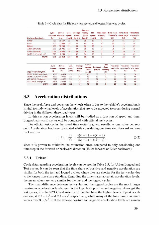
3.3. Acceleration distributions
Table 3.4 Cycle data for Highway test cycles, and logged Highway cycles.
!
"
#$%
"
$%&'%
"
('%
"
!"#$
) * +,- .-/$0 -.+ ++ '% // / -, .. 1+
!
"
#
"
$%&
#
"
%&'(&
#
"
)(&
#
* + ,-%& .&&/0( ..1 -0 -/ 21 0 12 2. ,.
3.3 Acceleration distributionsSince the peak force and power on the wheels often is due to the vehicle’s acceleration, itis vital to study what levels of acceleration that are to be expected to occur during normaldriving in the different three road types.
In this section acceleration levels will be studied as a function of speed and time.Logged real-world cycles will be compared with official test cycles.
For official test cycles the speed time series is given, usually as one value per sec-ond. Acceleration has been calculated while considering one time step forward and onebackward as
a(k) =dv
dt=v(k + 1)− v(k − 1)
t(k + 1)− t(k − 1), (3.2)
since it is proven to minimize the estimation error, compared to only considering onetime step in the forward or backward direction (Euler forward or Euler backward).
3.3.1 UrbanCycle data regarding acceleration levels can be seen in Table 3.5, for Urban Logged andTest cycles. It can be seen that the time share of positive and negative acceleration aresimilar for both the test and logged cycles, where they are shorter for the test cycles dueto the longer time share standing. Regarding the time shares at certain acceleration levels,the mean values are very similar for the test and the logged cycles.
The main difference between test cycles and the logged cycles are the much largermaximum acceleration levels seen in the logs, both positive and negative. Amongst thetest cycles, it is the NYCC and Artemis Urban that have the highest levels of peak accel-eration, at 2.7m/s2 and 2.4m/s2 respectively, while many of the logs have maximumvalues over 3m/s2. Still the average positive and negative acceleration levels are similar
39

Chapter 3. Road Type Driving Patterns, Road Grade and Daily Driven Distances
for all cycles, while the standard deviations are slightly higher for the logs. Another in-teresting point is that ECE has the lowest maximum acceleration level between the testcycles, yet in the same time it has the highest average acceleration, both positive andnegative.
Finally the mean RPA values are similar for the test and logged cycles. Many test cy-cles have RPA values around 0.17 to 0.20m/s2. However two cycles stand out; ArtemisUrban and NYCC, with RPA values of 0.30 and 0.29 respectively. The spread in RPAvalues seem to be larger for the logged cycles. The largest values are seen for the V744120312 (0.37) and XC60 .0.32m/s2.
Table 3.5 Acceleration cycle data for Urban test and Logged cycles.
!
"
!
"
!
#$
"
!
$##
"
!
##%
"
!
&%
"
!
"# $$%
"#
%
&'
()*
'( $) *$+ ,- *,. ,/ ,/ ,$ %) %- 0- - , ,
!
"
#
!
"
#
!
"
$%
#
!
"
%$$
#
!
"
$$&
#
!
"
'&
#
!"#$%& '
( #)$%$)$$ '
( #)$$)$%$ '
( #)$$ '
*(*!"$!+
* ' ' ''
*'$$, '
*$$,
-& ' ' '
() &% *+% ,- *,- ,- ,. ,+ +/ -% /& . % ,
The maximum acceleration as well as second based operating points, for the Testcycles can be seen in Figure 3.7 and for the Logged cycles in Figure 3.8. As can be seen,the largest acceleration levels are experienced at the lower speed levels.
For the test cycles, at speed levels up to around 40 km/h Artemis Urban, NYCC andSC03 have the highest levels of positive and negative acceleration at 1.7− 2.5m/s2 and−2.3 to−2.8m/s2. At higher speeds it is SC03, FTP75 and WLTC Middle that have thehighest positive acceleration levels, although strongly descending with increasing speed.At about 50 km/h the peak acceleration levels are around 0.4−1.4m/s2, while at about80 km/h they are around 0.2− 0.5m/s2.
As already noted from the cycle parameter data, the peak acceleration levels of thelogged cycles are higher compared to the test cycles, also when considering the differentspeed levels. For the logged cycles, at about 50 km/h the peak acceleration levels arearound 1 − 2.5m/s2, while at about 80 km/h the cycles have already reached their topspeed.
40

3.3. Acceleration distributions
0 20 40 60 80 100 120−3
−2
−1
0
1
2
3
Speed (km/h)
Acc
eler
ati
on
(m
/s2)
Artemis URBAN
NYCC
WLTC Cl.3 Low v5.3
FTP72 UDDS
SC03
jc08
WLTC Cl.3 Mdl v5.3
ECE
Figure 3.7 Maximum acceleration over speed along second with operation points per second, forUrban Test cycles.
0 20 40 60 80 100 120−8
−6
−4
−2
0
2
4
Speed (km/h)
Acc
eler
ati
on
(m
/s2)
Ecar500 120413 Linneg−City−CTH
Leaf 130321 CTH−Erksbrg
Leaf 130322 Korsv−Guldh
Prius 120329 Mlndl−Mlnlcke
Prius 120329 Mlnlcke−Mlndl
Prius 120403 Mlnlcke−CTH
V60PHEV Krsvgn−GalvBron
V744 120312 Cstat−CTH
V744 120318 Klltrp−CTH
V744 120327 CTH−Klltrp
XC60 CTH−Krthsg
Figure 3.8 Maximum acceleration over speed along second with operation points per second, forLogged Urban cycles.
In order to compare the distribution of acceleration over the speed range, betweenUrban test cycles and Logged Urban cycles, the relative time spent in bins of 0.5m/s2
and 5 km/h is depicted in Figure 3.9, along with the highest reached acceleration levelat each speed. When creating the plots, to each speed and acceleration operating point agaussian noise was added, which was later compensated for in the final result. The benefitis smoother contour lines, however a small error is also introduced, it can be regarded asnegligible. Hence the contour lines outside of the maximum acceleration graph shouldbe disregarded. The method is further illustrated in Appendix C.
As was also indicated by the standard deviations, the logged cycles spend a somewhatlarger share at slightly larger acceleration levels, compared to the test cycles. This can beseen by comparing the acceleration levels for the same time share contour line.
The figures show that for the test cycles, most of the time is spent around zero speed atvery low levels of accelerations (less than 1m/s2), due to frequent stops. For the logged
41

Chapter 3. Road Type Driving Patterns, Road Grade and Daily Driven Distances
cycles, most time is spent at speed levels around 5 to 10 km/h, but also within 1m/s2.Furthermore, the test cycles spend a somewhat larger time share at higher speed levelscompared to the logged cycles.
0 20 40 60 80 100−3
−2
−1
0
1
2
3
0.1
0.1
0.1
0.1
0.1
0.1
0.2 0.2
0.2
0.2
0.2
0.20.2
0.5
0.5
0.5
0.50.5
11
1
1
1
23
4
Speed (km/h)
Acc
eler
ati
on
(m
/s2)
0.5
1
1.5
2
2.5
3
3.5
4
(a) Urban Test cycles.
0 20 40 60 80 100−3
−2
−1
0
1
2
3
0.1
0.1
0.1
0.1
0.1
0.1
0.2
0.2
0.2
0.2
0.2
0.2
0.5
0.5
0.5
0.5
0.5
0.5
1
1
1
1
1
1
223
4
Speed (km/h)
Acc
eler
ati
on
(m
/s2)
0.5
1
1.5
2
2.5
3
3.5
4
(b) Logged Urban cycles.
Figure 3.9 Share of total time (%) of operation in acceleration bins of 0.5m/s2 and speed bins of5 km/h, with added noise, for all Urban Test and Logged cycles.
3.3.2 RuralCycle data regarding acceleration levels can be seen in Table 3.6, for Rural Logged andTest cycles. Also for the Rural cycles, the logs show higher peak acceleration levels andstandard deviations compared to the test cycles, while the average values are similar. Thetest cycles have a slightly larger time share below 1m/s2, while the logs have slightlya higher time share for acceleration levels between 1 to 2m/s2. Furthermore, high RPAvalues are more frequent amongst the logs.
For the test cycles it is the UC (LA92) cycle that has the highest peak accelerationboth positive and negative, as well as the highest RPA value. On the contrary, EUDC andNEDC have the lowest peak acceleration levels and the lowest RPA value.
Amongst the logs, two cycles have similar peak acceleration levels; C30d2 121219VCC-CTH and V744 120327 Klltrp-Cstat, however the later have a slightly higher aver-age acceleration, and a much larger RPA value (0.34 compared to 0.19m/s2).
The maximum acceleration as well as second based operating points, for the Testcycles can be seen in Figure 3.10 and for the Logged cycles in Figure 3.11.
In Figure 3.10 it is clearly seen that the two cycles UC LA92 and Artemis Ruraldiffers quite a bit from the others since the levels of acceleration are larger over thewhole speed range, and even more so for negative accelerations. Also when comparingwith the Urban test cycles, these two cycles stand out. For the logged cycles it can beseen in Figure 3.11 that the highest peak accelerations only occur at very low speedlevels (below 20 km/h). Around 40 km/h most cycles have peak accelerations between1.5 to 2.5m/s2, while for higher speed levels the difference between the cycles increase.
42

3.3. Acceleration distributions
Table 3.6 Acceleration cycle data for Rural test and Logged cycles.
!
!
"#
!
#""
!
""$
!
%$
!
!"
&' #( )* +* )+, +$ +- +#* $* ( ./ - + +
!
"
!
"
!
#$
"
!
$##
"
!
##%
"
!
&%
"
'( ) *% +, *+, +, +, +% , -) .% / $ +
At about 50 km/h the peak acceleration levels are around 1− 2.5m/s2 for the logsand 0.5 to 1.5m/s2 for the test cycles, while at about 80 km/h they are 0.5 − 2m/s2
for the logs and 0.3 to 1m/s2 for the test cycles.As for the Urban cycles, the relative time spent in acceleration bins of 0.5m/s2 and
5 km/h is depicted in Figure 3.12, along with the highest reached acceleration level ateach speed.
Also for the Rural cycles, the logged cycles spend slightly more time at somewhathigher acceleration levels over the whole speed range. I can also be seen that apart fromthe time spent at stand still and very low speed, also much of the time is spent around40 km/h for both test and logged cycles, 55 km/h for the test cycles, and finally around70 km/h for both test and logged cycles.
43

Chapter 3. Road Type Driving Patterns, Road Grade and Daily Driven Distances
0 20 40 60 80 100 120 140−4
−3
−2
−1
0
1
2
3
Speed (km/h)
Acc
eler
ati
on
(m
/s2)
UC LA92
EUDC
NEDC
Artemis RURAL
WLTC Cl.3 Hgh v5.3
Figure 3.10 Maximum acceleration over speed along second with operation points per second, forRural Test cycles.
0 20 40 60 80 100 120 140−4
−3
−2
−1
0
1
2
3
4
Speed (km/h)
Acc
eler
ati
on
(m
/s2)
C30d2 121219 CTH−VCC
C30d2 121219 Henan−Stnsnd
C30d2 121219 VCC−CTH
Ecar500 120413 CTH−Kllrd
C30d2 121219 Stnsnd−Henan
V744 120307 VCC−CTH
V744 120316 Klltrp−Csttn
V744 120320 Klltrp−Csttn
V744 120327 Klltrp−Cstat
Figure 3.11 Maximum acceleration over speed along second with operation points per second, forLogged Rural cycles.
0 20 40 60 80 100 120 140−3
−2
−1
0
1
2
3
0.1
0.1
0.1
0.1
0.1
0.1
0.2 0.20.2
0.2
0.2
0.2
0.5 0.5
0.5
0.50.5
0.5
0.5
0.5
1
1
1
1
12
1
0.12
Speed (km/h)
Accele
rati
on
(m
/s2)
0.2
0.4
0.6
0.8
1
1.2
1.4
1.6
1.8
2
(a) Rural Test cycles.
0 20 40 60 80 100 120 140−3
−2
−1
0
1
2
3
0.1
0.10.1
0.1
0.1
0.10.1
0.2
0.20.2
0.2
0.20.2
0.5
0.5 0.5
0.50.5
1
1
10.5
1
2
1
Speed (km/h)
Acc
eler
ati
on
(m
/s2)
0.2
0.4
0.6
0.8
1
1.2
1.4
1.6
1.8
2
(b) Logged Rural cycles.
Figure 3.12 Share of total time (%) of operation in acceleration bins of 0.5 m/s2 and speed binsof 5 km/h, with added noise, for all Rural Test and Logged cycles.
44

3.3. Acceleration distributions
3.3.3 Highway drivingCycle data regarding acceleration levels can be seen in Table 3.7, for Highway Loggedand Test cycles. As for the Urban and Rural cycles, the peak accelerations of the loggedHighway cycles are higher compared to the test cycles, while the average, standard devi-ations and the time shares at different acceleration levels are similar. In this case the testcycles have higher RPA values.
Amongst the test cycles, the US06 and REP05 have the highest peak accelerationlevels, however the average and standard deviation of acceleration as well as the RPAvalue is higher for US06.
The acceleration parameters of the logged cycles are rather similar to one another.
Table 3.7 Acceleration cycle data for Highway test and Logged cycles.
!
"
"
#$
"
$##
"
##%
"
&%
"
! "#$%
'( $ )* +* )+* +* +, +$% *- * ./ % $ +
!
"
#
"
#
"
$%
#
"
%$$
#
"
$$&
#
"
'&
#
() &* +& ,& +,& ,- ,- ,%% -. * ./ & , ,
The maximum acceleration as well as second based operating points, for the Testcycles can be seen in Figure 3.13 and for the Logged cycles in Figure 3.14.
As could be noted in the cycle parameters, the US06 and REP05 cycles have higherlevels of acceleration over the speed interval than the other test cycles, with many oper-ating points above 2m/s2 up to a speed level of 60 km/h. Next to US06 and REP05, theArtemis Motorway cycles have the highest acceleration levels over the speed range, anda particulary strong braking acceleration at high speed (about 2 to 3m/s2).
As can be seen in Figure 3.14, the peak acceleration over the speed range of thelogged Highway cycles are close to one another, but also fairly close to those of theUS06 and REP05.
The relative time spent in bins of 0.5m/s2 and 5 km/h is depicted in Figure 3.15,along with the highest reached acceleration level at each speed.
When comparing the distribution of logged cycles with the test cycles, the differencesin time spent at various acceleration levels over the speed range is rather small. The maindifference that can be seen is the relatively larger time spent at higher speed levels in thetest cycles compared to the logged cycles. It can be seen that in the test cycles most timeis spent at speed levels close to 80 to 130 km/h (110 km/h in particular), while for thelogged cycles most time is spent at 50 km/h and between 70 to 120 km/h.
45

Chapter 3. Road Type Driving Patterns, Road Grade and Daily Driven Distances
0 20 40 60 80 100 120 140 160−4
−3
−2
−1
0
1
2
3
4
Speed (km/h)
Acc
eler
ati
on
(m
/s2)
HWFET
US06
REP05
Artemis MW130
Artemis MW150
WLTC Cl.3 ExtrHgh v5.3
Figure 3.13 Maximum acceleration over speed along second with operation points per second, forHighway Test cycles.
0 20 40 60 80 100 120 140−4
−3
−2
−1
0
1
2
3
4
Speed (km/h)
Acc
eler
ati
on
(m
/s2)
C30d2 121219 Stnsnd−VCC
C30d2 121219 VCC−Stnsnd
V70 120510 CTH−Jnkpng
V70 120515 Jnkpng−CTH
Figure 3.14 Maximum acceleration over speed along second with operation points per second, forLogged Highway cycles.
0 20 40 60 80 100 120 140 160−3
−2
−1
0
1
2
3
0.1
0.1
0.1
0.1
0.1
0.10.1
0.1
0.2
0.2
0.2
0.2
0.20.2
0.5
0.5
0.5
0.5
1
1
1
1
0.1
0.1
0.2
0.2
2
0.2
2
0.5
Speed (km/h)
Acc
eler
ati
on
(m
/s2)
0.2
0.4
0.6
0.8
1
1.2
1.4
1.6
1.8
2
(a) Highway Test cycles.
0 20 40 60 80 100 120 140 160−3
−2
−1
0
1
2
3
0.1
0.1
0.1
0.1 0.1
0.10.10.1
0.2
0.2
0.2
0.2
0.2
0.2
0.2
0.5
0.5
0.5
0.5 0.5 1
1
11
1
2
2
2
0.2
0.2
0.5
0.5
3
3
2
2
0.5
44
3 5
Speed (km/h)
Acc
eler
ati
on
(m
/s2)
0.5
1
1.5
2
2.5
3
3.5
4
4.5
5
(b) Logged Highway cycles.
Figure 3.15 Share of total time (%) of operation in acceleration bins of 0.5 m/s2 and speed binsof 5 km/h, with added noise, for all Highway Test and Logged cycles.
46

3.4. Acceleration duration
3.4 Acceleration durationThe time duration of all accelerations and decelerations are calculated for both the Testand Logged cycles. The resulting cumulative frequency distribution is presented in Figure3.16. In general, the duration of accelerations are longer than the duration of decelera-tions. Typically, 80% of all accelerations are 12s-13s or shorter for the Test cycles, andaround 9s or shorter for the Logged cycles. Furthermore, 50% of all Test cycle accelera-tions are 5s-6s or shorter, and for the Logged cycles they are around 4s or shorter.
0 10 20 30 400
20
40
60
80
100
Time duration of Acc/dec (s)
Cum
ulat
ive
freq
uenc
y (%
)
Test cycles
Urban, AccUrban, DecRural, AccRural, DecHighway, AccHighway, Dec
(a) Test Cycles.
0 10 20 30 400
20
40
60
80
100
Time duration of Acc/dec (s)
Cum
ulat
ive
freq
uenc
y (%
)
Typical Logged cycles
Urban, AccUrban, DecRural, AccRural, DecHighway, AccHighway, Dec
(b) Logged typical cycles.
Figure 3.16 Cumulative frequency distribution of the time duration of each acceleration and decel-eration, counted between zero-crossings, for the Test and Logged cycles.
3.5 Road grade levelsAs with speed and acceleration, common levels of road grade are of great interest whenseeking typical vehicle load levels.
The Swedish office of traffic (Trafikverket) has specified recommended maximumroad grade levels for new roads to 6 %, and for improved roads to 8 %, in their guidelinesfor how roads are to be designed [70].
Similarly, according to [71] the National System of Interstate and Defence Highwaysin the US are designed after guidelines that state a recommended maximum grade leveldepending on the road’s speed limit. For speeds up to 90 km/h, maximum grade levelsof 5 % are recommended, while it is 6 % for mountainous areas. At higher speed levelsthe recommended max grade is 4 %. According to [25] p. 13, grade levels on US primaryand secondary roads may reach 10 to 12%.
Trafikverket also provide a searchable database called PMSV3 [72], that containsmeasured road data covering different roads in Sweden, which are gathered from severaloccasions over the last decades via a special measurement van. Amongst other data,road grade, road speed limit and speed of measurement vehicle have been recorded. Itis possible to make combined searches in the data base on one or more parameters. Asearch on speed limit of at least 110 km/h and grades of at least 6% but maximum 12%,
47

Chapter 3. Road Type Driving Patterns, Road Grade and Daily Driven Distances
results in three hits, i.e. three different highways in Sweden has sections of grade 6% orlarger. One is on E6 Bohuslän between Munkedal and Tanum, one in Dalarna betweenBorlänge and Falun, and one in Skåne south of Skottorp across Hallandsåsen with gradesof 6 − 7% over a distance of 1.8 km. Another steep slope with a grade of about 7 %, iswest of Jönköping on road 40 along a section of about 1 km at a speed limit of 90 km/h.Further searches leads to about a 170 hits on sections with speed limits of 100 km/h andgrades of at least 6% but maximum 12%, and 1 330 hits on sections with speed limitsof 90 km/h and grades of at least 6 % but maximum 12 %, for 70 km/h the number ofhits is 31 638, and for 50 km/h it is 5905. These numbers are however not to be blindlytrusted, since some of the later measurements are not coherent with the previous onesand thus indicates much larger grades than previously.
At low speed levels, e.g. in cities or on drive ways the road grade can be even larger,perhaps up to and above 30 % as indicated by [73] for several streets is San Francisco inthe US.
3.5.1 Measured road gradesRoad grade levels have also been estimated from the logged data, see histogram represen-tation in Figure 3.17. A fair accuracy of the estimation proved to be rather difficult withthe used measurement system at hand, especially at low speed levels. Nevertheless, theresulting data corresponds rather well to expected values with respect to the informationin the previous section.
Analysis showed only a small dependence on speed, i.e. that higher grade levels arerelatively less common for the Highway cycles.
0 2 4 6 8 100
2
4
6
8
10x 10
4
Road grade (%)
Occ
. F
req
. (−
)
(a) Urban.
0 2 4 6 8 100
2
4
6
8
10x 10
4
Road grade (%)
Occ
. F
req
. (−
)
(b) Rural.
0 2 4 6 8 100
0.5
1
1.5
2
2.5
3x 10
5
Road grade (%)
Occ
. F
req
. (−
)
(c) Highway.
Figure 3.17 Road grade histogram of all Logged Urban, Rural and Highway cycles.
Figure 3.18 presents the difference in altitude between the end and start of the Loggedcycles, as well as the difference between maximum and minimum reached altitudes. For acycle with a large positive difference between the end and the start altitude, a significantpart of the energy that is consumed during driving is due to the increases in potentialenergy. For those cycles that adhere to the same driving route and are driven in oppositedirections, it can be seen that the difference between end and start altitude is similar butwith opposite signs. Thus, the total energy consumption may be different for the twocycles.
48

3.5. Road grade levels
−200
−100
0
100
200
300
400
56
−38
59
53
−37 −
7
−
7 13
−
7
10
−52 −
14
−
8 25
−54
2 6
−68
−65
−70
45
−41
143
−149
64
55
97
94
95
95
32
14
60 72
68
55
52
50
100
51
49 7
9
70
77
60
68
334
334
Ele
vati
on
dif
fere
nce
(m
)
E
car5
00 1
20413 L
inneg−C
ity−C
TH
L
eaf 130321 C
TH
−E
rksbrg
L
eaf 130322 K
ors
v−G
uld
h
P
rius 1
20329 M
lndl−
Mln
lcke
P
rius 1
20329 M
lnlc
ke−M
lndl
P
rius 1
20403 M
lnlc
ke−C
TH
V
60P
HE
V K
rsvgn−G
alv
Bro
n
V
744 1
20312 C
sta
t−C
TH
V
744 1
20318 K
lltr
p−C
TH
V
744 1
20327 C
TH
−K
lltr
p
X
C60 C
TH
−K
rthsg
C
30d2 1
21219 C
TH
−V
CC
C
30d2 1
21219 H
enan−S
tnsnd
C
30d2 1
21219 V
CC
−C
TH
E
car5
00 1
20413 C
TH
−K
llrd
C
30d2 1
21219 S
tnsnd−H
enan
V
744 1
20307 V
CC
−C
TH
V
744 1
20316 K
lltr
p−C
stt
n
V
744 1
20320 K
lltr
p−C
stt
n
V
744 1
20327 K
lltr
p−C
stt
n
C
30d2 1
21219 S
tnsnd−V
CC
C
30d2 1
21219 V
CC
−S
tnsnd
V
70 1
20510 C
TH
−Jnkpng
V
70 1
20515 J
nkpng−C
TH
Urban Rural Highway
End − Start
Max. − Min.
Figure 3.18 The net altitude difference between the cycle end and start points, as well as the differ-ence between maximum and minimum altitude that is experienced during the Loggedcycles.
The time duration of all uphill and downhill cycle segments are calculated for theLogged cycles. The resulting cumulative frequency distribution is presented in Figure3.19. It can be noted that the time duration is generally longer for the Highway cycles.For 80% of the uphill occasions in the Urban and Rural cycles, the time duration is around25s or shorter, and it is 38s or shorter for the Highway cycles. Furthermore, for 50% ofthe uphill cycle segments, the time duration is 10s-14s or shorter. To conclude, the timeduration of grade climbing is generally more than twice the time duration of acceleration.
0 50 100 1500
20
40
60
80
100
Time duration of upphill/downhill (s)
Cum
ulat
ive
freq
uenc
y (%
)
Grade duration − Typical Logged cycles
Urban, AccUrban, DecRural, AccRural, DecHighway, AccHighway, Dec
Figure 3.19 Cumulative frequency distribution of the time duration of each uphill and downhill,counted between zero-crossings, for the Test and Logged cycles.
49

Chapter 3. Road Type Driving Patterns, Road Grade and Daily Driven Distances
3.6 Average daily driving/traveling distanceIn order to find suitable driving ranges for electric cars it is essential to gain knowledgeof how far drivers usually travel. By assuming that the only definite time to charge is overnight, one can consider information regarding traveled distances per day.
Many countries around the world try through surveys, to map typical mobility habitsof people traveling by different commodities. In these surveys respondents are askedto keep a traveling or driving journal usually for a single specified day, thus regardedto be typical, or in the case of some studies for a number of consecutive days. The maindrawbacks with these kinds of studies (when it comes to estimating necessary EV drivingrange) are that the results are strictly related to mobility of persons, who may use differentvehicles during the same day, but also that the quality of the results highly depend on theestimates done by the respondents as stated in [58]. More preferably, single vehicles aretracked and studied during a much longer period, e.g. The Swedish Car Movement DataProject or an American study in the Atlanta region [74].
The type of information gained may be average daily commuting distances, averagedaily driving over a whole population studied. It may also be a cumulative distribution ofshare of daily distances that at least has been covered.
According to National Household Travel Survey in the US(NHTS) [75], the averagecommuting distance by private vehicles in US was 19.5 km, and the average drivendistance per driver in 2001 and 2009 respectively were 55 and 49 km on a weekday and46 and 40 km on a Saturday or Sunday.
According to the latest major National Travel Survey in Sweden, the average drivendistance per day with private car in 2005/2006 range between 20 to 36 km dependingon region, with a national average of 30 km [76]. However according to another reportfrom the same period (Körsträckor 2006) which is based on data from vehicle trip meter(checked during yearly car check up at Bilprovningen), the average total driven distanceper vehicle during 2006 was 14 390 km, which gives an average daily driving distance ofabout 39 km [77].
A survey in Europe finds that the average driven distance in six European countries(France, Germany, Italy, Poland, Spain and UK) vary between 40 km (UK) to 80 km(Poland) per day, and shows no important difference between the days in a week [78].
Various sources have been found that present the needed type of data, [79], [80],[81], [82], [83], [84], [85] and [74]. However the results differ between countries, andstudies, and even between the same studies depending on how the answers are chosento be analyzed, which makes general conclusions difficult to make, see Figure 3.20. Formore details on the different studies, see the related references mentioned here.
50

3.6. Average daily driving/traveling distance
0 50 100 150 200 250 300 350 4000
20
40
60
80
100
Distance (km)
Cu
mu
lati
ve
sha
re (
%)
Nissan − USA
Nissan − China
Nissan − France
Nissan − Germany
Nissan − Japan
Nissan − England
S. Karlsson − Sweden − RES0506 Survey by Driver
TSS − Sweden − 2010−2012 Measurement by Car
Gbg Stad TrfKntr VV − RVU05 Survey by Driver
0 50 100 150 200 250 300 350 4000
20
40
60
80
100
Distance (km)
Cu
mu
lati
ve
share
(%
)
Nissan USA − unknown method
SAE USA − NHTS2009 Survey by selected Cars
USAXprize2001All
− NHTS2001 Survey by driver
USAXprize2001Urban
− NHTS2001 Survey by driver
USAXprize2001Rural
− NHTS2001 Survey by driver
USA SolarJournalAll
− NHTS2009 by Car
USA SolarJournalUrban
− NHTS2009 by Car
USA SolarJournalRural
− NHTS2009 by Car
USA PearreLowest
− 2004 Measurement by Car
USA PearreHighest
− 2004 Measurement by Car
Figure 3.20 Daily driving distances in various countries, for either drivers or cars, extracted bydifferent methods.
According to [79], 90 % of the people in European countries drive less than about120 km per day on an average, while 90 % of the people in USA drive less than 135 kmper day. It is also seen that Japan seem to have similar driving patterns as EU and thatChina seem to have similar driving patterns as US.
As can be seen the information regarding Sweden differs a bit between the differentsources, perhaps this is due to different methods used, see [80], [81] and [82]. Based onresults from The Swedish Car Movement Data Project which cover cars in the south westof Sweden, 90 % of the cars travel less than about 70 km per day on average.
In the US the spread between different published data is relatively large. As a sum-mery of all presented graphs, 50 % of the average daily driving distances are shorter than6 to 89 km, and 80 % of them are shorter than 16 km to 148 km. One study indicate thatlarger distances are covered during rural driving compared to urban driving, [85].
51

Chapter 3. Road Type Driving Patterns, Road Grade and Daily Driven Distances
52

Chapter 4
Performance Requirements andWheel Load Analysis of StudiedConcept Vehicles
Vehicle performance can be summarized in single quantitative measures such as: topspeed, minimum time to accelerate from 0− 100 km/h, and specifically for BEVs, driv-ing range. The work in this chapter and the next is concentrated to three concept lightduty BEVs, i.e. passenger cars, each with their own targeted qualitative specificationwhich can be seen in Table 4.1. Apart from the qualitative targets, all vehicles should beable to manage highway driving in most countries around the world.
In this section the stated qualitative targets will be further specified into quantitativeperformance requirements for each of the concept cars, with collected data on over 30existing light duty BEV models as a frame of reference.
Table 4.1 Qualitative design targets for the three concept BEVs.Seats Size Speed and acceleration Range
City 4-5 Small Medium MediumHighway 5 Medium High LongSport 2 Small Very high Very long
4.1 Performance requirements based on data of existingBEVs
The performance requirements of the three concept vehicles are mainly based on datafound on currently top selling BEV models. Car data that is relevant for this chapter is:curb weight, height and width in order to estimate effective vehicle area, drag coefficientCd, top speed, time to accelerate, certified driving range as well as energy consumptionper driven distance.
53

Chapter 4. Performance Requirements and Wheel Load Analysis of Studied ConceptVehicles
Data on top selling light duty BEV models (including concepts) has been gatheredmainly from vehicle manufacturers. The full list of vehicle models along with the col-lected data and their associated references is presented in Appendix A.
For some of the data there exists a level of uncertainty on the correctness and reli-ability, since it is not specified in a standardized way, and many sources do not declareunder which conditions the data is valid.
For example, mass for vehicles are often given as curb weight, which is usually de-fined as the mass of the specific model with standard equipment and neither passengersnor extra cargo. However, in manufacturer’s mass specifications it is not always evidentwhat is included in the presented value. Moreover, the cross sectional area is very seldomstated, thus it has to be estimated, e.g. by a method such as the ones suggested in Chapter2, i.e. as a weighted product of vehicle height and width.
Lastly, the vehicle driving range given is usually specified as the certified rangegained by driving according to either American EPA cycles or the European NEDC cy-cle, however in some sources this is not declared. The same issue is also valid for energyconsumption per distance.
For further ease of benchmarking, the existing vehicle models are sorted into the fourcategories: small, medium-large, high performing and sport, where the former two arebased on vehicle external volume calculation while assuming a rectangular block. Thesport category consists of high acceleration capable 2-seat models. The high performingcategory also consists of high acceleration capable models, but with five seats.
4.1.1 Speed and acceleration performanceAll three concept vehicles should be able to handle highway driving in most countries,which is typically between 110− 130 km/h, as stated in [86]. Only a few countries havespeed limits above this, where the highest limit is 150 km/h.
Data on top speed is available for all of the studied BEV models, and it shows arather wide variety. However the majority of the small-large models have top speedsaround 120-160 km/h. The top speed of the small cars ranges from 120 − 145 km/h,while it is 122 − 161 km/h for the medium-large cars, and 190 − 249 km/h the highperforming models. The top speed of the sport models varies between 170− 305 km/h.
Based on this, the top speed of the City car is settled to 135 km/h on a flat road inorder to manage highway driving in most countries with a small margin included. Thisspeed is somewhat higher compared to the lowest speed models, yet it is not as high asfor the fastest small cars. The top speed of the Highway car is set to 150 km/h to handlehighway driving in all countries. This speed level matches the fastest small size BEVs.The top speed of the Sport car is chosen to be 210 km/h on a flat road, which matchestwo of the existing sport cars, but not the fastest ones.
Acceleration performance is usually stated as the minimum time to accelerate from0 − 100 km/h or 0 − 60mph (which corresponds to 0 − 96.5 km/h), i.e. while usingthe maximum torque from the powertrain. This type of data is available for almost all ofthe studied BEVs.
The top speed and acceleration time of the three concept vehicles along with specifieddata of the existing BEVs can be seen in Figure 4.1.
54
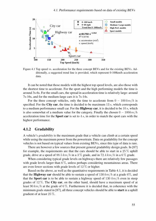
4.1. Performance requirements based on data of existing BEVs
100 150 200 250 300 3500
5
10
15
20
a=81750 v−1.812
R2=0.8746
a: acceleration (m/s2)v: speed (km/h)
Top Speed (km/h)
Acc
eler
atio
n T
ime
(s)
0−100 km/h0−60 mphTrend line 0−100km/h
Highway car
City car
Sport car
Small models
Medium−Large modelsHigh Perf. models
Sport models
Figure 4.1 Top speed vs. acceleration for the three concept BEVs and for the existing BEVs. Ad-ditionally, a suggested trend line is provided, which represent 0-100km/h accelerationdata.
It can be noted that those models with the highest top speed levels, are also those withthe shortest time to accelerate. For the sport and the high performing models the time isaround 3s-6s. For the small cars, the spread in acceleration time is relatively large: around7s-16s, and for the medium-large cars it is 7s-14s.
For the three concept vehicles, only the time to accelerate from 0 − 100 km/h isspecified. For the City car, the time is decided to be maximum 13 s, which correspondsto a medium performance small car. For the Highway car, it is decided to be 10 s, whichis also somewhat of a medium value for the category. Finally the chosen 0 − 100km/hacceleration time for the Sport car is set to 4 s, in order to match the sport cars with thehighest performance.
4.1.2 GradabilityA vehicle’s gradability is the maximum grade that a vehicle can climb at a certain speedwhile using the maximum power from the powertrain. Data on gradability for the conceptvehicles is not based on typical values from existing BEVs, since this type of data is rare.
There are however a few sources that present general gradability design goals. In [87]for example, the requirements are that the cars should be able to start in a 25 % uphillgrade, drive at a speed of 88.5 km/h in a 3 % grade, and in 72.4 km/h in a 6 % grade.
When considering typical grade levels on highways there are relatively few passageswith grade levels larger than 6 %, unless perhaps considering mountainous areas. Thereare even fewer sections with grade levels of 12 % or higher.
Based on the above, as well as the quantitative requirements in Table 4.1, it is decidedthat the Highway car should be able to sustain a speed of 130 km/h at a grade 6%, andthat the Sport car is to be able to sustain a highway speed of 130 km/h even in steepgrades of 12 %. The City car, on the other hand, should have a maximum speed of atleast 90 km/h at the grade of 6 %. Furthermore it is decided that, in coherence with theminimum goals stated in [87], all three concept vehicles should be able to start in a uphillgradient of at least 25 %.
55

Chapter 4. Performance Requirements and Wheel Load Analysis of Studied ConceptVehicles
4.1.3 Driving range and curb weightThe NEDC driving range for the small cars is between 85−160 km, and for the medium-large cars it is 162−250 km. For the high performing models it is 390−528 km, and forthe sport cars it is 200 − 600 km, or up to 450 km when excluding the Rimac ConceptOne.
It is decided that the concept City car is to have a NEDC range of about 160 km,which is as long as for the two top models in the category. As seen in Figure 3.20, thisdistance covers over 90 % of the average daily driven distances in many countries inthe world, although real world driving will most likely lead to a different driving range.For the Highway car the NEDC range should be around 200 km, in order to match themodels with the longest range, still not as long as for the Model S models. The NEDCrange of the Sport car is to be 300 km, which is longer than for two of the sport models,but much shorter than than the one with the longest range.
Data on curb weight is available for all BEV models. In general the small cars havethe lowest masses: around 900−1355 kg, and the medium-large cars’ weights are 1195−1725 kg (when excluding BYD e6 which has a weight of 2380 kg). The high performingmodels weigh around 2100 kg, and the sport models between 1200− 2110 kg.
Based on the reference data, it is decided that the curb weight of the concept City caris to be 1200 kg, which is in the higher range for the small car category. The weight ofthe Highway car is set to 1700 kg, which also reflects a value in the higher range for themedium-large cars. Finally the concept Sport car is to have a curb weight of 1900 kg,i.e. a rough mean value.
0 100 200 300 400 500 600800
1000
1200
1400
1600
1800
2000
2200
NEDC range (km)
Cur
b W
eigh
t (kg
)
Small modelsMedium−Large modelsHigh Perf. modelsSport models
Highway car
Sport carCity car
Figure 4.2 NEDC driving range vs. curb weight for the three concept BEVs as well as for theexisting BEVs.
4.1.4 Area, Cd and Cr
Data on vehicle front area was found for nine of the existing vehicles. Based on theinformation in Table A.7, the area for the rest of the vehicles is estimated as 86 % of theproduct of height and width. For simplicity it is here assumed that the same weightingfactor can be used for all cars.
The areas of the concept vehicles are mainly determined based on the estimated areasof the existing BEVs, as presented in Figure A.2. The area of the City car is chosen to
56

4.2. Wheel load analysis of chosen concepts
be 2.05m2, which resembles a small car, the Highway car area is chosen to be 2.3m2
which takes after the large cars, while the Sport car area is chosen to be 2.0m2.With the published Cd values of existing BEV’s as a reference the Cd value of the
City car is chosen to be 0.3, for the Highway car 0.28, and finally the Cd value of theSport car is chosen to resemble that of the Roadster, 0.35.
Data on tire radius of existing BEVs is not available, instead it has been estimatedbased on tire size, see Figure A.3. Based on this, the tire radius of concept models arechosen accordingly: the City car 0.31m, the Highway car 0.32m, and the Sport car0.34m.
inally, the tire rolling resistance coefficient Cr should be set for all of the conceptvehicles. Even though the rolling resistance is known to be speed dependent, there is noclear consensus on how this should be modeled (as shown in Figure 2.2) unless perhapstire specific data is available, which it is not in this case. Another aspect is that the typeof study in this thesis is of comparative nature, hence a possible speed dependence of therolling resistance is expected to have a rather small impact on the final result. With theseaspects as a background as well as the information presented on the topic in Chapter2 and Appendix A, it is assumed that the rolling resistance of the concept BEVs canbe estimated by the mean values: 0.009 for both the City car and the Highway carrepresenting low rolling resistance tires, while for the Sport car the tires are expected tobe optimized for performance rather than energy efficiency, leading to a value of 0.012.
4.1.5 Summary of requirements on chosen vehicle conceptsA summary of the stated requirements of the three concept cars presented in Table 4.2.
Table 4.2 Performance requirements of the three concept cars.City HW Sport
Seats 4-5 5 2 kgMass 1200 1700 1900 kgAcceleration 0-100 km/h 13 10 4 sTop speed 135 150 210 km/hNEDC Range 160 200 300 kmAearod. drag coeff. Cd 0.3 0.28 0.35 −Area 2.05 2.3 2.0 m2
Wheel radius 0.31 0.32 0.34 mRolling resist. coeff. Cr 0.009 0.009 0.012 −Starting gradability 25 % 25 % 25 % %Gradability (Speed at grade) 90 at 6% 130 at 6% 130 at 12% km/h, %
4.2 Wheel load analysis of chosen conceptsIn the wheel load analysis of the concept vehicles the levels of force, speed and power atthe wheels, are estimated based on the above stated quantitative vehicle requirements.
With help of the information in Chapter 2 regarding vehicle dynamics, the forces dueto aerodynamic drag (2.2), rolling resistance (2.3), road grade (2.4) as well as acceleration(2.1) are calculated for all of the concept vehicles, assuming a gravitational constant,g = 9.81m/s2 and an air density of ρ = 1.2 kg/m3. At this point no regard is taken to
57
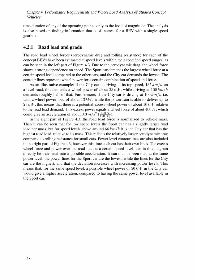
Chapter 4. Performance Requirements and Wheel Load Analysis of Studied ConceptVehicles
time duration of any of the operating points, only to the level of magnitude. The analysisis also based on finding information that is of interest for a BEV with a single speedgearbox.
4.2.1 Road load and gradeThe road load wheel forces (aerodynamic drag and rolling resistance) for each of theconcept BEVs have been estimated at speed levels within their specified speed ranges, ascan be seen in the left part of Figure 4.3. Due to the aerodynamic drag, the wheel forceshows a strong dependence on speed. The Sport car demands the largest wheel force at acertain speed level compared to the other cars, and the City car demands the lowest. Thecontour lines represent wheel power for a certain combination of speed and force.
As an illustrative example: if the City car is driving at its top speed, 135 km/h ona level road, this demands a wheel power of about 23 kW , while driving at 100 km/hdemands roughly half of that. Furthermore, if the City car is driving at 100 km/h i.e.with a wheel power load of about 13 kW , while the powertrain is able to deliver up to23 kW , this means that there is a potential excess wheel power of about 10 kW relativeto the road load demand. This excess power equals a wheel force of about 400N , whichcould give an acceleration of about 0.3m/s2 ( 400N
1200 kg ).In the right part of Figure 4.3, the road load force is normalized to vehicle mass.
Then it can be seen that for low speed levels the Sport car has a slightly larger roadload per mass, but for speed levels above around 66 km/h it is the City car that has thehighest road load, relative to its mass. This reflects the relatively larger aerodynamic dragcompared to rolling resistance for small cars. Power level contour lines are also includedin the right part of Figure 4.3, however this time each car has their own lines. The excesswheel force and power over the road load at a certain speed level, can in this diagramdirectly be translated into a possible acceleration. It can thus be seen that, at the samepower level, the power lines for the Sport car are the lowest, while the lines for the Citycar are the highest, and that the deviation increases with increasing power levels. Thismeans that, for the same speed level, a possible wheel power of 50 kW in the City carwould give a higher acceleration, compared to having the same power level available inthe Sport car.
58

4.2. Wheel load analysis of chosen concepts
0 50 100 150 2000
200
400
600
800
1000
1200
1400
1600
1800
10
10
20
30
40
50
60
70
80
90
Speed (km/h)
Wh
eel
Fo
rce
(N)
Wheel Forces at constant speed levels
0 50 100 150 2000
0.5
1
1.5
2
10
10
50
50
100
10
10
10
50
50
100
Mass normalized wheel Forces at constant speed levels
10
10
10
50
50
Speed (km/h)
No
rma
lize
d w
hee
l F
orc
e (N
/kg
)
Sport − P
wheel (kW)
Sport − Road load
Highway − Pwheel
(kW)
Highway − Road load
City − Pwheel
(kW)
City − Road load
Figure 4.3 Road load wheels force as a function of car speed on a level road, and mass normalizedwheel force, for all three concept cars. The contour lines represent wheel power for acertain combination of speed and force, which is the same for all cars in the left part ofthe figure, however not for the right part.
Figure 4.4 shows both absolute wheel forces and mass normalized wheel forces foreach concept car, for road loads at certain grade levels as well as at operating pointscorresponding to the specified speed and grade performance requirements.
Starting with the City car, Figure 4.4(a) shows that the top speed and the gradingrequirement at high speed, demand about the same levels of wheel power; 23 kW and26 kW respectively, while the force level at the grading requirement is roughly twice thatat the top speed (about 1 kN and 0.6 kN respectively). The takeoff requirement demandsthe largest force, almost 3 kN but since the speed is low, so is the power demand. Inthe right part of Figure 4.4(a) it can be seen that the takeoff requirement is equal to anacceleration of almost 2.5m/s2, as was predicted in Table 2.1, and as is also valid forthe other cars. To conclude, if the wheel force is limited to 3 kN at speed levels up to apower limit of 26 kW , above which the wheel force follows the power line, then all threespecified operating points will be achievable. As mentioned, the difference between themaximum available wheel force and the road load at a certain grade, equals the vehicle’sacceleration capacity. With the above limits, the initial acceleration at takeoff would beabout 2.4m/s2 on a flat road, at 50 km/h it would be about 1.4m/s2 and at 100 km/habout 0.47m/s2.
For the Highway car, shown in Figure 4.4(b), the top speed demands a force of about1 kN and a power of 34 kW , while the high speed grading requirement demands a forceof about 1.8 kN and a power of 60 kW , i.e. a larger difference between the requirementscompared to the City car (it can be seen that also for the Highway car the demandedpower at 6 % grade in 90 km/h is almost the same as that at the top speed). For theHighway car an initial force level of about 4.1 kN is required to manage the takeoffrequirement, up to about 50 km/h where the power thus can be limited to 60 kW .
The Sport car, shown in Figure 4.4(c), evidently demands the highest levels of forceand power compared to the other two cars. As for the City car, both the top speed andgrading requirements demands roughly the same power levels 96 kW and 108 kW re-spectively. The takeoff requirement demands an initial force of about 4.8 kN . This forcelevel may be sustained up to about 80 km/h, where the power may be limited to 108 kW .
59

Chapter 4. Performance Requirements and Wheel Load Analysis of Studied ConceptVehicles
0 20 40 60 80 100 1200
1000
2000
3000
4000
5000
23
23
23
26
26
26
50
50
100 150
Vehicle speed (km/h)
Wh
eel
forc
e (N
)
0 20 40 60 80 100 1200
0.5
1
1.5
2
2.5
3
3.5
4
23
23
23
26
26
26
50
50
100 150
Vehicle speed (km/h)
Wh
eel
forc
e/m
ass
(N
/kg)
Power
wheel (kW)
Road load on flat road
Road load at 6% grade
Road load at 25% grade
90 km/h at 6% grade
Top speed on level road
(a) City car.
0 50 100 1500
1000
2000
3000
4000
5000
6000
7000
8000
34
34
34
60
60
60
100
100
200
250
Vehicle speed (km/h)
Wh
eel
forc
e (N
)
0 50 100 1500
1
2
3
4
5
34
34
34
60
60
60
100
100
200
250
Vehicle speed (km/h)
Wh
eel
forc
e/m
ass
(N
/kg)
Power
wheel (kW)
Road load on flat road
Road load at 6% grade
Road load at 25% grade
130 km/h at 6% grade
Top speed on level road
(b) Highway car.
0 50 100 150 2000
5000
10000
15000
50
50
50
96
96
96
108
108
108
200
200
300
300
400
400
Vehicle speed (km/h)
Wh
eel
forc
e (N
)
0 50 100 150 2000
1
2
3
4
5
6
7
50
50
50
96
96
96
108
108
108
200
200
300
300
400
400
Vehicle speed (km/h)
Wh
eel
forc
e/m
ass
(N
/kg
)
Powerwheel
(kW)
Road load on flat road
Road load at 12% grade
Road load at 25% grade
130 km/h at 12% grade
Top speed on level road
(c) Sport car.
Figure 4.4 Force on wheels due to road load per speed level, and normalized force per vehiclemass, for all three concept cars, along with contour lines representing combinations ofwheel force and speed for different levels of wheel power.
4.2.2 AccelerationGiven the above stated demanded levels of force and power versus speed due to the threementioned requirement; top speed, grade at high speed and take-off at high grade, itcan be noted that the implied acceleration capacity of each car would be rather limited.Further investigations must be made to find suitable levels of force and power that willalso fulfill the acceleration requirements.
By assuming a torque and speed characteristic that is typical for an electric machine,
60

4.2. Wheel load analysis of chosen concepts
(i.e. a region of constant torque at low speeds followed by a region of constant power athigher speeds, where the torque is inversely proportional to the speed), various combi-nations of initial maximum levels of wheel force and wheel power limits can be found,such that they will all fulfill the acceleration requirement. Even though the accelerationtime from 0 − 100 km/h is the same for all combinations, the acceleration time from0 − 50 km/h, hence also 50 − 100 km/h differs. It can thus be concluded that the re-quirement on acceleration time from 0−100 km/h alone, is not enough when seeking tospecify a vehicles acceleration performance over the operational speed range. Few dataregarding acceleration times between different speed levels are available for the existingBEV models, see Appendix A. Acceleration times for 0 − 50 km/h are 3s-6s and for0− 60 km/h 3.7s-7.7s.
4.2.2.1 City car
In Figure 4.5, three combinations of initial max force and max power are presented,where the base speed values are set to 1/4, 1/3 and 1/2 of the top speed of the City car,i.e. similar to common ratios for electric machines.
0 5 10 150
50
100
Time (s)
Sp
eed
(k
m/h
)
5.8s
13.0s4.6s 13.0s3.8s
13.0s
0 50 1000
1
2
3
4
5
Speed (km/h)
Acc
. (m
/s2)
Ma
ss n
orm
. F
wh
eel (
N/k
g)
57kW
2.5 N/kg
48.5kW
3.2 N/kg
45kW
4.2 N/kg
0 50 1000
2
4
6
Speed (km/h)
Fw
hee
l (k
N)
57kW
3.0 kN
48.5kW
3.8 kN
45kW
5.0 kN
0 5 10 150
100
200
300
Time (s)
Dis
tan
ce (
m)
198m41m 218m33m 231m29m
Acc.
norm. Fwheel
Fwheel, max
Road load
Figure 4.5 Speed and distance over time, as well as wheel force and acceleration, for base speedsthat are 1/4, 1/3 and 1/2 of the top speed, during 0 − 100 km/h acceleration, for theconcept City car.
The lowest base speed is related to the largest initial force (5 kN), lowest power (45kW), fastest acceleration of 0− 50 km/h (just under 4 s) along with the shortest drivendistance during the acceleration, while the acceleration time of 50 − 100 km/h is thelongest. Given that this is the City car, it can be argued that low speed acceleration per-formance should be preferred over high speed performance. It is thus decided that the
61

Chapter 4. Performance Requirements and Wheel Load Analysis of Studied ConceptVehicles
lowest power level should be the design template. Compared to the power levels of ex-isting BEVs with similar acceleration times, the chosen power level is smaller. Howeverthe acceleration time 0 − 50 km/h complies rather well when comparing with some ofthe existing BEVs.
When comparing the results in Figure 4.5, with the ones found in Figure 4.4(a), theinitial force demanded by the acceleration requirement should be around 2 kN higherthan that for the takeoff requirement (of 3 kN ), while the power should be 19 kW higherthan that of the high speed gradient requirement (of 26 kW). It is thus the accelerationrequirement that will determine the maximum force and power that has to come to thewheels (via the gear box) from the powertrain.
4.2.2.2 Highway car
Combinations of initial force and power limits have been studied in the same manner forthe Highway car as well, see Figure 4.6.
0 5 100
50
100
Time (s)
Sp
eed
(k
m/h
)
3.3s10.0s3.9s 10.0s
4.7s10.0s
0 50 100 1500
1
2
3
4
5
Speed (km/h)
Acc
. (m
/s2)
Mass
norm
. F
wh
eel (
N/k
g)
82kW
4.5 N/kg
89kW
3.7 N/kg
109kW
3.1 N/kg
0 50 100 1500
2
4
6
8
Speed (km/h)
Fw
hee
l (k
N)
82kW7.7 kN
89kW6.3 kN
109kW5.2 kN
0 5 100
50
100
150
200
Time (s)
Dis
tan
ce (
m)
171m
25m161m
28m147m
33m
Acc.
norm. Fwheel
Fwheel, max
Road load
Figure 4.6 Speed and distance over time, as well as wheel force and acceleration, for base speedsthat are 1/4, 1/3 and 1/2 of the top speed, during 0 − 100 km/h acceleration, for theconcept Highway car.
Also here the result is that the combination that has the highest initial force (7.7 kN )and lowest power (82 kW ) result in the best low speed performance (3.3 s when acceler-ating 0−50 km/h). However since the 0−50 km/h and 0−60 km/h acceleration timesof the few existing BEVs that was found are around 4 s, this is here chosen as a targetedvalue also for the Highway car. Thus targeted initial force is 6.3 kN and power is 89 kW.That means that the initial force should be about 2.2 kN more than what was demandedby the takeoff requirement (of 4.1 kN ), and the power should be 29 kW more than that
62

4.2. Wheel load analysis of chosen concepts
of the high speed gradient requirement (of 60 kW ), as seen in Figure 4.4(b). This wouldresult in an initial acceleration level of about 3.7m/s2.
4.2.2.3 Sport car
Finally, for the Sport car, see Figure 4.7, an initial force of 16.6 kN and a power of251 kW result in the best low speed performance with an initial acceleration level of8.7m/s2 up to a speed of about 50 km/h.
0 1 2 3 4 50
50
100
Time (s)
Sp
eed
(k
m/h
)
1.7s4.0s1.9s 4.0s
2.0s4.0s
0 50 100 150 2000
5
10
Speed (km/h)
Acc
. (m
/s2)
Ma
ss n
orm
. F
wh
eel (
N/k
g)
251kW
8.7 N/kg
290kW
7.7 N/kg
397kW
7.2 N/kg
0 50 100 150 2000
5
10
15
20
Speed (km/h)
Fw
hee
l (k
N)
251kW16.6 kN
290kW14.6 kN
397kW13.6 kN
0 1 2 3 4 50
50
100
Time (s)
Dis
tan
ce (
m)
65m13m 61m14m 58m15m
Acc.
norm. Fwheel
Fwheel, max
Road load
Figure 4.7 Speed and distance over time, as well as wheel force and acceleration, for base speedsthat are 1/4, 1/3 and 1/2 of the top speed, during 0 − 100 km/h acceleration, for theconcept Sport car.
According to logged acceleration tests of performance vehicles presented in [86], thepeak acceleration is kept up to around 80 km/h for an acceleration time which is justabove 5 s, hence it is decided that the Sport car should also have a similar base speed.That means that the middle curve is chosen as the desired powertrain capability, with aninitial force of 14.6 kN and a power of 290 kW.
In this case another aspect needs to be considered; the maximum adhesive capabilitybetween the tires and the road, see Section 2.2.4. It might not be physically feasible tosustain such a large force on two wheels without loosing the grip. By assuming that theweight on the driving wheels during the acceleration is about 60 % of the vehicles weightand that the friction between the tire and the road is unity for dry asphalt and performancetires, then the maximum wheel force becomes 11.2 kN (0.6 · 1900 · 9.81 · 1 = 11.2 kN ).Perhaps this value could be larger if another weight distribution was assumed, or if thefriction constant was a bit larger. Nevertheless, to be on the safe side, an All-Wheel-Drive(AWD) is here assumed for the Sport car, resulting in a maximum total wheel force ofabout 18.6 kN .
63

Chapter 4. Performance Requirements and Wheel Load Analysis of Studied ConceptVehicles
4.3 Wheel load analysis for selected drive cyclesIn this section time traces of speed profiles are used as inputs when calculating demandedwheel power and energy for the three concept cars.
4.3.1 Peak wheel power per cycleFigure 4.8 shows peak positive and negative wheel power per car, for the Urban, Ruraland Highway test cycles. In general, the Sport car demands the largest power levels andthe City car the lowest. Similarly, the Urban cycles demand the lowest levels of peakpower, while the Highway cycles demand the highest. There are however a few highwaycycles with similar peak power levels as some of the Urban and Rural cycles. The relationbetween peak positive and negative power is rather small for the Urban and most of theRural cycles, while it is larger for many of the Highway cycles.
For the Urban cycles it is the SC03 and FTP cycles that have the highest wheel power.This can also be seen in Figure 3.7, as these cycles have the highest positive peak accel-erations at high speed. The same is also valid for UC LA92 and Artemis Rural for theRural cycles and REP05 and US06 for the Highway cycles.
With a wheel power of 45 kW for the City car, there may be a problem with the tworather aggressive Highway cycles; REP05 and US06, as well as full regenerative brakingin UC LA92, Artemis Rural and the Artemis Motorway cycles. Naturally, the highestspeed levels in Artemis150 would not be reached since it exceeds the top speed of theCity car. On the contrary, if the Highway car is equipped with a maximum power of89 kW , all cycles should be conceivable, except full regenerative braking in the ArtemisMotorway cycles. The Sport car will have no problem following the test cycles, since thehighest peak power is only 90 kW compared to the powertrain’s peak wheel power of290 kW .
−150
−100
−50
0
50
100
11 15
16 2
2
22
22 26 27
22 28
28 3
4
35
21
33 4
2
54 57
57
15 2
2
22 3
1
31 32 36 38
32 35
35
48
48
29
43
55
68
80
80
18 2
5
25 3
5
35 36 41 43
36 41
41
54
55
33
49
63
78
90
90
Po
siti
e a
nd
neg
ati
ve
max
wh
eel
po
wer
(k
W)
−1
0
−1
2
−1
5
−2
3
−3
2 −1
7
−2
0
−2
9
−2
2
−2
1
−2
1
−6
1 −5
3
−2
7 −1
6
−6
9
−6
9
−4
1
−3
7
−1
4
−1
7
−2
2
−3
4
−4
6
−2
5
−2
8
−4
1 −3
2
−3
2
−3
2
−8
7 −7
5
−3
9 −2
3
−9
9
−9
9
−5
8
−5
3
−1
5
−1
8
−2
4
−3
7
−5
1
−2
7
−3
1
−4
5 −3
5
−3
4
−3
4
−9
6 −8
3
−4
3 −2
5
−1
10
−1
10
−6
4
−5
8
E
CE
W
LTC
Low
jc08
W
LTC
Mid
dle
A
rtem
is U
RB
AN
N
YC
C
F
TP
72 U
DD
S S
C03
W
LTC
Hig
h E
UD
C N
ED
C U
C L
A92
A
rtem
is R
ura
l H
WFE
T
W
LTC
Extr
a H
igh
A
rtem
is 1
30
A
rtem
is 1
50
R
EP
05
U
S06
Urban Rural Highway
City car
Highway car
Sport car
Figure 4.8 Max positive and negative wheel power during Urban, Rural and Highway Test cycles,for all the three concept cars.
64

4.3. Wheel load analysis for selected drive cycles
The maximum positive and negative wheel power for the logged cycles can be seenin Figure 4.9. It can be seen that the City car may have problem to reach some operatingpoints in 2 of the Urban cycles, 3 of the Rural cycles and 3 of the Highway cycles, whilethe Highway car may have problem with only one of the Rural cycles, and the Sport caris likely to not have any problem to fulfill all power levels.
−150
−100
−50
0
50
100
150
25
48
35
32 4
3 51
36
20 22 26 31
67
48
43
37
60
30
29
44
43 5
3 55
54
54
−34
−45
−44
−45
−63 −
44 −
28
−23
−37 −26
−29
−42
−67
−40
−53
−60 −47
−38
−39
−47 −34
−40
−51
−46
36
67
49
46 6
0 71
51
29 32 37 44
94
65
59
51
83
42
39
62
59 7
3 74 75
76
−49
−65
−63
−65
−90
−63
−39
−32
−52 −38
−41
−62
−97
−57
−77
−88 −
67 −55
−56
−68 −
48
−58
−74
−65
41
76
55
52 6
8 80
57
33
36 42 50
106
74
67
58
94
48
45
70
67 8
2
84
85
85
−54
−71
−70
−72
−99
−70 −
43
−36
−58 −
42
−46
−68
−108
−63
−85
−97 −
74 −60
−62
−75 −
53
−64
−81
−72
Posi
tive
an
d n
egati
ve
max
wh
eel
Pow
er (
kW
)
E
car5
00 1
20413 L
inneg−C
ity−C
TH
L
eaf 130321 C
TH
−E
rksbrg
L
eaf 130322 K
ors
v−G
uld
h
P
rius 1
20329 M
lndl−
Mln
lcke
P
rius 1
20329 M
lnlc
ke−M
lndl
P
rius 1
20403 M
lnlc
ke−C
TH
V
60P
HE
V K
rsvgn−G
alv
Bro
n
V
744 1
20312 C
sta
t−C
TH
V
744 1
20318 K
lltr
p−C
TH
V
744 1
20327 C
TH
−K
lltr
p
X
C60 C
TH
−K
rthsg
C
30d2 1
21219 C
TH
−V
CC
C
30d2 1
21219 H
enan−S
tnsnd
C
30d2 1
21219 V
CC
−C
TH
E
car5
00 1
20413 C
TH
−K
llrd
C
30d2 1
21219 S
tnsnd−H
enan
V
744 1
20307 V
CC
−C
TH
V
744 1
20316 K
lltr
p−C
stt
n
V
744 1
20320 K
lltr
p−C
stt
n
V
744 1
20327 K
lltr
p−C
stt
n
C
30d2 1
21219 S
tnsnd−V
CC
C
30d2 1
21219 V
CC
−S
tnsnd
V
70 1
20510 C
TH
−Jnkpng
V
70 1
20515 J
nkpng−C
TH
Urban Rural Highway
City car
Highway
Sport car
Figure 4.9 Max positive and negative wheel power during Logged Urban, Rural and Highway cy-cles, for all the three concept cars.
4.3.2 Wheel energy per distance for the Test cyclesIn this section both the total positive and negative wheel energy per cycle are calculatedand divided by the cycle distance, in order to find the energy consumption for each of theconcept cars.
Cycle energy per distance for the three concept cars can be seen in Figure 4.10. Overall, the consumption levels are similar for both Urban and Rural cycles, while they aresomewhat higher for the Highway cycles. It is clear that the relative amount of brakingenergy is much larger for the Urban cycles, and rather limited for the Highway cycles.Furthermore, for the Urban cycles, acceleration and rolling resistance are the main causesof energy consumption, while the aerodynamic drag is rather small. Due to the somewhathigher speed levels in the Rural cycles, the aerodynamic drag becomes larger. Still for theRural cycles the energy consumption seem to be relatively evenly chaired between thethree sources. For the Highway cycles, the aerodynamic drag is the single largest causeof energy consumption, often followed by the rolling resistance. So, even though accel-eration is the main force to consider when studying peak power levels: when it comes toenergy consumption it is not always the dominating cause, at least not according to thetest cycles. For those cycles where acceleration is the main cause of energy consump-tion (Urban cycles in general, and NYCC, Artemis Urban and UC LA92 in particular),the braking energy is also larger compared to other cycles, thus there is a chance forrecuperation.
Amongst the Urban cycles it is the NYCC and Artemis that have the highest levels of
65

Chapter 4. Performance Requirements and Wheel Load Analysis of Studied ConceptVehicles
energy consumption, while ECE has the lowest. This can be related to Table 3.2 to 3.7,where it can be seen that NYCC, Artemis Urban and ECE have relatively low maximumand average speed values, but ECE have much lower maximum acceleration and RPAvalue than NYCC and Artemis Urban. For the Rural cycles, UC LA92 has the highestconsumption and NEDC the lowest. Both cycles have similar levels of average speedbut the UC LA92 has a large time share spent at higher speed levels. It is also the UCLA92 that has the highest maximum acceleration amongst the Urban cycles, as well asthe highest RPA value, while NEDC has the lowest. Finally the Artemis motorway cycleshave the highest consumption between the Highway cycles, and HWFET the lowest. Inthis case it is not the cycle with the highest acceleration or RPA values that consume themost energy, but it is that cycle that has the highest average speed and spend the mosttime at high speed levels.
−150
−100
−50
0
50
100
150
200
250
80 89
91
93
10
0
10
1 11
8
12
3
95
10
0
10
1
10
3 12
0
91
12
7
13
7
14
7
14
7
15
5
−4
0
−5
0
−3
9
−4
1
−4
8
−4
8
−8
2
−8
3
−2
8
−2
6
−3
2
−2
1
−5
2
−8
−2
2
−1
4
−3
8 −1
8
−1
7
11
0 12
4
12
3
12
4
13
5
13
7 16
5
17
2
12
2
12
7
13
1
12
9 15
8
11
0
15
4
16
3 18
2
17
5
18
2
−5
7
−7
3
−5
8
−5
9
−7
0
−7
0
−1
17
−1
19
−4
1
−3
9
−4
8
−3
2
−7
6
−1
3
−3
4
−2
3
−5
8 −2
9
−2
8
13
5 14
8
14
8
15
0
16
1
16
3 19
4
20
1
14
9
15
3
15
7
15
7 18
7
13
6
18
4
19
3 21
4
20
6
21
4
−6
1
−7
5
−6
0
−6
2
−7
4
−7
4
−1
24
−1
27
−4
4
−4
1
−5
0
−3
4
−8
1
−1
4
−3
6
−2
4
−6
2 −3
1
−3
0
Posi
tive
an
d n
egati
ve
wh
eel
ener
gy/
dis
t. (
Wh
/km
)
E
CE
W
LTC
Low
jc08
F
TP
72 U
DD
S W
LTC
Mid
dle
S
C03
N
YC
C
A
rtem
is U
RB
AN
N
ED
C W
LTC
Hig
h
A
rtem
is R
UR
AL
E
UD
C U
C L
A92
H
WFE
T R
EP
05
W
LTC
Extr
a H
igh
U
S06
A
rtem
is 1
30
A
rtem
is 1
50
Urban Rural Highway
City − Aero. drag
City − Roll. resist.
City − Acc.
Highway − Aero. drag
Highway − Roll. resist.
Highway − Acc.
Sport − Aero. drag
Sport − Roll. resist.
Sport − Acc.
Figure 4.10 Positive and negative wheel energy per driven distance during Urban, Rural and High-way Test cycles, for all of the three concept cars, while acceleration is calculated usingthe described forward-backward method.
The positive and "negative" values of wheel energy consumption per driven distance,are also illustrated as a function of average running speed for each cycle and car, inFigure 4.11. As a frame of reference, the calculated wheel energy per driven distancewhile driving at constant speed levels are also included in the figure, i.e. while onlyconsidering aerodynamic and rolling resistance. As shown, the energy per distance whendriving at constant speed increases with increasing speed, due to the speed dependencyof the aerodynamic drag. The deviations between the positive cycle values and constantspeed values of energy consumption represent the excess energy consumption due to theacceleration content in each cycle. At the same time, an equally large amount of "negativeenergy consumption" can potentially be regenerated with the electric powertrain, whichwould reduce the influence of acceleration on the net battery energy consumption.
66

4.3. Wheel load analysis for selected drive cycles
0 20 40 60 80 100−150
−100
−50
0
50
100
150
200
250
Cycle mean speed (km/h)
Po
siti
ve
an
d n
ega
tiv
e
wh
eel
ener
gy
/dis
t. (
Wh
/km
)
City − E
wheel, pos Test cycles
City − Ewheel, neg
Test cycles
City − Ewheel, pos
Const. speed
Highway − Ewheel, pos
Test cycles
Highway − Ewheel, neg
Test cycles
Highway − Ewheel, pos
Const. speed
Sport − Ewheel, pos
Test cycles
Sport − Ewheel, neg
Test cycles
Sport − Ewheel, pos
Const. speed
Figure 4.11 Wheel energy per driven distance during Urban, Rural and Highway Test cycles, forall the three concept cars.
4.3.2.1 The problem with 1 Hz speed data and acceleration calculation
It should be noted that the energy consumption per driven distance is sensitive to themethod which is used to estimate the acceleration from the reference speed trace. Asmentioned, most drive cycles are defined by one speed value per second, hence the asso-ciated acceleration must be calculated by differentiating the speed over time. This differ-entiation may be done using different methods such as the Forward, Backward or Centraldifference methods, where the acceleration of the current time step is calculated usingthe change in speed and time between the next and current time step, the current andprevious time step, or between the next and previous time step, respectively.
Due to the relatively low time resolution of the cycle speed compared to vehicle dy-namics, the resulting accelerations differ for the three methods. Both the Forward andBackward difference methods give exactly the same acceleration levels, but they areshifted one sample period in time and thus attributed to different speed levels. For pos-itive accelerations, the accelerations calculated with the Forward difference method areattributed to lower speed levels, and during braking they are attributed to higher speedlevels, while it is the opposite for the Backward difference method. The Central differ-ence method gives the average acceleration between the other two methods at the currenttime step, and is here regarded as the least erroneous method and has been used through-out this thesis.
It can thus be expected that the Backward method often will over estimate the propul-sion power and energy, and under estimate the braking power and energy, compared tothe Central method. The percent change in wheel energy consumption per driven distancedue to using the Backward difference method compared to using the Central differencemethod, can be seen in Figure 4.12 for propulsion and braking with the City car. As ex-pected, all cycles show an increase in propulsion energy consumption and most cyclesshow a decrease in available braking energy per distance, while four cycles show an in-crease in braking energy (Artemis RURAL, HWFET, REP05, and ArtemisMW130). Formost cycles the difference is around 1-6% in both propulsion and braking mode, while itis as much as 13% and 16% for the acceleration intense Artemis URBAN and NYCC in
67

Chapter 4. Performance Requirements and Wheel Load Analysis of Studied ConceptVehicles
propulsion mode.The large difference between the acceleration estimation methods is reduced (inverse
linearly) when the time resolution is increased. By re-sampling the speed vector throughlinear interpolation, it was noted that, at 6 Hz the difference is 1% or smaller for all cyclesexcept Artemis URBAN and NYCC, and at 15 Hz the difference is 1% or lower for allcycles.
−10
0
10
20
5.8 6.4 5.0 5.7
4.2 6.0
15.7
12.8
2.5 2.3
5.1
1.1 2.4
5.9
0.8
3.9
0.7
5.0
1.8
−5.5−4.7
−0.6
−5.4−3.3
−4.5−6.4−5.9
−3.4−2.7 3.3−1.0
−3.0−4.7
0.9
3.7
−0.7−0.6
4.6
Wh
eel
En
ergy/D
ist.
Rel
ati
ve
chan
ge
(%)
Back
ward
s co
mp
. C
entr
al
met
hod
E
CE
W
LTC
Low
jc08
F
TP
72 U
DD
S
W
LTC
Mid
dle
S
C03
N
YC
C
A
rtem
is U
RB
AN
N
ED
C
W
LTC
Hig
h
A
rtem
is R
UR
AL
E
UD
C
W
LTC
Cl.3
U
C L
A92
H
WFE
T
R
EP
05
W
LTC
Extr
a H
igh
U
S06
A
rtem
is 1
30
Urban cycles Rural cycles Highway cycles
Prop.
Brake
Figure 4.12 Change in wheel energy per distance due to Backwards method compared to Centraldifference method, during Propulsion and Braking of all Test cycles, for the City car.
4.3.3 Wheel energy per distance for the Logged cyclesThe wheel energy consumption per driven distance for the logged cycles can be seenin Figure 4.13. In these cycles, energy consumption referred to acceleration is the majorsource in both Urban and Rural cycles, although the consumption due to acceleration andto grade can not be separated, thus both are included in these figures. Furthermore, noclear conclusion regarding the comparison of absolute levels between the different typesof cycles can be drawn. The spread within the Urban cycles is quite large.
For comparison the energy consumption as a function of running average speed isalso presented for the logged cycles in Figure 4.14, showing a rather similar result.
68
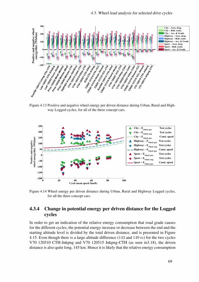
4.3. Wheel load analysis for selected drive cycles
−200
−100
0
100
200
300
123
103 1
35
106
97
97
106
147
97
98
101
108
95
102
117
118
96
88
85 1
16
111
117
113
108
Po
siti
ve
an
d n
ega
tiv
e w
hee
l en
erg
y/d
ist.
(W
h/k
m)
−66
−59
−61 −40
−58
−47
−66
−93
−52
−46
−85 −
48 −23
−42
−47
−40
−37
−58
−51
−82
−17
−17
−15
−13
167
151 172
143
142
139
153
200
141
141
153
165
125
140 1
70
170
148
135
137
182
140
147
143
129
−108
−86
−114 −
76
−101
−86
−100
−154
−72
−66
−120 −
72 −
39
−77
−74
−72
−58
−79
−69
−109
−30
−29
−29
−24
196
178 201
169
167
164 180
232
168
168
179
193
150
164 1
99
199
175
160
163
212
167
174
170
155
−115
−91
−121 −
79
−106
−90
−105
−164
−76
−68
−128
−75 −
39
−80
−79
−74
−60
−83
−72
−117
−31
−29
−30
−25
E
car5
00 1
20413 L
inneg−C
ity−C
TH
L
eaf 130321 C
TH
−E
rksbrg
L
eaf 130322 K
ors
v−G
uld
h
P
rius 1
20329 M
lndl−
Mln
lcke
P
rius 1
20329 M
lnlc
ke−M
lndl
P
rius 1
20403 M
lnlc
ke−C
TH
V
60P
HE
V K
rsvgn−G
alv
Bro
n
V
744 1
20312 C
sta
t−C
TH
V
744 1
20318 K
lltr
p−C
TH
V
744 1
20327 C
TH
−K
lltr
p
X
C60 C
TH
−K
rthsg
C
30d2 1
21219 C
TH
−V
CC
C
30d2 1
21219 H
enan−S
tnsnd
C
30d2 1
21219 V
CC
−C
TH
E
car5
00 1
20413 C
TH
−K
llrd
C
30d2 1
21219 S
tnsnd−H
enan
V
744 1
20307 V
CC
−C
TH
V
744 1
20316 K
lltr
p−C
stt
n
V
744 1
20320 K
lltr
p−C
stt
n
V
744 1
20327 K
lltr
p−C
stt
n
C
30d2 1
21219 S
tnsnd−V
CC
C
30d2 1
21219 V
CC
−S
tnsnd
V
70 1
20510 C
TH
−Jnkpng
V
70 1
20515 J
nkpng−C
TH
Urban Rural Highway
City − Aero. drag
City − Roll. resist.
City − Acc. & Grade
Highway − Aero. drag
Highway − Roll. resist.
Highway − Acc. & Grade
Sport − Aero. drag
Sport − Roll. resist.
Sport − Acc. & Grade
Figure 4.13 Positive and negative wheel energy per driven distance during Urban, Rural and High-way Logged cycles, for all of the three concept cars.
0 20 40 60 80 100−200
−150
−100
−50
0
50
100
150
200
250
Cycle mean speed (km/h)
Po
siti
ve
an
d n
ega
tiv
e
wh
eel
ener
gy
/dis
t. (
Wh
/km
)
City − E
wheel, pos Test cycles
City − Ewheel, neg
Test cycles
City − Ewheel, pos
Const. speed
Highway − Ewheel, pos
Test cycles
Highway − Ewheel, neg
Test cycles
Highway − Ewheel, pos
Const. speed
Sport − Ewheel, pos
Test cycles
Sport − Ewheel, neg
Test cycles
Sport − Ewheel, pos
Const. speed
Figure 4.14 Wheel energy per driven distance during Urban, Rural and Highway Logged cycles,for all the three concept cars.
4.3.4 Change in potential energy per driven distance for the Loggedcycles
In order to get an indication of the relative energy consumption that road grade causesfor the different cycles, the potential energy increase or decrease between the end and thestarting altitude level is divided by the total driven distance, and is presented in Figure4.15. Even though there is a large altitude difference (143 and 149m) for the two cyclesV70 120510 CTH-Jnkpng and V70 120515 Jnkpng-CTH (as seen in3.18), the drivendistance is also quite long, 145 km. Hence it is likely that the relative energy consumption
69

Chapter 4. Performance Requirements and Wheel Load Analysis of Studied ConceptVehicles
due to road grade is fairly small. In practice the energy consumption due to road gradewill naturally be larger than these values, due to the looses in the powertrain.
−60
−40
−20
0
20
40
60
80 1
4
−9
39
19
−12 −
2
−3
26
−3
4
−32
−3
−1
6
−6
0 1
−29
−30
−32
3
−3
3
−3
20
−13
55
27
−17
−3
−4
37
−4
6
−46
−4 −1
9
−8
0 2
−41
−42
−45
4
−4
4
−5
23
−15
61
30
−19
−3
−5
42
−4
6
−51
−5 −1
10
−9
0 2
−46
−47
−51
4
−4
5
−5
Ep
ote
nti
al i
nc.
/dec
. (W
h/k
m)
E
car5
00 1
20413 L
inneg−C
ity−C
TH
L
eaf 130321 C
TH
−E
rksbrg
L
eaf 130322 K
ors
v−G
uld
h
P
rius 1
20329 M
lndl−
Mln
lcke
P
rius 1
20329 M
lnlc
ke−M
lndl
P
rius 1
20403 M
lnlc
ke−C
TH
V
60P
HE
V K
rsvgn−G
alv
Bro
n
V
744 1
20312 C
sta
t−C
TH
V
744 1
20318 K
lltr
p−C
TH
V
744 1
20327 C
TH
−K
lltr
p
X
C60 C
TH
−K
rthsg
C
30d2 1
21219 C
TH
−V
CC
C
30d2 1
21219 H
enan−S
tnsnd
C
30d2 1
21219 V
CC
−C
TH
E
car5
00 1
20413 C
TH
−K
llrd
C
30d2 1
21219 S
tnsnd−H
enan
V
744 1
20307 V
CC
−C
TH
V
744 1
20316 K
lltr
p−C
stt
n
V
744 1
20320 K
lltr
p−C
stt
n
V
744 1
20327 K
lltr
p−C
stt
n
C
30d2 1
21219 S
tnsnd−V
CC
C
30d2 1
21219 V
CC
−S
tnsnd
V
70 1
20510 C
TH
−Jnkpng
V
70 1
20515 J
nkpng−C
TH
Urban Rural Highway
Figure 4.15 Change in potential energy between end point and starting point of the Logged cyclesper driven distance, for all the three concept cars; City-green (left), Highway-blue(middle) and Sport-Red (right).
70

Chapter 5
Powertrain Component Sizing,Modeling and Vehicle Simulation
As was found in Chapter 4, the demanded maximum torque and power from the power-train can be solely determined by the acceleration requirement for all of the three conceptcars. Furthermore, it was found that the acceleration requirements could be satisfied withmore than one combination of maximum wheel force and power. This means that theoutput requirement of the powertrain has some degree of freedom to it. Therefore thefinal choice will to a large part depend on the characteristics of the chosen componentsto be used.
In this chapter each of the concept cars will be assigned a base-line powertrain set-up,including sizing of, and models for; the electric machine, converter, battery and transmis-sion.
For simplicity auxiliary loads are excluded from the study, however they are likely tohave an important impact on BEV energy consumption, especially in particulary warmand cold conditions.
Furthermore it is decided that the acceleration requirement should be achieved at a10 % SOC level, and that the torque and power at higher SOC levels will not be functionsof the available DC voltage. This means that the powertrain will be slightly oversized athigher SOC levels.
5.1 Components used for modelingThe analysis is based on the powertrain components described in this section; electricmachine, battery and converters. The aim is to use components which are considered torepresent typical characteristics for this type of application, rather than state-of-the-artcomponents.
71

Chapter 5. Powertrain Component Sizing, Modeling and Vehicle Simulation
5.1.1 ConverterAs can be seen in Appendix A, most commercial BEVs have DC voltage levels of around300 − 400V . The only exceptions are the sport cars where the voltage levels are higher.Hence an IGBT module with a voltage rating around 650V is well suited, since thenthere is a margin for increasing battery voltage during braking, but also to handle otherphenomena occurring during operation such as induced voltage peaks during converterswitchings caused by stray inductances. Furthermore, it is assumed that the maximumconverter RMS phase current IRMS,max can be as high as 2/3 of the current rating in thedata sheet. Converter models from Infinieon found at [88] with different current ratingare used for all three cars.
5.1.2 Battery cellThe battery cell used is a Lithium-ion (cathode: LiNiO2 cathode active: LiMn2O4, an-ode: graphite) cell of laminate type, manufactured by the Japanese company AutomotiveEnergy Supply Corporation (AESC), where Nissan Motor Co. is a majority owner [89].Their batteries have also been used in the Nissan Leaf BEV models (96 in series and 2 inparallel). The US Idaho National Laboratory (INL) under the US Department of Energy(US DOE) have published measured data on the Nissan Leaf battery pack, including ter-minal voltage during a full discharge at a C/3 discharge rate, as well as the internal chargeand discharge resistances as a function of energy, in [90]. Based on the published data,the cell open circuit voltage, Voc has been estimated by approximating the resistive volt-age drop during a C/3 discharge rate, see Figure 5.1. The figure also includes assumedmaximum and minimum voltages, as well as denoted voltage levels at 10 and 90 % SOC.The average open circuit cell voltage within the used SOC window (10 to 90 %) has beenestimated to 3.88V , which is slightly higher than the stated nominal voltage by the man-ufacturer; 3.75V . The mean values of the charge and discharge resistances within 10 to90 % SOC are also presented in the figure. The average cell charge capacity is assumedto be 28.8Ah, [90], which can be compared to the manufacturer value of 32.5Ah.
0 20 40 60 80 1002
2.5
3
3.5
4
4.5
2.5 V
4.2 V
4.08 V
3.61 V
Voc, ave.
:3.88 V
SOC (%)
Cel
l V
olt
ag
e (V
)
Voc
Est.
Vt C/3 (US DOE)
Vt 0.3C (AESC)
Vt Max.
Vt Min.
0 20 40 60 80 1002.2
2.4
2.6
2.8
3
3.2
3.4
3.6
3.8
4
2.41 mΩ
2.88 mΩ
SOC (%)
Cel
l R
esis
tan
ce (
mΩ
)
Charge − meas. US DOE
Charge − ave. SOC10−90%
Discharge − US DOE
Discharge − ave. SOC10−90%
Figure 5.1 Estimated AESC battery cell no load voltage as a function of SOC, and estimated aver-age values of cell resistances, based on data from [US DOE, AESC].
72

5.1. Components used for modeling
5.1.3 Electric machineThe base for the electric machine used here, is a machine that was designed and built atthe division of Electric Power Engineering at Chalmers in the end of the 1990’s, and isdescribed in [91] and [53]. It is a four pole PMSM with inset magnets, designed for aseries HEV application, with water cooling. Machine voltage and current ratings ( [91]and [53]) along with measured machine parameters ( [36]) can be seen in Table 5.1.
Table 5.1 PMSM data.URMS,max,L−L 220 VIRMS,max 3min. 315 A
Phase resistance, Rs 7.9 mΩd-axis inductance, Ld 230 mHq-axis inductance, Lq (iq = 1pu) 420 mHFlux linkage related to magnet, Ψm 104 mWb
Stator outer diameter 189 mmStator inner diameter 110 mmStator core length 231 mmSlot fill factor 0.45Conductors per slot 3Conductors in parallel 2
Given the stated peak RMS current (which was a 3min. value) and winding struc-ture, the maximum current density can be found to be about 12A/mm2 (with a slot fillfactor of about 0.45, three turns per slot and two parallel windings the conductor area is13.47mm2 ). According to [34], a liquid cooled brushless machine can have a currentdensity between 10 to 30mm2. It is here chosen to increase the machine current densityto 20A/mm2, which leads to a max RMS current of about 540A.
As was done in [36] and [92], the core losses are estimated using the added coreresistance Rc described in Chapter 2. The core loss resistance as a function of speed isestimated based on measured no load losses over the machine speed range, presentedin [53] (paper E), as
Rc ≈3
2
(wel ψ)2
Pfe(5.1)
For each operating point, the machine core losses are then calculated as ( [92])
Pfe =3
2Rc(id,o − id)2 + (iq,o − iq)2); (5.2)
The efficiency and total losses of the originally sized electric machine (i.e. with unityscaling factors) can be seen in Figure 5.2, as well as maximum torque over speed usingthe MTPA control strategy as described in [92].
73

Chapter 5. Powertrain Component Sizing, Modeling and Vehicle Simulation
Speed (rpm)
To
rqu
e (N
m)
97
96
95
908
070
0 2000 4000 6000 8000 10000 120000
50
100
150
200
250
300
350
400
70
75
80
85
90
95ηPMSM, org
(%)
(a) Efficiency (%).
Speed (rpm)
To
rqu
e (N
m)
2
4
6
8
0 2000 4000 6000 8000 10000 120000
50
100
150
200
250
300
350
400
0
1
2
3
4
5
6
7
8P
loss,tot,PMSM, org (kW)
(b) Losses (kW).
Figure 5.2 Efficiency and total power losses for the electric machine with the original size, i.e.unity scaling factors.
5.1.3.1 PMSM active length scaling
During production of electric machines, the iron core laminations are often stampedfrom core plates [34]. Since the lamination design and stamp tool is rather expensiveto develop, electric machine manufacturers often offer different machine sizes that arebased on the same stamped laminations, but of different stack lengths. According to [34],the stack length-to-diameter ratio is typically 1 to 3, but it can also be higher. For lowlength/diameter ratios, the losses in the end windings will become more dominant, andthe torque production will be limited since only the stator and rotor package length con-tributes.
In order to achieve a desired output torque and power, the original machine is herescaled by changing the active length. All machine parameters (that is only the activeparts of the winding resistance and inductance) are expected to increase linearly with thelength, except the current rating. Also the no load losses used for the Rc estimation arescaled accordingly.
The winding resistance thus needs to be divided into one active part and one thatrepresents the winding overhang. According to [53] paper D p.92, the average conductorlength of a half turn, lav can be expressed as
lav = lactive + lpassive = lstk + 1.2τp + 2dext (5.3)
where lstk is the active lamination stack length, τp is the winding pole pitch and dextis the part of the end winding that is estimated to be axially extended outside of thelamination stack. The stack length is 231mm, the pole pitch is π D2 p , whereD is the statorinner diameter (110mm) and p is the pole pair number (two pole pairs), and finally the2dext is assumed to be 0.05m as in [53]. This gives a total average conductor length of384.7mm, where the active part is 231mm or 60 % and the over hang is 153.7mm or40 %, ( [53] paper D p.80). The end winding inductance is assumed to be very small,hence neglected, although as mentioned in [93] it may not be a viable assumption formotors with a low length/diameter ratio.
The length scaling is implemented using the stack length scaling factor, SFLstk.
74

5.2. Components sizing process
5.1.3.2 PMSM rewinding scaling
As described in [35], the machine voltage rating is assumed to be relatively freely adapt-able through rewinding of the machine, such that the maximum torque, speed and powerremain the same, as well as the losses and hence the efficiency. For simplicity, non-integerwinding turns are here allowed.
Then the total stator resistance and both inductances are scaled using the square ofthe rewinding scaling factor, SFrw, while the magnet flux and applied voltage is linearlyscaled, and finally the current is inversely scaled with SFrw.
5.2 Components sizing processThe sizing and modeling process for the City car can be seen in Figure 5.3, and for theHighway and Sport cars in Figure 5.4. As can be seen, two slightly different approachesare utilized, where some steps are independent while others build on previous steps. Eachstep will be further described in the following sections.
Chosen Fwheel, max
NEDC (Wh/km)ð Ebatt. (Wh)
γtm = wwheel, top/
wem, top
Tem, max =Fwheel, max r/(γgear ηTm (95 %))
ð SFLstk
IGBT VDC, max = 650 V
IGBT-module current Rating
≈ 3/2 IRMS, max
Vt (90% SOC) = 400 V
ð cells in series
Ebatt. & cells in series
ð cells in parallel
Vt (10 % SOC), during a
Pmax/ηPT (80 %) discharge
Vt (10% SOC)
ð SFrwð IRMS, max
Figure 5.3 BEV powertrain sizing and modeling algorithm for the City car.
75
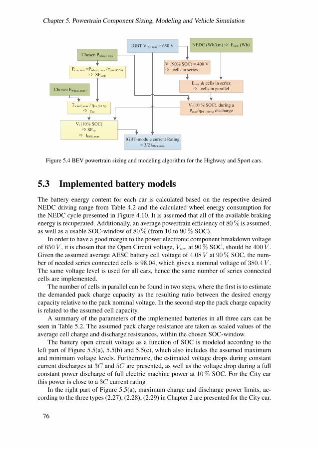
Chapter 5. Powertrain Component Sizing, Modeling and Vehicle Simulation
Chosen Pwheel, max
NEDC (Wh/km)ð Ebatt. (Wh)
Pem, max =Pwheel, max / ηtm (95 %)ð SFLstk
IGBT VDC, max = 650 V
IGBT-module current Rating
≈ 3/2 IRMS, max
Vt (90% SOC) = 400 V
ð cells in series
Ebatt. & cells in series
ð cells in parallel
Vt (10 % SOC), during a
Pmax/ηPT (80 %) discharge
Vt (10% SOC)
ð SFrwð IRMS, max
Twheel, max / ηtm (95 %)ð γtm
Chosen Fwheel, max
Figure 5.4 BEV powertrain sizing and modeling algorithm for the Highway and Sport cars.
5.3 Implemented battery modelsThe battery energy content for each car is calculated based on the respective desiredNEDC driving range from Table 4.2 and the calculated wheel energy consumption forthe NEDC cycle presented in Figure 4.10. It is assumed that all of the available brakingenergy is recuperated. Additionally, an average powertrain efficiency of 80 % is assumed,as well as a usable SOC-window of 80 % (from 10 to 90 % SOC).
In order to have a good margin to the power electronic component breakdown voltageof 650V , it is chosen that the Open Circuit voltage, Voc, at 90 % SOC, should be 400V .Given the assumed average AESC battery cell voltage of 4.08V at 90 % SOC, the num-ber of needed series connected cells is 98.04, which gives a nominal voltage of 380.4V .The same voltage level is used for all cars, hence the same number of series connectedcells are implemented.
The number of cells in parallel can be found in two steps, where the first is to estimatethe demanded pack charge capacity as the resulting ratio between the desired energycapacity relative to the pack nominal voltage. In the second step the pack charge capacityis related to the assumed cell capacity.
A summary of the parameters of the implemented batteries in all three cars can beseen in Table 5.2. The assumed pack charge resistance are taken as scaled values of theaverage cell charge and discharge resistances, within the chosen SOC-window.
The battery open circuit voltage as a function of SOC is modeled according to theleft part of Figure 5.5(a), 5.5(b) and 5.5(c), which also includes the assumed maximumand minimum voltage levels. Furthermore, the estimated voltage drops during constantcurrent discharges at 3C and 5C are presented, as well as the voltage drop during a fullconstant power discharge of full electric machine power at 10 % SOC. For the City carthis power is close to a 3C current rating
In the right part of Figure 5.5(a), maximum charge and discharge power limits, ac-cording to the three types (2.27), (2.28), (2.29) in Chapter 2 are presented for the City car.
76

5.3. Implemented battery models
The theoretical and the voltage limited discharge power limits are rather similar, whilethe current limited discharge power limits are substantially lower. Also a constant dis-charge power of 58 kW is depicted, and shows to be just a bit larger than the 3C limit.During charging, only the voltage limited charge power is presented. It shows a strongerdependence on SOC level compared to the discharge power. Similar characteristics arevalid for the Highway and Sport cars as well, although not shown here.
Table 5.2 Summary of battery data for all three cars.City Highway Sport
NEDC range 160 km 200 km 300 kmEnergy 19.3 kWh 29.9 kWh 56.6 kWhSeries cells 98.04 98.04 98.04Parallel cells 1.76 2.73 5.17Vt at 90 % SOC, PEM,max 325 V 317 V 283 VRdis 160.4 mΩ 103.4 mΩ 54.6 mΩRch 134 mΩ 86.4 mΩ 45.6 mΩ
0 20 40 60 80 100150
200
250
300
350
400
450
SOC (%)
Volt
age
(V)
325 V
401 V
412 V
245 V
Voc
Vt 3C
Vt 5C
Vt 58 kW
Vt, max
Vt, min
0 20 40 60 80 1000
50
100
150
200
250
300
350
SOC (%)
Pow
er (
kW
)
Pch.max
− Vmax
Pdis.max
− theoretic
Pdis.max
− Vmin
Pdis.max
− 3C
Pdis.max
− 5C
Pdis.max
− 58 kW
(a) City car.
0 20 40 60 80 100100
150
200
250
300
350
400
450
SOC (%)
Vo
lta
ge
(V)
317 V
401 V
412 V
245 V
Voc
Vt 3C
Vt 5C
Vt 111 kW
Vt, max
Vt, min
(b) Highway car.
0 20 40 60 80 100100
150
200
250
300
350
400
450
SOC (%)
Vo
lta
ge
(V)
283 V
401 V
412 V
245 V
Voc
Vt 3C
Vt 5C
Vt 363 kW
Vt, max
Vt, min
(c) Sport car.
Figure 5.5 No load voltage as a function of SOC-level, max and min terminal voltage, terminalvoltage during constant current during 3 and 5C discharge rates, as well as during aconstant EM max power discharge. In the right part of figure a for the City car: maxcharge and discharge power related to max voltage see (2.28), theoretical (2.27), currentlimited at 3 and 5C see (2.29), and finally for the EM max power.
77

Chapter 5. Powertrain Component Sizing, Modeling and Vehicle Simulation
5.4 Implemented EM models including transmissionsFor the City car it is decided that the total transmission ratio should be based on the directrelationship between the vehicle and machine top speed, as the base speed then is fairlyclose to the desired one from Figure 4.5, as well as the power level. The wheel radius, thegear ratio γtm and the desired maximum wheel force (compensated for a transmissionefficiency of 95 %) are then used as inputs when finding a suitable length scaling factor.Then a value for the rewinding scaling factor is found such that the DC voltage level ismatching the estimated DC voltage level during a full power discharge at SOC level of10 %. Finally, the resulting maximum RMS phase current, IRMS,max is noted and usedas a base for choosing the converter current rating, Ic,nom. It is assumed that a reasonablecurrent margin is achieved when Ic,nom ≈ 3/2 IRMS,max.
For the Highway and Sport cars, the transmission ratio is not initially decided. Insteadthe stack length is scaled until the desired output wheel power is reached. In order to re-alize the AWD functionality in the Sport car, it is decided that two equally sized electricmotors shall work in parallel; one on the rear drive axle, and one on the front. This im-plementation will also help keeping the length scaling down. Then the transmission ratiois decided as the ratio for which the desired wheel force is achieved (while consideringthe assumed transmission efficiency). Finally the rewinding scaling factor and resultingmaximum RMS phase current is found in the same manner as for the City car, as well asthe converter current rating.
The implemented electric machine torque and power levels as well as scaling factorsand transmission ratios can be seen in Table 5.3. The transmission ratio,γtm is defined asin
ωem = γtm ωwheel (5.4)
where ωem is the electric machine angular speed (rad/s), ωwheel is the angular speed ofthe wheel(rad/s).
Table 5.3 Summary of electric machine and transmission data for all three cars, along with vehiclepower-to-weight ratio.
City Highway Sportγtm 10.3882 7.62 6.22Pmax 49 kW 97 kW 153Tmax 140 Nm 280 Nm 420 NmFwheel,max 4750 N 6600 N 7700 Nnmax 12,000 rpm 9475 rpm 10,191 rpm
URMS,max,L−L 207 V 202 V 180 VIRMS,ph,max 233 A 468 A 786 ASFLstk 0.405 0.795 1.1925Lstk
Douter0.495 0.972 1.458
SFrw 2.32 1.154 0.687ηmax at 350 V 96.2 % 96.9 % 97.0 %Vehicle Power-to-weight ratio 41 W/kg 57 W/kg 153 W/kg
The resulting output torque and power as function of speed for all cars, can be seenin Figure 5.6, and the resulting wheel forces can be seen in Figure 5.7.
78
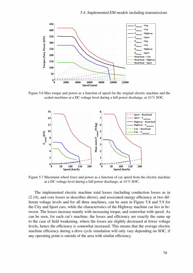
5.4. Implemented EM models including transmissions
0 2000 4000 6000 8000 10000 120000
50
100
150
200
250
300
350
400
450
Speed (rpm)
Tor
que
(Nm
), P
ower
(kW
)
TEM,max
− Org.
TEM,max
− City
TEM,max
− Highway
TEM,max
− Sport
PEM,max
− Org.
PEM,max
− City
PEM,max
− Highway
PEM,max
− Sport
Road load − CityRoad load − HighwayRoad load − Sport
Figure 5.6 Max torque and power as a function of speed for the original electric machine and thescaled machines at a DC voltage level during a full power discharge, at 10% SOC.
0 50 100 150 2000
2
4
6
8
10
12
14
16
Speed (km/h)
Fw
heel (
kN)
0 50 100 150 200
0
1
2
3
4
5
6
7
8
Speed (km/h)
Mas
s no
rn F
whe
el (N
/kg)
Sport − Road loadSport − F
wheel,max
Highway − Road loadHighway − F
wheel,max
City − Road loadCity − F
wheel,max
Figure 5.7 Maximum wheel force and power as a function of car speed from the electric machineat a DC voltage level during a full power discharge, at 10% SOC.
The implemented electric machine total losses (including conduction losses as in(2.14), and core losses as describes above), and associated energy efficiency at two dif-ferent voltage levels and for all three machines, can be seen in Figure 5.8 and 5.9 forthe City and Sport cars, while the characteristics of the Highway machine car lies in be-tween. The losses increase mainly with increasing torque, and somewhat with speed. Ascan be seen, for each car’s machine, the losses and efficiency are exactly the same upto the case of field weakening, where the losses are slightly decreased at lower voltagelevels, hence the efficiency is somewhat increased. This means that the average electricmachine efficiency during a drive cycle simulation will only vary depending on SOC, ifany operating point is outside of the area with similar efficiency.
79

Chapter 5. Powertrain Component Sizing, Modeling and Vehicle Simulation
0 2000 4000 6000 8000 10000 12000
−150
−100
−50
0
50
100
150
Speed (rpm)
Torq
ue
(Nm
)
70
80
90
95 96
9695
90
8070
VDC
= 412 V
VDC
= 325 V
(a) Efficiency (%).
0 2000 4000 6000 8000 10000 12000
−150
−100
−50
0
50
100
150
Speed (rpm)
Torq
ue
(Nm
)
1000
2000
3000
4000
1000
2000
3000
4000
5000
50005000 VDC
= 412 V
VDC
= 325 V
(b) Losses (W).
Figure 5.8 Implemented electric machine efficiency and power loss maps, for the City car.
0 2000 4000 6000 8000 10000 12000
−400
−300
−200
−100
0
100
200
300
400
Speed (rpm)
Torq
ue
(Nm
)
70
80
90
95
9697
70
80
90
95
9697
VDC
= 412 V
VDC
= 283 V
(a) Efficiency (%).
0 2000 4000 6000 8000 10000 12000
−400
−300
−200
−100
0
100
200
300
400
Speed (rpm)
Torq
ue
(Nm
)
2000
4000
6000
8000
2000
4000
6000
8000
VDC
= 412 V
VDC
= 283 V
(b) Losses (W).
Figure 5.9 Implemented electric machine efficiency and power loss maps, for the Sport car.
In Figure 5.10, the total powertrain efficiencies (excluding batteries) as a function ofmass normalized wheel force and car speed, can be seen. For the same level of speed andacceleration, it shows that the City car powertrain is a bit more efficient compared to theHighway and sport cars’s.
80

5.5. Implemented converter model
0 50 100 150 200
−8
−6
−4
−2
0
2
4
6
8
Speed (km/h)
Mas
s no
rm. F
whe
el (
N/k
g)
90
87
8070
CityHighwaySport
Figure 5.10 Total power train efficiency, including electric machine, converter and transmission,for the three concept cars, as a function of speed and normalized wheel force.
5.5 Implemented converter modelFor the City car a converter module with current rating of 400A (Infineon FS400R07A1E3_H5)is chosen, even though the rating might be a bit too low. For the Highway car a modulewith current rating of 800A (Infineon FS800R07A2E3) is implemented. Finally for theSport car; four modules are used, two in parallel for each of the two machines, wherethe module current rating is 600A (Infineon FS600R07A2E3). That will give a total con-verter current rating of 2.4 kA, which is assumed to be able to withstand an RMS currentof 1.6 kA, hence it is viable for the chosen machine size.
The extracted IGBT module parameters can be seen in Table 5.4, and adhere to chiptemperatures of 125 C and a gate voltage of 15V . The on-state threshold voltage andresistance parameters are estimated under consideration of expected current levels. Theswitching frequency is set to 10 kHz.
Table 5.4 IGBT module parameters, for all three cars, where the data for the Sport car represent allfour modules.
City car: Highway car: Sport car:IGBT Diode IGBT Diode IGBT Diode
Ic,nom 400 A 800 A 4*600 AIref : 400 A 550 A 4*400 AVref : 300 V 300 V 300 VOn-state threshold voltage 0.709V 0.803V 0.673V 0.761V 0.66V 0.775VOn-state resistance 2.468mΩ 1.999mΩ 1.336mΩ 1.12mΩ 0.441mΩ 0.352mΩTurn-on Energy loss 4.2mJ - 12mJ - 44mJ -Turn-off Energy loss 16.0mJ 7.25mJ 25mJ 9.5mJ 68mJ 28mJ
The total power losses are estimated using (2.20) to (2.23), and can be seen togetherwith energy efficiency in Figure 5.11 for the City car and in Figure 5.12 for the Sport car,in the machine torque and speed frame of reference, while the results for the Highwayconverter lies in between. The converter losses mainly increase with increasing torque,
81

Chapter 5. Powertrain Component Sizing, Modeling and Vehicle Simulation
while the efficiency has a strong speed dependency and increases with increasing speed.Unlike the electric machine, the converter losses vary somewhat depending on the DCvoltage level in the whole operating range. The efficiency is mostly higher at lower volt-age levels in the same torque and speed operating point, due to lower switching losses.
0 2000 4000 6000 8000 10000 12000
−150
−100
−50
0
50
100
150
Speed (rpm)
Torq
ue
(Nm
)
70
80
90
95
97
98
98
VDC
= 412 V
VDC
= 325 V
(a) Efficiency (%).
0 2000 4000 6000 8000 10000 12000
−150
−100
−50
0
50
100
150
Speed (rpm)
Torq
ue
(Nm
)
200
500
1000
VDC
= 412 V
VDC
= 325 V
(b) Losses (W).
Figure 5.11 Implemented converter efficiency and power loss maps at three DC voltage levels, forthe City car.
0 2000 4000 6000 8000 10000 12000
−400
−300
−200
−100
0
100
200
300
400
Speed (rpm)
Torq
ue
(Nm
)
70
80 90
95 9
7
97
VDC
= 412 V
VDC
= 283 V
(a) Efficiency (%).
0 2000 4000 6000 8000 10000 12000
−400
−300
−200
−100
0
100
200
300
400
Speed (rpm)
Torq
ue
(Nm
)
1000
2000
4000
6000
VDC
= 412 V
VDC
= 283 V
(b) Losses (W).
Figure 5.12 Implemented converter efficiency and power loss maps at three DC voltage levels, forthe Sport car.
5.6 Simulator structureA simplified presentation of the simulation structure, which was implemented in MatlabSimulink, is presented in Figure 5.13. The input to all simulations are the reference speedcycles as functions of time. The time resolution of the Test cycles are all 1Hz, whileit is 20Hz for the Logged cycles. All simulations are executed with a fixed time step
82

5.6. Simulator structure
of 0.01 s, which proved to provide reasonable stability. For the logged cycles, also theestimated road grade levels as a function of time is an input to the simulations.
In order to allow deviation from the speed reference a PI driver model is imple-mented. Its input is the difference between the reference speed and the simulated speed.The proportional Kp and integral Ki gains are chosen such that the reference speedand associated acceleration are followed fairly close by the simulation output (whereKp = Ki = 3). The output of the driver model is a signal between −1 to 1.
Drive Cycle PI Driver Model
Acceleration
Force
Calculation
Transmission EM Inverter Battery
- Reference Speed- Accelerator Pedal Position
- Brake Pedal Position - Wheel Torque
- Wheel Speed
- Vehicle Speed
- EM Torque
- EM Speed - EM Power - Inverter Power
- Battery Voltage
- Battery SOC
- Battery Energy
- Vehicle Speed
- Battery Voltage
- Wheel Torque
- Wheel Speed
- EM Speed - Battery Voltage
Figure 5.13 Simplified simulation structure.
The positive output from the driver model is regarded as an acceleration pedal sig-nal and the negative part as a brake pedal signal. These signals are then scaled by themaximum torque from the electric machine in motoring and generating mode, which areimplemented through look-up tables as functions of machine speed and DC-link voltage.Thus it gives the electric machine torque reference signals, via linear interpolation. It isthen assumed that the electric machine can fulfill the torque reference. No wheel slipis assumed, hence the electric machine speed is simply found via the simulated vehiclespeed, the wheel radius and the transmission ratio.
At each time step the sum of the resistive forces on the wheel (the vehicle’s aero-dynamic drag, rolling resistance and possibly also grading force) is converted to a totalresistive wheel torque. Given the total resistive torque together with the wheel torquefrom the electric machine via the transmission, and the vehicles estimated mass inertia,(as the product of the vehicle mass and the square of the wheel radius, while ignoringadditional rotating inertias), the resulting vehicle acceleration is calculated (as the ro-tational form of (2.1)). Furthermore, the simulated speed is then calculated as the timeintegral of the resulting acceleration.
Both the electric machine and converter power losses are implemented trough look-up tables that are functions of machine torque and speed, as well as DC-link voltage,where the output is found through linear interpolation. The power flow between electricmachine and converter is calculated as the added or subtracted losses to the mechanicalmachine output, depending on mode of operation. Likewise is the DC-link power flowcalculated via the additional converter losses. The DC-link power flow is then the inputto the battery model, where the current is found from division of the power with theterminal voltage from the previous time step. The current is then used to estimate the
83

Chapter 5. Powertrain Component Sizing, Modeling and Vehicle Simulation
SOC level, (as in (2.26)) as well as battery conduction losses together with the dischargeand charge internal resistances. Finally, the terminal voltage is found as the subtractedresistive voltage drop from the SOC dependent open circuit voltage.
Next follows results from the simulations in terms of requirement and drive cyclefulfillment as well as powertrain and energy consumption for the different drive cycles.
5.7 Simulated time to accelerate 0− 100 km/h
The simulation result from the 0−100 km/h acceleration test can be seen in Figure 5.14to 5.16, for the three cars respectively, where the ideal calculations for similar valuesof the initial maximum force and power, are also presented as a reference. Note that theideal calculations for the City car is here adjusted to comply with the implemented size ofthe electric machine. The tests have been conducted for both 10 % and 90 % SOC levels,which gave different results as expected.
0 20 40 60 80 100 1200
1
2
3
4
5
6
Speed (km/h)
Fw
hee
l (k
N)
46kW
4.5 kN
0 5 10 150
20
40
60
80
100
120
Time (s)
Sp
eed
(k
m/h
)
4.1s 13.0s
4.0s 12.8s
3.9s 11.3s
EM F
wheel, max.
calc. Fwheel, max.
Road load
Sim. Fwheel
SOCinit.
10%
Sim. Fwheel
SOCinit.
90%
Calc.
Sim. 10% SOCinit.
Sim. 90% SOCinit.
Figure 5.14 Comparison of acceleration test from 0 − 100 km/h, between calculation and simu-lation, as well as maximum force on wheels from the electric machine, for the Citycar.
For the City car, the time to accelerate from 0− 100 km/h by simulation was 12.8 s,at a battery SOC level of 10 % see Figure 5.14. This is about 1.5 % faster than the accel-eration requirement for the city car, which was 13 s. As can be seen in the figure, abovebase speed the simulated wheel force is somewhat larger than the ideally calculated force,hence the acceleration will be faster. The simulated wheel force is even larger at the 90%SOC level, resulting in an acceleration time of 11.3 s, i.e. 7.8 % shorter then at 10 %SOC. The simulated acceleration time to 50 km/h is 4 s at 10 % SOC and only slightlysmaller at the 90% SOC level, 3.9 s.
84

5.8. Simulated time to accelerate 0− 100 km/h with grade
0 20 40 60 80 100 1200
1
2
3
4
5
6
7
8
Speed (km/h)
Fw
hee
l (k
N)
89 kW
6.3 kN 52 km/h
0 2 4 6 8 10 120
20
40
60
80
100
120
Time (s)
Sp
eed
(k
m/h
)
3.9s 10.0s
3.9s 9.7s
3.9s 8.9s
EM Fwheel, max.
calc. Fwheel, max.
Road load
Sim. Fwheel
SOCinit.
10%
Sim. Fwheel
SOCinit.
90%
Calc.
Sim. 10% SOCinit.
Sim. 90% SOCinit.
Figure 5.15 Comparison of acceleration test from 0− 100 km/h, between calculation and simula-tion, as well as maximum force on wheels from the electric machine, for the Highwaycar.
Also the Highway car has a slightly shorter acceleration time to 100 km/h comparedto the ideal calculation; 9.7 s, which is 3 % faster. The difference between the two SOClevels is even larger than for the City car, where the time for the 90% SOC level is 8.9 swhich is 8.2 % faster than at 10 % SOC. The time to 50 km/h is the same for all cases.
0 20 40 60 80 100 1200
5
10
15
Speed (km/h)
Fw
hee
l (k
N)
290 kW14.6 kN
0 1 2 3 4 50
20
40
60
80
100
120
Time (s)
Sp
eed
(k
m/h
)
1.9s4.0s
1.9s
3.9s
1.9s3.8s
EM Fwheel, max.
calc. Fwheel, max.
Road load
Sim. Fwheel
SOCinit.
10%
Sim. Fwheel
SOCinit.
90%
Calc.
Sim. 10% SOCinit.
Sim. 90% SOCinit.
Figure 5.16 Comparison of acceleration test from 0 − 100 km/h, between calculation and simu-lation, as well as maximum force on wheels from the electric machine, for the Sportcar.
Finally for the Sport car the time to 50 km/h is the same for all cases, while the timeto 100 km/h is 3.9 s and 3.8 s for the 10 and 90 % SOC respectively, which means about2.5 and 5 % faster then the requirement.
5.8 Simulated time to accelerate 0−100 km/h with gradeHere an acceleration from 0 − 100 km/h is again simulated, but now for the case ofadded road grade as a form of controlling the fulfillment of the requirement to be able tohandle a grade at high speed. The results can be seen in Figure 5.17 to 5.19.
85

Chapter 5. Powertrain Component Sizing, Modeling and Vehicle Simulation
0 20 40 60 80 100 1200
1
2
3
4
5
6
Speed (km/h)
Fw
hee
l (k
N)
46kW
4.5 kN
0 5 10 15 20 250
20
40
60
80
100
120
Time (s)
Sp
eed
(k
m/h
)
4.9s 20.2s5.0s 19.9s
4.8s 16.1s
EM F
wheel, max.
calc. Fwheel, max.
Road load
Sim. Fwheel
SOCinit.
10%
Sim. Fwheel
SOCinit.
90%
Calc.
Sim. 10% SOCinit.
Sim. 90% SOCinit.
Figure 5.17 Comparison of acceleration test from 0− 100 km/h, between calculation and simula-tion, as well as maximum force on wheels from the electric machine, for a road gradeof 6%, for the City Car.
The City car was to be able to sustain a speed of 90 km/h in a uphill grade of 6 %,which it does. In this case it takes about 5 s for the City car to reach 50 km/h and about20 s to reach 100 km/h at 10 % SOC. The higher SOC level gives only minor effects onthe time to 50 km/h, while it needs 3.8 s less to reach 100 km/h compared to the 10 %SOC.
0 50 100 1500
1
2
3
4
5
6
7
8
Speed (km/h)
Fw
hee
l (k
N)
89 kW
6.3 kN
0 5 10 15 20 250
20
40
60
80
100
120
140
Time (s)
Sp
eed
(k
m/h
)
4.7s 13.1s4.8s 12.7s4.8s 11.4s
EM F
wheel, max.
calc. Fwheel, max.
Road load
Sim. Fwheel
SOCinit.
10%
Sim. Fwheel
SOCinit.
90%
Calc.
Sim. 10% SOCinit.
Sim. 90% SOCinit.
Figure 5.18 Comparison of acceleration test from 0− 100 km/h, between calculation and simula-tion, as well as maximum force on wheels from the electric machine, for a road gradeof 6%, for the Highway Car.
The Highway car is able to sustain the uphill grade of 6 % at the speed of 130 km/h.In this case the acceleration time difference between the no grade case is much smallercompared to the City car. Also less difference is noted between the two SOC levels, only1.3 s for 100 km/h, and none for 50 km/h.
86

5.9. Fulfillment of reference cycle speed in simulation
0 50 100 1500
5
10
15
Speed (km/h)
Fw
hee
l (k
N)
290 kW14.6 kN
0 2 4 6 80
20
40
60
80
100
120
140
Time (s)
Sp
eed
(k
m/h
)
2.0s 4.4s2.4s 4.9s
2.4s 4.7s
EM Fwheel, max.
calc. Fwheel, max.
Road load
Sim. Fwheel
SOCinit.
10%
Sim. Fwheel
SOCinit.
90%
Calc.
Sim. 10% SOCinit.
Sim. 90% SOCinit.
Figure 5.19 Comparison of acceleration test from 0− 100 km/h, between calculation and simula-tion, as well as maximum force on wheels from the electric machine, for a road gradeof 6%, for the Sport Car.
Finally, the Sport car can handle the 12 % uphill grade at 130 km/h. The time toaccelerate to 100 km/h only becomes 0.9 s longer compared to the case with no grade,for both SOC levels.
5.9 Fulfillment of reference cycle speed in simulationDue to the use of a driver model (i.e. a speed controller) in the simulation, naturallythe simulated speed will deviate from the reference speed trace, even for operating pointswell within the operating area of the powertrain. Hence when analyzing energy consump-tion and efficiency for a certain cycle, it must be remembered that a slightly different cy-cle than the reference, is analyzed. As a consequence, typical values of the difference be-tween reference speed and simulated speed have been studied. Another parameter worthstudying is the difference in positive and negative average energy at the wheels per drivendistance, between the simulation and the reference speed and acceleration. It might hap-pen that there is a large speed difference at a certain time step, but that it’s influence onthe average energy consumption difference is rather small.
For the Test cycles the speed differences range between 0.1 − 0.4 km/h, 0.2 −0.5 km/h and between 0.2 − 0.6 km/h for the City, Highway and Sport cars respec-tively. Typical values of the maximum difference between the simulated accelerationand the acceleration of the reference Test cycles are; 0.0 − 0.1m/s2, 0.0 − 0.2m/s2
and 0.0 − 0.1m/s2 for the City, Highway and Sport cars respectively. Worth noting isthat the time simulation inherently is a backward calculation, hence the Euler backwardmethod is used for the reference cycle acceleration, instead of the otherwise more accu-rate forward-backward method described in Chapter 3.
Moreover, during the modal European cycles (ECE, EUDC and NEDC) a minorspeed overshoot is noted when the reference speed of the cycle is changing rapidly froma constant acceleration to a constant speed, which gives a relatively small difference of0.2 km/h between the reference and simulated speed. This also results in a small oscil-lation in the simulated acceleration of 0.7m/s2. Nevertheless, these effects are seen tohave little influence on the average wheel energy consumption during the cycle, hencethey are ignored.
87

Chapter 5. Powertrain Component Sizing, Modeling and Vehicle Simulation
0 2000 4000 6000 8000 10000 12000−150
−100
−50
0
50
100
150
Speed (rpm)
EM
Tor
que
(Nm
)
Tmax
VDC, max
Tmax
VDC
350 V
Tmax
VDC
325 V
Artemis URBANNYCCWLTC Cl.3 Low v5.3FTP72 UDDSSC03jc08WLTC Cl.3 Mdl v5.3ECE
(a) Urban cycles.
0 2000 4000 6000 8000 10000 12000−150
−100
−50
0
50
100
150
Speed (rpm)
EM
Tor
que
(Nm
)
Tmax
VDC, max
Tmax
VDC
350 V
Tmax
VDC
325 V
HWFETUS06REP05Artemis MW130WLTC Cl.3 ExtrHgh v5.3
(b) Highway cycles.
Figure 5.20 EM operating points during the Urban and Highway cycles for the City car.
For the City car, three points in each of the two cycles US06 and REP05 were outsideof the powertrain’s operational area, causing a maximum deviation of 1.7 km/h from thereference speed, and 0.4m/s2 from the reference acceleration. These represent speed andacceleration levels of 56 km/h at 3m/s2, and 80 km/h at 2.2m/s2, and finally around120 km/h at 1.3m/s2. The consequence on the average energy consumption is negligi-ble in these cases. Also one point in the Artemis Motorway cycle during braking at highspeed is outside of the operating area of the electric machine, see Figure 5.20. The oper-ating points of the City car electric machine can be seen as gray dots in Figure 5.20 forthe Urban and Highway cycles. In the same figure also ideal electric machine operatingpoints for a lossless system is depicted for comparison, and color marked depending onthe type of cycle.
0 2000 4000 6000 8000 10000−300
−200
−100
0
100
200
300
Speed (rpm)
EM
Tor
que
(Nm
)
Tmax
VDC, max
Tmax
VDC
350 V
Tmax
VDC
325 V
Artemis URBANNYCCWLTC Cl.3 Low v5.3FTP72 UDDSSC03jc08WLTC Cl.3 Mdl v5.3ECE
(a) Urban cycles.
0 2000 4000 6000 8000 10000−300
−200
−100
0
100
200
300
Speed (rpm)
EM
Tor
que
(Nm
)
Tmax
VDC, max
Tmax
VDC
350 V
Tmax
VDC
325 V
HWFETUS06REP05Artemis MW130WLTC Cl.3 ExtrHgh v5.3
(b) Highway cycles.
Figure 5.21 EM operating points during the Urban and Highway cycles for the Highway car.
The US06 and REP05 cycles caused some deviations also for the Highway car ofmaximum 1.5 km/h and 0.2m/s2, however in this case the operating points that causeproblem are those that demand high acceleration (almost 4m/s2) from stand still, seeFigure 5.21. The problem appears twice in REP05 and once in US06. Also here there isno effect on the net average wheel energy.
For the Sport car, the operating points from all Test cycles are well within the limitsof the powertrain.
88

5.10. Simulated component efficiency per cycle
Furthermore, all cars are able to follow the Logged Urban cycles, with typical max-imum speed differences between the reference and simulated cycle as 0.3 − 0.8 km/h.One Rural cycle for the City car (C30d2 121219 Stnsnd-Henan) and all Highway cycleshave single large speed deviations with a relatively large effect on the average net wheelenergy. The Highway and Sport cars have no major deviations worthy to mention.
5.10 Simulated component efficiency per cycleThe average Test cycle efficiency separated into propulsion and braking mode can beseen in Figure 5.22 to 5.24, for the City, Highway and Sport cars respectively. Also theaverage cycle efficiency of each modeled component (electric machine, converter, batteryand transmission) is depicted in the figures for comparison.
Although the differences in efficiency between the cycles and cars are quite small (afew units of percent), some trends can be seen when comparing the results between thecycles and cars. One tendency is a slightly higher average total powertrain efficiency forthe highway cycles and a somewhat lower efficiency for the Urban cycles, for all of thecars. Also the total powertrain efficiency of the City car is generally a bit higher, and abit lower for the Sport car. Furthermore, the total powertrain cycle efficiency is normallya few units of percent higher in motoring mode compared to generating mode, which canalso be seen in Figure 5.10.
The lowest total efficiency for all cars is achieved in the NYCC cycle where both theelectric machine and converter efficiencies are low. The highest efficiencies are seen inthe WLTC Extra high and Atermis Motorway cycles. The Sport car converter configu-ration proves to give a rather poor efficiency for several of the Urban cycles. Perhaps abetter strategy is to implement a control system where the extra driving wheel pair is onlyengaged during higher power and torque demands.
The transmission efficiency is in line with the efficiency of the converter and electricmachine. Perhaps a more advanced loss model of the transmission would be preferredhere in order to differentiate between the various load cases.
70
80
90
100
11082 83 85 84 86 85 79 82 86 87 87 88 86 87 88 89 88 89
Pro
pu
lsio
n
Urban Rural Highway
Eff
icie
ncy (
%)
−110
−100
−90
−80
−70
80 81 83 81 84 83 78 80 83 85 84 86 83 85 84 85 84 85
Bra
kin
g
E
CE
W
LTC
Low
jc08
F
TP
72 U
DD
S W
LTC
Mid
dle
S
C03
N
YC
C A
rtem
is U
RB
AN
N
ED
C W
LTC
Hig
h
A
rtem
is R
UR
AL
E
UD
C U
C L
A92
H
WFE
T R
EP
05
W
LTC
Extr
a H
igh
U
S06
A
rtem
is 1
30
EM
Conv.
Bat.
Tm.
PTtot
Figure 5.22 Total powertrain efficiency per cycle in propulsion vs. braking mode (negative y-axis),and efficiency broken down per component, from simulation of the City car, with 90%initial SOC, for the Test cycles.
89

Chapter 5. Powertrain Component Sizing, Modeling and Vehicle Simulation
70
80
90
100
11080 81 84 83 85 84 77 80 85 86 87 87 85 87 87 88 87 88 88
Pro
pu
lsio
n
Urban Rural HighwayE
ffic
ien
cy
(%
)
−110
−100
−90
−80
−70
77 79 82 79 83 81 74 77 82 83 84 86 81 84 83 85 83 86 85
Bra
kin
g
E
CE
W
LTC
Low
jc08
F
TP
72 U
DD
S W
LTC
Mid
dle
S
C03
N
YC
C
A
rtem
is U
RB
AN
N
ED
C W
LTC
Hig
h
A
rtem
is R
UR
AL
E
UD
C U
C L
A92
H
WFE
T R
EP
05
W
LTC
Extr
a H
igh
U
S06
A
rtem
is 1
30
A
rtem
is 1
50
EM
Conv.
Bat.
Tm.
PTtot
Figure 5.23 Total powertrain efficiency per cycle in propulsion vs. braking mode (negative y-axis),and efficiency broken down per component, from simulation of the Highway car, with90% initial SOC, for the Test cycles.
70
80
90
100
11076 78 81 80 83 82 73 77 82 83 84 84 82 84 85 86 85 86 86
Pro
pu
lsio
n
Urban Rural Highway
Eff
icie
nc
y (
%)
−110
−100
−90
−80
−70
72 74 77 75 80 78 70 73 78 80 80 83 78 81 80 80 81 82 82
Bra
kin
g
E
CE
W
LTC
Low
jc08
F
TP
72 U
DD
S W
LTC
Mid
dle
S
C03
N
YC
C
A
rtem
is U
RB
AN
N
ED
C W
LTC
Hig
h
A
rtem
is R
UR
AL
E
UD
C U
C L
A92
H
WFE
T R
EP
05
W
LTC
Extr
a H
igh
U
S06
A
rtem
is 1
30
A
rtem
is 1
50
EM
Conv.
Bat.
Tm.
PTtot
Figure 5.24 Total powertrain efficiency per cycle in propulsion vs. braking mode (negative y-axis),and efficiency broken down per component, from simulation of the Sport car, with90% initial SOC, for the Test cycles.
Similarly, the total powertrain efficiency for the Logged cycles can be seen in Figure5.25 to 5.27, for the City, Highway and Sport cars respectively.
Generally the same trends can also be seen here. Nevertheless, the spread within theUrban and Rural road type categories is here a bit larger. The absolute efficiency valuesper car, are in line with those for the Test cycles, although a bit lower for the LoggedHighway cycles compared to the Highway Test cycles.
90

5.10. Simulated component efficiency per cycle
70
80
90
100
11081 84 82 86 85 86 81 80 86 86 79 87 87 86 87 86 86 85 85 87 85 85 86 85
Pro
pu
lsio
n
Urban Rural Highway
Eff
icie
ncy (
%)
−110
−100
−90
−80
−70
79 82 80 84 84 84 80 78 84 82 79 84 84 83 84 82 81 84 85 86 83 82 82 81
Bra
kin
g
E
car5
00 1
20413 L
inneg−C
ity−C
TH
L
eaf 130321 C
TH
−E
rksbrg
L
eaf 130322 K
ors
v−G
uld
h
P
rius 1
20329 M
lndl−
Mln
lcke
P
rius 1
20329 M
lnlc
ke−M
lndl
P
rius 1
20403 M
lnlc
ke−C
TH
V
60P
HE
V K
rsvgn−G
alv
Bro
n
V
744 1
20312 C
sta
t−C
TH
V
744 1
20318 K
lltr
p−C
TH
V
744 1
20327 C
TH
−K
lltr
p
X
C60 C
TH
−K
rthsg
C
30d2 1
21219 C
TH
−V
CC
C
30d2 1
21219 H
enan−S
tnsnd
C
30d2 1
21219 V
CC
−C
TH
E
car5
00 1
20413 C
TH
−K
llrd
C
30d2 1
21219 S
tnsnd−H
enan
V
744 1
20307 V
CC
−C
TH
V
744 1
20316 K
lltr
p−C
stt
n
V
744 1
20320 K
lltr
p−C
stt
n
V
744 1
20327 K
lltr
p−C
stt
n
C
30d2 1
21219 S
tnsnd−V
CC
C
30d2 1
21219 V
CC
−S
tnsnd
V
70 1
20510 C
TH
−Jnkpng
V
70 1
20515 J
nkpng−C
TH
EM
Conv.
Bat.
Tm.
PTtot
Figure 5.25 Total powertrain efficiency per cycle in propulsion vs. braking mode (negative y-axis),and efficiency broken down per component, from simulation of the City car, with 90%initial SOC, for the Logged cycles.
70
80
90
100
11079 82 80 85 84 85 78 78 85 84 76 86 87 85 87 87 86 85 85 87 85 85 86 85
Pro
pu
lsio
n
Urban Rural Highway
Eff
icie
ncy (
%)
−110
−100
−90
−80
−70
76 80 77 83 83 83 77 75 83 80 76 83 85 82 83 84 82 84 85 86 82 82 81 81
Bra
kin
g
E
car5
00 1
20413 L
inneg−C
ity−C
TH
L
eaf 130321 C
TH
−E
rksbrg
L
eaf 130322 K
ors
v−G
uld
h
P
rius 1
20329 M
lndl−
Mln
lcke
P
rius 1
20329 M
lnlc
ke−M
lndl
P
rius 1
20403 M
lnlc
ke−C
TH
V
60P
HE
V K
rsvgn−G
alv
Bro
n
V
744 1
20312 C
sta
t−C
TH
V
744 1
20318 K
lltr
p−C
TH
V
744 1
20327 C
TH
−K
lltr
p
X
C60 C
TH
−K
rthsg
C
30d2 1
21219 C
TH
−V
CC
C
30d2 1
21219 H
enan−S
tnsnd
C
30d2 1
21219 V
CC
−C
TH
E
car5
00 1
20413 C
TH
−K
llrd
C
30d2 1
21219 S
tnsnd−H
enan
V
744 1
20307 V
CC
−C
TH
V
744 1
20316 K
lltr
p−C
stt
n
V
744 1
20320 K
lltr
p−C
stt
n
V
744 1
20327 K
lltr
p−C
stt
n
C
30d2 1
21219 S
tnsnd−V
CC
C
30d2 1
21219 V
CC
−S
tnsnd
V
70 1
20510 C
TH
−Jnkpng
V
70 1
20515 J
nkpng−C
TH
EM
Conv.
Bat.
Tm.
PTtot
Figure 5.26 Total powertrain efficiency per cycle in propulsion vs. braking mode (negative y-axis),and efficiency broken down per component, from simulation of the Highway car, with90% initial SOC, for the Logged cycles.
91

Chapter 5. Powertrain Component Sizing, Modeling and Vehicle Simulation
70
80
90
100
11076 80 77 83 81 82 75 75 82 82 73 84 85 82 84 84 82 80 81 84 80 80 80 79
Pro
pu
lsio
n
Urban Rural HighwayE
ffic
ien
cy
(%
)
−110
−100
−90
−80
−70
71 76 73 79 79 79 72 71 80 76 72 79 80 76 80 77 75 79 80 82 74 75 72 72
Bra
kin
g
E
car5
00 1
20413 L
inneg−C
ity−C
TH
L
eaf 130321 C
TH
−E
rksbrg
L
eaf 130322 K
ors
v−G
uld
h
P
rius 1
20329 M
lndl−
Mln
lcke
P
rius 1
20329 M
lnlc
ke−M
lndl
P
rius 1
20403 M
lnlc
ke−C
TH
V
60P
HE
V K
rsvgn−G
alv
Bro
n
V
744 1
20312 C
sta
t−C
TH
V
744 1
20318 K
lltr
p−C
TH
V
744 1
20327 C
TH
−K
lltr
p
X
C60 C
TH
−K
rthsg
C
30d2 1
21219 C
TH
−V
CC
C
30d2 1
21219 H
enan−S
tnsnd
C
30d2 1
21219 V
CC
−C
TH
E
car5
00 1
20413 C
TH
−K
llrd
C
30d2 1
21219 S
tnsnd−H
enan
V
744 1
20307 V
CC
−C
TH
V
744 1
20316 K
lltr
p−C
stt
n
V
744 1
20320 K
lltr
p−C
stt
n
V
744 1
20327 K
lltr
p−C
stt
n
C
30d2 1
21219 S
tnsnd−V
CC
C
30d2 1
21219 V
CC
−S
tnsnd
V
70 1
20510 C
TH
−Jnkpng
V
70 1
20515 J
nkpng−C
TH
EM
Conv.
Bat.
Tm.
PTtot
Figure 5.27 Total powertrain efficiency per cycle in propulsion vs. braking mode (negative y-axis),and efficiency broken down per component, from simulation of the Sport car, with90% initial SOC, for the Logged cycles.
5.11 Simulated energy per driven distance, per cycleThe resulting battery energy per driven distance of the Test cycles can be seen in Figure5.28 to 5.30, for the City, Highway and Sport cars respectively. In the figures, data ondischarge and charged energy are separated from the net battery energy flow.
Since the average powertrain efficiency is rather similar for all road types, the batteryenergy consumption per driven distance will to a large part depend on the drive cycle andless on the powertrain. This can also be seen when comparing the relative levels of wheelenergy consumption in Figure 4.10, with the simulation results presented here.
There is a rather high coherence between the absolute values of the net energy con-sumption for the Urban cycles, except for the NYCC and Artemis Urban cycles whomhave higher consumption, with the lowest speed levels but the highest acceleration levels.The difference between these two cycles and the rest of the cycles is the smallest for theCity car and the largest for the Sport car. The lowest consumption for all cars, can benoted for the ECE cycle, which is explained by its relatively low speed levels and thelowest level of accelerations. This is also despite the relatively low powertrain efficiencyfor this cycle in all cars.
It can also be seen that the energy consumption of the European test cycle NEDC, isfairly close to the WLTC high and the Artemis Rural, but generally larger than for theUrban cycles and much smaller than for the Highway cycles.
The spread in absolute values is the largest for the Highway cycles, where HWFEThas the lowest levels of consumption per distance due to its low speed, while the ArtemisMotorway cycles have the highest consumption as well as speed levels. In general, thesimulations show a higher energy consumption per driven distance for the Highway cy-cles.
Those cycles with the highest discharge energy consumption are also those with high
92

5.11. Simulated energy per driven distance, per cycle
or the highest levels of acceleration and RPA value, within the same road type, and in thesame time they often have low maximum and average levels of speed. This is valid forNYCC, Artemis Urban, UC LA92 and US06.
0
50
100
150
200
250
97 109
109
111
117
121
155
157
110
116
119
118
142
105
148
155 1
71
168
32 4
2
34
34 4
1
41
68 71
23
23 2
9
18
45
7
21
12
35
17
65
67 7
5
77
76
80 8
7
86
87 9
4
90 100
98
97
127 1
43
136 1
50
Batt
ery e
ner
gy/d
ist.
(W
h/k
m)
E
CE
W
LTC
Low
jc08
F
TP
72 U
DD
S W
LTC
Mid
dle
S
C03
N
YC
C
A
rtem
is U
RB
AN
N
ED
C W
LTC
Hig
h
A
rtem
is R
UR
AL
E
UD
C U
C L
A92
H
WFE
T R
EP
05
W
LTC
Extr
a H
igh
U
S06
A
rtem
is 1
30
Urban Rural HighwayDischarge
Charge
Net
Figure 5.28 Average powertrain propulsion, braking and net energy consumption per driven dis-tance, from simulation of the City car, with 90% initial SOC, for the Test cycles.
0
50
100
150
200
250
137 1
55
149
152 160
165
225
225
144
148 157
148
191
128
182
186
215
201 210
44
59
49
48 5
9
59
93 98
34
33 4
4
28
64
12
32
20
52
27
26
93
96
100
104
101
106
133
127
110
116
113
120
126
116
150 1
66
163 174 184
Batt
ery e
ner
gy/d
ist.
(W
h/k
m)
E
CE
W
LTC
Low
jc08
F
TP
72 U
DD
S W
LTC
Mid
dle
S
C03
N
YC
C
A
rtem
is U
RB
AN
N
ED
C W
LTC
Hig
h
A
rtem
is R
UR
AL
E
UD
C U
C L
A92
H
WFE
T R
EP
05
W
LTC
Extr
a H
igh
U
S06
A
rtem
is 1
30
A
rtem
is 1
50
Urban Rural HighwayDischarge
Charge
Net
Figure 5.29 Average powertrain propulsion, braking and net energy consumption per driven dis-tance, from simulation of the Highway car, with 90% initial SOC.
93

Chapter 5. Powertrain Component Sizing, Modeling and Vehicle Simulation
0
100
200
300
177 192
185
190
198
203
275
271
182
185
193
186
231
163
222
225
258
243 252
44 5
6
48
48 6
0
60
92 99
34
33 4
4
29
66
11
32
19
54
28
26
133
135
137
141
137
144
182
172
148
152
149
157
165
152
190 2
06
204 215 226
Batt
ery e
ner
gy/d
ist.
(W
h/k
m)
E
CE
W
LTC
Low
jc08
F
TP
72 U
DD
S W
LTC
Mid
dle
S
C03
N
YC
C
A
rtem
is U
RB
AN
N
ED
C W
LTC
Hig
h
A
rtem
is R
UR
AL
E
UD
C U
C L
A92
H
WFE
T R
EP
05
W
LTC
Extr
a H
igh
U
S06
A
rtem
is 1
30
A
rtem
is 1
50
Urban Rural Highway Discharge
Charge
Net
Figure 5.30 Average powertrain propulsion, braking and net energy consumption per driven dis-tance, from simulation of the Sport car, with 90% initial SOC.
Similarly, the discharge, charged and net battery energy flow for the Logged cyclescan be seen in Figure 5.31 to 5.33, for all three cars. Perhaps more examples are neededin order to draw any general conclusions though.
The energy consumption coherence between the Logged road types, is not as high asfor the Test cycles, except when it comes to the Highway cycles which are very coherent.Not to forget, for the Logged cycles, not only speed and acceleration but also road gradelevels are included in the energy consumption figures shown.
The two cycles with the highest energy consumption for all three cars are the Urbanclassified cycles; Leaf 130322 Korsv-Guldh and V744 120312 Cstat-CTH. Also the cy-cle Ecar500 120413 Linneg-City-CTH has a relatively high energy consumption. FromFigure 4.15, the reason is a rather long uphill climbing which in these short cycles has amajor impact on the energy consumption.
It can also be seen that for the three cycles V744 Klltrp-Csttn at different days, twoof them have similar results while the third (120327) have a higher consumption, eventhough the average powertrain efficiency is somewhat higher for the third case comparedto the first two. In Table 3.3 it can be seen that the speed levels are similar, while as seenin Table 3.5 the maximum and average levels of acceleration as well as the RPA value ishigher in the third case, hence the higher consumption.
94

5.11. Simulated energy per driven distance, per cycle
0
50
100
150
200
152
124
165
123
114
114
132
184
114
115 1
30
125
109 1
20 1
34
122
113
105
100
134
116
115
117
109
53
49 50
34
49
40
54
74
44
38
68
41
20
35 40
26 31
49
43
71
14
14
12
11
99
75
115
89
65 7
3 78
110
70 7
6
62
84 9
0
85 9
5
95
82
55
56 6
3
102
101
105
98
Ba
tter
y e
ner
gy
/dis
t. (
Wh
/km
)
E
car5
00 1
20413 L
inneg−C
ity−C
TH
L
eaf 130321 C
TH
−E
rksbrg
L
eaf 130322 K
ors
v−G
uld
h
P
rius 1
20329 M
lndl−
Mln
lcke
P
rius 1
20329 M
lnlc
ke−M
lndl
P
rius 1
20403 M
lnlc
ke−C
TH
V
60P
HE
V K
rsvgn−G
alv
Bro
n
V
744 1
20312 C
sta
t−C
TH
V
744 1
20318 K
lltr
p−C
TH
V
744 1
20327 C
TH
−K
lltr
p
X
C60 C
TH
−K
rthsg
C
30d2 1
21219 C
TH
−V
CC
C
30d2 1
21219 H
enan−S
tnsnd
C
30d2 1
21219 V
CC
−C
TH
E
car5
00 1
20413 C
TH
−K
llrd
C
30d2 1
21219 S
tnsnd−H
enan
V
744 1
20307 V
CC
−C
TH
V
744 1
20316 K
lltr
p−C
stt
n
V
744 1
20320 K
lltr
p−C
stt
n
V
744 1
20327 K
lltr
p−C
stt
n
C
30d2 1
21219 S
tnsnd−V
CC
C
30d2 1
21219 V
CC
−S
tnsnd
V
70 1
20510 C
TH
−Jnkpng
V
70 1
20515 J
nkpng−C
TH
Urban Rural HighwayDischarge
Charge
Net
Figure 5.31 Average powertrain propulsion, braking and net energy consumption per driven dis-tance, from simulation of the City car, with 90% initial SOC, for the Logged cycles
0
100
200
300
219
173
237
171
159
157
190
266
157
159
189
169
141
166 177
179
152
140
131
181
161
161
163
153
73
69
69
49
72
59 7
5
102
63
54
94
61
31
53 60
54
46
72
64
105
23
21
20
17
146
104
168
122
87 9
9 115
164
94 105
95 108
110
113
118
125
106
67
67 7
6
139
140
143
136
Ba
tter
y e
ner
gy
/dis
t. (
Wh
/km
)
E
car5
00 1
20413 L
inneg−C
ity−C
TH
L
eaf 130321 C
TH
−E
rksbrg
L
eaf 130322 K
ors
v−G
uld
h
P
rius 1
20329 M
lndl−
Mln
lcke
P
rius 1
20329 M
lnlc
ke−M
lndl
P
rius 1
20403 M
lnlc
ke−C
TH
V
60P
HE
V K
rsvgn−G
alv
Bro
n
V
744 1
20312 C
sta
t−C
TH
V
744 1
20318 K
lltr
p−C
TH
V
744 1
20327 C
TH
−K
lltr
p
X
C60 C
TH
−K
rthsg
C
30d2 1
21219 C
TH
−V
CC
C
30d2 1
21219 H
enan−S
tnsnd
C
30d2 1
21219 V
CC
−C
TH
E
car5
00 1
20413 C
TH
−K
llrd
C
30d2 1
21219 S
tnsnd−H
enan
V
744 1
20307 V
CC
−C
TH
V
744 1
20316 K
lltr
p−C
stt
n
V
744 1
20320 K
lltr
p−C
stt
n
V
744 1
20327 K
lltr
p−C
stt
n
C
30d2 1
21219 S
tnsnd−V
CC
C
30d2 1
21219 V
CC
−S
tnsnd
V
70 1
20510 C
TH
−Jnkpng
V
70 1
20515 J
nkpng−C
TH
Urban Rural Highway Discharge
Charge
Net
Figure 5.32 Average powertrain propulsion, braking and net energy consumption per driven dis-tance, from simulation of the Highway car, with 90% initial SOC, for the Loggedcycles
95

Chapter 5. Powertrain Component Sizing, Modeling and Vehicle Simulation
0
100
200
300
267
211
285
209
193
192
232
318
193
195
230
204
174 2
01 214
219
189
175
167
219
206
207
207
199
72
69
67
48
71
58 7
3
102
64
53
93
60
29 5
0 60
50
43
71
63
106
21
20
18
15
195
142
218
161
122 134 1
59
216
129 142
138
144
145
151
154 169
146
103
103
113
185
187
189
183
Ba
tter
y e
ner
gy
/dis
t. (
Wh
/km
)
E
car5
00 1
20413 L
inneg−C
ity−C
TH
L
eaf 130321 C
TH
−E
rksbrg
L
eaf 130322 K
ors
v−G
uld
h
P
rius 1
20329 M
lndl−
Mln
lcke
P
rius 1
20329 M
lnlc
ke−M
lndl
P
rius 1
20403 M
lnlc
ke−C
TH
V
60P
HE
V K
rsvgn−G
alv
Bro
n
V
744 1
20312 C
sta
t−C
TH
V
744 1
20318 K
lltr
p−C
TH
V
744 1
20327 C
TH
−K
lltr
p
X
C60 C
TH
−K
rthsg
C
30d2 1
21219 C
TH
−V
CC
C
30d2 1
21219 H
enan−S
tnsnd
C
30d2 1
21219 V
CC
−C
TH
E
car5
00 1
20413 C
TH
−K
llrd
C
30d2 1
21219 S
tnsnd−H
enan
V
744 1
20307 V
CC
−C
TH
V
744 1
20316 K
lltr
p−C
stt
n
V
744 1
20320 K
lltr
p−C
stt
n
V
744 1
20327 K
lltr
p−C
stt
n
C
30d2 1
21219 S
tnsnd−V
CC
C
30d2 1
21219 V
CC
−S
tnsnd
V
70 1
20510 C
TH
−Jnkpng
V
70 1
20515 J
nkpng−C
TH
Urban Rural Highway Discharge
Charge
Net
Figure 5.33 Average powertrain propulsion, braking and net energy consumption per driven dis-tance, from simulation of the Sport car, with 90% initial SOC, for the Logged cycles
5.12 Simulated driving rangeSimulation of consecutive NEDC cycles for the City car can be seen in Figure 5.34. Theresulting driven distance was 174.7 km, which is fairly close to the set requirement of160 km. As can also be seen in the figure, the average powertrain efficiency is consistentover the discharge intervall, which can be expected as the operating points of the NEDCcycle are well within the non field weakening area of the machine even at the lowest levelof SOC where the machine efficiency is the same at all voltage levels. The average cycleefficiency is 86 % in motoring mode and 83 % in generator mode, which can be comparedto the efficiency estimation used (80 %) when seeking a suitable battery energy contentfor the range requirement.
The results from the range simulation of the Highway and Sport cars can be seen inTable 5.5. The average powertrain cycle efficiencies are higher than assumed also for theHighway and Sport cars, as can also be seen in the table. The highest average powertrainefficiency is achieved in the City car, as expected from the comparison in Figure 5.10,where the City car showed a higher efficiency for the same speed and acceleration. Giventhe resulting values of average efficiency, the energy capacity of the batteries could bereduced by about 3− 10 %.
96

5.12. Simulated driving range
0 2 4 6 8 10 12 14 160
20
40
60
80
100
120
140
160
180
86 86 86 86 86 86 86 86 86 86 86 86 86 86 86 8683 83 83 83 83 83 83 83 83 83 83 83 83 83 83 8377 77 77 77 77 77 77 77 77 77 77 77 77 77 77 77
X: 16
Y: 174.6
Number of NEDC cycles
Eff
icie
ncy
, S
pee
d, S
OC
lev
el
ηPT, avg.
− Prop. (%)
ηPT, avg.
− Brake (%)
ηPT, avg.
− Net (%)
Speed (m/s)
SOC (%)
Dist. (km)
Figure 5.34 Average powertrain propulsion, braking and net efficiency from simulation of City carNEDC driving range.
Table 5.5 NEDC range simulation results compared to requirements.City car: Highway car: Sport car:
Requirement 160 km 200 km 300 kmSimulation result 174.6 km 215.7 km 307.2 kmRelative increase + 9.2 % + 7.9 % + 2.4Propulsion efficiency 86 % 85 % 82 %Braking efficiency 83 % 82 % 79 %Net efficiency 77 % 73 % 71 %Suggested decreased battery size -1.9 kWh -1.5 kWh -1.5 kWh
Based on the simulation results of net battery energy consumption per driven dis-tance, possible driving range has been calculated for all Test cycles with the City andHighway cars, see Figure 5.35 and 5.36. In this illustrative example, the battery en-ergy content is estimated to 80 % of 19.3 kWh, which here results in a NEDC rangeof 178 km. The discrepancy with the value in Table 5.5, may be due to the assumed en-ergy content of the battery which in the simulation varies depending on the load situation.It can be seen that the lower energy consumption for the Urban cycles generally provides20− 50 km more than the NEDC cycle, while the range is shortened by about 50 km formost Highway cycles.
Similarly, for the Highway car, the range increase for most Urban cycles is 10 −30 km, and the decrease is about 20− 90 km for the Highway cycles, see Figure 5.36.
For comparison, the estimated driving range of the Logged cycles for the City carcan be seen in Figure 5.37. The ranges are about 130 − 250 km, 160 − 280 km and150−160 km for the Logged Urban, Rural and Highway cycles respectively, i.e. a largervariety than for the Test cycles.
97

Chapter 5. Powertrain Component Sizing, Modeling and Vehicle Simulation
0
100
200
300237 232
207 200 204 194177 179 178 165 172
155 158 159
121108 113 103
Batt
ery r
an
ge.
(k
m)
E
CE
W
LTC
Low
jc08
F
TP
72 U
DD
S
W
LTC
Mid
dle
S
C03
N
YC
C
A
rtem
is U
RB
AN
N
ED
C
W
LTC
Hig
h
A
rtem
is R
UR
AL
E
UD
C
U
C L
A92
H
WFE
T R
EP
05
W
LTC
Extr
a H
igh
U
S06
A
rtem
is 1
30
Urban Rural Highway
Figure 5.35 Estimated driving range for the Test Cycles with the City car.
0
100
200
300257 248 239 231 237 225
180 189217 207 212
199 190206
159144 147 137 130
Batt
ery r
an
ge.
(k
m)
E
CE
W
LTC
Low
jc08
F
TP
72 U
DD
S
W
LTC
Mid
dle
S
C03
N
YC
C
A
rtem
is U
RB
AN
N
ED
C
W
LTC
Hig
h
A
rtem
is R
UR
AL
E
UD
C
U
C L
A92
H
WFE
T R
EP
05
W
LTC
Extr
a H
igh
U
S06
A
rtem
is 1
30
A
rtem
is 1
50
Urban Rural Highway
Figure 5.36 Estimated driving range for the Test Cycles with the Highway car.
0
100
200
300
156
206
134
173
237
210197
140
221203
250
184172
181163 162
187
279 273
246
152 153 147157
Batt
ery r
an
ge.
(k
m)
E
car5
00 1
20413 L
inneg−C
ity−C
TH
L
eaf 130321 C
TH
−E
rksbrg
L
eaf 130322 K
ors
v−G
uld
h
P
rius 1
20329 M
lndl−
Mln
lcke
P
rius 1
20329 M
lnlc
ke−M
lndl
P
rius 1
20403 M
lnlc
ke−C
TH
V
60P
HE
V K
rsvgn−G
alv
Bro
n
V
744 1
20312 C
sta
t−C
TH
V
744 1
20318 K
lltr
p−C
TH
V
744 1
20327 C
TH
−K
lltr
p
X
C60 C
TH
−K
rthsg
C
30d2 1
21219 C
TH
−V
CC
C
30d2 1
21219 H
enan−S
tnsnd
C
30d2 1
21219 V
CC
−C
TH
E
car5
00 1
20413 C
TH
−K
llrd
C
30d2 1
21219 S
tnsnd−H
enan
V
744 1
20307 V
CC
−C
TH
V
744 1
20316 K
lltr
p−C
stt
n
V
744 1
20320 K
lltr
p−C
stt
n
V
744 1
20327 K
lltr
p−C
stt
n
C
30d2 1
21219 S
tnsnd−V
CC
C
30d2 1
21219 V
CC
−S
tnsnd
V
70 1
20510 C
TH
−Jnkpng
V
70 1
20515 J
nkpng−C
TH
Urban Rural Highway
Figure 5.37 Estimated driving range for the Logged Cycles with the City car.
98

Chapter 6
V-Shaped Reference PMSMs forCityII and HighwayII ConceptBEVs
In order to improve the representation of the electromagnetic losses as a function oftorque and speed, over those of the inset PMSM used in Chapter 5, a set of new referenceelectric motors have been designed, evaluated and implemented. They are used in both are-scaling study (Chapter 7) and in a thermal study (Chapters 8 and Chapter 9). The aimis that the new reference motors are of a representative machine type which can be foundin BEVs that are presently available on the market. A thorough market review shows thatthe PMSM machine is the most widely used motor type in current BEV powertrain’s,consequently this type is chosen.
Given the drive system limits, this section further presents the design, material se-lection and performance of the new reference motors, which are intended for a CityIIand a HighwayII concept BEV model that are also presented. Both the CityII and High-wayII BEV motor efficiencies are analyzed at different voltage levels and different stacklengths. Furthermore, the HighwayII BEV motor is analyzed for four different slot areas,while maintaining the same max rms phase current. Each stator geometry is modelled atthree different magnet and copper temperatures to account for reduced magnet strengthat higher temperatures, as well as increased copper resistivity.
In-depth design optimizations to enhance various performance measures, are howevernot considered.
6.1 CityII and HighwayII concept BEVsSimilar to what is done in Chapter 4, two new BEVs are conceptualized, based on anupdated review of performance data on commercially available BEVs, as presented inAppendix A. Their performance requirements are presented in Table 6.1.
There are only small differences in requirements between the new CityII and High-
99
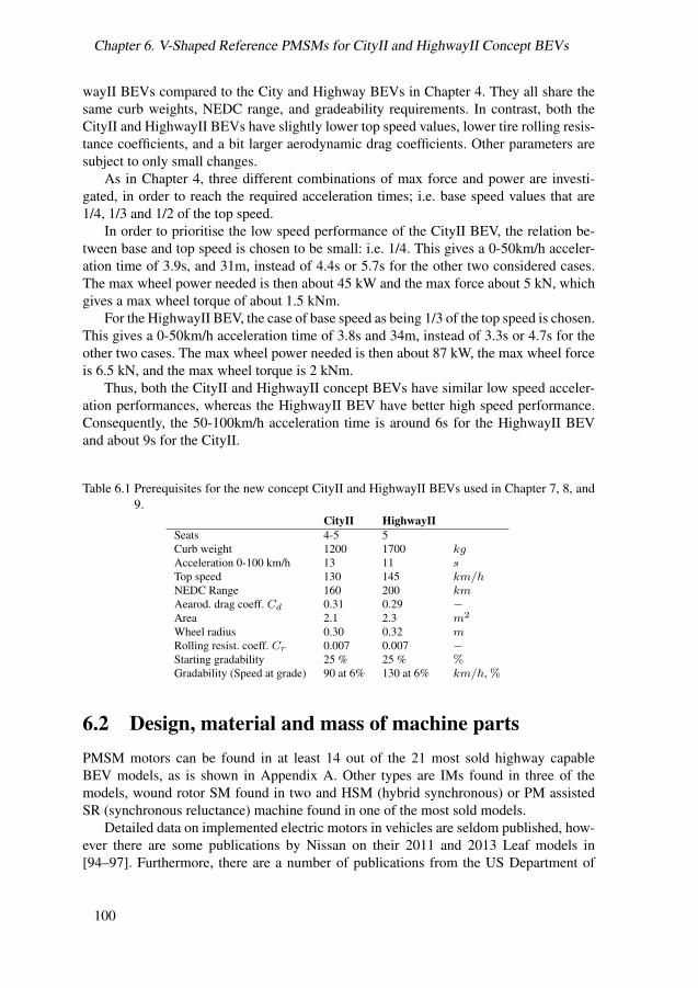
Chapter 6. V-Shaped Reference PMSMs for CityII and HighwayII Concept BEVs
wayII BEVs compared to the City and Highway BEVs in Chapter 4. They all share thesame curb weights, NEDC range, and gradeability requirements. In contrast, both theCityII and HighwayII BEVs have slightly lower top speed values, lower tire rolling resis-tance coefficients, and a bit larger aerodynamic drag coefficients. Other parameters aresubject to only small changes.
As in Chapter 4, three different combinations of max force and power are investi-gated, in order to reach the required acceleration times; i.e. base speed values that are1/4, 1/3 and 1/2 of the top speed.
In order to prioritise the low speed performance of the CityII BEV, the relation be-tween base and top speed is chosen to be small: i.e. 1/4. This gives a 0-50km/h acceler-ation time of 3.9s, and 31m, instead of 4.4s or 5.7s for the other two considered cases.The max wheel power needed is then about 45 kW and the max force about 5 kN, whichgives a max wheel torque of about 1.5 kNm.
For the HighwayII BEV, the case of base speed as being 1/3 of the top speed is chosen.This gives a 0-50km/h acceleration time of 3.8s and 34m, instead of 3.3s or 4.7s for theother two cases. The max wheel power needed is then about 87 kW, the max wheel forceis 6.5 kN, and the max wheel torque is 2 kNm.
Thus, both the CityII and HighwayII concept BEVs have similar low speed acceler-ation performances, whereas the HighwayII BEV have better high speed performance.Consequently, the 50-100km/h acceleration time is around 6s for the HighwayII BEVand about 9s for the CityII.
Table 6.1 Prerequisites for the new concept CityII and HighwayII BEVs used in Chapter 7, 8, and9.
CityII HighwayIISeats 4-5 5Curb weight 1200 1700 kgAcceleration 0-100 km/h 13 11 sTop speed 130 145 km/hNEDC Range 160 200 kmAearod. drag coeff. Cd 0.31 0.29 −Area 2.1 2.3 m2
Wheel radius 0.30 0.32 mRolling resist. coeff. Cr 0.007 0.007 −Starting gradability 25 % 25 % %Gradability (Speed at grade) 90 at 6% 130 at 6% km/h, %
6.2 Design, material and mass of machine partsPMSM motors can be found in at least 14 out of the 21 most sold highway capableBEV models, as is shown in Appendix A. Other types are IMs found in three of themodels, wound rotor SM found in two and HSM (hybrid synchronous) or PM assistedSR (synchronous reluctance) machine found in one of the most sold models.
Detailed data on implemented electric motors in vehicles are seldom published, how-ever there are some publications by Nissan on their 2011 and 2013 Leaf models in[94–97]. Furthermore, there are a number of publications from the US Department of
100

6.2. Design, material and mass of machine parts
Energy science and energy laboratory ORNL (Oak Ridge National Laboratory), cover-ing the electric powertrain in HEVs such as Toyota’s Prius 2004 and 2010 and Camry2007, Honda Accord 2014, Lexus LS 600h 2008, as well as the BEV Nissan Leaf 2011,e.g. in [98–100]. Although the motors in these vehicle models are of different power rat-ings and volumes, they share some common design features. They are all IPM (interiorpermanent magnet) SM motors with 48 stator slots, 8 poles, and distributed windings.The magnets in the rotor are configured in a V-shape in all models, except in Leaf andLS 600h where also a third magnet is used close to the air gap (forming a∇-shape). Thismachine type is known to fulfill design goals such as high torque and power density, highefficiency and wide constant power region, which are all highly desired in EVs [101].
The reference IPM SM stator and rotor core lamination designs are similar to that ofthe Toyota Prius 2004 motor, with 48 stator slots and 8 poles. However, the stator teethand yoke are thinner, and a different angle for the V-shaped magnet arrangement is used.Furthermore, the three phase winding is distributed, but with two layers, and four parallelbranches. The copper fill factor in the slot area is set to 45%. This is in line with the fillfactor of industrial IMs, which are in the range 35%-45%, according to [102].
The reference machine geometry is scalable, both by core length and diameter, hencea suitable machine size can easily be found for any desired peak torque performanceand length-to-diameter ratio. One reference machine is designed for the CityII BEV andone for the HighwayII. Both have length-to-diameter ratios around 0.8, which duringlength scaling between 50-200% of the reference length, gives length-to-diameter ratiosbetween about 0.4-1.6.
The dimensioning is done considering a max dc voltage of 400 V for both motors,and the max speed is limited to 12,000 rpm. The voltage and speed values are in line withwhat has been found for EMs in current BEVs, as shown in Appendix A. The number ofturns per coil is then adjusted in order for field weakening to start at around 3000 rpmfor the CityII EM and 4000 rpm for the HighwayII.
The gear ratios, kgear are simply taken as the relation between the top speed of themotor and wheel as in (5.4). With an assumed transmission efficiency of 97%, the maxelectric motor output torque and power are determined to be about 46 kW and 147.5 Nmfor the CityII BEV, and about 89 kW and 214 Nm for the HighwayII BEV.
The max rms current density Jrms,max in the slot is initially set to 20 A/mm2 (28.3A peak). The max rms phase current is then proportional to: the max rms current density;the slot fill factor kff ; the slot area Aslot; and the number of parallel branches nnpb, andinversely proportional to the number of layers nlayer and turns per coil ntpc, as in
Iph,rms,max. =Jrms,max kffAslot
nlayer
nnpbntpc
(6.1)
The assumed machine configuration is shown in Figure 6.1, along with an illustrationof the active machine parts, i.e. the parts that contribute to torque production. For sim-plicity, the machine configuration is limited to the main components: active parts, endwinding, frame, shaft and bearings. Selected machine data are shown in Table 6.2, forthe CityII and HighwayII reference motors.
101

Chapter 6. V-Shaped Reference PMSMs for CityII and HighwayII Concept BEVs
(a) Cross section. (b) Active parts.
Figure 6.1 Axial cross section of machine configuration, and the active machine parts, of V-shapedreference motors.
Table 6.2 Summary of PMSM data for the CityII and HighwayII BEV motors.CityII HighwayII
Peak Power 46 kW 89 kWMax Torque 147.5 Nm 214 NmBase speed 3000 rpm 4000 rpmMax speed 12,000 rpm 12,000 rpmGear ratio 10.440 9.984
Max DC voltage 400 V 400 VMax rms current density 20 A/mm2 20 A/mm2
Max rms phase current 125 A 251 APeak Efficiency at 400 Vdc 96.4 % 97.1 %
Core length 136 mm 150 mmCore stacking factor 0.95 0.95Lamination thickness 0.3 mm 0.3 mmNumber of slots 48 48Number of poles 8 8
Stator outer diameter 166 mm 182 mmStator inner diameter 112.05 mm 122.85 mmStator yoke thickness 9.445 mm 10.365 mmTooth width 4.33 mm 4.52 mmTooth height 17.53 mm 19.21 mmSlot opening width 1.66 mm 1.82 mmSlot area 69.67 mm2 83.74 mm2
Slot fill factor 45% 45%Turns per coil 10 6Coils per pole per phase 4 4
Rotor outer diameter 110.81 mm 121.485 mmRotor inner diameter 66.4 mm 72.8 mmAir gap length 0.62 mm 0.6825 mmMagnet thickness 3.7765 mm 4.1405 mmMagnet width 14.94 mm 16.38 mm
102

6.2. Design, material and mass of machine parts
6.2.1 FrameThe frame is assumed to be a hollow cylinder with an end cap on each side, all with athickness of 11 mm, and to be without any complex textures, for simplicity. The outerframe diameter is 102 mm and the length 262 mm. Furthermore, it is assumed to be madeof a die cast aluminum alloy (as in Nissan Leaf [94]), for a lightweight yet mechanicallystrong construction, with good thermal conductivity. It also includes a spiral coolingchannel for liquid cooling, see Section 8.1.1.
A number of different aluminum alloys are used for this purpose today, and theirnet thermal conductivity is less than that of pure aluminum, which is 237 W/mK at300K [48]. In publications regarding thermal modelling of electric motors, the value ofthermal conductivity of the frame’s aluminum alloy is seen to vary between 150 to 230W/mK [20, 49, 53, 103]. It is here assumed that the aluminum alloy 195 is used for theframe, which has a thermal conductivity of 168 W/mK at 300 K, a specific heat of 883J/kgK, and a density of 2790 kg/m3, [45, 48].
6.2.2 Core laminationThe chosen lamination material is the 0.3 mm thick NO30 by Tata Cogent [104]. Thisthickness is in line with published data of Toyota’s, Lexus’ and Nissan’s electric motorlaminations; which are 0.28-0.31 mm [94, 100]. The material’s B-H curve and loss dataare shown in Figure 6.2, along with the resulting approximated loss curves by the FEAsoftware program Ansys Maxwell. The FEA core losses are calculated as in (2.15), wherekh = 0.0583049W/kg, kc = 2.653 105W/kg, and n = 2.
The density of the NO30 grain is taken to be 7540 kg/m3, the thermal conductivity31 W/mK, which is a typical value at 100C, and the specific heat 557 J/kgK alsoat 100C [105]. Temperature dependency for thermal conductivity and specific heat ispresented in Appendix D.
H (A/m)0 500 1000 1500 2000
B (
T)
0
0.5
1
1.5Implemented data
B (T)0 0.5 1 1.5 2
Pco
re, l
oss
(W
/kg)
0
100
200
300
400
500
600Data sheet vs. FEA Approx.
50 Hz400 Hz2.5kHz5kHz10kHzFEA Approx.
Figure 6.2 Data sheet and implemented data for the chosen lamination material, NO30.
6.2.3 MagnetsA permanent magnet is mainly characterized by its remanent flux density, Br (T), and itsability to withstand demagnetization, or coercivity, Hc (A/m), both of which are temper-ature dependent. Permanent magnets consisting of NdFeB (neodymium iron boron) are
103

Chapter 6. V-Shaped Reference PMSMs for CityII and HighwayII Concept BEVs
commonly used in today’s EVs, so also in Toyotas, Hondas, Lexus’ and Nissans mod-els [99]. Published measurements indicate that the Br value for the motors in Prius 2010,LS600h and Camry 2007 are at least 1.3 T at 20C, and at least 1.1 T at 100C, whereasHc is between -1220 to -1440 kA/m at 100C [100]. Their temperature capability seemto be around 180-200C, or maybe even as low as 160C for Prius 2010.
The temperature capability of NdFeB magnets in electric vehicles, is often improvedby substituting some of the Nd for Dy (dysprosium). This additive helps to increase Hc,and to maintain high values of Hc at higher temperatures, however it also reduces the Brsomewhat. According to [106], typical values of Dy content in EV magnets, during 1985to 2011, were 8.5-11% of the magnet weight, which represent temperature capabilitiesaround 200-220C. A similar value is also presented in [107], where a Dy content of8.7w% is said to be typical for EV drives. However, due to a sudden and substantialprice increase of Dy in 2011, which is not yet fully recovered, magnet manufacturers arecurrently seeking to reduce the amount of Dy [106]. As an example, Nissan claims tohave lowered the Dy content by 40% in their 2013 Leaf model compared to the 2011model [97]. One publication from 2012, indicate that very low Dy contents may be usedin EVs, on an average 3.6-4w%, and single values up to 7.7w% [108], which representstemperature capabilities around 150C and 180C, according to [106].
For this reason, a magnet with a relatively low Dy content is chosen for the refer-ence motors; Hitachi NEOMAX NMX-37F, which is expected to have around 3.5-4.5w%Dy [109]. The material data is shown in Figure 6.3 [110], which indicate a temperaturecapability up to 140C. The Br value is around 1.2 T at 20C, and drops to 1.1 T at140C, whereas the Hc value is about -940 kA/m at 20C, and -790 kA/m at 140C. Asexpected, the Hc values are a bit lower compared to Toyotas and Lexus’ magnets, whichthus both can be assumed to have a larger Dy content.
The magnet density is taken to be 7500 kg/m3, the thermal conductivity as 7.5W/mK, and the specific heat as 410 J/kg K, as stated by Hitachi [111]. The elec-tric conductivity is taken to be 1.3 µΩm, and assumed to adhere to 20C [111]. Thetemperature coefficient of resistivity is here assumed to be 0.5%/C, which gives anelectrical conductivity of 750 469 S/m at 70C. The considered magnet material proper-ties at 20C, 70C and 120C are presented in Table 6.6.
Coercivity (kA/m)-1000 -800 -600 -400 -200 0
Flu
x de
nsit
y (T
)
0
0.2
0.4
0.6
0.8
1
1.2
1.4Hitachi NEOMAX NMX-37F Low Dy
20 oC
60 oC
100 oC140 oC
180 oC
220 oC
Figure 6.3 Data sheet data for chosen magnet material [110].
104

6.2. Design, material and mass of machine parts
6.2.4 Other machine parts and material summaryThe windings are made of copper that is assumed to have a density of 8933 kg/m3, ther-mal conductivity of 401 W/mK, and specific heat of 394 J/kg K, which all adhere to100C [45]. The copper resistivity at 20C, ρCu,20 is taken to be 1.68 10−8 Ωm, and thetemperature coefficient α to be 0.3862 %/K. The resistivity, ρCu at other temperaturesT , are calculated as
ρCu(T ) = ρCu,20[1 + α(T − 20)] (6.2)
The air is assumed to have a thermal conductivity of 0.03095 W/mK, and densityof 0.9458 kg/m3, which all adhere to 100C [48]. Temperature dependency parametersfor air is presented in Appendix D.
The mass density of the winding impregnation is assumed to be 1350 kg/m3, andthe specific heat 1700 J/kg K, which is also used in [20, 53], and stated as unsaturatedpolyester.
The shaft is assumed to have a length of 306 mm and a diameter of 40 mm exceptfor the part along the lamination stack, which is assumed to extend to the inner rotorlamination boundary (i.e. a diameter of 72.8 mm). Furthermore, the shaft is assumed to besolid and to be of carbon-silicon steel with the density 7817 kg/m3, thermal conductivityof 51W/mK [48]. The temperature dependency of the thermal conductivity is presentedin Appendix D.
The ball bearings for the HighwayII machine, are assumed to each have a width of15 mm, and inner and outer diameters of 40 mm and 68 mm respectively. The mass ofone unit is assumed to be 190 g, as is commonly found for this size of ball bearings fromthe bearing manufacturer SKF [112].
Table 6.3 Material properties of motor parts.Density Thermal Conductivity Specific Heat
(kg/m3) (W/mK) (J/kgK)Air 0.9458 0.03095 -Frame 2790 168 883Laminations 7540 31 557Winding 8933 401 385Winding slot impregnation 1350 0.2 1700Magnets 7500 7.5 410Shaft 7817 51.9 446
6.2.5 Mass of machine partsThe machine mass is estimated based on the simplified assumed configuration shownin Figure 6.1. For the active components, the mass is a product of density and volume,where volume is a product of cross sectional area and core lamination stack length. Thecross sectional area of the end winding is assumed to be the same as that of the activewinding. The end winding length is estimated using (5.3), with an assumed axial extentof 35 mm on each side of the lamination stack.
The mass of the different motor parts for the CityII and HighwayII BEV motorsare presented in Table 6.4. Information regarding slot impregnation material is given inSection 8.1.4.
105

Chapter 6. V-Shaped Reference PMSMs for CityII and HighwayII Concept BEVs
Table 6.4 Mass (kg) of selected main motor components for CityII and HighwayII motors.CityII HighwayII
Frame 4.7 5.5Stator Yoke 4.5 6.0Stator Teeth 3.7 4.9Active winding 1.8 2.4Slot impregnation 0.3 0.4End Winding 1.7 2.2Magnets 0.9 1.2Rotor laminations 5.0 6.7Shaft 4.6 5.8Bearings 0.4 0.4Total Lamination 13.3 17.6Total Copper 3.5 4.6Total Passive Parts 11.6 14.3Total Active Parts 16.0 21.2Total 27.6 35.5
6.3 FEA evaluation of performance and lossesThe reference motors have been simulated in 2D, in the electromagnetic FEM softwareAnsys Maxwell. The simulated machine geometry and mesh density is shown in Figure6.4, including a few example results. For simplicity, the lamination stacking factor isignored in all electromagnetic simulations.
(a) Mesh. (b) Flux lines, total losses and current den-sity.
Figure 6.4 FEA of one pole of the HighwayII motor at 4000 rpm, 251 A rms, showing mesh, vectorpotential flux lines, total losses in the core and magnets, as well as current density in thewindings, at a certain time instant.
For each machine geometry, at 13 different speed levels (i.e. at 1 rpm, and at every1000 rpm up to 12,000 rpm), 11×11 operating points in the id-iq plane have been evalu-ated for two electrical periods, with 101 sample points. Sinusoidal current excitation havebeen used in all operating points. The data resolution in the id-iq-plane is then increased
106

6.3. FEA evaluation of performance and losses
through interpolation, as shown in Figure 6.5(a). From this, the MTPA (Max Torque PerAmpere) operating points as well as the field weakening operation is numerically foundfor each integer torque level, within the allowed operating current and voltage limits, asexemplified in Figure 6.5(b). A final interpolation in the speed range is then conducted.
Selected data mainly consist of losses in the different machine parts, e.g. laminationlosses in the stator yoke, teeth, and rotor, dc resistive losses in the active part of thewinding, and eddy current losses in the magnets.
For the HighwayII motor, these motor simulations have been done for three additionalslot areas apart from the already presented motor geometry (further treated in section6.7). For all of the four slot geometries the simulations are done at the three differentmagnet temperatures; 20C; 70C and 120C, (section 6.6). For the CityII motor, thesimulations are done for a single geometry with magnet and copper temperatures of 70C(section 6.4). Finally, for both the CityII and the original geometry of the HighwayIImotors, simulations are done at half and double the stack length with a magnet and coppertemperature of 70C (section 6.5).
(a) FEA operating points and interpolated torque.
Id (A)
-400 -300 -200 -100 0
I q (
A)
0
50
100
150
200
250
300
350
400
50
100150
20025
0
300 Trq (Nm)
|Iph.max
|
|Vph.max
|
MTPA
1-3000 rpm
4000 rpm
5000 rpm
12,000 rpm
(b) Result of current control algorithm.
Figure 6.5 FEA simulated operating points for each speed level along with resulting interpolatedtorque, and current control id iq reference values for each integer torque level, at 1 rpmand every 1000 rpm up to max speed.
Both components of the core losses (hysteresis and eddy) increase with increasingmachine speed, as shown in Figure 6.6 for the two speed levels 4000 rpm and 12,000rpm. The figure also shows the transient behaviour of the hysteresis losses in the FEAsoftware program over the two simulated electrical periods, as well as the used meanvalue over the last period.
Eddy current losses in the magnets arise due to variation of flux density during oper-ation. In the FEA software the magnets are modeled as zero current carrying coils whileconsidering eddy effects. As mentioned, the conductivity values used are presented inTable 6.6.
107

Chapter 6. V-Shaped Reference PMSMs for CityII and HighwayII Concept BEVs
0 50 1000
500
1000
1500
Samples
PC
ore,
loss (
W)
4 krpm − Hyst. 4 krpm − Eddy12 krpm − Hyst.12 krpm − EddyAverage
Figure 6.6 Lamination core losses at around 250 A rms, 4000 rpm and 12,000 rpm, for the High-wayII motor.
The copper losses in the active part of the winding are extracted from the FEA soft-ware. Skin and proximitys effect is here ignored. Then the total copper losses are foundvia the relative length of the active part of the winding, by again using (5.3). The endwinding losses are simply the difference between the total and the active part. For theHighwayII reference motor, the active part is 52% of the total winding length, thus leav-ing 48% to the end windings.
6.3.1 Losses and efficiency of the HighwayII motorThe resulting loss components and efficiency for the HighwayII motor are presented forthe whole operating area in Figure 6.7, with the magnet and copper temperature of 70C.
The magnet losses are the lowest of all losses, only up to 13 W. Thus, the two domi-nating loss mechanisms are resistive copper losses and lamination core losses.
As the copper losses depend on the square of the current, their torque-speed-dependenceresembles that of the current magnitude’s. Below base speed there is no speed depen-dence, but there is thus a strong torque dependence. However, above base speed a largercurrent is needed (at the same torque level) in order to suppress the magnetic flux fromthe magnets, i.e. field weakening operation. At any given speed level, the copper lossesare the largest at the max torque level.
Both lamination and magnet losses strongly increase with speed, and somewhat withtorque. The lamination core losses reach the highest levels in the stator teeth, at leastwell above base speed. The largest values are reached above 10,000 rpm close to the maxtorque levels. The rotor core losses are relatively low, yet they also increase rather muchat combinations of high torque and speed.
For this reason, the peak total loss of about 6.4 kW is found at the combined maxtorque and speed operating point. The efficiency is over 90% in a large part of the oper-ating area, and reaches at most above 97.1%.
108

6.3. FEA evaluation of performance and losses
0 2000 4000 6000 8000 10000 120000
50
100
150
200
Speed (rpm)
Tor
que
(Nm
)
PCu,Act
(W)
500
1000
500
1000
Active WindingEnd Winding
2000
(a) Winding losses in W.
0 2000 4000 6000 8000 10000 120000
50
100
150
200
Speed (rpm)
Tor
que
(Nm
)
PFe,Stator
(W)
1000800400200
100
200300
TeethYoke
1500
(b) Stator lamination losses in W.
0 2000 4000 6000 8000 10000 120000
50
100
150
200
Speed (rpm)
Tor
que
(Nm
)
PRotor & PM
(W)
1050
100
1051
RotorMagnets
200
(c) Magnet and rotor lamination losses in W. (d) Total losses in W.
Figure 6.7 Electromagnetic losses as a function of torque and speed, for the HighwayII V-shapedreference motor.
The percent ratio of total copper losses over total motor losses is presented in Figure6.8(a). Generally, the copper losses dominate for torque levels above 50 Nm. As copperand core losses are the two main loss components, the rest of the losses in the figure ad-here to the core losses. Generally, the core losses are the main loss components for speedlevels above about 2000 rpm and torque levels below 50 Nm. Consequently, core lossescan be expected to dominate in drive cycles with low acceleration levels and relativelyhigh speed levels, whereas copper losses can be expected to dominate in drive cycleswith higher acceleration levels.
Finally, the percent ratio of core losses in the teeth over the total core losses is pre-sented in Figure 6.8(b). At speed levels below 6000 rpm around 50-60% of the core lossesare developed in the teeth. At higher speed levels the share increases to about 80% at topspeed. A similar study of the rotor reveals that its core losses are essentially well below10% of the total core losses in the whole operating area. This means that the rest of theloss share shown in Figure 6.8(b) principally adhere to the stator yoke.
109

Chapter 6. V-Shaped Reference PMSMs for CityII and HighwayII Concept BEVs
0 2000 4000 6000 8000 10000 120000
50
100
150
200
Speed (rpm)
Tor
que
(Nm
)P
Cu/P
Loss,tot (%)
90
75
50
25
10
(a) Share of total copper losses to the total electromag-netic losses, in %.
0 2000 4000 6000 8000 10000 120000
50
100
150
200
Speed (rpm)
Tor
que
(Nm
)
PFe, Teeth
/PFe,tot
(%)
7570656055
50
55
50
(b) Share of lamination teeth losses to the total statorand rotor lamination losses, in %.
Figure 6.8 Share of total losses as a function of torque and speed, for the HighwayII V-shapedreference motor.
6.4 CityII and HighwayII motor efficiency with differentdc voltage limits
Due to the dynamic behaviour of the battery voltage during vehicle operation, the motorlosses and efficiency are calculated for different levels of available dc voltage (between250-450V), as presented in Figure 6.9. In all cases the max rms phase current is unaltered.
If the max available voltage is increased, field weakening control can start at a higherspeed level, compared to a lower max voltage. In the same time, with a higher maxvoltage a lower field weakening current is needed in the same operating point, againcompared to the case of a lower max voltage. The result is that a higher max voltageleads to a higher efficiency in the field weakening region.
Also the max power increases with increased available voltage. The max power islinearly proportional to the change in available voltage, and changes about 25 kW per100 V for the HighwayII motor (or 11%-21%). Specifically, for the HighwayII motor themax power is 114 kW with 450 V, whereas it is 62 kW when 250V is available.
110

6.5. CityII and HighwayII motor efficiency at 50%, 100% and 200% of stack length
0 2000 4000 6000 8000 10000 120000
50
100
150
Speed (rpm)
Tor
que
(Nm
)
Efficiency (%)
95
70 90
450 Vdc
400 Vdc
350 Vdc
300 Vdc
250 Vdc
450Vdc
450Vdc
250Vdc
(a) CityII motor.
0 2000 4000 6000 8000 10000 120000
50
100
150
200
Speed (rpm)
Tor
que
(Nm
)
Efficiency (%)
70 90
96
450 Vdc
400 Vdc
350 Vdc
300 Vdc
250 Vdc
250Vdc
250Vdc
450Vdc
450Vdc
(b) HighwayII motor.
Figure 6.9 Electromagnetic efficiency contour lines at different levels of max dc voltage, for theCityII and HighwayII V-shaped reference motors.
6.5 CityII and HighwayII motor efficiency at 50%, 100%and 200% of stack length
Similarity as in Section 5.1.3.1, the stack length of the CityII and HighwayII motors arescaled linearly. During the length scaling the cross sectional geometry is unaltered, asis the dc voltage limit of 400 V, as well as the max rms current density of 20 A/mm2.However, the number of turns per coil are changed in order to keep the same base and maxspeed. When changing the stack length of the motors under these conditions, the passiveend winding losses remains the same, whereas the active losses are linearly proportionalto the stack length.
The mass of the motors are estimated as the sum of the parts that scale with the stacklength mlstk , and those parts that don’t mext. The parts that scale with the stack lengthare: both the stator and rotor laminations, the magnets, the active part of the winding,as well as those part of the frame and shaft that are within the stack length. The scalingfactor flstk represent the ratio of the scaled stack length and the reference stack length,i.e. it is 0.5 to 2. The mass of a scaled motor is thus
mEMscaled= mlstk + flstkmext (6.3)
The resulting mass of the re-scaled CityII and HighwayII motors are presented inFigure 6.10. Even though the motor masses change from 60% to 180% of the referencemotors, the effect on the vehicle mass is less than 1% for the 50% scaling factor and lessthan 2% for the 200% scaling factor, for both vehicles.
111

Chapter 6. V-Shaped Reference PMSMs for CityII and HighwayII Concept BEVs
0.5 1 1.5 210
20
30
40
50
60
70
EM scaling (%)
Mot
or m
ass
(kg)
0.5 1 1.5 20.5
1
1.5
2
EM scaling (%)
Nor
m M
otor
mas
s (−
)
CityIIHighwayII
CityIIHighwayII
Figure 6.10 Mass of CityII and HighwayII re-scaled motors, and motor masses normalized by thereference motors.
Simulations are done at all three length scalings: 50%, 100% and 200% of originalstack length. The losses and efficiency maps from the simulations are essentially identicalto the results when simply scaling the active part of the losses with the same factors asthe stack length. For simplicity, it therefore the latter method that is used for intermediatelength scalings of losses and torque levels, and the resulting efficiencies is presented inFigure 6.11. Additionally, selected data on three scalings for both motors are presentedin Table 6.5.
Table 6.5 Selected data on min and max length scaling of CityII and HighwayII V-shaped referencemotors.
CityII motor Lstk,min Lstk,ref Lstk,max
Core length 68 mm 136 mm 272 mmTurns per coil 20 10 5Max rms phase current 63 A 125 A 251 A
Active winding share 34% 51% 67%
Rs,Tot 204 mΩ 68 mΩ 26 mΩRs,ActWi 70 mΩ 35 mΩ 17 mΩRs,EndWi 134 mΩ 34 mΩ 8 mΩ
Motor mass 16.9 kg 27.6 kg 49.1 kg(61%) (100%) (178%)
HighwayII motor Lstk,min Lstk,ref Lstk,max
Core length 75 mm 150 mm 300 mmTurns per coil 12 6 3Max rms phase current 126 A 251 A 502 A
Active winding share 35% 52% 69%
Rs,Tot 65 mΩ 22 mΩ 8 mΩRs,ActWi 23 mΩ 11 mΩ 6 mΩRs,EndWi 42 mΩ 10 mΩ 3 mΩ
Motor mass 21.3 kg 35.5 kg 63.9 kg(60%) (100%) (180%)
112

6.6. HighwayII motor losses at three magnet and copper temperatures
0 2000 4000 6000 8000 10000 120000
50
100
150
200
250
300
Speed (rpm)
Tor
que
(Nm
)
Efficiency (%)
80 90
95
95
80
90
80
95
Lmax
Lref
Lmin
90
(a) CityII motors.
0 2000 4000 6000 8000 10000 120000
50
100
150
200
250
300
350
400
Speed (rpm)
Tor
que
(Nm
)
Efficiency (%)
70 90
96
90
96
70
90
96
Lmax
Lref
Lmin
70
(b) HighwayII motors.
Figure 6.11 Electromagnetic efficiency contour lines (%) for three different length scalings of theCityII and HighwayII motors.
6.6 HighwayII motor losses at three magnet and coppertemperatures
Simulations have been done with magnet and copper temperatures at 20C, 70C and120C using the magnet materia data in Table 6.6. As presented in the table, the magnetstrength (Br) decreases with increasing temperature. Since the max current does notdiffer between the cases, this thus also lead to a decreased max torque with increasingtemperature.
Table 6.6 Magnet simulation input data, phase resistance, and resulting max torque and power atthree temperatures of magnets and copper.
20C 70C 120CRemanent flux 1.236 T 1.1824 T 1.1244 T
(100%) (95.66%) (90.96%)Relative permeability 1.0432 1.0428 1.0446Coercivity -942,926 (A/m) -902,285 (A/m) -856,586 (A/m)Conductivity 769,231 (S/m) 750,469 (S/m) 732,601 (S/m)Phase resistance 18 mΩ 22 mΩ 26 mΩ
(100%) (119%) (139%)Max torque 220 Nm 215 Nm 210 Nm
(100%) (97.7%) (95.5%)Max power 5.7 kW 6.4 kW 6.9 kW
Due to the weakening of the magnet, at a certain torque level outside the field weak-ening area of operation, a larger current is needed at a higher temperature compared to alower. In contrast, within the field weakening area, the weaker magnet leads to a reducedneed for field weakening current, especially at the lower torque levels. Therefore, at acertain torque level a lower current is needed for higher temperatures compared to lower.This is illustrated in Figure 6.12(a).
113

Chapter 6. V-Shaped Reference PMSMs for CityII and HighwayII Concept BEVs
This reasoning also explains the presented copper losses in Figure 6.12(b), since cop-per losses are proportional to the square of the rms current. Naturally, also the windingresistance increase with temperature, which further enhances the differences of the cop-per losses’ behaviour in the torque-speed diagram between the studied temperatures. Dueto the linear dependency on current for the torque and the quadratic dependency for thewinding losses, the difference in losses between the three temperatures increase as thetorque becomes higher.
0 50 100 150 200 2500
50
100
150
200
250
Iph, RMS
(A)
Tor
que
(Nm
)
4000 rpm 8000 rpm12,000 rpm
20 oC 70 oC
120 oC
(a) Torque per input phase rms current.
0 2000 4000 6000 8000 10000 120000
50
100
150
200
Speed (rpm)
Tor
que
(Nm
)
PCu,tot
(W)
3000
1000
100
20 oC
70 oC
120 oC
(b) Winding loss contour lines at 100 W, 1000 W and3000 W.
Figure 6.12 Produced torque per applied rms phase current, and total winding losses as a functionof torque and speed, for the HighwayII V-shaped reference motor, at winding andmagnet temperature 20C, 70C and 120C.
The lower field weakening current also cause minor deviations in the magnet lossesin the torque-speed diagram shown in Figure 6.13(a).
Finally, the resulting total losses for the three different temperatures are presented inFigure 6.13(b).
114

6.7. HighwayII motor losses for four slot areas
0 2000 4000 6000 8000 10000 120000
50
100
150
200
Speed (rpm)
Tor
que
(Nm
)
PPM
(W)
105
31
20 oC
70 oC
120 oC
(a) Magnet loss contour lines at 1 W, 3 W, 5 W, and10 W.
0 2000 4000 6000 8000 10000 120000
50
100
150
200
Speed (rpm)
Tor
que
(Nm
)
Ploss,tot
(W)
500030001000
20 oC
70 oC
120 oC
(b) Total losses at 1 kW, 3 kW and 5 kW.
Figure 6.13 Magnet and total losses as a function of torque and speed, for the HighwayII V-shapereference motor, at winding and magnet temperature 20C, 70C and 120C.
6.7 HighwayII motor losses for four slot areasFEA simulations have been done for the HighwayII motor with four different slot areas:Small, Original, High and Large, shown in Figure 6.14. For the Small and Large slotsboth the height and width are changed compared to the Original slot, whereas for the Highslot only the height is increased. As the inner and outer stator diameters are unaltered,the Small slot has both wider teeth and yoke, whereas the Large slot has a bit thinnerteeth and yoke, and the High slot only thinner yoke. Since the copper fill factor is keptessentially the same in all four cases, thus the winding cross sectional area is changedwith the slot area. All stator geometries are simulated at the three copper and magnettemperatures 20C, 70C and 120C. In all cases the same max rms current of 251 Aand max dc voltage of 400V are used.
Figure 6.14 The FEA simulated different stator lamination geometries, as well as one of the wind-ing layers.
115

Chapter 6. V-Shaped Reference PMSMs for CityII and HighwayII Concept BEVs
The numerical values of the different slot areas are presented in Table 6.7, alongwith percentage ratios compared to the Original. Furthermore, the copper areas are arealso presented, and it is the smallest in the Small slot and the largest in the Large slot.Consequently, the current density is the largest in the Small slot and the lowest in theLarge slot. Additionally, the phase resistance, and max torque for all slots at the threemagnet and copper temperatures are also presented in the table.
It should be noted that the axial extent of the end winding is assumed to be differentfor the different slot areas. The extent is taken to be linearly proportional to the squareroot of the change in copper area from the original slot area to the others. For the smallslot geometry, the extent is shorter (29.7 mm), for the Large and High slot geometries itis longer (40.2 mm, and 37.2 mm respectively). .
Table 6.7 Parameters for the four stator slot sizes.Small Original Large High
Slot Area 60.96 mm2 83.74 mm2 109.66 mm2 94.30 mm2
(73%) (100%) (131%) (113%)
Total Copper Area 27.23 mm2 37.69 mm2 49.84 mm2 42.65 mm2
(72%) (100%) (132 %) (113 %)
Max rms current density 28 A/mm2 20 A/mm2 15 A/mm2 18 A/mm2
(138%) (100%) (76%) (88%)
Share Active part of winding 54.5% 52.3% 50.2 % 51.3 %Rs at 20C 24 mΩ 18 mΩ 14 mΩ 17 mΩRs at 70C 29 mΩ 22 mΩ 17 mΩ 20 mΩRs at 120C 34 mΩ 26 mΩ 20 mΩ 23 mΩ
(133%) (100%) (79%) (90%)Tmax at 20C 239 Nm 220 Nm 192 Nm 203 NmTmax at 70C 234 Nm 215 Nm 187 Nm 198 NmTmax at 120C 228 Nm 210 Nm 182 Nm 193 Nm
(109%) (100%) (87%) (92%)
The flux linkage from the magnet as a function of q-axis current for the different slotareas is shown in Figure 6.15, for the temperature of 70C. In general the flux from themagnet decreases with increasing q-axis current due to cross saturation. The saturationeffect is the largest in the stator geometry with the thinnest teeth and yoke: the Large slot,whereas it is the smallest for the geometry with the thickest teeth and yoke: the Smallslot.
116

6.7. HighwayII motor losses for four slot areas
0 100 200 300 4000.055
0.06
0.065
0.07
0.075
0.08
0.085
Iq (A)
ψ magnet (
Wb)
SmallOrginalLargeHigh
(a) Flux linkage from magnets (Wb).
0 100 200 300 4000.65
0.7
0.75
0.8
0.85
0.9
0.95
1
1.05
Iq (A)
Nor
mal
ized
ψmagnet (−
)
SmallOrginalLargeHigh
(b) Flux linkage from magnets normalized by thevalue at zero q-axis current.
Figure 6.15 Flux linkage from magnets as a function of q-axis current for the different stator slotareas at 70C copper and magnet temperature.
The four stator geometries also have different dq inductances, where the Small slotgeometry have the largest values and the Large slot have the lowest, in the whole id-iqplane. Also the absolute difference between the dq inductances (which is relevant for thereluctance torque production as expressed in (2.13) is the largest for the Small slot andthe smallest for the Large slot. These relations are the same at every speed level.
Consequently, both torque components: magnet and reluctance, are the highest for theSmall slot geometry in the whole dq current operating area, and the lowest for the Largeslot. The net produced torque for the different geometries is presented in the id iq planein Figure 6.16(a). As shown, the difference in produced torque between the geometriesdecreases with decreasing current, especially with decreasing q-axis current.
The resulting dq current operating points are presented in Figure 6.16(b), for a fewselected speed levels. Outside of the field weakening area the MTPA method result in asomewhat larger share of the q-axis current for the Small slot geometry compared to theothers. As a consequence, yet bit higher torque levels can be reached for the same currentmagnitude. The higher flux from the magnet also result in a stronger speed dependenceof the induced voltage, hence the base speed is lower for the Small slot compared to theothers. In the field weakening area, instead a larger d-axis current is needed in the Smallslot in order to suppress the flux from the magnet, that is even though its d-axis inductanceis larger. This counteracts some of the previous torque producing advantage with theSmall slot. As noted, the difference between the geometries decreases with increasingspeed regarding produced torque and resulting dq current operating points, i.e. whengoing further into the field weakening area.
117

Chapter 6. V-Shaped Reference PMSMs for CityII and HighwayII Concept BEVs
400
Iq (A)
200
00
-200
Id (A)
-400
400
0
100
200
300
Tor
que
(Nm
)
SmallOrginalLargeHigh
(a) Produced torque for different slot areas.
Id (A)
-400 -350 -300 -250 -200 -150 -100 -50 0
I q (
A)
0
50
100
150
200
250
300
350
400SmallOrginalLargeHigh
4000 rpm
1 rpm6000 rpm
12,000 rpm 8000 rpm
Imax
(b) Result of current control algorithm for differentslot areas at 1 rpm, 4000 rpm , 6000 rpm, 8000 rpmand 12,000 rpm.
Figure 6.16 Produced torque and result of current control algorithm as a function of dq current, forthe different stator geometries at 70C copper and magnet temperature.
As a consequence, at low speed levels the largest produced torque per input rms cur-rent is given by the Small slot geometry and the lowest by the Large slot. At higher speedlevels the difference is quite small. Still, it is then the Large slot that produces somewhathigher torque per input rms current compared to the other slot sizes. the tendency is a bithigher produced torque. The results are shown for a few example speed levels in Figure6.17(a). The resulting max torque as a function of speed is shown as the dashed line inFigure 6.17(b).
The total lamination core losses are also presented in Figure 6.17(b). As shown, theincrease with speed of the core losses is the smallest for the Small slot geometry andthe highest for the Large and High slot geometries. Likely, the larger cross sectionallamination area for the Small slot geometry cause somewhat lower flux density levels,and therefore also lower core losses. At low torque levels the core losses are the largestin the Large slot geometry, whereas they are the highest in the High slot at higher torquelevels. A similar relation is also noted for both the yoke and teeth losses separately,whereas the opposite order is noted in the rotor (although not shown here), i.e. largest forthe Small slot and lowest for the Large. Still, the magnitude of the core losses in the rotorare much lower than in the yoke and teeth, which is why the impact on the total losses issmall.
118

6.7. HighwayII motor losses for four slot areas
0 50 100 200 250 3000
50
100
150
200
250
150Iph, RMS
(A)
Tor
que
(Nm
)
4000 rpm 8000 rpm12,000 rpmSmallOrginalLargeHigh
Small
HighLarge
Original
(a) Torque per input rms phase current.
0 2000 4000 6000 8000 10000 120000
50
100
150
200
Speed (rpm)
Tor
que
(Nm
)
PFe,tot
(W)
1000500100
SmallOrginalLargeHigh
(b) Total lamination core loss contour lines at 500 Wand 1000 W.
Figure 6.17 Produced torque per input rms phase current, as well as total core losses as a function oftorque and speed, for the HighwayII V-shaped reference motor, for the Small, Original,Large and High slot areas.
In contrast with the core losses, a larger copper cross section leads to a lower windingresistance. Owing to this, the Small slot has the highest winding resistance, and the Largeslot the lowest. In the field weakening area the phase current is essentially the same in anyspeed torque operating point for all slot geometries. Then, the higher winding resistancein the Small slot causes larger copper losses in this region, as shown in Figure 6.18(a).Outside of the field weakening area, at the same torque level, the phase current is thehighest in the Large slot and the lowest in the Small. Thus, in this area the resistance andcurrent counteract each other in the loss creation. The result is still that the copper lossesare the highest for the Small slot geometry also outside of the field weakening area, andfairly similar between the other geometries.
Nevertheless, the difference in total losses between the four geometries is rathersmall, as shown in Figure 6.18(b). These small deviation s were a bit unanticipated, butindeed interesting to note. Essentially it is only the losses with the Small slot that deviatesnotably. In a large part of the operating area the losses with the Small slot are somewhathigher compared to the other slot geometries.
The main difference between the losses in the motors with different slot geometriesis thus not the total amount of losses, but the relation between copper and core losses (asshown for the Original slot in Figure 6.8(a)). The motor with the Small slot thus haveincreased its share of copper losses and decreased the share of core losses, whereas themotors with the Large and High slots have instead increased the share of core losses anddecreased the share of copper losses.
119

Chapter 6. V-Shaped Reference PMSMs for CityII and HighwayII Concept BEVs
0 2000 4000 6000 8000 10000 120000
50
100
150
200
Speed (rpm)
Tor
que
(Nm
)P
Cu,tot (W)
2000
500
SmallOrginalLargeHigh
(a) Copper loss contour lines at 500 W and 2000 W.
0 2000 4000 6000 8000 10000 120000
50
100
150
200
Speed (rpm)
Tor
que
(Nm
)
Ploss,tot
(W)
3000
1000
SmallOrginalLargeHigh
(b) Total loss contour lines at 1000 W and 3000 W.
Figure 6.18 Copper and total losses as a function of torque and speed, for the HighwayII V-shapedreference motor, for the Small, Original, Large and High slot areas.
The ratio of the copper losses in the Small slot machine over the copper losses inthe Original slot is presented in Figure 6.19. As expected, in the field weakening areawhere the rms currents are almost the same, the ratio is fairly constant (≈1.36). However,outside of the field weakening area the ratio decreases with increasing torque (≈1.1-1.3).
Figure 6.19 The ratio of the Small slot copper losses to the Original slot copper losses.
120

Chapter 7
Effects of CityII and HighwayIIMotor and Inverter Re-scalingon Performance and EnergyEfficiency
In this chapter, the electric motor and inverter of the CityII and the HighwayII conceptBEVs (described in Section 6.5) are resized in terms of torque and power rating as wellas losses and motor mass. After this, the consequence on vehicle performance and energyefficiency for the Test cycles are studied and quantified.
The re-scaling of the motors is simply a linear scaling of the active length, as isdescribed in Chapter 5. The scaling factors are here in steps of 10%, from 50% to 200%of the reference motors.
The inverter which is used in the City car in Chapter 5 (current rating 400 A rms), ishere used as a baseline inverter for both the CityII and HighwayII cars, for simplicity. Inorder for the converter losses to still be reasonably representative, the on-state resistanceand switching loss parameters are scaled with the same factors as the motor lengths.The resistances are inversely proportional and the switching loss parameters are linearlyproportional, while the constant voltage drop term in the collector-emitter path is leftunchanged.
The same simulation structure as in Chapter 5 is here used. Also, the configurationof the gear efficiency and batteries in the CityII and HighwayII cars are identical to thesettings in the City and Highway cars. On the other hand, only the losses in motoringmode of the electric machine and inverters are here implemented in the models. It is thusassumed that the loss maps in the generative mode are the same as in motoring mode.
121

Chapter 7. Effects of CityII and HighwayII Motor and Inverter Re-scaling onPerformance and Energy Efficiency
7.1 PerformanceAs noted in Section 6.5, the initial max torque levels of the re-scaled motors are linearlyproportional to the scaling factor. The max mass normalized wheel force for some of there-scaled electric motors can be seen in Figure 7.1, together with the vehicle’s road load,which remains essentially the same in all cases. Even the smallest motor size will be ableto sustain the vehicle’s top speed requirement.
0 50 100 1500
1
2
3
4
5
6
7
8
Vehicle speed (km/h)
Nor
m F
whe
el (N
m/k
g)
Scale 50 %Scale 80 %Scale 100 %Scale 120 %Scale 150 %Scale 200 %Road load
(a) CityII.
0 50 100 1500
1
2
3
4
5
6
7
8
Vehicle speed (km/h)
Nor
m F
whe
el (N
m/k
g)
Scale 50 %Scale 80 %Scale 100 %Scale 120 %Scale 150 %Scale 200 %Road load
(b) HighwayII.
Figure 7.1 Max mass normalized wheel force as a function of vehicle speed (at 400 V DC) alongwith road load, for the re-scaled CityII and HighwayII powertrains.
The resulting time to accelerate 0-50 km/h and 0-100 km/h, for an initial SOC levelof 90% is presented in Figure 7.2, both as a function of max torque and of max power.Naturally, the time to accelerate decreases for increasing max torque and power ratings,and it does so in a nonlinear way. For both cars, the time to accelerate at 50% scale factoris about 1.8-2.1 times longer compared to the reference length, and at 200% scale factor itis 0.5-0.6 times the value of the reference length. Furthermore, it can be noted that at anycertain max torque level, the acceleration time is shorter for the CityII car compared tothe HighwayII car. This can be expected since the City car is seen to have slightly highermass normalised wheel force values, compared to the HighwayII car. The difference iseven larger when comparing with max power levels, which is due to the different basespeed levels of the two cars’ motors.
The noted nonlinear dependency means that the effect of a change in stack length islargest for short stack lengths compared to long ones. This effect can be seen since thebase speed is kept the same during the scaling. For the acceleration time 0-100km/h, thedifference between the scale factors 50% and 80% is 12s for the CityII car, and 8s for theHighwayII. The difference between 120% and 150% is only about 2s for both cars. Forthe acceleration time 0-50km/h the differences between the same scale factors are a bitsmaller: around 3s and less than 1s for both cars.
122

7.2. System Efficiency and Cycle Energy Consumption
0 100 400 5000
5
10
15
20
25
30
Acc
eler
atio
n T
ime
(s)
200 300Max EM Torque (Nm)
CityIIHighwayII0−100km/h0−50mk/h
(a) Acceleration time related to max torque.
0 50 200 2500
5
10
15
20
25
30
100 150 Max Power (kW)
Acc
eler
atio
n T
ime
(s)
CityIIHighwayII0−100km/h0−50mk/h
(b) Acceleration time related to max power.
Figure 7.2 Acceleration time 0-50 km/h and 0-100 km/h, as a function of max torque and maxpower at 400 V, for the powertrain scale factors: 50%, 80%, 100% (black), 120%, 150%,and 200%.
7.2 System Efficiency and Cycle Energy ConsumptionAs a comparison, the total powertrain efficiency of the 50 % down scaled system togetherwith the baseline system, as functions of vehicle speed and mass normalized wheel force,is presented in Figure 7.3 for a DC voltage level of 400V . (For the sake of simplicitywhen creating the figure, the battery efficiency is here set to the fixed value of 98%, how-ever, this is not used in the simulations.) For the same speed and acceleration operatingpoints, the down-scaled system has a higher efficiency at lower force levels. However, asthe force increases so does the copper losses, which are higher in the down-scaled motor.The result is that the system with larger scale factor becomes more and more benefi-cial with increasing force levels. The transition is gradual for the different scale factors.The same trend can be seen for both the CityII and HighwayII powertrain systems. Atthe same time, the HighwayII system has a larger operating area with a high efficiency.These results are in line with what was seen for only the motor efficiency in Figure 6.11.
123

Chapter 7. Effects of CityII and HighwayII Motor and Inverter Re-scaling onPerformance and Energy Efficiency
0 20 40 80 100 1200
0.5
1
1.5
2
2.5
3
3.5
4
4.5
60Speed (km/h)
Nor
m. F
whe
el (
N/k
g)
88
858070
88
858070
50% − ηPT
50% − max force100% − η
PT
100% − max force
(a) CityII.
0 20 40 100 120 1400
0.5
1
1.5
2
2.5
3
3.5
4
60 80 Speed (km/h)
Nor
m. F
whe
el (
N/k
g)
88
858070
88
858070
50% − ηPT
50% − max force100% − η
PT
100% − max force
(b) HighwayII.
Figure 7.3 Total powertrain efficiency of the 50% down scaled system and the reference system(100 %) at 400 V DC.
The vehicle energy consumption for all Test cycles has been simulated for the re-scaled powertrain systems, and it was done similarly as described in Chapter 5.
For some cycles, the down-scaled systems were no longer able to sustain all of theoperating points in the reference speed’s time trace due to the limited acceleration capa-bility. In these cases there may be a rather large difference between the reference speedand the simulated speed. Even though the effect of this deviation on the average cy-cle energy consumption per driven distance may be relatively small, the max allowedspeed deviation is here set to 2 km/h. The same value is also the max allowed deviationbetween a test vehicle’s speed and the reference cycle (within one second) during stan-dardized consumption tests with NEDC in Europe [1]. In the US the max allowed speeddeviation is 3.2 km/h (2 mph) [113].
The resulting max speed deviations for the different powertrain systems and testdrive cycles are presented in Figure 7.4. As expected, it is the cycles with the highestlevels of peak acceleration that give too large speed errors for larger scale factors, es-pecially US06, and REP05, which are too large even for the CityII car with the 120%scale factor. Furthermore, tor the CityII car ArtemisMW130, LA92(UC), WLTC Ex-trHgh, NYCC, and ArtemisURBAN cause too large speed deviations for the 60% scalefactor and lower. Also for the HighwayII car it is LA92(UC), NYCC, ArtemisURBAN,SC03, and ArtemisRURAL that cause too large speed deviations for the 60% scale factorand lower.
124

7.2. System Efficiency and Cycle Energy Consumption
50 100 150 2000
1
2
3
4
5
6
7
EM scaling (%)
Max
Spe
ed E
rror
(km
/h)
ECEWLTC Lowjc08FTP72 (UDDS)WLTC MdlSC03NYCCArtemis URBANNEDCWLTC HghArtemis RURALEUDCWLTCLA92 (UC)HWFETREP05WLTC ExtrHghUS06ArtemisMW130
(a) CityII.
50 100 150 2000
1
2
3
4
5
6
EM scaling (%)
Max
Spe
ed E
rror
(km
/h)
ECEWLTC Lowjc08FTP72 (UDDS)WLTC MdlSC03NYCCArtemis URBANNEDCWLTC HghArtemis RURALEUDCWLTCLA92 (UC)HWFETREP05WLTC ExtrHghUS06ArtemisMW130
(b) HighwayII.
Figure 7.4 Max speed error per single Test drive cycle, as a function of powertrain system scal-ing factor. The horizontal lines represent the max allowed speed deviations of 2 km/h(solid), and 3.2 km/h (dashed).
The resulting net battery energy consumption per driven distance for each cycle andvehicle is presented in Figure 7.5. In the figure, results that adhere to too large max speeddeviations are omitted. As in Chapter 5, the consumption is the highest for Highway cy-cles, and the lowest for Urban cycles. In general, the energy consumption decreases withdecreasing system scaling. For some cycles, there is a minimum energy consumption fora certain down scaled value. The reason is that many cycles most often operate relativelyfar from the systems max force limit, which thus benefits the systems of lower scalingfactors.
50 100 150 20060
80
100
120
140
160
180
200
220
EM scaling (%)
Eba
tter
y (W
h/km
)
ECEWLTC Lowjc08FTP72 (UDDS)WLTC MdlSC03NYCCArtemis URBANNEDCWLTC HghArtemis RURALEUDCWLTCLA92 (UC)HWFETREP05WLTC ExtrHghUS06ArtemisMW130
(a) CityII.
50 100 150 20060
80
100
120
140
160
180
200
EM scaling (%)
Eba
tter
y (W
h/km
)
ECEWLTC Lowjc08FTP72 (UDDS)WLTC MdlSC03NYCCArtemis URBANNEDCWLTC HghArtemis RURALEUDCWLTCLA92 (UC)HWFETREP05WLTC ExtrHghUS06ArtemisMW130
(b) HighwayII.
Figure 7.5 Battery net energy consumption per driven distance per single drive cycle, as a functionof powertrain system scaling factor.
Figure 7.6, presents the results from Figure 7.5 which are all normalized by the con-sumption with 100% scale factor. It can be noted for both cars that the optimum scale
125
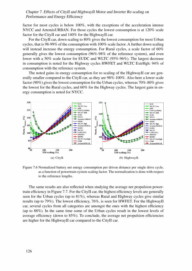
Chapter 7. Effects of CityII and HighwayII Motor and Inverter Re-scaling onPerformance and Energy Efficiency
factor for most cycles is below 100%, with the exceptions of the acceleration intenseNYCC and ArtemisURBAN. For those cycles the lowest consumption is at 120% scalefactor for the CityII car and 140% for the HighwayII car.
For the CityII car, down scaling to 80% gives the lowest consumption for most Urbancycles, that is 98-99% of the consumption with 100% scale factor. A further down scalingwill instead increase the energy consumption. For Rural cycles, a scale factor of 60%generally gives the lowest consumption (96%-98% of the reference system), and evenlower with a 50% scale factor for EUDC and WLTC (95%-96%). The largest decreasein consumption is noted for the Highway cycles HWFET and WLTC ExtrHgh: 94% ofconsumption with the reference system.
The noted gains in energy consumption for re-scaling of the HighwayII car are gen-erally smaller compared to the CityII car, as they are 98%-100%. Also here a lower scalefactor (90%) gives the lowest consumption for the Urban cycles, whereas 70%-80% givesthe lowest for the Rural cycles, and 60% for the Highway cycles. The largest gain in en-ergy consumption is noted for NYCC.
50 100 150 20090
95
100
105
110
115
120
EM scaling (%)
Nor
m. E
batt
ery (
%)
ECEWLTC Lowjc08FTP72 (UDDS)WLTC MdlSC03NYCCArtemis URBANNEDCWLTC HghArtemis RURALEUDCWLTCLA92 (UC)HWFETREP05WLTC ExtrHghUS06ArtemisMW130
(a) CityII.
50 100 150 20095
100
105
110
115
EM scaling (%)
Nor
m. E
batt
ery (
%)
ECEWLTC Lowjc08FTP72 (UDDS)WLTC MdlSC03NYCCArtemis URBANNEDCWLTC HghArtemis RURALEUDCWLTCLA92 (UC)HWFETREP05WLTC ExtrHghUS06ArtemisMW130
(b) HighwayII.
Figure 7.6 Normalized battery net energy consumption per driven distance per single drive cycle,as a function of powertrain system scaling factor. The normalization is done with respectto the reference lengths.
The same results are also reflected when studying the average net propulsion power-train efficiency in Figure 7.7. For the CityII car, the highest efficiency levels are generallyseen for the Urban cycles (up to 81%), whereas Rural and Highway cycles give similarresults (up to 79%). The lowest efficiency, 76%, is seen for HWFET. For the HighwayIIcar, several cycles from all categories are amongst the ones with the highest efficiency(up to 88%). In the same time some of the Urban cycles result in the lowest levels ofaverage efficiency (down to 85%). To conclude, the average net propulsion efficienciesare higher for the HighwayII car compared to the CityII car.
126
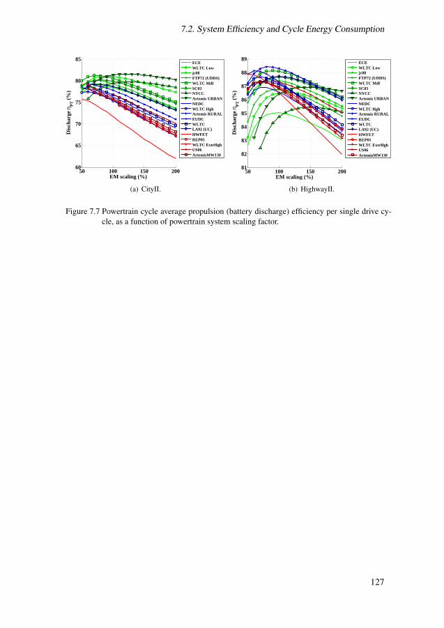
7.2. System Efficiency and Cycle Energy Consumption
50 100 150 20060
65
70
75
80
85
EM scaling (%)
Dis
char
ge η
PT (
%)
ECEWLTC Lowjc08FTP72 (UDDS)WLTC MdlSC03NYCCArtemis URBANNEDCWLTC HghArtemis RURALEUDCWLTCLA92 (UC)HWFETREP05WLTC ExtrHghUS06ArtemisMW130
(a) CityII.
50 100 150 20081
82
83
84
85
86
87
88
89
EM scaling (%)
Dis
char
ge η
PT (
%)
ECEWLTC Lowjc08FTP72 (UDDS)WLTC MdlSC03NYCCArtemis URBANNEDCWLTC HghArtemis RURALEUDCWLTCLA92 (UC)HWFETREP05WLTC ExtrHghUS06ArtemisMW130
(b) HighwayII.
Figure 7.7 Powertrain cycle average propulsion (battery discharge) efficiency per single drive cy-cle, as a function of powertrain system scaling factor.
127

Chapter 7. Effects of CityII and HighwayII Motor and Inverter Re-scaling onPerformance and Energy Efficiency
128

Chapter 8
Lumped-Parameter ThermalModel of HighwayII V-shapedReference PMSM
Electric machines in BEVs experience highly dynamic load cycles, which cause similarlyvarying internal losses, and therefore strongly time dependent temperature fluctuations.High temperatures can degrade the winding insulation and shorten the machine lifetime,or if high enough even cause immediate winding failure, whereas permanent magnetsrisk demagnetization [19, 46].
If the machine is sized to be able to continuously operate at the peak power neededin the application, it will result in an unnecessary large and expensive motor. In addition,the available space for electric machines in automotive applications, is often limited.Therefore, a trade-off has to be found between performance, volume and cost, so that themachine is not unnecessarily thermally over dimensioned.
In practice, often a lower level of torque and power is specified which the motor canhandle continuously, whereas it can handle a higher level for a shorter period of time,i.e. intermittently. Hence, BEV electric machines utilize temporary over-loading that islimited by the thermal capability of the machine.
A lumped-parameter transient thermal network is here presented for the HighwayIImotor with the four different slot areas, such that the temperature development in keymachine components can be estimated in various operating points and during load cycles.
8.1 Implemented thermal networkA wide range of suggested thermal networks can be found in literature with varying com-plexity and node configurations. However, since the object under consideration here is aconcept machine where only the active parts are geometrically determined with a highaccuracy, the level of complexity of the implemented network is to be adjusted accord-ingly. The implemented lumped-parameter network should include main heat transfer
129

Chapter 8. Lumped-Parameter Thermal Model of HighwayII V-shaped ReferencePMSM
paths, and be able to predict the transient temperature development in crucial machineparts such as the windings and magnets, while considering losses in bulk regions e.g.:stator yoke, stator teeth, active winding, end-winding, rotor yoke and magnets.
A suitable 10-node network for TEFC IMs (totally enclosed fan cooled induction ma-chines) is proposed in [19], where the T-equivalent node configuration is implemented.It assumes a uniform frame temperature, includes both radial and axial heat transfer inlaminations and winding, as well as a speed dependent air gap convection and fan speeddependent convection in the end cap region. A similar fan cooled IM 8-node networkis presented in [20], however without the T-equivalent node configuration. Furthermore,the axial heat transfer in the laminations are considered negligible, whereas bearing heattransfer is added. This network was later adjusted to a water cooled inset PMSM pre-sented in [53], by mainly modifying the rotor modelling. Here, the network has beenfurther adjusted for the used IPM rotor design. It is presented in Figure 8.1. Similar ad-justments to the rotor parts are also reported in [101, 114, 115]. Another modificationhere, is the added consideration of convection heat transfer to the cooling media.
Furthermore, it is assumed that the internal heat generation is uniformly distributedin each region, as is also assumed in [47, 56, 116]. Axial heat transfer is considered inthe copper windings and the shaft, whereas only radial heat transfer is considered for thelaminations and magnets, as is also done in [47]. Moreover, axial symmetry around themidpoint is assumed, as well as cylindrical symmetry both geometrically and thermally.
Figure 8.1 Implemented Thermal Network.
8.1.1 Frame and coolingSince the rms current densities are expected to reach around 15-28 A/mm2 in the dif-ferent slot areas described in Section 6.7, a liquid cooling system is implemented asrecommended in [34, p.90]. Additionally, liquid cooling is found to be frequently usedin current BEV models on the market, as shown in Table A.3 in Appendix A.
The intention is here to find a reasonable estimation of the thermal resistance be-tween the coolant and the frame nodes: Rth,Co−Fr. That is the sum of the resistances for
130

8.1. Implemented thermal network
the two main heat transfer modes involved: convection between the coolant medium andthe aluminum frame, and conduction inside the aluminum. Thus both natural convectionand radiation to the ambient air are considered negligible compared to the forced con-vection [52]. It is also desired to find an approximate value of the convection resistancefor the specific coolant temperatures 20C and 65C, as well as for certain flow rates.The higher of the two temperatures is here considered as the dimensioning temperaturefor the machines’ thermal capability, which is studied in Chapter 9. In order to estimatethese resistances a geometrical representation of the cooling channel is needed, as wellas material data of the coolant.
The cooling medium in current BEV models is found to typically consist of about50% deionized water and 50% ethylene-glycol, as stated for Ford Focus and ToyotaRAV4 EV in [117, 118] (it was also seen for Fiat 500e, Mercedes B-Class, Mitsubishii-MiEV, Nissan Leaf and Smart fortwo). The ethylene-glycol is added to prevent over-heating, freezing and corrosion. The cooling medium used here is assumed to be a mix-ture of 48% (by volume) water and 52% mono ethylene glycol [119]. Its material param-eters varies with temperature such that the density, thermal conductivity and dynamicviscosity decreases with increasing temperature, whereas the specific heat increases. Thetemperature dependencies are shown in Figure D.1 in Appendix D.
Various cooling circuits are possible for this application. However, for simplicity thecooling channel is assumed to form a spiral of four laps inside the aluminum frame, asillustrated in Figure 8.2. The cooling ducts have rectangular cross sections with a widthwduct of 30 mm, and a height hduct of 5 mm, and are separated by 10 mm. The radialdistances from the inner and outer frame boundaries lFr,lower to the ducts are 3 mm oneach side. Similar cooling channels with rectangular ducts are also used in BMW’s i3model with six laps [120], and in Nissan’s 2011 Leaf model with three parallel laps (i.eno spiral) [94].
Figure 8.2 The four laps spiral cooling channels with rectangular ducts, along with simplifiedframe, stator core and end windings.
8.1.1.1 Frame conductive thermal resistance
For simplicity, only one network node is used for the whole frame. Another simplifica-tion is to only consider the radial heat transfer between the stator back surface and theinner cooling duct surface. Therefore, the frame node is placed at half the radial distance
131

Chapter 8. Lumped-Parameter Thermal Model of HighwayII V-shaped ReferencePMSM
between these two boundaries. This part can be considered to be a hollow cylinder withthe inner and outer radii rFr,in and rFr,in + lFr,lower, and the length is here taken to bethat of the active core length lstk, of 150 mm. The conductive thermal resistance can thenbe expressed as
Rth,Fr =ln(
rFr,in+lFr,lower
rFr,in)
2πλAllstk(8.1)
8.1.1.2 Cooling convection thermal resistance
In order to estimate the thermal convection resistance between the cooling media and theframe (2.45), the heat transfer coefficient is approximated. Preferably measurements orCFD methods are to be used for this purpose. Here, however, a rough empirical approachto find suitable Reynolds and Nusselt numbers is considered accurate enough. A detaileddescription of the approach is given in Appendix E.
The average heat transfer coefficient hcool as a function of flow rate in liters perminute is presented in Figure 8.3 for four different coolant tempreatures. For laminarflow hcool is almost constant for all flow rates and temperatures: around 290 W/m2K.In contrast to laminar flow, for turbulent flow, hcool increases with both flow rate andtemperature and reach a few thousand W/m2K in the studied range. It is assumed that aturbulent flow is prefered. Therefore, in the case of 65C coolant, a flow rate of 6 L/minis chosen, which gives an hcool of 1988 W/m2K. In the case of 20C coolant the flowrate is set to 12 L/min, which gives an hcool of 1537 W/m2K. A similar value for thehigh coolant temperature is also noted to be used in BMW’s i3 model in [120], where thecoolant is said to reach up to 70C at inlet and 85C at outlet, when the flow rate is 6L/min. Here the temperature change of the coolant medium along the cooling channelis ignored, even though it may be up to 17C, as pointed out in Appendix E.
Flow rate (L/min)0 5 10 15 20
hco
ol (
W/m
2 K)
0
1000
2000
3000
4000
5000
6000
7000
h=1988
h=4023
h=292
h=1537
h=291
65oC
20oC
10oC5oC6 L/min12 L/min
Figure 8.3 The estimated average heat transfer coefficient of the coolant, as a function of flow rateand temperature.
Furthermore, it is assumed that 50% of the total heat flux between the stator back andthe cooling channel will pass through the inner duct surface. Therefore, a correction fac-tor kconv,corr of 0.5 is added to the convection thermal resistance of the cooling channel
132

8.1. Implemented thermal network
Rth,cool, which is
Rth,cool =kconv,corrhcoolAcool
(8.2)
where Acool is the surface area of the inner cooling duct boundaries, as in
Acool = 4× 2πwduct(rFr,in + lFr,lower) (8.3)
8.1.1.3 Thermal resistance between coolant and frame
The thermal resistance between the frame temperature node point and the cooling chan-nel’s average temperature is thus the sum of the cooling convection thermal resistanceand half of the conductive thermal resistance of the frame, as in
Rth,Co−Fr = Rth,cool +Rth,Fr/2 (8.4)
8.1.2 Stator yokeAs in [53, p.85], the stator yoke is modeled as a hollow cylinder consisting of stackedlaminated sheets of electrical steel with perfect insulation, thereby assuming a strictlyradial heat flow.
The thermally conductive core length lstk,cond is the product of the total core stacklength lstk, and the stacking factor ksf , which is here assumed to be 0.95, as in
lstk,cond = ksf lstk = 0.95 × 0.150 = 0.1425m (8.5)
The thermal resistance of the stator yoke, for radial heat flow thus depend on the innerand outer yoke radii: rY o,in and rY o,out respectively, as in
Rth,StY o =ln(
rY o,out
rY o,in)
2πλFelstk,cond(8.6)
8.1.2.1 Contact resistance between frame and stator yoke
Small air pockets inevitably exist between the aluminum frame and the stator back, who’ssize partly depend on the manufacturing process and surface roughness [19,102]. Due tothe relatively low thermal conductivity of air they need to be considered. The air pocketscan be modeled as a small equivalent air gap [102]. According to [102], the interface capbetween iron and aluminum is typically 0.6 − 6µm. However, further presented mea-surements on electric machines give an average gap between lamination and aluminumhousing of 0.037mm for different machine size, and the range 0.01 − 0.077mm. It ishere assumed that the gap distance, lcontFr−Y o is 10 µm, i.e. the lower limit in the mea-surement series.
The contact resistance is modeled as a hollow cylinder, as in
Rth,ContFr−Y o =ln(
rY o,out+lcontFr−Y o
rY o,out)
2πλAirlstk(8.7)
133

Chapter 8. Lumped-Parameter Thermal Model of HighwayII V-shaped ReferencePMSM
8.1.2.2 Thermal resistance between frame and stator yoke
The yoke node is placed radially in the middle of the yoke. The thermal resistance be-tween the frame and the yoke nodes thus consist of half of the frame and yoke conductiveresistances, as well as the contact gap resistance, as in
Rth,Fr−Y o = Rth,Fr/2 +Rth,ContFr−Y o +Rth,StY o/2 (8.8)
8.1.3 Stator teethThe assumed radial heat transfer in all of the stator teeth leads to parallel thermal resis-tances. The same method as in [20, p.69-70] and in [53, p.87-88] is here used to find thetotal radial thermal resistance of the teeth Rth,Te.
Ideally, the total thermal resistance of the teeth is found by integrating the radial crosssectional area of the teeth in the radial direction, as in
Rth,Te =
∫ rY o,in
rSt,in
1
λFeQs lstk,cond wtooth(r)dr (8.9)
where Qs is the number of teeth (and slots) and wtooth is the tooth width which varies inthe radial direction. In [20] and [53], however, the integration in (8.9) is replaced by ananalytical expression, in which the axial cross sectional view of one tooth is segmentedinto four indexed geometrical pieces in a non-curvature xy-plane. The y-componentsdenote the height of the segments (which represent the radial direction in the machine),and the x-components denote the width.
The fist segment (with xy-components indexed 1) belong to the rim rectangle. Thesecond component is a trapezoid placed above the rim, where the y-component denoteits height and the x-component its top width. The latter is also the lower tooth width.The third segment is the rectangular part of the tooth until the top curvature begins, atwhich its width is taken. The forth segment is the top of the tooth including a curvatureon both sides until the tip of the slot, and its width is the distance between two slot tips.The resulting expression for the thermal resistance is
Rth,Te =1
λFeQs lstk,cond
[y1x1
+y3x3
+y2
x1 − x2
(ln
∣∣∣∣ x1y2x1 − x2
∣∣∣∣−ln∣∣∣∣y2− x1y2x1 − x2
∣∣∣∣)−− π
4+
a√a2 − 1
arctan
(a+ 1√a2 − 1
)](8.10)
where a isa =
x3 + 2y42y4
(8.11)
8.1.3.1 Thermal resistance between stator yoke and teeth
The teeth node is placed radially in the middle of the teeth. Consequently, the thermalresistance between the yoke and teeth node is half of the thermal resistance for each part,
134

8.1. Implemented thermal network
as
Rth,Y o−Te = Rth,StY o/2 +Rth,Te/2 (8.12)
8.1.4 Stator windingAs copper losses are one of the main loss components in the motors the heat flow fromthe winding is large. This heat flow will pass through, not only the copper wires, but alsothe wire insulation, the impregnation, air pockets and the slot liner. Since the winding isnot geometrically well determined a specific geometrical representation is not possible.
Again, the same method as in [20, p.59-63] and [53, p.88-93] is here used, where theslot for simplicity is converted to an equivalent rectangular shape. The equivalent slot isthen divided into two thin surface layers representing the slot liner dslotliner of 0.2 mmand a thin air film dslotair of 10 µm, and where the rest of the volume consist of anequivalent winding mix representing copper and impregnation which is assumed to havea uniform heat generation.
The width of the winding mix’s part of the equivalent rectangular slot wslot,eq, istaken as the average of an upper and lower slot width (wslot,upper and wslot,lower) minustwo times the sum of the slot liner and air film, as in
wslot,eq =wslot,upper + wslot,lower
2− 2(dslotliner + dslotair) (8.13)
The height of the winding mix’s part of the rectangular slot hslot,eq, is the slot areadivided by the average of an upper and lower slot width minus two times the sum of theslot liner and air film, as in
hslot,eq =2Aslot
wslot,upper + wslot,lower− 2(dslotliner + dslotair) (8.14)
The slot liner’s and the winding impregnation’s thermal conductivities λslotliner andλimpreg are here assumed to be 0.2 W/mK, and that of the winding mix λWindMix isassumed to be 0.55 W/mK. The latter is approximated as 2.75 times that of the impreg-nation material, as suggested in [20, p.60] for a 45% slot fill factor.
8.1.4.1 Thermal resistance between active winding and teeth
The thermal resistance between the active winding and teeth is estimated as in [53, p.89-91]
Rth,Te−ActWi =RxRy
Qs lstk,cond (Rx +Ry)
(1− Rx0Ry0
720(Rx0 +Ry0)
)(8.15)
where Qs is the number of slots, and Rx, Ry , Rx0 and Ry0 represent thermal resistancesper unit length in the width (x) and height (y) directions of the rectangular equivalentslot. The resistances Rx are Ry are found as
Rx = 0.5(Rix +Rx0
6) (8.16)
135

Chapter 8. Lumped-Parameter Thermal Model of HighwayII V-shaped ReferencePMSM
Ry = 0.5(Riy +Ry0
6) (8.17)
where Rix and Riy represent the per unit length thermal resistances of the slot liner andair film, as in
Rix =dslotliner
λslotliner hslot,eq+
dslotairλair hslot,eq
(8.18)
Riy =dslotliner
λslotliner wslot,eq+
dslotairλair wslot,eq
(8.19)
The per unit length thermal resistances of the slot winding mix: Rx0 and Ry0 arefound as in
Rx0 =wslot,eq
λWindMix hslot,eq(8.20)
Ry0 =hslot,eq
λWindMix wslot,eq(8.21)
Since Ry0 is about ten times larger than Rx0 the heat flow from the slot to the yokeis assumed negligible.
8.1.4.2 Thermal resistance between the active winding and end winding nodes
The thermal resistance between the active winding and end winding is found as in [53,p.91-93]. The heat flow from the active part of the winding to the end winding is axial,with the cross sectional area of the copper ACu (m2)in each slot. Since the heat flowoccurs in parallel in the slots, the thermal resistance between the active and end windingnetwork nodes is found as in
Rth,AcWi−EnWi =lav
6QsACuλCu(8.22)
where Qs is the number of slots, lav is the average conductor length of half a turn, andis approximated as the sum of the active and passive winding length’s by (5.3). The endwinding axial extension outside of the lamination stack dext is here assumed to be 35mm on each side.
8.1.5 Air gapVarious suggested models of the air gap heat transfer can be found in publications, e.g.[19–22,47,53,102,121]. Many are based on the early work by Taylor 1935 [122], Gazley1958 [123] and Becker and Kaye 1962 [124]. Usually the axial heat flow is omittedfor machines with no internal forced air gap convection. The radial heat transfer is thendependent on the rotor speed, such that it is laminar i.e. conductive at low speed levelsand transitional and turbulent at higher speed levels. The speed dependence is calculatedby the Taylor number for which different critical values are set that represent laminar
136

8.1. Implemented thermal network
or turbulent flows. Different calculation methods are then given for the Nusselt numberdepending on the flow type.
The difference between the found models are usually the critical levels for the Taylornumber which dictate the type of flow, and the approximation of the Nusselt number.
Here the method described in [124] is used, which is also used in [20–22, 53, 121],however with varying critical Taylor values.
The thermal resistance across the air gap is
Rth,AirGap =1
hairgapAairgap(8.23)
where hairgap (W/m2K) is the air gap convection heat transfer coefficient, and Aairgap(m2) the cylinder surface area in the air gap (Aairgap = 2πrairgaplstk), and rairgap (m)is the average air gap radius.
The heat transfer coefficient and the Nusselt number are related as in
hairgap =Nuλair2 lairgap
(8.24)
where lairgap is the air gap length.The Nusselt number is approximated for different ranges of the modified Taylors
number as
Nu = 2 Tam < 1790 laminar flowNu = 0.128 ∗ T 0.367
am 1790 < Tam < 104 transitional flowNu = 0.409 ∗ T 0.241
am 104 < Tam < 107 fully turbulent flow
In [124] the critical value of the modified Taylors number between laminar and transi-tional flow is 1700, however, here the value is adjusted somewhat to avoid discontinuityat this transition.
Taylor’s number Ta is
Ta =ρ2air ω
2rotor rairgap l
3airgap
µ2air
(8.25)
where ρair (kg/m3) and µair (kg/ms) is the mass density and dynamic viscosity of air,respectively, and ωrotor (rad/s) is the angular speed of the rotor.
The Modified Taylors number Tam = Ta
Fg , is
Tam = Ta1697[0.0056 + 0.0571(
2rairgap+2.304lairgap
2rairgap−lairgap)2][1− lairgap
2rairgap]
π4(2rairgap−2.304lairgap
2rairgap−lairgap)
(8.26)
where the geometrical correction factor F−g 1 is close to unity, and therefore often ne-
glected.The material parameters of air are temperature dependent, as shown in Figure D.2
in Appendix D [48]. The air gap Nu number, heat convection coefficient, and resultingthermal resistance for the two temperatures 20C and 100C are presented in Figure 8.4,
137

Chapter 8. Lumped-Parameter Thermal Model of HighwayII V-shaped ReferencePMSM
as a function of rotor speed. Since the air temperature is not calculated by the thermalnetwork, the values at 100C are used in all cases.
Additionally, the air gap length due to thermal expansion of the machine. At 80 C,the air gap length may decrease to 85% of the value at 0 C. This effect is howeverignored here.
Speed (rpm)0 5000 10000 15000
Nu
airg
ap (
-)
2
3
4
5
6
7
8
20 oC
100 oC
(a) Nu.
Speed (rpm)0 2000 4000 6000 8000 10000 12000
hai
rgap
(W
/m2 K
)
20
40
60
80
100
120
14020 oC
100 oC
(b) hairgap.
Speed (rpm)0 2000 4000 6000 8000 10000 12000
Rth
,Air
Gap
(W
/mK
)
0.1
0.2
0.3
0.4
0.5
20 oC
100 oC
(c) Rth,AirGap.
Figure 8.4 Speed dependence of Nu, hairgap and Rth,AirGap.
8.1.6 Rotor core and magnetsAs for the stator, only radial heat flow is considered in the rotor. For simplicity, the rathercomplex magnet v-shape is replaced by an equivalent geometry with arced magnets,which is only used in the calculation of the thermal resistance, as shown in Figure 8.5for one 8th of the rotor. Similar conversions methods are also seen in [101, 115, 125].Additionally, a small air gap under the magnet is included with an assumed thickness of150 µm lMagGap. The equivalent thermal resistance is then a mix of series and parallelconnections in the rotor.
The equivalent rotor is divided into seven different segments: one lamination segmentthat is above the arced magnet (S4), and one that is below (S1); one that is the arcedmagnet (S7); one small air segment on each side of the magnet with same height as themagnet (S5, S6); and two lamination segments outside of the air segments (S2, S3).
The heat flow is assumed to be radial i all segments. Segment S1 and S4 are modelledas hollow cylinders, resulting in the expression
Rth,RoS:1,4 =ln( rout
rin)
2π λ lstk(8.27)
The heat flow in segment S2, S3, and S5-S7 as well as the small air gap under themagnet are modeled as pieces of a hollow cylinder based on (2.43), rendering
Rth,RoS:2,3,5−7 =ln( rout
rin)
φnpole λ lstk(8.28)
where npole is the number of poles. Furthermore, the radial heat flow in segment S2,S3,and S5-S7 is assumed to occur in parallel, and their equivalent resistance isRth,MagArcEq.The radii and angles used in the conversion is presented in Table 8.1, as noted in Figure8.5.
138

8.1. Implemented thermal network
Table 8.1 Parameters in the equivalent rotor geometry used in the thermal network.rout rin φ
Lamination Rth,RoS1 r1 rRot,in 2πLamination Rth,RoS2 r2 r1 2φ1Lamination Rth,RoS3 r2 r1 φ5Lamination Rth,RoS4 rRot,out r2 2πAir Rth,RoS5 r2 r1 2φ2Air Rth,RoS6 r2 r1 2φ4Magnet Rth,RoS7 r2 r1 2φ3Air Rth,MagAirgap r1 + lMagGap r1 2φ3
(a) Electromagnetic rotor geometry. (b) Thermal equivalent rotor geometry outline.
Figure 8.5 Rotor geometries in electromagnetic and thermal equivalent models.
8.1.6.1 Thermal resistance between tooth and magnets
The magnet node is placed in the radial middle of the arced equivalent magnet. Thethermal resistance between the stator tooth network node and the magnet node is thusfound as
Rth,Te−PM = Rth,Te/2 +Rth,AirGap +Rth,RoS4 +Rth,MagArcEq/2 (8.29)
8.1.6.2 Thermal resistance between magnets and rotor yoke
The rotor yoke node is placed in the radial middle of the lower rotor part. The thermalresistance between the magnet network node and the rotor node then becomes
Rth,RoY o−PM = Rth,MagArcEq/2 +Rth,MagAirgap +Rth,RoS1/2 (8.30)
8.1.7 ShaftThe shaft is assumed to be a lossless solid with only axial heat conduction, as also donein [47,53]. Furthermore, it is assumed to have a homogenous temperature distribution asin [53]. The shaft thermal resistance is divided into two sections depending on the shaft
139

Chapter 8. Lumped-Parameter Thermal Model of HighwayII V-shaped ReferencePMSM
radius. Within the length of the lamination stack lstk the shaft radius equals the rotoryoke inner radius rRoY o,in. Outside of the lamination stack the shaft radius rsh,ext is 20mm, and the distance to the bearings lsh,ext is 45 mm on each side.
Similarly as in [53], the shaft thermal resistance Rth,Sh is then
Rth,Sh =lstk
πr2RoY o,in λsteel+
2lsh,extπr2sh,ext λsteel
(8.31)
where λsteel is the thermal conductivity of the shaft steel material.
8.1.8 BearingsThe thermal resistance of the bearings Rth,Be is modeled as in [53], which is basedon empirical data of IMs in [20], but where the speed dependent term is neglected forsimplicity.
Rth,Be = 0.45 ∗ 33(0.12− db) (8.32)
where db is the average bearing diameter (54 mm).Another approach is suggested in [52, 102], where the bearing thermal resistance is
approximated to that of an equivalent interface gap. Empirical data is presented for foursmall IMs, with equivalent gaps between 0.23-0.4 mm. This method is not used here.
Also bearing losses are included in the thermal model. For simplicity they are as-sumed to only depend on motor torque [126], as
Ploss,Be =rBe µBe Trq,e wm
rRot,out(8.33)
where Trq,e is the motor torque, wm is the motor angular speed, rBe is the bearing boreradius (which equals the radius of the extended part of the shaft), µBe is the bearingfriction coefficient which is here assumed to be 0.0015 as typical for deep groove ballbearings in [126].
8.1.8.1 Contact resistance between rotor yoke and shaft
A 10 µm air film lcontRoY o−Sh is assumed between the rotor yoke and the shaft con-tact surfaces. The thermal resistance Rth,ContRoY o−Sh is here modelled as a hollow aircylinder.
8.1.8.2 Thermal resistance between bearings and frame
As suggested in [20, 53], the thermal resistance between the bearing and the frame is
Rth,Be−Fr = Rth,Be/4 (8.34)
8.1.8.3 Thermal resistance between rotor yoke and bearings
The thermal resistance between rotor Yoke and the bearings end up in
Rth,Be−RoY o = Rth,Y okeLower/2+Rth,ContRoY o−Sh+Rth,Sh/2+Rth,Be/4 (8.35)
140

8.1. Implemented thermal network
8.1.9 Internal airThe internal air is the air inside the frame except the air gap between the stator and ro-tor. Analytical modelling expressions are not applicable, rather empirical data must beused due to the complicated air flow paths in the geometrically complex region. There-fore, there are many published suggestions for modelling of the convective heat transferin this region [19, 20, 127]. A comparison between different heat transfer coefficient ex-pressions that are suggested in various publications, along with experimental results ofend winding convection, are presented in [127] (and partly in Figure 8.6). A fairly sim-ilar linear dependence on rotor speed is typically noted for the suggested heat transfercoefficients, with an offset which represents natural convection.
As suggested for the simple network in [20] and also used in [53], three separateconvective heat transfer coefficients to the internal air are here implemented: one to theinner frame surface, one to the rotor end shields and one to the end windings.
The heat transfer coefficient between the inner frame surface and the internal air isvia measurements empirically approximated in [20], as
hFr,in = 15 + 6.75v0.65r (8.36)
where vr (m/s) is the rotor peripheral speed. It should be noted that the approximationis a curve fit to data with a relatively large spread [20].
The inner frame surface area consist of the two inner end cap surfaces and the innerframe shell surface that extends outside both sides of the lamination stack.
The heat transfer coefficient between the rotor end shield surface and the internalair in [20], is approximated as
hRo = 16.5v0.65r (8.37)
The rotor end shield area is approximated by the circular surface area with the averageair gap radius.
The heat transfer coefficient between the end winding surface and the internal air isvia measurements empirically approximated in [20], as
hEnWi = 6.5 + 5.25v0.6r (8.38)
Also this approximation is based on data with a relatively large spread.As in [20], the surface area of the end winding is approximated as
AEnWi = π lpassive rEnWi,ave (8.39)
where lpassive is the average end winding conductor length as from (5.3), rEnWi,ave isthe average radial distance for the end winding.
A comparison between different found suggested values of convection heat transfercoefficient is shown in Figure 8.6. The speed range of found data are all up to 20 m/s,which represent about 3144 rpm of the here used HighwayII motor. The rotor speed de-pendence in the right part of Figure 8.6 is based on extrapolation of the velocity profiles.The Kylander [EW] data are similar to the Schubert [EW] data, whereas the Bogliettidata seem to have a larger speed proportionality coefficient. The Kylander [Fr] data arevery similar to the Stokum data for higher speed levels. The Kylander [Ro] data have theweakest speed dependence between all.
141

Chapter 8. Lumped-Parameter Thermal Model of HighwayII V-shaped ReferencePMSM
0 5 10 15Air velocity (m/s)
20
h(W
/m2 K
)
0
50
100
150
200
Rotor Speed (rpm)0 2000 4000 6000 8000 10000 12000
h (W
/m2 K
)
0
100
200
300
400
500
600MellorMellor eq. Schubert [EW] Schubert [Brg] StokumDi Gerlando [ER] Hamdi [ECap] Boglietti A [EW] Boglietti C [EW] Kylander [Fr] Kylander [EW] Kylander [Ro]
Figure 8.6 Comparison of suggested internal air convection heat transfer coefficients. Graphs in theleft part of the figure are original data from references, whereas graphs in the right partare extrapolated data for the HW machine speed range. Mellor eq. from [19], Kylanderfrom [20], the rest from [127].
The three thermal resistances to the internal air, are then converted from a Y to a∆, since the internal air temperature is not a desired network node. The net thermalconductance is
GT =1
Rth,InAir−Fr+
1
Rth,InAir−Ro+
1
Rth,InAir−EnWi(8.40)
8.1.9.1 The ∆-nodes thermal resistances
The thermal resistance between the rotor yoke network nodeRth,RoY o−Fr and the framenode is
Rth,RoY o−Fr = Rth,InAir−FrRth,InAir−RoGT /2 (8.41)
The thermal resistance between the end winding node Rth,EnWi−RoY o and the rotoryoke is
Rth,EnWi−RoY o = Rth,InAir−RoRth,InAir−EnWiGT /2 (8.42)
And finally, the thermal resistance between end winding and frame th, EnWi− Frnodes is
Rth,EnWi−Fr = Rth,InAir−FrRth,InAir−EndWiGT /2 (8.43)
8.1.10 Thermal capacitancesThe thermal capacitance of each motor part is the product of its mass and the specificheat of the material, and the mass is the product of its mass density and volume (2.47).
For the thermal capacitance of the frame, the volume includes the two end caps andthe whole frame cylinder, while excluding the volume of the cooling channel. Since theend winding extent varies between the motors with different slot areas, so does the length
142

8.1. Implemented thermal network
of the cylindrical part of the frame. This is to still keep a 10 mm distance from the endwinding to the inner side of the end cap. Therefore, the frame mass is somewhat lowerfor the Small slot geometry, and higher for the Large and High slot geometries.
The thermal capacitance of the yoke is modeled as a hollow cylinder.The thermal capacitance of the teeth is found via the geometrical surface area from
the FEA software, and the stack length.The thermal capacitance of the active part of the winding is found by taking the sum
of the active winding mass and the slot impregnation mass. The two volumes are foundvia the axial copper and slot cross sectional areas, the number of slots and the stacklength.
The thermal capacitance of the end winding is found in a similar way as the activepart of the winding, but the winding length is instead the passive part of half a turn,lpassive.
The thermal capacitance of the magnets and the rotor laminations is found in thesame way as the stator laminations.
The shaft thermal capacitance is here neglected. This is considered a valid simplifi-cation as its thermal time constant is about 1 h and thus have little effect on the rotor andmagnet temperatures, and even smaller on the stator laminations and windings.
The thermal capacitance of the bearings is found by using the mass in Section 6.2.5,and assuming that the specific heat is the same as for the shaft material.
The resulting network thermal capacitances are presented in Table 8.2, and in Figure8.7. The values adhere to material parameters at 100C. As shown, the thermal capaci-tance of the end winding is generally lower than it is for the active winding.
Table 8.2 Thermal capacitances in J/K in the thermal network for the four slot sizes.Small Original Large High
Frame Cth,Fr 4403 4568 4729 4636Stator yoke Cth,Y o 4039 3345 2631 2631Stator teeth Cth,Te 2686 2725 2695 3136Active winging and impreg. Cth,AcWi 1247 1716 2251 1934End winding Cth,EnWi 576 871 1250 1026Magnets Cth,PM 501 501 501 501Rotor yoke Cth,RoY o 3717 3717 3717 3717Bearings Cth,Be 169 169 169 169
0500
100015002000250030003500400045005000
Cth,Fr Cth,Yo Cth,Te Cth,AcWi Cth,EnWi Cth,PM Cth,RoYo Cth,Be
Ther
mal
cap
acita
nce
(J/K
) Small Original Large High
Figure 8.7 Thermal network node capacitances for the different slot areas.
143

Chapter 8. Lumped-Parameter Thermal Model of HighwayII V-shaped ReferencePMSM
8.1.11 Summary of thermal network node resistancesThe resulting network thermal resistances are presented in Table 8.3. The values adhereto a coolant temperature of 65C, a flow rate of 6 L/min and a rotor speed of 4000 rpm.The thermal resistance values are considered to be well in line with the values in [53].
Relative changes between the slot geometries per resistance is shown in Figure 8.8.
Table 8.3 Thermal resistances (W/mK) in the thermal network for the four slot sizes.Small Original Large High
Rth,Co−Fr 0.0037 0.0037 0.0037 0.0037Rth,Fr−Y o 0.0066 0.0060 0.0055 0.0055Rth,Y o−Te 0.0098 0.0115 0.0112 0.0115Rth,Te−AcWi 0.0092 0.0084 0.0079 0.0076Rth,AcWi−EnWi 0.0889 0.0669 0.0526 0.0603Rth,EnWi−RoY o 1.3527 1.3002 1.2540 1.2665Rth,Te−PM 0.2459 0.2482 0.2483 0.2483Rth,RoY o−PM 0.1446 0.1446 0.1446 0.1446Rth,EnWi−Fr 0.3422 0.3080 0.2796 0.3507Rth,Be−RoY o 1.2464 1.3301 1.4123 1.3649Rth,RoY o−Fr 0.5153 0.5150 0.5153 0.5169Rth,Be−Fr 0.2450 0.2450 0.2450 0.2450
0%10%20%30%40%50%60%70%80%90%
100%
Rth,Fr-Yo Rth,Yo-Te Rth,Te-AcWi Rth,AcWi-EnWi Rth,Te-PM Rth,Be-RoYo Rth,EnWi-RoYo Rth,EnWi-Fr
SmallOriginalLargeHigh
Figure 8.8 Relative thermal resistances for the different slot areas, normalized by the largest value.
8.2 Calculation set-up of lumped-parameter thermal modelThe thermal network calculation algorithm is presented in Figure 8.9. The calculationsare done for a specific coolant temperature and flow rate, which are treated in Section8.1.1. The second type of input is the motor’s torque and speed operating points thatare under consideration. For these operating points, the electromagnetic losses in the sixmotor parts for the three different magnet and copper temperatures are extracted, as wellas the bearing losses.
In the steady state solution for each operating point, an initial guess of the temperaturein the magnet and winding network nodes is first used when updating the motor losses forthe current temperatures, which is done via linear interpolation. Then follows an iterativeloop in which both the temperatures and the losses are updated with respect to eachother, until the temperature difference between the last to iterations fall below a specifiedthreshold value.
144

8.3. Steady state comparison of lumped network and FEA
In the transient solution, an initial temperature guess for the first value of the losses isdone similarly as in the steady state case. However, then the temperature increase duringone time step is calculated. In the next time step the losses are temperature corrected byusing the temperatures from the previous time step.
In both the steady state and the transient solution, some temperature depending pa-rameters are also updated. These are the copper and laminations’ thermal conductivityand specific heat, and the thermal conductivity of steel, which is used in the shaft andbearings. The time dependencies of these parameters are presented in Appendix D.
- Coolant temp.- Coolant flow rate- Motor torque- Motor speed
- Stator yoke losses- Stator teeth losses - Active winding losses- End winding losses- Magnets losses- Rotor yoke losses- Bearings losses- Material parameters
Lumped Parameter Network
EM - Torque- Speed
- Power losses of EM parts- Material parameters
- Temperature of EM parts
- Temperature of EM parts
Figure 8.9 Calculation loop for thermal performance of EM.
8.3 Steady state comparison of lumped network and FEAAs a frame of reference, a steady state comparison is here presented between the lumpedparameter network (LPN) and thermal simulation results from a 2D implementation ofthe motor in the FEA software Ansys Mechanical. Two motor operating points are con-sidered: 100 Nm at 4000 rpm, and 50 Nm at 12000 rpm. The former represent a mediumload situation where the total loss is 1.7 kW, and the latter a high load situation where thetotal loss is 3.6 kW. In both cases, the coolant temperature was set to 65C and the flowrate to 6 L/min.
In Ansys Mechanical the losses are implemented as averaged over the same motorregions as was used in the electromagnetic simulations. In order to make the two calcula-tion procedures comparable the following set-up was used in the Ansys Mechanical 2Dcalculation. Both the active and the end winding parts of the copper losses are appliedin the windings, since the end winding node is not possible to represent in the 2D struc-ture. Moreover, the other z-direction heat flows, through the shaft as well as through theinternal air, also had to be represented using an alternative approach. These heat flowswere calculated with the LPN, and then moved from the sending to the receiving regionsmanually. Moreover, the air gap is modeled as a conductive solid that has an equivalentthermal conductivity. This equivalent is found from the LPN air gap thermal resistance,the air gap thickness and a surface area in the middle of the air gap.
The results are presented in Table 8.4, along with illustrations of the temperaturedistribution in each case from Ansys Mechanical in Figure 8.10 and Figure 8.11.
For the medium load case the LPN temperatures are at most 3.7C (4%) higher thanthe FEA solution. The largest deviation is seen for the stator teeth, the magnets, rotoryoke and the winding, which are over estimated by the LPN by 1.1%.
145

Chapter 8. Lumped-Parameter Thermal Model of HighwayII V-shaped ReferencePMSM
At the high load, the LPN winding temperatures are up to 3.8C (3.1%) higher com-pared to the FEA solution. The largest deviations are seen in the same motor segments asfor the medium load. The temperature agreement is quite good, which is positive sincetheir temperatures are important for the study of the thermal performance of the motor.
Table 8.4 Steady state temperature comparison in C between the LPN and FEA software.100 Nm at 4000 rpm 50 Nm at 12,000 rpm
Motor Part LPN FEA (Diff.) LPN FEA (Diff.)Frame 71.3 71.3 (0) 78.1 78.5 (-0.4)Stator yoke 80.4 80.2 (0.2) 95.5 96.8 (-1.3)Stator teeth 95.6 91.9 (3.7) 126.4 122.6 (3.8)Active winding 103.2 102 (1.2) 138.0 139 (-1)End winding 127.2 - (-) 164.2 - (-)Magnets 93.9 91.7 (2.2) 123.7 120 (3.7)Rotor yoke 92.9 91.4 (1.5) 120.2 118.1 (2.1)
(a) Full cross section. (b) Zoom in.
Figure 8.10 Temperature distribution in the motor’s axial cross section, at 4000 rpm and 100 Nmload, with 65C coolant and 6 L/min.
146

8.4. Steady state sensitivity analysis for selected parameters
(a) Full cross section. (b) Zoom in.
Figure 8.11 Temperature distribution in the motor’s axial cross section, at 12,000 rpm and 50 Nmload, with 65C coolant and 6 L/min.
8.4 Steady state sensitivity analysis for selected parame-ters
Some of the assumptions made when forming the thermal network are based on empir-ical reference data. It is not clear how representative these assumptions are for this typeof motor. Contact air gaps between materials are for example highly dependent on theproduction process [102], which are not treated here. The thermal conductivity of thewinding mix depends both on the fill factor and on the distribution pattern of the conduc-tors, as investigated between ideal hexagon and square patterns in [128]. Furthermore,various suggested approximations of the convection heat transfer coefficients to the in-ternal air showed to vary quite much.
Therefore, a sensitivity analysis with the original slot geometry is here presented,which gives the difference in temperature in the network nodes when varying selecteduncertain parameters. The study is done with a coolant temperature at 65C and a flowrate at 6 L/min. The motor was operated at 50 Nm at 12000 rpm and the total losses are3.5 kW.
Initially, two different values of the cooling convection coefficient hcool (1000 and3000W/m2K) and the correction factor kconv,korr (0.4 and 0.6) are implemented. Thentwo contact air gaps are varied: between frame and stator yoke (5 µm and 15 µm), andbetween magnet and rotor yoke (10 µm and 200 µm). Also two values for the thermalconductivity of the winding mix is implemented, one that is λ × 0.5 and one that isλ × 1.5. Furthermore, two values of the thermal resistance of the bearing is studied (asRth× 0.5 and Rth× 1.5). Finally, the internal air heat transfer coefficients are varied (ash×0.5 and h×1.5). The resulting temperature difference compared to the non-modifiednetwork solution is presented in Table 8.5.
147

Chapter 8. Lumped-Parameter Thermal Model of HighwayII V-shaped ReferencePMSM
Table 8.5 Change in steady state temperature in C between the modified network and the non-modified, for the Original slot geometry at 50 Nm and 12000 rpm.
Fr StYo StTe AcWi EnWi PM RoYo Be
Reference temperatures 78.1 95.5 126.4 138.0 164.3 123.7 120.2 91.1hcool = 1000 12.7 12.7 12.1 12.5 13.9 12.3 12.5 12.7hcool = 3000 -4.3 -4.2 -3.8 -3.9 -4.4 -3.9 -4.1 -4.3kconv,korr = 0.4 -2.6 -2.5 -2.3 -2.3 -2.6 -2.3 -2.4 -2.5kconv,korr = 0.6 2.6 2.5 2.3 2.3 2.6 2.3 2.4 2.5lcontFr−Y o = 5µm 0.0 -5.2 -4.3 -4.2 -3.3 -3.2 -2.0 -0.3lcontFr−Y o = 15µm 0.0 5.1 4.3 4.3 3.3 3.2 2.1 0.3lMagGap = 10µm 0.0 0.0 -0.1 0.0 0.1 -1.3 1.5 0.2lMagGap = 200µm 0.0 0.0 0.0 0.0 0.0 0.3 -0.4 -0.1λWindMix = 0.275m 0.1 0.0 -0.1 5.0 3.8 0.3 0.6 0.1λWindMix = 0.825m 0.0 0.0 0.0 -1.7 -1.3 -0.1 -0.2 -0.1Rth,Be × 0.5 0.0 0.0 0.0 0.0 -0.1 -0.4 -0.7 -5.7Rth,Be × 1.5 0.0 0.0 0.0 0.0 0.1 0.3 0.6 4.7hFr,in × 0.5 (64 W/m2K) 0.0 0.7 2.1 2.9 9.4 6.7 11.3 1.8hFr,in × 1.5 (192 W/m2K) 0.0 -0.3 -0.9 -1.3 -4.1 -2.9 -4.9 -0.8hRo × 0.5 (138 W/m2K) 0.0 0.0 0.1 0.1 -0.3 3.2 6.3 1.0hRo × 1.5 (414 W/m2K) 0.0 0.0 -0.1 0.0 0.2 -1.7 -3.2 -0.5hEnWi × 0.5 (39 W/m2K) 0.2 1.3 3.4 5.2 18.9 0.5 -2.4 -0.2hEnWi × 1.5 (115 W/m2K) -0.1 -0.7 -1.9 -2.8 -10.3 -0.3 1.3 0.1
Setting the coolant heat transfer coefficient hcool to 1000 W/m2K gives a tempera-ture increase in all network nodes of around 12-14C. When setting it to 3000W/m2K,the temperature decrease is 4C in all points. Hence, the temperature change when goingfrom 1000 W/m2K to 2000 W/m2K is almost three times larger, compared to goingfrom 2000 W/m2K to 3000 W/m2K. Thus it seems that it is important to be able tomaintain a flow rate that can give a sufficient coolant heat transfer coefficient.
In the reference case, it is assumed that half (0.5) of the heat flux to the coolingchannels pass through the lower duct surfaces. When instead setting the share to 0.1more and less, the change in temperature in all network nodes is around 2-3C.
When the contact air gap between the magnet and rotor yoke is set to 10µm themagnet node temperature becomes about 1.3C colder, and the rotor yoke node 1.5Cwarmer. The other nodes are very little affected from this change, and are even lessaffected in the case of a 200µm gap length.
The same weak dependence is also noted for changes in the thermal resistance of thebearing, except in the bearing node itself.
When varying the contact gap length between the frame and stator yoke, on the otherhand, the stator yoke temperature changes about 1C per µm gap length. The othernode temperatures also change, however, the values decrease in the motors inward radialdirection. The end winding and active winding temperatures changes about 0.8-0.9 Cper µm gap length. In [102], gap lengths of up to 77µm are reported for some machines.Such a gap length in this operating point would lead to winding temperatures of around200C.
The temperature changes are notable when varying the internal air heat coefficientsto h× 0.5 and h× 1.5. The changes are the smallest for hRo and the largest for hEnWi.
For hRo the largest temperature changes of around 3%-5% is naturally seen in the
148

8.5. Transient thermal response to load step
rotor yoke, which is the closest node. The second closest node, the magnet, changes 1-2%. The temperature differences in the windings are very small and about the same inboth cases.
When varying hFr,in the largest temperature changes are noted in the rotor yokenode, and the second largest in the end winding node. The end winding increases about6% in the h × 0.5-case, and it decreases around 3% in the h × 1.5-case. The magnettemperature increase about 5% in the h × 0.5-case, and decreases around 2% in theh× 1.5-case.
The largest changes in the end wining temperatures are noted for changes of hEnWi.In the h × 0.5-case the temperature increase is about 12%, and in the h × 1.5-case thedecrease is around 6%. The effect on the active winding temperature is 2%-4%, on thestator teeth 1%-3%, and on the magnets it is less than half a percent.
When it comes to the studied contact gap lengths, winding mix thermal conductivity,and internal air heat transfer coefficients, it is difficult to analytically find assumptionsthat are more applicable than the empirical data presented in the references. However, ifexperimental results are available from a physical machine, it it highly recommended tocalibrate such network parameters towards measurements in order for the lumped param-eter network to better fit the specific machine.
8.5 Transient thermal response to load stepThe transient thermal response at two different load steps: 100 Nm at 4000 rpm, and 50Nm at 12000 rpm, with a coolant temperature of 65C and a flow rate of 6 L/min, arepresented in Figure 8.12 and Figure 8.13, for the Original slot.
At the lower speed level, mainly the copper losses increase with increasing windingtemperatures. Only minor changes can be seen for the lamination losses. At the higherspeed level, the lamination losses decrease somewhat with increasing temperature.
0 20 40 600
100
200
300
400
500
600
Time (min)
Plo
ss (
W)
EndWiActWiTeethStYoBerRotorPM
(a) Losses.
0 20 40 6060
70
80
90
100
110
120
130
Time (min)
Tem
p. (o C
)
EndWiActWiTeethPMRoYoStYoBeFr
(b) Temperatures.
Figure 8.12 Losses and temperatures as a function of time, during a load step of 100 Nm at 4000rpm with a coolant temperature of 65C and a flow rate of 6L/min, for the Originalslot geometry.
149

Chapter 8. Lumped-Parameter Thermal Model of HighwayII V-shaped ReferencePMSM
0 20 40 600
200
400
600
800
1000
1200
1400
Time (min)
Plo
ss (
W)
EndWiActWiTeethStYoBerRotorPM
(a) Losses.
0 20 40 6060
80
100
120
140
160
180
Time (min)
Tem
p. (o C
)
EndWiActWiTeethPMRoYoStYoBeFr
(b) Temperatures.
Figure 8.13 Losses and temperatures as a function of time, during a load step of 50 Nm at 12000rpm with a coolant temperature of 65C and a flow rate of 6L/min, for the Originalslot geometry.
The thermal time constants for the two load cases at two different coolant tempera-tures (20C and 65C) and related flow rates (12 L/min and 6 L/min), are presented inTable 8.6. The time constants are a bit longer in the case of the lower motor speed com-pared to the higher. Furthermore, the time constants at one speed level are only slightlylonger for the case of the cold coolant compared to the warm. It should be noted that thetime constants of the rotor and magnets would be a bit longer if also the shaft thermalcapacitance was included in the lumped network.
Table 8.6 Thermal time constants of lumped-parameter network nodes in minutes.
100 Nm at 4000 rpm 50 Nm at 12,000 rpm
20C 65C 20C 65CStator yoke 3.6 3.3 3.1 2.8Stator teeth 3.4 3.2 2.6 2.4Active winding and impreg. 3.3 3.0 2.6 2.4End windings 3.1 2.7 2.6 2.3Magnets 9.8 9.9 5.9 5.8Rotor yoke 14.0 14.6 9.1 9.3Bearings 5.2 5.1 4.8 4.4
150

Chapter 9
Thermal Performance forHighwayII PMSM with FourDifferent Slot Areas
A comparison between the the performance when using different slot area geometries,which were introduced in Section 6.7, is here presented regarding thermal steady state,over load capability and transient load cycle performance. The purpose is to investigatethe differences between the various slot geometries.
9.1 Steady state performanceAs was noted in Chapter 8, the four parts in the motor with the highest temperaturesare the two parts of the windings, the stator teeth, and the magnets. The steady statetemperature development as a function of torque and speed in these motor parts for theOriginal slot motor geometry, is presented in Figure 9.1, along with the road load ofthe HighwayII concept BEV. It can be noted, that the highest temperatures are reachedalong the max torque trajectory. When driving at the top speed on a flat road, the windingtemperature becomes around 120C, and the magnet temperature about 100C.
151

Chapter 9. Thermal Performance for HighwayII PMSM with Four Different SlotAreas
Speed (rpm)0 2000 4000 6000 8000 10000 12000
Tor
que
(Nm
)
50
100
150
200
70
80
80
100
100
100
120
120
120
150
150
150
180
180
180
200
200
200
500Temp StTe
Temp. (oC)T
EM,max (Nm)
Road load
(a) Stator teeth.
Speed (rpm)0 2000 4000 6000 8000 10000 12000
Tor
que
(Nm
)
0
50
100
150
200
70
80
80
100
100
100
120
120
120
150
150
150
180
180
180
200
200
200
500
500
500
Temp AcWi
Temp. (oC)T
EM,max (Nm)
Road load
(b) Active winding.
Speed (rpm)0 2000 4000 6000 8000 10000 12000
Tor
que
(Nm
)
0
50
100
150
200
70
80
80
100
100
120
120
120
150
150
150
180
180
180
200
200
200
500
500
500
1000
1000
1000
Temp EndWi
Temp. (ooC)T
EM,max (Nm)
Road load
(c) End winding.
Speed (rpm)0 2000 4000 6000 8000 10000 12000
Tor
que
(Nm
)
50
100
150
200
70
80
80
100
100
100
120
120
120
150
150
150
180
180
180
200
200
200
500Temp PM
Temp. (oC)T
EM,max (Nm)
Road load
(d) Magnets.
Figure 9.1 Steady state temperature contour lines in selected motor parts as a function of torque andspeed, for the Original slot geometry, with a coolant temperature of 65C and a flowrate of 6 L/min. The road load of the HighwayII BEV is also included as a reference.
In order for the lifetime of the motor to be as long as possible it is desired to limit themax temperature in the windings of an electric machine. The chosen critical temperaturedepends both on the winding insulation class and the number of working hours that isthe design target [46]. It is here assumed that the winding temperature should not exceed150C in transient mode, and be limited to 120C in continuous operation mode.
At the same time the magnet temperature should not exceed 140C, as noted in Sec-tion 6.2.3.
The torque-speed levels for when the winding reach its critical temperatures 120Cand 150C, and the magnet reach 100C and 140C, are presented for all four slotgeometries in Figure 9.2. As expected, it can be noted that the motor with the Smallslot will reach both the critical winding and magnet temperatures at lower torque levelscompared to the other slot geometries. The highest torque levels for the specified criticaltemperatures can be reached with the Large slot geometry. This is due to the lower losses,especially copper losses, in a large part of the motor operating area with the Large slotcompared to the other geometries (presented in Figure 6.18), and the higher losses for
152

9.2. Transient over load
the Small slot.
Speed (rpm)0 2000 4000 6000 8000 10000 12000
Tor
que
(Nm
)
0
50
100
150
200
250
Small 120oC
Small 150oCOriginal 120oC Original 150oC Large 120oC
Large 150oCHigh 120oC
High 150oC
(a) End winding.
Speed (rpm)0 2000 4000 6000 8000 10000 12000
Tor
que
(Nm
)
0
50
100
150
200
250
Small 100oC
Small 140oCOriginal 100oC
Origianl 140oC
Large 100oC
Large 140oCHigh 100oC
High 140oC
(b) Magnets.
Figure 9.2 Steady state temperature development in end windings and magnets for all slot geome-tries, at a coolant temperature of 65C and a flow rate of 6 L/min.
The max torque levels reached at the studied critical temperatures above, are pre-sented in Table 9.1. The magnet reaches the max temperature at lower torque levelscompared to the torque levels at which the end winding reaches the max temperature.It seems that the magnet’s temperature capability is not enough for this design and ap-plication, and perhaps it should be replaced by one that has a higher thermal capability.When considering the max torque at 120C, the ratio of peak to continuous torque isaround 2.8 for the Small slot, 2.2 for the Original, 1.8 for the Large, and 1.9 for the Highslot. As a frame of reference it is around 1.2-2 times for nine existing BEVs (as presentedin Figure A.4).
Table 9.1 Max torque reached at winding and magnet critical temperatures, for all slot geometries,at a coolant temperature of 65C and a flow rate of 6 L/min.
Small Original Large High
Max torque at 120C end winding 81.7 95.7 104.2 99.9(88%) (100%) (104%) (99%)
Max torque at 150C end winding 100.7 116.6 125.2 120.8(86%) (100%) (107%) (104%)
Max torque at 100C magnets 64.4 76.9 85.3 81.1(84%) (100%) (111%) (105%)
Max torque at 140C magnets 95.1 110.5 119.3 114.5(86%) (100%) (108%) (104%)
9.2 Transient over loadHere the max time duration in a certain operating point in the torque-speed-plane iscalculated, caused by a load step at a certain speed level. All load steps originates from
153

Chapter 9. Thermal Performance for HighwayII PMSM with Four Different SlotAreas
the torque level where the end winding has already reached 120C in steady state. Theinitial steady state temperatures of the other motor parts at this torque level are used as astarting point. Then load steps in the torque level are taken, whereupon the time until theend winding reaches 150C is found via the transient thermal response. The results arepresented in Figure 9.3.
As expected from the steady state results, the longest time at high torque levels can bereached with the Large slot geometry. With a load step up to the peak torque level for theLarge slot geometry, 182 Nm (at 2000 rpm), it takes 33s until the end winding reachesthe critical temperature of 150C. For the High slot it takes 27s, for the Original 25s, andfor the Small slot 13s. Considering that 80% of all accelerations in the Test and Loggedcycles are around 9s-13s (Section 3.4), and that this is a worst case approach by using avery high coolant temperature, the Small slot geometry may still be viable. It should alsobe noted that the comparison is done for a fixed max phase current. In case of a largercurrent, even larger torque levels could be thermally possible with the Original, Largeand High slot geometries.
2000 4000 6000 8000 10000 120000
50
100
150
200
Speed (rpm)
Tor
que
(Nm
)
10
1520
304060
300 600
Over load time (s) T
rq,max
Trq
EW 120oC
(a) Small slot area.
2000 4000 6000 8000 10000 120000
50
100
150
200
Speed (rpm)
Tor
que
(Nm
)
1520
304060
300300600
Over load time (s)T
rq,max
Trq
EW 120oC
(b) Original slot area.
2000 4000 6000 8000 10000 120000
50
100
150
Speed (rpm)
Tor
que
(Nm
)
40
60
300 600
Over load time (s) T
rq,max
Trq
EW 120oC
(c) Large slot area.
2000 4000 6000 8000 10000 120000
50
100
150
Speed (rpm)
Tor
que
(Nm
)
304060
300 600
Over load time (s) T
rq,max
Trq
EW 120oC
(d) High slot area.
Figure 9.3 Time spent in different operating points, before end winding reach 150 C, at 20 Ccoolant temperature, for two slot sizes.
154

9.3. Performance during drive cycles
9.3 Performance during drive cyclesThe motor’s temperature development during selected Urban, Rural and Highway Testdrive cycles are investigated and compared between the different stator geometries. Thecycles are repeated several times in order to reach thermal steady state. As an example,the motor part losses and temperature development during NEDC is presented in Figure9.4, and during ArtemisMW130 in Figure 9.5. It can be noted that the teeth losses arethe highest during high speed driving in both cycles. Large power loss peaks are reachedduring breaking in the ArtemisMW130 cycle, which cause a temperature rise in the endwinding of around 4-6C during 4s each. The peak end winding temperatures are thehighest in all cycles.
Time (s) #1041.08 1.1 1.12 1.14 1.16 1.18
Plo
ss (
W)
0
100
200
300
400
500
600
700
800 TeethStYoActWiEndWiBerRotorPM
(a) Losses during one cycle.
Time (s)0 2000 4000 6000 8000 10000 12000
Tem
p. (
o C)
65
70
75
80
85
90
95EndWiActWiTeethPMRoYoStYoBeFr
(b) Temperature during ten consecutive cycles.
Figure 9.4 Losses and temperature development during the NEDC cycle with the original slot, at acoolant temperature of 65C and a flow rate of 6 L/min.
Time (s) #1044.18 4.2 4.22 4.24 4.26
Plo
ss (
W)
0
500
1000
1500
2000
2500TeethStYoActWiEndWiBerRotorPM
(a) Losses.
Time (s) #1044.18 4.2 4.22 4.24 4.26
Tem
p. (
o C)
60
70
80
90
100
110
120
130EndWiActWiTeethPMRoYoStYoBeFr
(b) Temperature.
Figure 9.5 Losses and temperature development during the ArtemisMW130 cycle with the originalslot, at a coolant temperature of 65C and a flow rate of 6 L/min.
The peak and cycle average power losses, normalized to the values of the Original
155

Chapter 9. Thermal Performance for HighwayII PMSM with Four Different SlotAreas
slot geometry, are presented in Figure 9.6. The highest peak losses can be noted for theSmall slot geometry, and the lowest for the Large slot, except in the ECE case. The cycleaverage losses are the lowest for the Small slot during all cycles except the accelera-tion intense ArtemisURBAN, UCLA92, and US06, as well as in the high speed cycleArtemisMW130. In these cycles the losses are instead the highest for the Small slot, ex-cept in UCLA92 where the High slot cause the largest losses. Otherwise, the losses withthe Large slot are the highest in most cycles. The largest difference between the highestand lowest cycle average losses are noted for the HWFET cycle, which includes highspeed levels but relatively low acceleration levels.
The fact that the machine with the Small slot area has the lowest average cycle losseswas slightly unexpected. This in combination with the highest peak torque and leastamount of copper (which is more expensive than laminations per unit mass [128]), makesit a rather attractive design solution.
106%110%
117%
106%
113%
106% 106%
123%
108%
127% 126%
100% 100%100%
100% 100% 100% 100% 100% 100% 100% 100%
105%
97%99% 99%
86%
99% 99%
82%
100%
97%
83%
106%101% 102% 100%
91%
100%99%
92%
103% 104%
92%
80%85%90%95%
100%105%110%115%120%125%130%
Nor
mal
ized
pea
k po
wer
loss
es
Small Org Large High
(a) Normalized peak losses.
99% 100%
106%
97% 96%95%
99%
103%
92%
105%103%
100% 100% 100% 100% 100% 100% 100% 100% 100% 100% 100%
105% 105%
100%
107% 108% 108%
105% 103%
112%
102% 102%
105% 105%
102%
106% 106% 106%104% 104%
108%
101%100%
90%
95%
100%
105%
110%
115%
Nor
mal
ized
cyc
le a
vera
ge P
loss Small Org Large High
(b) Normalized cycle average losses.
Figure 9.6 Peak and cycle average losses during drive cycles, where all values are normalized bythe results for the Original slot size, at a coolant temperature of 65C and a flow rate of6 L/min.
156

9.3. Performance during drive cycles
The max magnet and end winding temperatures during the selected drive cycles arepresented in Figure 9.7. The max magnet temperature differ 2C or less between the dif-ferent slot geometries for the investigated drive cycles. The highest magnet temperaturesare seen for the two cycles with the highest average speed levels, but still they do notreach more than 99C.
The max winding temperature is the highest for the Small slot geometry for all cycles,followed by the Original slot, and the lowest for the Large slot geometry. As with themagnet, the largest peak temperatures are noted for the cycles with the highest speedlevels, and are close to the critical for the Small slot geometry.
6973 72 74
78 7881
7778
92
99
6973 72
74
78 7981
7779
92
99
6973 71
74
78 79 8076
79
91
97
69
7371
74
78 79 8077
79
91
97
65
70
75
80
85
90
95
100
105
Max
mag
net t
emp.
(o C) Small Org Large High
(a) Max magnet temperature.
74
88 92101 97
102
127
103
89
146 146
72
83 8490 89 92
109
9285
122 125
7180 81 85 86 87
99
87 84
112 113
7181 83
87 87 89
103
8984
116 117
65758595
105115125135145155
Max
end
win
ding
tem
p. (o C
) Small Org Large High
(b) Max end winding temperature.
Figure 9.7 Max magnet and end winding temperatures during drive cycles, at a coolant temperatureof 65C and a flow rate of 6 L/min.
157

Chapter 9. Thermal Performance for HighwayII PMSM with Four Different SlotAreas
158

Chapter 10
Conclusions and Future Work
10.1 ConclusionsIn this thesis, various drive cycles, legislative, official real-world and measured within theframe of the project, have been studied and characterized in terms of speed and accelera-tion cycle parameters, as well as acceleration and speed distribution. The objective was toassess typical vehicle usage on different road types, but also to study the implication onvehicle energy consumption due to the drive cycle’s characteristics. For this evaluation,three reference vehicles (a City car, a Highway car and a Sport car) were designed afterdifferent set performance requirements, with data on existing BEVs as a frame of ref-erence. An available traction motor, power electronic module and traction battery wereutilized. Furthermore, the electromagnetic efficiency of two v-shaped PMSM referencemotors (CityII and HighwayII) were evaluated when scaling the active length. Then theconsequence on acceleration performance, drive cycle fulfilment and energy consump-tion during re-scaling of the electric drive system was studied. Moreover, the electromag-netic losses for four different slot areas were compared (for the HighwayII motor), alongwith the thermal steady state and transient over load as well as temperature developmentduring drive cycles.
Since most of the legislative drive cycles were developed a few decades ago, whenthe performance of passenger cars were generally lower than today’s cars, the drive cy-cles are not fully representative for today’s typical driving. Through comparison withmeasured drive cycles, it was found that the measured cycles report higher peak levelsof acceleration for a certain speed level, and a larger number of speed fluctuations. Onthe other hand, when studying the relative time spent at certain levels of acceleration andspeed, the measured cycles spend only slightly more time at higher levels of accelerationcompared to the official cycles, at least on average over a group of similar cycles.
From a literature study, various estimation methods of vehicle frontal area werefound. These were compared with available manufacturer data from nine models. It wasfound that a suitable approximate estimation of the area is 86 % of the product of vehicletrack width and height. Furthermore, different, often referred to, estimations regardingthe speed dependency of tire rolling resistance were found to deviate from each otherrather much.
159

Chapter 10. Conclusions and Future Work
Through the mapping of existing BEVs it was found that there is a wide spread re-garding their top speed and acceleration performance, as well as driving range, whichmade a categorization ambiguous.
When comparing the three reference City, Highway, and Sport cars their road loadper mass while driving at a constant speed, it was found that the City car has a strongerspeed dependency than the other two, due to its relatively higher aerodynamic drag. Thiscauses it to have a higher road load relative to its mass for speed levels greater than66 km/h, compared to the Highway and Sport cars.
The needed wheel force and power, due to performance requirements regarding topspeed, time to accelerate to 100 km/h, take off at 25 % grade, and driving at a highgrade in a high speed were studied. In a comparison it turned out that the accelerationrequirement was the dominating one, hence the only one considered when specifying theneeded output from the powertrain.
Furthermore, it was found that the time to accelerate can be achieved with variouscombinations of initial maximum force and maximum power. For a higher initial max-imum force, the needed maximum power to reach 100 km/h at the specified time islower. This will lead to shorter time to accelerate to 50 km/h, but longer time to accel-erate from 50 to 100 km/h. The conclusion is that a requirement of time to acceleratefrom 0 to 100 km/h is not enough to describe the desired performance of a vehicle, theremust also be an expressed requirement on low and high speed performance, respectively.
Another important finding is that the time resolution of the speed time traces, thatdefines the official cycles, is relatively low compared to the rate of change of speed.Then the estimated correlated acceleration is highly dependent on the method used forcalculation, whether it is a forward and backward looking method or a simpler just back-ward looking method. The consequence on cycle energy consumption per distance is thenhighly sensitive to the method used for estimation of acceleration, where the differencemay be as large as 15 % for some cycles.
The resulting average cycle powertrain efficiency are fairly similar for the City andHighway cars, and indicate slightly lower values for the Urban cycles, 77%-86%, com-pared to the Rural 85%-88% and highway cycles 87%-89%. The Sport model give loweraverage efficiencies due to the higher power rating of the powertrain. Moreover, the av-erage efficiency values are very similar for both the test cycles and the logged cycles,within the same road-type category. For the two road-type categories with the lowestspeed levels, the logged cycles indicate a larger spread compared to the test cycles re-garding energy consumption per driven distance. Also within the same road-type cate-gory, those cycles that spend most time at high acceleration and speed levels are thosethat consume the most energy per distance during propulsion. At the same time, in thesecycles more braking energy is also available for regenerative braking, which makes thetotal energy consumption a bit less sensitive to speed fluctuations and high accelerationlevels, still the tendency is a higher energy consumption per driven distance.
The effect on acceleration due to re-scaling of motor active length, is largest for theshortest stack lengths and smallest for the longest. For the acceleration time 0-100km/h,the difference between the scale factors 50% and 80% is 12s for the CityII car, and 8s forthe HighwayII, whereas the difference between the scale factors 120% and 150% is onlyabout 2s for both cars.
Both the CityII and HighwayII concept BEVs can fulfill the speed reference of most
160

10.2. Future Work
Test cycles down to 70% of the original stack length. Also, for both cars, the energyconsumption per driven distance decreases with decreasing stack length, except for thetwo acceleration intense urban cycles NYCC and ArtemsURBAN whose minimum isreached with a up-scaled stack length. For the CityII car, the lowest values are down to94% of the consumption with the original stack length, and for the HighwayII car thelowest values are 98% of the original stack length. With both cars, the largest decrease isnoted for cycles with higher speed levels.
When varying the slot size for the v-shaped PMSM HighwayII reference motor whilekeeping the same max phase current and voltage, the amount of copper and core lossesare shifted. For a smaller slot area, the copper losses increase and the core losses de-crease, whereas the opposite applies to a larger slot and copper area. The resulting totallosses are then largest for the smaller slot geometry in a large part of the motor oper-ating area. Due to this, during thermal steady state, the small slot geometry reaches thechosen continuous end winding temperature at lower torque levels compared to the otherslot geometries. The largest continuous torque levels are reached with the large slot area.During a transient over load step which originates from the steady state torque level, themotor version with the largest slot area is capable of staying at its peak torque for 33s.The high, original high and small slot geometries are able to stay at the same operatingpoint for 27s, 25s, and 13s, respectively.
The small slot geometry had the highest peak losses during the drive cycles, however,on a cycle average it had the lowest losses for 7 of the 11 studied cycles. This fact,in combination with the highest peak torque and lowest material cost, makes it a veryinteresting option as an electric vehicle traction motor.
10.2 Future WorkAs the presented results are valid under the assumptions made and models used duringthe study, perhaps it would be valuable to assess the consequence on energy consump-tion while improving the level of detail regarding some of the assumptions and modelsused. For example, by modeling the rolling resistance as a function of speed, and by im-plementing a wheel slip model, the change in energy consumption could be assessed inorder to be able to draw conclusions on the necessary level of detail in the modeling ofthese phenomena. Also, a sensitivity study on the influence on energy consumption dueto different values of vehicle frontal areas and aerodynamic drag coefficients would beinteresting.
The accuracy of the battery losses and the dynamic voltage trajectory modeling couldbe improved by also implementing capacitive terms, although then perhaps a differentbattery cell should be modeled where more data is available.
Apart from energy consumption, range and acceleration performance, aspects suchas life cycle cost and environmental effects of the BEV powertrain design choices, e.g.recycling, are of vital importance and could be included in future studies.
A more detailed investigation of various cooling channel geometries, preferably incombination with CFD simulations would be highly valuable in order to assure a reason-able cooling solution. Additionally, CFD simulations of the motor’s internal air convec-tion would be valuable to better estimate the heat transfer coefficients. Furthermore, in
161

Chapter 10. Conclusions and Future Work
the lumped parameter network, perhaps the air temperatures could also be evaluated andit’s parameters temperature adjusted for a higher accuracy.
Moreover, it would be interesting to also study the temperature development duringthe Logges real-world drive cycles for the different slot areas, in order to determine theeffect on temperature for a larger number of speed fluctuations and various grade levels.
Finally, the derived drive cycles from the measured GPS and accelerometer signals,could perhaps be improved using more advanced filtering techniques.
162

References
References[1] (2012, may) Regulation no 101, official journal of european union. Economic
Commission for Europe of the United Nations. Accessed 2012-10-31.[Online]. Available: http://eur-lex.europa.eu/LexUriServ/LexUriServ.do?uri=OJ:L:2012:138:0001:0077:en:PDF
[2] A. Nordelöf, M. Messagie, A.-M. Tillman, M. Ljunggren Söderman, andJ. Van Mierlo, “Environmental impacts of hybrid, plug-in hybrid, and batteryelectric vehicles—what can we learn from life cycle assessment?” TheInternational Journal of Life Cycle Assessment, vol. 19, no. 11, pp. 1866–1890,2014. [Online]. Available: http://dx.doi.org/10.1007/s11367-014-0788-0
[3] (2015) Global ev outlook 2015. IEA, International En-ergy Agency, EVI, Electric Vehicles Initiative. Accessed 2015-04-27. [Online]. Available: http://cleanenergyministerial.org/Portals/2/pdfs/EVI-GlobalEVOutlook2015-v14-landscape.pdf
[4] P. Mock. (2014) European vehicle market statistics, 2014. The International Coun-cil of Clean Transportation (ICCT).
[5] K. Rajashekara, “Present status and future trends in electric vehicle propulsiontechnologies,” Emerging and Selected Topics in Power Electronics, IEEE Journalof, vol. 1, no. 1, pp. 3–10, March 2013.
[6] E. Ericsson. (2000) Driving pattern in urban areas - descriptive analysis andinitial prediction model. Lund Institue of Technology, Department of Technologyand Society, Traffic Planning. Accessed 2013-12-11. [Online]. Available:http://www.lunduniversity.lu.se/o.o.i.s?id=12683&postid=627123
[7] (2006, dec) Final technical support document, fuel economy labeling ofmotor vehicle revisions to improve calculation of fuel economy estimates.US Environmental Protection Agency (EPA), Office of Transportation and AirQuality. Accessed 2013-12-09. [Online]. Available: http://www.epa.gov/carlabel/documents/420r06017.pdf
[8] E. Ericsson, “Independent driving pattern factors and their influence on fuel-useand exhaust emission factors,” Transportation Research Part D: Transportand Environment, vol. 6, no. 5, pp. 325 – 345, 2001. [Online]. Available:http://www.sciencedirect.com/science/article/pii/S1361920901000037
[9] S. Samuel, L. Austin, and D. Morrey, “Automotive test drive cyclesfor emission measurement and real-world emission levels - a review,”Proceedings of the Institution of Mechanical Engineers, Part D: Journal ofAutomobile Engineering, vol. 216, no. 7, pp. 555–564, 2002, cited By (since1996)34. [Online]. Available: http://www.scopus.com/inward/record.url?eid=2-s2.0-0036964445&partnerID=40&md5=7dfe8159f1a6d5b00f7a8e1153ee5aa4
163

References
[10] (2012) Advanced powertrain research facility, avta nissan leaf testing and analysis.Idaho National Laboratory (INL), Advanced Vehicle Testing Activity (AVTA).Accessed 2013-10-17.
[11] S. Williamson, A. Emadi, and K. Rajashekara, “Comprehensive efficiency model-ing of electric traction motor drives for hybrid electric vehicle propulsion applica-tions,” Vehicular Technology, IEEE Transactions on, vol. 56, no. 4, pp. 1561–1572,July 2007.
[12] A. Boretti, “Analysis of the regenerative braking efficiency of a latest electric ve-hicle,” in SAE Technical Paper. SAE International, 11 2013.
[13] J. G. Hayes and K. Davis, “Simplified electric vehicle powertrain model for rangeand energy consumption based on epa coast-down parameters and test validationby argonne national lab data on the nissan leaf,” in Transportation ElectrificationConference and Expo (ITEC), 2014 IEEE, June 2014, pp. 1–6.
[14] F. An, M. Barth, and G. Scora, “Impacts of diverse driving cycles on electric andhybrid electric vehicle performance,” in SAE Technical Paper. SAE International,08 1997.
[15] M. D. Gennaro, E. Paffumi, G. Martini, U. Manfredi, H. Scholz, H. Lacher,H. Kuehnelt, and D. Simic, “Experimental investigation of the energy efficiency ofan electric vehicle in different driving conditions,” in SAE Technical Paper. SAEInternational, 04 2014.
[16] J.-M. Zaccardi and F. Le Berr, “Analysis and choice of representative drive cy-cles for light duty vehicles, case study for electric vehicles,” Proceedings of theInstitution of Mechanical Engineers, Part D: Journal of Automobile Engineering,2012.
[17] H. Neudorfer, A. Binder, and N. Wicker, “Analyse von unterschiedlichenfahrzyklen für den einsatz von elektrofahrzeugen,” Elektrotechnik und Informa-tionstechnik, vol. 123, no. 7-8, pp. 352–360, 2006.
[18] X. Wu, D. Freese, A. Cabrera, and W. A. Kitch, “Electric vehicles energy con-sumption measurement and estimation,” Transportation Research Part D: Trans-port and Environment, vol. 34, no. 0, pp. 52 – 67, 2015.
[19] P. Mellor, D. Roberts, and D. Turner, “Lumped parameter thermal model for elec-trical machines of tefc design,” Electric Power Applications, IEE Proceedings B,vol. 138, no. 5, pp. 205–218, Sept 1991.
[20] G. Kylander, “Thermal modelling of small cage induction motors,” Thesis forthe degree of Doctor of Philosophy in Engineering, Technical Report No. 265,Chalmers University of Technology, Feb 1995.
[21] J. Nerg, M. Rilla, and J. Pyrhonen, “Thermal analysis of radial-flux electrical ma-chines with a high power density,” Industrial Electronics, IEEE Transactions on,vol. 55, no. 10, pp. 3543–3554, Oct 2008.
164

References
[22] G. Demetriades, H. De La Parra, E. Andersson, and H. Olsson, “A real-time ther-mal model of a permanent-magnet synchronous motor,” Power Electronics, IEEETransactions on, vol. 25, no. 2, pp. 463–474, Feb 2010.
[23] J. Fan, C. Zhang, Z. Wang, Y. Dong, C. E. Nino, A. R. Tariq, and E. G. Strangas,“Thermal analysis of permanent magnet motor for the electric vehicle applicationconsidering driving duty cycle,” IEEE Transactions on Magnetics, vol. 46, no. 6,pp. 2493–2496, June 2010.
[24] J. M. Miller, Propulsion Systems for Hybrid Vehicles. Institution ofEngineering and Technology, London, United Kingdom, 2010. [Online].Available: http://digital-library.theiet.org/content/books/rn/pbrn007e
[25] T. D. Gillespie, Fundamentals Of Vehicle Dynamics, 1st ed. Society of Automo-tive Engineers, Inc., 1992.
[26] (2014, jan) Density of air. English Wikipedia, the free encyclopedia. Accessed2014-01-03. [Online]. Available: http://en.wikipedia.org/wiki/Density_of_air
[27] J. Y. Wong, Ed., Theory of Ground Vehicles, 4th ed. John Wiley & Sons , Inc.,2008.
[28] W.-H. Hucho, Ed., Aerodynamics of Road Vehicles, From Fluid Mechanics to Ve-hicle Engineering, 4th ed. Society of Automotive Engineers, Inc., 1998.
[29] R. B. GmbH, Automotive Handbook, 8th ed. John Wiley Sons, 2011.
[30] (2006, feb) The pneumatic tire, dot hs 810 561. NHTSA, National HighwayTraffic Safety Administration, U.S. Department of Transportation. Accessed2014-02-19. [Online]. Available: http://www.nhtsa.gov/staticfiles/safercar/pdf/PneumaticTire_HS-810-561.pdf
[31] L. Guzzella and A. Sciarretta, Vehicle Propulsion Systems - Introduction to Mod-eling and Optimization, 2nd ed. Springer, 2007.
[32] M. Ehsani, Y. Gao, and A. Emadi, Modern Electric, Hybrid Electric, and FuelCell Vehicles: Fundamentals, Theory, and Design, 2nd ed. CRC Press, Taylor &Francis Group., 2010.
[33] Tires and Passenger Vehicle Fuel Economy: Informing Consumers, ImprovingPerformance – Special Report 286. Washington, DC: The National AcademiesPress, 2006. [Online]. Available: http://www.nap.edu/
[34] J. Hendershot and T. Miller, Design of Brushless Permanent-Magnet Machines.Motor Design Books LLC, 2010.
[35] A. Rabiei, “Energy efficiency of an electric vehicle propulsion inverter usingvarious semiconductor technologies,” Thesis for the degree of Licentiate ofEngineering, Chalmers University of Technology, 2013. [Online]. Available:http://publications.lib.chalmers.se/records/fulltext/187097/187097.pdf
165

References
[36] O. Wallmark, “On control of permanent-magnet synchronous motors inhybrid-electric vehicle applications,” Thesis for the degree of Licentiate ofEngineering, Chalmers University of Technology, 2004. [Online]. Available:http://publications.lib.chalmers.se/records/fulltext/2386.pdf
[37] A. Wintrich, U. Nicolai, W. Tursky, and T. Reimann. (2011) Applicationmanual power semiconductors. Semikron International GmbH. [Online].Available: http://www.semikron.com/skcompub/en/SEMIKRON_Application_Manual_Power_Semiconductors_.pdf
[38] O. Josefsson, “Energy efficiency comparison between two-level and multilevelinverters for electric vehicle applications,” Thesis for the degree of Licentiateof Engineering, Chalmers University of Technology, 2013. [Online]. Available:http://publications.lib.chalmers.se/records/fulltext/174182/174182.pdf
[39] V. Johnson, “Battery performance models in ADVISOR,” Journal ofPower Sources, vol. 110, no. 2, pp. 321 – 329, 2002. [Online]. Available:http://www.sciencedirect.com/science/article/pii/S0378775302001945
[40] T. Reddy and D. Linden, Handbook of batteries, 4th ed. Mcgraw-Hill, 2011.
[41] J. Croes and S. Iqbal. D2.1 document 1: Literature survey: Gearlosses.ESToMaD, Energy Software Tools for Sustainable Machine Design. Accessed2014-04-25. [Online]. Available: http://www.estomad.org/documenten/D2_1/D2_1%20Document%201%20%20Literature%20survey%20gears.pdf
[42] E. Nam. (2004) Advanced technology vehicle modeling in pere. EPA, UnitedStates Environmental Protection Agency, Office of Transportation and AirQuality. Accessed 2014-04-15. [Online]. Available: http://www.epa.gov/otaq/models/ngm/420d04002.pdf
[43] T. Hofman and C. H. Dai, “Energy efficiency analysis and comparison of trans-mission technologies for an electric vehicle,” in Vehicle Power and PropulsionConference (VPPC), 2010 IEEE, Sept 2010, pp. 1–6.
[44] M. A. M. Chris Mi and D. W. Gao, Hybrid Electric Vehicles: Principles and Ap-plications with Practical Perspectives, 1st ed. John Wiley & Sons , Inc., 2011.
[45] F. Incropera, D. Dewitt, T. Bergman, and A. Lavine, Fundamentals of Heat andMass Transfer. John Wiley & Sons, 2007.
[46] J. Soparat and C. na Benyajati, “Liquid cooled induction motor: Computationaldesign, heat transfer analysis, parametric study, and performance testing,” SAEInt. J. Alt. Power., vol. 2, pp. 1–6, 03 2013.
[47] A. Boglietti, A. Cavagnino, M. Lazzari, and M. Pastorelli, “A simplified thermalmodel for variable-speed self-cooled industrial induction motor,” Industry Appli-cations, IEEE Transactions on, vol. 39, no. 4, pp. 945–952, July 2003.
[48] Y. A. Çengel, Introduction to Thermodynamics and Heat Transfer. Mcgraw-Hill,2008.
166

References
[49] Y. Chin and D. Staton, “Transient thermal analysis using both lumped-circuitapproach and finite element method of a permanent magnet traction motor,” inAFRICON, 2004. 7th AFRICON Conference in Africa, vol. 2, Sept 2004, pp.1027–1035 Vol.2.
[50] A. F. Mills, Heat Transfer. Prentice-Hall Inc., 1999.
[51] D. Staton, S. PICKERING, and D. LAMPARD, “Recent advancement in the ther-mal design of electric motors,” in SMMA 2001 Fall Technical Conference "Emerg-ing Technologies for the Electric Motion Industry", Raleigh-Durham, North Car-olina, USA, Oct 2001.
[52] A. Boglietti, A. Cavagnino, and D. Staton, “Determination of critical parametersin electrical machine thermal models,” Industry Applications, IEEE Transactionson, vol. 44, no. 4, pp. 1150–1159, July 2008.
[53] J. Lindström, “Development of an experimental permanent-magnet motor drive,”Licentiate of Engineering, Technical Report No. 312L, Chalmers University ofTechnology, apr 1999.
[54] I. J. PEREZ and J. G. KASSAKIAN, “A stationary thermal model forsmooth air-gap rotating electric machines,” Electric Machines & PowerSystems, vol. 3, no. 3-4, pp. 285–303, 1979. [Online]. Available: http://dx.doi.org/10.1080/03616967908955346
[55] D. Kuehbacher, A. Kelleter, and D. Gerling, “An improved approach for transientthermal modeling using lumped parameter networks,” in Electric Machines DrivesConference (IEMDC), 2013 IEEE International, May 2013, pp. 824–831.
[56] G. Dajaku and D. Gerling, “An improved lumped parameter thermal model forelectrical machines,” in 17th International conference on electrical machines(ICEM2006), 2006.
[57] F. Sprei, S. Karlsson, and J. Holmberg, “Better performance or lower fuel con-sumption. technological development in the swedish new-car fleet...” Transporta-tion Research Part D: Transport and Environment, vol. 13:2, s. 75-85, 2008.
[58] S. Karlsson. (2013) The swedish car movement data project final report.Division of Physical resource Theory, Chalmers University of Technology.[Online]. Available: http://publications.lib.chalmers.se/records/fulltext/187380/local_187380.pdf
[59] H. Watson. (1978) Vehicle driving patterns and measurement methods for energyand emission assessment. Bureau of Transport Economics, Canberra. Accessed2014-01-15. [Online]. Available: http://www.bitre.gov.au/publications/1978/files/op_030.pdf
[60] I. M. Berry, “The effects of driving style and vehicle performance on thereal-world fuel consumption of u.s. light-duty vehicles,” Master of Sciencein Mechanical Engineering and Master of Science in Technology and Policy,
167
References
Massachusetts Institute of Technology, feb 2010, accessed 2011-12-20. [Online].Available: http://web.mit.edu/sloan-auto-lab/research/beforeh2/files/IreneBerry_Thesis_February2010.pdf
[61] (1995, jan) Final technical report on aggressive driving behavior for therevised federal test procedure notice of proposed rulemaking. US EnvironmentalProtection Agency (EPA), Office of Transportation and Air Quality and U.S.Department of Transportation, National Highway Traffic Safety Administration(NHTSA). Accessed 2014-01-21. [Online]. Available: http://www.epa.gov/OMS/regs/ld-hwy/ftp-rev/ftp-us06.pdf
[62] (2011) Final rule, federal register, vol. 76, no. 129, part ii, 40 cfr parts85, 86 and 600. EPA, United States Environmental Protection Agency, Officeof Transportation and Air Quality. Accessed 2013-12-10. [Online]. Available:www.gpo.gov/fdsys/pkg/FR-2011-07-06/pdf/2011-14291.pdf
[63] Council. (1970, march) Council directive 70/220/eec of 20 march 1970 on theapproximation of the laws of the member states relating to measures to betaken against air pollution by gases from positive-ignition engines of motorvehicles. Official Journal of the European Communities. Accessed 2014-01-15.[Online]. Available: http://ec.europa.eu/enterprise/sectors/automotive/documents/directives/motor-vehicles/
[64] (2014, january) Emission standards, summary of wolrdwide engine emissionstandards. DieselNet, Ecopint Inc., Canada. Accessed 2014-01-16. [Online].Available: http://www.dieselnet.com/standards/
[65] A. Faiz, C. S. Weaver, and M. P. Walsh. (1996) Air pollition from motor vehicles- standards and technolgies fro controlling emissions. The International Bank forReconstruction and Development, The World Bank, Washington, D.C. Accessed2014-01-15. [Online]. Available: http://www.un.org/esa/gite/iandm/faizpaper.pdf
[66] M. André. (2004, jun) Real-world driving cycles for measuringcars pollutant emissions, part a: The artemis european driving cy-cles. ARTEMIS - Assessment and reliability of transport emissionmodels and inventory systems. Accessed 2014-01-10. [Online]. Avail-able: http://inrets.fr/ur/lte/publi-autresactions/fichesresultats/ficheartemis/road3/method31/Artemis_cycles_report_LTE0411.pdf
[67] (2013, nov) Development of a world-wide worldwide harmonized light dutydriving test cycle (wltc), draft technical report. United Nations EconomicCommission for Europe, Working Party on Pollution and Energy (GRPE),Worldwide harmonized Light vehicles Test Procedure (WLTP), WLTP Sub-groupon the Development of the Harmonized driving Cycle (DHC). Accessed 2013-11-14. [Online]. Available: https://www2.unece.org/wiki/download/attachments/15237269/WLTP-DHC-draft_technical_report_ver131101-4.doc?api=v2
[68] (2013, feb) Dynamometer drive schedules. EPA, United States EnvironmentalProtection Agency, Transportation and Air Quality. Accessed 2011-12-19. [On-line]. Available: http://www.epa.gov/nvfel/testing/dynamometer.htm#vehcycles/
168

References
[69] (2013, jan) Finalized test cycle, wltc. UNECE, United Nations EconomicCommission for Europe, Worldwide harmonized Light vehicles Test Procedure(WLTP). Accessed 2013-11-14. [Online]. Available: https://www2.unece.org/wiki/download/attachments/5801079/WLTP-DHC-16-06e_rev.xlsx?api=v2
[70] (2012) Krav för vägars och gators utformning. Trafikverket. Accessed 2013-10-01. [Online]. Available: http://publikationswebbutik.vv.se/shopping/ShowItem.aspx?id=5848
[71] (2005) A policy on design standards interstate system. Ameri-can Association of State Highway and Transport Officials. Accessed2013-10-01. [Online]. Available: http://www.dot.state.fl.us/rddesign/qa/Data/AASHTO-InterstateDesignStandards.pdf
[72] (2013) Pmsv3 database. Trafikverket. Accessed 2013-10-01. [Online]. Available:https://pmsv3.trafikverket.se/Pages/EnkelSok/EnkelSokView.aspx
[73] (2009, nov) San fransisco, ca, usa, streets colored by slope. DataPointed. Accessed 2013-10-01. [Online]. Available: http://www.datapointed.net/visualizations/maps/san-francisco/streets-slope/
[74] N. S. Pearre, W. Kempton, R. L. Guensler, and V. V. Elango, “Electric vehicles:How much range is required for a day’s driving?” Transportation Research Part C:Emerging Technologies, vol. 19, no. 6, pp. 1171 – 1184, 2011. [Online]. Available:http://www.sciencedirect.com/science/article/pii/S0968090X1100012X
[75] (2011) Summary of travel trends: 2009 national household travel survey.US Department of Transportation, Federal Highway Administration. Accessed2013-10-09. [Online]. Available: http://nhts.ornl.gov/2009/pub/stt.pdf
[76] (2007) Res 2005-2006, den nationella resvaneundersökningen. SIKA Statistik,Statens institut för kommunikationsanalys. Accessed 2010-12-21. [Online].Available: http://trafa.se/PageDocuments/ss_2007_19_1.pdf
[77] (2007) Körsträckor øor 2006. SIKA Statistik, Statens institut förkommunikationsanalys. Accessed 2010-12-21. [Online]. Available: http://www.scb.se/Statistik/TK/_dokument/Korstr_2006.pdf
[78] (2012) Driving and parking patterns of european car drivers, a mobilitysurvey. European Commission. Accessed 2013-10-10. [Online]. Available:http://publications.jrc.ec.europa.eu/repository/handle/111111111/26994/1/
[79] (2010) Ample driving range for everyday deeds. Nissan Motor Corporation.Accessed 2013-04-02. [Online]. Available: http://www.newsroom.nissan-europe.com/download/media/specialfile/41486_3_6.aspx
[80] S. Karlsson and E. Jonson, “The importance of car movement data for determiningdesign, viability and potential of phevs,” Proceedings of International AdvancedMobility Forum (IAMF) 2011, Geneva Switzerland, 2011.
169

References
[81] L.-H. Kullingsjö and S. Karlsson. (2012) The swedish car movementdata project. Division of Physical resource Theory, Chalmers Universityof Technology. [Online]. Available: http://publications.lib.chalmers.se/records/fulltext/local_165497.pdf
[82] (2007) Resvanor i göteborgsregionen 2005. Göteborgs Stad, Vägverket andVästtrafik. Accessed 2011-10-11. [Online]. Available: http://www2.trafikkontoret.goteborg.se/resourcelibrary/Resvanor.pdf
[83] J. Krumm, “How people use their vehicles: Statistics from the 2009 nationalhousehold travel survey,” SAE 2012 World Congress & Exhibition, 04 2012.[Online]. Available: http://dx.doi.org/10.4271/2012-01-0489
[84] (2007) Axp course design - baseline driving statistics. Automotive Xprice.Accessed 2011-10-08. [Online]. Available: http://www.progressiveautoxprize.org/files/downloads/auto/AXP_FHWA_driving_stats.pdf
[85] R. van Haaren. (2012) Assessment of electric car’s range requirements and usagepattern based on driving behavior recorded in the national household travelsurvey of 2009. Automotive Xprice. Accessed 2011-10-07. [Online]. Available:http://www.solarjourneyusa.com/HowFarWeDrive_v1.3.pdf
[86] E. A. Grunditz, “Bev powertrain component sizing with respect to performance,energy consumption and driving patterns,” Thesis for the degree of Licentiateof Engineering, Chalmers University of Technology, 2014. [Online]. Available:http://publications.lib.chalmers.se/records/fulltext/198921/198921.pdf
[87] (1999, oct) 1999 ev america technical specifications. Electric TransportationApplications. Accessed 2014-02-04. [Online]. Available: http://avt.inl.gov/fsev.shtml
[88] (2014) Igbt modules up to 600v, 650v. Infineon. Accessed 2014-03-20. [Online]. Available: http://www.infineon.com/cms/en/product/power/igbt/igbt-module/igbt-module-600v-650v/
[89] (2014, jan) Aesc home page. AESC, Automotive Energy Supply Corporation.Accessed 2014-03-14. [Online]. Available: http://www.eco-aesc-lb.com/en/aboutus/company/
[90] (2011) 2011 nissan leaf - vin 0356. Idaho National Laboratory (INL), AdvancedVehicle Testing Activity (AVTA). Accessed 2014-02-04. [Online]. Available:http://avt.inel.gov/pdf/fsev/batteryleaf0356.pdf
[91] J. Hellsing, “Design and otimization of a permanent magnet motor for a hybridelectric vehicle,” Licentiate of Engineering, Technical Report No. 282L, ChalmersUniversity of Technology, mar 1998.
[92] A. Rabiei, T. Thiringer, and J. Lindberg, “Maximizing the energy efficiency of apmsm for vehicular applications using an iron loss accounting optimization basedon nonlinear programming,” in Electrical Machines (ICEM), 2012 XXth Interna-tional Conference on, Sept 2012, pp. 1001–1007.
170

References
[93] M.-F. Hsieh, Y.-C. Hsu, D. Dorrell, and K.-H. Hu, “Investigation on end windinginductance in motor stator windings,” Magnetics, IEEE Transactions on, vol. 43,no. 6, pp. 2513–2515, June 2007.
[94] Y. Sato, S. Ishikawa, T. Okubo, M. Abe, and K. Tamai, “Development ofhigh response motor and inverter system for the nissan leaf electric vehicle,”in SAE Technical Paper. SAE International, 04 2011. [Online]. Available:http://dx.doi.org/10.4271/2011-01-0350
[95] S. Oki, S. Ishikawa, and T. Ikemi, “Development of high-power andhigh-efficiency motor for a newly developed electric vehicle,” SAE Int.J. Alt. Power., vol. 1, pp. 104–111, 04 2012. [Online]. Available: http://dx.doi.org/10.4271/2012-01-0342
[96] H. Shimizu, T. Okubo, I. Hirano, S. Ishikawa, and M. Abe, “Developmentof an integrated electrified powertrain for a newly developed electric vehicle,”in SAE Technical Paper. SAE International, 04 2013. [Online]. Available:http://dx.doi.org/10.4271/2013-01-1759
[97] T. Nakada, S. Ishikawa, and S. Oki, “Development of an electric motor for anewly developed electric vehicle,” in SAE Technical Paper. SAE International,04 2014. [Online]. Available: http://dx.doi.org/10.4271/2014-01-1879
[98] T. Burress and S. Campbell, “Benchmarking ev and hev power electronics andelectric machines,” in Transportation Electrification Conference and Expo (ITEC),2013 IEEE, June 2013, pp. 1–6.
[99] B. Ozpineci. (2014) Annual progress report for the power electronics and electricmotors program. Oak Ridge National Laboratory. Accessed 2015-04-23. [Online].Available: http://info.ornl.gov/sites/publications/Files/Pub52422.pdf
[100] T. A. B. et. al. (2011) Evaluation of the 2010 toyota prius hybrid synergydrive system. Oak Ridge National Laboratory. Accessed 2013-11-27. [Online].Available: http://info.ornl.gov/sites/publications/files/Pub26762.pdf
[101] A. EL-Refaie, N. Harris, T. Jahns, and K. Rahman, “Thermal analysis of multi-barrier interior pm synchronous machine using lumped parameter model,” EnergyConversion, IEEE Transactions on, vol. 19, no. 2, pp. 303–309, June 2004.
[102] D. Staton, A. Boglietti, and A. Cavagnino, “Solving the more difficult aspectsof electric motor thermal analysis in small and medium size industrial inductionmotors,” Energy Conversion, IEEE Transactions on, vol. 20, no. 3, pp. 620–628,Sept 2005.
[103] B. Zhang, R. Qu, W. Xu, J. Wang, and Y. Chen, “Thermal model of totally en-closed water-cooled permanent magnet synchronous machines for electric vehicleapplications,” in Electrical Machines (ICEM), 2014 International Conference on,Sept 2014, pp. 2205–2211.
171

References
[104] (2015) Hi-lite no30 data sheet. Cogent. Accessed 2015-05-19. [Online]. Available:http://cogent-power.com/cms-data/downloads/Hi-Lite_NO30.pdf
[105] M. D. Magnus Lindenmo and T. C. Support, “No30 hi-lite material data,” CogentPower / Surahammars Bruks AB, private Communication 2016-03-01.
[106] S. Constantinides. (2015) The important role of dysprosium in modernpermanent magnets. Arnold Magnetic Technologies Corp. Accessed 2016-03-18.[Online]. Available: http://www.arnoldmagnetics.com/en-us/Technical-Library/Technical-Publications
[107] (2011) Critical materials strategy. U.S. Department Of Energy. Accessed 2016-03-18. [Online]. Available: http://energy.gov/sites/prod/files/DOE_CMS2011_FINAL_Full.pdf
[108] S. Hoenderdaal, L. T. Espinoza, F. Marscheider-Weidemann, and W. Graus, “Cana dysprosium shortage threaten green energy technologies?” Energy, vol. 49,pp. 344 – 355, 2013. [Online]. Available: http://www.sciencedirect.com/science/article/pii/S0360544212008055
[109] (2014) Hitachi review vol. 63, no. 3, p.113. Hitachi Metals, Ltd. Accessed2015-05-28. [Online]. Available: http://www.hitachi.com/rev/specialissue/2014/ebook/index.html#page=1
[110] (2014) Neomax series, data sheets. Hitachi Metals, Ltd. Accessed 2015-05-29.[Online]. Available: http://www.hitachi-metals.co.jp/e/products/auto/el/pdf/nmx_a.pdf
[111] (2015) Neodymium-iron-boron magnets neomax, home page. Hitachi Metals,Ltd. Accessed 2015-05-27. [Online]. Available: http://www.hitachi-metals.co.jp/e/products/auto/el/p03_21.html
[112] (2016) Ball bearings. SKF. Accessed 2016-03-30. [Online]. Available: http://www.skf.com/group/products/bearings-units-housings/ball-bearings/index.html
[113] (2012, oct) Federal report, vol. 77, no. 199, final rule. US EnvironmentalProtection Agency (EPA), Department of Transportation, National HighwayTraffic Safety Administration (NHTSA). Accessed 2013-12-08. [Online].Available: http://www.epa.gov/otaq/climate/regs-light-duty.htm#new1
[114] P. Juris, A. Brune, and B. Ponick, “A coupled thermal-electromagnetic energyconsumption calculation for an electric vehicle with wheel hub drive consideringdifferent driving cycles,” in Vehicle Power and Propulsion Conference (VPPC),2012 IEEE, Oct 2012, pp. 28–31.
[115] A. Abdelli, “Optimal design of an interior permanent magnet synchronousmotor for wide constant-power region operation: Considering thermal andelectromagnetic aspects,” SAE Int. J. Alt. Power., vol. 3, pp. 129–138, 04 2014.[Online]. Available: http://dx.doi.org/10.4271/2014-01-1889
172

References
[116] J. Fan, C. Zhang, Z. Wang, and E. Strangas, “Thermal analysis of water cooledsurface mount permanent magnet electric motor for electric vehicle,” in ElectricalMachines and Systems (ICEMS), 2010 International Conference on, Oct 2010, pp.1024–1028.
[117] “2015 focus electric owner’s manual,” Ford Service Con-tent, 2014, accessed 2015-06-26. [Online]. Available: http://www.fordservicecontent.com/Ford_Content/Catalog/owner_information/2015-Focus-Electric-Owners-Manual-version-1_om_EN-US_11_2014.pdf
[118] “Rav4 ev 2012, quick reference guide,” Toyota, 2012, accessed 2015-05-17.[Online]. Available: http://www.myrav4ev.com/docs/RAV4EV_Owners_Manual.pdf
[119] (1991) Table 8-3-1 - properties of mixture water/glycol. Detector Cooling.Accessed 2016-02-02. [Online]. Available: https://detector-cooling.web.cern.ch/detector-cooling/data/Table%208-3-1.htm
[120] “Technical training. product information. bmw service i01 high-voltagecomponents,” Bayerische Motorenwerke Aktiengesellschaft, 2014, ac-cessed 2015-06-25. [Online]. Available: http://www.kneb.net/bmw/I01/06_I01High-voltageComponents.pdf
[121] G. Li, J. Ojeda, E. Hoang, M. Gabsi, and M. Lecrivain, “Thermal-electromagneticanalysis for driving cycles of embedded flux-switching permanent-magnet mo-tors,” Vehicular Technology, IEEE Transactions on, vol. 61, no. 1, pp. 140–151,Jan 2012.
[122] G. I. Taylor, “Distribution of velocity and temperature between concentricrotating cylinders,” Proceedings of the Royal Society of London A: Mathematical,Physical and Engineering Sciences, vol. 151, no. 874, pp. 494–512, 1935.[Online]. Available: http://rspa.royalsocietypublishing.org/content/151/874/494
[123] C. Gazley, “Heat transfer characteristics of rotational and axial flow between con-centric cylinders,” Transactions of the ASME, vol. 80, no. 1, pp. 79–90, 1958.
[124] K. M. Becker and J. Kaye, “Measurements of diabatic flow in an annulus with aninner rotating cylinder,” Journal of Heat Transfer, vol. 84, no. 2, pp. 97–104, may1962. [Online]. Available: http://dx.doi.org/10.1115/1.3684335
[125] B. Zhang, R. Qu, J. Wang, W. Xu, X. Fan, and Y. Chen, “Thermal model of to-tally enclosed water-cooled permanent-magnet synchronous machines for electricvehicle application,” Industry Applications, IEEE Transactions on, vol. 51, no. 4,pp. 3020–3029, July 2015.
[126] (2013) Ball bearings catalogue. SKF. Accessed 2016-04-30. [Online]. Available:http://www.skf.com/binary/138-121486/SKF-rolling-bearings-catalogue.pdf
[127] A. Boglietti and A. Cavagnino, “Analysis of the endwinding cooling effects in tefcinduction motors,” Industry Applications, IEEE Transactions on, vol. 43, no. 5, pp.1214–1222, Sept 2007.
173

References
[128] C. Du-Bar, “Design of a fault-tolerant fractional slot pmsm for a vehicleapplication,” Thesis for the degree of Licentiate of Engineering, ChalmersUniversity of Technology, 2014. [Online]. Available: http://publications.lib.chalmers.se/records/fulltext/206039/206039.pdf
[129] (2015) New pc registrations or sales. OICA, Organisation Internationaledes Constructeurs d’Automobiles. Accessed 2015-04-27. [Online]. Available:http://www.oica.net/wp-content/uploads//pc-sales-2014.pdf
[130] (2015) More than 740,000 cars worldwide powered by electricity. ZSW,Zentrum für Sonnenenergie- und Wasserstoff-Forschung, Baden-Württemberg.Accessed 2015-04-27. [Online]. Available: http://www.zsw-bw.de/uploads/media/pi06-2015-ZSW-E-Mobility.pdf
[131] (2015) New electric vehicle registrations in the european union.ACEA, European Automobile Manufacturers Association. Accessed2015-04-24. [Online]. Available: http://www.acea.be/press-releases/article/electric-vehicle-registrations-2014
[132] Electric vehicle sales. EVs Rock EVs Roll. [Accessed: Apr. 24, 2015]. [Online].Available: http://evsroll.com
[133] Usa december 2015. ev-sales.blogspot.com. [Accessed: Apr. 19, 2016].
[134] Europe december 2015, europe december 2014. ev-sales.blogspot.com. [Ac-cessed: Apr. 19, 2016, and Nov. 6, 2015].
[135] Japan december 2015, japan december 2014. ev-sales.blogspot.com. [Accessed:Apr. 19, 2016, and Nov. 6, 2015].
[136] “Simply electric. smart fortwo electric drive.” Smart UK, 2013, ac-cessed 2015-03-23. [Online]. Available: http://uk.smart.com/uk/en/index/smart-fortwo-electric-drive.html
[137] “Electric drive, frequently asked questions,” Smart USA, 2014, accessed 2015-03-26. [Online]. Available: http://www.smartusa.com/models/electric-drive/faq.aspx
[138] “Plug in. peel out, smart fortwo electric drive,” Smart USA, 2015, ac-cessed 2015-06-30. [Online]. Available: http://www.smartusa.com/Downloads/2015-smart-electric-drive-brochure.pdf
[139] M. Anderman. (2014) The tesla battery report. AdvancedAutomotive Batteries, (AAB). Accessed 2015-03-31. [Online].Available: https://www.advancedautobat.com/industry-reports/2014-Tesla-report/Extract-from-the-Tesla-battery-report.pdf
[140] “Smart brabus electric drive,” Smart, 2015, accessed 2015-03-23. [Online]. Avail-able: https://www.smart.com/en/en/index/smart-fortwo-electric-drive/BRABUS.html
174

References
[141] “Paris 2012,” Toyota Motor Europe, 2012, accessed 2015-03-23. [Online]. Avail-able: http://toyotamedia.iconicweb.com/mediasite/specs/Paris_MS_2012_EN.pdf
[142] “Scion iq ev electric 2013 model emergency response guide,” 2012 ToyotaMotor Corporation, 2012, accessed 2015-03-23. [Online]. Available: http://afvsafetytraining.com/erg/Scion-IQEV-2013.pdf
[143] “2014 scion iq specifications,” Scion USA, 2014, accessed 2015-03-23. [Online].Available: http://www.scion.com/cars/iQ2014/specs/
[144] “2015 fiat 500e specifications,” Fiat Chrysler Automobiles, 2014, accessed2015-03-20. [Online]. Available: http://www.media.chrysler.com/
[145] “Fiat 500e,” Fiat USA, 2013, accessed 2015-03-26. [Online]. Available:http://www.fiatusa.com/assets/pdf/brochures/fiat_500e.pdf
[146] “Citroen c-zero caracterisyiques techniques et equipements,” Citroen France,2014, accessed 2015-03-20. [Online]. Available: http://www.citroen.fr/vehicules/citroen/citroen-c-zero.html
[147] “Citroen c-zero,” Citroen France, 2015, accessed 2015-03-27. [Online]. Available:http://www.citroen.fr/vehicules/citroen/citroen-c-zero.html#sticky
[148] “Peugeot ion, preise, ausstattungen und technische daten,” Peugeot Ger-many, 2015, accessed 2015-03-27. [Online]. Available: http://www.peugeot.de/showroom/ion/5-turer/
[149] “2014 i-miev specs,” Mitsubishi Canada, 2014, accessed 2015-03-27.[Online]. Available: http://www.mitsubishi-motors.com/en/showroom/i-miev/specifications/
[150] “2014 fuel economy datafile,” Office of Transportation & Air Quality, U.S.Environmental Protection Agency, U.S. Department of Energy, 2014, accessed2015-03-20. [Online]. Available: http://www.fueleconomy.gov/feg/download.shtml
[151] “2014 i-miev specs,” Mitsubishi Canada, 2014, accessed 2015-03-27. [Online].Available: http://www.mitsubishi-motors.ca/en/vehicles/i-miev/2014/specs/
[152] “Tekniska data nya e-up!” Volkswagen Sweden, 2013, accessed 2015-03-18.[Online]. Available: http://personbilar.volkswagen.se/sv/models/up/broschyrer.html
[153] “e-up specifications,” Volkswagen Japan, 2015, accessed 2015-03-13. [Online].Available: http://web.volkswagen.co.jp/cms4/trimlevel/e-up_specs.html#url=
[154] “10 fragen zum e-up!” Volkswagen Das Auto Magazin, 2015,accessed 2015-07-02. [Online]. Available: http://magazin.volkswagen.de/e-up-elektromobilitaet-technik.html
175

References
[155] “2015 chevrolet spark specifications,” Chevrolet News, GM Media, 2015,accessed 2015-03-25. [Online]. Available: http://media.gm.com/media/us/en/chevrolet/vehicles/spark-ev/2015.tab1.html
[156] “Bluecar la citadine 100% electrique,” Bluecar France, 2015, accessed 2015-05-15. [Online]. Available: http://www.bluecar.fr/sites/bluecar/files/medias/bluecar_plaquette-vf.pdf
[157] “Minicab miev specifications,” Mitsubishi Motors Japan, 2014, accessed 2015-05-17. [Online]. Available: http://www.mitsubishi-motors.co.jp/minicab-miev/spec/pdf/minicab-miev_spec.pdf
[158] “Mitsubishi motors to launch new minicab-miev commercial electric vehiclein japan,” Mitsubishi Motors, 2011, accessed 2015-07-01. [Online]. Avail-able: http://www.mitsubishi-motors.com/publish/pressrelease_en/products/2011/news/detail0817.html
[159] “Specifications of the bmw i3, valid from 03/2014,” BMW Group PressClubGlobal, 2014, accessed 2015-03-26. [Online]. Available: https://www.press.bmwgroup.com/global/showTextTopic.html?left_menu_item=node__8601
[160] “Srvice and warranty information, 2014 bmw i3,” BMWService and Warranty Books, 2014, accessed 2015-07-02. [Online]. Available: http://www.bmwusa.com/Standard/Content/Explore/BMWValue/BMWUltimateService/ServiceandWarrantyBooks.aspx
[161] “Press kit, the bmw i3,” BMW Group, BMW Media Information,2013, accessed 2015-03-26. [Online]. Available: https://www.press.bmwgroup.com/global/pressDetail.html?title=the-bmw-i3&outputChannelId=6&id=T0148284EN&left_menu_item=node__8601
[162] “Renault zoe, simply revolutionary,” Renault UK, 2015, accessed 2015-06-30. [Online]. Available: https://www.renault.co.uk/brochures/brochure-download.html
[163] “Renault zoe,” Renault Sweden, 2015, accessed 2015-06-30. [Online]. Available:http://www.renault.se/bilar/elbilar/ZOE/ZOE/Versioner.jsp
[164] “Volvo c30 electric in cooperation with siemens,” Volvo Car Sverige AB, 2013,accessed 2013-09-02. [Online]. Available: https://www.media.volvocars.com/se/sv-se
[165] “Tekniska data 2012 volvo utg 3,” Volvo Car SverigeAB, 2011, accessed 2015-03-20. [Online]. Available: http://az685612.vo.msecnd.net/pdfs/fa036e925b36a32206104ac267a1e460b6eed952/P1-1148-C30_Electric_TP_14620-Web.pdf
[166] “2015 e-golf technical specifications,” Volks Wagen US Media Newsroom, 2015,accessed 2015-03-26. [Online]. Available: http://media.vw.com/model/pack/92/
176

References
[167] “Media information, 2015 volkswagen e-golf,” Volkswagen US Media Newsroom,2015, accessed 2015-03-26. [Online]. Available: http://media.vw.com/model/pack/92/
[168] “Saljstart for eldrivna volkswagen e-golf,” Volkswagen Group Sweden, 2014,accessed 2015-05-25. [Online]. Available: http://www.volkswagengroup.se/sv/Mediarummet/Pressrelease---visningsida/?pid=887747
[169] “Nissan leaf,” Nissan UK, 2015, accessed 2015-03-27. [Online]. Available: http://www.nissan.co.uk/dam/services/gb/brochure/Nissan_Leaf_technical_specs.pdf
[170] “Nissan leaf prislista,” Nissan Sweden, 2015, accessed 2015-03-27. [On-line]. Available: http://www.nissan.se/etc/medialib/nissaneu/_SE_sv/_Other_pdf/pricelists.Par.47200.File.dat/LEAF_Kundprislista__01-01-15_0509.pdf
[171] M. Ikezoe, N. Hirata, C. AMEMIYA, T. Miyamoto, Y. Watanabe, T. Hirai,and T. Sasaki, “Development of high capacity lithium- ion battery for nissanleaf,” in SAE Technical Paper. SAE International, 04 2012. [Online]. Available:http://dx.doi.org/10.4271/2012-01-0664
[172] “2016 leaf 30kwh, and technical specifications,” Nissan Newsroom Europe, 2015,accessed 2015-10-21. [Online]. Available: http://newsroom.nissan-europe.com/EU/en-gb/media/presskit.aspx?mediaid=138556&topicid=0&mediatypeid=2
[173] “2016 nissan leaf press kit,” Nissan Newsroom USA, 2015, accessed 2015-10-21. [Online]. Available: http://nissannews.com/en-US/nissan/usa/presskits/us-2016-nissan-leaf-press-kit
[174] “Fit ev 2014 specifications,” American Honda Motor Co., Inc., 2014,accessed 2015-02-14. [Online]. Available: http://automobiles.honda.com/fit-ev/specifications.aspx
[175] “2013 smart fortwo electric drive vs 2013 honda fit ev,” AutoBlog, 2013, accessed2015-04-22. [Online]. Available: http://www.autoblog.com/cars-compare?cur_page=details&v1=USC30SMC021A0&v2=&v3=&v4=&v5=&v6=&v7=&v8=&v9=&state=&mileage=
[176] “Renault fluence z.e. drive the change,” Renault Ireland, 2012, accessed 2015-03-30. [Online]. Available: http://www.renault.ie/media/e-brochures/att00426864/e-brochureFluenceZ.E..pdf
[177] “Renault fluence z.e.” Wikipedia, 2015, accessed 2015-03-30. [Online]. Available:http://en.wikipedia.org/wiki/Renault_Fluence_Z.E.
[178] “2015 focus specifications,” Ford USA, 2015, accessed 2015-03-30. [Online].Available: http://www.ford.com/cars/focus/specifications/view-all/
[179] “14 focus electric,” Ford, 2013, accessed 2015-01-18. [Online].Available: http://www.ford.com/services/assets/Brochure?make=Ford&model=FocusElectric&year=2014
177

References
[180] “2013 model year ford hybrid car and electric vehicle warranty guide,” Ford,2013, accessed 2015-07-02. [Online]. Available: http://www.ford.com/resources/ford/general/pdf/2013HybridWarranty.pdf
[181] “Kia soul ev faktablad,” Kia Motors Sweden AB, 2015, accessed 2015-04-02. [Online]. Available: https://www.kia.com/se/-/media/se/forms/brochure/pdf/faktablad/2015/20150216-soul-ev-faktablad.pdf
[182] “Kia soul ev technical specification,” Kia Motors UK, 2015, accessed 2015-04-02.[Online]. Available: http://www.kia.co.uk/new-cars/range/compact-cars/soul-ev/specification/technical%20specification.aspx
[183] “All-new 2015 soul ev,” Kia Motors America, 2014, accessed 2015-06-30. [On-line]. Available: http://cdn.dealereprocess.com/cdn/brochures/kia/2015-soulev.pdf
[184] “Mercedes-benz b-klasse electric drive: Technische daten,” Mercedes-Benz Germany, 2015, accessed 2015-04-02. [Online]. Available:http://www.mercedes-benz.de/content/germany/mpc/mpc_germany_website/de/home_mpc/passengercars/home/new_cars/models/b-class/w242/facts/technicaldata/model.html
[185] “The mercedes-benz b-class electric drive: Electric driving with-out compromises,” Daimler Global Media Site, 2014, accessed2015-04-02. [Online]. Available: http://media.daimler.com/dcmedia/0-921-1740090-1-1751040-1-0-0-1751123-0-1-12759-614216-0-0-0-0-0-0-0.html
[186] “2014 bmw i3 vs. 2014 mercedes benz b-class electric drive, final scoring,performance data, and complete specs,” Car And Driver, 2014, accessed2015-04-02. [Online]. Available: http://www.caranddriver.com
[187] “Byd e6 specs,” BYD Latin America, 2015, accessed 2015-04-10. [Online].Available: http://www.byd.com/la/auto/e6.html
[188] “Byd e6,” BYD North America, 2015, accessed 2015-04-10. [Online]. Available:http://www.byd.com/na/auto/e6.html
[189] “Byd e6 specifications,” BYD AUTO, 2015, accessed 2015-04-4. [Online].Available: http://www.byd.com/na/auto/e6.html#p2
[190] “Nissan e-nv200 combi, evalia,” Nissan Sweden, 2015, accessed 2015-05-15. [Online]. Available: http://www.nissan.se/etc/medialib/nissaneu/_SE_sv/_Other_pdf/pricelists.Par.67618.File.dat/e-NV200_Kundprislista_Combi_Evalia_03-03-15_0522.pdf
[191] “Nissan e-nv200,” Nissan UK, 2015, accessed 2015-05-18. [Online]. Available:http://www.nissan.co.uk/GB/en/tool/brochure/e-nv200.html
[192] “2014 rav4 ev,” Toyota, 2014, accessed 2015-05-17. [Online]. Available:http://www.toyota.com/content/ebrochure/2014/rav4ev_ebrochure.pdf
178

References
[193] “Rav4 ev,electric vehicle dismantling manual,” Toyota, 2012, accessed 2015-05-17. [Online]. Available: https://techinfo.toyota.com/techInfoPortal/staticcontent/en/techinfo/html/prelogin/docs/rav4evdisman2nd.pdf
[194] “Tesla model s,” Tesla Motors USA, 2015, accessed 2015-10-20. [Online].Available: http://www.teslamotors.com/models
[195] “Tesla model x,” Tesla Motors USA, 2015, accessed 2015-10-20. [Online].Available: http://www.teslamotors.com/modelx
[196] “Roadster features & specifications,” Tesla Motors, 2012, accessed 2012-04-17.[Online]. Available: http://www.teslamotors.com/roadster/specs
[197] “Tesla roadster, emergency responder guide,” Tesla Motors, 2009, accessed2015-03-31. [Online]. Available: https://www.teslamotors.com/sites/default/files/downloads/Tesla_Roadster_Emergency_Responder_Guide.pdf
[198] “Roadster, technology, battery,” Tesla Motors, 2015, accessed 2015-03-31.[Online]. Available: http://my.teslamotors.com/roadster/technology/battery
[199] “Concept one, specifications,” Rimac Automobili, 2015, accessed 2015-07-01. [Online]. Available: http://www.rimac-automobili.com/concept_one/specifications-10
[200] “Rimac automobili and vredestein at top marques monaco,” Rimac Automobili,2012, accessed 2014-02-12. [Online]. Available: http://www.rimac-automobili.com/press/rimac-automobili-and-vredestein-at-top-marques-monaco-p8
[201] “Sls amg electric drive, accumulated data,” Mercedes-Benz, 2015, accessed2015-03-20. [Online]. Available: http://www.mercedes-amg.com/webspecial/sls_e-drive/eng.php
[202] “Mercedes-benz sls amg coupé electric drive, electrifying the world’smost powerful electric super sports car,” Daimler Media, 2012, ac-cessed 2015-03-20. [Online]. Available: http://media.daimler.com/dcmedia/0-921-614307-1-1535313-1-0-0-0-0-0-11702-0-0-1-0-0-0-0-0.html
[203] “Mercedes-benz sls amg coupé electric drive,” Daimler Press Information,2013, accessed 2015-03-13. [Online]. Available: www.daimler.com/Projects/c2c/channel/documents/2292390_PM_SLS_AMG_en.doc
[204] “Lightning gt,” Lightning Car Company, 2015, accessed 2015-04-10. [Online].Available: http://www.lightningcarcompany.co.uk/Lightning/home.html
[205] “Lightning gt,” Car body design, 2008, accessed 2015-07-02. [Online]. Available:http://www.carbodydesign.com/archive/2008/07/25-lightning-gt/
[206] “Sp:01,” Detroit Electric, 2015, accessed 2015-07-01. [Online]. Available:http://detroit-electric-group.com/sp01.html
179
References
[207] “Fetish,” Venturi, 2015, accessed 2015-07-02. [Online]. Available: http://en.venturi.fr/vehicles/venturi-range/fetish/overview
[208] “America technical specifications,” Venturi, 2015, accessed 2015-07-02. [Online]. Available: http://en.venturi.fr/venturi/documents/vehicules/america/eBrochure_America.pdf
[209] “America,” Venturi, 2015, accessed 2015-07-02. [Online]. Available: http://en.venturi.fr/vehicles/venturi-range/america/overview
[210] “The coupe, production prototype,” Renovo Motors, 2015, accessed 2015-07-02.[Online]. Available: http://renovomotors.com/the-coupe/
[211] T. Lehner-Ilsanker, “Audi presents the new r8: The sporty spearheadjust got even sharper,” Audi Media Info, 2015, accessed 2015-07-06. [Online]. Available: https://www.audi-mediacenter.com/en/press-releases/audi-presents-the-new-r8-the-sporty-spearhead-just-got-even-sharper-391
[212] “Audi r8 e-tron,” Audi Technology Magazine, 2013, accessed2015-07-06. [Online]. Available: http://www.audi.com/content/dam/com/EN/corporate-responsibility/product/audi_technology_magazine.pdf
[213] “Innovative technologies in the new audi r8 model fam-ily,” Audi AG Product Communications, 2015, accessed 2015-07-06. [Online]. Available: https://www.audi-mediacenter.com/en/press-releases/audi-presents-the-new-r8-the-sporty-spearhead-just-got-even-sharper-391
[214] “Lampo 3 specifications,” Protoscar, 2012, accessed 2015-07-06. [On-line]. Available: http://www.protoscar.com/pdf/LAMPO3/LAMPO3_Technical_Specifications.pdf
[215] “Roadster 3.0,” Tesla Motors Blog, 2014, accessed 2015-03-31. [Online].Available: http://www.teslamotors.com/blog/roadster-30
[216] “Vehicle coefficient of drag list,” EcoModder Wiki, 2015, accessed 2015-03-23.[Online]. Available: http://ecomodder.com/wiki/index.php/Vehicle_Coefficient_of_Drag_List
[217] “2012 mitsubishi i-miev - features & specs,” Edmunds, 2012, accessed 2015-03-30. [Online]. Available: http://www.edmunds.com/mitsubishi/i-miev/2012/features-specs.html
[218] “Viavision march 2014 - volkswagen - shaping the future of mobility,”Volkswagen Media Services, 2014, accessed 2015-05-25. [Online]. Avail-able: https://www.volkswagen-media-services.com/documents/10541/1091571/ViaVision_2014_March.pdf
[219] W. Steiger, “Future mobility, volkswagen group’s solutions for sustainablemobility,” Volkswagen, 2014, accessed 2015-10-24. [Online]. Available: http://www.volkswagenag.com
180
http://www.audi.com/content/dam/com/EN/corporate-responsibility/product/audi_technology_magazine.pdf

References
[220] “2014 chevrolet spark ev vs. 2013 fiat 500e, 2014 ford focus electric, 2013honda fit ev, 2013 nissan leaf sl, 2013 smart fortwo ed cabriolet, finalscoring, performance data, and complete specs,” Car and Driver, 2013, accessed2015-03-30. [Online]. Available: http://www.caranddriver.com
[221] “2015 chevrolet spark product information,” Chevrolet News, GM Media,2015, accessed 2015-03-25. [Online]. Available: http://media.gm.com/media/us/en/chevrolet/vehicles/spark-ev/2015.html
[222] “Bmw i3 models,” BMW USA, 2015, accessed 2015-07-08. [Online]. Available:http://www.bmwusa.com/bmw/bmwi/i3
[223] “Bmw i3 and i3 with range extender (i01),” BMW UK, 2013, accessed 2015-03-26. [Online]. Available: https://www.press.bmwgroup.com/united-kingdom/download.html?textId=190985&textAttachmentId=234889
[224] “Overview: Renault at the paris motor show,” Under the Skin, AutomotiveTechnology Online, 2010, accessed 2014-02-13. [Online]. Available: http://under-the-skin.org.uk/news_renault_1010.html
[225] “Tekniska data 2012 volvo utg 3,” Volvo Car Sverige AB, 2011, accessed2015-03-20. [Online]. Available: https://www.media.volvocars.com/se/sv-se
[226] “Volvo c30 electric, siemens fleet in cooperation with volvo car corporation,”Siemens AG, Digital Factory, eCar Powertrain Systems, Feb 2015. [Online].Available: www.siemens.com/electriccar
[227] “World premieres of the e-up! and e-golf, international motor show(iaa) frankfurt, september 2013,” Volkswagen, 2013, accessed 2015-10-24. [Online]. Available: http://www.smmt.co.uk/wp-content/uploads/sites/2/Innovation-Stream-public-3.pdf
[228] “Nissan releases specs for the 2011 leaf ev,” Nissan in the News, 2010,accessed 2015-03-27. [Online]. Available: http://www.nissaninthenews.com/nissan-releases-specs-for-the-2011-leaf-ev/
[229] “2013 honda fit ev (model since july 2012 for north america u.s.) specifications& performance data review,” Automobile catalog, 2014, accessed 2015-03-30. [Online]. Available: http://www.automobile-catalog.com/car/2013/1761020/honda_fit_ev.html
[230] “Renault fluence z.e.” Renault Denmark, 2014, accessed 2014-02-07. [Online].Available: http://www.renault.co.uk/cars/electric-vehicles/fluence-ze/fluence-ze/specifications/index.jsp
[231] “Renault fluence z.e. drive the change,” Renault UK, 2013, accessed 2015-03-30.[Online]. Available: http://motorline.co.uk/renault/pdfs/fluence-ze.pdf
[232] “Ford focus electric,” Miljofordon.se, 2014, accessed 2014-03-13. [Online].Available: http://www.miljofordon.se/fordon?view=detalj&id=43532
181

References
[233] “Streamlined all-new ford focus significantly reduces aerody-namic drag, adding fuel efficiency,” The Ford Motor Com-pany Media Center, 2011, accessed 2014-03-13. [Online].Available: https://media.ford.com/content/fordmedia/fna/us/en/news/2011/01/24/streamlined-all-new-ford-focus-significantly-reduces-aerodynamic.html
[234] “Kia soul electric, pris - pris - utstyrsoversikt - tekniske data - tilbehor,”Kia Motors Norway AB, 2015, accessed 2015-04-02. [Online]. Available:http://www.kia.com/no/modeller/soul-electric/
[235] “Kia soul ev eco electric,” Kia Motors Sweden AB, 2014, accessed 2015-04-02. [Online]. Available: https://www.kia.com/se/-/media/se/forms/brochure/pdf/broschyrer/2014/150529-broschyr-soul-ev-final-swe.pdf
[236] “2015 kia soul ev review,” Automobile Magazine, 2014, accessed 2015-04-02. [Online]. Available: http://www.automobilemag.com/reviews/driven/1409-2015-kia-soul-ev-review/
[237] “2014 tesla model s - owner’s manual (north america),” Car Manuals,2014, accessed 2015-06-12. [Online]. Available: https://carmanuals2.com/get/tesla-model-s-2014-owner-s-manual-north-america-36741
[238] “Model s, specifikationer,” Tesla Motors Sweden, 2014, accessed 2014-02-07.[Online]. Available: http://www.teslamotors.com/sv_SE/models/specs
[239] “Drag queens: Aerodynamics compared,” Car and Driver, 2014, accessed2015-03-31. [Online]. Available: http://www.caranddriver.com
[240] “Model s efficiency and range,” Tesla Motors USA, Blog, 2012, ac-cessed 2015-03-31. [Online]. Available: http://www.teslamotors.com/blog/model-s-efficiency-and-range
[241] “Owners manual, roadster 2, roadster sport,” Tesla Motors, 2009, ac-cessed 2013-06-29. [Online]. Available: http://maben.homeip.net/static/auto/tesla/teslaroadster2ownersmanual.pdf
[242] “Tesla roadster review,” Edmunds, 2010, accessed 2013-06-29. [Online].Available: http://www.edmunds.com/tesla/roadster/
[243] “Concept one, propulsion system,” Rimac Automobili, 2015, accessed2014-02-11. [Online]. Available: http://www.rimac-automobili.com/concept_one/propulsion-system-8
[244] “Official: Mercedes-benz sls amg coupé electric drive,” GT Spirit, 2012,accessed 2015-03-18. [Online]. Available: http://www.gtspirit.com/2012/09/27/official-mercedes-benz-sls-amg-coupe-electric-drive/
[245] “Lightning gt,” Wikipedia English, 2015, accessed 2015-04-10. [Online].Available: http://en.wikipedia.org/wiki/Lightning_GT
182

References
[246] “Lightning gt,” TwinRev, 2008, accessed 2015-07-02. [Online]. Available:http://twinrev.com/supercar/Lightning-GT
[247] “Audi r8 coupe v10,” Audi Sweden, 2015, accessed 2015-07-06. [Online]. Available: http://www.audi.se/se/brand/sv/models/r8/r8-coupe/technical-data/dimensions.html
[248] “Fit ev,” Honda Japan, 2015, accessed 2015-07-08. [Online]. Available:http://www.honda.co.jp/FITEV/usability/
[249] “Lightning gt,” Lightning Car Company, 2015, accessed 2015-11-18. [Online].Available: http://www.lightningcarcompany.co.uk/Lightning/home.html
[250] “2013 smart fortwo electric drive,” AutoBlog, 2012, accessed2015-03-23. [Online]. Available: http://www.autoblog.com/2012/10/10/2013-smart-fortwo-electric-drive-first-drive-review/
[251] “2013 fiat 500e ev - first drive review,” Car and Driver, 2013, ac-cessed 2015-03-20. [Online]. Available: http://www.caranddriver.com/reviews/2013-fiat-500e-ev-first-drive-review
[252] “Bosch smg 180/120 electric motor: compact powerhouse,” BOSCH Media Ser-vice, 2013, accessed 2015-06-30. [Online]. Available: http://www.bosch-presse.de/presseforum/details.htm?txtID=6226&tk_id=108&locale=en
[253] “First uk electric car club powered by renault,” My Renault ZOE electric car,2013, accessed 2015-03-26. [Online]. Available: http://myrenaultzoe.com/index.php/2013/10/
[254] W. Steiger, “Driving the future, volkswagen group’s solution for sustainablemobility,” Volkswagen, 2013, accessed 2015-10-20. [Online]. Available: http://www.smmt.co.uk/wp-content/uploads/sites/2/Innovation-Stream-public-3.pdf
[255] “Der e-golf, technik und preise,” Volkswagen Germany, 2015, accessed2015-03-26. [Online]. Available: https://app-ssl.volkswagen.de/de/dialog_center/infomaterial_anfordern/produktbroschueren.htx
[256] H. Shimizu, T. Okubo, I. Hirano, S. Ishikawa, and M. Abe, “Developmentof an integrated electrified powertrain for a newly developed electric vehicle,”in SAE Technical Paper. SAE International, 04 2013. [Online]. Available:http://dx.doi.org/10.4271/2013-01-1759
[257] W. Hackman, “Electrical traction drives: Hev e-drive development andproducts,” Continental AG, 2012, accessed 2015-10-24. [Online]. Available:http://myrenaultzoe.com/Docs/2012_wien_vortrag_uv.pdf
[258] “Renault fluence z.e. and kangoo express z.e.: Finalized designs revealed andpre-reservations open,” Renault Denmark, 2010, accessed 2015-07-09. [Online].Available: http://large.stanford.edu/courses/2010/ph240/smillie1/docs/renault.pdf
183

References
[259] “2015 fuel economy datafile,” Office of Transportation & Air Quality, U.S.Environmental Protection Agency, U.S. Department of Energy, 2015, accessed2015-07-16. [Online]. Available: http://www.fueleconomy.gov/feg/download.shtml
[260] “Introducing the byd e6 electric car,” Tree Hugger, 2008, ac-cessed 2015-04-10. [Online]. Available: http://www.treehugger.com/cars/introducing-the-byd-e6-electric-car.html
[261] “Byd e6a auto owner’s manual,” BYD AUTO, 2009, accessed 2015-04-10. [Online]. Available: http://www.produktinfo.conrad.com/datenblaetter/250000-274999/251704-in-01-en-BYD_LITHIUM_FE_BLOCK_12V_10_AH_B_BMS.pdf
[262] “Model s specifications,” Tesla Motors USA, 2015, accessed 2015-03-31.[Online]. Available: http://www.teslamotors.com/support/model-s-specifications
[263] “Tesla model s 60kwh,” Miljofordon.se, 2015, accessed 2015-03-31. [Online].Available: http://www.miljofordon.se/fordon
[264] “Model s,” Tesla Motors Sweden, 2015, accessed 2015-03-20. [Online].Available: http://www.teslamotors.com/sv_SE/models
[265] “2013 tesla model s overview,” Hybrid Cars, 2013, accessed 2015-03-31.[Online]. Available: http://www.hybridcars.com/2013-tesla-model-s-overview/
[266] “2013 fuel economy datafile,” Office of Transportation & Air Quality, U.S.Environmental Protection Agency, U.S. Department of Energy, 2013, accessed2013-09-05. [Online]. Available: http://www.fueleconomy.gov/feg/download.shtml
[267] “Operator’s manual, smart fortwo coupé and smart fortwo cabriolet electricdrive,” Smart USA, 2013, accessed 2015-05-25. [Online]. Available: http://owners.smartusa.com/userfiles/file/2014-smart-electric-drive-owners-manual.pdf
[268] “Innovative charge management,” Smart, 2015, accessed 2015-07-06. [On-line]. Available: http://int.smart.com/en/en/index/smart-fortwo-electric-drive/charge-management.html
[269] “2012 toyota iq ev,” Top Speed, 2012, accessed 2015-07-07. [Online]. Available:http://www.topspeed.com/cars/toyota/2012-toyota-iq-ev-ar136554.html
[270] “2016 fuel economy datafile,” Office of Transportation & Air Quality, U.S.Environmental Protection Agency, U.S. Department of Energy, 2015, accessed2015-10-21. [Online]. Available: http://www.fueleconomy.gov/feg/download.shtml
[271] E. N. Zongguang Wang, Tetsuji Ukita and Y. Masuda, “Prediction of air coolingsystem for ev/hev battery pack,” in SAE Technical Paper. SAE International, 052011.
184

References
[272] “Viavision, electromobility, the e-up! made by volkswa-gen,” Volkswagen, 2013, accessed 2015-10-24. [Online]. Avail-able: http://www.volkswagenag.com/content/vwcorp/info_center/en/publications/2013/09/VIAVISION7.bin.html/binarystorageitem/file/VIAVISION_E.pdf
[273] “2015 chevrolet spark ev hatchback review,” Edmunds, 2015, accessed 2015-07-07. [Online]. Available: http://www.edmunds.com/chevrolet/spark-ev/2015/hatchback/review/
[274] (2015) Chademo-compatible evs. CHAdeMO. Accessed 2015-07-06. [Online].Available: http://www.chademo.com/wp/chademo-ev/
[275] “The new bmw i3,” BMW Group, BMW UK Ltd., 2013, accessed 2014-02-26. [Online]. Available: https://www.press.bmwgroup.com/united-kingdom/download.html?textId=190985&textAttachmentId=234890
[276] “The high voltage batteries of the bmw i3 and bmw i8,” BMW Group,BMW Media Information, 2014, accessed 2015-03-26. [Online]. Available:https://wiki.aalto.fi/download/attachments/91692283/high_voltage_batteries_of_bmw_vehicles.pdf?version=1&modificationDate=1398446470505&api=v2
[277] “Charging the bmw i3,” BMW UK Corporate Communications, 2013,accessed 2015-07-07. [Online]. Available: https://www.press.bmwgroup.com/united-kingdom/download.html?textId=190985&textAttachmentId=234885
[278] “Renault zoe,” Renault France, 2015, accessed 2015-06-30. [Online]. Available:http://www.renault.fr/e-brochure/ZOE_1/pdf/fullPDF.pdf
[279] “Brusa 22 kw charger for new volvo c30 electric,” BRUSA, 2013, accessed2015-07-07. [Online]. Available: www.brusa.eu/no_cache/en/news/news/article/brusa-22-kw-ladegeraet-im-neuen-volvo-c30-electric.html
[280] Y. Kinoshita, T. Hirai, Y. Watanabe, Y. Yamazaki, R. Amagai, and K. Sato,“Newly developed lithium-ion battery pack technology for a mass-market electricvehicle,” in SAE Technical Paper. SAE International, 04 2013. [Online].Available: http://dx.doi.org/10.4271/2013-01-1543
[281] “Soul ev 2015,” Kia Motors USA, 2015, accessed 2015-04-02. [Online].Available: http://www.kia.com/us/en/vehicle/soul-ev/2015/features
[282] “2014 mercedes b-class ed battery much bigger than previously stated,” AutoBlog,2014, accessed 2015-04-08. [Online]. Available: http://www.autoblog.com/2014/06/23/2015-mercedes-b-class-ed-battery-much-bigger-than-we-knew/
[283] “Byd e6a auto owner’s manual,” BYD AUTO, 2015, accessed 2015-04-10. [Online]. Available: http://www.byd-auto.net/medias/Owner’sManual/BYDE6Owner’smanual2011.6.22-usethis_en-update.pdf
[284] “Charging solutions,” BYD Europe, 2015, accessed 2015-07-07. [Online].Available: http://www.bydeurope.com/innovations/technology/index.php
185
References
[285] B. Fleming, “Electric vehicle collaboration-toyota motor corporation and teslamotors [automotive electronics],” Vehicular Technology Magazine, IEEE, vol. 8,no. 1, pp. 4–9, March 2013.
[286] “Rav4 ev 2012, warranty and maintenance guide,” Toyota, 2012, accessed 2015-05-17. [Online]. Available: http://www.myrav4ev.com/docs/RAV4EV_Warranty_and_Maintenance.pdf
[287] “Supercharger,” Tesla Motors USA, 2015, accessed 2015-07-07. [Online].Available: http://www.teslamotors.com/supercharger
[288] “2016 detroit electric sp:01 - on-sale date, specs, pictures,” Green Car Congress,2013, accessed 2015-07-08. [Online]. Available: http://www.greencarcongress.com/2013/04/sp01-20130404.html
[289] “Electric renovo coupe is an ev performance revolution,” Gas2,2014, accessed 2015-07-08. [Online]. Available: http://gas2.org/2014/08/15/electric-renovo-coupe-is-an-ev-performance-revolution/
[290] “Renovo coupe shapes high-performance electric car future,” CNET,2014, accessed 2015-07-08. [Online]. Available: http://www.cnet.com/news/renovo-coupe-shapes-high-performance-electric-car-future/
[291] “2011 mitsubishi minicab miev van,” Top Speed, 2012, accessed 2015-07-01.[Online]. Available: http://www.topspeed.com/trucks/truck-reviews/mitsubishi/2011-mitsubishi-minicab-miev-van-ar131865.html
[292] “Honda begins lease sales of fit ev in japan,” Honda World News Releases 2012,2012, accessed 2015-03-27. [Online]. Available: http://world.honda.com/news/2012/4120831Lease-Sales-Fit-EV-Japan/
[293] “Renault has already halted european production of fluencez.e. electric car,” Renault Denmark, 2014, accessed 2015-07-07. [Online]. Available: http://www.renault.dk/brochurer/att00200958/B-Fluence-ZE-Better-Place-DK-PDF_BD2.pdf
[294] “Focus electric prestanda och effektivitet,” Ford Sweden, 2015, accessed2015-03-30. [Online]. Available: http://www.ford.se/Personbilar/Focus-Electric/Prestanda-och-effektivitet
[295] “Byd aoto, a thriving star,” BYD Auto Co. LTD, 2015, accessed 2015-04-10. [Online]. Available: http://www.byd.com/la/auto/images/e6/download/BYD_Car_Series_Introduction.pdf
[296] “Tesla model s,” Tesla Motors Sweden, 2015, accessed 2015-10-20. [Online].Available: http://www.teslamotors.com/sv_SE/models
[297] “Tesla model s,” Tesla Motors USA, 2015, accessed 2015-07-14. [Online].Available: http://www.teslamotors.com/models
186

References
[298] “Tesla model x,” Tesla Motors Sweden, 2015, accessed 2015-10-20. [Online].Available: http://www.teslamotors.com/modelx
[299] “Tesla roadster,” Miljofordon.se, 2013, accessed 2013-09-05. [Online]. Available:http://www.miljofordon.se/fordon/detalj?id=37824
[300] “Production schedule and achievement of critical milestones oncrash tests and range testing,” Tesla Motors Blog, 2010, ac-cessed 2013-06-29. [Online]. Available: http://www.teslamotors.com/blog/tesla-motors-announces-2008-roadster-production-schedule-and-achievement-critic
[301] “Official: Mercedes-benz sls amg coupé electric drive,” Mercedes-Benz Sweden,2012, accessed 2014-02-12. [Online]. Available: http://www2.mercedes-benz.se/content/sweden/mpc/mpc_sweden_website/sv/home_mpc/passengercars/home/new_cars/models/sls_amg/_c197/facts_/drivetrain/alternativetransmission.html
[302] (2009, apr) Regulation (ec) no 1222/2009, on the labelling of tyres withrespect to fuel efficiency and other essential parameters. European Parliament,Council of the European Union. Accessed 2015-11-06. [Online]. Available:http://eur-lex.europa.eu/legal-content/EN/ALL/?uri=CELEX:32009R1222
[303] G. Pannone. (2015) Technical analysis of vehicle load reduction potential foradvanced clean cars. CONTROLTEC, LLC. Accessed 2015-11-11. [Online].Available: http://www.arb.ca.gov/research/apr/past/13-313.pdf
[304] (2013) Regulation no. 85. United Nations Economic Commission for Europe(UNECE). Accessed 2015-10-21. [Online]. Available: http://www.unece.org/fileadmin/DAM/trans/main/wp29/wp29regs/2013/R085r1e.pdf
[305] J. P. Holman, Heat Transfer, Ninth Edition. Mcgraw-Hill, 2002.
[306] D. A. Staton and A. Cavagnino, “Convection heat transfer and flow calculationssuitable for electric machines thermal models,” IEEE Transactions on IndustrialElectronics, vol. 55, no. 10, pp. 3509–3516, Oct 2008.
187

References
188
Appendix A
Sales and Specification BEV data
A.1 Top selling BEVs 2014 and 2015During 2014 about 65 million passenger cars were sold world wide [129]. Out of theseabout 320,000 [130] or 0.5% are estimated to have been electric vehicles (EVs), and57% of those are estimated to have been BEVs as opposed to PHEVs [3]. That is about180,000 BEVs or less than 0.3% of the global total passenger car sales.
The same year the absolute majority, about 94%, of all EVs (BEVs and PHEVs) weresold in the USA (37%), Europe (31%), China (17%) and Japan (10%) [130, 131]. In theUSA and Japan about half of the sales were BEVs, whereas the share was about 60%in China [3]. During 2014 the largest number of BEVs in Europe were sold in Norway(around 18,100), France (10,600), Germany (8,500) and the UK (7,400) [131]. Togetherthese four countries accounted for about 77% of the total European BEV sales that year.
The top selling highway capable (≥110km/h) BEVs during 2014 and 2015 in USA,Europe and Japan are presented in Figure A.1.
It should be noted that found sales data is not complete and differs somewhat betweensources as some figures are based on estimates, such as the Tesla data. Furthermore,it is not clear whether the sales data for i3 adheres to the BEV or the range extendedversion. Additionally, some top selling models are here ignored due to their low topspeed, e.g. Renault Twizy. Additionally, a few 2-seat vans are omitted since they areaimed for transport of goods rather than of people. Moreover, the Fiat 500e and ChevroletSpark EV are only for sale in California and Oregon.
All of the models mentioned in Figure A.1 are included in this paper. Toyota ScioniQ EV, Volvo C30 Electric, and ten 2-seat sport models are also included.
A.2 Specification BEV dataThe gathered BEV specifications are presented in the following tables. The vast majorityof the data originates from vehicle manufacturer specifications, advertising brochuresand media information, as well as governmental organisations such as EPA. A small partof the data are found in car magazines and similar web sites. These figures are printed in
189

Appendix A. Sales and Specification BEV data
0
20 000
40 000
60 000
80 000
100 000
120 000
Nissan LEAF Tesla Model S BMW i3 Renault Zoe Volkswagene‐Golf
Japan 2015 Japan 2014
Europe 2015 Europe 2014
USA 2015 USA 2014
(a) Top 5.
01 0002 0003 0004 0005 0006 0007 0008 0009 000
Japan 2015 Japan 2014
Europe 2015 Europe 2014
USA 2015 USA 2014
(b) Top 6-22.
Figure A.1 Top 22 of highway capable BEV sales in USA, Europe and Japan during 2014 and2015, [132–135].
gray color in the tables, which indicates a somewhat lower level of confidence. SI unitsare used throughout the tables, hence unit conversions have been made for some of thedata.
Through a deal between Mitsubishi Motors (Japan) and PSA Peugeot Citroën (France)Mitsubishi is manufacturing both Peugeot iOn and Citroen C-Zero similarly as Mit-subishi i-MiEV. Therefore, the three BEVs can be expected to have similar specifica-tions. It was however found that advertised specifications differ between countries on themanufactures’ web sites even for the same model. The deviations regard: the curb weight(1065-1185 kg), the motor maximum torque (180 Nm or 196 Nm), the speed at whichmaximum torque and power is reached (4 and 5 different data respectively), and the bat-tery energy capacity (14.5kWh or 16kWh). In contrast, data of the top speed and timeto accelerate 0-100km/h does not differ. The here presented data is assumed to be fairlyrepresentative for the latest models.
A.2.1 Brand, model and miscellaneous dataAvailable data regarding: brand, model, model year, number of seats, drive, standard tiresize on driving wheel pair, powertrain and battery warranty and battery type is shown inTable A.1, including a yes or no to whether or not the BEV model is derived from anexisting combustion engine vehicle (CEV) model under the same brand.
A.2.2 Dimensional specificationsDimensional data regarding weight, track width, external measures, area and aerody-namic drag coefficient is presented in Table A.2. The curb weight is here presented aswithout driver and extra cargo whenever possible. The average track width is the averagebetween front and rear. The width is without side mirrors, when data was available. ForC30 Electric the Cd value is assumed to be the same as for c30 DRIVe and for the FordFocus Electric the Cd value is assumed to be the same as for Ford Focus. The NissanLeaf is said to have different Cd values depending on tire rim: 0.291 for 16", and 0.289for 17" [169]. The coming updated Tesla Roadster 3.0 will have a Cd value of 0.31 forthe version that comes with a "retrofit aero kit" [215].
190

A.2. Specification BEV dataT a
ble
A.1
Bra
nd,m
odel
,driv
e,tir
e,w
arra
nty
and
batte
ryty
peda
ta.
Stan
dard
Pow
ertr
ain
Bat
tery
Con
v.Ti
resi
zeW
arra
nty
War
rant
yM
odel
from
ondr
ivin
gD
ista
nce/
Dis
tanc
e/B
atte
ryB
rand
Mod
elye
arC
EV
?Se
ats
Dri
vew
heel
pair
Year
sYe
ars
Type
Smar
tfo
rtw
o20
14[1
36]
Yes
2[1
36]
Rea
r[13
6]17
5/55
R15
[136
]50
kmi/4
yrs
[137
]50
kmi/4
yrs
[137
]L
i-io
n[1
36]
el.d
r.C
oupe
2015
[138
]Po
l.[1
39]
Smar
tfo
rtw
oB
RA
BU
S20
14[1
40]
Yes
2[1
40]
Rea
r [14
0]22
5/35
R17
[140
]L
i-io
n[1
40]
El.D
r .C
oupe
T oyt
aSc
ion
iQE
V20
12[1
41]
Yes
4[1
42]
Fron
t[14
1]17
5/60
R16
[143
]L
i-io
n[1
41]
Fiat
500e
2015
[144
]Y
es4
[144
]Fr
ont [
144]
185/
55R
15[1
44]
50km
i/4yr
s[1
45]
100k
mi/8
yrs
[145
]L
i-io
n[1
44]P
ri.[
139]
Citr
oën
C-Z
ER
O20
14[1
46]
Yes
4[1
46]
Rea
r[14
6]17
5/55
R15
[146
]10
0kkm
/8yr
s[1
47]
Li-
ion
[146
]Pe
ugeo
tiO
n20
14[1
48]
Yes
4[1
48]
Rea
r[14
8]17
5/55
R15
[148
]50
kkm
/5yr
s[1
48]
50kk
m/5
yrs
[148
]L
i-io
n[1
48]
Mits
ubis
hii-
MiE
V20
14[1
49]
Yes
4[1
49]
Rea
r[15
0]17
5/60
R15
[151
]10
0kkm
/5yr
s[1
51]
160k
km/8
yrs
[151
]L
i-io
n[1
51]P
ri.[
139]
V olk
swag
ene-
up!
2013
[152
]Y
es4
[153
]Fr
ont [
152]
165/
65R
15[1
52]
160k
km/8
yrs
[154
]L
i-io
n[1
52]
Che
vrol
etSp
ark
EV
2015
[155
]Y
es4
[155
]Fr
ont[
155]
185/
55R
15[1
55]
100k
mi/5
yrs
[155
]10
0km
i/8yr
s[1
55]
Li-
ion
[155
]B
ollo
reB
luec
ar20
15[1
56]
4[1
56]
Li-
ion
Pol.
[156
]M
itsub
ishi
Min
iCab
MiE
V20
14[1
57]
Yes
4[1
57]
Rea
r[15
8]14
5R12
[157
]L
i-io
n[1
58]
BM
Wi3
2014
[159
]N
o4
[159
]R
ear[
159]
155/
70R
19[1
59]
50km
i/4yr
s[1
60]
100k
mi/8
yrs
[160
]L
i-io
n[1
59]P
ri.[
139]
62km
i/8yr
s[1
61]
Ren
ault
Zoe
2015
[162
]N
o5
[162
]Fr
ont [
163]
185/
65R
15[1
62]
100k
mi/5
yrs
[162
]60
kmi/5
yrs
[162
]L
i-io
n[1
62]P
ol.[
139]
Volv
oC
30E
lect
ric
2013
[164
]Y
es4
[164
]20
5/55
R16
[165
]L
i-io
n[1
64]
V olk
swag
ene-
Gol
f20
15[1
66]
Yes
5[1
66]
Fron
t [16
6]20
5/55
R16
[166
]60
kmi/5
yrs
[167
]10
0km
i/8yr
s[1
67]
Li-
ion
Pri.
[167
]16
0kkm
/8yr
s[1
68]
Nis
san
Lea
f(V
isia
)20
15[1
69]
No
5[1
69]
Fron
t[16
9]20
5/55
R16
[169
]10
0kkm
/5yr
s[1
70]
100k
km/5
yrs
[170
]L
i-io
nL
am.[
171]
Nis
san
Lea
f (A
cent
a,SV
)20
16[1
72]
No
5[1
72]
Fron
t [17
2]20
5/55
R16
[172
]16
0kkm
/8yr
s[1
72]
Li-
ion
Lam
.[17
3]H
onda
FIT
EV
2014
[174
]Y
es5
[174
]Fr
ont[
174]
185/
65R
15[1
74]
60km
i/5yr
s[1
75]
60km
i/5yr
s[1
75]
Li-
ion
[174
]Pri
.[13
9]R
enau
ltFl
uenc
eZ
.E.
2012
[176
]Y
es5
[176
]Fr
ont [
177]
205/
55R
16[1
76]
100k
km/5
yrs
[176
]L
i-io
n[1
76]
Ford
Focu
sE
V20
15[1
78]
Yes
5[1
78]
Fron
t[17
8]22
5/50
R17
[179
]10
0km
i/8yr
s[1
80]
100k
mi/8
yrs
[180
]L
i-io
n[1
78]
Kia
Soul
Ele
ctri
c20
15[1
81]
Yes
5[1
82]
Fron
t[18
1]20
5/60
R16
[181
]10
0km
i/10y
r[18
3]10
0km
i/10y
rs[1
83]
Li-
ion
Pol.
[181
]15
0kkm
/7yr
s[1
81]
Mer
cede
s-B
enz
B-C
lass
El.
Dr.
2015
[184
]Y
es5
[184
]Fr
ont[
184]
205/
60R
16[1
84]
100k
km/8
yrs
[185
]L
i-io
n[1
84]C
yl.[
186]
BY
De6
2015
[187
]N
o5
[187
]Fr
ont[
150]
235/
65R
17[1
87]
10yr
s[1
88]
LiF
ePO
4[1
89]
Nis
san
e-N
V20
0(E
valia
)20
15[1
90]
Yes
5[1
90]
Fron
t[19
0]18
5/65
R15
[190
]10
0kkm
/5yr
s[1
90]
100k
km/5
yrs
[190
]L
i-io
n[1
91]
Toyo
taR
AV4
EV
2014
[192
]Y
es5
[192
]Fr
ont[
192]
225/
65R
17[1
92]
60km
i/5yr
s[1
92]
100k
mi/8
yrs
[192
]L
i-io
n[1
92]C
yl.[
193]
T esl
aM
odel
S20
15[1
94]
No
5[1
94]
Rea
r/A
WD
[194
]245
/45R
19[1
94]
unlim
./8yr
s[1
94]
unlim
./8yr
s[1
94]
Li-
ion
[194
]Cyl
.[13
9]T e
sla
Mod
elX
2015
[195
]N
o6/
7[1
95]
AW
D[1
95]
unlim
./8yr
s[1
95]
unlim
./8yr
s[1
95]
Tesl
aR
oads
ter
2012
[196
]N
o2
[196
]R
ear[
197]
225/
45R
17[1
96]
100k
mi/7
yrs
[196
]L
i-io
n[1
98]C
yl.[
139]
Rim
acC
once
ptO
ne20
15[1
99]
No
2[1
99]
AW
D[1
99]
F:24
5/35
R20
[200
]L
iFeP
O4
[199
]R
:295
/30R
20M
erce
des-
Ben
zSL
SA
MG
El.D
r.20
15[2
01]
Yes
2[2
01]
AW
D[2
01]
F:26
5/35
R19
[202
]L
i-io
n[2
03]
R:2
95/3
0R20
Lig
htni
ngL
ight
ning
GT
2015
[204
]N
o2
[204
]R
ear [
204]
245/
45R
20[2
05]
Li-
titan
[204
]D
etro
itE
lect
ric
SP:0
1Pu
re20
15[2
06]
No
2[2
06]
Rea
r[20
6]22
5/45
R17
[206
]D
etro
itE
lect
ric
SP:0
1Pe
rf.
2015
[206
]N
o2
[206
]R
ear [
206]
225/
45R
17[2
06]
Ven
turi
Fetis
h20
15[2
07]
2[2
07]
Li-
ion
Pol.
[207
]V
entu
riA
mer
ica
2014
[208
]2
[209
]R
ear[
209]
275/
45R
20[2
08]
Li-
ion
Pol.
[209
]R
enov
oC
oupe
2015
[210
]L
i-io
n[2
10]
Aud
iR
8e-
tron
2015
[211
]Y
es2
[212
]R
ear[
213]
275/
40R
19[2
13]
Li-
ion
[213
]Pr
otos
car
LA
MPO
320
11[2
14]
2+2
[214
]A
WD
[214
]F:
245/
40R
18[2
14]
Li-
ion
Pri.
[214
]R
:295
/35R
18
191

Appendix A. Sales and Specification BEV data
TableA
.2D
imensionaldata.
Weight
AverageC
urbM
ax.M
ax.Front/
TrackFront
Air
dragw
eightcargo
Weight
Rear
Width
Width
Height
Length
Area
coeff.A
*Cd
Model
(kg)(kg)
(kg)(%
)(m
m)
(mm
)(m
m)
(mm
)(m
2)C
d(m
2)
fortwo
900[136]
250[136]
1150[136]
1334[136]
1559[136]
1565[136]
2695[136]
0.29[175]
BR
AB
US
925[140]
150[140]
1150[140]
1317[140]
1559[140]
1565[140]
2727[140]
iQE
V1100
[142]1468
[143]1680
[141]1505
[141]3120
[141]2.15
[216]0.299
[216]0.64
cal.500e
1355[144]
57/43[144]
1402[144]
1627[144]
1527[144]
3617[144]
0.311[144]
C-Z
ER
O1065
[146]385
[146]1450
[146]44/56
[146]1290
[146]1475
[146]1608
[146]3475
[146]iO
n1065
[148]310
[148]1450
[148]1290
[148]1475
[148]1610
[148]3480
[148]2.14
cal.0.33
[148]0.706
[148]i-M
iEV
1085[149]
365cal.
1450[149]
46/54[151]
1290[149]
1475[149]
1615[151]
3675[151]
0.35[217]
e-Up!
1139[152]
361cal.
1500[152]
1426[152]
1645[152]
1489[152]
3540[152]
2.09cal.
0.308[218]
0.644[219]
SparkE
V1300
[155]52/48
[220]1401
[155]1627
[155]1590
[155]3720
[155]0.326
[221]B
luecar1120
[156]230
[156]1350
cal.1700
[156]1610
[156]3650
[156]M
iniCab
MiE
V1110
[157]200
[157]1310
cal.1303
[157]1475
[157]1810
[157]3395
[157]i3
1195[159]
425[159]
1620[159]
47/53[159]
1573[222]
1775[159]
1578[159]
3999[159]
2.38[159]
0.29[159]
0.69[223]
Zoe
1468[162]
475cal.
1943[162]
59/41[162]
1511[162]
1730[162]
1562[162]
4084[162]
2.59cal.
0.29[224]
0.75[162]
C30
El.
1725[164]
1546[225]
1782[226]
1447[226]
4266[226]
2.18[225]
0.28[225]
0.61cal.
e-Golf
1510[166]
422[166]
1960[166]
1528[166]
1799[166]
1450[166]
4270[166]
2.19cal.[227]
0.27[166]
0.59cal.[227]
Leaf’15
1474[169]
471cal.
1945[169]
1538[169]
1770[169]
1545[169]
4445[169]
2.27[228]
0.291[169]
0.66cal.
Leaf’16
1516[172]
454cal.
1970[172]
58/42[173]
1537[173]
1770[172]
1550[172]
4445[172]
0.29[172]
FITE
V1475
[174]55/45
[174]1474
[174]1721
[174]1579
[174]4114
[174]0.34
[229]Fluence
Z.E
.1535
[230]388
cal.2023
[176]46/54
[176]1546
[176]1809
[231]1458
[176]4748
[176]0.67
[231]Focus
EV
1642[178]
365[232]
2007cal.
1525[178]
1823[178]
1478[178]
4391[178]
0.295[233]
SoulElectric
1490[234]
470cal.
1960[181]
1582[235]
1800[181]
1593[181]
4140[181]
0.35[236]
B-C
lassE
l.Dr.
1650[184]
445[184]
2170[184]
1548[184]
1812[184]
1599[184]
4358[184]
0.28[184]
e62380
[187]375
[187]2755
cal.1573
[187]1822
[187]1645
[187]4560
[187]e-N
V200
1571[191]
483[190]
2220[190]
48/52[190]
1530[190]
1755[190]
1858[190]
4560[190]
RAV
4E
V1828
[192]1559
[192]1816
[192]1684
[192]4574
[192]0.30
[192]M
odelS2108
[194]482
cal.2590
[237]48/52
[194]1680
[194]1963
[194]1445
[238]4978
[194]2.34
[239]0.24
[240]0.56
cal.M
odelX0.24
[195]R
oadster1235
[196]249
cal.1484
[241]35/65
[242]1482
[196]1851
[196]1126
[196]3939
[196]0.36
[215]C
onceptOne
1950[243]
42/58[199]
1997[243]
1198[243]
4548[243]
SLS
AM
GE
l.Dr.2110
[203]250
[203]2435
[203]47/53
[244]1667
[203]1939
[203]1262
[203]4638
[203]L
ightningG
T1850
[245]1668
[246]1940
[245]1200
[245]4445
[245]SP:01
Pure1155
[206]1751
[206]1117
[206]3880
[206]SP:01
Perf.1175
[206]1751
[206]1117
[206]3880
[206]Fetish
1200[207]
Am
erica1525
[209]2060
[209]1450
[209]4125
[209]C
oupe1474
[210]R
8e-tron
1841[213]
40/60[213]
1617[247]
1929[247]
1252[212]
4431[212]
0.28[211]
LA
MPO
31700
[214]1998
[214]1307
[214]4687
[214]
192

A.3. Comments on selected data
A.2.3 Powertrain specificationsSpecifications found regarding the electric machine and battery are shown in Table A.3and Table A.4.
The Roadster has a max voltage of 420V [197]. The coming Roadster 3.0 will befitted with a 70kWh battery energy capacity [215]. The Japanese version of Honda FitEV comes with a CHAdeMO connection [248]. According to [249], the Lightning GT iscurrently undergoing a major powertrain update.
A.2.4 Performance specificationsSpecifications found regarding the performance such as top speed and acceleration, andalso energy consumption and range according to type approval tests in the US and Europeis presented in Table A.5. The presented EPA energy consumption and range data adhereto the adjusted values.
According to [169], the Nissan Leaf top speed is 140km/h on the 16" tire rims and144km/h on the 17" rims.
A.2.5 Terminated and coming BEV modelsBEV models that are no longer on the market for new sales and models that are expectedto be introduced to the market or as concepts shortly, are presented in Table A.6.
A.3 Comments on selected data
A.3.1 Area and aerodynamic drag coefficient, CdBased on data for nine of the BEV models the fractions between the area and the productof height and width, as well as height and track width, are shown in Table A.7. Here therange is 82%-96% of the height and width, and 96%-110% of the height and track width(from the driving wheel pair), with mean values of 86% and 99% respectively.
Data on area, Cd and CdA relative to curb weight for small, medium-large, highperforming and sport BEVs is shown in Fig. A.2. The figure also shows estimates ofarea, ranging from 80%-100% of height×width, as well as resulting CdA values as lineswhere marked dots represent the case of using an estimation factor of 86%. Low Cdvalues are more often seen for medium-large models compared to small models, whereasthe small models are seen to have slightly lower area values. The resulting CdA valuesare thus rather similar for both small and medium-large models, but they are the lowestfor the high performing Model S.
A.3.2 Rolling resistance coefficient, (Cr)The rolling resistance depends on the tire and road material as well as the tire operatingconditions. HenceCr varies for different tires and tire types. In the EU (European Union),tires are subject to the fuel efficiency classification regulation No. 1222/2009, where the
193
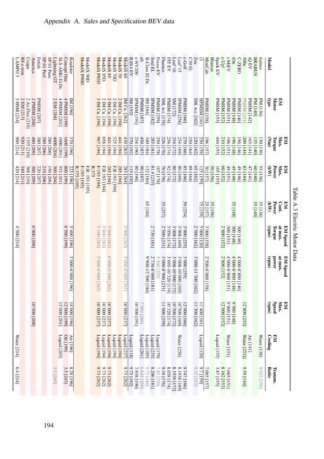
Appendix A. Sales and Specification BEV dataTable
A.3
Electric
MotorD
ataE
ME
ME
ME
MSpeed
EM
SpeedE
ME
MM
ax.M
ax.C
ont.atm
ax.atm
ax.M
ax.M
otorTorque
Power
Power
Torquepow
erSpeed
EM
Transm.
Model
type(N
m)
(kW)
(kW)
(rpm)
(rpm)
(rpm)
Cooling
Ratio
fortwo
PM[136]
130[136]
55[136]
35[136]
Water[138]
9.922[250]
BR
AB
US
PM[140]
135[140]
60[140]
35[140]
iQE
VPM
SM[142]
163[141]
47[141]
Air[141]
500ePM
SM[251]
200[144]
83[144]
12’800[252]
Water[252]]
9.59[144]
C-Z
ER
OPM
SM[146]
196[146]
49[146]
300[146]
4’000-8’800[146]
iOn
PMSM
[148]196
[148]49
[148]35
[148]300
[148]4’000-8’800
[148]9’500
[148]i-M
iEV
PMSM
[151]196
[151]49
[151]300
[151]4’000-8’800
[151]9’900
[151]W
ater[151]7.065
[151]e-U
p!PM
SM[152]
210[152]
60[152]
2’800[152]
2’800[152]
12’000[152]
8.162[153]
SparkE
VPM
SM[155]
444[155]
105[155]
Liquid
[155]3.87
[155]B
luecar50
[156]35
[156]M
iniCab
PMSM
[158]196
[157]30
[157]25
[157]3’000
[158]2’500-6’000
[158]7.065
[157]i3
HPM
SM[161]
250[159]
125[159]
75[159]
5’000[120]
11’400[161]
Liquid
[120]9.7
[159]Z
oeSM
,w.r.[162]
220[162]
65[162]
2’500[162]
3’000-11’300[162]
11’300[162]
9.32[253]
C30
El.
250[164]
89[164]
e-Golf
PMSM
[166]270
[166]85
[166]50
[254]3’000
[255]3’000
[255]12’000
[166]9.747
[166]L
eaf’15IPM
SM[256]
254[169]
80[169]
3’008[169]
3’008-10’000[169]
10’500[169]
Water[256]
8.1938[169]
Leaf’16
SM[172]
254[172]
80[172]
3’008[172]
3’008-10’000[172]
10’500[172]
8.1938[172]
FITE
VPM
SM[174]
256[174]
92[174]
3’056[174]
3’695-10’320[174]
10’320[174]
8.058[174]
Fluence.SM
,w.r.[176]
226[176]
70[176]
35[257]
2’500[231]
3’000-8’900[231]
11’000[258]
9.34[176]
FocusE
VPM
SM[259]
250[178]
107[178]
5’500[220]
Liquid
[179]7.82
[220]SoulE
l.IPM
SM[182]
285[181]
81.4[235]
2’730[181]
2’730-8’000[181]
Liquid
[235]8.206
[181]B
-Class
El.D
r.IM
[184]340
[184]132
[184]65
[184]9’900-12’500
[184]L
iquid[185]
9.73[186]
e6PM
SM[187]
450[187]
90[187]
7’000[260]
Liquid
[261]6.844
[260]e-N
V200
IPMSM
[191]254
[190]80
[190]10’500
[191]7.938
[190]R
AV4
EV
IM[192]
370[192]
115[192]
Liquid
[118]9.73
[192]M
odelS60
IMC
u.[262]430
[263]283
[264]5’000
[263]5’000-8’000
[265]16’000
[237]L
iquid[237]
9.73[262]
ModelS
702
IMC
u.[194]441
[194]285
[194]L
iquid[194]
ModelS
70D2
IMC
u.[194]525
[194]F,R
:193[194]
Liquid
[194]M
odelS85
2IM
Cu.[194]
441[194]
285[194]
5’800[263]
6’000-9’500[265]
16’000[237]
Liquid
[194]9.73
[262]M
odelS85D
2IM
Cu.[194]
658[194]
F,R:193
[194]5’800
[263]16’000
[237]L
iquid[194]
9.73[262]
ModelS
P85D3
IMC
u.[194]967
[194]F:193
[194]5’100
[263]5’000-8’600
[265]16’000
[237]L
iquid[194]
9.73[262]
R:375
ModelX
90DF,R
:193[195]
ModelX
P90DF:193
[195]R
:375[195]
Roadster
IM[196]
370[196]
225[196]
5’400[196]
5’000-6’000[196]
14’000[196]
Air[196]
8.28[196]
ConceptO
ne4
PMSM
[199]1600
[199]800
[199]6’500
[199]12’000
[199]O
il[199]3.5
[243]SL
SA
MG
El.D
r.4
PMSM
[201]1000
[201]552
[201]13’000
[201]L
iquid[203]
Lightning
GT
2E
M[204]
4000[204]
300[204]
5.5[245]
SP:01Pure
280[206]
150[206]
SP:01Perf.
280[206]
210[206]
FetishPM
SM[207]
380[207]
220[207]
Am
erica2
PMSM
[208]480
[209]300
[209]6’000
[208]10’500
[208]C
oupe2
Ax.Flux
[210]1355
[210]368
[210]R
8e-tron
2E
M[213]
920[211]
340[211]
LA
MPO
33
HSM
[214]900
[214]420
[214]4’500
[214]W
ater[214]6.4
[214]
194

A.3. Comments on selected data
T abl
eA
.4B
EV
Bat
tery
and
Cha
rgin
gD
ata
Bat
tery
Stan
dard
DC
Fast
Bat
tery
Bat
tery
(Con
t.)B
atte
ry(O
ptio
nal)
Cha
rgin
gE
nerg
yC
harg
eB
atte
ryM
ax.
Bat
tery
Spec
ific
AC
Cha
rge
Met
hod/
Cap
acity
Cap
acity
volta
gePo
wer
Num
ber
wei
ght
Ene
rgy
Bat
tery
Pow
erPe
akPo
wer
Mod
el(k
Wh)
(Ah)
(V)
(kW
)of
cells
(kg)
(Wh/
kg)
Coo
ling
(kW
)(k
W)
fort
wo
el.d
r.17
.6[1
36]
52[2
66]
339
[266
]93
[136
]17
8ca
l.98
,9[2
66]
Liq
uid
[267
]3.
3[1
38]
(22)
[268
]fo
rtw
oB
RA
BU
S17
.6[1
40]
93[1
40]
3.3
(22)
[140
]iQ
EV
12[1
41]
43[2
66]
277.
5[1
41]
150
[141
]22
0[1
42]
54.7
[266
]A
ir[1
41]
3[1
41]
CH
A[2
69]
500e
24[1
44]
63[2
59]
364
[144
]97
[144
]29
1[2
51]
88[2
59]
Liq
uid
[144
]6.
6[1
44]
C-Z
ER
O14
.5[1
46]
300
[146
]80
[146
]3.
2[1
46]
50[1
46]
iOn
14.5
[148
]80
[148
]22
1[1
48]
66ca
l.3.
2[1
48]
50/C
HA
[148
]i-
MiE
V16
[151
]50
[150
]33
0[1
51]
145
cal.
110
[270
]A
ir[2
71]
3.7
[149
]C
HA
[149
]e-
Up!
18.7
[152
]37
4n[1
52]
75[2
72]
204
[152
]23
0[1
52]
81ca
l.P a
ssiv
e[2
72]
3.6
[152
]40
/CC
S[1
52]
Spar
kE
V18
.4[1
55]
54[1
55]
400t
[155
]12
0[1
55]
192
[155
]21
5[1
55]
85[2
70]
Liq
uid
[155
]3.
3[2
73]
CC
S[1
55]
Blu
ecar
30[1
56]
410n
[156
]45
[156
]30
0[1
56]
100
cal.
Min
iCab
16[1
57]
330
[157
]3
[158
]C
HA
[274
]i3
22.0
[159
]60
[259
]36
0n[1
20]
(40)
[120
]96
[275
]23
3[2
76]
93[2
59]
Ref
rig.
[120
]7.
4[2
77]
50/C
CS
[277
]14
7[2
76]
Zoe
22[1
62]
400n
[162
]19
2[1
62]
290
[162
]76
cal.
43[2
78]
C30
El.
24[1
64]
330
[164
]73
cal.
22[2
79]
e-G
olf
24.2
[166
]75
[270
]32
3n[1
66]
264
[166
]31
8[1
66]
76.1
[270
]P a
ssiv
e[1
67]
7.2
[218
]50
/CC
S[2
18]
Lea
f’15
24[1
69]
66[2
59]
360
[169
]90
[280
]19
2[1
69]
273
cal.
87.9
[259
]Pa
ssiv
e[1
71]
3.6
(6.6
)[16
9]50
/CH
A[1
69]
Lea
f ’16
30[1
72]
83[2
70]
360
[270
]19
2[1
72]
294
cal.
102
[259
]3.
6(6
.6)[
172]
50/C
HA
[172
]FI
TE
V20
[174
]20
[150
]33
0[1
50]
100
[174
]22
4ca
l.89
.3[1
50]
6.6
[174
]C
HA
[248
]Fl
uenc
e22
[176
]65
[176
]39
8[1
76]
192
[231
]28
0[2
31]
79ca
l.3.
5(4
3)[1
77]
Focu
sE
V23
[178
]75
[259
]35
0[2
59]
287
cal.
80.2
[259
]L
iqui
d[1
78]
6.6
[178
]So
ulE
l.27
[181
]75
[259
]36
0[1
81]
90[2
35]
192
[182
]27
4.5
[182
]98
.4[2
81]
Air
[183
]6.
6[1
81]
50/C
HA
[181
]B
-Cla
ssE
l.Dr.
36[2
82]
120
[259
]36
7[2
59]
222
cal.
125.
9[2
59]
Liq
uid
[185
]10
[186
]e6
61.4
[187
]20
0[1
50]
307
[150
](1
62)[
283]
624
cal.
98.4
[150
]A
ir[2
83]
40[2
84]
100
[188
]27
0[2
83]
e-N
V20
024
[190
]36
0[1
91]
192
[191
]3.
6(6
.6)[
190]
CH
A[1
90]
RAV
4E
V41
.8[1
92]
130
[150
]38
6m[1
92]
129
[192
]45
00[2
85]
383.
5[1
92]
110.
3[1
50]
Liq
uid
[286
]10
[192
]M
odel
S60
60[2
64]
245
[259
]40
0[2
59]
353
cal.
170
[259
]M
odel
S85
85[2
64]
245
[264
]40
0[2
59]
500
cal.
170
[259
]L
iqui
d[2
37]
10(2
0)[2
62]
120/
Spr [
287]
Mod
elX
90[1
95]
250
[270
]35
0[2
70]
600
cal.
150
[270
]R
oads
ter
56[1
98]
366n
[197
]21
5[1
98]
683
1[1
96]
450
[198
]12
1[1
98]
Liq
uid
[198
]16
.8[2
41]
Con
cept
One
82[1
99]
650n
[199
](1
000)
[199
]1
400
[243
]L
iqui
d[1
99]
22[1
99]
50/C
CS
[199
]SL
SA
MG
El.D
r.60
[201
]40
0[2
01]
600
[202
]86
4[2
03]
548
[202
]10
9ca
l.L
iqui
d[2
03]
22[2
02]
Lig
htni
ngG
T44
[204
]45
0[2
04]
9[2
04]
50[2
04]
SP:0
137
[206
]7.
7[2
88]
Fetis
h54
[207
]A
mer
ica
53[2
09]
22[2
08]
Cou
pe30
[289
]74
0[2
10]
CH
A[2
90]
R8
e-tr
on90
.3[2
13]
385n
[213
]74
88[2
13]
595
[213
]15
2[2
13]
Liq
uid
[213
]7.
2[2
13]
50/C
CS
[213
]L
AM
PO3
32[2
14]
80[2
14]
400n
[214
]21
6[2
14]
360
[214
]89
cal.
Wat
er[2
14]
22[2
14]
CH
A[2
14]
195

Appendix A. Sales and Specification BEV data
TableA
.5Perform
ancedata.
Energy
Energy
Energy
Energy
Range
TopA
cc.Time
Acc.Tim
eA
cc.Time
p.dist.p.dist.
p.dist.p.dist.
Range
EPA
speed0-100
km/h
0-60m
ph(0-X
)km/h
NE
DC
EPA
City
EPA
Highw
.E
PAC
omb.
NE
DC
Com
b.M
odel(km
/h)(s)
(s)(s)
(Wh/km
)eq.(W
h/km)
eq.(Wh/km
)eq.(W
h/km)
(km)
eq.(km)
fortwo
Coupe
126[136]
11.5[136]
4.8(60)[136]
151[136]
172[259]
225[259]
196[259]
145[136]
109[266]
BR
AB
US
Coupe
130[140]
10.2[140]
163[140]
145[140]
iQE
V125
[141]14
[141]13.4
[143]134
[141]151
[266]200
[266]173
[266]85
[141]61
[266]500e
137[144]
8.9[251]
171[259]
194[259]
181[259]
140[259]
C-Z
ER
O130
[146]15.9
[146]5.9
(50)[146]126
[146]150
[146]iO
n130
[148]15.9
[148]126
[148]150
[148]i-M
iEV
130[149]
15.9[149]
125[149]
166[150]
212[150]
187[150]
160[149]
100[150]
e-Up!
130[152]
12.4[152]
8.1(80)[152]
117[152]
160[152]
SparkE
V145
[155]7.2
[221]3
(48)[155]163
[259]192
[259]176
[259]132
[259]B
luecar120
[156]6.3
(60)[156]M
iniCab
MiE
V114
[291]i3
150[159]
7.2[159]
7.0[222]
3.7(60)[223]
129[159]
152[259]
188[259]
168[259]
190[159]
130[259]
Zoe
135[162]
13.5[162]
4(48)[162]
133[278]
240[162]
C30
El.
125[164]
10.7[164]
5.9(70)[164]
175[164]
163[164]
e-Golf
140[255]
10.4[255]
6.9(80)[255]
127[255]
167[259]
199[259]
181[259]
190[255]
134[259]
Leaf’15
140[169]
11.5[169]
150[169]
166[259]
207[259]
184[259]
199[259]
135[259]
Leaf ’16
144[172]
11.5[172]
150[169]
170[270]
207[270]
186[270]
250[172]
172[270]
FITE
V148
[292]8.5
[220]3.1
(48)[220]159
[150]200
[150]177
[150]132
[150]Fluence
Z.E
.135
[176]13.7
[176]140
[293]185
[176]Focus
EV
137[294]
11.4[232]
154[232]
190[259]
211[259]
200[259]
162[294]
122[259]
SoulElectric
145[181]
11.2[181]
10.8[182]
147[181]
175[181]
228[259]
199[259]
212[181]
150[259]
B-C
lassE
l.Dr.
160[184]
7.9[184]
3.9(60)[184]
166[184]
245[259]
256[259]
250[259]
200[184]
140[259]
e6140
[187]9.2
[295]7.7
(60)[188]341
[150]322
[150]333
[150]204
[150]e-N
V200
/Evalia
122[191]
14[190]
165[191]
170[191]
RAV
4E
V161
[192]7.0
[285]267
[150]285
[150]275
[150]166
[150]M
odelS60
190[264]
6.2[264]
5.9[262]
188[263]
222[259]
217[259]
219[259]
390[264]
335[259]
ModelS
70225
[194]5.8
[296]5.5
[194]442
[296]386
[194]M
odelS70D
225[194]
5.4[296]
5.2[297]
420[296]
370[194]
ModelS
85225
[194]5.6
[296]5.4
[194]170
[263]238
[259]232
[259]235
[259]502
[296]426
[259]M
odelS85D
249[194]
4.4[296]
4.2[194]
170[263]
220[259]
198[259]
210[259]
528[296]
435[259]
ModelS
P85D249
[194]3.3
[296]3.1
[194]188
[263]234
[259]215
[259]225
[259]491
[296]407
[259]M
odelX90D
249[195]
5.0[298]
4.8[195]
232[270]
222[270]
227[270]
414[270]
ModelX
P90D249
[195]4.0
[298]3.8
[195]236
[270]233
[270]235
[270]402
[270]R
oadster201
[196]3.9
[196]160
[299]340
[299]393
[300]C
onceptOne
305[200]
2.8[199]
600[243]
SLS
AM
GE
l.Dr.
250[201]
3.9[201]
268[301]
250[201]
Lightning
GT
209[204]
5[204]
241[204]
SP:01Pure
170[206]
5.6[206]
5.3[206]
288[206]
SP:01Perf.
250[206]
3.9[206]
3.7[206]
288[206]
Fetish200
[207]4
[207]A
merica
220[209]
4.5[209]
14(200)[209]
Coupe
193[210]
3.4[210]
R8
e-tron250
[213]3.9
[211]450
[211]L
AM
PO3
220[214]
4.5[214]
200[214]
196

A.3. Comments on selected data
Table A.6 Terminated and coming BEV models.Terminated ComingScion iQ EV Chevrolet Bolt EVRenault Fluence Z.E. Porsche Concept Study Mission ERAV4 EV Audi e-tron Quattro ConceptTesla Model S 60kWh Tesla Roadster 3.0Tesla Roadster 2.5 Renovo Coupe
Detroit Electric SP:01Tesla Model 3
Table A.7 Front area vs. height times width or track width.Model iQ iOn e-Up! i3 Zoe C30 e-Golf Leaf ModelSAwh 85% 90% 85% 85% 96% 85% 84% 83% 82%Atw h 97% 103% 98% 96% 110% 97% 99% 96% 96%
1000 1200 1400 1600 1800 2000 22001.5
2
2.5
3
3.5
Curb weight (kg)
Are
a (m
2 )
Small Medium−Large High Perf. Sport
1000 1200 1400 1600 1800 2000 2200
0.25
0.3
0.35
Cd
Curb weight (kg)
1000 1200 1400 1600 1800 2000 2200
0.6
0.8
1
Cd A
(m
2 )
Curb weight (kg)
Figure A.2 Data on area, Cd and CdA, as well as estimates of area and CdA, using the foundCd values and area estimates of 80-100% of height and width, all as functions of curbweight.
classes are labeled A-G. Class A represent tires with the lowest coefficients ≤0.0065,class B 0.0066-0.0077, C 0.0078-0.009, as so on up to G ≥0.0121 [302].
Still, neither original tire brand and model, nor it’s rolling resistance coefficient
197

Appendix A. Sales and Specification BEV data
800 1000 1200 1400 1600 1800 2000 2200 2400
0.3
0.32
0.34
0.36
0.38
Curb weight (kg)
Est
. whe
el r
adiu
s (m
)
Small Medium−Large High Perf. Sport
Figure A.3 Tire radius estimation vs. curb weight.
are generally provided in BEV model specifications. Nevertheless, many manufacturersclaim to use low rolling resistance tires on their BEV models; 500e, iMiEV, Spark EV,i3, Zoe, e-Golf, Fluence, Focus, and Soul ("super low") [145,149,155,162,167,179,183,223,258,277]. In fact, only three references have been found that mentions a value; e-Up!0.007 [219], e-Golf 0.0065 [227], and Tesla Roadster 0.011, whereas the next Roadsterversion (3.0) will have 0.0089 [215].
Furthermore, few public sources of measured rolling resistance data exist. Yet in [33],data provided by a few different actors such as the US EPA (Environmental ProtectionAgency) and some of the major tire manufacturers (e.g. Michelin, Goodyear and Bridge-stone) is presented. In one of the later and largest data sets (from 2005), the Cr valuesrange from 0.0065-0.0133, with a mean value of 0.0102. It is also mentioned that dueto different factors, there is a tendency of higher average Cr values for groups of tiresmade for higher speed levels; for tires up to 180-190 km/h it was 0.0098, for tires up to210-240 km/h it was 0.0101, and for tires above 240km/h it was 0.0113. The tendency oflower Cr values for fuel economy focused vehicles and higher for performance focusedmodels is also reflected in [303], where estimated Cr values are analysed.
A.3.3 Wheel radius estimation from tire dimensionsEstimated wheel radius values for BEVs with found tire data are shown in Figure A.3as function of curb weight. Generally the small cars have a wheel radius below 0.3 m(with one exception: iQ), medium-large cars have a wheel radius between 0.31-0.37,while most values are within 0.31-0.32 m. The spread is quite large for the sport cars;0.32-0.38 m. It should be noted that the real tire radius naturally varies both by tireload and inflation pressure. It also varies during driving, since speed, acceleration anddeceleration all affect the load forces on the tires. The presented data can thus be thoughtof as maximum values.
198

A.3. Comments on selected data
A.3.4 Traction Electric Machine dataIt is here noted that the most dominating EM type in current BEVs is the permanentmagnet synchronous machine (PMSM), which can be found in at lest 22 models. Insome models, like Soul EV [182] and Leaf [256], it is specifically mentioned that inte-rior mounted permanent magnet machines (IPMSMs) are used. Five models; (B-Class,RAV4, ModelS, ModelX and Roadster) utilize induction machines (IMs), however, thesehave all been provided by Tesla Motors [185, 194, 285]. Renault’s two models Zoe andFluence are equipped with their wound rotor synchronous machine (SM w.r.) [162,176].In i3 the in-house developed hybrid permanent magnet synchronous machine (HPMSM)is used, i.e. a synchronous reluctance machine with added permanent magnets. A hybridsynchronous machine (HSM) by Brusa is also used in Lampo3. Renovo claim to use anaxial flux machine in Coupé [210].
Data on maximum torque and power is presented for almost all models while dataon continuous power is presented for 9 models. It is, however, quite unclear under whatcircumstances these values have been determined. The maximum and continuous torqueis typically strongly influenced by the machine’s cooling system design. Additionally,the maximum power level changes with the dc voltage level during driving. Some manu-facturers refer to the European type approval regulation UNECE R85 [304] in which themotor power measurement over a time duration of 30 min. is regulated as is a full loadtest over a non specified time duration of a motor that has first been run warm for threeminutes at 80% of full load. Still, the regulations leave room for interpretation, and thisshould be kept in mind when comparing data on BEV motors.
The range of maximum output torque levels are from about 130-1600 Nm (up to 440Nm for single motors), and the combined EM power range is 30-800 kW (up to 285 kWfor single motors). These are quite wide ranges. In Fig. A.4, it is shown that the maximumpower is about 1.2-2 times that of the continuous power for 9 of the models.
0 50 100 1501
1.2
1.4
1.6
1.8
2
2.2
EM Pmax.
(kW)
P max
./Pco
nt.
Small Medium−Large
Figure A.4 Max-to-continuous ratio of EM power vs. max power.
199

Appendix A. Sales and Specification BEV data
200

Appendix B
GPS-accelerometerMeasurement System
B.1 Description of the measurement systemThe measurement system is called MX3 and was delivered by HostMobility in Gothen-burg. Two units were purchased. Each unit includes a GPS along with a roof top mount-able antenna, a 3D accelerometer and 2 temperature sensors attached to the end of exten-sion cables of 1m and 3 m respectively. The GPS module is an IT500, by FasTrax. Theaccelerometer is a MMA7455L, by Freescale1, with a range of ± 2g, and a resolution ofg/64 = 0.15328(m/s2). The temperature sensors are SMT16030 by Smartec.
The unit is strapped on a flat surface in the test vehicle, with the accelerometer coor-dinate frame aligned with the vehicle’s coordinate frame. An external voltage source isneeded to power the unit, e.g. the vehicles 12V outlet or an external battery, see FigureB.1.
Data is then logged on a PC via a RS232/USB connection and a terminal software.The sampling frequency of the GPS signal is 5Hz, that of the accelerometer signal is20Hz and that of the temperature signal is 1Hz.
GPS data regarding GPS time, position (latitude, longitude and altitude), speed, dilu-tion of precision (hdop, vdop and pdop), nuber of satelites in fix etc. is received accordingto the NMEA format, from the GGA, GSA, GSV, and RMC packages. That is, no rawdata from the satellite communication (e.g distance to satellite) are available. Accordingto FasTrax, the GPS position accuracy is 1.8m, and the velocity accuracy is 0.1m/s.DGPS has not been utilized.
1The data sheet can be found at http://www.freescale.com/files/sensors/doc/data_sheet/MMA7455L.pdf
201

Appendix B. GPS-accelerometer Measurement System
(a) One of the measurement units. (b) The measurement unit strapped in a car.
Figure B.1 The measurement unit and an example of usage.
B.2 Filtering of measurement DataThe speed and altitude signals are low pass filtered with a cut off frequency of 0.5Hz,and the acceleration signal with a frequency of 2Hz. Then both speed and altitude areresampled to 20Hz. Traveled distance was calculated as the time integral of the speedsignal.
Road slope was estimated as the inverse sine of the ratio between a change in altitude(dh) and a change in traveled distance dS, for each sample (α = arcsin( dhdS )). It provedto be rather difficult to attain a fair estimate of the road slope, especially at low speedlevels close to stand still where with very small values of dh and dS, causing an unstablegrade value. In order to deal with this, a few different limiting strategies were applied,e.g. to smooth the grade within a time frame of 2 s during the mentioned situations.
Finally the estimated grade was utilized to compensate that part of the accelerometersignal that is caused by road grade, see Figure B.2.
80 100 120 140 160 180 200 220 240
−2
−1
0
1
2
3
Time (s)
Acc
eler
atio
n (m
/s2 )
Prius120403
Mlnlcke
CTH
Meas.LP Meas.GPS acc.LP Grade−corr. Meas.
Figure B.2 Example of correction for road grade of acceleration.
202

B.3. Ambiguity of measurements
B.3 Ambiguity of measurementsEven though the same driver was using the same car, drove the same route, at similartimes of the day, the logs are different, as can be seen in Table B.1, and Figure B.3 toB.5.
Table B.1 Cycle data for all CTH - Kålltorp logs.
V744
CTH Klltrp!
Cycles
Cycle!
duration!
(s)
Driven!
distance!
(m)
Max.!
speed!
(km/h)
Average!
speed!
(km/h)
Average!
running!
speed!
(km/h)
Std.!
speed!
(km/h)
Max.!pos.!
acc.!
(m/s^2)
Max.!neg.!
acc!
(m/s^2)
Average!
pos.!acc.!
(m/s^2)
Average!
neg.!acc.!
(m/s^2)
Std.!pos.!
acc.!
(m/s^2)
Std.!neg.!
acc.!
(m/s^2)
RPA!
(m/s^2)
Time!
share!pos.!
acc.!(%)
Time!
share!
neg.!acc.!
(%)
Time!
share!
standing!
(%)
120306 897 8 023 57 32 32 17 2.98 !3.10 0.42 !0.37 0.49 0.48 0.18 46 54 0.7
120307 769 7 937 63 37 37 15 2.17 !3.96 0.39 !0.40 0.36 0.47 0.18 51 49 0.2
120320 844 7 930 53 34 34 15 3.48 !3.60 0.38 !0.35 0.44 0.44 0.15 47 53 1.3
120325 737 7 854 60 38 38 16 3.28 !3.33 0.42 !0.41 0.51 0.49 0.16 45 55 0.1
120327 806 7 932 64 35 36 18 2.99 !2.70 0.43 !0.45 0.43 0.48 0.21 54 46 1.5
MEAN 811 7!935 59 35 36 16 2.98 3.34 0.41 0.40 0.45 0.47 0.18 49 51 0.8
As can be seen in Figure B.3, the exact same route was driven.
11.96 11.98 12 12.02 12.04 12.06
57.685
57.69
57.695
57.7
57.705
57.71
57.715
57.72
Long (DD)
Latit
ude
(DD
)
V744 CTH−Klltrp
12345
Figure B.3 Logs on map.
As can be seen in the upper right subplot in Figure B.4, the speed varies from log tolog. The difference may be about 20 km/h.
As can be seen in the lower right subplot in Figure B.4, the estimated road grade mayalso vary from log to log. But there is a fair level of consistency.
203

Appendix B. GPS-accelerometer Measurement System
0 100 200 300 400 500 600 700 800 9000
20
40
60
80
timeacc
(s)
Spe
ed (
km/h
)
V744 CTH−Klltrp
0 1 2 3 4 5 6 7 8 90
20
40
60
80
Distance (km)
Spe
ed (
km/h
)
V744 CTH−Klltrp
0 100 200 300 400 500 600 700 800 900−0.1
−0.05
0
0.05
0.1
timeacc
(s)
Gra
de (
rad)
V744 CTH−Klltrp
0 1 2 3 4 5 6 7 8 9−0.1
−0.05
0
0.05
0.1
Distance (km)
Gra
de (
rad)
V744 CTH−Klltrp
12345
12345
12345
12345
Figure B.4 Logged Speed and road grade.
0 100 200 300 400 500 600 700 800 900−4
−2
0
2
4
Timeacc
(s)
Acc
eler
atio
n (m
/s2 )
V744 CTH−Klltrp
0 1 2 3 4 5 6 7 8 9−4
−2
0
2
4
Distance (km)
Acc
eler
atio
n (m
/s2 )
V744 CTH−Klltrp
12345
12345
Figure B.5 Logged Acceleration.
B.4 Logged vehiclesCurb weight, powertrain power and the resulting power-to-weight-ratio for the vehiclesused during logging can be seen in Table B.2.
204

B.4. Logged vehicles
Table B.2 Selected data on logged vehicles.Brand Model Fuel type Curb Max. Power-to-weight
weight Power ratio(kg) (kW) (kW/kg)
E CAR 500 EV El. 1165 30 26Nissan Leaf El. 1613 80 50Tesla Roadster El. 1235 225 182Toyota Prius Gasoline 1365-1425 73 53Volvo C30 D2 Diesel 1428 84 59Volvo C30 Electric El. 1660 82 49Volvo V744 Gasoline 1370 86 63Volvo V70 Gasoline 1640 125 76Volvo XC60 Diesel 1920 120 63Volvo V60 PHEV Diesel & El. 2000 160+50 80 or 105
205

Appendix B. GPS-accelerometer Measurement System
206

Appendix C
Speed and Acceleration Dither
In order to get an idea of the total and relative time spent at different speed and accel-eration operating points for the Urban, Rural and Highway cycles, each cycle value isattributed to a certain acceleration and speed bin, of 0.5m/s2 and 5 km/h, see FigureC.1(a) for the Urban Test cycles. The result can also be visualized in a contour plot, seeFigure C.2(a) for total time in each bin and Figure C.2(b) for the share of total time ineach bin.
In order to get a more smooth looking contour plot, a random gaussian noise (withzero mean, and 0.5m/s2 respectively 1m/s standard deviation) was added to each op-erating point, so called dithering. Furthermore, each drive cycle with the added noise islooped 100 times, after which the total and relative time spent in each bin is divided bythe number of loops. The results can be seen in Figure C.1(b) and C.3(b), for the Urbancycles, and in Figure C.4 and C.5 for the Rural and Highway cycles respectively.
020
4060
80
−2
0
2
0
500
1000
1500
2000
Speed (km/h)Acceleration (m/s2)
Tota
l ti
me
in b
in (
s)
(a) No added noise.
020
4060
80
−4−2
02
4
0
1
2
3
4
5
x 104
Speed (km/h)Acceleration (m/s2)
To
tal
tim
e in
bin
(s)
(b) With added noise during 100 loops.
Figure C.1 Share of total time (%) of operation in acceleration bins of 0.5m/s2 and speed bins of5 km/h, for all Urban test cycles.
207

Appendix C. Speed and Acceleration Dither
0 20 40 60 80 100−4
−3
−2
−1
0
1
2
3
4
1
1
1
1
1
3
3
3
33
5
5
5
5
55
10
10
10
10
10
10
30
30
30
30
6060
60
60
120
120
30
30180
601
20
180 240 60240 60
5
Speed (km/h)
Acc
eler
ati
on
(m
/s2)
50
100
150
200
250
300
(a) Total time.
0 20 40 60 80 100−3
−2
−1
0
1
2
3
0.1
0.1
0.1
0.1
0.1
0.10.1
0.2
0.2
0.2
0.2
0.2
0.2
0.2
0.5
0.5
0.5
0.5
0.5
0.5
1
1
1
2
2 0.5
12345
1
678910
3
3
0.5
1
2
Speed (km/h)
Acc
eler
ati
on
(m
/s2)
2
4
6
8
10
12
14
16
18
20
(b) Share of total time.
Figure C.2 Total time (s) vs. Share of total time (%) of operation in acceleration bins of 0.5m/s2
and speed bins of 5 km/h, for all Urban test cycles, no added noise.
0 20 40 60 80 100−3
−2
−1
0
1
2
3
0.1
0.1
0.1
0.1
0.1
0.10.1
0.2
0.2
0.2
0.2
0.2
0.2
0.2
0.5
0.5
0.5
0.5
0.5
0.5
1
1
1
2
2 0.5
12345
1
678910
3
3
0.5
1
2
Speed (km/h)
Acc
eler
ati
on
(m
/s2)
2
4
6
8
10
12
14
16
18
20
(a) No added noise.
0 20 40 60 80 100−3
−2
−1
0
1
2
3
0.1
0.1
0.1
0.1
0.1
0.1
0.2 0.2
0.2
0.2
0.2
0.20.2
0.5
0.5
0.5
0.50.5
1
1
1
1
1
23
4
Speed (km/h)
Acc
eler
ati
on
(m
/s2)
0.5
1
1.5
2
2.5
3
3.5
4
(b) With added noise during 100 loops.
Figure C.3 Share of total time (%) of operation in acceleration bins of 0.5m/s2 and speed bins of5 km/h, for all Urban test cycles.
208

Appendix C. Speed and Acceleration Dither
0
50
100
−4
−2
0
2
0
200
400
600
Speed (km/h)Acceleration (m/s2)
Tota
l ti
me
in b
in (
s)
(a) No added noise.
0
50
100
−4−2
02
4
0
5000
10000
15000
Speed (km/h)Acceleration (m/s2)
Tota
l ti
me
in b
in (
s)
(b) With added noise during 100 loops.
Figure C.4 Share of total time (%) of operation in acceleration bins of 0.5m/s2 and speed bins of5 km/h, for all Rural test cycles.
0 20 40 60 80 100 120 140 160−3
−2
−1
0
1
2
3
0.1
0.10.10.1
0.1
0.1 0
.1
0.1
0.1
0.2
0.2
0.2
0.2 0.2
0.2
0.50.5
0.5
1
1
1
2
2
0.1
0.1
3
3
0.1
4 3
0.2
0.1
0.5
0.1
0.1
0.1
0.1
0.5
45
0.1
2
1
0.1
54 16
Speed (km/h)
Acc
eler
ati
on
(m
/s2)
1
2
3
4
5
6
(a) No added noise.
0 20 40 60 80 100 120 140 160−3
−2
−1
0
1
2
3
0.1
0.1
0.1
0.1
0.1
0.1
0.1 0.1
0.1
0.2
0.20.2
0.2
0.20.2
0.50.5
0.5
0.5
1
1
1
1
0.1
0.1
2
2
0.2
0.2
0.2
2
0.5
Speed (km/h)
Acc
eler
ati
on
(m
/s2)
0.2
0.4
0.6
0.8
1
1.2
1.4
1.6
1.8
2
(b) With added noise during 100 loops.
Figure C.5 Share of total time (%) of operation in acceleration bins of 0.5m/s2 and speed bins of5 km/h, for all Highway test cycles.
209

Appendix C. Speed and Acceleration Dither
210

Appendix D
Temperature Dependence ofsome Material Parameters
Cooling medium (ethylene-glycol) material parameters as a function of temperature, ispresented in Figure D.1 (data from [119]). Figure D.1 also include material parametersfor water [48] as a reference.
Temperature (oC)
0 50 100
Mas
s D
ensi
ty (
kg/m
3 )
950
1000
1050
1100 Glycol/Water MixWater
Temperature (oC)
0 50 100
Spec
ific
Hea
t (J
/kg
K)
3000
3500
4000
4500 Glycol/Water MixWater
Temperature (oC)
0 50 100Dyn
amic
Vis
cosi
ty (
kg/m
s)
0
0.01
0.02
0.03Glycol/Water MixWater
Temperature (oC)
0 50 100
The
rmal
Con
duct
ivit
y (W
/m K
)
0.3
0.4
0.5
0.6
0.7Glycol/Water MixWater
Figure D.1 Glycol/water mixed coolant material properties as a function of temperature [119]. Theproperties of water are also included as a reference [48]
The temperature dependence of material parameters of air is presented in Figure D.2.
211

Appendix D. Temperature Dependence of some Material Parameters
Temp. (oC)
-50 0 50 100 150 200
;ai
r (k
g/m
3 )
0.6
0.8
1
1.2
1.4
0.6
0.8
1
1.2
1.4absnorm
Temp. (oC)
-50 0 50 100 150 200
norm
;ai
r by
20oC
(-)
cp,ai
r (J/
kg K
)
1000
1010
1020
1030
norm
cp,
air b
y 20
oC
(-)
0.99
1
1.01
1.02absnorm
Temp. (oC)
-50 0 50 100 150 200
7ai
r (k
g/m
s)
#10-5
1.41.61.8
22.22.42.62.8
3
0.80.911.11.21.31.41.51.6
absnorm
Temp. (oC)
-50 0 50 100 150 200ai
r
norm
7ai
r by
20oC
(-)
6
(W/m
K)
0.02
0.025
0.03
0.035
0.04
norm
6ai
r by
20oC
(-)
0.8
1
1.2
1.4
1.6
absnorm
Figure D.2 Air material properties as a function of temperature, both absolute values and normal-ized to the value at 20C. [48]
The temperature dependence of thermal conductivity and specific heat, for the usedlamination core material is presented in Figure D.3.
Temp. (oC)
0 50 100 150 200
6la
m (
kg/m
s)
202224262830323436
norm
6la
m b
y 22
o C (
-)
11.11.21.31.41.51.61.71.8
absnorm
(a) Thermal conductivity.
Temp. (oC)
0 50 100 150 200
c p,la
m (
kg/m
s)
400
500
600
700
800
norm
cp,
lam
by
22o C
(-)
1
1.2
1.4
1.6
1.8absnorm
(b) Specific heat.
Figure D.3 Thermal conductivity and specific heat of lamination material (NO30) as a function oftemperature [105], both absolute values and normalized to the value at 22C.
The temperature dependence of thermal conductivity and specific heat, for copper(the used winding material) is presented in Figure D.4.
212

Appendix D. Temperature Dependence of some Material Parameters
Temp. ( oC)
0 100 200 300 400
6Cu
(W
/m K
)
360
380
400
420
norm
6Cu b
y 30
0K
0.94
0.96
0.98
1absnorm
(a) Thermal conductivity.
Temp. ( oC)
0 100 200 300 400
c p,C
u (J/
kg K
)
380
400
420
norm
c p,
Cu b
y 30
0K
1
1.05
1.1absnorm
(b) Specific heat.
Figure D.4 Thermal conductivity and specific heat of winding copper as a function of temperature[48], both absolute values and normalized to the value at 300 K.
Finally, the temperature dependence of thermal conductivity for the used shaft mate-rial (carbon-silicon steel) is presented in Figure D.5.
Temp. ( oC)
0 100 200 300 400
6Sh
aft (
W/m
K)
44
46
48
50
52
norm
6Sh
aft b
y 30
0K0.8
0.85
0.9
0.95
1absnorm
Figure D.5 Shaft material thermal conductivity as a function of temperature, both absolute valuesand normalized to the value at 300 K. [48]
213

Appendix D. Temperature Dependence of some Material Parameters
214

Appendix E
Cooling Channel Modelling
The Prandtl number of the coolant is much larger than one in the whole temperaturerange, as is shown in Figure E.1. This means that convection heat transfer is likely todominate over conductive heat transfer in the coolant medium.
Temperature (oC)
-40 0 40 80
Pra
ndtl
(-)
0
200
400
600
800Glycol/Water MixWater
Temperature (oC)
10 20 30 40 50 60 70
Pra
ndtl
(-)
10
20
30
40
50
60Glycol/Water MixWater
Figure E.1 The Prandtl number of the coolant as a function of temperature.
As mentioned in section 2.8.1, the heat transfer coefficient is often found via empir-ical approximations of the Nusselt number (Nu). There exist a number of different Nuapproximations for circular tubes in literature, for the three flow types: laminar, transi-tional and turbulent, which is determined by the Reynolds number (Re). The flow can beassumed to be laminar for Re ≤ 2300, and fully turbulent for Re ≥ 10, 000 [45, 48, 50].According to [45], these critical values can also be assumed for non-circular tubes. Inpractice, the critical Re values additionally depend on factors such as surface roughnessand vibrations [48], which makes them difficult to predict.
For these non-circular tubes, the hydraulic diameter Dh is used when calculating Nuand Re [48, 305]. It is four times the cross sectional area divided by the perimeter. For arectangular tube, with side a and b, Dh is
Dh =2ab
a+ b(E.1)
215

Appendix E. Cooling Channel Modelling
The Reynolds number ReD is here depending on the hydraulic diameter Dh, andthe average flow velocity vave (m/s), which in turn depends on the flow rate flL/min(liters/min), as
ReD =ρDh vave
µ=
2ρ
µ(a+ b)
flL/min
60× 103(E.2)
The Re number as a function of flow rate is presented in Figure E.2, for four differentcoolant temperatures. The flow rate needed to reach the Re value for critically turbulentflow is lower when the coolant is warmer, and higher when the coolant is colder.
Flow rate (L/min)0 5 10 15 20
Re D
,coo
l (-)
0
5000
10000
1500065oC
20oC
10oC5oC6 L/min12 L/minRe
Crit. Turb
ReFully Turb.
Figure E.2 The Reynolds number of the coolant as a function of flow rate and temperature.
For fully developed laminar flow the Nusselt number can be approximated as a con-stant that only depends on the cross sectional geometry [45, 48, 50, 305]. For rectangulartubes with width-to-height ratio of 6 (30/5 = 6), and under the assumption of a constantheat flux, Nu is 6.05 [48]. There are also expressions for how the Nu decays to that of thefully developed laminar flow value as a function of tube length, which also include en-trance effects [50,306]. For simplicity, the entrance effect is here neglected, even thoughit was noted that it could result in up to three times larger Nu values.
For turbulent flow with ReD 3000− 5× 10⁶ and Prandtl (Pr) 0.5-2000, the Nusseltnumber can be approximated to a reasonable accuracy [45, 48, 50, 306], as
Nu =(f/8)(ReD − 1000)Pr
1 + 12.7(f/8)1/2(Pr2/3 − 1)(E.3)
where the friction factor f , for smooth tubes can be approximated as
f = (0.790 ln(ReD)− 1.64)−2 (E.4)
The surface roughness for die cast aluminum is here estimated to approximately 5µm. This gives a relative roughness (i.e. ratio of surface roughness to hydraulic diameter)of 0.00006. According to a so called Moody diagram in e.g. [45], the friction factor forthis level of relative roughness may be approximated as that of a smooth surface forReDvalues lower than 106, i.e. well within the expected ReD range. Therefore, (E.4) is hereused.
216

Appendix E. Cooling Channel Modelling
The resulting Nu number as a function of flow rate is shown in Figure E.3, for dif-ferent coolant temperatures. Similarly to the ReD, the Nu number increases with bothtemperature and flow rate for turbulent flows.
Flow rate (L/min)0 5 10 15 20
Nu
cool
(-)
0
20
40
60
80
100
120
14065oC
20oC
10oC5oC6 L/min12 L/min
Figure E.3 The Nusselt number of the cooling circuit as a function of flow rate and temperature.
The temperature increase of the coolant is proportional to the amount of losses Plossabsorbed and inversely proportional to the flow rate [116], as in
∆Tcool =Ploss
ρcool cp,coolflL/min
60×103
(E.5)
The temperature increase of the coolant for different levels of total losses and flowrates is presented in Figure E.4, for the initial coolant temperature of 65C. Only minordifferences were noted for different initial coolant temperatures. For the highest lossesin the Original slot HighwayII motor: 6 kW, with a flow rate of 6 L/min, the coolanttemperature increase is at most 17C, and for moderate losses of 3 kW the temperatureincrease is 8C at most. At 12 L/min the temperature increase is 8C with 6 kW losses,and 4C with 3 kW.
Flow rate (L/min)0 5 10 15 20
"T
cool
(o C
)
0
5
10
15
20
25
30
35P
loss: ½ kW
Ploss
: 1 kW
Ploss
: 3 kW
Ploss
: 6 kW
Figure E.4 The expected increase in coolant temperature for different heat absorptions.
217