
Checking the efficiency of integrity tests in distributed and parallel database
Upload
khangminh22Category
view
1download
0
DEPARTMENT OF COMPUTER SCIENCE
SERIES OF PUBLICATIONS AREPORT A-2003-4
Design and Analysis of a Distributed Database Architecturefor IN/GSM Data
Juha Taina
To be presented, with the permission of the Faculty of Science of the Univer-sity of Helsinki, for public criticism in Sali 2, Metsätalo, on May 24th, 2003,at 10 o’clock.
UNIVERSITY OF HELSINKI
FINLAND

Contact information
Postal address:Department of Computer ScienceP.O.Box 26 (Teollisuuskatu 23)FIN-00014 University of HelsinkiFinland
Email address: [email protected]
URL: http://www.cs.Helsinki.FI/
Telephone: +358 9 1911
Telefax: +358 9 191 44441
Copyright c�
2003 Juha TainaISSN 1238-8645ISBN 952-10-1020-7 (paperback)ISBN 952-10-1023-1 (PDF)Computing Reviews (1998) Classification: C.3, H.2.1, H.2.2, H.2.4Helsinki 2003Helsinki University Printing House

Design and Analysis of a Distributed Database Architecturefor IN/GSM Data
Juha Taina
Department of Computer ScienceP.O. Box 26, FIN-00014 University of Helsinki, Finlandhttp://www.cs.helsinki.fi/u/taina/
PhD Thesis, Series of Publications A, Report A-2003-4Helsinki, May 2003, 130 pagesISSN 1238-8645ISBN 952-10-1020-7 (paperback)ISBN 952-10-1023-1 (PDF)
Abstract
Databases both in the Intelligent Networks (IN) and in the Global System for Mobile com-munications (GSM) have gained growing interest in the last few years. When the data volumeincreases, more efficient database solutions are needed to support temporal and logical consis-tency. In this thesis we give necessary background information to the IN and GSM architec-tures, do a detailed analysis of IN and GSM database data and architecture requirements, createa reference database management system architecture for IN/GSM data, define a toolbox ofqueueing model formulas for analyzing transaction-based systems, and do a detailed analysisof the reference database management system using our toolbox.
The data requirements for an IN/GSM database are based on the ITU-T recommendationsin the Q.12xx series. The GSM analysis is based on the GSM standard. Together we use thisinformation to define our multi-level distributed database management system for current andfuture Intelligent Networks.
Our database architecture is based on distribution and parallelism. It defines entry pointsfor both X.500 based requests and for internal database language requests. It is scalable, andallows specialized node-level architectures for special telecommunications services.
Using the architecture as a test system, we give a detailed queueing model analysis of it.The result of the analysis is twofold. First, the most important result is that even a complextransaction-based system may be analyzed accurately enough to get relevant and reasonableresults with our toolbox. Second, in IN and GSM environments, parallelism within a databaseis a more important aspect than distribution. Distribution has its use in a telecommunicationsdatabase, for instance to minimize physical distance from a client to the database. The specialnature of IN and GSM data allows parallel database architectures that are extremely scalable.

Computing Reviews (1998) Categories and Subject Descriptors:C.3 Special-purpose and application-based systemsH.2.1 Logical design, Information systems, models and principlesH.2.2 Physical design, Information systems, models and principlesH.2.4 Systems, Information systems, models and principles
General Terms:Analysis, Design, Evaluation
Additional Key Words and Phrases: Real-time databases, Intelligent Networks, telecom-munications requirements analysis, database architecture, queueing models, transactionprocessing analysis

AcknowledgmentsI am grateful to my supervisor, Professor Kimmo E. E. Raatikainen, for his encouragement,guidance, and endless patience in my studies. Without him I would have never completed thework. I am also grateful to Professor Sang H. Son from University of Virginia, Departmentof Computer Science, whom I was privileged to work with. He showed me a new way to doresearch and write good articles.
I would like to thank all the colleagues who were in the Darfin and Rodain projects. Ihighly appreciate the role of Professor Inkeri Verkamo, Professor Lea Kutvonen, ProfessorJukka Paakki, and Professor Timo Alanko for providing both a supportive and encouragingworking environment, and for offering interesting and valuable conversations.
The Department of Computer Science at the University of Helsinki has provided me withexcellent working conditions. I thank MA Marina Kurtén for correcting the language of thisthesis. Unfortunately my friend and colleague Pentti Elolampi, a most inspiring and goodperson, did not live to see the completion of this work. I would thank him warmly and deeplyif I could. Many thanks also belong to the other colleagues at the department.
Finally, I would like to express my deep gratitude to my parents, Anelma and Väinö Taina.They have always supported me and give courage to go on with my work. Thank you, my dearparents, thank you very much.
This work was partially supported by the University of Helsinki, Department of ComputerScience, Helsinki University of Technology, Department of Computer Science, and Helsinkigraduate school for Computer Science and Engineering (HeCSE).
Helsinki, April 14, 2003
Juha Taina


Contents
1 Introduction 1
2 Background 32.1 General database theory . . . . . . . . . . . . . . . . . . . . . . . . . . . . . . 32.2 Real-time databases . . . . . . . . . . . . . . . . . . . . . . . . . . . . . . . . 62.3 Distributed databases . . . . . . . . . . . . . . . . . . . . . . . . . . . . . . . 92.4 Intelligent Networks . . . . . . . . . . . . . . . . . . . . . . . . . . . . . . . 14
2.4.1 IN Conceptual Model . . . . . . . . . . . . . . . . . . . . . . . . . . . 152.4.2 The Future of Intelligent Networks . . . . . . . . . . . . . . . . . . . . 21
2.5 Current and future mobile networks . . . . . . . . . . . . . . . . . . . . . . . 212.5.1 GSM architecture . . . . . . . . . . . . . . . . . . . . . . . . . . . . . 222.5.2 Third generation mobile networks and beyond . . . . . . . . . . . . . 23
3 IN/GSM data analysis 273.1 IN data analysis . . . . . . . . . . . . . . . . . . . . . . . . . . . . . . . . . . 283.2 GSM data analysis . . . . . . . . . . . . . . . . . . . . . . . . . . . . . . . . 36
4 Yalin architecture 394.1 Database entry node . . . . . . . . . . . . . . . . . . . . . . . . . . . . . . . . 424.2 Clusters . . . . . . . . . . . . . . . . . . . . . . . . . . . . . . . . . . . . . . 454.3 Nodes . . . . . . . . . . . . . . . . . . . . . . . . . . . . . . . . . . . . . . . 474.4 Database transactions . . . . . . . . . . . . . . . . . . . . . . . . . . . . . . . 494.5 Database concurrency control . . . . . . . . . . . . . . . . . . . . . . . . . . . 514.6 Database global commits . . . . . . . . . . . . . . . . . . . . . . . . . . . . . 54
5 Database Analysis 575.1 General database analysis tools . . . . . . . . . . . . . . . . . . . . . . . . . . 57
5.1.1 Summary of notations and formulas . . . . . . . . . . . . . . . . . . . 645.2 Example: Traditional DBMS analysis . . . . . . . . . . . . . . . . . . . . . . 675.3 X.500 Database entry node analysis . . . . . . . . . . . . . . . . . . . . . . . 745.4 Cluster analysis . . . . . . . . . . . . . . . . . . . . . . . . . . . . . . . . . . 78
5.4.1 Cluster transaction patterns . . . . . . . . . . . . . . . . . . . . . . . . 805.4.2 Manager clusters and service times . . . . . . . . . . . . . . . . . . . 885.4.3 Analyzed transactions . . . . . . . . . . . . . . . . . . . . . . . . . . 915.4.4 Bottleneck analysis . . . . . . . . . . . . . . . . . . . . . . . . . . . . 92

vi CONTENTS
6 Conclusion 115
References 117

Chapter 1
Introduction
Specialization and reusability are the key components in current software engineering. High-quality software must be created efficiently and tailored for very specific application environ-ments. Yet often the requirements and architecture analysis are incomplete or missing. It isindeed difficult to analyze a complex piece of software from incomplete specifications.
One interesting area of specifically tailored software of standard components is arisingin database management systems. It is no longer sufficient to create a monolithic databasemanagement system and then sell it to everyone. Instead, customers are interested in tailoreddatabase solutions that offer services they need. The better the database management systemsare tailored for the customers, the smaller and more efficient they may become.
Unfortunately even a very good specification of database management needs may fail ifthe final product cannot justify data integrity and transaction throughput requirements. Withoutgood analysis tools we may be in a project of creating millions of lines of code for a product thatcan never be used. Bottlenecks must be identified and solved before we go from requirementsanalysis to design.
We are especially interested in telecommunications databases, an area which has been con-sidered very interesting both in the telecommunications and computer science research field.When database technology became mature enough to support telecommunications, new re-quirements soon started to arise. For instance, in his article, Ahn lists typical telecommunica-tions database tasks including such topics as maintaining reference data, processing traffic data,ability to process temporal queries, and high availability [Ahn94]. This information, whilespecific, is only a wish list from customers to database management system designers.
While telecommunications database research has mostly concentrated on embedded datamanagers and their requirements, little work has been done on defining and analyzing a stand-alone database architecture for telecommunications. A typical example of an embedded datamanager architecture is the IN solution for fixed and cellular networks from Nokia, as firstdescribed in 1995 [LW95]. While this is an interesting approach, it does not benefit from theclear distributed environment of the network. Such embedded systems do not form a singledistributed database nor are they very fruitful for a queueing model analysis.
The embedded system solution distributes and replicates data to several small embeddeddatabases. An alternative approach is to use a centralized fault-tolerant IN database. The bestknown research in this area is carried out at the University of Trondheim, Department of Com-puter and Information Science. Their Database systems research group is interested in creating
a very high throughput and fault-tolerant database management system. The starting point ofthe system is first described in 1991 [BS91]. Lately their research has concentrated on temporalobject-oriented databases [NB00].
Projects Darfin and Rodain at the University of Helsinki, Department of Computer Sciencehave produced a lot of interesting research results of real time fault-tolerant object-orienteddatabases for telecommunications. The most complete summary of Darfin/Rodain work is thatof the Rodain database management system architecture [TR96]. The latest results concentrateon distribution, main memory and telecommunications [LNPR00].
In addition to the telecommunication databases, both real-time and distributed databaseshave been an active research subject for several decades. The general result of combiningreal time and distribution in databases is clear: trying to add both in a general case does notwork. Fortunately for telecommunications databases we do not have to worry about the mostdifficult real-time and distribution combinations. It is sufficient to see how telecommunicationstransactions behave in a distributed environment.
In this thesis we define our database management system architecture for Intelligent Net-works (IN) and Global System for Mobile Communications (GSM). We define a toolbox ofqueueing model formulas for transaction based systems and use the formulas for a detailed bot-tleneck analysis of the IN/GSM database management system. In the analysis we use simplequeueing model tools that we have developed for this type of database management systemanalysis. We show that very large systems can be analyzed efficiently with our toolbox.
The rest of the thesis is structured in five chapters. Chapter 2 gives background informationon databases, Intelligent Networks, and current and future mobile networks. In Chapter 3we present our IN and GSM data analysis. In Chapter 4 we introduce our IN/GSM databasemanagement system architecture along with interesting areas of concurrency control and globaltransaction atomicity issues. In Chapter 5 we first introduce our derived queueing model fortransaction-based bottleneck analysis and then show how the model can be efficiently used inanalyzing a very complex database management system. The analysis is included, along withthe results. Finally, Chapter 6 summarizes our work.
Main contributionsIn the following we list the main contributions of the thesis.
1. We define a queueing model toolbox for transaction based systems. The model offerssimple yet comprehensive formulas for analyzing various types of systems that use trans-actions for data management and system execution. The formulas are defined to be usefulfor analyzing bottlenecks of database management systems.
2. We define our real-time distributed database reference architecture for IN/GSM and givea detailed analysis of the bottlenecks and transaction execution times of the system usingour queueing model tools.
3. We give a detailed IN and GSM data and transaction analysis that is based on the INrecommendations and GSM standardization. We use the analysis results in the IN/GSMdatabase analysis.
4. We show in the analysis that distribution is an over-valued aspect in an IN/GSM database.Instead, parallelism can be very useful in the database.

Chapter 2
Background
2.1 General database theoryA database is a collection of data that is managed by a software called a database managementsystem (DBMS). The DBMS is responsible for database data maintenance so that databaseclients can have reliable access to data. The DBMS must also ensure that database data is con-sistent with its real world equivalence. This property of database data is called data consistency.
The only way to access database data is with a transaction. A transaction is a collectionof database operations that can read and write data in a database. It is similar to a process inan operating system. Like processes in operating systems, transactions have identities and mayhave a priority. Transactions are the only way to access data in a DBMS.
When a transaction executes in a DBMS, the operations of the transaction are either allaccepted or none accepted. If the operations are accepted, the transaction has committed. Ifthey are not accepted, the transaction is aborted. Only after a commit the changes made by thetransaction are visible in the database.
A DBMS needs to support certain transaction properties to offer a reasonable access to thedatabase. Usually the properties are listed in four aspects of transactions: atomicity, consis-tency, isolation and durability. These are referred to as the ACID-properties of transactions.
� Transaction atomicity. Atomicity refers to the fact that a transaction is a unit of operationsthat are either all accepted or none accepted. The DBMS is responsible for maintainingatomicity by handling failure situations correctly when transactions execute in parallel.
� Transaction consistency. The consistency of a transaction defines its correctness. A cor-rect transaction transfers a database from one consistent state to another. An interestingclassification of consistency can be used with the general transaction consistency the-ory. This classification groups databases into four levels of consistency [GLPT76]. Theclassification is based on a concept of dirty data. A data item is called dirty if an uncom-mitted transaction has updated it. Using this definition, the four levels of consistency areas follows.
– Degree 4. Transaction T sees degree 4 consistency if
1. T does not overwrite dirty data of other transactions,

4 2 BACKGROUND
2. T does not commit any writes until it completes all its writes,3. T does not read dirty data from other transactions, and4. other transactions do not dirty any data read by T before T completes.
– Degree 3. Transaction T sees degree 3 consistency if
1. T does not overwrite dirty data of other transactions,2. T does not commit any writes until it completes all its writes, and3. T does not read dirty data from other transactions.
– Degree 2. Transaction T sees degree 2 consistency if
1. T does not overwrite dirty data of other transactions, and2. T does not commit any writes until it completes all its writes.
– Degree 1. Transaction T sees degree 1 consistency if
1. T does not overwrite dirty data of other transactions.� Transaction isolation. Isolation states that each transaction is executed in the database
as if it alone had all resources. Hence, a transaction does not see the other concurrentlyexecuting transactions.
� Transaction durability. Durability refers to transaction commitment. When a transactioncommits, the updates made by it to the database are permanent. A new transaction maynullify the updates but only after it has committed. Neither uncommitted transactions northe system itself can discard the changes. This requirement is important since it ensuresthat the results of a committed transaction are not lost for some unpredictable reason.
A good DBMS must support ACID-properties. Theoretically the simplest way to supportthe properties is to let every transaction access the entire database alone. This policy supportsatomicity, since a transaction never suffers interference from other transactions, consistency,since the database cannot become inconsistent when transactions cannot access uncommitteddata, isolation since each transaction has undisturbed access to the database, and durabilitysince the next transaction is not allowed to execute before the previous transaction has beencommitted or aborted. However, serial access to the database is not a good approach except tovery small databases since it seriously affects resource use. Whenever a transaction is blocked,for instance when disk access is needed, the whole database is unaccessible.
A better alternative than forcing serial access to the database is to allow transactions to exe-cute in parallel while taking care that they maintain data consistency in the database. When theDBMS supports data consistency, transaction operations may be interleaved. This is modeledby a structure called a history.
A history indicates the order in which operations of transactions were executed relative toeach other. It defines a partial order of operations since some operations may be executed inparallel. If a transaction Ti specifies the order of two of its operations, these two operationsmust appear in that order in any history that includes Ti. In addition, a history specifies theorder of all conflicting operations that appear in it.
Two operations are said to conflict if the order in which they are executed is relevant. Forinstance, when we have two read operations, the result of the operations is the same no matterwhich one is executed first. If we have a write operation and a read operation, it matters whetherthe read operation is executed before or after the write operation.
2.1 General database theory 5
A history H is said to be complete if for any transaction Ti in H the last operation is eitherabort or commit. Thus, the history includes only transactions that are completed.
While histories and complete histories are useful tools for analyzing transaction effects oneach other, they can also become very complex since they include all transaction operations.Yet usually we are mostly interested in conflicting operations and their effects. Due to this asimpler tool called serialization graph (SG) [BHG87] is derived from histories.
A serialization graph SG of history H, denoted as SG � H � , is a directed graph whose nodesare transactions that are committed in H, and whose edges are all Ti � Tj � i �� j � such that oneof Ti’s operations precedes and conflicts with one of Tj’s operations in H.
In order to display histories we use the following definitions. Let us define oi to be anoperation o for transaction Ti, and o j be an operation o for transaction Tj. Let the set of possibleoperations be {r,w,c,a} where r=read, w=write, c=commit, and a=abort. When operation oiprecedes operation o j, operation oi is listed before operation o j.
For example, let us have the following history.
H � r1 � x � w2 � x � r2 � y � c2w3 � y � c3w1 � x � c1
The history includes transactions T1 T2 T3. It is a complete history the last operation ofeach transaction is commit. The serialization graph of the history is
SG � H � � T1 � � T2 � T3 �The serialization graphs (and histories as well) are used in serialization theory. A history H
is said to be serializable if its committed projection, C � H � , is equivalent to a serial history Hs[BHG87]. The equivalence here states that the effects of the transactions in C � H � are equal tosome serial execution order of the same transactions.
A serializable history causes the same changes and results to a database as some serialexecution order of the same transactions. In other words, serializable transactions preserveconsistency of the database since serial transactions do the same.
In order to recognize serializable transaction execution orders, we need to examine historiesand serialization graphs. A history H is serializable, if and only if its serialization graph SG � H �is acyclic. This is the fundamental theorem of serializability theory. It can be found for instancefrom the book by Bernstein, Hadzilacos, and Goodman, pp. 33 [BHG87].
For instance, in the previous history example, the serialization graph contains a cycleT1 � T2 � T1. Hence, the history is not serializable.
Serializable transactions manage atomicity, consistency, and integrity of ACID-properties.Durability is not necessarily met in serializable transactions which can be seen in the followinghistory:
H � w1 � x � r2 � x � c2a1
History H is complete and its serialization graph SG � H � is acyclic. Yet the history does notpreserve durability. Since T1 is aborted, T2 should be aborted as well. Unfortunately this is notpossible. Transaction T2 has committed so it no longer exists in the system.
As the example shows, we must take extra care to preserve durability in histories. Thisaspect of transactions is called transaction recoverability.
The recovery system of a DBMS should force the database to contain all effects of commit-ted transactions and no effects of unfinished and aborted transactions. If every transaction will
6 2 BACKGROUND
eventually commit, all the DBMS has to do is to allow transactions to execute. No recovery isneeded. Hence, the recovery is needed only for managing the effects of aborted transactions.
When a transaction aborts, the DBMS must nullify all changes that the transaction hasmade to the database. This implies two types of changes: changes to data and changes to othertransactions that have read data that has been updated by the aborted transactions.
The DBMS can nullify the changes to data by restoring the old values. The changes totransactions is more complex. If transaction T1 reads data written by transaction T2 and T2aborts, T1 must also be aborted. Moreover, if transaction T3 reads data written by transactionT1, it must also be aborted even if it does not read data written by T2. This causes a cascadingabort where a chain of transactions must be aborted in order to nullify the effects of one abortingtransaction. Although a DBMS does not necessarily have to avoid cascading aborts, they aregenerally not acceptable. The cascading abort chain can be of arbitrary length and every abortwastes resources.
When the DBMS allows a transaction to commit, it at the same time guarantees that allthe results of the transactions are relevant. This is a stronger guarantee than one would firstthink. For instance, let us take the previous example with transactions T1 and T2. The initialconditions are the same but now transaction T2 commits. When transaction T1 is aborted, theresults of transaction T2 should be nullified. Unfortunately this is not possible, since durabilitystates that the changes T2 has made to the database are permanent. This execution order is notrecoverable.
A DBMS can tolerate cascading aborts, but due to the nature of the durability, it cannottolerate non-recoverable execution orders. Hence, all execution orders of transactions shouldalways be recoverable. Fortunately executions that avoid cascading aborts are a true subsetof executions that are recoverable [BHG87]. Thus, if a DBMS supports histories that avoidcascading aborts, it automatically supports recoverable histories.
We can avoid both non-recoverable executions and cascading aborts if we require that theexecution of a write operation to a data item x can be delayed until all transactions that havepreviously written to x are either committed or aborted, and that all read operations to x aredelayed until all transactions and did writes to x are either committed and aborted. Togetherthese define a strict transaction execution order. A strict order is basically the same than thedegree 2 consistency mentioned earlier.
2.2 Real-time databasesIn a real-time database management system (RT-DBMS) both data and transactions may havetiming constraints. A timing constraint states that an event must happen before or at a specifictime. Otherwise the element where the timing constraint is set, is invalidated. In data, a missedtiming constraint states that the data item becomes invalid. In transaction, it states that thetransaction cannot fulfill its task.
A data item that has a timing constraint is called temporal. A RT-DBMS must support theoperations and consistency of both static and temporal data. Temporal data is stored informationthat becomes outdated after a certain period of time [Ram93].
Real-time systems are used in environments where exact timing constraints are needed;databases are used in environments where logical data consistency is needed. Together theserequirements state when a real-time database is useful. As listed in [Ram93],

2.2 Real-time databases 7
� database schemas help to avoid redundancy of data as well as of its description;� data management support, such as indexing, assists in efficient access to the data; and� transaction support, where transactions have ACID-properties, assist in efficient concur-
rent application use.
Temporal and logical consistency can be divided into two aspects: data consistency andtransaction consistency [CDW93]. The former defines data issues. The latter defines dataaccess issues.
Data-temporal consistency deals with the question of when data in a database is valid. Staticdata is always valid. Temporal data is valid if it was previously updated within a predefined timeperiod. Data-logical consistency deals with the question of how data is consistent. A data entityis consistent if both its value and references to it are consistent with the rest of the database.
Transaction-temporal consistency deals with the question of when and how long a transac-tion is valid. Transaction-temporal consistency is maintained with deadlines that define whenat the latest a transaction should commit. Transaction-logical consistency deals with the ques-tion of how transactions can execute without interfering with each other for more than allowed.Usually the appropriate interference level is no interference. In such a case, transactions mayaccess data as long as their access histories can be ordered so that they could have been executedalone in the database.
From our analysis’ point of view, the most interesting entity in a RT-DBMS is a concurrencycontroller. Yu, Wu, Lin, and Son have written an excellent survey of concurrency control andscheduling in real-time databases [YWLS94]. In the article they list concurrency controllertasks such as conflict detection, conflict resolution, serialization order and run policy.
The concurrency controller is responsible for maintaining logical consistency at a prede-fined level. The temporal consistency level is more a design decision than a concurrency con-troller requirement since temporal consistency constraints are derived from the timing con-straints outside the database. Often a RT-DBMS that is logically consistent is also temporallyconsistent. However, this is not a requirement. Temporally correct serializable schedules are asubset of all serializable schedules [Ram93].
Generally we have two approaches for concurrency control: the pessimistic approach andthe optimistic approach. In a pessimistic concurrency control the concurrency controller as-sumes that a conflict will occur and checks this as early as possible. In an optimistic concur-rency control the concurrency controller assumes that no conflicts will occur and checks thisassumption as late as possible. Pessimistic methods cause blocking where a transaction mustwait for other transactions to release resources. Optimistic methods cause restarts where atransaction must be started over after a data access conflict has been detected.
When an access conflict is detected in a pessimistic concurrency controller, the controllermust either block or abort one of the conflicting transactions. In traditional database man-agement systems the latter transaction is usually blocked until the resource is free to use. In aRT-DBMS this policy may lead to priority inversion where a high priority transaction is waitingfor a low priority transaction to free resources. The simplest way to resolve a priority inversionconflict is to abort the low priority transaction. This wastes the resources that the lower prioritytransaction has already used. Sometimes the aborted transaction is very close to the finishingpoint, in which case it would be better to let the transaction finish its execution.
Next to aborting the low priority transaction, the other way to resolve the conflict is to let thelower priority transaction execute at a higher priority until it has released the needed resources.

8 2 BACKGROUND
In the simplest form, the lower priority transaction inherits the priority of the higher prioritytransaction. This method is called Priority Inheritance, as proposed in [SRL90]. This can leadto a priority inheritance chain where several low priority transactions must gain a higher priorityand finish execution before the high priority transaction gets the requested resources. In PriorityCeiling, also proposed in [SRL90], the high priority transaction is never blocked for more thana single lower priority transaction. This is achieved by keeping a priority ceiling to all lockedresources and keeping an ordered list of the prioritized transactions. A transaction may start anew critical section only if its priority is higher than the ceiling priorities of all the resources inthe section. The algorithm needs fixed priorities to the transactions. A similar method calledDynamic Priority Ceiling is proposed in [SRSC91], except that it accepts priorities that arerelative to transaction deadlines while Priority Ceiling needs fixed resources.
Two-phase locking (2PL) [EGLT76] and its variants are the most common pessimistic con-currency control method in current database management systems. They perform well in tra-ditional databases without transaction deadlines. Concurrency control in 2PL and its variantsis based on locks. The locks are used in two phases: expanding phase and shrinking phase. Inthe expanding phase a transaction asks locks to the resources it wants to access. In the shrink-ing phase the transaction releases the accessed locks and locked resources. The transaction isallowed to ask for more locks as long as it has not released any of the previous ones.
Optimistic methods are suitable for real-time databases. It is often easier to let a transactionexecute up to the commit point and then do a conflict check than to have full bookkeeping ofhard locks in pessimistic methods. Moreover, neither deadlocks nor priority inversion happen inoptimistic methods. Optimistic methods are not used in traditional databases since every restartof a transaction is expensive. The situation is different for real-time databases where the valueof a transaction is nullified or lowered after the deadline. Hence, if a low-priority transactionis aborted due to a conflict, it may not need a restart at all if it has already missed its deadlineor has no way to reach it. Naturally the number of aborted transactions should be minimizedsince resources are still wasted. Indeed, if deadlines allow, it may sometimes be reasonable tolet a low priority transaction commit and abort higher priority transactions. Usually at mosttwo transactions are conflicting with the committing transaction. The committing transaction isknown to commit while none of the conflicting transactions are guaranteed to meet deadlinesand commit.
The original optimistic methods are all used in real-time databases, but new methods havealso been designed. Perhaps the best method is called Dynamic adjustment of serializationorder, or OCC-TI [LS93]. It is based on the idea that transactions can be ordered dynamicallyat the validation phase to minimize conflicts and hence restarts. A revised version of the methodthat further minimizes the number of restarts has been presented by Lindström [Lin00].
A very interesting family of concurrency control algorithms, called Speculative Concur-rency Control (SCC) algorithms, is the latest major addition to the concurrency control field[BB95, BB96, BN96]. The SCC algorithms define a set of alternate transaction schedulingswhen a conflict candidate is detected. These shadow transactions execute speculatively on be-half of a given uncommitted transaction to protect against blockages and restarts The shadowtransactions are adopted only if one or more of the suspected conflicts materialize. In thegeneric Speculative Concurrency Control algorithm with k Shadows (SCC-kS), up to k shad-ows are generated after conflict candidate detection.
The SCC-kS algorithm shows a very interesting approach to concurrency control. It usesspare resources in a DBMS to create the shadow transactions. The authors have also proposed a

2.3 Distributed databases 9
RT-DBMS variation with deferred commit called SCC-DC that considers transaction deadlinesand criticality [BB96].
The question of what concurrency control methods best suit a database management sys-tem at different workloads and environments has been a major theme in performance studiesand concurrency control research, both in traditional and real-time databases. In conventionaldatabase systems pessimistic algorithms that detect conflicts before data item access and re-solve them by blocking transactions give better performance than optimistic algorithms, espe-cially when physical resources are limited. If resource utilization is low enough so that evena large amount of wasted resources can be tolerated, and there are a large number of transac-tions available to execute, then a restart-oriented optimistic method is a better choice [BHG87].In addition, the delayed conflict resolution of the optimistic approach helps in making betterdecisions in conflict resolution, since more information about conflicting transactions is avail-able at the later stage [LS94]. On the other hand, the immediate conflict resolution policy ofpessimistic methods may lead to useless blocking and restarts in real-time databases due to itslack of information on conflicting transactions at the time when a conflict is detected [HCL92].Also the SCC approach is interesting when resources are sufficient.
2.3 Distributed databasesThe history of distributed databases goes back to times when both disks and memory wereexpensive. Since those times the prices of memory and disks have decreased enough that theadvantages of distribution compared to a single system are not significant. Lately, however,new distributed applications find a distributed database architecture useful. Such applicationsinclude multimedia, World Wide Web, and telecommunications.
The authors in [CP84] give a definition for a distributed database:
A distributed database is a collection of data which are distributed over differentcomputers of a computer network. Each site of the network has autonomous pro-cessing capability and can perform local applications. Each site also participatesin the execution of at least one global application, which requires accessing data atseveral sites using a communication subsystem.
Data in a distributed database is divided into fragments. Each fragment is a set of data itemsthat are managed by a computer, or rather a local database management system in the computer.From now on we call the pair computer and its database management system a node. A nodein a distributed database may include several fragments, and a fragment may belong to severalnodes. Usually it is preferred that a node holds exactly one fragment of data, and a fragmentbelongs to exactly one node. It simplifies distributed database management and cooperationbetween database nodes.
Since the definition of a distributed database includes a set of local applications, ordatabases, it is natural to compare distributed and traditional non-distributed databases. It turnsout that the distributed database is very close to a traditional database. This implies that tradi-tional database results can be used or modified to suit distribution. The areas to consider are theACID-properties, data independence, data redundancy, physical implementation, recovery, andconcurrency control.

10 2 BACKGROUND
� ACID-properties. The ACID-properties, as mentioned earlier, are atomicity, consistency,isolation, and durability. We will cover them in turn here.
– Atomicity. Both traditional and distributed transactions are atomic. That is, thewrites that a transaction executes are visible to other transactions only after thetransaction commits. However, the methods to achieve atomicity differ in imple-mentations. In a distributed environment communication between nodes must alsobe taken into account.
– Consistency. Data in both a traditional database and in a distributed database mustbe consistent. The consistency to committed transactions is important since data canbe internally inconsistent as long as it is visible only to an uncommitted transaction.The same is true in a distributed database. The database must remain consistent alsoin case of communication failures between nodes.
– Isolation. An uncommitted transaction does not affect calculations and results ofother transactions. In a distributed database this includes both local-global andglobal-global transaction isolation. The former occurs when a local and a dis-tributed transaction try to access the same resources. The latter occurs when twodistributed transactions compete about the same resources.
– Durability. Once a transaction commits its changes to the data become permanentin the database. This holds true both in a traditional and in a distributed database. Ifthe changes affect a replicated data item, all replicants should hold the same valueafter the commit, or alternatively all replicants with old values should be madeinvalid.
� Data independence. Data independence states that the stored data in a database is in-dependent of the actual implementation of the data structures. This is true both for tra-ditional and distributed databases. However, distributed databases have a new aspect:distribution transparency. It states that to a certain level data is independent of its loca-tion. At the highest level a transaction does not see data distribution at all. At the lowestlevel each application can see data distribution and access data in a node independentlyfrom other nodes and other applications.
� Data redundancy. In a traditional database, redundant data is considered a drawback tothe system performance. Due to this, various approaches, such as normal forms in rela-tional databases, have been designed to reduce data redundancy. In a distributed database,data can sometimes be redundant. The level of redundancy depends on the chosen de-sign approach. Usually a single node holds one data item only once. A multiversioningdatabase is an exception to this rule. It may hold several versions of the same data item.Multiversioning is used in traditional databases as well. On the other hand, some datamay have copies on different nodes. This is called data replication. Usually replicationis invisible to transactions. It is used for minimizing distributed read transactions. Thedrawback is the extra complexity of update transactions and fault-tolerance.
� Fault tolerance and recovery. In a traditional database, fault-tolerance and recovery in-cludes policies for aborted transactions, and for physical and software system failures.When data is committed, it is available to other transactions. In a fault-tolerant envi-ronment, the recovery procedure is invisible to the users. The database is available even

2.3 Distributed databases 11
during a system failure. In a distributed environment, also site and network failures mustbe taken into account. This affects situations when nodes must co-operate and exchangemessages. It is not possible to create a protocol that can handle all recovery situations ina distributed database [BHG87].
� Concurrency control. Concurrency control allows transactions to execute in parallel andstill see the database as a single entity that is only for their use. This is achieved via aconcurrency control policy. The chosen policy must guarantee that transaction executionmaintains data consistency. In a distributed database, two levels of concurrency controlmust be taken into account. First, the local concurrency control policy in a node is similarto the policy in a traditional database. Second, a global concurrency control policy isneeded to guarantee serializability between distributed transactions. A local concurrencycontrol policy is not sufficient for this.
The concurrency control policy in a distributed database may be divided into two policies:local policy and global policy. The local policy affects all transactions that are active in a node.The global policy affects only transactions that are active in several nodes.
When a transaction exists only in a single node, it may still affect the global concurrencycontrol. For instance, let us have transactions T1,T2, and T3 in the distributed database. Thetransactions T1 and T3 are active in nodes 1 and 2, while transaction T2 is active only in node 1.Moreover let us have the following histories:
H1� r1 � x � w2 � x � r2 � y � w3 � y � c1c2c3
andH2
� r3 � z � w1 � z � c3c1 �If we take only global transactions T1 and T3, we do not have a cycle in the global serializationgraph SG � H1 H2 � . However, when T2 is included, we have a cycle T1 � T2 � T3 � T1 whichneeds to be detected.
A local concurrency control policy is similar to the local policy in non-distributed databases.Each transaction is controlled by the local concurrency controller. In principle, such transac-tions could have a different concurrency control policy on different nodes.
A global concurrency control policy needs to take care of conflicts that affect several nodes.In order to achieve this, three alternate policies are possible.
1. Local concurrency controllers co-operate to achieve global concurrency control. Thisis seldom done since depending on the chosen global concurrency control policy thiscan generate several messaging phases between local nodes. The overhead of such adistributed concurrency control policy is too high for most cases.
2. The distributed database has a global concurrency control coordinator. The coordinatoris responsible for the global concurrency control policy. The coordinator takes care ofthe global serialization by keeping track of global transaction conflicts. The advantageof this approach is that local concurrency controllers need not be aware of the globalconcurrency control policy. The global coordinator can manage all conflicts alone as longas it informs the local nodes of what to do in conflicts. The drawback of the approach isthat the global coordinator can easily become a bottleneck of the system. Neverthelessthis approach is better than the democratic approach where local concurrency controllersco-operate.

12 2 BACKGROUND
3. All transactions are considered local, and global concurrency control is achieved by con-trolling transactions in nodes. This is a restricting approach that works only with fewconcurrency control mechanisms.
When a new transaction request arrives to a transaction manager, it creates a new local trans-action for it. Alternatively, when it is known which nodes will participate in this transaction, thetransaction may immediately be divided into a set of subtransactions, each of which executesin one node. The transaction in the arriving node then becomes the leader of this transaction.
A local transaction may be promoted to a distributed transaction when it wants to accessa data item that is not in its node. In such a case the transaction manager sends a subtrans-action request to the node where the requested data item resides. Due to this the nodes musthave knowledge of data in other nodes. Usually this is implemented with directories. Theleader transaction gathers collected information from the subtransactions. When all necessaryinformation is collected, the leader is ready to commit.
Once the leader is ready to commit, it co-operates with the subtransactions to find out if thetransaction should commit or abort. There are several algorithms to implement cooperation,but the basic idea in all of them is that the commit should be atomic. Either the leader andsubtransactions are all committed, or they are all aborted. This is a approach that never violatesconsistency.
In any atomic commit protocol, each process may cast one of two votes for global commit:Yes or No, and may reach one of two decisions: commit or abort. Furthermore, in order toguarantee atomicity, the atomic commit protocol must allow all participants to reach decisionsthat guarantee the following rules [BHG87]:
1. All participants that reach a decision reach the same one.
2. A participant cannot reverse its decision once it has reached one.
3. The commit decision can only be reached if all participants voted Yes.
4. If there are no failures and all processes voted Yes, then the decision will be to commit.
5. Consider any execution containing only failures that the algorithm is designed to tolerate.At any point in this execution, if all existing failures are repaired and no new failuresoccur for sufficiently long, then all processes will eventually reach a decision.
Various protocols have been introduced to preserve atomicity. The best known of these iscalled the two-phase commit (2PC) protocol [Gra78]. Assuming no failures, it goes as follows:
1. The coordinator sends a VOTE-REQ (vote request) message to all subtransactions.
2. When a subtransaction receives a VOTE-REQ, it responds by sending to the coordinatora message containing that participant’s vote: Yes or No. If the subtransaction votes No,it decides to abort and stops.
3. The coordinator collects the vote messages from all participants. If all of them wereYes and the coordinator’s vote is also Yes, the coordinator decides to commit and sendsCOMMIT messages to all participants. Otherwise, the coordinator decides to abort andsends ABORT messages to all participants that voted Yes. In either case, the coordinatorthen stops.

2.3 Distributed databases 13
4. Each subtransaction that voted Yes waits for a COMMIT or ABORT message from thecoordinator. When it receives the message, it decides accordingly and stops.
The basic 2PC satisfies the listed rules for atomic commit protocols as long as failures donot occur. However, when for some reason the communication between subtransactions and thecoordinator is distracted, it is possible that a subtransaction is uncertain of the correct behavior.In such a case the subtransaction is in a blocked state. It neither can abort or commit since itdoes not know what the other subtransactions and the coordinator have decided. Naturally theblocked subtransaction may wait as long as the failure is corrected. This satisfies requirement5 earlier. Unfortunately the decision may be blocked for an indefinitely long time.
Since the uncertainty of the correct decision can cause serious problems, it would be de-sirable to have an atomic commit protocol where participants do not have uncertainty times.Unfortunately such a protocol would require that a participant would cast a vote and learn thevotes of all other participants all at once. In general, this is not possible [BHG87].
The basic 2PC may be too strict in a real-time environment. Time may be wasted in thecommit procedure when ready subtransactions must block their updated data items when theyare waiting for the global commit result from the leader. Due to this, a protocol called TheReal-time Implicit Yes-Vote protocol was proposed 1996 by Al-Houmaily and Chrysanthis[AHC96]. The protocol is based on the assumptions that 1) each node employs a strict 2PLprotocol for concurrency control that takes into consideration the priority of transactions, and2) a specific distributed logging protocol called physical page-level write-ahead logging. Withthese assumptions the protocol uses commit processing that is overlapped with the executionof the transactions’ operations [AHC96]. This algorithm is better suited for real-time environ-ments than a regular two-phase commit since it takes the priorities into account and allowstransactions to execute in parallel with the commit processing.
An optimistic 2PC-based commit protocol PROMPT (Permits Reading Of ModifiedPrepared-data for Timeliness) is based on the assumption that a distributed transaction willnot be aborted at commit time. The committing transaction can lend data to other transactionsso that it does not block them. In the algorithm, two situations may arise depending on thefinishing times of the committing transactions [GHRS96, HRG00]:
� Lender Finishes First. In this case the lending transaction receives its global decisionbefore the borrowing transaction. If the global decision is to commit, both transactionsare allowed to commit. If the decision is to abort, both transactions are aborted. Thelender is naturally aborted because of the abort decision. The borrower is aborted becauseit has read inconsistent data.
� Borrower Finishes First. In this case the borrower has reached its committing stagebefore the lender. The borrower is now made to wait and not allowed to send a YES votein response to the coordinator’s PREPARE message. The borrower has to wait until suchtime as the lender receives its global decision or its own deadline expires, whichevercomes earlier. In the former case, if the lender commits, the borrower is allowed torespond to the coordinator’s message. In the latter case, the borrower is aborted since ithas read inconsistent data.
In summary, the protocol allows transactions to read uncommitted data in the optimisticbelief that the lower priority transaction that is holding data will eventually commit. Usuallyit is not recommended that a transaction reads uncommitted data because this can lead to the

14 2 BACKGROUND
problem of cascading aborts [BHG87]. However, the problem does not occur in OptimisticCommit Protocol because the abort chain includes only the lender and the borrower. Othertransactions are not aborted if the lender aborts because the borrower is not in the preparedstate and hence it does not cause any further aborts [GHRS96].
An interesting class of atomic commit protocols called one-phase commit protocols havegot more attention especially in distributed real-time database research [AGP98], [HR00,SC90]. There is no explicit voting phase to decide on the outcome (commit or abort) of thetransaction in these protocols since subtransactions enter the prepared state at the time of send-ing the work completion message itself. Thus, the commit processing and data processingactivities are overlapped since not all subtransactions enter the prepare state at the same time.This in turn causes longer blocking times since the prepared subtransactions cannot be abortedbefore final consensus is reached. Due to this one-phase commit protocols are best suited fordistributed transactions with small subtransactions.
2.4 Intelligent NetworksIntelligent Networks (IN) are the first step towards an open telecommunications service envi-ronment. The basic idea of IN is to move service logic from switches to special IN functionlogics called Service control functions (SCF). With SCFs it is possible to let telephone switch-ing software be relatively static when new service logic programs are used in SCFs to imple-ment new services. Hence IN architecture can be used for special service creation, testing,maintenance, and execution.
Currently IN is used in most telecommunications environments. It is under standardizationboth in Europe and in the U.S. The standardization committees, ITU-T (International Telecom-munication Union - Telecommunication standardization sector), ETSI (European Telecommu-nications Standards Institute), and ANSI AIN committee (American National Standards In-stitute Advanced Intelligent Network committee) are all defining the IN concept. ETSI andITU-T define practically equal IN concepts. ANSI AIN is somewhat different although thereis substantial co-operation with the European standardization committees. We follow the ITU-T/ETSI recommendations for the Intelligent Networks.
The basic standard that defines the framework of other IN standards in ITU-T is the Q.120xseries. It defines a framework for ITU-T IN standards with possible revisions. The standardsthemselves are structured to Capability sets. The first Capability set CS-1 was introduced in theQ.121x series. The future Capability sets will be introduced in the Q.12nx series, where n is thecapability set number. This Section is based on IN CS-1 in the Q.121x series. The Capabilitysets are backward compatible to the previous ones so that the implementation of services canbe progressed through a sequence of phases [GRKK93].
The CS-1 capabilities support IN services that apply to only one party in a call. The CS-1capability set is independent of both the service and topology levels to any other call parties[ITU93b]. In other words, the services are only dependent on a single call party and the sameservice may be used again on a different environment with possibly different parameters. Thisdefinition restricts the CS-1 service definitions, but in turn it gives a good basis for the futureIN architectures.
The IN environment is based on hooks that recognize IN-based services. When a servicerequest arrives, a trigger in a basic call processing node activates the actual IN service logic
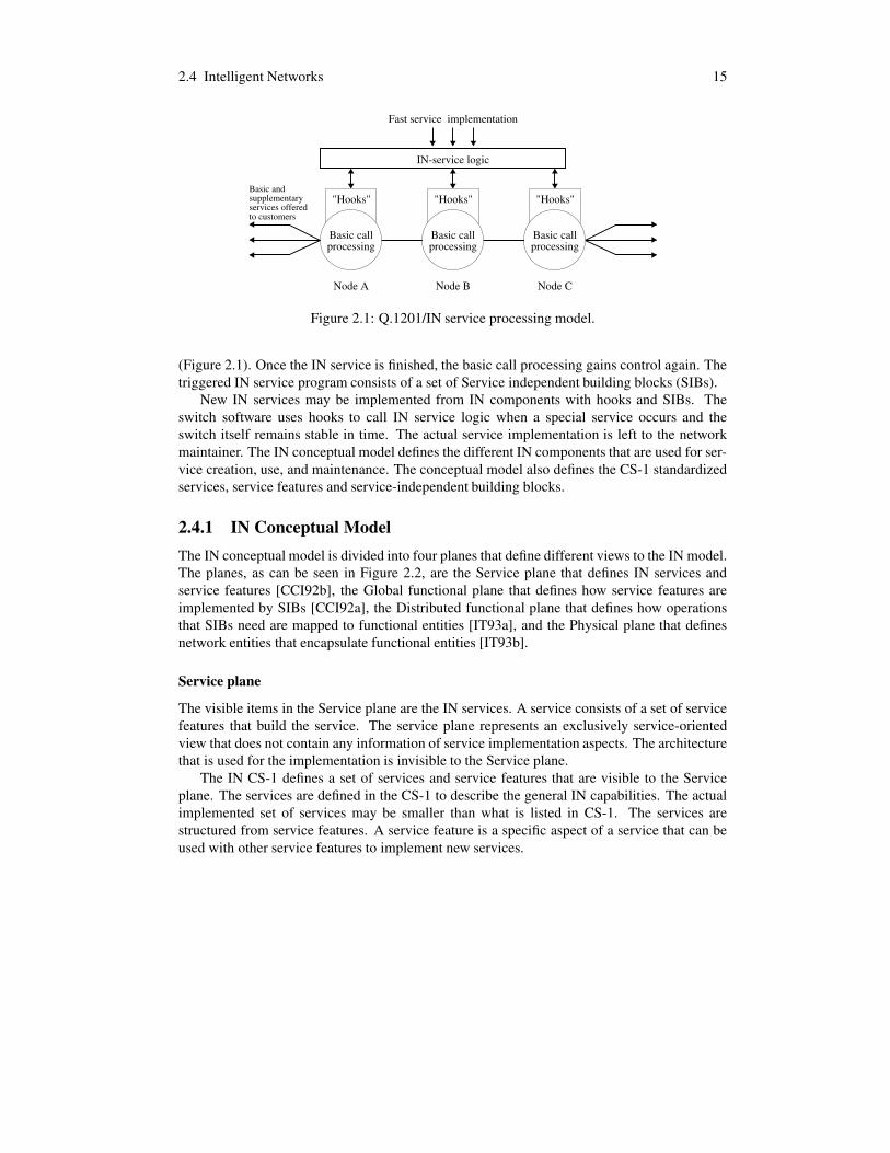
2.4 Intelligent Networks 15
IN-service logic
Fast service implementation
Basic callprocessing
"Hooks"
Node A
Basic callprocessing
"Hooks"
Node B
Basic callprocessing
"Hooks"
Node C
to customersservices offeredsupplementaryBasic and
Figure 2.1: Q.1201/IN service processing model.
(Figure 2.1). Once the IN service is finished, the basic call processing gains control again. Thetriggered IN service program consists of a set of Service independent building blocks (SIBs).
New IN services may be implemented from IN components with hooks and SIBs. Theswitch software uses hooks to call IN service logic when a special service occurs and theswitch itself remains stable in time. The actual service implementation is left to the networkmaintainer. The IN conceptual model defines the different IN components that are used for ser-vice creation, use, and maintenance. The conceptual model also defines the CS-1 standardizedservices, service features and service-independent building blocks.
2.4.1 IN Conceptual ModelThe IN conceptual model is divided into four planes that define different views to the IN model.The planes, as can be seen in Figure 2.2, are the Service plane that defines IN services andservice features [CCI92b], the Global functional plane that defines how service features areimplemented by SIBs [CCI92a], the Distributed functional plane that defines how operationsthat SIBs need are mapped to functional entities [IT93a], and the Physical plane that definesnetwork entities that encapsulate functional entities [IT93b].
Service plane
The visible items in the Service plane are the IN services. A service consists of a set of servicefeatures that build the service. The service plane represents an exclusively service-orientedview that does not contain any information of service implementation aspects. The architecturethat is used for the implementation is invisible to the Service plane.
The IN CS-1 defines a set of services and service features that are visible to the Serviceplane. The services are defined in the CS-1 to describe the general IN capabilities. The actualimplemented set of services may be smaller than what is listed in CS-1. The services arestructured from service features. A service feature is a specific aspect of a service that can beused with other service features to implement new services.

16 2 BACKGROUND
PE1
PE2
FE1FE3
FE1
BCP
POI
POR
SIB1
SIB2
SIBn
Service 1
Service 2
SF1
SF2
SF3
EF
EF
FEA
EF
EF
FEA
EF
EF
FEA
IFIF
IFFE1
FE2
FE3
Service plane
Global functional plane
Distributed functional plane
Physical plane
BCP Basic call processEF Elementary functionFE Functional entityFEA Functional entity actionIF Information flowP Protocol
P
PE Physical entityPOI Point of initiationPOR Point of returnSF Service featureSIB Service independent building-block
Figure 2.2: Q.1201/IN conceptual model.

2.4 Intelligent Networks 17
Global functional plane
The Global functional plane defines service feature functionality which is achieved by Service-independent building blocks (SIBs). Services that are identified in the service plane are de-composed into their service features, and then mapped into one or more SIBs in the Globalfunctional plane. The Basic call process (BCP) functional entity is the only entity that is visibleto the service. The Point of initiation (POI) initiates IN service logic and the Point of return(POR) returns control back to the basic call process.
The main SIB for database services is the Service data management SIB. It enables user-specific data to be replaced, retrieved, incremented, or decremented. It is the main persistentdata management block [ITU93a]. The other database-related SIB is the Translate SIB. It trans-lates input information and provides output information. It can be used for number translationsthat may depend on other parameters such as time of a day [ITU93a].
Distributed functional plane
The Distributed functional plane defines functional entities that SIBs use for actual serviceimplementation. A functional entity is a group of functions in a single location and a subsetof the total set of functions that is required to provide a service. Every functional entity isresponsible for a certain action. Together they form the IN service logic. The entities arevisible only on the Distributed functional plane which defines the logical functional model ofthe IN network. The physical network entities consist of functional entities. They are definedin the Physical plane.
The functional entities and their relationships that CS-1 defines are in Figure 2.3. The set ofrelationships in the IN distributed functional plane model also defines the regular IN call profileby showing how information flows between the functional entities. The first entity to reach isthe Call control agent function (CCAF). It is an interface between users and network call controlfunctions. It is first accessed when a user initiates a connection and gets a dial tone. After thatthe call control continues to the Call control function (CCF). It performs regular switching byconnecting and serving the call. In regular calls the only functional entities that are accessedare CCAF and CCF.
The Service switching function (SSF) recognizes service control triggering conditions whena special IN service is needed. It controls the IN service by co-operating with the Service controlfunction (SCF). SCF is the main functional entity of the IN distributed functional plane model.It executes service logic programs that consist of SIBs. When the service is finished the SCFreturns control to the SSF. It may also communicate with several SSFs depending on the natureof the service. For instance, SCF may consult both the caller SSF and the called SSF.
In service logic program execution, the SCF may also interact with other functional entitiesin order to access additional logic or to obtain information that is required to process a servicerequest. The main entities that the SCF communicates with are the Special resource function(SRF) and the Service data function (SDF).
The SRF provides specialized resources that are required for service execution, such asvoice recognition, digit receivers, announcements, and conference bridges. The exact resourcesthat the SRF offers are not specified in the CS-1. It is left open for any services that needspecialized resources. The SCF gives control to the SRF during the special resource execution.The SRF receives results from the SCF when the execution is finished.

18 2 BACKGROUND
CCAF CCF CCF CCF CCAF
SSF SSF
SRF
SDFSCF
SMF SMAF
SCEFAll other networkfunctions except CCAF
CCAF SMAF
SMF
SRF
SSF
SCEF
CCF
Call control agent function
Call control function
Service creation environment function
Service management access function
Service management function
Special resource function
Service switching functionSCF Service control function
SDF Service data function
Figure 2.3: Q.1204/IN distributed functional plane model.
The service, customer, and network related data is in a set of SDFs. The SCF communicateswith one or more SDFs to gain customer and network data that is needed for the executingservice. The SDFs offer most of the database services for the IN functional architecture. Again,the implementation of a SDF architecture is not specified in CS-1.
Finally, when the IN service is executed, the SCF returns control to the SSF which returnsit to the CCF. Once control is returned to the CCF, the CCF continues normal call controlexecution, if necessary. Often the IN-triggering call is terminated when the SCF returns controlto the SSF since most IN-specific services need access to SCF and IN-specific data during thecomplete call.
The rest of the functional entities, Service management function (SMF), Service manage-ment access function (SMAF), and Service creation environment function (SCEF), form a ser-vice maintenance environment where the service maintainers can design, implement, and main-tain IN services and service features. The Service management access function is the entry

2.4 Intelligent Networks 19
function to reach the management services. It provides an interface between service managersand the service managing environment. The SCEF provides an environment where new servicescan be defined, developed, tested, and input to the management environment.
The main component of the management is the Service management function (SMF). It isused for all IN functional entity and service maintenance. It can also be used for gatheringstatistic information or for modifications of service data. The management environment is un-defined in CS-1, but it will probably be closely related to the Telecommunications ManagementNetwork architecture (TMN).
Physical plane
The lowest plane in the IN conceptual model is the Physical plane. It describes how the func-tional entities are mapped into physical entities, and how the network itself is implemented. Thephysical architecture that is recommended in Q.1215 is in Figure 2.4, but the physical plane ar-chitecture is not strictly defined. It is possible to have various different mappings from logicalentities to physical entities.
The main physical entry point to the network is the Network access point (NAP). It consistsof a CCF and possibly a CCAF that allow the connection. The connection is then transported tothe Service switching point (SSP), which is the main entity of the IN physical architecture. TheSSP implements switching functions and IN service triggering. It consists of functional entitiesCCF and SSF. It may also consist of a SCF, a SRF, a CCAF, and a SDF. The definition allowsa physical architecture that consists of a SSP and the management entities alone.
Other versions of the SSP are the Service switching and control point (SSCP) and the Ser-vice node (SN). A SSCP may have the same functional entities as the SSP but it has a SCFand a SDF as core entities. A SN has a CCF, a SSF, a SCF, a SDF, and a SRF as core entities.In practice it is possible to add most functional entities to a single physical entity, and call itaccordingly. The definition allows different distribution levels to the architecture. There aretest architectures from total centralization to total distribution.
The presented architecture is an example of how the physical plane can be implemented.The recommendations give exact specifications of mappings from functional entities to phys-ical entities. The functional entities that implement IN logic are more important than theirdistribution to physical entities.
The actual IN service logic processing occurs in a Service control point (SCP). Function-ally it consists of a SCF and optionally a SDF. The SCP contains service logic programs anddata that are used to provide IN services. Multiple SCPs may contain the same service logicprograms and data to improve service reliability and load sharing. The SCP may access datadirectly from a SDP or through the signaling network. The SCP may also access data from aSDP in an external network. The SDP is responsible for giving a reply which either answersthe request or gives an address of another SDP that can answer it. An Adjunct (AD) is a specialSCP that has both a SCF and a SDF as core entities. As in switching points, various functionalentity distributions allow different distribution levels in the service control and data points.
The main physical database entity is the Service data point (SDP). It contains data that theservice logic programs need for individualized services. It can be accessed directly from a SCPor a SMP, or through the signaling network. It may also request services from other SDPs in itsown or other networks. Functionally it contains a SDF which offers database functionality andreal-time access to data.

20 2 BACKGROUND
SMAF
SMAP
SMF
SDF
SCEP
SDP
SCF
SDFAD
SRF
CCFSSF
IP
SCF
SSF
CCF SDF
SRFSN
SCP
SCF
SDF
SCF SRF
SSF
CCF
CCAFSDF
SMPSCEF
SMAFSCEF
To other PEs
To other SCPsor SDPs inthis or another network
Signalling Network
a)
a)
a) An SSCP PE includes the SCF and SDF as core elements
Transport
Signalling
Management, Provisioning & Control
FE
Optional FE
Functional entities (FEs)
CCF Call control function
Physical entities (PEs)SSP Service switching pointSCP Service control pointSDP Service data pointIP Intelligent peripheralSMP Service management pointSCEP Service creation environment pointAD AdjunctSN Services nodesSSCP Service switching and control point
SSP
NAP
CCF
CCAF
SMAP Service management access point
CCAF Call control agent function
SCF Service control function
SRF Special resource functionSSF Service switching functionSMF Service management functionSCEF Service creation environment functionSMAF Service management access function
NAP Network Access Point
SDF Service data function
Figure 2.4: Q.1205/Q.1215/IN scenarios for physical architectures.

2.5 Current and future mobile networks 21
The Intelligent peripheral (IP) is responsible for processing special IN requests such asspeech recognition or call conference bridges. Functionally it consists of a SRF, and possibly aSSF and a CCF. Usually it does not contain any entities other than the SRF.
Finally, the IN management is left to the Service management point (SMP) together withthe Service creation environment point (SCEP) and Service management access point (SMAP).A SMAP is used for maintenance access to the management points. Functionally it consists ofa SMAF. The SCEP implements a service creation and testing platform. Functionally it consistof a SCEF. The SMP handles the actual service management. It performs service managementcontrol, service provision control, and service deployment control. It manages the other INphysical entities, also the SDPs. It consists of at least a SMF, but optionally it may also consistof a SMAF. Again, this allows different functional distribution levels to the implementation.
2.4.2 The Future of Intelligent NetworksThe IN architecture, as described in CS-1, is already several years old. Naturally IN standard-ization has evolved a lot since the times of CS-1. A number of groups are currently developingtechnologies aimed at evolving and enhancing the capabilities of Intelligent Networks. Theseinitiatives include project PINT on how Internet applications can request and enrich telecom-munications services, The Parlay consortium that specifies an object-oriented service controlapplication interface for IN services, and the IN/CORBA interworking specification that en-ables CORBA-based systems to interwork with an existing IN infrastructure [BJMC00]. Simi-larly Telecommunications Information Networking Architecture (TINA) has been under heavydevelopment and research since 1993. TINA concepts are easily adaptable to the evolution ofIN [MC00].
The overall trend in IN seems to go towards IP-based protocols and easy integration to In-ternet services. For instance, Finkelstein et al. examine how IN can interwork with the Internetand packet-based networks to produce new hybrid services [FGSW00]. However, the underly-ing IN architecture is not changing in these scenarios. Hence the analysis and descriptions wehave given here are relevant regardless of future trends. The interworking services are at lowerabstraction levels, and need new gateways and interfaces to connect IN and IP-based services.This in turn affects the interfaces to globally accessible IN elements such as SSPs and perhapsSCFs. Even SDFs may need to have an interface for CORBA or TINA based requests.
2.5 Current and future mobile networksMobile networks use radio techniques to let portable communication devices (usually tele-phones) connect to telecommunications networks. The number of mobile connections is grow-ing rapidly while the number of connections in fixed networks has remained relatively stable. Ifthe trend continues, mobile networks will be a leading factor in the competition of teleoperators.
Currently first (1G) and second (2G) generation mobile systems are used in telecommuni-cations. The 1G mobile systems are based on analog techniques. Such networks are NordicMobile Telephone (NMT) in the Nordic countries and Advanced Mobile Telephone System(AMPS) in the U.S. The 1G systems no longer have a strong impact on mobile network archi-tectures due to their analog nature, voice-alone service, and closed architectures.
The 2G mobile networks, such as Global System for Mobile communications (GSM), use
22 2 BACKGROUND
digital techniques for mobility implementation. Their functional architectures are well designedand applicable for more than pure mobile connection services. The digital architectures allowseparation of services and connections.
The 2G architectures have a completely different approach from analog and closed 1Garchitectures. In 2G design defining open interfaces, and digital data and speech encoding arethe most important aspects. The data rate of 9.6kb/s was reasonable at the time of 2G definition.It was not a surprise that 2G soon became a major success, and especially GSM spread almosteverywhere in the world.
2.5.1 GSM architectureThe GSM architecture is built on a Public land mobile network (PLMN). It relies on fixednetworks in routing, except between a Mobile station (MS) and the GSM network. The networkhas three major subsystems: the Base station subsystem (BSS), the Network and switchingsubsystem (NSS), and the Operation subsystem (OSS) [MP92].
Next to the subsystems BSS, NSS, and OSS, the GSM network consists of a set of MSsthat usually are the only elements visible to the end users. The service area is divided intoa number of cells that a BSS serves. A MS has radio communications capability to the basestation of that cell. The Mobile service switching center (MSC) provides switching functionsand interconnects the MS with other MSs through the BSS or co-operates with public fixednetworks [Jab92].
The BSS includes the machines in charge of transmission and reception to the MSs. Itcontrols communication between MSs and the NSS which is responsible for routing calls fromand to MSs. The BSS consist of a set of Base transceiver stations (BTSs) that are in contactwith MSs, and a set of Base station controllers (BSCs) that are in contact with BTSs and theNSS. The BTS manages GSM cells that define coverage for MSs. The BSC manages the radioresources for one or more BTSs.
The NSS includes the main switching functions of GSM and the necessary databases thatare needed for subscriber data and mobility management. The name Network and switchingsubsystem comes from Mouly and Pautet [MP92]. The subsystem is also called the Switchingsubsystem since a GSM network includes both a BSS and a NSS [MP92]. The main role of theNSS is to manage communications between GSM users and other telecommunications networkusers.
The elements of the NSS can be seen in Figure 2.5. Next to the elements, the figure alsoshows a typical configuration of a NSS in a single teleoperator. The NSS includes a set of MSCsthat route MS calls, a set of Visitor location registers (VLRs) related to one or more MSCs thathold location information of mobile stations within its region, one or more Gateway mobileservice switching centers (GMSC) that are responsible for routing calls to external networks, anEquipment identity register (EIR) that maintains information for identifying Mobile equipment,and an Authentication center (AC) that is responsible for management of security data for theauthentication of subscribers.
Information on the location of the MS is updated in the reference database HLR. It containsrelevant permanent and temporary data about each subscriber. Additionally, information ismaintained in a local VLR. The VLR, corresponding to one or several MSCs, contains detaileddata of MS locations and subscribed GSM services. The MS-specific data is used for routingincoming and outgoing calls. VLR functions cover location updates, temporary mobile station

2.5 Current and future mobile networks 23
MSC Mobile service switching centerGMSC Gateway mobile switching centerVLR Visitor location register
HLR Home location registerEIR Equipment identity registerAC Authentication center
MSC
MSC
MSC
...
GMSC
AC
EIR
HLR
VLR
VLR
Figure 2.5: GSM Network and Switching Subsystem elements.
identity allocation for location confidentiality, and storage of a MS roaming number (MSRN)[Jab92]. The HLR is relatively static, while data in the VLR changes when the subscribermoves. The Signaling system 7 (SS7) connects MSCs, VLRs, and HLRs [PMHG95].
The OSS has three main tasks: subscriber management, system maintenance, and systemengineering and operation [MP92]. The OSS architecture is designed so that it is long-termcompatible with Telecommunications management network (TMN) [Pon93]. The TMN itselfis a complex and well defined architecture for telecommunications management. We do notcover TMN architecture in this thesis.
Subscriber management in the OSS has two main tasks: subscription and billing. Thesubscription task occurs when a new subscriber joins to the network. The information of thesubscriber and her mobile equipments must be registered. This involves the HLR that holds thesubscriber information, and possible other service provider related databases that are not listedin the GSM standard. The standard does not restrict the use of such databases [MP92]. Thebilling task occurs when a subscriber is billed from a service use. Usually the triggering clientof the service is a call, but it can also be a supplementary service or some external teleoperatorof an incoming call in case the subscriber is located in an external PLMN.
System maintenance includes the failure detection and repair of all GSM components. Thisis often accomplished by monitor computers and alarms.
The System Engineering and Operation is closely related to System Maintenance. However,in this category the management staff is more concerned of what kind of network architectureto create and how to run it efficiently.
2.5.2 Third generation mobile networks and beyondCurrently the third generation mobile networks (3G) are under development. They are based onsecond generation architectures but they also rely on IN services for multimedia architecture.Such systems are the Future Public Land Mobile Telecommunication System (FPLMTS) that

24 2 BACKGROUND
is under standardization in ITU Radiocommunications sector (ITU-R) and in ITU-T, and Uni-versal Mobile Telecommunication System (UMTS) that is under standardization in ETSI. TheUMTS is closely aligned to the FPLMTS. It is expected that the UMTS and the FPLMTS willbe compatible in the long run. Since the definition of the 3G wireless networks, network sys-tem architectures have gone through evolutionary phases and now the first 3G wireless networkoperators are ready to offer services in America, Europe, and Asia.
Some of the system characteristics for the FPLMTS were defined in the mid-90s [Pan95]:a digital system using 1.8 – 2.2 GHz band, multiple radio environments (cellular, cordless,satellites, and fixed wireless), multimode terminals to provide roaming capability, a wide rangeof telecommunication services, high quality and integrity – comparable to fixed networks, in-ternational roaming and inter system handover capability, use of IN capabilities for mobilitymanagement and service control, high levels of security and privacy, and flexible and opennetwork architectures.
The UMTS provides wireless communication services to users on the move. The serviceswill include high speed data services and video services like mobile videophone [Mit95]. Theusers will be provided with data rates of up to 144 kbit/s in macrocellular environments, up to384 kbit/s in microcellular environments, and up to 2 Mbit/s in indoor or picocellular environ-ments. The increase of data rate is the main benefit of UMTS systems. With higher data ratesnew multimedia services may be implemented.
The main functions of an UMTS database service are as follows [Mit95]:
� It offers basic database management system functionality of providing read and writeaccess to data,
� it locates requested data within the database,
� it moves data to locations close to the user when the user has roamed to provide fastaccess to data where it is frequently being used,
� it provides mechanisms that ensure the integrity and reliability of data even when it iscopied between locations and possibly duplicated, and
� it ensures that data is only accessed by entities that have been authorized to do so.
An interesting fact about database services in the UMTS is that their implementation is leftundefined in UMTS standardization. The radio interface independent functions, essentially callcontrol and mobility management, are outside the scope of the specifications and are handledby the core network [Ric00]. It is important to draw a distinction between 3G networks and 3Gservices.
Open interfaces are defined that allow teleoperators to use existing network architectures asmuch as possible. In practice this implies that UMTS mobility and call control support at archi-tecture level will be similar to 2G mobility and call control support. New special teleoperator-specific services will be implemented on top of the network and thus left undefined in thestandardization.
According to Pandya [Pan95] and Mitts [Mit95] Intelligent Networks and SS7 are seenas the basis for UMTS service implementation. Since the mid-90s when those articles werewritten, UMTS has evolved towards IP-based implementations. Yet IN still has a lot to offerto 3G networks. In principle, all 3G database services could be left for SDFs and SMFs. This

includes HLR, VLR, and EIR databases. Even when 3G architectures are fully IP-based, theIN architecture may be used on top of the IP-network.
Special services, management, and mobility need very different types of database services.Special services need fast read access to data, management needs reliable distributed updates,and mobility needs small and fast updates with the cost of reliability. It is imminent that not allthree can be fully satisfied. Compromises are needed if a single database management systemis intended to support all the categories.
The 3G wireless networks are not the final solution to wireless networks. First, they arebased on old ATM techniques. Second, their throughput is limited to 2Mb/s which is not enoughfor modern multimedia services [DF01]. Due to the limitations in 3G networks, the next evolu-tion to 4G wireless networks is under research. According to Becchetti et al. the 4G networkswill not be based on a standard interface in the same way as the 3G networks [BPI � 01]. Whileit is too early to state anything specific, it is clear that 4G wireless networks will be specializedon various application domains, standard interfaces between them, transparency, and quality ofservice. The architectures are IP-based rather than ATM-based [RKV � 01, TNA � 01].
The benefits of a fully IP-based architecture are clear. The IP approach allows a widerange of new services and shortens the service creation cycle. For example, voice/multimediacalls can be integrated with other services [YK00]. The cost on service creation, provisioning,and maintenance can be reduced due to a common platform. Also cost savings on ownership,management, transport, and interface implementation are significant.
It should be noted that while 3G is starting and 4G is under research, the limits of 2Gtechniques are not yet met. The Wireless Application Protocol (WAP), General Packet RadioService (GPRS), and enhanced data rates for GSM evolution (EDGE) have evolved GSM tonew usage levels [Pra99]. It is expected that GSM will dominate the mobile communicationmarket long after the first 3G network implementations are commercially available [Kon00].Yet eventually 2G wireless networks will evolve to 3G wireless networks, and finally to fullIP-based 4G wireless networks. We expect 2G wireless networks to be obsolete in 10 years,and 3G wireless networks in 15-20 years.


Chapter 3
IN/GSM data analysis
As we have already seen in the previous section, in the future it is most probable that IN willsupport mobility, and mobile networks will use IN services as a basis for special services. Dueto this it is natural to consider a common database management system architecture for IN andGSM. We call this an IN/GSM database architecture.
In order to define the IN/GSM database management system architecture we must firstunderstand the special nature of IN and GSM data and data stores. Both platforms offer a richset of details that can be analyzed and thus maintained in the IN/GSM database architecture.
The most important aspect in an IN/GSM database architecture is to support real-time ac-cess to data. This can be extracted from the IN recommendations. A deeper analysis is neededto understand what data types exist in the database. We base the analysis to the IN CS-1 servicefeatures and to the GSM frame architecture. A service feature is a building block of an INservice. Since all services are made of service features, analyzing the features gives the dataaspects of current and future services.
The analysis of both IN and GSM data is based on the object paradigm. Each analyzedservice feature is considered a client for an object-oriented database. The database holds a setof object classes each of which has a set of objects. Each object models a real-world entity,such as a subscriber or a phone line. We adopted this approach already in our early work[Tai94a, Tai94b, RKMT95, TRR95] since object-oriented databases are a natural expansion torelational databases, and the IN architecture is object-oriented.
In the analysis we have identified seven object classes whose objects are time-independent:Teleoperator, Subscriber, Charging account, Service, Phone line, Location, and Log informa-tion. We call these static object classes. Objects in these classes may be identified as traditionalobject-oriented database objects. Next to these we have identified six classes whose objectsare time-dependent: Closed user group data, Conference profile, Multi-Party call data, Masscalling, Visitor group data, and Virtual private network data. We call these dynamic objectclasses. Objects in these classes are dynamic in creation and deletion, and may have timingconstraints. Altogether these classes give a basis for analyzing IN/GSM database requirementsand solutions. The recognized classes and their relationships are in Figure 3.1.
The IN/GSM static object classes have hierarchical relationships with each other. The onlyserious exception to the hierarchy is the Service class that is in a one-many relationship to theTeleoperator class, and in a many-many relationship to the Charging account class. The dy-namic object classes have a more complex relationships with static objects. We give a detailed

28 3 IN/GSM DATA ANALYSIS
Static class Dynamic class
One−to−many relationship
Many−to−many relationship
Recognizedun−modelled class
One−to−one relationship
Multi−Party call data
Mass calling
Closed user group data
Teleoperator
Charging account
− UPT−data
Phone line−Routing information− Calling restrictions
Log information
Location
−Authentication
Visitor group data
Subscriber Service
Virtual private network data Conference profile
Figure 3.1: IN and GSM object classes.
analysis of the classes and their relationships in Section 3.1 for IN, and in Section 3.2 for GSM.
3.1 IN data analysisThe IN CS-1 lists 38 service features as listed in ITU-T recommendations [ITU93b] andsummarized by Raatikainen [Raa94]. We have divided them into the following categories:Virtual Private Network (VPN)-related features, management-related service features, regu-lar call-related features, service provider-related features, mass calling and televoting-relatedfeatures, teleconference-related features, and Universal Personal Telecommunications (UPT)-related features. This classification is somewhat artificial since some features may exist inseveral categories. However, even an artificial structure helps in the data analysis. Since the INrecommendations do not give exact database requirements for the service features, this analysisdoes not go to a detailed level. It is sufficient for our needs to recognize the most commonreal-world object classes that must be modeled in the database.
Basically all service features need a calling user profile, a used service profile, and logwriting. We will not mention these in the analysis unless the analyzed service feature has a
3.1 IN data analysis 29
specific treatment for them.
Virtual Private Network service features
A Virtual Private Network (VPN) is a subset of phone lines in a public telecommunicationsnetwork that behave as if they were a private network. The lines can be accessed from outsidethe VPN with a common center number. The phone lines in the VPN have short access numberswithin the network.
The VPN is one of the major aspects of IN. This can also be seen from the number of VPNservice features. They are Abbreviated dialing, Attendant, Authorization code, Closed usergroup, Follow-me diversion, Off-net access, Off-net calling, and Private numbering plan.
The Abbreviated dialing allows subscribers to shorten a phone number to two or moredigits. Next to the VPN, the feature can be used in the regular phone network. The databaseitems needed in this service feature are the abbreviated number, number translation, the possibleVPN data, and the subscriber profile. The abbreviated number is first translated to the VPNnumber, if the operation occurs in the VPN. The VPN number is then translated to a referenceto the physical phone line object.
The Attendant allows VPN users to access an attendant position within the VPN for pro-viding VPN service information. The attendants can be accessed by dialing a special accesscode. The database items needed for this service feature are the VPN data, the access code, anda number translation. The VPN data holds VPN service information. The database must alsostore access codes for number translation.
The Authorization code allows a VPN user to override calling restrictions of the VPN stationfrom which the call is made. Different sets of calling privileges can be assigned to differentauthorization codes and a given authorization code can be shared by multiple users. In thedatabase, the VPN data, VPN station data, and the authorization code are needed to fulfill theservice feature. The VPN data holds the information of the VPN stations connected to it. Eachstation has several authorization codes. This operation may be logged to the VPN station data.
The Closed user group (CUG) allows a user to be a member of a set of VPN users who arenormally authorized to make and/or receive calls only within the group. A user can belong tomore than one CUG. In this way, a CUG can be defined so that certain users are allowed eitherto make calls outside the CUG, or to receive calls from outside the CUG, or both. The databaseitems needed are the VPN data, CUG data, and user profiles. A VPN data entry has zero ormore CUG-data entries, each of which describes one closed user group. Each subscriber hasinformation in the user profile of her currently active closed user groups.
The Follow-me diversion allows a VPN user to change the routing number of her VPN codevia a Dual-Tone Multi-Frequency (DTMF) phone. The updated number can be another VPNcode or a regular number. The database items needed for this feature are the VPN data andpossibly the user profile. The VPN-data holds information about the current routing numbers.The update may be linked to the user profile.
The Off-net access allows a VPN user to access her VPN from any non-VPN station byusing a PIN code. Different sets of calling privileges can be assigned to different PINs, and agiven PIN can be shared by multiple users. This service feature needs the VPN data and thePIN code. The PIN code is needed to access the VPN. Once the PIN code is verified, the VPNdata is loaded and the network is ready for use.
The Off-net calling allows the user to call outside the VPN network. Calls from one VPN to

30 3 IN/GSM DATA ANALYSIS
another are also considered off-net. This service feature needs the VPN data and the outgoingnumber profile. The outgoing line is translated to the actual line number. The VPN-data andnumber profiles are used in the translation.
The Private numbering plan allows the subscriber to maintain a numbering plan withinher private network, which is separate from the public numbering plan. This is actually amanagement feature, but since it is part of the VPN, it is listed here. The database itemsneeded are the VPN data and the subscriber profile. The subscriber profile holds the neededinformation. A number translation is needed to and from VPN, among other things.
Management service features
The management service features are designed for subscribers to manage their private data.Each subscriber may manage her data within the allowed limits. We have included authenti-cation service feature to the management service features since it is closely related to manage-ment. The IN CS-1 does not specify IN management. Hence, these service features are by nomeans complete.
The management service features include Authentication and Customer profile manage-ment. The former is a general security service feature that is used in most secure services. Thelatter is a general management service for user information.
The Authentication allows the verification that a user is allowed to exercise certain optionsin a telephone network. In other words, the feature allows customer authentication via a Per-sonal Identification Number (PIN). This feature needs the user profile and the PIN code. Thedatabase must execute the authentication for security reasons. The less identification-specificinformation is available outside the database management system, the better is the IN security.Both internal and external Authentication requests should be served by the same database man-agement system. The result of the operation is a boolean value describing the validity of thePIN code. This operation may be logged in the database.
The Customer profile management allows the subscriber to access her service profile, i.e.,terminating destinations, announcements to be played, call distribution, and so on. This is theonly service feature that allows the subscriber to reach network data. Each subscriber maymanage her service profile in the database. Since this is a service feature, all security aspectshave been handled in other features. The only database object needed is the subscriber profile.
Regular call service features
The regular call service features are typical to everyday subscriber services. This distinguishesthem from service provider service features that are intended for subscribers that offer specialservices to others (usually with extra charging). A regular call service feature is generally aservice feature that concerns two regular phone lines. A service provider service feature oper-ates between several phones and may include several service number transactions and specialbilling. This division is somewhat artificial since most regular call services are widely used byservice providers, and some service provider service features are used in regular services.
The regular call service features are Automatic call back, Call forwarding, Call forward-ing on busy/don’t answer, Call logging, Call transfer, Call waiting, Consultation calling, Cus-tomized ringing, and Terminating call screening.

3.1 IN data analysis 31
The Automatic call back allows the called party to automatically call back the calling partyof the last call directed to the called party. The database must provide access to the incomingand outgoing phone line information, and the destination number. The called party receivesdynamic call data including incoming and outgoing line information. The line information isneeded for possible connection restrictions. The destination number included in the dynamiccall data may be translated to the actual number.
The Call forwarding allows the user to have her incoming calls addressed to another mem-ber, no matter what the called party line status may be. The data items needed are the incomingand outgoing user profiles, and the outgoing number profile. The incoming and outgoing userprofiles are needed for security reasons. The user may not forward calls to any destination.Once the operation is accepted, the forwarded number profile includes information of the newnumber. Circular call forwarding must be recognized.
The Call forwarding on busy/don’t answer feature allows the called user to forward partic-ular calls if the called user is busy or does not answer within a specified number of rings. Thisis a special case of the Call forwarding service feature.
The Call logging allows a record to be prepared each time that a call is received to a specifiedtelephone number. The database holds data about the number profile. The calls are loggedaccording to the number profile to a phone line and subscriber-specific log.
The Call transfer allows a subscriber to place a call on hold and transfer the call to anotherlocation. This service feature may need a number translation.
The Call waiting allows the called party to receive a notification that another party is tryingto reach her number while she is busy talking to another calling party. This feature is storedinto the called number profile.
The Consultation calling allows a subscriber to place a call on hold, in order to initiate anew call for consultation. This feature does not need database services.
The Customized ringing allows the subscriber to allocate a distinctive ringing to a list ofcalling parties. The database holds information about the possible calling parties in the calledline profile.
The Terminating call screening allows the user to screen calls based on the terminatingtelephone number dialed. The called line profile holds information about the restricted numbersor subscriber/line profiles. Alternatively the restriction information may be stored to the calledsubscriber profile.
Service provider service features
A service provider in this context is a subscriber who uses the IN services to give specialservices to her own customers. The service features needed are related to different types ofcompany phone services, such as help desks.
We have included Call distribution, Call gaping, Call hold with announcement, Call lim-iter, Call queueing, Customized recorder announcement, Destinating user prompter, One num-ber, Origin dependent routing, Originating call screening, Originating user prompter, Premiumcharging, Reverse charging, Split charging, and Time dependent routing under this category.Naturally all these services can be used by regular subscribers as well.
The Call distribution allows the served user to specify the percentage of calls to be dis-tributed among two or more destinations. Other criteria may also apply to the distribution ofcalls to each destination. The database must hold the called number profile which includes

32 3 IN/GSM DATA ANALYSIS
information and heuristics for the call distribution. The number is translated according to theprofile.
The Call gaping allows the service provider to automatically restrict the number of calls tobe routed to the subscriber. The database must hold the service provider profile and the servicesubscriber profile for this feature. The service provider profile holds information about servicesubscribers. Each subscriber profile of the service provider holds information about call gaping.
The Call hold with announcement allows a subscriber to place a call on hold with optionsto play music or customized announcements to the held party. The subscriber profile holdsinformation about announcement services. The announcements may be customized dependingon the receiver profile.
The Call limiter allows a served user to specify the maximum number of simultaneous callsto a served user’s destination. If the destination is busy, the call may be routed to an alternativedestination. The user profile and number profile together hold information about the maximumnumber of simultaneous calls. A number translation may be needed both when the call isforwarded and when the destination is busy.
The Call queueing allows a served user to have calls encountering busy at the scheduleddestination to be placed in a queue and connected as soon as a free condition is detected. Uponentering the queue, the caller hears an initial announcement informing the caller that the callwill be answered when a line is available. The delayed call is put on a wait queue. When a freecondition is detected, the database triggers the incoming switch to allow the connection.
The Customized recorder announcement allows a call to be completed to a terminatingannouncement instead of a subscriber line. The served user may define different announcementsfor unsuccessful call completions due to different reasons such as a call arrives outside businesshours or all lines are busy. This feature uses mostly the services of a Service Resource Function(SRF). The called number profile hold information about various announcement types.
The Destinating user prompter service feature enables to prompt the called party with aspecific announcement. Such an announcement may ask the called party to enter an extranumbering through a DTMF phone, or a voice instruction that can be used by the service logicto continue to process the call. This service feature uses the services of the SRF. The numberprofile holds information about various announcement types.
The One number allows a subscriber with two or more terminating lines in any numberof locations to have a single telephone number. This allows business to advertise just onetelephone number throughout their market area and to maintain their operations in differentlocations to maximize efficiency. The subscriber can specify which calls are to be terminatedon which terminating lines based on the area from which the calls originate. The database musthold the service provider profile and the incoming number profile. The subscriber profile holdsinformation about possible phone groups. When a group receives a call, the group profile holdsinformation about the possible alternatives. A tailored heuristics can then be used to access thecorrect number.
The Origin dependent routing enables the subscriber to accept or reject a call, and in caseof acceptance, to route this call, according to the calling party’s geographical location. Thisservice feature allows the served user to specify the destination installations according to thegeographical area from which the call originated. The database items needed are the userprofile, the number profile, and routing information. The user profile holds information aboutpossible routing plans. The number profile and routing information are used for routing the callto a new phone line.
3.1 IN data analysis 33
The Originating call screening allows the served user to bar calls from certain areas based onthe District code of the area from which the call originated. The subscriber or receiving phoneline profile holds information about banned areas. The incoming phone line profile holds thearea code.
The Originating user prompter allows a served user to provide an announcement whichwill request the caller to enter a digit or series of digits via a DTMF phone or generator. Thecollected digits will provide additional information that can be used for direct routing or as asecurity check during call processing. The user profile and called number profile holds infor-mation about the wanted digits and their translations. The received digits must be tested againstpossible typing errors and misuse.
The Premium charging allows for the pay-back of part of the cost of a call to the calledparty, when he is considered as a value added service provider. The database must hold thecaller and called number profiles, charging information and a log. The log is collected duringthe phone call. The number profiles and charging information together describe the actual costsfor both the caller and called phone lines.
The Reverse charging allows the service subscriber to accept to receive calls at its expenseand be charged for the entire cost of the call. This can be used to implement freephone ser-vices. The incoming call is logged and later updated to the subscriber’s charging account. Thedatabase holds the subscriber profile and log information.
The Split charging allows for the separation of charges for a specific call, the calling andcalled party each being charged for one part of the call. From the database point of view thisservice feature is similar to the Reverse charging. The incoming call is logged and the costs arelater updated to both the caller and called charging accounts.
The Time dependent routing enables the subscriber to accept or reject a call and, in case ofacceptance, to route this call, according to the time, the day in the week and the date. Fromthe database point of view this service feature is similar to the Origin dependent routing. Theuser profile holds information about possible routing plans. The number profile and routinginformation are used for routing the call to a new address.
Mass calling and televoting service features
The mass calling and televoting are special service features that have their own database re-quirements. The only service feature listed here is Mass calling. It allows processing of a largenumber of incoming calls generated by broadcast advertising or games.
The Mass calling needs a specialized database that is tailored for a huge number of shortsimultaneous write requests. Each request must be stored very fast to allow maximum requestthroughput. The incoming calls are stored as (called number,vote) -pairs and analyzed online.The called numbers may be restricted for a predefined number of votes (usually one). The dataitems can be written sequentially. A more structured storing method may be done after the masscalling is over.
This service feature can easily overload even a very fast DBMS. Due to this it should notbe allowed to execute in a regular IN database. A DBMS that is tailored for fast writes is aworking alternative.

34 3 IN/GSM DATA ANALYSIS
Teleconference service features
A teleconference in this context is a resource that can be accessed by two or more subscribers.The conference resource is reserved to a certain time at which the members may join it.
The IN lists two service features that are related to teleconferencing: Meet-me conference,and Multiway calling.
The Meet-me conference allows the user to reserve a conference resource for making amulti-party call, indicating the date, time, and conference duration. At the specified date andtime, each participant in the conference has to dial a designated number which has been as-signed to the reserved conference resource, in order to have access to that resource, and there-fore, the conference. The database must hold the conference resource, multi-party call data,and calling number profiles. The conference resource and multi-party call data together holdthe conference information. Number profiles are needed for accessing the resource.
The Multiway calling allows the user to establish multiple, simultaneous telephone callswith other parties. This service feature does not directly need any database services. Thesimultaneous telephone calls may trigger any IN service features.
Universal Personal Telecommunications service features
The Universal Personal Telecommunications is intended for giving a single phone number thatcan be used everywhere. The number is automatically connected to different phone lines de-pending on the date and time. The service is not fully defined in CS-1, and it holds only onefeature: Personal numbering.
The Personal numbering supports a Universal Personal Telecommunications (UPT) numberthat uniquely identifies each UPT user and is used by the caller to reach that UPT user. AUPT user may have more than one UPT number for different applications. However, a UPTuser will have only one UPT number per charging account. The database items needed arethe UPT subscriber profile, UPT data, and a charging account. The UPT data holds UPT-related information about the account. The user profile holds subscriber-specific information.A charging account is needed for each UPT number.
IN data summary
Although we have analyzed nearly forty service features, the number of classes found in themis relatively small. We will first list the static classes and their properties.
A teleoperator offers services to subscribers and also to other teleoperators. Hence theTeleoperator class is the core of the IN data hierarchy. Although it is not explicitly listed in thefeatures, it is the class on which an IN operator may access other networks. A Teleoperator haszero or more services to offer, and zero or more subscribers as customers. However, we arenot that much interested in the services and subscribers of all teleoperators. Rather we wantto have an entry upon which to request more information. Due to this the Teleoperator class isrecognized but not modeled.
All service features are initiated by a subscriber which gives us the class Subscriber. TheSubscriber class holds information about each customer of the teleoperator. A special sub-scriber subclass is a Service provider who has extra privileges (with extra costs). The UniversalPersonal Telecommunications data belongs to the Subscriber class since it is unique to a singlesubscriber.

3.1 IN data analysis 35
A subscriber may have several charging accounts each of which has a set of IN services. Acharging account has a set of IN services and a set of charged lines. This class may be combinedinto the Subscriber class but that would cause unwanted data replication.
Each account of a subscriber has a set of active services offered by her teleoperator. AService class holds information that is relevant to a single service. It has links to the chargingaccounts that have ordered this service.
Each charging account has zero or more phone lines that can be accessed directly via aphone number or indirectly via a number translation. A phone line belongs to exactly onecharging account and has the services that are active in the charging account. The line informa-tion class has routing information and call restrictions.
Whenever a phone line is accessed, a log information entry is created by the accessingtransaction.The log data is written in blocks and read when necessary directly or via the phoneline object.
The previous structure is fairly hierarchical. A teleoperator has zero or more subscribers.A subscriber has zero or more charging accounts. A charging account has zero or more phonelines, and a log is created for every access to a phone line. On the other hand, a teleoperatorhas zero or more services and a service may be subscribed by zero or more charging accounts.Hence, we get two access hierarchies: one from a subscriber and one from a service. Sometimesalso a direct access to a phone line and perhaps to log information is necessary. But altogetherthe major IN classes behave in a hierarchical manner.
Next to the regular classes that are fairly well organized and static, a set of dynamic classesexist. These classes break the hierarchy by referencing information at several levels. The classesare VPN-data, Mass calling data, Conference resource, Multi-party call data, and CUG-data..
The VPN-data class holds information about Virtual private networks. It is linked to Phonelines, Subscribers, and allowed Services. This class is usually fairly static but dynamic VPN-cases may also exist.
The Mass calling data class is needed only for mass calling and televoting. It stores blocksof (called number,vote)-pairs. It is not directly related to any other classes although it can accessthe called number data entry and via that the Subscriber data. Usually this is not necessary sincein televoting the voting privacy is as important as in regular voting.
The Conference resource class holds information that is needed to hold a teleconference. Ithas links to conference Subscribers and Phone lines. It is relatively dynamic in nature since itslife span is equal to the length of the corresponding conference.
The Multi-party call data holds information about the members of a call conference. Itis very dynamic in nature since in principle the participants of the conference are allowed tochange during the conference.
The CUG-data (closed user group data) is very dynamic in nature. It holds informationabout VPN members that belong to a specific closed user group. The group may send andreceive calls only from other members. The object exists only for the life span of the closeduser group itself which can be very short.
These dynamic class types do not behave well in the earlier static hierarchy. They eitheraccess objects at random levels of the hierarchy (such as VPN-data) or do not access any objects(such as Mass calling data). Their dynamic nature makes them behave more like special viewsto the static data.

36 3 IN/GSM DATA ANALYSIS
3.2 GSM data analysisUnlike IN data analysis, the GSM data analysis cannot be based on services. The GSM networkis mainly designed for fast and reliable access for mobile stations. While a GSM operator offersspecial services, the services are built on top of the GSM network instead of inside it. Due tothis, we must analyze the GSM data needs from the mobility point of view. It is most probablethat any mobility aspects in future IN will be based on the tested and working aspects of GSMnetworks. As such, the GSM gives an excellent framework upon which to expand current INdata requirements.
The three subsystems in GSM, BSS, NSS, and OSS, have different database needs startingfrom no requirements and ending in strong real-time requirements.
The BSS does not have any database requirements. If the BSS architecture uses databases,the databases are embedded into BSS elements and are vendor-specific. The BSS architecturedoes not affect the requirements.
The NSS manages the communications between the GSM users and other telecommunica-tions network users. The NSS has four major database management systems that are listed inthe GSM standards: HLR, VLR, AC, and EIR.
The HLR is the main database management system in a GSM network. It is an active com-ponent of the system and controls call and service related information. The HLR must offerreal-time database services. Its main functions include such time-critical tasks as finding sub-scriber information, informing the current location of a subscriber, billing and service control.Usually the architecture of HLR is not distributed. A HLR can handle hundreds of thousandssubscribers. If more capacity is needed, several HLRs can be executed in parallel. This canbe achieved since subscriber data is hierarchical. The VLR has detailed data on location andservice data regarding MSs that are in its coverage area for routing. This data is then used forincoming and outgoing calls. The VLR services include location updates, temporary mobilestation identity allocation for location confidentiality, and storage of mobile station roamingnumber. The VLR has a much smaller role than HLR. It is responsible for maintaining ex-act location information of subscribers that are in the area of its Mobile Switching Centers. Itcommunicates with the HLRs when calls are routed or charging information must be retrieved.Hence it can be considered as a specialized database node in a distributed real-time database.It has real-time and distribution requirements. However, the distribution requirements are notstrict. Updates occur only in one VLR, and the only distribution is into known HLRs. Sincethe information location is always known and a single HLR, distribution basically degeneratesinto message exchange. The AC is used to verify the authorization for required GSM services.As such it supports the same service as the IN authentication service feature. The AC needsto serve real-time requests, but it does not need distribution. It is often connected to the HLR,or a single database management system offers both HLR and AC services. Finally, the EIRmaintains information about MSs. It can be distributed since several EIRs may co-operate.
The most important database managers in GSM are HLR and VLR. The HLR always holdsstatic information about each subscriber. When a subscriber roams, the roaming information isheld on the corresponding VLR. Hence, a HLR has connections to several VLRs on differentnetworks and the connections are dynamic in nature. Together the HLR and VLR have thefollowing interactions:
� Roaming from one VLR area to another. This changes the subscriber location informa-tion in HLR and changes the VLR that holds location information.

3.2 GSM data analysis 37
� Routing a call from a subscriber to a mobile station and receiving a call from a subscriberto a mobile station. Both of these need interaction between the HLR and the current VLR.The HLR is responsible of the routing while the VLR gives enough location informationto make the routing possible.
� HLR and VLR failure and relocation procedures. These are needed when a system ornetwork failure occurs.
� HLR subscriber information update. This occurs when a subscriber is added to or deletedfrom a HLR, or subscriber information is changed. The changes are reflected to thecorresponding VLR, for instance when a subscriber is deleted.
� VLR information update. This occurs when a subscriber roams from one VLR coveragearea to another. The change is informed to the HLR.
The HLR architecture is best described as a parallel database architecture where severaldatabase nodes are connected together with a fast bus to form a logically uniform databasemanagement system. It exchanges information and messages with a set of VLRs, some ofwhich are in external networks. The HLR has distributed requests but they degenerate intomessage passing between the HLR and one or more VLRs. Data is not replicated and datalocation information is well known. All real-time reads occur only in a single node, since theneeded information is subscriber information which is hierarchical.
When a mobile equipment holding the mobile phone line is within the network of the sub-scriber’s teleoperator, location information is updated continuously to mobile phone line data.During this time the network has knowledge of the mobile phone line location. If the connec-tion is lost (either the mobile equipment was closed or the equipment is no longer within thereach of the network), the network has knowledge of the last location.
Sometimes a subscriber may roam to an area that is no longer part of the subscriber’s tele-operator network. In such a case, when an external network detects the mobile phone line, itasks the mobile phone line for its identity. The identity holds information about the subscriber’shome network.
Each teleoperator has information about other teleoperators. If an external network operatorand the home network operator have a roaming contract, the external network contacts thesubscriber’s home network and informs it that this mobile phone line is in its area, and it informsthe mobile phone line that external network services are available. After that the identity of thevisiting mobile phone line, location information, and link to the home information, is stored toa VLR.
Once a subscriber of a visiting mobile phone line wants to use any of its services, includinginitiating a phone call, the service requests are routed via the home network. This occurs aslong as the mobile equipment is within the network of the external teleoperator.
Later, when the mobile equipment leaves the network, the external VLR informs the homenetwork that the subscriber has left their network. The mobile equipment may start anothersession in a new network, and the previous recognition procedure happens again. Thus, duringthe time between the two networks, the home network has only knowledge of the last knownlocation of the mobile phone line.
The previous paragraphs describe the GSM visible database services, their distribution andreal-time aspects. While the GSM network includes several special services, such as ShortMessage Services (SMS) and WAP services, they are built on top of the GSM network and are

not very interesting to us. They use special communication protocols and service databases.The former is a network issue, the latter can be included to service data classes.
The OSS manages the GSM network. It includes subscriber management, system mainte-nance, and system engineering and operations. The OSS can have several database managementsystems, although the GSM standard does not specify them. The management databases neednot to be real-time databases. Although requests must be served rapidly, it is enough that theyare served with high throughput databases rather than real-time databases with deadlines.
The subscriber management service includes subscription, billing and accounting manage-ment. The subscription management is used when subscribers’ data is changed or a new sub-scriber is added to the network. The billing and accounting management are used when asubscriber is billed of the network use. While these services can be very complex in nature,they do not add anything new to the GSM object class analysis.
System maintenance includes failure detection and repair of GSM components. As suchit has a database of all GSM network elements. This is closely related to network elementmanagement in IN or TMN. System engineering and operation is closely related to the systemmaintenance. It includes tasks to design and optimize the GSM network architecture. As suchit needs similar database services as the network element management in system maintenance.
The GSM data items and IN data items have a direct correspondence with each other. TheGSM subscriber entity is related to IN subscriber, phone line, and charging account entities. TheGSM service entity is equal to an IN service entity. The GSM location entity is an expansionto IN entities but it is easy to embed in the IN phone line class. The GSM authentication entitycan be embedded in IN entities since the same service feature is defined in IN. The only reallynew entity is the Equipment entity. It is more of a management entity and does not need specialdatabase treatment. In fact it may be the best to implement as a distinct traditional databasemanagement system.
The data analysis also shows the benefits of distribution. Since the combined IN/GSMclass structure is mostly hierarchical, it is possible to fragment data into several nodes and stillhave mostly local transactions. This is a useful property because distributed transactions alwayscause more overhead than local transactions. With such a hierarchy it is possible to truly benefitfrom distribution instead of losing processing power to the overhead of distributed transactions.

Chapter 4
Yalin architecture
The IN/GSM data analysis in the previous chapter gives us a basis on which to design our archi-tecture. The identified classes have a nice hierarchical relationship, most IN/GSM services aretime-driven, and some information has a temporal nature. Due to these facts a good candidatefor an IN/GSM database management system is a RT-DBMS.
A chosen RT-DBMS architecture must support both IN/GSM database requirements anddistribution [TR00]. A large-scale real-time distributed database management system can ofcourse fulfill all real-time and distribution requirements. Unfortunately an implementation ofsuch a system is not a reasonable approach since this would also add unwanted functionalitythat affects general database performance [TS97b, TS96, TS97a]. Requiring both real-time anddistribution in the IN/GSM database management system causes at least three issues.
First, the transaction deadlines in an IN database are often very short. Even the geographicallatency of a distributed database can be too much for the shortest deadlines. Although it may bepossible to store data near the requesting client by using replication, some compromises mustbe made between distribution and replication. A heavily replicated distributed database solvesread problems but causes update and volume problems. A non-replicated distributed databaseneeds only a single update and optimizes the data storage volume, but then reads may sufferfrom distribution latencies.
Second, the data network reliability is an issue. If the IN/GSM database is to be fault-tolerant, the connections between distributed nodes must also be fault-tolerant. This can beachieved to a certain degree with replicated connections between network elements, but such asolution soon becomes very expensive. It has been shown that in a distributed network that is notfault-tolerant it is not possible to create a non-blocking atomic commit protocol [BHG87]. Thisaffects short deadlines. Also during the recovery time the system cannot fulfill its deadlines.Although SS7 is reasonably reliable, network failures still occur.
Third, a real-time distributed database allows any kind of semantic connections betweendata items. The IN/GSM data structure is hierarchical with few non-hierarchical relationships.This information can be used to optimize the IN/GSM architecture and data locations. Buildinga general RT-DBMS is a much more challenging task than building a tailored RT-DBMS thatbenefits from known semantic relationships between object classes.
Generally we want an architecture where we can minimize distribution of real-time trans-actions. Every distributed transaction causes overhead and unpredictability to the system. Wecan tolerate it to some extent when the system is not heavily loaded and when deadlines are

40 4 YALIN ARCHITECTURE
relatively long. However, these requirements are not met in regular IN/GSM transactions. Theload of the system can be very high at rush hours and deadlines are short.
Starting from the listed issues above, we have designed a reference architecture Yalin (Yes,A Lovely IN database architecture). This architecture is based on the IN/GSM data model andas such it is a very specialized one. We can use the analysis of the IN/GSM data hierarchy tojustify our architecture.
The IN/GSM data structure is hierarchical. It is also easy to translate into physical entities.Just like in regular distributed databases where data is divided into a set of fragments, we candivide the IN/GSM data into several fragments. We call this the fragmentation of the Yalindatabase (Figure 4.1).
The fragmentation of the Yalin database is specialized since the IN/GSM data is also spe-cialized. It consists of a root fragment, a set of regular fragments, a set of VLR fragments, anda set of Mass Calling fragments. The only non-fragmented class is the service class. Servicesare replicated to regular and root fragments.
The root fragment has teleoperator-related information. This information includes bothservices and subscribers, and also links to other teleoperators. The root of the IN/GSM datahierarchy resides in the root fragment. The other fragments have links to the root fragment.
The regular fragments have a subscriber-based view to the IN/GSM data hierarchy. Theactual classes are divided into one or more fragments. Hence, each fragment holds part of theIN/GSM data and most of the IN/GSM object classes. Each regular fragment has a link tothe root fragment which serves as the root of the tree. The regular fragments can be furtherdivided into new fragments. Each new fragment is an equal subtree whose root is the rootfragment. This is a logical fragmentation policy in the IN/GSM database because the data itselfis accessed hierarchically. Any other fragmentation policy would cause unnecessary distributedtransactions for each connection.
Next to the regular fragments, two special fragment sets are defined: VLR fragments andMass calling fragments. The VLR fragments hold data that is relevant to VLRs in the GSMphysical model. These fragments are separated from the regular fragments since their data is ofsubscribers from external networks. The Mass calling fragments are only for mass calling andtelevoting data. This data, while clearly part of the IN data hierarchy, is specialized enough tobe stored in separate fragments. Data on the Mass calling fragments is linked to the subscriberand service data when necessary. The data volume of mass calling and televoting fragmentsmay grow extremely fast.
The fragmentation of the Yalin database is simple to translate into a database managementsystem architecture. Each fragment belongs to one node in Yalin, and a node in Yalin has onefragment. Together the nodes form a distributed database management system.
The nodes of the fragmented Yalin database have clearly various types of data volume andaccess requirements. The size information of Yalin fragments affects architectural decisions ofthe Yalin database.
The Root fragment has information of teleoperators and services. It is a tiny fragment whichin principle can physically reside in one of the regular fragments. It is usually accessed fromexternal networks since local requests are easier to handle directly in the regular fragments.
The VLR fragment holds information about mobile visitors in our network. This special-ized information is relatively large in size. Fortunately this is a rather separated entity in thearchitecture since VLR data is seldom needed in the regular IN/GSM fragments. Thus, thisfragment is usually accessed directly when VLR services are needed.

41
Multi-Party call data
Mass calling
Virtual private network data Conference profile
Closed user group data
����������������������������
Replicated to all relevant fragments
������������������������������������������������������������������������������������������������������������������������������������
����������������������������������������������������������������������������������������������������������������������������
Subscriber
Charging account
- UPT-data
Phone line-Routing information- Calling restrictions
Log information
Location
-Authentication
Visitor group data
Service
Teleoperator
VLR-
Mass Callingfragment
Regular fragments
Root fragment
fragment
Figure 4.1: Yalin data hierarchy and fragmentation.

42 4 YALIN ARCHITECTURE
The regular fragments hold normal classes and dynamic groups. Most of the classes aresmall or medium in size. An exception here is the log information class which can grow rapidlyto very high volumes. The regular fragments may be accessed directly or via the root fragment.
Finally, the mass calling fragment has very specialized access requirements. During themass calling phase transactions only write to the fragment. Once data is analyzed, transactionsonly read from the fragment. This fragment is usually accessed directly.
Since we have both data volume and data access requirements that are specific to certaintypes of fragments, it is natural to have a specialized architecture for each of the fragments.The small fragments are easy to design within a single database node, but the larger ones needa parallel database architecture that we call a cluster. It is a parallel database that consists ofa set of shared-nothing parallel nodes. It behaves like a single database node in a distributeddatabase. This approach allows a cluster to be scalable. Large clusters have several simplenodes. Small clusters may need only one node.
The Yalin architecture can be seen in Figure 4.2. It consists of three abstraction levels:database, cluster, and node level. A local request may arrive to any of the levels. Requests fromexternal networks are restricted to the database level.
The database level abstraction gives a standardized view of the Yalin database. In the currentIN recommendations the standard view is based on the subset of the X.500 directory protocol[CCI89] which is also the basis of the database level abstraction [ITU96]. The database abstrac-tion view of the Yalin database offers the services of a X.500 Directory System Agent (DSA).This abstraction is defined mostly for external requests from untrusted sources. All trustedsources should use the lower abstraction levels for faster access.
The X.500 directory protocol is needed for compatibility reasons both for requests fromexternal networks and for applications that want a standard application interface to Yalin. Thedatabase does not have to use X.500 internally, and even local IN service requests may beserved directly without the X.500. A private interface is the primary entry to the database fortrusted applications. A verification system, such as a PIN code, may be necessary for someapplications.
The cluster level abstraction gives a distributed view to the Yalin database. It is best suitedfor transactions that must access data in several clusters. This abstraction defines an entry nodefor X.500 requests and a set of specialized clusters. Each cluster corresponds to one fragmentin the Yalin data fragmentation. The abstraction defines both an X.500 based access and aninternal optimized access to clusters. This way also standard IN-applications may have clusterlevel access.
The node level abstraction is the lowest abstraction level. At this level the internal structureof a cluster is visible. This is also the fastest access level. Each cluster consists of a cluster entrynode for database and cluster level requests. The entry node is responsible for forwarding therequests to appropriate nodes. Each node in a cluster can also be accessed directly. The nodesin a cluster are connected with a fast and reliable bus. This architecture is basically a parallelshared-nothing database architecture with an entry node.
4.1 Database entry nodeThe Yalin Database entry node implements the database level abstraction of the Yalin database.It offers an interface for X.500 based requests that are either from untrusted clients or are from
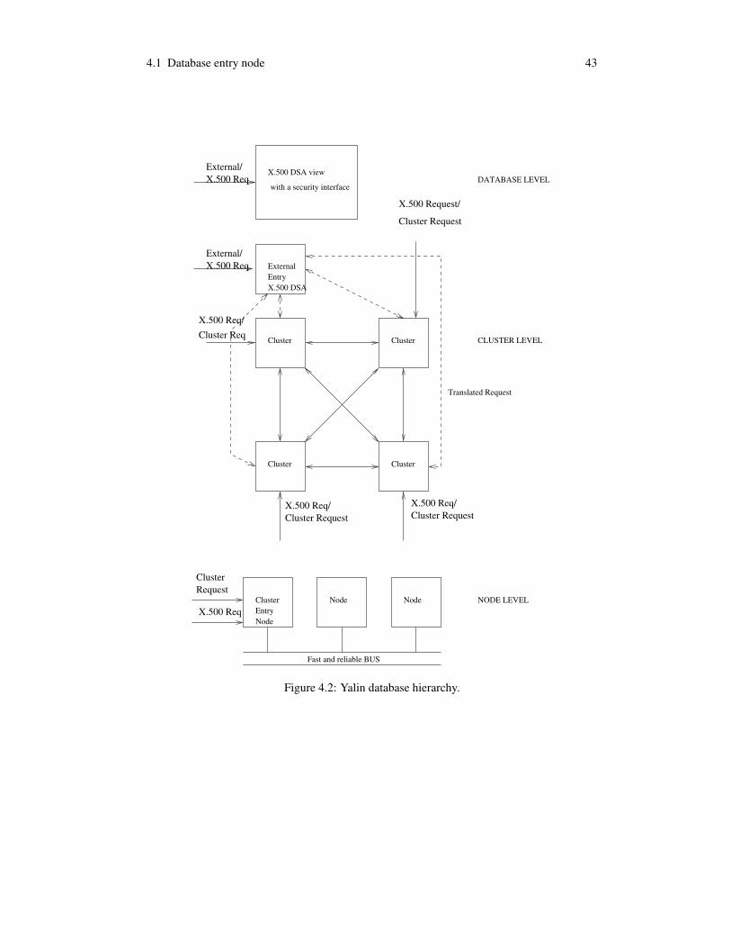
4.1 Database entry node 43
X.500 ReqExternal/
ExternalEntryX.500 DSA
Cluster Cluster
Cluster Cluster
External/X.500 Req
Cluster RequestCluster Request
Cluster ReqX.500 Req/
X.500 Req/X.500 Req/
DATABASE LEVEL
CLUSTER LEVEL
NODE LEVELNode NodeClusterEntryNode
Fast and reliable BUS
Translated Request
Cluster Request
X.500 Request/
X.500 DSA view
with a security interface
ClusterRequest
X.500 Req
Figure 4.2: Yalin database hierarchy.

44 4 YALIN ARCHITECTURE
X.500 and internaldirectory manager
Transaction request
Securitymanager
NAK
from clusters)
Acceptedrequest
Translation Translation/NAK
(From clusters)
Directoryread/update
Global request
(Root data)directoryInternal X.500
directory
X.500 request
request
(ACK arrives directly
To clusters
Directory update
X.500 interpreter
Figure 4.3: Database entry node.
local clients that want to use the standardized IN interface to access data. The entry node is theonly way that external clients may use to access the database. For local clients, the cluster levelabstraction offers an X.500 interface on each cluster.
Next to the interface services, the database entry node interprets the received X.500 requeststo internal transaction requests, offers root DSA services to other DSAs in clusters, co-operateswith other DSAs when necessary, and co-operates with other X.500 root DSAs in externalnetworks. It maintains X.500 level directory information about data locations and informationabout external network entry nodes and teleoperators.
The most important task that the database entry node fulfills is to offer a known entry forexternal clients to the network. As such it is mostly an X.500 root agent that co-operates withother X.500 root agents of external networks. When we have a well-known entry point into thedatabase, the rest of the architecture can be hidden from external clients.

4.2 Clusters 45
The architecture of the entry node consists of a Security manager, an X.500 DSA inter-preter, and an X.500 and internal data directory manager (Figure 4.3). The security manageraccepts requests from applications. It is responsible for checking the access rights of a request-ing client. Both external and local clients are checked when a request arrives. When the requestis accepted, it is forwarded to the X.500 DSA interpreter. The X.500 DSA interpreter is re-sponsible for interpreting an X.500 request to an internal request that can be sent to clusters. Inorder to do this the interpreter consults the X.500 and internal directory manager that has accessto interpretation data from the X.500 data tree to the Yalin data tree. Once an interpretation iscomplete, the interpreted request is sent to one of the clusters. Once the request is served, theresult is sent directly to the requesting application. The X.500 and internal directory managermanages both an X.500 specific data directory and a Yalin specific data directory. Both thesedirectories are plain directories. Actual data resides in clusters. When directory data needs anupdate, an update request is sent to the entry node.
The Yalin architecture allows several database entry nodes. This is probably not necessarysince the database entry node serves mostly requests to and from external networks. Since thetasks of the entry node are relatively simple, with proper hardware a single node should easilybe able to handle all external network traffic. If this is not the case, adding fully replicateddatabase entry nodes can be used to ease bottlenecks in the X.500 data model.
4.2 ClustersA cluster in Yalin behaves externally like a node in a distributed database. Each cluster has asimilar interface regardless of the data fragment that it supports. The interface supports bothX.500 requests and internal Yalin requests. All X.500 requests are interpreted to direct requests,so the clients should use the internal interface to Yalin whenever possible.
The cluster architecture consists of a cluster entry node and a set of database nodes. The en-try node co-operates with other clusters to create and maintain distributed transactions. Actualdata processing occurs in the database nodes. The architecture of a cluster can be seen in Figure4.4. It consists of elements that are in the cluster entry node: an X.500 interpreter, a Clusterdirectory manager, a Global transaction manager (GTM), and a Global concurrency controller(GCC). The nodes element which is also present in Figure 4.4, represents the database nodes inthe parallel database architecture.
The cluster entry node behaves like an X.500 DSA. The X.500 requests are interpretedto Yalin internal transaction language in the X.500 interpreter and then forwarded to the GTM.The X.500 interpreter consults the Cluster directory manager which holds directory informationabout cluster data. The interpretation is straightforward when the clusters follow the IN/GSMdata hierarchy. If the hierarchy is broken, the interpretation may create heavily distributedtransactions.
Sometimes the X.500 interpreter receives X.500 directory update requests from other DSAs.They are interpreted to the Yalin internal transaction language and forwarded to the Clusterdirectory manager. It updates directory information accordingly.
When an X.500 request is interpreted, or when a direct Yalin request is received, it arrives tothe Global transaction manager. The GTM creates a new transaction from the request and thenconsults the Cluster-directory manager to find out which node is best suited for this transaction.The transaction is then sent to the appropriate node which processes it.
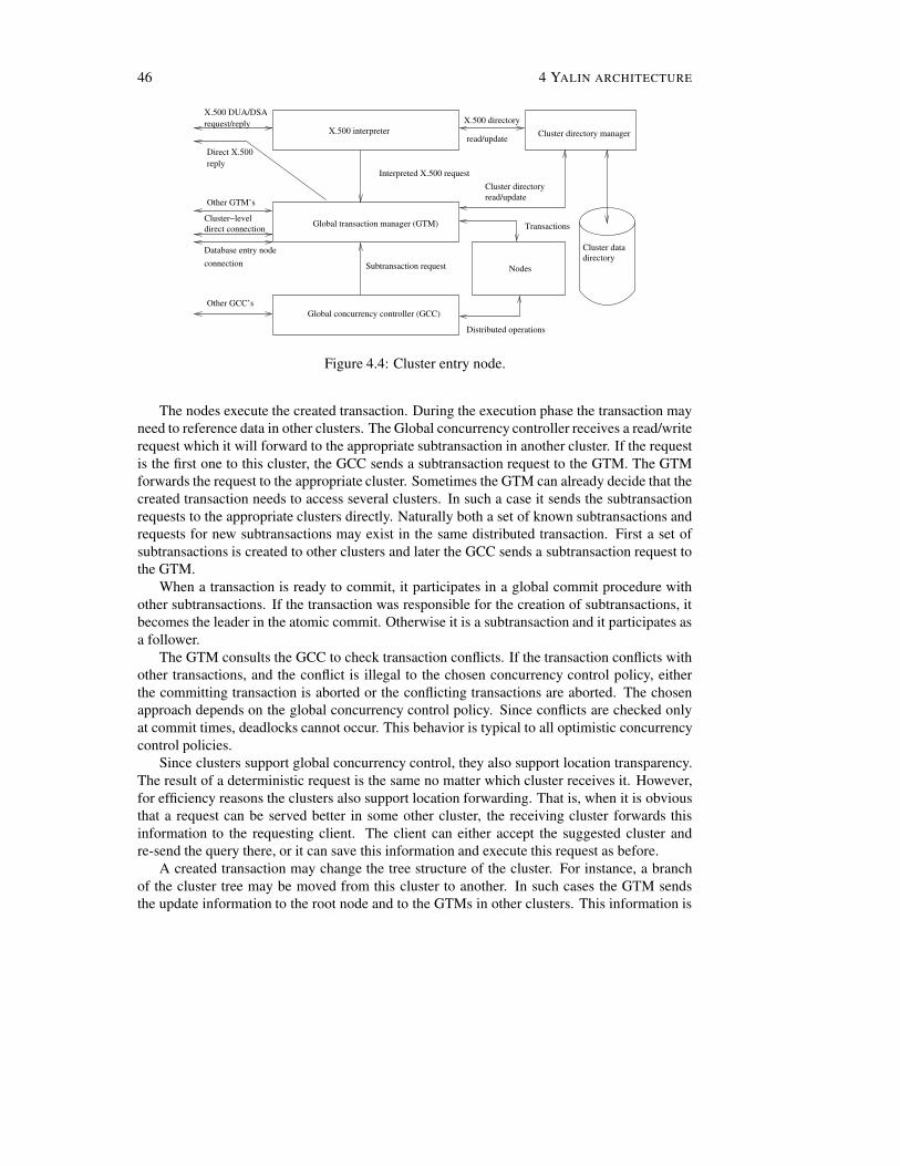
46 4 YALIN ARCHITECTURE
X.500 DUA/DSArequest/reply
Other GTM’s
Other GCC’s
Direct X.500reply
X.500 interpreter
Cluster datadirectory
Subtransaction request
Interpreted X.500 request
X.500 directory
read/update
Cluster directoryread/update
Transactions
Distributed operations
Global transaction manager (GTM)
Global concurrency controller (GCC)
Cluster−leveldirect connection
connection
Cluster directory manager
Database entry node
Nodes
Figure 4.4: Cluster entry node.
The nodes execute the created transaction. During the execution phase the transaction mayneed to reference data in other clusters. The Global concurrency controller receives a read/writerequest which it will forward to the appropriate subtransaction in another cluster. If the requestis the first one to this cluster, the GCC sends a subtransaction request to the GTM. The GTMforwards the request to the appropriate cluster. Sometimes the GTM can already decide that thecreated transaction needs to access several clusters. In such a case it sends the subtransactionrequests to the appropriate clusters directly. Naturally both a set of known subtransactions andrequests for new subtransactions may exist in the same distributed transaction. First a set ofsubtransactions is created to other clusters and later the GCC sends a subtransaction request tothe GTM.
When a transaction is ready to commit, it participates in a global commit procedure withother subtransactions. If the transaction was responsible for the creation of subtransactions, itbecomes the leader in the atomic commit. Otherwise it is a subtransaction and it participates asa follower.
The GTM consults the GCC to check transaction conflicts. If the transaction conflicts withother transactions, and the conflict is illegal to the chosen concurrency control policy, eitherthe committing transaction is aborted or the conflicting transactions are aborted. The chosenapproach depends on the global concurrency control policy. Since conflicts are checked onlyat commit times, deadlocks cannot occur. This behavior is typical to all optimistic concurrencycontrol policies.
Since clusters support global concurrency control, they also support location transparency.The result of a deterministic request is the same no matter which cluster receives it. However,for efficiency reasons the clusters also support location forwarding. That is, when it is obviousthat a request can be served better in some other cluster, the receiving cluster forwards thisinformation to the requesting client. The client can either accept the suggested cluster andre-send the query there, or it can save this information and execute this request as before.
A created transaction may change the tree structure of the cluster. For instance, a branchof the cluster tree may be moved from this cluster to another. In such cases the GTM sendsthe update information to the root node and to the GTMs in other clusters. This information is

4.3 Nodes 47
needed to maintain the global X.500 based view of the database. However, the cluster-specificmoves are not forwarded to the root node. The root node does not need to know about datalocations inside a cluster.
While the clusters in Yalin are specialized, the cluster level architecture is the same on allthe cluster types. The difference between the clusters is in their use. Regular clusters are forregular requests. The mass calling and televoting clusters may not be always accessible, butwhen they are needed, the volume of the requests is so high and specialized that the requestsshould not be allowed to affect transaction throughput in regular clusters. Finally, the VLRclusters are not part of the IN/GSM data tree. Rather, they hold information about visitors fromexternal networks.
4.3 NodesThe node architecture in Yalin is the core element in the database. Where the other elements aremostly transaction interpreters and organizers, the nodes handle database management systemoperations.
Each node may receive two types of transaction requests. First, cluster requests arrive fromthe cluster entry node. These requests are originally from the X.500 root node, from cluster-level clients, or from intra-cluster transactions. Second, a node may receive local requests.These requests are mostly for maintenance staff although in principle it is possible that a clientwants to access a cluster directly and thus bypass the cluster entry node.
The nodes in a cluster behave like a set of nodes in a parallel shared-nothing database. Thissolution allows expandable database nodes and transaction distribution between nodes insidethe cluster. It also simplifies expansions both at the cluster level and at the node level, sinceadding a new distributed database cluster expands Yalin at the cluster level, and adding a newparallel database node to a cluster expands Yalin at the node level. The former expansioncorresponds to a situation where the teleoperator opens a new branch to a new location. Thelatter expansion corresponds to a situation where the teleoperator has to increment the databasecapacity due to a customer volume increase in a local area.
At minimum, a cluster has a single node which is embedded into the cluster entry node.This architecture can be seen in Figure 4.4. The number of nodes in a cluster is limited only bythe hardware. The cluster level managers and transactions see only a single node architecture.
The node architecture follows general database architecture structures, including a Transac-tion manager (TM), a Scheduler, a Concurrency controller (CC), a Bus concurrency controller(BCC), and a Cache manager (CM). It is not meant to be a complete database managementsystem itself. Instead, it is a framework upon which to build the remaining elements. The nodearchitecture can be seen in Figure 4.5.
The TM accepts local and cluster level transaction and subtransaction requests. They all getsimilar treatment in the manager. A transaction request creates a new transaction. A subtrans-action request creates a new parallel database subtransaction that has a leader in some otherparallel database node in the cluster.
When a transaction or a subtransaction has finished, the TM manages bus-level atomiccommit procedures and local commits. The result of the commit or abort is then forwarded tothe cluster entry node. If the transaction is a participant of a distributed transaction, the finalresult of the commit status depends on the cluster level vote results. Thus, a transaction may

48 4 YALIN ARCHITECTURE
Scheduler
Cache manager
Transaction manager
Physicaldata
Concurrency controller Bus CC Bus CC
Global CC
Scheduler
Cache manager
Concurrency controller
Transaction manager
Cluster request
Physicaldata
Node architecture
Local request Cluster request Local request
Subtransaction
Figure 4.5: Regular node architecture.
be aborted at the cluster level even if it can commit at the node level. If the transaction is not aparticipant in a distributed transaction, the cluster level transaction manager accepts the commitimmediately.
When the TM has created a transaction, it sends the created transaction to the Scheduler.The Scheduler manages the transactions that are either executing, waiting for I/O, or ready toexecute. Each transaction receives the CPU according to the chosen scheduling policy.
A transaction may have three types of operations: read operations for reading data from thedatabase, write operations for writing data to the database, and execute operations for calculat-ing intermediate and final results from read data. These three operations are sufficient to modelscheduling and concurrency control in Yalin.
The read and write operations are forwarded to the CC. The CC keeps track of data itemsand transaction operations. It consults the CM when data has to be moved to and from the disk.If the requested data item does not exist in the local node database, the CC consults the BCCto see if the item exists in some other node. If this is the case, a new subtransaction is createdand the transaction becomes distributed within the bus nodes. The BCC may also consult theGCC in the cluster entry node if the data item does not exist in any of the nodes. In such acase the transaction becomes an intra-cluster distributed transaction. We will cover node levelconcurrency control in Section 4.5. Finally, the CM manages physical data in the database. Ithas only two operations fetch and flush. The fetch operation reads a physical data item fromthe disk to the main memory. The flush operation writes a physical data item from the mainmemory to the disk. The CM is the only manager that can access physical data.
The standard node architecture is stripped and follows general transaction managementprinciples. It is better to have a stripped but nevertheless a working model that we can analyzethan a fully equipped model where interesting analysis is lost into a number of uninterestingdetails. Due to this we have omitted such managers as recovery managers, query interpreters

4.4 Database transactions 49
and optimizers.
4.4 Database transactionsIn the IN/GSM data analysis in Chapter 3 we showed that the IN/GSM data hierarchy in-cludes the following classes: Teleoperator, Service, Subscriber, Charging account, Phone line,Log information, Mass calling data, Virtual Private Network (VPN) data, Conference resource,Multi-party call data, Closed user Group (CUG) data, Location information, Visitor group data,and Equipment identity register (EIR) data. This is a simplified model of a telecommunicationsdatabase classes but it still gives us a basis to define major transactions for Yalin.
The transaction types of Yalin can be identified from the IN/GSM service feature analysisand the Yalin database schema. In the analysis we have identified the following transactiontypes: IN service activation transactions, number translation transactions, mobile equipmentlocation update transactions, other mobile related transactions, query transactions for manage-ment, line profile transactions, call triggered transactions, charging transactions, dynamic grouprelated transactions, management update transactions, and EIR-specific transactions.
Regular service related transactions are used when a subscriber wants to activate an IN-service. They are real-time transactions and common in the system. They need read-access toService, Subscriber, and Charging account classes.
Next to the regular service related transactions, we have transactions that handle all kindsof number, charging and phone line translations. These transactions are real-time and commonin the system. They need read access to Service, Subscriber, Charging account, Phone line andLog information classes.
A typical transaction is a location update transaction. It is used every time a mobile equip-ment signals its current location to the network. The transactions are real-time and common inthe system. They need write access to the Location information class.
Communication transactions between a visitor’s HLR and a visiting VLR are mobile relatedtransactions. They are relatively common in the system and real-time. They need write accessto Visitor group data, Location information, and Phone line.
The management staff needs query transactions. The transactions need read access to allclasses. They may be long and distributed. The query transactions are not real-time and notvery common in the system.
Whenever a customer opens a phone line, a line profile transaction is triggered. It is usedfor receiving information about the services and phone lines of the customer. The transactionneeds read access to Service, Subscriber, Charging account, and Phone line classes.
A call triggers at least three transactions. First, when a call is initiated a transaction iscreated to gather IN and routing information, and to create a call log entry for the call. Second,when a call is answered a transaction is created to gather IN information and to update thecall log entry for this call. Third, when a call is finished a transaction is needed to update calllog information and decide charging. The Init call transaction needs read access to Locationinformation, Service, Subscriber, Charging account, and Phone line classes; and write accessto the Log information class. The answer call transaction needs similar read and write access,except that the Location information is no longer needed since the call is already connected.Finally, the finished call needs read access to Service and Phone line classes, and write accessto charging account and Log information classes.
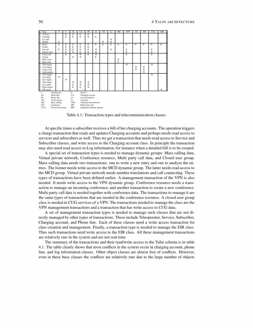
50 4 YALIN ARCHITECTURE
Type T S Su CA PL LI VG Lc MC VPN CR MP CUG EIRActivate R R R RTranslate R R R R RLoc upd WMobile R W WQuery R R R R R R R R R R R R R RProfile R R R RInit call R R R R R W R R RAnswer call R R R R W R RFinish call R W R W R RCharge R W RMass write WMass read RVPN mgmt W WConf mgmt W WCreate conf W WAdd member WCUG mgmt WTop mgmt WServ mgmt WSubs mgmt W W WAcc mgmt R W WPhone mgmt R R WEIR mgmt W
T Teleoperator S: ServiceSu: Subscriber CA: Charging accountPL: Phone line LI: Log informationVG: Visitor group Lc: LocationMC: Mass calling VPN: Virtual private networkCR: Conference MP: Multi-party callCUG: Closed user group EIR: Equipment identity register
Table 4.1: Transaction types and telecommunication classes.
At specific times a subscriber receives a bill of her charging accounts. The operation triggersa charge transaction that reads and updates Charging accounts and perhaps needs read access toservices and subscribers as well. Thus we get a transaction that needs read access to Service andSubscriber classes, and write access to the Charging account class. In principle the transactionmay also need read access to Log information, for instance when a detailed bill is to be created.
A special set of transaction types is needed to manage dynamic groups: Mass calling data,Virtual private network, Conference resource, Multi party call data, and Closed user group.Mass calling data needs two transactions: one to write a new entry and one to analyze the en-tries. The former needs write access to the MCD dynamic group. The latter needs read access tothe MCD group. Virtual private network needs number translations and call connecting. Thesetypes of transactions have been defined earlier. A management transaction of the VPN is alsoneeded. It needs write access to the VPN dynamic group. Conference resource needs a trans-action to manage an incoming conference, and another transaction to create a new conference.Multi-party call data is needed together with conference data. The transactions to manage it arethe same types of transactions that are needed in the conference resource. A closed user groupclass is needed in CUG-services of a VPN. The transactions needed to manage the class are theVPN management transactions and a transaction that has write access to CUG data.
A set of management transaction types is needed to manage such classes that are not di-rectly managed by other types of transactions. These include Teleoperator, Service, Subscriber,Charging account, and Phone line. Each of these classes need a write access transaction forclass creation and management. Finally, a transaction type is needed to manage the EIR class.Thus such transactions need write access to the EIR class. All these management transactionsare relatively rare in the system and are not real-time.
The summary of the transactions and their read/write access to the Yalin schema is in table4.1. The table clearly shows that most conflicts in the system occur in charging account, phoneline, and log information classes. Other object classes are almost free of conflicts. However,even in these busy classes the conflicts are relatively rare due to the large number of objects

4.5 Database concurrency control 51
in the classes. Along with the real-time requirements, the transaction analysis justifies opti-mistic concurrency control methods in Yalin. If conflicts were more common, a pessimisticconcurrency control with priorities would be a reasonable alternative.
4.5 Database concurrency controlSince we have short transactions with tight timing constraints, it is important to minimize theresources needed to manage transactions. This includes resources needed for concurrency con-trol. One very important area in this is global concurrency control.
In principle we can use any concurrency control policy in a distributed database. All wehave to do is to ensure that transactions behave well both locally and globally. This oftenleads to a two-level concurrency control management: local concurrency control and globalconcurrency control.
Local concurrency control management maintains the needed transaction isolation levelwithin nodes. It does not differ from concurrency control in non-distributed databases. Globalconcurrency control management maintains the same isolation level between nodes.
Usually local concurrency control management cannot ensure that transactions do not in-terfere with each other globally. Due to this unfortunate feature distributed databases need totake extra care in order to maintain the desired isolation level both globally and locally. It canbe done for instance by sharing serialization graphs between nodes and always checking if thecombined graph has a cycle. This can become very expensive.
In Yalin we wish to avoid global concurrency control as much as possible. From thedatabase and transaction analysis earlier we can see that the number of distributed transactionsis small compared to the total number of transactions. Most of the time distributed transactionsdo not interfere with each other. Yet every distributed operation may cause a cycle in the globalserialization graph and thus violate the global isolation level of Yalin.
Fortunately it is possible to avoid global concurrency control management completely wheneach node in a distributed database follows a strict concurrency control policy. In such a caselocal concurrency control management is sufficient at the global level as well. We will provethis in the next paragraphs.
Theorem 4.1 A concurrency control policy is strict if for every history H that is allowed bythe policy the following holds: whenever w j � x ��� oi � x ��� i �� j � , either a j � oi � x � or c j � oi � x �[BHG87]. Let us have a distributed database with nodes N1 ����� Nn. If on every node Ni the localconcurrency control policy is strict then transactions also serialize globally.
Proof: The strict concurrency control policy ensures that transactions are only allowed toreference data that has been written by a committed transaction. This ensures that all localserialization graphs SG1 � H � ����� SGn � H � are acyclic [BHG87].
Let us have two distributed transactions Tr1 and Tr2. If both transactions are aborted,no cycle can exist between the transactions. They do not affect the internal consistency of thedatabase and global serialization is maintained. If either of the transactions is aborted, itschanges to the database are nullified and thus no cycle can exist between the transactions. Nowlet us assume that both transactions will commit.
In order for the global serialization graph SG � H � to have a cycle we must have the followingpartial serialization graphs: Tr1 ��������� Tr2 and Tr2 ��������� Tr1. Since on strict policiestransactions cannot reference uncommitted data, we get c1 � c2 from the first serialization

52 4 YALIN ARCHITECTURE
graph, and c2 � c1 from the second serialization graph. Thus, the global serialization graphhas a dependency c1 � c2 � c1, which leads to c1 � c1. This is impossible, so one of thetransactions Tr1 Tr2 must violate local strict policy. Since the assumption is wrong, we cansay that the global serialization graph SG � H � is acyclic. �
It is easy to prove that a strict policy on all nodes is a necessary requirement to completelyavoid global concurrency control.
Theorem 4.2 Let us have a distributed database with nodes N1 ����� Nn. If any node Ni does notfollow a strict concurrency control policy, the local transaction policies cannot ensure globalserialization.
Proof: Let us have nodes Ni and N j � i �� j � where N j does not follow a strict policy. Thenthe following histories are possible:
Ni : o1 � x � c1 p2 � x � c2
N j : o2 � y � p1 � y � c2c1 where operations oi and pi are any conflicting operations.
The serialization graphs we get are SGi � H � � Tr1 � Tr2, and SG j � H � � Tr2 � Tr1. Thusthe global serialization graph has a cycle: Tr1 � Tr2 � Tr1. �
Since in the previous theorem the only requirement to the operations is that they conflict, thetheorem holds regardless of the types of conflicts. Thus, although strict recoverable concurrencycontrol policies are somewhat limiting, they alone can guarantee global transaction serializationfrom local serialization alone.
A corollary of the previous theorems shows that in order to achieve global isolation betweendistributed transactions, it is sufficient that distributed database nodes follow any local strictconcurrency control policy. This can be seen from the serialization graphs SGi � H � . The graphsare independent of the chosen concurrency control policy as long as the policy is strict. Wecan get different types of strict transaction histories depending on the chosen strict concurrencycontrol policy. The corollary also allows nodes to use both pessimistic and optimistic strictlocal concurrency control policies and still maintain global serialization.
Pessimistic concurrency control policies are often strict. This is due to the nature of thepolicies. When a transaction wants to access a data item, it must first get a lock to it. Mostpessimistic policies use hard locks: a lock is allowed only when no conflicting transaction exist.The requirement here is that the lock-holding transaction must keep the locks until it is readyto commit. This ensures that other transactions cannot access data items before the currentlyholding transaction has committed, and that way transactions may access only committed data.A typical variation of this is called Strict two-phase locking [BHG87].
Yet pessimistic concurrency control policies have another unwanted feature: deadlocks. Itis possible that two transactions are waiting for each other to release hard locks even whenlocal concurrency control is strict. Thus, other means are needed to detect deadlocks in a dis-tributed database. Instead of having a global concurrency controller, the database needs a globaldeadlock detector on each node. Again resources are needed to maintain global transactionmanagement.
Optimistic concurrency control policies are usually not strict. They allow read and writeconflicts during transaction execution. It is possible that on node N1 is a serialization graph

4.5 Database concurrency control 53
Tr1 � Tr2 while on node N2 the serialization graph is Tr2 � Tr1. Both histories are correctand well possible within optimistic concurrency control. Yet the global graph has a cycle. Dueto this using most optimistic concurrency control policies on distributed databases need globalconcurrency control managers on nodes that maintain global serialization. On the other hand,optimistic concurrency control policies avoid deadlocks since data items are never hard-locked.
Both pessimistic and optimistic concurrency control policies have variations that both allowstrict histories and avoid deadlocks. As such they are realistic alternatives to Yalin concurrencycontrol.
The pessimistic concurrency control policy that avoids deadlocks is called Conservativetwo-phase locking (or Conservative 2PL) [BHG87]. It avoids deadlocks by requiring eachtransaction to obtain all of its locks before any of its operations are executed. A deadlockcannot exist since it is not possible for a transaction to get more locks after the execution hasstarted. Thus two transactions can never wait for each other to release their locks. Togetherwith Strict 2PL we get a strict pessimistic concurrency control policy that avoids deadlocks.
The optimistic concurrency control policy that avoids global concurrency control is also themost traditional one. The policy goes as follows.
1. When a transaction is started, a local data area is initialized for its use.
2. Whenever a transaction wants to access a data item for reading or writing, the data itemis copied to the local data area where the transaction is allowed to modify the data item.A soft lock is set to the data item to keep track of transactions that have accessed this dataitem.
3. When the transaction is ready to commit, it is first checked if it has a conflict on anyof the data items. If the conflict exists, either the committing transaction is aborted orthe conflicting transactions are aborted. If the conflict is with an already committedtransaction, the committing transaction is always aborted.
4. Once the result of the commit is known, the transaction may join into an atomic commitprocedure. This finally determines the result of the commit.
5. If the transaction is allowed to commit, the modified data items are written back to thedatabase with one atomic operation.
This policy is strict since transactions are allowed to access only committed data. All mod-ifications are done in local data areas of executing transactions. It is also optimistic sincetransactions never have to wait for each other to release data items. All conflicts are resolved atcommit time. As a result it avoids global concurrency control management and deadlocks.
One of the good sides of optimistic concurrency control is that transactions never blockeach other. This feature allows real-time databases, such as Yalin, to use different schedulingpolicies with optimistic concurrency control. In pessimistic concurrency control this requiressome kind of priority policy: what to do when a low-priority transaction holds locks that a high-priority transaction wants to get. This problem has usually been solved by either aborting thelow-priority transaction or allowing it temporarily to have the same priority as the high-prioritytransaction. These solutions can be used in Yalin as well.
Nevertheless, an optimistic concurrency control policy is the best alternative for Yalin sinceit is a real-time database. Transaction deadline management is easier in an optimistic concur-rency control policy since the scheduler has full control of transactions. No kind of transaction

54 4 YALIN ARCHITECTURE
blocking is possible. Pessimistic concurrency control policies usually behave better in tradi-tional databases.
The traditional optimistic concurrency control policy is a candidate for Yalin concurrencycontrol management. It is both strict and optimistic, and so it fulfills the requirements thatwe set to the policy. The Strict OCC is a strong algorithm that causes lots of unnecessaryrestarts. A modified version of the algorithm lowers the number of restarts. When a transactionis marked for abortion due to a conflict with a committing transaction, it is put on a wait stateuntil the voting phase of the committing transaction is over. If the vote result is NO, the waitingtransaction is released. Otherwise it is aborted. Also, when a transaction is at the wait state, itcan lend uncommitted data to transactions in the optimistic assumption that it will commit. Ifthe transaction is aborted, the borrowing transactions are aborted as well. These optimizationsare based on the optimistic atomic commit protocol algorithm PROMPT [GHRS96, HRG00].
4.6 Database global commitsWhile the local concurrency control, as presented in the previous section, can alone maintainmost ACID-properties globally, it cannot guarantee Atomicity. This can easily be seen in thenext example.
Let us assume that we have transactions Tr1 and Tr2 that both execute on nodes N1 andN2. Using strict optimistic concurrency control we can guarantee that any history where thetransactions participate is serializable. However, if Tr1 on node N1 conflicts with Tr2 on nodeN1 while the transactions do not conflict on node N2, the transaction Tr1 (or Tr2 depending onthe commit policy) is aborted on node N1 while it is not aborted on node N2. Thus, transactionatomicity is violated even when global serialization is not.
Various atomic commit protocols have been proposed in literature. The most common onesare based on voting. Each participating subtransaction votes whether the transaction should becommitted or aborted. Depending on the algorithm some or all subtransactions must vote forcommit in order to allow the transaction to commit.
In Yalin we use the traditional two-phase commit protocol as described earlier. It is avery simple and elegant protocol which ensures atomic commitment of distributed transactions.Due to this it is very suitable for Yalin since it is simple to implement yet efficient enough.Its weaknesses are in failure conditions when a transaction is not certain if it should commitor abort. This condition is called a blocking condition since it blocks the transaction fromcommitting or aborting.
The blocking condition in a two-phase commit protocol is due to either a network or sitefailure. The Yalin network is very reliable since it is built on top of the telecommunicationsnetwork, and the bus architecture in clusters is almost error-free. Naturally a Yalin node maygo down due to a software failure, but even these cases should be rare.
If a two-phase commit protocol is not sufficient, the next alternative is to use the three-phase commit protocol as introduced by Skeen [Ske81]. The protocol adds one extra messagephase to the commit processing. The protocol is nonblocking when failures are restricted to sitefailures [OV99]. As such it suits Yalin well. Unfortunately it also adds new message exchangerounds between the leader and participants so committing is slower than in a two-phase commitprotocol.
Distributed transactions in Yalin may execute either at cluster level or at node level, or at

both levels. Due to this the Yalin atomic commit protocol is also a two-level commit protocol.The algorithm for this is simple. Let us consider a case where transaction Tr is ready to commit.
1. Set the result to abort or commit depending on the result of the transaction Tr.
2. If Tr is not a subtransaction of a node level transaction, go to 4.
3. Set Tr into a two-phase commit procedure at node level either as a leader or as a partici-pant. Save the result of the node procedure.
4. If Tr is not a subtransaction of a cluster level transaction, go to 6.
5. Set Tr into a two-phase commit procedure at node level either as a leader or as a partici-pant. Save the result of the cluster procedure.
6. Commit or abort the transaction depending on the result.
Unfortunately up to two voting sessions are needed to complete a transaction. This cannotbe avoided since cluster and node levels are independent of each other. On the other hand, thetwo-level architecture allows different protocols to be used at cluster and node levels. Thus, itis possible to use a three-phase commit protocol at cluster level and two-phase commit protocolat node level when necessary.


Chapter 5
Database Analysis
In this chapter we introduce our transaction-based queueing model analysis tools and use themfor Yalin performance evaluation. We use the approach presented by Highleyman [Hig89] andderive our specific model equations from it. Then we use our equations to analyze an X.500Database entry node and a cluster in Yalin.
The transaction types and data volumes have been defined in earlier chapters. This informa-tion, along with the Yalin architecture, gives a basis to analyze the system. We wish to find theYalin bottlenecks. We are especially interested to see how the X.500 Database entry node canaccept external requests, how distribution affects transaction execution times, how the clusterarchitecture behaves, how parallel nodes can co-operate, and what kind of estimates we canmake for transaction execution times.
Other interesting areas to consider would be various priority-based scheduling policies andfault tolerance. They are not included in the Yalin queueing model. The scheduling policiesare somewhat difficult to analyze with queueing models. The basis of our analysis resides in anon-priority transaction model. Fault tolerance is not analyzed since it is beyond the scope ofthe thesis. We assume that the bus, the network, and clusters are fault-tolerant.
5.1 General database analysis toolsAnalyzing such a complex transaction-based system as Yalin is not a straightforward task. Inorder to simplify the analysis we define a toolbox of queueing model analysis methods fortransaction-based systems.
The analysis toolbox is based on standard Yalin components: transactions, managers, andrequest arrival rates. We use the components to create a general database analysis tool that issuitable for analyzing Yalin traffic. The same tools can be used to analyze any transaction-basedsystem including a traditional database management system.
Most research in queueing theory has concentrated on very specific queueing models andtools. True enough, general formulas for queueing modeling allow a detailed analysis of asystem. The drawback of the detailed approach is that using general formulas requires a goodmathematical background, deep analysis, and perhaps a long time to create an appropriate anal-ysis model. In our thesis we take a different approach. We use a simple model where all arrivingrequests are Poisson-distributed, and the only shared resources are the CPU and servers. These

58 5 DATABASE ANALYSIS
simplifications allow us to generate efficient formulas for solving very complex transaction-based queueing models.
Let us have a set of server nodes Ni each of which has an incoming queue, a set of transactiontypes Tr j that arrive to the system, and a set of incoming service request arrival flows fk thatdescribe how requests traverse between server nodes:
N ��� N1 ������� Nn Tr ��� Tr1 ������! Trm
F �"� f1 ������! fl �(5.1)
Each flow fk has a request arrival rate Rk and an average service time tk. The request arrivalrate prescribes how many service requests arrive to a server in a time interval, and the servicetime prescribes how long the server needs to serve this kind of request when it has arrived.Thus,
fk� � Rk tk � (5.2)
where Rk is the request arrival rate for flow fk and tk is the average service time for flow fkrequests. Let us mark fk � R when we refer to element Rk of fk, and fk � t when we refer toelement tk of fk.
The transaction flow logic in the model is presented with transaction patterns. A transactionpattern is a route through the analyzed system for a transaction type Tr j. We have a set oftransaction patterns for each transaction type:
TP � Tr j � ��� T P1 � Tr j � ������ T Po � Tr j � (5.3)
where one transaction pattern T Ph � Tr j � is defined as follows:
T Ph � Tr j � ��� � Ni N j fi jk �$#Ni N j % N fi jk % F � (5.4)
The incoming flows to a server are divided into a set of transaction patterns, but in theanalysis they are calculated together. Thus, we define the incoming flows of transaction typeTr j for node Ni as follows:
F � Ni Tr j � �&� fi jk % F #'� A B fABk � % TPh � Tr j � A % N B � Ni T Ph � Tr j � % T P � Tr j � � (5.5)
The transaction patterns simplify model calculations. Although they are only a way toarrange request arrival rate flows, they give a possibility to analyze the system behavior insmaller parts. In a small or a medium system a few patterns are sufficient. For instance, inYalin analysis the X.500 Database entry node needs one transaction pattern. Large systemsneed a lot of possibly complex transaction patterns. For instance, the combined cluster andnode analysis of Yalin has six large transaction patterns.
The set of nodes N is divided into a set of clusters. Each cluster models a set of servers thatshare the same CPU. Some servers are completely hardware driven, for instance DMA-baseddisks. Such a server forms a cluster alone.
C �"� C1 ��'�(�( Ch Ci��� Ni #Ni % N � (5.6)

5.1 General database analysis tools 59
N1
N2
N3 N4f1
f2
f3
f5
f7
f4
f6
Figure 5.1: Example traffic model.
The clusters form a disjoint cover to the set N. Thus, each server must belong to exactlyone cluster.
iCi� N Ci ) C j
� /0 * Ci �� C j � (5.7)
Example 5.1 Let us consider a simple system that has one transaction type, four servers, andseven flows (Figure 5.1). The first server N1 receives flow f1. The flow is divided into two flowsf2 and f3 which connect to nodes N2 and N3. The flow f4 is a recursive flow in N2. Flows f5and f6 connect nodes N2 and N3 to server N4, and flow f7 leaves node N4.
The example system has two transaction patterns (Figure 5.2). First, we have a transactionpattern that starts from node N1, goes to node N2 where it has zero or more iterations in nodeN2. When the iterations are over, the pattern goes to node N4 where it exits. Second, we havea transaction pattern that starts from node N1, goes to node N3 and then to node N4 where itexits.
The example system had flows f1 to node N1 which is present in two transaction patterns.This is not possible since each flow is allowed to be present only in a single pattern. Thus,flow f1 is divided into two flows f1a and f1b. Similarly flow f7 is divided into two flows f7a andf7b. The divided flows represent the fact that some percentage of arriving requests take the firsttransaction pattern while the rest take the second transaction pattern. Thus, the combined flowf1a + f1b to node N1 is equal to the original flow f1.
Formally we have the following example system:
N ��� N1 N2 N3 N4 Tr ��� Tr1
T P � Tr1 � ��� T P1 � Tr1 � T P2 � Tr1 � T P1 � Tr1 � ��� � NIL N1 f1a � � N1 N2 f2 � � N2 N2 f4 � � N2 N4 f5 � � N4 NIL f7a � T P2 � Tr1 � ��� � NIL N1 f1b � � N1 N3 f3 � � N3 N4 f6 � � N4 NIL f7b �
Here NIL states that the server in the connection is missing. It is possible that one of theservers is missing in a transaction pattern element, but not both servers. The NIL connection issyntactic sugar. It only shows that the system is open: transaction requests arrive from outside,and they leave the system as well.
The transaction patterns T P1 and T P2 give us the flow information for each node. Following

60 5 DATABASE ANALYSIS
f1a
f1b
N1
f2
f4
f5
f7a
f3 f6
N2
N4
f7bN4N3N1
Figure 5.2: Example traffic model transaction patterns.
the definitions in equation 5.5 we get the following flow sets:
F � N1 Tr1 � ��� f1a f1b F � N2 Tr1 � ��� f2 f4 F � N3 Tr1 � ��� f3 F � N4 Tr1 � ��� f5 f6 �
Moreover let us assume that servers N1 and N4 are hardware driven and do not need CPUservices. Servers N2 and N3 share the same CPU. This division gives us the following clusters:
C1��� N1
C2��� N2 N3
C3��� N4 � �
In the transaction patterns of the example we omit queues and server circles. This is only adrawing convention that distinguishes transaction patterns from full queueing model figures.
A transaction pattern may have the same server several times since a transaction patterndescribes how control flows in the analyzed system. If we have a pattern that has several pathsvia the same server then the server appears several times in the transaction pattern. The clustertransaction patterns in Section 5.4 are examples of this.
For each incoming service request, the total time T in a server is the sum of the queuewaiting time Q and the service processing time S. The service processing time S is divided intotwo components: CPU dispatch time D and service execution time E. Thus, we get
T � Q + S S � E + D �
(5.8)

5.1 General database analysis tools 61
The queue waiting time Q depends on the average utilization L of the server and the remain-ing service time kS of the currently active transaction in the server. The formula, as in [Hig89],is
Q � L1 L
kS (5.9)
where k depends on the distribution of an arriving request. Usually the distribution is Poissondistribution, in which case k � 1. That is, on average the remaining time of the currentlyprocessed request is equal to the average time in the server [Fel50]. From now on we assumethat arriving requests are Poisson distributed: we set k � 1. Thus, we get
Q � L1 L
S � (5.10)
The utilization L tells how much the server is occupied. It is defined as
L � RS (5.11)
where R is the incoming request rate and S is the service processing time in the server.Now let us analyze the traffic model in a node Ni for transaction types in Tr. The node
Ni has incoming Tr j type requests from l sources. When all these are summarized, we get therequest arrival rate for transaction type Tr j in node Ni. When we summarize over all transactiontypes, we get the total arrival rate to node Ni:
Ri� m
∑j , 1
l
∑k , 1
fk � Ni Tr j � � R (5.12)
where fk � Ni Tr j � � R is the arriving rate to node Ni from transaction type Tr j and source flow fk.The total service time Ti in node Ni is
Ti� Qi + Si (5.13)
as earlier.The queue waiting time Qi depends on the node utilization Li and the service processing
time Si. The formula is the same as earlier:
Qi� Li
1 LiSi � (5.14)
The service processing time Si on node Ni is the sum of the service execution time Ei andthe CPU dispatch time Di. This gives us:
Si� Ei + Di � (5.15)
The service execution time Ei on node Ni is a weighted average of all execution times fromdifferent request sources. The weighting factor here is the request arrival rate. Thus, we get:
Ei� ∑m
j , 1 ∑lk , 1 � fk � Ni Tr j � � R �-� fk � Ni Tr j � � t �
Ri (5.16)

62 5 DATABASE ANALYSIS
where fk � Ni Tr j � � t is the average execution time in node Ni from transaction Tr j and sourceflow fk.
Let us define
wi� m
∑j , 1
l
∑k , 1
� fk � Ni Tr j � � R �-� fk � Ni Tr j � � t � � (5.17)
Then we can write
Ei� wi
Ri� (5.18)
When a service process receives a service request, it must first wait in the CPU queue togain access to the CPU. This wait time is modeled with the parameter D. We will assumethat the CPU is in cluster Cl % C. Here we assume that the cluster has at least two servers. Themore servers use the same CPU, the better the Poisson distribution estimation models the actualarrival rates.
We already know that the wait time in a queue is
Q � L1 L
S L � RS �
In the CPU dispatch case, R is the sum of the arrival rates in cluster Cc. The average executiontime d is the weighted average of the service execution times in the cluster, excluding dispatchtime. With this information we get:
Di� dc
� lc1 lc
sc (5.19)
where lc is the CPU utilization on cluster Cc, and sc is the average CPU service time on clusterCc.
Let us define
uc� ci
∑i , 1
m
∑j , 1
l
∑k , 1
� fk � Ni Tr j � � R �.� fk � Ni Tr j � � t � (5.20)
and
Rc� ci
∑i , 1
Ri � (5.21)
Then we get
lc � sc
ci
∑i , i
Ri� scRc (5.22)
and
sc� ∑ci
i , 1 ∑mj , 1 ∑l
k , 1 � fk � Ni Tr j � � R �-� fk � Ni Tr j � � t �∑ci
i , iRi
� uc
Rc� (5.23)
Moreover, uc may be written into a simpler form.
uc� ci
∑i , 1
wi � (5.24)

5.1 General database analysis tools 63
As a result, we get the following formula for the CPU dispatch time dc on cluster Cc:
Di� dc
� Rc � uc
Rc� 2
1 Rc � uc
Rc�� u2
c
Rc � 1 uc � � (5.25)
The CPU utilization on cluster Cc is as follows:
lc � scRc� uc
RcRc
� uc � (5.26)
A special case occurs to clusters with only one server node. Since the requests arrive onlyfrom one source, the distribution is no longer Poisson distributed. In fact, as long as the serverhas a queue we do not need a CPU dispatch time. Thus, in this special case dc
� 0.When we combine the previous formulas, we get the following utilization and service times
for node Ni:
Ti� Qi + Ei + Di
� Li
1 Li� Ei + Di � + � Ei + Di � � � Li
1 Li+ 1 �-� Ei + Di � � (5.27)
Furthermore we get
Li� RiSi
� Ri �wi
Ri+
u2c
Rc � 1 uc � �� wi +
Ri
Rc
u2c
1 uc� (5.28)
Finally this gives us the service time Ti:
Ti� � Li
1 Li+ 1 �.� wi
Ri+
u2c
Rc � 1 uc � � � (5.29)
The service time on node Ni for transaction Tr j is as follows:
Ti j� Qi + Ei j + Di
� Li
1 Li� Ei + Di � + Ei j + Di � (5.30)
The only new variable in the previous formula is Ei j. It is the average execution time for trans-action Tr j on node Ni. It is a weighted average of all incoming execution times for transactionTr j :
Ei j� ∑qi j
k , 1� fk � Ni Tr j � � R �-� fk � Ni Tr j � � t �
∑lk , 1 fk � Ni Tr j � � R � (5.31)
Let us define
wi j� l
∑k , 1
� fk � Ni Tr j � � R �-� fk � Ni Tr j � � t � (5.32)
and
Ri j� l
∑k , 1
fk � Ni Tr j � � R � (5.33)

64 5 DATABASE ANALYSIS
With these definitions we get the final form of the average service time for transaction Tr j onnode Ni.
Ti j� Li
1 Li
wi
Ri+
wi j
Ri j+ � Li
1 Li+ 1 � u2
c
Rc � 1 uc � � (5.34)
5.1.1 Summary of notations and formulasThe 34 equations above define both the middle and the final results of our toolbox. Here wesummarize the final results: toolbox notations and formulas. First, we describe our notations:
Ni : A server (node) in the system.
N : A set of nodes in the system.
Tr j : A transaction type in the system.
Tr : A set of transaction types in the system.
fk : A service request flow in the system.
F : A set of service request flows in the system.
fk � Ni Tr j � : Flow fk to node Ni of transaction type Tr j .
fk � Ni Tr j � � R : Request arrival rate for flow fk above.
fk � Ni Tr j � � t : Average service time for flow fk above.
T P � Tr j � : A set of transaction patterns for transaction type Tr j.
T Ph � Tr j � : One transaction pattern for transaction type Tr j .
F � Ni Tr j � : Node Ni service request flows of transaction type Tr j.
C : A set of clusters.
Ri : Node Ni request arrival rate.
wi : Node Ni average service time multiplier.
Ei : Node Ni service execution time.
Rc : Cluster Cc request arrival rate.
uc : Cluster Cc service time multiplier.
lc : Cluster Cc utilization.
dc : Cluster Cc CPU execution time.
Di : Cluster Cc dispatch time.
sc : Cluster Cc average service time.

5.1 General database analysis tools 65
Li : Node Ni utilization.
Ti : Node Ni total time.
wi j : Node Ni service time multiplier for transaction type Tr j.
Ri j : Node Ni request arrival rate for transaction type Tr j .
Ti j : Node Ni total time for transaction type Tr j .

66 5 DATABASE ANALYSIS
Using the notations above we summarize our formulas in equation 5.35:
N ��� N1 ������! Nn � NIL Tr ��� Tr1 ������! Trm F ��� f1 ������! fl fk� � Rk tk �
T P � Tr j � ��� TP1 � Tr j � ������ T Po � Tr j � T Ph � Tr j � ��� � Ni N j fi jk �-#Ni N j % N fi jk % F
F � Ni Tr j � ��� fi jk % F #'� A B fABk � % T Ph � Tr j � A % N B � Ni T Ph % TP � Tr j � C ��� C1 ��'�(�' Ch Ci
��� Ni #Ni % N Ri� m
∑j , 1
l
∑k , 1
fk � Ni Tr j � � R
wi� m
∑j , 1
l
∑k , 1
� fk � Ni Tr j � � R �-� fk � Ni Tr j � � t �
Ei� wi
Ri
Rc� ci
∑i , 1
Ri
uc� ci
∑i , 1
wi lc � uc dc� u2
c
Rc � 1 uc � Di� dc
sc� uc
Rc
Li� wi +
Ri
Rc
u2c
1 uc
Ti� � Li
1 Li+ 1 �.� wi
Ri+
u2c
Rc � 1 uc � �
wi j� l
∑k , 1
� fk � Ni Tr j � � R �-� fk � Ni Tr j � � t �
Ri j� l
∑k , 1
fk � Ni Tr j � � R
Ti j� Li
1 Li
wi
Ri+
wi j
Ri j+ � Li
1 Li+ 1 � u2
c
Rc � 1 uc � �
(5.35)

5.2 Example: Traditional DBMS analysis 67
R
E dn(R+E)
n(R+E) dn(R+E)
R
R
m(R+E)
R+E
n(R+E)R+E
p(R+E)p(R+E)
Delay
TM Sch CMNet In
Net Out
RDM
Figure 5.3: DBMS traffic model.
5.2 Example: Traditional DBMS analysisIn order to better understand the analysis tools, we will analyze a traditional database manage-ment system from both an optimistic and a pessimistic concurrency control point of view. Thequeueing model of the system can be seen in Figure 5.3.
In the example we want to compare optimistic and pessimistic concurrency control alongwith information of various database processes and possible bottlenecks. This information isbest analyzed with a single transaction type and a transaction pattern. Naturally in an actualcase several types of transactions may exist. We use an average transaction for calculations.The results are as accurate as they would be with several types of transactions.
For the transaction type Tr, we have an incoming request arrival rate R to the system. Eachrequest arrives to the incoming network server (Net In). From there it is forwarded to thetransaction manager (TM) that creates a new transaction.
The new transaction is sent to the scheduler which schedules transaction operations. Thetotal number of operations in the transaction is n + m, where n is the number of operations thatneed to access database data, and m is the number of operations that do some calculation withreceived data and thus need only the CPU.
The cache manager (CM) manages database data buffers. When an operation can be serveddirectly in the buffers, the operation is executed immediately and the result is sent back to thetransaction. If the operation cannot be served with memory buffers alone, the cache managerconsults the disk manager to physically access database disks. This happens with a probabilityd.
For each transaction, the probability for a conflict is p. The conflict management dependson whether we have an optimistic or a pessimistic concurrency control method.
In the optimistic concurrency control, the conflicts are resolved when a transaction is com-mitting. In this model we assume that the committing transaction is aborted and restarted if ithas conflicts.
The aborted transaction rate E depends on the probability that the transaction Tr has con-flicts with other transactions. This occurs with a probability p which depends on the read andwrite sets of the transactions.
For each transaction Tr, the probability of a conflict is p. Thus, in the first round we haveRp conflicts, in the second round Rp2 conflicts and so on. The total number of conflicts andrestarts is

68 5 DATABASE ANALYSIS
E � R∞
∑i , 1
pi � Rp
1 p � (5.36)
In the pessimistic concurrency control, on each CM operation the transaction may beblocked when it wants to lock a data item that has been locked by another transaction. Sincethe conflict probability for the transaction is p, the probability on a certain round is p / n. If theconflict occurs, the transaction is put into a wait state until the conflicting transaction releasesthe blocking lock. This occurs after the blocking transaction has finished.
Since the arrival rates to the system are Poisson distributed, the average waiting time for theblocking transaction is equal to the average execution time for a transaction Tr. After that thetransaction is released. In the queueing model this is modeled with a node Delay. A transactionwaits in the node for the average transaction execution time. The node Delay does not have aqueue.
The average transaction execution time is a sum of the execution times on each node. Theexecution times depend on how many times a transaction will visit each node and how long itwill spend on them. Thus, we get:
T � TN-I + TTM +0������+ TN-O +pnn
T * T pT � TN-I +0����� (5.37)
As a result we get the following total time equation:
T � TSUM
1 p (5.38)
where TSUM is a sum of the service times excluding the delay time.In addition to the previous managers, a pessimistic concurrency control database manage-
ment system has a manager that detects deadlocks. In the model we have modeled the Cachemanager to include its functionality. Whenever a CM operation occurs, it is also tested againstdeadlocks. This can be done with a deadlock detection graph or a similar algorithm. If adeadlock occurs, one of the deadlocking transactions is aborted.
The probability that a deadlock is detected depends on the probability of a conflict. We takea simple approach where the probability of a deadlock is p2, where p is the probability of a con-flict. This comes from an extremely pessimistic assumption that when a transaction conflicts,any of the possibly conflicting transactions may have an ongoing conflict with probability p.Since the transactions are independent, the total conflict probability is p2.
Whenever a deadlock is detected, one of the transactions must be aborted to solve the dead-lock. Thus also in a pessimistic concurrency control the restart rate E exists. We can use thesame formula as in the optimistic concurrency control, except that the probability of a restart isp2. This gives us
E � R∞
∑i , 1� p2 � i � R
p2
1 p2 � (5.39)
The average execution times ti jk for different incoming flows depend on the current hard-ware and database management system software. We do not get into such details here. Instead,on each node Ni we consider a fixed execution time ti for all incoming flows on node Ni. Thetimes in the example are based on modern hardware and software configurations but neverthe-less they are only estimates.

5.2 Example: Traditional DBMS analysis 69
The Net In and Net Out have very simple algorithms. The Net In accepts requests andforwards them to the TM. The Net Out accepts replies from TM and forwards them to theclients. We consider them to take an average 0.01ms for service processing.
The TM creates new transactions and commits or aborts finished ones. These tasks arerelatively simple so we consider them to need 0.1ms.
The Scheduler mostly decides which transaction is executed next. This is a straightforwardtask which needs 0.1ms. However, with probability m /1� n + m � the transaction needs only CPUaccess, at which time no other transactions can be scheduled (since they all use the same CPU).We consider the execution to take an average 1ms time. This gives us the average executiontime � n 2 0 � 1ms + m 2 1 � 0ms �!/1� m + n � .
The Cache manager must check if a requested data item is in the cache, manage lockingand possibly forward the request to the disk manager. This is not a straightforward task sincedata management must be taken into account. We consider this to take 1ms.
The Disk manager is a special manager since it offers a hardware connection to the disks.A disk access time can be estimated with the following formula:
tdisk� tseek + tdelay + taccess (5.40)
where
tdelay� 1
2vrotation / 60 (5.41)
andtaccess
� vaccess 2 sblock � (5.42)
Here tseek is the average seek time, vrotation is the disk rotation speed (rounds/minute), vaccessis the average access time (bytes/second), and sblock is the block size in bytes.
The disk read/write time depends on the data transfer rate, disk seek time, disk rotationspeed, and the size of the disk sector. A very good and efficient hard disk can handle a 20MB/sread and write access, a 4ms seek time, and a 7200 rounds/minute rotation time. We consider adisk sector to be 4096 bytes long. These values give us
tdisk 3 8 � 4ms � (5.43)
The Deadlock detector in the pessimistic concurrency control checks the deadlock graphfor possible cycles. At full scale this is an extremely difficult task since the cycles can be ofarbitrary length. However, since we gave a pessimistic value to the deadlock probability, wecan compensate it by giving an optimistic value to the deadlock detector algorithm. We use1ms for deadlock detection.
Finally, we have to consider the CPU clusters of the model. The Net In, Net Out, andDM are clearly hardware-driven with direct memory access to memory structures. Thus, eachof them forms a cluster. Since each cluster has only one server, there is no need to considerdispatch rates.
The rest of the servers, that is TM, Sch, and CM share the same CPU. They form a cluster inthe analysis. The pessimistic concurrency control lock delay is not an actual manager so it doesnot have a cluster. It affects the TM, Sch, and CM CPU utilization since waiting transactionsare eventually activated to the CM.
With this information we can compare optimistic and pessimistic concurrency control. Thevariables to consider are the conflict probability p and disk cache miss probability d. The

70 5 DATABASE ANALYSIS
0.5
1
Exe
c tim
e/se
cond
s
2 6 10 14 18 22 26 30 34 38 42 46Arriving requests
Optimistic Pessimistic
DBMS execution time
Figure 5.4: Average transaction execution time: p � 0, and d � 0.
varying parameter is the request arrival rate R. The average number of CM operations in atransaction is n � 10. The average number of calculation operations is m � 10.
We will start our analysis from a case, where both the disk cache miss probability and theconflict probability are zero. This is a clearly optimistic case so optimistic concurrency controlshould behave well. The average execution times can be seen in Figure 5.4.
As we can see from the figure, pessimistic concurrency control can manage about 26 re-quests/second while optimistic can handle over 40 requests/second. The result is natural sincepessimistic concurrency control must still check for deadlocks even when none exist. The dif-ference can clearly be seen in Figure 5.5 where optimistic and pessimistic concurrency controlmanager utilizations are described.
In optimistic concurrency control, the Scheduler is the first manager to overload. The Cachemanager and Transaction manager have clearly lighter utilizations. This is reasonable sincethe Scheduler also processes transaction operations that do not need database data. The diskmanager naturally has no utilization since the disk cache miss probability is zero.
Also in pessimistic concurrency control, the Scheduler is the first manager that overloads.However, here the Cache manager overloads much faster than in the optimistic case. This is dueto the deadlock detection that occurs in the cache manager. The extra CPU utilization affectsboth Scheduler and Cache manager as well. In fact the Scheduler in pessimistic concurrencycontrol receives less requests than in optimistic concurrency control, since the transaction restartrate is smaller in pessimistic concurrency control than in optimistic concurrency control. Yetthe pessimistic manager overloads faster than the optimistic one.
The figures are quite similar when we change the disk cache miss and conflict probabilitiesto 0.1. The average service time can now be seen in Figure 5.6.
The optimistic concurrency control is somewhat affected by the higher probabilities. Theeffect is on transaction restarts that stress the Scheduler more than in the previous case. Yet

5.2 Example: Traditional DBMS analysis 71
0
0.2
0.4
0.6
0.8
1
2 6 10 14 18 22 26 30 34 38 42 46 50Network managers Transaction manager
Scheduler Cache manager
Disk manager CPU
DBMS Manager LoadPessimistic Concurrency control
0
0.2
0.4
0.6
0.8
1
2 6 10 14 18 22 26 30 34 38 42 46 50Network managers Transaction manager
Scheduler Cache manager
Disk manager CPU
DBMS Manager LoadOptimistic Concurrency control
Figure 5.5: Concurrency control manager utilizations: p � 0, and d � 0.
0.5
1
Exe
c tim
e/se
cond
s
2 6 10 14 18 22 26 30 34 38Arriving requests
Optimistic Pessimistic
DBMS execution time
Figure 5.6: Average transaction execution time: p � 0 � 1, and d � 0 � 1.

72 5 DATABASE ANALYSIS
0
0.2
0.4
0.6
0.8
1
2 6 10 14 18 22 26 30 34 38 42 46 50Network managers Transaction manager
Scheduler Cache manager
Disk manager CPU
DBMS Manager LoadOptimistic Concurrency control
0
0.2
0.4
0.6
0.8
1
2 6 10 14 18 22 26 30 34 38 42 46 50Network managers Transaction manager
Scheduler Cache manager
Disk manager CPU
DBMS Manager LoadPessimistic Concurrency control
Figure 5.7: Concurrency control manager utilizations: p � 0 � 1, and d � 0 � 1.
the optimistic concurrency control still behaves better than the pessimistic one. However, thepessimistic concurrency control can handle as many requests as in the previous case. This is dueto the fact that the bottleneck is still the Scheduler which is affected only by the few restartedtransactions. The disk manager overloads much slower and thus does not affect the systemperformance. In both optimistic and pessimistic cases, the disk manager overloads slower thanthe Scheduler. Thus, it does not affect the request throughput pace that much (Figure 5.7).
In the previous cases the disk utilization is so small that dominating managers are all soft-ware based. However, when the conflict probabilities rise to 0.25, the situation changes. Thisgives traditional curves in Figure 5.8. Here the conflict probability is p � 0 � 25 and the diskcache miss probability is d � 0 � 25. At small arrival rates the optimistic concurrency controlgives slightly better throughput since the software managers still dominate. At around 15 ar-rivals/second the disk manager starts to dominate. The optimistic concurrency control receivesmore disk requests due to a higher restart rate. Thus, it also overloads faster.
The same result can be seen in Figure 5.9. Both in the optimistic and in the pessimisticconcurrency control the first manager to overload is the disk manager, but in the pessimisticcase the overload happens a little slower.
The same trend would continue when the disk cache miss probability becomes higher. Atthe same time the software advantages of optimistic concurrency control become negligiblecompared to the disk cache miss advantages. Thus, curves like those in Figure 5.8 are expectedin such cases.

5.2 Example: Traditional DBMS analysis 73
0.5
1
Exe
c tim
e/se
cond
s
2 4 6 8 10 12 14 16 18 20 22Arriving requests
Optimistic Pessimistic
DBMS execution time
Figure 5.8: Average transaction execution time: p � 0 � 25, and d � 0 � 25.
0
0.2
0.4
0.6
0.8
1
2 6 10 14 18 22 26 30 34 38 42 46 50Network managers Transaction manager
Scheduler Cache manager
Disk manager CPU
DBMS Manager LoadPessimistic Concurrency control
0
0.2
0.4
0.6
0.8
1
2 6 10 14 18 22 26 30 34 38 42 46 50Network managers Transaction manager
Scheduler Cache manager
Disk manager CPU
DBMS Manager LoadOptimistic Concurrency control
Figure 5.9: Concurrency control manager utilizations: p � 0 � 25, and d � 0 � 25.

74 5 DATABASE ANALYSIS
0.5
1
Exe
c tim
e/se
cond
s
2 4 6 8 10 12 14 16 18 20 22Arriving requests
Optimistic Pessimistic
DBMS execution time
Figure 5.10: Average transaction execution time: p � 0 � 5, and d � 0 � 1.
On the other hand, when the disk cache miss probability is small, the optimistic concurrencycontrol can tolerate quite high restart rates and still dominate over pessimistic concurrency con-trol. For instance in Figure 5.10 the conflict probability is p � 0 � 5 and the disk cache missprobability d � 0 � 1. Here the optimistic concurrency control still behaves better than the pes-simistic one. The restart rate of optimistic concurrency control is higher than in pessimisticconcurrency control, but the extra overhead of deadlock management and lock waits compen-sates this effectively.
As a result of this example analysis, it appears that pessimistic concurrency control is asuitable concurrency control policy in database management systems that have a medium orlarge numbers of disk operations. The disk manager becomes the bottleneck in such systems,and a pessimistic concurrency control needs less disk access due to a smaller restart rate. How-ever, the analysis shows that in database management systems with large memory buffers, andespecially in main memory databases, an optimistic concurrency control policy may in fact bebetter than a pessimistic concurrency control policy.
5.3 X.500 Database entry node analysisAs we described in Chapter 3, the X.500 Database entry node mainly accepts external requestsfrom other networks. It offers an X.500 Directory System Agent (DSA) interface for networkclients to the database. The entry may receive three types of operations: X.500 DSA requests,X.500 updates from other DSAs that are in Cluster entry nodes, and X.500 responses that arrivefrom clusters. The X.500 updates and responses are secure and can proceed immediately. TheX.500 requests are first tested in the security manager.
The behavior of the X.500 Database entry node depends on the type of the received opera-

5.3 X.500 Database entry node analysis 75
X.500
NET OUTOutgoing replies
NET IN
Incoming requests
Security
CM
CDM
Figure 5.11: X.500 Database entry node model.
tion. If the operation is an X.500 request, it is interpreted and the result is forwarded to one ofthe Cluster entry nodes in Yalin. If the operation is an X.500 response, it is forwarded imme-diately to the requester. If the operation is an X.500 update, the directory database is updated.The actual database operations occur in the nodes. Only the results are forwarded back to theX.500 which further forwards them to the request sources.
Since we have three types of requests to the X.500 Database entry node, we also have threetypes of transactions:
� Tr1 : X.500 DSA requests,� Tr2 : X.500 updates, and� Tr3 : X.500 responses.
The architecture of the entry node can be seen in Figure 5.11. It consists of the followingmanagers: the Incoming network request manager (Net In) that accepts new X.500 based trans-action requests, the Security manager (Security) that verifies requests from untrusted sources,the X.500 interpreter (X.500) that interprets requests to internal database management lan-guage, the Cluster directory manager (CDM) that maintains directory information about X.500tree structure, the Disk manager (DM) that offers disk read and write services to Security andCDM servers, and the Outgoing network reply manager (Net Out) that sends replies back to therequesting sources.
The clusters Ci in the X.500 are {Net In}, {Security, X.500, CDM}, {DM}, and {Net Out}.The Security, X.500, and CDM are software managers which share the same CPU. The rest arehardware managers with DMA access to main memory.
We analyze the X.500 Database entry node architecture with a single transaction pattern.When a request arrives, it is accepted into the Net In manager. From there it is sent to theSecurity manager if the request is not from a reliable source. This occurs with probability p j1which depends on the type of transaction Tr j. If the request is from a reliable source, it is sentdirectly to the X.500 interpreter for interpretation.

76 5 DATABASE ANALYSIS
seek Disk seek time in seconds 0.008000sdelay Disk rotation delay 0.004167saccess Disk access time bytes/second 25MB/sblock Disk block size 4096 bytes
Table 5.1: Disk parameters
When a transaction arrives to the Security manager, it has an identity code and a password.The Security manager verifies these and fails access with probability p j2. The Security managermay need to read identification data from the disk. This happens with probability p j3, in whichcase the Security manager consults the DM.
Once the identity and password of the incoming request have been verified, the request iseither accepted or rejected. If it is accepted, it is sent to the X.500 interpreter. If it is rejected,the rejection status is sent to the Net Out which forwards it back to the requesting source.
The X.500 interpreter needs n j rounds to the CDM to interpret the request. On each roundthe CDM may need disk access with probability p j4. In such a case it consults the DM.
Once the interpretation in the X.500 manager is over, the interpreted result is sent to the NetOut. The Net Out either forwards the interpreted result to an appropriate cluster, if it was anX.500 request, or returns it back to the sender if it was of any other type.
The service times in the X.500 follow the same pattern as in the traditional DBMS analysis.Net In and Net Out are simple managers that mostly forward requests to other managers. Weconsider them to take 0.01ms. The Security manager needs only to confirm the incoming re-quest identity and password. We consider this to take 0.1ms time. The X.500 interpreter needsboth to call the CDM for directory data and to do the interpretation. We consider this to take1ms on each round. This time includes interpretation, and result validation. The CDM is a di-rectory manager. As long as the directory data is in the main memory, accessing and validatingit is a straightforward task. We consider this to take 0.1ms.
Finally, the DM is a hardware manager for disks. This was analyzed in the traditionaldatabase management system example. The values used here are based on current state-of-the-art hard disk values for personal computers. We use a 4096 bytes/block block size,25MB/second disk access, 7200 rounds/minute disk rotation, and 8ms disk seek time. Thevalues and calculated intermediate results are summarized in Table 5.1.
With these values we gettdisk 3 12 � 3ms � (5.44)
The received disk access time for DM is larger than the DBMS example value since herewe use a more traditional disk seek time 8ms. These values are equivalent to good conventionalhard disk access times while earlier we used values for specialized database management disks.
In the analysis we use the following parameters:� Incoming transaction probability: Tr1 : 0 � 4 Tr2 : 0 � 2 Tr3 : 0 � 4� Probability that a service request is sent to the Security manager for authentication (p j1):
Tr1 : 1 Tr2 : 0 Tr3 : 0. Only the transaction type Tr1 needs authentication.� Probability that an illegal service request arrives and thus the authentication fails (p j2):
Tr1 : 0 � 05 � Tr2 : 0 Tr3 : 0.
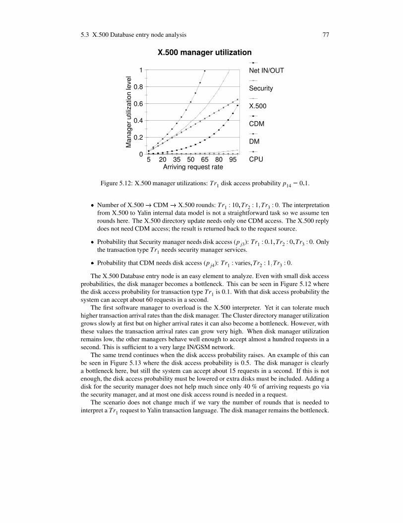
5.3 X.500 Database entry node analysis 77
0
0.2
0.4
0.6
0.8
1
Man
ager
util
izat
ion
leve
l
5 20 35 50 65 80 95Arriving request rate
Net IN/OUT
Security
X.500
CDM
DM
CPU
X.500 manager utilization
Figure 5.12: X.500 manager utilizations: Tr1 disk access probability p14� 0 � 1.
� Number of X.500 � CDM � X.500 rounds: Tr1 : 10 Tr2 : 1 Tr3 : 0. The interpretationfrom X.500 to Yalin internal data model is not a straightforward task so we assume tenrounds here. The X.500 directory update needs only one CDM access. The X.500 replydoes not need CDM access; the result is returned back to the request source.
� Probability that Security manager needs disk access (p j3): Tr1 : 0 � 1 Tr2 : 0 Tr3 : 0. Onlythe transaction type Tr1 needs security manager services.
� Probability that CDM needs disk access (p j4): Tr1 : varies Tr2 : 1 Tr3 : 0.
The X.500 Database entry node is an easy element to analyze. Even with small disk accessprobabilities, the disk manager becomes a bottleneck. This can be seen in Figure 5.12 wherethe disk access probability for transaction type Tr1 is 0.1. With that disk access probability thesystem can accept about 60 requests in a second.
The first software manager to overload is the X.500 interpreter. Yet it can tolerate muchhigher transaction arrival rates than the disk manager. The Cluster directory manager utilizationgrows slowly at first but on higher arrival rates it can also become a bottleneck. However, withthese values the transaction arrival rates can grow very high. When disk manager utilizationremains low, the other managers behave well enough to accept almost a hundred requests in asecond. This is sufficient to a very large IN/GSM network.
The same trend continues when the disk access probability raises. An example of this canbe seen in Figure 5.13 where the disk access probability is 0.5. The disk manager is clearlya bottleneck here, but still the system can accept about 15 requests in a second. If this is notenough, the disk access probability must be lowered or extra disks must be included. Adding adisk for the security manager does not help much since only 40 % of arriving requests go viathe security manager, and at most one disk access round is needed in a request.
The scenario does not change much if we vary the number of rounds that is needed tointerpret a Tr1 request to Yalin transaction language. The disk manager remains the bottleneck.

78 5 DATABASE ANALYSIS
0
0.2
0.4
0.6
0.8
1
Man
ager
util
izat
ion
leve
l
5 20 35 50 65 80 95Arriving request rate
Net IN/OUT
Security
X.500
CDM
DM
CPU
X.500 manager utilization
Figure 5.13: X.500 manager utilizations: Tr1 disk access probability p14� 0 � 5.
Node 1ClusterEntryNode
Fast and reliable BUS
Node n...
Tr requests
Transactionrequest
Resultreply
Figure 5.14: Cluster architecture.
5.4 Cluster analysisThe cluster architecture, as seen in Figure 5.14, is a parallel database architecture. It consistsof a cluster entry node and a set of database nodes. Transaction requests arrive to the clusterentry node and replies are sent back to the request source via it. Depending on the nature of therequest, six transaction types are possible: a local transaction, a bus-level master transaction,a subtransaction within a bus, a cluster-level master transaction, a cluster-level subtransaction,and an X.500 reply/update. Each of the transaction types has a transaction pattern.
The queueing model of the cluster entry node and one of the parallel database nodes canbe seen in Figure 5.15. In the architecture we have nc clusters, each of which has n0 paralleldatabase nodes. Both the network between clusters and the bus between parallel database nodesis modeled as well.
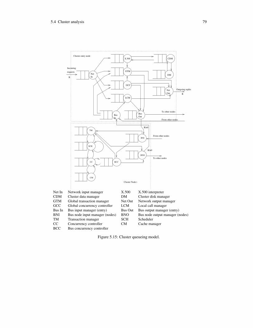
5.4 Cluster analysis 79
CDM
TM
SCH
CC BCC
Cluster Node i
BusIn
BusOut
GTM
GCC
LCM
X.500
Net
Cluster entry node
From other nodes
To other nodes
To other nodes
From other nodes
CM
R/n0
R/n0
Outgoing replies
ROut
DMIn
Net
R
Incoming
requests
BNO
BNI
Net In Network input manager X.500 X.500 interpreterCDM Cluster data manager DM Cluster disk managerGTM Global transaction manager Net Out Network output managerGCC Global concurrency controller LCM Local call managerBus In Bus input manager (entry) Bus Out Bus output manager (entry)BNI Bus node input manager (nodes) BNO Bus node output manager (nodes)TM Transaction manager SCH SchedulerCC Concurrency controller CM Cache managerBCC Bus concurrency controller
Figure 5.15: Cluster queueing model.

80 5 DATABASE ANALYSIS
00
0 0 0
0
1 0
2 0
2 0 n2p3R/n0
n2p3R/n0
R/nR/n
R/n R/n R/n
R/n
n R/n
n R/n
n R/nNet In LCM Bus Out BNI
BNOBus InLCMNet Out
TM Sch CC CMR R R
R R R
R: Incoming request arrival raten0: Number of nodes in a clustern1: Number of CPU-operation roundsn2: Number of CC-operation roundsp3: Probability for a CC-operation to need CM-services
Figure 5.16: Local transaction pattern.
5.4.1 Cluster transaction patternsThe Yalin cluster queueing model, as presented in Figure 5.15, is complex. It consists of 17managers, a bus, and a network. It has several execution paths through the system. In orderto simplify the process of analyzing the queueing model, we use six transaction patterns thatdescribe the transactions of the system. The cluster transaction patterns are as follows: localtransaction, master bus-level transaction, slave bus-level transaction, master cluster-level trans-action, slave cluster-level transaction, and X.500 service reply or directory update. The patternsare analyzed in turn.
We use constants ni to describe various request arrival rate multipliers in transaction pat-terns, and probabilities p j to describe probabilities for certain event occurrences. Each transac-tion pattern has its own constants and probabilities that are named locally within a pattern. Forinstance, the average number of non-database operations (named n1) in the local transactionpattern may be different from the average number of non-database operations (also named n1)in the master bus-level transaction pattern case. The names and descriptions are not ambiguoussince transaction patterns define a local name space.
Local transaction pattern
The first transaction pattern describes a transaction that is local to a single node. It can be seenin Figure 5.16. This is the most common transaction pattern.
The Net In accepts a request and sends it to the Local call manager (LCM). The LCMtranslates the request and forwards it to the appropriate node. This happens via the Bus Outmanager that is an entry point to the local bus. The requests are divided to all nodes in the bus.In the analysis we assume that the requests distribute evenly to all parallel database nodes inthe cluster. The number of arriving requests to a node Ni is R / n0, where n0 is the number ofnodes in the cluster and R is the local transaction request arrival rate in the system.
In the local node the Bus node input manager (BNI) accepts the request and sends it to theTransaction Manager (TM). The TM creates a transaction which it sends to the Scheduler. TheScheduler executes the transaction operations. The total number of transaction operations isn1 + n2 where n1 is the number of calculation operations executed in the Scheduler, and n2 isthe number of operations forwarded to the Concurrency controller (CC).
In the CC the database operation may need disk access. This happens with probability p3.If disk access is needed, a request is sent to the Cache Manager (CM) which executes it. The

5.4 Cluster analysis 81
0
0 0
0
0
0 p3 n0n2 R/
p3 n0n2 R/n2R/n0
n2R/n0
n1R/n0
n4R/n0
n4R/n0
n4R/n0
n4R/n0n4R/n0
n6 n0n5 R/
n6 n0n5 R/
n6 n0n5 R/
R/n
R/n R/n
R/n
R/n
R/n
R R RNet In LCM Bus Out BNI
BNOBus InLCMNet Out
TM Sch CC CM
BNO
BNI
BCC BNO
BCC BNI
R R R
R: Incoming request arrival raten0: Number of nodes in a clustern1: Number of CPU-operation roundsn2: Number of CC-operation roundsp3: Probability for a CC-operation to need CM-servicesn4: Number of bus-level BCC operation roundsn5: Number of master bus-level commit protocol message roundsn6: Average number of slave nodes in a bus transaction
Figure 5.17: Master bus-level transaction pattern.
result is then forwarded back to the CC which returns it to the Scheduler. The CM thus receivesn2 p3R / n0 requests.
Once the transaction is complete, its status is tested in the TM. If the transaction has noillegal conflicts, it is allowed to commit. Otherwise it is aborted. In both cases the TM sendsthe result via the Bus node output manager (BNO) to the bus, where cluster entry node Bus Inreceives it. The Bus In forwards the result back to the LCM which returns it to the Net Outmanager. The Net Out manager sends the result back to the transaction requester.
Master bus-level transaction pattern
The second transaction pattern describes a transaction that is bus-distributed to several paralleldatabase nodes in a cluster. In the pattern our node is a master in a transaction. The pattern canbe seen in Figure 5.17.
The first visited managers are similar to the local transaction pattern. The Net In managerreceives a request which is eventually forwarded to the database node Ni. In the node Ni the TMcreates a transaction and sends it to the Scheduler for scheduling. Now the transaction has threetypes of operations: n1 non-database operations, n2 local database operations, and n4 bus-leveldatabase operations.
The non-database operations and the local database operations are similar to the previouspattern. The CM access probability is p3. When a bus operation occurs, the Scheduler sendsthe operation request to the Bus concurrency controller (BCC). The BCC checks the status ofthe operation and forwards it to the appropriate node in the cluster. This forwarding is done viathe BNO manager.
Once the operation request is sent to the appropriate node, the transaction is put on holduntil the result arrives to the BNI manager. The manager forwards the result back to BCCwhich forwards it back to the Scheduler.
When the transaction is finished, the TM initiates a global commit procedure to all its sub-

82 5 DATABASE ANALYSIS
n2 2p3(R+ )
n2 2(R+ )n2 2(R+ )
n2 2(R+ )
2R+2R+
2R+
n1 2(R+ )
2 2
n7R
n7R
n7R 2
p3
R
RR
R
RR
R
R
R R R
BCC TM Sch CC CM
BCC BNO
BCC BNI
1,2
BNO
BNI
BNI
1
3
2
R R R
R R
BNO3R R
2R
R
BNI
R: Incoming create request arrival rate to a new transactionR2: Incoming bus-level operation request arrival rate to an existing transactionn1: Number of CPU-operation rounds in a bus-level operationn2: Number of CC-operation rounds in a bus-level operationp3: Probability for a CC-operation to need CM-servicesn7: Number of slave bus-level commit protocol message rounds
Figure 5.18: Slave bus-level transaction pattern.
transactions in slave nodes. It needs n5 rounds to the slave nodes to get a result. The averagenumber of slave nodes here is n6. Thus the total number of messages in the bus-level commitprocedure is n5n6R / n0.
Once the global commit procedure is finished, the transaction is either committed oraborted. In both cases the result is sent back to the cluster entry node via the BNO manager.The result is forwarded back to the request source like in the previous pattern.
Slave bus-level transaction pattern
The third transaction pattern describes a slave transaction in a bus-level distributed transaction.It can be seen in Figure 5.18. This pattern occurs whenever a bus-level master transactionwants to create a slave transaction to the analyzed node. It happens both after a master bus-level transaction pattern and also after a master or slave cluster-level transaction pattern sinceall three transaction types may be master transactions in a bus-level transaction.
The slave bus-level transaction pattern has three entry points: when a slave transaction iscreated, when a request arrives to an existing slave, and when the master initiates a globalcommit procedure.
First the node receives a request of a master from another node. The requests arrive at rateR. In the node the request arrives to the BNI manager which forwards it to the BCC of the node.The BCC checks if a slave transaction has already been created. Since this is the first call tothe BCC, a slave transaction has not been created yet. The request is sent to the TM for slavetransaction creation.
The TM creates a new transaction which executes the request. It needs to access local dataand perhaps do CPU operations. The total number of local data access operations is n1 andCPU operations is n2. When the first request has been calculated, the result is sent to the BCCwhich returns it back to the requesting BCC via the BNO manager. After that the transaction isput into a wait state until the next request arrives.
When the master transaction sends a later request, the BCC already knows to which trans-action in this node to forward it. The request is sent via BNI to the BCC which forwards it

5.4 Cluster analysis 83
to the Scheduler. After that the operation needs n1 CPU rounds, n2 CC rounds, and n2 p3 CMrounds. After data delivery and possible CPU operations the result of the request is sent backto the master transaction via BCC. The arrival rate of this type of requests is R2.
Once the master is ready to commit, it sends a commit request via BNI to the TM. Theslave needs to take n7 rounds before the commit result of the transaction is known. After thatthe transaction is either committed or aborted. In both cases the slave transaction sends anacknowledgment message back to the master transaction. The acknowledgment message goesfrom the TM via the BNO to the master transaction node. The master transaction is responsiblefor sending the final transaction result back to the requester.
In this pattern we thus have two arrival rates: R for new slave transaction creation requests,and R2 for old slave transaction operation requests. These arrival rates have a relationshipthat depends on the master transaction parameters on master bus-level transaction pattern, andmaster and slave cluster-level transaction patterns. It is simpler to use two request arrival ratesand later verify how they are related. We will analyze the relationship in Section 5.4.1.
Master cluster-level transaction pattern
The fourth transaction pattern describes a distributed transaction between several clusters. Thepattern can be seen in Figure 5.19. In the pattern we see the master transaction.
The incoming request arrival rate is R. When a request arrives to Net In, it is first checked tosee whether it is an X.500 request. In such a case it is sent to the X.500 manager for interpreta-tion. This happens with probability p9. The X.500 needs n9 rounds to CDM for interpretation.The CDM may need to access a disk manager DM on some of the rounds. The probability fora disk access is p10.
When the interpretation n9 rounds are over, the interpreted request is sent to the GTM. Ifthe request is not an X.500 request, it is directly sent to the GTM.
The GTM decides which parallel database node receives the request. The node Ni requestarrival rate is R / n0 since we assume that the requests are distributed evenly on all paralleldatabase nodes.
The TM creates a transaction that has four types of operations: n1 CPU operations, n2 localdatabase operations, n4 bus-level operations, and n8 network-level operations.
The CPU, local database, and bus-level operations follow the same pattern as in the previouscase. A network level request is first forwarded to the BCC. It sends the request via the BNOmanager to the cluster entry node. There the cluster entry node Bus In manager forwards it tothe Global concurrency controller (GCC). The number of global operations from this node isn8R / n0.
The GCC sends the request via the Net Out manager to the appropriate cluster. Once theresult is received from the appropriate cluster to the Net In manager, it is sent via the GCCand the Bus Out manager to the correct node. There the node BNI manager sends the result toBCC which forwards it to the Scheduler. When the result is received from the other cluster, themaster transaction may proceed.
Once the transaction is ready to commit, the commit is done at two levels. First, at bus-level the master transaction follows a bus-level commit procedure to decide if the transactioncan commit at the cluster level. If it can, the result is sent back to the GTM which executes anetwork-level commit procedure to decide if the transaction can commit globally. At bus leveln5 rounds are needed for completing the atomic commit procedure. The number of slave nodes

84 5 DATABASE ANALYSIS
n8R
n8R
n8R
n8R
n8R n8R
p9Rp9R
n9p9R
n9p9R
n9p9p12R
p9(1− )R
n8R/n0 n8R/n0
n8R/n0
n8R/n0
n8R/n0
0
0 0
0
0
0 p3 n0n2 R/
p3 n0n2 R/n2R/n0
n2R/n0
n1R/n0
n4R/n0
n4R/n0
n4R/n0
n4R/n0n4R/n0
n6 n0n5 R/
n6 n0n5 R/
n6 n0n5 R/
n11 n0R/n12
n11 n0R/n12
n11 n0R/n12
*)
R/n
R/n R/n
R/n
R/n
R/n
Bus InGCCNet Out
Net In GCC Bus Out BCC
Net In GTM
Bus InGTMNet Out
X.500 CDM
R R
RRR
DM*)
*)
Net In
Net Out
BCC
Bus Out TM Sch CC CM
BCC BNO
BCC BNI
BNO
BNI
BNI
BNO
BNI
BNO
R: Incoming request arrival raten0: Number of nodes in a clustern1: Number of CPU-operation roundsn2: Number of CC-operation roundsp3: Probability for a CC-operation to need CM-servicesn4: Number of bus-level BCC operation roundsn5: Number of master bus-level commit protocol message roundsn6: Average number of slave nodes in a bus transactionn8: Number of cluster-level BCC operation roundsn9: Number of X.500-CDM-X.500 roundsp9: Probability for an incoming request to be of X.500 typep10: Probability for CDM to need DM servicesn11: Number of master cluster-level commit protocol message roundsn12: Average number of slave clusters in a cluster transaction
Figure 5.19: Master cluster-level transaction pattern.
to participate in the procedure is n6. Hence n5n6 messages are sent and received in the protocol.At cluster level n11 rounds are needed, and the average number of slave clusters in a cluster-
level transaction is n12. Hence n11n12 messages are sent and received in the protocol. Once theGTM has decided the result for the committing transaction (commit or abort), the result is sentback to the requester via the Net Out manager.
Slave cluster-level transaction pattern
The fifth transaction pattern describes a transaction that is a slave in a network-level distributedtransaction. The pattern is in Figure 5.20. Like the slave bus-level transaction pattern, this pat-tern also has three entry points: a new transaction creation, a request to an existing transaction,and a global cluster-level commit protocol request.
First, a new operation request arrives from a master cluster. The arrival rate of these requestsis R. The Net In manager receives it and forwards it to the GCC. The GCC notifies that the

5.4 Cluster analysis 85
R2 R2R2
R+R2 R+R2 R+R2
n13 R
n13 R
n13 R
n0R2 / n0R2 / n0R2 /
R2 n0(R+ )/ R2 n0(R+ )/ R2 n0(R+ )/
R/n0
R/n0
R/n0
R/n0
R/n0
R/n0
R/n0
R/n0
n5n6R/n0
n5n6R/n0
n5n6R/n0
n02R/
R/n0 R2 n0(R+ )/n2
R2 n0(R+ )/n2
R2 n0(R+ )/n4
R2 n0(R+ )/n4
R2 n0(R+ )/n4
R2 n0(R+ )/n4
R2 n0(R+ )/n4
p3n2 R2 n0(R+ )/
p3n2 R2 n0(R+ )/
R2 n0(R+ )/n1
Net In GCC GTM Bus Out TM Sch CC
BCC
BCC
BNO BCCBus InGCCNet Out
Net In GCC Bus Out BCC
Net In GTM
Bus InGTM
Net In
Net Out
Bus OutNet Out
2
1,2
1
3
3
R R
R R R
R
R
R
*)
R
R
R
Bus Out
CM
*)
BNI
BNI
BNO
BNI
BNO
BNI
BNO
BNI
BNI
R: Incoming create request arrival rate to a new transactionR2: Incoming cluster-level operation request arrival rate to an existing transactionn0: Number of nodes in a clustern1: Number of CPU-operation rounds in a cluster-level operationn2: Number of CC-operation rounds in a cluster-level operationp3: Probability for a CC-operation to need CM-servicesn4: Number of master bus-level operation rounds in a cluster-level operationn5: Number of master bus-level commit protocol message roundsn6: Average number of slave nodes in a bus transactionn13: Number of slave cluster-level commit protocol message rounds
Figure 5.20: Slave cluster-level transaction pattern.
request is from a master transaction that does not yet have a slave in this cluster. It sends therequest to the GTM which creates a new cluster-level slave transaction.
The freshly created transaction is sent via Bus Out to an appropriate node in the cluster.The node BNI manager receives the transaction and forwards it to the TM in the node. The TMcreates a new bus-level transaction and starts execution. The number of incoming requests to aparallel database node is R / n0.
The new transaction executes the operations that were received from the master transaction.The transaction execution may trigger bus-level distributed operations which make the slavecluster transaction a master in a bus-level transaction. This part of the analyzed transactionpattern has been described in the master bus level transaction pattern analysis.
Once the current operation execution is over, the results are sent via the BCC out to theGCC that returns the result to the GCC of the master transaction cluster. The bus transactionitself is idle waiting for the next requests to arrive.
The next time an operation request arrives to this slave transaction, the GCC recognizes itand sends it directly via the bus to the appropriate node. The Scheduler activates the sleepingtransaction which then executes the received operations. Again the operations may be to bus-level slave transactions as well. When the operations have been executed the results are sentback to the master cluster-level transaction the same way as when the transaction was firstcreated.

86 5 DATABASE ANALYSIS
p10 R
p10 RX.500 CDM
R RR
R
RDM
RNet In Net Out
R: Incoming request arrival ratep10: Probability for CDM to need DM services
Figure 5.21: X.500 service reply/directory update pattern.
When the master cluster transaction is ready to commit, it sends a prepare message to theslave transaction. The prepare message is sent to the GTM which sends it to the bus transactionat the correct node.
If the slave transaction is a master at a bus level, it executes a bus master commit procedurepattern that we described in Section 5.4.1. Once the bus-level voting is finished, the slavetransaction knows how it will vote at a cluster-level voting procedure. Its vote is sent to theGTM which will participate in a cluster-level atomic commit procedure. The cluster-level voteneeds n13 rounds to complete.
Once the cluster-level commit procedure is finished, the result is sent back to the node.The node TM activates the bus transaction which then finishes the bus-level atomic commitprocedure (where it is a master transaction). Finally, the slave cluster-level transaction sends anacknowledgment to the master transaction. After that the slave transaction commits or abortsitself depending on the result of the cluster-level votes.
X.500 service reply/directory update
The last transaction pattern describes X.500 cluster replies and directory updates. They bothfollow the same pattern that can be seen in Figure 5.21. This is the simplest pattern. The otherX.500 operation, namely X.500 service request with interpretation is part of the master clustertransaction pattern.
The Net In manager receives a request and forwards it to the X.500 manager. The X.500manager does an interpretation and sends the result to the CDM manager. The CDM doesnecessary updates and returns acknowledgment to the X.500. After that the result is returnedvia Net Out back to the client. The CDM may need to consult the DM with probability p10.
Relationships between master and slave transactions
Both cluster-level and bus-level distributed transactions have master and slave transaction pat-terns. The master transactions initiate all actions. The slaves respond to master requests. Thus,we have a clear relationship between master and slave transaction patterns.
We will first analyze the simpler case: the relationship between cluster-level master andslave transaction patterns. This is a simpler case than the bus-level case since here we haveonly two patterns to deal with. In the bus-level case we have four patterns to consider since alsocluster-level master and slave transactions may participate as masters in bus-level distributedtransactions.
In the cluster-level transaction pattern, from the slave point of view we have an arrival rateof R incoming create requests and an arrival rate of R2 incoming regular operations. These

5.4 Cluster analysis 87
requests arrive from all other cc 1 clusters. Thus, the number of arriving requests from asingle master cluster is R /�� cc 1 � for create requests, and R2 /�� cc 1 � for incoming regularoperations.
From a master transaction point of view the total arrival rate of distributed operations isn8RM where n8 is the average number of distributed operation rounds, both create requests andregular operations; and RM is the arrival rate of all requests in a master node. Of the n8 rounds,one round is for a new slave transaction creation and n8 1 rounds are for regular operations.These operations are divided to all n11 slave nodes that participate in a distributed transaction.Thus, we have the following relationships:
R1
cc 1� RM
1n11
and R21
cc 1� RM
n8 1n11
� (5.45)
This gives us the relationships to R and R2 in the slave cluster-level transaction pattern:
R � RMcc 1
n11 and R2
� RM� n8 1 �.� cc 1 �
n11� (5.46)
Also a relationship between the number of master cluster commit protocol rounds n12 andslave cluster commit protocol rounds n13 exists in the slave cluster-level transaction pattern.For every sent request to the network there must be someone to receive it, and vice versa. In theanalysis we use a model where the master initiates all transactions between slaves and slaves re-spond to the master only. This gives us a relationship n13
� n12 1 because on each request theslave will respond, and the first prepare round is received at route Net In � GTM � Bus Out �etc. so that the bus-level commit procedure can be initiated and finished as well.
The bus-level master and slave transaction relationship is similar to the cluster-level re-lationship. However, in the bus-level case also cluster master and slave transactions may bebus-level master transactions. These requests must be included in the analysis.
From the slave point of view the situation is similar to the cluster-level slave transactions.We have an arrival rate R for incoming create requests, and an arrival rate R2 for incomingregular operations. The total number of nodes in a cluster is n0, and excluding our slave nodethe rest may send create requests to us. Thus, the total arrival rate of create requests from asingle node is R /�� n0 1 � , and the total arrival rate of regular operations is R2 /1� n0 1 � .
From the master point of view, we have three cases to consider: master bus-level trans-actions without cluster-level distribution, master bus-level transactions that are cluster-levelmasters, and master bus-level transactions that are cluster-level slaves. We analyze these inturn.
The master bus-level transaction has arrival rate Rm, and the number of bus-level requests toits slaves is n4. This includes both creation requests and regular operation requests. We renamethe n4 constant to n4m to avoid confusion with other local n4 constants later.
The master cluster-level transaction has similar figures: RM arrival rate and an averagen4M bus-level operations in a master bus-level transaction. Similarly the slave cluster-leveltransaction has RS + R2S request arrival rate and an average n4S bus-level operations in a masterbus-level transaction.
With these values, and with the analysis in the cluster-level transaction case, we get thefollowing formulas for slave bus-level transaction pattern:
R � Rcn0 1
n6 and R2
� Ron0 1
n6 (5.47)

88 5 DATABASE ANALYSIS
whereRc� Rm + RM + � RS + R2S � (5.48)
andRo
� � n4m 1 � Rm + � n4M 1 � RM + � n4S 1 �.� RS + R2S � � (5.49)
Just like in the cluster-level commit routine, also in the bus-level there is a relationshipbetween the number of master bus-level commit protocol rounds n5 and slave bus-level commitprotocol rounds n7. For every sent request to the bus there must be someone to receive it, andvice versa. In the analysis we use a model where the master initiates all transactions betweenslaves and slaves respond to the master only. This gives us a relationship n7
� n5 1 becauseon each request the slave will respond, and the first prepare round is received at route BNI� TM � etc. so that the bus-level commit procedure will be initiated.
5.4.2 Manager clusters and service timesIn the Cluster entry node, the clearly hardware-driven managers are Net In, Net Out, Bus In, andBus Out. Each of these receives requests and forwards them to appropriate software managers,to the network, or to the bus. We consider them to form a manager cluster although basicallywe could consider each of them to form a cluster on their own.
The software managers in the cluster entry node are X.500, CDM, GTM, GCC, and LCM.They clearly form a cluster since they share the same CPU.
The DM is a disk controller. As such it is neither a network hardware entity nor a softwaremanager. It forms a cluster alone in the model.
Second, we will consider manager service times. In principle every transaction pattern mayhave local service times since the service times are related to incoming request flows. Yet mostmanagers have equal service times regardless of the transaction pattern since similar incomingflows on each pattern present similar actions.
The service times depend on the hardware used, such as CPU, memory, and disk features.In the analysis we assume that we have state-of-the-art personal computer hardware. We arenot interested in analyzing architectures that are too expensive to build or use.
We consider the CPU and simple hardware service times to vary from 0.01ms to 1ms. Witha state-of-the-art CPU 1ms is over 500,000 machine operations when one operation takes fourCPU cycles.
The managers in the cluster-node analysis are both in the cluster entry node and in thedatabase nodes. The cluster entry node managers are Net In, Net Out, X.500, CDM, DM,GTM, GCC, LCM, Bus In, and Bus Out. The database node managers are BNI, BNO, TM,Scheduler, CC, CM, and BCC. Next to these managers, the Network and the Bus are modeledas managers. We now consider here the service execution times of all managers in turn.
The Net In manager accepts requests from the network and forwards them to appropriatecluster entry node managers. The operations are straightforward and simple to implement. Weconsider the manager to take 0.01ms. Similarly the Net Out manager receives requests fromvarious sources and forwards them to the network. We consider this manager to need 0.01msfor service execution as well.
The X.500 manager is responsible for translating incoming X.500 requests to the Yalininternal database model. This is not a straightforward task. In the operation the X.500 managermay need several consultation rounds to the CDM. We consider each X.500 round to take 1ms.

5.4 Cluster analysis 89
The CDM holds information of the Yalin data tree. This information is needed for X.500operations. The manager holds information in the main memory and transfers it from there viadirectories. We expect a single access to take 0.5ms.
Sometimes the CDM must consult the DM that holds directory information on a disk. TheDM is a regular hardware manager for disks. Each disk operation has elements that are equalto the earlier Database entry node analysis. Thus we can use the same parameter values that weused in the global entry disk manager analysis. This gives us the disk access time
tdisk 3 12 � 3ms � (5.50)
As earlier, the average service time is equivalent to the service time of a good modern hard disk.The GTM creates new global transactions and manages global commit procedures. These
tasks are not straightforward, so we consider them to take 1ms each. The same is true for theGCC manager which must decide which cluster to forward a service request. We consider thisto take 1ms on each request as well.
The LCM is an entry point for local transactions. It both receives requests from Net In anddecides which database node in the cluster should receive the request, and receives responsesfrom local database transactions and forwards them to the requesters. These are relativelystraightforward tasks since the receiver is already known when LCM services are called. Weconsider this to take 0.1ms.
The Bus In manager receives data from the common bus that is sent from database nodes tothe cluster entry node. The Bus Out manager sends cluster entry node data to the common busfor database nodes. Thus these managers are similar to Net In and Net Out. We consider alsothese managers to take 0.01ms for each service request.
On each database node, the TM creates new transactions and participates in bus-level com-mit procedures. These tasks are not straightforward so we consider them to take 1ms each.
A Scheduler in a database node has two tasks: it either forwards a data item request to CCor BCC, or it executes a CPU operation. The former we consider to take 1ms, the latter 5ms.
The CC and BCC manage operations for local and external data items, respectively. Theydo not have access to the physical database but they may access data items that are in the mainmemory. The CC manages local data items. We consider this task to take 1ms for each dataitem. The BCC decides where an external request is forwarded. This information is in localdirectories that are mostly in the main memory. We consider also this operation to take 1ms.
The CM is a disk manager like the DM in the cluster entry node. We use the same pa-rameters to the CM that we used for the DM. Thus, the average service time is about 12.3ms.Similarly the database node managers BNI and BNO are equal to cluster entry node managersBus In and Bus Out. We consider BNI and BNO both to take 0.01ms on each request.
The network and bus are also considered managers in the model. Both of them have servicetimes of types t � packet size / speed where the packet size is the average size of the sent orreceived packet in bits, and speed is the network or bus speed in bits/second. We consider theaverage packet size to be 256 bytes since most traffic both in network and in the bus is verysmall. The network speed is 64kb/s and bus speed is 25Mb/s. With these values the networkservice time is 32ms and the bus service time is 0.08ms. However, we very soon found out thatthe value 64kb/s gives boring results. The network overloads immediately and makes all globaltransactions impractical. Due to this we used a higher network speed 1Mb/s.
In the analysis we will examine the bus and network, cluster entry node managers, anddatabase node managers. We use the average service execution times and service analysis

90 5 DATABASE ANALYSIS
bus Bus speed bits/second 25Mb/snetwork Network speed bits/second 64kb/sbusblock Bus block size 256 Bnetblock Net block size 256 B
Table 5.2: Bus and network parameters.
t1 CEN Net In service time 0.000010st2 CEN Net Out service time 0.000010st3 CEN X.500 interpreter service time 0.001000st4 CEN Cluster directory manager service time 0.000500st5 CEN Disk manager service time 0.012331st6 CEN Global transaction manager service time 0.001000st7 CEN Global concurrency controller service time 0.001000st8 CEN Local call manager service time 0.000100st9 CEN Bus In service time 0.000010st10 CEN Bus Out service time 0.000010st11 Node Bus-in service time 0.000010st12 Node Bus-out service time 0.000010st13 Node Transaction manager service time 0.001000st14a Node Scheduler quick service time 0.001000st14b Node Scheduler slow service time 0.005000st15 Node Concurrency controller service time 0.001000st16 Node Cache manager service time 0.012331st17 Node Bus concurrency controller service time 0.005000st18 Network service time (1Mb/s speed) 0.002000st19 Bus service time (25Mb/s speed) 0.000082s
Table 5.3: Service time default values.
parameters as described earlier. The service times and parameters are also summarized here.Table 5.2 summarizes bus and network parameters. The network and bus speeds are based
on current hardware, except that the network speed is still relatively low. Yet when we wantto analyze a distributed database it is better to be conservative with network estimations. Al-though Yalin is not intended to work in a public network, network capacity can still becomea bottleneck. The network speed value 1Mb/s should be realistic enough while not giving toooptimistic estimates.
Table 5.3 summarizes the manager service times. The service times have been describedearlier and need not be repeated here. It should be noted that the CEN disk manager and thenode CM both use disk values that are derived from known hard disk parameters.
Excluding the Scheduler, each manager has a single service time for all incoming requestflows. This is a reasonable assumption since the managers mostly have few tasks to manage.An exception to this rule are transaction managers. They process transaction creation, deletion,and global commit procedure tasks. However, since all these tasks are about equally complex,

5.4 Cluster analysis 91
we have taken an approach to use a single service time for all the tasks. The Scheduler, how-ever, needs two service times: one for forwarding read and write operations to the concurrencycontroller, and one for executing CPU operations.
5.4.3 Analyzed transactionsThe Yalin system has 23 transaction types, as analyzed in Section 4.4. In the bottleneck analysiswe are mostly interested in transaction sizes and how they are distributed at cluster and bus lev-els. For the analysis we need to know transaction lengths, relative transaction frequencies, andprobabilities for transaction distribution levels (local, bus-level or cluster-level). Most of thisinformation can be extracted from the IN/GSM data and transaction analysis. We summarizethe analysis results in Table 5.4.
The relative transaction frequencies are estimated from IN/GSM transaction type analysisusing relative frequency weights. Rare transaction types, such as Query and management trans-action types, have a weight value 1. The higher the weight value of a transaction, the morefrequent it is compared to the value 1 transaction types. For instance, we estimated transactionsof the transaction type Profile to be a thousand times more common than transactions of thetransaction type Query. Thus, the weight value of the Profile transaction type is 1000. Theactual frequencies depend on request arrival rates and transaction type weights.
Each transaction has a priority that affects the scheduling order. We have ignored the pri-orities in the analysis since they are not important when estimating Yalin bottlenecks. Whenresources are sufficient, all transactions will eventually execute. The transaction priorities aredirectly comparable to transaction frequencies since high-priority transactions are the shortestand most common in Yalin. The bottleneck analysis gives a good estimation of the averageservice and execution times; the times can then be compared to transaction deadlines.
In the transaction length estimation we can use the information of probable class access assummarized in Table 4.1. On each transaction type the table lists IN/GSM object classes thatare accessed by transactions of that type. We convert this information to CPU and CC oper-ations with a simple algorithm. On each read access to an IN/GSM object class, we assumetwo CC operations: one for reading data and one for directory access. On each write access weassume three operations: directory, reading and writing. Since the read and write access infor-mation is present in the analysis, by adding the assumed operations we get the first estimate ofneeded CC operations. However, these values indicate a situation where a transaction accessesonly one object of each object class. Usually transactions access several objects and do CPUoperations to them. Due to this we include two multipliers: m1 for CPU operations and m2 forCC operations. The multipliers are used to estimate how many objects a transaction accesses onaverage and how many CPU operations are needed to calculate the final results. The multipliervalues are calculated from the IN/GSM data analysis and from Yalin architecture transactiontypes and accessed objects.
Next to the transaction sizes, relative transaction frequencies are also estimated. The es-timations are based on IN and GSM transaction and object analysis, but nevertheless they areguesswork. Finally for each transaction we have estimated the probability for a local trans-action, a bus-level transaction, and a cluster-level transaction. These estimates are based onthe transaction types and their descriptions in Section 4.4. The idea in the estimates is thatmost transactions are local unless we know from the description that the transaction type has adifferent distribution profile.

92 5 DATABASE ANALYSIS
Transaction type Weight m1 m2 n1 n2 Local p Bus p Clstr pLocation update 10000 0 0.33 0 1 0 0 1Initialize call 1000 1 3 19 57 0.2 0.4 0.4Answer call 900 1 3 15 45 0.2 0.4 0.4Finish call 900 1 3 14 42 0.2 0.4 0.4Translate 100 1 3 10 30 0.8 0.2 0Charge 900 1 3 7 21 0.2 0.4 0.4Mobile 100 1 3 8 24 0 0 1Activate 500 1 3 8 24 0.8 0.2 0Profile 1000 1 3 8 24 1 0 0Create Conf 10 1 3 6 18 0.8 0.2 0Add member 50 1 3 3 9 0.4 0.3 0.3Mass write 0 1 3 9 1 1 0 0Mass read 0 5000 10000 10000 20000 0 0.6 0.4Account mgmt 1 1 3 8 24 0.4 0.3 0.3Conference mgmt 1 1 3 6 18 0.8 0.2 0CUG management 1 1 3 3 9 0.4 0.3 0.3EIR management 1 1 3 3 9 0.4 0.3 0.3Phone line mgmt 1 1 3 7 21 0.4 0.3 0.3Service mgmt 1 1 3 3 9 0.4 0.3 0.3Subscriber mgmt 1 1 3 9 27 0.4 0.3 0.3Teleop mgmt 1 1 3 3 9 0.4 0.3 0.3VPN management 1 1 3 6 18 0.8 0.2 0Query 1 50 100 1400 2800 0.4 0.3 0.3
Weight: Relative transaction arrival frequencym1: CPU operation multiplierm2: CC operation multipliern1: Total number of CPU operationsn2: Total number of CC operationsLocal p: Local transaction probabilityBus p: Bus-level transaction probabilityClstr p:: Cluster-level transaction probability
Table 5.4: Transaction parameters.
The Mass write and Mass read transaction types are excluded from the analysis. The Masswrite transaction needs a database node that is tailored for this transaction alone. The Massread transaction needs mostly access to the Mass write database node. These transaction typeswould dominate analysis if they were used together with other transaction types.
5.4.4 Bottleneck analysisThe most important question in the Yalin architecture is how suitable it is for an IN/GSMdatabase architecture. The best analysis for this is to see how well various managers can handletransaction arrival rates. In this section we will analyze the Yalin manager bottlenecks, managerservice times, and average transaction execution times.
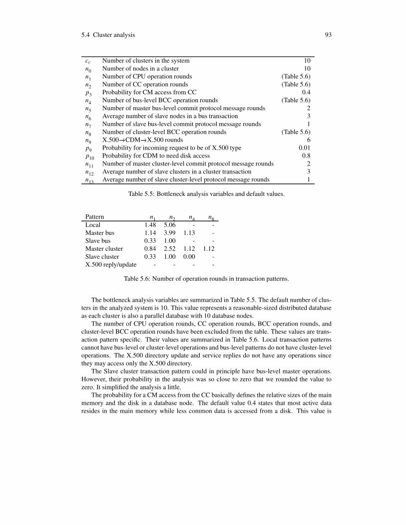
5.4 Cluster analysis 93
cc Number of clusters in the system 10n0 Number of nodes in a cluster 10n1 Number of CPU operation rounds (Table 5.6)n2 Number of CC operation rounds (Table 5.6)p3 Probability for CM access from CC 0.4n4 Number of bus-level BCC operation rounds (Table 5.6)n5 Number of master bus-level commit protocol message rounds 2n6 Average number of slave nodes in a bus transaction 3n7 Number of slave bus-level commit protocol message rounds 1n8 Number of cluster-level BCC operation rounds (Table 5.6)n9 X.500 � CDM � X.500 rounds 6p9 Probability for incoming request to be of X.500 type 0.01p10 Probability for CDM to need disk access 0.8n11 Number of master cluster-level commit protocol message rounds 2n12 Average number of slave clusters in a cluster transaction 3n13 Average number of slave cluster-level protocol message rounds 1
Table 5.5: Bottleneck analysis variables and default values.
Pattern n1 n2 n4 n8Local 1.48 5.06 - -Master bus 1.14 3.99 1.13 -Slave bus 0.33 1.00 - -Master cluster 0.84 2.52 1.12 1.12Slave cluster 0.33 1.00 0.00 -X.500 reply/update - - - -
Table 5.6: Number of operation rounds in transaction patterns.
The bottleneck analysis variables are summarized in Table 5.5. The default number of clus-ters in the analyzed system is 10. This value represents a reasonable-sized distributed databaseas each cluster is also a parallel database with 10 database nodes.
The number of CPU operation rounds, CC operation rounds, BCC operation rounds, andcluster-level BCC operation rounds have been excluded from the table. These values are trans-action pattern specific. Their values are summarized in Table 5.6. Local transaction patternscannot have bus-level or cluster-level operations and bus-level patterns do not have cluster-leveloperations. The X.500 directory update and service replies do not have any operations sincethey may access only the X.500 directory.
The Slave cluster transaction pattern could in principle have bus-level master operations.However, their probability in the analysis was so close to zero that we rounded the value tozero. It simplified the analysis a little.
The probability for a CM access from the CC basically defines the relative sizes of the mainmemory and the disk in a database node. The default value 0.4 states that most active dataresides in the main memory while less common data is accessed from a disk. This value is

94 5 DATABASE ANALYSIS
pa Probability for local transaction pattern 0.712833pb Probability for master bus-level transaction pattern 0.094235pc Probability for slave bus-level transaction pattern N/Apd Probability for master cluster-level transaction pattern 0.092932pe Probability for slave cluster-level transaction pattern N/Ap f Probability for X.500 transaction pattern 0.100000
Table 5.7: Transaction pattern probabilities.
large enough to include necessary updates to the disk so that the major copy of a data itemresides there. Hence, Yalin is not a main memory database management system architecture.
The number of master bus-level and master cluster-level commit protocol message roundsare chosen for a normal two-phase commit protocol. The average number of slave nodes in abus-level and cluster-level transactions is just a guess. The value cannot be very large since thenumber of distributed operations from a master node is small. That value is calculated fromtransaction type properties.
The number of X.500 interpretation rounds is also a guess. The value depends on howcomplex the X.500 operations generally are. The same is true of the probability for incomingX.500 type requests and the probability for CDM disk access.
The default CDM disk access probability is 0.8. This value indicates a small hot spot in thedatabase so that most data item requests must visit the physical database. This is true in theX.500 directory information since the X.500 operations are probably not limited to a specificarea of the database.
Table 5.7 summarizes various transaction pattern probabilities. The probabilities for patterna (local transaction), pattern b (bus-level master transaction), and pattern d (cluster-level mastertransaction) are calculated from the IN/GSM transaction and data analysis. The values arenormalized so that the probability for pattern f (X.500 reply/update transaction pattern) is a freevalue. The probabilities for pattern c (slave bus-level transaction pattern) and pattern e (slavecluster-level transaction pattern) are calculated from their relationships to the other transactionpatterns as described in Section 5.4.1.
Bus and network analysis
In the bus and network analysis we have first used the default values in Table 5.5. The trafficin a bus is between the database nodes and the cluster entry node. The traffic in the network isconsidered to include all clusters.
In the first case (Figure 5.22) we use the default X.25 signal speed 64kb/s for the network.The results are devastating. The network becomes an immediate bottleneck in the system. Thisresult is not surprising. Even a small number of distributed transactions in the system causesheavy traffic between clusters. If all traffic is considered to use the same wires with 64kb/sspeed then the global commit protocols alone cause a severe burden to the network. If the64kb/s is the network speed limit then distribution is out of the question in Yalin.
Fortunately we are not restricted to the old X.25 network. The third generation mobilenetworks already use TCP/IP based networks that offer higher network speeds than the X.25.The same can be true with the Yalin architecture. Only the entry points may need access to

5.4 Cluster analysis 95
0
0.2
0.4
0.6
0.8
1
Man
ager
util
izat
ion
leve
l
5 25 45 65 85 105125145165185Arriving request rate
Network
Bus
Bus/Network utilization level
Number of clusters in the system 10Number of nodes in a cluster 10Network speed 64kb/sNetwork block size 256BBus speed 25Mb/sBus block size 256BLocal transaction probability 0.712833Bus-level transaction probability 0.094235Cluster-level transaction probability 0.092932X.500 interpretation probability 0.100000X.500 interpretation rounds 6CM access probability 0.4
Figure 5.22: Bus and network utilization, network speed = 64kb/s.
X.25. The rest of the system, including connections to clusters, may use faster TCP/IP-basedconnections.
In the rest of the analysis we assume that the network speed is 1024kb/s. With this speedwe get more promising results, as can be seen in Figure 5.23. The network can handle about140 arriving requests/second in a cluster (when we have 10 clusters in the network) and it nolonger becomes the limiting factor.
The cluster bus throughput is much better than the network throughput. Although traffic ina cluster node is higher than traffic between two clusters, the bus speed is better. We use a busspeed of 25Mb/s which is a reasonable value for an external bus that connects shared-nothingdatabases. With this speed, having 10 nodes in a cluster does not create a bus bottleneck. In fact,as much as 150 nodes in a cluster may be supported (Figure 5.24). However, when extremelylarge numbers of nodes are modeled in the analysis, even small changes in parallel transaction

96 5 DATABASE ANALYSIS
0
0.2
0.4
0.6
0.8
1
Man
ager
util
izat
ion
leve
l
5 25 45 65 85 105125145165185Arriving request rate
Network
Bus
Bus/Network utilization level
Number of clusters in the system 10Number of nodes in a cluster 10Network speed 1Mb/sNetwork block size 256BBus speed 25Mb/sBus block size 256BLocal transaction probability 0.712833Bus-level transaction probability 0.094235Cluster-level transaction probability 0.092932X.500 interpretation probability 0.100000X.500 interpretation rounds 6CM access probability 0.4
Figure 5.23: Bus and network utilization, network speed = 1024kb/s.
probabilities affect the results. We believe that a more realistic result can be seen in an analysiswith 50 nodes and bus block size 512 bytes. The results of the analysis are in Figure 5.25.
The scalability of the Yalin bus is very good. This is basically due to the fact that only10 % of the requests trigger a bus-level transaction. These values have been calculated fromthe known transactions, their assumed distribution between local, bus-level, and cluster-leveltransactions, and from their analyzed database operations. However, the atomic bus block sizeaffects the Yalin shared-nothing architecture throughput. When the block size is raised to 1024bytes, the system can handle only 10 nodes in a cluster while with 512 byte blocks it can handle50 nodes. This can be seen in Figure 5.26.
Since the previous results of the bus scalability sounded almost too good, we wanted to trythe default values and an artificial probability of 0.8 for bus-level transactions (compared to thecalculated probability 0.09). Even then the bus behaved well enough as can be seen in Figure

5.4 Cluster analysis 97
0
0.2
0.4
0.6
0.8
1
Man
ager
util
izat
ion
leve
l
5 25 45 65 85 105125145165185Arriving request rate
Network
Bus
Bus/Network utilization level
Number of clusters in the system 10Number of nodes in a cluster 150Network speed 1Mb/sNetwork block size 256BBus speed 25Mb/sBus block size 256BLocal transaction probability 0.712833Bus-level transaction probability 0.094235Cluster-level transaction probability 0.092932X.500 interpretation probability 0.100000X.500 interpretation rounds 6CM access probability 0.4
Figure 5.24: Bus and network utilization, 150 nodes.
5.27. In the figure we have 10 database nodes and atomic blocks of size 256 bytes. The busnever becomes a bottleneck with these values.
Naturally these values are only estimates based on the IN/GSM object class and transactionanalysis. Yet real system object classes and transactions should not be too far from the Yalinsystem. Parallelism really helps in Yalin since most transactions are local to a single node.Local transactions can be distributed to several database nodes in a cluster with little extraburden from bus-level commit procedures for bus-level transactions.
As a conclusion to the bus and network analysis we can state that parallel database nodesare a better alternative than raw distribution in Yalin. It may even be possible to use a singleIN/GSM parallel database management system and hence avoid distribution completely. Onthe other hand, since most transactions are not distributed, geographically distributed clustersshorten access times for local transactions since the network delay from a client to the database

98 5 DATABASE ANALYSIS
0
0.2
0.4
0.6
0.8
1
Man
ager
util
izat
ion
leve
l
5 25 45 65 85 105125145165185Arriving request rate
Network
Bus
Bus/Network utilization level
Number of clusters in the system 10Number of nodes in a cluster 50Network speed 1Mb/sNetwork block size 256BBus speed 25Mb/sBus block size 512BLocal transaction probability 0.712833Bus-level transaction probability 0.094235Cluster-level transaction probability 0.092932X.500 interpretation probability 0.100000X.500 interpretation rounds 6CM access probability 0.4
Figure 5.25: Bus and network utilization, 50 nodes, bus block size = 512 bytes.
becomes shorter.It should also be noted that we did not analyze specialized nodes that are related to mass
calling and televoting. When using specialized clusters and nodes, those services can be sim-plified. This is an especially suitable idea for Yalin clusters. One database node in a clustermay be devoted to mass calling and televoting service alone. Mass calling writes are forwardeddirectly to the node. Mass calling reads are implemented similarly to other services, but theyare executed in the mass calling database node and then perhaps use bus-level subtransactionsin other nodes.

5.4 Cluster analysis 99
0
0.2
0.4
0.6
0.8
1
Man
ager
util
izat
ion
leve
l
5 25 45 65 85 105125145165185Arriving request rate
Network
Bus
Bus/Network utilization level
Number of clusters in the system 10Number of nodes in a cluster 10Network speed 1Mb/sNetwork block size 256BBus speed 25Mb/sBus block size 1024BLocal transaction probability 0.712833Bus-level transaction probability 0.094235Cluster-level transaction probability 0.092932X.500 interpretation probability 0.100000X.500 interpretation rounds 6CM access probability 0.4
Figure 5.26: Bus and network utilization, 10 nodes, bus block size = 1024 bytes.
Cluster entry node analysis
The Cluster entry node (CEN) has three tasks. It is an entry node for bus-level and local transac-tions, a communication node for cluster-level transactions, and an interpreter for X.500-basedqueries and responses. As such it is the only entry to a cluster.
In principle a cluster should not need any database nodes since the CEN has a disk managerfor X.500 directory information. This manager could be used for regular data management aswell. However, in Yalin all transactions are forwarded to database nodes. This simplifies theCEN architecture since transaction scheduling and concurrency control are processed in nodes.
The results of CEN analysis using default values is in Figure 5.28. The values seem to besufficient for Yalin use. The Global transaction manager (GTM) is the first manager to overloadbut even it can handle almost 200 requests in a second. The CPU utilization does not become an

100 5 DATABASE ANALYSIS
0
0.2
0.4
0.6
0.8
1
Man
ager
util
izat
ion
leve
l
5 25 45 65 85 105125145165185Arriving request rate
Network
Bus
Bus/Network utilization level
Number of clusters in the system 10Number of nodes in a cluster 10Network speed 1Mb/sNetwork block size 256 BBus speed 25Mb/sBus block size 256 BLocal transaction probability 0.157399Bus-level transaction probability 0.800000Cluster-level transaction probability 0.020520X.500 interpretation probability 0.022081X.500 interpretation rounds 6CM access probability 0.4
Figure 5.27: Bus and network utilization, bus-level transaction probability = 0.8.
issue, nor does the Disk manager. In fact, the Disk manager is underloaded. With these valuesit would be possible to have a hot data database in CEN.
One thing more to notice here is the Local control manager (LCM). It is responsible forcollecting local and bus-level requests and forwarding them to the appropriate database nodes.It is not at a risk of an overload at all. The conclusion of this is that it is possible to centralizerequest collection into the LCM and hence have a single entry to each cluster.
The CEN utilization changes dramatically when the system has 20 clusters instead of thedefault 10. This can be seen in Figure 5.29. Now the GTM soon becomes a bottleneck. This isdue to the extra global commit procedure processing. Similarly the CPU and the GCC can nolonger handle high request arrival rates. The LCM overloads as well, but not because of extralocal and bus-level requests, but because it has to wait for the CPU.
In Figure 5.30 we have 10 clusters and no cluster-level commit protocols. Now none of the

5.4 Cluster analysis 101
0
0.2
0.4
0.6
0.8
1
Man
ager
util
izat
ion
leve
l
5 25 45 65 85 105125145165185Arriving request rate
Net/bus
X.500
CDM
DM
GTM
GCC
LCM
CPU
Cluster entry node manager utilization
Number of clusters in the system 10Number of nodes in a cluster 10Network speed 1Mb/sNetwork block size 256 BBus speed 25Mb/sBus block size 256 BLocal transaction probability 0.712833Bus-level transaction probability 0.094235Cluster-level transaction probability 0.092932X.500 interpretation probability 0.100000X.500 interpretation rounds 6CM access probability 0.4
Figure 5.28: Cluster entry node utilization, default values.
managers become a bottleneck. This also ensures that the bottleneck in the CEN is in the globalcommit procedure management.
While giving up the global commit protocols may sound promising, the problems soonbecome unbearable. Without a global commit protocol, transactions may interfere with eachother. This easily violates database consistency, for instance when two global transactions wantto update the same data item. If some other method is used, such as a correcting transaction,the same problems with request throughput are evident as with global commit protocols, butwithout the benefits of the protocol.
Since the DM is underloaded even with a high probability of 0.8, an interesting questionis to see how much X.500 interpretations Yalin can handle. We analyzed this with the X.500interpretation probability value 0.4 (Figure 5.31). The chosen value is very high. Basicallyit states that requests are not optimized for Yalin at all. Now the DM is the first manager to

102 5 DATABASE ANALYSIS
00.10.20.30.40.50.60.70.80.9
1
Man
ager
util
izat
ion
leve
l
5 25 45 65 85 105125145165185Arriving request rate
Net/bus
X.500
CDM
DM
GTM
GCC
LCM
CPU
Cluster entry node manager utilization
Number of clusters in the system 20Number of nodes in a cluster 10Network speed 1Mb/sNetwork block size 256 BBus speed 25Mb/sBus block size 256 BLocal transaction probability 0.712833Bus-level transaction probability 0.094235Cluster-level transaction probability 0.092932X.500 interpretation probability 0.100000X.500 interpretation rounds 6CM access probability 0.4
Figure 5.29: Cluster entry node utilization, 20 clusters.
overload, but still it can handle 150 requests per second.If the DM overloads first only when the disk access probability is 0.8 and X.500 interpre-
tation probability is 0.4 then the DM definitely is underloaded. Hence, an easy optimizationmight be to add hot data to the DM and create very simple transactions for such access.
When X.500 is calculated to need 200 interpretation rounds, the cluster entry node utiliza-tion is similar to the utilization in the X.500 high probability case (Figure 5.32). Also nowthe DM is the first manager to overload, but it can still handle about 150 requests in a second.The X.500 and CDM managers can also handle the high interpretation rounds without prob-lems. The reason for this is the low probability for X.500 requests. A complete disaster occurswhen the X.500 interpretation probability is high and each interpretation needs a high numberof CDM access rounds. This can be seen in Figure 5.33 where the probability for X.500 accessis 0.4, and the number of interpretation rounds is as high as 50.

5.4 Cluster analysis 103
0
0.2
0.4
0.6
0.8
1
Man
ager
util
izat
ion
leve
l
5 25 45 65 85 105125145165185Arriving request rate
Net/bus
X.500
CDM
DM
GTM
GCC
LCM
CPU
Cluster entry node manager utilization
Number of clusters in the system 10Number of nodes in a cluster 10Network speed 1Mb/sNetwork block size 256 BBus speed 25Mb/sBus block size 256 BLocal transaction probability 0.712833Bus-level transaction probability 0.094235Cluster-level transaction probability 0.092932X.500 interpretation probability 0.100000X.500 interpretation rounds 6CM access probability 0.4
Figure 5.30: Cluster entry node utilization, no cluster-level commit protocol.
As a summary of the cluster entry node bottlenecks, the node can handle about 150 requestsin a second which should be sufficient. The total number of requests to all clusters is naturally1500 requests in a second which is quite a lot. Yet the cluster entry node disk manager was noteven close to overload. It might be a good idea to let some transactions execute in the CEN andthat way use the extra disk manager power there. It depends on how much disk resources theX.500 information maintenance takes.
Database node analysis
Each cluster has a Cluster entry node and a set of database nodes. A database node is a memberof a parallel database architecture (the cluster) and also a member of a distributed databasearchitecture (the Yalin architecture). All actual data processing is handled in transactions that

104 5 DATABASE ANALYSIS
0
0.2
0.4
0.6
0.8
1
Man
ager
util
izat
ion
leve
l
5 25 45 65 85 105125145165185Arriving request rate
Net/bus
X.500
CDM
DM
GTM
GCC
LCM
CPU
Cluster entry node manager utilization
Number of clusters in the system 10Number of nodes in a cluster 10Network speed 1Mb/sNetwork block size 256 BBus speed 25Mb/sBus block size 256 BLocal transaction probability 0.47522Bus-level transaction probability 0.062823Cluster-level transaction probability 0.061955X.500 interpretation probability 0.400000X.500 interpretation rounds 6CM access probability 0.4
Figure 5.31: Cluster entry node utilization, X.500 interpretation probability = 0.4.
execute in the database nodes.The transactions in the analysis consist of three types of operations: data reads, data writes,
and CPU operations. Data reads and data writes are processed in the concurrency controller.CPU operations are processed in the Scheduler manager space. All transactions are created ina Transaction Manager, executed, and finally committed or aborted. In both the commit andabort cases the result of the transaction is returned to the CEN.
Since both commits and aborts are managed the same way, we do not distinguish them inthe analysis. The reason for this is in the nature of real-time transactions. The tight deadlinesbasically state that it is not reasonable to re-execute a transaction when it is aborted. It wouldnot meet its deadline anyway. We can see this in the next section where we analyze averageexecution times for various transaction types.
In Figure 5.34 default values are used in the analysis. The scheduler is the first manager to
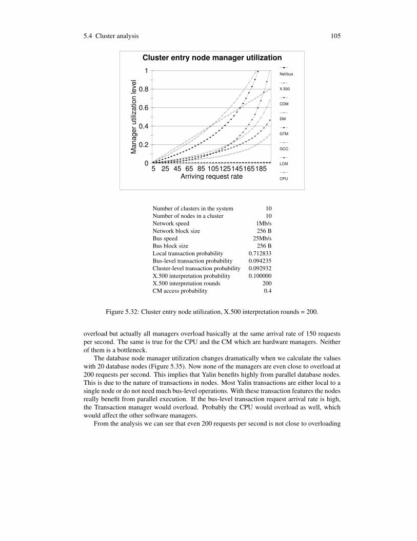
5.4 Cluster analysis 105
0
0.2
0.4
0.6
0.8
1
Man
ager
util
izat
ion
leve
l
5 25 45 65 85 105125145165185Arriving request rate
Net/bus
X.500
CDM
DM
GTM
GCC
LCM
CPU
Cluster entry node manager utilization
Number of clusters in the system 10Number of nodes in a cluster 10Network speed 1Mb/sNetwork block size 256 BBus speed 25Mb/sBus block size 256 BLocal transaction probability 0.712833Bus-level transaction probability 0.094235Cluster-level transaction probability 0.092932X.500 interpretation probability 0.100000X.500 interpretation rounds 200CM access probability 0.4
Figure 5.32: Cluster entry node utilization, X.500 interpretation rounds = 200.
overload but actually all managers overload basically at the same arrival rate of 150 requestsper second. The same is true for the CPU and the CM which are hardware managers. Neitherof them is a bottleneck.
The database node manager utilization changes dramatically when we calculate the valueswith 20 database nodes (Figure 5.35). Now none of the managers are even close to overload at200 requests per second. This implies that Yalin benefits highly from parallel database nodes.This is due to the nature of transactions in nodes. Most Yalin transactions are either local to asingle node or do not need much bus-level operations. With these transaction features the nodesreally benefit from parallel execution. If the bus-level transaction request arrival rate is high,the Transaction manager would overload. Probably the CPU would overload as well, whichwould affect the other software managers.
From the analysis we can see that even 200 requests per second is not close to overloading

106 5 DATABASE ANALYSIS
0
0.2
0.4
0.6
0.8
1
Man
ager
util
izat
ion
leve
l
5 25 45 65 85 105125145165185Arriving request rate
Net/bus
X.500
CDM
DM
GTM
GCC
LCM
CPU
Cluster entry node manager utilization
Number of clusters in the system 10Number of nodes in a cluster 10Network speed 1Mb/sNetwork block size 256 BBus speed 25Mb/sBus block size 256 BLocal transaction probability 0.475222Bus-level transaction probability 0.062823Cluster-level transaction probability 0.061955X.500 interpretation probability 0.400000X.500 interpretation rounds 50CM access probability 0.4
Figure 5.33: Cluster entry node utilization, X.500 interpretation rounds = 50, X.500 interpreta-tion probability = 0.4.
in any of the managers. The scalability of Yalin architecture is good. Since requests are dividedequally to all nodes in the cluster, the number of requests per second to one is significantlylower than with the default values. Also the average number of nodes that participate in a bus-level transaction is not changed so less bus-level transaction requests arrive to each databasenode. as well. Hence, database nodes should not be the first ones to overload when more nodesare added. The bus, as we have seen, is a more realistic candidate for overloading.
The number of nodes that participate in a bus-level transaction affects manager throughput.If we used very high values in the analysis, the transaction manager would overload. Yet this isnot an issue. Even if we add nodes, the nature of bus-level transactions does not change. In theanalysis we have calculated how much bus-level operations happen on average in a bus-leveltransaction. This number is relatively small so it is safe to assume that the average number of

5.4 Cluster analysis 107
0
0.2
0.4
0.6
0.8
1
Man
ager
util
izat
ion
leve
l
5 30 55 80 105 130 155 180Arriving request rate
Bus managers
TM
Scheduler
CC
CM
BCC
CPU
Database node manager utilization
Number of clusters in the system 10Number of nodes in a cluster 10Network speed 1Mb/sNetwork block size 256 BBus speed 25Mb/sBus block size 256 BLocal transaction probability 0.712833Bus-level transaction probability 0.094235Cluster-level transaction probability 0.092932X.500 interpretation probability 0.100000X.500 interpretation rounds 6CM access probability 0.4
Figure 5.34: Database node utilization, default values.
nodes that participate in a bus-level transaction is not very high.The CM access probability defines the relative size of the main memory compared to the
disk. The used value 0.4 is low which indicates a large main memory. In Figure 5.36 weuse a CM access probability of 0.8 which is not that uncommon either. Now the CM is the firstmanager to overload. As expected with these values, the disk becomes an immediate bottleneck.
The CM utilization can be lowered by adding new database nodes to a cluster. This can beseen in Figure 5.37. While this helps, it still lets the CM dominate the manager utilizations. Inoptimal settings all managers overload about at the same arriving request level, so none of thembecomes a bottleneck. Hence, a better alternative is to add more memory into database nodesand that way lower the disk access probability.
The original value 0.4 for disk access is close to the lowest possible value in a traditionaldisk-based system. All regularly read-accessed data must reside in a main memory so that read-

108 5 DATABASE ANALYSIS
0
0.2
0.4
0.6
0.8
1
Man
ager
util
izat
ion
leve
l
5 30 55 80 105 130 155 180Arriving request rate
Bus managers
TM
Scheduler
CC
CM
BCC
CPU
Database node manager utilization
Number of clusters in the system 10Number of nodes in a cluster 20Network speed 1Mb/sNetwork block size 256 BBus speed 25Mb/sBus block size 256 BLocal transaction probability 0.712833Bus-level transaction probability 0.094235Cluster-level transaction probability 0.092932X.500 interpretation probability 0.100000X.500 interpretation rounds 6CM access probability 0.4
Figure 5.35: Database node utilization, 20 database nodes in a cluster.
access is done mostly in the memory. Mostly write-accessed data may reside in a disk as wellsince changed data must be written to the disk anyway. A pure main memory database wouldlower the disk access probability but even then change log values must be written to a disk.The Yalin analysis shows that we can use a traditional disk-based approach when we use largeenough buffers.
A possible, while questionable, optimization is to exclude the global bus-level commit pro-tocol from bus-level transaction commits. This would violate transaction atomicity and possiblyinternal and external consistency. The results of this optimization can be seen in Figure 5.38.Compared to the analysis with default values (Figure 5.34), the effect to manager utilizationsis surprisingly small. The reason for this is that the number of bus-level transactions is smallin the first case, and the bus does not slow down commit execution that much. This is totallyopposite to the cluster-level commit procedure where the commit protocol dominated manager

5.4 Cluster analysis 109
0
0.2
0.4
0.6
0.8
1
Man
ager
util
izat
ion
leve
l
5 30 55 80 105 130 155 180Arriving request rate
Bus managers
TM
Scheduler
CC
CM
BCC
CPU
Database node manager utilization
Number of clusters in the system 10Number of nodes in a cluster 10Network speed 1Mb/sNetwork block size 256 BBus speed 25Mb/sBus block size 256 BLocal transaction probability 0.712833Bus-level transaction probability 0.094235Cluster-level transaction probability 0.092932X.500 interpretation probability 0.100000X.500 interpretation rounds 6CM access probability 0.8
Figure 5.36: Database node utilization, CM probability = 0.8.
utilizations. At the bus-level this kind of an optimization is useless in Yalin. If more transactionthroughput is needed, the best way to do it is to add more nodes into a cluster.
The previous analysis is based on the expected transaction distribution between local, bus,and cluster-level transactions, as was described in Table 5.7. The resulting distribution is thatmost transactions are local to a single database node. In the analysis shown in Figure 5.39 weused a bus-level transaction probability 0.8.
The result of the changed values is disastrous. Almost all managers overload immediately.Most resources are wasted in management of parallel transactions. It is clear that the Yalindatabase architecture is not suitable for application environments that need a lot of bus-leveltransactions.
As a conclusion of the database node analysis, the high proportion of local transactions inthe Yalin transaction model allows parallel database nodes to execute at almost full potential.

110 5 DATABASE ANALYSIS
0
0.2
0.4
0.6
0.8
1
Man
ager
util
izat
ion
leve
l
5 30 55 80 105 130 155 180Arriving request rate
Bus managers
TM
Scheduler
CC
CM
BCC
CPU
Database node manager utilization
Number of clusters in the system 10Number of nodes in a cluster 20Network speed 1Mb/sNetwork block size 256 BBus speed 25Mb/sBus block size 256 BLocal transaction probability 0.712833Bus-level transaction probability 0.094235Cluster-level transaction probability 0.092932X.500 interpretation probability 0.100000X.500 interpretation rounds 6CM access probability 0.8
Figure 5.37: Database node utilization, 20 nodes, CM probability = 0.8.
This makes the Yalin cluster architecture quite scalable with IN/GSM classes and transactions.On the other hand, the architecture is not suitable for environments where most cluster-leveltransactions need bus-level distribution.
Average execution times
After the bottleneck analysis we analyzed average transaction lengths of Location update, Initcall, and Query transactions. The set of analyzed transactions covers the properties of Yalintransactions well. We have a short transaction, a regular transaction, and a very long transactionto analyze.
The first analyzed transaction is the Location update transaction. It is the simplest and mostcommon transaction. All it needs to do is to update a mobile equipment location into the Yalin

5.4 Cluster analysis 111
0
0.2
0.4
0.6
0.8
1
Man
ager
util
izat
ion
leve
l
5 30 55 80 105 130 155 180Arriving request rate
Bus managers
TM
Scheduler
CC
CM
BCC
CPU
Database node manager utilization
Number of clusters in the system 10Number of nodes in a cluster 10Network speed 1Mb/sNetwork block size 256 BBus speed 25Mb/sBus block size 256 BLocal transaction probability 0.712833Bus-level transaction probability 0.094235Cluster-level transaction probability 0.092932X.500 interpretation probability 0.100000X.500 interpretation rounds 6CM access probability 0.4
Figure 5.38: Database node utilization, no bus-level commit protocol.
database. The average transaction execution times of the transaction can be seen in Figure 5.40.The Yalin architecture can handle Location update transactions quite well. Although even-
tually the transaction execution times will explode, up to 150 service requests may arrive to thesystem without overload.
The next analyzed transaction is the Init call transaction. It is used whenever a new call isinitialized. The analysis can be seen in Figure 5.41. We have three average service times in thetransaction: for local, bus, and cluster-level transaction. The Init call transaction may be of anyof the three types.
The results of the analysis are not promising in local and cluster level cases. The servicetimes grow too fast to over two seconds which is too much. The bus-level type behaves bet-ter because the transaction calculations may be divided into several database nodes withoutnetwork level extra costs.

112 5 DATABASE ANALYSIS
0
0.2
0.4
0.6
0.8
1
Man
ager
util
izat
ion
leve
l
5 30 55 80 105 130 155 180Arriving request rate
Bus managers
TM
Scheduler
CC
CM
BCC
CPU
Database node manager utilization
Number of clusters in the system 10Number of nodes in a cluster 10Network speed 1Mb/sNetwork block size 256 BBus speed 25Mb/sBus block size 256 BLocal transaction probability 0.157399Bus-level transaction probability 0.800000Cluster-level transaction probability 0.020520X.500 interpretation probability 0.022081X.500 interpretation rounds 6CM access probability 0.4
Figure 5.39: Database node utilization, bus-level transaction probability = 0.8,
The same trend can be seen in other similar transactions, such as Answer call, charge,various management transactions, and Profile. The service times are around one second each.The problem is not that much in the manager utilizations but more in the number of managers.Each manager needs time to execute its tasks, and combined the times grow this high. However,since this is not an issue of the bottlenecks in the system but rather of the manager service times,the problem can be at least partially corrected by using more efficient CPUs and optimizing diskaccess.
Finally, the Query transaction is the longest transaction in the Yalin architecture. The resultsof the Query transaction type analysis are in Figure 5.42. The service times of the Query trans-actions are around 100 seconds. Also here bus-level parallelism helps in transaction executiontimes.
While these service times are long, they are not unbearable. The Query transaction is for

5.4 Cluster analysis 113
0
0.2
0.4
0.6
0.8
1
Ser
vice
tim
e (s
econ
ds)
5 25 45 65 85 105125145165 185Arriving request rate
Local
Location update service times
Figure 5.40: Location transaction average service time.
0.20.40.60.8
11.21.41.61.8
2
Ave
rage
ser
vice
tim
e (s
econ
ds)
5 25 45 65 85 105125145165185Arriving request rate
Local
Bus
Cluster
Init call service times
Figure 5.41: Init call transaction average service times.

0
100
200
300
Ser
vice
tim
e (s
econ
ds)
5 25 45 65 85 105125145165185Arriving request rate
Local
Bus
Cluster
Query service times
Figure 5.42: Query transaction average service times.
management alone and even then it is not executed that often. Furthermore, in the analysis wehave assumed that Query transactions are long: 1400 CPU operations and 2800 CC operationsis assumed to be the average size of a Query type transaction.
Thus, as a result of the time analysis, the transaction execution lengths may be too longfor call-related transactions. Other transactions behave well enough. When time is an issue,transaction execution may be optimized for instance by letting a transaction have direct accessto nodes without the cluster entry node. Hardware elements may also be optimized. The finalway to optimize these transactions is to let them always do reads and writes to main memorydata. This definitely helps in service times, but it also makes the architecture more of a mainmemory database management system than earlier. While main memory is cheap, it is notcheap enough to let all data reside there.

Chapter 6
Conclusion
When new services and service features are introduced and implemented on Intelligent Net-works and 3G and 4G wireless networks, also new requirements arise for a database manage-ment system that maintains service data. The current database architecture is left open in theITU-T recommendations. Only the interfaces and efficiency requirements are listed. This thesishelps to clarify database requirements in these specific environments.
The ITU-T recommendations for Intelligent Networks state that the data management sys-tem is distributed to several Service data functions, and it must offer real-time access to data.The SDF architecture itself is mostly undefined. It can be implemented on various platformsand still fill the ITU-T recommendations. While distribution is present in the definitions, it isnot a necessity in the database implementation.
The data analysis and the Yalin architecture show that IN and wireless network data arecompatible at database level. Thus, in the future we can design and implement a single databasearchitecture that supports both platforms. This is a positive result since already 3G and 4Gwireless networks wish to use IN for special service creation, use, and management.
In the Yalin architecture analysis we noticed that distribution is actually not useful in theIN/GSM database. When data may be divided into distinct fragments the added computing anddisk power helps in transaction throughput. Unfortunately our analysis shows that even a smallnumber of distributed transactions affect database performance on the cluster level. Since X.500directory information must be updated after data item insertions and deletions, and the updatemust be reflected to every cluster, we will always have distributed transactions in the system. Ina small or a medium telecommunications network, a monolithic database management systemmay be the best solution for IN/GSM data management.
Where distribution is not useful, parallelism clearly is. Our analysis shows that several par-allel database nodes give a better request throughput than a single monolithic node of the samesize. Thus, the added CPU and disk capacity is not wasted to node-level atomicity management.
Specialized nodes offer an additional advantage in a parallel database architecture. We cancreate a Yalin variant where some nodes offer traditional services, some are specialized to massdata services (mass calling and televoting), and some are specialized to VLR services. Alltransaction requests may arrive via the same cluster entry node. Also the cluster entry nodefunctionality may be expanded to include requests to the X.500 Database entry node whichthen is a specialized database node in the parallel database architecture.
The next step in Yalin would be a pilot database management system. Yet while the results

of the Yalin architecture at analysis level are useful, we are cautious to go into implementation.A database management system of that size would need millions of lines of code. Right nowit is not worth the effort. Yet the results of Yalin data analysis, architecture, and bottleneckanalysis are useful for any current or future IN or GSM -based database management systemdesign.
The analysis has a value in itself regardless of the IN/GSM results. It clearly shows thatour derived queueing model toolbox is useful in transaction-based system analysis. With thetoolbox it is possible to create and analyze very complex transaction-based systems and findtheir bottlenecks. The price for the analysis simplicity is in the analysis details. Since we haveused shortcuts whenever possible without losing too much details, the model is best used forthe first analysis steps to recognize problematic elements in the system. In the later stages amore detailed analysis with more general (and complex) queueing model tools may be useful.
The queueing model toolbox presented here is only the first step. In the next step we wish toimplement a software tool that can be used to create transaction-based models that are based onour derived formulas. With such a tool it is possible to create and analyze complex transaction-based software for bottlenecks.
Next to the bottleneck analysis, also a transaction execution time analysis is important. Ina real-time database management system this implies transactions with priorities. The currentanalysis toolbox cannot be used for this since it assumes that transactions have the same priority.
In the future we wish to generalize our toolbox model to include transaction type priorities.This way we can better analyze real-time transaction execution times. At first we will use fixedpriorities and eventually update the toolbox to allow dynamic priorities when possible.
Altogether the work on this thesis gives a good basis for both IN/GSM database manage-ment system design and for transaction-based queueing model analysis. As such the work hasbeen beneficial.

References
[AGP98] M. Abdallah, R. Guerraoui, and P. Pucheral. One-phase commit: Does it makesense? In Proceedings of the 1998 International Conference on Parallel AndDistributed Systems, pages 182–192. IEEE, 1998.
[AHC96] Y. Al-Houmaily and P. Chrysanthis. In search for an efficient real-time atomiccommit protocol. In Proceedings of the IEEE Real-Time Systems Symposium WorkIn Progress, pages 51–54. IEEE, 1996.
[Ahn94] I. Ahn. Database issues in telecommunications network management. In ACMSIGMOD proceedings, pages 37–43. ACM, 1994.
[BB95] A. Bestavros and S. Braoudakis. Value-cognizant speculative concurrency control.In Proceedings of the 21th International Conference on Very Large Data Bases(VLDB’95), pages 122–133. Morgan Kaufmann, 1995.
[BB96] A. Bestavros and S. Braoudakis. Value-cognizant speculative concurrency controlfor real-time databases. Information Systems, 21(1):75–101, 1996.
[BHG87] P. Bernstein, V. Hadzilacos, and N. Goodman. Concurrency Control and Recoveryin Database Systems. Addison-Wesley, 1987.
[BJMC00] R. Brennan, B. Jennings, C. McArdle, and T. Curran. Evolutionary trends in Intel-ligent Networks. IEEE Communications Magazine, 38(6):86–93, June 2000.
[BN96] A. Bestavros and S. Nagy. Value-cognizant admission control for rtdb systems. InA. Bestavros, editor, Proceedings of the 17th IEEE Real-Time Systems Symposium,pages 230–239, 1996.
[BPI � 01] L. Becchetti, F. Priscoli, T. Inzerilli, P. Mähönen, and L. Munoz. Enhancing IPservice provision over heterogeneous wireless networks: A path toward 4G. IEEECommunications Magazine, 39(8):74–81, August 2001.
[BS91] K. Bratbergsengen and T. Sæter. The impact of high reliability, high capacitydatabase servers on telecommunication systems and services. In Proc. of the 6thWorld Telecommunication Exhibition and Forum, TeleCom 91, 1991.
[CCI89] CCITT. Recommendations x.500 to x.521 – data communication networks: Di-rectory. In CCITT Blue Book Volume VIII – Fascicle VIII.8, pages 1–225. CCITT,1989.
118 REFERENCES
[CCI92a] Intelligent Network - Global Functional Plane Architecture - RecommendationI.329 / Q.1203, 1992.
[CCI92b] CCITT. Intelligent Network – Service Plane Architecture - Recommendation I.328/ Q.1202, 1992.
[CDW93] L. B. Cingiser DiPippo and V. Wolfe. Object-based semantic real-time concurrencycontrol. In Real-Time Systems Symposium Conference Proceedings, pages 87–96.IEEE, 1993.
[CP84] S. Ceri and G. Pelagatti. Distributed Databases - Principles and Systems.McGraw-Hill, 1984.
[DF01] M. Dinis and J. Fernandes. Provision of sufficient transmission capacity for broad-band mobile multimedia: A step toward 4G. IEEE Communications Magazine,39(8):46–55, August 2001.
[EGLT76] K. Eswaran, J. Gray, R. Lorie and I. Traiger. The Notions of Consistency andPredicate Locks in a Database System. Communications of the ACM, 19(11):624–633, November 1976.
[Fel50] W. Feller. An introduction to probability theory and its applications. John Wiley,1950.
[FGSW00] M. Finkelstein, J. Garrahan, D. Shrader, and G. Weber. The future of the IntelligentNetwork. IEEE Communications Magazine, 38(6):100–107, June 2000.
[GHRS96] R. Gupta, J. Haritsa, K. Ramamritham, and S. Seshadri. Commit processing indistributed real-time database systems. In IEEE Real-Time Systems Symposium,pages 220–229. IEEE, 1996.
[GLPT76] J. N. Gray, R. A. Lorie, G. R. Putzolou, and I. L. Traiger. Granularity of locks anddegrees of consistency in a shared data base. In G. M. Nijssen, editor, Modeling inData Base Management Systems, pages 365–394, 1976.
[Gra78] J. N. Gray. Notes on Database Operating Systems, pages 393–481. Springer-Verlag, 1978.
[GRKK93] J. Garrahan, P. Russo, K. Kitami, and R. Kung. Intelligent Network overview.IEEE Communications Magazine, 31(3):30–36, 1993.
[HCL92] J. Haritsa, M. Carey, and M. Livny. Data access scheduling in firm real-timedatabase systems. Journal of Real-Time Systems, 4(3):203–241, 1992.
[Hig89] W. Highleyman. Performance Analysis of Transaction Processing Systems. Pren-tice Hall, Englewood Cliffs, New Jersey 07632, 1989.
[HR00] J. Haritsa and K. Ramamritham. Adding PEP to real-time distributed commit pro-cessing. In Proceedings of the 21st Real-Time Systems Symposium, pages 37–46.IEEE, 2000.

REFERENCES 119
[HRG00] J. Haritsa, K. Ramamritham, and R. Gupta. The PROMPT real-time commit pro-tocol. IEEE Transactions on Parallel and Distributed Systems, 11(2):160–181,February 2000.
[IT93a] ITU-T. Intelligent Network Distributed Functional Plane Architecture - Recom-mendation Q.1204, 1993.
[IT93b] ITU-T. Intelligent Network Physical Plane Architecture - RecommendationQ.1205, 1993.
[ITU93a] ITU-T. Global Functional Plane for Intelligent Network CS-1 - RecommendationQ.1213, 1993.
[ITU93b] ITU-T. Introduction to Intelligent Network Capability Set 1 - RecommendationQ.1211, 1993.
[ITU96] ITU-T. Distributed Functional Plane for Intelligent Network CS-2 - Recommen-dation Q.1224 (Draft), 1996.
[Jab92] B. Jabbari. Intelligent Network concepts in mobile communication. IEEE Com-munications Magazine, 30(2):64–69, 1992.
[Kon00] W. Konhäuser. Mobile communications on the way towards Internet on air. In Pro-ceedings of WCC-ICCT 2000 Communication Technology, volume 2, pages 993–1000. IEEE, 2000.
[Lin00] J. Lindström. Extensions to optimistic concurrency control with time intervals. InD. C. Young, editor, Proceedings of the 7th International Conference on Real-TimeComputing Systems and Applications, pages 108–115, 2000.
[LNPR00] J. Lindström, T. Niklander, P. Porkka, and K. Raatikainen. A distributed real-timemain-memory database for telecommunication. In Databases in Telecommunica-tions; International Workshop, Co-located with VLDB-99, 2000.
[LS93] J. Lee and S. H. Son. Using dynamic adjustment of serialization order for real-time database systems. In Real-Time Systems Symposium Conference Proceedings,pages 66–75. IEEE, 1993.
[LS94] J. Lee and S. Son. Semantic-based concurrency control for object-orienteddatabase systems supporting real-time applications. In 6th IEEE Euromicro Work-shop on Real-Time Systems, pages 156–161. IEEE, 1994.
[LW95] P. Lehtinen and A. Warsta. Nokia’s IN solution for fixed and cellular networks.In Jarmo Harju, Tapani Karttunen, and Olli Martikainen, editors, Intelligent Net-works, pages 61–67. Chapman & Hall, 1995.
[MC00] M. Mampaey and A. Couturier. Using TINA concepts for in evolution. IEEECommunications Magazine, 38(6):94–99, June 2000.
[Mit95] H. Mitts. Use of Intelligent Networks in the universal mobile telecommunicationsystem (UMTS). In Jarmo Harju, Tapani Karttunen, and Olli Martikainen, editors,Intelligent Networks, pages 236–245. Chapman & Hall, 1995.

120 REFERENCES
[MP92] M. Mouly and M. Pautet. The GSM System for Mobile Communications. Mouly& Pautet, 1992.
[NB00] K. Nørvåg and K. Bratbergsengen. Optimal object descriptor caching in temporalobject database systems. In K. Tanaka, S. Ghandeharizadeh, and Y. Kambayashi,editors, Information Organization and Databases, pages 235–248, Boston, Mass.,2000. Kluwer.
[OV99] M. Tamero Ozsu and P. Valduriez. Principles of Distributed Database Systems -Second Edition. Prentice Hall International Inc., 1999.
[Pan95] R. Pandya. Emerging mobile and personal communication systems. IEEE Com-munications Magazine, 33(6):44–52, 1995.
[PMHG95] G. Pollini, K. Meier-Hellstern, and D. Goodman. Signaling traffic volume gener-ated by mobile and personal communications. IEEE Communications Magazine,33(6):60–65, 1995.
[Pon93] C. Pontailler. TMN and new network architectures. IEEE Communications Mag-azine, 31(4):84–88, 1993.
[Pra99] N. Prasad. GSM evolution towards third generation UMTS/IMT2000. In IEEEConference on Personal Wireless Communication, pages 50–54. IEEE, 1999.
[Raa94] K. Raatikainen. Information aspects of services and service features in intelli-gent network capability set 1. Report C-1994-45, University of Helsinki, Dept. ofComputer Science, Helsinki, Finland, September 1994.
[Ram93] K. Ramamritham. Real-time databases. Distributed and Parallel Databases,1(2):199–226, 1993.
[Ric00] K. Richardson. UMTS overview. IEEE Electronics & Communications Engineer-ing Journal, 12(3):93–100, June 2000.
[RKMT95] K. Raatikainen, T. Karttunen, O. Martikainen, and J. Taina. Evaluation of databasearchitectures for intelligent networks. In Proceedings of the 7th World Telecom-munication Forum (Telecom 95), Technology Summit, Volume 2, pages 549–553,Geneva, Switzerland, September 1995. ITU.
[RKV � 01] T. Robles, A. Kadelka, H. Velayos, A. Lappetelainen, A. Kassler, H. Li, D.Mandato, J. Ojala, and B. Wegmann. QoS support for an all-IP system beyond3G. IEEE Communications Magazine, 39(8):64–73, August 2001.
[SC90] J. Stamos and F. Cristian. A low-cost atomic commit protocol. In Proceedingsof the 9th IEEE Symposium on Reliable Distributed Systems, pages 66–75. IEEE,1990.
[Ske81] D. Skeen. Nonblocking commit protocols. In Y. Edmund Lien, editor, Proceedingsof the 1981 ACM SIGMOD International Conference on Management of Data, AnnArbor, Michigan, April 29 - May 1, 1981, pages 133–142. ACM Press, 1981.

[SRL90] L. Sha, R. Rajkumar, and J. Lehoczky. Priority inheritance protocols: An approachto real-time synchronization. IEEE Transactions on Computers, 39(9):1175–1185,1990.
[SRSC91] L. Sha, R. Rajkumar, S. Son, and C. Chang. A real-time locking protocol. IEEETransactions on Computers, 40(7):793–800, 1991.
[Tai94a] J. Taina. Problem classes in intelligent network database design. In O. Martikainenand J. Harju, editors, Proceedings of IFIP TC6 Workshop on Intelligent Networks,pages 194–207, Lappeenranta, Finland, August 1994. Lappeenranta University ofTechnology, Chapman & Hall.
[Tai94b] J. Taina. Evaluation of OMG, ODMG, X.500, and X.700 data models. Technicalreport, University of Helsinki, Department of Computer Science, 1994.
[TNA � 01] T. Tjelta, A. Nordbotten, M. Annoni, E. Scarrone, S. Bizzarri, Laurissa Tokarchuk,John Bigham, Chris Adams, Ken Craig, and Manuel Dinis. Future broadband radioaccess systems for integrated services with flexible resource management. IEEECommunications Magazine, 39(8):56–63, August 2001.
[TR96] J. Taina and K. Raatikainen. Experimental real-time object-oriented database ar-chitecture for intelligent networks. Engineering Intelligent Systems, 4(3):57–63,September 1996.
[TR00] J. Taina and K. Raatikainen. Requirements analysis of distribution in databasesfor telecommunications. In Willem Jonker, Peter Apers, and Tore Sæter, editors,Proceedings of the Workshop on Databases in Telecommunications 1999, pages74–89. Springer, 2000.
[TRR95] J. Taina, M. Rautila, and K. Raatikainen. An experimental database architecturefor intelligent networks. In Proceedings of IFIP IN’95 Conference. IFIP, 1995.
[TS96] J. Taina and S. Son. Requirements for real-time object-oriented database models–how much is too much? In Proceedings of the Ninth Euromicro Workshop onReal-Time Systems, pages 258–265. IEEE, 1996.
[TS97a] J. Taina and S. Son. TARTOS - toolbox for active real-time object-orienteddatabase system models. In IEEE Workshop on Parallel And Distributed Systems(WPDRTS’97), pages 131–140. IEEE, 1997.
[TS97b] J. Taina and S. Son. A framework for real-time object-oriented database models.In International Workshop on Object-Oriented Real-Time and Dependable Systems(WORDS’97), pages 146–152. IEEE, 1997.
[YK00] J. Yang and I. Kriaras. Migration to all-IP based umts networks. In Proceedingsof the First International Conference on 3G Mobile Communication Technologies,pages 19–23. IEEE, 2000.
[YWLS94] P. Yu, K. Wu, K. Lin, and S. Son. On real-time databases: Concurrency controland scheduling. Proceedings of the IEEE, 82(1):140–157, 1994.

TIETOJENKÄSITTELYTIETEEN LAITOS DEPARTMENT OF COMPUTER SCIENCEPL 26 (Teollisuuskatu 23) P.O. Box 26 (Teollisuuskatu 23)00014 Helsingin yliopisto FIN-00014 University of Helsinki, FINLAND
JULKAISUSARJA A SERIES OF PUBLICATIONS A
Reports may be ordered from: Department of Computer Science, Library (A 214), P.O. Box 26, FIN-00014 University of Helsinki,FINLAND.
A-1990-1 K. Pohjonen & J. Tarhio (toim./eds.): Tietojenkäsittelyopin laitoksen tutkimusraportteja 1988–89 – Research reports atthe Department of Computer Science 1988–89. 27 pp.
A-1990-2 J. Kuittinen, O. Nurmi, S. Sippu & E. Soisalon-Soininen: Efficient implementation of loops in bottom-up evaluation oflogic queries. 14 pp.
A-1990-3 J. Tarhio & E. Ukkonen: Approximate Boyer-Moore string matching. 27 pp.
A-1990-4 E. Ukkonen & D. Wood: Approximate string matching with suffix automata. 14 pp.
A-1990-5 T. Kerola: Qsolver – a modular environment for solving queueing network models. 15 pp.
A-1990-6 Ker-I Ko, P. Orponen, U. Schöning & O. Watanabe: Instance complexity. 24 pp.
A-1991-1 J. Paakki: Paradigms for attribute-grammar-based language implementation. 71 + 146 pp. (Ph.D. thesis).
A-1991-2 O. Nurmi & E. Soisalon-Soininen: Uncoupling updating and rebalancing in chromatic binary search trees. 12 pp.
A-1991-3 T. Elomaa & J. Kivinen: Learning decision trees from noisy examples. 15 pp.
A-1991-4 P. Kilpeläinen & H. Mannila: Ordered and unordered tree inclusion. 22 pp.
A-1991-5 A. Valmari: Compositional state space generation. 30 pp.
A-1991-6 J. Tarhio & M. Tienari (eds.): Computer Science at the University of Helsinki 1991. 66 pp.
A-1991-7 P. Jokinen, J. Tarhio & E. Ukkonen: A comparison of approximate string matching algorithms. 23 pp.
A-1992-1 J. Kivinen: Problems in computational learning theory. 27 + 64 pp. (Ph.D. thesis).
A-1992-2 K. Pohjonen & J. Tarhio (toim./eds.): Tietojenkäsittelyopin laitoksen tutkimusraportteja 1990–91 – Research reports atthe Department of Computer Science 1990–91. 35 pp.
A-1992-3 Th. Eiter, P. Kilpeläinen & H. Mannila: Recognizing renamable generalized propositional Horn formulas is NP-complete.11 pp.
A-1992-4 A. Valmari: Alleviating state explosion during verification of behavioural equivalence. 57 pp.
A-1992-5 P. Floréen: Computational complexity problems in neural associative memories. 128 + 8 pp. (Ph.D. thesis).
A-1992-6 P. Kilpeläinen: Tree matching problems with applications to structured text databases. 110 pp. (Ph.D. thesis).
A-1993-1 E. Ukkonen: On-line construction of suffix-trees. 15 pp.
A-1993-2 Alois P. Heinz: Efficient implementation of a neural net α-β -evaluator. 13 pp.
A-1994-1 J. Eloranta: Minimal transition systems with respect to divergence preserving behavioural equivalences. 162 pp.(Ph.D. thesis).
A-1994-2 K. Pohjonen (toim./ed.): Tietojenkäsittelyopin laitoksen julkaisut 1992–93 – Publications from the Department of Com-puter Science 1992–93. 58 s./pp.
A-1994-3 T. Kujala & M. Tienari (eds.): Computer Science at the University of Helsinki 1993. 95 pp.
A-1994-4 P. Floréen & P. Orponen: Complexity issues in discrete Hopfield networks. 54 pp.
A-1995-1 P. Myllymäki: Mapping Bayesian networks to stochastic neural networks: a foundation for hybrid Bayesian-neural sys-tems. 93 pp. (Ph.D. thesis).
A-1996-1 R. Kaivola: Equivalences, preorders and compositional verification for linear time temporal logic and concurrent systems.185 pp. (Ph.D. thesis).
A-1996-2 T. Elomaa: Tools and techniques for decision tree learning. 140 pp. (Ph.D. thesis).
A-1996-3 J. Tarhio & M. Tienari (eds.): Computer Science at the University of Helsinki 1996. 89 pp.
A-1996-4 H. Ahonen: Generating grammars for structured documents using grammatical inference methods. 107 pp. (Ph.D. thesis).
A-1996-5 H. Toivonen: Discovery of frequent patterns in large data collections. 116 pp. (Ph.D. thesis).
A-1997-1 H. Tirri: Plausible prediction by Bayesian inference. 158 pp. (Ph.D. thesis).

A-1997-2 G. Lindén: Structured document transformations. 122 pp. (Ph.D. thesis).
A-1997-3 M. Nykänen: Querying string databases with modal logic. 150 pp. (Ph.D. thesis).
A-1997-4 E. Sutinen, J. Tarhio, S.-P. Lahtinen, A.-P. Tuovinen, E. Rautama & V. Meisalo: Eliot – an algorithm animation environ-ment. 49 pp.
A-1998-1 G. Lindén & M. Tienari (eds.): Computer Science at the University of Helsinki 1998. 112 pp.
A-1998-2 L. Kutvonen: Trading services in open distributed environments. 231 + 6 pp. (Ph.D. thesis).
A-1998-3 E. Sutinen: Approximate pattern matching with the q-gram family. 116 pp. (Ph.D. thesis).
A-1999-1 M. Klemettinen: A knowledge discovery methodology for telecommunication network alarm databases. 137 pp.(Ph.D. thesis).
A-1999-2 J. Puustjärvi: Transactional workflows. 104 pp. (Ph.D. thesis).
A-1999-3 G. Lindén & E. Ukkonen (eds.): Department of Computer Science: annual report 1998. 55 pp.
A-1999-4 J. Kärkkäinen: Repetition-based text indexes. 106 pp. (Ph.D. thesis).
A-2000-1 P. Moen: Attribute, event sequence, and event type similarity notions for data mining. 190+9 pp. (Ph.D. thesis).
A-2000-2 B. Heikkinen: Generalization of document structures and document assembly. 179 pp. (Ph.D. thesis).
A-2000-3 P. Kähkipuro: Performance modeling framework for CORBA based distributed systems. 151+15 pp. (Ph.D. thesis).
A-2000-4 K. Lemström: String matching techniques for music retrieval. 56+56 pp. (Ph.D.Thesis).
A-2000-5 T. Karvi: Partially defined Lotos specifications and their refinement relations. 157 pp. (Ph.D.Thesis).
A-2001-1 J. Rousu: Efficient range partitioning in classification learning. 68+74 pp. (Ph.D. thesis)
A-2001-2 M. Salmenkivi: Computational methods for intensity models. 145 pp. (Ph.D. thesis)
A-2001-3 K. Fredriksson: Rotation invariant template matching. 138 pp. (Ph.D. thesis)
A-2002-1 A.-P. Tuovinen: Object-oriented engineering of visual languages. 185 pp. (Ph.D. thesis)
A-2002-2 V. Ollikainen: Simulation techniques for disease gene localization in isolated populations. 149+5 pp. (Ph.D. thesis)
A-2002-3 J. Vilo: Discovery from biosequences. 149 pp. (Ph.D. thesis)
A-2003-1 J. Lindström: Optimistic concurrency control methods for real-time database systems. 111 pp. (Ph.D. thesis)
A-2003-2 H. Helin: Supporting nomadic agent-based applications in the FIPA agent architecture. 200+17 pp. (Ph.D. thesis)
A-2003-3 S. Campadello: Middleware infrastructure for distributed mobile applications. 164 pp. (Ph.D. thesis)


Copyright © 2022 FDOKUMEN