Deployment of mixed criticality and data driven systems on ...
196
HAL Id: tel-02086680 https://pastel.archives-ouvertes.fr/tel-02086680 Submitted on 1 Apr 2019 HAL is a multi-disciplinary open access archive for the deposit and dissemination of sci- entific research documents, whether they are pub- lished or not. The documents may come from teaching and research institutions in France or abroad, or from public or private research centers. L’archive ouverte pluridisciplinaire HAL, est destinée au dépôt et à la diffusion de documents scientifiques de niveau recherche, publiés ou non, émanant des établissements d’enseignement et de recherche français ou étrangers, des laboratoires publics ou privés. Deployment of mixed criticality and data driven systems on multi-cores architectures Roberto Medina To cite this version: Roberto Medina. Deployment of mixed criticality and data driven systems on multi-cores archi- tectures. Embedded Systems. Université Paris-Saclay, 2019. English. <NNT : 2019SACLT004>. <tel-02086680>
-
Upload
khangminh22 -
Category
Documents
-
view
2 -
download
0
Transcript of Deployment of mixed criticality and data driven systems on ...

HAL Id: tel-02086680https://pastel.archives-ouvertes.fr/tel-02086680
Submitted on 1 Apr 2019
HAL is a multi-disciplinary open accessarchive for the deposit and dissemination of sci-entific research documents, whether they are pub-lished or not. The documents may come fromteaching and research institutions in France orabroad, or from public or private research centers.
L’archive ouverte pluridisciplinaire HAL, estdestinée au dépôt et à la diffusion de documentsscientifiques de niveau recherche, publiés ou non,émanant des établissements d’enseignement et derecherche français ou étrangers, des laboratoirespublics ou privés.
Deployment of mixed criticality and data driven systemson multi-cores architectures
Roberto Medina
To cite this version:Roberto Medina. Deployment of mixed criticality and data driven systems on multi-cores archi-tectures. Embedded Systems. Université Paris-Saclay, 2019. English. <NNT : 2019SACLT004>.<tel-02086680>

Déploiement de Systèmes à Flots deDonnées en Criticité Mixte pour
Architectures Multi-cœurs
Deployment of Mixed-Criticality andData-Driven Systems on Multi-core
Architectures
Thèse de doctorat de l'Université Paris-Saclaypréparée à TELECOM ParisTech
École doctorale n°580 : Sciences et technologies de l’information etde la communication (STIC)
Spécialité de doctorat: Programmation : Modèles, Algorithmes, Langages,Architecture
Thèse présentée et soutenue à Paris, le 30 Janvier 2019, par
Roberto MEDINA
Composition du Jury :
Alix MUNIER-KORDONProfesseure, Sorbonne Université (LIP6) Présidente
Liliana CUCU-GROSJEANChargée de Recherche, INRIA de Paris (Kopernic) Rapporteuse
Laurent GEORGEProfesseur, ESIEE (LIGM) Rapporteur
Arvind EASWARANMaître de conférences, Nanyang Technological University Examinateur
Eric GOUBAULTProfesseur, Ecole Polytechnique (LIX) Examinateur
Emmanuel LEDINOTResponsable recherche et technologie, Dassault Aviation Examinateur
Isabelle PUAUTProfesseure, Université Rennes 1 (IRISA) Examinatrice
Laurent PAUTETProfesseur, TELECOM ParisTech (LTCI) Directeur de thèse
Etienne BORDEMaître de conférences, TELECOM ParisTech (LTCI) Co-Encadrant de thèse
NN
T :
20
19S
AC
LT004

ii © 2019 Roberto MEDINA

Acknowledgments
First and foremost, I would like to thank my advisors Laurent Pautet and Etienne Borde. Ifeel really lucky to have worked with them during these past 3 years and 4 months. Lau-rent was the person that introduced me to real-time systems and the interesting complexproblems that the community is facing. His insight was always helpful to identify andtackle challenging difficulties during this research. Etienne was an excellent supervisor.His constant encouragement, feedback and trust in my research kept me motivated andallowed me to complete this work. I am thankful to both of them for putting their trust inme and allowing me to pursue my career ambition of preparing a PhD.
Besides my advisors, I would like to thank Liliana Cucu-Grosjean and Laurent Georgefor accepting to examine my manuscript. Their feedback was really helpful and valuable. Iextend my appreciation to the rest of my PhD committee members Arvind Easwaran, EricGoubault, Emmanuel Ledinot, Alix Munier-Kordon and Isabelle Puaut for their interest inmy research.
Then I would like to thank the people I met at TELECOM ParisTech during thesepast few years. Especially, I want to thank my former colleagues Dragutin B., Robin D.,Romain G., Mohamed Tahar H., Jad K., Jean-Philippe M., Edouard R., and Kristen V., forall the conversations we had (even if it was just to chat about anime, films, TV series orvideo games).
Heartfelt thanks go to my friends for their unconditional support and friendship. I es-pecially want to thank Alexis, Anthony, Alexandre, Gabriela, Irene, Nathalie and Paulinafor sticking with me and always supporting me.
Finally, I would like to thank my parents, Dora and Hernán, and my sister Antonellafor their unconditional support, love and care.
© 2019 Roberto MEDINA iii

iv © 2019 Roberto MEDINA

Résumé
De nos jours, la conception de systèmes critiques va de plus en plus vers l’intégrationde différents composants système sur une unique plate-forme de calcul. Les systèmes àcriticité mixte permettent aux composants critiques ayant un degré élevé de confiance (c.-à-d. une faible probabilité de défaillance) de partager des ressources de calcul avec descomposants moins critiques sans nécessiter des mécanismes lourds d’isolation logicielle.
Traditionnellement, les systèmes critiques sont conçus à l’aide de modèles de calculcomme les graphes data-flow et l’ordonnancement temps-réel pour fournir un comporte-ment logique et temporel correct. Néanmoins, les ressources allouées aux data-flows etaux ordonnanceurs temps-réel sont fondées sur l’analyse du pire cas, ce qui conduit sou-vent à une sous-utilisation des processeurs. Les ressources allouées ne sont ainsi pastoujours entièrement utilisées. Cette sous-utilisation devient plus remarquable sur les ar-chitectures multi-cœurs où la différence entre le meilleur et le pire cas est encore plussignificative.
Le modèle d’exécution à criticité mixte propose une solution au problème susmen-tionné. Afin d’allouer efficacement les ressources tout en assurant une exécution correctedes composants critiques, les ressources sont allouées en fonction du mode opérationneldu système. Tant que des capacités de calcul suffisantes sont disponibles pour respectertoutes les échéances, le système est dans un mode opérationnel de « basse criticité ».Cependant, si la charge du système augmente, les composants critiques sont priorisés pourrespecter leurs échéances, leurs ressources de calcul augmentent et les composants moin-s/non critiques sont pénalisés. Le système passe alors à un mode opérationnel de « hautecriticité ».
L’ intégration des aspects de criticité mixte dans le modèle data-flow est néanmoinsun problème difficile à résoudre. Des nouvelles méthodes d’ordonnancement capables degérer des contraintes de précédences et des variations sur les budgets de temps doivent êtredéfinies.
Bien que plusieurs contributions sur l’ordonnancement à criticité mixte aient été pro-posées, l’ordonnancement avec contraintes de précédences sur multi-processeurs a rarementété étudié. Les méthodes existantes conduisent à une sous-utilisation des ressources, cequi contredit l’objectif principal de la criticité mixte. Pour cette raison, nous définissonsdes nouvelles méthodes d’ordonnancement efficaces basées sur une méta-heuristique pro-duisant des tables d’ordonnancement pour chaque mode opérationnel du système. Ces
v

tables sont correctes : lorsque la charge du système augmente, les composants critiquesne manqueront jamais leurs échéances. Deux implémentations basées sur des algorithmesglobaux préemptifs démontrent un gain significatif en ordonnançabilité et en utilisationdes ressources : plus de 60 % de systèmes ordonnançables sur une architecture donnée parrapport aux méthodes existantes.
Alors que le modèle de criticité mixte prétend que les composants critiques et non cri-tiques peuvent partager la même plate-forme de calcul, l’interruption des composants noncritiques réduit considérablement leur disponibilité. Ceci est un problème car les com-posants non critiques doivent offrir une degré minimum de service. C’est pourquoi nousdéfinissons des méthodes pour évaluer la disponibilité de ces composants. A notre con-naissance, nos évaluations sont les premières capables de quantifier la disponibilité. Nousproposons également des améliorations qui limitent l’impact des composants critiques surles composants non critiques. Ces améliorations sont évaluées grâce à des automates prob-abilistes et démontrent une amélioration considérable de la disponibilité : plus de 2 % dansun contexte où des augmentations de l’ordre de 10−9 sont significatives.
Nos contributions ont été intégrées dans un framework open-source. Cet outil fournitégalement un générateur utilisé pour l’évaluation de nos méthodes d’ordonnancement.
Mots-clés: Système temps réel, criticité mixte, multi-processeurs, flux de données
vi

Abstract
Nowadays, the design of modern Safety-critical systems is pushing towards the inte-gration of multiple system components onto a single shared computation platform. Mixed-Criticality Systems in particular allow critical components with a high degree of confi-dence (i.e. low probability of failure) to share computation resources with less/non-criticalcomponents without requiring heavy software isolation mechanisms (as opposed to parti-tioned systems).
Traditionally, safety-critical systems have been conceived using models of computa-tions like data-flow graphs and real-time scheduling to obtain logical and temporal correct-ness. Nonetheless, resources given to data-flow representations and real-time schedulingtechniques are based on worst-case analysis which often leads to an under-utilization ofthe computation capacity. The allocated resources are not always completely used. Thisunder-utilization becomes more notorious for multi-core architectures where the differ-ence between best and worst-case performance is more significant.
The mixed-criticality execution model proposes a solution to the abovementioned prob-lem. To efficiently allocate resources while ensuring safe execution of the most criticalcomponents, resources are allocated in function of the operational mode the system is in.As long as sufficient processing capabilities are available to respect deadlines, the sys-tem remains in a ‘low-criticality’ operational mode. Nonetheless, if the system demandincreases, critical components are prioritized to meet their deadlines, their computationresources are increased and less/non-critical components are potentially penalized. Thesystem is said to transition to a ‘high-criticality’ mode.
Yet, the incorporation of mixed-criticality aspects into the data-flow model of compu-tation is a very difficult problem as it requires to define new scheduling methods capableof handling precedence constraints and variations in timing budgets.
Although mixed-criticality scheduling has been well studied for single and multi-coreplatforms, the problem of data-dependencies in multi-core platforms has been rarely con-sidered. Existing methods lead to poor resource usage which contradicts the main purposeof mixed-criticality. For this reason, our first objective focuses on designing new efficientscheduling methods for data-driven mixed-criticality systems. We define a meta-heuristicproducing scheduling tables for all operational modes of the system. These tables areproven to be correct, i.e. when the system demand increases, critical components willnever miss a deadline. Two implementations based on existing preemptive global algo-
vii

rithms were developed to gain in schedulability and resource usage. In some cases theseimplementations schedule more than 60% of systems compared to existing approaches.
While the mixed-criticality model claims that critical and non-critical components canshare the same computation platform, the interruption of non-critical components degradestheir availability significantly. This is a problem since non-critical components need todeliver a minimum service guarantee. In fact, recent works in mixed-criticality have rec-ognized this limitation. For this reason, we define methods to evaluate the availability ofnon-critical components. To our knowledge, our evaluations are the first ones capable ofquantifying availability. We also propose enhancements compatible with our schedulingmethods, limiting the impact that critical components have on non-critical ones. Theseenhancements are evaluated thanks to probabilistic automata and have shown a consider-able improvement in availability, e.g. improvements of over 2% in a context where 10−9
increases are significant.Our contributions have been integrated into an open-source framework. This tool also
provides an unbiased generator used to perform evaluations of scheduling methods fordata-driven mixed-criticality systems.
Keywords: Safety-critical systems, mixed-criticality, multi-processors, directed acyclicgraphs, data-driven
viii

This work is licensed under a Creative Commons“Attribution-NonCommercial-ShareAlike 3.0 Unported” li-cense.
© 2019 Roberto MEDINA ix

x © 2019 Roberto MEDINA

Table of Contents
1 Introduction 1
1.1 General context and motivation overview . . . . . . . . . . . . . . . . . 1
1.2 Contributions . . . . . . . . . . . . . . . . . . . . . . . . . . . . . . . . 3
1.3 Thesis outline . . . . . . . . . . . . . . . . . . . . . . . . . . . . . . . . 5
2 Industrial needs and related works 7
2.1 Industrial context and motivation . . . . . . . . . . . . . . . . . . . . . . 7
2.1.1 The increasing complexity of safety-critical systems . . . . . . . 8
2.1.2 Adoption of multi-core architectures . . . . . . . . . . . . . . . . 9
2.2 Temporal correctness for safety-critical systems . . . . . . . . . . . . . . 10
2.2.1 Real-time scheduling . . . . . . . . . . . . . . . . . . . . . . . . 10
2.2.2 Off-line vs. on-line scheduling for real-time systems . . . . . . . 11
2.2.3 Real-time scheduling on multi-core architectures . . . . . . . . . 12
2.2.4 The Worst-Case Execution Time estimation . . . . . . . . . . . . 14
2.3 The Mixed-Criticality scheduling model . . . . . . . . . . . . . . . . . . 15
2.3.1 Mixed-Criticality mono-core scheduling . . . . . . . . . . . . . . 17
2.3.2 Mixed-Criticality multi-core scheduling . . . . . . . . . . . . . . 18
2.3.3 Degradation model . . . . . . . . . . . . . . . . . . . . . . . . . 19
2.4 Logical correctness for safety-critical systems . . . . . . . . . . . . . . . 21
2.4.1 The data-flow model of computation . . . . . . . . . . . . . . . . 21
2.4.2 Data-flow and real-time scheduling . . . . . . . . . . . . . . . . 22
2.5 Safety-critical systems’ dependability . . . . . . . . . . . . . . . . . . . 26
2.5.1 Threats to dependability . . . . . . . . . . . . . . . . . . . . . . 27
2.5.2 Means to improve dependability . . . . . . . . . . . . . . . . . . 27
2.6 Conclusion . . . . . . . . . . . . . . . . . . . . . . . . . . . . . . . . . 28
xi

Table of Contents
3 Problem statement 313.1 Scheduling mixed-criticality data-dependent tasks on multi-core architec-
tures . . . . . . . . . . . . . . . . . . . . . . . . . . . . . . . . . . . . . 32
3.1.1 Data-dependent scheduling on multi-core architectures . . . . . . 33
3.1.2 Adoption of mixed-criticality aspects: modes of execution and dif-
ferent timing budgets . . . . . . . . . . . . . . . . . . . . . . . . 35
3.2 Availability computation for safety-critical systems . . . . . . . . . . . . 39
3.3 Availability enhancements - Delivering an acceptable Quality of Service . 41
3.4 Hypotheses regarding the execution model . . . . . . . . . . . . . . . . . 43
3.5 Conclusion . . . . . . . . . . . . . . . . . . . . . . . . . . . . . . . . . 43
4 Contribution overview 454.1 Consolidation of the research context: Mixed-Criticality Directed Acyclic
Graph (MC-DAG) . . . . . . . . . . . . . . . . . . . . . . . . . . . . . . 47
4.2 Scheduling approaches for MC-DAGs . . . . . . . . . . . . . . . . . . . 49
4.3 Availability analysis and improvements for Mixed -Criticality systems . . 51
4.4 Implementation of our contributions and evaluation suite: the MC-DAG
Framework . . . . . . . . . . . . . . . . . . . . . . . . . . . . . . . . . 52
4.5 Conclusion . . . . . . . . . . . . . . . . . . . . . . . . . . . . . . . . . 53
5 Scheduling MC-DAGs on Multi-core Architectures 555.1 Meta-heuristic to schedule MC-DAGs . . . . . . . . . . . . . . . . . . . 56
5.1.1 Mixed-Criticality correctness for MC-DAGs . . . . . . . . . . . 57
5.1.2 MH-MCDAG, a meta-heuristic to schedule MC-DAGs . . . . . . 60
5.2 Scheduling HI-criticality tasks . . . . . . . . . . . . . . . . . . . . . . . 62
5.2.1 Limits of existing approaches: as soon as possible scheduling for
HI-criticality tasks . . . . . . . . . . . . . . . . . . . . . . . . . 62
5.2.2 Relaxing HI tasks execution: As Late As Possible scheduling in
HI-criticality mode . . . . . . . . . . . . . . . . . . . . . . . . . 65
5.2.3 Considering low-to-high criticality communications . . . . . . . 67
5.3 Global implementations to schedule multiple MC-DAGs . . . . . . . . . 70
5.3.1 Global as late as possible Least-Laxity First - G-ALAP-LLF . . . 72
5.3.2 Global as late as possible Earliest Deadline First - G-ALAP-EDF 79
5.4 Generalized N-level scheduling . . . . . . . . . . . . . . . . . . . . . . . 82
5.4.1 Generalized MC-correctness . . . . . . . . . . . . . . . . . . . . 82
xii © 2019 Roberto MEDINA

5.4.2 Generalized meta-heuristic: N-MH-MCDAG . . . . . . . . . . . 83
5.4.3 Generalized implementations of N-MH-MCDAG . . . . . . . . 86
5.5 Conclusion . . . . . . . . . . . . . . . . . . . . . . . . . . . . . . . . . 89
6 Availability on data-dependent Mixed-Criticality systems 916.1 Problem overview . . . . . . . . . . . . . . . . . . . . . . . . . . . . . . 92
6.2 Availability analysis for data-dependent MC systems . . . . . . . . . . . 94
6.2.1 Probabilistic fault model . . . . . . . . . . . . . . . . . . . . . . 95
6.2.2 Mode recovery mechanism . . . . . . . . . . . . . . . . . . . . . 97
6.2.3 Evaluation of the availability of LO-criticality outputs . . . . . . 100
6.3 Enhancements in availability and simulation analysis . . . . . . . . . . . 101
6.3.1 Limits of the discard MC approach . . . . . . . . . . . . . . . . 101
6.3.2 Fault propagation model . . . . . . . . . . . . . . . . . . . . . . 103
6.3.3 Fault tolerance in embedded systems . . . . . . . . . . . . . . . 105
6.3.4 Translation rules to PRISM automaton . . . . . . . . . . . . . . . 109
6.4 Conclusion . . . . . . . . . . . . . . . . . . . . . . . . . . . . . . . . . 115
7 Evaluation suite: the MC-DAG framework 1197.1 Motivation and features overview . . . . . . . . . . . . . . . . . . . . . . 120
7.2 Unbiased MC-DAG generation . . . . . . . . . . . . . . . . . . . . . . . 121
7.3 Benchmark suite . . . . . . . . . . . . . . . . . . . . . . . . . . . . . . 128
7.4 Conclusion . . . . . . . . . . . . . . . . . . . . . . . . . . . . . . . . . 129
8 Experimental validation 1318.1 Experimental setup . . . . . . . . . . . . . . . . . . . . . . . . . . . . . 131
8.2 Acceptance rates on dual-criticality systems . . . . . . . . . . . . . . . . 133
8.2.1 Single MC-DAG scheduling . . . . . . . . . . . . . . . . . . . . 133
8.2.2 Multiple MC-DAG scheduling . . . . . . . . . . . . . . . . . . . 140
8.3 A study on generalized MC-DAG systems . . . . . . . . . . . . . . . . . 147
8.3.1 Generalized single MC-DAG scheduling . . . . . . . . . . . . . 147
8.3.2 The parameter saturation problem . . . . . . . . . . . . . . . . . 151
8.4 Conclusion . . . . . . . . . . . . . . . . . . . . . . . . . . . . . . . . . 151
9 Conclusion and Research Perspectives 1559.1 Conclusions . . . . . . . . . . . . . . . . . . . . . . . . . . . . . . . . . 155
9.2 Open problems and research perspectives . . . . . . . . . . . . . . . . . 159
© 2019 Roberto MEDINA xiii

Table of Contents
9.2.1 Generalization of the data-driven MC execution model . . . . . . 160
9.2.2 Availability vs. schedulability: a dimensioning problem . . . . . 160
9.2.3 MC-DAG scheduling notions in other domains . . . . . . . . . . 161
List of Publications 163
Bibliography 165
xiv © 2019 Roberto MEDINA

List of figures
2.1 Real-time task characteristics . . . . . . . . . . . . . . . . . . . . . . . . 11
2.2 Example of a SDF graph . . . . . . . . . . . . . . . . . . . . . . . . . . 22
3.1 A task set schedulable in a dual-criticality system . . . . . . . . . . . . . 36
3.2 A deadline miss due to a mode transition . . . . . . . . . . . . . . . . . . 37
3.3 Interruption of non-critical tasks after a TFE . . . . . . . . . . . . . . . . 42
4.1 Contribution overview . . . . . . . . . . . . . . . . . . . . . . . . . . . 46
4.2 Example of a MCS S with two MC-DAGs . . . . . . . . . . . . . . . . . 49
5.1 Illustration of case 2: ψLOi (ri,k, t)<Ci(LO). . . . . . . . . . . . . . . . . 60
5.2 Example of MC-DAG . . . . . . . . . . . . . . . . . . . . . . . . . . . . 63
5.3 Scheduling tables for the MC-DAG of Fig. 5.2 . . . . . . . . . . . . . . . 65
5.4 Usable time slots for a HI-criticality task: ASAP vs. ALAP scheduling inHI and LO-criticality mode . . . . . . . . . . . . . . . . . . . . . . . . . 66
5.5 Improved scheduling of MC-DAG . . . . . . . . . . . . . . . . . . . . . 68
5.6 A MC-DAG with LO-to-HI communications . . . . . . . . . . . . . . . . 69
5.7 ASAP vs. ALAP with LO-to-HI communications . . . . . . . . . . . . . 70
5.8 MC system with two MC-DAGs . . . . . . . . . . . . . . . . . . . . . . 72
5.9 Transformation of the system S to its dual S� . . . . . . . . . . . . . . . 76
5.10 HI-criticality scheduling tables for the system of Fig. 5.8 . . . . . . . . . 76
5.11 LO-criticality scheduling table for the system of Fig. 5.8 . . . . . . . . . 78
5.12 Scheduling of the system in Fig. 5.8 with G-ALAP-EDF . . . . . . . . . 80
5.13 Scheduling with the federated approach . . . . . . . . . . . . . . . . . . 81
5.14 Representation of unusable time slots for a task τi in a generalized MCscheduling with ASAP execution . . . . . . . . . . . . . . . . . . . . . . 86
5.15 MC system with two MC-DAGs and three criticality modes . . . . . . . . 87
5.16 Scheduling tables for the system of Fig. 5.15 with three criticality levels . 88
xv

List of figures
6.1 Execution time distributions for a task . . . . . . . . . . . . . . . . . . . 956.2 Exceedance function for the pWCET distribution of a task . . . . . . . . 966.3 MC system example for availability analysis, D = 150 TUs. . . . . . . . 986.4 Scheduling tables for the system of Fig. 6.3 . . . . . . . . . . . . . . . . 996.5 Fault propagation model with an example . . . . . . . . . . . . . . . . . 1046.6 A TMR of the MC system of Fig. 6.3 . . . . . . . . . . . . . . . . . . . . 1066.7 (1−2)-firm task state machine . . . . . . . . . . . . . . . . . . . . . . . 1086.8 (m− k)-firm task execution example . . . . . . . . . . . . . . . . . . . . 1086.9 PRISM translation rules for availability analysis . . . . . . . . . . . . . . 1116.10 PA of the system presented in Fig.6.8 . . . . . . . . . . . . . . . . . . . 1136.11 Illustration of a generalized probabilistic automaton . . . . . . . . . . . . 115
7.1 Example of a dual-criticality randomly generated MC-DAG . . . . . . . . 127
8.1 Measured acceptance rate for different single MC-DAG scheduling heuristic1358.2 Comparison to existing multiple MC-DAG scheduling approach . . . . . 1418.3 Number of preemptions per job . . . . . . . . . . . . . . . . . . . . . . . 1458.4 Impact of having multiple criticality levels on single MC-DAG systems.
m = 8, |G|= 1, |V |= 20, e = 20%. . . . . . . . . . . . . . . . . . . . . 1498.5 Saturation problem in generation parameters . . . . . . . . . . . . . . . . 150
xvi © 2019 Roberto MEDINA

1 Introduction
TABLE OF CONTENTS
1.1 GENERAL CONTEXT AND MOTIVATION OVERVIEW . . . . . . . . . . . . . . 1
1.2 CONTRIBUTIONS . . . . . . . . . . . . . . . . . . . . . . . . . . . . . . . . 3
1.3 THESIS OUTLINE . . . . . . . . . . . . . . . . . . . . . . . . . . . . . . . . 5
1.1 General context and motivation overview
Safety-critical software applications [1] are deployed in systems such as airborne, rail-road, automotive and medical equipments. These systems must react to their environmentand adapt their behavior according to conditions presented by the latter. Therefore, thesesystems have stringent time requirements: the response time of the system must respecttime intervals imposed by its physical environment. For this reason, most safety-criticalsystems are also considered as real-time systems. The correctness of a real-time systemdepends not only on the logical correctness of its computations but also on the temporalcorrectness, i.e. the computation must complete within its pre-specified timing constraint(referred to as the deadline). In this dissertation, we focus on modern complex real-timesystems which are often composed of software applications with different degrees of crit-icality. A deadline miss on a high critical component can have severe consequences. Thatis the main reason why these systems are categorized as safety-critical: a failure or amalfunction could cause catastrophic consequences to human lives or cause environmen-tal harm. On the other hand, a deadline miss on a low critical/non-critical component,while it should occur on rare occasions, does not have catastrophic consequences on itsenvironment, it reduces the quality of service of the system significantly.
Ensuring logical and time correctness is a challenge for system designers of safety-critical systems. The real-time scheduling theory has defined workload models, schedulingpolicies and schedulability tests, to deem if a system is schedulable (i.e. that respects
1

Chapter 1. Introduction
deadlines) or not. At the same time, programs often communicate, and share physical andlogical resources: the interaction between these software components needs to be takeninto account to guarantee timeliness in a safety-critical system.
Besides real-time schedulability, logical correctness is also necessary in safety-criticalsystems: the absence of deadlocks, priority inversions, buffer overflows, among othersnon-desired behaviors, is often verified at design-time. For these reasons system designershave opted to use models of computation like data-flow graphs or time triggered execution.
The data-flow model of computation [2; 3] has been widely used in the safety-criticaldomain to model and deploy various applications. This model defines actors that commu-nicate with each other in order to make the system run: the system is said to be data-driven.The actors defined by this model can be tasks, jobs or pieces of code. An actor can onlyexecute if all its predecessors have produced the required amount of data. When this re-quirement is met, the actor also produces a given amount of data that can be consumedby its successors. Therefore, actors have data-dependencies in their execution. Theorybehind this model and its semantics provide interesting results in terms of logical correct-ness: deterministic execution, starvation freedom, bounded latency, are some examples ofproperties that can be formally proven thanks to data-flow graphs. Building upon thesetheoretical results, industrial tools like compilers, have been developed for safety-criticalsystems. Besides verifying logical correctness, these tools perform the deployment of thedata-flow graph into the targeted architecture, i.e. how actors are scheduled and wherethey are placed in the executing platform.
Current trends in safety-critical systems: In the last decade, safety-critical systemshave been facing issues related to stringent non-functional requirements like cost, size,weight, heat and power consumption. This has led to the inclusion of multi-core architec-
tures and the mixed-criticality scheduling model [4] in the design of such systems.
The adoption of multi-core architectures in the real-time scheduling theory led to theadaptation and development of new scheduling policies [5]. Processing capabilities of-fered by multi-core architectures are quite appealing for safety-critical systems since thereare important constraints in terms of power consumption and weight. Nonetheless, thistype of architecture was designed to optimize the average performance and not the worst-case. Due to shared hardware resources, this architecture is hardly predictable. The dif-ference between the best and worst-case becomes more significant. Since in hard real-time systems the Worst-Case Execution Time (WCET) is used to determine if a system isschedulable ensuring time correctness becomes harder when multi-core architectures areconsidered.
2 © 2019 Roberto MEDINA

1.2. Contributions
Safety standards are used in the safety-critical to certify systems requiring a certaindegree of confidence. Criticality or assurance levels define the degree of confidence thatis given to a software component. The higher the criticality level, the more conservativethe verification process and hence the greater the WCET of tasks will be. For example theavionic DO-178B standard defines five criticality levels (also called assurance levels). Tra-ditional safety-critical systems tend to isolate physically and logically programs that havedifferent levels of criticality, by using different processors or by using software partitions.Conversely, Mixed-Criticality advocates for having components with different criticalitylevels on the same execution platform. Since WCETs are often overestimated for themost critical components, computation resources are often wasted. Software componentswith lower criticalities could benefit from those processing resources. To guarantee thatthe most critical components will always deliver their functionalities, in Mixed-Criticalitythe less critical components are penalized to increase the processing resources given to themost critical components. The fact that the execution platform can be shared between soft-ware components with different criticalities improves resource usage considerably, moreso when multi-core architectures are considered (the WCET tends to be more overesti-mated for this type of architecture).
Multi-core mixed-criticality systems are a promising evolution of safety-critical sys-tems. However, there are unsolved problems that need to be leveraged for the design ofsuch systems, in particular when data-driven applications are considered. This thesis is aneffort towards designing techniques for data-driven mixed-criticality multi-core systemsthat yield efficient resource usage, guarantee timing constraint and deliver a good qualityof service.
The work presented in this dissertation was funded by the research chair in ComplexSystems (DGA, Thales, DCNS, Dassault Aviation, Télécom ParisTech, ENSTA and ÉcolePolytechnique). This chair aims at developing research around the engineering of complexsystem such as safety-critical systems.
1.2 Contributions
Regarding the deployment of data-driven applications for mixed-criticality multi-core sys-tems, our contributions are centered around two main axes. (i) We begin by definingefficient methods to schedule data-dependent tasks in mixed-criticality multi-coresystems. At the same time, dependability is essential for safety-critical systems and whilemixed-criticality has the advantage of improving resource usage, it compromises the avail-
ability (an attribute of dependability) of the less critical components. (ii) For this reason,
© 2019 Roberto MEDINA 3

Chapter 1. Introduction
we define methods to evaluate and improve the availability of mixed-criticality sys-tems.
The schedulability problem of real-time tasks in multi-core architectures is known tobe NP-hard [6; 7]. When considering mixed-criticality multi-core systems, the problemholds its complexity [8]. Thus, in our contributions we have designed a meta-heuristiccapable of computing scheduling tables that are deemed correct in the mixed-criticalitycontext. This meta-heuristic called MH-MCDAG, led to a global and generic implemen-tation presented in this dissertation. Existing scheduling approaches can be easily adaptedwith this generic implementation. Because we based our implementation in global ap-proaches there is an improvement in terms of resource usage compared to approaches ofthe state-of-the-art. Since most industrial standards define more than two levels of critical-ity, the generalization of the scheduling meta-heuristic to handle more than two criticalitymodes is also a contribution presented in our works. This extension is a recursive ap-proach of MH-MCDAG to which additional constraints are added in order to respect theschedulability of tasks executed in more than two criticality modes.
The second axis of contributions presented in this dissertation is related to the qualityof service that needs to be delivered by safety-critical systems. In fact, all mixed-criticalitymodels penalize the execution of tasks that are not considered with the highest criticalitylevel, that way tasks that have a higher criticality can extend their timing budget in orderto complete their execution. By guaranteeing that the highest criticality tasks will alwayshave enough processing time to complete their execution, mixed-criticality ensures thetime correctness of the system even under the most pessimistic conditions. While sometasks are not considered as high-criticality, they are still important for the system: theirservices are required to deliver a good quality of service. For this reason, we proposemethods to analyze the availability of tasks executing in a mixed-criticality system. Wehave defined methods in order to estimate how often tasks are correctly executed (time-wise). Additionally, we propose various enhancements to multi-core mixed-criticality sys-tems that considerably improve the availability of low criticality services. The inclusionof these enhancements has led to the development of translation rules to probabilistic au-tomaton, that way system simulations can be performed and an availability rate can beestimated thanks to appropriate tools.
The final contribution we present in this dissertation is the open source framework wedeveloped during our research works. This framework gathers the scheduling techniqueswe have developed in addition to the transformation rules that are used to estimate avail-ability rates. Another key aspect of the framework was the development of an unbiasedgenerator of data-driven mixed-criticality systems. In fact since our works are adjacent to
4 © 2019 Roberto MEDINA

1.3. Thesis outline
various research domains (real-time scheduling and operational research), we had to incor-porate different methods to assess statistically our scheduling techniques. This frameworkallowed us to perform experimental evaluations. We statistically compared our schedulingtechniques to the state-of-the-art in terms of acceptance rate and number of preemptions.We also present experimental results for generalized systems with more than two criticalitylevels. To our knowledge these experimentations are the first ones to consider generalizeddata-driven mixed-criticality systems.
1.3 Thesis outline
The organization and contents of the chapters of this thesis are summarized below.
• Chapter 2 presents industrial trends, background notions and related works. We startby describing the current industrial trends that led to the consideration of multi-coreand mixed-criticality. Then, we briefly describe how time correctness is obtained insafety-critical systems. The third part of the chapter presents the data-flow modelof computation that has been widely used in real-time applications to demonstratelogical correctness. Finally, a discussion about the importance of dependability as-pects is developed. In particular we look into the influence that data-driven andmixed-criticality applications have in the dependability of the system.
• Chapter 3 defines problems and sub-problems that we have identified and addressedin this dissertation. The scheduling of mixed-criticality systems composed of data-dependent task has been rarely addressed in the literature and most approachespresent limitations. At the same time, the most popular mixed-criticality executionmodel of the literature only copes with the schedulability of the system, whereasother aspects related to dependability, e.g. availability, are also important in thesafety-critical domain.
• Chapter 4 introduces the task model model we consider, in addition to an overviewof our contributions presented in this thesis. The MC-DAG model we define gath-ers all the relevant aspects related to our research works: data-dependencies withmixed-criticality real-time tasks. We briefly present how the contributions presentedthroughout this dissertation tackle the problems and sub-problems defined in Chap-ter 3.
• Chapter 5 presents our findings related to the scheduling of MC-DAGs in multi-core architectures. We begin by introducing the notion of MC-correctness for the
© 2019 Roberto MEDINA 5

Chapter 1. Introduction
scheduling of MC-DAGs. Then, we present a necessary condition ensuring MC-correctness. Building upon this condition, we designed a MC-correct meta-heuristic:MH-MCDAG. A generic and global implementation of MH-MCDAG is also pre-sented in this chapter: this implementation aims at solving the limits of existingapproaches that have also tackled the problem of MC-DAG scheduling. The fi-nal part of this chapter presents a generalization of the necessary condition and themeta-heuristic to handle an arbitrary number of criticality levels.
• Chapter 6 studies the availability analysis problem of MC system executing MC-DAGs. We first introduce the necessary information required in order to performavailability analyses for MC systems. The second part of the chapter proposes toenhance the availability for MC systems in order to deliver an improved quality ofservice for tasks that are not consider has highly critical. Translation rules in orderto obtain probabilistic automata have been defined. Probabilistic automata allow usto perform system simulations when the execution model of the system becomescomplex due to the availability enhancements we want to deploy.
• Chapter 7 describes the open-source framework tool we have developed during thisthesis. Existing contributions have mostly proposed theoretical results, therefore anobjective during this thesis was to develop a tool allowing us to compare our con-tributions to existing scheduling techniques. To achieve this objective we developedan unbiased generator for the task model we have defined.
• Chapter 8 presents the validation of our contributions thanks to experimental re-sults. First, an evaluation of the scheduling approaches presented in Chapter 5 isperformed. We statistically assess the performances of our scheduling strategiescompared to the existing approaches of the literature. Two important metrics forreal-time schedulers are considered: the acceptance rate (i.e. the number of systemsthat are schedulable) and the number of preemptions entailed by the algorithms. Sec-ond, we study the impact of having more than two criticality levels: since few workshave tackled the mixed-criticality scheduling problem with more than two levels ofcriticality, our results are the first ones to present experimental results consideringdata-driven applications in mixed-criticality multi-core systems. Many configura-tions for the generated systems were tested to carry out rigorous benchmarking.
• Chapter 9 is the conclusion of this dissertation. It summarizes our contributions anddiscusses future research perspectives.
6 © 2019 Roberto MEDINA

2 Industrial needs and related works
TABLE OF CONTENTS
2.1 INDUSTRIAL CONTEXT AND MOTIVATION . . . . . . . . . . . . . . . . . . . 7
2.2 TEMPORAL CORRECTNESS FOR SAFETY-CRITICAL SYSTEMS . . . . . . . . 10
2.3 THE MIXED-CRITICALITY SCHEDULING MODEL . . . . . . . . . . . . . . . 15
2.4 LOGICAL CORRECTNESS FOR SAFETY-CRITICAL SYSTEMS . . . . . . . . . 21
2.5 SAFETY-CRITICAL SYSTEMS’ DEPENDABILITY . . . . . . . . . . . . . . . . 26
2.6 CONCLUSION . . . . . . . . . . . . . . . . . . . . . . . . . . . . . . . . . . 28
In this chapter we present the engineering and technological trends related to our re-search works. These trends are pushing towards the reduction of non-functional proper-ties (e.g. cost, power, heat, etc) while still delivering more functionalities. This explainsthe motivation behind the adoption of multi-core architectures and mixed-criticality sys-
tems. We briefly recall principles of real-time scheduling, used to obtain temporal cor-rectness. Then, we discuss related contributions dealing with mixed-criticality. To obtainlogical correctness in safety-critical systems, we discuss works related to the design ofdata-flow/data-driven applications. For the final part of this chapter, we discuss the impor-tance of dependability on safety-critical systems and demonstrate how mixed-criticalityinfluences availability (a criteria of dependability). Our research works are related to allthese topics and we have identified objectives that need to be fulfilled to deploy data-drivenapplications into mixed-criticality multi-core systems.
2.1 Industrial context and motivation
Safety-critical systems are nowadays confronted to new industrial trends: (i) embeddedarchitectures used in the safety-critical domain, are putting efforts towards reducing size,
7

Chapter 2. Industrial needs and related works
weight and power of computing elements; but at the same time (ii) more and more servicesare expected to be delivered by safety-critical systems. These two trends have led toinnovation in terms of hardware (e.g. introduction of multi-core processors in embeddedsystems) and theory (e.g. mixed-criticality scheduling).
2.1.1 The increasing complexity of safety-critical systems
Nowadays, safety-critical systems are composed of many software and hardware compo-nents necessary to the correct execution of these systems into their physical environments.If we consider an airborne system for example, its services can be decomposed into thefollowing categories: cockpit, flight control, cabin, fuel and propellers. Each one of thiscategories is decomposed into various software functionalities as well: camera systems,audio control, displays, monitoring, data recording, are some examples of functionalitiesincluded in the cockpit. The design of safety-critical system is therefore very complex.Safety standards have defined criticality or assurance levels for software and hardwarecomponents that are deployed into safety-critical systems. The consequence of missing adeadline vary based on the software component criticality level. Standards such as DO-254, DO-178B and DO-178C (used for airborne systems), define five assurance levels:each one of these levels is characterized by a failure rate (level A 10−9 errors/h, levelB 10−7, and so on). A deadline miss on a level A task might lead to catastrophic con-sequences, while a deadline miss on a level E task has no impact on the system’s safety.Traditionally, services of different criticalities have been separated at a hardware level: infederated avionics for example, Line Replacement Units (LRUs) are used within the air-borne system to deliver one specific functionality. By having such a space isolation, failurepropagation is avoided. Modularity is also a key property achieved thanks to LRUs: a fail-ing LRU can be replaced when needed.
Nevertheless, during the past few years, the safety-critical industry is putting effortstowards reducing size, weight and power consumption. This trend essentially advocatesfor the integration of multiple functionalities on a common computing platform. Someexamples of this trend are the Integrated Modular Avionics (IMA) [9; 10] and the AUTo-motive Open System ARchitecture (AUTOSAR) [11] initiatives that aim at the integrationof functionalities onto common hardware, while maintaining compliance with safety stan-dards. The main focus of these initiatives is to maintain benefits of the isolation offered byseparated processing units but at a software level. In other words, a software componentlike a hypervisor [12] or a real-time operating system [13], will be responsible for execut-ing and isolating the different functionalities required by the safety-critical system. This
8 © 2019 Roberto MEDINA

2.1. Industrial context and motivation
integration has gained additional interest due to the constant innovation in integrated chipsas well, in particular thanks to multi-core processors.
2.1.2 Adoption of multi-core architectures
Multi-core architectures were proposed to solve problems related to power consumption,heat dissipation, design costs and hardware bugs that mono-core processors were facingdue to the constant miniaturization of transistors. Computational power is improved by
exploiting parallelism instead of increasing clock frequency of processors. This preventspower consumption to grow and limits heat dissipation. Architectural design errors arealso limited since in most multi-core architectures, all cores are identical.
Since manufacturers have decided to adopt multi-core architectures as the dominantarchitecture platform for embedded devices (for cost reasons, mainly due to scale fac-tors in mobile phone industry), the adoption of multi-core architectures is a necessity for
the safety-critical domain. Nevertheless, while multi-core architectures improve averageperformances, shared hardware resources like caches and memory buses makes these ar-
chitectures hardly predictable. To ensure temporal correctness, this limitation has beensolved by overestimating the worst behavior of applications deployed in the multi-coresystem. Real-time systems allocate processing resources to guarantee the execution oftasks even in their worst case.
In conclusion, to cope with current industrial needs, safety-critical systems need to: (i)execute efficiently in multi-core architectures. Efficiency in this case is related to numberof cores necessary to schedule a system, most embedded architectures are limited by thenumber of processors that can be integrated. (ii) Make good use of processing resourcesby delivering as many functionalities as possible, even if these functionalities differentcriticalities. These two requirements need to respect temporal and logical correctnesswhich are necessary in safety-critical systems. To do so, real-time scheduling and modelsof computation that assist system designers need to be adapted to these current trends.
In the next section we recall principles of real-time scheduling and present contribu-tions that allowed systems designers to deploy real-time systems into mono and multi-corearchitectures.
© 2019 Roberto MEDINA 9

Chapter 2. Industrial needs and related works
2.2 Temporal correctness for safety-critical systems
Like we mentioned in Chapter 1, the correctness of a safety-critical system not only de-pends on the logical correctness of its outputs but also on timeliness. To satisfy deadlinesimposed by their environments, safety-critical systems use models and theoretical resultsfrom real-time scheduling analyses and techniques. Nonetheless, resource allocation usedby real-time schedulers is based on worst-case analysis which is very difficult to estimate,more so when multi-core architectures are considered.
2.2.1 Real-time scheduling
The workload models used in the real-time scheduling theory define timing constraintssuch as deadlines and resource requirements of the system. The workload model [14]
we are interested in, also called task model, states that a program/function/piece of codebecomes available at some instant, consumes a certain time duration for its execution andis required to complete its execution within a deadline.
The periodic task model [14] is the most widespread model in the conception of safety-critical systems. Each task τi, is instantiated several times during the life-time of thesafety-critical system. These instances are called jobs.
Definition 1. Periodic task A periodic task is defined through the following parameters:
• Period Ti: the delay between two consecutive job activations/releases of τi.
• Execution time Ci: the required time for a processor to execute an instance of
the task τi. In general, this parameter is given by the Worst-Case Execution Time
(WCET) of the task. The WCET represents an upper-bound of the task execution
time.
• Deadline Di: the relative date at which the task must complete its execution.
Fig. 2.1 illustrates a Gantt diagram of a real-time task execution and its parameters.The actual execution of the task is represented with the blue box: two jobs are illustratedin the figure. These two jobs are released at the same the period of the task arrives and haveto complete before their respective deadlines. The second job of the task is preempted atsome point of its execution. Only one activation occurs during the Ti period.
The utilization factor Ui of a task τi is derived from these parameters:
Ui =Ci
Ti.
10 © 2019 Roberto MEDINA

2.2. Temporal correctness for safety-critical systems
Figure 2.1: Real-time task characteristics
A real-time system is said to be composed of a task set τ, and its utilization can also beeasily derived:
U = ∑τi∈τ
Ui.
Definition 2. Schedulability A task set τ is said to be schedulable under a scheduling
algorithm A , if for all possible releases of a task τi ∈ τ, τi can execute for Ci time units
and complete its execution within its deadline Di.
Therefore, the goal of real-time scheduling is to allocate tasks (i.e. give processing ca-pabilities to a task for a specific amount of time) so as to not provoke deadlines misses. Thereal-time scheduling can be performed off-line (i.e. static scheduling tables are producedat design-time and used at runtime) or on-line (i.e. processing capabilities are allocated totasks according to a scheduling policy during the execution of the system).
2.2.2 Off-line vs. on-line scheduling for real-time systems
To compute off-line schedulers for real-time systems, release times and deadlines of alltasks that constitute the system must be known a priori. A scheduling table needs tobe computed respecting these constraints. Integer linear or constraint programming [15]
are some of the techniques used to compute the scheduling tables. Once the table is ob-tained, the operating system uses it to allocate tasks into the computation platform. Someexamples of approaches that compute static scheduling tables are Time-Triggered (TT)systems [16]. An advantage of TT scheduling is its complete determinism, which makesthis approach easier to verify and certify: in the safety-critical domain systems need to becertified before they are deployed into their physical environment. Nonetheless, an impor-tant shortcoming of this approach is its flexibility: if new tasks need to be incorporated, anew table needs to be computed. The processing capabilities left cannot be easily used forextra services.
© 2019 Roberto MEDINA 11

Chapter 2. Industrial needs and related works
On-line schedulers generate the scheduling during runtime and are capable of incor-porating new tasks on-the-fly. This type of schedulers can be classified into fixed-priority
(FP) and dynamic-priority (DP). Some examples of well-known FP algorithms are RateMonotonic Scheduling (RMS) and Deadline Monotonic Scheduling (DMS) [14]. Thesescheduling policies have defined sufficient conditions to determine if a task is schedulablea priori of runtime. If the utilization rate of the system is equal or less than n(21/n − 1),where n is the number of implicit-deadline tasks, the task set will be schedulable withRMS on mono-core architectures. Earliest Deadline First (EDF) [14] and Least-LaxityFirst (LLF) [17] on the other hand are DP schedulers. It is known that EDF is an opti-mal scheduling algorithm for single-core architectures with implicit deadline tasks [14],i.e. the utilization of the system needs to be inferior or equal to one (U ≤ 1) to correctlyschedule the system. LLF is also an optimal algorithm for mono-core processors [17] butit entails more preemptions than EDF.
Definition 3. Utilization bound [18] A scheduling algorithm A can correctly schedule any
set of periodic tasks if the total utilization of the tasks is equal or less than the utilization
bound of the algorithm.
In the case of constrained deadlines (i.e. the deadline is inferior to the period) thedemand bound function can be used in order to test for schedulability and EDF is stilloptimal [19].
Different scheduling approaches to schedule a real-time task sets on a mono-core ar-chitecture have been proposed by the literature and optimality has proven to be obtainable.However, like we mentioned at the beginning of this chapter, current industrial needs arepushing towards the adoption of multi-core architectures.
2.2.3 Real-time scheduling on multi-core architectures
To support multi-core architectures, existing real-time scheduling algorithms developedfor mono-core processors were adapted. This adaptation followed two main principles:the partitioned or the global approach. A survey presenting different methods to schedulereal-time tasks on multi-core processors is presented in [7].
The partitioned approach consists in dividing the task set of the system into vari-ous partitions, and schedule them into a single core by applying a mono-core schedulingalgorithm in this partition. Therefore, existing scheduling algorithms for mono-core pro-cessors can be used as-is in the partition created. How partitions are formed and distributedamong cores is the main problem this approach needs to solve. It is widely known that suchpartitioning is equivalent to the bin-packing problem, and is therefore highly intractable:
12 © 2019 Roberto MEDINA

2.2. Temporal correctness for safety-critical systems
NP-hard in the strong sense [20]. Optimal implementations are impossible to be designed.Approximation algorithms are therefore used to perform such partitioning. For example,Partitioned-EDF (P-EDF) using First-fit Decreasing, Best-fit Decreasing and Worst-fit De-creasing heuristics have shown to have a speedup factor no larger than 4/3 [20].
Definition 4. (Clairvoyant optimal algorithm [21]) A clairvoyant optimal scheduling al-
gorithm is a scheduling algorithm that knows prior execution for how long each job of
each task will execute and is able to find a valid schedule for any feasible task set.
Such clairvoyant algorithm cannot be implemented. Nevertheless, the speedup factorquantifies the distance from optimality of the algorithm’s resource-usage efficiency.
Definition 5. (Speedup factor) The speedup factor φ ≥ 1 for a scheduling algorithm Acorresponds to the minimal factor by which the speed of each processor (of a set of unit-
speed processors) has to be increased such that any task set schedulable by a clairvoyant
scheduling algorithm becomes schedulable by A .
To avoid partitioning and its underlying bin-packing problem, global approaches havealso been developed by the real-time community. Other advantages over partitioned ap-proaches are the following: (i) spare capacity created when tasks execute for less than theirWCET can be utilized by all other tasks, (ii) there is no need to run load balancing/taskallocation algorithms when the task set changes. Some examples of global scheduling poli-cies are Global-EDF (G-EDF), which has a speedup factor of (2−1/m) [22] (where m isthe number of processors). An adaptation to use static priorities under the global approachwas proposed by Andersson et al [23] which has a utilization bound of m2/(3m−2). TheProportionate Fair (Pfair) [24] is based on the idea of fluid scheduling, where each taskmakes proportionate progress to its utilization. Pfair has been shown to be optimal forperiod tasksets with implicit deadlines and has a utilization bound of m [24]. Furtherimprovements to the fluid model have been designed by the community to gain in effi-ciency [25] since a limitation of the fluid is the number of preemptions generated by thistype of algorithm.
Efficient scheduling for multi-core real-time systems have been developed by the com-munity either by adapting existing scheduler (e.g. P-EDF, G-EDF) or by proposing com-pletely new models (e.g. Pfair). Nevertheless, real-time systems are dimensioned in func-tion of the WCET of tasks. In fact, estimating precise and tight WCET for a task is verydifficult and for safety reason it tends to be overestimated. This overestimation leads topoor resource usage since real-time systems are dimensioned taking into account thesepessimistic WCETs. This overestimation is more remarkable for multi-core architectures.
© 2019 Roberto MEDINA 13

Chapter 2. Industrial needs and related works
2.2.4 The Worst-Case Execution Time estimation
To ensure temporal correctness in the safety-critical domain, systems are dimensioned interms of tasks’ WCET. That way, in the worst-case scenario a task will have enough timingbudget to complete its execution. However, estimating the WCET of a task is a difficultproblem [26]. The WCET estimation has to take into account many factors: the targetarchitecture (e.g., optimizations at the hardware level to improve performance), the com-plexity of software (e.g. loops and if-else branches can significantly change the executiontime of a program), the shared resources (e.g. data caches shared among multi-core pro-cessors, software-level resources like semaphores and mutex), and so on. The estimationof WCET can be classified into three main categories: static analysis, measurement-based
and probabilistic approaches.
Static analysis is a generic method to determine properties of the dynamic behavior ofa task without actually executing it. Research around static analysis methods has shown tobe adaptable to different types of hardware architectures, ranging from simple processorsto complex out-of-order architectures. For example, WCET analysis taking into accountpipeline behavior was studied in [27]. Due to the large processor-memory gap, all modernprocessors have opted to employ a memory hierarchy including caches. Predicting cachesbehavior has been a major research perspective for WCET analysis [28] since executiontime of tasks is highly impacted by hits or misses on caches. Recent works are pushingtowards the modularity of the WCET analysis. For instance, integer linear programming toanalyze abstract pipeline graphs were studied in [29]. Another modular and reconfigurablemethod to perform the WCET analysis on different types of architectures was developedin [30]. The limit with static analysis comes from the model describing the software andthe architecture that needs to match the reality. Obtaining a realistic model can be verydifficult since it requires an extensive knowledge of the system components. Performingstatic analysis on hardware instructions or large programs becomes complex very easilyas well, so this approach is not appropriate during early stages of the development phase.
Measurement-based approaches is an alternate solution to static analysis that doesnot require an extensive knowledge of the software and hardware architecture. The princi-ple of measured-base analysis is to execute a given task on a given hardware or simulator toestimate bounds or distributions for the execution times of the task. Because the subset ofmeasurements is not guaranteed to contain the worst-case, this approach often requires toperform many tests. Test have to cover all potential execution scenarios which can also bedifficult since putting the hardware or software into specific states for testing might not be
14 © 2019 Roberto MEDINA

2.3. The Mixed-Criticality scheduling model
straightforward. Hybrid approaches try to overcome these limitations [31] by combiningstatic methods and completing them with measurement-based techniques.
Probabilistic timing analysis based on extreme value theory [32] aims at providingsound estimations in an efficient manner (i.e. with a low number of measurement runs).A probabilistic distribution which bounds the WCET is obtainable thanks to this method.This probabilistic WCET (pWCET) is derived for single and multi-path programs thanksto this method. The applicability of probabilistic timing analysis for IMA-based appli-cations was demonstrated in [33]. The approach showed that tight pWCET estimateswere obtainable and that the approach was scalable for large functions. Some of the mainchallenges that probabilistic timing analysis aims to solve nowadays are presented in [34].Determining if input samples to derive pWCETs are representative, reliable parameters forextreme value models and the interpretation on the consequences of the obtained resultsare some of the main open problems for probabilistic analysis nowadays.
As we have demonstrated, the worst-case execution time is a difficult problem whichbecomes even more difficult when multi-core architectures are considered. Multi-cores areharder to analyze due to inter-thread interferences when accessing shared resources (e.g.
shared bus or caches). The average performance is improved but the difference betweenbest and worst-case execution becomes significant. To be compliant with safety standards,system designers are enforced to give a large WCET for tasks that have a high assurancelevel. Yet, most of the time, tasks will not use all their timing budgets, leading to poorresource usage.
2.3 The Mixed-Criticality scheduling model
The design of Mixed-Criticality (MC) systems is a consequence of the overestimation ofWCET enforced by certification authorities and the need to integrate multiple functionali-ties of different criticalities on a common computing platform.
The seminal paper of Mixed-Criticality was presented by Vestal in [4]. This paperpresents the following observation: the higher the criticality level, the more conservativethe verification process and hence the greater the WCET of tasks will be. This is prob-lematic since enforcing a “pessimistic” WCET leads to poor resource usage, nonethelessfor safety reasons the WCET is used as the Ci timing budget in the periodic real-time taskmodel. Due to the fact that systems are dimensioned considering this pessimistic WCET,tasks are often going to finish their execution before their timing budget is consumed. MCsystems solve this issue since they are capable of considering various WCETs for tasks in
function of the criticality mode the system is in. This behavior allows system designers to
© 2019 Roberto MEDINA 15

Chapter 2. Industrial needs and related works
incorporate more tasks in their systems and improve resource usage. The safety-criticalsystem is enriched with the following parameters [35]:
• Set of criticality levels: a MC system is now composed of a finite set of criticality
levels. The most common MC model defines two levels of criticality: HI and LO-criticality. The system is said to be executing in a given criticality level/mode. It isassumed the system starts its execution in the lower criticality level.
• Criticality level of a task: a task is said to belong to one of the criticality levelsof the system. Depending on the criticality level the tasks belongs to, differenttiming budgets will be allocated to it. For example HI-criticality tasks in a dual-criticality system are executed in the LO and HI-criticality modes of the system,whereas LO-criticality tasks are often only executed in the LO-criticality mode [36;8; 37] or have reduced service guarantees in the HI-criticality mode [38].
• Set of timing budgets, periods and deadlines: since the exact WCET is very dif-ficult to estimate [26], MC systems define a vector of timing budgets for tasks thatexecute in more than one criticality level. Ci(χ j) is the timing budget given to taskτi in criticality mode χ j. Periods can also change in function of the criticality mode.In general, the following constraints need to be true for any task τi [35]:
χ1 � χ2 =⇒ Ci(χ1)≥Ci(χ2)
χ1 � χ2 =⇒ Ti(χ1)≤ Ti(χ2)
for any two criticality levels χ1 and χ2. The completion of the model to make thedeadline criticality-dependent has not been addressed in detail but greater or lowerdeadlines could be considered.
If any job attempts to execute for a longer time than is acceptable in a givenmode then a criticality mode change occurs. The majority of papers restrict themodel to increase the criticality mode.
Definition 6. Timing Failure Event The time at which a job consumes its task LO
time budget without completing its execution is called a Timing Failure Event (TFE).
Definition 7. MC task set A MC periodic task set τ, is defined by the tuple (χi,Ti,Ci,Di).
• χi the criticality level of the task.
• Ti the set of period values corresponding to the criticality levels.
16 © 2019 Roberto MEDINA

2.3. The Mixed-Criticality scheduling model
• Ci the set of execution time budgets of the task for the criticality levels of the system.
• Di the set of deadlines corresponding to the criticality levels.
Definition 8. MC-schedulable in dual-criticality systems A MC task set τ is said to be
MC-schedulable by a scheduling algorithm A if,
• LO-criticality guarantee: Each task in τ is able to complete its execution up to its
Ci(LO) within its deadline in LO-criticality mode (Di(LO)), and
• HI-criticality guarantee: Each task with a HI-criticality level is able to complete its
execution up to its Ci(HI) within its deadline in HI-criticality mode (Di(HI)).
The scheduling of MC tasks is computationally intractable [8; 39] for mono and multi-
core processors. The problem is NP-hard in the strong sense. In fact, the schedulabilityof the system has to be guaranteed in all the operational modes but also when the sys-
tem needs to perform a mode transition to the higher-criticality mode. The variations inexecution time can provoke a deadline miss if the scheduling is not performed correctly.Efficient (with polynomial or pseudo-polynomial complexity) scheduling algorithms havebeen designed by the community. Like when multi-core architectures where first intro-duced, existing real-time scheduling policies were adapted to support the MC model.Completely new approaches have also been developed in the literature of MC scheduling.Yet, most contributions have simplified the execution model by not considering commu-nication between tasks, concurrent resource sharing or more than two criticality levels. Areview of contributions related to Mixed-Criticality is maintained by Burns and Davis [35].
2.3.1 Mixed-Criticality mono-core scheduling
Similarly to the real-time scheduling policies, MC algorithms on mono-core processorscan be performed with FP or DP.
In FP scheduling, Response Time Analysis (RTA) is used to determine if the systemis schedulable. RTA determines the worst-case response time of a task. In the seminalwork of MC, Vestal [4] demonstrated that neither rate monotonic nor deadline monotonicpriority assignments were optimal for MC systems: Audsley’s priority assignment algo-rithm [40] was found to be applicable for this model when mono-core architectures areconsidered. The FP approach gave birth to the Adaptive Mixed-Criticality (AMC) [37]
which was extended many times to limit the number of preemptions [41] or gain in overallquality (i.e. improve the acceptance rate, decrease the speedup factor, among other quali-tative metrics). Santy et al. [42] propose to delay as much as possible the mode transition
© 2019 Roberto MEDINA 17

Chapter 2. Industrial needs and related works
to allow the completion of LO-criticality tasks under a FP scheduling. They have alsoproposed to switch back to a lower criticality mode when an idle time (i.e. no tasks beingscheduled on the system) occurs during the execution of the system.
Regarding DP scheduling, most MC scheduling approaches for mono-core architec-tures have been based on EDF. Baruah et al. [43] proposed a virtual deadline based EDFalgorithm called EDF-VD. Virtual deadlines for HI-criticality tasks are computed so thattheir execution in the LO-criticality mode is performed sufficiently soon to be schedulableduring the mode transition to the HI-criticality mode. It was demonstrated that EDF-VD has a speedup factor of 4/3, the optimal speedup factor for any MC scheduling algo-rithm [44]. Ekberg and Yi [45] introduced a schedulability test for constrained-deadlinedual-criticality systems using a demand bound function. A deadline tightening strategy forHI-criticality tasks was also introduced, showing that their algorithm performs better thanEDF-VD. Further improvements on the demand bound function test and in the deadlinetightening strategy were proposed by Easwaran in [46].
While scheduling approaches have been designed for mono-core processors and haveproven to be efficient (i.e. EDF-VD has the optimal speedup factor for mono-core MCsystems), MC scheduling also had to be adapted for multi-core processors. To adopt MCscheduling in modern safety-critical system, multi-core execution needs to be supported.
2.3.2 Mixed-Criticality multi-core scheduling
To adopt MC scheduling in current safety-critical design, scheduling strategies need to becapable of allocating tasks into multi-core architectures. Most of the existing multi-corescheduling algorithms have been designed based on partitioned or global scheduling.
Similarly to the partitioned strategies that were presented before in this chapter, parti-tioned MC scheduling needs to statically assign tasks to cores with a partitioning strat-
egy. Once the partitioning is performed, a single-core scheduling strategy is applied onthe partition. We say that a partitioning strategy is criticality-aware when higher critical-ity tasks are assigned to cores before lower criticality tasks. An appealing feature of thepartitioned approaches is that the mode transition to a higher criticality mode can be con-tained within the core that had the fault, limiting the fault propagation. The partitioningstrategy is criticality-unaware tasks’ criticalities do not have an influence on the parti-tioning policy. Baruah et al. [47] combined the EDF-VD schedulability test with a first-fitpartitioning strategy to derive a scheduling algorithm with a speedup factor of 8/3. In [48],criticality-aware partitioning was shown to perform better than criticality-unaware parti-tioning for dual-criticality systems. Consequently, improvements to the criticality-aware
18 © 2019 Roberto MEDINA

2.3. The Mixed-Criticality scheduling model
partitioning were designed by Gu et al. [49] and Han et al. [50]. Nonetheless, Ramanathanand Easwaran [51] recently developed a utilization-based partitioning strategy that givesbetter schedulability rates for criticality-aware and unaware partitioning. Gratia et al. [52]
extended the single-core server based scheduling algorithm RUN, developed for classicalreal-time systems, to implicit-deadline dual-criticality periodic MC systems. Their exper-imental results demonstrated that GMC-RUN generated less preemptions than schedulersbased on the fluid model [53].
Global MC scheduling allow task to execute on any of the processing cores and mi-grate between cores during runtime. While global MC scheduling approaches have provento be less efficient in terms of schedulability compared to partitioned approaches, theyare more flexible (e.g. no need to calculate new partitions when tasks are added to thesystem). Pathan [54] proposed a global FP scheduling algorithm based on RTA with aschedulability test based derived from Audsley’s approach [40]. A global adaptation ofthe EDF-VD algorithm was designed by Li et al. [55]. Lee et al. [56; 53] have adapted thefluid scheduling model [24] to handle MC systems. Their contribution called MC-Fluidassigns two execution rates to each task in function of the criticality mode of the system.An optimal rate assignment algorithm for such systems was also proposed and showedthat MC-Fluid has a speedup factor of (
√5+1)/2. Baruah et al. [57] proposed a simpli-
fied execution rate assignment called MCF and proved that both MC-Fluid and MCF arespeedup optimal with a speedup factor of 4/3.
MC semi-partitioned scheduling is an extension to partitioned scheduling that al-lows the migration of tasks between cores. The intention behind this approach is to im-prove the schedulability performance while maintaining the advantages of partitioning.Burns and Baruah [58] proposed a semi-partitioned scheduling of cyclic executives fordual-criticality MC systems. Awan et al. [59] extended semi-partitioned algorithms toconstrained-deadline dual-criticality MC systems. LO-criticality tasks are allowed to mi-grate between cores for better utilization.
In conclusion, there are many scheduling strategies for MC systems on multi-cores [35].Yet, most contributions employ a very pessimistic approach when a mode transition oc-curs: LO-criticality tasks are completely discarded/ignored. This is not suitable for manypractical systems that require minimum service guarantees for LO-criticality tasks.
2.3.3 Degradation model
The most widespread model of MC is the discard model [36; 8; 37] where LO-criticalityare completely discarded/ignored once the system makes a transition to the HI-criticality
© 2019 Roberto MEDINA 19

Chapter 2. Industrial needs and related works
mode. This approach has shown to give the best schedulability results compared to otherexisting degradation models but degrades the quality of service of LO-criticality taskssignificantly. To overcome this problem, several techniques have been proposed in thepast few years for mono and multi-core processors.
Selective Degradation is an improvement for MC systems first proposed by Ren et
al. in [60]. Task grouping is performed to limit the mode switching consequences withinthe group that had the failure. Al-bayati et al. [61] propose semi-partitioned scheduling inwhich LO-criticality tasks are able to migrate once the mode transition to the HI-criticalitymode occurred. The mode transition occurs for all cores simultaneously but LO-criticalitytasks are able to migrate to a different core so they can complete their execution. An-other take on semi-partitioned scheduling algorithms was proposed by Ramanathan andEaswaran [62], the utilization bound of their algorithm was derived and experimental re-sults demonstrated that their method outperforms other semi-partitioned approaches [63].
New conditions to restart the LO-criticality mode execution have been proposed bySanty et al. [42] and Bate et al. [64; 65]. These contributions can be categorized as Timely
recovery methods. By minimizing the duration in which the system is in the HI-criticality,the limited-service duration of LO-criticality tasks is reduced as much as possible so theiravailability increases.
Su et al. [38; 66] have extended the MC scheduling model with an Elastic task model.The LO-criticality tasks parameters are changed by increasing their period so that theirutilization is diminished. At the same time, LO-criticality jobs are released earlier so theslack time that HI-criticality tasks can have is utilized by the LO-criticality tasks that havea minimum service guarantee. EDF-VD is adapted to support this execution model.
Many scheduling algorithms for MC systems have been proposed by the literature.Mono and multi-core scheduling ensuring time correctness and efficient resource usagecan be obtained thanks to this model. There are limitations in terms of LO-criticalitytasks execution identified by the community and new improvements are being proposed.Nevertheless, most existing scheduling approaches for MC systems have been developedfor independent tasks sets, where no communication takes place. This is an importantlimitation regarding the adoption of MC scheduling for industrial safety-critical systems.In real applications tasks communicate or share resources. At the same time, industrialtools to design and verify safety-critical applications often describe software componentsthanks to graphs and data-flows with precedence constraints and data-dependencies.
20 © 2019 Roberto MEDINA

2.4. Logical correctness for safety-critical systems
2.4 Logical correctness for safety-critical systems
To assist in the design, implementation, deployment and verification of safety-critical sys-tem, Models of Computation (MoC) like data-flow graphs have been used in the safety-critical domain. These MoCs help to guarantee the logical correctness of software de-ployed in safety-critical systems. Tools and programming languages based on these mod-els have also been developed and are nowadays widely used by the industry. In this sectionwe present main contributions related to the design of reactive safety-critical systems us-ing this MoC. We also demonstrate that most data-flow MoCs are not adapted to handlethe MC execution model. The few contributions that do support variations in executiontimes of tasks and mode transitions have poor resource usage which is in contradictionwith the main purpose of the MC model.
2.4.1 The data-flow model of computation
The data-flow model of computation began with Kahn Process Networks (KPN) [2]. Thesenetworks model a collection of concurrent processes communicating with first-in, first-out(FIFO) channels. Data is represented as tokens that go through the network. A processblocks its execution if at least one of its input channels is empty. Once all inputs arepresent, the process is able to produce tokens in its output channels at any time. Chan-nels are supposed to be unbounded (i.e. have infinite memory). Data Process Networksalso known as Data-flow networks (DFN) are related to Kahn’s denotational semanticsand have been able to help the safety-critical community in different fields. As opposedto KPNs, due to their mathematical foundation, various properties can be checked anddemonstrated in DFNs, e.g. check if any deadlock can occur or to prove that an invariantis respected, if the number of tokens in the graph is always the same, channels can bebounded, and so on), therefore modeling a program with a Data-flow graph can be inter-esting. Specific tools (eg. Prelude [67], SynDEx [68], Lustre-v4, Polychrony, . . . ) areable to generate code from a data-flow specification, making development of applicationseasier for certification and less error-prone.
The Synchronous Data-flow (SDF) model [3; 69] is widely used in safety-critical sys-tems, in particular for reactive systems and signal processing because it provides a naturalrepresentation of data going throw processes. An application modeled with a SDF can beproven to be executable (indefinitely) in a periodic way.
Definition 9. Synchronous data-flow A Synchronous data-flow graph is defined by a tuple
G = (V,E, p,c):
© 2019 Roberto MEDINA 21

Chapter 2. Industrial needs and related works
Figure 2.2: Example of a SDF graph
• V is the vertex set of nodes also called actors. Vertices can also have execution times
but some models consider instant execution of vertices.
• E ⊆V ×V is the edge set between vertices.
• p : E → N is a function with p(e), which gives the number of produced tokens by
actor a for actor a� connected by edge e.
• c : E → N is a function with c(e), which gives the number of consumed tokens by
actor a in its edge e, connected to actor a�.
An example of SDF is presented in Fig. 2.2. This SDF is composed of three actorsand three edges. The production and consumption rates are annotated next to the edges.The black dots in the vertices represent the initial marking of the graph: between actors A
and C there are two tokens available and between actors B and C there is a single tokenavailable.
Mapping a SDF into a multi-core architecture is known to be a NP-complete com-plete problem and most approaches define heuristics or other approximation algorithmsin order to maximize specific criteria, e.g. throughput, reliability, efficiency. A generalsurvey of how graph based applications can be scheduled in many and multi-core archi-tectures is presented in [70]. In our context, we focus on approaches that are capable ofmapping data-flow with real-time constraints. That way, temporal and logical correctnessare ensured.
2.4.2 Data-flow and real-time scheduling
Besides the logical correctness that the data-flow MoC can provide, we are interestedin guaranteeing temporal correctness for software components deployed in safety-criticalsystems. The community around data-flow systems has also recognized the necessity todeliver services in a timely manner which led to the development of real-time schedulingtechniques for data-flow MoCs.
22 © 2019 Roberto MEDINA

2.4. Logical correctness for safety-critical systems
Directed Acyclic Graph real-time scheduling
In the seminal work of SDF scheduling [69], Lee and Messerschmitt demonstrate howthe SDF graph can be transformed into an acyclic precedence graph. This “unfolding”procedure can be done for a given number of periods of the SDF. The construction of astatic schedule with acyclic precedence graph, also called Directed Acyclic Graph (DAG),is well known in the literature of operational research [71; 72]. For example techniquesthat aim at minimizing the makespan of the DAG (i.e. the timespan between beginningand the end of the execution of the DAG) can be applicable to respect a deadline. Thistransformation has the advantage of opening the possibility to apply a large number of
contributions that have been proposed for the scheduling and allocation of DAG models
into computation platforms.
Other approaches to schedule DAGs with real-time approaches have also been de-veloped. For instance, sufficient conditions to schedule DAGs with real-time schedulingpolicies have been found. Fork-join DAG models and G-EDF scheduling was also tackledin [73] by Saifullah et al. Nevertheless, their scheduling method is restricted regarding theshape of the DAG that can be scheduled: not all DAGs can be represented with a fork-joinmodel. In [74] Saifullah et al. proposed transformation techniques to schedule generalizedDAG shapes with G-EDF. This approach is applicable to preemptive and non-preemptiveG-EDF scheduling. The speedup factor of this scheduling approach is 4, which is largerin comparison to the scheduling algorithms presented in Section 2.2. This shows that
the scheduling problem with data-dependencies and real-time constraints is more compli-
cated than independent real-time tasks. Recent works in response time analysis [75] aimat reducing the pessimism on sufficient conditions for G-EDF and G-DM scheduling ofDAG: these tests need to take into account the interruption that can be caused by vertices.Qamhieh et al. [76] have developed a method to deduce local offsets and deadlines forvertices of the DAG and apply G-EDF thanks to these parameters. A schedulability test isderived for their algorithm as well. Some optimizations to reduce the number of cores usedto schedule DAGs with real-time constraints were also developed by Qamhieh et al. [77;78]. Their stretching algorithm decomposes the sequential vertices to fill the slack that isleft between the completion of the latest vertex of the DAG and the deadline.
Baruah has proposed scheduling techniques for DAGs composed of dual-criticalityMC tasks for mono-core [79] and multi-core [80; 81] architectures. These approaches arebased on the same principle: a priority ordering is computed for the HI and LO-criticalitytasks independently (list scheduling [72] is used to obtain these orderings). To verifyMC-schedulability, the HI-criticality mode is scheduled first. If a feasible schedule is ob-
© 2019 Roberto MEDINA 23

Chapter 2. Industrial needs and related works
tainable in the HI-criticality mode, then the LO-criticality mode is tested. The particularityof the LO-criticality mode schedule is that HI-criticality tasks will always be scheduledas soon as possible, potentially preempting LO-criticality tasks that were being allocated.The speedup bound of this scheduling approach is equal to (2−1/m), inherited from theperformances of list scheduling. Similar works to schedule MC DAGs on multi-core ar-chitectures have been proposed in [82; 83] but their model is restricted to the case whereall vertices of a DAG have the same criticality level. Ekberg and Yi [84] have proposed agraph-based model called mode-switching digraph real-time (MS-DRT) task model. Theyhave established schedulability analyses for their task model based on EDF under unicoreprocessors.
Other data-flow scheduling algorithms
While the SDF model can be transformed into an acyclic precedence graph, this transfor-mation tends to be costly in terms of memory. For this reason, scheduling approaches forthe data-flow MoC have also been performed directly in the SDF graph.
Recent works to extend the SDF model in order to apply real-time scheduling poli-cies have been presented in [85; 86; 87]. Since the classical SDF graph representationdoes not include any information about deadlines that need to be respected by tasks, apre-processing phase is applied to the SDF by adding a source and destination node thatexecute exactly once per iteration. The idea is to specify the real-time latency constraintbetween the input and output of the SDF. Thanks to this transformation the SDF is trans-formed to a three-parameter sporadic task set. This task set can then be scheduled byuniprocessor real-time policies.
Other methods to schedule SDF with real-time constraints have used linear program-ming to find preemptive schedulers for dependent periodic tasks in [88]. Temporal isola-tion by adjusting offsets and deadlines for tasks are found, that way the dependent real-time task set is transformed into an independent one. Existing FP uniprocessors schedul-ing techniques are then applied on this newly generated task set. Linear programming wasalso used to schedule strictly period tasks modeled through SDF graphs without preemp-tions [89].
Dynamism on communication production and consumption rates
A major limitation of SDF graphs comes from their static behavior: communication rates,topology and execution times never change during the execution of the SDF. This is a
24 © 2019 Roberto MEDINA

2.4. Logical correctness for safety-critical systems
limitation for MC system which are based on modes of operations and changes betweenthese modes.
Cyclo-static data-flows (CSDF) [90; 91] have been proved to be schedulable with staticschedulers [90] and more recently with real-time policies [92]. CSDF differ from SDFsdue to their cyclic changing behavior, i.e. rates can vary from one iteration of the graphto another. However dynamic changes are known at compile-time, actors can produce/-consume different amount of tokens at each iteration of the graph. In [92], the authorsgo a step further in their analysis of the CSDF graphs: they apply real-time schedulingpolicies for the produced task set and consider multi-core architectures as their platform.Their contribution also aims to minimize buffer size between actors, calculate the min-imum number of processors and compute earliest starting times (i.e. start time for theactor). The CSDF is therefore a generalization of the SDF, however Bamakhrama et al.
do not support loops in the graph. Complete design of the real-time application is donein [93], the authors transform the program specification until a CSDF is generated. Fromthere, hard real-time scheduling policies are applied in order to schedule the actors of thegraph in a multi-core architecture.
Affine Data-flow graphs (ADF) is another form of variation in communication rates.This model was first studied in [94]. An affine function gives a relation between thedifferent clocks of actors in the data-flow graph, the graph becomes ultimately periodicafter a certain amount of firings. There is a (n,ϕ,d) relation between the actors a1 and a2,where n ∈ N∗ is the number of times actor a1 fires for each d ∈ N∗ activations of actor a2
and ϕ is the instant the affine relation starts.
This MoC inherits interesting functional properties like deadlock freedom, bounded-ness in communication channels, starvation freedom, among other properties. Bouakaz et
al. [95] also present a method to schedule ADF using partitioned multiprocessor schedul-ing. Given different data-flow graphs annotated with production and consumption rates,WCETs and user-provided timing requirements, the proposed method estimates periods,phases and process allocation in order to ensure that overflow/underflow is excluded, tim-ing requirements are met and overall throughput (i.e. production of data tokens) is maxi-mized. Since actors of the graphs are related by an affine relation a single variable needs tobe computed. The main challenge is to find a suitable factor that will respect the constraintmentioned before. For each possible value a parametric EDF schedulability analysis ismade, the analysis is made in two phases: a Quick convergence Processor demand Analy-sis is computed to find a schedulable configuration and then an optimization finds the besttrade-off between utilization of the processor, feasibility and processor demand. To extendtheir approach to multi-core systems, a best-fit allocation is used as a partitioning scheme.
© 2019 Roberto MEDINA 25

Chapter 2. Industrial needs and related works
While CSDF and ADF are models capable of representing dynamic changes on com-munication rates, they are known at design-time. Therefore, while allocating these tasksinto processors, system designers known exactly when changes are going to take place. Atthe same time, execution times for actors remains unchanged which is not the case for theMC scheduling model we want to adopt.
Variations in communications rates and execution times
Dynamism in communication rates and execution times have been included in Scenario-Aware Data-flow (SDAF) Graphs [96; 97]. The SDF model is enriched thanks to detectorsthat alert other vertices of changes in the behavior of the application. These vertices changetheir execution time and communication rate according to the scenario the system is in.SDAFs define semantics capable of performing the same formal verifications that SDFshave. However, regarding time analysis for this model, only the average execution time ofthe application can be performed and deadlines for vertices are not considered. This is alimitation on the applicability of this model to MC constraints.
The data-flow MoC has been widely used in the design and certification of safety-critical systems. Its mathematical foundation is interesting since properties like deadlockfreedom, boundedness in communication channels, starvation freedom can be formallyproven. In our context, we are interested in obtaining temporal correctness and resourceefficient scheduling (i.e. MC scheduling) for this MoC as well. We have demonstrated thatexisting approaches are capable of scheduling data-flow graphs into mono and multi-corearchitectures with different constraints (e.g. with or without preemptions, with varyingcommunication rates, etc). Nevertheless, the scheduling approaches defined for MC data-flow graphs lead to poor resource usage (i.e. federated approaches [81] require moreprocessing capabilities than what is actually needed) or exhibit pessimistic assumptionsfor the LO-criticality tasks.
2.5 Safety-critical systems’ dependability
Besides logical and temporal correctness an important aspect that needs to be consideredfor the development of safety-critical systems is dependability [1; 98].
26 © 2019 Roberto MEDINA

2.5. Safety-critical systems’ dependability
2.5.1 Threats to dependability
Dependability [98] is a generic concept incorporating various attributes such as reliability,availability, safety, integrity and maintainability. While safety-critical systems can be de-signed in a way that logical and temporal correctness were proven to be obtainable (thanksto data-flow models and real-time scheduling for instance); in the real world systems areoften confronted to threats to dependability.
In the context of MC scheduling: The discard MC model [36; 8; 37], the most com-mon approach to schedule MC systems, advocates for the interruption of LO-criticalitytasks after a timing failure occurs. This has a direct impact on the availability of LO-criticality tasks since they are not executed while the system is in the HI-criticality mode.While the discard MC approach has shown to give better schedulability results, deliveringa minimum service guarantee is a necessity for the applicability of the MC model into thesafety-critical domain. The literature around MC has recognized the necessity to improvethe availability (also related to the quality of service) for LO-criticality tasks [99] whichhas been considered in recent contributions.
Other types of threats to dependability can come from different sources and someof them are naturally unavoidable. For instance, an important aspect that safety-criticalsystem are confronted to, is the fact that these systems are often deployed in hazardousenvironments [1]. For example, satellites are exposed to radiation coming from the Sunand this has a direct impact on the usability/longevity of hardware components. If nomeasures are taken to handle these threats to dependability, then systems risk to produceerrors that can have tragic consequences.
Therefore, safety-critical systems are confronted to different types of threats that affectthe dependability of a system. Nonetheless, system designers are aware of this problemand have proposed means to improve dependability.
2.5.2 Means to improve dependability
One of the main arguments to use the data-flow MoC is actually related to the improvementon dependability it offers. Errors can be limited during the design-phase of safety-criticalsystems [100] thanks to the soundness of this MoC. This is actually one of the main reasonsbehind the success of industrial tools like SCADE or Simulink that use SDF models.
When we look into MC scheduling, the general solution that has been taken to im-prove dependability consists in limiting the non-execution of LO-criticality. By doing so,the availability rate of LO-criticality tasks remains acceptable for safety standards. Wepresented in Section 2.3, contributions that are capable of delivering a minimum service
© 2019 Roberto MEDINA 27

Chapter 2. Industrial needs and related works
guarantee for LO-criticality tasks. For example the elastic MC model [38; 66] changes theparameters of LO-criticality tasks in order to reduce their utilization in the HI-criticalitymode. Semi-partitioned approaches [63; 61; 62] are capable of limiting the mode transitionto certain cores and migrate LO-criticality tasks to other cores to allow them to completetheir execution. The problem with these enhancements is that they have only been appliedto independent task sets. For dependent task scheduling on MC with minimum serviceguarantee, Pathan [83] has designed a scheduling method that allow LO-criticality tasksto utilize the slack time left by HI-criticality tasks after they have been scheduled. Insteadof performing a mode switch everytime a tasks has a TFE, in [101] Burns et al. proposeto consider tasks that capable of dropping a job in order to balance the workload of thesystem. This enhancement has been applied to the AMC scheduler and they measure theirimpact on the acceptance rate of randomly generated task sets.
The approaches we have mentioned have proven to be effective but require to definenew scheduling methods. Other means to improve dependability that are orthogonal toscheduling can also be considered in order to deliver a minimum service guarantee. Forexample in reactive systems where tasks are sampled at certain frequencies, incoherent ormissing values are expected to be measured. Weakly-hard real-time tasks [102] can beused in those system since these tasks are capable of tolerating a fixed amount of failuresgiven a number of successive executions. Finally, while recent contributions around MCclaim that the quality of service of LO-criticality tasks is improved, there are no methodscapable of quantifying an availability rate for these LO-criticality tasks.
In conclusion, safety-critical systems are unavoidably confronted to threats to depend-ability. Given the environment these systems are executed in, means to improve depend-ability are necessary. Design methodologies like the data-flow MoC we presented in Sec-tion 2.4 have been adopted by system designers to limit errors at design-time. While MCscheduling improves considerably resource usage and allows to incorporate various func-tionalities into the same computing platform, a minimum service guarantee needs to beensured for practical safety-critical systems. The literature around MC systems has rec-ognized this limitation. New task models have been proposed to cope with these require-ments but new scheduling policies supporting these tasks models need to be developed.We also want to propose a generic method to evaluate the availability of less critical taskson data-driven MC systems which has not been explored before.
2.6 Conclusion
This chapter presented the context and related works we consider in this dissertation.
28 © 2019 Roberto MEDINA

2.6. Conclusion
To cope with current industrial needs, safety-critical systems need to (i) execute ef-
ficiently in multi-core architectures and (ii) make good use of precessing resources bydelivering as many functionalities as possible. These two trends have a direct impact onthe design and thus the deployment of safety-critical systems. Since logical and time cor-rectness need to be ensured for this type of systems, innovation in real-time schedulingand data-flow MoCs have been proposed to cope with these new objectives.
Real-time scheduling has been adapted to support execution in mutli-core architec-tures and to incorporate tasks with different criticalities into the same execution platform.That way, both necessities for modern safety-critical systems are satisfied. Nevertheless,most contributions handling the MC model have been simplified and are not directly ap-plicable to existing safety-critical systems design methodologies which often define data-dependencies.
On the other hand, while data-flow MoC are used to design and verify safety-criticalsystems, dynamism in their representation is very constrained. Incorporating mode tran-sitions and different executions budgets to support the MC scheduling model has startedto been addressed by the literature, yet current allocation policies often lead to poor re-source usage, e.g. more processors than what is actually need are required to find feasibleschedules.
For this reason, we need to define new scheduling methods capable of satisfying cur-rent industrial needs. These methods need to be efficient, logical and temporal correct andalso capable to satisfying data-dependencies.
We have also demonstrated that MC scheduling can compromise the availability of theless critical services which is a problem for safety-critical system that require to deliver aminimum service guarantee. Methods to evaluate and enhance the availability for this typeof tasks need to be developed, that way MC scheduling can be adopted in the safety-criticaldomain.
The next chapter establishes the problem statement of this dissertation, we explainand list the problems that need to be addressed in order to obtain an efficient deploymentof data-driven applications into MC multi-core systems delivering a minimum serviceguarantee.
© 2019 Roberto MEDINA 29

Chapter 2. Industrial needs and related works
30 © 2019 Roberto MEDINA

3 Problem statement
TABLE OF CONTENTS
3.1 SCHEDULING MIXED-CRITICALITY DATA-DEPENDENT TASKS ON MULTI-CORE ARCHITECTURES . . . . . . . . . . . . . . . . . . . . . . . . . . . . . 32
3.2 AVAILABILITY COMPUTATION FOR SAFETY-CRITICAL SYSTEMS . . . . . . . 39
3.3 AVAILABILITY ENHANCEMENTS - DELIVERING AN ACCEPTABLE QUALITY
OF SERVICE . . . . . . . . . . . . . . . . . . . . . . . . . . . . . . . . . . . 41
3.4 HYPOTHESES REGARDING THE EXECUTION MODEL . . . . . . . . . . . . . 43
3.5 CONCLUSION . . . . . . . . . . . . . . . . . . . . . . . . . . . . . . . . . . 43
The increasing popularity of the Mixed-Criticality (MC) model on safety-critical sys-tems led to the development of many scheduling algorithms. Since these systems have torespect real-time constraints (i.e. deadlines, periods), to ensure a correct execution, manyreal-time schedulers were adapted to support the MC model. Like it was pointed out inSection 2.3, most MC scheduling approaches in the literature [35] have only consideredthe independent task set model.
On the contrary, we are interested in designing a scheduler for MC tasks with datadependencies. Incorporating data dependencies on MC scheduling raises new challengesregarding (i) the schedulability of the system in all execution modes and (ii) on modetransitions to higher criticality modes. At the same time, designing scheduling approacheshas been the main focus in MC [35], yet we are also interested in the availability of non-critical tasks delivered by these systems. The principle of the MC model is to degrade theexecution of non-critical tasks’ in favor of HI-criticality tasks, their availability is thereforeinfluenced by this behavior.
In most reactive safety-critical systems, tasks communicate with each other in order toinform different components of changes that occur during the execution of such systems.
31

Chapter 3. Problem statement
For example, in a flight control system, data computed by a navigation functionality issent to an altitude controller in order to adjust the speed of the propellers. We are inter-ested in incorporating MC aspects to such systems in order to improve resource usage.Specially now that multi-core architectures are widely adopted in the industry, processingcapabilities are very promising.
Regarding the availability of non-critical tasks, they are often in charge of deliveringend-user functionalities, e.g. a satellite sending cellular signals, a drone sending images,etc. Executing them is therefore of prime importance to ensure a good quality-of-servicefor the system. However, due to mode transitions in MC, when the system makes a transi-tion to a HI-criticality mode, all non-critical tasks are less or no longer executed in favorof critical tasks. In consequence, we aim at defining methods to estimate and improve theavailability of non-critical tasks.
In this chapter we begin by defining the challenges related to the scheduling of MCdata-dependent tasks on multi-core architectures. We then present the limitations we needto address when evaluating the availability of MC systems. Finally, we demonstrate thatthe discard MC model, widely used in the literature, has limitations when considering theavailability of non-critical tasks.
3.1 Scheduling mixed-criticality data-dependent tasks onmulti-core architectures
There are two main aspects we have to consider when proposing a MC scheduler for data-dependent tasks on multi-core architectures. On the one hand, data dependencies betweentasks need to be respected, i.e. the predecessors of a task need to complete their executionbefore this task can be executed. While defining schedulers that satisfy this condition,we also need to ensure that deadlines for tasks are respected. On the other hand, weare interested in having a MC system with criticality modes and different timing budgetsfor tasks, in order to take advantage of the computation resources offered by multi-corearchitectures. Many schedulers satisfying data dependencies have been proposed in theliterature and have shown good performances. Nonetheless, the key aspects of the MCmodel are often missing in these scheduling approaches.
In this section, we show the different approaches used to solve the data-dependentscheduling on multi-core architectures, known to be a NP-hard problem. We then demon-strate that scheduling MC tasks with data dependencies is also NP-hard. The challengesthat are risen by considering the MC model are presented as well.
32 © 2019 Roberto MEDINA

3.1. Scheduling mixed-criticality data-dependent tasks on multi-core architectures
3.1.1 Data-dependent scheduling on multi-core architectures
To represent data dependencies between tasks, graphs are often used to describe appli-cations: vertices represent tasks or jobs and edges represent dependencies between thesejobs/tasks. Like we presented in 2.4, many graph models have been proposed in the litera-ture. In safety-critical systems, the communication model that is often deployed, consistsin having at least one execution of all the tasks’ predecessor before such task can be ex-ecuted. In other words, a task will not be able to execute if all its predecessors have notcompleted their execution. This communication model has been widely used in the Syn-chronous Dataflow (SDF) model [3] and in operational research with Directed AcyclicGraph (DAG) scheduling [103].
While SDF allocation on uni- and multi-core processors has seen many contributionssince it was first introduced, deadlines and periods are rarely considered on multi-core ar-chitectures. Most allocation techniques optimize a given metric, like memory buffers [104]
or throughput [105]. In our context, where deadlines and periods need to be respected, un-folding the SDF to obtain a DAG can be used to find feasible schedules where tasks respecttheir deadlines and periods [69]. As opposed to multimedia applications, the type of sys-tem’s specifications we are targeting do not have large numbers of executions of tasksduring one period of the application (tenths as opposed to thousands in multimedia appli-cations). Therefore, we consider that applications running in the safety-critical system areor can be transformed into DAGs. Each vertex is a task of the application and edges arethe dependencies between these tasks.
Deadline satisfaction problem of data-dependent tasks: Scheduling a DAG wheretasks have an arbitrary execution time, in a multi-core architecture, while minimizing itscompletion time, is known to be a NP-complete problem [106; 6]. The fact that com-pletion time of the DAG is minimized, is a desired aspect to design a scheduling ap-proach. If the algorithm tries to minimize the completion time (Cmax), it can also to satisfya deadline (D) given to the graph, if we have Cmax ≤ D. The problem are not equiva-lent, but makespan minimization can respect deadlines. Additionally, it has been proven
that no optimal scheduler in polynomial time can be found to solve this problem [106;6].
On-line scheduling approaches: Existing approaches have tried to transform the prob-lem of scheduling DAGs, into scheduling independent task sets. However this transfor-mation requires more resources than what is actually needed to solve the original schedul-ing problem. By computing offsets and deadlines for each task of the DAG, a globalreal-time scheduler (e.g. G-EDF, G-RMS) can be used to schedule the system and still
© 2019 Roberto MEDINA 33

Chapter 3. Problem statement
satisfy the original data dependencies. Sufficient conditions to determine if a set of data-dependent tasks will be schedulable using these approaches have been defined [73; 74;75]. Nonetheless, since the allocation of task to processor is not known in advance, thenumber of tasks that can interrupt the execution of another task has to be upper bounded,leading to an overestimation of tasks’ response times. This overestimation leads to a poorresource usage of the platform, since to satisfy sufficient conditions, processor time whereno tasks are running needs to be introduced in the system. While finding tighter boundson the response times of tasks is a current research perspective [107], overestimated re-sponse time is problematic in our context of MC systems: we want to take advantage ofthe computation resources offered by the platform.
Off-line scheduling approaches: In 2.4.2 we presented another family of contribu-tions that tackle the scheduling problem for data-dependent tasks, called List Scheduling(LS) heuristics. LS is an interesting solution since it can find feasible static schedules inpseudo-polynomial time. This family of scheduling techniques has a greedy behavior: aready task will always be scheduled if there is an available processor. Consequently, LSminimizes the makespan of the scheduled DAG while still taking advantage of the plat-form’s execution capabilities. LS computes static scheduling tables prior to runtime. Onlythe application of the LS heuristic will determine if the system is schedulable or not. Nev-ertheless, the heuristics are quite efficient even when the number of vertices and edges islarge [72].
It has been shown that LS has a worst-case approximation ratio (or speedup factor) of(2− 1
m), when comparing it to an optimal clairvoyant algorithm [103]. The approxima-tion ratio is calculated between the completion time of the LS algorithm and an optimalclairvoyant algorithm. If an optimal algorithm can generate an m-processor schedule ofwith a completion time Cmax, then LS generates a schedule of length ≤ (2− 1
m)×Cmax.A more recent result has demonstrated that (2− ς) is likely a lower bound on the worst-case approximation ratio of any polynomial-time heuristic, where ς is a constant close to0. This makes LS the closest best known heuristic to solve the scheduling problem inpolynomial time [108]. The benchmark studies in [72] list the most efficient LS heuristicsand demonstrate that, LS can be adapted to efficiently solve different and more complexscheduling problems. Communications costs between each vertex, heterogeneous archi-tectures, release dates, among other extensions, have been solved thanks to LS. However,most LS heuristics have not taken into consideration tasks with different timing budgetsand systems with various modes of execution, which are the foundation of the MC model.
To solve the scheduling problem of DAGs, two main categories of contributions haveshown promising results in the literature. The first category, transforms the DAG into
34 © 2019 Roberto MEDINA

3.1. Scheduling mixed-criticality data-dependent tasks on multi-core architectures
an independent tasks set by computing offsets and deadlines to implicitly respect data-dependencies [73; 74; 75; 107]. These approaches are interesting since the system isschedulable if the sufficient conditions are satisfied. Nonetheless, these approaches require
more processing capabilities than what is needed to satisfy sufficient conditions for globalreal-time schedulers like G-EDF or G-DMS. This is an important limitation if a MC sched-uler is to be defined using these approaches. The second category, the LS heuristics [103;72], have interesting properties that are desirable when defining a MC scheduler. Theheuristics are fast when trying to compute feasible schedules due to their polynomial com-plexity. The completion time of the DAG is minimized and therefore, it can implicitlyrespect a deadline. Finally, the greedy behavior of the heuristics takes advantage of thecomputation resources. By basing the MC scheduler on LS heuristics we can take advan-tage of the computation resources and still respect real-time constraints. Nonetheless, theproblem of scheduling MC tasks with data dependencies is even more complex than theproblem of scheduling DAGs, tasks have different timing budgets and mode transitionscan occur during the system’s execution.
3.1.2 Adoption of mixed-criticality aspects: modes of execution anddifferent timing budgets
While existing LS heuristics have proven to be quite efficient when computing feasibleschedules [72], only a few works have proposed to schedule data-dependent MC tasks us-ing these heuristics [79; 80]. Like it was explained in Section 2.3, in the MC model, asdefined by Vestal in [4], a system has different criticality levels which correspond to modesof execution. This decomposition allows to consider different timing budgets (correspond-ing to different WCET estimation) for tasks executed in the MC system. In a HI-criticalitymode, tasks can have a larger timing budget compared to the one given in a lower critical-ity mode. In the previous section we explained that scheduling data-dependent tasks wasalready a very complex problem, therefore considering MC tasks adds a layer of complex-ity to the scheduling problem. Schedulability in all modes of execution but also during thetransition to higher criticality modes need to be respected when defining a MC scheduler.
Problem 1 - Mixed-criticality scheduling problem: scheduling a system with datadependencies, in the form of DAGs, while respecting MC constraints, is NP-hard. We willdemonstrate its complexity by showing how data dependencies only render the schedulingproblem more difficult than regular MC scheduling.
© 2019 Roberto MEDINA 35

Chapter 3. Problem statement
(a) A set of data-dependentmixed-criticality tasks
(b) Proposed scheduling
Figure 3.1: A task set schedulable in a dual-criticality system
MC scheduling needs to respect the following constraints: first, the system needs torespect deadlines in all criticality modes, and second, the system must respect deadlineswhen the system makes a transition to a higher criticality mode.
Sub-problem 1.1 - Schedulability in all modes of execution: the systems needs tobe schedulable in all its modes of execution. An example of a schedulable task set isillustrated in Fig. 3.1. This figure illustrates a dual-criticality system (Fig. 3.1a) with atask set composed of four data-dependent tasks. Edges represent dependencies betweentasks and each task is annotated with its WCET(s). Tasks illustrated in gray are consideredto be HI-criticality tasks and tasks illustrated in white are LO-criticality tasks. In the LO-criticality mode (LO mode), all four tasks are executed in the system, whereas in theHI-criticality mode (HI mode), only the gray tasks are scheduled with an extended timingbudget (i.e. 65 TUs for τ1 and 70 TUs for τ2). The proposed scheduling of the MCS ispresented in Fig. 3.1b, since the deadline is respected in the LO mode, but also in the HImode, the system might be considered as schedulable. However, in the next paragraph weshow that the schedulability in all criticality modes is not sufficient for MC systems.
Sub-problem 1.2 - Schedulability in case of a mode transition: mode transitionsto higher criticality modes [109] often carry timing extension budgets for HI-criticalitytasks, which could lead to a deadline miss. A mode transition to a higher criticality modeis triggered by a Timing Failure Event (TFE), i.e. if a task did not complete its executionwithin the timing budget that was given. Having safe mode transitions for the system, i.e. amode transition that respects deadlines, is a desired property when designing a schedulingalgorithm for MC systems. In Fig. 3.2, we illustrate the problem of safe mode transitions
36 © 2019 Roberto MEDINA

3.1. Scheduling mixed-criticality data-dependent tasks on multi-core architectures
(a) Proposed scheduling tables
(b) Scenario with a TFE in τ2
Figure 3.2: A deadline miss due to a mode transition
when scheduling a MC system. We consider the same system of Fig. 3.1a, but this time,another proposed scheduling for the two modes of execution is presented in Fig. 3.2a, thisscheduling respects precedence constraints since τ1 (resp. τ2) is executed before τ3 (resp.τ4). Nonetheless, with these new scheduling tables, if a TFE occurs on task τ2 (Fig. 3.2b),the mode transition causes a deadline miss on task τ3.
Proof. NP-hardness: the scheduling problem for a task set represented by a DAG, wherevertices have an arbitrary execution times is known to be NP-complete [106; 6] and theproblem of MC task scheduling is known to be NP-hard [8; 39].
Sub-problem 1.1 - When we consider a MC system, the schedulability of the DAG (ora subset of it, some tasks can be interrupted depending on the criticality mode) needs tobe guaranteed on all modes of execution. In other words, we have to solve the schedulingproblem for a DAG M times, where M is the number of criticality levels, known to beNP-complete.
Sub-problem 1.2 - In addition, when the system makes a mode transitions to highercriticality modes, tasks that are executed in both criticality modes need to respect dead-lines and precedence constraints. This makes the scheduling more complex since timingbudgets can increase from one criticality mode to another. Ensuring this condition hasbeen shown to be NP-hard.
Therefore, scheduling MC data-dependent tasks, where sub-problem 1.1 and 1.2 needto be solved is NP-hard.
To summarize, the proposed scheduler for data-dependent tasks in a MC systems needsto satisfy: (i) the schedulability in all the criticality levels and (ii) ensure safe mode tran-
© 2019 Roberto MEDINA 37

Chapter 3. Problem statement
sitions to higher criticality modes.
Scheduling approaches based on LS to schedule dual-criticality MC data-dependenttasks in the form of DAGs have been proposed in the literature [79; 80; 81]. Computingstatic scheduling tables by defining a priority ordering for MC tasks with precedence con-straints is proposed in [79]. In this contribution, LS is used to find a priority ordering oftasks when the allocation decision is made. A priority ordering is found for HI-criticalitytasks and for LO-criticality tasks as well. These orderings are independent from each other.Nonetheless, HI-criticality tasks’ allocation is prioritized over LO-criticality tasks in theLO execution mode, ensuring safe mode transitions. However, this approach only con-siders mono-core architectures. The adaptation to multi-core architectures was proposedin [80]. The problem of scheduling multiple DAGs in a single MC system was tackledin [81]. The author proposes to transform the problem of scheduling multiple DAGs on amulti-core architecture, to schedule a single DAG on a cluster of cores of the multi-corearchitecture. The approach proposed in [81] relies on the method presented in [80] toschedule a DAG on its cluster.
Sub-problem 1.3 - Limits of existing approaches: as it is shown in [80; 81], adaptingLS to handle MC aspects on data-dependent tasks is possible and has been proven to becorrect (i.e. schedulability and safe mode transitions are delivered). Nonetheless, in thesecontributions only theoretical results have been presented, making it difficult to assessthe performances of these approaches, e.g. checking if a scheduling can be found fordifferent system configurations with various utilization rates. Prioritizing the allocation ofHI-criticality tasks whenever they are ready is also a pessimistic condition. LO-criticalitytasks also have dependencies among them, therefore if HI-criticality tasks preempt LO-criticality tasks too often, these preempted tasks (and their successors) will have a largeresponse time potentially leading to a deadline miss. With the priority ordering definedin [80; 81], the preemption of LO-criticality tasks can occur frequently if HI-criticality areconstantly being activated for example. This pessimistic condition has been used in orderto ensure safe mode transitions, but we will demonstrate that this pessimism can be lifted.
Another aspect that we have to address is the generalization of the scheduling methodto support an arbitrary number of criticality levels. This makes the scheduling problemmore difficult, because safe mode transitions need to be ensured in more than two critical-ity modes. As a matter of fact, industrial standards often define more than two criticalitylevels. For example, railroad systems have four levels, while airborne systems have five.
In conclusion, a correct scheduling of MC data-dependent tasks on multi-core archi-tectures is a complex problem: schedulability in all criticality modes needs to be respected
38 © 2019 Roberto MEDINA

3.2. Availability computation for safety-critical systems
but also when mode transitions take place. While LS heuristics are a good comprise interms of performance and optimality, existing approaches that have taken this directionare too restrictive: execution of HI-criticality tasks is prioritized systematically. Betterconditions to promote HI-criticality tasks’ allocation in the LO-criticality mode should befound. Additionally, existing approaches only consider dual-criticality systems, whereasstandards for safety-critical systems often define four or more criticality levels. There-fore, we are also interested in proposing a scheduling method for a MC system having anarbitrary number of criticality levels.
3.2 Availability computation for safety-critical systems
While defining a correct scheduler for mixed-criticality data-dependent tasks is of primeimportance for our works, we are also interested in the availability of services deliv-ered by these tasks. As a matter of fact, most contributions regarding MC systems havebeen focused on scheduling methods considering the MC discard approach [36; 8; 37].After a mode transition takes place in the system, timing budgets given to high criti-cality tasks increase. The MC discard approach has been the most dominant hypoth-esis considered when defining MC schedulers [35]. This approach has shown that in-terrupting the execution of non-critical tasks after the mode transition takes place givesa higher schedulability ratio for MC systems. While non-critical tasks are not consid-ered as highly critical, they are often in charge of the quality-of-service (QoS) of thesystem: their execution is important as well [110]. In practice, interrupting non-criticalservices indefinitely gives a very poor availability for MC systems. Recent trends inMC scheduling acknowledge this limitation and propose to guarantee a minimal execu-tion of LO-criticality tasks in the HI-criticality mode to deliver a minimum QoS [38;65]. Nonetheless, these approaches have defined specific scheduling methods that arenot applicable to data-dependent task sets. In this section we look into the requirementsto define availability estimations for MC systems following the discard approach. At thesame time, we show the limitations that the MC discard approach entails regarding theavailability of non-critical tasks.
Problem 2 - Estimating availability rates: the evaluation of availability in MC sys-tems can be performed in different manners, but it boils down to knowing how manytimes a task runs, divided by the number of times the system was executed (in LO andHI-criticality modes):
A(τi) =Executions of τi
Executions of the system. (3.1)
© 2019 Roberto MEDINA 39

Chapter 3. Problem statement
This availability equation can be solved numerically if the model of the system allows it.Otherwise, we need to perform simulations of the system’s execution in order to obtain anestimated value of the availability. In both cases, the most popular MC discard model ofthe literature [36; 8; 37] is missing necessary aspects to solve Eq. 3.1: (i) we need to knowhow often non-critical tasks are executed and interrupted, but (ii) we also need to proposea method to restore them in case a mode transition to a higher criticality mode occurred.The recovery of non-critical tasks is necessary because staying in a HI-criticality modeindefinitely would give very bad results on the availability of non-critical tasks. At thesame time, safety-critical systems are often used in hazardous environments where humanmaintenance is impossible or very difficult.
In order to solve Eq. 3.1, the first information we need to have is how many times a
task τi is executed? Since we are in a MC discard system, the execution of non-criticaltasks is dependent on the criticality level the system is in, i.e. if the system is in (or makesthe transition to) a HI-criticality mode, then non-critical tasks are not executed. Thus, weneed to know how often a TFE takes place in a MC system?
Subproblem 2.1 - Incorporating a fault model: to determine how often a systemswitches to a HI-criticality mode, we need to incorporate a fault model for tasks executedin the MC system. This fault model should assign failure probabilities to each task, i.e. theprobability a task will provoke a TFE and therefore a mode transition to a higher criticalitymode. The occurrence of failures within a period of time is actually used in safety-criticalstandards to certify that a functionality meets a certain criticality level. For example, theairborne standard DO-178B [111] defines five software levels (also called “assurance”levels), where each one of them has a Failure Rate. Highest level A has a rate of 10−9/h,level B 10−7/h, and so on.
Sub-problem 2.2 - Incorporating a mode recovery: while having information aboutfailure probabilities on tasks executed in the MC system is necessary for the availabilitycomputation, we also need to introduce a recovery mechanism for these tasks. Most ap-proaches of the literature of MC systems only limit themselves to ensure the safe modetransition to a higher criticality level [35]. Nevertheless, for safety-critical systems, stay-ing in the HI-criticality mode is a very important limitation since non-critical tasks are nolonger executed, having an undesired impact on their availability. The complete interrup-tion of non-critical tasks is a problem, since these tasks are often in charge of the QoSfor safety-critical systems, e.g. if an exploration drone fails to send images/videos, themission fails even if HI-criticality tasks allowed the drone to avoid crashing. We need toavoid human-maintenance since safety-critical systems are often used in hazardous envi-ronments, making this type of maintenance even impossible in some cases.
40 © 2019 Roberto MEDINA

3.3. Availability enhancements - Delivering an acceptable Quality of Service
Defining the fault model and the recovery process in the MC system will allow us to es-timate an availability rate for non-critical tasks quite efficiently: we can assess numericallythe availability rates for non-critical tasks. Nonetheless, in most MC contributions [36; 8;37], the fault propagation model considered is quite simplistic, in the sense that actualsafety-critical systems often incorporate mechanisms to limit the impact of faults on thesystem. These mechanisms have a positive impact on the availability of non-critical tasksand we would like to incorporate them in our analysis as well.
3.3 Availability enhancements - Delivering an acceptableQuality of Service
With the necessary information regarding the system’s failures and the recovery mecha-nism of non-critical tasks, we can propose methods to compute an availability rate. How-ever, in the discard MC model [36; 8; 37] we see limitations regarding the obtainableavailability.
Problem 3 - The discard MC model degrades availability significantly: sharing anarchitecture with functionalities of different criticalities has an impact on their availability.The problem is that even if functionalities are independent from each other, after a TFE oc-curs, the whole system makes a transition to a HI-criticality mode and LO-criticality tasksare no longer executed. Fig. 3.3 illustrates this scenario. We consider a dual-criticalitysystem presented in Fig. 3.3a, the deadline and period of the system is set to 160 TUs.The scheduling tables for the HI and LO-criticality mode are presented in Fig. 3.3b, wehave a dual-core processor to schedule the system. We suppose a TFE takes place whenτ7 is running (Fig. 3.3c), at this point the system switches to a HI-criticality mode, LO-criticality tasks are discarded and HI-criticality tasks have an extended timing budget. Inthis example, the problem of having a shared architecture can be seen with tasks τ4 and τ5
that are interrupted but are not dependent on the execution of task τ7 (i.e. there are no datadependencies between τ7 and τ4, τ5). In addition, the TFE took place during the executionof τ7 that is a LO-criticality task but HI-criticality task τ2, had its timing budget increased:it is possible that τ2 did not need this timing extension. Having a mode transition when-ever a task has a TFE is too pessimistic, specially when designers need to guarantee thatan availability rate is met. It is thus necessary to limit fault propagation to limit the impactof resource sharing on services’ availability.
Sub-problem 3.1 - Limiting the number of mode transitions to higher criticalitymodes: mode transitions to higher criticality modes are at the core of MC scheduling, and
© 2019 Roberto MEDINA 41

Chapter 3. Problem statement
(a) MC system, D = P = 160
(b) Scheduling tables
(c) TFE scenario: τ7 causes a mode transition
Figure 3.3: Interruption of non-critical tasks after a TFE
need to be conserved in order to guarantee a safe execution of HI-criticality tasks. Nev-ertheless, incorporating a more precise fault propagation model would allow us to preventunnecessary mode transitions to higher criticality modes. As a matter of fact, safety-critical system often integrate mechanisms to contain, mask or limit faults. For exampleReal-Time Operating Systems (RTOSes) [112] are conceived in a way that software com-ponents are isolated from each other, by partitioning the memory for example. That way,if a task has a failure, the kernel is capable of interrupting only faulty services and have therest of components running normally. Other types of measures like using design patterns,allow safety-critical system to be fault tolerant.
Sub-problem 3.2 - Incorporating availability enhancements : Incorporating soft-ware or hardware mechanisms to improve the availability of tasks, thanks to fault tol-erance, can have an impact on the system’s model, invalidating previous methods thatcompute availability rates for non-critical tasks. If we consider for example, weakly hardreal-time tasks [102], to know if the task is in an operational state we need to keep track
42 © 2019 Roberto MEDINA

3.4. Hypotheses regarding the execution model
of a given number of executions. To estimate an availability rate for these cases, we needto adapt the methods proposed. For instance, simulations of the system’s execution maybe required.
3.4 Hypotheses regarding the execution model
The following section presents a summarized table of the hypotheses that are made inorder to solve the abovementioned problems.
Table 3.1: Hypotheses of our execution model
Data-dependenciesGraph Directed acyclic graphs.Vertices Real-time tasks.Edges Precedence constraints.
Real-timeExecution time Tasks use all their timing budget.Period Tasks are periodic.Deadline Hard deadlines. Constrained or implicit.
ArchitectureProcessors Homogeneous.Communication costs Considered in tasks execution time.
Mixed-criticalityCriticality levels Two or more criticality levels.Timing budgets Monotonically increasing.Degradation Discarding lowest-criticality tasks.
Fault modelFailures Timing failure events.
A more detailed execution model capturing all the elements of our research context ispresented in the next chapter (Section 4.1).
3.5 Conclusion
We have presented in this chapter the main issues regarding the scheduling of MC taskswith precedence constraints, as well as the importance of ensuring an availability rate todeliver a proper QoS.
We started by demonstrating that scheduling MC tasks with precedence constraints ina multi-core architecture is a NP-hard problem (Problem 1). Without MC constraints,scheduling data-dependent tasks was already NP-complete, we are therefore tackling a
© 2019 Roberto MEDINA 43

Chapter 3. Problem statement
more difficult problem. The schedulability in all criticality modes needs be ensured whendesigning a new MC scheduler (Sub-problem 1.1), but we also need to guarantee thatmode transitions do not cause a deadline miss (Sub-problem 1.2). The most promisingapproaches of the literature have adapted a heuristic called List Scheduling in order toallocate MC tasks to multi-core processors. These heuristics are known to have the bestperformance in terms of time complexity (polynomial) while having a known speed-upfactor of (2− 1
m). They also take advantage of the processing capabilities of the targetedarchitecture due to their work-conserving behavior. Nonetheless, existing contributionshave some limitations we need to address (Sub-problem 1.3): (i) find better conditions toschedule HI-criticality tasks in LO-criticality modes, (ii) use less processing cores whenthe problem becomes more complex; and (iii) generalize the scheduling to support anarbitrary number of criticality levels for the system.
While defining a correct and efficient scheduler is a main concern for our works, we arealso interested in the availability offered by a MC systems (Problem 2). Non-critical tasksin safety-critical systems are often in charge of the QoS, for this reason we are interestedin knowing how often these tasks are executed in MC systems. To define methods forestimating an availability rate, we need to know how often a non-critical task is interrupted(Sub-problem 2.1). In most MC contributions, after the system is a HI-criticality mode,there is no recovery mechanism for non-critical tasks (Sub-problem 2.2).
In the discard MC model, when a timing fault occurs, the whole system makes a modetransition to a higher criticality mode, interrupting the execution of non-critical tasks. Inthe context of multi-core architectures this is very limiting since applications that are non-
dependent on the failing tasks are also interrupted (Problem 3). We want to address thisproblem by proposing a more detailed fault propagation model that could allow us to limitthe number of mode transitions (Sub-problem 3.1). Another aspect that has not beenconsidered in the literature of MC systems, are reliability mechanisms often deployed toensure that an availability rate for the system is met (Sub-problem 3.2). The necessity toevaluate and potentially improve the availability of non-critical tasks is a necessity for MCsystems minimum service guarantees are required by safety-critical standards.
The next chapter presents our contributions tackling these problems: scheduling ofMC data-dependent tasks, as well as methods to evaluate and improve availability on data-driven MC systems.
44 © 2019 Roberto MEDINA

4 Contribution overview
TABLE OF CONTENTS
4.1 CONSOLIDATION OF THE RESEARCH CONTEXT: MIXED-CRITICALITY DI-RECTED ACYCLIC GRAPH (MC-DAG) . . . . . . . . . . . . . . . . . . . . 47
4.2 SCHEDULING APPROACHES FOR MC-DAGS . . . . . . . . . . . . . . . . . 49
4.3 AVAILABILITY ANALYSIS AND IMPROVEMENTS FOR MIXED -CRITICALITY
SYSTEMS . . . . . . . . . . . . . . . . . . . . . . . . . . . . . . . . . . . . . 51
4.4 IMPLEMENTATION OF OUR CONTRIBUTIONS AND EVALUATION SUITE: THE
MC-DAG FRAMEWORK . . . . . . . . . . . . . . . . . . . . . . . . . . . . 52
4.5 CONCLUSION . . . . . . . . . . . . . . . . . . . . . . . . . . . . . . . . . . 53
The previous chapter detailed the problem we need to address in order to define a cor-rect and efficient MC scheduler for data-dependent tasks (Problem 1). We also presentedthe different requirements needed to compute (Problem 2) and improve the availability(Problem 3) of non-critical tasks.
In this chapter, we begin by defining the MC task model used throughout our contri-butions. This model, called Mixed-Criticality Directed Acyclic Graph (MC-DAG), takesinto account the different elements and constraints of our context: data dependencies, MCtiming budgets and real-time constraints (deadline and periods). In addition, our modelallows us to propose evaluation methods for the availability rate of non-critical tasks byincluding a failure model.
An overview of our contributions is illustrated in Fig. 4.1. When it comes to MC sys-tems our first contributions tackle the problem of scheduling data-dependent MC tasks onmulti-core architectures, represented by the blue box in the figure. These contributionstackle Problem 1. We designed a meta-heuristic, called MH-MCDAG, to find feasi-ble and correct schedules of MC-DAGs. Few modifications are required in order to ob-tain different implementations of MH-MCDAG. We have also managed to generalize our
45

Chapter 4. Contribution overview
Figure 4.1: Contribution overview
multi-periodic MC-DAG scheduler to handle an arbitrary number of criticality levels: themeta-heuristic can be recursively generalized to support more than two levels of criticality.
Our methods developed to solve Problem 2, the evaluation of the availability for MCsystems, are also described in this chapter. In Fig. 4.1, we represent this contribution withthe green box. If the system allows it, we apply formulas to compute an availability rate:these are the numerical evaluations. These first evaluations led to the incorporation ofenhancements to the MC model, in order to overcome Problem 3. These improvementsare twofold: we incorporated a more detailed fault propagation model and considered faulttolerant mechanisms. Nonetheless since the execution model differs from simple real-timetasks, the availability evaluation requires us to perform system simulations.
Finally, we present the framework that was developed in order to experimentally eval-uate our contributions. The framework is represented with the dotted box of Fig. 4.1 sinceit contains the implementations of our various contributions. Besides the implementationsof our meta-heuristic, we have also implemented the scheduling approaches of the litera-ture for MC-DAGs [80; 81] in order to compare us to the state-of-the-art. The frameworkalso includes model transformation rules to perform system simulations in order to eval-uate availability rates. A generator of random unbiased MC systems with data-dependenttasks is also included in the framework: this generator is of prime importance to assess theperformances of our scheduling methods.
46 © 2019 Roberto MEDINA

4.1. Consolidation of the research context: Mixed-Criticality Directed Acyclic Graph (MC-DAG)
4.1 Consolidation of the research context: Mixed-CriticalityDirected Acyclic Graph (MC-DAG)
In this section we present the model developed incorporating all the elements of our con-text: data-dependent tasks, MC timing budgets and our fault model. Like we explainedin 3.1.1, to incorporate data-dependencies between tasks, we assume that applications canbe modeled in the form of DAGs.
A Mixed-Criticality System (MCS) is defined by the tuple S = (G ,CL ,Π).
• G is the set of applications executed by the MCS. The definition of an application
is given in the next paragraph.
• CL = {χ1, . . . ,χn} is the set of criticality levels of the system. We consider this set isordered, i.e. and operator ≺ can be defined such as χ1 ≺ · · ·≺ χ� ≺ χ�+1 ≺ · · ·≺ χn.The transition to a higher criticality mode is progressive: if the system is in χ� mode,it will switch to χ�+1 mode.
• Π is the homogeneous multi-core processor, i.e. all processors have the same speedfor all the tasks in the system. |Π| = m is the number of cores available on thisplatform. Data can be sent through the cores thanks to an interconnect bus.
A Mixed-Criticality Directed Acyclic Graph (MC-DAG), G j ∈ G , represents an ap-
plication being executed in the system S . It is defined by the following tuple: G j =
(Vj,E j,D j,Pj).
• Vj is the set of vertices of the MC-DAG. Each vertex is a MC task executed by theapplication.
• E j ⊆ (V ×V ) is the set of edges between two tasks. If (τi,τ j)∈ E j , then task τi mustfinish its execution before task τ j can start. A vertex is ready to be executed as soonas all of its predecessors have been executed. We define succ(τi) (resp. pred(τi))the set of successors (resp. predecessors) of a task.
The existing model of MC-DAGs described in [80; 79; 81] is closed to ours. Nonethe-less, it has restricted communications coming from a lower-criticality level for safetyreasons: if a low-criticality predecessor of a high-criticality task does not produceits output, then the high-criticality task would not be able to execute. However, low-to-high communications often take place in safety-critical systems, one example isthe monitoring the execution of tasks to determine if there are errors on the values
© 2019 Roberto MEDINA 47

Chapter 4. Contribution overview
computed by tasks. Therefore, in our model low-to-high communications are al-lowed and in Chapter 5 we explain how the scheduling can take into account thistype of communication.
• D j ∈ N+ is the deadline of the graph, i.e. all vertices of the MC-DAG need to beexecuted before this deadline.
• Tj ∈ N+ is the period of the graph, i.e. vertices without predecessors become activeagain once this period has been reached. We have the following relation D j ≤ Tj.
Each vertex of the MC-DAG corresponds to a MC task, τi ∈ Vj, defined as followsτi = (χi,Ci(χ1), . . . ,Ci(χ�), pi(χ1), . . . , pi(χi−1)).
• χi ∈ CL is the criticality level of the task.
• Ci(χ1), ...,Ci(χn) is the set of WCETs of the task. {Ci(χ�)∈N | ∀χ�� χi,Ci(χ�)= 0}since we are in the discard MC model, the task is not executed on criticality levelsthat are higher than χi.
We assume that Ci(χn) is monotonically increasing when n increases, this corre-sponds to the observation of [4], the higher the criticality level is, the more overes-timated the WCET is. We also assume that the communication time is included inthe WCET of a task.
• pi(χ1), . . . , pi(χi) is the set of failure probabilities for task τi. Each pi(χn) ∈ [0;1]is the failure probability of task τi in the mode pi(χ�), i.e. the probability the taskcan cause a Timing Failure Event (TFE). These probabilities are deduced from theWCET estimation analysis [113]. In order to perform the availability analysis forour MC systems, this information needs to be provided.
• ji,k is the job of task τi. In a multi-periodic system a task can have multiple activa-tions, ji,k is the k-th activation of task τi.
In Fig. 4.2 we illustrate an example of a MCS system. For this example, we supposewe have the following criticality levels, CL = {L1,L2,L3}, L3 being the most critical level.The system presented, is composed of two MC-DAGs, G1 and G2, each one of them hasa different deadline and period. Tasks are annotated with their WCETs (if Ci(χ�) = 0, wedo not represent the value) and their failure probabilities. The criticality level of a taskis illustrated by the gray-scale: dark gray means the task has a L3 criticality level, whitemeans it has a L1 criticality level. Edges represent the data dependencies between the
48 © 2019 Roberto MEDINA

4.2. Scheduling approaches for MC-DAGs
Figure 4.2: Example of a MCS S with two MC-DAGs
tasks. As we can see, we have a communication that go from tasks of level L1 to tasksbelonging to level L2: τ12 communicates with task τ13 which would be restricted in theMC-DAG model of [80; 79; 81].
4.2 Scheduling approaches for MC-DAGs
Like we demonstrated in the previous chapter (section 3.1.2), the MC Scheduling of MC-DAGs (Problem 1) is a NP-hard problem. Promising approaches based on LS to solvethis problem have been proposed in the literature [80; 81] they handle the Schedulabil-ity in all modes of execution (Sub-problem 1.1) and also the Schedulability in caseof a mode transition (Sub-problem 1.2). Nonetheless, there are Limits of existing ap-proaches (Sub-problem 1.3): (i) the priority ordering used to schedule the MC systems,systematically prioritize high-criticality tasks in all criticality modes. At the same time,(ii) when multiple MC-DAGs are being scheduled, the existing approaches create clustersof cores in order to reduce the problem of scheduling multiple MC-DAGs to schedulinga single MC-DAG in its cluster. This leads to poor resource usage since more cores arerequired in order to obtain feasible schedules. The last limitation of these approaches isthe fact that they are (iii) applicable only to dual-criticality systems and in safety-criticalstandards more than two criticality levels are often used.
© 2019 Roberto MEDINA 49

Chapter 4. Contribution overview
We designed a meta-heuristic, called MH-MCDAG, capable of solving the schedulingproblem by respecting the schedulability in all criticality modes and by enforcing HI tasks’execution at precise instants in order to have safe mode transitions. Our implementationsof MH-MCDAG compute static scheduling tables, one for each criticality mode: the HI-criticality mode is scheduled first, and in the LO-criticality scheduling, HI-criticality taskscan preempt LO-criticality tasks in order to have safe mode transitions. Similarly to theapproaches of [80; 81], our scheduling strategies are list-based but the tables computedare Time Triggered (TT). We have improved the constraints enforced on high criticalitytasks to ensure safe mode transitions. Chapter 5 gives a detailed description of the meta-heuristic and its implementations. The recursive generalization to support an arbitrarynumber of criticality levels is also described in that chapter.
Global generic implementations of MH-MCDAG for CL = {LO,HI} and |G |= N
To schedule an arbitrary number of MC-DAGs on a multi-core architecture, we im-plemented MH-MCDAG following a global approach, i.e. all tasks of all MC-DAGs canbe scheduled in all cores. The targeted architecture is homogeneous and communicationcosts are assumed to be accounted for in the execution time of tasks. The first instance ofour implementation uses a priority ordering based on the laxity of each task. The laxityof a task is given by the difference between the deadline of the task, the current instantt and the remaining execution time. To prioritize tasks that have an important numberof successors, we calculate virtual deadlines for each vertex of the MC-DAGs. To re-spect safe mode transitions to the HI-criticality mode, HI-criticality tasks can preemptLO-criticality tasks during the computation of the LO-criticality scheduling table. Ourexperimental results comparing our heuristic to the existing method of the literature [80;81] showed that we outperform the state-of-the-art in terms of schedulability for randomlygenerated MC-DAGs. The comparison is done supposing a periodic activation of MC-DAGs which also benefits the federated scheduling approach [81]: offsets between MC-DAGs activations are non-existent which increases the resource usage of the platform. Alimit to our laxity-based scheduler is the number of preemption it entails, for this rea-son the second instance of our meta-heuristic defines a priority ordering based on G-EDF.Experimental results have shown that this instance generates up to 100 times less preemp-tions and performs better than existing approaches of the state-of-the-art in the majority ofcases.
Generalization of MH-MCDAG for |CL |= M and |G |= N
The meta-heuristic we developed to schedule MC-DAGs in dual-criticality systemscan be generalized to support an arbitrary number of criticality levels. This generalizationis done by recursively respecting activation times of high-criticality tasks. However, new
50 © 2019 Roberto MEDINA

4.3. Availability analysis and improvements for Mixed -Criticality systems
conditions on the finish time of high-criticality tasks need to be respected in order toallow timing budget extensions. We implemented this new meta-heuristic basing it on thelaxity of each task. The generalization of our previous heuristic consists in computing thescheduling tables starting with the highest criticality levels first. By doing so, in the lowestcriticality mode, the most critical tasks will have enough processing time to complete theirexecution if TFEs take place in all the criticality modes. To the best of our knowledge, ourapproach is the only one that has generalized the scheduling of multiple MC-DAGs on asystem with an arbitrary number of criticality levels.
Works related to the scheduling of MC-DAGs into multi-core architectures have beenpublished in two different conferences: at the International Conference on Reliable Soft-ware Technologies (Ada-Europe) in 2017 and at the Real-Time Systems Symposium (RTSS)in 2018. Details about these contributions are given in Chapter 5.
4.3 Availability analysis and improvements for Mixed -Criticality systems
To propose evaluation methods for availability analysis in order to overcome Problem 2,we considered a fault model for the MC system (Sub-problem 2.1). By including fail-ure probabilities for each task and thanks to the static scheduling tables computed by ourheuristics (Section 4.2), we are capable of defining methods to compute the availabilityrate of non-critical tasks numerically. The reincorporation of non-critical tasks is a neces-sity for the computation of availability rates: considering that the MC system stays in ahigh criticality mode indefinitely is too constraining for real industrial applications (Sub-problem 2.2). We considered a recovery mechanism of non-critical tasks once the systemmakes the transition to a high criticality mode: if all high criticality tasks are able to finishtheir execution within their low criticality WCET, we can start reincorporating low crit-icality tasks. Once all low criticality tasks have been reincorporated, we have made thetransition back to the low criticality mode. The availability of a task is given by its failureprobability, plus the failure probabilities of all tasks executed before it. This allows us tosolve the availability formula of Eq. 3.1.
The results we obtained with this recovery mechanism showed the problem we havewhen considering the discard MC model [36; 8; 37]: since we are sharing a single exe-cution platform, all tasks executing in the system have an influence on the availability ofother tasks (Problem 3). Even if there are no data-dependencies between two tasks, modetransitions occur in a synchronous way for the whole system: a task with a higher failure
© 2019 Roberto MEDINA 51

Chapter 4. Contribution overview
probability executing at the beginning of the scheduling table will influence the availabil-ity of a task executing at the end of the scheduling table. A TFE is more likely to occurduring the execution of this first task.
To overcome this problem, we incorporated a more detailed fault propagation model
that limits the interruption of non-critical tasks, and avoids unnecessary timing budget ex-tensions for high criticality tasks (Sub-problem 3.1). At the same time, we decided to takeinto account mechanisms deployed into safety-critical systems that improve the availabil-ity of tasks (Sub-problem 3.2). For instance, we considered tasks that are weakly-hardreal-time (they can tolerate a given number of faults within a number of successive exe-cutions) [102] and also design patterns that use redundancy to mask faults. Nonetheless,when these improvements are incorporated into the system, availability needs to be es-timated thanks to simulations of the system’s execution. To deal with this requirement,we defined translations rules to produce probabilistic automata that are then used in thePRISM model checker [114] to perform system’s simulations.
These analyses and improvements led to two publications at the Symposium on In-dustrial Embedded Systems (SIES) in 2016 and at Design, Automation & Test in EuropeConference & Exhibition (DATE) in 2018. More details about these contributions aregiven in Chapter 6.
4.4 Implementation of our contributions and evaluationsuite: the MC-DAG Framework
Our different contributions led to the development of an open source framework: the MC-DAG Framework1. This framework was developed in Java and is cross-platform. It iscomposed of a scheduling module, a translation module and a random MC-DAG generator.We briefly describe how these different modules work in this section.
Specification of a MC system - to model a MC system with all the elements describedin section 4.1, we use XML files. The scheduling tables, computed by our schedulers canalso be written to XML files. We chose this markup language because it has been used insimilar tools like SDF³ [115], and in some RTOSes.
Scheduling module - this module uses the specification of a MC-DAG system andapplies the requested scheduling heuristic using the number of cores that are given. If theheuristic managed to find a solution, the scheduling tables are written into a file. Otherwisean exception is thrown and an error message is returned to the user. The implementation
1MC-DAG framework - https://github.com/robertoxmed/MC-DAG
52 © 2019 Roberto MEDINA

4.5. Conclusion
of the scheduling module is multithreaded: we can test the schedulability of various sys-tems at the same time in order to perform benchmarks. These benchmarks are capable ofcomparing us to the state of the art [80; 81], but they also allow us to analyze the behaviorof our heuristics.
PRISM translation rules - this module takes the system and the scheduling tablesas an input in order to apply the translation rules to obtain PRISM automata. Two filesneed to be produced in this case, one for the model and another contains the formulas toevaluate the availability rate of non-critical tasks thanks to the simulations of the system.
Random MC-DAG generator - existing approaches of the literature to schedule MC-DAGs on multi-core architectures have only shown theoretical works. No benchmarkingtools were developed which was an important limitation we wanted to address. To test ourheuristics and compare our works to the state of the art, the MC-DAG framework includesa random MC-DAG generator. The generation of random MC-DAG has to be unbiasednonetheless. In order to achieve this unbiased generation, we incorporated existing worksof the literature regarding the generation of DAGs [116] but also the distribution of timingbudgets for tasks for MC systems [5; 55]. Nevertheless, we want to be able to controlsome parameters of this generation to assess statically our contributions.
4.5 Conclusion
This chapter presented an overview of our contributions that address the problems we pre-sented in Chapter 3. Our first contributions are related to the scheduling of MC-DAGs onmulti-core architectures. Since delivering a minimum service guarantee for the less criti-cal components is a necessity in safety-critical systems, we have also developed methodsto perform availability analyses.
To solve the scheduling problem of data-dependent tasks using the MC model, we de-signed a list-based meta-heuristic capable of computing scheduling tables for data-drivenMC systems. As opposed to existing approaches of the literature that have taken the sameroute, we defined improved conditions for the execution of HI-criticality tasks in the LO-criticality mode, in order to keep safe mode transitions. We have also implemented ourmeta-heuristic following a global approach which improves our schedulability rate com-pared to existing approaches of the literature. Our scheduling approach has been gen-eralized to support an arbitrary number of criticality levels as well. Details about ourscheduling approaches are given on Chapter 5.
The availability analysis and proposed improvements for MC systems are presentedin Chapter 6. We explain in detail how we calculate the availability of non-critical tasks
© 2019 Roberto MEDINA 53

Chapter 4. Contribution overview
thanks to our fault model. Our results also demonstrate that the discard MC model, whereLO-criticality tasks are discarded after a mode transition occurs, delivers a poor avail-ability rate for LO-criticality tasks. For this reason, we propose to include availabilityenhancements on MC systems. Our availability analysis is extended to support these en-hancements in the system.
The framework we developed incorporating all our contributions is presented in Chap-ter 7. In order to compare our methods to existing approaches of the literature, this frame-work includes a random MC-DAG generator, capable of generating unbiased graphs.
Finally, we present the experimental validations of our contributions in Chapter 8.We compare the performances of our scheduling heuristics to the existing methods of theliterature [80; 81]. This comparison uses metrics like acceptance rates and number ofpreemptions generated by the scheduling methods we propose. We also present a study onthe schedulability of MC systems that integrate more than two criticality levels.
54 © 2019 Roberto MEDINA

5 Scheduling MC-DAGs on Multi-coreArchitectures
TABLE OF CONTENTS
5.1 META-HEURISTIC TO SCHEDULE MC-DAGS . . . . . . . . . . . . . . . . . 56
5.2 SCHEDULING HI-CRITICALITY TASKS . . . . . . . . . . . . . . . . . . . . . 62
5.3 GLOBAL IMPLEMENTATIONS TO SCHEDULE MULTIPLE MC-DAGS . . . . . 70
5.4 GENERALIZED N-LEVEL SCHEDULING . . . . . . . . . . . . . . . . . . . . 82
5.5 CONCLUSION . . . . . . . . . . . . . . . . . . . . . . . . . . . . . . . . . . 89
Many scheduling algorithms have been proposed for the MC model, nevertheless tak-ing into account data dependencies (or precedence constraints) between tasks has rarelybeen addressed [35]. In chapter 3, we demonstrated that MC Scheduling of MC-DAGs(Problem 1) is a NP-hard problem. In this chapter we present the contributions related tosolving this problem.
We first present a meta-heuristic capable of scheduling MC systems executing appli-cations in the form of MC-DAGs on a multi-core architecture: MH-MCDAG. The meta-heuristic tries to compute feasible schedules to satisfy Schedulability in all modes ofexecution (Sub-problem 1.1). Nonetheless, when the low-criticality mode scheduling iscomputed, we need to take particular care of mode transitions to higher criticality modessince the Schedulability in case of a mode transition (Sub-problem 1.2) needs to beensured. In order to do so, we introduce a property that needs to be respected for high-criticality tasks when we are computing the low-criticality scheduling table. By doing so,we are sure to obtain MC-correct schedulers (solving Sub-problem 1.1 and 1.2) for anyimplementation of the meta-heuristic. Therefore, we propose a generic approach to solvethe MC Scheduling of MC-DAGs (Problem 1).
55

Chapter 5. Scheduling MC-DAGs on Multi-core Architectures
Works in the literature have tackled the problem of scheduling MC-DAGs in mono andmulti-core architectures [80; 79; 81; 82; 83]. We have categorized and proposed solutionsto Limits of existing approaches (Sub-problem 1.3) throughout this chapter.
First of all, (i) the execution of high-criticality tasks is heavily constrained since thesetasks are systematically prioritized even when the system is in low-criticality mode. Bydoing so, low-criticality tasks’ execution could be considerably delayed, potentially caus-ing a deadline miss. Therefore, we propose to relax the execution of high-criticality tasks
in high-criticality mode in order to obtain better schedulability while still guaranteeingMC-correctness. This relaxation is also motivated by the fact that communication between
low and high-criticality tasks are more likely to be satisfied when the scheduling of thesystem is less constrained.
Approaches in [81; 82; 83] advocate for the creation of core clusters when multiplesporadic MC-DAGs need to be scheduled: each cluster schedules a single MC-DAG. (ii)Clustering often leads to a poor resource usage when MC-DAGs are activated in a peri-odic manner. It is very likely that a MC-DAG will not use all the processing capabilitiesoffered by the cores of their clusters. To overcome this problem, we developed a global
and generic implementation of our meta-heuristic MH-MCDAG. Since the schedulingproblem is complex, we want to be able to solve it efficiently (e.g. in pseudo-polynomialtime) while still ensuring good resource usage of the targeted architecture. Two differentreal-time schedulers where adapted to fit this implementation. The scheduler builds tablesoff-line, similarly to Time-Triggered (TT) execution [16].
The final part of this chapter presents a generalization of MH-MCDAG to supportan arbitrary number of criticality levels: (iii) existing scheduling strategies for MC-DAGs
are limited to dual-criticality systems. New conditions on high-criticality tasks activationsneed to be introduced in order to have safe mode transitions to higher criticality modes.The generalization of the scheduling approach is motivated by the fact that industrial stan-dards often define more than two criticality levels for their systems.
5.1 Meta-heuristic to schedule MC-DAGs
When designing a scheduling approach for MC-DAGs executing in multi-core architec-tures, we need to make sure that the scheduling computed respects deadlines, data-dependenciesand mode transitions to the higher-criticality mode.
In this section we define a meta-heuristic to schedule MC-DAGs: MH-MCDAG. Thismeta-heuristic is applicable to schedule dual-criticality systems, i.e. MC systems withtwo levels of criticality: HI and LO. In order to achieve this, we define a condition on
56 © 2019 Roberto MEDINA

5.1. Meta-heuristic to schedule MC-DAGs
high-criticality tasks execution, that when respected, ensures that the system is capable ofswitching to the high-criticality mode without causing a deadline miss.
5.1.1 Mixed-Criticality correctness for MC-DAGs
To define a scheduling strategy for MC systems executing MC-DAGs, we begin by char-acterizing properties to be respected in order to satisfy Schedulability in all modes ofexecution (Sub-problem 1.1) and Schedulability in case of a mode transition (Sub-problem 1.2). In [81], Baruah introduced the notion of a MC-correct scheduling strategyfor MC-DAGs:
Definition 10. A MC-correct schedule is one which guarantees
1. Condition LO-Mode: If no vertex τi, of any MC-DAG in G executes beyond its
Ci(LO) then all the vertices complete execution by the deadlines; and
2. Condition HI-Mode: If no vertex τi, of any MC-DAG in G executes beyond its
Ci(HI) then all the vertices that are designated as being of HI-criticality complete
execution by their deadlines.
Condition LO-Mode in Definition 10 ensures the schedulability in LO mode: as longas all tasks execute within their Ci(LO) (i.e. no TFE occurs), a MC-correct schedulingsatisfies task deadlines and precedence constraints. Condition HI-Mode in Definition 10states that when HI-criticality vertices need to execute until their Ci(HI) (i.e. after a modetransition has occurred), a MC-correct scheduling satisfies deadlines and precedence con-straints for HI tasks. Condition HI-Mode needs to be ensure at all times for the MCsystem.
Guaranteeing Condition LO-Mode is possible as long as a correct scheduler for theMC system is found in the LO-criticality mode.
Definition 11. A correct schedule in a given criticality mode χ ∈ CL , is a schedule that
respects the deadline and precedence constraints on all task jobs of the MCS, considering
their Ci(χ) as execution time.
The difficulty in guaranteeing MC-correctness comes from the fact that Condition HI-Mode needs to be respected. In fact, having two independent correct schedulers for bothcriticality modes is not sufficient to guarantee MC-correctness: in other words havinga correct schedule in HI mode and another in LO mode is not sufficient to have MC-correctness. The HI-criticality mode scheduling needs to be correct allowing the system
© 2019 Roberto MEDINA 57

Chapter 5. Scheduling MC-DAGs on Multi-core Architectures
to switch to the HI-criticality mode without missing a deadline for HI-criticality tasks.This problem was demonstrated in Section 3.1.2 (Fig. 3.2), the scheduling of tasks inthe LO-criticality mode plays a major role in mode transitions. If HI-criticality tasks areactivated too late in the LO-criticality mode, then a possible deadline miss can occur. Toavoid this problem, we want to know when does a HI-criticality task need to be executed
in the LO-criticality mode, in order to not miss a deadline if a TFE occurs?
To answer this question, we define Safe Transition Property, a sufficient property onHI-criticality tasks execution in the LO-criticality mode. Respecting the property in theLO-criticality mode guarantees that the timing budget allocated to HI-criticality tasks islarge enough so they can complete their execution even after a mode transition. This canbe done by executing HI-criticality tasks in the LO-criticality mode, before or at the sametime they are executed in the HI-criticality mode.
To formalize this concept, we start by defining the function ψχi as follows:
ψχi (t1, t2) =
t2
∑s=t1
δχi (s). (5.1)
where
δχi (s) =
1 if τi is running at time s in mode χ,
0 otherwise.
This function defines the cumulated execution time allocated to task τi in χ mode fromtime t1 to time t2. In other words it counts how much time was allocated to task τi in the χmode during the timespan [t1; t2]. Thanks to this function we are now capable of definingthe sufficient property to have MC-correct scheduling.
Definition 12. Safe Transition Property (Safe Trans. Prop.)
ψLOi (ri,k, t)<Ci(LO) =⇒ ψLO
i (ri,k, t)≥ ψHIi (ri,k, t). (5.2)
where ri,k is the release date of the job k of task τi. Since we are considering real-timeperiodic systems, tasks can have multiple activations.
Safe Trans. Prop. states that, while the k-th activation of HI task τi has not been fullyallocated in LO mode, the budget allocated to this job in LO mode must be greater thanthe one allocated to it in HI mode. Intuitively this guarantees that whenever a TFE occurs,the final budget allocated to the job of τi is at least equal to its WCET in HI mode.
58 © 2019 Roberto MEDINA

5.1. Meta-heuristic to schedule MC-DAGs
Theorem 1. To ensure MC-correctness (Definition 10), it is sufficient to obtain a correct
schedule in HI-criticality mode and from this, define a correct schedule in LO-criticality
mode respecting Safe Trans. Prop.
Proof. We suppose that we have computed two scheduling tables using Theorem 1 for aMC system S . Let us prove that the scheduling tables obtained respect MC-correctness.
Condition LO-Mode is respected since the LO-criticality scheduling table obtainedthrough Theorem 1 is correct (Definition 11). Therefore tasks are able to complete theirexecution within their Ci(LO) and no deadline is missed.
Condition HI-Mode can be decomposed into two parts: (i) the scheduling table forthe HI-criticality is correct by construction (i.e. data-dependencies and deadlines are
respected), but we need to prove that (ii) mode transitions to the HI-criticality mode donot provoke deadline misses for HI-criticality tasks. To prove the second point, we needto demonstrate that HI-criticality tasks will have enough processing time to complete theirexecution without missing a deadline in case of a TFE. Let us assume a TFE occurs attime t, and let us consider the job ji,k of any HI-criticality task τi. At time t, ji,k has beenexecuted for ψLO
i (ri,k, t) (see Equation 5.1).
Case 1. If ψLOi (ri,k, t) =Ci(LO), ji,k has been fully allocated by the scheduler at time
t. τi was completely executed in LO mode and met its deadline. Indeed, the schedulingin LO mode is correct and ensures that all tasks meet their deadlines if they are executedwithin their Ci(LO).
Case 2. If ψLOi (ri,k, t)<Ci(LO), as a TFE occurs, the scheduling strategy triggers the
HI mode. Basically, it stops the LO-criticality scheduling to start the HI-criticality at timeinstant t. The WCET of ji,k is also updated to Ci(HI). At time instant t, job ji,k in LO modehas already been executed for ψLO
i (ri,k, t) and has Ci(HI)−ψHIi (ri,k, t) of execution time
available to complete its execution in HI mode. We want to know if the allocated budget islarge enough to respect the deadline di,k after the mode switch to the HI-criticality mode.
We define Bi,k(t) as the budget that would be allocated between the LO and the HI-criticality mode for job ji,k. This budget is decomposed in two parts. The LO mode partallocated during time interval [ri,k, t] and the HI mode part allocated during time interval[t,di,k]. More formally,
Bi,k(t) = ψLOi (ri,k, t)+ψHI
i (t,di,k)
Since Ci(HI) = ψHIi (ri,k, t)+ψHI
i (t,di,k), we have:
Bi,k(t) = ψLOi (ri,k, t)+Ci(HI)−ψHI
i (ri,k, t)
© 2019 Roberto MEDINA 59

Chapter 5. Scheduling MC-DAGs on Multi-core Architectures
Enforcing Safe Trans. Prop. in LO mode, we know that ψLOi (ri,k, t)≥ ψHI
i (ri,k, t). There-fore:
Bi,k(t)≥ ψHIi (ri,k, t)+Ci(HI)−ψHI
i (ri,k, t)
≥Ci(HI).
We conclude that the budget allocated to job ji,k when a TFE occurs, is large enough tocomplete its execution within its HI criticality WCET.
Figure 5.1: Illustration of case 2: ψLOi (ri,k, t)<Ci(LO).
To better understand the proof, Fig. 5.1 illustrates the behavior of the scheduling strat-egy respecting Safe Trans. Prop. and being schedulable in HI and LO modes. The redrectangles represent the available computation time for a job ji,k when a TFE occurs. It isclear from the figure that this computation time is large enough for the job to complete itsexecution within its Ci(HI).
To design a scheduling approach that is MC-correct and therefore that respects condi-tions Condition LO-Mode, Condition HI-Mode and correct execution in both criticalitymodes, we have introduced the sufficient property: Safe Trans. Prop. Building on thiscondition, we present MH-MCDAG, a meta-heuristic capable of scheduling MC systemscomposed of MC-DAGs.
5.1.2 MH-MCDAG, a meta-heuristic to schedule MC-DAGs
In this subsection we define MH-MCDAG, a meta-heuristic to schedule MC systems ex-ecuting multi-periodic MC-DAGs. This meta-heuristic is decomposed in two steps: thescheduling of the system in the HI-criticality mode, and the scheduling of the system inthe LO-criticality mode enforcing Safe Trans. Prop. MH-MCDAG schedules the systemin HI-criticality mode using an adaptation of a suitable scheduling algorithm for real-time
60 © 2019 Roberto MEDINA

5.1. Meta-heuristic to schedule MC-DAGs
tasks with data dependencies. Global-Earliest Deadline First (G-EDF) can be used forinstance. If the schedule is correct in HI-criticality mode, we then proceed to schedule thesystem in LO-criticality mode. The same scheduling algorithm can be used again for theLO-criticality mode, but we enforce Safe Trans. Prop. to guarantee Condition HI-Modeof MC-correctness (Definition 10). If the resulting schedule is correct in LO-criticalitymode, Condition LO-Mode of MC-correctness is also satisfied and therefore the sched-ule is MC-correct.
Definition 13. MH-MCDAG Meta-heuristic for multi-periodic MC-DAG scheduling
1. Schedule tasks in HI-criticality mode and check its correctness.
2. Schedule tasks in LO-criticality mode, enforcing Safe Trans. Prop. Check correct-
ness of the schedule in LO-criticality mode.
The main advantage of defining a meta-heuristic is its genericity: any implementationof MH-MCDAG will be able to obtain MC-correct schedulers for MC-DAGs. In fact,we simply need to adapt a scheduler to take into account real-time deadlines and data-dependencies. Different aspects can be considered when adapting a scheduler in order tofollow MH-MCDAG. If the user is looking to improve theacceptance rate for example,solutions based on the laxity of a task, like G-LLF, have shown to be efficient [117]. Onthe other hand, if the user is concerned about the number of preemptions entailed by theadapted scheduler, another algorithm like G-EDF would be more suitable than laxity-basedalgorithms. The only requirement for the adaptation is that Safe Trans. Prop. needs tobe ensured, this is not suitable for all scheduling algorithms since we need to count thetiming budget that is allocated for tasks in both criticality modes.
In the next section we begin to tackle the Limits of existing approaches (Sub-problem1.3). As a matter of fact, existing approaches that schedule MC-DAGs [79; 80; 81] canbe considered as implementations of MH-MCDAG. They implicitly enforce Safe Trans.Prop.. In these existing approaches, HI-criticality tasks are systematically prioritized dur-ing the scheduling of the two-criticality modes, that way HI-criticality tasks completetheir execution in the low-criticality mode before or at least at the same time than in theHI-criticality mode. We demonstrate that by doing so, HI-criticality tasks’ execution in thelow-criticality mode is too constrained which makes the MC scheduling problem harderthan it should be.
© 2019 Roberto MEDINA 61

Chapter 5. Scheduling MC-DAGs on Multi-core Architectures
5.2 Scheduling HI-criticality tasks
Existing approaches of the literature to schedule MC-DAGs [79; 80; 81] on dual-criticalitysystems (i.e. system having a LO and HI execution mode) are implicit implementationsof MH-MCDAG. These approaches, based on List Scheduling (LS), compute two sep-arate priority orderings for HI and LO-criticality tasks. Condition HI-Mode of MC-correctness (Definition 10) is ensured by systematically prioritizing the execution of HI-
criticality tasks in both criticality modes. In this section we explain (i) why constrainingHI-criticality task this way is detrimental for the schedulability of the MC system. Thus,(ii) we propose to compute the HI-criticality scheduling by maximizing their completiontime. This relaxation of HI-criticality tasks’ execution also allows to (iii) incorporate low-to-high communication more easily than in the existing approaches.
5.2.1 Limits of existing approaches: as soon as possible schedulingfor HI-criticality tasks
The adoption of LS heuristics to schedule a MC-DAG into a multi-core processor was firstproposed by Baruah in [80]. This contribution proposes a method to schedule a MC-DAGusing the MC discard model with two levels of criticality: HI and LO. The motivationbehind the contribution is to keep the performances of LS scheduling (i.e. polynomialcomplexity to find feasible solutions) but include constraints on HI-criticality tasks inorder to have safe mode transitions.
In order to obtain the scheduling for a MC-DAG, [80] establishes a priority orderingfor HI-criticality tasks: this priority ordering is used to sort a list of ready tasks (i.e. tasksthat have met their precedence constraints). The order gives more or less priority to taskswhen the allocation decision is made, i.e. when a task is scheduled in a core for a giventimeslot. In [80] proved that the heuristic is valid for any priority ordering obtained by
LS algorithms: in other words, the approach is generic as long as a LS algorithm is usedto obtain the priority ordering of vertices for the MC-DAG. A HI-criticality schedulingtable (SHI) is then computed by picking the top elements of the list. The list is updatedprogressively when tasks finish their execution or when tasks have met their precedenceconstraints and become ready. In the HI-criticality mode, tasks cannot be preempted.
If the system is schedulable in the HI-criticality mode, then the LO-criticality schedul-ing table is computed by considering tasks with their Ci(LO). Another priority ordering iscalculated for all tasks but LO and HI-criticality priority orderings are independent. Whilecomputing the scheduling table, HI-criticality tasks always have a greater priority than LO-
62 © 2019 Roberto MEDINA

5.2. Scheduling HI-criticality tasks
(a) MC-DAG in LO mode (b) MC-DAG in HI mdoe
Figure 5.2: Example of MC-DAG
criticality tasks. In order to have safe mode transitions to the higher criticality mode, HI-criticality tasks can also preempt LO-criticality tasks. In other words, HI-criticality tasksare executed As Soon As Possible (ASAP), while LO-criticality tasks can be preempted.Proofs of MC-correctness for the heuristic are included in the publications supporting thecontribution [80; 81].
Thanks to an example of a MC-DAG (illustrated in Fig. 5.2) we explain how the algo-rithm of [80] computes the scheduling tables for the MC system. We aim to demonstratehow HI-criticality tasks’ execution affects the scheduling in the LO-criticality mode, moreprecisely how LO-criticality tasks can be affected by the ASAP execution of HI-criticalitytasks. While the algorithm of [80] might declare a system as non-schedulable, we showthat a MC-correct schedule can be obtained if HI-criticality tasks are less constrained.
The MC-DAG in LO mode is represented in Fig. 5.2a, and the HI mode is shown inFig. 5.2b. Gray vertices represent HI-criticality tasks and white vertices LO-criticalitytasks. The number labels on the vertices represent the WCET in LO mode (Ci(LO)) and inHI mode (Ci(HI)). The WCET is represented in Time Units (TUs). We consider that thedeadline and period of this MC-DAG are equal to 18 TUs. We define the utilization for aMC-DAG on criticality level χ� as:
Uχ�(G) = ∑τi∈V
Ci(χ�)
Tj. (5.3)
The utilization rate can be generalized for the whole system S :
Uχ�(S) = ∑G j∈G
Uχ�(G j). (5.4)
© 2019 Roberto MEDINA 63

Chapter 5. Scheduling MC-DAGs on Multi-core Architectures
We define Umax(S) = max{Uχ�(S) | ∀χ� ∈ CL}. This value allows us to deduce the lowerbound for the number of cores required to schedule the system S : mmin = �Umax(S)�. IfUmax(S)> m, (where m is the number of cores available in the architecture) we know fora fact that the processor Π does not have enough processors to schedule the system. Inour example (Fig. 5.2), the utilization in LO mode is obtained with Eq. 5.3: U(LO) =1+7+3+5+1+3+3+2+2+1+1
18 ≈ 1.61 and U(HI) ≈ 1.67. Therefore we need at least mmin =
�max(1.61,1.67)�= 2 cores to schedule the system.
As we mentioned before, the contribution in [80] demonstrated that any priority or-dering can be used for the LS heuristic to compute the scheduling tables for the MC-DAG. With the execution model that we have, Highest Level First with Estimated Times(HLFET) has shown to be the most efficient in terms of complexity and makespan mini-mization. Therefore, HLFET has better chances to find a feasible schedule with the dead-line that was given to the DAG [72]. With this priority ordering and thanks to the exampleof Fig. 5.2, we demonstrate how LO-criticality tasks’ execution is affected by the constantpreemption caused by HI-criticality tasks.
HLFET bases its priority ordering on a level coefficient, given by the longest path toan exit vertex, considering timing budgets given to tasks. This path is known in graphtheory as the critical path from a vertex to an sink vertex. The critical path of a MC-DAGis the largest critical path from an entry vertex to a sink vertex. For example in Fig. 5.2a,the HLFET level/critical path of vertices K and J in the LO-criticality mode is 10, becausethey are exit vertices with no successors. The HLFET level of A in the LO mode is 110,and so on. When we apply the heuristic proposed in [80] using HLFET as the priorityordering, we obtain the scheduling tables presented in Fig. 5.3 considering a dual-corearchitecture. The priority orderings calculated thanks to HLFET are the following. Forthe HI-criticality mode: : �A ≺HI D ≺HI C ≺HI F ≺HI G ≺HI I ≺HI J�. For the LO-criticality mode: �A ≺LO C ≺LO D ≺LO G ≺LO F ≺LO I ≺LO J� for HI tasks and �B ≺LO
E ≺LO H ≺LO K� for LO tasks.
As we can see the system is schedulable in the HI-criticality mode (Fig. 5.3a): thedeadline is respected as well as data-dependencies between tasks. Nonetheless, the SLO
table in Fig. 5.3b shows that the deadline given to the MC-DAG is not respected for taskK. The missed deadline is due to the fact that task B is being constantly preempted byHI-criticality tasks. Task B becomes ready right after the execution of task A, i.e. at timeslot 10, but it only starts its execution at time slot 70. HI-criticality tasks C,F,G, I and J
are being allocated before task B because they are HI-criticality tasks.
Intuitively, we can see that some HI-criticality tasks like I and J do not need to bescheduled as soon as they become ready to respect their deadlines and have safe mode tran-
64 © 2019 Roberto MEDINA

5.2. Scheduling HI-criticality tasks
(a) SHI scheduling table
(b) SLO scheduling table
Figure 5.3: Scheduling tables for the MC-DAG of Fig. 5.2
sitions. We can also conclude that LO-criticality tasks might need to be scheduled beforesome HI-criticality tasks in order to respect the deadline. If a LO-criticality task responsetime is too large, then its successors might be activated too late. While the approach [80]
advocates for the systematic execution of HI-criticality tasks in the LO-criticality mode,we demonstrate in the next subsection that this constraint can be relaxed. The relaxationof HI-criticality tasks’ execution tends to improve LO-criticality tasks response times andresults in a better acceptance rate for MC systems. This latest affirmation will be demon-strated in Chapter 8, where we measure acceptance rates for our scheduling method andthe scheduling method of [80].
5.2.2 Relaxing HI tasks execution: As Late As Possible scheduling inHI-criticality mode
The scheduling approach proposed in [80] constrains the activation and execution of HI-criticality tasks As Soon As Possible (ASAP) in the LO-criticality mode, in order to en-sure MC-correctness. In Section 5.1.1 we demonstrated that, as long as the Safe Trans.Prop. is respected in the LO-criticality mode, the scheduling computed by the schedulingstrategy will be MC-correct. The key difference with the existing approach [80], is thatHI-criticality tasks in our implementations, are not systematically prioritized during thecomputation of the LO-criticality scheduling. The promotion of HI-criticality tasks onlytakes place if Safe Trans. Prop. would not be respected during the allocation.
To ease the computation of the LO scheduling table, we want to ease the enforcementSafe Trans. Prop. To do so, ψHI
i (ri,k, t) should be kept minimal as long as ψLOi (ri,k, t)<
Ci(LO). In other words, HI-criticality tasks in HI mode should be scheduled As Late
© 2019 Roberto MEDINA 65

Chapter 5. Scheduling MC-DAGs on Multi-core Architectures
Figure 5.4: Usable time slots for a HI-criticality task: ASAP vs. ALAP scheduling in HIand LO-criticality mode
As Possible (ALAP) and not as soon as they become ready. In Fig. 5.4 we illustrate how aHI-criticality task τ is constrained in three different cases: (i) when the HI-criticality taskis scheduled ASAP in HI and LO-criticality modes [80], (ii) when the HI-criticality tasksis scheduled ASAP in the HI-criticality mode but only Safe Trans. Prop. is enforced; and(iii) when the HI-criticality tasks is scheduled ALAP in the HI-criticality mode and SafeTrans. Prop. is enforced.
The down arrow in Fig. 5.4 represents the time slot at which τ becomes ready (i.e. itsdata dependencies have been met). This time slot is different in the HI and LO-criticalitymode since tasks have different timing budgets in both criticality mode and data depen-dencies can be satisfied earlier in the LO-criticality mode (we have Ci(LO)≤Ci(HI)). Wehighlighted in green the time slots that task τ can use to execute. The first two timetablesrepresent the scheduling that would be performed by the approach in [80]: HI-criticalitytasks are scheduled ASAP in both criticality modes, leaving very few usable slots for taskτ. The two middle timetables present the execution of τ that respects Safe Trans. Prop.with HI-criticality tasks scheduled ASAP in the HI-criticality mode. For the LO-criticalitymode, we lift the ASAP constraint on HI-criticality tasks and show where task τ needs tobe scheduled in order to respect Safe Trans. Prop. Finally, the last two timetables demon-strate the interest of the approach we chose: if HI-criticality tasks are scheduled ALAP inthe HI-criticality mode, when the LO-criticality scheduling table respecting Safe Trans.Prop. is computed, task τ has a larger amount of usable time slots for its execution.
66 © 2019 Roberto MEDINA

5.2. Scheduling HI-criticality tasks
The scheduling approaches we propose throughout this chapter are based on the thirdtimetables: we execute HI-criticality tasks ALAP in order to obtain more usable time slotsfor HI-criticality tasks to execute.
In [118], we proposed a scheduling approach for single MC-DAGs based on LS aswell. The difference with [80] is the relaxation of HI-criticality tasks in the LO-criticalitymode. The algorithm has the following differences:
• HI-criticality tasks are scheduled ALAP in the HI-criticality mode.
• We use a single priority ordering, ≺, for all tasks independently of their criticalitylevel in the LO-criticality mode. Safe Trans. Prop. is enforced in the LO-criticalitymode, i.e. HI-criticality tasks can preempt LO-criticality tasks to respect the prop-erty for every time slot.
When we apply the HLFET priority ordering to our scheduling approach, we obtain thefollowing orders, in the HI-criticality mode: �A ≺ D ≺ C ≺ F ≺ G ≺ I ≺ J� and in theLO-criticality mode: �A ≺ B ≺ D ≺C ≺ F ≺ E ≺ G ≺ H ≺ I ≺ J ≺ K�. The HI-criticalityscheduling table is presented in Fig. 5.5a. As we mentioned, tasks are scheduled ALAP butthe scheduling needs to remain correct, i.e. data-dependencies and deadlines need to berespected. The LO-criticality scheduling table is presented in Fig. 5.5b. A major differencewhen comparing our HI-criticality scheduling table to the one in Fig. 5.3a is that task B
starts its execution at time slot 10 (as opposed to 7). This allows LO-criticality tasks to notmiss the deadline in our case. We can also notice that task B is preempted at time slot 4,this is due to the fact that Safe Trans. Prop. needs to be respected in order to have MC-correct scheduling tables. In Chapter 8 we present a comparison in terms of acceptancerate for our scheduling approach and the one proposed in [80]. The experiments confirmthe statistical gain of our approach due to the relaxation of HI-criticality tasks executionin the LO-criticality mode.
5.2.3 Considering low-to-high criticality communications
Another motivation to have an ALAP scheduling for HI-criticality tasks in the HI-criticalitymode is related to the LO-to-HI communications that we consider in our execution model(Chapter 4 Section 4.1). The execution model adopted in [79; 80; 81], restricts the commu-nication LO-to-HI tasks. This could be in fact be a problem: LO-criticality components donot go through the same certification process than HI-criticality components do, thereforea failure on their execution is more likely to happen. If a HI-criticality task needs the inputof the LO-criticality tasks, then the HI-criticality task risks to not be capable of executing.
© 2019 Roberto MEDINA 67

Chapter 5. Scheduling MC-DAGs on Multi-core Architectures
(a) ALAP scheduling in HI mode
(b) Scheduling in LO mode
Figure 5.5: Improved scheduling of MC-DAG
Nonetheless, in safety-critical systems HI-criticality components could be in charge ofmonitoring LO-criticality tasks: their outputs are used by the HI-criticality components.For example a HI-criticality task can be in charge of controlling values computed by a LO-criticality tasks in order to detect if these values are correct, e.g values are between boundsor do not have drastic changes. In this subsection we answer the following problem: what
are the implications of the LO-to-HI communication in terms of scheduling?
Characterization of the LO-to-HI communication
For LO-to-HI communications, we need to respect the precedence constraint: the LO-criticality task needs to be scheduled before the HI-criticality successor. Nonetheless, theHI-criticality task is capable of fulfilling its execution even if the LO-criticality task did
not produce any data (caused by the a TFE and the mode transition to the HI-criticalitymode for example). The semantic for this type of communication is defined as follows:
Definition 14. A soft data-dependency is used when the transmitting task has a lower crit-
icality level than the receiving task. While the precedence constraint needs to be respected
in all criticality modes where both tasks are executed on, the receiving tasks is capable of
completing its execution even if the transmitting task was not able to produce its outputs
(due to a TFE for example).
In Fig. 5.6 we represent a MC-DAG with a LO-to-HI communication. HI-criticalitytasks are represented in gray (τ1 and τ3). These tasks are annotated with their WCET inLO and HI-criticality mode. τ2 is a LO-criticality task represented in white, annotatedwith its WCET in LO mode. The communication between τ2 and τ3 is considered to be
68 © 2019 Roberto MEDINA

5.2. Scheduling HI-criticality tasks
Figure 5.6: A MC-DAG with LO-to-HI communications
a soft data-dependency. The deadline/period for the MC-DAG is equal to 5 TUs. Thanksto this example we explain how the ASAP strategy is often not capable of scheduling thesystem whereas a MC-correct schedule for this system exists.
Constraints on the scheduling
When it comes to scheduling MC-DAGs containing LO-to-HI communications, we cancharacterize a necessary condition for LO-criticality tasks that emit data to HI-criticalitytasks. This condition applies to off-line scheduling methods. The following conditionneeds to be respected in the LO-criticality mode:
tLOcomp( ji,k)≤ min
�di,k, min
τ j ∈ succ(τi)
�tHIready(τ j)
��. (5.5)
The condition states that the completion time of a job ji,k in the LO-criticality mode,noted tLO
comp( ji,k), needs to be inferior or equal to: the minimum between deadline of thejob di,k and; the minimum of the time at which HI-criticality task become ready in theHI-criticality mode. Respecting this conditions ensures that data produced by the LO-criticality tasks will be available when the HI-criticality task is executed. Also it guar-antees that the HI-criticality task can execute in the HI-criticality mode without causingdeadline misses.
We illustrate this necessary condition in Fig. 5.7 by scheduling the system illustratedin Fig. 5.6 on a dual-core architecture. The scheduling tables obtained by using the ASAPscheduling of [80] are illustrated in Fig. 5.7a. As we can see, the system is schedulablein the HI-criticality mode: deadlines are respected, as well as precedence constraints.Nonetheless, in the LO-criticality mode there is an incoherence in the scheduling tables:at time slot 3, τ2 is still being scheduled while τ3 starts its execution because it needs torespect Safe Trans. Prop.. The precedence constraint between τ2 and τ3 is not respected
in this case. In Fig. 5.7b, we illustrate the scheduling tables using an ALAP strategy for
© 2019 Roberto MEDINA 69

Chapter 5. Scheduling MC-DAGs on Multi-core Architectures
(a) HI-criticality ASAP (b) HI-criticality ALAP
Figure 5.7: ASAP vs. ALAP with LO-to-HI communications
HI-criticality tasks. Again the system is schedulable in the HI-criticality mode. This timein the LO-criticality mode, there are no incoherence because τ3 is capable of starting itsexecution at a later time slot.
In this section we have presented the limits regarding the scheduling of HI-criticalitytasks on existing approaches of the literature. Because HI-criticality tasks are sched-uled ASAP in all criticality modes, systems are deemed as non-schedulable when feasibleand MC-correct solutions exist. Relaxing the execution of HI-criticality tasks in the HI-criticality mode by using an ALAP strategy allows us to gain in schedulability and alsoallows systems to have LO-to-HI communication. The next section presents our contri-bution related to the scheduling of multiple MC-DAGs: existing approaches have reducedthe multiple MC-DAG scheduling problem to the scheduling of a single MC-DAG on acluster of cores. This reduction often leads to poor resource usage.
5.3 Global implementations to schedule multiple MC-DAGs
In this section we present our global implementation of MH-MCDAG tackling the prob-lem of multiple periodic MC-DAG scheduling for multi-core architecture. Existing contri-butions [81; 82; 83] scheduling multiple MC-DAGs have chosen to follow the federated
approach. The idea behind federated approaches is to create clusters of cores for DAGsthat have a high utilization, i.e. Umax(G j) > 1. A MC-DAG then has exclusive accessto �Umax(G j)� cores. By doing so, the problem of scheduling multiple MC-DAGs into amulti-core architecture is transformed into single MC-DAG scheduling (in a set of cores).For MC-DAGs with Umax(G j)≤ 1, they are transformed into sequential tasks and are ex-
70 © 2019 Roberto MEDINA

5.3. Global implementations to schedule multiple MC-DAGs
ecuted with a MC scheduling policy [35] on the remaining cores after the clustering hastaken place.
While federated approaches have the advantage of being quite simple and being capa-ble of supporting sporadic activations of MC-DAGs, they lead to poor resource usage. Forexample in a system composed of two MC-DAGs G1 and G2 with the following utilizationrates Umax(G1) = 3.1 and Umax(G2) = 1.2, the federated approach of [81] needs at least 6cores to schedule the system, �Umax(G1)�+ �Umax(G2)� = 4+2 = 6. Nonetheless, sincethe utilization of the system is closer to 5: Umax(S) = 3.1+ 1.2 = 4.5, we would like todefine a scheduling approach capable of computing tables with the least amount of coresrequired.
To overcome poor resource usage, we have designed a global version of MH-MCDAGfor multi-periodic MC-DAGs. Multi-periodicity of software components is often used inthe design of reactive safety-critical systems and better scheduling methods can be defined.The implementation of MH-MCDAG, called G-ALAP, is based on the principle that HI-criticality tasks are scheduled ALAP in the HI-criticality mode and that all cores can beused during the allocation of the vertices. G-ALAP computes static scheduling tablesoff-line that are MC-correct. This implementation has been instantiated three times byusing different real-time scheduling algorithm: because the implementation is generic we
can easily choose one of the three adaptations. We instantiate our algorithm by adaptingreal-time scheduling algorithms instead of using LS heuristics like HLFET. HLFET is
not applicable for the case when multiple MC-DAGs are considered since it only usesexecution times to calculate the priority ordering of tasks. Conversely, we need to respectperiods and deadlines of tasks as well.
By choosing global scheduling policies we are capable of taking into account dead-lines and also allocate tasks on all the cores that are available in the architecture. The firstinstance of G-ALAP is based on the Global Least-Laxity First (G-LLF) algorithm knownto give good performances in terms of acceptance rates. The second instance is based onGlobal Earliest Deadline First (G-EDF), it entails less preemptions and migrations whichare relevant aspects when designing schedulers for safety-critical systems. The third in-stance of our scheduling algorithm combines both G-EDF and G-LLF. We limit the num-ber of preemptions in the HI-criticality mode by using G-EDF and improve schedulabilityin the LO-criticality mode by using G-LLF. Other adaptations of MH-MCDAG could alsobe considered and we show that few modifications are required in order to obtain them.
In Fig. 5.8 we present a MC system composed of two MC-DAGs. Fig. 5.8a repre-sents the system in the LO-criticality mode, numbers correspond to the Ci(LO) of tasks.Fig. 5.8b represents the system in HI-criticality mode. This system includes the previous
© 2019 Roberto MEDINA 71

Chapter 5. Scheduling MC-DAGs on Multi-core Architectures
(a) LO-criticality mode (b) HI-criticality mode
Figure 5.8: MC system with two MC-DAGs
MC-DAG presented in Fig. 5.2, noted G1, with a new period/deadline of 24 TUs. Weconsider MC-DAGs have implicit deadlines deduced by their periods. The second MC-DAG, G2, has a period/deadline of 12 TUs. Since the system is multi-periodic due to thetwo MC-DAGs, scheduling tables need to be computed for the hyper-period of the sys-tem. The hyper-period H is equal to the least common multiplier of all the periods of theMC-DAGs. In this example lcm(24,12) = 24. Therefore, MC-DAG G2 will have twoexecutions, while MC-DAG G1 will have only one execution during the hyper-period.
5.3.1 Global as late as possible Least-Laxity First - G-ALAP-LLF
In this subsection we present the global implementation of MH-MCDAG, called G-ALAP.We detail how the algorithm works considering the G-LLF instance of the algorithm. G-ALAP is decomposed in two steps: (i) compute the HI-criticality scheduling table; and (ii)compute the LO-criticality scheduling table enforcing Safe Trans. Prop.
HI-criticality scheduling table: Algorithm 1 presents the computation of the HI-criticality scheduling table (SHI). Like we mentioned in the previous section, in order toease the computation of the LO-criticality scheduling table for HI-criticality tasks, we aregoing to allocate HI-criticality tasks ALAP in the HI-criticality mode. An easy way to ob-tain such behavior is to produce dual task graphs of the MC-DAGs and schedule this new
72 © 2019 Roberto MEDINA

5.3. Global implementations to schedule multiple MC-DAGs
set using an ASAP strategy. A dual task graph is obtained by inversing the precedenceconstraints. Obtain a dual for each graph of the system can also be performed, we use thefollowing notation: S� for the dual of the system and G� for the dual of a single MC-DAG.Once a correct scheduling is found for the dual graphs, the final step of the algorithm in-verses the table: we horizontally “flip” the scheduling table, since data-dependencies wererespected for the dual system, once the horizontal flip is performed data-dependencies willbe respected for the normal system. The transformation of the system to its dual is donein line 2 of Alg. 1. The inversion of the scheduling table is done in line 27.
The rest of the algorithm is straightforward. We begin by initializing the remainingtime of all HI-criticality tasks and by inserting source vertices into the ready list (l. 5-8). RHI
i is the variable that stores the remaining time that needs to be allocated for atask job. The next step consists in building the scheduling table slot by slot until thehyper-period. Before the scheduling decisions for each core are made, we sort the readylist. The SORTHI (l. 9) function is the core of our scheduling strategy: jobs that arein the ready list are sorted according to a specific priority ordering. In the G-ALAP-LLFimplementation, SORTHI order is determined by the laxity of each task, therefore SORTHIneeds to compute laxities of ready tasks to then sort them in ascending order.
To obtain a scheduler based on G-LLF we need to define a laxity formula in the contextof tasks with precedence constraints. We consider critical path (CPχ
i ) of a vertex τi inmode χ. The laxity of the k-th job of task τi (noted ji,k), at time slot t, in the criticalitymode χ is defined as follows:
Lχi,k(t) = di,k − t − (CPχ
i +Rχi,k). (5.6)
di,k is the deadline of job ji,k. Rχi,k is the remaining execution time of the job ji,k, i.e.
Rχi,k =Ci(χ)−ψχ
i (ri,k, t −1). Like for the normal G-LLF, a lower laxity leads to a higherpriority of the task allocation.
Once laxities are updated and the list is sorted, the function VERIFYCONSTRAINTS
is called (l. 10). This utility function needs to be defined differently depending on thescheduling policy used to implement MH-MCDAG. In the case of G-ALAP-LLF, thefollowing constraints have to always be respected:
• Number of tasks with zero-laxities: the number of tasks with zero-laxities needsto be inferior or equal to the number of cores available.
• Non-negative laxities: if a task has a negative laxity it means that it has accumulatedsome delay. Due to precedence constraints this cannot be tolerated (delays could bepropagated to successors of tasks, leading to a deadline miss).
© 2019 Roberto MEDINA 73

Chapter 5. Scheduling MC-DAGs on Multi-core Architectures
Algorithm 1 Computation of the HI scheduling table with G-ALAP
1: function CALCSHI(S : MC system to schedule)2: Transform system S to S�
3: Ready ← /0 � List of ready tasks
4: for all HI tasks τi do5: RHI
i ←Ci(HI) � Remaining execution time6: Ready ← Ready∪{τi | pred(τi) = /0} � Add source vertices7: end for
8: for all timeslots t < H do9: SORTHI(Ready, t) � Updates ready list order if necessary
10: if VERIFYCONSTRAINTS(Ready, t) =⊥ then11: return NOTSCHEDULABLE
12: end if13: for all cores c ∈ Π do14: τi ← head of Ready not being allocated15: SHI[t][c]← τi � Allocate task τi16: RHI
i ← RHIi −1
17: end for18: Ready ← Ready ∪ {succ(τi) | ∀τ j ∈ pred(succ(τi)),RHI
i = 0}19: Ready ← Ready \ {τi ∈ Ready | RHI
i = 0}
20: for all G j ∈ G do21: if t +1 mod Tj = 0 then � Reactivation of G j22: ∀τi ∈ G j, RHI
i ←Ci(HI)23: Ready ← Ready∪{τi ∈ G j | pred(τi) = /0} � Add source vertices24: end if25: end for
26: end for27: Reverse the scheduling table SHI
28: return SHI scheduling table29: end function
74 © 2019 Roberto MEDINA

5.3. Global implementations to schedule multiple MC-DAGs
• Number of slots left in the scheduling table: the number of available time slotsis equal to the difference between the hyper-period and the current time slot t mul-tiplied by the number of cores: (H − t)×m. If the total remaining times of allready tasks is superior than this value, then there are not enough time slots left inthe scheduling table to allocate all tasks.
If one of these constraints is not respected, VERIFYCONSTRAINTS returns a false booleanand we stop the scheduling heuristic, declaring the system as NOTSCHEDULABLE.
The next step in the algorithm is to allocate tasks to cores (l. 15-19). We just needto grab up to m (m being the number of available cores of Π) tasks that are in Ready andallocate them to the available cores. The remaining time for each of the allocated task isupdated as well (l. 18).
Once tasks are allocated to the available cores, the algorithm can perform two typesof updates on the ready list. The first one consists in activating new jobs (l. 18), if allthe predecessors of a task have been scheduled then the task’s job becomes ready and isadded to the list. The second update removes tasks that have been fully allocated, i.e. theirremaining time reached zero (l. 19).
After updating the ready list, we verify if any MC-DAG of the system has a new activa-tion (l. 22-27). Since the scheduling table is computed during the hyper-period, MC-DAGscan have multiple activations during the computation of the table. If the period of a MC-DAG is reached, then we reinitialize the remaining time of tasks (l. 24) and reincorporatejobs of the source vertices of the MC-DAG (l. 25). Finally, if the algorithm was capable ofgoing through all timeslots until the hyper-period and VERIFYCONSTRAINTS was neverfalse, then we reverse the scheduling table calculated for S� (l. 27) and return it (l. 30).
Application of Alg. 1 with G-ALAP-LLF in an example: Let us demonstrate theapplication of the algorithm with the MC system presented in Fig. 5.8. We have the fol-lowing utilization rates for the MC-DAGs: for G1 ULO(G1) ≈ 1.21 and UHI(G1) = 1.25,for G2 ULO(G2) = 1.5 and UHI(G2)≈ 1.33. The maximum utilization rate for the systemis therefore Umax(S)≈ 2.71 and the lower bound of of cores required is mmin = �2.71�= 3.We apply the Alg. 1 on system S of Fig. 5.8 with a tri-core architecture.
The transformation of the system to its dual is presented in Fig. 5.9. Like we men-tioned, the transformation consists of inversing data dependencies: source vertices becomeexit vertices and vice versa. With the dual system S�, we initialize remaining times for allthe HI-criticality task jobs and add the first vertices to the ready list, task jobs jI,0, jJ,0, jd,0and je,0 in this case.
The main loop is then reached, and we start the allocation process core by core.The SORTHI function starts by calculating laxities of the ready tasks for time slot 0:
© 2019 Roberto MEDINA 75

Chapter 5. Scheduling MC-DAGs on Multi-core Architectures
Figure 5.9: Transformation of the system S to its dual S�
(a) HI-criticality scheduling for S�
(b) HI-criticality scheduling with ALAP execution
Figure 5.10: HI-criticality scheduling tables for the system of Fig. 5.8
LHId,1(0) = 2, LHI
e,1(0) = 2, LHII,1(0) = 6 and LHI
J,1(0) = 8. None of the constraints of VERIFY-CONSTRAINTS is violated so the function does not return false. Since we only have fourready tasks and three available cores, only tasks d,e and I are allocated at this time slot.No updates are performed to the ready list because none of the task finished its execution.Also we have not reached the period of another MC-DAG. Moving to the next slot t = 1,we have the following laxities: LHI
d,1(1) = 2, LHIe,1(1) = 2, LHI
I,1(1) = 6 and LHIJ,1(1) = 7.
The same allocation as the previous slot takes place. At time slot t = 2 however, tasks I
and J will have the same laxity, the algorithm has an arbitrary order when tasks have thesame laxities so in this case, tasks d,e and J are allocated. Also tasks d and e finish theirexecution thus the ready list is updated: tasks c has its dependencies met therefore it isadded to the ready list, and tasks d and e are removed from the ready list. These steps arereproduced until time slot 12: G2 is then reactivated because we have reached its period.
76 © 2019 Roberto MEDINA

5.3. Global implementations to schedule multiple MC-DAGs
The final scheduling tables produced by Alg. 1 for the system of Fig. 5.8 are presentedin Fig. 5.10. Blue boxes represent the execution MC-DAG G1 and its tasks. Orange boxesrepresent the execution of MC-DAG G2. For this example, the system is in fact schedula-ble, constraints in VERIFYCONSTRAINTS were never violated during the computation ofthe scheduling table. Fig. 5.10a presents the scheduling tables of the dual system createdby the inversion of dependencies. The final table for system S is presented in Fig. 5.10b.
LO-criticality scheduling table: Algorithm 2 presents the computation of the LO-criticality scheduling table (SLO). This table is computed almost the same way as the HI-criticality table (Alg. 1). However, for this criticality mode we do not perform a systemtransformation. The only requirement in order to obtain a MC-correct scheduling is torespect Safe Trans. Prop. and obtain a correct scheduler in LO-criticality mode.
Like for Alg. 1, we start by initializing remaining times and adding source vertices tothe ready list (l. 4-7). Then the main loop allocates tasks to cores slot by slot until it reachesthe hyper-period. The sorting function SORTLO, is called for each slot (l. 8): laxities arecalculated and the ready list is sorted. However, the main difference between SORTHI andthis function, is the fact that Safe Trans. Prop. will be enforced by SORTLO. Thus, inorder to respect Safe Trans. Prop. (Eq. 5.2), if at the current time slot the condition doesnot hold, then the task is promoted with the highest priority and put at the beginning of theready list. The rest of the function is similar to Alg. 1: the ready list is updated by addingnewly activated tasks (l. 19) and by removing tasks that finished their execution (l. 20),MC-DAGs are reactivated when we reach their period (l. 21-26) and, the final step returnsthe scheduling table if VERIFYCONSTRAINTS has not been violated.
Going back to the example presented in Fig. 5.8, we are going to apply Alg. 2 onthat system. The ready list is initialized and the source vertices A,a and b are added first.Their laxities are the following: LLO
a,1(0) = 2, LLOb,1(0) = 2 and LLO
A,1(0) = 12. Once task A
is fully allocated at time slot 10, tasks B,C,D and G are activated and added to the readylist. We have the following laxities LLO
a,1(1) = 2, LLOb,1(1) = 2, LLO
B,1(1) = 12, LLOD,1(1) =
12, LLOC,1(1) = 14 and LLO
G,1(1) = 19. Tasks are allocated according to their laxities untiltime slot 7, where tasks C and G are promoted (i.e. they are considered as zero-laxitytasks for that time slot and are put at the top of the ready list) in order to respect SafeTrans. Prop.. Other promotions occur at time slots 8 (task C), 10 (task D), 11 (task D),14 (task F), 15 (task F) and 20 (task J).
The final LO-criticality scheduling table is illustrated in Fig. 5.11. Again, blue boxesrepresent the execution of MC-DAG G1 and orange boxes represent the execution of MC-DAG G2. The system is schedulable in LO-criticality mode and thanks to the task pro-
© 2019 Roberto MEDINA 77

Chapter 5. Scheduling MC-DAGs on Multi-core Architectures
Algorithm 2 Computation of the LO scheduling table with G-ALAP
1: function CALCSLO(S : MC system to schedule)2: Ready ← /0 � List of ready tasks sorted by laxities
3: for all τi do4: RLO
i ←Ci(LO) � Remaining execution time5: Ready ← Ready∪{τi | pred(τi) = /0} � Add source vertices6: end for
7: for all timeslots t < H do8: SORTLO(Ready, t)9: if VERIFYCONSTRAINTS(Ready) =⊥ then
10: return NOTSCHEDULABLE
11: end if12: for all cores c ∈ Π do13: τi ← head of Ready not being allocated14: SLO[t][c]← τi � Allocate task τi15: RLO
i ← RLOi −1
16: end for17: Ready ← Ready∪{succ(τi) | ∀τ j ∈ pred(succ(τi)),RLO
i = 0}18: Ready ← Ready \ {τi ∈ Ready | RLO
i = 0}
19: for all G j ∈ G do20: if t +1 mod Tj = 0 then � Reactivation of G j21: ∀τi ∈ G j, RLO
i ←Ci(LO)22: Ready ← Ready∪{τi ∈ G j | pred(τi) = /0} � Add source vertices23: end if24: end for
25: end for26: return SLO scheduling table27: end function
Figure 5.11: LO-criticality scheduling table for the system of Fig. 5.8
78 © 2019 Roberto MEDINA

5.3. Global implementations to schedule multiple MC-DAGs
motions that were performed by the algorithm, Safe Trans. Prop. (Eq. 5.2) is respected.Thus, by construction the scheduling tables that were produced are MC-correct.
While the G-LLF adaptation of the G-ALAP algorithm is capable of finding MC-correct scheduling tables, it can entail an important number of preemptions. In the examplewe have presented, the scheduling produces 13 preemptions for 44 activations of tasks forboth criticality modes. The next subsection presents another adaptation of G-ALAP thathas a lowest acceptance ratio but it entails less preemptions.
5.3.2 Global as late as possible Earliest Deadline First - G-ALAP-EDF
A known limitation for LLF is the fact that the strategy usually generates numerous pre-emptions and migrations. This can be seen in Fig. 5.11 during time slots 11-15 wheretasks B and F preempt each other. Improvements to avoid this type of behavior have beenproposed in the literature [119] and can be included in our heuristic. Nonetheless, in orderto demonstrate the genericity of our approach, we detail how we can obtain a version ofG-ALAP based on G-EDF, we refer to this adaptation as G-ALAP-EDF.
To adapt the implementation of the meta-heuristic we define a function for the priorityordering of tasks that will be used for the SORTHI and SORTLO functions of Alg. 1and Alg. 2. Since we are basing the algorithm in G-EDF, the priority ordering needsdeadlines for each task. While we could choose the deadline of the MC-DAG (D j), dueto precedence constraints this is not a good alternative: we would like to prioritize tasksthat are predecessors to have better chances of finding a correct scheduler for example.Therefore, we define dχ
i as the virtual deadline of task τi in criticality mode χ:
dχi = D j −CPχ
i . (5.7)
Where D j is the deadline of the MC-DAG G j, and CPχi is the critical path of the vertex’
successors.
The constraints that has to be respected during the computation of the scheduling tablesand that are verified by VERIFYCONSTRAINTS are the following:
• Respecting virtual deadlines: tasks must always respect their virtual deadlines,otherwise their successors could miss the deadline for the MC-DAG, D j.
• Number of slots left: the sum of remaining times of ready tasks needs to always beinferior or equal to the number of slots available.
© 2019 Roberto MEDINA 79

Chapter 5. Scheduling MC-DAGs on Multi-core Architectures
(a) HI-criticality mode
(b) LO-criticality mode
Figure 5.12: Scheduling of the system in Fig. 5.8 with G-ALAP-EDF
For the SORTHI and SORTLO functions the difference with the previous implementa-tion is that, tasks are sorted in ascending order in function of their virtual deadlines. Forthe HI-criticality mode, the priority ordering of the ready list does not change in functionof the time slot that is being allocated. Nonetheless, preemption occurs when a task withan earlier deadline is activated at some point. In the LO-criticality mode, virtual deadlinesare also used and preemption can occur as well. Nonetheless, like for the SORTLO versionof G-ALAP-LLF, we need to ensure that Safe Trans. Prop. is respected, therefore if atask can potentially violate Eq. 5.2, then it is promoted and it is put at the beginning of theready list. Because G-ALAP-EDF is an implementation of MH-MCDAG, by constructionwe will obtain MC-correct scheduling tables.
In Fig. 5.12 we represent the scheduling tables that are found for the system of Fig. 5.8using G-ALAP-EDF. Fig. 5.12a shows that a correct scheduler for the HI-criticality modecan be found. The SLO table is represented in Fig. 5.12b, the system is also schedulablein this criticality mode and task promotions took place for time slots 7, 8 (tasks D and G)and 19 (task J). As we can see, the number of preemptions is also lower to the numberof preemptions produced by G-ALAP-LLF: we have 8 preemptions for the 44 activationsof tasks. Chapter 8 presents detailed results in terms of acceptance rate for both G-ALAP-LLF, G-ALAP-EDF and G-ALAP-HYB.
G-ALAP-HYB is the third instance of our algorithms combining both G-EDF for theHI-criticality mode and G-LLF for the LO-criticality mode. For the SORTHI functionEq. 5.7 is used to order tasks in the ready list, and SORTLO uses Eq. 5.6 to sort ready listsin addition to Safe Trans. Prop.
80 © 2019 Roberto MEDINA

5.3. Global implementations to schedule multiple MC-DAGs
(a) Federated approach: HI-criticality mode
(b) Federated approach: LO-criticality mode
Figure 5.13: Scheduling with the federated approach
The Federated approach
The scheduling tables that are computed by the federated approach [81] are illustrated inFig. 5.13. Each MC-DAG of Fig. 5.8, has a maximum utilization rate greater than 1 andlower than 2, therefore we need two clusters of two cores to schedule each of these MC-DAGs. Like we explained in Section 5.2, in [79; 81] the author advocates for the executionof HI-criticality tasks as soon as they become ready in order to ensure MC-correctness.Nonetheless, like we demonstrated throughout this section, G-ALAP-LLF and G-ALAP-EDF were capable of finding MC-correct schedules for the same system with only threecores, which corresponds to the lower bound of required cores to schedule the system.
In this section we have presented our global and generic implementation of the MH-MCDAG meta-heuristic: G-ALAP. The main objective of this implementations was toovercome the limitation regarding the scheduling of multiple MC-DAGs: the creation ofclusters to schedule MC-DAGs leads to poor performance usage. To achieve improvedperformances in terms of resource usage and acceptance rate we adapted global real-timescheduler (G-LLF and G-EDF). In Chapter 8 we experimentally assess the performancesof our heuristics and we compare them to the state of the art [81]. In the next sectionwe tackle the final limitation we have identified for existing approaches: safety-criticalsystems often define more than two levels of criticalities. We propose a generalization ofour meta-heuristic to handle an arbitrary number of criticality levels.
© 2019 Roberto MEDINA 81

Chapter 5. Scheduling MC-DAGs on Multi-core Architectures
5.4 Generalized N-level scheduling
In safety-critical systems, certifications standards usually define more than two criticalitylevels, as opposed to most contribution in MC [35]. For example, for railroad systems fourdifferent Safety Integrity Levels (SIL) are used to categorize applications that are hosted inthe system. In airborne systems, the DO-178B certification defines five different Softwarelevels, depending on the effects of a failure condition in the system. Therefore, our finalobjective when it comes to scheduling MC-DAGs in multi-core architectures, is to definean approach capable of handling an arbitrary number of criticality levels.
We begin by extending the definition of MC-correctness, firstly introduced by Baruahin [81]. Thanks to this definition, we design a new meta-heuristic to schedule MC-DAGswith an arbitrary number of criticality levels in a multi-core architecture. At the end ofthis section, we briefly describe a N-criticality levels implementation of the meta-heuristicbased on G-LLF.
5.4.1 Generalized MC-correctness
To define a scheduling strategy for a generalized MC system, we have to introduce newproperties in order to satisfy Schedulability in all modes of execution (Sub-problem1.1) and Schedulability in case of a mode transition (Sub-problem 1.2). Consideringmore than two criticality modes makes the MC scheduling problem of the system moredifficult: the scheduling needs to be compatible in all criticality modes.
In Chapter 4, we defined the task model for a MC system with N criticality modes ofexecution. We remind some key aspects of the generalization:
• Criticality modes can be ordered as a set of N elements: χ1 ≺ χ2 ≺ · · ·≺ χN . Whena TFE occurs in mode χ� the system makes a transition to mode χ�+1. The systemalways starts its execution in mode χ1.
• Timing budgets are monotonically increasing, i.e. Ci(χ1)≤Ci(χ2)≤ · · ·≤Ci(χN).
• A task is considered to be of χ�-criticality if it executes in modes {χ1, . . . ,χ�}.
Definition 15. Generalized MC-correctness - A generalized MC-correct scheduling is one
that guarantees:
1. If all vertices of any MC-DAG execute within their Ci(χ1), then all vertices complete
their execution by the deadlines; and
82 © 2019 Roberto MEDINA

5.4. Generalized N-level scheduling
2. If no vertex of any MC-DAG executes beyond its Ci(χ�), then all vertices that are
designed as being of χ�-criticality complete their execution by their deadlines.
The first point of Definition 15 ensures the schedulability in the lowest-criticalitymode: if all tasks complete their execution within their Ci(χ1) then the system must sat-isfy all deadlines. The second point states that when the system is operating in the χ�
mode, then all tasks that belong to that criticality level are capable of completing theirexecution within their Ci(χ�). This definition is a simple induction of the MC-correct def-inition (Definition 10). We now define the necessary property that allows MC system withN-criticality modes to have safe mode transitions to the higher criticality level.
Definition 16. Generalized Safe Trans. Prop.
ψχ�i (ri,k, t)<Ci(χ�) =⇒ ψχ�
i (ri,k, t)≥ ψχ�+1i (ri,k, t). (5.8)
The principle of Safe Trans. Prop. (Eq. 5.2) is generalized by induction with thisdefinition. Its generalization states that a χ�+1-criticality task should not have executedfor less time in the χ� than it has executed in χ�+1 mode. Respecting this condition willguarantee the second part of Definition 15, since χ�+1-criticality tasks will have enoughtime to extend their timing budget and complete their execution within their Ci(χ�+1).
5.4.2 Generalized meta-heuristic: N-MH-MCDAG
Thanks to Definition 15 and 16, we can design a new meta-heuristic to schedule multipleMC-DAG with an arbitrary number of criticality modes.
Definition 17. N-MH-MCDAG Meta-heuristic for multi-periodic MC-DAG scheduling
with an arbitrary number of criticality levels.
1. Schedule the MC system in descending order: starting by the highest criticality
mode and going towards the lowest criticality mode.
2. While scheduling criticality modes that are not the highest-criticality mode, enforce
Generalized Safe Trans. Prop..
Due to the fact that N-MH-MCDAG enforces Generalized Safe Trans. Prop. duringthe computation of the criticality tables, we obtain Generalized MC-correctness for thescheduling produced by this meta-heuristic.
In the generalization of our scheduling heuristics, we also aim at relaxing the execu-tion of tasks that are executed in more than one criticality mode. This can be done byscheduling these tasks ALAP for all the criticality modes they are executed in.
© 2019 Roberto MEDINA 83

Chapter 5. Scheduling MC-DAGs on Multi-core Architectures
Safe Transition Property for Dual Graphs
When scheduling tasks ALAP in more than one criticality, we need to take particular careof Generalized Safe Trans. Prop. We define an equivalent necessary property that needsto be respected while we are scheduling the dual of the system. Respecting the propertyensures that Generalized Safe Trans. Prop. is satisfied once we perform the horizontalflip of the scheduling tables.
Definition 18. Dual Graph Generalized Safe Transition Property:
ψχ�+1i (r�i,k, t
�)≤Ci(χ�+1)−Ci(χ�) =⇒ ψχ�i (r�i,k, t
�) = 0. (5.9)
This property states that while the timing budget Ci(χ�+1)−Ci(χ�) of task τi has not beenfully allocated in the χ�+1 mode, then the task start its execution in the χ� mode.
Theorem 2. Respecting Dual Graph Generalized Safe Transition Property on the schedul-
ing of the dual MC-DAGs in all criticality modes is equivalent to respecting GeneralizedSafe Trans. Prop. on the normal MC-DAGs.
Proof. We recall the definition of ψχ�i (t1, t2) = ∑t2
s=t1 δχ�i (s), where
δχ�i (s) =
1 if τi is running at time s in mode χ�,
0 otherwise.
The dual operation on the system transform a job ji,k into a dual job j�i,k� of a task ofperiod P as follows, n×P being the hyper-period:
A job ji,k with the following release date and deadline [ri,k = k×P, di,k = (k+1)×P],is transformed into the dual job j�i,k� with parameter [ri,k� = k�×P, di,k� = (k�+ 1)×P]
with k� = n−1− k.For instance, if during the hyper-period a task of period 10 has 3 jobs (0, 1, 2), the
event consisting in the release of job k = 2 occurs at time slot 10 and in the dual space, itcorresponds to the deadline of job k� = 0 at time 10.
This allows us to define the following properties for any task job ji,k:
1. ψχ�i (ri,k, t)+ψχ�
i (t,di,k) =Ci(χ�).
2. ψχ�i (t,di,k) = ψχ�
i (ri,k� , t�) and ψχ�i (ri,k, t) = ψχ�
i (t�,di,k�) where t� = n×P− t.
We simplify the following notations for clarity in the proof ψχ�i ≡ ψχ� , ri,k� ≡ r�, ri,k ≡
r, di,k� ≡ d�, Ci(χ�)≡C(χ�).
84 © 2019 Roberto MEDINA

5.4. Generalized N-level scheduling
Generalized Safe Trans. Prop. states:
ψχ�(r, t)<C(χ�) =⇒ ψχ�(r, t)≥ ψχ�+1(r, t)
C(χ�)−ψχ�(t,d)<C(χ�) =⇒ C(χ�)−ψχ�(t,d)≥C(χ�+1)−ψχ�+1(t,d) with Prop. 1
ψχ�(t,d)> 0 =⇒ ψχ�+1(t,d)−ψχ�(t,d)≥C(χ�+1)−C(χ�)
ψχ�(r�, t�)> 0 =⇒ ψχ�+1(r�, t�)−ψχ�(r�, t�)≥C(χ�+1)−C(χ�) with Prop. 2.
This can be used as is. If we take the contraposition it states that:
ψχ�+1(r�, t�)−ψχ�(r�, t�)≤C(χ�+1)−C(χ�) =⇒ ψχ�(r�, t�)≤ 0
but we have ψχ�(t1, t2)≥ 0 for any t1, t2, thus:
ψχ�+1(r�, t�)−ψχ�(r�, t�)≤C(χ�+1)−C(χ�) =⇒ ψχ�(r�, t�) = 0.
ALAP strategy with N criticality modes
In Section 5.2, we explained the motivation behind the idea of executing HI-criticalitytasks ALAP in the HI-criticality mode. By doing so, the usable slots for all tasks duringthe computation of the LO-criticality scheduling table is significantly larger. This leads toa better schedulability of MC-systems.
In practice, we will apply the same type of task graph transformation we had in Sec-tion 5.3: by inverting data dependencies on MC-DAGs and scheduling the system with anASAP strategy, we obtain an ALAP behavior for the scheduling tables once we inverse it.We will compute scheduling tables on the dual of the system: S�, for all criticality modesthat are not the lowest criticality mode. Nonetheless, by doing so we need to enforce theDual Graph Generalized Safe Transition Property for tasks that are executed in morethan one criticality level.
In Fig. 5.14, we illustrate how the scheduling of the dual graph is constrained duringthe allocation of a task τ for the criticality modes χ�+1,χ� and χ�−1. The first time diagramrepresents the scheduling obtained for the χ�+1 mode, the task can be executed at all timeslots that are represented. Once the scheduling in the χ�+1 mode is found, we proceed toschedule the task in the χ� mode. The time slots highlighted in red represent slots thatcannot be used by the τ task, if the task is scheduled in those slots then Dual GraphGeneralized Safe Transition Property is not respected. Once the χ� mode has been
© 2019 Roberto MEDINA 85

Chapter 5. Scheduling MC-DAGs on Multi-core Architectures
Figure 5.14: Representation of unusable time slots for a task τi in a generalized MCscheduling with ASAP execution
scheduled, then we can proceed to the χ�−1 mode. Again slots highlighted in red cannotbe used by τ.
5.4.3 Generalized implementations of N-MH-MCDAG
Like for MH-MCDAG, we have implemented a generic and global version of N-MH-MCDAG. Like the implementation of MH-MCDAG we presented in this chapter, thealgorithm produces static scheduling tables for all criticality modes. We also have adaptedthe implementation to use priority orderings based on G-LLF and G-EDF. For both adapta-tions the equations for the priority orderings of jobs remain unchanged (Eq. 5.6 for G-LLFand Eq. 5.7 for G-EDF).
The algorithms to schedule the system are very similar to Alg. 1 and 2 as well. Toschedule the system in criticality modes that are not lowest criticality mode, we havealmost the same algorithm than Alg. 1: the scheduling is performed with the S� system,and it is done slot by slot. The sorting function needs more tuning however, we needto enforce Dual Graph Generalized Safe Transition Property in addition to sort jobsaccording to their laxities or deadlines. Therefore tasks can be suspended as long as Eq. 5.9holds: this is the behavior we represented in Fig. 5.14 with the time slots being highlighted
86 © 2019 Roberto MEDINA

5.4. Generalized N-level scheduling
Figure 5.15: MC system with two MC-DAGs and three criticality modes
in red. Once the tables for the modes have been computed we can perform the horizontalflip in order to obtain the ALAP behavior in all tables. For the lowest criticality mode,the algorithm is almost identical to Alg. 2, the sorting function uses the chosen priorityordering for the ready list and tasks’ jobs are promoted in order to respect GeneralizedSafe Trans. Prop. (Eq. 5.8).
The VERIFYCONSTRAINTS function of Alg. 1 and Alg. 2 are the same that were pre-sented on the dual-criticality version of the algorithms. For the G-LLF adaptation: jobsmust not have negative laxities, not more than m tasks have zero laxities. For the G-EDFadaptation: jobs must always respect their virtual deadlines. And for both implementa-tions the number of available slots always needs to be superior or equal to the remainingtime to be allocated for jobs in the ready list.
To illustrate how the generalized scheduling works, we schedule the system presentedin Fig. 5.15 with the G-LLF adaptation of the generalized algorithm. This system is com-posed of three criticality modes and it is based on the system of Fig. 5.8. The gray-scalerepresent the criticality a task belongs to: dark gray means the task belongs to the highest-criticality mode, light gray to the second higest-criticality mode and white tasks are onlyexecuted in the lowest-criticality mode. Vertices are annotated with the WCETs in allcriticality modes.
The scheduling tables produced by the G-LLF adaptation are illustrated in Fig. 5.16.We assume the system has three criticality levels: χ1 �χ2 �χ3. Like we explained before,in order to compute generalized MC-correct scheduling tables, the heuristics starts by thehigher-criticality level, which is χ3 in this case. During the computation of this criticalitymode, there are no constraints to be respected, jobs are ordered simply according to theirlaxities. The scheduling table is illustrated in Fig. 5.16a. Once the χ3 has been scheduled,the algorithm proceeds to compute the scheduling for the χ2 mode. For this mode, Dual
© 2019 Roberto MEDINA 87

Chapter 5. Scheduling MC-DAGs on Multi-core Architectures
(a) Scheduling in the χ3 mode
(b) Scheduling in the χ2 mode
(c) Sscheduling in the χ1 mode
Figure 5.16: Scheduling tables for the system of Fig. 5.15 with three criticality levels
88 © 2019 Roberto MEDINA

5.5. Conclusion
Graph Generalized Safe Transition Property is enforced. The final scheduling tablecomputed by the algorithm is presented in Fig. 5.16b.
The final scheduling table is computed for the χ1 mode, where an ASAP strategy isused. In this case, we schedule the normal system and not its dual. We also enforceGeneralized Safe Trans. Prop. in this case. The table is illustrated in Fig. 5.16c.
5.5 Conclusion
This chapter presented our contributions regarding the MC Scheduling of MC-DAGs(Problem 1). Like it was stated in Chapter 3, the MC scheduling problem can be de-composed into two different sub-problems: the Schedulability in all modes of execution(Sub-problem 1.1) and the Schedulability in case of a mode transition (Sub-problem1.2). In the first part of this chapter, we defined a property to characterize when a system iscapable of performing a safe mode transition: Safe Trans. Prop. Building upon this prop-erty, we designed a meta-heuristic called MH-MCDAG capable of producing MC-correctscheduling tables. To solve the Schedulability in all modes of execution (Sub-problem1.1), correct scheduling (i.e. a scheduler that respects deadlines and data dependencies)are produced for the HI and LO-criticality mode. To solve Schedulability in case of amode transition (Sub-problem 1.2), HI-criticality tasks can preempt LO-criticality tasksin the LO-criticality mode to respect Safe Trans. Prop..
While MH-MCDAG solves Sub-problem 1.1 and 1.2, there are Limits of existingapproaches (Sub-problem 1.3) to schedule MC-DAGs into multi-core architectures [80;81; 82]. These limitations can be listed as follows: • HI-criticality tasks are too constrainedon their execution in LO-criticality mode, • poor resource usage of the architecture whenmultiple MC-DAGs are considered; and • only dual-criticality systems are considered bythese approaches.
Our global implementation of MH-MCDAG presented in this chapter, G-ALAP dealswith the first two limitations. Our improvements over the state-of-the-art come from thefact that HI-criticality tasks execution in the LO-criticality is less constrained. We sched-uled HI-criticality tasks as late as possible in the HI-criticality mode to allow LO-criticalitytasks to complete their execution even when HI-criticality tasks are ready to be allocated.Another advantage of our heuristics is that they improve resource usage due to the factthat they are based on global schedulers: G-ALAP has been adapted to use the G-LLF andG-EDF real-time schedulers. The federated approaches [81; 82] advocate for the creationof core-clusters to schedule MC-DAGs while we are capable of using all cores for all tasksof MC-DAGs of the system.
© 2019 Roberto MEDINA 89

Chapter 5. Scheduling MC-DAGs on Multi-core Architectures
The final part of this chapter deals with the last limitation of existing approaches: thegeneralization of the scheduling of MC-DAGs to support an arbitrary number of criti-cality levels. By applying a simple induction of MH-MCDAG we are able to scheduleMC-DAGs with an arbitrary number of criticality levels on multi-core architectures. Thedefinition of MC-correctness was generalized and we also established a new necessaryproperty: Generalized Safe Trans. Prop., so that tasks executing in more than one criti-cality level will have enough time to extend their timing budget and not miss the deadline.Besides defining this condition we introduced its equivalent for the dual MC-system (i.e. asystem with inversed data-dependencies). The scheduling on the dual system needs to beperformed in order to constraint as less as possible the allocation of tasks during the com-putation of the scheduling tables. An implementation of the generalized MH-MCDAGbased on global algorithms has also been developed and is used as an example in thischapter.
90 © 2019 Roberto MEDINA

6 Availability on data-dependent Mixed-Criticality systems
TABLE OF CONTENTS
6.1 PROBLEM OVERVIEW . . . . . . . . . . . . . . . . . . . . . . . . . . . . . . 92
6.2 AVAILABILITY ANALYSIS FOR DATA-DEPENDENT MC SYSTEMS . . . . . . . 94
6.3 ENHANCEMENTS IN AVAILABILITY AND SIMULATION ANALYSIS . . . . . . . 101
6.4 CONCLUSION . . . . . . . . . . . . . . . . . . . . . . . . . . . . . . . . . . 115
In the previous chapter we characterized MC-correctness of scheduling strategies forMC-DAGs executing in a multi-core architecture: the system needs to be schedulable inall criticality modes and we have to be capable of making the transition to the highercriticality mode without missing deadlines for tasks. We also developed a meta-heuristicguaranteeing MC-correctness thanks to the enforcement of a safe transition property. Thegenericity of this meta-heuristic was demonstrated thanks to the different implementationspresented in the chapter.
While the main focus of research related to mixed-criticality has been the develop-ment of scheduling policies; in our works, we are also interested in the Quality of Service(QoS) of these systems. In this chapter we look into the availability of mixed-criticality
systems, in particular the availability of non-critical tasks: how often non-critical servicesare executed defines the QoS of the safety-critical system. In fact, high-criticality tasks aremostly reserved to guarantee the system’s safety since they often go through costly cer-tification processes: for example functions to avoid that the drone or the satellite crasheswill be high-criticality. Nevertheless, in a safety-critical system, the end-user applicationsare often executed by tasks characterized as non-critical (or low-criticality): for exam-ple recording video on a exploration drone, sending telecommunication signals to mobile
91

Chapter 6. Availability on data-dependent Mixed-Criticality systems
phones on a satellite, etc. While maintaining the system from crashing is very important,delivering end-user functionalities is the main reason the system was deployed, thereforethe availability of non-critical tasks is also important.
As we explained in Chapter 2, recent trends in mixed-criticality systems recognize thenecessity to guarantee a minimal QoS for non-critical tasks [99; 38]. Therefore, our firstobjective consists in Estimating availability rates (Problem 2): this can be done eithernumerically or experimentally, but in both cases the MC model is lacking information. Toovercome this problem, we introduce in this chapter a Fault model (Sub-problem 2.1)allowing us to estimate how often mode transitions to higher criticality modes occur. Atthe same time, in most MC models once the transition to the high-criticality mode is made,there is no recovery method to reincorporate low-criticality tasks: we also propose in thischapter a Recovery mechanism (Sub-problem 2.2) for low-criticality tasks.
The final part of this chapter demonstrates how the Discard MC model degradesavailability (Problem 3) of the system. To address this limitation we propose differentenhancements for MC systems: the first enhancement Limiting the number of modetransitions to higher criticality modes (Sub-problem 3.1) and the second enhancementconsists in Incorporate mechanisms for availability enhancement (Sub-problem 3.2)to re-evaluate the availability of the system.
6.1 Problem overview
Commercialized safety-critical systems are subject to meticulous development cycles,tests and certification processes in order to guarantee reliability, availability, maintain-ability, safety, security, (RAMS) properties [110]. When we look into MC systems,safety is ensured thanks to high-criticality execution modes: the most critical softwarecomponents are capable of extending their timing budget in order to complete their ex-ecution, guaranteeing that their services will be available in case of a TFE. As a matterof fact, in the literature of MC systems, most contributions are focused on the schedul-ing problem [35] and in order to schedule such systems, the discard approach [36; 8;37] has been the prevailing model. Nonetheless, since the discard model advocates for theinterruption of LO-criticality tasks when a TFE occurs, the availability of these tasks isaffected. Even if tasks are considered as LO-criticality, their execution on a safety-criticalsystem is also important: most functionalities that are not related to the system’s safetywill be executed by LO-criticality tasks. For example video recording for an explorationdrone will most likely be executed by LO-criticality tasks while the autopilot software willbe of HI-criticality to avoid crashing or losing the drone. The main propose of the drone is
92 © 2019 Roberto MEDINA

6.1. Problem overview
to collect exploration data by the means of video, yet tasks fulfilling this duty are consid-ered as LO-criticality and can potentially be interrupted if HI-criticality tasks need moreprocessing time. At the same time, it is unrealistic to assign the highest criticality to alltasks in a system since certification processes are very costly and computation resourceswould be wasted.
In this chapter we want to answer the following question: how available are LO-
criticality tasks in a MC system? Calculating the availability of a task boils down todetermining a ratio between the expected uptime of a task (i.e. the time the task executeswithout failures) to the aggregate of expected values of up and downtime (i.e. the timethe task was supposed to be executed but was discarded). The availability of a task τi ismeasured for a given timelapse. Its formula is given by:
Ai(t1, t2) =U ptimei
U ptimei +Downtimei. (6.1)
When we consider periodic systems, like the MC-DAGs we introduced in Chapter 4(Section 4.1), the availability can be measured in function of the hyper-period of the sys-tem. At each hyper-period we can verify which tasks were and were not executed. In fact,during the hyper-period, a task is supposed to be executed a fixed number of times: HP/Pi.The availability of a task is therefore given by the following equation:
Ai(t1, t2) =Ni
N × HPPi
.
The availability of a task is measured during the time interval [t1, t2]. Ni is the number oftimes task τi is executed during the interval specified. N is the number of times the systemwas executed during its hyper-period between t1 and t2. Therefore N × HP
Piis the number
of times the task was supposed to be executed during the N hyper-periods that took placein the interval [t1, t2]. Nonetheless, a TFE can be triggered by any task at some pointduring the execution of the system, potentially interrupting the execution of τi: this affectsthe value Ni, while the value N keeps increasing since the system keeps its execution ina higher-criticality mode. Therefore, we need to know how often mode transitions aretriggered in the MC system by incorporating a Fault model (Sub-problem 2.1) . MostMC contributions only consider the degradation of LO-criticality tasks in favor of HI-criticality tasks, for this reason, we want to incorporate a Recovery mechanism (Sub-problem 2.2) of LO-criticality tasks, i.e. a mechanisms that would allow the system toswitch from the HI-criticality to the LO-criticality mode. Without a recovery mechanism
© 2019 Roberto MEDINA 93

Chapter 6. Availability on data-dependent Mixed-Criticality systems
the availability of LO-criticality tasks becomes negligible since only the N value increasesas time progresses.
Our contributions related the availability of MC systems demonstrate that the DiscardMC model degrades availability (Problem 3). Since we are considering multi-core ar-chitectures for our works, when a TFE occurs, the system changes to the HI-criticalitymode in a synchronous way, i.e. all cores start executing tasks in the HI-criticality modeand LO-criticality tasks are discarded. This is a limitation in terms of availability sinceLO-criticality tasks can be interrupted by independent tasks that were executed in othercores, in other words, some tasks are being interrupted while they could finish their execu-tion. Therefore, Limiting the number of mode transitions to higher criticality modes(Sub-problem 3.1) is a relevant enhancement that can be considered. We propose a moredetailed fault propagation model in order to contain faults and limit the number of modetransitions. This same principle of limiting the interruption of LO-criticality tasks hasbeen presented in partitioned [61] and semi-partitioned [63] MC models but for indepen-dent tasks and performing tasks migrations. The approach that we have taken is closerto the selective degradation proposed in [60], where tasks are grouped in order to reducethe impact of mode switch within that group. Finally, commercialized safety-critical sys-tems Incorporate mechanisms for availability enhancement (Sub-problem 3.2) andoften define more than two criticality levels. We propose to look into two different fault-tolerance mechanisms: design patterns using replicas with voting mechanisms [120] andthe (m− k) firm tasks [102]. The incorporation of such mechanisms changes the execu-tion model of the system and analyzing the availability of non-critical tasks consideringmore than two criticality levels forces us to run systems simulations in order to estimateavailability rates. To perform these simulations we transform the system and its schedul-ing tables into probabilistic automata. Then the PRISM model checker [114] is capable ofperforming the system simulations to estimate the availability.
6.2 Availability analysis for data-dependent MC systems
In this section we present how we perform the availability analysis for non-critical tasksin MC systems (Problem 2). We begin by presenting the fault model we consider in orderto estimate how often mode transitions to the higher criticality mode occur (Sub-problem2.1). Then we explain the mode recovery mechanism that can be used in order to reincor-porate non-critical tasks and switch back to the low-criticality mode (Sub-problem 2.2).We are only interested in the availability of LO-criticality outputs since data produced bythese tasks are used by the end-user or other devices.
94 © 2019 Roberto MEDINA

6.2. Availability analysis for data-dependent MC systems
Figure 6.1: Execution time distributions for a task
6.2.1 Probabilistic fault model
The works of this thesis are based on the MC model first introduced by Vestal [4], thebasis of this model relies on the fact that different timing budgets can be given to a taskdepending on the assurance level that needs to be ensured: the higher the assurance levelis, the more conservative the verification process and hence the greater the timing budgetwill be. Criticality modes were introduced [36; 8; 37] for dual-criticality systems, inorder to allow tasks to switch from one timing budget to another: this change occurswhenever a HI-criticality task needs more timing budget to complete its execution (or ifa LO-criticality task did not complete its execution). The fault model that we present inthis section only takes into account timing failures that would cause mode transitions, wecalled them Timing Failure Events (TFEs) in the previous chapters. These failures canbe caused by various things like execution paths in the software, shared caches and databuses in the architecture, etc. We explain how we incorporate and the logic behind theprobabilistic fault model for MC systems that we consider. Other types of failures areout-of-scope for this thesis but can be considered as perspectives for future works relatedto the availability analysis of MC systems.
During the conception of a safety-critical system, system designers need to estimatethe WCET of tasks that will be executed in the system. Like we explained in Chapter 2,finding a tight WCET is very difficult [26] and due to certification processes, upper-boundsfor WCETs are often used. This procedure often leads to poor resource usage since theupper-bounded WCET is almost never consumed by the task during its execution.
Fig. 6.1 (based on [26]) presents the detailed execution time distribution for a task.Depending on the method applied to estimate the WCET, the range of observed executiontimes can vary. For instance the execution time range covered by measurement techniques,e.g. Measured Based Timing Analysis (MBTA) for instance, tend to be more restrictedthan the range produced by static methods. In Fig. 6.1 we can see that “measured execu-
© 2019 Roberto MEDINA 95

Chapter 6. Availability on data-dependent Mixed-Criticality systems
Figure 6.2: Exceedance function for the pWCET distribution of a task
tion times”‘, typically obtained by MBTA, do not include the actual WCET of the task.What we want to demonstrate is that the estimation of the WCET is related to the prob-
ability of having a TFE. For example if the system designer decides to use the maximalobserved time as the timing budget for its task, then there is a non-negligible probabilitythat a TFE will occur because the task needs more processing time in order to completeits execution. This can be clearly seen in Fig. 6.1: the execution time distribution goesbeyond the maximal observed execution time. With the MC model, the maximal mea-sured execution time and the upper-bounded WCET can be used: typically one would bethe Ci(LO) capable of satisfying the execution for most cases; and the other would be theCi(HI) for the rare cases when the task needs more timing budget.
In the context of safety-critical systems, standards define levels of assurance for tasksexecuted in the system. A failure in the higher levels can cause important losses, thereforelower failure probability are ensured, e.g. on airborne systems Level A of the DO-178Bcertification [111] has a failure rate of 10−9/h, while Level C has a failure rate of 10−5/h.The certification process for a Level A task will most likely demand that an upper-boundedWCET is used, and therefore the 10−9/h failure rate can always be guaranteed. On theother hand, if the maximal observed execution is used then the failure rate would be closerto 10−7/h. Therefore we can associate failure probabilities to tasks in function of their
timing budget. This conjecture is also used in the works from [113], where a failure prob-ability can be deduced in function of the WCET that is assigned to a task. The objective isto choose a WCET accordingly to the failure probability and therefore the failure rate weneed to guarantee.
96 © 2019 Roberto MEDINA

6.2. Availability analysis for data-dependent MC systems
In Fig. 6.2 (extracted from [113]), the exceedance function for the probabilistic-WCET(pWCET) of a task is illustrated. From this function, an execution time that has no higherprobability of being exceeded can be deduced. The figure shows that the selected Ci(LO)
has a probability pi(LO) = 10−8 of causing a TFE. For the Ci(HI) the probability is equalto 10−12 (a lower probability than the failure rate for the Level A of the DO-178B stan-dard).
Complementing the task model we presented in Chapter 4, a task τi is therefore char-acterized by a set of failure probabilities, pi(χ�) is the timing failure probability of taskτi for the χ� criticality mode. Timing failure probabilities are monotonically decreasingfollowing the observation from the seminal work on MC [4]: higher assurance level im-plicate that lower failure probabilities are enforced. This set of timing failure probabilitiesis our probabilistic fault model for MC systems and solves Sub-problem 2.1 since we cannow estimate how often a mode transition to the higher criticality mode occurs.
6.2.2 Mode recovery mechanism
With the probabilistic fault model we have defined, we have the first requirement in orderto estimate the availability rates thanks to Eq. 6.1. Nonetheless, few MC scheduling tech-niques are capable of reincorporating LO-criticality tasks after the system has switched tothe HI-criticality mode. Most works interested in the QoS for LO-criticality tasks proposeto degrade the execution of these tasks either by changing their periods [38], migratingthem to other cores [61; 63] or interrupt only a subgroup of tasks [60]. The problemwith these approaches is that they rely on the hypothesis that enough processing poweris available to not drop completely the execution of LO-criticality tasks. Reincorporat-ing LO-criticality tasks after they have been dropped due to the mode transition to hasbeen proposed for the Adaptive Mixed-Criticality scheduler and independent task sets [64;65]. Since our works are based on data-dependent tasks, we need to consider a differentrecovery mechanism.
The mode recovery we consider in our works consists in resuming the execution of the
MC system in the LO-criticality mode at the hyper-period. Since our scheduling meth-ods are work-conserving it is rare that idle instants will occur during the execution of thesystem. Assuming that the scheduling strategy is MC-correct, the system can start allo-cating LO-criticality tasks once again when the hyper-period is reached. If other failuresoccur after the system is executing in the LO-criticality mode, then the mode transition isguaranteed to not miss a deadline (characteristic guaranteed by the MC-correctness).
© 2019 Roberto MEDINA 97

Chapter 6. Availability on data-dependent Mixed-Criticality systems
(a) LO-criticality mode (b) HI-criticality mode
Figure 6.3: MC system example for availability analysis, D = 150 TUs.
Thanks to the Recovery mechanism (Sub-problem 2.2) we have introduced and to theFault model (Sub-problem 2.1) , the availability of LO-criticality tasks can be estimated.The number of task executions (Ni in Eq. 6.1) will not remain constant if a TFE takes place.As a matter of fact, the availability for a k-th job ji,k of task τi in a dual-criticality systemin the LO-criticality mode can be estimated with the following formula, for t ∈ [0;+∞[:
ALOi,k = 1−
pi(LO)+ ∑
τ j ∈ be f ore( ji,k)p j(LO)
. (6.2)
Where be f ore( ji,k) is the set of tasks executed before the task job ji,k by the schedulingstrategy. The availability of the task itself is equal to the average of jobs’ availability.
The formula states that the availability of a task is equal to the probability of the tasknot failing in the LO mode (1− pi(LO)), to which we need to add the failure probabilityof tasks executed before τi in the scheduling table (∑τ j∈be f ore( ji,k) p j(LO)). The recoverymechanism allows tasks to execute again after the hyper-period has been reached.
Let us consider the MC system presented in Fig. 6.3, we illustrate our recovery mech-anism and how we are capable of obtaining the availability rates for LO-criticality outputsthanks to this example: we limit the example to a single dual-criticality MC-DAG forclarity, nonetheless multiple MC-DAGs can be considered for the analysis. The systempresented in the figure has three HI-criticality tasks represented in gray, and five LO-criticality tasks represented in white. The LO-criticality mode is illustrated in Fig. 6.3aand the HI-criticality mode in Fig. 6.3b. Full arrowed lines represent data dependencies
98 © 2019 Roberto MEDINA

6.2. Availability analysis for data-dependent MC systems
(a) LO-criticality mode
(b) HI-criticality mode
(c) Mode recovery explanation
Figure 6.4: Scheduling tables for the system of Fig. 6.3
among tasks and dotted lines represent output data production (i.e. data produced by thesetasks is used by the user or other devices). For the LO-criticality mode (Fig. 6.3a), timingbudgets are annotated by the upper numbers on the vertices. The second number includedin the vertex is the timing failure probability of a task: like we explained in the previoussubsection, the failure probability is related to the timing budget that was given to the task.For the HI-criticality mode (Fig. 6.3b), only the timing budgets are given: the system can-not make an additional transition to a higher-criticality mode. The deadline for the systemis 150 TUs. The utilization in LO mode is ULO(S) ≈ 1.67 and in HI mode UHI(S) = 1.Hence, at least 2 cores are needed in order to schedule the system.
For this example, we apply the G-ALAP-EDF our scheduling algorithm presentedin Chapter 5 since it entails less preemptions than G-ALAP-LLF. The scheduling tablesobtained are illustrated in Fig. 6.4 for the LO-criticality mode (Fig. 6.4a) and the HI-criticality mode (Fig. 6.4b). The hyper-period of the system is at 150 TUs and is alsocalled an iteration.
Let us now consider a scenario where task F has a TFE for an iteration i. Fig. 6.4crepresents such scenario. At 60 TUs, the expected completion time for task F , the OSdetects a failure and the system changes to a HI-criticality mode. Since we are in a discardMC system, LO-criticality tasks are dropped (i.e. they are no longer executed) and HI-criticality tasks execute with an extended timing budget. The dashed line in red illustratesthe TFE that occurred during the execution of task F . In order to reestablish the executionof LO-criticality tasks, for the i+1-th iteration of the system, we start executing the LO-criticality scheduling table again. The reasoning behind this approach is that, if tasks are
© 2019 Roberto MEDINA 99
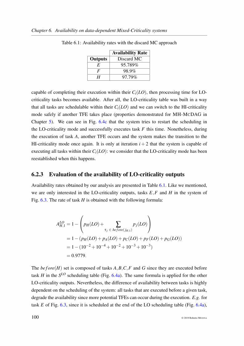
Chapter 6. Availability on data-dependent Mixed-Criticality systems
Table 6.1: Availability rates with the discard MC approach
Availability RateOutputs Discard MC
E 95.789%F 98.9%H 97.79%
capable of completing their execution within their Ci(LO), then processing time for LO-criticality tasks becomes available. After all, the LO-criticality table was built in a waythat all tasks are schedulable within their Ci(LO) and we can switch to the HI-criticalitymode safely if another TFE takes place (properties demonstrated for MH-MCDAG inChapter 5). We can see in Fig. 6.4c that the system tries to restart the scheduling inthe LO-criticality mode and successfully executes task F this time. Nonetheless, duringthe execution of task A, another TFE occurs and the system makes the transition to theHI-criticality mode once again. It is only at iteration i+ 2 that the system is capable ofexecuting all tasks within their Ci(LO): we consider that the LO-criticality mode has beenreestablished when this happens.
6.2.3 Evaluation of the availability of LO-criticality outputs
Availability rates obtained by our analysis are presented in Table 6.1. Like we mentioned,we are only interested in the LO-criticality outputs, tasks E,F and H in the system ofFig. 6.3. The rate of task H is obtained with the following formula:
ALOH,1 = 1−
pH(LO)+ ∑
τ j ∈ be f ore( jH,1)
p j(LO)
= 1− (pH(LO)+ pA(LO)+ pC(LO)+ pF(LO)+ pG(LO))
= 1− (10−2 +10−4 +10−2 +10−3 +10−3)
= 0.9779.
The be f ore(H) set is composed of tasks A,B,C,F and G since they are executed beforetask H in the SLO scheduling table (Fig. 6.4a). The same formula is applied for the otherLO-criticality outputs. Nevertheless, the difference of availability between tasks is highlydependent on the scheduling of the system: all tasks that are executed before a given task,degrade the availability since more potential TFEs can occur during the execution. E.g. fortask E of Fig. 6.3, since it is scheduled at the end of the LO scheduling table (Fig. 6.4a),
100 © 2019 Roberto MEDINA

6.3. Enhancements in availability and simulation analysis
its availability is lower than task H even if both have the same failure probability. Thisdifference of almost 2% is quite significative for safety-critical systems, like we explained,failure rates are measured up to the 10−9.
As we have demonstrated in this section, thanks to the probabilistic Fault model (Sub-problem 2.1) and to the Recovery mechanism (Sub-problem 2.2), we are capable ofEstimating availability rates (Problem 2) for LO-criticality tasks. In the next sectionwe present enhancements that can be deployed on MC systems in order to improve theavailability of LO-criticality tasks since the Discard MC model degrades availability(Problem 3).
6.3 Enhancements in availability and simulation analysis
In the previous section we enriched the MC-DAG model with a probabilistic failure modelto represent potential TFEs that can occur during the execution of the system. At thesame time, we introduced a recovery mechanism allowing us to perform an availabilityanalysis and concluded that the discard MC model [36; 8; 37] degrades the availabilityof LO-criticality tasks significantly. In this section we detail the limits in terms of avail-ability of the MC discard approach, to then propose two different types of enhancementsallowing us to improve significantly the availability of LO-criticality tasks. The inclusionof enhancements to MC systems led to the necessity of defining translation rules to prob-abilistic automata: the production of these automata is defined for the generalized casewhere systems have more than two criticality levels.
6.3.1 Limits of the discard MC approach
The MC discard approach [36; 8; 37] has been the most dominant model for MC schedul-ing due to its simplicity and its results in terms of acceptance rate. Because LO-criticalitytasks are completely interrupted when the system makes the transition and are not exe-cuted in the HI-criticality mode, HI-criticality tasks have better chances of being schedu-lable since the whole architecture is available to them. This approach is only focusedon safety, i.e. guaranteeing that HI-criticality tasks will be able to complete their ex-ecution, to the detriment of availability for LO-criticality tasks. Some recent contribu-tions in MC acknowledge that the complete interruption of LO-criticality tasks affectsthe QoS [99; 38], which is a main concern for safety-critical systems. For example theelastic MC model [38; 66] proposes to change periods of LO-criticality tasks when thesystem is in a HI-criticality mode in order to execute them less often, the utilization
© 2019 Roberto MEDINA 101

Chapter 6. Availability on data-dependent Mixed-Criticality systems
of LO-criticality tasks is reduced by applying this period transformation. Other typeof service guarantee schedulers have been proposed since then, partitioned and semi-partitioned systems are capable of limiting the mode transition to their partitions andmigrate LO-criticality tasks to other cores so they can complete their execution [61;63]. Other adaptations of LO-criticality tasks execution have also been proposed [49;83]. Our approach is similar to the selective degradation proposed in [60], the impact ofthe TFE will only affect a subgroup of tasks. Our goal is to deploy enhancements to the
system while still conserving the execution model we introduced in Chapter 4: thus, we
want to incorporate enhancements to the MC discard model.The limits we have identified thanks to our availability analysis are the following:
• Mode transitions to higher criticality modes are made in a synchronous mannerwhere all cores switch to the higher criticality scheduling table. While this is nec-essary in most cases to guarantee MC correctness, tasks can be interrupted by anytask that was executed before, regardless of their criticality. For example, sinceLO-criticality tasks are less constrained in terms of service guarantee, it is naturalthat their failure rate is greater than HI-criticality tasks’ rates: a TFE coming froma LO-criticality task triggers a mode transition, yet HI-criticality tasks should bemore capable of completing their execution within their Ci(LO). In other words,HI-criticality will have their timing budget extended, but it is very likely that it wasnot necessary since the TFE was caused by a LO-criticality task. Limiting the num-ber of mode transitions to higher criticality modes (Sub-problem 3.1) is the firstobjective we want to solve, in order to avoid discarding non-criticality tasks.
• Safety-critical systems often Incorporate mechanisms for availability enhance-ment (Sub-problem 3.2). The notion of robustness on MC systems is studiedin [101]. In this section, we explain how these enhancements can be deployed intothe system and how the availability rate can be estimated. These mechanisms shouldbe compatible with the MC discard approach. We focus only on two mechanismsto demonstrate the interest of the enhancements. Due to the execution behavior ofthese robust mechanisms we are forced to estimate availability thanks to system’ssimulations. Future works can be built on our results in order to consider other typesof enhancements.
We present in the next subsections our contributions in terms of availability enhance-ments for non-criticality tasks. These contributions are described for a generalized MCsystem with an arbitrary number of criticality levels. For clarity, throughout the exam-ples we just present results on a dual-criticality system. We begin by describing a fault
102 © 2019 Roberto MEDINA

6.3. Enhancements in availability and simulation analysis
propagation model capable of limiting the number of mode transitions to higher criticalitymodes. We then incorporate design patterns like Triple Modular Redundancy [120] andweakly hard real-time tasks [102] as additional enhancements to the overall system. Inorder to estimate the availability of a system enriched with these enhancements and withmore than two criticality levels, we have defined translation rules in order to obtain PRISMprobabilistic automata [114].
6.3.2 Fault propagation model
The first enhancement for MC system we consider is a detailed fault propagation model.In fact, safety-critical systems are equipped with software or hardware mechanisms thatlimit fault propagations to other components so as to improve dependability [121; 122;123]. Instead of switching systematically to the higher criticality mode whenever a taskhas a timing failure, we differentiate TFEs coming from a task with the same criticalitylevel the system is executed in, or a TFE coming for a task with a higher criticality levelthan the system is executed in. The main objective of this fault propagation model is toavoid dropping the execution of tasks that could complete their execution by performingunnecessary mode transitions to the higher criticality mode. This principle of limitingthe fault propagation for MC systems has been initially studied in [60]. Nonetheless, itdiffers from our fault model since we try to limit the number of mode transitions in func-tion of tasks’ criticalities, whereas the proposed approach performs the mode transitionswhenever a TFE takes place.
The fault propagation model we define has the two following behaviors:
1. When system is executing in the χ� mode and a χ�+1-criticality task has a timingfailure: make the mode transition to the χ�+1-criticality mode.
2. When the system is executing in the χ� mode and a χ�-criticality task has atiming failure: interrupt only the successors of the task that had a failure (i.e. tasksthat depend on the data produced by the failing task). χ�+1-criticality task (or higher)and unaffected χ�-criticality tasks can finish their execution within their Ci(χ�).
By considering this fault propagation model in our MC systems, the availability for-mula changes for the dual-criticality case:
ALOi,k = 1−
pi(LO)+ ∑
τ j ∈ pred(τi) ∪ be f oreHI( ji,k)p j(LO)
. (6.3)
© 2019 Roberto MEDINA 103

Chapter 6. Availability on data-dependent Mixed-Criticality systems
(a) MC system (b) Scenario with TFEs on LO and HI-criticality tasks
Figure 6.5: Fault propagation model with an example
The set considered of tasks that can affect the availability tends to be smaller: pred(τi) isthe set of predecessors of the task (predecessors in the DAG, i.e. tasks that send data toτi) and be f oreHI(τi) is the set of HI-criticality tasks executed before τi. If any of thesetasks fail then τi is interrupted. This set covers all tasks that have an influence on task τi
execution, the others are not communicating directly or indirectly with it, so they can beignored by the availability formula.
Fig. 6.5 illustrates our fault propagation model. The iteration of the system illustratedin Fig. 6.5b, shows the behavior of our fault propagation model when a LO-criticality taskhas a TFE. In the example, task G had a failure and task H depends on its output, as shownin Fig. 6.5a, we just discard task H (represented with the dotted box). In order to keepLO-criticality tasks running, we discard only tasks that have dependencies with the failingtask, in other words the successors of the task that had a failure are no longer executed.At the same time, since HI-criticality tasks are capable of completing their execution evenwhen they communicate with LO-criticality tasks (Chapter 5 Section 5.2.3), we allowthem to complete their execution within their Ci(LO).
The second iteration of the system illustrated in Fig. 6.5b shows the behavior of thefailure propagation model when a HI-criticality task has a timing failure. In this case,task A has a TFE and the system makes a transition to the HI-criticality mode (droppingLO-criticality tasks and extending timing budgets for HI tasks). Since HI-criticality tasksmust always complete their execution within their deadlines even in the case of a TFE, wedrop all LO-criticality tasks, the timing budget that was previously used by LO-criticalitytasks can potentially be used by HI-criticality tasks.
104 © 2019 Roberto MEDINA

6.3. Enhancements in availability and simulation analysis
The availability of task H of Fig. 6.5a can be calculated as follows:
ALOH,1 = 1−
pH(LO)+ ∑
τ j∈pred(H) ∪ be f oreHI( jH,1)
p j(LO)
= 1− (pH(LO)+ pA(LO)+ pC(LO)+ pG(LO))
= 1− (10−2 +10−4 +10−2 +10−3)
= 0.9889.
As opposed to the previous calculus now the availability of task H is only dependent on theexecution of tasks A,C and G (as opposed to A,C,F and G). The availability was increasedof 1.1% thanks to the fault propagation model. We provide results for the rest of LO-criticality outputs in the next subsection where we present the fault-tolerant mechanismswe consider in our availability analysis.
6.3.3 Fault tolerance in embedded systems
Fault-tolerant mechanisms have been widely deployed into safety-critical systems in orderto improve dependability. In this subsection we describe how a MC system can incorporatedesign patterns like Triple Modular Redundancy (TMR) [120] and/or weakly hard real-time tasks [102] in order to improve the availability of LO-criticality tasks. We presentthe deployment of these mechanisms with the example of the system presented in Fig. 6.3,our goal is to improve the availability of output E, which has the lowest availability rateout of all LO-criticality outputs (as shown in Table 6.1). We detail the changes that takeplace in the execution model of the system and our contributions in order to estimate theavailability rate of the MC system with these new enhancements.
Triple Modular Redundancy
Design patterns like Triple Modular Redundancy (TMR) [120] are widely used in safety-critical systems in order to improve RAMS properties. We focus only on one designpattern as a motivating example to demonstrate the interest of considering such designpatterns during the conception of MC systems.
The TMR consists in replicating a software (or hardware) component three times andcomparing the produced results of these replicas thanks to voting mechanisms. If at leasttwo out-of three results are the same, then the correct output can be deduced: the majorityhas the advantage. The idea is to mask faults that can occur during the execution of one ofthe replicas. In fact, having a failure in one of the replicas already occurs on rare occasions
© 2019 Roberto MEDINA 105

Chapter 6. Availability on data-dependent Mixed-Criticality systems
Figure 6.6: A TMR of the MC system of Fig. 6.3
for a safety-critical system, consequently having two or more replicas in a failing state atthe same time is almost impossible.
To take into account the presence of replicas on the availability rates we apply a prob-ability tree to deduce the following formula:
ALO,T MRi = (ALO
i )3 +3�(ALO
i )2 × (1−ALOi )
�. (6.4)
The availability of a task with a TMR is the equal to the combination of the three repli-cas being in a functional state (ALO
i )3, plus the states when at least two replicas are in afunctional state: 3×
�(ALO
i )2 × (1−ALOi )
�.
The application of a TMR design pattern is presented in Fig. 6.6. We incorporatedvoting mechanisms, vertices labeled as the V task, responsible for checking outputs pro-duced by task D and its replicas. We consider the execution of these voting mechanismsis negligible compared to the timing budget of tasks. The failure probabilities for tasksF and G remains unchanged in each one of the replicas, since the TMR does not affectthem (i.e. none of these tasks communicate with the voting mechanism and are executedbeforehand). For the E task however, its availability changes since the probability that taskD has a failure is now different:
pT MRD (LO) = 3×
�(1−10−2)× (10−2)2�+(10−2)3
= 0.000298.
The equation is again an application of a probability tree to deduce the states where taskD has a failure even with the voting mechanism. D is said to be in a failing state whenat least two of the replicas are also in a failing state: 3×
�(1−10−2)× (10−2)2� or when
106 © 2019 Roberto MEDINA

6.3. Enhancements in availability and simulation analysis
Table 6.2: Availability rates for LO-criticality outputs with availability enhancements
Availability RateOutputs Discard MC Enhanced FP Enhanced FP + TMR
E 95.78900% 96.98900% 99.87675%F 98.90000% 98.90000% 99.96397%H 97.79000% 98.89000% 99.96331%
the three replicas are simultaneously in a failure state (10−2)3. We can see that the failureprobability was reduced considerably (it used to be 0.01%).
The availability obtained for the LO-criticality outputs using the TMR design patternare resumed in Table 6.2. We present the availability values for all LO-criticality out-puts considering the normal discard MC approach (column “Discard MC”), the enhancedmodel with fault propagation (column “Enhanced FP”) and the enhanced fault propaga-tion model with TMR (column “Enhanced FP + TMR”). These results clearly show theimprovements in availability that we can obtain using this type of fault tolerance mech-anisms: for example, task E which has the lower criticality, increased its availability byover 1% with our enhanced fault propagation model and by over 4% with the TMR. Nev-ertheless, using a TMR might not always be possible due to budget, space, or power con-straints. For this reason we look into another method of fault tolerance in order to improvethe availability of LO-criticality outputs.
Weakly hard real-time task
Tolerating a given number of deadline misses on hard real-time tasks was presented in [102].On monitoring systems or automatic control systems for example, sampling periods needto be set. These periods tend to be set as fast as possible in order to detect changes thatthe system might need to handle. Nonetheless, for safety reasons periods tend to be fasterthan what is actually required. Therefore, missing one or more measurements within afixed number of executions of the sampler can actually be tolerated, as long as the actionfrom monitoring can be done within the delay caused by the missing measurements. Inother words, provided that the effect on such a delay does not have severe consequences,deadlines can be missed.
We represent the behavior of a Weakly Hard Real-time Task (WHRT) in Fig. 6.7. Thetask represented in a (1−2)-firm task which means that out-of two successive executions,we tolerate one deadline miss. The state machine representing its behavior is composedof four states: white states in the figure indicate that the task is functional, the red staterepresents that the task is in a failure state. Each state is annotated with a bitset, this bitset
© 2019 Roberto MEDINA 107

Chapter 6. Availability on data-dependent Mixed-Criticality systems
Figure 6.7: (1−2)-firm task state machine
(a) MC system (b) Scenario with TFEs on LO and HI-criticality tasks
Figure 6.8: (m− k)-firm task execution example
records the execution history for the number of successive executions we are interestedin: 1’s are recorded when the task completed its execution within its Ci(LO) and 0’s arerecorded when a TFE occurred. Arrows between states are labeled with “TFE” or “Ok”indicating what state is reached after the task has a TFE or when the task completed itsexecution with the timing budget given.
Let us now consider a WHRT in the system we have presented throughout this chapter.In Fig. 6.8 we have represented the WHRT with a blue label: task D is now considered tobe a (1−2)-firm task, i.e. one fault is tolerated out of two successive executions (Fig. 6.8a).The time diagrams represented in Fig. 6.8b show how the task is capable of maintaining itsexecution on iteration i even after a TFE occurred. Nevertheless, on iteration i+1, the sec-ond successive TFE provokes the interruption of the successors of the task, in this case taskE. Due to the fact that the functional (or non-functional) state of the task is now depen-dent on a series of executions, the availability formula (Eq. 6.3) can no longer be used to
108 © 2019 Roberto MEDINA

6.3. Enhancements in availability and simulation analysis
estimate the availability rate: the failure probability of a task is more complex to estimate.In order to solve this problem we propose to transform the system and its scheduling toperform system simulations. These simulations are performed thanks to the PRISM [114]
model checker since it allows us to incorporate all the aspects presented throughout thechapter: failure model, recovery mechanism and the fault propagation model.
6.3.4 Translation rules to PRISM automaton
The incorporation of WHRT tasks changes the execution behavior of the MC system quitesignificantly, since the failure probability of a task is now dependent on a sequence ofexecutions. In order to estimate the availability rate when this type of task is deployed inthe system we need to perform system simulations. This type of analysis is completely newto the domain of MC systems with data-dependent tasks. We need to choose an adaptedtool capable of modeling all the aspects that we have presented in this chapter until now.The challenges of this procedure are the following: (i) there has to be a way to keep trackof tasks’ executions in order to estimate their availability rate, (ii) failure probabilitiesneed to be considered, (iii) the fault propagation model we propose capable of limitingthe number of mode transitions also needs to be taken into account, and (iv) a record ofsequential executions of the system needs to be stored.
The tool that allows us to perform system simulations considering all the abovemen-tioned aspects is the PRISM model checker [114]. We introduce translations rules that takethe MC system specification and the scheduling tables as an input to produce probabilistic
automaton. This probabilistic automaton represents the state of the multi-core processors,the criticality mode the system is in and the tasks that are being executed on it. The trans-lation rules have been defined for the generalized case where systems can have more thantwo criticality levels: when more than two criticality levels are considered the number of
scenarios that lead to the execution or interruption of a task increases significantly whichalso motivates the introduction of translation rules. The availability of a task is thereforea measurement when we consider the automaton we produce: by simulating the executionof the system for a long period of time, we estimate what the availability rate is.
The implementation under PRISM uses the following aspects offered by the tool:
• States in the automaton allow us to represent the state of the processor, i.e. whattasks are running in the architecture at a certain instant. By doing so we can repre-sent the system running in any χ�-criticality mode.
© 2019 Roberto MEDINA 109

Chapter 6. Availability on data-dependent Mixed-Criticality systems
• Probabilistic automata allow us to encapsulate our failure model: probabilistic tran-sitions are used to represent if the task did complete its execution within its Ci(χ�)
or if it had a TFE.
• The fault propagation model is captured by the use of boolean variables in the au-tomaton. If the output of a task was produced, the boolean is marked as true, oth-erwise it is marked as false. To detect if an output is available, we check if allthe predecessors of the output produced data, i.e. we verify that the conjunction ofbooleans is true.
• The behavior of the WHRT is simulated thanks to a bit set. This bit set will beupdated according to the task’s behavior: a 1 is added at the end of the bit set if datawas produced, otherwise a 0 is added. Once the bit set is updated, we check thenumber of bits marked with 1 to deduce if the task is a failure state or not.
• The fault recovery process can be easily represented thanks to a transition that goesto the first state representing the beginning of the lowest criticality scheduling table.
• Transitions can update counters used to measure the number of times a tasks isexecuted and the number of times the system is executed. The formula of Eq. 6.1 isthen applied to obtain the availability rates of outputs.
General principle: The idea behind the translation of scheduling tables to a proba-bilistic automaton (PA) is to represent the state of the processor, i.e. which task is runningand in which mode. Since we are executing MC-DAGs in multi-core architectures, wecould transform the scheduling table of each core into an automaton. However, havingparallel automata in PRISM increases significantly the simulation time due to the largenumber of possible states. To limit the number of states on the PA and because TFEs canonly be detected at the the end of the timing budget given to a task, we only include
states that represent the end of the timing budget given to a task for a given criticality
mode. This means that if a task job is preempted several times during its execution, in theautomaton we will only have one state representing the end of its timing budget. Since thecompletion of all tasks need to be checked, doing it in a sequential manner does not changethe final result for the availability rates but significantly reduces the simulation time.
Translation rules: To check the completion of tasks, we sort them by considering
their end of time window in the scheduling tables. The first step is to create ordered listof tasks for each criticality level. For each task τi in this list (where i is the index of thistask in the list) we create a state Sχ�
i and a boolean variable bi. The state represents theend of the timing budget given to a task job for its execution at that time instant, and
110 © 2019 Roberto MEDINA

6.3. Enhancements in availability and simulation analysis
the boolean is used to notify the successors that output was produced or not. Tasks thatare executed in more than one criticality level have more than one state in the automaton:each state represents the execution of the task in the criticality modes it is executed in. Dueto parallelism obtainable thanks to multi-core processors, tasks can have the same end oftime window. This has to be taken into consideration for the availability computation sincemode transitions can be triggered by tasks that have a higher criticality level than the levelthe system is executed in; but outputs can be available at the same time slot. Ties in thelist need to be broken with the following rules:
1. Tasks that are exit nodes in the mode considered go first: we need to know if theiroutput is available.
2. Tasks with a higher criticality level than the mode considered go afterwards, a modetransition occurs when they have a TFE.
3. Other tasks are checked at the end, no mode transition occurs even if they fail. Inreality, some tasks could have been dropped because one (or more) of their prede-cessors failed to complete their execution. While the state is always presented in theautomata, detecting faulty predecessors takes place in the transition that is taken toleave the state.
After generating the states representing the execution of tasks in all criticality modes,we connect them with the rules illustrated in Fig. 6.9. How tasks are connected is essentialfor the PA, the rules presented avoid deadlocks, are coherent with the execution of thesystem and represent the potential TFEs that can occur during the system’s execution.
1. From a state Sχ�i when the task TFE cannot cause a mode transition to higher crit-
icality mode: we add two probabilistic transitions connecting Sχ�i to Sχ�
i+1. One ofthe probabilistic transition represents the occurrence of a TFE (with a probabilitypi) and updates bi to false, whereas the other (with a probability 1− pi) updates bi
to true. This rule is illustrated in Fig. 6.9a, the dotted/dashed lines represent theprobabilistic transitions, the left label is the probability and the right label is theassignment of the boolean bi.
2. From a state Sχ�i when the criticality mode considered is not the highest criticality
mode the task it is executed in: we add a probabilistic transition with a probability1− pi to the next state Sχ�
i+1, boolean bi is marked as true. A second probabilistictransition with a probability pi is added to a state Sχ�+1
i : the system performs amode transition to the higher criticality mode. This translation rule is represented inFig. 6.9b.
© 2019 Roberto MEDINA 111

Chapter 6. Availability on data-dependent Mixed-Criticality systems
(a) Same criticality level rule (b) Higher criticality level rule
(c) Output rule
(d) WHRT rule
Figure 6.9: PRISM translation rules for availability analysis
112 © 2019 Roberto MEDINA

6.3. Enhancements in availability and simulation analysis
Figure 6.10: PA of the system presented in Fig.6.8
3. The translation rule of Fig. 6.9c is used when a task is also an output for the critical-ity mode considered. After applying the rule of Fig. 6.9a, we need to add an extrastate, named Sχ�
out,i, that checks if all the predecessors of the task were able to com-plete their execution (
�τ j∈pred(τi) b j). If that was the case, then the availability of the
output is incremented thanks to PRISM counters: each output has its own counterand the system has a counter to check if the system completed its execution in theLO or HI-criticality mode. If the conjunction of booleans is false, the availabilitycounter for the LO-criticality output is not incremented.
4. The final translation rule, illustrated in Fig. 6.9d represents a WHRT task. Like wementioned before, to capture the behavior of the WHRT task we use a bit set thatkeeps track of the successive executions of the task. The size of the bit set naturallykeeps track of the right amount of successive executions we are interested in. Likeit is represented in the figure, the probabilistic transitions are in charge of updatingthe bit set: if the task did not fail, a 1 is added at the end of the bit set; and if there isa TFE, a 0 is added at the end of the bit set. The oldest bit is erased after during theupdate. A state, Sχ�
wh,i∗ is added for WHRT tasks in order to check the status of thetask, if the number of bits equal to 1 is superior to the number tolerated faults, thenthe task is in a functional state and its boolean bi is marked as true. Otherwise thetask is considered to be in a failing state and its boolean is marked as false.
Application to the example and results: When we apply the translation rules tothe system and the scheduling tables (Fig. 6.7 and Fig. 6.4), we obtain the automaton
© 2019 Roberto MEDINA 113

Chapter 6. Availability on data-dependent Mixed-Criticality systems
Table 6.3: Availability rates for LO-criticality outputs with availability enhancements
Availability RateOutputs Discard MC Enhanced FP Enhanced FP + WHRT
E 95.78900% 96.98900% 97.90121%F 98.90000% 98.90000% 98.90099%H 97.79000% 98.89000% 98.89441%
presented in Fig. 6.10. White states represent the system’s execution in the LO-criticalitymode, while gray states represent the HI-criticality mode. Like we mention, the first stepof the translation, creates the states representing the completion time of tasks for eachoperational mode. Afterwards, rules to connect each state are applied like we previouslyexplained. Once this automaton is obtained, we can use it in the PRISM model checker inorder to estimate the availability rate.
Table 6.3 presents the results obtained for the LO-criticality outputs when we con-sider a WHRT task. Again we show the gains in availability for all outputs of the system.First, the values obtained with the classic MC discard model are presented. Like for Ta-ble 6.2, we present the results obtained when we consider the fault propagation model wedescribed: there is an increase in availability for tasks E and H of 1.2% and 1.1% respec-tively. The last column presents the results obtained with the PRISM model checker afterperforming simulations of the system. As we can see, the experimental results are equiva-lent to the numerical values obtained for tasks F and H. For task E, since its predecessortask D is a (1−2)-firm task, we can see another improvement in its availability: we gainedalmost 1%, demonstrating the interest of including WHRT tasks in the system in order togain in availability for LO-criticality tasks.
An example of the generalized translation: Fig. 6.11 presents a simplified represen-tation of a probabilistic automaton for a system with N-levels of criticality. This illus-tration demonstrates the interest of performing translation rules for systems composed ofmore than two levels of criticality. As an example let us assume we are interested in theavailability of task τi2 . In the automaton we can see that this task is executed in modes χ0
and χ1. Thus, in order to evaluate the availability of τi2 , we need to know how many timesthis task was executed in both operational modes. The lines illustrated in red represent thedifferent paths leading to the execution of task τi2 for modes χ0 and χ1. As we can see thereare four possible combinations that lead to the complete execution of τi2 . Nonetheless fortasks that are further in the scheduling table and that executed in various criticality levels,the number of possible paths that lead to the complete execution of a task grows rapidly.While enumerating the possible execution paths for the system leading to the execution of
114 © 2019 Roberto MEDINA

6.4. Conclusion
Figure 6.11: Illustration of a generalized probabilistic automaton
a task is possible, it easily becomes error prone. In addition, the translation rules can becombined, so we can have WHRT tasks in addition to an arbitrary number of criticalitylevels. For this reason translation rules are also interesting when more than two criticalitylevels are used in the MC system.
In this section we presented our solutions tackling the following problem: DiscardMC model degrades availability (Problem 3). We started by introducing a more de-tailed fault propagation model aiming at Limiting the number of mode transitions tohigher criticality modes (Sub-problem 3.1) . Thanks to this model, outputs that areunaffected by the TFE can complete their execution. The other type of enhancement weconsidered, is the fact that safety-critical systems Incorporate mechanisms for avail-ability enhancement (Sub-problem 3.2). While the TMR has shown to greatly improvethe availability rate for all LO-criticality tasks, it might not always be possible to deployreplicas in the targeted system. For this reason we have also considered WHRT tasks andproposed translation rules that allow us to perform simulations of the system in order toestimate availability rates.
6.4 Conclusion
In this chapter we presented our availability analysis for MC systems. We suppose MCsystems are described following the MC-DAG model presented in Chapter 4 (Section 4.1)and are scheduled with static scheduling tables considered to be MC-correct: for exam-
© 2019 Roberto MEDINA 115

Chapter 6. Availability on data-dependent Mixed-Criticality systems
ple our implementations of the MH-MCDAG meta-heuristic (Chapter 5) can be used toschedule these systems.
Thanks to these hypotheses we can Estimate availability rates (Problem 2) for LO-criticality outputs. This quantification of availability has not been considered before forMC systems. The scheduling methods we consider is based on the discard MC model [36;8; 37] of literature: LO-criticality tasks are discarded once a mode transition to the HI-criticality mode has to be performed. We defined a probabilistic Fault model (Sub-problem 2.1) in order to estimate how often LO-criticality tasks are discarded and aRecovery mechanism (Sub-problem 2.2) to reincorporate the discarded tasks once pro-cessing time is available once again. Availability formulas for LO-criticality outputs arethen established thanks to the fault model and the recovery process.
While these enrichments to the execution model of MC-DAGs allowed us to calcu-late the availability rate for LO-criticality outputs, we demonstrated that the Discard MCmodel degrades availability (Problem 3). This is due to the fact that any TFE occurringin the system provokes a mode transition to the HI-criticality mode, and therefore tasksthat are executed last in the scheduling table have the lowest availability rate. We solvedthis limitation in two ways: first of all, we incorporated a fault propagation model thatcontains faults in order to Limit the number of mode transitions to higher critical-ity modes (Sub-problem 3.1). Second, since safety-critical systems often Incorporatemechanisms for availability enhancement (Sub-problem 3.2), we considered them intoour analysis. Throughout the chapter we demonstrated the significant improvements inthe availability rate of LO-criticality tasks that were obtained thanks to our enhancements.In the example considered, the fault propagation model increased the availability of sometasks by over 1%. When we incorporated fault tolerance mechanisms in addition to thefault propagation model, we increased between 1% and 4% of availability. This changesare quite significant since certification processes measure the availability of tasks up to10−9.
In this chapter we have also presented translation rules to obtain PRISM automatafrom MC systems specifications and scheduling tables. These translation rules are appliedwhen the execution model of the system becomes too complex, i.e. when enhancementslike weakly hard real-time tasks are incorporated in the system, or when the system hasmore than two criticality levels. The automata produced by our rules simulates the stateof the processor during its execution. Availability rates are estimated thanks to executionsimulations of this representation.
In the next chapter, we present the MC-DAG framework. This open source tool wedeveloped incorporates the model transformation rules we defined in Section 6.3.3, used
116 © 2019 Roberto MEDINA

6.4. Conclusion
to estimate availability rates thanks to simulations of the system. The framework is alsocapable of scheduling systems and performing benchmarks in order to assess statically ourcontribution regarding the scheduling of MC-DAGs in multi-core architectures.
© 2019 Roberto MEDINA 117

Chapter 6. Availability on data-dependent Mixed-Criticality systems
118 © 2019 Roberto MEDINA

7 Evaluation suite: the MC-DAG frame-work
TABLE OF CONTENTS
7.1 MOTIVATION AND FEATURES OVERVIEW . . . . . . . . . . . . . . . . . . . 120
7.2 UNBIASED MC-DAG GENERATION . . . . . . . . . . . . . . . . . . . . . . 121
7.3 BENCHMARK SUITE . . . . . . . . . . . . . . . . . . . . . . . . . . . . . . . 128
7.4 CONCLUSION . . . . . . . . . . . . . . . . . . . . . . . . . . . . . . . . . . 129
In this chapter, we present the MC-DAG framework, an open-source tool developedto perform the scheduling and availability analyses of MC data-driven systems. This toolconsolidates all our contributions and is composed of four different modules:
• A scheduling module capable of applying the G-ALAP-LLF, G-ALAP-HYB and G-ALAP-EDF heuristics to schedule a system (contributions presented in Chapter 5).
• An unbiased and random MC-DAG generator. This module has been developed inorder to compare our scheduling methods to existing approaches of the literature.Since different aspects need to be considered in order to obtain an unbiased MC-DAG we had to combine different generation methods of the literature.
• A benchmark suite to measure acceptance rates and number of preemptions for thescheduling heuristic we have developed, but also to compare them to schedulingpolicies of the state-of-the-art [80; 81].
• An availability module that applies transformation rules to obtain PRISM automatafrom the system and its scheduling tables (this contribution is presented in Chap-ter 6).
119

Chapter 7. Evaluation suite: the MC-DAG framework
We begin by presenting the motivation and an overview of the features included in theMC-DAG framework. Details about how we developed the unbiased MC-DAG generationare presented afterwards. The final part of this chapter explains how benchmarks are donein order to compare our contributions to the state-of-the-art.
7.1 Motivation and features overview
When we look at existing approaches capable of scheduling MC-DAGs on multi-corearchitectures [80; 81; 82; 83], two of them only present theoretical results and the othertwo have a restricted execution model where all vertices of the MC-DAG belong to thesame criticality mode. The scheduling approaches of MC-DAGs [82; 83] have shownexperimental results, nevertheless their evaluation framework has not been made publiclyavailable.
The MC-DAG framework we have developed provides the abovementioned feature:scheduling for MC data-driven systems. The framework is hosted on GitHub 2 under theApache 2 license. It was developed in Java in order to be cross-platform and different JARfiles can be created to execute the modules included in the tool.
One JAR module handles the scheduling of MC systems. This module takes a MCsystem specification as an input. To specify a MC systems a XML file needs to be cre-ated following the specification described in the GitHub wiki (https://github.com/robertoxmed/MC-DAG/wiki/Declaring-a-XML-MxC-System). The MC-DAG specifi-cation includes the vertices, edges, timing budgets in all criticality modes, number of avail-able cores and number of criticality levels. If the debugging flag is turned on, then all thesteps of the scheduling table computation are displayed. The user can choose between thethree heuristics we have implemented (G-ALAP-LLF, G-ALAP-HYB or G-ALAP-EDF)in order to schedule the system. Whenever VERIFYCONSTRAINTS of Alg. 1 or Alg. 2returns false, the programs stops and returns an exception since scheduling tables couldnot be computed. When the scheduling of the MC system in all criticality modes succeeds,the scheduling tables are written in a XML output file and are displayed if debugging ison.
To statistically assess our contribution, we need to perform benchmarks. Nonetheless,publicly available tools usually only deal with one of the aspects of our research: forexample we can find random DAG generators (e.g. TGFF [124], GGEN [116]) but theexecution time allocated to vertices in the graphs is not controlled like for task sets whenreal-time scheduling policies are evaluated. On the other hand, task set generators are not
2MC-DAG Framework - https://www.github.com/robertoxmed/MC-DAG
120 © 2019 Roberto MEDINA

7.2. Unbiased MC-DAG generation
capable of creating MC-DAGs. For these reasons one of our objectives was to integrate agenerator of MC-DAGs that would be publicly available and reusable by the community.The MC-DAG generator and the benchmark suite are also contained in the framework.Many parameters need to be set for the MC-DAG generator, in the next section we explainhow we achieve an unbiased generation. The program can generate an important numberof random systems with the parameters chosen by the end-user. Generated systems arewritten into XML files so they can be read by the scheduling module if the user desires. Togenerate a graphical representation of the system that was generated, a .dotfile is writtenso it can be transformed into post script using Graphviz tools3. With these generatedsystems, the benchmark suite is capable of performing tests to evaluate acceptance ratesand measure the number of preemptions generated by different scheduling policies. Sincethese tests can take a large amount of time, the suite is fully automated for the generationand the performance evaluation.
Additionally, when we look into availability or quality-of-service aspects related toMC systems the same problem also exists: there are not publicly available tools in order toevaluate the availability of non-critical tasks of MC systems. For the availability analysis,the module takes the MC system specification as an input file as well. This JAR filecan use scheduling tables given as an additional input or it can calculate the schedulingtables on the fly thanks to our heuristics. With these two inputs, the transformation rulesdefined in Chapter 6 are applied and the automata are build. Two output files are created:one contains the probabilistic automata (a .pm file) and the other contains formulas tomeasure the availability rates of the non-critical tasks (a .pctl file). With these two filesthe PRISM model checker can be run from the command line or by using the GUI to obtainthe availability rates for the non-critical tasks.
7.2 Unbiased MC-DAG generation
In this section we describe how we perform an unbiased generation for systems composedof MC-DAGs. We developed this module of the framework in order to perform statis-tical analyses. In particular, we planned to compare our scheduling methods to existingapproaches of the state-of-the-art [80; 81]. Like we mentioned before, a tool capable ofgenerating DAGs with MC tasks was not available publicly. In order to overcome thislimitation we incorporated different aspects related to the generation of unbiased DAGsand the generation of task sets to evaluate real-time scheduling policies.
3Graphviz layout programs - http://www.graphviz.org
© 2019 Roberto MEDINA 121

Chapter 7. Evaluation suite: the MC-DAG framework
First of all, when it comes to DAG generation, in [116] Cordeiro et al. describe variousalgorithms capable of creating DAGs with random topologies. We decided to extend theLayer-by-Layer [125] method due to its simplicity and effectiveness. The idea behindthis procedure is to progressively create vertices by assigning them a “layer” level. Foreach layer level a given number of vertices is created. The number of vertices and layersis parameterized by the user. As layers are created, edges are formed between verticesfollowing a probability rate, i.e. there is a probability e of having an edge between twovertices of different layers. To avoid cycles during the formation of edges, an edge canonly be added if the source vertex has a lower layer level than the destination vertex.
The second part of the generation, is related to the real-time aspect of our heuristics.We want to tests the limits of our scheduling method by having control over the utilization
rate of the system. Scheduling policies are often judged based on how they can performwhen a system has a high utilization rate: high utilization rates translate to a more diffi-cult scheduling problem. As a matter of fact, many contributions have been proposed inthe literature to perform evaluations of real-time scheduling policies. Nonetheless, UU-NIFAST [126] has proven to be the most used generation method due to the fact that anuniform distribution of utilization rates can be obtain easily and quickly. Therefore inorder to distribute an utilization rate among tasks we use UUNIFAST and its multi-coreadaptation UUNIFASTDISCARD [5]. UUNIFAST is used to distribute an overall utiliza-tion rate among a given number of MC-DAGs included in the system. Since the utilizationrate of a MC-DAG can be greater than 1, we do not need to filter utilization rate sets likeUUNIFASTDISCARD does. Nevertheless, when we distribute the utilization rate amongvertices we use UUNIFASTDISCARD, we cannot have a vertex with a utilization greaterthan 1 since it would implicate that more than one processor is needed to scheduled asequential task.
Generation of a MC system
Algorithm 3 presents the random system generation of our tool. Seven parameters need tobe given by the user:
• Umax ∈ R∗+ the maximum utilization of the system in all the criticality modes.
• nG ∈ N the number of MC-DAGs that will be included in the system.
• {χ1, . . . ,χN} the set of criticality levels.
• nV the number of vertices that need to be create for each MC-DAG.
122 © 2019 Roberto MEDINA

7.2. Unbiased MC-DAG generation
Algorithm 3 Unbiased System generation1: function GENERATESYSTEM(Umax: utilization of the system in all modes,
nG : number of DAGs to create,{χ1, . . . ,χN}: set of criticality levels,nV : number of vertices to create,e: probability of having an edge,p: vertices/layer lower-bound,r: reduction factor)
2: S ← new MC system3: |S .Π|← �Umax� � Number of available cores4: S .χ ← {χ1, . . . ,χN} � Set of criticality levels5: UGset []← new set of utilizations for DAGs6: UUNIFAST(UGset ,Umax) � Distribute utilization rates7: for all i < nG do8: S .G ← S .G ∪ GENERATEGRAPH(UGset [i],S .χ,nV ,e, p,r)9: end for
10: return S11: end function
• e the probability of having an edge between two vertices.
• p an lower-bound on the number of vertices that belong to a layer.
• r a reduction factor for the utilization of tasks executed in more than one criticalitymode.
After the system is instantiated and initialized with the architecture and the criticalitymodes (l. 2-4), an array of utilization rates is created (l. 5). This array UGset of size nG ,is used by UUNIFAST to distribute the utilization rate of the system to each MC-DAG (l.6). The idea behind UUNIFAST is to distribute the utilization Umax among the slots ofUGset uniformly. Once the distribution is performed, we proceed to create the number ofMC-DAGs requested by the user (l. 7-8).
Generation of a MC-DAG
The function GENERATEGRAPH is detailed in Algorithm 4. The Layer-by-layer
procedure described in [125; 116] is used as a basis for the algorithm. The timing bud-get distribution and assignment to each vertex of the MC-DAG is done before edges arecreated.
The parameters used by the function are almost identical to parameters used by GEN-ERATESYSTEM. The only difference is the utilization rate that will be used by the verticesof the graph: UGset ∈ R∗
+.
© 2019 Roberto MEDINA 123

Chapter 7. Evaluation suite: the MC-DAG framework
Algorithm 4 Unbiased MC-DAG generation1: function GENERATEGRAPH(UG: DAG utilization,
χ: criticality levels,nV : number of tasks,e: edge probability,p: vertices/layer upper-bound,r: reduction factor)
2: G ← new MC-DAG � Initialization block3: D ← random deadline from pre-defined list4: budget[]← �D×UG�5: prevLayer ← 06: for all χ� ∈ χ in decreasing order do � Generation7: layer ← rand(0, prevLayer)8: Uset []← array of utilization rates for each task
9: repeat � Generate the utilization for each task10: returnUUD ← UUNIFASTDISCARD(Uset ,budget[χ�]/D)11: until returnUUD =�
12: tasksToGen ← n13: while budget[χ�]> 0 ∧ tasksToGen > 0 do � Vertices generation phase14: count ← 015: while count ≤ p ∧ tasksToGen > 0 do16: τi ← new vertex17: Ci(χ�)← �D×Uset [i]�18: budget[χ�]← budget[χ�]−Ci(χ�)19: τi.layer ← layer
20: if layer �= 0 then � Edges incorporation phase21: for all {τ j ∈ G | τ j.layer > τi.layer} do22: if rand(0,1)≤ e ∧ CPχ�
j +Ci(χ�)≤ D then23: G.E ← G.E ∪ (τ j,τi)24: end if25: end for26: end if
27: G.V ← G.V ∪ {τi}28: tasksToGen ← tasksToGen−129: count ← count +130: end while31: layer ← layer+132: end while
124 © 2019 Roberto MEDINA

7.2. Unbiased MC-DAG generation
33: if χ� ≥ χ2 then � Reduction phase34: Ureduc ←UG/r � Reduce by the reduction factor35: budgetreduc ←Ureduc ×D36: repeat37: for all τi ∈ G do38: Ci(χ�−1)← rand(1,Ci(χ�))39: end for40: until budgetreduc < ∑τi∈GCi(χ�−1)41: budget[χ�−1]← budget[χ�−1]−budgetreduc42: end if43: prevLayer ← layer44: end for
45: return G46: end function
Initialization phase (l. 2-5): The function starts by creating a MC-DAG and assigningit a deadline (l. 3). This deadline is randomly selected from a pre-defined list: {100,120, 150, 180, 200, 220, 250, 300, 400, 500}. Since industrial implementations oftenavoid large hyper-periods caused by prime numbers between deadlines of applications, wefollow the same principle with this list of possible deadlines. With the utilization and thedeadline of the MC-DAG, we can deduce the timing budgets that needs to be distributedamong tasks in all criticality levels (l. 4). Budgets are stored in an array of size |χ|, thecardinality of the criticality levels. The timing budget is used for all tasks that are executedin a given criticality level: this includes tasks that are executed in more than one criticalitylevel. For example, let us consider a system of three criticality modes composed of 30vertices/tasks: in the highest criticality mode, the timing budget is distributed among 10tasks. Once we move to the second highest criticality level, the timing budget is dividedamong 20 tasks, the 10 tasks that were created in the previous criticality mode (with areduced timing budget since Ci(χ�)≤Ci(χ�+1)), in addition to the 10 new tasks that needto be added. The final level will distribute the timing budget between 30 tasks.
Generation initialization (l.7-11): The generation phase of Alg. 4 (l. 6-44) then startsby looping over the criticality levels in descending order. A layer value is randomly se-lected (l. 7): in the highest criticality level, we are forced to start with layer number 0,but for subsequent criticality levels, we can start in a deeper layer. This prevents biasesthat could be caused by having too many source vertices and MC-DAGs with very fewconsecutive tasks. The next step consists in creating an array of utilization ranges. Thisarray Uset of size n, is used to store the utilization given to each task created in the χ�
level. In order to do so, we use the adaptation of UUNIFAST for multi-core architectures:
© 2019 Roberto MEDINA 125

Chapter 7. Evaluation suite: the MC-DAG framework
UUNIFASTDISCARD [5]. The idea behind this method is to use UUNIFAST but discarda set of utilization rates where one (or more) value is greater than one. This needs to beavoided since it would mean that a sequential task would need more than 1 CPU in orderto complete its execution, which is impossible. Since UUNIFASTDISCARD can take sev-eral tries to create an acceptable utilization array, the procedure is called as many time asit is required (l. 9-11). (For Alg. 3, regular UUNIFAST is used since a MC-DAG can havea utilization greater than one).
Vertex generation phase (l.12-32): With the utilization rates for each task being cre-ated, the vertex generation phase starts. We need to create n vertices per level, and upto p vertices per layer. After the vertex is created (l. 16), we transform the utilizationrate obtained thanks to UUNIFASTDISCARD to timing budget Ci(χ�) (l. 17), the overallbudget for the criticality level is then updated (l. 18) and the current layer level is given tothe task (l. 19).
Incorporation of edges (l.20-26): If the current layer is not the 0-layer, then we tryto add edges between the newly created vertex and all the vertices that have a lower layerlevel (l. 20-26). By only having edges that go from a low-level layer to a high-level layerwe prevent the creation of cycles in the graph: a cycle would imply that an edge goesfrom a high layer communicates with a low layer vertex at some point. We do follow theprobability e to have an edge but also verify that adding an edge would not create a criticalpath bigger than the deadline assigned to the MC-DAG: CPχ�
j +Ci(χ�)≤ D (l. 22).
Once the edges are created, we add this new vertex to the graph (l. 27), update thenumber of tasks to create (l. 28) and the number of tasks created in the layer (l. 29). Thisprocedure is repeated until the timing budget has been distributed.
Reduction phase (l.33-42): Once all tasks for the current criticality level have beencreated, we check if we are not in the lowest-criticality level (l. 33). If that is not thecase, the reduction phase takes place. This reduction phase creates timing budgets fortasks executed in the χ� criticality mode for the χ�−1 mode. We start by dividing thelevel utilization, UG , by the reduction factor r (l. 34) and we obtain the targeted timingbudget for all tasks afterwards (l. 35). The process to reduce timing budgets for the χ�−1-criticality mode then starts: we randomly generate the Ci(χ�−1) timing budget to avoid anhomogeneous reduction that could also introduce biases for the scheduling (l. 38). Theonly restriction is that timing budgets need to be monotonically decreasing in functionof the criticality-level: Ci(χ�) ≤ Ci(χ�+1). This reduction is applied to all tasks until thetargeted budget is reached (l. 36-40). The budget array is also updated (l. 41) for tasksthat will be exclusive to the χ�−1-criticality mode.
126 © 2019 Roberto MEDINA

7.2. Unbiased MC-DAG generation
Figure 7.1: Example of a dual-criticality randomly generated MC-DAG
After the generator has iterated through all levels and through all layers, the generatedMC-DAG is returned (l. 45) and is added into the system (Alg. 3 l. 8).
An example of the random generation
Like for the scheduling module, the random generator is capable of generating multiplesystems in parallel. This feature is very convenient for our benchmarking suite. An exam-ple of generated system is illustrated in Fig. 7.1. The generator was set to use the followingparameters: nG = 1, UG = 2, χ = {HI,LO}, n = 16, e = 20%, p = 2, r = 2. Vertices areannotated with their IDs and with their timing budgets: HI-criticality tasks have two non-
© 2019 Roberto MEDINA 127

Chapter 7. Evaluation suite: the MC-DAG framework
null timing budgets, while LO-criticality tasks have one non-null timing budget. Edgesrepresent the data-dependencies among vertices.
Thanks to Alg. 3 and Alg. 4 we can generate a large number of unbiased and randomMC-DAGs in order to perform benchmarks of our scheduling algorithm. This generationis generalized and MC systems with more than two criticality levels can be created. In thenext section, we present the benchmark suite we have developed, as well as the metricsthat can be obtained thanks to this module of the framework.
7.3 Benchmark suite
Like we explained at the beginning of this chapter, most contributions that tackle the prob-lem of MC-DAG scheduling have only presented theoretical work [80; 79; 81] or have notpublished open tools [82; 83] that could be used by the community. To overcome this lim-itation and in order to evaluate our contributions by comparing them to the state-of-the-art,our MC-DAG framework includes a benchmark suite.
The suite is a combination of a Python script and two Java JAR files. One JAR filecontains the generation tool we described in the previous section. The other JAR fileperforms schedulability tests and measures the number of preemptions for G-ALAP-LLF,G-ALAP-HYB, G-ALAP-EDF and FEDMCDAG from [80; 81]. The script was created inorder to perform and automatize a large number of tests.
In the script, the user needs to set the following parameters: number of tasks per MC-DAG (nV ), number of MC-DAGs (nG ), number of cores, the probabilities of having anedge between two vertices (e), the number of threads that are used by the benchmark suiteand the number of files to create for each combination of parameters. All combinations ofthese parameters are used by the script in order to generate unbiased random MC-DAGsthanks to Alg. 3 and Alg. 4; and to perform benchmarks on these generated systems.Extensive tests are needed in order to cover a large space of possible MC system config-urations. For example in Chapter 8 where we compare our results to existing approaches,we tested 500 systems for a single point of some graphs and tests took about 8hrs for over350,000 files.
The benchmark module (the second JAR file of the benchmark suite) takes an arbitrarynumber of input files (XML MC system specifications) to perform tests, the user canchoose which scheduling algorithms are used by the tool and needs to specify an outputpath to write detailed results in addition to an output path were the summarized results arewritten. Detailed and summarized results are written in the form of CSV files in order toplot curves afterwards.
128 © 2019 Roberto MEDINA

7.4. Conclusion
7.4 Conclusion
The MC-DAG framework, an open-source tool developed in order to have a platformcapable of analyzing MC systems composed of MC-DAGs was presented in this chapter.Since existing works scheduling MC-DAGs have not released publicly available tools andsince availability analyses for MC-DAGs has never been performed before, we developedthis tool so the community can use it and extend it at will.
This framework is decomposed in different independent modules. The schedulingmodule contains our scheduling heuristics (contribution detailed in Chapter 5). An un-biased random MC-DAG generator is also included in the framework. Finally, transfor-mation rules to obtain probabilistic automata from MC systems are included on anothermodule (contribution presented in Chapter 6).
While two modules are simply the implementations of our contributions (Chapter 5and 6), in this chapter we have presented another key contribution included in our frame-work: the unbiased MC-DAG generator. By combining different methods of the literatureregarding DAG generation (the Layer-by-Layer method [116; 125]) and task set uti-lization distribution (UUNIFAST [126] and UUNIFASTDISCARD [5]), we have developeda random MC-DAG generator. Thanks to this generator we can evaluate the performancesof our scheduling methods and compare them to existing methods of the state-of-the-art.
The benchmark suite included in this framework was used for the experiments pre-sented in the following chapter. We give detailed results of our scheduling heuristicsregarding acceptance rates and number of preemptions for randomly generated systems.
© 2019 Roberto MEDINA 129

Chapter 7. Evaluation suite: the MC-DAG framework
130 © 2019 Roberto MEDINA

8 Experimental validation
TABLE OF CONTENTS
8.1 EXPERIMENTAL SETUP . . . . . . . . . . . . . . . . . . . . . . . . . . . . . 131
8.2 ACCEPTANCE RATES ON DUAL-CRITICALITY SYSTEMS . . . . . . . . . . . . 133
8.3 A STUDY ON GENERALIZED MC-DAG SYSTEMS . . . . . . . . . . . . . . . 147
8.4 CONCLUSION . . . . . . . . . . . . . . . . . . . . . . . . . . . . . . . . . . 151
This chapter presents our experimental validation for the scheduling contributions pre-sented in this dissertation. We begin by describing our experimental setup. Many param-eters have to be considered for the generation of MC-DAGs so we describe the rationalebehind the setup that we use. The second section of this chapter aims at demonstrating howour scheduling approaches for a dual-criticality system outperform the state-of-the-art [80;81]. We measure the acceptance rate and the number of preemptions for the G-ALAP im-plementations of MH-MCDAG and for the FEDMCDAG algorithm of [81]. These twometrics are decisive when judging the quality of real-time scheduling policies. Finally, wepresent experiments of our scheduling approach when we consider MC systems composedof more than two levels of criticality. To best of our knowledge this is the first statisticalanalysis performed on MC data-driven systems executing MC-DAGs where vertices canhave different criticality levels. The influence that the number of criticality levels have onthe acceptance rate is demonstrated.
8.1 Experimental setup
In the previous chapter we presented our contribution regarding the generation of unbiasedMC-DAGs. In order to statistically assess the performance of our scheduling algorithmswe need to see the influence of generation parameters on the performance criteria we use:
131

Chapter 8. Experimental validation
acceptance rate and number of preemptions. The following list gives the parameters thatwe varied in order to perform the assessment of our scheduling approaches:
• Utilization of the system: the main parameter used in order to assess the qualityof real-time schedulers is the utilization of the system. Having a higher utilizationmakes the scheduling problem more difficult as the processor is more demanded.Therefore, a scheduling approach is efficient if it continues to find feasible schedulesas utilization increases.
• Probability of having an edge between two vertices: the density of graphs we tryto schedule has a big influence on the scheduling problem. Increasing the numberof data dependencies makes the scheduling problem more difficult. For our exper-imentations we chose to set this parameter to 20% or 40%. Having denser graphsis not a problem for the generator of MC-DAGs but does not represent the normalamount of precedence constraints in industrial safety-critical systems.
• Number of tasks per DAG: each MC-DAG is fragmented into a set of tasks andthe size of this set has an influence on the scheduling problem. The overall timingbudget that needs to be distributed among tasks is fixed once the utilization of thesystem and the deadline of the graph have been set. Having a small number of tasksimplies that each task has a large timing budget Ci. The scheduling problem tendsto become easier when the number of tasks increases given a set utilization rate anddeadline as timing budgets become smaller.
• Number of DAGs: having various MC-DAGs in the system implies that tasks havedifferent periods and need to be activated more than once during the hyper-period ofthe system. This has an impact on the scheduling problem since from one activationto the other, the number of jobs that need to be scheduled can be different.
• Number of cores for a given architecture: by increasing the number of coresconsidered in the architecture, the scheduling problem also becomes more difficult.For a given utilization rate, timing budgets that need to be distributed among tasksbecome greater, subsequently increasing tasks’ timing budgets. Again allocating‘larger” tasks is more difficult for the approximation algorithms we study. We con-sider architectures having four and eight cores for our experiments. Consideringarchitectures with more than eight cores switching to higher criticality mode in asynchronous manner is unrealistic [127]. There is latency in messages provoked bythe network-on-chip.
132 © 2019 Roberto MEDINA

8.2. Acceptance rates on dual-criticality systems
• Number of criticality levels: intuitively by increasing the number of levels thescheduling problem becomes more complex. More tables need to be computed andhave to be schedulable. At the same time safe transitions need to be ensured betweenmore criticality modes.
The generation of MC-DAGs is a combination of all these parameters and in orderto cover as much as possible all configurations, we need to generate an important num-ber of test files. The influence of other generation parameters was also studied but thevariations on acceptance rates and number of preemptions were not relevant enough topresent them in this manuscript. The next section evaluates the behavior and perfor-mances of our scheduling approaches compared to existing works of the literature [80;81] for dual-criticality systems.
8.2 Acceptance rates on dual-criticality systems
The first experiments we present are centered around dual-criticality systems. Like wehave mentioned before, existing approaches capable of scheduling MC-DAGs have onlybeen developed for dual-criticality systems. In our experimentations we want to evaluatethe performance gain of our scheduling approach compared to schedulers defined in [80;81]. This evaluation remains experimental and we do not provide a theoretical proof ofdominance over the existing approaches of the literature. Nonetheless, we explain the keyaspects that differentiate our implementations of MH-MCDAG from the ones proposedin [80; 81].
Our study is divided in two parts: we begin by performing an analysis on MC systemscomposed of a single DAG, to then evaluate performances on multiple MC-DAG systems.For all experimentations we have instantiated the G-ALAP-LLF, G-ALAP-EDF, G-ALAP-HYB version of our meta-heuristic and GENSCHEDMULTIPROC [80] / FEDMCDAG [81]
to compare results.
8.2.1 Single MC-DAG scheduling
In our first experiments, we compare our scheduling heuristic to the approach presentedin [80; 81] for a system composed of a single MC-DAG with a utilization superior to one:this implies that more than one processor is needed to schedule the MC-DAG. Like we ex-plain in the Chapter 5, the approach presented in [80; 81] uses LS to find a priority orderingfor HI and LO-criticality tasks. The two priority orderings are independent. HI-criticalitytasks’ allocation is systematically prioritized in order to obtain MC-correct schedules, i.e.
© 2019 Roberto MEDINA 133

Chapter 8. Experimental validation
when a HI-criticality task becomes active it will be executed ASAP potentially preemptingany LO-criticality task that was running in the architecture. On the other hand, we haveproposed to schedule HI-criticality tasks ALAP and only preempt LO-criticality tasks inorder to respect Safe Trans. Prop. (see Definition 12 in Chapter 5). The idea is toconstraint as less as possible the computation of the LO-criticality scheduling table.
Besides the comparison to the state-of-the-art, we show the impact of some generationparameters like (i) the number of tasks per DAG, (ii) the probability to have an edgebetween two vertices and (ii) the number of cores available in the architecture. Therefore,the first experiments we present are configured as follows:
• A single MC-DAG is generated for the system.
• The number of tasks progressively changes between 20 and 50.
• The probability to have an edge between two vertices is set to 20% or 40%.
• The number of cores increases from four to eight.
• The reduction factor is set to two: the utilization rate given to HI-criticality task isreduced by half when the timing budgets for the LO-criticality mode are generated.Other reduction factors can be considered but a reducing budgets by half ensuresthat LO-criticality tasks will have large timing budgets and HI-criticality tasks inLO mode will also have an impact on the scheduling.
• The ratio between HI and LO-criticality tasks is set to 1:1, the same amount of LOand HI-criticality tasks is created for each MC-DAG. Like for the reduction factor,other values could have been considered, but the idea is to have both types of tasksfor all the experiments.
Acceptance rate
Fig. 8.1, presents our results in terms of acceptance rate (i.e. the percentage of systems thatwere schedulable) for our scheduling heuristics compared to the heuristic of the state-of-the-art. In the plots that we present, we have represented the measured rates in addition totheir polynomial fitting curve for readability reasons.The X-axis represents the normalizedutilization while the Y-axis is the acceptance rate. For each point of the graph we generated500 random MC systems.
For GENSCHEDMULTIPROC of [80], we implemented it using the most efficient LSheuristic to minimize the makespan considering our hypotheses for the MC system: High-est Level First with Estimated Times (HLFET). This heuristic is based on the longest
134 © 2019 Roberto MEDINA

8.2. Acceptance rates on dual-criticality systems
0.2 0.3 0.4 0.5 0.6 0.7 0.8 0.9 10
0.10.20.30.40.50.60.70.80.9
1
Acc
epta
nce
rate
(%)
G-ALAP-LLFG-ALAP-EDF
G-ALAP-HYBRIDGENSCHEDMULTIPROC
(a) m = 4, |G|= 1, |V |= 20, e = 20%
0.2 0.3 0.4 0.5 0.6 0.7 0.8 0.9 10
0.10.20.30.40.50.60.70.80.9
1
(b) m = 4, |G|= 1, |V |= 50, e = 20%
0.2 0.3 0.4 0.5 0.6 0.7 0.8 0.9 10
0.10.20.30.40.50.60.70.80.9
1
Acc
epta
nce
rate
(%)
(c) m = 4, |G|= 1, |V |= 20, e = 40%
0.2 0.3 0.4 0.5 0.6 0.7 0.8 0.9 10
0.10.20.30.40.50.60.70.80.9
1
(d) m = 4, |G|= 1, |V |= 50, e = 40%
0.2 0.3 0.4 0.5 0.6 0.7 0.8 0.9 10
0.10.20.30.40.50.60.70.80.9
1
Unorm(S)
Acc
epta
nce
rate
(%)
(e) m = 8, |G|= 1, |V |= 20, e = 20%
0.2 0.3 0.4 0.5 0.6 0.7 0.8 0.9 10
0.10.20.30.40.50.60.70.80.9
1
Unorm(S)(f) m = 8, |G|= 1, |V |= 50, e = 20%
Figure 8.1: Measured acceptance rate for different single MC-DAG scheduling heuristic
© 2019 Roberto MEDINA 135

Chapter 8. Experimental validation
cumulative path, considering timing budgets from an exit vertex. In [72] it was demon-strated that this heuristic is the most efficient when homogeneous architectures and nocommunication costs are considered. Also it holds the lowest complexity which makes itan efficient algorithm.
In Fig. 8.1a we show the results obtained for a MC system composed of a single MC-DAG with 20 vertices in a four cores architecture. The scheduler that has the best perfor-mance is G-ALAP-LLF, followed by G-ALAP-HYB. We recall the principle of G-ALAP-HYB: the HI-criticality mode is scheduled with the EDF priority ordering we definedthanks to Eq.5.7 (see Chapter 5) and in the LO-criticality mode we use the LLF prior-ity ordering (Eq. 5.6 of Chapter 5). For G-ALAP-LLF the acceptance rate is very goodsince more than 90% of the generated systems are schedulable until the utilization reaches90%. For G-ALAP-HYB, the acceptance rate degrades faster compared to G-ALAP-LLF.After the system is at 65% of its utilization, the acceptance rate drops below 90%. Nev-ertheless, results are still good: when the system has a utilization of 80%, almost 60% ofsystems remain schedulable. When we look into the results obtained by G-ALAP-EDFand GENSCHEDMULTIPROC, their performances are similar to each other, specially afterthe utilization reaches 60%. These two approaches present the lowest acceptance rate: lessthan 60% when the utilization of the system is at 60%. G-ALAP-EDF and GENSCHED-MULTIPROC are very similar when the utilization of the system is high, due to the factthat HLFET and EDF define a similar priority ordering (based on critical paths) and HI-criticality tasks become bigger so executing them ALAP or ASAP does not influence onthe acceptance rate anymore.
Influence on the number of tasks: In Fig. 8.1b, we present the results obtained bythe schedulers when the number of tasks is incremented from 20 to 50. The fact thatmore tasks are created implicates that potentially more precedence constraints need tobe respected. However, these tasks tend to have a smaller execution time, so for certainutilization rates the scheduling problem becomes easier.
Again the best performances are obtained by the G-ALAP-LLF implementation. Yet,when the normalized utilization reaches 70%, the acceptance rate goes below 90% andprogressively degrades. The degradation on the acceptance rate is more notorious thanwhen 20 tasks were created for each MC-DAG. Nonetheless, the performance is still goodsince over 70% of systems were schedulable when the utilization is below 80%.
For the G-ALAP-HYB implementation, once the utilization is over 65%, the acceptancerate degrades faster than in Fig. 8.1a. For example in Fig. 8.1b when Unorm(S) = 0.8 theacceptance rate is at 54% as opposed to 60% in Fig. 8.1a However, since the differencebetween Fig. 8.1a and Fig. 8.1b is around 5%, results are still interesting for this heuristic.
136 © 2019 Roberto MEDINA

8.2. Acceptance rates on dual-criticality systems
The behavior of G-ALAP-EDF is a bit different: the degradation on the acceptancerate is only visible when the system reaches a utilization of 50%, as opposed to 40%in Fig. 8.1a. There is an improvement in the acceptance rate due to the fact that theutilization is distributed among more tasks. This be seen when the system’s utilization isat 0.6: 60% of schedulable systems for Fig. 8.1a whereas in in Fig. 8.1b 70% of systemsare schedulable. Once the utilization goes beyond 70% there is a slight degradation interms of acceptance rate, around 5%, between Fig. 8.1a and Fig. 8.1b.
Finally, the results of GENSCHEDMULTIPROC show that having more tasks greatly af-fects the performances of the algorithm. For example when Unorm(S)= 0.4, the acceptancerate drops from over 80%, to a bit over 50%. In this case, our heuristics clearly outperformthe existing approach, until the utilization reaches 70% where G-ALAP-EDF and GEN-SCHEDMULTIPROC perform almost identically. There are two main reasons that explainthis behavior. (i) HI-criticality tasks are scheduled until their completion by GENSCHED-MULTIPROC and because we incremented the number of tasks we also incremented thenumber of HI-criticality tasks. Our approach on the other hand, can preempt HI-criticalityif a task with a higher priority becomes active and does not violate Safe Trans. Prop. (ii)A second source of optimization comes from the fact that HI-criticality tasks are sched-uled ALAP in the HI-criticality mode, which relaxes the execution of LO-criticality tasks.This difference in scheduling becomes negligible after the utilization of the system reaches70% but this is due to the fact that HI-criticality tasks become bigger and scheduling themASAP or ALAP does not have an impact anymore.
Influence of the graph’s density: In Fig. 8.1c and Fig. 8.1d we evaluated the impact ofthe probability to have a data dependency between two vertices. This probability increasedfrom 20% to 40%.
Between Fig. 8.1c and Fig. 8.1a the only parameter that changed was the probability tohave an edge. The overall behavior of the four scheduling heuristics is the same betweenthe two plots that we mentioned: G-ALAP-LLF shows the best performance, followed byG-ALAP-HYB, and G-ALAP-EDF is comparable to GENSCHEDMULTIPROC. Nonethe-less, there is a general deterioration on performances of all heuristics, which was expectedsince graphs are denser (i.e. more dependencies need to be considered).
The results of Fig. 8.1d are quite different from the behavior observed in Fig. 8.1b: forthese two plots we set the number of tasks to 50. Because the number of tasks is biggerand due to the increment in data dependencies, the results of our three implementationsare “closer”, e.g. for G-ALAP-LLF and G-ALAP-HYB there is only a 10% difference inthe acceptance rate. The gap between G-ALAP-HYB and G-ALAP-EDF is also tinner, wehave on average a 20% difference between both curves. This behavior can be explained by
© 2019 Roberto MEDINA 137

Chapter 8. Experimental validation
the increment of data dependencies and tasks which makes the scheduling problem quitedifficult to solve.
For GENSCHEDMULTIPROC we can also see a general deterioration on its performancedue to the numerous precedence constraints that need to be considered to compute thescheduling tables. Nonetheless when the system has a utilization higher than 65%, GEN-SCHEDMULTIPROC has a better performance than G-ALAP-EDF. This can be explainedby the fact that the priority ordering we defined based on G-EDF is too permissive for sometasks that can have the exact same deadline but not the same execution time. Nonetheless,GENSCHEDMULTIPROC is only better than G-ALAP-EDF by a very small margin.
Influence of the targeted architecture: The final experiments presented in Fig. 8.1demonstrate the effects of the number of cores considered in the targeted architecture. Weincreased this number from four to eight. The probability to have a data dependency is setto 20% and the number of tasks varies from 20 (Fig. 8.1e) to 50 (Fig. 8.1f).
Because the number of cores has increased, the timing budget that is given to tasksalso increases in function of the normalized utilization. As we can see, this has an impacton the performance of all the scheduling heuristics. While G-ALAP-LLF still shows thebest performance in this case, its results are not that different from G-ALAP-HYB. Thedeterioration in its performance is also visible: for a system with a utilization of 80% infour cores, 90% of systems were schedulable (Fig. 8.1a) as opposed to 48% (Fig. 8.1e).Nevertheless, when we look into the results obtained in Fig. 8.1f, G-ALAP-LLF has abetter acceptance ratio. Tasks with smaller execution times explain this improvement but islimited when the utilization increases: 60% of systems are schedulable when Unorm(S) =0.8 as opposed to 80% (Fig. 8.1b).
The performance of G-ALAP-HYB also suffers from a general deterioration but lessvisible than results obtained by G-ALAP-LLF. Considering the case where a MC-DAGhas 20 vertices, when the utilization is at 80%, the acceptance rate diminished from 60%(Fig. 8.1a) to almost 40% (Fig. 8.1e). This decrement is also visible when a MC-DAG has50 vertices: for Unorm(S) = 0.8 we have a 25% of acceptance rate (Fig. 8.1f) as opposedto 55% (Fig. 8.1b).
When we look into the results obtained by G-ALAP-EDF, we notice that there is al-most no impact on the acceptance rate when the number of cores increases and MC-DAGshave 20 vertices. The curves and values from Fig. 8.1a and Fig. 8.1e are almost the same.However, when the number of cores and the number of tasks increases this is no longer thecase. The acceptance rate drops almost in a linear fashion for G-ALAP-EDF when MC-DAGs have 50 vertices and the architecture has eight cores (Fig. 8.1f). A similar linear
138 © 2019 Roberto MEDINA

8.2. Acceptance rates on dual-criticality systems
degradation is seen when the architecture has only four cores (Fig. 8.1b) but it occurs at alater point in Fig. 8.1f, i.e. when the utilization is over 40%.
For GENSCHEDMULTIPROC, when the number of tasks is set to 20 (Fig. 8.1e) theresults are similar to what we observed for G-ALAP-EDF: the results are quite similar be-tween four (Fig. 8.1a) and eight (Fig. 8.1e) cores. Nonetheless, when the number of tasksand cores increases (Fig. 8.2c) there is a more significant difference specially when the uti-lization of the system is low (below 50%). We can also observe the fact that GENSCHED-MULTIPROC outperforms G-ALAP-EDF when the utilization of the system is higher than60%, this is due to the fact the the G-EDF priority ordering of tasks is more permissive(the same behavior was observed in Fig. 8.1d).
Conclusion on single MC-DAG scheduling
The following conclusions can be established thanks to our experimental results:
• G-ALAP-LLF gives the better performance in terms of acceptance rates which is inaccordance with the result presented in [117]: G-EDF is dominated by G-LLF. G-ALAP-HYB has the second best performance followed by G-ALAP-EDF and GEN-SCHEDMULTIPROC. In some situations GENSCHEDMULTIPROC has better perfor-mances than G-ALAP-EDF.
• Increasing the number of tasks tends to make the scheduling more difficult when theutilization of the system is elevated. Conversely when the utilization of the system islow, having more vertices makes the scheduling problem easier: the timing budgetsare smaller so allocating them is easier.
• Increasing the probability to have an edge between two vertices is one of the mainparameters affecting the scheduling problem of MC-DAGs. When the number oftasks is not very high (20 or less for example), the degradation is not very conse-quent. However if a lot of tasks need to be scheduled by the system and there is ahigh probability to have an edge between them, the performances of our schedulingheuristics were clearly affected (e.g. there is 60% decrease in the acceptance ratefor G-ALAP-LLF when Unorm(S) = 0.8).
• Considering a bigger architecture with more cores has an implication on the timingbudgets that tasks will have. This has shown to have consequences on the per-formance of G-ALAP-LLF rending the scheduling problem more difficult for thisscheduler. G-ALAP-EDF and GENSCHEDMULTIPROC seem to be less affected bythis change when 20 tasks are on the system. Nonetheless, when more cores and
© 2019 Roberto MEDINA 139

Chapter 8. Experimental validation
tasks are considered(eight cores and 50 tasks), G-ALAP-EDF and GENSCHEDMUL-TIPROC see a degradation on their performances.
In the next section we present a study comparing our scheduling heuristics to themethod presented in the state-of-the-art [81] when multiple MC-DAGs with different pe-riods are on the same system . We include results presenting the number of preemptionsper job generated for each heuristic: we did not present these results for single MC-DAG
scheduling since they had the same order of magnitude and conclusions can be drawnfrom our experiments with multiple MC-DAGs. While G-ALAP-LLF might give betterperformances in terms of acceptance rate, it is known that solutions based on laxities en-tail an important number of preemptions which could compromise the feasibility of thescheduler.
8.2.2 Multiple MC-DAG scheduling
We now present the results of our analysis on MC systems composed of more than oneMC-DAG. Our main objective is to statistically evaluate how our heuristic outperform thefederated approach of the literature [81]. Like we explained in Chapter 5, the federated ap-proach [81] creates clusters of cores to reduce the multiple MC-DAG scheduling to varioussingle MC-DAG scheduling sub-problems. The advantage of this approach is that sporadicactivations of MC-DAGs are possible and therefore the execution model is more genericthan our global implementations of MH-MCDAG. Nonetheless, by considering periodicactivations of MC-DAGs, the federated approach has better resource utilization since thereis no offset between MC-DAG activations. At the same time, the type of data-driven re-active systems we are interested in (e.g. flight control systems) follow periodic activationsof software components. Finally, to the best of our knowledge only the federated ap-proach [81] is the only existing algorithm capable of scheduling multiple MC-DAGs in asingle architecture.
We measured the acceptance rate of our heuristics (G-ALAP-LLF, G-ALAP-HYB andG-ALAP-EDF) compared to FEDMCDAG [81]. We also provide an analysis on the num-ber of preemptions that are produced by all scheduling heuristics since it is an importantaspect to consider for the feasibility of the schedulers. The generation parameters for therandom MC systems are the following:
• Multi-core architectures have four or eight cores.
• We increase the number of MC-DAGs from two to four. The periods given to theMC-DAGs are chosen randomly from a pre-defined list of periods (like it was ex-plained in Section 7.2, Chapter 7).
140 © 2019 Roberto MEDINA

8.2. Acceptance rates on dual-criticality systems
0.2 0.3 0.4 0.5 0.6 0.7 0.8 0.9 10
0.10.20.30.40.50.60.70.80.9
1A
ccep
tanc
era
te(%
)
G-ALAP-LLFG-ALAP-EDF
G-ALAP-HYBRIDFEDMCDAG
(a) m = 4, |G|= 2, ∑ |V |= 100, e = 20%
0.2 0.3 0.4 0.5 0.6 0.7 0.8 0.9 10
0.10.20.30.40.50.60.70.80.9
1
(b) m = 4, |G|= 4, ∑ |V |= 100, e = 20%
0.2 0.3 0.4 0.5 0.6 0.7 0.8 0.9 10
0.10.20.30.40.50.60.70.80.9
1
Unorm(S)
Acc
epta
nce
rate
(%)
(c) m = 8, |G|= 2, ∑ |V |= 100, e = 20%
0.2 0.3 0.4 0.5 0.6 0.7 0.8 0.9 10
0.10.20.30.40.50.60.70.80.9
1
Unorm(S)(d) m = 8, |G|= 4, ∑ |V |= 100, e = 20%
Figure 8.2: Comparison to existing multiple MC-DAG scheduling approach
• The number of tasks is fixed to 100, i.e. between all the MC-DAGs that are createdwe have 100 tasks in total.
• The probability to have an edge between two vertices was set to 20% since it repre-sents the normal amount of data-dependencies that are included in industrial safety-critical applications.
This evaluation method is therefore focused on the effects of multi-periodicity caused bythe inclusion of more than one MC-DAG in a single MC system.
Acceptance rate
Fig. 8.2 presents the results obtained in terms of acceptance rate for our scheduling heuris-tics compared to the federated approach of literature. Points in the curve present the mea-surements obtained by the scheduling heuristics and for clarity we have also presentedthe polynomial fitting curves (like we did for Fig. 8.1). 500 random MC systems were
© 2019 Roberto MEDINA 141

Chapter 8. Experimental validation
generated for each experiment. The Y-axis represents the acceptance rate for randomlygenerated MC systems, while the X-axis gives the normalized utilization of the architec-ture considered for the generation.
Like we mentioned at the beginning of this subsection, our study is mostly focused onthe effects of multi-periodicity: tasks now have to be scheduled multiple times during thehyper-period. Fig. 8.2a and Fig. 8.2c presents the results obtained when 2 MC-DAGs areconsidered in the system and both of them have 50 vertices. We increased the number ofMC-DAGs to four in Fig. 8.2b and Fig. 8.2d.
Like for single MC-DAG scheduling the general observation in terms of performanceremains the same: it is G-ALAP-LLF that shows the best performances, followed by G-ALAP-HYB, then G-ALAP-EDF and finally FEDMCDAG.
For G-ALAP-LLF, the performances obtained by the scheduling heuristic are quitegood when two MC-DAGs are deployed into a quad-core architecture (Fig. 8.2a): over80% of systems are schedulable when Unorm = 0.8 with this heuristic. If we increase thenumber of MC-DAGs considering the same hardware architecture (Fig. 8.2b) and the samecumulative number of tasks (∑ |V | = 100): the performance of the heuristic is similar tothe previous case up to the point when the system is at 80% of its utilization, afterwardsthe degradation is more significant. However, when we increase the number of cores fromfour to eight, for two (Fig. 8.2c) and four MC-DAGs (Fig. 8.2d) performances change moresignificantly between both experiments. Comparing to the case when the architecture hadonly four cores, we can draw the following conclusion: the performance is significantlydegraded because the timing budgets for tasks becomes bigger. For instance betweenFig. 8.2a and Fig. 8.2c, instead of having 80% of schedulable systems in four cores, wehave 70% in eight cores. In fact, the degradation is more noticeable when more MC-DAGsare in the system and the architecture has more processors. This last observation is due tothe fact that tasks have more than one activation during the computation of the schedulingtable and their timing budget is larger (Fig. 8.2d).
When we look into the behavior of G-ALAP-HYB, its performance is almost com-parable to what G-ALAP-LLF produced when the system has four cores (Fig. 8.2a andFig. 8.2c). The biggest difference in terms of acceptance rate is seen when two MC-DAGs are considered in the system and the utilization is over 80% (Fig. 8.2a): on aver-age G-ALAP-LLF schedules 15% more systems than G-ALAP-HYB. This difference isless remarkable when four MC-DAGs are considered in the architecture, after the systemreaches 70% G-ALAP-LLF only outperforms G-ALAP-HYB by a 10% margin. The factthat G-ALAP-LLF dominates G-ALAP-HYB can be explained by the fact that schedulingthe system in the HI-criticality mode is also a difficult problem, which G-LLF tends to
142 © 2019 Roberto MEDINA

8.2. Acceptance rates on dual-criticality systems
do better than G-EDF. When the number of cores increases to eight, G-ALAP-HYB showsa degraded performance and the difference with G-ALAP-LLF is less important. Whentwo MC-DAGs are on the system (Fig. 8.2c), after the system reaches a utilization rate of55%, G-ALAP-HYB degrades in a linear fashion. The same type of degradation is visiblefor MC systems with four MC-DAGs and when the utilization is over 50% (Fig. 8.2d).However, the difference between G-ALAP-LLF and G-ALAP-HYB is less visible in thiscase.
The analysis of G-ALAP-EDF is the following: when the system considered has fourcores its performances are good until the point where the system has a utilization inferior to70%. There is a degradation in performance after this point for both cases, when two MC-DAGs are in the system (Fig. 8.2a) G-ALAP-EDF follows a polynomial decrease whilewhen four MC-DAGs are in the system there is linear degradation (Fig. 8.2b). Like insingle MC-DAG results, G-ALAP-EDF suffers a performance loss when the architecturehas more cores (Fig. 8.2c and Fig. 8.2d). The scheduling problem does become moredifficult when more MC-DAGs are in the system, but the difference is very slight (only 5%difference in acceptance rate). Another important observation concerns results producedby G-ALAP-EDF and by the approach from the literature [81]. G-ALAP-EDF clearlyoutperforms FEDMCDAG when only two MC-DAGs are in the system and the architecturehas four or eight cores (Fig. 8.2a and Fig. 8.2c).
The principle of FEDMCDAG to create clusters of cores for MC-DAGs that have a highutilization (greater than one), has the advantage of being quite simple and inherit fromthe correctness of single MC-DAG scheduling. However, the results shown in Fig. 8.2clearly shows that our heuristics outperform this method in terms of acceptance rate. Forexample when only two MC-DAGs are in the system (Fig. 8.2a and Fig. 8.2c), the resultsof FEDMCDAG are up to 50% less effective than G-ALAP-LLF with four cores(Fig. 8.2a)or even 70% when eight cores are considered (Fig. 8.2c). The fact that our approachis global and not federated is why systems are more schedulable in our case. There isan improvement in the results delivered by the approach when the number of MC-DAGsincreases (Fig. 8.2b and Fig. 8.2d) which was expected because MC-DAGs with a lowutilization (lower than one) are transformed into sequential tasks and isolated into a singlecluster. These results are also comparable to the performance of G-ALAP-EDF which isin accordance to the previous results we had for single MC-DAG scheduling.
Considering multiple MC-DAGs in a single system does in fact make the problemmore difficult for most of the heuristics that we study. The general observation in termsof performance between the heuristics is the same that we established for single MC-DAG scheduling: G-ALAP-LLF gives the best results, followed by G-ALAP-HYB, G-
© 2019 Roberto MEDINA 143

Chapter 8. Experimental validation
ALAP-EDF and FEDMCDAG. For some configurations, the last two are almost identicalwhen the utilization of the system increases. When MC systems are composed of MC-DAGs with a high utilization, FEDMCDAG tends to give the worst performances. Onthe other hand, when the utilization of the system is decomposed into more MC-DAGs,since their utilization can be inferior to one, they are transformed into sequential tasks byFEDMCDAG. By doing so, the schedulability of this algorithm improves but it defeats thepurpose of having MC-DAGs and parallel execution in applications in the first place.
Entailed number of preemptions
Besides the acceptance rate obtained by a scheduling approach, another metric that needsto be taken into account is the number of preemptions for jobs. In fact, having too manypreemptions in the system could invalidate the theoretical results obtained since the over-head caused by context switches and migrations would not be negligible and potentialdeadline misses could occur. For this reason we look into the number of preemptionsper job produced by each one of the heuristics we have presented. We limit the resultsto the most relevant cases since the magnitude order across all results was similar. Forsingle MC-DAG scheduling the results also showed the same magnitude order so we havenot included them in this chapter. We have also limited our study to the cases where allscheduling approaches were able to schedule a system. For instance, when the utiliza-tion is high and G-ALAP-LLF is the only heuristic capable of scheduling the system, thenumber of preemptions is not comparable since the other algorithms were unable to find afeasible MC correct schedule.
The results regarding the number of preemptions are illustrated in Fig. 8.3. Like for theacceptance rate experiments, we generated 500 random MC systems and tried to schedulethem with the four heuristics presented in this chapter. Points in the plots represent anaverage of the number of preemptions for schedulable systems out of the 500 randomlygenerated test files. We aim to demonstrate the impact that some generation parametershave on the number of preemptions for each heuristic we have studied. The parameterchanges we present are the following:
• Fig. 8.3a is used as a basis for our comparisons.
• The number of DAGs is increased from two to four in Fig. 8.3b.
• The number of tasks per DAG is decreased from 50 to 20 in Fig. 8.3c.
• The number of cores is increased from four to eight in Fig. 8.3d.
144 © 2019 Roberto MEDINA

8.2. Acceptance rates on dual-criticality systems
0.2 0.4 0.6 0.8
0.1
1
Pree
mpt
ions
perj
ob
G-ALAP-LLFG-ALAP-EDF
G-ALAP-HYBRIDFEDMCDAG
(a) m = 4, |G|= 2, ∑ |V |= 100, e = 20%.
0.2 0.4 0.6 0.8
0.01
0.1
1
(b) m = 4, |G|= 4, ∑ |V |= 100, e = 20%.
0.2 0.4 0.6 0.8
0.1
1
Pree
mpt
ions
perj
ob
(c) m = 4, |G|= 2, ∑ |V |= 40, e = 20%.
0.2 0.4 0.6 0.80.01
0.1
1
(d) m = 8, |G|= 2, ∑ |V |= 100, e = 20%.
0.2 0.4 0.6 0.8
0.1
1
Unorm(S)
Pree
mpt
ions
perj
ob
(e) m = 4, |G|= 2, ∑ |V |= 100, e = 40%.
Figure 8.3: Number of preemptions per job
© 2019 Roberto MEDINA 145

Chapter 8. Experimental validation
• The density becomes greater (from 20% to 40%) in the graph of Fig. 8.3e.
For all the plots in Fig. 8.3, the X-axis is the normalized utilization of the system. TheY-axis gives the average number of preemptions per job: it is the division between thenumber of preemptions and the number of jobs activations. We use a logarithmic scaleon the Y-axis to illustrate the results.
Solutions based on G-LLF: Like it was expected, solutions based on the G-LLFscheduler entail more preemptions: between 0.4 to 4 preemptions per job for G-ALAP-LLF and between 0.3 to 1 for G-ALAP-HYB. When the utilization of the system increases,the average number of preemptions increases as well. This increment is caused by taskswith an increased timing budget which causes them to be executed for a longer period oftime and therefore the chances to be preempted increase as well. This type of behaviorcan be seen for the set of plots presented in Fig. 8.3.
An important result we want to insist on is the number of preemptions that G-ALAP-HYB produces compared to G-ALAP-LLF. The purpose of a hybrid algorithm combiningG-EDF for the HI-criticality mode and G-LLF for the LO-criticality mode was to limitthe number of preemptions that can be generated while the algorithm computes the HI-criticality scheduling table. The results of Fig. 8.3 show that we were in fact capable oflimiting the number of preemptions thanks to G-ALAP-HYB. At the same time, whileG-ALAP-LLF and G-ALAP-HYB generate more preemptions they tend to use less coresto find feasible schedules since clusters are not necessary for the scheduling of the system.
G-ALAP-EDF vs. Federated approach: When comparing the results in terms ofnumber of preemptions between G-ALAP-EDF and FEDMCDAG, the results are moresparse and different conclusions can be established.
When we look into the results presented Fig. 8.3a, Fig. 8.3c and Fig. 8.3e, we have thesame behavior for both heuristics: at the beginning FEDMCDAG generates more preemp-tions but as utilization increases, G-ALAP-EDF takes the upper hand and entails morepreemptions compared to FEDMCDAG. Nevertheless, we can see that while G-ALAP-EDF tends to generate more preemptions, both heuristics are placed in the same thresholdvarying from 0.01 to 0.4 average number of preemptions per job.
In the last two figures we have two different behaviors. When the number of MC-DAGs is increased to four, Fig. 8.3b shows that G-ALAP-EDF has more preemptions thanFEDMCDAG: since FEDMCDAG transforms MC-DAGs with a low utilization into a singlebigger sequential task, the number of jobs decreases and therefore the average number ofpreemptions is inferior in this case. Also the clustering of MC-DAGs gives exclusivecores to tasks which limits the cases when tasks need to be preempted. In Fig. 8.3d on theother hand, we can see that FEDMCDAG creates the most preemptions when the number of
146 © 2019 Roberto MEDINA

8.3. A study on generalized MC-DAG systems
cores increases to eight. This can be explained by the fact that HI-criticality tasks are beingscheduled ASAP and potentially preempting LO-criticality that were being executed. Thisdoes not happen for G-ALAP-EDF at the beginning but as utilization increases we can seethat both curves tend to group around the same value.
While G-ALAP-LLF and G-ALAP-HYB give the better results in terms of acceptancerate (Fig. 8.1 and Fig. 8.2), we have seen that these solutions tend to entail an importantnumber of preemptions (Fig. 8.3). In comparison to G-ALAP-EDF and FEDMCDAG,our solution based on G-LLF generates on average 100 times more preemptions per job.However, without knowing the implications that a preemption and context switch has onthe targeted system/architecture it is impossible to draw a conclusion on the applicabilityof our scheduling heuristics. We are conscious of this limitation and is the main reasonwe have proposed solutions using both G-LLF and G-EDF or only G-EDF to scheduleMC-DAGs on multi-core architectures.
8.3 A study on generalized MC-DAG systems
In this section we present a study on the schedulability of MC systems composed of MC-DAGs with more than two criticality levels. To the best of our knowledge, our heuristics(G-ALAP-LLF, G-ALAP-HYBand G-ALAP-EDF) are the only ones capable of perform-ing this type of scheduling. Other approaches considering more than two criticality levelshave not been adapted to handle precedence constraints. We aim at analyzing the impactthat criticality levels have on the scheduling problem of MC-DAGs on multi-core proces-sors.
8.3.1 Generalized single MC-DAG scheduling
In the previous section we demonstrated the influence that generation parameters have onthe acceptance rate and number of preemptions for our heuristics. In order to analyzeexclusively the effects that multiple criticality levels have on the acceptance rate, we havedecided to fix most of the generation parameters.
The experimental evaluation is set as follows:
• There is a single MC-DAG in the system.
• The number of vertices for the MC-DAG is set to 20.
• The number of cores is set to eight.
© 2019 Roberto MEDINA 147

Chapter 8. Experimental validation
• The probability to have an edge between two is set to 20%.
• Criticality levels are set to two, three and five. In airborne systems the maximumlevels of criticality is five, so we do not test systems with more than five criticalitylevels. It is very unlikely that a single architecture will host five different criticalitylevels as well.
• The reduction factor is set to two: the utilization rate occupied by tasks that have ahigher level than the level considered during the generation is divided by two.
• The number of tasks that are created at each level is proportional to the number oflevels, i.e. when five criticality levels are considered, four tasks have the highestcriticality levels and four tasks have the lowest criticality level.
Acceptance rate
Fig. 8.4 presents the results we have obtained for our three heuristics in terms of accep-tance rate (Y-axis) in function of the normalized utilization (X-axis). Each point that ispresented in the graphs represents the acceptance rate of 500 randomly generated MCsystems.
The behavior of G-ALAP-LLF when the MC systems has two or more criticality levelsis presented in Fig. 8.4a. Each curve in the plot gives the acceptance rate for systemswith two, three and five criticality levels. For the dual-criticality case, we already sawthe performances of G-ALAP-LLF in Fig. 8.1e: the acceptance rate is quite good sincemore than 60% of systems are schedulable when the utilization is lower than 75%. Thegreen polynomial approximation with the triangle marks represent the acceptance for threecriticality levels: like we anticipated the scheduling problem becomes more complex andtherefore an important degradation in the acceptance rate is visible, when Unorm(S) = 0.6the acceptance rate was almost at 78% as opposed to 49%. When five criticality levels areconsidered for the MC system, the acceptance rate drops to 33% for Unorm(S) = 0.6.
The effects of multiple criticality levels on G-ALAP-HYB are illustrated in Fig. 8.4b.G-ALAP-HYB schedules all the criticality modes that are not the lowest one using the G-EDF priority ordering we defined, it is only at the lowest criticality mode that the heuristicapplies the G-LLF priority ordering. Again the behavior for dual-criticality systems wasshown in Fig. 8.1e, and while results were inferior to G-ALAP-LLF, the acceptance ratewas still quite good: over 60% of schedulable system when the utilization is lower than70%. We can see there is an important degradation when three criticality levels: on aver-age G-ALAP-HYB schedules 30% less MC systems. This performance loss is also visible
148 © 2019 Roberto MEDINA

8.3. A study on generalized MC-DAG systems
0.2 0.3 0.4 0.5 0.6 0.7 0.8 0.9 10
0.10.20.30.40.50.60.70.80.9
1
Acc
epta
nce
rate
(%) |CL |= 2
|CL |= 3|CL |= 5
(a) G-ALAP-LLF
0.2 0.3 0.4 0.5 0.6 0.7 0.8 0.9 10
0.10.20.30.40.50.60.70.80.9
1
(b) G-ALAP-HYB
0.2 0.3 0.4 0.5 0.6 0.7 0.8 0.9 10
0.10.20.30.40.50.60.70.80.9
1
Unorm(S)
Acc
epta
nce
rate
(%)
(c) G-ALAP-EDF
Figure 8.4: Impact of having multiple criticality levels on single MC-DAG systems.m = 8, |G|= 1, |V |= 20, e = 20%.
© 2019 Roberto MEDINA 149

Chapter 8. Experimental validation
0.2 0.3 0.4 0.5 0.6 0.7 0.8 0.9 10
0.10.20.30.40.50.60.70.80.9
1
Acc
epta
nce
rate
(%)
|CL |= 2|CL |= 3|CL |= 5
(a) G-ALAP-LLFm = 4, |G|= 1, |V |= 50, e = 20%.
0.2 0.3 0.4 0.5 0.6 0.7 0.8 0.9 10
0.10.20.30.40.50.60.70.80.9
1
(b) G-ALAP-EDFm = 8, |G|= 4, ∑ |V |= 80, e = 40%.
Figure 8.5: Saturation problem in generation parameters
between three and five criticality levels, on average 20% less of MC systems are schedu-lable with five criticality levels.
Fig. 8.4c presents the results obtained for G-ALAP-EDF when two and more criticalitylevels are considered in the system. Like in the two previous cases, G-ALAP-EDF hasmore troubles to schedule systems when the number of criticality levels increases. Thedifference is nonetheless less remarkable compared to results obtained by G-ALAP-LLFand G-ALAP-HYB: the performance loss is around 20% when we compare two criticalitylevels to three levels, and also around 20% when the system has five criticality levels.
Like it was stated, the fact that more criticality levels are included in the systems makesthe scheduling of MC-DAGs more difficult. The performance loss for all our heuristicswas expected, nonetheless the curves follow a polynomial performance loss.
It was not possible to establish a conclusion regarding the number of preemptions.Because the scheduling problem becomes more difficult as the number of criticality levelsincreases there are less schedulable systems. Therefore the average number of preemptionsentailed by our algorithms also decreased. This gives the impression that by increasing thenumber of criticality levels, we are decreasing the average number of preemptions neededto find a feasible MC correct schedule. This may not be true since more tasks need respectthe Generalized Safe Trans. Prop. which implies more preemptions.
In the next part of our analysis for generalized MC-DAGs, we present the effects thatsome generation parameters had on the schedulability of the system.
150 © 2019 Roberto MEDINA

8.4. Conclusion
8.3.2 The parameter saturation problem
For our evaluations on the generalized scheduling of MC systems, we tested many com-binations of generation parameters for MC-DAGs. Like we stated at the beginning of thischapter, there are many configurations that can be considered for the generation of MCsystems. We wanted to test as many configurations as possible to establish a conclusionon the influence on the number of criticality levels a system can have. Nonetheless, afterperforming various experimentations, we realized that some of these parameters tend toproduce specific MC-DAG shapes influencing the scheduling problem to a point wherecriticality levels do not play a major role on schedulability. We refer to this phenomena asthe parameter saturation problem.
As a matter of fact, in Fig. 8.1d (one MC-DAG, with e = 40% and |V | = 50), westarted to see this problem when the number of tasks and the graph’s density increased ina dual-criticality system: the acceptance rates for all heuristics were less sparse becausethe only schedulable cases were specific to certain MC-DAG shapes that were easier toschedule (e.g. all HI-criticality vertices are sources or are always scheduled before LO-criticality tasks). Fig. 8.5 shows a couple of examples of the parameter saturation problem.When we increased the number of tasks and had an architecture of only four cores, for G-ALAP-LLF the difference in terms of acceptance rate between two, three and five levels ofcriticality was almost negligible (Fig. 8.5a). We can see that there is still a degradation inthe acceptance rate when the number of criticality levels increases, but as opposed to theresults obtained in Fig. 8.4, this difference is very small: between 1 and 3%, as opposedto 30%. In Fig. 8.5b, we can also see that increasing the number of criticality levels hasalmost no influence in the acceptance rate of G-ALAP-EDF. In this case, we considereda MC system with four MC-DAGs containing each 20 vertices, a probability to have anedge of 40% and an octo-core architecture. The two results that were presented are justsome examples to illustrate the saturation generation problem, other configurations facedthe same limitation.
8.4 Conclusion
The experimental validation of our contributions related to the scheduling of MC-DAGson multi-core processors was presented in this chapter.
We started by comparing our scheduling heuristics to the methods proposed by thestate-of-the-art [80; 81]. This dual-criticality study was decomposed into single and mul-
tiple MC-DAG scheduling. Throughout all experimentations we confirmed that our G-
© 2019 Roberto MEDINA 151

Chapter 8. Experimental validation
LLF-based solutions have a better performance in terms of acceptance rate compared tosolutions based on G-EDF and to the state-of-the-art. In most cases, G-ALAP-EDF gavebetter results in terms of acceptance rate compared to the state-of-the-art [80; 81]. Andeven in configurations where this was no longer the case, the difference in acceptance ratebetween G-ALAP-EDF and existing contributions [80; 81] remained small: between 1%and 5%.
We analyzed the influence that certain parameters have on the schedulability of MC-DAGs: the number of vertices, the number of cores in the architecture and the graph’sdensity (i.e. the probability to have an edge between two vertices) have an importantimpact on the difficulty of the scheduling problem. We found that graph’s density and thetargeted architecture in particular have a major impact in the schedulability problem forthe heuristics that were studied.
The difference in terms of acceptance rate between our global approaches and the fed-erated approach [81] was more notorious when multiple MC-DAGs with different periodswere considered in the system. This was expected since the federated approach reduces themultiple MC-DAG scheduling problem into the scheduling of a single MC-DAG in a clus-ter of cores. In many cases, the cluster will not be used to its full capacity and more coresthan what is actual needed are demanded by the federated algorithm. This performancedifference was quite notorious under certain hypotheses, e.g. our approach was capableof scheduling over 60% more systems than the federated approach. For the multiple MC-DAG scheduling problem we also provided results on the number of preemptions per jobthat are generated by each one of the scheduling heuristic we analyzed. It is well-knownthat laxity based schedulers tend to generate more preemptions than deadline based sched-ulers. This was in fact confirmed by our experimentations since G-ALAP-LLF wouldgenerate 100 times more preemptions per job than our solution based on G-EDF. If thenumber of preemptions is a limiting factor for system designers our two other heuristicsG-ALAP-HYB and G-ALAP-EDF have demonstrated to give better schedulability resultswith less preemptions.
The final part of this chapter presented an evaluation of our scheduling heuristics forMC systems with an increasing number of criticality levels. The scheduling problem ofMC-DAGs into multi-core architectures becomes more difficult since more tables needto be computed and they need to be compatible in order to ensure safe mode transitionsto higher criticality levels. We saw that all our heuristic suffered from a performanceloss when the criticality levels increased from two to three, and from three to five. Thisperformance loss was not less than 20% on average.
152 © 2019 Roberto MEDINA

8.4. Conclusion
This concludes our exhaustive statistical validation of our scheduling heuristics definedin Chapter 5. Many configurations for the generated systems were tested and the influenceof the generation parameters were presented throughout the chapter. Overall our heuristicshave proven to be more efficient in terms of acceptance rate. Therefore, system designerscan choose a solution among the heuristics we have presented in function of their needs.For example, systems with a high utilization are more likely to be schedulable with ourG-LLF adaptations. If the number of preemptions needs to be kept minimal, G-ALAP-EDF can be tested first to see if feasible schedulers can be found. This latest heuristicentails a comparable number of preemptions to approaches of the state-of-the-art [80;81].
© 2019 Roberto MEDINA 153

Chapter 8. Experimental validation
154 © 2019 Roberto MEDINA

9 Conclusion and Research Perspectives
TABLE OF CONTENTS
9.1 CONCLUSIONS . . . . . . . . . . . . . . . . . . . . . . . . . . . . . . . . . . 155
9.2 OPEN PROBLEMS AND RESEARCH PERSPECTIVES . . . . . . . . . . . . . . . 159
This chapter presents the conclusion for this dissertation. We also proceed to identifyfuture research perspectives.
9.1 Conclusions
Safety-critical systems are facing two major trends in their design and deployment. Firstof all, manufacturers are pushing towards the reduction of non-stringent functional con-straints like power consumption, size, weight, price and heat. Thanks to processing ca-pabilities offered by multi-core architectures this objective is tangible. Conversely, thedemand to deliver additional functionalities on safety-critical systems keeps increasing.Research around the Mixed-Criticality execution model has given promising results toachieve this last objective since temporal correctness is ensured while additional function-alities are delivered.
Logical correctness required in the safety-critical domain is often achieved thanks tocomputation models like data-flow graphs which have data dependencies and are said tobe data-driven. For this reason, in this thesis we have studied the problem of deployingMixed-Criticality (MC) data-driven applications into multi-core architectures.
To propose solutions to this complex problem, we started by looking into the schedul-ing of MC applications with precedence constraints into multi-core processors. At thesame time, while the MC model claims that less critical services become available thanksto this execution model, there has not been contributions capable of quantifying the avail-
155

Chapter 9. Conclusion and Research Perspectives
ability of less critical software components. In case the minimum service guarantee is notsatisfied, means to improve availability can be used to achieve this objective.
The contributions that have been presented in this manuscript are the following:
• The task model we defined is presented in Chapter 4. The MC-DAG model incor-porates all the necessary aspects related to our research works: the MC executionmodel, precedence constraints in the form of graphs and a fault model to performavailability analyses.
• In Chapter 5, we presented our contributions related to the scheduling of MC-DAGsinto multi-core architectures. The scheduling problem for MC dual-criticality sys-tems and data-dependent applications is known to be very complex (NP-hard in thestrong sense).
To propose an efficient approximate solution, we started by defining a property toensure safe mode transitions to the HI-criticality mode: Safe Trans. Prop. Thisproperty states that, as long as a sufficient timing budget was given to HI-criticalitytasks in the LO-criticality mode, the mode transition to the HI-criticality mode cantake place without missing any deadline. Building upon this property we defined ageneric meta-heuristic to produce MC-correct scheduling tables for MC-DAGs:MH-MCDAG. The genericity of our approach allowed us to adapt efficient real-time scheduling algorithms for multi-core architectures.
Existing approaches capable of scheduling MC-DAGs on multi-core architecturesare implicit implementations of MH-MCDAG. Nevertheless, they show the fol-lowing limitations: (i) HI-criticality tasks are scheduled as soon as possible whichconstraints the execution of LO-criticality tasks significantly. (ii) When multipleMC-DAGs with different periods have to be scheduled, the problem is reduced tovarious single MC-DAG scheduling on a cluster of cores. Therefore, this schedulingapproach often needs more cores than what is actually needed to find MC-correctscheduling tables.
To overcome these limitations our implementations of MH-MCDAG are based onthe two following principles: (i) the scheduling of HI-criticality tasks is done aslate as possible in the HI-criticality mode in order to constrain as less as possiblethe LO-criticality tasks scheduling. LO-criticality tasks will only be preempted if aHI-criticality tasks has to be scheduled in order to respect Safe Trans. Prop. (ii)Our implementation of MH-MCDAG is global, i.e. all tasks can be executedon all cores. We defined a priority ordering based on G-LLF since it is known to
156 © 2019 Roberto MEDINA

9.1. Conclusions
give good performances in terms of acceptance rate. We have also defined a priorityordering based on G-EDF which generates less preemptions.
The final part of the chapter presents a generalization of our scheduling heuristicto support an arbitrary number of criticality levels. The generalization is aninductive application of the scheduling method we designed for the dual-criticalitycase. Nonetheless, to guarantee safe mode transitions and maintain an “as late aspossible” behavior in more than two criticality levels, we had to introduce a newconstraint on the scheduling of tasks to guarantee MC-correctness in the generalizedsystem.
• We defined techniques to perform the availability analysis of MC systems executingMC-DAGs in Chapter 6. This chapter also presented different improvements wehave considered in order to enhance availability. To the best of our knowledge,the contributions presented in this chapter are the first ones to actually quantify theavailability of LO-criticality tasks in MC systems.
By defining a fault model for tasks (i.e. how often a TFE takes place) and a recovery
mechanism for LO-criticality tasks after the system has performed a mode transitionto the HI-criticality mode, we were able to estimate the availability rate for LO-criticality tasks under the discard MC model (the most widespread MC model ofthe literature). Thanks to this numerical evaluation, we concluded that the discardMC model degrades the availability of LO-criticality tasks significantly. This is animportant limitation to the adoption of MC on practical safety-critical systems sincea minimum service guarantee is expected to be delivered even for the less criticalsoftware components.
In order to limit the degradation caused by the discard MC model, we have pro-posed to incorporate two different types of enhancements on MC systems. Thefirst enhancement consists in defining a more precise fault propagation model,i.e. instead of systematically switching to the HI-criticality mode whenever a LO-criticality task produces a timing failure, only successors of this task are interrupted.By doing so, independent LO-criticality tasks are capable of completing their exe-cution even after a TFE occurs in a LO-criticality task. This enhancement showed asignificant improvement on the availability rate for the LO-criticality tasks, e.g. upto 1% in a context where availability is measured up to 10−9.
The second type of enhancement is the incorporation of additional components toimprove availability. For instance availability formulas we defined in this chaptercan be easily adapted to consider design patterns used in safety-critical systems like
© 2019 Roberto MEDINA 157

Chapter 9. Conclusion and Research Perspectives
Triple Modular Redundancy. This replication of components in addition to our faultpropagation model improved the availability of LO-criticality tasks even further:up to a 4% increase. However, some design patterns are not applicable to systemslimited in power consumption or weight. In this case, extensions to the real-timeexecution model can be considered. For instance, we looked into weakly-hard real-time tasks which are capable of missing a fixed number of deadlines within a fixedamount of sequential executions. To estimate the availability rate when this typeof task is deployed in the system, we developed translation rules to obtain prob-abilistic automata. The availability equations we previously defined do not takeinto account previous states the task was in, which forces us to perform simulations.Probabilistic automata are capable of capturing all the elements related to the ex-ecution model of the system: the fault and fault propagation model, in addition tothe recovery process. The PRISM model checker is used to perform system’s sim-ulations and obtain an estimation of the availability rate. This latest enhancementshowed an improved of over 2% for tasks that were the most impacted by the discardMC model.
These translation rules can be applied to MC systems with more than two crit-icality levels. The possible execution states that the system can be in when morethan two levels of criticality are considered in the system, is another reason to useprobabilistic automata to estimate the availability rate of MC systems.
• The abovementioned contributions have been integrated into an open-source tool:the MC-DAG framework presented in Chapter 7. This tool is decomposed into threemodules: a scheduling module (contributions presented in Chapter 5), an availabilitymodule to obtain probabilistic automata (contributions of Chapter 6) and an unbi-ased random MC-DAG generator.
To achieve an unbiased generation for MC-DAGs we had to combine different con-tributions of the literature for DAG scheduling and real-time systems. This gener-ation is unbiased in the sense that shapes that influence DAG’s schedulability areavoided. At the same time, since the utilization given to the system and its task setis one of the main attributes used to judge the quality of an scheduling algorithm, weused existing works of the literature to uniformly distribute this utilization amongthe vertices of the MC-DAGs we create.
• The experimental validation of our scheduling contributions performed thanks tothe MC-DAG framework is discussed in Chapter 8. The evaluation was divided into
158 © 2019 Roberto MEDINA

9.2. Open problems and research perspectives
dual-criticality assessment and a study of schedulability of generalized MC systems(i.e. systems with more than two criticality levels).
In the dual-criticality assessment we compared the implementations of our meta-heuristic to the existing methods of the state-of-art [80; 81]. Like we expected, ourG-LLF based heuristics outperforms the state-of-the-art in terms of acceptancerate: the difference is notorious and goes up to a 60% in some cases. On the otherhand, while our implementation based on tends to outperform the state-of-the-art,for systems with a high utilization the priority ordering can be too permissive. Inthose cases, the existing approaches [80; 81] perform better than our heuristic bya small margin. The number of preemptions was also measured for our schedulingmethods and for the state-of-art. While it is true that laxity-based heuristics generatemore preemptions, the acceptance rate obtained was significantly superior. The hy-brid approach using the G-EDF priority ordering in the HI-criticality mode and theG-LLF priority ordering in the LO-criticality mode, can be used as a middle-groundsolution to achieve a good acceptance rate and limit the number of preemptions.
The incidence of generation parameters on the acceptance rate and on the num-ber of preemptions was also demonstrated in our experimental evaluations:increasing the density of the graph or the number of cores in the architecture con-sidered have a major impact on the performances of all the scheduling heuristics.
To the best of our knowledge, our experimental evaluations on generalized MC-DAGs is the first one to consider data-dependent MC tasks with an arbitrarynumber of criticality levels. Like it was expected, considering multiple criticalitylevels increases the complexity of the scheduling problem: we saw an average of20-30% degradation in the performance of our three heuristics as we increased thenumber of criticality to three and then five.
This dissertation presented two complementary contributions: (i) a scheduling algo-rithm and (ii) methods to evaluate and enhance availability for data-driven MC systems.These contributions were generalized to MC systems with an arbitrary number of critical-ity levels and were validated thanks to rigorous and precise evaluations.
9.2 Open problems and research perspectives
In this section we present some open problems and research perspectives for future works.
© 2019 Roberto MEDINA 159

Chapter 9. Conclusion and Research Perspectives
9.2.1 Generalization of the data-driven MC execution model
Considering different periods on vertices
Some reactive safety-critical systems have incorporated periods within vertices of a graph.This is has been seen in Flight Control Systems for example. Defining feasible and MC-correct schedulers in this case is more complicated in this case: firings of vertices cannotoccur as soon as input data is available, the vertex can only execute after its release dateand needs to complete its execution before its next period. In other words, the data-
dependency needs to satisfied within a timespan. We pictured two possibilities that can beexplored to solve this issue: (i) include “virtual” vertices that are allocated into “virtual”cores to enforce the interarrival time between activations of a vertex; or (ii) adopt a methodto transform the SDF graph into a classic sporadic MC real-time task set.
Considering elastic tasks
We demonstrated that the discard MC model degrades the availability of LO-criticalitytasks significantly. In order to improve and deliver a minimum service guarantee for LO-criticality tasks, the elastic task model [38; 66] is another solution that has been pro-posed in the literature. By decreasing the timing budget and increasing the period ofLO-criticality tasks in the HI-criticality mode, some applications are capable of deliveringa degraded service. The implications of such a transformation in the context of data-
driven applications has not been explored yet but is an interesting research perspective.Our means to improve availability might not be applicable to all safety-critical systems sohaving an execution model with elastic tasks is another way to improve availability of MCsystems.
9.2.2 Availability vs. schedulability: a dimensioning problem
In Chapter 6 we presented the dimensioning problem of safety-critical systems. An over-estimated WCET leads to less timing failure events but is also responsible for the under-utilization of the system. There is a trade-off to consider when systems are dimensioned. Ifsystem designers incorporate as many tasks as possible by reducing their timing budgets,tasks are prone to overrun and more mode transitions will occur. Availability is degradedin this case. On the other hand, incorporating less tasks with an increased timing budgetwill limit the number of mode transitions. Less LO-criticality services will be incorpo-rated but will be more available in this case. Defining architectural exploration techniques
160 © 2019 Roberto MEDINA

9.2. Open problems and research perspectives
that take into account the trade-off between availability and schedulability can be another
research perspective of our works.
9.2.3 MC-DAG scheduling notions in other domains
Data-driven models of computation have been used in other domains than safety-criticalsystems. For example DAG representations are used in scientific workflows. These work-flows are then executed by distributed systems. Some aspects about workflow computingare adjacent to real-time scheduling. For instance, trying to respect deadlines or mini-mizing response time are some problems that this domain tries to solve. We believe our
contributions defining mode transitions and different execution times for vertices can be
of use in workflow computing as well. Computation processes of the scientific workflowcan require more or less time depending on previous results or on system demand.
© 2019 Roberto MEDINA 161

Chapter 9. Conclusion and Research Perspectives
162 © 2019 Roberto MEDINA

List of Publications
[MBP16] Roberto Medina, Etienne Borde, and Laurent Pautet. Availability analysis forsynchronous data-flow graphs in mixed-criticality systems. In 2016 11th IEEE
Symposium on Industrial Embedded Systems (SIES), pages 1–6. IEEE, 2016.
[MBP17] Roberto Medina, Etienne Borde, and Laurent Pautet. Directed acyclic graphscheduling for mixed-criticality systems. In Ada-Europe International Con-
ference on Reliable Software Technologies, pages 217–232. Springer, 2017.
[MBP18a] Roberto Medina, Etienne Borde, and Laurent Pautet. Availability enhance-ment and analysis for mixed-criticality systems on multi-core. In Design,
Automation & Test in Europe Conference & Exhibition (DATE), 2018, pages1271–1276. IEEE, 2018.
[MBP18b] Roberto Medina, Etienne Borde, and Laurent Pautet. Scheduling multi-periodic mixed criticality dags on multi-core architectures. In 2018 IEEE
Real-Time Systems Symposium (RTSS). IEEE, 2018.
163

List of Publications
164 © 2019 Roberto MEDINA

Bibliography
[1] N. R. Storey, Safety critical computer systems. Addison-Wesley Longman Publish-ing Co., Inc., 1996.
[2] G. Kahn, “The semantics of a simple language for parallel programming,” Informa-
tion processing, vol. 74, pp. 471–475, 1974.
[3] E. A. Lee and D. G. Messerschmitt, “Synchronous data flow,” Proceedings of the
IEEE, vol. 75, no. 9, pp. 1235–1245, 1987.
[4] S. Vestal, “Preemptive scheduling of multi-criticality systems with varying degreesof execution time assurance,” in Real-Time Systems Symposium, 2007. RTSS 2007.
28th IEEE International, pp. 239–243, IEEE, 2007.
[5] R. I. Davis and A. Burns, “Priority assignment for global fixed priority pre-emptivescheduling in multiprocessor real-time systems,” in Real-Time Systems Symposium,
2009, RTSS 2009. 30th IEEE, pp. 398–409, IEEE, 2009.
[6] M. R. Garey and D. S. Johnson, Computers and intractability, vol. 29. wh freemanNew York, 2002.
[7] R. I. Davis and A. Burns, “A survey of hard real-time scheduling for multiprocessorsystems,” ACM computing surveys (CSUR), vol. 43, no. 4, p. 35, 2011.
[8] S. Baruah, “Mixed criticality schedulability analysis is highly intractable,” 2009.
[9] P. J. Prisaznuk, “Integrated modular avionics,” in Aerospace and electronics confer-
ence, 1992. naecon 1992., proceedings of the ieee 1992 national, pp. 39–45, IEEE,1992.
[10] C. B. Watkins and R. Walter, “Transitioning from federated avionics architecturesto integrated modular avionics,” in Digital Avionics Systems Conference, 2007.
DASC’07. IEEE/AIAA 26th, pp. 2–A, IEEE, 2007.
165

Bibliography
[11] “Autosar consortium. automotive open system architecture (autosar).” https://
www.autosar.org/.
[12] X. Jean, Maîtrise de la couche hyperviseur sur les architectures multi-coeurs COTS
dans un contexte avionique. PhD thesis, Télécom ParisTech, 2015.
[13] R. Kaiser and S. Wagner, “Evolution of the pikeos microkernel,” in First Interna-
tional Workshop on Microkernels for Embedded Systems, p. 50, 2007.
[14] C. L. Liu and J. W. Layland, “Scheduling algorithms for multiprogramming in ahard-real-time environment,” Journal of the ACM (JACM), vol. 20, no. 1, pp. 46–61, 1973.
[15] K. Schild and J. Würtz, “Scheduling of time-triggered real-time systems,” Operat-
ing Systems of the 90s and Beyond, vol. 5, no. 4, pp. 335–357, 2000.
[16] H. Kopetz, “The time-triggered model of computation,” in Real-Time Systems Sym-
posium, 1998.
[17] A. K.-L. Mok, Fundamental design problems of distributed systems for the hard-
real-time environment. PhD thesis, Massachusetts Institute of Technology, 1983.
[18] F. Liu, A. Narayanan, and Q. Bai, Real-time systems. Citeseer, 2000.
[19] S. Baruah and J. Goossens, “Scheduling real-time tasks: Algorithms and com-plexity,” Handbook of scheduling: Algorithms, models, and performance analysis,vol. 3, 2004.
[20] S. Baruah, “Partitioned edf scheduling: a closer look,” Real-Time Systems, vol. 49,no. 6, pp. 715–729, 2013.
[21] B. Kalyanasundaram and K. Pruhs, “Speed is as powerful as clairvoyance,” Journal
of the ACM (JACM), vol. 47, no. 4, pp. 617–643, 2000.
[22] C. A. Phillips, C. Stein, E. Torng, and J. Wein, “Optimal time-critical schedulingvia resource augmentation,” in Proceedings of the twenty-ninth annual ACM sym-
posium on Theory of computing, pp. 140–149, ACM, 1997.
[23] B. Andersson, S. Baruah, and J. Jonsson, “Static-priority scheduling on multipro-cessors,” in Real-Time Systems Symposium, 2001.(RTSS 2001). Proceedings. 22nd
IEEE, pp. 193–202, IEEE, 2001.
166 © 2019 Roberto MEDINA

[24] S. K. Baruah, N. K. Cohen, C. G. Plaxton, and D. A. Varvel, “Proportionateprogress: A notion of fairness in resource allocation,” Algorithmica, vol. 15, no. 6,pp. 600–625, 1996.
[25] J. H. Anderson and A. Srinivasan, “Mixed pfair/erfair scheduling of asynchronousperiodic tasks,” Journal of Computer and System Sciences, vol. 68, no. 1, pp. 157–204, 2004.
[26] R. Wilhelm, J. Engblom, A. Ermedahl, N. Holsti, S. Thesing, D. Whalley,G. Bernat, C. Ferdinand, R. Heckmann, T. Mitra, et al., “The worst-case execution-time problem—overview of methods and survey of tools,” ACM Transactions on
Embedded Computing Systems (TECS), vol. 7, no. 3, p. 36, 2008.
[27] J. Engblom, Processor pipelines and static worst-case execution time analysis. PhDthesis, Acta Universitatis Upsaliensis, 2002.
[28] C. Ferdinand and R. Wilhelm, “Efficient and precise cache behavior prediction forreal-time systems,” Real-Time Systems, vol. 17, no. 2-3, pp. 131–181, 1999.
[29] I. J. Stein, ILP-based path analysis on abstract pipeline state graphs. epubli, 2010.
[30] A. Colin and I. Puaut, “A modular and retargetable framework for tree-based wcetanalysis,” in Real-Time Systems, 13th Euromicro Conference on, 2001., pp. 37–44,IEEE, 2001.
[31] A. Betts, N. Merriam, and G. Bernat, “Hybrid measurement-based wcet analysis atthe source level using object-level traces,” in OASIcs-OpenAccess Series in Infor-
matics, vol. 15, Schloss Dagstuhl-Leibniz-Zentrum fuer Informatik, 2010.
[32] L. Cucu-Grosjean, L. Santinelli, M. Houston, C. Lo, T. Vardanega, L. Kosmidis,J. Abella, E. Mezzetti, E. Quiñones, and F. J. Cazorla, “Measurement-based prob-abilistic timing analysis for multi-path programs,” in Real-Time Systems (ECRTS),
2012 24th Euromicro Conference on, pp. 91–101, IEEE, 2012.
[33] F. Wartel, L. Kosmidis, C. Lo, B. Triquet, E. Quinones, J. Abella, A. Gogonel,A. Baldovin, E. Mezzetti, L. Cucu, et al., “Measurement-based probabilistic timinganalysis: Lessons from an integrated-modular avionics case study,” in Industrial
Embedded Systems (SIES), 2013 8th IEEE International Symposium on, pp. 241–248, IEEE, 2013.
© 2019 Roberto MEDINA 167

Bibliography
[34] S. J. Gil, I. Bate, G. Lima, L. Santinelli, A. Gogonel, and L. Cucu-Grosjean, “Openchallenges for probabilistic measurement-based worst-case execution time,” IEEE
Embedded Systems Letters, vol. 9, no. 3, pp. 69–72, 2017.
[35] A. Burns and R. Davis, “Mixed criticality systems-a review,” Department of Com-
puter Science, University of York, Tech. Rep, pp. 1–69, 2013.
[36] S. K. Baruah, V. Bonifaci, G. D’Angelo, H. Li, A. Marchetti-Spaccamela,N. Megow, and L. Stougie, “Scheduling real-time mixed-criticality jobs,” in Inter-
national Symposium on Mathematical Foundations of Computer Science, pp. 90–101, Springer, 2010.
[37] S. K. Baruah, A. Burns, and R. I. Davis, “Response-time analysis for mixed critical-ity systems,” in Real-Time Systems Symposium (RTSS), 2011 IEEE 32nd, pp. 34–43,IEEE, 2011.
[38] H. Su and D. Zhu, “An elastic mixed-criticality task model and its scheduling algo-rithm,” in Proceedings of the Conference on Design, Automation and Test in Europe,pp. 147–152, EDA Consortium, 2013.
[39] K. Agrawal and S. Baruah, “Intractability issues in mixed-criticality schedul-ing,” in LIPIcs-Leibniz International Proceedings in Informatics, vol. 106, SchlossDagstuhl-Leibniz-Zentrum fuer Informatik, 2018.
[40] N. C. Audsley, “On priority asignment in fixed priority scheduling,” Information
Processing Letters, vol. 79, no. 1, pp. 39–44, 2001.
[41] Q. Zhao, Z. Gu, and H. Zeng, “Pt-amc: integrating preemption thresholds intomixed-criticality scheduling,” in Proceedings of the Conference on Design, Au-
tomation and Test in Europe, pp. 141–146, EDA Consortium, 2013.
[42] F. Santy, L. George, P. Thierry, and J. Goossens, “Relaxing mixed-criticalityscheduling strictness for task sets scheduled with fp,” in Real-Time Systems
(ECRTS), 2012 24th Euromicro Conference on, pp. 155–165, IEEE, 2012.
[43] S. K. Baruah, V. Bonifaci, G. D’Angelo, A. Marchetti-Spaccamela, S. Van Der Ster,and L. Stougie, “Mixed-criticality scheduling of sporadic task systems,” in Euro-
pean Symposium on Algorithms, pp. 555–566, Springer, 2011.
168 © 2019 Roberto MEDINA

[44] S. Baruah, V. Bonifaci, G. DAngelo, H. Li, A. Marchetti-Spaccamela, S. VanDer Ster, and L. Stougie, “The preemptive uniprocessor scheduling of mixed-criticality implicit-deadline sporadic task systems,” in Real-Time Systems (ECRTS),
2012 24th Euromicro Conference on, pp. 145–154, IEEE, 2012.
[45] P. Ekberg and W. Yi, “Bounding and shaping the demand of generalized mixed-criticality sporadic task systems,” Real-time systems, vol. 50, no. 1, pp. 48–86,2014.
[46] A. Easwaran, “Demand-based scheduling of mixed-criticality sporadic tasks on oneprocessor,” in 2013 IEEE 34th Real-Time Systems Symposium, pp. 78–87, IEEE,2013.
[47] S. Baruah, B. Chattopadhyay, H. Li, and I. Shin, “Mixed-criticality scheduling onmultiprocessors,” Real-Time Systems, vol. 50, no. 1, pp. 142–177, 2014.
[48] P. Rodriguez, L. George, Y. Abdeddaïm, and J. Goossens, “Multicriteria evaluationof partitioned edf-vd for mixed-criticality systems upon identical processors,” inWorkshop on Mixed Criticality Systems, 2013.
[49] X. Gu and A. Easwaran, “Dynamic budget management with service guarantees formixed-criticality systems,” in 2016 IEEE Real-Time Systems Symposium (RTSS),pp. 47–56, IEEE, 2016.
[50] J.-J. Han, X. Tao, D. Zhu, and H. Aydin, “Criticality-aware partitioning for multi-core mixed-criticality systems,” in Parallel Processing (ICPP), 2016 45th Interna-
tional Conference on, pp. 227–235, IEEE, 2016.
[51] S. Ramanathan and A. Easwaran, “Utilization difference based partitioned schedul-ing of mixed-criticality systems,” in Proceedings of the Conference on Design, Au-
tomation & Test in Europe, pp. 238–243, European Design and Automation Asso-ciation, 2017.
[52] R. Gratia, T. Robert, and L. Pautet, “Generalized mixed-criticality scheduling basedon run,” in Proceedings of the 23rd International Conference on Real Time and
Networks Systems, pp. 267–276, ACM, 2015.
[53] J. Lee, S. Ramanathan, K.-M. Phan, A. Easwaran, I. Shin, and I. Lee, “Mc-fluid:Multi-core fluid-based mixed-criticality scheduling,” IEEE Transactions on Com-
puters, no. 1, pp. 1–1, 2018.
© 2019 Roberto MEDINA 169

Bibliography
[54] R. M. Pathan, “Schedulability analysis of mixed-criticality systems on multipro-cessors,” in 2012 24th Euromicro Conference on Real-Time Systems, pp. 309–320,IEEE, 2012.
[55] H. Li and S. Baruah, “Outstanding paper award: Global mixed-criticality schedul-ing on multiprocessors,” in Real-Time Systems (ECRTS), 2012 24th Euromicro Con-
ference on, pp. 166–175, IEEE, 2012.
[56] J. Lee, K.-M. Phan, X. Gu, J. Lee, A. Easwaran, I. Shin, and I. Lee, “Mc-fluid:Fluid model-based mixed-criticality scheduling on multiprocessors,” in Real-Time
Systems Symposium (RTSS), 2014 IEEE, IEEE, 2014.
[57] S. Baruah, A. Eswaran, and Z. Guo, “Mc-fluid: simplified and optimally quanti-fied,” in Real-Time Systems Symposium, 2015 IEEE, pp. 327–337, IEEE, 2015.
[58] A. Burns and S. Baruah, “Semi-partitioned cyclic executives for mixed critical-ity systems,” in Proc. 3rd Workshop on Mixed Criticality Systems (WMC), RTSS,pp. 36–41, 2015.
[59] M. A. Awan, K. Bletsas, P. F. Souto, and E. Tovar, “Semi-partitioned mixed-criticality scheduling,” in International Conference on Architecture of Computing
Systems, pp. 205–218, Springer, 2017.
[60] J. Ren and L. T. X. Phan, “Mixed-criticality scheduling on multiprocessors usingtask grouping,” in Real-Time Systems (ECRTS), 2015 27th Euromicro Conference
on, pp. 25–34, IEEE, 2015.
[61] Z. Al-bayati, Q. Zhao, A. Youssef, H. Zeng, and Z. Gu, “Enhanced partitionedscheduling of mixed-criticality systems on multicore platforms,” in Design Automa-
tion Conference (ASP-DAC), 2015 20th Asia and South Pacific, pp. 630–635, IEEE,2015.
[62] S. Ramanathan and A. Easwaran, “Mixed-criticality scheduling on multiprocessorswith service guarantees,” in 2018 IEEE 21st International Symposium on Real-Time
Distributed Computing (ISORC), pp. 17–24, IEEE, 2018.
[63] H. Xu and A. Burns, “Semi-partitioned model for dual-core mixed criticality sys-tem,” in Proceedings of the 23rd International Conference on Real Time and Net-
works Systems, pp. 257–266, ACM, 2015.
170 © 2019 Roberto MEDINA

[64] I. Bate, A. Burns, and R. I. Davis, “A bailout protocol for mixed criticality systems,”in Real-Time Systems (ECRTS), 2015 27th Euromicro Conference on, pp. 259–268,IEEE, 2015.
[65] I. Bate, A. Burns, and R. I. Davis, “An enhanced bailout protocol for mixed crit-icality embedded software,” IEEE Transactions on Software Engineering, vol. 43,no. 4, pp. 298–320, 2017.
[66] H. Su, N. Guan, and D. Zhu, “Service guarantee exploration for mixed-criticalitysystems,” in 2014 IEEE 20th International Conference on Embedded and Real-Time
Computing Systems and Applications (RTCSA), pp. 1–10, IEEE, 2014.
[67] M. Cordovilla, F. Boniol, J. Forget, E. Noulard, and C. Pagetti, “Developing criticalembedded systems on multicore architectures: the prelude-schedmcore toolset,” in19th International Conference on Real-Time and Network Systems, 2011.
[68] C. Lavarenne, O. Seghrouchni, Y. Sorel, and M. Sorine, “The syndex software envi-ronment for real-time distributed systems design and implementation,” in European
Control Conference, vol. 2, pp. 1684–1689, 1991.
[69] E. A. Lee and D. G. Messerschmitt, “Static scheduling of synchronous data flowprograms for digital signal processing,” IEEE Transactions on computers, vol. 100,no. 1, pp. 24–35, 1987.
[70] A. K. Singh, M. Shafique, A. Kumar, and J. Henkel, “Mapping on multi/many-coresystems: survey of current and emerging trends,” in Design automation conference
(dac), 2013 50th acm/edac/ieee, pp. 1–10, IEEE, 2013.
[71] T. L. Adam, K. M. Chandy, and J. Dickson, “A comparison of list schedules forparallel processing systems,” Communications of the ACM, vol. 17, no. 12, pp. 685–690, 1974.
[72] Y.-K. Kwok and I. Ahmad, “Benchmarking and comparison of the task graphscheduling algorithms,” Journal of Parallel and Distributed Computing, vol. 59,no. 3, pp. 381–422, 1999.
[73] A. Saifullah, J. Li, K. Agrawal, C. Lu, and C. Gill, “Multi-core real-time schedulingfor generalized parallel task models,” Real-Time Systems, vol. 49, no. 4, pp. 404–435, 2013.
© 2019 Roberto MEDINA 171

Bibliography
[74] A. Saifullah, D. Ferry, J. Li, K. Agrawal, C. Lu, and C. D. Gill, “Parallel real-time scheduling of dags,” IEEE Transactions on Parallel and Distributed Systems,vol. 25, no. 12, pp. 3242–3252, 2014.
[75] A. Parri, A. Biondi, and M. Marinoni, “Response time analysis for g-edf and g-dm scheduling of sporadic dag-tasks with arbitrary deadline,” in Proceedings of the
23rd International Conference on Real Time and Networks Systems, pp. 205–214,ACM, 2015.
[76] M. Qamhieh, F. Fauberteau, L. George, and S. Midonnet, “Global edf schedulingof directed acyclic graphs on multiprocessor systems,” in Proceedings of the 21st
International conference on Real-Time Networks and Systems, pp. 287–296, ACM,2013.
[77] M. Qamhieh, L. George, and S. Midonnet, “A stretching algorithm for parallel real-time dag tasks on multiprocessor systems,” in Proceedings of the 22Nd Interna-
tional Conference on Real-Time Networks and Systems, p. 13, ACM, 2014.
[78] M. Qamhieh, L. George, and S. Midonnet, “Stretching algorithm for global schedul-ing of real-time dag tasks,” Real-Time Systems, pp. 1–31, 2018.
[79] S. Baruah, “Implementing mixed-criticality synchronous reactive programs uponuniprocessor platforms,” Real-Time Systems, vol. 50, no. 3, pp. 317–341, 2014.
[80] S. Baruah, “Implementing mixed criticality synchronous reactive systems uponmultiprocessor platforms,” The University of North Carolina at Chapel Hill, Tech.
Rep, 2013.
[81] S. Baruah, “The federated scheduling of systems of mixed-criticality sporadic dagtasks,” in Real-Time Systems Symposium (RTSS), 2016 IEEE, pp. 227–236, IEEE,2016.
[82] J. Li, D. Ferry, S. Ahuja, K. Agrawal, C. Gill, and C. Lu, “Mixed-criticality fed-erated scheduling for parallel real-time tasks,” Real-Time Systems, vol. 53, no. 5,pp. 760–811, 2017.
[83] R. M. Pathan, “Improving the schedulability and quality of service for federatedscheduling of parallel mixed-criticality tasks on multiprocessors,” in LIPIcs-Leibniz
International Proceedings in Informatics, vol. 106, Schloss Dagstuhl-Leibniz-Zentrum fuer Informatik, 2018.
172 © 2019 Roberto MEDINA

[84] P. Ekberg and W. Yi, “Schedulability analysis of a graph-based task model formixed-criticality systems,” Real-Time Systems, vol. 52, pp. 1–37, jan 2016.
[85] A. Singh, P. Ekberg, and S. Baruah, “Applying real-time scheduling theory to thesynchronous data flow model of computation,” in LIPIcs-Leibniz International Pro-
ceedings in Informatics, vol. 76, Schloss Dagstuhl-Leibniz-Zentrum fuer Infor-matik, 2017.
[86] A. Singh, P. Ekberg, and S. Baruah, “Applying real-time scheduling theory to thesynchronous data flow model of computation,” in Proceedings of the 29th Euromi-
cro Conference on Real-Time Systems (ECRTS) (M. Bertogna, ed.), vol. 76 ofLeibniz International Proceedings in Informatics (LIPIcs), (Dagstuhl, Germany),pp. 8:1–8:22, Schloss Dagstuhl–Leibniz-Zentrum fuer Informatik, 2017.
[87] A. Singh, P. Ekberg, and S. Baruah, “Uniprocessor scheduling of real-time syn-chronous dataflow tasks,” Real-Time Systems, pp. 1–31, 2018.
[88] E. C. Klikpo and A. Munier-Kordon, “Preemptive scheduling of dependent peri-odic tasks modeled by synchronous dataflow graphs,” in Proceedings of the 24th
International Conference on Real-Time Networks and Systems, pp. 77–86, ACM,2016.
[89] K. Jad, Modeling and scheduling embedded real-time systems using Synchronous
Data Flow Graphs. PhD thesis, Sorbonne Université, 2018.
[90] G. Bilsen, M. Engels, R. Lauwereins, and J. Peperstraete, “Static schedulingof multi-rate and cyclo-static dsp-applications,” in VLSI Signal Processing, VII,
1994.,[Workshop on], pp. 137–146, IEEE, 1994.
[91] G. Bilsen, M. Engels, R. Lauwereins, and J. Peperstraete, “Cycle-static dataflow,”IEEE Transactions on signal processing, vol. 44, no. 2, pp. 397–408, 1996.
[92] M. Bamakhrama and T. Stefanov, “Hard-real-time scheduling of data-dependenttasks in embedded streaming applications,” in Proceedings of the ninth ACM inter-
national conference on Embedded software, pp. 195–204, ACM, 2011.
[93] M. A. Bamakhrama, J. T. Zhai, H. Nikolov, and T. Stefanov, “A methodology forautomated design of hard-real-time embedded streaming systems,” in Proceedings
of the Conference on Design, Automation and Test in Europe, pp. 941–946, EDAConsortium, 2012.
© 2019 Roberto MEDINA 173

Bibliography
[94] A. Bouakaz, J.-P. Talpin, and J. Vitek, “Affine data-flow graphs for the synthesisof hard real-time applications,” in Application of Concurrency to System Design
(ACSD), 2012 12th International Conference on, pp. 183–192, IEEE, 2012.
[95] A. Bouakaz, T. Gautier, and J.-P. Talpin, “Earliest-deadline first scheduling of mul-tiple independent dataflow graphs.,” in SiPS, pp. 292–297, Citeseer, 2014.
[96] B. D. Theelen, M. C. Geilen, T. Basten, J. P. Voeten, S. V. Gheorghita, and S. Stu-ijk, “A scenario-aware data flow model for combined long-run average and worst-case performance analysis,” in Formal Methods and Models for Co-Design, 2006.
MEMOCODE’06. Proceedings. Fourth ACM and IEEE International Conference
on, pp. 185–194, IEEE, 2006.
[97] S. Stuijk, M. Geilen, B. Theelen, and T. Basten, “Scenario-aware dataflow: Model-ing, analysis and implementation of dynamic applications,” in Embedded Computer
Systems (SAMOS), 2011 International Conference on, pp. 404–411, IEEE, 2011.
[98] A. Avizienis, J.-C. Laprie, B. Randell, and C. Landwehr, “Basic concepts and tax-onomy of dependable and secure computing,” IEEE transactions on dependable
and secure computing, vol. 1, no. 1, pp. 11–33, 2004.
[99] A. Burns and S. Baruah, “Towards a more practical model for mixed criticalitysystems,” in Workshop on Mixed-Criticality Systems (colocated with RTSS), 2013.
[100] N. Halbwachs, P. Caspi, P. Raymond, and D. Pilaud, “The synchronous data flowprogramming language lustre,” Proceedings of the IEEE, vol. 79, no. 9, pp. 1305–1320, 1991.
[101] A. Burns, R. I. Davis, S. Baruah, and I. J. Bate, “Robust mixed-criticality systems,”IEEE Transactions on Computers, 2018.
[102] G. Bernat, A. Burns, and A. Liamosi, “Weakly hard real-time systems,” IEEE trans-
actions on Computers, vol. 50, no. 4, pp. 308–321, 2001.
[103] R. L. Graham, “Bounds for certain multiprocessing anomalies,” Bell Labs Technical
Journal, vol. 45, no. 9, pp. 1563–1581, 1966.
[104] M. Geilen, T. Basten, and S. Stuijk, “Minimising buffer requirements of syn-chronous dataflow graphs with model checking,” in Proceedings of the 42nd annual
Design Automation Conference, pp. 819–824, ACM, 2005.
174 © 2019 Roberto MEDINA

[105] S. Stuijk, T. Basten, M. Geilen, and H. Corporaal, “Multiprocessor resource allo-cation for throughput-constrained synchronous dataflow graphs,” in Proceedings of
the 44th annual Design Automation Conference, pp. 777–782, ACM, 2007.
[106] M. R. Garey and D. S. Johnson, ““strong”np-completeness results: Motivation,examples, and implications,” Journal of the ACM (JACM), vol. 25, no. 3, pp. 499–508, 1978.
[107] H. S. Chwa, J. Lee, J. Lee, K.-M. Phan, A. Easwaran, and I. Shin, “Global edfschedulability analysis for parallel tasks on multi-core platforms,” IEEE Transac-
tions on Parallel and Distributed Systems, vol. 28, no. 5, pp. 1331–1345, 2017.
[108] O. Svensson, “Conditional hardness of precedence constrained scheduling on iden-tical machines,” in Proceedings of the forty-second ACM symposium on Theory of
computing, pp. 745–754, ACM, 2010.
[109] A. Burns, “System mode changes-general and criticality-based,” in Proc. of 2nd
Workshop on Mixed Criticality Systems (WMC), pp. 3–8, 2014.
[110] D. L. Parnas, A. J. Van Schouwen, and S. P. Kwan, “Evaluation of safety-criticalsoftware,” Communications of the ACM, vol. 33, no. 6, pp. 636–648, 1990.
[111] L. A. Johnson et al., “Do-178b, software considerations in airborne systems andequipment certification,” Crosstalk, October, vol. 199, 1998.
[112] G. Klein, K. Elphinstone, G. Heiser, J. Andronick, D. Cock, P. Derrin, D. Elkaduwe,K. Engelhardt, R. Kolanski, M. Norrish, et al., “sel4: Formal verification of an oskernel,” in Proceedings of the ACM SIGOPS 22nd symposium on Operating systems
principles, pp. 207–220, ACM, 2009.
[113] D. Maxim, R. I. Davis, L. Cucu-Grosjean, and A. Easwaran, “Probabilistic analysisfor mixed criticality systems using fixed priority preemptive scheduling,” in Pro-
ceedings of the 25th International Conference on Real-Time Networks and Systems,pp. 237–246, ACM, 2017.
[114] M. Kwiatkowska, G. Norman, and D. Parker, “PRISM 4.0: Verification of prob-abilistic real-time systems,” in Proc. 23rd International Conference on Computer
Aided Verification (CAV’11) (G. Gopalakrishnan and S. Qadeer, eds.), vol. 6806 ofLNCS, pp. 585–591, Springer, 2011.
© 2019 Roberto MEDINA 175

Bibliography
[115] S. Stuijk, M. Geilen, and T. Basten, “Sdfˆ 3: Sdf for free,” in Application of Con-
currency to System Design, 2006. ACSD 2006. Sixth International Conference on,pp. 276–278, IEEE, 2006.
[116] D. Cordeiro, G. Mounié, S. Perarnau, D. Trystram, J.-M. Vincent, and F. Wag-ner, “Random graph generation for scheduling simulations,” in Proceedings of the
3rd international ICST conference on simulation tools and techniques, p. 60, ICST(Institute for Computer Sciences, Social-Informatics and Telecommunications En-gineering), 2010.
[117] J. Lee, A. Easwaran, I. Shin, and I. Lee, “Zero-laxity based real-time multiprocessorscheduling,” Journal of Systems and Software, vol. 84, no. 12, pp. 2324–2333, 2011.
[118] R. Medina, E. Borde, and L. Pautet, “Directed acyclic graph scheduling for mixed-criticality systems,” in Ada-Europe International Conference on Reliable Software
Technologies, pp. 217–232, Springer, Cham, 2017.
[119] S.-H. Oh and S.-M. Yang, “A modified least-laxity-first scheduling algorithm forreal-time tasks,” in Real-Time Computing Systems and Applications, 1998. Pro-
ceedings. Fifth International Conference on, pp. 31–36, IEEE, 1998.
[120] R. E. Lyons and W. Vanderkulk, “The use of triple-modular redundancy to improvecomputer reliability,” IBM Journal of Research and Development, vol. 6, no. 2,pp. 200–209, 1962.
[121] J. Rushby, “Bus architectures for safety-critical embedded systems,” in Interna-
tional Workshop on Embedded Software, pp. 306–323, Springer, 2001.
[122] H. Kopetz, “Fault containment and error detection in the time-triggered architec-ture,” in Autonomous Decentralized Systems, 2003. ISADS 2003. The Sixth Interna-
tional Symposium on, pp. 139–146, IEEE, 2003.
[123] A. Goldberg and G. Horvath, “Software fault protection with arinc 653,” inAerospace Conference, 2007 IEEE, pp. 1–11, IEEE, 2007.
[124] R. P. Dick, D. L. Rhodes, and W. Wolf, “Tgff: task graphs for free,” in Proceed-
ings of the 6th international workshop on Hardware/software codesign, pp. 97–101,IEEE Computer Society, 1998.
176 © 2019 Roberto MEDINA

[125] T. Tobita and H. Kasahara, “A standard task graph set for fair evaluation of multi-processor scheduling algorithms,” Journal of Scheduling, vol. 5, no. 5, pp. 379–394,2002.
[126] E. Bini and G. C. Buttazzo, “Measuring the performance of schedulability tests,”Real-Time Systems, vol. 30, no. 1-2, pp. 129–154, 2005.
[127] G. Giannopoulou, N. Stoimenov, P. Huang, L. Thiele, and B. D. de Dinechin,“Mixed-criticality scheduling on cluster-based manycores with shared communica-tion and storage resources,” Real-Time Systems, vol. 52, no. 4, pp. 399–449, 2016.
© 2019 Roberto MEDINA 177

Titre : Deploiement de Systemes a Flots de Donnees en Criticite Mixte pour Architectures Multi-cœurs
Mots cles : Ordonnancement, temps-reel, criticite mixte, architectures multi-cœurs, flux de donnees
Resume : De nos jours, la conception de systemescritiques va de plus en plus vers l’integration dedifferents composants systeme sur une unique plate-forme de calcul dans le but de reduire la taille, poid,cout et diffusion de chaleur de ces systemes.Traditionnellement, les systemes critiques sontconcus a l’aide de modeles de calcul comme lesgraphes data-flow et l’ordonnancement temps-reelpour fournir un comportement logique et temporel cor-rect. Neanmoins, les ressources allouees aux data-flows et aux ordonnanceurs temps-reel sont fondeessur l’analyse du pire cas, ce qui conduit souvent aune sous-utilisation des processeurs. Cette sous-utilisation devient plus remarquable sur les architec-tures multi-cœurs ou la difference entre le meilleur etle pire cas est encore plus significative.Le modele d’execution a criticite mixte propose unesolution au probleme susmentionne : les ressourcessont allouees en fonction du mode operationnel dusysteme. Tant que des capacites de calcul suffisantessont disponibles pour respecter toutes les echeances,le systeme est dans un mode operationnel de � basse
criticite �. Cependant, si la charge du systeme aug-mente, les composants critiques sont priorises pourrespecter leurs echeances, leurs ressources de calculaugmentent et les composants moins/non critiquessont penalises. Le systeme passe alors a un modeoperationnel de � haute criticite �.L’ integration des aspects de criticite mixte dans lemodele data-flow est neanmoins un probleme diffi-cile a resoudre. Des nouvelles methodes d’ordon-nancement capables de gerer des contraintes deprecedences et des variations sur les budgets detemps doivent etre definies.Alors que le modele de criticite mixte pretend que lescomposants critiques et non critiques peuvent parta-ger la meme plate-forme de calcul, l’interruption descomposants non critiques reduit considerablementleur disponibilite. Ceci est un probleme car les com-posants non critiques doivent offrir une degre mini-mum de service. C’est pourquoi nous definissons desmethodes pour evaluer et ameliorer la disponibilite deces composants.
Title : Deployment of Mixed-Criticality and Data-Driven Systems on Multi-core Architectures
Keywords : Scheduling theory, real-time systems, mixed-criticality, multi-core architectures, data-driven
Abstract : Nowadays, the design of modern Safety-critical systems is pushing towards the integrationof multiple system components onto a single sharedcomputation platform in order to reduce cost, size,weight, heat and power consumption.Traditionally, safety-critical systems have been concei-ved using models of computations like data-flowgraphs and real-time scheduling to obtain logical andtemporal correctness. Nonetheless, resources givento data-flow representations and real-time schedulingtechniques are based on worst-case analysis whichoften leads to an under-utilization of the computationcapacity. The allocated resources are not always com-pletely used. This under-utilization becomes more no-torious for multi-core architectures where the diffe-rence between best and worst-case performance ismore significant.The mixed-criticality execution model proposes a so-lution to the abovementioned problem. To efficientlyallocate resources while ensuring safe execution ofthe most critical components, resources are allocatedin function of the operational mode the system is in.As long as sufficient processing capabilities are avai-
lable to respect deadlines, the system remains in a‘low-criticality’ operational mode. Nonetheless, if thesystem demand increases, critical components areprioritized to meet their deadlines, their computationresources are increased and less/non-critical compo-nents are potentially penalized. The system is said totransition to a ‘high-criticality’ operational mode.Yet, the incorporation of mixed-criticality aspects intothe data-flow model of computation is a very difficultproblem as it requires to define new scheduling me-thods capable of handling precedence constraints andvariations in timing budgets.While the mixed-criticality model claims that criticaland non-critical components can share the samecomputation platform, the interruption of non-criticalcomponents degrades their availability significantly.This is a problem since non-critical components needto deliver a minimum service guarantee. In fact, recentworks in mixed-criticality have recognized this limi-tation. For this reason, we define methods to eva-luate and improve the availability of non-critical com-ponents.
Universite Paris-SaclayEspace Technologique / Immeuble DiscoveryRoute de l’Orme aux Merisiers RD 128 / 91190 Saint-Aubin, France