Demonstration of Nitrate-Enhanced In Situ Bioremediation at a

Petroleum Hydrocarbon Contaminated Site

by

Dale Leslie Holtze

A thesis

presented to the University of Waterloo

in fulfillment of the

thesis requirement for the degree of

Master of Science

in

Earth Sciences

Waterloo, Ontario, Canada, 2011

© Dale Leslie Holtze 2011

ii

Author’s Declaration

I hereby declare that I am the sole author of this thesis. This is a true copy of the thesis, including any

required final revisions, as accepted by my examiners.

I understand that my thesis may be made electronically available to the public.

iii

Abstract

Alternative strategies involving in situ remediation technologies have been developed to assist with

property clean up, however, cost-effectiveness and discrepancies in success rates and timeliness continue.

The objective of my research was to critically demonstrate the application and usefulness of an in situ

remediation technology at a petroleum hydrocarbon impacted site. This project was proposed as part of

the research programs: Groundwater Plume Formation and Remediation of Modern Gasoline Fuels in the

Subsurface and Enhancing In Situ Bioremediation at Brownfield Sites funded by the Ontario Centres of

Excellence for Earth and Environmental Technologies as part of the multiphase project entitled

“Enhancing in situ Bioremediation at Brownfield Sites”.

This research focused on the demonstration of nitrate-enhanced in situ bioremediation at a

decommissioned service station. Petroleum hydrocarbon impacted soil and groundwater is a common

occurrence at gasoline distribution facilities, where toxicological effects are known for gasoline

constituents of interest such as benzene, toluene, ethylbenzene and total xylenes (BTEX). These

chemicals are volatile, readily soluble, and persistent in groundwater. In particular, residual contaminants

present in the saturated zone were targeted for remediation as they serve as a long term source of

contamination and contribute to mobile vapour phase and dissolved phase plumes. Site investigations

characterized the complex hydrogeological conditions and contaminant distribution present in order to

effectively design an in situ bioremediation treatment system.

The addition of nitrate as a terminal electron acceptor (TEA) to an aquifer enhances in situ

biodegradation of petroleum hydrocarbons, by providing the microbes with a sustainable energy source to

promote cell maintenance and growth of the microbial population. The remediation strategy involved

pulsed injections of remedial solution amended with a conservative bromide (200 mg/L Br-) and reactive

nitrate (90 to 265 mg/L NO3-) tracers with the purpose of providing a continuous supply of TEA available

to the indigenous microbial populations. Nitrate was selected as an alternative electron acceptor over the

thermodynamically favoured O2 because of typical challenges encountered using O2 in bioremediation

applications in addition to the existing anaerobic environment. In situ anaerobic degradation of BTEX

iv

compound using TEA amendments has been well documented; however benzene is often recalcitrant

under denitrification conditions.

The results of the Br- tracer breakthrough curves indicate that different preferential flow pathways

were established under the transient saturated conditions present at the Site, although the behaviour of the

injected remedial slug was generally consistent between the different units and the test solution was

ultimately delivered to the target zone. The delivery of the remedial test solution was greatly influenced

by the hydrogeological conditions present at the time of injection. The injectate was preferentially

transported in the high permeability zone of sandy gravel aquifer Unit 3 under high saturated condition

and background hydraulic gradients. However the seasonal decline in groundwater levels and hydraulic

gradients resulted in the lower portion of Unit 4 comprised of higher permeable materials being able to

transmit the test solution more effectively.

Given the variable hydrogeological conditions present at the Site influenced by seasonal effects, the

delivery of the remedial solution to target zones containing petroleum hydrocarbons at residual saturation

is more effective under reduced saturated conditions. The delivery of TEA amended water to enhance the

in situ biodegradation of petroleum contaminants is more effective when the treatment water has an

increased residence time in the target remedial zone, attributed to low gradients and groundwater

transport velocities at the Site. Longer residence periods enable the indigenous microbes to have

increased contact time with the TEA which will be preferentially utilized to degrade the contaminants.

v

A reducing zone enriched with TEA in the anaerobic aquifer was established following consecutive

injections of remedial test solution. A cumulative mass of 4 kg of NO3- was added to the target aquifer

during the course of the remedial injections. Evidence demonstrating NO3- utilized as a terminal electron

acceptor in the bioremediation of the petroleum-contaminated aquifer include: laboratory microcosm

study confirming local indigenous microbial population’s ability to degrade hydrocarbons using NO3- as

the TEA in addition to observed decrease in NO3- relative to a conservative Br- tracer and generation of

nitrite, an intermediate product in denitrification in the pilot-scale operation.

Contaminant mass removal likely occurred as Br- tracer evidence indicates that NO3- was utilized in

the study area based on the inference of denitrification rates. Post-injection groundwater sampling

indicate declining concentrations of toluene, however long term monitoring is recommended in order to

evaluate the success of the remediation activity and assess the potential for rebound. Post-injection soil

core results are unable to demonstrate the reduction in individual toluene, let alone BTEXTMB

hydrocarbon levels, as a result of insufficient quantities of nitrate delivered to the target zone relative to

the significant but heterogeneously distributed residual mass in the subsurface.

vi

Acknowledgements

I am grateful for the wonderful opportunity my supervisor Dr. Jim Barker provided me for my thesis. His

guidance, expertise and mentoring helped me to address the many challenges encountered with both the

research and my own demons. Jim patiently supported me throughout the various trials, tribulations and

chapter edits. Jim was always readily available, be it in person or via email, which became particularly

necessary when I moved to Ottawa in my final year to pursue a career in hydrogeology. I would also like

to thank the following members of my committee; Dr. Barb Butler for introduced me to the wonders of

microbiology and Dr. Will Robertson for provided expertise and insight on the unique hydrogeological

characteristics of the research site. Thank you both for reviewing and providing feedback on this work.

Special thanks to the SNC Lavalin Inc. team I worked with including Susan Froud, Allison Reid

MacFadden, Jacqueline Kreller and Lane Cavalier and providing me access to the study site. I was given

a unique opportunity of working in collaboration with and learning from skilled contaminated

groundwater management professionals. I am truly fortunate to have had the pleasure of working with

Allison throughout various stages of my research. Her support, commitment and enthusiasm towards the

project from beginning to end is very much appreciated. We managed to do a fine job entertaining

ourselves and shared some pretty good times while overcoming challenges and mysteries encountered in

the field.

A significant amount of field information was gathered throughout the various stages of the

project. My research was made possible by an incredible task force of researchers and fellow students.

Marianne VanderGrient proved an invaluable resource for my analytical chemistry, soil extraction and

microcosm needs. Thank you for analyzing countless groundwater and soil cores that often required

several dilutions. I would also like to thank Shirley Chatten, Justin Harbin, Wayne Noble, Ralph Dickout,

Cynthia Nixon, Leah Siczkar, Xuu Zhang and Dave Dilworth for laboratory support. Field investigations

could not have been possible without the help of Bob Ingleton who provided excellent technical guidance

and support from the preliminary stages to the design and implementation of the in situ remediation

vii

system. I would also like to thank Paul Johnson, Bobbie Adams, Jenny Lambert, Trevor Tompkins, Lily

Whitehead, Marcelo Sousa, Dr. Juliana Freitas, Kate Critchley, Adam Fuller, Bobby Katanchi, Neelmoy

Biswas and Matt Schumacher who also assisted me along the way, whether it be in the field, lab or during

countless discussions trying to figure out what may actually be occurring at the site, within the realms of

hydrogeology.

I am thankful to Shell Canada Products, the Ontario Centres of Excellence, Petro Canada,

Solinst, SNC Lavalin Inc, the American Petroleum Institute and the National Sciences and

Engineering Council of Canada for providing generous financial support.

Finally, thank you to my family and friends who continued to support me throughout this

lengthy journey. One advantage of taking a little extra time completing my Masters was having

the opportunity to befriend a new batch of eager graduate students every fall. Thank you all for

the memorable University of Waterloo experience.

viii

Dedication

I would like to dedicate this thesis to my parents who have provided me with everlasting love and support

while following my dreams and passions.

ix

Table of Contents

Author’s Declaration ..................................................................................................................................... ii 

Abstract ........................................................................................................................................................ iii 

Acknowledgements ...................................................................................................................................... vi 

Dedication .................................................................................................................................................. viii 

Table of Contents ......................................................................................................................................... ix 

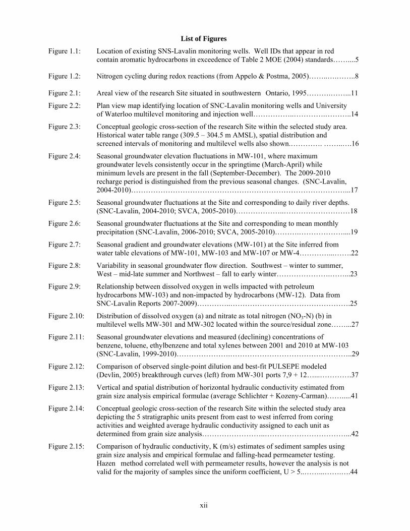
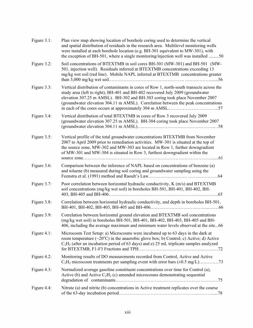
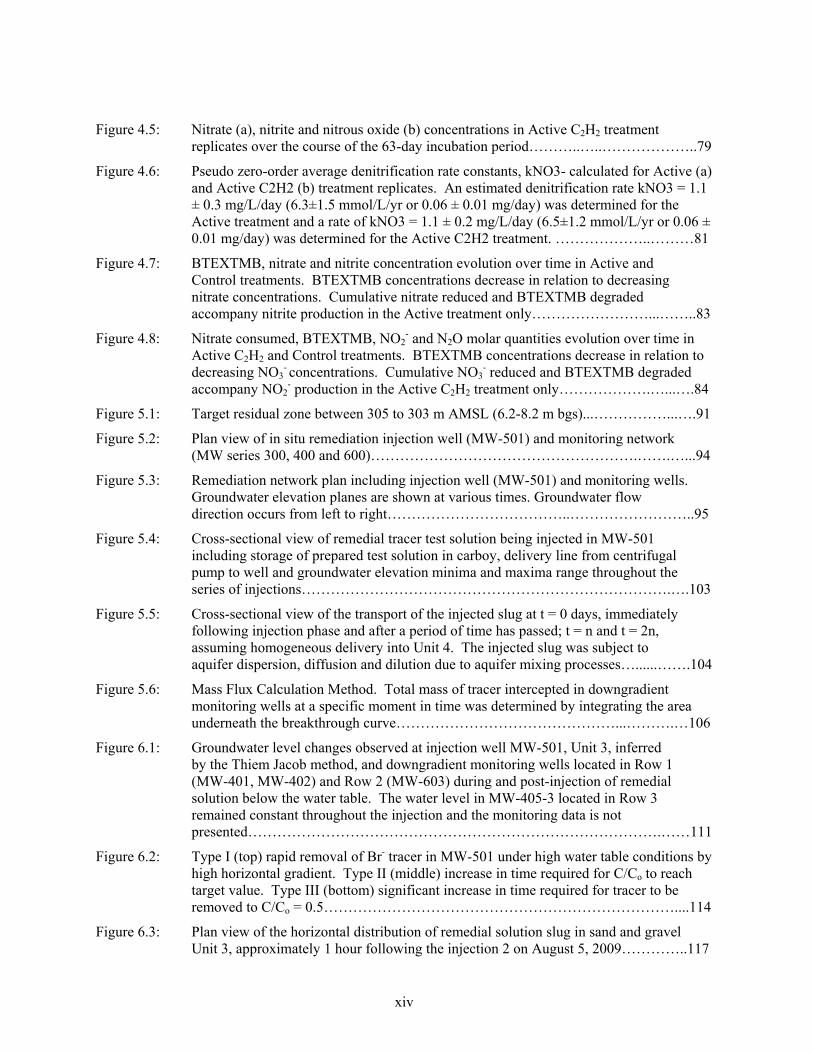
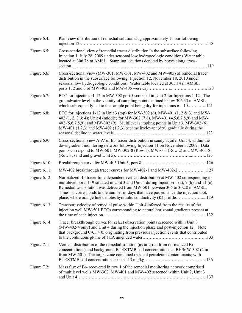
List of Figures ............................................................................................................................................. xii 

List of Tables ........................................................................................................................................... xviii 

Chapter 1: Introduction ................................................................................................................................ 1 

1.1 Overview ..................................................................................................................................... 1 

1.2 Site Description ........................................................................................................................... 3 

1.3 Subsurface Contamination ........................................................................................................... 3 

1.4 Enhanced In Situ Bioremediation ................................................................................................ 5 

1.5 Nitrate as a Terminal Electron Acceptor ..................................................................................... 6 

Chapter 2: Site Characterization ................................................................................................................ 11 

2.1 Geographic Setting .................................................................................................................... 11 

2.2 Site Geology .............................................................................................................................. 12 

2.3 Site Instrumentation ................................................................................................................... 13 

2.4 Site Hydrogeology ..................................................................................................................... 15 

2.4.1 Seasonal Water Table Fluctuations .................................................................................. 16 

2.4.2 Transient Groundwater Flow Conditions ......................................................................... 21 

2.5 Aquifer Geochemistry ............................................................................................................... 23 

2.5.1 Dissolved Oxygen ............................................................................................................ 23 

2.5.2 Alternate Electron Acceptors ........................................................................................... 25 

2.5.3 Evidence of Natural Attenuation ...................................................................................... 28 

2.6 Physical Aquifer Characterization ............................................................................................. 29 

2.6.1 Conventional Slug Test .................................................................................................... 29 

2.6.2 Single-Multilevel Well Point Dilution Test ..................................................................... 33 

2.6.3 Grain Size Analysis .......................................................................................................... 39 

2.6.4 Falling-Head Permeameter Test ....................................................................................... 43 

2.7 Site Characterization Summary ................................................................................................. 45 

Chapter 3: Characterization of Subsurface Contaminants ......................................................................... 46 

3.1 Origin of Contaminants in the Subsurface ................................................................................. 46 

3.2 Nature of the Contaminants ....................................................................................................... 47 

3.3 Contaminant Distribution .......................................................................................................... 48 

3.3.1 Seasonal Water Table Fluctuations .................................................................................. 48 

x

3.3.2 Residual Phase NAPL in the Select Research Area ......................................................... 49 

3.3 Estimation of the Mass of Residuals ......................................................................................... 50 

3.3.1 Coring Results .................................................................................................................. 55 

3.3.3 Dissolved Phase within the Source Zone ......................................................................... 59 

3.3.4 Residual Distribution and Hydraulic Conductivity .......................................................... 64 

Chapter 4: Laboratory Microcosm Experiment ......................................................................................... 67 

4.1 Introduction ............................................................................................................................... 67 

4.2 Acetylene Block Technique Method ......................................................................................... 67 

4.3 Microcosm Results .................................................................................................................... 73 

4.3.1 Availability of Dissolved Oxygen .................................................................................... 73 

4.3.2 Biodegradation of BTEXTMB ......................................................................................... 73 

4.3.3 Denitrification .................................................................................................................. 77 

4.4 Interpretation of BTEXTMB Biodegradation ........................................................................... 81 

4.4.1 Nitrate Utilization ............................................................................................................ 81 

4.4.2 Utilization of Alternative TEAs ....................................................................................... 86 

4.5 Microcosm Summary ................................................................................................................ 88 

Chapter 5: Residual Zone Treatment System Design ................................................................................ 89 

5.1 Remediation Approach .............................................................................................................. 89 

5.2 Target Remediation Zone .......................................................................................................... 89 

5.3 Remediation System Design ...................................................................................................... 91 

5.3.1 Injection Well ................................................................................................................... 92 

5.3.2 Monitoring Well Network ................................................................................................ 93 

5.4 Enhanced, In Situ Denitrification Treatment System ................................................................ 96 

5.4.1 Site Suitability .................................................................................................................. 96 

5.4.2 Mass of Contaminants in the Targeted Source Zone ....................................................... 98 

5.4.4 Expected Success of Remediation System ..................................................................... 100 

5.5 Remediation Tracer Test Procedure ........................................................................................ 101 

5.6 Tracer Analysis of Remedial Test Solution ............................................................................. 104 

5.7 Treatment System Evaluation .................................................................................................. 106 

5.7.1 Field Biodegradation Rates ............................................................................................ 106 

5.7.2 Post-Injection Residual Evaluation ................................................................................ 107 

Chapter 6: Remedial Tracer Test Br- Results ............................................................................................ 109 

6.1 Evaluation of the Delivery of Remedial Tracer Solution ........................................................ 109 

6.2 Injection Effects on Hydrogeologic Flow Regime .................................................................. 109 

6.3 Subsurface Behaviour of the Remedial Tracer Test Solution.................................................. 111 

6.3.1 Injection Well MW-501 ................................................................................................. 111 

xi

6.3.2 Delivery of Remedial Tracer Solution within the Monitoring Network ........................ 115 

6.3.3 Temporal Distribution of Injectate at Downgradient Monitors ..................................... 120 

6.3.4 Delivery of Remedial Solution in Heterogeneous Layers .............................................. 127 

6.4 Transportation of the Remedial Test Solution ......................................................................... 130 

6.5 Remedial Tracer Test Summary .............................................................................................. 134 

Chapter 7: Remediation System Evaluation ............................................................................................. 135 

7.1 Delivery of Remedial Solution amended with TEA to Target Zone ....................................... 135 

7.2 Mass Flux of Remedial Tracer Solution .................................................................................. 136 

7.3.1 Measurements of Degradation ....................................................................................... 138 

7.2.2 Denitrification Intermediate Products ............................................................................ 145 

7.2.3 Biostimulation of Indigenous Microbial Populations .................................................... 146 

7.2.3 Alternative Electron Acceptors ...................................................................................... 148 

7.3 Post-Injection Assessment of Subsurface Contaminants ......................................................... 153 

7.3.1 Post-Injection Groundwater Sampling Results .............................................................. 154 

7.3.2 Results of Pre- and Post-Injection Soil Coring .............................................................. 159 

Chapter 8: Conclusions and Recommendations ................................................................................ …....166

References ................................................................................................................................................. 169 

Appendix A Well Construction Details, Boreholes and Information Supporting Site

Characterization ................................................................................................................. 183 

Appendix B Charaterization of Contaminants at the Site including Pre-Injection Soil Coring

and Groundwater Sampling Procedures and Results ......................................................... 246

Appendix C Microcosm Experiment ........................................................................................................ 269

Appendix D Remediation Tracer Test Procedure ..................................................................................... 274 

Appendix E Remedial Tracer Test Injection Analysis of the Results ....................................................... 278 

Appendix F Analysis of Nitrate Utilization .............................................................................................. 315 

xii

List of Figures

Figure 1.1: Location of existing SNS-Lavalin monitoring wells. Well IDs that appear in red contain aromatic hydrocarbons in exceedence of Table 2 MOE (2004) standards……....5

Figure 1.2: Nitrogen cycling during redox reactions (from Appelo & Postma, 2005)……..….……..8 Figure 2.1: Areal view of the research Site situated in southwestern Ontario, 1995……….……...11

Figure 2.2: Plan view map identifying location of SNC-Lavalin monitoring wells and University of Waterloo multilevel monitoring and injection well……………..………….………..14

Figure 2.3: Conceptual geologic cross-section of the research Site within the selected study area. Historical water table range (309.5 – 304.5 m AMSL), spatial distribution and screened intervals of monitoring and multilevel wells also shown.…………. ……..….16

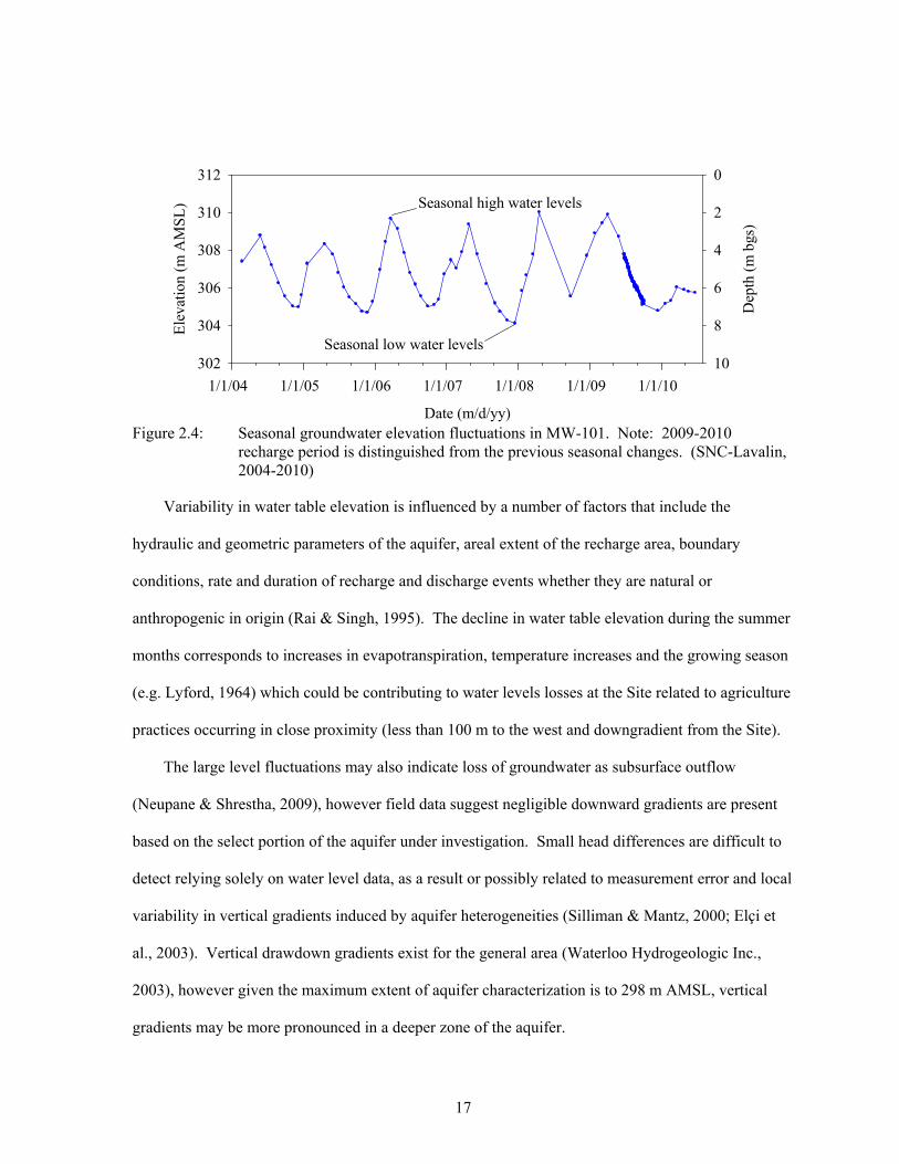
Figure 2.4: Seasonal groundwater elevation fluctuations in MW-101, where maximum groundwater levels consistently occur in the springtime (March-April) while minimum levels are present in the fall (September-December). The 2009-2010 recharge period is distinguished from the previous seasonal changes. (SNC-Lavalin, 2004-2010)……………………………………………………………………………...17

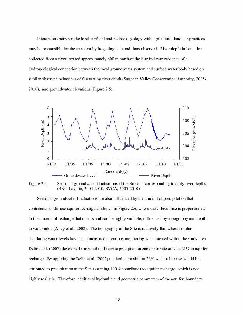
Figure 2.5: Seasonal groundwater fluctuations at the Site and corresponding to daily river depths. (SNC-Lavalin, 2004-2010; SVCA, 2005-2010)………………..………………………18

Figure 2.6: Seasonal groundwater fluctuations at the Site and corresponding to mean monthly precipitation (SNC-Lavalin, 2006-2010; SVCA, 2005-2010)……….………………....19

Figure 2.7: Seasonal gradient and groundwater elevations (MW-101) at the Site inferred from water table elevations of MW-101, MW-103 and MW-107 or MW-4…………...…….22

Figure 2.8: Variability in seasonal groundwater flow direction. Southwest – winter to summer, West – mid-late summer and Northwest – fall to early winter………………….……...23

Figure 2.9: Relationship between dissolved oxygen in wells impacted with petroleum hydrocarbons MW-103) and non-impacted by hydrocarbons (MW-12). Data from SNC-Lavalin Reports 2007-2009)…………..………………………………………….25

Figure 2.10: Distribution of dissolved oxygen (a) and nitrate as total nitrogen (NO3-N) (b) in multilevel wells MW-301 and MW-302 located within the source/residual zone……...27

Figure 2.11: Seasonal groundwater elevations and measured (declining) concentrations of benzene, toluene, ethylbenzene and total xylenes between 2001 and 2010 at MW-103 (SNC-Lavalin, 1999-2010)………………….…………………………………………..29

Figure 2.12: Comparison of observed single-point dilution and best-fit PULSEPE modeled (Devlin, 2005) breakthrough curves (left) from MW-301 ports 7,9 + 12…...………….37

Figure 2.13: Vertical and spatial distribution of horizontal hydraulic conductivity estimated from grain size analysis empirical formulae (average Schlichter + Kozeny-Carman)…….....41

Figure 2.14: Conceptual geologic cross-section of the research Site within the selected study area depicting the 5 stratigraphic units present from east to west inferred from coring activities and weighted average hydraulic conductivity assigned to each unit as determined from grain size analysis……………………..……………………………...42

Figure 2.15: Comparison of hydraulic conductivity, K (m/s) estimates of sediment samples using grain size analysis and empirical formulae and falling-head permeameter testing. Hazen method correlated well with permeameter results, however the analysis is not valid for the majority of samples since the uniform coefficient, U > 5..……...…….….44

xiii

Figure 3.1: Plan view map showing location of borehole coring used to determine the vertical and spatial distribution of residuals in the research area. Multilevel monitoring wells were installed at each borehole location (e.g. BH-301 equivalent to MW-301), with the exception of BH-501, where a single monitoring/injection well was installed .........50

Figure 3.2: Soil concentrations of BTEXTMB in soil cores BH-301 (MW-301) and BH-501 (MW-501, injection well). Residuals inferred at BTEXTMB concentrations exceeding 13 mg/kg wet soil (red line). Mobile NAPL inferred at BTEXTMB concentrations greater than 3,000 mg/kg wet soil.…………………………………………. ……..……….......56

Figure 3.3: Vertical distribution of contaminants in cores of Row 1, north-south transects across the study area (left to right); BH-401 and BH-402 recovered July 2009 (groundwater elevation 307.25 m AMSL). BH-302 and BH-303 coring took place November 2007 (groundwater elevation 304.11 m AMSL). Correlation between the peak concentrations in each of the cores occurs at approximately 304 m AMSL.…………………………...57

Figure 3.4: Vertical distribution of total BTEXTMB in cores of Row 3 recovered July 2009 (groundwater elevation 307.25 m AMSL). BH-304 coring took place November 2007 (groundwater elevation 304.11 m AMSL)….…………………….………………….…58

Figure 3.5: Vertical profile of the total groundwater concentrations BTEXTMB from November 2007 to April 2009 prior to remediation activities. MW-301 is situated at the top of the source zone, MW-302 and MW-303 are located in Row 1, further downgradient of MW-301 and MW-304 is situated in Row 3, furthest downgradient within the source zone………………………………………………………………………….......61

Figure 3.6: Comparison between the inference of NAPL based on concentrations of benzene (a) and toluene (b) measured during soil coring and groundwater sampling using the Feenstra et al. (1991) method and Raoult’s Law.……………………. …….………….64

Figure 3.7: Poor correlation between horizontal hydraulic conductivity, K (m/s) and BTEXTMB soil concentrations (mg/kg wet soil) in boreholes BH-501, BH-401, BH-402, BH- 403, BH-405 and BH-406…………………………………….…………………….…..65

Figure 3.8: Correlation between horizontal hydraulic conductivity, and depth in boreholes BH-501, BH-401, BH-402, BH-403, BH-405 and BH-406.………………………………...……66

Figure 3.9: Correlation between horizontal ground elevation and BTEXTMB soil concentrations (mg/kg wet soil) in boreholes BH-501, BH-401, BH-402, BH-403, BH-405 and BH- 406, including the average maximum and minimum water levels observed at the site...66

Figure 4.1: Microcosm Test Setup: a) Microcosms were incubated up to 63 days in the dark at room temperature (~20oC) in the anaerobic glove box; b) Control; c) Active; d) Active C2H2 (after an incubation period of 63 days) and e) 25 mL triplicate samples analyzed for BTEXTMB, F1-F3 Fractions and TPH…………………………………….…….…72

Figure 4.2: Monitoring results of DO measurements recorded from Control, Active and Active C2H2 microcosm treatments per sampling event with error bars (±0.5 mg/L)….………73

Figure 4.3: Normalized average gasoline constituent concentrations over time for Control (a), Active (b) and Active C2H2 (c) amended microcosms demonstrating sequential degradation of contaminants……………………………………………………….….75

Figure 4.4: Nitrate (a) and nitrite (b) concentrations in Active treatment replicates over the course of the 63-day incubation period……………………………………………..……….....78

xiv

Figure 4.5: Nitrate (a), nitrite and nitrous oxide (b) concentrations in Active C2H2 treatment replicates over the course of the 63-day incubation period………..…..………………..79

Figure 4.6: Pseudo zero-order average denitrification rate constants, kNO3- calculated for Active (a) and Active C2H2 (b) treatment replicates. An estimated denitrification rate kNO3 = 1.1 ± 0.3 mg/L/day (6.3±1.5 mmol/L/yr or 0.06 ± 0.01 mg/day) was determined for the Active treatment and a rate of kNO3 = 1.1 ± 0.2 mg/L/day (6.5±1.2 mmol/L/yr or 0.06 ± 0.01 mg/day) was determined for the Active C2H2 treatment. ………………..………81

Figure 4.7: BTEXTMB, nitrate and nitrite concentration evolution over time in Active and Control treatments. BTEXTMB concentrations decrease in relation to decreasing nitrate concentrations. Cumulative nitrate reduced and BTEXTMB degraded accompany nitrite production in the Active treatment only……………………...……..83

Figure 4.8: Nitrate consumed, BTEXTMB, NO2- and N2O molar quantities evolution over time in

Active C2H2 and Control treatments. BTEXTMB concentrations decrease in relation to decreasing NO3

- concentrations. Cumulative NO3- reduced and BTEXTMB degraded

accompany NO2- production in the Active C2H2 treatment only……………….…...….84

Figure 5.1: Target residual zone between 305 to 303 m AMSL (6.2-8.2 m bgs)...……………...….91

Figure 5.2: Plan view of in situ remediation injection well (MW-501) and monitoring network (MW series 300, 400 and 600)……………………………………………….…….…...94

Figure 5.3: Remediation network plan including injection well (MW-501) and monitoring wells. Groundwater elevation planes are shown at various times. Groundwater flow direction occurs from left to right………………………………..……………………..95

Figure 5.4: Cross-sectional view of remedial tracer test solution being injected in MW-501 including storage of prepared test solution in carboy, delivery line from centrifugal pump to well and groundwater elevation minima and maxima range throughout the series of injections………………………………………………………………….….103

Figure 5.5: Cross-sectional view of the transport of the injected slug at t = 0 days, immediately following injection phase and after a period of time has passed; t = n and t = 2n, assuming homogeneous delivery into Unit 4. The injected slug was subject to aquifer dispersion, diffusion and dilution due to aquifer mixing processes…......…….104

Figure 5.6: Mass Flux Calculation Method. Total mass of tracer intercepted in downgradient monitoring wells at a specific moment in time was determined by integrating the area underneath the breakthrough curve………………………………………...……….…106

Figure 6.1: Groundwater level changes observed at injection well MW-501, Unit 3, inferred by the Thiem Jacob method, and downgradient monitoring wells located in Row 1 (MW-401, MW-402) and Row 2 (MW-603) during and post-injection of remedial solution below the water table. The water level in MW-405-3 located in Row 3 remained constant throughout the injection and the monitoring data is not presented………………………………………………………………………….……111

Figure 6.2: Type I (top) rapid removal of Br- tracer in MW-501 under high water table conditions by high horizontal gradient. Type II (middle) increase in time required for C/Co to reach target value. Type III (bottom) significant increase in time required for tracer to be removed to C/Co = 0.5………………………………………………………………....114

Figure 6.3: Plan view of the horizontal distribution of remedial solution slug in sand and gravel Unit 3, approximately 1 hour following the injection 2 on August 5, 2009…………..117

xv

Figure 6.4: Plan view distribution of remedial solution slug approximately 1 hour following injection 12……………………………………………………………..……………...118

Figure 6.5: Cross-sectional view of remedial tracer distribution in the subsurface following Injection 1, July 28, 2009 under seasonal low hydrogeologic conditions Water table located at 306.78 m AMSL. Sampling locations denoted by boxes along cross- section……………………………………………………………………………….…119

Figure 6.6: Cross-sectional view (MW-301, MW-501, MW-402 and MW-405) of remedial tracer distribution in the subsurface following Injection 12, November 18, 2010 under seasonal low hydrogeologic conditions. Water table located at 305.14 m AMSL, ports 1, 2 and 3 of MW-402 and MW-405 were dry……………...……….……….….120

Figure 6.7: BTC for injections 1-12 in MW-302 port 5 screened in Unit 2 for Injections 1-12. The groundwater level in the vicinity of sampling point declined below 306.33 m AMSL, which subsequently led to the sample point being dry for injections 6 – 10.……..…..121

Figure 6.8: BTC for injections 1-12 in Unit 3 (top) for MW-302 (6), MW-401 (1, 2 & 3) and MW-402 (1, 2, 3 & 4); Unit 4 (middle) for MW-302 (7,8), MW-401 (4,5,6,7,8,9) and MW-402 (5,6,7,8,9); and MW-302 (9). Multilevel sampling points in Unit 3, MW-302 (6), MW-401 (1,2,3) and MW-402 (1,2,3) became irrelevant (dry) gradually during the seasonal decline in water levels……………………………………………..…….…..123

Figure 6.9: Cross-sectional view A-A′ of Br- tracer distribution in sandy aquifer Unit 4, within the downgradient monitoring network following Injection 11 on November 3, 2009. Data points correspond to MW-501, MW-302-8 (Row 1), MW-603 (Row 2) and MW-405-8 (Row 3, sand and gravel Unit 5)……………………………………………...……….125

Figure 6.10: Breakthrough curve for MW-405 Unit 5, port 8………………….………….………..126

Figure 6.11: MW-402 breakthrough tracer curves for MW-402-1 and MW-402-2………………...127

Figure 6.12: Normalized Br- tracer time dependent vertical distribution at MW-402 corresponding to multilevel ports 1- 9 situated in Unit 3 and Unit 4 during Injection 1 (a), 7 (b) and 11 (c). Remedial test solution was delivered from MW-501 between 306 to 302.8 m AMSL. Time – t, corresponds to the number of days that have passed since the injection took place, where orange line denotes hydraulic conductivity (K) profile………………....129

Figure 6.13: Transport velocity of remedial pulse within Unit 4 inferred from the results of the injection well MW-501 BTCs corresponding to natural horizontal gradients present at the time of each injection. ……………………………………………………………132

Figure 6.14: Tracer breakthrough curves for select observation points screened within Unit 3 (MW-402-4 only) and Unit 4 during the injection phase and post-injection 12. Note that background C/Co > 0, originating from previous injection events that contributed to the continuous plume of TEA amended water……………………………….……..133

Figure 7.1: Vertical distribution of the remedial solution (as inferred from normalized Br- concentrations) and background BTEXTMB soil concentrations at BH/MW-302 (2 m from MW-501). The target zone contained residual petroleum contaminants; with BTEXTMB soil concentrations exceed 13 mg/kg………………………...…….…….136

Figure 7.2: Mass flux of Br- recovered in row 1 of the remedial monitoring network comprised of multilevel wells MW-302, MW-401 and MW-402 screened within Unit 2, Unit 3 and Unit 4……………………………….…………………………….………….……137

xvi

Figure 7.3: Normalized concentrations of Br-, NO3- and concentration of nitrite of select

downgradient multilevel wells MW-302-6 and MW-402- 2 screened within Unit 3 during Injection 6……………………………………………….………………….….140

Figure 7.4: Normalized concentration of Br-, NO3- and the concentration of nitrite occurring in

the injection well MW-501 and downgradient multilevel well MW-302-7 screened partially within Unit 3 and 4 (a) and within Unit 4 (b) during injection 12…………...141

Figure 7.5: Calculated first-order nitrate degradation in Unit 3, from Figures 7.4a and b for downgradient multilevel wells MW-302 Port 6 (a) and MW-402 Port 2 (b) following Injection 6. The remedial test solution was amended with 90 mg/L NO3

-…………....143

Figure 7.6: Calculated first-order degradation of nitrate at the injection well within Unit 3 and Unit 4, from Figures 7.5a and b for MW-501 (a) and downgradient monitor MW-302-7 (b) following Injection 12. Remedial test solution amended with 265 mg/L NO3

-……………………………………………………………………………..144

Figure 7.7: Comparison between the behaviour of conservative and reactive tracers, Br-, NO3-, and potential alternative TEA, SO42- present in the remedial test solution originating from the municipal water supply in downgradient monitorsMW-302-6 and MW-402- 2 measured during injection 6. ………………………………………….…….………151

Figure 7.8: Comparison between the behaviour of conservative and reactive tracers, Br-, NO3-

and potential alternative TEA, SO42- present in the remedial test solution originating

from the municipal water supply in the injection well (a) and downgradient monitor MW-302-7 measured during injection 12…………………………………....………..152

Figure 7.9: Historical results of toluene (C7H8) present in the groundwater at MW-303 in Ports 6 and 7 screened between 305.3 and 305.1 m AMSL and 304.3 and 304.1 m AMSL, respectively. Error bars denote typical seasonal fluctuations in measured concentrations of toluene attributed to the transient hydrogeological conditions that exist at the Site.………………………..……………………………...…….…………155

Figure 7.10: Historical results of toluene (C7H8) present in the groundwater at multilevel MW-302 in Ports 7 and 8 screened between 304.33 and 304.13 m AMSL and 303.33 and 303.13 m AMSL, respectively. Error bars denote typical seasonal fluctuations in measured concentrations of toluene attributed to the transient hydrogeological conditions that exist at the site……………………………….……...156

Figure 7.11: Post-injection BTEXTMB concentration in groundwater in non-treated treated zone at multilevel well MW-303 at ports 6, 7 and 10……………………………….………157

Figure 7.12: Post-injection BTEXTMB concentrations in groundwater in treated zone at multilevel well MW-302 at ports 7, 8 and 9, where remedial tracer solution was consistently recovered……………………………………………………………...….158

Figure 7.13: Vertical distribution of toluene (mg/kg) wet soil extraction concentrations at the borehole locations of the 600 series monitoring wells from north to south (BH-604, BH-603, BH-602 and BH-601) in Row 2 retrieved in October 2009 following the delivery of remedial solution to targeted areas of the contaminated aquifer. Vertical red line denotes residual NAPL inferred at total extraction concentrations exceeding 13 mg/kg wet soil……………………………………………………………….…..…160

xvii

Figure 7.14: Toluene (mg/kg) wet soil concentrations, where BH-303, BH-304 and BH-406 were retrieved pre- injection of remedial solution and BH-601 was retrieved post- injection……………………………………………………………………...…….…..161

Figure 7.15: Pre- and post-injection measurement of toluene concentrations (mg/kg) wet soil, where BH-501, BH-302 and BH-405 were retrieved prior to injection of remedial solution to areas of the aquifer containing residual contaminants……………….……162

Figure 7.16: Pre- and post-injection measurement of toluene concentrations (mg/kg) wet soil, where BH-402 and BH-405 were retrieved prior to injection of remedial solution to areas of the aquifer containing residual contaminants………………………….……..163

Figure 7.17: Pre- and post-injection measurement of toluene concentrations (mg/kg) wet soil, where BH-401, BH-403 and BH-405 were retrieved prior to injection of remedial solution to areas of the aquifer containing residual contaminants………..……….…..164

xviii

List of Tables

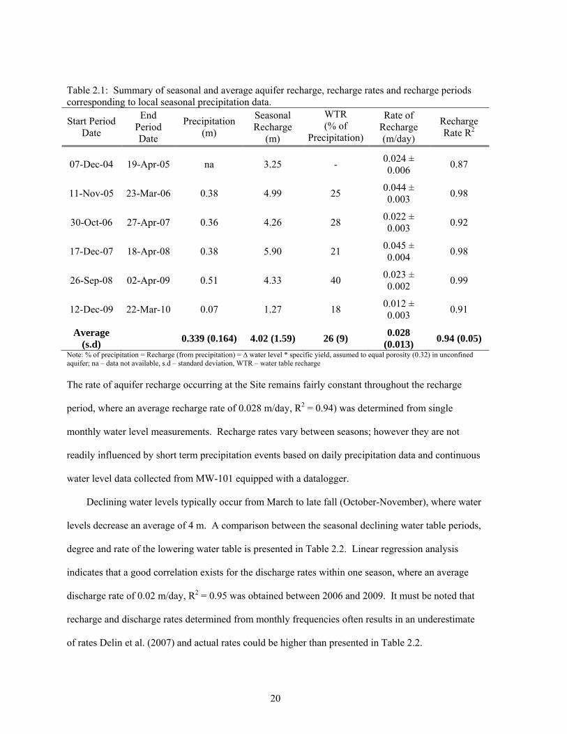
Table 2.1: Summary of seasonal and average aquifer recharge, recharge rates and recharge periods corresponding to local seasonal precipitation data…………….………………….…….20

Table 2.2: Summary of seasonal and average aquifer discharge, discharge rates and discharge periods..………………………………………………………………………………... 21

Table 2.3: Redox Parameters measured from select non-contaminated monitoring well (MW-109) and petroleum impacted well (MW-103………………………………………………..26

Table 2.4: Summary of bulk aquifer parameters transmissivity and storativity estimated from injection 12 using various analytical methods…………………………………..……...32

Table 2.5: Summary of hydraulic conductivity and average groundwater velocities estimated from single-well dilution tests conducted within various intervals of the screened aquifer [method from Drost & Neumaier (1974)]…………………………………………...….35

Table 2.6: Summary of best-fit PULSPE 1D advection-dispersion solutions corresponding to observed bromide tracer breakthrough within select multilevel ports of MW-301…….38

Table 2.7: Summary of average hydraulic conductivity estimates using Kozeny-Carman and Schlitchter empirical solutions for select boreholes…………………………………….40

Table 3.1: Summary of chemical properties for the individual gasoline constituents……………..47

Table 3.2: Calculated hypothetical maximum total soil concentration for the gasoline constituents of interest i, including applicable parameter values……………………………..……...53

Table 3.4: Presence of NAPL inferred using Raoult’s Law by comparing observed groundwater concentrations with LNAPL collected from the Site. …………………………....….…62

Table 4.1: Summary of microcosm test design applied in the study……………………………….69

Table 4.2: Summary of initial organic contaminant content present in each microcosm as aqueous concentration, Cw,i; dissolved mass, Mi and number of moles , ni of each constituent present………………………………………………………………………………..…70

Table 4.3: Summary of the average percent remaining of select aromatic hydrocarbons following 63 days of incubation under mixed microaerophilic and anaerobic conditions in nitrate amended microcosms relative to sterile controls………………..……………………...76

Table 5.1: Remedial Tracer Test details and injection schedule……………………...…………..102

Table 6.1: Method A average linear groundwater velocity estimates from the injection interval, Unit 2, Unit 3 and Unit 4 determined from MW-302 and MW-402 multilevel ports....131

Table 7.1: Results of microbial enumerations (CFU/mL) of groundwater water sampled from the study area pre- and post-injection determined by the HPC method…………………...147

Table 7.2: Results of the post-injection geochemical analysis of groundwater sampled within the study area, including concentrations of alternative TEAs or electron donors to NO3...149

1

Chapter 1: Introduction

1.1 Overview

Research was conducted as part of a multiphase project entitled ‘Enhancing in situ Bioremediation at

Brownfield Sites’, funded by the Ontario Centres of Excellence for Earth and Environmental

Technologies. This project was proposed as part of the research programs: Groundwater Plume

Formation and Remediation of Modern Gasoline Fuels in the Subsurface and Enhancing In Situ

Bioremediation at Brownfield Sites.

A brownfield site consists of an idle or abandoned industrialized property that has often been

subject to soil and/or groundwater contamination as a result of historic land use practices. An

estimated 30,000 brownfield sites are present in Canada to which many consist of water fronts,

former refineries, railway yards, service stations and commercial properties that utilized hazardous

chemicals (NRTEE, 2003).

Brownfield properties tend to be situated in prime locations and in close proximity to existing

infrastructure. Their clean up and potential for redevelopment has the ability to provide economical,

social and environmental benefits to the local community. These properties typically have a high

land reuse value, where reclamation of former industrial sites for affordable housing and

infrastructure can be a lucrative activity depending on site remediation costs and market prices.

Remediation strategies involve the mitigation and/or removal of contaminants that have the potential

to cause a risk to health thereby improving the overall social and environmental well being of the

community.

To encourage redevelopment, existing brownfield legislation provides property owners with

general protection from environmental cleanup orders for historic contamination once they have

appropriately remediated a site to meet specific standards. Brownfield reclamation in Ontario is

subject to the Record of Site Condition Regulation (O. Reg. 153/04) which contains specifications

2

related to site assessment and remediation targets according to its classified land use. A Record of

Site Condition (RSC) is a statement filed by a qualified person that is issued after completing a Phase

II Environmental Site Assessment. A RSC is required whenever a property undergoes changes in

ownership or is utilized for more sensitive land applications.

The revitalization of former industrial sites is an environmentally sound and sustainable

approach to meeting the demands of economic and population growth while reducing urban sprawl,

preserving green spaces and agricultural lands (NRTEE, 2003). Redevelopment of these

contaminated properties is often problematic due to the nature and extent of the contamination

present, however land use restrictions and engineering controls may be applied to reduce the risk.

Popular practices for mitigating soil and groundwater compliance issues involves off-site remedies or

removal of contaminated materials, referred to as ex situ treatment that may involve excavation of

impacted soil that exceeds generic criteria through dig and dump techniques and groundwater pump

and treat systems. Ex-situ treatment can be beneficial as the process can be completed within an

intermediate time-frame and is advantageous in land acquisition scenarios. However, ex situ

treatment and/or disposal of soil and contaminated groundwater to hazardous waste facilities can be

costly or non-practical given the amount of contamination present.

Alternative strategies involving in situ remediation technologies have been developed to assist

with property clean up, however, cost-effectiveness and discrepancies in success rates and timeliness

continue. The objective of my research is to critically demonstrate the application and usefulness of

an in situ remediation technology at a decommissioned gasoline service station. Petroleum

hydrocarbon impacted soil and groundwater contamination is a common occurrence in brownfield

sites relating to fuel storage and distribution facilities. In particular, residual contaminants present in

the saturated zone will be targeted for remediation. The mitigation of the migration and occurrence of

contaminants in the subsurface requires that the site specific mechanisms driving groundwater solute

transport be well understood and addressed in the design and implementation of an in situ

groundwater remediation system. The research project involved site investigations to characterize the

3

hydrogeological conditions and contaminant distribution present in order to effectively design an in

situ bioremediation treatment system.

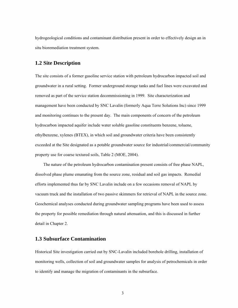
1.2 Site Description

The site consists of a former gasoline service station with petroleum hydrocarbon impacted soil and

groundwater in a rural setting. Former underground storage tanks and fuel lines were excavated and

removed as part of the service station decommissioning in 1999. Site characterization and

management have been conducted by SNC Lavalin (formerly Aqua Terre Solutions Inc) since 1999

and monitoring continues to the present day. The main components of concern of the petroleum

hydrocarbon impacted aquifer include water soluble gasoline constituents benzene, toluene,

ethylbenzene, xylenes (BTEX), in which soil and groundwater criteria have been consistently

exceeded at the Site designated as a potable groundwater source for industrial/commercial/community

property use for coarse textured soils, Table 2 (MOE, 2004).

The nature of the petroleum hydrocarbon contamination present consists of free phase NAPL,

dissolved phase plume emanating from the source zone, residual and soil gas impacts. Remedial

efforts implemented thus far by SNC Lavalin include on a few occasions removal of NAPL by

vacuum truck and the installation of two passive skimmers for retrieval of NAPL in the source zone.

Geochemical analyses conducted during groundwater sampling programs have been used to assess

the property for possible remediation through natural attenuation, and this is discussed in further

detail in Chapter 2.

1.3 Subsurface Contamination

Historical Site investigation carried out by SNC-Lavalin included borehole drilling, installation of

monitoring wells, collection of soil and groundwater samples for analysis of petrochemicals in order

to identify and manage the migration of contaminants in the subsurface.

4

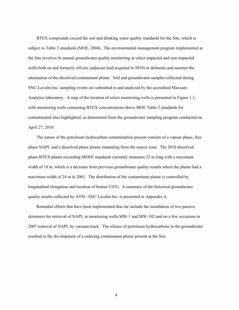
BTEX compounds exceed the soil and drinking water quality standards for the Site, which is

subject to Table 2 standards (MOE, 2004). The environmental management program implemented at

the Site involves bi-annual groundwater quality monitoring at select impacted and non-impacted

wells both on and formerly off-site (adjacent land acquired in 2010) to delineate and monitor the

attenuation of the dissolved contaminant plume. Soil and groundwater samples collected during

SNC-Lavalin Inc. sampling events are submitted to and analyzed by the accredited Maxxam

Analytics laboratory. A map of the location of select monitoring wells is presented in Figure 1.1,

with monitoring wells containing BTEX concentrations above MOE Table 2 standards for

contaminated sites highlighted, as determined from the groundwater sampling program conducted on

April 27, 2010.

The nature of the petroleum hydrocarbon contamination present consists of a vapour phase, free

phase NAPL and a dissolved phase plume emanating from the source zone. The 2010 dissolved

phase BTEX plume exceeding MOEE standards currently measures 22 m long with a maximum

width of 18 m, which is a decrease from previous groundwater quality results where the plume had a

maximum width of 24 m in 2001. The distribution of the contaminant plume is controlled by

longitudinal elongation and location of former USTs. A summary of the historical groundwater

quality results collected by ATSI –SNC Lavalin Inc. is presented in Appendix A.

Remedial efforts that have been implemented thus far include the installation of two passive

skimmers for retrieval of NAPL in monitoring wells MW-1 and MW-102 and on a few occasions in

2007 removal of NAPL by vacuum truck. The release of petroleum hydrocarbons to the groundwater

resulted in the development of a reducing contaminant plume present at the Site.

5

MW-109

MW-3MW-5

MW-106

MW-4

MW-107

MW-101

MW-1

MW-102

MW-103

MW-12

MW-201

MW-202

MW-203 MW-204

MW-205

MW-206

Scale 1:400

0 5 10 m

MONITORING WELL

PHC MOE EXCEEDANCE WELL

PROPERTY LINE

EXISTING BUILDING

INFRASTRUCTURE

FORMER INFRASTRUCTURE

CHAIN LINK FENCE

UNDERGROUND TANK

FORMER UNDERGROUND TANK

MW-ID

N

groundwater flow direction

Figure 1.1: Location of existing SNC-Lavalin monitoring wells. Well IDs that appear in red contain aromatic hydrocarbons in exceedence of Table 2 MOE (2004) standards.

1.4 Enhanced In Situ Bioremediation

Natural attenuation involves the natural environment’s (subsurface) ability to recover from damage

sustained from the release of contaminants via natural processes such as biodegradation, dilution,

dispersion and sorption, which limits the transport of contaminants in groundwater and thus reduces

impacts to sensitive receptors. Natural attenuation is influenced by geochemical (oxidation-reduction

processes, presence of electron acceptors), biological (indigenous microbial populations) and physical

characteristics (hydraulic gradients, porosity, heterogeneity) of the aquifer. Indigenous microbes

6

present in the subsurface are capable of utilizing select organic pollutants as a carbon and energy

source in the metabolism and synthesis of cells and as a result, contaminants are degraded.

Hydrogeological conditions are variable from site to site and the behaviour of the pollutant(s) is

subject to the subsurface conditions in addition to physical (sorption and adsorption), chemical

(oxidation and reduction) and biological processes (aerobic or anaerobic biodegradation). The

implementation of a suitable remediation system at a contaminated site requires an understanding of

the hydrogeological conditions present and expertise on the selected remediation technology(ies)

(Sims et al., 1992). The feasibility of in situ bioremediation application(s) is also influenced by the

location of the contaminant source, whether it be above or below the water table.

In situ bioremediation utilizes the same processes of natural attenuation; however the strategy

involves the addition of terminal electron acceptors (TEA) (oxygen, nitrate, sulphate or iron III) to the

aquifer to enhance natural degradation processes. The addition of O2 (air sparging, hydrogen

peroxide) to promote aerobic respiration is the most thermodynamically favourable TEA for microbes

in the oxidation of hydrocarbon compounds. However, challenges associated with the use of O2

additions include rapid utilization, low solubility in water and possible reduced hydraulic conductivity

as a result of excessive microbial growth and iron precipitates clogging the porous media. An

alternative approach involves the anaerobic treatment using nitrate as a TEA. Advantages of nitrate

include higher solubility, more cost-effective than O2, while minimizing unwanted reactions with

non-target dissolved metals such as Fe(II). Nitrate addition has the ability to enhance bioremediation

of the target aromatic compounds, however it has not been demonstrated to stimulate the

biodegradation of the saturated hydrocarbon fraction of gasoline.

1.5 Nitrate as a Terminal Electron Acceptor

The objective of this thesis is to evaluate the potential for injecting nitrate (NO3-) as a terminal

electron acceptor to enhance the bioremediation of residual hydrocarbons in a complex sand/gravel

7

unconfined aquifer. In order to mitigate the migration and occurrence of contaminants in the

subsurface, the site specific mechanisms driving groundwater solute transport must be well

understood and addressed in the design and implementation of an in situ groundwater remediation

system. Nitrate was selected as an alternative electron acceptor over the thermodynamically favoured

O2 because of typical challenges encountered using O2 in bioremediation applications.

Nitrate in groundwater systems may originate from decaying plant material or anthropogenic

processes associated with agricultural practices such as the excessive application of fertilizers that

leach into the groundwater supply and pose a potential health risk. NO3- removal from the subsurface

system is mediated by abiotic chemical transformations and biotically by indigenous microbes that

utilize the electron acceptor as an energy supply to promote further growth and development.

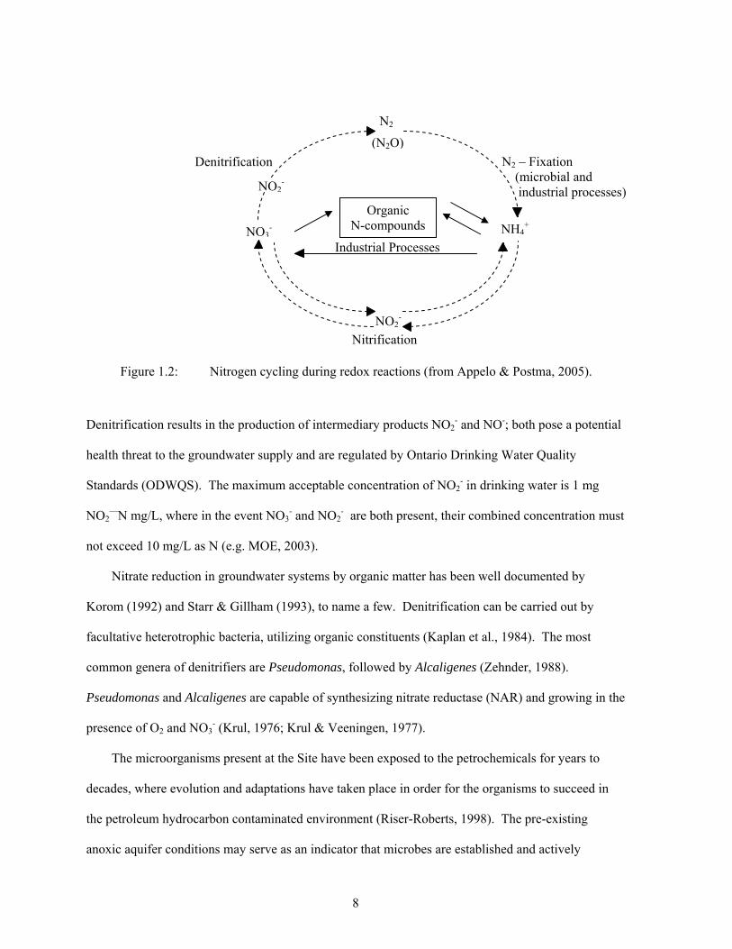
The nitrogen (N) cycle is comprised of a number of redox reaction pathways as described in Figure

1.2, where N is either assimilated into organic compounds or dissimilated from organic matter.

Denitrification involves the microbial reduction of NO3- to intermediate products nitrite (NO2

-),

nitric oxide (NO-), nitrogen oxide (N2O) and the final product elemental nitrogen (N2) with the use of

an electron donor such as organic carbon, equation (1.1) (e.g. Stumm & Morgan, 1981):

NO3-(aq)NO2

-(aq)NO (enzyme complex)N2O(g)N2(g)  (1.1) 

8

Denitrification results in the production of intermediary products NO2- and NO-; both pose a potential

health threat to the groundwater supply and are regulated by Ontario Drinking Water Quality

Standards (ODWQS). The maximum acceptable concentration of NO2- in drinking water is 1 mg

NO2—N mg/L, where in the event NO3

- and NO2- are both present, their combined concentration must

not exceed 10 mg/L as N (e.g. MOE, 2003).

Nitrate reduction in groundwater systems by organic matter has been well documented by

Korom (1992) and Starr & Gillham (1993), to name a few. Denitrification can be carried out by

facultative heterotrophic bacteria, utilizing organic constituents (Kaplan et al., 1984). The most

common genera of denitrifiers are Pseudomonas, followed by Alcaligenes (Zehnder, 1988).

Pseudomonas and Alcaligenes are capable of synthesizing nitrate reductase (NAR) and growing in the

presence of O2 and NO3- (Krul, 1976; Krul & Veeningen, 1977).

The microorganisms present at the Site have been exposed to the petrochemicals for years to

decades, where evolution and adaptations have taken place in order for the organisms to succeed in

the petroleum hydrocarbon contaminated environment (Riser-Roberts, 1998). The pre-existing

anoxic aquifer conditions may serve as an indicator that microbes are established and actively

N2

(N2O)

NO3-

NO2-

NO2-

Nitrification

Denitrification

Organic N-compounds

N2 – Fixation (microbial and industrial processes)

Industrial Processes

NH4+

Figure 1.2: Nitrogen cycling during redox reactions (from Appelo & Postma, 2005).

9

biodegrading petroleum hydrocarbons. However, the indigenous microbes have not historically been

exposed to an abundant supply of NO3- and their ability to degrade organic contaminants via

denitrification is being evaluated. The stoichiometry of the overall reaction of denitrification using

organic matter is shown in equation (1.2) (e.g. Pederson et al, 1991; Korom, 1991):

5CH2O + 4NO3-(aq) + 4H+ 5CO2(g) + 2N2 + 7H2O(l)  (1.2) 

Geochemical species present in the reduced groundwater environments, where denitrification is

actively occurring may also serve as electron donors including Fe2+, H2S and CH4. However, these

compounds are not as thermodynamically favourable and are limiting compared to the organic

contaminants present, therefore they likely only play a limited role as electron donors. For example,

the oxidation of iron sulphide is presented in equations (1.3) and (1.4) (e.g. Kolle et al, 1983; Postma

et al., 1991; Robertson et al., 1996):

5FeS2 + 14NO3-(aq) + 4H+ 7N2 + 10SO4

2-(aq) + 5Fe2+

(aq) + 2H2O(l)  (1.3)

5Fe2+(aq) + NO3

-(aq) + 12H2O(l) 5Fe(OH)3 + ½N2 + 9H+ (1.4)

Nitrate can also be transformed assimilatory into ammonia (NH3) where N is taken up and

incorporated into biomass or dissimilated into ammonium (NH4+) during nitrate reduction in

groundwater systems (Smith et al, 1991). However, the latter does not represent a dominant process.

Dissimilatory nitrate reduction to ammonium (DNRA) is presented in equation (1.5) from Tiedje et

al. (1982):

2H+(aq) + NO3

-(aq) + 2CH2O NH4

+ + 2CO2 + 2H2O (1.5)

10

Denitrification is predominantly favoured in the reducing environments because it yields more

metabolic energy compared to DNRA (e.g. Korom, 1992), which tends to be limited by electron

acceptor availability (Tiedje, 1988). DNRA is regulated by O2 that leads to N2 as previously

demonstrated in equation (1.1) or reduction to NH4+ equation (1.6).

NO3- NO2

- NH4+  (1.6) 

Facultative bacteria are capable of growth under anaerobic conditions utilizing NO3-or NO2

-,

however anaerobic and facultative anaerobic bacteria are capable of dissimilatory nitrate reduction to

NH4+ (e.g. Zehnder, 1988). Ammonium production during the denitrification process involving the

consumption of organic compounds may occur in groundwater systems, however not in great

amounts (e.g. Smith et al, 1991; Appelo & Postma, 2005).

In situ anaerobic degradation of BTEX compound using TEA amendments has been well

documented (e.g. Acton & Barker, 1992; Barbaro et al., 1992; Barker et al., 1987; Hutchins et al.,

1991a). NO3- has been successfully used to accelerate the bioremediation of monoaromatic

hydrocarbons, gasoline constituents toluene, ethylbenzene and xylenes, however benzene was

recalcitrant (e.g. Barbaro et al., 1992, Reinhard, 1994). NO3- has also demonstrated to be used in the

biodegradation of polyaromatic hydrocarbons (PAHs), however, it has not been shown to degrade

aliphatic compounds (Brown, Mahaffey, & Norris, 1993). Biodegradation of higher molecular

weight hydrocarbons by denitrification may result in an increased number of intermediate oxidation

products, which may accumulate to inhibitory level, where the alcohols of C5 to C9 alkanes were

inhibitory (Bartha & Atlas, 1977).

11

Chapter 2: Site Characterization

2.1 Geographic Setting

The Site consists of a former gasoline service station decommissioned in 1999 situated in a small

rural community in southwestern Ontario. Petroleum hydrocarbon impacted soil and groundwater are

present at the Site related to historic operational activities. Details pertaining to the specific location

of the research Site are not disclosed; however a map describing the proximity to housing,

agricultural operations and the local waterway are presented in Figure 2.1. The Site is situated 311 m

above mean sea level (m AMSL) for the given area (Google Earth, 2010), where groundwater

elevations were approximated in relation to an arbitrary benchmark used during monitoring well

surveying.

Figure 2.1: Aerial view of the research Site situated in southwestern Ontario, 1995 (MTO, 1995).

12

2.2 Site Geology

The geology at the Site is highly heterogeneous unconsolidated sediments consisting of various fine

to medium grain sand, silty sand and gravelly sands identified through coring investigations.

Geological mapping of the area indicates that surficial deposits in the area consist of a glaciofluvial

outwash sand lobe with minor gravel deposits located within the Elma till that originated during the

Pleistocene Late Wisconsinian period (Cowan et al., 1986). Stratigraphic mapping of the surficial

materials indicate that outwash materials were deposited as stratified drift consisting of sand and

gravel materials laid down in smooth and gently sloping plains (Hoffman & Richards, 1954). Coring

investigations are consistent with this. Sand and gravel units interlaid with till and lacustrine silty

sand layers have been observed during Site characterization, whereby these deposits likely developed

during periods of glacial surging. Grain-size analyses on sediments cored demonstrate poor to

moderate sorting of unsaturated zone and aquifer materials.

Drilling at the Site has been to an assumed elevation of 298 m AMSL, within unconsolidated

material, where drift thickness maps and nearby borehole records estimate 15-20 m (296-291 m

AMSL) of overburden material in the area (Kelly & Carter, 1993; MOE, 2011). The underlying

bedrock is comprised of grey-brown limestone and dolostone of Middle-Devonian Detroit River

Group (Freeman, 1978) and at one time had been mined for aggregate at a former nearby quarry.

13

2.3 Site Instrumentation

The Site is well characterized with a monitoring network comprised of 32 wells. The monitoring

network is equipped with wells installed by SNC-Lavalin and University of Waterloo monitoring

wells installed as part of the research project in a specified study area. The distribution of wells in the

monitoring network and the location of the area where research was focused on are presented in

Figure 2.2. A summary of the well details is presented in Appendix A (Table A.1 and A.2), with

accompanying borehole logs.

The property was initially instrumented with 17 monitoring wells installed by SNC-Lavalin Inc.

for aquifer monitoring and characterization located upgradient, downgradient and beyond the zone of

influence of former petroleum service station operations. SNC-Lavalin monitoring wells are screened

between 311.47 and 300.95 m AMSL and are comprised of 0.051 m or 0.102 m inner diameter PVC

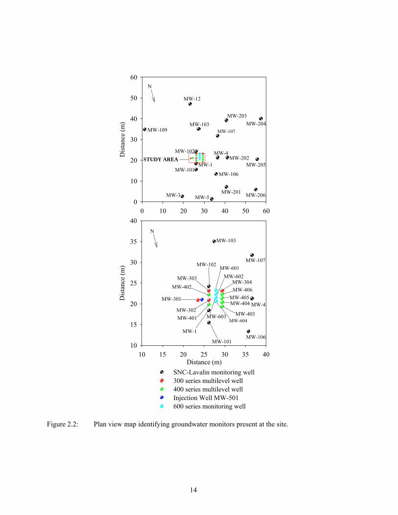
well materials containing a 3.05-7.62 m 0.00254 m slotted screen.

Additional monitoring wells were installed in a selected study area on three separate occasions

by licensed well drillers (Geo Environmental Drilling Inc.) as part of the research project. Four

multilevel wells were installed as part of the research project in November 2007 to determine the

vertical distribution of the contaminants in the groundwater. The multilevel wells identified as MW-

301, MW-302, MW-303 and MW-304 consist of a 0.0127 m inner diameter (ID) PVC centre stock

pipe surrounded by several 0.00635 m ID low-density polyethylene tubing pieces screened at various

depths below the ground surface at 1 m intervals from 308.81 to 298.13 m ASML. All wells

contained a 0.20 m slotted interval wrapped with 200 µm Nytex ® mesh screen.

14

Figure 2.2: Plan view map identifying groundwater monitors present at the site.

0 10 20 30 40 50 60

Dis

tanc

e (m

)

0

10

20

30

40

50

60

MW-109

MW-3 MW-5

MW-101

MW-107

MW-1

MW-103

MW-4

MW-201

MW-202

MW-203

MW-204

MW-205

MW-206

MW-12

MW-102

MW-106

Distance (m)10 15 20 25 30 35 40

Dis

tanc

e (m

)

10

15

20

25

30

35

40

MW-101

MW-107

MW-1

MW-103

MW-4

MW-102

MW-106

MW-304

MW-406

MW-405MW-404

MW-403

MW-301

MW-401

MW-402

MW-302

MW-303

MW-601

MW-602

MW-603MW-604

STUDY AREA

N

SNC-Lavalin monitoring well300 series multilevel well400 series multilevel wellInjection Well MW-501600 series monitoring well

N

15

Another set of multilevel wells were installed in July 2009 to serve as part of a remediation

system monitoring network. The multilevel wells MW-401, MW-402, MW-403, MW-404, MW-405

and MW-406 are constructed of 0.019 m ID PVC centre stock surrounded by 8 0.0127 m ID low-

density polyethylene tubing pieces screened at 0.5 m intervals between 5 and 9.5 m below ground

surface (310.40 to 315.09 m AMSL). All wells contained a 0.5 m slotted interval wrapped with 200

µm Nytex ® mesh screen. Injection well MW-501 comprised of 0.051 m ID PVC well material

equipped with a 2 m 0.00254 m slotted screen interval, 306.09 to 301.40 m AMSL was also installed

at this time to deliver the remedial solution.

The study area was equipped with 4 additional wells (600 series) as part of a separate research

project conducted by another University of Waterloo M Sc. Bobby Katanchi in October 2009. The

wells were used in conjunction with the 300 and 400 series multilevel wells used as part of evaluation

of the remediation system. Wells MW-601, MW-602, MW-603 and MW-604 were constructed of

0.0254 m ID dense PVC tubing containing a 0.50 m well screen and wrapped with 200 µm Nytex ®

mesh screen. The 600 series wells are screened between 304.11 and 302.40 m AMSL.

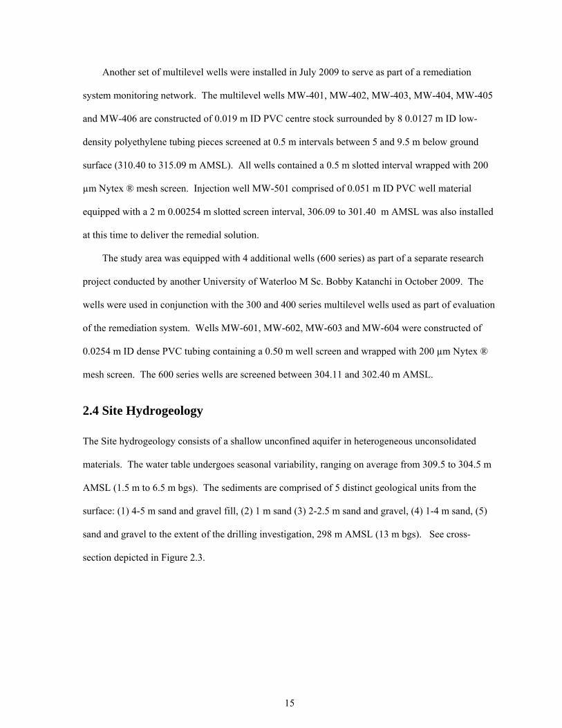
2.4 Site Hydrogeology

The Site hydrogeology consists of a shallow unconfined aquifer in heterogeneous unconsolidated

materials. The water table undergoes seasonal variability, ranging on average from 309.5 to 304.5 m

AMSL (1.5 m to 6.5 m bgs). The sediments are comprised of 5 distinct geological units from the

surface: (1) 4-5 m sand and gravel fill, (2) 1 m sand (3) 2-2.5 m sand and gravel, (4) 1-4 m sand, (5)

sand and gravel to the extent of the drilling investigation, 298 m AMSL (13 m bgs). See cross-

section depicted in Figure 2.3.

16

Distance (m)

0 2 4 6 8 10 12 14 16

MW-301MW-501 Row 1 Row 3Row 2

Ele

vatio

n (m

AM

SL)

Dep

th (

m b

gs)

0

2

4

6

8

10

308.5

303.5

UNIT 2

UNIT 3

UNIT 4

UNIT 5

UNIT 1

SAND

SAND & GRAVEL

SAND

SAND & GRAVEL

FILL

Figure 2.3: Conceptual geologic cross-section of the research Site within the selected study area. Historical water table range (309.5 – 304.5 m AMSL), spatial distribution and screened intervals of monitoring and multilevel wells also shown.

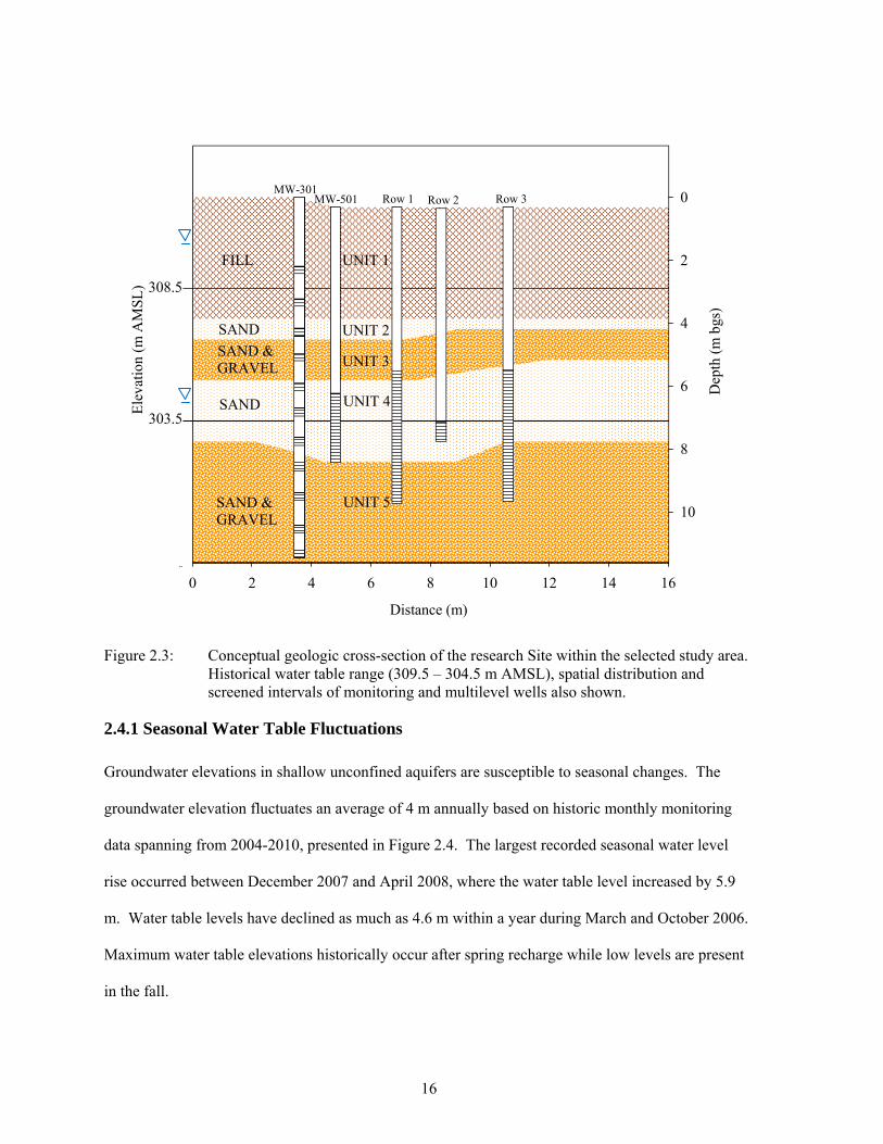
2.4.1 Seasonal Water Table Fluctuations

Groundwater elevations in shallow unconfined aquifers are susceptible to seasonal changes. The

groundwater elevation fluctuates an average of 4 m annually based on historic monthly monitoring

data spanning from 2004-2010, presented in Figure 2.4. The largest recorded seasonal water level

rise occurred between December 2007 and April 2008, where the water table level increased by 5.9

m. Water table levels have declined as much as 4.6 m within a year during March and October 2006.

Maximum water table elevations historically occur after spring recharge while low levels are present

in the fall.

17

Date (m/d/yy)

1/1/04 1/1/05 1/1/06 1/1/07 1/1/08 1/1/09 1/1/10

Ele

vatio

n (m

AM

SL

)

302

304

306

308

310

312

Dep

th (

m b

gs)

0

2

4

6

8

10

Seasonal high water levels

Seasonal low water levels

Figure 2.4: Seasonal groundwater elevation fluctuations in MW-101. Note: 2009-2010 recharge period is distinguished from the previous seasonal changes. (SNC-Lavalin, 2004-2010)

Variability in water table elevation is influenced by a number of factors that include the

hydraulic and geometric parameters of the aquifer, areal extent of the recharge area, boundary

conditions, rate and duration of recharge and discharge events whether they are natural or

anthropogenic in origin (Rai & Singh, 1995). The decline in water table elevation during the summer

months corresponds to increases in evapotranspiration, temperature increases and the growing season

(e.g. Lyford, 1964) which could be contributing to water levels losses at the Site related to agriculture

practices occurring in close proximity (less than 100 m to the west and downgradient from the Site).

The large level fluctuations may also indicate loss of groundwater as subsurface outflow

(Neupane & Shrestha, 2009), however field data suggest negligible downward gradients are present

based on the select portion of the aquifer under investigation. Small head differences are difficult to

detect relying solely on water level data, as a result or possibly related to measurement error and local

variability in vertical gradients induced by aquifer heterogeneities (Silliman & Mantz, 2000; Elçi et

al., 2003). Vertical drawdown gradients exist for the general area (Waterloo Hydrogeologic Inc.,

2003), however given the maximum extent of aquifer characterization is to 298 m AMSL, vertical

gradients may be more pronounced in a deeper zone of the aquifer.

18

Interactions between the local surficial and bedrock geology with agricultural land use practices

may be responsible for the transient hydrogeological conditions observed. River depth information

collected from a river located approximately 800 m north of the Site indicate evidence of a

hydrogeological connection between the local groundwater system and surface water body based on

similar observed behaviour of fluctuating river depth (Saugeen Valley Conservation Authority, 2005-

2010), and groundwater elevations (Figure 2.5).

Date (m/d/yy)

1/1/04 1/1/05 1/1/06 1/1/07 1/1/08 1/1/09 1/1/10 1/1/11

Riv

er D

epth

(m

)

0

1

2

3

4

5

6

Ele

vatio

n (m

AM

SL

)

302

304

306

308

310

Groundwater Level River Depth

Figure 2.5: Seasonal groundwater fluctuations at the Site and corresponding to daily river depths. (SNC-Lavalin, 2004-2010; SVCA, 2005-2010)

Seasonal groundwater fluctuations are also influenced by the amount of precipitation that

contributes to diffuse aquifer recharge as shown in Figure 2.6, where water level rise is proportionate

to the amount of recharge that occurs and can be highly variable, influenced by topography and depth

to water table (Alley et al., 2002). The topography of the Site is relatively flat, where similar

oscillating water levels have been measured at various monitoring wells located within the study area.

Delin et al. (2007) developed a method to illustrate precipitation can contribute at least 21% to aquifer

recharge. By applying the Delin et al. (2007) method, a maximum 26% water table rise would be

attributed to precipitation at the Site assuming 100% contributes to aquifer recharge, which is not

highly realistic. Therefore, additional hydraulic and geometric parameters of the aquifer, boundary

19

conditions and areal extent of the recharge area must also be influencing seasonal fluctuations of the

water table.

Date (m/d/yy)

1/1/06 1/1/07 1/1/08 1/1/09 1/1/10 1/1/11

Tot

al P

reci

pita

tion

(mm

)

0

50

100

150

200

250

Ele

vatio

n (m

asl

)

300

302

304

306

308

310

312

Mean Precipitation Groundwater Level

Figure 2.6: Seasonal groundwater fluctuations at the Site and corresponding to mean monthly precipitation (SNC-Lavalin, 2006-2010; SVCA, 2005-2010)

Aquifer recharge between December 2009 and March 2010 was limited to 1.27 m, which is

significantly less than characteristic recorded events onwards of 4 m. Only 20% of the typical

amount of cumulative precipitation fell during that time span (0.07 m compared to an average of 0.34

m for similar seasonal recharge periods from 2005-June 2010). A summary of the approximate

aquifer recharge periods, water table recharge heights and rates corresponding to local precipitation

data is presented in Table 2.1.

20

Table 2.1: Summary of seasonal and average aquifer recharge, recharge rates and recharge periods corresponding to local seasonal precipitation data.

Start Period Date

End Period Date

Precipitation (m)

Seasonal Recharge

(m)

WTR (% of

Precipitation)

Rate of Recharge (m/day)

Recharge Rate R2

07-Dec-04 19-Apr-05 na 3.25 - 0.024 ± 0.006

0.87

11-Nov-05 23-Mar-06 0.38 4.99 25 0.044 ± 0.003

0.98

30-Oct-06 27-Apr-07 0.36 4.26 28 0.022 ± 0.003

0.92

17-Dec-07 18-Apr-08 0.38 5.90 21 0.045 ± 0.004

0.98

26-Sep-08 02-Apr-09 0.51 4.33 40 0.023 ± 0.002

0.99

12-Dec-09 22-Mar-10 0.07 1.27 18 0.012 ± 0.003

0.91

Average (s.d)

0.339 (0.164) 4.02 (1.59) 26 (9) 0.028

(0.013) 0.94 (0.05)

Note: % of precipitation = Recharge (from precipitation) = ∆ water level * specific yield, assumed to equal porosity (0.32) in unconfined aquifer; na – data not available, s.d – standard deviation, WTR – water table recharge

The rate of aquifer recharge occurring at the Site remains fairly constant throughout the recharge

period, where an average recharge rate of 0.028 m/day, R2 = 0.94) was determined from single

monthly water level measurements. Recharge rates vary between seasons; however they are not

readily influenced by short term precipitation events based on daily precipitation data and continuous

water level data collected from MW-101 equipped with a datalogger.

Declining water levels typically occur from March to late fall (October-November), where water

levels decrease an average of 4 m. A comparison between the seasonal declining water table periods,

degree and rate of the lowering water table is presented in Table 2.2. Linear regression analysis

indicates that a good correlation exists for the discharge rates within one season, where an average

discharge rate of 0.02 m/day, R2 = 0.95 was obtained between 2006 and 2009. It must be noted that

recharge and discharge rates determined from monthly frequencies often results in an underestimate

of rates Delin et al. (2007) and actual rates could be higher than presented in Table 2.2.

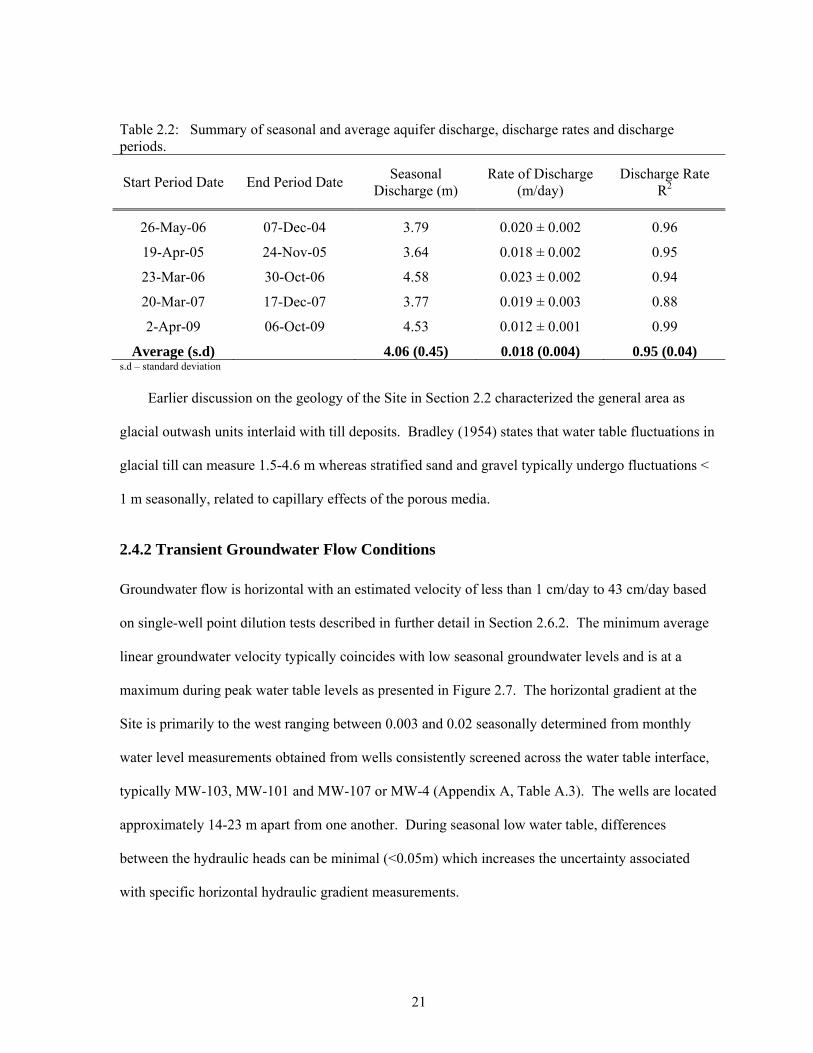
21

Table 2.2: Summary of seasonal and average aquifer discharge, discharge rates and discharge periods.

Start Period Date End Period Date Seasonal

Discharge (m) Rate of Discharge

(m/day) Discharge Rate

R2

26-May-06 07-Dec-04 3.79 0.020 ± 0.002 0.96

19-Apr-05 24-Nov-05 3.64 0.018 ± 0.002 0.95

23-Mar-06 30-Oct-06 4.58 0.023 ± 0.002 0.94

20-Mar-07 17-Dec-07 3.77 0.019 ± 0.003 0.88

2-Apr-09 06-Oct-09 4.53 0.012 ± 0.001 0.99

Average (s.d) 4.06 (0.45) 0.018 (0.004) 0.95 (0.04) s.d – standard deviation

Earlier discussion on the geology of the Site in Section 2.2 characterized the general area as

glacial outwash units interlaid with till deposits. Bradley (1954) states that water table fluctuations in

glacial till can measure 1.5-4.6 m whereas stratified sand and gravel typically undergo fluctuations <

1 m seasonally, related to capillary effects of the porous media.

2.4.2 Transient Groundwater Flow Conditions

Groundwater flow is horizontal with an estimated velocity of less than 1 cm/day to 43 cm/day based

on single-well point dilution tests described in further detail in Section 2.6.2. The minimum average

linear groundwater velocity typically coincides with low seasonal groundwater levels and is at a

maximum during peak water table levels as presented in Figure 2.7. The horizontal gradient at the

Site is primarily to the west ranging between 0.003 and 0.02 seasonally determined from monthly

water level measurements obtained from wells consistently screened across the water table interface,

typically MW-103, MW-101 and MW-107 or MW-4 (Appendix A, Table A.3). The wells are located

approximately 14-23 m apart from one another. During seasonal low water table, differences

between the hydraulic heads can be minimal (<0.05m) which increases the uncertainty associated

with specific horizontal hydraulic gradient measurements.

22

Date (m/d/yy)

1/1/04 1/1/05 1/1/06 1/1/07 1/1/08 1/1/09 1/1/10

Ele

vatio

n (m

AM

SL

)

302

304

306

308

310

312

Gra

dien

t (dh

/dl)

0.000

0.005

0.010

0.015

0.020

0.025

Horizontal Gradient Groundwater Level

Figure 2.7: Seasonal gradient and groundwater elevations (MW-101) at the Site inferred from water table elevations of MW-101, MW-103 and MW-107 or MW-4.

The mean and standard deviation of the seasonally variable groundwater flow direction is

S83oW, and 17o, respectively as determined from historical water table data collected during monthly

monitoring events between 2004- June 2010. The interpreted direction of groundwater flow is in the

west-southwest direction in the late winter – early spring during periods of recharge and maximum

water table elevations, then drifting towards the west throughout the summer as the water table

declines. Groundwater flow is towards the north-northwest in the fall-winter during periods of

minimum water table elevations, as demonstrated in Figure 2.8 and Table A.3.

The transient nature of the hydrogeological conditions present at the Site may also be in

accordance with the behaviour of aquifers located in close proximity to a groundwater divide (Doss,

1993). Physical hydrogeological characteristics near a groundwater divide include large seasonal

water table fluctuations, variable groundwater flow directions and low hydraulic gradients (Toth,

1963). In order to better understand the driving force behind the transient groundwater flow

conditions, a large-scale water balance budget is required for the local watershed that is beyond the

scope of this research. The large magnitude in water table variability is of particular interest at the

Site due to the redistribution and re-mobilization of petroleum hydrocarbons which will be discussed

in further detail in Chapter 3.

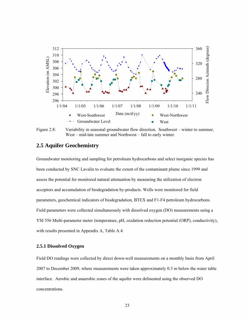
23

Date (m/d/yy)

1/1/04 1/1/05 1/1/06 1/1/07 1/1/08 1/1/09 1/1/10 1/1/11

Flo

w D

irec

ion

Azi

mut

h (d

egre

es)

240

280

320

360E

leva

tion

(m A

MS

L)

296

298

300

302

304

306

308

310

312

Groundwater Level

West-Southwest

West

West-Northwest

Figure 2.8: Variability in seasonal groundwater flow direction. Southwest – winter to summer, West – mid-late summer and Northwest – fall to early winter.

2.5 Aquifer Geochemistry

Groundwater monitoring and sampling for petroleum hydrocarbons and select inorganic species has

been conducted by SNC Lavalin to evaluate the extent of the contaminant plume since 1999 and

assess the potential for monitored natural attenuation by measuring the utilization of electron

acceptors and accumulation of biodegradation by-products. Wells were monitored for field

parameters, geochemical indicators of biodegradation, BTEX and F1-F4 petroleum hydrocarbons.

Field parameters were collected simultaneously with dissolved oxygen (DO) measurements using a

YSI 556 Multi-parameter meter (temperature, pH, oxidation reduction potential (ORP), conductivity),

with results presented in Appendix A, Table A.4.

2.5.1 Dissolved Oxygen

Field DO readings were collected by direct down-well measurements on a monthly basis from April

2007 to December 2009, where measurements were taken approximately 0.3 m below the water table

interface. Aerobic and anaerobic zones of the aquifer were delineated using the observed DO

concentrations.

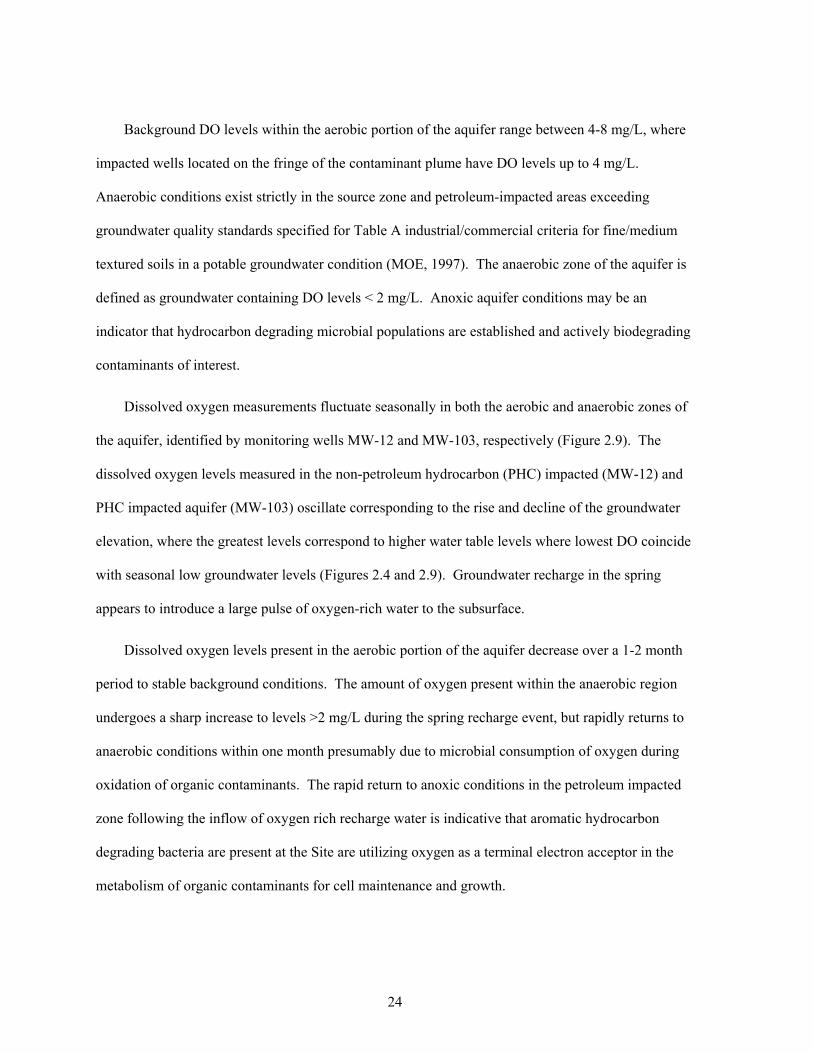
24

Background DO levels within the aerobic portion of the aquifer range between 4-8 mg/L, where

impacted wells located on the fringe of the contaminant plume have DO levels up to 4 mg/L.

Anaerobic conditions exist strictly in the source zone and petroleum-impacted areas exceeding

groundwater quality standards specified for Table A industrial/commercial criteria for fine/medium

textured soils in a potable groundwater condition (MOE, 1997). The anaerobic zone of the aquifer is

defined as groundwater containing DO levels < 2 mg/L. Anoxic aquifer conditions may be an

indicator that hydrocarbon degrading microbial populations are established and actively biodegrading

contaminants of interest.

Dissolved oxygen measurements fluctuate seasonally in both the aerobic and anaerobic zones of

the aquifer, identified by monitoring wells MW-12 and MW-103, respectively (Figure 2.9). The

dissolved oxygen levels measured in the non-petroleum hydrocarbon (PHC) impacted (MW-12) and

PHC impacted aquifer (MW-103) oscillate corresponding to the rise and decline of the groundwater

elevation, where the greatest levels correspond to higher water table levels where lowest DO coincide

with seasonal low groundwater levels (Figures 2.4 and 2.9). Groundwater recharge in the spring

appears to introduce a large pulse of oxygen-rich water to the subsurface.

Dissolved oxygen levels present in the aerobic portion of the aquifer decrease over a 1-2 month

period to stable background conditions. The amount of oxygen present within the anaerobic region

undergoes a sharp increase to levels >2 mg/L during the spring recharge event, but rapidly returns to

anaerobic conditions within one month presumably due to microbial consumption of oxygen during

oxidation of organic contaminants. The rapid return to anoxic conditions in the petroleum impacted

zone following the inflow of oxygen rich recharge water is indicative that aromatic hydrocarbon

degrading bacteria are present at the Site are utilizing oxygen as a terminal electron acceptor in the

metabolism of organic contaminants for cell maintenance and growth.

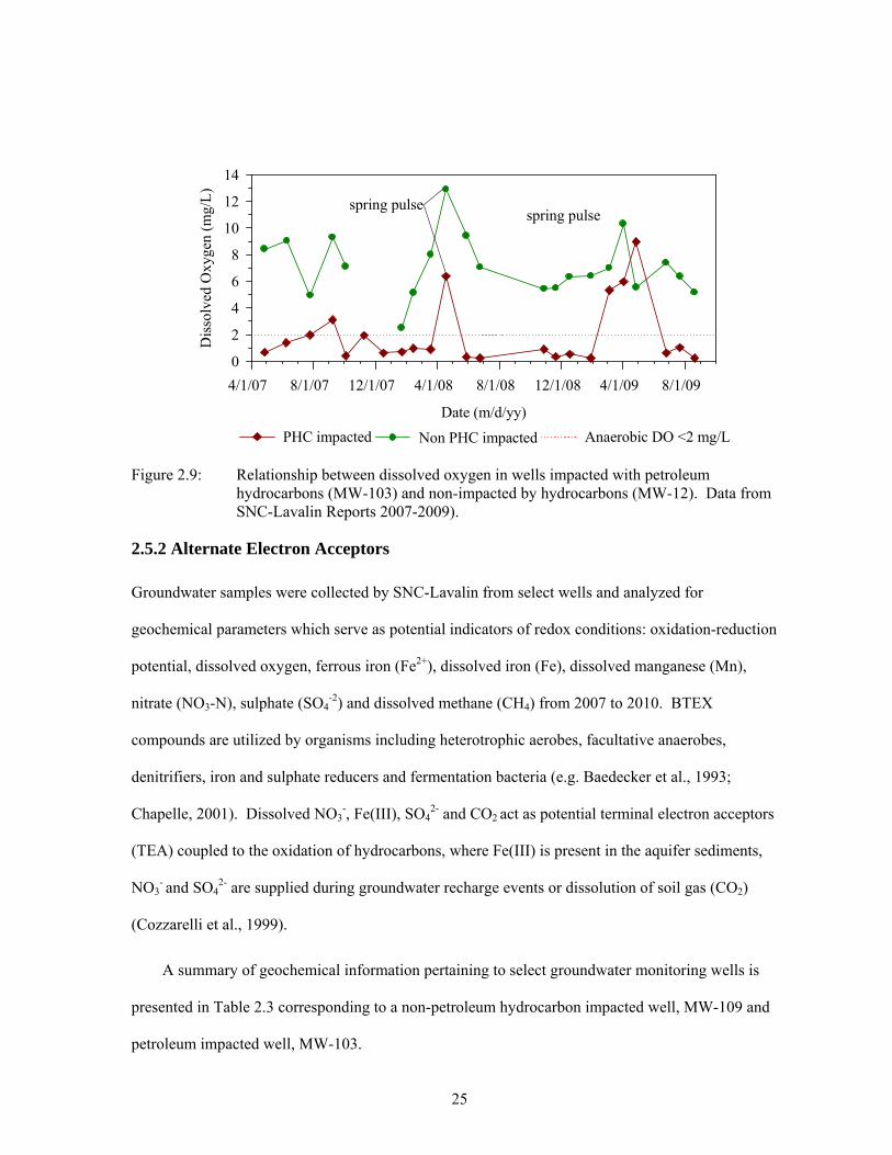
25

Date (m/d/yy)

4/1/07 8/1/07 12/1/07 4/1/08 8/1/08 12/1/08 4/1/09 8/1/09

Dis

solv

ed O

xyge

n (m

g/L

)

0

2

4

6

8

10

12

14

Anaerobic DO <2 mg/L

spring pulsespring pulse

Non PHC impactedPHC impacted

Figure 2.9: Relationship between dissolved oxygen in wells impacted with petroleum hydrocarbons (MW-103) and non-impacted by hydrocarbons (MW-12). Data from SNC-Lavalin Reports 2007-2009).

2.5.2 Alternate Electron Acceptors

Groundwater samples were collected by SNC-Lavalin from select wells and analyzed for

geochemical parameters which serve as potential indicators of redox conditions: oxidation-reduction

potential, dissolved oxygen, ferrous iron (Fe2+), dissolved iron (Fe), dissolved manganese (Mn),

nitrate (NO3-N), sulphate (SO4-2) and dissolved methane (CH4) from 2007 to 2010. BTEX

compounds are utilized by organisms including heterotrophic aerobes, facultative anaerobes,

denitrifiers, iron and sulphate reducers and fermentation bacteria (e.g. Baedecker et al., 1993;

Chapelle, 2001). Dissolved NO3-, Fe(III), SO4

2- and CO2 act as potential terminal electron acceptors

(TEA) coupled to the oxidation of hydrocarbons, where Fe(III) is present in the aquifer sediments,

NO3- and SO4

2- are supplied during groundwater recharge events or dissolution of soil gas (CO2)

(Cozzarelli et al., 1999).

A summary of geochemical information pertaining to select groundwater monitoring wells is

presented in Table 2.3 corresponding to a non-petroleum hydrocarbon impacted well, MW-109 and

petroleum impacted well, MW-103.

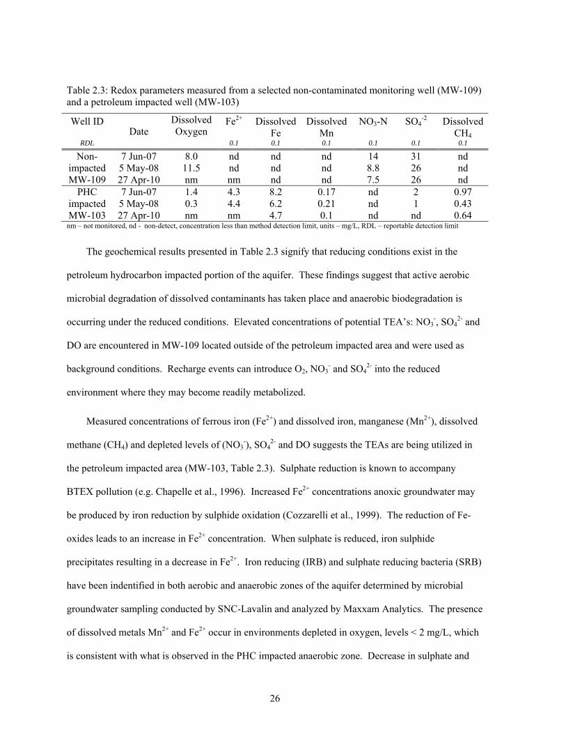
26

Table 2.3: Redox parameters measured from a selected non-contaminated monitoring well (MW-109) and a petroleum impacted well (MW-103)

Well ID

RDL

Date Dissolved Oxygen

Fe2+

0.1

Dissolved Fe 0.1

Dissolved Mn 0.1

NO3-N

0.1

SO4-2

0.1

Dissolved CH4

0.1

Non-impacted MW-109

7 Jun-07 5 May-08 27 Apr-10

8.0 11.5 nm

nd nd nm

nd nd nd

nd nd nd

14 8.8 7.5

31 26 26

nd nd nd

PHC impacted MW-103

7 Jun-07 5 May-08 27 Apr-10

1.4 0.3 nm

4.3 4.4 nm

8.2 6.2 4.7

0.17 0.21 0.1

nd nd nd

2 1 nd

0.97 0.43 0.64

nm – not monitored, nd - non-detect, concentration less than method detection limit, units – mg/L, RDL – reportable detection limit

The geochemical results presented in Table 2.3 signify that reducing conditions exist in the

petroleum hydrocarbon impacted portion of the aquifer. These findings suggest that active aerobic

microbial degradation of dissolved contaminants has taken place and anaerobic biodegradation is

occurring under the reduced conditions. Elevated concentrations of potential TEA’s: NO3-, SO4

2- and

DO are encountered in MW-109 located outside of the petroleum impacted area and were used as

background conditions. Recharge events can introduce O2, NO3- and SO4

2- into the reduced

environment where they may become readily metabolized.

Measured concentrations of ferrous iron (Fe2+) and dissolved iron, manganese (Mn2+), dissolved

methane (CH4) and depleted levels of (NO3-), SO4

2- and DO suggests the TEAs are being utilized in

the petroleum impacted area (MW-103, Table 2.3). Sulphate reduction is known to accompany

BTEX pollution (e.g. Chapelle et al., 1996). Increased Fe2+ concentrations anoxic groundwater may

be produced by iron reduction by sulphide oxidation (Cozzarelli et al., 1999). The reduction of Fe-

oxides leads to an increase in Fe2+ concentration. When sulphate is reduced, iron sulphide

precipitates resulting in a decrease in Fe2+. Iron reducing (IRB) and sulphate reducing bacteria (SRB)

have been indentified in both aerobic and anaerobic zones of the aquifer determined by microbial

groundwater sampling conducted by SNC-Lavalin and analyzed by Maxxam Analytics. The presence

of dissolved metals Mn2+ and Fe2+ occur in environments depleted in oxygen, levels < 2 mg/L, which

is consistent with what is observed in the PHC impacted anaerobic zone. Decrease in sulphate and

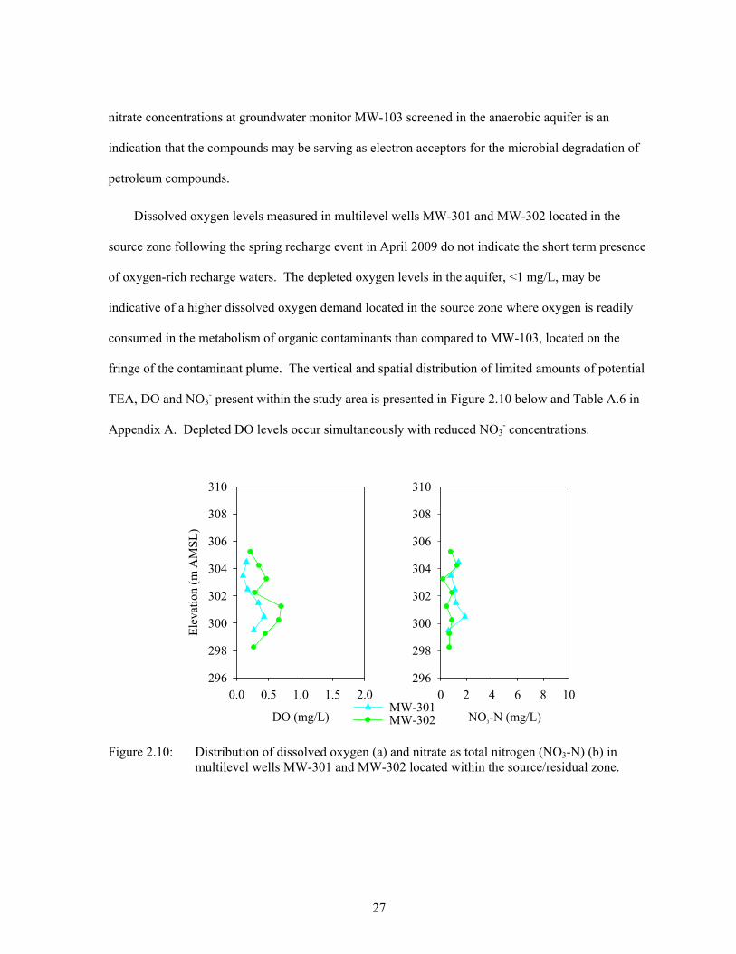
27

nitrate concentrations at groundwater monitor MW-103 screened in the anaerobic aquifer is an

indication that the compounds may be serving as electron acceptors for the microbial degradation of

petroleum compounds.

Dissolved oxygen levels measured in multilevel wells MW-301 and MW-302 located in the

source zone following the spring recharge event in April 2009 do not indicate the short term presence

of oxygen-rich recharge waters. The depleted oxygen levels in the aquifer, <1 mg/L, may be

indicative of a higher dissolved oxygen demand located in the source zone where oxygen is readily

consumed in the metabolism of organic contaminants than compared to MW-103, located on the

fringe of the contaminant plume. The vertical and spatial distribution of limited amounts of potential

TEA, DO and NO3- present within the study area is presented in Figure 2.10 below and Table A.6 in

Appendix A. Depleted DO levels occur simultaneously with reduced NO3- concentrations.

DO (mg/L)

0.0 0.5 1.0 1.5 2.0

Ele

vatio

n (m

AM

SL

)

296

298

300

302

304

306

308

310

MW-302 NO3-N (mg/L)

0 2 4 6 8 10296

298

300

302

304

306

308

310

MW-301

Figure 2.10: Distribution of dissolved oxygen (a) and nitrate as total nitrogen (NO3-N) (b) in multilevel wells MW-301 and MW-302 located within the source/residual zone.

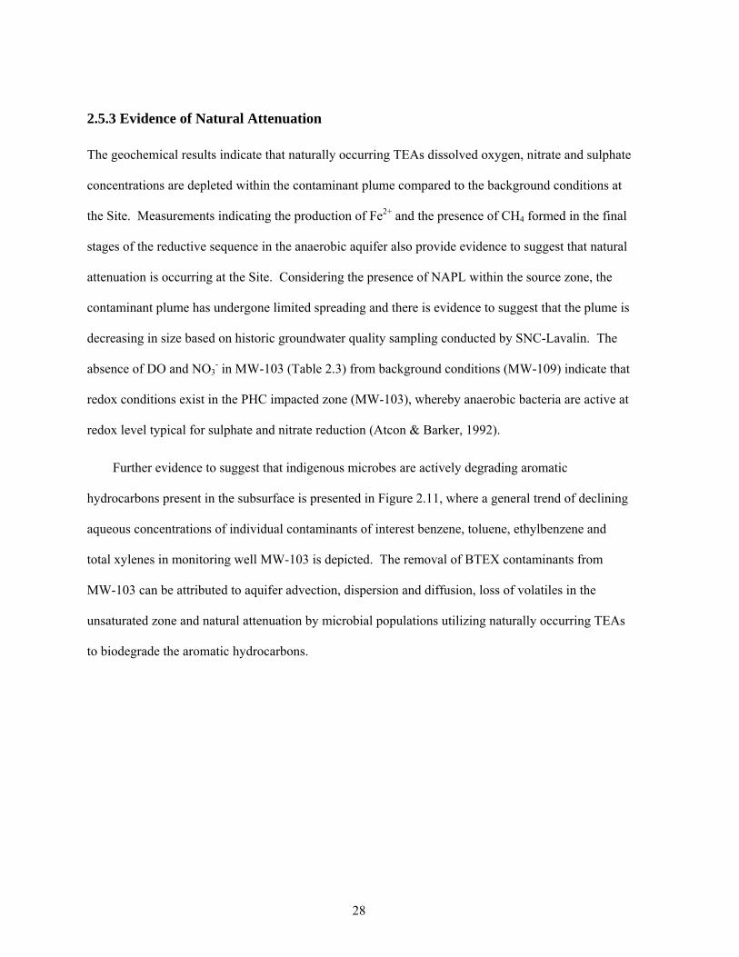
28

2.5.3 Evidence of Natural Attenuation

The geochemical results indicate that naturally occurring TEAs dissolved oxygen, nitrate and sulphate

concentrations are depleted within the contaminant plume compared to the background conditions at

the Site. Measurements indicating the production of Fe2+ and the presence of CH4 formed in the final

stages of the reductive sequence in the anaerobic aquifer also provide evidence to suggest that natural

attenuation is occurring at the Site. Considering the presence of NAPL within the source zone, the

contaminant plume has undergone limited spreading and there is evidence to suggest that the plume is

decreasing in size based on historic groundwater quality sampling conducted by SNC-Lavalin. The

absence of DO and NO3- in MW-103 (Table 2.3) from background conditions (MW-109) indicate that

redox conditions exist in the PHC impacted zone (MW-103), whereby anaerobic bacteria are active at

redox level typical for sulphate and nitrate reduction (Atcon & Barker, 1992).

Further evidence to suggest that indigenous microbes are actively degrading aromatic

hydrocarbons present in the subsurface is presented in Figure 2.11, where a general trend of declining

aqueous concentrations of individual contaminants of interest benzene, toluene, ethylbenzene and

total xylenes in monitoring well MW-103 is depicted. The removal of BTEX contaminants from

MW-103 can be attributed to aquifer advection, dispersion and diffusion, loss of volatiles in the

unsaturated zone and natural attenuation by microbial populations utilizing naturally occurring TEAs

to biodegrade the aromatic hydrocarbons.

29

Date (m/d/yy)

1/1/01 1/1/02 1/1/03 1/1/04 1/1/05 1/1/06 1/1/07 1/1/08 1/1/09 1/1/10 1/1/11

Con

cent

ratio

n (

g/L

)

0

50

100

150

200

250

300

Ele

vatio

n (m

AM

SL

)

300

302

304

306

308

310

312

Water Level Benzene Toluene Ethylbenzene Total Xylenes

Figure 2.11: Seasonal groundwater elevations and measured concentrations of benzene, toluene, ethylbenzene and total xylenes between 2001 and 2010 at MW-103 (SNC-Lavalin, 1999-2010).

2.6 Physical Aquifer Characterization

Subsurface heterogeneities play an important role in the transmittance of groundwater, the

distribution of contaminants and subsequently the delivery of remediation treatments to targeted areas

of the subsurface. Physical properties of the aquifer materials including hydraulic conductivity (K),

porosity (n), groundwater velocity (v), longitudinal dispersivity (αL) and hydrodynamic dispersion

(D) were determined to evaluate the effect of heterogeneities on groundwater flow and the

distribution of residual petroleum hydrocarbon sources of contamination. Field and lab testing were

conducted in order to estimate aquifer hydraulic parameters included slug testing, single-well point

dilution test, falling-head permeameter test and grain size analysis, while a 1D advection-dispersion

solution was applied to single-well point dilution field data.

2.6.1 Conventional Slug Test

Hydraulic conductivity was estimated using rising and falling head slug tests conducted in the

injection well, MW-501, at various time in order to assess groundwater flow conditions prior to and

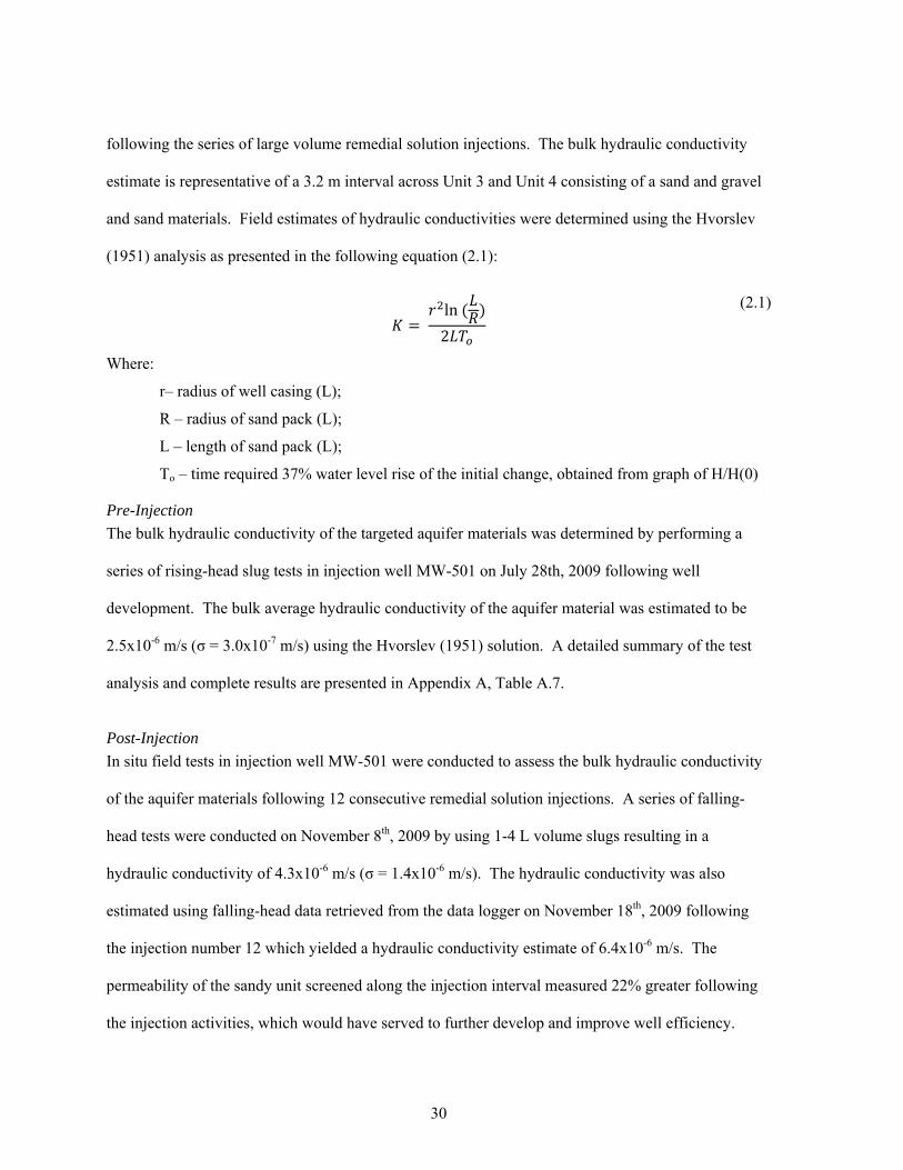
30

following the series of large volume remedial solution injections. The bulk hydraulic conductivity

estimate is representative of a 3.2 m interval across Unit 3 and Unit 4 consisting of a sand and gravel

and sand materials. Field estimates of hydraulic conductivities were determined using the Hvorslev

(1951) analysis as presented in the following equation (2.1):

ln

2

(2.1)

Where:

r– radius of well casing (L);

R – radius of sand pack (L);

L – length of sand pack (L);

To – time required 37% water level rise of the initial change, obtained from graph of H/H(0)

Pre-Injection

The bulk hydraulic conductivity of the targeted aquifer materials was determined by performing a

series of rising-head slug tests in injection well MW-501 on July 28th, 2009 following well

development. The bulk average hydraulic conductivity of the aquifer material was estimated to be

2.5x10-6 m/s (σ = 3.0x10-7 m/s) using the Hvorslev (1951) solution. A detailed summary of the test

analysis and complete results are presented in Appendix A, Table A.7.

Post-Injection

In situ field tests in injection well MW-501 were conducted to assess the bulk hydraulic conductivity

of the aquifer materials following 12 consecutive remedial solution injections. A series of falling-

head tests were conducted on November 8th, 2009 by using 1-4 L volume slugs resulting in a

hydraulic conductivity of 4.3x10-6 m/s (σ = 1.4x10-6 m/s). The hydraulic conductivity was also

estimated using falling-head data retrieved from the data logger on November 18th, 2009 following

the injection number 12 which yielded a hydraulic conductivity estimate of 6.4x10-6 m/s. The

permeability of the sandy unit screened along the injection interval measured 22% greater following

the injection activities, which would have served to further develop and improve well efficiency.

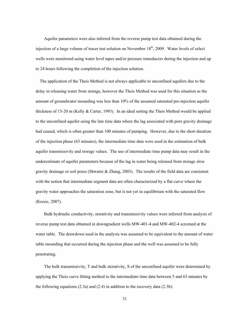
31

Aquifer parameters were also inferred from the reverse pump test data obtained during the

injection of a large volume of tracer test solution on November 18th, 2009. Water levels of select

wells were monitored using water level tapes and/or pressure transducers during the injection and up

to 24 hours following the completion of the injection solution.

The application of the Theis Method is not always applicable to unconfined aquifers due to the

delay in releasing water from storage, however the Theis Method was used for this situation as the

amount of groundwater mounding was less than 10% of the assumed saturated pre-injection aquifer

thickness of 15-20 m (Kelly & Carter, 1993). In an ideal setting the Theis Method would be applied

to the unconfined aquifer using the late time data where the lag associated with pore gravity drainage

had ceased, which is often greater than 100 minutes of pumping. However, due to the short duration

of the injection phase (63 minutes), the intermediate time data were used in the estimation of bulk

aquifer transmissivity and storage values. The use of intermediate time pump data may result in the

underestimate of aquifer parameters because of the lag in water being released from storage slow

gravity drainage or soil pores (Shwartz & Zhang, 2003). The results of the field data are consistent

with the notion that intermediate segment data are often characterized by a flat curve where the

gravity water approaches the saturation zone, but is not yet in equilibrium with the saturated flow

(Kresic, 2007).

Bulk hydraulic conductivity, storativity and transmissivity values were inferred from analysis of

reverse pump test data obtained in downgradient wells MW-401-4 and MW-402-4 screened at the

water table. The drawdown used in the analysis was assumed to be equivalent to the amount of water

table mounding that occurred during the injection phase and the well was assumed to be fully

penetrating.

The bulk transmissivity, T and bulk storativity, S of the unconfined aquifer were determined by

applying the Theis curve fitting method to the intermediate time data between 5 and 63 minutes by

the following equations (2.3a) and (2.4) in addition to the recovery data (2.3b):

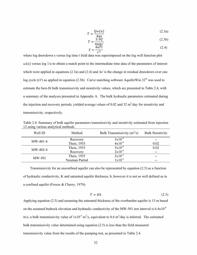
32

4πs

(2.3a)

2.34π∆s′

(2.3b)

4

(2.4)

where log drawdown s versus log time t field data was superimposed on the log well function plot

versus log 1/u to obtain a match point to the intermediate time data of the parameters of interest

which were applied in equations (2.3a) and (2.4) and ∆s′ is the change in residual drawdown over one

log cycle (t/t′) as applied in equation (2.3b). Curve matching software AquiferWin 32® was used to

estimate the best-fit bulk transmissivity and storativity values, which are presented in Table 2.4, with

a summary of the analyses presented in Appendix A. The bulk hydraulic parameters estimated during

the injection and recovery periods, yielded average values of 0.02 and 32 m2/day for storativity and

transmissivity, respectively.

Table 2.4: Summary of bulk aquifer parameters transmissivity and storativity estimated from injection 12 using various analytical methods.

Well ID Method Bulk Transmissivity (m2/s) Bulk Storativity

MW-401-4 Recovery

Theis, 1935 3x10-4 4x10-4

-- 0.02

MW-402-4 Theis, 1935 Recovery

5x10-4

2x10-4 0.02

--

MW-501 Theis, 1935

Neuman Partial 2x10-5 1x10-4

-- --

Transmissivity for an unconfined aquifer can also be represented by equation (2.5) as a function

of hydraulic conductivity, K and saturated aquifer thickness, b, however it is not as well defined as in

a confined aquifer (Freeze & Cherry, 1979):

(2.5)

Applying equation (2.5) and assuming the saturated thickness of the overburden aquifer is 15 m based

on the assumed bedrock elevation and hydraulic conductivity of the MW-501 test interval is 6.4x10-6

m/s, a bulk transmissivity value of 1x10-4 m2/s, equivalent to 8.6 m2/day is inferred. The estimated

bulk transmissivity value determined using equation (2.5) is less than the field measured

transmissivity value from the results of the pumping test, as presented in Table 2.4.

33

For unconfined aquifers, the storativity value is equal to the specific yield Sy and ranges between

0.01 and 0.30 related to dewatering of soil pores by gravity drainage (Freeze & Cherry, 1979).

Storativity values estimated for the sand and gravelly sand units are within the expected range for

these unconsolidated materials (Freeze & Cherry, 1979). Under ideal conditions, late time data

consisting of periods greater than 100 minutes would be used to Theis curve match parameters where

aquifer recharge and saturated flow have achieved equilibrium as a result of the injection (Kresic,

2007).

The observed changes in groundwater elevation throughout the injection phase fit well with the

Theis curve to approximate parameters of interest, despite use of intermediate time data in the

analysis. Late time data is ideal in the estimation of bulk hydraulic parameters as the effects of elastic

storage which set in after pumping is initiated have dissipated. Pumping tests in unconfined aquifers

must be carried out for a long duration until steady state is reached, where early time data are valid,

however data changes due to de-watering of pore spaces which is time-lagged. A reverse pumping

test resulted in water table mounding in the vicinity of the injection well, accompanied by changes in

the vadose zone which becomes temporarily saturated during the injection phase.

2.6.2 Single-Multilevel Well Point Dilution Test

A series of single-well point dilution tests, referred to as natural gradient tests were conducted in

multilevel well MW-301 in select ports screened over various aquifer materials in order to assess the

vertical distribution of hydraulic conductivity within the aquifer following the procedure described by

Halevy et al. (1967) and Drost et al. (1968). The multilevel wells were comprised of 0.00635 m ID

low-density polyethylene tubing containing a 0.20 m screened interval from an elevation of 304.5 to

299.5 m AMSL spaced 1 m apart to derive hydraulic conductivity estimates within various

stratigraphic formations.

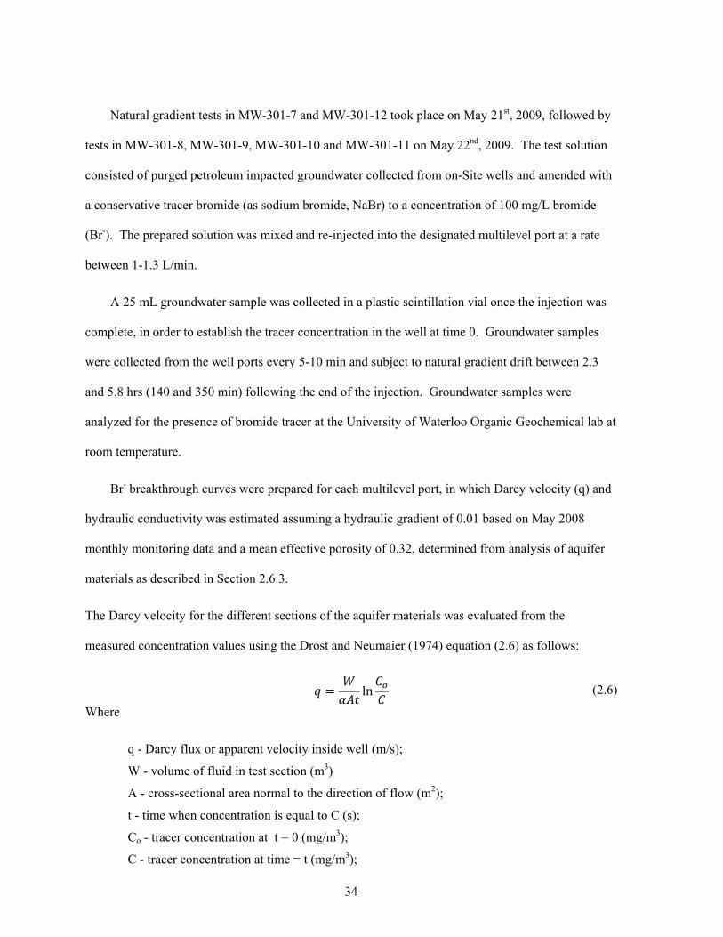
34

Natural gradient tests in MW-301-7 and MW-301-12 took place on May 21st, 2009, followed by

tests in MW-301-8, MW-301-9, MW-301-10 and MW-301-11 on May 22nd, 2009. The test solution

consisted of purged petroleum impacted groundwater collected from on-Site wells and amended with

a conservative tracer bromide (as sodium bromide, NaBr) to a concentration of 100 mg/L bromide

(Br-). The prepared solution was mixed and re-injected into the designated multilevel port at a rate

between 1-1.3 L/min.

A 25 mL groundwater sample was collected in a plastic scintillation vial once the injection was

complete, in order to establish the tracer concentration in the well at time 0. Groundwater samples

were collected from the well ports every 5-10 min and subject to natural gradient drift between 2.3

and 5.8 hrs (140 and 350 min) following the end of the injection. Groundwater samples were

analyzed for the presence of bromide tracer at the University of Waterloo Organic Geochemical lab at

room temperature.

Br- breakthrough curves were prepared for each multilevel port, in which Darcy velocity (q) and

hydraulic conductivity was estimated assuming a hydraulic gradient of 0.01 based on May 2008

monthly monitoring data and a mean effective porosity of 0.32, determined from analysis of aquifer

materials as described in Section 2.6.3.

The Darcy velocity for the different sections of the aquifer materials was evaluated from the

measured concentration values using the Drost and Neumaier (1974) equation (2.6) as follows:

ln (2.6)

Where

q - Darcy flux or apparent velocity inside well (m/s);

W - volume of fluid in test section (m3)

A - cross-sectional area normal to the direction of flow (m2);

t - time when concentration is equal to C (s);

Co - tracer concentration at t = 0 (mg/m3);

C - tracer concentration at time = t (mg/m3);

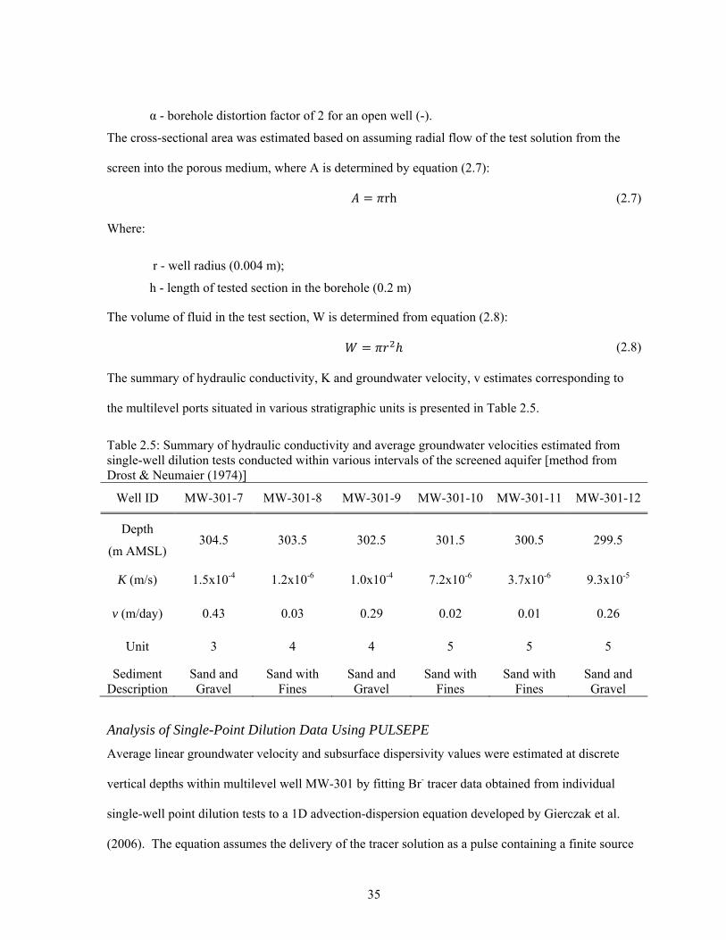
35

α - borehole distortion factor of 2 for an open well (-).

The cross-sectional area was estimated based on assuming radial flow of the test solution from the

screen into the porous medium, where A is determined by equation (2.7):

rh (2.7)

Where:

r - well radius (0.004 m);

h - length of tested section in the borehole (0.2 m)

The volume of fluid in the test section, W is determined from equation (2.8):

(2.8)

The summary of hydraulic conductivity, K and groundwater velocity, v estimates corresponding to

the multilevel ports situated in various stratigraphic units is presented in Table 2.5.

Table 2.5: Summary of hydraulic conductivity and average groundwater velocities estimated from single-well dilution tests conducted within various intervals of the screened aquifer [method from Drost & Neumaier (1974)]

Well ID MW-301-7 MW-301-8 MW-301-9 MW-301-10 MW-301-11 MW-301-12

Depth

(m AMSL) 304.5 303.5 302.5 301.5 300.5 299.5

K (m/s) 1.5x10-4 1.2x10-6 1.0x10-4 7.2x10-6 3.7x10-6 9.3x10-5

v (m/day) 0.43 0.03 0.29 0.02 0.01 0.26

Unit 3 4 4 5 5 5

Sediment Description

Sand and Gravel

Sand with Fines

Sand and Gravel

Sand with Fines

Sand with Fines

Sand and Gravel

Analysis of Single-Point Dilution Data Using PULSEPE

Average linear groundwater velocity and subsurface dispersivity values were estimated at discrete

vertical depths within multilevel well MW-301 by fitting Br- tracer data obtained from individual

single-well point dilution tests to a 1D advection-dispersion equation developed by Gierczak et al.

(2006). The equation assumes the delivery of the tracer solution as a pulse containing a finite source

36

width utilizing equations (2.8) and (2.9) as described by Devlin & Barker (1996) and Gierczak et al.

(2006):

,2

erfc 22 / erfc 2

2/ (2.8)

∗ (2.9)

Where:

Co - the concentration of the tracer injected (mg/L);

x – distance from the source (m);

w – source width (m);

D – dispersion coefficient (m2/s);

t – time (s);

v – average linear groundwater velocity (m/s);

αL – longitudinal dispersivity (m);

D* - effective diffusion coefficient (m/s)

Tracer test breakthrough data was inputted into PULSPE model with initial estimate parameters;

v = 2.5x10-6 m/s, αL = 0.038 m, w = 0.01 m, x = 0.025 m and D* = 1x10-8 m/s. The location of the

injection well was the same as the source, however the distance of the well from the source was

assumed to be 0.025 m in order to apply the model to the data set. The results of the best-fit PULSPE

model to the field data are presented in Figure 2.12 and Table 2.6 while data are presented in

Appendix A Table A.8.

Average linear groundwater velocity, hydrodynamic dispersion and longitudinal dispersivity

estimates were determined for aquifer materials screened within MW-301-7, MW-301-9, MW-301-12

using PULSEPE to find a best-fit solution. The model did not converge for MW-301-8, MW-301-10

and MW-301-11 screened across lower conductive units.

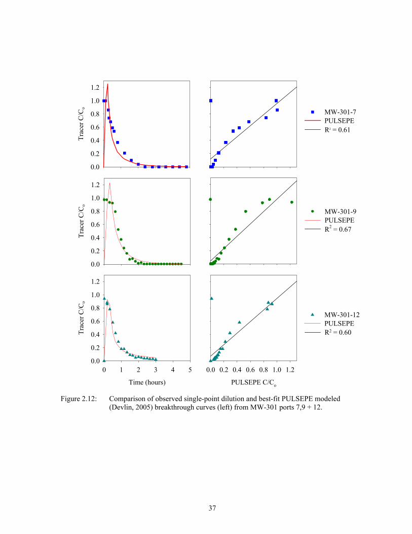
37

Tra

cer

C/C

o

0.0

0.2

0.4

0.6

0.8

1.0

1.2

MW-301-7PULSEPE

Tra

cer

C/C

o

0.0

0.2

0.4

0.6

0.8

1.0

1.2

MW-301-9PULSEPE

Time (hours)

0 1 2 3 4 5

Tra

cer

C/C

o

0.0

0.2

0.4

0.6

0.8

1.0

1.2

R2 = 0.61

R2 = 0.67

PULSEPE C/Co

0.0 0.2 0.4 0.6 0.8 1.0 1.2

R2 = 0.60

MW-301-12PULSEPE

Figure 2.12: Comparison of observed single-point dilution and best-fit PULSEPE modeled (Devlin, 2005) breakthrough curves (left) from MW-301 ports 7,9 + 12.

38

Table 2.6: Summary of best-fit PULSPE 1D advection-dispersion solutions corresponding to observed bromide tracer breakthrough within select multilevel ports of MW-301.

Well ID MW-301-7

(Unit 4)

MW-301-9

(Unit 4)

MW-301-12

(Unit 5) Arithmetic Mean

Depth (m AMSL) 304.50 302.50 299.50 --

v (m/day) 1.6 1.2 0.9 1.3

αL (m) 0.02 0.01 0.04 0.02

D (m2/day) 0.03 1.2 3.8 1.7

95% C.I v (m/s) 1.20 to 2.59 0.86 to1.64 0.58 to 2.16 --

95% C.I αL(m) 0.008 to 0.068 0.005 to 0.032 0.01to 1.04 --

No solution for MW-301-8, MW-301-10 or MW-301-11: PULSEPE model did not converge. v – average linear groundwater velocity, αL – longitudinal dispersivity, D – calculated hydrodynamic dispersion coefficient, D = αL+ D*, No solution – PULSEPE model did not converge

Average linear velocity estimates using PULSPE varied between 0.9-1.6 m/day and were greater

than those determined using Drost & Neumaier (1974) analysis. The PULSPE solution most likely

provided an overestimation of average linear velocity due to aquifer heterogeneities and local

variations in flow. Advection is an important transport process at the Site due to the relatively

permeable aquifer materials in addition to dispersion. Estimates of longitudinal dispersivity values of

sand and gravel units ranged from 0.01 to 0.04 m and were determined within direct proximity to the

source showing relatively limited dispersion. Low reliability longitudinal dispersivity estimates the

aquifer materials are often associated with small-scale estimates (< 3m) (Gelhar et al., 1955-1974,

1992). Longitudinal dispersion is a function of scale and will increase further away from the source

due to large-scale heterogeneity until it eventually reaches a constant (Shwartz & Zhang, 2001).

Although the PUSLEPE model may have overestimated the average linear groundwater velocity

within select zones of the aquifer, it was useful in determining the variability in longitudinal

dispersion in two separate sand and gravel units.

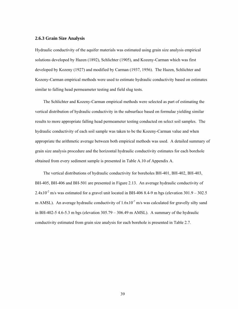
39

2.6.3 Grain Size Analysis

Hydraulic conductivity of the aquifer materials was estimated using grain size analysis empirical

solutions developed by Hazen (1892), Schlichter (1905), and Kozeny-Carman which was first

developed by Kozeny (1927) and modified by Carman (1937, 1956). The Hazen, Schlichter and

Kozeny-Carman empirical methods were used to estimate hydraulic conductivity based on estimates

similar to falling head permeameter testing and field slug tests.

The Schlichter and Kozeny-Carman empirical methods were selected as part of estimating the

vertical distribution of hydraulic conductivity in the subsurface based on formulae yielding similar

results to more appropriate falling head permeameter testing conducted on select soil samples. The

hydraulic conductivity of each soil sample was taken to be the Kozeny-Carman value and when

appropriate the arithmetic average between both empirical methods was used. A detailed summary of

grain size analysis procedure and the horizontal hydraulic conductivity estimates for each borehole

obtained from every sediment sample is presented in Table A.10 of Appendix A.

The vertical distributions of hydraulic conductivity for boreholes BH-401, BH-402, BH-403,

BH-405, BH-406 and BH-501 are presented in Figure 2.13. An average hydraulic conductivity of

2.4x10-2 m/s was estimated for a gravel unit located in BH-406 8.4-9 m bgs (elevation 301.9 – 302.5

m AMSL). An average hydraulic conductivity of 1.6x10-7 m/s was calculated for gravelly silty sand

in BH-402-5 4.6-5.3 m bgs (elevation 305.79 – 306.49 m AMSL). A summary of the hydraulic

conductivity estimated from grain size analysis for each borehole is presented in Table 2.7.

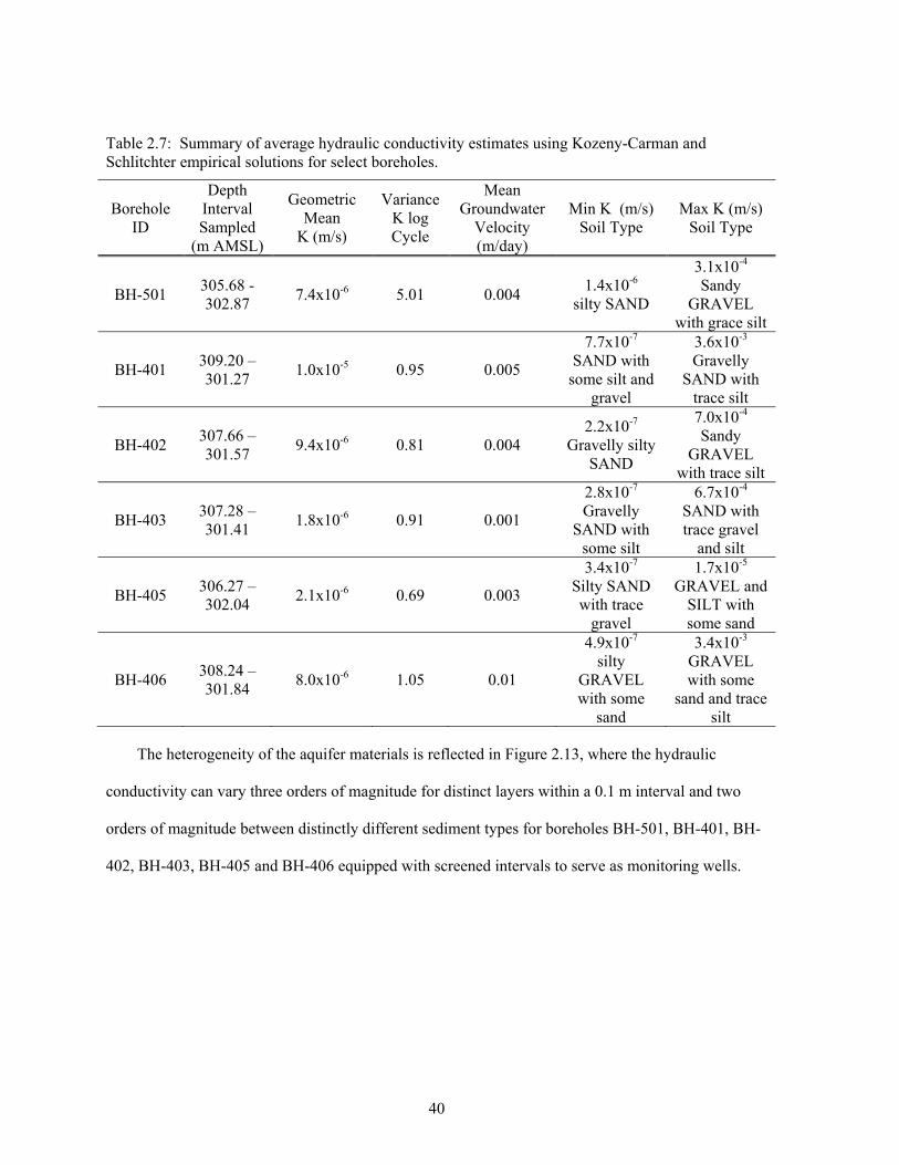
40

Table 2.7: Summary of average hydraulic conductivity estimates using Kozeny-Carman and Schlitchter empirical solutions for select boreholes.

Borehole ID

Depth Interval Sampled

(m AMSL)

Geometric Mean

K (m/s)

Variance K log Cycle

Mean Groundwater

Velocity (m/day)

Min K (m/s) Soil Type

Max K (m/s) Soil Type

BH-501 305.68 - 302.87

7.4x10-6 5.01 0.004 1.4x10-6

silty SAND

3.1x10-4 Sandy

GRAVEL with grace silt

BH-401 309.20 – 301.27

1.0x10-5 0.95 0.005

7.7x10-7 SAND with

some silt and gravel

3.6x10-3 Gravelly

SAND with trace silt

BH-402 307.66 – 301.57

9.4x10-6 0.81 0.004 2.2x10-7

Gravelly silty SAND

7.0x10-4 Sandy

GRAVEL with trace silt

BH-403 307.28 – 301.41

1.8x10-6 0.91 0.001

2.8x10-7 Gravelly

SAND with some silt

6.7x10-4 SAND with trace gravel

and silt

BH-405 306.27 – 302.04

2.1x10-6 0.69 0.003

3.4x10-7 Silty SAND with trace

gravel

1.7x10-5 GRAVEL and

SILT with some sand

BH-406 308.24 – 301.84

8.0x10-6 1.05 0.01

4.9x10-7 silty

GRAVEL with some

sand

3.4x10-3 GRAVEL with some

sand and trace silt

The heterogeneity of the aquifer materials is reflected in Figure 2.13, where the hydraulic

conductivity can vary three orders of magnitude for distinct layers within a 0.1 m interval and two

orders of magnitude between distinctly different sediment types for boreholes BH-501, BH-401, BH-

402, BH-403, BH-405 and BH-406 equipped with screened intervals to serve as monitoring wells.

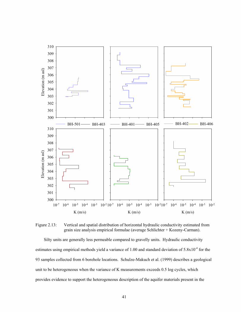
41

Ele

vati

on (

m a

sl)

300

301

302

303

304

305

306

307

308

309

310

BH-501

K (m/s)

10-7 10-6 10-5 10-4 10-3 10-2

BH-406

K (m/s)

10-7 10-6 10-5 10-4 10-3 10-2

BH-405

K (m/s)

10-7 10-6 10-5 10-4 10-3 10-2

Ele

vati

on (

m a

sl)

300

301

302

303

304

305

306

307

308

309

310BH-403 BH-402BH-401

Figure 2.13: Vertical and spatial distribution of horizontal hydraulic conductivity estimated from grain size analysis empirical formulae (average Schlichter + Kozeny-Carman).

Silty units are generally less permeable compared to gravelly units. Hydraulic conductivity

estimates using empirical methods yield a variance of 1.00 and standard deviation of 5.8x10-4 for the

93 samples collected from 6 borehole locations. Schulze-Makuch et al. (1999) describes a geological

unit to be heterogeneous when the variance of K measurements exceeds 0.5 log cycles, which

provides evidence to support the heterogeneous description of the aquifer materials present in the

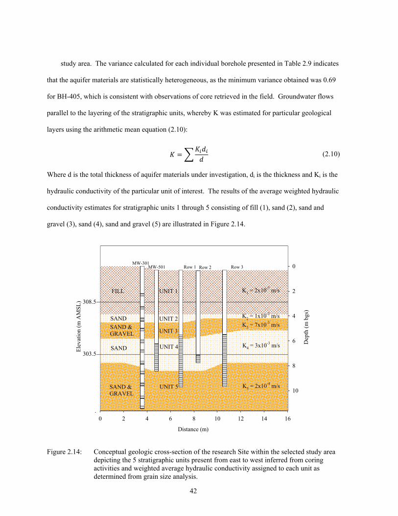
42

study area. The variance calculated for each individual borehole presented in Table 2.9 indicates

that the aquifer materials are statistically heterogeneous, as the minimum variance obtained was 0.69

for BH-405, which is consistent with observations of core retrieved in the field. Groundwater flows

parallel to the layering of the stratigraphic units, whereby K was estimated for particular geological

layers using the arithmetic mean equation (2.10):

(2.10)

Where d is the total thickness of aquifer materials under investigation, di is the thickness and Ki is the

hydraulic conductivity of the particular unit of interest. The results of the average weighted hydraulic

conductivity estimates for stratigraphic units 1 through 5 consisting of fill (1), sand (2), sand and

gravel (3), sand (4), sand and gravel (5) are illustrated in Figure 2.14.

Distance (m)

0 2 4 6 8 10 12 14 16

MW-301MW-501 Row 1 Row 3Row 2

Ele

vatio

n (m

AM

SL

)

Dep

th (

m b

gs)

0

2

4

6

8

10

308.5

303.5

UNIT 2

UNIT 3

UNIT 4

UNIT 5

UNIT 1

SAND

SAND & GRAVEL

SAND

SAND & GRAVEL

FILL

K2 = 1x10-2 m/s

K3 = 7x10-3 m/s

K4 = 3x10-3 m/s

K5 = 2x10-4 m/s

K1 = 2x10-7 m/s

Figure 2.14: Conceptual geologic cross-section of the research Site within the selected study area depicting the 5 stratigraphic units present from east to west inferred from coring activities and weighted average hydraulic conductivity assigned to each unit as determined from grain size analysis.

43

2.6.4 Falling-Head Permeameter Test

The falling-head permeameter test was performed to estimate the saturated hydraulic conductivity for

select sediment samples, from boreholes, following the test procedure developed by Oldman (1998).

The hydraulic conductivity of the saturated material is estimated from the following equation (2.11)

developed after Todd (1959):

ln (2.11)

where a is the cross-sectional area of the column which falls from the initial head Ho to Hl during a

timed interval t, A is the cross-sectional area of the soil column and L is the length of the soil sample.

The hydraulic conductivity estimated using the falling head permeameter in the laboratory setting was

subject to a 1.34 correction factor to account for temperature differences between the lab

(approximately 20°C) and the mean average annual groundwater temperature at the Site (10°C). The

correction temperature dependent parameters fluid viscosity μ and density ρ are governed by the

equation (2.12) for hydraulic conductivity, K:

(2.12)

where k is the permeability of the sediment and g is the acceleration due to gravity. The permeability

of each sample was not calculated; however the relationship between fluid viscosity and density was

used to adjust the hydraulic conductivity to groundwater flow conditions at 10oC. Hydraulic

conductivity determined by the falling-head permeameter method ranged from 2x10-4 to 5x10-7 m/s.

Data and complete results of the falling head estimates of the saturated hydraulic conductivity are

presented in Table A.11 of Appendix A. Falling head permeameter tests were limited to 17 of the

114 soil samples collected throughout the drilling activities, which were primarily composed of sand

with less than 35% gravel and silt constituents. Samples with very fine materials that were lost or

containing large proportions of gravel prevented adequate packing of the soil column. Falling head

permeameter test details including sediment descriptions are presented in Table A.11. Only samples

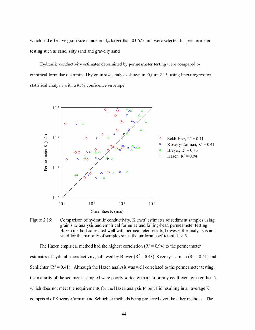
44

which had effective grain size diameter, d10 larger than 0.0625 mm were selected for permeameter

testing such as sand, silty sand and gravelly sand.

Hydraulic conductivity estimates determined by permeameter testing were compared to

empirical formulae determined by grain size analysis shown in Figure 2.15, using linear regression

statistical analysis with a 95% confidence envelope.

Grain Size K (m/s)

10-7 10-6 10-5 10-4

Per

mea

met

er K

(m

/s)

10-7

10-6

10-5

10-4

Schlichter, R2 = 0.41Kozeny-Carman, R2 = 0.41Breyer, R2 = 0.43Hazen, R2 = 0.94

Figure 2.15: Comparison of hydraulic conductivity, K (m/s) estimates of sediment samples using grain size analysis and empirical formulae and falling-head permeameter testing. Hazen method correlated well with permeameter results, however the analysis is not valid for the majority of samples since the uniform coefficient, U > 5.

The Hazen empirical method had the highest correlation (R2 = 0.94) to the permeameter

estimates of hydraulic conductivity, followed by Breyer (R2 = 0.43), Kozeny-Carman (R2 = 0.41) and

Schlichter (R2 = 0.41). Although the Hazen analysis was well correlated to the permeameter testing,

the majority of the sediments sampled were poorly sorted with a uniformity coefficient greater than 5,

which does not meet the requirements for the Hazen analysis to be valid resulting in an average K

comprised of Kozeny-Carman and Schlichter methods being preferred over the other methods. The

45

Schlitchter method had a tendency to underestimate the hydraulic conductivity values compared to

falling-head permeameter testing. Kozeny-Carman and Breyer empirical analyses had an equal

tendency to either over or underestimate K compared to permeameter results. Hydraulic

conductivities estimated from permeameter falling-head tests typically are more representative of in

situ hydraulic conductivities compared to grain size analysis because a larger sample of aquifer

material is being investigated. Hydraulic conductivity increases with scale of measurement in

heterogeneous media (Schulze-Makuch et al., 1999) and unconsolidated sediments (Herzog & Morse,

1984; Bradbury & Muldoon, 1990).

2.7 Site Characterization Summary

A detailed investigation of the physical and geochemical aspects of the hydrogeological setting of the

Site was conducted in order to effectively design, implement and evaluate the delivery of a remedial

solution to targeted areas of the aquifer. Historic information pertaining to the hydrogeologic flow

regime and groundwater quality provided by SNC-Lavalin Inc. was useful in characterizing the

aquifer and identifying a target study area. Additional subsurface investigations carried out as part of

the research project provided further details pertaining to the transport of groundwater and

contaminants. The results of the geochemical investigation were applied to the design phase of an in

situ remediation system in order to stimulate biodegradation of aromatic hydrocarbons. There is field

evidence to suggest indigenous microbial populations are readily utilizing naturally occurring

terminal electron acceptors present in the subsurface such as dissolved O2, NO3- and SO4

2- in the

biodegradation of aromatic hydrocarbons as the TEAs are present in depleted amounts compared to

the background, non-petroleum hydrocarbon impacted aerobic zone of the aquifer. Design and

delivery of the remediation system will be discussed in further detail in Chapter 5.

46

Chapter 3: Characterization of Subsurface Contaminants

3.1 Origin of Contaminants in the Subsurface

Groundwater and soil contamination at the Site originated from leaky underground storage tanks (LUST)

releasing light non-aqueous phase liquid (LNAPL) petroleum products into the subsurface. LNAPL

compounds are less dense then water and have a tendency to float on top of the capillary fringe. The

historical period of release of petrochemicals from the USTs is unknown, however, the Site operated for

50 years prior to the tanks and infrastructure being removed in 1999 as part of the decommissioning

procedure.

During a spill event, LNAPL flows by gravity downward through the unsaturated zone until it

reaches residual saturation and is retained by capillary forces or is transported further downward to the

saturated zone boundary referred to as the capillary fringe. Upon arrival at the capillary fringe, the NAPL

will spread out laterally as it pools at the interface, changing the wetting properties of water and causing

the capillary fringe to collapse. Dissolution of NAPL leads to the migration of dissolved phase

contaminants in the groundwater system which is subject to retardation by the constant dissolution-

adsorption-dissolution processes occurring in the smear zone (Mose & Mushrush, 2000).

The spatial distribution of LNAPL in the subsurface is influenced by the volume and chemical

composition of the NAPL as well as hydrogeological properties of the subsurface materials. Vadose zone

and aquifer heterogeneities, location of the capillary fringe and the hydrogeological flow regime present

at the Site also play an important role in the transport of NAPL in the subsurface.

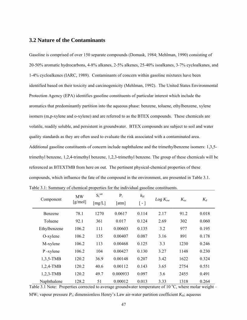
47

3.2 Nature of the Contaminants

Gasoline is comprised of over 150 separate compounds (Domask, 1984; Mehlman, 1990) consisting of

20-50% aromatic hydrocarbons, 4-8% alkanes, 2-5% alkenes, 25-40% isoalkanes, 3-7% cycloalkanes, and

1-4% cycloalkenes (IARC, 1989). Contaminants of concern within gasoline mixtures have been

identified based on their toxicity and carcinogenicity (Mehlman, 1992). The United States Environmental

Protection Agency (EPA) identifies gasoline constituents of particular interest which include the

aromatics that predominantly partition into the aqueous phase: benzene, toluene, ethylbenzene, xylene

isomers (m,p-xylene and o-xylene) and are referred to as the BTEX compounds. These chemicals are

volatile, readily soluble, and persistent in groundwater. BTEX compounds are subject to soil and water

quality standards as they are often used to evaluate the risk associated with a contaminated area.

Additional gasoline constituents of concern include naphthalene and the trimethylbenzene isomers: 1,3,5-

trimethyl benzene, 1,2,4-trimethyl benzene, 1,2,3-trimethyl benzene. The group of these chemicals will be

referenced as BTEXTMB from here on out. The pertinent physical-chemical properties of these

compounds, which influence the fate of the compound in the environment, are presented in Table 3.1.

Table 3.1: Summary of chemical properties for the individual gasoline constituents.

Component MW

[g/mol]

Sisat

[mg/L]

Pi

[atm]

kH

[ - ] Log Kow Koc Kd

Benzene 78.1 1270 0.0617 0.114 2.17 91.2 0.018

Toluene 92.1 361 0.017 0.124 2.69 302 0.060

Ethylbenzene 106.2 111 0.00603 0.135 3.2 977 0.195

O-xylene 106.2 135 0.00407 0.087 3.16 891 0.178

M-xylene 106.2 113 0.00468 0.125 3.3 1230 0.246

P -xylene 106.2 104 0.00427 0.130 3.27 1148 0.230

1,3,5-TMB 120.2 36.9 0.00148 0.207 3.42 1622 0.324

1,2,4-TMB 120.2 40.6 0.00112 0.143 3.65 2754 0.551

1,2,3-TMB 120.2 49.7 0.000933 0.097 3.6 2455 0.491

Naphthalene 128.2 51 0.00012 0.013 3.33 1318 0.264 Table 3.1 Note: Properties corrected to average groundwater temperature of 10 oC, where molar weight –

MW; vapour pressure Pi; dimensionless Henry’s Law air-water partition coefficient KH; aqueous

48

solubility Sisat; octanol-water partition coefficient Kow; organic carbon/water partition coefficient Koc,; and

the soil –water distribution coefficient Kd obtained from Environmental Organic Chemistry 2nd Edition

(2003) and (SPARC, 2009).

3.3 Contaminant Distribution

The source area consists of a complex distribution of free-phase and residual NAPL, aqueous and vapour

phase contaminants which can partition into vadose zone and aquifer materials. Site investigation

involved the occasional recovery of NAPL in select monitoring wells, the collection of soil cores to

determine the presence of residual NAPL and groundwater quality sampling at discrete intervals using

multilevel wells to evaluate the distribution of contaminants in the aquifer profile as part of the research

project.

3.3.1 Seasonal Water Table Fluctuations

Free product has been recovered from monitoring wells MW-102 (screened 1.5 -9.2 m bgs), MW-1

(screened 4.6-7.6 m bgs), MW-301-6 (screened 5.8-6 m bgs), MW-401-1 (screened 5-5.5 m bgs) and

MW-401-2 (screened 5.5 – 6 m bgs) throughout the duration of the Site investigation. NAPL distribution

in the subsurface is influenced by the location of the water table, where the amount of free phase

decreases at higher water levels Oliveira (2009). Residual NAPL can undergo re-mobilization in the

subsurface related to a declining water table involving imbibition and drainage of the porous media,

resulting in larger NAPL thicknesses being observed and recovered in monitoring wells. The observed

NAPL thickness trend at the Site is consistent with Oliveira (2009), where greater NAPL thickness is

present during periods of low groundwater levels in the fall months based on historical Site data provided

by SNC Lavalin.

Seasonal variability of the water table, combined with the downgradient migration of the mobile

NAPL has created a complex re-distribution of contaminants in the heterogeneous setting. LNAPL

floating on the capillary fringe tends to migrate downwards with seasonal water table decline and may

become trapped at greater depths by capillary forces or underneath low permeable units following periods

49

of water table rise. Evidence of this occurring at the Site has been observed in multilevel well MW-301

port 6 screened between 305.6 and 305.4 m AMSL (5.8 and 6 m bgs) in sandy gravel materials where free

product has been recovered at various times throughout the year up to 3 m below the then-current water

table. The sandy gravel unit containing the NAPL pool is overlaid by approximately 0.75 m of lower

permeability fine sand that likely prevented the re-mobilization of the NAPL during water table rise.

In an unconfined aquifer, LNAPLs can pool as a lens at the capillary fringe and move laterally in

response to capillary and gravitational forces where ganglia occurring below the lens at lower saturation

are trapped as small, isolated and discontinuous droplets (Chevalier et al, 1998). Seasonal water table

level fluctuations result in a smear zone (Reddi & Pant, 1998) about 5 m thick at the Site between 309 and

304 m AMSL, which coincides with the vertical extent of the minimum (1.5 m bgs) and maximum (6.5 m

bgs) water table fluctuations as previously discussed in Chapter 2. The distribution of residual NAPL

contamination present within the study area was determined by using soil extraction techniques discussed

in more detail in Section 3.3.2.

3.3.2 Residual Phase NAPL in the Select Research Area

The selected research area was determined from the compilation of historical soil and groundwater

analysis provided by SNC Lavalin, in conjunction with soil core data obtained during the November 2007

and July 2009 installation of multilevel wells (see Figure 3.1). Borehole (BH) locations correspond to

existing monitoring well (MW) locations. Soil cores were collected using a hollow stem split spoon

auger. Soil cores were located in the expected area of residual LNAPL, based on previous SNC-Lavalin

reports and proximity to the location of former USTs and loading racks. Soil cores were analyzed for

critical aromatics BTEXTMB as described in Appendix B.

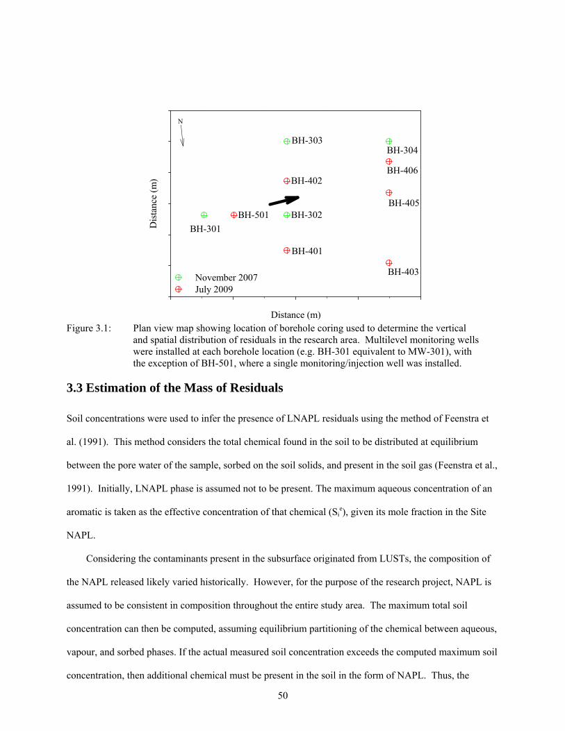
50

Distance (m)

Dis

tanc

e (m

)

November 2007July 2009

BH-403

BH-401

BH-402

BH-301

BH-501 BH-302BH-405

BH-406

BH-304BH-303

N

Figure 3.1: Plan view map showing location of borehole coring used to determine the vertical and spatial distribution of residuals in the research area. Multilevel monitoring wells were installed at each borehole location (e.g. BH-301 equivalent to MW-301), with the exception of BH-501, where a single monitoring/injection well was installed.

3.3 Estimation of the Mass of Residuals

Soil concentrations were used to infer the presence of LNAPL residuals using the method of Feenstra et

al. (1991). This method considers the total chemical found in the soil to be distributed at equilibrium

between the pore water of the sample, sorbed on the soil solids, and present in the soil gas (Feenstra et al.,

1991). Initially, LNAPL phase is assumed not to be present. The maximum aqueous concentration of an

aromatic is taken as the effective concentration of that chemical (Sie), given its mole fraction in the Site

NAPL.

Considering the contaminants present in the subsurface originated from LUSTs, the composition of

the NAPL released likely varied historically. However, for the purpose of the research project, NAPL is

assumed to be consistent in composition throughout the entire study area. The maximum total soil

concentration can then be computed, assuming equilibrium partitioning of the chemical between aqueous,

vapour, and sorbed phases. If the actual measured soil concentration exceeds the computed maximum soil

concentration, then additional chemical must be present in the soil in the form of NAPL. Thus, the

51

approach identifies the presence of NAPL when the hypothetical maximum concentration of a chemical,

Ct, exceeds the concentration measured in the soil. Ct is defined by equations (3.1) to (3.3):

(3.1)

(3.2)

(3.3)

Where:

Ms - mass of chemical sorbed on soil solids (mg);

Mw - mass of chemical in pore water (mg);

Ma - mass of chemical in soil gas (mg);

ρb - dry bulk density of the soil sample (g/cm3);

Cti - the total soil chemical concentration (mg/kg dry weight);

Cs - chemical concentration sorbed on the soil solids (mg/kg dry weight);

Cw - chemical concentration in the pore water (mg/L);

Ca - chemical concentration in the soil gas (mg/L);

φw - water-filled porosity (volume fraction);

φa - air-filled porosity (volume fraction);

Kd - partition coefficient between pore water and soil solids (cm3/g);

Hc - dimensionless Henry’s Law Constant;

i - gasoline constituent.

Kd, partition coefficient between the sediments and pore-water, is computed using equation (3.4):

K K f (3.4)

Where Koc is the organic carbon-water partition coefficient for the gasoline constituent and foc is the

fraction of organic carbon in the soil. A conservative estimate of foc equal to 0.0002 was selected for this

calculation based on foc data determined for the Borden sandy aquifer (Mackay et al., 1986a)

52

Re-arranging the equation in terms of the pore-water concentration yields equation (3.5):

(3.5)

Equation (3.5) can be simplified to equation (3.6) by neglecting HcΦa, since the core was water-saturated:

(3.6)

The total soil concentration can then be expressed in terms of the pore-water concentration by equation

(3.7):

(3.7)

The effective solubility Sie of the chemical of interest i was used as the pore-water concentration Cw to

determine the maximum total concentration within the pore-space in the absence of a NAPL phase as

presented in equation (3.8) adapted from Raoult’s Law:

(3.8)

Where Xi NAPL is the mole fraction of the chemical constituent in the gasoline mixture and Sisat is the pure

phase solubility of the compound (Shiu et al, 1998).

This relationship has been reasonably approximated by laboratory studies conducted by Banerjee

(1984) for structurally similar hydrophobic organic liquids and an error not to exceed a factor of two for

complex organic mixtures (Leinonen et al., 1973). The mole fraction of selected gasoline components in

the weathered NAPL recovered on-Site (Appendix B Table B.1) was used in this analysis.

The total soil extract concentrations determined using equation (3.9) are expressed in mg/kg dry soil

which were converted to wet soil concentrations and compared to concentrations of contaminants

measured in the field cores by the following expressions (3.9 and 3.10):

(3.9)

(3.10)

Where ρm is the wet bulk density of the soil, 2.13 g/cm3 based on an average dry bulk density of 1.81

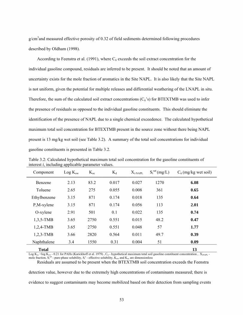
53

g/cm3and measured effective porosity of 0.32 of field sediments determined following procedures

described by Oldham (1998).

According to Feenstra et al. (1991), where Cti exceeds the soil extract concentration for the

individual gasoline compound, residuals are inferred to be present. It should be noted that an amount of

uncertainty exists for the mole fraction of aromatics in the Site NAPL. It is also likely that the Site NAPL

is not uniform, given the potential for multiple releases and differential weathering of the LNAPL in situ.

Therefore, the sum of the calculated soil extract concentrations (Cti’s) for BTEXTMB was used to infer

the presence of residuals as opposed to the individual gasoline constituents. This should eliminate the

identification of the presence of NAPL due to a single chemical exceedence. The calculated hypothetical

maximum total soil concentration for BTEXTMB present in the source zone without there being NAPL

present is 13 mg/kg wet soil (see Table 3.2). A summary of the total soil concentrations for individual

gasoline constituents is presented in Table 3.2.

Table 3.2: Calculated hypothetical maximum total soil concentration for the gasoline constituents of interest i, including applicable parameter values.

Component Log Kow Koc Kd Xi-NAPL Sisat (mg/L) Cti (mg/kg wet soil)

Benzene 2.13 83.2 0.017 0.027 1270 6.08

Toluene 2.65 275 0.055 0.008 361 0.65

Ethylbenzene 3.15 871 0.174 0.018 135 0.64

P,M-xylene 3.15 871 0.174 0.056 113 2.01

O-xylene 2.91 501 0.1 0.022 135 0.74

1,3,5-TMB 3.65 2750 0.551 0.015 48.2 0.47

1,2,4-TMB 3.65 2750 0.551 0.048 57 1.77

1,2,3-TMB 3.66 2820 0.564 0.011 49.7 0.39

Naphthalene 3.4 1550 0.31 0.004 51 0.09

Total 13 Log Koc =log Kow - 0.21 for PAHs (Karickhoff et al. 1979) , Cti - hypothetical maximum total soil gasoline constituent concentration , XiNAPL - mole fraction, Si

sat - pure-phase solubility, Sie - effective solubility, Kow and Koc are dimensionless

Residuals are assumed to be present when the BTEXTMB soil concentration exceeds the Feenstra

detection value, however due to the extremely high concentrations of contaminants measured; there is

evidence to suggest contaminants may become mobilized based on their detection from sampling events

54

conducted at periods of low and moderate water table elevations. Typical residual saturation of LNAPL

volume to the volume of pore volume can range from 10-20% in the unsaturated zone to 15-50% of the

pore volume in the saturated zone as described by Mercer & Cohen (1990).

Residual saturation provides an indication as to the concentration above which LNAPL may be

mobile and below which LNAPL will be immobile due to entrapment by capillary forces. NAPL must

displace water from the pore space within the capillary fringe and overcome the capillary pressure in

order to migrate laterally. Wilson and Conrad (1984) established that NAPL could undergo both vertical

and horizontal re-mobilization in gravel materials, whereas movement was restricted to vertical

movement in sand and inhibited in clay and silt.

The NAPL concentration at 100% residual saturation (C100% Sr) present in the select research area was

determined using equation (3.11) below:

% 1

(3.11)

Where:

Sr – residual saturation

n – porosity, 0.32

GNAPL – specific gravity of aquifer materials, 0.80 g/cm3

Gsolids – specific gravity of aquifer materials, 2.7 g/cm3

The application of equation (3.11) to site specific conditions yields a maximum concentration of

NAPL of approximately 140,000 mg/kg. The NAPL continuum developed by Boynton (2009) states that

NAPL has the potential to be mobilized or recovered at saturation exceeding 10%, equivalent to 14,000

mg/kg NAPL. BTEXTMB gasoline constituents comprised approximately 21% of the total NAPL

recovered from the Site. Based on the measured composition of the NAPL, BTEXTMB soil extract

concentrations exceeding 3,000 mg/kg (10% of 14,000 mg/kg TPH) would be the expected minimum

concentration required for the NAPL to be mobile.

55

3.3.1 Coring Results

Characterization of the residual distribution in the study area was determined by soil coring activities that

took place in November 2007 and July 2009. Coring was conducted within the former locations of UST

and loading racks (BH-301 and BH-501), downgradient in Row 1 (BH-302, BH-303, BH-401, BH-402)

and further downgradient within the source zone, Row 3 (BH-304, BH-403, BH-405 and BH-406), as

presented in Figure 3.1.

Using the Feenstra et al. (1991), residuals are inferred to be present when the total soils extract

concentrations of BTEXTMB exceed 13 mg/kg wet soil. The total soil concentrations measured in the

majority of the samples are significantly greater than 13 mg/kg. The inference of residuals at BTEXTMB

soil concentrations exceeding 13 mg/kg is in general agreement with the value exceeding 11 mg/kg where

residual are inferred for Borden sand (Yang, 2008).

The vertical distribution of BTEXTMB is presented in Figures 3.2 to 3.4, in order of increasing

distance downgradient from the presumed release area. Trends of total BTEXTMB concentrations in

individual cores were highly variable throughout the vertical profile. BTEXTMB soil extract

concentrations measured during the coring program were consistently greater than 13 m/kg, however less

than 3,000 mg/kg which is an indication that NAPL is primarily present in the study area at residual

saturation and possibly immobile. Results of the soil coring investigation are summarized in Table B.2

through B.11 in Appendix B.

56

Concentration (mg/kg) Wet Soil

0 800 1600 2400 3200

Ele

vatio

n (m

AM

SL

)

298

300

302

304

306

308

310

312

BH-301

Mobile NAPL > 3000 mg/kgResidual NAPL > 13 mg/kg

Concentration (mg/kg) Wet Soil

0 800 1600 2400 3200

BH-501

Figure 3.2: Soil concentrations of BTEXTMB in soil cores BH-301 (MW-301) and BH-501 (MW-501, injection well). Residuals inferred at BTEXTMB concentrations exceeding 13 mg/kg wet soil (red line). Mobile NAPL inferred at BTEXTMB concentrations greater than 3,000 mg/kg wet soil.

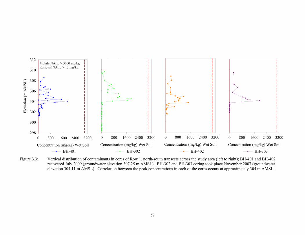
57

Concentration (mg/kg) Wet Soil

0 800 1600 2400 3200

Ele

vatio

n (m

AM

SL)

298

300

302

304

306

308

310

312

BH-401

Mobile NAPL > 3000 mg/kgResidual NAPL > 13 mg/kg

Concentration (mg/kg) Wet Soil

0 800 1600 2400 3200

BH-302

Concentration (mg/kg) Wet Soil

0 800 1600 2400 3200

BH-402

Concentration (mg/kg) Wet Soil

0 800 1600 2400 3200

BH-303

Figure 3.3: Vertical distribution of contaminants in cores of Row 1, north-south transects across the study area (left to right); BH-401 and BH-402 recovered July 2009 (groundwater elevation 307.25 m AMSL). BH-302 and BH-303 coring took place November 2007 (groundwater elevation 304.11 m AMSL). Correlation between the peak concentrations in each of the cores occurs at approximately 304 m AMSL.

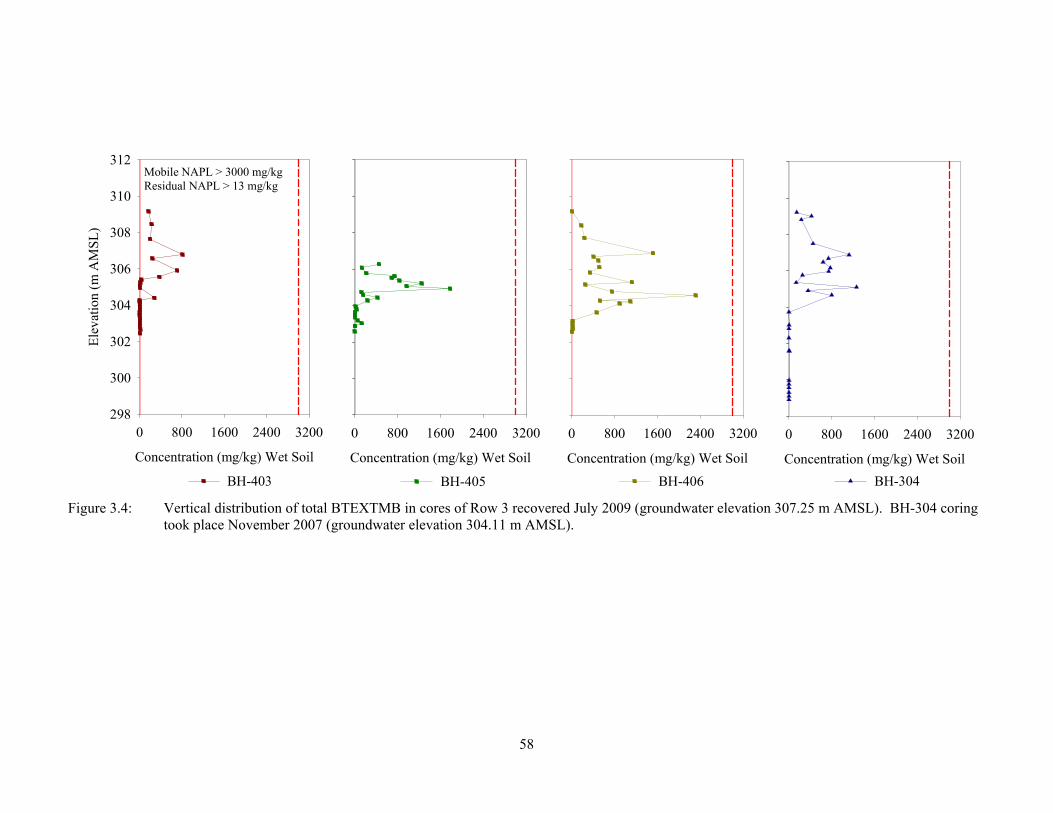
58

Concentration (mg/kg) Wet Soil

0 800 1600 2400 3200

Ele

vatio

n (m

AM

SL

)

298

300

302

304

306

308

310

312

BH-403

Mobile NAPL > 3000 mg/kgResidual NAPL > 13 mg/kg

Concentration (mg/kg) Wet Soil

0 800 1600 2400 3200

BH-405

Concentration (mg/kg) Wet Soil

0 800 1600 2400 3200

BH-406

Concentration (mg/kg) Wet Soil

0 800 1600 2400 3200

BH-304

Figure 3.4: Vertical distribution of total BTEXTMB in cores of Row 3 recovered July 2009 (groundwater elevation 307.25 m AMSL). BH-304 coring took place November 2007 (groundwater elevation 304.11 m AMSL).

59

LNAPL has the ability to migrate below the water table and become trapped at lower elevations due

to seasonal fluctuations in addition to LNAPL being confined to the network of larger pore-spaces. The

distribution of contaminants observed at the Site is generally not consistent with the standard conceptual

model where the bulk of the NAPL is present above capillary fringe as discussed in Section 3.1. The

results of the coring investigation at the Site reveal the bulk of the NAPL distribution to be found below

the water table.

The maximum concentration of total critical aromatics in soil were generally concentrated around

305 m AMSL during fall 2007 and July 2009 and independent of the location of the water table at the

time of coring, about 304.1 m AMSL and 307.3 m AMSL, respectively. The elevated concentration of

contaminants in the soil at this level may be attributed to the presence of potential mobile NAPL even

though concentrations less than 3,000 kg/mg wet soil were observed.

The residual hydrocarbon distribution in the unsaturated and saturated zone is consistent with the

seasonal minimum and maximum groundwater elevations, where a smear zone has been generated by the

fluctuating water table. The concentration of residual NAPL decreases significantly beyond the minimum

seasonal groundwater low where no residual contamination is inferred beyond elevation 308.9 m ASML

(11.5 m bgs) for BH-301, 311.5 (8.6 m bgs) for BH-302, 312.2 (7.9 m bgs) BH-303 and 313.7 (7.2 m

bgs) for BH-304.

3.3.3 Dissolved Phase within the Source Zone

Four multilevel wells were installed by the University of Waterloo in November 2007 as part of the

preliminary research to determine the vertical distribution of the contaminants in the dissolved phase in

the locations corresponding to boreholes BH-301, BH-302, BH-303 and BH-304. The groundwater flow

system serves as the primary migratory pathway for petroleum hydrocarbon impacted groundwater. The

results of the groundwater sampling program were used to determine whether concentrations of

contaminants of interest in the dissolved phase were consistent with the presence of residual LNAPL. A

summary of the well details was previously discussed in Chapter 2 with additional relevant well

60

information presented in Appendix A.

Groundwater samples were collected from the 300 Series UW multilevel wells and analyzed for total

BTEXTMB on four occasions corresponding with seasonal groundwater maxima and minima: December

2007, May 2008, November 2008 and April 2009 (Figure 3.5). BTEXTMB concentrations in the

dissolved phase of the source zone ranged between 900 μg/L and 42,000 μg/L. The highest concentration

was measured in MW-301, located at the eastern portion of the source zone, closest to the former LUSTs

(see Figure 3.1). Maximum dissolved phase concentrations generally decreased downgradient within the

source zone from MW-302 and MW-303 (Row 1) to MW-304 (Row 3) situated approximately 6 m away.

On all sampling occasions, concentrations generally increased with depth, with peak concentrations

occurring between 305 and 303 m AMSL located within the proximity of seasonal groundwater minimum

at the Site.

Only slight differences in the vertical distribution of contaminants in the groundwater were noted

between periods of low water table elevation (fall) and high water table (spring), however a similar

contaminant profile is apparent under the different hydrogeologic conditions. The variability in measured

concentration of BTEXTMB within the 4 seasonal sampling events may be attributed to transient nature

of the aquifer, where groundwater elevation, flow path and changes in the contact zone of NAPL

dissolution of the saturated zone influence the aqueous concentrations (Davis et al., 1999). Complete

results of the four groundwater sampling events are presented in Appendix B, Table B.13 through B.17.

The history of the release of LNAPL is unknown, however the source zone has likely been

established from several spill events, as a single release event is not documented resulting in several

LNAPL compositions being present. The percentage of aromatics in gasoline can vary considerably

depending on the composition of the gasoline source (Cline et al., 1991), resulting in different estimates

for the aqueous concentration Sie in equilibrium for a particular NAPL. A degree of uncertainty is

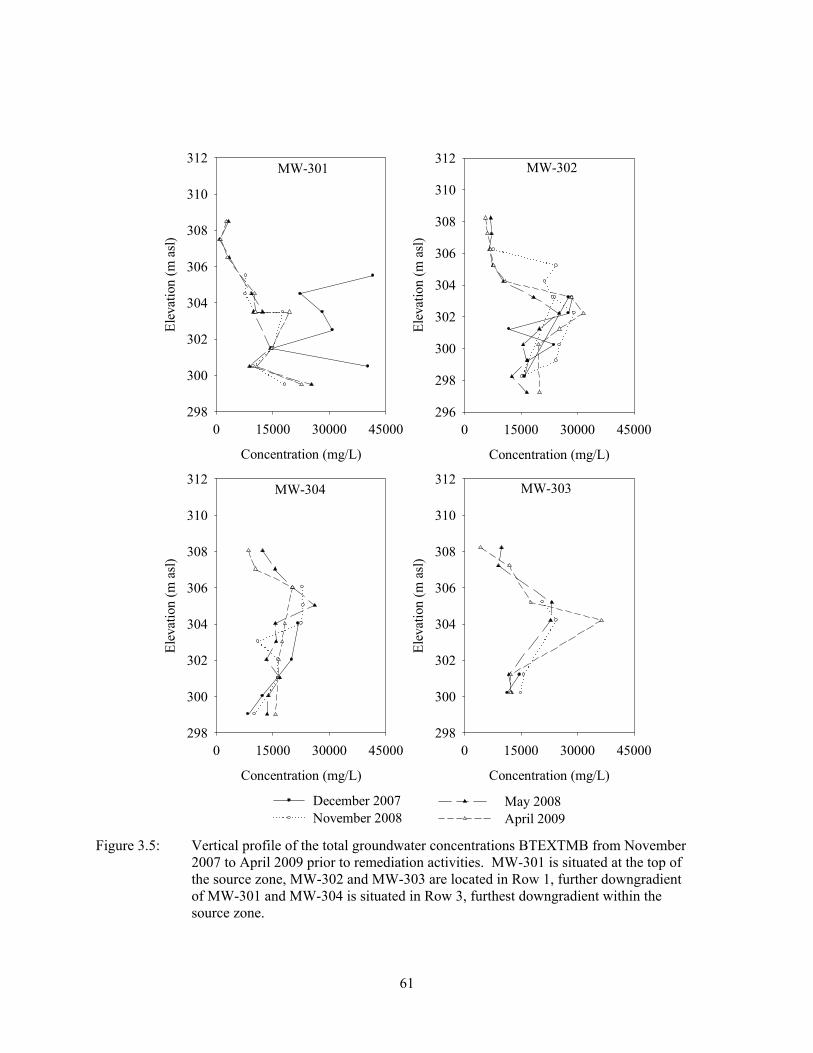
61

Concentration (mg/L)

0 15000 30000 45000

Ele

vatio

n (m

asl

)

298

300

302

304

306

308

310

312

December 2007November 2008

MW-304

Concentration (mg/L)

0 15000 30000 45000E

leva

tion

(m a

sl)

296

298

300

302

304

306

308

310

312MW-302

Concentration (mg/L)

0 15000 30000 45000

Ele

vatio

n (m

asl

)

298

300

302

304

306

308

310

312MW-301

Concentration (mg/L)

0 15000 30000 45000

Ele

vatio

n (m

asl

)

298

300

302

304

306

308

310

312

May 2008April 2009

MW-303

Figure 3.5: Vertical profile of the total groundwater concentrations BTEXTMB from November 2007 to April 2009 prior to remediation activities. MW-301 is situated at the top of the source zone, MW-302 and MW-303 are located in Row 1, further downgradient of MW-301 and MW-304 is situated in Row 3, furthest downgradient within the source zone.

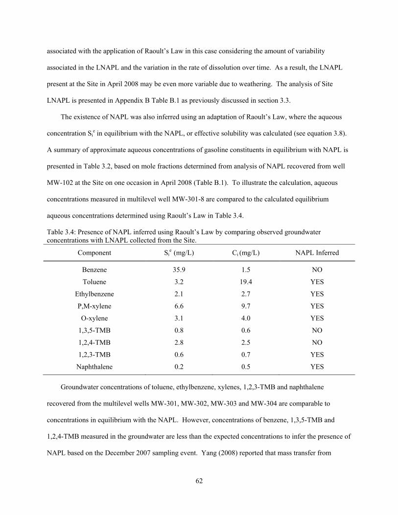
62

associated with the application of Raoult’s Law in this case considering the amount of variability

associated in the LNAPL and the variation in the rate of dissolution over time. As a result, the LNAPL

present at the Site in April 2008 may be even more variable due to weathering. The analysis of Site

LNAPL is presented in Appendix B Table B.1 as previously discussed in section 3.3.

The existence of NAPL was also inferred using an adaptation of Raoult’s Law, where the aqueous

concentration Sie in equilibrium with the NAPL, or effective solubility was calculated (see equation 3.8).

A summary of approximate aqueous concentrations of gasoline constituents in equilibrium with NAPL is

presented in Table 3.2, based on mole fractions determined from analysis of NAPL recovered from well

MW-102 at the Site on one occasion in April 2008 (Table B.1). To illustrate the calculation, aqueous

concentrations measured in multilevel well MW-301-8 are compared to the calculated equilibrium

aqueous concentrations determined using Raoult’s Law in Table 3.4.

Table 3.4: Presence of NAPL inferred using Raoult’s Law by comparing observed groundwater concentrations with LNAPL collected from the Site.

Component Sie (mg/L) Ci (mg/L) NAPL Inferred

Benzene 35.9 1.5 NO

Toluene 3.2 19.4 YES

Ethylbenzene 2.1 2.7 YES

P,M-xylene 6.6 9.7 YES

O-xylene 3.1 4.0 YES

1,3,5-TMB 0.8 0.6 NO

1,2,4-TMB 2.8 2.5 NO

1,2,3-TMB 0.6 0.7 YES

Naphthalene 0.2 0.5 YES

Groundwater concentrations of toluene, ethylbenzene, xylenes, 1,2,3-TMB and naphthalene

recovered from the multilevel wells MW-301, MW-302, MW-303 and MW-304 are comparable to

concentrations in equilibrium with the NAPL. However, concentrations of benzene, 1,3,5-TMB and

1,2,4-TMB measured in the groundwater are less than the expected concentrations to infer the presence of

NAPL based on the December 2007 sampling event. Yang (2008) reported that mass transfer from

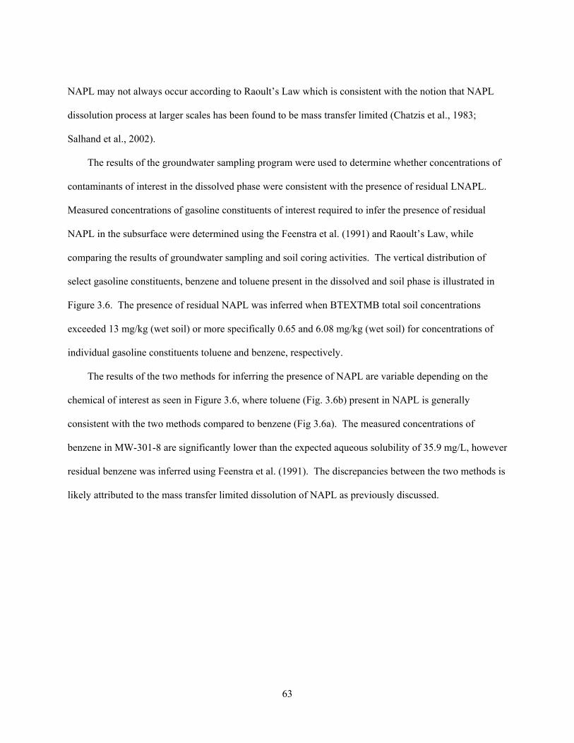
63

NAPL may not always occur according to Raoult’s Law which is consistent with the notion that NAPL

dissolution process at larger scales has been found to be mass transfer limited (Chatzis et al., 1983;

Salhand et al., 2002).

The results of the groundwater sampling program were used to determine whether concentrations of

contaminants of interest in the dissolved phase were consistent with the presence of residual LNAPL.

Measured concentrations of gasoline constituents of interest required to infer the presence of residual

NAPL in the subsurface were determined using the Feenstra et al. (1991) and Raoult’s Law, while

comparing the results of groundwater sampling and soil coring activities. The vertical distribution of

select gasoline constituents, benzene and toluene present in the dissolved and soil phase is illustrated in

Figure 3.6. The presence of residual NAPL was inferred when BTEXTMB total soil concentrations

exceeded 13 mg/kg (wet soil) or more specifically 0.65 and 6.08 mg/kg (wet soil) for concentrations of

individual gasoline constituents toluene and benzene, respectively.

The results of the two methods for inferring the presence of NAPL are variable depending on the

chemical of interest as seen in Figure 3.6, where toluene (Fig. 3.6b) present in NAPL is generally

consistent with the two methods compared to benzene (Fig 3.6a). The measured concentrations of

benzene in MW-301-8 are significantly lower than the expected aqueous solubility of 35.9 mg/L, however

residual benzene was inferred using Feenstra et al. (1991). The discrepancies between the two methods is

likely attributed to the mass transfer limited dissolution of NAPL as previously discussed.

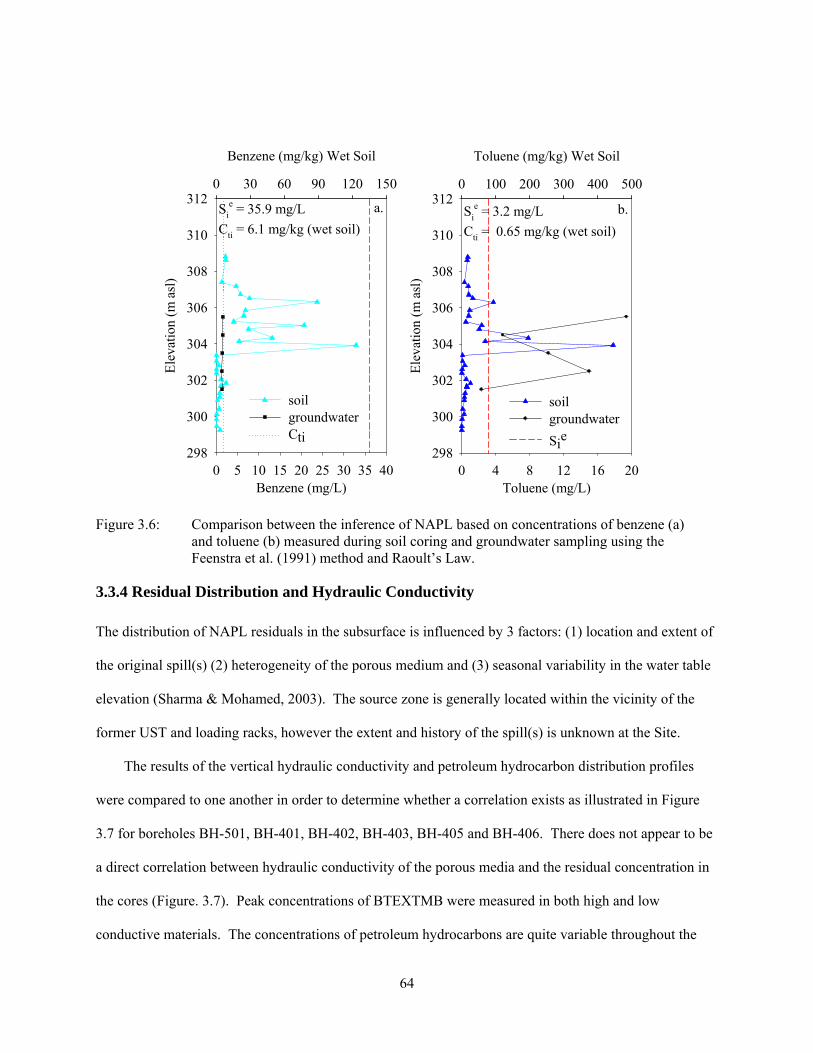
64

Benzene (mg/kg) Wet Soil

0 30 60 90 120 150E

leva

tion

(m a

sl)

298

300

302

304

306

308

310

312

Benzene (mg/L)0 5 10 15 20 25 30 35 40

soilgroundwaterCti

a.

Toluene (mg/kg) Wet Soil

0 100 200 300 400 500

Ele

vatio

n (m

asl

)

298

300

302

304

306

308

310

312

Toluene (mg/L)0 4 8 12 16 20

soilgroundwater

Sie

b.Sie = 35.9 mg/L

Cti = 6.1 mg/kg (wet soil)Si

e = 3.2 mg/L

Cti = 0.65 mg/kg (wet soil)

Figure 3.6: Comparison between the inference of NAPL based on concentrations of benzene (a) and toluene (b) measured during soil coring and groundwater sampling using the Feenstra et al. (1991) method and Raoult’s Law.

3.3.4 Residual Distribution and Hydraulic Conductivity

The distribution of NAPL residuals in the subsurface is influenced by 3 factors: (1) location and extent of

the original spill(s) (2) heterogeneity of the porous medium and (3) seasonal variability in the water table

elevation (Sharma & Mohamed, 2003). The source zone is generally located within the vicinity of the

former UST and loading racks, however the extent and history of the spill(s) is unknown at the Site.

The results of the vertical hydraulic conductivity and petroleum hydrocarbon distribution profiles

were compared to one another in order to determine whether a correlation exists as illustrated in Figure

3.7 for boreholes BH-501, BH-401, BH-402, BH-403, BH-405 and BH-406. There does not appear to be

a direct correlation between hydraulic conductivity of the porous media and the residual concentration in

the cores (Figure. 3.7). Peak concentrations of BTEXTMB were measured in both high and low

conductive materials. The concentrations of petroleum hydrocarbons are quite variable throughout the

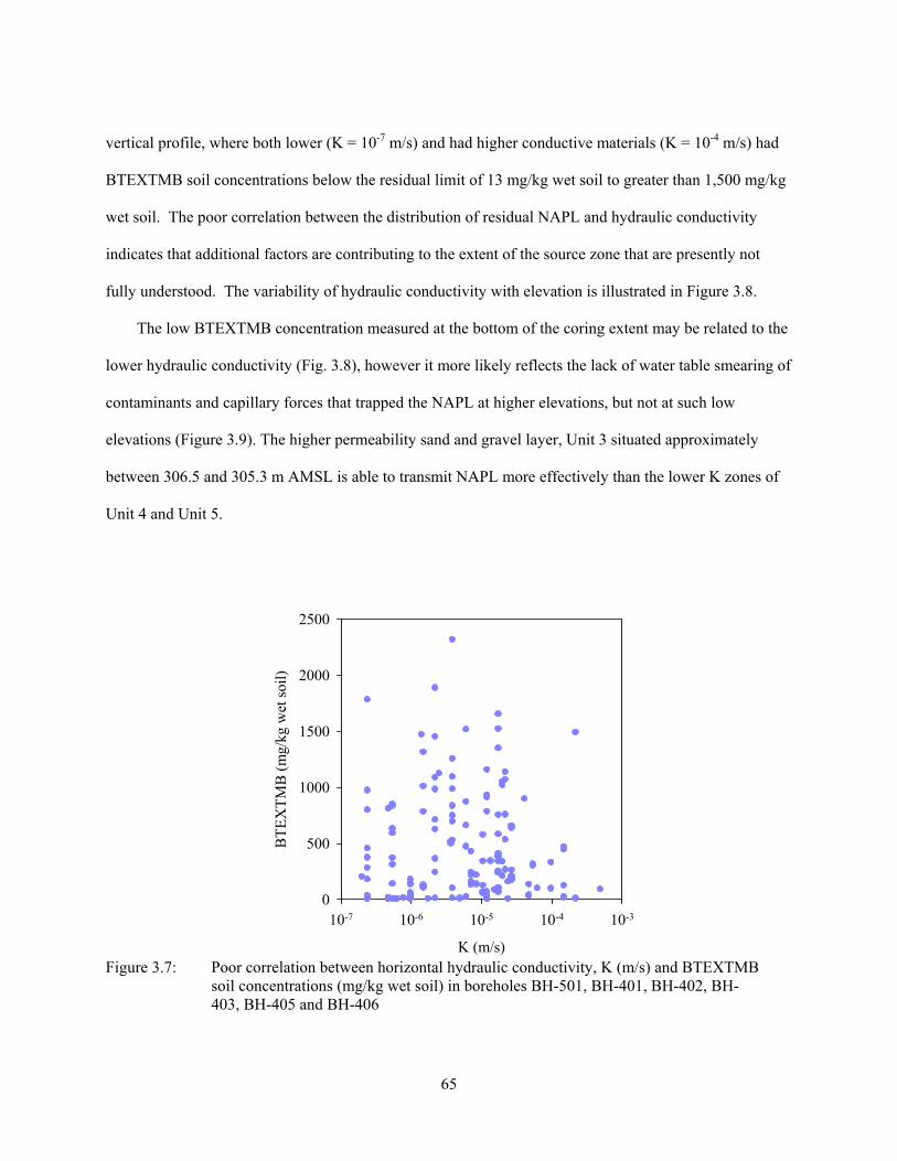
65

vertical profile, where both lower (K = 10-7 m/s) and had higher conductive materials (K = 10-4 m/s) had

BTEXTMB soil concentrations below the residual limit of 13 mg/kg wet soil to greater than 1,500 mg/kg

wet soil. The poor correlation between the distribution of residual NAPL and hydraulic conductivity

indicates that additional factors are contributing to the extent of the source zone that are presently not

fully understood. The variability of hydraulic conductivity with elevation is illustrated in Figure 3.8.

The low BTEXTMB concentration measured at the bottom of the coring extent may be related to the

lower hydraulic conductivity (Fig. 3.8), however it more likely reflects the lack of water table smearing of

contaminants and capillary forces that trapped the NAPL at higher elevations, but not at such low

elevations (Figure 3.9). The higher permeability sand and gravel layer, Unit 3 situated approximately

between 306.5 and 305.3 m AMSL is able to transmit NAPL more effectively than the lower K zones of

Unit 4 and Unit 5.

K (m/s)

10-7 10-6 10-5 10-4 10-3

BT

EX

TM

B (

mg/

kg w

et s

oil)

0

500

1000

1500

2000

2500

Figure 3.7: Poor correlation between horizontal hydraulic conductivity, K (m/s) and BTEXTMB soil concentrations (mg/kg wet soil) in boreholes BH-501, BH-401, BH-402, BH- 403, BH-405 and BH-406

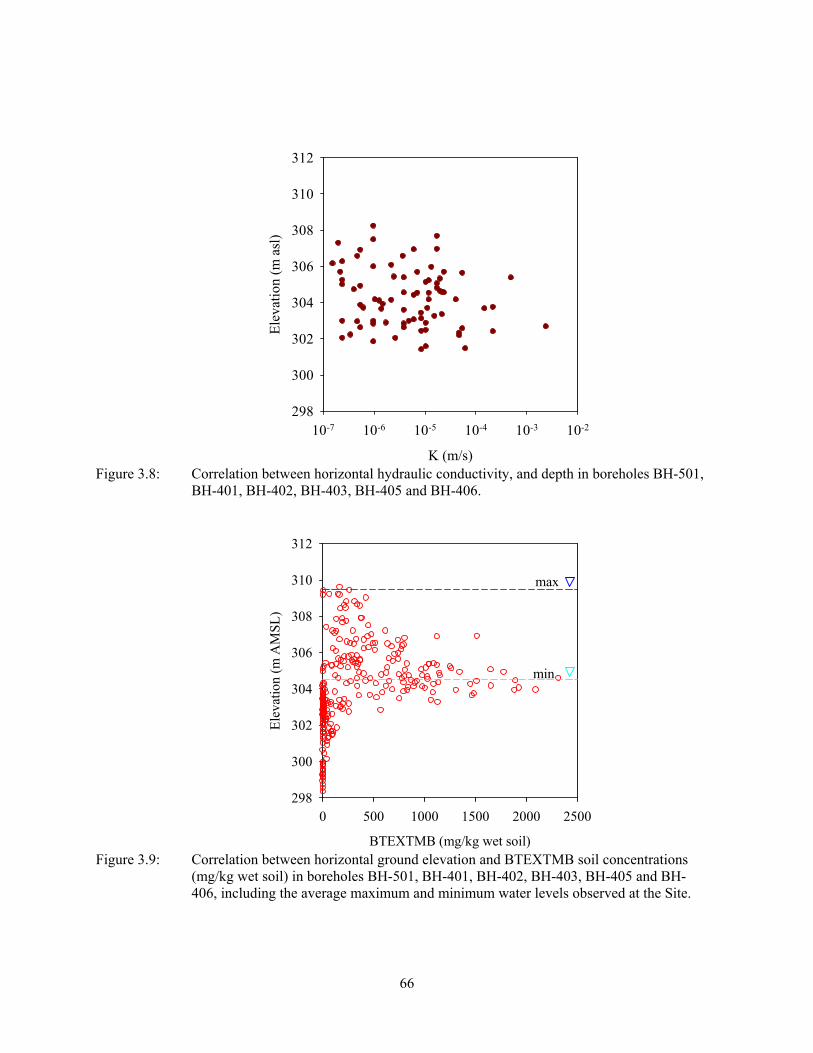
66

K (m/s)

10-7 10-6 10-5 10-4 10-3 10-2

Ele

vati

on (

m a

sl)

298

300

302

304

306

308

310

312

Figure 3.8: Correlation between horizontal hydraulic conductivity, and depth in boreholes BH-501, BH-401, BH-402, BH-403, BH-405 and BH-406.

BTEXTMB (mg/kg wet soil)

0 500 1000 1500 2000 2500

Ele

vatio

n (m

AM

SL

)

298

300

302

304

306

308

310

312

max

min

Figure 3.9: Correlation between horizontal ground elevation and BTEXTMB soil concentrations (mg/kg wet soil) in boreholes BH-501, BH-401, BH-402, BH-403, BH-405 and BH- 406, including the average maximum and minimum water levels observed at the Site.

67

Chapter 4: Laboratory Microcosm Experiment

4.1 Introduction

The objective of the experiment was to demonstrate the consumption of aromatics in a controlled

anaerobic setting, utilizing nitrate as a terminal electron acceptor in order to confirm the suitability of the

remediation technology at the field setting. Groundwater was collected from on-site petroleum impacted

monitoring wells (MW-501 and MW-302 Port 7) situated within the remedial zone of interest and

amended with nitrate and necessary nutrients to enhance microbial degradation of gasoline constituents

through denitrification in a laboratory controlled microcosm experiment. Microcosm experiments can be

used to demonstrate that a particular compound can and does degrade under ambient subsurface

conditions and in the evaluation of the effect of environmental variables on the rate and extent of

biodegradation (Border et al., 1997).

4.2 Acetylene Block Technique Method

The microcosm experiment involved the anaerobic incubation of triplicate treatment test units consisting

of a control, microbial active and microbial active amended with acetylene (C2H2). The acetylene (C2H2)

block technique is used to inhibit the reduction of nitrous oxide (N2O), to dinitrogen (N2), resulting in an

accumulation of N2O, which is indicative of denitrification (Tiedje, 1982; Yoshinari & Knowles, 1976;

Balderston et al., 1976)). The procedure involves the addition of purified acetylene gas to microcosms

containing active microbial populations. Acetylene inhibits the function of nitrous oxide reductase,

essentially stopping the reduction of nitrous oxide to elemental nitrogen (N2), in which the rate of nitrous

oxide accumulation can be measure.

BTEXTMB, F1-F3 fractions and TPH were measured in sacrificial microcosm test units throughout

the course of the 63 day incubation period in order to assess the biodegradation of contaminants. Nitrate

nitrite and nitrous oxide (acetylene amended treatment only) and DO were measured in sacrificial

68

replicate microcosms throughout the duration of the incubation period which can be used order to

establish the denitrification potential attributed to the consumption of petroleum hydrocarbons and

evaluate the anoxic conditions.

Laboratory microcosms containing groundwater and aquifer sediments (dried) collected from the

Site were augmented with nitrate and nutrients in 3 test treatments: 1) Sterile Control, 2) Active and 3)

Active C2H2 amended with 1% purified acetylene gas. Acetylene gas was purified in a gas scrubbing

train utilizing an acetylene trap scheme developed by Hyman & Arp (1987) to remove contaminants such

as acetone and carbon monoxide (CO) which may interfere with denitrification. Each individual

microcosm was spiked with a solution containing approximately 265 mg/L NO3- (0.24 mmol or 14.6 mg

NO3-), serving as the primary electron acceptor under anaerobic conditions attributed to the dominant

supply available. The acetylene block technique is useful for determining measurements of denitrification

potential, especially in systems with high concentrations of nitrate (Groffman et al., 2006).

The test solution comprised of petroleum impacted groundwater mixed with nutrients and NO3- prior

to being separated into two individual batches, Active (A) and Control (B) treatments. Batch A was

prepared as described below for the Active and Active C2H2 treatments, while batch B (control) was also

amended with 10% v/v sodium azide (NaN3), which served as a biostat limiting microbial degradation by

inhibiting NO3- reductase (Castignetti & Hollocher, 1982). Control treatment test vials and aquifer

materials were also sterilized by autoclave prior to the dispensation of the test solution. Both batches

were mixed for 1-hr using a magnetic stirrer prior to being dispensed into the designated vials.

Test treatments were prepared in sacrificial quadruplets, where 1 replicate per treatment was used to

monitor DO levels per sampling occasion. Each microcosm unit was comprised of a 60 mL clear glass

vial containing 15 g (dry weight) of pristine aquifer material, 55 mL of groundwater consisting 22 mg/L

total petroleum hydrocarbons (TPH), spiked with 60 mg/L NO3-N (265 mg/L NO3- in the form of sodium

nitrate, NaNO3) as the terminal electron acceptor and inorganic nutrients 5 mg/L NH4-N as NH4Cl and 2

mg/L phosphorus as KH2PO4 leaving approximately 4 mL of headspace. Control and active test units

69

were sealed with a Teflon-lined septum screw cap, while the Active C2H2 units were sealed with a

MinivertTM valve screw cap in order to facilitate the addition of purified acetylene gas. The Mininert TM

cap was quickly removed and approximately 1 mL of purified C2H2 was added to each Active C2H2 vial

via syringe followed by recapping and manually shaking the vial for 30 seconds in order for the aqueous

phase to equilibrate with the 4 mL headspace.

Microcosms were prepared in the anaerobic chamber containing 1% CO2, 2.5% H2O and 96.5% N2

gas, however batch test solutions were not mixed in the anaerobic setting considering the measured DO

content of the test solution was below 1 mg/L and no headspace was present in the container during

sample collection. The samples were subject to slight aeration (DO levels increased to approximately ~2

mg/L) as a result of the homogenization of the test solution, whereby the initial conditions of the

microcosm test consisted of a mixed nitrate/oxygen setup. Batch solutions were mixed intermittently

between dispensing test volumes, which re-suspended sediments and promoted representative samples

between the treatments and test replicates. Table 4.1 summarizes the list of materials and amendments in

each respective test treatment.

Table 4.1: Summary of microcosm test design applied in the study.

Batch Treatment Additives Microcosm Setup

A Active NO3-, Nutrients 4 replicates containing 15 g (dry wt)

pristine aquifer material, 55 mL test solution and 4 mL headspace in 60 mL vial, screw cap sealed

A Active C2H2 NO3-, Nutrients, C2H2

B Control NO3-, Nutrients, NaN3 biostat

The bulk of the test solution used for the microcosm study consisted of contaminated groundwater

containing approximately 13 mg/L BTEXTMB and a total of 22 mg/L TPH. The amount of available

organic contaminants serving as electron donors for microbial degradation was corrected to account for

volatile contaminant mass that was removed from the aqueous phase through partitioning into the 4 mL of

headspace. Approximately 15-30% reductions in TPH groundwater concentrations were observed in the

sterile Control units between initial (day 0) and final measurements at the end of the experiment (day 63).

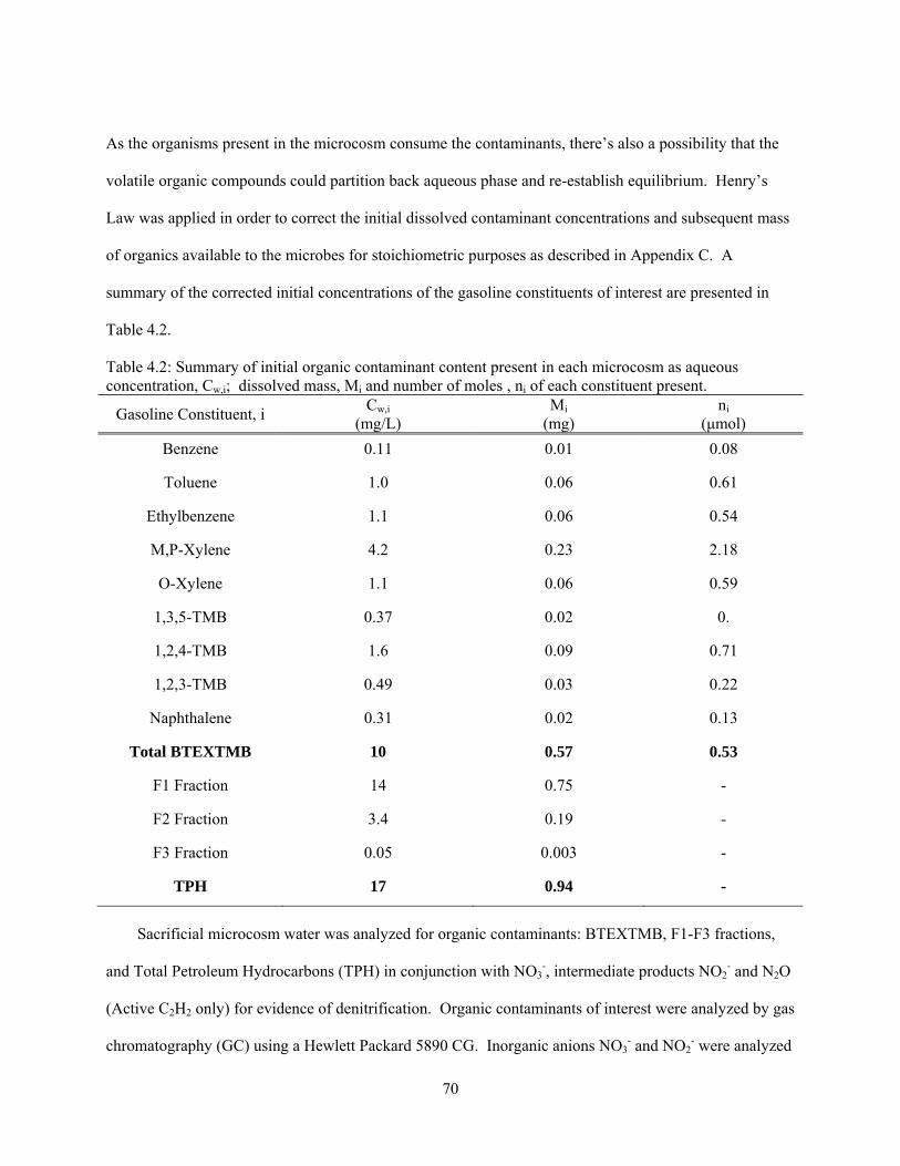
70

As the organisms present in the microcosm consume the contaminants, there’s also a possibility that the

volatile organic compounds could partition back aqueous phase and re-establish equilibrium. Henry’s

Law was applied in order to correct the initial dissolved contaminant concentrations and subsequent mass

of organics available to the microbes for stoichiometric purposes as described in Appendix C. A

summary of the corrected initial concentrations of the gasoline constituents of interest are presented in

Table 4.2.

Table 4.2: Summary of initial organic contaminant content present in each microcosm as aqueous concentration, Cw,i; dissolved mass, Mi and number of moles , ni of each constituent present.

Gasoline Constituent, i Cw,i

(mg/L) Mi

(mg) ni

(μmol)

Benzene 0.11 0.01 0.08

Toluene 1.0 0.06 0.61

Ethylbenzene 1.1 0.06 0.54

M,P-Xylene 4.2 0.23 2.18

O-Xylene 1.1 0.06 0.59

1,3,5-TMB 0.37 0.02 0.

1,2,4-TMB 1.6 0.09 0.71

1,2,3-TMB 0.49 0.03 0.22

Naphthalene 0.31 0.02 0.13

Total BTEXTMB 10 0.57 0.53

F1 Fraction 14 0.75 -

F2 Fraction 3.4 0.19 -

F3 Fraction 0.05 0.003 -

TPH 17 0.94 -

Sacrificial microcosm water was analyzed for organic contaminants: BTEXTMB, F1-F3 fractions,

and Total Petroleum Hydrocarbons (TPH) in conjunction with NO3-, intermediate products NO2

- and N2O

(Active C2H2 only) for evidence of denitrification. Organic contaminants of interest were analyzed by gas

chromatography (GC) using a Hewlett Packard 5890 CG. Inorganic anions NO3- and NO2

- were analyzed

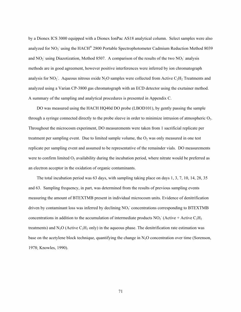
71

by a Dionex ICS 3000 equipped with a Dionex IonPac AS18 analytical column. Select samples were also

analyzed for NO3- using the HACH® 2800 Portable Spectrophotometer Cadmium Reduction Method 8039

and NO2- using Diazotization, Method 8507. A comparison of the results of the two NO3

- analysis

methods are in good agreement, however positive interferences were inferred by ion chromatograph

analysis for NO2-. Aqueous nitrous oxide N2O samples were collected from Active C2H2 Treatments and

analyzed using a Varian CP-3800 gas chromatograph with an ECD detector using the exetainer method.

A summary of the sampling and analytical procedures is presented in Appendix C.

DO was measured using the HACH HQ40d DO probe (LBOD101), by gently passing the sample

through a syringe connected directly to the probe sleeve in order to minimize intrusion of atmospheric O2.

Throughout the microcosm experiment, DO measurements were taken from 1 sacrificial replicate per

treatment per sampling event. Due to limited sample volume, the O2 was only measured in one test

replicate per sampling event and assumed to be representative of the remainder vials. DO measurements

were to confirm limited O2 availability during the incubation period, where nitrate would be preferred as

an electron acceptor in the oxidation of organic contaminants.

The total incubation period was 63 days, with sampling taking place on days 1, 3, 7, 10, 14, 28, 35

and 63. Sampling frequency, in part, was determined from the results of previous sampling events

measuring the amount of BTEXTMB present in individual microcosm units. Evidence of denitrification

driven by contaminant loss was inferred by declining NO3- concentrations corresponding to BTEXTMB

concentrations in addition to the accumulation of intermediate products NO2- (Active + Active C2H2

treatments) and N2O (Active C2H2 only) in the aqueous phase. The denitrification rate estimation was

base on the acetylene block technique, quantifying the change in N2O concentration over time (Sorenson,

1978; Knowles, 1990).

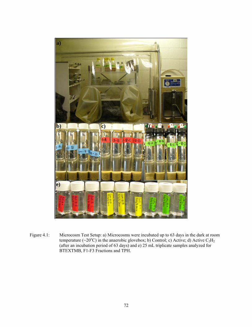
72

Figure 4.1: Microcosm Test Setup: a) Microcosms were incubated up to 63 days in the dark at room temperature (~20oC) in the anaerobic glovebox; b) Control; c) Active; d) Active C2H2 (after an incubation period of 63 days) and e) 25 mL triplicate samples analyzed for BTEXTMB, F1-F3 Fractions and TPH.

a)

b) c) d)

e)

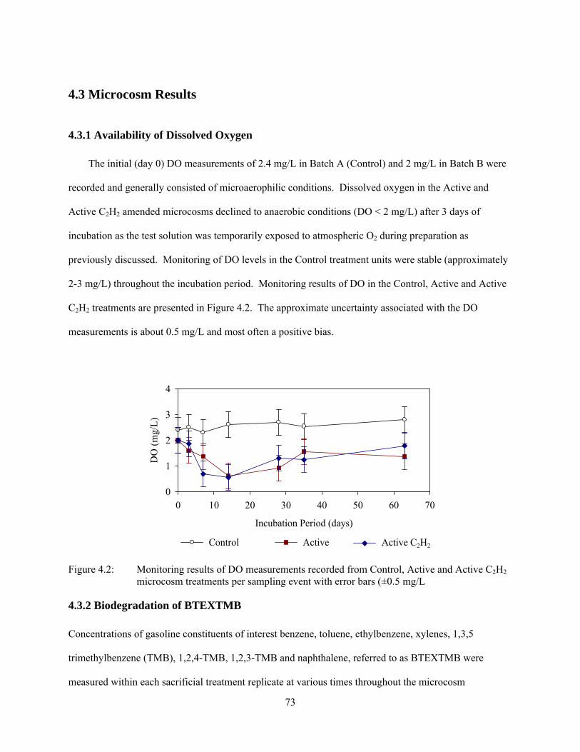
73

4.3 Microcosm Results

4.3.1 Availability of Dissolved Oxygen

The initial (day 0) DO measurements of 2.4 mg/L in Batch A (Control) and 2 mg/L in Batch B were

recorded and generally consisted of microaerophilic conditions. Dissolved oxygen in the Active and

Active C2H2 amended microcosms declined to anaerobic conditions (DO < 2 mg/L) after 3 days of

incubation as the test solution was temporarily exposed to atmospheric O2 during preparation as

previously discussed. Monitoring of DO levels in the Control treatment units were stable (approximately

2-3 mg/L) throughout the incubation period. Monitoring results of DO in the Control, Active and Active

C2H2 treatments are presented in Figure 4.2. The approximate uncertainty associated with the DO

measurements is about 0.5 mg/L and most often a positive bias.

Incubation Period (days)

0 10 20 30 40 50 60 70

DO

(m

g/L

)

0

1

2

3

4

Active C2H2Control Active

Figure 4.2: Monitoring results of DO measurements recorded from Control, Active and Active C2H2 microcosm treatments per sampling event with error bars (±0.5 mg/L

4.3.2 Biodegradation of BTEXTMB

Concentrations of gasoline constituents of interest benzene, toluene, ethylbenzene, xylenes, 1,3,5

trimethylbenzene (TMB), 1,2,4-TMB, 1,2,3-TMB and naphthalene, referred to as BTEXTMB were

measured within each sacrificial treatment replicate at various times throughout the microcosm

74

experiment in order to assess whether the native microbes are capable of degrading hydrocarbons under

denitrifying conditions. A summary of the average normalized concentration changes over the 63 day

incubation period in BTEXTMB aromatic hydrocarbons for the Control, Active and Active C2H2

treatments for the individual compounds is presented in Figure 4.3. A complete summary of the aqueous

concentrations of individual aromatic compounds, petroleum hydrocarbon fractions and TPH is presented

in Appendix C.

Average measured concentrations of BTEXTMB in the Control treatments (Fig. 4.3a) remained

relatively unchanged throughout the duration of the experiment, which is consistent with the notion that

sodium azide was applied to inhibit microbial activity. Declining concentrations of BTEXTMB were

observed in the Active and Active C2H2 treatments attributed to biodegradation (Fig.4.3b,c) The removal

of the mass of contaminants in the aqueous phase followed a sequential degradation pattern where

ethylbenzene was the first compound to be fully removed followed by toluene and naphthalene (Figures

4.3b,c). The degradation of benzene appeared to be following a similar trend (up to 14 days) when

conditions were likely microaerophilic. Degradation of o-xylene and the trimethylbenzene isomers

underwent similar behaviour to benzene, however they did not exhibit big differences during the early

phase of incubation time.

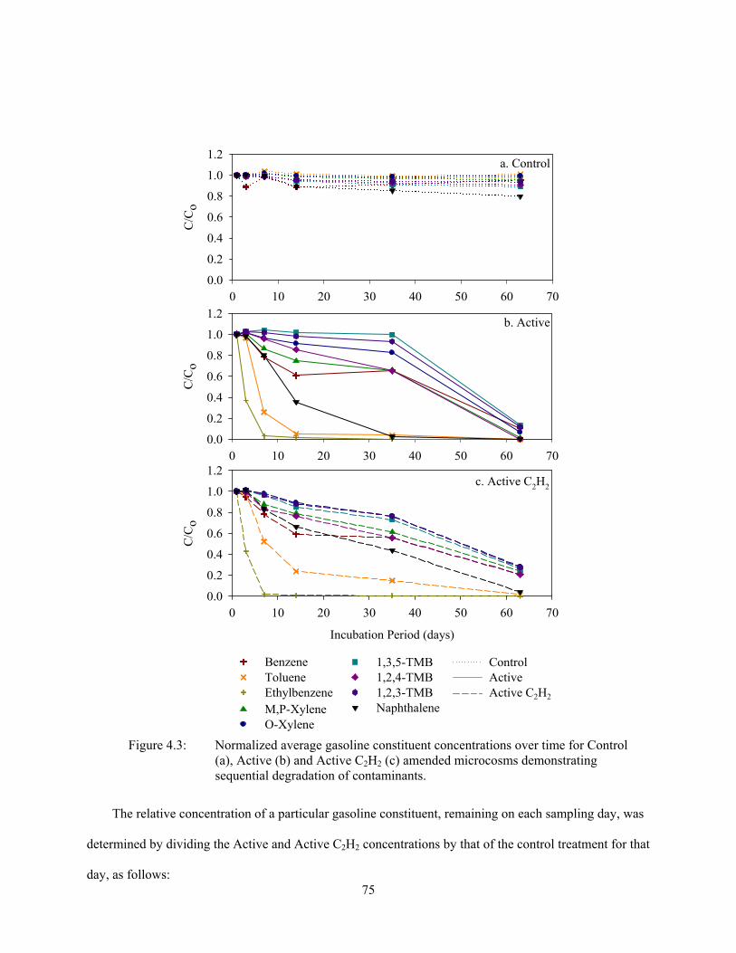
75

a. Control

0 10 20 30 40 50 60 70

C/C

o

0.0

0.2

0.4

0.6

0.8

1.0

1.2

BenzeneTolueneEthylbenzeneM,P-XyleneO-Xylene

b. Active

0 10 20 30 40 50 60 70

C/C

o

0.0

0.2

0.4

0.6

0.8

1.0

1.2

c. Active C2H2

Incubation Period (days)

0 10 20 30 40 50 60 70

C/C

o

0.0

0.2

0.4

0.6

0.8

1.0

1.2

ControlActiveActive C2H2

1,3,5-TMB1,2,4-TMB1,2,3-TMBNaphthalene

The relative concentration of a particular gasoline constituent, remaining on each sampling day, was

determined by dividing the Active and Active C2H2 concentrations by that of the control treatment for that

day, as follows:

Figure 4.3: Normalized average gasoline constituent concentrations over time for Control (a), Active (b) and Active C2H2 (c) amended microcosms demonstrating sequential degradation of contaminants.

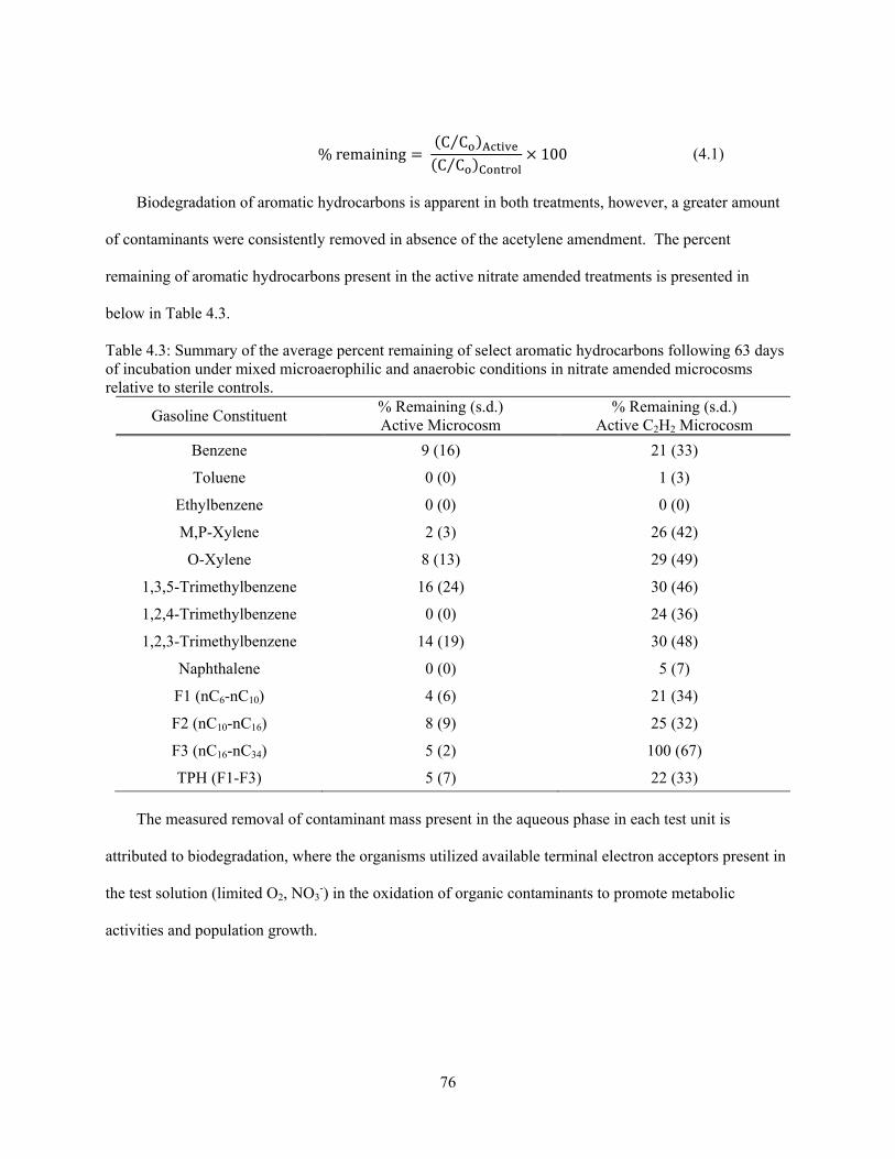
76

%remainingC C⁄

C C⁄100 (4.1)

Biodegradation of aromatic hydrocarbons is apparent in both treatments, however, a greater amount

of contaminants were consistently removed in absence of the acetylene amendment. The percent

remaining of aromatic hydrocarbons present in the active nitrate amended treatments is presented in

below in Table 4.3.

Table 4.3: Summary of the average percent remaining of select aromatic hydrocarbons following 63 days of incubation under mixed microaerophilic and anaerobic conditions in nitrate amended microcosms relative to sterile controls.

Gasoline Constituent % Remaining (s.d.) Active Microcosm

% Remaining (s.d.) Active C2H2 Microcosm

Benzene 9 (16) 21 (33)

Toluene 0 (0) 1 (3)

Ethylbenzene 0 (0) 0 (0)

M,P-Xylene 2 (3) 26 (42)

O-Xylene 8 (13) 29 (49)

1,3,5-Trimethylbenzene 16 (24) 30 (46)

1,2,4-Trimethylbenzene 0 (0) 24 (36)

1,2,3-Trimethylbenzene 14 (19) 30 (48)

Naphthalene 0 (0) 5 (7)

F1 (nC6-nC10) 4 (6) 21 (34)

F2 (nC10-nC16) 8 (9) 25 (32)

F3 (nC16-nC34) 5 (2) 100 (67)

TPH (F1-F3) 5 (7) 22 (33)

The measured removal of contaminant mass present in the aqueous phase in each test unit is

attributed to biodegradation, where the organisms utilized available terminal electron acceptors present in

the test solution (limited O2, NO3-) in the oxidation of organic contaminants to promote metabolic

activities and population growth.

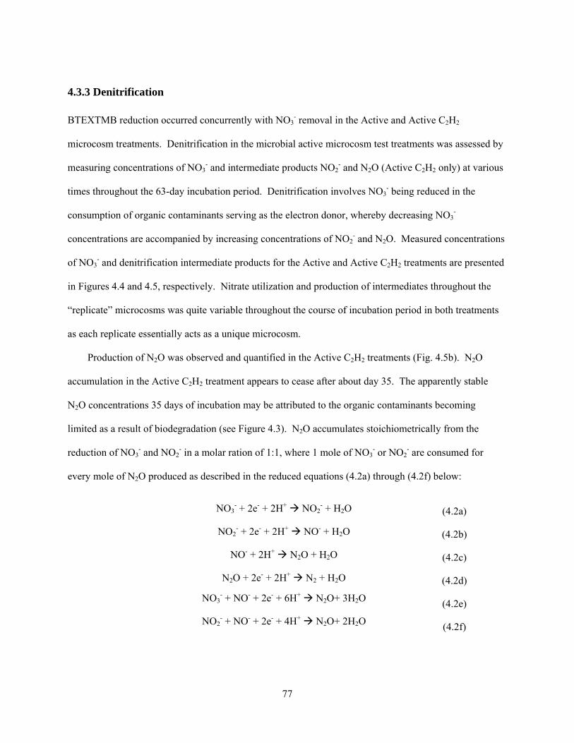
77

4.3.3 Denitrification

BTEXTMB reduction occurred concurrently with NO3- removal in the Active and Active C2H2

microcosm treatments. Denitrification in the microbial active microcosm test treatments was assessed by

measuring concentrations of NO3- and intermediate products NO2

- and N2O (Active C2H2 only) at various

times throughout the 63-day incubation period. Denitrification involves NO3- being reduced in the

consumption of organic contaminants serving as the electron donor, whereby decreasing NO3-

concentrations are accompanied by increasing concentrations of NO2- and N2O. Measured concentrations

of NO3- and denitrification intermediate products for the Active and Active C2H2 treatments are presented

in Figures 4.4 and 4.5, respectively. Nitrate utilization and production of intermediates throughout the

“replicate” microcosms was quite variable throughout the course of incubation period in both treatments

as each replicate essentially acts as a unique microcosm.

Production of N2O was observed and quantified in the Active C2H2 treatments (Fig. 4.5b). N2O

accumulation in the Active C2H2 treatment appears to cease after about day 35. The apparently stable

N2O concentrations 35 days of incubation may be attributed to the organic contaminants becoming

limited as a result of biodegradation (see Figure 4.3). N2O accumulates stoichiometrically from the

reduction of NO3- and NO2

- in a molar ration of 1:1, where 1 mole of NO3- or NO2

- are consumed for

every mole of N2O produced as described in the reduced equations (4.2a) through (4.2f) below:

NO3- + 2e- + 2H+ NO2

- + H2O (4.2a)

NO2- + 2e- + 2H+ NO- + H2O (4.2b)

NO- + 2H+ N2O + H2O (4.2c)

N2O + 2e- + 2H+ N2 + H2O (4.2d)

NO3- + NO- + 2e- + 6H+ N2O+ 3H2O (4.2e)

NO2- + NO- + 2e- + 4H+ N2O+ 2H2O (4.2f)

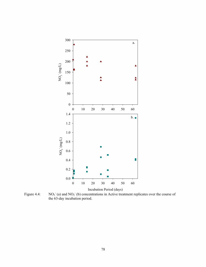
78

0 10 20 30 40 50 60

NO

3- (m

g/L

)

0

50

100

150

200

250

300

Incubation Period (days)

0 10 20 30 40 50 60

NO

2- (m

g/L

)

0.0

0.2

0.4

0.6

0.8

1.0

1.2

1.4b.

a.

Figure 4.4: NO3

- (a) and NO2- (b) concentrations in Active treatment replicates over the course of

the 63-day incubation period.

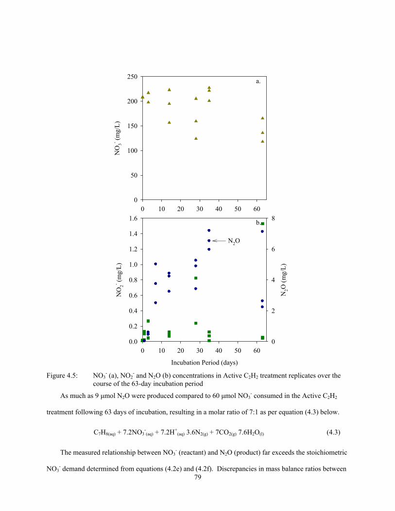
79

Incubation Period (days)

0 10 20 30 40 50 60

NO

2- (m

g/L

)

0.0

0.2

0.4

0.6

0.8

1.0

1.2

1.4

1.6

N2O

(m

g/L

)

0

2

4

6

8

0 10 20 30 40 50 60

NO

3- (m

g/L

)

0

50

100

150

200

250

N2O

a.

b.

Figure 4.5: NO3- (a), NO2

- and N2O (b) concentrations in Active C2H2 treatment replicates over the course of the 63-day incubation period

As much as 9 μmol N2O were produced compared to 60 μmol NO3- consumed in the Active C2H2

treatment following 63 days of incubation, resulting in a molar ratio of 7:1 as per equation (4.3) below.

C7H8(aq) + 7.2NO3-(aq) + 7.2H+

(aq) 3.6N2(g) + 7CO2(g) 7.6H2O(l) (4.3)

The measured relationship between NO3- (reactant) and N2O (product) far exceeds the stoichiometric

NO3- demand determined from equations (4.2e) and (4.2f). Discrepancies in mass balance ratios between

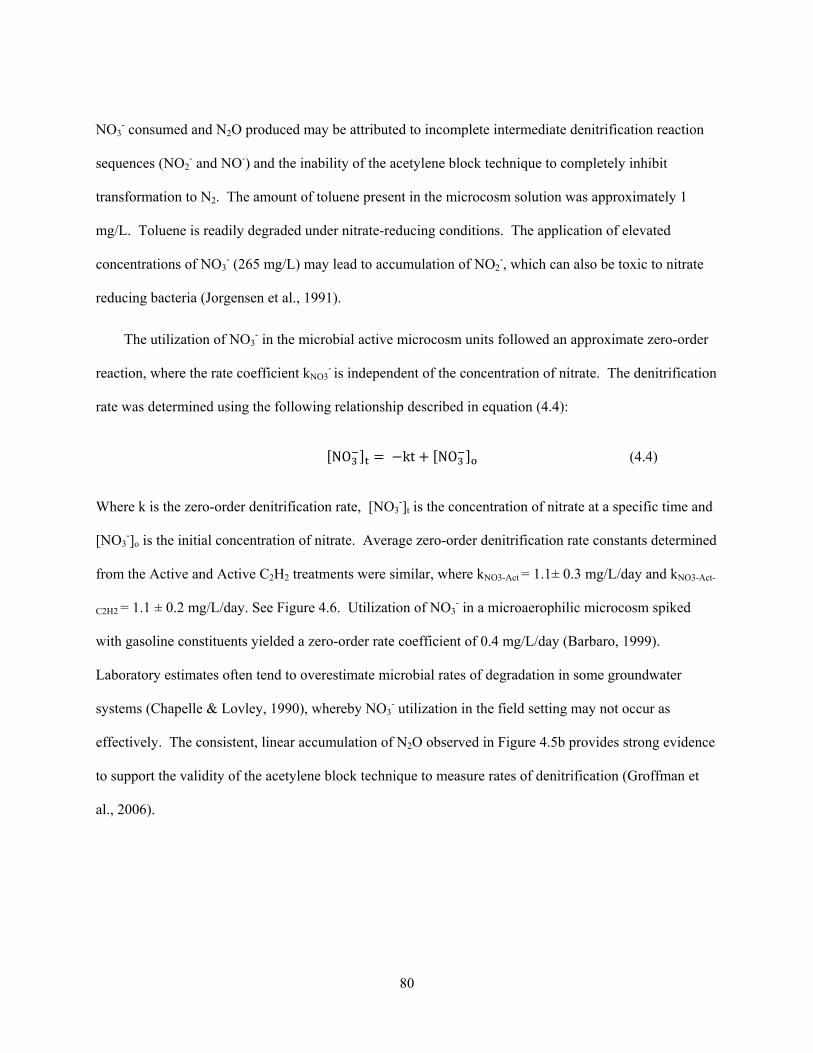
80

NO3- consumed and N2O produced may be attributed to incomplete intermediate denitrification reaction

sequences (NO2- and NO-) and the inability of the acetylene block technique to completely inhibit

transformation to N2. The amount of toluene present in the microcosm solution was approximately 1

mg/L. Toluene is readily degraded under nitrate-reducing conditions. The application of elevated

concentrations of NO3- (265 mg/L) may lead to accumulation of NO2

-, which can also be toxic to nitrate

reducing bacteria (Jorgensen et al., 1991).

The utilization of NO3- in the microbial active microcosm units followed an approximate zero-order

reaction, where the rate coefficient kNO3- is independent of the concentration of nitrate. The denitrification

rate was determined using the following relationship described in equation (4.4):

NO kt NO (4.4)

Where k is the zero-order denitrification rate, [NO3-]t is the concentration of nitrate at a specific time and

[NO3-]o is the initial concentration of nitrate. Average zero-order denitrification rate constants determined

from the Active and Active C2H2 treatments were similar, where kNO3-Act = 1.1± 0.3 mg/L/day and kNO3-Act-

C2H2 = 1.1 ± 0.2 mg/L/day. See Figure 4.6. Utilization of NO3- in a microaerophilic microcosm spiked

with gasoline constituents yielded a zero-order rate coefficient of 0.4 mg/L/day (Barbaro, 1999).

Laboratory estimates often tend to overestimate microbial rates of degradation in some groundwater

systems (Chapelle & Lovley, 1990), whereby NO3- utilization in the field setting may not occur as

effectively. The consistent, linear accumulation of N2O observed in Figure 4.5b provides strong evidence

to support the validity of the acetylene block technique to measure rates of denitrification (Groffman et

al., 2006).

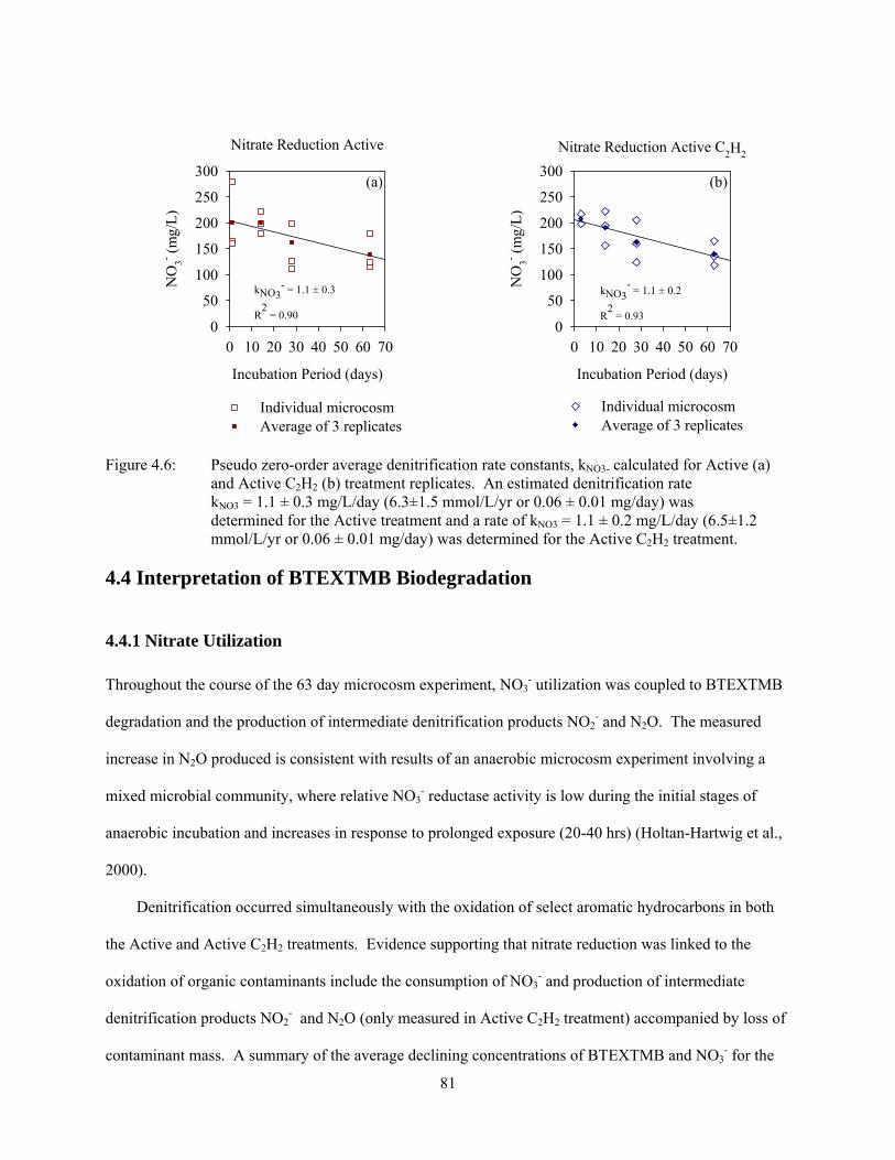
81

Nitrate Reduction Active C2H2

Incubation Period (days)

0 10 20 30 40 50 60 70

NO

3- (m

g/L

)

0

50

100

150

200

250

300

Individual microcosmAverage of 3 replicates

Nitrate Reduction Active

Incubation Period (days)

0 10 20 30 40 50 60 70

NO

3- (m

g/L

)

0

50

100

150

200

250

300

Individual microcosmAverage of 3 replicates

kNO3- = 1.1 ± 0.2

R2

= 0.93

kNO3- = 1.1 ± 0.3

R2

= 0.90

(a) (b)

Figure 4.6: Pseudo zero-order average denitrification rate constants, kNO3- calculated for Active (a) and Active C2H2 (b) treatment replicates. An estimated denitrification rate kNO3 = 1.1 ± 0.3 mg/L/day (6.3±1.5 mmol/L/yr or 0.06 ± 0.01 mg/day) was determined for the Active treatment and a rate of kNO3 = 1.1 ± 0.2 mg/L/day (6.5±1.2 mmol/L/yr or 0.06 ± 0.01 mg/day) was determined for the Active C2H2 treatment.

4.4 Interpretation of BTEXTMB Biodegradation

4.4.1 Nitrate Utilization

Throughout the course of the 63 day microcosm experiment, NO3- utilization was coupled to BTEXTMB

degradation and the production of intermediate denitrification products NO2- and N2O. The measured

increase in N2O produced is consistent with results of an anaerobic microcosm experiment involving a

mixed microbial community, where relative NO3- reductase activity is low during the initial stages of

anaerobic incubation and increases in response to prolonged exposure (20-40 hrs) (Holtan-Hartwig et al.,

2000).

Denitrification occurred simultaneously with the oxidation of select aromatic hydrocarbons in both

the Active and Active C2H2 treatments. Evidence supporting that nitrate reduction was linked to the

oxidation of organic contaminants include the consumption of NO3- and production of intermediate

denitrification products NO2- and N2O (only measured in Active C2H2 treatment) accompanied by loss of

contaminant mass. A summary of the average declining concentrations of BTEXTMB and NO3- for the

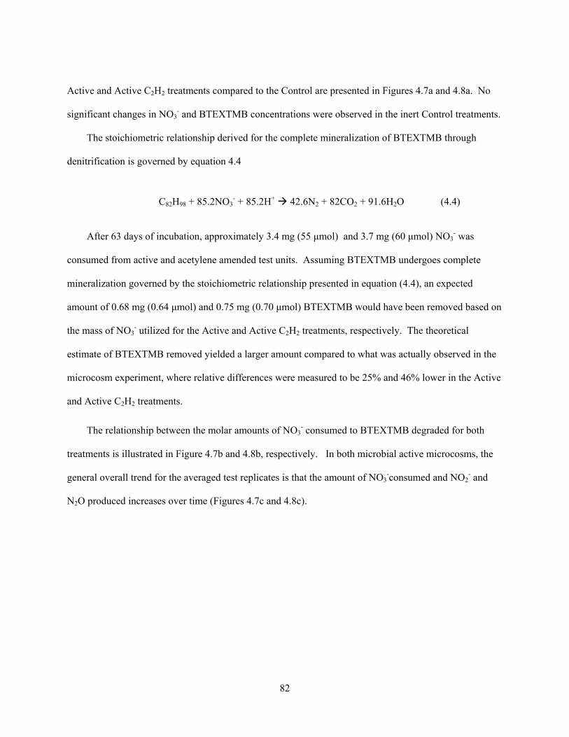
82

Active and Active C2H2 treatments compared to the Control are presented in Figures 4.7a and 4.8a. No

significant changes in NO3- and BTEXTMB concentrations were observed in the inert Control treatments.

The stoichiometric relationship derived for the complete mineralization of BTEXTMB through

denitrification is governed by equation 4.4

C82H98 + 85.2NO3- + 85.2H+ 42.6N2 + 82CO2 + 91.6H2O (4.4)

After 63 days of incubation, approximately 3.4 mg (55 μmol) and 3.7 mg (60 μmol) NO3- was

consumed from active and acetylene amended test units. Assuming BTEXTMB undergoes complete

mineralization governed by the stoichiometric relationship presented in equation (4.4), an expected

amount of 0.68 mg (0.64 μmol) and 0.75 mg (0.70 μmol) BTEXTMB would have been removed based on

the mass of NO3- utilized for the Active and Active C2H2 treatments, respectively. The theoretical

estimate of BTEXTMB removed yielded a larger amount compared to what was actually observed in the

microcosm experiment, where relative differences were measured to be 25% and 46% lower in the Active

and Active C2H2 treatments.

The relationship between the molar amounts of NO3- consumed to BTEXTMB degraded for both

treatments is illustrated in Figure 4.7b and 4.8b, respectively. In both microbial active microcosms, the

general overall trend for the averaged test replicates is that the amount of NO3-consumed and NO2

- and

N2O produced increases over time (Figures 4.7c and 4.8c).

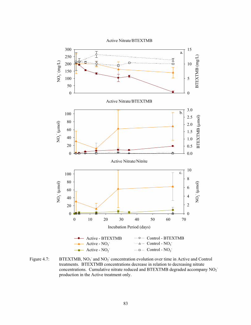
83

Active Nitrate/BTEXTMB

BT

EX

TM

B (

mg/

L)

0

5

10

15

NO

3- (m

g/L

)

0

50

100

150

200

250

300

Active - BTEXTMBActive - NO3

-

Active - NO2-

Active Nitrate/BTEXTMB

NO

3- (m

ol)

0

20

40

60

80

100

BT

EX

TM

B (m

ol)

0.0

0.5

1.0

1.5

2.0

2.5

3.0

Control - BTEXTMBControl - NO3

-

Control - NO2-

Active Nitrate/Nitrite

Incubation Period (days)

0 10 20 30 40 50 60 70

NO

3- (m

ol)

0

20

40

60

80

100

NO

2- (m

ol)

0

2

4

6

8

10

a.

b.

c.

Figure 4.7: BTEXTMB, NO3

- and NO2- concentration evolution over time in Active and Control

treatments. BTEXTMB concentrations decrease in relation to decreasing nitrate concentrations. Cumulative nitrate reduced and BTEXTMB degraded accompany NO2

- production in the Active treatment only.

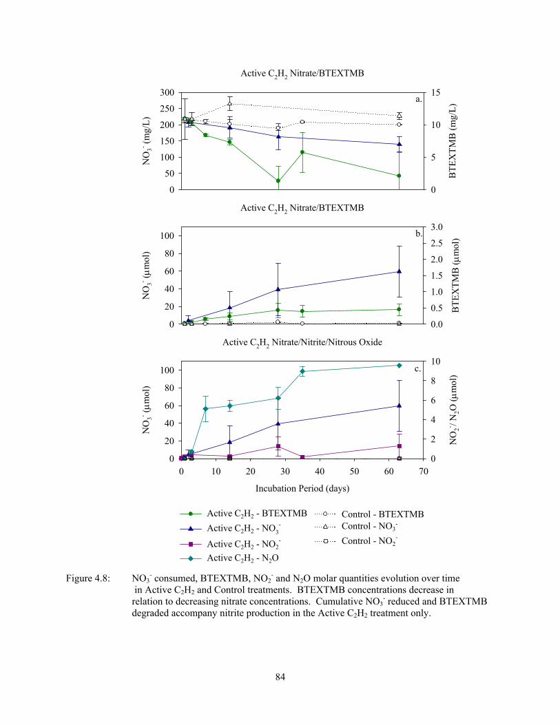
84

Active C2H2 Nitrate/Nitrite/Nitrous Oxide

Incubation Period (days)

0 10 20 30 40 50 60 70

NO

3- (m

ol)

0

20

40

60

80

100

NO

2- / N2O

(m

ol)

0

2

4

6

8

10

Active C2H2 Nitrate/BTEXTMB

BT

EX

TM

B (m

ol)

0.0

0.5

1.0

1.5

2.0

2.5

3.0

NO

3- (m

ol)

0

20

40

60

80

100

Active C2H2 - BTEXTMB

Active C2H2 - NO3-

Active C2H2 - NO2-

Active C2H2 - N2O

Active C2H2 Nitrate/BTEXTMB

NO

3- (m

g/L

)

0

50

100

150

200

250

300

BT

EX

TM

B (

mg/

L)

0

5

10

15

Control - BTEXTMBControl - NO3

-

Control - NO2-

b.

a.

c.

Figure 4.8: NO3

- consumed, BTEXTMB, NO2- and N2O molar quantities evolution over time

in Active C2H2 and Control treatments. BTEXTMB concentrations decrease in relation to decreasing nitrate concentrations. Cumulative NO3

- reduced and BTEXTMB degraded accompany nitrite production in the Active C2H2 treatment only.

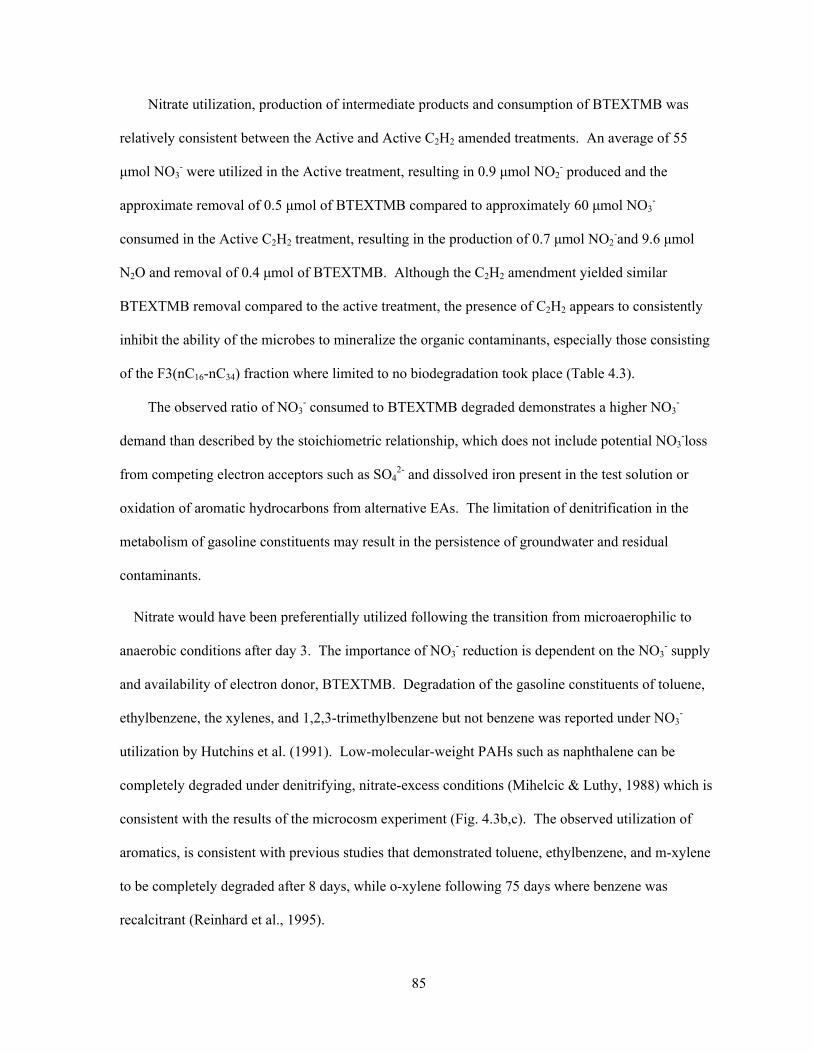
85

Nitrate utilization, production of intermediate products and consumption of BTEXTMB was

relatively consistent between the Active and Active C2H2 amended treatments. An average of 55

μmol NO3- were utilized in the Active treatment, resulting in 0.9 μmol NO2

- produced and the

approximate removal of 0.5 μmol of BTEXTMB compared to approximately 60 μmol NO3-

consumed in the Active C2H2 treatment, resulting in the production of 0.7 μmol NO2-and 9.6 μmol

N2O and removal of 0.4 μmol of BTEXTMB. Although the C2H2 amendment yielded similar

BTEXTMB removal compared to the active treatment, the presence of C2H2 appears to consistently

inhibit the ability of the microbes to mineralize the organic contaminants, especially those consisting

of the F3(nC16-nC34) fraction where limited to no biodegradation took place (Table 4.3).

The observed ratio of NO3- consumed to BTEXTMB degraded demonstrates a higher NO3

-

demand than described by the stoichiometric relationship, which does not include potential NO3-loss

from competing electron acceptors such as SO42- and dissolved iron present in the test solution or

oxidation of aromatic hydrocarbons from alternative EAs. The limitation of denitrification in the

metabolism of gasoline constituents may result in the persistence of groundwater and residual

contaminants.

Nitrate would have been preferentially utilized following the transition from microaerophilic to

anaerobic conditions after day 3. The importance of NO3- reduction is dependent on the NO3

- supply

and availability of electron donor, BTEXTMB. Degradation of the gasoline constituents of toluene,

ethylbenzene, the xylenes, and 1,2,3-trimethylbenzene but not benzene was reported under NO3-

utilization by Hutchins et al. (1991). Low-molecular-weight PAHs such as naphthalene can be

completely degraded under denitrifying, nitrate-excess conditions (Mihelcic & Luthy, 1988) which is

consistent with the results of the microcosm experiment (Fig. 4.3b,c). The observed utilization of

aromatics, is consistent with previous studies that demonstrated toluene, ethylbenzene, and m-xylene

to be completely degraded after 8 days, while o-xylene following 75 days where benzene was

recalcitrant (Reinhard et al., 1995).

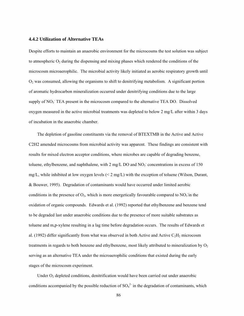
86

4.4.2 Utilization of Alternative TEAs

Despite efforts to maintain an anaerobic environment for the microcosms the test solution was subject

to atmospheric O2 during the dispensing and mixing phases which rendered the conditions of the

microcosm microaerophilic. The microbial activity likely initiated as aerobic respiratory growth until

O2 was consumed, allowing the organisms to shift to denitrifying metabolism. A significant portion

of aromatic hydrocarbon mineralization occurred under denitrifying conditions due to the large

supply of NO3- TEA present in the microcosm compared to the alternative TEA DO. Dissolved

oxygen measured in the active microbial treatments was depleted to below 2 mg/L after within 3 days

of incubation in the anaerobic chamber.

The depletion of gasoline constituents via the removal of BTEXTMB in the Active and Active

C2H2 amended microcosms from microbial activity was apparent. These findings are consistent with

results for mixed electron acceptor conditions, where microbes are capable of degrading benzene,

toluene, ethylbenzene, and naphthalene, with 2 mg/L DO and NO3- concentrations in excess of 150

mg/L, while inhibited at low oxygen levels (< 2 mg/L) with the exception of toluene (Wilson, Durant,

& Bouwer, 1995). Degradation of contaminants would have occurred under limited aerobic

conditions in the presence of O2, which is more energetically favourable compared to NO3-in the

oxidation of organic compounds. Edwards et al. (1992) reported that ethylbenzene and benzene tend

to be degraded last under anaerobic conditions due to the presence of more suitable substrates as

toluene and m,p-xylene resulting in a lag time before degradation occurs. The results of Edwards et

al. (1992) differ significantly from what was observed in both Active and Active C2H2 microcosm

treatments in regards to both benzene and ethylbenzene, most likely attributed to mineralization by O2

serving as an alternative TEA under the microaerophilic conditions that existed during the early

stages of the microcosm experiment.

Under O2 depleted conditions, denitrification would have been carried out under anaerobic

conditions accompanied by the possible reduction of SO42- in the degradation of contaminants, which

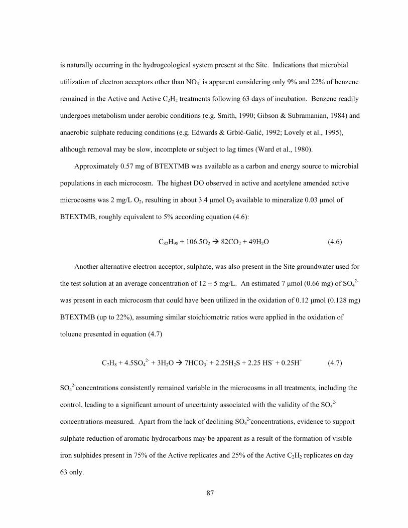
87

is naturally occurring in the hydrogeological system present at the Site. Indications that microbial

utilization of electron acceptors other than NO3- is apparent considering only 9% and 22% of benzene

remained in the Active and Active C2H2 treatments following 63 days of incubation. Benzene readily

undergoes metabolism under aerobic conditions (e.g. Smith, 1990; Gibson & Subramanian, 1984) and

anaerobic sulphate reducing conditions (e.g. Edwards & Grbić-Galić, 1992; Lovely et al., 1995),

although removal may be slow, incomplete or subject to lag times (Ward et al., 1980).

Approximately 0.57 mg of BTEXTMB was available as a carbon and energy source to microbial

populations in each microcosm. The highest DO observed in active and acetylene amended active

microcosms was 2 mg/L O2, resulting in about 3.4 μmol O2 available to mineralize 0.03 μmol of

BTEXTMB, roughly equivalent to 5% according equation (4.6):

C82H98 + 106.5O2 82CO2 + 49H2O (4.6)

Another alternative electron acceptor, sulphate, was also present in the Site groundwater used for

the test solution at an average concentration of 12 ± 5 mg/L. An estimated 7 μmol (0.66 mg) of SO42-

was present in each microcosm that could have been utilized in the oxidation of 0.12 μmol (0.128 mg)

BTEXTMB (up to 22%), assuming similar stoichiometric ratios were applied in the oxidation of

toluene presented in equation (4.7)

C7H8 + 4.5SO42- + 3H2O 7HCO3

- + 2.25H2S + 2.25 HS- + 0.25H+ (4.7)

SO42-concentrations consistently remained variable in the microcosms in all treatments, including the

control, leading to a significant amount of uncertainty associated with the validity of the SO42-

concentrations measured. Apart from the lack of declining SO42-concentrations, evidence to support

sulphate reduction of aromatic hydrocarbons may be apparent as a result of the formation of visible

iron sulphides present in 75% of the Active replicates and 25% of the Active C2H2 replicates on day

63 only.

88

4.5 Microcosm Summary

Biodegradation of BTEXTMB, F1-F3 fractions and TPH occurred in microcosms equipped with a

mixed indigenous microbial source obtained from the study area. The acetylene block microcosm

experiment was successful in establishing that the organisms were capable of utilizing nitrate in the

metabolism of petroleum hydrocarbons. In general, the consumption of NO3- coincided with

reductions in the mass of BTEXTMB present in the microcosm units, in addition to the observed

increase in the production of denitrification intermediate products NO2- (Active and Active C2H2) and

N2O (Active C2H2 only). The findings of the microcosm experiment confirm that the application of

NO3- to enhance the microbial degradation of petroleum hydrocarbons at a larger scale field setting is

a suitable remedial approach to target contaminants at residual saturation in the anaerobic aquifer

present at the Site.

89

Chapter 5: Residual Zone Treatment System Design

5.1 Remediation Approach

Several pulses consisting of known mass of non-reactive (Br-) and reactive tracer (NO3-) solution

were released into the anaerobic aquifer. The pulse solution was allowed to drift under natural

gradient conditions to target residual contaminants distributed within Unit 3 (sand and gravel) and

Unit 4 (sand). Three dimensional monitoring of the Br- tracer plume was carried out using an

extensive multilevel well network downgradient of the injection well. The analysis of the Br- tracer

monitoring determined the variability of hydraulic conductivity and contaminant distribution, as

previously discussed in Chapters 2 and 3.

A series of field tracer injections characterized the transport and utilization rates of NO3- in a

portion of the residual petroleum hydrocarbon impacted zone. The tracer test solution was delivered

by a consecutive series of injections with the purpose of providing a continuous supply of TEA

available to the indigenous microbial populations. The tracer injection test was designed to:

1) Evaluate the delivery of remedial solution to distinct geological layers of different permeability

2) Estimate denitrification rates using tracer breakthrough curves (BTCs) in a heterogeneous aquifer, and

3) Evaluate the removal of residual saturation contaminants in the study area using soil coring techniques and post-treatment groundwater sampling to evaluate the dissolved phase.

5.2 Target Remediation Zone

The selected target treatment zone was based on the aquifer composition, distribution of residuals,

and the vertical extent of the seasonal saturated zone. The target zone is located 305 to 303 m AMSL

(6.2 to 8.2 meters below ground surface). The remedial system design established delivery of the

remedial solutions to Unit 4 situated below the seasonal minimal water table in an area where

residuals are present. Residuals serve as a long term source of contamination and contribute to

90

vapour phase and dissolved phase plumes, thus the residual zone was targeted for biostimulation to

enhance in situ bioremediation. The removal of contaminant source mass is advantageous in

remediation technologies as there is a reduction in the mass of contaminants discharged to the plume

(e.g. Rao et al., 2001).

Additional soil coring (400 series cores) confirmed that Unit 4 is to some extent continuous at

the same depth down gradient and comes into contact with similar materials throughout the study

area, as indicated by the borehole logs presented in Appendix B. Investigating sediment

characterization revealed that Unit 4 is subject to small scale heterogeneities inferred from hydraulic

conductivity estimates carried out by grain size analysis. Therefore, Unit 4 was selected as a suitable

treatment zone to promote the effective delivery and performance of the remedial solution within the

target residual zone as heterogeneities in aquifer sediments can constrain hydrogeologic transport of

remedial additions and biogeochemical reactions (e.g. Cozzarelli et al., 1999).

As discussed in Chapter 3, it was challenging to determine the complex distribution of residual

contaminants in the subsurface. The vertical and spatial distribution of BTEXTMB soil

concentrations indicate that the majority of the aquifer materials investigated to depths between 310

and 302 m AMSL (1 and 9 mbgs) contain immobile NAPL phase. The presence of NAPL is inferred

based on the soil concentrations exceeding 13 mg/kg (wet soil), with the value determined, using the

Feenstra et al. method (1991) while mobile NAPL is inferred for BTEXTMB exceeding 3,000 mg/k

(wet soil) as previously discussed. Measured concentrations did not surpass 3,000 mg/kg, however

NAPL recovered in the field reveal that seasonal re-distribution of NAPL is likely occurring under

dynamic hydrogeologic conditions.

To satisfy the requirements that the remedial solution be transferred below the water table at any

given time and administered within stratigraphic Unit 4, BTEXTMB soil extract concentrations in

BH-301 and BH-302 retrieved in fall 2007 were then examined to assess the distribution of

contaminants. The targeted depth interval selected based on the aforementioned criteria was between

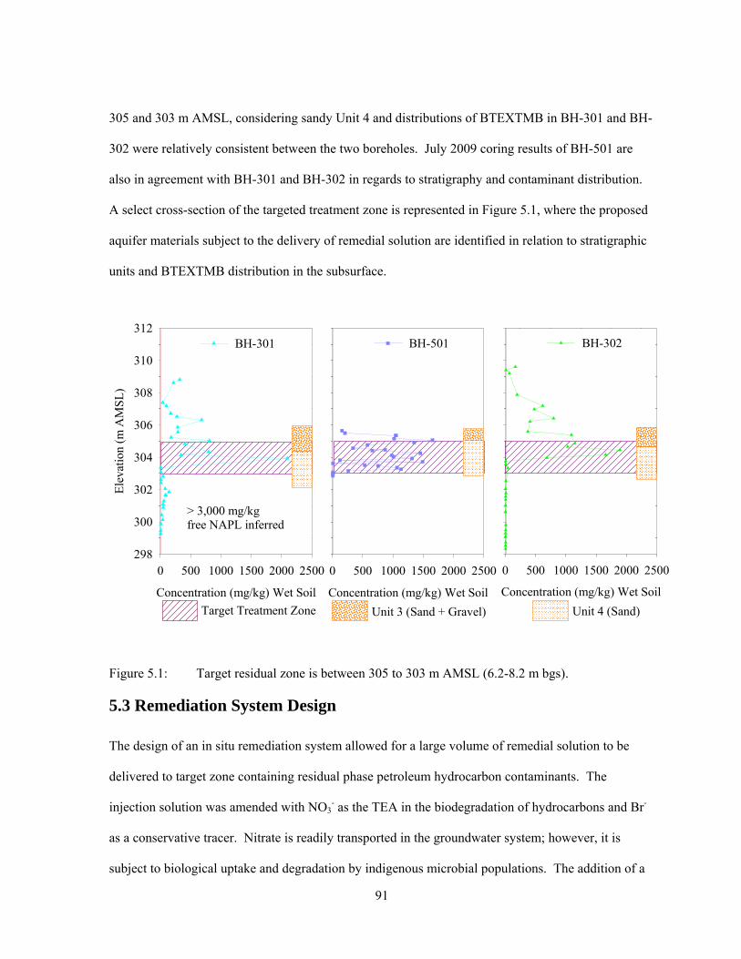
91

305 and 303 m AMSL, considering sandy Unit 4 and distributions of BTEXTMB in BH-301 and BH-

302 were relatively consistent between the two boreholes. July 2009 coring results of BH-501 are

also in agreement with BH-301 and BH-302 in regards to stratigraphy and contaminant distribution.

A select cross-section of the targeted treatment zone is represented in Figure 5.1, where the proposed

aquifer materials subject to the delivery of remedial solution are identified in relation to stratigraphic

units and BTEXTMB distribution in the subsurface.

Concentration (mg/kg) Wet Soil

0 500 1000 1500 2000 2500

Ele

vatio

n (m

AM

SL

)

298

300

302

304

306

308

310

312BH-301

Concentration (mg/kg) Wet Soil

0 500 1000 1500 2000 2500

BH-501

Concentration (mg/kg) Wet Soil

0 500 1000 1500 2000 2500

BH-302

Unit 3 (Sand + Gravel) Unit 4 (Sand)Target Treatment Zone

> 3,000 mg/kg free NAPL inferred

Figure 5.1: Target residual zone is between 305 to 303 m AMSL (6.2-8.2 m bgs).

5.3 Remediation System Design

The design of an in situ remediation system allowed for a large volume of remedial solution to be

delivered to target zone containing residual phase petroleum hydrocarbon contaminants. The

injection solution was amended with NO3- as the TEA in the biodegradation of hydrocarbons and Br-

as a conservative tracer. Nitrate is readily transported in the groundwater system; however, it is

subject to biological uptake and degradation by indigenous microbial populations. The addition of a

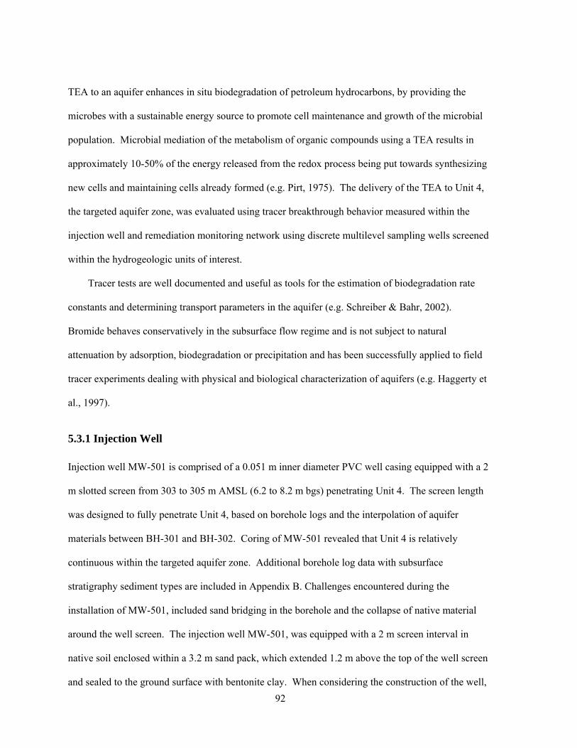
92

TEA to an aquifer enhances in situ biodegradation of petroleum hydrocarbons, by providing the

microbes with a sustainable energy source to promote cell maintenance and growth of the microbial

population. Microbial mediation of the metabolism of organic compounds using a TEA results in

approximately 10-50% of the energy released from the redox process being put towards synthesizing

new cells and maintaining cells already formed (e.g. Pirt, 1975). The delivery of the TEA to Unit 4,

the targeted aquifer zone, was evaluated using tracer breakthrough behavior measured within the

injection well and remediation monitoring network using discrete multilevel sampling wells screened

within the hydrogeologic units of interest.

Tracer tests are well documented and useful as tools for the estimation of biodegradation rate

constants and determining transport parameters in the aquifer (e.g. Schreiber & Bahr, 2002).

Bromide behaves conservatively in the subsurface flow regime and is not subject to natural

attenuation by adsorption, biodegradation or precipitation and has been successfully applied to field

tracer experiments dealing with physical and biological characterization of aquifers (e.g. Haggerty et

al., 1997).

5.3.1 Injection Well

Injection well MW-501 is comprised of a 0.051 m inner diameter PVC well casing equipped with a 2

m slotted screen from 303 to 305 m AMSL (6.2 to 8.2 m bgs) penetrating Unit 4. The screen length

was designed to fully penetrate Unit 4, based on borehole logs and the interpolation of aquifer

materials between BH-301 and BH-302. Coring of MW-501 revealed that Unit 4 is relatively

continuous within the targeted aquifer zone. Additional borehole log data with subsurface

stratigraphy sediment types are included in Appendix B. Challenges encountered during the

installation of MW-501, included sand bridging in the borehole and the collapse of native material

around the well screen. The injection well MW-501, was equipped with a 2 m screen interval in

native soil enclosed within a 3.2 m sand pack, which extended 1.2 m above the top of the well screen

and sealed to the ground surface with bentonite clay. When considering the construction of the well,

93

the injectate distribution was assumed to occur throughout the entire vertical extent of the well screen

and sand pack (3.2 m or 306 to 302.8 m AMSL). The delivery interval includes Unit 3 (sand and

gravel) and Unit 4 (sand) materials.

5.3.2 Monitoring Well Network

A network of one upgradient (MW-301), nine downgradient multilevel wells (MW-302, MW-303,

MW-304, MW-401, MW-402, MW-403, MW-404, MW-405 and MW-406) and an additional four

downgradient monitoring wells (MW-601, MW-603, MW-602 and MW-604) were used to determine

the spatial distribution and tracer breakthrough periods within specific stratigraphic layers. A plan

view distribution of the injection well and monitoring well network is presented in Figure 5.2.

Downgradient multilevel monitoring wells are screened within aquifer Units 2, 3, 4 and 5.

Monitoring wells are screened in aquifer materials approximately 1.5 m above the target zone and 2

m below the injection well screen. Multilevel wells were used to evaluate the vertical distribution of

the delivery of the remedial tracer solution to different hydrogeologic units of variable hydraulic

conductivity and contaminant distributions. Borehole logs prepared by SNC-Lavalin during the

installation of monitoring wells are found in Appendix 2. Information is also included pertaining to

sediment descriptions, formations screened and well construction materials.

94

Distance (m)

0 1 2 3 4 5 6 7 8

Dis

tanc

e (m

)

0

1

2

3

4

5

6

MW-303

MW-402

MW-302

MW-401

MW-601

MW-602

MW-603

MW-604

MW-304

MW-406

MW-405

MW-404

MW-403

Row 1 Row 2 Row 3

MW-501

MW-301

Figure 5.2: Plan view of in situ remediation injection well (MW-501), target remedial zone (red box) and monitoring network (MW series 300, 400 and 600).

Multilevel well MW-301 is located 1 m upgradient from the injection well. Downgradient

monitoring wells are organized in a series of 3 rows, located approximately 2 m (Row 1), 3.7 m (Row

2) and 5.4 m (Row 3) from MW-501, as represented in Figure 5.3. Spacing between monitoring wells

within a select row ranges between 1 to 1.5 m apart. The wells are closely spaced in order to

minimize the potential of the injected slug passing in between two monitoring points and not being

traced. The close well-spacing is also useful in identifying the trajectory of the injected slug and

delineating the horizontal distribution of the tracer immediately following the injection and over time

under the transient hydrogeologic conditions present at the Site. The spatial and vertical distribution

of the monitoring network in relation to the injection well and the maximal and minimal groundwater

elevations encountered within the duration of the test are depicted in Figure 5.3.

The 300 series multilevel monitoring wells, installed in November 2007, are part of the initial

site characterization. The wells consist of a 0.0127 m ID standpipe center stock surrounded by eight

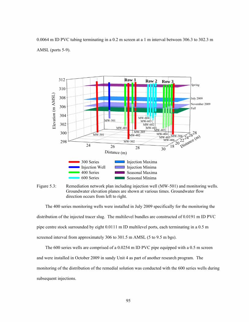
95

0.0064 m ID PVC tubing terminating in a 0.2 m screen at a 1 m interval between 306.3 to 302.3 m

AMSL (ports 5-9).

298

300

302

304

306

308

310

312

1820

2224

2628

24 26 28 30

Ele

vatio

n (m

AM

SL

)

Distance (m

)

Distance (m)

Injection MaximaInjection MinimaSeasonal MaximaSeasonal Minima

MW-301

MW-501

MW-401

MW-302

MW-303MW-402

MW-604MW-603

MW-602MW-601

MW-403MW-404

MW-405MW-406

MW-304

Row 2Row 1 Row 3Spring

Fall

July 2009

November 2009

300 SeriesInjection Well400 Series600 Series

Figure 5.3: Remediation network plan including injection well (MW-501) and monitoring wells. Groundwater elevation planes are shown at various times. Groundwater flow direction occurs from left to right.

The 400 series monitoring wells were installed in July 2009 specifically for the monitoring the

distribution of the injected tracer slug. The multilevel bundles are constructed of 0.0191 m ID PVC

pipe centre stock surrounded by eight 0.0111 m ID multilevel ports, each terminating in a 0.5 m

screened interval from approximately 306 to 301.5 m AMSL (5 to 9.5 m bgs).

The 600 series wells are comprised of a 0.0254 m ID PVC pipe equipped with a 0.5 m screen

and were installed in October 2009 in sandy Unit 4 as part of another research program. The

monitoring of the distribution of the remedial solution was conducted with the 600 series wells during

subsequent injections.

96

5.4 Enhanced, In Situ Denitrification Treatment System

The target residual contaminant zone consists of an anaerobic environment to which the necessary

reduced conditions for denitrification to occur exist. Nitrate in drinking water supplies is regulated by

the Ontario Drinking Water Quality Standards (ODWQS), where the maximum contaminant level

(MCL) for nitrate (as nitrogen, NO3-N) is 10 mg/L NO3-N as (MOE, 2003). A certificate of approval

from the Ontario Ministry of Environment (MOE) was granted in order to permit the application of

NO3- at concentrations 2-6 times ODWQS.

Given that the addition of NO3- at levels exceeding regulation was introduced into the petroleum

impacted environment, it was assumed that the NO3- would be readily degraded under the anaerobic

conditions, as a sufficient supply of dissolved, residual and free-phase petroleum hydrocarbons was

present to serve as electron donors. Sentinel wells located downgradient from the injection well,

within the monitoring network, were monitored for NO3- to evaluate the potential migration of a NO3

-

contaminant plume beyond the property limits in the event that significant denitrification in the

contaminated aquifer was not apparent.

5.4.1 Site Suitability

The application of nitrate-amended treatment water to enhance anaerobic biodegradation of residual

PHCs is a suitable technology given the physical and geochemical properties of the aquifer materials.

Cunningham et al. (2001) describe typical site conditions that are suited to the biostimulation of

indigenous microbial populations with the addition of a TEA to promote the oxidation of organic

contaminants, including:

1)  Anaerobic groundwater conditions exist at the Site with a presence of anaerobic bacteria; 

2)  Supply of electron acceptor and/or removal of inhibitors are limiting 

3)  Aquifer solids are sufficiently permeable, and

4)  Additional lab and field data provide evidence to support technology.

 

97

Site characterization involving geochemical analysis of groundwater and aquifer material

permeability testing indicate that the Site meets the criteria for enhanced in situ bioremediation of

BTEX contaminated groundwater. Anaerobic groundwater conditions are present within the study

area and exist strictly in the petroleum impacted areas, where the concentration of TEAs: dissolved

O2, NO3- and SO4

2- are significantly depleted compared to background conditions as previously

discussed in Chapter 2. Surface water infiltration can introduce O2, NO3- and SO4

2- into the reduced

environment where they may become readily metabolized in the petroleum impacted aquifer under

redox conditions. The geochemical results discussed in Chapter 2 signify that reducing conditions

exist in the PHC impacted portion of the aquifer, suggesting that active aerobic microbial degradation

of dissolved contaminants has taken place and anaerobic biodegradation is occurring.

Significant bacteria-mediated denitrification in the aquifer only occurs in the absence of O2,

related to the fact that most denitrifying bacteria are facultative aerobes and have the ability to utilize

both electron acceptors in metabolic processes. These bacteria are capable of readily adapting to both

aerobic and anaerobic conditions. The presence of denitrifyers in aquifers was not targeted for

analysis as it was assumed that a sustainable population was present within the research area given

the geochemical and microbiological data available for the Site.

The concentration of nitrate added (90 – 265 mg/L NO3-) was far in excess of other naturally

occurring TEAs in the petroleum impacted region of the aquifer in order to sustain the preferential

metabolism of NO3- as a terminal electron acceptor in the oxidation of organic contaminants where

0.3 to 1.4 mg/L O2 and 1 to 2 mg/L SO42 have been historically measured at MW-103 (SNC Lavalin,

2008). Upgradient concentrations of 7.5 to 14 mg/L NO3-N have been measured by SNC Lavalin in

MW-109 which may be indicative of how much TEA is available naturally at the Site, whereas

concentrations below detection limit have consistently been measured in the petroleum impacted

aquifer.

98

The targeted aquifer sediments predominantly consist of a sandy layer, Unit 4, where K =

3.1x10-5 m/s) with a small portion of the overlying sand and gravel layer (Unit 3, K = 6.9x10-5 m/s) in

the screened portion of the injection well. The aquifer sediments are sufficiently permeable to

transmit a remedial solution amended with TEA to the contaminated zone; a requirement according to

Cunningham et al. (2001). The injection solution is preferentially transported in higher permeable

aquifer units and may have a shorter residence time in these areas compared to less conductive units.

The issue of heterogeneity was not recognized by Cunningham et al. (2001) and is a key issue

followed in this experiment. Lower permeability (but still very permeable) units of the heterogeneous

aquifer are of interest in the assessment of delivery of the treatment solution. The presence of

anaerobic microbial populations at the Site meet the criteria specified by Cunningham et al. (2001).

Iron and sulphate reducing bacteria were identified during microbiological groundwater sampling

conducted by SNC-Lavalin in 2007 in the reduced study area conditions. As discussed in Chapter 4,

a microcosm study confirmed that the indigenous microbes were capable of degrading petroleum

hydrocarbons utilizing nitrate as a terminal electron acceptor.

5.4.2 Mass of Contaminants in the Targeted Source Zone

A remedial zone was selected based on the understanding of the spatial distribution of contaminants

determined during the analysis of the soil extraction concentrations obtained during the November

2007 and July 2009, prior to the coring activities associated with the remedial solution injections.

The remedial zone consisted of a 48 m3 volume of aquifer materials (6 m length x 4 m wide x 2 m

thick). The zone of interest included aquifer materials between elevations 305 and 303 m AMSL and

encompassing wells MW-501; MW-401, MW-402, MW-302 (Row 1); MW-601, MW-602, MW-603

and MW-604 (Row 2) and MW-403, MW-404, MW-405, MW-406 and MW-304 (Row 3) as

illustrated in Figure 5.2 and Figure 5.8.

The total mass of contaminants located within the target zone (MT) was estimated using total soil

extract concentrations determined during the two soil coring events, prior to the remedial injections.

99

The mass of contaminants Mj, for each core was determined by summing the product of each

individual sample soil extract concentration Cti, with the inferred core sample thickness (hi,j), over all

n core segments. The Mj for each core is assumed constant over an area extending to half the

distance to the nearest core, Aj, the Thiessen area. MT is then calculated using equation (5.1):

A ρ C , h , (5.1)

An estimated 600 kg of total petroleum hydrocarbons consisting of approximately 126 kg of total

BTEXTMB remains within the targeted source zone based on the results of the soil extract

concentration investigations after applying equation (5.1).

5.4.3 Mass of Nitrate Required

The remediation system was designed and implemented to specifically target the mass reduction of

residual toluene in the aquifer, while evaluating the success of the addition of NO3- to biostimulate the

degradation of petroleum hydrocarbons. Soil core results were analyzed during preliminary site

investigations to delineate a study area and target the delivery of remedial solution to residual

saturation aquifer materials. Saturated hydrocarbons are readily biodegraded in groundwater under

nitrate-reducing conditions (Holliger & Zehnder, 1996), however the target contaminants of interest

for biodegradation are BTEXTMB due to the associated health risks.

A total of 600 kg of TPH (F1-F3), including 126 kg (BTEXTMB was inferred within the target

remedial zone from interpretation of soil coring results as previously described in Section 5.4.2.

Approximately 18 kg or 193 moles of toluene was present in the study area prior to the application of

remediation efforts. The stoichiometry of the biologically mediated denitrification reaction using

toluene as the electron donor is presented as followed in equation (5.2):

100

C7H8(aq) + 7.2NO3-(aq) + 7.2H+

(aq) 3.6N2(g) + 7CO2(g) 7.6H2O(l)  (5.2) 

Assuming the reaction goes to completion, approximately 5 mg of nitrate are required to oxidize

and remove 1 mg of toluene. Based on the relationship of 7.2 moles NO3- required to degrade 1 mole

C7H8 approximately (7.2 mol x18 mol toluene) 130 kg of NO3 would be necessary to provide a

sufficient supply of TEA to the microbes, assuming the reaction goes to completion. Considering the

600 kg of TPH contaminants present within the study area, a minimum of 3,000 kg NO3- would be

required to degrade all the PHCs in the entire 48 m3 source zone, assuming the degradation of TPH

follows a similar nitrate demand as toluene.

5.4.4 Expected Success of Remediation System

Seasonal groundwater sampling revealed that an average of 30 mg/L total petroleum hydrocarbons

(TPH) (F1-F3 fractions) is present within the study area in the dissolved phase. The dissolved phase

component would provide an additional 0.46 kg of contaminant mass, requiring an additional (5 x

0.46 kg) 2.3 kg of NO3-. That is an insignificant TEA demand compared to the 3,000 kg demand

estimated in section 5.4.3, above. This is why removal of residual NAPL was targeted, with NAPL

serving as a long term source of contaminants.

A total of 3.7 kg NO3- was applied during the remedial efforts which served as a TEA to

stimulate in situ biodegradation of petroleum contaminants, however this TEA mass was essentially

insignificant compared to the mass of contaminants present. If we then assume that only

monoaromatics (BTEXTMB) are degradable by denitrification, (inferred from Brown, Mahaffey, &

Norris, 1993), less than 1% of the 126 kg of BTEXTMB could be biodegraded with the 3.7 kg of

nitrate added in this experiment. Assuming complete mineralization of contaminants of interest based

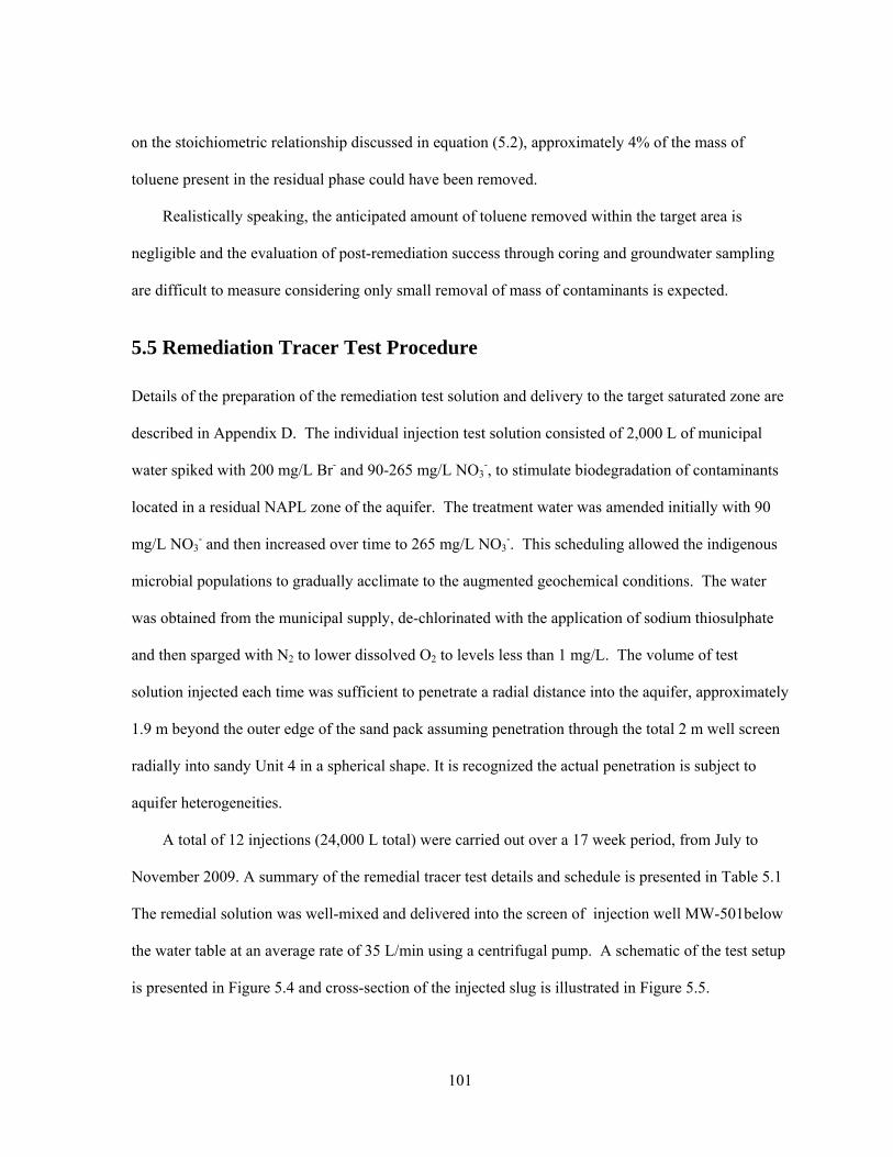
101

on the stoichiometric relationship discussed in equation (5.2), approximately 4% of the mass of

toluene present in the residual phase could have been removed.

Realistically speaking, the anticipated amount of toluene removed within the target area is

negligible and the evaluation of post-remediation success through coring and groundwater sampling

are difficult to measure considering only small removal of mass of contaminants is expected.

5.5 Remediation Tracer Test Procedure

Details of the preparation of the remediation test solution and delivery to the target saturated zone are

described in Appendix D. The individual injection test solution consisted of 2,000 L of municipal

water spiked with 200 mg/L Br- and 90-265 mg/L NO3-, to stimulate biodegradation of contaminants

located in a residual NAPL zone of the aquifer. The treatment water was amended initially with 90

mg/L NO3- and then increased over time to 265 mg/L NO3

-. This scheduling allowed the indigenous

microbial populations to gradually acclimate to the augmented geochemical conditions. The water

was obtained from the municipal supply, de-chlorinated with the application of sodium thiosulphate

and then sparged with N2 to lower dissolved O2 to levels less than 1 mg/L. The volume of test

solution injected each time was sufficient to penetrate a radial distance into the aquifer, approximately

1.9 m beyond the outer edge of the sand pack assuming penetration through the total 2 m well screen

radially into sandy Unit 4 in a spherical shape. It is recognized the actual penetration is subject to

aquifer heterogeneities.

A total of 12 injections (24,000 L total) were carried out over a 17 week period, from July to

November 2009. A summary of the remedial tracer test details and schedule is presented in Table 5.1

The remedial solution was well-mixed and delivered into the screen of injection well MW-501below

the water table at an average rate of 35 L/min using a centrifugal pump. A schematic of the test setup

is presented in Figure 5.4 and cross-section of the injected slug is illustrated in Figure 5.5.

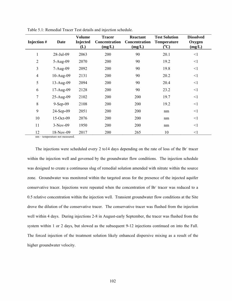
102

Table 5.1: Remedial Tracer Test details and injection schedule.

Injection # Date Volume Injected

(L)

Tracer Concentration

(mg/L)

Reactant Concentration

(mg/L)

Test Solution Temperature

(oC)

Dissolved Oxygen (mg/L)

1 28-Jul-09 2063 200 90 20.1 <1

2 5-Aug-09 2070 200 90 19.2 <1

3 7-Aug-09 2092 200 90 19.8 <1

4 10-Aug-09 2131 200 90 20.2 <1

5 13-Aug-09 2094 200 90 20.4 <1

6 17-Aug-09 2128 200 90 23.2 <1

7 25-Aug-09 2102 200 200 19.7 <1

8 9-Sep-09 2108 200 200 19.2 <1

9 24-Sep-09 2051 200 200 nm <1

10 15-Oct-09 2076 200 200 nm <1

11 3-Nov-09 1950 200 200 nm <1

12 18-Nov-09 2017 200 265 10 <1 nm – temperature not measured.

The injections were scheduled every 2 to14 days depending on the rate of loss of the Br- tracer

within the injection well and governed by the groundwater flow conditions. The injection schedule

was designed to create a continuous slug of remedial solution amended with nitrate within the source

zone. Groundwater was monitored within the targeted areas for the presence of the injected aquifer

conservative tracer. Injections were repeated when the concentration of Br- tracer was reduced to a

0.5 relative concentration within the injection well. Transient groundwater flow conditions at the Site

drove the dilution of the conservative tracer. The conservative tracer was flushed from the injection

well within 4 days. During injections 2-8 in August-early September, the tracer was flushed from the

system within 1 or 2 days, but slowed as the subsequent 9-12 injections continued on into the Fall.

The forced injection of the treatment solution likely enhanced dispersive mixing as a result of the

higher groundwater velocity.

103

Figure 5.4: Cross-sectional view of remedial tracer test solution being injected in MW-501 including storage of prepared test solution in carboy, delivery line from centrifugal pump to well and groundwater elevation minima and maxima range throughout the series of injections.

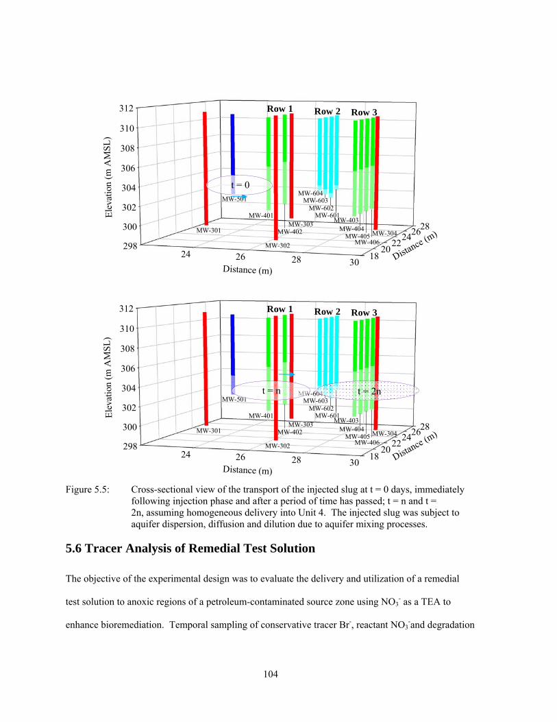
104

298

300

302

304

306

308

310

312

1820

2224

2628

24 26 28 30

Ele

vatio

n (m

AM

SL

)

Distance (m

)

Distance (m)

MW-301

MW-501

MW-401

MW-302

MW-303MW-402

MW-604MW-603

MW-602MW-601

MW-403MW-404

MW-405MW-406

MW-304

Row 2Row 1 Row 3

298

300

302

304

306

308

310

312

1820

2224

2628

24 26 28 30

Ele

vatio

n (m

AM

SL

)

Distance (m

)

Distance (m)

MW-301

MW-501

MW-401

MW-302

MW-303MW-402

MW-604MW-603

MW-602MW-601

MW-403MW-404

MW-405MW-406

MW-304

Row 2Row 1 Row 3

Figure 5.5: Cross-sectional view of the transport of the injected slug at t = 0 days, immediately following injection phase and after a period of time has passed; t = n and t = 2n, assuming homogeneous delivery into Unit 4. The injected slug was subject to aquifer dispersion, diffusion and dilution due to aquifer mixing processes.

5.6 Tracer Analysis of Remedial Test Solution

The objective of the experimental design was to evaluate the delivery and utilization of a remedial

test solution to anoxic regions of a petroleum-contaminated source zone using NO3- as a TEA to

enhance bioremediation. Temporal sampling of conservative tracer Br-, reactant NO3-and degradation

t = 0

t = n t = 2n

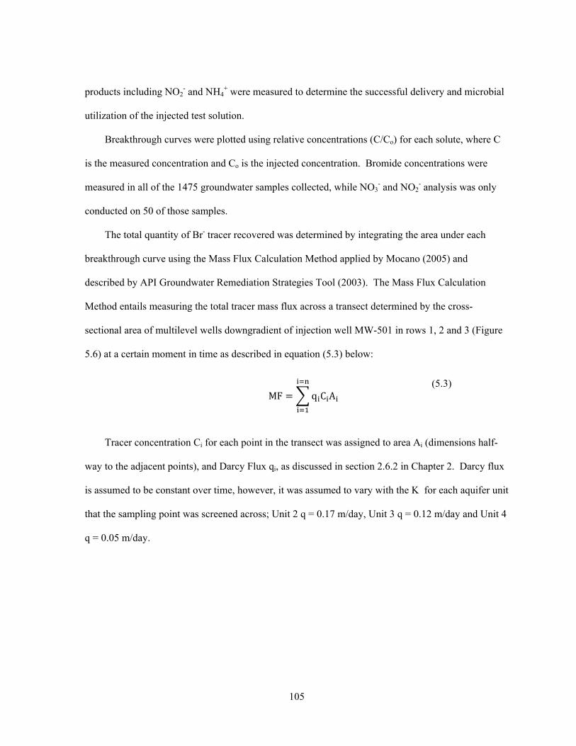
105

products including NO2- and NH4

+ were measured to determine the successful delivery and microbial

utilization of the injected test solution.

Breakthrough curves were plotted using relative concentrations (C/Co) for each solute, where C

is the measured concentration and Co is the injected concentration. Bromide concentrations were

measured in all of the 1475 groundwater samples collected, while NO3- and NO2

- analysis was only

conducted on 50 of those samples.

The total quantity of Br- tracer recovered was determined by integrating the area under each

breakthrough curve using the Mass Flux Calculation Method applied by Mocano (2005) and

described by API Groundwater Remediation Strategies Tool (2003). The Mass Flux Calculation

Method entails measuring the total tracer mass flux across a transect determined by the cross-

sectional area of multilevel wells downgradient of injection well MW-501 in rows 1, 2 and 3 (Figure

5.6) at a certain moment in time as described in equation (5.3) below:

MF q C A

(5.3)

Tracer concentration Ci for each point in the transect was assigned to area Ai (dimensions half-

way to the adjacent points), and Darcy Flux qi, as discussed in section 2.6.2 in Chapter 2. Darcy flux

is assumed to be constant over time, however, it was assumed to vary with the K for each aquifer unit

that the sampling point was screened across; Unit 2 q = 0.17 m/day, Unit 3 q = 0.12 m/day and Unit 4

q = 0.05 m/day.

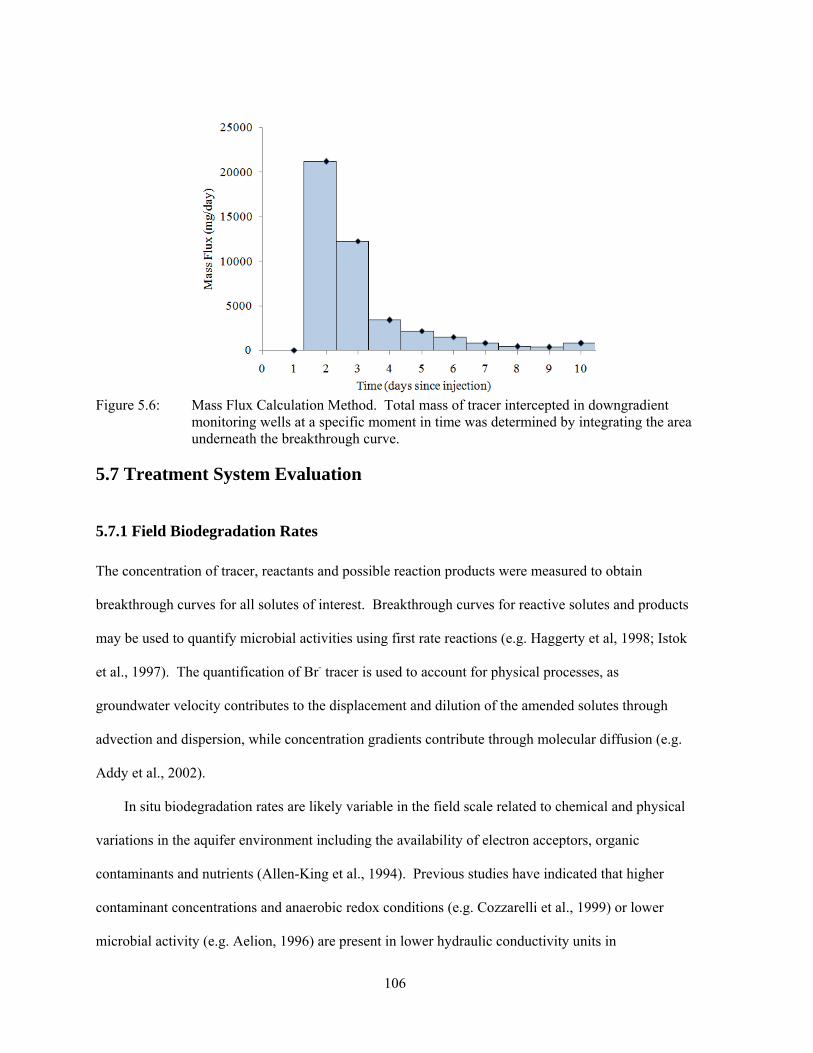
106

Figure 5.6: Mass Flux Calculation Method. Total mass of tracer intercepted in downgradient monitoring wells at a specific moment in time was determined by integrating the area underneath the breakthrough curve.

5.7 Treatment System Evaluation

5.7.1 Field Biodegradation Rates

The concentration of tracer, reactants and possible reaction products were measured to obtain

breakthrough curves for all solutes of interest. Breakthrough curves for reactive solutes and products

may be used to quantify microbial activities using first rate reactions (e.g. Haggerty et al, 1998; Istok

et al., 1997). The quantification of Br- tracer is used to account for physical processes, as

groundwater velocity contributes to the displacement and dilution of the amended solutes through

advection and dispersion, while concentration gradients contribute through molecular diffusion (e.g.

Addy et al., 2002).

In situ biodegradation rates are likely variable in the field scale related to chemical and physical

variations in the aquifer environment including the availability of electron acceptors, organic

contaminants and nutrients (Allen-King et al., 1994). Previous studies have indicated that higher

contaminant concentrations and anaerobic redox conditions (e.g. Cozzarelli et al., 1999) or lower

microbial activity (e.g. Aelion, 1996) are present in lower hydraulic conductivity units in

107

heterogeneous units of petroleum-contaminated sites. It is essential to identify lower permeable units

containing residual contaminants as they will influence the remediation time periods. The variable

permeability of the aquifer materials was previously addressed in Chapters 2 and 3, in relation to

contaminant distributions. Aelion (1996) described biodegradation rates of toluene and benzene

varying as a function of sediment type and levels of microbial activity, where fine grained clay

materials had increased sorption and limited biodegradation.

Rates of denitrification are obtained by computing first-order rate constants for the utilization of

NO3-. First-order reaction assumes that the reactant is transformed in the aquifer and is corrected for

dilution effects according to equation (5.4):

ln

∗

∗

(5.4)

Where C*NO3- is the relative concentration of the reactant, nitrate and C*Br- is the relative

concentration of the Br- tracer, t is the time elapsed since the end of the injection and k is the first-

order denitrification rate coefficient. A plot of ln (C*NO3-/C*Br-) versus t generates a straight line with

a slope –k. Estimates of first-order rate coefficients for NO3- reduction were determined by fitting the

slope and intercept of the equation to experimental breakthrough data. The first-order reaction

analysis assumes that the injected test solution within the aquifer is well mixed and that the

advection-dispersion-sorption transport properties of the tracer and reactant are similar (e.g. Haggerty

et al, 1998; Schroth et al, 2001).

5.7.2 Post-Injection Residual Evaluation

Soil cores were retrieved from the experimental zone in October 2009 by another MSc. Earth

Sciences Candidate, Bobby Katanchi, and analyzed for the critical aromatics BTEXTMB. The soil

cores were collected in the zone of the aquifer where significant NAPL concentrations had been

found, extending between 308 and 302 m AMSL (3 and 9 m bgs). The targeted residual zone of

interest within the aquifer was 303 to 305 m AMSL (6.2 to 6.8 m bgs).

108

Groundwater samples collected from multilevel sampling points in the aquifer target area were

analyzed for BTEXTMB and TPH. Groundwater quality measurements were not anticipated to differ

from pre-treatment results, considering the dissolution of residual NAPL remaining would cause

groundwater concentrations to rebound (e.g. Cunningham et al., 2001). The results of the tracer test

experiment and evaluation of bioremediation via denitrification are discussed in further detail in

Chapters 6 and Chapter 7, respectively.

109

Chapter 6: Remedial Tracer Test Br- Results

6.1 Evaluation of the Delivery of Remedial Tracer Solution

The delivery of the remedial test solution below the water table targeted a select zone of the aquifer

contaminated with residual petroleum hydrocarbons. The test solution was amended with conservative

bromide (Br-) and reactive nitrate (NO3-) tracers. Groundwater tracer utilization allowed for detection of

contaminant transport pathways and the ultimate delivery of remedial solution to petroleum hydrocarbon

impacted zones. This chapter discusses the delivery results of the remedial solution within target zones of

the aquifer and the effect of natural transient hydrogeological conditions present at the Site.

6.2 Injection Effects on Hydrogeologic Flow Regime

The forced injection of a large volume (2.05 m3) of remedial tracer test solution resulted in a localized

water-table rise, noted in wells up to 3.7 m away. Water table mounding occurred as a result of the

remedial solution displacing existing groundwater within the immediate vicinity of the injection interval.

The hydrogeological changes were relatively short-lived, with the water level within the zone of influence

recovering 80-100% within 90 minutes of the completion of the injection phase.

Water levels in MW-501 and neighbouring wells were monitored during the delivery of the test

solution to establish hydrogeological characteristics of the aquifer materials in relation to the injected

remedial slug below the water table. The observed water level changes throughout injection and recovery

phases are presented for injection 12 (November 18th, 2010) in Figure 6.1. Observation wells were

screened within the same aquifer formations as the injection well (primarily Unit 4), although portions of

the delivery interval also penetrated the overlying sand and gravel, Unit 3. Water levels were monitored

at MW-401 and MW-402, screened across the static water table and located in Unit 3 (MW-402 port 4)

and Unit 4 (MW-401 port 4), consistent with the injection interval. MW-603 is screened at greater depth

(7.43-7.93 m AMSL) across Unit 4 (sand) and Unit 5 (sand and gravel, till) as described in Appendix A.

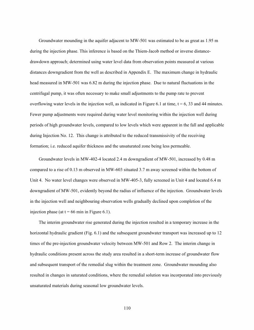
110

Groundwater mounding in the aquifer adjacent to MW-501 was estimated to be as great as 1.95 m

during the injection phase. This inference is based on the Thiem-Jacob method or inverse distance-

drawdown approach; determined using water level data from observation points measured at various

distances downgradient from the well as described in Appendix E. The maximum change in hydraulic

head measured in MW-501 was 6.82 m during the injection phase. Due to natural fluctuations in the

centrifugal pump, it was often necessary to make small adjustments to the pump rate to prevent

overflowing water levels in the injection well, as indicated in Figure 6.1 at time, t = 6, 33 and 44 minutes.

Fewer pump adjustments were required during water level monitoring within the injection well during

periods of high groundwater levels, compared to low levels which were apparent in the fall and applicable

during Injection No. 12. This change is attributed to the reduced transmissivity of the receiving

formation; i.e. reduced aquifer thickness and the unsaturated zone being less permeable.

Groundwater levels in MW-402-4 located 2.4 m downgradient of MW-501, increased by 0.48 m

compared to a rise of 0.13 m observed in MW-603 situated 3.7 m away screened within the bottom of

Unit 4. No water level changes were observed in MW-405-3, fully screened in Unit 4 and located 6.4 m

downgradient of MW-501, evidently beyond the radius of influence of the injection. Groundwater levels

in the injection well and neighbouring observation wells gradually declined upon completion of the

injection phase (at t = 66 min in Figure 6.1).

The interim groundwater rise generated during the injection resulted in a temporary increase in the

horizontal hydraulic gradient (Fig. 6.1) and the subsequent groundwater transport was increased up to 12

times of the pre-injection groundwater velocity between MW-501 and Row 2. The interim change in

hydraulic conditions present across the study area resulted in a short-term increase of groundwater flow

and subsequent transport of the remedial slug within the treatment zone. Groundwater mounding also

resulted in changes in saturated conditions, where the remedial solution was incorporated into previously

unsaturated materials during seasonal low groundwater levels.

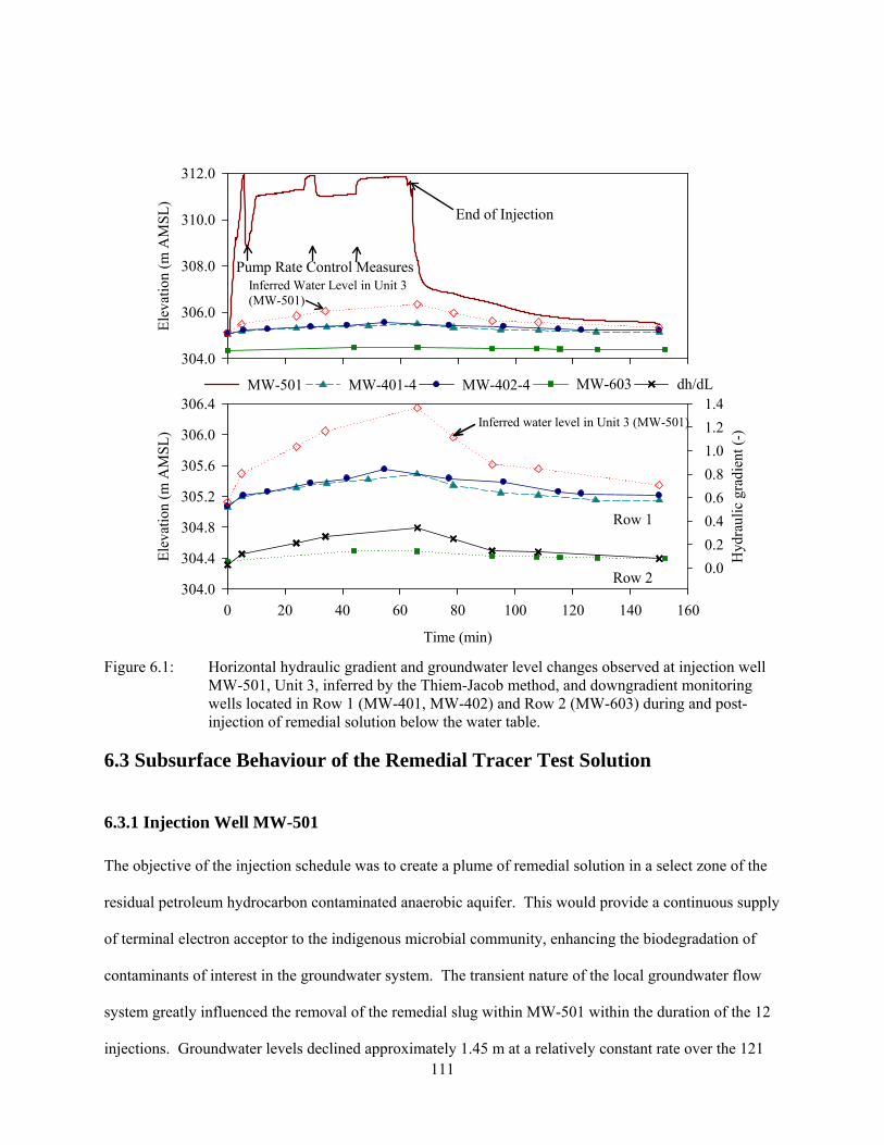
111

MW-501 MW-401-4 MW-402-4

Time (min)

0 20 40 60 80 100 120 140 160

Ele

vatio

n (m

AM

SL

)

304.0

304.4

304.8

305.2

305.6

306.0

306.4

Hyd

raul

ic g

radi

ent (

-)

0.0

0.2

0.4

0.6

0.8

1.0

1.2

1.4dh/dL

Ele

vatio

n (m

AM

SL)

304.0

306.0

308.0

310.0

312.0

MW-603

Inferred water level in Unit 3 (MW-501)

Row 1

Row 2

End of Injection

Inferred Water Level in Unit 3 (MW-501)

Pump Rate Control Measures

Figure 6.1: Horizontal hydraulic gradient and groundwater level changes observed at injection well MW-501, Unit 3, inferred by the Thiem-Jacob method, and downgradient monitoring wells located in Row 1 (MW-401, MW-402) and Row 2 (MW-603) during and post- injection of remedial solution below the water table.

6.3 Subsurface Behaviour of the Remedial Tracer Test Solution

6.3.1 Injection Well MW-501

The objective of the injection schedule was to create a plume of remedial solution in a select zone of the

residual petroleum hydrocarbon contaminated anaerobic aquifer. This would provide a continuous supply

of terminal electron acceptor to the indigenous microbial community, enhancing the biodegradation of

contaminants of interest in the groundwater system. The transient nature of the local groundwater flow

system greatly influenced the removal of the remedial slug within MW-501 within the duration of the 12

injections. Groundwater levels declined approximately 1.45 m at a relatively constant rate over the 121

112

day period the tracer tests were conducted. The remedial solution was consistently delivered below the

water table; although the groundwater level dropped beneath the top of the sand pack in Unit 3, to

approximately 0.15 m above the screened interval of MW-501 within Unit 4 during Injection 11 and

Injection 12.

The remedial pulse delivered to the subsurface environment mixed and dispersed within the

background contaminated groundwater. In general, normalized Br- tracer concentrations (C/Co) remained

approximately 1.0 in MW-501 for at least an hour following the injection prior to being dispersed by the

local hydrogeological flow regime. The transport of the injected remedial slug from the injection well is

generally described by three unique type behaviour breakthrough curves (BTC) observed throughout the

12 injections performed over the 121 day period. Representative Type I, Type II and Type III BTCs,

obtained from Br- tracer monitoring of MW-501, are presented in Figure 6.2. Transient groundwater flow

conditions drove the dilution and rate of removal of Br- tracer in MW-501.

Breakthrough curves (BTC) are classified as Type I for injections 1-6, occurring between July 28 and

August 17, 2009 and are illustrated in Figure 6.2a. The BTC for the initial injection possesses a longer

elution tail compared to the other injections also classified as Type I. This may be attributed to the

limited initial well development, as the hydrogeological conditions only differed slightly over the course

of the 6 injections. Due to the rapid disappearance of Br- in MW-501 (at times less than 2 days), it was

not possible to satisfy the conditions where a subsequent injection would be initiated at the target

concentration, when C/Co ≈ 0.5.

Type II Br- tracer BTCs (Fig. 6.2b) depict the removal of Br- from the injection well for injections 7

and 8 which took place on August 25 and September 9, 2010, respectively. Relative tracer concentrations

reached the target concentration within 4 days of the injection. Groundwater levels had reduced by

approximately 0.85 m since injection 1 and a decrease in hydraulic gradient from 0.007 to 0.004 was

observed across the Site.

113

BTCs for injections 9-12, between September 24 and November 18, 2009 are classified as Type III

cases (Fig. 6.2c). Both groundwater levels and hydraulic gradients, i, were at a seasonal low during the

Type III case (i < 0.004), resulting in limitations to the transport of remedial solution within the saturated

zone. Normalized Br- tracer concentrations were indeed greater than the injection criteria 24 to 121 days

following an injection, indicating an increase in the residence time of the injected slug. The pulse of

remedial solution delivered to the groundwater flow system was generally subject to less advective

compared to dispersive dilution processes under the reduced hydrogeological conditions encountered in

the fall. Under these conditions, increased tailing of C/Co > 0.5 was observed as great as 121 days post-

injection.

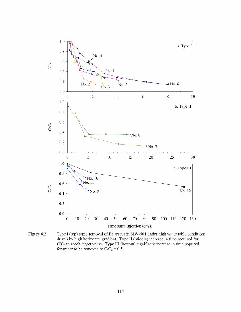
114

0 2 4 6 8 10

C/C

o

0.0

0.2

0.4

0.6

0.8

1.0

0 5 10 15 20 25 30

C/C

o

0.0

0.2

0.4

0.6

0.8

1.0

Time since Injection (days)

0 10 20 30 40 50 60 70 80 90 100 110 120 130

C/C

o

0.0

0.2

0.4

0.6

0.8

1.0

a. Type I

b. Type II

c. Type III

No. 9

No. 11No. 10

No. 12

No. 7

No. 8

No. 2No. 3

No. 1

No. 5 No. 6

No. 4

Figure 6.2: Type I (top) rapid removal of Br- tracer in MW-501 under high water table conditions driven by high horizontal gradient. Type II (middle) increase in time required for C/Co to reach target value. Type III (bottom) significant increase in time required for tracer to be removed to C/Co = 0.5.

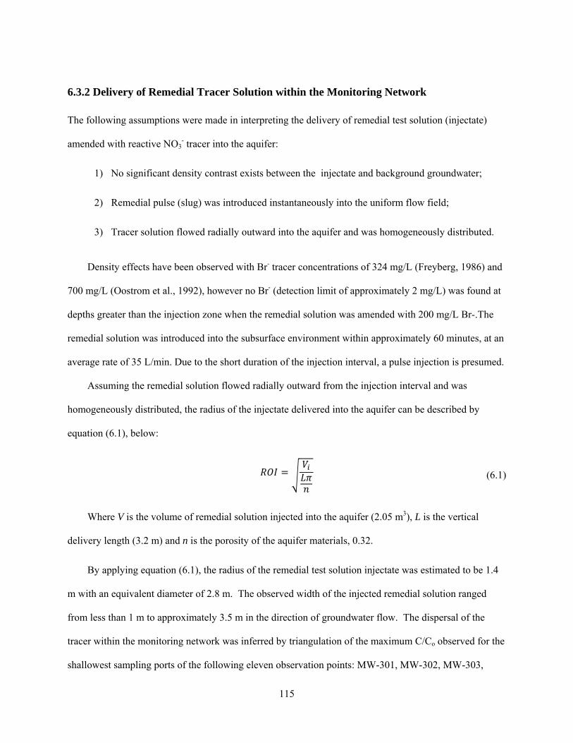
115

6.3.2 Delivery of Remedial Tracer Solution within the Monitoring Network

The following assumptions were made in interpreting the delivery of remedial test solution (injectate)

amended with reactive NO3- tracer into the aquifer:

1) No significant density contrast exists between the injectate and background groundwater;

2) Remedial pulse (slug) was introduced instantaneously into the uniform flow field;

3) Tracer solution flowed radially outward into the aquifer and was homogeneously distributed.

Density effects have been observed with Br- tracer concentrations of 324 mg/L (Freyberg, 1986) and

700 mg/L (Oostrom et al., 1992), however no Br- (detection limit of approximately 2 mg/L) was found at

depths greater than the injection zone when the remedial solution was amended with 200 mg/L Br-.The

remedial solution was introduced into the subsurface environment within approximately 60 minutes, at an

average rate of 35 L/min. Due to the short duration of the injection interval, a pulse injection is presumed.

Assuming the remedial solution flowed radially outward from the injection interval and was

homogeneously distributed, the radius of the injectate delivered into the aquifer can be described by

equation (6.1), below:

(6.1)

Where V is the volume of remedial solution injected into the aquifer (2.05 m3), L is the vertical

delivery length (3.2 m) and n is the porosity of the aquifer materials, 0.32.

By applying equation (6.1), the radius of the remedial test solution injectate was estimated to be 1.4

m with an equivalent diameter of 2.8 m. The observed width of the injected remedial solution ranged

from less than 1 m to approximately 3.5 m in the direction of groundwater flow. The dispersal of the

tracer within the monitoring network was inferred by triangulation of the maximum C/Co observed for the

shallowest sampling ports of the following eleven observation points: MW-301, MW-302, MW-303,

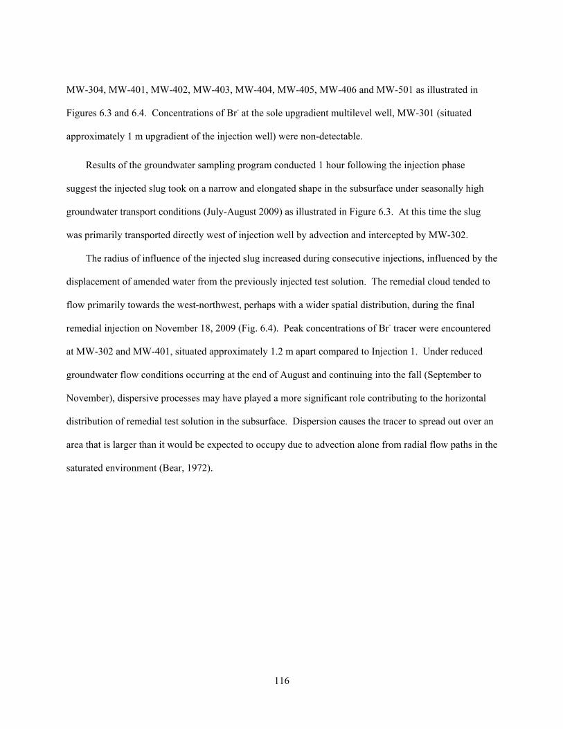
116

MW-304, MW-401, MW-402, MW-403, MW-404, MW-405, MW-406 and MW-501 as illustrated in

Figures 6.3 and 6.4. Concentrations of Br- at the sole upgradient multilevel well, MW-301 (situated

approximately 1 m upgradient of the injection well) were non-detectable.

Results of the groundwater sampling program conducted 1 hour following the injection phase

suggest the injected slug took on a narrow and elongated shape in the subsurface under seasonally high

groundwater transport conditions (July-August 2009) as illustrated in Figure 6.3. At this time the slug

was primarily transported directly west of injection well by advection and intercepted by MW-302.

The radius of influence of the injected slug increased during consecutive injections, influenced by the

displacement of amended water from the previously injected test solution. The remedial cloud tended to

flow primarily towards the west-northwest, perhaps with a wider spatial distribution, during the final

remedial injection on November 18, 2009 (Fig. 6.4). Peak concentrations of Br- tracer were encountered

at MW-302 and MW-401, situated approximately 1.2 m apart compared to Injection 1. Under reduced

groundwater flow conditions occurring at the end of August and continuing into the fall (September to

November), dispersive processes may have played a more significant role contributing to the horizontal

distribution of remedial test solution in the subsurface. Dispersion causes the tracer to spread out over an

area that is larger than it would be expected to occupy due to advection alone from radial flow paths in the

saturated environment (Bear, 1972).

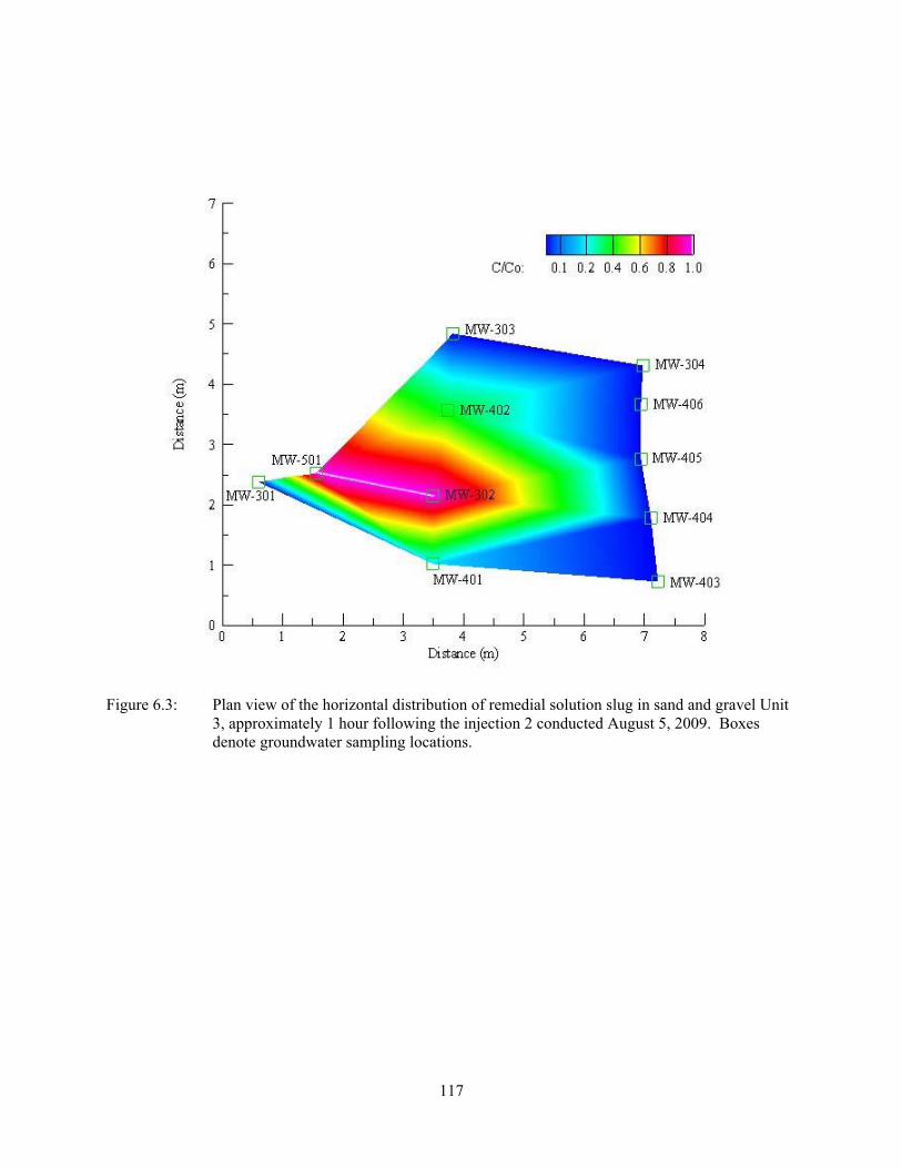
117

Figure 6.3: Plan view of the horizontal distribution of remedial solution slug in sand and gravel Unit 3, approximately 1 hour following the injection 2 conducted August 5, 2009. Boxes denote groundwater sampling locations.

118

Figure 6.4: Plan view distribution of remedial solution slug in Unit 4, approximately 1 hour following the injection 12. Boxes denote groundwater sampling locations.

The remedial slug was assumed to flow radially from the injection interval, however the shape of the

injected slug within the subsurface was subject to aquifer heterogeneities, the initial saturated thickness

delivery interval, the injection rate and duration, in addition to well construction and development

methods (Istok et al, 1997).

The radius of influence (ROI) within the injection interval is primarily influenced by the hydraulic

conductivity (K) of the heterogeneous aquifer materials (Fig. 6.5). The injection well is screened across a

2 m interval of Unit 4 (K4 = 3.1x10-5 m/s), with the sand pack extending 1.2 m above into a slightly more

permeable Unit 3 (K3 = 6.9x10-5 m/s). Under high saturated conditions encountered during the early

injections, remedial solution delivered to Unit 3 had a greater radius of influence compared to Unit 4 due

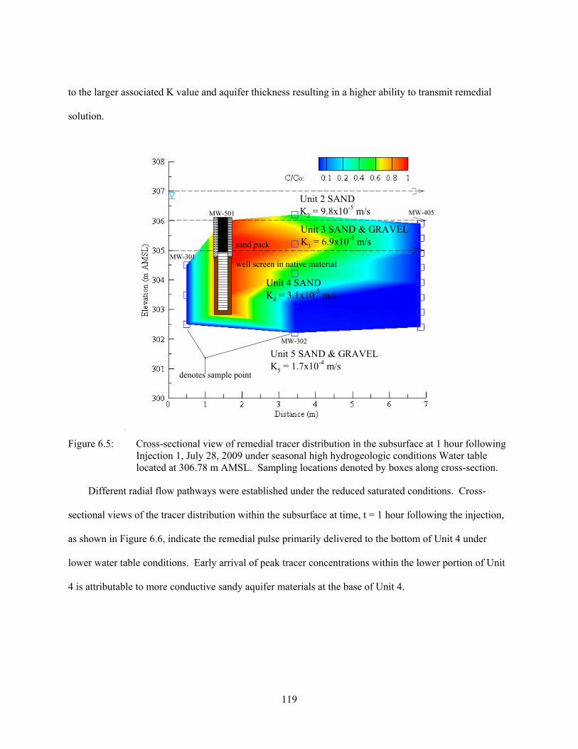
119

to the larger associated K value and aquifer thickness resulting in a higher ability to transmit remedial

solution.

MW-301

MW-501

MW-302

MW-405

Unit 4 SANDK4 = 3.1x10-5 m/s

Unit 3 SAND & GRAVELK3 = 6.9x10-5 m/s

Unit 5 SAND & GRAVELK5 = 1.7x10-4 m/s

Unit 2 SANDK2 = 9.8x10-5 m/s

denotes sample point

sand pack

well screen in native material

 

Figure 6.5: Cross-sectional view of remedial tracer distribution in the subsurface at 1 hour following Injection 1, July 28, 2009 under seasonal high hydrogeologic conditions Water table located at 306.78 m AMSL. Sampling locations denoted by boxes along cross-section.

Different radial flow pathways were established under the reduced saturated conditions. Cross-

sectional views of the tracer distribution within the subsurface at time, t = 1 hour following the injection,

as shown in Figure 6.6, indicate the remedial pulse primarily delivered to the bottom of Unit 4 under

lower water table conditions. Early arrival of peak tracer concentrations within the lower portion of Unit

4 is attributable to more conductive sandy aquifer materials at the base of Unit 4.

120

MW-402

MW-301

MW-501

 

well screen in native material

Unit 4 SANDK4 = 3.1x10-5 m/s

Unit 3 SAND & GRAVELK3 = 6.9x10-5 m/s

MW-405

Unit 5 SAND & GRAVELK5 = 1.7x10-4 m/s

Figure 6.6: Cross-sectional view (MW-301, MW-501, MW-402 and MW-405) of remedial tracer distribution in the subsurface following Injection 12, November 18, 2010 under seasonal low hydrogeologic conditions. Water table located at 305.14 m AMSL, ports 1, 2 and 3 of MW-402 and MW-405 were dry.

6.3.3 Temporal Distribution of Injectate at Downgradient Monitors

BTCs were generated for select monitoring wells and are organized by the stratigraphic unit screened;

Unit 2 (sand), Unit 3 (sand + gravel till), Unit 4 (sand) and Unit 5 (sand + gravel till). The well

description and location of each groundwater monitor is presented in Appendix 2.

Br- tracer behaviour in Unit 2 (0.5 m average thickness across study area) was monitored by

sampling groundwater at MW-302-5, screened 306.3 and 306.1 m AMSL (4.8-6.0 m bgs) and directly

above the interval of injection (306 to 302.8 m AMSL). Peak relative concentration of Br- recovered in

Unit 2 ranged between 0.6 and 1.0 for injections 1 through 6 (Fig. 6.7).

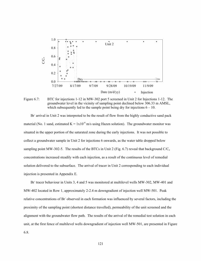
121

Date (m/d/yy)

7/27/09 8/17/09 9/7/09 9/28/09 10/19/09 11/9/09

C/C

o

0.0

0.2

0.4

0.6

0.8

1.0

Injection

Unit 2

Dry

Figure 6.7: BTC for injections 1-12 in MW-302 port 5 screened in Unit 2 for Injections 1-12. The groundwater level in the vicinity of sampling point declined below 306.33 m AMSL, which subsequently led to the sample point being dry for injections 6 – 10.

Br- arrival in Unit 2 was interpreted to be the result of flow from the highly conductive sand pack

material (No. 1 sand, estimated K = 1x10-4 m/s using Hazen solution). The groundwater monitor was

situated in the upper portion of the saturated zone during the early injections. It was not possible to

collect a groundwater sample in Unit 2 for injections 6 onwards, as the water table dropped below

sampling point MW-302-5. The results of the BTCs in Unit 2 (Fig. 6.7) reveal that background C/Co

concentrations increased steadily with each injection, as a result of the continuous level of remedial

solution delivered to the subsurface. The arrival of tracer in Unit 2 corresponding to each individual

injection is presented in Appendix E.

Br- tracer behaviour in Units 3, 4 and 5 was monitored at multilevel wells MW-302, MW-401 and

MW-402 located in Row 1, approximately 2-2.4 m downgradient of injection well MW-501. Peak

relative concentrations of Br- observed in each formation was influenced by several factors, including the

proximity of the sampling point (shortest distance travelled), permeability of the unit screened and the

alignment with the groundwater flow path. The results of the arrival of the remedial test solution in each

unit, at the first fence of multilevel wells downgradient of injection well MW-501, are presented in Figure

6.8.

122

The highest relative concentrations of Br- tracer within formations 3, 4 and 5 occurred repeatedly in

MW-302, situated nearest to the injection well and within the direct path of groundwater flow, as

illustrated in Figure 6.8. Multilevel wells MW-401 and MW-402 were each located the equivalent

distance away from the injection well; however, groundwater flow direction was inferred to be slightly

towards the west-southwest for most of the injections and primarily intercepted by MW-402.

There was no evidence of important preferential subsurface flow found in the measured Br-

breakthrough curves within each respective aquifer unit comprised of similar aquifer materials (Fig. 6.8),

however the evaluation of BTCs gave indication of fast preferential flow paths between units 2, 3, 4 and 5

(Fig. 6.7 and 6.8) based on peak concentration arrival times. Later injections in October and November

reveal that MW-401 had C/Co breakthrough values similar to MW-402 in Unit 3(Injection No. 8,

onwards) and Unit 4 (Injection 12 only), possibly resulting from seasonal changes in groundwater flow

patterns. Peak concentrations of Br-, measured in Units 3 and 4, occur immediately following an

injection, however, there is an apparent delay in tracer arrival in Unit 5 within injections 1-9, where a

maximum C/Co value was not measured until post-injection 4. In general, the peaks of the BTCs and

elution trails broadened over time due to effects of dispersion which increased as transport velocities

decreased due to seasonal effects.

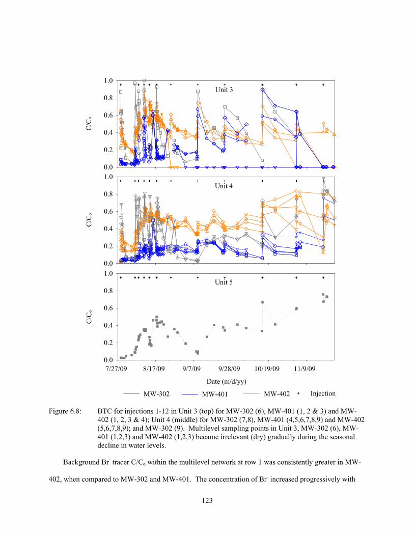
123

C/C

o

0.0

0.2

0.4

0.6

0.8

1.0C

/Co

0.0

0.2

0.4

0.6

0.8

1.0

Date (m/d/yy)

7/27/09 8/17/09 9/7/09 9/28/09 10/19/09 11/9/09

C/C

o

0.0

0.2

0.4

0.6

0.8

1.0

Injection

Unit 3

Unit 4

Unit 5

MW-302 MW-401 MW-402

Figure 6.8: BTC for injections 1-12 in Unit 3 (top) for MW-302 (6), MW-401 (1, 2 & 3) and MW-402 (1, 2, 3 & 4); Unit 4 (middle) for MW-302 (7,8), MW-401 (4,5,6,7,8,9) and MW-402 (5,6,7,8,9); and MW-302 (9). Multilevel sampling points in Unit 3, MW-302 (6), MW-401 (1,2,3) and MW-402 (1,2,3) became irrelevant (dry) gradually during the seasonal decline in water levels.

Background Br- tracer C/Co within the multilevel network at row 1 was consistently greater in MW-

402, when compared to MW-302 and MW-401. The concentration of Br- increased progressively with

124

each pulse introduced due to the accumulation of mass solutes (Br-) in the groundwater following

consecutive injections. Throughout each consecutive injection, the most recent injected slug displaced

pre-existing amended groundwater, resulting in a wider distribution of the remedial cloud in the

subsurface as time progressed, however dispersive mixing was relatively minor given the short injection

time. The average background C/Co between injections in MW-402 Unit 3 and 4 was approximately 0.4,

whereas the maximum average background C/Co of 0.3 was calculated for MW-302 Unit 5. A complete

summary of tracer conditions in specific aquifer formations of Row 1, immediately prior to each

injection, is presented in Appendix E. The importance of the distribution of tracer between injections

involves the delivery of remedial solution to target zones containing residual petroleum hydrocarbons and

the duration of exposure, discussed in detail in subsequent sections of this chapter.

A fence of groundwater wells was installed in October 2009, parallel to the existing multilevel

monitoring network, as part of B. Katanchi’s research project (Katanchi, 2011) and referred to as Row 2,

as previously discussed in Chapter 5. The wells, utilized to monitor the presence of the remedial plume

between Row 1 and 3, were applicable to the monitoring program post-injection 10. A maximum relative

concentration 0.1 of Br- tracer was observed in MW-603, situated in Row 2 and approximately 3.7 m

downgradient of the injection well in November 2009, however concentrations declined over time. A

cross-sectional view of the horizontal distribution of the Br- tracer/ remedial plume along the groundwater

flow path is presented in Figure 6. 9 illustrating the decrease in Br- tracer concentrations with increasing

distance from the injection well related to dispersive processes.

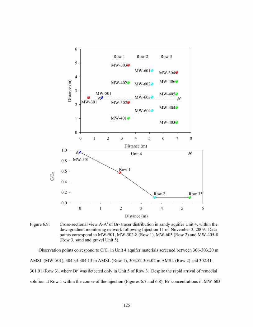
125

Distance (m)

0 1 2 3 4 5 6

C/C

o

0.0

0.2

0.4

0.6

0.8

1.0

MW-501

Row 1

Row 2 Row 3*

Unit 4

Distance (m)

0 1 2 3 4 5 6 7 8

Dis

tanc

e (m

)

0

1

2

3

4

5

6

MW-301

MW-501

MW-303

MW-402

MW-302

MW-401

MW-601

MW-602

MW-603

MW-604

MW-304

MW-406

MW-405

MW-404

MW-403

A'A

A'A

Row 1 Row 2 Row 3

Figure 6.9: Cross-sectional view A-A′ of Br- tracer distribution in sandy aquifer Unit 4, within the downgradient monitoring network following Injection 11 on November 3, 2009. Data points correspond to MW-501, MW-302-8 (Row 1), MW-603 (Row 2) and MW-405-8 (Row 3, sand and gravel Unit 5).

Observation points correspond to C/Co in Unit 4 aquifer materials screened between 306-303.20 m

AMSL (MW-501), 304.33-304.13 m AMSL (Row 1), 303.52-303.02 m AMSL (Row 2) and 302.41-

301.91 (Row 3), where Br- was detected only in Unit 5 of Row 3. Despite the rapid arrival of remedial

solution at Row 1 within the course of the injection (Figures 6.7 and 6.8), Br- concentrations in MW-603

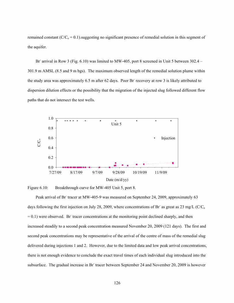
126

remained constant (C/Co = 0.1).suggesting no significant presence of remedial solution in this segment of

the aquifer.

Br- arrival in Row 3 (Fig. 6.10) was limited to MW-405, port 8 screened in Unit 5 between 302.4 –

301.9 m AMSL (8.5 and 9 m bgs). The maximum observed length of the remedial solution plume within

the study area was approximately 6.5 m after 62 days. Poor Br- recovery at row 3 is likely attributed to

dispersion dilution effects or the possibility that the migration of the injected slug followed different flow

paths that do not intersect the test wells.

Date (m/d/yy)

7/27/09 8/17/09 9/7/09 9/28/09 10/19/09 11/9/09

C/C

o

0.0

0.2

0.4

0.6

0.8

1.0

Injection

Unit 5

Figure 6.10: Breakthrough curve for MW-405 Unit 5, port 8.

Peak arrival of Br- tracer at MW-405-9 was measured on September 24, 2009, approximately 63

days following the first injection on July 28, 2009, where concentrations of Br- as great as 23 mg/L (C/Co

= 0.1) were observed. Br- tracer concentrations at the monitoring point declined sharply, and then

increased steadily to a second peak concentration measured November 20, 2009 (121 days). The first and

second peak concentrations may be representative of the arrival of the centre of mass of the remedial slug

delivered during injections 1 and 2. However, due to the limited data and low peak arrival concentrations,

there is not enough evidence to conclude the exact travel times of each individual slug introduced into the

subsurface. The gradual increase in Br- tracer between September 24 and November 20, 2009 is however

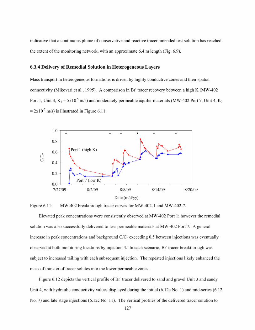
127

indicative that a continuous plume of conservative and reactive tracer amended test solution has reached

the extent of the monitoring network, with an approximate 6.4 m length (Fig. 6.9).

6.3.4 Delivery of Remedial Solution in Heterogeneous Layers

Mass transport in heterogeneous formations is driven by highly conductive zones and their spatial

connectivity (Mikovari et al., 1995). A comparison in Br- tracer recovery between a high K (MW-402

Port 1, Unit 3, K1 = 5x10-5 m/s) and moderately permeable aquifer materials (MW-402 Port 7, Unit 4, K7

= 2x10-7 m/s) is illustrated in Figure 6.11.

Date (m/d/yy)

7/27/09 8/2/09 8/8/09 8/14/09 8/20/09

C/C

o

0.0

0.2

0.4

0.6

0.8

1.0

Port 7 (low K)

Port 1 (high K)

Figure 6.11: MW-402 breakthrough tracer curves for MW-402-1 and MW-402-7.

Elevated peak concentrations were consistently observed at MW-402 Port 1; however the remedial

solution was also successfully delivered to less permeable materials at MW-402 Port 7. A general

increase in peak concentrations and background C/Co exceeding 0.5 between injections was eventually

observed at both monitoring locations by injection 4. In each scenario, Br- tracer breakthrough was

subject to increased tailing with each subsequent injection. The repeated injections likely enhanced the

mass of transfer of tracer solutes into the lower permeable zones.

Figure 6.12 depicts the vertical profile of Br- tracer delivered to sand and gravel Unit 3 and sandy

Unit 4, with hydraulic conductivity values displayed during the initial (6.12a No. 1) and mid-series (6.12

No. 7) and late stage injections (6.12c No. 11). The vertical profiles of the delivered tracer solution to

128

Unit 3 and Unit 4 is consistent with what was previously seen in Figure 6.8 immediately following the

injection. For injection 1, Br- had dropped to C/Co = 0.2, while for later injections, the tracer remained

near or above 0.4 after 8 days. This indicates that a continuous supply of remedial chemical was delivered

to the subsurface, with higher concentrations being achieved during later injections when the ambient

groundwater velocity was lower. The spatial variation in K inferred from grain-size analysis was often

poorly correlated with the breakthrough data, especially under higher flow conditions apparent during

injections 1 through 7. The Br- breakthrough profile for Injection 11 is in better agreement with the

vertical distribution of K values, most likely the result of the low gradient present across the Site at the

time of the injection.

Under elevated groundwater levels (July – August, injection 1-6), early-time arrival of Br- tracer (t=1

hour post-injection) occurred in the high permeability layers of Unit 2 and 3 and the upper zone of Unit 4.

Reduced water levels (November, injections 11 and 12) led to remedial solution also being delivered

quickly to deeper regions (Unit 4) (Fig. 6.12c). During seasonal high groundwater levels, the test solution

flowed preferentially through the lower permeable zones of Unit 3 (Fig. 6.12a: MW-402, ports 1, 2, 3 &

4). The high permeable zone located in the lower portion of Unit 4 (Figure 6.12c: MW-402, ports 7, 8 &

9) was able to transmit the test solution more effectively under low seasonal groundwater levels.

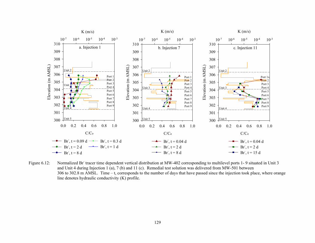
129

K (m/s)

10-7 10-6 10-5 10-4 10-3

Ele

vatio

n (m

AM

SL

)

300

301

302

303

304

305

306

307

308

309

310

C/Co

0.0 0.2 0.4 0.6 0.8 1.0

Br-, t = 0.3 dBr-, t = 1 d

Unit 2

Unit 3

Unit 4

Unit 5

a. Injection 1

Port 1Port 2Port 3Port 4Port 5Port 6Port 7Port 8Port 9

Br-, t = 0.09 d

Br-, t = 2 d

Br-, t = 8 d

b. Injection 7

K (m/s)

10-7 10-6 10-5 10-4 10-3

Ele

vatio

n (m

AM

SL

)

300

301

302

303

304

305

306

307

308

309

310

C/Co

0.0 0.2 0.4 0.6 0.8 1.0

Br-, t = 0.04 dBr-, t = 2 dBr-, t = 8 d

Unit 2

Unit 3

Unit 4

Unit 5

Port 1Port 2Port 3Port 4Port 5Port 6Port 7Port 8Port 9

c. Injection 11

K (m/s)

10-7 10-6 10-5 10-4 10-3

Ele

vatio

n (m

AM

SL

)

300

301

302

303

304

305

306

307

308

309

310

C/Co

0.0 0.2 0.4 0.6 0.8 1.0

Br-, t = 0.04 dBr-, t = 2 dBr-, t = 15 d

Unit 2

Unit 3

Unit 4

Unit 5

Port 1xPort 2Port 3Port 4Port 5Port 6Port 7Port 8Port 9

Figure 6.12: Normalized Br- tracer time dependent vertical distribution at MW-402 corresponding to multilevel ports 1- 9 situated in Unit 3 and Unit 4 during Injection 1 (a), 7 (b) and 11 (c). Remedial test solution was delivered from MW-501 between 306 to 302.8 m AMSL. Time – t, corresponds to the number of days that have passed since the injection took place, where orange line denotes hydraulic conductivity (K) profile.

130

6.4 Transportation of the Remedial Test Solution

Characterization of aquifer parameters and groundwater velocity are important in determining the main

transport processes in the aquifer. The fate and behaviour of the mass solutes (Br-, NO3-) present in the

remedial solution is consistent with the transport of the contaminants within the study area. Average

linear groundwater velocities for the specific units were estimated from the Br- tracer breakthrough data.

The groundwater velocity was determined by measuring the departure of the centre of mass of the

remedial solution within the injection well. The distance the centre of mass of the slug had to travel was

established using the injection radius of influence (ROI) as previously described in equation (6.1). The

average linear groundwater velocity, v was determined from the following distance over time relationship

presented in equation (6.2) below:

.

(6.2)

Where t0.5 is the time for the C/Co of the BTC to be reduced to half of the maximum relative tracer

concentration measured in the injection well or at the downgradient multilevel wells located in Row 1.

An example of the graphical determination of t0.5 is shown in Appendix E. The linear groundwater

velocity was calculated based on the removal of the remedial solution in the injection well, MW-501 and

the arrival at the downgradient network of multilevel wells MW-302 and MW-402 situated in Row 1.

Remedial test solution transport velocities were calculated for specific observation points screened in

the various aquifer formations. The results of estimated values of v corresponding to individual

stratigraphic units are summarized in Table 6.1. The measured horizontal hydraulic gradient at the time of

the injection, determined from monitoring groundwater levels at MW-103, MW-101 and MW-107 as

previously discussed, is also presented in Table 6.1. A complete evaluation of linear groundwater

velocities for each multilevel sampler during injections 1 through 12 is presented in Appendix E.

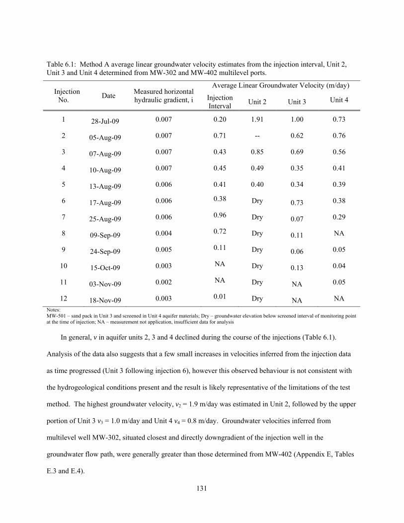
131

Table 6.1: Method A average linear groundwater velocity estimates from the injection interval, Unit 2, Unit 3 and Unit 4 determined from MW-302 and MW-402 multilevel ports.

Injection No.

Date Measured horizontal hydraulic gradient, i

Average Linear Groundwater Velocity (m/day)

Injection Interval

Unit 2 Unit 3 Unit 4

1 28-Jul-09 0.007 0.20 1.91 1.00 0.73

2 05-Aug-09 0.007 0.71 -- 0.62 0.76

3 07-Aug-09 0.007 0.43 0.85 0.69 0.56

4 10-Aug-09 0.007 0.45 0.49 0.35 0.41

5 13-Aug-09 0.006 0.41 0.40 0.34 0.39

6 17-Aug-09 0.006 0.38 Dry 0.73 0.38

7 25-Aug-09 0.006 0.96 Dry 0.07 0.29

8 09-Sep-09 0.004 0.72 Dry 0.11 NA

9 24-Sep-09 0.005 0.11 Dry 0.06 0.05

10 15-Oct-09 0.003 NA Dry 0.13 0.04

11 03-Nov-09 0.002 NA Dry NA 0.05

12 18-Nov-09 0.003 0.01 Dry NA NA

Notes: MW-501 – sand pack in Unit 3 and screened in Unit 4 aquifer materials; Dry – groundwater elevation below screened interval of monitoring point at the time of injection; NA – measurement not application, insufficient data for analysis

In general, v in aquifer units 2, 3 and 4 declined during the course of the injections (Table 6.1).

Analysis of the data also suggests that a few small increases in velocities inferred from the injection data

as time progressed (Unit 3 following injection 6), however this observed behaviour is not consistent with

the hydrogeological conditions present and the result is likely representative of the limitations of the test

method. The highest groundwater velocity, v2 = 1.9 m/day was estimated in Unit 2, followed by the upper

portion of Unit 3 v3 = 1.0 m/day and Unit 4 v4 = 0.8 m/day. Groundwater velocities inferred from

multilevel well MW-302, situated closest and directly downgradient of the injection well in the

groundwater flow path, were generally greater than those determined from MW-402 (Appendix E, Tables

E.3 and E.4).

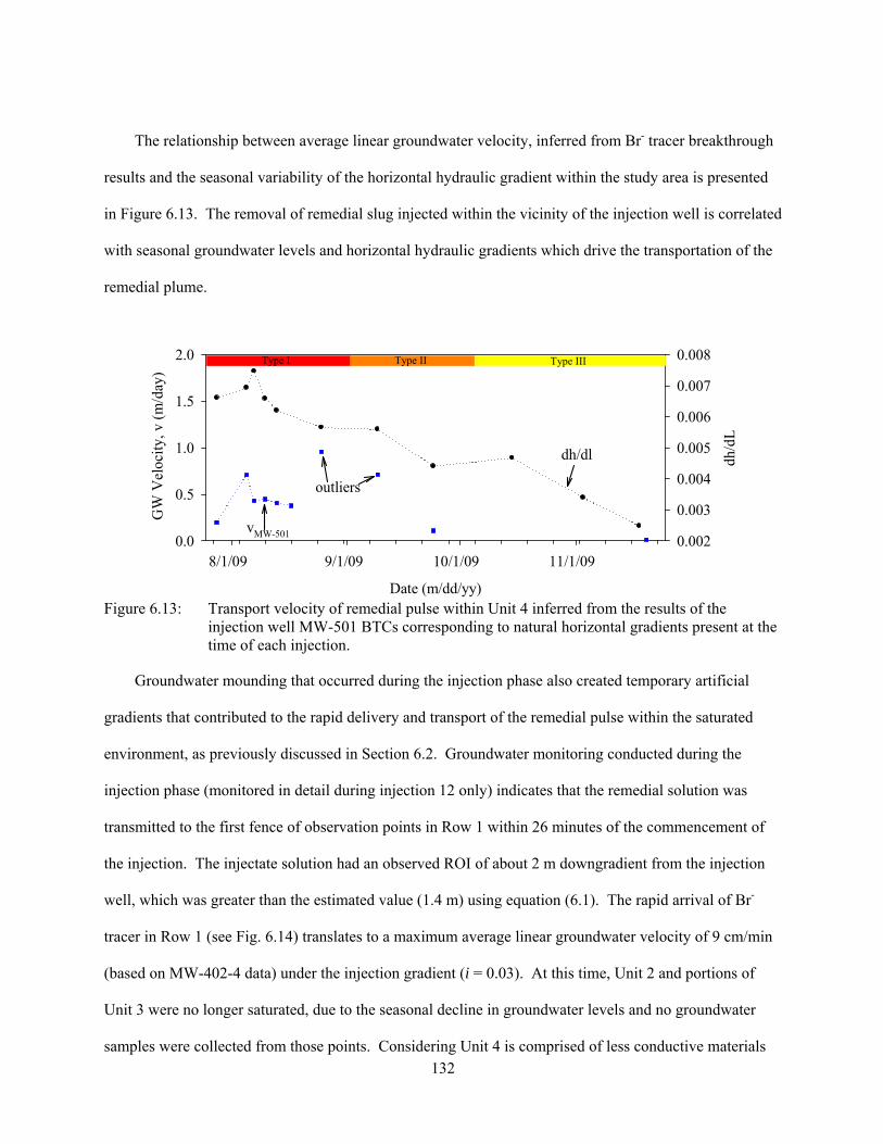
132

The relationship between average linear groundwater velocity, inferred from Br- tracer breakthrough

results and the seasonal variability of the horizontal hydraulic gradient within the study area is presented

in Figure 6.13. The removal of remedial slug injected within the vicinity of the injection well is correlated

with seasonal groundwater levels and horizontal hydraulic gradients which drive the transportation of the

remedial plume.

Date (m/dd/yy)

8/1/09 9/1/09 10/1/09 11/1/09

GW

Vel

ocity

, v (

m/d

ay)

0.0

0.5

1.0

1.5

2.0

dh/d

L

0.002

0.003

0.004

0.005

0.006

0.007

0.008Type I Type II Type III

dh/dl

vMW-501

outliers

Figure 6.13: Transport velocity of remedial pulse within Unit 4 inferred from the results of the

injection well MW-501 BTCs corresponding to natural horizontal gradients present at the time of each injection.

Groundwater mounding that occurred during the injection phase also created temporary artificial

gradients that contributed to the rapid delivery and transport of the remedial pulse within the saturated

environment, as previously discussed in Section 6.2. Groundwater monitoring conducted during the

injection phase (monitored in detail during injection 12 only) indicates that the remedial solution was

transmitted to the first fence of observation points in Row 1 within 26 minutes of the commencement of

the injection. The injectate solution had an observed ROI of about 2 m downgradient from the injection

well, which was greater than the estimated value (1.4 m) using equation (6.1). The rapid arrival of Br-

tracer in Row 1 (see Fig. 6.14) translates to a maximum average linear groundwater velocity of 9 cm/min

(based on MW-402-4 data) under the injection gradient (i = 0.03). At this time, Unit 2 and portions of

Unit 3 were no longer saturated, due to the seasonal decline in groundwater levels and no groundwater

samples were collected from those points. Considering Unit 4 is comprised of less conductive materials

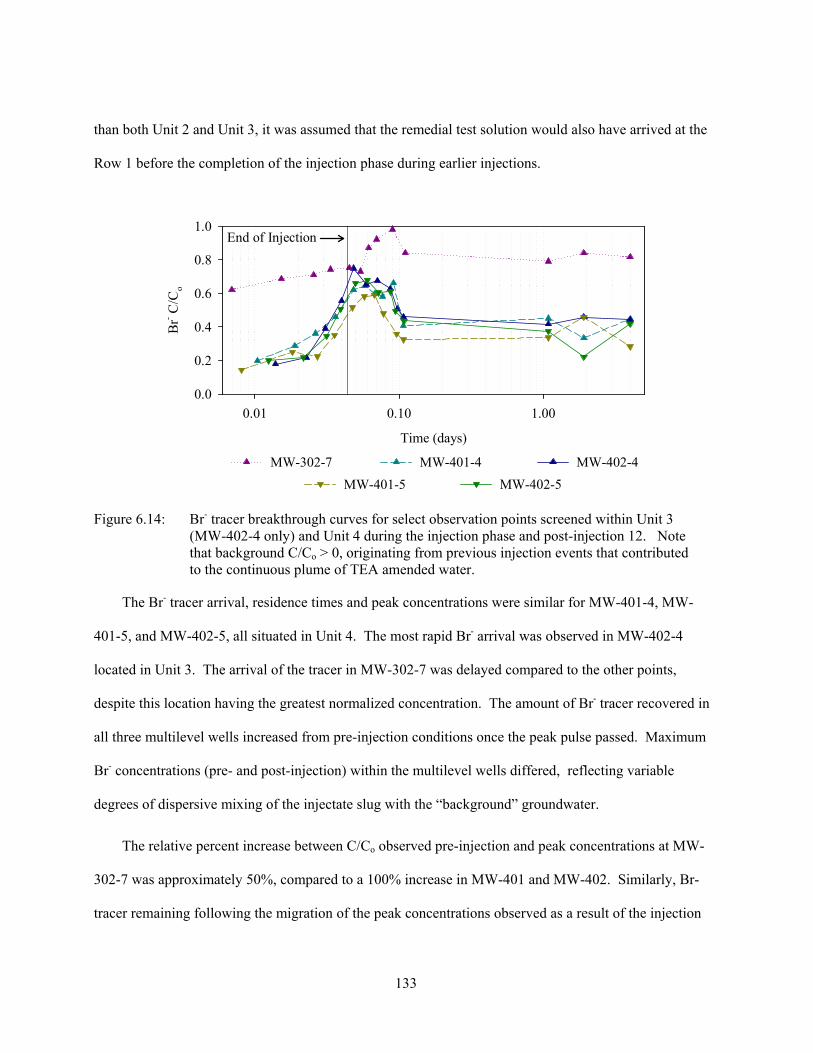
133

than both Unit 2 and Unit 3, it was assumed that the remedial test solution would also have arrived at the

Row 1 before the completion of the injection phase during earlier injections.

Time (days)

0.01 0.10 1.00

Br- C

/Co

0.0

0.2

0.4

0.6

0.8

1.0

MW-402-5

End of Injection

MW-401-5

MW-401-4 MW-402-4MW-302-7

Figure 6.14: Br- tracer breakthrough curves for select observation points screened within Unit 3 (MW-402-4 only) and Unit 4 during the injection phase and post-injection 12. Note that background C/Co > 0, originating from previous injection events that contributed to the continuous plume of TEA amended water.

The Br- tracer arrival, residence times and peak concentrations were similar for MW-401-4, MW-

401-5, and MW-402-5, all situated in Unit 4. The most rapid Br- arrival was observed in MW-402-4

located in Unit 3. The arrival of the tracer in MW-302-7 was delayed compared to the other points,

despite this location having the greatest normalized concentration. The amount of Br- tracer recovered in

all three multilevel wells increased from pre-injection conditions once the peak pulse passed. Maximum

Br- concentrations (pre- and post-injection) within the multilevel wells differed, reflecting variable

degrees of dispersive mixing of the injectate slug with the “background” groundwater.

The relative percent increase between C/Co observed pre-injection and peak concentrations at MW-

302-7 was approximately 50%, compared to a 100% increase in MW-401 and MW-402. Similarly, Br-

tracer remaining following the migration of the peak concentrations observed as a result of the injection

134

declined by approximately 40% at MW-401 and 402 and only 22% at MW-302 over the same period of

time.

6.5 Remedial Tracer Test Summary

The delivery of the remedial test solution to a target zone of the aquifer contaminated with residual

petroleum hydrocarbons was evaluated by monitoring groundwater for Br- tracer. The injectate was also

amended with nitrate serving as a TEA and reactive tracer to enhance in-situ biodegradation in the

petroleum hydrocarbon contaminated residual zone of the anaerobic aquifer. The results of the Br- tracer

breakthrough data provide insight into the groundwater transport processes, the subsequent transport of

mass contaminants and remedial solution present at the Site under variable hydrogeological conditions.

Details pertaining to the delivery and utilization of nitrate in the degradation of petroleum contaminants

from denitrification are discussed in Chapter 7.

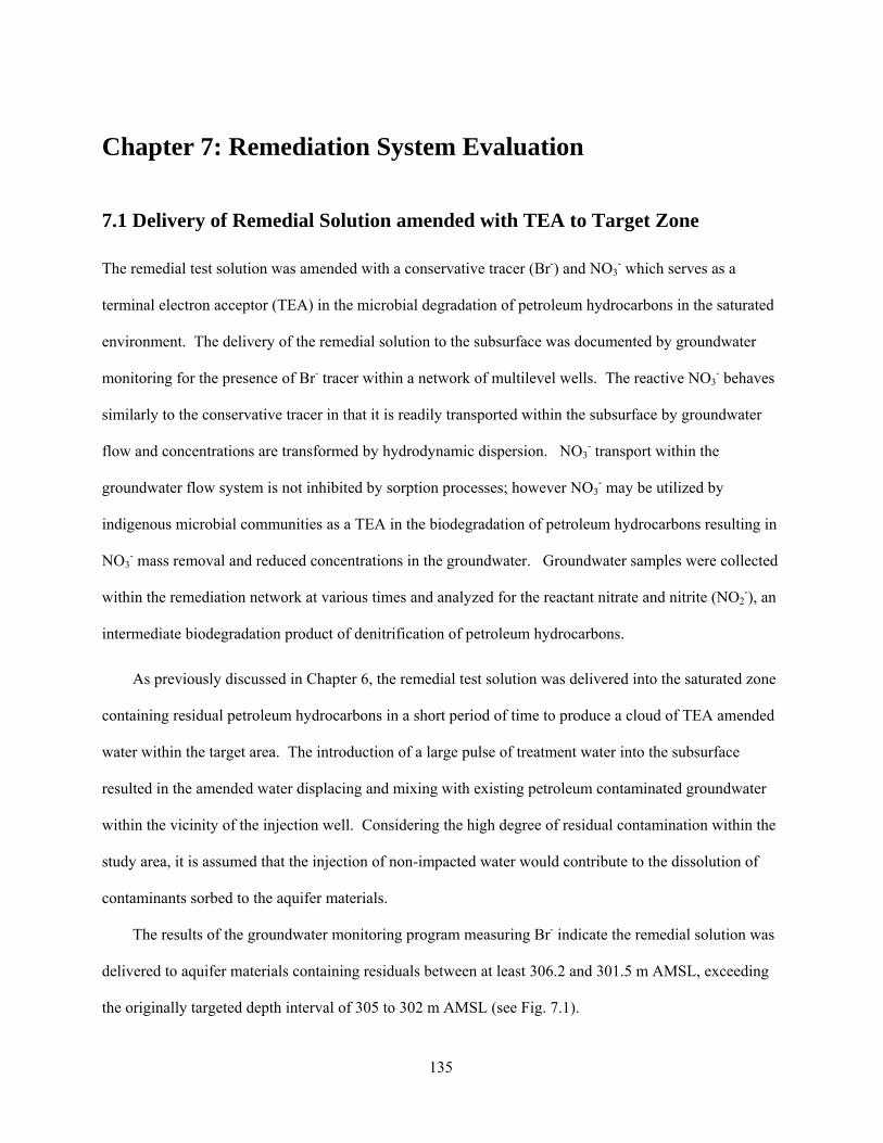
135

Chapter 7: Remediation System Evaluation

7.1 Delivery of Remedial Solution amended with TEA to Target Zone

The remedial test solution was amended with a conservative tracer (Br-) and NO3- which serves as a

terminal electron acceptor (TEA) in the microbial degradation of petroleum hydrocarbons in the saturated

environment. The delivery of the remedial solution to the subsurface was documented by groundwater

monitoring for the presence of Br- tracer within a network of multilevel wells. The reactive NO3- behaves

similarly to the conservative tracer in that it is readily transported within the subsurface by groundwater

flow and concentrations are transformed by hydrodynamic dispersion. NO3- transport within the

groundwater flow system is not inhibited by sorption processes; however NO3- may be utilized by

indigenous microbial communities as a TEA in the biodegradation of petroleum hydrocarbons resulting in

NO3- mass removal and reduced concentrations in the groundwater. Groundwater samples were collected

within the remediation network at various times and analyzed for the reactant nitrate and nitrite (NO2-), an

intermediate biodegradation product of denitrification of petroleum hydrocarbons.

As previously discussed in Chapter 6, the remedial test solution was delivered into the saturated zone

containing residual petroleum hydrocarbons in a short period of time to produce a cloud of TEA amended

water within the target area. The introduction of a large pulse of treatment water into the subsurface

resulted in the amended water displacing and mixing with existing petroleum contaminated groundwater

within the vicinity of the injection well. Considering the high degree of residual contamination within the

study area, it is assumed that the injection of non-impacted water would contribute to the dissolution of

contaminants sorbed to the aquifer materials.

The results of the groundwater monitoring program measuring Br- indicate the remedial solution was

delivered to aquifer materials containing residuals between at least 306.2 and 301.5 m AMSL, exceeding

the originally targeted depth interval of 305 to 302 m AMSL (see Fig. 7.1).

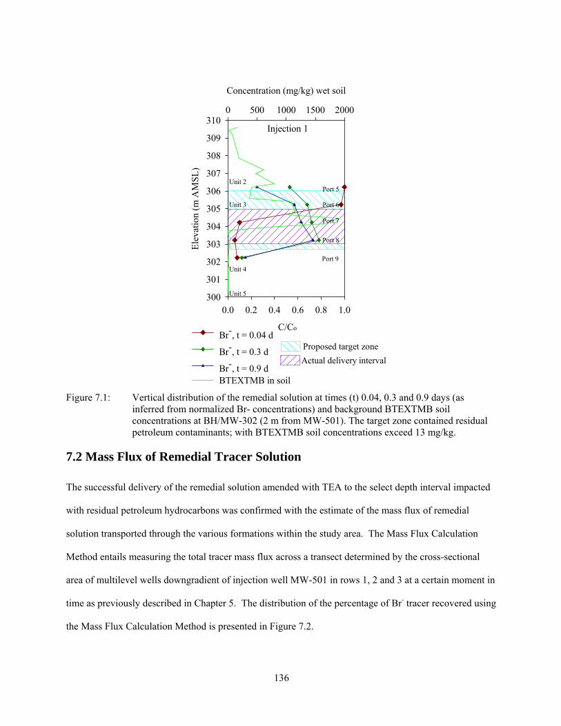
136

Injection 1

C/Co

0.0 0.2 0.4 0.6 0.8 1.0

Ele

vatio

n (m

AM

SL

)

300

301

302

303

304

305

306

307

308

309

310

Concentration (mg/kg) wet soil

0 500 1000 1500 2000

Br-, t = 0.04 d

Br-, t = 0.3 d

Br-, t = 0.9 dBTEXTMB in soil

Unit 2

Unit 3

Unit 4

Unit 5

Port 5

Port 6

Port 7

Port 8

Port 9

Proposed target zone

Actual delivery interval

Figure 7.1: Vertical distribution of the remedial solution at times (t) 0.04, 0.3 and 0.9 days (as inferred from normalized Br- concentrations) and background BTEXTMB soil concentrations at BH/MW-302 (2 m from MW-501). The target zone contained residual petroleum contaminants; with BTEXTMB soil concentrations exceed 13 mg/kg.

7.2 Mass Flux of Remedial Tracer Solution

The successful delivery of the remedial solution amended with TEA to the select depth interval impacted

with residual petroleum hydrocarbons was confirmed with the estimate of the mass flux of remedial

solution transported through the various formations within the study area. The Mass Flux Calculation

Method entails measuring the total tracer mass flux across a transect determined by the cross-sectional

area of multilevel wells downgradient of injection well MW-501 in rows 1, 2 and 3 at a certain moment in

time as previously described in Chapter 5. The distribution of the percentage of Br- tracer recovered using

the Mass Flux Calculation Method is presented in Figure 7.2.

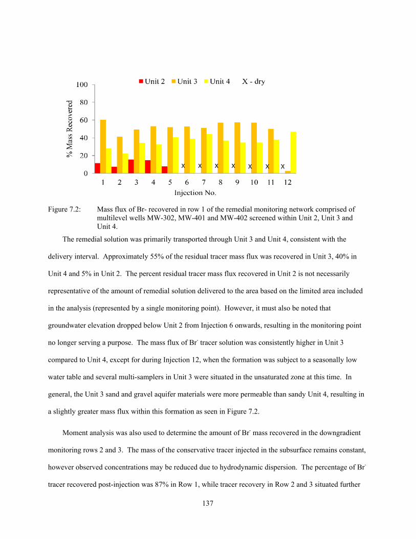
137

Figure 7.2: Mass flux of Br- recovered in row 1 of the remedial monitoring network comprised of multilevel wells MW-302, MW-401 and MW-402 screened within Unit 2, Unit 3 and Unit 4.

The remedial solution was primarily transported through Unit 3 and Unit 4, consistent with the

delivery interval. Approximately 55% of the residual tracer mass flux was recovered in Unit 3, 40% in

Unit 4 and 5% in Unit 2. The percent residual tracer mass flux recovered in Unit 2 is not necessarily

representative of the amount of remedial solution delivered to the area based on the limited area included

in the analysis (represented by a single monitoring point). However, it must also be noted that

groundwater elevation dropped below Unit 2 from Injection 6 onwards, resulting in the monitoring point

no longer serving a purpose. The mass flux of Br- tracer solution was consistently higher in Unit 3

compared to Unit 4, except for during Injection 12, when the formation was subject to a seasonally low

water table and several multi-samplers in Unit 3 were situated in the unsaturated zone at this time. In

general, the Unit 3 sand and gravel aquifer materials were more permeable than sandy Unit 4, resulting in

a slightly greater mass flux within this formation as seen in Figure 7.2.

Moment analysis was also used to determine the amount of Br- mass recovered in the downgradient

monitoring rows 2 and 3. The mass of the conservative tracer injected in the subsurface remains constant,

however observed concentrations may be reduced due to hydrodynamic dispersion. The percentage of Br-

tracer recovered post-injection was 87% in Row 1, while tracer recovery in Row 2 and 3 situated further

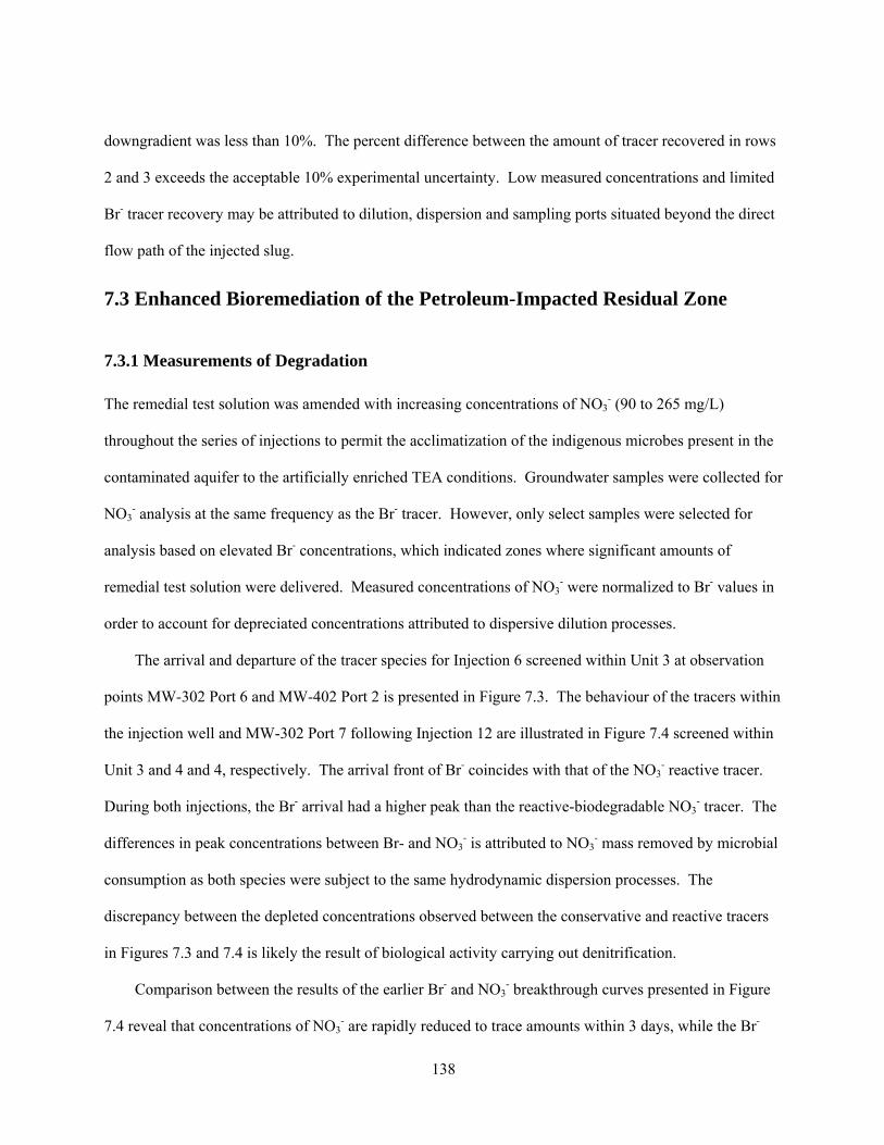
138

downgradient was less than 10%. The percent difference between the amount of tracer recovered in rows

2 and 3 exceeds the acceptable 10% experimental uncertainty. Low measured concentrations and limited

Br- tracer recovery may be attributed to dilution, dispersion and sampling ports situated beyond the direct

flow path of the injected slug.

7.3 Enhanced Bioremediation of the Petroleum-Impacted Residual Zone

7.3.1 Measurements of Degradation

The remedial test solution was amended with increasing concentrations of NO3- (90 to 265 mg/L)

throughout the series of injections to permit the acclimatization of the indigenous microbes present in the

contaminated aquifer to the artificially enriched TEA conditions. Groundwater samples were collected for

NO3- analysis at the same frequency as the Br- tracer. However, only select samples were selected for

analysis based on elevated Br- concentrations, which indicated zones where significant amounts of

remedial test solution were delivered. Measured concentrations of NO3- were normalized to Br- values in

order to account for depreciated concentrations attributed to dispersive dilution processes.

The arrival and departure of the tracer species for Injection 6 screened within Unit 3 at observation

points MW-302 Port 6 and MW-402 Port 2 is presented in Figure 7.3. The behaviour of the tracers within

the injection well and MW-302 Port 7 following Injection 12 are illustrated in Figure 7.4 screened within

Unit 3 and 4 and 4, respectively. The arrival front of Br- coincides with that of the NO3- reactive tracer.

During both injections, the Br- arrival had a higher peak than the reactive-biodegradable NO3- tracer. The

differences in peak concentrations between Br- and NO3- is attributed to NO3

- mass removed by microbial

consumption as both species were subject to the same hydrodynamic dispersion processes. The

discrepancy between the depleted concentrations observed between the conservative and reactive tracers

in Figures 7.3 and 7.4 is likely the result of biological activity carrying out denitrification.

Comparison between the results of the earlier Br- and NO3- breakthrough curves presented in Figure

7.4 reveal that concentrations of NO3- are rapidly reduced to trace amounts within 3 days, while the Br-

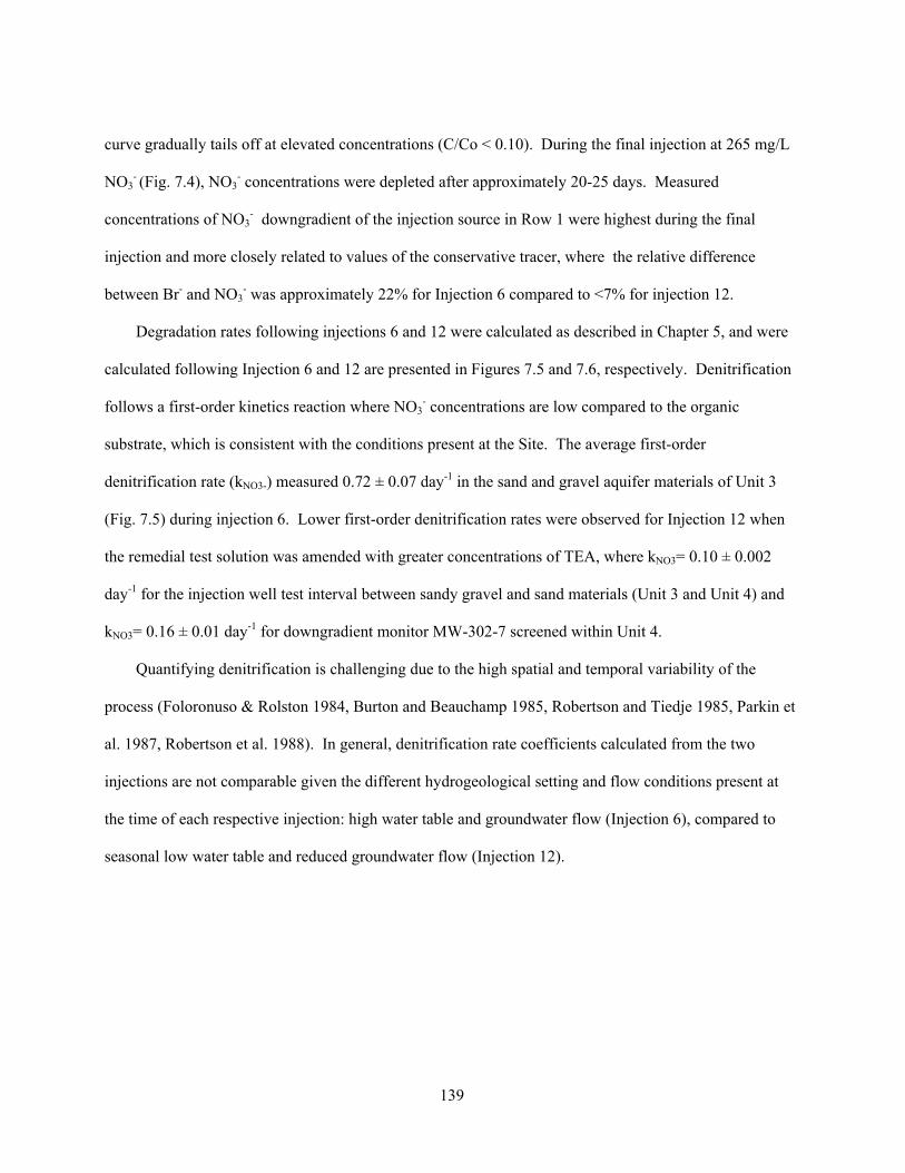
139

curve gradually tails off at elevated concentrations (C/Co < 0.10). During the final injection at 265 mg/L

NO3- (Fig. 7.4), NO3

- concentrations were depleted after approximately 20-25 days. Measured

concentrations of NO3- downgradient of the injection source in Row 1 were highest during the final

injection and more closely related to values of the conservative tracer, where the relative difference

between Br- and NO3- was approximately 22% for Injection 6 compared to <7% for injection 12.

Degradation rates following injections 6 and 12 were calculated as described in Chapter 5, and were

calculated following Injection 6 and 12 are presented in Figures 7.5 and 7.6, respectively. Denitrification

follows a first-order kinetics reaction where NO3- concentrations are low compared to the organic

substrate, which is consistent with the conditions present at the Site. The average first-order

denitrification rate (kNO3-) measured 0.72 ± 0.07 day-1 in the sand and gravel aquifer materials of Unit 3

(Fig. 7.5) during injection 6. Lower first-order denitrification rates were observed for Injection 12 when

the remedial test solution was amended with greater concentrations of TEA, where kNO3= 0.10 ± 0.002

day-1 for the injection well test interval between sandy gravel and sand materials (Unit 3 and Unit 4) and

kNO3= 0.16 ± 0.01 day-1 for downgradient monitor MW-302-7 screened within Unit 4.

Quantifying denitrification is challenging due to the high spatial and temporal variability of the

process (Foloronuso & Rolston 1984, Burton and Beauchamp 1985, Robertson and Tiedje 1985, Parkin et

al. 1987, Robertson et al. 1988). In general, denitrification rate coefficients calculated from the two

injections are not comparable given the different hydrogeological setting and flow conditions present at

the time of each respective injection: high water table and groundwater flow (Injection 6), compared to

seasonal low water table and reduced groundwater flow (Injection 12).

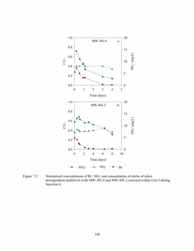
140

Time (days)

0 2 4 6 8 10

C/C

o

0.0

0.2

0.4

0.6

0.8

1.0

NO

2- (m

g/L

)

0

5

10

15

20

NO2-

MW-402-2 b.

Time (days)

0 1 2 3 4 5

C/C

o

0.0

0.2

0.4

0.6

0.8

1.0

NO

2- (m

g/L

)

0

5

10

15

20MW-302-6 a.

NO3- Br-

Figure 7.3: Normalized concentrations of Br-, NO3- and concentration of nitrite of select

downgradient multilevel wells MW-302-6 and MW-402- 2 screened within Unit 3 during Injection 6.

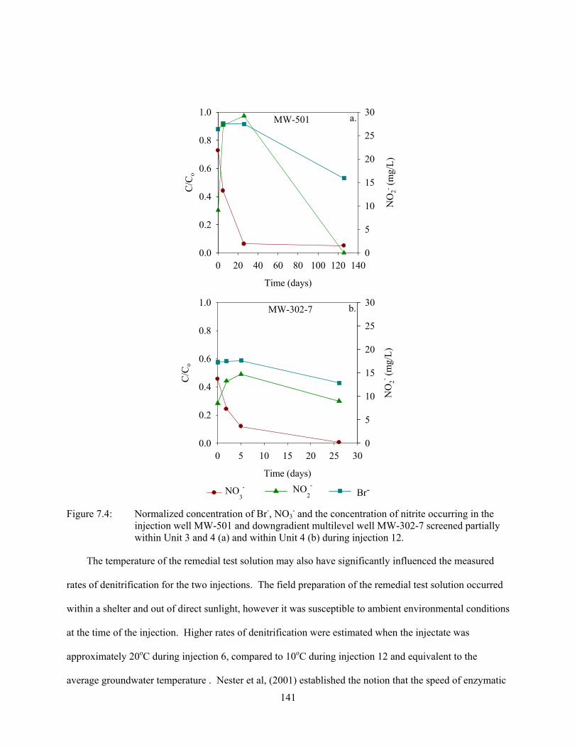
141

Time (days)

0 20 40 60 80 100 120 140

C/C

o

NO

2- (m

g/L

)

0

5

10

15

20

25

30

0.0

0.2

0.4

0.6

0.8

1.0MW-501

Time (days)

0 5 10 15 20 25 30

C/C

o

0.0

0.2

0.4

0.6

0.8

1.0

NO

2- (m

g/L

)

0

5

10

15

20

25

30

NO2

-

MW-302-7

a.

b.

NO3

-Br-

Figure 7.4: Normalized concentration of Br-, NO3

- and the concentration of nitrite occurring in the injection well MW-501 and downgradient multilevel well MW-302-7 screened partially within Unit 3 and 4 (a) and within Unit 4 (b) during injection 12.

The temperature of the remedial test solution may also have significantly influenced the measured

rates of denitrification for the two injections. The field preparation of the remedial test solution occurred

within a shelter and out of direct sunlight, however it was susceptible to ambient environmental conditions

at the time of the injection. Higher rates of denitrification were estimated when the injectate was

approximately 20oC during injection 6, compared to 10oC during injection 12 and equivalent to the

average groundwater temperature . Nester et al, (2001) established the notion that the speed of enzymatic

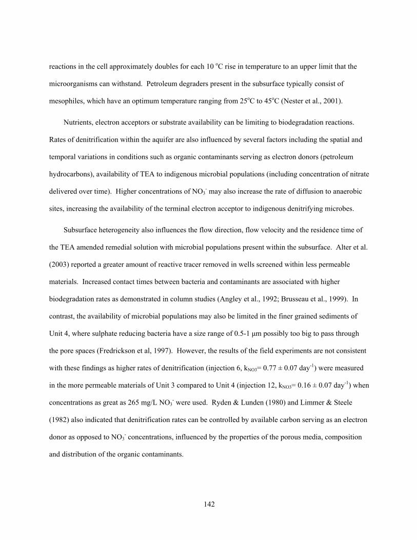
142

reactions in the cell approximately doubles for each 10 oC rise in temperature to an upper limit that the

microorganisms can withstand. Petroleum degraders present in the subsurface typically consist of

mesophiles, which have an optimum temperature ranging from 25oC to 45oC (Nester et al., 2001).

Nutrients, electron acceptors or substrate availability can be limiting to biodegradation reactions.

Rates of denitrification within the aquifer are also influenced by several factors including the spatial and

temporal variations in conditions such as organic contaminants serving as electron donors (petroleum

hydrocarbons), availability of TEA to indigenous microbial populations (including concentration of nitrate

delivered over time). Higher concentrations of NO3- may also increase the rate of diffusion to anaerobic

sites, increasing the availability of the terminal electron acceptor to indigenous denitrifying microbes.

Subsurface heterogeneity also influences the flow direction, flow velocity and the residence time of

the TEA amended remedial solution with microbial populations present within the subsurface. Alter et al.

(2003) reported a greater amount of reactive tracer removed in wells screened within less permeable

materials. Increased contact times between bacteria and contaminants are associated with higher

biodegradation rates as demonstrated in column studies (Angley et al., 1992; Brusseau et al., 1999). In

contrast, the availability of microbial populations may also be limited in the finer grained sediments of

Unit 4, where sulphate reducing bacteria have a size range of 0.5-1 μm possibly too big to pass through

the pore spaces (Fredrickson et al, 1997). However, the results of the field experiments are not consistent

with these findings as higher rates of denitrification (injection 6, kNO3= 0.77 ± 0.07 day-1) were measured

in the more permeable materials of Unit 3 compared to Unit 4 (injection 12, kNO3= 0.16 ± 0.07 day-1) when

concentrations as great as 265 mg/L NO3- were used. Ryden & Lunden (1980) and Limmer & Steele

(1982) also indicated that denitrification rates can be controlled by available carbon serving as an electron

donor as opposed to NO3- concentrations, influenced by the properties of the porous media, composition

and distribution of the organic contaminants.

143

Time (days)

0 5 10 15 20 25 30

ln (

CN

O3- /C

Br-)

-5

-4

-3

-2

-1

0

kNO3- = 0.77 ± 7 % day-1

Time (days)

0 5 10 15 20 25 30

ln (

CN

O3- /C

Br-)

-5

-4

-3

-2

-1

0

kNO3- = 0.66 ± 7 % day-1

a.

b.

MW-302-6

MW-402-2

Figure 7.5: Calculated first-order nitrate degradation in Unit 3, from Figures 7.4a and b for downgradient multilevel wells MW-302 Port 6 (a) and MW-402 Port 2 (b) following Injection 6. The remedial test solution was amended with 90 mg/L NO3

-.

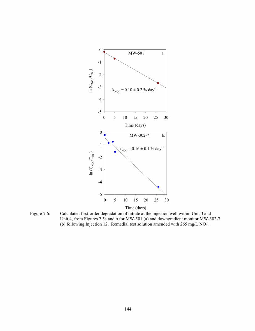
144

Time (days)

0 5 10 15 20 25 30

ln (

CN

O3- /C

Br-)

-5

-4

-3

-2

-1

0

kNO3- = 0.10 ± 0.2 % day-1

Time (days)

0 5 10 15 20 25 30

ln (

CN

O3- /C

Br-)

-5

-4

-3

-2

-1

0

kNO3- = 0.16 ± 0.1 % day-1

MW-302-7 b.

MW-501 a.

Figure 7.6: Calculated first-order degradation of nitrate at the injection well within Unit 3 and Unit 4, from Figures 7.5a and b for MW-501 (a) and downgradient monitor MW-302-7 (b) following Injection 12. Remedial test solution amended with 265 mg/L NO3

-.

145

7.2.2 Denitrification Intermediate Products

Microbial utilization of NO3 was also inferred by measuring concentrations of NO2 in the groundwater, an

intermediate product of denitrification (Postma & Appelo, 2005). Measured concentrations of nitrite as

nitrogen (NO2-N) in groundwater within the study area prior to remedial solution injections were <1 mg/L

NO2-N.

An increase and eventual decline in NO2- concentrations versus time were measured following

injection 6 and 12, as illustrated in Figures 7.3 and 7.4, respectively. Nitrite present in the area infused

with the remedial test solution was observed following several pulsed injections of TEA amended water.

Concentrations of NO2- remained fairly consistent in downgradient monitors following injection 6, with

an average value of 8 mg/L, despite declining concentrations of reactive and conservative tracers, Figure

7.3. Greater concentrations of NO2- were measured following injection 12, as high as 30 mg/L in the

injection well and 15 mg/L in the downgradient monitor as illustrated in Figure 7.4.

Kuhn et al. (1988) found that NO2- exhibited toxic effects when above 5 mM (200 mg/L) to microbial

populations degrading toluene, which is significantly higher than the maximum observed in the field of

0.7 mM (30 mg/L). Microbial toxicity effects related to temporary elevated amounts of NO2-produced

during denitrification are not anticipated to occur within the study due to the low levels generated.

Declining concentrations of NO2- were observed in the injection well and downgradient monitor when

levels of NO3-, serving as the primary TEA, were depleted (Fig. 7.4). The denitrification process

continues with the microbes utilizing NO2- as a TEA (Postma & Appelo, 2005) for metabolic processes,

whereby depleting NO2- concentrations observed in Figure 7.4 may be attributed to dilution attributed to

aquifer dispersion in addition to mass removed related to biological activity.

Nitrate removal in the groundwater system may be the result of processes other than NO3-assimilation

or respiratory denitrification. Dissimilatory nitrate reduction to ammonium (DRNA) involves the

microbially mediated transformation of NO3- to ammonium (NH4

+) as opposed to assimilatory processes

that utilize nitrogen (N) towards microbial biomass. Geochemical analysis of groundwater sampled

146

within the radius of influence of the injectate (MW-302-7) revealed 3.3 mg/L NH4+ present approximately

181 days following the final injection. Nitrate is reduced to ammonium under anaerobic conditions when

biochemical demands involve a highly reduced environment and excess organic carbon (eg. Freeze &

Cherry, 1979; Keeney, 1989), which are consistent with the conditions at the Site. The DNRA process

may result in the production of NH4+ that can then be assimilated into cellular constituents (Schilling,

2002) or adsorbed on silt and clay-sized particles in the aquifer (DeSimone & Howes, 1998; Freeze &

Cherry, 1979). The relatively low concentration of NH4+ measured in the study area compared to the

concentrations of NO3- in the injectate indicates that NH4

+ production as a result of the NO3-amendment

may be occurring in the subsurface, however not in significant amounts considering the stoichiometry of

DNRA as previously discussed in Chapter 1, equation (1.5).

7.2.3 Biostimulation of Indigenous Microbial Populations

Groundwater samples were collected on April 27, 2009 from multilevel wells MW-301 Ports 7, 12 and

MW-302 Port 7, situated upgradient and downgradient of the injection well, respectively, to establish

background microbial numbers prior to the installation of the injection well and subsequent delivery of

remedial test solution to the subsurface. Post-injection groundwater samples were collected on November

3, 2009 following 10 injections and on April 27, 2010 to assess changes in the abundance of microbes

present within the study area following the addition of an artificial supply of NO3-.

Aerobic heterotrophic plate counts (HPC) were conducted to establish pre- and post-injection

microbial populations present in the groundwater system within the select remedial zone. The HPC

method provides an estimate of the number of bacteria present in a known volume of water measured in

colony forming units per milliliter (CFU/mL). However, microbial plate enumerations can be quite

variable (Riser-Roberts, 1992) as most microbes in the groundwater system are attached to sediments.

The results of the HPCs pre- and post-injection of remedial solution are summarized in Table 7.1.

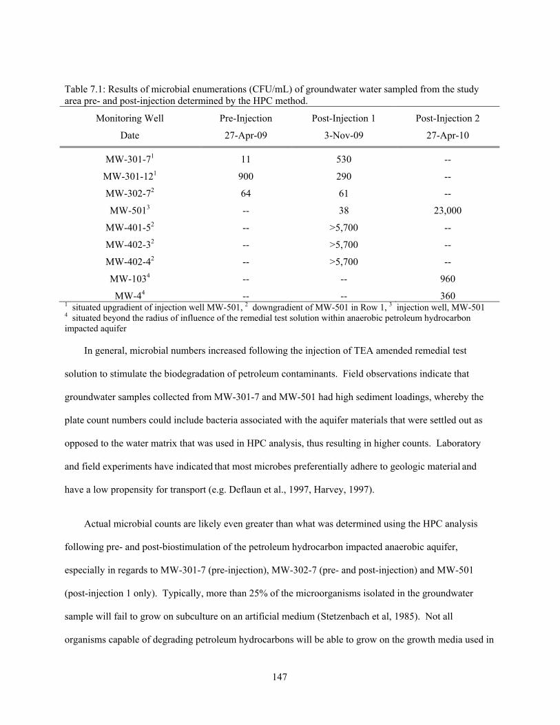
147

Table 7.1: Results of microbial enumerations (CFU/mL) of groundwater water sampled from the study area pre- and post-injection determined by the HPC method.

Monitoring Well

Date

Pre-Injection

27-Apr-09

Post-Injection 1

3-Nov-09

Post-Injection 2

27-Apr-10

MW-301-71 11 530 --

MW-301-121 900 290 --

MW-302-72 64 61 --

MW-5013 -- 38 23,000

MW-401-52 -- >5,700 --

MW-402-32 -- >5,700 --

MW-402-42 -- >5,700 --

MW-1034 -- -- 960

MW-44 -- -- 360 1 situated upgradient of injection well MW-501, 2 downgradient of MW-501 in Row 1, 3 injection well, MW-501 4 situated beyond the radius of influence of the remedial test solution within anaerobic petroleum hydrocarbon impacted aquifer

In general, microbial numbers increased following the injection of TEA amended remedial test

solution to stimulate the biodegradation of petroleum contaminants. Field observations indicate that

groundwater samples collected from MW-301-7 and MW-501 had high sediment loadings, whereby the

plate count numbers could include bacteria associated with the aquifer materials that were settled out as

opposed to the water matrix that was used in HPC analysis, thus resulting in higher counts. Laboratory

and field experiments have indicated that most microbes preferentially adhere to geologic material and

have a low propensity for transport (e.g. Deflaun et al., 1997, Harvey, 1997).

Actual microbial counts are likely even greater than what was determined using the HPC analysis

following pre- and post-biostimulation of the petroleum hydrocarbon impacted anaerobic aquifer,

especially in regards to MW-301-7 (pre-injection), MW-302-7 (pre- and post-injection) and MW-501

(post-injection 1 only). Typically, more than 25% of the microorganisms isolated in the groundwater

sample will fail to grow on subculture on an artificial medium (Stetzenbach et al, 1985). Not all

organisms capable of degrading petroleum hydrocarbons will be able to grow on the growth media used in

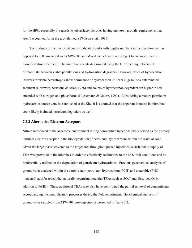
148

for the HPC, especially in regards to subsurface microbes having unknown growth requirements that

aren’t accounted for in the growth media (Wilson et al., 1986).

The findings of the microbial counts indicate significantly higher numbers in the injection well as

opposed to PHC impacted wells MW-103 and MW-4, which were not subject to enhanced in-situ

bioremediation treatment. The microbial counts determined using the HPC technique to do not

differentiate between viable populations and hydrocarbon degraders. However, ratios of hydrocarbon

utilizers to viable heterotrophs show dominance of hydrocarbon utilizers in gasoline-contaminated

sediment (Horowitz, Sexstone & Atlas, 1978) and counts of hydrocarbon degraders are higher in soil

amended with nitrogen and phosphorus (Huesemann & Moore, 1993). Considering a mature petroleum

hydrocarbon source zone is established at the Site, it is assumed that the apparent increase in microbial

count likely included petroleum degraders as well.

7.2.3 Alternative Electron Acceptors

Nitrate introduced to the anaerobic environment during consecutive injections likely served as the primary

terminal electron acceptor in the biodegradation of petroleum hydrocarbons within the residual zone.

Given the large mass delivered to the target area throughout pulsed injections, a sustainable supply of

TEA was provided to the microbes in order to effectively acclimatize to the NO3- rich conditions and be

preferentially utilized in the degradation of petroleum hydrocarbons. Previous geochemical analysis of

groundwater analyzed within the aerobic (non-petroleum hydrocarbon, PCH) and anaerobic (PHC-

impacted) aquifer reveal that naturally occurring potential TEAs such as SO42- and dissolved O2 in

addition to Fe(III). These additional TEAs may also have contributed the partial removal of contaminants

accompanying the denitrification processes during the field experiment. Geochemical analysis of

groundwater sampled from MW-501 post-injection is presented in Table 7.2.

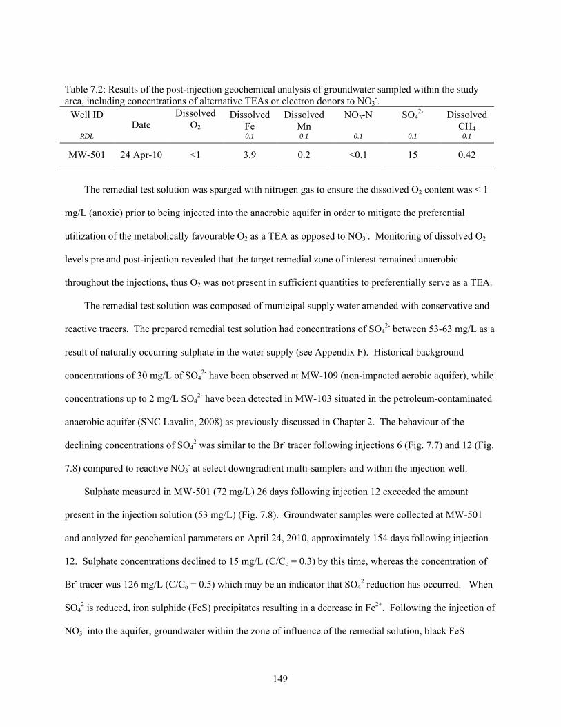
149

Table 7.2: Results of the post-injection geochemical analysis of groundwater sampled within the study area, including concentrations of alternative TEAs or electron donors to NO3

-. Well ID

RDL

Date Dissolved

O2

Dissolved Fe 0.1

Dissolved Mn 0.1

NO3-N

0.1

SO42-

0.1

Dissolved CH4

0.1

MW-501 24 Apr-10 <1 3.9 0.2 <0.1 15 0.42

The remedial test solution was sparged with nitrogen gas to ensure the dissolved O2 content was < 1

mg/L (anoxic) prior to being injected into the anaerobic aquifer in order to mitigate the preferential

utilization of the metabolically favourable O2 as a TEA as opposed to NO3-. Monitoring of dissolved O2

levels pre and post-injection revealed that the target remedial zone of interest remained anaerobic

throughout the injections, thus O2 was not present in sufficient quantities to preferentially serve as a TEA.

The remedial test solution was composed of municipal supply water amended with conservative and

reactive tracers. The prepared remedial test solution had concentrations of SO42- between 53-63 mg/L as a

result of naturally occurring sulphate in the water supply (see Appendix F). Historical background

concentrations of 30 mg/L of SO42- have been observed at MW-109 (non-impacted aerobic aquifer), while

concentrations up to 2 mg/L SO42- have been detected in MW-103 situated in the petroleum-contaminated

anaerobic aquifer (SNC Lavalin, 2008) as previously discussed in Chapter 2. The behaviour of the

declining concentrations of SO42 was similar to the Br- tracer following injections 6 (Fig. 7.7) and 12 (Fig.

7.8) compared to reactive NO3- at select downgradient multi-samplers and within the injection well.

Sulphate measured in MW-501 (72 mg/L) 26 days following injection 12 exceeded the amount

present in the injection solution (53 mg/L) (Fig. 7.8). Groundwater samples were collected at MW-501

and analyzed for geochemical parameters on April 24, 2010, approximately 154 days following injection

12. Sulphate concentrations declined to 15 mg/L (C/Co = 0.3) by this time, whereas the concentration of

Br- tracer was 126 mg/L (C/Co = 0.5) which may be an indicator that SO42 reduction has occurred. When

SO42 is reduced, iron sulphide (FeS) precipitates resulting in a decrease in Fe2+. Following the injection of

NO3- into the aquifer, groundwater within the zone of influence of the remedial solution, black FeS

150

precipitate was observed in several of the multilevel samplers, which provides evidence that the study

environment is anaerobic and sulphate reduction is occurring.

The variable reduction in SO42 observed during the remedial plume’s drift phase provides evidence to

suggest that indigenous microbial populations may be utilizing SO42 as an alternative electron acceptor to

NO3- in the enhanced degradation of organic contaminants. However, SO4

2- was not present in significant

quantities to serve as the primary TEA in the biodegradation of petroleum hydrocarbons. Nitrate is more

energetically favourable and preferentially utilized by the microbes in the oxidation of organic

contaminants compared to sulphate (e.g. Mackay & Cherry, 1989; Ball & Reinhard, 1996) and a

continuous abundant supply of NO3- was provided to the microbes during the 121 day period when 12

injections of remedial solution took place.

Sulphate utilization may become significant when NO3- levels have been substantially depleted by

redox processes and a sustainable supply is no longer present. The degradation of benzene is described by

the following equation 7.1 (Borden et al., 1995):

C7H8 + 4.5SO42- + 3H2O(l) 2.25H2S(g) + 2.25HS- + 7HCO3

-(l) + 0.25H+ (7.1)

The use of sulphate as a terminal electron acceptor will result in increases of carbonate (HCO3-) and

hydrogen sulphide (H2S) concentrations however, neither were measured during the field experiment.

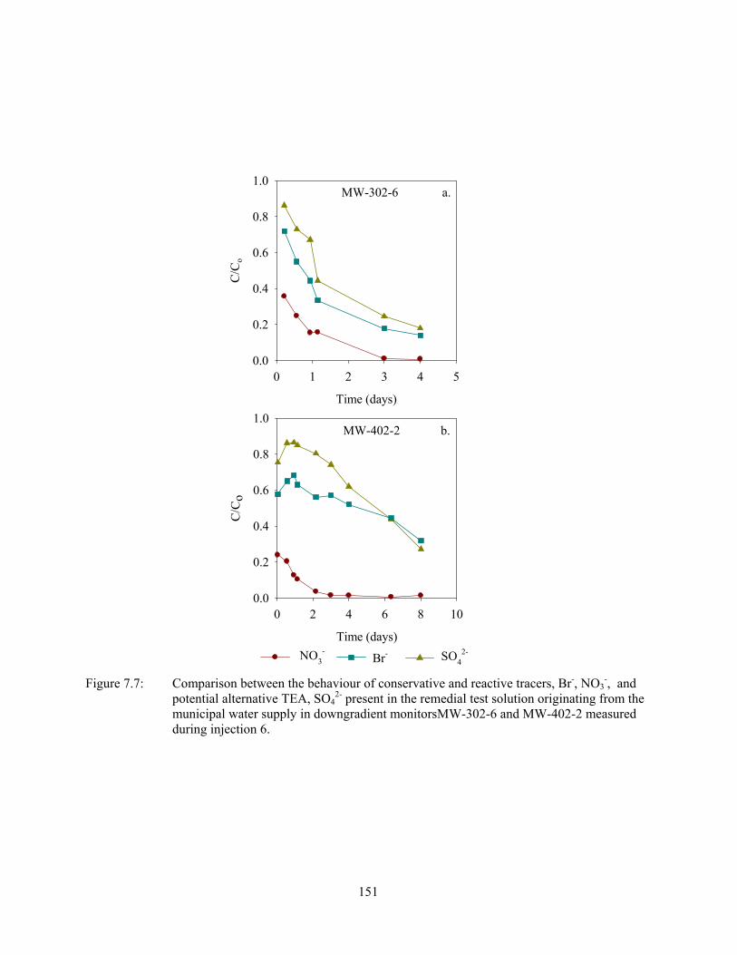
151

Time (days)

0 2 4 6 8 10

C/C

o

0.0

0.2

0.4

0.6

0.8

1.0

Br-

MW-402-2 b.

Time (days)

0 1 2 3 4 5

C/C

o

0.0

0.2

0.4

0.6

0.8

1.0MW-302-6 a.

NO3- SO

42-

Figure 7.7: Comparison between the behaviour of conservative and reactive tracers, Br-, NO3

-, and potential alternative TEA, SO4

2- present in the remedial test solution originating from the municipal water supply in downgradient monitorsMW-302-6 and MW-402-2 measured during injection 6.

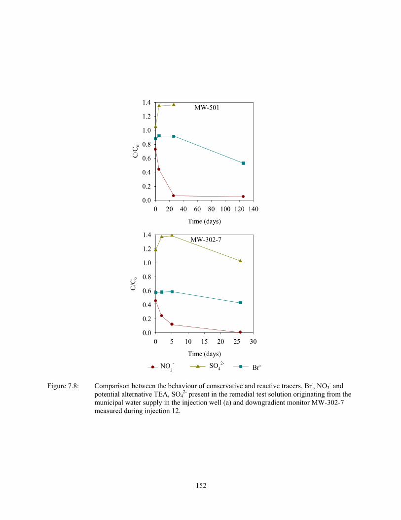
152

Time (days)

0 20 40 60 80 100 120 140

C/C

o

0.0

0.2

0.4

0.6

0.8

1.0

1.2

1.4MW-501

Time (days)

0 5 10 15 20 25 30

C/C

o

0.0

0.2

0.4

0.6

0.8

1.0

1.2

1.4

SO42-

MW-302-7

NO3

-Br-

Figure 7.8: Comparison between the behaviour of conservative and reactive tracers, Br-, NO3- and

potential alternative TEA, SO42- present in the remedial test solution originating from the

municipal water supply in the injection well (a) and downgradient monitor MW-302-7 measured during injection 12.

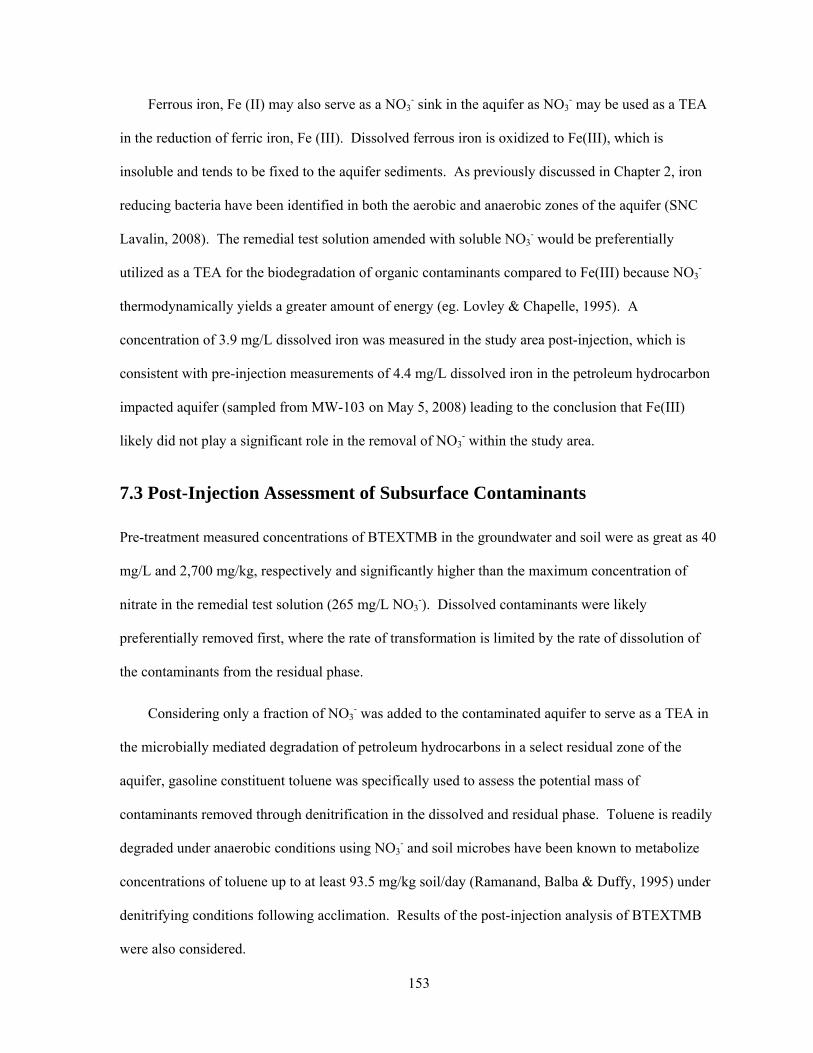
153

Ferrous iron, Fe (II) may also serve as a NO3- sink in the aquifer as NO3

- may be used as a TEA

in the reduction of ferric iron, Fe (III). Dissolved ferrous iron is oxidized to Fe(III), which is

insoluble and tends to be fixed to the aquifer sediments. As previously discussed in Chapter 2, iron

reducing bacteria have been identified in both the aerobic and anaerobic zones of the aquifer (SNC

Lavalin, 2008). The remedial test solution amended with soluble NO3- would be preferentially

utilized as a TEA for the biodegradation of organic contaminants compared to Fe(III) because NO3-

thermodynamically yields a greater amount of energy (eg. Lovley & Chapelle, 1995). A

concentration of 3.9 mg/L dissolved iron was measured in the study area post-injection, which is

consistent with pre-injection measurements of 4.4 mg/L dissolved iron in the petroleum hydrocarbon

impacted aquifer (sampled from MW-103 on May 5, 2008) leading to the conclusion that Fe(III)

likely did not play a significant role in the removal of NO3- within the study area.

7.3 Post-Injection Assessment of Subsurface Contaminants

Pre-treatment measured concentrations of BTEXTMB in the groundwater and soil were as great as 40

mg/L and 2,700 mg/kg, respectively and significantly higher than the maximum concentration of

nitrate in the remedial test solution (265 mg/L NO3-). Dissolved contaminants were likely

preferentially removed first, where the rate of transformation is limited by the rate of dissolution of

the contaminants from the residual phase.

Considering only a fraction of NO3- was added to the contaminated aquifer to serve as a TEA in

the microbially mediated degradation of petroleum hydrocarbons in a select residual zone of the

aquifer, gasoline constituent toluene was specifically used to assess the potential mass of

contaminants removed through denitrification in the dissolved and residual phase. Toluene is readily

degraded under anaerobic conditions using NO3- and soil microbes have been known to metabolize

concentrations of toluene up to at least 93.5 mg/kg soil/day (Ramanand, Balba & Duffy, 1995) under

denitrifying conditions following acclimation. Results of the post-injection analysis of BTEXTMB

were also considered.

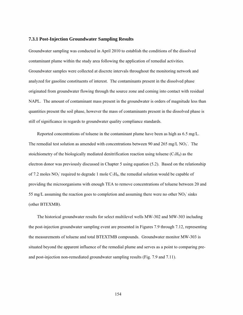
154

7.3.1 Post-Injection Groundwater Sampling Results

Groundwater sampling was conducted in April 2010 to establish the conditions of the dissolved

contaminant plume within the study area following the application of remedial activities.

Groundwater samples were collected at discrete intervals throughout the monitoring network and

analyzed for gasoline constituents of interest. The contaminants present in the dissolved phase

originated from groundwater flowing through the source zone and coming into contact with residual

NAPL. The amount of contaminant mass present in the groundwater is orders of magnitude less than

quantities present the soil phase, however the mass of contaminants present in the dissolved phase is

still of significance in regards to groundwater quality compliance standards.

Reported concentrations of toluene in the contaminant plume have been as high as 6.5 mg/L.

The remedial test solution as amended with concentrations between 90 and 265 mg/L NO3-. The

stoichiometry of the biologically mediated denitrification reaction using toluene (C7H8) as the

electron donor was previously discussed in Chapter 5 using equation (5.2). Based on the relationship

of 7.2 moles NO3- required to degrade 1 mole C7H8, the remedial solution would be capable of

providing the microorganisms with enough TEA to remove concentrations of toluene between 20 and

55 mg/L assuming the reaction goes to completion and assuming there were no other NO3- sinks

(other BTEXMB).

The historical groundwater results for select multilevel wells MW-302 and MW-303 including

the post-injection groundwater sampling event are presented in Figures 7.9 through 7.12, representing

the measurements of toluene and total BTEXTMB compounds. Groundwater monitor MW-303 is

situated beyond the apparent influence of the remedial plume and serves as a point to comparing pre-

and post-injection non-remediated groundwater sampling results (Fig. 7.9 and 7.11).

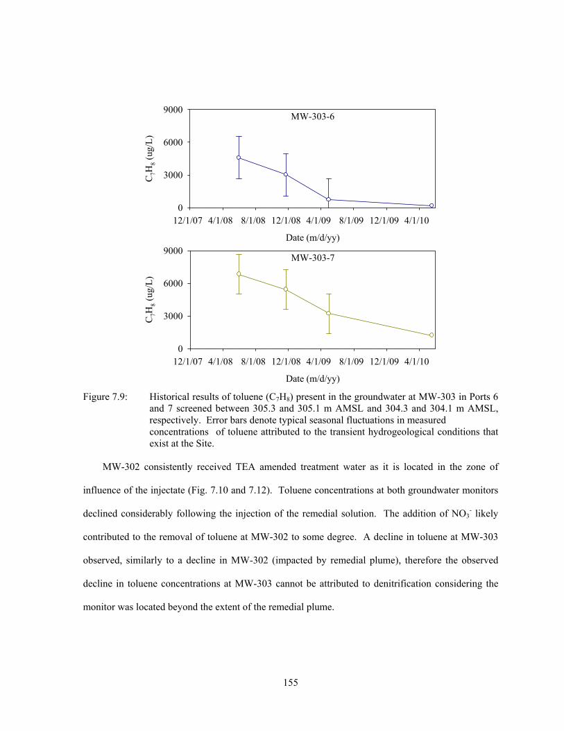
155

Date (m/d/yy)

12/1/07 4/1/08 8/1/08 12/1/08 4/1/09 8/1/09 12/1/09 4/1/10

C7H

8 (u

g/L

)

0

3000

6000

9000Date (m/d/yy)

12/1/07 4/1/08 8/1/08 12/1/08 4/1/09 8/1/09 12/1/09 4/1/10

C7H

8 (u

g/L

)

0

3000

6000

9000MW-303-6

MW-303-7

Figure 7.9: Historical results of toluene (C7H8) present in the groundwater at MW-303 in Ports 6 and 7 screened between 305.3 and 305.1 m AMSL and 304.3 and 304.1 m AMSL, respectively. Error bars denote typical seasonal fluctuations in measured concentrations of toluene attributed to the transient hydrogeological conditions that exist at the Site.

MW-302 consistently received TEA amended treatment water as it is located in the zone of

influence of the injectate (Fig. 7.10 and 7.12). Toluene concentrations at both groundwater monitors

declined considerably following the injection of the remedial solution. The addition of NO3- likely

contributed to the removal of toluene at MW-302 to some degree. A decline in toluene at MW-303

observed, similarly to a decline in MW-302 (impacted by remedial plume), therefore the observed

decline in toluene concentrations at MW-303 cannot be attributed to denitrification considering the

monitor was located beyond the extent of the remedial plume.

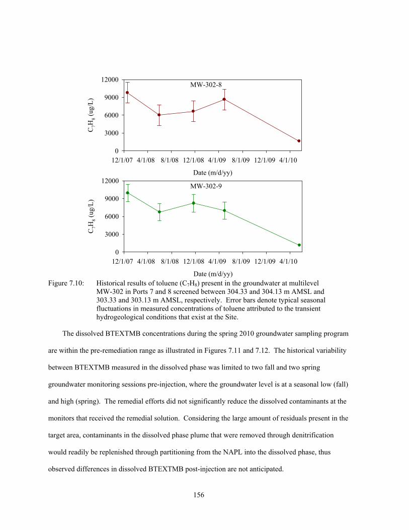
156

Date (m/d/yy)

12/1/07 4/1/08 8/1/08 12/1/08 4/1/09 8/1/09 12/1/09 4/1/10

C7H

8 (u

g/L

)

0

3000

6000

9000

12000

Date (m/d/yy)

12/1/07 4/1/08 8/1/08 12/1/08 4/1/09 8/1/09 12/1/09 4/1/10

C7H

8 (u

g/L

)

0

3000

6000

9000

12000

MW-302-8

MW-302-9

Figure 7.10: Historical results of toluene (C7H8) present in the groundwater at multilevel MW-302 in Ports 7 and 8 screened between 304.33 and 304.13 m AMSL and 303.33 and 303.13 m AMSL, respectively. Error bars denote typical seasonal fluctuations in measured concentrations of toluene attributed to the transient hydrogeological conditions that exist at the Site.

The dissolved BTEXTMB concentrations during the spring 2010 groundwater sampling program

are within the pre-remediation range as illustrated in Figures 7.11 and 7.12. The historical variability

between BTEXTMB measured in the dissolved phase was limited to two fall and two spring

groundwater monitoring sessions pre-injection, where the groundwater level is at a seasonal low (fall)

and high (spring). The remedial efforts did not significantly reduce the dissolved contaminants at the

monitors that received the remedial solution. Considering the large amount of residuals present in the

target area, contaminants in the dissolved phase plume that were removed through denitrification

would readily be replenished through partitioning from the NAPL into the dissolved phase, thus

observed differences in dissolved BTEXTMB post-injection are not anticipated.

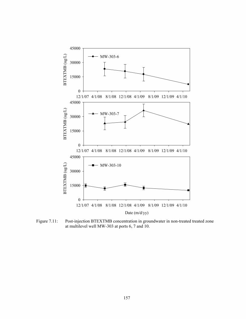
157

Date (m/d/yy)

12/1/07 4/1/08 8/1/08 12/1/08 4/1/09 8/1/09 12/1/09 4/1/10

BT

EX

TM

B (

ug/L

)

0

15000

30000

45000

MW-303-10

12/1/07 4/1/08 8/1/08 12/1/08 4/1/09 8/1/09 12/1/09 4/1/10

BT

EX

TM

B (

ug/L

)

0

15000

30000

45000

MW-303-7

12/1/07 4/1/08 8/1/08 12/1/08 4/1/09 8/1/09 12/1/09 4/1/10

BT

EX

TM

B (

ug/L

)

0

15000

30000

45000

MW-303-6

Figure 7.11: Post-injection BTEXTMB concentration in groundwater in non-treated treated zone at multilevel well MW-303 at ports 6, 7 and 10.

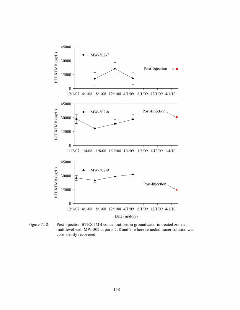
158

12/1/07 4/1/08 8/1/08 12/1/08 4/1/09 8/1/09 12/1/09 4/1/10

BT

EX

TM

B (

ug/L

)

0

15000

30000

45000

MW-302-7

1/12/07 1/4/08 1/8/08 1/12/08 1/4/09 1/8/09 1/12/09 1/4/10

BT

EX

TM

B (

ug/L

)

0

15000

30000

45000

MW-302-8

Date (m/d/yy)

12/1/07 4/1/08 8/1/08 12/1/08 4/1/09 8/1/09 12/1/09 4/1/10

BT

EX

TM

B (

ug/L

)

0

15000

30000

45000

MW-302-9

Post-Injection

Post-Injection

Post-Injection

Figure 7.12: Post-injection BTEXTMB concentrations in groundwater in treated zone at multilevel well MW-302 at ports 7, 8 and 9, where remedial tracer solution was consistently recovered.

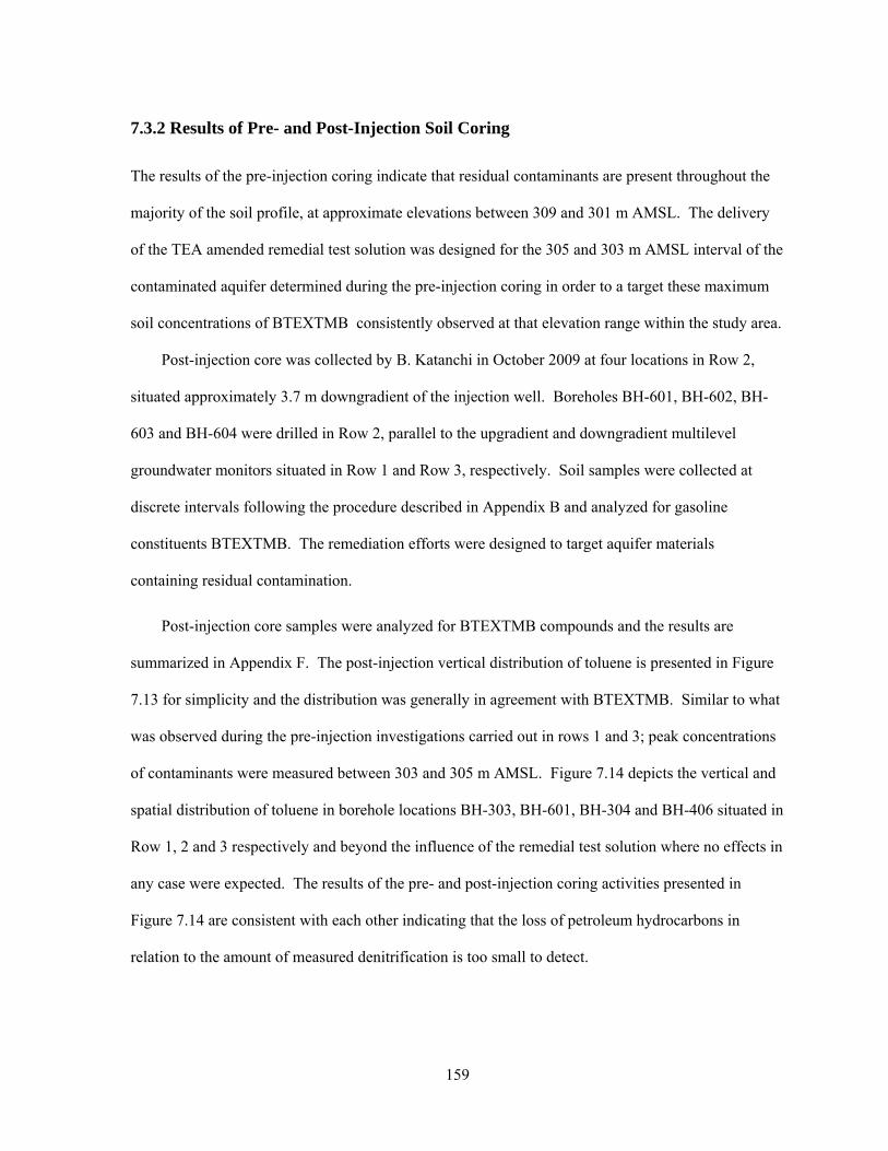
159

7.3.2 Results of Pre- and Post-Injection Soil Coring

The results of the pre-injection coring indicate that residual contaminants are present throughout the

majority of the soil profile, at approximate elevations between 309 and 301 m AMSL. The delivery

of the TEA amended remedial test solution was designed for the 305 and 303 m AMSL interval of the

contaminated aquifer determined during the pre-injection coring in order to a target these maximum

soil concentrations of BTEXTMB consistently observed at that elevation range within the study area.

Post-injection core was collected by B. Katanchi in October 2009 at four locations in Row 2,

situated approximately 3.7 m downgradient of the injection well. Boreholes BH-601, BH-602, BH-

603 and BH-604 were drilled in Row 2, parallel to the upgradient and downgradient multilevel

groundwater monitors situated in Row 1 and Row 3, respectively. Soil samples were collected at

discrete intervals following the procedure described in Appendix B and analyzed for gasoline

constituents BTEXTMB. The remediation efforts were designed to target aquifer materials

containing residual contamination.

Post-injection core samples were analyzed for BTEXTMB compounds and the results are

summarized in Appendix F. The post-injection vertical distribution of toluene is presented in Figure

7.13 for simplicity and the distribution was generally in agreement with BTEXTMB. Similar to what

was observed during the pre-injection investigations carried out in rows 1 and 3; peak concentrations

of contaminants were measured between 303 and 305 m AMSL. Figure 7.14 depicts the vertical and

spatial distribution of toluene in borehole locations BH-303, BH-601, BH-304 and BH-406 situated in

Row 1, 2 and 3 respectively and beyond the influence of the remedial test solution where no effects in

any case were expected. The results of the pre- and post-injection coring activities presented in

Figure 7.14 are consistent with each other indicating that the loss of petroleum hydrocarbons in

relation to the amount of measured denitrification is too small to detect.

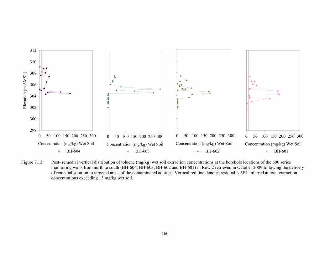
160

Concentration (mg/kg) Wet Soil

0 50 100 150 200 250 300

Ele

vatio

n (m

AM

SL)

298

300

302

304

306

308

310

312

BH-604

Concentration (mg/kg) Wet Soil

0 50 100 150 200 250 300

BH-603

Concentration (mg/kg) Wet Soil

0 50 100 150 200 250 300

BH-602

Concentration (mg/kg) Wet Soil

0 50 100 150 200 250 300

BH-601

Figure 7.13: Post- remedial vertical distribution of toluene (mg/kg) wet soil extraction concentrations at the borehole locations of the 600 series monitoring wells from north to south (BH-604, BH-603, BH-602 and BH-601) in Row 2 retrieved in October 2009 following the delivery of remedial solution to targeted areas of the contaminated aquifer. Vertical red line denotes residual NAPL inferred at total extraction concentrations exceeding 13 mg/kg wet soil.

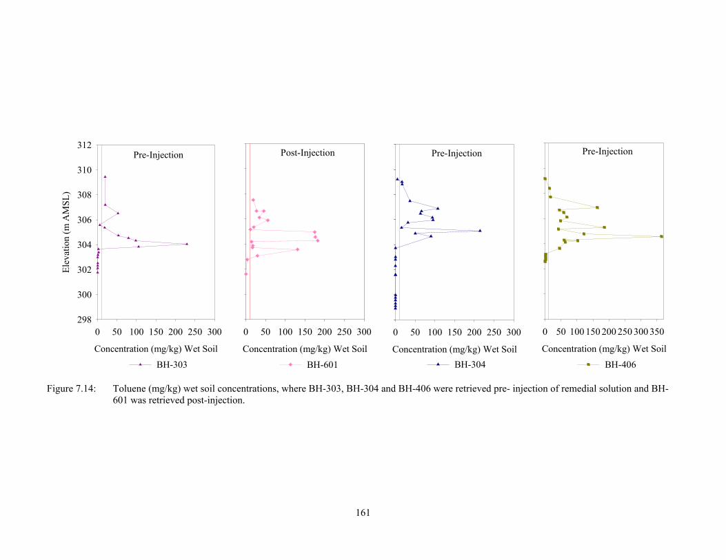
161

Concentration (mg/kg) Wet Soil

0 50 100 150 200 250 300

Ele

vatio

n (m

AM

SL

)

298

300

302

304

306

308

310

312

BH-303

Pre-Injection

Concentration (mg/kg) Wet Soil

0 50 100 150 200 250 300

BH-601

Post-Injection

Concentration (mg/kg) Wet Soil

0 50 100 150 200 250 300

BH-304

Pre-Injection

Concentration (mg/kg) Wet Soil

0 50 100 150 200 250 300 350

BH-406

Pre-Injection

Figure 7.14: Toluene (mg/kg) wet soil concentrations, where BH-303, BH-304 and BH-406 were retrieved pre- injection of remedial solution and BH- 601 was retrieved post-injection.

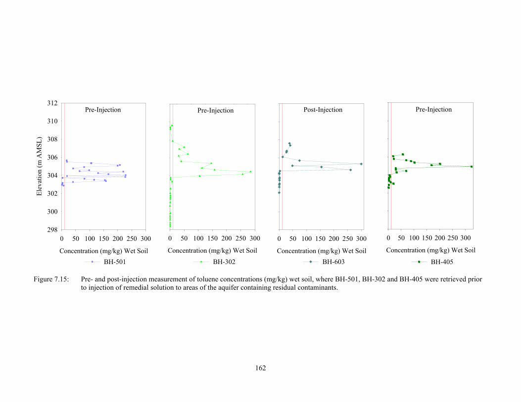
162

Concentration (mg/kg) Wet Soil

0 50 100 150 200 250 300

Ele

vatio

n (m

AM

SL

)

298

300

302

304

306

308

310

312

BH-501

Pre-Injection

Concentration (mg/kg) Wet Soil

0 50 100 150 200 250 300

BH-302

Pre-Injection

Concentration (mg/kg) Wet Soil

0 50 100 150 200 250 300

BH-603

Post-Injection

Concentration (mg/kg) Wet Soil

0 50 100 150 200 250 300

BH-405

Pre-Injection

Figure 7.15: Pre- and post-injection measurement of toluene concentrations (mg/kg) wet soil, where BH-501, BH-302 and BH-405 were retrieved prior to injection of remedial solution to areas of the aquifer containing residual contaminants.

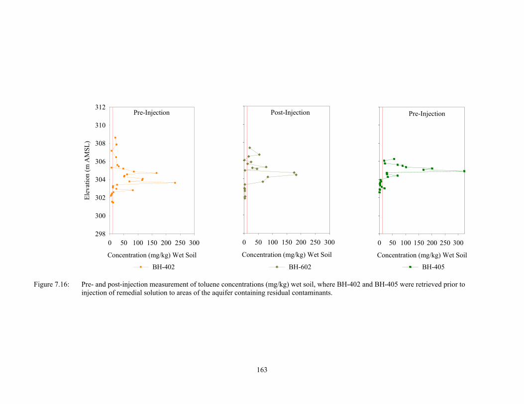
163

Concentration (mg/kg) Wet Soil

0 50 100 150 200 250 300

Ele

vatio

n (m

AM

SL

)

298

300

302

304

306

308

310

312

BH-402

Pre-Injection

Concentration (mg/kg) Wet Soil

0 50 100 150 200 250 300

BH-602

Post-Injection

Concentration (mg/kg) Wet Soil

0 50 100 150 200 250 300

BH-405

Pre-Injection

Figure 7.16: Pre- and post-injection measurement of toluene concentrations (mg/kg) wet soil, where BH-402 and BH-405 were retrieved prior to injection of remedial solution to areas of the aquifer containing residual contaminants.

164

Concentration (mg/kg) Wet Soil

0 50 100 150 200 250 300

Ele

vatio

n (m

AM

SL

)

298

300

302

304

306

308

310

312

BH-401

Pre-Injection

Concentration (mg/kg) Wet Soil

0 50 100 150 200 250 300

BH-604

Post-Injection

Concentration (mg/kg) Wet Soil

0 50 100 150 200 250 300

BH-403

Pre-Injection

Concentration (mg/kg) Wet Soil

0 50 100 150 200 250 300

BH-405

Pre-Injection

Figure 7.17: Pre- and post-injection measurement of toluene concentrations (mg/kg) wet soil, where BH-401, BH-403 and BH-405 were retrieved prior to injection of remedial solution to areas of the aquifer containing residual contaminants.

165

Using the Feenstra et al. (1991) rationale discussed in Chapter 3, residuals are inferred when the total

soil extract concentration of BTEXTMB compounds exceed 13 mg/kg wet soil and NAPL is potentially

mobile at BTEXTMB concentrations exceeding 3,000 mg/kg. The vertical distribution of toluene in

regions of the study area subject to the delivery of the remedial test solution is presented in Figures 7.15,

7.16 and 7.17. A continuous plume of TEA amended water was well documented between MW-501 and

Row 1, however only limited quantities of Br- tracer were recovered in Row 2 (MW-602 and MW-603)

and Row 3 (MW-405, only). The overall content of target aromatic hydrocarbons in regions of the

aquifer containing residual NAPL was not reduced by the remedial injections, which is a reflection of the

limited amount of nitrate delivered to the target residual zone compared to the large contaminant mass

present.

The results of the vertical distribution of BTEXTMB and in particular toluene following the delivery

of a continuous supply of TEA to the target zone are consistent with the pre-injection investigation

results. The vertical distribution of toluene is variable; however there is the same concentrated area of

contaminants at the interval 305 to 303 m AMSL that was measured during pre-injection coring.

Contaminant mass removal must have occurred as Br- tracer evidence indicates that NO3- was utilized in

the study area based on the inference of denitrification rates. However, the post-injection soil core results

are unable to demonstrate the reduction in individual toluene, let alone BTEXTMB hydrocarbon levels,

reflecting the limited nitrate provided relative to the significant but heterogeneously distributed residual

mass in the target zone.

166

Chapter 8: Conclusions and Recommendations

The nitrate-amended remedial solution was successfully delivered to the target zone of the anaerobic

aquifer containing residual hydrocarbons. A plume of remedial solution was established within the

remedial monitoring network, following consecutive pulsed injections of remedial solutions where Br-

tracer concentrations were eventually equivalent to greater than 50% of the concentration injected.

Denitrification in the study area was induced by the addition of nitrate reactant in the form of sodium

nitrate (NaNO3) in concentrations ranging between 90 and 265 mg/L NO3- while residual and dissolved

hydrocarbon contaminants present in the aquifer served as the carbon source. The concentration of nitrate

within the remedial solution was increased over time as the microbes had the opportunity to acclimate to

the TEA enriched conditions and groundwater quality monitoring from downgradient wells revealed that

nitrate was being readily attenuated. Post-injection groundwater monitoring revealed that nitrate and

nitrite concentrations were well below the ODWQS of 10 mg/L as total nitrogen despite elevated

concentrations used in the injections.

A continuous zone of remedial test solution amended with TEA developed as a result of the

consecutive series of pulsed injections delivered via the injection well, thereby providing a sustainable

supply of TEA to promote in situ biodegradation of petroleum contaminants. Background concentrations

of Br- within the monitoring network increased during the series of injections, as the amended treatment

water was more prone to mixing with the remaining remedial plume situated in the vicinity of the

injection well.

The results of the Br- tracer breakthrough curves indicate that different preferential flow pathways

were established under the transient saturated conditions present at the Site, although the behaviour of the

injected remedial slug was generally consistent between the different units and the test solution was

ultimately delivered to the target zone. The injectate primarily moved in the high K zone of Unit 3 under

high saturated conditions, which eventually became unsaturated due to seasonal declines of the

167

groundwater level. The lower portion of Unit 4 comprised of higher permeable materials was able to

transmit the test solution more effectively under low seasonal groundwater levels.

It is clear that the delivery of the remedial test solution upon injection is influenced by the

heterogeneous characteristics of the aquifer materials and the transient hydrogeological conditions present

at the Site. Upon the return to natural gradient conditions, the injected remedial slug was transported

through the aquifer at velocities characterized by the porous media and the hydraulic conditions. In

general, the remedial solution was transported more rapidly under high groundwater elevations and

gradients, where maximum velocities corresponding to Unit 2, 3 and 4 of 1.91, 1.00 and 0.76 m/day

respectively were observed. Under low groundwater elevations and gradient, the remedial solution was

not transported in Unit 2 because it was no longer saturated, while minimum velocities were observed in

Unit 3 and Unit 4, 0.06 and 0.04 m/day. Groundwater velocities estimated from the removal of Br- tracer

within the injection well were less than 0.01 m/day under the reduced hydrogeological conditions

observed during the November injections. The remedial solutes were transported in sand and gravel Unit

5 at an approximate rate of 0.10 m/day, estimated from the arrival of the Br- tracer at Row 3, 62 days after

the first injection.

A cumulative mass of 3.7 kg of nitrate was added to the target aquifer during the course of the

remedial injections. Evidence demonstrating NO3- was used a terminal electron acceptor in the

bioremediation of the petroleum-contaminated aquifer include: 1) laboratory confirmation of the

indigenous microbial population’s capability to degrade hydrocarbons using nitrate as the TEA,

2) decrease of nitrate relative to a conservative Br- tracer, 3) generation of nitrite, an intermediate in

denitrification and 4) reduction in dissolved phase toluene.

Soil coring and groundwater sampling was conducted downgradient from the injection source zone

in order to assess measured changes in quantities of toluene in each respective medium by enhancing in-

situ bioremediation of petroleum hydrocarbons at the Site with the addition of nitrate as a terminal

electron acceptor. Pre-treatment measured peak concentrations of BTEXTMB in the groundwater (40

168

mg/L) and soil (2,700 mg/kg wet soil) were significantly higher than the maximum concentration of

nitrate in the remedial test solution (265 mg/L NO3-). However, the results of the post-injection coring

indicate insufficient quantities of nitrate were added to the system in order to induce a clear decline in

residual toluene or BTEXTMB concentrations.

Given the variable hydrogeological conditions present at the Site influenced by seasonal effects, the

delivery of the remedial solution to target zones containing petroleum hydrocarbons at residual saturation

is more effective under lower gradient, low water-table conditions. The delivery of TEA amended water

to enhance the in situ biodegradation of petroleum contaminants is more effective when the treatment

water has an increased residence time in the target remedial zone, attributed to low gradients and

groundwater transport velocities at the Site. Longer residence periods enable the indigenous microbes to

have increased contact time with the TEA which will be preferentially utilized to degrade the

contaminants.

Nitrate enhanced in situ bioremediation has been successfully demonstrated at a petroleum impacted

aquifer, however a large scale application of the remedial strategy and long term monitoring would be

required in order to evaluate the potential for measurable reductions in mass of contaminant emanating

from the source zone. Based on the range of nitrate utilization rates inferred in situ (0.10 to 0.77 day-1), it

would take at onwards of 2 to 50+ years to remove the estimated 193 mol or 18 kg of toluene present in

the subsurface based on weekly remedial solution injections (2.05 m3, 265 mg/L NO3-) using a single

injection well depending on the rate of nitrate utilization. The bioremediation timeframe could likely be

reduced by increasing the number of injection wells or naturally with the use of utilization of alternative

electron acceptors present in the subsurface.

169

References

Aelion, C.M. (1996). Impact of aquifer sediment grain size on petroleum hydrocarbon distribution and biodegradation. Journal of Contaminant Hydrology. 22: 109-121.

Allen-King, R.M., O’Leary, K.E., Gillham, R.W., and Barker, J.F. (1994). Limitations on the biodegradation rate of dissolved BTEX in a natural, unsaturated, sandy soil: Evidence from field and laboratory experiments, ed. R.E. Hinchee, B.C. Alleman, R.E. Hoeppel, and R.N. Miller. In Second International Symposium on In Situ and On-Site Bioreclamation, San Diego, California. Hydrocarbon Bioremediaiton. 2(2): 175-191.

Alley, W.M., Healy, R.W., LaBaugh, J.W. and Reilly, T.E. (2002). Flow and storage in groundwater systems. Science. 296: 1985-1990.

Almeida, J.S., Reis, M.A.M., and Carrondo, M.J.T. (1995). Competition between nitrate and nitrite reduction in denitrification by Pseudomonas fluorescens. Biotechnologhy and Bioengineering. 46: 476-484

Acton, D.W. and Barker, J.F. (1992). In situ biodegradation potential of aromatic hydrocarbons in anaerobic groundwaters. Journal of Contaminant Hydrology. 9: 325-352

Angley, J., Brusseau, M., Miller, W., Delfino, J. (1992). Nonequilibrium sorption and aerobic biodegradation of dissolved alkylbenzenes during transport in aquifer material: column experiments and evaluation of a coupled-process model. Environmental Science and Technology. 26(7): 1404-1410

Aral, M.M. and Liao, B. (2002). Effect of groundwater table fluctuations on LNAPL thickness in monitoring wells. Environmental Geology. 42: 151-161

Baedecker, M.J., Cozzarelli, I.M., Siegel, D.I., Bennet, P.C. and Eganhouse, R.P. (1993). Crude oil in a shallow sand and gravel aquifer. Appl. Geochem. 8, 569-586

Balderston, W.L., Sherr, B. & Payne, W, L. (1976). Blockage by acetylene of nitrous oxide reduction in Pseudomonas perfectomarinus. Appl. Environ. Microbiol. 31: 504-504

Ball, H.A. and Reinhard, M. (1996). Monoaromatic hydrocarbon transformation under anaerobic conditions at Seal Beach, California: Laboratory studies. Environ Toxicol. And Chemistry. 15(2): 114-122

Banerjee, S. (1984). Solubility of organic mixtures in water. Environmental Science & Technology. 18: 587-591

Barbaro, J.R., Barker, J.F., Lemon, L.A., and Mayfield, C.I. (1992). Biotransformation of BTEX under anaerobic, denitrifying conditions: Field and laboratory observations. Journal of Contaminant Hydrology. 11: 245-272

Barbaro, J.R. (1999). Enhanced bioremediation of dissolved aromatic hydrocarbons within a gasoline source area using nitrate and oxygen as electron acceptors. PhD Thesis, Department of Earth Sciences, University of Waterloo, Canada.

170

Barbaro, J.R. (2000). Controlled field study on the use of nitrate and oxygen for bioremediation of a gasoline source zone. Bioremediation Journal, 4(4): 259-270

Barker, J.F., Patrick, G.C. and Major, D. (1987). Natural attenuation of aromatic hydrocarbons in a shallow sand aquifer. Ground Water Monit Rev, 7: 64-71

Barth, G.R., Illangasekare, T.H. and Rajaram, H. (2003). The effect of entrapped nonaqueous phase liquids on tracer transport in heterogeneous porous media: laboratory experiments at the intermediate scale. Journal of Contaminant Hydrology. 67: 247-268

Bear, J., 1972. Dynamics of Fluids in Porous Media. Elsevier, New York. 764 pp.

Beller, H.R., Grbić-Galić, D., and Reinhard, M. (1992). Microbial degradation of toluene under sulfate-reducing conditions and the influence of iron on the process. Appl. Environ. Microbiol. 58(3): 786-793

Betlach, M.R. and Tiedje, J.M. (1981). Kinetic explanation for accumulation of nitrite, nitric oxide, and nitrous oxide during bacterial denitrification. Appl. Environ. Microbio. 42: 1074-1084 Bleakley, B.H. and Tiedje, J.M. (1982). Nitrous oxide production by organisms other than nitrifiers or denitrifiers. Appl. Environ. Microbiol. 44: 1342-1348

Burland, S.M. and Edwards, E.A. (1999). Anaerobic benzene biodegradation linked to nitrate reduction. Applied and Environmental Microbiology. 65 (2): 529-533

Blanchard, M.C. and Bradbury, K.R. (1987). A comparison of office-derived vs. field-derived water table maps for a sandy unconfined aquifer. Ground Water Monitoring & Remediation. 7 (2): 74-78

Borden, R.C., Gomez, C.A., and Becker, M.T. (1995). Geochemical indicators of intrinsic bioremediation. Groundwater. 33(2): 180-189

Borden, R.C., Hunt, M.J., Schafer, M.B. and Barlaz, M.A. (1997). Anaerobic biodegradation of BTEX in aquifer material, EPA/600/S-97/003. Research and Development, National Risk Management Research Laboratory (Ada, OK)

Bouwer, H. and Rice, R.C. (1976). A slug test method for determining hydraulic conductivity of unconfined aquifers with completely or partially penetrating wells, Water Resources Research, vol. 12, no. 3, pp. 423-428

Burford, J.R. and Bremner, J.M. (1975). Relationships between the denitrification capacities of soils and total water soluble and readily decomposable soil organic matter. Soil Biology & Biochemistry, 7: 389-394

Bragan, R.J., Starr, J.L. and Parkin, T.B., (1997). Shallow groundwater denitrification rate measurement by acetylene block. J. Env. Qual. (26): 1531-1538

Brusseau, M., Hu, M., Wang, J. Maier, R. (1999). Biodegradation during contaminant transport in porous media: 2. The influence of physicochemical factors. Environmental Science and Technology. 33(1): 96-103

171

Caldwell, M.E., Tanner, R.S. and Suflita, J.M. (1999). Microbial metabolism of benzene and the oxidation of ferrous iron under anaerobic conditions: Implications for bioremediation. Anaerobe Environmental Microbiology. 4: 595-603

Castignetti, D. and Hollocher, T.C. (1982). Nitrogen Redox Metabolism of a Heterotrophic, Nitrifying-Denitrifying Alcaligenes sp. From Soil. Applied and Environmental Microbiology, 44(4). P 923-928

Chapelle, F.H. (2001). Groundwater microbiology and geochemistry, 2nd ed. Wiley and Sons, New York, 477 pp.

Chesnaux, R. (2007). Analytical closed-form solutions for assessing pumping cycles, times and costs required for NAPL remediation. Environ Geol. Department of Earth Sciences, Simon Fraser University, British Columbia, Canada.

Cho, J.S., Wilson, J.T., DiGiulio, D.C., Vardy, J.A. and Choi, W. (1997). Implementation of natural attenuation at a JP-4 jet fuel release after active remediation. Biodegradation. 8: 265-273

Cirpka, O.A., Windfuhr, C., Bisch, G., Granzow, S., Scholz-Muramatsu, H., Kobus, H., 1999. Microbial reductive dechlorination in large-scale sandbox model. Journal of Environmental Engineering-Asce 125 (9), 861–870.

Cirpka, O.A., Kitanidis, P.K., 2000. Characterization of mixing and dilution in heterogeneous aquifers by means of local temporal moments. Water Resources Research 36 (5), 1221–1236.

Clarke, J.S. and West, C.T. (1997). Ground-water levels, predevelopment ground-water flow, and stream-aquifer relations in the vicinity of the Savannah River Site, Georgia and South Carolina. Water-Resources Investigations Report 97-4197. U.S. Geological Survey. United States.

Cline, P.V., Delfino, J.J. and Rao, S.C. (1991). Partitioning of aromatic constituents into water from gasoline and other complex solvent mixtures. Environ. Sci. Technol. 25: 914-920

Coates, J.D., Anderson, R.T., Woodward, J.C., Phillips, E.J.P. and Lovely, D.R. (1996). Anaerobic hydrocarbon degradation in petroleum-contaminated harbour sediments under sulfate-reducing and artificially imposed iron-reducing conditions. Environ Sci. Technol. 30: 2784-2789

Cole, B., and Silliman, S. (1996). Estimating the horizontal gradient in heterogeneous, unconfined aquifers: Comparison of three-point schemes. Ground Water Monitoring and Remediation. 16(2): 84-91

Corapcioglu, M.Y (ed). (1996). Advances in Porous Media. Volume 3. Elsevier Science Ltd. P. 1-440.

Cowan, W.R., Cooper, A.J,, and Pinch, J.J.(1986). Quaternary Geology of the Wingham-Lucknow Area, Southern Ontario; Ontario Geological Survey, Map P.2957. Geological Series-Preliminary Map. scale 1:50000. Geology 1973-1978.

Cozzarelli, I.M., Herman, J.S., Baedecker, M.J. and Fischer, J.M. (1999). Geochemical heterogeneity of a gasoline-contaminated aquifer. Journal of Contaminant Hydrology. 40: 261-284

172

Cunningham, J.A., Rahme, H., Hopkins, G.D., Lebron, C. And Reinhard, M. (2001). Enhanced in situ bioremediation of BTEX-contaminated groundwater by combined injection of nitrate and sulphate. Environ. Sci. Technol. 35: 1663-1670

Daniel, R.A., and Borden, R.C. (1997). Spatial variability in intrinsic bioremediation rates: effects on contaminant transport. In: Alleman, B.C., Lesson, A. Eds. In Situ and On-Site Bioremediation, Vol. 1. Battelle Press, Columbus, OH. Bioremediation 4(1): 29-34

Darcy, H. (1856). Les Fontaines Publiques de la Ville de Dijon, Dalmont, Paris. p 647.

Darling, B.K. and Hibbs, B.J. (2001). Chapter 16: The aquifers of Red Light Draw, Green River Valley, and Eagle Flat, from Report 356 Aquifers of West Texas, Texas Water Development Board. Edited by Mace, R.E., Mullican III, W.F. and Angle, E.S.

Datry, T., Malard, F. and Gibert, J. (2004). Dynamics of solutes and dissolved oxygen in shallow urban groundwater below a stormwater infiltration basin. Science of the Total Environment. 329: 215-229

Davis, G.B., Barber, C., Power, T.R., Thierrin, J., Patterson, B.M., Rayner, J.L. and Wu, Q. (1999). The variability and intrinsic remediation of a BTEX plume in anaerobic sulphate-rich groundwater. Journal of Contaminant Hydrology. 36: 265-290

DeFlaun, M. F., C. J. Murray, W. Holben, T. Scheibe, A. Mills, T. Ginn, T. Griffin, E. Majer, and J. L. Wilson. (1997). Preliminary observations on bacterial transport in a coastal plain aquifer. FEMS Microbiol. Rev. 20:473-487

Delin, G.N., Healy, R.W., Lorenz, D.L., and Nimmo, J.R., (2007). Comparison of local-to regional-scale estimates of ground-water recharge in Minnesota, USA. Journal of Hydrology. 334(1-2): 231-249

Devlin, R.J. and Barker, J.F. (1994). Semipassive nutrient injection scheme for enhanced in situ bioremediation. Ground Water. 32(3): 374-380

Devlin, J.F., (1996). A method to assess analytical uncertainties over large concentration ranges with reference to volatile organics in water. Ground Water Monit. Remediat. 16 (3), 179–185.

Dobson, R., Schroth, M.H. and Zeyer, J. (2007). Effect of water-table fluctuation on dissolution and biodegradation of a multi-component, light nonaqueous-phase liquid. Journal of Contaminant Hydrology, 94 (3-4): 235-248

Domask, WG. (1984). Introduction to petroleum hydrocarbons: Chemistry and composition in relation to petroleum-derived fuels and solvents. In: Mehlman MA, Hemstreet GP, Thorpe JJ, et al., eds. Advances in modern environmental toxicology. Vol VII: Renal effects of petroleum hydrocarbons. Princeton, NJ: Princeton Scientific Publishers, Inc., 1-23.

Doss, P.K. (1993). The nature of a dynamic water table in a system of non-tidal, freshwater coastal wetlands. Journal of Hydrology, 141: 107-126

173

Dott, W., Feidieker, D., Steiof, M., Becker, P.M. and Kampfer, P. (1995). Comparison of ex situ and in situ techniques for bioremediation of hydrocarbon-polluted soils. International Biodeterioration & Biodegradation. 35 (1-3): 301-316

Dou, J., Liu, X., Hu, Z. and Deng, D. (2008). Anaerobic BTEX biodegradation linked to nitrate and sulfate reduction. Journal of Hazardous Materials. 151: 720-729

Dou, J., Liu, X. and Ding, A. (2009). Anaerobic degradation of naphthalene by the mixed bacteria under nitrate reducting conditions. Journal of Hazardous Materials. 165: 325-331

Drost, W., Klotz, D., Koch, A., Moser, H. Neumaier, F. and Rauert. (1968). Point dilution methods of investigating groundwater flow by means of rasioisotopes. Water Resources Res., 4: 125-146

Eckert, P. and Appelo, C.A.J. (2002). Hydrogeochemical modeling of enhanced benzene, toluene, ethylbenzene, xylene (BTEX) remediation with nitrate. Water Resources Research. 38 (8): 5.1-5.11

Edwards, E.A. and Grbić-Galić, D. (1992). Complete mineralization of benzene by aquifer microorganisms under strictly anaerobic conditions. Applied and Environmental Microbiology. 58(8): 2663-2566

Edwards, E.A., Willis, L.E., Reinhard, M., and Grbić-Galić, D. (1992). Anaerobic degradation of toluene and xylene by aquifer microorganisms under sulfate-reducing conditions. Appl. Environ. Microbiol. 58: 794-800

Edwards, E.A. and Grbić-Galić, D. (1994). Anaerobic degradation of toluene and o-xylene by a methanogenic consortium. Applied and Environmental Microbiology. 60 (1): 313-322

Elçi, A., Flach, G.P. and Molz, F.J. (2003). Detrimental effects of natural vertical head gradients on chemical and water level measurements in observation wells: identification and control. Journal of Hydrology. 281: 70-81

Falta, R.W., P.S.C. Rao, and N. Basu. (2005). Assessing the impacts of partial mass depletion in DNAPL source zones: I. Analytical modeling of source strength functions and plume response. Journal of Contaminant Hydrology.78 (4): 259–280

Feenstra, S., Mackay, D. M. and Cherry, J. A. (1991). A method for assessing residual NAPL based on organic chemical concentrations in soil samples. Ground Water Mon. Remed. 11: 128-136.

Fetter, C.W. (1993). Applied Hydrogeology, 3rd Edition. Prentice-Hall. New Jersey.

Fetter, C.W. (1999). Contaminant Hydrogeology; Prentice-Hall: New York.

Focht, D.D. (1978). Methods for analysis of denitrification in soils, p. 433-490, in D.R. Nielsen and J.G. MacDonald (eds.), Nitrogen in the environment, Vol. 2, Soil-plant relationships. Academic Press, New York

Fretwell, B.A., Burgess, W.G., Barker, J.A. and Jefferies, N.L. (2005). Redistribution of contaminants by a fluctuating water table in a micro-porous, double-porosity aquifer: Field observations and model simulations. Journal of Contaminant Hydrology. 78: 27-52

174

Frederickson, J.K., McKinley, J.P., Bjornstad, B.N., Long, P.E., Ringelber, D.B., White, D.C., Krumholz, L, R. Sulfita, J.M., Colwell, F.S., Lehman, R.M., and Phelps, T.J. (1997). Pore-size constrains on the activity and survival of subsurface bacteria in a late Cretaceous shale-sandstone sequence, northwestern New Mexico, Geomicrobiol. J. 14: 183-202.

Freeze, R. A. and J. A. Cherry. 1979. Groundwater. Englewood Cliffs, New Jersey: Prentice Hall.

Freyberg, D.L. (1986). A natural gradient experiment on solute transport in a sand aquifer, 2. Spatial moments and the advection and dispersion of nonreactive tracers. Water Resources Research, 22: 2031-2046

Geller, J.T., and Hunt, J.R. (1993). Mass transfer from non-aqueous phase organic liquids in water-saturated porous media. Water Resour. Res. 29(4): 833-845

Gibson, D.T. and Subramanian, V. (1984). Microbial degradation of aromatic hydrocarbons. p. 181-252. In D.T. Gibson (ed.), Microbial degradation of organic compounds. Marcel Dekker, Inc., New York

Gierczak, R.F.D., Devlin, J.F. and Rudolph, D.L. (2006). Combined use of field and laboratory testing to predict preferred flow paths in an heterogeneous aquifer. Journal of Contaminant Hydrology 82. pp. 75-98

Gillham, R. W. and Cherry. (1978). Field evidence of denitrification in shallow groundwater flow systems, in Proceedings. Thirteenth Canadian Symposium on Water Pollution Research, McMaster University, Hamilton, Ontario, Canada. Pp. 53-71

Grathwohl, P., Klenk, I.D., Eberhardt, C., Maier, U., 2001. Steady state plumes: mechanisms of transverse mixing in aquifers. In: Seiler, Wohnlich (Eds.), New Approaches Characterizing Groundwater Flow. Balkema, pp. 89–93.

Groffman, P.M., Altabet, M.A., Böhlke, J.K., Butterbach-Bahl, K., David, M.B., Firestone, M.K., Giblin, A.E., Kana, T.M., Nielson, L.P. and Voytek, M.A. (2006). Methods for measuring denitrification: Diverse approaches to a difficult problem. Ecological Applications. 16 (6): 2091-2122

Halevy, E., Moser, H., Zellhofer, O. and Zuber, A. (1967). Borehole dilution techniques: a critical review. Isotopes in Hydrology. IAEA, Vienna. pp. 531-564

Ham, P.A.S., Schotting, R., Prommer, H., Davis, G.B. (2004). Effects of hydrodynamic dispersion on plume lengths for instantaneous bimolecular reactions. Advances in Water Resources 27 (8), 808–813.

Harvey, R. W. (1997). Microorganisms as tracers in groundwater injection and recovery experiments: a review. FEMS Microbiol. Rev. 20:461-472

Hickman, G.T., and Novak, J.T. (1989). Relationship between subsurface biodegradation rates and microbial density. Environ Sci Technol, 23: 525-532

Hiergesell, R.A. (1998). A regional water table map for the Savannah River site and related coverages, WSRC-TR-98-0045. Westinghouse Savannah River Company, Aiken, SC 29808.

175

Hinchee RE,Wilson JT & Downey DC (1995) Intrinsic Bioremediation. Battelle Press, Columbus

Hoffman, R. and Richards, N.R. (1954). Soil Survey of Bruce County. Report No. 16 of the Ontario Soil Survey. Experimental Farms Service, Canada Department of Agriculture and the Ontario Agriculture College, Guelph, Ontario. Canada

Holliger, C. and Zehnder, J, B. (1996). Anaerobic biodegradation of hydrocarbons. Curr. Opin. Biotechnol. 7: 326-330

Horowitz, A., Sexstone, A., and Atlas, R.M. (1978). Hydrocarbons and microbial activities in sediment of an Arctic lake one year after contamination with leaded gasoline. Arctic. 31:180-191

Hötzl , H and Werner, A. (eds). (1992). Tracer Hydrololgy: Proceedings of the 6th International Symposium on Water Tracing Karlsruhe, Germany, 21-26 September, 1992. A.A. Balkema, Rotterdam.

Huesemann, M.H., and Moore, K.O. (1993). Compositional changes during landfarming of weathered Michigan crude oil-contaminated soil. J. Soil. Contam. 2(3): 245-264

Hutchins, S.R., Miller, D.E. and Thomas, A. (1998). Combined laboratory/field study on the use of nitrate for in situ bioremediation of a fuel-contaminated aquifer. Environ. Sci. Technol. 32: 1832-1840

Hutchins, S.R. (1992). Inhibition of alkylbenzene biodegradation under denitrifying conditions by using the acetylene block technique. Applied and Environmental Microbiology. 58 (10): 3395-3398

Hutchins, S.R. (1991). Biodegradation of monoaromatic hydrocarbons by aquifer microorganisms using oxygen, nitrate, or nitrous oxide as the terminal electron acceptor. Applied and Environmental Microbiology. 57 (8): 2403-2407

Hutchins, S.R., Sewell, G.W., Kovacs, D.A. and Smith, G.A. (1991a). Biodegradation of Aromatic Hydrocarbons by aquifer microorganisms under denitrifying conditions. Environ. Sci. Technol. 25: 68-76

Hutchins, S.R., Downs, W.C., Wilson, J.T., Smith, G.B., Kovacs, D.A., Fine, D.D., Douglass, R.H. and Hendrix, D.J. (1991b). Effect of nitrate addition on biorestoration of fuel-contaminated aquifer: Field demonstration. Groundwater. 29 (4): 571-580

Hvorslev, M.J. (1951). Time Lag and Soil Permeability in Ground-Water Observations, Bull. No. 36, Waterways Exper. Sta. Corps of Engrs, U.S. Army, Vicksburg, Mississippi, pp. 1-50

Hyman, M and Dupont, R.R. (2001). Groundwater and soil remediation: process design and cost Estimating of proven technologies. ASCE Press. American Society of Civil Engineers. Reston, Virginia, USA

IARC. (1989). IARC monographs on the evaluation of carcinogenic risks to humans. Vol. 45: Occupational exposures in petroleum refining; crude oil and major petroleum fuels. Lyon, France: World Health Organization, International Agency for Research on Cancer, pp. 159-201

176

Jorgensen C, Jensen BK, Arvin E & Mortensen E ( 1991) Biodegradation of toluene by a denitrifying enrichment culture. In: Hinchee RE & Olfenbuttel RF (eds) In situ Bioreclamation (pp 480-487). Butterworth-Heinamann, Stoneham MA, USA

Kao, C.M. and Wang, C.C. (2000). Control of BTEX migration by intrinsic bioremediation at a gasoline spill site. Wat. Res. 34 (13): 3413-3423

Kaplan, D.L., Riley, P.A., Pierce, J. & Kaplan, A.M. (1984). U.S. Army Natick R&D Centre. Report No. NATICK/TR-05/003.

Kelly, R.I. and Carter, T.R. (1993). Drift thickness. Wingham area,southern Ontario; Ontario Geological Survey, Preliminary Map. P.3204, Scale 1:50000. Ministry of Northern Development and Mines. Mines and Mineral Division of Ontario Geological Society

Knowles, R. (1990). Acetylene Inhibition technique: Development, advantages, and potential problems. In: Revsbech NP & Sorensen J (Eds). Denitrification in Soils and Sediment (pp 151-166). FEMS Symp. No. 56, Plenum Press, New York

Korom, S.F. (1991). Comment on ‘Modeling of multicomponent transport with microbial transformation in groundwater: The Fuhrberg case’. By E.O. Frind et al., Water Resour. Res. (27): 3271-3274

Korom, S.F. (1992). Natural denitrification in the saturated zone: A review. Water Resources Research. 28 (6): 1657-1668

Kresic, N. (2006). Hydrogeology and Groundwater Modeling, 2nd edition. CRC Press

Limmer, A.W. and Steele, K.W. (1982). Denitrification potentials: Measurement of seasonal variation using a short-term anaerobic incubation technique. . 14: 179-184

Lee, J.Y., Lee, C.H. and Lee, K.K. (2003). Evaluation of remedial alternatives for a petroleum contaminated unconfined aquifer with fluctuating groundwater level. Environmental Geology. 44: 968-978

Leinonen, P.J. and Mackay, D. (1973). The multicomponent solubility of hydrocarbons in water. Canadian Journal of Chemical Engineering, 51: 230-233.

Lovley, D.R., Woodward, J.C. and Chapelle, F.H. (1994a). Stimulated anoxic biodegradation of aromatic hydrocarbons using Fe(III) ligands. Nature. 370: 128-131

Lovley, D.R., Woodward, J.C. and Chapelle, F.H. (1994b). Use of dissolved H2 concentrations to determine the distribution of microbially catalyzed redox reactions in anoxic ground water. Environ Sci Technol. 28: 1025-1210.

Lovley, D.R. and Chapelle, F.H. (1995). Deep subsurface microbial processes. Rev Geophys. 33: 365-381

Lovley, D.R., Coates, J.D., Woodward, J.C., and Phillips, E. (1995). Benzene oxidation coupled to sulfate reduction. Appl. Environ Microbiol. 61(3): 953-958

177

Lu, G., Clement, T.P., Zheng, C. and Wiedemeier, T.H. (1999). Natural attenuation of BTEX compounds: Model development and field-scale application. Groundwater. 37 (5): 707-717

Lu, G., Zheng, C. and Wolfsberg, A. (2005). Effect of uncertain hydraulic conductivity on the simulated fate and transport of BTEX compounds at a field site. Journal of Environmental Engineering. 131 (5): 767-776

Lundegard, P.D. and Johnson, P.C. (2006). Source zone natural attenuation at a petroleum hydrocarbon spill sites-II: Application to a former oil field. Ground Water Monitoring & Remediation. 25 (4): 93-106

Lyford, W.H. (1964). Water table fluctuations in periodically wet soils of central New England. Harvard Forest Paper. 8: 1-13. Harvard University, Petersham, Massachusetts, United States.

Mackay, D.M., Ball, W.P. and Durant, M.G. (1986a). Variability of aquifer sorption properties in a field experiment on ground water transport of organic solutes: Methods and preliminary results. J. Contam. Hydrol. V.1: 119-132

Mackay, D.M., Freyberg, D.L., Roberts, P.V. and Cherry, J.A. (1986b). A natural gradient experiment on solute transport in a sand aquifer 1. Approach and overview of plume movement. Water Resource Research. 22 (13): 2017-2029

Mackay, D.M. and Cherry, J.A. (1989). Groundwater contamination: Pump-and-treat remediation. Second of a five-part series. Environ. Sci. Technol. 23(6): 630-636

Macpherson, G.L. and Sophocleous, M. (2004). Fast ground-water mixing and basal recharge in an unconfined alluvial aquifer, Konza LTER Site, Northeastern Kansas. Journal of Hydrology. 286: 271-299

MacQuarrie, K.T.B., and Sudicky, E.A. (1990). Simulation of bio-degradable organic contaminants in groundwater 2. Plume behaviour uniform and random flow fields. Water Resour. Res. 26(2): 223-239.

McGuire, J.T., Long, D.T., Klug, M.J., Haack, S.K. and Hyndman, D.W. (2002). Evaluating behaviour of oxygen, nitrate, and sulphate during recharge and quantifying reduction rates in a contaminated aquifer. Environ. Sci. Technol. 36: 2693-2700

Mehlman, M.A. (1990). Dangerous properties of petroleum refining products: Carcinogenicity of motor fuels (gasoline). Teratogenesis Carcinog Mutagen 10: 399-408

Mehlman, M.A. (1992). Dangerous and cancer-causing properties of products and chemicals in the oil refining and petrochemical industry. VIII. Health effects of motor fuels: carcinogenicity of gasoline-scientific update, Environ. Res.59: 238–249

Mercer, J.W. and Cohen, R.M. (1990). A review of immiscible fluids in the subsurface: properties, models, characterization and remediation, Journal of Contaminant Hydrology. 6: 107-163

178

Mesearch, M.B. and Nies, L. (1997). Modification of heterotrophic plate counts for assessing the bioremediation potential of petroleum-contaminated soils. Environmental Technology. (18)., pp 639-646

Mester, K.G. and Kosson, D.S. (1996). Anaerobic biodegradation of toluene under denitrifying conditions in contaminated groundwater and soil. Journal of Hazardous Materials. 45: 219-232

Ministry of Environment and Energy (MOEE), 1997. Guideline for Use at Contaminated Sites in Ontario. February 1997.

Ministry of the Environment (MOE), (2002). Ontario Drinking-Water Quality Standards Regulation O. Reg. 169/03, Safe Drinking Water Act, 2002.

Mocano, M.T. (2006). Behaviour of oxygenates and aromatic hydrocarbons in groundwater from gasoline residuals. MSc Thesis, Department of Earth Sciences, University of Waterloo, Canada.

Morkin, M., Devlin, J.F., Barker, J.F. and Butler, B.J. (2000). In situ sequential treatment of a mixed contaminant plume. Journal of Contaminant Hydrology. 45: 283-302

Mose, D.G. and Mushrush, G.W. (2000). Long-term bioremediation of a subsurface plume in silty soil. Energy Sources. 22(5): 393-402

National Research Council (NRC). (1993). In Situ Bioremediation: When Does It Work?. National Academy Press: Washington, DC.

Nester, Eugene W., Denise G. Anderson, C. Evans Roberts Jr., Nancy N. Pearsall, and Martha T. Nester. 2001. Microbiology: A Human Perspective. 3 rd ed. New York: McGraw-Hill

Odermatt, J.R. (1994). Natural chromatographic separation of benzene, toluene, ethylbenzene, and xylenes (BTEX compounds) in a gasoline contaminated ground water aquifer. Org. Geochem. 21 (10/11): 1141-1150

Oliveira, E. (2009). Organic Contaminants in the Subsurface. Earth 657 Organic Contaminants Course Notes, University of Waterloo, Waterloo, ON. March 2, 2009.

Oostrom, M., Hayworth, J.S., Dane, J.H. and Guven, O. (1992). Behaviour of dense aqueous phase leachate plumes in homogeneous porous media. Water Resources Research. 28(8): 2123-2134

Oostrom, M., Hofstee, C. and Wietsma, T.W. (2006). Behaviour of a viscous LNAPL under variable water table conditions. Soil & Sediment Contamination. 15: 543-564

Ostendorf, D.W., Rees, P.L.S., Kelley, S.P. and Luteneggar, A.J. (2004). Steady, annual, and monthly recharge implied by deep unconfined aquifer flow. Journal of Hydrology. 290: 259-274

Parker, J.C., Lenhard, R.J. and Kuppusamy, T. (1987). A parametric model for constitutive properties governing multiphase flow in porous media. Water Resources Res. 23: 618-624.

179

Paterson, A., d’Onofrio, A., Allain, C., Hulin, J.P., Rosen, M., and Gauthier, C. (1996). Tracer Dispersion in a Polymer Solution Flowing Through a Double Porosity Porous Medium. J. Phys. II France 6: 1639-1654

Patrick, G.C. (1986). A natural gradient tracer experiment of dissolved benzene, toluene and xylenes in a shallow sand aquifer. MSc. Thesis. University of Waterloo, Ontario, Canada.

Peyton, B.M. (1996). Improved biomass distribution using pulsed injections of electron donor and acceptor. Wat. Res. 30 (3): 756-758

Phillips, O.M. (2003). Groundwater flow patterns in extensive shallow aquifers with gentle relief: Theory and application to the Galena/Locust Grove region of eastern Maryland. Water Resources Research. 39 (6): SBH 4.1-4.12

Pirt, S.J. (1975). Principles of microbe and cell cultivation. Blackwell Scientific, Oxford

Ptak, T and Teutsch, G. (1992). Macrodispersivity in highly heterogeneous porous aquifers. Tracer Hydrololgy: Proceedings of the 6th International Symposium on Water Tracing Karlsruhe, Germany, 21-26 September, 1992. A.A. Balkema, Rotterdam, p 149-155

Rai, S.N., Manglik, A. and Singh, R.N. (1994) Water table fluctuation in response to transient recharge from a rectangular basin. Water Resources Management. 8: 1-10

Rai, S.N. and Singh, R.N. (1995). Two-dimensional modelling of water table fluctuation in response to localised transient recharge. Journal of Hydrology. 167: 167-174

Rai, S.N., Manglik, A. and Singh, V.S. (2006). Water table fluctuation owing to time-varying recharge, pumping and leakage. Journal of Hydrology. 324: 350-358

Rao, P.S.C., Annable, M.D. and Kim,H. (2000). NAPL source zone characterization and remediation technology performance assessment: recent developments and applications of tracer techniques. Journal of Contaminant Hydrology. 45: 63-78

Rao, P.S.C., J.W. Jawitz, C.G. Enfield, R. Falta, M.D. Annable, and Wood, A.L. (2001). Technology Integration for Contaminated Site Remediation: Cleanup Goals and Performance Metrics. Sheffield, UK: Ground Water Quality.

Reddi, L.N., Menon, S. And Pant, A. (1998). Pore-scale inverstigations on vibratory mobilization of LNAPL ganglia. Journal of Hazardous Materials. 62: 211-230

Reinhard, M., Shang, S., Kitanidis, P.K., Orwin, E., Hopkins, G.D. and Lebron, C.A. (1997). In situ BTEX biotransformation under enhanced nitrate- and sulphate-reducing conditions. Environ. Sci. Technol. 37: 28-36

Rivett, M.O., Feenstra, S. and Cherry, J.A. (1994). Transport of a dissolved-phase plume from a residual solvent source in a sand aquifer. Journal of Hydrology. 159: 27-41

Robertson, L.A. and Kuene, J.G. (1984). Aerobic denitrification: a controversy revived. Arch. Microbiol. 139: 351-354

180

Robertson, W.D., Russell, B.M. and Cherry, J.A. (1996). Attenuation of nitrate in aquitard sediments of southern Ontario. Journal of Hydrology. 180: 267-281

Ryden, J.L. and Lund, L, J. (1980). Nature and extent of directly measured denitrification losses from some irrigated vegetable crop production units. Journal Soil Science Society of America, 44: 505-511

Schäfer, W. and Therrien, R. (1995). Simulating transport and removal of xylene during remediation of a sandy aquifer. Journal of Contaminant Hydrology. 19: 205-236

Sharma, R.S. and Mohamed, M.H.A. (2003). An experimental investigation of LNAPL migration in an unsaturated/saturated sand. Engineering Geology. 70(3-4): 305-313

Scholl, M.A. (2000). Effects of heterogeneity in aquifer permeability and biomass on biodegradation rate calculations – Results from numerical simulations. Ground Water. 38 (5): 702-712

Schulze-Makuch, D., Carlson, D.A., Cherkauer, D.S. and Malik, P. (1999). Scale dependency of hydraulic conductivity in heterogeneous media. Ground Water. 37 (6): 904-919

Shiu, W. Y. A., Maijanen, A. L. Y. Ng. and Mackay, D. (1988). Preparation of aqueous solutions of sparingly soluble organic substances: II. Multicomponent systems–Hydrocarbon mixtures and petroleum products. Environmental Toxicology and Chemistry, 7, 125-137

Silliman, S.E., and Frost, C. (1998). Monitoring of the hydraulic gradient using a three-point estimator. J. Envir. Eng. 124(6): 517-523

Silliman, S.E. and Mantz, G. (2000). The effect of measurement error on estimating the hydraulic gradient in three dimensions. Ground Water. 38 (1): 114-120

Sims, J. L., Suflita, J. M. & Russell, H. H. (1992). In-situ bioremediation of contaminated ground water, Ground Water Issue, EPA/540/S-92/003, U.S.EPA, R.S. Kerr Environ. Res. Lab., Ada, OK, 11 pp.

Stetzenbach, L.D., Kelley, L.M., Stezenbach, K.J., and Sinclair, N.A. (1985). Decreases in hydrocarbons by soil bacteria In Proc. Symp. On Groundwater Contamination and Reclamation. American Water Research Association. Pp.55-60

Smith, R.K. (1990). The biodegradation of aromatic hydrocarbons by bacteria. Biodegradation. (1): 191-206

Smith, R.L., Garabedian, S.L. and Brooks, M.H., (1996). Comparison of denitrification activity measurements in groundwater using cores and natural-gradient tracer tests. Env. Sci. Technol. (30): 3448-3456

Sorensen, J. (1978). Denitrification rates in a marine sediment as measured by the acetylene inhibition technique. Appl. Environ. Microbiol. 36: 139-143

Starr, R.C. and Gillham, R.W. (1993). Denitrification and organic availability in two aquifers. Groundwater. 31 (6): 934-937

181

Steffy, D.A., Johnston, C.D. and Barry, D.A. (1995). A field study of the vertical immiscible displacement of LNAPL associated with a fluctuating water table. Groundwater Quality: Remediation and Protection (Proceedings of the Prague Conference, May, 1995). 225: 49-57

Strumm, W. and Morgan, J.J. (1981). Aquatic Chemistry, 2nd ed., 780 pp. John Wiley, New York.

Sudicky, E.A. (1986). A natural gradient experiment on solute transport in a sand aquifer: Spatial variability of hydraulic conductivity and its role in the dispersion process. Water Resources Research. 22 (13): 2069-2082

Tiedje, J.M., Sexstone, A.J., Myroid, D.D. and Robinson, R.A. (1982). Denitrification: Ecological niches, competition and survival. Antoine van Leeuwenhoek, International Journal of General and Molecular Microbiology. 48(6): 569-583

Todd, D.K. (1959). Ground Water Hydrology. John Wiley & Sons, New York.

Toth, J. (1963). A theoretical analysis of groundwater flow in small discharge basins. Journal of Geophysical Research. 68 (16): 4795-4812

Valocchi, A.J. (1985). Validity of the local equilibrium assumption for modeling sorbing solute transport through homogeneous soils. Water Resour. Res. 21(6). 808-820.

Vomocil, R.I.J. (1965). Porosity. Methods of Soil Analysis, Part 1, ed. C.A. Black. American Society of Agronomy, Madison, Wis., pp. 229-314

Ward, D.M., Atlas, R.M., Boehn, P.D., and Calder, J.A., (1980). Microbial degradation and chemical evolution of oil from the Amoco spill. Ambio 9: 277-283.

White, D.C., Smith, G.A., Gehron, M.S., Parker, J.H., Findlay, R.H., Martz, R.F., and Fredickson, H.L. (1983). The groundwater aquifer microbiota: Biomass, community, structure and nutritional status. Developments in Industrial Microbiology., (24): 201-210

Wiesner, M.R., Grant, M.C., and Hutchins, S.R. (1996). Reduced permeability in groundwater remediation systems: Role of mobilized colloids and injected chemicals. Environmental Science and Technology. 30(11): 201-210

Wilson, R.D., and Mackay, D.M (1993). The Use of Sulphur Hexafluoride as a Conservative Tracer in Saturated Sandy Media. Ground Water, 31(5): 719-724

Wilson, J.L., Conrad, S.H., Mason, W.R., Peplinski, W. (1990). Laboratory investigation of residual liquid organics from spills, leaks, and the disposal of hazardous wastes in groundwater, EPA/600/6-90/004. Washington, DC. United States.

Wilson, J.T., Leach, L.E., Henson, M., and Jones, J.N. (1986). In situ biorestoration as a groundwater remediation technique. Ground Water Monitor. Rev. 56-64

Wilson, J.L and Conrad, S.H. (1984). Is physical displacement of residual hydrocarbons a realistic possibility in aquifer restoration? Conference on Petroleum Hydrocarbons and Organic Chemicals in Ground Water; National Ground Water Association: Dublin, OH, 1984; pp 274-297.

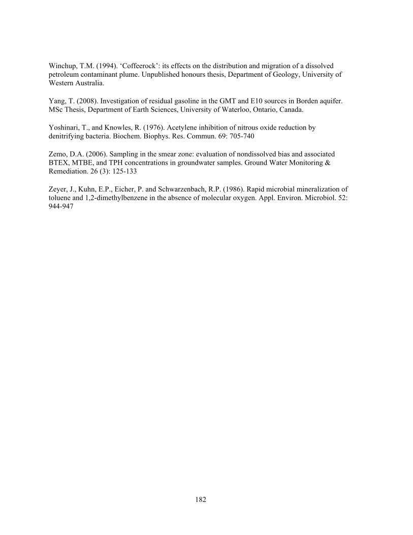
182

Winchup, T.M. (1994). ‘Coffeerock’: its effects on the distribution and migration of a dissolved petroleum contaminant plume. Unpublished honours thesis, Department of Geology, University of Western Australia.

Yang, T. (2008). Investigation of residual gasoline in the GMT and E10 sources in Borden aquifer. MSc Thesis, Department of Earth Sciences, University of Waterloo, Ontario, Canada.

Yoshinari, T., and Knowles, R. (1976). Acetylene inhibition of nitrous oxide reduction by denitrifying bacteria. Biochem. Biophys. Res. Commun. 69: 705-740

Zemo, D.A. (2006). Sampling in the smear zone: evaluation of nondissolved bias and associated BTEX, MTBE, and TPH concentrations in groundwater samples. Ground Water Monitoring & Remediation. 26 (3): 125-133

Zeyer, J., Kuhn, E.P., Eicher, P. and Schwarzenbach, R.P. (1986). Rapid microbial mineralization of toluene and 1,2-dimethylbenzene in the absence of molecular oxygen. Appl. Environ. Microbiol. 52: 944-947

Appendix A

Well Construction Details, Boreholes and Information Supporting Site Characterization

183

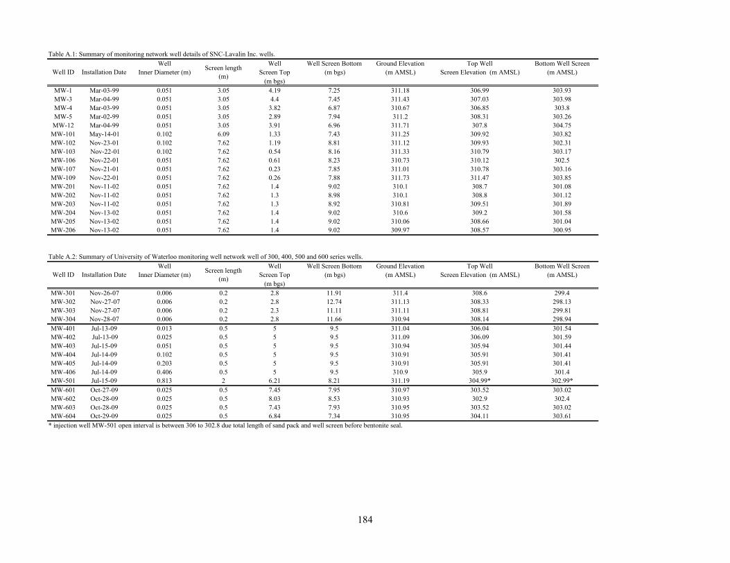
Table A.1: Summary of monitoring network well details of SNC-Lavalin Inc. wells.

Well Well Well Screen Bottom Ground Elevation Top Well Bottom Well ScreenInner Diameter (m) Screen Top (m bgs) (m AMSL) Screen Elevation (m AMSL) (m AMSL)

(m bgs)MW-1 Mar-03-99 0.051 3.05 4.19 7.25 311.18 306.99 303.93MW-3 Mar-04-99 0.051 3.05 4.4 7.45 311.43 307.03 303.98MW-4 Mar-03-99 0.051 3.05 3.82 6.87 310.67 306.85 303.8MW-5 Mar-02-99 0.051 3.05 2.89 7.94 311.2 308.31 303.26MW-12 Mar-04-99 0.051 3.05 3.91 6.96 311.71 307.8 304.75

MW-101 May-14-01 0.102 6.09 1.33 7.43 311.25 309.92 303.82MW-102 Nov-23-01 0.102 7.62 1.19 8.81 311.12 309.93 302.31MW-103 Nov-22-01 0.102 7.62 0.54 8.16 311.33 310.79 303.17MW-106 Nov-22-01 0.051 7.62 0.61 8.23 310.73 310.12 302.5MW-107 Nov-21-01 0.051 7.62 0.23 7.85 311.01 310.78 303.16MW-109 Nov-22-01 0.051 7.62 0.26 7.88 311.73 311.47 303.85MW-201 Nov-11-02 0.051 7.62 1.4 9.02 310.1 308.7 301.08MW-202 Nov-11-02 0.051 7.62 1.3 8.98 310.1 308.8 301.12MW-203 Nov-11-02 0.051 7.62 1.3 8.92 310.81 309.51 301.89MW-204 Nov-13-02 0.051 7.62 1.4 9.02 310.6 309.2 301.58MW-205 Nov-13-02 0.051 7.62 1.4 9.02 310.06 308.66 301.04MW-206 Nov-13-02 0.051 7.62 1.4 9.02 309.97 308.57 300.95

Table A.2: Summary of University of Waterloo monitoring well network well of 300, 400, 500 and 600 series wells.

Well Well Well Screen Bottom Ground Elevation Top Well Bottom Well ScreenInner Diameter (m) Screen Top (m bgs) (m AMSL) Screen Elevation (m AMSL) (m AMSL)

(m bgs)MW-301 Nov-26-07 0.006 0.2 2.8 11.91 311.4 308.6 299.4MW-302 Nov-27-07 0.006 0.2 2.8 12.74 311.13 308.33 298.13MW-303 Nov-27-07 0.006 0.2 2.3 11.11 311.11 308.81 299.81MW-304 Nov-28-07 0.006 0.2 2.8 11.66 310.94 308.14 298.94MW-401 Jul-13-09 0.013 0.5 5 9.5 311.04 306.04 301.54MW-402 Jul-13-09 0.025 0.5 5 9.5 311.09 306.09 301.59MW-403 Jul-15-09 0.051 0.5 5 9.5 310.94 305.94 301.44MW-404 Jul-14-09 0.102 0.5 5 9.5 310.91 305.91 301.41MW-405 Jul-14-09 0.203 0.5 5 9.5 310.91 305.91 301.41MW-406 Jul-14-09 0.406 0.5 5 9.5 310.9 305.9 301.4MW-501 Jul-15-09 0.813 2 6.21 8.21 311.19 304.99* 302.99*MW-601 Oct-27-09 0.025 0.5 7.45 7.95 310.97 303.52 303.02MW-602 Oct-28-09 0.025 0.5 8.03 8.53 310.93 302.9 302.4MW-603 Oct-28-09 0.025 0.5 7.43 7.93 310.95 303.52 303.02MW-604 Oct-29-09 0.025 0.5 6.84 7.34 310.95 304.11 303.61

* injection well MW-501 open interval is between 306 to 302.8 due total length of sand pack and well screen before bentonite seal.

Well ID Installation DateScreen length

(m)

Well ID Installation DateScreen length

(m)

184

SNC-Lavalin (ATSI) prepared boreholes for coring and installation of multilevel wells and an injection well between November 2007 and October 2009 for the University of Waterloo.

185

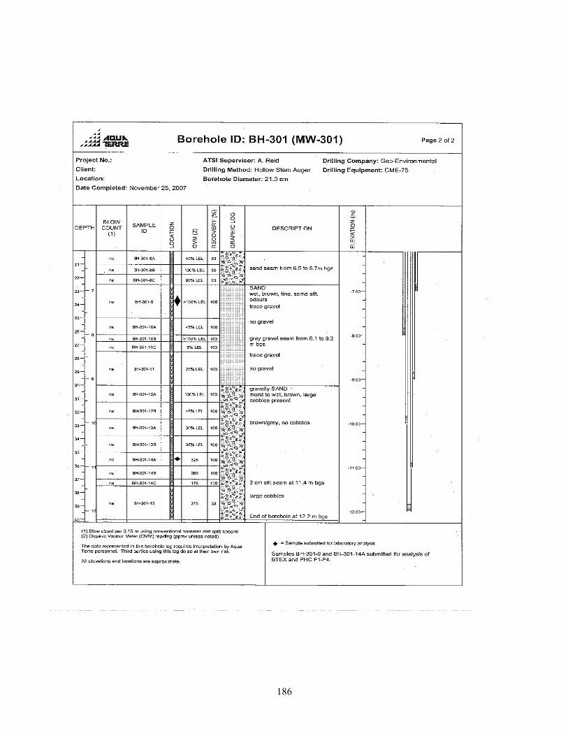
186

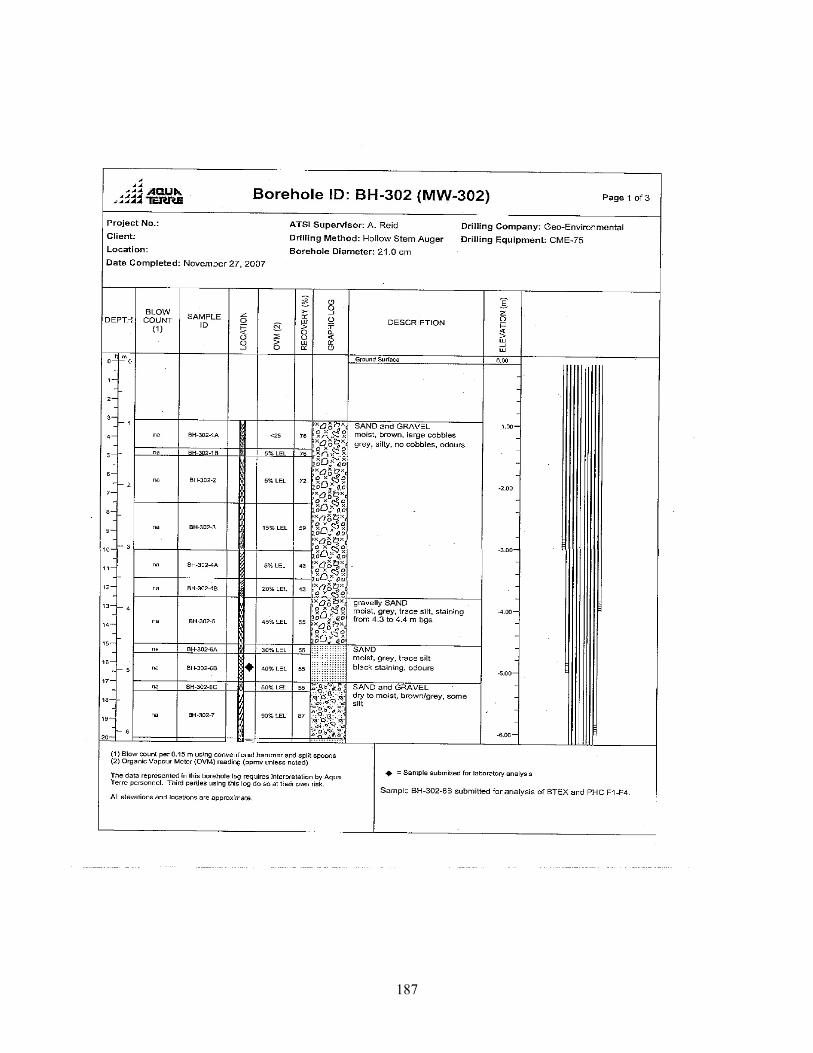
187

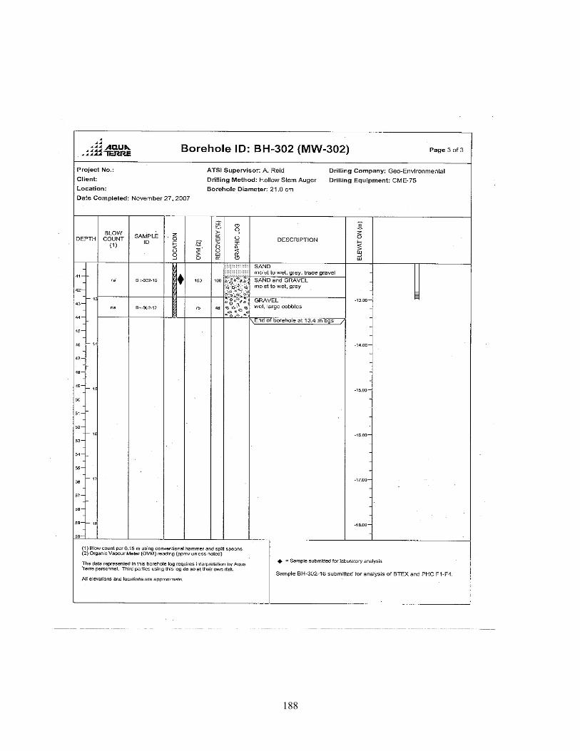
188

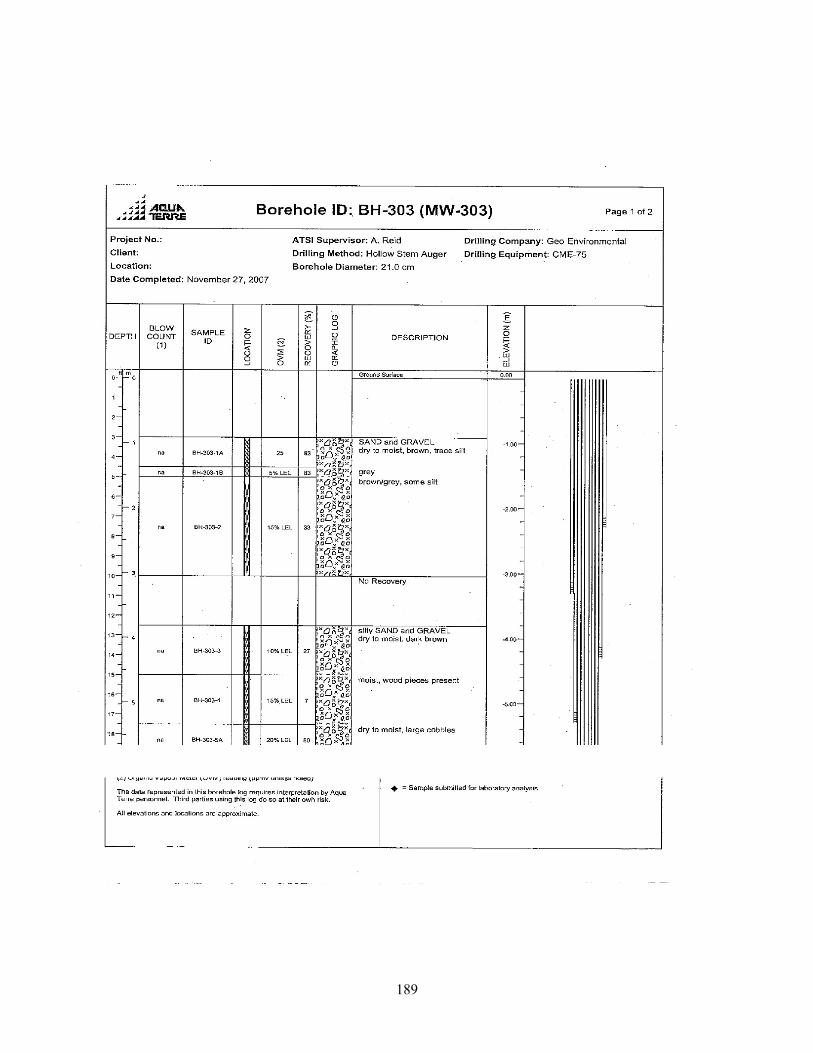
189

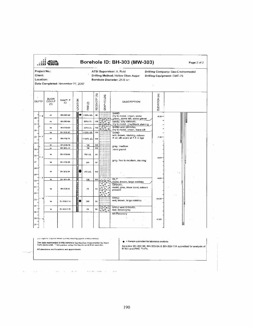
190

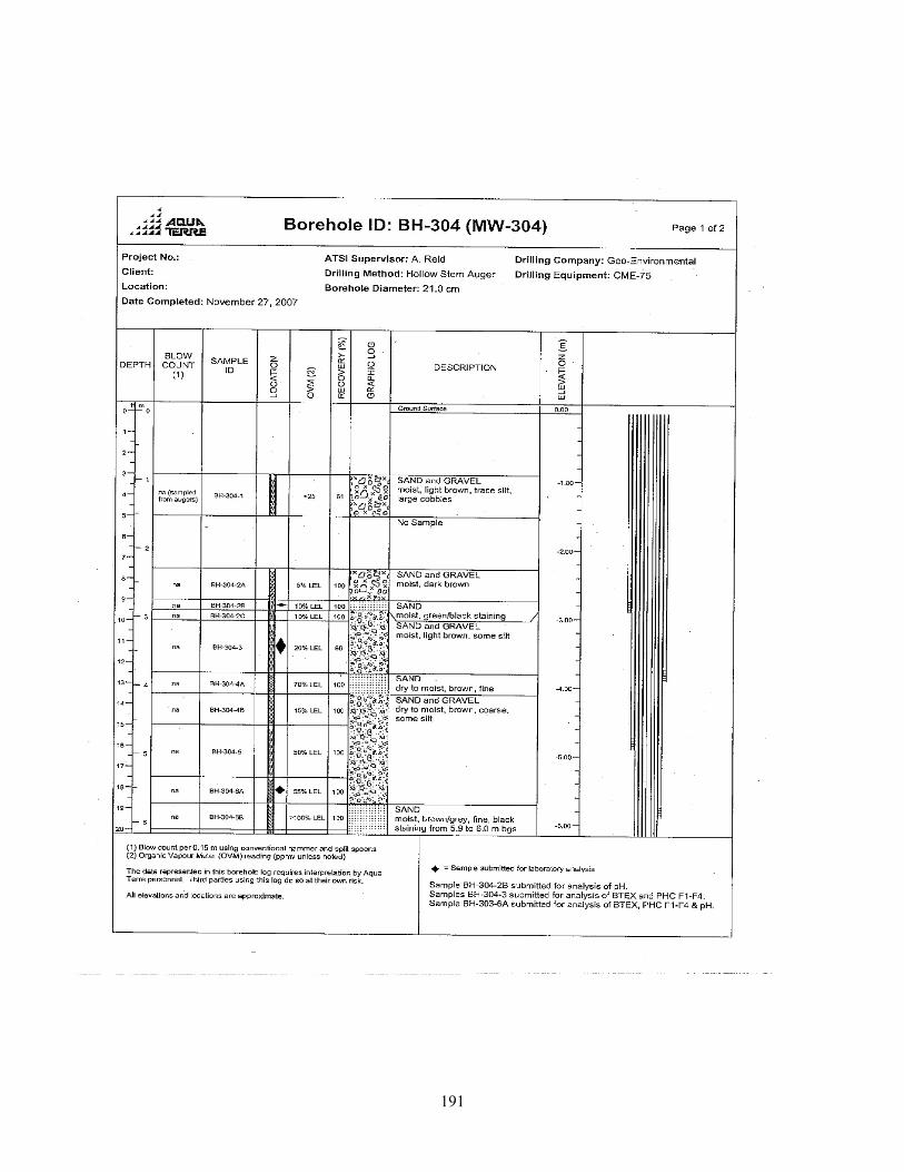
191

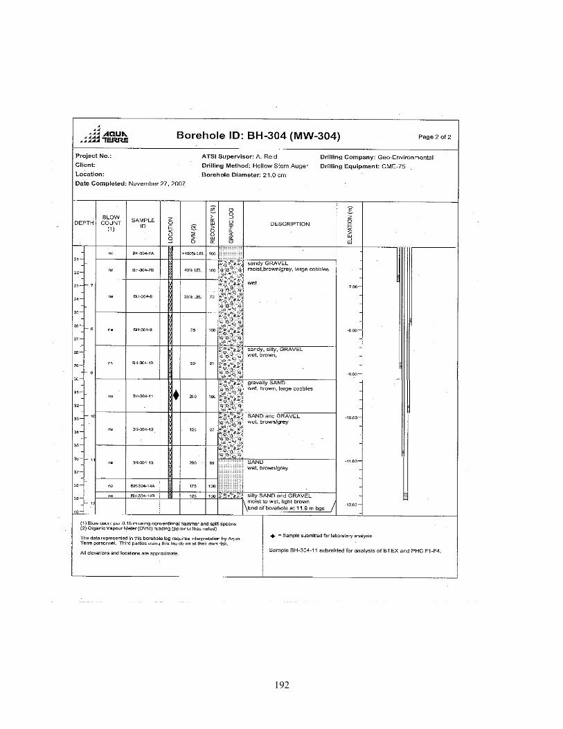
192

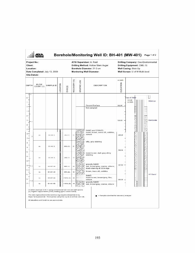
193

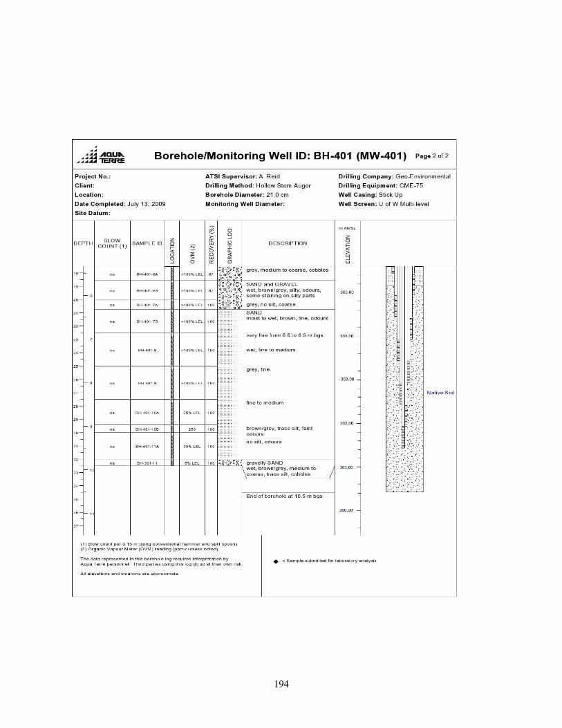
194

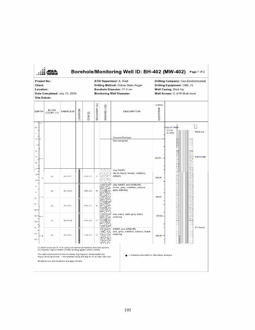
195

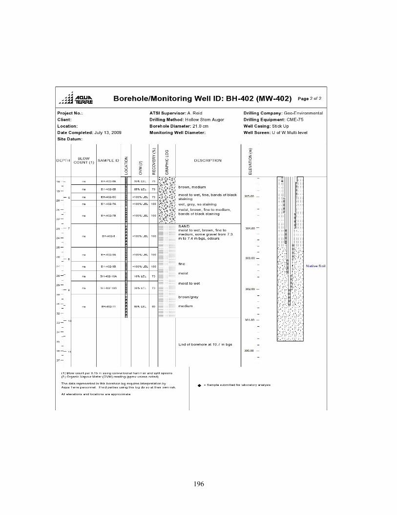
196

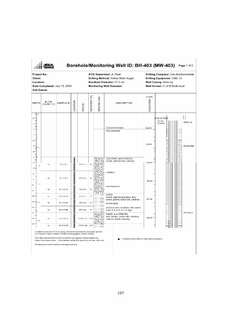
197

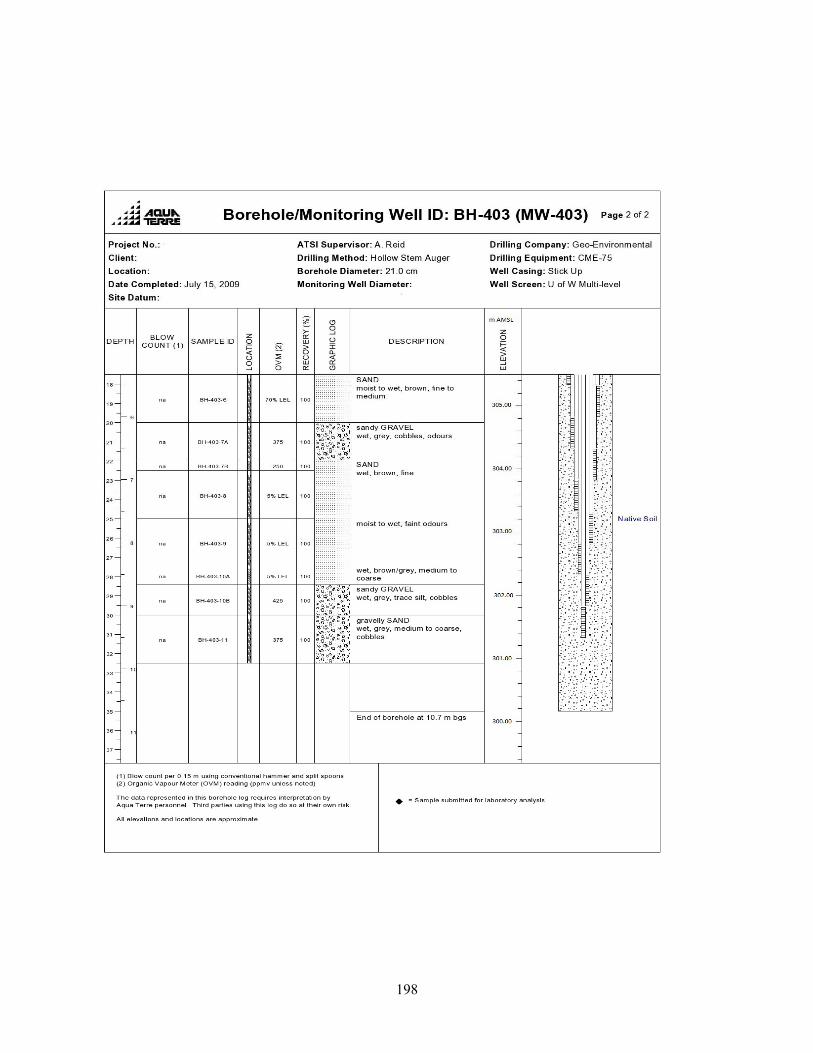
198

199

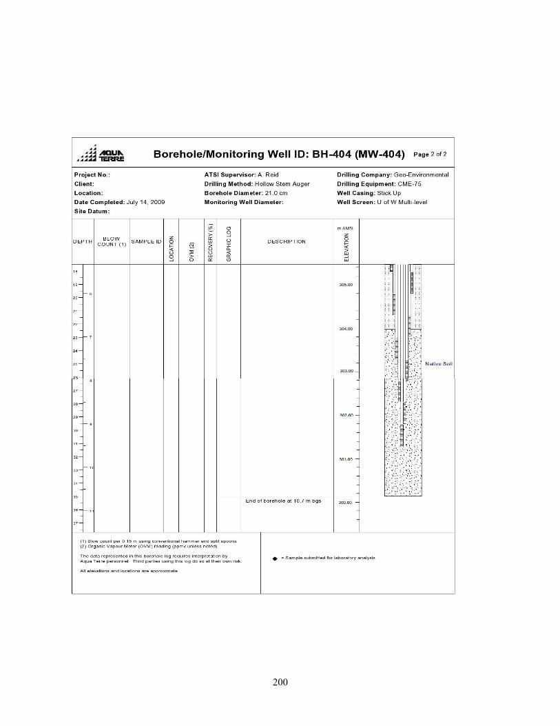
200

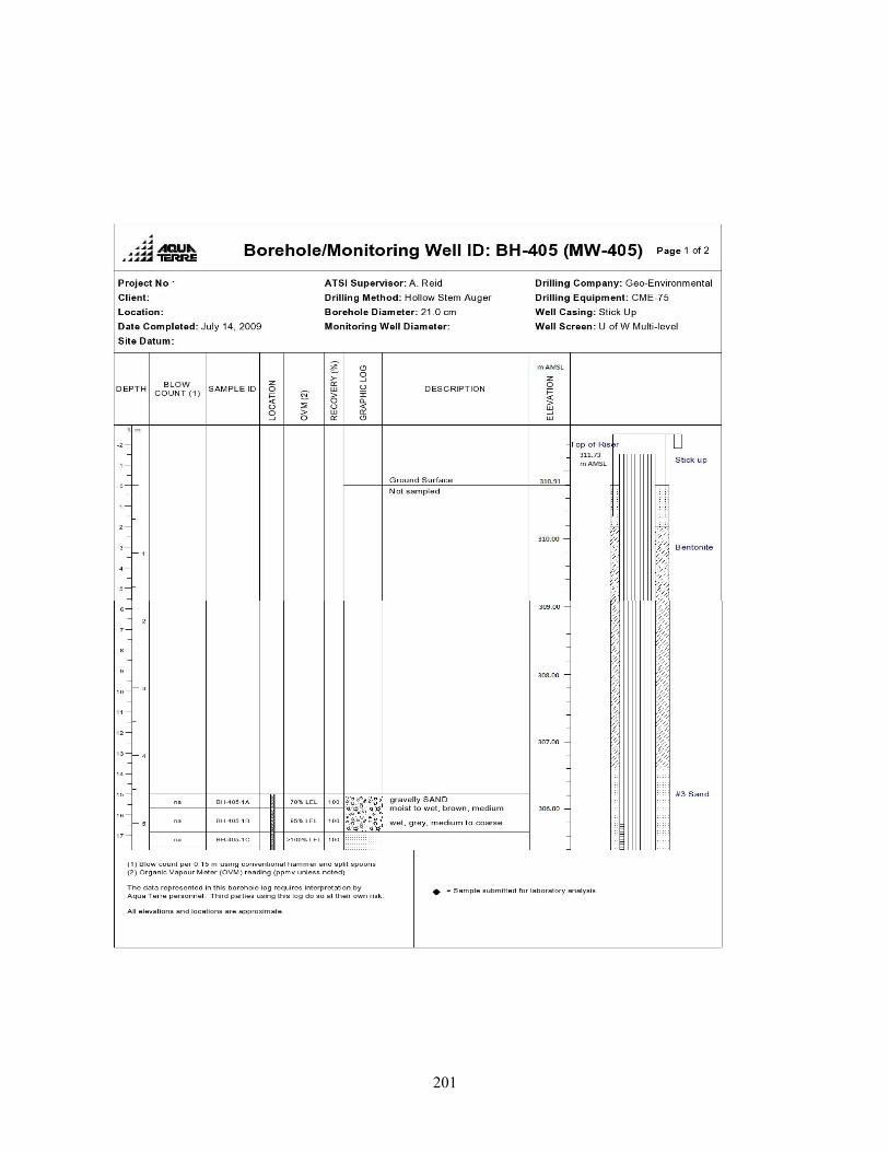
201

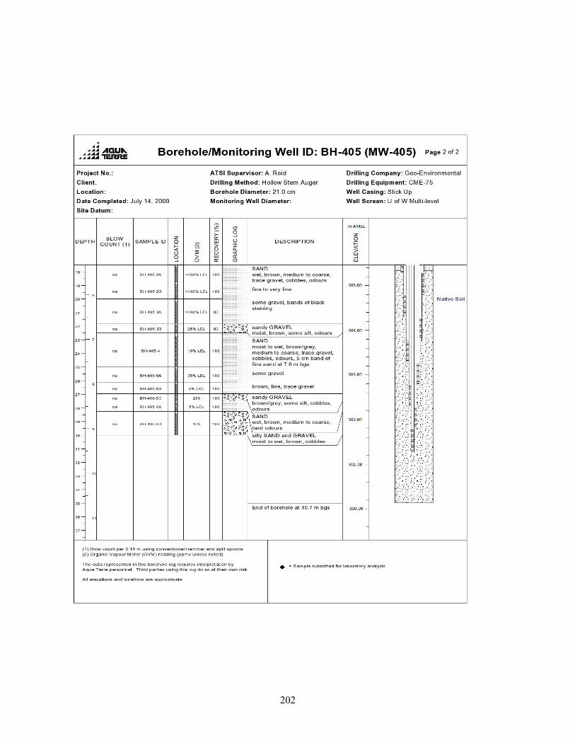
202

203

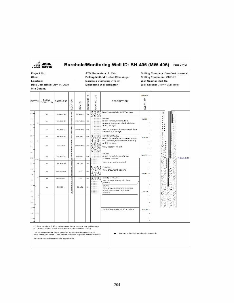
204

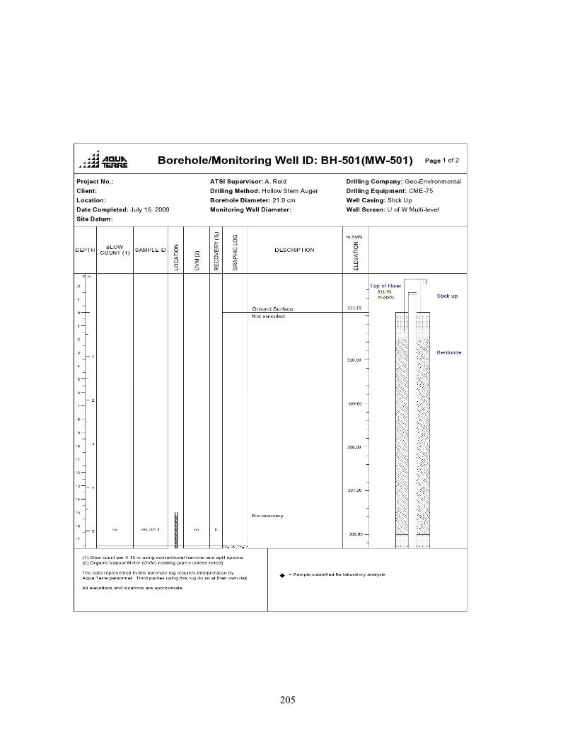
205

206

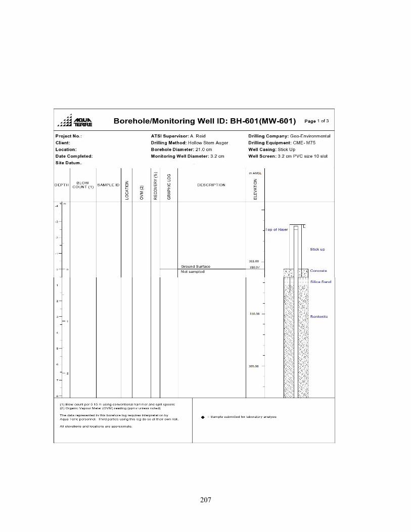
207

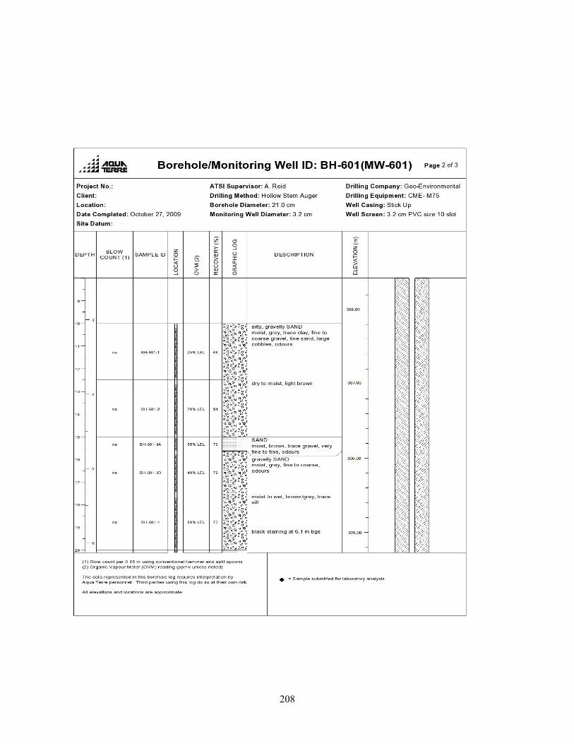
208

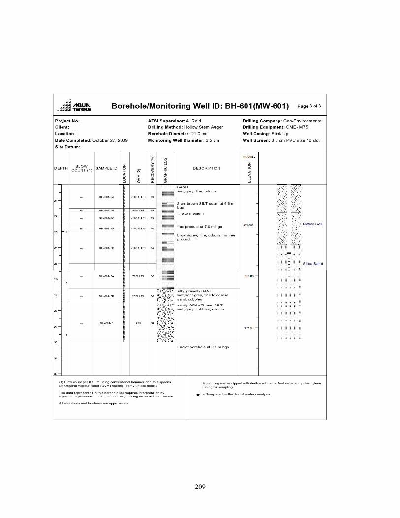
209

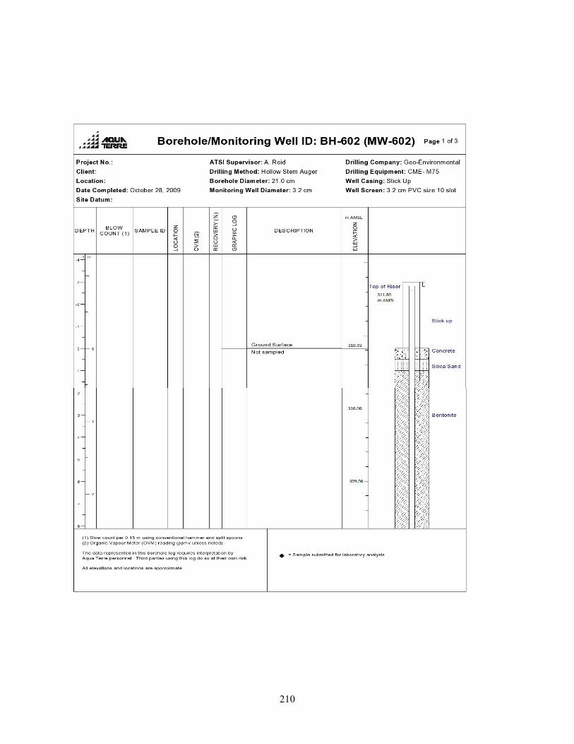
210

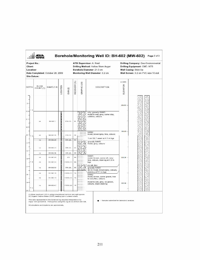
211

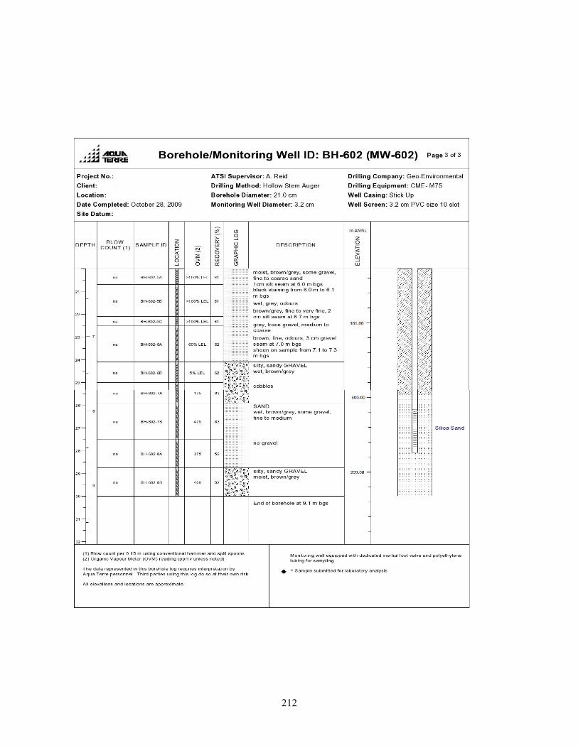
212

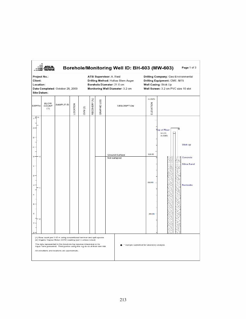
213

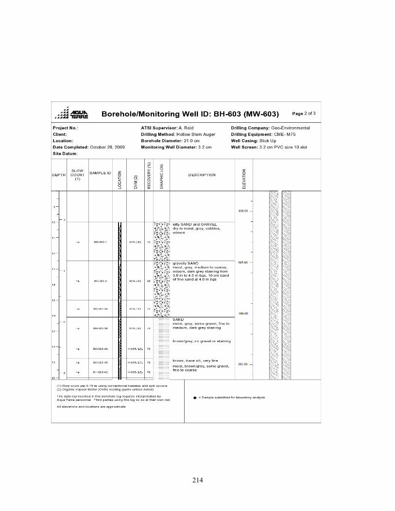
214

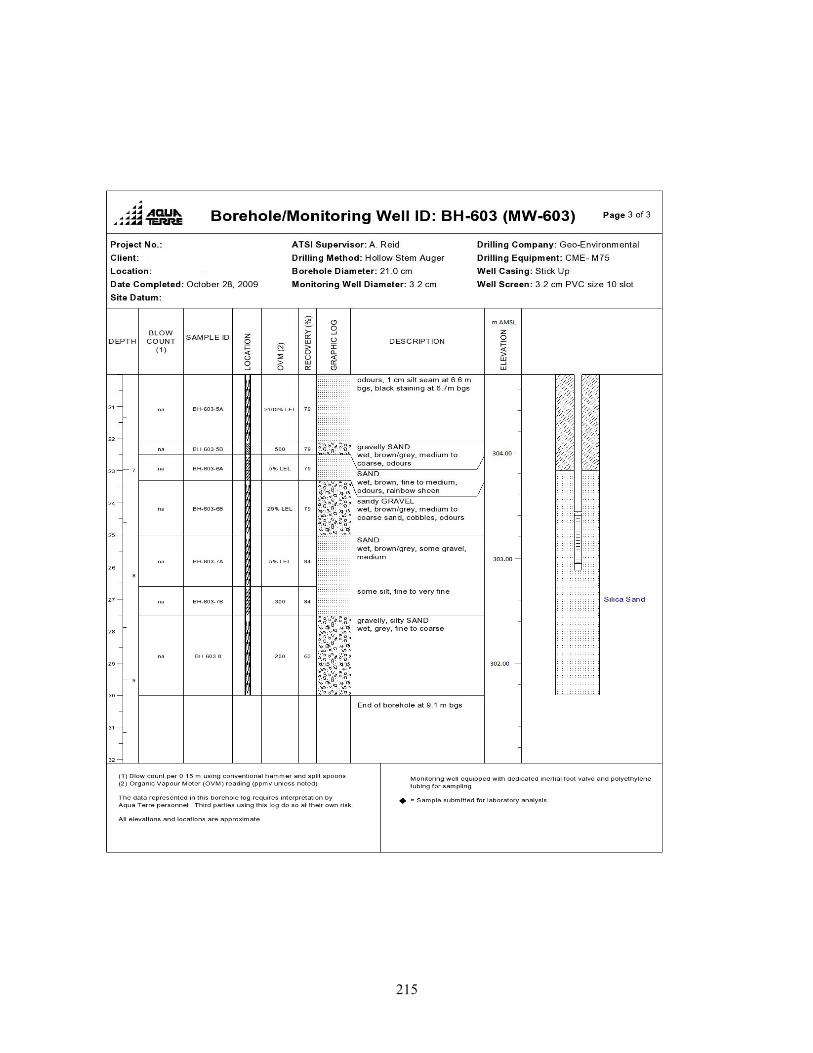
215

216

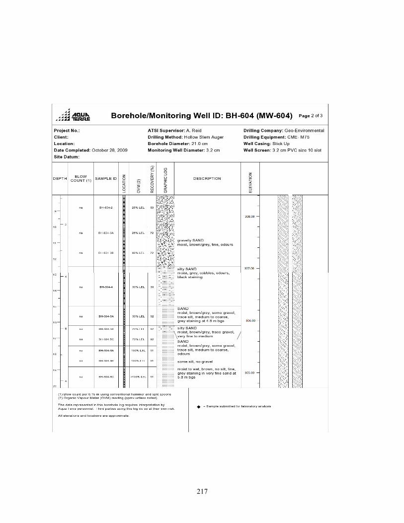
217

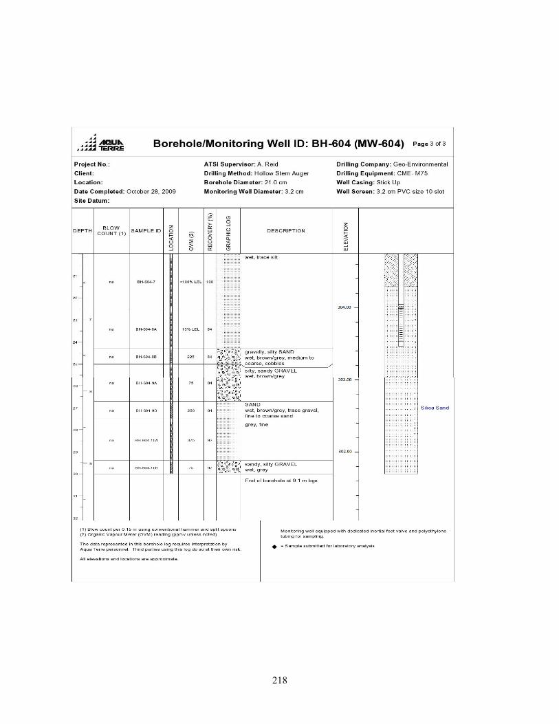
218

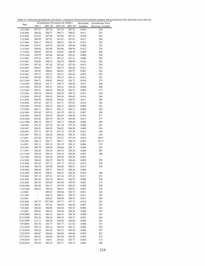
Table A.3 Historical groundwater elevations , estimation of horizontal hydraulic gradient and groundwater flow direction across the site

MW-4 MW-101 MW-103 MW-107

2/25/2004 307.23 307.34 307.34 307.22 0.014 2585/26/2004 308.56 308.71 308.71 308.62 0.011 2536/18/2004 307.87 307.98 307.98 307.91 0.020 2497/22/2004 306.99 307.07 307.07 307.03 0.013 2408/27/2004 306.15 306.23 306.23 306.19 0.013 2839/29/2004 305.47 305.54 305.54 305.49 0.008 27011/9/2004 304.94 305.06 305.06 304.94 0.012 27612/7/2004 304.95 305.05 305.05 304.95 0.009 280

12/21/2004 305.59 305.66 305.66 305.61 0.004 2981/21/2005 307.22 307.27 307.27 307.21 0.006 2634/19/2005 308.09 308.16 308.16 308.09 0.016 2445/31/2005 307.56 307.62 307.62 307.56 0.015 2446/29/2005 306.67 306.73 306.73 306.68 0.011 2527/28/2005 305.95 306.01 306.01 305.97 0.007 2638/25/2005 305.37 305.51 305.51 305.45 0.018 2839/28/2005 305.08 305.27 305.27 305.15 0.012 291

10/27/2005 304.71 304.81 304.81 304.71 0.010 27911/24/2005 304.64 304.77 304.77 304.65 0.012 28012/22/2005 305.24 305.31 305.31 305.24 0.004 2881/27/2006 306.91 306.95 306.95 306.91 0.004 2732/23/2006 308.24 308.30 308.30 308.22 0.015 2443/23/2006 309.42 309.56 309.56 309.45 0.016 2404/27/2006 308.90 309.02 309.02 308.93 0.011 2445/30/2006 307.65 307.71 307.71 307.67 0.010 2426/29/2006 306.68 306.72 306.72 306.69 0.009 2417/27/2006 306.11 306.17 306.17 306.13 0.005 2648/24/2006 305.48 305.55 305.55 305.51 0.007 2689/28/2006 304.95 305.05 305.05 304.95 0.010 277

10/30/2006 305.03 305.19 305.19 305.04 0.015 27712/21/2006 306.70 306.73 306.73 306.68 0.006 2801/24/2007 307.35 307.39 307.39 307.34 0.009 2472/20/2007 306.91 306.95 306.95 306.90 0.009 2463/20/2007 307.71 307.76 307.76 307.69 0.013 2444/25/2007 309.12 309.26 309.26 309.14 0.022 2496/7/2007 307.58 307.67 307.67 307.59 0.016 249.5

7/24/2007 306.12 306.17 306.17 306.14 0.007 255.59/6/2007 305.11 305.19 305.19 305.13 0.006 276

10/2/2007 304.70 304.80 304.80 304.71 0.009 28211/7/2007 304.26 304.34 304.34 304.26 0.008 285

12/17/2007 304.10 304.19 304.19 304.09 0.007 2801/22/2008 305.84 305.89 305.89 305.85 0.002 -2/14/2008 306.65 306.70 306.70 306.64 0.003 2953/19/2008 307.63 307.72 307.72 307.63 0.012 2584/18/2008 309.78 309.98 309.98 309.87 0.012 2595/28/2008 308.44 308.71 308.53 308.46 0.009 -6/24/2008 308.39 308.61 308.45 308.40 0.010 2407/30/2008 307.19 307.41 307.24 307.21 0.011 2518/20/2008 306.56 306.70 306.61 306.57 0.006 2509/26/2008 305.93 305.99 305.96 305.95 0.003 273

10/28/2008 305.49 305.57 305.59 306.53 0.009 29911/20/2008 306.62 306.68 306.67 306.61 0.007 276

4/2/2009 - 309.87 309.86 309.75 0.012 2625/27/2009 - 308.72 308.61 308.53 0.011 2526/4/2009 - 308.62 308.50 308.41 0.013 240

6/25/2009 307.72 307.924 307.77 307.73 0.010 2527/22/2009 306.81 307.01 306.85 306.82 0.007 2477/28/2009 306.66 306.80 306.69 306.67 0.006 2438/5/2009 306.43 306.14 306.46 306.45 0.006 247

8/10/2009 306.32 306.35 306.35 306.34 0.009 2478/13/2009 306.26 306.29 306.29 306.27 0.007 2608/25/2009 213.11 306.09 306.09 306.06 0.004 2639/9/2009 305.70 305.77 305.77 311.01 0.008 2731/21/2010 305.14 305.16 305.19 305.15 0.004 2832/19/2010 305.26 305.29 305.32 305.28 0.004 2933/22/2010 306.07 306.04 306.09 306.06 0.002 2874/27/2010 305.85 305.88 305.89 305.85 0.003 2755/19/2010 305.75 305.8 305.81 305.77 0.003 2756/22/2010 305.69 305.74 305.77 305.72 0.006 280

Groundwater Flow Direction Azimuth

DateGroundwater Elevations (m AMSL) Horizontal

Gradient

219

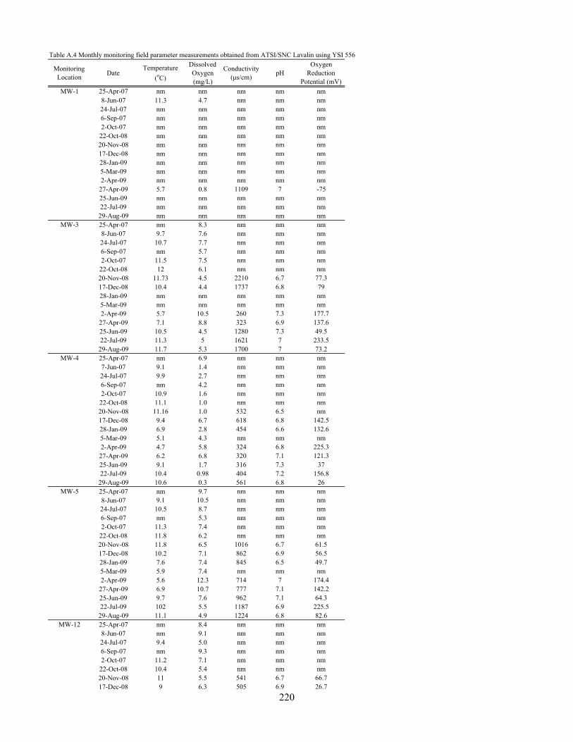
Table A.4 Monthly monitoring field parameter measurements obtained from ATSI/SNC Lavalin using YSI 556

Monitoring Location

DateTemperature

(oC)

Dissolved Oxygen (mg/L)

Conductivity (μs/cm)

pHOxygen

Reduction Potential (mV)

MW-1 25-Apr-07 nm nm nm nm nm8-Jun-07 11.3 4.7 nm nm nm24-Jul-07 nm nm nm nm nm6-Sep-07 nm nm nm nm nm2-Oct-07 nm nm nm nm nm

22-Oct-08 nm nm nm nm nm20-Nov-08 nm nm nm nm nm17-Dec-08 nm nm nm nm nm28-Jan-09 nm nm nm nm nm5-Mar-09 nm nm nm nm nm2-Apr-09 nm nm nm nm nm

27-Apr-09 5.7 0.8 1109 7 -7525-Jun-09 nm nm nm nm nm22-Jul-09 nm nm nm nm nm

29-Aug-09 nm nm nm nm nmMW-3 25-Apr-07 nm 8.3 nm nm nm

8-Jun-07 9.7 7.6 nm nm nm24-Jul-07 10.7 7.7 nm nm nm6-Sep-07 nm 5.7 nm nm nm2-Oct-07 11.5 7.5 nm nm nm

22-Oct-08 12 6.1 nm nm nm20-Nov-08 11.73 4.5 2210 6.7 77.317-Dec-08 10.4 4.4 1737 6.8 7928-Jan-09 nm nm nm nm nm5-Mar-09 nm nm nm nm nm2-Apr-09 5.7 10.5 260 7.3 177.7

27-Apr-09 7.1 8.8 323 6.9 137.625-Jun-09 10.5 4.5 1280 7.3 49.522-Jul-09 11.3 5 1621 7 233.5

29-Aug-09 11.7 5.3 1700 7 73.2MW-4 25-Apr-07 nm 6.9 nm nm nm

7-Jun-07 9.1 1.4 nm nm nm24-Jul-07 9.9 2.7 nm nm nm6-Sep-07 nm 4.2 nm nm nm2-Oct-07 10.9 1.6 nm nm nm

22-Oct-08 11.1 1.0 nm nm nm20-Nov-08 11.16 1.0 532 6.5 nm17-Dec-08 9.4 6.7 618 6.8 142.528-Jan-09 6.9 2.8 454 6.6 132.65-Mar-09 5.1 4.3 nm nm nm2-Apr-09 4.7 5.8 324 6.8 225.3

27-Apr-09 6.2 6.8 320 7.1 121.325-Jun-09 9.1 1.7 316 7.3 3722-Jul-09 10.4 0.98 404 7.2 156.8

29-Aug-09 10.6 0.3 561 6.8 26MW-5 25-Apr-07 nm 9.7 nm nm nm

8-Jun-07 9.1 10.5 nm nm nm24-Jul-07 10.5 8.7 nm nm nm6-Sep-07 nm 5.3 nm nm nm2-Oct-07 11.3 7.4 nm nm nm

22-Oct-08 11.8 6.2 nm nm nm20-Nov-08 11.8 6.5 1016 6.7 61.517-Dec-08 10.2 7.1 862 6.9 56.528-Jan-09 7.6 7.4 845 6.5 49.75-Mar-09 5.9 7.4 nm nm nm2-Apr-09 5.6 12.3 714 7 174.4

27-Apr-09 6.9 10.7 777 7.1 142.225-Jun-09 9.7 7.6 962 7.1 64.322-Jul-09 102 5.5 1187 6.9 225.5

29-Aug-09 11.1 4.9 1224 6.8 82.6MW-12 25-Apr-07 nm 8.4 nm nm nm

8-Jun-07 nm 9.1 nm nm nm24-Jul-07 9.4 5.0 nm nm nm6-Sep-07 nm 9.3 nm nm nm2-Oct-07 11.2 7.1 nm nm nm

22-Oct-08 10.4 5.4 nm nm nm20-Nov-08 11 5.5 541 6.7 66.717-Dec-08 9 6.3 505 6.9 26.7

220

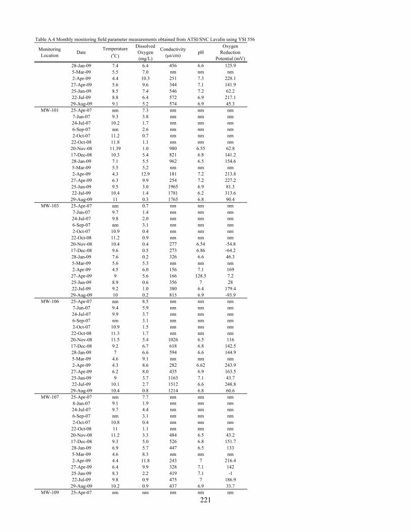
Table A.4 Monthly monitoring field parameter measurements obtained from ATSI/SNC Lavalin using YSI 556

Monitoring Location

DateTemperature

(oC)

Dissolved Oxygen (mg/L)

Conductivity (μs/cm)

pHOxygen

Reduction Potential (mV)

28-Jan-09 7.4 6.4 456 6.6 125.95-Mar-09 5.5 7.0 nm nm nm2-Apr-09 4.4 10.3 251 7.3 228.1

27-Apr-09 5.6 9.6 344 7.1 141.925-Jun-09 8.5 7.4 546 7.2 62.222-Jul-09 8.8 6.4 572 6.9 217.1

29-Aug-09 9.1 5.2 574 6.9 45.3MW-101 25-Apr-07 nm 7.3 nm nm nm

7-Jun-07 9.3 3.8 nm nm nm24-Jul-07 10.2 1.7 nm nm nm6-Sep-07 nm 2.6 nm nm nm2-Oct-07 11.2 0.7 nm nm nm

22-Oct-08 11.8 1.1 nm nm nm20-Nov-08 11.39 1.0 980 6.55 62.817-Dec-08 10.3 5.4 821 6.8 141.228-Jan-09 7.1 5.5 962 6.5 154.65-Mar-09 5.5 5.2 nm nm nm2-Apr-09 4.3 12.9 181 7.2 213.8

27-Apr-09 6.3 9.9 254 7.2 227.225-Jun-09 9.5 3.0 1965 6.9 81.322-Jul-09 10.4 1.4 1781 6.2 313.6

29-Aug-09 11 0.3 1765 6.8 90.4MW-103 25-Apr-07 nm 0.7 nm nm nm

7-Jun-07 9.7 1.4 nm nm nm24-Jul-07 9.8 2.0 nm nm nm6-Sep-07 nm 3.1 nm nm nm2-Oct-07 10.9 0.4 nm nm nm

22-Oct-08 11.2 0.9 nm nm nm20-Nov-08 10.4 0.4 277 6.54 -54.817-Dec-08 9.6 0.5 273 6.86 -64.228-Jan-09 7.6 0.2 326 6.6 46.35-Mar-09 5.6 5.3 nm nm nm2-Apr-09 4.5 6.0 156 7.1 169

27-Apr-09 9 5.6 166 128.5 7.225-Jun-09 8.9 0.6 356 7 2822-Jul-09 9.2 1.0 380 6.4 179.4

29-Aug-09 10 0.2 815 6.9 -93.9MW-106 25-Apr-07 nm 8.5 nm nm nm

7-Jun-07 9.4 5.9 nm nm nm24-Jul-07 9.9 3.7 nm nm nm6-Sep-07 nm 3.1 nm nm nm2-Oct-07 10.9 1.5 nm nm nm

22-Oct-08 11.3 1.7 nm nm nm20-Nov-08 11.5 5.4 1026 6.5 11617-Dec-08 9.2 6.7 618 6.8 142.528-Jan-09 7 6.6 594 6.6 144.95-Mar-09 4.6 9.1 nm nm nm2-Apr-09 4.3 8.6 282 6.62 243.9

27-Apr-09 6.2 8.0 435 6.9 163.525-Jun-09 9 3.7 1163 7.1 43.722-Jul-09 10.1 2.7 1512 6.6 248.8

29-Aug-09 10.4 0.8 1214 6.8 60.6MW-107 25-Apr-07 nm 7.7 nm nm nm

8-Jun-07 9.1 1.9 nm nm nm24-Jul-07 9.7 4.4 nm nm nm6-Sep-07 nm 3.1 nm nm nm2-Oct-07 10.8 0.4 nm nm nm

22-Oct-08 11 1.1 nm nm nm20-Nov-08 11.2 3.3 484 6.5 43.217-Dec-08 9.3 5.0 526 6.8 151.728-Jan-09 6.9 5.7 447 6.5 1335-Mar-09 4.6 8.3 nm nm nm2-Apr-09 4.4 11.8 243 7 216.4

27-Apr-09 6.4 9.9 328 7.1 14225-Jun-09 8.3 2.2 419 7.1 -122-Jul-09 9.8 0.9 475 7 186.9

29-Aug-09 10.2 0.9 437 6.9 33.7MW-109 25-Apr-07 nm nm nm nm nm

221

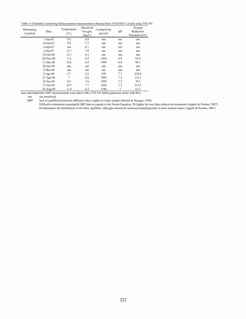
Table A.4 Monthly monitoring field parameter measurements obtained from ATSI/SNC Lavalin using YSI 556

Monitoring Location

DateTemperature

(oC)

Dissolved Oxygen (mg/L)

Conductivity (μs/cm)

pHOxygen

Reduction Potential (mV)

7-Jun-07 9.5 8.0 nm nm nm24-Jul-07 9.9 7.1 nm nm nm6-Sep-07 nm 6.1 nm nm nm2-Oct-07 11.7 7.0 nm nm nm

22-Oct-08 12.1 6.2 nm nm nm20-Nov-08 112 6.9 1464 6.8 65.417-Dec-08 10.6 6.9 1498 6.8 96.128-Jan-09 nm nm nm nm nm5-Mar-09 nm nm nm nm nm2-Apr-09 5.7 8.2 938 7.1 234.9

27-Apr-09 7 8.6 1083 7.2 123.125-Jun-09 9.9 7.6 1205 7.2 70.522-Jul-09 10.7 7.1 1456 7.1 233.5

29-Aug-09 11.8 6.2 1594 7 63.2

nm not monitoredORP lack of equilibrium between different redox couples in water sample (Stumm & Morgan, 1996)

Difficult to determine meaningful ORP data in regards to the Nernst Equation, Eh higher for oxic than reduced environments (Appelo & Postma, 2007)Eh determines the distribution of all redox equilibria, although cnanont be measured unambiguously in most natural waters (Appelo & Postma, 2007)

June and September 2007 measurements were taken with a YSI 556 Multi-parameter meter with flow

222

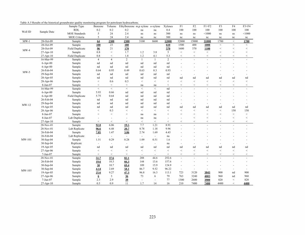
Table A.5 Results of the historical groundwater quality monitoring program for petroleum hydrocarbons.Sample Type Benzene Toluene Ethylbenzene m,p xylene o-xylene Xylenes F1 F2 F1+F2 F3 F4 F3+F4

RDL 0.2 0.2 0.2 na na 0.4 100 100 100 100 100 100MOE Standards 5 24 2.4 ns ns 300 ns ns <1000 ns ns <1000MOE Criteria 5 24 2.4 nc nc 300 nc nc nc nc nc nc

MW-1 28-Oct-09 Sample 64 2300 2300 3100 8600 12000 32000 15000 31000 1700 < 170028-Oct-09 Sample 100 23 180 610 1500 400 1000 < < <28-Oct-09 Field Duplicate 96 21 170 570 1600 370 1100 < < <27-Apr-10 Sample 0.8 < 1.7 1.2 3.8 5 < < < < < <27-Apr-10 Field Duplicate 0.8 < 1.8 1.2 4.1 5.3 < < < < < <16-Mar-99 Sample 4 4 2 1 1 2 - - - - - -6-Apr-00 Sample nd nd nd nd nd nd - - - - - -6-Apr-00 Sample nd nd nd nd nd nd - - - - - -26-Feb-04 Sample 0.64 0.95 0.49 0.63 0.3 0.93 - - - - - -29-Sep-04 Sample nd nd nd nd nd nd - - - - - -20-Apr-05 Sample nd nd nd nd nd nd nd nd nd nd nd nd28-Apr-06 Sample < 0.6 0.3 < < < < < < < < <8-Jun-07 Sample < < < na na < < < < < < <

16-Mar-99 Sample < < < < < nd - - - - - -6-Apr-00 Sample 5.93 0.66 nd nd nd nd - - - - - -6-Apr-00 Field Duplicate 5.75 0.64 nd nd nd nd - - - - - -26-Feb-04 Sample nd nd nd nd nd nd - - - - - -29-Sep-04 Sample nd nd nd nd nd nd - - - - - -19-Apr-05 Sample nd nd nd nd nd nd nd nd nd nd nd nd28-Apr-06 Sample < 0.3 < < < < < < < < 150 1508-Jun-07 Sample < < < na na < < < < < < <8-Jun-07 Lab Duplicate - - - na na - - < < - < <

27-Apr-10 Sample < < < < < < < < < < < <28-Nov-01 Sample 92.8 6.06 19.5 7.7 1.21 8.91 - - - - - -28-Nov-01 Lab Replicate 96.6 6.48 20.7 8.78 1.18 9.96 - - - - - -26-Feb-04 Sample 7.85 1.47 3.06 2.74 1.69 4.43 - - - - - -26-Feb-04 Lab Replicate - - - - - na - - - - - -30-Sep-04 Sample 1.51 0.29 0.28 1.09 0.51 1.6 - - - - - -30-Sep-04 Replicate - - - - - na - - - - - -19-Apr-05 Sample nd nd nd nd nd nd nd nd nd nd nd nd27-Apr-06 Sample < < < < < < < < < < < <7-Jun-07 Sample < < < - - < < < < < < <

28-Nov-01 Sample 51.7 37.6 82.1 208 44.6 252.6 - - - - - -26-Feb-04 Sample 19.6 10.3 66.3 144 13.6 157.6 - - - - - -30-Sep-04 Sample 30 10.7 69.4 109 15.9 124.9 - - - - - -30-Sep-04 Sample 4.14 2.69 58.1 86.7 9.52 96.22 - - - - - -19-Apr-05 Sample 25.6 9.27 47.3 96.8 16.3 113.1 723 3120 3843 900 nd 90027-Apr-06 Sample 6 3 36 73 6 79 763 3240 4003 960 nd 9607-Jun-07 Sample 2.3 2.9 39 - - 77 1300 2600 3900 820 < 820

27-Apr-10 Sample 0.5 0.9 11 1.7 14 16 210 7400 7400 4400 < 4400

Well ID Sample Date

MW-4

MW-5

MW-12

MW-101

MW-103

223

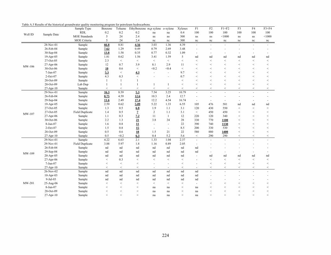
Table A.5 Results of the historical groundwater quality monitoring program for petroleum hydrocarbons.Sample Type Benzene Toluene Ethylbenzene m,p xylene o-xylene Xylenes F1 F2 F1+F2 F3 F4 F3+F4

RDL 0.2 0.2 0.2 na na 0.4 100 100 100 100 100 100MOE Standards 5 24 2.4 ns ns 300 ns ns <1000 ns ns <1000MOE Criteria 5 24 2.4 nc nc 300 nc nc nc nc nc nc

Well ID Sample Date

28-Nov-01 Sample 66.8 8.81 4.56 3.03 1.36 4.39 - - - - - -26-Feb-04 Sample 7.62 1.29 0.49 0.79 2.69 3.48 - - - - - -30-Sep-04 Sample 13.8 1.58 0.35 0.77 0.32 1.09 - - - - - -19-Apr-05 Sample 1.81 0.62 1.56 3.41 1.59 5 nd nd nd nd nd nd27-Oct-05 Sample 2.3 < < < < < < < < < < <27-Apr-06 Sample 12 0.7 3.9 8.1 2.9 11 < < < < < <30-Oct-06 Sample 10 0.6 < <0.2 <0.4 < < < < < < <7-Jun-07 Sample 5.3 < 4.3 - - 9.7 < < < < < <2-Oct-07 Sample 4.3 0.3 < - - 0.7 < < < < < <

28-Oct-09 Sample 1 1 1 < < < < < < <28-Oct-09 Lab Dup 1 1 1 1 1 < < < < < < <27-Apr-10 Sample < < < < < < < < < < < <29-Nov-01 Sample 16.3 8.59 5.3 7.54 3.25 10.79 - - - - - -26-Feb-04 Sample 8.75 4.59 12.6 10.3 2.4 12.7 - - - - - -29-Sep-04 Sample 11.6 2.49 17.4 12.2 4.54 16.74 - - - - - -19-Apr-05 Sample 2.59 0.62 5.09 5.22 1.33 6.55 105 476 581 nd nd nd27-Oct-05 Sample 1.3 0.5 6.8 1.9 1.1 3.1 120 430 550 < < <27-Oct-05 Field Duplicate 1.4 0.5 7 2 1.1 3.1 < 450 450 < < <27-Apr-06 Sample 1.1 0.3 7.2 11 1 12 220 120 340 < < <30-Oct-06 Sample 2.2 1.3 21 3.8 24 28 330 770 1100 < < <8-Jun-07 Sample 1.6 0.8 11 - - 22 390 740 1130 < < <2-Oct-07 Sample 1.5 0.8 15 - - 8.5 200 330 530 < < <

28-Oct-09 Sample 0.5 0.6 18 1.5 21 22 580 880 1400 < < <27-Apr-10 Sample 0.5 <0.2 6.3 0.4 5.2 5.6 < 290 290 < < <29-Nov-01 Sample 4.22 6.63 2.1 1.33 1.04 2.37 - - - - - -29-Nov-01 Field Duplicate 3.88 5.97 1.8 1.16 0.89 2.05 - - - - - -26-Feb-04 Sample nd nd nd nd nd nd nd - - - - -29-Sep-04 Sample nd nd nd nd nd nd nd - - - - -20-Apr-05 Sample nd nd nd nd nd nd - nd nd nd nd nd27-Apr-06 Sample < 0.3 < < < < - < < < < <7-Jun-07 Sample < < < - - < - < < < < <

27-Apr-10 Sample < < < - - < - < < < < <26-Nov-02 Sample nd nd nd nd nd nd nd - - - - -10-Apr-03 Sample nd nd nd nd nd nd nd - - - - -9-Jul-03 Sample nd nd nd nd nd nd nd - - - - -

25-Aug-06 Sample < < < < < < - < < < < <8-Jun-07 Sample < < < na na < na < < < < <

28-Oct-09 Sample < < < na na < na < < < < <27-Apr-10 Sample < < < na na < na < < < < <

MW-106

MW-107

MW-109

MW-201

224

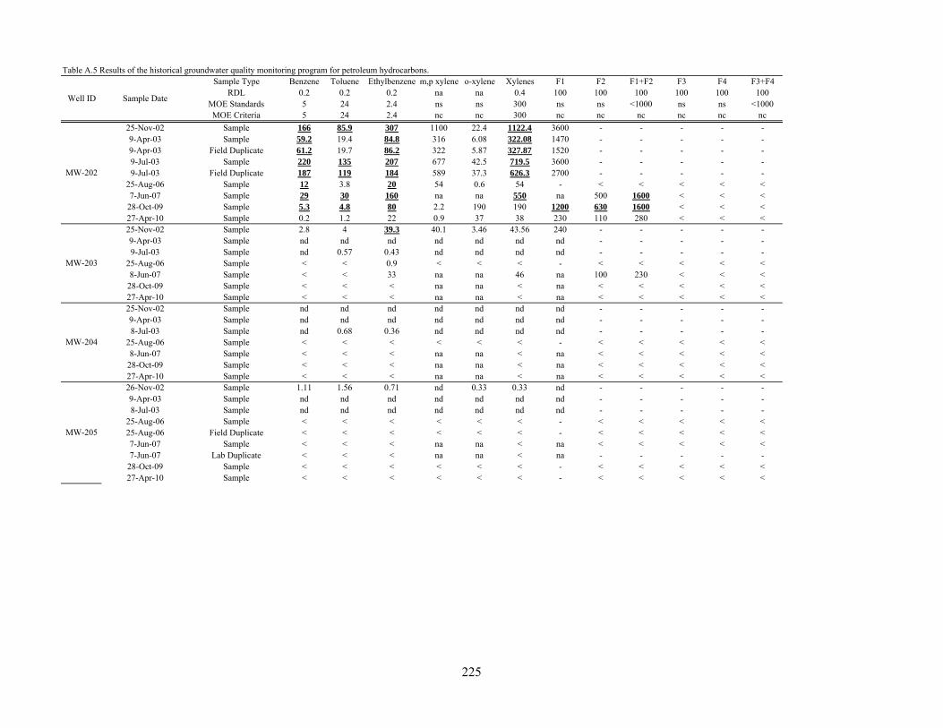
Table A.5 Results of the historical groundwater quality monitoring program for petroleum hydrocarbons.Sample Type Benzene Toluene Ethylbenzene m,p xylene o-xylene Xylenes F1 F2 F1+F2 F3 F4 F3+F4

RDL 0.2 0.2 0.2 na na 0.4 100 100 100 100 100 100MOE Standards 5 24 2.4 ns ns 300 ns ns <1000 ns ns <1000MOE Criteria 5 24 2.4 nc nc 300 nc nc nc nc nc nc

Well ID Sample Date

25-Nov-02 Sample 166 85.9 307 1100 22.4 1122.4 3600 - - - - -9-Apr-03 Sample 59.2 19.4 84.8 316 6.08 322.08 1470 - - - - -9-Apr-03 Field Duplicate 61.2 19.7 86.2 322 5.87 327.87 1520 - - - - -9-Jul-03 Sample 220 135 207 677 42.5 719.5 3600 - - - - -9-Jul-03 Field Duplicate 187 119 184 589 37.3 626.3 2700 - - - - -

25-Aug-06 Sample 12 3.8 20 54 0.6 54 - < < < < <7-Jun-07 Sample 29 30 160 na na 550 na 500 1600 < < <

28-Oct-09 Sample 5.3 4.8 80 2.2 190 190 1200 630 1600 < < <27-Apr-10 Sample 0.2 1.2 22 0.9 37 38 230 110 280 < < <25-Nov-02 Sample 2.8 4 39.3 40.1 3.46 43.56 240 - - - - -9-Apr-03 Sample nd nd nd nd nd nd nd - - - - -9-Jul-03 Sample nd 0.57 0.43 nd nd nd nd - - - - -

25-Aug-06 Sample < < 0.9 < < < - < < < < <8-Jun-07 Sample < < 33 na na 46 na 100 230 < < <

28-Oct-09 Sample < < < na na < na < < < < <27-Apr-10 Sample < < < na na < na < < < < <25-Nov-02 Sample nd nd nd nd nd nd nd - - - - -9-Apr-03 Sample nd nd nd nd nd nd nd - - - - -8-Jul-03 Sample nd 0.68 0.36 nd nd nd nd - - - - -

25-Aug-06 Sample < < < < < < - < < < < <8-Jun-07 Sample < < < na na < na < < < < <

28-Oct-09 Sample < < < na na < na < < < < <27-Apr-10 Sample < < < na na < na < < < < <26-Nov-02 Sample 1.11 1.56 0.71 nd 0.33 0.33 nd - - - - -9-Apr-03 Sample nd nd nd nd nd nd nd - - - - -8-Jul-03 Sample nd nd nd nd nd nd nd - - - - -

25-Aug-06 Sample < < < < < < - < < < < <25-Aug-06 Field Duplicate < < < < < < - < < < < <7-Jun-07 Sample < < < na na < na < < < < <7-Jun-07 Lab Duplicate < < < na na < na - - - - -

28-Oct-09 Sample < < < < < < - < < < < <27-Apr-10 Sample < < < < < < - < < < < <

MW-203

MW-204

MW-205

MW-202

225

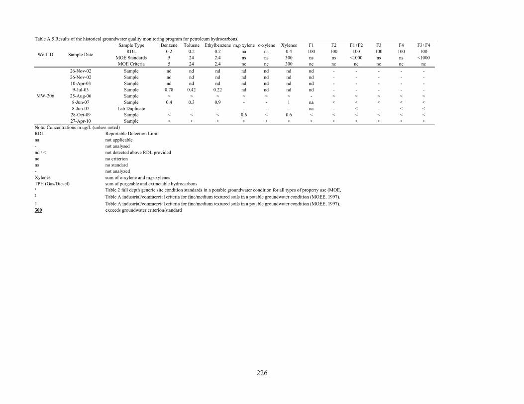
Table A.5 Results of the historical groundwater quality monitoring program for petroleum hydrocarbons.Sample Type Benzene Toluene Ethylbenzene m,p xylene o-xylene Xylenes F1 F2 F1+F2 F3 F4 F3+F4

RDL 0.2 0.2 0.2 na na 0.4 100 100 100 100 100 100MOE Standards 5 24 2.4 ns ns 300 ns ns <1000 ns ns <1000MOE Criteria 5 24 2.4 nc nc 300 nc nc nc nc nc nc

Well ID Sample Date

26-Nov-02 Sample nd nd nd nd nd nd nd - - - - -26-Nov-02 Sample nd nd nd nd nd nd nd - - - - -10-Apr-03 Sample nd nd nd nd nd nd nd - - - - -9-Jul-03 Sample 0.78 0.42 0.22 nd nd nd nd - - - - -

25-Aug-06 Sample < < < < < < - < < < < <8-Jun-07 Sample 0.4 0.3 0.9 - - 1 na < < < < <8-Jun-07 Lab Duplicate - - - - - - na - < - < <

28-Oct-09 Sample < < < 0.6 < 0.6 < < < < < <27-Apr-10 Sample < < < < < < < < < < < <

Note: Concentrations in ug/L (unless noted)RDL Reportable Detection Limitna not applicable- not analysednd / < not detected above RDL providednc no criterionns no standard- not analyzedXylenes sum of o-xylene and m,p-xylenesTPH (Gas/Diesel) sum of purgeable and extractable hydrocarbons¹2 Table A industrial/commercial criteria for fine/medium textured soils in a potable groundwater condition (MOEE, 1997).

1 Table A industrial/commercial criteria for fine/medium textured soils in a potable groundwater condition (MOEE, 1997).500 exceeds groundwater criterion/standard

MW-206

Table 2 full depth generic site condition standards in a potable groundwater condition for all types of property use (MOE,

226

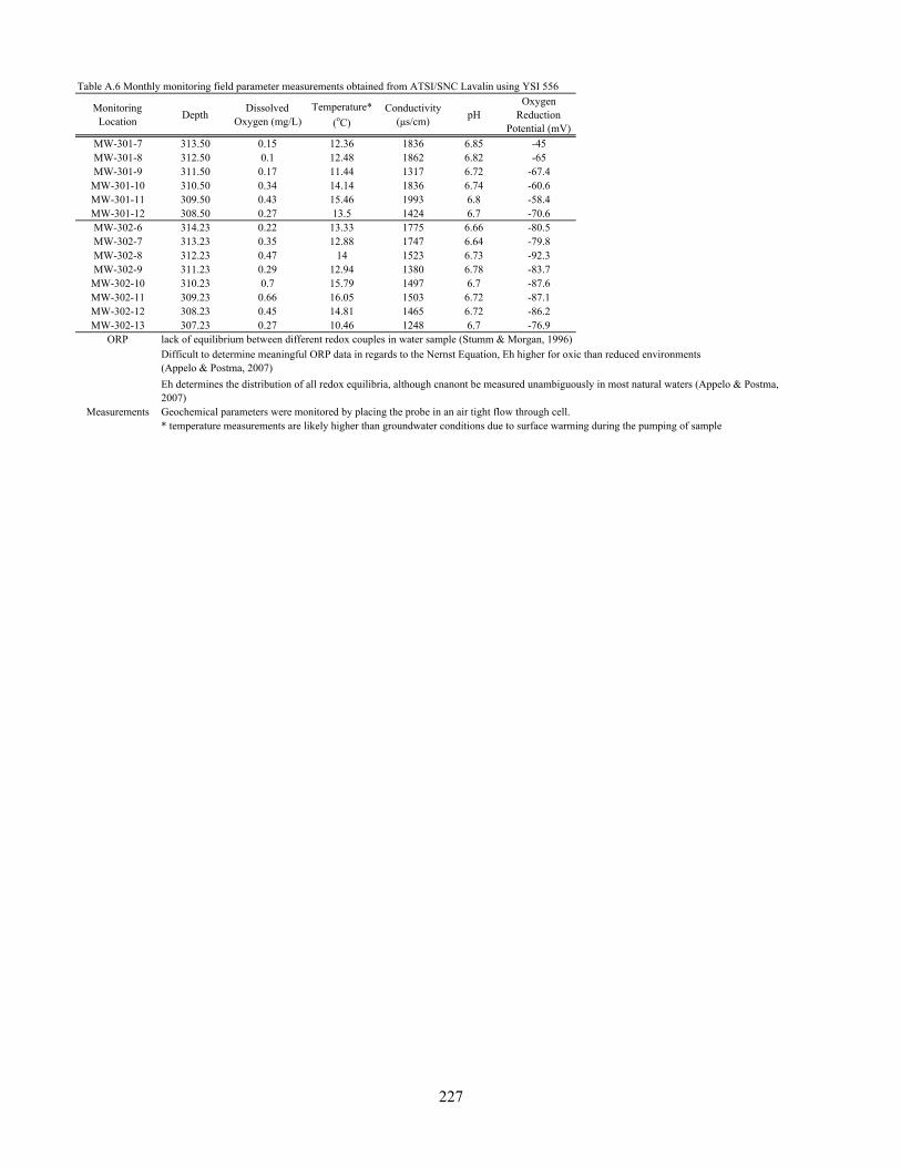
Table A.6 Monthly monitoring field parameter measurements obtained from ATSI/SNC Lavalin using YSI 556

Monitoring Location

DepthDissolved

Oxygen (mg/L)Temperature*

(oC)Conductivity

(μs/cm)pH

Oxygen Reduction

Potential (mV)

MW-301-7 313.50 0.15 12.36 1836 6.85 -45MW-301-8 312.50 0.1 12.48 1862 6.82 -65MW-301-9 311.50 0.17 11.44 1317 6.72 -67.4

MW-301-10 310.50 0.34 14.14 1836 6.74 -60.6MW-301-11 309.50 0.43 15.46 1993 6.8 -58.4MW-301-12 308.50 0.27 13.5 1424 6.7 -70.6MW-302-6 314.23 0.22 13.33 1775 6.66 -80.5MW-302-7 313.23 0.35 12.88 1747 6.64 -79.8MW-302-8 312.23 0.47 14 1523 6.73 -92.3MW-302-9 311.23 0.29 12.94 1380 6.78 -83.7

MW-302-10 310.23 0.7 15.79 1497 6.7 -87.6MW-302-11 309.23 0.66 16.05 1503 6.72 -87.1MW-302-12 308.23 0.45 14.81 1465 6.72 -86.2MW-302-13 307.23 0.27 10.46 1248 6.7 -76.9

ORP lack of equilibrium between different redox couples in water sample (Stumm & Morgan, 1996)

Measurements Geochemical parameters were monitored by placing the probe in an air tight flow through cell. * temperature measurements are likely higher than groundwater conditions due to surface warming during the pumping of sample

Difficult to determine meaningful ORP data in regards to the Nernst Equation, Eh higher for oxic than reduced environments (Appelo & Postma, 2007)

Eh determines the distribution of all redox equilibria, although cnanont be measured unambiguously in most natural waters (Appelo & Postma, 2007)

227

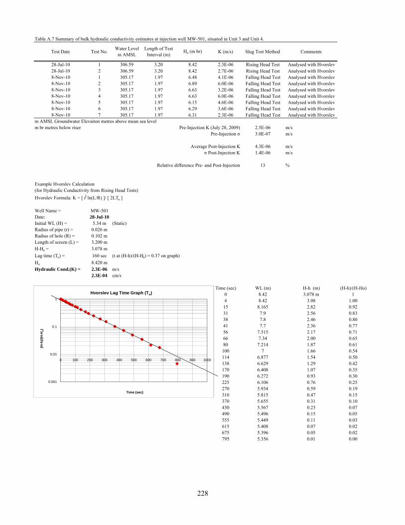
Table A.7 Summary of bulk hydraulic conductivity estimates at injection well MW-501, situated in Unit 3 and Unit 4.

Test Date Test No.Water Level

m AMSLLength of Test

Interval (m)Ho (m br) K (m/s) Slug Test Method Comments

28-Jul-10 1 306.59 3.20 8.42 2.3E-06 Rising Head Test Analysed with Hvorslev28-Jul-10 2 306.59 3.20 8.42 2.7E-06 Rising Head Test Analysed with Hvorslev8-Nov-10 1 305.17 1.97 6.48 4.1E-06 Falling Head Test Analysed with Hvorslev8-Nov-10 2 305.17 1.97 6.89 6.0E-06 Falling Head Test Analysed with Hvorslev8-Nov-10 3 305.17 1.97 6.63 3.2E-06 Falling Head Test Analysed with Hvorslev8-Nov-10 4 305.17 1.97 6.63 6.0E-06 Falling Head Test Analysed with Hvorslev8-Nov-10 5 305.17 1.97 6.15 4.6E-06 Falling Head Test Analysed with Hvorslev8-Nov-10 6 305.17 1.97 6.29 3.6E-06 Falling Head Test Analysed with Hvorslev8-Nov-10 7 305.17 1.97 6.31 2.3E-06 Falling Head Test Analysed with Hvorslev

m AMSL Groundwater Elevaiton metres above mean sea levelm br metres below riser Pre-Injection K (July 28, 2009) 2.5E-06 m/s

Pre-Injection σ 3.0E-07 m/s

Average Post-Injection K 4.3E-06 m/sσ Post-Injection K 1.4E-06 m/s

Relative difference Pre- and Post-Injection 13 %

Example Hvorslev Calculation(for Hydraulic Conductivity from Rising Head Tests)

Hvorslev Formula: K = [ r2 ln(L/R) ]/ [ 2LTo ]

Well Name = MW-501Date: 28-Jul-10Initial WL (H) = 5.34 m (Static)Radius of pipe (r) = 0.026 mRadius of hole (R) = 0.102 mLength of screen (L) = 3.200 mH-Ho = 3.078 m

Lag time (To) = 160 sec (t at (H-h)/(H-Ho) = 0.37 on graph)

Ho 8.420 mHydraulic Cond.(K) = 2.3E-06 m/s

2.3E-04 cm/s

Time (sec) WL (m) H-h (m) (H-h)/(H-Ho)0 8.42 3.078 m 14 8.42 3.08 1.00

15 8.165 2.82 0.9231 7.9 2.56 0.8338 7.8 2.46 0.8041 7.7 2.36 0.7756 7.515 2.17 0.7166 7.34 2.00 0.6580 7.214 1.87 0.61100 7 1.66 0.54114 6.877 1.54 0.50138 6.629 1.29 0.42170 6.408 1.07 0.35190 6.272 0.93 0.30225 6.106 0.76 0.25270 5.934 0.59 0.19310 5.815 0.47 0.15370 5.655 0.31 0.10430 5.567 0.23 0.07490 5.496 0.15 0.05555 5.449 0.11 0.03615 5.408 0.07 0.02675 5.396 0.05 0.02795 5.356 0.01 0.00

0.001

0.01

0.1

1

0 100 200 300 400 500 600 700 800 900 1000

(H-h

)/(H

-Ho)

Time (sec)

Hvorslev Lag Time Graph (To)

228

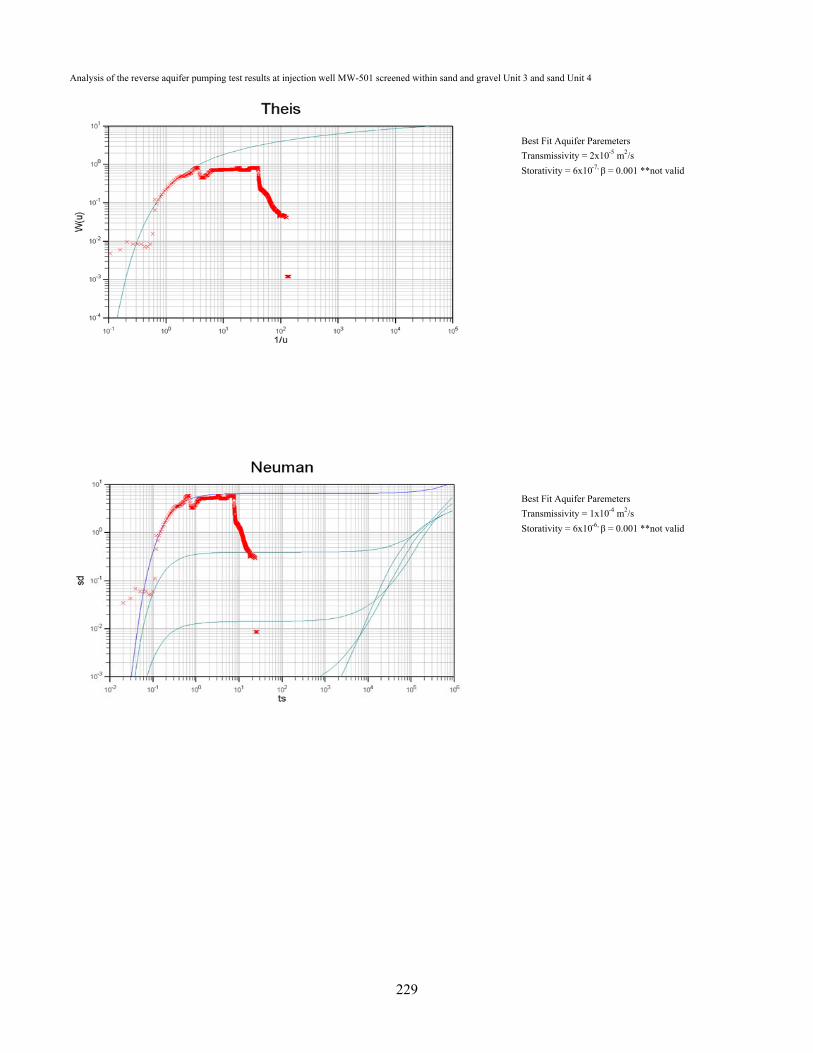
Analysis of the reverse aquifer pumping test results at injection well MW-501 screened within sand and gravel Unit 3 and sand Unit 4

Best Fit Aquifer Paremeters

Transmissivity = 2x10-5 m2/s

Storativity = 6x10-7, β = 0.001 **not valid

Best Fit Aquifer Paremeters

Transmissivity = 1x10-4 m2/s

Storativity = 6x10-6, β = 0.001 **not valid

229

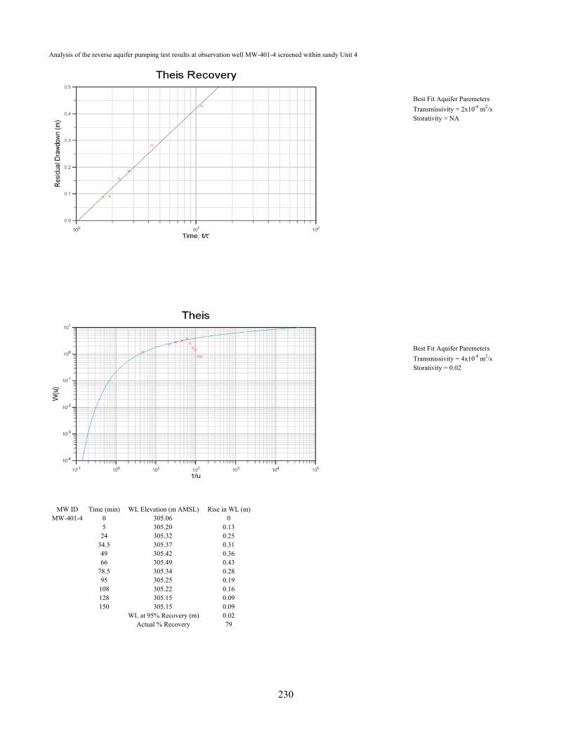
Analysis of the reverse aquifer pumping test results at observation well MW-401-4 screened within sandy Unit 4

Best Fit Aquifer Paremeters

Transmissivity = 2x10-4 m2/sStorativity = NA

Best Fit Aquifer Paremeters

Transmissivity = 4x10-4 m2/sStorativity = 0.02

MW ID Time (min) WL Elevation (m AMSL) Rise in WL (m)MW-401-4 0 305.06 0

5 305.20 0.1324 305.32 0.25

34.5 305.37 0.3149 305.42 0.3666 305.49 0.43

78.5 305.34 0.2895 305.25 0.19108 305.22 0.16128 305.15 0.09150 305.15 0.09

WL at 95% Recovery (m) 0.02Actual % Recovery 79

230

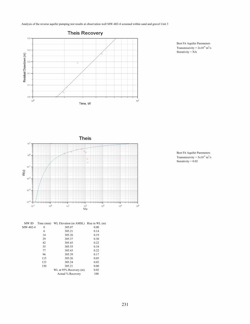
Analysis of the reverse aquifer pumping test results at observation well MW-402-4 screened within sand and gravel Unit 3

Best Fit Aquifer Paremeters

Transmissivity = 2x10-4 m2/sStorativity = NA

Best Fit Aquifer Paremeters

Transmissivity = 5x10-4 m2/sStorativity = 0.02

MW ID Time (min) WL Elevation (m AMSL) Rise in WL (m)MW-402-4 0 305.07 0.00

6 305.21 0.1414 305.26 0.1929 305.37 0.3042 305.43 0.2255 305.55 0.3477 305.43 0.2296 305.39 0.17

115 305.26 0.05123 305.24 0.02150 305.21 0.00

WL at 95% Recovery (m) 0.02Actual % Recovery 100

231

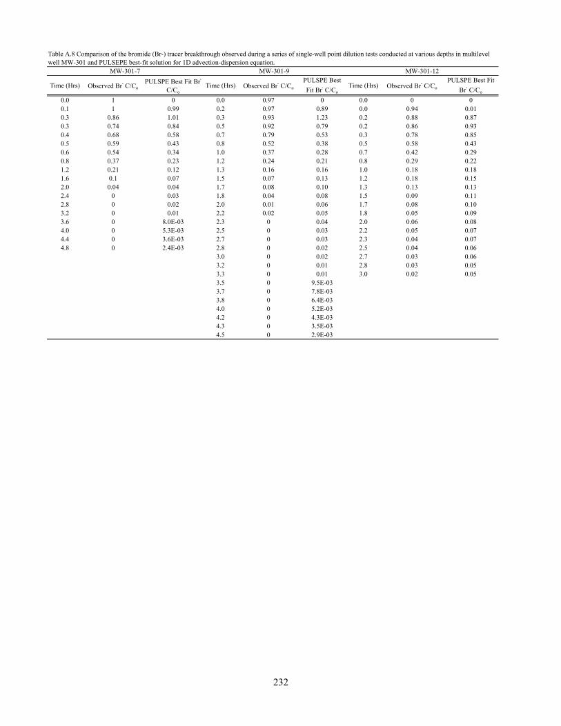
Time (Hrs) Observed Br- C/CoPULSPE Best Fit Br-

C/CoTime (Hrs) Observed Br- C/Co

PULSPE Best

Fit Br- C/CoTime (Hrs) Observed Br- C/Co

PULSPE Best Fit

Br- C/Co

0.0 1 0 0.0 0.97 0 0.0 0 00.1 1 0.99 0.2 0.97 0.89 0.0 0.94 0.010.3 0.86 1.01 0.3 0.93 1.23 0.2 0.88 0.870.3 0.74 0.84 0.5 0.92 0.79 0.2 0.86 0.930.4 0.68 0.58 0.7 0.79 0.53 0.3 0.78 0.850.5 0.59 0.43 0.8 0.52 0.38 0.5 0.58 0.430.6 0.54 0.34 1.0 0.37 0.28 0.7 0.42 0.290.8 0.37 0.23 1.2 0.24 0.21 0.8 0.29 0.221.2 0.21 0.12 1.3 0.16 0.16 1.0 0.18 0.181.6 0.1 0.07 1.5 0.07 0.13 1.2 0.18 0.152.0 0.04 0.04 1.7 0.08 0.10 1.3 0.13 0.132.4 0 0.03 1.8 0.04 0.08 1.5 0.09 0.112.8 0 0.02 2.0 0.01 0.06 1.7 0.08 0.103.2 0 0.01 2.2 0.02 0.05 1.8 0.05 0.093.6 0 8.0E-03 2.3 0 0.04 2.0 0.06 0.084.0 0 5.3E-03 2.5 0 0.03 2.2 0.05 0.074.4 0 3.6E-03 2.7 0 0.03 2.3 0.04 0.074.8 0 2.4E-03 2.8 0 0.02 2.5 0.04 0.06

3.0 0 0.02 2.7 0.03 0.063.2 0 0.01 2.8 0.03 0.053.3 0 0.01 3.0 0.02 0.053.5 0 9.5E-033.7 0 7.8E-033.8 0 6.4E-034.0 0 5.2E-034.2 0 4.3E-034.3 0 3.5E-034.5 0 2.9E-03

MW-301-7 MW-301-9 MW-301-12

Table A.8 Comparison of the bromide (Br-) tracer breakthrough observed during a series of single-well point dilution tests conducted at various depths in multilevel well MW-301 and PULSEPE best-fit solution for 1D advection-dispersion equation.

232

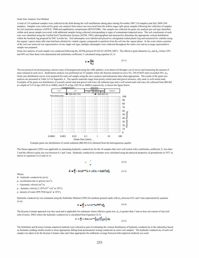
Grain Size Analysis Test Method

(A.1)

A total of 114 sediment samples were collected in the field during the well installations taking place during November 2007 (10 samples) and July 2009 (104 samples). Samples were retrieved for grain size analysis from intact core recovered from the hollow-auger split spoon sampler following the collection of samples for soil extraction analysis of BTEX, TMB and naphthalene contaminants (BTEXTMB). One sample was collected for grain size analysis per soil type identified within each spoon sample recovered, with additional samples being collected corresponding to signs of contaminant impacted areas. The soil constituents of each core were identified using the Unified Soil Classification System (ASTM, 1985), photographed and measured to determine the appropriate vertical distribution within the borehole log prepared by SNC Lavalin Inc. Soil subsamples were labeled and placed in a designated sealed plastic bag and measured for volatiles using the organic vapour meter after time had been allotted for volatile organic compounds to partition from the soil into the vapour phase. In the event where a portion of the soil core retrieved was representative of one single soil type, multiple subsamples were collected throughout the entire core and an average representative sample was prepared.

Grain size analysis of each sample was conducted following the ASTM protocol D 422-63 (ASTM, 2007). The effective grain diameters d10 and d60 (where 10% and 60% are finer than) were determined and uniformity coefficient, U calculated using equation (A.1):

The test protocol involved passing a known mass of homogenized (using the riffle splitter), oven-dried soil through a set of sieves and measuring the amount of mass retained in each sieve. Hydrometer analysis was performed on 52 samples where the fraction retained on sieve No. 230 (0.0625 mm) exceeded 10%, d10. Grain size distribution curves were prepared for each soil sample using the sieve analysis and hydrometer data when appropriate. The results of the grain size analysis are presented in Table A.9 of Appendix A. The aquifer materials range from poorly sorted sand and gravel mixtures, silty sand, to well sorted sand. Examples of the grain size distribution of a poorly sorted sand and gravel with trace silt sediment type and a well sorted sand with trace silt collected from BH-402 at a depth of 5.47 m bgs (305.62 m AMSL) and 8.53 m bgs (302.56 m AMSL) respectively, is shown the figure below.

0

10

20

30

40

50

60

70

80

90

100

0.0001 0.001 0.01 0.1 1 10 100

Per

cent

Pas

sing

BH-402-10A BH-402-6A

PEBBLESSAND SIZES

SILTCLAYCOARSFINE MEDIUM

Sieve Sizes (mm)

HYDROMETER DATA SEIVE DATA

Example grain size distribution of sorted sediment (BH-402-6A) obtained from the heterogeneous aquifer.

(A.2)

(A.3)Where:K - hydraulic conductivity (m/s);

g - acceleration due to gravity (m/s2);

v - kinematic velocity (m2/s);

μ – dynamic velocity (1.307x10-6 s/m2 at 10°C);

ρ - density of water (999.7026 kg/m3 at 10°C).

(A.4)

(A.5)

The Schlichter and Kozeny-Carman empirical methods were selected as part of estimating the vertical distribution of hydraulic conductivity in the subsurface based on formulae yielding similar results to more appropriate falling head permeameter testing conducted on select soil samples. The hydraulic conductivity of each soil sample was taken to be the Kozeny-Carman value and when appropriate the arithmetic average between both empirical methods was used.

Hydraulic conductivity was estimated using the Schlichter Method (1905) for medium grained sands with d10 between 0.01 and 5 mm represented by equation (A.4):

The Kozeny-Carman approach was also used and is applicable for sediments whose effective grain size, d10 is greater than 3 mm or does not consist of clay-rich soils (Carrier, 2003) where the hydraulic conductivity is calculated from Equation (A.5):

The Hazen approach (1892) was applicable in estimating hydraulic conductivity for the 24 samples that were well sorted with a uniformity coefficient, U, less than

5 and the effective grain size was between 0.1 and 3 mm. Hydraulic conductivity estimates were calculated using the physical properties of groundwater at 10oC as shown in equations (A.2) and (A.3).

Grain Size (mm)…

233

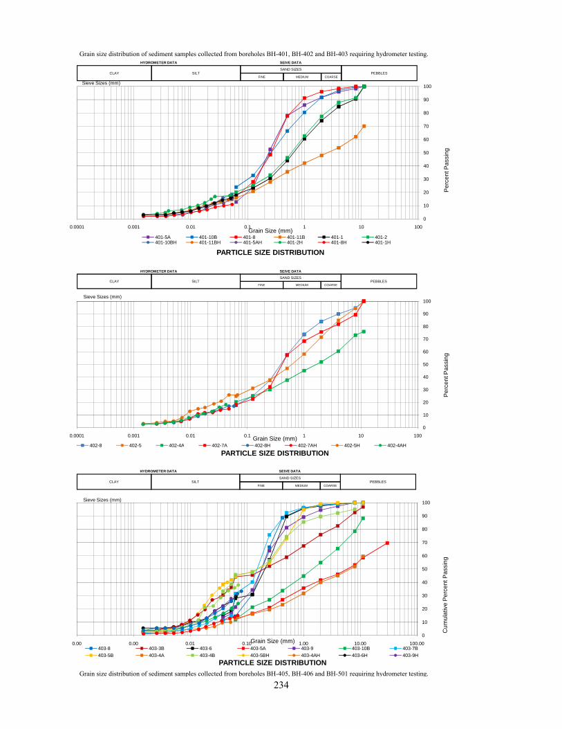
Grain size distribution of sediment samples collected from boreholes BH-401, BH-402 and BH-403 requiring hydrometer testing.

30

40

50

60

70

80

90

100

Pe

rce

nt P

ass

ing

PEBBLESSAND SIZES

SILTCLAYCOARSEFINE MEDIUM

Sieve Sizes (mm)

HYDROMETER DATA SEIVE DATA

0

10

20

30

40

50

60

70

80

90

100

0.0001 0.001 0.01 0.1 1 10 100

Pe

rce

nt P

ass

ing

Grain Size (mm)

PARTICLE SIZE DISTRIBUTION

401-5A 401-10B 401-8 401-11B 401-1 401-2401-10BH 401-11BH 401-5AH 401-2H 401-8H 401-1H

PEBBLESSAND SIZES

SILTCLAYCOARSEFINE MEDIUM

Sieve Sizes (mm)

HYDROMETER DATA SEIVE DATA

Grain size distribution of sediment samples collected from boreholes BH-405, BH-406 and BH-501 requiring hydrometer testing.

0

10

20

30

0.0001 0.001 0.01 0.1 1 10 100

Pe

rce

nGrain Size (mm)

PARTICLE SIZE DISTRIBUTION402-8 402-5 402-4A 402-7A 402-8H 402-7AH 402-5H 402-4AH

0

10

20

30

40

50

60

70

80

90

100

0.00 0.00 0.01 0.10 1.00 10.00 100.00

Cu

mu

lativ

e P

erc

en

t Pa

ssin

g

Grain Size (mm)

PARTICLE SIZE DISTRIBUTION

403-8 403-3B 403-6 403-5A 403-9 403-10B 403-7B

403-5B 403-4A 403-4B 403-5BH 403-4AH 403-6H 403-9H

PEBBLESSAND SIZES

SILTCLAYCOARSEFINE MEDIUM

Sieve Sizes (mm)

HYDROMETER DATA SEIVE DATA

234

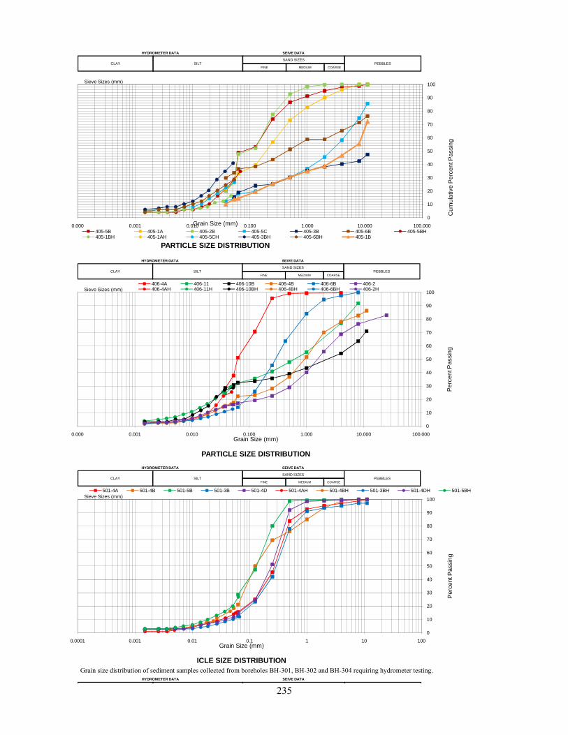
0

10

20

30

40

50

60

70

80

90

100

0.000 0.001 0.010 0.100 1.000 10.000 100.000

Cu

mu

lativ

e P

erc

en

t Pa

ssin

g

Grain Size (mm)

PARTICLE SIZE DISTRIBUTION

405-5B 405-1A 405-2B 405-5C 405-3B 405-6B 405-5BH405-1BH 405-1AH 405-5CH 405-3BH 405-6BH 405-1B

PEBBLESSAND SIZES

SILTCLAYCOARSEFINE MEDIUM

Sieve Sizes (mm)

HYDROMETER DATA SEIVE DATA

20

30

40

50

60

70

80

90

100

Pe

rce

nt P

ass

ing

406-4A 406-11 406-10B 406-4B 406-6B 406-2406-4AH 406-11H 406-10BH 406-4BH 406-6BH 406-2H

PEBBLESSAND SIZES

SILTCLAYCOARSEFINE MEDIUM

Sieve Sizes (mm)

HYDROMETER DATA SEIVE DATA

Grain size distribution of sediment samples collected from boreholes BH-301, BH-302 and BH-304 requiring hydrometer testing.

0

10

20

30

0.000 0.001 0.010 0.100 1.000 10.000 100.000

Pe

r

Grain Size (mm)

PARTICLE SIZE DISTRIBUTION

0

10

20

30

40

50

60

70

80

90

100

0.0001 0.001 0.01 0.1 1 10 100

Pe

rce

nt P

ass

ing

Grain Size (mm)

ICLE SIZE DISTRIBUTION

501-4A 501-4B 501-5B 501-3B 501-4D 501-4AH 501-4BH 501-3BH 501-4DH 501-5BH

PEBBLESSAND SIZES

SILTCLAYCOARSEFINE MEDIUM

Sieve Sizes (mm)

HYDROMETER DATA SEIVE DATA

HYDROMETER DATA SEIVE DATA

235

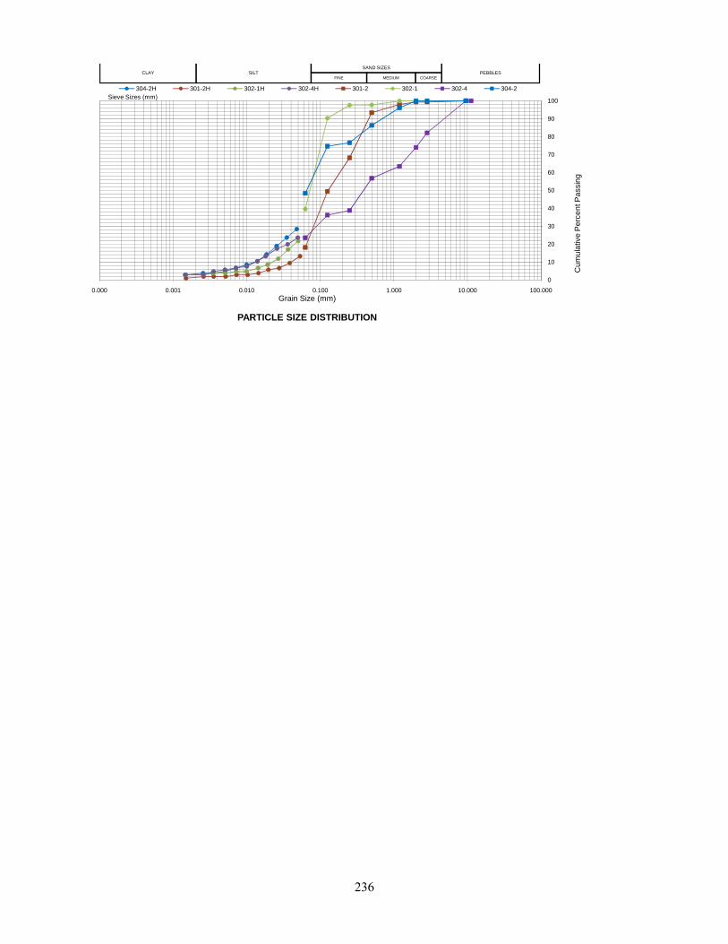
0

10

20

30

40

50

60

70

80

90

100

0.000 0.001 0.010 0.100 1.000 10.000 100.000

Cu

mu

lativ

e P

erc

en

t Pa

ssin

g

Grain Size (mm)

PARTICLE SIZE DISTRIBUTION

304-2H 301-2H 302-1H 302-4H 301-2 302-1 302-4 304-2

PEBBLESSAND SIZES

SILTCLAYCOARSEFINE MEDIUM

Sieve Sizes (mm)

236

Grain size distribution of sediment samples collected from borehole BH-401.

0

10

20

30

40

50

60

70

80

90

100

0.0001 0.001 0.01 0.1 1 10 100

Cu

mu

lativ

e P

erc

en

t Pa

ssin

g

Grain Size (mm)PARTICLE SIZE DISTRIBUTION

401-9 401-5A 401-10A 401-7B 401-11A 401-4A 401-10B 401-4B 401-8401-3 401-11B 401-6B 401-7A 401-5B 401-1 401-6A 401-2

PEBBLESSAND SIZES

SILTCLAYCOARSEFINE MEDIUM

Sieve Sizes (mm)

HYDROMETER DATA SEIVE DATA

20

30

40

50

60

70

80

90

100

ve P

erc

en

t Pa

ssin

g

PEBBLESSAND SIZES

SILTCLAYCOARSEFINE MEDIUM

Sieve Sizes (mm)

HYDROMETER DATA SEIVE DATA

Grain size distribution of sediment samples collected from borehole BH-402.

0

10

20

30

0.000 0.001 0.010 0.100 1.000 10.000 100.000

Cu

mu

lativ

e P

erc

Grain Size (mm)

PARTICLE SIZE DISTRIBUTION

401-9 401-10A 401-11A 401-4A 401-4B 401-6B 401-7A 401-5B 401-6A 401-7B

0

10

20

30

40

50

60

70

80

90

100

0.000 0.001 0.010 0.100 1.000 10.000 100.000

Pe

rce

nt P

ass

ing

Grain Size (mm)

PARTICLE SIZE DISTRIBUTION

401-16 401-19 401-14 401-12 401-4 Dale 401-36 401-19 DUP

PEBBLESSAND SIZES

SILTCLAYCOARSEFINE MEDIUM

Sieve Sizes (mm)

HYDROMETER DATA SEIVE DATA

237

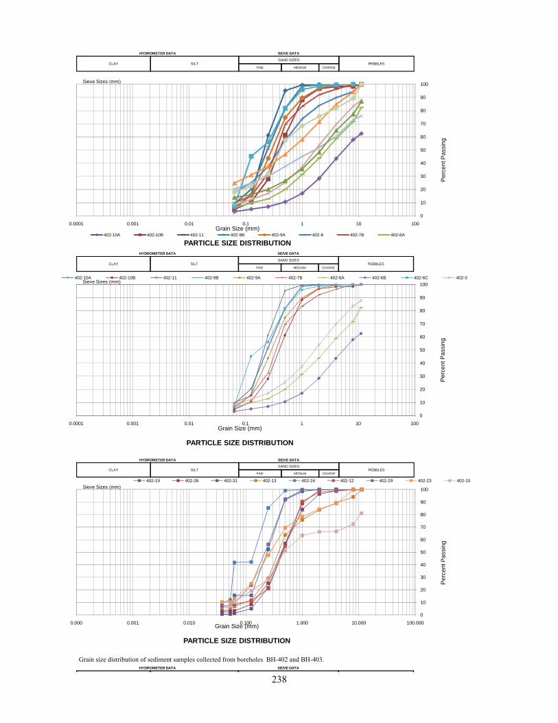
0

10

20

30

40

50

60

70

80

90

100

0.0001 0.001 0.01 0.1 1 10 100

Pe

rce

nt P

ass

ing

Grain Size (mm)

PARTICLE SIZE DISTRIBUTION402-10A 402-10B 402-11 402-9B 402-9A 402-8 402-7B 402-6A

PEBBLESSAND SIZES

SILTCLAYCOARSEFINE MEDIUM

Sieve Sizes (mm)

HYDROMETER DATA SEIVE DATA

20

30

40

50

60

70

80

90

100

Pe

rce

nt P

ass

ing

402-10A 402-10B 402-11 402-9B 402-9A 402-7B 402-6A 402-6B 402-6C 402-3

PEBBLESSAND SIZES

SILTCLAYCOARSEFINE MEDIUM

Sieve Sizes (mm)

HYDROMETER DATA SEIVE DATA

Grain size distribution of sediment samples collected from boreholes BH-402 and BH-403.

0

10

20

30

0.0001 0.001 0.01 0.1 1 10 100

Pe

Grain Size (mm)

PARTICLE SIZE DISTRIBUTION

0

10

20

30

40

50

60

70

80

90

100

0.000 0.001 0.010 0.100 1.000 10.000 100.000

Pe

rce

nt P

ass

ing

Grain Size (mm)

PARTICLE SIZE DISTRIBUTION

402-19 402-26 402-31 402-13 402-24 402-12 402-29 402-23 402-10

PEBBLESSAND SIZES

SILTCLAYCOARSEFINE MEDIUM

Sieve Sizes (mm)

HYDROMETER DATA SEIVE DATA

HYDROMETER DATA SEIVE DATA

238

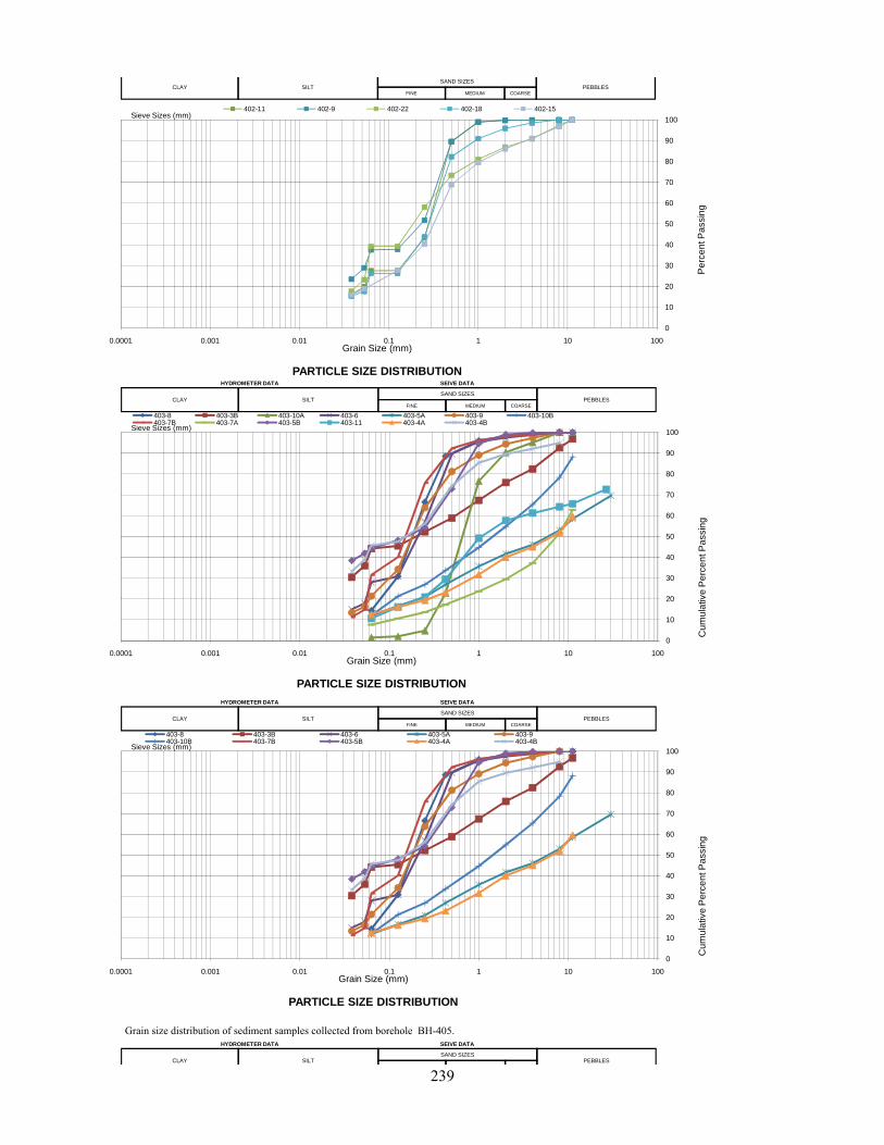
0

10

20

30

40

50

60

70

80

90

100

0.0001 0.001 0.01 0.1 1 10 100

Pe

rce

nt P

ass

ing

Grain Size (mm)

PARTICLE SIZE DISTRIBUTION

402-11 402-9 402-22 402-18 402-15

PEBBLESSAND SIZES

SILTCLAYCOARSEFINE MEDIUM

Sieve Sizes (mm)

10

20

30

40

50

60

70

80

90

100

mu

lativ

e P

erc

en

t Pa

ssin

g

403-8 403-3B 403-10A 403-6 403-5A 403-9 403-10B403-7B 403-7A 403-5B 403-11 403-4A 403-4B

PEBBLESSAND SIZES

SILTCLAYCOARSEFINE MEDIUM

Sieve Sizes (mm)

HYDROMETER DATA SEIVE DATA

Grain size distribution of sediment samples collected from borehole BH-405.

0

10

20

0.0001 0.001 0.01 0.1 1 10 100

Cu

mu

lativ

Grain Size (mm)

PARTICLE SIZE DISTRIBUTION

0

10

20

30

40

50

60

70

80

90

100

0.0001 0.001 0.01 0.1 1 10 100

Cu

mu

lativ

e P

erc

en

t Pa

ssin

g

Grain Size (mm)

PARTICLE SIZE DISTRIBUTION

403-8 403-3B 403-6 403-5A 403-9403-10B 403-7B 403-5B 403-4A 403-4B

PEBBLESSAND SIZES

SILTCLAYCOARSEFINE MEDIUM

Sieve Sizes (mm)

HYDROMETER DATA SEIVE DATA

PEBBLESSAND SIZES

SILTCLAYCOARSEFINE MEDIUM

HYDROMETER DATA SEIVE DATA

239

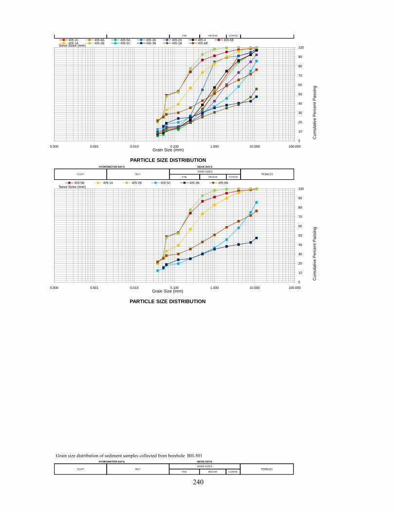
0

10

20

30

40

50

60

70

80

90

100

0.000 0.001 0.010 0.100 1.000 10.000 100.000

Cu

mu

lativ

e P

erc

en

t Pa

ssin

g

Grain Size (mm)

PARTICLE SIZE DISTRIBUTION

405-1C 405-6A 405-5A 405-3A 405-2A 405-4 405-5B405-1A 405-2B 405-5C 405-3B 405-1B 405-6B

COARSEFINE MEDIUM

Sieve Sizes (mm)

10

20

30

40

50

60

70

80

90

100

Cu

mu

lativ

e P

erc

en

t Pa

ssin

g

405-5B 405-1A 405-2B 405-5C 405-3B 405-6B

PEBBLESSAND SIZES

SILTCLAYCOARSEFINE MEDIUM

Sieve Sizes (mm)

HYDROMETER DATA SEIVE DATA

Grain size distribution of sediment samples collected from borehole BH-501

0

10

0.000 0.001 0.010 0.100 1.000 10.000 100.000

Cu

mu

la

Grain Size (mm)

PARTICLE SIZE DISTRIBUTION

PEBBLESSAND SIZES

SILTCLAYCOARSEFINE MEDIUM

HYDROMETER DATA SEIVE DATA

240

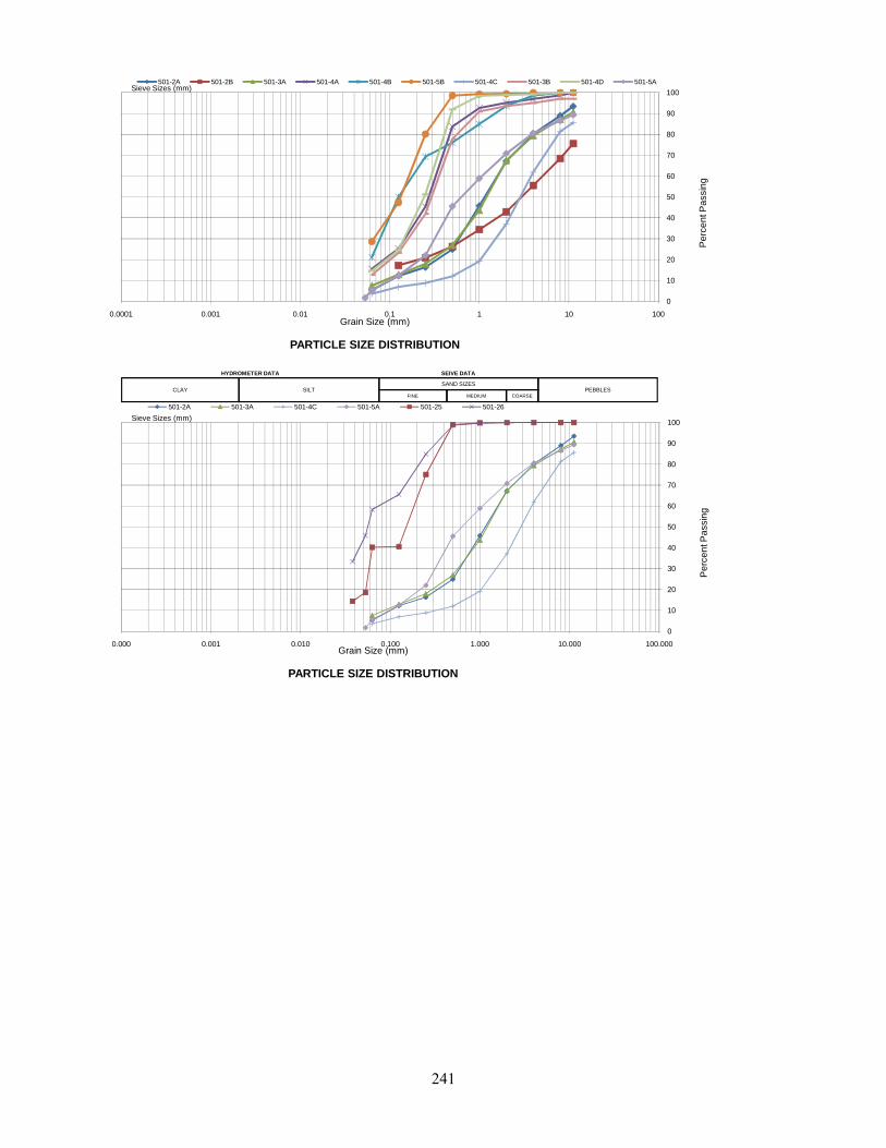
0

10

20

30

40

50

60

70

80

90

100

0.0001 0.001 0.01 0.1 1 10 100

Pe

rce

nt P

ass

ing

Grain Size (mm)

PARTICLE SIZE DISTRIBUTION

501-2A 501-2B 501-3A 501-4A 501-4B 501-5B 501-4C 501-3B 501-4D 501-5ASieve Sizes (mm)

10

20

30

40

50

60

70

80

90

100

Pe

rce

nt P

ass

ing

501-2A 501-3A 501-4C 501-5A 501-25 501-26

PEBBLESSAND SIZES

SILTCLAYCOARSEFINE MEDIUM

Sieve Sizes (mm)

HYDROMETER DATA SEIVE DATA

0

10

0.000 0.001 0.010 0.100 1.000 10.000 100.000Grain Size (mm)

PARTICLE SIZE DISTRIBUTION

241

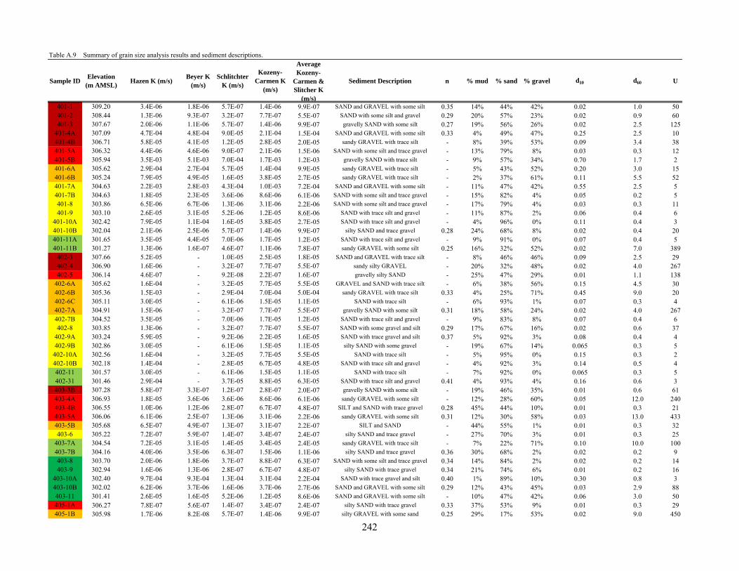
Table A.9 Summary of grain size analysis results and sediment descriptions.

Sample IDElevation

(m AMSL)Hazen K (m/s)

Beyer K (m/s)

Schlitchter K (m/s)

Kozeny-Carmen K

(m/s)

Average Kozeny-

Carmen & Slitcher K

(m/s)

Sediment Description n % mud % sand % gravel d10 d60 U

401-1 309.20 3.4E-06 1.8E-06 5.7E-07 1.4E-06 9.9E-07 SAND and GRAVEL with some silt 0.35 14% 44% 42% 0.02 1.0 50401-2 308.44 1.3E-06 9.3E-07 3.2E-07 7.7E-07 5.5E-07 SAND with some silt and gravel 0.29 20% 57% 23% 0.02 0.9 60401-3 307.67 2.0E-06 1.1E-06 5.7E-07 1.4E-06 9.9E-07 gravelly SAND with some silt 0.27 19% 56% 26% 0.02 2.5 125

401-4A 307.09 4.7E-04 4.8E-04 9.0E-05 2.1E-04 1.5E-04 SAND and GRAVEL with some silt 0.33 4% 49% 47% 0.25 2.5 10401-4B 306.71 5.8E-05 4.1E-05 1.2E-05 2.8E-05 2.0E-05 sandy GRAVEL with trace silt - 8% 39% 53% 0.09 3.4 38401-5A 306.32 4.4E-06 4.6E-06 9.0E-07 2.1E-06 1.5E-06 SAND with some silt and trace gravel - 13% 79% 8% 0.03 0.3 12401-5B 305.94 3.5E-03 5.1E-03 7.0E-04 1.7E-03 1.2E-03 gravelly SAND with trace silt - 9% 57% 34% 0.70 1.7 2401-6A 305.62 2.9E-04 2.7E-04 5.7E-05 1.4E-04 9.9E-05 sandy GRAVEL with trace silt - 5% 43% 52% 0.20 3.0 15401-6B 305.24 7.9E-05 4.9E-05 1.6E-05 3.8E-05 2.7E-05 sandy GRAVEL with trace silt - 2% 37% 61% 0.11 5.5 52401-7A 304.63 2.2E-03 2.8E-03 4.3E-04 1.0E-03 7.2E-04 SAND and GRAVEL with some silt - 11% 47% 42% 0.55 2.5 5401-7B 304.63 1.8E-05 2.3E-05 3.6E-06 8.6E-06 6.1E-06 SAND with some silt and trace gravel - 15% 82% 4% 0.05 0.2 5401-8 303.86 6.5E-06 6.7E-06 1.3E-06 3.1E-06 2.2E-06 SAND with some silt and trace gravel - 17% 79% 4% 0.03 0.3 11401-9 303.10 2.6E-05 3.1E-05 5.2E-06 1.2E-05 8.6E-06 SAND with trace silt and gravel - 11% 87% 2% 0.06 0.4 6

401-10A 302.42 7.9E-05 1.1E-04 1.6E-05 3.8E-05 2.7E-05 SAND with trace silt and gravel - 4% 96% 0% 0.11 0.4 3401-10B 302.04 2.1E-06 2.5E-06 5.7E-07 1.4E-06 9.9E-07 silty SAND and trace gravel 0.28 24% 68% 8% 0.02 0.4 20401-11A 301.65 3.5E-05 4.4E-05 7.0E-06 1.7E-05 1.2E-05 SAND with trace silt and gravel - 9% 91% 0% 0.07 0.4 5401-11B 301.27 1.3E-06 1.6E-07 4.6E-07 1.1E-06 7.8E-07 sandy GRAVEL with some silt 0.25 16% 32% 52% 0.02 7.0 389

402-3 307.66 5.2E-05 - 1.0E-05 2.5E-05 1.8E-05 SAND and GRAVEL with trace silt - 8% 46% 46% 0.09 2.5 29402-4 306.90 1.6E-06 - 3.2E-07 7.7E-07 5.5E-07 sandy silty GRAVEL - 20% 32% 48% 0.02 4.0 267402-5 306.14 4.6E-07 - 9.2E-08 2.2E-07 1.6E-07 gravelly silty SAND - 25% 47% 29% 0.01 1.1 138

402-6A 305.62 1.6E-04 - 3.2E-05 7.7E-05 5.5E-05 GRAVEL and SAND with trace silt - 6% 38% 56% 0.15 4.5 30402-6B 305.36 1.5E-03 - 2.9E-04 7.0E-04 5.0E-04 sandy GRAVEL with trace silt 0.33 4% 25% 71% 0.45 9.0 20402-6C 305.11 3.0E-05 - 6.1E-06 1.5E-05 1.1E-05 SAND with trace silt - 6% 93% 1% 0.07 0.3 4402-7A 304.91 1.5E-06 - 3.2E-07 7.7E-07 5.5E-07 gravelly SAND with some silt 0.31 18% 58% 24% 0.02 4.0 267402-7B 304.52 3.5E-05 - 7.0E-06 1.7E-05 1.2E-05 SAND with trace silt and gravel - 9% 83% 8% 0.07 0.4 6402-8 303.85 1.3E-06 - 3.2E-07 7.7E-07 5.5E-07 SAND with some gravel and silt 0.29 17% 67% 16% 0.02 0.6 37

402-9A 303.24 5.9E-05 - 9.2E-06 2.2E-05 1.6E-05 SAND with trace gravel and silt 0.37 5% 92% 3% 0.08 0.4 4402-9B 302.86 3.0E-05 - 6.1E-06 1.5E-05 1.1E-05 silty SAND with some gravel - 19% 67% 14% 0.065 0.3 5

402-10A 302.56 1.6E-04 - 3.2E-05 7.7E-05 5.5E-05 SAND with trace silt - 5% 95% 0% 0.15 0.3 2402-10B 302.18 1.4E-04 - 2.8E-05 6.7E-05 4.8E-05 SAND with trace silt and gravel - 4% 92% 3% 0.14 0.5 4402-11 301.57 3.0E-05 - 6.1E-06 1.5E-05 1.1E-05 SAND with trace silt - 7% 92% 0% 0.065 0.3 5402-31 301.46 2.9E-04 - 3.7E-05 8.8E-05 6.3E-05 SAND with trace silt and gravel 0.41 4% 93% 4% 0.16 0.6 3403-3B 307.28 5.8E-07 3.3E-07 1.2E-07 2.8E-07 2.0E-07 gravelly SAND with some silt - 19% 46% 35% 0.01 0.6 61403-4A 306.93 1.8E-05 3.6E-06 3.6E-06 8.6E-06 6.1E-06 sandy GRAVEL with some silt - 12% 28% 60% 0.05 12.0 240403-4B 306.55 1.0E-06 1.2E-06 2.8E-07 6.7E-07 4.8E-07 SILT and SAND with trace gravel 0.28 45% 44% 10% 0.01 0.3 21403-5A 306.06 6.1E-06 2.5E-07 1.3E-06 3.1E-06 2.2E-06 sandy GRAVEL with some silt 0.31 12% 30% 58% 0.03 13.0 433403-5B 305.68 6.5E-07 4.9E-07 1.3E-07 3.1E-07 2.2E-07 SILT and SAND - 44% 55% 1% 0.01 0.3 32403-6 305.22 7.2E-07 5.9E-07 1.4E-07 3.4E-07 2.4E-07 silty SAND and trace gravel - 27% 70% 3% 0.01 0.3 25

403-7A 304.54 7.2E-05 3.1E-05 1.4E-05 3.4E-05 2.4E-05 sandy GRAVEL with trace silt - 7% 22% 71% 0.10 10.0 100403-7B 304.16 4.0E-06 3.5E-06 6.3E-07 1.5E-06 1.1E-06 silty SAND and trace gravel 0.36 30% 68% 2% 0.02 0.2 9403-8 303.70 2.0E-06 1.8E-06 3.7E-07 8.8E-07 6.3E-07 SAND with some silt and trace gravel 0.34 14% 84% 2% 0.02 0.2 14403-9 302.94 1.6E-06 1.3E-06 2.8E-07 6.7E-07 4.8E-07 silty SAND with trace gravel 0.34 21% 74% 6% 0.01 0.2 16

403-10A 302.40 9.7E-04 9.3E-04 1.3E-04 3.1E-04 2.2E-04 SAND with trace gravel and silt 0.40 1% 89% 10% 0.30 0.8 3403-10B 302.02 6.2E-06 3.7E-06 1.6E-06 3.7E-06 2.7E-06 SAND and GRAVEL with some silt 0.29 12% 43% 45% 0.03 2.9 88403-11 301.41 2.6E-05 1.6E-05 5.2E-06 1.2E-05 8.6E-06 SAND and GRAVEL with some silt - 10% 47% 42% 0.06 3.0 50405-1A 306.27 7.8E-07 5.6E-07 1.4E-07 3.4E-07 2.4E-07 silty SAND with trace gravel 0.33 37% 53% 9% 0.01 0.3 29405-1B 305.98 1.7E-06 8.2E-08 5.7E-07 1.4E-06 9.9E-07 silty GRAVEL with some sand 0.25 29% 17% 53% 0.02 9.0 450

242

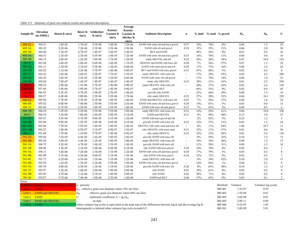
Table A.9 Summary of grain size analysis results and sediment descriptions.

Sample IDElevation

(m AMSL)Hazen K (m/s)

Beyer K (m/s)

Schlitchter K (m/s)

Kozeny-Carmen K

(m/s)

Average Kozeny-

Carmen & Slitcher K

(m/s)

Sediment Description n % mud % sand % gravel d10 d60 U

405-1C 305.67 1.4E-05 1.7E-05 4.3E-06 1.0E-05 7.2E-06 SAND with some silt and trace gravel 0.27 18% 74% 8% 0.06 1.5 26405-2A 305.38 9.2E-06 7.2E-06 2.3E-06 5.5E-06 3.9E-06 SAND with silt and gravel 0.29 35% 35% 31% 0.04 2.0 50405-2B 305.00 7.2E-07 6.7E-07 1.4E-07 3.4E-07 2.4E-07 SILT and SAND - 46% 54% 0% 0.01 0.2 16405-3A 304.53 2.3E-05 2.3E-05 4.3E-06 1.0E-05 7.2E-06 SAND with some silt and trace gravel 0.33 14% 76% 11% 0.06 0.6 10405-3B 304.15 2.0E-05 1.2E-05 7.0E-06 1.7E-05 1.2E-05 sandy GRAVEL and silt 0.25 36% 26% 38% 0.07 10.0 143405-4 303.68 2.6E-05 3.0E-05 6.6E-06 1.6E-05 1.1E-05 GRAVEL and SAND with trace silt 0.28 7% 36% 57% 0.07 1.2 18

405-5A 303.11 2.2E-05 2.1E-05 5.2E-06 1.2E-05 8.6E-06 SAND with some gravel and silt 0.29 11% 73% 16% 0.06 1.6 26405-5B 302.82 3.1E-06 3.2E-06 5.7E-07 1.4E-06 9.9E-07 SILT and SAND with trace gravel 0.33 47% 48% 5% 0.02 0.2 8405-5C 302.62 1.6E-06 2.6E-07 3.2E-07 7.7E-07 5.5E-07 sandy GRAVEL with some silt - 17% 28% 55% 0.02 4.2 280405-6A 302.42 2.6E-05 2.2E-05 5.2E-06 1.2E-05 8.6E-06 SAND with some silt and gravel - 11% 76% 14% 0.06 1.4 23405-6B 302.04 7.4E-07 1.4E-07 1.4E-07 3.4E-07 2.4E-07 sandy silty GRAVEL 0.32 28% 31% 41% 0.01 2.5 250406-2 308.24 2.9E-06 1.1E-06 5.7E-07 1.4E-06 9.9E-07 sandy GRAVEL with some silt - 20% 37% 43% 0.02 2.6 130

406-4A 307.48 2.9E-06 1.9E-06 5.7E-07 1.4E-06 9.9E-07 sandy SILT - 66% 33% 0% 0.02 0.9 45406-4B 306.95 5.2E-05 4.7E-05 1.0E-05 2.5E-05 1.8E-05 gravelly silty SAND - 25% 46% 29% 0.09 1.5 18406-5 306.57 6.4E-06 2.0E-06 2.2E-06 5.2E-06 3.7E-06 silty sandy GRAVEL 0.25 27% 20% 53% 0.04 10.1 259

406-6A 305.96 7.7E-05 3.3E-05 8.1E-06 1.9E-05 1.4E-05 SAND and GRAVEL with trace silt 0.47 7% 56% 37% 0.08 1.8 24406-6B 305.42 6.0E-06 7.4E-06 1.5E-06 3.5E-06 2.5E-06 SAND with some silt and trace gravel 0.29 14% 81% 5% 0.03 0.4 13406-7A 305.04 6.7E-05 6.3E-05 1.0E-05 2.5E-05 1.8E-05 SAND with trace silt and gravel 0.37 7% 91% 2% 0.09 0.5 6406-7B 304.54 1.2E-05 2.2E-06 2.3E-06 5.5E-06 3.9E-06 sandy GRAVEL with some silt 0.32 14% 26% 61% 0.04 10.0 250406-8 304.16 1.2E-04 1.0E-04 2.4E-05 5.8E-05 4.1E-05 SAND and GRAVEL 0.31 4% 48% 48% 0.13 3.0 23

406-9A 303.67 4.5E-04 5.7E-04 9.0E-05 2.1E-04 1.5E-04 SAND with trace gravel and silt - 2% 92% 5% 0.25 1.2 5406-9B 303.06 9.8E-06 1.5E-05 3.6E-06 8.6E-06 6.1E-06 gravelly SAND with some silt 0.25 12% 57% 31% 0.05 1.2 24

406-10A 302.68 7.2E-03 7.5E-03 1.4E-03 3.4E-03 2.4E-03 GRAVEL with some sand and trace silt - 6% 11% 84% 1.00 10.7 11406-10B 302.22 1.0E-06 6.5E-07 2.1E-07 4.9E-07 3.5E-07 silty GRAVEL with some sand 0.31 32% 11% 57% 0.01 0.6 50406-11 301.84 1.7E-06 1.1E-06 5.7E-07 1.4E-06 9.9E-07 silty sandy GRAVEL 0.25 32% 23% 45% 0.02 2.6 130501-2A 305.68 7.2E-05 6.9E-05 1.4E-05 3.4E-05 2.4E-05 gravelly SAND with trace silt - 9% 59% 32% 0.10 1.5 15501-2B 305.30 5.8E-05 5.4E-05 1.2E-05 2.8E-05 2.0E-05 sandy GRAVEL with some silt - 19% 34% 46% 0.09 1.5 17501-3A 304.79 5.2E-05 4.7E-05 1.0E-05 2.5E-05 1.8E-05 gravelly SAND with trace silt - 11% 58% 31% 0.09 1.5 18501-3B 304.40 1.5E-05 2.1E-05 3.6E-06 8.6E-06 6.1E-06 silty SAND with trace gravel 0.30 24% 70% 6% 0.05 0.4 7501-4A 304.13 5.4E-06 7.2E-06 1.3E-06 3.1E-06 2.2E-06 SAND with some silt and trace gravel 0.29 17% 79% 5% 0.03 0.3 8501-4B 303.90 5.1E-06 5.2E-06 9.0E-07 2.1E-06 1.5E-06 silty SAND with trace gravel 0.34 22% 72% 6% 0.03 0.2 7501-4C 303.73 6.5E-04 6.5E-04 1.3E-04 3.1E-04 2.2E-04 sandy GRAVEL with trace silt - 4% 34% 63% 0.30 3.8 13501-4D 303.58 1.2E-05 1.3E-05 2.3E-06 5.5E-06 3.9E-06 SAND with some silt and trace gravel - 14% 85% 1% 0.04 0.3 8501-5A 303.34 4.9E-05 6.5E-05 1.3E-05 3.1E-05 2.2E-05 gravelly SAND with trace silt 0.28 8% 63% 28% 0.10 1.2 13501-25 302.97 1.5E-05 1.9E-05 2.9E-06 7.0E-06 5.0E-06 silty SAND 0.01 39% 61% 0% 0.05 0.2 4501-5B 302.96 4.7E-06 3.1E-06 5.7E-07 1.4E-06 9.9E-07 silty SAND 0.42 28% 71% 0% 0.02 0.2 9501-26 302.87 9.7E-06 7.4E-06 1.0E-06 2.5E-06 1.8E-06 SAND and SILT 0.46 57% 43% 0% 0.03 0.1 3

NotesUnit 1 FILL n - porosity Borehole Variance Variance log cyclesUnit 2 SAND d10 - effective grain size diameter where 10% are finer BH-401 1.1E-07 0.95

Unit 3 SAND and GRAVEL d60 effective grain size diameter where 60% are finer BH-402 1.5E-08 0.81

Unit 4 SAND U uniformity coefficient, U = d60/d10 BH-403 3.6E-09 0.91Unit 5 SAND and GRAVEL - no data BH-405 2.0E-11 0.69Unit 6 SAND where variance log cycles is equivalent to the total sum of the differences between log K and the average log K. BH-406 4.1E-07 1.05

heterogeneity is inferred when variance log cycle exceeds 0.5. BH-501 3.8E-09 5.01

243

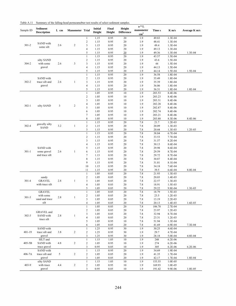
Table A.11 Summary of the falling-head permeamebter test results of select sediment samples.

Sample IDSediment Description

L cm Manometer TrialInitial Height

Final Height

Height Difference

a * L manometer

cm2Time s K m/s Average K m/s

1 1.15 0.95 20 1.9 49.83 1.3E-042 1.15 0.95 20 1.9 48.41 1.3E-043 1.15 0.95 20 1.9 49.4 1.3E-044 1.15 0.95 20 1.9 49.13 1.3E-045 1.15 0.95 20 1.9 49.36 1.3E-04 1.3E-041 1.15 0.95 20 1.9 43.57 1.5E-042 1.15 0.95 20 1.9 43.6 1.5E-043 1.15 0.95 20 1.9 44 1.5E-044 1.15 0.95 20 1.9 44.13 1.5E-045 1.15 0.95 20 1.9 44.14 1.5E-04 1.5E-041 1.15 0.95 20 1.9 36.58 1.8E-042 1.15 0.95 20 1.9 35.49 1.8E-043 1.15 0.95 20 1.9 35.39 1.8E-044 1.15 0.95 20 1.9 36.06 1.8E-045 1.15 0.95 20 1.9 36.31 1.8E-04 1.8E-041 1.05 0.95 10 1.9 203.53 8.4E-062 1.05 0.95 10 1.9 203.23 8.4E-063 1.05 0.95 10 1.9 203.31 8.4E-064 1.05 0.95 10 1.9 202.28 8.4E-065 1.05 0.95 10 1.9 202.87 8.4E-066 1.05 0.95 10 1.9 202.74 8.4E-067 1.05 0.95 10 1.9 203.21 8.4E-068 1.05 0.95 10 1.9 203.88 8.3E-06 8.4E-061 1.15 0.95 20 7.8 21.7 1.2E-032 1.15 0.95 20 7.8 20.09 1.3E-033 1.15 0.95 20 7.8 20.44 1.3E-03 1.2E-031 1.15 0.95 20 7.8 38.84 6.7E-042 1.15 0.95 20 7.8 33.53 7.7E-043 1.15 0.95 20 7.8 31.57 8.2E-044 1.15 0.95 20 7.8 30.13 8.6E-045 1.15 0.95 20 7.8 29.98 8.6E-046 1.15 0.95 20 7.8 29.59 8.7E-047 1.15 0.95 20 7.8 29.72 8.7E-048 1.15 0.95 20 7.8 30.87 8.4E-049 1.15 0.95 20 7.8 31.81 8.1E-0410 1.15 0.95 20 7.8 34.18 7.6E-0411 1.15 0.95 20 7.8 39.5 6.6E-04 8.0E-041 1.05 0.85 20 7.8 21.93 1.3E-032 1.05 0.85 20 7.8 20.03 1.4E-033 1.05 0.85 20 7.8 22.57 1.3E-034 1.05 0.85 20 7.8 18.91 1.5E-035 1.05 0.85 20 7.8 29.22 9.8E-04 1.3E-031 1.05 0.85 20 7.8 18.79 1.5E-032 1.05 0.85 20 7.8 23.5 1.2E-033 1.05 0.85 20 7.8 13.19 2.2E-034 1.05 0.85 20 7.8 20.13 1.4E-03 1.6E-031 1.05 0.85 20 7.8 106.78 2.7E-042 1.05 0.85 20 7.8 23.97 1.2E-033 1.05 0.85 20 7.8 32.94 8.7E-044 1.05 0.85 20 7.8 23.31 1.2E-035 1.05 0.95 10 7.8 51.94 1.3E-046 1.05 0.85 20 7.8 41.69 6.9E-04 7.3E-041 1.25 0.95 30 1.9 30.25 4.6E-042 1.25 0.95 30 1.9 29.7 4.7E-043 1.25 0.95 30 1.9 28.18 5.0E-04 4.8E-041 1.15 1.05 10 1.9 248 6.2E-062 1.05 0.95 10 1.9 274 6.2E-063 0.95 0.85 10 1.9 305 6.2E-06 6.2E-061 1.15 0.95 20 1.9 34.69 1.9E-042 1.05 0.85 20 1.9 41.35 1.7E-043 1.05 0.85 20 1.9 42.17 1.7E-04 1.8E-041 1.15 1.05 10 1.9 153.55 1.0E-052 1.05 0.95 10 1.9 169.93 1.0E-053 0.95 0.85 10 1.9 191.42 9.9E-06 1.0E-05

SAND with some silt

301-2

304-2silty SAND with some

gravel

302-2SAND with trace silt and

gravel

2.6

2.6

2.6

3.2

2.6

406-7A

403-9

3

301-4sandy

GRAVEL with trace silt

301-3

GRAVEL with some

sand and trace silt

302-1 silty SAND

gravelly silty SAND

302-4

301-1SAND with some gravel and trace silt

401-19

405-5B

SAND with trace silt and

gravelSILT and

SAND with trace gravel

302-3GRAVEL and SAND with

trace silt

2.8

2.8

2.8

4.8

3.8

5

4.4

SAND with trace silt and

gravelsilty SAND with trace

gravel

2

3

1

2

1

1

1

1

2

2

2

2

1

244

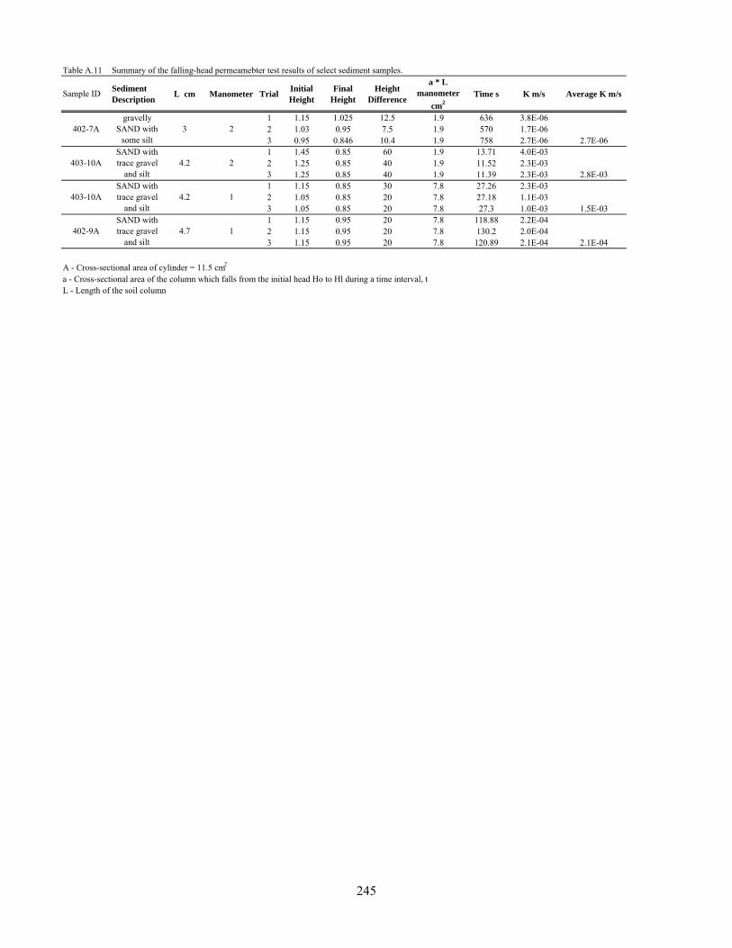
Table A.11 Summary of the falling-head permeamebter test results of select sediment samples.

Sample IDSediment Description

L cm Manometer TrialInitial Height

Final Height

Height Difference

a * L manometer

cm2Time s K m/s Average K m/s

1 1.15 1.025 12.5 1.9 636 3.8E-062 1.03 0.95 7.5 1.9 570 1.7E-063 0.95 0.846 10.4 1.9 758 2.7E-06 2.7E-061 1.45 0.85 60 1.9 13.71 4.0E-032 1.25 0.85 40 1.9 11.52 2.3E-033 1.25 0.85 40 1.9 11.39 2.3E-03 2.8E-031 1.15 0.85 30 7.8 27.26 2.3E-032 1.05 0.85 20 7.8 27.18 1.1E-033 1.05 0.85 20 7.8 27.3 1.0E-03 1.5E-031 1.15 0.95 20 7.8 118.88 2.2E-042 1.15 0.95 20 7.8 130.2 2.0E-043 1.15 0.95 20 7.8 120.89 2.1E-04 2.1E-04

A - Cross-sectional area of cylinder = 11.5 cm2

a - Cross-sectional area of the column which falls from the initial head Ho to Hl during a time interval, tL - Length of the soil column

402-7A

403-10A

403-10A

SAND with trace gravel

and silt

4.2

4.2

4.7

SAND with trace gravel

and siltSAND with trace gravel

and silt

402-9A

3gravelly

SAND with some silt

2

2

1

1

245

Appendix B

Charaterization of Contaminants at the Site including Pre-Injection Soil Coring and Groundwater

Sampling Procedures and Results

246

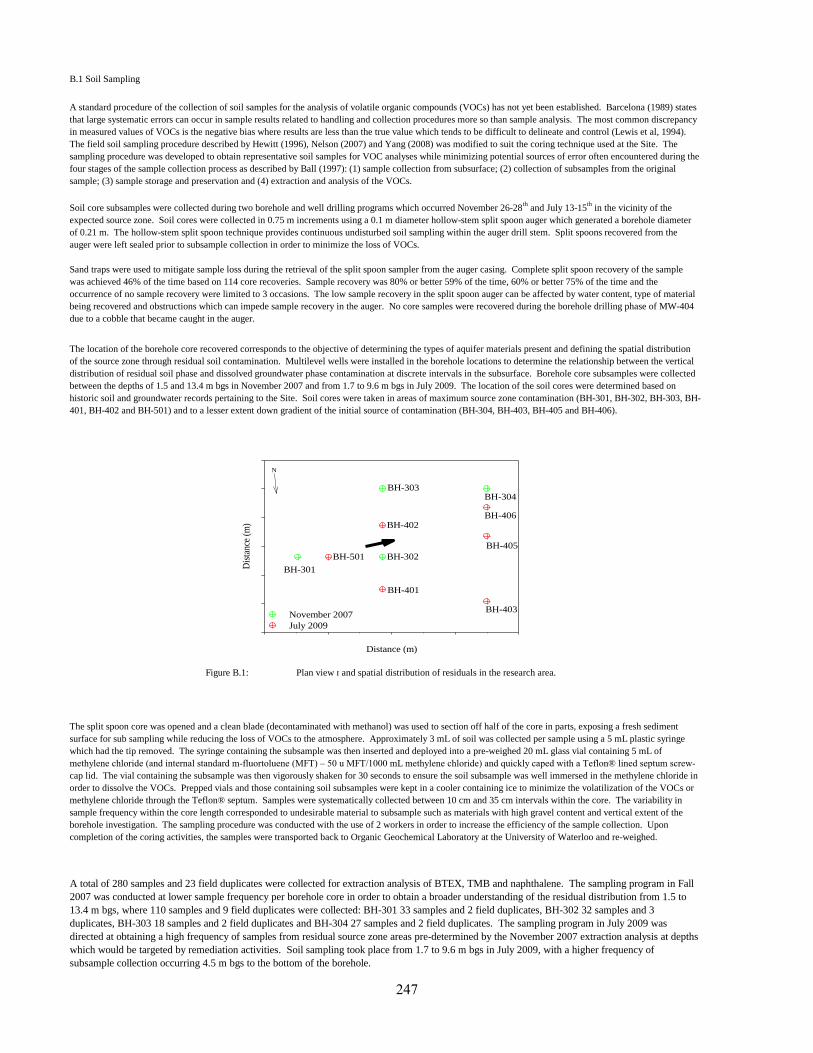
B.1 Soil Sampling

Figure B.1: Plan view map showing location of borehole coring used to determine the vertical and spatial distribution of residuals in the research area.

A standard procedure of the collection of soil samples for the analysis of volatile organic compounds (VOCs) has not yet been established. Barcelona (1989) states

that large systematic errors can occur in sample results related to handling and collection procedures more so than sample analysis. The most common discrepancy

in measured values of VOCs is the negative bias where results are less than the true value which tends to be difficult to delineate and control (Lewis et al, 1994).

The field soil sampling procedure described by Hewitt (1996), Nelson (2007) and Yang (2008) was modified to suit the coring technique used at the Site. The

sampling procedure was developed to obtain representative soil samples for VOC analyses while minimizing potential sources of error often encountered during the

four stages of the sample collection process as described by Ball (1997): (1) sample collection from subsurface; (2) collection of subsamples from the original

sample; (3) sample storage and preservation and (4) extraction and analysis of the VOCs.

Soil core subsamples were collected during two borehole and well drilling programs which occurred November 26-28th

and July 13-15th

in the vicinity of the

expected source zone. Soil cores were collected in 0.75 m increments using a 0.1 m diameter hollow-stem split spoon auger which generated a borehole diameter

of 0.21 m. The hollow-stem split spoon technique provides continuous undisturbed soil sampling within the auger drill stem. Split spoons recovered from the

auger were left sealed prior to subsample collection in order to minimize the loss of VOCs.

Sand traps were used to mitigate sample loss during the retrieval of the split spoon sampler from the auger casing. Complete split spoon recovery of the sample

was achieved 46% of the time based on 114 core recoveries. Sample recovery was 80% or better 59% of the time, 60% or better 75% of the time and the

occurrence of no sample recovery were limited to 3 occasions. The low sample recovery in the split spoon auger can be affected by water content, type of material

being recovered and obstructions which can impede sample recovery in the auger. No core samples were recovered during the borehole drilling phase of MW-404

due to a cobble that became caught in the auger.

The location of the borehole core recovered corresponds to the objective of determining the types of aquifer materials present and defining the spatial distribution

of the source zone through residual soil contamination. Multilevel wells were installed in the borehole locations to determine the relationship between the vertical

distribution of residual soil phase and dissolved groundwater phase contamination at discrete intervals in the subsurface. Borehole core subsamples were collected

between the depths of 1.5 and 13.4 m bgs in November 2007 and from 1.7 to 9.6 m bgs in July 2009. The location of the soil cores were determined based on

historic soil and groundwater records pertaining to the Site. Soil cores were taken in areas of maximum source zone contamination (BH-301, BH-302, BH-303, BH-

401, BH-402 and BH-501) and to a lesser extent down gradient of the initial source of contamination (BH-304, BH-403, BH-405 and BH-406).

The split spoon core was opened and a clean blade (decontaminated with methanol) was used to section off half of the core in parts, exposing a fresh sediment

surface for sub sampling while reducing the loss of VOCs to the atmosphere. Approximately 3 mL of soil was collected per sample using a 5 mL plastic syringe

which had the tip removed. The syringe containing the subsample was then inserted and deployed into a pre-weighed 20 mL glass vial containing 5 mL of

methylene chloride (and internal standard m-fluortoluene (MFT) – 50 u MFT/1000 mL methylene chloride) and quickly caped with a Teflon® lined septum screw-

cap lid. The vial containing the subsample was then vigorously shaken for 30 seconds to ensure the soil subsample was well immersed in the methylene chloride in

order to dissolve the VOCs. Prepped vials and those containing soil subsamples were kept in a cooler containing ice to minimize the volatilization of the VOCs or

methylene chloride through the Teflon® septum. Samples were systematically collected between 10 cm and 35 cm intervals within the core. The variability in

sample frequency within the core length corresponded to undesirable material to subsample such as materials with high gravel content and vertical extent of the

borehole investigation. The sampling procedure was conducted with the use of 2 workers in order to increase the efficiency of the sample collection. Upon

completion of the coring activities, the samples were transported back to Organic Geochemical Laboratory at the University of Waterloo and re-weighed.

A total of 280 samples and 23 field duplicates were collected for extraction analysis of BTEX, TMB and naphthalene. The sampling program in Fall

2007 was conducted at lower sample frequency per borehole core in order to obtain a broader understanding of the residual distribution from 1.5 to

13.4 m bgs, where 110 samples and 9 field duplicates were collected: BH-301 33 samples and 2 field duplicates, BH-302 32 samples and 3

duplicates, BH-303 18 samples and 2 field duplicates and BH-304 27 samples and 2 field duplicates. The sampling program in July 2009 was

directed at obtaining a high frequency of samples from residual source zone areas pre-determined by the November 2007 extraction analysis at depths

which would be targeted by remediation activities. Soil sampling took place from 1.7 to 9.6 m bgs in July 2009, with a higher frequency of

subsample collection occurring 4.5 m bgs to the bottom of the borehole.

Distance (m)

Dis

tanc

e (m

)

November 2007

July 2009

BH-403

BH-401

BH-402

BH-301

BH-501 BH-302

BH-405

BH-406

BH-304BH-303

N

247

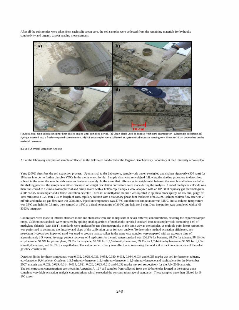
B.2 Soil Chemical Extraction Analysis

Yang (2008) describes the soil extraction process. Upon arrival to the Laboratory, sample vials were re-weighed and shaken vigorously (350 rpm) for

18 hours in order to further dissolve VOCs in the methylene chloride. Sample vials were re-weighed following the shaking procedure to detect lost

solvent in the event the sample vials were not fastened securely. In the event that differences in weight exist between the sample vial before and after

the shaking process, the sample was either discarded or weight calculation corrections were made during the analysis. 1 ml of methylene chloride was

then transferred to a 2 ml autosampler vial and crimp sealed with a Teflon cap. Samples were analyzed with an HP 5890 capillary gas chromatogram,

a HP 7673A autosampler and a flame ionization detector. Three ml of methylene chloride was injected in splitless mode (purge on 0.5 min, purge off

10.0 min) onto a 0.25 mm x 30 m length of DB5 capillary column with a stationary phase film thickness of 0.25µm. Helium column flow rate was 2

ml/min and make-up gas flow rate was 30ml/min. Injection temperature was 275ºC and detector temperature was 325ºC. Initial column temperature

was 35ºC and held for 0.5 min, then ramped at 15ºC to a final temperature of 300ºC and held for 2 min. Data integration was completed with a HP

3393A integrator.

Calibrations were made in internal standard mode and standards were run in triplicate at seven different concentrations, covering the expected sample

range. Calibration standards were prepared by spiking small quantities of methanolic certified standard into autosampler vials containing 1 ml of

methylene chloride (with MFT). Standards were analyzed by gas chromatography in the same way as the samples. A multiple point linear regression

was performed to determine the linearity and slope of the calibration curve for each analyte. To determine method extraction efficiency, non-

petroleum hydrocarbon impacted sand was used to prepare matrix spikes in the same way samples were prepared with an exposure time of

approximately 3.5 weeks. Average percent recovery of 4 replicates for the mid range standard was 106.9% for benzene, 98.3% for toluene, 98.1% for

ethylbenzene, 97.9% for p+m-xylene, 99.9% for o-xylene, 99.5% for 1,3,5-trimethylbenezene, 99.7% for 1,2,4-trimethylbenezene, 99.9% for 1,2,3-

trimethylbenezene, and 96.8% for naphthalene. The extraction efficiency was effective at measuring the total soil extract concentrations of the select

gasoline constituents.

Detection limits for these compounds were 0.032, 0.028, 0.036, 0.058, 0.030, 0.033, 0.034, 0.034 and 0.055 mg/kg wet soil for benzene, toluene,

ethylbenzene, P,M-xylene, O-xylene, 1,3,5-trimethylbenzene, 1,2,4-trimethylbenzene, 1,2,3-trimethylbenzene and naphthalene for the November

2007 analysis and 0.029, 0.029, 0.014, 0.014, 0.021, 0.020, 0.033, 0.015 and 0.033 mg/kg wet soil respectively for the July 2009 analysis.

The soil extraction concentrations are shown in Appendix A. 157 soil samples from collected from the 10 boreholes located in the source zone

contained very high extraction analysis concentrations which exceeded the concentration rage of standards. These samples were then diluted for 5-

100 times.

After all the subsamples were taken from each split spoon core, the soil samples were collected from the remaining materials for hydraulic

conductivity and organic vapour reading measurements.

Figure B.2: (a) Split spoon container kept sealed sealed until sampling period. (b) Clean blade used to expose fresh core segment for subsample collection. (c)

Syringe inserted into a freshly exposed core segment. (d) Soil subsamples were collected at systematical intervals ranging rom 10 cm to 25 cm depending on the

material recovered.

All of the laboratory analyses of samples collected in the field were conducted at the Organic Geochemistry Laboratory at the University of Waterloo.

248

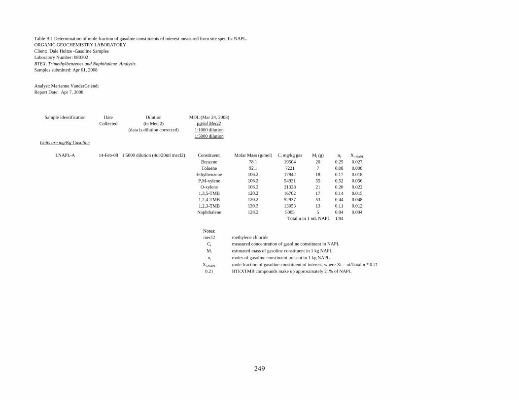
Table B.1 Determination of mole fraction of gasoline constituents of interest measured from site specific NAPL.

ORGANIC GEOCHEMISTRY LABORATORY

Client: Dale Holtze -Gasoline Samples

Laboratory Number: 080302

BTEX, Trimethylbenzenes and Naphthalene Analysis

Samples submitted: Apr 01, 2008

Analyst: Marianne VanderGriendt

Report Date: Apr 7, 2008

Sample Identification Date Dilution MDL (Mar 24, 2008)

Collected (in Mecl2) µg/ml Mecl2

(data is dilution corrected) 1:1000 dilution

1:5000 dilution

Units are mg/Kg Gasoline

LNAPL-A 14-Feb-08 1:5000 dilution (4ul/20ml mecl2) Constituenti Molar Mass (g/mol) Ci mg/kg gas Mi (g) ni Xi-NAPL

Benzene 78.1 19504 20 0.25 0.027

Toluene 92.1 7221 7 0.08 0.008

Ethylbenzene 106.2 17942 18 0.17 0.018

P,M-xylene 106.2 54931 55 0.52 0.056

O-xylene 106.2 21328 21 0.20 0.022

1,3,5-TMB 120.2 16702 17 0.14 0.015

1,2,4-TMB 120.2 52937 53 0.44 0.048

1,2,3-TMB 120.2 13053 13 0.11 0.012

Naphthalene 128.2 5005 5 0.04 0.004

Total n in 1 mL NAPL 1.94

Notes:

mecl2 methylene chloride

Ci measured concentration of gasoline constituent in NAPL

Mi estimated mass of gasoline constituent in 1 kg NAPL

ni moles of gasoline constituent present in 1 kg NAPL

Xi-NAPL mole fraction of gasoline constituent of interest, where Xi = ni/Total n * 0.21

0.21 BTEXTMB compounds make up approximately 21% of NAPL

249

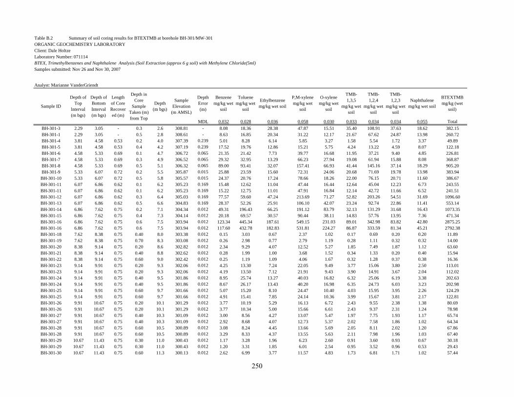
Table B.2 Summary of soil coring results for BTEXTMB at borehole BH-301/MW-301

ORGANIC GEOCHEMISTRY LABORATORY

Client: Dale Holtze

Laboratory Number: 071114

BTEX, Trimethylbenzenes and Naphthalene Analysis (Soil Extraction (approx 6 g soil) with Methylene Chloride(5ml)

Samples submitted: Nov 26 and Nov 30, 2007

Analyst: Marianne VanderGriendt

Depth

Error

(m)

Benzene

mg/kg wet

soil

Toluene

mg/kg wet

soil

Ethylbenzene

mg/kg wet soil

P,M-xylene

mg/kg wet

soil

O-xylene

mg/kg wet

soil

TMB-

1,3,5

mg/kg wet

soil

TMB-

1,2,4

mg/kg wet

soil

TMB-

1,2,3

mg/kg wet

soil

Naphthalene

mg/kg wet soil

BTEXTMB

mg/kg (wet

soil)

MDL 0.032 0.028 0.036 0.058 0.030 0.033 0.034 0.034 0.055 Total

BH-301-3 2.29 3.05 - 0.3 2.6 308.81 - 8.08 18.36 28.38 47.87 15.51 35.40 108.91 37.63 18.62 382.15

BH-301-1 2.29 3.05 - 0.5 2.8 308.61 - 8.63 16.85 20.34 31.22 12.17 21.67 67.62 24.87 13.98 260.72

BH-301-4 3.81 4.58 0.53 0.2 4.0 307.39 0.239 5.01 8.28 6.14 5.85 3.27 1.58 5.54 1.72 3.37 49.89

BH-301-5 3.81 4.58 0.53 0.4 4.2 307.19 0.239 17.52 19.76 12.86 15.21 5.75 4.24 13.22 4.59 8.07 122.18

BH-301-6 4.58 5.33 0.69 0.1 4.7 306.72 0.065 21.35 21.42 7.73 39.77 16.68 11.95 37.21 9.40 4.85 226.81

BH-301-7 4.58 5.33 0.69 0.3 4.9 306.52 0.065 29.32 32.95 13.29 66.23 27.94 19.08 61.94 15.88 8.08 368.87

BH-301-8 4.58 5.33 0.69 0.5 5.1 306.32 0.065 89.00 93.41 32.07 157.41 66.93 41.44 145.16 37.14 18.29 905.20

BH-301-9 5.33 6.07 0.72 0.2 5.5 305.87 0.015 25.88 23.59 15.60 72.31 24.06 20.68 71.69 19.78 13.98 383.94

BH-301-10 5.33 6.07 0.72 0.5 5.8 305.57 0.015 24.37 20.76 17.24 78.66 18.26 22.00 76.15 20.71 11.60 386.67

BH-301-11 6.07 6.86 0.62 0.1 6.2 305.23 0.169 15.48 12.62 11.04 47.44 16.44 12.64 45.04 12.23 6.73 243.55

BH-301-11 6.07 6.86 0.62 0.1 6.2 305.23 0.169 15.22 12.75 11.01 47.91 16.84 12.14 42.72 11.66 6.52 241.51

BH-301-12 6.07 6.86 0.62 0.3 6.4 305.03 0.169 77.57 59.60 47.24 213.69 71.27 52.82 203.26 54.51 31.69 1096.60

BH-301-13 6.07 6.86 0.62 0.5 6.6 304.83 0.169 28.37 52.26 25.91 106.10 42.07 23.24 92.74 22.86 11.41 553.14

BH-301-14 6.86 7.62 0.75 0.2 7.1 304.34 0.012 49.31 196.43 66.25 191.12 83.79 32.13 131.29 31.68 16.43 1073.35

BH-301-15 6.86 7.62 0.75 0.4 7.3 304.14 0.012 20.18 69.57 30.57 90.44 38.11 14.83 57.76 13.95 7.36 471.34

BH-301-16 6.86 7.62 0.75 0.6 7.5 303.94 0.012 123.34 445.34 187.61 549.15 231.03 89.01 342.98 83.82 42.80 2875.25

BH-301-16 6.86 7.62 0.75 0.6 7.5 303.94 0.012 117.60 432.78 182.83 531.81 224.27 86.87 333.59 81.34 45.21 2792.38

BH-301-18 7.62 8.38 0.75 0.40 8.0 303.38 0.012 0.15 3.03 0.67 2.37 1.02 0.17 0.69 0.20 0.20 11.89

BH-301-19 7.62 8.38 0.75 0.70 8.3 303.08 0.012 0.26 2.98 0.77 2.79 1.19 0.28 1.11 0.32 0.32 14.00

BH-301-20 8.38 9.14 0.75 0.20 8.6 302.82 0.012 2.34 9.29 4.07 12.52 5.27 1.85 7.49 1.87 1.12 63.60

BH-301-21 8.38 9.14 0.75 0.40 8.8 302.62 0.012 0.28 1.99 1.00 3.68 1.52 0.34 1.33 0.20 0.40 15.94

BH-301-22 8.38 9.14 0.75 0.60 9.0 302.42 0.012 0.25 1.19 1.09 4.06 1.67 0.32 1.28 0.37 0.38 16.36

BH-301-23 9.14 9.91 0.75 0.20 9.3 302.06 0.012 4.25 13.30 7.24 22.05 9.49 3.77 15.06 3.80 2.50 113.01

BH-301-23 9.14 9.91 0.75 0.20 9.3 302.06 0.012 4.19 13.50 7.12 21.91 9.43 3.90 14.91 3.67 2.04 112.02

BH-301-24 9.14 9.91 0.75 0.40 9.5 301.86 0.012 8.95 25.74 13.27 40.03 16.82 6.32 25.06 6.19 3.38 202.63

BH-301-24 9.14 9.91 0.75 0.40 9.5 301.86 0.012 8.67 26.17 13.43 40.20 16.98 6.35 24.73 6.03 3.23 202.98

BH-301-25 9.14 9.91 0.75 0.60 9.7 301.66 0.012 5.07 15.20 8.10 24.47 10.40 4.03 15.95 3.95 2.26 124.29

BH-301-25 9.14 9.91 0.75 0.60 9.7 301.66 0.012 4.91 15.41 7.85 24.14 10.36 3.99 15.67 3.81 2.17 122.81

BH-301-26 9.91 10.67 0.75 0.20 10.1 301.29 0.012 3.77 10.19 5.29 16.13 6.72 2.43 9.55 2.38 1.38 80.69

BH-301-26 9.91 10.67 0.75 0.20 10.1 301.29 0.012 3.77 10.34 5.00 15.66 6.61 2.43 9.37 2.31 1.24 78.98

BH-301-27 9.91 10.67 0.75 0.40 10.3 301.09 0.012 3.00 8.56 4.27 13.07 5.47 1.97 7.75 1.93 1.17 65.74

BH-301-27 9.91 10.67 0.75 0.40 10.3 301.09 0.012 2.92 8.68 4.07 12.73 5.37 2.02 7.58 1.86 1.02 64.34

BH-301-28 9.91 10.67 0.75 0.60 10.5 300.89 0.012 3.08 8.24 4.45 13.66 5.69 2.05 8.11 2.02 1.20 67.86

BH-301-28 9.91 10.67 0.75 0.60 10.5 300.89 0.012 3.29 8.33 4.37 13.55 5.63 2.11 7.98 1.96 1.03 67.40

BH-301-29 10.67 11.43 0.75 0.30 11.0 300.43 0.012 1.17 3.28 1.96 6.23 2.60 0.91 3.60 0.93 0.67 30.18

BH-301-29 10.67 11.43 0.75 0.30 11.0 300.43 0.012 1.20 3.31 1.85 6.01 2.54 0.95 3.52 0.96 0.53 29.43

BH-301-30 10.67 11.43 0.75 0.60 11.3 300.13 0.012 2.62 6.99 3.77 11.57 4.83 1.73 6.81 1.71 1.02 57.44

Depth

(m bgs)

Sample

Elevation

(m AMSL)

Sample ID

Depth of

Top

lnterval

(m bgs)

Depth of

Bottom

Interval

(m bgs)

Length

of Core

Recover

ed (m)

Depth in

Core

Sample

Taken (m)

from Top

250

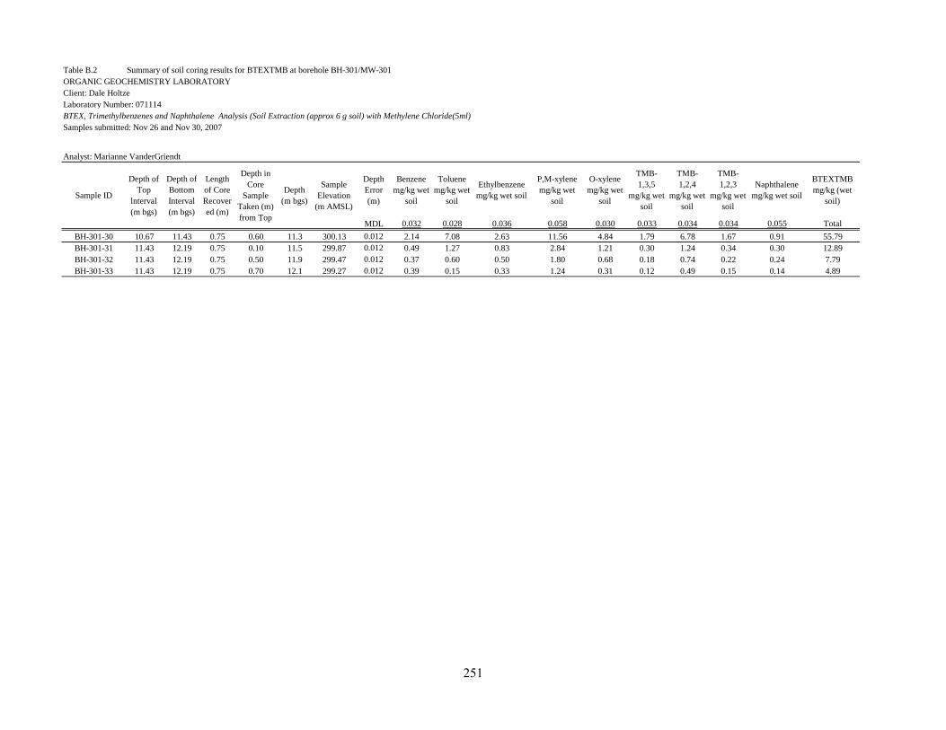
Table B.2 Summary of soil coring results for BTEXTMB at borehole BH-301/MW-301

ORGANIC GEOCHEMISTRY LABORATORY

Client: Dale Holtze

Laboratory Number: 071114

BTEX, Trimethylbenzenes and Naphthalene Analysis (Soil Extraction (approx 6 g soil) with Methylene Chloride(5ml)

Samples submitted: Nov 26 and Nov 30, 2007

Analyst: Marianne VanderGriendt

Depth

Error

(m)

Benzene

mg/kg wet

soil

Toluene

mg/kg wet

soil

Ethylbenzene

mg/kg wet soil

P,M-xylene

mg/kg wet

soil

O-xylene

mg/kg wet

soil

TMB-

1,3,5

mg/kg wet

soil

TMB-

1,2,4

mg/kg wet

soil

TMB-

1,2,3

mg/kg wet

soil

Naphthalene

mg/kg wet soil

BTEXTMB

mg/kg (wet

soil)

MDL 0.032 0.028 0.036 0.058 0.030 0.033 0.034 0.034 0.055 Total

Depth

(m bgs)

Sample

Elevation

(m AMSL)

Sample ID

Depth of

Top

lnterval

(m bgs)

Depth of

Bottom

Interval

(m bgs)

Length

of Core

Recover

ed (m)

Depth in

Core

Sample

Taken (m)

from Top

BH-301-30 10.67 11.43 0.75 0.60 11.3 300.13 0.012 2.14 7.08 2.63 11.56 4.84 1.79 6.78 1.67 0.91 55.79

BH-301-31 11.43 12.19 0.75 0.10 11.5 299.87 0.012 0.49 1.27 0.83 2.84 1.21 0.30 1.24 0.34 0.30 12.89

BH-301-32 11.43 12.19 0.75 0.50 11.9 299.47 0.012 0.37 0.60 0.50 1.80 0.68 0.18 0.74 0.22 0.24 7.79

BH-301-33 11.43 12.19 0.75 0.70 12.1 299.27 0.012 0.39 0.15 0.33 1.24 0.31 0.12 0.49 0.15 0.14 4.89

251

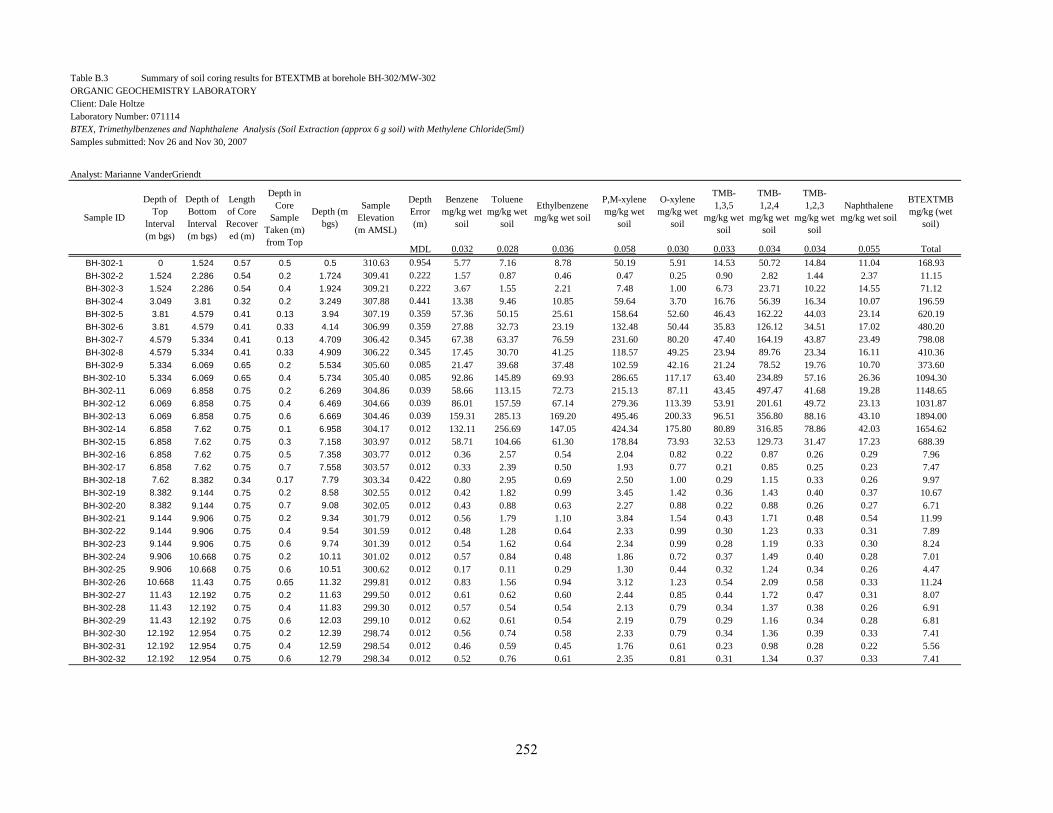
Table B.3 Summary of soil coring results for BTEXTMB at borehole BH-302/MW-302

ORGANIC GEOCHEMISTRY LABORATORY

Client: Dale Holtze

Laboratory Number: 071114

BTEX, Trimethylbenzenes and Naphthalene Analysis (Soil Extraction (approx 6 g soil) with Methylene Chloride(5ml)

Samples submitted: Nov 26 and Nov 30, 2007

Analyst: Marianne VanderGriendt

Depth

Error

(m)

Benzene

mg/kg wet

soil

Toluene

mg/kg wet

soil

Ethylbenzene

mg/kg wet soil

P,M-xylene

mg/kg wet

soil

O-xylene

mg/kg wet

soil

TMB-

1,3,5

mg/kg wet

soil

TMB-

1,2,4

mg/kg wet

soil

TMB-

1,2,3

mg/kg wet

soil

Naphthalene

mg/kg wet soil

BTEXTMB

mg/kg (wet

soil)

MDL 0.032 0.028 0.036 0.058 0.030 0.033 0.034 0.034 0.055 Total

BH-302-1 0 1.524 0.57 0.5 0.5 310.63 0.954 5.77 7.16 8.78 50.19 5.91 14.53 50.72 14.84 11.04 168.93

BH-302-2 1.524 2.286 0.54 0.2 1.724 309.41 0.222 1.57 0.87 0.46 0.47 0.25 0.90 2.82 1.44 2.37 11.15

BH-302-3 1.524 2.286 0.54 0.4 1.924 309.21 0.222 3.67 1.55 2.21 7.48 1.00 6.73 23.71 10.22 14.55 71.12

BH-302-4 3.049 3.81 0.32 0.2 3.249 307.88 0.441 13.38 9.46 10.85 59.64 3.70 16.76 56.39 16.34 10.07 196.59

BH-302-5 3.81 4.579 0.41 0.13 3.94 307.19 0.359 57.36 50.15 25.61 158.64 52.60 46.43 162.22 44.03 23.14 620.19

BH-302-6 3.81 4.579 0.41 0.33 4.14 306.99 0.359 27.88 32.73 23.19 132.48 50.44 35.83 126.12 34.51 17.02 480.20

BH-302-7 4.579 5.334 0.41 0.13 4.709 306.42 0.345 67.38 63.37 76.59 231.60 80.20 47.40 164.19 43.87 23.49 798.08

BH-302-8 4.579 5.334 0.41 0.33 4.909 306.22 0.345 17.45 30.70 41.25 118.57 49.25 23.94 89.76 23.34 16.11 410.36

BH-302-9 5.334 6.069 0.65 0.2 5.534 305.60 0.085 21.47 39.68 37.48 102.59 42.16 21.24 78.52 19.76 10.70 373.60

BH-302-10 5.334 6.069 0.65 0.4 5.734 305.40 0.085 92.86 145.89 69.93 286.65 117.17 63.40 234.89 57.16 26.36 1094.30

BH-302-11 6.069 6.858 0.75 0.2 6.269 304.86 0.039 58.66 113.15 72.73 215.13 87.11 43.45 497.47 41.68 19.28 1148.65

BH-302-12 6.069 6.858 0.75 0.4 6.469 304.66 0.039 86.01 157.59 67.14 279.36 113.39 53.91 201.61 49.72 23.13 1031.87

BH-302-13 6.069 6.858 0.75 0.6 6.669 304.46 0.039 159.31 285.13 169.20 495.46 200.33 96.51 356.80 88.16 43.10 1894.00

BH-302-14 6.858 7.62 0.75 0.1 6.958 304.17 0.012 132.11 256.69 147.05 424.34 175.80 80.89 316.85 78.86 42.03 1654.62

BH-302-15 6.858 7.62 0.75 0.3 7.158 303.97 0.012 58.71 104.66 61.30 178.84 73.93 32.53 129.73 31.47 17.23 688.39

BH-302-16 6.858 7.62 0.75 0.5 7.358 303.77 0.012 0.36 2.57 0.54 2.04 0.82 0.22 0.87 0.26 0.29 7.96

BH-302-17 6.858 7.62 0.75 0.7 7.558 303.57 0.012 0.33 2.39 0.50 1.93 0.77 0.21 0.85 0.25 0.23 7.47

BH-302-18 7.62 8.382 0.34 0.17 7.79 303.34 0.422 0.80 2.95 0.69 2.50 1.00 0.29 1.15 0.33 0.26 9.97

BH-302-19 8.382 9.144 0.75 0.2 8.58 302.55 0.012 0.42 1.82 0.99 3.45 1.42 0.36 1.43 0.40 0.37 10.67

BH-302-20 8.382 9.144 0.75 0.7 9.08 302.05 0.012 0.43 0.88 0.63 2.27 0.88 0.22 0.88 0.26 0.27 6.71

BH-302-21 9.144 9.906 0.75 0.2 9.34 301.79 0.012 0.56 1.79 1.10 3.84 1.54 0.43 1.71 0.48 0.54 11.99

BH-302-22 9.144 9.906 0.75 0.4 9.54 301.59 0.012 0.48 1.28 0.64 2.33 0.99 0.30 1.23 0.33 0.31 7.89

BH-302-23 9.144 9.906 0.75 0.6 9.74 301.39 0.012 0.54 1.62 0.64 2.34 0.99 0.28 1.19 0.33 0.30 8.24

BH-302-24 9.906 10.668 0.75 0.2 10.11 301.02 0.012 0.57 0.84 0.48 1.86 0.72 0.37 1.49 0.40 0.28 7.01

BH-302-25 9.906 10.668 0.75 0.6 10.51 300.62 0.012 0.17 0.11 0.29 1.30 0.44 0.32 1.24 0.34 0.26 4.47

BH-302-26 10.668 11.43 0.75 0.65 11.32 299.81 0.012 0.83 1.56 0.94 3.12 1.23 0.54 2.09 0.58 0.33 11.24

BH-302-27 11.43 12.192 0.75 0.2 11.63 299.50 0.012 0.61 0.62 0.60 2.44 0.85 0.44 1.72 0.47 0.31 8.07

BH-302-28 11.43 12.192 0.75 0.4 11.83 299.30 0.012 0.57 0.54 0.54 2.13 0.79 0.34 1.37 0.38 0.26 6.91

BH-302-29 11.43 12.192 0.75 0.6 12.03 299.10 0.012 0.62 0.61 0.54 2.19 0.79 0.29 1.16 0.34 0.28 6.81

BH-302-30 12.192 12.954 0.75 0.2 12.39 298.74 0.012 0.56 0.74 0.58 2.33 0.79 0.34 1.36 0.39 0.33 7.41

BH-302-31 12.192 12.954 0.75 0.4 12.59 298.54 0.012 0.46 0.59 0.45 1.76 0.61 0.23 0.98 0.28 0.22 5.56

BH-302-32 12.192 12.954 0.75 0.6 12.79 298.34 0.012 0.52 0.76 0.61 2.35 0.81 0.31 1.34 0.37 0.33 7.41

Sample

Elevation

(m AMSL)

Sample ID

Depth of

Top

lnterval

(m bgs)

Depth of

Bottom

Interval

(m bgs)

Length

of Core

Recover

ed (m)

Depth in

Core

Sample

Taken (m)

from Top

Depth (m

bgs)

252

Table B.3 Summary of soil coring results for BTEXTMB at borehole BH-302/MW-302

ORGANIC GEOCHEMISTRY LABORATORY

Client: Dale Holtze

Laboratory Number: 071114

BTEX, Trimethylbenzenes and Naphthalene Analysis (Soil Extraction (approx 6 g soil) with Methylene Chloride(5ml)

Samples submitted: Nov 26 and Nov 30, 2007

Analyst: Marianne VanderGriendt

Depth

Error

(m)

Benzene

mg/kg wet

soil

Toluene

mg/kg wet

soil

Ethylbenzene

mg/kg wet soil

P,M-xylene

mg/kg wet

soil

O-xylene

mg/kg wet

soil

TMB-

1,3,5

mg/kg wet

soil

TMB-

1,2,4

mg/kg wet

soil

TMB-

1,2,3

mg/kg wet

soil

Naphthalene

mg/kg wet soil

BTEXTMB

mg/kg (wet

soil)

MDL 0.032 0.028 0.036 0.058 0.030 0.033 0.034 0.034 0.055 Total

Sample

Elevation

(m AMSL)

Sample ID

Depth of

Top

lnterval

(m bgs)

Depth of

Bottom

Interval

(m bgs)

Length

of Core

Recover

ed (m)

Depth in

Core

Sample

Taken (m)

from Top

Depth (m

bgs)

253

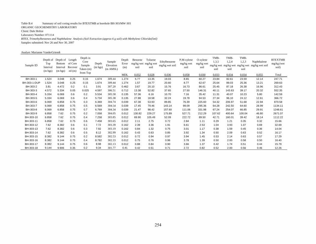
Table B.4 Summary of soil coring results for BTEXTMB at borehole BH-303/MW-303

ORGANIC GEOCHEMISTRY LABORATORY

Client: Dale Holtze

Laboratory Number: 071114

BTEX, Trimethylbenzenes and Naphthalene Analysis (Soil Extraction (approx 6 g soil) with Methylene Chloride(5ml)

Samples submitted: Nov 26 and Nov 30, 2007

Analyst: Marianne VanderGriendt

Depth

Error

(m)

Benzene

mg/kg wet

soil

Toluene

mg/kg wet

soil

Ethylbenzene

mg/kg wet soil

P,M-xylene

mg/kg wet

soil

O-xylene

mg/kg wet

soil

TMB-

1,3,5

mg/kg wet

soil

TMB-

1,2,4

mg/kg wet

soil

TMB-

1,2,3

mg/kg wet

soil

Naphthalene

mg/kg wet soil

BTEXTMB

mg/kg (wet

soil)

MDL 0.032 0.028 0.036 0.058 0.030 0.033 0.034 0.034 0.055 Total

BH-303-1 1.524 3.048 0.25 0.15 1.674 309.44 1.274 5.77 13.35 19.03 8.65 60.27 23.84 82.61 23.59 12.14 247.71

BH-303-1-DUP 1.524 3.048 0.25 0.15 1.674 309.44 1.274 1.57 19.77 20.60 8.77 62.67 25.64 89.03 25.36 13.21 269.63

BH-303-2 3.81 4.472 0.2 0.1 3.91 307.20 0.462 3.67 20.10 15.76 16.73 86.61 25.45 87.18 26.38 16.96 312.43

BH-303-3 4.572 5.334 0.05 0.025 4.597 306.51 0.712 13.38 52.82 37.65 27.50 146.31 40.11 143.63 39.17 20.32 552.35

BH-303-4 5.334 6.069 0.6 0.2 5.534 305.58 0.135 57.36 6.16 10.70 7.16 35.42 11.31 40.07 10.23 5.80 142.59

BH-303-5 5.334 6.069 0.6 0.4 5.734 305.38 0.135 27.88 18.58 32.24 19.78 94.53 27.34 96.10 24.12 12.61 366.72

BH-303-6 6.069 6.858 0.75 0.3 6.369 304.74 0.039 67.38 53.93 89.85 76.39 225.60 54.32 206.97 51.68 22.94 870.58

BH-303-7 6.069 6.858 0.75 0.5 6.569 304.54 0.039 17.45 79.46 143.14 99.09 295.36 64.28 242.50 64.60 28.99 1134.11

BH-303-8 6.069 6.858 0.75 0.7 6.769 304.34 0.039 21.47 98.42 157.60 111.06 331.98 67.24 254.07 66.85 29.91 1248.61

BH-303-9 6.858 7.62 0.75 0.2 7.058 304.05 0.012 130.82 229.27 175.89 527.71 212.29 107.62 400.64 100.04 46.80 2671.07

BH-303-10 6.858 7.62 0.75 0.4 7.258 303.85 0.012 69.90 105.49 52.09 222.72 89.50 42.71 160.01 39.42 18.14 1112.22

BH-303-11 6.858 7.62 0.75 0.6 7.458 303.65 0.012 2.11 2.75 0.72 2.84 1.11 0.29 1.21 0.35 0.32 15.66

BH-303-12 7.62 8.382 0.6 0.1 7.72 303.39 0.162 2.39 3.36 1.91 6.61 2.53 1.04 3.93 1.07 0.69 32.69

BH-303-13 7.62 8.382 0.6 0.3 7.92 303.19 0.162 0.84 1.32 0.75 3.01 1.17 0.38 1.59 0.45 0.36 14.04

BH-303-14 7.62 8.382 0.6 0.5 8.12 302.99 0.162 0.43 0.63 0.85 3.92 1.34 0.50 2.09 0.63 0.52 16.17

BH-303-15 8.382 9.144 0.75 0.2 8.582 302.53 0.012 0.72 0.94 0.97 3.94 1.45 0.53 2.14 0.63 0.57 17.29

BH-303-16 8.382 9.144 0.75 0.4 8.782 302.33 0.012 0.75 0.76 0.96 3.78 1.39 0.50 2.00 0.58 0.50 16.40

BH-303-17 8.382 9.144 0.75 0.6 8.98 302.13 0.012 0.88 0.84 0.90 3.66 1.37 0.42 1.74 0.51 0.44 15.79

BH-303-18 9.144 9.906 0.35 0.2 9.34 301.77 0.41 0.42 0.51 0.71 2.72 0.82 0.52 2.00 0.56 0.46 12.26

Sample

Elevation

(m AMSL)

Sample ID

Depth of

Top

lnterval

(m bgs)

Depth of

Bottom

Interval

(m bgs)

Length

of Core

Recover

ed (m)

Depth in

Core

Sample

Taken (m)

from Top

Depth

(m bgs)

254

Table B.5 Summary of soil coring results for BTEXTMB at borehole BH-304/MW-304

ORGANIC GEOCHEMISTRY LABORATORY

Client: Dale Holtze

Laboratory Number: 071114

BTEX, Trimethylbenzenes and Naphthalene Analysis (Soil Extraction (approx 6 g soil) with Methylene Chloride(5ml)

Samples submitted: Nov 26 and Nov 30, 2007

Analyst: Marianne VanderGriendt

Depth

Error

(m)

Benzene

mg/kg

(wet soil)

Toluene

mg/kg

(wet soil)

Ethylbenzene

mg/kg (wet

soil)

P,M-xylene

mg/kg (wet

soil)

O-xylene

mg/kg (wet

soil)

TMB-

1,3,5

mg/kg

(wet soil)

TMB-

1,2,4

mg/kg

(wet soil)

TMB-

1,2,3

mg/kg

(wet soil)

Naphthalene

mg/kg wet soil

BTEXTMB

mg/kg (wet

soil)

MDL 0.032 0.028 0.036 0.058 0.030 0.033 0.034 0.034 0.055 Total

BH-304-1 1.524 3.048 0.75 0.20 3.25 307.69 0.774 0.45 4.93 14.01 29.08 12.12 16.34 54.84 13.61 6.35 151.73

BH-304-2 1.524 3.048 0.75 0.40 3.45 307.49 0.774 2.57 16.54 27.30 59.86 28.62 51.13 171.97 45.33 22.90 426.23

BH-304-3 1.524 3.048 0.75 0.60 3.65 307.29 0.774 6.37 17.07 7.14 52.44 23.72 22.10 76.02 19.50 10.09 234.45

BH-304-4 3.048 3.810 0.52 0.40 4.21 306.73 0.242 17.98 36.90 20.47 115.34 49.39 36.08 128.15 32.45 16.12 452.88

BH-304-5 3.810 4.572 0.75 0.25 4.82 306.12 0.012 54.26 107.67 56.77 295.28 121.13 85.01 299.37 74.36 32.37 1126.21

BH-304-6 3.810 4.572 0.75 0.45 5.02 305.92 0.012 32.42 66.16 65.37 183.83 76.62 53.60 192.44 48.40 22.64 741.49

BH-304-7 3.810 4.572 0.75 0.65 5.22 305.72 0.012 29.16 63.56 55.81 167.34 68.99 41.49 152.89 43.36 18.95 641.54

BH-304-8 4.572 5.334 0.75 0.20 5.53 305.41 0.012 38.52 93.84 69.21 204.71 84.51 47.20 173.66 44.06 21.41 777.12

BH-304-9 4.572 5.334 0.75 0.40 5.73 305.21 0.012 36.67 95.51 66.19 194.21 81.24 44.95 165.83 42.05 20.84 747.49

BH-304-10 4.572 5.334 0.75 0.60 5.93 305.01 0.012 9.81 31.99 15.12 68.95 29.35 16.99 62.34 15.49 8.15 258.18

BH-304-11 5.334 6.069 0.75 0.25 6.32 304.62 0.012 4.11 15.37 7.55 35.06 15.51 9.76 36.54 9.33 5.14 138.37

BH-304-12 5.334 6.069 0.75 0.50 6.57 304.37 0.012 84.62 210.96 65.42 295.36 117.99 63.60 241.19 59.42 25.90 1164.47

BH-304-12-DUP 5.334 6.069 0.75 0.50 6.57 304.37 0.012 87.22 214.60 105.79 319.68 124.50 67.35 255.72 63.50 28.30 1266.66

BH-304-13 5.334 6.069 0.75 0.70 6.77 304.17 0.012 23.32 50.24 29.62 92.87 36.26 20.18 80.09 19.85 9.02 361.46

BH-304-14 6.069 6.858 0.75 0.20 7.06 303.88 0.039 65.84 90.23 70.98 220.03 86.89 41.86 168.79 41.77 18.10 804.48

BH-304-16 6.858 7.620 0.54 0.35 7.97 302.97 0.222 0.30 0.26 0.40 1.59 0.63 0.27 1.09 0.31 0.25 5.09

BH-304-17 7.620 8.382 0.75 0.30 8.68 302.26 0.012 0.46 0.39 0.61 2.33 0.99 0.42 1.74 0.46 0.32 7.72

BH-304-18 7.620 8.382 0.75 0.50 8.88 302.06 0.012 0.20 0.14 0.35 1.53 0.53 0.32 1.25 0.35 0.28 4.94

BH-304-19 8.382 9.144 0.61 0.25 9.39 301.55 0.15 0.16 0.09 0.37 1.71 0.54 0.36 1.39 0.39 0.27 5.28

BH-304-20 9.144 9.906 0.75 0.20 10.11 300.83 0.012 0.29 0.18 0.47 2.04 0.67 0.42 1.64 0.46 0.36 6.52

BH-304-21 9.144 9.906 0.75 0.20 10.11 300.83 0.012 0.54 0.50 1.18 4.73 1.68 0.73 3.00 0.86 0.50 13.72

BH-304-21-DUP 9.144 9.906 0.75 0.20 10.11 300.83 0.012 0.30 0.17 0.58 2.50 0.83 0.47 1.87 0.52 0.39 7.63

BH-304-22 10.668 11.430 0.75 0.30 11.73 299.21 0.012 0.51 0.51 0.52 2.19 0.76 0.37 1.46 0.41 0.31 7.04

BH-304-23 10.668 11.430 0.75 0.50 11.93 299.01 0.012 0.45 0.25 0.45 1.87 0.67 0.33 1.32 0.37 0.28 5.98

BH-304-24 10.668 11.430 0.75 0.70 12.13 298.81 0.012 0.33 0.15 0.39 1.72 0.58 0.32 1.25 0.35 0.24 5.33

BH-304-25 11.430 12.192 0.75 0.20 12.39 298.55 0.012 0.35 0.19 0.43 1.90 0.64 0.37 1.45 0.41 0.32 6.05

BH-304-26 11.430 12.192 0.75 0.40 12.59 298.35 0.012 0.32 0.19 0.41 1.73 0.63 0.34 1.38 0.38 0.26 5.63

BH-304-27 11.430 12.192 0.75 0.60 12.79 298.15 0.012 0.22 0.09 0.36 1.65 0.53 0.27 1.06 0.31 0.20 4.68

Sample

Elevation

(m AMSL)

Sample ID

Depth of

Top

lnterval

(m bgs)

Depth of

Bottom

Interval

(m bgs)

Length

of Core

Recover

ed (m)

Depth in

Core

Sample

Taken (m)

from Top

Depth

(m bgs)

255

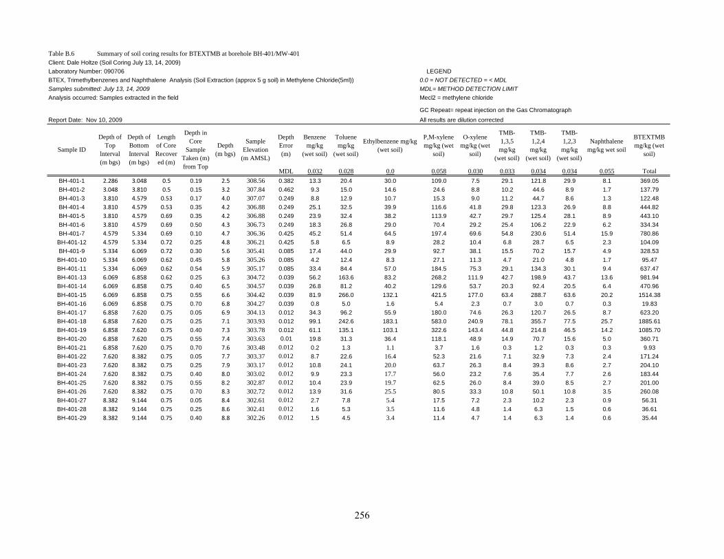
Table B.6 Summary of soil coring results for BTEXTMB at borehole BH-401/MW-401

Client: Dale Holtze (Soil Coring July 13, 14, 2009)

Laboratory Number: 090706 LEGEND

BTEX, Trimethylbenzenes and Naphthalene Analysis (Soil Extraction (approx 5 g soil) in Methylene Chloride(5ml)) 0.0 = NOT DETECTED = < MDL

Samples submitted: July 13, 14, 2009 MDL= METHOD DETECTION LIMIT

Analysis occurred: Samples extracted in the field Mecl2 = methylene chloride

GC Repeat= repeat injection on the Gas Chromatograph

Report Date: Nov 10, 2009 All results are dilution corrected

Depth

Error

(m)

Benzene

mg/kg

(wet soil)

Toluene

mg/kg

(wet soil)

Ethylbenzene mg/kg

(wet soil)

P,M-xylene

mg/kg (wet

soil)

O-xylene

mg/kg (wet

soil)

TMB-

1,3,5

mg/kg

(wet soil)

TMB-

1,2,4

mg/kg

(wet soil)

TMB-

1,2,3

mg/kg

(wet soil)

Naphthalene

mg/kg wet soil

BTEXTMB

mg/kg (wet

soil)

MDL 0.032 0.028 0.0 0.058 0.030 0.033 0.034 0.034 0.055 Total

BH-401-1 2.286 3.048 0.5 0.19 2.5 308.56 0.382 13.3 20.4 30.0 109.0 7.5 29.1 121.8 29.9 8.1 369.05

BH-401-2 3.048 3.810 0.5 0.15 3.2 307.84 0.462 9.3 15.0 14.6 24.6 8.8 10.2 44.6 8.9 1.7 137.79

BH-401-3 3.810 4.579 0.53 0.17 4.0 307.07 0.249 8.8 12.9 10.7 15.3 9.0 11.2 44.7 8.6 1.3 122.48

BH-401-4 3.810 4.579 0.53 0.35 4.2 306.88 0.249 25.1 32.5 39.9 116.6 41.8 29.8 123.3 26.9 8.8 444.82

BH-401-5 3.810 4.579 0.69 0.35 4.2 306.88 0.249 23.9 32.4 38.2 113.9 42.7 29.7 125.4 28.1 8.9 443.10

BH-401-6 3.810 4.579 0.69 0.50 4.3 306.73 0.249 18.3 26.8 29.0 70.4 29.2 25.4 106.2 22.9 6.2 334.34

BH-401-7 4.579 5.334 0.69 0.10 4.7 306.36 0.425 45.2 51.4 64.5 197.4 69.6 54.8 230.6 51.4 15.9 780.86

BH-401-12 4.579 5.334 0.72 0.25 4.8 306.21 0.425 5.8 6.5 8.9 28.2 10.4 6.8 28.7 6.5 2.3 104.09

BH-401-9 5.334 6.069 0.72 0.30 5.6 305.41 0.085 17.4 44.0 29.9 92.7 38.1 15.5 70.2 15.7 4.9 328.53

BH-401-10 5.334 6.069 0.62 0.45 5.8 305.26 0.085 4.2 12.4 8.3 27.1 11.3 4.7 21.0 4.8 1.7 95.47

BH-401-11 5.334 6.069 0.62 0.54 5.9 305.17 0.085 33.4 84.4 57.0 184.5 75.3 29.1 134.3 30.1 9.4 637.47

BH-401-13 6.069 6.858 0.62 0.25 6.3 304.72 0.039 56.2 163.6 83.2 268.2 111.9 42.7 198.9 43.7 13.6 981.94

BH-401-14 6.069 6.858 0.75 0.40 6.5 304.57 0.039 26.8 81.2 40.2 129.6 53.7 20.3 92.4 20.5 6.4 470.96

BH-401-15 6.069 6.858 0.75 0.55 6.6 304.42 0.039 81.9 266.0 132.1 421.5 177.0 63.4 288.7 63.6 20.2 1514.38

BH-401-16 6.069 6.858 0.75 0.70 6.8 304.27 0.039 0.8 5.0 1.6 5.4 2.3 0.7 3.0 0.7 0.3 19.83

BH-401-17 6.858 7.620 0.75 0.05 6.9 304.13 0.012 34.3 96.2 55.9 180.0 74.6 26.3 120.7 26.5 8.7 623.20

BH-401-18 6.858 7.620 0.75 0.25 7.1 303.93 0.012 99.1 242.6 183.1 583.0 240.9 78.1 355.7 77.5 25.7 1885.61

BH-401-19 6.858 7.620 0.75 0.40 7.3 303.78 0.012 61.1 135.1 103.1 322.6 143.4 44.8 214.8 46.5 14.2 1085.70

BH-401-20 6.858 7.620 0.75 0.55 7.4 303.63 0.01 19.8 31.3 36.4 118.1 48.9 14.9 70.7 15.6 5.0 360.71

BH-401-21 6.858 7.620 0.75 0.70 7.6 303.48 0.012 0.2 1.3 1.1 3.7 1.6 0.3 1.2 0.3 0.3 9.93

BH-401-22 7.620 8.382 0.75 0.05 7.7 303.37 0.012 8.7 22.6 16.4 52.3 21.6 7.1 32.9 7.3 2.4 171.24

BH-401-23 7.620 8.382 0.75 0.25 7.9 303.17 0.012 10.8 24.1 20.0 63.7 26.3 8.4 39.3 8.6 2.7 204.10

BH-401-24 7.620 8.382 0.75 0.40 8.0 303.02 0.012 9.9 23.3 17.7 56.0 23.2 7.6 35.4 7.7 2.6 183.44

BH-401-25 7.620 8.382 0.75 0.55 8.2 302.87 0.012 10.4 23.9 19.7 62.5 26.0 8.4 39.0 8.5 2.7 201.00

BH-401-26 7.620 8.382 0.75 0.70 8.3 302.72 0.012 13.9 31.6 25.5 80.5 33.3 10.8 50.1 10.8 3.5 260.08

BH-401-27 8.382 9.144 0.75 0.05 8.4 302.61 0.012 2.7 7.8 5.4 17.5 7.2 2.3 10.2 2.3 0.9 56.31

BH-401-28 8.382 9.144 0.75 0.25 8.6 302.41 0.012 1.6 5.3 3.5 11.6 4.8 1.4 6.3 1.5 0.6 36.61

BH-401-29 8.382 9.144 0.75 0.40 8.8 302.26 0.012 1.5 4.5 3.4 11.4 4.7 1.4 6.3 1.4 0.6 35.44

Sample

Elevation

(m AMSL)

Sample ID

Depth of

Top

lnterval

(m bgs)

Depth of

Bottom

Interval

(m bgs)

Length

of Core

Recover

ed (m)

Depth in

Core

Sample

Taken (m)

from Top

Depth

(m bgs)

256

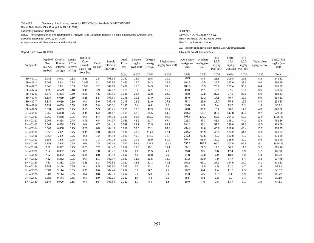
Table B.7 Summary of soil coring results for BTEXTMB at borehole BH-402/MW-402

Client: Dale Holtze (Soil Coring July 13, 14, 2009)

Laboratory Number: 090706 LEGEND

BTEX, Trimethylbenzenes and Naphthalene Analysis (Soil Extraction (approx 5 g soil) in Methylene Chloride(5ml)) 0.0 = NOT DETECTED = < MDL

Samples submitted: July 13, 14, 2009 MDL= METHOD DETECTION LIMIT

Analysis occurred: Samples extracted in the field Mecl2 = methylene chloride

GC Repeat= repeat injection on the Gas Chromatograph

Report Date: Nov 10, 2009 All results are dilution corrected

Depth

Error

(m)

Benzene

mg/kg

(wet soil)

Toluene

mg/kg

(wet soil)

Ethylbenzene

mg/kg (wet soil)

P,M-xylene

mg/kg (wet

soil)

O-xylene

mg/kg (wet

soil)

TMB-

1,3,5

mg/kg

(wet soil)

TMB-

1,2,4

mg/kg

(wet soil)

TMB-

1,2,3

mg/kg

(wet soil)

Naphthalene

mg/kg wet soil

BTEXTMB

mg/kg (wet

soil)

MDL 0.032 0.028 0.036 0.058 0.030 0.033 0.034 0.034 0.055 Total

BH-402-1 2.286 3.048 0.38 0.18 2.5 308.62 0.382 16.2 19.8 29.9 98.3 8.4 25.6 109.8 27.6 8.2 343.82

BH-402-2 3.048 3.81 0.33 0.165 3.2 307.88 0.432 18.0 24.3 32.8 104.5 10.5 29.5 127.0 31.2 9.0 386.66

BH-402-2 3.048 3.81 0.33 0.165 3.2 307.88 0.439 18.0 24.3 31.8 102.8 10.5 28.9 125.4 30.7 8.4 380.79

BH-402-4 3.81 4.579 0.18 0.11 3.9 307.17 0.575 8.8 6.7 13.0 49.0 2.7 7.7 37.5 10.0 3.6 138.94

BH-402-5 4.579 5.334 0.59 0.05 4.6 306.46 0.145 23.4 22.8 24.5 78.0 12.8 22.5 97.1 23.5 5.9 310.47

BH-402-6 5.334 6.069 0.59 0.15 5.5 305.61 0.145 20.6 27.0 30.0 85.0 32.2 17.5 79.7 17.7 5.0 314.62

BH-402-7 5.334 6.069 0.59 0.3 5.6 305.46 0.145 21.6 31.9 27.1 75.3 29.9 17.0 75.3 16.3 4.4 298.83

BH-402-8 5.334 6.069 0.59 0.45 5.8 305.31 0.145 5.4 6.4 8.3 25.6 9.5 5.4 23.7 5.2 1.5 90.92

BH-402-9 5.334 6.069 0.75 0.55 5.9 305.21 0.039 18.3 47.9 28.7 88.8 35.2 18.2 80.5 17.8 4.9 340.32

BH-402-10 6.069 6.858 0.75 0.15 6.2 304.87 0.039 37.9 85.5 51.6 166.0 65.7 33.0 147.8 32.6 9.2 629.30

BH-402-11 6.069 6.858 0.75 0.3 6.4 304.72 0.039 64.5 166.2 94.3 308.9 122.0 58.5 264.3 59.3 17.6 1155.48

BH-402-12 6.069 6.858 0.75 0.45 6.5 304.57 0.039 43.6 61.7 67.4 223.7 87.3 43.6 198.1 44.1 12.8 782.36

BH-402-13 6.069 6.858 0.75 0.6 6.7 304.42 0.039 58.1 52.5 81.7 284.1 96.1 52.2 236.0 52.5 16.5 929.66

BH-402-14 6.069 6.858 0.75 0.69 6.8 304.33 0.012 53.5 51.1 84.4 292.9 94.6 48.9 218.8 48.4 15.7 908.35

BH-402-15 6.858 7.62 0.75 0.15 7.0 304.08 0.012 49.2 117.2 72.1 234.0 95.9 40.8 184.2 41.1 12.2 846.57

BH-402-16 6.858 7.62 0.75 0.3 7.2 303.93 0.012 49.9 115.2 70.8 230.8 93.5 40.2 182.0 40.2 12.1 834.59

BH-402-17 6.858 7.62 0.75 0.45 7.3 303.78 0.012 34.8 69.9 50.3 164.4 65.0 30.1 135.6 30.2 8.9 588.99

BH-402-18 6.858 7.62 0.75 0.6 7.5 303.63 0.012 97.9 231.8 122.1 393.7 163.7 65.3 307.9 66.9 19.2 1468.33

BH-402-19 7.62 8.382 0.75 0.05 7.7 303.42 0.012 13.6 26.1 19.1 59.1 22.3 11.3 50.2 11.1 3.2 215.96

BH-402-20 7.62 8.382 0.75 0.2 7.8 303.27 0.012 4.6 11.5 7.0 23.8 9.5 3.6 17.4 3.9 1.2 82.38

BH-402-21 7.62 8.382 0.75 0.35 8.0 303.12 0.012 4.0 10.8 7.2 24.8 10.0 3.9 18.8 4.2 1.3 85.02

BH-402-22 7.62 8.382 0.75 0.5 8.1 302.97 0.012 11.3 23.5 15.2 51.2 20.0 7.9 37.7 8.4 2.3 177.46

BH-402-23 7.62 8.382 0.75 0.65 8.3 302.82 0.012 33.8 82.1 49.1 157.6 63.1 27.3 124.5 27.7 8.1 573.51

BH-402-24 8.382 9.144 0.55 0.1 8.5 302.61 0.212 5.7 13.1 8.6 29.1 11.5 4.5 21.1 4.7 1.4 99.73

BH-402-25 8.382 9.144 0.55 0.25 8.6 302.46 0.212 3.0 8.2 4.7 16.2 6.4 2.4 11.2 2.5 0.9 55.32

BH-402-26 8.382 9.144 0.55 0.4 8.8 302.31 0.212 2.0 5.8 3.2 11.3 4.5 1.7 8.1 1.9 0.2 38.72

BH-402-27 8.382 9.144 0.55 0.5 8.9 302.21 0.212 1.4 4.4 2.3 8.4 3.4 1.3 6.0 1.4 0.6 29.19

BH-402-30 9.144 9.906 0.55 0.4 9.5 301.55 0.212 3.7 8.4 5.5 19.0 7.6 2.8 13.7 3.1 1.0 64.81

Sample

Elevation

(m AMSL)

Sample ID

Depth of

Top

lnterval

(m bgs)

Depth of

Bottom

Interval

(m bgs)

Length

of Core

Recover

ed (m)

Depth in

Core

Sample

Taken (m)

from Top

Depth

(m bgs)

257

Table B.8 Summary of soil coring results for BTEXTMB at borehole BH-403/MW-403

Client: Dale Holtze (Soil Coring July 13, 14, 2009)

Laboratory Number: 090706 LEGEND

BTEX, Trimethylbenzenes and Naphthalene Analysis (Soil Extraction (approx 5 g soil) in Methylene Chloride(5ml)) 0.0 = NOT DETECTED = < MDL

Samples submitted: July 13, 14, 2009 MDL= METHOD DETECTION LIMIT

Analysis occurred: Samples extracted in the field Mecl2 = methylene chloride

GC Repeat= repeat injection on the Gas Chromatograph

Report Date: Nov 10, 2009 All results are dilution corrected

Depth

Error

(m)

Benzene

mg/kg

(wet soil)

Toluene

mg/kg

(wet soil)

Ethylbenzene

mg/kg (wet soil)

P,M-xylene

mg/kg (wet

soil)

O-xylene

mg/kg (wet

soil)

TMB-

1,3,5

mg/kg

(wet soil)

TMB-

1,2,4

mg/kg

(wet soil)

TMB-

1,2,3

mg/kg

(wet soil)

Naphthalene

mg/kg wet soil

BTEXTMB

mg/kg (wet

soil)

MDL 0.032 0.028 0.036 0.058 0.030 0.033 0.034 0.034 0.055 Total

BH-403-1 1.524 2.286 0.25 0.5 1.8 309.17 0.262 7.3 7.82 14.1 54.5 5.3 11.8 52.3 12.5 3.8 169.54

BH-403-2 2.286 3.048 0.20 0.48 2.5 308.45 0.282 11.4 10.65 21.3 78.7 7.0 15.5 64.9 15.5 5.0 229.85

BH-403-3 3.05 4.58 0.25 0.53 3.3 307.64 1.001 22.4 29.90 0.0 50.7 20.4 11.7 55.8 7.1 2.2 200.37

BH-403-5 3.81 4.58 0.35 0.65 4.2 306.78 0.119 38.4 52.72 69.6 206.5 82.5 55.9 225.2 48.1 29.8 808.85

BH-403-6 3.81 4.58 0.55 0.65 4.4 306.58 0.119 11.8 29.18 20.9 67.1 28.0 12.6 52.8 11.5 7.7 241.48

BH-403-7 4.58 5.33 0.45 0.75 5.0 305.91 0.005 44.3 60.50 59.5 180.1 69.7 45.1 187.0 40.1 23.6 709.92

BH-403-9 5.334 6.069 0.05 0.75 5.4 305.56 0.005 21.6 29.02 32.3 109.0 44.4 20.3 89.6 20.0 6.6 372.79

BH-403-10 5.334 6.069 0.20 0.75 5.5 305.41 0.015 1.6 2.57 2.9 10.3 4.1 1.8 7.9 1.8 0.7 33.76

BH-403-11 5.334 6.069 0.35 0.75 5.7 305.26 0.015 0.6 0.95 1.1 4.5 1.7 0.7 3.3 0.8 0.6 14.29

BH-403-12 5.334 6.069 0.50 0.75 5.8 305.11 0.015 0.2 0.45 0.6 2.5 0.9 0.4 1.7 0.4 0.3 7.48

BH-403-13 5.334 6.069 0.65 0.75 6.0 304.96 0.015 0.2 0.68 0.7 2.7 1.0 0.3 1.4 0.4 0.3 7.68

BH-403-16 6.069 6.858 0.47 0.75 6.5 304.40 0.015 20.2 24.13 26.6 86.2 37.5 9.4 58.0 12.5 3.7 278.21

BH-403-17 6.069 6.858 0.60 0.75 6.7 304.27 0.039 0.3 0.72 0.5 1.7 0.7 0.2 0.8 0.2 0.1 5.15

BH-403-18 6.069 6.858 0.70 0.75 6.8 304.17 0.039 0.2 0.60 0.5 1.8 0.7 0.2 0.7 0.2 0.1 4.83

BH-403-19 6.858 7.62 0.05 0.75 6.9 304.03 0.039 0.3 1.30 0.5 1.8 0.7 0.2 0.9 0.2 0.2 6.03

BH-403-20 6.858 7.62 0.20 0.75 7.1 303.88 0.012 0.3 1.46 0.6 2.0 0.8 0.2 1.1 0.3 0.2 7.00

BH-403-22 6.858 7.62 0.50 0.75 7.4 303.58 0.012 0.3 1.78 0.4 1.3 0.5 0.2 0.7 0.2 0.2 5.37

BH-403-23 6.858 7.62 0.65 0.75 7.5 303.43 0.01 0.2 1.34 0.3 1.1 0.4 0.1 0.6 0.2 0.2 4.56

BH-403-24 7.62 8.382 0.05 0.75 7.7 303.27 0.012 0.6 2.03 0.8 2.6 1.1 0.4 1.8 0.4 0.2 9.91

BH-403-25 7.62 8.382 0.20 0.75 7.8 303.12 0.012 0.4 1.57 0.5 1.7 0.7 0.2 1.0 0.2 0.1 6.25

BH-403-26 7.62 8.382 0.35 0.75 8.0 302.97 0.012 0.4 1.60 0.6 2.0 0.8 0.3 1.3 0.3 0.2 7.58

BH-403-27 7.62 8.382 0.50 0.75 8.1 302.82 0.012 0.4 1.48 0.5 1.7 0.7 0.2 1.0 0.2 0.1 6.27

BH-403-28 7.62 8.382 0.65 0.75 8.3 302.67 0.012 1.0 1.89 1.2 4.0 1.7 0.7 3.2 0.7 0.1 14.46

BH-403-29 8.382 9.144 0.10 0.75 8.5 302.46 0.012 0.5 2.33 0.7 2.5 1.0 0.3 1.1 0.3 0.3 8.99

Sample

Elevation

(m AMSL)

Sample ID

Depth of

Top

lnterval

(m bgs)

Depth of

Bottom

Interval

(m bgs)

Length

of Core

Recover

ed (m)

Depth in

Core

Sample

Taken (m)

from Top

Depth

(m bgs)

258

Table B.9 Summary of soil coring results for BTEXTMB at borehole BH-405/MW-405

Client: Dale Holtze (Soil Coring July 13, 14, 2009)

Laboratory Number: 090706 LEGEND

BTEX, Trimethylbenzenes and Naphthalene Analysis (Soil Extraction (approx 5 g soil) in Methylene Chloride(5ml)) 0.0 = NOT DETECTED = < MDL

Samples submitted: July 13, 14, 2009 MDL= METHOD DETECTION LIMIT

Analysis occurred: Samples extracted in the field Mecl2 = methylene chloride

GC Repeat= repeat injection on the Gas Chromatograph

Report Date: Nov 10, 2009 All results are dilution corrected

Depth

Error

(m)

Benzene

mg/kg

(wet soil)

Toluene

mg/kg

(wet soil)

Ethylbenzene

mg/kg (wet soil)

P,M-xylene

mg/kg (wet

soil)

O-xylene

mg/kg (wet

soil)

TMB-

1,3,5

mg/kg

(wet soil)

TMB-

1,2,4

mg/kg

(wet soil)

TMB-

1,2,3

mg/kg

(wet soil)

Naphthalene

mg/kg wet soil

BTEXTMB

mg/kg (wet

soil)

MDL 0.032 0.028 0.036 0.058 0.030 0.033 0.034 0.034 0.055 Total

BH-405-1 4.579 5.334 0.75 0.05 4.63 306.28 0.005 18.8 56.2 38.52 129.2 54.8 23.2 102.4 23.1 7.6 453.91

BH-405-2 4.579 5.334 0.75 0.25 4.83 306.08 0.005 5.9 18.6 11.91 39.4 16.1 6.6 28.4 6.5 2.2 135.54

BH-405-3 4.58 5.33 0.75 0.55 5.13 305.78 0.005 9.9 21.2 19.90 67.1 27.2 10.7 46.5 10.5 3.9 217.02

BH-405-4 4.58 5.33 0.75 0.70 5.28 305.63 0.005 37.0 69.7 69.94 229.9 95.0 37.0 159.3 35.9 12.7 746.41

BH-405-5 5.33 6.07 0.75 0.05 5.38 305.53 0.015 34.8 88.1 61.74 202.4 85.4 33.0 144.4 32.7 10.6 693.06

BH-405-6 5.33 6.07 0.75 0.20 5.53 305.38 0.015 40.0 101.6 75.49 245.4 103.7 40.5 174.7 39.3 12.7 833.32

BH-405-7 5.334 6.069 0.75 0.35 5.68 305.23 0.015 63.6 200.8 106.46 346.0 146.1 57.1 258.2 57.1 17.6 1253.00

BH-405-8 5.334 6.069 0.75 0.50 5.83 305.08 0.015 48.7 167.9 82.51 264.2 111.2 45.5 193.1 43.0 14.3 970.42

BH-405-9 5.334 6.069 0.75 0.65 5.98 304.93 0.015 91.7 323.3 146.30 476.0 203.8 82.3 353.3 78.1 25.8 1780.42

BH-405-11 6.069 6.858 0.62 0.25 6.32 304.59 0.169 8.1 28.6 12.41 42.3 17.9 7.3 33.1 7.3 2.2 159.24

BH-405-11 6.069 6.858 0.62 0.25 6.32 304.59 0.169 8.1 29.0 11.92 41.3 18.0 7.2 32.9 7.1 2.1 157.63

BH-405-12 6.069 6.858 0.62 0.40 6.47 304.44 0.169 21.8 69.4 32.33 111.2 48.6 20.2 95.8 20.5 5.7 425.49

BH-405-13 6.069 6.858 0.62 0.55 6.62 304.29 0.169 13.3 32.2 19.28 65.9 27.1 11.7 55.4 11.9 3.0 239.83

BH-405-14 6.858 7.62 0.75 0.10 6.96 303.95 0.012 1.7 4.9 1.64 5.8 2.4 0.8 3.9 0.9 0.3 22.34

BH-405-15 6.858 7.62 0.75 0.25 7.11 303.80 0.012 2.6 6.7 2.92 9.7 4.2 1.6 8.1 1.7 0.5 37.95

BH-405-16 6.858 7.62 0.75 0.40 7.26 303.65 0.012 0.6 2.9 0.71 2.8 1.1 0.3 1.4 0.4 0.3 10.50

BH-405-17 6.858 7.62 0.75 0.55 7.41 303.50 0.012 0.3 2.0 0.43 1.7 0.7 0.2 0.8 0.2 0.2 6.55

BH-405-18 6.858 7.62 0.75 0.70 7.56 303.35 0.012 0.5 3.1 0.56 2.3 0.9 0.3 1.2 0.3 0.3 9.41

BH-405-19 7.62 8.382 0.75 0.10 7.72 303.19 0.012 3.6 8.9 4.52 15.1 6.4 2.6 12.5 2.7 0.8 57.23

BH-405-20 7.62 8.382 0.75 0.25 7.87 303.04 0.012 8.2 19.6 10.90 35.5 15.1 6.3 30.7 6.6 1.7 134.63

BH-405-21 7.62 8.382 0.75 0.40 8.02 302.89 0.012 0.4 1.6 0.39 1.6 0.6 0.2 0.7 0.2 0.2 5.80

BH-405-22 7.62 8.382 0.75 0.40 8.02 302.89 0.012 0.4 1.8 0.40 1.6 0.6 0.2 0.7 0.2 0.2 5.96

BH-405-23 7.62 8.382 0.75 0.70 8.32 302.59 0.012 0.3 1.0 0.37 1.4 0.6 0.2 0.8 0.2 0.2 5.06

Sample

Elevation

(m AMSL)

Sample ID

Depth of

Top

lnterval

(m bgs)

Depth of

Bottom

Interval

(m bgs)

Length

of Core

Recover

ed (m)

Depth in

Core

Sample

Taken (m)

from Top

Depth

(m bgs)

259

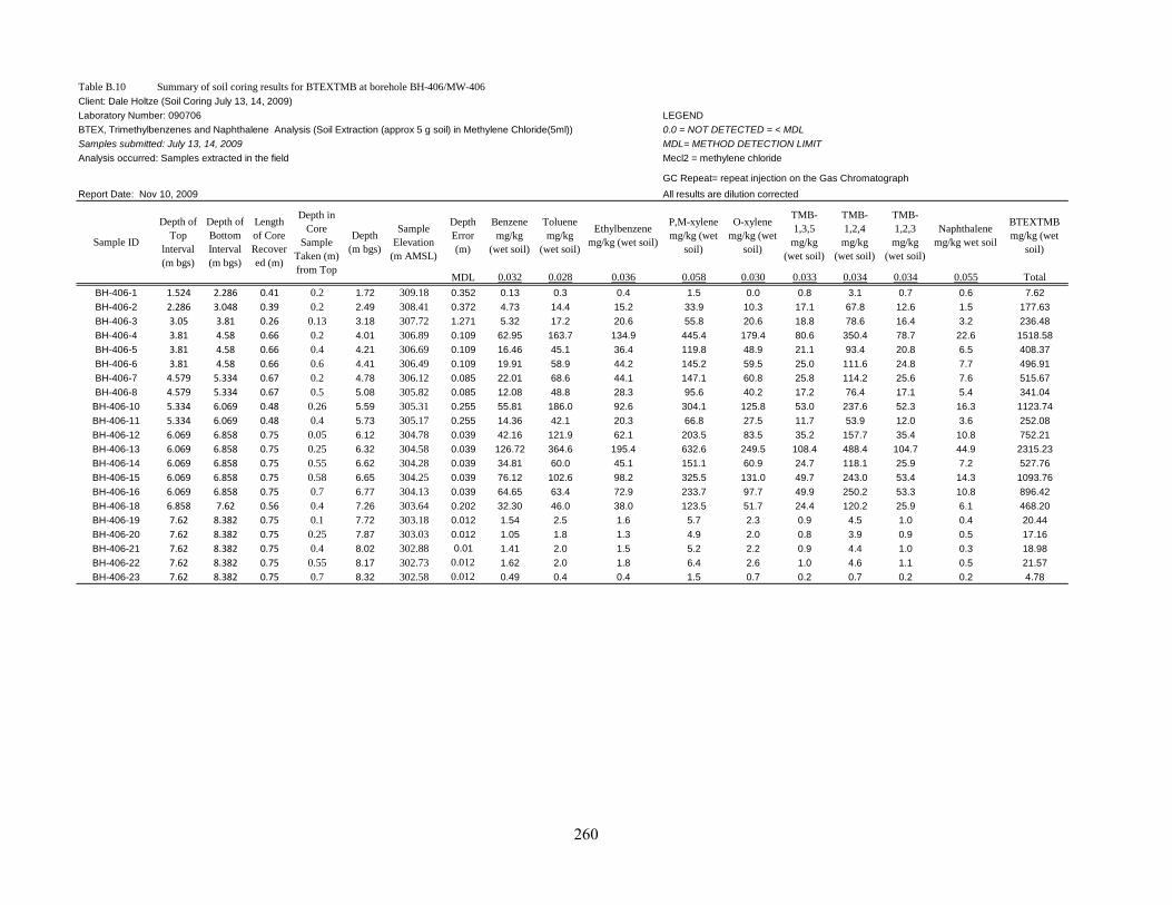
Table B.10 Summary of soil coring results for BTEXTMB at borehole BH-406/MW-406

Client: Dale Holtze (Soil Coring July 13, 14, 2009)

Laboratory Number: 090706 LEGEND

BTEX, Trimethylbenzenes and Naphthalene Analysis (Soil Extraction (approx 5 g soil) in Methylene Chloride(5ml)) 0.0 = NOT DETECTED = < MDL

Samples submitted: July 13, 14, 2009 MDL= METHOD DETECTION LIMIT

Analysis occurred: Samples extracted in the field Mecl2 = methylene chloride

GC Repeat= repeat injection on the Gas Chromatograph

Report Date: Nov 10, 2009 All results are dilution corrected

Depth

Error

(m)

Benzene

mg/kg

(wet soil)

Toluene

mg/kg

(wet soil)

Ethylbenzene

mg/kg (wet soil)

P,M-xylene

mg/kg (wet

soil)

O-xylene

mg/kg (wet

soil)

TMB-

1,3,5

mg/kg

(wet soil)

TMB-

1,2,4

mg/kg

(wet soil)

TMB-

1,2,3

mg/kg

(wet soil)

Naphthalene

mg/kg wet soil

BTEXTMB

mg/kg (wet

soil)

MDL 0.032 0.028 0.036 0.058 0.030 0.033 0.034 0.034 0.055 Total

BH-406-1 1.524 2.286 0.41 0.2 1.72 309.18 0.352 0.13 0.3 0.4 1.5 0.0 0.8 3.1 0.7 0.6 7.62

BH-406-2 2.286 3.048 0.39 0.2 2.49 308.41 0.372 4.73 14.4 15.2 33.9 10.3 17.1 67.8 12.6 1.5 177.63

BH-406-3 3.05 3.81 0.26 0.13 3.18 307.72 1.271 5.32 17.2 20.6 55.8 20.6 18.8 78.6 16.4 3.2 236.48

BH-406-4 3.81 4.58 0.66 0.2 4.01 306.89 0.109 62.95 163.7 134.9 445.4 179.4 80.6 350.4 78.7 22.6 1518.58

BH-406-5 3.81 4.58 0.66 0.4 4.21 306.69 0.109 16.46 45.1 36.4 119.8 48.9 21.1 93.4 20.8 6.5 408.37

BH-406-6 3.81 4.58 0.66 0.6 4.41 306.49 0.109 19.91 58.9 44.2 145.2 59.5 25.0 111.6 24.8 7.7 496.91

BH-406-7 4.579 5.334 0.67 0.2 4.78 306.12 0.085 22.01 68.6 44.1 147.1 60.8 25.8 114.2 25.6 7.6 515.67

BH-406-8 4.579 5.334 0.67 0.5 5.08 305.82 0.085 12.08 48.8 28.3 95.6 40.2 17.2 76.4 17.1 5.4 341.04

BH-406-10 5.334 6.069 0.48 0.26 5.59 305.31 0.255 55.81 186.0 92.6 304.1 125.8 53.0 237.6 52.3 16.3 1123.74

BH-406-11 5.334 6.069 0.48 0.4 5.73 305.17 0.255 14.36 42.1 20.3 66.8 27.5 11.7 53.9 12.0 3.6 252.08

BH-406-12 6.069 6.858 0.75 0.05 6.12 304.78 0.039 42.16 121.9 62.1 203.5 83.5 35.2 157.7 35.4 10.8 752.21

BH-406-13 6.069 6.858 0.75 0.25 6.32 304.58 0.039 126.72 364.6 195.4 632.6 249.5 108.4 488.4 104.7 44.9 2315.23

BH-406-14 6.069 6.858 0.75 0.55 6.62 304.28 0.039 34.81 60.0 45.1 151.1 60.9 24.7 118.1 25.9 7.2 527.76

BH-406-15 6.069 6.858 0.75 0.58 6.65 304.25 0.039 76.12 102.6 98.2 325.5 131.0 49.7 243.0 53.4 14.3 1093.76

BH-406-16 6.069 6.858 0.75 0.7 6.77 304.13 0.039 64.65 63.4 72.9 233.7 97.7 49.9 250.2 53.3 10.8 896.42

BH-406-18 6.858 7.62 0.56 0.4 7.26 303.64 0.202 32.30 46.0 38.0 123.5 51.7 24.4 120.2 25.9 6.1 468.20

BH-406-19 7.62 8.382 0.75 0.1 7.72 303.18 0.012 1.54 2.5 1.6 5.7 2.3 0.9 4.5 1.0 0.4 20.44

BH-406-20 7.62 8.382 0.75 0.25 7.87 303.03 0.012 1.05 1.8 1.3 4.9 2.0 0.8 3.9 0.9 0.5 17.16

BH-406-21 7.62 8.382 0.75 0.4 8.02 302.88 0.01 1.41 2.0 1.5 5.2 2.2 0.9 4.4 1.0 0.3 18.98

BH-406-22 7.62 8.382 0.75 0.55 8.17 302.73 0.012 1.62 2.0 1.8 6.4 2.6 1.0 4.6 1.1 0.5 21.57

BH-406-23 7.62 8.382 0.75 0.7 8.32 302.58 0.012 0.49 0.4 0.4 1.5 0.7 0.2 0.7 0.2 0.2 4.78

Sample

Elevation

(m AMSL)

Sample ID

Depth of

Top

lnterval

(m bgs)

Depth of

Bottom

Interval

(m bgs)

Length

of Core

Recover

ed (m)

Depth in

Core

Sample

Taken (m)

from Top

Depth

(m bgs)

260

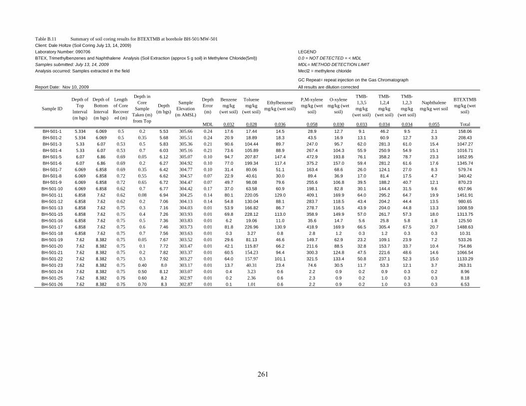
Table B.11 Summary of soil coring results for BTEXTMB at borehole BH-501/MW-501

Client: Dale Holtze (Soil Coring July 13, 14, 2009)

Laboratory Number: 090706 LEGEND

BTEX, Trimethylbenzenes and Naphthalene Analysis (Soil Extraction (approx 5 g soil) in Methylene Chloride(5ml)) 0.0 = NOT DETECTED = < MDL

Samples submitted: July 13, 14, 2009 MDL= METHOD DETECTION LIMIT

Analysis occurred: Samples extracted in the field Mecl2 = methylene chloride

GC Repeat= repeat injection on the Gas Chromatograph

Report Date: Nov 10, 2009 All results are dilution corrected

Depth

Error

(m)

Benzene

mg/kg

(wet soil)

Toluene

mg/kg

(wet soil)

Ethylbenzene

mg/kg (wet soil)

P,M-xylene

mg/kg (wet

soil)

O-xylene

mg/kg (wet

soil)

TMB-

1,3,5

mg/kg

(wet soil)

TMB-

1,2,4

mg/kg

(wet soil)

TMB-

1,2,3

mg/kg

(wet soil)

Naphthalene

mg/kg wet soil

BTEXTMB

mg/kg (wet

soil)

MDL 0.032 0.028 0.036 0.058 0.030 0.033 0.034 0.034 0.055 Total

BH-501-1 5.334 6.069 0.5 0.2 5.53 305.66 0.24 17.6 17.44 14.5 28.9 12.7 9.1 46.2 9.5 2.1 158.06

BH-501-2 5.334 6.069 0.5 0.35 5.68 305.51 0.24 20.9 18.89 18.3 43.5 16.9 13.1 60.9 12.7 3.3 208.43

BH-501-3 5.33 6.07 0.53 0.5 5.83 305.36 0.21 90.6 104.44 89.7 247.0 95.7 62.0 281.3 61.0 15.4 1047.27

BH-501-4 5.33 6.07 0.53 0.7 6.03 305.16 0.21 73.6 105.89 88.9 267.4 104.3 55.9 250.9 54.9 15.1 1016.71

BH-501-5 6.07 6.86 0.69 0.05 6.12 305.07 0.10 94.7 207.87 147.4 472.9 193.8 76.1 358.2 78.7 23.3 1652.95

BH-501-6 6.07 6.86 0.69 0.2 6.27 304.92 0.10 77.0 199.34 117.4 375.2 157.0 59.4 281.2 61.6 17.6 1345.74

BH-501-7 6.069 6.858 0.69 0.35 6.42 304.77 0.10 31.4 80.06 51.1 163.4 68.6 26.0 124.1 27.0 8.3 579.74

BH-501-8 6.069 6.858 0.72 0.55 6.62 304.57 0.07 22.9 40.61 30.0 89.4 36.9 17.0 81.4 17.5 4.7 340.42

BH-501-9 6.069 6.858 0.72 0.65 6.72 304.47 0.07 49.7 98.08 79.6 255.6 106.8 39.5 188.2 40.7 12.1 870.23

BH-501-10 6.069 6.858 0.62 0.7 6.77 304.42 0.17 37.0 63.58 60.9 198.1 82.8 30.1 144.4 31.5 9.6 657.96

BH-501-11 6.858 7.62 0.62 0.08 6.94 304.25 0.14 80.1 220.05 129.0 409.1 169.9 64.0 295.2 64.7 19.9 1451.91

BH-501-12 6.858 7.62 0.62 0.2 7.06 304.13 0.14 54.8 130.04 88.1 283.7 118.5 43.4 204.2 44.4 13.5 980.65

BH-501-13 6.858 7.62 0.75 0.3 7.16 304.03 0.01 53.9 166.82 86.7 278.7 116.5 43.9 204.0 44.8 13.3 1008.59

BH-501-15 6.858 7.62 0.75 0.4 7.26 303.93 0.01 69.8 228.12 113.0 358.9 149.9 57.0 261.7 57.3 18.0 1313.75

BH-501-16 6.858 7.62 0.75 0.5 7.36 303.83 0.01 6.2 19.06 11.0 35.6 14.7 5.6 25.8 5.8 1.8 125.50

BH-501-17 6.858 7.62 0.75 0.6 7.46 303.73 0.01 81.8 226.96 130.9 418.9 169.9 66.5 305.4 67.5 20.7 1488.63

BH-501-18 6.858 7.62 0.75 0.7 7.56 303.63 0.01 0.3 3.27 0.8 2.8 1.2 0.3 1.2 0.3 0.3 10.31

BH-501-19 7.62 8.382 0.75 0.05 7.67 303.52 0.01 29.6 81.13 46.6 149.7 62.9 23.2 109.1 23.9 7.2 533.26

BH-501-20 7.62 8.382 0.75 0.1 7.72 303.47 0.01 42.1 115.87 66.2 211.6 88.5 32.8 153.7 33.7 10.4 754.86

BH-501-21 7.62 8.382 0.75 0.2 7.82 303.37 0.01 60.5 154.23 94.4 300.3 124.8 47.5 221.6 48.6 14.6 1066.54

BH-501-22 7.62 8.382 0.75 0.3 7.92 303.27 0.01 64.0 157.97 101.1 321.5 133.4 50.8 237.1 52.3 15.0 1133.29

BH-501-23 7.62 8.382 0.75 0.40 8.0 303.17 0.01 13.7 40.31 23.4 74.6 30.5 11.7 53.3 12.1 3.7 263.31

BH-501-24 7.62 8.382 0.75 0.50 8.12 303.07 0.01 0.4 3.23 0.6 2.2 0.9 0.2 0.9 0.3 0.2 8.96

BH-501-25 7.62 8.382 0.75 0.60 8.2 302.97 0.01 0.2 2.36 0.6 2.3 0.9 0.2 1.0 0.3 0.3 8.18

BH-501-26 7.62 8.382 0.75 0.70 8.3 302.87 0.01 0.1 1.01 0.6 2.2 0.9 0.2 1.0 0.3 0.3 6.53

Sample

Elevation

(m AMSL)

Sample ID

Depth of

Top

lnterval

(m bgs)

Depth of

Bottom

Interval

(m bgs)

Length

of Core

Recover

ed (m)

Depth in

Core

Sample

Taken (m)

from Top

Depth

(m bgs)

261

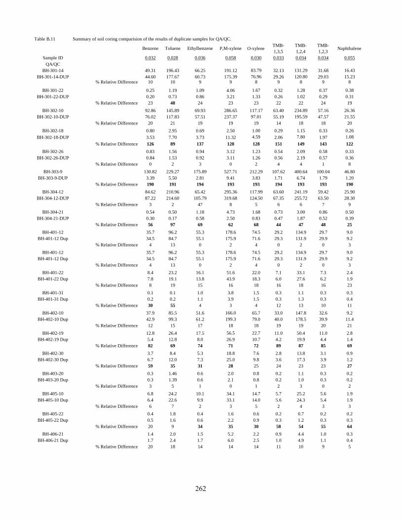
Table B.11 Summary of soil coring comparision of the results of duplicate samples for QA/QC.

Benzene Toluene Ethylbenzene P,M-xylene O-xyleneTMB-

1,3,5

TMB-

1,2,4

TMB-

1,2,3Naphthalene

Sample ID 0.032 0.028 0.036 0.058 0.030 0.033 0.034 0.034 0.055

QA/QC

BH-301-14 49.31 196.43 66.25 191.12 83.79 32.13 131.29 31.68 16.43

BH-301-14-DUP 44.60 177.67 60.73 175.39 76.96 29.26 120.80 29.03 15.23% Relative Difference 10 10 9 9 8 9 8 9 8

BH-301-22 0.25 1.19 1.09 4.06 1.67 0.32 1.28 0.37 0.38

BH-301-22-DUP 0.20 0.73 0.86 3.21 1.33 0.26 1.02 0.29 0.31

% Relative Difference 23 48 24 23 23 22 22 24 19

BH-302-10 92.86 145.89 69.93 286.65 117.17 63.40 234.89 57.16 26.36

BH-302-10-DUP 76.02 117.83 57.51 237.37 97.01 55.19 195.59 47.57 21.55

% Relative Difference 20 21 19 19 19 14 18 18 20

BH-302-18 0.80 2.95 0.69 2.50 1.00 0.29 1.15 0.33 0.26

BH-302-18-DUP 3.53 7.70 3.73 11.32 4.59 2.06 7.80 1.97 1.08

% Relative Difference 126 89 137 128 128 151 149 143 122

BH-302-26 0.83 1.56 0.94 3.12 1.23 0.54 2.09 0.58 0.33

BH-302-26-DUP 0.84 1.53 0.92 3.11 1.26 0.56 2.19 0.57 0.36

% Relative Difference 0 2 3 0 2 4 4 1 8

BH-303-9 130.82 229.27 175.89 527.71 212.29 107.62 400.64 100.04 46.80

BH-303-9-DUP 3.39 5.50 2.81 9.41 3.83 1.71 6.74 1.79 1.20

% Relative Difference 190 191 194 193 193 194 193 193 190

BH-304-12 84.62 210.96 65.42 295.36 117.99 63.60 241.19 59.42 25.90

BH-304-12-DUP 87.22 214.60 105.79 319.68 124.50 67.35 255.72 63.50 28.30

% Relative Difference 3 2 47 8 5 6 6 7 9

BH-304-21 0.54 0.50 1.18 4.73 1.68 0.73 3.00 0.86 0.50

BH-304-21-DUP 0.30 0.17 0.58 2.50 0.83 0.47 1.87 0.52 0.39

% Relative Difference 56 97 69 62 68 44 47 48 25

BH-401-12 35.7 96.2 55.3 178.6 74.5 29.2 134.9 29.7 9.0

BH-401-12 Dup 34.5 84.7 55.1 175.9 71.6 29.3 131.9 29.9 9.2

% Relative Difference 4 13 0 2 4 0 2 0 3

BH-401-12 35.7 96.2 55.3 178.6 74.5 29.2 134.9 29.7 9.0

BH-401-12 Dup 34.5 84.7 55.1 175.9 71.6 29.3 131.9 29.9 9.2

% Relative Difference 4 13 0 2 4 0 2 0 3

BH-401-22 8.4 23.2 16.1 51.6 22.0 7.1 33.1 7.3 2.4

BH-401-22 Dup 7.8 19.1 13.8 43.9 18.3 6.0 27.6 6.2 1.9

% Relative Difference 8 19 15 16 18 16 18 16 23

BH-401-31 0.1 0.1 1.0 3.8 1.5 0.3 1.1 0.3 0.3

BH-401-31 Dup 0.2 0.2 1.1 3.9 1.5 0.3 1.3 0.3 0.4

% Relative Difference 30 55 4 3 4 12 13 10 11

BH-402-10 37.9 85.5 51.6 166.0 65.7 33.0 147.8 32.6 9.2

BH-402-10 Dup 42.9 99.3 61.2 199.3 79.0 40.0 178.5 39.9 11.4

% Relative Difference 12 15 17 18 18 19 19 20 21

BH-402-19 12.8 26.4 17.5 56.5 22.7 11.0 50.4 11.0 2.8

BH-402-19 Dup 5.4 12.8 8.0 26.9 10.7 4.2 19.9 4.4 1.4

% Relative Difference 82 69 74 71 72 89 87 85 69

BH-402-30 3.7 8.4 5.3 18.8 7.6 2.8 13.8 3.1 0.9

BH-402-30 Dup 6.7 12.0 7.3 25.0 9.8 3.6 17.3 3.9 1.2

% Relative Difference 59 35 31 28 25 24 23 23 27

BH-403-20 0.3 1.46 0.6 2.0 0.8 0.2 1.1 0.3 0.2

BH-403-20 Dup 0.3 1.39 0.6 2.1 0.8 0.2 1.0 0.3 0.2

% Relative Difference 3 5 1 0 1 2 3 0 2

BH-405-10 6.8 24.2 10.1 34.1 14.7 5.7 25.2 5.6 1.9

BH-405-10 Dup 6.4 22.6 9.9 33.1 14.0 5.6 24.3 5.4 1.9

% Relative Difference 6 7 2 3 5 2 4 3 3

BH-405-22 0.4 1.8 0.4 1.6 0.6 0.2 0.7 0.2 0.2

BH-405-22 Dup 0.5 1.6 0.6 2.2 0.9 0.3 1.2 0.3 0.3

% Relative Difference 20 9 34 35 30 58 54 55 64

BH-406-21 1.4 2.0 1.5 5.2 2.2 0.9 4.4 1.0 0.3

BH-406-21 Dup 1.7 2.4 1.7 6.0 2.5 1.0 4.9 1.1 0.4

% Relative Difference 20 18 14 14 14 11 10 9 5

262

B.3 Groundwater Sample Collection and Analysis

Quality Assurance and quality control measures involved collection of duplicate and equipment blanks every 10 samples.

Groundwater samples were collected in the field in 40 mL glass teflon lined screw caped lids using a low-flow peristaltic pump equipped and zero-headspace.

Samples were preserved with 0.4 mL 10% sodium azide (v/v) in the field and immediately placed in a cooler with ice and transported back to the Organic

Geochemistry Laboratory at the University of Waterloo for analysis. Samples were stored in a refrigerator at 4 oC and analyzed within 14 days of sample

collection. Groundwater samples were analyzed for BTEXTMB and TPH using a HP 5890 capillary gas chromatograph (GC) equipped with a HP7673A

autosampler and flame ionization detector at the Organic Geochemistry laboratory at the University of Waterloo following the methods of Henderson et al. (1976).

263

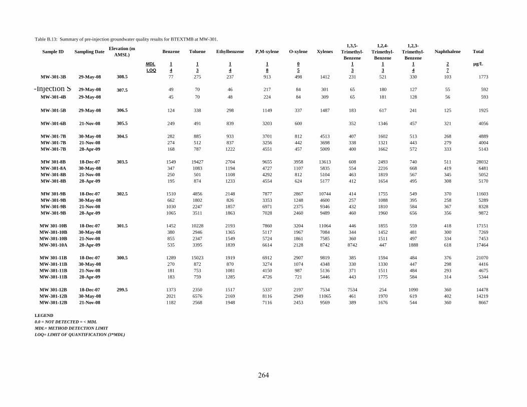
Table B.13: Summary of pre-injection groundwater quality results for BTEXTMB at MW-301.

Sample ID Sampling DateElevation (m

AMSL)Benzene Toluene Ethylbenzene P,M-xylene O-xylene Xylenes

1,3,5-

Trimethyl-

Benzene

1,2,4-

Trimethyl-

Benzene

1,2,3-

Trimethyl-

Benzene

Naphthalene Total

MDL 1 1 1 1 0 1 1 1 2 µg/L

LOQ 4 3 4 8 5 3 3 4 7

MW-301-3B 29-May-08 308.5 77 275 237 913 498 1412 231 521 330 103 1773

Characterization of Contaminants at the Site including Pre-Injection Soil Coring, Groundwater Sampling Procedures and Results29-May-08 307.5 49 70 46 217 84 301 65 180 127 55 592

MW-301-4B 29-May-08 45 70 48 224 84 309 65 181 128 56 593

MW-301-5B 29-May-08 306.5 124 338 298 1149 337 1487 183 617 241 125 1925

MW-301-6B 21-Nov-08 305.5 249 491 839 3203 600 352 1346 457 321 4056

MW-301-7B 30-May-08 304.5 282 885 933 3701 812 4513 407 1602 513 268 4889

MW-301-7B 21-Nov-08 274 512 837 3256 442 3698 338 1321 443 279 4004

MW-301-7B 28-Apr-09 168 787 1222 4551 457 5009 400 1662 572 333 5143

MW 301-8B 18-Dec-07 303.5 1549 19427 2704 9655 3958 13613 608 2493 740 511 28032

MW-301-8A 30-May-08 347 1083 1194 4727 1107 5835 554 2216 668 419 6481

MW-301-8B 21-Nov-08 250 501 1108 4292 812 5104 463 1819 567 345 5052

MW-301-8B 28-Apr-09 195 874 1233 4554 624 5177 412 1654 495 308 5170

MW 301-9B 18-Dec-07 302.5 1510 4856 2148 7877 2867 10744 414 1755 549 370 11603

MW-301-9B 30-May-08 662 1802 826 3353 1248 4600 257 1088 395 258 5289

MW-301-9B 21-Nov-08 1030 2247 1857 6971 2375 9346 432 1810 584 367 8328

MW-301-9B 28-Apr-09 1065 3511 1863 7028 2460 9489 460 1960 656 356 9872

MW 301-10B 18-Dec-07 301.5 1452 10228 2193 7860 3204 11064 446 1855 559 418 17151

MW-301-10B 30-May-08 380 2946 1365 5117 1967 7084 344 1452 481 300 7269

MW-301-10B 21-Nov-08 855 2347 1549 5724 1861 7585 360 1511 497 334 7453

MW-301-10A 28-Apr-09 535 3395 1839 6614 2128 8742 8742 447 1888 618 17464

MW 301-11B 18-Dec-07 300.5 1289 15023 1919 6912 2907 9819 385 1594 484 376 21070

MW-301-11B 30-May-08 270 872 870 3274 1074 4348 330 1330 447 298 4416

MW-301-11B 21-Nov-08 181 753 1081 4150 987 5136 371 1511 484 293 4675

MW-301-11B 28-Apr-09 183 759 1285 4726 721 5446 443 1775 584 314 5344

MW 301-12B 18-Dec-07 299.5 1373 2350 1517 5337 2197 7534 7534 254 1090 360 14478

MW-301-12B 30-May-08 2021 6576 2169 8116 2949 11065 461 1970 619 402 14219

MW-301-12B 21-Nov-08 1182 2568 1948 7116 2453 9569 389 1676 544 360 8667

LEGEND

0.0 = NOT DETECTED = < MDL

MDL= METHOD DETECTION LIMIT

LOQ= LIMIT OF QUANTIFICATION (3*MDL)

264

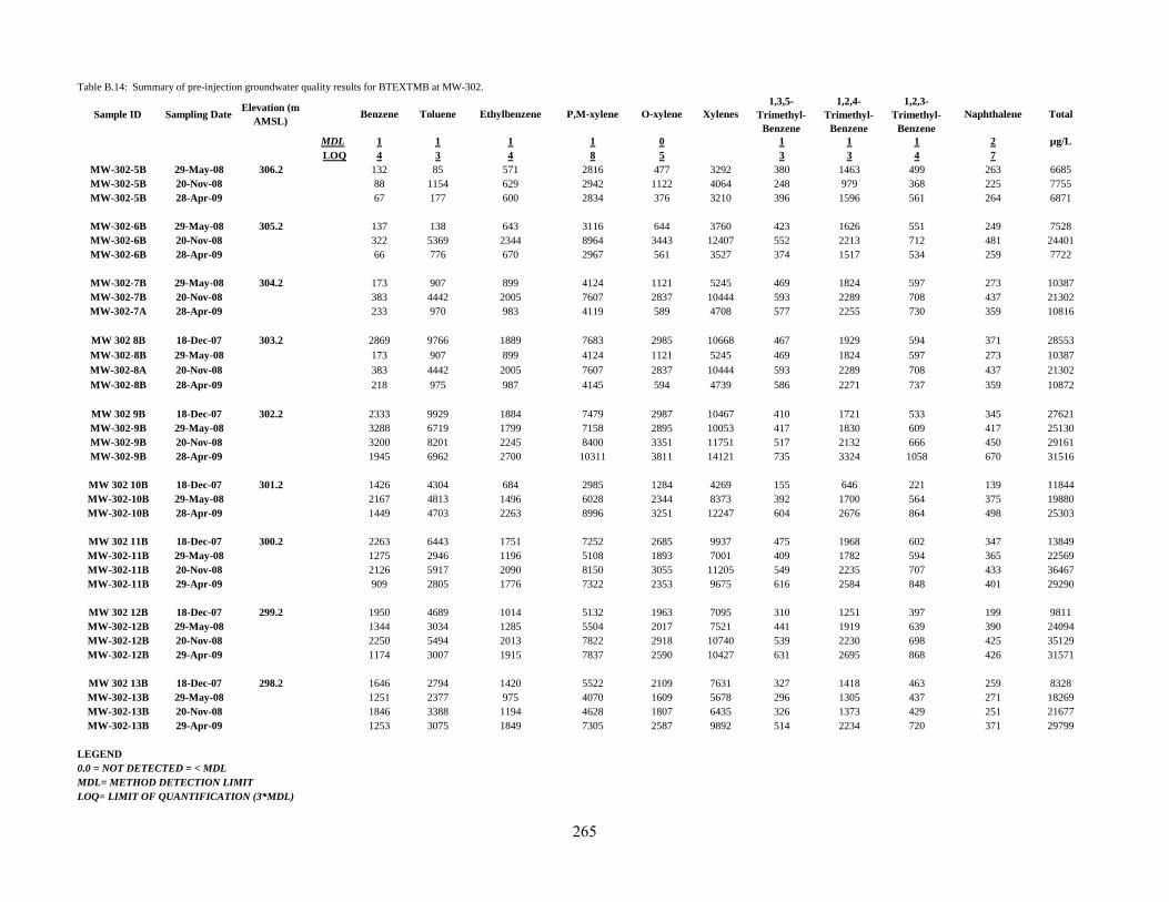
Table B.14: Summary of pre-injection groundwater quality results for BTEXTMB at MW-302.

Sample ID Sampling DateElevation (m

AMSL)Benzene Toluene Ethylbenzene P,M-xylene O-xylene Xylenes

1,3,5-

Trimethyl-

Benzene

1,2,4-

Trimethyl-

Benzene

1,2,3-

Trimethyl-

Benzene

Naphthalene Total

MDL 1 1 1 1 0 1 1 1 2 µg/L

LOQ 4 3 4 8 5 3 3 4 7

MW-302-5B 29-May-08 306.2 132 85 571 2816 477 3292 380 1463 499 263 6685

MW-302-5B 20-Nov-08 88 1154 629 2942 1122 4064 248 979 368 225 7755

MW-302-5B 28-Apr-09 67 177 600 2834 376 3210 396 1596 561 264 6871

MW-302-6B 29-May-08 305.2 137 138 643 3116 644 3760 423 1626 551 249 7528

MW-302-6B 20-Nov-08 322 5369 2344 8964 3443 12407 552 2213 712 481 24401

MW-302-6B 28-Apr-09 66 776 670 2967 561 3527 374 1517 534 259 7722

MW-302-7B 29-May-08 304.2 173 907 899 4124 1121 5245 469 1824 597 273 10387

MW-302-7B 20-Nov-08 383 4442 2005 7607 2837 10444 593 2289 708 437 21302

MW-302-7A 28-Apr-09 233 970 983 4119 589 4708 577 2255 730 359 10816

MW 302 8B 18-Dec-07 303.2 2869 9766 1889 7683 2985 10668 467 1929 594 371 28553

MW-302-8B 29-May-08 173 907 899 4124 1121 5245 469 1824 597 273 10387

MW-302-8A 20-Nov-08 383 4442 2005 7607 2837 10444 593 2289 708 437 21302

MW-302-8B 28-Apr-09 218 975 987 4145 594 4739 586 2271 737 359 10872

MW 302 9B 18-Dec-07 302.2 2333 9929 1884 7479 2987 10467 410 1721 533 345 27621

MW-302-9B 29-May-08 3288 6719 1799 7158 2895 10053 417 1830 609 417 25130

MW-302-9B 20-Nov-08 3200 8201 2245 8400 3351 11751 517 2132 666 450 29161

MW-302-9B 28-Apr-09 1945 6962 2700 10311 3811 14121 735 3324 1058 670 31516

MW 302 10B 18-Dec-07 301.2 1426 4304 684 2985 1284 4269 155 646 221 139 11844

MW-302-10B 29-May-08 2167 4813 1496 6028 2344 8373 392 1700 564 375 19880

MW-302-10B 28-Apr-09 1449 4703 2263 8996 3251 12247 604 2676 864 498 25303

MW 302 11B 18-Dec-07 300.2 2263 6443 1751 7252 2685 9937 475 1968 602 347 13849

MW-302-11B 29-May-08 1275 2946 1196 5108 1893 7001 409 1782 594 365 22569

MW-302-11B 20-Nov-08 2126 5917 2090 8150 3055 11205 549 2235 707 433 36467

MW-302-11B 29-Apr-09 909 2805 1776 7322 2353 9675 616 2584 848 401 29290

MW 302 12B 18-Dec-07 299.2 1950 4689 1014 5132 1963 7095 310 1251 397 199 9811

MW-302-12B 29-May-08 1344 3034 1285 5504 2017 7521 441 1919 639 390 24094

MW-302-12B 20-Nov-08 2250 5494 2013 7822 2918 10740 539 2230 698 425 35129

MW-302-12B 29-Apr-09 1174 3007 1915 7837 2590 10427 631 2695 868 426 31571

MW 302 13B 18-Dec-07 298.2 1646 2794 1420 5522 2109 7631 327 1418 463 259 8328

MW-302-13B 29-May-08 1251 2377 975 4070 1609 5678 296 1305 437 271 18269

MW-302-13B 20-Nov-08 1846 3388 1194 4628 1807 6435 326 1373 429 251 21677

MW-302-13B 29-Apr-09 1253 3075 1849 7305 2587 9892 514 2234 720 371 29799

LEGEND

0.0 = NOT DETECTED = < MDL

MDL= METHOD DETECTION LIMIT

LOQ= LIMIT OF QUANTIFICATION (3*MDL)

265

Table B.15: Summary of pre-injection groundwater quality results for BTEXTMB at MW-303.

Sample ID Sampling DateElevation (m

AMSL)Benzene Toluene Ethylbenzene P,M-xylene O-xylene Xylenes

1,3,5-

Trimethyl-

Benzene

1,2,4-

Trimethyl-

Benzene

1,2,3-

Trimethyl-

Benzene

Naphthalene Total

MDL 1 1 1 1 0 1 1 1 2 µg/L

LOQ 4 3 4 8 5 3 3 4 7

MW-303-3B 30-May-08 308.0 920 453 503 3600 1241 4840.8 514 1751 670 189 9841

MW-303-3B 28-Apr-09 408.73 30.81 184.72 1676.21 389.28 2065.5 354.93 680.57 358.69 122.58 4207

Characterization of Contaminants at the Site including Pre-Injection Soil Coring, Groundwater Sampling Procedures and ResultsMW-303-4B 28-Apr-09 307.0 668.49 211.24 1012.16 5384.13 661.26 6045.4 579.46 2220.39 808.54 343.04 11889

MW-303-6B 30-May-08 305.0 2049 4574 1843 6929 2469 9399 758 3025 912 656 23216

MW-303-6A 21-Nov-08 1463.97 3024.70 1819.16 7597.75 2530.71 10128.47 611.41 2476.01 767.72 468.47 20760

MW-303-6A 28-Apr-09 793.31 712.39 1728.58 7657.80 2094.45 9752.26 636.00 2718.53 888.39 434.31 17664

MW-303-7B 30-May-08 304.0 2766 6837 1539 6320 2370 8689.40 436 1746 564 329 22905

MW-303-7B 21-Nov-08 1795.78 5431.53 1903.37 7887.99 2861.73 10749.72 640.10 2578.68 791.20 493.84 24384

MW-303-7A 29-Apr-09 662.33 3218.95 3445.71 13129.41 4612.39 17741.80 1486.66 6632.42 2052.03 1206.14 36446

MW 303-10B 18-Dec-07 301.0 1117.4 2948.4 1262.3 5108.3 1714.0 6822.3 375.1 1553.8 479.3 272.6 14831

MW-303-10B 30-May-08 272 1005 985 4586 1484 6070 513 2173 693 86 11797

MW-303-10B 21-Nov-08 486.24 1666.09 1439.40 6245.00 1863.61 8109 574.34 2345.89 730.61 391.01 15742

MW-303-10A 29-Apr-09 271.66 689.23 1156.75 5067.29 1379.24 6447 541.82 2207.91 714.74 302.01 12331

MW 303-11B 18-Dec-07 300.0 482.6 1100.6 1118.2 4498.0 1472.9 5971.0 381.9 1587.8 493.2 265.0 11400

MW-303-11B 30-May-08 163 324 1083 5024 1527 6551 627 2564 779 334 12425

MW-303-11B 21-Nov-08 276.61 803.03 1446.22 6203.28 1782.54 7986 630.68 2596.02 791.84 421.22 14951

MW-303-11B 29-Apr-09 101.41 358.27 1076.22 4858.85 1288.52 6147 640.42 2706.49 847.89 349.23 12227

LEGEND

0.0 = NOT DETECTED = < MDL

MDL= METHOD DETECTION LIMIT

LOQ= LIMIT OF QUANTIFICATION (3*MDL)

266

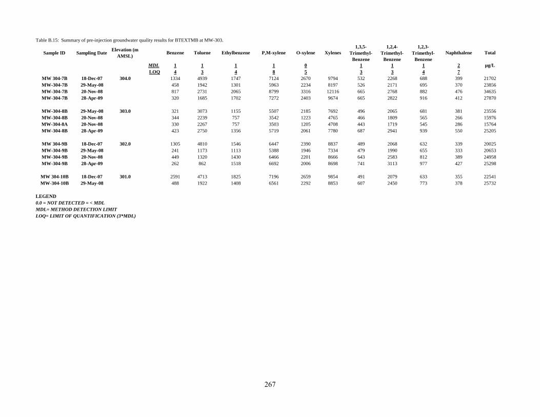
Table B.15: Summary of pre-injection groundwater quality results for BTEXTMB at MW-303.

Sample ID Sampling DateElevation (m

AMSL)Benzene Toluene Ethylbenzene P,M-xylene O-xylene Xylenes

1,3,5-

Trimethyl-

Benzene

1,2,4-

Trimethyl-

Benzene

1,2,3-

Trimethyl-

Benzene

Naphthalene Total

MDL 1 1 1 1 0 1 1 1 2 µg/L

LOQ 4 3 4 8 5 3 3 4 7

MW 304-7B 18-Dec-07 304.0 1334 4939 1747 7124 2670 9794 532 2268 688 399 21702

MW-304-7B 29-May-08 458 1942 1301 5963 2234 8197 526 2171 695 370 23856

MW-304-7B 20-Nov-08 817 2731 2065 8799 3316 12116 665 2768 882 476 34635

MW-304-7B 28-Apr-09 320 1685 1702 7272 2403 9674 665 2822 916 412 27870

MW-304-8B 29-May-08 303.0 321 3073 1155 5507 2185 7692 496 2065 681 381 23556

MW-304-8B 20-Nov-08 344 2239 757 3542 1223 4765 466 1809 565 266 15976

MW-304-8A 20-Nov-08 330 2267 757 3503 1205 4708 443 1719 545 286 15764

MW-304-8B 28-Apr-09 423 2750 1356 5719 2061 7780 687 2941 939 550 25205

MW 304-9B 18-Dec-07 302.0 1305 4810 1546 6447 2390 8837 489 2068 632 339 20025

MW-304-9B 29-May-08 241 1173 1113 5388 1946 7334 479 1990 655 333 20653

MW-304-9B 20-Nov-08 449 1320 1430 6466 2201 8666 643 2583 812 389 24958

MW-304-9B 28-Apr-09 262 862 1518 6692 2006 8698 741 3113 977 427 25298

MW 304-10B 18-Dec-07 301.0 2591 4713 1825 7196 2659 9854 491 2079 633 355 22541

MW-304-10B 29-May-08 488 1922 1408 6561 2292 8853 607 2450 773 378 25732

LEGEND

0.0 = NOT DETECTED = < MDL

MDL= METHOD DETECTION LIMIT

LOQ= LIMIT OF QUANTIFICATION (3*MDL)

267

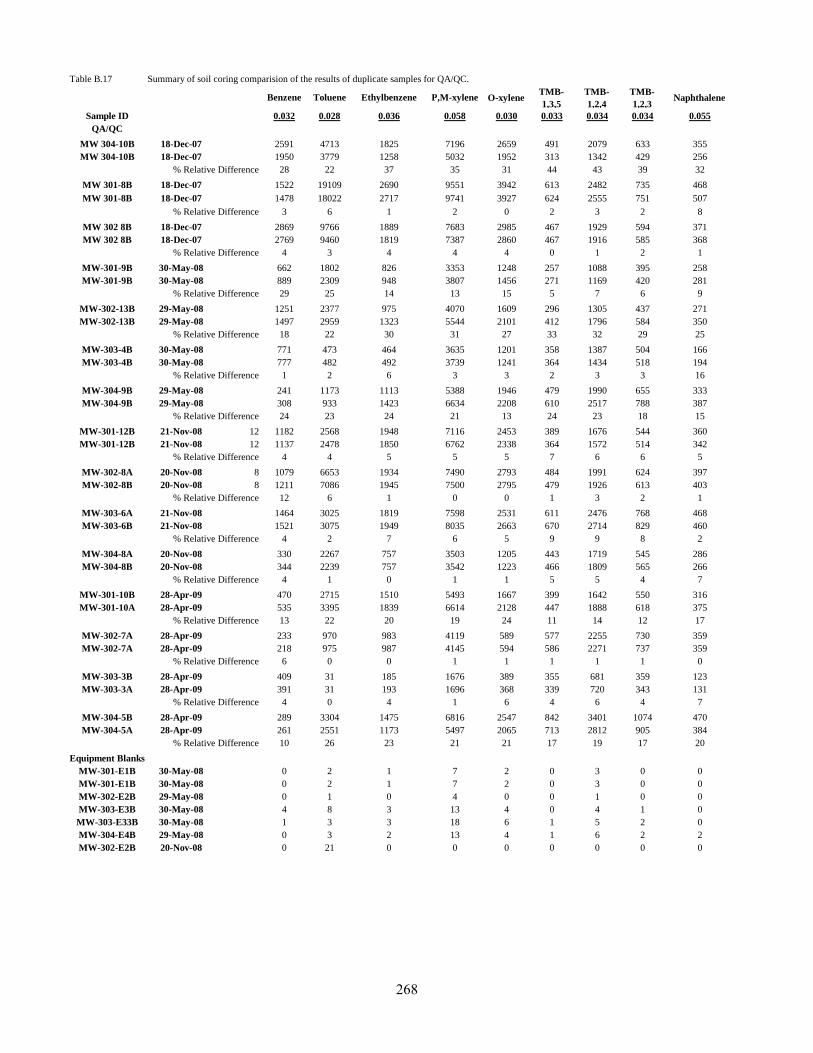
Table B.17 Summary of soil coring comparision of the results of duplicate samples for QA/QC.

Benzene Toluene Ethylbenzene P,M-xylene O-xyleneTMB-

1,3,5

TMB-

1,2,4

TMB-

1,2,3Naphthalene

Sample ID 0.032 0.028 0.036 0.058 0.030 0.033 0.034 0.034 0.055

QA/QC

MW 304-10B 18-Dec-07 2591 4713 1825 7196 2659 491 2079 633 355

MW 304-10B 18-Dec-07 1950 3779 1258 5032 1952 313 1342 429 256

% Relative Difference 28 22 37 35 31 44 43 39 32

MW 301-8B 18-Dec-07 1522 19109 2690 9551 3942 613 2482 735 468

MW 301-8B 18-Dec-07 1478 18022 2717 9741 3927 624 2555 751 507

% Relative Difference 3 6 1 2 0 2 3 2 8

MW 302 8B 18-Dec-07 2869 9766 1889 7683 2985 467 1929 594 371

MW 302 8B 18-Dec-07 2769 9460 1819 7387 2860 467 1916 585 368

% Relative Difference 4 3 4 4 4 0 1 2 1

MW-301-9B 30-May-08 662 1802 826 3353 1248 257 1088 395 258

MW-301-9B 30-May-08 889 2309 948 3807 1456 271 1169 420 281

% Relative Difference 29 25 14 13 15 5 7 6 9

MW-302-13B 29-May-08 1251 2377 975 4070 1609 296 1305 437 271

MW-302-13B 29-May-08 1497 2959 1323 5544 2101 412 1796 584 350

% Relative Difference 18 22 30 31 27 33 32 29 25

MW-303-4B 30-May-08 771 473 464 3635 1201 358 1387 504 166

MW-303-4B 30-May-08 777 482 492 3739 1241 364 1434 518 194

% Relative Difference 1 2 6 3 3 2 3 3 16

MW-304-9B 29-May-08 241 1173 1113 5388 1946 479 1990 655 333

MW-304-9B 29-May-08 308 933 1423 6634 2208 610 2517 788 387

% Relative Difference 24 23 24 21 13 24 23 18 15

MW-301-12B 21-Nov-08 12 1182 2568 1948 7116 2453 389 1676 544 360

MW-301-12B 21-Nov-08 12 1137 2478 1850 6762 2338 364 1572 514 342

% Relative Difference 4 4 5 5 5 7 6 6 5

MW-302-8A 20-Nov-08 8 1079 6653 1934 7490 2793 484 1991 624 397

MW-302-8B 20-Nov-08 8 1211 7086 1945 7500 2795 479 1926 613 403

% Relative Difference 12 6 1 0 0 1 3 2 1

MW-303-6A 21-Nov-08 1464 3025 1819 7598 2531 611 2476 768 468

MW-303-6B 21-Nov-08 1521 3075 1949 8035 2663 670 2714 829 460

% Relative Difference 4 2 7 6 5 9 9 8 2

MW-304-8A 20-Nov-08 330 2267 757 3503 1205 443 1719 545 286

MW-304-8B 20-Nov-08 344 2239 757 3542 1223 466 1809 565 266

% Relative Difference 4 1 0 1 1 5 5 4 7

MW-301-10B 28-Apr-09 470 2715 1510 5493 1667 399 1642 550 316

MW-301-10A 28-Apr-09 535 3395 1839 6614 2128 447 1888 618 375

% Relative Difference 13 22 20 19 24 11 14 12 17

MW-302-7A 28-Apr-09 233 970 983 4119 589 577 2255 730 359

MW-302-7A 28-Apr-09 218 975 987 4145 594 586 2271 737 359

% Relative Difference 6 0 0 1 1 1 1 1 0

MW-303-3B 28-Apr-09 409 31 185 1676 389 355 681 359 123

MW-303-3A 28-Apr-09 391 31 193 1696 368 339 720 343 131

% Relative Difference 4 0 4 1 6 4 6 4 7

MW-304-5B 28-Apr-09 289 3304 1475 6816 2547 842 3401 1074 470

MW-304-5A 28-Apr-09 261 2551 1173 5497 2065 713 2812 905 384

% Relative Difference 10 26 23 21 21 17 19 17 20

Equipment Blanks

MW-301-E1B 30-May-08 0 2 1 7 2 0 3 0 0

MW-301-E1B 30-May-08 0 2 1 7 2 0 3 0 0

MW-302-E2B 29-May-08 0 1 0 4 0 0 1 0 0

MW-303-E3B 30-May-08 4 8 3 13 4 0 4 1 0

MW-303-E33B 30-May-08 1 3 3 18 6 1 5 2 0

MW-304-E4B 29-May-08 0 3 2 13 4 1 6 2 2

MW-302-E2B 20-Nov-08 0 21 0 0 0 0 0 0 0

268

Appendix C

Microcosm Experiment

269

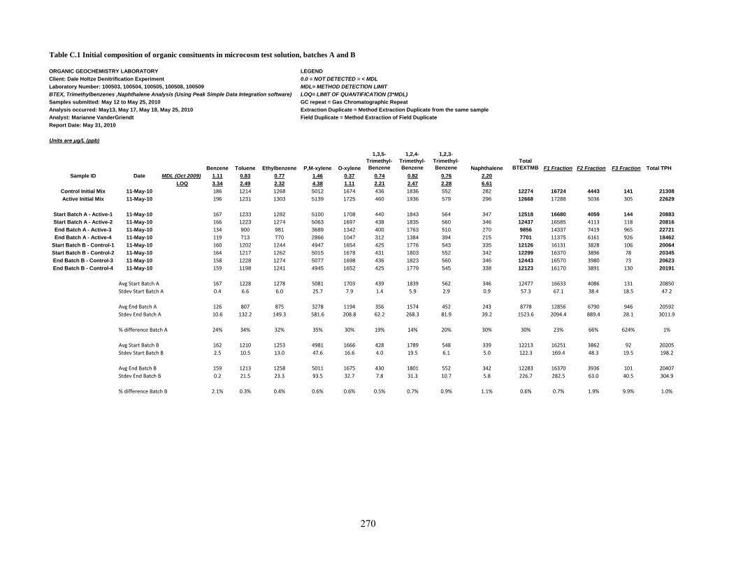
Table C.1 Initial composition of organic consituents in microcosm test solution, batches A and B

ORGANIC GEOCHEMISTRY LABORATORY LEGEND

Client: Dale Holtze Denitrification Experiment 0.0 = NOT DETECTED = < MDL

Laboratory Number: 100503, 100504, 100505, 100508, 100509 MDL= METHOD DETECTION LIMIT

BTEX, Trimethylbenzenes ,Naphthalene Analysis (Using Peak Simple Data Integration software) LOQ= LIMIT OF QUANTIFICATION (3*MDL)

Samples submitted: May 12 to May 25, 2010 GC repeat = Gas Chromatographic Repeat

Analysis occurred: May13, May 17, May 18, May 25, 2010 Extraction Duplicate = Method Extraction Duplicate from the same sample

Analyst: Marianne VanderGriendt Field Duplicate = Method Extraction of Field Duplicate

Report Date: May 31, 2010

Units are μg/L (ppb)

Benzene Toluene Ethylbenzene P,M-xylene O-xylene

1,3,5-

Trimethyl-

Benzene

1,2,4-

Trimethyl-

Benzene

1,2,3-

Trimethyl-

Benzene Naphthalene

Total

BTEXTMB F1 Fraction F2 Fraction F3 Fraction Total TPH

Sample ID Date MDL (Oct 2009) 1.11 0.83 0.77 1.46 0.37 0.74 0.82 0.76 2.20

LOQ 3.34 2.49 2.32 4.38 1.11 2.21 2.47 2.28 6.61

Control Initial Mix 11-May-10 186 1214 1268 5012 1674 436 1836 552 282 12274 16724 4443 141 21308

Active Initial Mix 11-May-10 196 1231 1303 5139 1725 460 1936 579 296 12668 17288 5036 305 22629

Start Batch A - Active-1 11-May-10 167 1233 1282 5100 1708 440 1843 564 347 12518 16680 4059 144 20883

Start Batch A - Active-2 11-May-10 166 1223 1274 5063 1697 438 1835 560 346 12437 16585 4113 118 20816

End Batch A - Active-3 11-May-10 134 900 981 3689 1342 400 1763 510 270 9856 14337 7419 965 22721

End Batch A - Active-4 11-May-10 119 713 770 2866 1047 312 1384 394 215 7701 11375 6161 926 18462

Start Batch B - Control-1 11-May-10 160 1202 1244 4947 1654 425 1776 543 335 12126 16131 3828 106 20064

Start Batch B - Control-2 11-May-10 164 1217 1262 5015 1678 431 1803 552 342 12299 16370 3896 78 20345

End Batch B - Control-3 11-May-10 158 1228 1274 5077 1698 436 1823 560 346 12443 16570 3980 73 20623

End Batch B - Control-4 11-May-10 159 1198 1241 4945 1652 425 1779 545 338 12123 16170 3891 130 20191

Avg Start Batch A 167 1228 1278 5081 1703 439 1839 562 346 12477 16633 4086 131 20850

Stdev Start Batch A 0.4 6.6 6.0 25.7 7.9 1.4 5.9 2.9 0.9 57.3 67.1 38.4 18.5 47.2

Avg End Batch A 126 807 875 3278 1194 356 1574 452 243 8778 12856 6790 946 20592

Stdev End Batch A 10.6 132.2 149.3 581.6 208.8 62.2 268.3 81.9 39.2 1523.6 2094.4 889.4 28.1 3011.9

% difference Batch A 24% 34% 32% 35% 30% 19% 14% 20% 30% 30% 23% 66% 624% 1%

Avg Start Batch B 162 1210 1253 4981 1666 428 1789 548 339 12213 16251 3862 92 20205

Stdev Start Batch B 2.5 10.5 13.0 47.6 16.6 4.0 19.5 6.1 5.0 122.3 169.4 48.3 19.5 198.2

Avg End Batch B 159 1213 1258 5011 1675 430 1801 552 342 12283 16370 3936 101 20407

Stdev End Batch B 0.2 21.5 23.3 93.5 32.7 7.8 31.3 10.7 5.8 226.7 282.5 63.0 40.5 304.9

% difference Batch B 2.1% 0.3% 0.4% 0.6% 0.6% 0.5% 0.7% 0.9% 1.1% 0.6% 0.7% 1.9% 9.9% 1.0%

270

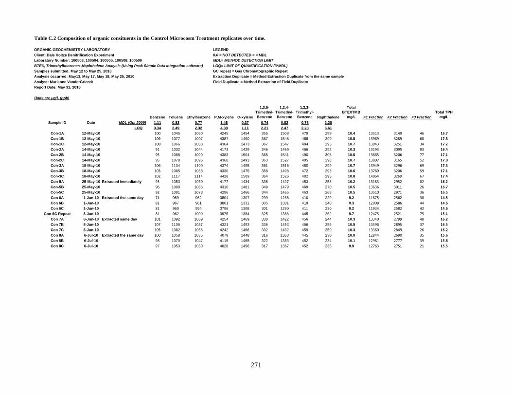
Table C.2 Composition of organic consituents in the Control Microcosm Treatment replicates over time.

ORGANIC GEOCHEMISTRY LABORATORY LEGEND

Client: Dale Holtze Denitrification Experiment 0.0 = NOT DETECTED = < MDL

Laboratory Number: 100503, 100504, 100505, 100508, 100509 MDL= METHOD DETECTION LIMIT

BTEX, Trimethylbenzenes ,Naphthalene Analysis (Using Peak Simple Data Integration software) LOQ= LIMIT OF QUANTIFICATION (3*MDL)

Samples submitted: May 12 to May 25, 2010 GC repeat = Gas Chromatographic Repeat

Analysis occurred: May13, May 17, May 18, May 25, 2010 Extraction Duplicate = Method Extraction Duplicate from the same sample

Analyst: Marianne VanderGriendt Field Duplicate = Method Extraction of Field Duplicate

Report Date: May 31, 2010

Units are μg/L (ppb)

Benzene Toluene Ethylbenzene P,M-xylene O-xylene

1,3,5-

Trimethyl-

Benzene

1,2,4-

Trimethyl-

Benzene

1,2,3-

Trimethyl-

Benzene Naphthalene

Total

BTEXTMB

mg/L F1 Fraction F2 Fraction F3 Fraction

Total TPH

mg/L

Sample ID Date MDL (Oct 2009) 1.11 0.83 0.77 1.46 0.37 0.74 0.82 0.76 2.20

LOQ 3.34 2.49 2.32 4.38 1.11 2.21 2.47 2.28 6.61

Con-1A 12-May-10 100 1045 1060 4245 1454 355 1508 479 299 10.4 13513 3149 46 16.7

Con-1B 12-May-10 109 1077 1097 4387 1490 367 1548 488 299 10.8 13969 3289 68 17.3

Con-1C 12-May-10 108 1066 1088 4364 1473 367 1547 484 295 10.7 13943 3251 34 17.2

Con-2A 14-May-10 91 1032 1044 4173 1429 346 1469 466 292 10.3 13193 3095 83 16.4

Con-2B 14-May-10 95 1085 1099 4383 1504 365 1541 490 305 10.8 13865 3206 77 17.1

Con-2C 14-May-10 95 1078 1096 4368 1493 363 1527 485 298 10.7 13807 3165 52 17.0

Con-3A 18-May-10 106 1104 1100 4374 1495 361 1516 480 299 10.7 13949 3296 69 17.3

Con-3B 18-May-10 103 1085 1088 4330 1475 358 1498 472 293 10.6 13789 3206 59 17.1

Con-3C 18-May-10 102 1117 1114 4428 1509 364 1526 482 295 10.8 14064 3269 67 17.4

Con-5A 25-May-10 Extracted Immediately 93 1053 1050 4177 1434 336 1427 453 258 10.2 13183 2952 82 16.2

Con-5B 25-May-10 96 1090 1086 4316 1481 349 1479 469 270 10.5 13636 3011 26 16.7

Con-5C 25-May-10 92 1081 1078 4296 1466 344 1465 463 268 10.5 13510 2971 36 16.5

Con 6A 1-Jun-10 Extracted the same day 74 959 952 3804 1307 299 1285 410 229 9.2 11875 2562 30 14.5

Con 6B 1-Jun-10 81 967 961 3801 1331 305 1301 419 240 9.3 12008 2586 44 14.6

Con 6C 1-Jun-10 81 960 954 3796 1308 301 1290 411 230 9.2 11934 2582 42 14.6

Con-6C Repeat 8-Jun-10 81 962 1000 3975 1384 325 1388 445 262 9.7 12475 2521 75 15.1

Con 7A 8-Jun-10 Extracted same day 101 1092 1069 4254 1469 330 1422 456 244 10.3 13340 2799 40 16.2

Con 7B 8-Jun-10 107 1106 1087 4321 1493 336 1453 466 255 10.5 13596 2895 37 16.5

Con 7C 8-Jun-10 105 1082 1066 4242 1466 332 1432 459 250 10.3 13360 2849 26 16.2

Con 8A 6-Jul-10 Extracted the same day 100 1058 1035 4079 1448 316 1363 445 230 10.0 12844 2690 35 15.6

Con 8B 6-Jul-10 98 1070 1047 4115 1465 322 1383 452 234 10.1 12981 2777 39 15.8

Con 8C 6-Jul-10 97 1053 1030 4028 1456 317 1367 452 236 9.9 12763 2751 21 15.5

271

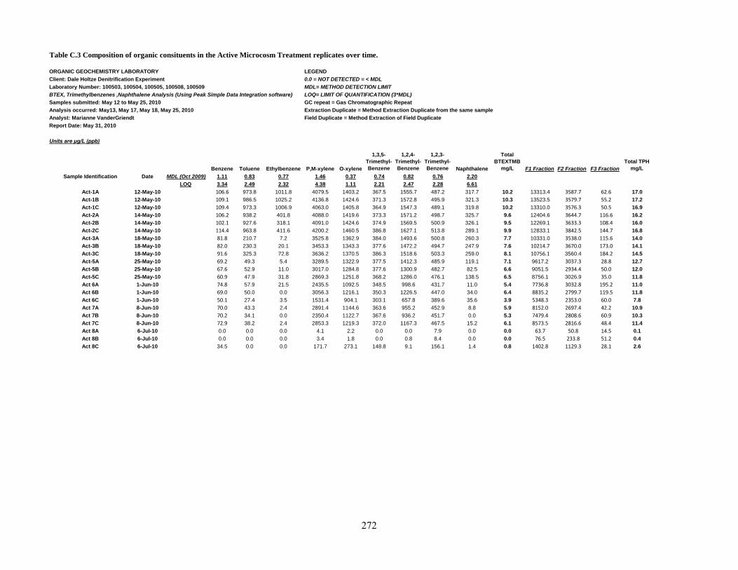
Table C.3 Composition of organic consituents in the Active Microcosm Treatment replicates over time.

ORGANIC GEOCHEMISTRY LABORATORY LEGEND

Client: Dale Holtze Denitrification Experiment 0.0 = NOT DETECTED = < MDL

Laboratory Number: 100503, 100504, 100505, 100508, 100509 MDL= METHOD DETECTION LIMIT

BTEX, Trimethylbenzenes ,Naphthalene Analysis (Using Peak Simple Data Integration software) LOQ= LIMIT OF QUANTIFICATION (3*MDL)

Samples submitted: May 12 to May 25, 2010 GC repeat = Gas Chromatographic Repeat

Analysis occurred: May13, May 17, May 18, May 25, 2010 Extraction Duplicate = Method Extraction Duplicate from the same sample

Analyst: Marianne VanderGriendt Field Duplicate = Method Extraction of Field Duplicate

Report Date: May 31, 2010

Units are μg/L (ppb)

Benzene Toluene Ethylbenzene P,M-xylene O-xylene

1,3,5-

Trimethyl-

Benzene

1,2,4-

Trimethyl-

Benzene

1,2,3-

Trimethyl-

Benzene Naphthalene

Total

BTEXTMB

mg/L F1 Fraction F2 Fraction F3 Fraction

Total TPH

mg/L

Sample Identification Date MDL (Oct 2009) 1.11 0.83 0.77 1.46 0.37 0.74 0.82 0.76 2.20

LOQ 3.34 2.49 2.32 4.38 1.11 2.21 2.47 2.28 6.61

Act-1A 12-May-10 106.6 973.8 1011.8 4079.5 1403.2 367.5 1555.7 487.2 317.7 10.2 13313.4 3587.7 62.6 17.0

Act-1B 12-May-10 109.1 986.5 1025.2 4136.8 1424.6 371.3 1572.8 495.9 321.3 10.3 13523.5 3579.7 55.2 17.2

Act-1C 12-May-10 109.4 973.3 1006.9 4063.0 1405.8 364.9 1547.3 489.1 319.8 10.2 13310.0 3576.3 50.5 16.9

Act-2A 14-May-10 106.2 938.2 401.8 4088.0 1419.6 373.3 1571.2 498.7 325.7 9.6 12404.6 3644.7 116.6 16.2

Act-2B 14-May-10 102.1 927.6 318.1 4091.0 1424.6 374.9 1569.5 500.9 326.1 9.5 12269.1 3633.3 108.4 16.0

Act-2C 14-May-10 114.4 963.8 411.6 4200.2 1460.5 386.8 1627.1 513.8 289.1 9.9 12833.1 3842.5 144.7 16.8

Act-3A 18-May-10 81.8 210.7 7.2 3525.8 1362.9 384.0 1493.6 500.8 260.3 7.7 10331.0 3538.0 115.6 14.0

Act-3B 18-May-10 82.0 230.3 20.1 3453.3 1343.3 377.6 1472.2 494.7 247.9 7.6 10214.7 3670.0 173.0 14.1

Act-3C 18-May-10 91.6 325.3 72.8 3636.2 1370.5 386.3 1518.6 503.3 259.0 8.1 10756.1 3560.4 184.2 14.5

Act-5A 25-May-10 69.2 49.3 5.4 3289.5 1322.9 377.5 1412.3 485.9 119.1 7.1 9617.2 3037.3 28.8 12.7

Act-5B 25-May-10 67.6 52.9 11.0 3017.0 1284.8 377.6 1300.9 482.7 82.5 6.6 9051.5 2934.4 50.0 12.0

Act-5C 25-May-10 60.9 47.9 31.8 2869.3 1251.8 368.2 1286.0 476.1 138.5 6.5 8756.1 3026.9 35.0 11.8

Act 6A 1-Jun-10 74.8 57.9 21.5 2435.5 1092.5 348.5 998.6 431.7 11.0 5.4 7736.8 3032.8 195.2 11.0

Act 6B 1-Jun-10 69.0 50.0 0.0 3056.3 1216.1 350.3 1226.5 447.0 34.0 6.4 8835.2 2799.7 119.5 11.8

Act 6C 1-Jun-10 50.1 27.4 3.5 1531.4 904.1 303.1 657.8 389.6 35.6 3.9 5348.3 2353.0 60.0 7.8

Act 7A 8-Jun-10 70.0 43.3 2.4 2891.4 1144.6 363.6 955.2 452.9 8.8 5.9 8152.0 2697.4 42.2 10.9

Act 7B 8-Jun-10 70.2 34.1 0.0 2350.4 1122.7 367.6 936.2 451.7 0.0 5.3 7479.4 2808.6 60.9 10.3

Act 7C 8-Jun-10 72.9 38.2 2.4 2853.3 1219.3 372.0 1167.3 467.5 15.2 6.1 8573.5 2816.6 48.4 11.4

Act 8A 6-Jul-10 0.0 0.0 0.0 4.1 2.2 0.0 0.0 7.9 0.0 0.0 63.7 50.8 14.5 0.1

Act 8B 6-Jul-10 0.0 0.0 0.0 3.4 1.8 0.0 0.8 8.4 0.0 0.0 76.5 233.8 51.2 0.4

Act 8C 6-Jul-10 34.5 0.0 0.0 171.7 273.1 148.8 9.1 156.1 1.4 0.8 1402.8 1129.3 28.1 2.6

272

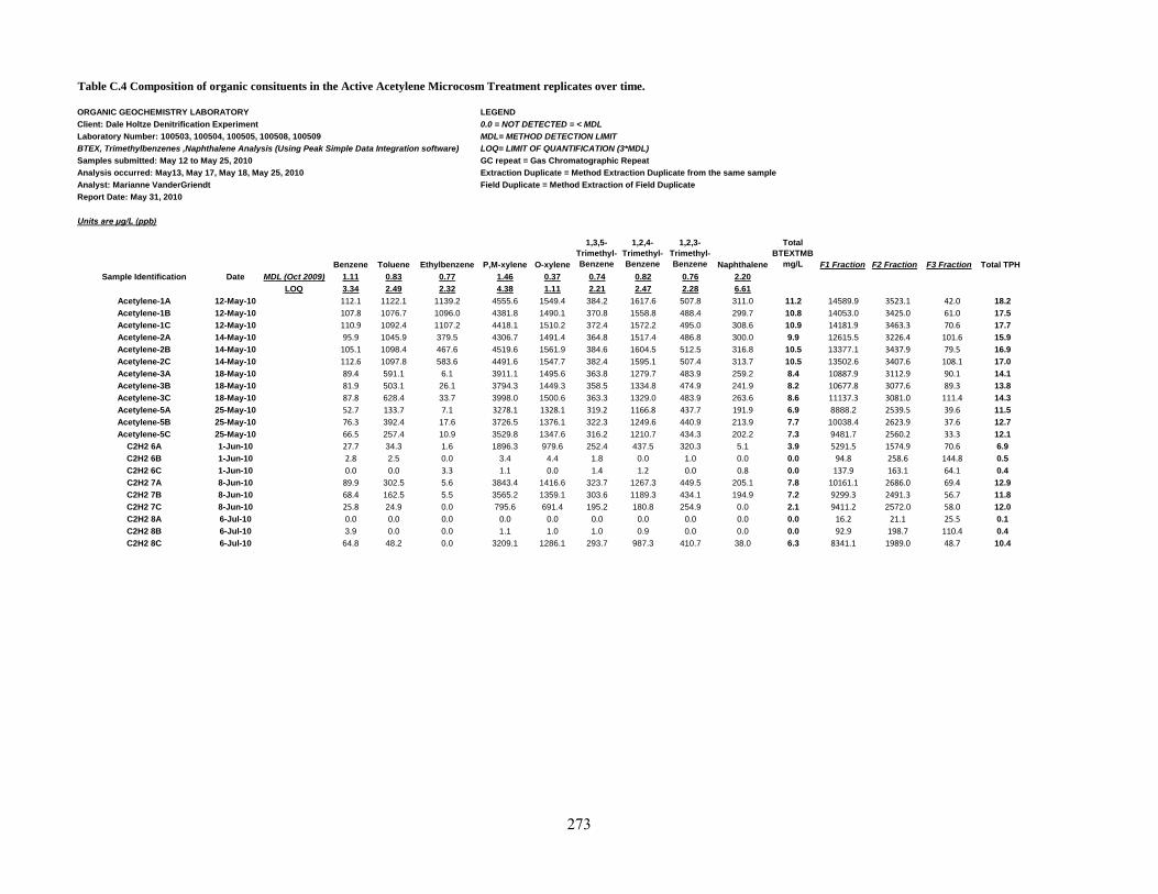
Table C.4 Composition of organic consituents in the Active Acetylene Microcosm Treatment replicates over time.

ORGANIC GEOCHEMISTRY LABORATORY LEGEND

Client: Dale Holtze Denitrification Experiment 0.0 = NOT DETECTED = < MDL

Laboratory Number: 100503, 100504, 100505, 100508, 100509 MDL= METHOD DETECTION LIMIT

BTEX, Trimethylbenzenes ,Naphthalene Analysis (Using Peak Simple Data Integration software) LOQ= LIMIT OF QUANTIFICATION (3*MDL)

Samples submitted: May 12 to May 25, 2010 GC repeat = Gas Chromatographic Repeat

Analysis occurred: May13, May 17, May 18, May 25, 2010 Extraction Duplicate = Method Extraction Duplicate from the same sample

Analyst: Marianne VanderGriendt Field Duplicate = Method Extraction of Field Duplicate

Report Date: May 31, 2010

Units are μg/L (ppb)

Benzene Toluene Ethylbenzene P,M-xylene O-xylene

1,3,5-

Trimethyl-

Benzene

1,2,4-

Trimethyl-

Benzene

1,2,3-

Trimethyl-

Benzene Naphthalene

Total

BTEXTMB

mg/L F1 Fraction F2 Fraction F3 Fraction Total TPH

Sample Identification Date MDL (Oct 2009) 1.11 0.83 0.77 1.46 0.37 0.74 0.82 0.76 2.20

LOQ 3.34 2.49 2.32 4.38 1.11 2.21 2.47 2.28 6.61

Acetylene-1A 12-May-10 112.1 1122.1 1139.2 4555.6 1549.4 384.2 1617.6 507.8 311.0 11.2 14589.9 3523.1 42.0 18.2

Acetylene-1B 12-May-10 107.8 1076.7 1096.0 4381.8 1490.1 370.8 1558.8 488.4 299.7 10.8 14053.0 3425.0 61.0 17.5

Acetylene-1C 12-May-10 110.9 1092.4 1107.2 4418.1 1510.2 372.4 1572.2 495.0 308.6 10.9 14181.9 3463.3 70.6 17.7

Acetylene-2A 14-May-10 95.9 1045.9 379.5 4306.7 1491.4 364.8 1517.4 486.8 300.0 9.9 12615.5 3226.4 101.6 15.9

Acetylene-2B 14-May-10 105.1 1098.4 467.6 4519.6 1561.9 384.6 1604.5 512.5 316.8 10.5 13377.1 3437.9 79.5 16.9

Acetylene-2C 14-May-10 112.6 1097.8 583.6 4491.6 1547.7 382.4 1595.1 507.4 313.7 10.5 13502.6 3407.6 108.1 17.0

Acetylene-3A 18-May-10 89.4 591.1 6.1 3911.1 1495.6 363.8 1279.7 483.9 259.2 8.4 10887.9 3112.9 90.1 14.1

Acetylene-3B 18-May-10 81.9 503.1 26.1 3794.3 1449.3 358.5 1334.8 474.9 241.9 8.2 10677.8 3077.6 89.3 13.8

Acetylene-3C 18-May-10 87.8 628.4 33.7 3998.0 1500.6 363.3 1329.0 483.9 263.6 8.6 11137.3 3081.0 111.4 14.3

Acetylene-5A 25-May-10 52.7 133.7 7.1 3278.1 1328.1 319.2 1166.8 437.7 191.9 6.9 8888.2 2539.5 39.6 11.5

Acetylene-5B 25-May-10 76.3 392.4 17.6 3726.5 1376.1 322.3 1249.6 440.9 213.9 7.7 10038.4 2623.9 37.6 12.7

Acetylene-5C 25-May-10 66.5 257.4 10.9 3529.8 1347.6 316.2 1210.7 434.3 202.2 7.3 9481.7 2560.2 33.3 12.1

C2H2 6A 1-Jun-10 27.7 34.3 1.6 1896.3 979.6 252.4 437.5 320.3 5.1 3.9 5291.5 1574.9 70.6 6.9

C2H2 6B 1-Jun-10 2.8 2.5 0.0 3.4 4.4 1.8 0.0 1.0 0.0 0.0 94.8 258.6 144.8 0.5

C2H2 6C 1-Jun-10 0.0 0.0 3.3 1.1 0.0 1.4 1.2 0.0 0.8 0.0 137.9 163.1 64.1 0.4

C2H2 7A 8-Jun-10 89.9 302.5 5.6 3843.4 1416.6 323.7 1267.3 449.5 205.1 7.8 10161.1 2686.0 69.4 12.9

C2H2 7B 8-Jun-10 68.4 162.5 5.5 3565.2 1359.1 303.6 1189.3 434.1 194.9 7.2 9299.3 2491.3 56.7 11.8

C2H2 7C 8-Jun-10 25.8 24.9 0.0 795.6 691.4 195.2 180.8 254.9 0.0 2.1 9411.2 2572.0 58.0 12.0

C2H2 8A 6-Jul-10 0.0 0.0 0.0 0.0 0.0 0.0 0.0 0.0 0.0 0.0 16.2 21.1 25.5 0.1

C2H2 8B 6-Jul-10 3.9 0.0 0.0 1.1 1.0 1.0 0.9 0.0 0.0 0.0 92.9 198.7 110.4 0.4

C2H2 8C 6-Jul-10 64.8 48.2 0.0 3209.1 1286.1 293.7 987.3 410.7 38.0 6.3 8341.1 1989.0 48.7 10.4

273

Appendix D

Remediation Tracer Test Procedure

274

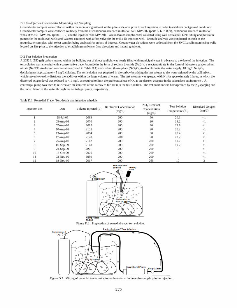
D.1 Pre-Injection Groundwater Monitoring and Sampling

D.2 Test Solution Preparation

Table D.1: Remedial Tracer Test details and injection schedule.

Figure D.1: Preparation of remedial tracer test solution.

Figure D.2: Mixing of remedial tracer test solution in order to homogenize sample prior to injection.

-

-

-

23.2

19.7

19.2

10

<1

<1

<1

<1

<1

<1

<1

<1

<1

<1

<1

3

200

200

90

90

90

90

90

90

200

200

200

200

200

200

200

200

03-Nov-09

18-Nov-09

2063

2070

2092

2131

2094

2128

2102

2108

2051

2076

1950

2017

200

Volume Injected (L)Br

- Tracer Concentration

(mg/L)

NO3- Reactant

Concentration

(mg/L)

Test Solution

Temperature (oC)

11

12

28-Jul-09

05-Aug-09

07-Aug-09

10-Aug-09

13-Aug-09

17-Aug-09

25-Aug-09

09-Sep-09

24-Sep-09

15-Oct-09

6

7

8

9

10

265

200

200

Groundwater samples were collected within the monitoring network of the pilot-scale area prior to each injection in order to establish background conditions.

Groundwater samples were collected routinely from the discontinuous screened multilevel well MW-302 (ports 5, 6, 7, 8, 9), continuous screened multilevel

wells MW-401, MW-402 (ports 1 – 9) and the injection well MW-501. Groundwater samples were collected using well dedicated LDPE tubing and peristaltic

pumps for the multilevel wells and Waterra equipped with a foot valve for the 0.051 ID injection well. Bromide analysis was conducted on each of the

groundwater samples, with select samples being analyzed for anions of interest. Groundwater elevations were collected from the SNC Lavalin monitoring wells

located on Site prior to the injection to establish groundwater flow directions and natural gradients.

A 2052 L (550 gal) carboy located within the building out of direct sunlight was nearly filled with municipal water in advance to the date of the injection. The

test solution was amended with a conservative tracer bromide in the form of sodium bromide (NaBr) , a reactant nitrate in the form of laboratory grade sodium

nitrate (NaNO3) to desired concentrations (listed in Table D.1) and sodium thiosulphate (NaS2O5) to de-chlorinate the water supply. 18 mg/L NaS2O3

dechlorinates approximately 5 mg/L chlorine. The test solution was prepared in the carboy by adding the test solutes to the water agitated by the drill mixer,

which served to readily distribute the additives within the large volume of water. The test solution was sparged with N2 for approximately 1 hour, in which the

dissolved oxygen level was reduced to < 1 mg/L as required to limit the preferential use of O2 as an electron acceptor in the subsurface environment . A

centrifugal pump was used to re-circulate the contents of the carboy to further mix the test solution. The test solution was homogenized by the N2 sparging and

the recirculation of the water through the centrifugal pump, respectively.

Injection No.

1

Dissolved Oxygen

(mg/L)

2

3

4

5

200

200

200

200

20.1

19.2

19.8

20.2

20.4

Date

275

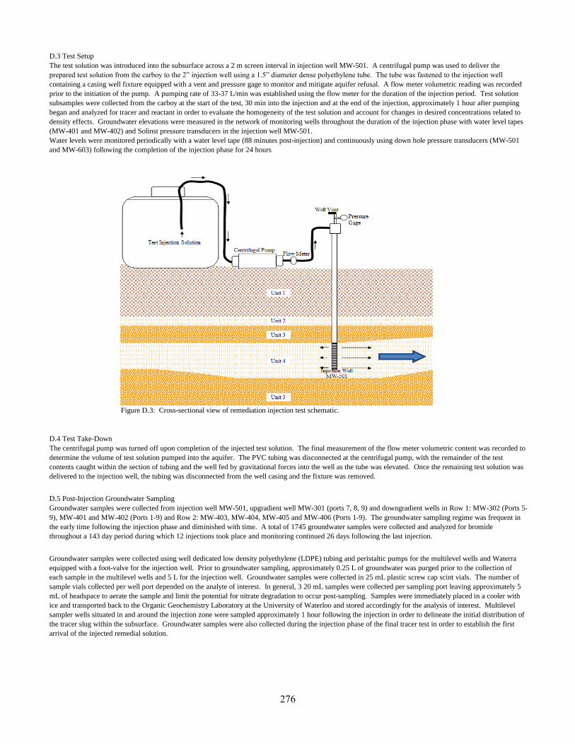
Figure D.3: Cross-sectional view of remediation injection test schematic.

D.4 Test Take-Down

D.5 Post-Injection Groundwater Sampling

Groundwater samples were collected using well dedicated low density polyethylene (LDPE) tubing and peristaltic pumps for the multilevel wells and Waterra

equipped with a foot-valve for the injection well. Prior to groundwater sampling, approximately 0.25 L of groundwater was purged prior to the collection of

each sample in the multilevel wells and 5 L for the injection well. Groundwater samples were collected in 25 mL plastic screw cap scint vials. The number of

sample vials collected per well port depended on the analyte of interest. In general, 3 20 mL samples were collected per sampling port leaving approximately 5

mL of headspace to aerate the sample and limit the potential for nitrate degradation to occur post-sampling. Samples were immediately placed in a cooler with

ice and transported back to the Organic Geochemistry Laboratory at the University of Waterloo and stored accordingly for the analysis of interest. Multilevel

sampler wells situated in and around the injection zone were sampled approximately 1 hour following the injection in order to delineate the initial distribution of

the tracer slug within the subsurface. Groundwater samples were also collected during the injection phase of the final tracer test in order to establish the first

arrival of the injected remedial solution.

D.3 Test Setup

The test solution was introduced into the subsurface across a 2 m screen interval in injection well MW-501. A centrifugal pump was used to deliver the

prepared test solution from the carboy to the 2” injection well using a 1.5” diameter dense polyethylene tube. The tube was fastened to the injection well

containing a casing well fixture equipped with a vent and pressure gage to monitor and mitigate aquifer refusal. A flow meter volumetric reading was recorded

prior to the initiation of the pump. A pumping rate of 33-37 L/min was established using the flow meter for the duration of the injection period. Test solution

subsamples were collected from the carboy at the start of the test, 30 min into the injection and at the end of the injection, approximately 1 hour after pumping

began and analyzed for tracer and reactant in order to evaluate the homogeneity of the test solution and account for changes in desired concentrations related to

density effects. Groundwater elevations were measured in the network of monitoring wells throughout the duration of the injection phase with water level tapes

(MW-401 and MW-402) and Solinst pressure transducers in the injection well MW-501.

Water levels were monitored periodically with a water level tape (88 minutes post-injection) and continuously using down hole pressure transducers (MW-501

and MW-603) following the completion of the injection phase for 24 hours

The centrifugal pump was turned off upon completion of the injected test solution. The final measurement of the flow meter volumetric content was recorded to

determine the volume of test solution pumped into the aquifer. The PVC tubing was disconnected at the centrifugal pump, with the remainder of the test

contents caught within the section of tubing and the well fed by gravitational forces into the well as the tube was elevated. Once the remaining test solution was

delivered to the injection well, the tubing was disconnected from the well casing and the fixture was removed.

Groundwater samples were collected from injection well MW-501, upgradient well MW-301 (ports 7, 8, 9) and downgradient wells in Row 1: MW-302 (Ports 5-

9), MW-401 and MW-402 (Ports 1-9) and Row 2: MW-403, MW-404, MW-405 and MW-406 (Ports 1-9). The groundwater sampling regime was frequent in

the early time following the injection phase and diminished with time. A total of 1745 groundwater samples were collected and analyzed for bromide

throughout a 143 day period during which 12 injections took place and monitoring continued 26 days following the last injection.

276

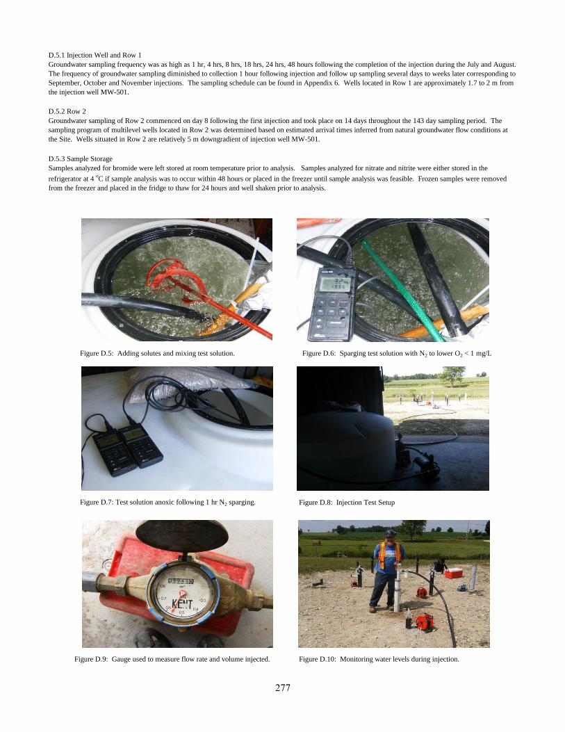
D.5.1 Injection Well and Row 1

D.5.2 Row 2

D.5.3 Sample Storage

Figure D.7: Test solution anoxic following 1 hr N2 sparging.

Figure D.10: Monitoring water levels during injection.Figure D.9: Gauge used to measure flow rate and volume injected.

Samples analyzed for bromide were left stored at room temperature prior to analysis. Samples analyzed for nitrate and nitrite were either stored in the

refrigerator at 4 oC if sample analysis was to occur within 48 hours or placed in the freezer until sample analysis was feasible. Frozen samples were removed

from the freezer and placed in the fridge to thaw for 24 hours and well shaken prior to analysis.

Figure D.5: Adding solutes and mixing test solution.

Figure D.8: Injection Test Setup

Groundwater sampling frequency was as high as 1 hr, 4 hrs, 8 hrs, 18 hrs, 24 hrs, 48 hours following the completion of the injection during the July and August.

The frequency of groundwater sampling diminished to collection 1 hour following injection and follow up sampling several days to weeks later corresponding to

September, October and November injections. The sampling schedule can be found in Appendix 6. Wells located in Row 1 are approximately 1.7 to 2 m from

the injection well MW-501.

Groundwater sampling of Row 2 commenced on day 8 following the first injection and took place on 14 days throughout the 143 day sampling period. The

sampling program of multilevel wells located in Row 2 was determined based on estimated arrival times inferred from natural groundwater flow conditions at

the Site. Wells situated in Row 2 are relatively 5 m downgradient of injection well MW-501.

Figure D.6: Sparging test solution with N2 to lower O2 < 1 mg/L

277

Appendix E

Remedial Tracer Test Injection Analysis of the Results

278

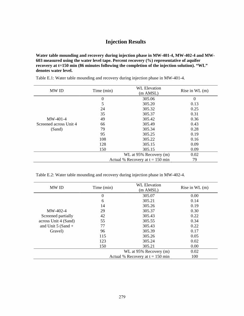
Injection Results

Water table mounding and recovery during injection phase in MW-401-4, MW-402-4 and MW-603 measured using the water level tape. Percent recovery (%) representative of aquifer recovery at t=150 min (86 minutes following the completion of the injection solution). “WL” denotes water level.

Table E.1: Water table mounding and recovery during injection phase in MW-401-4.

MW ID Time (min) WL Elevation

(m AMSL) Rise in WL (m)

MW-401-4 Screened across Unit 4

(Sand)

0 305.06 0 5 305.20 0.13

24 305.32 0.25 35 305.37 0.31 49 305.42 0.36 66 305.49 0.43 79 305.34 0.28 95 305.25 0.19

108 305.22 0.16 128 305.15 0.09 150 305.15 0.09

WL at 95% Recovery (m) 0.02 Actual % Recovery at t = 150 min 79

Table E.2: Water table mounding and recovery during injection phase in MW-402-4.

MW ID Time (min) WL Elevation

(m AMSL) Rise in WL (m)

MW-402-4 Screened partially

across Unit 4 (Sand) and Unit 5 (Sand +

Gravel)

0 305.07 0.00 6 305.21 0.14

14 305.26 0.19 29 305.37 0.30 42 305.43 0.22 55 305.55 0.34 77 305.43 0.22 96 305.39 0.17

115 305.26 0.05 123 305.24 0.02 150 305.21 0.00

WL at 95% Recovery (m) 0.02 Actual % Recovery at t = 150 min 100

279

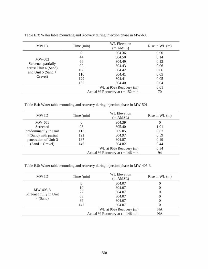
Table E.3: Water table mounding and recovery during injection phase in MW-603.

MW ID Time (min) WL Elevation

(m AMSL) Rise in WL (m)

MW-603 Screened partially

across Unit 4 (Sand) and Unit 5 (Sand +

Gravel)

0 304.36 0.00 44 304.50 0.14 66 304.49 0.13 92 304.43 0.06

108 304.42 0.06 116 304.41 0.05 129 304.41 0.05 152 304.40 0.04

WL at 95% Recovery (m) 0.01 Actual % Recovery at t = 152 min 70

Table E.4: Water table mounding and recovery during injection phase in MW-501.

MW ID Time (min) WL Elevation

(m AMSL) Rise in WL (m)

MW-501 Screened

predominantly in Unit 4 (Sand) with partial penetration of Unit 3

(Sand + Gravel)

0 304.39 0 98 305.40 1.01

113 305.05 0.67 121 304.97 0.59 137 304.87 0.49 146 304.82 0.44

WL at 95% Recovery (m) 0.34 Actual % Recovery at t = 146 min 94

Table E.5: Water table mounding and recovery during injection phase in MW-405-3.

MW ID Time (min) WL Elevation

(m AMSL) Rise in WL (m)

MW-405-3 Screened fully in Unit

4 (Sand)

0 304.07 0 10 304.07 0 27 304.07 0 63 304.07 0 89 304.07 0

147 304.07 0 WL at 95% Recovery (m) NA

Actual % Recovery at t = 146 min NA

280

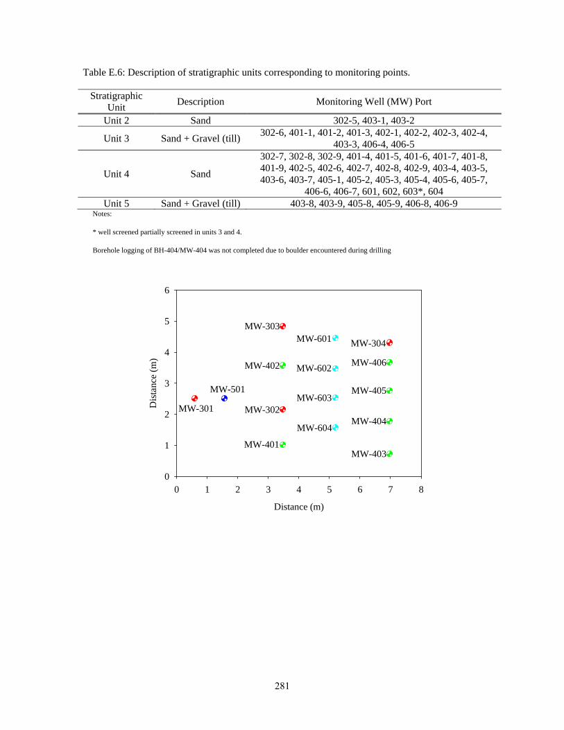
Table E.6: Description of stratigraphic units corresponding to monitoring points.

Stratigraphic Unit

Description Monitoring Well (MW) Port

Unit 2 Sand 302-5, 403-1, 403-2

Unit 3 Sand + Gravel (till) 302-6, 401-1, 401-2, 401-3, 402-1, 402-2, 402-3, 402-4,

403-3, 406-4, 406-5

Unit 4 Sand

302-7, 302-8, 302-9, 401-4, 401-5, 401-6, 401-7, 401-8, 401-9, 402-5, 402-6, 402-7, 402-8, 402-9, 403-4, 403-5, 403-6, 403-7, 405-1, 405-2, 405-3, 405-4, 405-6, 405-7,

406-6, 406-7, 601, 602, 603*, 604 Unit 5 Sand + Gravel (till) 403-8, 403-9, 405-8, 405-9, 406-8, 406-9

Notes:

* well screened partially screened in units 3 and 4.

Borehole logging of BH-404/MW-404 was not completed due to boulder encountered during drilling

Distance (m)

0 1 2 3 4 5 6 7 8

Dis

tanc

e (m

)

0

1

2

3

4

5

6

MW-301

MW-501

MW-303

MW-402

MW-302

MW-401

MW-601

MW-602

MW-603

MW-604

MW-304

MW-406

MW-405

MW-404

MW-403

281

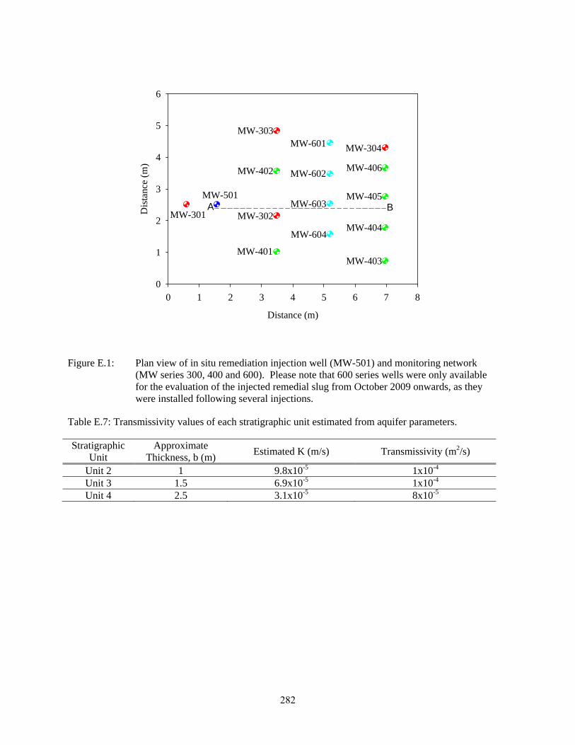
Distance (m)

0 1 2 3 4 5 6 7 8

Dis

tanc

e (m

)

0

1

2

3

4

5

6

MW-301

MW-501

MW-303

MW-402

MW-302

MW-401

MW-601

MW-602

MW-603

MW-604

MW-304

MW-406

MW-405

MW-404

MW-403

BA

Figure E.1: Plan view of in situ remediation injection well (MW-501) and monitoring network (MW series 300, 400 and 600). Please note that 600 series wells were only available for the evaluation of the injected remedial slug from October 2009 onwards, as they were installed following several injections.

Table E.7: Transmissivity values of each stratigraphic unit estimated from aquifer parameters.

Stratigraphic Unit

Approximate Thickness, b (m)

Estimated K (m/s) Transmissivity (m2/s)

Unit 2 1 9.8x10-5 1x10-4 Unit 3 1.5 6.9x10-5 1x10-4 Unit 4 2.5 3.1x10-5 8x10-5

282

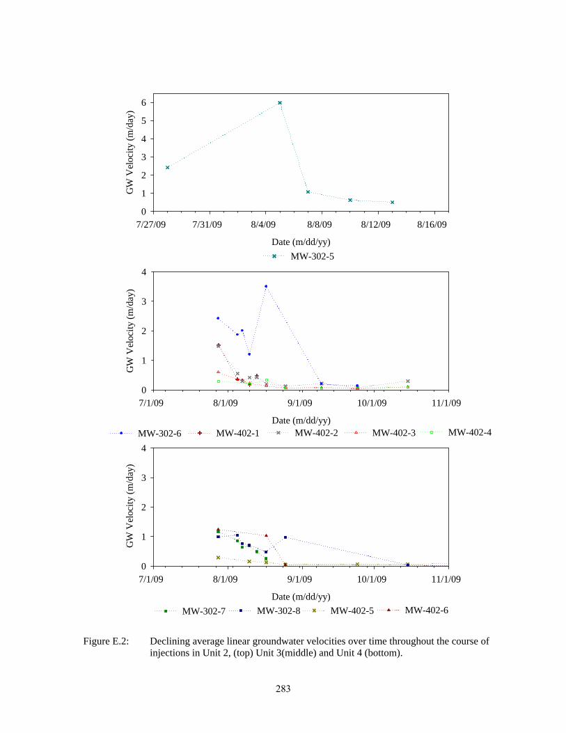
Date (m/dd/yy)

7/1/09 8/1/09 9/1/09 10/1/09 11/1/09

GW

Vel

ocity

(m

/day

)

0

1

2

3

4

MW-302-6 MW-402-1 MW-402-2 MW-402-3 MW-402-4

Date (m/dd/yy)

7/1/09 8/1/09 9/1/09 10/1/09 11/1/09

GW

Vel

ocity

(m

/day

)

0

1

2

3

4

MW-302-8 MW-402-5 MW-402-6 MW-302-7

Date (m/dd/yy)

7/27/09 7/31/09 8/4/09 8/8/09 8/12/09 8/16/09

GW

Vel

ocity

(m

/day

)

0

1

2

3

4

5

6

MW-302-5

Figure E.2: Declining average linear groundwater velocities over time throughout the course of injections in Unit 2, (top) Unit 3(middle) and Unit 4 (bottom).

283

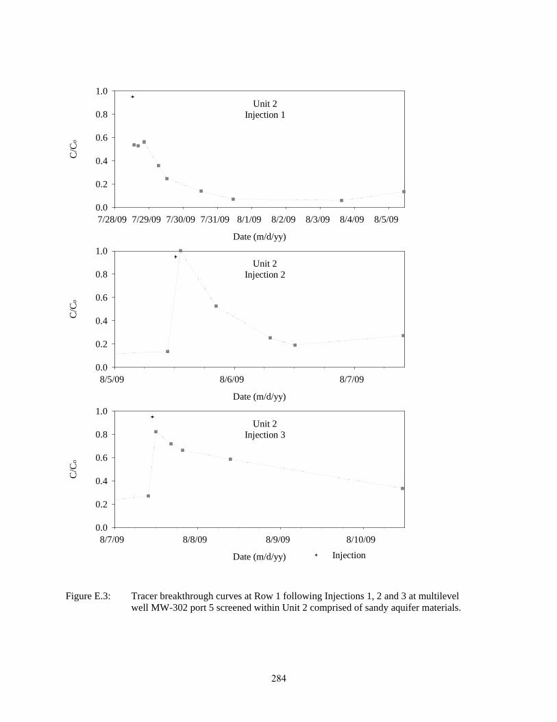
Date (m/d/yy)

7/28/09 7/29/09 7/30/09 7/31/09 8/1/09 8/2/09 8/3/09 8/4/09 8/5/09

C/C

o

0.0

0.2

0.4

0.6

0.8

1.0Unit 2

Injection 1

Date (m/d/yy)

8/5/09 8/6/09 8/7/09

C/C

o

0.0

0.2

0.4

0.6

0.8

1.0Unit 2

Injection 2

Date (m/d/yy)

8/7/09 8/8/09 8/9/09 8/10/09

C/C

o

0.0

0.2

0.4

0.6

0.8

1.0

Injection

Unit 2Injection 3

Figure E.3: Tracer breakthrough curves at Row 1 following Injections 1, 2 and 3 at multilevel well MW-302 port 5 screened within Unit 2 comprised of sandy aquifer materials.

284

Date (m/d/yy)

8/10/09 8/11/09 8/12/09 8/13/09

C/C

o

0.0

0.2

0.4

0.6

0.8

1.0Unit 2

Injection 4

Date (m/d/yy)

8/13/09 8/14/09 8/15/09 8/16/09 8/17/09

C/C

o

0.0

0.2

0.4

0.6

0.8

1.0

Injection

Unit 2Injection 5

Figure E.3: Tracer breakthrough curves at Row 1 following Injections 4 and 5 at multilevel well MW-302 port 5 screened within Unit 2 comprised of sandy aquifer materials.

285

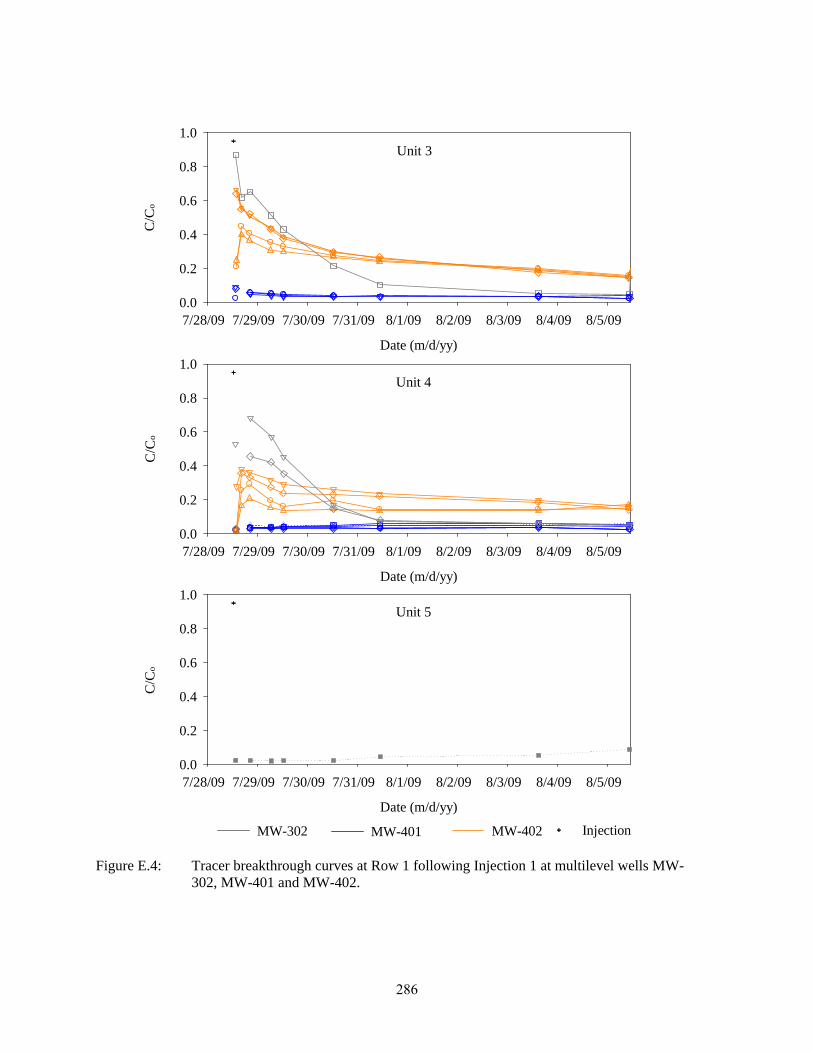
Date (m/d/yy)

7/28/09 7/29/09 7/30/09 7/31/09 8/1/09 8/2/09 8/3/09 8/4/09 8/5/09

C/C

o

0.0

0.2

0.4

0.6

0.8

1.0

Date (m/d/yy)

7/28/09 7/29/09 7/30/09 7/31/09 8/1/09 8/2/09 8/3/09 8/4/09 8/5/09

C/C

o

0.0

0.2

0.4

0.6

0.8

1.0

Date (m/d/yy)

7/28/09 7/29/09 7/30/09 7/31/09 8/1/09 8/2/09 8/3/09 8/4/09 8/5/09

C/C

o

0.0

0.2

0.4

0.6

0.8

1.0

Injection

Unit 3

Unit 4

Unit 5

MW-302 MW-401 MW-402

Figure E.4: Tracer breakthrough curves at Row 1 following Injection 1 at multilevel wells MW- 302, MW-401 and MW-402.

286

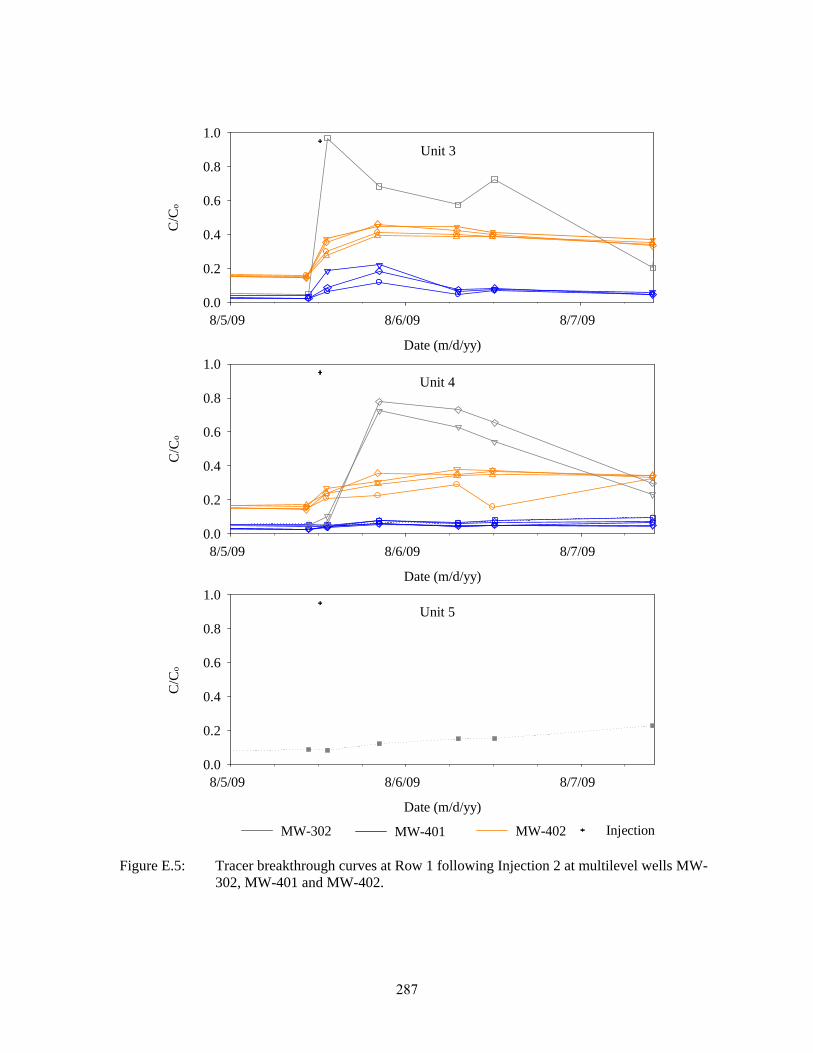
Date (m/d/yy)

8/5/09 8/6/09 8/7/09

C/C

o

0.0

0.2

0.4

0.6

0.8

1.0

Date (m/d/yy)

8/5/09 8/6/09 8/7/09

C/C

o

0.0

0.2

0.4

0.6

0.8

1.0

Date (m/d/yy)

8/5/09 8/6/09 8/7/09

C/C

o

0.0

0.2

0.4

0.6

0.8

1.0

Injection

Unit 3

Unit 4

Unit 5

MW-302 MW-401 MW-402

Figure E.5: Tracer breakthrough curves at Row 1 following Injection 2 at multilevel wells MW- 302, MW-401 and MW-402.

287

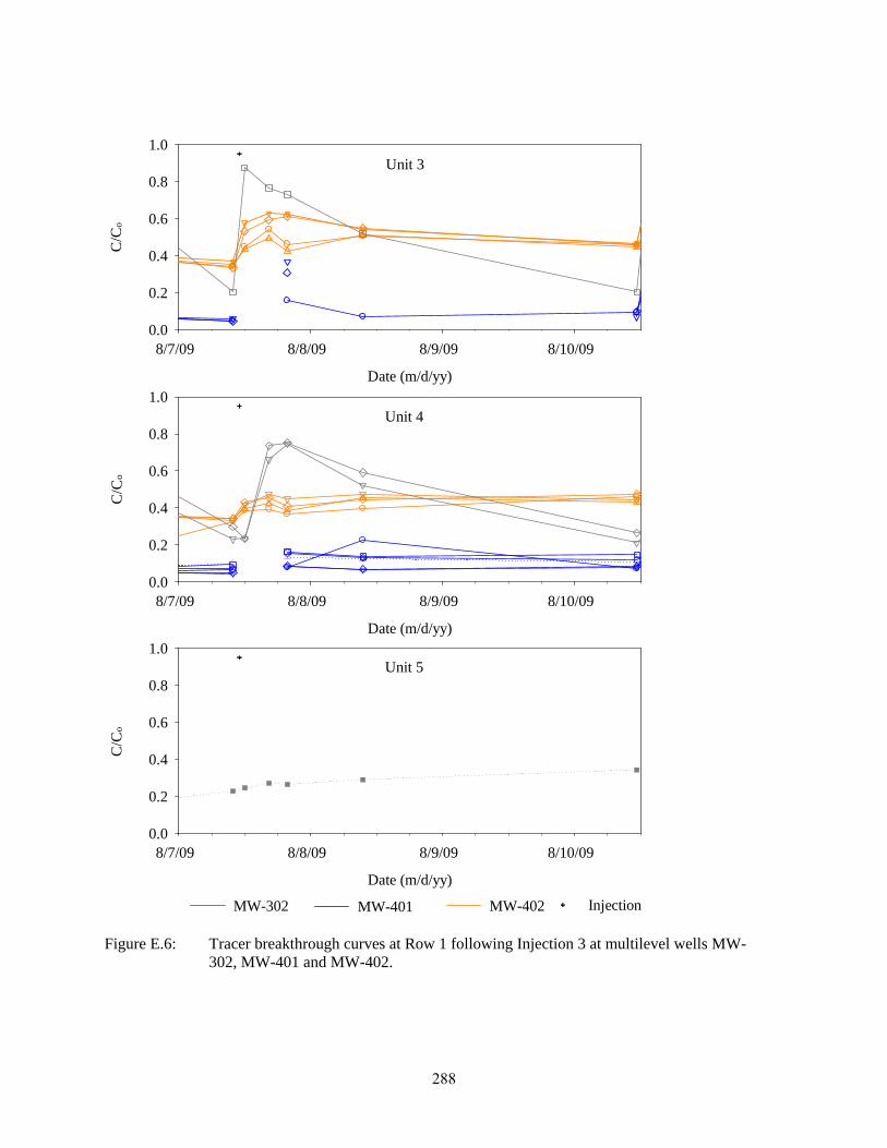
Date (m/d/yy)

8/7/09 8/8/09 8/9/09 8/10/09

C/C

o

0.0

0.2

0.4

0.6

0.8

1.0

Date (m/d/yy)

8/7/09 8/8/09 8/9/09 8/10/09

C/C

o

0.0

0.2

0.4

0.6

0.8

1.0

Date (m/d/yy)

8/7/09 8/8/09 8/9/09 8/10/09

C/C

o

0.0

0.2

0.4

0.6

0.8

1.0

Injection

Unit 3

Unit 4

Unit 5

MW-302 MW-401 MW-402

Figure E.6: Tracer breakthrough curves at Row 1 following Injection 3 at multilevel wells MW- 302, MW-401 and MW-402.

288

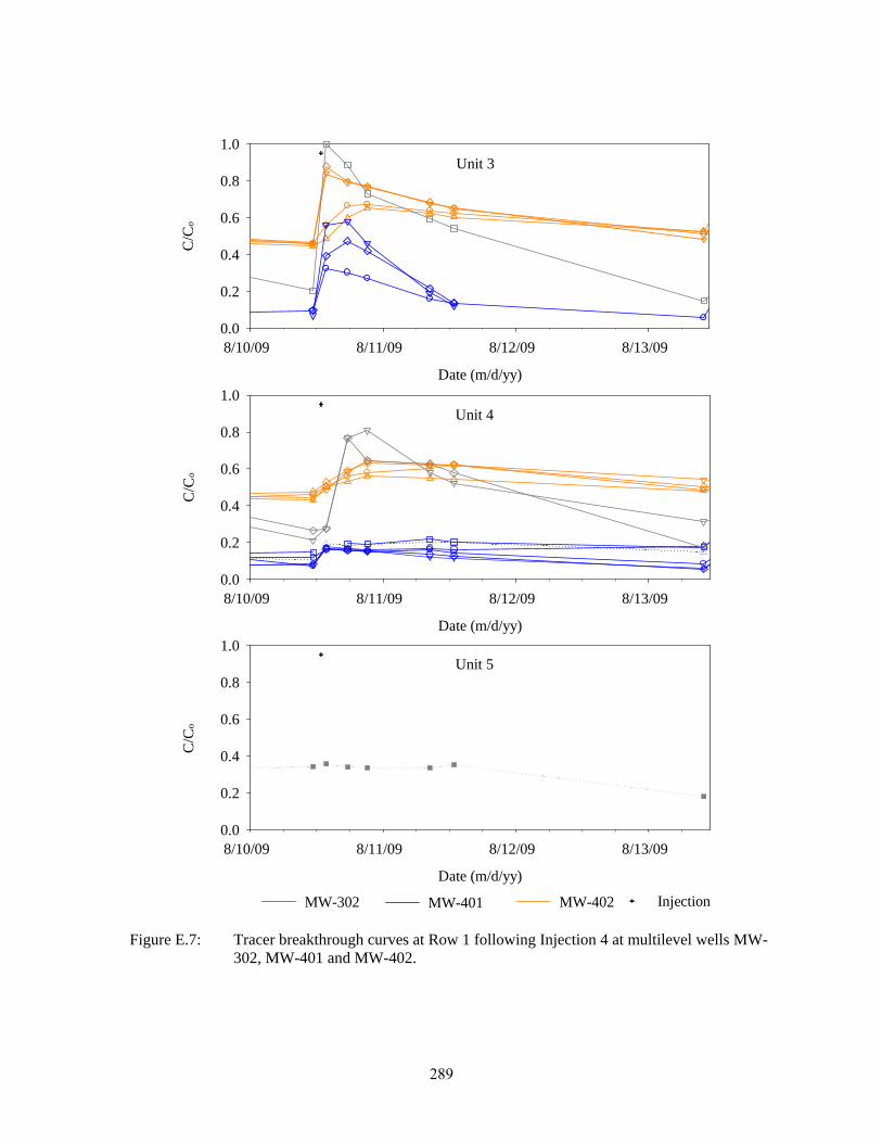
Date (m/d/yy)

8/10/09 8/11/09 8/12/09 8/13/09

C/C

o

0.0

0.2

0.4

0.6

0.8

1.0

Date (m/d/yy)

8/10/09 8/11/09 8/12/09 8/13/09

C/C

o

0.0

0.2

0.4

0.6

0.8

1.0

Date (m/d/yy)

8/10/09 8/11/09 8/12/09 8/13/09

C/C

o

0.0

0.2

0.4

0.6

0.8

1.0

Injection

Unit 3

Unit 4

Unit 5

MW-302 MW-401 MW-402

Figure E.7: Tracer breakthrough curves at Row 1 following Injection 4 at multilevel wells MW- 302, MW-401 and MW-402.

289

Date (m/d/yy)

8/13/09 8/14/09 8/15/09 8/16/09 8/17/09

C/C

o

0.0

0.2

0.4

0.6

0.8

1.0

Date (m/d/yy)

8/13/09 8/14/09 8/15/09 8/16/09 8/17/09

C/C

o

0.0

0.2

0.4

0.6

0.8

1.0

Date (m/d/yy)

8/13/09 8/14/09 8/15/09 8/16/09 8/17/09

C/C

o

0.0

0.2

0.4

0.6

0.8

1.0

Injection

Unit 3

Unit 4

Unit 5

MW-302 MW-401 MW-402

Figure E.8: Tracer breakthrough curves at Row 1 following Injection 5 at multilevel wells MW- 302, MW-401 and MW-402.

290

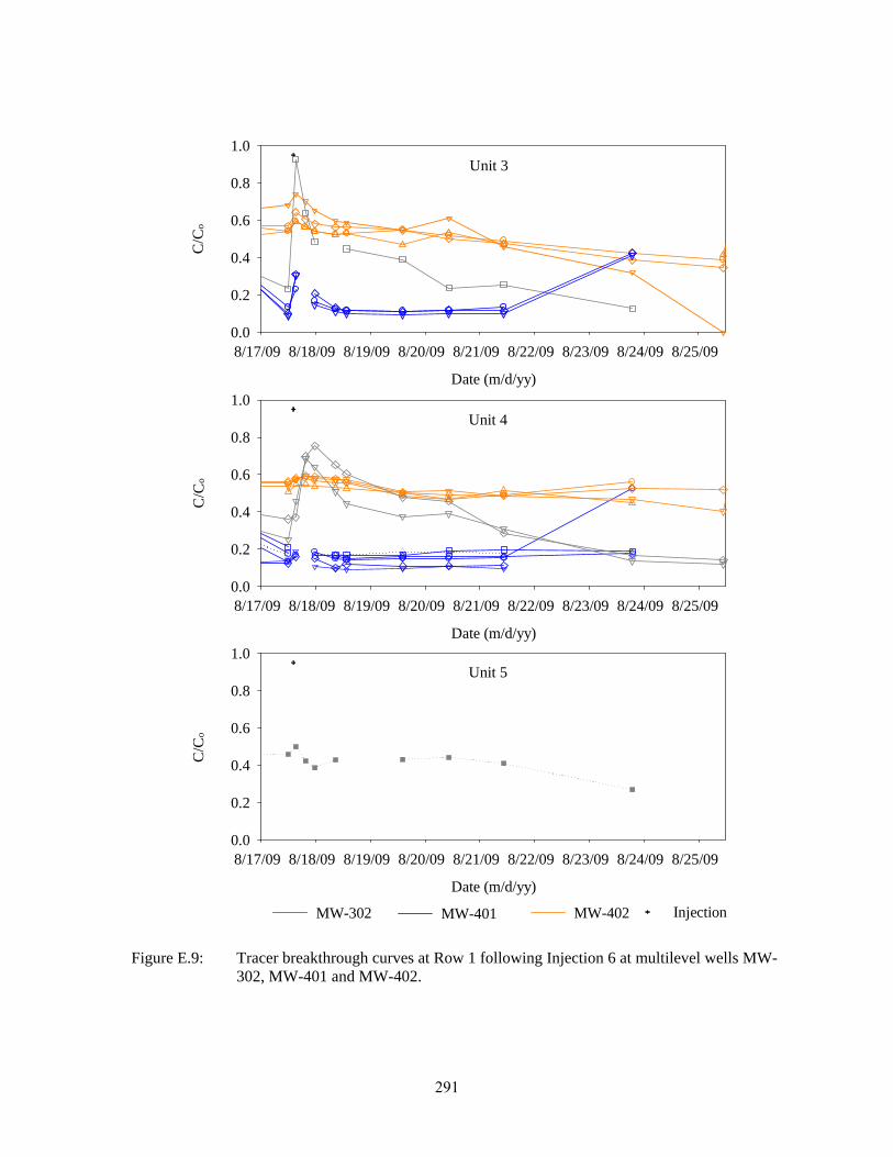
Date (m/d/yy)

8/17/09 8/18/09 8/19/09 8/20/09 8/21/09 8/22/09 8/23/09 8/24/09 8/25/09

C/C

o

0.0

0.2

0.4

0.6

0.8

1.0

Date (m/d/yy)

8/17/09 8/18/09 8/19/09 8/20/09 8/21/09 8/22/09 8/23/09 8/24/09 8/25/09

C/C

o

0.0

0.2

0.4

0.6

0.8

1.0

Date (m/d/yy)

8/17/09 8/18/09 8/19/09 8/20/09 8/21/09 8/22/09 8/23/09 8/24/09 8/25/09

C/C

o

0.0

0.2

0.4

0.6

0.8

1.0

Injection

Unit 3

Unit 4

Unit 5

MW-302 MW-401 MW-402

Figure E.9: Tracer breakthrough curves at Row 1 following Injection 6 at multilevel wells MW- 302, MW-401 and MW-402.

291

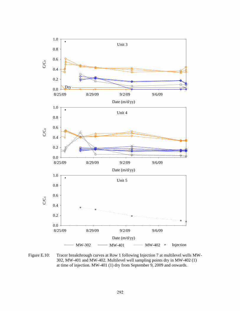
Date (m/d/yy)

8/25/09 8/29/09 9/2/09 9/6/09

C/C

o

0.0

0.2

0.4

0.6

0.8

1.0

Date (m/d/yy)

8/25/09 8/29/09 9/2/09 9/6/09

C/C

o

0.0

0.2

0.4

0.6

0.8

1.0

Date (m/d/yy)

8/25/09 8/29/09 9/2/09 9/6/09

C/C

o

0.0

0.2

0.4

0.6

0.8

1.0

Injection

Unit 3

Unit 4

Unit 5

MW-302 MW-401 MW-402

Dry

Figure E.10: Tracer breakthrough curves at Row 1 following Injection 7 at multilevel wells MW- 302, MW-401 and MW-402. Multilevel well sampling points dry in MW-402 (1) at time of injection. MW-401 (1) dry from September 9, 2009 and onwards.

292

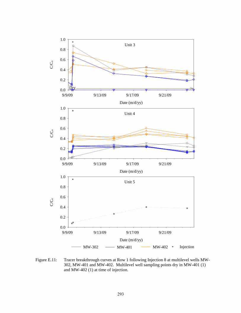
Date (m/d/yy)

9/9/09 9/13/09 9/17/09 9/21/09

C/C

o

0.0

0.2

0.4

0.6

0.8

1.0

Date (m/d/yy)

9/9/09 9/13/09 9/17/09 9/21/09

C/C

o

0.0

0.2

0.4

0.6

0.8

1.0

Date (m/d/yy)

9/9/09 9/13/09 9/17/09 9/21/09

C/C

o

0.0

0.2

0.4

0.6

0.8

1.0

Injection

Unit 3

Unit 4

Unit 5

MW-302 MW-401 MW-402

Dry

Figure E.11: Tracer breakthrough curves at Row 1 following Injection 8 at multilevel wells MW- 302, MW-401 and MW-402. Multilevel well sampling points dry in MW-401 (1) and MW-402 (1) at time of injection.

293

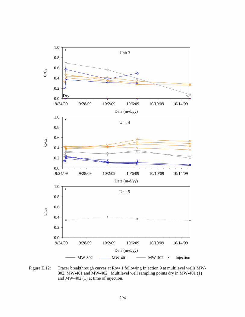
Date (m/d/yy)

9/24/09 9/28/09 10/2/09 10/6/09 10/10/09 10/14/09

C/C

o

0.0

0.2

0.4

0.6

0.8

1.0

Date (m/d/yy)

9/24/09 9/28/09 10/2/09 10/6/09 10/10/09 10/14/09

C/C

o

0.0

0.2

0.4

0.6

0.8

1.0

Date (m/d/yy)

9/24/09 9/28/09 10/2/09 10/6/09 10/10/09 10/14/09

C/C

o

0.0

0.2

0.4

0.6

0.8

1.0

Injection

Unit 3

Unit 4

Unit 5

MW-302 MW-401 MW-402

Dry

Figure E.12: Tracer breakthrough curves at Row 1 following Injection 9 at multilevel wells MW- 302, MW-401 and MW-402. Multilevel well sampling points dry in MW-401 (1) and MW-402 (1) at time of injection.

294

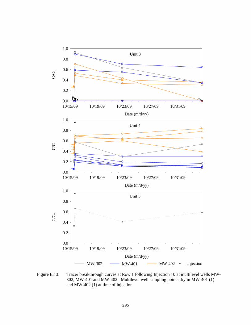
Date (m/d/yy)

10/15/09 10/19/09 10/23/09 10/27/09 10/31/09

C/C

o

0.0

0.2

0.4

0.6

0.8

1.0

Date (m/d/yy)

10/15/09 10/19/09 10/23/09 10/27/09 10/31/09

C/C

o

0.0

0.2

0.4

0.6

0.8

1.0

Date (m/d/yy)

10/15/09 10/19/09 10/23/09 10/27/09 10/31/09

C/C

o

0.0

0.2

0.4

0.6

0.8

1.0

Injection

Unit 3

Unit 4

Unit 5

MW-302 MW-401 MW-402

Dry

Figure E.13: Tracer breakthrough curves at Row 1 following Injection 10 at multilevel wells MW- 302, MW-401 and MW-402. Multilevel well sampling points dry in MW-401 (1) and MW-402 (1) at time of injection.

295

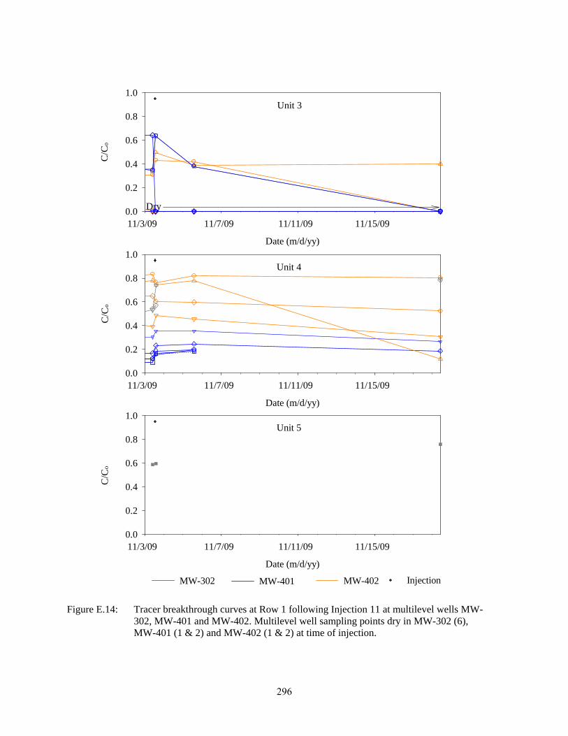
Date (m/d/yy)

11/3/09 11/7/09 11/11/09 11/15/09

C/C

o

0.0

0.2

0.4

0.6

0.8

1.0

Date (m/d/yy)

11/3/09 11/7/09 11/11/09 11/15/09

C/C

o

0.0

0.2

0.4

0.6

0.8

1.0

Date (m/d/yy)

11/3/09 11/7/09 11/11/09 11/15/09

C/C

o

0.0

0.2

0.4

0.6

0.8

1.0

Injection

Unit 3

Unit 4

Unit 5

MW-302 MW-401 MW-402

Dry

Figure E.14: Tracer breakthrough curves at Row 1 following Injection 11 at multilevel wells MW- 302, MW-401 and MW-402. Multilevel well sampling points dry in MW-302 (6), MW-401 (1 & 2) and MW-402 (1 & 2) at time of injection.

296

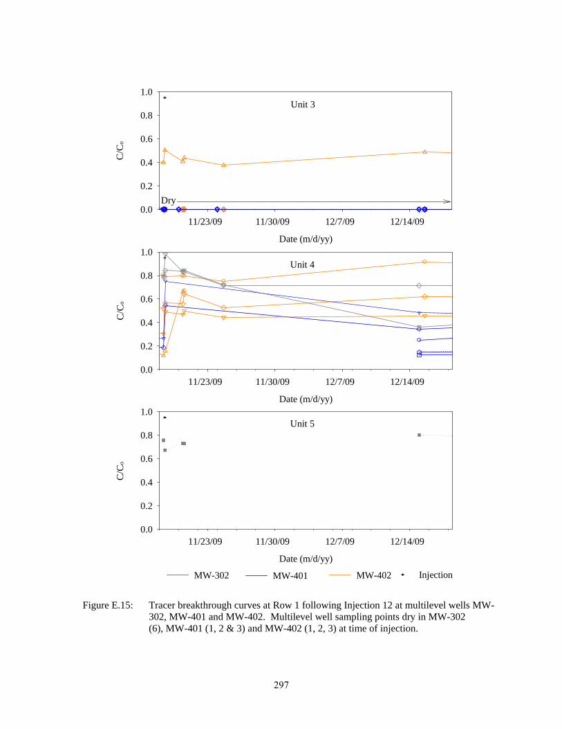
Date (m/d/yy)

11/23/09 11/30/09 12/7/09 12/14/09

C/C

o

0.0

0.2

0.4

0.6

0.8

1.0

Date (m/d/yy)

11/23/09 11/30/09 12/7/09 12/14/09

C/C

o

0.0

0.2

0.4

0.6

0.8

1.0

Date (m/d/yy)

11/23/09 11/30/09 12/7/09 12/14/09

C/C

o

0.0

0.2

0.4

0.6

0.8

1.0

Injection

Unit 3

Unit 4

Unit 5

MW-302 MW-401 MW-402

Dry

Figure E.15: Tracer breakthrough curves at Row 1 following Injection 12 at multilevel wells MW- 302, MW-401 and MW-402. Multilevel well sampling points dry in MW-302 (6), MW-401 (1, 2 & 3) and MW-402 (1, 2, 3) at time of injection.

297

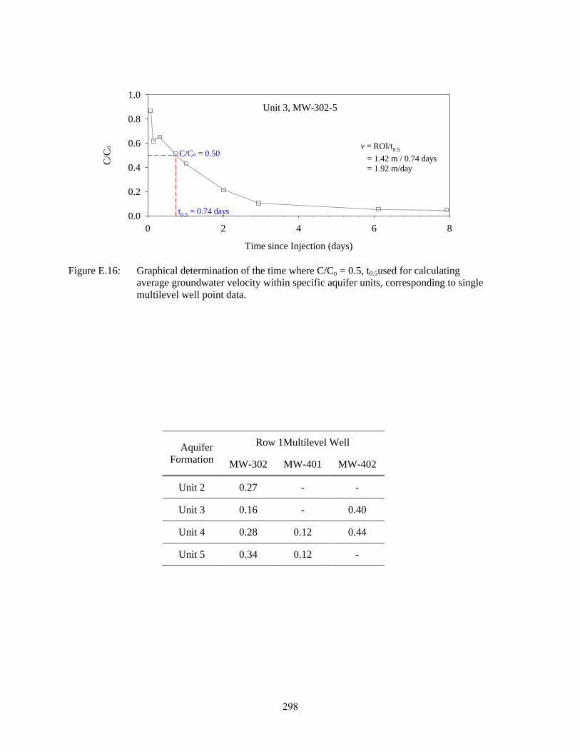
Time since Injection (days)

0 2 4 6 8

C/C

o

0.0

0.2

0.4

0.6

0.8

1.0Unit 3, MW-302-5

t0.5 = 0.74 days

C/Co = 0.50v = ROI/t0.5

= 1.42 m / 0.74 days = 1.92 m/day

Figure E.16: Graphical determination of the time where C/Co = 0.5, t0.5used for calculating average groundwater velocity within specific aquifer units, corresponding to single multilevel well point data.

Aquifer Formation

Row 1Multilevel Well

MW-302 MW-401 MW-402

Unit 2 0.27 - -

Unit 3 0.16 - 0.40

Unit 4 0.28 0.12 0.44

Unit 5 0.34 0.12 -

298

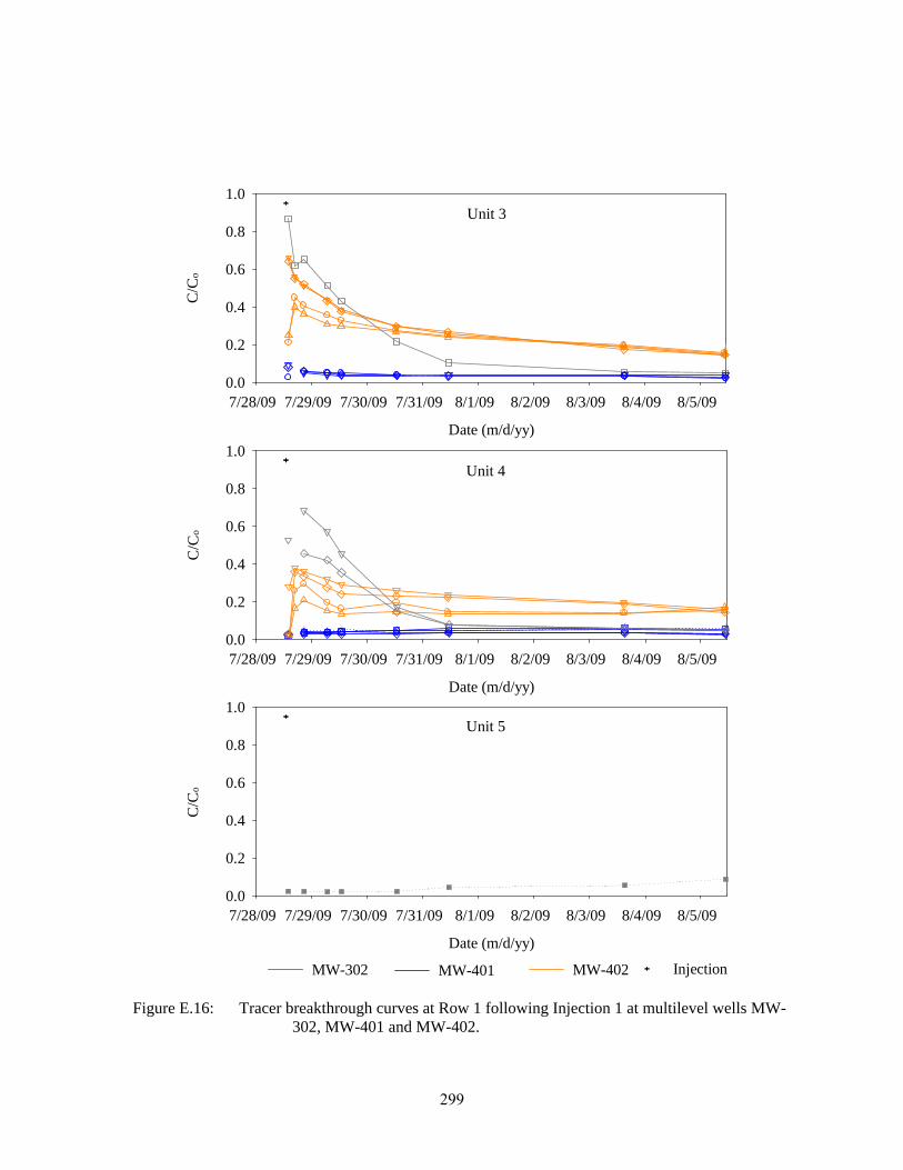
Date (m/d/yy)

7/28/09 7/29/09 7/30/09 7/31/09 8/1/09 8/2/09 8/3/09 8/4/09 8/5/09

C/C

o

0.0

0.2

0.4

0.6

0.8

1.0

Date (m/d/yy)

7/28/09 7/29/09 7/30/09 7/31/09 8/1/09 8/2/09 8/3/09 8/4/09 8/5/09

C/C

o

0.0

0.2

0.4

0.6

0.8

1.0

Date (m/d/yy)

7/28/09 7/29/09 7/30/09 7/31/09 8/1/09 8/2/09 8/3/09 8/4/09 8/5/09

C/C

o

0.0

0.2

0.4

0.6

0.8

1.0

Injection

Unit 3

Unit 4

Unit 5

MW-302 MW-401 MW-402

Figure E.16: Tracer breakthrough curves at Row 1 following Injection 1 at multilevel wells MW- 302, MW-401 and MW-402.

299

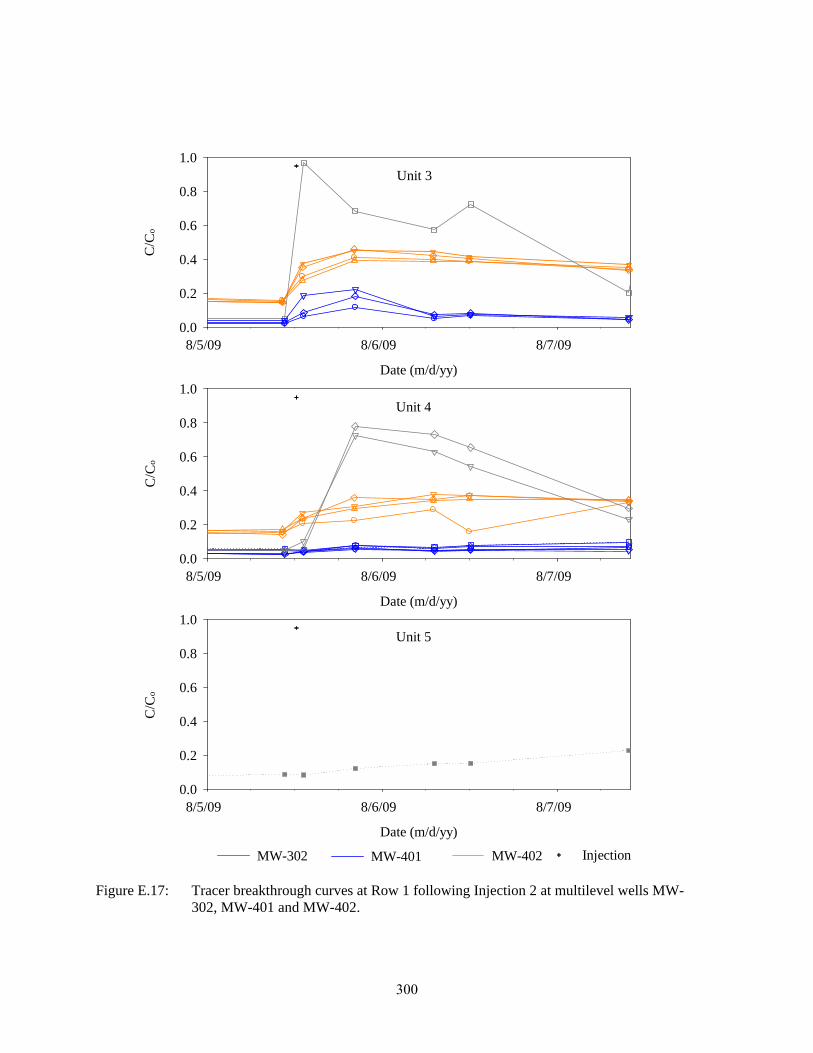
Date (m/d/yy)

8/5/09 8/6/09 8/7/09

C/C

o

0.0

0.2

0.4

0.6

0.8

1.0

Date (m/d/yy)

8/5/09 8/6/09 8/7/09

C/C

o

0.0

0.2

0.4

0.6

0.8

1.0

Date (m/d/yy)

8/5/09 8/6/09 8/7/09

C/C

o

0.0

0.2

0.4

0.6

0.8

1.0

Injection

Unit 3

Unit 4

Unit 5

MW-302 MW-401 MW-402

Figure E.17: Tracer breakthrough curves at Row 1 following Injection 2 at multilevel wells MW- 302, MW-401 and MW-402.

300

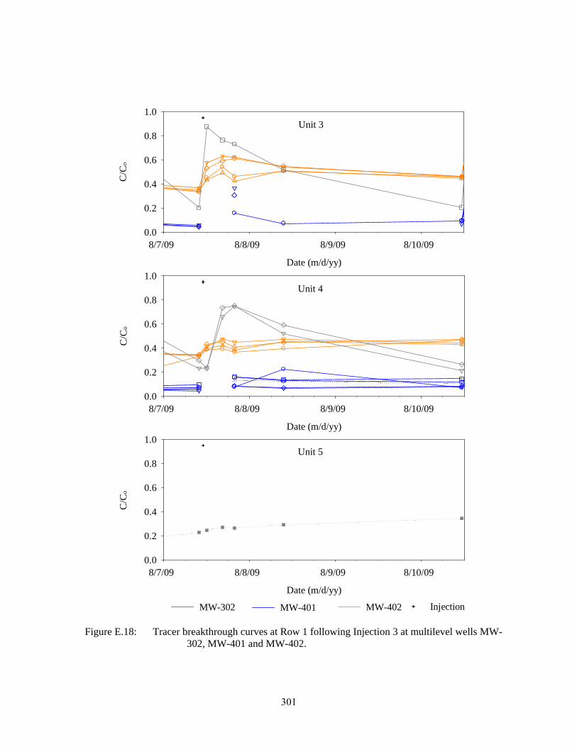
Date (m/d/yy)

8/7/09 8/8/09 8/9/09 8/10/09

C/C

o

0.0

0.2

0.4

0.6

0.8

1.0

Date (m/d/yy)

8/7/09 8/8/09 8/9/09 8/10/09

C/C

o

0.0

0.2

0.4

0.6

0.8

1.0

Date (m/d/yy)

8/7/09 8/8/09 8/9/09 8/10/09

C/C

o

0.0

0.2

0.4

0.6

0.8

1.0

Injection

Unit 3

Unit 4

Unit 5

MW-302 MW-401 MW-402

Figure E.18: Tracer breakthrough curves at Row 1 following Injection 3 at multilevel wells MW- 302, MW-401 and MW-402.

301

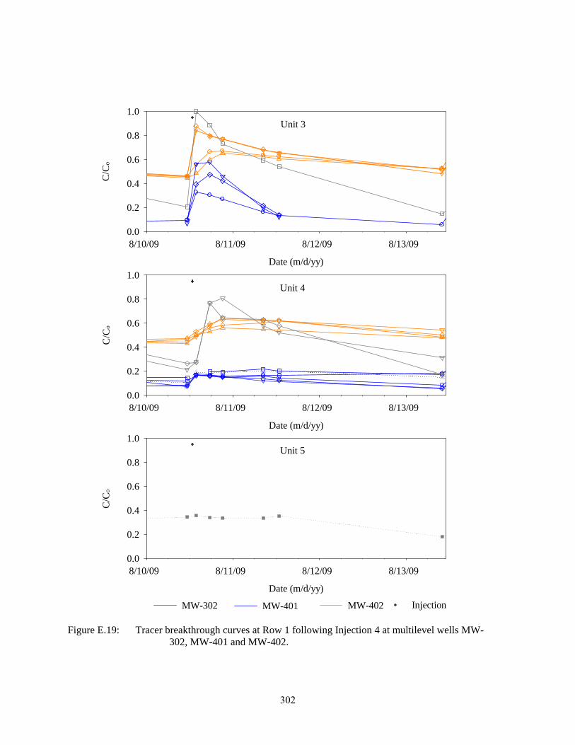
Date (m/d/yy)

8/10/09 8/11/09 8/12/09 8/13/09

C/C

o

0.0

0.2

0.4

0.6

0.8

1.0

Date (m/d/yy)

8/10/09 8/11/09 8/12/09 8/13/09

C/C

o

0.0

0.2

0.4

0.6

0.8

1.0

Date (m/d/yy)

8/10/09 8/11/09 8/12/09 8/13/09

C/C

o

0.0

0.2

0.4

0.6

0.8

1.0

Injection

Unit 3

Unit 4

Unit 5

MW-302 MW-401 MW-402

Figure E.19: Tracer breakthrough curves at Row 1 following Injection 4 at multilevel wells MW- 302, MW-401 and MW-402.

302

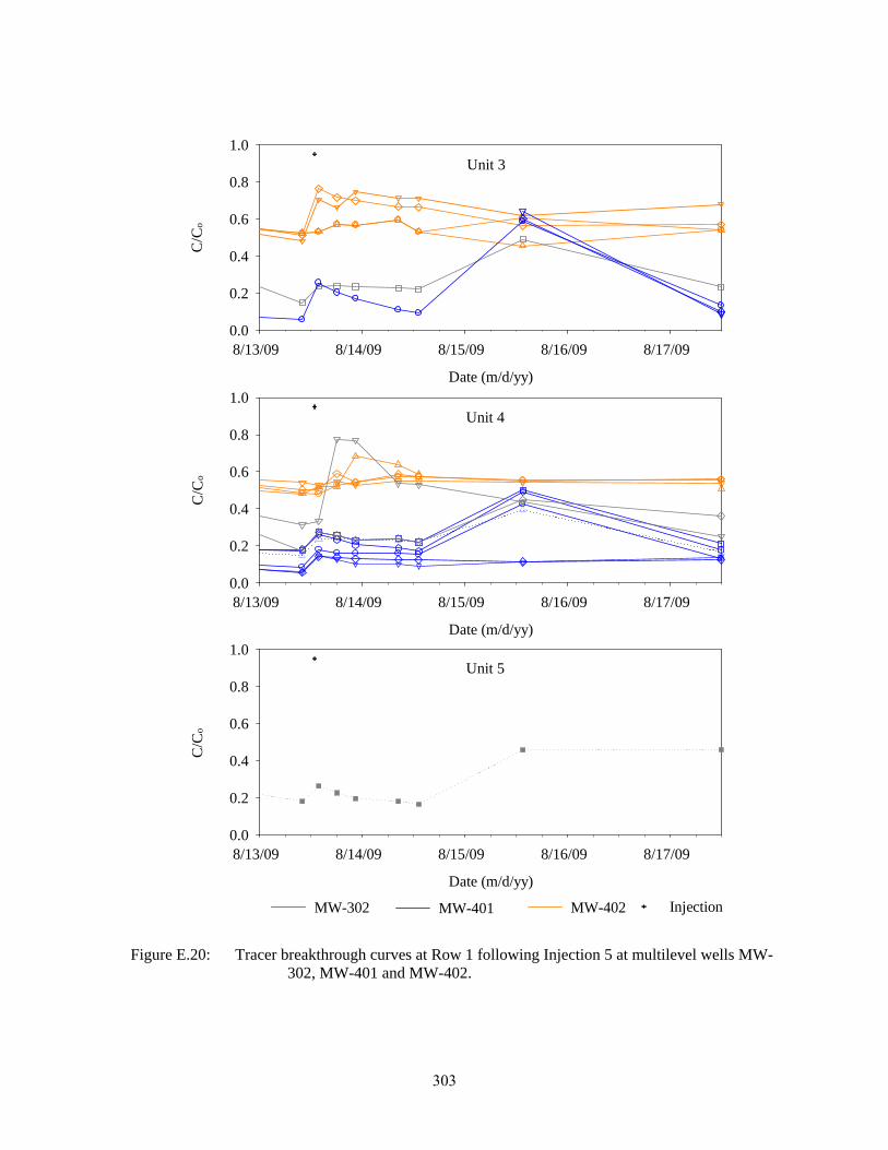
Date (m/d/yy)

8/13/09 8/14/09 8/15/09 8/16/09 8/17/09

C/C

o

0.0

0.2

0.4

0.6

0.8

1.0

Date (m/d/yy)

8/13/09 8/14/09 8/15/09 8/16/09 8/17/09

C/C

o

0.0

0.2

0.4

0.6

0.8

1.0

Date (m/d/yy)

8/13/09 8/14/09 8/15/09 8/16/09 8/17/09

C/C

o

0.0

0.2

0.4

0.6

0.8

1.0

Injection

Unit 3

Unit 4

Unit 5

MW-302 MW-401 MW-402

Figure E.20: Tracer breakthrough curves at Row 1 following Injection 5 at multilevel wells MW- 302, MW-401 and MW-402.

303

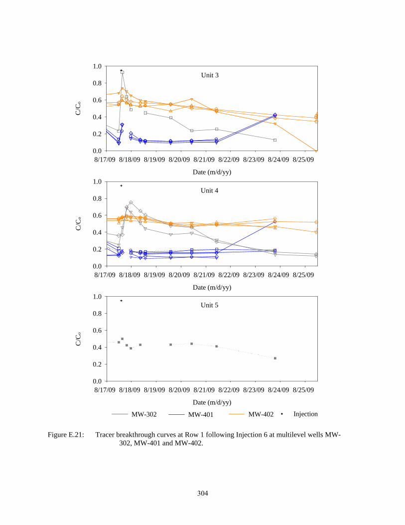
Date (m/d/yy)

8/17/09 8/18/09 8/19/09 8/20/09 8/21/09 8/22/09 8/23/09 8/24/09 8/25/09

C/C

o

0.0

0.2

0.4

0.6

0.8

1.0

Date (m/d/yy)

8/17/09 8/18/09 8/19/09 8/20/09 8/21/09 8/22/09 8/23/09 8/24/09 8/25/09

C/C

o

0.0

0.2

0.4

0.6

0.8

1.0

Date (m/d/yy)

8/17/09 8/18/09 8/19/09 8/20/09 8/21/09 8/22/09 8/23/09 8/24/09 8/25/09

C/C

o

0.0

0.2

0.4

0.6

0.8

1.0

Injection

Unit 3

Unit 4

Unit 5

MW-302 MW-401 MW-402

Figure E.21: Tracer breakthrough curves at Row 1 following Injection 6 at multilevel wells MW- 302, MW-401 and MW-402.

304

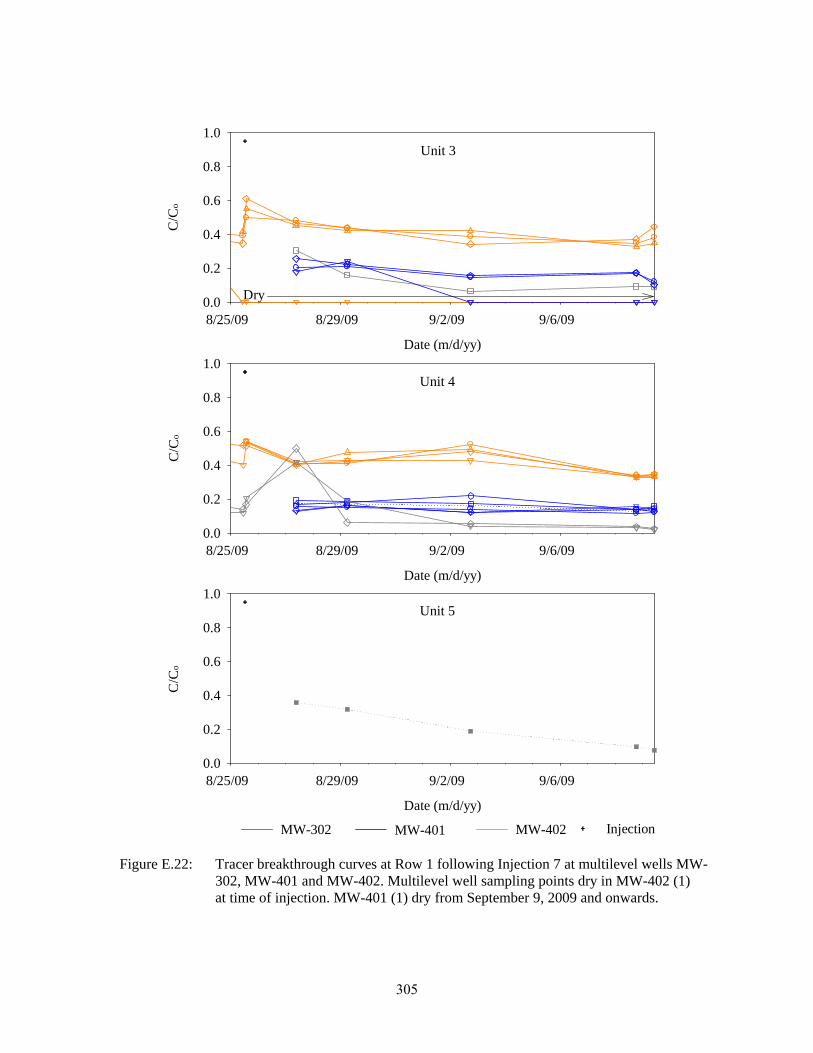
Date (m/d/yy)

8/25/09 8/29/09 9/2/09 9/6/09

C/C

o

0.0

0.2

0.4

0.6

0.8

1.0

Date (m/d/yy)

8/25/09 8/29/09 9/2/09 9/6/09

C/C

o

0.0

0.2

0.4

0.6

0.8

1.0

Date (m/d/yy)

8/25/09 8/29/09 9/2/09 9/6/09

C/C

o

0.0

0.2

0.4

0.6

0.8

1.0

Injection

Unit 3

Unit 4

Unit 5

MW-302 MW-401 MW-402

Dry

Figure E.22: Tracer breakthrough curves at Row 1 following Injection 7 at multilevel wells MW- 302, MW-401 and MW-402. Multilevel well sampling points dry in MW-402 (1) at time of injection. MW-401 (1) dry from September 9, 2009 and onwards.

305

Date (m/d/yy)

9/9/09 9/13/09 9/17/09 9/21/09

C/C

o

0.0

0.2

0.4

0.6

0.8

1.0

Date (m/d/yy)

9/9/09 9/13/09 9/17/09 9/21/09

C/C

o

0.0

0.2

0.4

0.6

0.8

1.0

Date (m/d/yy)

9/9/09 9/13/09 9/17/09 9/21/09

C/C

o

0.0

0.2

0.4

0.6

0.8

1.0

Injection

Unit 3

Unit 4

Unit 5

MW-302 MW-401 MW-402

Dry

Figure E.23: Tracer breakthrough curves at Row 1 following Injection 8 at multilevel wells MW- 302, MW-401 and MW-402. Multilevel well sampling points dry in MW-401 (1) and MW-402 (1) at time of injection.

306

Date (m/d/yy)

9/24/09 9/28/09 10/2/09 10/6/09 10/10/09 10/14/09

C/C

o

0.0

0.2

0.4

0.6

0.8

1.0

Date (m/d/yy)

9/24/09 9/28/09 10/2/09 10/6/09 10/10/09 10/14/09

C/C

o

0.0

0.2

0.4

0.6

0.8

1.0

Date (m/d/yy)

9/24/09 9/28/09 10/2/09 10/6/09 10/10/09 10/14/09

C/C

o

0.0

0.2

0.4

0.6

0.8

1.0

Injection

Unit 3

Unit 4

Unit 5

MW-302 MW-401 MW-402

Dry

Figure E.24: Tracer breakthrough curves at Row 1 following Injection 9 at multilevel wells MW- 302, MW-401 and MW-402. Multilevel well sampling points dry in MW-401 (1) and MW-402 (1) at time of injection.

307

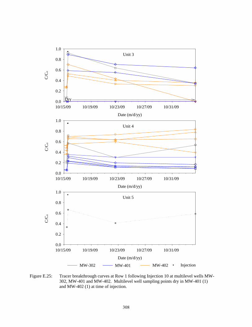
Date (m/d/yy)

10/15/09 10/19/09 10/23/09 10/27/09 10/31/09

C/C

o

0.0

0.2

0.4

0.6

0.8

1.0

Date (m/d/yy)

10/15/09 10/19/09 10/23/09 10/27/09 10/31/09

C/C

o

0.0

0.2

0.4

0.6

0.8

1.0

Date (m/d/yy)

10/15/09 10/19/09 10/23/09 10/27/09 10/31/09

C/C

o

0.0

0.2

0.4

0.6

0.8

1.0

Injection

Unit 3

Unit 4

Unit 5

MW-302 MW-401 MW-402

Dry

Figure E.25: Tracer breakthrough curves at Row 1 following Injection 10 at multilevel wells MW- 302, MW-401 and MW-402. Multilevel well sampling points dry in MW-401 (1) and MW-402 (1) at time of injection.

308

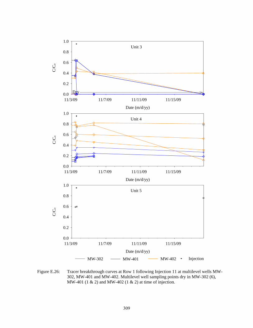
Date (m/d/yy)

11/3/09 11/7/09 11/11/09 11/15/09

C/C

o

0.0

0.2

0.4

0.6

0.8

1.0

Date (m/d/yy)

11/3/09 11/7/09 11/11/09 11/15/09

C/C

o

0.0

0.2

0.4

0.6

0.8

1.0

Date (m/d/yy)

11/3/09 11/7/09 11/11/09 11/15/09

C/C

o

0.0

0.2

0.4

0.6

0.8

1.0

Injection

Unit 3

Unit 4

Unit 5

MW-302 MW-401 MW-402

Dry

Figure E.26: Tracer breakthrough curves at Row 1 following Injection 11 at multilevel wells MW- 302, MW-401 and MW-402. Multilevel well sampling points dry in MW-302 (6), MW-401 (1 & 2) and MW-402 (1 & 2) at time of injection.

309

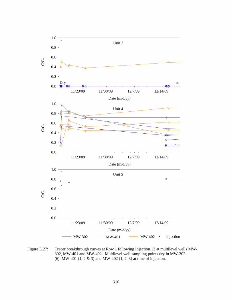
Date (m/d/yy)

11/23/09 11/30/09 12/7/09 12/14/09

C/C

o

0.0

0.2

0.4

0.6

0.8

1.0

Date (m/d/yy)

11/23/09 11/30/09 12/7/09 12/14/09

C/C

o

0.0

0.2

0.4

0.6

0.8

1.0

Date (m/d/yy)

11/23/09 11/30/09 12/7/09 12/14/09

C/C

o

0.0

0.2

0.4

0.6

0.8

1.0

Injection

Unit 3

Unit 4

Unit 5

MW-302 MW-401 MW-402

Dry

Figure E.27: Tracer breakthrough curves at Row 1 following Injection 12 at multilevel wells MW- 302, MW-401 and MW-402. Multilevel well sampling points dry in MW-302 (6), MW-401 (1, 2 & 3) and MW-402 (1, 2, 3) at time of injection.

310

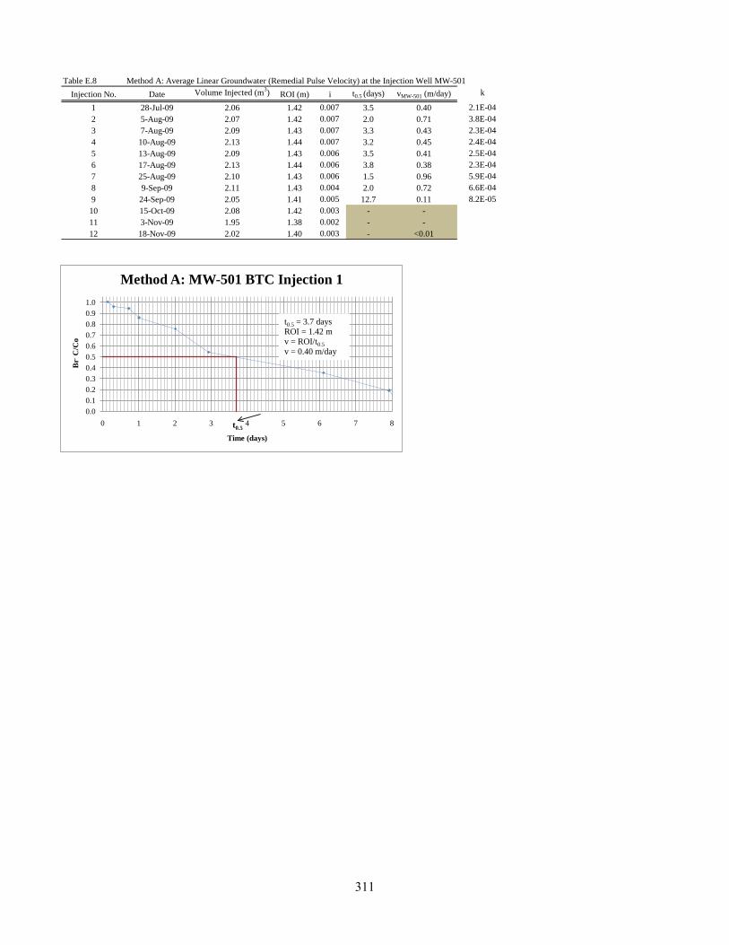
Table E.8 Method A: Average Linear Groundwater (Remedial Pulse Velocity) at the Injection Well MW-501

Injection No. Date Volume Injected (m3) ROI (m) i t0.5 (days) vMW-501 (m/day) k

1 28-Jul-09 2.06 1.42 0.007 3.5 0.40 2.1E-042 5-Aug-09 2.07 1.42 0.007 2.0 0.71 3.8E-043 7-Aug-09 2.09 1.43 0.007 3.3 0.43 2.3E-044 10-Aug-09 2.13 1.44 0.007 3.2 0.45 2.4E-045 13-Aug-09 2.09 1.43 0.006 3.5 0.41 2.5E-046 17-Aug-09 2.13 1.44 0.006 3.8 0.38 2.3E-047 25-Aug-09 2.10 1.43 0.006 1.5 0.96 5.9E-048 9-Sep-09 2.11 1.43 0.004 2.0 0.72 6.6E-049 24-Sep-09 2.05 1.41 0.005 12.7 0.11 8.2E-0510 15-Oct-09 2.08 1.42 0.003 - -11 3-Nov-09 1.95 1.38 0.002 - -12 18-Nov-09 2.02 1.40 0.003 - <0.01

0.0

0.1

0.2

0.3

0.4

0.5

0.6

0.7

0.8

0.9

1.0

0 1 2 3 4 5 6 7 8

Br-

C/C

o

Time (days)

Method A: MW-501 BTC Injection 1

t0.5 = 3.7 daysROI = 1.42 mv = ROI/t0.5v = 0.40 m/day

t0.5

311

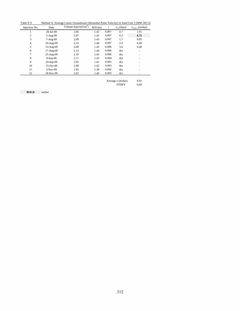
Table E.9 Method A: Average Linear Groundwater (Remedial Pulse Velocity) in Sand Unit 2 (MW-302-5)

Injection No. Date Volume Injected (m3) ROI (m) i t0.5 (days) vUnit 2 (m/day)

1 28-Jul-09 2.06 1.42 0.007 0.7 1.912 5-Aug-09 2.07 1.42 0.007 0.3 4.733 7-Aug-09 2.09 1.43 0.007 1.7 0.854 10-Aug-09 2.13 1.44 0.007 2.9 0.495 13-Aug-09 2.09 1.43 0.006 3.6 0.406 17-Aug-09 2.13 1.44 0.006 dry -7 25-Aug-09 2.10 1.43 0.006 dry -8 9-Sep-09 2.11 1.43 0.004 dry -9 24-Sep-09 2.05 1.41 0.005 dry -10 15-Oct-09 2.08 1.42 0.003 dry -11 3-Nov-09 1.95 1.38 0.002 dry -12 18-Nov-09 2.02 1.40 0.003 dry -

Average v (m/day) 0.91STDEV 0.69

BOLD outlier

312

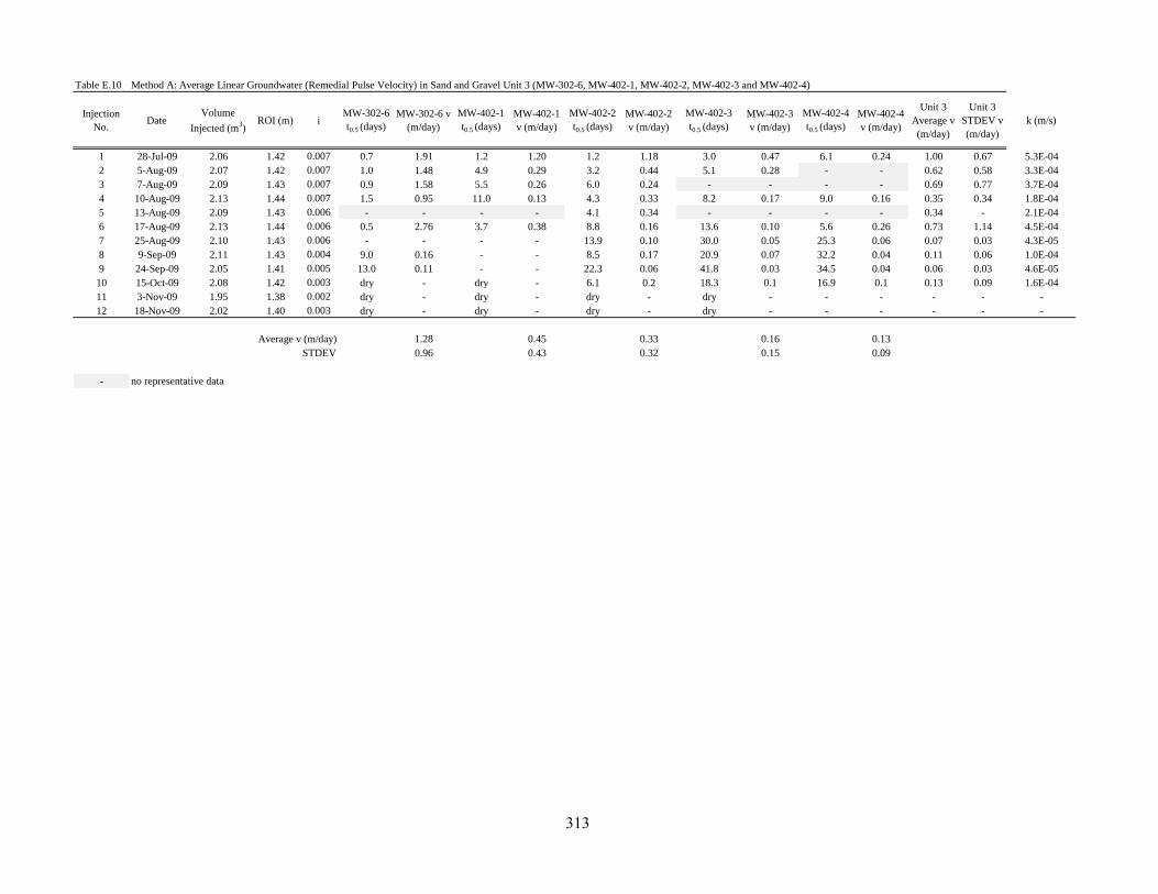
Table E.10 Method A: Average Linear Groundwater (Remedial Pulse Velocity) in Sand and Gravel Unit 3 (MW-302-6, MW-402-1, MW-402-2, MW-402-3 and MW-402-4)

Injection No.

DateVolume

Injected (m3)ROI (m) i

MW-302-6 t0.5 (days)

MW-302-6 v (m/day)

MW-402-1 t0.5 (days)

MW-402-1 v (m/day)

MW-402-2 t0.5 (days)

MW-402-2 v (m/day)

MW-402-3 t0.5 (days)

MW-402-3 v (m/day)

MW-402-4 t0.5 (days)

MW-402-4 v (m/day)

Unit 3 Average v (m/day)

Unit 3 STDEV v (m/day)

k (m/s)

1 28-Jul-09 2.06 1.42 0.007 0.7 1.91 1.2 1.20 1.2 1.18 3.0 0.47 6.1 0.24 1.00 0.67 5.3E-042 5-Aug-09 2.07 1.42 0.007 1.0 1.48 4.9 0.29 3.2 0.44 5.1 0.28 - - 0.62 0.58 3.3E-043 7-Aug-09 2.09 1.43 0.007 0.9 1.58 5.5 0.26 6.0 0.24 - - - - 0.69 0.77 3.7E-044 10-Aug-09 2.13 1.44 0.007 1.5 0.95 11.0 0.13 4.3 0.33 8.2 0.17 9.0 0.16 0.35 0.34 1.8E-045 13-Aug-09 2.09 1.43 0.006 - - - - 4.1 0.34 - - - - 0.34 - 2.1E-046 17-Aug-09 2.13 1.44 0.006 0.5 2.76 3.7 0.38 8.8 0.16 13.6 0.10 5.6 0.26 0.73 1.14 4.5E-047 25-Aug-09 2.10 1.43 0.006 - - - - 13.9 0.10 30.0 0.05 25.3 0.06 0.07 0.03 4.3E-058 9-Sep-09 2.11 1.43 0.004 9.0 0.16 - - 8.5 0.17 20.9 0.07 32.2 0.04 0.11 0.06 1.0E-049 24-Sep-09 2.05 1.41 0.005 13.0 0.11 - - 22.3 0.06 41.8 0.03 34.5 0.04 0.06 0.03 4.6E-0510 15-Oct-09 2.08 1.42 0.003 dry - dry - 6.1 0.2 18.3 0.1 16.9 0.1 0.13 0.09 1.6E-0411 3-Nov-09 1.95 1.38 0.002 dry - dry - dry - dry - - - - - -12 18-Nov-09 2.02 1.40 0.003 dry - dry - dry - dry - - - - - -

Average v (m/day) 1.28 0.45 0.33 0.16 0.13STDEV 0.96 0.43 0.32 0.15 0.09

- no representative data

313

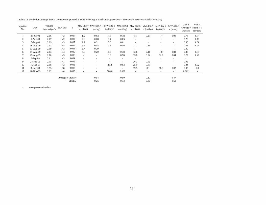
Table E.11 Method A: Average Linear Groundwater (Remedial Pulse Velocity) in Sand Unit 4 (MW-302-7, MW-302-8, MW-402-5 and MW-402-6)

Injection No.

DateVolume

Injected (m3)ROI (m) i

MW-302-7 t0.5 (days)

MW-302-7 v (m/day)

MW-302-8 t0.5 (days)

MW-302-8 v (m/day)

MW-402-5 t0.5 (days)

MW-402-5 v (m/day)

MW-402-6 t0.5 (days)

MW-402-6 v (m/day)

Unit 4 Average v (m/day)

Unit 4 STDEV v (m/day)

1 28-Jul-09 2.06 1.42 0.007 1.5 0.93 1.8 0.78 6.1 0.23 1.4 0.98 0.73 0.342 5-Aug-09 2.07 1.42 0.007 2.1 0.68 1.7 0.83 - - - - 0.76 0.113 7-Aug-09 2.09 1.43 0.007 2.8 0.51 2.3 0.61 - - - - 0.56 0.084 10-Aug-09 2.13 1.44 0.007 2.7 0.54 2.6 0.56 11.1 0.13 - - 0.41 0.245 13-Aug-09 2.09 1.43 0.006 3.7 0.39 - - - - - - 0.396 17-Aug-09 2.13 1.44 0.006 7.1 0.20 3.8 0.38 13.6 0.11 1.8 0.82 0.38 0.317 25-Aug-09 2.10 1.43 0.006 - - 1.8 0.78 33.8 0.04 32.9 0.04 0.29 0.428 9-Sep-09 2.11 1.43 0.004 - - - - - - - - -9 24-Sep-09 2.05 1.41 0.005 - - - - 26.3 0.05 - - 0.05

10 15-Oct-09 2.08 1.42 0.003 - - 45.2 0.03 25.9 0.05 - - 0.04 0.0211 3-Nov-09 1.95 1.38 0.002 - - - - 19.5 0.1 71.0 0.02 0.05 0.012 18-Nov-09 2.02 1.40 0.003 - - 588.6 0.002 - - - - 0.002 -

Average v (m/day) 0.54 0.50 0.10 0.47STDEV 0.25 0.33 0.07 0.51

- no representative data

314

Appendix F

Analysis of Nitrate Utilization

315

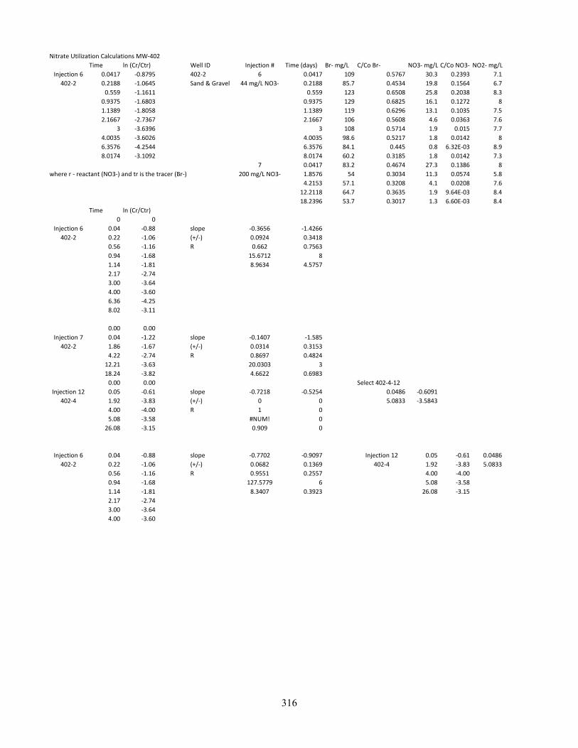
Nitrate Utilization Calculations MW-402

Time ln (Cr/Ctr) Well ID Injection # Time (days) Br- mg/L C/Co Br- NO3- mg/L C/Co NO3- NO2- mg/L

Injection 6 0.0417 -0.8795 402-2 6 0.0417 109 0.5767 30.3 0.2393 7.1

402-2 0.2188 -1.0645 Sand & Gravel 44 mg/L NO3- 0.2188 85.7 0.4534 19.8 0.1564 6.7

0.559 -1.1611 0.559 123 0.6508 25.8 0.2038 8.3

0.9375 -1.6803 0.9375 129 0.6825 16.1 0.1272 8

1.1389 -1.8058 1.1389 119 0.6296 13.1 0.1035 7.5

2.1667 -2.7367 2.1667 106 0.5608 4.6 0.0363 7.6

3 -3.6396 3 108 0.5714 1.9 0.015 7.7

4.0035 -3.6026 4.0035 98.6 0.5217 1.8 0.0142 8

6.3576 -4.2544 6.3576 84.1 0.445 0.8 6.32E-03 8.9

8.0174 -3.1092 8.0174 60.2 0.3185 1.8 0.0142 7.3

7 0.0417 83.2 0.4674 27.3 0.1386 8

where r - reactant (NO3-) and tr is the tracer (Br-) 200 mg/L NO3- 1.8576 54 0.3034 11.3 0.0574 5.8

4.2153 57.1 0.3208 4.1 0.0208 7.6

12.2118 64.7 0.3635 1.9 9.64E-03 8.4

18.2396 53.7 0.3017 1.3 6.60E-03 8.4

Time ln (Cr/Ctr)

0 0

Injection 6 0.04 -0.88 slope -0.3656 -1.4266

402-2 0.22 -1.06 (+/-) 0.0924 0.3418

0.56 -1.16 R 0.662 0.7563

0.94 -1.68 15.6712 8

1.14 -1.81 8.9634 4.5757

2.17 -2.74

3.00 -3.64

4.00 -3.60

6.36 -4.25

8.02 -3.11

0.00 0.00

Injection 7 0.04 -1.22 slope -0.1407 -1.585

402-2 1.86 -1.67 (+/-) 0.0314 0.3153

4.22 -2.74 R 0.8697 0.4824

12.21 -3.63 20.0303 3

18.24 -3.82 4.6622 0.6983

0.00 0.00 Select 402-4-12

Injection 12 0.05 -0.61 slope -0.7218 -0.5254 0.0486 -0.6091

402-4 1.92 -3.83 (+/-) 0 0 5.0833 -3.5843

4.00 -4.00 R 1 0

5.08 -3.58 #NUM! 0

26.08 -3.15 0.909 0

Injection 6 0.04 -0.88 slope -0.7702 -0.9097 Injection 12 0.05 -0.61 0.0486

402-2 0.22 -1.06 (+/-) 0.0682 0.1369 402-4 1.92 -3.83 5.0833

0.56 -1.16 R 0.9551 0.2557 4.00 -4.00

0.94 -1.68 127.5779 6 5.08 -3.58

1.14 -1.81 8.3407 0.3923 26.08 -3.15

2.17 -2.74

3.00 -3.64

4.00 -3.60

316

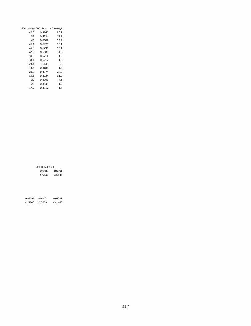
SO42- mg/LC/Co Br- NO3- mg/L

40.2 0.5767 30.3

31 0.4534 19.8

46 0.6508 25.8

46.1 0.6825 16.1

45.3 0.6296 13.1

42.9 0.5608 4.6

39.6 0.5714 1.9

33.1 0.5217 1.8

23.4 0.445 0.8

14.5 0.3185 1.8

29.5 0.4674 27.3

19.1 0.3034 11.3

20 0.3208 4.1

20 0.3635 1.9

17.7 0.3017 1.3

Select 402-4-12

0.0486 -0.6091

5.0833 -3.5843

-0.6091 0.0486 -0.6091

-3.5843 26.0833 -3.1483

317

Nitrate Utilization Calculations MW-302

Date & Time Time (days) Br/Br NO3/NO3 no3/br ln (Cr/Ctr) Time (days)ln (Cr/Ctr)

302-6 8/17/2009 15:10 0.0 0.9 0.6 0.6 -0.5 0.0 -0.5

8/17/2009 19:25 0.2 0.7 0.4 0.5 -0.7 0.2 -0.7

8/17/2009 23:35 0.6 0.6 0.2 0.5 -0.8 0.6 -0.8

8/18/2009 8:40 0.9 0.4 0.2 0.3 -1.1 0.9 -1.1

8/18/2009 13:30 1.1 0.3 0.2 0.5 -0.8 1.1 -0.8

8/20/2009 10:25 3.0 0.2 0.0 0.1 -2.8 3.0 -2.8

8/21/2009 10:30 4.0 0.1 0.0 0.1 -2.9 4.0 -2.9

302-7 11/18/2009 12:00 0.0 0.6 0.5 0.8 -0.2 0.0 -0.2

11/18/2009 12:00 0.1 0.6 0.5 0.8 -0.2 0.1 -0.2

11/20/2009 10:00 1.9 0.6 0.2 0.4 -0.9 1.9 -0.9

11/22/2009 14:00 4.0 0.6 0.3 0.5 -0.8 4.0 -0.8

11/24/2009 16:00 5.1 0.7 0.1 0.2 -1.6 5.1 -1.6

11/24/2009 16:00 5.1 0.6 0.1 0.2 -1.6 5.1 -1.6

12/15/2009 14:00 26.1 0.4 0.0 0.0 -4.4 26.1 -4.4

Time (days) Br/Br no3/br ln (Cr/Ctr) ln (Cr/Ctr)

0 0 0

302-6 Inj 6 0.04 -0.45 slope -0.7 -0.4 per day -0.45 per day

0.22 -0.70 (+/-) 0.1 0.1 -0.70

0.56 -0.80 R 0.9 0.3 -0.80

0.94 -1.05 80.1 5.0 -1.05

1.15 -0.76 6.0 0.4 -0.76

3.00 -2.78 -2.78

4.00 -2.88 -2.88

0.00 0.00 0.00

302-7 inj 7 1.86 -1.80 slope -1.0 0.1 -1.80

4.22 -4.25 (+/-) 0.0 0.0 -4.25

R 1.0 0.0

3.0 0.0

Time (days)

0.00 0 0

302-7-12 0.01 -0.25 slope -0.15 -0.45 -0.25

0.07 -0.23 (+/-) 0.01 0.15 -0.23

1.92 -0.88 R 0.98 0.29 -0.88

5.08 -1.59 143.06 3.00 -1.59

26.08 -4.40 11.70 0.25 -4.40

Time

302-7-7 8/27/2009 9:10 1.86 -1.80

8/29/2009 5:45 4.22 -4.25

318

Nitrate Utilization Calculations MW-501

Time ln (Cr/Ctr)

0 0

501-12 0.04 -0.19 slope -0.10 -0.22

5.08 -0.74 (+/-) 0.00 0.04

26.08 -2.69 R 1.00 0.05

319

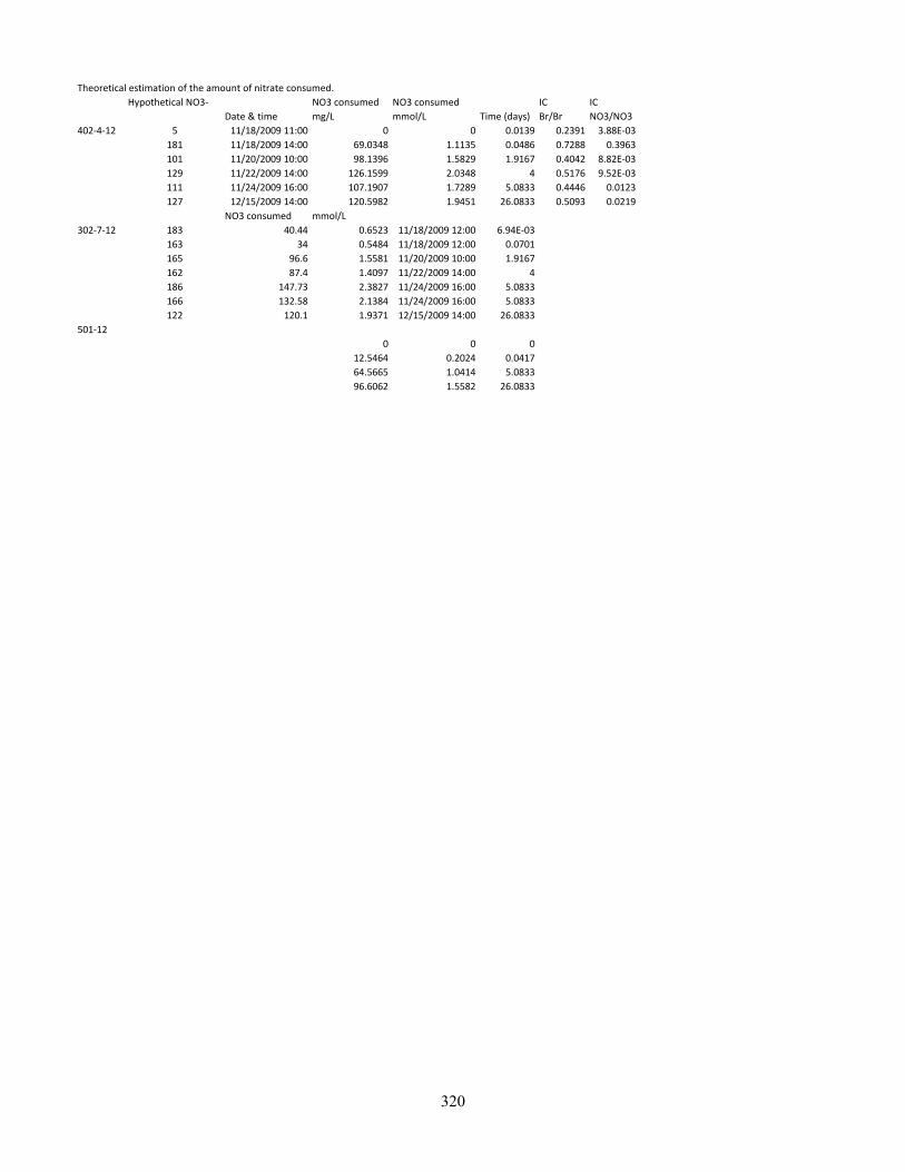
Theoretical estimation of the amount of nitrate consumed.

Hypothetical NO3- NO3 consumed NO3 consumed IC IC

Date & time mg/L mmol/L Time (days) Br/Br NO3/NO3

402-4-12 5 11/18/2009 11:00 0 0 0.0139 0.2391 3.88E-03

181 11/18/2009 14:00 69.0348 1.1135 0.0486 0.7288 0.3963

101 11/20/2009 10:00 98.1396 1.5829 1.9167 0.4042 8.82E-03

129 11/22/2009 14:00 126.1599 2.0348 4 0.5176 9.52E-03

111 11/24/2009 16:00 107.1907 1.7289 5.0833 0.4446 0.0123

127 12/15/2009 14:00 120.5982 1.9451 26.0833 0.5093 0.0219

NO3 consumed mmol/L

302-7-12 183 40.44 0.6523 11/18/2009 12:00 6.94E-03

163 34 0.5484 11/18/2009 12:00 0.0701

165 96.6 1.5581 11/20/2009 10:00 1.9167

162 87.4 1.4097 11/22/2009 14:00 4

186 147.73 2.3827 11/24/2009 16:00 5.0833

166 132.58 2.1384 11/24/2009 16:00 5.0833

122 120.1 1.9371 12/15/2009 14:00 26.0833

501-12

0 0 0

12.5464 0.2024 0.0417

64.5665 1.0414 5.0833

96.6062 1.5582 26.0833

320

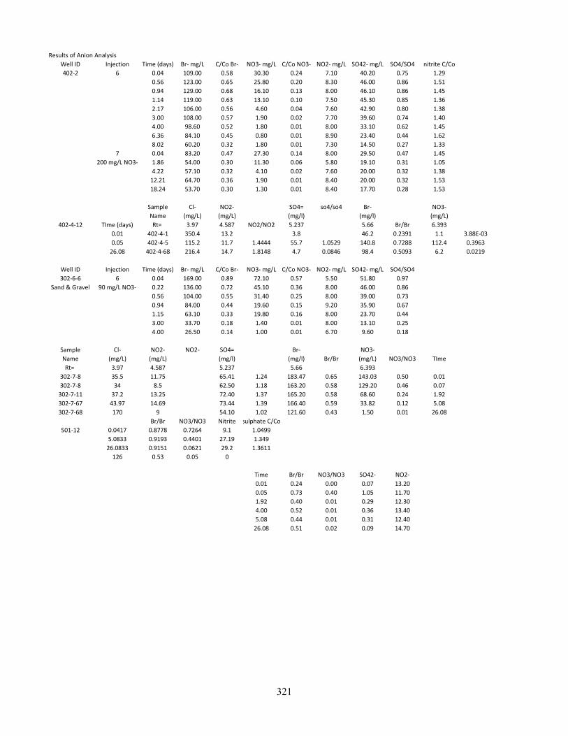
Results of Anion Analysis

Well ID Injection Time (days) Br- mg/L C/Co Br- NO3- mg/L C/Co NO3- NO2- mg/L SO42- mg/L SO4/SO4 nitrite C/Co

402-2 6 0.04 109.00 0.58 30.30 0.24 7.10 40.20 0.75 1.29

0.56 123.00 0.65 25.80 0.20 8.30 46.00 0.86 1.51

0.94 129.00 0.68 16.10 0.13 8.00 46.10 0.86 1.45

1.14 119.00 0.63 13.10 0.10 7.50 45.30 0.85 1.36

2.17 106.00 0.56 4.60 0.04 7.60 42.90 0.80 1.38

3.00 108.00 0.57 1.90 0.02 7.70 39.60 0.74 1.40

4.00 98.60 0.52 1.80 0.01 8.00 33.10 0.62 1.45

6.36 84.10 0.45 0.80 0.01 8.90 23.40 0.44 1.62

8.02 60.20 0.32 1.80 0.01 7.30 14.50 0.27 1.33

7 0.04 83.20 0.47 27.30 0.14 8.00 29.50 0.47 1.45

200 mg/L NO3- 1.86 54.00 0.30 11.30 0.06 5.80 19.10 0.31 1.05

4.22 57.10 0.32 4.10 0.02 7.60 20.00 0.32 1.38

12.21 64.70 0.36 1.90 0.01 8.40 20.00 0.32 1.53

18.24 53.70 0.30 1.30 0.01 8.40 17.70 0.28 1.53

Sample Cl- NO2- SO4= so4/so4 Br- NO3-

Name (mg/L) (mg/L) (mg/l) (mg/l) (mg/L)

402-4-12 TIme (days) Rt= 3.97 4.587 NO2/NO2 5.237 5.66 Br/Br 6.393

0.01 402-4-1 350.4 13.2 3.8 46.2 0.2391 1.1 3.88E-03

0.05 402-4-5 115.2 11.7 1.4444 55.7 1.0529 140.8 0.7288 112.4 0.3963

26.08 402-4-68 216.4 14.7 1.8148 4.7 0.0846 98.4 0.5093 6.2 0.0219

Well ID Injection Time (days) Br- mg/L C/Co Br- NO3- mg/L C/Co NO3- NO2- mg/L SO42- mg/L SO4/SO4

302-6-6 6 0.04 169.00 0.89 72.10 0.57 5.50 51.80 0.97

Sand & Gravel 90 mg/L NO3- 0.22 136.00 0.72 45.10 0.36 8.00 46.00 0.86

0.56 104.00 0.55 31.40 0.25 8.00 39.00 0.73

0.94 84.00 0.44 19.60 0.15 9.20 35.90 0.67

1.15 63.10 0.33 19.80 0.16 8.00 23.70 0.44

3.00 33.70 0.18 1.40 0.01 8.00 13.10 0.25

4.00 26.50 0.14 1.00 0.01 6.70 9.60 0.18

Sample Cl- NO2- NO2- SO4= Br- NO3-

Name (mg/L) (mg/L) (mg/l) (mg/l) Br/Br (mg/L) NO3/NO3 TIme

Rt= 3.97 4.587 5.237 5.66 6.393

302-7-8 35.5 11.75 65.41 1.24 183.47 0.65 143.03 0.50 0.01

302-7-8 34 8.5 62.50 1.18 163.20 0.58 129.20 0.46 0.07

302-7-11 37.2 13.25 72.40 1.37 165.20 0.58 68.60 0.24 1.92

302-7-67 43.97 14.69 73.44 1.39 166.40 0.59 33.82 0.12 5.08

302-7-68 170 9 54.10 1.02 121.60 0.43 1.50 0.01 26.08

Br/Br NO3/NO3 Nitrite sulphate C/Co

501-12 0.0417 0.8778 0.7264 9.1 1.0499

5.0833 0.9193 0.4401 27.19 1.349

26.0833 0.9151 0.0621 29.2 1.3611

126 0.53 0.05 0

Time Br/Br NO3/NO3 SO42- NO2-

0.01 0.24 0.00 0.07 13.20

0.05 0.73 0.40 1.05 11.70

1.92 0.40 0.01 0.29 12.30

4.00 0.52 0.01 0.36 13.40

5.08 0.44 0.01 0.31 12.40

26.08 0.51 0.02 0.09 14.70

321