della thomas*, s. surendran† and nj vasa

IX International Conference on Computational Methods in Marine Engineering

MARINE 2021

I.M. Viola and F. Brennan (Eds)

ALTERNATE METHOD FOR DETERMINING RESISTANCE OF SHIP

WITH FOULED HULL

MARINE 2021

DELLA THOMAS*, S. SURENDRAN

† AND N.J. VASA

†

* Department of Ocean Engineering

Indian Institue of Technology, Madras

Chennai 600036, India

e-mail: [email protected], [email protected]

† Department of Engineering Design

Indian Institute of Technology, Madras

Chennai 600036, India

Key words: Towing tank setup, Biofouling roughness.

Abstract. Recent research shows that planks of various roughness can be towed in water, and

the frictional resistance obtained can be extended to hull forms. Thus, the resistance is

determined experimentally with the help of towing tank setup. The estimation of resistance of

planks of varied roughness by towing them in the towing tank will help determine frictional

resistance of the ship.

In the studies of Schultz (Schultz 2007), it is reported that higher drag values are reported for

small coverage of barnacles, and smaller drag values are reported for large coverage. The skin

friction coefficients for different plate lengths are extrapolated to ship size and speed. Usually,

the variation in drag coefficients is minimal for planks of length above 50 feet.

1 INTRODUCTION

Recent papers have reported a lot of work on extending the frictional resistance from planks

to ships (Demirel et al. 2017). Biofouling is a major research area where the resistance has to

be estimated based on a lot of parameters and extrapolated to ship hulls (Uzun et al. 2020).

Towing a unit plank and pasting various roughness conditions for estimating ship resistance

with roughness condition is explained in the paper.

One of the other approaches tried in the paper is the estimation of ship resistance with various

roughness condition across the ship hull. There have been many studies where the

heterogenous roughness difference in ship hulls has been incorporated in resistance

calculations. In the paper, a formula has been proposed to calculate the ΔCf values with

various roughness condition. This will help to estimate the average ΔCf values for a given

ship configuration with different fouling conditions across the hull. Databases have been

reported for ship hull fouling penalty calculations (Hunsucker et al. 2014), with different hull

mailto:[email protected]

mailto:[email protected]

Della Thomas, S. Surendran and N.J. Vasa

2

fouling conditions. In this paper, modelling of roughness functions for different fouling

conditions has also been done.

Biofilm community structure on ship has also been widely studied (Zargiel, Coogan, and

Swain 2011). In their paper the different biofouling community diatom distribution across the

ship has been tabulated in the literature. Community structure has been tabulated in

commercially available ship hull coatings and in-service ships.

2 METHODOLOGY

CTM is calculated corresponding to each speed, from the model test results as follows (Ghose

and Gokarn 2004).

where RTM - total model resistance, - density of water, - model speed and – model

wetted surface area.

The frictional resistance coefficient CFM is calculated for each speed as follows.

where RnM - Reynold’s number.

The residuary resistance coefficient is obtained at each speed with the following equation,

where k – form factor. Here form factor of 1.05 (Ghose and Gokarn 2004) was considered for

calculations.

The resistance of the bare hull is determined in the towing tank and skin friction for roughness

is determined using Townsin formulae (Townsin 2003). To simulate the effect of the various

biofouling growth stages, the ∆CF or correlation allowance factor (also denoted by CA) was

varied. Hence, the viscous resistance co-efficient has to be added with “roughness allowance”

or the correlation allowance as per equation 4 below.

(1)

(2)

(3)

(4)


3

Here ks - average amplitude of roughness of the wetted surface of the ship, the typical value

for the hull roughness is 150*10-6. L - waterline length of the hull in m.

Given below is the recent version of the ITTC 1978 method.

Calculations were also carried out by employing Granville’s method in this paper. The recent

article on this approach (Song, Demirel, and Atlar 2020), reported the increase in the

frictional drag was estimated by using Granville's approach for the calculation of ∆CF values.

An increase in frictional resistance using Granville's method is accepted by researchers to

arrive at the frictional resistance of the prototype based on resistance of plank and Reynold's

number. Granville's similarity law is relied upon and is discussed in the chapter.

3 EXPERIMENTAL SETUP AND SAMPLE PREPARATION

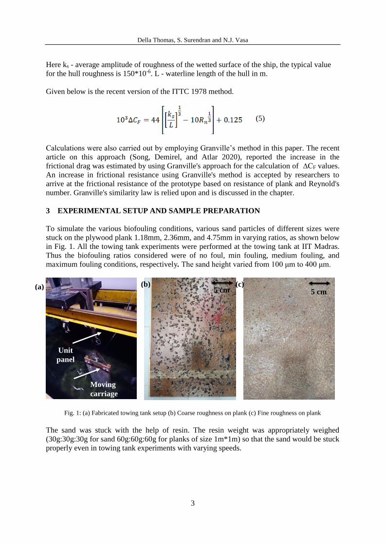
To simulate the various biofouling conditions, various sand particles of different sizes were

stuck on the plywood plank 1.18mm, 2.36mm, and 4.75mm in varying ratios, as shown below

in Fig. 1. All the towing tank experiments were performed at the towing tank at IIT Madras.

Thus the biofouling ratios considered were of no foul, min fouling, medium fouling, and

maximum fouling conditions, respectively. The sand height varied from 100 μm to 400 μm.

Fig. 1: (a) Fabricated towing tank setup (b) Coarse roughness on plank (c) Fine roughness on plank

The sand was stuck with the help of resin. The resin weight was appropriately weighed

(30g:30g:30g for sand 60g:60g:60g for planks of size 1m*1m) so that the sand would be stuck

properly even in towing tank experiments with varying speeds.

(a) (b) (c)

Unit

panel

Moving

carriage

5 cm 5 cm

(5)


4

4 TOWING TANK SETUP

The towing tank setup was designed as given in Fig. 2 below. The load cell was placed in the

vertical position, and the setup will deploy the panel in the towing tank such that the water

forces act along the surface of the plank. This is done so that the forces acting on the plank are

minimum, and only the forces are accounted for which act along the surface of the plank. The

immersed plank area dimensions are 0.5 m by 1m, so that the total surface area of the plank

comes up to 1 m2. The load cell used for the setup was of 10 kg capacity. The load cell was

also provided with additional support with the help of a clamp joint. Ball-bearing support was

given for maintaining the plank’s position during towing, with the help of double angle joint

at an angle of 30⁰. The setup was fabricated, and it was tested in the towing tank. The

experiments with various velocities were done in the towing tank.

Fig 2: Towing tank test setup (a) Perspective (b) Body plan (c) Profile view

5 RESULTS AND DISCUSSION

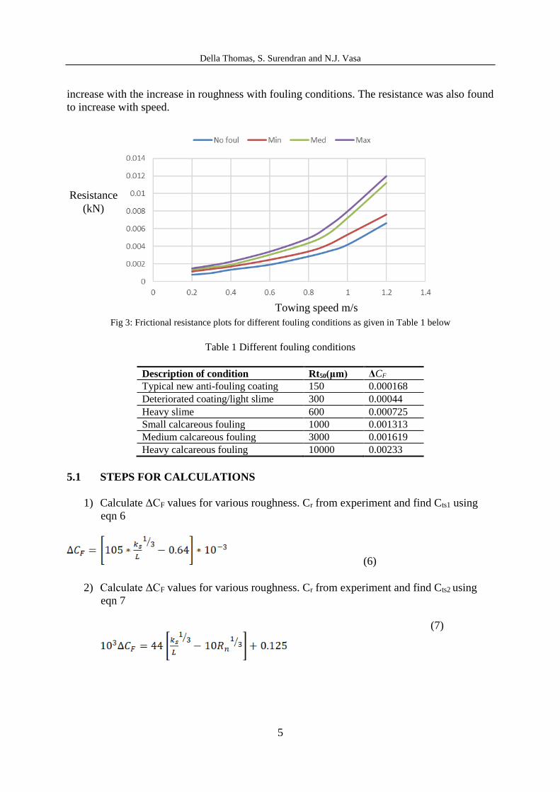
Below shown in Fig. 3 is the resistance curves for different fouling condition of planks as

shown in Table 1. The resistance tests were conducted in towing tank. The towing speeds

were varied from 0.2 m/s to 1.2 m/s. It was found that the frictional resistance is found to

TOWING

DIRECTION

CONNECTION TO

TOWING

CARRIAGE

WL

WL WL

(a) (b) (c)

WL

WL

WL


5

increase with the increase in roughness with fouling conditions. The resistance was also found

to increase with speed.

Fig 3: Frictional resistance plots for different fouling conditions as given in Table 1 below

Table 1 Different fouling conditions

Description of condition Rt50(μm) ΔCF

Typical new anti-fouling coating 150 0.000168

Deteriorated coating/light slime 300 0.00044

Heavy slime 600 0.000725

Small calcareous fouling 1000 0.001313

Medium calcareous fouling 3000 0.001619

Heavy calcareous fouling 10000 0.00233

5.1 STEPS FOR CALCULATIONS

1) Calculate ΔCF values for various roughness. Cr from experiment and find Cts1 using

eqn 6

(3.4)

2) Calculate ΔCF values for various roughness. Cr from experiment and find Cts2 using

eqn 7

(3.5)

Towing speed m/s

(6)

(7)

Resistance

(kN)


6

3) Find Cts3 using Granville’s method (3.6)

Table 2 Calculation of Cts using three different methods

Cf ΔCF gran ΔCF Cts1 Cts2 Cts3

0.002 0.000168 0.0002 50.31657 50.1457 50.31654

0.00239 0.00044 0.0004 49.05145 48.91576 49.05149

0.002246 0.000725 0.0006 47.84964 47.73105 47.84977

0.002083 0.001619 0.0016 48.42364 48.31926 48.42366

0.002029 0.00162 49.26266 49.16802 49.26104

The calibration plot for the 10 kg load cell is given in the plot as in Fig. 4 below.

0

1

2

3

4

5

6

0 0.2 0.4 0.6 0.8 1

We

igh

t (k

g)

Voltage (V)

Calibration

Calibration

Fig 4: Calibration plots for 10 kg load cell

Table 3 Load cell calibration values

Weight kg Load cell

V

1 0.19

2 0.38

3 0.57

4 0.76

5 0.95

The calibration for the load cell is as given in Table 3 above. The force values were calculated

from the voltage values. The constants were calculated corresponding to various speeds of the


7

panel. At low speed, Cr can have lower values. This study proposes developing a new

algorithm that can be employed for the resistance calculation for different biofouling

conditions of the ship.

Cf values were calculated for all the towing speeds. The calculated Cf values are plotted in the

graph in Fig 5.

0

0.0005

0.001

0.0015

0.002

0.0025

0.003

5.2 5.4 5.6 5.8 6 6.2

Cf

log Rn

Fig 5: Calculated Cf values for various ship speeds

The non-dimensional resistance of the ship is found out from the towing tank experiments.

The Cf values were calculated as per ITTC formula as already mentioned and both Cf and Ct

are plotted and shown in Figs 6-8. Due to the additional ΔCf value, the residual resistance will

be reduced by ΔCfm. This causes the Crm value at A to be lesser. For the smaller Crm value, of

course, the speed will be less at point B. The difference remaining between the Cr and Cf

curve is ΔCf. By transposing the Cr value in the co-efficient curve, we can estimate the ship's

minimum velocity due to the considered fouling condition. The methodology for calculation

is depicted in Fig 6. In papers published, the CF and CV values were plotted from the smooth

schoenerr line. The methodology proposed in this paper will help to estimate the average

velocity with different fouling conditions from the frictional resistance co-efficients,


8

Fig. 6: Graph adopted for calculation

Each tow is at a speed, that is Vm for which Cr values were calculated. Vlow was used for

calculations.

Ctm-(Cfm+ΔCf)=Cr

Corresponding to different ship speeds, Cf values were also calculated.

Cf=.075/(log Rn-2)2

Cfm=.075/(log Rn-2)2, where Rn =v*l/ ν.

The shifting for Cr values were done for different draft conditions, and it was found that the

Vavg values are found to increase with the increase in the total resistance. Below given in Figs

7 and 8, are the graphs for design draft condition with Va and Vb values where the Ct and Cf

values are plotted.

ΔCfm

Cf Ct

Vav

g


9

Fig 7: Calculated Ct and Cr values for 0.165m draft condition for Vb=1.1

Fig 8: Calculated Ct and Cr values for 0.165m draft condition for Vb=0.9

Similarly, the plots were done for the three roughness conditions. The plot lines were shifted

towards the Cf line such that the value of Vb was obtained. The average velocity was

calculated, which was used for the resistance calculations. The speeds calculated for design

draft 16.5 m are given in Fig 9. As the velocity increases, the Vavg speed is found to increase,

as can be seen from the graphs.


10

Fig 9: Calculated Ct and Cr values for 0.165m draft condition for Vb corresponding to different fouling conditions

The Vavg values are found to increase with the resistance values, as shown in Fig 10.

Fig 10: Vaverage values for different total resistance values

3.001E+06

2.7 E+06

2.4E+06

2.1E+06

1.9E+06

1.3E+06

1.001E+06

Vavg

Roughness

(μm)


11

Vs is unknown here. The calculations were repeated to calculate the Rts values for different

fouling conditions by accounting for varied roughness conditions. For each ΔCf, three values

plotted with Ctm of other method only slight difference as in Fig 11. Rts1, Rts2 and Rts3 for each

ΔCf corresponds to plank roughness.

Fig. 11: Total resistance values plotted for different roughness conditions

The total resistance values were calculated for different fouling conditions and are plotted in

Fig. 12 below.

Fig 12: Calculated total resistance values for different fouling conditions

Vs m/s

6.001E+06

5.001E+06

4.001E+06 3.001E+06

2.001E+06

1.001E+06

Rts

(N)

RR+RF

(N)

Vs (m/s)


12

Calculate the same parameters by changing surface area (S) values and get a plot for other

drafts. The calculations may be also extended to the ship hull with various fouling growth at

different points.

6 SUMMARY

Here a methodology is proposed whereby it is possible to estimate ship resistance by

incorporating different fouling conditions. Other fouling conditions were incorporated by

estimating the resistance for a unit plank which was towed in the towing tank with different

speeds. Change in resistance co-efficient due to the fouling was determined. Appropriate

model speeds are arrived at matching the resistance components. The resistance calculated for

unit planks can be extrapolated to full-scale ship. The result appears to be acceptable for

researchers and analysts.

REFERENCES

Demirel, Yigit Kemal, Dogancan Uzun, Yansheng Zhang, Ho Chun Fang, Alexander H. Day,

and Osman Turan. 2017. “Effect of Barnacle Fouling on Ship Resistance and Powering.”

Biofouling 33 (10): 819–34. https://doi.org/10.1080/08927014.2017.1373279.

Ghose, J. P., and R. P. Gokarn. 2004. Basic Ship Propulsion. Allied Publishers.

Hunsucker, Kelli Zargiel, Abhishek Koka, Geir Lund, and Geoffrey Swain. 2014. “Diatom

Community Structure on In-Service Cruise Ship Hulls.” Biofouling 30 (9): 1133–40.

https://doi.org/10.1080/08927014.2014.974576.

Schultz, M. P. 2007. “Effects of Coating Roughness and Biofouling on Ship Resistance and

Powering.” Biofouling 23 (5): 331–41. https://doi.org/10.1080/08927010701461974.

Song, Soonseok, Yigit Kemal Demirel, and Mehmet Atlar. 2020. “Penalty of Hull and

Propeller Fouling on Ship Self-Propulsion Performance.” Applied Ocean Research 94

(November 2019). https://doi.org/10.1016/j.apor.2019.102006.

Townsin, R. L. 2003. “The Ship Hull Fouling Penalty.” Biofouling 19 (September 2013): 9–

15. https://doi.org/10.1080/0892701031000088535.

Uzun, Dogancan, Refik Ozyurt, Yigit Kemal Demirel, and Osman Turan. 2020. “Does the

Barnacle Settlement Pattern Affect Ship Resistance and Powering?” Applied Ocean

Research 95 (November 2019): 102020. https://doi.org/10.1016/j.apor.2019.102020.

Zargiel, Kelli A., Jeffrey S. Coogan, and Geoffrey W. Swain. 2011. “Diatom Community

Structure on Commercially Available Ship Hull Coatings.” Biofouling 27 (9): 955–65.

https://doi.org/10.1080/08927014.2011.618268.

della thomas*, s. surendran† and nj vasa

Documents

Transcript of della thomas*, s. surendran† and nj vasa