Deep Learning-Enabled Technologies for Bioimage Analysis

��

Citation: Rabbi, F.; Dabbagh, S.R.;

Angin, P.; Yetisen, A.K.; Tasoglu, S.

Deep Learning-Enabled Technologies

for Bioimage Analysis. Micromachines

2022, 13, 260. https://doi.org/

10.3390/mi13020260

Academic Editor: Shohei

Yamamura

Received: 13 January 2022

Accepted: 3 February 2022

Published: 6 February 2022

Publisher’s Note: MDPI stays neutral

with regard to jurisdictional claims in

published maps and institutional affil-

iations.

Copyright: © 2022 by the authors.

Licensee MDPI, Basel, Switzerland.

This article is an open access article

distributed under the terms and

conditions of the Creative Commons

Attribution (CC BY) license (https://

creativecommons.org/licenses/by/

4.0/).

micromachines

Review

Deep Learning-Enabled Technologies for Bioimage AnalysisFazle Rabbi 1, Sajjad Rahmani Dabbagh 1,2,3 , Pelin Angin 4 , Ali Kemal Yetisen 5 and Savas Tasoglu 1,2,3,6,7,*

1 Department of Mechanical Engineering, Koç University, Sariyer, Istanbul 34450, Turkey;[email protected] (F.R.); [email protected] (S.R.D.)

2 Koç University Arçelik Research Center for Creative Industries (KUAR), Koç University, Sariyer,Istanbul 34450, Turkey

3 Koc University Is Bank Artificial Intelligence Lab (KUIS AILab), Koç University, Sariyer,Istanbul 34450, Turkey

4 Department of Computer Engineering, Middle East Technical University, Ankara 06800, Turkey;[email protected]

5 Department of Chemical Engineering, Imperial College London, London SW7 2AZ, UK;[email protected]

6 Institute of Biomedical Engineering, Bogaziçi University, Çengelköy, Istanbul 34684, Turkey7 Physical Intelligence Department, Max Planck Institute for Intelligent Systems, 70569 Stuttgart, Germany* Correspondence: [email protected]

Abstract: Deep learning (DL) is a subfield of machine learning (ML), which has recently demonstratedits potency to significantly improve the quantification and classification workflows in biomedicaland clinical applications. Among the end applications profoundly benefitting from DL, cellularmorphology quantification is one of the pioneers. Here, we first briefly explain fundamental conceptsin DL and then we review some of the emerging DL-enabled applications in cell morphologyquantification in the fields of embryology, point-of-care ovulation testing, as a predictive tool forfetal heart pregnancy, cancer diagnostics via classification of cancer histology images, autosomalpolycystic kidney disease, and chronic kidney diseases.

Keywords: deep learning; machine learning; bioimage quantification; cell morphology classification;cancer diagnosis

1. Introduction

Early detection and treatment of illnesses (e.g., cancer) can substantially increasethe survival rate, life quality of patients, and, on the other hand, can reduce healthcare-related costs [1,2]. Despite investing a tremendous amount of money in the research anddevelopment of diagnostic approaches, the outcome of clinical treatments is not ideal sofar [3–5]. This problem can stem from the inability of clinicians to acquire enough data,and to analyze healthcare data comprehensively in time [3]. Recent advancements indigital imaging and automated microscopes have led to the creation of copious data ata high pace, addressing the issue of data acquisition for clinicians [1,3,6]. Contemporaryautomated microscopes, for instance, can produce 105 images per day [7,8]. However,the overwhelming size of the produced data has already outpaced the ability of humanexperts to efficaciously extract and analyze data in order to make diagnostic decisionsaccordingly [1,9]. Besides being time-consuming and labor-intensive, human-based analysiscan be susceptible to bias [8,10,11]. A combination of modern high throughput clinicalmethods with the rapidly expanding computational power allows the detection of diseasesin a shorter time more accurately, resulting in more robust and accessible health careservices for the growing population of the world [9].

Bioimages refer to visual observations of biological processes and structures (storedas digital image data) at various spatiotemporal resolutions. Frequently used techniquesin biomedical image analysis are morphology-based cell image analysis, electric signal

Micromachines 2022, 13, 260. https://doi.org/10.3390/mi13020260 https://www.mdpi.com/journal/micromachines

https://doi.org/10.3390/mi13020260

https://doi.org/10.3390/mi13020260

https://creativecommons.org/

https://creativecommons.org/licenses/by/4.0/

https://creativecommons.org/licenses/by/4.0/

https://www.mdpi.com/journal/micromachines

https://www.mdpi.com

https://orcid.org/0000-0001-8888-6106

https://orcid.org/0000-0002-6419-2043

https://orcid.org/0000-0003-4604-217X

https://doi.org/10.3390/mi13020260

https://www.mdpi.com/journal/micromachines

https://www.mdpi.com/article/10.3390/mi13020260?type=check_update&version=2

Micromachines 2022, 13, 260 2 of 28

analysis, and image texture analysis (ranging from single cells to organs and embryos) [12].For instance, cell morphology, as a decisive aspect of the phenotype of a cell, is critical inthe regulation of cell activities [13]. This approach can help clinicians to understand thefunctionality of various pathogenesis by analyzing the structural behavior of cells [1,12].Therefore, rapid quantification/analysis of bioimages could pave the path for early de-tection of disease [14]. However, bioimages exhibit a large variability due to the differentpossible combinations of imaging modalities and acquisition parameters, sample prepara-tion protocols, and phenotypes of interest, resulting in time-consuming and error-proneanalysis by human experts [1,15]. Employing deep learning (DL) techniques can facilitateinterpretation of multi-spectral heterogeneous medical data by providing insight for clin-icians, contributing to easier identification of high-risk patients with real-time analytics,timely decision making, and optimized care delivery [16,17]. Moreover, DL can supportmedical decisions made by clinicians, and improve targeted treatment as well as medicaltreatment surveillance by determination of deviation of the treatment process from theideal condition [11,18–21].

DL is significantly contributing to the medical informatics, bioinformatics, and publichealth sectors. This article provides an overview of DL-enabled technologies in biomedicaland clinical applications. We discuss the working principles and outputs of differentDL-based applications: architecture models in microfluidics, embryology, point-of-careovulation testing, as a predictive algorithm for fetal heart pregnancy, cancer diagnostics viaclassification of cancer histology images, and diagnostic of chronic kidney diseases.

1.1. Deep Learning

Machine learning (ML) is a branch of artificial intelligence (AI), which empowerscomputers to learn using past experiences and example data without being explicitlyprogrammed [22,23]. At a high level, ML algorithms learn to map input feature vectors intoan output space, the granularity and data type of which is determined by the particularalgorithm used. ML algorithms have been successfully applied in a variety of tasks,including classification, data clustering, time series modeling, and regression. ML methodsare broadly categorized as supervised learning algorithms, which utilize labeled data asinput to create a model during the training phase, and unsupervised learning algorithmsthat utilize unlabeled input instances during training. Neural networks are a class of MLalgorithms inspired by the human brain, which simulate the encoding, processing, andtransmission of information through interconnected neural activities resulting from theexcitement or inhibition of neurons in the complex network [23,24].

The foundations of neural networks date back to the 1940s. Hebbian learning ruleswere introduced in 1949 [25], followed by the first perceptron (1958) [26], the back-propagationalgorithm (1974) [27], neocognitron, which was considered as the ancestor of convolutionalneural networks (CNNs) (1980) [28,29], Boltzmann machine (1985) [30], recurrent neuralnetwork (RNN) (1986) [31], and autoencoders (1987) [32,33]. LeNet, which was the startingpoint for the era of CNNs, was initially designed for the classification of handwrittendigits and reading of zip-code directly from the input without preprocessing (1989) [34].This was followed by deep belief networks (DBNs) (2006) [31,35], deep Boltzmann ma-chine (2009) [36], and AlexNet, which was the commencement of image classification byCNNs (2012) [31,37,38].

A perceptron, being one of the earliest neural network structures [39], is a linearclassifier for binary classifications. A binary classifier is a function that can decide whetheran input (i.e., a vector of numbers), fits into a specific class. Perceptron consists of a singleinput layer directly connected to an output node as shown in Figure 1A, representingthe biological process of the human neurons with an activation function and a set ofweights [40]. The ML process of a perceptron starts with random weights assigned toeach input, which are summed and passed through an activation function that producesan output. The model training process continues with multiple iterations, adjusting theweights, where the ultimate goal is to minimize the total error in the output, i.e., the


difference between the output of the model and the actual outputs that should be achievedwith the given data instances [41,42].


between the output of the model and the actual outputs that should be achieved with the given data instances [41,42].

A multi-layer perceptron (MLP), on the other hand, includes a set of hidden layers between the input and output layers to model more complex networks. While simple per-ceptron algorithms (i.e., single-layer perceptrons) can learn only linearly separable pat-terns, MLPs (i.e., feed-forward NNs) possess a greater processing power. A sample MLP containing one hidden layer with n nodes and k output nodes is shown in Figure 1B. Here, each input node is connected to each hidden node and each hidden node is connected to each output node, with each edge having weights adjusted during the training process. An MLP can include multiple hidden layers and the hidden layers can consist of varying numbers of nodes. The training process utilizes a back-propagation algorithm [43] that aims to minimize the total error in the outputs of the model by adjusting the weights on the edges in each iteration of the algorithm. The number of input nodes in an MLP is determined by the dimensionality of the input feature vectors, whereas the number of output nodes is decided by the specific ML task. For example, in the case of a regression task, a single output node will be present, whereas, for a classification task, the number of output nodes will be equal to the number of possible classes. In some ML cases, the pattern of data points on the X-Y plane cannot be fully described by a straight line (i.e., a line would not be good enough to predict values) [44,45]. Moreover, when a line is fitted on the data, the output of the function (i.e., predictions) can range from negative infinity to positive infinity (not limited between any ranges). In these cases, non-linear activation functions are a useful tool to remap available data points to a specific range (e.g., between 0 [for highly negative values] to +1 [for highly positive values] for sigmoid function), al-lowing intentional bending of the regression line (i.e., activation functions are what makes a regression model non-linear to better fit the data) [45–47]. Non-linear activation function can result in a more effective and faster algorithm with a lower chance of getting trapped in local minima during training for large/complex datasets with high variety. Typical non-linear activation functions utilized in MLP include sigmoids described by 푦(푣 ) =t푎푛ℎ (푣 ) and 푦(푣 ) = tanh(푣 ) + (1 + 푒 ) . The first formula represents a hyperbolic tangent ranging from −1 to +1, while the second equation is the logistic function with a similar shape ranging from 0 to +1. Here, 푦(푣 ) is the output of the ith node (neuron) and 푣 is the weighted sum of the input connections [46].

Figure 1. Neural networks. (A) The architecture of a perceptron. (B) A multi-layer perceptron.

Early neural networks such as MLP consisted of a limited set of hidden layers (typi-cally 2–3 layers) due to the computational capacities of the machines on which they were trained, confining their modeling ability to simple tasks on well-structured data. With the advances in computer hardware and remote processing capabilities provided by cloud computing, neural networks have evolved into deep neural networks (DNN) containing


A multi-layer perceptron (MLP), on the other hand, includes a set of hidden layersbetween the input and output layers to model more complex networks. While simpleperceptron algorithms (i.e., single-layer perceptrons) can learn only linearly separablepatterns, MLPs (i.e., feed-forward NNs) possess a greater processing power. A sample MLPcontaining one hidden layer with n nodes and k output nodes is shown in Figure 1B. Here,each input node is connected to each hidden node and each hidden node is connected toeach output node, with each edge having weights adjusted during the training process.An MLP can include multiple hidden layers and the hidden layers can consist of varyingnumbers of nodes. The training process utilizes a back-propagation algorithm [43] thataims to minimize the total error in the outputs of the model by adjusting the weights onthe edges in each iteration of the algorithm. The number of input nodes in an MLP isdetermined by the dimensionality of the input feature vectors, whereas the number ofoutput nodes is decided by the specific ML task. For example, in the case of a regressiontask, a single output node will be present, whereas, for a classification task, the num-ber of output nodes will be equal to the number of possible classes. In some ML cases,the pattern of data points on the X-Y plane cannot be fully described by a straight line(i.e., a line would not be good enough to predict values) [44,45]. Moreover, when a lineis fitted on the data, the output of the function (i.e., predictions) can range from negativeinfinity to positive infinity (not limited between any ranges). In these cases, non-linearactivation functions are a useful tool to remap available data points to a specific range(e.g., between 0 [for highly negative values] to +1 [for highly positive values] for sigmoidfunction), allowing intentional bending of the regression line (i.e., activation functionsare what makes a regression model non-linear to better fit the data) [45–47]. Non-linearactivation function can result in a more effective and faster algorithm with a lower chanceof getting trapped in local minima during training for large/complex datasets with highvariety. Typical non-linear activation functions utilized in MLP include sigmoids describedby y(vi) = tanh



A multi-layer perceptron (MLP), on the other hand, includes a set of hidden layers between the input and output layers to model more complex networks. While simple per-ceptron algorithms (i.e., single-layer perceptrons) can learn only linearly separable pat-terns, MLPs (i.e., feed-forward NNs) possess a greater processing power. A sample MLP containing one hidden layer with n nodes and k output nodes is shown in Figure 1B. Here, each input node is connected to each hidden node and each hidden node is connected to each output node, with each edge having weights adjusted during the training process. An MLP can include multiple hidden layers and the hidden layers can consist of varying numbers of nodes. The training process utilizes a back-propagation algorithm [43] that aims to minimize the total error in the outputs of the model by adjusting the weights on the edges in each iteration of the algorithm. The number of input nodes in an MLP is determined by the dimensionality of the input feature vectors, whereas the number of output nodes is decided by the specific ML task. For example, in the case of a regression task, a single output node will be present, whereas, for a classification task, the number of output nodes will be equal to the number of possible classes. In some ML cases, the pattern of data points on the X-Y plane cannot be fully described by a straight line (i.e., a line would not be good enough to predict values) [44,45]. Moreover, when a line is fitted on the data, the output of the function (i.e., predictions) can range from negative infinity to positive infinity (not limited between any ranges). In these cases, non-linear activation functions are a useful tool to remap available data points to a specific range (e.g., between 0 [for highly negative values] to +1 [for highly positive values] for sigmoid function), al-lowing intentional bending of the regression line (i.e., activation functions are what makes a regression model non-linear to better fit the data) [45–47]. Non-linear activation function can result in a more effective and faster algorithm with a lower chance of getting trapped in local minima during training for large/complex datasets with high variety. Typical non-linear activation functions utilized in MLP include sigmoids described by 𝑦(𝑣 ) =t𝑎𝑛ℎ (𝑣 ) and 𝑦(𝑣 ) = tanh(𝑣 ) + (1 + 𝑒 ) . The first formula represents a hyperbolic tangent ranging from −1 to +1, while the second equation is the logistic function with a similar shape ranging from 0 to +1. Here, 𝑦(𝑣 ) is the output of the ith node (neuron) and 𝑣 is the weighted sum of the input connections [46].



and y(vi) = tanh



A multi-layer perceptron (MLP), on the other hand, includes a set of hidden layers between the input and output layers to model more complex networks. While simple per-ceptron algorithms (i.e., single-layer perceptrons) can learn only linearly separable pat-terns, MLPs (i.e., feed-forward NNs) possess a greater processing power. A sample MLP containing one hidden layer with n nodes and k output nodes is shown in Figure 1B. Here, each input node is connected to each hidden node and each hidden node is connected to each output node, with each edge having weights adjusted during the training process. An MLP can include multiple hidden layers and the hidden layers can consist of varying numbers of nodes. The training process utilizes a back-propagation algorithm [43] that aims to minimize the total error in the outputs of the model by adjusting the weights on the edges in each iteration of the algorithm. The number of input nodes in an MLP is determined by the dimensionality of the input feature vectors, whereas the number of output nodes is decided by the specific ML task. For example, in the case of a regression task, a single output node will be present, whereas, for a classification task, the number of output nodes will be equal to the number of possible classes. In some ML cases, the pattern of data points on the X-Y plane cannot be fully described by a straight line (i.e., a line would not be good enough to predict values) [44,45]. Moreover, when a line is fitted on the data, the output of the function (i.e., predictions) can range from negative infinity to positive infinity (not limited between any ranges). In these cases, non-linear activation functions are a useful tool to remap available data points to a specific range (e.g., between 0 [for highly negative values] to +1 [for highly positive values] for sigmoid function), al-lowing intentional bending of the regression line (i.e., activation functions are what makes a regression model non-linear to better fit the data) [45–47]. Non-linear activation function can result in a more effective and faster algorithm with a lower chance of getting trapped in local minima during training for large/complex datasets with high variety. Typical non-linear activation functions utilized in MLP include sigmoids described by 𝑦(𝑣 ) =t𝑎𝑛ℎ (𝑣 ) and 𝑦(𝑣 ) = tanh(𝑣 ) + (1 + 𝑒 ) . The first formula represents a hyperbolic tangent ranging from −1 to +1, while the second equation is the logistic function with a similar shape ranging from 0 to +1. Here, 𝑦(𝑣 ) is the output of the ith node (neuron) and 𝑣 is the weighted sum of the input connections [46].



+ (1 + e−vi )−1. The first formula represents a hyperbolictangent ranging from −1 to +1, while the second equation is the logistic function with asimilar shape ranging from 0 to +1. Here, y(vi) is the output of the ith node (neuron) and isthe weighted sum of the input connections [46].

Early neural networks such as MLP consisted of a limited set of hidden layers (typi-cally 2–3 layers) due to the computational capacities of the machines on which they weretrained, confining their modeling ability to simple tasks on well-structured data. With theadvances in computer hardware and remote processing capabilities provided by cloudcomputing, neural networks have evolved into deep neural networks (DNN) containingmany more hidden layers allowing for the expression of more complex hypotheses through


capturing the non-linear relationships in the network [24]. DL algorithms empower ML todeal with complex multi-dimensional ill-structured data for more real-life applications [23].DL algorithms utilize multiple layers of artificial neurons to gradually and automaticallyextract higher-level structures and features from (raw) inputs, including images, videos,and sensor data. Industries, including automotive, aviation, defense, and pharmaceuticals,have recently started to embed DL-enabled technologies into their product development.Training of DL algorithms can be performed with labeled data (supervised learning) fordata-driven applications, including face recognition, segmentation, object detection, andimage classification [7,48]. On the other hand, unlabeled and unstructured data, whichis ubiquitous especially in medical applications, can also be used for the training of DLalgorithms (unsupervised learning). Unsupervised DL methods can be used for classifi-cation purposes to find structures and similarities among data. DL has revealed superiorperformance compared to conventional ML methods in many tasks [1,7].

Widely in use DL methods are deep autoencoders, deep Boltzmann machines (DBM),RNNs, DBN, and deep CNN [49]. We describe CNNs in detail below, due to their continuedsuccess, especially in automated medical image analysis.

1.2. Convolutional Neural Networks (CNN)

DL algorithms including autoencoders, DBN, DBM, and RNN do not scale well inthe case of being fed by multi-dimensional input with locally correlated data, as in thecase of images [24], which involve huge numbers of nodes and parameters. Convolutionalneural networks (CNNs, also known as ConvNet), inspired by the neurobiological modelof the visual cortex [50], were proposed to analyze imagery data [51] and became highlysuccessful, forming the basis of many complex automated image analysis tasks today. ACNN is a feed-forward neural network in which signals move in the network withoutforming loops or cycles [11]. Recently, CNNs have received more attention for medicalimage analysis and computer vision owing to their ability in extracting task-related featuresautonomously with no need for human expert intervention, the capability of extracting end-to-end model training parameters by the gradient descent method, and high accuracy [49].

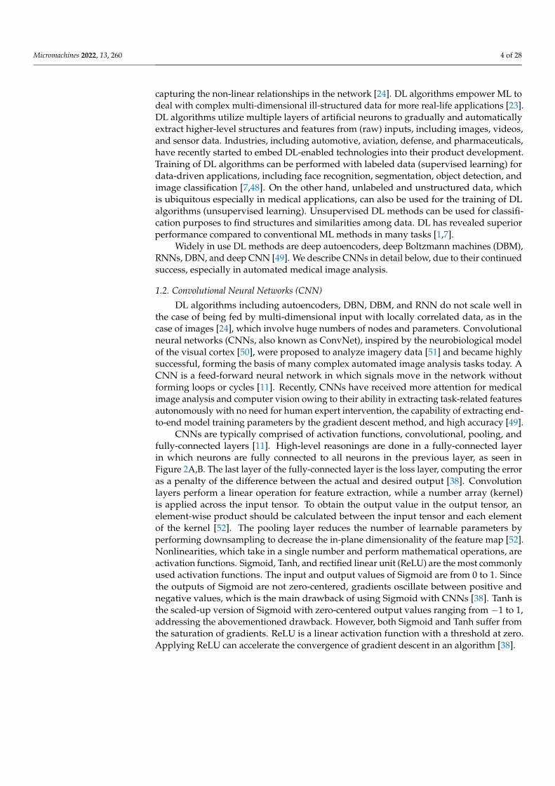
CNNs are typically comprised of activation functions, convolutional, pooling, andfully-connected layers [11]. High-level reasonings are done in a fully-connected layerin which neurons are fully connected to all neurons in the previous layer, as seen inFigure 2A,B. The last layer of the fully-connected layer is the loss layer, computing the erroras a penalty of the difference between the actual and desired output [38]. Convolutionlayers perform a linear operation for feature extraction, while a number array (kernel)is applied across the input tensor. To obtain the output value in the output tensor, anelement-wise product should be calculated between the input tensor and each elementof the kernel [52]. The pooling layer reduces the number of learnable parameters byperforming downsampling to decrease the in-plane dimensionality of the feature map [52].Nonlinearities, which take in a single number and perform mathematical operations, areactivation functions. Sigmoid, Tanh, and rectified linear unit (ReLU) are the most commonlyused activation functions. The input and output values of Sigmoid are from 0 to 1. Sincethe outputs of Sigmoid are not zero-centered, gradients oscillate between positive andnegative values, which is the main drawback of using Sigmoid with CNNs [38]. Tanh isthe scaled-up version of Sigmoid with zero-centered output values ranging from −1 to 1,addressing the abovementioned drawback. However, both Sigmoid and Tanh suffer fromthe saturation of gradients. ReLU is a linear activation function with a threshold at zero.Applying ReLU can accelerate the convergence of gradient descent in an algorithm [38].

Micromachines 2022, 13, 260 5 of 28Micromachines 2022, 13, 260 5 of 29

Figure 2. Neural network architectures. (A) A convolutional neural network sequence to identify handwritten digits. (B) A classic convolutional architecture. Reproduced with permission from [53,54].

Five popular deep CNNs for feature extraction and classification purposes are AlexNet, visual geometry group network (VGGNet), GoogLeNet, U-Net, and residual network (ResNet) [55]. AlexNet was the first CNN to achieve good performance for object detection and classification purposes [55]. VGGNet and AlexNet are similar networks where VGGNet owns additional convolutional layers. Thirteen convolutional, pooling, rectification, and three fully-connected layers are the constituting layers of VGGNet [56]. However, unlike VGGNet, all convolutional layers are stacked together in AlexNet [38]. GoogLeNet was the first network to implement the Inception module. The Inception mod-ule approximates an optimal local sparse structure in a CNN to achieve more efficient computation through dimensionality reduction. The first GoogLeNet was comprised of 22 layers, including rectified linear operation layers, three conventional layers, two fully-connected layers, and pooling layers [38,55]. GoogLeNet possesses fewer parameters com-pared to AlexNet [38]. U-Net is an architecture with a contracting path and an expansive path, which gives it the U-shaped architecture for semantic segmentation (initially de-signed for biomedical image segmentation) [57–59]. It consists of the repeated application of two 3×3 convolutions (unpadded convolutions), each followed by a ReLU and a 2×2 max pooling operation with stride 2 for downsampling (i.e., 23 convolutional layers in total) [57]. ResNet displayed acceptable classification performance on the ImageNet da-taset. In ResNet, instead of learning on referenced functions, the layers learn residual func-tions with respect to the received input. Combining multiple-sized convolutional filters, ResNet can reduce required training time with an easier optimization process [38,55,56].

2. Deep Learning Applications in Microfluidics Microfluidics allows for multiplexing biotechnological techniques and enabling ap-

plications ranging from single-cell analysis [60–64] to on-chip applications [65,66]. It is commonly used in biomedical and chemical research [67–73] to transcend traditional tech-

Figure 2. Neural network architectures. (A) A convolutional neural network sequence to iden-tify handwritten digits. (B) A classic convolutional architecture. Reproduced with permissionfrom [53,54].

Five popular deep CNNs for feature extraction and classification purposes are AlexNet,visual geometry group network (VGGNet), GoogLeNet, U-Net, and residual network(ResNet) [55]. AlexNet was the first CNN to achieve good performance for object detectionand classification purposes [55]. VGGNet and AlexNet are similar networks where VGGNetowns additional convolutional layers. Thirteen convolutional, pooling, rectification, andthree fully-connected layers are the constituting layers of VGGNet [56]. However, unlikeVGGNet, all convolutional layers are stacked together in AlexNet [38]. GoogLeNet wasthe first network to implement the Inception module. The Inception module approximatesan optimal local sparse structure in a CNN to achieve more efficient computation throughdimensionality reduction. The first GoogLeNet was comprised of 22 layers, includingrectified linear operation layers, three conventional layers, two fully-connected layers, andpooling layers [38,55]. GoogLeNet possesses fewer parameters compared to AlexNet [38].U-Net is an architecture with a contracting path and an expansive path, which gives it theU-shaped architecture for semantic segmentation (initially designed for biomedical imagesegmentation) [57–59]. It consists of the repeated application of two 3 × 3 convolutions(unpadded convolutions), each followed by a ReLU and a 2 × 2 max pooling operation withstride 2 for downsampling (i.e., 23 convolutional layers in total) [57]. ResNet displayedacceptable classification performance on the ImageNet dataset. In ResNet, instead oflearning on referenced functions, the layers learn residual functions with respect to thereceived input. Combining multiple-sized convolutional filters, ResNet can reduce requiredtraining time with an easier optimization process [38,55,56].

2. Deep Learning Applications in Microfluidics

Microfluidics allows for multiplexing biotechnological techniques and enabling ap-plications ranging from single-cell analysis [60–64] to on-chip applications [65,66]. It iscommonly used in biomedical and chemical research [67–73] to transcend traditional tech-niques with the capability of trapping, aligning, and manipulating single cells for cell


combination [74], phenotyping [75–77], cell classification [78–81], and flow-based cytom-etry [82–84], cell capture [85,86], such as circulating tumor cells [87], and cell motility(e.g., sperm movement [88,89], mass [90], and volume sensing [91]). These applicationsgenerate high volumes of data of diverse types [92,93]. For instance, a common time-lapsemicroscopy imaging can create more than 100 GB of data over a day. The advances in DLoffer a path to enhance the quality of data analytics when handling large amounts of datasuch as sequences and images.

Conventional DL algorithms have been paired with microfluidics analysis. Thisstrategy has enabled progress in numerical approaches, including cancer screening [94,95],cell counting [96], and single-cell lipid screening [97]. DNNs have been applied to a widerange of fields, including computational biology [98], biomedicine [23,99], single-moleculescience [100]. Architectures used in microfluidic applications can be classified based on thetype of input and output data (Figure 3) [101].


niques with the capability of trapping, aligning, and manipulating single cells for cell com-bination [74], phenotyping [75–77], cell classification [78–81], and flow-based cytometry [82–84], cell capture [85,86], such as circulating tumor cells [87], and cell motility (e.g., sperm movement [88,89], mass [90], and volume sensing [91]). These applications gener-ate high volumes of data of diverse types [92,93]. For instance, a common time-lapse mi-croscopy imaging can create more than 100 GB of data over a day. The advances in DL offer a path to enhance the quality of data analytics when handling large amounts of data such as sequences and images.

Conventional DL algorithms have been paired with microfluidics analysis. This strat-egy has enabled progress in numerical approaches, including cancer screening [94,95], cell counting [96], and single-cell lipid screening [97]. DNNs have been applied to a wide range of fields, including computational biology [98], biomedicine [23,99], single-mole-cule science [100]. Architectures used in microfluidic applications can be classified based on the type of input and output data (Figure 3) [101].

Singh et al. [94] presented digital holographic microscopy to identify tumor cells in the blood. The cells were classified according to size, maximum intensity, and mean in-tensity. The device can detain each cell flowing across a microchannel at 10,000 cells per second. Utilizing ML methods, vigorous gating conditions were established to classify tu-mor cells in the context of blood cells. As a training set, 100,000 cells were used, and the classifier was made by using the features from those training sets. The resultant area un-der the curve (AUC) was greater than 0.9. The ML algorithm enabled the examination of approximately 100 cells and 4500 holograms, reaching a yield of 450,000 cells for each sample. Ko et al. [95] applied an ML algorithm to produce an anticipated panel to specify samples extracted from heterogeneous cancer-bearing individuals. A nanofluidic multi-channel device was developed to examine raw clinical samples. This device was used to separate exosomes from benign and unhealthy murine and clinical cohorts and contoured the ribonucleic acid (RNA) inside these exosomes. Linear discriminant analysis (LDA) was used to recognize the mRNA profile’s linear relationships that can identify the mice as healthy, tumor, or PanIN. The resulting AUC was 0.5 for healthy vs. PanIN and 0.53 for healthy vs. tumor.

Figure 3. Illustration of applications showing different DL architecture. Reproduced with permis-sion from [101].

Figure 3. Illustration of applications showing different DL architecture. Reproduced with permissionfrom [101].

Singh et al. [94] presented digital holographic microscopy to identify tumor cells in theblood. The cells were classified according to size, maximum intensity, and mean intensity.The device can detain each cell flowing across a microchannel at 10,000 cells per second.Utilizing ML methods, vigorous gating conditions were established to classify tumor cellsin the context of blood cells. As a training set, 100,000 cells were used, and the classifierwas made by using the features from those training sets. The resultant area under the curve(AUC) was greater than 0.9. The ML algorithm enabled the examination of approximately100 cells and 4500 holograms, reaching a yield of 450,000 cells for each sample. Ko et al. [95]applied an ML algorithm to produce an anticipated panel to specify samples extractedfrom heterogeneous cancer-bearing individuals. A nanofluidic multichannel device wasdeveloped to examine raw clinical samples. This device was used to separate exosomesfrom benign and unhealthy murine and clinical cohorts and contoured the ribonucleic acid(RNA) inside these exosomes. Linear discriminant analysis (LDA) was used to recognizethe mRNA profile’s linear relationships that can identify the mice as healthy, tumor, orPanIN. The resulting AUC was 0.5 for healthy vs. PanIN and 0.53 for healthy vs. tumor.

Huang et al. [96] applied DL on a microfluidic device for the blood cell countingprocess. Two different ML algorithms were compared for computing blood cells, namelyExtreme Learning Machine Based Super Resolution (ELMSR) and CNN-Based Super Res-


olution (CNNSR). The device took a low-resolution image as input and converted it intoa high-resolution image as output. The ELM algorithm is a feed-forward neural networkwith a single input layer, a single-output layer, and a single hidden layer. Alternatively,a CNN was extensively implemented in DL while working with big datasets. Compar-ing with ELM, CNN can have more than one hidden layer. An advantage of ELM wasthe creation of weights arbitrarily between the input layer and the hidden layer so thatwithout recursive training, it is tuning-free. When various types of cells need to be trainedunder distinct qualities, ELMSR is ideal for accelerating the training operation if the num-ber of available images is high. On the other hand, the direct construction of retrievaland integration of patches, as convolutional layers, was the benefit of using CNNSR. Forthis particular experiment, resolution improving, CNNSR produced 9.5% better resultscompared to ELMSR.

Guo et al. [97] introduced a high-throughput label-free single-cell screening of lipid-producing microalgal cells using optofluidic time-stretch quantitative phase microscopy.The microscope offers a phase map as well as the opacity of each cell at a high throughputof 10,000 cells/s, allowing precise cell categorization. An ML algorithm was employed tocharacterize the phase and intensity pictures obtained from the microscopy. After locatingthe cells, the noise from the background was eliminated. Subsequently, 188 featureswere chosen from an open-source software named CellProfiler to classify the images.Eventually, binary classification was performed by training a support vector classifier. Theaccuracy of that classification was 97.85%. The combination of high-throughput quick pathinterconnected (QPI) and ML was yielded outstanding performance in that the formeroffers large data for classification while the latter handles large data in an efficient way,improving the precision of cell classification.

Table 1 provides the applications, input and output data type, and examples of widelyused architecture models in microfluidic applications. Categorization unstructured datarefers to a feature vector, where the order of elements is not critical, whereas structured datarefers to a feature vector that needs to preserve the order of elements such as a sequenceor image.

Table 1. Representation of the architecture model in microfluidic applications.

Deep Neural NetworkModel Application Input Parameters Output Parameters Example

Unstructured-to-Unstructured

Classify cells usingmanually processed

cell traits

Cell attribute(Perimeter, length of

major axis, circularity)

Cell type (colon cancercell, blood cell)

Cell segmentation andclassification with 85%mean accuracy [102]

Sequence-to-Unstructured

Signal processing(evaluate electrical

signal to featurethe device)

Structured electricaldata (sequence

of voltage)

Differentcharacterization

(pressure atdifferent locations)

Labeling of the softsensor with 6.2%

NRMSE [103]

Sequence-to-Sequence

Monitoring the growthof cell (mass [104] or

volume [91]) for a longperiod of time

A sequence of data(voltage, current)

A classified sequenceof data

DNA base calling with83.2% accuracy [105]

Image-to-UnstructuredImage Processing

(detection of lines andedges)

ImagesDetection or

characterization resultof the image

Bacterial growthmeasuring in a

microfluidic systemwith 0.97 R2 value fordeep neural network

output [106]

Image-to-ImagePartition of images,

anticipating followingimages in a video

Images Images with detailedinformation

Partition of a nerve cellimages into differentareas with maximum95% accuracy on mice

TEM [107]


3. Emerging Deep Learning-Enabled Technologies in Clinical Applications

DL has created highly effective approaches in the biomedical domain, advancing theimaging systems for embryology and point-of-care ovulation testing, predicting fetal heartpregnancy. DL has been used in classifying breast cancer histology, detecting colorectalcancer tissue, and diagnosing different chronic kidney diseases. In this section, a briefdescription of these emerging DL-enabled technologies in clinical applications is discussed.

3.1. Deep Learning-Based Applications in the Field of Embryology and Fertility3.1.1. Embryology and Ovulation Analysis

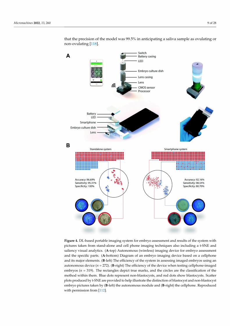
Globally, almost 50 million couples suffer from infertility [108]. In vitro fertilization(IVF) and time-lapse imaging (TPI) are the most widely used methods for embryology;however, they are costly and time-consuming [109,110], even in developed nations [111].Additional processes of embryo analyses, which entail genotypical and phenotypicalassessment, are not cost-effective. A DL method has been developed to resolve theseproblems by creating two moveable, low-cost (<$100 and <$5) optical methods for humanembryo evaluation, utilizing a DNN prepared through a step-by-step transfer learningsystem (Figure 4A) [112]. First, the algorithm was pretrained with 2450 embryo imageswith a commercial TPI method. Second, the algorithm was retrained with embryo picturesobserved with the moveable optical instruments. The performance evaluation of the devicewas carried out with 272 test embryo images. The evaluation was achieved using twotypes of images (blastocytes and non-blastocytes). The precision of the CNN model incategorizing between blastocytes and non-blastocytes pictured with the stand-alone processwas 96.69% (Figure 4B) [112].

More than 40% of all pregnancies worldwide are unplanned or unintentional [113,114].Among the different approaches for family planning or pregnancy tests, saliva ferninganalysis is relatively simple and low cost [115]. Ferning formations are checked in womenovulating during a 4-day period near the ovulation day [116]. Nevertheless, present ovula-tion assessments are manual and deeply abstract, resulting in an error when conducted by alay user [117]. With the help of DL and microfluidic devices, a stand-alone cellphone-baseddevice was developed for point-of-care ovulation assessment (Figure 5) [118]. Nowadays,smartphone-assisted measurements attract more attention due to their low-cost, acceptabledetection resolution, and portability [119–122]. To get rapid and accurate results, a neuralnetwork model was run on this device, which completed the process in 31 s. Samplesfrom both artificial saliva and human participants were used to perform the training andtesting of the DL algorithm. Thirty-four ovulation specimens ranging from 5.6% to 1.4%,and 30 non-ovulation samples ranging from 0.1% to 1.4% of the synthetic saliva sampleswere simulated. Lastly, samples of naturally dried saliva were scanned using the opticalmethod based on the cellphone. At total of 1640 pictures of both types of samples wereacquired. The pictures were then divided into ovulating pictures (29%), and non-ovulatingpictures (71%), depending on the pattern of ferning [118]. A neural network architecture(MobileNet) has been pretrained with 1.4 million pictures from ImageNet to identify thefern structure on a cellphone [123]. ImageNet offers a freely accessible dataset, contain-ing different types of non-saliva pictures. MobileNet’s trained model achieved a top-oneprecision of 64% and a top-five precision of 85.4% over 1000 ImageNet database classes.

The capability of the MobileNet to anticipate accurate outputs was tested with 100 ferningpattern pictures and 100 without ferning pattern pictures of simulated artificial saliva. Theperformance of the algorithm in the evaluation of naturally dried saliva specimens was 90%with 95% confidence intervals (84.98–93.78%) (Figure 5E). While analyzing fern patterns ofartificial saliva samples, the algorithm acted with a sensitivity of 97.62% (CI: 91.66–99.71%)and a specificity of 84.48% (CI: 76.59–90.54%) (Figure 5E). The positive and negativeprognostic values for the test set were 82% and 98%, respectively (Figure 5E). Figure 5Grepresents a t-SNE diagram for displaying the degree of data divergence in a 2D area, whichindicates a strong degree of distinction between the two phenomena. Figure 5F indicates


that the precision of the model was 99.5% in anticipating a saliva sample as ovulating ornon-ovulating [118].


The capability of the MobileNet to anticipate accurate outputs was tested with 100 ferning pattern pictures and 100 without ferning pattern pictures of simulated artificial saliva. The performance of the algorithm in the evaluation of naturally dried saliva spec-imens was 90% with 95% confidence intervals (84.98–93.78%) (Figure 5E). While analyzing fern patterns of artificial saliva samples, the algorithm acted with a sensitivity of 97.62% (CI: 91.66–99.71%) and a specificity of 84.48% (CI: 76.59–90.54%) (Figure 5E). The positive and negative prognostic values for the test set were 82% and 98%, respectively (Figure 5E). Figure 5G represents a t-SNE diagram for displaying the degree of data divergence in a 2D area, which indicates a strong degree of distinction between the two phenomena. Figure 5F indicates that the precision of the model was 99.5% in anticipating a saliva sam-ple as ovulating or non-ovulating [118].

Figure 4. DL-based portable imaging system for embryo assessment and results of the system with pictures taken from stand-alone and cell phone imaging techniques also including a t-SNE and sa-liency visual analytics. (A-top) Autonomous (wireless) imaging device for embryo assessment and the specific parts. (A-bottom) Diagram of an embryo imaging device based on a cellphone and its major elements. (B-left) The efficiency of the system in assessing imaged embryos using an autono-mous device (n = 272). (B-right) The efficiency of the device when testing cellphone-imaged embryos

Figure 4. DL-based portable imaging system for embryo assessment and results of the system withpictures taken from stand-alone and cell phone imaging techniques also including a t-SNE andsaliency visual analytics. (A-top) Autonomous (wireless) imaging device for embryo assessmentand the specific parts. (A-bottom) Diagram of an embryo imaging device based on a cellphoneand its major elements. (B-left) The efficiency of the system in assessing imaged embryos using anautonomous device (n = 272). (B-right) The efficiency of the device when testing cellphone-imagedembryos (n = 319). The rectangles depict true marks, and the circles are the classification of themethod within them. Blue dots represent non-blastocysts, and red dots show blastocysts. Scatterplots produced by t-SNE are provided to help illustrate the distinction of blastocyst and non-blastocystembryo pictures taken by (B-left) the autonomous module and (B-right) the cellphone. Reproducedwith permission from [112].

Micromachines 2022, 13, 260 10 of 28Micromachines 2022, 13, 260 11 of 29

Figure 5. Schematic of the cellphone-based imaging system and reusable microfluidic kit and the system output also with a t-SNE representation with human and artificial saliva samples. (A) The view of the autonomous (wireless) optical device and its parts. (B) The photograph of the manufac-tured autonomous imaging method using a smartphone for fern structure imaging and evaluation in naturally dried saliva specimens. (C) The schematic of the tool with a holding box. (D) A real microfluidic system put near a quarter-coin of US. (E) The scatter plot demonstrates the performance of the system in assessing samples of naturally dried unreal saliva (n = 200). (F) The scatter plot displays the performance of the system when assessing samples of naturally dried human saliva. The rectangles portray true marks, and the circles are the categorization of the scheme. (G) The scatter diagram serves to illustrate the distinction of ovulating and non-ovulating types depending on the fern structures shown by the naturally dried human and artificial saliva. Reproduced with permission from [118].

Figure 5. Schematic of the cellphone-based imaging system and reusable microfluidic kit and thesystem output also with a t-SNE representation with human and artificial saliva samples. (A) The viewof the autonomous (wireless) optical device and its parts. (B) The photograph of the manufacturedautonomous imaging method using a smartphone for fern structure imaging and evaluation innaturally dried saliva specimens. (C) The schematic of the tool with a holding box. (D) A realmicrofluidic system put near a quarter-coin of US. (E) The scatter plot demonstrates the performanceof the system in assessing samples of naturally dried unreal saliva (n = 200). (F) The scatter plotdisplays the performance of the system when assessing samples of naturally dried human saliva.The rectangles portray true marks, and the circles are the categorization of the scheme. (G) Thescatter diagram serves to illustrate the distinction of ovulating and non-ovulating types dependingon the fern structures shown by the naturally dried human and artificial saliva. Reproduced withpermission from [118].

Bormann et al. [124] designed a DL algorithm for scoring an embryo and compared theoutput with the results conducted by experienced embryologists. A total of 3469 embryo


images were used with two distinct post-insemination (hpi) time periods to train thearchitecture. Embryo images were divided into five different categories according to theirmorphology. To examine the embryo scoring, those images were graded by using themodel and the embryologists separately. A higher rate of inconsistency was seen among theembryologists while examining the embryos with an average variability rate of more than82%. However, CNN showed an outstanding result with a 100% recurrence for categorizingthe embryo images. Bormann et al. conducted another assessment by selecting the embryoimages for biopsy and cryopreservation. For the second task, it was reported that theembryologists picked the embryo images for biopsy with an accuracy of 52%, while theaccuracy for the CNN model was 84%. Both results show the supremacy of the DL modelfor assessing embryology. However, further improvement can be made by enhancing thetraining facilities of the model.

Chen et al. [125] introduced a DL model for grading embryo images using a “bigdataset” of microscopic embryo images. Around 170,000 microscopic images were capturedfrom 16,000 embryos on day 5 or 6 after fertilization. ResNet50 model was used for refiningthe ImageNet metrics and a CNN was applied to the microscopic embryo images. Thelabeling of the images was done by using three separate parameters, blastocyte develop-ment, inner cell mass (ICM) quality, and trophectoderm (TE) quality. The overall accuracyachieved by the model was 75.3%. Other top-notch research on embryo assessment using aDL network [126] utilized the ANNs model with around 450 images, achieving a precisionof 76%. Khosravi et al. [127] designed a DNN using time-lapse photography for continuousautomated blastocyte assessment. An accuracy of 98% was achieved in binary classification.

3.1.2. Anticipating the Fetal Heart Pregnancy by Deep Learning

Proper transmission of a single blastocyst will help the mother and child to preventseveral adverse medical conditions [128,129]. TPI has a significant impact on valid embryoselection. Since this process requires subjective manual selection, DL provides the possibil-ity for normalization and automation of the embryo selection process. A fully-automatedDL model was developed to anticipate the likelihood of fetal heart pregnancy directlyfrom the raw time-lapse videos [130]. This study was conducted in eight different IVFlaboratories. Each institute followed its own process of superovulation, egg accumulation,and embryo accumulation. The videos were collected from new embryos, which werefertilized and cultured in a time-lapse incubator for 5 years, and a contemplation analysiswas performed. The experiment conducted 1835 different treatments on 1648 patients.The embryos were divided into three categories: multiple transfer cycles (20%), preservedembryos (20%), and fresh embryos (60%).

The performance characteristics of the DL models were evaluated using the receiveroperating characteristic (ROC) curve. This curve was produced by plotting the sensitivityagainst the I-specificity across every possible thresholding value using the anticipatedconfidence score compared to the actual fetal heart (FH) pregnancy result. Sensitivity andspecificity rates could be conducted by selecting a threshold value. A small threshold valuewill indicate a higher sensitivity with lower specificity and vice versa. The character of thisinterchange could be evaluated by computing the AUC of the ROC curve. To ensure therobustness of the model, a 5-fold stratified cross-validation was performed [131]. The entiredataset was divided into five equal-sized subsets maintaining the exact ratio of positiveembryos. The consequent AUC of the system to anticipate FH pregnancy on the testingdataset was 0.93 with a 95% confidence interval (CI) value, which varied from 0.92 to 0.94.The mean AUC calculated for 5-fold cross-validation was 0.93 [130].

3.2. Deep Learning Approaches for Cancer Diagnosis

The treatment of cancers imposes substantial financial burdens on health systemsworldwide [132,133]. Breast cancer is the most diagnosed cancer in women worldwide withmore than 2 million new cases and an estimated 627,000 deaths in 2018 [132]. In moderncancer treatments, a specific molecular alteration (which can be identified in tumors), is


targeted before treatment initiation. The process of visual inspection by a pathologist ofbiomarker expression on tissue sections from a tumor is a broadly used technique fordetermining the targeted treatment method. For instance, the semi-quantitative evaluationof the sign of the human epidermal growth factor receptor 2 (HER2), as identified byimmunohistochemistry (IHC), indicates the necessity of anti-HER2 therapies for a breastcancer patient. In the case of overexpressed HER2 in the tumor, a treatment against HER2is more effective compared to chemotherapy alone [134]. Pathologists have reported aconsiderable variety in diagnostic reports [135–139]; in which 18% of positive cases and 4%of negative cases were misguided [137,140]. The increase in the number of biomarkers willrequire highly-trained pathologists [141].

To examine the tissues and tumors precisely in a short time, automated diagnosiscan be potent for clinical decision-making in personalized oncology. The US food anddrug administration (FDA) endorsed the commercial algorithms for computer-aided HER2scoring [142]. However, despite image analysis-based platforms providing precise IHCbiomarker scoring in tumors [138,139], the uses of computerized diagnosis by pathologistshave remained restricted. This may be attributed to insufficient proof of clinical significanceand the long period needed to specify tumor area in the tissue sample [143]. Recently, DLhas been introduced to train computers to identify objects in images [144] of tumors withhigh accuracy, which will eventually decrease the manual examinations of pathologists.The pathology community is also keen on utilizing DL [145], showing DL-based imageanalysis can identify cells and categorize cells within distinct cell types [146,147], and findout tumor areas within tissues [148,149]. A further study has been conducted (1) to assessthe performance of ConvNets to automatically identify different types of cancer cells and(2) to measure the accuracy of ConvNets to produce precise HER2 condition review inclinical situations.

Images were analyzed to identify cells, and DL was employed to characterize cells intoseven different varieties to score HER2 activity in tumor cells (Figure 6). A total of 74 full-slide photographs of resection samples of breast tumors were obtained from a commercialvendor. After an initial review, 71 carcinoma samples were chosen for further investigation.Then tissues with an automated threshold operation were isolated from the background,and a further phase of color deconvolution was conducted [150] to distinguish these linesfor the brown HER2 staining and the blue haematoxyl staining from the actual color picture.HER2 staining and haematoxylin staining networks were uniformly associated with asingle photo as a consequence: pixels of a nucleus having a negative value and pixels ofpositive HER2 membrane staining having positive values. The watershed model [151]was used to divide the tissues into a cell. Conventional ML models were developed toanticipate the type of cell depending on the cell attributes employing architectures in the Rprogramming environment. Based on popularity and high accuracy in several classificationtasks [152], linear support vector machine (LSVM) [153], and random forests [154] modelswere selected. The accuracy achieved for hand-crafted features with LSVM was 68%, forhand-crafted features with random forests was 70%, and for ConvNets was 78%.


[146,147], and find out tumor areas within tissues [148,149]. A further study has been con-ducted (1) to assess the performance of ConvNets to automatically identify different types of cancer cells and (2) to measure the accuracy of ConvNets to produce precise HER2 con-dition review in clinical situations.

Images were analyzed to identify cells, and DL was employed to characterize cells into seven different varieties to score HER2 activity in tumor cells (Figure 6). A total of 74 full-slide photographs of resection samples of breast tumors were obtained from a com-mercial vendor. After an initial review, 71 carcinoma samples were chosen for further in-vestigation. Then tissues with an automated threshold operation were isolated from the background, and a further phase of color deconvolution was conducted [150] to distin-guish these lines for the brown HER2 staining and the blue haematoxyl staining from the actual color picture. HER2 staining and haematoxylin staining networks were uniformly associated with a single photo as a consequence: pixels of a nucleus having a negative value and pixels of positive HER2 membrane staining having positive values. The water-shed model [151] was used to divide the tissues into a cell. Conventional ML models were developed to anticipate the type of cell depending on the cell attributes employing archi-tectures in the R programming environment. Based on popularity and high accuracy in several classification tasks [152], linear support vector machine (LSVM) [153], and random forests [154] models were selected. The accuracy achieved for hand-crafted features with LSVM was 68%, for hand-crafted features with random forests was 70%, and for Con-vNets was 78%.

Figure 6. Detection and ranking of tumor cells. Cells are identified using a watershed algorithm and are categorized using DL into seven different types. Reproduced with permission from [142].

To comprehend the advantages of ConvNets, principal component analysis was per-formed to map the hand-crafted high-dimensional aspects, and the ConvNets developed characters through a dynamic 3D environment. Figure 7 shows that the cells in the ConvNets trained feature space are mostly segregated by phenotype while the cells with different phenotypes overlapped in the hand-crafted feature area more. DL has been used in the diagnosis of breast cancer. The diagnosis of tissue growth in breast cancer is made based on primary spotting through palpation and routine check-ups using mammography imaging [155,156]. A pathologist assesses the condition and differentiates the tissues. This diagnosis process requires a manual assessment by a highly-qualified pathologist. A CNN model was designed for the analysis of breast cancer images, which eventually helped pathologists to make decisions more precisely and quickly [155]. To design the algorithm, a dataset of images was composed with high resolution, decom-pressed, and annotated H&E stain pictures from the Bioimaging 2015 breast histology classification challenge [155]. Four categories of 200× magnified images were classified with the help of a pathologist. A total of 249 images were used to compose the training set, while the test set consisted of 20 images to design the CNN architecture. Preprocessing was performed to normalize the images [157]. Two images are shown in Figure 8 before and after the normalization of the images. CNNs were used to assign the image patches into distinct tissue classes (a) normal tissue, (b) benign tissue, (c) in situ carcinoma, and

Figure 6. Detection and ranking of tumor cells. Cells are identified using a watershed algorithm andare categorized using DL into seven different types. Reproduced with permission from [142].


To comprehend the advantages of ConvNets, principal component analysis was per-formed to map the hand-crafted high-dimensional aspects, and the ConvNets developedcharacters through a dynamic 3D environment. Figure 7 shows that the cells in the Con-vNets trained feature space are mostly segregated by phenotype while the cells withdifferent phenotypes overlapped in the hand-crafted feature area more. DL has been usedin the diagnosis of breast cancer. The diagnosis of tissue growth in breast cancer is madebased on primary spotting through palpation and routine check-ups using mammographyimaging [155,156]. A pathologist assesses the condition and differentiates the tissues. Thisdiagnosis process requires a manual assessment by a highly-qualified pathologist. A CNNmodel was designed for the analysis of breast cancer images, which eventually helpedpathologists to make decisions more precisely and quickly [155]. To design the algorithm,a dataset of images was composed with high resolution, decompressed, and annotatedH&E stain pictures from the Bioimaging 2015 breast histology classification challenge [155].Four categories of 200× magnified images were classified with the help of a pathologist.A total of 249 images were used to compose the training set, while the test set consistedof 20 images to design the CNN architecture. Preprocessing was performed to normalizethe images [157]. Two images are shown in Figure 8 before and after the normalizationof the images. CNNs were used to assign the image patches into distinct tissue classes(a) normal tissue, (b) benign tissue, (c) in situ carcinoma, and (d) carcinoma. The accuracyof this method was 66.7% for four classes [155]. The accuracy was 81% for binary carcinomaor non-carcinoma classification [155].


(d) carcinoma. The accuracy of this method was 66.7% for four classes [155]. The accuracy was 81% for binary carcinoma or non-carcinoma classification [155].

Figure 7. Principal Factor Review of the learned and hand-designed features. The point diagram displays the three primary component values of (A) the hand-designed features, and (B) the features learned from the convolution neural network. Reproduced with permission from [142].

Figure 8. Histology images before and after stain normalization condition. Reproduced with per-mission from [158].

A multi-task DL (MTDL) was used to solve the data insufficiency issue in cancer di-agnosis [159]. Although gene expression data are widely in use to develop DL methods for cancer classification, a number of tumors have insufficient gene expression, leading to the loss of the accuracy of the developed DL algorithm. By setting a shared hidden unit, the proposed MTDL was able to share information across different tasks. Moreover, for faster training compared to the Tanh unit, ReLU was chosen as the activation function, along with is Sigmond function in order to get labels in the output layer. Traditional DNN and Sparse autoencoders were used to evaluate the performance of the proposed MTDL. The available data sets were divided into 10 segments, where nine parts were used for training and one part for testing. It was demonstrated that the MTDL achieved a superior classification performance compared to DNN and Sparse autoencoder with smaller stand-ard deviation in results, pointing out a more stable performance [159].

A novel multi-view CNN with multi-task learning (MTL) was utilized to develop a clinical decision support system to specify mammograms that can be correctly classified by the algorithm and those which require radiologist reading for the final decision. Using the proposed method, the number of radiologist readings was reduced by 42.8%, aug-menting detection speed, and saving time as well as money [160].

A deep transfer learning computer-aided diagnosis (CADx) method is used for the treatment of breast cancer using multiparametric magnetic resonance imaging (mpMRI)

Figure 7. Principal Factor Review of the learned and hand-designed features. The point diagramdisplays the three primary component values of (A) the hand-designed features, and (B) the featureslearned from the convolution neural network. Reproduced with permission from [142].


(d) carcinoma. The accuracy of this method was 66.7% for four classes [155]. The accuracy was 81% for binary carcinoma or non-carcinoma classification [155].

Figure 7. Principal Factor Review of the learned and hand-designed features. The point diagram displays the three primary component values of (A) the hand-designed features, and (B) the features learned from the convolution neural network. Reproduced with permission from [142].

Figure 8. Histology images before and after stain normalization condition. Reproduced with per-mission from [158].

A multi-task DL (MTDL) was used to solve the data insufficiency issue in cancer di-agnosis [159]. Although gene expression data are widely in use to develop DL methods for cancer classification, a number of tumors have insufficient gene expression, leading to the loss of the accuracy of the developed DL algorithm. By setting a shared hidden unit, the proposed MTDL was able to share information across different tasks. Moreover, for faster training compared to the Tanh unit, ReLU was chosen as the activation function, along with is Sigmond function in order to get labels in the output layer. Traditional DNN and Sparse autoencoders were used to evaluate the performance of the proposed MTDL. The available data sets were divided into 10 segments, where nine parts were used for training and one part for testing. It was demonstrated that the MTDL achieved a superior classification performance compared to DNN and Sparse autoencoder with smaller stand-ard deviation in results, pointing out a more stable performance [159].

A novel multi-view CNN with multi-task learning (MTL) was utilized to develop a clinical decision support system to specify mammograms that can be correctly classified by the algorithm and those which require radiologist reading for the final decision. Using the proposed method, the number of radiologist readings was reduced by 42.8%, aug-menting detection speed, and saving time as well as money [160].

A deep transfer learning computer-aided diagnosis (CADx) method is used for the treatment of breast cancer using multiparametric magnetic resonance imaging (mpMRI)

Figure 8. Histology images before and after stain normalization condition. Reproduced with permis-sion from [158].


A multi-task DL (MTDL) was used to solve the data insufficiency issue in cancerdiagnosis [159]. Although gene expression data are widely in use to develop DL methodsfor cancer classification, a number of tumors have insufficient gene expression, leading tothe loss of the accuracy of the developed DL algorithm. By setting a shared hidden unit, theproposed MTDL was able to share information across different tasks. Moreover, for fastertraining compared to the Tanh unit, ReLU was chosen as the activation function, along withis Sigmond function in order to get labels in the output layer. Traditional DNN and Sparseautoencoders were used to evaluate the performance of the proposed MTDL. The availabledata sets were divided into 10 segments, where nine parts were used for training and onepart for testing. It was demonstrated that the MTDL achieved a superior classificationperformance compared to DNN and Sparse autoencoder with smaller standard deviationin results, pointing out a more stable performance [159].

A novel multi-view CNN with multi-task learning (MTL) was utilized to develop aclinical decision support system to specify mammograms that can be correctly classified bythe algorithm and those which require radiologist reading for the final decision. Using theproposed method, the number of radiologist readings was reduced by 42.8%, augmentingdetection speed, and saving time as well as money [160].

A deep transfer learning computer-aided diagnosis (CADx) method is used for thetreatment of breast cancer using multiparametric magnetic resonance imaging (mpMRI) [161].Features of dynamic contrast-enhanced (DCE)-MRI sequence and T2-weighted (T2W) MRIsequence were extracted using a pre-trained CNN with 3-channel (red, green, and blue[RGB]) input images. The extracted features were used to train a support vector machine(SVM) classifier to distinguish between malignant and benign lesions. The SVM classifierwas chosen because SVMs were able to yield acceptable performance on sparse high-dimensional data. Using ROC analysis, the performance of the classifier was evaluated byserving the area under the ROC curve as the figure of merit. The AUCs of 0.85 and 0.78were reported in a single-sequence classifier for DCE and T2W, respectively, demonstratingthe superiority of the purposed system for the classification of breast cancer [161].

In another study, CNNs, including AlexNet, VGG 16, ResNet−50, Inception-BN, andGoogleLeNet, were used for CADx application [55]. Two different methodologies wereused for the training of CNNs: (i) fine-tuning, in which weights of the network werepreviously pre-trained using ImageNet dataset; and (ii) from scratch, in which weightsof the network are initialized from a random distribution. While the convergence of allnetwork parameters in (ii) took more time compared to (i), increasing the depth of thenetwork brought about a better ability of discrimination. The fine-tuning method is simplersince most of the corrections of network parameters are applied to the last layers. Themaximum performance was reported for ResNet-50 using fine-tuning [55].

In another study, transfer learning was integrated with CNN to classify breast cancercases [162]. GoogleLeNet, VGGNet, and ResNet, as three different CNN architectures,were used individually to pre-train the proposed framework. Subsequently, using transferlearning, the learning data was transferred into combined feature extraction. The averageclassification accuracy of GoogleLeNet, VGGNet, and ResNet were 93.5%, 94.15%, and94.35%, respectively, whereas the proposed framework yielded 97.525% accuracy [162].

A computational method was developed which receives risk patterns from individualmedical records to anticipate the outcome of the patient biopsy, for classification of cervicalcancer. By formalizing a new loss function to perform dimensionality reduction as wellas classification jointly, the AUC of 0.6875 was reported, outperforming the denoisingautoencoder method [163].

Colorectal cancer is the third most common cancer in the United States. Reliablemetastases detection is needed to diagnose colon cancer. High-resolution images are neededto distinguish between benign colon tissue, cancerous colon tissue, benign peritoneum, andcancerous peritoneum. To produce these images, confocal laser microscopy (CLM) is usedto capture sub-micrometer resolution images [164]. These images are then examined by thepathologists to find out the defected region.


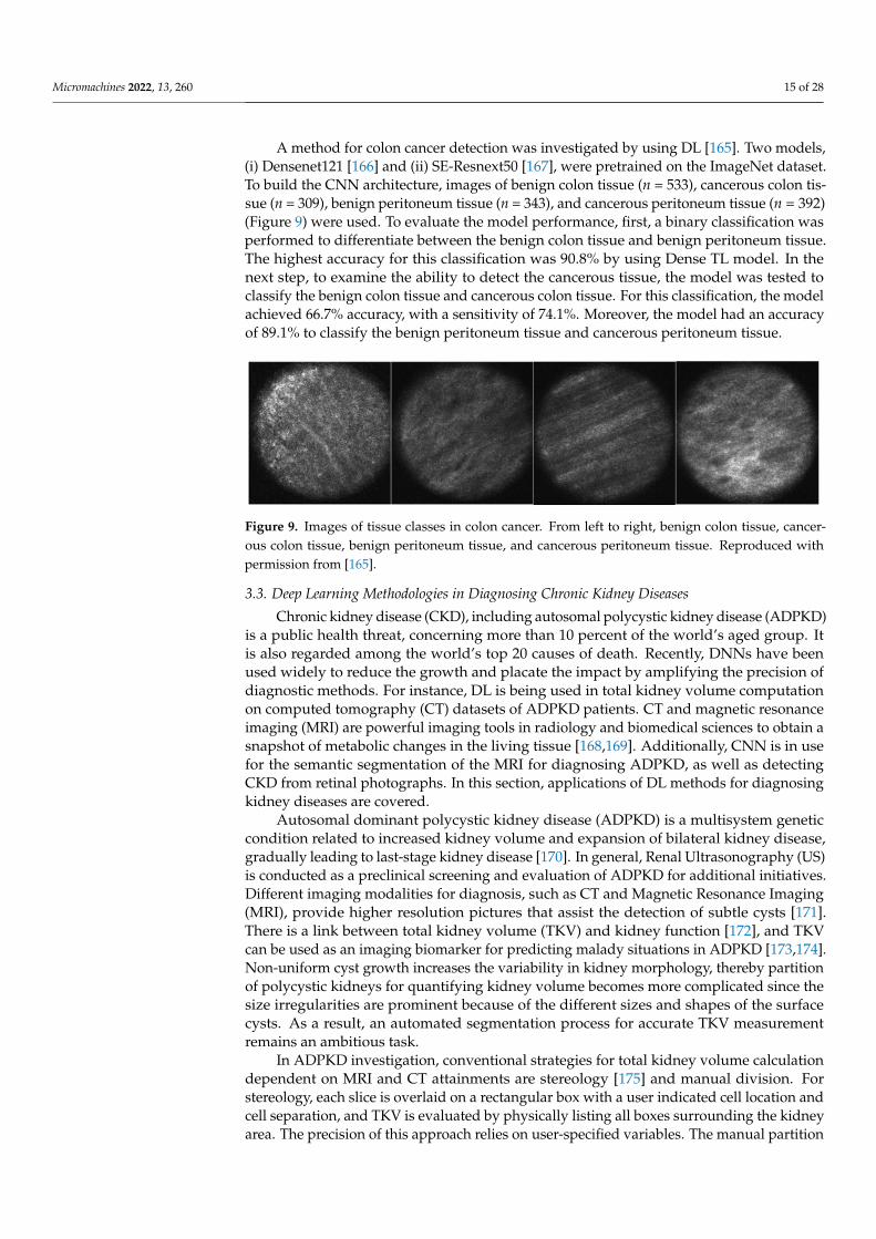
A method for colon cancer detection was investigated by using DL [165]. Two models,(i) Densenet121 [166] and (ii) SE-Resnext50 [167], were pretrained on the ImageNet dataset.To build the CNN architecture, images of benign colon tissue (n = 533), cancerous colon tis-sue (n = 309), benign peritoneum tissue (n = 343), and cancerous peritoneum tissue (n = 392)(Figure 9) were used. To evaluate the model performance, first, a binary classification wasperformed to differentiate between the benign colon tissue and benign peritoneum tissue.The highest accuracy for this classification was 90.8% by using Dense TL model. In thenext step, to examine the ability to detect the cancerous tissue, the model was tested toclassify the benign colon tissue and cancerous colon tissue. For this classification, the modelachieved 66.7% accuracy, with a sensitivity of 74.1%. Moreover, the model had an accuracyof 89.1% to classify the benign peritoneum tissue and cancerous peritoneum tissue.


Figure 9. Images of tissue classes in colon cancer. From left to right, benign colon tissue, cancerous colon tissue, benign peritoneum tissue, and cancerous peritoneum tissue. Reproduced with permis-sion from [165].

3.3. Deep Learning Methodologies in Diagnosing Chronic Kidney Diseases Chronic kidney disease (CKD), including autosomal polycystic kidney disease

(ADPKD) is a public health threat, concerning more than 10 percent of the world’s aged group. It is also regarded among the world’s top 20 causes of death. Recently, DNNs have been used widely to reduce the growth and placate the impact by amplifying the precision of diagnostic methods. For instance, DL is being used in total kidney volume computation on computed tomography (CT) datasets of ADPKD patients. CT and magnetic resonance imaging (MRI) are powerful imaging tools in radiology and biomedical sciences to obtain a snapshot of metabolic changes in the living tissue [168,169]. Additionally, CNN is in use for the semantic segmentation of the MRI for diagnosing ADPKD, as well as detecting CKD from retinal photographs. In this section, applications of DL methods for diagnosing kidney diseases are covered.

Autosomal dominant polycystic kidney disease (ADPKD) is a multisystem genetic condition related to increased kidney volume and expansion of bilateral kidney disease, gradually leading to last-stage kidney disease [170]. In general, Renal Ultrasonography (US) is conducted as a preclinical screening and evaluation of ADPKD for additional ini-tiatives. Different imaging modalities for diagnosis, such as CT and Magnetic Resonance Imaging (MRI), provide higher resolution pictures that assist the detection of subtle cysts [171]. There is a link between total kidney volume (TKV) and kidney function [172], and TKV can be used as an imaging biomarker for predicting malady situations in ADPKD [173,174]. Non-uniform cyst growth increases the variability in kidney morphology, thereby partition of polycystic kidneys for quantifying kidney volume becomes more complicated since the size irregularities are prominent because of the different sizes and shapes of the surface cysts. As a result, an automated segmentation process for accurate TKV measurement remains an ambitious task.

In ADPKD investigation, conventional strategies for total kidney volume calculation dependent on MRI and CT attainments are stereology [175] and manual division. For ste-reology, each slice is overlaid on a rectangular box with a user indicated cell location and cell separation, and TKV is evaluated by physically listing all boxes surrounding the kid-ney area. The precision of this approach relies on user-specified variables. The manual partition needs representation of the kidney on each portion using either an accessible hand shaping method or an adaptation to a different technique that manages the user while outlining the subject of concern. CNNs have been suggested for the specificity and differentiation of kidney cells with gentle morphological improvements in medical diag-nostics, employing patch-wise strategies on CT [176,177].

Participants were categorized systematically into the testing and training set for the final test, attempting to obtain a comparative allocation in every set based on the usable TKV ranging from 0.321 L to 14.670 L. Two distinct techniques were developed to reduce overfitting and accomplish decent speculation on the training dataset [178]. First, by mov-ing the picture in x–y orientation, and then by distorting the individual slice with non-

Figure 9. Images of tissue classes in colon cancer. From left to right, benign colon tissue, cancer-ous colon tissue, benign peritoneum tissue, and cancerous peritoneum tissue. Reproduced withpermission from [165].

3.3. Deep Learning Methodologies in Diagnosing Chronic Kidney Diseases

Chronic kidney disease (CKD), including autosomal polycystic kidney disease (ADPKD)is a public health threat, concerning more than 10 percent of the world’s aged group. Itis also regarded among the world’s top 20 causes of death. Recently, DNNs have beenused widely to reduce the growth and placate the impact by amplifying the precision ofdiagnostic methods. For instance, DL is being used in total kidney volume computationon computed tomography (CT) datasets of ADPKD patients. CT and magnetic resonanceimaging (MRI) are powerful imaging tools in radiology and biomedical sciences to obtain asnapshot of metabolic changes in the living tissue [168,169]. Additionally, CNN is in usefor the semantic segmentation of the MRI for diagnosing ADPKD, as well as detectingCKD from retinal photographs. In this section, applications of DL methods for diagnosingkidney diseases are covered.

Autosomal dominant polycystic kidney disease (ADPKD) is a multisystem geneticcondition related to increased kidney volume and expansion of bilateral kidney disease,gradually leading to last-stage kidney disease [170]. In general, Renal Ultrasonography (US)is conducted as a preclinical screening and evaluation of ADPKD for additional initiatives.Different imaging modalities for diagnosis, such as CT and Magnetic Resonance Imaging(MRI), provide higher resolution pictures that assist the detection of subtle cysts [171].There is a link between total kidney volume (TKV) and kidney function [172], and TKVcan be used as an imaging biomarker for predicting malady situations in ADPKD [173,174].Non-uniform cyst growth increases the variability in kidney morphology, thereby partitionof polycystic kidneys for quantifying kidney volume becomes more complicated since thesize irregularities are prominent because of the different sizes and shapes of the surfacecysts. As a result, an automated segmentation process for accurate TKV measurementremains an ambitious task.

In ADPKD investigation, conventional strategies for total kidney volume calculationdependent on MRI and CT attainments are stereology [175] and manual division. Forstereology, each slice is overlaid on a rectangular box with a user indicated cell location andcell separation, and TKV is evaluated by physically listing all boxes surrounding the kidneyarea. The precision of this approach relies on user-specified variables. The manual partition


needs representation of the kidney on each portion using either an accessible hand shapingmethod or an adaptation to a different technique that manages the user while outliningthe subject of concern. CNNs have been suggested for the specificity and differentiation ofkidney cells with gentle morphological improvements in medical diagnostics, employingpatch-wise strategies on CT [176,177].

Participants were categorized systematically into the testing and training set for thefinal test, attempting to obtain a comparative allocation in every set based on the usableTKV ranging from 0.321 L to 14.670 L. Two distinct techniques were developed to reduceoverfitting and accomplish decent speculation on the training dataset [178]. First, bymoving the picture in x–y orientation, and then by distorting the individual slice withnon-rigidity and imposing a low-frequency variance in intensity. In the case of the vitalanalysis, this increases the training data collection almost three times to its previous number.Every one of these data sets is used for the training process to allow it to acquire preferredinvariance; for example, shift variance or variable polycystic forms of the kidneys. Theslices were mixed before inputting into the CNN. The estimation of output was obtainedfrom the foreground (kidney) and the background (non-kidney) pixels, where pixels with aprobability higher than 0.5 were seen as foreground (kidney) pixels.

Baseline and follow-up CT acquisition were 165 training sets and 79 test sets from125 ADPKD patients, while the TKV ranged from 0.321 L to 1.467 L [178]. Finally, threedifferent types of analysis were performed to summarize the results of this experiment.

Segmentation Similarity Analysis: CNN was used for segmentation analysis toproduce the output for four patients (Figure 10). This automated segmentation requiredseveral seconds [178] for each patient’s CT acquisition, although it took 30 min for eachpatient to separate manually. The average mean F1 score between automated processclassification and ground truth classification from a professional specialist of the kidneywas 0.85 ± 0.08 for the entire test set.

TKV agreement analysis: A volumetric estimation on kidney differentiation wasconducted by using the CNN and contrasted the automated TKV with the actual TKV on thebasis of measurement precision [178]. For the first study, there was a generous intensity ofthe relationship between the automated TKV and real TKV, and the concordance correlationcoefficient (CCC) was 0.99, while the confidence interval was 95% (Figure 11 top left). Theaverage TKV deviation between automated and real observations was −32.9± 170.8 mL(n = 26 samples), and the average TKV deviation was 1.3 ± 10.3%. Furthermore, BlandAltman plots were used for estimating the collaboration between the two approaches. Forthe first study, the variances between the minimum and maximum limits of agreement(LOA) were −18.6% and 20.3%, respectively (Figure 11 top right).


rigidity and imposing a low-frequency variance in intensity. In the case of the vital anal-ysis, this increases the training data collection almost three times to its previous number. Every one of these data sets is used for the training process to allow it to acquire preferred invariance; for example, shift variance or variable polycystic forms of the kidneys. The slices were mixed before inputting into the CNN. The estimation of output was obtained from the foreground (kidney) and the background (non-kidney) pixels, where pixels with a probability higher than 0.5 were seen as foreground (kidney) pixels.

Baseline and follow-up CT acquisition were 165 training sets and 79 test sets from 125 ADPKD patients, while the TKV ranged from 0.321 L to 1.467 L [178]. Finally, three different types of analysis were performed to summarize the results of this experiment.

Segmentation Similarity Analysis: CNN was used for segmentation analysis to pro-duce the output for four patients (Figure 10). This automated segmentation required sev-eral seconds [178] for each patient’s CT acquisition, although it took 30 min for each pa-tient to separate manually. The average mean F1 score between automated process classi-fication and ground truth classification from a professional specialist of the kidney was 0.85 ± 0.08 for the entire test set.

Figure 10. ADPKD Kidney CNN assumptions. Four representations (red contour) of ADPKD kid-neys from multiple patient accomplishments. The subsequent CNN-produced graphs are included in pseudo-colors. Reproduced with permission from [178].

TKV agreement analysis: A volumetric estimation on kidney differentiation was conducted by using the CNN and contrasted the automated TKV with the actual TKV on the basis of measurement precision [178]. For the first study, there was a generous inten-sity of the relationship between the automated TKV and real TKV, and the concordance correlation coefficient (CCC) was 0.99, while the confidence interval was 95% (Figure 11 top left). The average TKV deviation between automated and real observations was −32.9± 170.8 mL (n = 26 samples), and the average TKV deviation was 1.3 ± 10.3%. Furthermore, Bland Altman plots were used for estimating the collaboration between the two ap-proaches. For the first study, the variances between the minimum and maximum limits of agreement (LOA) were −18.6% and 20.3%, respectively (Figure 11 top right).

For the second and third studies, 53 test cases were performed in combination (Figure 11 bottom left). The real TKV and automated measurements held an average intensity of association of 0.94 CCC. The average TKV deviation between actual and automated meas-urements was 44.1 ± 694 mL. (Figure 11 bottom right) shows the Bland–Altman plot, where the minimum LOA was −29.6%, and the maximum LOA was 38.9%.

Cross-Validation Analysis: To verify the performance from the experimental results, a 3-fold cross-validation was conducted [178]. The Dice Score Coefficients for cross-vali-dation sets were 0.85 ± 0.2, 0.84 ± 0.7, and 0.86 ± 0.5. The mean absolute percentage error

Figure 10. ADPKD Kidney CNN assumptions. Four representations (red contour) of ADPKD kidneysfrom multiple patient accomplishments. The subsequent CNN-produced graphs are included inpseudo-colors. Reproduced with permission from [178].



varied from 14 to 15%. The Coefficient of variation for all three sets varied from 14 to 15, while the root mean squared percentage error changed from 19 to 21.

Bevilacqua et al. [179] described two different approaches for the semantic segmen-tation of images that contain polycystic kidneys using CNN algorithms. In the first ap-proach, the whole image was taken as input, without any preprocessing, whereas the sec-ond method consisted of two steps. First, a CNN algorithm detected the region of interest automatically, and the semantic segmentation was carried out using the convolutional classifier on the region of interest (ROIs). Multiple topologies were constructed to perform the classification by following the algorithms of SegNet [180] and a fully convolutional network (FCN) [181]. Finally, various matrices, for instance, accuracy and F1 score, were considered to examine the separate classifiers. While the accuracy for the semantic seg-mentation for the first method was more than 86%, the accuracy for the ROIs classifier was 84%. It is apparent that both methods are equivalent and can be regarded as effective means for the completely automated classification of kidneys impaired by ADPKD when there is a deficit of efficiency in automatic or semi-automatic methodologies, such as func-tion-, atlas-, or model-based strategies.

Figure 11. Concordance Correlation Coefficient (CCC) plots demonstrating affiliation intensity (left). Bland–Altman plots display TKV evaluation agreement (right). Reproduced with permission from [178].

Subanayagam et al. [182] designed a DL algorithm (DLA) to identify chronic kidney disease using retinal images. Three separate DLAs were developed: (1) using retinal im-

Figure 11. Concordance Correlation Coefficient (CCC) plots demonstrating affiliation inten-sity (left). Bland–Altman plots display TKV evaluation agreement (right). Reproduced withpermission from [178].

For the second and third studies, 53 test cases were performed in combination(Figure 11 bottom left). The real TKV and automated measurements held an average inten-sity of association of 0.94 CCC. The average TKV deviation between actual and automatedmeasurements was 44.1 ± 694 mL. (Figure 11 bottom right) shows the Bland–Altman plot,where the minimum LOA was −29.6%, and the maximum LOA was 38.9%.

Cross-Validation Analysis: To verify the performance from the experimental results, a3-fold cross-validation was conducted [178]. The Dice Score Coefficients for cross-validationsets were 0.85 ± 0.2, 0.84 ± 0.7, and 0.86 ± 0.5. The mean absolute percentage error variedfrom 14 to 15%. The Coefficient of variation for all three sets varied from 14 to 15, while theroot mean squared percentage error changed from 19 to 21.

Bevilacqua et al. [179] described two different approaches for the semantic segmenta-tion of images that contain polycystic kidneys using CNN algorithms. In the first approach,the whole image was taken as input, without any preprocessing, whereas the secondmethod consisted of two steps. First, a CNN algorithm detected the region of interestautomatically, and the semantic segmentation was carried out using the convolutionalclassifier on the region of interest (ROIs). Multiple topologies were constructed to performthe classification by following the algorithms of SegNet [180] and a fully convolutionalnetwork (FCN) [181]. Finally, various matrices, for instance, accuracy and F1 score, wereconsidered to examine the separate classifiers. While the accuracy for the semantic segmen-tation for the first method was more than 86%, the accuracy for the ROIs classifier was 84%.It is apparent that both methods are equivalent and can be regarded as effective means for


the completely automated classification of kidneys impaired by ADPKD when there is adeficit of efficiency in automatic or semi-automatic methodologies, such as function-, atlas-,or model-based strategies.

Subanayagam et al. [182] designed a DL algorithm (DLA) to identify chronic kidneydisease using retinal images. Three separate DLAs were developed: (1) using retinal images;(2) considering different risk factors (RF), for instance, age, diabetes, as well as ethnicity; and(3) combining DLA with images and RF. The data for internal validation were taken fromthe Singapore Epidemiology of eye diseases (SEED) study [183–185], and, for the testingof DLAs, two separate datasets were chosen from Singapore prospective study program(SP2) [186], as well as the Beijing eye study (BES) [187]. Approximately 13,000 images wereused to train the DLAs, where the DL architecture relied on cCondenseNet [188] with fiveblocks. Five-fold cross-validation was used to examine the efficiency of the models. Thedetailed results for the different datasets are shown in Table 2.

Table 2. Accuracy and performance of the DLAs for different test sets [182].

Area Under theCurve (95% CI) Sensitivity Specificity Positive

Predictive ValueNegative

Predictive Value

Singapore Epidemiology ofEye DiseaseImage only 0.91 (0.89–0.93) 0.83 0.83 0.54 0.96

RF only 0.92 (0.89–0.94) 0.82 0.84 0.54 0.95Hybrid 0.94 (0.92–0.96) 0.84 0.85 0.57 0.96

Singapore Prospective StudyProgram

Image only 0.73 (0.7–0.77) 0.7 0.7 0.14 0.97RF only 0.83 (0.8–0.86) 0.73 0.8 0.2 0.98Hybrid 0.81 (0.78–0.84) 0.74 0.75 0.16 0.98

Beijing Eye studyImage only 0.84 (0.77–0.9) 0.75 0.75 0.09 0.99

RF only 0.89 (0.83–0.95) 0.79 0.82 0.14 0.99Hybrid 0.86 (0.8–0.9) 0.79 0.79 0.11 0.99

To determine the estimated glomerular filtration rate (eGFR) automatically, Kuo et al. [189]proposed a DL algorithm using ultrasound-based kidney images. The neural networkwas trained by Adam optimizer and optimized by incorporating the robust ResNet modelon an ImageNet dataset to predict the function of the kidney. This optimizer is useful toadjust the learning rate automatically for each metric. To anticipate the continuous eGFR,the model gained a correlation of 0.74 with a mean absolute error (MAE) of 17.6 on thetesting dataset. In order to classify eGFR with a fixed threshold, the system accomplishedan overall precision of 85.6% and area under the ROC of 0.904. The likelihood and efficacyof the model were checked by comparing ResNet-101 model with Inception V4 [190] andVGG-19 [191]. As a result, VGG-19 reduced MAE to 3.1%, while this model demands moresophisticated operations and model sizes compared to ResNet-101.

3.4. COVID-19

Coronavirus disease 2019 (COVID-19) rapidly became a global health issue. Radiolog-ical imaging of COVID-19 pneumonia revealed the destruction of pulmonary parenchyma,including extensive interstitial and consolidation inflammation which can be used as ameans to identify infected people for further treatment. As a result of the COVID-19outbreak, a large volume of radiological images was obtained daily, outpacing clinicians’capacity to interpret images. ML has found emerging applications in COVID-19 diagnosisby assisting clinicians to differentiate between COVID-19 and non-COVID19 pneumo-nia as both COVID-19 and other pneumonia can have similar radiological characteris-tics [192–197]. In this regard, an EfficientNet architecture (consisting of mobile invertedbottleneck MBConv blocks) was developed to classify COVID-19 and non-COVID-19 pa-


tients [192]. Classification accuracy of 96% was achieved using a fully connected two-classclassification layer (pre-trained on ImageNet). The model was trained using 521 COVID-19 CT images and 665 non–COVID-19 pneumonia images that were split into training,validation, and test sets in a 7:2:1 ratio [192]. In another study, chest X-rays images wereclassified using a deep two-class classification method, yielding a classification accuracy of96.34% (between COVID-19 and bacterial pneumonia chest X-rays) and 97.56% (betweenCOVID-19 and non-COVID-19 viral pneumonia chest X-rays) [193]. The training wasperformed using 130 COVID-19 and 428 non-COVID-19 pneumonia chest X-rays [193]. Inorder to demonstrate the possibility of implementation of DL-based COVID-19 detectionon public datasets, 6868 chest CT images (3102 images labeled as COVID-19-positive and3766 images labeled as COVID-19-negative) were used to train a ResNet50 CNN algorithm,resulting in a 95.6% accuracy (AUC) on an independent testing dataset [194]. Therefore,ML-assisted COVID-19 diagnosis can facilitate detection of infection in order to take properaction (e.g., isolation and treatment), instead of relying only on human experts to analyzeradiological images which is labor-intense, time-consuming, and error-prone.

4. Challenges and Concluding Remarks

High-throughput biotechnologies, including microfluidics, could reach a new levelof competency by leveraging DL techniques. DL algorithms can find relevant and robustfeatures for the analysis of structured input data (images). This is faster than a humanobserver capable of extracting a limited set of features or algorithms requiring manualinputs without learning the latent structures in the data. Biotechnology can benefit from DLfor analyzing the vast amount of data to predict multifaceted outputs with high accuracy.

The “black-box” issue is one of the main challenges of DL [198]. Although DL (withhidden layers) is a human-designed algorithm, it is not fully understood how these algo-rithms analyze input data and reach a logical decision inside hidden layers. This issue isnot a serious concern in annotating images and voice recognition applications as the usercan instantaneously validate the outcome of the DL algorithm to confirm the accuracy aswell as the quality of the result. Nonetheless, the black-box issue can cause some concernsin biomedical applications since the employed DL algorithms are inextricably associatedwith patients’ health (e.g., the DL method can be used to determine the dosage of a drugby receiving the symptoms of the patient as the input data). Lack of transparency on howthe DL algorithm determines drug elements can cause a dilemma for both patients andclinicians: whether a patient would be eager to use prescriptions of ML architectures or aclinician should trust the recommended drug as the end product [199]. Moreover, differentDL algorithms may suggest different outcomes for the same input data, exacerbating thisuncertainty [23,200]. In addition, demanding a large dataset is another challenge of DLconsidering the fact that in some biomedical fields a limited number of ill people may bewilling to participate in clinical research (mainly due to data privacy concerns) [198]. Evenwith an adequate number of participants and data, disease symptoms and evolution ofa known disease can vary from person to person, bringing about uncertainty about thereliability of results of a currently well-performing algorithm for new circumstances.

While existing DL algorithms provide accurate results for classification tasks in thepresence of sufficiently labeled data samples for different classes, equally important isthe ability to detect occurrences of rare events for which not many data samples existduring training. The ability to accurately detect anomalies in medical data of various typeswill not only help practitioners identify deviations from the normal state of a patient, butalso create opportunities for the diagnosis of rare diseases. As opposed to supervisedclassification tasks, where the DL models are trained with labeled instances from multipleclasses, anomaly detection algorithms are trained with predominantly normal data todetect significant deviations from the normal data they observed during the trainingprocess. DL algorithms such as CNN, deep autoencoders [201], long short-term memory(LSTM) networks [202], DBN [203], generative adversarial networks (GAN) [204], andthe ensembles of these with classical ML algorithms have been applied for the detection


of anomalies in fraud, cyber-intrusion, sensor network anomaly, industrial automationsystem anomaly, and video surveillance. DL-based anomaly detection also holds significantpotential for cell morphology quantification.

Despite their success in classification tasks, classical DL algorithms are usually data-hungry models and do not achieve the same performance when much fewer labeled datasamples are used during training. Sufficient training data can be difficult to obtain insome cases due to not only legal restrictions and anonymization requirements, but alsothe human labor needed to label the data. Recent work in the computer vision communityto alleviate this problem has resulted in a class of DL algorithms called one-shot learningmodels [205], which are capable of learning accurate representations of different classesfrom even a single training instance. In these cases, where slightly more data instancesare available for training, few-shot learning algorithms are utilized. Although popular inthe imaging domain so far, these new classes of DL algorithms hold significant potentialfor application in biomedicine to overcome the difficulties of obtaining a large volume oflabeled data. Another method to deal with large unlabeled datasets is the “active learning”method which attempts to maximize the performance of a model while annotating thefewest samples possible [206,207]. In this method, the user initially needs to label a smallportion of available data and train the algorithm on that portion (even with low accuracy).Then, the active learning algorithm can prioritize/select a small part of unlabeled data (outof all available data) that needs to be labeled by the user (instead of all available unlabeleddata) in order to improve the performance of the training. However, with this method,there is a risk of overwhelming the algorithm with uninformative examples [206–208].

With advances in DL, medical diagnostics is expected to experience unprecedentedautomation in highly accurate detection processes using a variety of data sources. Modelsthat perform a fusion of data from multiple sources will especially provide detailed insightsinto latent patterns and shape the future of DL-enabled diagnosis.

Author Contributions: Writing—original draft preparation, F.R., S.R.D.; writing—review and edit-ing, P.A., A.K.Y.; supervision, S.T. All authors have read and agreed to the published version ofthe manuscript.

Funding: S.T. acknowledges Tubitak 2232 International Fellowship for Outstanding ResearchersAward (118C391), Alexander von Humboldt Research Fellowship for Experienced Researchers, MarieSkłodowska-Curie Individual Fellowship (101003361), and Royal Academy Newton-Katip ÇelebiTransforming Systems Through Partnership award (120N019) for financial support of this research.

Acknowledgments: Opinions, interpretations, conclusions, and recommendations are those of theauthor and are not necessarily endorsed by the TÜBITAK. The authors have no other relevantaffiliations or financial involvement with any organization or entity with a financial interest inor financial conflict with the subject matter or materials discussed in the manuscript apart fromthose disclosed.

Conflicts of Interest: Authors do not have a financial or personal relationship with a third partywhose interests could be positively or negatively influenced by the article’s content.

References1. Hasan, M.R.; Hassan, N.; Khan, R.; Kim, Y.-T.; Iqbal, S.M. Classification of cancer cells using computational analysis of dynamic

morphology. Comput. Methods Programs Biomed. 2018, 156, 105–112. [CrossRef] [PubMed]2. Tasoglu, S. Toilet-based continuous health monitoring using urine. Nat. Rev. Urol. 2022, 1–12. [CrossRef] [PubMed]3. Belle, A.; Thiagarajan, R.; Soroushmehr, S.; Navidi, F.; Beard, D.A.; Najarian, K. Big data analytics in healthcare. BioMed Res. Int.

2015, 2015, 370194. [CrossRef] [PubMed]4. Yu, Z.; Jiang, N.; Kazarian, S.G.; Tasoglu, S.; Yetisen, A.K. Optical sensors for continuous glucose monitoring. Prog. Biomed. Eng.

2021, 3, 022004. [CrossRef]5. Jiang, N.; Tansukawat, N.D.; Gonzalez-Macia, L.; Ates, H.C.; Dincer, C.; Güder, F.; Tasoglu, S.; Yetisen, A.K. Low-Cost Optical

Assays for Point-of-Care Diagnosis in Resource-Limited Settings. ACS Sens. 2021, 6, 2108–2124. [CrossRef] [PubMed]6. Al-Ali, H.; Gao, H.; Dalby-Hansen, C.; Peters, V.A.; Shi, Y.; Brambilla, R. High content analysis of phagocytic activity and cell

morphology with PuntoMorph. J. Neurosci. Methods 2017, 291, 43–50. [CrossRef]

http://doi.org/10.1016/j.cmpb.2017.12.003

http://www.ncbi.nlm.nih.gov/pubmed/29428061

http://doi.org/10.1038/s41585-021-00558-x


http://doi.org/10.1155/2015/370194


http://doi.org/10.1088/2516-1091/abe6f8

http://doi.org/10.1021/acssensors.1c00669


http://doi.org/10.1016/j.jneumeth.2017.08.004


7. Sommer, C.; Gerlich, D.W. Machine learning in cell biology—Teaching computers to recognize phenotypes. J. Cell Sci. 2013,126, 5529–5539. [CrossRef]

8. Dabbagh, S.R.; Rabbi, F.; Dogan, Z.; Yetisen, A.K.; Tasoglu, S. Machine learning-enabled multiplexed microfluidic sensors.Biomicrofluidics 2020, 14, 061506. [CrossRef]

9. Andreu-Perez, J.; Poon, C.C.Y.; Merrifield, R.D.; Wong, S.T.C.; Yang, G. Big Data for Health. IEEE J. Biomed. Health Inform. 2015,19, 1193–1208. [CrossRef]

10. Mirsky, S.K.; Barnea, I.; Levi, M.; Greenspan, H.; Shaked, N.T. Automated analysis of individual sperm cells using stain-freeinterferometric phase microscopy and machine learning. Cytometry A 2017, 91, 893–900. [CrossRef]

11. Hu, Z.; Tang, J.; Wang, Z.; Zhang, K.; Zhang, L.; Sun, Q. Deep learning for image-based cancer detection and diagnosis—A survey.Pattern Recogn. 2018, 83, 134–149. [CrossRef]

12. Roy, M.; Chakraborty, S.; Mali, K.; Chatterjee, S.; Banerjee, S.; Mitra, S.; Naskar, R.; Bhattacharjee, A. Cellular image processingusing morphological analysis. In Proceedings of the 2017 IEEE 8th Annual Ubiquitous Computing, Electronics and MobileCommunication Conference (UEMCON), New York, NY, USA, 19–21 October 2017.

13. Kuo, C.K.; Li, W.-J.; Tuan, R.S. Chapter II.6.8—Cartilage and Ligament Tissue Engineering: Biomaterials, Cellular Interactions,and Regenerative Strategies. In Biomaterials Science, 3rd ed.; Ratner, B.D., Hoffman, A.S., Schoen, F.J., Lemons, J.E., Eds.; AcademicPress: Cambridge, MA, USA, 2013; pp. 1214–1236.

14. Caicedo, J.C.; Cooper, S.; Heigwer, F.; Warchal, S.; Qiu, P.; Molnar, C.; Vasilevich, A.S.; Barry, J.D.; Bansal, H.S.; Kraus, O.; et al.Data-analysis strategies for image-based cell profiling. Nat. Methods 2017, 14, 849–863. [CrossRef] [PubMed]

15. Hallou, A.; Yevick, H.G.; Dumitrascu, B.; Uhlmann, V. Deep learning for bioimage analysis in developmental biology. Development2021, 148, dev199616. [CrossRef] [PubMed]

16. Wang, Z.; Chen, X.; Tan, X.; Yang, L.; Kannapur, K.; Vincent, J.L.; Kessler, G.N.; Ru, B.; Yang, M. Using Deep Learning to IdentifyHigh-Risk Patients with Heart Failure with Reduced Ejection Fraction. J. Health Econ. Outcomes Res. 2021, 8, 6. [CrossRef]

17. Zhang, L.; Dong, D.; Zhang, W.; Hao, X.; Fang, M.; Wang, S.; Li, W.; Liu, Z.; Wang, R.; Zhou, J.; et al. A deep learning riskprediction model for overall survival in patients with gastric cancer: A multicenter study. Radiother. Oncol. 2020, 150, 73–80.[CrossRef]

18. Cha, K.H.; Hadjiiski, L.; Chan, H.-P.; Weizer, A.Z.; Alva, A.; Cohan, R.H.; Caoili, E.M.; Paramagul, C.; Samala, R.K. Bladder cancertreatment response assessment in CT using radiomics with deep-learning. Sci. Rep. 2017, 7, 8738. [CrossRef]

19. Xu, Y.; Hosny, A.; Zeleznik, R.; Parmar, C.; Coroller, T.; Franco, I.; Mak, R.H.; Aerts, H.J. Deep learning predicts lung cancertreatment response from serial medical imaging. Clin. Cancer Res. 2019, 25, 3266–3275. [CrossRef]

20. Tourassi, G. Deep learning enabled national cancer surveillance. In Proceedings of the 2017 IEEE International Conference on BigData (Big Data), Boston, MA, USA, 11–14 December 2017.

21. Mehta, N.; Pandit, A. Concurrence of big data analytics and healthcare: A systematic review. Int. J. Med. Inform. 2018, 114, 57–65.[CrossRef]

22. Williamson, D.J.; Burn, G.L.; Simoncelli, S.; Griffié, J.; Peters, R.; Davis, D.M.; Owen, D.M. Machine learning for cluster analysis oflocalization microscopy data. Nat. Commun. 2020, 11, 1493. [CrossRef]

23. Mamoshina, P.; Vieira, A.; Putin, E.; Zhavoronkov, A. Applications of deep learning in biomedicine. Mol. Pharm. 2016,13, 1445–1454. [CrossRef]

24. Ravì, D.; Wong, C.; Deligianni, F.; Berthelot, M.; Andreu-Perez, J.; Lo, B.; Yang, G.Z. Deep Learning for Health Informatics. IEEE J.Biomed. Health Inform. 2016, 21, 4–21. [CrossRef] [PubMed]

25. Hebb, D.O. The first stage of perception: Growth of the assembly. Organ. Behav. 1949, 4, 60–78.26. Rosenblatt, F. The perceptron: A probabilistic model for information storage and organization in the brain. Psychol. Rev. 1958,

65, 386. [CrossRef] [PubMed]27. Werbos, P. Beyond Regression: New Tools for Prediction and Analysis in the Behavioral Sciences. Ph.D. Thesis, Harvard

University, Cambridge, MA, USA, January 1974.28. Fukushima, K. Biological cybernetics neocognitron: A self-organizing neural network model for a mechanism of pattern

recognition unaffected by shift in position. Biol. Cybern. 1980, 36, 193–202. [CrossRef]29. Fukushima, K.; Miyake, S. Neocognitron: A self-organizing neural network model for a mechanism of visual pattern recognition.

In Competition and Cooperation in Neural Nets; Springer: Berlin/Heidelberg, Germany, 1982; pp. 267–285.30. Ackley, D.H.; Hinton, G.E.; Sejnowski, T.J. A learning algorithm for Boltzmann machines. Cogn. Sci. 1985, 9, 147–169. [CrossRef]31. Voulodimos, A.; Doulamis, N.; Doulamis, A.; Protopapadakis, E. Deep learning for computer vision: A brief review. Comput.

Intell. Neurosci. 2018, 2018, 7068349. [CrossRef]32. Rumelhart, D.E.; Hinton, G.E.; Williams, R.J. Learning Internal Representations by Error Propagation; California University, La Jolla

Institute for Cognitive Science: San Diego, CA, USA, 1985.33. Baldi, P. Autoencoders, unsupervised learning, and deep architectures. In Proceedings of the ICML Workshop on Unsupervised

and Transfer Learning, Washington, DC, USA, 1 June 2012.34. LeCun, Y.; Boser, B.; Denker, J.S.; Henderson, D.; Howard, R.E.; Hubbard, W.; Jackel, L.D. Backpropagation applied to handwritten

zip code recognition. Neural Comput. 1989, 1, 541–551. [CrossRef]35. Hinton, G.E.; Osindero, S.; The, Y.-W. A fast learning algorithm for deep belief nets. Neural Comput. 2006, 18, 1527–1554. [CrossRef]36. Salakhutdinov, R.; Hinton, G. Deep boltzmann machines. Artif. Intell. Stat. 2009, 5, 448–455.

http://doi.org/10.1242/jcs.123604

http://doi.org/10.1063/5.0025462

http://doi.org/10.1109/JBHI.2015.2450362

http://doi.org/10.1002/cyto.a.23189

http://doi.org/10.1016/j.patcog.2018.05.014

http://doi.org/10.1038/nmeth.4397


http://doi.org/10.1242/dev.199616


http://doi.org/10.36469/jheor.2021.25753

http://doi.org/10.1016/j.radonc.2020.06.010

http://doi.org/10.1038/s41598-017-09315-w

http://doi.org/10.1158/1078-0432.CCR-18-2495

http://doi.org/10.1016/j.ijmedinf.2018.03.013

http://doi.org/10.1038/s41467-020-15293-x

http://doi.org/10.1021/acs.molpharmaceut.5b00982

http://doi.org/10.1109/JBHI.2016.2636665


http://doi.org/10.1037/h0042519


http://doi.org/10.1007/BF00344251

http://doi.org/10.1207/s15516709cog0901_7

http://doi.org/10.1155/2018/7068349

http://doi.org/10.1162/neco.1989.1.4.541

http://doi.org/10.1162/neco.2006.18.7.1527


37. Krizhevsky, A.; Sutskever, I.; Hinton, G.E. Imagenet classification with deep convolutional neural networks. Commun. ACM 2017,60, 84–90. [CrossRef]

38. Min, S.; Lee, B.; Yoon, S. Deep learning in bioinformatics. Brief. Bioinform. 2016, 18, 851–869. [CrossRef] [PubMed]39. Rosenblatt, F. The Perceptron, a Perceiving and Recognizing Automaton; Cornell Aeronautical Laboratory: Buffalo, NY, USA, 1957;

Report No. 85-460-1.40. Freund, Y.; Schapire, R.E. Large margin classification using the perceptron algorithm. Mach. Learn. 1999, 37, 277–296. [CrossRef]41. Krishna, C.L.; Reddy, P.V.S. An Efficient Deep Neural Network Multilayer Perceptron Based Classifier in Healthcare System. In

Proceedings of the 2019 3rd International Conference on Computing and Communications Technologies (ICCCT), Chennai, India,21–22 February 2019.

42. Moreira, M.W.; Rodrigues, J.J.; Kumar, N.; Al-Muhtadi, J.; Korotaev, V. Nature-inspired algorithm for training multilayerperceptron networks in e-health environments for high-risk pregnancy care. J. Med. Syst. 2018, 42, 1–10. [CrossRef] [PubMed]

43. Rumelhart, D.E.; Hinton, G.E.; Williams, R.J. Learning representations by back-propagating errors. Nature 1986, 323, 533–536.[CrossRef]

44. Mirshahvalad, R.; Zanjani, N.A. Diabetes prediction using ensemble perceptron algorithm. In Proceedings of the 2017 9th Interna-tional Conference on Computational Intelligence and Communication Networks (CICN), Girne, Cyprus, 16–17 September 2017.

45. Mosavi, M.R.; Khishe, M.; Naseri, M.J.; Parvizi, G.R.; Ayat, M. Multi-layer perceptron neural network utilizing adaptive best-massgravitational search algorithm to classify sonar dataset. Arch. Acoust. 2019, 44, 137–151.

46. Yavuz, B.Ç.; Yurtay, N.; Ozkan, O. Prediction of protein secondary structure with clonal selection algorithm and multilayerperceptron. IEEE Access 2018, 6, 45256–45261. [CrossRef]

47. Heidari, A.A.; Faris, H.; Aljarah, I.; Mirjalili, S. An efficient hybrid multilayer perceptron neural network with grasshopperoptimization. Soft Comput. 2019, 23, 7941–7958. [CrossRef]

48. He, R.; Li, Y.; Wu, X.; Song, L.; Chai, Z.; Wei, X. Coupled adversarial learning for semi-supervised heterogeneous face recognition.Pattern Recognit. 2021, 110, 107618. [CrossRef]

49. Wang, S.-H.; Phillips, P.; Sui, Y.; Liu, B.; Yang, M.; Cheng, H. Classification of Alzheimer’s disease based on eight-layerconvolutional neural network with leaky rectified linear unit and max pooling. J. Med. Syst. 2018, 42, 85. [CrossRef]

50. Hubel, D.H.; Wiesel, T.N. Receptive fields, binocular interaction and functional architecture in the cat’s visual cortex. J. Physiol.1962, 160, 106–154. [CrossRef]

51. Lecun, Y.; Bottou, L.; Bengio, Y.; Haffner, P. Gradient-based learning applied to document recognition. IEEE J. Mag.1998, 86, 2278–2324. [CrossRef]

52. Yamashita, R.; Nishio, M.; Do, R.K.G.; Togashi, K. Convolutional neural networks: An overview and application in radiology.Insights Imaging 2018, 9, 611–629. [CrossRef] [PubMed]

53. Nadeem, M.W.; Goh, H.G.; Ali, A.; Hussain, M.; Khan, M.A. Bone Age Assessment Empowered with Deep Learning: A Survey,Open Research Challenges and Future Directions. Diagnostics 2020, 10, 781. [CrossRef] [PubMed]

54. Kerenidis, I.; Landman, J.; Prakash, A. Quantum algorithms for deep convolutional neural networks. arXiv 2019, arXiv:1911.01117.55. Tsochatzidis, L.; Costaridou, L.; Pratikakis, I. Deep Learning for Breast Cancer Diagnosis from Mammograms—A Comparative

Study. J. Imaging 2019, 5, 37. [CrossRef] [PubMed]56. Tekchandani, H.; Verma, S.; Londhe, N.D.; Jain, R.R.; Tiwari, A. Differential diagnosis of Cervical Lymph Nodes in CT images

using modified VGG-Net. In Proceedings of the 2021 11th International Conference on Cloud Computing, Data Science &Engineering (Confluence), Noida, India, 28–29 January 2021; pp. 369–373.

57. Ronneberger, O.; Fischer, P.; Brox, T. U-net: Convolutional networks for biomedical image segmentation. In Proceedingsof the International Conference on Medical Image Computing and Computer-Assisted Intervention, Munich, Germany, 5–9October 2015; Springer: Berlin/Heidelberg, Germany, 2015.

58. Çiçek, Ö.; Abdulkadir, A.; Lienkamp, S.S.; Brox, T.; Ronneberger, O. 3D U-Net: Learning dense volumetric segmentationfrom sparse annotation. In Proceedings of the International Conference on Medical Image Computing and Computer-AssistedIntervention, Athens, Greece, 17–21 October 2016; Springer: Berlin/Heidelberg, Germany.

59. Yao, W.; Zeng, Z.; Lian, C.; Tang, H. Pixel-wise regression using U-Net and its application on pansharpening. Neurocomputing2018, 312, 364–371. [CrossRef]

60. Sackmann, E.K.; Fulton, A.L.; Beebe, D.J. The present and future role of microfluidics in biomedical research. Nature 2014,507, 181–189. [CrossRef]

61. Tasoglu, S.; Tekin, H.C.; Inci, F.; Knowlton, S.; Wang, S.; Wang-Johanning, F.; Johanning, G.; Colevas, D.; Demirci, U. Advances innanotechnology and microfluidics for human papillomavirus diagnostics. Proc. IEEE 2015, 103, 161–178. [CrossRef]

62. Knowlton, S.M.; Sadasivam, M.; Tasoglu, S. Microfluidics for sperm research. Trends Biotechnol. 2015, 33, 221–229. [CrossRef]63. Luo, Z.; Güven, S.; Gozen, I.; Chen, P.; Tasoglu, S.; Anchan, R.M.; Bai, B.; Demirci, U. Deformation of a single mouse oocyte in a

constricted microfluidic channel. Microfluid. Nanofluids 2015, 19, 883–890. [CrossRef]64. Ozdalgic, B.; Ustun, M.; Dabbagh, S.R.; Haznedaroglu, B.Z.; Kiraz, A.; Tasoglu, S. Microfluidics for Microalgal Biotechnology.

Biotechnol. Bioeng. 2021, 118, 1716–1734. [CrossRef] [PubMed]65. Ustun, M.; Rahmani Dabbagh, S.; Ilci, I.S.; Bagci-Onder, T.; Tasoglu, S. Glioma-on-a-Chip Models. Micromachines 2021, 12, 490.

[CrossRef] [PubMed]66. Horejs, C. Organ chips, organoids and the animal testing conundrum. Nat. Rev. Mater. 2021, 6, 372–373. [CrossRef] [PubMed]

http://doi.org/10.1145/3065386

http://doi.org/10.1093/bib/bbw068


http://doi.org/10.1023/A:1007662407062

http://doi.org/10.1007/s10916-017-0887-0


http://doi.org/10.1038/323533a0

http://doi.org/10.1109/ACCESS.2018.2864665

http://doi.org/10.1007/s00500-018-3424-2

http://doi.org/10.1016/j.patcog.2020.107618

http://doi.org/10.1007/s10916-018-0932-7

http://doi.org/10.1113/jphysiol.1962.sp006837

http://doi.org/10.1109/5.726791

http://doi.org/10.1007/s13244-018-0639-9


http://doi.org/10.3390/diagnostics10100781


http://doi.org/10.3390/jimaging5030037


http://doi.org/10.1016/j.neucom.2018.05.103

http://doi.org/10.1038/nature13118

http://doi.org/10.1109/JPROC.2014.2384836

http://doi.org/10.1016/j.tibtech.2015.01.005

http://doi.org/10.1007/s10404-015-1614-0

http://doi.org/10.1002/bit.27669


http://doi.org/10.3390/mi12050490


http://doi.org/10.1038/s41578-021-00313-z



67. Temirel, M.; Dabbagh, S.R.; Tasoglu, S. Hemp-Based Microfluidics. Micromachines 2021, 12, 182. [CrossRef]68. Zhao, X.; Bian, F.; Sun, L.; Cai, L.; Li, L.; Zhao, Y. Microfluidic generation of nanomaterials for biomedical applications. Small 2020,

16, 1901943. [CrossRef]69. Dabbagh, S.R.; Becher, E.; Ghaderinezhad, F.; Havlucu, H.; Ozcan, O.; Ozkan, M.; Yetisen, A.K.; Tasoglu, S. Increasing the packing

density of assays in paper-based microfluidic devices. Biomicrofluidics 2021, 15, 011502. [CrossRef]70. Sarabi, M.R.; Ahmadpour, A.; Yetisen, A.K.; Tasoglu, S. Finger-Actuated Microneedle Array for Sampling Body Fluids. Appl. Sci.

2021, 11, 5329. [CrossRef]71. Temirel, M.; Yenilmez, B.; Tasoglu, S. Long-term cyclic use of a sample collector for toilet-based urine analysis. Sci. Rep. 2021,

11, 2170. [CrossRef]72. Ghaderinezhad, F.; Koydemir, H.C.; Tseng, D.; Karinca, D.; Liang, K.; Ozcan, A.; Tasoglu, S. Sensing of electrolytes in urine using

a miniaturized paper-based device. Sci. Rep. 2020, 10, 13620. [CrossRef]73. Amin, R.; Ghaderinezhad, F.; Li, L.; Lepowsky, E.; Yenilmez, B.; Knowlton, S.; Tasoglu, S. Continuous-ink, multiplexed pen-plotter

approach for low-cost, high-throughput fabrication of paper-based microfluidics. Anal. Chem. 2017, 89, 6351–6357. [CrossRef]74. Skelley, A.M.; Kirak, O.; Suh, H.; Jaenisch, R.; Voldman, J. Microfluidic control of cell pairing and fusion. Nat. Methods 2009,

6, 47–52. [CrossRef] [PubMed]75. Wang, B.L.; Ghaderi, A.; Zhou, H.; Agresti, J.; Weitz, D.A.; Fink, G.R.; Tasoglu, S. Microfluidic high-throughput culturing of single

cells for selection based on extracellular metabolite production or consumption. Nat. Biotechnol. 2014, 32, 473–478. [CrossRef][PubMed]

76. Knowlton, S.; Joshi, A.; Syrrist, P.; Coskun, A.F.; Tasoglu, S. 3D-printed smartphone-based point of care tool for fluorescence-andmagnetophoresis-based cytometry. Lab Chip 2017, 17, 2839–2851. [CrossRef] [PubMed]

77. Tasoglu, S.; Khoory, J.A.; Tekin, H.C.; Thomas, C.; Karnoub, A.E.; Ghiran, I.C.; Demirci, U. Levitational image cytometry withtemporal resolution. Adv. Mater. 2015, 27, 3901–3908. [CrossRef]

78. Yenilmez, B.; Knowlton, S.; Yu, C.H.; Heeney, M.M.; Tasoglu, S. Label-free sickle cell disease diagnosis using a low-cost, handheldplatform. Adv. Mater. Technol. 2016, 1, 1600100. [CrossRef]

79. Knowlton, S.; Yu, C.H.; Jain, N.; Ghiran, I.C.; Tasoglu, S. Smart-phone based magnetic levitation for measuring densities. PLoSONE 2015, 10, e0134400. [CrossRef]

80. Yenilmez, B.; Knowlton, S.; Tasoglu, S. Self-contained handheld magnetic platform for point of care cytometry in biologicalsamples. Adv. Mater. Technol. 2016, 1, 1600144. [CrossRef]

81. Knowlton, S.; Sencan, I.; Aytar, Y.; Khoory, J.; Heeney, M.; Ghiran, I.; Tasoglu, S. Sickle cell detection using a smartphone. Sci. Rep.2015, 5, 15022. [CrossRef]

82. Gossett, D.R.; Tse, H.T.K.; Lee, S.A.; Ying, Y.; Lindgren, A.G.; Yang, O.O.; Rao, J.; Clark, A.T.; Di Carlo, D. Hydrodynamicstretching of single cells for large population mechanical phenotyping. Proc. Natl. Acad. Sci. USA 2012, 109, 7630–7635. [CrossRef]

83. Mazutis, L.; Gilbert, J.; Ung, W.L.; Weitz, D.A.; Griffiths, A.D.; Heyman, J.A. Single-cell analysis and sorting using droplet-basedmicrofluidics. Nat Protoc. 2013, 8, 870–891. [CrossRef]

84. Amin, R.; Knowlton, S.; Yenilmez, B.; Hart, A.; Joshi, A.; Tasoglu, S. Smart-phone attachable, flow-assisted magnetic focusingdevice. RSC Adv. 2016, 6, 93922–93931. [CrossRef]

85. Nagrath, S.; Sequist, L.V.; Maheswaran, S.; Bell, D.W.; Irimia, D.; Ulkus, L.; Smith, M.R.; Kwak, E.L.; Digumarthy, S.;Muzikansky, A.; et al. Isolation of rare circulating tumour cells in cancer patients by microchip technology. Nature 2007, 450,1235–1239. [CrossRef] [PubMed]

86. Sarioglu, A.F.; Aceto, N.; Kojic, N.; Donaldson, M.C.; Zeinali, M.; Hamza, B.; Engstrom, A.; Zhu, H.; Sundaresan, T.K.;Miyamoto, D.T.; et al. A microfluidic device for label-free, physical capture of circulating tumor cell clusters. Nat. Methods 2015,12, 685–691. [CrossRef] [PubMed]

87. Amin, R.; Knowlton, S.; Dupont, J.; Bergholz, J.S.; Joshi, A.; Hart, A.; Yenilmez, B.; Yu, C.H.; Wentworth, A.; Zhao, J.J.; et al.3D-printed smartphone-based device for label-free cell separation. J. 3D Print. Med. 2017, 1, 155–164. [CrossRef]

88. Nosrati, R.; Vollmer, M.; Eamer, L.; Gabriel, M.C.S.; Zeidan, K.; Zini, A.; Sinton, D. Rapid selection of sperm with high DNAintegrity. Lab Chip 2014, 14, 1142–1150. [CrossRef]

89. Nosrati, R.; Graham, P.J.; Zhang, B.; Riordon, J.; Lagunov, A.; Hannam, T.G.; Escobedo, C.; Jarvi, K.; Sinton, D. Microfluidics forsperm analysis and selection. Nat. Rev. Urol. 2017, 14, 707–730. [CrossRef]

90. Cermak, N.; Olcum, S.; Delgado, F.F.; Wasserman, S.C.; Payer, K.R.; Murakami, M.A.; Knudsen, S.M.; Kimmerling, R.J.; Stevens,M.M.; Kikuchi, Y.; et al. High-throughput measurement of single-cell growth rates using serial microfluidic mass sensor arrays.Nat. Biotechnol. 2016, 34, 1052–1059. [CrossRef]

91. Riordon, J.; Nash, M.; Jing, W.; Godin, M. Quantifying the volume of single cells continuously using a microfluidic pressure-driventrap with media exchange. Biomicrofluidics 2014, 8, 011101. [CrossRef]

92. Amin, R.; Knowlton, S.; Hart, A.; Yenilmez, B.; Ghaderinezhad, F.; Katebifar, S.S.; Messina, M.; Khademhosseini, A.; Tasoglu, S.3D-printed microfluidic devices. Biofabrication 2016, 8, 022001. [CrossRef]

93. Knowlton, S.; Yu, C.H.; Ersoy, F.; Emadi, S.; Khademhosseini, A.; Tasoglu, S. 3D-printed microfluidic chips with patterned,cell-laden hydrogel constructs. Biofabrication 2016, 8, 025019. [CrossRef]

94. Singh, D.K.; Ahrens, C.C.; Li, W.; Vanapalli, S.A. Label-free, high-throughput holographic screening and enumeration of tumorcells in blood. Lab Chip 2017, 17, 2920–2932. [CrossRef] [PubMed]

http://doi.org/10.3390/mi12020182

http://doi.org/10.1002/smll.201901943

http://doi.org/10.1063/5.0042816

http://doi.org/10.3390/app11125329

http://doi.org/10.1038/s41598-021-81842-z

http://doi.org/10.1038/s41598-020-70456-6

http://doi.org/10.1021/acs.analchem.7b01418



http://doi.org/10.1038/nbt.2857


http://doi.org/10.1039/C7LC00706J


http://doi.org/10.1002/adma.201405660

http://doi.org/10.1002/admt.201600100

http://doi.org/10.1371/journal.pone.0134400

http://doi.org/10.1002/admt.201600144

http://doi.org/10.1038/srep15022

http://doi.org/10.1073/pnas.1200107109

http://doi.org/10.1038/nprot.2013.046

http://doi.org/10.1039/C6RA19483D





http://doi.org/10.2217/3dp-2016-0007

http://doi.org/10.1039/c3lc51254a

http://doi.org/10.1038/nrurol.2017.175

http://doi.org/10.1038/nbt.3666

http://doi.org/10.1063/1.4867035

http://doi.org/10.1088/1758-5090/8/2/022001

http://doi.org/10.1088/1758-5090/8/2/025019

http://doi.org/10.1039/C7LC00149E



95. Ko, J.; Bhagwat, N.; Yee, S.S.; Ortiz, N.; Sahmoud, A.; Black, T.; Aiello, N.M.; McKenzie, L.; O’Hara, M.; Redlinger, C.; et al.Combining Machine Learning and Nanofluidic Technology to Diagnose Pancreatic Cancer Using Exosomes. ACS Nano 2017,11, 11182–11193. [CrossRef] [PubMed]

96. Huang, X.; Jiang, Y.; Liu, X.; Xu, H.; Han, Z.; Rong, H.; Yang, H.; Yan, M.; Yu, H. Machine Learning Based Single-FrameSuper-Resolution Processing for Lensless Blood Cell Counting. Sensors 2016, 16, 1836. [CrossRef] [PubMed]

97. Guo, B.; Lei, C.; Kobayashi, H.; Ito, T.; Yalikun, Y.; Jiang, Y.; Tanaka, Y.; Ozeki, Y.; Goda, K. High-throughput, label-free, single-cell,microalgal lipid screening by machine-learning-equipped optofluidic time-stretch quantitative phase microscopy. Cytometry A2017, 91, 494–502. [CrossRef]

98. Angermueller, C.; Pärnamaa, T.; Parts, L.; Stegle, O. Deep learning for computational biology. Mol. Syst. Biol. 2016, 12, 878.[CrossRef]

99. Ching, T.; Himmelstein, D.S.; Beaulieu-Jones, B.K.; Kalinin, A.A.; Do, B.T.; Way, G.P.; Ferrero, E.; Agapow, P.M.; Zietz, M.;Hoffman, M.M.; et al. Opportunities and obstacles for deep learning in biology and medicine. J. R. Soc. Interface 2018, 15, 20170387.[CrossRef]

100. Albrecht, T.; Slabaugh, G.; Alonso, E.; Al-Arif, M.R. Deep learning for single-molecule science. Nanotechnology 2017, 28, 423001.[CrossRef]

101. Riordon, J.D.; Sanner, S.; Sinton, D. Deep Learning with Microfluidics for Biotechnology. Trends Biotechnol. 2018, 37, 310–324.[CrossRef]

102. Chen, C.L.; Mahjoubfar, A.; Tai, L.-C.; Blaby, I.K.; Huang, A.; Niazi, K.R.; Jalali, B. Deep Learning in Label-free Cell Classification.Sci. Rep. 2016, 6, 21471. [CrossRef]

103. Han, S.; Kim, T.; Kim, D.; Park, Y.-L. Use of Deep Learning for Characterization of Microfluidic Soft Sensors. IEEE Robot. Autom.Lett. 2018, 3, 873–880. [CrossRef]

104. Godin, M.; Delgado, F.F.; Son, S.; Grover, W.H.; Bryan, A.K.; Tzur, A.; Jorgensen, P.; Payer, K.; Grossman, A.D.;Kirschner, M.W.; et al. Using buoyant mass to measure the growth of single cells. Nat. Methods 2010, 7, 387–390. [Cross-Ref] [PubMed]

105. Boža, V.; Brejová, B.; Vinar, T. DeepNano: Deep recurrent neural networks for base calling in MinION nanopore reads. PLoS ONE2017, 12, e0178751. [CrossRef] [PubMed]

106. Kim, K.; Kim, S.; Jeon, J.S. Visual Estimation of Bacterial Growth Level in Microfluidic Culture Systems. Sensors 2018, 18, 447.[CrossRef] [PubMed]

107. Zaimi, A.; Wabartha, M.; Herman, V.; Antonsanti, P.-L.; Perone, C.S.; Cohen-Adad, J. AxonDeepSeg: Automatic axon and myelinsegmentation from microscopy data using convolutional neural networks. Sci. Rep. 2018, 8, 3816. [CrossRef] [PubMed]

108. Hodin, S. The Burden of Infertility: Global Prevalence and Women’s Voices from Around the World; Maternal Health Task Force: Boston,MA, USA, 2017.

109. Sundvall, L.; Ingerslev, H.J.; Knudsen, U.B.; Kirkegaard, K. Inter- and intra-observer variability of time-lapse annotations. Hum.Reprod. 2013, 28, 3215–3221. [CrossRef] [PubMed]

110. Wu, Y.-G.; Lazzaroni-Tealdi, E.; Wang, Q.; Zhang, L.; Barad, D.H.; Kushnir, V.A.; Darmon, S.K.; Albertini, D.F.; Gleicher, N.Different effectiveness of closed embryo culture system with time-lapse imaging (EmbryoScope(TM)) in comparison to standardmanual embryology in good and poor prognosis patients: A prospectively randomized pilot study. Reprod. Biol. Endocrinol. 2020,14, 49. [CrossRef] [PubMed]

111. Chen, M.; Wei, S.; Hu, J.; Yuan, J.; Liu, F. Does time-lapse imaging have favorable results for embryo incubation and selectioncompared with conventional methods in clinical in vitro fertilization? A meta-analysis and systematic review of randomizedcontrolled trials. PLoS ONE 2017, 12, e0178720. [CrossRef]

112. Kanakasabapathy, M.K.; Thirumalaraju, P.; Bormann, C.L.; Kandula, H.; Dimitriadis, I.; Souter, I.; Yogesh, V.; Pavan, S.K.S.;Yarravarapu, D.; Gupta, R.; et al. Development and evaluation of inexpensive automated deep learning-based imaging systemsfor embryology. Lab Chip 2019, 19, 4139–4145. [CrossRef]

113. Keenan, K. Novel methods for capturing variation in unintended pregnancy across time and place. Lancet Glob. Health 2018,6, e352–e353. [CrossRef]

114. Bearak, J.; Popinchalk, A.; Alkema, L.; Sedgh, G. Global, regional, and subregional trends in unintended pregnancy and itsoutcomes from 1990 to 2014: Estimates from a Bayesian hierarchical model. Lancet Glob. Health 2018, 6, e380–e389. [CrossRef]

115. Su, H.W.; Yi, Y.C.; Wei, T.Y.; Chang, T.C.; Cheng, C.M. Detection of ovulation, a review of currently available methods. Bioeng.Transl. Med. 2017, 2, 238–246. [CrossRef] [PubMed]

116. Salmassi, A.; Schmutzler, A.G.; Pungel, F.; Schubert, M.; Alkatout, I.; Mettler, L. Ovulation detection in saliva, is it possible.Gynecol. Obstet. Investig. 2013, 76, 171–176. [CrossRef] [PubMed]

117. Guida, M.; Tommaselli, G.A.; Palomba, S.; Pellicano, M.; Moccia, G.; Di Carlo, C.; Nappi, C. Efficacy of methods for determiningovulation in a natural family planning program. Fertil. Steril. 1999, 72, 900–904. [CrossRef]

118. Potluri, V.; Kathiresan, P.S.; Kandula, H.; Thirumalaraju, P.; Kanakasabapathy, M.K.; Pavan, S.K.S.; Yarravarapu, D.;Soundararajan, A.; Baskar, K.; Gupta, R.; et al. An inexpensive smartphone-based device for point-of-care ovulation testing. LabChip 2018, 19, 59–67. [CrossRef] [PubMed]

119. Alseed, M.M.; Dabbagh, S.R.; Zhao, P.; Ozcan, O.; Tasoglu, S. Portable magnetic levitation technologies. Adv. Opt. Technol. 2021,10, 109–121. [CrossRef]

http://doi.org/10.1021/acsnano.7b05503


http://doi.org/10.3390/s16111836


http://doi.org/10.1002/cyto.a.23084

http://doi.org/10.15252/msb.20156651

http://doi.org/10.1098/rsif.2017.0387

http://doi.org/10.1088/1361-6528/aa8334

http://doi.org/10.1016/j.tibtech.2018.08.005


http://doi.org/10.1109/LRA.2018.2792684






http://doi.org/10.3390/s18020447


http://doi.org/10.1038/s41598-018-22181-4


http://doi.org/10.1093/humrep/det366


http://doi.org/10.1186/s12958-016-0181-x



http://doi.org/10.1039/C9LC00721K

http://doi.org/10.1016/S2214-109X(18)30076-7

http://doi.org/10.1016/S2214-109X(18)30029-9

http://doi.org/10.1002/btm2.10058


http://doi.org/10.1159/000354354


http://doi.org/10.1016/S0015-0282(99)00365-9

http://doi.org/10.1039/C8LC00792F


http://doi.org/10.1515/aot-2021-0010


120. Hassan, S.-u.; Tariq, A.; Noreen, Z.; Donia, A.; Zaidi, S.Z.; Bokhari, H.; Zhang, X. Capillary-driven flow microfluidics combinedwith smartphone detection: An emerging tool for point-of-care diagnostics. Diagnostics 2020, 10, 509. [CrossRef] [PubMed]

121. Farshidfar, N.; Hamedani, S. The potential role of smartphone-based microfluidic systems for rapid detection of COVID-19 usingsaliva specimen. Mol. Diagn. Ther. 2020, 24, 371–373. [CrossRef]

122. Dabbagh, S.R.; Alseed, M.M.; Saadat, M.; Sitti, M.; Tasoglu, S. Biomedical Applications of Magnetic Levitation. Adv. Nano Biomed.Res. 2021, 2100103. [CrossRef]

123. Howard, A.G.; Zhu, M.; Chen, B.; Kalenichenko, D.; Wang, W.; Weyand, T.; Andreetto, M.; Adam, H. MobileNets: EfficientConvolutional Neural Networks for Mobile Vision Applications. arXiv 2017, arXiv:1704.04861.

124. Bormann, C.L.; Thirumalaraju, P.; Kanakasabapathy, M.K.; Kandula, H.; Souter, I.; Dimitriadis, I.; Gupta, R.; Pooniwala, R.;Shafiee, H. Consistency and objectivity of automated embryo assessments using deep neural networks. Fertil. Steril. 2019,113, 781–787. [CrossRef]

125. Chen, T.-J.; Zheng, W.-L.; Liu, C.-H.; Huang, I.; Lai, H.-H.; Liu, M. Using Deep Learning with Large Dataset of Microscope Imagesto Develop an Automated Embryo Grading System. Fertil. Reprod. 2019, 1, 51–56. [CrossRef]

126. Rocha, J.C.; Passalia, F.J.; Matos, F.D.; Takahashi, M.B.; de Souza Ciniciato, D.; Maserati, M.P.; Alves, M.F.; De Almeida, T.G.;Cardoso, B.L.; Basso, A.C.; et al. A Method Based on Artificial Intelligence to Fully Automatize the Evaluation of Bovine BlastocystImages. Sci. Rep. 2017, 7, 7659. [CrossRef] [PubMed]

127. Khosravi, P.; Kazemi, E.; Zhan, Q.; Toschi, M.; Malmsten, J.E.; Hickman, C.; Meseguer, M.; Rosenwaks, Z.; Elemento, O.;Zaninovic, N.; et al. Robust Automated Assessment of Human Blastocyst Quality using Deep Learning. bioRxiv 2018, 394882.[CrossRef]

128. Adashi, E.Y.; Barri, P.N.; Berkowitz, R.; Braude, P.; Bryan, E.; Carr, J.; Cohen, J.; Collins, J.; Devroey, P.; Frydman, R.; et al. Infertilitytherapy-associated multiple pregnancies (births): An ongoing epidemic. Reprod. Biomed. Online 2003, 7, 515–542. [CrossRef]

129. Sullivan, E.A.; Wang, Y.A.; Hayward, I.; Chambers, G.M.; Illingworth, P.; McBain, J.; Norman, R.J. Single embryo transfer reducesthe risk of perinatal mortality, a population study. Hum. Reprod. 2012, 27, 3609–3615. [CrossRef] [PubMed]

130. Tran, D.; Cooke, S.; Illingworth, P.J.; Gardner, D.K. Deep learning as a predictive tool for fetal heart pregnancy following time-lapseincubation and blastocyst transfer. Hum. Reprod. 2019, 34, 1011–1018. [CrossRef]

131. Kuhn, M.; Johnson, K. Applied Predictive Modeling; Spinger: Berlin/Heidelberg, Germany, 2013.132. Semin, J.N.; Palm, D.; Smith, L.M.; Ruttle, S. Understanding breast cancer survivors’ financial burden and distress after financial

assistance. Support Care Cancer 2020, 28, 1–8. [CrossRef]133. Dabbagh, S.R.; Sarabi, M.R.; Rahbarghazi, R.; Sokullu, E.; Yetisen, A.K.; Tasoglu, S. 3D-Printed Microneedles in Biomedical

Applications. iScience 2020, 24, 102012. [CrossRef]134. Arteaga, C.L.; Sliwkowski, M.X.; Osborne, C.K.; Perez, E.A.; Puglisi, F.; Gianni, L. Treatment of HER2-positive breast cancer:

Current status and future perspectives. Nat. Rev. Clin. Oncol. 2011, 9, 16–32. [CrossRef]135. Vogel, C.; Bloom, K.; Burris, H.; Gralow, J.; Mayer, M.; Pegram, M.; Rugo, H.S.; Swain, S.M.; Yardley, D.A.; Chau, M.; et al.

P1-07-02: Discordance between Central and Local Laboratory HER2 Testing from a Large HER2-Negative Population in VIRGO,a Metastatic Breast Cancer Registry. Cancer Res. 2011, 71, 1–7.

136. Roche, P.C.; Suman, V.J.; Jenkins, R.B.; Davidson, N.E.; Martino, S.; Kaufman, P.A.; ddo, F.K.; Murphy, B.; Ingle, J.N.; Perez, E.A.Concordance Between Local and Central Laboratory HER2 Testing in the Breast Intergroup Trial N9831. JNCI J. Natl. Cancer Inst.2002, 94, 855–857. [CrossRef]

137. Perez, E.A.; Suman, V.J.; Davidson, N.E.; Martino, S.; Kaufman, P.A.; Lingle, W.L.; Flynn, P.J.; Ingle, J.N.; Visscher, D.;Jenkins, R.B. HER2 Testing by Local, Central, and Reference Laboratories in Specimens from the North Central Cancer TreatmentGroup N9831 Intergroup Adjuvant Trial. J. Clin. Oncol. 2016, 24, 3032–3038. [CrossRef] [PubMed]

138. Gavrielides, M.A.; Gallas, B.D.; Lenz, P.; Badano, A.; Hewitt, S.M. Observer Variability in the Interpretation of HER2/neuImmunohistochemical Expression with Unaided and Computer-Aided Digital Microscopy. Arch. Pathol. Lab. Med. 2011,135, 233–242. [CrossRef] [PubMed]

139. Bloom, K.; Harrington, D. Enhanced accuracy and reliability of HER-2/neu immunohistochemical scoring using digital mi-croscopy. Am. J. Clin. Pathol. 2004, 121, 620–630. [CrossRef] [PubMed]

140. Kaufman, P.A.; Bloom, K.J.; Burris, H.; Gralow, J.R.; Mayer, M.; Pegram, M.; Rugo, H.S.; Swain, S.M.; Yardley, D.A.; Chau, M.; et al.Assessing the discordance rate between local and central HER2 testing in women with locally determined HER2-negative breastcancer. Cancer 2014, 120, 2657–2664. [CrossRef]

141. Robboy, S.J.; Weintraub, S.; Horvath, A.E.; Jensen, B.W.; Alexander, C.B.; Fody, E.P.; Crawford, J.M.; Clark, J.R.; Cantor-Weinberg, J.;Joshi, M.G.; et al. Pathologist workforce in the United States: I. Development of a predictive model to examine factors influencingsupply. Arch. Pathol. Lab. Med. 2013, 137, 1723–1732. [CrossRef]

142. Vandenberghe, M.E.; Scott, M.L.J.; Scorer, P.W.; Söderberg, M.; Balcerzak, D.; Barker, C. Relevance of deep learning to facilitate thediagnosis of HER2 status in breast cancer. Sci. Rep. 2017, 7, 45938. [CrossRef]

143. Montalto, M.C. An industry perspective: An update on the adoption of whole slide imaging. J. Pathol. Inform. 2016, 7. [CrossRef]144. LeCun, Y.; Bengio, Y.; Hinton, G. Deep learning. Nature 2015, 521, 436–444. [CrossRef]145. Janowczyk, A.; Madabhushi, A. Deep learning for digital pathology image analysis: A comprehensive tutorial with selected use

cases. J. Pathol. Inform. 2016, 7, 29. [CrossRef]

http://doi.org/10.3390/diagnostics10080509


http://doi.org/10.1007/s40291-020-00477-4

http://doi.org/10.1002/anbr.202100103

http://doi.org/10.1016/j.fertnstert.2019.12.004

http://doi.org/10.1142/S2661318219500051

http://doi.org/10.1038/s41598-017-08104-9


http://doi.org/10.1101/394882

http://doi.org/10.1016/S1472-6483(10)62069-X

http://doi.org/10.1093/humrep/des315


http://doi.org/10.1093/humrep/dez064

http://doi.org/10.1007/s00520-019-05271-5

http://doi.org/10.1016/j.isci.2020.102012

http://doi.org/10.1038/nrclinonc.2011.177

http://doi.org/10.1093/jnci/94.11.855

http://doi.org/10.1200/JCO.2005.03.4744


http://doi.org/10.5858/135.2.233


http://doi.org/10.1309/Y73U8X72B68TMGH5


http://doi.org/10.1002/cncr.28710

http://doi.org/10.5858/arpa.2013-0200-OA


http://doi.org/10.4103/2153-3539.180014


http://doi.org/10.4103/2153-3539.186902


146. Ciresan, D.C.; Giusti, A.; Gambardella, L.M.; Schmidhuber, J. Mitosis detection in breast cancer histology images with deep neuralnetworks. In Proceedings of the International Conference on Medical Image Computing and Computer-Assisted Intervention,Athens, Greece, 17–21 October 2013; Springer: Berlin/Heidelberg; Volume 16, pp. 411–418.

147. Su, H.; Xing, F.; Kong, X.; Xie, Y.; Zhang, S.; Yang, L. Robust Cell Detection and Segmentation in Histopathological ImagesUsing Sparse Reconstruction and Stacked Denoising Autoencoders. In Proceedings of the International Conference on MedicalImage Computing and Computer-Assisted Intervention, Munich, Germany, 5–9 October 2015; Springer: Cham, Switzerland;pp. 383–390.

148. Su, H.; Liu, F.; Xie, Y.; Xing, F.; Meyyappan, S.; Yang, L. Region segmentation in histopathological breast cancer images using deepconvolutional neural network. In Proceedings of the 2015 IEEE 12th International Symposium on Biomedical Imaging (ISBI),Brooklyn, NY, USA, 16–19 April 2015; pp. 55–58.

149. Hou, L.; Samaras, D.; Kurc, T.M.; Gao, Y.; Davis, J.E.; Saltz, J.H. Patch-based Convolutional Neural Network for Whole SlideTissue Image Classification. In Proceedings of the IEEE Conference on Computer Vision and Pattern Recognition, Boston, MA,USA, 7–12 June 2015; pp. 2424–2433.

150. van Der Laak, J.A.; Pahlplatz, M.M.; Hanselaar, A.G.; de Wilde, P.C. Hue-saturation-density (HSD) model for stain recognition indigital images from transmitted light microscopy. Cytometry 2000, 39, 275–284. [CrossRef]

151. Vincent, L.; Soille, P. Watersheds in digital spaces: An efficient algorithm based on immersion simulations. IEEE J. Mag. 1991,mboxemph13, 583–598. [CrossRef]

152. Kumar, R.; Srivastava, R.; Srivastava, S. Detection and Classification of Cancer from Microscopic Biopsy Images Using ClinicallySignificant and Biologically Interpretable Features. J. Med. Eng. 2015, 2015, 457906. [CrossRef] [PubMed]

153. Cortes, C.; Vapnik, V. Support-vector networks. Mach. Learn. 1995, 20, 273–297. [CrossRef]154. Breiman, L. Random Forests. Mach. Learn. 2001, 45, 5–32. [CrossRef]155. Araújo, T.; Aresta, G.; Castro, E.; Rouco, J.; Aguiar, P.; Eloy, C.; Polónia, A.; Campilho, A. Classification of breast cancer histology

images using Convolutional Neural Networks. PLoS ONE 2017, 12, e0177544. [CrossRef]156. Joy, J.E.; Penhoet, E.E.; Petitti, D.B. (Eds.) Institute of Medicine (US) and National Research Council (US) Committee on New

Approaches to Early Detection and Diagnosis of Breast Cancer. In Saving Women’s Lives: Strategies for Improving Breast CancerDetection and Diagnosis; National Academies Press (US): Washington, DC, USA, 2005, Appendix A, Breast Cancer TechnologyOverview. [PubMed]

157. Macenko, M.; Niethammer, M.; Marron, J.S.; Borland, D.; Woosley, J.T.; Guan, X.; Schmitt, C.; Thomas, N.E. A method fornormalizing histology slides for quantitiative analysis. In Proceedings of the International Symposium on Biomedical Imaging(ISBI), Boston, MA, USA, 28 June–1 July 2009.

158. Vesal, S.; Ravikumar, N.; Davari, A.; Ellmann, S.; Maier, A. Classification of Breast Cancer Histology Images Using TransferLearning. In Proceedings of the International Conference Image Analysis and Recognition, Póvoa de Varzim, Porto, Portugal,27–29 June 2018; Springer: Cham, Switzerland; pp. 812–819.

159. Liao, Q.; Ding, Y.; Jiang, Z.; Wang, X.; Zhang, Q. Multi-task deep convolutional neural network for cancer diagnosis. Neurocomput-ing 2018, 348, 66–73. [CrossRef]

160. Kyono, T.; Gilbert, F.J.; van der Schaar, M. MAMMO: A deep learning solution for facilitating radiologist-machine collaborationin breast cancer diagnosis. arXiv 2018, arXiv:1811.02661.

161. Hu, Q.; Whitney, H.M.; Giger, M.L. A deep learning methodology for improved breast cancer diagnosis using multiparametricMRI. Sci. Rep. 2020, 10, 10536. [CrossRef]

162. Khan, S.; Islam, N.; Jan, Z.; Din, I.U.; Rodrigues, J.J.C. A novel deep learning based framework for the detection and classificationof breast cancer using transfer learning. Pattern Recognit. Lett. 2016, 125, 1–6. [CrossRef]

163. Fernandes, K.; Chicco, D.; Cardoso, J.S.; Fernandes, J. Supervised deep learning embeddings for the prediction of cervical cancerdiagnosis. PeerJ Comput. Sci. 2018, 4, e154. [CrossRef]

164. Ellebrecht, D.B.; Kuempers, C.; Horn, M.; Keck, T.; Kleemann, M. Confocal laser microscopy as novel approach for real-timeand in-vivo tissue examination during minimal-invasive surgery in colon cancer. Surg. Endosc. 2018, 33, 1811–1817. [CrossRef][PubMed]

165. Gessert, N.; Witting, L.; Drömann, D.; Keck, T.; Schlaefer, A.; Ellebrecht, D.B. Feasibility of Colon Cancer Detection in ConfocalLaser Microscopy Images Using Convolution Neural Networks. In Bildverarbeitung für die Medizin; Springer Vieweg: Wiesbaden,Germany, 2019; pp. 327–332. [CrossRef]

166. Huang, G.; Liu, Z.; van der Maaten, L.; Weinberger, K.Q. Densely Connected Convolutional Networks. In Proceedings of theIEEE Conference on Computer Vision and Pattern Recognition, Honolulu, HI, USA, 21–26 July 2017; pp. 4700–4708.

167. Hu, J.; Shen, L.; Sun, G. Squeeze-and-Excitation Networks. In Proceedings of the IEEE Conference on Computer Vision andPattern Recognition (CVPR), South Lake City, UT, USA, 18–22 June 2018; pp. 7132–7141.

168. Deshmukh, K.P.; Rahmani Dabbagh, S.; Jiang, N.; Tasoglu, S.; Yetisen, A.K. Recent Technological Developments in the Diagnosisand Treatment of Cerebral Edema. Adv. NanoBiomed Res. 2021, 1, 2100001. [CrossRef]

169. Ghadimi, M.; Sapra, A. Magnetic Resonance Imaging Contraindications. [Updated 2021 May 9]; In StatPearls [Internet]; StatPearlsPublishing: Treasure Island, FL, USA, January 2022.

170. Rastogi, A.; Ameen, K.M.; Al-Baghdadi, M.; Shaffer, K.; Nobakht, N.; Kamgar, M.; Lerma, E.V. Autosomal dominant polycystickidney disease: Updated perspectives. Ther. Clin. Risk. Manag. 2019, 15, 1041–1052. [CrossRef] [PubMed]

http://doi.org/10.1002/(SICI)1097-0320(20000401)39:4<275::AID-CYTO5>3.0.CO;2-8

http://doi.org/10.1109/34.87344

http://doi.org/10.1155/2015/457906


http://doi.org/10.1007/BF00994018

http://doi.org/10.1023/A:1010933404324



http://doi.org/10.1016/j.neucom.2018.06.084

http://doi.org/10.1038/s41598-020-67441-4

http://doi.org/10.1016/j.patrec.2019.03.022

http://doi.org/10.7717/peerj-cs.154

http://doi.org/10.1007/s00464-018-6457-9


http://doi.org/10.1007/978-3-658-25326-4_72

http://doi.org/10.1002/anbr.202100001

http://doi.org/10.2147/TCRM.S196244



171. Pei, Y. Diagnostic Approach in Autosomal Dominant Polycystic Kidney Disease. Clin. J. Am. Soc. Nephrol. 2006, 1, 1108–1114.[CrossRef]

172. Chapman, A.B.; Bost, J.E.; Torres, V.E.; Guay-Woodford, L.; Bae, K.T.; Landsittel, D.; Li, J.; King, B.F.; Martin, D.; Wetzel, L.H.; et al.Kidney Volume and Functional Outcomes in Autosomal Dominant Polycystic Kidney Disease. Clin. J. Am. Soc. Nephrol. 2012,7, 479–486. [CrossRef]

173. Grantham, J.J.; Torres, V.E.; Chapman, A.B.; Guay-Woodford, L.M.; Bae, K.T.; King, B.F.J.; Wetzel, L.H.; Baumgarten, D.A.;Kenney, P.J.; Harris, P.C.; et al. Volume Progression in Polycystic Kidney Disease. N. Engl. J. Med. 2009, 345, 2122–2130. [CrossRef]

174. Grantham, J.J.; Torres, V.E. The importance of total kidney volume in evaluating progression of polycystic kidney disease. Nat.Rev. Nephrol. 2016, 12, 667–677. [CrossRef]

175. Bae, K.T.; Commean, P.K.; Lee, J. Volumetric Measurement of Renal Cysts and Parenchyma Using MRI: Phantoms and Patientswith Polycystic Kidney Disease. J. Comput. Assist. Tomogr. 2000, 24, 614–619. [CrossRef]

176. Thong, W.; Kadoury, S.; Piché, N.; Pal, C.J. Convolutional networks for kidney segmentation in contrast-enhanced CT scans.Comput. Methods Biomech. Biomed. Eng. Imaging Vis. 2016, 3, 277–282. [CrossRef]

177. Zheng, Y.; Liu, D.; Georgescu, B.; Xu, D.; Comaniciu, D. Deep Learning Based Automatic Segmentation of Pathological Kidneyin CT: Local Versus Global Image Context. In Deep Learning and Convolutional Neural Networks for Medical Image Computing;SpringerLink: New York, NY, USA, 2017; pp. 241–255.

178. Sharma, K.; Rupprecht, C.; Caroli, A.; Aparicio, M.C.; Remuzzi, A.; Baust, M.; Navab, N. Automatic Segmentation of Kidneysusing Deep Learning for Total Kidney Volume Quantification in Autosomal Dominant Polycystic Kidney Disease. Sci. Rep. 2017,7, 2049. [CrossRef] [PubMed]

179. Bevilacqua, V.; Brunetti, A.; Cascarano, G.D.; Palmieri, F.; Guerriero, A.; Moschetta, M. A Deep Learning Approach for the AutomaticDetection and Segmentation in Autosomal Dominant Polycystic Kidney Disease Based on Magnetic Resonance Images; SpringerLink: NewYork, NY, USA, 2018.

180. Badrinarayanan, V.; Kendall, A.; Cipolla, R. SegNet: A Deep Convolutional Encoder-Decoder Architecture for Image Segmentation.IEEE J. Mag. 2017, 39, 2481–2495. [CrossRef] [PubMed]

181. Gabriel, J.; Brostow, J.F.; Cipolla, R. Semantic object classes in video: A high-definition ground truth database. Pattern Recognit.Lett. 2008, 30, 88–97.

182. Sabanayagam, C.; Xu, D.; Ting, D.S.; Nusinovici, S.; Banu, R.; Hamzah, H.; Lim, C.; Tham, Y.-C.; Cheung, C.Y.; Tai, E.S.T.; et al. ADeep Learning Algorithm to Detect Chronic Kidney Disease from Retinal Photographs in Community-Based Populations. LancetDigit. Health 2020, 2, e295–e302. [CrossRef]

183. Foong, A.W.P.; Saw, S.-M.; Loo, J.-L.; Shen, S.; Loon, S.-C.; Rosman, M.; Aung, T.; Tan, D.T.; Tai, E.S.; Wong, T.Y. Rationaleand Methodology for a Population-Based Study of Eye Diseases in Malay People: The Singapore Malay Eye Study (SiMES).Ophthalmic Epidemiol. 2007, 14, 25–35. [CrossRef] [PubMed]

184. Lavanya, R.; Jeganathan, V.S.E.; Zheng, Y.; Raju, P.; Cheung, N.; Tai, E.S.; Wang, J.J.; Lamoureux, E.; Mitchell, P.; Young, T.L.; et al.Methodology of the Singapore Indian Chinese Cohort (SICC) Eye Study: Quantifying ethnic variations in the epidemiology ofeye diseases in Asians. Ophthalmic Epidemiol. 2009, 16, 325–336. [CrossRef]

185. Sabanayagam, C.; Yip, W.; Gupta, P.; Mohd Abdul, R.B.; Lamoureux, E.; Kumari, N.; Cheung, G.C.; Cheung, C.Y.; Wang, J.J.;Cheng, C.Y.; et al. Singapore Indian Eye Study-2: Methodology and impact of migration on systemic and eye outcomes. Clin.Experiment. Ophthalmol. 2017, 45, 779–789. [CrossRef]

186. Sabanayagam, C.; Tai, E.S.; Shankar, A.; Lee, J.; Sun, C.; Wong, T.Y. Retinal arteriolar narrowing increases the likelihood of chronickidney disease in hyperthension. J. Hypertens. 2009, 27, 2209–2217. [CrossRef]

187. Xu, J.; Xu, L.; Wang, Y.X.; You, Q.S.; Jonas, J.B.; Wei, W.B. Ten-Year Cumulative Incidence of Diabetic Retinopathy. The Beijing EyeStudy 2001/2011. PLoS ONE 2014, 9, e111320. [CrossRef]

188. Xu, D.; Lee, M.L.; Hsu, W. Propagation Mechanism for Deep and Wide Neural Networks. In Proceedings of the IEEE/CVFConference on Computer Vision and Pattern Recognition, Long Beach, CA, USA, 15–20 June 2019.

189. Kuo, C.-C.; Chang, C.-M.; Liu, K.-T.; Lin, W.-K.; Chiang, H.-Y.; Chung, C.-W.; Ho, M.R.; Sun, P.R.; Yang, R.L.; Chen, K.T.Automation of the kidney function prediction and classification through ultrasound-based kidney imaging using deep learning.NPJ Digit. Med. 2019, 2, 1–9. [CrossRef]

190. Szegedy, C.; Ioffe, S.; Vanhoucke, V.; Alemi, A. Inception-v4, Inception-ResNet and the Impact of Residual Connections on Learn-ing. In Proceedings of the Thirty-First AAAI Conference on Artificial Intelligence, San Francisco, CA, USA, 4–9 February 2017.

191. Simonyan, K.; Zisserman, A. Very Deep Convolutional Networks for Large-Scale Image Recognition. arXiv 2014, arXiv:1409.1556.192. Bai, H.X.; Wang, R.; Xiong, Z.; Hsieh, B.; Chang, K.; Halsey, K.; Tran, T.M.L.; Choi, J.W.; Wang, D.C.; Shi, L.B.; et al. Artificial

intelligence augmentation of radiologist performance in distinguishing COVID-19 from pneumonia of other origin at chest CT.Radiology 2020, 296, E156–E165. [CrossRef] [PubMed]

193. Hussain, L.; Nguyen, T.; Li, H.; Abbasi, A.A.; Lone, K.J.; Zhao, Z.; Zaib, M.; Chen, A.; Duong, T.Q. Machine-learning classificationof texture features of portable chest X-ray accurately classifies COVID-19 lung infection. Biomed. Eng. Online 2020, 19, 1–18.[CrossRef] [PubMed]

194. Javor, D.; Kaplan, H.; Kaplan, A.; Puchner, S.; Krestan, C.; Baltzer, P. Deep learning analysis provides accurate COVID-19diagnosis on chest computed tomography. Eur. J. Radiol. 2020, 133, 109402. [CrossRef]

http://doi.org/10.2215/CJN.02190606

http://doi.org/10.2215/CJN.09500911

http://doi.org/10.1056/NEJMoa054341

http://doi.org/10.1038/nrneph.2016.135

http://doi.org/10.1097/00004728-200007000-00019

http://doi.org/10.1080/21681163.2016.1148636

http://doi.org/10.1038/s41598-017-01779-0


http://doi.org/10.1109/TPAMI.2016.2644615


http://doi.org/10.1016/S2589-7500(20)30063-7

http://doi.org/10.1080/09286580600878844


http://doi.org/10.3109/09286580903144738

http://doi.org/10.1111/ceo.12974

http://doi.org/10.1097/HJH.0b013e328330141d


http://doi.org/10.1038/s41746-019-0104-2

http://doi.org/10.1148/radiol.2020201491


http://doi.org/10.1186/s12938-020-00831-x


http://doi.org/10.1016/j.ejrad.2020.109402


195. Shi, W.; Peng, X.; Liu, T.; Cheng, Z.; Lu, H.; Yang, S.; Zhang, J.; Wang, M.; Gao, Y.; Shi, Y.; et al. A deep learning-based quantitativecomputed tomography model for predicting the severity of COVID-19: A retrospective study of 196 patients. Ann. Transl. Med.2021, 9, 216. [CrossRef]

196. Diniz, J.O.; Quintanilha, D.B.; Santos Neto, A.C.; da Silva, G.L.; Ferreira, J.L.; Netto, S.; Araújo, J.D.; Da Cruz, L.B.; Silva, T.F.; da SMartins, C.M.; et al. Segmentation and quantification of COVID-19 infections in CT using pulmonary vessels extraction and deeplearning. Multimed. Tools Appl. 2021, 80, 29367–29399. [CrossRef]

197. Zhang, K.; Liu, X.; Shen, J.; Li, Z.; Sang, Y.; Wu, X.; Zha, Y.; Liang, W.; Wang, C.; Wang, K.; et al. Clinically applicable AI systemfor accurate diagnosis, quantitative measurements, and prognosis of COVID-19 pneumonia using computed tomography. Cell2020, 181, 1423–1433.e11. [CrossRef]

198. Miotto, R.; Wang, F.; Wang, S.; Jiang, X.; Dudley, J.T. Deep learning for healthcare: Review, opportunities and challenges. Brief.Bioinform. 2018, 19, 1236–1246. [CrossRef]

199. Vamathevan, J.; Clark, D.; Czodrowski, P.; Dunham, I.; Ferran, E.; Lee, G.; Li, B.; Madabhushi, A.; Shah, P.; Spitzer, M.; et al.Applications of machine learning in drug discovery and development. Nat. Rev. Drug Discov. 2019, 18, 463–477. [CrossRef]

200. Akay, A.; Hess, H. Deep learning: Current and emerging applications in medicine and technology. IEEE J. Biomed. Health Inform.2019, 23, 906–920. [CrossRef]

201. Zhou, C.; Paffenroth, R.C. Anomaly Detection with Robust Deep Autoencoders. In Proceedings of the 23rd ACM SIGKDDInternational Conference on Knowledge Discovery and Data Mining, Halifax, NS, Canada, 13–17 August 2017.

202. Zhang, R.; Zou, Q. Time Series Prediction and Anomaly Detection of Light Curve Using LSTM Neural Network. J. Phys. Conf. Ser.2018, 1061, 012012. [CrossRef]

203. Gao, N.; Gao, L.; Gao, Q.; Wang, H. An Intrusion Detection Model Based on Deep Belief Networks. In Proceedings of the 2014Second International Conference on Advanced Cloud and Big Data, Huangshan, China, 20–22 November 2015.

204. Matsubara, T.; Tachibana, R.; Uehara, K. Anomaly Machine Component Detection by Deep Generative Model with UnregularizedScore. In Proceedings of the 2018 International Joint Conference on Neural Networks (IJCNN), Rio de Janeiro, Brazil, 8–13July 2018.

205. Vinyals, O.; Blundell, C.; Lillicrap, T.; Kavukcuoglu, K.; Wierstra, D. Matching Networks for One Shot Learning. Adv. Neural Inf.Processing Syst. 2016, 29, 3637–3645.

206. Konyushkova, K.; Sznitman, R.; Fua, P. Learning active learning from data. arXiv 2017, arXiv:1703.03365.207. Ren, P.; Xiao, Y.; Chang, X.; Huang, P.-Y.; Li, Z.; Gupta, B.B.; Chen, X.; Wang, X. A survey of deep active learning. ACM Comput.

Surv. 2021, 54, 1–40. [CrossRef]208. Knudde, N.; Couckuyt, I.; Shintani, K.; Dhaene, T. Active learning for feasible region discovery. In Proceedings of the 2019 18th

IEEE International Conference on Machine Learning and Applications (ICMLA), Boca Raton, FL, USA, 16–19 December 2019.

http://doi.org/10.21037/atm-20-2464

http://doi.org/10.1007/s11042-021-11153-y

http://doi.org/10.1016/j.cell.2020.04.045

http://doi.org/10.1093/bib/bbx044

http://doi.org/10.1038/s41573-019-0024-5

http://doi.org/10.1109/JBHI.2019.2894713

http://doi.org/10.1088/1742-6596/1061/1/012012

http://doi.org/10.1145/3472291

Deep Learning-Enabled Technologies for Bioimage Analysis

Documents

Transcript of Deep Learning-Enabled Technologies for Bioimage Analysis