Declarative Diagnosis of Temporal Concurrent

Constraint Programs

Moreno Falaschi, Carlos Olarte, Catuscia Palamidessi, Frank Valencia

To cite this version:

Moreno Falaschi, Carlos Olarte, Catuscia Palamidessi, Frank Valencia. Declarative Diagnosisof Temporal Concurrent Constraint Programs. Veronica Dahl and Ilkka Niemela. 23rd Inter-national Conference in Logic Programming (ICLP’07), Sep 2007, Porto, Portugal. Springer,4670, pp.271–285, Lecture Notes in Computer Science; Proceedings of the 23rd InternationalConference in Logic Programming. <10.1007/978-3-540-74610-2 19>. <inria-00201065>

HAL Id: inria-00201065

https://hal.inria.fr/inria-00201065

Submitted on 22 Dec 2007

HAL is a multi-disciplinary open accessarchive for the deposit and dissemination of sci-entific research documents, whether they are pub-lished or not. The documents may come fromteaching and research institutions in France orabroad, or from public or private research centers.

L’archive ouverte pluridisciplinaire HAL, estdestinee au depot et a la diffusion de documentsscientifiques de niveau recherche, publies ou non,emanant des etablissements d’enseignement et derecherche francais ou etrangers, des laboratoirespublics ou prives.

Declarative Diagnosis of Temporal Concurrent

Constraint Programs

M. Falaschi1, C. Olarte2,4, C. Palamidessi2, and F. Valencia3

1 Dip. Scienze Matematiche e Informatiche, Universita di Siena, Italy.moreno.falaschi@unisi.it.

2 INRIA Futurs and LIX, Ecole Polytechnique, France.3 CNRS and LIX, Ecole Polytechnique, France.

{colarte,catuscia, fvalenci}@lix.polytechnique.fr.4 Dept. Computer Science, Javeriana University, Cali, Colombia.

Abstract. We present a framework for the declarative diagnosis of non-deterministic timed concurrent constraint programs. We present a deno-tational semantics based on a (continuous) immediate consequence oper-ator, TD, which models the process behaviour associated with a programD given in terms of sequences of constraints. Then, we show that, giventhe intended specification of D, it is possible to check the correctnessof D by a single step of TD. In order to develop an effective debuggingmethod, we approximate the denotational semantics of D. We formal-ize this method by abstract interpretation techniques, and we derive afinitely terminating abstract diagnosis method, which can be used stati-cally. We define an abstract domain which allows us to approximate theinfinite sequences by a finite ‘cut’. As a further development we showhow to use a specific linear temporal logic for deriving automaticallythe debugging sequences. Our debugging framework does not require theuser to either provide error symptoms in advance or answer questionsconcerning program correctness. Our method is compositional, that mayallow to master the complexity of the debugging methodology.

Keywords: timed concurrent constraint programs, (modular) declara-tive debugging, denotational semantics, specification logic.

1 Introduction

The main motivation for this work is to provide a methodology for develop-ing effective (modular) debugging tools for timed concurrent constraint (tcc)languages.

Finding program bugs is a long-standing problem in software construction.However, current debugging tools for tcc do not enforce program correctnessadequately as they do not provide means to find bugs in the source code w.r.t.the intended program semantics. We are not aware of the existence of sophis-ticated debuggers for this class of languages. It would be certainly possible todefine some trace debuggers based on suitable extended box models which helpdisplay the execution. However, due to the complexity of the semantics of tcc

programs, the information obtained by tracing the execution would be diffi-cult to understand. Several debuggers based on tracing have been defined fordifferent declarative programming languages. For instance [11] in the contextof integrated languages. To improve understandability, a graphic debugger forthe multi–paradigm concurrent language Curry is provided within the graphicalenvironment CIDER [12] which visualizes the evaluation of expressions and isbased on tracing. TeaBag [3] is both a tracer and a runtime debugger providedas an accessory of a Curry virtual machine which handles non–deterministicprograms. For Mercury, a visual debugging environment is ViMer [5], whichborrows techniques from standard tracers, such as the use of spypoints. In [14],the functional logic programming language NUE-Prolog has a more declarative,algorithmic debugger which uses the declarative semantics of the program andworks in the style proposed by Shapiro [19]. Thus, an oracle (typically the user)has to provide the debugger with error symptoms, and has to correctly answeroracle questions driven by proof trees aimed at locating the actual source of er-rors. Unfortunately, when debugging real code, the questions are often textuallylarge and may be difficult to answer.

Abstract diagnosis [8] is a declarative debugging framework which extendsthe methodology in [10,19], based on using the immediate consequence operatorto identify bugs in logic programs, to diagnosis w.r.t. computed answers. Animportant advantage of this framework is to be goal independent and not torequire the determination of symptoms in advance. In [2], the declarative diag-nosis methodology of [8] was generalized to the debugging of functional logicprograms, and in [1] it was generalized to functional programs.

In this paper we aim at defining a framework for the abstract diagnosis oftcc programs. The idea for abstract debugging follows the methodology in [1],but we have to deal with the extra complexity derived from having constraints,concurrency, and time issues. Moreover, our framework introduces several nov-elties, since we delevop a compositional semantics and we show how to deriveautomatically the debugging symptoms from a specification given in terms of alinear temporal logic. We proceed as follows.

First, we associate a (continuous) denotational semantics to our programs.This leads us to a fixpoint characterization of the semantics of tcc programs.Then we show that, given the intended specification I of a program D, we cancheck the correctness of D by a single step of this operator. The specification Imay be partial or complete, and can be expressed in several ways: for instance,by (another) tcc program, by an assertion language [6] or by sets of constraintsequences (in the case when it is finite). The diagnosis is based on the detection ofincorrect rules and uncovered constraint sequences, which both have a bottom-updefinition (in terms of one application of the continuous operator to the abstractspecification). It is worth noting that no fixpoint computation is required, sincethe (concrete) semantics does not need to be computed.

In order to provide a practical methodology, we also present an effective de-bugging methodology which is based on abstract interpretation. Following anidea inspired in [4,8], and developed in [1] we use over and under specifications

2

I+ and I− to correctly over- (resp. under-) approximate the intended specifica-tion I of the semantics. We then use these two sets respectively for approximatingthe input and the output of the operator associated by the denotational seman-tics to a given program, and by a simple static test we can determine whethersome of the program rules are wrong. The method is sound in the sense thateach error which is found by using I+, I− is really a bug w.r.t. I.

The rest of the paper is organized as follows. Section 2 recalls the syntax ofthe ntcc calculus, a non-deterministic extension of tcc model. Section 3 and4 are devoted to present a denotational semantics for ntcc programs. We alsoformulate an operational semantics and show the correspondence with the leastfixpoint semantics. Section 5 provides an abstract semantics which correctlyapproximates the fixpoint semantics of D. In Section 6 we introduce the generalnotions of incorrectness and insufficiency symptoms. We give an example of apossible abstract domain, by considering a ‘cut’ to finite depth of the constraintsequences and show how it can be used to detect errors in some benchmarkprograms. We also show how to derive automatically the elements (sequences)of the domain for debugging from a specification in linear temporal logic. Section7 concludes.

2 The language and the semantic framework

In this section we describe the ntcc calculus [15], a non-deterministic temporalextension of the concurrent constraint (cc) model [18].

2.1 Constraint Systems.

cc languages are parametrized by a constraint system. A constraint system pro-vides a signature from which syntactically denotable objects called constraintscan be constructed, and an entailment relation |= specifying interdependenciesbetween such constraints.

Definition 1. (Constraint System). A constraint system is a pair (Σ, ∆)where Σ is a signature specifying constants, functions and predicate symbols,and ∆ is a consistent first-order theory over Σ.

Given a constraint system (Σ, ∆), let L be the underlying first-order language(Σ,V ,S), where V is a countable set of variables and S is the set of logicalsymbols including ∧, ∨, ⇒, ∃, ∀, true and false which denote logical conjunc-tion, disjunction, implication, existential and universal quantification, and thealways true and false predicates, respectively. Constraints, denoted by c, d, . . .are first-order formulae over L. We say that c entails d in ∆, written c |= d, ifthe formula c ⇒ d holds in all models of ∆. As usual, we shall require |= to bedecidable.

We say that c is equivalent to d, written c ≈ d, iff c |= d and d |= c.Henceforth, C is the set of constraints modulo ≈ in (Σ, ∆).

3

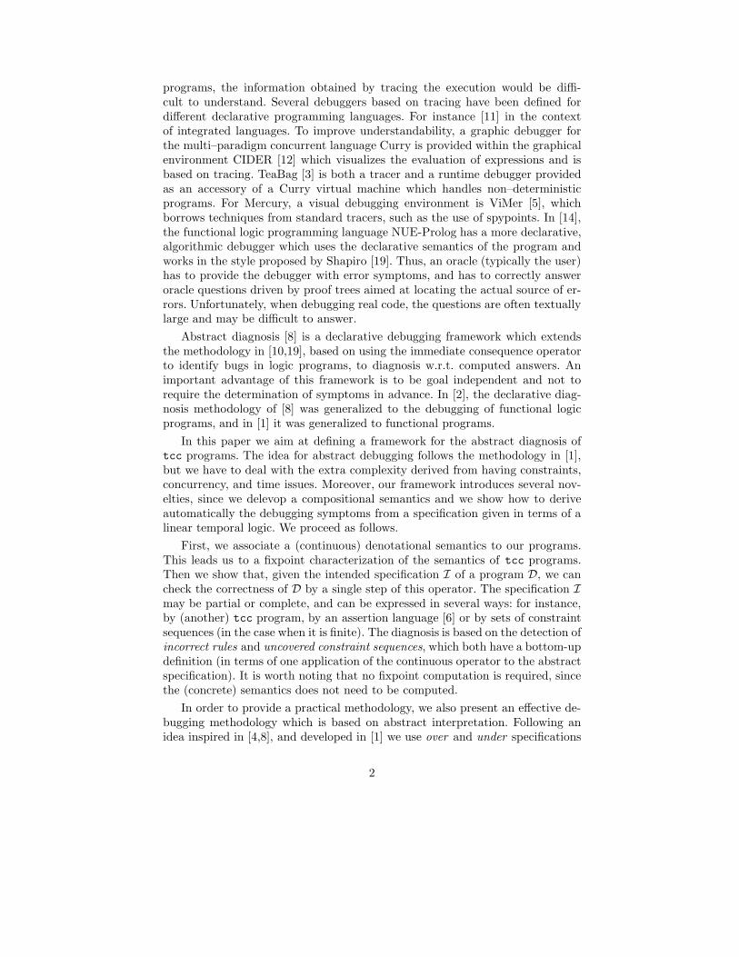
2.2 Process Syntax

In ntcc time is conceptually divided into discrete intervals (or time-units). In-tuitively, in a particular time interval, a cc process P receives a stimulus (i.e.a constraint) from the environment, it executes with this stimulus as the initialstore, and when it reaches its resting point, it responds to the environment withthe resulting store. The resting point also determines a residual process Q, whichis then executed in the next time interval.

Definition 2 (Syntax). Processes P , Q, . . .∈ Proc are built from constraintsc ∈ C and variables x ∈ V in the underlying constraint system (Σ, ∆) as follows:

P, Q, . . . ::= skip | tell(c) |∑

j∈J

when cj do Pj | P ‖ Q

| (local x) inP | nextP | ? P | p(x)

Process skip does nothing. Process tell(c) adds the constraint c to the cur-rent store, thus making c available to other processes in the current time interval.Process

∑

j∈J

when cj do Pj where J is a finite set of indexes, represents a process

that non-deterministically choose a process Pj s.t cj is entailed by the currentstore. The chosen alternative, if any, precludes the others. If no choice is possi-ble in the current time unit, all the alternatives are precluded from execution.We shall use

∑

j∈J

Pj when the guards are true (“blind-choice”) and we omit∑

j∈J

when J is a singleton. Process P ‖ Q represents the parallel composition of Pand Q. Process (local x) inP behaves like P , except that all the informationon x produced by P can only be seen by P and the information on x producedby other processes cannot be seen by P .

The only move of nextP is a unit-delay for the activation of P . We usenextn(P ) as an abbreviation for next(next(. . . (next P ) . . . )), where nextis repeated n times. ? P represents an arbitrary long but finite delay for theactivation of P. It can be viewed as P + nextP + next 2P....

Recursion in ntcc is defined by means of processes definitions of the form

p(x1, .., xn)def

= A

p(y1, ..., yn) is an invocation and intuitively the body of the process definition(i.e. A) is executed replacing the formal parameter x by the actual parametersy. When |x| = 0, we shall omit the parenthesis.

To avoid non-terminating sequences of internal reductions (i.e non-terminatingcomputation within a time interval), recursive calls must be guarded in the con-text of next (see [15] for further details). In what follows D shall denote a setof processes definitions.

3 Operational Semantics

Operationally, the information in the current time unit is represented as a con-straint c ∈ C, so-called store. Following standard lines [18], we extend the syntax

4

with a construct (local x, d) inP which represents the evolution of a process ofthe form (local x) inQ, where d is the local information (or private store) pro-duced during this evolution. Initially d is “empty”, so we regard (local x) inPas (local x, true) inP .

The operational semantics will be given in terms of the reduction relations−→, =⇒⊆ Proc × C × Proc × C defined in Table 1. The internal transition〈P, c〉 −→ 〈Q, d〉 should be read as “P with store c reduces, in one internal

step, to Q with store d ”. The observable transition P(c,d)

====⇒ Q should beread as “P on input c from the environment, reduces in one time unit to Qand outputs d to the environment”. Process Q is the process to be executed inthe next time unit. Such a reduction is obtained from a sequence of internalreductions starting in P with initial store c and terminating in a process Q′ withstore d. Crudely speaking, Q is obtained by removing from Q′ what was meantto be executed only during the current time interval. In ntcc the store d is notautomatically transferred to the next time unit. If needed, information in d canbe transfered to next time unit by process P .

Let us describe some of the rules for the internal transitions. Rule TELLsays that constraint c is added to the current store d. SUM chooses non-deterministically a process Pj for execution if its guard (cj) can be entailedfrom the store. In PARr and PARl, if a process P can evolve, this evolution cantake place in the presence of some other process Q running in parallel. Rule LOCis the standard rule for locality (or hiding) (see [18,9]). CALL shows how a pro-cess definition is replaced by its body according to the set of process definitionin D. Finally, STAR executes P in some time-unit in the future.

Let us now describe the rule for the observable transitions. Rule OBS saysthat an observable transition from P labeled by (c, d) is obtained by performinga terminating sequence of internal transitions from 〈P, c〉 to 〈Q, d〉, for some Q.The process to be executed in the next time interval, F (Q) (“future” of Q), isobtained as follows:

Definition 3. (Future Function). Let F : Proc ⇀ Proc be defined by

F (P ) =

skip if P = skipskip if P = when c do QF (P1) ‖ F (P2) if P = P1 ‖ P2

(local x) inF (Q) if P = (local x, c) inQQ if P = next Q

In this paper we are interested in the so called quiescent input sequences ofa process. Intuitively, those are sequences of constraints on input of which Pcan run without adding any information, wherefore what we observe is thatthe input and the output coincide. The set of quiescent sequences of a processP is thus equivalent to the observation of all sequences that P can possiblyoutput under the influence of arbitrary environment. We shall refer to the set ofquiescent sequences of P as the strongest postcondition of P written sp(P ), w.r.tthe set of sequences of constraints denoted by C∗. In what follows, let s, s1,etc

5

TELL〈tell(c), d〉 −→ 〈skip, d ∧ c〉

SUMd |= cj j ∈ J

D

P

j∈Jwhen cj do Pj , d

E

−→ 〈Pj , d〉

PARr

〈P, c〉 −→ 〈P ′, d〉

〈P ‖ Q, c〉 −→ 〈P ′ ‖ Q, d〉PARl

〈Q, c〉 −→ 〈Q′, d〉

〈P ‖ Q, c〉 −→ 〈P ‖ Q′, d〉

CALLp(x) : −A ∈ D

〈p(x), d〉 −→ 〈A,d〉STAR

n ≥ 0

〈? P, d〉 −→ 〈next nP, d〉

LOC〈P, c ∧ (∃xd)〉 −→ 〈P ′, c′ ∧ (∃xd)〉

〈(local x, c) inP, d ∧ ∃xc〉 −→ 〈(local (x, c′)) inP ′, d ∧ ∃xc′〉

OBS〈P, c〉 −→∗ 〈Q, d〉 6−→ R ≡ F (Q)

P(c,d)

====⇒ R

Table 1. Rules for the internal reduction −→ and the observable reduction =⇒

range over elements in C∗ and s(i) be the i-th element in s. We note that, as inDijkstra’s strongest postcondition approach, proving whether P satisfies a given(temporal) property A, in the presence of any environment, reduces to provingwhether sp(P ) is included in the set of sequences satisfying A [15].

Definition 4 (Observables). The behavioral observations that can be made ofa process are given by the strongest postcondition (or quiescent) behavior of P

sp(P ) = {s | P(s,s)

====⇒∗

for some s ∈ C∗}.

where P(s,s)

====⇒∗

≡ P(s(1),s(1))====⇒ P ′ (s(2),s(2))

====⇒ . . .

4 Denotational Semantics

In this section we give a denotational characterization of the strongest postcon-dition observables of ntcc following ideas developed in [15] and [17].

The denotational semantics is defined as a function [[·]] which associatesto each process a set of finite sequences of constraints, namely [[·]] : (Proc →P(C∗)) → (ProcHeads → P(C∗)), where ProcHeads denotes the set of processnames with their formal parameters. The definition of this function is given inTable 2. We use ∃xs to represent the sequence obtained by applying ∃x to eachconstraint in s. We call the functions in the domain ProcHeads → P(C∗) asInterpretations. We consider the following order on (infinite) sequences s ≤ s′ iff∀i.s′(i) |= s(i). For what concern finite sequences we can order them similarly.Let s and s′ be finite sequences, then if s has length less or equal to s′ thens ≤ s′ iff ∀i = 1, 2, . . . length(s).s′(i) |= s(i)

6

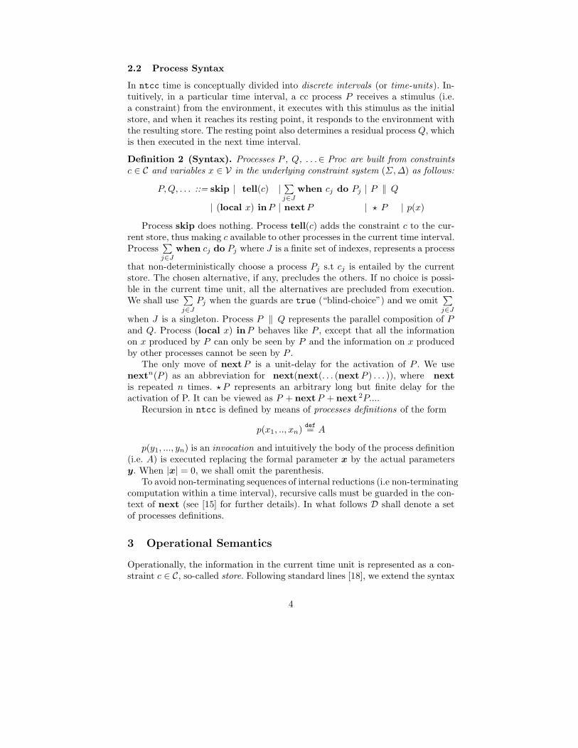
Intuitively, [[P ]] is meant to capture the quiescent sequences of a process P .For instance, all sequence whose first element is stronger than c is quiescentfor tell(c) (D1). Process nextP has not influence on the first element of asequence, thus d.s is quiescent for it if s is quiescent for P (D5). The semanticsfor a procedure call p(x) is directly given by the interpretation I provided (D6).A sequence is quiescent for ? P if there is a suffix of it which is quiescent for P(D7). The other rules can be explained analogously.

D1 [[tell(c)]]I = {d.s | d |= c, s ∈ C∗}D2 [[

P

j∈Jwhen cj do Pj ]]J =

S

j∈J{d.s | d |= cj , d.s ∈ [[Pj ]]J}

∪T

j∈J{d.s | d 6|= cj , d.s ∈ C∗}

D3 [[P ‖ Q]]I = [[P ]]I ∩ [[Q]]ID4 [[local x in P ]]I = {s | there exists s′ ∈ [[P ]]I s.t. ∃xs = ∃xs′}D5 [[next P ]]I = C1 ∪ {d.s | d ∈ C, s ∈ [[P ]]I}D6 [[p(x)]]I = I(p(x))D7 [[? P ]]I = {s.s′ | s ∈ C∗ and s′ ∈ [[P ]]I}

Table 2. Denotational semantics of ntcc

Formally the semantics is defined as the least fixed-point of the correspondingoperator TD ∈ (ProcHeads → P(C∗)) → (ProcHeads → P(C∗))

TD(I)(p(x)) = [[∃y(A ‖ dxy)]]I if p(y) : −A ∈ D

where dxy is the diagonal element used to represent parameter passing (see [18]for details). The following example illustrates the TD operator.

Example 1. Consider a control system that must exhibit the control signal stopwhen some component malfunctions (i.e. the environment introduces as stimulusthe constraint failure). The following (incorrect) program intends to implementsuch a system:

control = when failure do next action || next controlaction = tell(stop)

Starting from the bottom interpretation I⊥ assigning to every process the emptyset (i.e I⊥(control) = I⊥(action) = ∅), TD is computed as follows:

TD(I⊥)(control) = [[when failure do next action || next control]]I⊥= {d1.d2.s|d1 |= failure ⇒ d1.d2.s ∈ [[next action]]I⊥}∩{C1 ∪ {d1.s|s ∈ [[control]]I⊥}}

= {d1.d2.s|d1 |= failure ⇒ d1.d2.s ∈ {C1 ∪ ∅}} ∩ C1 = C1

TD(I⊥)(action) = [[tell(stop)]]I⊥ = {d1.s|d1 |= stop}

7

Let now I1 = TD(I⊥):

TD(I1)(control) = {d1.d2.s|d1 |= failure ⇒ d1.d2.s ∈ [[next action]]I1}∩(

C1 ∪ {d.s|s ∈ [[control]]I1})

= {d1.d2.s|d1 |= failure ⇒ d1.d2.s ∈(

C1 ∪ {d1.d2.s|d2 |= stop})

}∩

(

C1 ∪ C2)

= {d1.d2|d1 |= failure ⇒ d2 |= stop}

5 Abstract Semantics

In this section, starting from the fixpoint semantics in Section 4, we develop anabstract semantics which approximates the observable behavior of the programand is adequate for modular data-flow analysis.

We will focus our attention now on a special class of abstract interpretationswhich are obtained from what we call a sequence abstraction τ : (C∗,≤) →(AS, .). We require that (AS, .) is noetherian and that τ is surjective andmonotone.

We start by choosing as abstract domain A := P(AS), ordered by an exten-sion to sets X .S Y iff ∀x ∈ X ∃y ∈ Y : (x . y). We will call elements of A

abstract sequences. The concrete domain E is P(C∗), ordered by set inclusion.Then we can lift τ to a Galois Insertion of A into E by defining

α(E)(p) := {τ(s) | s ∈ E(p)}

γ(A)(p) := {s | τ(s) ∈ A(p)}

for some ProcHead p. Then, we can lift in the standard way to abstract Interpre-tations the approximation induced by the above abstraction. The Interpretationf : ProcHeads → P(C∗) can be approximated by fα : ProcHeads → α(P(C∗)).

The only requirement we put on τ is that α(Sem (D)) is finite, where Sem (D)is the (concrete) semantics of D.

Now we can derive the optimal abstract version of TD as T αD := α ◦ TD ◦ γ.

By applying the previous definition of α and γ this turns out to be equivalentto the following definition.

Definition 5. Let τ be a sequence abstraction, X ∈ A be an abstract Interpre-tation. Then,

T αD(X)(p(x)) = τ([[∃y(A ‖ dxy)]]X) if p(y) : −A ∈ D

where the abstract denotational semantics is defined in Table 3.Abstract interpretation theory assures that T α

D ↑ ω is the best correct ap-proximation of Sem (D). Correct means α(Sem (D)) v T α

D ↑ ω and best meansthat it is the minimum w.r.t. v of all correct approximations.

Now we can define the abstract semantics as the least fixpoint of this (con-tinuous) operator.

Definition 6. The abstract least fixpoint semantics of a program D is definedas Fα(D) = T α

D ↑ ω.

By our finiteness assumption on τ we are guaranteed to reach the fixpoint in afinite number of steps, that is, there exists h ∈ N s.t. T α

D ↑ ω = T αD ↑ h.

8

D1 [[tell(c)]]τI = τ ({d.β | d |= c, β ∈ C∗})D2 [[

P

j∈Jwhen cj do Pj ]]

τJ =

S

i∈Jτ ({d.β | d |= ci, d.β ∈ [[Pi]]

τI })

∪T

i∈J τ ({d.β | d 6|= ci, d.β ∈ C∗})D3 [[P ‖ Q]]τI = [[P ]]τI ∩ [[Q]]τID4 [[local x in P ]]τI = {β | there exists β′ ∈ [[P ]]τI s.t. ∃xβ = ∃xβ′}D5 [[next P ]]I = τ (C) ∪ τ ({d.β | d ∈ C, β ∈ [[P ]]I})D6 [[p(x)]]τI = τ (I(p(x)))D7 [[? P ]]τI = τ ({β.β′ | β ∈ C∗, β′ ∈ [[P ]]τI })

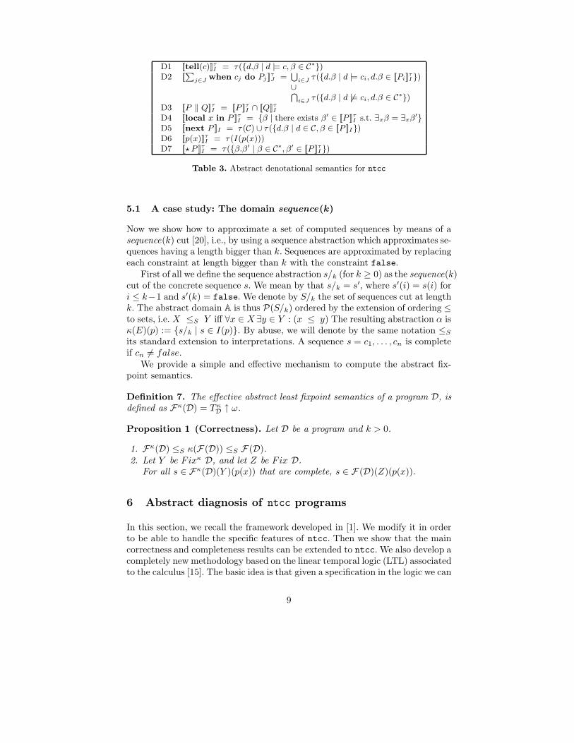
Table 3. Abstract denotational semantics for ntcc

5.1 A case study: The domain sequence(k)

Now we show how to approximate a set of computed sequences by means of asequence(k) cut [20], i.e., by using a sequence abstraction which approximates se-quences having a length bigger than k. Sequences are approximated by replacingeach constraint at length bigger than k with the constraint false.

First of all we define the sequence abstraction s/k (for k ≥ 0) as the sequence(k)cut of the concrete sequence s. We mean by that s/k = s′, where s′(i) = s(i) fori ≤ k−1 and s′(k) = false. We denote by S/k the set of sequences cut at lengthk. The abstract domain A is thus P(S/k) ordered by the extension of ordering ≤to sets, i.e. X ≤S Y iff ∀x ∈ X ∃y ∈ Y : (x ≤ y) The resulting abstraction α isκ(E)(p) := {s/k | s ∈ I(p)}. By abuse, we will denote by the same notation ≤S

its standard extension to interpretations. A sequence s = c1, . . . , cn is completeif cn 6= false.

We provide a simple and effective mechanism to compute the abstract fix-point semantics.

Definition 7. The effective abstract least fixpoint semantics of a program D, isdefined as Fκ(D) = T κ

D ↑ ω.

Proposition 1 (Correctness). Let D be a program and k > 0.

1. Fκ(D) ≤S κ(F (D)) ≤S F (D).2. Let Y be Fixκ D, and let Z be Fix D.

For all s ∈ Fκ(D)(Y )(p(x)) that are complete, s ∈ F (D)(Z)(p(x)).

6 Abstract diagnosis of ntcc programs

In this section, we recall the framework developed in [1]. We modify it in orderto be able to handle the specific features of ntcc. Then we show that the maincorrectness and completeness results can be extended to ntcc. We also develop acompletely new methodology based on the linear temporal logic (LTL) associatedto the calculus [15]. The basic idea is that given a specification in the logic we can

9

generate automatically the sequences which we use for debugging the program.Let us recall the syntax and semantics of this logic (see [15] for further details).

Formulae in the ntcc LTL are given by the following grammar:

A, B, ... : c | A·⇒ A |

·¬A |

·

∃xA | ◦ A | 3A | 2A

c is a constraint.·⇒,

·¬ and

·

∃x represent the linear-temporal logic implication,negation and existential quantification, respectively. These symbols should notbe confused with their counterpart in the constraint system (i.e ⇒ , ¬ and ∃).Symbols ◦ , 2 and 3 denote the temporal operators next, always and eventually.

The interpretation structures of formulae in this logic are infinite sequencesof constraints. We say that β ∈ C∗ is a model of (or that it satisfies) A, notationβ |= A, if 〈β, 1〉 |= A where:

〈β, i〉 |= c iff β(i) |= c

〈β, i〉 |=·¬A iff 〈β, i〉 |=\ A

〈β, i〉 |= A1·⇒ A2 iff 〈β, i〉 |= A1 implies〈β, i〉 |= A2

〈β, i〉 |= ◦A iff 〈β, i + 1〉 |= A〈β, i〉 |= 2A iff ∀j≥i〈β, j〉 |= A〈β, i〉 |= 3A iff ∃j≥i s.t.〈β, j〉 |= A

〈β, i〉 |=·

∃xA iff exists β′ s.t. ∃xβ = ∃xβ′

The LTL is then used to specify (temporal) properties of programs:

Definition 8. We say that P satisfies some property A written P ` A, iffsp(P ) ⊆ [[A]] where [[A]] is the collection of all models of A, i.e., [[A]] = {β |= A}

Program properties which can be of interest are Galois Insertions betweenthe concrete domain (the set of interpretations ordered pointwise) and the ab-stract domain chosen to model the property. The following Definition extendsto abstract diagnosis the definitions given in [19,10,13] for declarative diagnosis.In the following, Iα is the specification of the intended behavior of a program.

Definition 9. [1] Let D be a program and α be a property.

1. D is partially correct w.r.t. Iα if Iα v α(Sem (D)).2. D is complete w.r.t. Iα if α(Sem (D)) v Iα.3. D is totally correct w.r.t. Iα, if it is partially correct and complete.

Note that the above definition is given in terms of the abstraction of the concretesemantics α(Sem (D)) and not in terms of the (possibly less precise) abstractsemantics Semα(D). This means that Iα is the abstraction of the intended con-crete semantics of D. In other words, the specifier can only reason in terms ofthe properties of the expected concrete semantics without being concerned with(approximate) abstract computations.

The diagnosis determines the “basic” symptoms and, in the case of incor-rectness, the relevant rule in the program. This is modeled by the definitions ofabstractly incorrect rule and abstract uncovered equation.

10

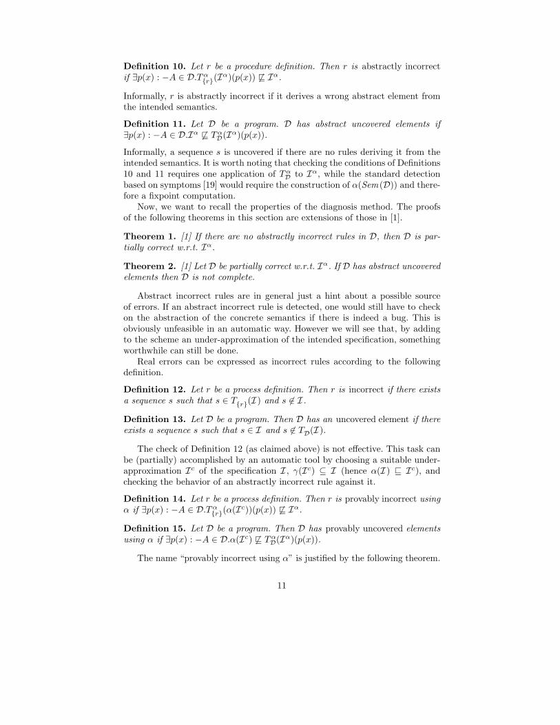
Definition 10. Let r be a procedure definition. Then r is abstractly incorrectif ∃p(x) : −A ∈ D.T α

{r}(Iα)(p(x)) 6v Iα.

Informally, r is abstractly incorrect if it derives a wrong abstract element fromthe intended semantics.

Definition 11. Let D be a program. D has abstract uncovered elements if∃p(x) : −A ∈ D.Iα 6v T α

D(Iα)(p(x)).

Informally, a sequence s is uncovered if there are no rules deriving it from theintended semantics. It is worth noting that checking the conditions of Definitions10 and 11 requires one application of T α

D to Iα, while the standard detectionbased on symptoms [19] would require the construction of α(Sem (D)) and there-fore a fixpoint computation.

Now, we want to recall the properties of the diagnosis method. The proofsof the following theorems in this section are extensions of those in [1].

Theorem 1. [1] If there are no abstractly incorrect rules in D, then D is par-tially correct w.r.t. Iα.

Theorem 2. [1] Let D be partially correct w.r.t. Iα. If D has abstract uncoveredelements then D is not complete.

Abstract incorrect rules are in general just a hint about a possible sourceof errors. If an abstract incorrect rule is detected, one would still have to checkon the abstraction of the concrete semantics if there is indeed a bug. This isobviously unfeasible in an automatic way. However we will see that, by addingto the scheme an under-approximation of the intended specification, somethingworthwhile can still be done.

Real errors can be expressed as incorrect rules according to the followingdefinition.

Definition 12. Let r be a process definition. Then r is incorrect if there existsa sequence s such that s ∈ T{r}(I ) and s 6∈ I .

Definition 13. Let D be a program. Then D has an uncovered element if thereexists a sequence s such that s ∈ I and s 6∈ TD(I ).

The check of Definition 12 (as claimed above) is not effective. This task canbe (partially) accomplished by an automatic tool by choosing a suitable under-approximation Ic of the specification I , γ(Ic) ⊆ I (hence α(I ) v Ic), andchecking the behavior of an abstractly incorrect rule against it.

Definition 14. Let r be a process definition. Then r is provably incorrect usingα if ∃p(x) : −A ∈ D.T α

{r}(α(Ic))(p(x)) 6v Iα.

Definition 15. Let D be a program. Then D has provably uncovered elementsusing α if ∃p(x) : −A ∈ D.α(Ic) 6v T α

D(Iα)(p(x)).

The name “provably incorrect using α” is justified by the following theorem.

11

Theorem 3. [1] Let r be a program rule (process) and Ic such that (γα)(Ic) =Ic. Then if r is provably incorrect using α it is also incorrect.

By choosing a suitable under-approximation we can refine the check for wrongrules. For all abstractly incorrect rules we check if they are provably incorrectusing α. If it so then we report an error, otherwise we can just issue a warning.

As we will see in the following, this property holds (for example) for our casestudy. By Proposition 1 the condition (γα)(Ic) = Ic is trivially satisfied by anysubset of the ‘finite’ sequences in the over-approximation. We can also consider afinite subset of the sequences in which we do the following change: if a sequenceis such that all its elements starting from the length k are equal to false, wereplace such elements by true.

Theorem 4. [1] Let D be a program. If D has a provably uncovered elementusing α, then D is not complete.

Abstract uncovered elements are provably uncovered using α. However, The-orem 4 allows us to catch other incompleteness bugs that cannot be detected byusing Theorem 2 since there are provably uncovered elements using α which arenot abstractly uncovered.

The diagnosis w.r.t. approximate properties is always effective, because theabstract specification is finite. As one can expect, the results may be weaker thanthose that can be achieved on concrete domains just because of approximation:

– every incorrectness error is identified by an abstractly incorrect rule. Howeveran abstractly incorrect rule does not always correspond to a bug. Anyway,

– every abstractly incorrect rule which is provably incorrect using α corre-sponds to an error.

– provably uncovered equations always correspond to incompleteness bugs.– there exists no sufficient condition for completeness.

6.1 Our case study

An efficient debugger can be based on the notion of over-approximation andunder-approximation for the intended fixpoint semantics that we have intro-duced. The basic idea is to consider two sets to verify partial correctness anddetermine program bugs: Iα which over-approximates the intended semantics I(that is, I ⊆ γ(Iα)) and Ic which under-approximates I (that is, γ(Ic) ⊆ I ).

Let us now derive an efficient debugger by choosing suitable instances ofour general framework. Let α be the sequence(k) abstraction κ of the programthat we have defined in previous section. Thus we choose Iκ = Fκ(I ) as anover-approximation of the values of a program. We can consider any of the setsdefined in the works of [4,7] as an under-approximation of I . In concrete, we takethe finite abstract sequences of Iκ as Ic but replacing the constraint false bytrue after the position κ. This provides a simple albeit useful debugging schemewhich is satisfactory in practice.

12

Another possibility is to generate the sequences for the under and the over-approximation from the sequences that are models for a LTL formula specifyingthe intended behavior of the program. Let us illustrate the method by using theguiding example.

Example 2. Let first consider what the intended behaviour of the system pro-posed in Example 1 should be. We require that as soon as the constraint failurecan be entailed from the store, the system must exhibit the constraint stop. Thisspecification can be provided by means of another (correct) program or by a for-mula in the LTL. Let us explore both cases.

Let control′ and action′ be the intended system:

control′ = when failure do action || next control′

action′ = tell(stop)

and A be the LTL formula:

A = 2(failure ⇒ stop)

Sequences generated by A and by the processes control′ and action′ coincidesand can be used to compute the intended behavior I, the corresponding over-approximation Iα = Iκ and the under-approximation Ic as was defined previ-ously. The intended behaviour I is then:

I(control′) = {s′.d.s′′|d |= failure ⇒ d.s′′ ∈ [[action′]]I} for any s′ and s′′

I(action′) = {d.s|d |= stop}

According to Definition 14, let us compute T α{control}(α(Ic))(control):

T α{control}(α(Ic))(control) = τ({d1...dk.true∗|d1 |= failure ⇒ d2 |= stop

and ∀i>1di |= failure ⇒ di |= stop})

Given s1 = failure.stop.true∗ ∈ T α{control}(α(Ic))(control) and s2 = failure∧

stop.true∗ ∈ Iα, notice that s1 6≤ s2 suggesting that control is provably incor-rect. The error is due to it delays one time unit the call to the process action.

Example 3. In this example we debug a program capturing the behaviour of aRCX-based robot that can go right or left. The movement of the robot is definedby the following rules: 1) If the robot goes right in the current time unit, it mustturn left in the next one. 2) After two consecutive time units moving to the left,next decision must be turn right. The program proposed is depicted below:

GoR = tell(a0 = r)||next tell(a1 = r)GoL = tell(a0 = l)||next tell(a1 = l)Update = when a1 = l do next tell(a2 = l)+

when a1 = r do next tell(a2 = r)Zigzag = when a2 6= r do GoR + when a2 6= l do GoL||

Update||nextZigzag

13

GoR and GoL represent the decision of turning right or left respectively.Update keeps track of the second-to-last action and ZigZag controls the be-haviour of the robot. Variables a0, a1 and a2 represent the current, the previousand the second-to-last decisions respectively.

Now we provide the intended specification for each process:

I(GoR) = {s|∀i. s(i) |= (a0 = r) and s(i + 1) |= (a1 = r)}I(GoL) = {s|∀i. s(i) |= (a0 = l) and s(i + 1) |= (a1 = l)}I(Update) = {s|∀i. s(i) |= (a1 = l) ⇒ s(i + 1) |= (a2 = l)}∪

{s|∀i. s(i) |= (a1 = r) ⇒ s(i + 1) |= (a2 = r)}

Specification of Zigzag can be stated by the following LTL formula:

A = 2((a0 = r)·⇒ ◦(a0 = l)

·∧ ((a0 = l)

·∧ ◦(a0 = l)

·⇒ ◦ ◦ (a0 = r)))

The property states that always is true that 1)if the current decision is go right,the next decision must be go left and 2)if the robot goes left in two consecutivetime units, the next decision must be turn right. I(Zigzag) can be then viewedas all the possible models of the formula A, i.e. [[A]]:

I(Zigzag) = {s|s(i) |= (a0 = r) ⇒ s(i + 1) |= (a0 = l)}∪{s| (s(i) |= (a0 = l) ∧ s(i + 1) |= (a0 = l)) ⇒ s(i + 2) |= (a0 = r)}

Let Iα be the abstraction Iκ representing the over-approximation of I andIc the under-approximation as before. Let us compute a step of T α

{Zigzag}:

T α{Zigzag}(α(Ic))(Zigzag) = [[when a2 6= r do GoR + when a2 6= l do GoL||

Update]]α(Ic)

= ({d1.s|d1 |= (a2 6= r) ⇒ d1.s ∈ [[GoR]]α(Ic)}∪{d1.s|d1 |= (a2 6= l) ⇒ d1.s ∈ [[GoL]]α(Ic)})∩{d.s|s ∈ [[Zigzag]]α(Ic)} ∩ [[Update]]α(Ic)

Notice that the sequence d1.d2 where d1 |= (a0 = r) and d2 |= (a0 = r) is asequence that can be generated from T α

{Zigzag}(α(Ic))(Zigzag) but d1.d2 /∈ Iα.Using Definition 14 we can say that Zigzag is provably incorrect. The bug inthis case, is that guard in the sub-process when a2 6= r do GoR must be a1 6= r.

7 Conclusions

We have presented a framework for the declarative debugging of tcc programsw.r.t. the set of computed constraint sequences. Our method is based on a de-notational semantics for tcc programs which models the semantics in a com-positional manner. Moreover, we have shown that it is possible to use a lineartemporal logic for providing a specification of correct programs, and generateautomatically from it the sequences which are necessary for debugging.

We follow the idea of considering declarative specifications as programs. Theintended specification can then be automatically abstracted and can be usedto automatically debug the final program. As future work we are developing aprototype of our debugging system on top of an implementation of an interpreterof the ntcccalculus that we developed in [16].

14

References

1. M. Alpuente, M. Comini, S. Escobar, M. Falaschi, and S. Lucas. Abstract Diagnosisof Functional Programs. In M. Leuschel and F. Bueno, editors, Proc. of LOPSTR2002, pages 1–16. Springer LNCS 2664, 2003.

2. M. Alpuente, F. Correa, and M. Falaschi. A Debugging Scheme for FunctionalLogic Programs. In M. Hanus, editor, Proc. of WFLP 2001, volume 64 of ENTCS.Elsevier, 2002.

3. S. Antoy and S. Johnson. TeaBag: A Functional Logic Debugger. In H. Kuchen,editor, Proc. of WFLP 2004, pages 4–18, 2004.

4. F. Bueno, P. Deransart, W. Drabent, G. Ferrand, M Hermenegildo, J. Maluszynski,and G. Puebla. On the role of semantic approximations in validation and diagnosisof constraint logic programs. In Proc. of AADEBUG’97, pages 155–170. U. ofLinkoping Press, 1997.

5. M. Cameron, M. Garcıa de la Banda, K. Marriott, and P. Moulder. Vimer: a visualdebugger for mercury. In Proc. of the 5th PPDP, pages 56–66. ACM Press, 2003.

6. M. Comini, R. Gori, and G. Levi. Assertion based Inductive Verification Methodsfor Logic Programs. In A. K. Seda, editor, Proceedings of MFCSIT’2000, volume 40of ENTCS. Elsevier Science Publishers, 2001.

7. M. Comini, G. Levi, M. C. Meo, and G. Vitiello. Proving properties of Logic Pro-grams by Abstract Diagnosis. In M. Dams, editor, Proc. of LOMAPS’96, volume1192 of LNCS, pages 22–50, Berlin, 1996. Springer-Verlag.

8. M. Comini, G. Levi, M. C. Meo, and G. Vitiello. Abstract diagnosis. Journal ofLogic Programming, 39(1-3):43–93, 1999.

9. F. S. de Boer, M. Gabbrielli, E. Marchiori, and C. Palamidessi. Proving concurrentconstraint programs correct. ACM TOPLAS, 19(5):685–725, 1997.

10. G. Ferrand. Error Diagnosis in Logic Programming, an Adaptation ofE.Y.Shapiro’s Method. Journal of Logic Programming, 4(3):177–198, 1987.

11. M. Hanus and B. Josephs. A debugging model for functional logic programs. Proc.of 5th PLILP, volume 714 of LNCS, pages 28–43. Springer, 1993.

12. M. Hanus and J. Koj. An integrated development environment for declarativemulti-paradigm programming. In Proc. of the International Workshop on LogicProgramming Environments (WLPE’01), pages 1–14, Paphos (Cyprus), 2001.

13. J. W. Lloyd. Declarative error diagnosis. New Generation Computing, 5(2):133–154, 1987.

14. L. Naish and T. Barbour. Towards a portable lazy functional declarative debugger.Australian Computer Science Communications, 18(1):401–408, 1996.

15. M. Nielsen, C. Palamidessi, and F.D. Valencia. Temporal concurrent constraintprogramming: Denotation, logic and applications. Nordic Journal of Computing,9(1):145–188, 2002.

16. C. Olarte, C. Rueda. A Stochastic Concurrent Constraint Based Framework toModel and Verify Biological Systems. Clei Electronic Journal Vol 9:2, 2005.

17. V. Saraswat, R. Jagadeesan, and V. Gupta. Foundations of timed concurrentconstraint programming. In Proc. of the Ninth Annual IEEE Symposium on Logicin Computer Science, pages 71–80. IEEE Computer Society Press, 1994.

18. V.A. Saraswat. Semantic Foundation of Concurrent Constraint Programming. InProc. of 18th ACM POPL. ACM, New York, 1991.

19. E. Y. Shaphiro. Algorithmic Program Debugging. The MIT Press, Cambridge,Massachusetts, 1982. ACM Distinguished Dissertation.

20. H. Tamaki and T. Sato. Unfold/Fold Transformations of Logic Programs. InS. Tarnlund, editor, Proc. of 2nd ICLP, pages 127–139, 1984.

15