A UNIFIED APPROACH TO CONCURRENT

DEBUGGING

APPROVED BYDISSERTATION COMMITTEE:

Copyright

by

Syed Irfan Hyder

1994

To My Father and Mother

Without their sacrifice, encouragement, and high

expectations, I may not have undertaken

this work and persevered to take

it to completion.

A UNIFIED APPROACH TO CONCURRENT

DEBUGGING

by

SYED IRFAN HYDER, B.E., M.B.A., M.S (EE)

DISSERTATION

Presented to the Faculty of the Graduate School of

The University of Texas at Austin

in Partial Fulfillment of

the Requirements for

the Degree of

DOCTOR OF PHILOSOPHY

THE UNIVERSITY OF TEXAS AT AUSTIN

December 1994

v

Acknowledgments

All praise to Allah, the Most Beneficent, the Most Merciful, for giving

me the strength, resources and the will to complete this work.

I appreciate the support and help of my advisor, Dr. James. C. Browne.

His vision and ability to abstract away the details has taught me how to discern

the forest from the trees. Working with him, I learned the full import of what it

means to ask the right questions. His questions would often send me scurrying

on a search path that would clarify my confusions and would lead me to a true

understanding of the problem, and hence, to the solution.

I am indebted to my wife for her support and understanding. She sus-

tained me through times when I was not making progress and was, thus, often

unreasonable, and through times when I was making progress and was, thus,

vigorously at work away from home. I also owe to my sons the time that I

spent away from them which was justifiably theirs.

I am full of gratitude for my family. Their continuous support, help and

shouldering of the responsibilities made possible the completion of this work.

Working on this dissertation has been a particularly exciting experi-

ence for me; if perhaps more drawn out than what my parents and I expected. I

would not have embarked on it but for the encouragement of my father and

mother. Their encouragement has always been a great source of inspiration in

my life. I appreciate their patience and waiting as I tried hard, the best I could,

to finish the work.

vi

A UNIFIED APPROACH TO CONCURRENT

DEBUGGING

Publication No. ______________

Syed Irfan Hyder, Ph.D.

The University of Texas at Austin, 1994

Supervisor: James. C. Browne

Debugging is a process that involves establishing relationships be-

tween several entities: The behavior specified in the program, P, the model/-

predicate of the expected behavior, M, and the observed execution behavior,

E. The thesis of the unified approach is that a consistent representation for P,

M and E greatly simplifies the problem of concurrent debugging, both from

the viewpoint of the programmer attempting to debug a program and from the

viewpoint of the implementor of debugging facilities. Provision of such a con-

sistent representation becomes possible when sequential behavior is separated

from concurrent or parallel structuring. Given this separation, the program be-

comes a set of sequential actions and relationships among these actions. The

debugging process, then, becomes a matter of specifying and determining rela-

tions on the set of program actions. The relations are specified in P, modeled in

M and observed in E. This simplifies debugging because it allows the program-

mer to think in terms of the program which he understands. It also simplifies

the development of a unified debugging system because all of the different ap-

proaches to concurrent debugging become instances of the establishment of re-

lationships between the actions.

vii

The unified approach defines a formal model for concurrent debugging

in which the entire debugging process is specified in terms of program actions.

The unified model places all of the approaches to debugging of parallel pro-

grams such as execution replay, race detection, model/predicate checking, exe-

cution history displays and animation, which are commonly formulated as

disjoint facilities, in a single, uniform framework.

We have also developed a feasibility demonstration prototype imple-

mentation of this unified model of concurrent debugging in the context of the

CODE 2.0 parallel programming system. This implementation demonstrates

and validates the claims of integration of debugging facilities in a single

framework. It is further the case that the unified model of debugging greatly

simplifies the construction of a concurrent debugger. All of the capabilities

previously regarded as separate for debugging of parallel programs, both in

shared memory models of execution and distributed memory models of execu-

tion, are supported by this prototype.

viii

Table of Contents

List of Figures .................................................................................................xii

List of Tables.................................................................................................. xiv

Chapter 1. Introduction ................................................................................ 1

1.1 The Unified Approach................................................................ 21.1.1 The Abstraction of Computation Actions............................ 31.1.2 Program and its Execution................................................... 5

1.2 The Debugging Process.............................................................. 61.2.1 Block Triangular Solver Example ....................................... 71.2.2 Different Parts of the Debugging Process............................ 9

1.3 Overview of the Unified Debugger .......................................... 121.3.1 The Actual Execution Behavior......................................... 131.3.2 Restricting Execution to Selected Actions......................... 141.3.3 Predicate/Model of the Expected Behavior ....................... 141.3.4 Automatic Checking of the Expected Behavior ................ 151.3.5 Display of the Unexpected Behavior ................................. 151.3.6 Cyclical Debugging ........................................................... 161.3.7 Support for Interactive Debugging .................................... 16

Chapter 2. State of the Art and the Related Work...................................... 17

2.1 Sequential and Concurrent Debugging..................................... 172.1.1 Sequential Debugging........................................................ 192.1.2 Concurrent Debugging Facilities ....................................... 20

2.2 Problems in Various Parts of the Cycle.................................... 212.2.1 Mapping Ambiguities ........................................................ 242.2.2 Ordering Ambiguities ........................................................ 262.2.3 Modeling Problems............................................................ 272.2.4 Filtering Ambiguities ......................................................... 27

Chapter 3. The Unified Model of Concurrent Debugging ......................... 29

3.1 The Specified Behavior ............................................................ 293.1.1 The Elaborated Graph........................................................ 303.1.2 Firing and Routing Rules................................................... 31

3.2 The Observed Behavior............................................................ 323.2.1 Causality of Data Flow Dependences................................ 333.2.2 Execution History Pomsets ................................................ 343.2.3 Concurrent Execution State ............................................... 353.2.4 Animation .......................................................................... 36

3.3 The Expected Behavior ............................................................ 36

ix

3.3.1 Representing Expected Behavior....................................... 363.3.2 Recognizing the Expected Behavior.................................. 38

3.4 Shared Data Dependences ........................................................ 413.5 Execution Replay...................................................................... 433.6 Race Detection.......................................................................... 46

Chapter 4. Implementation Concepts......................................................... 49

4.1 Overview .................................................................................. 494.2 CODE 2 Environment .............................................................. 51

4.2.1 Templates and their Executable Instances ......................... 534.2.2 UC Execution Event .......................................................... 554.2.3 CODE 2 Runtime System.................................................. 56

4.3 Debugging Environment .......................................................... 574.3.1 News from the Instrumentation ......................................... 584.3.2 The Debugger Task............................................................ 594.3.3 Communicating with the Instrumentation ......................... 60

4.4 Internal Structures .................................................................... 614.4.1 Debugger Symbol Table .................................................... 614.4.2 Dynamic Instance Tree ...................................................... 624.4.3 Event Records and Event Graph........................................ 64

4.5 Selecting a Scope...................................................................... 664.5.1 Selecting an Instance with a given Pathname.................... 674.5.2 Constructing the Pathname for an Instance ....................... 68

Chapter 5. Debugging Instrumentation ...................................................... 69

5.1 Information Requirements........................................................ 695.1.1 Global Information ............................................................ 695.1.2 Action Specific Information .............................................. 70

5.2 Full-Recording Instrumentation ............................................... 725.2.1 Determination of Flow Predecessors ................................. 725.2.2 Determination of Shared-Predecessors .............................. 74

5.3 Restricting Instrumentation ...................................................... 755.3.1 Determining the Effective Recording Option.................... 755.3.2 Turning Off the Recording of a UC Action....................... 775.3.3 Restricting the Recording of a UC Action......................... 77

5.4 Replay Instrumentation ............................................................ 785.4.1 Enforcing Previously Recorded Flow Orderings............... 785.4.2 Enforcing Shared Access in the Recorded Order .............. 80

5.5 Interactive Instrumentation....................................................... 815.5.1 Controlling the Course of Execution ................................. 815.5.2 User Breakpoints................................................................ 82

x

Chapter 6. Debugging Facilities................................................................. 83

6.1 Post Restriction......................................................................... 836.1.1 Partial Orderings ................................................................ 846.1.2 Options Available with Post-Restriction ........................... 84

6.2 Information Requirements........................................................ 856.3 Topological Sorting .................................................................. 87

6.3.1 Support for Post-Restriction .............................................. 906.3.2 Deletion of Information no Longer Needed ...................... 92

6.4 Display Facility ........................................................................ 946.4.1 Display of Mappings.......................................................... 956.4.2 Displaying Progress of Execution (Animation)................. 97

6.5 Checker Facility...................................................................... 1006.5.1 Checking Relationships ................................................... 1006.5.2 Post-restriction and Vector Clocks .................................. 1026.5.3 Checker Commands......................................................... 1046.5.4 Command Translation...................................................... 105

Chapter 7. Interactive Facility.................................................................. 107

7.1 Controlling the Execution....................................................... 1077.1.1 Controlling the Execution of a UC Action ...................... 1087.1.2 Global Control of the Execution...................................... 1097.1.3 Rerunning the Execution ................................................. 112

7.2 User Breakpoints .................................................................... 1147.3 Evaluation of User Commands............................................... 1167.4 Querying the State of Actions ................................................ 117

7.4.1 Local State of an action ................................................... 1177.4.2 Debugger Defined Objects............................................... 1187.4.3 Addresses of Objects ....................................................... 119

Chapter 8. Future Work............................................................................ 121

8.1 Enhancements to the Unified Model ...................................... 1228.1.1 Dynamic Vector Clocks................................................... 1228.1.2 Hierarchical Representation of Events ............................ 1238.1.3 Hierarchical Replay ......................................................... 124

8.2 Interfaces to Other Systems.................................................... 1248.2.1 Interpreter and Stepping Facility .................................... 1248.2.2 Static Analysis and Symbolic Analysis ........................... 125

8.3 Enhancements to the Current Implementation ....................... 1258.3.1 A Graphical User Interface (GUI) ................................... 1268.3.2 Distributed Implementation ............................................. 126

xi

8.3.3 Recovery and Roll-Back.................................................. 1298.3.4 Extending Facilities for Model Checking........................ 1308.3.5 Implementation of Race Detection .................................. 1308.3.6 Optimizing the Replay Recording ................................... 1318.3.7 Implementation of Other Options .................................... 1318.3.8 Buffering Requirements................................................... 132

8.4 Textual languages................................................................... 133

Chapter 9. Conclusions ............................................................................ 135

Appendix A. Computation Actions in a Textual Representation................. 137

A.1 Extracting a Graphical Representation................................... 137A.2 Extraction of Computation Actions........................................ 139

Appendix B. The Unified Debugger for CODE 2 ....................................... 142

B.1 Description of Commands...................................................... 142B.2 Syntax of Commands ............................................................. 143

References ..................................................................................................... 147

Vita ................................................................................................................ 155

xii

List of Figures

Figure1-1. Abstraction of a computation action...........................................4

Figure1-2. (a) Matrix, A and vector, b. (b) Replacing b with vector x........8

Figure1-3. Data-flow for Block Triangular Solver......................................8

Figure1-4. CODE 2 Graph for Block Triangular Solver (DoBTS)..............9

Figure1-5. (a) Graph of M, (b) Graph of E, (c) Elaborated graph of M.....11

Figure1-6. Available facilities...................................................................13

Figure2-1. Debugging facilities target individual problem areas...............21

Figure2-2. Ambiguities in various parts of the cycle.................................22

Figure2-3. (a) Time-process graph (b) Program text (c) Event traces.......25

Figure3-1. (a)Program graph (b) Elaborated graph (c) Pomset execution30

Figure3-2. (a) Elaborated Graph. (b) Execution........................................37

Figure3-3. (a) Expected Behavior. (b) Restricted execution.....................38

Figure3-4. (a) Dependences. (b) Orderings................................................42

Figure3-5. Precedence of a write event to a read and a write event...........43

Figure4-1. Debugging run-modes..............................................................49

Figure4-2. Available facilities....................................................................50

Figure4-3. CODE 2’s Unit of Computation (UC)......................................51

Figure4-4. Block triangular solver main program graph............................52

Figure4-5. Internal representation of a UC node instance (UC action).....54

Figure4-6. Execution of a Template Instance............................................55

Figure4-7. Debugging Environment..........................................................57

Figure4-8. The Debugger Task..................................................................59

Figure4-9. Translator generated symbol table entry routine......................61

Figure4-10. Data-flow relationships of the dynamic instance graph..........63

Figure4-11. Nesting relationship in the dynamic instance tree...................63

Figure4-12. Event record and event id.........................................................65

Figure4-13. Event history graph of the DoBTS example for N=4...............66

xiii

Figure 4-14. Mappings between templates, actions, and events. .................. 67

Figure 6-1. Relationships between selected actions.................................... 83

Figure 6-2. Sorting information for each event........................................... 88

Figure 6-3. Need for maintaining restriction information with actions. ..... 92

Figure 6-4. Successor counts in the restricted recording mode................... 94

Figure 6-5. Mappings between program, elaborated and event graph. ....... 96

Figure 6-6. Displaying the progress of execution (animation).................... 98

Figure 6-7. User options for the visualizations. ........................................ 100

Figure 7-1. State transitions for a UC action............................................. 108

Figure 7-2. Global state transitions in response to global commands...... 110

Figure 7-3. Compiler generated routine for obtaining addresses. ............. 119

Figure A-1. (a) Process main (b) Synchronization-control-flow graph. .... 138

Figure A-2. (a) Worker i (b) Synchronization-control-flow graph............ 139

Figure A-3. (a) Computation actions a and f, and (b) w ............................ 140

xiv

List of Tables

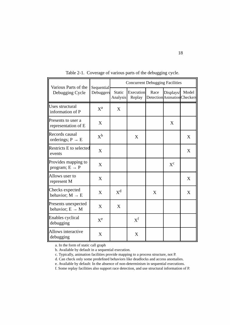
Table 2-1. Coverage of various parts of the debugging cycle. .................. 18

Table 3-1. Recording and restricting instrumentation ............................... 39

Table 3-2. Replay instrumentation for D in S........................................... 45

Table 3-3. Instrumentation for data-race detection.................................... 47

Table 5-1. Global Information used by the Instrumentation...................... 70

Table 5-2. Action-specific information needed by the instrumentation. .. 71

Table 5-3. Instrumentation inserted in a template routine. ....................... 73

Table 5-4. Effective recording options for UC and call instances............. 76

Table 6-1. Various options offered by different facilities.......................... 85

Table 6-2. Availability of various facilities in different modes................. 86

Table 6-3. Action specific information needed by the facilities. .............. 87

Table 6-4. Display post restriction............................................................. 93

Table 8-1. Data-race detection instrumentation with vector clocks. ....... 130

Table B-1. Brief listing of the available commands................................. 142

1

Chapter 1. Introduction

Debugging is a process that establishes a relationship between the pro-

gram (typically some small segment of a large program) and its execution be-

havior. The process involves several entities and relationships between those

entities. It starts with a program that has been observed to produce invalid fi-

nal states for one or more initial states. The segment of the program that is sus-

pected of being faulty is selected for monitoring. Expectations about the

execution behavior of the suspect program segment are specified in a model or

a predicate. The program is, then, run and its actual execution behavior is ob-

served. The actual execution behavior is checked against the model/predicate

to reveal any unexpected behavior. Mapping of the unexpected behavior back

to the program brings the programmer closer to the bug. This completes one

cycle of a process that is repeated until the bug is located.

The entities involved in the debugging process include the program, P,

the model/predicate of the expected behavior, M, and the actual execution be-

havior, E. Ideally M and E should be expressed in a representation consistent

with the program P so that the programmer is not forced to understand and ma-

nipulate several different notations. Additionally, the facilities provided by a

debugger in each part of the debugging process should help in manipulating

and establishing relationships between the entities involved in that part of the

process.

Debugging of even sequential programs becomes difficult when debug-

gers for conventional text string languages use unrelated and typically infor-

mal representations for M and E. The problem exacerbates for concurrent

programs written in pure text forms which often require a different representa-

tion for each of the three entities; P, M and E. Such programs often express

concurrency by adding synchronization and communication primitives to the

sequential text. This produces a complex entanglement of the concurrent con-

siderations of synchronizations and communications with the sequential con-

siderations of flow of control and flow of data. This entanglement gives rise to

2

ambiguities among various parts of the debugging process for concurrent pro-

grams by tu rn ing each par t o f the process in to a separa te problem

(Section 2.2). These ambiguities obscure the relationship between the differ-

ent representations used for the entities. Debugging facilities that establish re-

lationships among P, M and E appear to be incompatible or even orthogonal.

Incompatibility of the facilities for different parts of concurrent debugging

forces the programmer to either use different facilities for different parts of the

cycle or debug without them. Use of multiple representations for P, M and E

typically compels the debuggers to either constrain the range of behaviors that

can be checked [ReSc94]; or to tolerate the ambiguities in the observed behav-

ior [EGP89], [HMW90], [NM91a]; or to demand extra programming effort

[SBN89], [LMF90], [Bat89].

Using separate representations for different portions of the debugging

process introduces special problems into the debugging of concurrent or paral-

lel programs. Many approaches to debugging parallel programs appear to be

different when approached conventionally. There is a long list of supposedly

different debugging facilities for concurrent programs: execution replay facili-

ties [LM86], [MiC89], [Net93], race detection facilities [NM91b], [Sch89],

predicate/model checking facilities [Bat89], [HsK90], [WaG91], execution

history displays [PaU89], [FLM89], [Ho91] and animation facilities [PaU89].

This multiplicity of different views of concurrent debugging forces the pro-

grammer to learn many different representations (Section 2.1.2).

1.1 The Unified Approach

The thesis of our approach is that a consistent representation for all of

the different entities (P, M and E) involved in the debugging process greatly

simplifies the problem of concurrent debugging, both from the viewpoint of

the programmer attempting to debug a program and from the viewpoint of the

implementor of debugging facilities. Provision of such a consistent representa-

tion becomes possible when sequential behavior is separated from concurrent

or parallel structuring. Given this separation in the representation, the pro-

3

gram becomes a set of sequential actions and relationships among these se-

quential actions. The abstractions in this representation, which are defined

below, have a natural graphical representation. We will use the graphical repre-

sentation in all of our discussions, although textual representations capturing

the graphical structures are equivalent.

The debugging process for concurrent programs, then, becomes a mat-

ter of specifying and determining relations on the set of program actions.

These are specified in the program, modeled in the expected behavior and ob-

served (recorded) in the actual execution behavior (Chapter 3). This simplifies

the task of debugging because it allows the programmer to think in terms of

the program which he understands. It also allows for the automation of the te-

dious tasks of establishing relationships between the entities. Moreover, the

use of actions allows a clean separation between the measurement parts of a

debugging tool and the analysis parts of debugging tools. This separation

makes the task of the developer of the debugging systems for concurrent pro-

grams much more simple as all of the different approaches to debugging of

parallel programs become instances of the establishment of relationships be-

tween the program’s actions.

1.1.1 The Abstraction of Computation Actions

Def. 1-1 An action is an operation for which there exists a known

input/output relation for a given initial state.

Although concurrent debuggers define execution events to be the exe-

cution occurrences of program actions, they often leave the specifications of

actions implicit. Unlike other approaches that typically use events, the ap-

proach described in this dissertation is formulated in terms of actions. The uni-

fied model of concurrent debugging formalized in Chapter 3, debugs the

concurrent behavior in terms of relations on the set ofcomputation actions:

Def. 1-2 A computation action is a piece of program text that starts and/or

ends with a synchronization statement.

4

The abstraction of computation actions and the “causality” of their de-

pendence relations allows the unified approach to disentangle concurrent syn-

chronization and communication from sequential flow of control and flow of

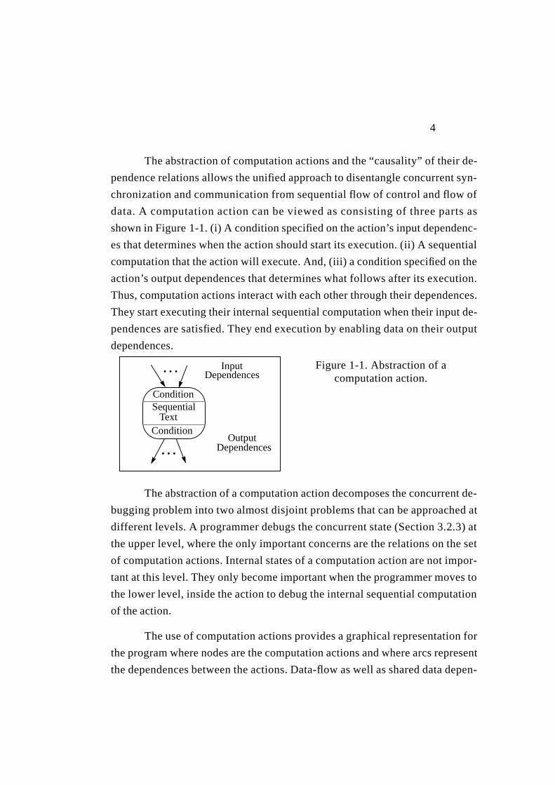
data. A computation action can be viewed as consisting of three parts as

shown in Figure1-1. (i) A condition specified on the action’s input dependenc-

es that determines when the action should start its execution. (ii) A sequential

computation that the action will execute. And, (iii) a condition specified on the

action’s output dependences that determines what follows after its execution.

Thus, computation actions interact with each other through their dependences.

They start executing their internal sequential computation when their input de-

pendences are satisfied. They end execution by enabling data on their output

dependences.

The abstraction of a computation action decomposes the concurrent de-

bugging problem into two almost disjoint problems that can be approached at

different levels. A programmer debugs the concurrent state (Section3.2.3) at

the upper level, where the only important concerns are the relations on the set

of computation actions. Internal states of a computation actionare not impor-

tant at this level. They only become important when the programmer moves to

the lower level, inside the action to debug the internal sequential computation

of the action.

The use of computation actions provides a graphical representation for

the program where nodes are the computation actions and where arcs represent

the dependences between the actions. Data-flow as well as shared data depen-

Condition

Condition

Sequential

Input

Output

Text

Dependences

Dependences• • •

• • •

Figure1-1. Abstraction of acomputation action.

5

dences are represented. Computation actions are naturally available in graphi-

cal visual programming languages like CODE 2 [New93], the language for

which we have implemented the unified debugger (Chapter 4). Computation

actions can also be obtained from a textual representation of the program as ex-

plained in Appendix A.

1.1.2 Program and its Execution

The key concept in providing a consistent representation is that both

the structure of a program and its execution behavior have natural representa-

tions as graphs when actions are represented at an appropriate level of abstrac-

tion. The program, P, is a directed graph (perhaps not defined until runtime,

Section3.1) whose nodes are sites for the execution of computation actions,

and arcs are the dependences with which the actions synchronize and commu-

nicate. There are also hyper-edges between nodes representing shared data-de-

pendences between actions (Section3.4).

The execution, E, of a program (Section3.2) is the traversal of the runt-

ime instantiation of the program graph starting with an assignment to an initial

state, until the instantiation of a final state. Traversal of the graph causes exe-

cution of actions at the nodes and generates a partially ordered set of execution

occurrences of actions or events.

Def. 1-3 An event is an execution of the action at a node of the program

graph.

Therefore, each event maps to the action of which it was an execution

occurrence. This provides a unique identifier for each event that consists of the

id of the action and its execution count. The unique identifiers allow the debug-

ger to record the execution, E, as a partial order on the set of events. As each

action is capable of executing multiple number of times, the recorded partial

order is a “pomset” [Pra86]; a partial order on the multi-set of occurrences of

actions as events (Section3.2.2).

6

In the recorded partial-order, the orderings indicate much more than a

mere temporal order. They indicate (data-flow and shared-data) dependences

that “cause” the actions to execute at the nodes. A debugger can, then, collect

the dependence information from the orderings of different executions of the

same action, and deduce the conditions that govern the execution of the action

(Section3.2.2). Therefore, a programmer can describe the expected behavior,

M, as some conditions on the expected dependences of selected actions. Then,

the debugger can observe the execution orderings of those actions, and deduce

the conditions governing their execution. It can raise an exception if they

don’t match the expected behavior (Section3.3). This guides the programmer

towards the offending action. Thus,

Def. 1-4 Debugging is the process of identifying those actions of the

program that are responsible for the failure of the program to

meet its final state specification.

1.2 The Debugging Process

The use of actions by the unified model of concurrent debugging pro-

vides a consistent representation for all the entities (P, M, and E) involved in

the debugging process (Chapter 3). This not only simplifies the task of the pro-

grammer, but also simplifies the provision of debugging facilities that estab-

l ish relationships between the entit ies. The feasibil i ty demonstration

prototype of the unified model of concurrent debugging has been implemented

in the CODE 2 environment (Chapter 4). It covers all the different parts of the

debugging process and provides facilities that:

1. Record and display the actual execution behavior of the program.

2. Restrict the recorded execution behavior to selected actions of the program.

3. Allow the user to specify a model/predicate of the expected behavior.

4. Automate the checking of the expected behavior.

7

5. Display any unexpected behavior that is detected during checking. This dis-

play allows the user to map the unexpected behavior to the program.

6. Provide post-restriction of the recorded information to selected actions.

7. Make cyclical debugging possible by providing a replay capability.

8. Provide support for interactive debugging.

Note that the provision of all of the above facilities is made possible by the

same recorded information; namely, the “causal” orderings among the execu-

tions of actions (Chapter 3).

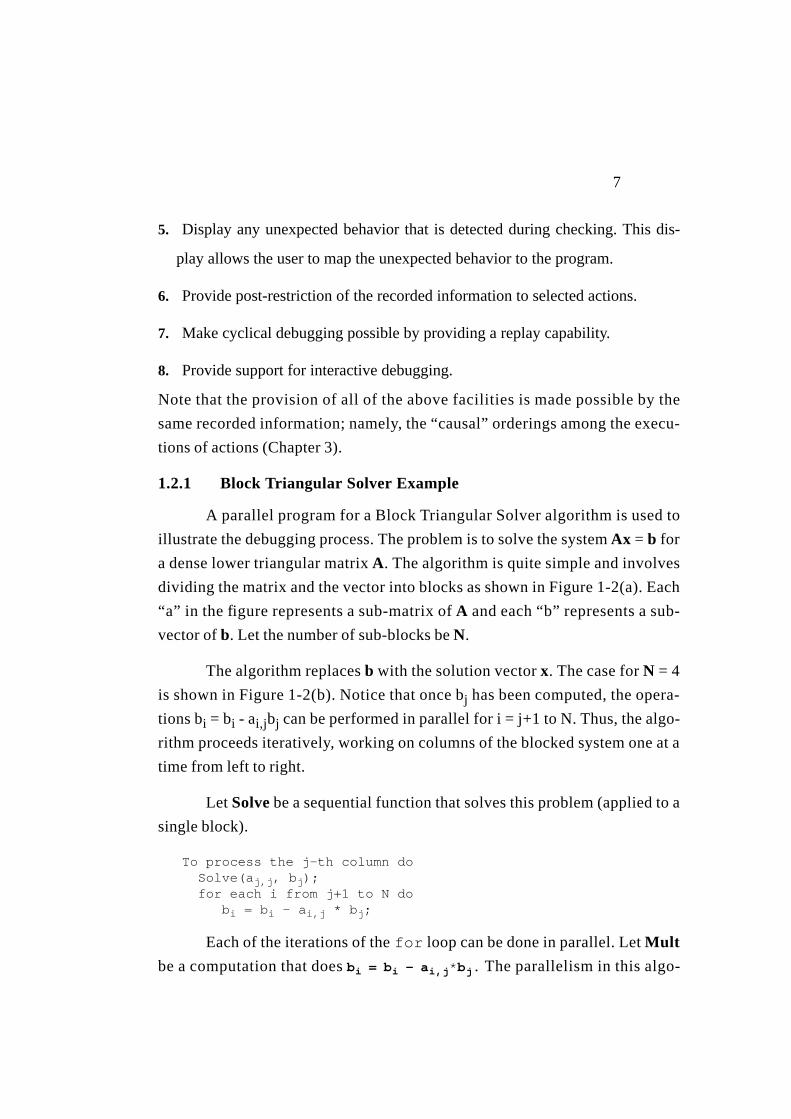
1.2.1 Block Triangular Solver Example

A parallel program for a Block Triangular Solver algorithm is used to

illustrate the debugging process. The problem is to solve the systemAx = b for

a dense lower triangular matrixA. The algorithm is quite simple and involves

dividing the matrix and the vector into blocks as shown in Figure 1-2(a). Each

“a” in the figure represents a sub-matrix of A and each “b” represents a sub-

vector ofb. Let the number of sub-blocks beN.

The algorithm replacesb with the solution vectorx. The case forN = 4

is shown in Figure 1-2(b). Notice that once bj has been computed, the opera-

tions bi = bi - ai,jbj can be performed in parallel for i = j+1 to N. Thus, the algo-

rithm proceeds iteratively, working on columns of the blocked system one at a

time from left to right.

Let Solve be a sequential function that solves this problem (applied to a

single block).

To process the j-th column doSolve(aj,j, bj);for each i from j+1 to N do

bi = bi - ai,j * bj;

Each of the iterations of thefor loop can be done in parallel. LetMult

be a computation that doesbi = bi - ai,j*bj. The parallelism in this algo-

8

rithm stems from the ability to perform theMult computations “beneath” the

Solve computation for a column in parallel. This is readily seen in the data-

flow graph for the algorithm as shown in Figure 1-3. The “s” nodes are calls to

Solve and the “m” nodes are calls toMult.

Figure 1-4 shows an implementation of this program in the CODE 2

graphical/visual parallel programming environment. NodeDist sends the ap-

propriate segments ofb to the nodes that perform thes andm operations of

Figure 1-3. A single instance of nodeSolve performs, one after another, all of

thes operations, whereasN-1 instances of nodeMult perform them opera-

a1,1

a2,1 a2,2

a3,1

a4,1

a3,2 a3,3

a4,2 a4,3 a4,4

b1

b2

b3

b4

b1 a1 1,1− b1=

b2 a2 2,1− b2 a2 1, b1−( )=

b3 a3 3,1− b3 a3 1, b1− a3 2, b2−( )=

b4 a4 4,1− b4 a4 1, b1− a4 2, b2− a4 3, b3−( )=

Figure1-2. (a) Matrix,A and vector, b. (b) Replacingb with vectorx.

s1

s

s

2

3

s 4m3

1

m21

b

b

b

b

1

2

3

3

x

x

x

x

1

2

3

4

m11

m32 m3

3

m22

Figure1-3. Data-flow for Block Triangular Solver.

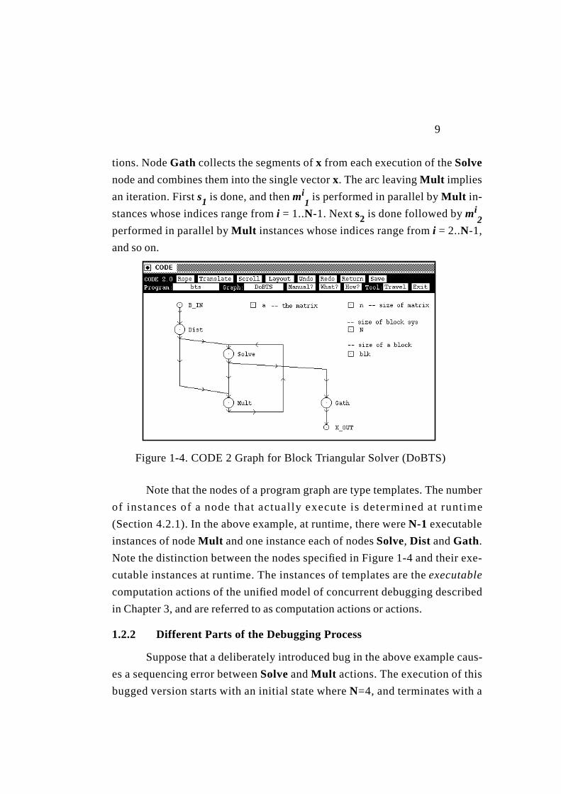
9

tions. Node Gath collects the segments of x from each execution of the Solve

node and combines them into the single vector x. The arc leaving Mult implies

an iteration. First s1 is done, and then mi1 is performed in parallel by Mult in-

stances whose indices range from i = 1..N-1. Next s2 is done followed by mi2

performed in parallel by Mult instances whose indices range from i = 2..N-1,

and so on.

Note that the nodes of a program graph are type templates. The number

of instances of a node that actually execute is determined at runtime

(Section 4.2.1). In the above example, at runtime, there were N-1 executable

instances of node Mult and one instance each of nodes Solve, Dist and Gath.

Note the distinction between the nodes specified in Figure 1-4 and their exe-

cutable instances at runtime. The instances of templates are the executable

computation actions of the unified model of concurrent debugging described

in Chapter 3, and are referred to as computation actions or actions.

1.2.2 Different Parts of the Debugging Process

Suppose that a deliberately introduced bug in the above example caus-

es a sequencing error between Solve and Mult actions. The execution of this

bugged version starts with an initial state where N=4, and terminates with a

Figure 1-4. CODE 2 Graph for Block Triangular Solver (DoBTS)

10

segmentation fault. We now follow the different steps of the debugging pro-

cess:

1. Identify and select the portions of the program whose behavior is to be moni-

tored.

This is a set of “suspect” nodes or subgraphs. Note that it is typically

impossible to monitor the entire execution behavior of the large complex pro-

grams which are actually the ones that need debugging. The visual/graphical

representation of P makes the selection of suspect portions of the program

easy. In our example, we can click on theSolve andMult nodes of the graph

of Figure 1-4 to inform the debugger that they need to be monitored. The de-

bugger makes additional preparations to filter out event executions of other

nodes likeDist andGath (Section3.3.2). This greatly helps in later steps as

much of the irrelevant information is filtered out.

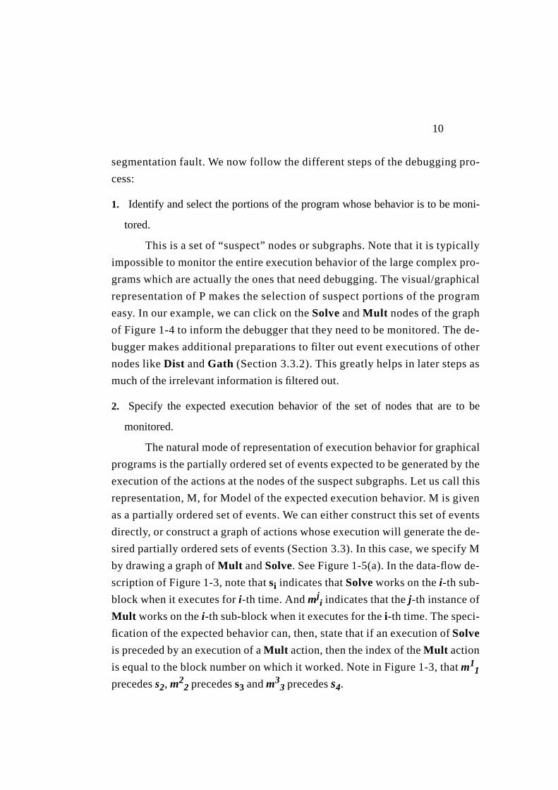
2. Specify the expected execution behavior of the set of nodes that are to be

monitored.

The natural mode of representation of execution behavior for graphical

programs is the partially ordered set of events expected to be generated by the

execution of the actions at the nodes of the suspect subgraphs. Let us call this

representation, M, for Model of the expected execution behavior. M is given

as a partially ordered set of events. We can either construct this set of events

directly, or construct a graph of actions whose execution will generate the de-

sired partially ordered sets of events (Section3.3). In this case, we specify M

by drawing a graph ofMult andSolve. See Figure 1-5(a). In the data-flow de-

scription of Figure 1-3, note thatsi indicates thatSolve works on thei-th sub-

block when it executes fori-th time. Andmji indicates that thej-th instance of

Mult works on thei-th sub-block when it executes for thei-th time. The speci-

fication of the expected behavior can, then, state that if an execution ofSolve

is preceded by an execution of aMult action, then the index of theMult action

is equal to the block number on which it worked. Note in Figure 1-3, thatm11

precedess2, m22 precedess3 andm3

3 precedess4.

11

3. Capture the execution behavior of the selected portions of the program.

This is a partially ordered sequence of events that actually occurred in

the execution (Section3.2). Let us call this partially ordered set of events E.

This is obtained by annotating the program graph with specifications to record

only the events and the orderings resulting from the execution of the suspect

nodes or subgraphs. The selection ofMult andSolve nodes in step 1 produced

such an annotation. As a result, the actual execution behavior observed by the

debugger as shown in Figure 1-5(b), contains event executions of only the se-

lected nodes (Section3.3.2). In the figure,si indicates thei-th execution of

Solve and eventmji indicates thei-th execution of that executable instance of

Mult whose node index isj.

4. Map E to M to determine the locations where the actual and expected events

first diverge.

The mapping of E to M can be done automatically since they are speci-

fied from the same representation. The result is identification of event sequenc-

es in E that do not correspond to the allowed set defined in M. In Figure 1-

5(b), we note that eventsm11, m2

1 andm31 precede events2, s3 ands4, respec-

tively. We, however, expected eventmjj to precede eventsi, wherej = i-1. This

detects the occurrence of the unexpected behavior; eventm21 preceding s3,

and eventm31 precedings4. The events map to actionsm2, m3 ands as shown

Solve (s)

Mult (m)

Figure1-5. (a) Graph of M, (b) Graph of E, (c) Elaborated graph of M.

(a) (b) (c)

s3

s2

s4m31

m11

m21

s1

s

m1m2m3

12

in Figure 1-5(c). Apparently, actionsm2, andm3 sent data tothe actions in

their wrong executions. (mj should have sent data when its execution counts

was equal toj, i.e. during eventmjj.)

Note that mapping of E to M gives an elaborated graph of M as shown

in Figure 1-5(c). This is a run-time structure that shows dynamically created

instances of node templates (Section3.1.1). The elaborated graph is obtained

from the partial order graph of E in Figure 1-5(b) by folding back subsequent

executions of a node, to its first execution.

5. Map the elaborated graph of M back to P to define corrective action.

Since the elaborated graph of M contains instances of the node tem-

plates of P, the mapping is automatic, and guides us towards the offending ac-

tion in P. The mapping from Figure 1-5(c) to Figure 1-4, helps in identifying

the offending action. Note that we ascertained above that data is sent by ac-

tions ofMult in the wrong executions toSolve. By looking at the specification

of the output rule ofMult , we found that the data was being sent out toSolve

without checking that the index of the action was equal to its execution count

(or the count of the sub-block which it was solving).

1.3 Overview of the Unified Debugger

The use of actions allows us to separate the analysis and presentation

concerns of the debugger from its measurement and recording concerns (Chap-

ter 4). Instrumentation inserted in the actions is only responsible for control-

ling their executions and generating the event information (Chapter 5). The

analysis and presentation of this information is separately carried out by the

debugging facilities (Chapter 6). The interactive facility allows the user to con-

trol the execution of actions and query their state at runtime (Chapter 7). See

Figure 1-5. The event information generated by the instrumentation during the

recording run, replay run, or the restricting run of the actions, can either be

used by the facilities on-the-fly, or in a postmortem fashion. The event infor-

mation is first topologically sorted to ensure a causal arrival of events

13

(Section6.3). Then, depending upon the options selected by the user, it is giv-

en to one or more of the following facilities that provide:

1. Animation and execution history displays (Section6.4).

2. Checking of the expected behavior (Section6.5).

3. Post-restriction to interesting events (Section6.1).

4. Filing for postmortem display or checking (Section6.1.2).

Note that the trace event records from an earlier execution are used for replay.

1.3.1 The Actual Execution Behavior

An event is identified by the id of the action and its execution count. In-

strumentation inserted in each action is only responsible for recording its exe-

cution and informing its successors about its event id. The execution event

On-the-flyPostmortem

Topological Sorting

Animation History

Figure1-6. Available facilities

RestrictingChecking DisplayTracingInteractive

Control

Recording Restricting ReplayingInstrumentation

runrunrunTraceRecords

TraceFile

CYCLICAL

C Y C L I C A L

14

record of each action contains the ids of its predecessors. This information is

used to construct a partial order representation of E that provides a definition

of the concurrent state (Section 3.2). The predecessors and successors of an

event in this partial order, indicate the conditions that triggered and followed

each event.

Execution history display is a pictorial view of the concurrent state of

E. Animation is simply a display of the progress of execution as E is mapped

to M (Section 3.2.4). During animation, the elaborated graph acts as an under-

lying structure whose nodes and arcs are highlighted in the topological sort or-

der as each event and its orderings are mapped to the nodes and the arcs of the

elaborated graph.

1.3.2 Restricting Execution to Selected Actions

The restriction facility records the executions of actions selected for

monitoring, and filters out the executions of remaining actions. An action se-

lected for monitoring records its execution and forwards the id of each of its

execution event to its successors (Section 3.3). An action whose execution is

not to be recorded simply forwards its predecessor list to its successors. The

forwarded list eventually reaches a selected action that records it. Execution

trace is, thus, restricted to contain only the execution events of selected ac-

tions and their orderings. This filtering greatly simplifies the checking of the

model of the expected behavior. Note that the restriction described above is

done by the instrumentation inserted in the actions at runtime. The unified de-

bugger also provides facilities for post-restricting the event trace generated by

the instrumentation. The event trace can be post-restricted to actions selected

for display, and actions selected for checking (Section 6.1).

1.3.3 Predicate/Model of the Expected Behavior

A model/predicate of the expected behavior may specify immediate or-

derings, or transitive orderings between execution events of the selected ac-

tions (Section 3.3). It may also specify absence of orderings. A race condition,

15

for example, is a model of expected behavior that specifies absence of order-

ings between executions of actions whose data accesses may conflict

(Section 3.6).

The model/predicate of the expected behavior may be formally or infor-

mally specified by the programmer. The checker facility provided by the de-

bugger automatically checks for the formally specified behavior (Section 6.4).

The programmer must visually check the (informally specified) behavior

against the displays provided by the debugger (Section 6.5). The ability of our

approach to restrict the traces to only the selected actions helps both the pro-

grammer and the checker facility.

1.3.4 Automatic Checking of the Expected Behavior

Expected behavior specifying immediate orderings can be checked eas-

ily as these orderings are available in the execution event records of actions.

However, checking of transitive orderings or absence of orderings between ex-

ecution events is much more involved.

The checker has to collect the predecessor information from the event

records of each action to establish transitive orderings. Our checker establish-

es these orderings with the help of vector clocks (Section 6.4). The size of the

clock vector depends upon the number of actions whose relationships are be-

ing checked. The checker updates and maintains the vector clock during the to-

pological sorting of the event records.

1.3.5 Display of the Unexpected Behavior

It is not enough for the checker facility of a debugger to come back to

the user with a terse statement saying that the expected behavior did not occur.

It should additionally be capable of displaying to the user the unexpected be-

havior that actually happened. Thus, event records need to be sorted and saved

during checking as the user may later request their display (Section 6.1). We,

therefore, postpone the updating of vector clocks until the topological sorting

16

of the execution event records. This avoids any extra overhead that may be in-

curred by the actions in maintaining the vector clocks during their execution.

1.3.6 Cyclical Debugging

A programmer often cycles through the debugging steps a number of

times before identifying a bug. Execution replay (Section 3.5) allows the user

to exactly replay an execution with the exact ordering of events as in the initial

execution. The program is first run to record the non-deterministic choices of

dependences with which each action executes. It is, then, replayed by forcing

the actions to make the choices recorded in the earlier run (Section 5.4).

1.3.7 Support for Interactive Debugging

The use of actions simplifies interactive control over the execution

(Chapter 7). The elaborated graph provides mapping between the run-time ob-

jects and the symbols defined in the program. These mappings are helpful in

controlling the execution of actions, and querying their state at run-time. The

debugger provides the usual breakpoint facilities.

17

Chapter 2. State of the Art and the Related Work

Debugging of parallel and distributed programs has been a subject of

much research in recent years. There are over 600 citations contained in the

two bibliographies published in 1989 [UtP89] and in 1993 [PaN93]. The work

surveyed in these bibliographies describes many different approaches for con-

current debugging and reports on the implementation of many different facili-

ties. Bates and LeBlanc note in [LeM89] that the previous work provides no

framework or model for the total process of concurrent debugging. There is no

definition of concurrent debugging that says why a particular facility or fea-

ture is provided and how it relates to the process of debugging. The result is

that most of the facilities or tools which have been proposed or implemented

are restricted to some subpart of the debugging process and that the tools are

generally incompatible. In this circumstance, the programmer must learn and

use many different methods and tools. The programmer typically has to com-

pose his own process for debugging of parallel programs and use different con-

cepts and different facilities for different steps in debugging.

Chapter 1 gave a specification of the process of debugging which in-

volves relationships between the program, P, the expected behavior of the pro-

gram, M, and the observed actual execution behavior, E. Debugging consists

of a series of mappings between these entities. In particular, the mappings

which are important are P → M → Ε → M → P. This process definition is used

as a framework for defining previous work. The analysis focuses on the restric-

tion in concepts that have tended to partition the different subparts of the de-

bugging process making each part a separate problem area. It is clearly

impractical to attempt to give a detailed discussion of all of the previous work.

Rather, this chapter relates what this approach considers to be the most signifi-

cant previous work in the context of the debugging process.

2.1 Sequential and Concurrent Debugging

Table 2-1 shows how major concurrent debugging facilities relate to

different parts of the debugging process.

18

a. In the form of static call graphb. Available by default in a sequential execution.c. Typically, animation facilities provide mapping to a process structure, not P.d. Can check only some predefined behaviors like deadlocks and access anomalies.e. Available by default: In the absence of non-determinism in sequential executions.f. Some replay facilities also support race detection, and use structural information of P.

Table2-1. Coverage of various parts of the debugging cycle.

Various Parts of theDebugging Cycle

Sequential Debuggers

Concurrent Debugging Facilities

StaticAnalysis

ExecutionReplay

RaceDetection

Displays/Animation

ModelCheckers

Uses structural information of P

Xa X

Presents to user a representation of E

X X

Records causal orderings; P→ E

Xb X X

Restricts E to selected events

X X

Provides mapping to program; E→ P

X Xc

Allows user to represent M

X X

Checks expected behavior; M→ E

X Xd X X

Presents unexpected behavior; E→ M

X X

Enables cyclical debugging

Xe Xf

Allows interactive debugging

X X

19

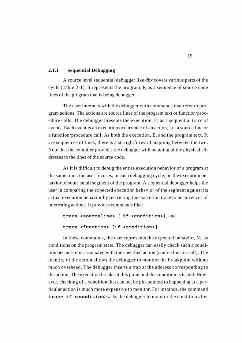
2.1.1 Sequential Debugging

A source level sequential debugger like dbx covers various parts of the

cycle (Table 2-1). It represents the program, P, as a sequence of source code

lines of the program that is being debugged.

The user interacts with the debugger with commands that refer to pro-

gram actions. The actions are source lines of the program text or function/proc-

edure calls. The debugger presents the execution, E, as a sequential trace of

events. Each event is an execution occurrence of an action, i.e. a source line or

a function/procedure call. As both the execution, E, and the program text, P,

are sequences of lines, there is a straightforward mapping between the two.

Note that the compiler provides the debugger with mapping of the physical ad-

dresses to the lines of the source code.

As it is difficult to debug the entire execution behavior of a program at

the same time, the user focuses, in each debugging cycle, on the execution be-

havior of some small segment of the program. A sequential debugger helps the

user in comparing the expected execution behavior of the segment against its

actual execution behavior by restricting the execution trace to occurrences of

interesting actions. It provides commands like:

trace <sourceline> [ if <condition>], and

trace <function> [if <condition>].

In these commands, the user represents the expected behavior, M, as

conditions on the program state. The debugger can easily check such a condi-

tion because it is associated with the specified action (source line, or call). The

identity of the action allows the debugger to monitor the breakpoint without

much overhead. The debugger inserts a trap at the address corresponding to

the action. The execution breaks at this point and the condition is tested. How-

ever, checking of a condition that can not be pin-pointed to happening at a par-

ticular action is much more expensive to monitor. For instance, the command

trace if <condition> asks the debugger to monitor the condition after

20

the execution of every source line. This monitoring is very expensive and such

commands are often avoided by the programmer.

The debugger provides interactive support using static and dynamic

structure of the program. Static call graph is available in the symbol table in-

formation. At runtime, the debugger maintains the current stack of active call

frames. Note that each instance of a call (or a block of code) is represented in

memory with a frame. This provides the debugger with the dynamic structure

of the computation. In addition, the debugger maintains mappings which help

in providing breakpoint control of the execution and querying the runtime

state of objects. Following mappings are maintained:

1. Mappings between source lines and the addresses of their generated code.

2. Mappings between calls and the addresses of their executable code.

3. Mappings between active blocks (scopes) and their frame addresses.

2.1.2 Concurrent Debugging Facilities

A concurrent execution introduces problems arising from multiple

threads of control, synchronizations among these threads of control, probe ef-

fect, race conditions and non-determinism [McH89]. This makes concurrent

debugging much more difficult than sequential debugging. Therefore, concur-

rent debugging facilities often tend to develop around one of these problems.

See Figure 2-11.

Execution history displays help user in keeping track of the numerous synchroni-

zations that have taken place among various threads of execution[LMF90],

[FLM89], [PaU89]. The focus of such displays is, thus, limited toΕ.

Animation facilities help in following the progress of execution “instantaneously”

in each thread of control[HoC87], [PaU89], [HoC90], [SBN89], [ZeR91],

[Ho91]. The focus of animation is mappingΕ to P.

1 Dotted lines show that some approaches may address more than one problem area.

21

Race detection facilities detect simultaneous accesses to shared data (R-W, W-W)

[NM90a], [EGP89], [HMW90], [Sch89]. Their focus israce behavior in the P

→ E part of the debugging cycle.

Predicate/model checkers automate the process of verifying the expected behav-

ior of events happening at various sites in a distributed system [HHK85],

[BFM83], [BH83], [HsK90], [WaG91], [Bat89],[GaW92], [ReSc94]. They

allow a user to specify M, but, are limited to M→ Ε part of the debugging

cycle.

Execution replay facilities overcome the non-determinism of a concurrent execu-

tion [LM86], [For89], [MiC89], [Net93]. They make cyclical debugging pos-

sible, but often ignore individual parts of a cycle.

Static analysis extracts more information from P when “probe-effect” [Sto88], a

principle similar to Hiesenberg's uncertainty principle, limits further instru-

mentation [Tay83], [TaO80], [BBC88], [CaS89], [McD89]. They analyze P

and are limited to the P→ Μ part of the debugging cycle.

2.2 Problems in Various Parts of the Cycle

Fig. 2-2 shows the problems and ambiguities often encountered during

the mapping between different representations in various parts of the debug-

ging cycle.

StaticProbe Effect

Non-Determinism

Shared MemoryAccess

Distributed Systems

Multiple ExecutionThreads

NumerousSynchronizations

Problem Areas

Figure2-1. Debugging facilities target individual problem areas

Analysis

ExecutionReplay

RaceDetection

ModelCheckers

AnimationFacilities

HistoryDisplays

22

Parallel and distributed execution environments typically provide pro-

cesses or threads as executable units to run the program text. There is often a

complex multiplexing of the program text among instances of the pro-

cess/thread structure during execution due to resource limitations, scheduler

policies, and other constraints. A concurrent debugger must resolve the map-

ping and timing ambiguities resulting from such multiplexing. A visualization

of execution history [PaU89], [McH89] can help in resolving some of these

ambiguities by displaying various threads of control and the synchronizations

among them. This is typically a time-process graph representation of the exe-

cution [LMF90], [FLM89]. Events in such a representation are defined in the

context of the process/threads of the execution environment and not as occur-

rences of program actions. This creates ambiguities in mapping the observed

execution behavior to the program (Section 2.2.1). An animation facility can

help in resolving some of these ambiguities in the E → P part of the cycle. Ani-

mation facilities [HoC87], [PaU89], [McH89], [Ho91] provide an instanta-

neous view of the mapping of events of a time-process graph to a graphical

structure. This, however, translates into extra effort for the user who must then

P

M

E

M

P

E

MappingOrdering

CheckingFiltering

Modeling

AnimationRace

Model Checkers

Execution historyDetection

Figure 2-2. Ambiguities in various parts of the cycle

Ambiguities Ambiguities

Problems

Problems Ambiguities

displays

23

develop a graphical structure that can support animation [HoC90], [SBN89],

[Ho91], [ZeR91]. Such structures are, however, unable to support the visual-

ization of the abstractions defined by the user. This has forced some of the ap-

proaches to abandon the use of visualizations [CFH93].

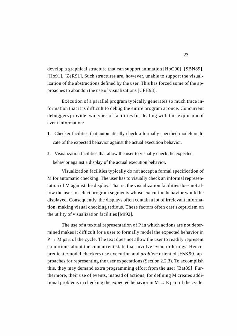
Execution of a parallel program typically generates so much trace in-

formation that it is difficult to debug the entire program at once. Concurrent

debuggers provide two types of facilities for dealing with this explosion of

event information:

1. Checker facilities that automatically check a formally specified model/predi-

cate of the expected behavior against the actual execution behavior.

2. Visualization facilities that allow the user to visually check the expected

behavior against a display of the actual execution behavior.

Visualization facilities typically do not accept a formal specification of

M for automatic checking. The user has to visually check an informal represen-

tation of M against the display. That is, the visualization facilities does not al-

low the user to select program segments whose execution behavior would be

displayed. Consequently, the displays often contain a lot of irrelevant informa-

tion, making visual checking tedious. These factors often cast skepticism on

the utility of visualization facilities [Mi92].

The use of a textual representation of P in which actions are not deter-

mined makes it difficult for a user to formally model the expected behavior in

P → M part of the cycle. The text does not allow the user to readily represent

conditions about the concurrent state that involve event orderings. Hence,

predicate/model checkers use execution andproblem oriented [HsK90] ap-

proaches for representing the user expectations(Section 2.2.3). To accomplish

this, they may demand extra programming effort from the user [Bat89]. Fur-

thermore, their use of events, instead of actions, for defining M creates addi-

tional problems in checking the expected behavior in M→ E part of the cycle.

24

These problems can, in turn, constrain the range of expected behaviors that a

checker will allow a user to represent in M [Ho91], [WaG91], [ReSc94].

In the P → E part of the cycle, debuggers for shared memory and dis-

tributed systems approach the problem of recording causal orderings different-

ly. Shared memory debuggers typically do not record the inter-process

orderings. They only approximate the orderings from the sequential traces ob-

tained for each process [HMW90], [NM91a], [Sch89], [EGP89]. This restricts

their model checking ability to only one type of expected behavior; the race

behavior resulting from the non-deterministic access of shared data. Thus,

they only provide a facility for race detection. On the other hand, distributed

debuggers like [GaW92] provide more generalized predicate/model checking

facilities. They use specialized clocks [Mat89], [Fid89] for time stamping

events and recording the causal orderings. This allows them a greater flexibili-

ty in checking a variety of predicates/models of expected behaviors. However,

this creates the overhead of maintaining these vector clocks [ReSc94].

In M → P part of the cycle, the user maps any unexpected behavior in

M to the program in order to get closer to the bug. A terse message from the

checker stating that the check for expected behavior has failed, is not enough

to the user. The checker must help the user by presenting the unexpected be-

havior that caused the check to fail [Bat89]. However, existing checkers sel-

dom keep enough information during measurement that would allow them to

present the unexpected behavior to the user. This forces the user to exert extra

effort in repeatedly querying the debugger for the same information.

2.2.1 Mapping Ambiguities

In E → P part of the cycle, a debugger has to map the events defined in

the context of processes/threads of the execution environment on to the pro-

gram text. However, ambiguities arise in mapping intra-process arcs of a time-

process graph to their corresponding sequential text in the program. For in-

stance, in Fig. 2-3(a) there is an ambiguity about the intra-process arc x of Pro-

cess 3. x can either map to the sequential text S or to the sequential text T of

25

Fig. 2-3(b). Eventw that immediately followsx, and maps to the synchroniza-

tion statementwait (ev) is not of much help.wait (ev) is neither associated

with S nor with T. The synchronization event simply sits at the boundary

where a piece of text ends and another one starts. Note that an event’s associa-

tion in a time process graph is with a process (#3 in this case), not with an ac-

tion of the program text.

Instead of letting a synchronization statement sit ambiguously on the

border of two sequential text segments, we propose an abstraction that perma-

nently associates the synchronization statements of a program with its sequen-

tial text segments. The abstractions resulting from this association is that of a

computation action as given in Section 1.1.1. The concept of computation ac-

tion disentangles the sequential control-flow considerations from the synchro-

nization considerations. The programmer is, then, able to concentrate on

dependences between actions instead of scheduling entities such as a process.

Animation facilities[McH89], [PaU89] typically require an underly-

ing process structure for supporting their visualizations of the E→ P mapping.

In this structure, nodes are processes and arcs are synchronization/communica-

tion links between processes. Current animation facilities often demand extra

user effort to develop an alternate structure for supporting the visualizations

of theE → P mapping. A textual representation of P can not directly support

this visualization because it conceals the synchronization dependences to

Process 3: /* sequential control- */: /* flow text; S */

while (...) {wait (ev);: /* sequential */

/* control- */: /* flow text; T */

}

post ev

post ev

wait ev

1

2

3

(b)

x

(a)

Figure2-3. (a) Time-process graph (b) Program text (c) Event traces.

p

p

w

1

2

3w

(c)

ev

ev

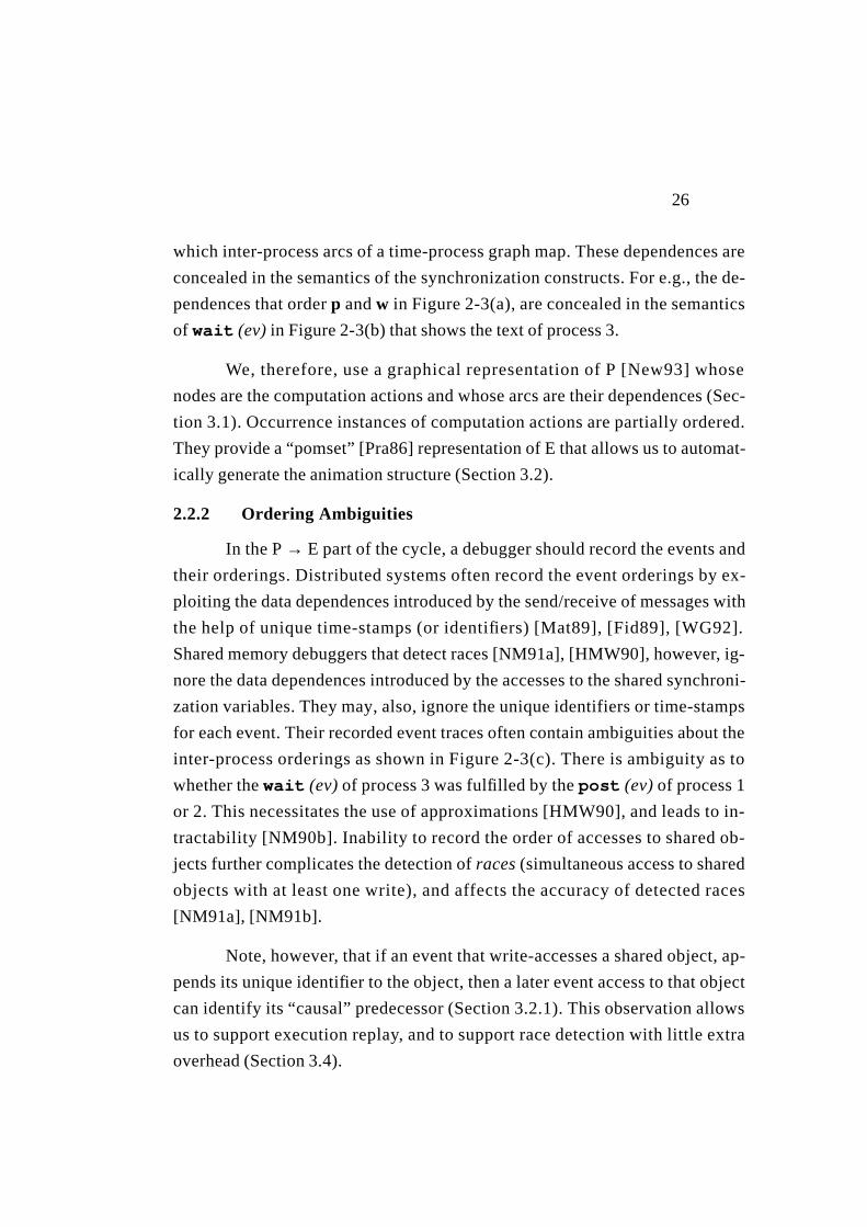
26

which inter-process arcs of a time-process graph map. These dependences are

concealed in the semantics of the synchronization constructs. For e.g., the de-

pendences that orderp andw in Figure 2-3(a), are concealed in the semantics

of wait (ev) in Figure 2-3(b) that shows the text of process 3.

We, therefore, use a graphical representation of P [New93] whose

nodes are the computation actions and whose arcs are their dependences (Sec-

tion 3.1). Occurrence instances of computation actions are partially ordered.

They provide a “pomset” [Pra86] representation of E that allows us to automat-

ically generate the animation structure (Section 3.2).

2.2.2 Ordering Ambiguities

In the P→ E part of the cycle, a debugger should record the events and

their orderings. Distributed systems often record the event orderings by ex-

ploiting the data dependences introduced by the send/receive of messages with

the help of unique time-stamps (or identifiers) [Mat89], [Fid89], [WG92].

Shared memory debuggers that detect races[NM91a], [HMW90], however, ig-

nore the data dependences introduced by the accesses to the shared synchroni-

zation variables. They may, also, ignore the unique identifiers or time-stamps

for each event. Their recorded event traces often contain ambiguities about the

inter-process orderings as shown in Figure 2-3(c). There is ambiguity as to

whether thewait (ev) of process 3 was fulfilled by thepost (ev) of process 1

or 2. This necessitates the use of approximations[HMW90], and leads to in-

tractability [NM90b]. Inability to record the order of accesses to shared ob-

jects further complicates the detection ofraces (simultaneous access to shared

objects with at least one write), and affects the accuracy of detected races

[NM91a], [NM91b].

Note, however, that if an event that write-accesses a shared object, ap-

pends its unique identifier to the object, then a later event access to that object

can identify its “causal” predecessor (Section 3.2.1). This observation allows

us to support execution replay, and to support race detection with little extra

overhead (Section 3.4).

27

2.2.3 Modeling Problems

A sequentialdbx debugger is user-friendly. It allows the user to associ-

ate expected conditions with a program action. For instance, in adbx com-

mand such as “when at <stmt> if <condition>”, the user associates a

condition about the sequential state of the executing program with a statement

of interest. Later, the debugger allows the user to interactively follow the con-

ditional progress of the execution that has been restricted to the interesting ac-

tions. Such aprogram oriented approach[HsK90] is not possible with a

“textual” representation of a concurrent program. Unlike dbx conditions, con-

ditions about the concurrent state involve event orderings whose correspond-

ing dependences are not visible in the textual representation. For instance,

event orderings in an expected behavior like “(w ∧ p) precedew” for Figure 2-

3(a), correspond to dependences that are not visible in the textual representa-

tion of Figure 2-3(b). Hence, assertion/model checkers[HsK90], [McH89]

adopt execution oriented approaches that use models like temporal logic, inter-

leaving, partial order or automatas[Ho91]. In P→ M part of the cycle, there-

fore, a user has to exert extra effort to learn a new language, specify the

expected behavior and, then, debug it foruser errors [Bat89] before debug-

ging the original program.

2.2.4 Filtering Ambiguities

In M → E part of the cycle, assignment andresolution problems

[Bat89] are typical of the ambiguities that arise during filtering and recogni-

tion of the expected behavior. As most existing checkers are execution orient-

ed, they use events in their representation of the expected behavior, and leave

the actions implicit. This conceals the information that (i) eventsare actually

multiple occurrences of actions, and (ii) the observed event orderings are the

unrolling of the communication/synchronization structure of the program ac-

tions. For instance, a behavior like “p precedesw” gives no information to the

debugger about the actions that correspond to eventsp andw. Ambiguities

can, then, arise whenever more than one observed behavior fits the expected

28

behavior. In Fig.2-3(a), “p precedesw” can fit several behaviors; p of process

2 precedes the first w of process 1,p of process 1 precedes the secondw of pro-

cess 2, orp of process 2 precedes the secondw of process 3. Such ambiguities

restrict the range of checkable behaviors. This, in turn, restricts the range of

behaviors that can be represented in M[Ho91], [Bat89].

Information defining actions such as their statement line numbers,

could have resolved these ambiguities. We, therefore, use such information

about the actions to simplify the filtering and recognition of the expected be-

havior (Section 3.3).

29

Chapter 3. The Unified Model of Concurrent Debugging

The unified model presented in this chapter decomposes the problem of

debugging a concurrent program into two levels. A programmer debugs the

concurrent state at the upper level, where the only important concerns are the

relations on the set of computation actions; specified in the program, P, mod-

eled in the expected behavior, M, and observed in the execution behavior, E.

Internal states of a computation action are not important at this level because

the execution occurrences of the computation action are considered atomic.

These states only become important when the programmer moves to the lower

level, inside the computation action, to debug its internal sequential text.

3.1 The Specified Behavior

Notation3-1 ΣP is the set of computation actions specified in the program.

Data dependences that force the computation actions to execute in a

particular order are represented by ordered pairs:

Def. 3-1 The set of data-flow dependences is FP ⊆ ΣP × ΣP.

For instance, the dependence of areceive of a message on itssend,

the dependence of aP of a semaphore on itsV, or the dependence of await of

a synchronization event on itspost, represent such data-flow dependences.

The write-read dependence on a shared synchronization variable, or on a mes-

sage, forces the actions to execute in a particular order. The motivation for rep-

resenting the synchronization dependences as data-flow dependences comes

from the language independence and machine independence goals of the

CODE graphical programming environment [BAS90],[NB92]. The data flow

characterization of the synchronization and control-flow dependences in

CODE allow the environment to support shared memory, as well as, distribut-

ed systems.

The set of ordered pairsFP gives a graphical representation of the pro-

gram. The nodes of the program graph (ΣP, FP) are the set of computation ac-

tions, and its arcs are the data-flow dependences. See Figure 3-1(a).

30

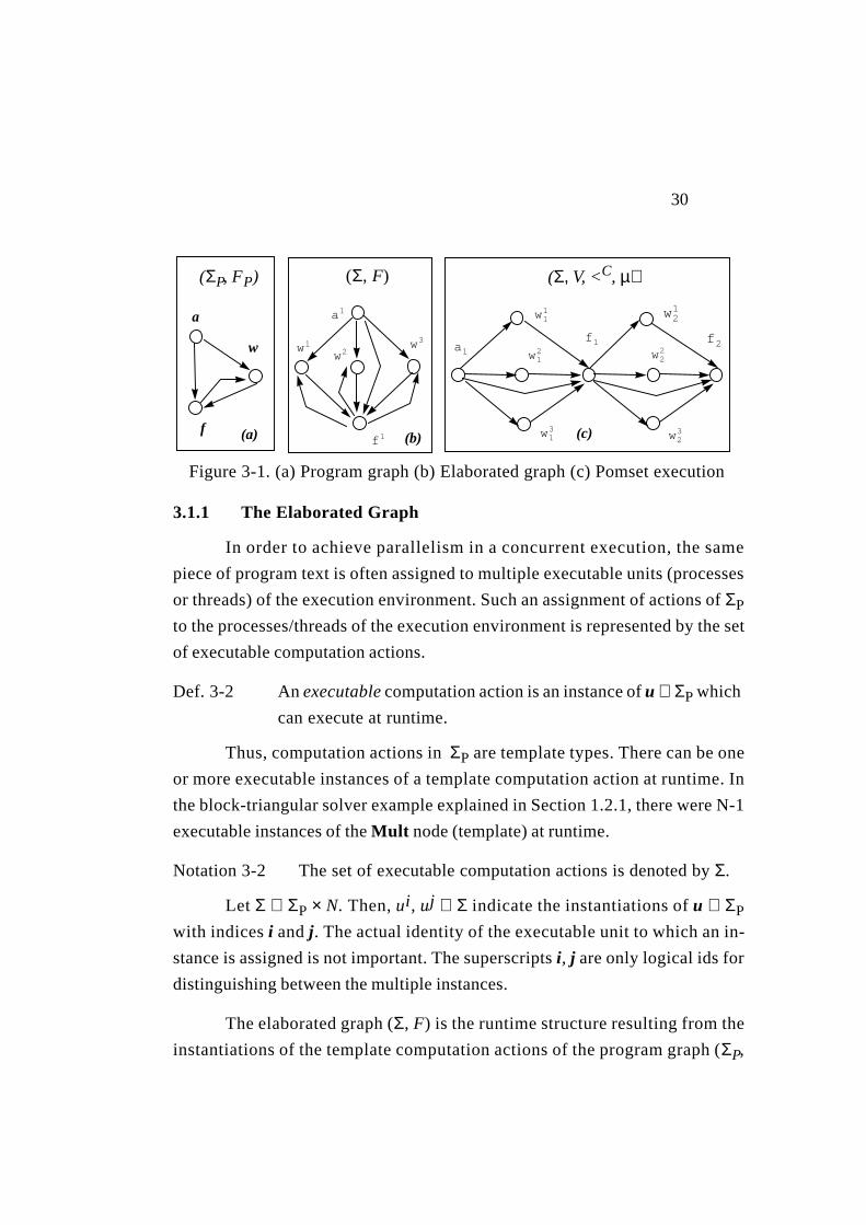
3.1.1 The Elaborated Graph

In order to achieve parallelism in a concurrent execution, the same

piece of program text is often assigned to multiple executable units (processes

or threads) of the execution environment. Such an assignment of actions of ΣP

to the processes/threads of the execution environment is represented by the set

of executable computation actions.

Def. 3-2 An executable computation action is an instance of u ∈ ΣP which

can execute at runtime.

Thus, computation actions in ΣP are template types. There can be one

or more executable instances of a template computation action at runtime. In

the block-triangular solver example explained in Section 1.2.1, there were N-1

executable instances of the Mult node (template) at runtime.

Notation 3-2 The set of executable computation actions is denoted by Σ.

Let Σ ⊆ ΣP × N. Then, ui, uj ∈ Σ indicate the instantiations of u ∈ ΣP

with indices i and j. The actual identity of the executable unit to which an in-

stance is assigned is not important. The superscripts i, j are only logical ids for

distinguishing between the multiple instances.

The elaborated graph (Σ, F) is the runtime structure resulting from the

instantiations of the template computation actions of the program graph (ΣP,

f (c)

a

w w12

w11 w2

1

w13

w22

w23

f1a1w1

f1

w2

a1

w3

(a) (b)

f2

Figure 3-1. (a) Program graph (b) Elaborated graph (c) Pomset execution

(ΣP, FP) (Σ, F) (Σ, V, <C, µ)

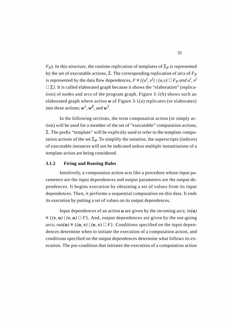
31

FP). In this structure, the runtime replication of templates ofΣP is represented

by the set of executable actions,Σ. The corresponding replication of arcs ofFP

is represented by the data flow dependences,F ≡ {(ui, vj) | (u,v) ∈ FP and ui, vj

∈ Σ}. It is called elaborated graph because it shows the “elaboration” (replica-

tion) of nodes and arcs of the program graph. Figure 3-1(b) shows such an

elaborated graph where actionw of Figure 3-1(a) replicates (or elaborates)

into three actions;w1, w2, andw3.

In the following sections, the term computation action (or simply ac-

tion) will be used for a member of the set of “executable” computation actions,

Σ. The prefix “template” will be explicitly used to refer to the template compu-

tation actions of the setΣP. To simplify the notation, the superscripts (indices)

of executable instances will not be indicated unless multiple instantiations of a

template action are being considered.

3.1.2 Firing and Routing Rules

Intuitively, a computation action acts like a procedure whose input pa-

rameters are the input dependences and output parameters are the output de-

pendences. It begins execution by obtaining a set of values from its input

dependences. Then, it performs a sequential computation on this data. It ends

its execution by putting a set of values on its output dependences.

Input dependences of an actionu are given by the incoming arcs;in(u)

≡ { (v, u) | (v, u) ∈ F}. And, output dependences are given by the out-going

arcs;out(u) ≡ { (u, v) | (u, v) ∈ F}. Conditions specified on the input depen-

dences determine when to initiate the execution of a computation action, and

conditions specified on the output dependences determine what follows its ex-

ecution. The pre-condition that initiates the execution of a computation action

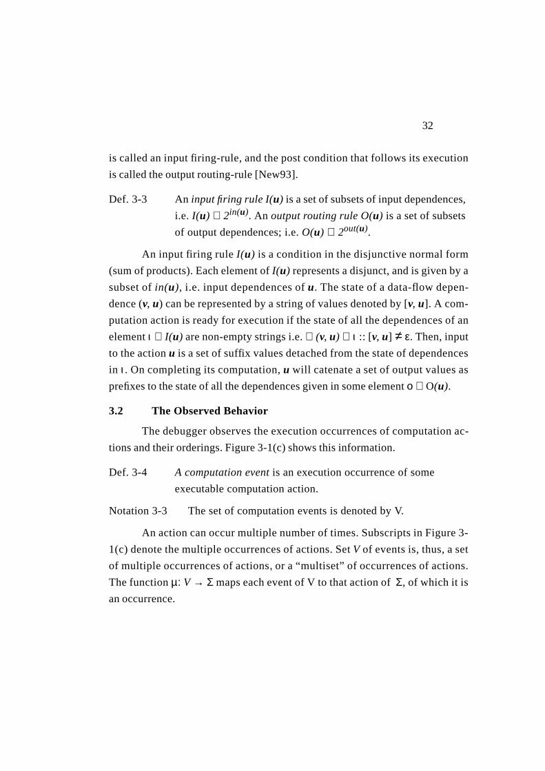
32

is called an input firing-rule, and the post condition that follows its execution

is called the output routing-rule [New93].

Def. 3-3 An input firing ruleI(u) is a set of subsets of input dependences,

i.e. I(u) ⊆ 2in(u). An output routing rule O(u) is a set of subsets

of output dependences; i.e.O(u) ⊆ 2out(u).

An input firing rule I(u) is a condition in the disjunctive normal form

(sum of products). Each element ofI(u) represents a disjunct, and is given by a

subset ofin(u), i.e. input dependences ofu. The state of a data-flow depen-

dence (v, u) can be represented by a string of values denoted by [v, u]. A com-

putation actionis ready for executionif the state of all the dependences of an

elementι ∈ I(u) are non-empty strings i.e.∀ (v, u) ∈ ι :: [v, u] ≠ ε. Then, input

to the actionu is a set of suffix values detached from the state of dependences

in ι. On completing its computation,u will catenate a set of output values as

prefixes to the state of all the dependences given in someelementο ∈ O(u).

3.2 The Observed Behavior

The debugger observes the execution occurrences of computation ac-

tions and their orderings. Figure 3-1(c) shows this information.

Def. 3-4 A computation event is an execution occurrence of some

executable computation action.

Notation3-3 The set of computation events is denoted by V.

An actioncan occur multiple number of times. Subscripts in Figure 3-

1(c) denote the multiple occurrences of actions. SetV of events is, thus, a set

of multiple occurrences of actions, or a “multiset” of occurrences of actions.

The functionµ: V → Σ maps each event of V to that action ofΣ, of which it is

an occurrence.

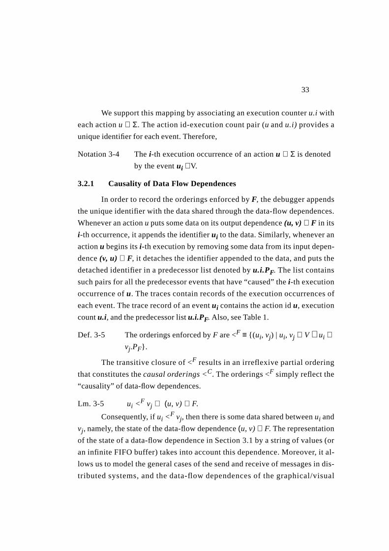
33

We support this mapping by associating an execution counteru.i with

each actionu ∈ Σ. The action id-execution count pair (u andu.i) provides a

unique identifier for each event. Therefore,

Notation3-4 The i-th execution occurrence of an actionu ∈ Σ is denoted

by the eventui ∈V.

3.2.1 Causality of Data Flow Dependences

In order to record the orderings enforced byF, the debugger appends

the unique identifier with the data shared through the data-flow dependences.

Whenever an actionu puts some data on its output dependence(u, v) ∈ F in its

i-th occurrence, it appends the identifier ui to the data. Similarly, whenever an

actionu begins itsi-th execution by removing some data from its input depen-

dence(v, u) ∈ F, it detaches the identifier appended to the data, and puts the

detached identifier in a predecessor list denoted byu.i.PF. The list contains

such pairs for all the predecessor events that have “caused” thei-th execution

occurrence ofu. The traces contain records of the execution occurrences of

each event. The trace record of an eventui contains the action idu, execution

countu.i, andthe predecessor listu.i.PF. Also, see Table 1.

Def. 3-5 The orderings enforced byF are <F ≡ {( ui, vj) | ui, vj ∈ V ∧ ui ∈vj.PF}.

The transitive closure of <F results in an irreflexive partial ordering

that constitutes thecausal orderings <C. The orderings <F simply reflect the

“causality” of data-flow dependences.

Lm. 3-5 ui <F vj ⇒ (u, v) ∈ F.

Consequently, if ui <F vj, then there is some data shared betweenui and

vj, namely, the state of the data-flow dependence(u, v) ∈ F. The representation

of the state of a data-flow dependence in Section3.1 by a string of values (or

an infinite FIFO buffer) takes into account this dependence. Moreover, it al-

lows us to model the general cases of the send and receive of messages in dis-

tributed systems, and the data-flow dependences of the graphical/visual

34

languages like CODE [BAS90],[NB92]. But, the representation may create

problems in modeling the synchronization primitives of shared memory sys-

tems. However, as seen in Section 3.2.3, concurrent state does not depend

upon the internal representation of the states of the data-flow dependences. It

only depends upon the event orderings. Thus, we can represent the state of a

synchronization dependence, with a string (or a buffer) of length one. It will

denote the data dependence due to the shared synchronization variable (whose

only permitted values are set or reset). The debugger records the causal order-

ings by appending and detaching the identifier to the shared synchronization

variable.

3.2.2 Execution History Pomsets

As seen above, actions can occur multiple number of times as events,

i.e. the set V of events is related to the set Σ of actions through the function µ:V → Σ. This effectively turns the poset (V, <C) into a pomset (Σ, V, <C, µ)

[Gai88], [Gis88], [Pra86]. A POMSET is a Partially Ordered MultiSET of oc-

currences of actions, in much the same way as a string is a TOMSET; a Total-

ly Ordered MultiSET of occurrences of alphabets. The pomset (Σ, V, <C, µ) is

called a causal pomset because <C are the causal orderings. It is instrumental

in unifying our model because its expression of the concurrency properties is

independent of the way time or events are modeled in a system [Gai88].

A pictorial representation of the causal pomset is an execution history

display. We can now explain why execution history displays are so helpful in

debugging. They display the causal orderings of events. These orderings allow

a programmer to determine the conditions that initiated and followed each exe-

cution occurrence of an action. From Lemma 3-5, an immediate predecessor

of ui must map to an input dependence of u; and from Def. 3-3, an element of

the input firing rule of u is a subset of input dependences. Hence, immediate

predecessors of an event ui inform the programmer about that element of the

input firing-rule that initiated the i-th occurrence of u. Similarly, immediate

successors of an event ui inform the programmer about that element of the out-

35

put routing-rule that determined the condition following thei-th execution oc-

currenceof u.

Notation3-6 •ui ≡ { (v, u) | vj <F ui} and ui

• ≡ { (u, v) | ui <F vj }

Def. 3-6 A causal pomset(Σ, V, <c, µ) is compatible with the firing and

routing rules iff ∀ui ∈V :: •ui ∈ I(u) ∧ ui• ∈ O(u).

This shows the compatibility of the immediate orderings of a given

event with the rules specified on the immediate dependences of its correspond-

ing action. In Section3.3.1, we extend this compatibility of immediate order-

ings with the immediate dependences to the compatibility of transitive

orderings with the transitive dependences. This provides a framework for rep-

resenting and checking the expected behavior.

3.2.3 Concurrent Execution State

There is non-determinism associated with the choices of the elements

given in the input firing rules. An action can non-deterministically select dif-

ferent elements of a firing rule. In Figure 2-3, the second occurrence of action

w can non-deterministically select any element from itsinput firing rule. Dur-

ing execution replay, a record of the causal orderingsinforms our debugger to

select the right element of the firing rules for each execution occurrence of an

action. Thus, it reconstructs the states of the previous execution. Using <c and

following [Mat89], we find a notion of concurrent state:

Def. 3-7 A concurrent state of an execution(Σ, V, <C, µ) is a consistent

cut-set of the poset (V, <C). A setCS ⊆ V is a consistent cut-set

if f ui ∈ CS ∧ vj <C ui ⇒ vj ∈ CS.

Thus, the state of an actionu after itsi-th occurrence is represented by

its causal history, namely, the partially ordered set of all the events that were

causally beforeui. Note that the above definition is independent of the local

state of an action. It is, also, independent of the contents of the messages ex-

changed by the actions. It only depends upon the order of events. Hence, dis-

tributed systems often reduce their roll-back and recovery overhead by only

36

recording the event orderings, and not the content of messages or the check-

points of the local states [JhZw90]. Therefore, our execution replay facility ex-

ploits this definition to reduce the recording overhead (Section3.5).

3.2.4 Animation

Animation provides an instantaneous view of the progress of execu-

tion. It is simply the process of displaying Def. 3-6 on the elaborated graph

while traversing the execution pomset.

During animation, the debugger traverses the execution pomset. On en-

countering thei-th event occurrence of an actionu, it highlights in the elabo-

rated graph those input dependences of the actionthat correspond to the

immediate predecessors of itsi-th event occurrence. It, then, highlights the ac-

tion u. Then, it highlights those output dependences of the action that corre-

spond to the immediate successors of itsi-th event occurrence.

We can automatically generate an elaborated graph from the execution

pomset. Note that the structure shown in Figure 3-1(b) is obtained by folding

all the subsequent occurrences of actions in Figure 3-1(c) to their first occur-

rences. This fulfills the requirement of a strong coupling between animation

and execution history[McH89].

3.3 The Expected Behavior

A user represents the expected behavior by selecting some“interest-

ing” actionsΣM from Σ. Then, the expectations about the execution behavior

of the selected actions are specified as some conditionsIM, OM on their expect-

ed dependences,FM.

3.3.1 Representing Expected Behavior

A dbx debugger is closely coupled with the program because it com-

pels the programmer to use only those objects that already exist in the pro-

gram; e.g. it would not allow a user to specify a non-existent print variable.

Taking cue fromdbx, we closely couple our checker with the program and

37

only allow the user to work with only those actions that are specified in the

program.

Note that if a user expects that eventsui andvj will be ordered in the ex-

ecution, then their actionsu andv, must exhibit a (transitive) data-flow depen-

dence in the program. That is,ui <C vj ⇒ (u, v) ∈ F*, whereF* is a transitive

closure ofF. This also follows from Lemma 3-5. For instance,m1 <C c1 in Fig-

ure 3-2(b) corresponds to thetransitive data-flow dependence between m andc

of Figure 3-2(a); both are shown by dotted lines. Thus, any pattern that is ex-

pected in an execution, must be the unrolling of a pattern already present in the

program structure.

Thus, a user starts specifying expected behavior by selecting a subset

ΣM of interesting actions from the program;ΣM ⊆ Σ. Figure 3-2(a) shows a se-

lection of such actions. The user can then specify a dependence between the se-

lected actions only if it corresponds to some dependence ofF*. Some of such

selected dependences are shown as FM in Figure 3-2(a).

Def. 3-8 FM are the selected dependences from the transitive data-flow

dependences F* restricted to interesting actions i.e.FM ⊆ F* /

ΣM, whereΣM ⊆ Σ.

An observed ordering like(m2, ?) in Figure 3-2(b), that can not be

mapped to a data-flow dependence fromFM is, therefore, symptomatic of a

bug!

(Σ, F)

n

cp

ma

f

a1

n1 c1 n2

m1 p1 m2 p2 m3

f1

(a)

Figure3-2. (a) Elaborated Graph. (b) Execution.

(Σ, V, <, µ)

?

(b)

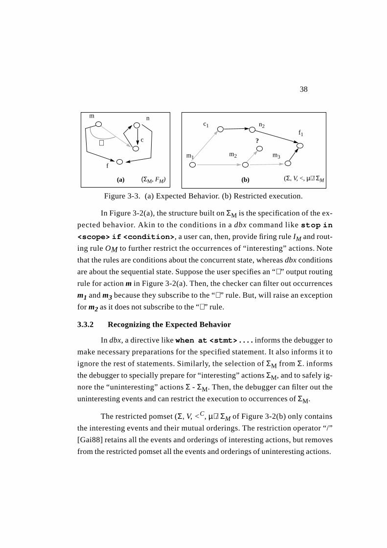
38

In Figure 3-2(a), the structure built onΣM is the specification of the ex-

pected behavior. Akin to the conditions in adbx command likestop in

<scope> if <condition>, a user can, then, provide firing ruleIM and rout-

ing ruleOM to further restrict the occurrences of “interesting” actions.Note

that the rules are conditions about the concurrent state, whereasdbx conditions

are about the sequential state. Suppose the user specifies an “∨” output routing

rule for actionm in Figure 3-2(a). Then, the checker can filter out occurrences

m1 andm3 because they subscribe to the “∨” rule. But, will raise an exception

for m2 as it does not subscribe to the “∨” rule.

3.3.2 Recognizing the Expected Behavior

In dbx, a directive likewhen at <stmt> . . . . informsthe debugger to

make necessary preparations for the specified statement. It also informs it to

ignore the rest of statements. Similarly, the selection ofΣM from Σ. informs

the debugger to specially prepare for “interesting” actionsΣM, and to safely ig-

nore the “uninteresting” actionsΣ - ΣM. Then, the debugger can filter out the

uninteresting events and can restrict the execution to occurrences ofΣM.

The restricted pomset (Σ, V, <C, µ)/ ΣM of Figure 3-2(b) only contains

the interesting events and their mutual orderings. The restriction operator “/”

[Gai88] retains all the events and orderings of interesting actions, but removes

from the restricted pomset all the events and orderings of uninteresting actions.

Figure3-3. (a) Expected Behavior. (b) Restricted execution.

c1 n2

m1m2

f1

n

c

m

f

m3

∨ ?

(ΣM, FM) (Σ, V, <, µ)/ ΣM(a) (b)

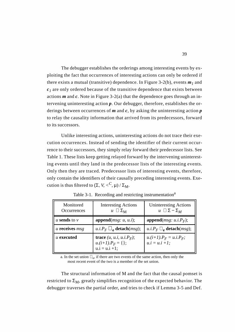
39

The debugger establishes the orderings among interesting events by ex-

ploiting the fact that occurrences of interesting actions can only be ordered if

there exists a mutual (transitive) dependence. In Figure 3-2(b), eventsm1 and

c1 are only ordered because of the transitive dependence that exists between

actionsm andc. Note in Figure 3-2(a) that the dependence goes through an in-

tervening uninteresting actionp. Our debugger, therefore, establishes the or-

derings between occurrences ofm andc, by asking the uninteresting actionp

to relay the causality information that arrived from its predecessors, forward

to its successors.

Unlike interesting actions, uninteresting actions do not trace their exe-

cution occurrences. Instead of sending the identifier of their current occur-

rence to their successors, they simply relay forward their predecessor lists. See

Table 1. These lists keep getting relayed forward by the intervening uninterest-

ing events until they land in the predecessor lists of the interesting events.

Only then they are traced. Predecessor lists of interesting events, therefore,

only contain the identifiers of their causally preceding interesting events. Exe-

cution is thus filtered to(Σ, V, <C, µ) / ΣM.

The structural information of M and the fact that the causal pomset is

restricted toΣM, greatly simplifies recognition of the expected behavior. The

debugger traverses the partial order, and tries to check if Lemma 3-5and Def.

a. In the set union∪e, if there are two events of the same action, then only themost recent event of the two is a member of the set union.

Table3-1. Recording and restricting instrumentationa

MonitoredOccurrences

Interesting Actionsu ∈ ΣM

Uninteresting Actionsu ∈ Σ − ΣM

u sends to v append(msg: u, u.i); append(msg: u.i.PF);

u receives msg u.i.PF ∪e detach(msg); u.i.PF ∪e detach(msg);

u executed trace (u, u.i, u.i.PF);u.(i+1).PF = {};u.i = u.i +1;

u.(i+1).PF = u.i.PF;u.i = u.i +1;

40

3-6 also hold for M. It checks whether each immediate successor vj of a given

event ui corresponds to some successor v of the action u in the dependences

FM. Additionally, the debugger checks whether the immediate predecessors

and successors of an event ui satisfy the input firing and output routing rules

IM and OM for u. If an ordering ui <F vj fails to correspond to some depen-

dence (u, v) ∈ FM, or the immediate predecessors •ui or successors ui• fail to

meet the expected conditions IM(u) or OM(u), then an error has been recog-

nized. This happens for the unexpected orderings of m2 in Figure 3-2(b).

Def. 3-9 Event ui is in error if ui• ∉OM(u) ∨ •ui ∉ IM(u).

Thus, concurrent debugging is the process of following the unexpected order-ings given by the erroneous events, in the direction of causality.

41

3.4 Shared Data Dependences

Unlike data-flow dependencesF that force an ordering on the execu-

tion of actions, shared data dependences do not impose any particular order-

ings. A shared data object is therefore modeled by the set of actions that share

the object. The set of those objects is denoted by S.

Def. 3-10 The set of shared data dependences is S⊆ 2Σ. A shared data

dependence is a setD of computation actions, D ⊆ Σ (or D ∈ S).

The actions that participate in a shared data dependenceD are classi-

fied into disjoint sets ofreaders andwriters.

Notation3-7 Readers of D are denoted byRD andwriters are denoted by

WD; where RD ∪ WD ≡ D, RD ∩ WD ≡ φ.

For example, in Fig.3-4(a), shared data dependenceD = {a, r, w} is

shown by the hyper-edge connecting actionsa, r andw. The set ofreaders, RD

= {r} and set of writers,WD = {a, w}.

The order of accesses to shared objects is recorded with the same mech-

anism that was used in recording the<Forderings (Section3.2.1). This, how-

ever, requires a protocol for ensuring a valid serialization on the accesses to

shared objects like the CREW (concurrent read exclusive write) protocol

[LM86] . Note that membersu andv of a shared data dependence have a valid

serialization if for every occurrenceui of a write-access and every occurrence

vj of another access, eitherui occurs beforevj, or vj occurs beforeui. The pro-

tocol, therefore, disallows simultaneous write-access to a shared object with

other accesses. The unified debugger ensures a deterministic replay by imple-

menting the protocol as in[LM86] . Without the implementation, simultaneous

accesses to a shared object can hinder a deterministic replay by corrupting the

object and giving unpredictable results. Moreover, as explained later, the pro-

tocol is also helpful in detecting race conditions.

Unlike [LM86] that uses versions of shared objects to record the order-

ings, we use a simpler mechanism for recording the order <D of accesses to a

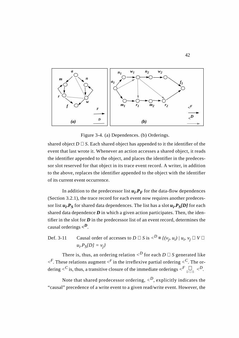
42

shared objectD ∈ S. Each shared object has appended to it the identifier of the

event that last wrote it. Whenever an action accesses a shared object, it reads

the identifier appended to the object, and places the identifier in the predeces-

sor slot reserved for that object in its trace event record. A writer, in addition

to the above, replaces the identifier appended to the object with the identifier

of its current event occurrence.

In addition to the predecessor listui.PF for the data-flow dependences

(Section3.2.1), the trace record for each event now requires another predeces-

sor listui.PS for shared data dependences. The list has a slotui.PS[D] for each

shared data dependenceD in which a given action participates. Then, the iden-

tif ier in the slot forD in the predecessor list of an event record, determines the

causal orderings<D.

Def. 3-11 Causal order of accesses to D ∈ S is <D ≡ {(vj, ui) | ui, vj ∈ V ∧ui.PS[D] = vj}

There is, thus, an ordering relation<D for eachD ∈ S generated like

<F. These relations augment <F in the irreflexive partial ordering<C. The or-

dering<C is, thus, a transitive closure of the immediate orderings<F <D.

Note that shared predecessor ordering,<D, explicitly indicates the

“causal” precedence of a write event to a given read/write event. However, the

Figure3-4. (a) Dependences. (b) Orderings.

n

wr

m

a

f

a1

n1w1 n2

m1 r1 m2 r2

f1

w2

(a) (b)

<F

<D

F

D

D S∈∪

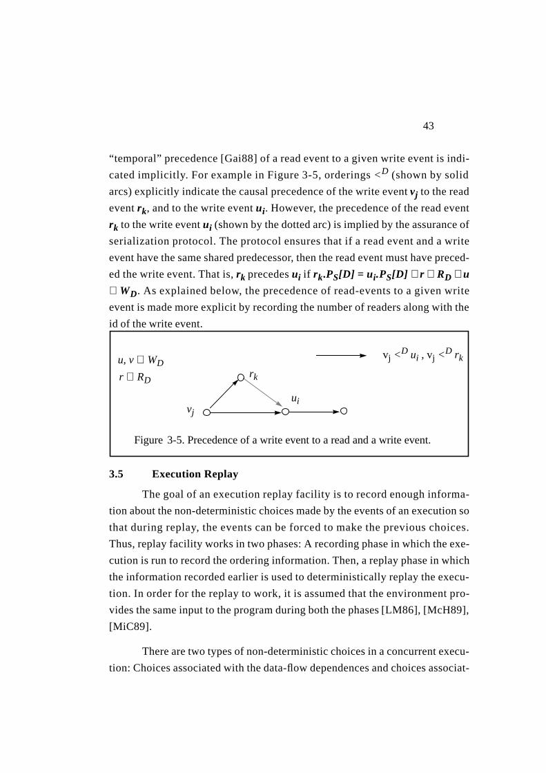
43

“temporal” precedence [Gai88] of a read event to a given write event is indi-

cated implicitly. For example in Figure 3-5, orderings<D (shown by solid

arcs) explicitly indicate the causal precedence of the write eventvj to the read

eventrk, and to the write eventui. However, the precedence of the read event

rk to the write eventui (shown by the dotted arc) is implied by the assurance of

serialization protocol. The protocol ensures that if a read event and a write

event have the same shared predecessor, then the read event must have preced-

ed the write event. That is,rk precedesui if rk.PS[D] = ui.PS[D] ∧ r ∈ RD ∧ u

∈ WD. As explained below, the precedence of read-events to a given write

event is made more explicit by recording the number of readers along with the

id of the write event.

3.5 Execution Replay

The goal of an execution replay facility is to record enough informa-

tion about the non-deterministic choices made by the events of an execution so

that during replay, the events can be forced to make the previous choices.

Thus, replay facility works in two phases: A recording phase in which the exe-

cution is run to record the ordering information. Then, a replay phase in which

the information recorded earlier is used to deterministically replay the execu-

tion. In order for the replay to work, it is assumed that the environment pro-

vides the same input to the program during both the phases[LM86] , [McH89],

[MiC89].

There are two types of non-deterministic choices in a concurrent execu-

tion: Choices associated with the data-flow dependences and choices associat-

uivj

rk

u, v ∈ WDvj <D ui , vj <D rk

r ∈ RD

Figure 3-5. Precedence of a write event to a read and a write event.

44

ed with the shared data dependences. The unified model separately deals with

the choices associated with each type of dependence.

A record of causal orderings <F is sufficient to overcome the non-deter-

minism associated with the choices of elements in a firing rule. During the

checking of the input firing rules, the replay mechanism not only checks if the

state of an input dependence is not empty (Section 3.1.2), but also ensures that

the event id appended to the value obtained from the dependence is from the

same event that fired the earlier execution. Thus, during the i-th execution of

u, a firing rule ι ∈ Ι(u) is only satisfied if ∀ (x, u) ∈ ι :: [x,u] ≠ ε ∧ appende-

d_id ∈ ui.PF, where appended_id is the id appended to the value on the given

dependence.

The other source of non-determinism is associated with shared data de-

pendences. These dependences do not force the actions to execute in any par-

ticular order. The debugger, therefore, records the non-deterministic order of

accesses to shared objects so that during the replay phase, the accesses can be

forced to occur in the previously recorded order. The replay mechanism en-

sures that (i) the write access that preceded a given access during the recording

phase must also precede during the replay phase, and (ii) all the readers that

preceded a given write event in the recording phase must also precede during

the replay phase. For this purpose, the recording instrumentation maintains a

count of readers in addition to the id of the last write event with each shared

object. The debugging information appended to each shared object D ∈ S is,

then, a tuple (ω.D, η.D):

Notation 3-8 ω.D is the id of the computation event that last wrote D.

Notation 3-9 η.D is the current count of the computation events that have

read D after it was written by ω.D.

In the recording phase, the replay instrumentation performs the actions

shown in Table 3-2 during each execution of a computation action u ∈ D. If u

is a reader, the instrumentation saves the id of the last write event in ui.PS[D],

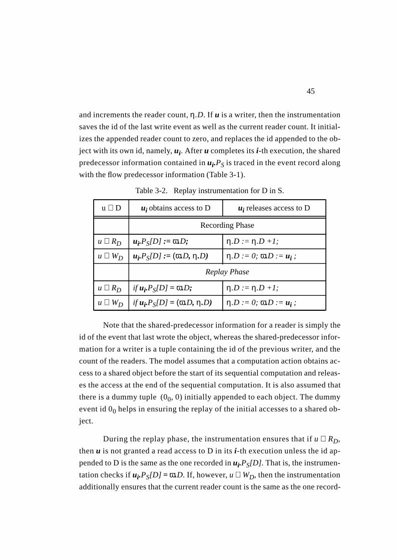
45

and increments the reader count, η.D. If u is a writer, then the instrumentation

saves the id of the last write event as well as the current reader count. It initial-

izes the appended reader count to zero, and replaces the id appended to the ob-

ject with its own id, namely, ui. After u completes itsi-th execution, the shared

predecessor information contained inui.PS is traced in the event record along

with the flow predecessor information (Table 3-1).

Note that the shared-predecessor information for a reader is simply the

id of the event that last wrote the object, whereas the shared-predecessor infor-

mation for a writer is a tuple containing the id of the previous writer, and the

count of the readers. The model assumes that a computation action obtains ac-

cess to a shared object before the start of its sequential computation and releas-

es the access at the end of the sequential computation. It is also assumed that

there is a dummy tuple (00, 0) initially appended to each object. The dummy

event id 00 helps in ensuring the replay of the initial accesses to a shared ob-

ject.

During the replay phase, the instrumentation ensures that ifu ∈ RD,

thenu is not granted a read access to D in itsi-th execution unless the id ap-

pended to D is the same as the one recorded inui.PS[D]. That is, the instrumen-

tation checksif ui.PS[D] = ω.D. If, however, u ∈ WD, then the instrumentation

additionally ensures that the current reader count is the same as the one record-

Table3-2. Replay instrumentation for Din S.

u ∈ D ui obtains access to D ui releases access to D

Recording Phase

u ∈ RD ui.PS[D] := ω.D; η.D := η.D +1;

u ∈ WD ui.PS[D] := (ω.D, η.D) η.D := 0; ω.D := ui ;

Replay Phase

u ∈ RD if ui.PS[D] = ω.D; η.D := η.D +1;

u ∈ WD if ui.PS[D] = (ω.D, η.D) η.D := 0; ω.D := ui ;

46

ed earlier. That is, the instrumentation does not grant access until the append-

ed id is the same as the recorded id, and the appended reader count is the same

as the recorded reader count contained inui.PS[D].

3.6 Race Detection

Simultaneous accesses (with at least one write) to a shared object can

race with each other and can corrupt the shared data with unpredictable re-

sults. Races are detected by identifying those pairs of events whose accesses

to a shared object included at least one write and whose accesses would have

been unordered in the absence of the debugger’s enforcement of the serializa-

tion protocol. For e.g., dotted arcs of Fig.3-4(b) show the <D orderings for

eventsw1 andr1 (andw1 andr2) that were forced by the debugger’s serializa-

tion protocol. The events are otherwise unordered under <F. Without the de-

bugger’s protocol, these <D orderings may not exist, thereby, causing a data-

race. Then,w1 andr1 (or w1, r2) can execute simultaneously with unpredict-

able results. Thus, all <D orderings observed under the serialization protocol,

should be supported by <F (i.e. should be causally ordered) as, for instance,

the ordering betweena1 andw1.

Notation3-10 ρ.D is the set of computation events that have read D after it

was written byω.D.

Table 3-2 describes the instrumentation needed for race detection. Note

that the instrumentation for race detection maintains the set of current readers,

ρ.D, whereas the replay instrumentation described in Table 3-2 simply main-

tained the count of readers,η.D. The orderings are, however, recorded similar-

ly: A reader only saves the id of the previous write event inui.PS[D], whereas

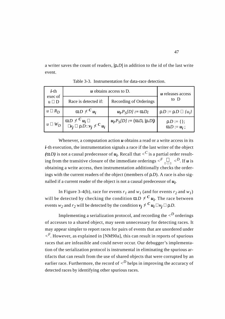
47

a writer saves the count of readers,|ρ.D| in addition to the id of the last write

event.

Whenever, a computation actionu obtains a read or a write access in its

i-th execution, the instrumentation signals a race if the last writer of the object

(ω.D) is not a causal predecessor ofui. Recall that<C is a partial order result-

ing from the transitive closure of the immediate orderings<F <D. If u is

obtaining a write access, then instrumentation additionally checks the order-

ings with the current readers of the object (members ofρ.D). A race is also sig-

nalled if a current reader of the object is not a causal predecessor ofui.

In Figure 3-4(b), race for eventsr1 andw1 (and for eventsr2 andw1)

will be detected by checking the conditionω.D C ui. The race between

eventsw2 andr2 will be detected by the conditionvjC ui ∧ vj ∈ ρ.D.

Implementing a serialization protocol, and recording the<D orderings

of accesses to a shared object, may seem unnecessary for detecting races. It

may appear simpler to report races for pairs of events that are unordered under

<F. However, as explained in[NM90a], this can result in reports of spurious

races that are infeasible and could never occur. Our debugger’s implementa-

tion of the serialization protocol is instrumental in eliminating the spurious ar-

tifacts that can result from the use of shared objects that were corrupted by an

earlier race. Furthermore, the record of<D helps in improving the accuracy of

detected races by identifying other spurious races.

Table3-3. Instrumentation for data-race detection.

i-thexec ofu ∈ D

u obtains access to D.u releases access

to DRace is detected if: Recording of Orderings

u ∈ RD ω.D C ui ui.PS[D] := ω.D; ρ.D := ρ.D ∪ {ui}

u ∈ WDω.D C ui ∨

∃vj ∈ ρ.D::vjC ui

ui.PS[D] := (ω.D, |ρ.D|) ρ.D := {};ω.D := ui ;

<

<<

D S∈∪

<

<

48

Vector clocks are often used to maintain a condensed representation of

the (transitive) causal history of events of an execution [Fid89], [Mat89],

[GaW92]. If events are timestamped with vector clocks, then checking of tran-

sitive relationship between any two given events can be done in unit time.

Note that race detection in our model requires the implementation of the dy-

namic vector clocks (Section 8.1.1). By associating such a vector clock with

each event, we can compute the transitive closure of <D and <F, and can detect

the races at runtime as explained in Section 8.3.5. Moreover, this can allow us

to further optimize the amount of recording done for replay purposes

(Section 8.3.6).

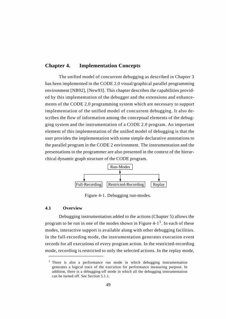
49

Chapter 4. Implementation Concepts

The unified model of concurrent debugging as described in Chapter 3

has been implemented in the CODE 2.0 visual/graphical parallel programming

environment [NB92], [New93]. This chapter describes the capabilities provid-

ed by this implementation of the debugger and the extensions and enhance-

ments of the CODE 2.0 programming system which are necessary to support

implementation of the unified model of concurrent debugging. It also de-

scribes the flow of information among the conceptual elements of the debug-

ging system and the instrumentation of a CODE 2.0 program. An important

element of this implementation of the unified model of debugging is that the

user provides the implementation with some simple declarative annotations to

the parallel program in the CODE 2 environment. The instrumentation and the

presentations to the programmer are also presented in the context of the hierar-

chical dynamic graph structure of the CODE program.

4.1 Overview

Debugging instrumentation added to the actions (Chapter 5) allows the

program to be run in one of the modes shown in Figure 4-11. In each of these

modes, interactive support is available along with other debugging facilities.

In the full-recording mode, the instrumentation generates execution event

records for all executions of every program action. In the restricted-recording

mode, recording is restricted to only the selected actions. In the replay mode,

1 There is also a performance run mode in which debugging instrumentationgenerates a logical trace of the execution for performance measuring purpose. Inaddition, there is a debugging-off mode in which all the debugging instrumentationcan be turned off. See Section 5.1.1.

Replay

Figure 4-1. Debugging run-modes.

Restricted-RecordingFull-Recording

Run-Modes

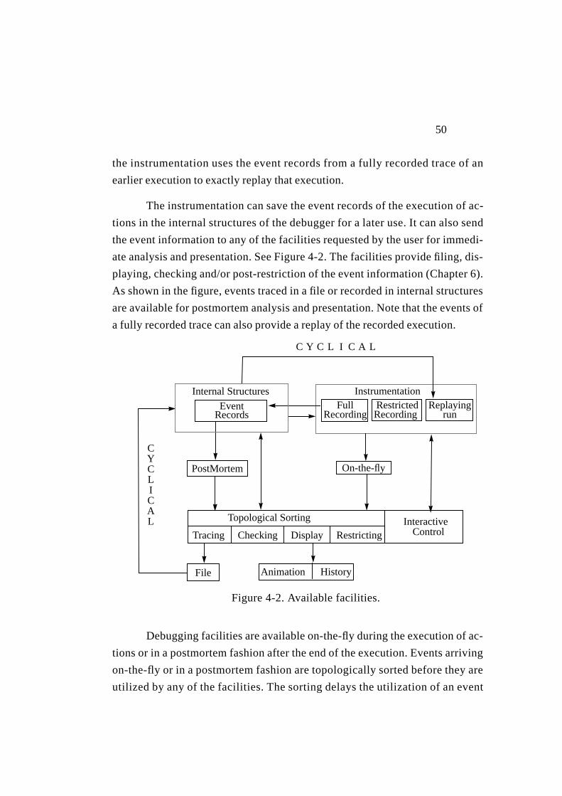
50

the instrumentation uses the event records from a fully recorded trace of an

earlier execution to exactly replay that execution.

The instrumentation can save the event records of the execution of ac-

tions in the internal structures of the debugger for a later use. It can also send

the event information to any of the facilities requested by the user for immedi-

ate analysis and presentation. See Figure 4-2. The facilities provide filing, dis-

playing, checking and/or post-restriction of the event information (Chapter 6).

As shown in the figure, events traced in a file or recorded in internal structures

are available for postmortem analysis and presentation. Note that the events of

a fully recorded trace can also provide a replay of the recorded execution.

Debugging facilities are available on-the-fly during the execution of ac-

tions or in a postmortem fashion after the end of the execution. Events arriving

on-the-fly or in a postmortem fashion are topologically sorted before they are

utilized by any of the facilities. The sorting delays the utilization of an event

On-the-flyPostMortem

Topological Sorting

Animation History

Figure4-2. Available facilities.

RestrictingChecking DisplayTracingInteractive

Control

Full Restricted ReplayingInstrumentation

runRecordingRecordingEvent

Records

CYCLICAL

C Y C L I C A L

File

Internal Structures

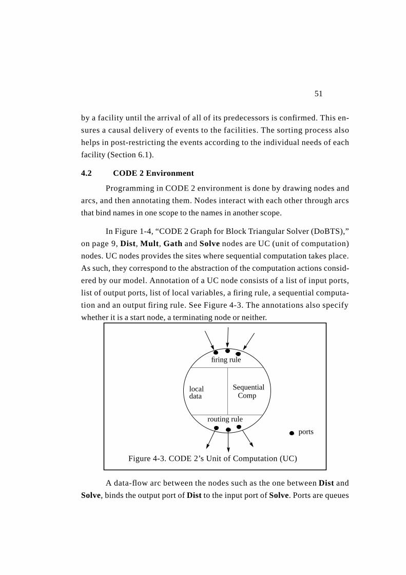
51

by a facility until the arrival of all of its predecessors is confirmed. This en-

sures a causal delivery of events to the facilities. The sorting process also

helps in post-restricting the events according to the individual needs of each

facility (Section6.1).

4.2 CODE 2 Environment

Programming in CODE 2 environment is done by drawing nodes and

arcs, and then annotating them. Nodes interact with each other through arcs

that bind names in one scope to the names in another scope.

In Figure1-4, “CODE 2 Graph for Block Triangular Solver (DoBTS),”

on page9, Dist, Mult, Gath andSolve nodes are UC (unit of computation)

nodes. UC nodes provides the sites where sequential computation takes place.

As such, they correspond to the abstraction of the computation actions consid-

ered by our model. Annotation of a UC node consists of a list of input ports,

list of output ports, list of local variables, a firing rule, a sequential computa-

tion and an output firing rule. See Figure 4-3. The annotations also specify

whether it is a start node, a terminating node or neither.

A data-flow arc between the nodes such as the one betweenDist and

Solve, binds the output port ofDist to the input port ofSolve. Ports are queues

Complocaldata

Sequential

firing rule

routing rule

ports

Figure4-3. CODE 2’s Unit of Computation (UC)

52

of data that leave or enter a node. Each node uses its own local names for the

ports so that nodes can be reused in different contexts.

A firing rule for a UC serves two purposes. It defines condition under

which the node is permitted to execute. Second, it describes which local vari-

ables would have data placed in them that has been removed from the designat-

ed input port. A routing rule for a UC determines the data that will be placed

on the output ports.

Figure 4-4 shows the main program graph for the block triangular solv-

er example explained in Section 1.2.1. Nodes rdsys and dobts in this graph

are call nodes. They call other graphs. For example, dobts calls the graph

DoBTS shown in Fig. 1-4. Thus, CODE programs can be hierarchical. Nodes

like creation parameter and interface nodes aid in this hierarchical composi-

tion. Creation parameters are visible to all the nodes within a given call graph.

Interface nodes of a call graph are like formal parameters to a function call.

They are thus aliases for the nodes within the call graph.

There are also name sharing nodes that contain the objects to be shared

by various UCs. A UC declares itself to be a reader or a writer of a shared ob-

ject of a name sharing node. The UC declares its intention to share with the

Figure 4-4. Block triangular solver main program graph.

53

node through a shared dependence arc. See [New93] for more information

about CODE 2 program graphs.

4.2.1 Templates and their Executable Instances

Nodes of a CODE 2 program graph are type templates. It is their in-

stances that exist and execute at run-time, and create other instances by send-

ing data to them. A policy of lazy creation of instances is employed. That is,

executable instances are not created until they are needed. For example, an in-

stance for a template like Solve in Figure 1-4 will not be created unless data is

sent to it. This happens when Dist puts data on its output port that is bound to

the input port of Solve.

A UC template may be instantiated one or more number of times. The

number of times it gets instantiated is determined dynamically at run-time.

This depends upon the binding on the output arc connected to a port specified

in the output rule. For example, the binding on the arc connecting templates

Dist and Mult in Fig. 1-4 specifies that the data placed on the output port

B_TO_M[i] of Dist goes to an input port of the instance Multi. Dist node can

now determine the number of Mult instances in existence by sending data on

appropriate indices of the output port B_TO_M. If it sends data on output port

B_TO_M[i] where i=1..N-1, the binding would cause the data to be received

by N-1 instances of Mult. Instances Mult1, Mult2, ..., MultN-1 would, then,

be created if they are not already instantiated.

Instances of a UC and call node templates exist in the CODE 2 run-

time environment as structs. The struct for a UC node instance contains its

template UID, and its index (see Figure 4-5). The UID is a unique identifier as-

signed to each template node by the CODE 2 front-end. The index helps in dif-

ferentiating one instance of a template from another in a given instance of the

call node template. Thus, the Mult instances considered above are differentiat-

ed by their indices. In addition, each instance contains the local state, the nest-

ing context (Section 4.4.2), and some other information needed by the run-

time environment. Action-specific debugging information needed by the in-

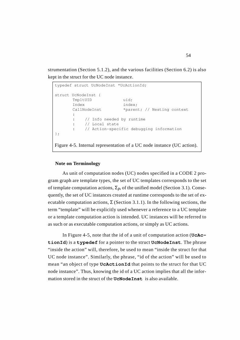
54

strumentation (Section5.1.2), and the various facilities (Section6.2) is also

kept in the struct for the UC node instance.

Note on Terminology

As unit of computation nodes (UC) nodes specified in a CODE 2 pro-

gram graph are template types, the set of UC templates corresponds to the set

of template computation actions,ΣP, of the unified model (Section3.1). Conse-

quently, the set of UC instances created at runtime corresponds to the set of ex-

ecutable computation actions,Σ (Section3.1.1). In the following sections, the

term “template” will be explicitly used whenever a reference to a UC template

or a template computation action is intended. UC instances will be referred to

as such or as executable computation actions, or simply as UC actions.

In Figure 4-5, note that the id of a unit of computation action (UcAc-

tionId) is atypedef for a pointer to the structUcNodeInst. The phrase

“inside the action” will, therefore, be used to mean “inside the struct for that

UC node instance”. Similarly, the phrase, “id of the action” will be used to

mean “an object of typeUcActionId that points to the struct for that UC

node instance”. Thus, knowing the id of a UC action implies that all the infor-

mation stored in the struct of theUcNodeInst is also available.

typedef struct UcNodeInst *UcActionId;

struct UcNodeInst {TmpltUID uid;Index index;CallNodeInst *parent; // Nesting context:: // Info needed by runtime: // Local state: // Action-specific debugging information

};

Figure4-5. Internal representation of a UC node instance (UC action).

55

4.2.2 UC Execution Event

An event for the CODE 2 implementation of the unified concurrent de-

bugger is an execution occurrence of a unit of computation or UC action. A

UC action starts executing by checking the firing rules. See Figure4-6. If the

condition of a rule evaluates to “true”, data is removed from the input ports

specified in the rule, and the data values are bound to the local variables. The

UC action, then, tries to acquire read and write locks for any shared objects

which it has declared that it wants to access. On success, the action performs

the specified sequential computation. It then selects a satisfied routing rule,

and sends out data on the output ports specified by the rule. This completes

one execution (event) of the action, and modifies the state of input ports of

those actions to which data was sent. This also readies for execution the ac-

tions to which data was sent.Template routine

Figure4-6. Execution of a Template Instance.

Firing Rule 2:

• •

••

• •

Firing Rulei:

Remove inportp

Check inportpFiring Rule 1:

Get R/W Lock1

Get R/W Lock2

• •

•

Sequential

Computation

Routing Rule1

Routing Rule2

• •

•

Routing Rule k:

Send outports

• •

•

Send outportt

Remove inportq

Check inportq

• •

•

56

4.2.3 CODE 2 Runtime System

The CODE 2 runtime system implements the execution of a UC action

by a routine that is generated by the translator for each UC template. The tem-

plate routine takes as an argument the id of the action whose execution it is go-

ing to implement. The id allows the routine to access the local state and

nesting context of the UC action. Note that at the time of its creation, each ac-

tion is provided with a pointer to the template routine that implements its exe-

cution.

The CODE 2 execution environment for Sequent shared memory ma-

chine consists of a ready queue, a number of worker tasks, and the template

routines that implement actions [New93]. The ready queue contains ids of the

actions that have received new data on their input ports. The worker tasks are

light-weight FastThread threads. Each worker loops around looking for a UC

action to run from the ready queue. On finding one, it executes the action by

running its corresponding template routine. The execution of the action

would, in turn, ready for execution the actions to which the data is sent.

CODE 2 is a retargetable, machine independent parallel programming

environment [New93]. In addition to the parallel implementation of the runt-

ime system on the Sequent shared memory machine, there is a serial and a dis-

tributed implementation. The serial implementation of the runtime system is

on a Sun-4 workstation and is quite similar to the parallel Sequent implementa-

tion. The only difference is that the serial implementation employs only one

worker task and no synchronizations. The distributed implementation of the

CODE 2 runtime system is on a network of workstations using PVM message

passing primitives [Vok94].

The description of the unified debugger given below is for the parallel

Sequent implementation. The serial implementation of the debugger is very

similar. Distributed implementation of the unified debugger is discussed in

Section 8.3.2.

57

4.3 Debugging Environment

Figure 4-7 shows the debugging environment for the Sequent shared

memory parallel machine. As mentioned above, worker tasks execute the UC

actions by running their corresponding template routines. Instrumentation add-

ed to these routines provides debugging support for replaying, recording and

restricting traces (Chapter 5). The instrumentation sends an on-the-fly stream

of information about the execution of these actions to the debugger on the

NewsQ. The worker tasks and the debugger task can, therefore, run asynchro-

nously. The debugger task is then free to interact with the user, respond to the

execution information, provide display and other facilities, and maintain de-

bugging information (Chapter 6).

Information about the symbols and templates of the program, actions,

and event occurrences are maintained in various internal s t ructures

ReadyQ

User

StopQ

Worker tasks

structInstance

Figure 4-7. Debugging Environment

Template Routines with

recordsEvent

SymTabProgram

Debugger Task

NewsQ

Instrumentation

InteractiveControl

Sorting

internalstructures

File Restrict Display Check

58

(Section 4.4). These structures allow the debugger to map between the tem-

plates, actions, and events (Section 4.5).

4.3.1 News from the Instrumentation

Instrumentation inserted in the template routines sends news about the

execution of UC actions to the debugger task. The news are about the event oc-

currences, state changes and encountering of breakpoints.

News About the Event Occurrences

After each execution of a selected action, the instrumentation sends a

news item to the debugger task containing the event record that was generated

or used during the execution. Note that during the recording mode, the instru-

mentation generates a new event record for each execution of a selected ac-

tion. These records are later used during the replay mode to re-execute the

action.

The information contained in these records is utilized by the facilities

for model checking, display, filing or for further restriction of the trace. So, the

records are sent to the debugger task only if the user has requested one or more

facilities.

News about the Stopped/Running State of an Action

The instrumentation can change the execution state of an action when

it stops the action by enqueuing it in the StopQ. The state also changes when

the instrumentation resumes the execution of the action from wherever it was

stopped. The news about the change in the state is sent to the debugger task.

The debugger task then forwards the news to the user. The user can, then, em-

ploy the interactive facility for querying the state of the stopped action (Chap-

ter 7). The interactive facility can later be employed for continuing the

execution of the action. This is done by enqueuing the id of the action in the

ReadyQ.

59

News about the Encountering of Breakpoints

A user can set various kinds of breakpoints for an action (Section 7.2).

Depending upon their type, the breakpoints are conditionally or unconditional-

ly evaluated at selected points during the execution of the action. The instru-

mentation sends news about the results of these evaluations to the debugger

task.

4.3.2 The Debugger Task

The debugger task continuously loops around looking for the input

from the user, and for the execution information coming from the instrumenta-

tion on the NewsQ. See Figure 4-8.

On recognizing some input from the user, the debugger interprets the

command. If the command is executable, it is immediately executed. Other-

wise, it is handed over to one of the facilities for translation. The facility, then,

sets breakpoints for the specified action(s) where the translated command will

be evaluated. The user-breakpoint (Section 7.2), checker-breakpoint

Get Input

SortGet Event News

Interpret

Execute Cmd

Translate Cmd

Chkr Bpt

Disp Bpt

User Bpt

Save Record

Display

File

Check

Post-Restrict

Figure 4-8. The Debugger Task.

60

(Section6.5.4), and the display-breakpoint (Section6.4) are respectively set

by the interactive, checking and display facilities.

Any execution information that is seen by the debugger task on the

NewsQ is handed over to the sorting facility. The sorting delays each event un-

til its causal arrival is confirmed. Once an event gets sorted, post restriction

takes place (Section6.1). The sorted event is then given to the facilities select-

ed for displaying, checking and/or filing. The checker facility, if selected, eval-

uates the translated commands associated with the checker breakpoints and

signals any exceptions (Section6.5). Similarly, the display facility, if selected,

presents the event information as specified by the user (Section6.4). If ar-

chiving of the event trace is requested, then the event is filed in the specified

format. Once the facilities have utilized the information in the record of the

sorted event, the record is deleted if saving of the event trace has not been re-

quested by the user (Section6.3.2). Note that the user can request to have the

trace of event records internally saved for a later replay and/or postmortem uti-

lization.

4.3.3 Communicating with the Instrumentation

The debugger task provides the instrumentation with information

(Section5.1) that allows it to properly execute the actions in the selected

mode. This includes:

1. Global information that applies to the execution of all the actions.

This is distributed by means of shared variables.

2. Action-specific information that may be different for different actions.

This is stored inside the selected actions. The instrumentation obtains

access to this information when the template routine provides it with the ac-

tion id.

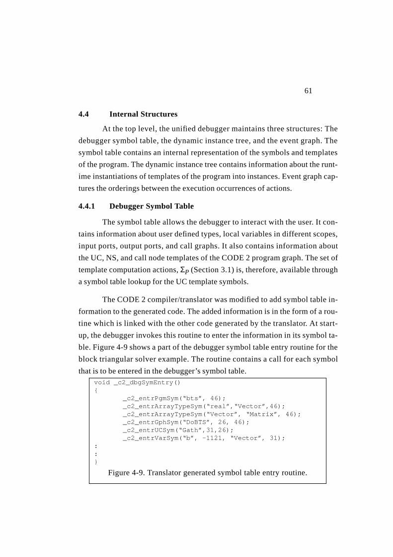
61

4.4 Internal Structures

At the top level, the unified debugger maintains three structures: The

debugger symbol table, the dynamic instance tree, and the event graph. The

symbol table contains an internal representation of the symbols and templates

of the program. The dynamic instance tree contains information about the runt-

ime instantiations of templates of the program into instances. Event graph cap-

tures the orderings between the execution occurrences of actions.

4.4.1 Debugger Symbol Table

The symbol table allows the debugger to interact with the user. It con-

tains information about user defined types, local variables in different scopes,

input ports, output ports, and call graphs. It also contains information about

the UC, NS, and call node templates of the CODE 2 program graph. The set of

template computation actions,ΣP (Section3.1) is, therefore, available through

a symbol table lookup for the UC template symbols.

The CODE 2 compiler/translator was modified to add symbol table in-

formation to the generated code. The added information is in the form of a rou-

tine which is linked with the other code generated by the translator. At start-

up, the debugger invokes this routine to enter the information in its symbol ta-

ble. Figure 4-9 shows a part of the debugger symbol table entry routine for the

block triangular solver example. The routine contains a call for each symbol

that is to be entered in the debugger’s symbol table.void _c2_dbgSymEntry(){

_c2_entrPgmSym(“bts”, 46);_c2_entrArrayTypeSym(“real”,“Vector”,46);_c2_entrArrayTypeSym(“Vector”, “Matrix”, 46);_c2_entrGphSym(“DoBTS”, 26, 46);_c2_entrUCSym(“Gath”,31,26);_c2_entrVarSym(“b”, -1121, “Vector”, 31);

::}

Figure4-9. Translator generated symbol table entry routine.

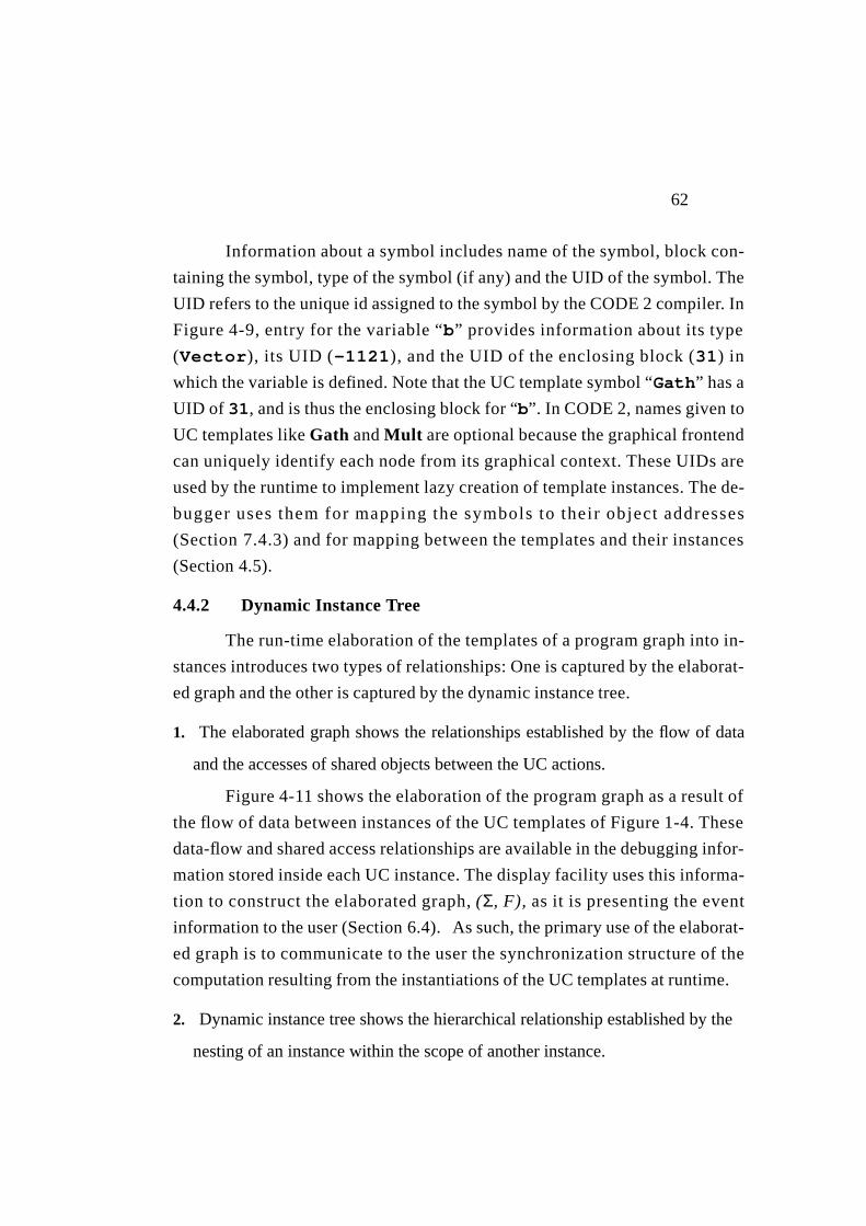
62

Information about a symbol includes name of the symbol, block con-

taining the symbol, type of the symbol (if any) and the UID of the symbol. The

UID refers to the unique id assigned to the symbol by the CODE 2 compiler. In

Figure 4-9, entry for the variable “b” provides information about its type

(Vector), its UID (-1121), and the UID of the enclosing block (31) in

which the variable is defined. Note that the UC template symbol “Gath” has a

UID of 31, and is thus the enclosing block for “b”. In CODE 2, names given to

UC templates likeGath andMult are optional because the graphical frontend

can uniquely identify each node from its graphical context. These UIDs are

used by the runtime to implement lazy creation of template instances. The de-

bugger uses them for mapping the symbols to their object addresses

(Section7.4.3) and for mapping between the templates and their instances

(Section4.5).

4.4.2 Dynamic Instance Tree

The run-time elaboration of the templates of a program graph into in-

stances introduces two types of relationships: One is captured by the elaborat-

ed graph and the other is captured by the dynamic instance tree.

1. The elaborated graph shows the relationships established by the flow of data

and the accesses of shared objects between the UC actions.

Figure 4-11 shows the elaboration of the program graph as a result of

the flow of data between instances of the UC templates of Figure 1-4. These

data-flow and shared access relationships are available in the debugging infor-

mation stored inside each UC instance. The display facility uses this informa-

tion to construct the elaborated graph,(Σ, F), as it is presenting the event

information to the user (Section6.4). As such, the primary use of the elaborat-

ed graph is to communicate to the user the synchronization structure of the

computation resulting from the instantiations of the UC templates at runtime.

2. Dynamic instance tree shows the hierarchical relationship established by the

nesting of an instance within the scope of another instance.

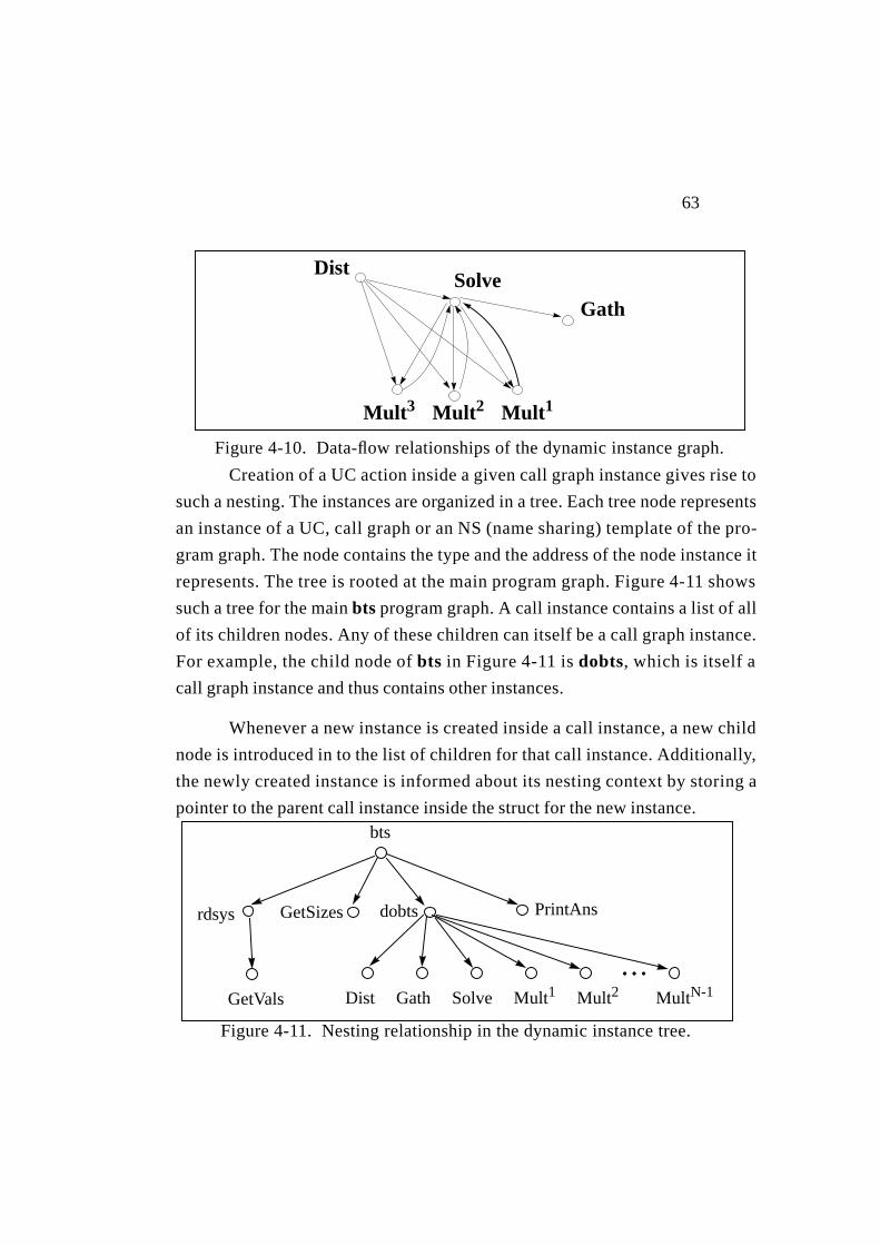
63

Creation of a UC action inside a given call graph instance gives rise to

such a nesting. The instances are organized in a tree. Each tree node represents

an instance of a UC, call graph or an NS (name sharing) template of the pro-

gram graph. The node contains the type and the address of the node instance it

represents. The tree is rooted at the main program graph. Figure 4-11 shows

such a tree for the mainbts program graph. A call instance contains a list of all

of its children nodes. Any of these children can itself be a call graph instance.

For example, the child node ofbts in Figure 4-11 is dobts, which is itself a

call graph instance and thus contains other instances.

Whenever a new instance is created inside a call instance, a new child

node is introduced in to the list of children for that call instance. Additionally,

the newly created instance is informed about its nesting context by storing a

pointer to the parent call instance inside the struct for the new instance.

Solve

Mult1Mult2Mult3

Dist

Gath

Figure4-10. Data-flow relationships of the dynamic instance graph.

bts

GetSizes dobtsrdsys PrintAns

GathDist Mult1Solve Mult2 MultN-1• • •

Figure4-11. Nesting relationship in the dynamic instance tree.

GetVals

64

As the execution proceeds, the newly created instances keep getting

added to the dynamic instance tree. The tree therefore contains the current in-

formation about all the dynamically created instances. It is, therefore, also of

use to the run-time for managing the creation of instances. To avoid duplica-

tion, our implementation uses the tree maintained by the runtime. It obtains a

handle to the graph by storing the identity of the root of the instance tree. Note

that the instance of the root program graph is created by the runtime system at

start-up.

The dynamic instance tree is mainly used by the debugger for organiz-

ing and maintaining the internal debugging information. The root of the tree

serves as a representation for the scope of the program. The debugger uses the

handle to the root of the dynamic instance tree in implementing functionality

that requires iterating on all the instances. For example, determining the mem-

bership of the set of executable computation actions,Σ (Section3.1), selecting

a particular scope (Section4.5.1), determining the effective recording option

of all the instances (Section5.3.1), preparing all the instances for a new run

(Section7.1.3) requires such iteration.

4.4.3 Event Records and Event Graph

An event is an execution occurrence of a UC action. It is therefore iden-

tif ied by the id of the action (a pointer to the struct of its UC node instance)

and its execution count. The event record of the execution of a UC action con-

tains information about the ids of the predecessor events and the counts of the

successor events. See Figure 4-12. Note that the id of the action in the event

record (and the event id) maps the event to its corresponding action and, thus,

supports the mappingµ: V → Σ needed by the unified model (Section3.2.2).

The list of flow-predecessors contains ids of the events whose data was

removed by the action from its input ports. The list of shared predecessors con-

tains ids of the events that last wrote the objects that were shared accessed by

the action in this execution. These lists are the implementations of the sets

ui.PF (Section3.2), andui.PS (Section3.4) for an eventui in V.

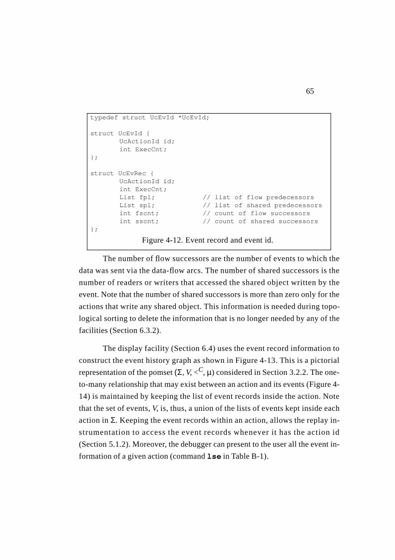
65

The number of flow successors are the number of events to which the

data was sent via the data-flow arcs. The number of shared successors is the

number of readers or writers that accessed the shared object written by the

event. Note that the number of shared successors is more than zero only for the

actions that write any shared object. This information is needed during topo-

logical sorting to delete the information that is no longer needed by any of the

facilities (Section 6.3.2).

The display facility (Section 6.4) uses the event record information to

construct the event history graph as shown in Figure 4-13. This is a pictorial

representation of the pomset (Σ, V, <C, µ) considered in Section 3.2.2. The one-

to-many relationship that may exist between an action and its events (Figure 4-

14) is maintained by keeping the list of event records inside the action. Note

that the set of events, V, is, thus, a union of the lists of events kept inside each

action in Σ. Keeping the event records within an action, allows the replay in-

strumentation to access the event records whenever it has the action id

(Section 5.1.2). Moreover, the debugger can present to the user all the event in-

formation of a given action (command lse in Table B-1).

typedef struct UcEvId *UcEvId;

struct UcEvId {UcActionId id;int ExecCnt;

};

struct UcEvRec {UcActionId id;int ExecCnt;List fpl; // list of flow predecessorsList spl; // list of shared predecessorsint fscnt; // count of flow successorsint sscnt; // count of shared successors

};

Figure 4-12. Event record and event id.

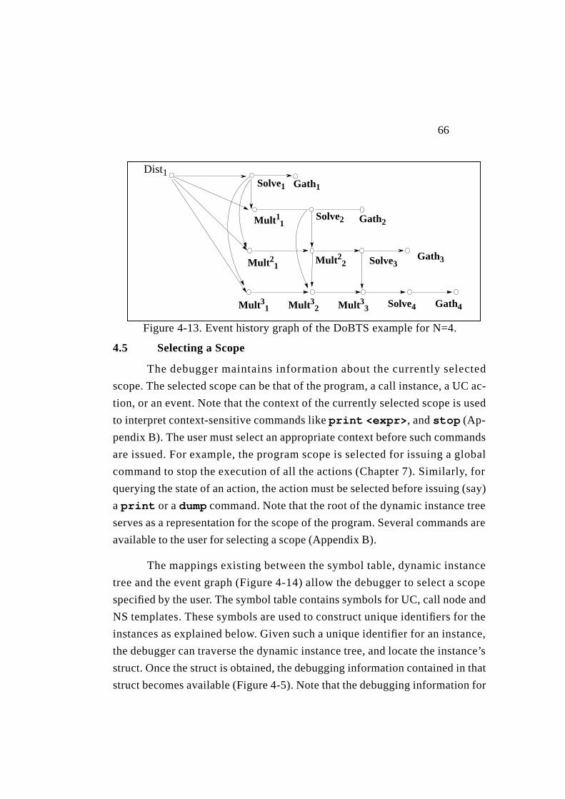
66

4.5 Selecting a Scope

The debugger maintains information about the currently selected

scope. The selected scope can be that of the program, a call instance, a UC ac-

tion, or an event. Note that the context of the currently selected scope is used

to interpret context-sensitive commands likeprint <expr>, andstop (Ap-

pendix B). The user must select an appropriate context before such commands

are issued. For example, the program scope is selected for issuing a global

command to stop the execution of all the actions (Chapter 7). Similarly, for

querying the state of an action, the action must be selected before issuing (say)

aprint or adump command. Note that the root of the dynamic instance tree

serves as a representation for the scope of the program. Several commands are

available to the user for selecting a scope (Appendix B).

The mappings existing between the symbol table, dynamic instance

tree and the event graph (Figure 4-14) allow the debugger to select a scope

specified by the user. The symbol table contains symbols for UC, call node and

NS templates. These symbols are used to construct unique identifiers for the

instances as explained below. Given such a unique identifier for an instance,

the debugger can traverse the dynamic instance tree, and locate the instance’s

struct. Once the struct is obtained, the debugging information contained in that

struct becomes available (Figure 4-5). Note that the debugging information for

Solve3

Solve2

Solve4

Mult11

Mult21

Solve1

Dist1

Gath3

Gath2

Gath4

Gath1

Mult31 Mult3

2 Mult33

Mult22

Figure4-13. Event history graph of the DoBTS example for N=4.

67

a UC action contains the list of its events (Section 5.1.2). If an event of the ac-

tion is to be located, then this list is searched for the given execution count to

obtain the desired event record.

Unique Identification of Instances

It is possible to have several instances of the same template with the

same index in various call graph instances. Unique identification of an in-

stance, therefore, requires the nesting context of the instance in addition to its

template id and the index. Consider for example, that an instance of the main

program graph contains two instances of DoBTS call graph; dobts1 and

dobts2. If both contain a UC action Mult 3, then the two Mult 3 actions in

dobts1 and dobts2 would have the same template UID and the same index (i.e.

3). The only way of distinguishing between the two actions is their nesting

context. This involves giving each instance a path-name similar to the one

Unix assigns to a file in a directory. Then, the two UC actions are uniquely

identified by /dobts1/Mult 3 and /dobts2/Mult 3. Therefore, commands that re-

fer to UC, call graph and NS instances require the full pathname (Appendix B).

4.5.1 Selecting an Instance with a given Pathname

Searching for an instance with the given pathname is recursive and

starts at the root of the dynamic instance tree. The search for (say) /dobts2/-

Mult 3, starts with the lookup for the name dobts in the symbol table. This

Symbol Table Dynamic Instance Tree Event Graph

Mult

Mult 3

Mult 2

Mult 1

Mult 22

Mult 21

Figure 4-14. Mappings between templates, actions, and events.

Templates Actions Events

68

yields the corresponding symbol which provides the UID of the dobts tem-

plate. The search then examines each child of the root for an instance with

UID of dobts and index of 2. As each instance contains the UID of its corre-

sponding template and its index, the search would eventually locate the in-

stance dobts2, if it exists. As dobts is an instance of a call graph, and the path

name still has an extension (Mult3), the search continues by descending inside

the dobts2 call instance and examining its children. The lookup for Mult in

the symbol table yields its UID. The index 3 is given in the pathname. So, the

search examines the children of dobts2 for an instance with the UID and index

of Mult. If the search fails at any of these steps, the search exits with the error

status. The search succeeds if all the instances given in the pathname have

been located in their proper context.

4.5.2 Constructing the Pathname for an Instance

Given the UC action id, the full pathname of an instance can be con-

structed. The struct for each instance contains its UID, its instance index and

its nesting context. Using the UID, the symbol table lookup yields the symbol

for the corresponding template. As UID is unique for a template, there is no

ambiguity. The nesting context of an instance is available as a pointer to the

parent call instance (Figure 4-5). The UID in the parent instance struct allows

us to obtain the symbol for the parent graph. The symbols for each of the par-

ent along the path is, thus, obtained recursively. The recursion ends at the root

graph instance which does not have a parent (indicated by a nil pointer).

69

Chapter 5. Debugging Instrumentation

Debugging instrumentation is inserted in the executable code generat-

ed by the CODE 2.0 translator to relieve the debugger task from micro-manag-

ing the execution of UC actions. This obviates the need for intrusion from a

“centralized” monitor/debugger as the instrumentation takes over the responsi-

bility for recording the execution information, controlling what is recorded,

and controlling the execution itself. The debugger task, then, uses the informa-

tion generated by the instrumentation to implement the facilities provided to

the user. The instrumentation is in the form of calls to a library of runtime rou-

tines that perform various action-specific debugging activities. The calls are

inserted at different points in a template routine where they can record, replay,

restrict, and interactively control the execution of an action. See Table5-2. Be-

fore explaining these calls, this chapter explains the information needed by the

instrumentation to ensure the execution of actions in the proper debugging

mode.

5.1 Information Requirements

The debugger requires both global information and action specific in-

formation. Global information is provided through shared variables in the Se-

quent implementation. Action-specific information is provided by storing it

inside each action. The instrumentation obtains the action-specific informa-

tion when the instrumentation calls are invoked from the template routine with

the action id as a parameter. Recall that id of the action makes available the de-

bugging information inside the struct for that action.

5.1.1 Global Information

The information about the currently selected mode for running the pro-

gram is available inCurMode. See Table5-1. During the execution of each ac-

tion, CurMode selects appropriate instrumentation for the full-recording,

restricted recording and the replay mode. Commands fornext-ing andstop-

ping of actions provided by the interactive facility (Chapter 7) require coopera-

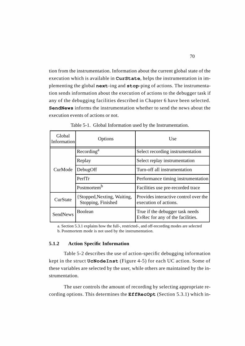
70

tion from the instrumentation. Information about the current global state of the

execution which is available in CurState, helps the instrumentation in im-

plementing the global next-ing and stop-ping of actions. The instrumenta-

tion sends information about the execution of actions to the debugger task if

any of the debugging facilities described in Chapter 6 have been selected.

SendNews informs the instrumentation whether to send the news about the

execution events of actions or not.

5.1.2 Action Specific Information

Table 5-2 describes the use of action-specific debugging information

kept in the struct UcNodeInst (Figure 4-5) for each UC action. Some of

these variables are selected by the user, while others are maintained by the in-

strumentation.

The user controls the amount of recording by selecting appropriate re-

cording options. This determines the EffRecOpt (Section 5.3.1) which in-

a. Section 5.3.1 explains how the full-, restricted-, and off-recording modes are selectedb. Postmortem mode is not used by the instrumentation.

Table 5-1. Global Information used by the Instrumentation.

GlobalInformation

Options Use

CurMode

Recordinga Select recording instrumentation

Replay Select replay instrumentation

DebugOff Turn-off all instrumentation

PerfTr Performance timing instrumentation

Postmortemb Facilities use pre-recorded trace

CurState{Stopped,Nexting, Waiting,

Stopping, FinishedProvides interactive control over theexecution of actions.

SendNewsBoolean True if the debugger task needs

EvRec for any of the facilities.

71

forms the instrumentation what information to record in the restricted

recording mode. The user may set a breakpoint, or issue a command to control

the execution of an action.UsrBpOn, UCCommand, andIsStopped inform

that portion of the instrumentation which implements the interactive facility

what actions to take. Instrumentation calls are inserted “at”various points in a

template routine (Table5-2). CurAt indicates the most recent instrumentation

call made by an action. This is helpful in resuming the execution of an action

from the point where it was stopped by the instrumentation.

The instrumentation maintains the current count of the number of times

an action has executed.ExecCount is updated after each execution of an ac-

tion.

Whenever an action begins a new execution,CurEvRec is made to

point to an appropriate record. During replay mode,CurEvRec points to the

event record whose information is being used to replay the current execution.

Table5-2. Action-specific information needed by the instrumentation.

Field Type Usage

ExecCount int Recording, replaying, checking

CurEvRec pointer toEvRec Recording, restricting, replaying

EvRecList list of EvRec Recording, replaying

CurFp pointer Replaying

SelRecOpt {full, restrict, off} DeterminesEffRecOpt

EffRecOpt {full, restrict, off} Recording, restricting

CurSp pointer Replaying

CurAt At (see Table5-2) Interactive

UCCommand {cont, next, stop} Interactive

IsStopped Boolean Interactive

UsrBpOn Boolean Interactive

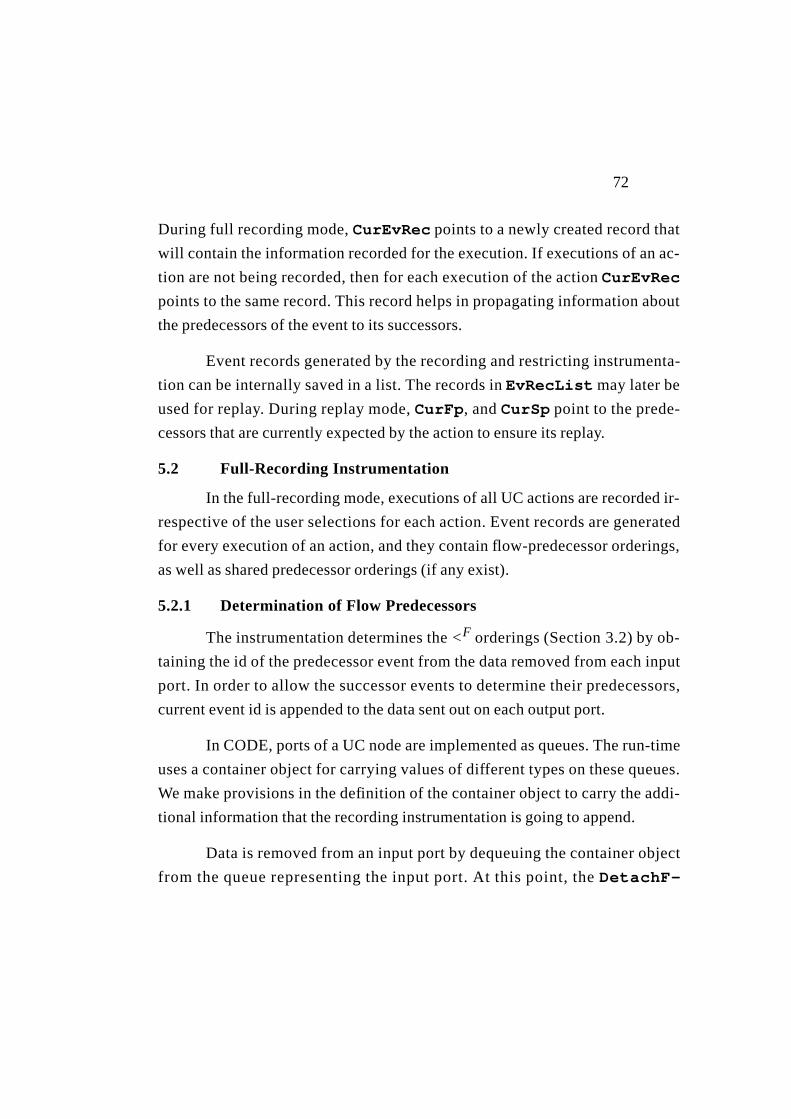
72

During full recording mode, CurEvRec points to a newly created record that

will contain the information recorded for the execution. If executions of an ac-

tion are not being recorded, then for each execution of the action CurEvRec

points to the same record. This record helps in propagating information about

the predecessors of the event to its successors.

Event records generated by the recording and restricting instrumenta-

tion can be internally saved in a list. The records in EvRecList may later be

used for replay. During replay mode, CurFp, and CurSp point to the prede-

cessors that are currently expected by the action to ensure its replay.

5.2 Full-Recording Instrumentation

In the full-recording mode, executions of all UC actions are recorded ir-

respective of the user selections for each action. Event records are generated

for every execution of an action, and they contain flow-predecessor orderings,

as well as shared predecessor orderings (if any exist).

5.2.1 Determination of Flow Predecessors

The instrumentation determines the <F orderings (Section 3.2) by ob-

taining the id of the predecessor event from the data removed from each input

port. In order to allow the successor events to determine their predecessors,

current event id is appended to the data sent out on each output port.

In CODE, ports of a UC node are implemented as queues. The run-time

uses a container object for carrying values of different types on these queues.

We make provisions in the definition of the container object to carry the addi-

tional information that the recording instrumentation is going to append.

Data is removed from an input port by dequeuing the container object

from the queue representing the input port. At this point, the DetachF-

73

pAct() routine detaches the predecessor information from the object and

adds it to the predecessor list in the current event record.

Sending of a value on an output port is more involved. The run-time

first locates the destination action using the binding specified for the output

port. It creates the action if it is not already in existence. Then, the value to be

sent is placed in a container object. At this point, AppendFpAct() appends

Table 5-3. Instrumentation inserted in a template routine.

InstrumentationBreakpoint

Actions

Point At whichinserted

See Figure 4-6.Usage Action

voidBeginEvAct()

Start of templateroutine

Recording, restrict-ing, replaying,interactive

Get CurEvRec for anew UC exec

voidEndEvAct()

End of templateroutine

Recording, restrict-ing, replaying

Send and/or saveCurEvRec info

voidDetachFpAct()

On removingfrom an input port

Recording, restrict-ing, interactive

Remove dbg. info.appended to data

voidAppendFpAct()

Before sending onan output port

Recording, restrict-ing, replaying,interactive

Append dbg. info. todata sent out

voidReadSpAct()

About to acquire aR/W lock

Recording, restrict-ing, replaying

Read appended info toshared object

voidWriteSpAct()

About to release awrite lock

Recording, restrict-ing, replaying

Write to info appendedto shared object

BooleanCheckFpAct()

Checking/ remov-ing from an inport

Replaying Check id appended toinput data

BooleanCheckSpAct()

About to acquire aR/W lock

Replaying Check id appended to ashared object

BooleanAftCompAct()

After sequentialcomputation

Interactive Evaluate any userbreakpoints here

BooleanBefCompAct()

Before sequentialcomputation

Interactive Evaluate any userbreakpoints here

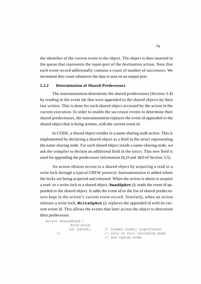
74

the identifier of the current event to the object. The object is then inserted in

the queue that represents the input-port of the destination action. Note that

each event record additionally contains a count of number of successors. We

increment this count whenever the data is sent on an output port.

5.2.2 Determination of Shared-Predecessors

The instrumentation determines the shared predecessors (Section3.4)

by reading in the event ids that were appended to the shared objects by their

last writers. This is done for each shared object accessed by the action in the

current execution. In order to enable the successor events to determine their

shared predecessors, the instrumentation replaces the event id appended to the

shared object that is being written, with the current event id.

In CODE, a shared object resides in a name sharing node action. This is

implemented by declaring a shared object as a field in the struct representing

the name sharing node. For each shared object inside a name-sharing node, we

ask the compiler to declare an additional field in the struct. This new field is

used for appending the predecessor information (η.D and ω.D of Section3.5).

An action obtains access to a shared object by acquiring a read or a

write lock through a typical CREW protocol. Instrumentation is added where

the locks are being acquired and released. When the action is about to acquire

a read- or a write-lock to a shared object,ReadSpAct() reads the event id ap-

pended to the shared object. It adds the event id to the list of shared predeces-

sors kept in the action’s current event record. Similarly, when an action

releases a write lock,WriteSpAct() replaces the appended id with its cur-

rent event id. This allows the events that later access the object to determine

their predecessor.struct SharedPred {

EvId evid;int rdrcnt; // reader count; significant

}; // only in full recording mode// and replay mode.

75

The predecessor information that is written to or read from the exten-

sion to to the shared object definition contains a reader-count in addition to the

event id. This is helpful during replay when a writer must wait until all the

readers of the object written by its predecessor have come and read the object

(see also Table 3-2).

In ReadSpAct(), an action acquiring access to an object reads the

event id appended to the object as explained above. In addition, however, if

the action is acquiring read-access, then it increments the reader-count. But, if

the action is acquiring a write-access, then it records the appended reader-

count. InWriteSpAct(), the action releasing the write-lock, appends its id

to the object, and initializes the reader-count to zero.

5.3 Restricting Instrumentation

In the restricted-recording mode, the user has several options to control

the amount of recorded information:

1. Option to turn off or on, the recording of events of selected actions.

2. Option to record flow predecessor orderings with the shared predecessor

orderings or without them.

3. Option to override the selected options for all actions in a given scope.

5.3.1 Determining the Effective Recording Option

The amount of recording is controlled by the “effective” recording op-

tion. EffRecOpt may be different from the option “selected” by the user.

SelRecOpt can be overridden by the parent scope’s option. Table 5-4 de-

scribes the possible recording actions for UC and call instances.

The effective recording option of an instance depends upon (i) the in-

stance’s selected option, and (ii) its parent’s effective option. The selected op-

76

tion is effective only if the parent’sEffRecOpt is Restrict. Otherwise,

the action’s effective option is the one inherited from its parent action. That is,

This rule is applied recursively to all the instances of the dynamic in-

stance tree starting from its root. The root’sEffRecOpt is always equal to

SelRecOpt. If a new option is selected for a call instance, then the rule is re-

cursively applied to all the instances inside the scope of that instance.

Thus, full recording mode of the execution is chosen by selecting a

Full option for the root of the dynamic instance tree, i.e. the program scope.

This overrides the selections of all internal instances and forces aFull effec-

tive option for all the instances of the tree. Similarly, the restricted recording

mode is chosen by selecting theRestrict option for the root. Similarly, the

off recording mode is chosen by selecting theOff option for the root that

turns off the recording of all the instances by overriding their selected record-

ing options.

Table5-4. Effective recording options for UC and call instances.

Instance Type

EffRecOpt Recording Action

UC

Full Record flow and shared predecessors.

Restrict Record only flow predecessors.

Off Do not generate any event records.

Call

Full Turn to full the recording of all internal instances.

Restrict Defer to individual selections for internal instances.

Off Turn off the recording of all internal instances.

if my parent’s EffRecOpt is Restrictthen

my EffRecOpt = my SelRecOpt;else /* Full or Off */

my EffRecOpt = my parent’s EffRecOpt

77

5.3.2 Turning Off the Recording of a UC Action

Each action has to maintain the list of its predecessors; even those ac-

tions not selected for full recording. The list of predecessors maintained by the

actions that were not selected for recording, helps in establishing orderings be-

tween event occurrences of the selected actions (Table 3-1). Instrumentation

for an action whose recording is turned off, forwards the list of the predecessor

events to the successor events.

This requires that the provision for appending to the data sent on the

queues should be capable of holding more than one event id; it must be a list of

event ids. A similar provision is needed in the extension to the definition of a

shared object. An event record is used for temporarily accumulating the prede-

cessors. It is pointed to by theCurEvRec. During each execution, the prede-

cessors are accumulated in this event record. By the end of the execution,

these predecessors have been forwarded to the successor events.

DetachFpAct(), andReadSpAct() are responsible for detachin-

g/reading a list of event ids, and then concatenating the list to the list of prede-

cessors kept in the current event record. Note that the list may contain one or

more event ids.

Forwarding of the flow-predecessors information is done inAppendF-

pAct() where a copy of the list of flow-predecessors is appended to the data

sent on the output port. Similarly, in WriteSpAct(), extension to the shared

object definition is replaced with a copy of the list of shared predecessors.

5.3.3 Restricting the Recording of a UC Action

With theRestrict recording option, instrumentation only records

flow-predecessors. It does not record shared predecessors. Therefore, it em-

ploys some of the instrumentation for thefull option recording, and some of

the instrumentation for theoff option.

78

A new event record is generated for each execution. In this event

record, DetachFpAct() and ReadSpAct() accumulate the flow and the

shared predecessors as described above. As the list of flow-predecessors so ac-

cumulated is to be retained, AppendFpAct() will only forward the current

event-id to its successors. However, the list of shared predecessors is not to be

retained. So, WriteSpAct() will forward the entire list of shared predeces-

sors to its successors as described above.

5.4 Replay Instrumentation

Replay instrumentation is responsible for enforcing that an action exe-

cutes with the same orderings that were recorded in an earlier execution

(Section 3.4). The record of orderings is available in the list of event records

kept with each action. If the action is starting its n-th execution, then Be-

ginEvAct() would fetch the event record whose execution count is n from

this list.

During the execution, the replay mechanism uses the recorded order-

ings for overcoming the two sources of non-determinism: One source of non-

determinism is associated with the data-flow orderings and appears as choices

in the firing rules of a UC. The other source of non-determinism is associated

with the choices of ordering with which concurrent actions could obtain ac-

cess to shared objects. Running the execution in replay mode, therefore, re-

quires that the event records contain both the list of flow-predecessors and the

list of shared-predecessors. This means that the available trace should have

been recorded at the full option.

At the end of the execution, EndEvAct() sends information to the de-

bugger task that it has successfully replayed the execution event.

5.4.1 Enforcing Previously Recorded Flow Orderings

It may appear that we can force an action to fire with the previously re-

corded orderings if we only ensure that the rule firing the current execution is

the same as the one that fired the previous execution. This could have been the

79

case if the input ports were not capable of receiving data from more than one

action. However in CODE 2, input ports can receive data from different ac-

tions. The data gets merged in the port queue in some nondeterministic order.

Then, simply ensuring that the same rule fires is not enough. We must ensure

that (i) the same rule fires, (ii) the data that was checked on a port, was from

the same predecessor, and (iii) the data that was removed from the port was

also from the same predecessor.

Consider for example firing rule i in Figure 4-6. There is a checking

phase in which ports p, q, ... specified by the rule are checked for data. This is

followed (if the checking is successful) by a removing phase in which data is

removed from each of the ports p, q, .... As mentioned above, ports are queues.

So, the queue for inport p may have data from different predecessors. The re-

play instrumentation must therefore search the entire queue looking for the

data from a particular predecessor. If data from the desired predecessor is

found, then the checking of a port is successful. The checking phase completes

successfully if each port contains data from the expected predecessor. Now the

removing phase can begin. The replay instrumentation must again access each

port and remove data of the expected predecessor. Simply, checking and re-

moving from the head of the queue is not enough.

Note that each predecessor in the list is associated with the port-queue

from which it was removed. The same queue must be checked and removed

from during replay. This association can be established by recording not only

the predecessor id, but also the id of the port from which it was detached. Dur-

ing replay, it is then simple to identify the predecessor that need to be checked

for a given port. This, however, incurs extra overhead. Our implementation cir-

cumvents this overhead by the following observation.

The list of flow-predecessors in an event record contains event-ids in

the order in which the firing rule removed the data from the input ports. This

order is the same as the order in which the compiler arranges the checking of

the input ports. We keep a pointer to the predecessor that is being checked. If

80

the checking is successful, it is made to point to the next predecessor in the

list. Otherwise, it is simply rewound to the first predecessor in the list.

Initially, when the checking of a firing rule starts, the current flow pre-

decessor, CurFp, points to the first predecessor in the list.For each port speci-

fied by the rule,CheckFpAct() is used to check if there is data from the

currently pointed predecessor. The instrumentation call goes through the

queue checking for the data from the required predecessor. If it f inds the right

predecessor, the pointer is advanced to the next predecessor in the list. Then,

the next port of the rule is checked. This continues until the predecessor list is

exhausted or the checking fails to find data on the port, or data is found on the

port but not from the same predecessor. The checking of a rule succeeds only

if all the predecessors in the list match the appended ids of the data in each in-

put port. If the checking succeeds then the action goes and removes the data.

5.4.2 Enforcing Shared Access in the Recorded Order

Note that the list of shared-predecessors available in the event record is

in the order in which shared locks are acquired by an action. The current

shared-predecessor pointer, CurSp, kept in the action is used to remember

the next predecessor that needs to be checked. At the start of the execution,

this is rewound to the first predecessor in the list. An action trying to acquire a

read-lock or a write-lock checks the id appended to the object with the id giv-

en by the current shared predecessor.

If the action tries to acquire a read-lock and the comparison between

the id appended to the shared object is the same as the id of the current-shared

predecessor, then it will increment the appended reader-count inCheck-

SpAct() and will be granted the lock. A writer not only has to compare the id

appended to the object with the current shared-predecessor, but also has to

compare if the appended reader count is same as the reader count given in the

current-flow predecessor record. This is done inCheckSpAct(). The writer

is not granted the lock until both the conditions are met. After obtaining ac-

cess, current shared-predecessor is made to point to the next shared-predeces-

81

sor in the list. Note that a writer replaces the id appended to the object with its

current event id, and initializes the reader count to zero as in the recording

phase when it releases the lock.

5.5 Interactive Instrumentation

The instrumentation for supporting user interactions with the the pro-

gram execution provides break-points in the execution of actions where user

commands can be evaluated. These commands can either alter the normal

course of execution, or they can cause the evaluation of other commands that

can provide the user with on-the-fly information about the local states of ac-

tions. Note that all of this is done asynchronously from the debugger task.

5.5.1 Controlling the Course of Execution

This requires instrumentation for stopping the execution of an action,

resuming its execution from whereever it was stopped, and nexting to the suc-

cessors.

Stopping and Continuing

The concurrent and local state is undefined during the execution of a

UC action when firing and routing is taking place. Stopping of the execution is

only meaningful (and safe from the runtime point of view) after the firing

takes place and before the routing starts. Currently, our implementation sup-

ports two places where the execution can be stopped; before the start of the

computation and after the end of the computation.

BefCompAct() andAftCompAct() determine if the action has to

stop its execution. If theUCCommand is stop or theCurState is Stop-

ping, then the instrumentation would change the stopped status of the action

to true, and would enque the action in theStopQ. After sending the “news” to

the debugger that the action has stopped, the template routine returns prema-

turely. That is, if it is being stopped byBefCompAct(), then it will not pro-

ceed wi th the sequent ia l computat ion, and i f i t is being stopped by

AftCompAct(), then it will not start the routing. Thereafter it is the debugger

82

tasks duty to inform the user, respond to the user queries, and ready the action

for execution.

Eventually the action begins its execution. BeginEvAct(), then,

finds out that the action was stopped. So, it makes the routine to jump to the lo-

cation where the action was stopped. Note that CurAt in the action keeps

track of the point from which the last instrumentation call was invoked.

Nexting to the Successors

If the UCCommand is next or the CurState is Nexting, then Ap-

pendFpAct() appends a stop command to the data being sent on the output

port. This command is then seen by the DetachFpAct() of the successor

event. If DetachFpAct() sees a stop command, the command is simply

placed inside the action. This command would then be evaluated after the fir-

ing by BefCompAct(). This would cause the action to stop as explained

above.

5.5.2 User Breakpoints

A user breakpoints can be of two types: It may be an unconditional

command to stop or next the execution as explained above. Or, it may be a

conditional command that can be evaluated at different points during the exe-

cution of actions. The conditional command specifies the place where the con-

dition is to be evaluated. It can also specify a condition on local state that must

be evaluated at that place. The evaluation of the condition is done depending

upon whether the UsrBpOn flag is true or false. This is set by the interactive

facility at the time of creation of an action or before the start of the execution.

If breakpoint is on, the condition is evaluated and any associated commands

executed. The commands may ask the action to stop its execution, print the lo-

cal state, or next to the successors. Currently, we do this evaluation only in

BefCompAct() and AftCompAct(). Section 8.2.1 explains how this can

be done at other places in the sequential computation.

83

Chapter 6. Debugging Facilities

Event information generated by the instrumentation is analyzed and

presented by various debugging facilities. This chapter explains the facilities

provided by the debugger task for sorting, post-restricting, checking, display-

ing, and filing. The facility that provides interactive control over the execution

of actions requires cooperation between the instrumentation and the debugger

task and is explained in the next chapter.

6.1 Post Restriction

The restricted recording mode is useful in collecting only the event in-

formation which is needed for displaying and/or checking purposes. However,

it is often the case that the information collected is much more than what the

user is currently interested in viewing through one of the facilities. The debug-

ging information may have been previously collected in a trace, or it may be

that it is being collected on-the-fly from a full recording run or the replay run

of the program. The user may want to have different views of this information;

each one restricted to a different set of actions. The post restriction facility al-

lows further restriction of the information recorded at runtime. Note that when

the program is run in either the full recording mode or the replay mode the in-

formation arriving at the debugger task is typically much more than what the

user is currently interested in viewing.

∑disp

∑record

∑check

∑

Figure 6-1. Relationships between selected actions.

∑∑record

∑disp

∑check

: Set of all actions

: Selected for recording

: Selected for displaying

: Selected for checking

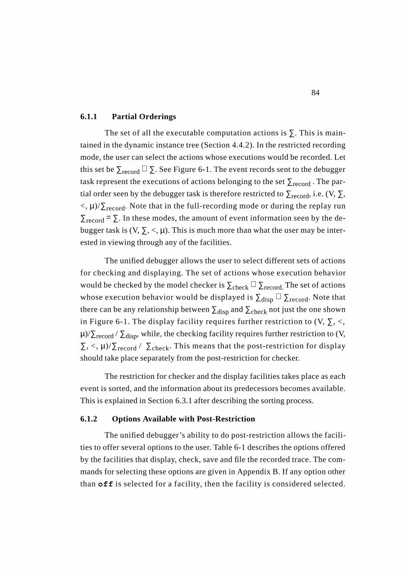
84

6.1.1 Partial Orderings

The set of all the executable computation actions is∑. This is main-

tained in the dynamic instance tree (Section4.4.2). In the restricted recording

mode, the user can select the actions whose executions would be recorded. Let

this set be∑record⊆ ∑. See Figure6-1. The event records sent to the debugger

task represent the executions of actions belonging to the set∑record. The par-

tial order seen by the debugger task is therefore restricted to∑record, i.e. (V, ∑,

<, µ)/∑record. Note that in the full-recording mode or during the replay run

∑record= ∑. In these modes, the amount of event information seen by the de-

bugger task is (V, ∑, <, µ). This is much more than what the user may be inter-

ested in viewing through any of the facilities.

The unified debugger allows the user to select different sets of actions

for checking and displaying. The set of actions whose execution behavior

would be checked by the model checker is∑check⊆ ∑record.The set of actions

whose execution behavior would be displayed is∑disp ⊆ ∑record. Note that

there can be any relationship between∑disp and∑check not just the one shown

in Figure 6-1. The display facility requires further restriction to (V, ∑, <,

µ)/∑record / ∑disp, while, the checking facility requires further restriction to (V,

∑, <, µ)/∑record / ∑check. This means that the post-restriction for display

should take place separately from the post-restriction for checker.

The restriction for checker and the display facilities takes place as each

event is sorted, and the information about its predecessors becomes available.

This is explained in Section6.3.1 after describing the sorting process.

6.1.2 Options Available with Post-Restriction

The unified debugger’s ability to do post-restriction allows the facili-

ties to offer several options to the user. Table 6-1 describes the options offered

by the facilities that display, check, save and file the recorded trace. The com-

mands for selecting these options are given in Appendix B. If any option other

thanoff is selected for a facility, then the facility is considered selected.

85

DispTr, FileTr, SaveTr, CheckTr are flags which indicate whether a fa-

cility is selected or not.

6.2 Information Requirements

The user can select one or more facilities. The flags DispTr, FileTr,

SaveTr and CheckTr inform the debugger what facilities are selected. Note

that all the facilities are not available in every debugging mode. Table 6-2

shows the availability of the facilities in each debugging mode. The user can

only select from the facilities that are available in a given mode.Only those fa-

cilities are available in a given mode which make sense. For example, in the

Table 6-1. Various options offered by different facilities.

Facilities Options Description

DispTr

record Display recorded trace; restricted to ∑record

check Display trace post-restricted to ∑check

disp Display trace post-restricted to ∑disp

off DispTr is false

CheckTron Check the trace post-restricted to ∑check

off CheckTr is false

SaveTr

record Save the recorded trace; restricted to ∑record

disp Save the trace post-restricted to ∑disp

check Save the trace post-restricted to ∑check

off SaveTr is false

FileTr

xgrab Use format displayable by XGRAB [RDB+87] system

edge Use format displayable by EDGE [] graph editor

perftr Use format for performance post-processing

default Use the default debugger format.

off FileTr is false

86

performance tracing mode, the facilities for filing, displaying and checking of

event trace are not available because they may disrupt the timings that are be-

ing recorded. In the replay mode, saving of the event trace is not available be-

cause the instrumentation is using the event records that are already saved.

The facilities provided by the debugger task need action-specific infor-

mation described in Table 6-3. Note that the action specific information need-

ed by the instrumentation is maintained in the action (Section5.1.2). The

information needed by the facilities is also kept inside the action1. This infor-

mation becomes accessible to the facilities whenever they have the action id

1 This organization will have to change in the distributed implementation.

Table6-2. Availability of various facilities in different modes.

Current ModeFacilities Utilizing Event Trace Interactive

FacilityDispTr CheckTr FileTr SaveTr

Run Modes

(On-the-fly)

Replay Run X X X X

RestrictedRecording

X X X X X

FullRecording

X X X X X

RecordingOff

X

Performance Tracing

X

DebuggingOff

PostmortemModes

FromFile

X X X

FromRecords

X X X

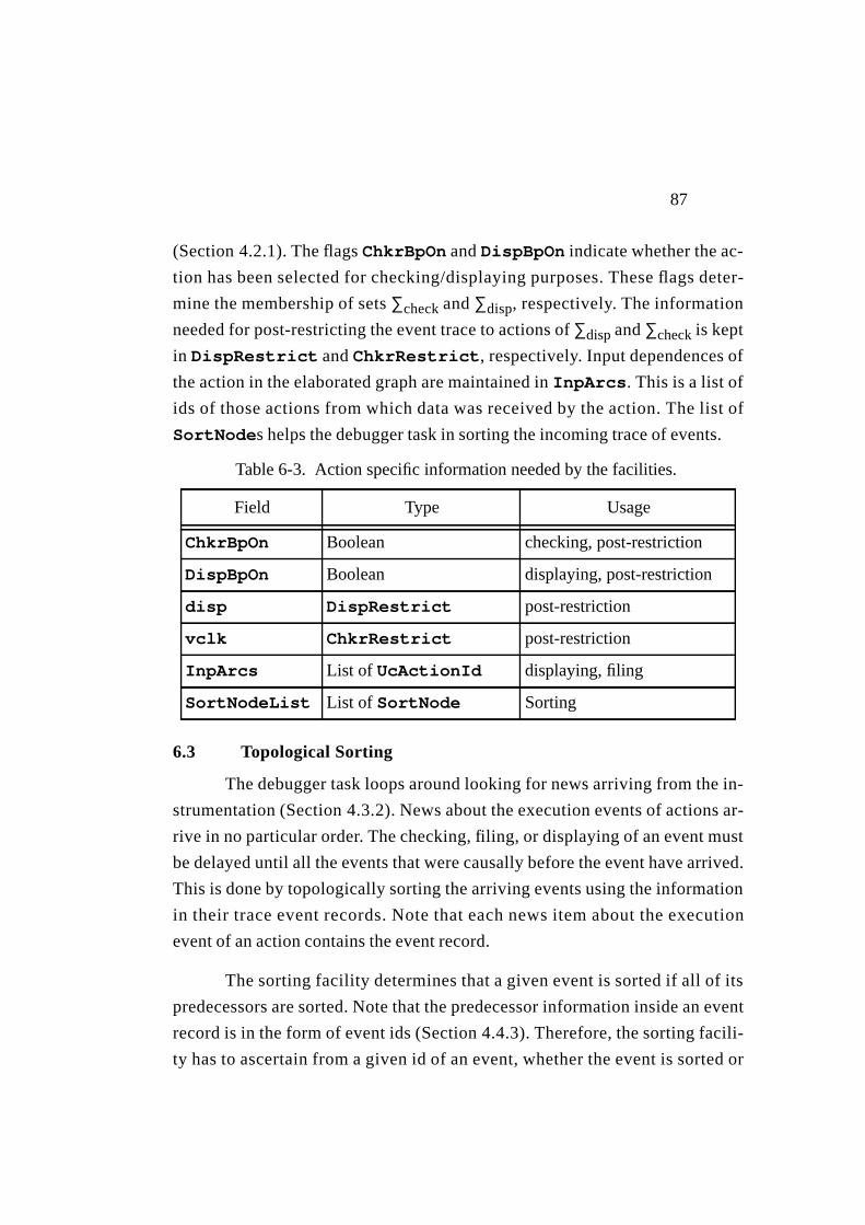
87

(Section4.2.1). The flagsChkrBpOn andDispBpOn indicate whether the ac-

tion has been selected for checking/displaying purposes. These flags deter-

mine the membership of sets∑check and∑disp, respectively. The information

needed for post-restricting the event trace to actions of∑disp and∑check is kept

in DispRestrict andChkrRestrict, respectively. Input dependences of

the actionin the elaborated graph are maintained inInpArcs. This is a list of

ids of those actions from which data was received by the action. The list of

SortNodes helps the debugger task in sorting the incoming trace of events.

6.3 Topological Sorting

The debugger task loops around looking for news arriving from the in-

strumentation (Section4.3.2). News about the execution events of actions ar-

rive in no particular order. The checking, filing, or displaying of an event must

be delayed until all the events that were causally before the event have arrived.

This is done by topologically sorting the arriving events using the information

in their trace event records. Note that each news item about the execution

event of an action contains the event record.

The sorting facility determines that a given event is sorted if all of its

predecessors are sorted. Note that the predecessor information inside an event

record is in the form of event ids (Section4.4.3). Therefore, the sorting facili-

ty has to ascertain from a given id of an event, whether the event is sorted or

Table6-3. Action specific information needed by the facilities.

Field Type Usage

ChkrBpOn Boolean checking, post-restriction

DispBpOn Boolean displaying, post-restriction

disp DispRestrict post-restriction

vclk ChkrRestrict post-restriction

InpArcs List of UcActionId displaying, filing

SortNodeList List of SortNode Sorting

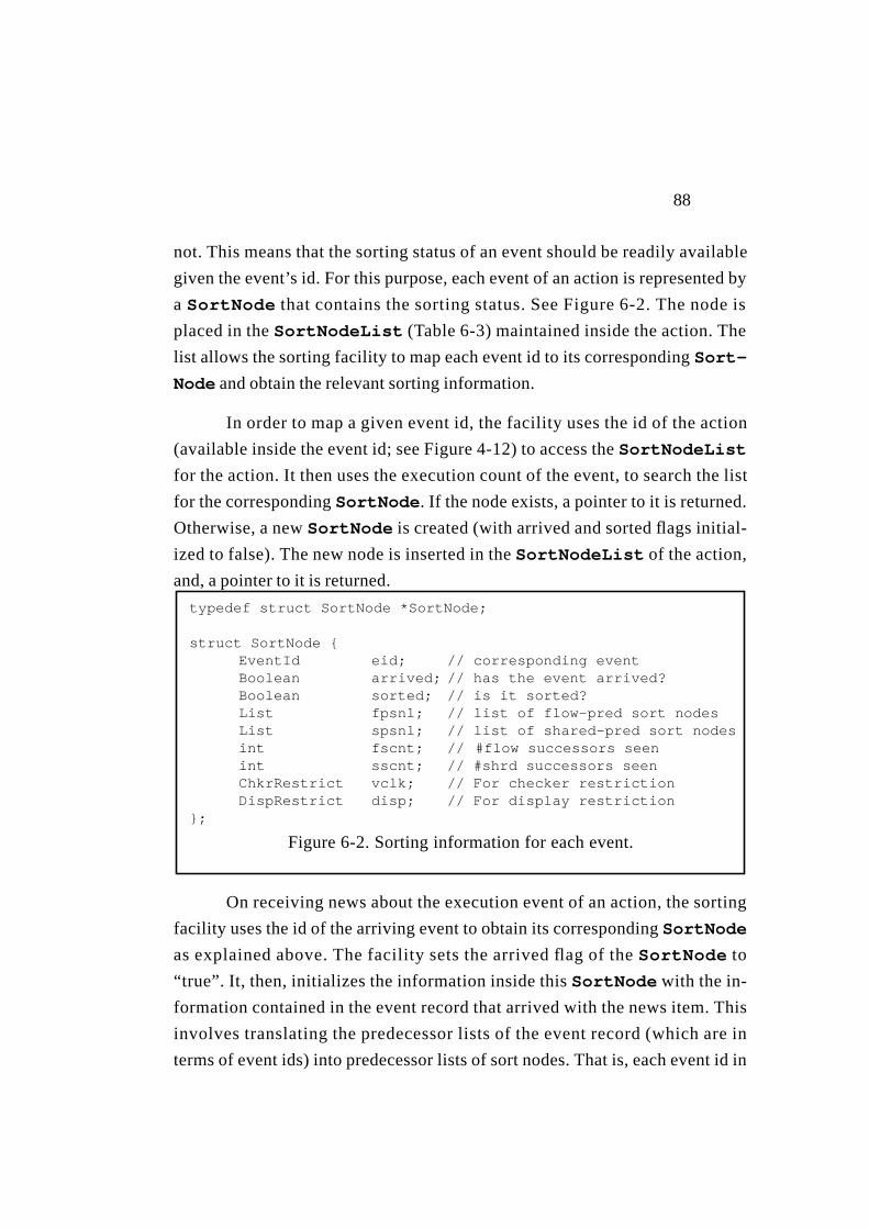
88

not. This means that the sorting status of an event should be readily available

given the event’s id. For this purpose, each event of an action is represented by

a SortNode that contains the sorting status. See Figure 6-2. The node is

placed in theSortNodeList (Table 6-3) maintained inside the action. The

list allows the sorting facility to map each event id to its correspondingSort-

Node and obtain the relevant sorting information.

In order to map a given event id, the facility uses the id of the action

(available inside the event id; see Figure 4-12) to access theSortNodeList

for the action. It then uses the execution count of the event, to search the list

for the correspondingSortNode. If the node exists, a pointer to it is returned.

Otherwise, a newSortNode is created (with arrived and sorted flags initial-

ized to false). The new node is inserted in theSortNodeList of the action,

and, a pointer to it is returned.

On receiving news about the execution event of an action, the sorting

facility uses the id of the arriving event to obtain its correspondingSortNode

as explained above. The facility sets the arrived flag of theSortNode to

“true”. It, then, initializes the information inside thisSortNode with the in-

formation contained in the event record that arrived with the news item. This

involves translating the predecessor lists of the event record (which are in

terms of event ids) into predecessor lists of sort nodes. That is, each event id in

typedef struct SortNode *SortNode;

struct SortNode {EventId eid; // corresponding eventBoolean arrived; // has the event arrived?Boolean sorted; // is it sorted?List fpsnl; // list of flow-pred sort nodesList spsnl; // list of shared-pred sort nodesint fscnt; // #flow successors seenint sscnt; // #shrd successors seenChkrRestrict vclk; // For checker restrictionDispRestrict disp; // For display restriction

};

Figure6-2. Sorting information for each event.

89

the predecessor list of the event record, is mapped to its correspondingSort-

Node. The objective is to make the sorting status of the predecessors readily

available to the sorting facility. Once this is done, the arrivedSortNode is in-

serted in theWaitList. This list contains sort nodes of all those events that

have arrived and are waiting to be sorted (arrived flag is true, andsorted

flag is false).

The sorting algorithm picks up aSortNode from theWaitList, and

checks if all the predecessors of the event (represented by the node) have been

sorted. This is done by looking at thesorted flag of the predecessor sort

nodes. If they are all sorted, then the node is deleted from theWaitList, and

is marked as sorted. The event information inside the sorted node is then used

for post-restriction as explained below. Then, the node is given to the facilities

requested by the user. After that each predecessor sort node is accessed and the

count of successors seen by the predecessor is incremented. The predecessor

node is deleted if no other successors are expected by it. The algorithm, then,

picks up the next node (if any) from theWaitList, and repeats the above pro-

cess.

Note that the algorithm sketched above can be made more efficient by

adding additional information toSortNode as explained in [KiZe93].

void sortTrace(){

foreach SortNode sn in WaitListif (areAllPredSorted(sn)) {

delete sn from WaitList;sn->sorted = true;doPostRestriction(sn);provideFacilities(sn);delPredsIfNoSucc(sn);

}endfor;

}

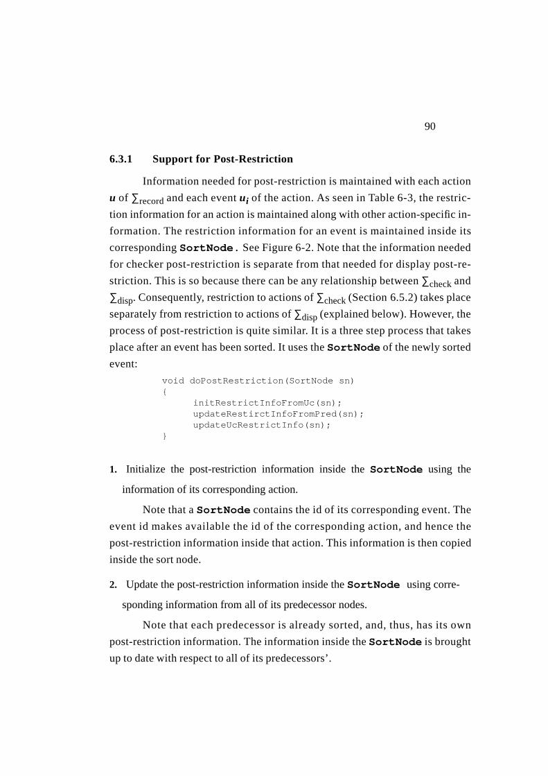
90

6.3.1 Support for Post-Restriction

Information needed for post-restriction is maintained with each action

u of ∑record and each eventui of the action. As seen in Table 6-3, the restric-

tion information for an action is maintained along with other action-specific in-

formation. The restriction information for an event is maintained inside its

correspondingSortNode. See Figure 6-2. Note that the information needed

for checker post-restriction is separate from that needed for display post-re-

striction. This is so because there can be any relationship between∑check and

∑disp. Consequently, restriction to actions of∑check (Section6.5.2) takes place

separately from restriction to actions of∑disp (explained below). However, the

process of post-restriction is quite similar. It is a three step process that takes

place after an event has been sorted. It uses theSortNode of the newly sorted

event:

1. Initialize the post-restriction information inside theSortNode using the

information of its corresponding action.

Note that aSortNode contains the id of its corresponding event. The

event id makes available the id of the corresponding action, and hence the

post-restriction information inside that action. This information is then copied

inside the sort node.

2. Update the post-restriction information inside theSortNode using corre-

sponding information from all of its predecessor nodes.

Note that each predecessor is already sorted, and, thus, has its own

post-restriction information. The information inside theSortNode is brought

up to date with respect to all of its predecessors’.

void doPostRestriction(SortNode sn){

initRestrictInfoFromUc(sn);updateRestirctInfoFromPred(sn);updateUcRestrictInfo(sn);

}

91

3. Update the post-restriction information inside the action using the sorted

event’s information.

The post-restriction information inside theSortNode was more cur-

rent than the information inside its corresponding action. So, information in-

side the action is brought up to date using the information inside the

SortNode. This is necessary because this information will be later copied in-

side aSortNode when the next event occurrence of the action is sorted.

Need for Maintaining Information with Actions

In order to enable post-restriction, later event occurrences of an action

in ∑record - ∑restrict, must be informed about the predecessor events known to

the action through its earlier occurrences. For this purpose, post-restriction in-

formation is maintained inside each action. This is a list of its currently known

predecessor events. The information allows thei-th event occurrence of an ac-

tion u in ∑record - ∑restrict to forward the predecessor information of eventui to

the successors of its later event occurrences;ui+1, ui+2, ....

To see why it is necessary to maintain current post-restriction informa-

tion with each action, consider the situation depicted in Figure 6-3. The prede-

cessor information available withu i has to be carried over to its later

occurrence;ui+1, so that it can eventually be forwarded tovj.2 The information

maintained with eachu in ∑record - ∑restrict allows this when it is copied inside

theSortNode. When step (3) of the above process is run forui, the post-re-

striction information withu will have the predecessor idxk. Whenstep (1) is

performed forui+1, the post-restriction information withSortNode of ui+1

will get xk from u. Eventually, when step (2) is performed forvj , its sort node

will get the idxk from the sort node ofui+1.

2 Note that ui ∉ ui+1.P. The precedence ofui to ui+1 is only indicated by theexecution count stored in their event records.

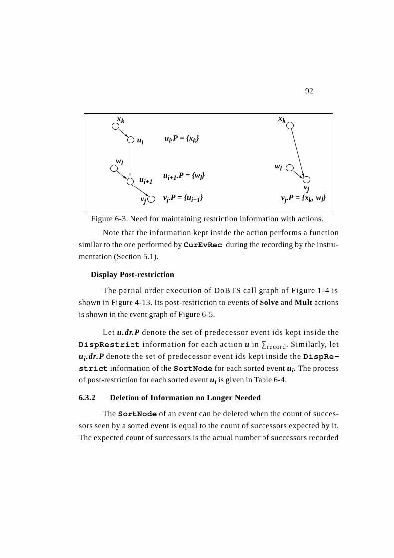
92

Note that the information kept inside the action performs a function

similar to the one performed by CurEvRec during the recording by the instru-

mentation (Section 5.1).

Display Post-restriction

The partial order execution of DoBTS call graph of Figure 1-4 is

shown in Figure 4-13. Its post-restriction to events of Solve and Mult actions

is shown in the event graph of Figure 6-5.

Let u.dr.P denote the set of predecessor event ids kept inside the

DispRestrict information for each action u in ∑record. Similarly, let

ui.dr.P denote the set of predecessor event ids kept inside the DispRe-

strict information of the SortNode for each sorted event ui. The process

of post-restriction for each sorted event ui is given in Table 6-4.

6.3.2 Deletion of Information no Longer Needed

The SortNode of an event can be deleted when the count of succes-

sors seen by a sorted event is equal to the count of successors expected by it.

The expected count of successors is the actual number of successors recorded

vj

xk

ui+1

ui

Figure 6-3. Need for maintaining restriction information with actions.

ui.P = {xk}

vj.P = {ui+1}vj

xk

vj.P = {xk, wl}

ui+1.P = {wl}

wl wl

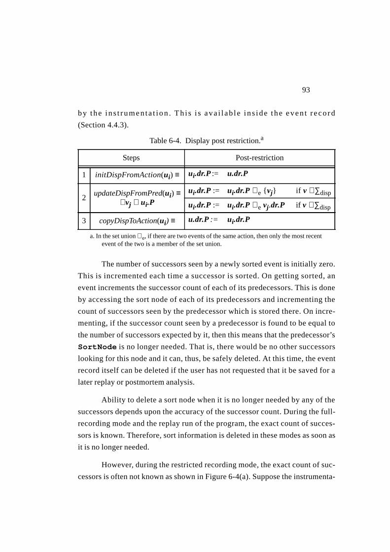
93

by the ins t rumenta t ion . Th is i s ava i lab le ins ide the event record

(Section4.4.3).

The number of successors seen by a newly sorted event is initially zero.

This is incremented each time a successor is sorted. On getting sorted, an

event increments the successor count of each of its predecessors. This is done

by accessing the sort node of each of its predecessors and incrementing the

count of successors seen by the predecessor which is stored there. On incre-

menting, if the successor count seen by a predecessor is found to be equal to

the number of successors expected by it, then this means that the predecessor’s

SortNode is no longer needed. That is, there would be no other successors

looking for this node and it can, thus, be safely deleted. At this time, the event

record itself can be deleted if the user has not requested that it be saved for a

later replay or postmortem analysis.

Ability to delete a sort node when it is no longer needed by any of the

successors depends upon the accuracy of the successor count. During the full-

recording mode and the replay run of the program, the exact count of succes-

sors is known. Therefore, sort information is deleted in these modes as soon as

it is no longer needed.

However, during the restricted recording mode, the exact count of suc-

cessors is often not known as shown in Figure 6-4(a). Suppose the instrumenta-

a. In the set union∪e, if there are two events of the same action, then only the most recentevent of the two is a member of the set union.

Table6-4. Display post restriction.a

Steps Post-restriction

1 initDispFromAction(ui) ≡ ui.dr.P := u.dr.P

2updateDispFromPred(ui) ≡

∀vj ∈ ui.P

ui.dr.P := ui.dr.P ∪e { vj} if v ∈∑disp

ui.dr.P := ui.dr.P ∪e vj.dr.P if v ∉∑disp

3 copyDispToAction(ui) ≡ u.dr.P := ui.dr.P

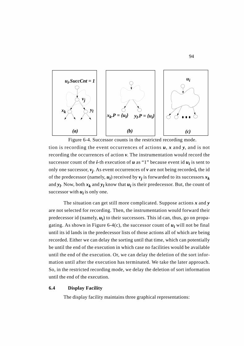
94

tion is recording the event occurrences of actionsu, x andy, and is not

recording the occurrences of actionv. The instrumentation would record the

successor count of thei-th execution ofu as “1” because event idui is sent to

only one successor, vj. As event occurrences ofv are not being recorded, the id

of the predecessor (namely, ui) received byvj is forwarded to its successorsxk

andyl. Now, bothxk andyl know thatui is their predecessor. But, the count of

successor withui is only one.

The situation can get still more complicated. Suppose actionsx andy

are not selected for recording. Then, the instrumentation would forward their

predecessor id (namely, ui) to their successors. This id can, thus, go on propa-

gating. As shown in Figure 6-4(c), the successor count ofui will not be final

until its id lands in the predecessor lists of those actions all of which are being

recorded. Either we can delay the sorting until that time, which can potentially

be until the end of the execution in which case no facilities would be available

until the end of the execution. Or, we can delay the deletion of the sort infor-

mation until after the execution has terminated. We take the later approach.

So, in the restricted recording mode, we delay the deletion of sort information

until the end of the execution.

6.4 Display Facility

The display facility maintains three graphical representations:

ui.SuccCnt = 1

vj

xk yl

ui

Figure6-4. Successor counts in the restricted recording mode.

yl.P = {ui}xk.P = {ui}

(a) (b) (c)

95

1. An event history graph which shows the ordering relations of an event with

respect to other events.

2. An elaborated graph which shows the dependence relations between the

actions introduced at runtime, and

3. A program graph which shows the relations between templates specified by

the programmer.

Figure 6-5 shows the three graphs restricted to actions and events of

templatesSolve andMult of the DoBTS call graph of Figure 1-4.

The display facility shows mappings between events, actions, and tem-

plates on these graphs. The mappings connect the three graphs together. These

mappings can be viewed statically when the execution has finished or is

stopped at a breakpoint. Or, they can be viewed dynamically as the events ar-

rive during the execution or in a postmortem fashion. The dynamic view

shows the progress of the execution and is often termed animation.

Our implementation currently displays these graphs textually. It thus

uses the same internal structures for display purposes as are used for other pur-

poses. A proper GUI interface may require separate structures that would be

linked with the internal debugger structures. Note that the user has the option

to dump the graphs to a file, and then display them using XGRAB graph

browsing system (Table 6-1). Work on a proper GUI interface is currently in

progress (Section8.3.1).

6.4.1 Display of Mappings

The user may view these mappings by selecting an action, a template or

an event.

By Selecting an Event

If an event is selected, the display would highlight its corresponding ac-

tion and template. For example, if we select eventm32 in Figure 6-5(c), then

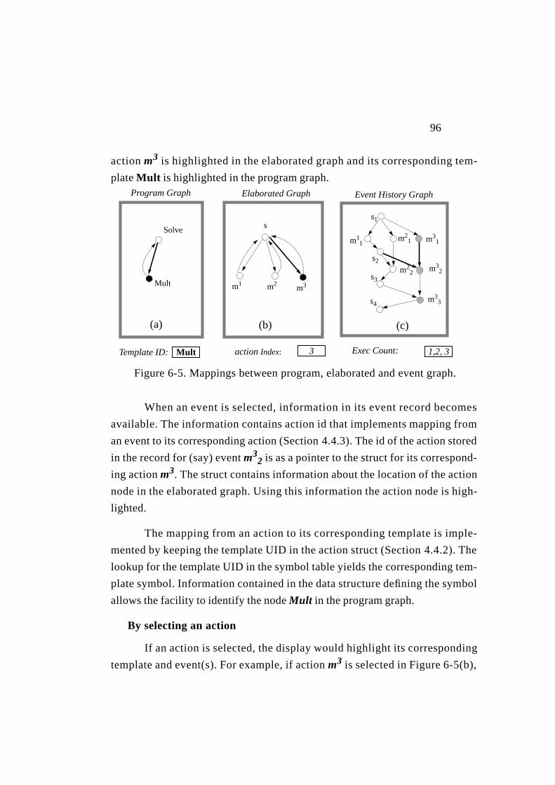
96

action m3 is highlighted in the elaborated graph and its corresponding tem-

plate Mult is highlighted in the program graph.

When an event is selected, information in its event record becomes

available. The information contains action id that implements mapping from

an event to its corresponding action (Section 4.4.3). The id of the action stored

in the record for (say) event m32 is as a pointer to the struct for its correspond-

ing action m3. The struct contains information about the location of the action

node in the elaborated graph. Using this information the action node is high-

lighted.

The mapping from an action to its corresponding template is imple-

mented by keeping the template UID in the action struct (Section 4.4.2). The

lookup for the template UID in the symbol table yields the corresponding tem-

plate symbol. Information contained in the data structure defining the symbol

allows the facility to identify the node Mult in the program graph.

By selecting an action

If an action is selected, the display would highlight its corresponding

template and event(s). For example, if action m3 is selected in Figure 6-5(b),

Template ID:

Program Graph

action Index:

Elaborated Graph

Exec Count:

Event History Graph

Mult

Solve

m3m2m1

s

m22

m33

m32

m31m2

1

s2

s3

s4

s1

m11

Mult 3 1,2, 3

Figure 6-5. Mappings between program, elaborated and event graph.

(a) (b) (c)

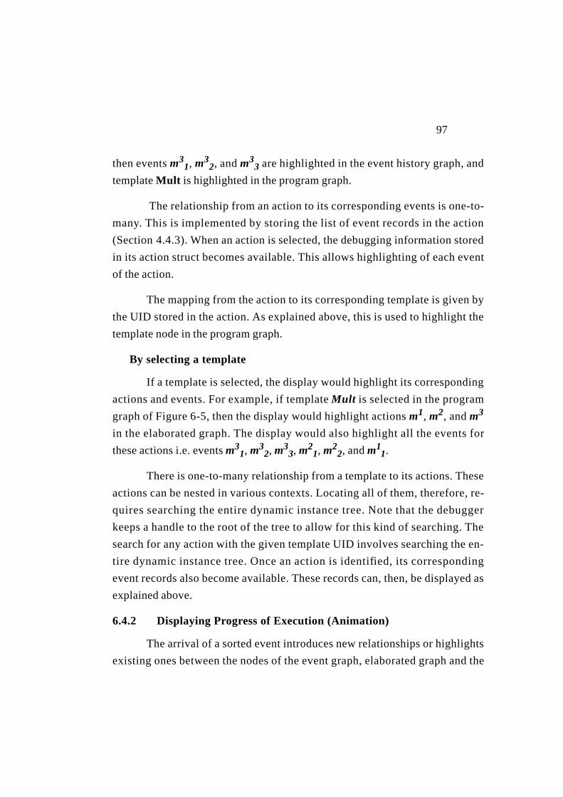
97

then events m31, m3

2, and m33 are highlighted in the event history graph, and

template Mult is highlighted in the program graph.

The relationship from an action to its corresponding events is one-to-

many. This is implemented by storing the list of event records in the action

(Section 4.4.3). When an action is selected, the debugging information stored

in its action struct becomes available. This allows highlighting of each event

of the action.

The mapping from the action to its corresponding template is given by

the UID stored in the action. As explained above, this is used to highlight the

template node in the program graph.

By selecting a template

If a template is selected, the display would highlight its corresponding

actions and events. For example, if template Mult is selected in the program

graph of Figure 6-5, then the display would highlight actions m1, m2, and m3

in the elaborated graph. The display would also highlight all the events for

these actions i.e. events m31, m3

2, m33, m2

1, m22, and m1

1.

There is one-to-many relationship from a template to its actions. These

actions can be nested in various contexts. Locating all of them, therefore, re-

quires searching the entire dynamic instance tree. Note that the debugger

keeps a handle to the root of the tree to allow for this kind of searching. The

search for any action with the given template UID involves searching the en-

tire dynamic instance tree. Once an action is identified, its corresponding

event records also become available. These records can, then, be displayed as

explained above.

6.4.2 Displaying Progress of Execution (Animation)

The arrival of a sorted event introduces new relationships or highlights

existing ones between the nodes of the event graph, elaborated graph and the

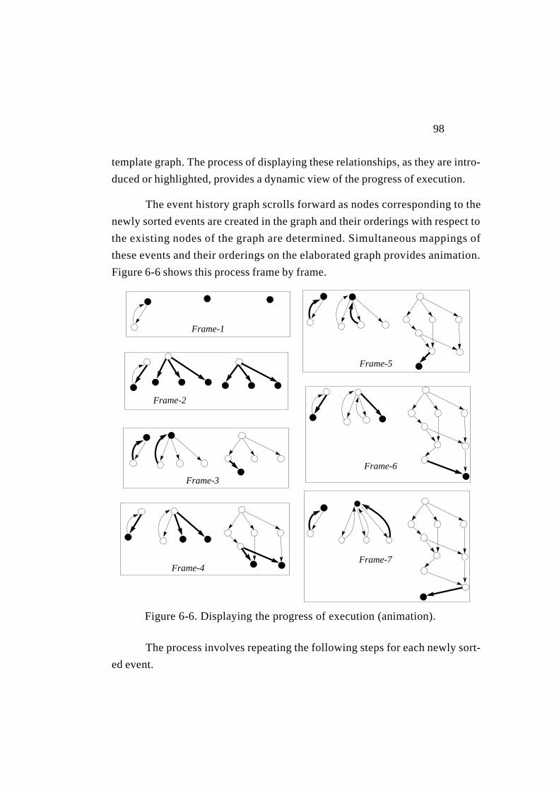
98

template graph. The process of displaying these relationships, as they are intro-

duced or highlighted, provides a dynamic view of the progress of execution.

The event history graph scrolls forward as nodes corresponding to the

newly sorted events are created in the graph and their orderings with respect to

the existing nodes of the graph are determined. Simultaneous mappings of

these events and their orderings on the elaborated graph provides animation.

Figure 6-6 shows this process frame by frame.

The process involves repeating the following steps for each newly sort-

ed event.

Figure 6-6. Displaying the progress of execution (animation).

Frame-1

Frame-2

Frame-3

Frame-4

Frame-5

Frame-6

Frame-7

99

1. Create an event node corresponding to the event in the event history graph.

Establish the mapping between the event and the newly created node.

2. Display the predecessor orderings of the event.

For each predecessor of the new event, the corresponding node is iden-

tif ied in the event history graph. Note that sorting ensures that such a node al-

ready exists. An arc is introduced from this predecessor event node to the new

event node. This arc is highlighted. After the orderings with all the predeces-

sors have, thus, been displayed, the new event node is highlighted.

3. Identify the action node in the elaborated graph corresponding to the event.

Create the action node if it does not already exist. This is the current ac-

tion node.

4. Highlight the dependences of the current action node that correspond to the

predecessor orderings.

For each predecessor of the newly sorted event, the corresponding ac-

tion node is identified. Sorting again ensures that the action node is already

present in the elaborated graph. A dependence arc is introduced between the

predecessor action node and the current action node if it does not already ex-

ist. If it exists, then it is simply highlighted. After all the dependences corre-

sponding to the predecessor events have been highlighted, then the current

action node is highlighted.

5. Highlight the mappings to the templates of the program graph.

As each action is highlighted, its corresponding template is highlight-

ed. Similarly, as each dependence in the elaborated graph is highlighted, its

corresponding dependence in the program graph is highlighted. Note that tem-

plate UID’s associated with each action allow us to identify and display these

mappings.

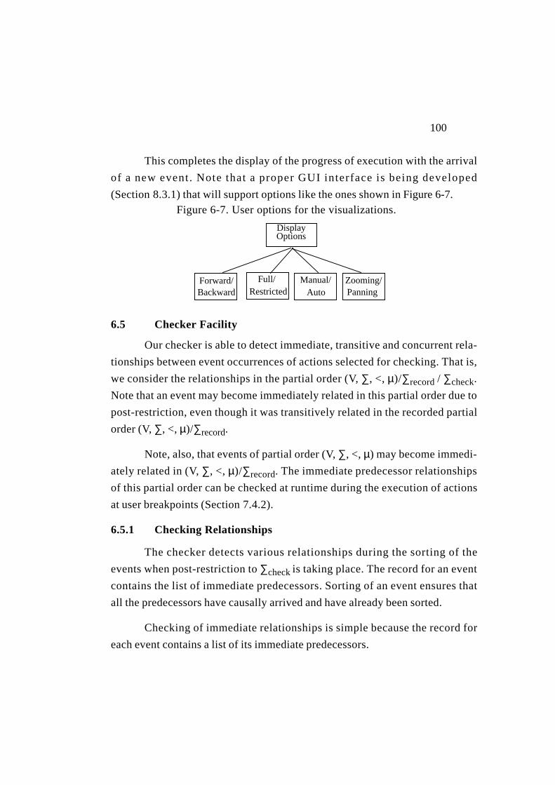
100

This completes the display of the progress of execution with the arrival

of a new event . Note that a proper GUI interface is being developed

(Section 8.3.1) that will support options like the ones shown in Figure 6-7.

6.5 Checker Facility

Our checker is able to detect immediate, transitive and concurrent rela-

tionships between event occurrences of actions selected for checking. That is,

we consider the relationships in the partial order (V, ∑, <, µ)/∑record / ∑check.

Note that an event may become immediately related in this partial order due to

post-restriction, even though it was transitively related in the recorded partial

order (V, ∑, <, µ)/∑record.

Note, also, that events of partial order (V, ∑, <, µ) may become immedi-

ately related in (V, ∑, <, µ)/∑record. The immediate predecessor relationships

of this partial order can be checked at runtime during the execution of actions

at user breakpoints (Section 7.4.2).

6.5.1 Checking Relationships

The checker detects various relationships during the sorting of the

events when post-restriction to ∑check is taking place. The record for an event

contains the list of immediate predecessors. Sorting of an event ensures that

all the predecessors have causally arrived and have already been sorted.

Checking of immediate relationships is simple because the record for

each event contains a list of its immediate predecessors.

DisplayOptions

Figure 6-7. User options for the visualizations.

Full/RestrictedBackward

Manual/Auto

Forward/ Zooming/Panning

101

Checking of transitive relationships of an event can either be done by

recursively searching each predecessor of the event, or by timestamping each

event with a vector clock. Searching the predecessors in a breadth-first or a

depth first manner may require the traversal of entire causal history (state) of

the event which is often expensive [FoZw90]. On the other hand, vector clocks

provide a brief summary of the causal history. Each element of a vector clock

corresponds to an action and identifies the most recent predecessor event

known through the clock [Mat89].

We decided to use the vector clocks because they not only help in estab-

lishing ordering relationship between events, but are also helpful in establish-

ing concurrent relationships.

Vector clocks can either be maintained during the execution of actions,

or they can be maintained during sorting of the events by the checker as ex-

plained below. We take the latter approach for several reasons:

1. It allows separation of the checker concerns from those of the recording and

instrumentation concerns.

2. It avoids runtime overhead.

Maintaining vector clocks during sorting avoids the computation and

communication overhead incurred when the clocks are maintained during the

execution of actions.

3. Events are sent to the checker and other facilities anyway for detecting of con-

current relationships, displays, and/or filing.

As events are sent irrespective of whether the vector clocks are main-

tained during the execution or during the sorting, it is, therefore, more effi-

cient to maintain the vector clocks with the checker. Note that events must

also be sent in case the user requests a view of the unexpected behavior. As

mentioned in Section1.3.5, it is not enough for the checker to simply state

102

whether a relationship holds or not. It should also be able to provide more in-

formation about the actual execution behavior.

The downside for maintaining the vector clock with the checker is that

it may delay the triggering of breakpoints. But, this happens in any case for

conditions that can not be checked locally [WaG91], [ReSc94].

6.5.2 Post-restriction and Vector Clocks

Post-restriction to actions of∑check is carried out using the same vector

clocks that are being maintained for the checker. This involves the following

steps:

1. Associate a vector clock with each action.

Each action in∑record maintains current information about its most re-

cent predecessor events. This information is restricted to the events of∑check

and is thus maintained in a vector clock of size |∑check |.

Let u.T be the vector clock maintained for an actionu ∈ ∑record. Thus,

theChkrRestrict information seen in Table 6-3 and in Figure 6-2 actually

refers to a vector clock. Each slot of this vector corresponds to an action in

∑check, and contains the execution count of that action. Note that an event is

identified by the action id and the execution count. Thus, if the slot corre-

sponding to action idu in the vector contains the execution count i, then the

most recent event ofu that is known through this vector isui.

The reason for maintaining vector clocks for actions of∑check is that

their relationships is being checked by the model checker. However, the rea-

son for maintaining vector clocks for actions of∑record - ∑check is to help in

post-restriction as explained in Section6.3.1.

2. After each event occurrence of an action, increment the slot for the action in

the action’s vector clock.

103

The events seen by the sorting facility are the executions of actions of

∑record. Whenever an eventui gets sorted,u’s vector clock is incremented only

if u is a member of∑check.

If u ∈ ∑check, then its event occurrences are recognized by the checker.

Therefore, the slot foru in its vector clock is incremented i.e.u.T[u] := u.T[u]

+1. However, if u ∉ ∑check, then its occurrences are not being recognized.

There is no slot foru in u.T. So, there is no change in the current value of the

vector clocku.T.

3. Time-stamp each event occurrence of the action with the current vector clock

of the action.

Whenever an eventui is sorted, it is time-stamped with the current val-

ue ofu.T. This is done by copying the vectoru.T inside its corresponding

SortNode. Let this time-stamp beui.T.

4. Update the event’s timestamp using the timestamp of each of its predecessors.

Note that each predecessor is already sorted, and, hence, its vector

timestamp is available. So,∀ vj ∈ ui.P, we do:

updateVclk(ui.T, vj.T) ≡

∀ w ∈ ∑check: ui.T[w] < vj.T[w] :: ui.T[w] = vj.T[w]

5. Use event’s timestamp to update its action’s vector clock.

After the update in (4), the event’s timestamp,ui.T, contains the most

recent information about the event’s causal predecessors. This information is,

then, used to bring the vector clock of its corresponding action,u.T, up to date

by performingupdateVclk(u.T, ui.T). Note that the value of the vector clock,

u.T, resulting from this update will be later used to time-stamp thenext event

occurrence of the action.

104

6.5.3 Checker Commands

Currently, the unified debugger supports two types of commands. One

checks predecessor relationships and the other concurrent relationships be-

tween occurrences of actions. Each command issued to the checker is assigned

a reference id and is entered in a reference list CmdRefList . As explained lat-

er, this list is used in translation of each command into an appropriate break-

point before the execution is run. The reference id is also used in deletion of

the breakpoints and their associated commands.

Checking immediate and/or transitive predecessors

If u, v, w are the action identifiers supplied by the user, then the com-

mand to check if event occurrences of u are preceded by an event of v, and an

event of w is:

check pred u{ v, w}

That is, ∀ui ∈V : ∃ vj, wk ∈ V :: vj <c ui ∧ wk <c ui.

The command is thus of the form check pred <action_id> ‘{’

<action_id_list> ‘}’ and is checked using vector clocks [Mat89].

Each <action_id> is composed of a template identifier and an in-

dex. Syntax for the debugger commands is given in Appendix B. Two com-

mands for the same action result in the or-ing of the checking. Note that a

firing rule is a set of subsets of input dependences. So, to construct a firing rule

like {{(u, v), (v, v), (w, v)}, {(w, v), (x, v)}} the user has to give two check pre-

decessor commands.

check pred v{ u, v, w} , and check pred v{ w, x}

The result of these two commands is ∀vi ∈V ::

(∃ vj, um, wk ∈ V :: vj <c vi ∧ um <c vi ∧ wk <c vi) ∨

(∃ wk, xl ∈ V:: wk <c vi ∧ xl <c vi)

105

Checking concurrent relationship

The checker command to see if any event occurrences of a set of ac-

tions were concurrent is check parallel ‘(‘<action_id_list> ‘)‘ .

check parallel ( u, v, w) detects if there were any events of u, v

and w that occurred concurrently. That is, ∃ ui, vj, wk ∈ V :: ui || vj || wk. The

alogrithm described in [GaW92] is used for checking concurrent relationships.

6.5.4 Command Translation

The size of the vector clock used for checking depends upon the num-

ber of actions being checked i.e. | ∑check|. The number of such actions is not

known until the start of the execution because a user may add or delete the

commands issued to the checker. So, each command that is issued to the check-

er is simply inserted in the CmdRefList . The commands in this list are trans-

lated just before the start of the execution. The translation generates a

ChkNode for each action that is mentioned in a command. The list of these

nodes, ChkList, now represents the set ∑check. The size of the vector clock,

i.e. | ∑check|, is the number of check nodes in this list. The check node for an

action is used for the following purposes:

1. It maintains the current vector clock for the action.

2. It determines the mapping between the <action_id> and the check id.

The check id of an action determines the slot in the vector clock re-

served for the action. Note that during checking, the actions are identified by

this id.

struct ChkNode {TmpltUID uid;Index index; // index of the actionUcActionId id; // pointer to the inst structVclk vc; // Vector clock for instChkId cid; // checker id; slot in vectorList chkcmds; // commands to be checked

};

106

3. The node keeps the list of commands that need to be evaluated by the checker

for each occurrence event of the action. Note that each action specified in the

command is represented by the check-id.

4. The node allows the insertion of a checker breakpoint in actions that would

be later created or re-run.

Because of their lazy creation (Section4.2.1) and the dynamism of the

CODE 2 programs, UC actions may not exist when the checker command is is-

sued or translated. The insertion of a checker breakpoint for an action has to be

delayed until when it is created or re-run. The check node keeps theTmpl-

tUID and theIndex which was obtained from the<action_id> given on

the command line by the user. The mapping of this identifier to theUcAc-

tionId is established later when the action is created or re-run. Whenever a

new action is created, its UID and index is used to search theChkList for a

ChkNode with the same UID and Index. If there exists such a node, then the

action id is noted inside theChkNode for later reference. The breakpoint is in-

serted in the action by turning theChkBpkon flag inside the action (Table 6-

3).

After post-restriction, each sorted event is given to the facilities select-

ed by the user. Recall that the event information is now represented by a

SortNode, and contains the up to dateChkrRestrict information

(Section6.3). As explained above this information is actually a vector clock

for the event. If the event is of an action of∑check, then there is a correspond-

ing ChkNode containing the list of commands that need to be checked for the

action. The relationships specified by these commands are checked using the

vector clock for the event. Note that the current vector clocks of all the actions

with which the relationship has to be checked are available inChkList. The

predecessor and concurrent relationships between actions are checked in the

usual manner [ReSc94], [GaW92].

107

Chapter 7. Interactive Facility

The interactive facility establishes cooperation between the instrumen-

tation inserted inside each action, and the debugger task. This also requires co-

operation from the runtime system. The facility allows the user to interactively

control the execution of actions and to query their local state at various break-

points set by the user.

7.1 Controlling the Execution

Interactive control is available at the scope of the program and at the

scope of an action. A given command is interpreted in the context of the cur-

rently selected scope (Section4.5). If the currently selected scope is that of the

whole program, then the commands are considered global. Otherwise, they are

applied to the currently selected scope of the action.

Running the program under the control of a traditional debugger like

dbx typically involves the use of signals andptrace utilities. In response to a

run command, such a debugger would usually execute the object file of the

program with someexecv type of a (Unix) command in a child process. The

debugger would maintain the current state of all processes being run by the ap-

plication. It would manage their creation and deletion and would catch all the

signals generated by the processes. Querying the state of each process would

involve switching from the context of the debugger process to the context of

the desired process and then interpreting the commands. Re-running would in-

volve exiting the child process and doing anotherexecv of the object file.

Running the program under the control of the unified debugger is, how-

ever, much simpler in our implementation because we deal with the actions

and not processes. The template routine of an action executes like a thread in

the name space of other actions3. The actions cooperate with the debugger

3 This is true for all actions in the Sequent runtime system [New93]. It is true forthose actions that have been mapped to the same PVM task by the distributedruntime system [Vok94].

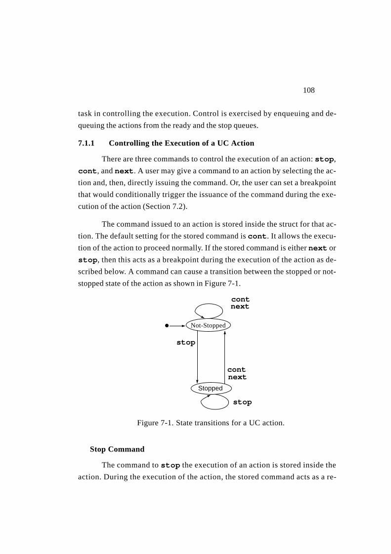
108

task in controlling the execution. Control is exercised by enqueuing and de-

queuing the actions from the ready and the stop queues.

7.1.1 Controlling the Execution of a UC Action

There are three commands to control the execution of an action: stop,

cont, and next. A user may give a command to an action by selecting the ac-

tion and, then, directly issuing the command. Or, the user can set a breakpoint

that would conditionally trigger the issuance of the command during the exe-

cution of the action (Section 7.2).

The command issued to an action is stored inside the struct for that ac-

tion. The default setting for the stored command is cont. It allows the execu-

tion of the action to proceed normally. If the stored command is either next or

stop, then this acts as a breakpoint during the execution of the action as de-

scribed below. A command can cause a transition between the stopped or not-

stopped state of the action as shown in Figure 7-1.

Stop Command

The command to stop the execution of an action is stored inside the

action. During the execution of the action, the stored command acts as a re-

Figure 7-1. State transitions for a UC action.

Not-Stopped

Stopped

stop

nextcont

nextcont

stop

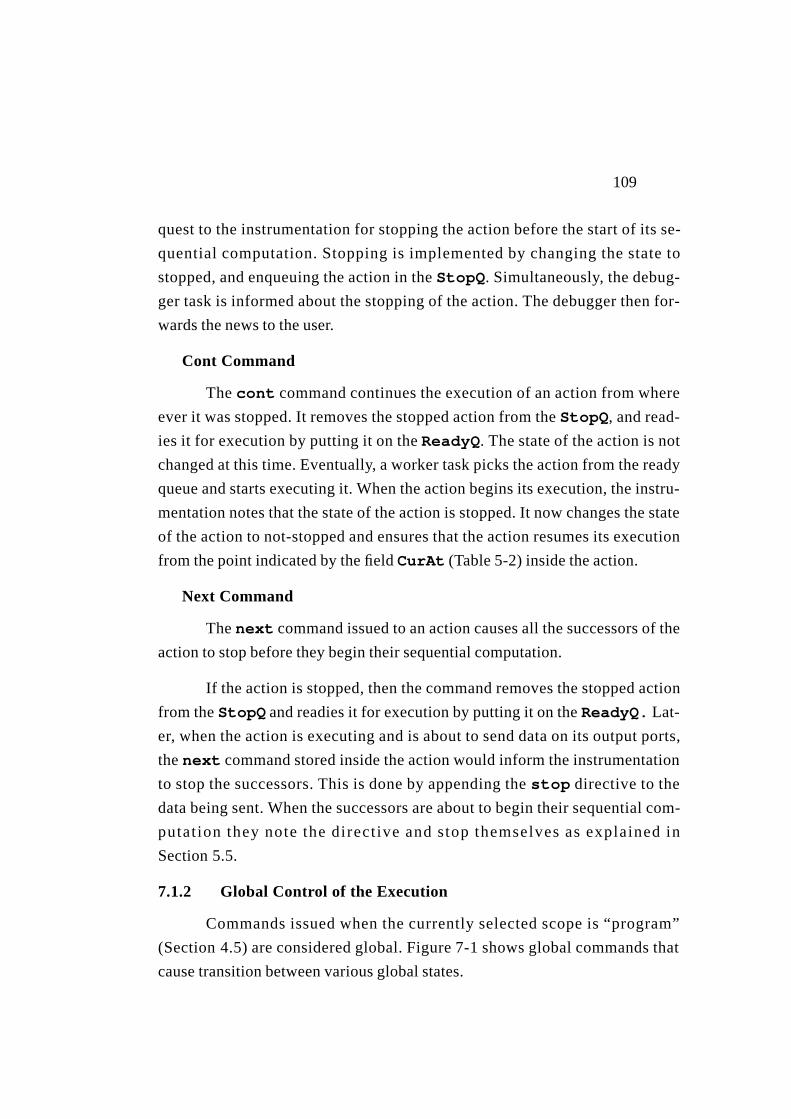
109

quest to the instrumentation for stopping the action before the start of its se-

quential computation. Stopping is implemented by changing the state to

stopped, and enqueuing the action in theStopQ. Simultaneously, the debug-

ger task is informed about the stopping of the action. The debugger then for-

wards the news to the user.

Cont Command

Thecont command continues the execution of an action from where

ever it was stopped. It removes the stopped action from theStopQ, and read-

ies it for execution by putting it on theReadyQ. The state of the action is not

changed at this time. Eventually, a worker task picks the action from the ready

queue and starts executing it. When the action begins its execution, the instru-

mentation notes that the state of the action is stopped. It now changes the state

of the action to not-stopped and ensures that the action resumes its execution

from the point indicated by the fieldCurAt (Table 5-2) inside the action.

Next Command

Thenext command issued to an action causes all the successors of the

action to stop before they begin their sequential computation.

If the action is stopped, then the command removes the stopped action

from theStopQ and readies it for execution by putting it on theReadyQ. Lat-

er, when the action is executing and is about to send data on its output ports,

thenext command stored inside the action would inform the instrumentation

to stop the successors. This is done by appending thestop directive to the

data being sent. When the successors are about to begin their sequential com-

putat ion they note the direct ive and stop themselves as explained in

Section5.5.

7.1.2 Global Control of the Execution

Commands issued when the currently selected scope is “program”

(Section4.5) are considered global. Figure 7-1 shows global commands that

cause transition between various global states.

110

Running

The user starts a new execution with a run command. The command

causes a transition to Running state when the start node specified in the

CODE 2 program graph is readied for execution by putting it on the ReadyQ.

Running state indicates that one or more actions are executing or are ready to

execute.

Execution of the start node readies for execution all the actions to

which it sends data. Their execution would, in turn, ready other actions for ex-

ecution and so on. Eventually, the termination node specified in the CODE 2

program graph would complete its execution.This would cause a transition to

Finished state. The state indicates that the program has run to completion.

Continuing

Issuance of a cont command readies for execution all the stopped ac-

tions by flushing them from the StopQ to the ReadyQ. This causes a transi-

tion to Running state.

Stopping

The user can stop all the actions that are running by issuing a stop

command. This causes a transition to Stopping state. The state informs the

StoppingNexting

Waiting

Finished

Stopped

Running

stop

cont, run

next

runcont

UsrBpt

next

Figure 7-2. Global state transitions in response to global commands.

111

instrumentation to stop any action that is about to begin its sequential compu-

tation. Eventually, all the actions that were executing or were ready to run

would stop. This would cause a transition toStopped state as explained be-

low.

Nexting

The user can ask the successors of all the actions that can run to stop by

issuing anext command. The command causes all the stopped actions to be

readied for execution by flushing theStopQ to theReadyQ. It also causes a

transition toNexting state. The state informs the instrumentation to ask ev-

ery successor of the currently executing action tostop. This is done by ap-

pending thestop command with each data that is sent out on an output port.

Eventually, all the executing actions would stop causing a transition toWait-

ing state.

Waiting or Stopped

Waiting andStopped states indicate that there are no actions that

are ready to run (the ready queue is empty), and there are no actions that are

currently being executed by any of the workers (workers are idle). This im-

plies that an action can not become ready for execution except through a user

command. It is, then, safe for the user to query the state of the actions and is-

sue other global commands.

Soon after the debugger comes up, the global state becomesWaiting.

This happens becauseReadyQ is empty and all the workers are idle. Issuing

the run command can then start the execution. The stopping of an action on a

set breakpoint may also cause a transition toWaiting state. This can happen

if all the other actions that can currently execute are dependent upon the ac-

tion. So, the action’s stopping will cause them to starve for data and eventually

stop. For instance, in Figure 4-13, ifDist action stops as a result of a user

breakpoint, then all actions would eventually become idle because they de-

112

pended on Dist for the data that could have triggered their execution, causing

an eventual transition to Waiting state.

Recall that workers loop around looking for actions to run from the

ReadyQ. A worker that fails in a certain number of attempts to find an action

to run from the ready queue, declares itself to be idle. This activates a typical

termination detection algorithm [ChMi88] for detecting whether all the work-

ers are idle or not. If it turns out that all the workers are idle, then the global

state is changed to Stopped if the current state is Stopping. Otherwise, it

is changed to Waiting.

Our shared memory implementation of the termination detection is sim-

ple. When the application starts, each worker task is assigned a logical id. The

worker with the largest id is designated as the decider. Each worker only

checks for the workers with lower ids. A worker task idles itself if it is idle and

all the workers whose ids are less than its id, are also idle. Eventually, the de-

cider worker (one with the maximum id), discovers that all other workers are

idle. So, it idles itself and declares the state to be Waiting or Stopped.

7.1.3 Rerunning the Execution

Rerunning the program involves preparation of the objects created in

the previous execution by the program and the debugger for a new run. Some

of these objects will be reused in the new run. Therefore, they need to be re-ini-

tialized. Others objects are no longer useful and the storage allocated to them

must be recovered. Re-initialization and storage recovery of objects created

by the debugger is simple because the debugger knows what objects it created

and what are their initial values. However, re-initialization and storage recov-

ery of the objects created by the program is difficult because the debugger has

no knowledge about those objects.

Objects Created by the Debugger

Rerunning the program in a given mode requires mode-specific prepa-

rations of the objects created by the debugger. If the program is being run in

113

the replay mode, then the debugger ensures that event records are available

from which the execution would be replayed. It also determines whether the

events were recorded in the full-recording mode. Note that in order to ensure a

proper replay, the trace should have been recorded in the full recording mode.

If the program is being rerun in the recording mode, then the instrumen-

tation will be generating new event records. So, previously recorded events of

the actions are deleted. This is done by accessing the debugging information

kept for each action and deleting the event records in the list kept there. Ac-

tion-specific information maintained by the instrumentation (Section 5.1.2)

and the facilities (Section 6.2) is re-initialized. Some of the previous user se-

lections like recording options are, however, retained.

Display, checker and user breakpoints are reevaluated to reflect any de-

letions or insertions. All the check nodes are deleted and the checker com-

mands are re-translated to generate a new list of check nodes (Section 6.5).

Options selected for various facilities (Table 6-1) are retained subject to the

availability of the facilities (Table 6-2). ReadyQ, StopQ and NewsQ are emp-

tied.

Objects Created by the Program

When a program is rerun by a traditional debugger like dbx, recovering

the storage allocated in its previous execution is relatively simple. It only in-

volves exit-ing the child process that exec-d the program object file when

the program was run. However, in our implementation there is no child pro-

cess with which the program was executed, that could be exited to get rid of

the storage allocated by the program.

The debugger task and the worker tasks are simply light-weight

threads. Actions that execute are objects (Figure 4-5) that hang around along

with all their local state. Their local state consists of objects that were allocat-

ed by the specifications provided by the user. The only objects of the program

that the debugger knows about are the actions created during the execution

114

(Section4.4.2). Local state of the actions is entirely managed by the program.

There are two ways of recovering the storage allocated by the program:

1. Exit the debugger along with the program and then re-run the program. Exit-

ing will recover all the storage allocated by the program.

2. Re-run the program without exiting the debugger. The debugger must recover

all the storage allocated by the program.

Exiting and reentering the program each time the execution is run is not a

user-friendly option. Furthermore, exiting the program with the debugger would

also destroy the debugger objects that need to be reused. This would necessitate

dumping of the contents of those objects to a file before the debugger is exited,

and then their re-construction when the debugger is reentered.Note that event

records use pointers to action structs for action ids. In the replay mode, these

records are used for enforcing replay. Exiting and then reentering meant that

we will have to reconstruct the pointers when new actions are created as the

program is rerun.

Hence, we decided to reuse the existing actions and recover the local

state allocated by the program.4 Fortunately, CODE 2 runtime system manag-

es all the objects that are allocated on the heap, and keeps a table of the space

allocated to them. The table was accessible to the debugger. So, a complete

clean up of all the objects allocated by the action was possible.

7.2 User Breakpoints

The interactive facility allows the user to set various breakpoints for a

specified action. The instrumentation arranges to break the execution of the ac-

tion at these points, and execute the breakpoint commands conditionally or un-

conditionally, as specified. Setting of a breakpoint requires the following

information:

4 The ability to reconstruct the debugger state is also quite useful. It will be neededwhen we implement the starting of another session (or replaying) from a file.

115

1. The id of the action for which the breakpoint is being set.

The action id may be explicitly supplied in commands likestop in

<action_id>. Otherwise in commands likestop if condition, it is as-

sumed to be the currently selected scope (Section4.5).

2. The point where the break should occur during the execution of the action.

Currently, the user has option to break the execution of an action at two

points; before the serial computation of a UC or after the computation of a UC.

The option to break at other points within the sequential computation is fairly

well understood in the context of sequential debugging and was, thus, not im-

plemented. Its implementation is tied with the provision of stepping facility as

described in Section8.2.1.

3. The commands that need to be executed on hitting the breakpoint.

The user can specify the commands that would be executed at a break-

point. For example,when at bpt {cmd1; cmd2; ...}allows the user to

specify the commands to be executed at the specified breakpoint. These com-

mands are only allowed to access and change the local state of the action.

Their syntax is given in Appendix B.

4. The condition under which to execute the specified commands.

This is optional. The breakpoint commands can, thus, be conditionally

or unconditionally evaluated. The specified condition is on the local state of

the action and may specify the immediate predecessors expected for the given

execution. Note that the immediate predecessors of an action can be checked

easily during the execution of the action because the current event record

(Section5.1.2) maintains this information.

The commands to set user breakpoints are entered in a list. The list

helps in insertion, and deletion of breakpoints. Each command in the list is

translated into aUsrBreakPt. The breakpoint contains a reference to the

command that produced it. It contains the point where the break should occur,

and the list of commands that are to be executed. There is an AST correspond-

116

ing to each command in this list. As the commands may have to be conditional-

ly evaluated, the AST includes any specified conditions.

The breakpoint contains the<action_id> given by the user. When-

ever a new action is created, the breakpoint list is consulted to see if there is a

breakpoint specified for this action. If there is, then the action is informed

about the breakpoint by settingUsrBpOn (Section5.5.2) to true. The id of the

action is noted for future reference. The list of breakpoints is, therefore, useful

in setting and un-setting of breakpoints.

7.3 Evaluation of User Commands

The evaluation of a user command can simultaneously occur in differ-

ent contexts. It may be the case that when the debugger frontend is evaluating

a user command, several UC actions could be at their respective breakpoints

evaluating their breakpoint commands. At the same time, the checker could be

busy evaluating its commands. The routine that evaluates user commands

should, therefore, be simultaneously callable from several contexts. This is en-

abled by allocating a separate stack for each context from which the evalua-

tion routine is invoked. The context information is associated with the stack.

Evaluation of context sensitive commands likeprint <expr>, then, takes

place depending upon the context in which the evaluation is being done.

• Evaluation by the Debugger

The debugger maintains information about the currently selected scope

(Section4.5). Conditions and expressions specified in a command are evaluat-

ed in the context of the currently selected scope. For example, if the debugger

struct UsrBreakPt {UsrBpCmd usrref; // Reference to bp commandWhere point; // point of insertionList commands; // actions to be takenUcActionId id; // back-end id of actionTmpltUID uid; // front-end idIndex index; // index of action

};

117

is evaluating the command print <expr>, then the names given in the

<expr> are evaluated in the context of the currently selected action.

• Evaluation at a User Breakpoint

During the execution of an action, commands evaluated at a user break-

point refer to the scope of the action. For example, the condition specified in

print in Solveif <bool_expr> refers to the scope of Solve. So, when

the breakpoint is hit during the execution of Solve, the evaluation routine is

given the base address of Solve where the local state is saved. Evaluation of

<bool_expr> takes place in this context.

• Evaluation by the Checker

The checker evaluates the commands during sorting. The only infor-

mation that is available to it is the event information. The commands are thus

interpreted in the scope of the event that has just been sorted. The user may

need to trigger other commands as a result of this checking. However, this was

not implemented.

7.4 Querying the State of Actions

It is safe to query the local state of an action when it is stopped. It is

also safe to query any action when the global state is stopped or waiting.

7.4.1 Local State of an action

Given the name of a symbol, the symbol table provides information

about the type of the symbol, its UID and a reference to the symbol of its en-

closing block (Section 4.4.1). This information is needed for printing the val-

ue of a given symbol or testing conditions on its state.

In a CODE 2 program, the programmer can declare objects of various

types within the scope of an action. The available types are array, struct,

int, real, and char.

118

CODE 2 arrays are dynamic. A two dimensional array is actually an ar-

ray of arrays. A multi-dimensional array is an array of an array, and so on. The

size of the array is runtime dependent. In order to print out the contents of a

given array, we need the size of the array and the index into it. The CODE 2

runtime library provides a routine that returns the size of the array given its ad-

dress. Symbol table information provides the type of the array. Therefore, the

contents of a given array can be printed. The debugger not only allows the user

to see the contents of an array, but also provides the ability to index into a par-

ticular element of the array and see its contents. Note that the content of a giv-

en index of an array may be a single object or a (multi-dimensional) array.

An input port of an action is a queue of a given type. The user can look

at the data values currently waiting in a given input port. The debugger obtains

the address of the port, and uses some runtime knowledge about the queue for

printing out the values waiting inside the queue.

7.4.2 Debugger Defined Objects

In order to help the user in debugging, access to three objects available

to the debugger was found to be useful. These are ExecCnt (Table 5-2), No-

deIndex (Figure 4-5), and Pred (Figure 4-12). These objects are used by the

debugger for supporting various facilities. The user may employ these sym-

bols in the conditions and expressions specified for various commands. For ex-

ample,

stop inMult if NodeIndex = 3

will cause the stopping of that action of Mult whose index is 3. Similarly,

stop in Mult if ExecCnt = 3

will stop any action of Mult that executes for the third time. Similarly, the user

can insert a breakpoint that tests for the immediate predecessors:

stop in Gath if Pred (Mult )

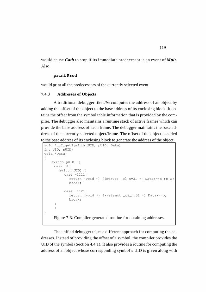
119

would causeGath to stop if its immediate predecessor is an event ofMult.

Also,

print Pred

would print all the predecessors of the currently selected event.

7.4.3 Addresses of Objects

A traditional debugger likedbx computes the address of an object by

adding the offset of the object to the base address of its enclosing block. It ob-

tains the offset from the symbol table information that is provided by the com-

piler. The debugger also maintains a runtime stack of active frames which can

provide the base address of each frame. The debugger maintains the base ad-

dress of the currently selected object/frame. The offset of the object is added

to the base address of its enclosing block to generate the address of the object.

The unified debugger takes a different approach for computing the ad-

dresses. Instead of providing the offset of a symbol, the compiler provides the

UID of the symbol (Section4.4.1). It also provides a routine for computing the

address of an object whose corresponding symbol’s UID is given along with

void *_c2_getSymAddr(UID, pUID, Data)int UID, pUID;void *Data;{

switch(pUID) {case 31:

switch(UID) {case -1111:

return (void *) ((struct _c2_nv31 *) Data)->B_FR_S;break;

case -1121:return (void *) &((struct _c2_nv31 *) Data)->b;break;

::

}

Figure7-3. Compiler generated routine for obtaining addresses.

120

the parent UID and the address of the symbol’s enclosing block. A part of the

code generated by the compiler is shown in Figure 7-3.

121

Chapter 8. Future Work

The research reported in this dissertation includes both the definition of

the unified model of concurrent debugging and also a feasibility demonstra-

tion implementation of the unified model. It has become clear that the unified

model does provide a framework for a complete and comprehensive debug-

ging system for parallel and concurrent programming. The future work which

would be needed to realize this comprehensive debugging system for concur-

rent and parallel software includes the following:

1. Enhancements and extensions to the current unified model for concurrent and

parallel debugging. The extensions include:

* Dynamic vector clocks.

* Hierarchical representation of the events.

* Hierarchical replay.

2. Interfaces to other modes of program validation:

* Integration with an interpreter-based sequential debugger.

* Interface to or integration with static analysis and symbolic analysis systems.

3. Enhancements of the implementation making it more effective for the user

and more user friendly. These enhancements include:

* A graphical user interface for the debugger and a better integration with the

CODE2 programming interface.

* An implementation for a distributed execution environment.

* Implementation of rollback and recovery.

* Buffering of logical event traces for performance measurements.

* A stepping facility for sequential code of the computation actions.

122

* More extensive facilities for model checking.

* Definition of hierarchical replay.

* Reconstruction of a debugging session from a file.

Another extension which would be significant, although not a part of

the unified model of debugging itself, is to map programs written in sequential

and parallel text string languages into the action/relationship programming

model so that the unified debugger can be applied to them as well.

The following sections explain each of the above points.

8.1 Enhancements to the Unified Model

Extensions to the unified model for concurrent debugging will allow

the debugger to support dynamic vector clocks, hierarchical representation of

events, and optimization of the amount of recording necessary for replay.

8.1.1 Dynamic Vector Clocks

The use of vector clocks typically assumes that the number of slots in a

vector is fixed, and the mapping of each slot to its corresponding executable

entity (process/thread) is already available [GaW92], [Mat89], [ReSc94],

[Fid89]. However, when the number of executable entities vary or when the

entities migrate, the assumption is no longer valid. For example, processes

may get created (or deleted) at runtime, or they may migrate. The interpreta-

tion of the slots in the vector clock must reflect these changes.

The unified debugger requires dynamic vector clocks for implement-

ing race detection (Section8.3.5) and optimizing the recording overhead for

replay (Section8.3.6). The vector clocks used by the unified debugger map

each slot of a vector to an action (Section6.5.2). As UC actions are instances

of templates, and their number varies at runtime (Section4.2.1), the vector

clocks should be able to adjust to an increasing number of slots (i.e. actions).

Note that the checker facility of the unified debugger currently uses

vector clocks for checking relationships among occurrences of actions

123

(Section6.5). It fixes the size of the vector before the execution is run to the

number of actions whose relationships are being checked. The dynamic vector

clocks will also make possible the deletion and addition of commands given to

the checker during the execution. Note that the checker fixes the number of ac-

tions before the execution, and addition and deletion of commands can vary

the number of actions, and hence the interpretation of the slots of the vector.

Dynamic vector clocks will also allow the checker facility to check re-

lationships between the templates. Currently, the facility, checks relationships

among execution occurrences of UC actions. It is unable to check relation-

ships among the templates, because the number of instances of a template can

vary at runtime.

The problem of increasing number of slots in the vector clock can be

addressed by (say) maintaining a current count of slots with each vector clock

object. The creation of a new instance, will cause a new slot to be added to the

vector. The routine that evaluates the checker commands and interprets the

slots will be informed of the new mapping.

8.1.2 Hierarchical Representation of Events

CODE 2 graphs are hierarchical. The runtime hierarchical context of

each UC action is available in the dynamic instance tree (Section4.4.2). How-

ever, the events of these actions are not displayed in their hierarchical context

because the notion of a graph event is not defined. In order to represent the

events hierarchically, it is necessary to define the conditions that determine

when the execution of a graph started and when it ended.

Note that there are explicit firing and routing rules that determine the

start and the end of an execution of a computation action (Section3.1.2). But,

there are no such rules for a CODE 2 call graph. Once a CODE 2 call graph is

instantiated, the actions inside the graph can execute independently of the

graph whenever the firing rules of the actions are satisfied [New93].

124

There are several definitions which give semantics to the execution of a

graph [Ho91], [ZeR91], [ReSc94]. The execution of a graph can also be con-

sidered as a sub-pomset [Pra86], and therefinement operator [Gis88] can,

then, be used to map one pomset to another. Given an appropriate definition, it

is possible to use the information currently available at runtime with the uni-

fied debugger to represent the events in their hierarchical contexts.

8.1.3 Hierarchical Replay

The storage requirements for the execution replay facility can be fur-

ther reduced by only recording the event orderings of actions belonging to a

set of selected subgraphs. Event orderings of actions that do not belong to this

set of subgraphs will not be recorded. The subgraphs whose orderings are not

being recorded will be considered as “holes”.

In the recording phase (Section3.5), the instrumentation will record

the contents of any communication that occurs across these holes. An event

record will, then, contain the content of the message from a predecessor event

if the predecessor belongs to a subgraph that is not selected. However, the

record will only contain the id of the predecessor if the predecessor belongs to

a selected subgraph. The replay phase will work as follows: An action will get

the actual message sent by the predecessor during replay if the predecessor be-

longs to a selected subgraph. The action will, however, be given the pre-re-

corded message if the predecessor belongs to a subgraph that is not selected.

8.2 Interfaces to Other Systems

The capability of the unified debugger can be greatly enhanced by inter-

facing it with an interpreter-based sequential debugger and systems for static

and symbolic analysis.

8.2.1 Interpreter and Stepping Facility

Advanced debuggers often use an interpreter to obviate the need to re-

compile each time a small modification is made to the user code [Sy83]. The

interpreter can especially be useful in the CODE 2 runtime system for a net-

125

work of heterogenous workstations where compiling code for different ma-

chines can be time consuming. An interpreter like UPS [Rus91] can be

interfaced with the unified debugger to support small modifications made to

the sequential computation of a UC action.

The interpreter could also provide a facility to step through the sequen-

tial computation. The interactive facility currently allows stopping at the start

and at the end of the sequential computation in a UC action (Chapter 7). It sup-

ports next-ing from the beginning of the sequential computation of a UC ac-

tion to its end, and next-ing from the end of the sequential computation of a

stopped action to the beginning of the computation of all of its logical succes-

sors. The interactive facility currently does not support stepping through the

sequential computation. Ability to step through the sequential code is howev-

er quite useful and can be provided with an interpreter. The interpreter will

only be invoked only when the user requests single stepping of the sequential

computation. Otherwise the execution will proceed through the computation

as it does currently.

8.2.2 Static Analysis and Symbolic Analysis

Information generated during static analysis has been used to simplify

the runtime information requirements for race detection and execution replay

[MiC89]. It is, however, also possible to use the information collected at runt-

ime to manage the complexity of static analysis facilities. Note that the static

analysis of parallel programs for detecting access anomalies and deadlocks is

intractable [Tay84]. The logical orderings of events actually exhibited by the

execution at runtime can be used for simplifying static analysis because this in-

formation is not available at compile time. Similarly, this information can also

be used for simplifying symbolic analysis [YoTa86].

8.3 Enhancements to the Current Implementation

The objective of the implementation described in Chapter 4-Chapter 7

was to demonstrate that the unified model of concurrent debugging provides a

framework that allows a single debugger to support all of the debugging facili-

126

ties that have previously been defined separately. The current implementation

is a prototype that provides the basic functionality needed for a demonstration

of feasibility. In order to allow the user to fully exploit this functionality fol-

lowing enhancements in the short-term are foreseen.

8.3.1 A Graphical User Interface (GUI)

The implementation currently uses a modification of the textual inter-

face provided by the Berkeley (BSD)dbx. The interface is only capable of ac-

cepting textual input and providing a textual output. In order to view the

different graphical representations produced by the debugger, the graphs are

first dumped using one of the filing options described in Section6.1.2. The

dumped file can, then, be picked up and displayed with the XGRAB graphical

editor [RDB+87].

Work on the next generation of CODE 2’s graphical frontend is current-

ly in progress. The plan includes the provision of a proper GUI environment

for interactive debugging. In this interface, interactions between the user and

the debugger would be based on the display of three graphs; the elaborated

graph, program graph and the execution event graph (Section6.4). The figure

given on the next page shows some of the icons and displays planned for the

interface. The user would be able to click on the interesting nodes of these

graphs to see their execution behavior, and make various selections. The com-

mands and selections described in Appendix B will be offered through icons

and buttons.

8.3.2 Distributed Implementation

This dissertation describes the implementation of the unified model of

concurrent debugging in the context of a shared memory machine. However,

the abstractions used by the model are machine independent and are also appli-

cable in a distributed environment.

CODE 2 environment is able to translate the programs into executables

that can run on a network of workstations using PVM message passing primi-

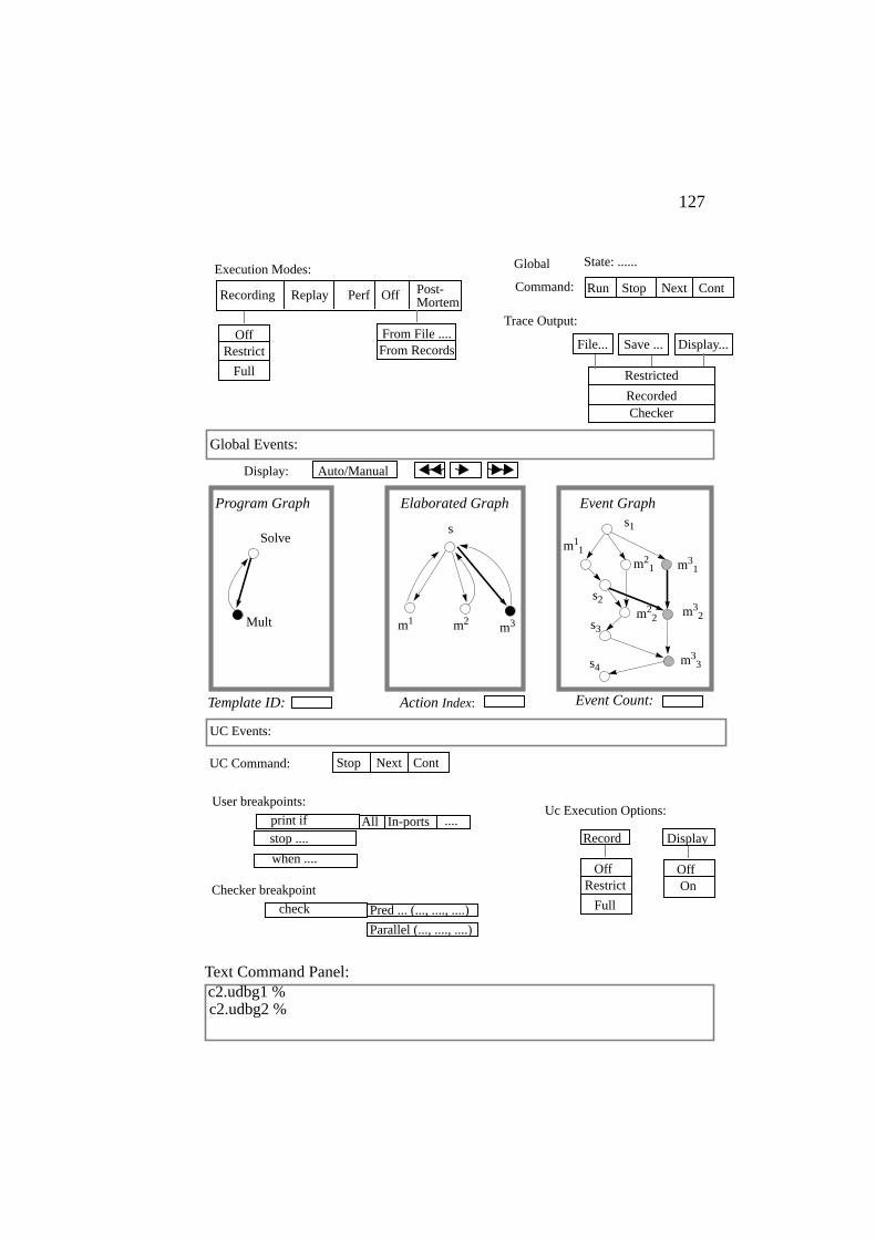
127

Template ID:

Program Graph

Action Index:

Elaborated Graph

Event Count:

Event Graph

Global Events:

Uc Execution Options:

Trace Output:

Execution Modes:

UC Command:

stop ....

Text Command Panel:c2.udbg1 %c2.udbg2 %

Display...Save ...File...

ContStop Next

Record Display

OffOn

UC Events:

All In-ports ....

User breakpoints:

Auto/Manual

OffRestrict

Full

Display:

Command: ContRun Stop Next

when ....

OffReplay Perf

print if

Pred ... (..., ...., ....)check

Parallel (..., ...., ....)

Mult

Solve

m3m2m1

s

m22

m33

m32

m31m2

1

s2

s3

s4

s1

m11

Restricted

Recorded

Recording

Global

Checker

State: ......

Post-Mortem

OffRestrict

Full

From File ....From Records

Checker breakpoint

128

tives [Vok94]. Current implementation of the unified debugger for Sequent

shared memory machine was designed keeping in view this distributed imple-

mentation of the CODE runtime system. For example, the decision to have a

separate debugger task that would communicate with the worker tasks through

NewsQ and StopQ (Section 4.3) was prompted by this consideration. Note

that the debugger task could have been implemented in a manner similar to a

template routine (Section 4.2.2) that is picked up by a worker task for periodic

running.

The distributed implementation of the unified model has been designed

and is being implemented. In this implementation, the debugger task and the

worker tasks will be PVM tasks (processes). Interactions between the debug-

ger task and the instrumentation described in Section 4.3, will be through the

PVM messages. Global commands will be sent to each worker task. Whereas,

commands that only apply to a particular action will be sent to that worker

task to which the action has been mapped by the runtime system. In order to

execute the debugger commands on a remote machine, there will be a remote

debugger with the worker task executing on that machine. The worker task

and the remote debugger will multiplex their execution as they do in the serial

implementation of the debugger. Note that there is a serial implementation of

the unified debugger for the CODE 2 runtime system for Sun4 workstations.

The remote debugger will execute the commands sent to it. It will maintain the

structures local to the machine like the ReadyQ and StopQ. It will also con-

trol the instrumentation inserted inside the UC actions that have been mapped

to its machine by the runtime system.

The central debugger task will maintain the NewsQ. News from the in-

strumentation (Section 4.3.1) will be directly sent to the central debugger

from the remote locations. The central debugger task will maintain a dynamic

instance tree which will be a union of all the branches instantiated by the runt-

ime system at various machines. It will also maintain a StopQ that will reflect

the status of all the stop queues at remote locations.

129

The manner of identifying an action will change. Currently, the debug-

ger identifies an action with a pointer (Section4.2.1). In the distributed envi-

ronment, this pointer may not be unique. So, the debugger will maintain

another level of indirection between the full-pathnames with which an in-

stance is identified by the user (Section4.5), and the address of the struct with

which the runtime system identifies the instance at a remote location.

8.3.3 Recovery and Roll-Back

The replay facility exactly replays an earlier execution using the order-

ing information recorded for that execution (Section5.4). The information re-

quired for recovery and roll back of a concurrent execution [JhZw90] is

contained in the information recorded for replay purposes. So, the capability

provided by the replay facility can be extended to provide roll back and recov-

ery. The orderings will, then, have to be recorded on a stable storage. Note,

however, that the replay facility can only replay the execution from the begin-

ning. During recovery and rollback it is not always convenient, or even feasi-

ble, to re-start the execution from the beginning each time there is a crash. In

order to avoid this, the recovery mechanism can periodically checkpoint the

state of the execution on stable storage. The execution can, then, be started

from the last checkpoint.

In the CODE 2 environment, a facility for checkpointing is already

available for process migration and load balancing purposes [Wag94]. This

checkpointing facility can be used in conjunction with the replay facility to

provide recovery and roll-back from the last checkpoint. The checkpointing

and recording of orderings will, then, have to done on stable storage. Note that

it is not necessary to checkpoint the entire state of each process. The recovery

mechanism can benefit from approaches like [MiC89]. These approaches use

data-flow analysis to limit the amount of information that must be recorded in

order to replay an execution from some point in the past. This can greatly re-

duce the checkpointing overhead.

130

8.3.4 Extending Facilities for Model Checking

The checker facility currently provides checking of three types of rela-

tionships (Section 6.5). The implemented functionality is, however, also capa-

ble of supporting the checking of several other types of relationships. For

example, linked predicates [MiC88] and path expressions [HsK90]. These

predicates/models only require immediate ordering information which is cur-

rently available. Disjunctive predicates [GaW92] require maintenance of vec-

tor clocks which are also currently available. There are other relationships

[ReSc94] which can also be supported by the implemented functionality.

8.3.5 Implementation of Race Detection

As explained in Section 3.4, the orderings <C are the transitive closure

of the immediate orderings recorded by the debugger. The instrumentation de-

scribed for race detection in Table 3-3 makes use of these orderings. These <C

orderings are not directly available from the immediate orderings that are be-

ing recorded. These can, however, become available if the instrumentation

maintains the vector clocks as described in Table 8-1. Note that ω.D.T is the

vector timestamp of the last writer, and ρ.D.T is the combined timestamp for

all the readers of an object.

a. If wk = ω.D.T, then ω.D.T ui.T if ω.D.T[w] ui.T[w]b. update(T, T’) ≡ ∀u: T’[u] > T[u] :: T[u] := T’[u]

Table 8-1. Data-race detection instrumentation with vector clocks.

u ∈ Dui obtains access to D. ui releases access

to DRace is detected if: If race is detected

u ∈ RD ω.D.T ui.Ta updateb(ui.T, ω.D.T);

ρ.D := ρ.D ∪ {ui};update(ρ.D.T, ui.T)

u ∈ WD

ω.D.T ui.T update(ui.T, ω.D.T); ρ.D := {};ω.D := ui ;

ω.D.T:= ui.Tvj ∈ ρ.D ∧

vj.T[v] ui.T[v]update(ui.T, ρ.D.T)

<

< <

<

<

131

8.3.6 Optimizing the Replay Recording

The replay facility currently records all the flow-predecessor and

shared predecessor orderings (Section3.5). It is possible to optimize the

amount of recording necessary for replay [Net93]. The unified model of con-

current debugging can provide further optimization by only recording the non-

deterministic choices. But, this requires the provision of dynamic vector

clocks (that can adjust according to increasing number of actions), and imple-

mentation of the race detection facility at runtime. The instrumentation will

check the races as explained in Table 8-1, but will record the orderings as de-

scribed in Table 3-3 only if a race is detected.

8.3.7 Implementation of Other Options

Section6.1.2 describes several options that are offered by various de-

bugging facilities. Most of these options have been implemented and can be se-

lected by the user. However, the options to save and/or file the post-restricted

event trace is not implemented. That is, the implementation can currently file/-

save the events of the partial order which has been restricted to∑record, but is

unable to file/save the events of the partial order that has been post-restricted

to actions of∑disp or ∑check. This remains to be implemented.

In the postmortem mode, facilities offered by the unified debugger uti-

lize event records that were traced in an earlier execution (Table 6-2). The

trace can be in a file or in the form of records saved in internal structures. The

implementation currently provides postmortem utilization of trace from the

records, but does not provide utilization from a trace file. That is, the loop

from the trace file to records as depicted in Figure 4-2 is not implemented.

Dumping the state of a debugging session to a file and reconstructing it

later can be quite useful to the user. Although, the debugger can “source” the

commands saved in a file (Appendix B), it is unable to reconstruct the entire

debugging session. This ability remains to be implemented.

132

The interactive facility provides two types of commands for setting

user breakpoints;stop at.... andwhen at....<cmd_list>.

(Section7.2). Other types of breakpoints can also be implemented with the

current functionality. For example, breakpoints likeonce at.... and

watch at... <var_list>. The former is activated “once” the execution

reaches the specified point, and is then reset. The latter monitors the changes

to the variables at a given point and only informs the user when the value

changes. Similarly, the ability to “assign” a different value to a variable at runt-

ime when stopped at a breakpoint may also be quite useful to the user.

8.3.8 Buffering Requirements

A buffer maintained with each worker task can make the performance

tracing mode more robust, and can make the evaluation of commands at a

breakpoint more efficient.

Performance Tracing

The unified debugger provides a performance-tracing mode for generat-

ing the timings of the logical trace of the execution (Section5.1.1). In this

mode, the instrumentation saves the event records with timing information in

the internal structures. No input/output is allowed during performance tracing

because it may disrupt the timings that are being recorded. After the execu-

tion, the mode is switched to the postmortem mode. Then, the event records

saved during the performance-tracing mode are dumped to a file in theper-

ftr format mentioned in Table 6-1.

Saving all the event records in internal structures until the execution

has run to completion can potentially cause the memory to run out. The prob-

lem can be avoided by implementing (say) a circular buffer with each worker

task. Each worker task, after executing an action (Section4.2.3), will put the

execution event record in its buffer. The debugger task will, then, be responsi-

ble for periodically removing the event records from the buffers and dumping

them to a file.

133

Breakpoint Evaluations

The interactive instrumentation (Section 5.5) can use the buffer main-

tained with each worker task for performance-tracing purposes. Note that the

evaluation of commands at a user breakpoint requires a separate stack

(Section 7.3). Currently, the implementation reserves a chunk of memory for

the stack each time the breakpoint command evaluation routine is entered dur-

ing the execution of an action. The allocation and de-allocation that takes

place each time an action enters and exits the breakpoint evaluation routine is

inefficient. If there is a buffer maintained with each worker task, then this buff-

er can be used as a stack during the evaluation of the breakpoint commands.

Note that there is no conflict in this usage because the performance tracing

mode and the modes in which interactive facility is available are mutually ex-

clusive (Table 6-2).

Furthermore, the commands activated at a user breakpoint often gener-

ate information that has to be communicated to the debugger task. Currently,

the result of these commands is printed on the standard output. This is unsatis-

factory, because the information should be sorted and presented to the user in

the context of the execution event of the action. The buffer allocated for each

worker task can also serve the purpose of saving the partial results of com-

mand evaluations. It will be filled with the result of any breakpoint commands

executed during the execution of actions. After the execution of the action, the

contents of the buffer will be communicated to the debugger task.

8.4 Textual languages

Computation actions are naturally available in the CODE 2 graphical

programming environment. These are not readily available in the textual paral-

lel languages which add synchronization/communication to an existing se-

quential language. However, as explained in Appendix A, the computation

actions can be extracted from the graphical representation of the program

maintained by the compilers. The unified model of concurrent debugging can,

then, be applied to these languages.

134

This requires that the mappings from the basic blocks of the graphical

representation maintained by the compiler to the computation actions of the

program graph needs to be formalized. Furthermore, the runtime should be

able to map the instances of these computation actions to the templates defined

in the program graph. This may involve extra work for the debugger if these in-

stances are allocated on the stack by the runtime system. Note that in the

CODE 2 runtime system, instances of a template are allocated on the heap and

the mapping information is readily available to the debugger in the struct for

each action (Section 4.2.1).

135

Chapter 9. Conclusions

This dissertation has defined and described a formal model of concur-

rent debugging in which the entire debugging process is specified in terms of

program actions and executions of program actions. This unified model of par-

allel debugging places all of the approaches to debugging of parallel programs

such as execution replay, race detection, model/predicate checking, execution

history displays and animation, which are commonly formulated as disjoint fa-

cilities, in a single, uniform framework.

We have also developed a feasibility demonstration prototype of a de-

bugger implementing this unified model of concurrent debugging in the con-

text of the CODE 2.0 parallel programming system. This implementation

demonstrates and validates the claims of integration of debugging facilities in

a single framework. It is further the case that the unified model of debugging

greatly simplifies the construction of a concurrent debugger. All of the capabil-

ities previously regarded as separate for debugging of parallel programs, both

in shared memory models of execution and distributed memory models of exe-

cution, have been given an implementation in this prototype.

The critical concept underlying the unification of concurrent debug-

ging is the concept of separation of concerns. Separation of concerns leads to

parallel programs which are formulated so that specifications for parallel con-

siderations such as synchronization and communication are completely sepa-

rated from the specification of sequential transformations on data. The model

of concurrent debugging which we have specified here can be applied to any

parallel programming language or system in which this condition is met. The

CODE 2.0 parallel programming system is an example of such a programming

system.

It is the case, however, that conventional text string parallel program-

ming systems do not explicitly display such a structure unless separately ana-

lyzed to identify the computation actions. However, this analysis to identify

136

computational actions and to separate specification of sequential computa-

tions from specification of communication and synchronization can be accom-

plished with the data gathered by the parallelizing compilers. Therefore the

unified model of parallel debugging is, in fact, applicable to all parallel pro-

grams provided they have been pre-processed into an appropriate extended

generalized data-flow graph where computational actions are cleanly specified

and separated from communication and synchronization behavior. It is our be-

lief that this representation of programs is in itself beneficial and its adaptation

will lead to simpler and more effective parallel programming.

137

Appendix A. Computation Actions in a TextualRepresentation

The computation actions used by the unified model are naturally available

in the CODE 2 graphical parallel programming environment. As explained below,

the abstraction of computation actions can also be extracted from a parallel pro-

gram written in a textual sequential language with extensions for synchronizations

and communications. Note that the abstraction of computation actions perma-

nently associates the synchronization statements of a concurrent program with its

sequential text segments. It permanently associates a blocking synchronization

with the sequential text that follows it, and permanently associates a signal syn-

chronization with the sequential text that precedes it.

A.1 Extracting a Graphical Representation

A parallel program written in a sequential language with extensions for

synchronization primitives may be considered as consisting of three types of

statements;blocking synchronization, signal synchronization andnon-syn-

chronization statements:

• A blocking synchronization makes the execution progress of a process

where it resides, dependent on the occurrence of one or more

synchronizations elsewhere. Execution of the process suspends if the

corresponding synchronization has not occurred. For examples,call

evwait() in Cray Fortran, in() or read() in Linda, rendezvous in

Ada, P operation on a semaphore, and so on. In distributed systems, the

primitive is usually areceive() of message. Note that a non-blocking

receive is actually a blocking receive at a lower level [Lam86].

• A signal synchronization is a non-blocking synchronization operation that

does not change the execution state of the process in which it executes. It is

independent of the execution state of any other process, but may be

instrumental in changing the execution state of a dependent process.

138

Examples: call evpost() in Cray Fortran, out() in Linda, V

operation on a semaphore,set() in PPL, and so on. Its equivalent in

distributed systems is thesend() of a message.

From a text containingblocking synchronization, signal synchroniza-

tion andnon-synchronization statements,static analysis techniques routinely

extract a synchronization-control-flow graph [Tay83], [TO80], [BBC88],

[CaS89], [McD89], [MiC89]. The graph typically contains three types of

nodes and two types of arcs. Nodes represent blocking synchronization, signal

synchronization, and control decision statements. While arcs represent inter-

process synchronization dependences and intra-process control-flow depen-

dences.

FigureA-1(a), and FigureA-2(a) showa textual parallel program writ-

ten in a PPL like extension ofC. Processmain signalsn workers to starts, and

then waits on a synchronization counterct. On completion, eachworker re-

ports by incrementingct. When countct reachesn, main wakes up. It deter-

mines if more work is needed. If not then it exits, else it signals theworkers

again, and so on.

FigureA-1(b), and FigureA-2(b) show the synchronization control

flow graphs extracted from their corresponding text. Note that in FigureA-

main () {: /* workers = n */: /* counter ct = n */post (evi : i = 1..n);while (1) {

c_wait (ct);: /* calculate work done */:if (work_done)

exit ();post (evi : i = 1..n);

} }

f

ct

exit

evi : i = 1..n

q

evi : i = 1..n

main

(a)

(b)

a

FigureA-1. (a) Processmain (b) Synchronization-control-flow graph.

p

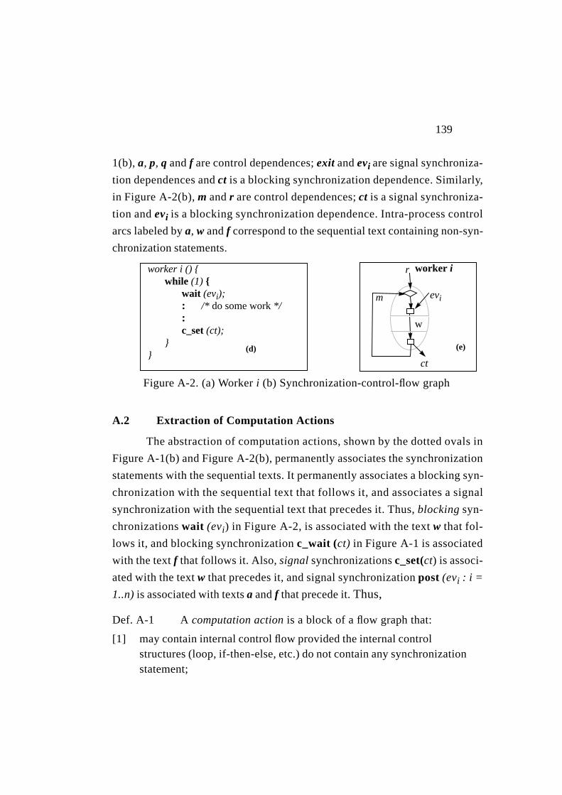
139

1(b),a, p, q andf are control dependences;exit andevi are signal synchroniza-

tion dependences andct is a blocking synchronization dependence. Similarly,

in FigureA-2(b), m andr are control dependences;ct is a signal synchroniza-

tion andevi is a blocking synchronization dependence. Intra-process control

arcs labeled bya, w andf correspond to the sequential text containing non-syn-

chronization statements.

A.2 Extraction of Computation Actions

The abstraction ofcomputation actions, shown by the dotted ovals in

FigureA-1(b) and FigureA-2(b), permanently associates the synchronization

statements with the sequential texts. It permanently associates a blocking syn-

chronization with the sequential text that follows it, and associates a signal

synchronization with the sequential text that precedes it. Thus,blocking syn-

chronizationswait (evi) in FigureA-2, is associated with the textw that fol-

lows it, and blocking synchronizationc_wait (ct) in FigureA-1 is associated

with the textf that follows it. Also,signal synchronizationsc_set(ct) is associ-

ated with the textw that precedes it, and signal synchronizationpost (evi : i =

1..n) is associated with textsa andf that precede it. Thus,

Def. A-1 A computation action is a block of a flow graph that:

[1] may contain internal control flow provided the internal controlstructures (loop, if-then-else, etc.) do not contain any synchronizationstatement;

FigureA-2. (a) Worker i (b) Synchronization-control-flow graph

worker i () {while (1) {

wait (evi);: /* do some work */:c_set (ct);

}}

w

ct

evi

worker i

m

r

(d) (e)

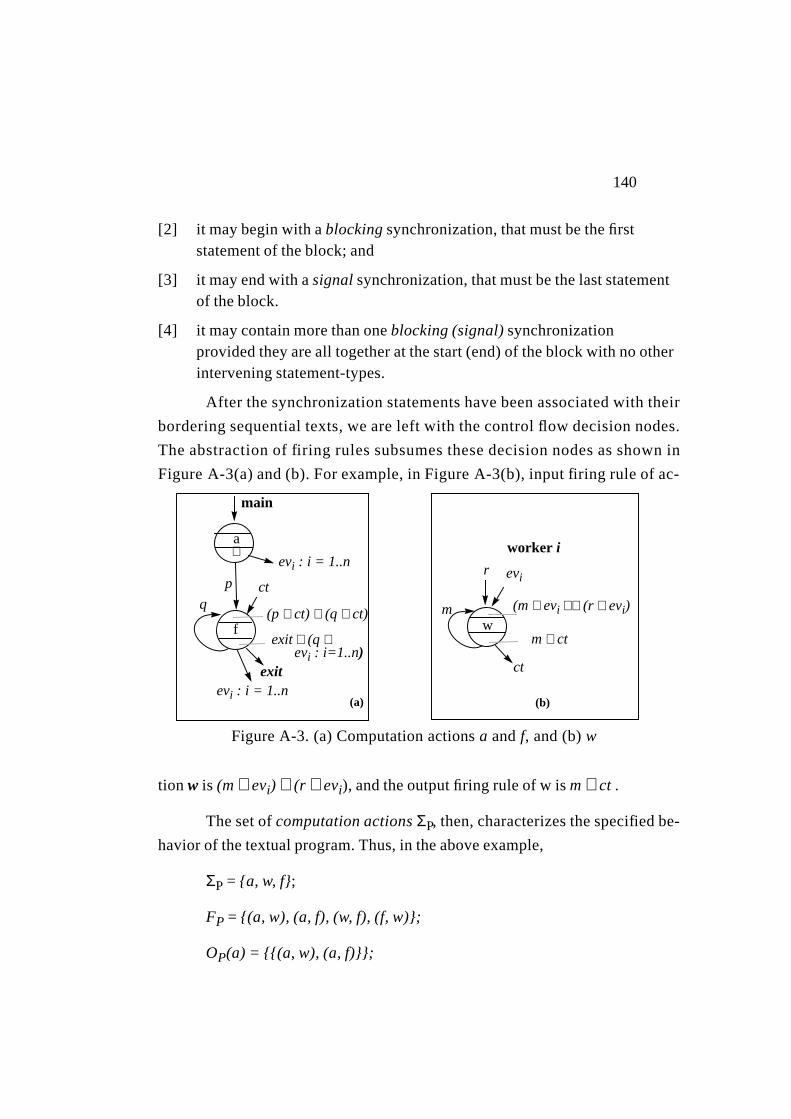
140

[2] it may begin with ablocking synchronization, that must be the firststatement of the block; and

[3] it may end with asignal synchronization, that must be the last statementof the block.

[4] it may contain more than oneblocking (signal) synchronizationprovided they are all together at the start (end) of the block with no otherintervening statement-types.

After the synchronization statements have been associated with their

bordering sequential texts, we are left with the control flow decision nodes.

The abstraction of firing rules subsumes these decision nodes as shown in

FigureA-3(a) and (b). For example, in FigureA-3(b), input firing rule of ac-

tion w is (m ∧ evi) ∨ (r ∧ evi), and the output firing rule of w ism ∧ ct .

The set ofcomputation actions ΣP, then, characterizes the specified be-

havior of the textual program. Thus, in the above example,

ΣP = {a, w, f};

FP = {(a, w), (a, f), (w, f), (f, w)};

OP(a) = {{(a, w), (a, f)}};

f

qct

exitevi : i = 1..n

exit ∨ (q ∧

(p ∧ ct) ∨ (q ∧ ct)

evi : i=1..n)

evi : i = 1..n

main

p

∧

(a)

a

FigureA-3. (a)Computation actionsa andf, and (b)w

wm ∧ ct

ct

evi

worker i

m

r

(m ∧ evi

(b)

) ∨ (r ∧ evi)

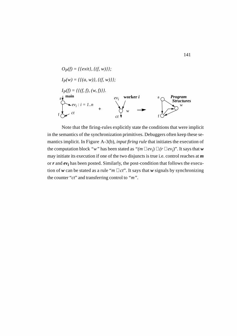
141

OP(f) = {{exit}, {(f, w)}};

IP(w) = {{(a, w)}, {(f, w)}};

IP(f) = {{(f, f), (w, f)}}.

Note that thefiring-rules explicitly state the conditions that were implicit

in the semantics of the synchronization primitives. Debuggers often keep these se-

mantics implicit. InFigureA-3(b), input firing rule that initiates the execution of

the computation block “w” has been stated as“(m ∧ evi) ∨ (r ∧ evi)”. It says thatw

may initiate its execution if one of the two disjuncts is true i.e. control reaches atm

or r andevi has been posted. Similarly, the post-condition that follows the execu-

tion of w can be stated as a rule “m∧ ct”. It says thatw signals by synchronizing

the counter “ct” and transferring control to“m” .

f

a

w

f

a

w

evi : i = 1..n

ct

evi worker i

ct

main

+

ProgramStructures

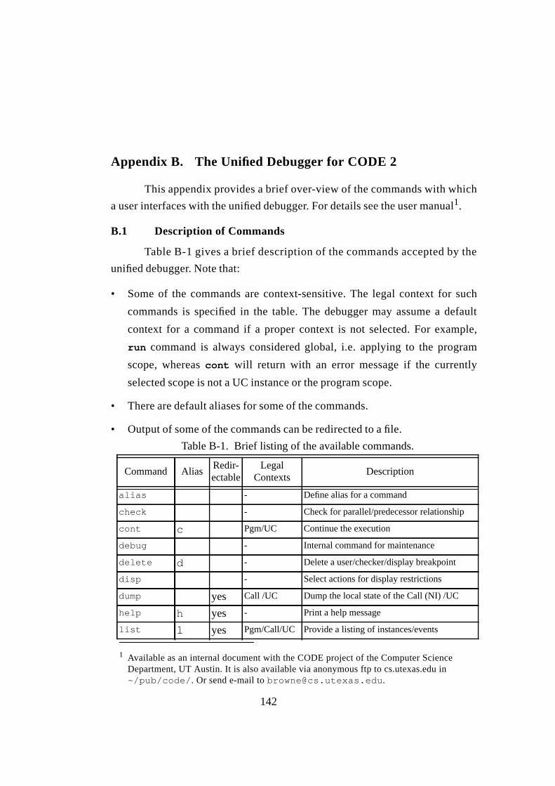
142

Appendix B. The Unified Debugger for CODE 2

This appendix provides a brief over-view of the commands with which

a user interfaces with the unified debugger. For details see the user manual1.

B.1 Description of Commands

Table B-1 gives a brief description of the commands accepted by the

unified debugger. Note that:

• Some of the commands are context-sensitive. The legal context for such

commands is specified in the table. The debugger may assume a default

context for a command if a proper context is not selected. For example,

run command is always considered global, i.e. applying to the program

scope, whereascont will return with an error message if the currently

selected scope is not a UC instance or the program scope.

• There are default aliases for some of the commands.

• Output of some of the commands can be redirected to a file.

1 Available as an internal document with the CODE project of the Computer ScienceDepartment, UT Austin. It is also available via anonymous ftp to cs.utexas.edu in~/pub/code/. Or send e-mail tobrowne@cs.utexas.edu.

TableB-1. Brief listing of the available commands.

Command AliasRedir-ectable

LegalContexts

Description

alias - Define alias for a command

check - Check for parallel/predecessor relationship

cont c Pgm/UC Continue the execution

debug - Internal command for maintenance

delete d - Delete a user/checker/display breakpoint

disp - Select actions for display restrictions

dump yes Call /UC Dump the local state of the Call (NI) /UC

help h yes - Print a help message

list l yes Pgm/Call/UC Provide a listing of instances/events

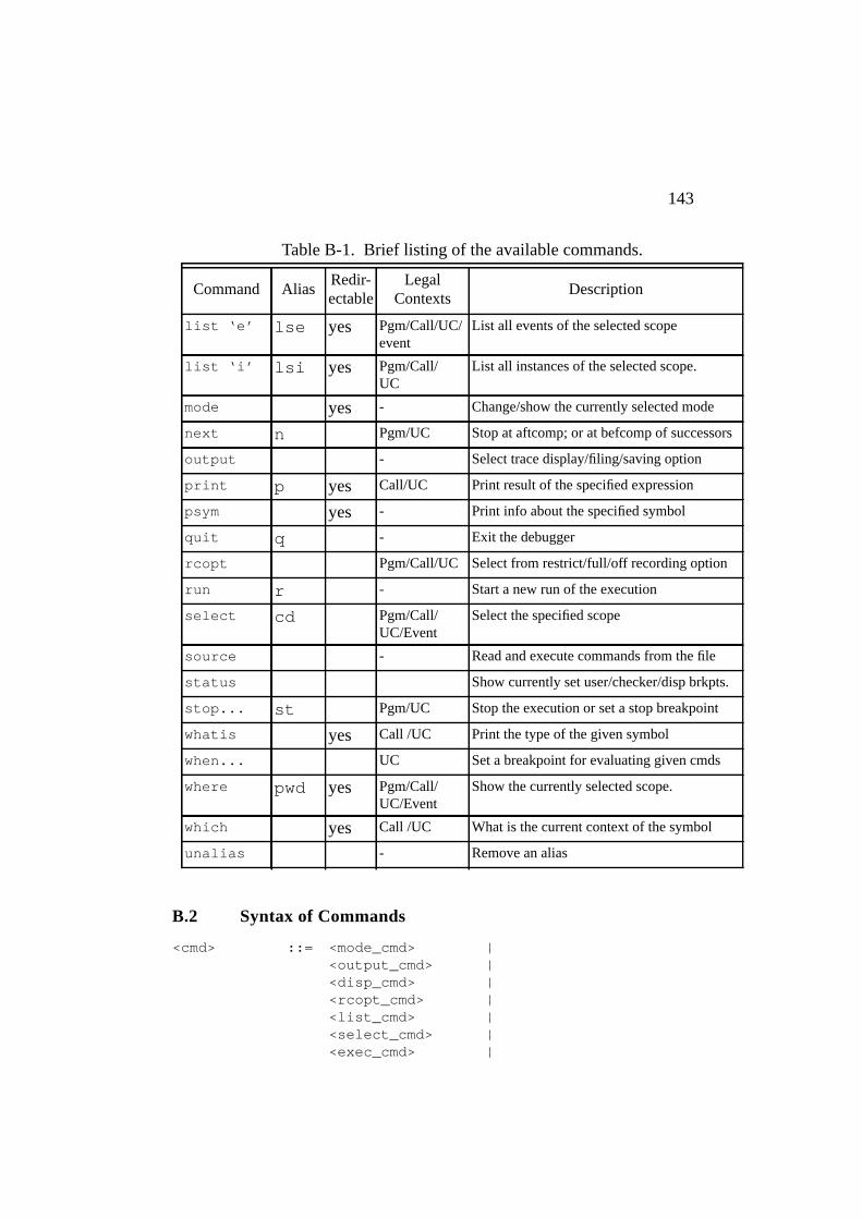
143

B.2 Syntax of Commands

<cmd> ::= <mode_cmd> |<output_cmd> |<disp_cmd> |<rcopt_cmd> |<list_cmd> |<select_cmd> |<exec_cmd> |

list ‘e’ lse yes Pgm/Call/UC/event

List all events of the selected scope

list ‘i’ lsi yes Pgm/Call/UC

List all instances of the selected scope.

mode yes - Change/show the currently selected mode

next n Pgm/UC Stop at aftcomp; or at befcomp of successors

output - Select trace display/filing/saving option

print p yes Call/UC Print result of the specified expression

psym yes - Print info about the specified symbol

quit q - Exit the debugger

rcopt Pgm/Call/UC Select from restrict/full/off recording option

run r - Start a new run of the execution

select cd Pgm/Call/UC/Event

Select the specified scope

source - Read and execute commands from the file

status Show currently set user/checker/disp brkpts.

stop... st Pgm/UC Stop the execution or set a stop breakpoint

whatis yes Call /UC Print the type of the given symbol

when... UC Set a breakpoint for evaluating given cmds

where pwd yes Pgm/Call/UC/Event

Show the currently selected scope.

which yes Call /UC What is the current context of the symbol

unalias - Remove an alias

TableB-1. Brief listing of the available commands.

Command AliasRedir-ectable

LegalContexts

Description

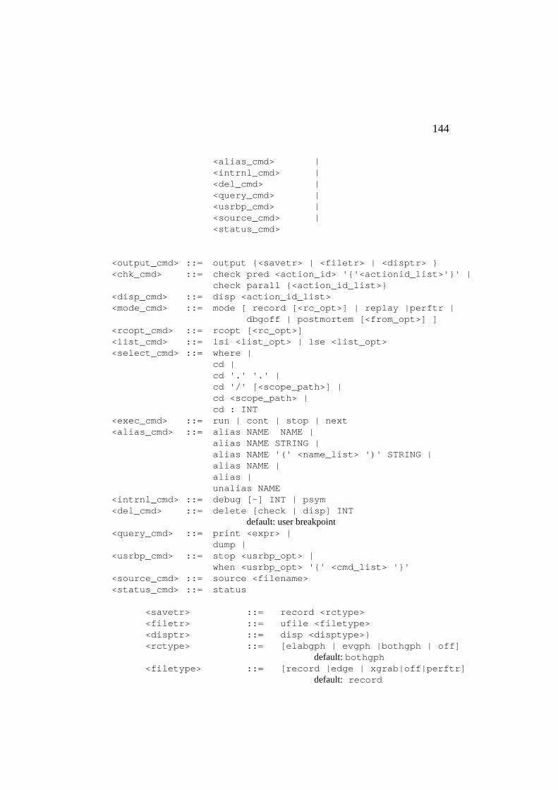
144

<alias_cmd> |<intrnl_cmd> |<del_cmd> |<query_cmd> |<usrbp_cmd> |<source_cmd> |<status_cmd>

<output_cmd> ::= output {<savetr> | <f iletr> | <disptr> }<chk_cmd> ::= check pred <action_id> '{'<actionid_list>'}' |

check parall {<action_id_list>}<disp_cmd> ::= disp <action_id_list><mode_cmd> ::= mode [ record [<rc_opt>] | replay |perftr |

dbgoff | postmortem [<from_opt>] ]<rcopt_cmd> ::= rcopt [<rc_opt>]<list_cmd> ::= lsi <list_opt> | lse <list_opt><select_cmd> ::= where |

cd |cd '.' '.' |cd '/' [<scope_path>] |cd <scope_path> |cd : INT

<exec_cmd> ::= run | cont | stop | next<alias_cmd> ::= alias NAME NAME |

alias NAME STRING |alias NAME '(' <name_list> ')' STRING |alias NAME |alias |unalias NAME

<intrnl_cmd> ::= debug [-] INT | psym<del_cmd> ::= delete [check | disp] INT

default: user breakpoint<query_cmd> ::= print <expr> |

dump |<usrbp_cmd> ::= stop <usrbp_opt> |

when <usrbp_opt> '{' <cmd_list> '}'<source_cmd> ::= source <f ilename><status_cmd> ::= status

<savetr> ::= record <rctype><f iletr> ::= uf ile <f iletype><disptr> ::= disp <disptype>}<rctype> ::= [elabgph | evgph |bothgph | off]

default: bothgph<f iletype> ::= [record |edge | xgrab|off| perftr]

default: record

145

<disptype> ::= [restrict |record |check| off]default: record

<rc_opt> ::= restrict | off | full<from_opt> ::= record | uf ile<scope> ::= <tmplt_name> |

<tmplt_name> <index_list><action_id> ::= <scope>

(of a UC action)<action_id_list> :: <action_id> |

<action_id> ',' <action_id_list><name_list> ::= NAME | NAME ',' <name_list><f ile_name> ::= STRING<tmplt_name> ::= NAME | UID

(of a UC , NS or a Call node template)<index_list> ::= '[' <int_list> ']'<usrbp_opt> ::= [in <where_in>] [at <where_at>]

[if <bool_exp>]<cmd_list> ::= <cmd> ';' |

<cmd> ';' <cmd_list><where_in> ::= <scope><where_at> ::= befcomp | aftcomp<int_list> ::= INT | <int_list> INT<bool_expr> ::= Pred '('action_id_list ')' |

<expr> (of type boolean)<expr> ::= SYMBOL |

CONSTANT |<expr> '[' expr_list ']' |<expr> '.' NAME |'+' <expr> |'-' <expr> |'&' <expr> |<expr> '*' <expr> |<expr> '+' <expr> |<expr> '/' <expr> |<expr> DIV <expr> |<expr> MOD <expr> |<expr> AND <expr> |<expr> OR <expr> |<expr> '<' <expr> |<expr> '<' '=' <expr> |<expr> '>' '=' <expr> |<expr> '=' '=' <expr> | '(' <expr> ')'

(local to a UC scope)

Special Symbols:

NodeIndex ExecCnt Pred

146

Keywords:

alias aftcomp and at befcompcheck cont debug dbgoff deletedisp div edge ufile fullhelp if in list modmode next nil not oroff output perftr parall postmortempred print psym quit recordreplay restrict run select sourcestatus step stop rcopt unaliasuse whatis when where whereiswhich xgrab

147

References

[BAS89] J. C. Browne, M. Azam, and S. Sobek, “A Unified Approach to

Parallel Programming”,IEEE Software, Jul ‘89.

[Bat89] Peter Bates, “Debugging Heterogeneous Distributed Systems using

Event-Based Models of Behavior,”Proceedings of the ACM

SIGPLAN/SIGOPS Workshop on Parallel and Distributed Debugging,

ACM SIGPLAN Notices, 24(1), pp. 11–22, January 1989.

[BH83] Bernd Bruegge and Peter Hibbard. Generalized path expressions: A

high level debugging mechanism.ACM SIGPLAN Notices,

18(8):34–44, March 1983.

[BFM83] F. Baiardi, N.De Francesco, E.Matteoli, S.Stefanini, and G.Vaglini.

Development of a debugger for a concurrent language.Proceedings of

the ACM SIGSOFT/SIGPLAN Software Engineering Symposium on

High-Level Debugging, published in ACM SIGPLAN Notices,

18(8):98–106, August 1983.

[BJN95] J. C. Browne, J. Dongarra, S. I. Hyder, K. Moore and P. Newton,

“Experience with CODE and HeNCE in Visual Programming for

Parallel Computing,” To appear inIEEE Parallel and Distributed

Technology, 1995

[BBC88] V. Balasundaram, D.Baumgartner, D.Callahan, K.Kennedy, and

J.Subhlok, “PTOOL: A System for Static Analysis of Parallelism in

Programs,” Technical Report TR88-71, Rice University, Department

of Computer Science, June 1988.

[CaS89] David Callahan and Jaspal Subhlok, “Static Analysis of Low-level

Synchronization,” Proceedings of the ACM SIGPLAN/SIGOPS

Workshop on Parallel and Distributed Debugging, ACM SIGPLAN

Notices, 24(1), pp. 100–111, January 1989.

148

[ChS91] Jong-Deok Choi and Janice M. Stone, “Balancing Runtime and Replay

Costs in a Trace-and-Replay System,”Proceedings of the ACM/ONR

Workshop on Parallel and Distributed Debugging, in ACM SIGPLAN

Notices, 26(12), pp. 26-35, Dec. 1991.

[ChMi88] K. Mani Chandy and J. Misra, “Parallel Program Design,” Addison-

Wesley, 1988.

[CFH93] J. E. Cuny, G. Forman, A. Hough, J. Kundu, C. Lin, L. Snyder, “The

Ariadane Debugger: Scalable Application of Event Based

Abstractions,” ACM/ONR Workshop on Parallel and Distributed

Debugging, pp. 85-95, 1993.

[EGP89] PerryA. Emrath, Sanjoy Ghosh, and DavidA. Padua, “Event

Synchronization Analysis for Debugging Parallel Programs,” In

Proceedings of Supercomputing ’89, pp. 580–588, Reno NV,

November 1989.

[Fid89] C. J. Fidge, “Partial Orders for Parallel Debugging,”Proceedings of

the ACM SIGPLAN/SIGOPS Workshop on Parallel and Distributed

Debugging, published in ACM SIGPLAN Notices 24(1), Jan. 1989.

[FLM89] RobertJ. Fowler, ThomasJ. LeBlanc, and JohnM. Mellor-Crummey,

“An Integrated Approach to Parallel Program Debugging and

Performance Analysis on Large-scale Multiprocessors,”Proceedings

of the ACM Workshop on Parallel and Distributed Debugging, ACM

SIGPLAN NOTICES, 24(1), pp. 163–173, January 1989.

[For89] Alessandro Forin. Debugging of heterogeneous parallel systems.

Proceedings of the ACM SIGPLAN/SIGOPS Workshop on Parallel

and Distributed Debugging, published in ACM SIGPLAN Notices,

24(1):130–140, January 1989.

[FoZw90] J. Fowler and W. Zwaenpoel, “Causal Distributed Breakpoints,” proc.

10th International Conference on Distributed Computing, France, pp.

149

134-41, May 1990

[Gai88] Haim Gaifman, “Modeling Concurrency by Partial Orders and

Nonlinear Transition Systems,”Linear Time, Branching Time, and

Partial Order in Logics and Models of Concurrency, LNCS, (354), pp.

467–488, May 1988.

[GaW92] V. K. Garg and B. Waldecker, “Detection of Unstable Predicates in

Distributed Programs,”Proc. 12th Conference of the Foundations of

Software Technology and Theoretical Computer Science, R.

SShyamasundra (ed.), Springer-Verlag, LNCS 652, pp. 253-264,

1992.

[HWB93] S. I. Hyder, J. F. Werth, J. C. Browne, “A Unified Model for

Concurrent Debugging,” Proc. Intl. Conf. on Parallel Processing, pp.

II-58-67, Chicago, July 1993.

[HHK85] PaulK. Harter, Jr., DennisM. Heimbigner, and Roger King, “IDD: An

Interactive Distributed Debugger,” Technical report, University of

Colorado, 1985.

[HoC87] Alfred A. Hough and JaniceE. Cuny, “Belvedere: Prototype of a

Pattern-oriented Debugger for Highly Parallel Computation,” In

Proceedings of the 1987 International Conference on Parallel

Processing, pp. 735–738, University Park PA, 1987.

[HoC90] Alfred A. Hough and JaniceE. Cuny, “Perspective views: A

Technique for Enhancing Parallel Program Visualization,” In

Proceedings of 1990 International Conference on Parallel

Processing, pp. II.124–II.132, University Park PA, August 1990.

[Ho91] Alfred A. Hough, “Debugging Parallel Programs using Abstract

Visualizations, “Technical Report 91:53, University of Massachusetts

at Amherst, Computer Sciences Department, September 1991.

[HsK90]] Wenway Hseush and GailE. Kaiser, “Modeling Concurrency in

150

Parallel Debugging,” InSecond ACM SIGPLAN Symposium on

Principles and Practice of Parallel Programming, pp. 11–20, Seattle

WA, March 1990.

[HMW90] DavidP. Helmbold, CharlesE. McDowell, and Jian-Zhong Wang,

“Analyzing Traces with Anonymous Synchronization,” In

Proceedings of 1990 International Conference on Parallel

Processing, pp. II.70–II.77, University Park PA, August 1990.

[JhZw90] D.B. Johnson and W. Zwaenpoel, “Recovery in Distributed Systems

Using Optimistic Message Logging and Checkpointing,” Journal of

Algorithms, Vol. II, No. 3, pp. 462-91, Sep. 1990.

[KiZe93] Doug Kimelman and Dror Zernik, “On-the-fly topological sort- A

Basis for Interactive Debugging and Live Visualizations of Parallel

Programs, ACM/ONR Workshop on Parallel and Distributed

Debugging, ACM Sigplan Notices, Vol. 28(12), pp. 12-20 Dec. 1993.

[Lam86] Leslie Lamport, “Mutual exclusion problem: Part I – a theory of

interprocess communication, “Journal of ACM, 33(2), pp. 313–326,

April 1986.

[LM86] ThomasJ. LeBlanc and JohnM. Mellor-Crummey, “Debugging

Parallel Programs with Instant Replay,” IEEE Transactions on

Computers, Vol. C-36, NO. 4, 471-81, April 1987.

[LeM89] Ed. T.J. Leblanc and B.P. Miller, “Workshop Summary: What we

have learned and where do we go from here?” InACM

SIGPLAN/SIGOPS Workshop on Parallel and Distributed Debugging,

ACM SIGPLAN Notices, 24(1), pp. ix–xxii, January 1989.

[LMF90] ThomasJ. LeBlanc, JohnM. Mellor-Crummey, and RobertJ. Fowler,

“Analyzing Parallel Program Executions using Multiple Views,”

Journal of Parallel and Distributed Computing, 9, pp. 203–217, June

1990.

151

[Mat89] Friedemann Mattern, “Virtual Time and Global States of Distributed

Systems,”Parallel and Distributed Algorithms, pp. 215–226, 1989.

[McD89] CharlesE. McDowell, “A Practical Algorithm for Static Analysis of

Parallel Programs,”Journal of Parallel and Distributed Computing, 6,

pp. 515–536, 1989.

[McH89] CharlesE. McDowell and DavidP. Helmbold, “Debugging

Concurrent Programs,”ACM Computing Surveys, 21(4), pp. 593–622,

December 1989.

[Mi92] B. P. Miller, “What to draw? When to draw? An assay on Parallel

Program Visualization,” TR-1103, University of Wisconsin, Madison,

WI, July 1992.

[MiC88] Barton P. Miller and Jong-Deok Choi, “Breakpoints and Halting in

Distributed Programs,”Proc. 8th Intl. Conf. on Distributed Computing

Systems, pp. 316-23, Jan 1988.

[MiC89] Barton P. Miller and Jong-Deok Choi, “A Mechanism for Efficient

Debugging of Parallel Programs,”Proceedings of the ACM

SIGPLAN/SIGOPS Workshop on Parallel and Distributed Debugging,

ACM SIGPLAN Notices, 24(1), pp. 141-50, Jan 1989.

[MaI92] Y. Manabe and M. Imase, “Global Conditions in Debugging

Distributed Programs,” Journal of Parallel and Distributed Computing,

No. 15, pp. 62-69, 1992.

[NM90a] Robert H.B. Netzer and BartonP. Miller, “Detecting Data Races in

Parallel Program Executions,” InProc. of Third Workshop on

Programming Languages and Compilers for Parallel Computing,

August 1990.

[NM90b] Robert H.B. Netzer and BartonP. Miller, “On the Complexity of

Event Ordering for Shared-Memory Parallel Program Executions,” In

Proceedings of 1990 International Conference on Parallel

152

Processing, pp. II.93–II.97, University Park PA, August 1990.

[NM91a]] Robert H.B. Netzer and BartonP. Miller, “Improving the Accuracy of

Data race detection,”Proc. of the 3rd ACM Symposium on Principles

and Practices of Parallel Programming, Williamsburg, VA, (April

1991).

[NM91b] Robert H.B. Netzer and BartonP. Miller, “What are Race

Coonditions? Some Issues and Formalism,” Technical Report TR91-

1014, University of Wisconsin, Madison, Department of Computer

Science, March 1991.

[Net93] Robert H.B. Netzer, “Optimal Tracing and Replay for Debugging

Shared Memory Parallel Programs,” Proc. of ACM/ONR Workshop

on Parallel and Distributed Debugging, Sigplan Notices 28(12), pp. 1-

11, Dec. 1993.

[NeB92] P. Newton and J. C. Browne, “The Code 2.0 Graphical Programming

Environment,” InProceedings of ACM Intl. Conf. on Supercomputing,

July 1992.

[New93] Peter Newton, “A Graphical Retargetable Parallel Programming

Environment and its Efficient Implementation, Ph. D. Dissertation,

The University of Texas at Austin, December 1993.

[PaU89] CherriM. Pancake and Sue Utter, “Models for Visualization in

Parallel Debuggers,” InProceedings of Supercomputing ’89, pp.

627–636, Reno NV, November 1989.

[PaN93] Cherri M. Pancake and Robert H. B. Netzer, “A Bibliography of

Parallel Debuggers, 1993 Edition,” Proc ACM/ONR Workshop on

Parallel and Distributed Debugging, ACM Sigplan Notices, 28(12),

pp. 169-86, Dec. 1993.

[Pra86] Vaughan Pratt, “Modeling Concurrency with Partial Orders,”

International Journal of Parallel Programming, 15(1), pp. 33–71,

153

1986.

[RDB+87] L. A. Rowe, M. Davis, E. Messinger, C. Meyer, C., Spirakis and A.

Tuan. “A Browser for Directed Graphs” , Software Practice &

Experience, Volume 17, #1, pp. 61-76, January 1987.

[ReSc94]] Reinhard Schwarz and Friedemann Mattern, “Detecting Causal

Relationships in Distributed Computations:In Search of the Holy

Grail,” Distibuted Computing 7(3), pp. 149-174, (1994)

[Rus91] Mark Russel <mtr@ukc.ac.uk>, “UPS: interpreter, symbolic

debugger,” package available by ftp fromcontrib/ups*.tar.Z from

export.lcs.mit.edu

[SBN89] David Socha, MaryL. Bailey, and David Notkin, “Voyeur: Graphical

Views of Parallel Programs,” Proceedings of the ACM

SIGPLAN/SIGOPS Workshop on Parallel and Distributed Debugging,

published in ACM SIGPLAN NOTICES, 24(1), pp. 206–215, January

1989.

[Sch89] Edith Schonberg. On-the-fly detection of access anomalies.

Proceedings of the SIGPLAN ’89 Conference on Programming

Language Design and Implementation, published in ACM SIGPLAN

Notices, 24(7):285–297, July 1989.

[Sy83] Proceedings of the ACM SIGSOFT/SIGPLAN Software Engineering

Symposium on High-level Debugging, Pacific Grove, CA, March

1983. Also published inSigplan Notices, Vol 18(8), Aug. 1983.

[Tay83] RichardN. Taylor, “A General Purpose Algorithm for Analyzing

Concurrent Programs,”Communications of the ACM, 26(5), pp.

362–376, May 1983.

[Tay84] Richard N. Taylor, “Complexity of Analyzing the Synchronization

Structure of Concurrent Programs,”Acta Informatica, 19(1), pp. 57-

84, 1983.

154

[TaO80] RichardN. Taylor and LeonJ. Osterweil, “Anomaly detection in

Concurrent Software by Static Data-Flow Analysis,”IEEE

Transactions on Software Engineering, SE-6(3), pp. 265–278, May

1980.

[UtP89] Sue Utter and CherriM. Pancake, “A Bibliography of Parallel

Debugging Tools,”ACM SIGPLAN Notices, 24(10), pp. 24–42, 1989.

[Vok94] Rajeev M. Vokkarne, “Distributed Execution Environments for the

CODE 2.0 Parallel Programming System,” Masters Thesis,

Department of Computer Science, UT Austin, December 1994.

[WaG91] Brian Waldecker and Vijay Garg, “Detection of Predicates in

Distributed Programs,” Ph.D. dissertation, Univ. of Texas at Austin,

1991.

[Wag94] Yogesh S. Wagle, “Process Migration In Network Parallel

Software Systems,” Masters Thesis, UT Austin, December 1994.

[YoTa86] M. Young and R. N. Taylor, “Combining Static Concurrency Analysis

with Symbolic Execution”, Proceedings Workshop on Software

Testing, pp. 10-18, 1986,

[ZeR91] Dror Zernik and Mark Rudolph, “Animating Work and Time for

Debugging Parallel Programs; Foundation and Experience,”

Proceedings of the ACM/ONR Workshop on Parallel and Distributed

Debugging, ACM Sigplan Notices, 26(12), pp. 46-56. Dec 1991.

Vita

Syed Irfan Hyder was born in Rawalpindi, Pakistan on August 29,

1962, the son of Syed Ahsan Hyder and Huzabra Hyder. He did his intermedi-

ate from Islamabad College for Boys in 1979 and secured a silver medal in the

Higher Secondary School Certificate examination of the Federal Board. He re-

ceived the degree of Bachelor of Engineering in E. E. from the NED Universi-

ty of Engineering and Technology, Karachi, in 1985. He, then, obtained the

M.B.A degree from the Institute of Business Administration, Karachi Univer-

sity in 1987. After a brief stay at Space and Upper Atmosphere Research Com-

mission (SUPARCO), Karachi, he entered the Graduate School of the

University of Texas in August of 1987. In 1989, he obtained an M.S. degree

from the Department of Electrical Engineering. Since then, he has been work-

ing as a Research Assistant in the CODE graphical/visual parallel program-

ming project of the Department of Computer Science.

Permanent address: 201/O Block-II, PECHS, Karachi-75400, Pakistan

This dissertation was typed by the author.