Decentralized inventory control in a two-level distribution system

Theory and Methodology

Decentralized inventory control in a two-level distribution system

Jonas Andersson, Johan Marklund *

Department of Industrial Engineering, Lund University, P.O. Box 118, 221 00 Lund, Sweden

Received 1 September 1998; accepted 1 April 1999

Abstract

We consider a model for decentralized inventory control in a two-level distribution system with one central ware-

house and N non-identical retailers. All installations use continuous review installation stock �R;Q�-policies for re-

plenishing their inventories. Our approach is based on an approximate cost evaluation technique, where the retailers

replace their stochastic lead-times by correct averages. By introducing a modi®ed cost-structure at the warehouse, the

multi-level inventory control problem can be decomposed into N � 1 single level sub-problems, one problem for each

installation. The sub-problems are then solved in an iterative manner by a simple coordination procedure, which can be

interpreted as a negotiation process. In the case of normally distributed demand we show that the procedure converges

to a near optimal solution. To assess the quality of the involved approximation an upper bound for the relative cost

increase of using the obtained solution is derived. We also provide a numerical study illustrating the performance of our

approach. Ó 2000 Elsevier Science B.V. All rights reserved.

Keywords: Supply chain; Inventory; Multi-echelon; Decentralization; Stochastic; Arborescent systems; Batch ordering

1. Introduction

An important issue in managing a supply chainis to reduce the cost of capital tied up in inventory,while still maintaining a high service level towardsthe end customers. To succeed, the inventory de-cisions at di�erent installations in the supply chainneed to be e�ciently coordinated. For small sys-tems where, typically, all installations belong to

the same organization and all relevant informationabout the system is readily available, the naturalapproach to achieve such coordination is to cen-tralize all inventory decisions. For larger systems,especially when di�erent organizations are in-volved, centralized control is often not a viableoption. The di�culties that arise are both technicaland managerial. Technically it is a huge challengeto obtain and process all the relevant data for theentire system centrally. From a managerial pointof view it is very di�cult to centralize the inven-tory control if the basic organizational structure isdecentralized. These problems are of course evenmore accentuated in supply chains where the

European Journal of Operational Research 127 (2000) 483±506www.elsevier.com/locate/dsw

* Corresponding author. Tel.: +46-46-222-4811; fax: +46-46-

222-4649.

E-mail address: [email protected] (J. Marklund).

0377-2217/00/$ - see front matter Ó 2000 Elsevier Science B.V. All rights reserved.

PII: S 0 3 7 7 - 2 2 1 7 ( 9 9 ) 0 0 3 3 2 - X

installations belong to independently owned com-panies.

In this paper we focus on a model for highlydecentralized inventory control in a two-level dis-tribution system with one central warehouse and Nnon-identical retailers. It is especially suitable fordecentralized organizations, where each installa-tion is seen as a cost center responsible for thecosts it can a�ect. The model is based on a simpleapproximate cost allocation scheme where thecentral warehouse is charged a penalty cost basedon its inability to deliver on time to the retailers inthe system. The approximation involved is closelyrelated to the well known METRIC approach, seeSherbrooke (1968), where the stochastic lead-timesperceived by the retailers are replaced by theircorrect averages. In other words, the decentralizedmodel is based on limited information about thelead-time characteristics. A more technical de-scription of our approach, reveals that it is anextension of the decentralized control procedure inAndersson et al. (1998), to the case of completelynon-identical retailers.

The outlay of the paper is as follows: The restof this section is devoted to a brief literature reviewand a discussion of related models. Section 2contains a detailed description of the inventorysystem. We discuss the speci®c assumptions made,and de®ne the cost functions used in the exact andapproximate models, respectively. Section 3 fo-cuses on how to solve the approximate problem bydecomposing the entire system into N � 1 coordi-nated single level problems. In Section 4 we derivean upper bound on a performance ratio relatingthe total cost obtained from the approximate so-lution, to the true minimum cost. To compute thebound we need to derive the lead-time distributionfor each retailer. In Appendix A we present amethod, which provides an accurate approxima-tion of this distribution. In Section 5 we discuss asimple approximate expression for the expectedlead-time perceived by a certain retailer. We alsoinvestigate in detail how to solve the generatedsub-problems. Finally, we present some numericalresults to illustrate the performance of our coor-dination procedure and the approximations in-volved. Section 6 concludes and summarizes ourresults.

1.1. Literature review

A lot of research has been devoted to costevaluation and optimization of stochastic multi-echelon inventory systems under various controlpolicies. For recent general overviews we refer toAxs�ater (1993), Federgruen (1993), Van Houtumet al. (1996) and Diks et al. (1996). A number ofthese existing models use control policies based oncentralized information. An important example isechelon stock policies, where decisions at each sitedepend on information from all downstream in-stallations. The echelon stock concept was ®rstintroduced in the seminal work by Clark and Scarf(1960). For recent applications to divergent sys-tems under continuous review see, for example,Chen and Zheng (1997) and Axs�ater (1997). Inanother important class of models the decisionsmade at each installation depend only upon localinformation. One common example of this type ofcontrol policy is an installation stock �R;Q�-policy.In this policy the decisions to order from an up-stream installation depend only upon the localinventory position. From this perspective manycontrol methods are decentralized. However, inmost of the existing models, even though thecontrol variables are de®ned using local informa-tion, the determination of optimal control policiesis done in a centralized manner. A model for jointoptimization of reorder points in a multi-levelsystem using installation stock �R;Q�-policies is,for example, centralized from this perspective, seeAxs�ater (1998), for an exact model when the de-mand is compound Poisson. To a large extentthese `decentralized' models still su�er from thetechnical and managerial di�culties discussedabove.

Models for stochastic multi-echelon inventorycontrol, which are decentralized also in terms ofthe way the optimal control policies are evaluated,represent a small but growing body of the litera-ture. Lee and Whang (1994) provide an incentive-compatible scheme for a serial system based on theClark and Scarf model, where the installations aremanaged as cost centers. The scheme is based ontransfer payments between the di�erent installa-tions. The idea to achieve decentralization by de-signing new cost structures also governs the work

484 J. Andersson, J. Marklund / European Journal of Operational Research 127 (2000) 483±506

by Axs�ater (1995), which deals with a conceptualframework for decentralized inventory control ofdivergent systems. Andersson et al. (1998) focus ona model for decentralized control of a divergentdistribution system, under the restriction of limitedinformation availability. As mentioned above,their model is closely related to ours but restrictedto the case where all retailers use an identical orderquantity. Chen (1997) like Lee and Whang (1994)considers a serial system and bases the analysis onthe Clark and Scarf model. Otherwise these twomodels are quite di�erent. Instead of designingnew cost structures Lee and Billington (1993) fa-cilitate decentralized control by using service-levelconstraints for upstream installations. There alsoexist some earlier work by Muckstadt and Thomas(1980), followed up by Hausman and Erkip (1994).In both cases decentralized control policies formulti-echelon inventory systems with low-demanditems in an emergency resupply model are con-sidered. More precisely, they compare the use ofsingle echelon models with service level constraintsto the performance of a multi-echelon model forthe same system.

Although the main feature of our model is thedecentralization aspect, an important ingredientin our approach is the quality of the imposedlead-time approximation. As indicated above, theidea to approximate the stochastic retailer lead-time with its mean originates from the METRICmodel by Sherbrooke (1968). One of the mostwell known examples where this idea has beenapplied to a divergent batch ordering system isthe model by Deuermeyer and Schwarz (1981).They consider a system similar to ours with theexceptions that in their case demand is Poissonand all retailers are identical. Their objective is tocompute good approximations of the ®llrate at allthe installations in the system. Apart from usingthe discussed lead-time approximation they alsoapproximate the warehouse lead-time demandwith a normal distribution. Based on a numericalstudy they conclude that the method performsquite well and closely estimates the exact ®llrates.An evaluation of how well the Deuermeyer±Sch-warz approach works when used to approximatethe costs of the system was done in Svoronos andZipkin (1988), which investigates several re®ne-

ments of the Deuermeyer±Schwarz model. Themost notable ones are that they estimate both themean and variance of the retailer lead-time inorder to approximate the retailer lead-time de-mand. They also use a mixture of two translatedPoisson distributions (called an MTP distribu-tion) to approximate the warehouse lead-timedemand. Based on a numerical study, they con-clude that their method is more accurate than theDeuermeyer±Schwarz model when it comes toevaluating the system costs, especially for situa-tions where the standard deviation of the lead-time demand is large compared to its mean.Recently, Forsberg (1997) presented a method forexact cost evaluation of a slightly more generalsystem than investigated in Svoronos and Zipkin(1988) where the retailers are allowed to becompletely non-identical. A small numericalstudy veri®es that the Svoronos±Zipkin modelperforms quite well especially for low demandintensities.

A comparison between our approximate modeland the Deuermeyer±Schwarz method implies thatour model should be more robust although notnecessarily always better. The motive being thatwe invoke only one of the approximations used byDeuermeyer and Schwarz. Qualitatively relatingour model to the one by Svoronos and Zipkin ismore di�cult and we have therefore performed asmall numerical study, see Appendix B, for thespecial case where all retailers use the same orderquantity (the most general case the Svoronos±Zipkin model can handle). In all these numericalexamples our method produced near optimal pol-icies of better quality than the Svoronos±Zipkinmodel.

2. Problem formulation

2.1. The inventory system

As indicated above, the inventory system underconsideration consists of one central warehouseand an arbitrary number of non-identical retailers,see Fig. 1.

The customer demand takes place at the re-tailers, which replenish their stock from the

J. Andersson, J. Marklund / European Journal of Operational Research 127 (2000) 483±506 485

warehouse. Transportation times for such deliv-eries are assumed to be constant but additionaldelays may occur due to stockouts at the ware-house. The warehouse on the other hand replen-ishes its stock from an outside supplier, whichprovides constant delivery lead-times. The ware-house only allows for complete deliveries. Thismeans that in case of stockouts no deliveries to acertain retailer will be executed until the wholeorder quantity is available at the warehouse. Thisis a plausible policy not uncommon in practice(see for example Deuermeyer and Schwarz, 1981),especially when there is a ®xed cost connected toeach transport. The otherwise prevailing as-sumption in the literature on modeling divergentmulti-level inventory systems is to use a deliverypolicy allowing for partial deliveries, i.e., units areshipped to the designated retailer as soon as theyare available at the warehouse. Stockouts at bothechelons are handled according to a ®rst-come-®rst-served strategy and all facilities apply con-tinuous review installation stock �R;Q�-policies.This means that as soon as the inventory positionat a certain installation (� inventory on hand +outstanding orders ) backorders) drops to or be-low the reorder point, R, an order of size Q isinitiated to the upstream installation. The motivesfor studying this particular policy, even though itmight not be the optimal one, are its wide prac-tical application and its high generality. Con-cerning the cost structure we consider holdingcosts at both echelons and shortage costsproportional to the time until delivery at theretailers.

For a further discussion of the assumptionsde®ning our system, we need to introduce somenotation:

We assume that all order quantities are ®xedand predetermined, which means that the onlydecision variables under consideration are the re-order points:

The assumption of predetermined and ®xedorder quantities might appear as a signi®cantweakness of our model. However, we argue thatthis restriction is not as damaging as it might seem.Physical restrictions such as container size oftenleave little room for varying the order quantities.Furthermore, indications are that using determin-istic lot sizing methods in a stochastic environmentwill only have a marginal e�ect on the expectedcost, provided that the reorder points are adjustedaccordingly, see for example Zheng (1992) andAxs�ater (1996). An appealing heuristic, suggestedby several researchers, see for example Chen andZheng (1997), is therefore to use a deterministicmodel to determine the order quantities. Nearoptimal reorder points, for the given set of order

N number of retailers (i � 1; 2; . . . ;N ),Q the size of a subbatch in number of units

(we de®ne a subbatch to be the largestcommon divisor of all order quantities inthe system),

qi the batch size used by retailer i, expressedin units of Q,

Qi the batch size used by retailer i, expressedin number of units, Qi � qiQ,

Q0 warehouse batch size, in units of Q,L0 constant lead-time for an order to arrive at

the warehouse,li transportation time between the

warehouse and retailer i,Li lead-time for an order to arrive at retailer i,

stochastic variable (s.v.),�Li expected lead time for an order to arrive at

retailer i ��Li � E�Li��.

Ri reorder point for retailer i, continuousvariable �i � 1; 2; . . . ;N�,

R0 warehouse reorder point, in units of Q,RE�

0 true optimal warehouse reorder point, inunits of Q,

RA�0 optimal warehouse reorder point in the

approximate model, in units of Q.

Fig. 1. The structure of the multi-echelon inventory system.


quantities, can then be found by applying a sto-chastic model to the system.

The motive for restricting the warehouse reor-der point to be in units of Q, is that if the initialinventory position at the warehouse is an integermultiple of Q, it follows from the ordering policyat the retailers that one optimal value of R0 mustalso be an integer multiple of Q. We further re-strain the analysis to values of R0 greater than orequal to )1, i.e. ÿQ units. The restriction meansthat each retailer order will be covered by itemsfrom a warehouse order initiated at the retailer-ordering instance or earlier. This limits the maxi-mum stockout delay that a retailer order canexperience to L0. It also means that the lead-timefor a certain retailer order is independent of thedemand at the warehouse after the retailer order inquestion has been placed. Consequently, the lead-times, Li �i � 1; 2; . . . ;N�, can from the retailerspoint of view be treated as exogenously generatedstochastic variables.

An important characterization of the system isthe properties of the stochastic demand faced bythe retailers. Initially we assume, as in Anderssonet al. (1998), that the cumulative demand perceivedby a single retailer can be modeled as a non-decreasing continuous stochastic process, withstationary and independent increments. In thiscase the inventory position at each retailer willbe uniformly distributed over the interval�Ri;Ri � Qi�, see Browne and Zipkin (1991) andZheng (1992). Later, we will focus on the specialcase when the cumulative customer demandfollows a Wiener process with drift.

A new feature of this problem formulationcompared to the related problem investigated inAndersson et al. (1998) is that we allow each re-tailer to use an individual order quantity. Thisseemingly minor generalization signi®cantly en-hances the practical value of the model but alsomakes the mathematical analysis more intricate.

2.2. Cost functions in the exact and approximateproblems

The expected cost for the entire system can beexpressed in the following schematic way:

TCE � C0 �XN

i�1

CEi ; �1�

where TCE is the expected total system cost pertime unit, CE

i the expected cost per time unit atretailer i and C0 is the expected warehouse cost pertime unit.

We also need to de®ne what will be denoted asthe approximate problem or the approximatemodel for the remainder of this paper. In the exactmodel above the replenishment lead-time for re-tailer i, Li, is a stochastic variable. In the ap-proximate model these stochastic lead-times(Li; i � 1; 2; . . . ;N� are replaced by their expectedvalues, �Li; i � 1; 2; . . . ;N . The total cost in theapproximate model can be expressed as follows:

TCA � C0 �XN

i�1

CAi ; �2�

where TCA is the expected total system cost pertime unit in the approximate model and CA

i isthe expected cost per time unit at retailer i in theapproximate model.

2.3. The retailer cost function

Traditionally the inventory cost at an installa-tion is divided into ordering costs, inventoryholding costs, and some sort of shortage orbackorder costs, see for example Hadley andWhitin (1963). Since the ordering cost is una�ectedby the choice of ordering point, Ri, we exclude thiscomponent from the retailer cost function. Thisleaves us with an expression evaluating the in-ventory holding costs and the backorder costs. Fora certain choice of ordering point at the ware-house, R0, the replenishment lead-time for retaileri in the approximate model (�Li�R0�) is constant.The expected cost per time unit is then given by (3)(see for example Zheng, 1992):

CAi �Rij�Li�R0�� 1

Qi

Z Ri�Qi

Ri

EDi��Li�

hi�yh

ÿ Di��Li�� pi�Di��Li� ÿ y��i

dy; �3�


where �x�� max�x; 0�, hi the holding cost perunit and time unit at retailer i, pi the shortage costper unit and time unit at retailer i, or, equivalently,according to LittleÕs formula, per average numberof backorders, and Di�t� is the customer demand atretailer i during the time period t, (s.v.).

It is worth stressing that the expected lead-times, �Li, are di�erent for di�erent retailers. Whenmodeling a system with non-identical retailers thisproperty becomes crucial and we deal with thisissue both in Appendix A and in Section 5.

In the exact model where the replenishmentlead-time for retailer i, Li, is stochastic, we canobtain the expected cost by conditioning on thelead-time. In practice this expression is di�cult toevaluate since the distribution of Li is hard toobtain.

CEi �RijLi�R0�� ELi�R0�

1

Qi

Z Ri�Qi

Ri

EDi�Li�

24hi�y� ÿ Di�Li�� pi�Di�Li� ÿ y��jLi

�dy

35: �4�

Note that expression (4) is only valid for exoge-nously generated lead-times, that is, whenR0 Pÿ 1 (see Andersson et al., 1998). Also notethat expression (4) holds because the warehouseonly allows for deliveries of complete batches, Qi,to retailer i.

2.4. The cost function at the central warehouse

The fact that we allow each retailer to havedi�erent order quantities, Qi, together with thedelivery policy of only shipping complete retailerbatches from the warehouse, leads to the occur-rence of reserved units. A reserved unit is orderedby a retailer and available at the warehouse but itis not yet shipped. The reason for this is thatthere is not enough inventory on hand at thewarehouse to ®ll the entire retailer order inquestion, i.e., the reserved units must wait for thearrival of deliveries from the external supplierbefore they can be shipped. Due to the existence

of reserved subbatches at the warehouse, the in-ventory position (� inventory on hand + out-standing orders ) backorders) is not uniformlydistributed between R0 � 1 and R0 � Q0. To han-dle this complication we utilize an idea used inLee and Moinzadeh (1987) and treat the reservedunits separately. This is done by de®ning amodi®ed inventory position, y0� inventory onhand + outstanding orders ) backorders ) reservedunits, which is uniformly distributed over theinterval �R0;R0 � Q0�. The cost function at thecentral warehouse C0 can then be expressed asfollows:

C0�R0� � h0QQ0

XR0�Q0

y0�R0�1

ED0�L0� �y0

� ÿ D0�L0��

� h0QE�Br0� � h0Q�E�I0� � E�Br

0��; �5�

where y0 is the modi®ed inventory position at thewarehouse expressed in units of Q, h0 the holdingcost per unit and time unit at the warehouse,D0�t� the retailer demand at the warehouse dur-ing the time period t expressed in units of Q, Br

0

the number of reserved subbatches at the ware-house in steady state, and I0 is the inventory onhand at the central warehouse in steady state,expressed in units of Q, excluding the reservedsubbatches Br

0.Note that the only cost component considered

at the warehouse is the inventory holding cost.From the systems perspective shortage costs onlyoccur when customer demand is backordered at aretailer, not when a retailer, order is delayed at thewarehouse.

3. Decomposition and coordination

In this section we will discuss how to solve theapproximate problem by using a decompositiontechnique together with an iterative coordinationprocedure. The approach that we use is based onthe one in Andersson et al. (1998), but it is mod-i®ed to handle our situation with non-identicalretailers using individual order quantities andcomplete deliveries from the warehouse.


3.1. Decomposition of the approximate problem

We would like to transform the approximateproblem, which is a complicated multi-level in-ventory problem, into N � 1 conceptually simplesingle-level problems coordinated by using a lim-ited amount of information.

The basic idea is that each installation must usea cost function, which re¯ects the impact that acertain choice of its reorder point has on the totalsystem cost. Obviously, the retailer cost function,CA

i , ful®lls these requirements in its present form.Consequently we de®ne the N retailer problems inthe following way:

minRi

CAi �Rij�Li�; i � 1; 2; . . . ;N : �6�

The optimal solution to (6), given a certain valueof �Li, will be denoted R�i . Note that since R�i is afunction of �Li the proper denotation would beR�i ��Li), for notational convenience we disregardthis when there is no loss of clarity.

Turning to the situation at the central ware-house, we can conclude that a certain choice ofreorder point, R0, will a�ect the cost at the retailerlevel, and thereby the total cost through the ex-pected lead-times, �Li. We capture this mechanismby including the marginal cost for lead-timechange in the cost function, ~C0�R0�, used by thewarehouse (see Eq. (7)).

minR0

~C0�R0�

� minR0

C0�R0� �XN

i�1

dCAi �R�i j�Li�d�Li

� ��Li�R0� ÿ li�

� minR0

C0�R0� �XN

i�1

bili � ��Li�R0� ÿ li�: �7�

Note, in Eq. (7), �Li�R0� is a function of R0 while �Li

is a ®xed parameter.The interaction between the warehouse prob-

lem and the N retailer problems is illustrated inFig. 2. We can conclude that the coordination ofthe warehouse problem and the N retailer prob-lems is facilitated through the information con-veyed by the parameters bi and �Li (i � 1; 2; . . . ;N ).We can interpret bi as a transfer cost, which re-distributes the total shortage cost between thewarehouse and the retailers according to theprinciple that each installation should carry itsown costs.

3.2. The coordination procedure ± general case

To ®nd candidate solutions to the decomposedproblem, de®ned in the previous section, we canapply a simple iterative procedure, which solvesthe warehouse problem and the N retailer prob-lems in a sequential manner.

The procedure was ®rst presented in Anderssonet al. (1998) and is easily described fromFig. 2. First, set the expected lead-times, �Li

�i � 1; 2; . . . ;N� to some initial values in the cor-rect intervals �li; li � L0�. Given these expectedlead-times all the retailer problems can easily besolved independently of each other, rendering us aset of shortage costs b � fb1; b2; . . . ; bNg. Usingthese shortage costs, it is fairly easy to solve thewarehouse problem (7). The new value of R0 willthen determine a new set of expected lead-times forwhich the retailer problems can be resolved and soon. The successive updates of the warehouse andretailer problems continue until a stationary solu-tion (or equivalently a Nash equilibrium) is found,provided one exists. A stationary solution for thedecomposed problem (Rs

0, Rs � fRs1;R

s2; . . . ;Rs

Ng) isde®ned as a solution, which does not change dur-ing two successive iterations. From a managerial

CAi �R�i j�Li� the minimum cost for retailer i in

the approximate model given �Li,bi shortage cost per unit and time unit,

for backlogged units at the ware-house ordered by retailer i,bi � �dCA

i �R�i j�Li�=d�Li��1=li�,li expected demand per time unit at

retailer i, expressed in number ofunits.

Fig. 2. The structure of the decomposed approximate problem.


point of view the coordination procedure can beinterpreted as a negotiation process, where thewarehouse will reimburse each retailer for the costit su�ers due to late deliveries. The negotiationsand successive updates continue until a stationarysolution is found. The only information that has tobe conveyed from a certain retailer i to the centralwarehouse is the current shortage penalty cost forlate deliveries, bi.

A weakness with the suggested procedure isthat for a general demand process satisfying theconditions discussed in Section 2, we cannot besure that any stationary solution exists. Further-more, even if one does exist there is no guaranteethat the procedure will ®nd it, cycling could verywell occur. Another di�culty is that even if we ®nda stationary solution, this is not necessarily theoptimal solution to the decomposed problem.

3.3. The coordination procedure ± the case ofnormally distributed demand

As we have seen above, we cannot guaranteethe usefulness of the coordination procedure for®nding the optimal solution to the approximateproblem in the general case. Fortunately, thereexist at least one special case where we can showthat the procedure will enable us to ®nd the opti-mal solution we are looking for. This occurs whenthe cumulative lead-time demand Di(t) at everyretailer i is normally distributed with mean lit andstandard deviation rit1=2. A nice property worthstressing is that the entire class of demand pro-cesses de®ned in Section 2, will render a cumula-tive lead-time demand which will be approximatelynormally distributed, provided that the lead-timeis long enough. This is a direct consequence of thecentral limit theorem, see also Andersson et al.(1998). However, a drawback with the normaldistribution is that it allows for negative demandto occur. This is discouraging since one of the as-sumptions made in Section 2 was that the demandprocess should be non-negative. The consequencesare that the retailer inventory position is no longerexactly uniformly distributed over �Ri;Ri � Qi�,and that the lead-time distribution derived in Ap-pendix A is approximate. However, these theo-

retical problems will diminish when the probabilityof negative demand is close to zero. That is, whenlit is relatively large compared to rit1=2.

Now, if the cumulative lead-time demand isnormally distributed we can express the costfunction at retailer i in terms of the standardnormal density function u and the standard nor-mal cumulative distribution function U, see An-dersson et al. (1998) or Silver and Peterson (1985):

CAi �Rij�Li� � hi

Qi

2

�� Ri ÿ li

�Li

�� hi � pi�

r2i�Li

2QiH

Ri ÿ li�Li

ri�L1=2

i

!"ÿ H

Ri ÿ li�Li � Qi

ri�L1=2

i

!#;

�8�where

H�v� � �v2 � 1��1ÿ U�v�� ÿ vu�v�: �9�The ®rst order optimality condition for the retailerproblem (6) given a certain expected lead-time, �Li,can be expressed as follows:

oCAi �Rij�Li�oRi

� hiÿ �hi� pi�

ri�L1=2

i

QiG

Riÿ li�Li

ri �L1=2i

!"ÿG

Riÿ li�Li�Qi

ri �L1=2i

!#� 0;

�10�where

G�v� �Z 1

v�xÿ v�u�x� dx

� u�v� ÿ v�1ÿ U�v��: �11�By using the optimality condition above we candeduce the expression for the derivative ofthe minimum cost at retailer i with respect to theexpected lead-time.

dCAi �R�i j�Li�d�Li

� �hi � pi�

r2i

2QiU

R�i ÿ li�Li � Qi

ri�L1=2

i

!"ÿ U

R�i ÿ li�Li

ri�L1=2

i

!#:

�12�


The key property, which assures convergence ofthe coordination procedure in the case of normallydistributed demand, is the concavity of CA

i �R�i j�Li�.A necessary but not very restricting condition forthis property to hold is that the unit costs at re-tailer i must satisfy; pi P hi, see Andersson et al.(1998).

Proposition 1. Given that pi P hi, CAi �R�i j�Li� is a

concave function in �Li.

A complete analysis of the relationship betweenthe stationary solutions and the optimal solutionto the problem in question, together with a thor-ough investigation of the behavior of the coordi-nation procedure, can be found in Andersson et al.(1998). We will here only summarize the keyobservations.

First of all, in the decomposed model thewarehouse minimizes a cost function, which is anupper bound to the total cost in the approximatemodel. This follows from the expressions belowtogether with the concavity of CA

i �R�i j�Li�.Remember that R�i is a function of �Li.

De®ne

~CAi �R�i j�Li�R0�� CA

i �R�i j�Li�Rs0��

� dCAi �R�i j�Li�Rs

0��d�Li�Rs

0��Li�R0� ÿ �Li�Rs

0��

P CAi �R�i j�Li�R0��; �13�

T~CA � C0�R0� �XN

1

~CAi ��Li�R0��P TCA: �14�

Note that minimizing T~CA will render the sameoptimal value of R0 as minimizing ~C0 (see (7)),since CA

i �R�i j�Li�Rs0�� is a constant in (13). We can

also see that in a stationary solution whereR0 � Rs

0, T~CA is equal to TCA. Based on theseobservations, Proposition 2 can be derived, seeAndersson et al. (1998).

Proposition 2. The optimal solution to the approx-imate problem must be a stationary solution to thedecomposed problem.

The set of stationary solutions can easily bedetermined by using the coordination procedureoutlined above within a larger framework. Thebasic logic of this framework rests on two fairlyeasily validated observations concerning the dy-namic relationships between the reorder point atthe warehouse, R0, and the variables bi and �Li fori � 1; 2; . . . ;N . From the expressions for �Li inAppendix A, it can be shown that �Li �i � 1;2; . . . ;N� are non-increasing functions in R0. Withthis in mind, we can see from Eq. (7) that R0 is anon-decreasing function in �b1; . . . ; bN �. Now,suppose that all the expected lead-times, �Li, areinitially set to their smallest values, which meansthat �Li � li for i � 1; 2; . . . ;N . Due to the con-cavity of CA

i �R�i j�Li� and the fact that R0 is anon-decreasing function in bi, the coordinationprocedure will render us a stationary solution,(Ru

0 ;Rl), where Ru

0 is an upper bound for all sta-tionary values of R0. At the same time the vectorRl represents a lower bound for the reorderingpoint at each retailer. The procedure can then berestarted with the initial lead-times set to theirlargest values; �Li � li � L0 for all i � 1; 2; . . . ;N .The iterative procedure will this time present uswith a stationary solution (Rl

0;Ru) where Rl

0 consti-tutes a lower bound for RA�

0 . If Ru0 � Rl

0 then theoptimal solution to the approximate problem isfound. If this is not the case, we need to investigatethe ®nite number of solutions in the interval �Rl

0;Ru0 �.

Remember that each value of R0, through the ex-pected lead-times �Li�R0�, uniquely determines theoptimal retailer reorder points R�i ��Li�R0�� for all i.

An interesting perspective, which emphasizesthe usefulness of our method for decentralizedcontrol, arises if we focus our attention on theshortage penalty cost bi. It is clear that if we knowthe optimal values of bi (for all i), it is easy tocalculate the optimal solution to the approximateproblem. In a practical situation, where each re-tailer minimizes its cost according to (6) and theprime objective at the warehouse is to minimize(7), applying the optimal biÕs will force the systemto operate at the optimal solution to the approxi-mate model. In order to achieve a `fair' sharing ofcosts, in the sense that all parties will be satis®ed,the warehouse must physically reimburse each re-tailer for late deliveries according to bi. The actual


cost at the warehouse per time unit will then beC0�RA�

0 � �PN

1 bili��Li�RA�0 � ÿ li� and the cost at

retailer i amounts to CAi �R�i j�Li�RA�

0 �� ÿPN

1 bili

��Li�RA�0 � ÿ li�. A similar transfer payment scheme

is also suggested in Lee and Whang (1994).The incentive for the involved parties to par-

ticipate and accept this cost-sharing scheme is theknowledge that it will lead to a near optimal so-lution for the entire system. Consequently, we as-sume that all installations are unsel®sh andwithout any inclination to try and gain any per-sonal advantages by gaming. At ®rst glance thismight seem as an unrealistic assumption. However,in a supply chain where all actors are committed toa long-term relationship, possibly as the only meanto survive, cheating can be very costly. We there-fore argue that the assumption of a system wherethe main objective for all installations is the wellbeing of the entire system is not too far-fetched.Our model should therefore be a useful tool for asupply chain manager whose purpose is to ®ndways to improve the cooperation and coordinationbetween the di�erent installations in the chain.

3.4. An alternative optimization procedure

A shortcoming with the optimization procedurediscussed in the previous section is that if the gapbetween Ru

0 and Rl0 is large, we basically have to

solve the problem by enumeration. It is worthmentioning that we have not encountered any suchsituation while running test problems, still from atheoretical point of view it might very well occur.In this section we will therefore present an alter-native way of ®nding the optimal solution to theapproximate problem with better convergenceproperties. The drawbacks are that this method isconceptually more complex and also requires moreinformation to be conveyed from the retailers tothe warehouse.

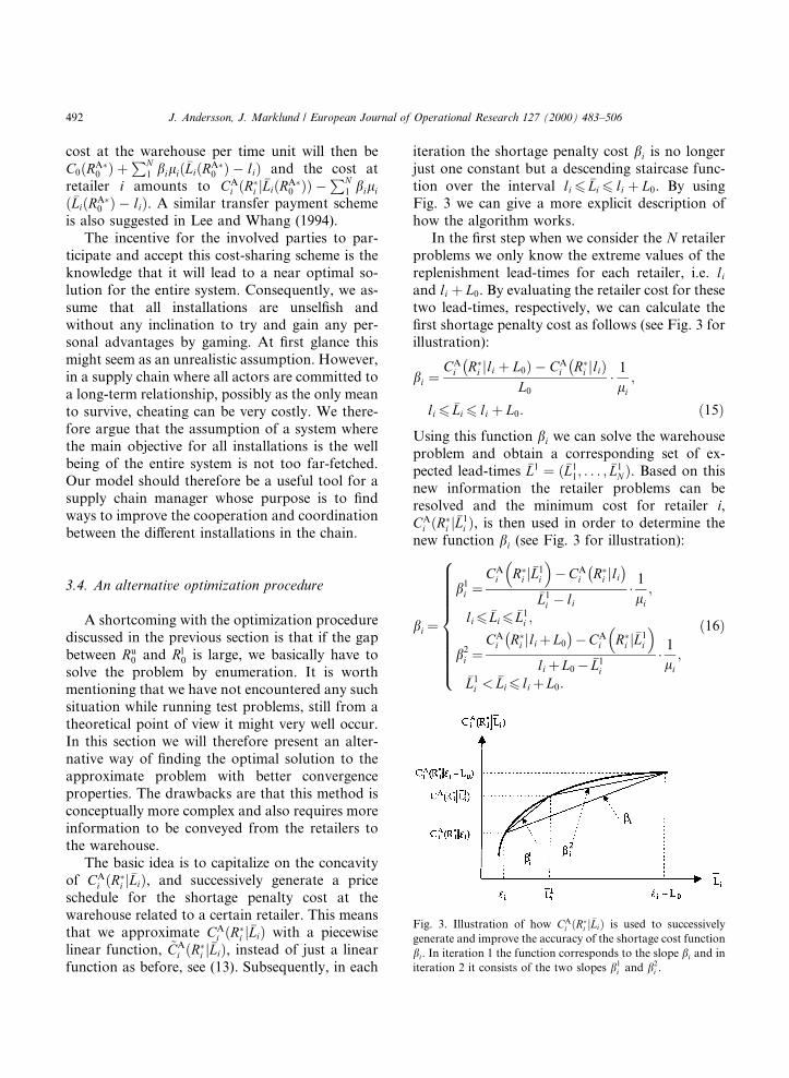
The basic idea is to capitalize on the concavityof CA

i �R�i j�Li�, and successively generate a priceschedule for the shortage penalty cost at thewarehouse related to a certain retailer. This meansthat we approximate CA

i �R�i j�Li� with a piecewiselinear function, ~CA

i �R�i j�Li�, instead of just a linearfunction as before, see (13). Subsequently, in each

iteration the shortage penalty cost bi is no longerjust one constant but a descending staircase func-tion over the interval li6 �Li6 li � L0. By usingFig. 3 we can give a more explicit description ofhow the algorithm works.

In the ®rst step when we consider the N retailerproblems we only know the extreme values of thereplenishment lead-times for each retailer, i.e. li

and li � L0. By evaluating the retailer cost for thesetwo lead-times, respectively, we can calculate the®rst shortage penalty cost as follows (see Fig. 3 forillustration):

bi �CA

i R�i jli � L0

ÿ � ÿ CAi R�i jli

ÿ �L0

� 1

li;

li6 �Li6 li � L0: �15�Using this function bi we can solve the warehouseproblem and obtain a corresponding set of ex-pected lead-times �L1 � ��L1

1; . . . ; �L1N �. Based on this

new information the retailer problems can beresolved and the minimum cost for retailer i,CA

i �R�i j�L1i �, is then used in order to determine the

new function bi (see Fig. 3 for illustration):

bi �

b1i �

CAi R�i j�L1

i

� �ÿCA

i R�i jli

ÿ ��L1

i ÿ li� 1

li;

li6 �Li6 �L1i ;

b2i �

CAi R�i jli�L0

ÿ �ÿCAi R�i j�L1

i

� �li�L0ÿ �L1

i

� 1

li;

�L1i <

�Li6 li�L0:

8>>>>>>>>><>>>>>>>>>:�16�

Fig. 3. Illustration of how CAi �R�i j�Li� is used to successively

generate and improve the accuracy of the shortage cost function

bi. In iteration 1 the function corresponds to the slope bi and in

iteration 2 it consists of the two slopes b1i and b2

i .


This new penalty cost function can be used to re-solve the warehouse problem etc. The algorithmstops when the solution does not change in twoconsecutive iterations.

Before we show that the algorithm is guaran-teed to ®nd the optimum solution for the ap-proximate problem (RA�

0 ;RA�) we need to give ageneral mathematical description of the costfunctions involved.

Assume that bi consists of K steps, i.e.,bi � �b1

i ; b2i ; . . . ; bK

i �, where b1i is only valid over

the interval ��L0i � li; �L1

i � and bKi is only valid over

��LKÿ1i ; �LK

i � li � L0� etc. When �Lnÿ1i 6 �Li6 �Ln

i ;n � 1; 2; . . . K, it follows that

~CAi R�i j�Li

� �� ~CA

i R�i jli

ÿ �� li

Xnÿ1

j�1

bji

�Lji

�(ÿ �Ljÿ1

i

�� bn

i�Li

�ÿ �Lnÿ1

i

�)6CA

i R�i j�Li

� �;

�17�

~C0�R0� � C0�R0� �XN

i�1

li

Xnÿ1

j�1

bji

�Lji

�(ÿ �Ljÿ1

i

�� bn

i�Li

�ÿ �Lnÿ1

i

�); �18�

T~CA R0� � � C0�R0� �XN

i�1

~CAi R�i j�Li�R0��

6TCA R0� �:

�19�

From (17)±(19) we can see to that minimizing thewarehouse cost function ~C0�R0�is equivalent tominimizing the total cost function in the decom-posed model T~CA�R0�. It also follows that both~C0�R0� and T~CA�R0� for each R0 represent lowerbounds to the total cost in the approximate modelTCA(R0).

An important observation concerning the con-vergence properties of the algorithm is that if twosuccessive iterations produce the same lead-timevector �L this means that ~CA

i �R�i j�Li� � CAi �R�i j�Li� for

all i � 1; . . . ;N . Consequently, we can concludethat

min T~CA � T~CA�RA�0 � � TCA�RA�

0 � � min TCA:

The last equality follows from the fact thatT~CA�R0� constitutes a lower bound to TCA(R0) forevery R0, and that this lower bound is made tighterin every iteration when bi for i � 1; . . . ;N is up-dated. Since R0 is a discrete variable the algorithmwill ®nd the optimum solution within a ®nitenumber of steps.

It is rather complicated to determine a `fair'physical reimbursement from the warehouse toeach retailer using the staircase function bi. Forpractical purposes we therefore recommend thatthe optimization algorithm discussed in this sec-tion is used only for ®nding the optimal solution tothe approximate problem. We can then apply theshortage penalty cost de®ned in Section 3.3 todetermine an e�cient cost-sharing scheme for thesystem.

4. Error bounds

In this section we derive a performance ratio forthe approximate problem, which is an upperbound on the maximum approximation error. Thebound is valid when the cumulative demand ateach retailer follows a non-decreasing stochasticprocess with stationary and independent incre-ments, as discussed in Section 2. The approach weare using is mainly based on the theoretical resultspresented in Andersson et al. (1998). However, byusing the lead-time distribution derived in Ap-pendix A we are able to get a much tighter bound.When the demand process is modeled as a Wienerprocess with drift, the performance ratio is nolonger a bound but a reasonable quality mea-surement, provided that the probability of nega-tive demand is small.

An interesting interpretation of the error boundis that it re¯ects the relative cost of reduced in-formation availability. In our case this means themaximum cost of using the average lead-time in-stead of the entire lead-time distribution whendeciding on the optimal policy parameters.

An important property of the retailer costfunction in the approximate model is that it is


convex in the expected lead-time for ®xed values ofthe reorder point.

Proposition 3. CAi �Rij�Li� is a convex function in �Li

for every given value of Ri.

We omit the proof and refer to Andersson et al.(1998).

Proposition 3 holds for all stationary demandprocesses with independent and non-negative in-crements. The convexity of CA

i �Rij�Li� enables us torelate the total cost in the approximate model tothe total cost for the system. The results aresummarized in Propositions 4 and 5 below. How-ever, before we look at these ®ndings we need tode®ne some additional notation.

Proposition 4. CAi RA�

i �R0�ÿ �

6CEi RE�

i �R0�ÿ �

:

Using Proposition 4 it is fairly easy to obtainthe following.

Proposition 5.

TCA RA�0 ;RA��RA�

0 �ÿ �

6TCE RE�0 ;R

E��R0�ÿ �

:

The performance ratio, r, relates the minimumtotal system cost when the optimal solution to the

approximate problems is used, to the minimumtotal cost for the exact model. This means that rcan be expressed in the following way:

r � TCE RA�0 ;RA��RA�

0 �ÿ �

=TCE RE�0 ;R

E��RE�0 �

ÿ �:

�20�

The expression for r is not very practical since thedenominator involves the true optimal solution�RE�

0 ;RE��, which is unknown to us. However, by

using Proposition 5 it is easy to construct an upperbound for r, which can be evaluated with theavailable information.

Proposition 6. The performance ratio r is boundedfrom above by the following expression:

r6 r

�C0�RA�

0 � �PN

i�1 ELi�RA�0� CA

i RA�i �RA�

0 �jLi�RA�0 �

ÿ �� TCA RA�

0 ;RA��RA�0 �� :

�21�

Proof. The result follows directly from Proposition5 together with the de®nition of TCE: �

In order to evaluate the bound on the perfor-mance ratio we must know the distribution ofLi�RA�

0 �. An approximate method for obtainingthis rather elusive distribution is presented inAppendix A.

5. Computational aspects

In this section we will discuss the optimizationof the decomposed approximate problem in moredetail. We will also introduce a simple and intu-itive approximate expression for the expected lead-time, �Li. From a computational point of view thisapproximation is much simpler than the methoddescribed in Appendix A. Finally, we will presentsome numerical results, which illustrate the per-formance of the di�erent approximations com-pared to simulated results.

RE�i �R0� true optimal reorder point for

retailer i given a certainreorder point R0 at thewarehouse, RE��R0�� RE�

1 �R0�; . . . ;RE�N �R0��,

RA�i �R0� optimal reorder point for

retailer i in the approximatemodel given a certain reorderpoint R0 at the warehouse,RA��R0� � �RA�

1 �R0�; . . . ;RA�N �R0��,

CAi RA�

i �R0�ÿ �

the minimum cost at retailer i inthe approximate model given acertain warehouse reorder point,R0, (�CA

i �R�i j�Li�R0�� in previousnotation),

CEi RE�

i �R0�ÿ �

the minimum cost at retailer iin the exact model given a cer-tain warehouse reorder point R0.


5.1. Optimization of the decomposed approximateproblem

The structure of the decomposed approximateproblem is illustrated in Fig. 2. We will here in-vestigate how the subproblems can be evaluatedwhen the cumulative demand at each retailer isnormally distributed. We will focus our attentionon the sub-problems related to the optimizationprocedure discussed in Section 3.3 and only brie¯ycomment what minor changes must be done tohandle the alternative procedure presented inSection 3.4.

Consider the retailer problem (6) for an arbi-trary retailer i given a certain lead-time, �Li; weknow that the cost function CA

i �Rij�Li� is convex inRi (see Zheng, 1992). Consequently, the retailerproblem is e�ciently solved by a simple one-di-mensional search procedure. When the optimalreorder point, for the current value of �Li, R�i ��Li� isfound, we can easily obtain the correspondingvalue of bi ��dCA

i �R�i j�Li�=d�Li��1=li�� from expre-ssion (12). If the alternative optimization proce-dure is used the staircase function bi is determinedas described in Section 3.4.

Turning to the warehouse problem (7) we wantto minimize the cost function ~C�R0� with respect toR0. To evaluate ~C�R0� we need to compute thenumber of reserved subbatches at the warehouse,E�Br

0�. Through LittleÕs formula E�Br0� can be ex-

pressed as a function of the mean lead-times,�Li�R0� (for i � 1; 2; . . . ;N ), and the expectednumber of backordered subbatches at the ware-house, E�B0�:

E Br0

� � �XN

i�1

li

Q��Li ÿ li� ÿ E B0� �; �22�

E�B0� � 1

Q0

XR0�Q0

y0�R0�1

ED0�L0� �D0�L0�� ÿ y0��

�: �23�

To compute the expected lead-time for retailer i,�Li�R0�, we can use the method in Appendix A. Wealso need to ®nd the distribution of D0�L0� byconvoluting the distributions of the warehousedemand emanating from each retailer.

The optimal R0, which minimizes ~C�R0� givena set of shortage costs (b1; . . . ; bN ), is denoted byR�0. A complication when optimizing ~C�R0� is thatit is not necessarily convex in R0. However, itdoes possess a certain degree of regularity, whichcan be capitalized on to restrict the number ofvalues of R0 that need to be evaluated in searchof R�0. The idea is to use the fact that ~C�R0�consists of three di�erent components E�I0�R0��,E�B0�R0�� and E�Br

0�R0�� (see (5), (7) and (22)). Byusing what we know about the behavior of the®rst two components, and by bounding the in-¯uence of the last one, we are able to ®nd con-ditions that de®ne dynamic upper and lowerbounds on R�0.

Lemma 1. R�06Ru0, where Ru

0 is the smallest value ofR0 satisfying the conditions

h0�E�I0�Ru0 � 1�� ÿ E�I0�Ru

0�� max

i�bi��E�B0�Ru

0 � 1�� ÿ E�B0�Ru0��P 0;

�24�

~C�Ru0� ÿ Q�h0 �max

i�bi��E�Br

0�Ru0��P min

R0 6Ru0

~C�R0�:

�25�

Proof. De®ne

DI0�k� � E I0�Ru0

� � k��ÿ E I0�Ru0�

� �;

DB0�k� � E B0�Ru0

� � k��ÿ E B0�Ru0�

� �;

DBr0�k� � E Br

0�Ru0

� � k��ÿ E Br0�Ru

0��

;

D�Li�k� � �Li�Ru0 � k� ÿ �Li�Ru

0�:

It is well known that E�I0�R0�� is an increasingconvex function and that E�B0�R0�� is a decreasingconvex function of R0, see Zheng (1992) andZipkin (1986). Consequently, DI0(k) > 0 andDB0(k) < 0. Furthermore, from the expressions inAppendix A it can be shown that �Li�R0� is a non-increasing function of R0. Using these propertiestogether with (22) and the fact that E�Br

0�R0�� is anon-negative function of R0 it follows that


~C�Ru0 � k� ÿ ~C�Ru

0�

� h0Q DI0�k�ÿ � DBr

0�k��XN

i�1

biliD�Li�k�

P h0Q DI0�k�ÿ � DBr

0�k��max

i�bi�XN

i�1

liD�Li�k�

� Q h0DI0�k��

�maxi�bi�DB0�k�

�� Q h0

��max

i�bi��

DBr0�k�

P Q h0DI0�k��

�maxi�bi�DB0�k�

�ÿ Q h0

��max

i�bi��

E Br0�Ru

0��

P kQ h0DI0�1��

�maxi�bi�DB0�1�

�ÿ Q h0

��max

i�bi��

E Br0�Ru

0��

Pÿ Q h0

��max

i�bi��

E Br0�Ru

0��

for all k P 0;

�26�where the last inequality follows from condition(24). We can conclude that when (25) is satis®ed,R�0 is the solution to minR0 6Ru

0

~C�R0�: �

It can be shown that Lemma 1 also holds forthe alternative optimization procedure when~C�R0� is de®ned by (18). The only di�erence is thatbi is replaced by bi�li�, which denotes the value ofthe function bi for �Li � li. In the same way asLemma 1 provides us with two conditions, whichcan be used to identify an upper limit for theoptimal value of R0, Lemma 2 below allow us todetermine a lower bound for R�0. Lemma 2 can beproven using the same technique as in the proof ofLemma 1.

Lemma 2. R�0 P Rlb0 , where Rlb

0 is the largest value ofR0 satisfying the conditions:

h0�E�I0�Rlb0 ÿ 1��ÿE�I0�Rlb

0 ��min

i�bi��E�B0�Rlb

0 ÿ 1��ÿE�B0�Rlb0 ��P0; �27�

~C�Rlb0 � ÿ Q�h0 �min

i�bi��E�Br

0�Rlb0 ��P min

Rlb0<R0

~C�R0�:

�28�

For the alternative optimization algorithm inSection 3.4, where ~C�R0� is de®ned by (18), Lemma2 will still hold provided that bi in (27) and (28) isreplaced by bi�li � L0�. Applying Lemma 1 andLemma 2 we can device an e�cient method for®nding R�0 based on a successive search procedureoriginating from a suitable starting value, R0. Areasonable starting value is for example the opti-mal solution to the convex problem:

minR0

C�R0� � Q h0E�I0��

�mini�bi�E�B0�

�: �29�

Note that choosing R0 as the optimal solution to(29) means that condition (27) in Lemma 2 willalways be satis®ed for R06 R0. The same statementis true for the alternative optimization algorithm ifbi is replaced by bi�li � L0�.

5.2. Approximations of E�br0� and �Li

Evaluation of �Li for i � 1; 2; . . . ;N is a vitalelement in the solution of the decomposed ap-proximate problem. A drawback with the methodfor calculating �Li presented in Appendix A, is itscomputational complexity. As an alternative,which require less information and computationale�ort, we suggest an intuitive approximation of �Li,see Eq. (30) below. The structure of (30) stemsfrom numerical observations that a large retailer interms of li and Qi tends to have a longer meanlead-time, �Li. In other words, a retailer which or-ders often and in large quantities have, relativelyspeaking, more units backordered and reserved atthe warehouse than a retailer with low orderingfrequency and small order quantities. It is worthstressing that this observation does not carry overto situations where the order frequency is large butthe order quantity is small or vise versa. For ex-ample, in a situation where all retailers use acommon batch size, a high demand rate for oneretailer does not necessarily imply a longer ex-pected lead-time for that retailer.


De®ne

�Li � �D1 � �D1

li�Qi ÿ Q� ÿ �g1=N�g1

� �� D2

li�Qi ÿ Q�g1

� li: �30�

The ®rst two terms in (30) represent an estimate ofthe mean delivery delay to retailer i due to stockoutsat the warehouse. The estimate is found by di�er-entiating the average delivery delay due to stock-outs over all retailers based on the relative size of theretailer in question. More precisely we use the re-tailerÕs relative deviation from the average retailersize, measured in terms of the product li�Qi ÿ Q�, asa basis for estimating the stockout delivery delay tothat same retailer. The third term in (30) representsan estimate of the mean delivery delay to retailer idue to the existence of reserved units at the ware-house. In this case, the term that is being disaggre-gated is the average delay over all retailers due to theexistence of reserved units at the warehouse. Themotive for using the product li�Qi ÿ Q� is that if aretailer uses an order quantity equal to the subbatchsize Q, there will never exist any reserved units atthe warehouse destined for this retailer. The lastterm in (30) is just the constant transportation time.

Note that (30) will be exact when all retailersare identical since both the second and the thirdterm will be zero. We can also see that if we havenon-identical retailers, which use a common batchsize, the second and third term will disappear.Consequently, the lead-time approximation (30)reduces to a direct application of LittleÕs formula.

A di�culty with evaluating (30) is that it in-cludes the term E�Br

0�, which we do not have an

explicit expression for. To handle this problem wesuggest another approximation, see (31), which isinspired by an idea in Lee and Moinzadeh (1987).This approximation is based on the observationthat reserved units only occur when a fraction of aretailerÕs order quantity is backordered. If we lookat (31), the parameter �Q can be interpreted as anaverage batch size, which takes into account boththe size and frequency of the retailer orders ar-riving at the warehouse. If we divide the number ofbackordered units B0 by �Q and the result is frac-tional, say 2.45, this indicates, due to the completedelivery policy at the warehouse, that the totalnumber of delayed units is 3 �Q and subsequentlythat 0:55 �Q units are reserved at the warehouse.

De®ne

xd e � the smallest integer P x;

�Q �Xn

i�1

li

Qik0

� Qi �Xn

i�1

li

k0

;

k0 �Xn

i�1

li

Qi� demand intensity at the warehouse

in number of retailer orders;

E�Br0� � E

B0

�Q

� ��Q

� �ÿ E�B0�: �31�

An important property of the simple approxima-tion of �Li�R0� de®ned by (30) and (31) is that it isnon-increasing with R0. This follows from the ob-servation that E�B0�R0�� is decreasing and convexin R0 and that E�Br

0�R0�� as approximated in (31) isnon-increasing in R0. Since �Li�R0� is non-increasingwe can still apply the coordination procedures inSections 3.3 and 3.4 to ®nd the optimal solution tothe approximate problem. It also means thatLemmas 1 and 2 will be valid and consequently wecan use the optimization technique discussed inSection 5.1.

5.3. Numerical results

In this section, we present a number of nu-merical examples in order to shed some light overthe performance of the coordination procedure,

�D1 � E�B0�Q=l0 mean delivery delay dueto stockouts at thewarehouse,

�D2 � E�Br0�Q=l0 mean delivery delay due

to reserved units waitingto be shipped,

l0 �PN

i�1 li demand intensity at thewarehouse expressed innumber of units,

g1 �PN

i�1 li�Qi ÿ Q�,


and the suggested approximations. We also illus-trate the relationships between the shortage costsbi and pi, for near optimal solutions. For claritythe sophisticated approximation of �Li, discussed inAppendix A, will be denoted A1 and the simpleone de®ned by (30) and (31) will be referred toas A2.

We have used two di�erent problem con®gu-rations, Problem type 1 and Problem type 2. Theformer consists of one central warehouse and ®venon-identical retailers, 16 problem instances withthis con®guration have been evaluated. Problemtype 2 is made up of one central warehouse andthree non-identical retailers. Four problem in-stances of this type have been studied. The mainpurpose in this case is to ®nd the `optimal' solutionthrough an extensive simulation search. Due to thecomplexity this is hardly feasible for type 1 prob-lems. In all test problems h0 � hi � 1 andpi � 10 �i � 1; 2; . . . ;N�.

Tables 1 and 2 de®ne the 16 problems of type 1that we have studied. Table 3 shows the corre-sponding near optimal solutions, found by opti-mizing the approximate model with normallydistributed demand, using A1 and A2, respective-ly. Table 3 also contains the quality measurement rand the average total cost per time unit TCsim. Thiscost corresponds to a solution obtained byrounding o� the values of RA�

i �i � 1; 2; . . . ;N� tothe closest integer. TCsim is evaluated throughdiscrete event simulation, where the customer de-mand is modeled as a Poisson process with thesame mean and variance as indicated in Table 1.The motivation for using this method is twofold.First of all, in reality customers and in general alsoproducts exist only in discrete units. To use acontinuous demand process and allow for frac-tional reorder points is therefore an approxima-tion in itself. The obvious way to deal with afractional solution in practice would be to use the

closest integer solution. Secondly, it is quite di�-cult to simulate an inventory system of this com-plexity using a continuous model.

An important issue is to assess the quality ofthe simple lead-time approximation A2 comparedto A1. Note that A1 should be very accurate forthe problems at hand. From Table 3 we can seethat in all 16 cases, the total cost (TCA) for A2underestimates the total cost corresponding to A1.Another apparent tendency is that the di�erence intotal cost (TCA) between the two approximationsincreases with Q. This supports the statement inSection 5.2 that A2 will be less accurate when thereare large di�erences between retailers in terms oforder quantity and demand intensity. The mostrelevant way to assess the quality of the solutionobtained by A2 compared to A1 is probably tostudy the simulated cost TCsim or more preciselyDTCsim. We can conclude that in 12 of the casesthere are no signi®cant di�erence in total costbetween the closest integer solutions associated

Table 1

Problem type 1, numerical data for the di�erent retailers (hi� 1 and pi� 10 8i � 1; 2; . . . ; 5)

Retailer 1 2 3 4 5

qi 1 2 3 4 5

li 40 50 60 70 80

ri �� lip � 6.32 7.07 7.74 8.36 8.94

Table 2

Problem type 1, de®nition of the parameter values for the 16

test problems (h0� 1 in all test problems)

Problem Q0 Q l L0

1 5 4 1 1

2 5 4 1 0.5

3 5 4 2 1

4 5 4 2 0.5

5 5 8 1 1

6 5 8 1 0.5

7 5 8 2 1

8 5 8 2 0.5

9 8 4 1 1

10 8 4 1 0.5

11 8 4 2 1

12 8 4 2 0.5

13 8 8 1 1

14 8 8 1 0.5

15 8 8 2 1

16 8 8 2 0.5


Ta

ble

3

Nu

mer

ical

resu

lts

for

the

16

pro

ble

ms

of

typ

e1

a

Pro

ble

mR

0R

1R

2R

3R

4R

5T

CA

rT

Csi

mr s

imD

TC

sim

1A

16

65

0.3

60.8

71.5

82.4

93.3

84.6

1.1

196.2

0.7

2

A2

66

49

.660.0

70.8

82.1

93.8

82.6

)95.3

0.6

3)

0.9

2A

13

04

9.5

59.8

70.3

80.8

91.4

83.9

1.0

792.2

0.4

8

A2

30

48

.959.1

69.6

80.4

91.7

81.6

)91.8

0.5

6)

0.4

3A

16

59

4.1

115.1

136.2

157.3

178.6

110.6

1.0

6119.7

1.1

7

A2

65

93

.4114.2

135.5

157.1

179.3

108.6

)119.2

0.8

1)

0.5

4A

13

09

2.8

113.5

134.2

154.9

175.6

110.0

1.0

4118.0

1.0

6

A2

29

92

.7113.3

134.2

155.5

177.2

107.8

)118.1

1.0

60.1

5A

13

14

9.7

59.8

70.6

80.7

90.8

106.6

1.1

4122.6

0.5

9

A2

30

49

.459.3

70.1

81.6

94.1

101.7

)126.6

0.7

24.0�

6A

11

44

8.0

57.7

67.7

77.1

86.4

105.6

1.0

9117.2

0.4

4

A2

12

48

.758.4

68.8

80.0

91.9

100.8

)124.2

0.5

77.0�

7A

13

19

2.9

113.1

133.8

153.9

174.0

129.6

1.0

9142.7

1.0

8

A2

30

92

.7112.6

133.4

154.9

177.2

124.6

)145.4

1.0

42.7

8A

11

49

1.3

111.0

131.0

150.4

169.7

128.8

1.0

6137.7

0.9

9

A2

12

91

.9111.7

132.1

153.2

175.1

123.8

)144.3

0.7

36.6�

9A

16

45

0.6

61.2

71.9

82.9

93.9

84.8

1.1

297.5

0.7

9

A2

64

49

.860.3

71.2

82.6

94.6

82.8

)96.7

0.6

5)

0.8

10

A1

28

49

.760.1

70.7

81.3

92.1

84.2

1.0

993.6

0.6

5

A2

28

49

.159.4

70.0

81.0

92.4

81.9

)92.3

0.5

2)

1.3

11

A1

63

94

.4115.5

136.6

157.8

179.2

110.7

1.0

7119.8

1.2

0

A2

64

93

.2114.0

135.1

156.7

178.7

108.8

)120.2

1.0

10.4

12

A1

27

93

.6114.4

135.4

156.3

177.4

110.2

1.0

5117.3

1.0

8

A2

27

92

.9113.6

134.6

156.0

177.9

108.1

)118.3

0.9

81.0

13

A1

28

51

.361.7

72.8

83.5

94.9

107.5

1.2

0128.3

0.6

7

A2

28

49

.960.0

70.9

82.8

95.5

102.4

)130.9

0.6

42.6

14

A1

11

49

.659.6

70.0

80.1

90.4

106.6

1.1

7125.1

0.6

6

A2

10

49

.259.0

69.7

81.1

93.4

101.5

)128.7

0.5

13.6�

15

A1

28

94

.5114.9

136.1

156.7

178.0

130.3

1.1

3148.3

1.1

7

A2

28

93

.1113.3

134.2

156.0

178.7

125.2

)150.5

1.1

12.2

16

A1

10

93

.8114.2

134.6

155.1

175.9

129.5

1.1

2147.6

1.1

3

A2

10

92

.4112.3

133.0

154.3

176.5

124.4

)146.7

1.0

3)

0.9

aR

0,

R1,

R2,

R3,

R4,

R5

an

dT

CA

de®

nes

aso

luti

on

toth

eap

pro

xim

ate

mo

del

wit

hn

orm

all

yd

istr

ibu

ted

lead

-tim

ed

eman

d,

solv

edb

yth

eco

ord

inati

on

pro

ced

ure

for

lead

-

tim

ea

pp

rox

ima

tio

nA

1a

nd

A2

,re

spec

tiv

ely.

TC

sim

isth

esi

mu

late

daver

age

tota

lsy

stem

cost

base

do

nth

ecl

ose

stin

teger

solu

tio

nan

do

nP

ois

son

dis

trib

ute

dd

eman

d.

r sim

isth

ees

tim

ate

dst

an

da

rdd

evia

tio

no

fT

Csi

m.D

TC

sim

isth

ed

i�er

ence

bet

wee

nT

Csi

mfo

rth

eso

luti

on

rela

ted

toA

2an

dth

eso

luti

on

for

A1.

*T

he

di�

eren

ceis

sig

ni®

can

to

nth

ele

vel

0.1

%(l

arg

erth

an

thre

est

an

dard

dev

iati

on

s).


with A2 and A1. (signi®cance level 0.1%). Fur-thermore, in all four cases where there are signi®-cant cost reductions by using A1, Q is large, whichsupports the previous discussion on the impor-tance of Q. If we consider the mean deviations inTCsim between solutions corresponding to A1 andA2 in Table 3, we can conclude that on an average,there is a signi®cant increase of about 1% in thetotal cost. To summarize, the overall performanceof the intuitive lead-time approximation seems tobe quite good and considering the reduction incomplexity, computationally as well as conceptu-ally, it represents an interesting alternative to themore sophisticated method, A1.

To assess the quality of the approximate solu-tion (RA�

0 ;RA�) compared to the exact solution(RE�

0 ;RE�) we will use the quality measure r. In the

demand processes used (see Table 1), the proba-bility of negative demand to occur is close to zero.Consequently, we know that the lead-time ap-proximation A1 will be almost exact, and that thequality measure r will be close to an upper bound.Of course the weakness with r is that it tells uswhen a solution is good but not when it is of poorquality. From Table 3 we can see that the values ofr range from 1.04 to 1.20 with an average of 1.10.This indicates that in many cases the decentralizedmodel will produce solutions of quite reasonablequality. Also from the simulation study of type 2problems indications are that the bound mightgive an overly pessimistic impression of the qualityof the approximate solution (see Table 6).

In general we would expect the approximatemodel to be less accurate in situations where thevariability of the retailer lead-time is high com-pared to its mean. This statement can be sub-stantiated by a closer look at Tables 2 and 3. Wecan see that the value of r is less favorable inproblems where l is small, Q0 is large or Q is large.

In all test problems of type 1 the retailershortage cost, pi, is set to 10. An interesting ®gureis the corresponding shortage penalty cost relatedto retailer i at the warehouse bi. In Table 4 wepresent the values for bi �i � 1; 2; . . . ;N� for all 16test problems when these are solved by using ap-proximation, A1. The average value of bi over allproblems and all retailers is less than 1% of theshortage cost pi at the retailers. The implication

being that a relatively large part of the total safetystock should be allocated to the retailer level. Anexamination of the ®llrates for the installations inthe 16 problems highlights this fact even more.

Let ai0 be the ®llrate for deliveries from the

warehouse to retailer i. This ®gure is calculatedfrom the lead-time distribution, by ai

0 �Pr�Li � li�. The ®llrate at retailer i, is harder toobtain. However, if we assume that the replenish-ment lead-time is constant and equal to �Li, anapproximate ®llrate, ai, can be obtained from (32),see also Deuermeyer and Schwarz (1981). E�BQi�denotes the expected number of backordered unitsper order cycle:

ai�1ÿE BQi� �Qi

�

1ÿri �L

1=2i G Riÿli

�Li

� �ri �L

1=2i

.� �ÿG Riÿli

�Li�Qi

� �ri �L

1=2i

.� �� Qi

:

�32�

From Table 4 we can see that the service level atthe warehouse is very low ± the ®llrate is on anaverage 11% and never above 20% ± while theservice level towards the end customers is consid-erably higher. The estimated ®llrate at the retailers,ai, is on an average 78%. Another interesting ob-servation to be made from Table 4 is that largerretailers in terms of order quantity and demandintensity will have a lower service. This is of coursea direct consequence of the standard assumptionsof complete deliveries and a ®rst-come-®rst-servedpolicy at the warehouse.

Now, let us turn to the problems of type 2,which consists of one central warehouse and threeretailers. In the simulation study we search overthe reorder points for all installations with theobjective to ®nd a policy with lower costs than thepolicy obtained from solving the approximateproblem. The numerical data de®ning the di�erenttest problems are presented in Table 5.

Table 6 displays the best policies found throughthe simulation search and the policies rendered bythe coordination procedure using lead-time ap-proximation A1. It also shows the simulated costscorresponding to these solutions together with theperformance measurement r. We can see that al-though r is rather high, we are unable to ®nd any


Table 4

The penalty cost, b, the ®llrate at the warehouse, a0, and the estimated retailer ®llrates, a, for the 16 problems of type 1, when solved by

approximation A1

Problem Retailer Average

1 2 3 4 5

1 b 0.13 0.12 0.10 0.09 0.08 0.11

a0 (%) 14 12 10 8 7 10

a (%) 87 84 81 79 78 82

2 b 0.14 0.12 0.10 0.09 0.08 0.11

a0 (%) 15 13 10 8 7 11

a (%) 87 84 81 79 78 82

3 b 0.10 0.09 0.08 0.07 0.06 0.08

a0 (%) 10 8 7 6 4 7

a (%) 88 86 84 82 81 84

4 b 0.10 0.09 0.08 0.07 0.06 0.08

a0 (%) 15 13 10 8 7 11

a (%) 88 86 84 82 81 84

5 b 0.13 0.10 0.09 0.08 0.07 0.09

a0 (%) 17 14 10 8 9 12

a (%) 81 74 69 65 62 70

6 b 0.13 0.11 0.09 0.08 0.07 0.10

a0 (%) 29 24 15 15 18 20

a (%) 81 74 68 64 61 70

7 b 0.10 0.08 0.07 0.06 0.05 0.07

a0 (%) 17 14 10 8 9 12

a (%) 84 78 74 70 68 75

8 b 0.10 0.08 0.07 0.06 0.05 0.07

a0 (%) 29 24 15 15 18 20

a (%) 84 78 74 70 67 75

9 b 0.13 0.12 0.10 0.09 0.08 0.10

a0 (%) 13 11 9 8 7 10

a (%) 87 84 81 79 78 82

10 b 0.14 0.12 0.10 0.09 0.08 0.11

a0 (%) 15 12 10 8 7 10

a (%) 87 84 81 79 78 82

11 b 0.10 0.09 0.08 0.07 0.06 0.08

a0 (%) 10 8 7 6 4 7

a (%) 88 86 84 82 81 84

12 b 0.10 0.09 0.08 0.07 0.06 0.08

a0 (%) 11 9 7 6 5 8

a (%) 88 86 84 82 81 84

13 b 0.13 0.10 0.09 0.07 0.07 0.09

a0 (%) 12 9 6 5 6 8

a (%) 81 74 69 65 62 70

14 b 0.13 0.10 0.09 0.08 0.07 0.09

a0 (%) 20 16 10 10 11 13

a (%) 81 74 69 65 61 70

15 b 0.09 0.08 0.07 0.06 0.05 0.07

a0 (%) 12 9 6 5 6 8

a (%) 84 78 74 71 68 75

16 b 0.09 0.08 0.07 0.06 0.05 0.07

a0 (%) 13 9 6 6 7 8

a (%) 84 78 74 71 68 75

Average over

all problems

b 0.12 0.10 0.09 0.07 0.07 0.09

a0 (%) 16 13 9 8 8 11

a (%) 84 77 72 68 64 78


policies that are signi®cantly better (signi®cancelevel 5%) than those obtained from our decen-tralized method.

6. Contributions and conclusions

In this paper we have analyzed a conceptuallyquite simple model for highly decentralized controlof a two-level distribution system consisting of onecentral warehouse and an arbitrary number ofnon-identical retailers. All installations applycontinuous review installation stock �R;Q�-poli-cies. The ®ndings on decentralization involve theformulation of the approximate cost evaluationmodel, the use of a modi®ed cost structure and theprinciples behind the presented coordination pro-cedure. However, these ideas also appear in An-dersson et al. (1998). Our main contribution in thispaper is that we extend their model to a moregeneral situation where the retailers are allowed touse non-identical order quantities. We also presentan alternative optimization procedure with betterconvergence properties. Furthermore, we derive atighter bound for the performance ratio indicating

the excess cost of using the decentralized control,in relation to the solution from a centralized multi-echelon model.

From the numerical tests we can conclude thatthe near optimal solutions obtained from solvingthe approximate model seem to be of reasonablygood quality. We can also conclude that the simpleapproximation of the expected retailer lead-timesperforms quite well. Finally, an interesting, al-though not unexpected, observation regarding thegeneral behavior of our inventory system, is that ina near optimal situation the service level at thewarehouse is much lower than the service level atthe retailers. The implication being that a largeproportion of the total safety stock should be al-located to the retailers.

Appendix A. Evaluation of lead-time distributions

In this appendix we derive the probability dis-tributions and the expected values for the sto-chastic lead-times, Li, facing the retailers in theconsidered inventory system. This evaluation relieson the assumption that the retailers face customer

Table 6

Policies found by an extensive simulation search (Sim) compared to the policies obtained from solving the approximate problem with

lead-time approximation A1 (A1)

Problem R0 R1 R2 R3 r TCsim DTCsima rDTCsim

b

1 Sim 31 62 62 95 56.66

A1 30 63 63 96 1.16 57.16 )0.50 0.48

2 Sim 13 64 64 100 67.60

A1 12 65 65 102 1.21 68.97 )1.38 0.85

3 Sim 30 62 62 96 57.84

A1 28 64 64 99 1.20 59.21 )1.38 0.78

4 Sim 11 68 68 104 71.82

A1 11 66 66 103 1.30 72.77 )0.95 0.71

a Di�erence between the cost of the sim-policy and the A1-policy.b Standard deviation for DTCsim.

Table 5

Problem type 2, numerical data for the di�erent test problems, ri�� lip �

Problem Q q0 q1 q2 q3 l1 l2 l3 r1 r2 r3

1 5 4 1 1 3 50 50 80 7.07 7.07 8.94

2 10 4 1 1 3 50 50 80 7.07 7.07 8.94

3 5 6 1 1 3 50 50 80 7.07 7.07 8.94

4 10 6 1 1 3 50 50 80 7.07 7.07 8.94


demand modeled as non-decreasing stochasticprocesses with independent increments, and thateach retailer order consists of only one orderquantity, Qi. Consequently, this analysis is ap-proximate both for the Wiener process case andthe case of general non-decreasing stochasticprocesses with independent increments. However,the method is exact when customer demand fol-lows a stochastic process with independent in-crements and continuos non-decreasing samplepaths.

Consider a time epoch, t1, when an arbitraryretailer, say retailer i, initiates an order of qi sub-batches. In the forthcoming analysis identify thisretailer order as the considered retailer order. Wederive the lead-time-distribution for this delivery.The time epoch just before the considered retailerorder is triggered is labeled tÿ1 . De®ne t2 as the timeinstance when the warehouse initiated the order ofQ0 subbatches, which contains the last subbatch inthe delivery covering the considered retailer order.Identify this warehouse order as the consideredwarehouse order.

Let Ti be the time units that elapse between theconsidered warehouse order and the consideredorder from retailer i � t1 ÿ t2, (Ti P 0 sinceR0 P ÿ1); Ui the number of subbatch demands,counted backwards from tÿ1 , to the subbatch de-mand which triggers the considered warehouseorder, given that retailer i initiates an order at t1;hk

i the time until the kth subbatch demand occursat the warehouse, counted backwards from tÿ1 ,given that retailer i initiates an order at t1; andDi

0�t� is aggregate demand at the warehouse in thetime interval (tÿ1 ÿ t; tÿ1 ), given that retailer i initi-ates an order at t1.

For a stochastic variable X we denote the cu-mulative distribution function by FX �� and theprobability function by fX ��. Also de®nex� � max�0; x� and dxe� the smallest integer P x.

As discussed in Section 2.1 the restrictionR0 Pÿ1 means that li6 Li6 li � L0. Since theconsidered warehouse order arrives at the ware-house at the time epoch t2 � L0, the consideredlead-time and its distribution can be expressed asfollows:

Li � li � L0� ÿ Ti��; �A:1�

FLi�t� � 1ÿ FTi�L0 � li ÿ t�; li6 t6 li � L0:

�A:2�If we determine the distribution for Ti, then thedistribution for Li can be obtained from (A.2).However, let us ®rst consider the stochastic vari-able Ui. Lemma A.1 shows that Ui can be derivedfrom the warehouse inventory position at the ep-och tÿ1 , IP(tÿ1 ).

Lemma A.1.

Ui � R0

ÿ � Q0 � 1ÿ IP0�tÿ1 �� A�IP0�tÿ1 �� ÿ 1� � Q0

��; �A:3�

where

A�IP0�tÿ1 �� 1� IP0�tÿ1 � ÿ qi

Q0

� �: �A:4�

Proof. Enumerate the warehouse orders initiatedbefore tÿ1 by counting backwards from tÿ1 , i.e. themost recent order is number one and the secondmost recent order is number two, etc. The nextwarehouse order to occur, at tÿ1 or thereafter willbe number zero. We ®rst show that A(IP(tÿ1 )) givenby (A.4) is the number assigned to the consideredwarehouse order.

IP0�tÿ1 � ÿ qi can be interpreted as the numberof subbatches at hand or in transit to the ware-house (backorders excluded), after the consideredretailer order has been executed, but before thewarehouse initiates any new orders, triggered bythe retailer order at t1. Negative values ofIP0�tÿ1 � ÿ qi means that subbatch demands in theconsidered retailer order is covered by a ware-house batch ordered at the same time instance asthe considered retailer order, that is A(IP(tÿ1 ))� 0.

If 06 IP0�tÿ1 � ÿ qi6Q0 ÿ 1, then the number ofsubbatches on hand or in transit to the warehouse(backorders excluded) is less than one orderquantity at the warehouse. This means that the lastsubbatch of the considered retailer order is coveredby the most recent warehouse order and henceA(IP(tÿ1 ))� 1. Furthermore, if the stock on handor in transit after the considered order as been


executed exceeds Q0 ÿ 1, but is less than twowarehouse order quantities, then A(IP(tÿ1 ))� 2. Ingeneral we have for positive integers k,

IP0�tÿ1 � ÿ qi 2 �k� ÿ 1� � Q0; k � Q0 ÿ 1�) A�IP0�tÿ1 �� k:

This is just an alternative formulation of (A.4).R0 � Q0 � 1ÿ IP0�tÿ1 � can be interpreted as thenumber of subbatch demands, counting back-wards from t1, until the subbatch demand thattriggered the most recent warehouse order.�A�IP0� ÿ 1� � Q0 is the number of subbatch de-mands between the considered warehouse orderand the most recent warehouse order.

R0 � Q0 � 1 ÿ IP0�tÿ1 � � �A�IP0�tÿ1 �� ÿ 1� � Q0

6 0 means that the considered warehouse order istriggered by a subbatch demand in the consideredretailer order at t1. In this case Ui � 0 and there-fore Ui is given by (A.3). �

Lemma A.1 shows that we can obtain completeinformation of how many subbatch demands thathave occurred between t2 and t1 just by studyingthe inventory position at the warehouse at tÿ1 .

Lemma A.2. IP0�Tÿ1 � is uniformly distributed on theintegers R0 � 1; . . . ;R0 � Q0.

We omit the proof for this lemma, since thisproperty is well established in the literature, see forexample Axs�ater (1998b). Proposition A.1 pro-vides the distribution for Ui.

Proposition A.1. FUi�x� � �qi ÿ R0 ÿ 1� x�=Q0 for�R0 � 2ÿ qi��6 x6R0 � Q0 ÿ qi � 1:

Proof. De®ne U 0i � R0 � Q0 � 1ÿ IP0�tÿ1 ��A�IP0�tÿ1 �� ÿ 1� � Q0: Then Ui � �U 0i ��. Conse-quently the proposition follows if we show that U 0iis uniformly distributed on the integers�R0 � 2ÿ qi;R0 � Q0 ÿ qi � 1�. First we show thatVi � U 0i � qi ÿ R0 ÿ 1 is uniform on the integers1; 2; . . . ;Q0. Using (A.3) we obtain

Vi � 1� IP0�tÿ1 � ÿ qi

Q0

� �� Q0 � qi ÿ IP0�tÿ1 �:

Introduce the function

Wn�z� � 1� zn

� �� nÿ z:

With Wn�� we can express

Vi � WQ0IP0�tÿ1 �ÿ ÿ qi

�:

It is rather straightforward to verify that Wn��is a one-to-one mapping from every set of n con-secutive integers onto the set of integers, �1; n�.This speci®cally means that WQ0

�� is a one-to-one mapping from the integers �R0 � 1ÿ qi;R0 � Q0 ÿ qi� to the integers �1;Q0�. Then Vi isuniformly distributed on this set, since IP0�tÿ1 � ÿ qi

is uniform on �R0 � 1ÿ qi;R0 � Q0 ÿ qi�. Conse-quently U 0i is uniformly distributed on the integers�R0 � 2ÿ qi;R0 � Q0 ÿ qi � 1� and the propositionfollows. �

Recall that hxi is the time, counted backwards

from t1, until the xth subbatch is demanded at thewarehouse. Consequently

FTi�t� �XR0�Q0ÿqi�1

u��R0�2ÿqi��fUi�u� � Fhu

i�t�: �A:5�

The distribution function Fhxi�t� can be derived

from the demand distribution at the warehouse bysample path arguments.

Lemma A.3.

Fhxi�t� � 1ÿ FDi

0�t��x� 1�: �A:6�

Proof. The lemma follows from the observationthat for a non-decreasing demand process theevent fhx

i 6 tg is the same event as fDi0�t�P xg: �

From our ®ndings so far we can state the mainresult of this section, which is that the cumulativedistribution function for the lead-time Li can beexpressed as a weighted average of cumulativeaggregate demand probabilities.


Proposition A.2.

FLi t� � �XR0�Q0ÿqi�1

u��R0�2ÿqi��FDi

0�L0�liÿt� 1� � u� � fUi�u�;

li6 t6 li � L0: �A:7�

Proof. Combine (A.2), (A.5) and (A.6) and theresult follows. �

Finally the expected lead-time, �Li can be ob-tained in the following way:

�Li � li � L0 ÿXR0�Q0ÿqi�1

u��R0�2ÿqi��

Z L0

0

FDi0�t� 1�

24 � u� dt

35� fUi�u�: �A:8�

Appendix B

In order to evaluate the performance of thelead-time approximation used in this paper wehave compared our model with the method sug-gested by Svoronos and Zipkin (1988). An inven-tory system with one central warehouse and fourretailers, with identical order quantities, was con-sidered. Note that our methodology allows fornon-identical order quantities at the retailers,while the Svoronos±Zipkin methodology does not.We computed the optimal reorder points for theinventory system, ®rst using our approach (with �Li

"i determined by using the method in AppendixA) and then using the method suggested bySvoronos and Zipkin. The corresponding averagelong run costs was evaluated through simulation.

In all test problems we used L0 � 1, h0 � 1,hi � 1; pi � 20 and li � 1 �i � 1; . . . ; 4�. The cus-

tomer demand at each retailer is Poisson with in-tensities: l1 � 10; l2 � 20, l3 � 30; l4 � 40. Notethat the Svoronos±Zipkin methodology is de-signed for Poisson demand, whereas our methodassumes normally distributed demand. Conse-quently, we need to approximate the Poissondistributed customer demand with a normal dis-tribution with the same mean and variance whencalculating the reorder points with our method.Table 7 contains the problem speci®c data andresults. TC is the average total costs obtained bysimulation and rTC is the standard deviation ofthe simulated costs. D is the relative increase incosts by using the Svoronos±Zipkin methodcompared with our method.

From Table 7 we can see that in all test prob-lems our model outperforms the one suggested bySvoronos and Zipkin. The signi®cant increase intotal costs is, on an average, 4.4%. However, thecharacteristics of the test problems may be favor-able for our method since it is better suited forproblems with customer demand with low coe�-cients of variation. For problems with high vari-ability in the customer demand the Svoronos andZipkin approach would probably perform better.The motive being that they include the e�ects oflead-time variability when evaluating the costs atthe retailers.

References

Andersson, J., Axs�ater, S., Marklund, J., 1998. Decentralized

multi-echelon inventory control. Production and Operations

Management 7, 370±386.

Axs�ater, S., 1993. Continuous review policies for multi-level

inventory systems with stochastic demand. In: Graves S.C.

et al. (Eds.), Handbooks in OR & MS, vol. 4, pp. 175±197.

Axs�ater, S., 1995. A framework for decentralized multi-echelon

inventory control. Working paper, Lund University.

Table 7

Problem data and results

Problem Q Q0 Andersson and Marklund Svoronos and Zipkin D (%)

TC rTC TC rTC

1 4 16 52.48 0.011 54.82 0.014 4.5

2 8 32 60.00 0.016 61.19 0.022 2.0

3 4 32 56.85 0.019 59.79 0.023 5.2

4 8 64 74.08 0.018 78.50 0.013 6.0


Axs�ater, S., 1996. Using the deterministic EOQ formula in

stochastic inventory control. Management Science 42, 830±

834.

Axs�ater, S., 1997. Simple evaluation of echelon stock �R;Q�-policies for two-level inventory systems. IIE Transactions

29, 661±669.

Axs�ater, S., 1998a. Exact analysis of continuous review �R;Q�-policies in two-echelon inventory systems with compound

Poisson demand. Working paper, Lund University.

Axs�ater, S., 1998b. Evaluation of installation stock based

�R;Q�-policies for two-level inventory systems with Poisson

demand. Operations Research 46, 135±145.

Browne, S., Zipkin, P., 1991. Inventory models with continuous

stochastic demands. The Annals of Applied Probability 1,

419±435.

Chen, F., 1997. Decentralized supply chains subject to infor-

mation delays. Working paper, Graduate School of Busi-

ness, Columbia University, New York.

Chen, F., Zheng, Y.S., 1997. One warehouse multi-retailer

systems with centralized stock information. Operations

Research 45, 275±287.

Clark, A.J., Scarf, H., 1960. Optimal policies for a multi-echelon

inventory problem. Management Science 6, 475±490.

Diks, E.B., De Kok, A.G., Lagodimos, A.G., 1996. Multi-

echelon systems: A service measure perspective. European

Journal of Operational Research 95, 241±263.

Deuermeyer, B.L., Schwarz, L.B., 1981. A model for the

analysis of system service level in warehouse-retailer distri-

bution systems: The identical retailer case. In: Schwarz, L.

(Ed.), Multilevel Production/Inventory Control Systems, ch.

13, TIMS Studies in Management Science, vol. 16. Elsevier,

New York.

Federgruen, A., 1993. Centralized planning models for multi-

echelon inventory systems under uncertainty. In: Graves

S.C. et al. (Eds.), Handbooks in OR & MS, vol. 4. North-

Holland, Amsterdam, pp. 133±173.

Forsberg, R., 1997. Exact evaluation of �R;Q�-policies for two-

level inventory systems with Poisson demand. European

Journal of Operational Research 96, 130±138.

Hadley, G., Whitin,T.M., 1963. Analysis of Inventory Systems.

Prentice-Hall, Englewood Cli�s, NJ.

Hausman, W.H., Erkip, N.K., 1994. Multi-echelon vs. single-

echelon inventory control policies for low-demand items.

Management Science 40, 597±602.

Lee, H., Billington, C., 1993. Material management in decen-

tralized supply chains. Operations Research 41, 835±847.

Lee, H., Moinzadeh, K., 1987. Operating characteristics of a

two-echelon inventory system for repairable and consum-

able items under batch ordering and shipment policy. Naval

Research Logistics 34, 365±380.

Lee, H., Whang, S., 1994. Decentralized multi-echelon inven-

tory control systems incentives and information. Working

paper, Stanford University.

Muckstadt, J.A., Thomas, L.J., 1980. Are multi-echelon inven-

tory models worth implementing in systems with low-

demand-rate items? Management Science 26, 483±494.

Sherbrooke, C.C., 1968. METRIC: A multi-echelon technique

for recoverable item control. Operations Research 16,

122±141.

Silver, E.A., Peterson, R., 1985. Decision Systems for Inventory

Management and Production Planning, second ed. Wiley,

New York.

Svoronos, A., Zipkin, P., 1988. Estimating the performance of

multi-level inventory systems. Operations Research 36,

57±72.

Van Houtum, G.J., Inderfurth, K., Zijm, W.H.M., 1996.

Materials coordination in stochastic multi-echelon systems.

European Journal of Operational Research 95, 1±23.

Zheng, Y.S., 1992. On properties of stochastic inventory

systems. Management Science 38, 87±103.

Zipkin, P., 1986. Inventory service-level measures convexity

and approximation. Management Science 33, 975±981.


Decentralized inventory control in a two-level distribution system

Documents

Transcript of Decentralized inventory control in a two-level distribution system