Computers & Industrial Engineering 73 (2014) 21–31

Contents lists available at ScienceDirect

Computers & Industrial Engineering

journal homepage: www.elsevier .com/ locate/caie

Decentralized and centralized model predictive control to reduce thebullwhip effect in supply chain management q

http://dx.doi.org/10.1016/j.cie.2014.04.0030360-8352/� 2014 Elsevier Ltd. All rights reserved.

q This manuscript was processed by Area Editor Alexandre Dolgui.⇑ Corresponding author. Tel.: +32 092645583.

E-mail address: dongfei.fu@ugent.be (D. Fu).

Dongfei Fu a,⇑, Clara M. Ionescu a, El-Houssaine Aghezzaf b, Robin De Keyser a

a Department of Electrical energy, Systems and Automation, Ghent University, Technologiepark 913, Zwijnaarde 9052, Belgiumb Department of Industrial Management, Ghent University, Technologiepark 903, Zwijnaarde 9052, Belgium

a r t i c l e i n f o a b s t r a c t

Article history:Received 23 September 2013Received in revised form 13 February 2014Accepted 14 April 2014Available online 24 April 2014

Keywords:Model predictive controlSupply chain managementOptimizationBullwhip effect

Mitigating the bullwhip effect is one of crucial problems in supply chain management. In this research,centralized and decentralized model predictive control strategies are applied to control inventory posi-tions and to reduce the bullwhip effect in a benchmark four-echelon supply chain. The supply chainunder consideration is described by discrete dynamic models characterized by balance equations onproduct and information flows with an ordering policy serving as the control schemes. In the decentral-ized control strategy, a MPC-EPSAC (Extended Prediction Self-Adaptive Control) approach is used to pre-dict the changes in the inventory position levels. A closed-form solution of an optimal ordering decisionfor each echelon is obtained by locally minimizing a cost function, which consists of the errors betweenpredicted inventory position levels and their setpoints, and a weighting function that penalizes orders.The single model predictive controller used in centralized control strategy optimizes globally and findsan optimal ordering policy for each echelon. The controller relies on a linear discrete-time state-spacemodel to predict system outputs. But the predictions are approached by either of two multi-step predic-tors depending on whether the states of the controller model are directly observed or not. The objectivefunction takes a quadratic form and thus the resulting optimization problem can be solved via standardquadratic programming method. The comparisons on performances of the two MPC strategies are illus-trated with a numerical example.

� 2014 Elsevier Ltd. All rights reserved.

1. Introduction

A supply chain network is an integrated manufacturing processwith highly interconnected facilities and distribution channels thatfunction together to acquire raw materials, transform raw materi-als into intermediate and final products, and deliver final productsto retailers (Beamon, 1998). Such a supply chain can be repre-sented by a directed graph composed of nodes and arrows. Supplychain management (SCM), or supply chain optimization, is a set ofapproaches utilized to efficiently integrate suppliers, manufactur-ers, distributors and retailers, so that goods are produced and dis-tributed in the right quantities, to the right locations, and at theright time, in order to minimize system-wide costs while satisfyingservice level requirements (Aghezzaf, Sitompul, & Van DenBroecke, 2011; Simchi-Levi, Kaminski, & Simchi-Levi, 1999).

The decisions in SCM are classified into three categories withrespect to their impact and time scale: strategic planning, tactical

planning and operational level (Aghezzaf, Sitompul, & Najid,2010). However, in the major part of the literature SCM employedonly heuristics or mathematical programming techniques for sim-plified representations of the real process (Beamon, 1998; Mestan,Turkay, & Arkun, 2006). It is becoming increasingly difficult forcompanies to compete on a global scale with only heuristic deci-sions on simplified representations. In many corporations, man-agement has reached the conclusion that optimizing the productflows cannot be achieved without applying a systematic approachto the business. More and more methods and techniques from con-trol engineering are now utilized to design SCM strategies foraccomplishing various goals. The approach this research advocatesis to develop decision policies based on a control oriented formu-lation. The reader is referred to several excellent review paperson the application of classical control theory to the SCM problems(Hoberg, Thonemann, & Bradley, 2007; Ortega & Lin, 2004;Sarimveis, Patrinos, Tarantilis, & Kiranoudis, 2008; Subramanian,Rawlings, Maravelias, Flores-Cerrillo, & Megan, 2013).

Viewed as a complex network, there are many aspects toresearch in SCM. One of these is the improvement of inventorymanagement policies, the goal of which is to maintain the

22 D. Fu et al. / Computers & Industrial Engineering 73 (2014) 21–31

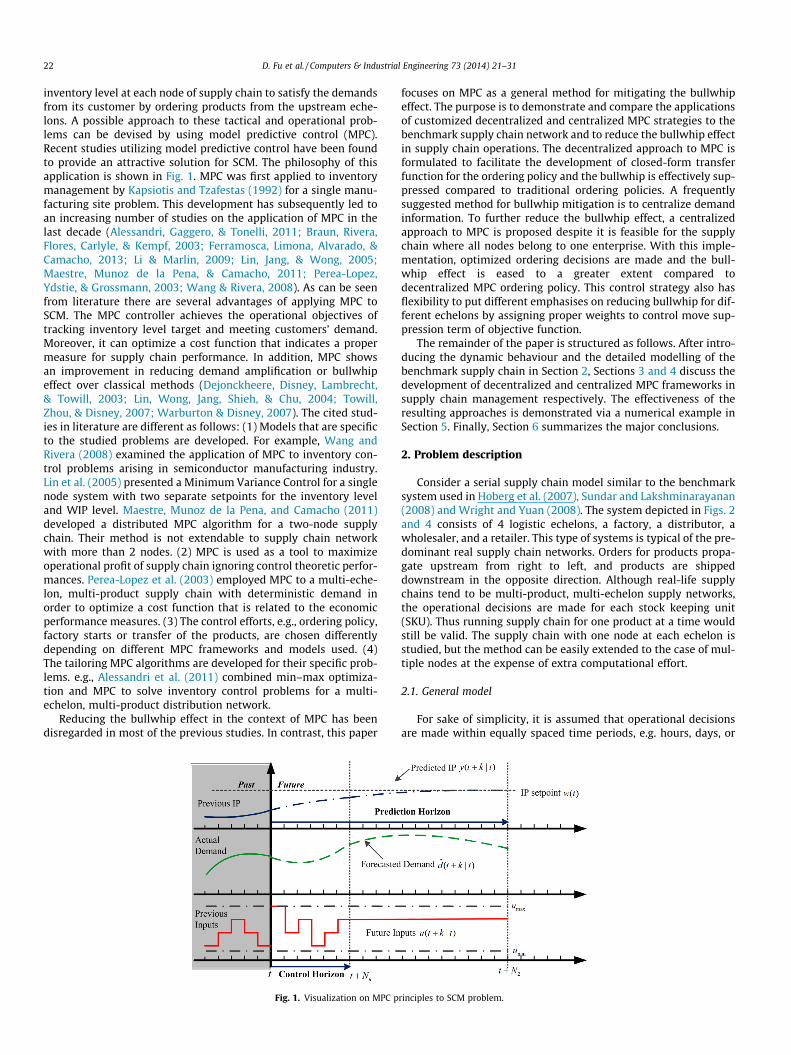
inventory level at each node of supply chain to satisfy the demandsfrom its customer by ordering products from the upstream eche-lons. A possible approach to these tactical and operational prob-lems can be devised by using model predictive control (MPC).Recent studies utilizing model predictive control have been foundto provide an attractive solution for SCM. The philosophy of thisapplication is shown in Fig. 1. MPC was first applied to inventorymanagement by Kapsiotis and Tzafestas (1992) for a single manu-facturing site problem. This development has subsequently led toan increasing number of studies on the application of MPC in thelast decade (Alessandri, Gaggero, & Tonelli, 2011; Braun, Rivera,Flores, Carlyle, & Kempf, 2003; Ferramosca, Limona, Alvarado, &Camacho, 2013; Li & Marlin, 2009; Lin, Jang, & Wong, 2005;Maestre, Munoz de la Pena, & Camacho, 2011; Perea-Lopez,Ydstie, & Grossmann, 2003; Wang & Rivera, 2008). As can be seenfrom literature there are several advantages of applying MPC toSCM. The MPC controller achieves the operational objectives oftracking inventory level target and meeting customers’ demand.Moreover, it can optimize a cost function that indicates a propermeasure for supply chain performance. In addition, MPC showsan improvement in reducing demand amplification or bullwhipeffect over classical methods (Dejonckheere, Disney, Lambrecht,& Towill, 2003; Lin, Wong, Jang, Shieh, & Chu, 2004; Towill,Zhou, & Disney, 2007; Warburton & Disney, 2007). The cited stud-ies in literature are different as follows: (1) Models that are specificto the studied problems are developed. For example, Wang andRivera (2008) examined the application of MPC to inventory con-trol problems arising in semiconductor manufacturing industry.Lin et al. (2005) presented a Minimum Variance Control for a singlenode system with two separate setpoints for the inventory leveland WIP level. Maestre, Munoz de la Pena, and Camacho (2011)developed a distributed MPC algorithm for a two-node supplychain. Their method is not extendable to supply chain networkwith more than 2 nodes. (2) MPC is used as a tool to maximizeoperational profit of supply chain ignoring control theoretic perfor-mances. Perea-Lopez et al. (2003) employed MPC to a multi-eche-lon, multi-product supply chain with deterministic demand inorder to optimize a cost function that is related to the economicperformance measures. (3) The control efforts, e.g., ordering policy,factory starts or transfer of the products, are chosen differentlydepending on different MPC frameworks and models used. (4)The tailoring MPC algorithms are developed for their specific prob-lems. e.g., Alessandri et al. (2011) combined min–max optimiza-tion and MPC to solve inventory control problems for a multi-echelon, multi-product distribution network.

Reducing the bullwhip effect in the context of MPC has beendisregarded in most of the previous studies. In contrast, this paper

Fig. 1. Visualization on MPC p

focuses on MPC as a general method for mitigating the bullwhipeffect. The purpose is to demonstrate and compare the applicationsof customized decentralized and centralized MPC strategies to thebenchmark supply chain network and to reduce the bullwhip effectin supply chain operations. The decentralized approach to MPC isformulated to facilitate the development of closed-form transferfunction for the ordering policy and the bullwhip is effectively sup-pressed compared to traditional ordering policies. A frequentlysuggested method for bullwhip mitigation is to centralize demandinformation. To further reduce the bullwhip effect, a centralizedapproach to MPC is proposed despite it is feasible for the supplychain where all nodes belong to one enterprise. With this imple-mentation, optimized ordering decisions are made and the bull-whip effect is eased to a greater extent compared todecentralized MPC ordering policy. This control strategy also hasflexibility to put different emphasises on reducing bullwhip for dif-ferent echelons by assigning proper weights to control move sup-pression term of objective function.

The remainder of the paper is structured as follows. After intro-ducing the dynamic behaviour and the detailed modelling of thebenchmark supply chain in Section 2, Sections 3 and 4 discuss thedevelopment of decentralized and centralized MPC frameworks insupply chain management respectively. The effectiveness of theresulting approaches is demonstrated via a numerical example inSection 5. Finally, Section 6 summarizes the major conclusions.

2. Problem description

Consider a serial supply chain model similar to the benchmarksystem used in Hoberg et al. (2007), Sundar and Lakshminarayanan(2008) and Wright and Yuan (2008). The system depicted in Figs. 2and 4 consists of 4 logistic echelons, a factory, a distributor, awholesaler, and a retailer. This type of systems is typical of the pre-dominant real supply chain networks. Orders for products propa-gate upstream from right to left, and products are shippeddownstream in the opposite direction. Although real-life supplychains tend to be multi-product, multi-echelon supply networks,the operational decisions are made for each stock keeping unit(SKU). Thus running supply chain for one product at a time wouldstill be valid. The supply chain with one node at each echelon isstudied, but the method can be easily extended to the case of mul-tiple nodes at the expense of extra computational effort.

2.1. General model

For sake of simplicity, it is assumed that operational decisionsare made within equally spaced time periods, e.g. hours, days, or

rinciples to SCM problem.

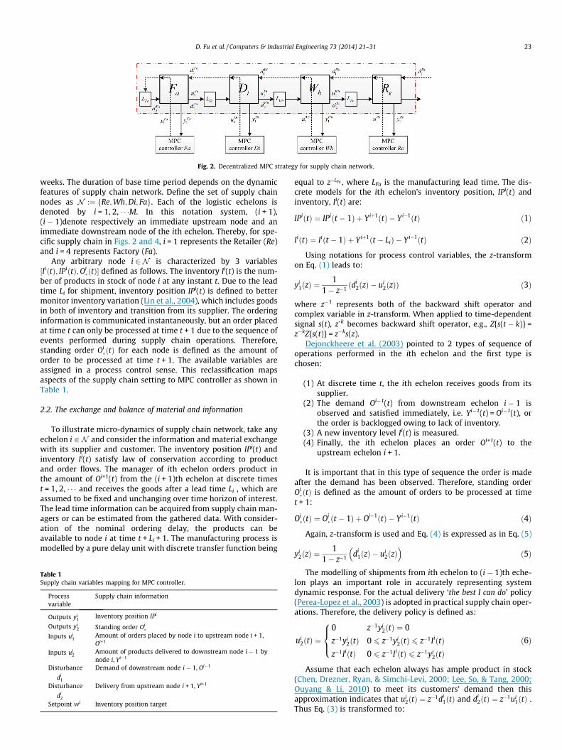
Fig. 2. Decentralized MPC strategy for supply chain network.

D. Fu et al. / Computers & Industrial Engineering 73 (2014) 21–31 23

weeks. The duration of base time period depends on the dynamicfeatures of supply chain network. Define the set of supply chainnodes as N :¼ Re;Wh;Di; Faf g. Each of the logistic echelons isdenoted by i = 1, 2, � � �M. In this notation system, (i + 1),(i � 1)denote respectively an immediate upstream node and animmediate downstream node of the ith echelon. Thereby, for spe-cific supply chain in Figs. 2 and 4, i = 1 represents the Retailer (Re)and i = 4 represents Factory (Fa).

Any arbitrary node i 2 N is characterized by 3 variables½IiðtÞ; IPiðtÞ;Oi

�ðtÞ� defined as follows. The inventory Ii(t) is the num-ber of products in stock of node i at any instant t. Due to the leadtime Li for shipment, inventory position IPi(t) is defined to bettermonitor inventory variation (Lin et al., 2004), which includes goodsin both of inventory and transition from its supplier. The orderinginformation is communicated instantaneously, but an order placedat time t can only be processed at time t + 1 due to the sequence ofevents performed during supply chain operations. Therefore,standing order Oi

�ðtÞ for each node is defined as the amount oforder to be processed at time t + 1. The available variables areassigned in a process control sense. This reclassification mapsaspects of the supply chain setting to MPC controller as shown inTable 1.

2.2. The exchange and balance of material and information

To illustrate micro-dynamics of supply chain network, take anyechelon i 2 N and consider the information and material exchangewith its supplier and customer. The inventory position IPi(t) andinventory Ii(t) satisfy law of conservation according to productand order flows. The manager of ith echelon orders product inthe amount of Oi+1(t) from the (i + 1)th echelon at discrete timest = 1, 2, � � � and receives the goods after a lead time Li , which areassumed to be fixed and unchanging over time horizon of interest.The lead time information can be acquired from supply chain man-agers or can be estimated from the gathered data. With consider-ation of the nominal ordering delay, the products can beavailable to node i at time t + Li + 1. The manufacturing process ismodelled by a pure delay unit with discrete transfer function being

Table 1Supply chain variables mapping for MPC controller.

Processvariable

Supply chain information

Outputs yi1

Inventory position IPi

Outputs yi2 Standing order Oi

�Inputs ui

1Amount of orders placed by node i to upstream node i + 1,Oi+1

Inputs ui2

Amount of products delivered to downstream node i � 1 bynode i, Yi�1

Disturbance

di1

Demand of downstream node i � 1, Oi�1

Disturbance

di2

Delivery from upstream node i + 1, Yi+1

Setpoint wi Inventory position target

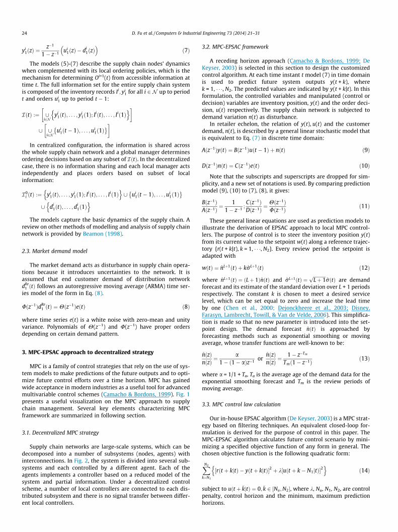
equal to z�LFa , where LFa is the manufacturing lead time. The dis-crete models for the ith echelon’s inventory position, IPi(t) andinventory, Ii(t) are:

IPiðtÞ ¼ IPiðt � 1Þ þ Yiþ1ðtÞ � Yi�1ðtÞ ð1Þ

IiðtÞ ¼ Iiðt � 1Þ þ Yiþ1ðt � LiÞ � Yi�1ðtÞ ð2Þ

Using notations for process control variables, the z-transformon Eq. (1) leads to:

yi1ðzÞ ¼

11� z�1 ðd

i2ðzÞ � ui

2ðzÞÞ ð3Þ

where z�1 represents both of the backward shift operator andcomplex variable in z-transform. When applied to time-dependentsignal s(t), z-k becomes backward shift operator, e.g., Z{s(t � k)} =z�kZ{s(t)} = z�ks(z).

Dejonckheere et al. (2003) pointed to 2 types of sequence ofoperations performed in the ith echelon and the first type ischosen:

(1) At discrete time t, the ith echelon receives goods from itssupplier.

(2) The demand Oi�1(t) from downstream echelon i � 1 isobserved and satisfied immediately, i.e. Yi�1(t) = Oi�1(t), orthe order is backlogged owing to lack of inventory.

(3) A new inventory level Ii(t) is measured.(4) Finally, the ith echelon places an order Oi+1(t) to the

upstream echelon i + 1.

It is important that in this type of sequence the order is madeafter the demand has been observed. Therefore, standing orderOi�ðtÞ is defined as the amount of orders to be processed at time

t + 1:

Oi�ðtÞ ¼ Oi

�ðt � 1Þ þ Oi�1ðtÞ � Yi�1ðtÞ ð4Þ

Again, z-transform is used and Eq. (4) is expressed as in Eq. (5)

yi2ðzÞ ¼

11� z�1 di

1ðzÞ � ui2ðzÞ

� �ð5Þ

The modelling of shipments from ith echelon to (i � 1)th eche-lon plays an important role in accurately representing systemdynamic response. For the actual delivery ‘the best I can do’ policy(Perea-Lopez et al., 2003) is adopted in practical supply chain oper-ations. Therefore, the delivery policy is defined as:

ui2ðtÞ ¼

0 z�1yi2ðtÞ ¼ 0

z�1yi2ðtÞ 0 6 z�1yi

2ðtÞ 6 z�1IiðtÞz�1IiðtÞ 0 6 z�1IiðtÞ 6 z�1yi

2ðtÞ

8><>: ð6Þ

Assume that each echelon always has ample product in stock(Chen, Drezner, Ryan, & Simchi-Levi, 2000; Lee, So, & Tang, 2000;Ouyang & Li, 2010) to meet its customers’ demand then thisapproximation indicates that ui

2ðtÞ ¼ z�1di1ðtÞ and di

2ðtÞ ¼ z�1ui1ðtÞ .

Thus Eq. (3) is transformed to:

24 D. Fu et al. / Computers & Industrial Engineering 73 (2014) 21–31

yi1ðzÞ ¼

z�1

1� z�1 ui1ðzÞ � di

1ðzÞ� �

ð7Þ

The models (5)-(7) describe the supply chain nodes’ dynamicswhen complemented with its local ordering policies, which is themechanism for determining Oi+1(t) from accessible information attime t. The full information set for the entire supply chain systemis composed of the inventory records Ii; yi

1 for all i 2 N up to periodt and orders ui

1 up to period t � 1:

IðtÞ :¼ [i2N

yi1ðtÞ; . . . ; yi

1ð1Þ; IiðtÞ; . . . ; Iið1Þn o� �

[ [i2N

ui1ðt � 1Þ; . . . ;ui

1ð1Þ� �� �

In centralized configuration, the information is shared acrossthe whole supply chain network and a global manager determinesordering decisions based on any subset of IðtÞ. In the decentralizedcase, there is no information sharing and each local manager actsindependently and places orders based on subset of localinformation:

I0i ðtÞ :¼ yi

1ðtÞ; . . . ; yi1ð1Þ; IiðtÞ; . . . ; Iið1Þ

n o[ ui

1ðt � 1Þ; . . . ; ui1ð1Þ

� �[ di

1ðtÞ; . . . ;di1ð1Þ

n oThe models capture the basic dynamics of the supply chain. A

review on other methods of modelling and analysis of supply chainnetwork is provided by Beamon (1998).

2.3. Market demand model

The market demand acts as disturbance in supply chain opera-tions because it introduces uncertainties to the network. It isassumed that end customer demand of distribution networkdRe

1 ðtÞ follows an autoregressive moving average (ARMA) time ser-ies model of the form in Eq. (8).

Uðz�1ÞdRe1 ðtÞ ¼ Hðz�1ÞeðtÞ ð8Þ

where time series e(t) is a white noise with zero-mean and unityvariance. Polynomials of H(z�1) and U(z�1) have proper ordersdepending on certain demand pattern.

3. MPC-EPSAC approach to decentralized strategy

MPC is a family of control strategies that rely on the use of sys-tem models to make predictions of the future outputs and to opti-mize future control efforts over a time horizon. MPC has gainedwide acceptance in modern industries as a useful tool for advancedmultivariable control schemes (Camacho & Bordons, 1999). Fig. 1presents a useful visualization on the MPC approach to supplychain management. Several key elements characterizing MPCframework are summarized in following section.

3.1. Decentralized MPC strategy

Supply chain networks are large-scale systems, which can bedecomposed into a number of subsystems (nodes, agents) withinterconnections. In Fig. 2, the system is divided into several sub-systems and each controlled by a different agent. Each of theagents implements a controller based on a reduced model of thesystem and partial information. Under a decentralized controlscheme, a number of local controllers are connected to each dis-tributed subsystem and there is no signal transfer between differ-ent local controllers.

3.2. MPC-EPSAC framework

A receding horizon approach (Camacho & Bordons, 1999; DeKeyser, 2003) is selected in this section to design the customizedcontrol algorithm. At each time instant t model (7) in time domainis used to predict future system outputs y(t + k), wherek = 1, � � �, N2. The predicted values are indicated by y(t + k|t). In thisformulation, the controlled variables and manipulated (control ordecision) variables are inventory position, y(t) and the order deci-sion, u(t) respectively. The supply chain network is subjected todemand variation n(t) as disturbance.

In retailer echelon, the relation of y(t), u(t) and the customerdemand, n(t), is described by a general linear stochastic model thatis equivalent to Eq. (7) in discrete time domain:

Aðz�1ÞyðtÞ ¼ Bðz�1Þuðt � 1Þ þ nðtÞ ð9Þ

Dðz�1ÞnðtÞ ¼ Cðz�1ÞeðtÞ ð10Þ

Note that the subscripts and superscripts are dropped for sim-plicity, and a new set of notations is used. By comparing predictionmodel (9), (10) to (7), (8), it gives:

Bðz�1ÞAðz�1Þ ¼

11� z�1 ;

Cðz�1ÞDðz�1Þ ¼

Hðz�1ÞUðz�1Þ ð11Þ

These general linear equations are used as prediction models toillustrate the derivation of EPSAC approach to local MPC control-lers. The purpose of control is to steer the inventory position y(t)from its current value to the setpoint w(t) along a reference trajec-tory {r(t + k|t), k = 1, � � �, N2}. Every review period the setpoint isadapted with

wðtÞ ¼ nLþ1ðtÞ þ krLþ1ðtÞ ð12Þ

where nLþ1ðtÞ ¼ ðLþ 1ÞnðtÞ and rLþ1ðtÞ ¼ffiffiffiffiffiffiffiffiffiffiffiLþ 1p

rðtÞ are demandforecast and its estimate of the standard deviation over L + 1 periodsrespectively. The constant k is chosen to meet a desired servicelevel, which can be set equal to zero and increase the lead timeby one (Chen et al., 2000; Dejonckheere et al., 2003; Disney,Farasyn, Lambrecht, Towill, & Van de Velde, 2006). This simplifica-tion is made so that no new parameter is introduced into the set-point design. The demand forecast nðtÞ is approached byforecasting methods such as exponential smoothing or movingaverage, whose transfer functions are well-known to be:

nðzÞnðzÞ ¼

a1� 1� að Þz�1 or

nðzÞnðzÞ ¼

1� z�Tm

Tmð1� z�1Þ ð13Þ

where a = 1/1 + Ta, Ta is the average age of the demand data for theexponential smoothing forecast and Tm is the review periods ofmoving average.

3.3. MPC control law calculation

Our in-house EPSAC algorithm (De Keyser, 2003) is a MPC strat-egy based on filtering techniques. An equivalent closed-loop for-mulation is derived for the purpose of control in this paper. TheMPC-EPSAC algorithm calculates future control scenario by mini-mizing a specified objective function of any form in general. Thechosen objective function is the following quadratic form:

XN2

k¼N1

rðt þ kjtÞ � yðt þ kjtÞ½ �2 þ k uðt þ k� N1jtÞ½ �2n o

ð14Þ

subject to uðt þ �kjtÞ ¼ 0; �k 2 ½Nu;N2�, where k, Nu, N1, N2, are controlpenalty, control horizon and the minimum, maximum predictionhorizons.

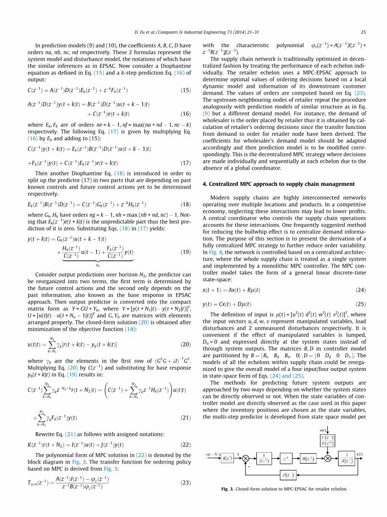
Fig. 3. Closed-form solution to MPC-EPSAC for retailer echelon.

D. Fu et al. / Computers & Industrial Engineering 73 (2014) 21–31 25

In prediction models (9) and (10), the coefficients A, B, C, D haveorders na, nb, nc, nd respectively. These 2 formulas represent thesystem model and disturbance model, the notations of which havethe similar inferences as in EPSAC. Now consider a Diophantineequation as defined in Eq. (15) and a k-step prediction Eq. (16) ofoutput:

Cðz�1Þ ¼ Aðz�1ÞDðz�1ÞEkðz�1Þ þ z�kFkðz�1Þ ð15Þ

Aðz�1ÞDðz�1Þyðt þ kjtÞ ¼ Bðz�1ÞDðz�1Þuðt þ k� 1jtÞþ Cðz�1Þeðt þ kjtÞ ð16Þ

where Ek, Fk are of orders ne = k � 1, nf = max(na + nd � 1, nc � k)respectively. The following Eq. (17) is given by multiplying Eq.(16) by Ek and adding to (15):

Cðz�1Þyðt þ kjtÞ ¼ Ekðz�1ÞBðz�1ÞDðz�1Þuðt þ k� 1jtÞ

þFkðz�1ÞyðtÞ þ Cðz�1ÞEkðz�1Þeðt þ kjtÞ ð17Þ

Then another Diophantine Eq. (18) is introduced in order tosplit up the predictor (17) in two parts that are depending on pastknown controls and future control actions yet to be determinedrespectively.

Ekðz�1ÞBðz�1ÞDðz�1Þ ¼ Cðz�1ÞGkðz�1Þ þ z�kHkðz�1Þ ð18Þ

where Gk, Hk have orders ng = k � 1, nh = max (nb + nd, nc) � 1. Not-ing that Ek(z�1)e(t + k|t) is the unpredictable part thus the best pre-diction of it is zero. Substituting Eqs. (18) in (17) yields:

yðt þ kjtÞ ¼ Gkðz�1Þuðt þ k� 1jtÞ

þ Hkðz�1ÞCðz�1Þ uðt � 1Þ þ Fkðz�1Þ

Cðz�1Þ yðtÞ|fflfflfflfflfflfflfflfflfflfflfflfflfflfflfflfflfflfflfflfflfflfflfflfflfflfflfflffl{zfflfflfflfflfflfflfflfflfflfflfflfflfflfflfflfflfflfflfflfflfflfflfflfflfflfflfflffl}yb

ð19Þ

Consider output predictions over horizon N2, the predictor canbe reorganized into two terms, the first term is determined bythe future control actions and the second only depends on thepast information, also known as the base response in EPSACapproach. Then output predictor is converted into the compactmatrix form as Y = GU + Yb, where Y = [y(t + N1|t)� � �y(t + N2|t)]T,U = [u(t|t)� � �u(t + Nu � 1|t)]T and G, Yb are matrices with elementsarranged properly. The closed-form solution (20) is obtained afterminimization of the objective function (14):

uðtjtÞ ¼XN2

k¼N1

ck½rðt þ kjtÞ � ybðt þ kjtÞ� ð20Þ

where ck are the elements in the first row of ðGT Gþ kIÞ�1GT .

Multiplying Eq. (20) by C(z�1) and substituting for base responseyb(t + k|t) in Eq. (19) results in:

Cðz�1ÞXN2

k¼N1

ckz�N2þkrðt þ N2jtÞ ¼ Cðz�1Þ þXN2

k¼N1

ckz�1Hkðz�1Þ !

uðtjtÞ

þXN2

k¼N1

ckFkðz�1ÞyðtÞ ð21Þ

Rewrite Eq. (21) as follows with assigned notations:

Kðz�1Þrðt þ N2Þ ¼ Iðz�1ÞuðtÞ þ Jðz�1ÞyðtÞ ð22Þ

The polynomial form of MPC solution in (22) is denoted by theblock diagram in Fig. 3. The transfer function for ordering policybased on MPC is derived from Fig. 3:

Tu=nðz�1Þ ¼ Aðz�1ÞIðz�1Þ �ucðz�1Þz�1Bðz�1Þucðz�1Þ ð23Þ

with the characteristic polynomial uc(z�1) = A(z�1)I(z�1) +z�1B(z�1)J(z�1).

The supply chain network is traditionally optimized in decen-tralized fashion by treating the performance of each echelon indi-vidually. The retailer echelon uses a MPC-EPSAC approach todetermine optimal values of ordering decisions based on a localdynamic model and information of its downstream customerdemand. The values of orders are computed based on Eq. (23).The upstream neighbouring nodes of retailer repeat the procedureanalogously with prediction models of similar structure as in Eq.(9) but a different demand model. For instance, the demand ofwholesaler is the order placed by retailer thus it is obtained by cal-culation of retailer’s ordering decisions since the transfer functionfrom demand to order for retailer node have been derived. Thecoefficients for wholesaler’s demand model should be adaptedaccordingly and then prediction model is to be modified corre-spondingly. This is the decentralized MPC strategy where decisionsare made individually and sequentially at each echelon due to theabsence of a global coordinator.

4. Centralized MPC approach to supply chain management

Modern supply chains are highly interconnected networksoperating over multiple locations and products. In a competitiveeconomy, neglecting these interactions may lead to lower profits.A central coordinator who controls the supply chain operationsaccounts for these interactions. One frequently suggested methodfor reducing the bullwhip effect is to centralize demand informa-tion. The purpose of this section is to present the derivation of afully centralized MPC strategy to further reduce order variability.In Fig. 4, the network is controlled based on a centralized architec-ture, where the whole supply chain is treated as a single systemand implemented by a monolithic MPC controller. The MPC con-troller model takes the form of a general linear discrete-timestate-space:

xðt þ 1Þ ¼ AxðtÞ þ BlðtÞ ð24Þ

yðtÞ ¼ CxðtÞ þ DlðtÞ ð25Þ

The definition of input is l(t) = [uT(t) dT(t) wT(t) vT(t)]T, wherethe input vectors u, d, w, v represent manipulated variables, loaddisturbances and 2 unmeasured disturbances respectively. It isconvenient if the effect of manipulated variables is lumped,Du = 0 and expressed directly at the system states instead ofthrough system outputs. The matrices B, D in controller modelare partitioned by B ¼ ½Bu Bd Bw 0� ;D ¼ ½0 Dd 0 Dv �. Themodels of all the echelons within supply chain could be reorga-nized to give the overall model of a four input/four output systemin state-space form of Eqs. (24) and (25).

The methods for predicting future system outputs areapproached by two ways depending on whether the system statescan be directly observed or not. When the state variables of con-troller model are directly observed as the case used in this paperwhere the inventory positions are chosen as the state variables,the multi-step predictor is developed from state space model per

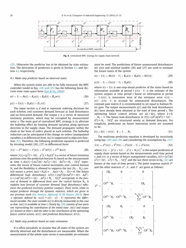
Fig. 4. Centralized MPC strategy for supply chain network.

26 D. Fu et al. / Computers & Industrial Engineering 73 (2014) 21–31

(25). Otherwise the predictor has to be obtained by state estima-tion. The derivation of predictors is given in Section 4.1 and Sec-tion 4.2 respectively.

4.1. Multi-step predictor based on observed states

When the system states are able to be fully measured, the MPCcontroller model in Eqs. (24) and (25) has the following linear dis-crete-time state-space form (Lee & Yu, 1994):

xðt þ 1Þ ¼ AxðtÞ þ BuuðtÞ þ BddðtÞ þ BwwðtÞ ð26Þ

yðtÞ ¼ CxðtÞ þ DddðtÞ þ DvvðtÞ ð27Þ

The input vectors u, d and w represent ordering decisions foreach echelon, end customer demand forecast as load disturbanceand un-forecasted demand. The output y is a vector of measuredinventory positions, which may be corrupted by measurementnoise v. The main goal of centralized MPC strategy is to alleviatethe bullwhip effect by limiting demand variation along upstreamdirection in the supply chain. The demand propagates within thechain in the form of orders placed at each echelon. The bullwhipreduction can be anticipated if the change on orders (manipulatedvariables u in differenced form Du) is suppressed in objective func-tion (33). Therefore, the following prediction equation is preferredby iterating model (26), (27) in differenced form:

YðtÞ ¼ SDxDxðtÞ þ I yyðtÞ þ SDDDðtÞ þ SDUDUðtÞ ð28Þ

where Y(t) = [yT(t + 1|t)� � �yT(t + N2|t)]T is a vector of future inventorypositions over the prediction horizon N2 based on the measurementat time t; DU(t) = [DuT(t|t) DuT(t + 1|t)� � �DuT(t + Nu � 1|t)]T repre-sents the vector of future control increments over control horizonNu and the flexibility is allowed to suppress the last (N2 � Nu) con-trol moves a priori, Du(t + Nu|t) = � � �Du(t + N2 � 1|t) = 0. The futuredifferenced load disturbance DD(t) = [DdT(t|t)DdT(t + 1|t)� � �DdT(-t) = [DdT(t|t)DdT(t + 1|t)� � �DdT(t + Nu � 1|t)]T corresponds to the fore-cast of demand in differenced form over the control horizon Nu. Itexplains how forecast of customer demand (load disturbance) influ-ences the predicted inventory position (output). These terms relate tooutput predictor through the dynamic matrices, which are given inour previous work (Fu, Ionescu, Aghezzaf, & De Keyser, 2013). HereD operator defined by D⁄(t): = ⁄(t) � ⁄(t � 1) represents the differ-enced variable. The state variable x(t) is directly measurable in this caseso that Dx(t) is available at time t. Clearly Eq. (28) consists of two partsone representing the contribution of the initial state Dx(t) and outputy(t) known at time t, and the other is the contribution of the optimizingfuture control actions DUðtÞ and predicted disturbances DDðtÞ.

4.2. Multi-step predictor based on state estimation

It is often unrealistic to assume that all states of the system aredirectly observed and the disturbances are measurable. When themeasurement of the whole state vector is unavailable, an estimator

must be used. The predictions of future unmeasured disturbancesare zero and nominal models (26) and (27) are used to estimatethe future states of the system

xðt þ 1jtÞ ¼ Axðtjt � 1Þ þ BuuðtÞ þ BddðtÞ þ KeðtjtÞ ð29Þ

yðtjt � 1Þ ¼ Cxðtjt � 1Þ þ DddðtÞ ð30Þ

where xðt þ 1jtÞ is one-step-ahead predictor of the states based oninformation available at period t; yðtjt � 1Þ is the estimate of thesystem outputs at time period t based on information at periodt � 1; eðtjtÞ is innovation term of the estimator error eðtjtÞ ¼yðtÞ � yðtjt � 1Þ to account for unmeasured disturbances. Theconstant gain matrix K is recommended to set equal to Kalman fil-ter gain. The output measurements y(t) and the load disturbancesd(t) have already been obtained at the start of time period t. Theoptimizing future control actions are u(t + k|t), where k = 0,� � �N2 � 1. The future load disturbances in D(t) = [dT(t|t)dT(t + 1|t)� � �dT(t + Nu � 1|t)]T are structured wisely as demand forecasts. Forsimplicity, predictions on future innovation terms are assumedto be:

eðt þ kjtÞ ¼ eðtjtÞ k ¼ 1; . . . N2 ð31Þ

The multistep prediction equation is developed by recursivelyusing Eqs. (29) and (30) and considering the assumptions Eq. (31):

YðtÞ ¼ SUUðtÞ þ SDDðtÞ þ Sxxðtjt � 1Þ þ SeeðtjtÞ ð32Þ

where YðtÞ ¼ yTðt þ 1jtÞ � � � yTðt þ N2jtÞ �T is the output prediction of

supply chain system based on the measurements until time periodt, and UðtÞ is a vector of future manipulated variables, U(t) = [uT(t|t)uT(t + 1|t)� � �uT(t + Nu � 1|t)]T and the last three terms in Eq. (32) areknown at the start of time period t. The pulse response matrix SU

and the other matrices SD, Se, and Sx are given as follows:

SU ¼

CBu 0 � � � 0

..

. ... ..

. ...

CANu�1Bu � � � � � � CBu

..

. ... ..

. ...

CAN2�1Bu CAN2�2Bu � � �XN2�Nuþ1

j¼1

CAj�1Bu

266666666666664

377777777777775;

SD ¼

CBd Bd � � � 0

..

. ... ..

. ...

CANu�1Bd � � � CBd Bd

..

. ... ..

. ...

CAN2�1Bd CAN2�2Bd � � �XN2�Nuþ1

j¼1

CAj�1Bd

266666666666664

377777777777775;

D. Fu et al. / Computers & Industrial Engineering 73 (2014) 21–31 27

Sx ¼ ðCAÞT � � � ðCAN2 ÞT

h iT;Se ¼ ðCKÞT � � � C

XN2

k¼1

Ak�1

!K

!T" #T

:

The differenced form of the predictor based on state estimationis derived by defining DUðtÞ as DUðtÞ ¼ RDUðtÞ � dðtÞ with

RD ¼

I 0 0 � � � 0�I I 0 � � � 0... ..

. ... ..

. ...

0 0 � � � �I I

266664

377775; dðtÞ ¼ uTðt � 1Þ0 � � �0

�:

Both approaches to the multi-step predictor are exhibited inthese two sections. The two multi-step predictors should be cho-sen depending on the measurability of the states of controllermodel.

4.3. MPC control law calculation

The predicted system outputs YðtÞ depend on past inputs andoutputs as well as the future control scenario UðtÞ. The MPC algo-rithm tries to calculate this control scenario by minimizing a spec-ified objective function of any form in general. In the application ofMPC formulation to SCM, the controller considers at each time per-iod t the previous information on inventory position of each node,actual customer demand, order of each node and future informa-tion on inventory position setpoint, forecasted demand in orderto calculate the sequence of future order decisions on the basisof the following objective function:

VðtÞ¼XNu

k¼1

kPðkÞDuðtþk�1jtÞk2

|fflfflfflfflfflfflfflfflfflfflfflfflfflfflfflfflfflfflfflfflfflfflffl{zfflfflfflfflfflfflfflfflfflfflfflfflfflfflfflfflfflfflfflfflfflfflffl}penalty on changes of order

þXN2

k¼1

k QðkÞðyðtþkjtÞ� rðtþkjtÞÞ½ �k2

|fflfflfflfflfflfflfflfflfflfflfflfflfflfflfflfflfflfflfflfflfflfflfflfflfflfflfflfflfflfflfflffl{zfflfflfflfflfflfflfflfflfflfflfflfflfflfflfflfflfflfflfflfflfflfflfflfflfflfflfflfflfflfflfflffl}keep inventory position at set point

ð33Þ

where r(t + k|t) is a reference vector for inventory positions at timet + k projected at time t, QðkÞ and P(k) are penalty weight matriceson control error and control move size respectively, which enablethe controller to satisfy inventory position setpoint tracking, andto adjust order variability. The small variation of demand at retailerend will be amplified to the upstream end, which is known as bull-whip effect. Penalizing excess change of the manipulated variablesis conducive to reducing the bullwhip effect. In addition, suppres-sion of excess movement of the manipulated variables leads tosmoothed ordering pattern and thus results in reduced variabilityon factory starts. The objective function is described in the follow-ing vector form:

minDUðkÞVðtÞ ¼ k½QðYðtÞ �RðtÞÞ�k2 þ kPDUðtÞk2 ð34Þ

where Q = diag[Q(1)� � �Q(N2)] and P = diag[P(1)� � �P(Nu)] stand forpenalty matrix on control error and move suppression penaltymatrix respectively, the reference trajectory is R(t) = [rT(t + 1|t)� � �rT(t + N2|t)]T.

It should be noted that in addition to the control-theoretic ori-ented objective function an economic cost function could be opti-mized as in the cases of Mestan et al. (2006), Li and Marlin (2009).Their works consider the most general objective of supply chainoptimization as the maximization of the overall profit. The practi-cal requirements in SCM are appropriately posed as constraints onthe system variables. Three types of constraints are considered inmost of studies depending on practical conditions of the supplychain operations.

(a) Output variable constraints. The controller minimizes thedeviation of inventory position of each echelon from its set-points. But the inventory positions can only stay within highand low limits on account of restrictions on capacity of thewarehouse.

YminðtÞ 6 YðtÞ 6 YmaxðtÞ ð35Þ

(b) Manipulated variable rate constraints. There are some hardhigh bounds for ordering rates made by each echelon. Ifproper constraints on changes of orders are applied, demandvariation reduction can be expected and thus result in lessfluctuation in factory thrash.

jDUðkÞj 6 DUmaxðkÞ ð36Þ

(c) Manipulated variable constraints. In addition to manipulatedvariable rate constraints, the control variables are all non-negative and they are also subject to some low and high lim-its on the quantities of orders because of capacity limitationon transportation. Note that UminðtÞP 0.

UminðtÞ 6 UðtÞ 6 UmaxðtÞ ð37Þ

The control of supply chain is now formulated as an optimiza-tion problem in which the control moves DU(t) are computed onthe basis of Eq. (34) subject to the linear inequality constraints.The control law does not require too much computation effortin the absence of constraints. In presence of constraints (35)-(37), the MPC problem based on objective function (34) andprediction Eq. (28) or Eq. (32) is then solved by standard QPalgorithms (Fletcher, 1981) subject to appropriate inequalityconstraints:

min12

DUðkÞTHDUðkÞ � DUðkÞTG ð38Þ

where the gradient vector G and Hessian matrix H of objectivefunction are to be constructed according to different predictionequations used. Instead of 4 separate controllers as implementedin decentralized control strategy, a single controller is used by aglobal coordinator in centralized MPC strategy to make orderingdecisions for each node. In this case, order and inventory informa-tion at each echelon are fed to the central controller as illustratedin Fig. 4. The centralized MPC controller, based on overall models(24), (25) of the supply chain network, calculates all the controlmoves DU(t) via the optimization problem Eq. (38) and sends thefirst element of U(t) as ordering decisions at current time t tomanager of each echelon.

5. Simulation results

In this simulation the MPC frameworks presented in Sections 3and 4 are applied to the management of a single-item supply chainmade of 4 nodes. The constraints are not involved in 2 conven-tional ordering polices. In order to compare the performance ofcentralized and decentralized MPC ordering polices with themunder the same conditions in simulation, the two MPC orderingpolices are considered in unconstrained cases. The two MPCapproaches to supply chain optimization are applied to illustratetheir capabilities to track demand variation and to reduce the bull-whip effect.

5.1. Initialization of simulation

The supply chain is considered over 100 weeks (the operationaldecisions are reviewed per week). The market demand is modelledas Eq. (8) in Section 2 and the end-customer demand nRe(t) is gen-erated as follows:

Fig. 5. Actual demand and forecasted customer demand based on moving averageforecasting of 10 time periods.

Table 2Simulation data and initial state of supply chain operations.

Supply chainnode

PTD(weeks)

IIL (units ofproduct)

iWIP (units ofproduct)

Retailer 2 10 5Wholesaler 2 10 5Distributor 2 10 5Factory 2 10 5

28 D. Fu et al. / Computers & Industrial Engineering 73 (2014) 21–31

nReð0Þ ¼ eð0Þ þ lnReðtÞ ¼ uðnReðt � 1Þ � lÞ þ eðtÞ � heðt � 1Þ þ l

�ð39Þ

where l is the mean of ARMA demand pattern and assumed to be 8units, u = 0.8 is auto regressive coefficient and h = 0.6 is the movingaverage coefficient. The forecasted demand corresponds to 10 timeperiods moving average and it is illustrated along with the actualdemand in Fig. 5.

Table 2 reports the supplier’s production/transportation delay(PTD), initial inventory level (IIL) and initial work-in-process(iWIP) at each node. The model is initialized by setting parametersas specified in Table 2.

Many researchers have been using Eq. (40) as a measure of bull-whip, where u, n refer to the orders placed on a supplier and cus-tomer demands respectively, and r2, l denote the variance andthe mean value of the variables.

Bullwhip ¼ r2u=lu

r2n=ln

ð40Þ

Fig. 6. Simulation results for decentralized MPC strategy: left figure i

5.2. Numerical simulation results

In decentralized control strategy, each node applies a MPC con-troller to compute the ordering decision via Eq. (23), where thetuning parameters N1 = 1, Nu = 1 are default values. The predictionhorizon is chosen as N2 = 3 because it is sufficient for the local con-troller to predict outputs over future 3 weeks, i.e. 2 weeks trans-portation delay and 1 week ordering delay. The time behavioursof the simulation are presented in Fig. 6.

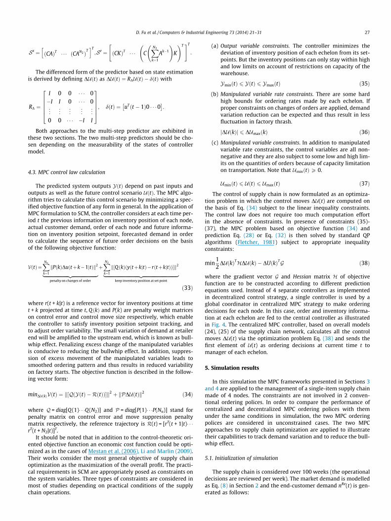
In the centralized case, the prediction horizon is N2 = 15 and thecontrol horizon is Nu = 10, both of which exceed the collective sumof the nominal ordering and transportation delays along 4 serialnodes in supply chain. The 2 long horizons are required by the cen-tralized decision-making in order to execute necessary feed-for-ward anticipations. The output weight matrix Q is set in a waythat it is 1 for corresponding controlled variable, while move sup-pression matrix P is tuned to compare the effects of differentweights on bullwhip reduction.

The simulation results shown in Fig. 7 compare the inventoryposition levels and control efforts under 2 different control movesuppression matrices. The upper figures show the results with sup-pression matrix P = [1000; 0100; 0010; 0001], where the weightson control move sizes are all the same for each node. The orderingdecisions are adjusted aggressively at first time periods and inven-tory positions keep a small fluctuation after the 30th week. Theoscillation on inventory positions is mainly caused by trackingthe setpoints. The magnitude of variance of orders is amplifiedfrom retailer to factory at start time periods and ordering decisionsbetween the 25th and 100th week continue to keep a good track-ing of end-customer demand variation. In lower figures, the weighton control move size for factory’s orders increased to 5, which islarger than that in upper figures. The magnitude of variance of fac-tory’s orders is reduced so that the factory’s ordering decisions aresmoothed and stabilized. This ordering pattern is favourable for

s for ordering decisions and right figure is for inventory position.

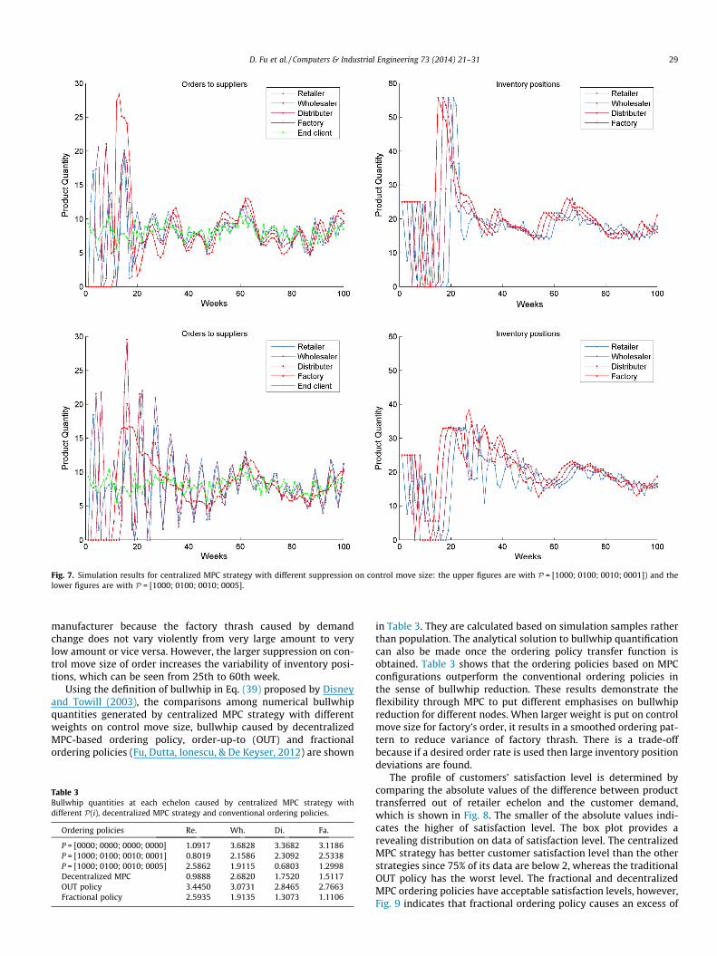
Fig. 7. Simulation results for centralized MPC strategy with different suppression on control move size: the upper figures are with P = [1000; 0100; 0010; 0001]) and thelower figures are with P = [1000; 0100; 0010; 0005].

D. Fu et al. / Computers & Industrial Engineering 73 (2014) 21–31 29

manufacturer because the factory thrash caused by demandchange does not vary violently from very large amount to verylow amount or vice versa. However, the larger suppression on con-trol move size of order increases the variability of inventory posi-tions, which can be seen from 25th to 60th week.

Using the definition of bullwhip in Eq. (39) proposed by Disneyand Towill (2003), the comparisons among numerical bullwhipquantities generated by centralized MPC strategy with differentweights on control move size, bullwhip caused by decentralizedMPC-based ordering policy, order-up-to (OUT) and fractionalordering policies (Fu, Dutta, Ionescu, & De Keyser, 2012) are shown

Table 3Bullwhip quantities at each echelon caused by centralized MPC strategy withdifferent P(i), decentralized MPC strategy and conventional ordering policies.

Ordering policies Re. Wh. Di. Fa.

P = [0000; 0000; 0000; 0000] 1.0917 3.6828 3.3682 3.1186P = [1000; 0100; 0010; 0001] 0.8019 2.1586 2.3092 2.5338P = [1000; 0100; 0010; 0005] 2.5862 1.9115 0.6803 1.2998Decentralized MPC 0.9888 2.6820 1.7520 1.5117OUT policy 3.4450 3.0731 2.8465 2.7663Fractional policy 2.5935 1.9135 1.3073 1.1106

in Table 3. They are calculated based on simulation samples ratherthan population. The analytical solution to bullwhip quantificationcan also be made once the ordering policy transfer function isobtained. Table 3 shows that the ordering policies based on MPCconfigurations outperform the conventional ordering policies inthe sense of bullwhip reduction. These results demonstrate theflexibility through MPC to put different emphasises on bullwhipreduction for different nodes. When larger weight is put on controlmove size for factory’s order, it results in a smoothed ordering pat-tern to reduce variance of factory thrash. There is a trade-offbecause if a desired order rate is used then large inventory positiondeviations are found.

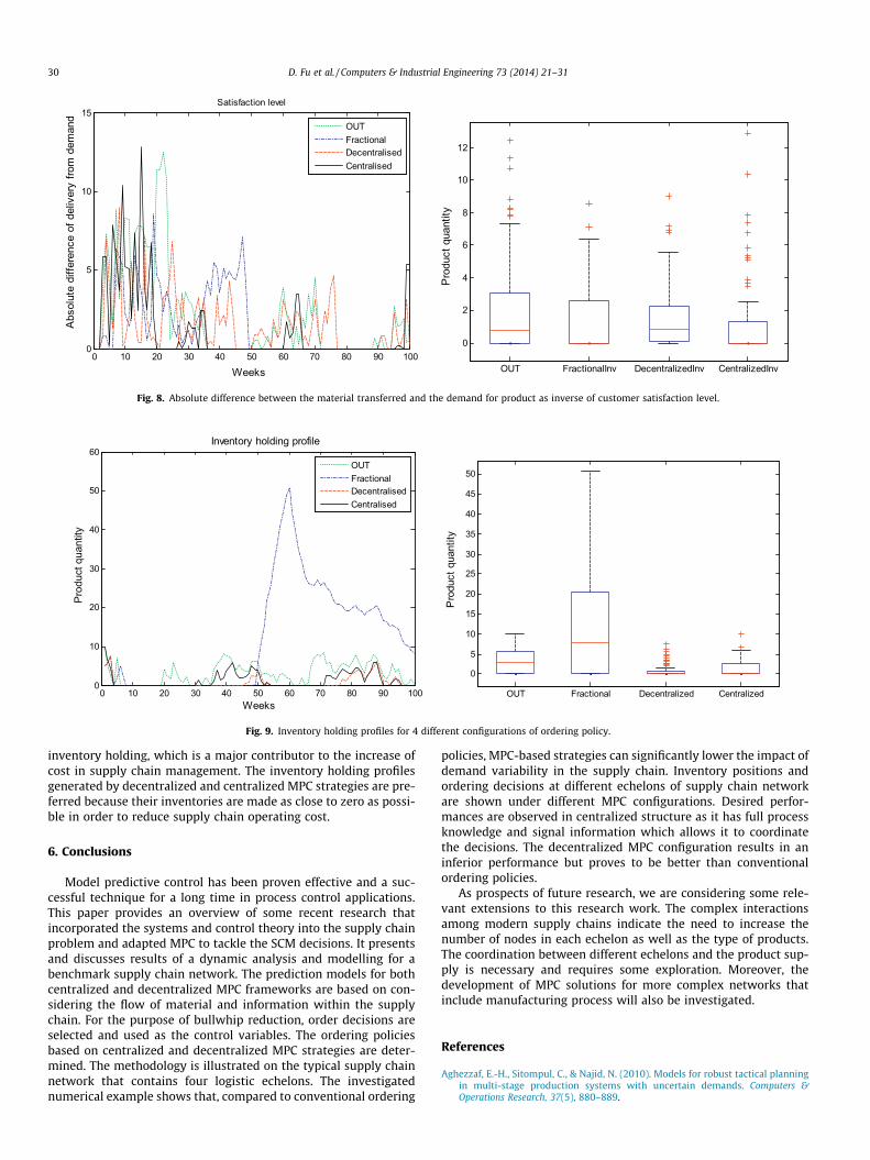
The profile of customers’ satisfaction level is determined bycomparing the absolute values of the difference between producttransferred out of retailer echelon and the customer demand,which is shown in Fig. 8. The smaller of the absolute values indi-cates the higher of satisfaction level. The box plot provides arevealing distribution on data of satisfaction level. The centralizedMPC strategy has better customer satisfaction level than the otherstrategies since 75% of its data are below 2, whereas the traditionalOUT policy has the worst level. The fractional and decentralizedMPC ordering policies have acceptable satisfaction levels, however,Fig. 9 indicates that fractional ordering policy causes an excess of

0 10 20 30 40 50 60 70 80 90 1000

5

10

15

Weeks

Abs

olut

e di

ffere

nce

of d

eliv

ery

from

dem

and

Satisfaction level

OUTFractionalDecentralisedCentralised

OUT FractionalInv DecentralizedInv CentralizedInv

0

2

4

6

8

10

12

Pro

duct

qua

ntity

Fig. 8. Absolute difference between the material transferred and the demand for product as inverse of customer satisfaction level.

0 10 20 30 40 50 60 70 80 90 1000

10

20

30

40

50

60

Weeks

Prod

uct q

uant

ity

Inventory holding profile

OUTFractionalDecentralisedCentralised

OUT Fractional Decentralized Centralized

0

5

10

15

20

25

30

35

40

45

50

Pro

duct

qua

ntity

Fig. 9. Inventory holding profiles for 4 different configurations of ordering policy.

30 D. Fu et al. / Computers & Industrial Engineering 73 (2014) 21–31

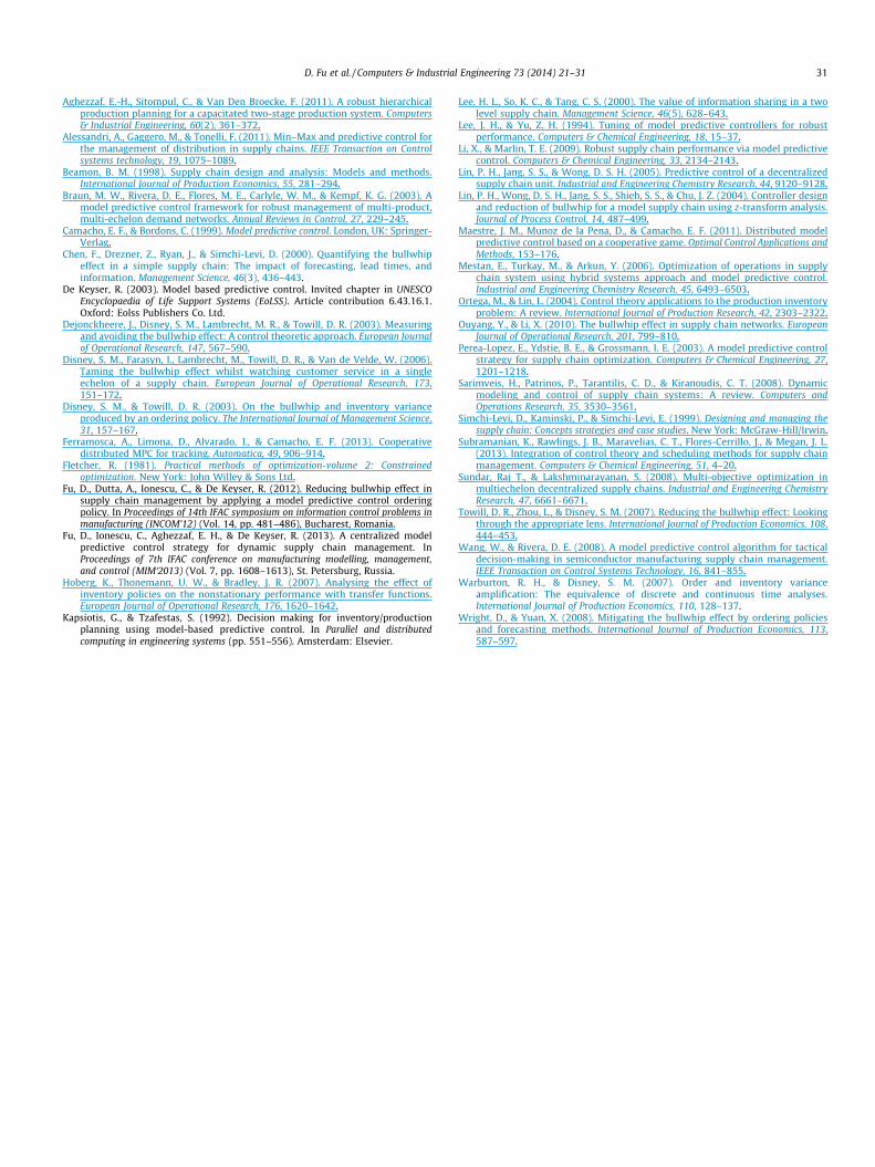
inventory holding, which is a major contributor to the increase ofcost in supply chain management. The inventory holding profilesgenerated by decentralized and centralized MPC strategies are pre-ferred because their inventories are made as close to zero as possi-ble in order to reduce supply chain operating cost.

6. Conclusions

Model predictive control has been proven effective and a suc-cessful technique for a long time in process control applications.This paper provides an overview of some recent research thatincorporated the systems and control theory into the supply chainproblem and adapted MPC to tackle the SCM decisions. It presentsand discusses results of a dynamic analysis and modelling for abenchmark supply chain network. The prediction models for bothcentralized and decentralized MPC frameworks are based on con-sidering the flow of material and information within the supplychain. For the purpose of bullwhip reduction, order decisions areselected and used as the control variables. The ordering policiesbased on centralized and decentralized MPC strategies are deter-mined. The methodology is illustrated on the typical supply chainnetwork that contains four logistic echelons. The investigatednumerical example shows that, compared to conventional ordering

policies, MPC-based strategies can significantly lower the impact ofdemand variability in the supply chain. Inventory positions andordering decisions at different echelons of supply chain networkare shown under different MPC configurations. Desired perfor-mances are observed in centralized structure as it has full processknowledge and signal information which allows it to coordinatethe decisions. The decentralized MPC configuration results in aninferior performance but proves to be better than conventionalordering policies.

As prospects of future research, we are considering some rele-vant extensions to this research work. The complex interactionsamong modern supply chains indicate the need to increase thenumber of nodes in each echelon as well as the type of products.The coordination between different echelons and the product sup-ply is necessary and requires some exploration. Moreover, thedevelopment of MPC solutions for more complex networks thatinclude manufacturing process will also be investigated.

References

Aghezzaf, E.-H., Sitompul, C., & Najid, N. (2010). Models for robust tactical planningin multi-stage production systems with uncertain demands. Computers &Operations Research, 37(5), 880–889.

D. Fu et al. / Computers & Industrial Engineering 73 (2014) 21–31 31

Aghezzaf, E.-H., Sitompul, C., & Van Den Broecke, F. (2011). A robust hierarchicalproduction planning for a capacitated two-stage production system. Computers& Industrial Engineering, 60(2), 361–372.

Alessandri, A., Gaggero, M., & Tonelli, F. (2011). Min–Max and predictive control forthe management of distribution in supply chains. IEEE Transaction on Controlsystems technology, 19, 1075–1089.

Beamon, B. M. (1998). Supply chain design and analysis: Models and methods.International Journal of Production Economics, 55, 281–294.

Braun, M. W., Rivera, D. E., Flores, M. E., Carlyle, W. M., & Kempf, K. G. (2003). Amodel predictive control framework for robust management of multi-product,multi-echelon demand networks. Annual Reviews in Control, 27, 229–245.

Camacho, E. F., & Bordons, C. (1999). Model predictive control. London, UK: Springer-Verlag.

Chen, F., Drezner, Z., Ryan, J., & Simchi-Levi, D. (2000). Quantifying the bullwhipeffect in a simple supply chain: The impact of forecasting, lead times, andinformation. Management Science, 46(3), 436–443.

De Keyser, R. (2003). Model based predictive control. Invited chapter in UNESCOEncyclopaedia of Life Support Systems (EoLSS). Article contribution 6.43.16.1.Oxford: Eolss Publishers Co. Ltd.

Dejonckheere, J., Disney, S. M., Lambrecht, M. R., & Towill, D. R. (2003). Measuringand avoiding the bullwhip effect: A control theoretic approach. European Journalof Operational Research, 147, 567–590.

Disney, S. M., Farasyn, I., Lambrecht, M., Towill, D. R., & Van de Velde, W. (2006).Taming the bullwhip effect whilst watching customer service in a singleechelon of a supply chain. European Journal of Operational Research, 173,151–172.

Disney, S. M., & Towill, D. R. (2003). On the bullwhip and inventory varianceproduced by an ordering policy. The International Journal of Management Science,31, 157–167.

Ferramosca, A., Limona, D., Alvarado, I., & Camacho, E. F. (2013). Cooperativedistributed MPC for tracking. Automatica, 49, 906–914.

Fletcher, R. (1981). Practical methods of optimization-volume 2: Constrainedoptimization. New York: John Willey & Sons Ltd.

Fu, D., Dutta, A., Ionescu, C., & De Keyser, R. (2012). Reducing bullwhip effect insupply chain management by applying a model predictive control orderingpolicy. In Proceedings of 14th IFAC symposium on information control problems inmanufacturing (INCOM’12) (Vol. 14, pp. 481–486), Bucharest, Romania.

Fu, D., Ionescu, C., Aghezzaf, E. H., & De Keyser, R. (2013). A centralized modelpredictive control strategy for dynamic supply chain management. InProceedings of 7th IFAC conference on manufacturing modelling, management,and control (MIM‘2013) (Vol. 7, pp. 1608–1613), St. Petersburg, Russia.

Hoberg, K., Thonemann, U. W., & Bradley, J. R. (2007). Analysing the effect ofinventory policies on the nonstationary performance with transfer functions.European Journal of Operational Research, 176, 1620–1642.

Kapsiotis, G., & Tzafestas, S. (1992). Decision making for inventory/productionplanning using model-based predictive control. In Parallel and distributedcomputing in engineering systems (pp. 551–556). Amsterdam: Elsevier.

Lee, H. L., So, K. C., & Tang, C. S. (2000). The value of information sharing in a twolevel supply chain. Management Science, 46(5), 628–643.

Lee, J. H., & Yu, Z. H. (1994). Tuning of model predictive controllers for robustperformance. Computers & Chemical Engineering, 18, 15–37.

Li, X., & Marlin, T. E. (2009). Robust supply chain performance via model predictivecontrol. Computers & Chemical Engineering, 33, 2134–2143.

Lin, P. H., Jang, S. S., & Wong, D. S. H. (2005). Predictive control of a decentralizedsupply chain unit. Industrial and Engineering Chemistry Research, 44, 9120–9128.

Lin, P. H., Wong, D. S. H., Jang, S. S., Shieh, S. S., & Chu, J. Z. (2004). Controller designand reduction of bullwhip for a model supply chain using z-transform analysis.Journal of Process Control, 14, 487–499.

Maestre, J. M., Munoz de la Pena, D., & Camacho, E. F. (2011). Distributed modelpredictive control based on a cooperative game. Optimal Control Applications andMethods, 153–176.

Mestan, E., Turkay, M., & Arkun, Y. (2006). Optimization of operations in supplychain system using hybrid systems approach and model predictive control.Industrial and Engineering Chemistry Research, 45, 6493–6503.

Ortega, M., & Lin, L. (2004). Control theory applications to the production inventoryproblem: A review. International Journal of Production Research, 42, 2303–2322.

Ouyang, Y., & Li, X. (2010). The bullwhip effect in supply chain networks. EuropeanJournal of Operational Research, 201, 799–810.

Perea-Lopez, E., Ydstie, B. E., & Grossmann, I. E. (2003). A model predictive controlstrategy for supply chain optimization. Computers & Chemical Engineering, 27,1201–1218.

Sarimveis, H., Patrinos, P., Tarantilis, C. D., & Kiranoudis, C. T. (2008). Dynamicmodeling and control of supply chain systems: A review. Computers andOperations Research, 35, 3530–3561.

Simchi-Levi, D., Kaminski, P., & Simchi-Levi, E. (1999). Designing and managing thesupply chain: Concepts strategies and case studies. New York: McGraw-Hill/Irwin.

Subramanian, K., Rawlings, J. B., Maravelias, C. T., Flores-Cerrillo, J., & Megan, J. L.(2013). Integration of control theory and scheduling methods for supply chainmanagement. Computers & Chemical Engineering, 51, 4–20.

Sundar, Raj T., & Lakshminarayanan, S. (2008). Multi-objective optimization inmultiechelon decentralized supply chains. Industrial and Engineering ChemistryResearch, 47, 6661–6671.

Towill, D. R., Zhou, L., & Disney, S. M. (2007). Reducing the bullwhip effect: Lookingthrough the appropriate lens. International Journal of Production Economics, 108,444–453.

Wang, W., & Rivera, D. E. (2008). A model predictive control algorithm for tacticaldecision-making in semiconductor manufacturing supply chain management.IEEE Transaction on Control Systems Technology, 16, 841–855.

Warburton, R. H., & Disney, S. M. (2007). Order and inventory varianceamplification: The equivalence of discrete and continuous time analyses.International Journal of Production Economics, 110, 128–137.

Wright, D., & Yuan, X. (2008). Mitigating the bullwhip effect by ordering policiesand forecasting methods. International Journal of Production Economics, 113,587–597.