Decentralized leader-follower consensus for multiple ...
149
HAL Id: tel-02304668 https://tel.archives-ouvertes.fr/tel-02304668 Submitted on 3 Oct 2019 HAL is a multi-disciplinary open access archive for the deposit and dissemination of sci- entific research documents, whether they are pub- lished or not. The documents may come from teaching and research institutions in France or abroad, or from public or private research centers. L’archive ouverte pluridisciplinaire HAL, est destinée au dépôt et à la diffusion de documents scientifiques de niveau recherche, publiés ou non, émanant des établissements d’enseignement et de recherche français ou étrangers, des laboratoires publics ou privés. Decentralized leader-follower consensus for multiple cooperative robots under temporal constraints Pipit Anggraeni To cite this version: Pipit Anggraeni. Decentralized leader-follower consensus for multiple cooperative robots under tem- poral constraints. Multiagent Systems [cs.MA]. Université de Valenciennes et du Hainaut-Cambresis, 2019. English. NNT : 2019VALE0012. tel-02304668
-
Upload
khangminh22 -
Category
Documents
-
view
1 -
download
0
Transcript of Decentralized leader-follower consensus for multiple ...

HAL Id: tel-02304668https://tel.archives-ouvertes.fr/tel-02304668
Submitted on 3 Oct 2019
HAL is a multi-disciplinary open accessarchive for the deposit and dissemination of sci-entific research documents, whether they are pub-lished or not. The documents may come fromteaching and research institutions in France orabroad, or from public or private research centers.
L’archive ouverte pluridisciplinaire HAL, estdestinée au dépôt et à la diffusion de documentsscientifiques de niveau recherche, publiés ou non,émanant des établissements d’enseignement et derecherche français ou étrangers, des laboratoirespublics ou privés.
Decentralized leader-follower consensus for multiplecooperative robots under temporal constraints
Pipit Anggraeni
To cite this version:Pipit Anggraeni. Decentralized leader-follower consensus for multiple cooperative robots under tem-poral constraints. Multiagent Systems [cs.MA]. Université de Valenciennes et du Hainaut-Cambresis,2019. English. NNT : 2019VALE0012. tel-02304668

These de doctorat
Pour obtenir le grade de Docteur Sciences et Technologie
UNIVERSITE POLYTECHNIQUE HAUTS-DE-FRANCE
Discipline, specialite selon la liste des specialites pour lesquelles l’Ecole Doctorale est accreditee:
Automatique Genie Informatique
Presentee et soutenue par Pipit ANGGRAENI
Le 11/06/2019, a Valenciennes
Ecole doctorale:
Sciences Pour l’Ingenieur (SPI)
Equipe de recherche, Laboratoire:
Laboratoire d’Automatique, de Mecanique et d’Informatique Industrielles et Humaines (LAMIH)
Consensus Decentralise de Type Meneur/Suiveur pour Une Flotte de Robots
Cooperatifs Soumis a des Contraintes Temporelles
JURY :
President du Jury:
M. Noureddine Manamanni - Professeur, Universite de Reims Champagne-Ardenne Reims, Reims
Rapporteurs
M. Faiz Ben Amar - Professeur, ISIR - Universite Pierre-et-Marie-Curie, Paris
M. Noureddine Manamanni - Professeur, Universite de Reims Champagne-Ardenne Reims, Reims
Examinateurs:
Mme. Annemarie Kokosy - Maitre de Conferences, ISEN - Universite Catholique de Lille, Lille
M. Juan Diego Sanchez Torres - Maitre de Conferences, ITESO - Guadalajara, Mexique
M. Abdul Muis - Maitre de Conferences, Universite d’Indonesie, Indonesie
Directeur de These:
M. Mohamed Djemai - Professeur, LAMIH - UPHF, Valenciennes
Co-Directeur:
M. Michael Defoort - Maitre de Conferences, LAMIH - UPHF, Valenciennes

Doctoral thesis
To obtain the degree of Doctor Science and Technology
UNIVERSITE POLYTECHNIQUE HAUTS-DE-FRANCE
Discipline, specialty according to the list of specialties for which the Doctoral School is accredited:
Automatique Genie Informatique
Presented and defended by Pipit ANGGRAENI
Le 11/06/2019, a Valenciennes
Doctoral School:
Sciences for the Engineer (SPI)
Research team, Laboratory:
Laboratory of Industrial and Human Automation control, Mechanical engineering and Computer Science
(LAMIH)
Decentralized Leader-Follower Consensus for Multiple Cooperative Robots under
Temporal Constraints
JURY :
President of Jury:
M. Noureddine Manamanni - Professor, University of Reims Champagne-Ardenne Reims, Reims
Reviewers:
M. Faiz Ben Amar - Professor, ISIR - Pierre and Marie Curie University, Paris
M. Noureddine Manamanni - Professor, University of Reims Champagne-Ardenne Reims, Reims
Examiners:
Mme. Annemarie Kokosy - Associate Professor, ISEN - Catholic University of Lille, Lille
M. Juan Diego Sanchez Torres - Associate Professor, ITESO - Guadalajara, Mexico
M. Abdul Muis - Associate Professor, University of Indonesia, Indonesia
Supervisor:
M. Mohamed Djemai - Professor, LAMIH - UPHF, Valenciennes
Co-Supervisor:
M. Michael Defoort - Associate Professor, LAMIH - UPHF, Valenciennes

Abstract
Nowadays, robots have become increasingly important to investigate hazardous and dangerous
environments. A group of collaborating robots can often deal with tasks that are difficult, or even
impossible, to be accomplished by a single robot. Multiple robots working in a cooperative manner
is called as a Multi-Agent System (MAS). The interaction between agents to achieve a global task is
a key in cooperative control. Cooperative control of MASs poses significant theoretical and practical
challenges. One of the fundamental topics in cooperative control is the consensus where the objective
is to design control protocols between agents to achieve a state agreement. This thesis improves the
navigation scheme for MASs, while taking into account some practical constraints (robot model and
temporal constraints) in the design of cooperative controllers for each agent, in a fully decentralized
way. In this thesis, two directions are investigated.
On one hand, the convergence rate is an important performance specification to design the con-
troller for a dynamical system. As an important performance measure for the coordination control
of MASs, fast convergence is always pursued to achieve better performance and robustness. Most of
the existing consensus algorithms focus on asymptotic convergence, where the settling time is infinite.
However, many applications require a high speed convergence generally characterized by a finite-time
control strategy. Moreover, finite-time control allows some advantageous properties but the settling
time depend on the initial states of agents. The objective here is to design a fixed-time leader-follower
consensus protocol for MASs described in continuous-time. This problem is studied using the powerful
theory of fixed-time stabilization, which guarantee that the settling time is upper bounded regardless
to the initial conditions. Sliding mode controllers and sliding mode observers are designed for each
agent to solve the fixed-time consensus tracking problem when the leader is dynamic.
On the other hand, compared with continuous-time systems, consensus problem in a discrete-time
framework is more suitable for practical applications due to the limitation of computational resources
for each agent. Model Predictive Control (MPC) has the ability to handle control and state constraints
for discrete-time systems. In this thesis, this method is applied to deal with the consensus problem in
discrete-time by letting each agent to solve, at each step, a constrained optimal control problem involv-
ing only the state of neighboring agents. The tracking performances are also improved in this thesis
by adding new terms in the classical MPC technique. The proposed controllers will be simulated and
implemented on a team of multiple Mini-Lab Enova Robots using ROS (Robotic Operating System)
which is an operating system for mobile robots. ROS provides not only standard operating system
services but also high-level functionalities. In this thesis, some solutions corresponding to problem of
connection between multiple mobile robots in a decentralized way for a wireless robotic network, of
tuning of the sampling periods and control parameters are also discussed.
KEYWORDS: Cooperative control; Multi-agent system; Leader-Follower consensus; Mobile robot; Fixed-
time stability; Model predictive control; Robotic Operating System (ROS)

Resume
Un groupe de robots collaboratifs peut gerer des taches qui sont difficiles, voire impossibles, a
accomplir par un seul. On appelle un ensemble de robots cooperant un systeme multi-agents (SMA).
L’interaction entre agents est un facteur cle dans la commande cooperative qui pose d’importants defis
theoriques et pratiques. L’une des taches du controle cooperatif est le consensus dont l’objectif est de
concevoir des protocoles de commande afin de parvenir a un accord entre leurs etats respectifs. Cette
these ameliore la navigation pour les SMA, tout en tenant compte de certaines contraintes pratiques
(modele du robot et contraintes temporelles) dans la conception de controleurs cooperatifs pour chaque
agent, de maniere decentralisee. Dans cette these, deux directions sont etudiees.
D’une part, le taux de convergence est une specification de performance importante pour la con-
ception du controleur pour un systeme dynamique. La convergence rapide est toujours recherchee
pour ameliorer les performances et la robustesse. La plupart des algorithmes de consensus existants
se concentrent sur la convergence asymptotique, ou le temps d’etablissement est infini. Cependant,
de nombreuses applications necessitent une convergence rapide generalement caracterisee par une
strategie de commande a temps fini. De plus, la commande a temps fini autorise certaines proprietes
interessantes, mais le temps de stabilisation depend des conditions initiales des agents. L’objectif ici
est de concevoir un protocole de consensus leader-follower a temps fixe pour les SMA decrits en temps
continu. Ce probleme est etudie en utilisant la theorie de la stabilisation a temps fixe, qui garantit
que le temps de stabilisation est borne quelles que soient les conditions initiales. Les controleurs et les
observateurs a modes glissants sont concus pour que chaque agent resolve le probleme du consensus a
temps fixe lorsque le leader est dynamique.
D’autre part, par rapport aux systemes a temps continu, le probleme du consensus dans un cadre
a temps discret convient mieux aux applications pratiques en raison de la limitation des ressources de
calcul pour chaque agent. Le modele de commande predictive (MPC) permet de gerer les contraintes
de commande et d’etat des systemes. Dans cette these, cette methode est appliquee pour traiter le
probleme du consensus en temps discret en laissant chaque agent resoudre, a chaque etape, un probleme
de commande optimale contraint impliquant uniquement l’etat des agents voisins. Les performances
de suivi sont egalement ameliorees dans cette these en ajoutant de nouveaux termes a partir du MPC
classique. Les controleurs proposes sont simules et implementes sur un groupe compose de plusieurs
robots reels en utilisant ROS (Robotic Operating System). Dans cette these, quelques solutions cor-
respondant au probleme de la connexion entre plusieurs robots mobiles de maniere decentralisee, du
reglage des periodes d’echantillonnage et des parametres de controle sont egalement abordees.
MOTS-CLES: Controle cooperatif; Systeme multi-agents; Consensus Meneur/Suiveur; Robot mobile;
Stabilite a temps fixe; Commande predictive; Robotic Operating System (ROS)
4

Contents
Acknowledgements 7
General Introduction 9
1 State of the art 17
1.1 Algebraic Graph Theory Background . . . . . . . . . . . . . . . . . . . . . . . . . . . . 17
1.1.1 Graph Theory Basics . . . . . . . . . . . . . . . . . . . . . . . . . . . . . . . . . 17
1.1.2 Adjacency Matrices . . . . . . . . . . . . . . . . . . . . . . . . . . . . . . . . . 19
1.1.3 Laplacian Matrices . . . . . . . . . . . . . . . . . . . . . . . . . . . . . . . . . . 20
1.2 Consensus Control Strategy . . . . . . . . . . . . . . . . . . . . . . . . . . . . . . . . . 21
1.2.1 Overview of Cooperative Control . . . . . . . . . . . . . . . . . . . . . . . . . . 21
1.2.2 Communication Graphs and Consensus . . . . . . . . . . . . . . . . . . . . . . 23
1.2.3 Consensus Algorithm . . . . . . . . . . . . . . . . . . . . . . . . . . . . . . . . . 24
1.2.4 Leaderless and Leader-Follower Consensus . . . . . . . . . . . . . . . . . . . . . 25
1.3 Convergence Rate Analysis . . . . . . . . . . . . . . . . . . . . . . . . . . . . . . . . . 27
1.3.1 Asymptotic stability . . . . . . . . . . . . . . . . . . . . . . . . . . . . . . . . . 28
1.3.2 Finite-time stability . . . . . . . . . . . . . . . . . . . . . . . . . . . . . . . . . 28
1.3.3 Fixed-time stability . . . . . . . . . . . . . . . . . . . . . . . . . . . . . . . . . 29
1.4 Consensus in Discrete-time . . . . . . . . . . . . . . . . . . . . . . . . . . . . . . . . . 31
1.4.1 Notation and Basic Definition . . . . . . . . . . . . . . . . . . . . . . . . . . . . 31
1.4.2 Discrete-time Consensus Algorithm . . . . . . . . . . . . . . . . . . . . . . . . . 32
1.5 Model Predictive Control (MPC) . . . . . . . . . . . . . . . . . . . . . . . . . . . . . . 33
1.6 Conclusion . . . . . . . . . . . . . . . . . . . . . . . . . . . . . . . . . . . . . . . . . . 35
2 Fixed-Time Leader-Follower Consensus Control Strategy for MAS 37
2.1 Introduction . . . . . . . . . . . . . . . . . . . . . . . . . . . . . . . . . . . . . . . . . . 37
2.2 Problem Statement and Assumptions . . . . . . . . . . . . . . . . . . . . . . . . . . . . 38
2.3 Consensus of MAS with Single-Integrator Dynamics . . . . . . . . . . . . . . . . . . . 40
2.3.1 Fixed-Time Observer-Based Consensus Protocol . . . . . . . . . . . . . . . . . 40
5

2.3.2 Simulation Results . . . . . . . . . . . . . . . . . . . . . . . . . . . . . . . . . . 43
2.4 Consensus of MAS with Double-Integrator Dynamics . . . . . . . . . . . . . . . . . . . 46
2.4.1 Fixed-Time Observer-Based Consensus Protocol . . . . . . . . . . . . . . . . . 46
2.4.2 Simulation Results . . . . . . . . . . . . . . . . . . . . . . . . . . . . . . . . . . 49
2.5 Consensus of MAS with Unicycle-Type Dynamics . . . . . . . . . . . . . . . . . . . . . 50
2.5.1 Fixed-time trajectory tracking problem for a single unicycle-type mobile robot 53
2.5.2 Simulation Results . . . . . . . . . . . . . . . . . . . . . . . . . . . . . . . . . . 56
2.6 Consensus of MAS with Unicycle-Type Mobile Robot Dynamics . . . . . . . . . . . . 56
2.6.1 Fixed-Time Observer-Based Consensus Protocol . . . . . . . . . . . . . . . . . 59
2.6.2 Simulation Results . . . . . . . . . . . . . . . . . . . . . . . . . . . . . . . . . . 66
2.7 Conclusion . . . . . . . . . . . . . . . . . . . . . . . . . . . . . . . . . . . . . . . . . . 67
3 Consensus for MAS Using DMPC 71
3.1 Introduction . . . . . . . . . . . . . . . . . . . . . . . . . . . . . . . . . . . . . . . . . . 71
3.2 Problem statement and considered assumptions . . . . . . . . . . . . . . . . . . . . . . 72
3.3 Distributed model predictive controller based consensus . . . . . . . . . . . . . . . . . 72
3.3.1 Generalities on model predictive controller . . . . . . . . . . . . . . . . . . . . . 72
3.3.2 Further improvements on MPC . . . . . . . . . . . . . . . . . . . . . . . . . . . 74
3.3.3 Distributed MPC for linear MAS . . . . . . . . . . . . . . . . . . . . . . . . . . 74
3.4 Simulation results . . . . . . . . . . . . . . . . . . . . . . . . . . . . . . . . . . . . . . 78
3.4.1 First-order integrator MAS . . . . . . . . . . . . . . . . . . . . . . . . . . . . . 78
3.4.2 Second-order integrator MAS . . . . . . . . . . . . . . . . . . . . . . . . . . . . 81
3.5 Conclusion . . . . . . . . . . . . . . . . . . . . . . . . . . . . . . . . . . . . . . . . . . 84
4 Experimental Setup 85
4.1 Introduction . . . . . . . . . . . . . . . . . . . . . . . . . . . . . . . . . . . . . . . . . . 85
4.2 Minilab Enova Robot . . . . . . . . . . . . . . . . . . . . . . . . . . . . . . . . . . . . . 86
4.2.1 MiTAC Board Intel X86 . . . . . . . . . . . . . . . . . . . . . . . . . . . . . . . 87
4.2.2 TL-WR802N 300Mbps Wireless N Nano Router . . . . . . . . . . . . . . . . . 88
4.2.3 D-Link USB HUB . . . . . . . . . . . . . . . . . . . . . . . . . . . . . . . . . . 89
4.2.4 DC Motor . . . . . . . . . . . . . . . . . . . . . . . . . . . . . . . . . . . . . . . 89
4.2.5 Roboteq Controller . . . . . . . . . . . . . . . . . . . . . . . . . . . . . . . . . . 90
4.2.6 Arduino Micro Board . . . . . . . . . . . . . . . . . . . . . . . . . . . . . . . . 91
4.2.7 Infrared SHARP 2Y0A21 . . . . . . . . . . . . . . . . . . . . . . . . . . . . . . 91
4.2.8 Orbbec Astra Pro Camera . . . . . . . . . . . . . . . . . . . . . . . . . . . . . . 91
4.2.9 Power-Sonic Battery . . . . . . . . . . . . . . . . . . . . . . . . . . . . . . . . . 92
4.3 Robotic Operating System . . . . . . . . . . . . . . . . . . . . . . . . . . . . . . . . . . 92
4.3.1 ROS File System Level . . . . . . . . . . . . . . . . . . . . . . . . . . . . . . . 93
6

4.3.2 ROS Computation Graph Level . . . . . . . . . . . . . . . . . . . . . . . . . . . 95
4.3.3 Community level . . . . . . . . . . . . . . . . . . . . . . . . . . . . . . . . . . . 98
4.3.4 ROS General Communication . . . . . . . . . . . . . . . . . . . . . . . . . . . . 98
4.4 Gazebo-ROS Simulation . . . . . . . . . . . . . . . . . . . . . . . . . . . . . . . . . . . 99
4.5 MiniLab as Platform for Cooperative Control of Multi-Agent Systems . . . . . . . . . 101
4.5.1 Multi-Robots Wireless Configuration . . . . . . . . . . . . . . . . . . . . . . . . 101
4.5.2 Decentralized communication architecture . . . . . . . . . . . . . . . . . . . . . 104
4.5.3 Leader-Follower Node Communication . . . . . . . . . . . . . . . . . . . . . . . 106
4.6 Conclusion . . . . . . . . . . . . . . . . . . . . . . . . . . . . . . . . . . . . . . . . . . 108
5 Experimental results on Consensus for a Group of Minilab Robots 109
5.1 Introduction . . . . . . . . . . . . . . . . . . . . . . . . . . . . . . . . . . . . . . . . . . 109
5.2 Fixed-Time tracking for agents with Single-Integrator dynamics . . . . . . . . . . . . . 111
5.2.1 Fixed-Time trajectory Tracking for Single-Integrator Dynamics . . . . . . . . . 111
5.2.2 Fixed-Time Consensus for MAS with Single-Integrator Dynamics . . . . . . . . 114
5.3 Fixed-Time Tracking for agents with Double-Integrator Dynamics . . . . . . . . . . . 116
5.3.1 Fixed-Time trajectory Tracking for Double-Integrator Dynamics . . . . . . . . 117
5.3.2 Fixed-Time Consensus for MAS with Double-Integrator Dynamics . . . . . . . 119
5.4 Fixed-Time Tracking for agents with Unicycle-type Dynamics . . . . . . . . . . . . . . 122
5.4.1 Fixed-Time Trajectory Tracking for Unicycle-type Dynamics . . . . . . . . . . 123
5.4.2 Fixed-Time Consensus for MAS with Unicycle-type Dynamics . . . . . . . . . . 125
5.5 Conclusion . . . . . . . . . . . . . . . . . . . . . . . . . . . . . . . . . . . . . . . . . . 128
General conclusion and perspectives 129
7

8

Acknowledgements
Firstly, I would like to express my sincere gratitude to my supervisor, Prof. Mohamed DJEMAI,
for the continuous support of my Ph.D study and related research, for his patience, motivation and
immense knowladge. He has been helping me come up with the thesis topic of multi-agent systems
whilst allowing me the room to work in my own way.
Greatest thanks must go to my coordinating supervisor, Dr. Michael DEFOORT, for his valuable
discussions, helpful suggestions, and endless support. His guidance helped me in all the time of
research and writing of this thesis. I could not have imagined having a better advisor and mentor for
my Ph.D study.
Beside my advisor, I would like to thank to Dr. Zongyu ZUO, from Beihang University, for his
great support and excellent advice. Dr. Zuo helped me find out some promising directions in the
fixed-time consensus field, which serve as the foundation of this thesis.
My sincere thanks also goes to Dr. Abdul MUIS and Dr.Aries SUBIANTORO, from Indonesia
University, who provided me an opportunity to join their team as part of NUSANTARA Project and
who gave research facilities. Without their precious support it would not be possible to conduct this
research.
I am immensely grateful to The Directorate General of Resources for Science, Technology and
Higher Education (DG-RSTHE) of the Indonesia Republic for its continuous financial support over
my Ph.D period of time and its very generous donation, your contribution has dramatically helped
me developed and succeed in my study.
I thank my fellow doctoral students, Ajie, Mohamed, Guillaume, Lidya, Van Anh, Hanane, Karim,
Anas for their cooperation and of course friendship and all the fun we have had in the last four
years. Some special words of gratitude go to my colleagues of Mechatronics Dept. who have always
been a major source of support when things would get a bit discouraging: Nur Wisma, Adhitya, Siti,
Nuryanti.
Last but not least, I would like to thank my family: my parents, Obay SOBARI and Lilis DJUAR-
IAH, Lantip WIDODO, Agustina PURNANINGSIH, my beloved husband and daughters, Wahyu
Adhie CANDRA, Azaria WAHYU and Elektra WAHYU, for supporting me spiritually throughout
writing this thesis and my life in general.
9

10

General Introduction
This chapter illustrates some general introductory knowledge about cooperative control of multi-agent
systems (MASs). The research work was done in Automation and Control Department of LAMIH
UMR CNRS 8201 (Laboratory of Industrial and Human Automation control, Mechanical engineering
and Computer Science) which has been structured into two complementary themes: Robustness Com-
plexity (ROC) and Cooperating Intelligent Systems (SIC). Since we deal with MASs, this research
work is in the intersection of Robustness Complexity and Cooperating Intelligent Systems themes.
More precisely, it deals with decentralized cooperative control for MASs while taking into account the
time constraints.
Context
Nowadays, mobile robots become more and more complex, integrate capacities of perception, com-
munication and adaptation to diverse situations and aim at bigger and bigger requirements in terms
of robustness, ergonomics and safety. Through the last century, robots have changed the structure of
the society and have allowed for safer conditions for work.
For the society, robots can assist humans by taking place on the jobs that are dirty, dull or dan-
gerous. Beyond the factory floor, robots have been instrumental in performing tasks that would be
impossible for humans. In automobile industry, robots are used to assist in building cars. These
high-powered machines have mechanical arms with tools, wheels and sensors that make them ideal for
assembly line jobs. Not only robots save more money in manufacturing systems, but they also perform
tough tasks at a pace no human could possibly do. Robots have become increasingly important for
investigating hazardous and dangerous environments. These robots are capable of entering an active
volcano to collect data or a burning building to search for victims. In addition, the implementation
of advanced robotics in the military and NASA fields has changed the landscape of national defense
and space exploration.
The introduction of multiple robots increases robustness through redundancy. A group of collabo-
11

rating robots can often deal with tasks that are difficult, or even impossible, to be accomplished by a
single robot. The problem of cooperative control between various robots around a common objective is
a stake both from the economic and the scientific point of view. Multiple robots working in a cooper-
ative manner is called as Multi-Agent System (MAS). We denote any system with sensing, computing
and communicating capabilities, such as robots, sensors with the word “agent”. This set of agents
interact with each other, situated in a common environment, eventually, building or participating to,
an organisation.
There are many applications of MASs (see Fig. 1). It usually concerns robots in hostile environ-
ments realizing dangerous or very painful tasks for men. A classical application is the monitoring of
a geographical area by measuring the temperature, pollution or humidity of a specified area. Mining
robotics, certain applications of robotics in the construction field (i.e. the transport of heavy ob-
jects by means of several autonomous vehicles), or robotics in high-risk areas (i.e. mine clearance,
intervention in a radioactive environment) also belong to this kind of applications.
Figure 1: Applications of MASs.
The interaction between agents to achieve a global task is a key in cooperative control. Cooperative
control of MASs poses significant theoretical and practical challenges. One of the fundamental topics
in cooperative control is the consensus where the objective is to design control protocols between
agents to achieve a state agreement, such as position and velocity. Since the exchange of information
can only occur between the agent and its neighbours, the state consensus control of MASs becomes
difficult and challenging.
12

Objectives and Motivation
In this thesis, we will improve the navigation scheme for Multi-Agent Systems, while taking into
account some practical constraints. We are mainly interested in designing cooperative controllers for
each agent, in a fully decentralized way, while considering the robot model and temporal constraints.
To consider the temporal constraints, two directions will be investigated:
• The consensus problem in a fixed-time framework. Indeed, for many practical appli-
cations (including manufacturing systems, missile guidance, spacecraft, etc.), the convergence
rate is an important performance specification to design the controller for a dynamical system.
As an important performance measure also for coordination control of multi-agent systems, fast
convergence is always pursued to achieve better performance and robustness, such as hybrid
formation flying, consensus subject to switching topology, etc. In practice, the communication
bandwidth and connectivity of multiple agents are often limited and the information exchange
among agents may be unreliable. In manufacturing systems, the navigation of multi-agents
while taking into account the temporal constraints is very important. Hence, it is interesting
to achieve consensus in a predefined-time, i.e. the settling time is uniformly bounded and in-
dependent of initial conditions. The estimation of the settling time could be very useful when
switching topology or networks of clusters are considered.
Most of the existing consensus algorithms focus on asymptotic convergence, where the settling
time is infinite. However, many applications require a high speed convergence generally charac-
terized by a finite-time control strategy. Moreover, finite-time control allows some advantageous
properties such as good disturbance rejection and good robustness against uncertainties. For in-
stance, a recursive terminal sliding mode controller has been introduced for the tracking control
of unicycle-type mobile robots in finite-time. The finite-time consensus problem for multi-agent
systems has been studied for single integrator, double integrator and inherent non-linear dynam-
ics.
Using finite time controller, an estimation of the settling time could be very useful when switch-
ing topology or networks of clusters are considered. It is worthy of noting that, for the above-
mentioned works, the explicit expressions for the bound of the settling time depend on the initial
states of agents. Therefore, the knowledge of these initial conditions usually prevent us from the
estimation of the settling time using distributed architectures. A new approach, called fixed-time
stability has been recently proposed to define algorithms which guarantee that the settling time
is upper bounded regardless to the initial conditions.
13

Based on the above observations, the objective will be to design a fixed-time leader-follower con-
sensus protocol for MASs described in continuous-time. This problem will be studied using the
powerful theory of fixed-time stabilization. Sliding mode controllers and sliding mode observers
will be designed for each follower to solve the fixed-time consensus tracking problem when the
leader is dynamic.
• The consensus problem in a discrete-time framework. Compared with continuous-time
systems, discrete-time systems are more suitable for practical applications. The limitation of
computational resources of each agent becomes a significant challenge. If the communication
network among agents allows continuous communication or if the communication bandwidth
is sufficiently large, then the information state update of each agent can be modeled using a
differential equation. On the other hand, if the communication data arrives in discrete packets,
then the information state update is modeled using a difference equation.
The dynamic behavior of discrete-time multi-agent systems with general communication topolo-
gies and the associated consensus problem have been considered by many researchers. It was
proved that the states of internal agents converge to a convex combination of boundary agents
in the case of communication time delays. Furthermore, Model Predictive Control (MPC) has
ability to handle control and state constraints for discrete-time systems. This method can be
applied for the control of a group of agents by letting each agent solve, at each step, a constrained
finite-time optimal control problem involving the state of neighboring agents. MPC is a form of
control in which the output of the system can be predicted from some prediction horizon. The
output of the MPC controller is determined based on input and output at a previous time and
the control signal along the control horizon.
Here, the motivation of this research direction comes from the lack of decentralized discrete-time
controllers which solve the consensus problem for multi-agent systems with double integrator
dynamics. The proposed methodology will be based on decentralized model predictive control.
Furthermore, in contrast to classical model predictive controllers, we propose to modify the clas-
sical methodology in order to improve the tracking performances.
Finally, the proposed controllers will be implemented on a team of mobile robots using multiple Mini-
Lab Enova Robots and ROS (Robotic Operating System).
14

Previously, every robotics designer and researcher have spent a considerable amount of time to
design the embedded software within a robot, as well as the hardware itself. This requires skills in
mechanical engineering, electronics and embedded programming (to name a few). There was a consid-
erable re-use of programs, as they were strongly linked to the underlying hardware. The main idea of
a robotics OS is to avoid continuously reinventing and to offer standardized functionalities performing
hardware abstraction, just like a conventional OS for PCs.
Robot Operating System (ROS) is an operating system for robots. In the same way as operating
systems for PCs, servers or standalone devices, ROS is a full operating system for service robotics.
It provides not only standard operating system services (hardware abstraction, contention manage-
ment, process management), but also high-level functionalities (asynchronous and synchronous calls,
centralised database, a robot configuration system, etc.).
Some of the theoretical results on the consensus problem will be experimentally implemented and
validated on a mobile actuator and sensor network platform using ROS using a wireless network. This
research motivation comes from the challenge of the implementation of our proposed controllers in a
decentralized way using Mini-Lab mobile robots in the ROS environment. This implementation will
require the resolution of some problems corresponding to the connection of multiple mobile robots
in a decentralized way in wireless robotic networks, finding good sampling to implement the control
algorithm, etc.
Thesis Outline
The remainder of this thesis is organized into five chapters as follows:
Chapter 1. The first chapter is a brief overview on multi-agent systems, fixed-time control strat-
egy and model predictive control. First, the formal definition of consensus for multi-agent systems
is given. After, some recalls on fixed-time stability, the concepts of stability for fixed-time control
are discussed. We will present some results on fixed-time stability to establish the foundation for the
understanding of our work. At the end, an overview on model predictive control for discrete-time
multi-agents systems is given.
Chapter 2. In this chapter, we will propose fixed-time control strategies to solve the tracking problem
for a mobile robot. Then, the fixed-time approach is applied to solve the leader-follower consensus
problem for multi-agent systems in this chapter. A decentralized observer-based control protocol is
proposed for each agent to solve the leader-follower consensus problem in a fixed-time. Some simula-
tions will show the effectiveness of the proposed scheme.
Chapter 3. We analyse in this chapter the consensus for multi-agent systems using distributed
15

MPC. In the first part, we will deal with the consensus control problem for multi-agent systems with
single-integrator dynamics. We will present, the distributed MPC scheme. The criteria function is
designed using the difference between two consecutive inputs. Furthermore, multi-agent systems with
double-integrator dynamics will discuss. Illustrative examples will be given.
Chapter 4. We will present in this chapter an experimental platform for the implementation of the
theoretical results using mini-lab robots. Also, the architecture of multi-master ROS and the wireless
robot network connectivity will be discussed in this chapter.
Chapter 5. In this chapter, we apply the consensus-based design scheme to two applications, single
agent and multi-agents systems. In single agent application, we design node of path planning in ROS
such that the robot can track the desired trajectory in termd of fixed-time tracking. In multiple mo-
bile robots application, we explore issues and challenges in cooperative control with communication
constraints.
General conclusion and perspectives. This chapter is a general conclusion. A contribution of the
works performed in this thesis and the results given in the study of consensus under time constraints
will be presented as well as perspectives on future works. Several problems and methods remain open
and need to be developed.
Scientific productions
International refereed journals:
• Pipit Anggraeni, Michael Defoort, Mohamed Djemai and Zongyu Zuo (20xx) ”Fixed-Time
Leader-Follower Consensus Control Strategy for Multi-Agent Systems with Chained-form Dy-
namics”, Nonlinear Dynamics Journal Springer, (under revision).
(This work is presented in Chapter 2)
International conferences:
• Pipit Anggraeni, Michael Defoort, Mohamed Djemai and Zongyu Zuo (2017) ”Fixed-Time Track-
ing Control of Chained-form Nonholonomic System with External Disturbances”, The 5th In-
ternational Conference on Control Engineering and Information Technology (CEIT’2017), De-
cember, Sousse, Tunisia.
(This work is presented in Chapter 2)
• Pipit Anggraeni, Michael Defoort, Mohamed Djemai, Aries Subiantoro and Abdul Muis (2017)
”Consensus of Double Integrator Multi-Agent Systems Using Decentralized Model Predictive
Control”, The 5th International Conference on Control Engineering and Information Technology
16

(CEIT’2017), December, Sousse, Tunisia.
(This work is presented in Chapter 3)
• Pipit Anggraeni, Mariem Mrabet, Michael Defoort, Mohamed Djemai (2018) ”Development of a
wireless communication platform for multiple-mobile robots using ROS”, The 6th International
Conference on Control Engineering and Information Technology (CEIT’2018), October, Istan-
bul, Turkey.
(This work is presented in Chapter 4)
17

18
Chapter 1
State of the art
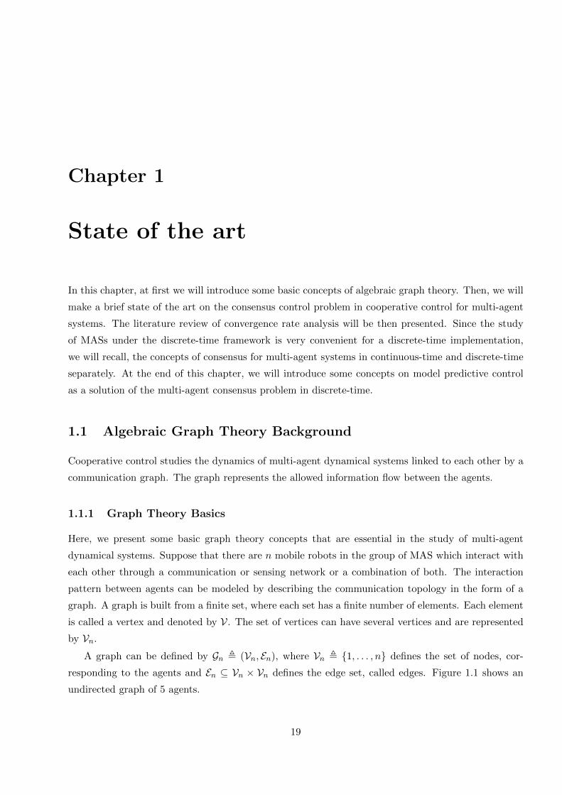
In this chapter, at first we will introduce some basic concepts of algebraic graph theory. Then, we will
make a brief state of the art on the consensus control problem in cooperative control for multi-agent
systems. The literature review of convergence rate analysis will be then presented. Since the study
of MASs under the discrete-time framework is very convenient for a discrete-time implementation,
we will recall, the concepts of consensus for multi-agent systems in continuous-time and discrete-time
separately. At the end of this chapter, we will introduce some concepts on model predictive control
as a solution of the multi-agent consensus problem in discrete-time.
1.1 Algebraic Graph Theory Background
Cooperative control studies the dynamics of multi-agent dynamical systems linked to each other by a
communication graph. The graph represents the allowed information flow between the agents.
1.1.1 Graph Theory Basics
Here, we present some basic graph theory concepts that are essential in the study of multi-agent
dynamical systems. Suppose that there are n mobile robots in the group of MAS which interact with
each other through a communication or sensing network or a combination of both. The interaction
pattern between agents can be modeled by describing the communication topology in the form of a
graph. A graph is built from a finite set, where each set has a finite number of elements. Each element
is called a vertex and denoted by V. The set of vertices can have several vertices and are represented
by Vn.
A graph can be defined by Gn , (Vn, En), where Vn , 1, . . . , n defines the set of nodes, cor-
responding to the agents and En ⊆ Vn × Vn defines the edge set, called edges. Figure 1.1 shows an
undirected graph of 5 agents.
19

Figure 1.1: A communication graph of MAS with 5 vertices and 6 edges.
It is natural to model the interaction among agents by directed or undirected graphs. A link (i, j)
in the edge set of a directed graph denotes that agent j can obtain information from agent i, but not
necessarily vice versa. Self-edges (i, i) are not allowed unless otherwise indicated. For the edge (i, j),
i is the parent node and j is the child node. If an edge (i, j) ∈ E , then node i is a neighbor of node
j. The set of neighbors of node i is denoted as Ni = j 6= i : (j, i) ∈ E. In contrast to a directed
graph, the pairs of nodes in an undirected graph are unordered, where the edge (i, j) denotes that
agents i and j can obtain information from each other. Note that an undirected graph can be viewed
as a special case of a directed graph, where an edge (i, j) in the undirected graph corresponds to the
edges (i, j) and (j, i) in the directed graph. A weighted graph associates a weight with every edge in
the graph. The union of a collection of graphs is a graph whose node and edge sets are the unions of
the node and edge sets of the graphs in the collection.
Figure 1.2 shows the communication graph among 4 agents in the directed graph. An arrow from
node i to node j indicates that agent j receives information from agent i.
Figure 1.2: A directed graph with 4 vertices.
A directed path is a sequence of edges in a directed graph of the form (i1, i2), (i2, i3), .... An undi-
rected path in an undirected graph is defined analogously. In a directed graph, a cycle is a directed
path that starts and ends at the same node. A directed graph is strongly connected if there is a
directed path from every node to every other node. An undirected graph is connected if there is an
undirected path between every pair of distinct nodes. An undirected graph is fully connected if there
is an edge between every pair of distinct nodes. A directed graph is complete if there is an edge from
20

every node to every other node. A directed tree is a directed graph in which every node has exactly
one parent except for one node, called the root, which has no parent and which has directed paths to
all other nodes. Note that a directed tree has no cycle because every edge is oriented away from the
root. In undirected graphs, a tree is a graph in which every pair of nodes is connected by exactly one
undirected path.
A subgraph (V1, E1) of (V, E) is a graph such that V1 ⊆ V and E1 ⊆ E ∩ (V1×V1). A directed span-
ning tree (V1, E1) of the directed graph (V, E) is a subgraph of (V, E) such that (V1, E1) is a directed
tree and V1 = V . An undirected spanning tree of an undirected graph is defined analogously. The
directed graph (V, E) has or contains a directed spanning tree if a directed spanning tree is a subgraph
of (V, E). Note that the directed graph (V, E) has a directed spanning tree if and only if (V, E) has
at least one node with directed paths to all other nodes. In undirected graphs, the existence of an
undirected spanning tree is equivalent to being connected. However, in directed graphs, the existence
of a directed spanning tree is a weaker condition than being strongly connected.
Graphs, can also be represented by a matrix for further analysis. For undirected graphs Gn, the
degree of vertex d(vi) is related to the neighbor set Ni, and equals to the number of adjacent vertices
with vertex vi in graph Gn. In Figure 1.1, the degree of vertex is:
d(v1) = 3; d(v2) = 2; d(v3) = 3; d(v4) = 2; d(v5) = 1
The vertex degree above can be expressed with a degree matrix 4(G), in the form of a diagonal
matrix measuring n× n whose diagonal component is the degree of vertex in graph G, as:
4(G) =
d(v1) 0 · · · 0
0 d(v2) · · · 0...
.... . .
...
0 0 · · · d(vn)
(1.1)
1.1.2 Adjacency Matrices
The adjacency matrix A , [aij ] ∈ Rn×n of a directed graph (V, E) is defined such that aij is a pos-
itive weight if (j, i) ∈ E and aij = 0 if (j, i) /∈ E . Self-edges are not allowed (i.e., aii = 0) unless
otherwise indicated. The adjacency matrix of an undirected graph is defined analogously except that
aij = aji for all i 6= j because (j, i) ∈ E implies (i, j) ∈ E . Note that aji denotes the weight for the
edge (j, i) ∈ E . If the weight is not relevant, then aji is set equal to 1 if (j, i) ∈ E . The in-degree
and out-degree of node i are defined as, respectively,∑n
j=1 aij and∑n
j=1 aji. A node i is balanced if∑nj=1 aij =
∑nj=1 aji. A graph is balanced if
∑nj=1 aij =
∑nj=1 aji, for all i. For an undirected graph,
21

A is symmetric, and thus every undirected graph is balanced.
Here below are the degree matrix and the adjacency matrix for the undirected graph given in
Figure 1.1:
4(G) =
3 0 0 0 0
0 2 0 0 0
0 0 4 0 0
0 0 0 2 0
0 0 0 0 1
A(G) =
0 1 1 1 0
1 0 1 0 0
1 1 0 1 1
1 0 1 0 0
0 0 1 0 0
For the directed graph in Figure 1.2, the degree matrix and the adjacency matrix are as follows:
4(D) =
2 0 0 0
0 1 0 0
0 0 1 0
0 0 0 1
A(D) =
0 1 1 0
0 0 0 0
0 0 0 1
0 0 0 0
1.1.3 Laplacian Matrices
Many properties of a graph may be studied in terms of its Laplacian. In fact, we shall see that the
Laplacian matrix is of extreme importance in the study of cooperative control of multi-agent systems.
Define the matrix L , [lij ] ∈ Rn×n as
lii =n∑
j=1,j 6=iaij , lij = −aij , i 6= j (1.2)
Note that if (j, i) /∈ E then lij = −aij = 0. The matrix L satisfies
lij ≤ 0, i 6= j,n∑j=1
lij = 0, i = 1, ..., n. (1.3)
L is called the Laplacian matrix. For an undirected graph, L is symmetric. However, for a directed
graph, L is not necessarily symmetric and is sometimes called the nonsymmetric Laplacian matrix or
directed Laplacian matrix. In both the undirected and directed cases, since L has zero row sums, 0 is
an eigenvalue of L with the associated eigenvector 1 , [1, . . . , 1]T , the n × 1 column vector of ones.
Note that L is diagonally dominant and has nonnegative diagonal entries. If follows from Gershgorin’s
disc theorem [?] that, for an undirected graph, all of the nonzero eigenvalues of L are positive (L is
positive semidefinite), whereas, for a directed graph, all of the nonzero eigenvalues of L have positive
real parts. Therefore, all of the nonzero eigenvalues of −L have negative real parts.
22

For example, the Laplacian matrix for the undirected graph in Figure 1.1 is:
L(G) = 4(G)−A(G) =
3 −1 −1 −1 0
−1 2 −1 0 0
−1 −1 4 −1 0
−1 0 −1 2 0
0 0 −1 0 1
For Figure 1.2, the Laplacian matrix is:
L(D) = 4(D)−A(D) =
2 −1 −1 0
0 1 0 0
0 0 1 −1
0 0 0 1
For an undirected graph, 0 is a simple eigenvalue of L if and only if the undirected graph is
connected [?]. For a directed graph, 0 is a simple eigenvalue of L if the directed graph is strongly
connected [5, Proposition 3], although the converse does not hold. For an undirected graph, let λi(L)
be the ith smallest eigenvalue of L with λ1(L) ≤ λ2(L) ≤ . . . ≤ λn(L) so that λ1(L) = 0. For an
undirected graph, λ2(L) is the algebraic connectivity, which is positive if and only if the undirected
graph is connected [?]. The algebraic connectivity quantifies the convergence rate of a consensus
algorithm [?].
1.2 Consensus Control Strategy
1.2.1 Overview of Cooperative Control
A multi-agent system is a system that consists of multiple intelligent agents and their environment.
The word “agent” represents any system with sensing, computing and communicating capabilities,
such as a wheeled mobile robot, an unmanned air vehicle (UAV), an autonomous underwater vehicle
(AUV), a manipulator or sensors. The agents interact with one-another to achieve a global task. To
successfully interact, they will require the ability to cooperate, coordinate and negotiate with each
other. The interaction between agents to achieve a global task is called cooperative control. Figure 1.3
shows different types of agents (Figure 1.3(a) for wheeled mobile robots, Figure 1.3(b) for unmanned
air vehicles, Figure 1.3(c) for autonomous underwater vehicles).
Over the last decade, an enormous amount of researchers have drawn great interest on cooper-
ative control of MAS) because of its variety of applications in several areas, e.g., unmanned aerial
vehicle surveillance, hazardous material handling, mine-sweeping and deep sea exploration. Figure
1.4 illustrates some applications of MAS. To enable these applications, various cooperative control
23

(a) (b)
(c)
Figure 1.3: Example of different agents.
capabilities need to be developed, including target tracking [?] [?] [?] [?] [?], flocking [?] [?] [?] [?],
swarming [?] [?], rendezvous [?] [?], area coverage [?] [?] [?], monitoring [?] [?], formation control [?] [?]
[?] [?] [?], etc. In these works, it has been shown that the use of multi-agent cooperative systems en-
ables to accomplish complex tasks which are difficult or impossible compared to the use of a single one.
Figure 1.4: Multi-agent system applications.
Cooperative control of multi-agent systems poses significant theoretical and practical challenges.
Indeed, the objective is to develop a system of subsystems rather than a single system that has team
goals and individual goals which have to be negotiated, while taking into account the limited computa-
24

tional resources of each individual agent, the locally sensed information, and limited inter-component
communications. The consensus/agreement/synchronization/rendezvous problem is one fundamental
research topic of cooperative control of MASs, which focuses on designing distributed controllers to
drive agents to achieve state agreement or forcing a group of agents states to reach an agreement on
a quantity of interest such as the rendezvous position, velocity and heading direction. It is crucial to
design appropriate control protocols for agents with information interactions over the network.
In Figure 1.5, we show a MAS consisting of four mobile robot labeled from 1 to 4. The information
transmission can be either unidirectional or bidirectional as indicated by the arrow directions. The
figure shows that agent 3 receives information from agent 2, but the information of agent 3 can not
be transmitted to agent 2. The bidirectional communication channel between agent 1 and 2 or agent
3 and 4 means that two agents can receive information from each other.
Figure 1.5: Illustration of a MAS: A group of five mobile robots.
1.2.2 Communication Graphs and Consensus
A network may be considered as a set of nodes or agents that collaborate to achieve a common
objective. To capture the notion of dynamical agents, each node i of a graph endowed with a time-
varying state vector xi(t) ∈ Rn. A graph with node dynamics [10] is G(x) with (G being a graph having
n nodes and x = [xT1 , ..., xTn ]T a global state vector, where the state of each node evolves according to
the following differential equation:
xi(t) = F (xi(t), ui(t)) with i = 1, 2, ..., n. (1.4)
where ui(t) ∈ Rm is the control input of agent i (resp. control input) of the multi-agent system,
F : Rn × Rm → Rn.
25

Definition 1 Decentralized Control Protocol. The control given by ui = ki(xi1, xi2, ..., ximi)
for some function ki(.) is said to be distributed if mi < n, ∀i, that is, the control input of each
node depends on some proper subset of all the nodes. It is said to be a protocol with topology G if
ui = ki(xi, xj |j ∈ Ni), that is, each node can obtain information about the state only of itself and
its neighbors.
Cooperative control, or control of distributed dynamical systems on graphs, refers to the situation
where each node can obtain information for control design only from itself and its neighbors. The
graph might represent a communication network topology that restricts the allowed communications
between the nodes. This has also been referred to as multi-agent control, but is not the same as the
notion of multi-agent systems used by the Computer Science community [20].
1.2.3 Consensus Algorithm
When agents reach an agreement on a certain common feature, they are said to have reached consen-
sus. Information consensus guarantees that agents sharing information over a network topology have
a consistent view of information that is critical to the coordination task. To achieve consensus, there
must be a shared variable of feature, called the information state, as well as appropriate algorith-
mic methods for negotiating to reach consensus on the value of that variable, called the consensus
algorithm. The information state represents an instantiation of the coordination variable for the team.
The basic idea of a consensus algorithm is to impose similar dynamics on the information states
of each agents. If the communication network among agents allows continuous communication or if
the communication bandwidth is sufficiently large, then the information state update of each agent is
modeled using a differential equation. On the other hand, if the communication data arrive in discrete
packets, then the information state update is modeled using a difference equation.
A basic control design objective is the following.
Definition 2 Consensus Problem. Find a distributed control protocol that drives several or all
states to the same values xi = xj , ∀i, j . This value is known as a consensus value.
The most common continuous-time consensus algorithm [?],[?] [?] [?] [?] is given by:
xi(t) = −n∑j=1
aij [xi(t)− xj(t)], i = 1, . . . , n. (1.5)
where aij(t) is the (i, j) entry of adjacency matrixA ∈ Rn×n associated with G and xi is the information
state of the ith agent. A consequence of Equation (1.5) is that the information state xi(t) of agent i
is driven toward the information state xj(t) of its neighbors j.
26

Average Consensus
The average consensus is discussed in [?], [?], [?], [?]. All agents in the MAS will converge to the
exact average value of their initial states. When an agent moves, the average value of the states can
remain constant by changing another agent’s states with the same magnitude in the opposite direction
[?], [?]. More complicated situations such as switching topologies, time-varying delays in the average
consensus problem are discussed in [?]. Figure 1.6 illustrated the average consensus problem where
the state of all agents converge to an average value.
Figure 1.6: Average Consensus.
1.2.4 Leaderless and Leader-Follower Consensus
According to the number of leaders in a group of multi-agent system, current researches about the
consensus problem are classified into three fields, i.e., leaderless consensus, leader-following consensus
problem with a single leader, and containment control with multiple leaders.
Leaderless Consensus
In leaderless consensus, all agents have the same role. For leaderless consensus, control strategies are
proposed for first-order [?] [?], second-order [?] [?], high-order [?] [?] multi-agent systems. In [?], it
has been shown that for MAS represented by a simple integrator, the algebraic connectivity, that
is to say, the smallest positive eigenvalue of the Laplacian graph, determines the convergence time.
[?] provides an overview of consensus for first-order multi-agent systems and also some theoretical
27
results on information consensus-seeking under both time-invariant and time-varying communication
topologies. Figure 1.7 described the leaderless consensus problem where the state of all agents converge
to a consensus point.
Figure 1.7: Leaderless Consensus.
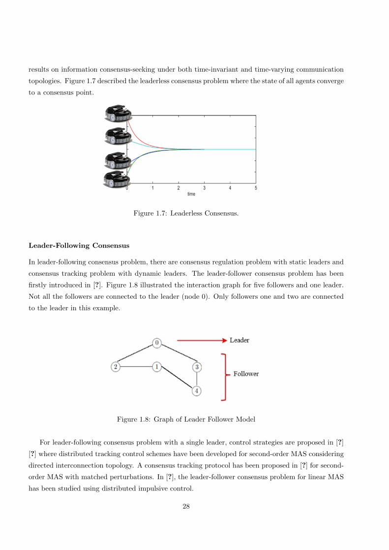
Leader-Following Consensus
In leader-following consensus problem, there are consensus regulation problem with static leaders and
consensus tracking problem with dynamic leaders. The leader-follower consensus problem has been
firstly introduced in [?]. Figure 1.8 illustrated the interaction graph for five followers and one leader.
Not all the followers are connected to the leader (node 0). Only followers one and two are connected
to the leader in this example.
Figure 1.8: Graph of Leader Follower Model
For leader-following consensus problem with a single leader, control strategies are proposed in [?]
[?] where distributed tracking control schemes have been developed for second-order MAS considering
directed interconnection topology. A consensus tracking protocol has been proposed in [?] for second-
order MAS with matched perturbations. In [?], the leader-follower consensus problem for linear MAS
has been studied using distributed impulsive control.
28

Figure 1.9: Leader Follower Consensus
Containment Control
The objective of containment control is to drive the states of followers into a convex hull spanned by
those multiple leaders. In practical scenarios, it is sometimes more interesting if followers move to an
area stretched by several leaders instead of tracking a specific desired path [?]. One possible scenario
is that groups of vehicles moves from one place to a target while only a small portion of vehicles has
sensing capabilities to detect dangerous obstacles. In this case, all groups have to safely reach the
destination as long as followers (vehicles without sensing capabilities) remain in the safe zone formed
by leaders (vehicles with sensing capabilities). Some results are reported on the containment control
problem for single-integrator [?] or double-integrator [?] multi-agent systems.
1.3 Convergence Rate Analysis
The consensus problem of multi-agent systems has received much attention in recent years and many
interesting results have been discussed from different directions. An important topic in the study
of the consensus problem is the settling time, which characterizes the rate of convergence rate of a
closed-loop system. It is well recognized as one of the performance specifications for the control system
design. Fast convergence is usually pursued in practice in order to achieve better performance and
robustness. It is clear that for the cooperative control of MAS, the convergence rate is one critical
index to evaluate the proposed control methods.
To illustrate this important specification index, let us consider the first-order system
x = u (1.6)
where x ∈ R is the state and u ∈ R is the control input. Figure 1.10 shows the trajectory of system
(1.6) under different control input (u = −x, u = −sign(x) and u = −(|x|2 + 1)sign(x)). One can see
the asymptotic, finite-time and fixed-time properties of the corresponding closed-loop system.
29

Figure 1.10: Asymptotic, finite-time and fixed-time properties of the first-order system
1.3.1 Asymptotic stability
Most of the existing consensus control algorithms for multi-agent systems are asymptotic consensus
algorithms. It means that the convergence rate is at best exponential with infinite settling time. In
other words, the states cannot reach a consensus in finite time. In the context of cooperative control,
an initial result [?] shows that for MAS represented by a simple integrator, the algebraic connectivity,
that is to say, the smallest eigenvalue of the Laplacian graph, determines the convergence rate. In
[?], the authors have proposed an approach to increase this algebraic connectivity. However, linear
algorithms have only focused on asymptotic convergence, where the time to reach consensus can be
arbitrarily large. In [?], the convergence rate can be enhanced by maximizing the algebraic connectivity
of the communication topology.
1.3.2 Finite-time stability
Most aforementioned consensus works can only achieve state agreement over an infinite time horizon,
which fails to meet specific convergence requirements in an unknown environment. Nevertheless, in
some practical cases, finite-time convergence is very interesting in terms of accuracy (which depends
on the sampling period) and robustness against perturbations [?].
Before giving a brief state of the art on finite-time consensus, let us recall some basics on finite-
time stability. The key point in finite time stability is that the power exponent should be less than one.
Generally, consider the following systemx(t) = F (t, x(t))
x(0) = x0
(1.7)
where x ∈ Rn is the state, F : R+ × Rn → Rn is an upper semicontinuous mapping in an open
30

neighborhood F (t, 0) = 0 for t > 0. The solution of system (1.7) are understood in the Filippov sense
[?] if F (t, x) is discontinuous. Let x(t, x0) be an arbitrary solution of the Cauchy problem of system
(1.7).
Definition 3 [?] The origin of system (1.7) is a globally finite-time equilibrium if there is a function
T : Rn → R+ such that for all x0 ∈ Rn, the solution x(t, x0) of system (1.7) is defined and x(t, x0) ∈ Rn
for t ∈ [0, T (x0)) limt→T (x0) x(t, x0) = 0
x(t, x0) = 0 ∀t > T (x0)(1.8)
T (x0) is called the settling time function.
Finite-time stability of the origin implies the asymptotic stability of the origin.
Lemma 1 [?] Assume that there exists a continuously differentiable positive definite and radially
unbounded function V : Rn → R+ such that
V (x) ≤ −αV p(x) (1.9)
with α > 0 and 0 < p < 1. Then, the origin of system (1.7) is globally finite-time stable with settling
time estimate
T (x0) ≤ 1
α(1− p)V 1−p(x0) (1.10)
In [?], the authors provide a finite-time consensus protocol for single-integrator MAS using an
appropriate Lyapunov function and time-varying weighted directed graphs. In [?], the authors have
introduced a terminal-sliding mode controller to deal with the finite-time consensus problem of second-
order linear uncertain systems. In [?], [?], the finite-time tracking problem has been addressed for
second-order MAS. In [?], a recursive terminal sliding mode controller has been introduced for the
tracking control problem of uncertain chained-form systems in finite-time. Nevertheless, in these
studies, the estimated bound of the settling time depends on the initial states of all the agents.
Therefore, this bound cannot be a priori estimated in decentralized architectures. Hence, in some
practical applications, it is required to achieve consensus in a prescribed time.
1.3.3 Fixed-time stability
Although finite-time consensus has many advantages, the estimation of convergence time depends on
initial states of the networked agents. This will give limitation in practice since the knowledge of initial
conditions is usually unavailable. This motivation gives rise to provide the convergence information in
advance to yield more options for designers. According to this issue, a new strategy called fixed-time
consensus is proposed.
31
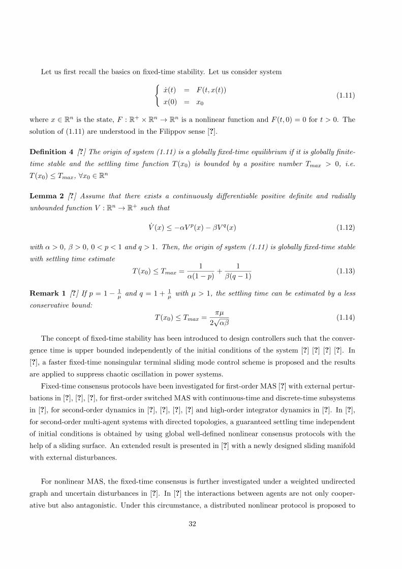
Let us first recall the basics on fixed-time stability. Let us consider systemx(t) = F (t, x(t))
x(0) = x0
(1.11)
where x ∈ Rn is the state, F : R+ × Rn → Rn is a nonlinear function and F (t, 0) = 0 for t > 0. The
solution of (1.11) are understood in the Filippov sense [?].
Definition 4 [?] The origin of system (1.11) is a globally fixed-time equilibrium if it is globally finite-
time stable and the settling time function T (x0) is bounded by a positive number Tmax > 0, i.e.
T (x0) ≤ Tmax, ∀x0 ∈ Rn
Lemma 2 [?] Assume that there exists a continuously differentiable positive definite and radially
unbounded function V : Rn → R+ such that
V (x) ≤ −αV p(x)− βV q(x) (1.12)
with α > 0, β > 0, 0 < p < 1 and q > 1. Then, the origin of system (1.11) is globally fixed-time stable
with settling time estimate
T (x0) ≤ Tmax =1
α(1− p)+
1
β(q − 1)(1.13)
Remark 1 [?] If p = 1 − 1µ and q = 1 + 1
µ with µ > 1, the settling time can be estimated by a less
conservative bound:
T (x0) ≤ Tmax =πµ
2√αβ
(1.14)
The concept of fixed-time stability has been introduced to design controllers such that the conver-
gence time is upper bounded independently of the initial conditions of the system [?] [?] [?] [?]. In
[?], a faster fixed-time nonsingular terminal sliding mode control scheme is proposed and the results
are applied to suppress chaotic oscillation in power systems.
Fixed-time consensus protocols have been investigated for first-order MAS [?] with external pertur-
bations in [?], [?], [?], for first-order switched MAS with continuous-time and discrete-time subsystems
in [?], for second-order dynamics in [?], [?], [?], [?] and high-order integrator dynamics in [?]. In [?],
for second-order multi-agent systems with directed topologies, a guaranteed settling time independent
of initial conditions is obtained by using global well-defined nonlinear consensus protocols with the
help of a sliding surface. An extended result is presented in [?] with a newly designed sliding manifold
with external disturbances.
For nonlinear MAS, the fixed-time consensus is further investigated under a weighted undirected
graph and uncertain disturbances in [?]. In [?] the interactions between agents are not only cooper-
ative but also antagonistic. Under this circumstance, a distributed nonlinear protocol is proposed to
32

guarantee the state agreement in a fixed time as long as the interaction topologies are both struc-
turally balanced and structurally unbalanced. Few consensus protocols consider nonlinear MAS (such
as chained-form dynamics), which can model dynamics of robots. In [?], a class of multi-scale coor-
dination control problem is solved by using a fixed-time controller such that the multi vehicles with
disturbances are guaranteed to achieve consensus on a common quantity but of their own scales. Re-
cently, a switching strategy has been introduced to deal with the fixed-time consensus problem for
multiple nonholonomic agents [?]. However, in this work, the leader was static and no uncertainty
was considered.
1.4 Consensus in Discrete-time
Consensus problems can be studied in different time domains: continuous-time and discrete-time.
Many research studies are focused on continuous-time consensus protocols. On the other hand, it
becomes more convenient and popular to study MASs under the discrete-time framework due to the
development of the digital signal processing and communication technologies. Compared with the
continuous-time systems, discrete-time systems are more suitable for practical applications.
Some interesting works related to the topic of first-order discrete-time consensus stability analysis
were reported in [?] [?] [?]. The main objective of [?] was to theoretically study the coordination of a
group of autonomous agents using the Vicsek model. In [?], some consensus protocols for discrete-time
systems with switching topology were provided and the robustness against time delays was analyzed.
These two kinds of protocols are based using the same data at two time-steps. The dynamic behavior
of discrete-time multi-agent systems with general communication topologies was considered in [?]. For
topologies that have a spanning tree, the consensus problem was studied. It was proved that the states
of internal agents converge to a convex combination of boundary agents in the case of communication
time delays. Much attention on discrete-time consensus can be found in [?] [?] [?], etc.
Despite much effort has been produced for the two types of time domain above, the solutions are
not yet satisfied because MASs are usually operated using the analog measurement and embedded
microcontrollers to process digital signals. In sampled-data control system, the work requires both
continuous-time dynamics and discrete-time controllers. The sampling is usually assumed periodic
and synchronized for all agents [?] [?].
1.4.1 Notation and Basic Definition
We use Z+ to denote the set of all nonnegative integers. Euclidean norm is denoted simply as | · |.For any function φ : Z+ → Rn, ‖φ‖ = sup|φ(k)| : k ∈ Z+ ≤ ∞. Br is the closed ball of radius r, i.e.
Br = x ∈ Rn||x| ≤ r. A continuous function α(·) : R+ → R+ is a K function if α(0) = 0, α(s) > 0
33

for all s > 0 and it is strictly increasing. A continuous function β : R+ × Z+ → R+ is a KL function
if β(s, t) is a K function in s for any t ≥ 0 and for each s > 0 β(s, ·) is decreasing and β(s, t) → 0 as
t→∞. MΩ is the set of signals in some subset Ω.
Definition 5 [?] [?] (Stability) Given the discrete-time dynamic system
x(k + 1) = f(x(k)) (1.15)
where the origin x∗ = 0 ∈ Ω ⊂ Rn is an equilibrium point. If there exists a function V : Rn → R+ and
functions α and β of class K such that
α(||x||) ≤ V (x) ≤ β(||x||), ∀x ∈ Ω ⊂ Rn (1.16)
Then, the origin of system (1.15) is said
1. Stable if
∆V (x(k)) ≤ 0, ∀x ∈ Ω, x 6= 0 (1.17)
with
∆V (x(k)) = V (x(k + 1))− V (x(k)) = V (f(x(k)))− V (x(k)) (1.18)
2. Asymptotically stable if there exists a function ϕ of class K such that
∆V (x(k)) ≤ −ϕ(||x||), x ∈ Ω, x(k) 6= 0 (1.19)
3. Exponentially stable if there exists a constants α1, α2, α3, p > 0 such that the following properties
are satisfied for all x ∈ Ω ⊂ Rn
α2||x||p ≤ V (x) ≤ α1||x||p (1.20)
and
∆V (x(k)) ≤ −α3||x||p (1.21)
1.4.2 Discrete-time Consensus Algorithm
When interaction among agents occurs at discrete instants, the information state is updated using a
difference equation. The most common discrete-time consensus algorithm has the following form [?]
[?] [?] [?]:
xi(k + 1) = −n∑j=1
aij(xi(k)− xj(k)), i = 1, . . . , n. (1.22)
where k denotes a sampling variable, aij is the (i, j) entry of the adjacency matrix of the graph that
represents the communication topology. Intuitively, the information state of each vehicle is updated
as the weighted average of its current state and the current states of its neighbors. Note that a vehicle
34

maintains its current information state if it does not exchange information with other vehicles at that
sampling time instant. The discrete-time consensus algorithm (1.22) is written in matrix form as
x(k + 1) = −Lx(k)
where L is the Laplacian matrix. Similar to the continuous case, consensus is achieved if, for all xi(0)
and for all i, j = 1, . . . , n, |xi(k)− xj(k)| → 0 as k →∞.
One interesting scheme to design the consensus algorithm for discrete-time multi-agent systems is
to use a model predictive controller. This is the main topic of the next subsection.
1.5 Model Predictive Control (MPC)
A brief history of MPC techniques is shown in Figure 1.11. It depicts the evolution of the most sig-
nificant MPC algorithms, illustrating their connections in a concise way. The story begins with the
modern control concept of the Kalman’s work, i.e. a great solution of the problem known as Linear
Quadratic Gaussian (LQG) controller. The first description of MPC applications was presented by
Richalet et al. in 1976. They described their approach as model predictive heuristic control (MPHC).
The solution software was referred to as IDCOM, an acronym for Identification and Command [?].
Then, engineers at Shell Oil developed their own independent MPC approach in the early 1970s, with
an initial application in 1973. Cutler and Ramaker presented details of an unconstrained multivari-
able control algorithm which they named dynamic matrix control (DMC) at the 1979 National AIChE
meeting [?]. In the late 1980’s, engineers at Shell Research in France developed the Shell Multivari-
able Optimizing Controller (SMOC) which they described as a bridge between state-space and MPC
algorithms [?].
Figure 1.11: Evolution of the most significant MPC algorithms.
Model Predictive Control (MPC), also known as receding horizon control (RHC) or Generalized
Predictive Control (GPC) or Dynamical Matrix Control (DMC), as solution for the consensus prob-
35

lem of MAS has also received great interest [1]. MPC is a form of control in which the output of
the system can be predicted from some prediction horizon. The output of the MPC controller is
determined based on input and output at a previous time and the control signal along the control
horizon. Control algorithms of MPC are based on numerically solving an optimization problem at
each step through constrained optimization. However, the control update rates use plenty of time for
the necessary on-line computations [?].
Figure 1.12: MPC concepts.
Figure 1.12 shows the general concepts of MPC algorithm for a single-input-single-output (SISO)
system. At current time, say k, the system’s future response (predicted output) yp(k) on a finite
horizon Hp, say [k|k+Hp], is predicted using the system model and the predicted control input up(k),
[k|k+Hu]. Hp is named as the prediction horizon and Hu is named as the control horizon (Hu ≤ Hp).
Usually, the system’s future response is expected to return to a desired set point s(k) by following
a reference trajectory r(k) from the current states. The difference between the predicted output yp(k)
and the reference trajectory r(k) is called the predicted error. A finite horizon optimal control problem
with a performance index that usually penalizes the predicted control input and the predicted error
is solved online and an optimal control input u∗(k), [k|k + Hu], is obtained. Only the first element
of u∗(k) is implemented to the plant. All the other elements are discarded. Then, at the next time
k + 1, the whole procedure is repeated. The predicted control input up(k + 1) at time k + 1 can be
built by u∗(k) with linear extrapolation. Since the prediction horizon and control horizon move one
step further into future at each time interval, MPC is also named as receding horizon control (RHC).
36

For cooperative behavior mechanism and effective control of MAS, MPC technique has several
advantages such as the acceleration of the convergence speed, the possible consideration of multi-
variable constraints and the increase of the range of sampling periods. In a distributed architecture,
each agent uses only local information. According to their own and neighbors’s information (both
actual and past), MPC may precisely reflect the autonomy of an agent. The predictive mechanism
of MPC is used to predict the output state in the short-term prediction horizon. Each agent solves
an optimization problem using its own and neighbor information data, to design the control input at
each moment, and then realize the cooperative control.
One of the major advantages of the MPC approach is that the cooperative control will be conducted
from an optimization point of view. Some physical limits such as input bounds, safety regions for the
collision avoidance can be formulated as constraints in the optimization problem. MPC has the ability
to handle control and state constraints for discrete-time systems [?]. This method can be applied for
the control of a group of agents by letting each agent solve, at each step, a constrained finite-time
optimal control problem involving the state of neighboring agents. For agents modeled by a discrete-
time system, [?] proposed decentralized MPC schemes with control input constraints and showed that
under the proposed decentralized schemes, multi-agent systems with single- and double-integrator dy-
namics asymptotically achieves consensus under mild assumptions. However, it was assumed that the
control horizon equals the prediction control, which reduced the degree of freedom for the controller
design. To remove the problem in degree of freedom for the controller design, [1] proposed a consensus
scheme for discrete-time single-integrator MAS under switching directed interaction graphs where the
control horizon can be arbitrarily picked from one to prediction horizon. Another result of MPC is
[?] which proposed a MPC strategy to increase the consensus convergence rate in MASs under some
special communication networks.
1.6 Conclusion
We have discussed in this chapter the basic concepts of algebraic graph theory for describing the
communication topology among the agents. Consensus control problem in cooperative control for
multi-agent systems has been also introduced. Convergence rates are discussed, which motivates us
to conduct a more in-depth study to investigate how a fast controller can be designed. The concepts
of consensus for multi-agent systems in continuous-time and discrete-time are separately discussed
where discrete-time systems are more suitable for practical applications. Model predictive control as
a solution of the multi-agent consensus problem in discrete-time has been introduced.
37

38

Chapter 2
Fixed-Time Leader-Follower Consensus
Control Strategy for MAS
2.1 Introduction
This chapter is concerned with the fixed-time leader-follower consensus problem of multi-agent systems.
The first part of this chapter formulates the general control objective and the considered assumptions
to solve the fixed-time leader-follower consensus problem. The second and third part of this chapter
deal with the consensus tracking problem for linear multi-agent systems (i.e. single-integrator and
double-integrator dynamics). Here, the leader (which can be dynamic) only transmits its state to its
neighbors. A decentralized controller, which uses the available local information, is designed to track
the desired trajectory of the leader in a prescribed time. Using the proposed controller, an upper
bound of the settling time is provided regardless of the initial conditions.
The fourth part of this chapter studies the fixed-time tracking problem for a single unicycle-type
mobile robot. First, the resulting tracking error dynamics is transformed into two second-order cou-
pled subsystems. Then, the two subsystems are studied and a step-by-step fixed-time control strategy
is designed. An upper bound of the settling time, which only depends on the controller parameters is
estimated regardless of the initial conditions. Finally, some simulation results are given to show the
effectiveness of the proposed controller.
The fifth part is concerned with the fixed-time consensus problem of multi-agent system for
unicycle-type mobile robots. For each agent, a distributed observer is designed to estimate the leader
state in a fixed-time. Contrary to finite-time schemes, the estimation of the settling time does not
require the knowledge of the initial state, allowing a step by step design for the controller. A decentral-
ized observer-based control protocol is proposed for each agent to solve the leader-follower consensus
39

problem in a fixed-time.
The main contributions of the proposed scheme can be summarized as follows:
i) To remove the problem of the communication loop due to the dependence of the control inputs
of the followers on the inputs of its neighbors in [?][?], distributed observers are designed to
estimate the leader state in a prescribed time which does not depend on the initial state contrary
to existing finite-time observers.
ii) A new decentralized observer-based control protocol is proposed for each follower to solve the
fixed-time consensus tracking problem when the leader is dynamic.
iii) Robustness properties against matched perturbations are guaranteed.
iv) An upper bound of the settling time, which only depends on the controller parameters is esti-
mated independently of the initial conditions, contrary to existing finite-time controllers.
The remaining parts of this chapter are organized as follows. Section 2.2 introduces some as-
sumptions and formulates the general control objective. The main theoretical results on the consensus
tracking problem are presented for single-integrator and double-integrator dynamics in Section 2.3 and
2.4. In Section 2.5, a fixed-time tracking control law for a single agent with unicycle-type dynamics is
provided. In section 2.6, the main theoretical results on the consensus tracking problem are presented
for unicycle-type dynamics. Section 2.7 concludes this chapter.
2.2 Problem Statement and Assumptions
Let us consider a group of N + 1 agents with one leader (which could be virtual) labeled by 0 and
N followers, labeled by i ∈ 1, . . . , N. The dynamics of the leader is given by the following general
system
x0(t) = F (x0(t), u0(t)) (2.1)
where x0 ∈ Rn is the leader state and u0 ∈ Rm is the leader control input. F : Rn × Rm → Rn is
known. Here, it should be highlighted that solutions of (2.1) are understood in the Filippov sense [?].
The dynamics of the ith follower is as follows
xi(t) = F (xi(t), ui(t)) with i = 1, 2, . . . , N. (2.2)
where xi ∈ Rn is the state and ui ∈ Rm is the control input of the ith follower. The unknown pertur-
bation of the ith agent is given by di(t) ∈ Rn. Here, it should be highlighted that solutions of (2.2)
40

are understood in the Filippov sense [?].
Among the N followers, the communication topology can be represented by graph G = V, Ewhere V = 1, . . . , N defines the set of nodes, corresponding to the followers, and E ⊆ V × Vdefines the edge set. A link (j, i) ∈ E , with i 6= j, exists if agent i receive information from its
neighbor j. The adjacency matrix A = (aij) ∈ RN×N satisfies aij > 0 if (j, i) ∈ E and aij = 0,
otherwise. The corresponding Laplacian matrix is given by L = (lij) ∈ RN×N with lii =∑N
j=1, j 6=i aij
and lij = −aij for i 6= j. The links between the leader and the followers are characterized by matrix
B = diag(b1, . . . , bN ) where bi > 0 if the leader state is available to follower i and where bi = 0
otherwise.
Hereafter, it is assumed that the following hypotheses hold to derive the proposed fixed-time
controllers.
Assumption 1 It is assumed that the communication topology among the N followers is undirected,
fixed, connected. It means that the adjacency matrix A is symmetric. It is also assumed that there is
at least one strictly positive parameter bi.
Assumption 2 The followers do not know the leader control input u0. Nevertheless, its neighboring
agents know its upper bounds.
Assumption 3 For each follower, the perturbation di(t) is unknown but it is bounded by a known
constant.
Remark 2 Assumption 1 is conventional to deal with the leader-follower consensus problem. Hypoth-
esis 2-3 are not restrictive since the bounds of perturbations and leader input can be estimated a priori
for any system.
Here, the purpose is to derive a decentralized controller ui (i = 1, . . . , N) for each follower, based
on available information, such that the leader-follower consensus problem is solved in a fixed-time, in
spite of matched external perturbations. It means that there exists a positive constant T , such that
∀xi(0), ∀i = 1, . . . , N ,
limt→T ‖xi(t)− x0(t)‖ = 0
xi(t) = x0(t), ∀t ≥ T(2.3)
Remark 3 One can note that the settling time T does not depend on the initial states of the agents. It
removes some limitations on existing finite-time consensus schemes for the application in decentralized
architectures. The settling time can be prescribed according to some high-level policies (for instance
in flexible manufacturing systems, when an operation should be performed before a deadline), or when
cluster networks or switching communication topologies are considered [?].
41

2.3 Consensus of MAS with Single-Integrator Dynamics
Let us first consider a holonomic mobile robot moving in a two-dimensional plane. The axes of
the workspace are shown in Figure 2.1. Since we assume that motions along the x and y-axes are
Figure 2.1: Top view of the considered mobile robot
decoupled, the system dynamics can be modeled as
xi(t) = ux(t)
yi(t) = uy(t)(2.4)
where xi(t) ∈ R and yi(t) ∈ R are the position, ux(t) ∈ R and uy(t) ∈ R are the control inputs along
the x-axis and y-axis, respectively.
Remark 4 In the following, let us only consider the dynamics along the x-direction.
Along the x-direction, the leader dynamics is given by the following single-integrator system
x0(t) = u0(t) (2.5)
where x0 ∈ R (resp. u0 ∈ R) is the leader state (resp. leader control input). Along the x-direction,
the dynamics of the ith follower is as follows
xi(t) = ui(t) + di(t) (2.6)
where xi ∈ R (resp. ui ∈ R) is the state (resp. control input) of the ith follower. The unknown
perturbation of the ith agent is given by di ∈ R.
2.3.1 Fixed-Time Observer-Based Consensus Protocol
For single-integrator dynamics MAS under matched perturbations, we propose an observer-based
consensus protocol to deal with the leader-follower consensus problem.
42

Distributed fixed-time observer
To estimate the leader state in a prescribed time, distributed observers are designed for each follower
i ∈ 1, . . . , N. Indeed, the leader state is only available to its neighboring followers. Let us introduce
the following observer
˙xi = ρ sign
N∑j=1
aij(xj − xi) + bi(x0 − xi)
+ σ
N∑j=1
aij(xj − xi) + bi(x0 − xi)
2
(2.7)
where xi is the estimation of the leader state x0 for the ith follower, ρ and σ are positive constants,
which will be given hereafter.
The fixed-time stabilization of the estimation errors
xi = xi − x0 (i = 1, . . . , N) (2.8)
is introduced in the following theorem.
Theorem 1 Suppose that Assumptions 1-2 are satisfied. If the gains of the distributed observer (2.7)
verify σ = ε√N
(2λmin(L+B))32
ρ = umax0 + ε√
λmax(L+B)2λmin(L+B)
(2.9)
with ε > 0, then, for any initial condition, the estimation errors (2.8) converge to zero. An upper
bound of the convergence time can be given as
To =π
ε(2.10)
Proof. Using (2.7), the dynamics of the observation error is given by
˙xi = ρ sign
N∑j=1
aij(xj − xi)− bixi
+ σ
N∑j=1
aij(xj − xi)− bixi
2
− u0 (2.11)
Let us denote
x = [x1, . . . , xN ]T (2.12)
Then, for x, one can obtain
˙x = −ρ sign ((L+B)x)− σ d(L+B)xc2 − 1u0 (2.13)
We complete the proof by consider the candidate Lyapunov function for system (2.13)
V1 =1
2xT (L+B)x (2.14)
43

Its time derivative is given by
V1 = xT (L+B)(−ρ sign ((L+B)x)− σ d(L+B)xc2 − 1u0
)≤ −(ρ− umax0 )‖(L+B)x‖1 − σN−
12 (2λmin(L+B))
32V
32
≤ −εV12
1 − εV32
1
Using Lemma 2, this inequality ensures that x converges to zero in a finite-time bounded by πε .
Remark 5 The conditions (2.9) on the observer gains are relatively strong since global information
like N , λmin(L + B) and λmax(L + B) is required to guarantee the fixed-time convergence. Hence,
each agent must have some global knowledge about the communication topology similarly to existing
works on fixed-time consensus. One should highlight that such global information is needed to provide
an explicit estimate of the settling time (which is a very interesting feature of the proposed scheme).
It is worthy of noting that if a prescribed convergence time To is required, one can easily tune the
observer gains according to (2.9) to estimate the leader state. Similarly to the work of [?], parameter
ε should be tuned to obtain a good compromise between robustness against measurement noises (in the
presence of measurement noises, only a neighborhood of the origin of the observation error system,
which depends on the size of noise and ε, could be fixed-time stable) and sufficiently fast estimation.
When the observer gains are selected, through conditions (2.9), the proposed scheme can be considered
as a decentralized one since each neighboring agent only exchanges local information during the process.
Decentralized fixed-time controller
From Theorem 1, one can conclude that xi = x0 for all t ≥ To. Hence, after time To, each follower is
able to indirectly access to the state of the leader and uses the estimate xi in the consensus protocol.
Let us denote the tracking errors as follows
ei = xi − xi = xi − x0 − xi (2.15)
From (2.5)-(2.6) and using Theorem 1, for each follower i = 1, . . . , N and for all t ≥ To, the tracking
error dynamics becomes
ei = ui + di − u0 (2.16)
It is clear that dynamics (2.16) is a first-order system.
In the following theorem, the control strategy is derived to solve the leader-follower consensus
problem for MAS with single-integrator dynamics, in a fixed-time, in spite of the presence of matched
perturbations.
44

Theorem 2 Let us consider the leader-follower system (2.5)-(2.6). Suppose that Assumptions 1-3 are
satisfied and the gains of the distributed observer (2.7) verify Eq. (2.9). The leader-follower consensus
problem is solved in a fixed-time using the decentralized controller
ui =
0 ,∀t < To
−(α+ ai)beie2 − β sign (ei) ,∀t ≥ To(2.17)
where α, β are positive constants and ai is a positive constant given hereafter. The settling time is
explicitly defined as
T = To +π√αβ
(2.18)
Proof. We complete the proof by showing that the origin is fixed-time stable with the settling
time estimate T under the control law (2.17). It will be also proved that in spite of the presence of
matched perturbations, the fixed-time leader-follower consensus problem is solved.
Let us first consider system (2.16).
ei = ui + di − u0
According to Assumptions 2-3, let us denote ai as
ai ≥ di + u0 (2.19)
Following [?], let us consider the candidate Lyapunov function V2 = 12 |ei|
2. Its derivative is,
V2 ≤ −α|ei|3 + β|ei|≤ −α(2V2)
32 + β(2V2)
12
(2.20)
It is clear using Lemma 2 that ei = 0 when t ≥ T .
This concludes the proof.
2.3.2 Simulation Results
The simulation results for all the following subsections (i.e. simple integrator, double integrator,
chained-form system) are done using the same topology. A multi-agent system with N = 6 followers
labeled by 1 − 6 and one leader labeled by 0 is considered. Figure 2.2 shows the communication
topology. One can see that it is fixed and connected. It is characterized by the following Laplacian L
and the matrix B which describes links between the leader and the followers given as follows
L =
2 −1 0 0 0 −1
−1 2 −1 0 0 0
0 −1 3 −1 0 −1
0 0 −1 1 0 0
0 0 0 0 1 −1
−1 0 −1 0 −1 3
, B =
0 0 0 0 0 0
0 1 0 0 0 0
0 0 0 0 0 0
0 0 0 0 0 0
0 0 0 0 1 0
0 0 0 0 0 0
45

Figure 2.2: Communication topology for the considered MAS.
From matrix B, it is clear that agents 1, 3, 4 and 6 do not have direct link with agent 0. Assumption
1 is satisfied.
The performances of the proposed observer-based leader-follower consensus controller for single in-
tegrator are studied through numerical simulations. The dynamics of the leader (resp. the followers)
is given by Eq. (2.5) (resp. Eq. (2.6)).
Let us set α = β = 0.5 and ai = 0.3 for protocol (2.17). Using Theorem 1, the distributed observer
(2.7) guarantees the stabilization of the estimation errors (2.8) to the origin in a finite-time bounded
by To = 1s. Figure 2.3 shows that the distributed observers accurately reconstruct the leader state
for each agent before To. One can obtain T = 7.28s. Hence, the origin of the closed-loop system is
globally finite-time stable contrary to existing controllers which only provide semi-global finite-time
stability property. Furthermore, since T does not depend on the initial states of agents, the proposed
protocol is distributed.
The tracking errors are depicted in Figure 2.4. One can see that the tracking errors between
each follower and the leader converge to zero before T . One can conclude that using the proposed
controller, the leader-follower consensus is achieved in a prescribed time. The control inputs for each
agent are shown in Figure 2.5. One can note that the magnitude of control inputs may be large during
the transients to achieve a fast convergence of the sliding surfaces given by the different steps of the
consensus protocol. Hence, the control parameters should be adjusted to obtain a good compromise
between magnitude of the control inputs and settling time.
46

Figure 2.3: Evolution of the estimation errors (2.8) for each follower
Figure 2.4: Evolution of the tracking errors between each agent and the leader.
Figure 2.5: Control input for each agent
47

2.4 Consensus of MAS with Double-Integrator Dynamics
Consider a multi-agent system consisting of a leader (which could be virtual) labeled by 0, and N
followers, labeled by i ∈ 1, . . . , N. In the following, let us only consider the dynamics along the
x-direction. The leader dynamics is given by the following double-integrator systemx1,0(t) = x2,0(t)
x2,0(t) = u0(t)(2.21)
where x0 = [x1,0, x2,0]T ∈ R2 (resp. u0 ∈ R) is the leader state (resp. leader control input) along the
x-axis. The dynamics of the ith follower is as followsx1,i(t) = x2,i(t)
x2,i(t) = ui(t) + di(t)(2.22)
where xi = [x1,i, x2,i]T ∈ R2 (resp. ui ∈ R) is the state (resp. control input) of the ith follower. The
unknown perturbation of the ith agent is given by di ∈ R.
2.4.1 Fixed-Time Observer-Based Consensus Protocol
For double-integrator dynamics MAS under matched perturbations, we propose an observer-based
consensus protocol to deal with the leader-follower consensus problem.
Distributed fixed-time observer
To estimate the leader state in a prescribed time, distributed observers are designed for each follower
i ∈ 1, . . . , N. Indeed, the leader state is only available to its neighboring followers. Let us introduce
the following observer as follows
˙x1,i = x2,i + ρ1 sign(∑N
j=1 aij(x1,j − x1,i) + bi(x1,0 − x1,i))
+σ1
⌈∑Nj=1 aij(x1,j − x1,i) + bi(x1,0 − x1,i)
⌋2
˙x2,i = ρ2 sign(∑N
j=1 aij(x2,j − x2,i) + bi(x2,0 − x2,i))
+σ2
⌈∑Nj=1 aij(x2,j − x2,i) + bi(x2,0 − x2,i)
⌋2
(2.23)
where xk,i (k = 1, 2) is the estimation of the leader state xk,0 for the ith follower, ρk and σk are
positive constants, which will be given hereafter.
The fixed-time stabilization of the estimation errors
xk,i = xk,i − xk,0 (i = 1, . . . , N, k = 1, 2) (2.24)
is introduced in the following theorem.
48

Theorem 3 Suppose that Assumptions 1-2 are satisfied. If the gains of the distributed observer (2.23)
verify σk = ε
√N
(2λmin(L+B))32, ∀k = 1, 2
ρ1 = ε√
λmax(L+B)2λmin(L+B)
ρ2 = umax0 + ε√
λmax(L+B)2λmin(L+B)
(2.25)
with ε > 0, then, for any initial condition, the estimation errors (2.24) converge to zero. An upper
bound of the convergence time can be given as
To =2π
ε(2.26)
Proof. Using (2.23), the dynamics of the observation error is given by
˙x1,i = x2,i + ρ1 sign(∑N
j=1 aij(x1,j − x1,i)− bix1,i
)+σ1
⌈∑Nj=1 aij(x1,j − x1,i)− bix1,i
⌋2
˙x2,i = ρ2 sign(∑N
j=1 aij(x2,j − x2,i)− bix2,i
)+σ2
⌈∑Nj=1 aij(x2,j − x2,i)− bix2,i
⌋2− u0
(2.27)
Let us denote
xk = [xk,1, . . . , xk,N ]T (2.28)
Then, for x1 and x2, one can obtain
˙x1 = x2 − ρ1 sign ((L+B)x1)− σ1 d(L+B)x1c2 (2.29)
˙x2 = −ρ2 sign ((L+B)x2)− σ2 d(L+B)x2c2 − 1u0 (2.30)
We complete the proof by two steps.
• Let us system (2.30). Consider a candidate Lyapunov function for subsystem (2.30) similar to
the previous subsection. Using Lemma 2, one can prove that x2 converges to zero in a finite-time
bounded by πε .
• After x2 converges to zero (i.e. when t ≥ πε ), the dynamics of x1 becomes
˙x1 = −ρ1 sign ((L+B)x1)− σ1 d(L+B)x1c2 (2.31)
Similarly to the previous step, the x1 dynamics converges to zero. Indeed, consider the candidate
Lyapunov function for system (2.31)
V3 =1
2xT1 (L+B)x1 (2.32)
49

Its time derivative along (2.31) is given by
V3 = xT1 (L+B)(−ρ1 sign ((L+B)x1)− σ1 d(L+B)x1c2
)≤ −ρ1‖(L+B)x1‖1 − σ1N
− 12 (2λmin(L+B))
32V
32
2
≤ −εV12
3 − εV32
3
Hence, one can conclude that x1 converges to zero and after that x2 converges to zero in a
finite-time bounded by 2πε .
Hence, one can conclude that the estimation errors (2.24) converge to zero in a fixed-time bounded
by To.
Decentralized fixed-time controller
From Theorem 3, one can conclude that xi = [x1,i, x2,i]T = x0 for all t ≥ To. Hence, after time To,
each follower is able to indirectly access to the state of the leader and uses the estimate xi in the
consensus protocol.
Let us denote the tracking errors as follows
ek,i = xk,i − xk,i = xk,i − xk,0 − xk,i (i = 1, 2, k = 1, 2) (2.33)
From (2.21)-(2.22) and using Theorem 3, for each follower i = 1, . . . , N and for all t ≥ To, the
tracking error dynamics becomes
(Σ1)e1,i = e2,i
e2,i = ui + di − u0
(2.34)
It is clear that dynamics (2.34) is a second-order subsystem. To deal with the observer-based consensus
tracking problem, for each follower i = 1, . . . , N, the control objective is to design ui such that the
origin of system Σ1 is fixed-time stable with the settling time estimate T in spite of the presence of
matched perturbations.
Theorem 4 Let us consider the leader-follower system (2.21)-(2.22). Suppose that Assumptions 1-3
are satisfied and the gains of the distributed observer (2.23) verify Eq. (2.25). The leader-follower
consensus problem is solved in a fixed-time using the decentralized controllers
ui =
0 , ∀t < To
−α1+3β1e21,i+2ai2 sign (si)− bα2si + β2bsie3e
12 ,∀t ≥ To
(2.35)
with the sliding surface
si = e2,i + bbe2,ie2 + α1e1,i + β1be1,ie3e12 (2.36)
50
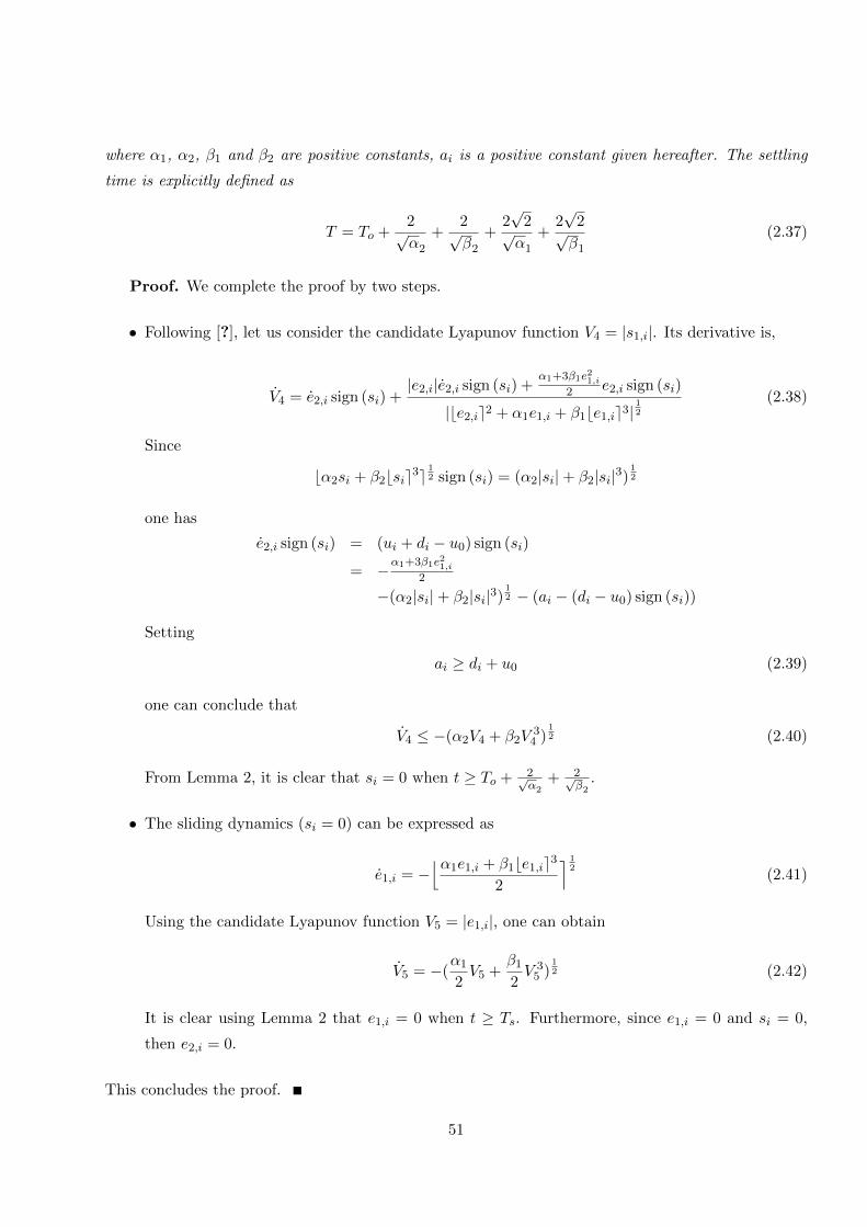
where α1, α2, β1 and β2 are positive constants, ai is a positive constant given hereafter. The settling
time is explicitly defined as
T = To +2√α2
+2√β2
+2√
2√α1
+2√
2√β1
(2.37)
Proof. We complete the proof by two steps.
• Following [?], let us consider the candidate Lyapunov function V4 = |s1,i|. Its derivative is,
V4 = e2,i sign (si) +|e2,i|e2,i sign (si) +
α1+3β1e21,i2 e2,i sign (si)
|be2,ie2 + α1e1,i + β1be1,ie3|12
(2.38)
Since
bα2si + β2bsie3e12 sign (si) = (α2|si|+ β2|si|3)
12
one has
e2,i sign (si) = (ui + di − u0) sign (si)
= −α1+3β1e21,i2
−(α2|si|+ β2|si|3)12 − (ai − (di − u0) sign (si))
Setting
ai ≥ di + u0 (2.39)
one can conclude that
V4 ≤ −(α2V4 + β2V3
4 )12 (2.40)
From Lemma 2, it is clear that si = 0 when t ≥ To + 2√α2
+ 2√β2
.
• The sliding dynamics (si = 0) can be expressed as
e1,i = −⌊α1e1,i + β1be1,ie3
2
⌉ 12
(2.41)
Using the candidate Lyapunov function V5 = |e1,i|, one can obtain
V5 = −(α1
2V5 +
β1
2V 3
5 )12 (2.42)
It is clear using Lemma 2 that e1,i = 0 when t ≥ Ts. Furthermore, since e1,i = 0 and si = 0,
then e2,i = 0.
This concludes the proof.
51
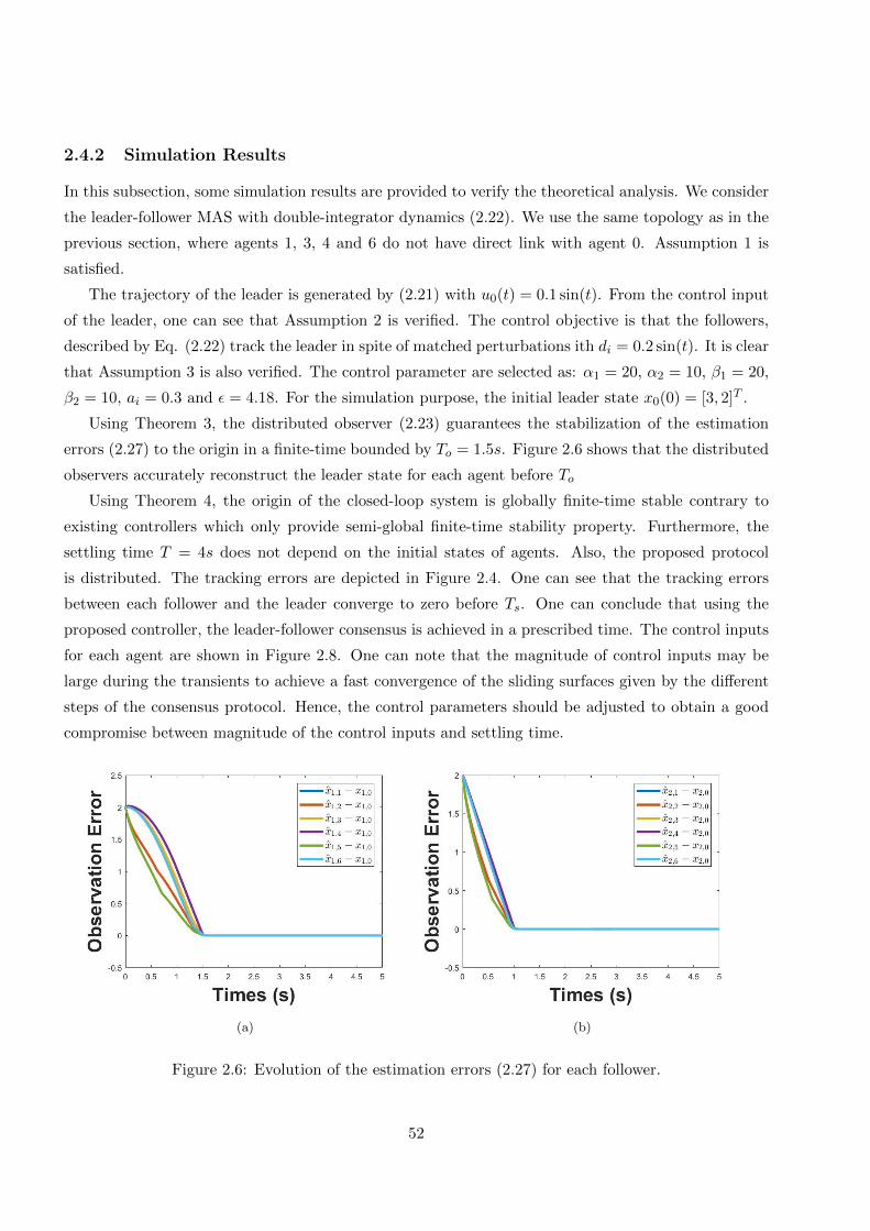
2.4.2 Simulation Results
In this subsection, some simulation results are provided to verify the theoretical analysis. We consider
the leader-follower MAS with double-integrator dynamics (2.22). We use the same topology as in the
previous section, where agents 1, 3, 4 and 6 do not have direct link with agent 0. Assumption 1 is
satisfied.
The trajectory of the leader is generated by (2.21) with u0(t) = 0.1 sin(t). From the control input
of the leader, one can see that Assumption 2 is verified. The control objective is that the followers,
described by Eq. (2.22) track the leader in spite of matched perturbations ith di = 0.2 sin(t). It is clear
that Assumption 3 is also verified. The control parameter are selected as: α1 = 20, α2 = 10, β1 = 20,
β2 = 10, ai = 0.3 and ε = 4.18. For the simulation purpose, the initial leader state x0(0) = [3, 2]T .
Using Theorem 3, the distributed observer (2.23) guarantees the stabilization of the estimation
errors (2.27) to the origin in a finite-time bounded by To = 1.5s. Figure 2.6 shows that the distributed
observers accurately reconstruct the leader state for each agent before To
Using Theorem 4, the origin of the closed-loop system is globally finite-time stable contrary to
existing controllers which only provide semi-global finite-time stability property. Furthermore, the
settling time T = 4s does not depend on the initial states of agents. Also, the proposed protocol
is distributed. The tracking errors are depicted in Figure 2.4. One can see that the tracking errors
between each follower and the leader converge to zero before Ts. One can conclude that using the
proposed controller, the leader-follower consensus is achieved in a prescribed time. The control inputs
for each agent are shown in Figure 2.8. One can note that the magnitude of control inputs may be
large during the transients to achieve a fast convergence of the sliding surfaces given by the different
steps of the consensus protocol. Hence, the control parameters should be adjusted to obtain a good
compromise between magnitude of the control inputs and settling time.
(a) (b)
Figure 2.6: Evolution of the estimation errors (2.27) for each follower.
52

(a) (b)
Figure 2.7: Evolution of the tracking errors between each agent and the leader.
Figure 2.8: Control input for each agent.
2.5 Consensus of MAS with Unicycle-Type Dynamics
Let us now consider a nonholonomic mobile robot moving in a two-dimensional plane. The axes of
the workspace are shown in Figure 2.9. The kinematics of the unicycle-type mobile robot is described
under the nonholonomic constraints (contains the time derivatives of the generalized coordinates of
the system and is not integrable). The configuration of the robot i can be represented by:
qi(t) = (xi(t), yi(t), θi(t))T (2.43)
where xi(t) ∈ R, yi(t) ∈ R describe the robot position and θi(t) is its orientation in the global frame.
The pure rolling and nonslipping conditions are described by:
GT (qi)qi = 0 with GT (qi) = (− sin(θi) cos(θi) 0) (2.44)
53

Under the hypothesis of pure rolling and nonslipping condition, the kinematic equations can be written
as follows:
qi(t) = f(qi(t), ui(t)) (2.45)
where vector field f : R3 × R2 → R3 and control inputs ui are defined as:f(qi(t), ui(t)) =
cos(θi) 0
sin(θi) 0
0 1
ui(t)
ui(t) = (υi(t), ωi(t))T
(2.46)
υi(t) and ωi(t) are the linear and angular velocities, respectively.
Figure 2.9: Top view of the considered mobile robot.
Before designing the consensus protocol, let us consider the classical transformation
qi1(t) = θi(t)
qi2(t) = xi sin(θi(t))− yi cos(θi(t))
qi3(t) = xi cos(θi(t)) + yi sin(θi(t))
ui1(t) = ωi(t)
ui2(t) = υi(t)− qi2(t)ωi(t)
(2.47)
Using (2.47), system (2.45) can be written in chained-form as follows:
qi1(t) = ui1(t)
qi2(t) = qi3(t)ui1(t)
qi3(t) = ui2(t)
(2.48)
To deal with the robustness properties, some matched perturbations are added. Furthermore, for
the purpose of the controller design, an additional dynamic extension is added to the chained-form
dynamics. Therefore, the dynamics (2.48) becomes:
x1(t) = x2(t)
x2(t) = u1(t) + d1(t)
x3(t) = x4(t)x2(t)
x4(t) = u2(t) + d2(t)
(2.49)
54

where x = [x1, x2, x3, x4]T ∈ R4 (resp. u = [u1, u2]T ∈ R2) is the state (resp. control input) of the
chained-form unicycle-type mobile robot, d = [d1, d2]T ∈ R2 represents the unknown disturbances of
the chained-form dynamics.
The dynamics of the desired trajectory is generated using the following system:
x1,d(t) = x2,d(t)
x2,d(t) = u1,d(t)
x3,d(t) = x4,d(t)x2,d(t)
x4,d(t) = u2,d(t)
(2.50)
where xd = [x1,d, x2,d, x3,d, x4,d]T ∈ R4 (resp. ud = [u1,d, u2,d]
T ∈ R2) is the state (resp. control input)
of the desired trajectory.
Before dealing with the consensus tracking problem, let us study the fixed-time trajectory tracking
problem for only one single unicycle-type mobile robot. Figure 2.10 illustrates the control objective
studied in the next subsection, i.e. the unicycle-type mobile robot tracks a desired trajectory in a
prescribed-time.
Figure 2.10: Illustration of the fixed-time trajectory tracking problem for a single agent.
2.5.1 Fixed-time trajectory tracking problem for a single unicycle-type mobile
robot
In this subsection, let us first study the fixed-time trajectory tracking problem for only one single
unicycle-type mobile robot. The control objective is to design a fixed-time trajectory tracking con-
troller such that system (2.49) tracks the trajectory of system (2.50) in spite of the presence of matched
perturbations.
55

Assumption 4 It is assumed that the perturbations d1(t) and d2(t) are unknown but are bounded by
known constants (i.e. d1,max and d2,max).
Assumption 5 It is assumed that the desired state x2,d satisfies the following condition
x2,d(t) 6= 0 (2.51)
Remark 6 Hypothesis 4 is not restrictive since the bounds of perturbations can be estimated a priori
for any system. Assumption 10 is relatively not restrictive since only the case x2,d(t) 6= 0 is not
considered in the proposed scheme. Therefore, the motion planner for the desired trajectory should
take into account this constraint (to avoid any loss of controllability). Indeed, when x2,d(t) = 0, we
loose controllability since the state x3,d cannot be controlled. Since the agent track the leader, it also
looses controllability in this case.
Remark 7 Note that there exist several tools to plan the trajectory for the leader. For instance, in
[?], based on nonlinear programming and flatness properties, a constrained receding horizon planner is
applied to design the state and the control input of the leader. One can easily extend this work while
taking into account constraints given in Assumptions 4-10.
Let us define the tracking errors as
e(t) = x(t)− xd(t) (2.52)
with e = [e1, e2, e3, e4]T ∈ R4. The tracking error dynamics satisfy the following differential equations:
(Σ1)e1(t) = x2(t)− x2,d(t)
e2(t) = u1(t) + d1(t)− u1,d(t)
(Σ2)e3(t) = x4(t)x2(t)− x4,d(t)x2,d(t)
e4(t) = u2(t) + d2(t)− u2,d(t)
(2.53)
To simplify the controller design, dynamics (2.53) is divided into two second-order coupled sub-
systems. To solve the fixed-time trajectory tracking problem, two steps are defined:
• Stabilization of subsystem Σ1 in a fixed time Ts using control u1,
• After t > Ts, stabilization of subsystem Σ2 in a fixed time T using control u2.
Figure 2.11 illustrated how the fixed-time trajectory tracking problem solved.
To design the fixed-time consensus tracking algorithm for a single unicycle-type mobile robot, the
following theorem is derived.
56

Figure 2.11: Stabilization of the two subsystems.
Theorem 5 Assuming that Assumptions 4-10 hold. Consider system (2.53) with the trajectory track-
ing control law defined as:
u1 = u1,d + ϕ1
(e1, e2
)
u2 =
1 ,∀t < Ts
u2,d −e4u1,dx2,d
+ 1x2,d
ϕ2
(e3, ζ4
),∀t ≥ Ts
(2.54)
with ζ4 = e4x2,d.
The sliding mode controllers are as follows:
ϕ1
(e1, e2
)= −α1+3β1e21+2d1,max
2 sign(s1
(e1, e2
))−bα2s1
(e1, e2
)+ β2bs1
(e1, e2
)e3e
12
ϕ2
(e3, ζ4
)= −α1+3β1e23+2d2,max
2 sign(s2
(e3, ζ4
))−bα2s2
(e3, ζ4
)+ β2bs2
(e3, ζ4
)e3e
12
(2.55)
with sliding surfaces
s1
(e1, e2
)= e2 + bbe2e2 + α1e1 + β1be1e3e
12
s2
(e3, ζ4
)= ζ4 + bbζ4e2 + α1e3 + β1be3e3e
12
(2.56)
The switching time is Ts = 2√α2
+ 2√β2
+ 2√
2√α1
+ 2√
2√β1
and constants αi, βi (i = 1, 2) are positive.
Then, the origin of system (2.53) is globally fixed-time stable with settling time:
T = 2Ts (2.57)
Hence, the fixed-time trajectory tracking problem is solved.
Proof. The proof is divided into two steps.
• Let us first consider the time interval t ∈ [0, Ts]. Using controller (2.54), it is clear that subsystem
Σ1 has been already discussed in the section double-integrator system. One can conclude that
e1 = 0 and e2 = 0.
57

• Let us now consider t > Ts. From previously, subsystem Σ2 can be written as:
e3 = e4x2,d
e4 = u2 + d2 − u2,d
(2.58)
Setting ζ4 = e4x2,d, system (2.58) can be expressed as:
e3 = ζ4
ζ4 = (u2 + d2 − u2,d)x2,d + e4u1,d
(2.59)
Using controller (2.54), system (2.59) becomes:
e3 = ζ4
ζ4 = ϕ2 + d2x2,d
(2.60)
Using Assumptions 4-10 and following the same procedure as in the first step, one can conclude
that the origin of system (2.59) is globally fixed-time state with settling time T given by Eq.
(2.57). It is clear that the origin of system (2.53) is globally fixed-time stable with settling time
T .
Remark 8 It should be highlighted that since the settling time T is independent of the initial sys-
tem conditions and can be estimated a priori, global finite-time stability of the closed-loop system is
guaranteed (contrary to many existing works which only guarantee semi-global finite-time stability).
2.5.2 Simulation Results
In this subsection, some simulation results are provided to verify the theoretical analysis.
We consider the unicycle-type mobile robot (2.49) where the perturbations are d1 = sin(20t) and
d2 = 10 cos(10t). The desired trajectory is generated by (2.50) with xd(0) = [0, 2, 0, 0]T , u1,d(t) =
2 + sin(t) and u2,d(t) = 1. The control objective is that system (2.49) follows its derived trajectory
xd. It is clear that Assumptions 4-10 are verified. The control parameter are selected as: α1 = 20,
α2 = 10, β1 = 20, β2 = 10 and Ts = 2.5s. For the simulation purpose, the initial conditions of
system (2.49) are set as: x(0) = [10, 1, 3, 1]T . Using Theorem 5, the robust controller (2.54) solves
the fixed-time trajectory tracking problem with an estimation of the settling time T = 4.5s. Figure
2.12 shows that the origin of subsystem Σ1 is globally fixed-time stable with a settling time less than
Ts = 2.5s.
Figure 2.13 shows that the origin of subsystem Σ2 is globally fixed-time stable with a settling time
less than T = 5s.
Figure 2.14 displays the tracking errors. It can be seen that the trajectory tracking problem is
solve in fixed-time.
58

(a) (b)
Figure 2.12: Actual trajectory x1, x2 and desired state trajectories x1,d, x2,d
(a) (b)
Figure 2.13: Actual trajectory x3, x4 and desired state trajectories x3,d, x4,d
2.6 Consensus of MAS with Unicycle-Type Mobile Robot Dynamics
Consider a multi-agent system consisting of a leader (which could be virtual) labeled by 0, and N
followers, labeled by i ∈ 1, . . . , N. The leader dynamics is given by the following chained-form
unicycle-type mobile robot x1,0(t) = x2,0(t)
x2,0(t) = u1,0(t)
x3,0(t) = x4,0(t)x2,0(t)
x4,0(t) = u2,0(t)
(2.61)
59

Figure 2.14: Tracking errors e
where x0 = [x1,0, x2,0, x3,0, x4,0]T ∈ R4 (resp. u0 = [u1,0, u2,0]T ∈ R2) is the leader state (resp. leader
control input). The dynamics of the ith follower is as followsx1,i(t) = x2,i(t)
x2,i(t) = u1,i(t) + d1,i(t)
x3,i(t) = x4,i(t)x2,i(t)
x4,i(t) = u2,i(t) + d2,i(t)
(2.62)
where xi = [x1,i, x2,i, x3,i, x4,i]T ∈ R4 (resp. ui = [u1,i, u2,i]
T ∈ R2) is the state (resp. control input)
of the ith follower. The unknown perturbation of the ith chained-form is given by di = [d1,i, d2,i]T ∈ R2.
Figure 2.15 provides an illustration of fixed-time consensus tracking problem. To solve this prob-
lem, the following assumptions are considered.
Assumption 6 It is assumed that the communication topology among the N followers is undirected,
fixed, connected. It means that the adjacency matrix A is symmetric. It is also assumed that there is
at least one strictly positive parameter bi.
Assumption 7 The followers do not known the leader control input. Nevertheless, its neighboring
agents know its upper bounds u1,0 and u2,0, defined as follows|u1,0(t)| ≤ umax1,0
|u2,0(t)| ≤ umax2,0
(2.63)
with umax1,0 , umax2,0 ∈ R+.
60

Figure 2.15: Illustration of the fixed-time consensus tracking problem.
Assumption 8 For each follower, the perturbation di(t) is unknown but it is bounded as follows
|d1,i(t)| ≤ dmax1,i
|d2,i(t)| ≤ dmax2,i
(2.64)
with dmax1,i , dmax2,i ∈ R+.
Assumption 9 It is assumed that the leader state x2,0 satisfies the following condition
x2,0(t) 6= 0 (2.65)
2.6.1 Fixed-Time Observer-Based Consensus Protocol
For chained-form dynamics MAS under matched perturbations, we propose an observer-based consen-
sus protocol to deal with the leader-follower consensus problem. Figure 2.16 illustrates the proposed
control strategy to solve the consensus problem of MAS with chained-form dynamics.
Distributed fixed-time observer
To estimate the leader state in a prescribed time, distributed observers are designed for each follower
i ∈ 1, . . . , N. Indeed, the leader state is only available to its neighboring followers. Let us introduce
61

Figure 2.16: Proposed control strategy to solve the consensus problem of MAS with chained-form
dynamics.
the following observer as follows
˙x1,i = x2,i + ρ1 sign(∑N
j=1 aij(x1,j − x1,i) + bi(x1,0 − x1,i))
+σ1
⌈∑Nj=1 aij(x1,j − x1,i) + bi(x1,0 − x1,i)
⌋2
˙x2,i = ρ2 sign(∑N
j=1 aij(x2,j − x2,i) + bi(x2,0 − x2,i))
+σ2
⌈∑Nj=1 aij(x2,j − x2,i) + bi(x2,0 − x2,i)
⌋2
˙x3,i = x4,ix2,i + ρ3 sign(∑N
j=1 aij(x3,j − x3,i) + bi(x3,0 − x3,i))
+σ3
⌈∑Nj=1 aij(x3,j − x3,i) + bi(x3,0 − x3,i)
⌋2
˙x4,i = ρ4 sign(∑N
j=1 aij(x4,j − x4,i) + bi(x4,0 − x4,i))
+σ4
⌈∑Nj=1 aij(x4,j − x4,i) + bi(x4,0 − x4,i)
⌋2
(2.66)
where xk,i (k = 1, . . . , 4) is the estimation of the leader state xk,0 for the ith follower, ρk and σk are
positive constants, which will be given hereafter.
The fixed-time stabilization of the estimation errors
xk,i = xk,i − xk,0 (i = 1, . . . , N, k = 1, . . . , 4) (2.67)
is introduced in the following theorem.
Theorem 6 Suppose that Assumptions 6-7 are satisfied. If the gains of the distributed observer (2.66)
62

verify
σk = ε√N
(2λmin(L+B))32, ∀k = 1, . . . , 4
ρ1 = ε√
λmax(L+B)2λmin(L+B)
ρ2 = umax1,0 + ε√
λmax(L+B)2λmin(L+B)
ρ3 = ε√
λmax(L+B)2λmin(L+B)
ρ4 = umax2,0 + ε√
λmax(L+B)2λmin(L+B)
(2.68)
with ε > 0, then, for any initial condition, the estimation errors (2.67) converge to zero. An upper
bound of the convergence time can be given as
To =2π
ε(2.69)
Proof. Using (2.66), the dynamics of the observation error is given by
˙x1,i = x2,i + ρ1 sign(∑N
j=1 aij(x1,j − x1,i)− bix1,i
)+σ1
⌈∑Nj=1 aij(x1,j − x1,i)− bix1,i
⌋2
˙x2,i = ρ2 sign(∑N
j=1 aij(x2,j − x2,i)− bix2,i
)+σ2
⌈∑Nj=1 aij(x2,j − x2,i)− bix2,i
⌋2− u1,0
˙x3,i = ρ3 sign(∑N
j=1 aij(x3,j − x3,i)− bix3,i
)+σ3
⌈∑Nj=1 aij(x3,j − x3,i)− bix3,i
⌋2+ x4,ix2,i − x4,0x2,0
˙x4,i = ρ4 sign(∑N
j=1 aij(x4,j − x4,i)− bix4,i
)+σ4
⌈∑Nj=1 aij(x4,j − x4,i)− bix4,i
⌋2− u2,0
(2.70)
Let us denote
xk = [xk,1, . . . , xk,N ]T (2.71)
Then, for x1, x2 and x4, one can obtain
˙x1 = x2 − ρ1 sign ((L+B)x1)− σ1 d(L+B)x1c2 (2.72)
˙x2 = −ρ2 sign ((L+B)x2)− σ2 d(L+B)x2c2 − 1u1,0 (2.73)
˙x4 = −ρ4 sign ((L+B)x4)− σ4 d(L+B)x4c2 − 1u2,0 (2.74)
We complete the proof by three steps.
• Let us first study subsystems (2.72)-(2.73). Consider the candidate Lyapunov function for sub-
system (2.73):
V5 =1
2xT2 (L+B)x2 (2.75)
63

Its time derivative is given by
V5 = −ρ2xT2 (L+B) sign ((L+B)x2)
+xT2 (L+B)(−σ2 d(L+B)x2c2 − 1u1,0
)≤ −(ρ2 − umax1,0 )‖(L+B)x2‖1
−β2N− 1
2 (2λmin(L+B))32V
32
5
≤ −εV12
5 − εV32
5
Using Lemma 2, this inequality guarantees that x2 is fixed-time stable at the origin with the
settling time bounded by πε .
After x2 converges to zero (i.e. when t ≥ πε ), the dynamics of x1 reduces to
˙x1 = −ρ1 sign ((L+B)x1)− σ1 d(L+B)x1c2 (2.76)
Similarly to the previous step, the x1 dynamics converges to zero. Indeed, consider the Lyapunov
function:
V6 =1
2xT1 (L+B)x1 (2.77)
Its time derivative is given by
V6 = −ρ1xT1 (L+B) sign ((L+B)x1)
−σ1xT1 (L+B) d(L+B)x1c2
≤ −ρ1‖(L+B)x1‖1
−σ1N− 1
2 (2λmin(L+B))32V
32
6
≤ −εV12
6 − εV32
6
Hence, one can conclude that x2 converges to zero and after that x1 converges to zero in a
fixed-time bounded by 2πε .
• Let us now study subsystem (2.74).
The time derivative of the following candidate Lyapunov function
V7 =1
2xT4 (L+B)x4 (2.78)
is given by
V7 = xT4 (L+B)(−ρ4 sign ((L+B)x4)− σ4 d(L+B)x4c2 − 1u2,0
)≤ −(ρ4 − umax2,0 )‖(L+B)x4‖1 − σ4N
− 12 (2λmin(L+B))
32V
32
7
≤ −εV12
7 − εV32
7
Using Lemma 2, this inequality ensures that x4 converges to zero in a finite-time bounded by πε .
64

• After x2 and x4 converge to zero (i.e. when t ≥ πε ), the dynamics of x3 becomes
˙x3 = −ρ3 sign ((L+B)x3)− σ3 d(L+B)x3c2 (2.79)
Similarly to previously, considering the candidate Lyapunov function V8 = 12 x
T3 (L+B)x3 yields
in the fixed-time stable at the origin of x3 with the settling time bounded by 2πε .
Hence, one can conclude that the estimation errors (2.67) converge to zero in a fixed-time bounded
by To.
Decentralized fixed-time controller
From Theorem 6, one can conclude that xi = [x1,i, x2,i, x3,i, x4,i]T = x0 for all t ≥ To. Hence, after
time To, each follower is able to indirectly access to the state of the leader and uses the estimate xi in
the consensus protocol.
Let us denote the tracking errors as follows
ek,i = xk,i − xk,i = xk,i − xk,0 − xk,i (i = 1, . . . , N, k = 1, . . . , 4) (2.80)
For each follower i = 1, . . . , N and for all t ≥ To, the tracking error dynamics becomes
(Σ1)e1,i = e2,i
e2,i = u1,i + d1,i − u1,0
(Σ2)e3,i = e4,ix2,0 + (e4,i + x4,0)e2,i
e4,i = u2,i + d2,i − u2,0
(2.81)
It is clear that dynamics (2.81) is divided into two coupled second-order subsystems (i.e. Σ1 and Σ2).
To deal with the observer-based consensus tracking problem, for each follower i = 1, . . . , N, the
following two steps are introduced:
• Design u1,i such that the origin of subsystem Σ1 is fixed-time stable with the settling time
estimate T1 < T .
• For t ≥ T1, design u2,i such that the origin of subsystem Σ2 is fixed-time stable with the settling
time estimate T . Note that for t ≥ T1, subsystem Σ2 becomes
e3,i = e4,ix2,0
e4,i = u2,i + d2,i − u2,0
(2.82)
It is clear that for t ≥ T1, the two subsystems are decoupled.
In the following theorem, the control strategy is derived to solve the leader-follower consensus
problem for MAS with chained-form dynamics, in a fixed-time, in spite of the presence of matched
perturbations.
65

Theorem 7 Let us consider the leader-follower system (2.61)-(2.62). Suppose that Assumptions 6-9
are satisfied and the gains of the distributed observer (2.66) verify Eq. (2.68). The leader-follower
consensus problem is solved in a fixed-time using the decentralized controllers
u1,i =
0 , ∀t < To
−α1+3β1e21,i+2ai2 sign (s1,i)− bα2s1,i + β2bs1,ie3e
12 ,∀t ≥ To
(2.83)
with the sliding surface
s1,i = e2,i + bbe2,ie2 + α1e1,i + β1be1,ie3e12 (2.84)
and
u2,i =
0 ,∀t < Ts
− 1x2,0
(e4,i
˙x2,0 +α1+3β1e23,i+2bi
2 sign (s2,i) + bα2s2,i + β2bs2,ie3e12
),∀t ∈ [Ts, T ]
−bi sign (e4,i) ,∀t > T
(2.85)
with the sliding surface
s2,i = e4,ix2,0 + bbe4,ix2,0e2 + γ1e3,i + µ1be3,ie3e12 (2.86)
where α1, α2, β1 and β2 are positive constants, ai and bi are positive constants given hereafter, and
the switching time is explicitly defined as
Ts = To +2√α2
+2√β2
+2√
2√α1
+2√
2√β1
(2.87)
Proof. We complete the proof by three steps. First, it will be shown that the origin of subsystem
Σ1 is fixed-time stable with the settling time estimate Ts under the control law (2.83)-(2.84). Then, the
protocol (2.83)-(2.86) guarantees that the origin of subsystem Σ2 is fixed-time stable with the settling
time estimate T . At last, it will be proved that in spite of the presence of matched perturbations, the
fixed-time leader-follower consensus problem is solved.
• Let us first consider subsystem Σ1. Following [?], let us consider the candidate Lyapunov function
V9 = |s1,i|. Its derivative is,
V9 = e2,i sign (s1,i) +|e2,i|e2,i sign (s1,i) +
α1+3β1e21,i2 e2,i sign (s1,i)
|be2,ie2 + α1e1,i + β1be1,ie3|12
(2.88)
Since
bα2s1,i + β2bs1,ie3e12 sign (s1,i) = (α2|s1,i|+ β2|s1,i|3)
12
one has
e2,i sign (s1,i) = (u1,i + d1,i − u1,0) sign (s1,i)
= −α1+3β1e21,i2
−(α2|s1,i|+ β2|s1,i|3)12 − (ai − (d1,i − u1,0) sign (s1,i))
66

Setting
ai ≥ dmax1,i + umax1,0 (2.89)
one can conclude that
V9 ≤ −(α2V9 + β2V3
9 )12 (2.90)
From Lemma 2, it is clear that s1,i = 0 when t ≥ To + 2√α2
+ 2√β2
.
The sliding dynamics (s1,i = 0) can be expressed as
e1,i = −⌊α1e1,i + β1be1,ie3
2
⌉ 12
(2.91)
Using the candidate Lyapunov function V10 = |e1,i|, one can obtain
V10 = −(α1
2V10 +
β1
2V 3
10)12 (2.92)
It is clear using Lemma 2 that e1,i = 0 when t ≥ Ts. Furthermore, since e1,i = 0 and s1,i = 0,
then e2,i = 0.
• Let us now consider subsystem Σ2 for t ∈ [Ts, T ]. In this case, since e1,i = e2,i = 0, subsystem
Σ2 becomes (2.82). Note that Assumption 4 is introduced to avoid singularity problem in the
controller design. Hence, let us set ζi = e4,ix2,0. Dynamics (2.82) can be written as follows,
e3,i = ζi
ζi = e4,ix2,0 + x2,0(u2,i + d2,i − u2,0)(2.93)
Setting
bi ≥ dmax2,i + umax2,0 (2.94)
and using the controller (2.85)-(2.86), similarly to the previous step, one can easily deduce that
e3,i = 0 for all t ≥ T = Ts + 2√α2
+ 2√β2
+ 2√
2√α1
+ 2√
2√β1
. Furthermore, since e3,i = 0 and s2,i = 0,
then e4,i = 0.
• The last step is to study subsystem Σ2 for t > T . From subsystem Σ2, one can obtain
e4,i = −bi sign (e4,i) + d2,i − u2,0 (2.95)
The controller u2,i is used to reject the effect of uncertain terms d2,i and u2,0. Let us consider
the candidate Lyapunov function V11 = 12e
24,i. Its derivative is given by
V11 = −bi|e4,i|+ e4,i (d2,i − u2,0)
≤ −(bi + dmax2,i + umax2,0 )|e4,i|≤ 0
(2.96)
For the previous step, one has e3,i(T ) = e4,i(T ) = 0. Hence, one can conclude that for any initial
condition, the tracking errors converge to zero in a finite-time bounded by T and remains there
in spite of the presence of matched perturbations.
67

This concludes the proof.
Remark 9 When the settling time T is prescribed, the switching time Ts should be appropriately tuned
using α1, α2, β1 and β2 through Eq. (2.87).
Remark 10 In the presence of measurement noise or unmatched perturbations, only practical con-
sensus (i.e. uniformly ultimate boundedness of the tracking errors) can be achieved.
Remark 11 The design guidelines for our fixed-time controller are as follows:
• Select the parameter ε. Parameter ε should be tuned to obtain a good compromise between
robustness against measurement noises and sufficiently fast estimation (To can be computed
according to Eq. (2.69)).
• Design the observer gain parameters using Eq. (2.68).
• Select the settling time T . This parameter T should be tuned to obtain a good compromise between
the control magnitudes and sufficiently fast convergence for the tracking errors.
• Select the switching time Ts as follows:
Ts =T − To
2
It enables to divide the time interval [To, Ts] into two equal parts. This is useful for our two
steps procedure described previously (i.e. fixed-time stabilization of system Σ1 and system Σ2
described in Eq. (2.81)).
• Knowing To and Ts, select the parameters γ1, γ2, µ1 and µ2 according to (2.87). A possible
choice for these parameters is the following:
(µ1/2) = µ2 = (γ1/2) = γ2 =64
(Ts − To)2(2.97)
• Select the control parameters ai and bi which satisfy inequalities (2.89) and (2.94).
2.6.2 Simulation Results
Here, the performances of the proposed observer-based leader-follower consensus controller are studied
through numerical simulations. Suppose that the MAS is composed of N = 6 followers labeled by 1−6
and one leader labeled by 0. The nonlinear dynamics of the leader (resp. the followers) is given by Eq.
(2.61) (resp. Eq. (2.62)). Hereafter, the leader control input is set as u0 = [0.1 sin(t),−0.5 cos(0.5t)].
Each follower is affected by the unknown perturbation di =[0.2 sin(x1,i), 0.3e
−t)]. Therefore, one can
easily verify that Assumptions 7-8 are fulfilled with u1,max = 0.1, u2,max = 0.5, d1,max = 0.2 and
d2,max = 0.3.
68

Using the same topology as previous section, from matrix B, it is clear that agents 1, 3, 4 and
6 do not have direct link with agent 0. Assumption 6 is satisfied. The initial leader state is set as
x0(0) = [3, 2, 2, 0.5]T . From the control input of the leader, one can see that Assumption 9 is verified.
The parameters of the distributed observer are selected as ρ1 = ρ3 = 10, ρ2 = 10.1, ρ4 = 10.5
and σk = 24, ∀k = 1, . . . , 4. The parameters of the decentralized controller are chosen as follows:
α1 = 5.12, β1 = 5.12, α2 = 2.56, β2 = 2.56, ai = 0.3 and bi = 0.8.
Using Theorem 6, the distributed observer (2.66) guarantees the stabilization of the estimation
errors (2.67) to the origin in a finite-time bounded by To = 1s. Figure 2.17 shows that the distributed
observers accurately reconstruct the leader state for each agent before To. Contrary to [?, ?], the
proposed fixed-time observer removes the problem of the communication loop due to the dependence
of the control inputs of the followers on the inputs of its neighbors. The switching time can be
calculated using Eq. (2.69). One can obtain Ts = 4.5s. Hence, the origin of the closed-loop system is
globally finite-time stable contrary to existing controllers which only provide semi-global finite-time
stability property. Furthermore, since Ts does not depend on the initial states of agents, the proposed
protocol is distributed.
Here, an upper bound of the settling time, independently of the initial conditions, can be estimated
using Eq. (2.87), i.e. T = 9s from Theorem 7. The tracking errors are depicted in Fig. 2.18. One can
see that the tracking errors between each follower and the leader converge to zero before T . From Fig.
2.18, one can conclude that using the proposed controller, the leader-follower consensus is achieved in
a prescribed time. The control inputs for each agent are shown in Fig. 2.19. One can note that the
magnitude of control inputs may be large during the transients to achieve a fast convergence of the
sliding surfaces given by the different steps of the consensus protocol. Hence, the control parameters
should be adjusted to obtain a good compromise between magnitude of the control inputs and settling
time.
Based on the simulation results, one can see that the proposed observer-based controller achieves
the fixed-time leader-follower consensus for MAS with chained-form dynamics in spite of the presence
of matched perturbations.
2.7 Conclusion
For the second and third section, the fixed-time consensus problem of linear multi-agent systems (i.e.
single-integrator and double-integrator dynamics) has been considered. The proposed distributed ob-
servers has been used to estimate the leader state in a fixed-time. A decentralized controller has been
designed for each agent to solve the leader-follower consensus problem in a prescribed-time.
For the fourth section, the fixed-time trajectory tracking problem for unicycle-type mobile robots
has been considered. A switching controller has been proposed to solve this problem. An upper bound
69

(a) (b)
(c) (d)
Figure 2.17: Evolution of the estimation errors (2.67) for each follower
of the settling time, which only depends on the controller parameters has been estimated regardless
of the initial conditions. Some simulation results have been given to show the effectiveness of the
proposed controller.
In the fifth section, the fixed-time consensus problem of multiple unicycle-type mobile robots under
matched perturbations has been considered. Thanks to the proposed distributed observers, the leader
state has been estimated in a fixed-time. A decentralized observer-based control protocol has been
proposed for each agent to solve the leader-follower consensus problem in a fixed-time.
70

(a) (b)
(c) (d)
Figure 2.18: Evolution of the tracking errors between each agent and the leader.
(a) (b)
Figure 2.19: Control input for each agent
71

72
Chapter 3
Consensus for Multi-Agent Systems
Using Distributed Model Predictive
Control
3.1 Introduction
This chapter is concerned with the consensus problem for a group of mobile agents which have a
discrete-time dynamics using distributed model predictive control (DMPC). The first part of this
chapter formulates the general control objective and the considered assumptions to solve the con-
sensus problem under switching topologies. The second and third part of this chapter deal with the
consensus problem for linear multi-agent systems (i.e. single-integrator and double-integrator dynam-
ics). The proposed consensus control protocol is distributed and is designed by combining graph
theory with a predictive control algorithm to take into account the switches on the communication
topology. The predictive strategy is used to estimate input and output of agent through a receding
horizon. Contrary to many existing works, the cost function is designed using the difference between
two consecutive inputs. The controller has integrator properties to eliminate steady-state errors.
The objective is to develop a DMPC protocol such that the states of all agents reach an agreement
eventually. The main features of the proposed scheme can be summarized as follows:
i) The control horizon can be arbitrarily picked from one to less than the prediction horizon, which
increases the degree of freedom in controller design.
ii) The communication topolgy is assumed to be directed and dynamically switching.
iii) The sampling period can be arbitrarily large provided that each communication topology has a
directed spanning tree.
73

The remaining parts of this chapter are organized as follows. Section 3.2 introduces some assump-
tions and formulates the general control objective. The distributed model predictive controller based
consensus strategy is introduced in Section 3.3. Some simulation results are given in Section 3.4 to
illustrate the effectiveness and advantages of the proposed scheme for single and double integrator
dynamic. Section 3.5 concludes this chapter.
3.2 Problem statement and considered assumptions
Let us consider a group of N agents labeled by i ∈ 1, . . . , N. The dynamics of each agent is expressed
by the following discrete-time equation
xi(k + 1) = F (xi(k), ui(k)) (3.1)
where xi(k) ∈ Rn is the state of agent i and ui(k) ∈ Rm is the control input of agent i. F : Rn×Rm →Rn is known. T ∈ R+ is the sampling period.
Among the N agents, at time t = kT , the communication topology can be represented by the
time-varying digraph G(k) = V, E(k) where V = 1, . . . , N defines the set of nodes, corresponding
to the agents, and E(k) ⊆ V × V defines the edge set at time kT . An edge (j, i) ∈ E(k), with i 6= j,
exists if at time kT agent i receive information from its neighbor j. At time k, the set of neighbors to
the node i ∈ V is Ni(k) = j ∈ V : (j, i) ∈ E(k) and |Ni(k)|, i ∈ V, is the valency or degree of i-th node
at time k. The adjacency matrix A(k) = (aij(k)) ∈ RN×N satisfies aij(k) > 0 if (j, i) ∈ E at time kT
and aij(k) = 0, otherwise. The corresponding Laplacian matrix is given by L(k) = (lij(k)) ∈ RN×N
with lii(k) =∑N
j=1, j 6=i aij(k) and lij(k) = −aij(k) for i 6= j.
Hereafter, it is assumed that the following hypothesis holds to derive the proposed DMPC scheme.
Assumption 10 It is assumed that the communication topology among the N agents is directed and
dynamical switching and at each time kT it contains a directed spanning tree.
Such time-varying graphs can be found in many engineering applications due to the creation or failure
of communication links, reconfiguration of formations, presence of obstacles and so on.
Here, the purpose is to derive a decentralized controller ui (i = 1, . . . , N) for each agent, based on
available information, such that the consensus problem is solved. It means that
limk→∞
‖xi(k)− xj(k)‖ = 0 ∀i, j ∈ V, i 6= j (3.2)
3.3 Distributed model predictive controller based consensus
3.3.1 Generalities on model predictive controller
MPC (Model Predictive Control) is a kind of finite horizon optimal control. It solves a finite horizon
optimal control and applies the first part of the resulting optimal control sequence to the plant at
74

every sampling instant.
In this subsection, the general structure of MPC is briefly introduced. Let us consider a discrete-
time linear system described by
x(k + 1) = Ax(k) +Bu(k) (3.3)
where x(k) ∈ Rn and u(k) ∈ Rm are the state and control input, respectively. A ∈ Rn×n and
B ∈ Rn×m are the state and input matrices, respectively.
The MPC implementation can be formulated by introducing the following optimization problem
at every time instant kT :
minu(.) J(Hp,Hu)(k) (3.4)
subject to
x(k + l|k) = Ax(k + l − 1|k) +Bu(k + l − 1|k), l = 1, 2, . . . ,Hp
xmin ≤ x(k + l|k) ≤ xmax, l = 1, 2, . . . ,Hp
umin ≤ u(k + l|k) ≤ umax, l = 0, 1, 2, . . . ,Hu − 1
(3.5)
The performance index is defined as
J(Hp,Hu)(k) =
Hp∑l=1
xT (k + l|k)Qx(k + l|k) +
Hu−1∑l=0
uT (k + l|k)Ru(k + l|k) (3.6)
where Q ∈ Rn×n and R ∈ Rm×m are the weighting matrices, with Q = QT > 0, R = RT > 0. Hp
and Hu denote the length of the prediction horizon and the length of the control horizon, respectively.
Usually, Hp ≥ Hu. The first term is called the state penalty while the second one is called the control
penalty.
Equations (3.3)-(3.8) define a quadratic optimization problem and many algorithms and software
packages are available to solve it. When the optimal control sequence u(k + l|k), l = 0, . . . ,Hu − 1 is
obtained, only the first control input uk|k)(0|x(k) is applied to the system at time kT according to
the so-called receding horizon principle. The rest of the control sequence is discarded. Then, at the
next time (k + 1)T a new quadratic optimization problem (Equation (3.4)) begins and the process is
repeated.
The generic MPC algorithm can be described as follows,
1. At current time kT , measure the current state x(k).
2. Solve the optimization control problem (3.4) with the initial condition x(k). It yields the optimal
control sequence u(k + l|k) over the control horizon.
3. Apply the first element in control sequence u(k+ l|k) to the system. The remaining elements of
the control sequence is discarded.
4. At time (k + 1)T , repeat from step 1.
75

3.3.2 Further improvements on MPC
In classical MPC, the control objective is to minimize the cost function (3.4). In the following, in
order to improve the performances in terms of steady state error, we introduce in the cost function
the difference ∆u between two consecutive inputs.
Therefore, let us define the following optimization problem at every time instant kT :
minu(.) J(Hp,Hu)(k) (3.7)
subject to
x(k + l|k) = Ax(k + l − 1|k) +B(∆u(k + l − 1|k) + u(k + l − 1|k)), l = 1, 2, . . . ,Hp
xmin ≤ x(k + l|k) ≤ xmax, l = 1, 2, . . . ,Hp
umin ≤ u(k + l|k) ≤ umax, l = 0, 1, 2, . . . ,Hu − 1
(3.8)
The performance index is defined as
J(Hp,Hu)(k) =
Hp∑l=1
xT (k + l|k)Qx(k + l|k) +
Hu−1∑l=0
∆uT (k + l|k)R∆u(k + l|k) (3.9)
The difference ∆u between two consecutive inputs is as follows
∆u(k + l|k) =
u(k + l|k)− u(k + l − 1|k) 0 ≤ l ≤ Hu − 1
0 Hu ≤ l ≤ Hp
(3.10)
3.3.3 Distributed MPC for linear MAS
Next, we will introduce the common method to design MPC input ui(k) for agent i at instant k.
Let us consider a group of N agents. The dynamics of each agent is expressed by the following
discrete-time linear equation as:
xi(k + 1) = Axi(k) +Bui(k) ∀i ∈ 1, . . . , N (3.11)
where xi(k) ∈ Rn and ui(k) ∈ Rm are the state and the control input of agent i, respectively.
Basically, the distributed model predictive control (DMPC) strategy is a model predictive control
(MPC) strategy in the form of a distributed optimization problem for each agent. The proposed
DMPC controller is designed by optimizing a quadratic optimization function which depends on the
difference between the state of the agent and the reference value of the agent state along the prediction
horizon Hp. Hu denotes the control horizon. Using the proposed scheme, each agent in the fleet
design its own control protocol for each DMPC iteration, by only taking into account the state of the
neighbor agents. The proposed method solves the consensus problem even in the presence of switched
communication topologies. Indeed, the proposed DMPC strategy is able to adapt to the changes in
76

the MAS parameters (for instance the topology) and to predict the state of the agent up to a few
steps along the prediction horizon Hp.
Define the quadratic cost function as below:
Ji(k) =
Hp∑l=1
(xTi (k + l|k)− rTi (k))Q(xi(k + l|k)− ri(k)) +
Hu−1∑l=0
uTi (k + l|k)Rui(k + l|k)
=
Hp∑l=1
‖xi(k + l|k)− ri(k)‖2Q +
Hu−1∑l=0
‖u(k + l|k)‖2R
(3.12)
subject to
xi(k + l|k) = Axi(k + l − 1|k) +Bui(k + l − 1|k), l = 1, 2, . . . ,Hp
xi min ≤ xi(k + l|k) ≤ xi max, l = 1, 2, . . . ,Hp
ui min ≤ ui(k + l|k) ≤ ui max, l = 0, 1, 2, . . . ,Hu − 1
(3.13)
The reference state is chosen as
ri(k) =1
|Ni(k)|+ 1
∑j∈Ni(k)
⋃i
xj(k) (3.14)
It is important to note that this reference only depends on the states of the ith agent and its neighbors.
This implies that the cost function is distributed. Furthermore, it evolves during time according to
the communication topology through the set Ni(k).
Similarly to the previous subsection, let us introduce the difference ∆ui between two consecutive
inputs proposed. The control input for each agent is then defined as
∆ui(k + l|k) =
ui(k + l|k)− ui(k + l − 1|k) 0 ≤ l ≤ Hu − 1
0 Hu ≤ l ≤ Hp
(3.15)
Hence, the first equation of (3.13) can be rewritten as
xi(k + l|k) = Axi(k + l − 1|k) +B(∆ui(k + l − 1|k) + ui(k + l − 1|k)), l = 1, 2, . . . ,Hp (3.16)
77

Therefore, the prediction states xi(k + l|k), (l = 1, 2, ...,Hp) at time k can be derived as follows:
xi(k + 1|k) = Axi(k) +B(∆ui(k) + ui(k))
xi(k + 2|k) = Axi(k + 1|k) +Bui(k + 1)
= A(Axi(k) +B(∆ui(k) + ui(k)))
)+B(∆ui(k + 1) + ∆ui(k) + ui(k))
= A2xi(k) +AB +B)∆ui(k) +B∆ui(k + 1) + (AB +B)ui(k)
xi(k + 3|k) = Axi(k + 2|k) +Bui(k + 2)
= A3xi(k) + (A2B +AB +B)∆ui(k) + (AB +B)∆ui(k + 1) +B∆ui(k + 2)
+(A2B +AB +B)ui(k)
xi(k +Hp|k) = AHpxi(k) +
(Hp−1∑l=0
AlB
)∆ui(k) +
(Hp−2∑l=0
AlB
)∆ui(k + 1) + . . .
B∆ui(k +Hp − 1) +
(Hp−1∑l=0
AlB
)ui(k)
Hence, one can write the previous equalities as follows:
xi(k + 1|k)
xi(k + 2|k)
xi(k + 3|k)...
xi(k +Hp|k)
=
A
A2
A3
...
AHp
xi(k) +
B
AB +B
A2B +AB +B...
Hp−1∑l=0
AlB
ui(k)+
B 0 0 0
AB +B B 0 0
A2B +AB +B AB +B B...
......
. . ....
Hp−1∑l=0
AlBHp−2∑l=0
AlB . . . B
∆ui(k)
∆ui(k + 1)
∆ui(k + 2)...
∆ui(k +Hp − 1)
In a compact form, the dynamic system becomes as follows:
Xi(k) = Pxxi(k) + Puui(k) + P4∆Ui(k) (3.17)
with Xi(k) =
xi(k + 1|k)
xi(k + 2|k)
xi(k + 3|k)...
xi(k +Hp|k)
, ∆Ui(k) =
∆ui(k)
∆ui(k + 1)
∆ui(k + 2)...
∆ui(k +Hp − 1)
,
78
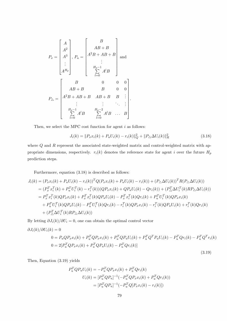
Px =
A
A2
A3
...
AHp
, Pu =
B
AB +B
A2B +AB +B...
Hp−1∑l=0
AlB
and
P4 =
B 0 0 0
AB +B B 0 0
A2B +AB +B AB +B B...
......
. . ....
Hp−1∑l=0
AlBHp−2∑l=0
AlB . . . B
.
Then, we select the MPC cost function for agent i as follows:
Ji(k) = ‖Pxxi(k) + PuUi(k)− ri(k)‖2Q + ‖P4∆Ui(k)‖2R (3.18)
where Q and R represent the associated state-weighted matrix and control-weighted matrix with ap-
propriate dimensions, respectively. ri(k) denotes the reference state for agent i over the future Hp
prediction steps.
Furthermore, equation (3.18) is described as follows:
Ji(k) = (Pxxi(k) + PuUi(k)− ri(k))TQ(Pxxi(k) + PuUi(k)− ri(k)) + (P4∆Ui(k))TR(P4∆Ui(k))
= (P Tx xTi (k) + P Tu U
Ti (k)− rTi (k))(QPxxi(k) +QPuUi(k)−Qri(k)) + (P T4∆UTi (k)RP4∆Ui(k))
= P Tx xTi (k)QPxxi(k) + P Tx x
Ti (k)QPuUi(k)− P Tx xTi (k)Qri(k) + P Tu U
Ti (k)QPxxi(k)
+ P Tu UTi (k)QPuUi(k)− P Tu UTi (k)Qri(k)− rTi (k)QPxxi(k)− rTi (k)QPuUi(k) + rTi (k)Qri(k)
+ (P T4∆UTi (k)RP4∆Ui(k))
By letting ∂Ji(k)/∂Ui = 0, one can obtain the optimal control vector
∂Ji(k)/∂Ui(k) = 0
0 = PuQPxxi(k) + P Tu QPxxi(k) + P Tu QPuUi(k) + P Tu QTPuUi(k)− P Tu Qri(k)− P Tu QT ri(k)
0 = 2[P Tu QPxxi(k) + P Tu QPuUi(k)− P Tu Qri(k)]
(3.19)
Then, Equation (3.19) yields
P Tu QPuUi(k) = −P Tu QPxxi(k) + P Tu Qri(k)
Ui(k) = [P Tu QPu]−1(−P Tu QPxxi(k) + P Tu Qri(k))
= [P Tu QPu]−1(−P Tu Q[Pxxi(k)− ri(k)])
79

Remark 12 It should be notified that the proposed cost function (3.18) is distributed since the refer-
ence state ri(k) only depends on the neighboring agents of agent i at time k.
After the design of the control protocol, one must guarantee that the consensus problem is solved
(i.e. Eq. (3.2)). Equation (3.2) illustrates that a MAS has reached a consensus if for time goes to
infinity, the difference in the state between two agents is zero. It is clear the minimization of the cost
function (3.18) implies that
xi(k + 1) =1
|Ni(k)|+ 1
∑j∈Ni(k)
⋃i
xj(k) (3.20)
In a compact form, Eq. (3.21) is equivalent to
x(k + 1) = D(k)x(k) (3.21)
Due to properties of matrix D, the consensus is achieved.
3.4 Simulation results
The simulation results for all the following subsections (i.e. simple integrator, double integrator) are
done using the switching topology. A multi-agent system with N = 4 followers labeled by 1 − 4 is
considered. Figure 3.1 shows the switching communication topology. One can see that it is switched
and connected. In the following, G(k) periodically switches from G1 to G2 and then to G3 every δ = 0.1
Figure 3.1: Switching communication topologies between agents
seconds. The process then repeats. Note that each graph of the collection G1,G2,G3 has a directed
spanning tree.
3.4.1 First-order integrator MAS
Consider a multi-agent system consisting of N agents with discrete-time single-integrator model
xi(k + 1) = xi(k) + Tui(k) (3.22)
where T ∈ R+ is the sampling period, xi(k) ∈ Rm and ui(k) ∈ Rm are the state and the control input
to be designed for agent i, respectively.
80

Let us define the quadratic optimization problem as (3.18) subject to (3.16). It is clear that
Assumption 10 is satisfied. The initial states of the agents are given as x1(0) = 50, x2(0) = −35,
x3(0) = 60, x4(0) = −200. The parameters are set as Hu = 2 and different values of Hp (i.e.
Hp = 3, 6, 9.
As shown in Figure 3.2, the consensus problem for MAS with dynamics (3.22) is achieve using the
control protocol (3.15). We can see that the state of all agents converge to a consensus point. Figure
3.2.a. shows that the state x converges toward the consensus point.
(a) (b)
(c) (d)
Figure 3.2 illustates the influence of the prediction horizon Hp especially in terms of convergence
time. The higher Hp is, the fast convergence rate for to achieve consensus is. When Hp = 3, the
consensus is achieved at t = 10s and when Hp = 9, the consensus point achieved at t = 6s
81

(e) (f)
Figure 3.2: Evolution of agent state x and control input u for a. Hp = 3, b. Hp = 6 and c. Hp = 9
Comparison Results
Hereafter, we give a comparison between the consensus protocol proposed in this chapter and the one
proposed in [1] (without the use of difference between input, i.e. ∆ui). Using the same switching
topology, let us set the same parameters Hp = 10, Hu = 6, sampling time δ = 0.1s and initial state of
agents between the two schemes. The comparison between our proposed controller with [1] is shown
in the following figures.
(a) (b)
Figure 3.3: Evolution of agent state x and control input u using our proposed DMPC
As seen in Figures 3.3 and 3.4, we can see the influence of the controller parameters. Our proposed
controller is designed using the difference between two consecutive inputs. The controller has integrator
properties to eliminate the steady-state errors. In Figure 3.3, the state of all agents converge to a
82
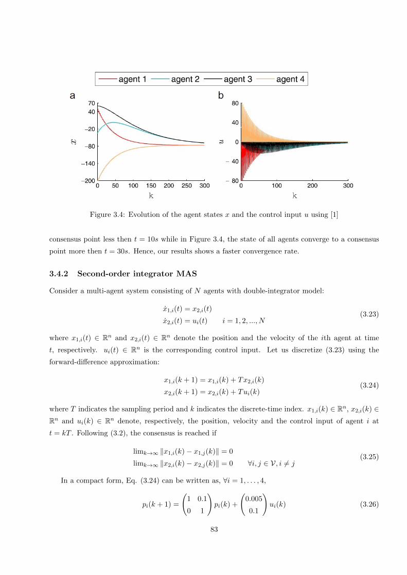
Figure 3.4: Evolution of the agent states x and the control input u using [1]
consensus point less then t = 10s while in Figure 3.4, the state of all agents converge to a consensus
point more then t = 30s. Hence, our results shows a faster convergence rate.
3.4.2 Second-order integrator MAS
Consider a multi-agent system consisting of N agents with double-integrator model:
x1,i(t) = x2,i(t)
x2,i(t) = ui(t) i = 1, 2, ..., N(3.23)
where x1,i(t) ∈ Rn and x2,i(t) ∈ Rn denote the position and the velocity of the ith agent at time
t, respectively. ui(t) ∈ Rn is the corresponding control input. Let us discretize (3.23) using the
forward-difference approximation:
x1,i(k + 1) = x1,i(k) + Tx2,i(k)
x2,i(k + 1) = x2,i(k) + Tui(k)(3.24)
where T indicates the sampling period and k indicates the discrete-time index. x1,i(k) ∈ Rn, x2,i(k) ∈Rn and ui(k) ∈ Rn denote, respectively, the position, velocity and the control input of agent i at
t = kT . Following (3.2), the consensus is reached if
limk→∞ ‖x1,i(k)− x1,j(k)‖ = 0
limk→∞ ‖x2,i(k)− x2,j(k)‖ = 0 ∀i, j ∈ V, i 6= j(3.25)
In a compact form, Eq. (3.24) can be written as, ∀i = 1, . . . , 4,
pi(k + 1) =
(1 0.1
0 1
)pi(k) +
(0.005
0.1
)ui(k) (3.26)
83

The control parameter are selected as Hp = 3, Hp = 6, Hp = 9 and Hu = 2. The initial states of each
agent are given by: x1(0) =
[10
0
], x2(0) =
[0
0
], x3(0) =
[−2
0
], x4(0) =
[6
0
]
The consensus problem described in Equation 3.25 is achieved using the proposed distributed
model predictive control. We can see that the state of all agents converge to a consensus point. Figure
3.5.a (resp Figure 3.5.b) shows the state x1,i (resp. the state x2,i) . it can be seen that the consensus
is achieved with a convergence time which depends on the value of the prediction horizon Hp. When
Hp = 3, the consensus point of agent position x1,i is achieved at t = 40s. When Hp = 6 and Hp = 9,
the consensus point is achieved at t = 25s and t = 15s. The consensus point for agent velocity x2,i,
with Hp = 3, Hp = 6, Hp = 9 is t = 40s, t = 25s and t = 20s.
(a) (b)
(c) (d)
84

(e) (f)
Figure 3.5: Evolution of agent state x1,i and x2,i with a.Hp = 3, b.Hp = 6, c.Hp = 9
The corresponding control input is given in Figure 3.6.
(a) (b)
(c)
Figure 3.6: Evolution of the control input ui
85

3.5 Conclusion
In this chapter, a model predictive control protocol is developed for consensus of MASs with discrete-
time linear dynamics under time-varying directed interaction topologies. The control protocol is
distributed and is designed by combining graph theory with a predictive control algorithm to take
into account the switches on the communication topology. The cost function is design using the
difference between two consecutive inputs. The controller has integrator properties to reduce the
steady-state errors. The convergence time of consensus depends on the prediction horizon parameter.
Some simulation results have been given to show the effectiveness of the proposed controller.
86

Chapter 4
Experimental Setup
4.1 Introduction
For the reader convenience, this chapter briefly introduces the experimental platform Minilab Robot,
available at the Department of Automation and Control, LAMIH (Laboratory of Industrial and Hu-
man Automation Control, Mechanical Engineering and Computer Science), Universite Polytechnique
Hauts-de-France. The platform was used to test and validate the effectiveness of the theoretical re-
sults given in the previous chapters. Figure 4.1 shows the architecture of the experimental platform.
In this process, control algorithms are programmed using ROS (Robotic Operating System) with
Gazebo-ROS as a reality virtual simulation.
Figure 4.1: Multiple Minilab robots with wireless communication architecture.
Experiments were performed on a group of three mobile robots supplied by Enova Robotics to
verify the feasibility and effectiveness of the proposed consensus control strategies. The three robots
consist of one robot which was designated as the leader, and two robots were designated as the
87

followers. Figure 4.2 illustrates the experiments which were carried out in an indoor environment.
Figure 4.2: Illustration of the experimental setup.
Generally, in ROS environment, we can control one robot by one or several machines/ workstations.
Except in the case of using Gazebo simulator, we can perform simulation for several robots by only one
workstation. Instead of using multiple machines/ workstation, in this chapter we demonstrate the idea
of gazebo simulator into real robots to reduce cost and utilisation of several workstations. Since we
are working on consensus problem for multi-agent systems and we are using only one workstation, we
need to appropriately select the wifi configuration and design multiple master ROS in a decentralized
architecture for multiple robots. Furthermore, since there are some difficulties to create the leader-
follower topology in this ROS multi-agent system network, we have to propose an algorithm to solve
this problem.
The remainder of this chapter is organized as follows. Section 4.2 describes the Minilab Enova robot
platform. Section 4.3 introduces the robotic operating system (ROS). In Section 4.4, reality virtual
simulation using Gazebo-ROS examples are provided. MiniLab robots as platform for cooperative
control of multi-agent systems are given in Section 4.5. Section 4.6 concludes this chapter.
4.2 Minilab Enova Robot
The Minilab robot, as shown in Figure 4.3, is a medium-sized two wheels mobile robot designed by
Enova Robotics. The left and right wheels, are controlled independently using two DC motors to
design the linear and angular speed such that robot can move in its environment. The robot can
navigate autonomously or be teleoperated using its camera, which transmits video in real time. Each
MiniLab robot is equipped with an intel X86 main board, an hard drive and also a wide variety of parts
and sensors that are useful for navigation tasks, such as 5 ultrasonic sensors, 5 infra-red (IR) distance
88

sensors which provide the distance from obstacles to the robot, orbbec depth camera, encoders with
a resolution of 16 bits, LED indicators, buttons and arduino microcontroller.
Figure 4.3: Minilab Enova Robot.
MiniLab is optimized for indoor applications, with dimensions of 0.409m x 0.364m x 0.231m in
width x length x height and weight 11.5kg. It also has a load capacity of 3kg. Figure 4.4 shows the
dimensions of Minilab robot.
Figure 4.4: Minilab physical dimensions.
The control architecture of the Minilab robot is an open-source based on the Robot Operating
System (ROS). ROS is a flexible framework for writing robotic software. It includes several contributed
libraries and packages as localization, mapping, planning, perception, etc. Figure 4.5 shows the
hardware features of Minilab robot.
Table 4.1 illustrates some hardware configurations of the Minilab. Some hardware descriptions of the
Minilab Enova robot will be explained in the following subsection.
4.2.1 MiTAC Board Intel X86
The processing on the Minilab is performed by an Intel X86. Intel Atom is the brand name for a line
of ultra-low-voltage x86-64 microprocessors by Intel Corporation. Atom is mainly used in netbooks,
nettops, embedded applications ranging from health care to advanced robotics, and mobile Internet
devices (MIDs). The line was originally designed in 45 nm complementary metal–oxide–semiconductor
(CMOS) technology and subsequent models, codenamed Cedar, used a 32 nm process. Figure 4.6
89

Figure 4.5: Minilab hardware features.
Table 4.1: Parts of the Minilab components
Component Description
Main board Intel X86
Wifi module TL-WR802N 300Mbps Wireless N Nano Router
USB HUB D-Link DGS-105 Gigabit Ethernet Switches
Motors Max speed of the robot is 1.5m/s
Wheels controller Roboteq SDC2130 Controller
Encoders 16 bits resolution
Sensor board Arduino Micro Board
Infrared array 5 SHARP 2Y0A21 F 46 sensors, range from 10 cm to 80 cm
Ultrasound 5 MaxSonar-EZ0 sensors, range from 0 m to 6.45 m, resolution 2.54 cm
ORBBEC depth camera ORBBEC Asrtra pro camera
Batteries 12 Volts/ 10 Ampere-hour, sealed lead/acid battery
depicts the processor board of Intel Atom N2800 1.86GHz Dual-Core 4Gb DDR3-1066MHz Mini ITX
Motherboard.
4.2.2 TL-WR802N 300Mbps Wireless N Nano Router
Each robot equipped with one TL-WR802N wireless router as shown in Figure 4.7 to connect the
Minilab to the network. It allows to design a communication network for multiple robots. This device
performs the functions of a router and also includes functions of wireless access point. It is used to
90

Figure 4.6: Intel Atom N2800.
provide access to Internet or a private computer network. This router has 300Mbps wireless data
rate with several operation modes such as router, repeater, client, access point and hotspot. Powered
through a micro USB port by an external power adapter or USB connection to a computer it provides
flexibility for any situation.
Figure 4.7: TL-WR802N Wireless routers.
4.2.3 D-Link USB HUB
The DUB-H7 as shown in Figure 4.8 is fully compliant to USB 2.0 specifications with data transfer
rates of up to 480 Mbps. It is an ideal solution for transferring data between intel x86 and USB
devices (Orbbec Camera and Roboteq controller). The DUB-H7 features 7 USB fast charging ports
which are designed to feed high currents up to 2.4A when the DUB-H7 is powered by the included
power adapter in fast charging mode or of up to 1.5A via battery charging. Power input for this USB
hub is 5 V / 3A DC.
4.2.4 DC Motor
The maximum speed of the robot is 1.5 m/s in both forward and backward movement but for safety
reason maximum allowed speed is 0.8 m/s. The maximum slope angle is 10o. Each wheel has a driving
DC motor mounted on his axis. The wheels have been chosen to provide more accurate odometry
91

Figure 4.8: DUB-H7 7-Port USB 2.0 HUB.
localization. The DC motor, shown in Figure 4.9, is brushed moter with permanent magnet. Input
voltage for the motor is 12 V and torque 0.07 Nm. Rotational speed of motor is 3,000 rpm.
Figure 4.9: Buhler Motor DC.
4.2.5 Roboteq Controller
Fitting into a very compact 73x73mm enclosure, Roboteq’s SDC2130 controller is designed to convert
commands received from an RC radio, Analog Joystick, wireless modem, PC (via RS232 or USB) or
microcomputer into high voltage and high current output for driving one or two DC motors. A CAN
bus interface allows up to 127 controllers to communicate at up to 1Mbit/s on a single twisted pair.
Figure 4.10 illustrates the Roboteq controller.
Figure 4.10: Roboteq SDC2130 controller.
The controller features a high-performance 32-bit microcomputer and quadrature encoder inputs
to perform advanced motion control algorithms in open loop or closed loop (speed or position). The
SDC21xx features several analog, pulse and digital I/Os which can be remapped as command or
feedback inputs, limit switches, or many other functions. For mobile robotic applications, the controller
two motor channels can either be operated independently or mixed to set the direction and rotation
of a vehicle by coordinating the motion of each motor.
92

4.2.6 Arduino Micro Board
The Arduino Micro board, illustrated in Figure 4.11, is a microcontroller board based on the AT-
mega32u4, developed in conjunction with Adafruit. It has 20 digital input/output pins (of which 7
can be used as PWM outputs and 12 as analog inputs), a 16 MHz crystal oscillator, a micro USB
connection, an ICSP header, and a reset button. It contains everything needed to support the micro-
controller. Micro USB cable is used to connect Arduino board with computer. It has a form factor
that enables it to be easily placed on a breadboard.
The Micro has built-in USB communication, eliminating the need for a secondary processor. This
allows the Micro to appear to a connected computer as a mouse and keyboard, in addition to a virtual
(CDC) serial / COM port. It also has other implications for the behavior of the board.
Figure 4.11: Arduino Micro Board.
4.2.7 Infrared SHARP 2Y0A21
Infrared SHARP as shown in Figure 4.12 is a distance measuring sensor unit, composed of an integrated
combination of PSD (position densitive detector), IRED (infrared emitting diode) and signal processing
circuit. This device outputs the voltage corresponding to the detection distance between 10 to 80 cm.
So this sensor can also be used as a proximity sensor.
Figure 4.12: Infrared sensor SHARP.
4.2.8 Orbbec Astra Pro Camera
Orbbec Astra Pro is optimized for applications that require high RGB stream quality. Astra Pro is
world first 3D sensor that can stream 30 FPS HD RGB stream and VGA depth at the same time
through USB 2.0. Astra Pro now comes in a bundle with the powerful gestural Interaction SDK
by Gestoos. Gestoos interact using C++, Java and Processing to develop and enhance applications.
Figure 4.13 illustrates the camera.
93

Figure 4.13: Orbbec Astra Pro Camera.
4.2.9 Power-Sonic Battery
The Minilab use 12V rechargeable batteries for all its system, as shown in Figure 4.14, with 4 hours
of autonomy. Power-Sonic battery are lead-lead dioxide systems. The dilute sulphuric acid electrolyte
is suspended and thus immobilised. Otherwise, the battery is completely sealed and is, therefore,
maintenance-free and leak proof.
Figure 4.14: Power-Sonic Battery
4.3 Robotic Operating System
Robot Operating System (ROS) is an open-source platform, meta-operating system that is widely
used in robotics. The philosophy is to make a piece of software that could work in other robots by
making little changes in the code. What we get with this idea is to create functionalities that can be
shared and used in other robots without much effort so that we do not reinvent the wheel. It provides
libraries and tools to help software developers create robot applications. Primary goal of ROS is to
support code reuse in robotics research and development. ROS framework is easy to implement in
any modern programming language such as Python, C++, and Lisp (experimental libraries in Java
and Lua).
ROS was originally developed in 2007 by the Stanford Artificial Intelligence Laboratory (SAIL)
with the support of the Stanford AI Robot project. As of 2008, development continues primarily at
Willow Garage, a robotics research institute, with more than 20 institutions collaborating within a
federated development model. A lot of research institutions have started to develop projects in ROS
by adding hardware and sharing their code samples. Also, the companies have started to adapt their
94

products to be used in ROS.
The sensors and actuators used in robotics have also been adapted to be used with ROS. Every day
an increasing number of devices are supported by this framework. ROS provides standard operating
system facilities such as hardware abstraction, low-level device control, implementation of commonly
used functionalities, message passing between processes, and package management. It is based on
graph architecture with a centralized topology where processing takes place in nodes that may receive
or post, such as multiplex sensor, control, state, planning, actuator, and so on. ROS currently only
runs on Unix-based platforms. Software for ROS is primarily tested on Ubuntu and Mac OS X sys-
tems. While a port to Microsoft Windows for ROS is possible, it has not yet been fully explored.
The ROS architecture has been designed and divided into three sections or levels of concepts:
• File system level
• Computation Graph level
• Community level
More detailed for ROS architecture explanations will be given in the following subsection.
4.3.1 ROS File System Level
The first level is the Filesystem level. In this level, a group of concepts are used to explain how
ROS is internally formed, the folder structure, and the minimum number of files that it needs to work.
Figure 4.15 illustrated level in ROS Filesystem.
Figure 4.15: ROS File System Level.
95

Package
Packages are the software organization unit of ROS code. Each package can contain ROS runtime
processes (nodes), a ROS-dependent library, datasets, configuration files, or anything else that is
usefully organized together. ROS uses packages to organize its programs. A package can be describe
as all the files that a specific ROS program contains; all its cpp files, python files, configuration files,
compilation files, launch files, and parameters files.
Catkin is the official build system of ROS and the successor to the original ROS build system,
rosbuild. Catkin combines CMake macros and Python scripts to provide some functionality on top
of CMake’s normal workflow. Catkin was designed to be more conventional than rosbuild, allowing
for better distribution of packages, better cross-compiling support, and better portability. Catkin’s
workflow is very similar to CMake’s but adds support for automatic ’find package’ infrastructure and
building multiple, dependent projects at the same time.
All those files in the package are organized with the following structure:
launch folder Contain launch files
src folder Source files (cpp, phyton)
CMakelist.txt file List of cmake rules for compilation
package.xml file Package information and dependencies
Meta-Package
This is a collection of packages forming a higher level library (previously called stacks). The concept
of stacks was removed with catkin command to simplify the growing code base and to support better
distribution of packages.
Manifests
Manifests (manifest.xml) provide metadata about a package, including its license information and
dependencies, as well as language-specific information such as compiler flags.
Stacks
Stacks are collections of packages that provide aggregate functionality, such as a ”navigation stack”.
Stacks are also how ROS software is released and have associated version numbers.
Stack Manifests
Stack manifests (stack.xml) provide data about a stack, including its license information and its
dependencies on other stacks.
96

Message (msg) types
Message descriptions are stored in a package msg MyMessageType.msg. It defines the data structures
for messages sent in ROS.
Service (srv) types
Service descriptions are stored in a package srv MyServiceType.srv. It defines the request and response
data structures for services in ROS.
4.3.2 ROS Computation Graph Level
The second level is the Computation Graph level where communication between processes and
systems happens. In this subsection, we will see all the concepts and mechanisms that ROS has to set
up systems, handle all the processes, and communicate with more than a single computer, and so on.
Figure 4.16: ROS Computation Graph Level.
Figure 4.16 show contents of computation graph level. The illustration on how computation graph
work can be shown in Figure 4.17. More detail information about computation graph will be given in
the following explanations.
Figure 4.17: ROS Computation Graph Level.
97

Node
A node is a participant in the ROS graph. ROS nodes use a ROS client library to communicate with
other nodes. Nodes can publish or subscribe to a topic using typed messages. Nodes can also provide
or use a Service. Services means request / response paradigm (think of method or operation) via typed
messages. There are configurable parameters associated with a node. Connections between nodes are
established through a distributed discovery process. Nodes may be located in the same process, in
different processes, or in different machines. Nodes are processes which perform specific computations,
for example: control robot wheel motors, acquire data from laser scanner, acquire images from camera,
perform localisation, perform path planning, provide graphical visualisation of the system
Master
The ROS Master provides name registration and lookup to the rest of the Computation Graph.
Without the Master, nodes would not be able to find each other, exchange messages, or invoke services.
Master is the core node of ROS, called roscore. Roscore is a collection of nodes and programs that
are pre-requisites of a ROS-based system. We must have a roscore running in order for ROS nodes to
communicate. It is launched using the roscore command in the terminal.
Messages
Nodes communicate with each other by passing messages. A message is simply a data structure,
comprising typed fields. Standard primitive types (integer, floating point, boolean, etc.) are supported,
and arrays of primitive types. Messages can include arbitrarily nested structures and arrays (much
like C structs).
Topic
Messages are routed via a transport system with publish / subscribe semantics. A node sends out a
message by publishing it to a given topic. The topic is a name that is used to identify the content
of the message. A node that is interested in a certain kind of data will subscribe to the appropriate
topic. There may be multiple concurrent publishers and subscribers for a single topic, and a single
node may publish and/or subscribe to multiple topics. In general, publishers and subscribers are
not aware of each others’ existence. The idea is to decouple the production of information from its
consumption. Logically, one can think of a topic as a strongly typed message bus. Each bus has a
name, and anyone can connect to the bus to send or receive messages as long as they are the right type.
98
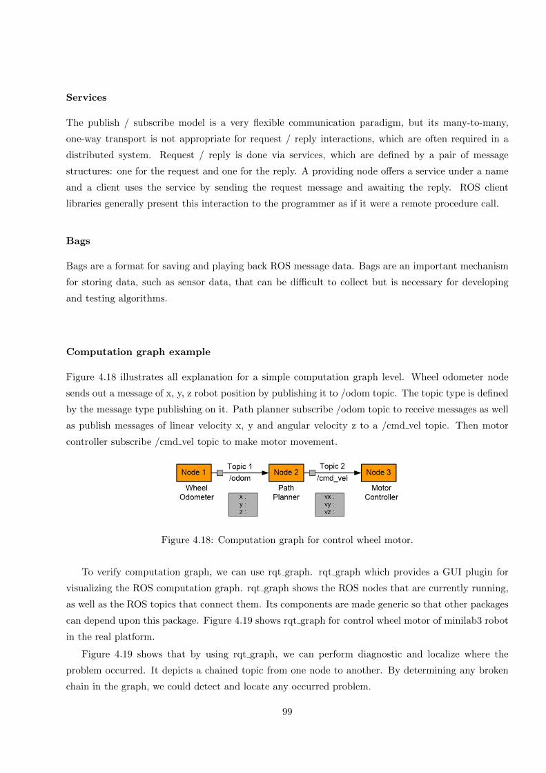
Services
The publish / subscribe model is a very flexible communication paradigm, but its many-to-many,
one-way transport is not appropriate for request / reply interactions, which are often required in a
distributed system. Request / reply is done via services, which are defined by a pair of message
structures: one for the request and one for the reply. A providing node offers a service under a name
and a client uses the service by sending the request message and awaiting the reply. ROS client
libraries generally present this interaction to the programmer as if it were a remote procedure call.
Bags
Bags are a format for saving and playing back ROS message data. Bags are an important mechanism
for storing data, such as sensor data, that can be difficult to collect but is necessary for developing
and testing algorithms.
Computation graph example
Figure 4.18 illustrates all explanation for a simple computation graph level. Wheel odometer node
sends out a message of x, y, z robot position by publishing it to /odom topic. The topic type is defined
by the message type publishing on it. Path planner subscribe /odom topic to receive messages as well
as publish messages of linear velocity x, y and angular velocity z to a /cmd vel topic. Then motor
controller subscribe /cmd vel topic to make motor movement.
Figure 4.18: Computation graph for control wheel motor.
To verify computation graph, we can use rqt graph. rqt graph which provides a GUI plugin for
visualizing the ROS computation graph. rqt graph shows the ROS nodes that are currently running,
as well as the ROS topics that connect them. Its components are made generic so that other packages
can depend upon this package. Figure 4.19 shows rqt graph for control wheel motor of minilab3 robot
in the real platform.
Figure 4.19 shows that by using rqt graph, we can perform diagnostic and localize where the
problem occurred. It depicts a chained topic from one node to another. By determining any broken
chain in the graph, we could detect and locate any occurred problem.
99

Figure 4.19: rqt graph for control wheel motors.
4.3.3 Community level
The third level is the Community level, which comprises a set of tools and concepts to share
knowledge, algorithms, and code between developers. This level is of great importance. As with most
open source software projects, having a strong community not only improves the ability of newcomers
to understand the intricacies of the software as well as solve the most common issues, it is also the
main force driving its growth.
4.3.4 ROS General Communication
In general, Minilab robot has its own ROS network (either wired, wireless or a combination of both),
where a single roscore manages all the communications between all the ROS nodes, either in a single
computer or multiple computers in the same network (depending on the complexity and computational
needs of the system). Figure 4.20 shows a generic hardware setup/ configuration as explained above.
Figure 4.20: MiniLab robot setup for a single ROS system.
Communication among the mobile robots plays an important role in the successful coordination
of a multi-agent system. Minilab provides the ad-hoc peer-to-peer wireless TCP/IP protocol for
multi-vehicle information interactions. Each robots is configured with a predefined unique IP address.
When the power of the Minilab is turned on, the Host PC can detect a network called ML201704001-3
100

(robot1, 2, 3), as shown in Figure 4.21(a) for Minilab1. The IP address of the Host PC is set as shown
in Figure 4.21(b).
(a) (b)
Figure 4.21: Wireless network setup on the host PC.
The connection between robots and the host PC can be checked by the command address of the
Minilab in the terminal run box. Figure 4.22 shows an example of successful connection.
Figure 4.22: Communication checking results.
To download the compiled file into the Minilab, IP addresses of the targets are specified as linux-
verdex targets and the default model URI is replaced by the IP address of the target vehicles, i.e.,
tcpip://182.168.0.101 for Minilab1.
4.4 Gazebo-ROS Simulation
Gazebo-ROS is a robot simulator that allows to accurately design, simulate and test robots in various
environments. It uses the URDF file format, which is an XML format used to describe objects and
101

environments in robot simulators and was originally developed specifically for Gazebo. Below we
quickly go through some of the XML tags that are important to understand and show what kind of
environments we use.
With Gazebo we are able to create a 3D scenario on our computer with robots, obstacles and
many other objects. Gazebo also uses a physical engine for illumination, gravity, inertia, etc. We can
evaluate and test our robot in difficult or dangerous scenarios without any harm to our robot. Most
of the time it is faster to run a simulator instead of starting the whole scenario on our real robot.
Originally Gazebo was designed to evaluate algorithms for robots. For many applications it is
essential to do some tests, like error handling, battery life, localization, navigation and grasping.
Gazebo was developed and improved as well as significant requirement on multi-robot simulation.
Gazebo provides a set of ROS APIs that allows users to modify and get information about various
aspects of the simulated world. The complete list of ROS messages and services for gazebo can be
found here also.
The simulation world and minilab objects can be created for only one robot and multiple ones.
Figure 4.23(a) shows visualisation of Gazebo-ROS simulation for one minilab robot and Figure 4.3 (b)
shows visualisation of Gazebo-ROS simulation for multiple-minilab robots.
(a)
(b)
Figure 4.23: Gazebo-ROS simulation for minilab robot.
We verify the computation graph for Gazebo-ROS using rqt graph. Figure 4.24 shows the rqt graph
for controlling minilab3 robot in the Gazebo-ROS simulation. From Figure 4.24, we can verify that
all nodes are connected in the network as required. For example, this figure shows that node minilab3
102

Figure 4.24: rqt graph for minilab in Gazebo-ROS
with topic odom and cmd vel are connected and provide data to node recorder. Node controller
move pub Leader and node gazebo are connected and in two way communication to node minilab3.
On the other hand, if there is any broken chained link, using this graph, we can detect and locate the
problem.
4.5 MiniLab as Platform for Cooperative Control of Multi-Agent
Systems
In this section, we will present the procedure for the implementation of the wireless configuration
among robots described in Figure 4.25 and the decentralized communication architecture described in
Figure 4.29. First, we need to configure address reservation and verify the reservation from the PC
workstation. To have a proper configuration of the network, we need to modify the /etc/hosts file for
each robot and PC. Afterward we can start multimaster fkie package for our topology. Then, we
can implement our cooperative control protocol on this ROS network configuration.
4.5.1 Multi-Robots Wireless Configuration
Let we consider Figure 4.25. This is an example of possible hardware configuration for a wireless
decentralized communication architecture between multiple robots. Note that in Figure 4.25, the
multi-agent system consists of master and two slaves which are connected to the master wireless
network and one monitoring workstation which is also connected to the master.
Router Address Reservation
We need to specify a dedicated IP address for all robots and workstation in the ROS Network, such
that all robots and workstation will always receive the same IP address each time when it connects
103

Figure 4.25: Network topology for the illustrative example.
to the DHCP (Dynamic Host Configuration Protocol Server) server. Since each MiniLab Enova robot
requires a permanent IP address, we need to configure the address reservation of the router.
First, we open the web browser and in the address bar, we type in: http://192.168.0.254. Then,
we type the username and password in the login page. Then, we should click on DHCP−>Address
Reservation on the left side and click Add New button. The MAC and IP address should be given
and the status should be selected as enabled. This configuration is shown in Figure 4.26.
Note that the MAC address is the MAC address of the device where we want to reserve the
IP address. For our case, we need to know the MAC address of each router in the robot and PC
workstation. The IP address of the robots are reserved with 192.168.0.2xx and for the workstation
192.168.0.11x
Master-slave wireless configuration
To verify the reservation of the IP address for the PC workstation, we have just to connect to the wifi
of the leader. Then, we can check from connection information of the PC workstation as shown in
Figure 4.21(b).
Host name and IP address binding
For each robot and workstation, it is necessary to modify the /etc/hosts file using text editor. Figure
4.27 shows the contents of this file for the workstation for the example presented in Figure 4.25. Figure
104

Figure 4.26: TP-Link address reservation.
4.28 shows the contents of this file for each robot for the example presented in Figure 4.1.
Figure 4.27: Contents of the /etc/hosts file for the workstation for the example presented in Fig. 4.1.
Figure 4.28: Contents of the /etc/hosts file for each robot for the example presented in Fig. 4.1.
To verify the appropriate configuration of the network, before launching any ROS nodes, it is
interesting to ping all other robots from the workstation, using both the host name and the IP
address. If all the pings return a reply, the network has been properly configured. Using the current
console, the following command should be executed, where hostname or IP address must be the IP
address or host name of each robot and the workstation.:
$export ROS MASTER URI=http://<host ip>:11311
$ROS MASTER URI command is required to inform the nodes where they able to locate the master.
For all robots and the workstation, we have to verify if the multicast feature (group communication)
is temporary enabled using the following command:
105

$sudo sh -c "echo 0 /proc/sys/net/ipv4/icmp echo ignore broadcasts"
If this command returns 0, the multicast feature is enabled. However, when all robots and work-
station restart, this configuration will be lost. Now, the ROS wireless network for multiple robots
has been configured. The next step is to discover and synchronize each robot and the workstation to
obtain a decentralized communication architecture.
4.5.2 Decentralized communication architecture
In multi-agent systems, multiple robots need to exchange information. Using ROS, there is two
possible solutions which can create a single large ROS network managed by a single roscore node or
create a configuration to allow information to be exchanged between ROS sub-systems.
Figure 4.29: MiniLab robot runs its own master managing local communication.
Figure 4.29 illustrates the configuration of 3 robots to allow information to be exchanged between
ROS sub-systems. With this distributed approach, every robot executes its own master. Local inter-
process communication is handled by the local master while global communication between robots is
handled by a special communication package. Robots may communicate directly forming an ad hoc
wireless network and do not rely on a central controller.
Multimaster fkie
ROS multi-master system is built from two or more ROS networks, each one with its own roscore
node. For this purpose, we need a package called multimaster fkie [?]. This package can be easily
installed as shown below:
$sudo apt-get install ros-indigo-multimaster-fkie
This package offers a set of nodes to establish and manage a multi-master network. This requires no
106

or minimal configuration. The changes are automatically detected and synchronized. The multimas-
ter fkie allows two substantial nodes: the master discovery and the master sync nodes to run
simultaneously. The main features of master discovery is to send multicast messages periodically
to the ROS network to make the other roscore environments aware of its presence. It also detects
the changes in the local network and informs all roscore about these changes. The other nodes called
master sync enable us to select which hosts, topics and services which should be synchronized or
ignored between different roscore. It also helps to register and update information of topics and
services to the local roscore.
Figure 4.30 presents an illustration of ROS multi-master system. For our experimental setup, we
have four master ROS (workstation, Minilab 1, Minilab 2 and Minilab 3). Each ROS Master will be
detected and discovered by any other master in the network.
Figure 4.30: Multimaster fkie for multiple-minilab robots.
Multi-master Configuration
Now, we can launch the multimaster fkie nodes and take a first look at how it works. First of all,
it is needed to launch a local roscore on each computer, i.e.
$roscore
Then, the master discovery node should be launched in each computer, passing as an argument
the mcast group parameter to specify the multicast address to be used, i.e.
$rosrun master discovery fkie master discovery mcast group:=224.0.0.1
Afterwards, the master sync node should be launched in each computer. Without any additional
parameter, all topics and services on all computers will be synchronized with all others, i.e.
$rosrun master sync fkie master sync
107

When both nodes are running on all robots and workstation, the following command will list all
the available ROS masters on the common network:
$rosservice call /master discovery/list masters
Figure 4.31 shows the information reported by this command for the example presented in Figure 4.1.
Figure 4.31: rosservice call command result.
4.5.3 Leader-Follower Node Communication
This subsection deals with node communication in terms of multi-robot configuration. “Node” is the
ROS term for an executable that is connected to the ROS network. Here, we define a publisher node
which will continually broadcast a message and a subscriber node which will continually receive a
message.
Figure 4.32: Communication topology.
Both publisher and subscriber nodes are configured according to the communication topology. For
example, in our case as shown in Figure 4.32, we will define the leader “minilab 3” as a publisher
of his position and velocity to follower “minilab 1”. Furthermore, the follower “minilab 1” is also
configured as a subscriber of the leader “minilab 3”. At the same time, follower “minilab 1” also sets
as a publisher to follower “minilab 2” and follower “minilab 2” is configured as a subscriber of follower
“minilab 1”.
The example code of publisher and subscriber are shown below. The first one is the leader’s code
and the second one is the follower’s code.
108
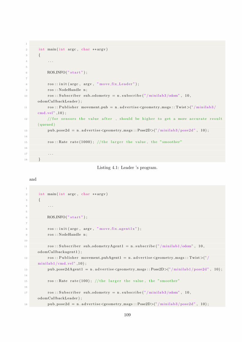
1
2 i n t main ( i n t argc , char ∗∗ argv )3 4 . . .
5
6 ROS INFO(” s t a r t ” ) ;
7
8 ro s : : i n i t ( argc , argv , ”move f ix Leader ” ) ;
9 ro s : : NodeHandle n ;
10 ro s : : Subsc r ibe r sub odometry = n . sub s c r i b e ( ”/mini lab3 /odom” , 10 ,
odomCallbackLeader ) ;
11 ro s : : Pub l i sher movement pub = n . adve r t i s e<geometry msgs : : Twist>(”/mini lab3 /
cmd vel ” ,10) ;
12 // f o r s en so r s the value a f t e r , should be h igher to get a more accurate r e s u l t
( queued )
13 pub pose2d = n . adve r t i s e<geometry msgs : : Pose2D>(”/mini lab3 /pose2d” , 10) ;
14
15 ro s : : Rate ra t e (1000) ; // the l a r g e r the value , the ” smoother”
16
17 . . .
18
Listing 4.1: Leader ’s program.
and
1
2 i n t main ( i n t argc , char ∗∗ argv )3 4 . . .
5
6 ROS INFO(” s t a r t ” ) ;
7
8 ro s : : i n i t ( argc , argv , ”move f ix agent1x ” ) ;
9 ro s : : NodeHandle n ;
10
11 ro s : : Subsc r ibe r sub odometryAgent1 = n . sub s c r i b e ( ”/mini lab1 /odom” , 10 ,
odomCallbackagent1 ) ;
12 ro s : : Pub l i sher movement pubAgent1 = n . adve r t i s e<geometry msgs : : Twist>(”/
mini lab1 / cmd vel ” ,10) ;
13 pub pose2dAgent1 = n . adve r t i s e<geometry msgs : : Pose2D>(”/mini lab1 /pose2d” , 10) ;
14
15 ro s : : Rate ra t e (100) ; // the l a r g e r the value , the ” smoother”
16
17 ro s : : Subsc r ibe r sub odometry = n . sub s c r i b e ( ”/mini lab3 /odom” , 10 ,
odomCallbackLeader ) ;
18 pub pose2d = n . adve r t i s e<geometry msgs : : Pose2D>(”/mini lab3 /pose2d” , 10) ;
109

19
20 . . .
21
Listing 4.2: Follower ’s program.
NodeHandle is the main access point to communications with the ROS system. The first con-
structed NodeHandle will fully initialize this node, and the last destructed NodeHandle will close
down the node.
The advertise() function is how we tell ROS that we want to publish on a given topic name.
This invokes a call to the ROS master node, which keeps a registry of who is publishing and who is
subscribing. After this advertise() call is made, the master node will notify anyone who is trying to
subscribe to this topic name, and they will in turn negotiate a peer-to-peer connection with this node.
advertise() returns a Publisher object which allows us to publish messages on that topic through a
call to publish(). Once all copies of the returned Publisher object are destroyed, the topic will be
automatically unadvertised. The second parameter to advertise() is the size of the message queue
used for publishing messages. If messages are published more quickly than we can send them, the
number here specifies how many messages to buffer up before throwing some away.
4.6 Conclusion
The multi-agent system framework was presented using Robot Operating System (ROS). Due to the
requirements of the proposed consensus algorithms, we first introduce the robot hardware specifica-
tions, communication network configuration and minimum amount of workstation we can use for the
coordination of multi-robots using ROS and multi Minilab robots.
Using a wireless master-slave scheme, it is possible that multiple robots communicate through a
wireless network with only one workstation for monitoring and control. This configuration is a low
cost configuration. For decentralized architectures, multimaster fkie is a solution to the multi-
master ROS problem. Node calling algorithm has allowed to create leader-follower topology in this
ROS multi-agent system network. This algorithm has used a publisher and a subscriber to broadcast
and/or receive messages continually from each other.
In next chapter, a group of Minilab are used to test the decentralized leader-follower consensus
algorithms.
110

Chapter 5
Experimental results on Consensus for
a Group of Minilab Robots
5.1 Introduction
In this chapter, using our experimental setup described in the previous chapter, we apply the schemes
designed in Chapter 2 for two applications, e.g. fixed-time trajectory tracking and leader-follower
consensus. First, we study the fixed-time trajectory tracking control algorithms for one agent with
single-integrator dynamics. Then, we analyze the results for the leader-follower consensus algorithms.
The same is done for double-integrator dynamics. At last, since nonholonomic dynamics can better
describe the motion of mobile robots in a real world, we implement the proposed scheme to achieve
fixed-time consensus tracking for a multi-agent system with unicycle-type dynamics.
The fixed-time methodology used in this chapter guarantees that a settling time bound can be
prescribed without depending on the initial states of the agents. More specifically, for the consen-
sus problem, a distributed protocol based on fixed-time stability techniques is implemented for each
follower to accomplish the consensus tracking in a desired time. We provide experiment to demon-
strate the effectiveness of the proposed controllers for fixed-time trajectory tracking and consensus.
Using Gazebo ROS simulation and Minilab Enova robotic platform, the experimental results show the
effectiveness and robustness of the proposed algorithms.
The experiments for all the following subsections (i.e. simple integrator, double integrator, chained-
form dynamics) are done using the same fixed topologies. Figure 5.1 shows the communication topol-
ogy for the leader-follower MAS scenario in ROS-Gazebo. A MAS with N = 6 followers labeled by
1− 6 and one leader labeled by 0 is considered. One can see that the communication topology is fixed
and connected. It is characterized by the following Laplacian L and the matrix B which describes
111

links between the leader and the followers given as follows
L =
2 −1 −1 0 0 0
−1 1 0 0 0 0
−1 0 2 −1 0 0
0 0 −1 1 0 0
0 0 0 0 1 −1
0 0 0 0 −1 1
, B =
1 0 0 0 0 0
0 0 0 0 0 0
0 0 0 0 0 0
0 0 0 0 0 0
0 0 0 0 1 0
0 0 0 0 0 0
From matrix B, it is clear that agents 2, 3, 4 and 6 do not have direct link with agent 0. Assumption
1 is satisfied.
For the implementation using the available multiple minilab robots, since we have only three
robots, the topology, shown in Figure 5.2 corresponds to node 0 as leader, 1− 2 as followers.
Figure 5.1: Topology of MAS using ROS for six agents.
Figure 5.2: Topology of MAS using using our Minilab Enova robot platform.
The remainder of the chapter is organized as follows. Section 5.2 considers the fixed-time trajectory
tracking and leader-follower consensus problems for agents with single-integrator dynamics. The same
problems are studied for double-integrator dynamics in Section 5.3. In Section 5.4, experimental
112

results are provided to verify the effectiveness of the proposed methods for nonholonomic systems.
Section 5.5 concludes this chapter.
5.2 Fixed-Time tracking for agents with Single-Integrator dynamics
In this section, we show some experimental results using Gazebo-ROS and Minilab robot platform for
tracking and consensus with Single-Integrator Dynamics to verify the theoretical analysis.
5.2.1 Fixed-Time trajectory Tracking for Single-Integrator Dynamics
For the trajectory tracking application, the Minilab robots are modeled as a single-integrator system:
x(t) = u(t) (5.1)
where x ∈ R (resp. u ∈ R) is the state (resp. control input) of the single-integrator system. In this
experiment, the state can be described as the robot position x(t) and the control input u(t) as the
linear velocity of the robot.
The dynamics of the desired trajectory is generated using the following system:
xd(t) = ud(t) (5.2)
where xd ∈ R (resp. ud ∈ R) is the state (resp. control input) of the desired trajectory. The control
objective is that system (5.1) follows the desired trajectory (5.2) in a fixed-time.
As described in Chapter 2, the fixed-time tracking problem is solved using the following controller:
u = −(α+ a)bee2 − β sign (e) (5.3)
where e = x− xd, α, β and a are positive constants. The settling time is explicitly defined as
T =π√αβ
(5.4)
The corresponding algorithm is given in Algorithm 1. At each sampling time instant tk, we
calculate the desired position and determine the error position between the desired trajectory and
the actual robot position. After calculating the controller u, we implement the corresponding linear
velocity input of the robot.
Step Linear Velocity Input for the desired trajectory
The control parameters are selected as: α = β = 0.5 for protocol (5.3). The initial state of the robot
is x = −2. Based on the control parameters, the settling time is T = 6.28s. The desired trajectory is
generated by (5.2) with xd(0) = 0, ud(t) = 0.2. Since a ≥ d+ ud, we set a = 1. The control objective
is that system (5.1) tracks the desired trajectory xd.
113

Algorithm 1 Fixed-time Tracking controller for Single Integrator dynamics
Input: xd(tk), x(tk)
Parameters: α, β, a
Output: v(t), tk ≤ t < tk+1
1: if t = tk then
2: Compute e(tk) = x(tk)− xd(tk)3: Compute u = −(α+ a)bee2 − β sign (e)
4: Implement the linear velocity v(t)
5: end if
x(tk) is the x position of the Minilab robot at instant tk, xd(tk) is the x desired position at instant tk
Using Theorem 1, the tracking controller (5.3) guarantees the stabilization of the tracking errors
to the origin in a finite-time bounded by T = 6.28s. Figure 5.3.a. shows that the actual state
trajectory x accurately tracks the desired state xd before T in spite of the presence of disturbances
and uncertainties inherent to the experimental setup. Hence, the origin of the closed-loop system is
globally finite-time stable. Furthermore, since T does not depend on the initial states, the proposed
protocol is a fixed-time controller.
(a) (b)
Figure 5.3: Experimental results for Algorithm 1: Time response of actual state trajectory x and
desired state trajectory xd with constant linear desired velocity.
The tracking errors are depicted in Figure 5.3. One can see that the tracking errors between
the actual trajectory and the desired trajectory converge to zero at T = 3.5s. Using the proposed
controller, the tracking controller is achieved in a prescribed time before T = 6.28s. The control inputs
for linear x velocity are shown in Figure 5.3.b. One can note that the magnitude of control inputs
may be large during the transients to achieve a fast convergence of the sliding surface e. The control
114

parameters should be adjusted to obtain a good compromise between magnitude of the control input
and the settling time.
Sinusoidal Linear Velocity Input for the desired trajectory
The control parameters are selected as: α = β = 1 and a = 1 for protocol (5.3). The initial state of
the robot is x = −1.5. Based on the control parameters, the settling time is T = 3.14s. The desired
trajectory is generated by (5.2) with xd(0) = 0, ud(t) = 0.2sin(2πt). The control objective is that
system (5.1) tracks the desired trajectory xd.
Figure 5.4 shows that the tracking controller (5.3) guarantees the stabilization of the tracking
errors to the origin in a finite-time bounded by T = 3.14s. From Figure 5.4.b., one can see that the
actual state trajectory x accurately tracks the desired state xd before 2.5s.
(a) (b)
(c)
Figure 5.4: Experimental results for Algorithm 1: Time response of actual state trajectory x and
desired state trajectory xd with sinusoidal linear desired velocity.
115

5.2.2 Fixed-Time Consensus for MAS with Single-Integrator Dynamics
For the consensus tracking application, the Minilab robots are modeled as system (5.1). The dynamics
of the leader is generated by (5.2). The control objective is that system (5.1) follows the leader (5.2) in
a fixed-time using only local exchanged information. The communication topology is given by Figure
5.1.
The initial position of the robots is given by the following vector x(0) = [3, 2, 1,−1,−2,−3]T .
Recall that To is time needed for an agent to estimate the leader state (prescribed time observation).
It should be noted that the estimation in (2.10) depends on the gains of observer. The settling time
is explicitly defined as T = To + π√αβ
.
The corresponding fixed-time algorithm for MAS with single integrator dynamics is given in Al-
gorithm 2. At each sampling time instant tk, based on local exchanged information, each agent i
estimates the leader position xi and compute the tracking error between the leader, itself and neigh-
boring agents. After calculating the controller u, we implement the corresponding linear velocity input
of the robot.
Algorithm 2 Fixed-time consensus for MAS with Single Integrator dynamics
For each agent i,
Input: x0(tk) (if bi = 1), xi(tk), xj(tk) (for all j such that aij 6= 0)
Parameters: ρ, σ, α, β, ai
Output: vi(t), tk ≤ t < tk+1
1: if t = tk then
2: When t < To, vi(t) = 0
3: Agent i samples its current states xi(t), its estimate of the leader xi(t) and broadcasts it to its
neighbors
4: Compute the estimation error xi = xi − x0
5: Update the distributed observer (2.7) (convergence in time To)
6: When t ≥ To, compute the tracking error ei = xi − xi7: Compute u = −(α+ ai)beie2 − β sign (ei)
8: Implement the linear velocity
9: end if
xi(tk) is the x position of Minilab robot i at instant tk, x0(tk) is x leader position at instant tk
The performances of the proposed observer-based leader-follower consensus controller for single
integrator MAS are studied through the following experimental results.
116

Step Linear Velocity Input for the leader trajectory
The control parameters are selected as: α = β = 1 for protocol (2.17). The initial state of the robots is
x(0) = [3, 2, 1,−1,−2,−3]T . The desired trajectory of the leader is generated by (2.5) with x0(0) = 0,
u0(t) = 0.2. Since ai ≥ di + u0, we set ai = 1. The control objective is that each system (2.6) tracks
the leader x0 using only local information.
Using Theorem 1, the distributed observer (2.7) guarantees the stabilization of the estimation
errors (2.8) to the origin in a finite-time bounded by To = 5s. The distributed observers accurately
reconstruct the leader state for each agent before To. Using Theorem 2, the tracking controller
guarantees the stabilization of the tracking errors to the origin in a finite-time bounded by T = 15s.
Figure 5.5.a. shows that the actual state trajectory x accurately tracks the leader state x0 before T
in spite of the presence of disturbances and uncertainties inherent to the experimental setup. One can
conclude that using the proposed controller, the leader-follower consensus is achieved in a prescribed
time. The control inputs for each agent are shown in Figure 5.5.b. One can note that the magnitude
of control inputs may be large during the transients to achieve a fast convergence of the sliding
surface given by the different steps of the consensus protocol. Hence, the control parameters should
be adjusted to obtain a good compromise between magnitude of the control input and the settling
time. The origin of the closed-loop system is globally finite-time stable contrary to existing controllers
which only provide semi-global finite-time stability property. Furthermore, since T does not depend
on the initial states of agents, the proposed protocol is distributed.
(a) (b)
Figure 5.5: Experimental results for Algorithm 2: Time response of the actual state trajectory of the
followers and of the leader with a step linear leader trajectory.
117

Sinusoidal Linear Velocity Input for the leader trajectory
The control parameters are selected as: α = β = 1.5, ai = 1, ε = 0.52 for protocol (2.17). The initial
state of the robots is x(0) = [3, 2, 1,−1,−2,−3]T . The desired trajectory of the leader is generated
by (2.5) with x0(0) = 0, u0(t) = 0.2sin(2πt). Based on the control parameters, the settling time is
T = 10.71s (To = 6s). The control objective is that each system (2.6) tracks the leader x0 using only
local information.
The fixed-time consensus tracking performance of the MAS with single-integrator dynamics when
the leader input has a sinusoidal linear velocity is shown in Figure 5.6. Using Theorem 2, the robust
controller 2.17 solves the fixed-time trajectory tracking problem with an estimation of the settling
time less than T . Figure 5.6(a) shows that the tracking controller guarantees the stabilization of the
tracking errors to the origin in a finite-time bounded by Ts (a zoom is given in Figure 5.6(b)). From
Figure 5.7, one can see that the corresponding control inputs.
(a) (b)
Figure 5.6: Experimental results for Algorithm 2: Time response of the actual state trajectory of the
followers and of the leader with a sinusoidal linear leader trajectory.
5.3 Fixed-Time Tracking for agents with Double-Integrator Dynam-
ics
In this section, we show some experimental results using Gazebo-ROS and Minilab robot platform for
tracking and consensus with double-integrator dynamics to verify the theoretical analysis.
118

(a) (b)
Figure 5.7: Experimental results for Algorithm 2: Control input for each agent and the leader.
5.3.1 Fixed-Time trajectory Tracking for Double-Integrator Dynamics
For the trajectory tracking application, the Minilab robots are modeled as a double-integrator system:
x1(t) = x2(t)
x2(t) = u(t)(5.5)
where x = [x1, x2]T ∈ R2 (resp. u ∈ R) is the state (resp. control input) of the double-integrator
system. In this experiment, the state can be described as the robot position x1(t) and the linear
velocity x2(t) with the control input u(t) as the linear acceleration of the robot.
The dynamics of the desired trajectory is generated using the following system:
x1,d(t) = x2,d(t)
x2,d(t) = ud(t)(5.6)
where xd = [x1,d, x2,d]T ∈ R2 (resp. ud ∈ R) is the state (resp. control input) of the desired trajectory.
The control objective is that system (5.5) follows the desired trajectory (5.6) in a fixed-time.
Let us define the tracking errors as
e(t) = x(t)− xd(t) (5.7)
As described in Chapter 2, the fixed-time tracking problem is solved using the following controller:
u = ud + ϕ(e)
(5.8)
withϕ(e)
= −α1+3β1e21+2dmax
2 sign(s1
(e1, e2
))−bα2s
(e1, e2
)+ β2bs
(e1, e2
)e3e
12
(5.9)
119

and
s(e1, e2
)= e2 + bbe2e2 + αe1 + β1be1e3e
12 (5.10)
where α1, α2, β1, β2 and a are positive constants. The settling time is explicitly defined as
T =2√α2
+2√β2
+2√
2√α1
+2√
2√β1
(5.11)
The corresponding algorithm is given in Algorithm 3. At each sampling time instant tk, the robot
calculates the desired position and velocity. Then, it determines the error position between the desired
trajectory and the actual robot position and velocity. After calculating the controller u, we implement
the corresponding input of the robot.
Algorithm 3 Fixed-time Tracking for Double-Integrator dynamics
Input: x1,d(tk), x2,d(tk), x1(tk), x2(tk)
Parameter: α1, β1, α2, β2, a
Output: v(t), tk ≤ t < tk+1
1: if t = tk then
2: Compute e(tk) = x(tk)− xd(tk)3: Compute ϕ(e), u = ud + ϕ(e)
4: Implement the linear velocity v(t)
5: end if
x(tk) is x position of the Minilab robot at instant tk, xd(tk) is x desired position at instant tk
Step Linear Acceleration Input for the desired trajectory
The initial state of the robot is x = [x1 = −1.5, x2 = 0]T ∈ R2. Based on the control parameters, the
settling time is T = 3.05s. The desired trajectory is generated by (5.6) with xd(0) = 0, ud(t) = 0.2.
Since a ≥ d+ud, we set a = 1. The control objective is that system (5.5) follows the desired trajectory
xd.
Using Theorem 4, the tracking controller (5.8) guarantees the stabilization of the tracking errors to
the origin in a finite-time bounded by T = 3.05s. Figure 5.8.a. shows that the actual state trajectory
x accurately tracks the desired state xd at 1.2s for the first state and from Figure 5.8.b. for the second
state at 1.25s. Hence, the origin of the closed-loop system is globally finite-time stable. Furthermore,
since T does not depend on the initial states, the proposed protocol is a fixed-time controller. The
control inputs for linear x acceleration are shown in Figure 5.8.c.
Sinusoidal Linear acceleration Input for the desired trajectory
The initial state of the robot is x = [x1 = −1.5, x2 = 0]T ∈ R2. Based on the control parameters,
the settling time is T = 2.67s. The desired trajectory is generated by (5.6) with xd(0) = 0, ud(t) =
120

(a) (b)
(c)
Figure 5.8: Experimental results for Algorithm 3: Time response of actual state trajectory x and
desired state trajectory xd with constant linear desired control input.
0.2sin(2πt). The control objective is that system (5.5) follows the desired trajectory xd.
Figure 5.9 shows that the tracking controller (5.8) guarantees the stabilization of the tracking
errors to the origin in a finite-time bounded by T = 2.67s for all the state. Figure 5.9 shows the actual
and desired state position trajectories (convergence at 1.25s). Figure 5.10.a. shows the actual and
desired velocities (convergence at 1.3s). The control inputs are shown in Figure 5.10.b.
5.3.2 Fixed-Time Consensus for MAS with Double-Integrator Dynamics
Similarly as previously, the communication topology is given by Figure 5.1. It is fixed and connected
where the agent 2, 3, 4 and 6 do not have direct link with agent 0. Assumption 1 is satisfied. For the
consensus tracking application, the Minilab robots are modeled as system (5.5). The dynamics of the
leader is generated by (5.6). The control objective is that system (5.5) follows the leader (5.6) in a
121
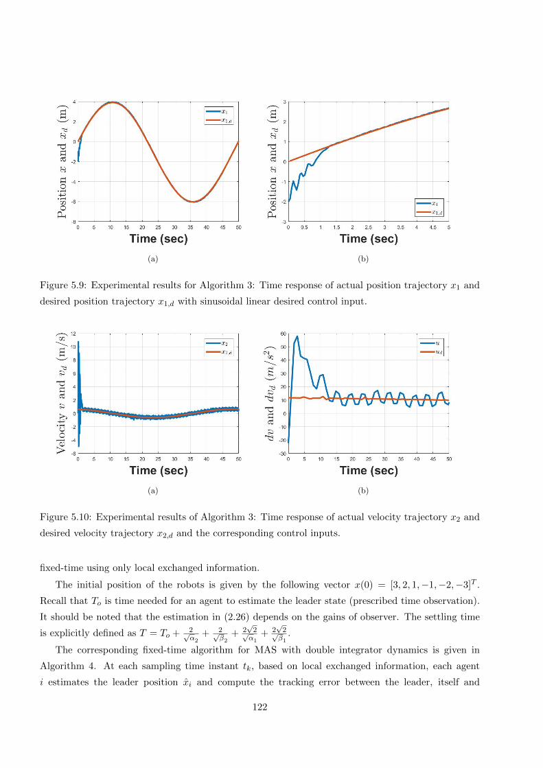
(a) (b)
Figure 5.9: Experimental results for Algorithm 3: Time response of actual position trajectory x1 and
desired position trajectory x1,d with sinusoidal linear desired control input.
(a) (b)
Figure 5.10: Experimental results of Algorithm 3: Time response of actual velocity trajectory x2 and
desired velocity trajectory x2,d and the corresponding control inputs.
fixed-time using only local exchanged information.
The initial position of the robots is given by the following vector x(0) = [3, 2, 1,−1,−2,−3]T .
Recall that To is time needed for an agent to estimate the leader state (prescribed time observation).
It should be noted that the estimation in (2.26) depends on the gains of observer. The settling time
is explicitly defined as T = To + 2√α2
+ 2√β2
+ 2√
2√α1
+ 2√
2√β1
.
The corresponding fixed-time algorithm for MAS with double integrator dynamics is given in
Algorithm 4. At each sampling time instant tk, based on local exchanged information, each agent
i estimates the leader position xi and compute the tracking error between the leader, itself and
122

neighboring agents. After calculating the controller u, we implement the corresponding linear velocity
input of the robot.
Algorithm 4 Fixed-time consensus for MAS with Double Integrator dynamics
For each agent i, Input: x1,0(tk), x2,0(tk) (if bi = 1), x1,i(tk), x2,i(tk), x1,j(tk), x2,j(tk) (for all j such
that aij 6= 0)
Parameter: ρ1 and σ1, ρ2 and σ2, α1, β1, α2, β2, a
Output: vi(t), tk ≤ t < tk+1
1: if t = tk then
2: When t < To, vi(t) = 0
3: Agent i samples its current states xi(t), its estimate of the leader xi(t) and broadcasts it to its
neighbors
4: Compute the estimation error xi = xi − x0
5: Update the distributed observer (2.23) (convergence in time To)
6: When t ≥ To, compute the tracking error ei = xi − xi7: Compute u according to Equation (2.35)
8: Implement the linear velocity
9: end if
x1,i(tk) is x position of Minilab robot i and x1,0(tk) is x leader position at instant tk. x2,i(tk) is x
linear velocity of Minilab robot i and x2,0(tk) is x leader velocity at instant tk.
The performances of the proposed observer-based leader-follower consensus controller for double
integrator MAS are studied through the following experimental results.
Step Linear Input for the leader trajectory
The control parameter are selected as: α1 = α2 = β1 = β2 = 10 for protocols 2.35. The initial position
of the robots is [3, 2, 1,−1,−2,−3]T while the initial velocity is 0. The desired trajectory is generated
by (5.6) with x1,0(0) = 0, x2,0(t) = 0.2. Hence, we set a = 1. The control objective is that each system
(5.5) tracks the leader x0 using only local information.
Using Theorem 3, the distributed observer (2.23) guarantees the stabilization of the estimation
errors to the origin in a finite-time bounded by To = 1s. The distributed observers accurately recon-
struct the leader state for each agent before To. Using Theorem 4, the tracking controller guarantees
the stabilization of the estimation errors to the origin in a finite-time bounded by T = 6.55s. Figure
5.11 shows that the actual state trajectory accurately tracks the leader state before T in spite of the
presence of disturbances and uncertainties inherent to the experimental setup. One can conclude that
using the proposed controller, the leader-follower consensus is achieved in a prescribed time. The
123

origin of the closed-loop system is globally finite-time stable contrary to existing controllers which
only provide semi-global finite-time stability property. Furthermore, since T does not depend on the
initial states of agents, the proposed protocol is distributed.
(a) (b)
Figure 5.11: Experimental results for Algorithm 4: Time response of the actual state trajectory of the
followers and of the leader with a step linear leader trajectory.
Sinusoidal Linear Input for the leader trajectory
The control parameters are selected as: α1 = α2 = β1 = β2 = 2 and a = 1 for protocol 2.35. The initial
position of the robots is [3, 2, 1,−1,−2,−3]T while the initial velocity is 0. The desired trajectory of
the leader is generated by (5.6) with u0(t) = 0.2 sin(2πt). Based on the control parameters, the settling
time is T = 15s (To = 5s). The control objective is that each system (5.5) tracks the leader x0 using
only local information.
The fixed-time consensus tracking performance of the MAS with double-integrator dynamics when
the leader input has a sinusoidal linear input is shown in Figure 5.12. Using Theorem 4, the robust
controller (2.35) solves the fixed-time trajectory tracking problem with an estimation of the settling
time less than T . Figure 5.12.(a) shows that the tracking controller guarantees the stabilization of
the tracking errors in position to the origin in a finite-time bounded by T . Figure 5.12.(b) shows the
tracking errors in velocity.
5.4 Fixed-Time Tracking for agents with Unicycle-type Dynamics
In this section, we show some experimental results using Gazebo-ROS and Minilab robot platform for
tracking and consensus with unicycle-type dynamics to verify the theoretical analysis.
124

(a) (b)
Figure 5.12: Experimental results for Algorithm 4: Time response of the actual state trajectory of the
followers and of the leader with a sinusoidal leader trajectory.
5.4.1 Fixed-Time Trajectory Tracking for Unicycle-type Dynamics
The algorithm for trajectory tracking is given in Algorithm 5. At each sampling time instant tk, the
robot calculates the desired position and velocity. Then, it determines the error position between
the desired trajectory and its actual position. After calculating the controller u, we implement the
corresponding linear and angular velocity input of the robot.
Algorithm 5 Fixed-time Tracking for Unicycle-type Dynamics
Input: x1(tk), x2(tk), x3(tk), x4(tk), x1,d(tk), x2,d(tk), x3,d(tk), x4,d(tk)
Parameters: α1, β1, α2, β2, a
Output: vlinear x(t), vangular(t), tk ≤ t < tk+1
1: if t = tk then
2: Compute the tracking errors e(t) = x(t)− xd(t)3: Compute s1, ϕ1, u1
4: Compute s2, ϕ2, u2
5: Implement the linear velocity
6: Implement the angular velocity
7: end if
First, the desired trajectory is illustrated in Figure 5.13. It is composed of a line and a circle (see
the curve in blue color). The control parameter are selected as: α1 = β1 = 20, α2 = β2 = 10, a = b = 1
for controller (2.54). The initial state of the robot is x(0) = −2, y(0) = −2, θ(0) = 0. Based on the
control parameters, the settling time is T = 2.6s. Figure 5.13 shows the time response of x and y
position of the robot. The robot successfully tracks the desired trajectory with an offset 0.25m (which
125

has been added for collision avoidance consideration).
Using Theorem 5, the tracking controller (2.54) guarantees the stabilization of the tracking errors to
the origin in a finite-time bounded by T = 2.6s. Figure 5.14 shows the actual and desired trajectories
in x (both in position and velocity). It is shown that the actual position x accurately tracks the
desired state xd before T (i.e. 0.8s) in spite of the presence of disturbances and uncertainties inherent
to the experimental setup.
Figure 5.13: Actual and desired trajectory of the robot in the plane
(a) (b)
Figure 5.14: Time evolution of the x position and x velocity
Figure 5.15 shows the actual and desired trajectories in θ (both in position and velocity). It is
shown that the actual position θ accurately tracks the desired state θd before T (i.e. 0.8s) in spite of
the presence of disturbances and uncertainties inherent to the experimental setup. Hence, the origin
of the closed-loop system is globally finite-time stable. Furthermore, since T does not depend on the
126

initial position and linear velocity, the proposed protocol is fixed-time.
(a) (b)
Figure 5.15: Time evolution of the θ position and angular velocity
5.4.2 Fixed-Time Consensus for MAS with Unicycle-type Dynamics
The communication topology is given in Figure 5.2. Assumption 1 is satisfied. For the consensus
tracking application, the Minilab robots are modeled as system (2.49). The dynamics of the leader
is generated by (2.61). The control objective is that systems (2.49) follow the leader in a fixed-time
using only local exchanged information.
The initial x − y position of the robots is given by the following vector (−1,−1) and (1, 1) for
robot 1 and 2 respectively. Recall that To is time needed for agents to estimate the leader state (in
a prescribed time). It should be note that the estimation in (2.26) depends on the gains of observer.
The settling time is explicitly defined as T = To + 2√α2
+ 2√β2
+ 2√
2√α1
+ 2√
2√β1
.
The corresponding fixed-time algorithm for MAS with unicycle-type is given in Algorithm 6. At
each sampling time instant tk, based on local exchanged information, each agent i estimates the leader
position xi and compute the tracking error between the leader, itself and neighboring agents. After
calculating the controller u, we implement the corresponding linear and angular velocity input of the
robot.
127

Algorithm 6 Fixed-time consensus algorithm for MAS with Unicycle-type dynamics
For each agent i, Input: x1,0(tk), x2,0(tk), x3,0(tk), x4,0(tk) (if bi = 1), x1,i(tk), x2,i(tk), x3,i(tk), x4,i(tk),
x1,j(tk), x2,j(tk), x3,j(tk), x4,j(tk) (for all j such that aij 6= 0)
Parameter: ρ1 and σ1, ρ2 and σ2, α1, β1, α2, β2, a
Output: vlinear,i(t), vangular,i(t), tk ≤ t < tk+1
1: if t = tk then
2: Agent i samples its current states, its estimate of the leader and broadcasts it to its neighbors
3: Compute the estimation error xi = xi − x0
4: Update the distributed observer (convergence in time To)
5: When t ≥ To, compute the tracking error
6: Compute the control inputs
7: Implement the linear and angular velocities
8: end if
The performances of the proposed observer-based leader-follower consensus controller for unicycle-
type are studied through experimental results. The control parameter are selected as: α1 = β1 =
12, α2 = β2 = 12 for protocols (2.85). The desired trajectory is generated by (2.61) with initial desired
position (0,0), ulinear d(t) = 0.2 and uangular d(t) = 0.8. Hence, since a ≥ d1 + u1,d and b ≥ d2 + u2,d,
we set a = b = 1. The control objective is that system (2.62) tracks the leader x0 and y0 using only
local information. Based on the control parameters, the settling time is T = 6.78s.
(a) (b)
Figure 5.16: Time response of the tracking for x position and vx linear velocity
Using Theorem 6, the distributed observer (2.66) guarantees the stabilization of the estimation
errors (2.67) to the origin in a finite-time bounded by To = 4s. Figure 5.16 shows the distributed
observers accurately reconstruct the leader state for each agent before To. Using Theorem 7, the
128

tracking controller guarantees the stabilization of the estimation errors (2.67) to the origin in a finite-
time bounded by T = 6s.
(a) (b)
Figure 5.17: Time response of the tracking for y position and vy linear velocity
Figures 5.18 (a) and (b) show that the real orientation θi and angular velocity ωi have converged
to their respective desired trajectories θd and ωd.
(a) (b)
Figure 5.18: Time response of the tracking for θ position and ω angular velocity
Unlike the previous sections, the results presented herein have proven the consensus to be harder
to achieve due to multiple hardware constraints. In fact, the maximum sampling rate in the Minilab
robots are limited to 10 Hz maximum, and collisions often occurred while agents tried to achieve their
convergence.
129

5.5 Conclusion
In this chapter, the fixed-time consensus tracking problem for a group of Minilab robots is investigated.
Both of tracking and consensus algorithms for single-integrator, double-integrator, and unicycle-type
systems was developed respectively. The observer gains are properly chosen and sufficient conditions
are established in terms of the graph connectivity to ensure consensus. The effectiveness is validated
by experimental results.
However, when it came to real robot experimentations, hardware constraints imposed limitations
on the proposed scheme, and therefor, convergence was harder to attain in optimal conditions. The
robots’ sampling rates restrict the performances of our proposed controller and prevent it from working
properly. The collisions have often occurred while robots tried to achieve their convergence. The real
robot experiments also depend on the performance of the workstation. The latter is responsible for the
control as well as monitoring the experiments. An increasing amount of robots would require better
workstation performances.
130

General conclusion and perspectives
The work of this thesis has been focussed on the study of the navigation scheme for MAS, while
taking into account some practical constraints. We were mainly interested in designing cooperative
controllers for each agent, in a fully decentralized way, while considering the robot model and temporal
constraints. The temporal constraints have been investigated in two directions: consensus problem in
a fixed-time framework and consensus problem in a discrete-time framework.
General conclusion
The main results of this thesis are summarized as follows:
• In the first chapter, we have presented the basic concepts of algebraic graph theory for describing
the communication topology among the agents. Furthermore, we have given a brief general
overview on MAS and consensus control problem in cooperative control both in continuous-time
and discrete-time. Convergence rates motivated us to investigate how a fast controller can be
designed.
• In the second chapter, it was considered fixed-time leader-follower consensus tracking problem
for MAS. Over a fixed topology, distributed observers and decentralized controllers have been de-
signed for each agent to solve the leader-follower consensus problem in a fixed time. Distributed
observers have been proposed for each agent to estimate the leader state in a fixed-time. A
switching controller has been proposed to solve the consensus problem. An upper bound of the
settling time, which only depends on the controller parameters has been estimated regardless of
the initial conditions. First, the study of fixed-time leader-follower consensus has been addressed
for linear MAS (i.e. single-integrator and double-integrator dynamics). Subsequently, the fixed-
time consensus tracking problem has been investigated for multiple unicycle-type mobile robots
under matched perturbations.
131

• In chapter 3, we have proposed a distributed model predictive control protocol for consensus of
MAS with discrete-time linear dynamics under time-varying directed topologies. The control
protocol is designed by combining graph theory with a predictive control algorithm to take into
account the switches on the communication topology. Our proposed controller has been designed
using the difference between two consecutive inputs. The controller has also integrator properties
to eliminate the steady-state errors. The convergence time of the closed-loop system depends
on the prediction horizon parameters. First, the study of distributed model predictive control
consensus protocol has focussed on MAS with single-integrator dynamics. Some comparative
studies have shown the advantage of the proposed scheme compared to existing ones. Then, the
extension to MAS with double-integrator dynamics have been successfully done.
• In chapter 4, we have discussed about the implementation of the proposed control schemes for
MAS. Due to the requirements of the proposed consensus algorithms, we have first introduced
the robot hardware specifications, communication network configuration and minimum amount
of workstations we can use for the coordination of multi-robots using Robot Operating System
(ROS) and multiple Minilab robots. Multiple robots communicate through a wireless network
with only one workstation for monitoring and control using a wireless master-slave scheme. This
configuration is a low cost configuration.
In this ROS MAS network, decentralized architectures were solved using multi-master ROS. The
package of multimaster fkie is shown as a solution for a decentralized implementation. Node calling
algorithm has allowed to create the leader-follower topology. This algorithm has used a publisher and a
subscriber to broadcast and/or receive messages continually from each other.
• In chapter 5, we have experimentally implemented and validated the fixed-time consensus tracking con-
troller on a group of Minilab robots using ROS with a wireless network. The sampling rate of the minilab
robot is only 10 Hz. Both tracking and consensus algorithms for single-integrator, double-integrator,
and unicycle-type systems were successfully implemented. The effectiveness of the theoretical results was
validated by experimental results.
Perspectives
Despite the results that have been proposed in this thesis, there are still several aspects that could
be further investigated in future works. Some of related topics for future research are highlighted as
follows.
• In chapter 2, we have dealt with the fixed-time leader-follower consensus problem for MAS with
linear dynamics and multiple unicycle-type mobile robots under matched perturbations. It will
be possible to investigate the fixed-time leader-follower consensus control problem for MAS with
132

chained-form dynamics in consideration of unmatched perturbations and noise measurement.
We have also dealt with fixed topology and undirected graph. Hence, it would be an interesting
direction if the communication network is switching and include a collection of directed graphs.
Obviously, new controllers and Lyapunov functions should be designed to deal with general
switching directed graphs.
We have investigated the fixed-time leader-follower consensus problem for MAS with single-
integrator, double-integrator and unicycle-type mobile robot dynamics separately. However, in
a leader-following architecture, it is possible that leaders have different dynamics from the fol-
lowers. In fact, in the group of leaders or followers, the dynamics could also be different to build
a complex network. Hence, it will be interesting to investigate the fixed-time leader-follower
consensus problem for MAS with heterogeneous dynamics.
The fixed-time leader-follower consensus developed in this thesis is achieved and guarantees that
the settling time is estimated regardless of the initial condition of the agents. However, this esti-
mate is sometimes too large. To improve this estimate, the concept of predefined-time stability
could be interesting to obtain the least upper bound of the settling time.
• In chapter 3, we have studied a distributed model predictive control protocol consensus for
MASs with discrete-time linear dynamics under time-varying directed topologies. The proposed
controller has only focused on the leaderless case. We plan to extend the results to the leader-
follower consensus problem. Another interesting concern for the future work of Chapter 3 can be
design of distributed model predictive control protocol consensus for MASs with unicycle-type
dynamics. A proof of stability should also be investigated.
• The works presented in Chapters 4 and 5 have focused on the implementation of consensus
protocols for a group of multiple Minilab robots. This work for the coordination between robots
only use the odometry sensors of each minilab robot. Hence, it may be interesting to develop a
visual based motion for future works.
Due to the method of multimaster fkie, the obtained results depend on the specification of the Mas-
ter Workstation. It will be interesting to have good specifications for the Master Workstation. Another
physical limitation is the sampling rate which significantly influences the performances of the proposed
controllers. Interesting extensions of this work can also be pursued to consider physical hardware speci-
fications of the agents and workstation.
133

It should be noted that in our experiments, the results of fixed-time leader-following consensus are ob-
tained without considering the collision avoidance. Collision between agents and obstacle avoidance are
not discussed in this thesis, which motivates us to conduct a more in-depth study to investigate consensus
while avoiding collisions.
134

List of Figures
1 Applications of MASs. . . . . . . . . . . . . . . . . . . . . . . . . . . . . . . . . . . . . 10
1.1 A communication graph of MAS with 5 vertices and 6 edges. . . . . . . . . . . . . . . 18
1.2 A directed graph with 4 vertices. . . . . . . . . . . . . . . . . . . . . . . . . . . . . . . 18
1.3 Example of different agents. . . . . . . . . . . . . . . . . . . . . . . . . . . . . . . . . . 22
1.4 Multi-agent system applications. . . . . . . . . . . . . . . . . . . . . . . . . . . . . . . 22
1.5 Illustration of a MAS: A group of five mobile robots. . . . . . . . . . . . . . . . . . . . 23
1.6 Average Consensus. . . . . . . . . . . . . . . . . . . . . . . . . . . . . . . . . . . . . . 25
1.7 Leaderless Consensus. . . . . . . . . . . . . . . . . . . . . . . . . . . . . . . . . . . . . 26
1.8 Graph of Leader Follower Model . . . . . . . . . . . . . . . . . . . . . . . . . . . . . . 26
1.9 Leader Follower Consensus . . . . . . . . . . . . . . . . . . . . . . . . . . . . . . . . . 27
1.10 Asymptotic, finite-time and fixed-time properties of the first-order system . . . . . . . 28
1.11 Evolution of the most significant MPC algorithms. . . . . . . . . . . . . . . . . . . . . 33
1.12 MPC concepts. . . . . . . . . . . . . . . . . . . . . . . . . . . . . . . . . . . . . . . . . 34
2.1 Top view of the considered mobile robot . . . . . . . . . . . . . . . . . . . . . . . . . . 40
2.2 Communication topology for the considered MAS. . . . . . . . . . . . . . . . . . . . . 44
2.3 Evolution of the estimation errors (2.8) for each follower . . . . . . . . . . . . . . . . . 45
2.4 Evolution of the tracking errors between each agent and the leader. . . . . . . . . . . . 45
2.5 Control input for each agent . . . . . . . . . . . . . . . . . . . . . . . . . . . . . . . . . 45
2.6 Evolution of the estimation errors (2.27) for each follower. . . . . . . . . . . . . . . . . 50
2.7 Evolution of the tracking errors between each agent and the leader. . . . . . . . . . . . 51
2.8 Control input for each agent. . . . . . . . . . . . . . . . . . . . . . . . . . . . . . . . . 51
2.9 Top view of the considered mobile robot. . . . . . . . . . . . . . . . . . . . . . . . . . . 52
2.10 Illustration of the fixed-time trajectory tracking problem for a single agent. . . . . . . 53
2.11 Stabilization of the two subsystems. . . . . . . . . . . . . . . . . . . . . . . . . . . . . 54
2.12 Actual trajectory x1, x2 and desired state trajectories x1,d, x2,d . . . . . . . . . . . . . 57
2.13 Actual trajectory x3, x4 and desired state trajectories x3,d, x4,d . . . . . . . . . . . . . 57
2.14 Tracking errors e . . . . . . . . . . . . . . . . . . . . . . . . . . . . . . . . . . . . . . . 58
135

2.15 Illustration of the fixed-time consensus tracking problem. . . . . . . . . . . . . . . . . 58
2.16 Proposed control strategy to solve the consensus problem of MAS with chained-form
dynamics. . . . . . . . . . . . . . . . . . . . . . . . . . . . . . . . . . . . . . . . . . . . 59
2.17 Evolution of the estimation errors (2.67) for each follower . . . . . . . . . . . . . . . . 68
2.18 Evolution of the tracking errors between each agent and the leader. . . . . . . . . . . . 69
2.19 Control input for each agent . . . . . . . . . . . . . . . . . . . . . . . . . . . . . . . . . 69
3.1 Switching communication topologies between agents . . . . . . . . . . . . . . . . . . . 78
3.2 Evolution of agent state x and control input u for a. Hp = 3, b. Hp = 6 and c. Hp = 9 80
3.3 Evolution of agent state x and control input u using our proposed DMPC . . . . . . . 80
3.4 Evolution of the agent states x and the control input u using [1] . . . . . . . . . . . . 81
3.5 Evolution of agent state x1,i and x2,i with a.Hp = 3, b.Hp = 6, c.Hp = 9 . . . . . . . . 83
3.6 Evolution of the control input ui . . . . . . . . . . . . . . . . . . . . . . . . . . . . . . 83
4.1 Multiple Minilab robots with wireless communication architecture. . . . . . . . . . . . 85
4.2 Illustration of the experimental setup. . . . . . . . . . . . . . . . . . . . . . . . . . . . 86
4.3 Minilab Enova Robot. . . . . . . . . . . . . . . . . . . . . . . . . . . . . . . . . . . . . 87
4.4 Minilab physical dimensions. . . . . . . . . . . . . . . . . . . . . . . . . . . . . . . . . 87
4.5 Minilab hardware features. . . . . . . . . . . . . . . . . . . . . . . . . . . . . . . . . . 88
4.6 Intel Atom N2800. . . . . . . . . . . . . . . . . . . . . . . . . . . . . . . . . . . . . . . 89
4.7 TL-WR802N Wireless routers. . . . . . . . . . . . . . . . . . . . . . . . . . . . . . . . 89
4.8 DUB-H7 7-Port USB 2.0 HUB. . . . . . . . . . . . . . . . . . . . . . . . . . . . . . . . 90
4.9 Buhler Motor DC. . . . . . . . . . . . . . . . . . . . . . . . . . . . . . . . . . . . . . . 90
4.10 Roboteq SDC2130 controller. . . . . . . . . . . . . . . . . . . . . . . . . . . . . . . . . 90
4.11 Arduino Micro Board. . . . . . . . . . . . . . . . . . . . . . . . . . . . . . . . . . . . . 91
4.12 Infrared sensor SHARP. . . . . . . . . . . . . . . . . . . . . . . . . . . . . . . . . . . . 91
4.13 Orbbec Astra Pro Camera. . . . . . . . . . . . . . . . . . . . . . . . . . . . . . . . . . 92
4.14 Power-Sonic Battery . . . . . . . . . . . . . . . . . . . . . . . . . . . . . . . . . . . . . 92
4.15 ROS File System Level. . . . . . . . . . . . . . . . . . . . . . . . . . . . . . . . . . . . 93
4.16 ROS Computation Graph Level. . . . . . . . . . . . . . . . . . . . . . . . . . . . . . . 95
4.17 ROS Computation Graph Level. . . . . . . . . . . . . . . . . . . . . . . . . . . . . . . 95
4.18 Computation graph for control wheel motor. . . . . . . . . . . . . . . . . . . . . . . . . 97
4.19 rqt graph for control wheel motors. . . . . . . . . . . . . . . . . . . . . . . . . . . . . . 98
4.20 MiniLab robot setup for a single ROS system. . . . . . . . . . . . . . . . . . . . . . . . 98
4.21 Wireless network setup on the host PC. . . . . . . . . . . . . . . . . . . . . . . . . . . 99
4.22 Communication checking results. . . . . . . . . . . . . . . . . . . . . . . . . . . . . . . 99
4.23 Gazebo-ROS simulation for minilab robot. . . . . . . . . . . . . . . . . . . . . . . . . . 100
4.24 rqt graph for minilab in Gazebo-ROS . . . . . . . . . . . . . . . . . . . . . . . . . . . 101
136

4.25 Network topology for the illustrative example. . . . . . . . . . . . . . . . . . . . . . . . 102
4.26 TP-Link address reservation. . . . . . . . . . . . . . . . . . . . . . . . . . . . . . . . . 103
4.27 Contents of the /etc/hosts file for the workstation for the example presented in Fig. 4.1.103
4.28 Contents of the /etc/hosts file for each robot for the example presented in Fig. 4.1. . . 103
4.29 MiniLab robot runs its own master managing local communication. . . . . . . . . . . . 104
4.30 Multimaster fkie for multiple-minilab robots. . . . . . . . . . . . . . . . . . . . . . . . 105
4.31 rosservice call command result. . . . . . . . . . . . . . . . . . . . . . . . . . . . . . . . 106
4.32 Communication topology. . . . . . . . . . . . . . . . . . . . . . . . . . . . . . . . . . . 106
5.1 Topology of MAS using ROS for six agents. . . . . . . . . . . . . . . . . . . . . . . . . 110
5.2 Topology of MAS using using our Minilab Enova robot platform. . . . . . . . . . . . . 110
5.3 Experimental results for Algorithm 1: Time response of actual state trajectory x and
desired state trajectory xd with constant linear desired velocity. . . . . . . . . . . . . . 112
5.4 Experimental results for Algorithm 1: Time response of actual state trajectory x and
desired state trajectory xd with sinusoidal linear desired velocity. . . . . . . . . . . . . 113
5.5 Experimental results for Algorithm 2: Time response of the actual state trajectory of
the followers and of the leader with a step linear leader trajectory. . . . . . . . . . . . 115
5.6 Experimental results for Algorithm 2: Time response of the actual state trajectory of
the followers and of the leader with a sinusoidal linear leader trajectory. . . . . . . . . 116
5.7 Experimental results for Algorithm 2: Control input for each agent and the leader. . . 117
5.8 Experimental results for Algorithm 3: Time response of actual state trajectory x and
desired state trajectory xd with constant linear desired control input. . . . . . . . . . . 119
5.9 Experimental results for Algorithm 3: Time response of actual position trajectory x1
and desired position trajectory x1,d with sinusoidal linear desired control input. . . . . 120
5.10 Experimental results of Algorithm 3: Time response of actual velocity trajectory x2
and desired velocity trajectory x2,d and the corresponding control inputs. . . . . . . . 120
5.11 Experimental results for Algorithm 4: Time response of the actual state trajectory of
the followers and of the leader with a step linear leader trajectory. . . . . . . . . . . . 122
5.12 Experimental results for Algorithm 4: Time response of the actual state trajectory of
the followers and of the leader with a sinusoidal leader trajectory. . . . . . . . . . . . . 123
5.13 Actual and desired trajectory of the robot in the plane . . . . . . . . . . . . . . . . . . 124
5.14 Time evolution of the x position and x velocity . . . . . . . . . . . . . . . . . . . . . . 124
5.15 Time evolution of the θ position and angular velocity . . . . . . . . . . . . . . . . . . . 125
5.16 Time response of the tracking for x position and vx linear velocity . . . . . . . . . . . 126
5.17 Time response of the tracking for y position and vy linear velocity . . . . . . . . . . . 127
5.18 Time response of the tracking for θ position and ω angular velocity . . . . . . . . . . . 127
137

138

List of Tables
4.1 Parts of the Minilab components . . . . . . . . . . . . . . . . . . . . . . . . . . . . . . 88
139

140

Bibliography
[1] Roger A Horn and Charles R Johnson. Matrix analysis cambridge university press. New York,
37, 1985.
[2] Russell Merris. Laplacian matrices of graphs: a survey. Linear algebra and its applications,
197:143–176, 1994.
[3] Yoonsoo Kim and Mehran Mesbahi. On maximizing the second smallest eigenvalue of a state-
dependent graph laplacian. IEEE transactions on Automatic Control, 51(1):116–120, 2006.
[4] Sonia MartıNez and Francesco Bullo. Optimal sensor placement and motion coordination for
target tracking. Automatica, 42(4):661–668, 2006.
[5] Yongcan Cao and Wei Ren. Distributed coordinated tracking with reduced interaction via a
variable structure approach. IEEE Transactions on Automatic Control, 57(1):33–48, 2012.
[6] X Luo, D Liu, X Guan, and S Li. Flocking in target pursuit for multi-agent systems with partial
informed agents. IET control theory & applications, 6(4):560–569, 2012.
[7] Zhan Li, Hugh HT Liu, Bo Zhu, and Huijun Gao. Robust second-order consensus tracking of
multiple 3-dof laboratory helicopters via output feedback. IEEE/ASME Transactions on Mecha-
tronics, 20(5):2538–2549, 2015.
[8] Yang Tang, Xing Xing, Hamid Reza Karimi, Ljupco Kocarev, and Jurgen Kurths. Tracking con-
trol of networked multi-agent systems under new characterizations of impulses and its applications
in robotic systems. IEEE Transactions on Industrial Electronics, 63(2):1299–1307, 2016.
[9] Dongbing Gu and Zongyao Wang. Leader–follower flocking: algorithms and experiments. IEEE
Transactions on Control Systems Technology, 17(5):1211–1219, 2009.
[10] Jingyuan Zhan and Xiang Li. Flocking of multi-agent systems via model predictive control based
on position-only measurements. IEEE Transactions on Industrial Informatics, 9(1):377–385, 2013.
[11] Wei Li and Mark W Spong. Analysis of flocking of cooperative multiple inertial agents via
a geometric decomposition technique. IEEE Transactions on Systems, Man, and Cybernetics:
Systems, 44(12):1611–1623, 2014.
141

[12] Yongnan Jia and Long Wang. Leader–follower flocking of multiple robotic fish. IEEE/ASME
Transactions on Mechatronics, 20(3):1372–1383, 2015.
[13] Swagatam Das, Udit Halder, and Dipankar Maity. Chaotic dynamics in social foraging
swarms—an analysis. IEEE Transactions on Systems, Man, and Cybernetics, Part B (Cyber-
netics), 42(4):1288–1293, 2012.
[14] Andrea Gasparri, Giuseppe Oriolo, Attilio Priolo, and Giovanni Ulivi. A swarm aggregation algo-
rithm based on local interaction for multi-robot systems with actuator saturations. In Intelligent
Robots and Systems (IROS), 2012 IEEE/RSJ International Conference on, pages 539–544. IEEE,
2012.
[15] Jorge Cortes, Sonia Martınez, and Francesco Bullo. Robust rendezvous for mobile autonomous
agents via proximity graphs in arbitrary dimensions. IEEE Transactions on Automatic Control,
51(8):1289–1298, 2006.
[16] Jie Lin, A Stephen Morse, and Brian DO Anderson. The multi-agent rendezvous problem. part
2: The asynchronous case. SIAM Journal on Control and Optimization, 46(6):2120–2147, 2007.
[17] Jorge Cortes, Sonia Martinez, Timur Karatas, and Francesco Bullo. Coverage control for mobile
sensing networks. IEEE Transactions on robotics and Automation, 20(2):243–255, 2004.
[18] Islam I Hussein and Dusan M Stipanovic. Effective coverage control for mobile sensor net-
works with guaranteed collision avoidance. IEEE Transactions on Control Systems Technology,
15(4):642–657, 2007.
[19] Xinmiao Sun and Christos G Cassandras. Optimal dynamic formation control of multi-agent
systems in constrained environments. Automatica, 73:169–179, 2016.
[20] Sara Susca, Francesco Bullo, and Sonia Martinez. Monitoring environmental boundaries with a
robotic sensor network. IEEE Transactions on Control Systems Technology, 16(2):288–296, 2008.
[21] Matthew Dunbabin and Lino Marques. Robots for environmental monitoring: Significant ad-
vancements and applications. IEEE Robotics & Automation Magazine, 19(1):24–39, 2012.
[22] Michael Defoort, Thierry Floquet, Annemarie Kokosy, and Wilfrid Perruquetti. Sliding-mode
formation control for cooperative autonomous mobile robots. IEEE Transactions on Industrial
Electronics, 55(11):3944–3953, 2008.
[23] Khac Duc Do. Bounded assignment formation control of second-order dynamic agents.
IEEE/ASME Transactions on Mechatronics, 19(2):477–489, 2014.
142

[24] Zhiyun Lin, Lili Wang, Zhimin Han, and Minyue Fu. Distributed formation control of multi-agent
systems using complex laplacian. IEEE Transactions on Automatic Control, 59(7):1765–1777,
2014.
[25] Lara Brinon-Arranz, Alexandre Seuret, and Carlos Canudas-de Wit. Cooperative control design
for time-varying formations of multi-agent systems. IEEE Transactions on Automatic Control,
59(8):2283–2288, 2014.
[26] Kwang-Kyo Oh, Myoung-Chul Park, and Hyo-Sung Ahn. A survey of multi-agent formation
control. Automatica, 53:424–440, 2015.
[27] J Alexander Fax and Richard M Murray. Information flow and cooperative control of vehicle
formations. IEEE transactions on automatic control, 49(9):1465–1476, 2004.
[28] Ali Jadbabaie, Jie Lin, and A Stephen Morse. Coordination of groups of mobile autonomous
agents using nearest neighbor rules. IEEE Transactions on automatic control, 48(6):988–1001,
2003.
[29] Zhiyun Lin, Mireille Broucke, and Bruce Francis. Local control strategies for groups of mobile
autonomous agents. IEEE Transactions on automatic control, 49(4):622–629, 2004.
[30] Reza Olfati-Saber and Richard M Murray. Consensus problems in networks of agents with switch-
ing topology and time-delays. IEEE Transactions on automatic control, 49(9):1520–1533, 2004.
[31] Wei Ren and Randal W Beard. Consensus seeking in multiagent systems under dynamically
changing interaction topologies. IEEE Transactions on automatic control, 50(5):655–661, 2005.
[32] Jian Wu and Yang Shi. Average consensus in multi-agent systems with time-varying delays and
packet losses. In 2012 American Control Conference (ACC), pages 1579–1584. IEEE, 2012.
[33] Hamed Rezaee and Farzaneh Abdollahi. Consensus problem over high-order multiagent systems
with uncertain nonlinearities under deterministic and stochastic topologies. IEEE transactions
on cybernetics, 47(8):2079–2088, 2017.
[34] Wenhui Liu, Feiqi Deng, Jiarong Liang, and Haijun Liu. Distributed average consensus in multi-
agent networks with limited bandwidth and time-delays. IEEE/CAA Journal of Automatica
Sinica, 1(2):193–203, 2014.
[35] Christoforos N Hadjicostis and Themistoklis Charalambous. Average consensus in the presence
of delays in directed graph topologies. IEEE Transactions on Automatic Control, 59(3):763–768,
2014.
143

[36] Yuan Gong Sun, Long Wang, and Guangming Xie. Average consensus in networks of dynamic
agents with switching topologies and multiple time-varying delays. Systems & Control Letters,
57(2):175–183, 2008.
[37] Wei Ren, Randal W Beard, and Ella M Atkins. Information consensus in multivehicle cooperative
control. IEEE Control Systems, 27(2):71–82, 2007.
[38] Wei Ren and Randal W Beard. Consensus algorithms for double-integrator dynamics. Distributed
Consensus in Multi-vehicle Cooperative Control: Theory and Applications, pages 77–104, 2008.
[39] Haibo Du, Shihua Li, and Peng Shi. Robust consensus algorithm for second-order multi-agent
systems with external disturbances. International Journal of Control, 85(12):1913–1928, 2012.
[40] Wenwu Yu, Guanrong Chen, Wei Ren, Jurgen Kurths, and Wei Xing Zheng. Distributed higher
order consensus protocols in multiagent dynamical systems. IEEE Transactions on Circuits and
Systems I: Regular Papers, 58(8):1924–1932, 2011.
[41] Bin Zhou and Zongli Lin. Consensus of high-order multi-agent systems with large input and
communication delays. Automatica, 50(2):452–464, 2014.
[42] Jiangping Hu and Gang Feng. Distributed tracking control of leader–follower multi-agent systems
under noisy measurement. Automatica, 46(8):1382–1387, 2010.
[43] Wanli Guo, Jinhu Lu, Shihua Chen, and Xinghuo Yu. Second-order tracking control for leader–
follower multi-agent flocking in directed graphs with switching topology. Systems & Control
Letters, 60(12):1051–1058, 2011.
[44] Guoqiang Hu. Robust consensus tracking of a class of second-order multi-agent dynamic systems.
Systems & Control Letters, 61(1):134–142, 2012.
[45] Wangli He, Guanrong Chen, Qing-Long Han, and Feng Qian. Network-based leader-following con-
sensus of nonlinear multi-agent systems via distributed impulsive control. Information Sciences,
380:145–158, 2017.
[46] Zhiyun Lin, Wei Ding, Gangfeng Yan, Changbin Yu, and Alessandro Giua. Leader–follower
formation via complex laplacian. Automatica, 49(6):1900–1906, 2013.
[47] Giuseppe Notarstefano, Magnus Egerstedt, and M Haque. Containment in leader–follower net-
works with switching communication topologies. Automatica, 47(5):1035–1040, 2011.
[48] Jiahu Qin, Wei Xing Zheng, Huijun Gao, Qichao Ma, and Weiming Fu. Containment control for
second-order multiagent systems communicating over heterogeneous networks. IEEE transactions
on neural networks and learning systems, 28(9):2143–2155, 2017.
144

[49] Peng Yang, Randy A Freeman, Geoffrey J Gordon, Kevin M Lynch, Siddhartha S Srinivasa, and
Rahul Sukthankar. Decentralized estimation and control of graph connectivity for mobile sensor
networks. Automatica, 46(2):390–396, 2010.
[50] Wilfrid Perruquetti and Jean-Pierre Barbot. Sliding mode control in engineering. CRC Press,
2002.
[51] AF Filippov. Differential Equations with Discontinuous Righthand Sides: Control Systems, vol-
ume 18. Springer Science & Business Media, 1988.
[52] Sanjay P Bhat and Dennis S Bernstein. Geometric homogeneity with applications to finite-time
stability. Mathematics of Control, Signals and Systems, 17(2):101–127, 2005.
[53] Long Wang and Feng Xiao. Finite-time consensus problems for networks of dynamic agents.
IEEE Transactions on Automatic Control, 55(4):950–955, 2010.
[54] Suiyang Khoo, Lihua Xie, and Zhihong Man. Robust finite-time consensus tracking algorithm
for multirobot systems. IEEE/ASME transactions on mechatronics, 14(2):219–228, 2009.
[55] Yu Zhao, Zhisheng Duan, Guanghui Wen, and Yanjiao Zhang. Distributed finite-time track-
ing control for multi-agent systems: an observer-based approach. Systems & Control Letters,
62(1):22–28, 2013.
[56] Yu Zhao, Zhisheng Duan, Guanghui Wen, and Guanrong Chen. Distributed finite-time tracking
for a multi-agent system under a leader with bounded unknown acceleration. Systems & Control
Letters, 81:8–13, 2015.
[57] Saleh Mobayen. Finite-time tracking control of chained-form nonholonomic systems with external
disturbances based on recursive terminal sliding mode method. Nonlinear Dynamics, 80(1-2):669–
683, 2015.
[58] Andrey Polyakov. Nonlinear feedback design for fixed-time stabilization of linear control systems.
IEEE Transactions on Automatic Control, 57(8):2106–2110, 2012.
[59] Sergey Parsegov, Andrey Polyakov, and Pavel Shcherbakov. Nonlinear fixed-time control protocol
for uniform allocation of agents on a segment. In Decision and Control (CDC), 2012 IEEE 51st
Annual Conference on, pages 7732–7737. IEEE, 2012.
[60] Emmanuel Cruz-Zavala, Jaime A Moreno, and Leonid Fridman. Uniform second-order sliding
mode observer for mechanical systems. In Variable Structure Systems (VSS), 2010 11th Interna-
tional Workshop on, pages 14–19. IEEE, 2010.
[61] SE Parsegov, AE Polyakov, and PS Shcherbakov. Fixed-time consensus algorithm for multi-agent
systems with integrator dynamics. IFAC Proceedings Volumes, 46(27):110–115, 2013.
145

[62] Andrey Polyakov and Leonid Fridman. Stability notions and lyapunov functions for sliding mode
control systems. Journal of the Franklin Institute, 351(4):1831–1865, 2014.
[63] Junkang Ni, Ling Liu, Chongxin Liu, Xiaoyu Hu, and Shilei Li. Fast fixed-time nonsingular
terminal sliding mode control and its application to chaos suppression in power system. IEEE
Transactions on Circuits and Systems II: Express Briefs, 64(2):151–155, 2017.
[64] Zongyu Zuo and Lin Tie. A new class of finite-time nonlinear consensus protocols for multi-agent
systems. International Journal of Control, 87(2):363–370, 2014.
[65] Zongyu Zuo and Lin Tie. Distributed robust finite-time nonlinear consensus protocols for multi-
agent systems. International Journal of Systems Science, 47(6):1366–1375, 2016.
[66] Michael Defoort, Andrey Polyakov, Guillaume Demesure, Mohamed Djemai, and Kalyana Velu-
volu. Leader-follower fixed-time consensus for multi-agent systems with unknown non-linear
inherent dynamics. IET Control Theory & Applications, 9(14):2165–2170, 2015.
[67] Huifen Hong, Wenwu Yu, Guanghui Wen, and Xinghuo Yu. Distributed robust fixed-time con-
sensus for nonlinear and disturbed multiagent systems. IEEE Transactions on Systems, Man,
and Cybernetics: Systems, 47(7):1464–1473, 2017.
[68] Xue Lin and Yuanshi Zheng. Finite-time consensus of switched multiagent systems. IEEE Trans-
actions on Systems, Man, and Cybernetics: Systems, 47(7):1535–1545, 2017.
[69] Zongyu Zuo. Nonsingular fixed-time consensus tracking for second-order multi-agent networks.
Automatica, 54:305–309, 2015.
[70] Junjie Fu and Jinzhi Wang. Fixed-time coordinated tracking for second-order multi-agent systems
with bounded input uncertainties. Systems & Control Letters, 93:1–12, 2016.
[71] Junkang Ni, Ling Liu, Chongxin Liu, Xiaoyu Hu, and Tianshi Shen. Fixed-time dynamic surface
high-order sliding mode control for chaotic oscillation in power system. Nonlinear Dynamics,
86(1):401–420, 2016.
[72] Zongyu Zuo, Bailing Tian, Michael Defoort, and Zhengtao Ding. Fixed-time consensus tracking
for multiagent systems with high-order integrator dynamics. IEEE Transactions on Automatic
Control, 63(2):563–570, 2018.
[73] Deyuan Meng and Zongyu Zuo. Signed-average consensus for networks of agents: a nonlinear
fixed-time convergence protocol. Nonlinear Dynamics, 85(1):155–165, 2016.
[74] Deyuan Meng and Yingmin Jia. Robust consensus algorithms for multiscale coordination con-
trol of multivehicle systems with disturbances. IEEE Transactions on industrial electronics,
63(2):1107–1119, 2016.
146

[75] Michael Defoort, Guillaume Demesure, Zongyu Zuo, Andrey Polyakov, and Mohamed Djemai.
Fixed-time stabilisation and consensus of non-holonomic systems. IET Control Theory & Appli-
cations, 10(18):2497–2505, 2016.
[76] Feng Xiao and Long Wang. Consensus protocols for discrete-time multi-agent systems with time-
varying delays. Automatica, 44(10):2577–2582, 2008.
[77] L Wang and F Xiao. Dynamic behavior of discrete-time multi-agent systems with general com-
munication structure. Physical A, 370(2):364–380, 2006.
[78] Mauro Franceschelli, Alessandro Giua, and Carla Seatzu. A gossip-based algorithm for discrete
consensus over heterogeneous networks. IEEE Transactions on Automatic Control, 55(5):1244–
1249, 2010.
[79] Chong Tan and Guo-Ping Liu. Consensus of discrete-time linear networked multi-agent systems
with communication delays. IEEE Transactions on Automatic Control, 58(11):2962–2968, 2013.
[80] Shaobao Li, Gang Feng, Xiaoyuan Luo, and Xinping Guan. Output consensus of heterogeneous
linear discrete-time multiagent systems with structural uncertainties. IEEE transactions on cy-
bernetics, 45(12):2868–2879, 2015.
[81] Jian Wu and Yang Shi. Consensus in multi-agent systems with random delays governed by a
markov chain. Systems & Control Letters, 60(10):863–870, 2011.
[82] Bingxian Mu, Huxiong Li, Jie Ding, and Yang Shi. Consensus in second-order multiple flying
vehicles with random delays governed by a markov chain. Journal of the Franklin Institute,
352(9):3628–3644, 2015.
[83] Hassan K Khalil. Noninear systems. Prentice-Hall, New Jersey, 2(5):5–1, 1996.
[84] Mircea Lazar, WPMH Heemels, Alberto Bemporad, and Siep Weiland. On the stability and
robustness of non-smooth nonlinear model predictive control. In Workshop on Assessment and
Future Directions of NMPC, pages 327–334. Freudenstadt-Lauterbad Germany, 2005.
[85] John Tsitsiklis, Dimitri Bertsekas, and Michael Athans. Distributed asynchronous determinis-
tic and stochastic gradient optimization algorithms. IEEE transactions on automatic control,
31(9):803–812, 1986.
[86] Luc Moreau. Stability of multiagent systems with time-dependent communication links. IEEE
Transactions on automatic control, 50(2):169–182, 2005.
[87] J Richalet, A Rault, JL Testud, and J Papon. Model algorithmic control of industrial processes.
IFAC Proceedings Volumes, 10(16):103–120, 1977.
147

[88] Charles R Cutler and Brian L Ramaker. Dynamic matrix control?? a computer control algorithm.
In joint automatic control conference, number 17, page 72, 1980.
[89] S Joe Qin and Thomas A Badgwell. A survey of industrial model predictive control technology.
Control engineering practice, 11(7):733–764, 2003.
[90] Zhaomeng Cheng, Ming-Can Fan, and Hai-Tao Zhang. Distributed mpc based consensus for
single-integrator multi-agent systems. ISA transactions, 58:112–120, 2015.
[91] David Q Mayne, James B Rawlings, Christopher V Rao, and Pierre OM Scokaert. Constrained
model predictive control: Stability and optimality. Automatica, 36(6):789–814, 2000.
[92] Giancarlo Ferrari-Trecate, Luca Galbusera, Marco Pietro Enrico Marciandi, and Riccardo Scat-
tolini. Model predictive control schemes for consensus in multi-agent systems with single-and
double-integrator dynamics. IEEE Transactions on Automatic Control, 54(11):2560–2572, 2009.
[93] H-T Zhang, Michael ZhiQiang Chen, and Tao Zhou. Improve consensus via decentralized predic-
tive mechanisms. EPL (Europhysics Letters), 86(4):40011, 2009.
[94] Tomas Menard, Emmanuel Moulay, and Wilfrid Perruquetti. Fixed-time observer with simple
gains for uncertain systems. Automatica, 81:438–446, 2017.
[95] Michael Defoort, Jorge Palos, Annemarie Kokosy, Thierry Floquet, and Wilfrid Perruquetti.
Performance-based reactive navigation for non-holonomic mobile robots. Robotica, 27(2):281–
290, 2009.
[96] ROS. Line spacing in latex documents. http://wiki.ros.org/multimaster_fkie. Accessed
April, 2018.
148