Dear Martin Dameris, dear referees, We would like to thank you for ...

Dear Martin Dameris, dear referees,

We would like to thank you for your very valuable suggestions and comments. All reviewers

commented on the fact that we do not cover the tropospheric jet response sufficiently

according to the title of the paper. We give a general answer to the editor and all reviewers

about this issue in the beginning and give detailed answers to the specific points of the

different reviewers highlighted in blue below.

At the end of this document, a revised version of the manuscript is attached. All changes made

in this manuscript are highlighted in yellow.

Best regards,

Sabine Haase on behalf of all authors

General answer to the editor and all referees

Most referees are concerned that the tropospheric jet response to ozone depletion under the

different chemistry settings is not addressed sufficiently with respect to the title.

Furthermore, the statistical significance of the chemistry impact on the tropospheric jet was

questioned.

We agree with the reviewers and to resolve these issues we changed the title as

recommended by some of the referees, included an additional figure that evaluates the

difference in the trend of the tropospheric jet strength and latitude (new Fig. 10), and adapted

the manuscript text accordingly.

The title does not refer to the tropospheric jet in particular anymore and the new analysis

shows that the difference in the shift of the tropospheric jet between interactive and specified

chemistry settings is not statistically significant. We adapted the conclusion and discussion of

our results accordingly.

Abstract:

Line 14: “This difference between interactive and specified chemistry in the stratospheric

response to ozone depletion also affects the tropospheric response. However, an impact

on the poleward shift of the tropospheric jet stream is not detected.”

Results:

Line 395: “Figure 10 shows the trend for the tropospheric jet latitude and strength at 850

hPa. There is no statistically significant difference between the chemistry settings in the

trend of the tropospheric jet position and strength. All experiments have a similar mean

jet latitude trend and there is a large spread among ensemble members in the trend of

the jet strength, which leads to hardly significant trends in the ensemble means.

Therefore, the impact of interactive chemistry that is significant in the stratosphere does

not seem to show the same significance in the troposphere.”

Line 418: “[…] the too short tropospheric SAM timescale in WACCM, which is found in all

our experiments independent of the chemistry setting (Fig. 11), indicates that the coupling

between the stratosphere and troposphere is very likely too weak. This could explain why

we do not find significant differences in the tropospheric jet trends between our

experiments (Fig. 10) […].”

Conclusions:

Line 493: “However, the impact of interactive chemistry on the tropospheric jet could not

be validated by our study. […] Although not directly affecting the position of the

tropospheric jet, the differences we find between the chemistry settings (Fig. 9), show a

stronger tropospheric response to ozone depletion when interactive chemistry is included.

An updated model version of WACCM, based on the CAM5 physics, might improve our

understanding of the stratospheric impact onto the troposphere under different chemistry

settings.”

Anonymous Referee #1

This manuscript examines the impact of the representation of stratospheric ozone on climate

model simulations of tropospheric jet trends, by comparing ensembles of simulation with (i)

interactive chemistry, (ii) prescribed zonal-mean ozone, and (iii) prescribed 3D ozone. This is

an important topic that is relevant for ACP, and the manuscript is generally well written and

presents some new results. However, before it can be published there needs to be more,

quantitative analysis of the differences in jet trends among simulations, as well as discussion

of some relevant previous studies that have not been cited.

MAJOR COMMENTS

1. The title indicated that the tropospheric jet is the focus of this study, but most of the

focus is on the stratosphere and not the troposphere. Only one subsection of results

is on tropospheric jet, only 2 out 9 figures show the tropospheric jet, and the first 1.5

pages of Introduction are on stratosphere and only at line 85 is surface/tropospheric

features discussed. I think there should be more discussion and analysis of the

tropospheric jet, and less material on stratospheric changes.

We agree that the title was not chosen wisely since a large part of the paper is focusing on the

stratosphere. We also agree that we valued the impact of interactive chemistry onto the

tropospheric jet too much. We adapted these sections in the paper (see also your minor

comments) and included an additional Figure on the 850 hPa trends of the jet stream in the

revised manuscript (new Fig. 10). This additional analysis to better describe the impact of

interactive chemistry on the jet stream in the troposphere is presented below (answer to

major comment 2).

However, we do not want to cut on the stratospheric part of the paper since this is the region

in which the strongest differences occur and which is needed to understand the mechanism.

2. Regarding additional analysis, there are statements on how the shift in the jet differs

between the ON, OF and OFF 3D runs (lines 364-370 and 435) but this is not quantified.

The near-surface differences shown in the fig 9c and e and small (and generally

insignificant), and it is not clear from these plots how different the jet trends are. As

the tropospheric jet response is the focus not the paper trends in the latitude and

strength of the tropospheric jet (e.g. u at 850 hPa) need to be calculated, and

compared between different model runs (as well as reanalyses). Do the trends differ,

and how large is the difference compared to model-data differences? This is important

given the comment on lines 3 and 22 in the abstract (see minor comment 1), and also

Seviour et al. (2017) (Major Comment 3).

As proposed we calculated the jet latitude and strength at 850 hPa. We followed the

procedure as described in Seviour et al. (2017), defining the jet latitude and strength as the

location of the maximum of a quadratic fitted to the 850 hPa zonal mean zonal wind at its

maximum grid point and the two points either side.

Figure A 1: 850hPa jet latitude and amplitude difference between 1958-1968 and 1995-2005 for the different chemistry settings in CESM1-WACCM. The dashed line indicates the result for ERA data (combination of ERA-40 and ERA-Interim). The ensemble members are shown in gray while the ensemble mean is shown in black. Solid circles indicate significance at the 95% level using a t-test.

Figure A 1 shows the tropospheric jet latitude and trend as the difference between the

averages over the periods 1958-1968 and 1995 to 2005 for a better comparison to Seviour et

al. 2017. The three different WACCM experiments basically agree on the mean trend in jet

latitude and strength. The differences are statistically not significant (not shown). Compared

to the multi-model mean presented in Seviour et al. 2017, the trends for our WACCM

simulations are stronger for the jet latitude and weaker for the jet amplitude but well in

between the spread among the different models used in Seviour et al. 2017. The comparison

to a combined data set using ERA-40 and ERA-Interim data shows that WACCM rather

underestimates the trends in the strength of the tropospheric jet as well as in the jet latitude

although the trend in jet latitude is better captured than the trend in the strength of the

tropospheric jet.

For the paper, we decided to use the linear regression method (Fig. A 2) as we did for the

other figures. The main result is the same as in Figure 1 A. There is no significant difference

between the chemistry settings considering the trend of the jet position or strength. Using a

linear regression, though, reduces the significance of the ensemble mean trend for the

strength of the tropospheric jet (open circles in Fig. A 2 as compared to filled ones in Fig. A 1),

due to the large spread among ensemble members.

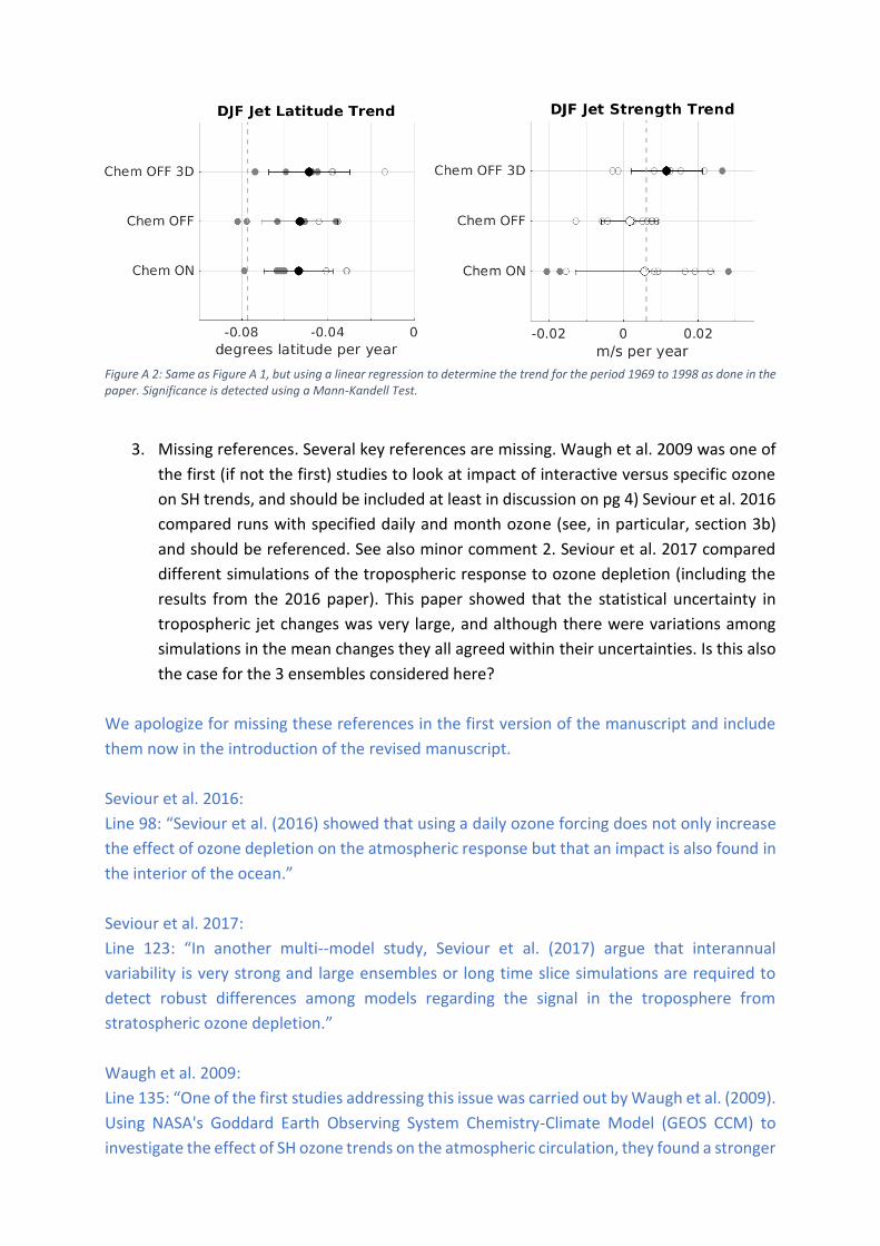
Figure A 2: Same as Figure A 1, but using a linear regression to determine the trend for the period 1969 to 1998 as done in the paper. Significance is detected using a Mann-Kandell Test.

3. Missing references. Several key references are missing. Waugh et al. 2009 was one of

the first (if not the first) studies to look at impact of interactive versus specific ozone

on SH trends, and should be included at least in discussion on pg 4) Seviour et al. 2016

compared runs with specified daily and month ozone (see, in particular, section 3b)

and should be referenced. See also minor comment 2. Seviour et al. 2017 compared

different simulations of the tropospheric response to ozone depletion (including the

results from the 2016 paper). This paper showed that the statistical uncertainty in

tropospheric jet changes was very large, and although there were variations among

simulations in the mean changes they all agreed within their uncertainties. Is this also

the case for the 3 ensembles considered here?

We apologize for missing these references in the first version of the manuscript and include

them now in the introduction of the revised manuscript.

Seviour et al. 2016:

Line 98: “Seviour et al. (2016) showed that using a daily ozone forcing does not only increase

the effect of ozone depletion on the atmospheric response but that an impact is also found in

the interior of the ocean.”

Seviour et al. 2017:

Line 123: “In another multi--model study, Seviour et al. (2017) argue that interannual

variability is very strong and large ensembles or long time slice simulations are required to

detect robust differences among models regarding the signal in the troposphere from

stratospheric ozone depletion.”

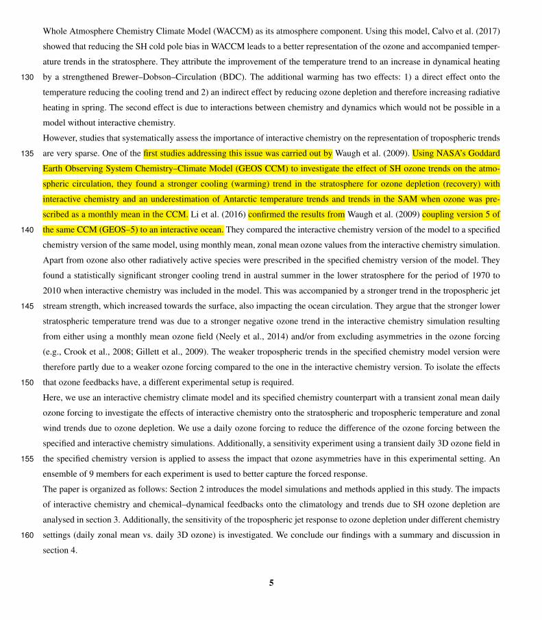
Waugh et al. 2009:

Line 135: “One of the first studies addressing this issue was carried out by Waugh et al. (2009).

Using NASA's Goddard Earth Observing System Chemistry-Climate Model (GEOS CCM) to

investigate the effect of SH ozone trends on the atmospheric circulation, they found a stronger

cooling (warming) trend in the stratosphere for ozone depletion (recovery) with interactive

chemistry and an underestimation of Antarctic temperature trends and trends in the SAM

when ozone was prescribed as a monthly mean in the CCM. Li et al. (2016) confirmed the

results from Waugh et al. (2009) coupling version 5 of the same CCM (GEOS-5) to an

interactive ocean. […]”

MINOR COMMENTS

Line 3: "differ largely" and Line 22 "crucial for representing" both appear to be

overstatements, both based on previous studies and this study. Yes there are

differences depending on the ozone but I am not sure can be classed as large or crucial.

We rephrased these sentences a follows:

- […] differ among climate models […]

- […] could also have an influence on the representation of […]

Line 10: "In contrast to earlier studies, we use daily-resolved ozone fields". This is not

the first study to use daily-resolved ozone (e.g. Neely et al, Seviour et al. 2016).

We deleted “In contrast to earlier studies” here and included the Seviour study in the

introduction of the revised manuscript.

Line 390, 445: Iyvanciu et al. (in prep). At the very least a paper needs to be submitted

before it can be referenced.

The paper is now submitted and will shortly be a discussion paper in ACP as well. We

adapted the reference accordingly.

Line 410: I don’t understand what is meant by "The LW heating rate trend does not

add more information".

We meant that the LW heating rate is only a response to the dynamical heating and the

SW heating and that it does not add more knowledge to why the patterns differ between

Chem ON and Chem OFF. To avoid confusion here, we rephrased the sentence by deleting

“does not add more infromation”.

“The LW heating rate trend (Fig. 12) dampens the signal from the dynamical heating rate

trend.”


Summary: I quite liked reviewing this paper. The authors systematically compared two

configurations of the same chemistry-climate model (CESM1-WACCM plus some

modifications) that differ in that one configuration has fully interactive ozone chemistry,

whereas the other uses prescribed ozone fields generated by the same model. The authors

also test the sensitivity to prescribing zonally symmetric versus zonally resolved ozone fields.

They find that the two model configurations produce qualitatively similar results but with

important quantitative differences, e.g. regarding the coupling of the polar vortex strength

with ozone depletion, timescales of variability of the Southern Annular Mode, an acceleration

of the westerlies in the Southern Hemisphere, etc. They find that prescribing zonally resolved

ozone produces results that are generally closer to those produced using interactive ozone.

The results are of interest to climate modellers weighing up whether to include interactive

ozone in climate projection simulations. Often the additional computational cost and scientific

effort needed to sustain this functionality are considered prohibitive.

There is a small number of other papers that characterize the advantages of interactively

simulating ozone, and often these papers involve comparisons that are not entirely balanced,

e.g. by comparing groups of different models. There is thus clearly a niche for this paper that

aims to quantify the differences between the two approaches with minimal interference from

other model differences (that are not ozone). (The authors do not divulge any details about

the computational costs of their three ensembles; maybe this small detail can be added.)

In a few places error bounds should be stated before an explanation is given for why two

quantities are different. Otherwise we cannot be sure that such differences are not

coincidental in nature.

Haase and Matthes (2019) are cited extensively. Perhaps the authors could elaborate a bit

more how the results produced here compare to the results shown in that reference. Do the

differences come down to the same mechanism in both hemispheres?

I could not discern whether the model is in a coupled atmosphere-ocean or an atmosphere-

only configuration. If it is coupled, do perhaps slow modes of oceanic variability influence the

results (that perhaps evolve differently in the different ensembles)?

I also agree with another reviewer that the title should be revised given the balance of

evidence presented in this paper. The SH tropospheric jet seems to be a relatively minor topic

here. While the authors state that HM19 is about NH results, they are cited in reference to SH

features too, so a bit more discussion about the key differences between the two papers

would be good to have.

The language is mostly fine (some minor style issues are listed below), the figures are

informative and about right in number, the conclusions are balanced. I thus recommend

publication in ACP once my comments are addressed.

Thank you for your comments and suggestions. As described above, we adapted the title and

included additional analysis on the tropospheric jet trend, specifically the trends in 850 hPa

jet latitude and strength.

It is stated in the manuscript that we use the fully-coupled model version (e.g., lines 8 and 182

in the first version of the manuscript). To make this clearer, we now explicitly state that an

interactive ocean is included.

Line 164: “CESM1(WACCM) is a fully coupled climate model with interactive ocean,

land and sea ice components.“

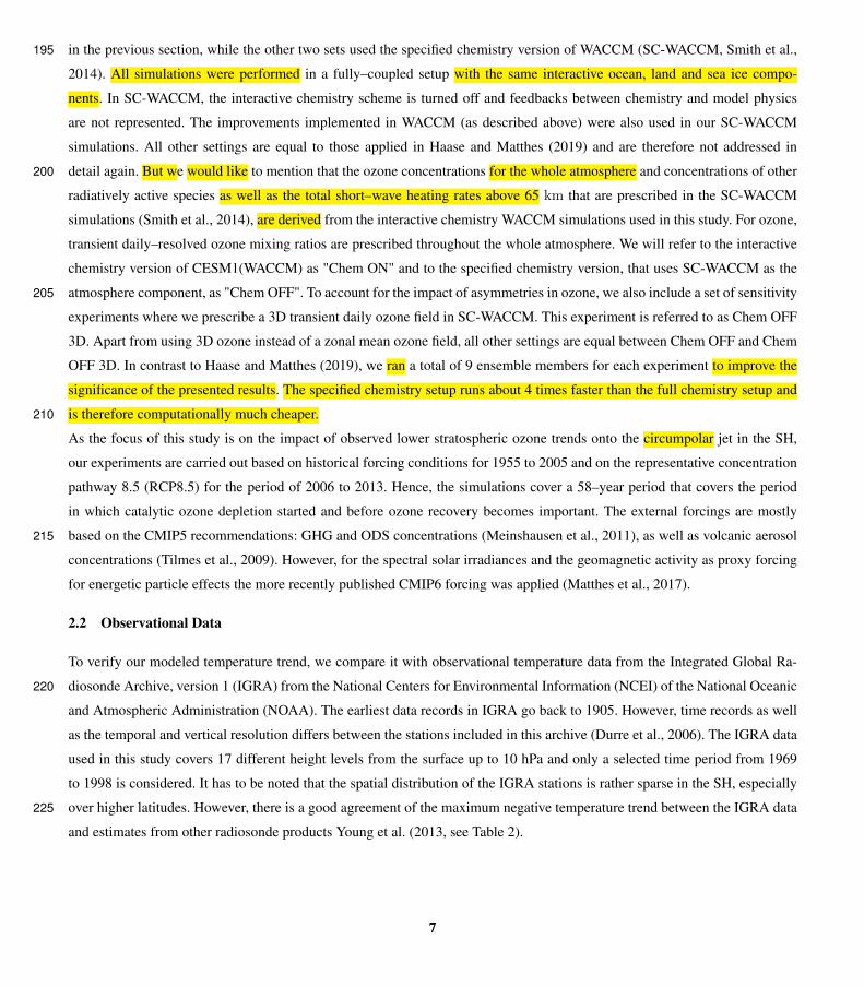
Line 196: “All simulations were performed in a fully–coupled setup with the same

interactive ocean, land and sea ice components.”

Possible impacts of the ocean on our results are now mentioned in the discussion part of the

paper. We suggest that these impacts are low following the findings of Gillett et al. 2019, but

cannot exclude that SST and sea ice biases might feed back onto the position of the

tropospheric jet stream.

Line 493: “However, the impact of interactive chemistry on the tropospheric jet could

not be validated by our study. This might be due to the weak stratosphere-

troposphere-coupling in the model that is indicated by the low tropospheric time scale

of the SAM. This feature might be connected to the interactive ocean, which shows

large biases in sea ice retreat in the seasonal cycle (Landrum et al. 2012; Marsh et al.

2013). However, a recent study by Gillett et al. (2019) showed that the response

between ozone depletion and the SAM was independent from coupling an interactive

ocean to WACCM or running it with observed SSTs.”

We included an additional sentence on the NH paper (Haase and Matthes 2019), but

otherwise think it is sufficiently covered already.

Line 89: “They found especially the negative feedback at the end of the winter season

to be important for the difference between specified and interactive chemistry

simulations, which led to a more rapid and earlier stratospheric vortex break-down in

the interactive chemistry simulations.”

We now include a remark on the computational costs of the different WACCM settings. Thank

you for this suggestion!

Line 209: “The specified chemistry setup runs about 4 times faster than the full

chemistry setup and is therefore computationally much cheaper.”

Minor comments:

L5 and line 63: I suggest to replace “accurate” with “appropriate”, “self-consistent” or similar.

Eyring et al. (2013) showed for CMIP5 models that interactive ozone models can fail to

produce “accurate” fields: (https://doi.org/10.1002/jgrd.50316)

We now use “appropriate”.

L52: Whether ozone recovery will ever be stronger than GHG influences may also be a function

of the assumed GHG scenario.

Yes, indeed. We included this point in the sentence:

“However, when exactly ozone recovery is strong enough to compensate GHG cooling is an

open question and also depends on future GHG levels.”

L62-72: A third, fairly widespread method is to use an online parameterization for ozone (i.e.

make ozone interactive but not use comprehensive chemistry). This route is followed in

several CMIP6 models, sometimes to the point that models with and without comprehensive-

chemistry ozone schemes are almost indistinguishable in their performances (e.g. CNRM

models). Given the results of this paper (showing that prescribing 3D ozone fields already

constitutes progress) I’d say that for some groups this might be the way forward.

Thank you for pointing this out. We now also mention this method in the introduction.

Line 106: “For example, an online parameterization or simplified online scheme for ozone can

be applied. This is a step in between a fully-interactive and a specified chemistry setup and

allows the ozone field to follow the dynamics to a certain degree, e.g., as in CNRM-CM6

(Voldoire et al. 2019) or E3SM-1-0 (Golaz et al. 2019).”

L89: Cut out “along”.

Thanks for the suggestion. We changed the sentence accordingly.

L153: Replace “as well as” with “like”.


L160: Replace “from the land fraction factor” with “on land fraction”.


L162-163: How do you know the cold-pole bias has been reduced in pre-industrial

simulations? Almost nothing is known about the pre-industrial stratosphere.

This sentence is referring to a model simulation only. We ran the two different WACCM

configuration (with and without the changes applied to the model code as described in the

paper) only under piControl conditions, unfortunately. We found that without the adaptations

to the model code the stratospheric polar vortex is colder and stronger under this piControl

conditions. We think it is appropriate to assume that under historical conditions a similar

weakening of the polar vortex is achieved when applying the same modifications to the model

code.

L236: Replace “It was shown in Haase and Matthes (2019)” with “HM19 showed”.

We changed the structure of the sentence as suggested but did not use the abbreviation since

it is introduced here.

L245: I don’t understand why the amplitude of the response should be smaller with a larger

ensemble. The mean response should be better defined as the ensemble size decreases.

Please expand / explain.

Of course, it depends on which ensemble member you compare to the ensemble mean. Since

the ensemble mean is an average, the individual members can show smaller or larger values

at a specific position and time. On the NH, which is showing strong variability on the

interannual scale individual members show strong differences, which differ only slightly in

time or space. Averaging will result in an overall lower amplitude. Often features in the NH

stratosphere are large in amplitude but small in significance since the impact of natural

variability is dominating.

For the SH, this might not always be the case since the strong trend signal is very similar

between the different individual members of an ensemble. For an example, we refer to the

supplementary figure on the SAM timescale, which shows the individual ensemble members

of the Chem ON simulation. Some of the individual model results show a much longer

timescale than the ensemble mean shown in the main body of the paper (only one member

shows a shorter time scale, three members agree in amplitude with the ensemble mean).

There is also a disagreement in timing of the longest SAM timescale in the stratosphere

between the ensemble members. Averaging these leads to a smaller amplitude but of course,

to a better defined mean response. We slightly changed the wording in the manuscript saying

that we do not find it unexpected to find a weaker response (line 266).

L330: Whether these numbers are indeed different requires some kind of analysis of the

statistical uncertainties. If they are not different within their uncertainty bounds, the

argument would fall apart.

Figure 7b shows that the trend difference between Chem ON and Chem OFF is significant

starting in December. We think that is sufficient to prove our argumentation.

L373ff: Note also https://doi.org/10.1002/2014JD023009 (Dennison et al. 2015) who also

studied stratospheric SAM variability and found an increase in variability under ozone

depletion.

Thank you for pointing that out. We included this reference in the revised manuscript.

Line 403: “Dennison et al. (2015), for example, showed that under ozone depletion the SAM

timescale is enhanced and stratosphere-troposphere-coupling is strengthened.”

L390ff: I don’t think it’s appropriate here to discuss an unpublished paper. If it has meanwhile

been published (but perhaps not fully peer-reviewed) that would be OK. If not, I suggest to

remove this section.

The mentioned paper is submitted to ACPD now, too. We updated the reference.

L399: I’m sure the “polar stereographic” map projections are not relevant here, but rather the

physical quantities / questions that you want to address. Which fields are you assessing here?

We revised this sentence as follows:

Line 433: “To better understand the improvement in the Chem OFF 3D ensemble over the

Chem OFF ensemble we consider spatially asymmetric trends of temperature, SW, LW and

dynamical heating rates in the following.”

L447: Please spell out code availability, a requirement for publication in ACP.

We include this now in the dedicated section.


This paper reported simulations of the climate responses to ozone depletion by WACCM, and

compared the ones with interactive chemistry schemes with those prescribing zonal and 3d

daily ozone. Each experiment consists of 9 ensembles with fully coupled ocean. It is found that

interactive chemistry produces stronger stratospheric cooling, stronger strengthening of the

polar night jet, and stronger poleward shift of the tropospheric jet, despite of the identical

changes in ozone and shortwave heating rates. The authors attribute the difference to a

chemistry-dynamics feedback that is absent when ozone is prescribed. This work highlights

the importance to include the interactive chemistry into the climate simulations, and sheds

light on understanding the complex coupling between the stratospheric ozone and the climate

system. The paper is logically organized and well written. I am not fully convinced by the

mechanisms the authors provided to explain the “chemistry-dynamics feedback”, but I do

think the results deserve publication. Below is my detailed comments:

1. The authors suggested that there is both positive and negative feedbacks between

ozone changes and dynamics, which occurs at different seasons and levels, which

involves the background zonal wind condition and wave-mean flow interaction.

However, it is not clear why interactive chemistry and specified chemistry would

behave different based on this mechanism. Both of them have the same changes in

ozone and SW heating rates, then the initial changes in the zonal winds should also be

similar since that simply follows the thermal wind balance. Wave-mean flow

interaction would also work in a similar fashion in the two experiments.

In the specified chemistry setting, the ozone concentration is not dependent on the dynamics

as it is the case for the interactive chemistry simulations. For example, the strength of the

Brewer Dobson Circulation does not influence the ozone concentrations in Chem OFF, but it

does in Chem ON. While a strong BDC in Chem ON would lead to a higher ozone concentration

and therefore to a warming anomaly due to dynamics and ozone abundances, in Chem OFF

only the dynamical warming would be guaranteed. By chance there might be also a higher

ozone abundance but that is not necessarily the case since dynamics and chemistry are not

coupled in Chem OFF. On the other hand, if there is an extreme high ozone year prescribed to

Chem OFF, this will also be associated by a positive temperature anomaly due to radiative

heating when sufficient solar energy is available, i.e. only the spring season (and early winter

maybe) can effectively be affected by this. During such high ozone conditions, a cold winter

vortex is still possible in Chem OFF, whereas unlikely in Chem ON.

We therefore think that the comparison of Chem ON and Chem OFF reveals feedbacks as

discussed in the paper.

2. The mechanism for the “positive feedback” over the lower stratosphere in Nov/Dec is

especially unclear, which is a key component to explain the stronger cooling seen in

the interactive chemistry simulations. If the authors are referring to the positive

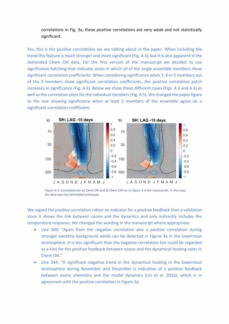
correlations in Fig. 3a, these positive correlations are very weak and not statistically

significant.

Yes, this is the positive correlations we are talking about in the paper. When including the

trend this feature is much stronger and more significant (Fig. A 3), but it is also apparent in the

detrended Chem ON data. For the first version of the manuscript we decided to use

significance hatching that indicates areas in which all of the single ensemble members show

significant correlation coefficients. When considering significance when 7, 6 or 5 members out

of the 9 members show significant correlation coefficients, the positive correlation patch

increases in significance (Fig. A 4). Below we show these different cases (Figs. A 3 and A 4) as

well as the correlation plots for the individual members (Fig. A 5). We changed the paper figure

to the one showing significance when at least 5 members of the ensemble agree on a

significant correlation coefficient.

We regard the positive correlation rather an indicator for a positive feedback than a validation

since it shows the link between ozone and the dynamics and only indirectly includes the

temperature response. We changed the wording in the manuscript where appropriate:

Line 300: “Apart from the negative correlation also a positive correlation during

stronger westerly background winds can be detected in Figure 3a in the lowermost

stratosphere. It is less significant than the negative correlation but could be regarded

as a hint for the positive feedback between ozone and the dynamical heating rates in

Chem ON.”

Line 344: “A significant negative trend in the dynamical heating in the lowermost

stratosphere during November and December is indicative of a positive feedback

between ozone chemistry and the model dynamics (Lin et al. 2016), which is in

agreement with the positive correlation in Figure 3a.

a) b)

Figure A 3: Correlation for a) Chem ON and b) Chem OFF as in Figure 3 in the manuscript. In this case, the data was not detrended previously.

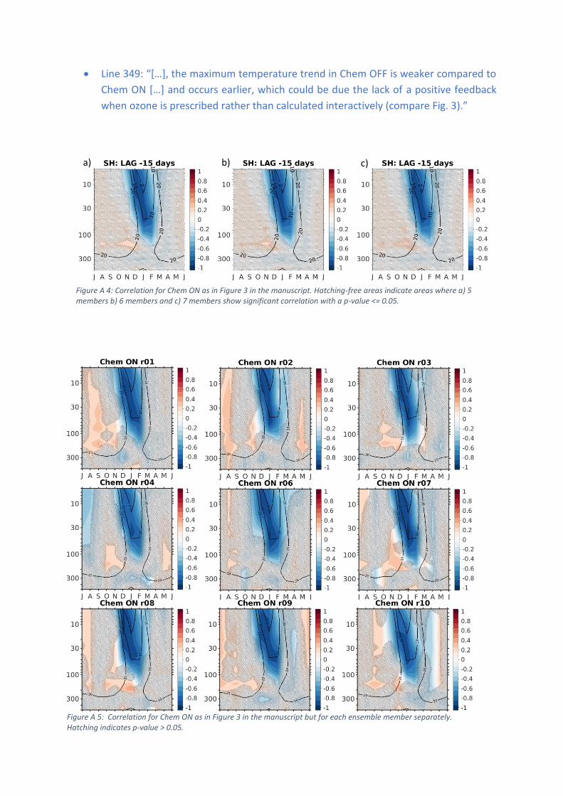
Line 349: “[…], the maximum temperature trend in Chem OFF is weaker compared to

Chem ON […] and occurs earlier, which could be due the lack of a positive feedback

when ozone is prescribed rather than calculated interactively (compare Fig. 3).”

a) b) c)

Figure A 4: Correlation for Chem ON as in Figure 3 in the manuscript. Hatching-free areas indicate areas where a) 5 members b) 6 members and c) 7 members show significant correlation with a p-value <= 0.05.

Figure A 5: Correlation for Chem ON as in Figure 3 in the manuscript but for each ensemble member separately. Hatching indicates p-value > 0.05.

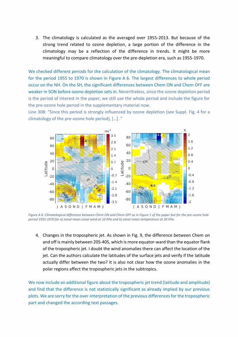
3. The climatology is calculated as the averaged over 1955-2013. But because of the

strong trend related to ozone depletion, a large portion of the difference in the

climatology may be a reflection of the difference in trends. It might be more

meaningful to compare climatology over the pre-depletion era, such as 1955-1970.

We checked different periods for the calculation of the climatology. The climatological mean

for the period 1955 to 1970 is shown in Figure A 6. The largest differences to whole period

occur on the NH. On the SH, the significant differences between Chem ON and Chem OFF are

weaker in SON before ozone depletion sets in. Nevertheless, since the ozone depletion period

is the period of interest in the paper, we still use the whole period and include the figure for

the pre-ozone hole period in the supplementary material now.

Line 308: “Since this period is strongly influenced by ozone depletion (see Suppl. Fig. 4 for a

climatology of the pre-ozone hole period), […] .”

Figure A 6: Climatological difference between Chem ON and Chem OFF as in Figure 1 of the paper but for the pre-ozone hole period 1955-1970 for a) zonal mean zonal wind at 10 hPa and b) zonal mean temperature at 30 hPa.

4. Changes in the tropospheric jet. As shown in Fig. 9, the difference between Chem on

and off is mainly between 20S-40S, which is more equator-ward than the equator flank

of the tropospheric jet. I doubt the wind anomalies there can affect the location of the

jet. Can the authors calculate the latitudes of the surface jets and verify if the latitude

actually differ between the two? It is also not clear how the ozone anomalies in the

polar regions affect the tropospheric jets in the subtropics.

We now include an additional figure about the tropospheric jet trend (latitude and amplitude)

and find that the difference is not statistically significant as already implied by our previous

plots. We are sorry for the over-interpretation of the previous differences for the tropospheric

part and changed the according text passages.

5. Line 301-303: The first sentence here seems to suggest both the model used here and

WACCM4 have stronger trends than WACCM-CCMI. But the second sentence suggests

the opposite.

We rephrased the sentence:

Line 324: “The reduction in the trend from WACCM4 to WACCM-CCMI ca be […]”


Review of “Sensitivity of the southern hemisphere tropospheric jet response to Antarctic

ozone depletion: prescribed versus interactive chemistry” by Haase et al.

This paper investigates how Antarctic stratosphere and troposphere mean climate and climate

change is affected by the model representation of Antarctic ozone. Three ensembles were

performed for the 1955-2013 period using CESM with different ozone approach: interactive

ozone, prescribed zonal-mean daily ozone, and prescribed 3D daily ozone. The results are

consistent with previous studies that interactive ozone causes stronger Antarctic lower

stratospheric cooling and stronger stratospheric jet response in austral summer.

This paper advances the understanding of the effects of interactive ozone on Antarctic climate

change. Specifically, it emphasizes the role of reduced dynamical heating in causing Antarctic

lower stratospheric cooling with interactive ozone. It also quantifies the impact of ozone-

dynamics feedbacks and ozone zonal asymmetry on simulated temperature and jet trends.

However, I think the authors’ interpretation of how interactive ozone affects tropospheric jet

trends needs to be clarified.

Major Comments:

I don’t think the results presented in Figure 9 support the conclusion that interactive ozone

leads to stronger poleward shift of the tropospheric jet. Figure 9 shows that interactive ozone

does not significantly influence the tropospheric jet trends poleward of 40S. Significantly

different tropospheric jet trends are only found between 20S and 40S (Fig. 9c), where the

westerly trends are weaker in the interactive ozone simulations than in the prescribed ozone

simulations. It would be useful to find out why interactive and prescribed ozone simulate

different tropospheric subtropical jet trends.

However, the major point is that the large stratospheric circumpolar jet differences between

interactive and prescribed ozone simulations do not propagate downward into the

troposphere.

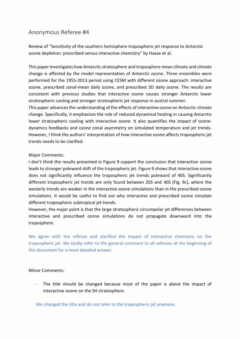
We agree with the referee and clarified the impact of interactive chemistry on the

tropospheric jet. We kindly refer to the general comment to all referees at the beginning of

this document for a more detailed answer.

Minor Comments:

- The title should be changed because most of the paper is about the impact of

interactive ozone on the SH stratosphere.

We changed the title and do not refer to the tropospheric jet anymore.

- Lines 251-252: Why interactive ozone causes a weaker shallow BDC branch?

We think that the weaker shallow branch of the BDC is due to the fact the polar vortex is

stronger in the Chem ON simulation leading to a reduced wave forcing and hence to a

weakening of the BDC. Such a signature is evident in the shallow branch of the BDC (w* at

50 and 70 hPa in the Supplement). The response of the shallow branch could be due to

the fact that this branch is faster reacting to changes in wave-breaking. To understand the

process better, though, it might be necessary to investigate tropical upwelling. In our

analysis, we did not consider the tropics so far.

- In some occasions, PNJ should be replaced with circumpolar jet.

We carefully went through the manuscript and changed PNJ to circumpolar jet where we

thought it appropriate. See, for example lines 278, 283, and 303.

Susan Solomon (Referee)

This is an interesting and timely paper attacking an important problem. The findings are novel

and certainly merit publication. I do have a number of questions and comments that I hope

the authors find helpful in revising their paper. I don’t think these suggestions are necessary

since the paper is already quite good, but I do think they may make it clearer and stronger.

Substantive comments

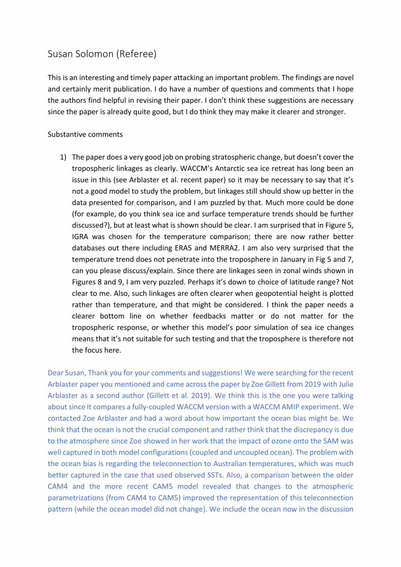
1) The paper does a very good job on probing stratospheric change, but doesn’t cover the

tropospheric linkages as clearly. WACCM’s Antarctic sea ice retreat has long been an

issue in this (see Arblaster et al. recent paper) so it may be necessary to say that it’s

not a good model to study the problem, but linkages still should show up better in the

data presented for comparison, and I am puzzled by that. Much more could be done

(for example, do you think sea ice and surface temperature trends should be further

discussed?), but at least what is shown should be clear. I am surprised that in Figure 5,

IGRA was chosen for the temperature comparison; there are now rather better

databases out there including ERA5 and MERRA2. I am also very surprised that the

temperature trend does not penetrate into the troposphere in January in Fig 5 and 7,

can you please discuss/explain. Since there are linkages seen in zonal winds shown in

Figures 8 and 9, I am very puzzled. Perhaps it’s down to choice of latitude range? Not

clear to me. Also, such linkages are often clearer when geopotential height is plotted

rather than temperature, and that might be considered. I think the paper needs a

clearer bottom line on whether feedbacks matter or do not matter for the

tropospheric response, or whether this model’s poor simulation of sea ice changes

means that it’s not suitable for such testing and that the troposphere is therefore not

the focus here.

Dear Susan, Thank you for your comments and suggestions! We were searching for the recent

Arblaster paper you mentioned and came across the paper by Zoe Gillett from 2019 with Julie

Arblaster as a second author (Gillett et al. 2019). We think this is the one you were talking

about since it compares a fully-coupled WACCM version with a WACCM AMIP experiment. We

contacted Zoe Arblaster and had a word about how important the ocean bias might be. We

think that the ocean is not the crucial component and rather think that the discrepancy is due

to the atmosphere since Zoe showed in her work that the impact of ozone onto the SAM was

well captured in both model configurations (coupled and uncoupled ocean). The problem with

the ocean bias is regarding the teleconnection to Australian temperatures, which was much

better captured in the case that used observed SSTs. Also, a comparison between the older

CAM4 and the more recent CAM5 model revealed that changes to the atmospheric

parametrizations (from CAM4 to CAM5) improved the representation of this teleconnection

pattern (while the ocean model did not change). We include the ocean now in the discussion

(line 496) but do not think that it is the main reason for the relatively weak coupling to the

troposphere.

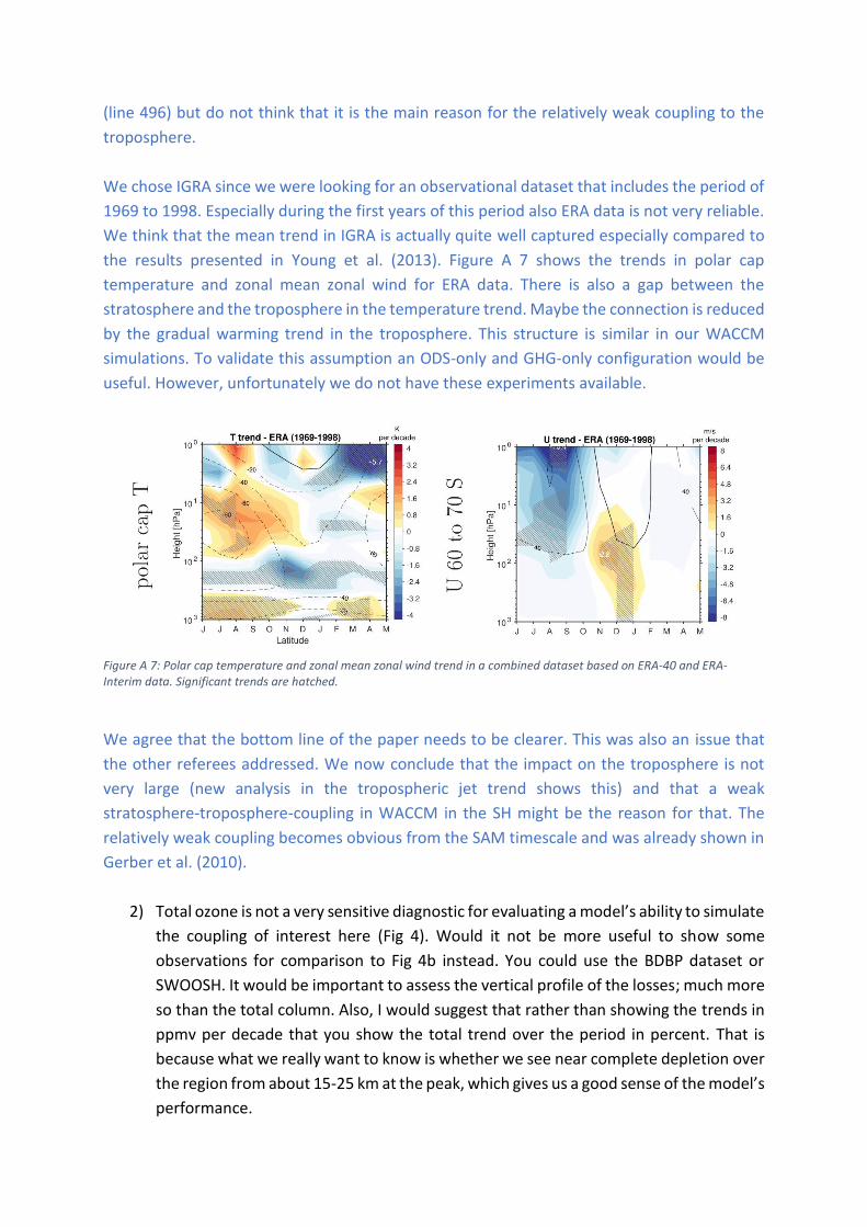
We chose IGRA since we were looking for an observational dataset that includes the period of

1969 to 1998. Especially during the first years of this period also ERA data is not very reliable.

We think that the mean trend in IGRA is actually quite well captured especially compared to

the results presented in Young et al. (2013). Figure A 7 shows the trends in polar cap

temperature and zonal mean zonal wind for ERA data. There is also a gap between the

stratosphere and the troposphere in the temperature trend. Maybe the connection is reduced

by the gradual warming trend in the troposphere. This structure is similar in our WACCM

simulations. To validate this assumption an ODS-only and GHG-only configuration would be

useful. However, unfortunately we do not have these experiments available.

Figure A 7: Polar cap temperature and zonal mean zonal wind trend in a combined dataset based on ERA-40 and ERA-Interim data. Significant trends are hatched.

We agree that the bottom line of the paper needs to be clearer. This was also an issue that

the other referees addressed. We now conclude that the impact on the troposphere is not

very large (new analysis in the tropospheric jet trend shows this) and that a weak

stratosphere-troposphere-coupling in WACCM in the SH might be the reason for that. The

relatively weak coupling becomes obvious from the SAM timescale and was already shown in

Gerber et al. (2010).

2) Total ozone is not a very sensitive diagnostic for evaluating a model’s ability to simulate

the coupling of interest here (Fig 4). Would it not be more useful to show some

observations for comparison to Fig 4b instead. You could use the BDBP dataset or

SWOOSH. It would be important to assess the vertical profile of the losses; much more

so than the total column. Also, I would suggest that rather than showing the trends in

ppmv per decade that you show the total trend over the period in percent. That is

because what we really want to know is whether we see near complete depletion over

the region from about 15-25 km at the peak, which gives us a good sense of the model’s

performance.

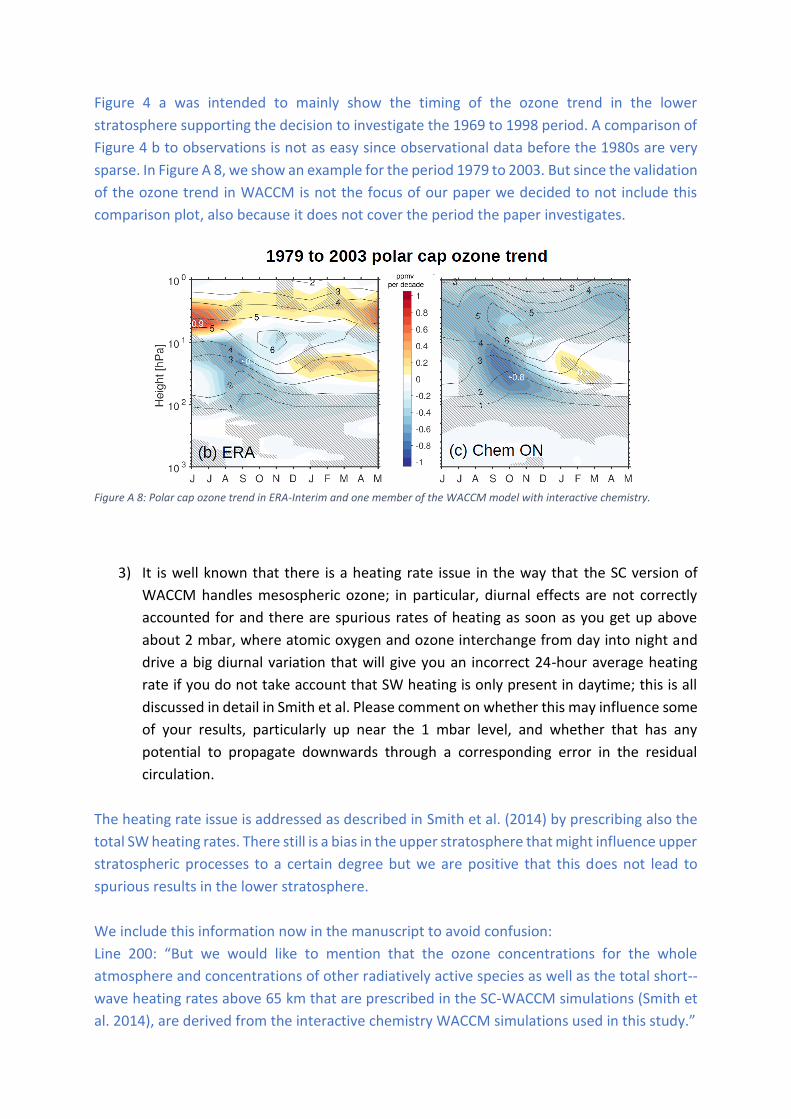
Figure 4 a was intended to mainly show the timing of the ozone trend in the lower

stratosphere supporting the decision to investigate the 1969 to 1998 period. A comparison of

Figure 4 b to observations is not as easy since observational data before the 1980s are very

sparse. In Figure A 8, we show an example for the period 1979 to 2003. But since the validation

of the ozone trend in WACCM is not the focus of our paper we decided to not include this

comparison plot, also because it does not cover the period the paper investigates.

Figure A 8: Polar cap ozone trend in ERA-Interim and one member of the WACCM model with interactive chemistry.

3) It is well known that there is a heating rate issue in the way that the SC version of

WACCM handles mesospheric ozone; in particular, diurnal effects are not correctly

accounted for and there are spurious rates of heating as soon as you get up above

about 2 mbar, where atomic oxygen and ozone interchange from day into night and

drive a big diurnal variation that will give you an incorrect 24-hour average heating

rate if you do not take account that SW heating is only present in daytime; this is all

discussed in detail in Smith et al. Please comment on whether this may influence some

of your results, particularly up near the 1 mbar level, and whether that has any

potential to propagate downwards through a corresponding error in the residual

circulation.

The heating rate issue is addressed as described in Smith et al. (2014) by prescribing also the

total SW heating rates. There still is a bias in the upper stratosphere that might influence upper

stratospheric processes to a certain degree but we are positive that this does not lead to

spurious results in the lower stratosphere.

We include this information now in the manuscript to avoid confusion:

Line 200: “But we would like to mention that the ozone concentrations for the whole

atmosphere and concentrations of other radiatively active species as well as the total short--

wave heating rates above 65 km that are prescribed in the SC-WACCM simulations (Smith et

al. 2014), are derived from the interactive chemistry WACCM simulations used in this study.”

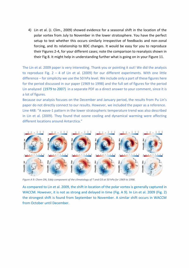
4) Lin et al. (J. Clim., 2009) showed evidence for a seasonal shift in the location of the

polar vortex from July to November in the lower stratosphere. You have the perfect

setup to test whether this occurs similarly irrespective of feedbacks and non-zonal

forcing, and its relationship to BDC changes. It would be easy for you to reproduce

their Figures 2-4, for your different cases; note the comparison to reanalysis shown in

their Fig 8. It might help in understanding further what is going on in your Figure 11.

The Lin et al. 2009 paper is very interesting. Thank you or pointing it out! We did the analysis

to reproduce Fig. 2 – 4 of Lin et al. (2009) for our different experiments. With one little

difference – for simplicity we use the 50 hPa level. We include only a part of these figures here

for the period discussed in our paper (1969 to 1998) and the full set of figures for the period

Lin analyzed (1979 to 2007) in a separate PDF as a direct answer to your comment, since it is

a lot of figures.

Because our analysis focuses on the December and January period, the results from Pu Lin’s

paper do not directly connect to our results. However, we included the paper as a reference.

Line 448: “A wave-1 pattern in the lower stratospheric temperature trend was also described

in Lin et al. (2009). They found that ozone cooling and dynamical warming were affecting

different locations around Antarctica.”

Figure A 9: Chem ON, Eddy component of the climatology of T and O3 at 50 hPa for 1969 to 1998.

As compared to Lin et al. 2009, the shift in location of the polar vortex is generally captured in

WACCM. However, it is not as strong and delayed in time (Fig. A 9). In Lin et al. 2009 (Fig. 2)

the strongest shift is found from September to November. A similar shift occurs in WACCM

from October until December.

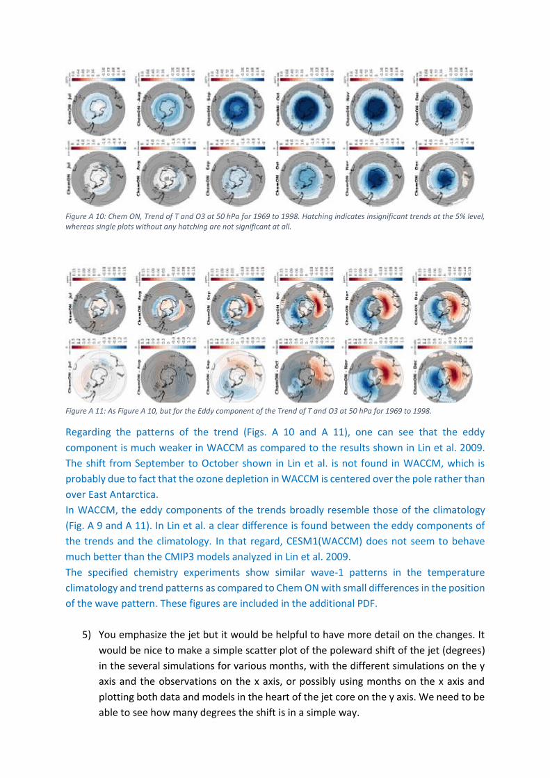
Figure A 10: Chem ON, Trend of T and O3 at 50 hPa for 1969 to 1998. Hatching indicates insignificant trends at the 5% level, whereas single plots without any hatching are not significant at all.

Figure A 11: As Figure A 10, but for the Eddy component of the Trend of T and O3 at 50 hPa for 1969 to 1998.

Regarding the patterns of the trend (Figs. A 10 and A 11), one can see that the eddy

component is much weaker in WACCM as compared to the results shown in Lin et al. 2009.

The shift from September to October shown in Lin et al. is not found in WACCM, which is

probably due to fact that the ozone depletion in WACCM is centered over the pole rather than

over East Antarctica.

In WACCM, the eddy components of the trends broadly resemble those of the climatology

(Fig. A 9 and A 11). In Lin et al. a clear difference is found between the eddy components of

the trends and the climatology. In that regard, CESM1(WACCM) does not seem to behave

much better than the CMIP3 models analyzed in Lin et al. 2009.

The specified chemistry experiments show similar wave-1 patterns in the temperature

climatology and trend patterns as compared to Chem ON with small differences in the position

of the wave pattern. These figures are included in the additional PDF.

5) You emphasize the jet but it would be helpful to have more detail on the changes. It

would be nice to make a simple scatter plot of the poleward shift of the jet (degrees)

in the several simulations for various months, with the different simulations on the y

axis and the observations on the x axis, or possibly using months on the x axis and

plotting both data and models in the heart of the jet core on the y axis. We need to be

able to see how many degrees the shift is in a simple way.

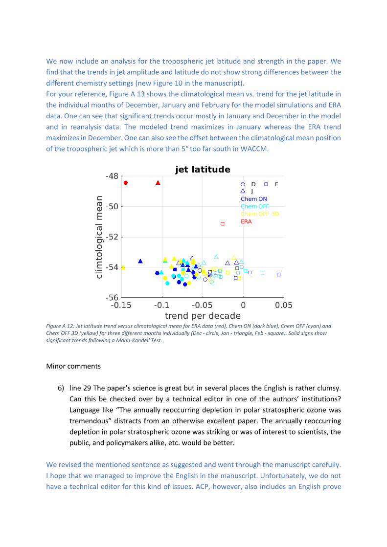
We now include an analysis for the tropospheric jet latitude and strength in the paper. We

find that the trends in jet amplitude and latitude do not show strong differences between the

different chemistry settings (new Figure 10 in the manuscript).

For your reference, Figure A 13 shows the climatological mean vs. trend for the jet latitude in

the individual months of December, January and February for the model simulations and ERA

data. One can see that significant trends occur mostly in January and December in the model

and in reanalysis data. The modeled trend maximizes in January whereas the ERA trend

maximizes in December. One can also see the offset between the climatological mean position

of the tropospheric jet which is more than 5° too far south in WACCM.

Figure A 12: Jet latitude trend versus climatological mean for ERA data (red), Chem ON (dark blue), Chem OFF (cyan) and Chem OFF 3D (yellow) for three different months individually (Dec - circle, Jan - triangle, Feb - square). Solid signs show significant trends following a Mann-Kandell Test.

Minor comments

6) line 29 The paper’s science is great but in several places the English is rather clumsy.

Can this be checked over by a technical editor in one of the authors’ institutions?

Language like “The annually reoccurring depletion in polar stratospheric ozone was

tremendous” distracts from an otherwise excellent paper. The annually reoccurring

depletion in polar stratospheric ozone was striking or was of interest to scientists, the

public, and policymakers alike, etc. would be better.

We revised the mentioned sentence as suggested and went through the manuscript carefully.

I hope that we managed to improve the English in the manuscript. Unfortunately, we do not

have a technical editor for this kind of issues. ACP, however, also includes an English prove

reading after acceptance of the manuscript, which hopefully helps with the most clumsy

wordings.

7) line 30 Political action was taken to ban the responsible substances (termed: ozone

depleting substances, ODSs) under the Montreal Protocol in 1987 is incorrect. Political

action was begun that ultimately led to a ban on the responsible substances (termed:

ozone depleting substances, ODSs) under the Montreal Protocol in 1987. The original

Protocol in 1987 did not mandate a ban, only a freeze on emission at then-current

rates.

Thank you for the comment. We corrected the sentence!

8) line 37 Need a reference to the first paper showing this by Shine (GRL, 1986).

We included the missing reference. Thank you pointing it out!

9) line 103 Please clarify what the shortcoming of Rae et al. is; this is not very clear here.

How does it work and why doesn’t it capture heterogeneous loss?

The aim of their method is to generate a zonally asymmetric ozone field that is consistent with

the model dynamics from a prescribed zonal mean ozone field while maintaining the

climatological zonal mean as prescribed. They use potential vorticity asymmetries to generate

an asymmetry-scaling coefficient factor to apply to the prescribed zonal mean ozone. Since

this method depends on the spatial pattern of PV, heterogeneous loss is not directly covered.

So, only when ozone is following the dynamics, the method works properly. For more details

we have to refer to the study of Rae et al. (2019).

We revised the section in the manuscript as follows:

Line 111: “Also worth mentioning is Rae et al. (2019), who designed a computationally efficient

method to interactively re-scale prescribed ozone values to a dynamically model--consistent

3D ozone field based on the potential vorticity field of the model. This method, unfortunately,

is not well suited to represent the observed SH ozone depletion since it follows a solely

dynamical approach and has therefore difficulties to account for heterogeneous chemistry

processes.”

References

Gerber, E. P., and Coauthors, 2010: Stratosphere-troposphere coupling and annular mode variability in chemistry-climate models. J. Geophys. Res., 115, D00M06, doi:10.1029/2009JD013770.

Gillett, Z. E., and Coauthors, 2019: Evaluating the relationship between interannual variations in the Antarctic ozone hole and Southern Hemisphere surface climate in Chemistry-Climate Models. J. Clim., 32, 3131–3151, doi:10.1175/JCLI-D-18-0273.1.

Lin, P., Q. Fu, S. Solomon, and J. M. Wallace, 2009: Temperature Trend Patterns in Southern Hemisphere High Latitudes: Novel Indicators of Stratospheric Change. J. Clim., 22, 6325–6341, doi:10.1175/2009JCLI2971.1.

Rae, C. D., J. Keeble, P. Hitchcock, and J. A. Pyle, 2019: Prescribing Zonally Asymmetric Ozone Climatologies in Climate Models: Performance Compared to a Chemistry-Climate Model. J. Adv. Model. Earth Syst., 11, 918–933, doi:10.1029/2018MS001478. https://onlinelibrary.wiley.com/doi/abs/10.1029/2018MS001478.

Seviour, W. J. M. M., D. W. Waugh, L. M. Polvani, G. J. P. P. Correa, and C. I. Garfinkel, 2017: Robustness of the Simulated Tropospheric Response to Ozone Depletion. J. Clim., 30, 2577–2585, doi:10.1175/JCLI-D-16-0817.1.

Smith, K. L., R. R. Neely, D. R. Marsh, and L. M. Polvani, 2014: The Specified Chemistry Whole Atmosphere Community Climate Model (SC-WACCM). J. Adv. Model. Earth Syst., 6, 883–901, doi:10.1002/2014MS000346.

Young, P. J., A. H. Butler, N. Calvo, L. Haimberger, P. J. Kushner, D. R. Marsh, W. J. Randel, and K. H. Rosenlof, 2013: Agreement in late twentieth century southern hemisphere stratospheric temperature trends in observations and ccmval-2, CMIP3, and CMIP5 models. J. Geophys. Res. Atmos., 118, 605–613, doi:10.1002/jgrd.50126.

Sensitivity of the southern hemisphere circumpolar jet response toAntarctic ozone depletion: prescribed versus interactive chemistrySabine Haase1, Jaika Fricke1, Tim Kruschke2, Sebastian Wahl1, and Katja Matthes1,3

1GEOMAR Helmholtz Center for Ocean Research Kiel, Kiel, Germany2Swedish Meteorological and Hydrological Institute - Rossby Centre, Norrköping, Sweden3Christian-Albrechts-Universität zu Kiel, Kiel, Germany

Correspondence: Sabine Haase ([email protected])

Abstract. Southern hemisphere lower stratospheric ozone depletion has been shown to lead to a poleward shift of the tropo-

spheric jet stream during austral summer, influencing surface atmosphere and ocean conditions, such as surface temperatures

and sea ice extent. The characteristics of stratospheric and tropospheric responses to ozone depletion, however, differ among

climate models depending on the representation of ozone in the models.

The most appropriate way to represent ozone in a model is to calculate it interactively. However, due to computational costs,5

in particular for long–term coupled ocean–atmosphere model integrations, the more common way is to prescribe ozone from

observations or calculated model fields. Here, we investigate the difference between an interactive and a specified chemistry

version of the same atmospheric model in a fully–coupled setup using a 9–member chemistry–climate model ensemble. In

the specified chemistry version of the model the ozone fields are prescribed using the output from the interactive chemistry

model version. We use daily–resolved ozone fields in the specified chemistry simulations to achieve a very good comparability10

between the ozone forcing with and without interactive chemistry. We find that although the short–wave heating rate trend in

response to ozone depletion is the same in the different chemistry settings, the interactive chemistry ensemble shows a stronger

trend in polar cap stratospheric temperatures (by about 0.7 Kdecade−1) and circumpolar stratospheric zonal mean zonal winds

(by about 1.6 ms−1 decade−1) as compared to the specified chemistry ensemble. This difference between interactive and spec-

ified chemistry in the stratospheric response to ozone depletion also affects the tropospheric response. However, an impact on15

the poleward shift of the tropospheric jet stream is not detected.

We attribute part of the differences found in the experiments to the missing representation of feedbacks between chemistry and

dynamics in the specified chemistry ensemble, which affect the dynamical heating rates, and part of it to the lack of spatial

asymmetries in the prescribed ozone fields. This effect is investigated using a sensitivity ensemble that was forced by a three–

dimensional instead of a two–dimensional ozone field.20

This study emphasizes the value of interactive chemistry for the representation of the southern hemisphere stratospheric jet

response to ozone depletion and infers that for periods with strong ozone variability (trends) the details of the ozone forcing

could also have an influence on the representation of southern hemispheric climate variability.

1

Copyright statement.

1 Introduction25

The last two decades of the 20th century were characterized by a strong loss in polar lower stratospheric ozone during spring

through catalytic heterogeneous chemical processes involving anthropogenically released halogenated compounds, such as

those including chlorine and bromine (Solomon et al., 2014). Ozone depletion was especially strong in the southern hemi-

sphere (SH) due to more favourable environmental conditions, i.e. a very stable, strong and cold polar stratospheric vortex.

The annually reoccurring depletion in polar stratospheric ozone was striking. Political action was begun that ultimately led to30

a ban on the responsible substances (termed: ozone depleting substances, ODSs) under the Montreal Protocol in 1987. Nev-

ertheless, due to their long lifetimes, ODSs still influence chemistry and radiation balances in the atmosphere and SH spring

ozone concentrations will remain low until the middle of the 21st century. Latest simulations from the Chemistry–Climate

Model Initiative (CCMI) predict the return of polar Antarctic total column ozone to 1980 values for the period of 2055 to 2066

(Dhomse et al., 2018).35

The enhanced ozone depletion during SH spring is enabled by the formation of polar stratospheric clouds, acting as a surface

for heterogeneous chemistry, activating halogens from ODSs that catalytically destroy ozone when the Sun comes back to the

high latitudes in spring (Solomon et al., 1986). Ozone depletion positively feeds back on the anomalously low temperatures in

the lower polar stratosphere by reducing the absorption of solar radiation in that region (e.g., Shine, 1986; Ramaswamy et al.,

1996; Randel and Wu, 1999), which in turn can lead to enhanced ozone depletion. In addition to ozone depletion, also the40

increase in greenhouse gas (GHG) concentrations contributes to low temperatures in the stratosphere (Fels et al., 1980). How-

ever, while ozone depletion and the connected radiative cooling are constrained mainly to the lower stratosphere, GHG–induced

cooling spreads throughout the whole stratosphere. Both cooling effects can therefore have an influence on the dynamics of the

stratosphere and possibly also on the troposphere. During the last decades of the 20th century, along with the ozone depletion,

a positive trend in the Southern Annular Mode (SAM) was observed (Thompson and Solomon, 2002). This trend is connected45

to a strengthening and a poleward shift of the tropospheric jet (see reviews by, e.g., Thompson et al., 2011; Previdi and Polvani,

2014), that also affects the Southern Ocean (e.g., Sigmond and Fyfe, 2010; Ferreira et al., 2015). There have been a number of

model studies aiming at separating the influence of GHGs and ODSs onto this observed trend of the tropospheric jet, i.e. the

SAM (e.g., McLandress et al., 2011; Polvani et al., 2011b; Morgenstern et al., 2014; Solomon et al., 2017). McLandress et al.

(2011), for example, found that the observed SH ozone depletion had a significant impact onto the positive SAM trend during50

austral summer (December to February, DJF). Several studies agree that during this time of the year the impact from ODSs

dominates over that from GHGs (e.g., McLandress et al., 2011; Polvani et al., 2011b; Solomon et al., 2017). Under ozone

recovery conditions, that are projected for the upcoming decades, the radiative heating effects of ozone (positive) and GHGs

(negative) will counteract each other (McLandress et al., 2011; Polvani et al., 2011a). However, when exactly ozone recovery is

strong enough to compensate GHG cooling is an open question and also depends on future GHG levels. Recent studies discuss55

the possibility that polar stratospheric ozone recovery started already (Solomon et al., 2016; Kuttippurath and Nair, 2017). The

2

recovery signal, however, is hard to detect and the impact of low ozone concentrations especially at polar southern latitudes

will continue to influence atmospheric circulation in the near future (Bednarz et al., 2016).

A better understanding of the interaction between ozone chemistry and atmospheric dynamics is therefore crucial for future

climate simulations. The way ozone is represented in climate models has a large impact onto the model’s ability to simulate60

interactions between chemistry and dynamics. With this study we want to improve the knowledge about chemistry–climate

interactions in the past to shed light onto how important the representation of ozone in climate models is also for future climate

projections.

There are different ways to represent ozone in climate models: 1) Ozone can be calculated interactively using a chemistry

scheme within a climate model. This is computationally very expensive, but the most appropriate representation of ozone and65

other trace gases, linking them directly with the radiation code and model dynamics. Models that implement such a chemistry

scheme are referred to as chemistry–climate models (CCMs) and are commonly used for stratospheric applications such as in

the WCRP–SPARC initiatives and the WMO ozone assessment reports. 2) Another way to represent ozone in a climate model

is to prescribe it based on observed and/or modeled ozone fields, as provided, for example, by the IGAC/SPARC initiatives for

the Climate Model Intercomparison Project, Phases 5 and 6 (CMIP5 and CMIP6; see Cionni et al., 2011; Checa-Garcia et al.,70

2018). As a consequence, the specified ozone field is normally not consistent with the internal model dynamics and does not

allow for two–way interactions between ozone chemistry and atmospheric physics, since ozone is fixed and will not react to

changes in transport, dynamics, radiation or temperature. Feedbacks between ozone concentrations and model physics are only

possible if ozone is calculated interactively.

These feedbacks have been shown to contribute to shaping the response of atmospheric dynamics and modes of variability,75

such as the SAM, to SH ozone depletion by, for example, enabling the interaction between GHG cooling and ozone chem-

istry (Morgenstern et al., 2014). Others discuss the influence that chemical–dynamical feedbacks have on wave–mean flow

interactions within the stratosphere (Manzini et al., 2003; Albers et al., 2013), including positive and negative feedbacks based

on the strength of the background westerlies following the Charney–Drazin criterion (Charney and Drazin, 1961). Positive

feedbacks can therefore only occur during strong westerly wind regimes. Under these conditions an additional cooling due80

to ozone depletion leads to a decrease in vertically propagating planetary waves, which further strengthens the polar vortex,

further decreases the intrusion of ozone rich air masses from above and from lower latitudes and thereby further contributes

to ozone depletion. Negative feedbacks come into play when the background westerlies are weak and an initial cooling due to

ozone depletion would lead to an increase in upward wave propagation, decreasing the strength of the polar vortex and thereby

increasing the intrusion of relatively ozone rich air masses. The negative feedback is especially important in spring (Manzini85

et al., 2003), since this is the time of the year when the westerly wind strength normally decreases and eventually turns easterly.

Recently, such feedbacks have been discussed to be important also for surface climate variability on both hemispheres (Calvo

et al., 2015; Lin et al., 2017; Haase and Matthes, 2019). Negative and positive feedbacks between chemistry and dynamics

are discussed in detail in Haase and Matthes (2019) for the NH. They found especially the negative feedback at the end of

the winter season to be important for the difference between specified and interactive chemistry simulations, which led to a90

more rapid and earlier stratospheric vortex break–down in the interactive chemistry simulations. Here, we will focus on the

3

sensitivity of SH climate and trends to the representation of ozone and the associated chemical–dynamical feedbacks.

In addition to the lack of feedbacks, prescribing ozone comes with other inaccuracies. Until recently it was recommended

to use a zonally averaged, monthly mean ozone field as an input in ocean–atmosphere coupled climate models (CMIP5; see

Cionni et al., 2011). This neglects temporal and spatial variabilities in atmospheric ozone concentrations. Using monthly mean95

fields introduces biases in the model’s ozone field that reduce the strength of the actual seasonal ozone cycle due to the inter-

polation of the prescribed ozone field to the model time step. To reduce these biases, a daily ozone forcing can be applied as

demonstrated in Neely et al. (2014). Seviour et al. (2016) showed that using a daily ozone forcing does not only increase the

effect of ozone depletion on the atmospheric response but that an impact is also found in the interior of the ocean. Furthermore,

ozone is not distributed zonally symmetric in the real atmosphere, therefore prescribing zonal mean ozone values inhibits the100

effect that an asymmetric ozone field can have onto the dynamics (Albers and Nathan, 2012). Different studies showed that

including 3–dimensional (3D) ozone in a model simulation would lead to a cooler and stronger SH polar vortex during austral

spring and/or summer (Crook et al., 2008; Gillett et al., 2009). The recommended ozone forcing for CMIP6 now uses a derived

3D ozone field, but does not include variability on time scales smaller than a month (Checa-Garcia et al., 2018).

Since a dynamically consistent representation of ozone that does not require an interactive chemistry scheme is of large in-105

terest to the scientific community, alternative methods of ozone representations are considered in the literature. For example,

an online parameterization or simplified online scheme for ozone can be applied. This is a step in between a fully–interactive

and a specified chemistry setup and allows the ozone field to follow the dynamics to a certain degree, e.g., as in CNRM–CM6

(Voldoire et al., 2019) or E3SM–1–0 (Golaz et al., 2019). Another possibility is described in Nowack et al. (2018), who apply

machine learning to achieve a higher consistency between the model’s ozone field and the actual climate state of the model for110

specific scenarios. Also worth mentioning is Rae et al. (2019), who designed a computationally efficient method to interactively

re–scale prescribed ozone values to a dynamically model–consistent 3D ozone field based on the potential vorticity field of the

model. This method, unfortunately, is not well suited to represent the observed SH ozone depletion since it follows a solely

dynamical approach and has therefore difficulties to account for heterogeneous chemistry processes. Therefore, until now a

fully–coupled chemistry scheme is the only way to guarantee for the complete range of chemical–dynamical interactions.115

For the investigation of the SH ozone trend and its effect onto the tropospheric jet, different representations of ozone were

applied in climate model studies. Recently, Son et al. (2018) compared different high–top CMIP5 models, and the latest CCMI

model simulations with and without an interactive ocean, with regard to their representation of the tropospheric jet response

to SH ozone depletion. They found that all models capture the poleward shift and intensification of the tropospheric jet in re-

sponse to ozone depletion. Nevertheless, Son et al. (2018) also point out that there is a large inter–model spread in the strength120

of the jet shift and intensification, partly due to differences in the ozone trends, but also influenced by differences in the model

dynamics. The degree to which interactive versus specified chemistry plays a role for the tropospheric jet response to ozone

depletion can not be inferred from such a multi–model study. In another multi–model study, Seviour et al. (2017) argue that

interannual variability is very strong and large ensembles or long time slice simulations are required to detect robust differences

among models regarding the signal in the troposphere from stratospheric ozone depletion. Therefore, to assess this problem,125

we focus on a 9–member ensemble using a single CCM; the Community Earth System Model, version 1 (CESM1), with the

4

Whole Atmosphere Chemistry Climate Model (WACCM) as its atmosphere component. Using this model, Calvo et al. (2017)

showed that reducing the SH cold pole bias in WACCM leads to a better representation of the ozone and accompanied temper-

ature trends in the stratosphere. They attribute the improvement of the temperature trend to an increase in dynamical heating

by a strengthened Brewer–Dobson–Circulation (BDC). The additional warming has two effects: 1) a direct effect onto the130

temperature reducing the cooling trend and 2) an indirect effect by reducing ozone depletion and therefore increasing radiative

heating in spring. The second effect is due to interactions between chemistry and dynamics which would not be possible in a

model without interactive chemistry.

However, studies that systematically assess the importance of interactive chemistry on the representation of tropospheric trends

are very sparse. One of the first studies addressing this issue was carried out by Waugh et al. (2009). Using NASA’s Goddard135

Earth Observing System Chemistry–Climate Model (GEOS CCM) to investigate the effect of SH ozone trends on the atmo-

spheric circulation, they found a stronger cooling (warming) trend in the stratosphere for ozone depletion (recovery) with

interactive chemistry and an underestimation of Antarctic temperature trends and trends in the SAM when ozone was pre-

scribed as a monthly mean in the CCM. Li et al. (2016) confirmed the results from Waugh et al. (2009) coupling version 5 of

the same CCM (GEOS–5) to an interactive ocean. They compared the interactive chemistry version of the model to a specified140

chemistry version of the same model, using monthly mean, zonal mean ozone values from the interactive chemistry simulation.

Apart from ozone also other radiatively active species were prescribed in the specified chemistry version of the model. They

found a statistically significant stronger cooling trend in austral summer in the lower stratosphere for the period of 1970 to

2010 when interactive chemistry was included in the model. This was accompanied by a stronger trend in the tropospheric jet

stream strength, which increased towards the surface, also impacting the ocean circulation. They argue that the stronger lower145

stratospheric temperature trend was due to a stronger negative ozone trend in the interactive chemistry simulation resulting

from either using a monthly mean ozone field (Neely et al., 2014) and/or from excluding asymmetries in the ozone forcing

(e.g., Crook et al., 2008; Gillett et al., 2009). The weaker tropospheric trends in the specified chemistry model version were

therefore partly due to a weaker ozone forcing compared to the one in the interactive chemistry version. To isolate the effects

that ozone feedbacks have, a different experimental setup is required.150

Here, we use an interactive chemistry climate model and its specified chemistry counterpart with a transient zonal mean daily

ozone forcing to investigate the effects of interactive chemistry onto the stratospheric and tropospheric temperature and zonal

wind trends due to ozone depletion. We use a daily ozone forcing to reduce the difference of the ozone forcing between the

specified and interactive chemistry simulations. Additionally, a sensitivity experiment using a transient daily 3D ozone field in

the specified chemistry version is applied to assess the impact that ozone asymmetries have in this experimental setting. An155

ensemble of 9 members for each experiment is used to better capture the forced response.

The paper is organized as follows: Section 2 introduces the model simulations and methods applied in this study. The impacts

of interactive chemistry and chemical–dynamical feedbacks onto the climatology and trends due to SH ozone depletion are

analysed in section 3. Additionally, the sensitivity of the tropospheric jet response to ozone depletion under different chemistry

settings (daily zonal mean vs. daily 3D ozone) is investigated. We conclude our findings with a summary and discussion in160

section 4.

5

2 Data and Methods

Similar to Haase and Matthes (2019), we use NCAR’s CESM1 model, with WACCM version 4 as the atmosphere component

(CESM1(WACCM); Marsh et al., 2013)). CESM1(WACCM) is a fully coupled climate model with interactive ocean, land and

sea ice components. For a detailed description of the model setup we refer to Haase and Matthes (2019) and references therein.165

WACCM4 is a fully–interactive CCM, which reproduces stratospheric dynamics and chemistry very well (Marsh et al., 2013).

Nevertheless, WACCM4 has, like many other CCMs, a cold pole bias on the SH, which leads to a stronger and longer lasting

polar vortex as compared to observations on the SH (Richter et al., 2010). This bias also influences the strength of the simulated

ozone hole since ozone depletion can be more effective/severe under lower temperature conditions. At the same time, mixing

of ozone rich air masses into the polar regions is inhibited by a strong polar night jet (PNJ), reducing ozone concentrations170

further.

Therefore, in this study, an improved version of WACCM4 was used. We implemented a few modifications in the model code

published in Garcia et al. (2014); Smith et al. (2015) and Garcia et al. (2017): 1) the dependency of the orographic gravity

wave drag on land fraction was removed at all latitudes; 2) the Prandtl number was increased, which increases diffusion and

thereby influences the downward transport of trace gases at the winter pole; and 3) the portion of energy from gravity wave175

dissipation, that is transformed into heat was reduced from 100% to 30%. These improvements help to reduce the cold pole

bias in the model upper stratosphere by 2.5 K in the annual mean in a pre–industrial control setting (Suppl. Fig. 1). Our version

of WACCM does not include all modifications introduced by Garcia et al. (2017). Namely, it still lacks the impact of the

updated chemistry scheme and does not include all of the adjustments made to the gravity wave parameterizations (only those

mentioned above, since these were known to us when the experiments were performed). Therefore, this model version is not180

the same as the so–called WACCM-CCMI version described in Calvo et al. (2017), but a step in between the CMIP5 version

of WACCM (WACCM4) and WACCM-CCMI. Despite the remaining differences to WACCM-CCMI (see Supplement), the

reduction of the cold pole bias (by 2.5 K in the annual mean) and the weakening of the PNJ, by about 9 ms−1 in the annual

mean, is significant (Suppl. Fig. 1). The impact of the model adjustments to the seasonal mean zonal mean temperature and

zonal mean zonal wind climatologies can also be found in the Supplement (Suppl. Fig. 2).185

Apart from theses adaptations, WACCM4 is used in its standard configuration at a horizontal resolution of 1.9◦latitude by

2.5◦longitude and 66 levels in the vertical up to the lower thermosphere (upper lid at 5.1x10−6hPa or about 140 km) as

described in Haase and Matthes (2019). The chemistry in this configuration is still based on the Model for Ozone and Related

Chemical Tracers, version 3, (MOZART3; Kinnison et al., 2007). The Quasi-Biennial Oscillation (QBO) is not generated

internally, and hence in our simulations stratospheric equatorial winds were relaxed towards an idealized QBO with a fixed190

periodicity of 28 months as described in Matthes et al. (2010).

2.1 Model Simulations

To investigate the importance of interactive chemistry on the impact of ozone depletion on the SH jet, we performed three sets

of experiments as summarized in Table 1. The first set used the interactive chemistry version of CESM1(WACCM) as described

6

in the previous section, while the other two sets used the specified chemistry version of WACCM (SC-WACCM, Smith et al.,195

2014). All simulations were performed in a fully–coupled setup with the same interactive ocean, land and sea ice compo-

nents. In SC-WACCM, the interactive chemistry scheme is turned off and feedbacks between chemistry and model physics

are not represented. The improvements implemented in WACCM (as described above) were also used in our SC-WACCM

simulations. All other settings are equal to those applied in Haase and Matthes (2019) and are therefore not addressed in

detail again. But we would like to mention that the ozone concentrations for the whole atmosphere and concentrations of other200

radiatively active species as well as the total short–wave heating rates above 65 km that are prescribed in the SC-WACCM

simulations (Smith et al., 2014), are derived from the interactive chemistry WACCM simulations used in this study. For ozone,

transient daily–resolved ozone mixing ratios are prescribed throughout the whole atmosphere. We will refer to the interactive

chemistry version of CESM1(WACCM) as "Chem ON" and to the specified chemistry version, that uses SC-WACCM as the

atmosphere component, as "Chem OFF". To account for the impact of asymmetries in ozone, we also include a set of sensitivity205

experiments where we prescribe a 3D transient daily ozone field in SC-WACCM. This experiment is referred to as Chem OFF

3D. Apart from using 3D ozone instead of a zonal mean ozone field, all other settings are equal between Chem OFF and Chem

OFF 3D. In contrast to Haase and Matthes (2019), we ran a total of 9 ensemble members for each experiment to improve the

significance of the presented results. The specified chemistry setup runs about 4 times faster than the full chemistry setup and

is therefore computationally much cheaper.210

As the focus of this study is on the impact of observed lower stratospheric ozone trends onto the circumpolar jet in the SH,

our experiments are carried out based on historical forcing conditions for 1955 to 2005 and on the representative concentration

pathway 8.5 (RCP8.5) for the period of 2006 to 2013. Hence, the simulations cover a 58–year period that covers the period

in which catalytic ozone depletion started and before ozone recovery becomes important. The external forcings are mostly

based on the CMIP5 recommendations: GHG and ODS concentrations (Meinshausen et al., 2011), as well as volcanic aerosol215

concentrations (Tilmes et al., 2009). However, for the spectral solar irradiances and the geomagnetic activity as proxy forcing

for energetic particle effects the more recently published CMIP6 forcing was applied (Matthes et al., 2017).

2.2 Observational Data

To verify our modeled temperature trend, we compare it with observational temperature data from the Integrated Global Ra-

diosonde Archive, version 1 (IGRA) from the National Centers for Environmental Information (NCEI) of the National Oceanic220

and Atmospheric Administration (NOAA). The earliest data records in IGRA go back to 1905. However, time records as well

as the temporal and vertical resolution differs between the stations included in this archive (Durre et al., 2006). The IGRA data

used in this study covers 17 different height levels from the surface up to 10 hPa and only a selected time period from 1969

to 1998 is considered. It has to be noted that the spatial distribution of the IGRA stations is rather sparse in the SH, especially

over higher latitudes. However, there is a good agreement of the maximum negative temperature trend between the IGRA data225

and estimates from other radiosonde products Young et al. (2013, see Table 2).

7

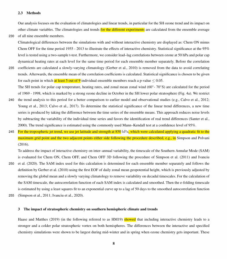
2.3 Methods

Our analysis focuses on the evaluation of climatologies and linear trends, in particular for the SH ozone trend and its impact on

other climate variables. The climatologies and trends for the different experiments are calculated from the ensemble average

of all nine ensemble members.230

Climatological differences between the simulations with and without interactive chemistry are displayed as: Chem ON minus

Chem OFF for the time period 1955 - 2013 to illustrate the effects of interactive chemistry. Statistical significance at the 95%

level is tested using a two-sample t-test. Furthermore, we consider lead–lag correlations between ozone at 50 hPa and polar cap

dynamical heating rates at each level for the same time period for each ensemble member separately. Before the correlation

coefficients are calculated a slowly-varying climatology (Gerber et al., 2010) is removed from the data to avoid correlating235

trends. Afterwards, the ensemble mean of the correlation coefficients is calculated. Statistical significance is chosen to be given

for each point in which at least 5 out of 9 individual ensemble members reach a p-value ≤ 0.05.

The SH trends for polar cap temperature, heating rates, and zonal mean zonal wind (60◦- 70◦S) are calculated for the period

of 1969 - 1998, which is marked by a strong ozone decline in October in the SH lower polar stratosphere (Fig. 4a). We restrict

the trend analysis to this period for a better comparison to earlier model and observational studies (e.g., Calvo et al., 2012;240

Young et al., 2013; Calvo et al., 2017). To determine the statistical significance of the linear trend differences, a new time

series is produced by taking the difference between the time series of the ensemble means. This approach reduces noise levels

by subtracting the variability of the individual time series and favors the identification of real trend differences (Santer et al.,

2000). The trend significance is estimated using the commonly used Mann–Kendall test at a confidence level of 95%.

For the tropospheric jet trend, we use jet latitude and strength at 850 hPa, which were calculated applying a quadratic fit to the245

maximum grid point and the two adjacent points either side following the procedure described, e.g., in Simpson and Polvani

(2016).

To address the impact of interactive chemistry on inter–annual variability, the timescale of the Southern Annular Mode (SAM)

is evaluated for Chem ON, Chem OFF, and Chem OFF 3D following the procedure of Simpson et al. (2011) and Ivanciu

et al. (2020). The SAM index used for this calculation is determined for each ensemble member separately and follows the250

definition by Gerber et al. (2010) using the first EOF of daily zonal mean geopotential height, which is previously adjusted by

removing the global mean and a slowly varying climatology to remove variability on decadal timescales. For the calculation of

the SAM timescale, the autocorrelation function of each SAM index is calculated and smoothed. Then the e-folding timescale

is estimated by using a least squares fit to an exponential curve up to a lag of 50 days to the smoothed autocorrelation function

(Simpson et al., 2011; Ivanciu et al., 2020).255

3 The impact of stratospheric chemistry on southern hemispheric climate and trends

Haase and Matthes (2019) (in the following referred to as HM19) showed that including interactive chemistry leads to a

stronger and a colder polar stratospheric vortex on both hemispheres. The differences between the interactive and specified

chemistry simulations were shown to be largest during mid-winter and in spring when ozone chemistry gets important. These

8

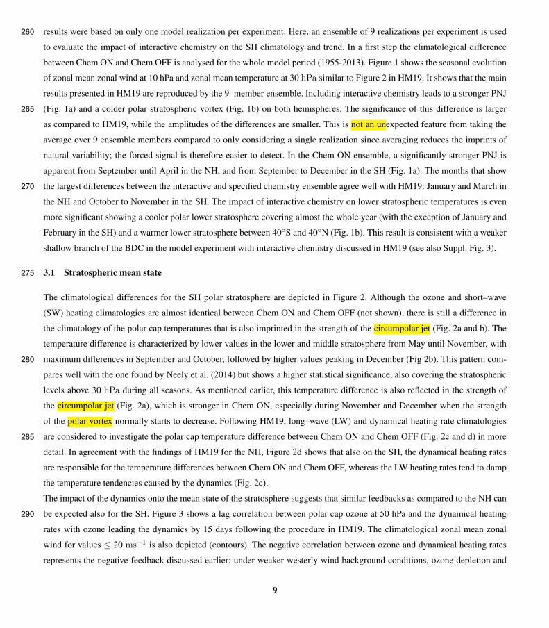
results were based on only one model realization per experiment. Here, an ensemble of 9 realizations per experiment is used260

to evaluate the impact of interactive chemistry on the SH climatology and trend. In a first step the climatological difference

between Chem ON and Chem OFF is analysed for the whole model period (1955-2013). Figure 1 shows the seasonal evolution

of zonal mean zonal wind at 10 hPa and zonal mean temperature at 30 hPa similar to Figure 2 in HM19. It shows that the main

results presented in HM19 are reproduced by the 9–member ensemble. Including interactive chemistry leads to a stronger PNJ

(Fig. 1a) and a colder polar stratospheric vortex (Fig. 1b) on both hemispheres. The significance of this difference is larger265

as compared to HM19, while the amplitudes of the differences are smaller. This is not an unexpected feature from taking the

average over 9 ensemble members compared to only considering a single realization since averaging reduces the imprints of

natural variability; the forced signal is therefore easier to detect. In the Chem ON ensemble, a significantly stronger PNJ is

apparent from September until April in the NH, and from September to December in the SH (Fig. 1a). The months that show

the largest differences between the interactive and specified chemistry ensemble agree well with HM19: January and March in270

the NH and October to November in the SH. The impact of interactive chemistry on lower stratospheric temperatures is even

more significant showing a cooler polar lower stratosphere covering almost the whole year (with the exception of January and

February in the SH) and a warmer lower stratosphere between 40◦S and 40◦N (Fig. 1b). This result is consistent with a weaker

shallow branch of the BDC in the model experiment with interactive chemistry discussed in HM19 (see also Suppl. Fig. 3).

3.1 Stratospheric mean state275

The climatological differences for the SH polar stratosphere are depicted in Figure 2. Although the ozone and short–wave

(SW) heating climatologies are almost identical between Chem ON and Chem OFF (not shown), there is still a difference in

the climatology of the polar cap temperatures that is also imprinted in the strength of the circumpolar jet (Fig. 2a and b). The

temperature difference is characterized by lower values in the lower and middle stratosphere from May until November, with

maximum differences in September and October, followed by higher values peaking in December (Fig 2b). This pattern com-280

pares well with the one found by Neely et al. (2014) but shows a higher statistical significance, also covering the stratospheric

levels above 30 hPa during all seasons. As mentioned earlier, this temperature difference is also reflected in the strength of

the circumpolar jet (Fig. 2a), which is stronger in Chem ON, especially during November and December when the strength

of the polar vortex normally starts to decrease. Following HM19, long–wave (LW) and dynamical heating rate climatologies

are considered to investigate the polar cap temperature difference between Chem ON and Chem OFF (Fig. 2c and d) in more285

detail. In agreement with the findings of HM19 for the NH, Figure 2d shows that also on the SH, the dynamical heating rates

are responsible for the temperature differences between Chem ON and Chem OFF, whereas the LW heating rates tend to damp

the temperature tendencies caused by the dynamics (Fig. 2c).

The impact of the dynamics onto the mean state of the stratosphere suggests that similar feedbacks as compared to the NH can

be expected also for the SH. Figure 3 shows a lag correlation between polar cap ozone at 50 hPa and the dynamical heating290

rates with ozone leading the dynamics by 15 days following the procedure in HM19. The climatological zonal mean zonal

wind for values ≤ 20 ms−1 is also depicted (contours). The negative correlation between ozone and dynamical heating rates

represents the negative feedback discussed earlier: under weaker westerly wind background conditions, ozone depletion and

9

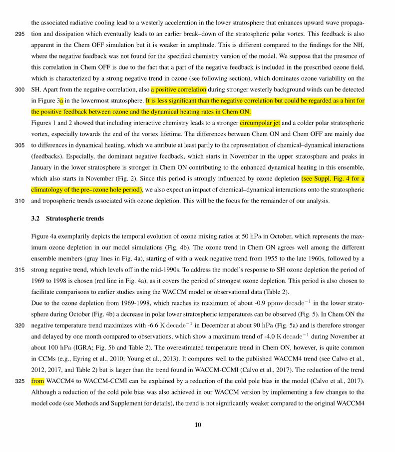
the associated radiative cooling lead to a westerly acceleration in the lower stratosphere that enhances upward wave propaga-

tion and dissipation which eventually leads to an earlier break–down of the stratospheric polar vortex. This feedback is also295

apparent in the Chem OFF simulation but it is weaker in amplitude. This is different compared to the findings for the NH,

where the negative feedback was not found for the specified chemistry version of the model. We suppose that the presence of

this correlation in Chem OFF is due to the fact that a part of the negative feedback is included in the prescribed ozone field,

which is characterized by a strong negative trend in ozone (see following section), which dominates ozone variability on the

SH. Apart from the negative correlation, also a positive correlation during stronger westerly background winds can be detected300

in Figure 3a in the lowermost stratosphere. It is less significant than the negative correlation but could be regarded as a hint for

the positive feedback between ozone and the dynamical heating rates in Chem ON.

Figures 1 and 2 showed that including interactive chemistry leads to a stronger circumpolar jet and a colder polar stratospheric

vortex, especially towards the end of the vortex lifetime. The differences between Chem ON and Chem OFF are mainly due

to differences in dynamical heating, which we attribute at least partly to the representation of chemical–dynamical interactions305

(feedbacks). Especially, the dominant negative feedback, which starts in November in the upper stratosphere and peaks in

January in the lower stratosphere is stronger in Chem ON contributing to the enhanced dynamical heating in this ensemble,

which also starts in November (Fig. 2). Since this period is strongly influenced by ozone depletion (see Suppl. Fig. 4 for a

climatology of the pre–ozone hole period), we also expect an impact of chemical–dynamical interactions onto the stratospheric

and tropospheric trends associated with ozone depletion. This will be the focus for the remainder of our analysis.310

3.2 Stratospheric trends

Figure 4a exemplarily depicts the temporal evolution of ozone mixing ratios at 50 hPa in October, which represents the max-

imum ozone depletion in our model simulations (Fig. 4b). The ozone trend in Chem ON agrees well among the different

ensemble members (gray lines in Fig. 4a), starting of with a weak negative trend from 1955 to the late 1960s, followed by a

strong negative trend, which levels off in the mid-1990s. To address the model’s response to SH ozone depletion the period of315

1969 to 1998 is chosen (red line in Fig. 4a), as it covers the period of strongest ozone depletion. This period is also chosen to

facilitate comparisons to earlier studies using the WACCM model or observational data (Table 2).

Due to the ozone depletion from 1969-1998, which reaches its maximum of about -0.9 ppmv decade−1 in the lower strato-

sphere during October (Fig. 4b) a decrease in polar lower stratospheric temperatures can be observed (Fig. 5). In Chem ON the

negative temperature trend maximizes with -6.6 Kdecade−1 in December at about 90 hPa (Fig. 5a) and is therefore stronger320

and delayed by one month compared to observations, which show a maximum trend of -4.0 Kdecade−1 during November at

about 100 hPa (IGRA; Fig. 5b and Table 2). The overestimated temperature trend in Chem ON, however, is quite common

in CCMs (e.g., Eyring et al., 2010; Young et al., 2013). It compares well to the published WACCM4 trend (see Calvo et al.,

2012, 2017, and Table 2) but is larger than the trend found in WACCM-CCMI (Calvo et al., 2017). The reduction of the trend

from WACCM4 to WACCM-CCMI can be explained by a reduction of the cold pole bias in the model (Calvo et al., 2017).325

Although a reduction of the cold pole bias was also achieved in our WACCM version by implementing a few changes to the

model code (see Methods and Supplement for details), the trend is not significantly weaker compared to the original WACCM4

10

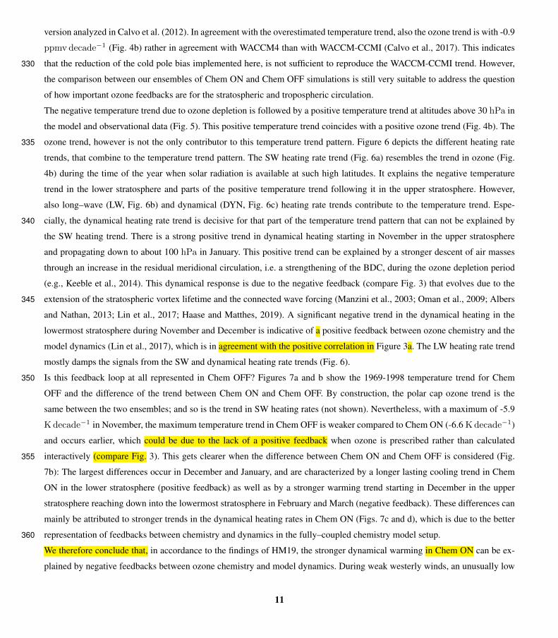
version analyzed in Calvo et al. (2012). In agreement with the overestimated temperature trend, also the ozone trend is with -0.9

ppmv decade−1 (Fig. 4b) rather in agreement with WACCM4 than with WACCM-CCMI (Calvo et al., 2017). This indicates

that the reduction of the cold pole bias implemented here, is not sufficient to reproduce the WACCM-CCMI trend. However,330

the comparison between our ensembles of Chem ON and Chem OFF simulations is still very suitable to address the question

of how important ozone feedbacks are for the stratospheric and tropospheric circulation.

The negative temperature trend due to ozone depletion is followed by a positive temperature trend at altitudes above 30 hPa in

the model and observational data (Fig. 5). This positive temperature trend coincides with a positive ozone trend (Fig. 4b). The

ozone trend, however is not the only contributor to this temperature trend pattern. Figure 6 depicts the different heating rate335

trends, that combine to the temperature trend pattern. The SW heating rate trend (Fig. 6a) resembles the trend in ozone (Fig.

4b) during the time of the year when solar radiation is available at such high latitudes. It explains the negative temperature

trend in the lower stratosphere and parts of the positive temperature trend following it in the upper stratosphere. However,

also long–wave (LW, Fig. 6b) and dynamical (DYN, Fig. 6c) heating rate trends contribute to the temperature trend. Espe-

cially, the dynamical heating rate trend is decisive for that part of the temperature trend pattern that can not be explained by340

the SW heating trend. There is a strong positive trend in dynamical heating starting in November in the upper stratosphere

and propagating down to about 100 hPa in January. This positive trend can be explained by a stronger descent of air masses

through an increase in the residual meridional circulation, i.e. a strengthening of the BDC, during the ozone depletion period

(e.g., Keeble et al., 2014). This dynamical response is due to the negative feedback (compare Fig. 3) that evolves due to the

extension of the stratospheric vortex lifetime and the connected wave forcing (Manzini et al., 2003; Oman et al., 2009; Albers345

and Nathan, 2013; Lin et al., 2017; Haase and Matthes, 2019). A significant negative trend in the dynamical heating in the

lowermost stratosphere during November and December is indicative of a positive feedback between ozone chemistry and the

model dynamics (Lin et al., 2017), which is in agreement with the positive correlation in Figure 3a. The LW heating rate trend

mostly damps the signals from the SW and dynamical heating rate trends (Fig. 6).

Is this feedback loop at all represented in Chem OFF? Figures 7a and b show the 1969-1998 temperature trend for Chem350

OFF and the difference of the trend between Chem ON and Chem OFF. By construction, the polar cap ozone trend is the

same between the two ensembles; and so is the trend in SW heating rates (not shown). Nevertheless, with a maximum of -5.9

Kdecade−1 in November, the maximum temperature trend in Chem OFF is weaker compared to Chem ON (-6.6 Kdecade−1)

and occurs earlier, which could be due to the lack of a positive feedback when ozone is prescribed rather than calculated

interactively (compare Fig. 3). This gets clearer when the difference between Chem ON and Chem OFF is considered (Fig.355

7b): The largest differences occur in December and January, and are characterized by a longer lasting cooling trend in Chem

ON in the lower stratosphere (positive feedback) as well as by a stronger warming trend starting in December in the upper

stratosphere reaching down into the lowermost stratosphere in February and March (negative feedback). These differences can

mainly be attributed to stronger trends in the dynamical heating rates in Chem ON (Figs. 7c and d), which is due to the better

representation of feedbacks between chemistry and dynamics in the fully–coupled chemistry model setup.360

We therefore conclude that, in accordance to the findings of HM19, the stronger dynamical warming in Chem ON can be ex-

plained by negative feedbacks between ozone chemistry and model dynamics. During weak westerly winds, an unusually low

11

ozone concentration can lead to enhanced upward planetary wave propagation by extending the lifetime of the westerly wind

regime, which enhances a descent over polar latitudes resulting in an additional adiabatic warming. Apart from the negative

feedback, which was found to be apparent also in the NH, a positive feedback can be detected in the SH ozone depletion period365

during stronger westerly background winds. It is statistically significant only for 7 out of 9 members (not shown) and restricted

to the lowermost stratosphere. This positive correlation is only found in the interactive chemistry setup and could explain the

stronger dynamical cooling in Chem ON compared to Chem OFF (Fig. 7). It has to be noted that Chem OFF is able to represent

the negative feedback pattern to a certain extent (Fig. 3) because of the strong ozone signal that the model is forced with (parts

of the feedback can be considered to be included in the prescribed ozone fields).370

The negative temperature trend in the lower polar stratosphere increases the meridional temperature gradient and leads to a

strengthening of the PNJ, especially towards the end of the polar vortex lifetime as discussed before. Figures 8a and b show that

the maximum trend in zonal mean zonal wind in the PNJ region is stronger in Chem ON (9.2 ms−1 decade−1) compared to

Chem OFF (7.8 ms−1 decade−1). The largest differences in the zonal mean zonal wind trend can be found in the middle strato-

sphere during December (Fig. 8c), which supports our earlier argumentation about the characteristics of chemical–dynamical375

feedbacks in the two ensembles. Namely, that an extension of the vortex lifetime, which is stronger in Chem ON compared to

Chem OFF, favors the occurrence of the negative feedback. However, in both ensembles a significant zonal mean zonal wind

trend can be found also at the surface from November through February, which will be investigated in the following with a

focus on the austral summer season (DJF).

3.3 Tropospheric jet trend and SAM timescale380

Figure 9 shows the 1969-1998 trend for zonal mean zonal wind with latitude and height (color shading) along with the cli-

matological wind over the same period (contours) for DJF. It is evident that the strengthening of the PNJ is connected also to

a strengthening of the tropospheric jet and its poleward displacement in agreement with earlier studies (e.g., Thompson and

Solomon, 2002; Son et al., 2008; Eyring et al., 2013). In Chem OFF, the strengthening of the poleward flank of the tropo-

spheric jet compares well to the signal in Chem ON, but the weakening of the equatorward flank is weaker. Hence, part of the385

differences found in the stratosphere also have an effect onto the troposphere.

Apart from the insufficient representation of chemical–dynamical feedbacks in the Chem OFF ensemble, also the decision to

prescribe zonal mean ozone can have an impact onto the characteristics of the tropospheric jet trend associated with ozone

depletion (Crook et al., 2008; Gillett et al., 2009; Rae et al., 2019). We therefore, additionally consider an experiment that uses

3D ozone in the prescribed ozone fields (Chem OFF 3D, Figs. 9d and e). Including 3D ozone improves the representation of390

the circumpolar jet trend in response to ozone depletion in comparison to using a zonal mean ozone field. The strengthening of

the poleward flank of the circumpolar jet is very well captured in the troposphere and stratosphere, while the weakening of the

equatorward flank of the tropospheric jet is lower compared to Chem ON but much better represented compared to Chem OFF.

Whether the difference in the mid–latitude DJF zonal mean zonal wind trend really impacts the trend of the tropospheric jet,

is addressed in the following. Figure 10 shows the trend for the tropospheric jet latitude and strength at 850 hPa. There is no395

statistically significant difference between the chemistry settings in the trend of the tropospheric jet position and strength. All

12

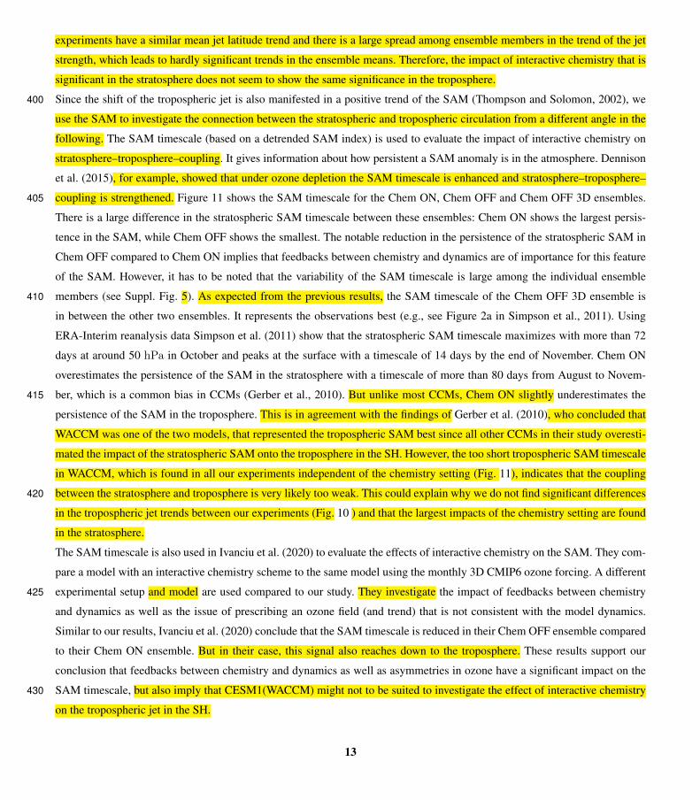
experiments have a similar mean jet latitude trend and there is a large spread among ensemble members in the trend of the jet

strength, which leads to hardly significant trends in the ensemble means. Therefore, the impact of interactive chemistry that is

significant in the stratosphere does not seem to show the same significance in the troposphere.

Since the shift of the tropospheric jet is also manifested in a positive trend of the SAM (Thompson and Solomon, 2002), we400

use the SAM to investigate the connection between the stratospheric and tropospheric circulation from a different angle in the

following. The SAM timescale (based on a detrended SAM index) is used to evaluate the impact of interactive chemistry on

stratosphere–troposphere–coupling. It gives information about how persistent a SAM anomaly is in the atmosphere. Dennison

et al. (2015), for example, showed that under ozone depletion the SAM timescale is enhanced and stratosphere–troposphere–

coupling is strengthened. Figure 11 shows the SAM timescale for the Chem ON, Chem OFF and Chem OFF 3D ensembles.405

There is a large difference in the stratospheric SAM timescale between these ensembles: Chem ON shows the largest persis-

tence in the SAM, while Chem OFF shows the smallest. The notable reduction in the persistence of the stratospheric SAM in

Chem OFF compared to Chem ON implies that feedbacks between chemistry and dynamics are of importance for this feature

of the SAM. However, it has to be noted that the variability of the SAM timescale is large among the individual ensemble

members (see Suppl. Fig. 5). As expected from the previous results, the SAM timescale of the Chem OFF 3D ensemble is410

in between the other two ensembles. It represents the observations best (e.g., see Figure 2a in Simpson et al., 2011). Using

ERA-Interim reanalysis data Simpson et al. (2011) show that the stratospheric SAM timescale maximizes with more than 72

days at around 50 hPa in October and peaks at the surface with a timescale of 14 days by the end of November. Chem ON

overestimates the persistence of the SAM in the stratosphere with a timescale of more than 80 days from August to Novem-

ber, which is a common bias in CCMs (Gerber et al., 2010). But unlike most CCMs, Chem ON slightly underestimates the415

persistence of the SAM in the troposphere. This is in agreement with the findings of Gerber et al. (2010), who concluded that

WACCM was one of the two models, that represented the tropospheric SAM best since all other CCMs in their study overesti-

mated the impact of the stratospheric SAM onto the troposphere in the SH. However, the too short tropospheric SAM timescale

in WACCM, which is found in all our experiments independent of the chemistry setting (Fig. 11), indicates that the coupling

between the stratosphere and troposphere is very likely too weak. This could explain why we do not find significant differences420

in the tropospheric jet trends between our experiments (Fig. 10 ) and that the largest impacts of the chemistry setting are found

in the stratosphere.

The SAM timescale is also used in Ivanciu et al. (2020) to evaluate the effects of interactive chemistry on the SAM. They com-

pare a model with an interactive chemistry scheme to the same model using the monthly 3D CMIP6 ozone forcing. A different

experimental setup and model are used compared to our study. They investigate the impact of feedbacks between chemistry425

and dynamics as well as the issue of prescribing an ozone field (and trend) that is not consistent with the model dynamics.

Similar to our results, Ivanciu et al. (2020) conclude that the SAM timescale is reduced in their Chem OFF ensemble compared

to their Chem ON ensemble. But in their case, this signal also reaches down to the troposphere. These results support our

conclusion that feedbacks between chemistry and dynamics as well as asymmetries in ozone have a significant impact on the

SAM timescale, but also imply that CESM1(WACCM) might not to be suited to investigate the effect of interactive chemistry430

on the tropospheric jet in the SH.

13

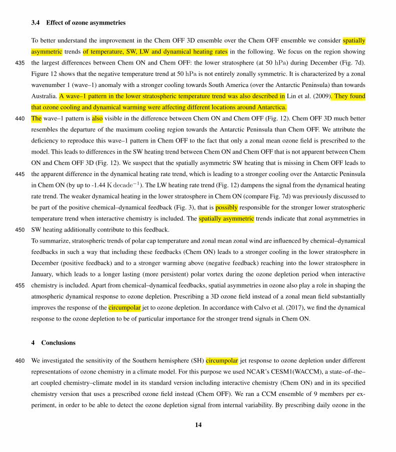
3.4 Effect of ozone asymmetries

To better understand the improvement in the Chem OFF 3D ensemble over the Chem OFF ensemble we consider spatially

asymmetric trends of temperature, SW, LW and dynamical heating rates in the following. We focus on the region showing

the largest differences between Chem ON and Chem OFF: the lower stratosphere (at 50 hPa) during December (Fig. 7d).435

Figure 12 shows that the negative temperature trend at 50 hPa is not entirely zonally symmetric. It is characterized by a zonal

wavenumber 1 (wave–1) anomaly with a stronger cooling towards South America (over the Antarctic Peninsula) than towards

Australia. A wave–1 pattern in the lower stratospheric temperature trend was also described in Lin et al. (2009). They found

that ozone cooling and dynamical warming were affecting different locations around Antarctica.

The wave–1 pattern is also visible in the difference between Chem ON and Chem OFF (Fig. 12). Chem OFF 3D much better440

resembles the departure of the maximum cooling region towards the Antarctic Peninsula than Chem OFF. We attribute the

deficiency to reproduce this wave–1 pattern in Chem OFF to the fact that only a zonal mean ozone field is prescribed to the

model. This leads to differences in the SW heating trend between Chem ON and Chem OFF that is not apparent between Chem

ON and Chem OFF 3D (Fig. 12). We suspect that the spatially asymmetric SW heating that is missing in Chem OFF leads to

the apparent difference in the dynamical heating rate trend, which is leading to a stronger cooling over the Antarctic Peninsula445

in Chem ON (by up to -1.44 Kdecade−1). The LW heating rate trend (Fig. 12) dampens the signal from the dynamical heating

rate trend. The weaker dynamical heating in the lower stratosphere in Chem ON (compare Fig. 7d) was previously discussed to

be part of the positive chemical–dynamical feedback (Fig. 3), that is possibly responsible for the stronger lower stratospheric

temperature trend when interactive chemistry is included. The spatially asymmetric trends indicate that zonal asymmetries in

SW heating additionally contribute to this feedback.450

To summarize, stratospheric trends of polar cap temperature and zonal mean zonal wind are influenced by chemical–dynamical

feedbacks in such a way that including these feedbacks (Chem ON) leads to a stronger cooling in the lower stratosphere in

December (positive feedback) and to a stronger warming above (negative feedback) reaching into the lower stratosphere in

January, which leads to a longer lasting (more persistent) polar vortex during the ozone depletion period when interactive

chemistry is included. Apart from chemical–dynamical feedbacks, spatial asymmetries in ozone also play a role in shaping the455

atmospheric dynamical response to ozone depletion. Prescribing a 3D ozone field instead of a zonal mean field substantially

improves the response of the circumpolar jet to ozone depletion. In accordance with Calvo et al. (2017), we find the dynamical

response to the ozone depletion to be of particular importance for the stronger trend signals in Chem ON.

4 Conclusions

We investigated the sensitivity of the Southern hemisphere (SH) circumpolar jet response to ozone depletion under different460

representations of ozone chemistry in a climate model. For this purpose we used NCAR’s CESM1(WACCM), a state–of–the–

art coupled chemistry–climate model in its standard version including interactive chemistry (Chem ON) and in its specified

chemistry version that uses a prescribed ozone field instead (Chem OFF). We ran a CCM ensemble of 9 members per ex-

periment, in order to be able to detect the ozone depletion signal from internal variability. By prescribing daily ozone in the

14

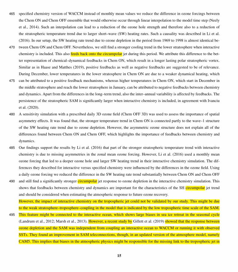
specified chemistry version of WACCM instead of monthly mean values we reduce the difference in ozone forcings between465

the Chem ON and Chem OFF ensemble that would otherwise occur through linear interpolation to the model time step (Neely

et al., 2014). Such an interpolation can lead to a reduction of the ozone hole strength and therefore also to a reduction of

the stratospheric temperature trend due to larger short–wave (SW) heating rates. Such a causality was described in Li et al.

(2016). In our setup, the SW heating rate trend due to ozone depletion in the period from 1969 to 1998 is almost identical be-

tween Chem ON and Chem OFF. Nevertheless, we still find a stronger cooling trend in the lower stratosphere when interactive470

chemistry is included. This also feeds back onto the circumpolar jet during this period. We attribute this difference to the bet-

ter representation of chemical–dynamical feedbacks in Chem ON, which result in a longer lasting polar stratospheric vortex.

Similar as in Haase and Matthes (2019), positive feedbacks as well as negative feedbacks are suggested to be of relevance.

During December, lower temperatures in the lower stratosphere in Chem ON are due to a weaker dynamical heating, which

can be attributed to a positive feedback mechanisms, whereas higher temperatures in Chem ON, which start in December in475

the middle stratosphere and reach the lower stratosphere in January, can be attributed to negative feedbacks between chemistry

and dynamics. Apart from the differences in the long–term trend, also the inter–annual variability is affected by feedbacks. The

persistence of the stratospheric SAM is significantly larger when interactive chemistry is included, in agreement with Ivanciu

et al. (2020).

A sensitivity simulation with a prescribed daily 3D ozone field (Chem OFF 3D) was used to assess the importance of spatial480

asymmetry effects. It was found that, the stronger temperature trend in Chem ON is connected partly to the wave–1 structure

of the SW heating rate trend due to ozone depletion. However, the asymmetric ozone structure does not explain all of the

differences found between Chem ON and Chem OFF, which highlights the importance of feedbacks between chemistry and

dynamics.

Our findings support the results by Li et al. (2016) that part of the stronger stratospheric temperature trend with interactive485

chemistry is due to missing asymmetries in the zonal mean ozone forcing. However, Li et al. (2016) used a monthly mean

ozone forcing that led to a deeper ozone hole and larger SW heating trend in their interactive chemistry simulation. The dif-

ferences they described for interactive versus specified chemistry were influenced by the differences in the ozone field. Using

a daily ozone forcing we reduced the difference in the SW heating rate trend substantially between Chem ON and Chem OFF

and still find a significantly stronger circumpolar jet response to ozone depletion in the interactive chemistry simulation. This490

shows that feedbacks between chemistry and dynamics are important for the characteristics of the SH circumpolar jet trend

and should be considered when estimating the atmospheric response to future ozone recovery.

However, the impact of interactive chemistry on the tropospheric jet could not be validated by our study. This might be due

to the weak stratosphere–troposphere–coupling in the model that is indicated by the low tropospheric time scale of the SAM.

This feature might be connected to the interactive ocean, which shows large biases in sea ice retreat in the seasonal cycle495

(Landrum et al., 2012; Marsh et al., 2013). However, a recent study by Gillett et al. (2019) showed that the response between

ozone depletion and the SAM was independent from coupling an interactive ocean to WACCM or running it with observed

SSTs. They found an improvement in SAM teleconnections, though, in an updated version of the atmosphere model, namely

CAM5. This implies that biases in the atmospheric physics might be responsible for the missing link to the tropospheric jet in

15

our study.500

Although not directly affecting the position of the tropospheric jet, the differences we find between the chemistry settings (Fig.

9 ), show a stronger tropospheric response to ozone depletion when interactive chemistry is included. An updated model version

of WACCM, based on the CAM5 physics, might improve our understanding of the stratospheric impact onto the troposphere

under different chemistry settings.

Code and data availability. The IGRA radiosonde data used in this paper is publicly available at https://www1.ncdc.noaa.gov/pub/data/igra/v1/.505

Pre-processed model data to reproduce the figures in the manuscript can be found under https://doi.org/10.5281/zenodo.3785404. Further

CESM1(WACCM) model data requests should be addressed to Katja Matthes ([email protected]). The scientific code will be shared

upon request to Sabine Haase ([email protected]).

Author contributions. SH wrote the manuscript. KM and SH decided about the analysis and experimental design. TK and SW carried out

the model simulations. JF carried out the data analysis and produced all the figures. All co-authors commented on the manuscript.510

Competing interests. The authors declare that they have no competing interests.

Acknowledgements. We thank Ioana Ivanciu for helpful discussions especially on the SAM timescale. We thank the computing center at

Christian–Albrechts–University in Kiel and at the Deutsches Klimarechenzentrum (DKRZ) for support and computer time.

16

References

Albers, J. R. and Nathan, T. R.: Pathways for Communicating the Effects of Stratospheric Ozone to the Polar Vortex: Role of Zonally515

Asymmetric Ozone, Journal of the Atmospheric Sciences, 69, 785–801, https://doi.org/10.1175/JAS-D-11-0126.1, http://journals.ametsoc.

org/doi/abs/10.1175/JAS-D-11-0126.1, 2012.

Albers, J. R. and Nathan, T. R.: Ozone Loss and Recovery and the Preconditioning of Upward-Propagating Planetary Wave Activity, Jour-

nal of the Atmospheric Sciences, 70, 3977–3994, https://doi.org/10.1175/JAS-D-12-0259.1, http://journals.ametsoc.org/doi/abs/10.1175/

JAS-D-12-0259.1http://search.proquest.com/docview/1465006174?accountid=26529, 2013.520

Albers, J. R., Mccormack, J. P., and Nathan, T. R.: Stratospheric ozone and the morphology of the northern hemisphere planetary waveguide,

Journal of Geophysical Research: Atmospheres, 118, 563–576, https://doi.org/10.1029/2012JD017937, 2013.

Bednarz, E. M., Maycock, A. C., Abraham, N. L., Braesicke, P., Dessens, O., and Pyle, J. A.: Future Arctic ozone recovery: the importance

of chemistry and dynamics, Atmospheric Chemistry and Physics, 16, 12 159–12 176, https://doi.org/10.5194/acp-16-12159-2016, 2016.

Calvo, N., Garcia, R. R., Marsh, D. R., Mills, M. J., Kinnison, D. E., and Young, P. J.: Reconciling modeled and observed temperature525

trends over Antarctica, Geophysical Research Letters, 39, 1–6, https://doi.org/10.1029/2012GL052526, http://doi.wiley.com/10.1029/

2012GL052526, 2012.

Calvo, N., Polvani, L. M., and Solomon, S.: On the surface impact of Arctic stratospheric ozone extremes, Environmental Research Letters,

10, 094 003, https://doi.org/10.1088/1748-9326/10/9/094003, 2015.

Calvo, N., Garcia, R. R., and Kinnison, D. E.: Revisiting Southern Hemisphere Polar Stratospheric Temperature Trends in WACCM: The530

Role of Dynamical Forcing, Geophysical Research Letters, 44, 3402–3410, https://doi.org/10.1002/2017GL072792, http://doi.wiley.com/

10.1002/2017GL072792, 2017.

Charney, J. G. and Drazin, P. G.: Propagation of planetary-scale disturbances from the lower into the upper atmosphere, Journal of Geophys-

ical Research, 66, 83–109, https://doi.org/10.1029/JZ066i001p00083, http://doi.wiley.com/10.1029/JZ066i001p00083, 1961.

Checa-Garcia, R., Hegglin, M. I., Kinnison, D., Plummer, D. A., and Shine, K. P.: Historical Tropospheric and Stratospheric Ozone Radiative535

Forcing Using the CMIP6 Database, Geophysical Research Letters, 45, 3264–3273, https://doi.org/10.1002/2017GL076770, http://doi.

wiley.com/10.1002/2017GL076770, 2018.

Cionni, I., Eyring, V., Lamarque, J. F., Randel, W. J., Stevenson, D. S., Wu, F., Bodeker, G. E., Shepherd, T. G., Shindell, D. T., and

Waugh, D. W.: Ozone database in support of CMIP5 simulations: Results and corresponding radiative forcing, Atmospheric Chemistry

and Physics, 11, 11 267–11 292, https://doi.org/10.5194/acp-11-11267-2011, 2011.540

Crook, J. A., Gillett, N. P., and Keeley, S. P. E.: Sensitivity of Southern Hemisphere climate to zonal asymmetry in ozone, Geophysical

Research Letters, 35, 3–7, https://doi.org/10.1029/2007GL032698, 2008.

Dennison, F. W., McDonald, A. J., and Morgenstern, O.: The effect of ozone depletion on the Southern Annular Mode and stratosphere-

troposphere coupling, Journal of Geophysical Research Atmospheres, 120, 1–8, https://doi.org/10.1002/2014JD023009, 2015.

Dhomse, S. S., Kinnison, D., Chipperfield, M. P., Salawitch, R. J., Cionni, I., Hegglin, M. I., Abraham, N. L., Akiyoshi, H., Archibald, A. T.,545

Bednarz, E. M., Bekki, S., Braesicke, P., Butchart, N., Dameris, M., Deushi, M., Frith, S., Hardiman, S. C., Hassler, B., Horowitz, L. W.,

Hu, R. M., Jöckel, P., Josse, B., Kirner, O., Kremser, S., Langematz, U., Lewis, J., Marchand, M., Lin, M., Mancini, E., Marécal, V.,

Michou, M., Morgenstern, O., O’Connor, F. M., Oman, L., Pitari, G., Plummer, D. A., Pyle, J. A., Revell, L. E., Rozanov, E., Schofield,

R., Stenke, A., Stone, K., Sudo, K., Tilmes, S., Visioni, D., Yamashita, Y., and Zeng, G.: Estimates of ozone return dates from Chemistry-

17

https://doi.org/10.1175/JAS-D-11-0126.1

http://journals.ametsoc.org/doi/abs/10.1175/JAS-D-11-0126.1




http://journals.ametsoc.org/doi/abs/10.1175/JAS-D-12-0259.1 http://search.proquest.com/docview/1465006174?accountid=26529



https://doi.org/10.1029/2012JD017937

https://doi.org/10.5194/acp-16-12159-2016

https://doi.org/10.1029/2012GL052526

http://doi.wiley.com/10.1029/2012GL052526



https://doi.org/10.1088/1748-9326/10/9/094003

https://doi.org/10.1002/2017GL072792




https://doi.org/10.1029/JZ066i001p00083

http://doi.wiley.com/10.1029/JZ066i001p00083

https://doi.org/10.1002/2017GL076770




https://doi.org/10.5194/acp-11-11267-2011

https://doi.org/10.1029/2007GL032698

https://doi.org/10.1002/2014JD023009

Climate Model Initiative simulations, Atmospheric Chemistry and Physics, 18, 8409–8438, https://doi.org/10.5194/acp-18-8409-2018,550

2018.

Durre, I., Vose, R. S., and Wuertz, D. B.: Overview of the Integrated Global Radiosonde Archive, Journal of Climate, 19, 53–68,

https://doi.org/10.1175/JCLI3594.1, 2006.

Eyring, V., Shepherd, T. G., and Waugh, D. W.: SPARC CCMVal Report on the Evaluation of Chemistry-Climate Models, Tech. rep., SPARC,

http://www.sparc-climate.org/publications/sparc-reports/, 2010.555

Eyring, V., Arblaster, J. M., Cionni, I., Sedlácek, J., Perlwitz, J., Young, P. J., Bekki, S., Bergmann, D., Cameron-Smith, P., Collins, W. J.,

Faluvegi, G., Gottschaldt, K.-D., Horowitz, L. W., Kinnison, D. E., Lamarque, J.-F., Marsh, D. R., Saint-Martin, D., Shindell, D. T., Sudo,

K., Szopa, S., and Watanabe, S.: Long-term ozone changes and associated climate impacts in CMIP5 simulations, Journal of Geophysical

Research: Atmospheres, 118, 5029–5060, https://doi.org/10.1002/jgrd.50316, http://doi.wiley.com/10.1002/jgrd.50316, 2013.

Fels, S. B., Mahlman, J. D., Schwarzkopf, M. D., and Sinclair, R. W.: Stratospheric Sensitivity to Perturbations in Ozone and Car-560

bon Dioxide: Radiative and Dynamical Response, Journal of the Atmospheric Sciences, 37, 2265–2297, https://doi.org/10.1175/1520-

0469(1980)037<2265:SSTPIO>2.0.CO;2, 1980.

Ferreira, D., Marshall, J., Bitz, C. M., Solomon, S., and Plumb, A.: Antarctic ocean and sea ice response to ozone depletion: A two-time-scale

problem, Journal of Climate, 28, 1206–1226, https://doi.org/10.1175/JCLI-D-14-00313.1, 2015.

Garcia, R. R., López-Puertas, M., Funke, B., Marsh, D. R., Kinnison, D. E., Smith, A. K., and González-Galindo, F.: On the distribu-565

tion of CO2 and CO in the mesosphere and lower thermosphere, Journal of Geophysical Research: Atmospheres, 119, 5700–5718,

https://doi.org/10.1002/2013JD021208, 2014.

Garcia, R. R., Smith, A. K., Kinnison, D. E., de la Cámara, Á., and Murphy, D. J.: Modification of the Gravity Wave Parameterization

in the Whole Atmosphere Community Climate Model: Motivation and Results, Journal of the Atmospheric Sciences, 74, 275–291,

https://doi.org/10.1175/JAS-D-16-0104.1, http://journals.ametsoc.org/doi/10.1175/JAS-D-16-0104.1, 2017.570

Gerber, E. P., Baldwin, M. P., Akiyoshi, H., Austin, J., Bekki, S., Braesicke, P., Butchart, N., Chipperfield, M., Dameris, M., Dhomse,

S., Frith, S. M., Garcia, R. R., Garny, H., Gettelman, A., Hardiman, S. C., Karpechko, A., Marchand, M., Morgenstern, O., Nielsen,

J. E., Pawson, S., Peter, T., Plummer, D. A., Pyle, J. A., Rozanov, E., Scinocca, J. F., Shepherd, T. G., and Smale, D.: Stratosphere-

troposphere coupling and annular mode variability in chemistry-climate models, Journal of Geophysical Research, 115, D00M06,

https://doi.org/10.1029/2009JD013770, 2010.575

Gillett, N. P., Scinocca, J. F., Plummer, D. a., and Reader, M. C.: Sensitivity of climate to dynamically-consistent zonal asymmetries in ozone,

Geophysical Research Letters, 36, 1–5, https://doi.org/10.1029/2009GL037246, 2009.

Gillett, Z. E., Arblaster, J. M., Dittus, A. J., Deushi, M., Jöckel, P., Kinnison, D. E., Morgenstern, O., Plummer, D. A., Revell, L. E.,

Rozanov, E., Schofield, R., Stenke, A., Stone, K. A., and Tilmes, S.: Evaluating the relationship between interannual variations in

the Antarctic ozone hole and Southern Hemisphere surface climate in Chemistry-Climate Models, Journal of Climate, 32, 3131–3151,580

https://doi.org/10.1175/JCLI-D-18-0273.1, 2019.

Golaz, J. C., Caldwell, P. M., Van Roekel, L. P., Petersen, M. R., Tang, Q., Wolfe, J. D., Abeshu, G., Anantharaj, V., Asay-Davis, X. S.,

Bader, D. C., Baldwin, S. A., Bisht, G., Bogenschutz, P. A., Branstetter, M., Brunke, M. A., Brus, S. R., Burrows, S. M., Cameron-Smith,

P. J., Donahue, A. S., Deakin, M., Easter, R. C., Evans, K. J., Feng, Y., Flanner, M., Foucar, J. G., Fyke, J. G., Griffin, B. M., Hannay, C.,

Harrop, B. E., Hoffman, M. J., Hunke, E. C., Jacob, R. L., Jacobsen, D. W., Jeffery, N., Jones, P. W., Keen, N. D., Klein, S. A., Larson,585

V. E., Leung, L. R., Li, H. Y., Lin, W., Lipscomb, W. H., Ma, P. L., Mahajan, S., Maltrud, M. E., Mametjanov, A., McClean, J. L., McCoy,

R. B., Neale, R. B., Price, S. F., Qian, Y., Rasch, P. J., Reeves Eyre, J. E., Riley, W. J., Ringler, T. D., Roberts, A. F., Roesler, E. L.,

18

https://doi.org/10.5194/acp-18-8409-2018

https://doi.org/10.1175/JCLI3594.1

http://www.sparc-climate.org/publications/sparc-reports/

https://doi.org/10.1002/jgrd.50316

http://doi.wiley.com/10.1002/jgrd.50316

https://doi.org/10.1175/1520-0469(1980)037%3C2265:SSTPIO%3E2.0.CO;2



https://doi.org/10.1175/JCLI-D-14-00313.1

https://doi.org/10.1002/2013JD021208


http://journals.ametsoc.org/doi/10.1175/JAS-D-16-0104.1

https://doi.org/10.1029/2009JD013770

https://doi.org/10.1029/2009GL037246


Salinger, A. G., Shaheen, Z., Shi, X., Singh, B., Tang, J., Taylor, M. A., Thornton, P. E., Turner, A. K., Veneziani, M., Wan, H., Wang, H.,

Wang, S., Williams, D. N., Wolfram, P. J., Worley, P. H., Xie, S., Yang, Y., Yoon, J. H., Zelinka, M. D., Zender, C. S., Zeng, X., Zhang, C.,

Zhang, K., Zhang, Y., Zheng, X., Zhou, T., and Zhu, Q.: The DOE E3SM Coupled Model Version 1: Overview and Evaluation at Standard590

Resolution, Journal of Advances in Modeling Earth Systems, 11, 2089–2129, https://doi.org/10.1029/2018MS001603, 2019.

Haase, S. and Matthes, K.: The importance of interactive chemistry for stratosphere-troposphere coupling, Atmospheric Chemistry and

Physics, 19, 3417–3432, https://doi.org/10.5194/acp-19-3417-2019, 2019.

Ivanciu, I., Matthes, K., Wahl, S., Harlaß, J., and Biastoch, A.: Effects of prescribed CMIP6 ozone on simulating the Southern Hemisphere

atmospheric circulation response to ozone depletion, submitted to Atmos. Chem. Phys. Discuss., 2020.595

Keeble, J., Braesicke, P., Abraham, N. L., Roscoe, H. K., and Pyle, J. A.: The impact of polar stratospheric ozone loss on Southern Hemisphere

stratospheric circulation and climate, Atmospheric Chemistry and Physics Discussions, 14, 18 049–18 082, https://doi.org/10.5194/acpd-

14-18049-2014, http://www.atmos-chem-phys-discuss.net/14/18049/2014/, 2014.

Kinnison, D. E., Brasseur, G. P., Walters, S., Garcia, R. R., Marsh, D. R., Sassi, F., Harvey, V. L., Randall, C. E., Emmons, L., Lamarque,

J. F., Hess, P., Orlando, J. J., Tie, X. X., Randel, W., Pan, L. L., Gettelman, A., Granier, C., Diehl, T., Niemeier, U., and Simmons,600

A. J.: Sensitivity of chemical tracers to meteorological parameters in the MOZART-3 chemical transport model, Journal of Geophysical

Research, 112, D20 302, https://doi.org/10.1029/2006JD007879, http://doi.wiley.com/10.1029/2006JD007879, 2007.

Kuttippurath, J. and Nair, P. J.: The signs of Antarctic ozone hole recovery, Scientific Reports, 7, 585, https://doi.org/10.1038/s41598-017-

00722-7, 2017.

Landrum, L., Holland, M. M., Schneider, D. P., and Hunke, E.: Antarctic sea ice climatology, variability, and late twentieth-century change605

in CCSM4, Journal of Climate, 25, 4817–4838, https://doi.org/10.1175/JCLI-D-11-00289.1, 2012.

Li, F., Vikhliaev, Y. V., Newman, P. A., Pawson, S., Perlwitz, J., Waugh, D. W., and Douglass, A. R.: Impacts of Interactive Stratospheric

Chemistry on Antarctic and Southern Ocean Climate Change in the Goddard Earth Observing System, Version 5 (GEOS-5), Journal of

Climate, 29, 3199–3218, https://doi.org/10.1175/JCLI-D-15-0572.1, http://journals.ametsoc.org/doi/10.1175/JCLI-D-15-0572.1, 2016.

Lin, P., Fu, Q., Solomon, S., and Wallace, J. M.: Temperature Trend Patterns in Southern Hemisphere High Latitudes: Novel Indicators of610

Stratospheric Change, Journal of Climate, 22, 6325–6341, https://doi.org/10.1175/2009JCLI2971.1, 2009.

Lin, P., Paynter, D., Polvani, L., Correa, G. J. P., Ming, Y., and Ramaswamy, V.: Dependence of model-simulated response to ozone depletion

on stratospheric polar vortex climatology, Geophysical Research Letters, 44, 6391–6398, https://doi.org/10.1002/2017GL073862, 2017.

Manzini, E., Steil, B., Brühl, C., Giorgetta, M. A., and Krüger, K.: A new interactive chemistry-climate model: 2. Sensitivity of the middle

atmosphere to ozone depletion and increase in greenhouse gases and implications for recent stratospheric cooling, Journal of Geophysical615

Research, 108, 4429, https://doi.org/10.1029/2002JD002977, 2003.

Marsh, D. R., Mills, M. J., Kinnison, D. E., Lamarque, J.-F., Calvo, N., and Polvani, L. M.: Climate Change from 1850 to 2005 Simulated in

CESM1(WACCM), Journal of Climate, 26, 7372–7391, https://doi.org/10.1175/JCLI-D-12-00558.1, 2013.

Matthes, K., Marsh, D. R., Garcia, R. R., Kinnison, D. E., Sassi, F., and Walters, S.: Role of the QBO in modulating the in-

fluence of the 11 year solar cycle on the atmosphere using constant forcings, Journal of Geophysical Research, 115, D18 110,620

https://doi.org/10.1029/2009JD013020, 2010.

Matthes, K., Funke, B., Andersson, M. E., Barnard, L., Beer, J., Charbonneau, P., Clilverd, M. A., Dudok de Wit, T., Haberreiter, M., Hendry,

A., Jackman, C. H., Kretzschmar, M., Kruschke, T., Kunze, M., Langematz, U., Marsh, D. R., Maycock, A. C., Misios, S., Rodger, C. J.,

Scaife, A. A., Seppälä, A., Shangguan, M., Sinnhuber, M., Tourpali, K., Usoskin, I., van de Kamp, M., Verronen, P. T., and Versick, S.:

Solar forcing for CMIP6 (v3.2), Geoscientific Model Development, 10, 2247–2302, https://doi.org/10.5194/gmd-10-2247-2017, 2017.625

19

https://doi.org/10.1029/2018MS001603

https://doi.org/10.5194/acp-19-3417-2019

https://doi.org/10.5194/acpd-14-18049-2014



http://www.atmos-chem-phys-discuss.net/14/18049/2014/

https://doi.org/10.1029/2006JD007879

http://doi.wiley.com/10.1029/2006JD007879

https://doi.org/10.1038/s41598-017-00722-7

https://doi.org/10.1038/s41598-017-00722-7

https://doi.org/10.1038/s41598-017-00722-7



http://journals.ametsoc.org/doi/10.1175/JCLI-D-15-0572.1

https://doi.org/10.1175/2009JCLI2971.1

https://doi.org/10.1002/2017GL073862

https://doi.org/10.1029/2002JD002977


https://doi.org/10.1029/2009JD013020

https://doi.org/10.5194/gmd-10-2247-2017

McLandress, C., Shepherd, T. G., Scinocca, J. F., Plummer, D. A., Sigmond, M., Jonsson, A. I., and Reader, M. C.: Separating the Dynam-

ical Effects of Climate Change and Ozone Depletion. Part II: Southern Hemisphere Troposphere, Journal of Climate, 24, 1850–1868,

https://doi.org/10.1175/2010JCLI3958.1, 2011.

Meinshausen, M., Smith, S. J., Calvin, K., Daniel, J. S., Kainuma, M. L. T., Lamarque, J.-F., Matsumoto, K., Montzka, S. A., Raper, S. C. B.,

Riahi, K., Thomson, A., Velders, G. J. M., and Vuuren, D. P. P.: The RCP greenhouse gas concentrations and their extensions from 1765630

to 2300, Climatic Change, 109, 213–241, https://doi.org/10.1007/s10584-011-0156-z, 2011.

Morgenstern, O., Zeng, G., Dean, S. M., Joshi, M., Abraham, N. L., and Osprey, A.: Direct and ozone-mediated forcing of the Southern

Annular Mode by greenhouse gases, Geophysical Research Letters, 41, 9050–9057, https://doi.org/10.1002/2014GL062140, 2014.

Neely, R. R., Marsh, D. R., Smith, K. L., Davis, S. M., and Polvani, L. M.: Biases in southern hemisphere climate trends

induced by coarsely specifying the temporal resolution of stratospheric ozone, Geophysical Research Letters, 41, 8602–8610,635

https://doi.org/10.1002/2014GL061627, 2014.

Nowack, P., Braesicke, P., Haigh, J., Abraham, N., Pyle, J., and Voulgarakis, A.: Using machine learning to build temperature-based

ozone parameterizations for climate sensitivity simulations, Environmental Research Letters, https://doi.org/10.1088/1748-9326/aae2be

Manuscript, 2018.

Oman, L., Waugh, D. W., Pawson, S., Stolarski, R. S., and Newman, P. A.: On the influence of anthropogenic forcings on changes in the640

stratospheric mean age, Journal of Geophysical Research Atmospheres, 114, 1–15, https://doi.org/10.1029/2008JD010378, 2009.

Polvani, L. M., Previdi, M., and Deser, C.: Large cancellation, due to ozone recovery, of future Southern Hemisphere atmospheric circulation

trends, Geophysical Research Letters, 38, 1–6, https://doi.org/10.1029/2011GL046712, 2011a.

Polvani, L. M., Waugh, D. W., Correa, G. J. P., and Son, S.-W.: Stratospheric Ozone Depletion: The Main Driver of Twentieth-Century

Atmospheric Circulation Changes in the Southern Hemisphere, Journal of Climate, 24, 795–812, https://doi.org/10.1175/2010JCLI3772.1,645

2011b.

Previdi, M. and Polvani, L. M.: Climate system response to stratospheric ozone depletion and recovery, Quarterly Journal of the Royal

Meteorological Society, 140, 2401–2419, https://doi.org/10.1002/qj.2330, 2014.

Rae, C. D., Keeble, J., Hitchcock, P., and Pyle, J. A.: Prescribing Zonally Asymmetric Ozone Climatologies in Climate Mod-

els: Performance Compared to a Chemistry-Climate Model, Journal of Advances in Modeling Earth Systems, 11, 918–933,650

https://doi.org/10.1029/2018MS001478, https://onlinelibrary.wiley.com/doi/abs/10.1029/2018MS001478, 2019.

Ramaswamy, V., Schwarzkopf, M. D., and Randel, W. J.: Fingerprint of ozone depletion in the spatial and temporal pattern of recent lower-

stratospheric cooling, Nature, 382, 616–618, https://doi.org/10.1038/382616a0, 1996.

Randel, W. J. and Wu, F.: Cooling of the Arctic and Antarctic polar stratospheres due to ozone depletion, Journal of Climate, 12, 1467–1479,

https://doi.org/10.1175/1520-0442(1999)012<1467:COTAAA>2.0.CO;2, 1999.655

Richter, J. H., Sassi, F., and Garcia, R. R.: Toward a Physically Based Gravity Wave Source Parameterization in a General Circulation Model,

Journal of the Atmospheric Sciences, 67, 136–156, https://doi.org/10.1175/2009JAS3112.1, http://journals.ametsoc.org/doi/abs/10.1175/

2009JAS3112.1, 2010.

Santer, B. D., Wigley, T. M. L., Boyle, J. S., Gaffen, D. J., Hnilo, J. J., Nychka, D., Parker, D. E., and Taylor, K. E.: Statistical significance of

trends and trend differences in layer-average atmospheric temperature time series, Journal of Geophysical Research: Atmospheres, 105,660

7337–7356, https://doi.org/10.1029/1999JD901105, 2000.

20


https://doi.org/10.1007/s10584-011-0156-z

https://doi.org/10.1002/2014GL062140

https://doi.org/10.1002/2014GL061627

https://doi.org/10.1088/1748-9326/aae2be Manuscript



https://doi.org/10.1029/2008JD010378

https://doi.org/10.1029/2011GL046712


https://doi.org/10.1002/qj.2330

https://doi.org/10.1029/2018MS001478

https://onlinelibrary.wiley.com/doi/abs/10.1029/2018MS001478

https://doi.org/10.1038/382616a0

https://doi.org/10.1175/1520-0442(1999)012%3C1467:COTAAA%3E2.0.CO;2

https://doi.org/10.1175/2009JAS3112.1

http://journals.ametsoc.org/doi/abs/10.1175/2009JAS3112.1



https://doi.org/10.1029/1999JD901105

Seviour, W. J. M., Gnanadesikan, A., and Waugh, D. W.: The Transient Response of the Southern Ocean to Stratospheric Ozone De-

pletion, Journal of Climate, pp. JCLI–D–16–0198.1, https://doi.org/10.1175/JCLI-D-16-0198.1, http://journals.ametsoc.org/doi/10.1175/

JCLI-D-16-0198.1, 2016.

Seviour, W. J. M., Waugh, D. W., Polvani, L. M., Correa, G. J. P., and Garfinkel, C. I.: Robustness of the Simulated Tropospheric Response665

to Ozone Depletion, Journal of Climate, 30, 2577–2585, https://doi.org/10.1175/JCLI-D-16-0817.1, 2017.

Shine, K. P.: On the modelled thermal response of the Antarctic stratosphere to a depletion of ozone, Geophysical Research Letters, 13,

1331–1334, https://doi.org/10.1029/GL013i012p01331, 1986.

Sigmond, M. and Fyfe, J. C.: Has the ozone hole contributed to increased Antarctic sea ice extent?, Geophysical Research Letters, 37, 2–6,

https://doi.org/10.1029/2010GL044301, 2010.670

Simpson, I. R. and Polvani, L. M.: Revisiting the relationship between jet position, forced response, and annular mode variability in the

southern midlatitudes, Geophysical Research Letters, https://doi.org/10.1002/2016GL067989, 2016.

Simpson, I. R., Hitchcock, P., Shepherd, T. G., and Scinocca, J. F.: Stratospheric variability and tropospheric annular-mode timescales,

Geophysical Research Letters, 38, n/a–n/a, https://doi.org/10.1029/2011GL049304, http://doi.wiley.com/10.1029/2011GL049304, 2011.

Smith, A. K., López-Puertas, M., Funke, B., García-Comas, M., Mlynczak, M. G., and Holt, L. A.: Nighttime ozone variability in the high675

latitude winter mesosphere, Journal of Geophysical Research: Atmospheres, 119, 13,547–13,564, https://doi.org/10.1002/2014JD021987,

2015.

Smith, K. L., Neely, R. R., Marsh, D. R., and Polvani, L. M.: The Specified Chemistry Whole Atmosphere Community Climate Model

(SC-WACCM), Journal of Advances in Modeling Earth Systems, 6, 883–901, https://doi.org/10.1002/2014MS000346, 2014.

Solomon, S., Garcia, R. R., Rowland, F. S., and Wuebbles, D. J.: On the depletion of Antarctic ozone, Nature, 321, 755–758,680

https://doi.org/10.1038/321755a0, 1986.

Solomon, S., Haskins, J., Ivy, D. J., and Min, F.: Fundamental differences between Arctic and Antarctic ozone depletion., Proceedings of the

National Academy of Sciences of the United States of America, 111, 6220–5, https://doi.org/10.1073/pnas.1319307111, 2014.

Solomon, S., Ivy, D. J., Kinnison, D., Mills, M. J., Neely, R. R., and Schmidt, A.: Emergence of healing in the Antarctic ozone layer, Science,

0061, 269–274, https://doi.org/10.1126/science.aae0061, 2016.685

Solomon, S., Ivy, D., Gupta, M., Bandoro, J., Santer, B., Fu, Q., Lin, P., Garcia, R. R., Kinnison, D., and Mills, M.: Mirrored changes in

Antarctic ozone and stratospheric temperature in the late 20th versus early 21st centuries, Journal of Geophysical Research: Atmospheres,

122, 8940–8950, https://doi.org/10.1002/2017JD026719, 2017.

Son, S.-W., Polvani, L. M., Waugh, D. W., Akiyoshi, H., Garcia, R., Kinnison, D., Pawson, S., Rozanov, E., Shepherd, T. G., and Shi-

bata, K.: The impact of stratospheric ozone recovery on the Southern Hemisphere westerly jet, Science (New York, N.Y.), 320, 1486–9,690

https://doi.org/10.1126/science.1155939, 2008.

Son, S.-W., Han, B.-R., Garfinkel, C. I., Kim, S.-Y., Park, R., Abraham, N. L., Akiyoshi, H., Archibald, A. T., Butchart, N., Chipperfield,

M. P., Dameris, M., Deushi, M., Dhomse, S. S., Hardiman, S. C., Jöckel, P., Kinnison, D., Michou, M., Morgenstern, O., O’Connor,

F. M., Oman, L. D., Plummer, D. A., Pozzer, A., Revell, L. E., Rozanov, E., Stenke, A., Stone, K., Tilmes, S., Yamashita, Y., and Zeng, G.:

Tropospheric jet response to Antarctic ozone depletion: An update with Chemistry-Climate Model Initiative (CCMI) models, Environmen-695

tal Research Letters, 13, 054 024, https://doi.org/10.1088/1748-9326/aabf21, https://iopscience.iop.org/article/10.1088/1748-9326/aabf21,

2018.

Thompson, D. W. J. and Solomon, S.: Interpretation of Recent Southern Hemisphere Climate Change, Science, 296, 895–899,

https://doi.org/10.1126/science.1069270, 2002.

21






https://doi.org/10.1029/GL013i012p01331

https://doi.org/10.1029/2010GL044301

https://doi.org/10.1002/2016GL067989

https://doi.org/10.1029/2011GL049304


https://doi.org/10.1002/2014JD021987

https://doi.org/10.1002/2014MS000346

https://doi.org/10.1038/321755a0

https://doi.org/10.1073/pnas.1319307111

https://doi.org/10.1126/science.aae0061

https://doi.org/10.1002/2017JD026719

https://doi.org/10.1126/science.1155939

https://doi.org/10.1088/1748-9326/aabf21

https://iopscience.iop.org/article/10.1088/1748-9326/aabf21

https://doi.org/10.1126/science.1069270

Thompson, D. W. J., Solomon, S., Kushner, P. J., England, M. H., Grise, K. M., and Karoly, D. J.: Signatures of the Antarctic ozone hole in700

Southern Hemisphere surface climate change, Nature Geoscience, 4, 741–749, https://doi.org/10.1038/ngeo1296, 2011.

Tilmes, S., Garcia, R. R., Kinnison, D. E., Gettelman, A., and Rasch, P. J.: Impact of geoengineered aerosols on the troposphere and strato-

sphere, Journal of Geophysical Research Atmospheres, 114, 1–22, https://doi.org/10.1029/2008JD011420, 2009.

Voldoire, A., Saint-Martin, D., Sénési, S., Decharme, B., Alias, A., Chevallier, M., Colin, J., Guérémy, J. F., Michou, M., Moine, M. P.,

Nabat, P., Roehrig, R., Salas y Mélia, D., Séférian, R., Valcke, S., Beau, I., Belamari, S., Berthet, S., Cassou, C., Cattiaux, J., Deshayes,705

J., Douville, H., Ethé, C., Franchistéguy, L., Geoffroy, O., Lévy, C., Madec, G., Meurdesoif, Y., Msadek, R., Ribes, A., Sanchez-Gomez,

E., Terray, L., and Waldman, R.: Evaluation of CMIP6 DECK Experiments With CNRM-CM6-1, Journal of Advances in Modeling Earth

Systems, 11, 2177–2213, https://doi.org/10.1029/2019MS001683, 2019.

Waugh, D. W., Oman, L., Newman, P. a., Stolarski, R. S., Pawson, S., Nielsen, J. E., and Perlwitz, J.: Effect of zonal

asymmetries in stratospheric ozone on simulated Southern Hemisphere climate trends, Geophysical Research Letters, 36, 1–6,710

https://doi.org/10.1029/2009GL040419, 2009.

Young, P. J., Butler, A. H., Calvo, N., Haimberger, L., Kushner, P. J., Marsh, D. R., Randel, W. J., and Rosenlof, K. H.: Agreement in

late twentieth century southern hemisphere stratospheric temperature trends in observations and ccmval-2, CMIP3, and CMIP5 models,

Journal of Geophysical Research Atmospheres, 118, 605–613, https://doi.org/10.1002/jgrd.50126, 2013.

22

https://doi.org/10.1038/ngeo1296

https://doi.org/10.1029/2008JD011420

https://doi.org/10.1029/2019MS001683

https://doi.org/10.1029/2009GL040419

https://doi.org/10.1002/jgrd.50126

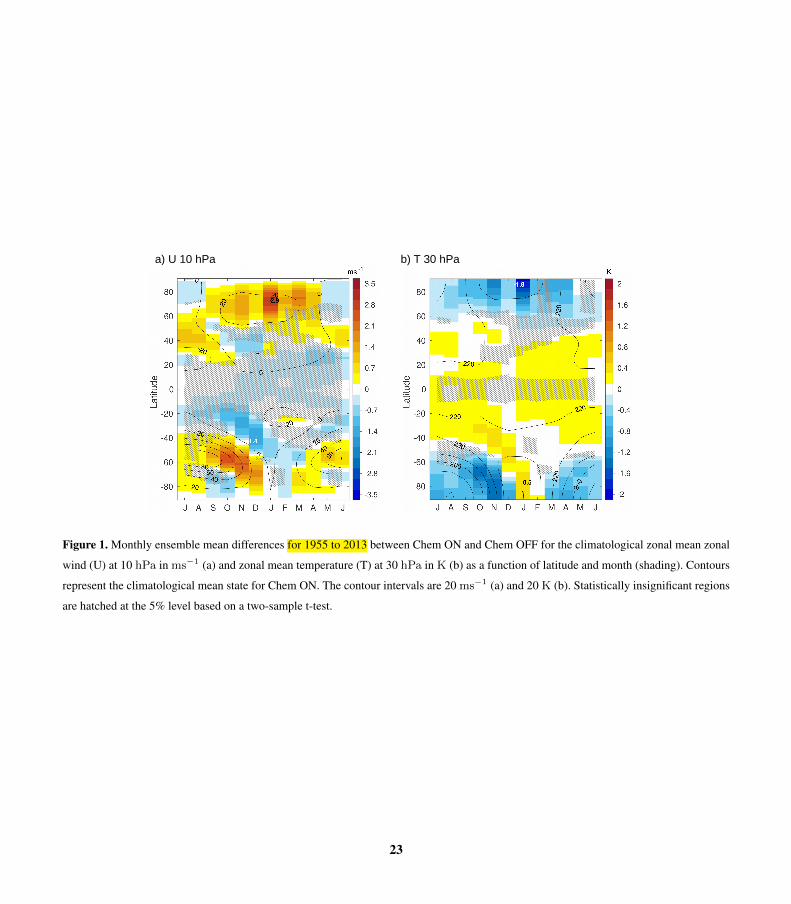
a) U 10 hPa b) T 30 hPa

Figure 1. Monthly ensemble mean differences for 1955 to 2013 between Chem ON and Chem OFF for the climatological zonal mean zonal

wind (U) at 10 hPa in ms−1 (a) and zonal mean temperature (T) at 30 hPa in K (b) as a function of latitude and month (shading). Contours

represent the climatological mean state for Chem ON. The contour intervals are 20 ms−1 (a) and 20 K (b). Statistically insignificant regions

are hatched at the 5% level based on a two-sample t-test.

23

a) U (60-70°S)

b) T (65-90°S)

d) DYN (65-90°S)

c) LW (65-90°S) Kday

Kday

Figure 2. SH ensemble mean differences between Chem ON and Chem OFF for the climatological zonal mean zonal wind (U) in ms−1

(a), polar cap temperature (T) in K (b), long–wave heating rate (LW) in Kday−1 (c), and dynamical heating rate (DYN) Kday−1 (d) as a

function of height (shading). Contours represent the climatology of Chem ON. The contour intervals are 20 ms−1 (a), 10 K (b), 1 Kday−1

(c), and 0.5 Kday−1 (d). Statistically insignificant regions are hatched at the 5% level based on a two-sample t-test.

24

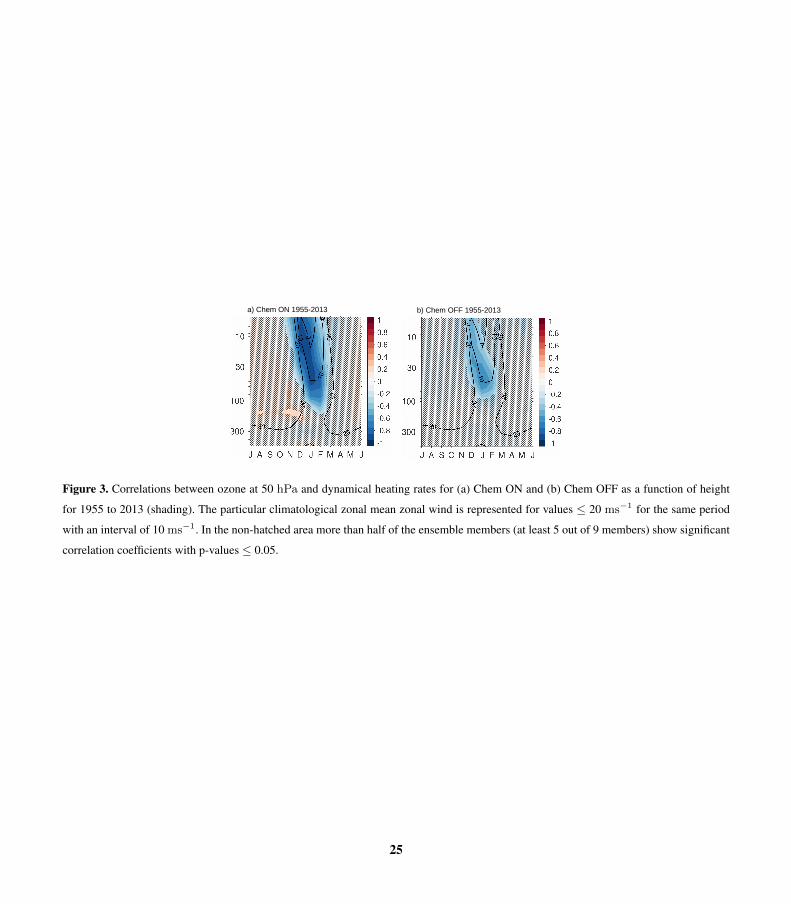
b) Chem OFF 1955-2013 a) Chem ON 1955-2013

Figure 3. Correlations between ozone at 50 hPa and dynamical heating rates for (a) Chem ON and (b) Chem OFF as a function of height

for 1955 to 2013 (shading). The particular climatological zonal mean zonal wind is represented for values ≤ 20 ms−1 for the same period

with an interval of 10 ms−1. In the non-hatched area more than half of the ensemble members (at least 5 out of 9 members) show significant

correlation coefficients with p-values ≤ 0.05.

25

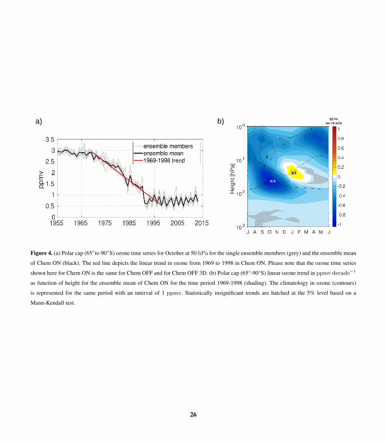
a) b)

Figure 4. (a) Polar cap (65◦to 90◦S) ozone time series for October at 50 hPa for the single ensemble members (grey) and the ensemble mean

of Chem ON (black). The red line depicts the linear trend in ozone from 1969 to 1998 in Chem ON. Please note that the ozone time series

shown here for Chem ON is the same for Chem OFF and for Chem OFF 3D. (b) Polar cap (65°-90°S) linear ozone trend in ppmv decade−1

as function of height for the ensemble mean of Chem ON for the time period 1969-1998 (shading). The climatology in ozone (contours)

is represented for the same period with an interval of 1 ppmv. Statistically insignificant trends are hatched at the 5% level based on a

Mann-Kendall test.

26

a) Chem ON b) IGRA

Figure 5. Polar cap (65°-90°S) linear temperature trend in Kdecade−1 as function of height for the ensemble mean of (a) Chem ON and (b)

IGRA for the time period 1969-1998 (shading). The particular climatologies (contours) are represented for the same period with an interval

of 20 K. Statistically insignificant regions are hatched at the 5% level based on a Mann-Kendall test.

27

a) SW b) LW c) DYN KdayKdayKdayKday

Figure 6. Polar cap (65°-90°S) linear (a) SW, (b) LW and (c) DYN heating rate trends in Kday−1 decade−1 as function of height for the

ensemble mean of Chem ON for the time period 1969-1998 (shading). The particular climatologies (contours) are represented for the same

period with an interval of 2 Kday−1. Statistically insignificant regions are hatched at the 5% level based on a Mann-Kendall test.

28

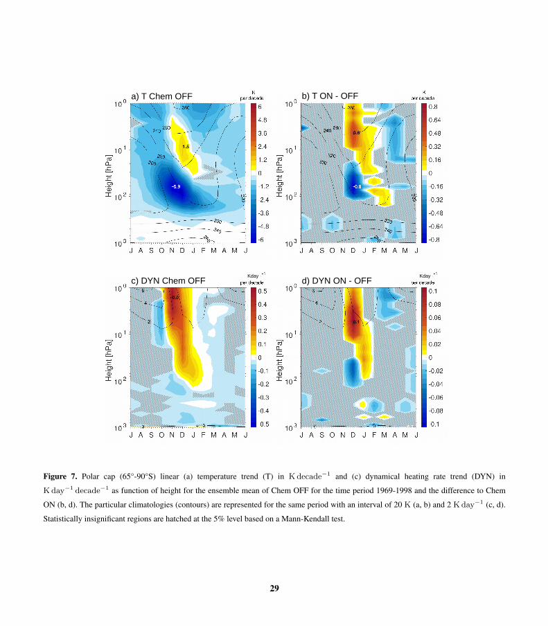
a) T Chem OFF b) T ON - OFF

c) DYN Chem OFF d) DYN ON - OFF KdayKdayKdayKday KdayKdayKdayKday

Figure 7. Polar cap (65°-90°S) linear (a) temperature trend (T) in Kdecade−1 and (c) dynamical heating rate trend (DYN) in

Kday−1 decade−1 as function of height for the ensemble mean of Chem OFF for the time period 1969-1998 and the difference to Chem

ON (b, d). The particular climatologies (contours) are represented for the same period with an interval of 20 K (a, b) and 2 Kday−1 (c, d).

Statistically insignificant regions are hatched at the 5% level based on a Mann-Kendall test.

29

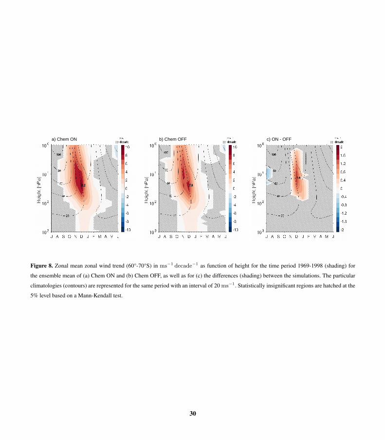
a) Chem ON b) Chem OFF c) ON - OFF

Figure 8. Zonal mean zonal wind trend (60°-70°S) in ms−1 decade−1 as function of height for the time period 1969-1998 (shading) for

the ensemble mean of (a) Chem ON and (b) Chem OFF, as well as for (c) the differences (shading) between the simulations. The particular

climatologies (contours) are represented for the same period with an interval of 20 ms−1. Statistically insignificant regions are hatched at the

5% level based on a Mann-Kendall test.

30

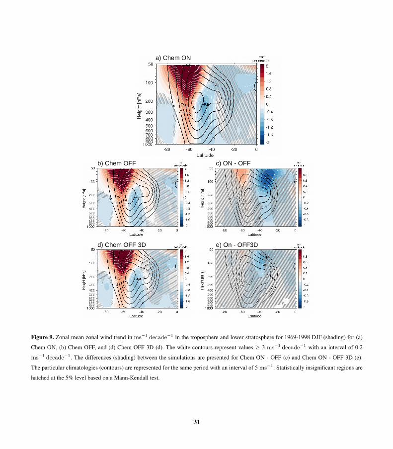
a) Chem ON

d) Chem OFF 3D e) On - OFF3D

b) Chem OFF c) ON - OFF

Figure 9. Zonal mean zonal wind trend in ms−1 decade−1 in the troposphere and lower stratosphere for 1969-1998 DJF (shading) for (a)

Chem ON, (b) Chem OFF, and (d) Chem OFF 3D (d). The white contours represent values ≥ 3 ms−1 decade−1 with an interval of 0.2

ms−1 decade−1. The differences (shading) between the simulations are presented for Chem ON - OFF (c) and Chem ON - OFF 3D (e).

The particular climatologies (contours) are represented for the same period with an interval of 5 ms−1. Statistically insignificant regions are

hatched at the 5% level based on a Mann-Kendall test.

31

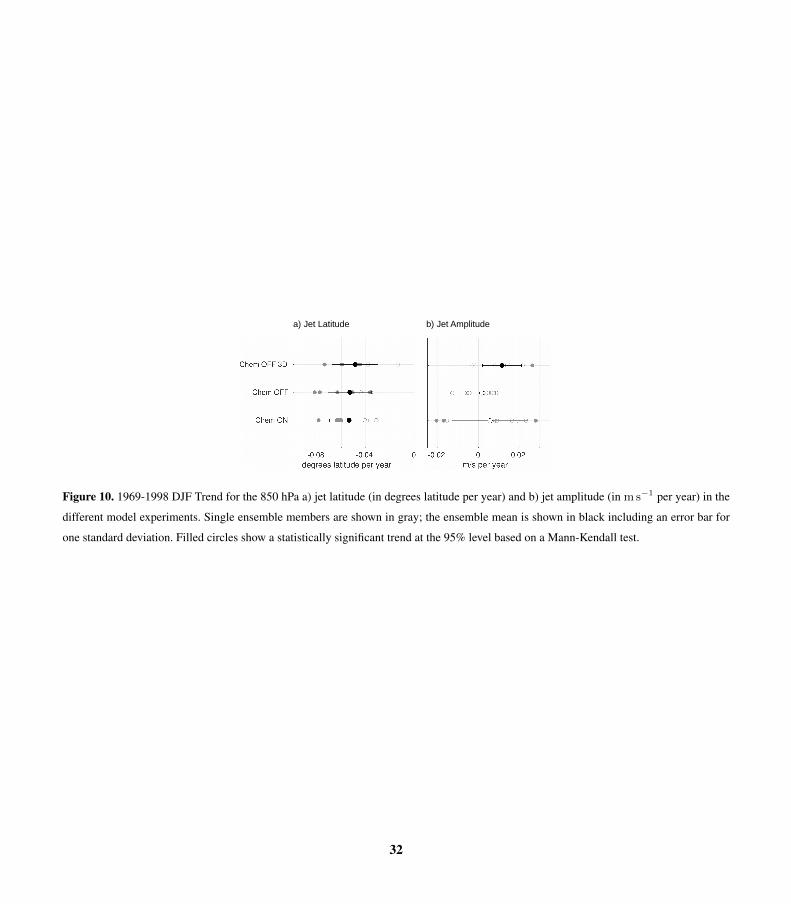
b) Jet Amplitude a) Jet Latitude

Figure 10. 1969-1998 DJF Trend for the 850 hPa a) jet latitude (in degrees latitude per year) and b) jet amplitude (in ms−1 per year) in the

different model experiments. Single ensemble members are shown in gray; the ensemble mean is shown in black including an error bar for

one standard deviation. Filled circles show a statistically significant trend at the 95% level based on a Mann-Kendall test.

32

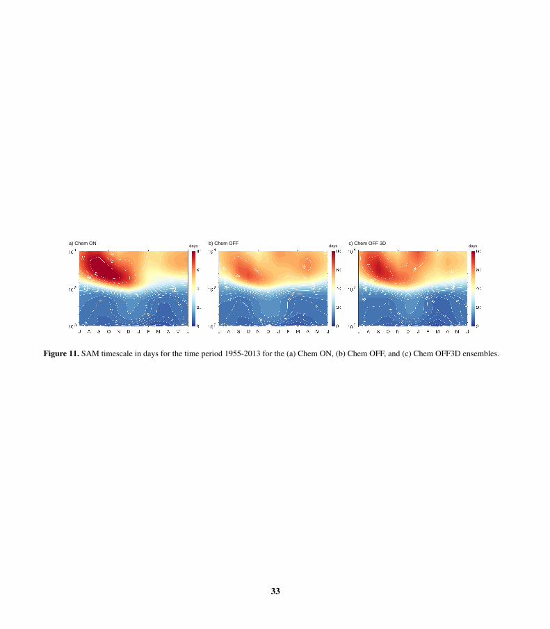
a) Chem ON b) Chem OFF c) Chem OFF 3D days days days

Figure 11. SAM timescale in days for the time period 1955-2013 for the (a) Chem ON, (b) Chem OFF, and (c) Chem OFF3D ensembles.

33

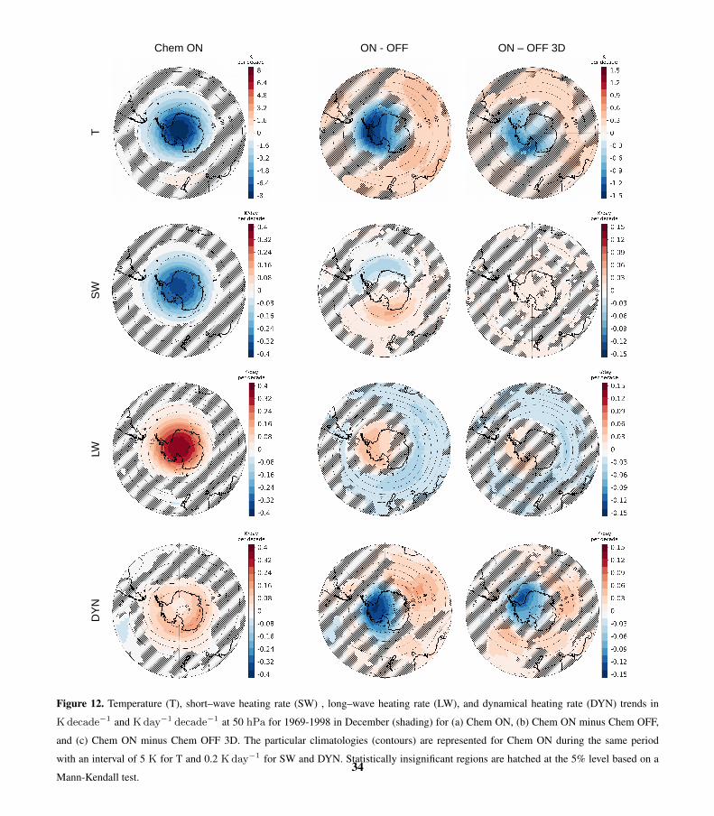
Chem ON

TS

WLW

DY

N

ON - OFF ON – OFF 3D

Figure 12. Temperature (T), short–wave heating rate (SW) , long–wave heating rate (LW), and dynamical heating rate (DYN) trends in

Kdecade−1 and Kday−1 decade−1 at 50 hPa for 1969-1998 in December (shading) for (a) Chem ON, (b) Chem ON minus Chem OFF,

and (c) Chem ON minus Chem OFF 3D. The particular climatologies (contours) are represented for Chem ON during the same period

with an interval of 5 K for T and 0.2 Kday−1 for SW and DYN. Statistically insignificant regions are hatched at the 5% level based on a

Mann-Kendall test.34

Table 1. Different model settings of CESM1 used in this study and their respective abbreviations.

Model Version Ensemble Members Years Ozone Setting Abbreviation

CESM1(WACCM) 9 1955-2013 Interactive Chem ON

CESM1(SC-WACCM) 9 1955-2013 Daily zonally symmetric* Chem OFF

CESM1(SC-WACCM) 9 1955-2013 Daily asymmetric* Chem OFF 3D

* The ozone data used for prescription originates from the Chem ON run.

35

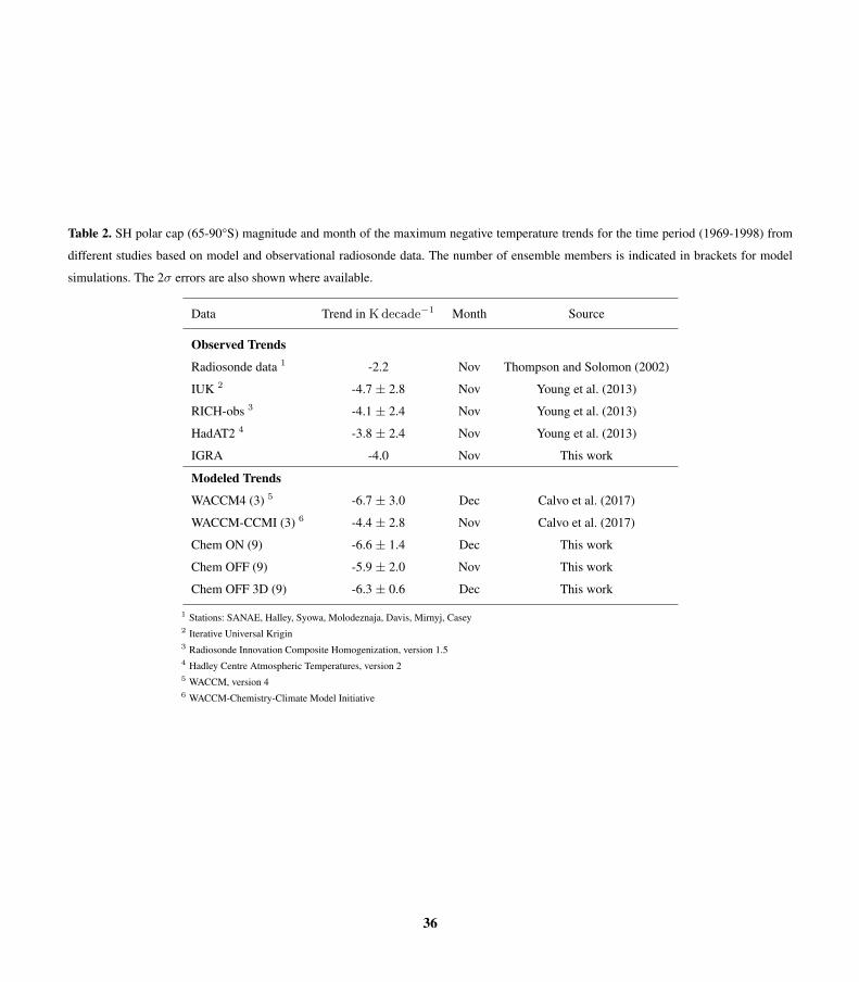
Table 2. SH polar cap (65-90°S) magnitude and month of the maximum negative temperature trends for the time period (1969-1998) from

different studies based on model and observational radiosonde data. The number of ensemble members is indicated in brackets for model

simulations. The 2σ errors are also shown where available.

Data Trend in Kdecade−1 Month Source

Observed Trends

Radiosonde data 1 -2.2 Nov Thompson and Solomon (2002)

IUK 2 -4.7 ± 2.8 Nov Young et al. (2013)

RICH-obs 3 -4.1 ± 2.4 Nov Young et al. (2013)

HadAT2 4 -3.8 ± 2.4 Nov Young et al. (2013)

IGRA -4.0 Nov This work

Modeled Trends

WACCM4 (3) 5 -6.7 ± 3.0 Dec Calvo et al. (2017)

WACCM-CCMI (3) 6 -4.4 ± 2.8 Nov Calvo et al. (2017)

Chem ON (9) -6.6 ± 1.4 Dec This work

Chem OFF (9) -5.9 ± 2.0 Nov This work

Chem OFF 3D (9) -6.3 ± 0.6 Dec This work

1 Stations: SANAE, Halley, Syowa, Molodeznaja, Davis, Mirnyj, Casey2 Iterative Universal Krigin3 Radiosonde Innovation Composite Homogenization, version 1.54 Hadley Centre Atmospheric Temperatures, version 25 WACCM, version 46 WACCM-Chemistry-Climate Model Initiative

36

Dear Martin Dameris, dear referees, We would like to thank you for ...

Documents

Transcript of Dear Martin Dameris, dear referees, We would like to thank you for ...