Dear Editors and Reviewer,

Thank you very much for your messages and your efforts in processing our manuscript “Spatiotemporal

analysis of flash flooding events in mountainous area of China during 1950–2015” (MS No.: nhess-2019-

150). My colleagues and I are very grateful to you for the valuable comments. Based on them we have

revised the paper which is attached for your further consideration. Please refer to the enclosed

“Responses to the referee #2’s comments” for details on the substantial revisions we have made. Our

responses are right after each comment.

Please feel free to contact us if you have any questions with our revision of this paper.

Sincerely,

Nan Wang

Institute of Geographic Sciences and Natural Resources Research, Chinese Academy of Sciences, 11A,

Datun Road, Chaoyang District, Beijing, China

Tel.: +86 13011870541

Email: wnan@lreis.ac.cn

Responses to the referee #2’s comments

General comments

Comments: This study uses a very interesting data set about flood event across China for the last 75

years. It analyses spatio-temporal patterns and attempts to link them to rainfall and soil moisture.

Although I think that this data set may offer a great opportunity and that the research question is of high

importance, the manuscript contains flaws, does not given the information to understand the methods

and results and is not written in a concise way.

Response: Thank you very much for your time on our manuscript and the opportunity to revise the work.

We took these comments and suggestions seriously and addressed them in every detail we could. We

hope the revisions can help you and the readers to understand the methods and results more easily. We

have carefully modified the language in the original manuscript to make it in a more understandable and

concise way. The key points of the revision are as follows:

1) The writing has been improved and checked throughout the whole manuscript. The errors in the

pictures and table has been corrected.

2) The structure of the manuscript has been modified and the Dataset, Results and Discussion sections

have been separated.

3) The confused items and statements have been clarified to better explain our methods and finding in

the spatiotemporal patterns of flash flood disasters.

4) Some supplement to the method has been added to make the results more credible.

Major comments

Comments: Manuscript lacks conciseness: The manuscript is hard to understand as it lacks conciseness.

For example, sentences like “. . .Precipitation anomalies and soil moisture were detected to have a close

correlation with FFEs, however, the interplay of climatic variations and anthropogenic activities may

impose greatly impacts on the occurrence and evolution of the flash flooding disasters on a large extent. . .”

leave the reader with an uneasy feeling as it is not completely clear what is meant by this sentence and

by some of its parts (such as “. . . on a large extent. . .”).

Response: Thank you for your kind comments and suggestions. We checked throughout the whole

manuscript to make it more concise.

Comments: On many locations, the reader knows what is meant, but still it is not concise. An example

(Line 42): “. . .driven by increasing precipitation and atmospheric circulation. . .”: I assume that it is not

increasing atmospheric circulation but changes in the frequency and persistence of flood-related

circulation patterns.

Response: Thank you for your kind comments and suggestions. We modified the description in the

revised version.

Revised (Lines 74-76 in the revised version): A clear upward trend in flood frequency in Germany was

proven to be driven by extreme precipitation and atmospheric circulation (Petrow and Merz, 2009).

Comments: Another example is Line 77: “. . .including temporal variation, temporal mutation, temporal

periodic, and temporal clustering. . .”: Is temporal variation different from the 3 other terms? What is

meant by temporal mutation and temporal periodic?

Response: Thank you for your kind comments and suggestions. Firstly, we agree with you that the term

“temporal variation” is somewhat confusion, therefore, we changed it into “temporal evolution”.

Temporal evolution was intended to analyse the long-term time series based on the annual number of

FFEs in each geomor-region. In addition, “temporal mutation” was changed into “temporal trends”.

Temporal trends were supposed to detect the upward/downward trends of the occurrence of FFEs in each

watershed. It can also reveal the distribution of the divergent temporal trends in spatial. Finally,

“temporal periodic” was changed into “temporal period”, which was used to detect whether there were

predominant periods at different scales or not in the temporal evolution of FFEs.

Revised (Lines 108-110 in the revised version): This is followed by the analysis of spatiotemporal

characteristics of FFEs, including temporal evolution, trends, period, and clustering in Section 4.

Comments: The manuscript also contains statements that are not substantiated and may mislead the

reader. For example: “. . .Our research has shown that currently there is not strong enough evidence to

support whether climate change will do good or harm to the flash flooding disaster in the future. . .” I

would rather argue that this manuscript has not addressed this question. There is a large body of literature

and very elaborated methods on attributing changes (for example in rainfall or flooding) to climate

change. Hence, saying that an important question cannot be answered as there is not enough evidence is

inappropriate, when the research has not even attempted to address the attribution question.

Response: Thank you for pointing out the not rigorous statements in the original manuscript and we have

corrected them. In this paper, we intended to induce the statement that the climate change might has a

complex impact on the flash floods. But we did not have strong enough evidence to support these

statements.

Revised (Lines 578-579 in the revised version): Our research has not provided strong enough evidence

to support whether climate change will mitigate or propagate flash flood disasters in the future.

Comments: Another example for unconcise wording: “. . . Besides, the results suggest that the temporal

variations were closely related to the climatic variations and anthropogenic activities in China. . .”:

Anthropogenic activities are mentioned in a very general way, and the manuscript does not contain any

analyses or specific statements about anthropogenic activities. Unfortunately, these are only a few

examples.

Response: Thank you for the insightful comments. We have deleted the unconcise wording in the revised

version.

Comments: Manuscript contains a number of errors: An example is the caption of Figure 1: (b) is the

trend and not the intra-year series, and (c) is the intra-year distribution and not the inter-year series.

Response: Thank you for the detailed comments. We have checked throughout the figures and tables in

the manuscript and corrected the errors.

Revised (Figure 1 in the revised version):

Figure 1: Location and inter-year and intra-year series of FFEs in China over 1950-2015. (a) the spatial location of

the study area and the distribution of FFEs; (b) the inter-year series of FFEs; (c) the intra-year series of FFEs.

Comments: Another example: Sections 4.4.1 and 4.4.2 have exactly the same title (Intra-annual

clustering), but have different contents.

Response: Thank you for the comments. We have modified the titles of Sections 4.4.1 and 4.4.2.

Revised (Lines 339 and 388 in the revised version): 4.4.1 Intra-annual clustering; 4.4.2 Inter-annual

clustering

Comments: The English is poor, and often very difficult to understand.

Response: Thank you for the comments and we improved the English writing style to make it more

understandable.

Comments: Structure of the manuscript: The discussion chapter takes up a new issue and introduces

additional data (precipitation and soil moisture). I strongly recommend to rearrange the contents such

that all data, methods and results are reported in the data, methods and results sections, respectively, and

that the discussion section only discusses the findings.

Response: Thank you for the insightful suggestion. According to your suggestion, we compiled all data

used in this study in the Section 2. In the discussion, we focused on the more notable period with the

high occurrence of FFEs. Besides, we attempted to analyze some of the important factors which may

explain the reason for the temporal variation of FFEs.

Comments: Abstract: The abstract cannot be fully understood since terms are used which can have

different meanings, but are not explained.

Response: Thank you for the suggestion. We modified the abstract and used the more understanding

terms to make it more clear.

Revised (Lines 17-36 in the revised version): To bridge this gap in the research on the spatiotemporal

characteristics of flash flood events (FFEs), this study used a Mann-Kendall (MK) test, wavelet analysis,

monthly frequency, and index of dispersion (D), based on the longest time series available of FFEs in

China to detect the temporal evolution, trends, period, and clustering of FFEs in six geomorphological

regions (geomor-regions: the EP, SEM, NCP, NWB, SWM, and TP) of China. The results indicated that:

(1) the frequency of FFEs in the EP and NCP regions increased steadily with rates of change of 3.34 and

1.86 per year and at rates of 9.32 and 8.05 per year in the SEM and SWM, and increased dramatically in

TP and NWB in the last twenty years; (2) the watersheds with upward trends at the 99% significance

level were mainly located in the SEM and SWM regions, while those with downward trends at the 90%

significance level were only detected in the EP region; (3) in EP, SEM, and SWM, there were three clear

oscillation periods on the time scale of 12–25a and two clear oscillation periods on the scale of 2–8a; (4)

the highest monthly frequency of FFEs was more likely to occur in July, and it appeared to occur after

July in EP, NCP, and TP and before July in SEM and NWB; (5) The inter-annual clustering of FFEs

played a dominant role across China, while the typical pattern of FFE occurrence was only detected in

six (five percent) watersheds.

Comments: I am confused by the use of the term “Flash Flooding”. Flash floods are different from river

floods. In the introduction, several “flash flood” studies are cited, but these studies actually discuss river

floods and not flash floods. First, I thought that the authors had not carefully read the literature they were

citing, but later I got very confused as they speak about large watershed (“. . . 133 watersheds, with the

watershed area ranged from 0.3 to 60 ×104 km2 . . .”). Is this paper about flash floods or river floods? I

also propose that they introduce their definition of flash flood events early in the paper.

Response: Thank you for the thoughtful comments. Firstly, for the term “flash flooding” we used in this

paper maybe not so widespread, we changed the “flash flooding” into “flash floods” throughout the paper.

Secondly, the flash floods analysed in this paper included the water floods, debris flows and landslides

etc., which occurred in the mountainous area and caused the economic losses or the people death. The

flash flood events we discussed in this paper is comprised of several kinds of disasters triggered by high-

intensity and short-duration rainfall (or snowmelt). Therefore, the studies we cited in Section 1 included

river floods and flash floods. The watersheds were used as the basic units to sum up the number of FFEs

in the analysis of monthly frequency, index of dispersion, and the relationship between climatic factors

and FFEs. According to your kindly suggestion, we mentioned the definition of flash flood events in

Section 1, and we also added some description of the FFEs inventory in Section 2 to make it more

understandable for readers.

Revised (Lines 120-122 in the revised version): The FFEs analysed in this paper included water floods,

debris flows, and landslides which occurred in mountainous areas and caused economic losses or human

fatalities.

Comments: Selection of Events and FFE database (Section 2.1): The criteria when an event has been

counted/documented in the database are not given. The data set needs to be described in detail. For

example, has been taken care of the reporting bias? Without a detailed description, the reader cannot

really interpret the results of the study.

Response: Thank you for the useful suggestion. The FFEs in this study were obtained by the official

documents and the published literature, which were considered as the trustful information sources.

What’s more, some interview and field work have been done to deal with the records which have no

detailed description. In the FFEs database, each FFE was labelled with the unique PID, which indicated

the index of the administrative village. In this study, we have also dealt with the repeated records with

the same PID and the same detailed information to avoid the repetitive records.

Revised (Lines 122-124 in the revised version): In addition, we have eliminated repeated instances of

FFEs from the data to ensure that each event is recorded only once in the same administrative village

(which is the smallest administrative unit in China) and at the same date.

Comments: Division into regions (Section 2.2): The justification for dividing the country into these 6

regions is not given. Why these 6 regions? Are 6 regions detailed enough for such a large country?

Response: Thank you for the comments. The geomorphological regionalization (geomor-region) we

used in this paper were widely acknowledged by researchers for the division of China into some sub-

regions. We analysed the spatiotemporal characteristics of FFEs in six geomor-regions in China based

on the following points. Firstly, the topographic features of watersheds, including slope, aspect, relief,

etc., have an important impact on the occurrence of flash floods. Secondly, the watersheds within the

same geomor-region tend to share the same or similar climatic conditions. Thirdly, the six geomor-

regions showed distinctive characteristics in terrain, climate, soil, vegetation, together with population

distribution, which are widely recognized by researchers. For the huge divergent of China, the

spatiotemporal analysis of FFEs was conducted in six geomor-regions respectively can reveal more

detailed information. However, if we adopted a more detailed division, there will not be sufficient FFE

samples for a complete long-term record in each detailed division. Therefore, after the comparison and

consideration, we selected the six geomor-regions as the proper division of spatiotemporal analysis of

FFEs.

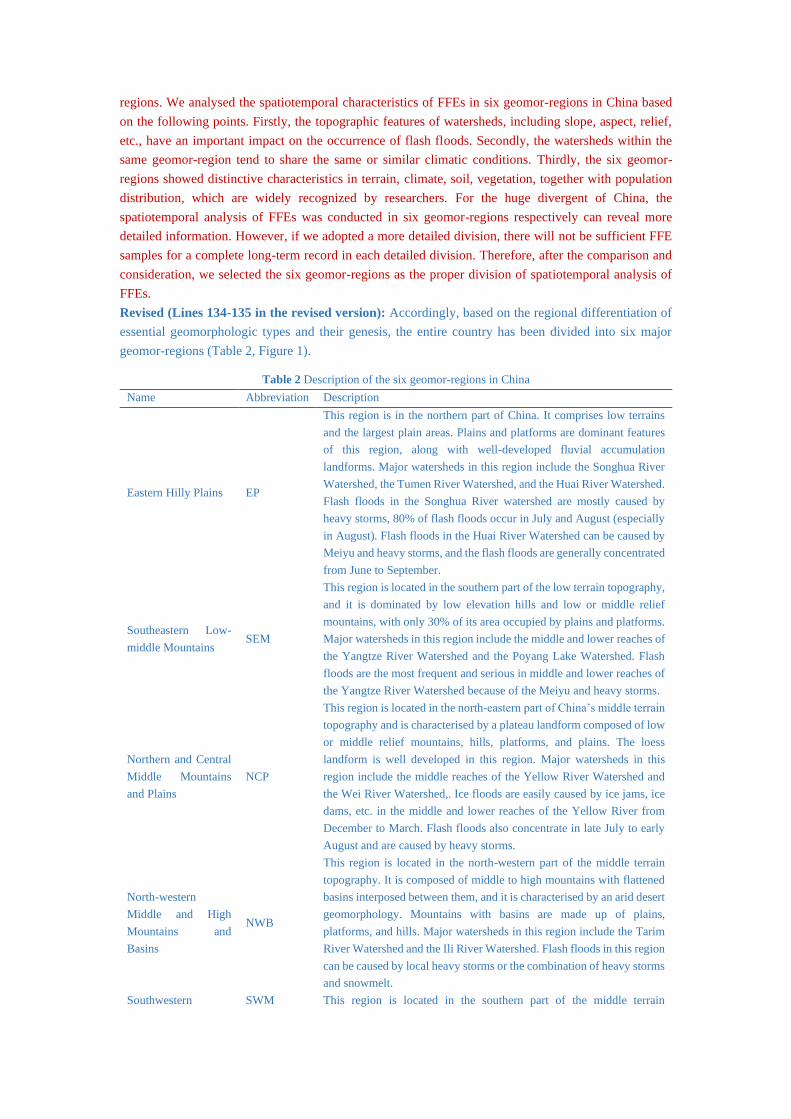
Revised (Lines 134-135 in the revised version): Accordingly, based on the regional differentiation of

essential geomorphologic types and their genesis, the entire country has been divided into six major

geomor-regions (Table 2, Figure 1).

Table 2 Description of the six geomor-regions in China

Name Abbreviation Description

Eastern Hilly Plains EP

This region is in the northern part of China. It comprises low terrains

and the largest plain areas. Plains and platforms are dominant features

of this region, along with well-developed fluvial accumulation

landforms. Major watersheds in this region include the Songhua River

Watershed, the Tumen River Watershed, and the Huai River Watershed.

Flash floods in the Songhua River watershed are mostly caused by

heavy storms, 80% of flash floods occur in July and August (especially

in August). Flash floods in the Huai River Watershed can be caused by

Meiyu and heavy storms, and the flash floods are generally concentrated

from June to September.

Southeastern Low-

middle Mountains SEM

This region is located in the southern part of the low terrain topography,

and it is dominated by low elevation hills and low or middle relief

mountains, with only 30% of its area occupied by plains and platforms.

Major watersheds in this region include the middle and lower reaches of

the Yangtze River Watershed and the Poyang Lake Watershed. Flash

floods are the most frequent and serious in middle and lower reaches of

the Yangtze River Watershed because of the Meiyu and heavy storms.

Northern and Central

Middle Mountains

and Plains

NCP

This region is located in the north-eastern part of China’s middle terrain

topography and is characterised by a plateau landform composed of low

or middle relief mountains, hills, platforms, and plains. The loess

landform is well developed in this region. Major watersheds in this

region include the middle reaches of the Yellow River Watershed and

the Wei River Watershed,. Ice floods are easily caused by ice jams, ice

dams, etc. in the middle and lower reaches of the Yellow River from

December to March. Flash floods also concentrate in late July to early

August and are caused by heavy storms.

North-western

Middle and High

Mountains and

Basins

NWB

This region is located in the north-western part of the middle terrain

topography. It is composed of middle to high mountains with flattened

basins interposed between them, and it is characterised by an arid desert

geomorphology. Mountains with basins are made up of plains,

platforms, and hills. Major watersheds in this region include the Tarim

River Watershed and the Ili River Watershed. Flash floods in this region

can be caused by local heavy storms or the combination of heavy storms

and snowmelt.

Southwestern SWM This region is located in the southern part of the middle terrain

Subalpine Mountains topography. Evidencing a typical karst landform, middle or high

mountains with middle or high reliefs are widespread with wide valley

basins interspersed between them. Major watersheds in this region

include the upper and middle reaches of the Yangtze River Watershed

and the Jialing River Watershed. Influenced by the plateau monsoon

climate, the storm period in this region is long and usually multi-peaked.

Tibetan Plateau TP

This region encompasses China’s high terrain topography. It is

composed of plains and high mountains at elevations above 4,000 m

which account for three-fourths of the area of the region. It is

characterised by glacial and periglacial landforms. Major watersheds in

this region include the Yarlung Zangbo River Watershed, Nu River

Watershed, and Shiquan River Watershed. Local persistent heavy rain

are the main cause of flash floods in the tributaries of the middle reaches

of the Yarlung Zangbo River Watershed.

Comments: Description of data is incomplete (Section 2.4): A much more detailed description of the

data used is necessary. For instance, how many rainfall stations are available? What is the (grid)

resolution of the simulated soil moisture?

Response: Thank you for the detailed suggestion. We have added the essential information you

suggested into the data resources to make it more complete.

Revised (Lines 147-153 in the revised version): Daily precipitation data were provided by the China

Meteorological Administration (http://data.cma.cn/). In this study, only the stations (there are 824 basic

weather stations in total) with complete data from 1980–2010 were selected. Climate Prediction Center

(CPC) soil moisture (SM) data were provided by the National Oceanic Atmospheric Administration

(NOAA)/Oceanic and Atmospheric Research (OAR)/Earth Systems Research Laboratory (ESRL)

Physical Sciences Division (PSD), Boulder, Colorado, USA, from the Web site

https://www.esrl.noaa.gov/psd/. The monthly data set consisted of a file containing monthly averaged

soil moisture water height equivalents with spatial resolution of 0.5° x 0.5°. The data is model-calculated

and not measured directly.

Comments: Section 2.4: Rainfall data is only available for 1980–2010, but the event FFE analysis is

carried out for 1950–2015. What is done for the periods where rainfall data is missing?

Response: Thank you for the comments. In the discussion, we selected the period of 1980–2010, which

has a more obvious temporal variation, as the study object to analyse the relationship between climate

indicators and FFEs. As for your confusion, we added some reasons for the selection of 1980–2010

period at the beginning of the Section “5. Discussion”.

Revised (Lines 420-427 in the revised version): The long-term evolution trends indicated that the

number of FFEs in all six geomor-regions were relatively low before 1980. On one hand, this variation

may be attributed to poor data acquisition methods and inadequate data records before 1980, which may

have resulted in the lower occurrence observations in the historical period to some extent. On the other

hand, some climate factors, e.g. precipitation, may have had an effect on the FFEs. With the changing

climate, increasing frequency of extreme precipitation may have caused greater numbers of flash flood

disasters in recent years. To reveal the potential factors of the FFE trends and better understand the peaks

in the FFE time series, we discuss the potential relationships between climatic factors and FFEs in the

following section.

Comments: Figure 1: It is not clear what Figure 1c shows. What is the meaning of the blue polygon?

Response: Thank you for the question. Figure 1c shows the accumulation number of FFEs in each month

during 1950–2015, which can clearly reflect the intra-annual difference of the FFEs occurrence. To better

display the intra-annual distribution of FFEs, we changed the radar chart into bar chart in the revised

version.

Comments: Methods: Different methods are used but only for the trend analysis with Sen’s slope, the

significance is calculated. I feel that it is absolutely necessary to provide significance statements also for

the other analyses (reported in 4.1, 4.3, 4.4).

Response: Thank you for the insightful suggestion. Actually, we have done the significance test for MK

test and monthly frequency. The significance test for MK test was detected by Z-statistics. When the Z-

statistics with the absolute value larger than 1.28, 1.64 and 2.32, it represents the trend goes through the

90%, 95% and 99% significance test, respectively. The significance test for monthly frequency was

obtained by the lower and upper bounds (𝐿𝐿𝑁 and 𝐿𝑈

𝑁), which indicated the confidence of 95%. Besides,

referred to Merz et al. (Merz et al., 2016), we explored the time scale (T = 1a, 2a, 3a, 4a, 5a) and the start

aggregation time of the time series at the 95% significant level, the results were as follows. The results

indicated that the flash floods occurrence was not sensitive to the time scale and the start aggregation

time of the time series in most area of this study.

Revised (Lines 389-401 in the revised version): To examine the inter-annual FFEs clustering, D was

calculated based on the FFEs occurrence frequency data. D quantifies the deviation of annual occurrence

rates from the expected occurrence rates. A D value larger than 0 was observed for all six geomor-regions

across China, indicating that inter-annual clustering played a dominant role in FFE occurrence (Figure

9). Extensive significant clustering, a large D value of up to 4, can be detected for the SEM, SWM, and

TP geomor-regions. The largest D value (D = 12) observed in the Wujiang River, which is located in the

middle of the Yangtze River, means that on average FFEs occurred 12 times more often in FFE-rich

years than would be expected from the Poisson distribution. The clustering strength diminished from

eastern to western China. Nevertheless, six of the watersheds exhibited statistically significant results of

a negative D, which indicated that the inter-annual occurrence of FFEs in these watersheds were under-

dispersed. In this study, the characteristic under-dispersion of FFEs was mainly identified in western

China, including in NWB, NCP, TP, and SWM, appeared to have a more regular temporal pattern

between years.

Figure 9: D value of FFEs in watersheds for the period of 1950–2015. The solid circles indicate the clustering at

95% significant level, and the circles with white hole indicate the insignificant D values.

Comments: Methods/results: Figure 2 shows “. . . trend line based on the least-squares linear

regression. . .”. This is inconsistent with the Methods Section where it is stated that the trend is estimated

by Sen’s slope.

Response: Thank you for the question. The trend line in Figure 2 was obtain based on the original time

series of FFEs, which was not mentioned in Section 2 Methods. The least-squares linear regression we

mentioned here was supposed to reveal the long-term evolution of the FFEs in each geomor-region.

While, the Sen’s slope in Section 4.2 was used to shed light on the magnitude of upward/downward trend

in each watershed.

Comments: Methods/results: The grey, yellow and blue lines seem to decrease to 0 at the end of the

time series. I guess that this is not a real decline in the occurrence of floods (then the red line would not

increase), but is an artefact of the method/presentation used. This needs to be clarified.

Response: Thank you for the comment. In the original manuscript, the x-axis was ended at the year of

2016, which actually does not have data. Therefore, it seemed like the lines decrease to 0 at the end of

the time series. We have modified the x-axis to end at 2015 to avoid the misunderstanding.

Revised (Figure 2 in the revised version):

Figure 2: Time series of the annual mean number of FFEs in six geomor-regions in China from 1950 to 2015. The

grey line is the original time series; the yellow and blue lines are the 5-year and 10-year moving averages,

respectively; the red line is the cumulative number of FFEs; and the black dashed line is the trend line based on the

least-squares linear regression for (a) EP, (b) SEM, (c) NCP, (d) NWB, (e) SWM, and (f) TP.

Comments: Method (Line 192): The sentence “The statistic results presented an overall agreement

between MK testing and Sen’s slope estimator. . .” is unclear (as MK tests the significance and Sen

provides the slope of the trend).

Response: Thank you for the comment. The description was unclear and we modified it in the revised

version. The positive and negative values of Z in MK test indicate increasing and decreasing tendencies,

respectively. While, the positive and negative values of 𝛽 in Sen’s slope estimator test also represent

increasing and decreasing trends, respectively. Here, we were supposed to compare the

increasing/decreasing trend of FFEs in each watershed by the results obtained from these two methods.

We have deleted the confusing statement in the revised version.

Comments: Section 4.1 and 4.2: Both sections present trend analyses. Why are there 2 sections with

different methods looking at the trend? I rather feel that the reader is confused by these 2 sections (in

particular as the section titles are not understandable).

Response: Thank you for the question. First of all, we have changed the title of Section 4.1 to “Temporal

evolution analysis”. The method we used in Section 4.1 was 5-year and 10-year moving average, which

was supposed to obtain the long-term evolution of the time series of FFEs in each geomor-regions.

Secondly, the title of Section 4.2 was change to “Temporal trends analysis”. The method used in Section

4.2 was MK test. MK test was intended to detected the upward/downward trending of FFEs occurrence

in each watershed, which revealed more detailed information in spatial.

Revised (Lines 217 and 243 in the revised version): Section 4.1 Temporal evolution analysis; Section

4.2 Temporal trends analysis

Comments: Figure 3: The value of the trend (Sen’s slope) should be given in relation to a certain quantity,

e.g. X% per decade in relation to average value. Otherwise, these numbers do not give any information.

Similarly, I wonder whether the reader can interpret the Z-statistics of the MK test. I would rather report

the p-value which is typically used.

Response: Thank you for the suggestion. Firstly, we have modified the value of Sen’s slope to make it

understandable. Furthermore, as far as we concerned, the Z-statistics was the most common used value

for the interpretation of the results of the MK test. Positive values of Z stand for upward trend, and the

downward trend would be indicated by negative Z. When the Z-statistics with the absolute value larger

than 1.28, 1.64 and 2.32, it represents the trend goes through the 90%, 95% and 99% significance test,

respectively.

Revised (Lines 258-261 in the revised version): The results of the Sen’s slope estimator test

demonstrated that the regional average increasing rate of the FFE numbers of EP, SEM, NCP, NWB,

SWM, and TP were 0.37, 2.37, 0.03, 0.23, 2.23, and 0.18 per year, respectively.

Comments: Figure 4/Figure 5: The wavelet results look quite different to the many wavelet results I

have seen in other studies. I propose to use the setup of the seminal paper on wavelets of Torrence and

Compo (1998). Further, one needs to add the cone of influence to understand where the results are not

reliable. In addition, I wonder why 3 wavelet diagrams are shown (Fig. 4, 5a, 5b). Why do they differ?

Response: Thank you for the suggestion. Firstly, we obtained the wavelet results by using the Matlab

toolbox based on the theory of Torrence and Compo (1998), which is a convenient and reliable tool for

wavelet analysis. The results we obtained in this research were similar to the results revealed in many

studies which have been published (Wang et al., 2017; Fu et al., 2018; Bi et al., 2019). In addition, Figure

4, 5a, 5b explained the different aspect of the temporal period. Figure 4 indicates the real-part of the

wavelet coefficient, which reflects the periodic variation of the FFEs sequence. Figure 5a indicates the

modulus of the wavelet coefficients, which reflects the distribution of energy density. The energy density

corresponds to the period of change of the different events in the time domain. And in the revised

manuscript, we deleted the Figure 5b, which showed somewhat similar trends with Figure 5a.

Reference:

[1] Wang, H., Shao, Z., Gao, T., Zou, T., Liu, J. and Yuan, H.: Extreme precipitation event over the

Yellow Sea western coast: Is there a trend?, Quaternary International, 441, 1-17, doi:

10.1016/j.quaint.2016.08.014, 2017.

[2] Fu, Q., Zhou, Z., Li, T., Liu, T., Liu, D., Hou, R., Cui, S. and Yan, P.: Spatiotemporal characteristics

of droughts and floods in northeastern China and their impacts on agriculture, Stochastic Environmental

Research and Risk Assessment, 32, 2913-2931, doi: 10.1007/s00477-018-1543-z, 2018.

[3] Bi, S., Bi, S., Lu, Y., Qu, Y. and Zhao, F.: Temporal and spatial characteristics of droughts and floods

in northern China from 1644 to 1911, Journal of Earth System Science, 128, 98, doi: 10.1007/s12040-

019-1121-x, 2019.

Revised (Figures 4 and 5 in the revised version):

Figure 4: The real part of the wavelet coefficient of FFEs in six geomor-regions of China: (a) EP, (b) SEM, (c) NCP,

(d) NWB, (e) SWM, and (f) TP.

Figure 5: The modulus of FFEs wavelet coefficients in six geomor-regions of China: (a) EP, (b) SEM, (c) NCP, (d)

NWB, (e) SWM, and (f) TP.

Comments: Wavelet results: I wonder why the annual scale is not prominent. Figure 1c seems to suggest

that there is a very strong seasonality in the occurrence of FFEs; then this should show up in the wavelet

results. (But maybe I misinterpret Figure 1c, because it is not explained what this figure (blue polygone)

means).

Response: Thank you for the comment. The wavelet analysis was carried out on the basis of annual

accumulation of the FFEs number. Therefore, there is no seasonal characteristics can be interpreted in

these results.

Comments: Figure 7: I understand that Figure 7 shows a transects at the main periods (10a, 5a) through

the wavelet diagram (Figure 4), but I cannot understand at all the explanation of this figure (Lines 233-

238).

Response: Thank you for the comments. We have modified the description of the main period in Figure

6 (in the revised version).

Revised (Lines 315-325 in the revised version): The wavelet variance map reflects the distribution of

the energy fluctuation of the FFEs time series with different time scales. It can be used to determine the

main period of FFEs evolution. In Figure 6, all geomor-regions except TP demonstrated the most obvious

peak of 18–19a, indicating the strongest and the first main period of FFEs. For the characteristics

temporal scale of 18–19a, the average variation in FFE periods in EP, SEM, NCP, NWB, and SWM are

7–7.5a. Moreover, the second main period of FFEs in EP, SEM, and SWM are 5a (Figures 6a, 6b, and

6e), and NCP and NWB are 11–12a (Figures 6c and 6d). However, in TP, the first main period is detected

as 26a and the second as 8a (Figure 6f).

Figure 6: The wavelet variance analysis of FFEs in six geomor-regions of China: (a) EP, (b) SEM, (c) NCP, (d)

NWB, (e) SWM, and (f) TP.

Comments: Methods: Intra-annual clustering (Section 4.4.2): It is not clear what is shown and discussed

in Figure 10 and in section 4.4.2. For example, the calculation of D requires selecting the aggregation

period T; this information is not given. What exactly is meant by intra-annual clustering? Further,

significance of clustering derived by the index of dispersion method is sensitive to the selection of the

starting time point of the aggregation window (see Merz et al., 2016). This issue should be considered.

Response: Thank you for your kindly comment and suggestion. Firstly, the inter-year clustering was

supposed to detect the obvious rich/poor year of flash floods in each watershed. The rich year of flash

floods was characterized as over-dispersion, which showed the clustering pattern of flash floods during

the study period. The poor year of flash floods is characterized as under-dispersion, which shows the

regular pattern of flash floods in the study period. Secondly, the window length T in this study was set

as 1 year with the consideration of total time series length (66 years). Furthermore, we added the

discussion of the influence of the time scale and the start time point of the aggregation window.

Revised (Lines 210-211 in the revised version): where Z(T) is the series of FFE counts within a time

window with length T (here, T was set as 1 year), Var(Z(T)) is the variance of the FFE counts, and

E(Z(T)) is the expected value.

Revised (Lines 407-416 in the revised version): Figure 10 shows the influence of the time scales on D

and its sensitivity to the start year of the aggregation time windows. In SWM, there is no difference in

the percentage of watersheds with significant clustering (at 95% significant level) at various time scales

and the start year of the aggregation time windows, while in EP there was a slight difference at various

time scales. However, in SEM, NCP, NWB, and TP, the percentage of watersheds with significant

clustering varied at different time scales and the start of aggregation time windows. In SEM, an

increasing clustering value percentage was detected at the larger time scale, while in NCP the clustering

values percentage decreased at larger time scales. In TP, the highest clustering value percentage was

obtained at a time scale of four years. In NWB, the highest (94%) and lowest (69%) clustering value

percentages were both detected at a time scale of five years. These results demonstrate an obvious

sensitivity to shifts in the start of aggregation time windows.

Figure 10: Percentage of watersheds in significant FFE clusters at a 95% significant level in the six geomor-regions.

T indicates the time scale (1a, 2a, 3a, 4a, and 5a), and the x-axis indicates the shifting start time of the aggregation

time window.

Comments: Figure 11 and 12: I assume that ‘number of FFEs’ means the total number of documented

FFEs within each year (from Jan to Dec). This needs to be said. More disturbing is that the x-axis of

Figure 11 seems to have wrong labels as the numbers are 2 orders of magnitude smaller than Figure 12.

Response: Thank you for the comment. Firstly, we added the accurate information of data we used for

analysis in this Section. Secondly, the reason for the difference between the x-axis of Figure 11 and

Figure 12 was caused by the different regression equation. In Figure 11, the x-axis actually indicated the

log value of the number of FFEs, and the y-axis indicated the log value of precipitation. Thank you for

your kindly reminder, and we classified the x-axis and y-axis of Figure 11 in the revised version.

Revised (Lines 443-447 in the revised version): In this section, we selected the annual total

precipitation for days with daily precipitation exceeding the 90th percentile of 1980–2010 daily

precipitation (R90p) and the mean soil moisture of summer (May to August), together with the annual

occurrence of FFEs (yearly cumulative number of FFEs) in each watershed, to detect the potential

impacts that may be caused by these indicators.

Figure 11: The relationship between R90p and FFEs for (a) EP, (b) SEM, (c) NCP, (d) NWB, (e) SWM, and (f) TP.

R90p indicates the annual total precipitation of rainy days exceeding the 90th percentile of 1980–2010 daily

precipitation.

Figure 12: The relationship between the mean soil moisture in summer (May–August) and FFEs for (a) EP, (b)

SEM, (c) NCP, (d) NWB, (e) SWM, and (f) TP.

Comments: Figure 13: The text does not contain a hint to and discussion of Figure 13. However, this is

necessary, as it is not that obvious from Figure 13 that FFEs occurrence and high positive anomalies

match.

Response: Thank you for the comment and suggestion. For better understanding, we modified the

discussion in Section 5.2 and added the reference information of Figure 13 in the text.

Revised (Lines 540-571 in the revised version): In 1998, about 80% of FFEs were located in the zone

with precipitation anomalies above zero (Table 5). In August 1998, the main rainfall belt was located

over the Yangtze River, with precipitation 100% or more above normal (Figure 13d), and a typical

Secondary Meiyu occurred. Tropical and subtropical circulation systems were characterised by a stronger

than normal and more westward-extending Western Pacific Subtropical High (WPSH), a weaker than

normal EASM, and the anomalous convergence of moisture flux in the middle and lower reaches of the

Yangtze River. These circulation anomalies were attributed to the tropical sea surface temperature

anomaly patterns of the preceding seasons, i.e. the super El Niño and strong warming of the tropical

Indian Ocean (Yuan et al., 2017). The precipitation anomalies resulted in the rainfall belt moving from

the lower to upper reaches of the Yangtze River from June to August (Figures 13b, 13c, and 13d).

However, the FFEs that occurred in September and October were not detected in the heavy rainfall centre

(with the anomalies of precipitation more than 100%) (Figures 13e, and 13f), indicating there may be

other factors inducing flash floods together with the precipitation anomalies during this period.

In 2010, more than 90% of the FFEs were distributed in the zone of the precipitation anomalies, with the

zone of 60–80% and more than 100% ranking in the top two (Table 5). Studies indicated that an El Niño

Modoki (a special flavour of the El Niño, which is a part of the El Niño Southern Oscillation (ENSO))

with strong warming in the central Pacific was detected, which caused the rainfall belt to shift northward.

The extreme precipitation appeared in the Huai-Yellow River along with a weakened Indian summer

monsoon and strengthened EASM (Wang et al., 2012). The cluster centre of the FFEs moved from the

Yangtze River to the Huai River and then to the Yellow River from May to July (Figures 13g, 13h, and

13i), demonstrating the close connection with precipitation anomalies.

Studies have indicated that the El Niño Modoki was different from a typical El Niño with respect to its

evolution and climate impact (Feng et al., 2011).The Pacific Decadal Oscillation (PDO) phenomenon

presents above the Pacific Ocean with alternating positive (warm) and negative (cold) phases, and it has

a clear impact on natural disasters as indicated in multiple studies (Seiler et al., 2012; Xiao et al., 2015;

Zhong et al., 2017). The PDO has greatly affected periodic climate change in the area, resulting in an

alternative variation in FFE-poor and FFE-rich areas in China since the 1980s. Studies have demonstrated

that the warm phase of PDO was conducive for positive precipitation anomalies in eastern China for the

1960s–2010s time period (Zhu et al., 2015; Si, 2016). As with the temporal periodic analysis in our study,

the 10–20a periodicity of FFEs existed during the periods of 1995–2000 and 2008–2013 for most of

China. Moreover, El Niño and La Niña induced an alternative variation in floods, and a drought was

detected during the period of 18–19a which usually lasted for 7–7.5a, with about four rich-poor

oscillations. Besides, the fluctuations in El Niño and EASM activities also correspond well with the

variation of FFEs and global climate change effects in China.

Minor comments

Comments: Line 19: Please relate the growth rate (“. . . with a growth rate of 23.62 per year. . .” to the

average number per year or give the growth rate in %. Otherwise its relevance cannot be understood.

Response: Thank you for the suggestion. Here, the changing rate indicated the number of FFEs varying

with the year(t). We added the regression equation into the text to make it more understandable.

Revised (Lines 22-26 in the revised version): (1) the frequency of FFEs in the EP and NCP regions

increased steadily with rates of change of 3.34 and 1.86 per year and at rates of 9.32 and 8.05 per year in

the SEM and SWM, and increased dramatically in TP and NWB in the last twenty years;

Revised (Lines 219-221 in the revised version): The results showed a marked rise in the number of

FFEs in China, with a growth rate of 25.63 per year since 1950 (y=25.63(t-1950)-151.48, R2=0.39).

Comments: Line 20, 21: Please specify what is meant by “. . . large scale. . .”, “. . . small scale. . .”.

Response: Thank you for the question. As it known to us, wavelet analysis provides a flexible way to

reveal periodic features of a time series in different timescales by composing it into a time-frequency

space (Torrence and Compo, 1998). Therefore, we analysis the two kinds of periods. On the large scale

indicated the main periodicity characteristic with a longer time span (e.g. 12-25a), while, on the small

scale meant the periodicity with a shorter time span (e.g. 2-8a)

Revised (Lines 30-32 in the revised version): (3) in EP, SEM, and SWM, there were three clear

oscillation periods on the time scale of 12–25a and two clear oscillation periods on the scale of 2–8a;

Comments: Line 22: The sentence: “. . . intra-annual frequency distribution of FFEs can be divided into

three types, right-skew, left-skew and symmetry;. . .” cannot be understood; at this point it is not clear

what is meant by intra-annual frequency distribution.

Response: Thank you for the comments. The intra-annual frequency distribution here referred to the

distribution of the high monthly frequency of FFEs. We have modified the description in the original

manuscript to make it more understandable.

Revised (Lines 32-34 in the revised version): (4) the highest monthly frequency of FFEs was more

likely to occur in July, and it appeared to occur after July in EP, NCP, and TP and before July in SEM

and NWB;

Figure 7: Monthly frequency of FFEs in six geomor-regions. The grey line is the monthly frequency of the

watersheds within each geomor-region, the red line is the mean monthly frequency of each geomor-region, and the

horizontal blue dashed line is the confidence intervals of 95% in the case of a non-seasonality pattern for (a) EP, (b)

SEM, (c) NCP, (d) NWB, (e) SWM, and (f) TP.

Comments: Line 23: Again, it is unclear what is meant by “. . . inter-annual clustering . . .” and “. . .

under-dispersions. . .”.

Response: Thank you for the suggestion. We have modified the Abstract to make it more understandable.

Revised (Lines 34-39 in the revised version): (5) The inter-annual clustering of FFEs played a dominant

role across China, while the typical pattern of FFE occurrence was only detected in six (five percent)

watersheds. In addition, precipitation anomalies and soil moisture were closely correlated with FFEs.

Comments: Line 35: “. . .impacts of global change on climate, severe weather in the form of heavy

rainfall and river discharge conditions . . .”: What exactly is meant here? Are the second and third causes

not consequences of the first cause? Or do you mean that surface processes change (independent of the

climate)?

Response: Thank you for the comment. Here, we meant that the global change has an impact on the

climate, severe weather and river discharge conditions. The severe weather showed an important

influence on flash floods in the form of heavy rainfall. The all three factors may lead to the increasing in

the frequency and severity of flash floods. The description in the original manuscript may be confusion

to readers, therefore, we modified the structure of the sentence.

Revised (Lines 47-50 in the revised version): Flash flood disasters are expected to increase in frequency

and severity due to the impacts of climate change on severe weather events (especially in the form of

heavy rainfall) and river discharge conditions (Beniston et al., 2011; Kleinen and Petschel-Held, 2007).

Comments: Line 39: This sentence is unclear: “. . .Most previous studies related to the multivariate

frequency analysis of extreme events assumed temporal stationarity. . ..” Firstly, I do not understand

what is meant by multivariate frequency analysis; secondly, I think that there are many papers meanwhile

that have not assumed stationarity.

Response: Thank you for the comment. The description in the original manuscript may lead to the

confusion, therefore, we modified it in the revised version. Here, we are supposed to indicate that the

temporal stationarity of extreme events has not been considered in some of the previous studies. However,

the climate change has an impact on the extreme events, which results in the different variation of

extreme events in different periods.

Revised (Lines 77-79 in the revised version): However, most previous studies that conducted a

susceptibility analysis of the flash flood disasters may have ignored unstable variations in the time series

(Bui et al., 2019; Shehata and Mizunaga, 2018; Zhao et al., 2018; Abuzied et al., 2016).

Comments: Line 49: “. . .However, few studies have been focused on the spatiotemporal changing of

flash flooding on the national scale in China. . .”: Please list these studies here.

Response: Thank you for the suggestion. However, we are intended to address that there can hardly find

study focused on the spatiotemporal changing of flash floods across the different geomorphological

regionalization in China, and this is the reason why we were supposed to focus on this topic in this paper.

Revised (Lines 71-72 in the revised version): However, few studies have focused on the spatiotemporal

changes of flash floods across different geomorphological regions in China.

Comments: Line 58: What is meant by “. . .of the flash flooding intra annual clustering. . .”?

Response: Thank you for the question. “…the flash flooding intra annual clustering…” indicated the

clustering period for the occurrence of flash floods in each year. As we all know, the flash flood disasters

mainly triggered by rainfall or snowmelt, which has a closely relationship with season. With the huge

diversity, the high occurrence of flash floods in different regions of China may concentrate in different

seasons. Therefore, we are supposed to reveal the intra-annual clustering of flash floods in this study.

Comments: Line 59: What is meant by “. . .most probable flash flooding generation processes can

therefore assist in the identification of homogeneous regions with a dominant flash flooding season. . .”?

Response: Thank you for the question. Maybe, there are some ambiguity in the original manuscript. We

are supposed to describe that the geographical location and regional climate is the most important factor

influencing the intra-year clustering of flash floods, and this can be an important evidence for the

identification of the dominant flash floods season in the homogeneous regions.

Revised (Lines 88-91 in the revised version): A better understanding of flash floods intra-annual

clustering and hence the most probable flash floods generation processes can therefore assist in

identifying the dominant season of flash floods in homogeneous regions (Hall and Blöschl, 2018).

Comments: Line 67: What are “. . .geomor-regions. . .”?

Response: Thank you for the comments. As we have explained in Section 2.2 geomorphologic

regionalization (geomor-regions) was the boundary which divided China into six parts on the basis of

regional similarities and differences of essential geomorphologic types (e.g. plain, hill, mountain) and

their genesis (e.g. alluvial, fluvial). The six geomor-regions in China are Eastern Hilly Plain (EP),

Southeastern Low-middle Mountains (SEM), Northern and Central Middle Mountains and Plains (NCP),

Northwestern Middle and High Mountains and Basins (NWB), Southwestern Subalpine Mountains

(SWM), and Tibetan Plateau (TP). We added the detailed description of characteristics of watersheds

and streams in each geomor-region in Table 2.

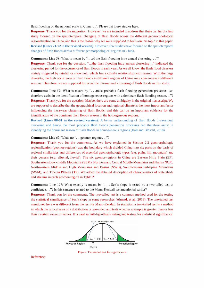
Comments: Line 127: What exactly is meant by “. . . Sen’s slope is tested by a two-tailed test at

confidence. . .”? Is this sentence related to the Mann-Kendall test mentioned earlier?

Response: Thank you for the comments. The two-tailed test is a common method used for the testing

the statistical significance of Sen’s slope in some researches (Ahmad, et al., 2018). The two-tailed test

mentioned here was different from the test for Mann-Kendall. In statistics, a two-tailed test is a method

in which the critical area of a distribution is two-sided and tests whether a sample is greater than or less

than a certain range of values. It is used in null-hypothesis testing and testing for statistical significance.

Figure. Two-tailed test for significance

Reference:

[1] Ahmad, I., Zhang, F., Tayyab, M., Anjum, M. N., Zaman, M., Liu, J., Farid, H. U. and Saddique, Q.:

Spatiotemporal analysis of precipitation variability in annual, seasonal and extreme values over upper

Indus River basin, Atmospheric Research, 213, 346-360, doi: 10.1016/j.atmosres.2018.06.019, 2018.

Revised (Lines 172-174 in the revised version): The magnitude of a trend was estimated by Sen’s slope

(Sen, 1968). The positive β value represents an increasing trend, while a negative value indicates a

decreasing trend over the study period. Sen’s slope is tested by the significance test at the 90% confidence

level.

Comments: Table 4: Please explain in the caption the meaning of the colours in the table.

Response: Thank you for the suggestion. We added the description of the colours in the table caption.

Revised (Table 5 in the revised version):

Table 5 Distribution of the number of FFEs within a precipitation anomaly zone

Anomalies of

precipitation (%)

1998 2010

May Jun Jul Aug Sep Oct May Jun Jul Aug Sep Oct

<-40 1 14 25 48 15 2 1 45 22 46 2 1

-40 ~ -20 6 9 75 42 13 3 15 21 55 32 2 0

-20 ~ 0 30 39 209 29 9 3 22 32 66 54 19 24

0 ~ 20 30 53 143 68 7 0 19 60 130 144 31 170

20 ~ 40 13 60 137 97 4 0 31 65 294 52 24 119

40 ~ 60 6 75 149 57 1 0 28 103 381 28 43 184

60 ~ 80 9 107 133 67 1 1 31 161 457 11 13 283

80 ~ 100 5 231 95 31 2 0 6 92 417 5 11 77

≥100 21 239 261 140 0 3 5 110 613 6 25 32

The bold numbers indicate the top three anomalies of precipitation for each month. The red colour indicates the

anomalies of precipitation below zero, and the blue colour indicates the anomalies of precipitation above zero.

Comments: Line 337: Please explain the term ‘El Niño Modoki’.

Response: Thank you for the suggestion. The definition of the term ‘El Niño Modoki’ has been added

in the revised manuscript.

Revised (Lines 553-555 in the revised version): Studies indicated that an El Niño Modoki (a special

flavour of the El Niño, which is a part of the El Niño Southern Oscillation (ENSO)) with strong warming

in the central Pacific was detected, which caused the rainfall belt to shift northward.