DE BROGLIE TIRED LIGHT MODEL AND THE REALITY OF THE QUANTUM WAVES

DE BROGLIE TIRED LIGHT MODEL AND THE REALITY OF THE QUANTUM WAVES

J.R. Croca

Departamento de Física

Faculdade de Ciências da Universidae de Lisboa Ed C8 Campo Grande – Lisboa - Portugal

Email: [email protected]

Abstract: In the early sixties of the XX century de Broglie was able to explain the cosmological observable red shift, without ad hoc assumptions. Starting from basic quantum considerations he developed his tired light model for the photon. This model explains in a single and beautiful way the cosmological redshift without need of assuming the Big Bang and consequently a beginning for the universe. Evidence coming from Earth sciences seems also to confirm these ideas and furthermore concrete proposal of laboratorial scale experiments which can test the model are here reviewed. Key words: Fundamental quantum physics, nonlinear quantum physics, de Broglie tired light model, fourth order interferometry, local wavelet analysis, redshift, de Broglie aging constant. 1 - Introduction In the early sixties of the last century de Broglie published two important papers [1, 2] on the properties of the photon. In this paper we recall his pioneering work, which, unfortunately, only recently reach my hands due to the difficulty in finding the original papers. Some more recent works [3] done by myself and other researchers [4] on the subject are here reviewed. Experimental evidence, whether we like it or not, clearly indicates that the strange quantum entity we name under the name of photon, just like any other quantum particle, is indeed a very complex being. Nevertheless it is possible to describe most of its basic properties in terms of a general causal framework valid for any quantum particle. A first approach [4] consists in describing a quantum particle in general and the photon in particular by means of local wavelet analysis [5] that contemplates both the local and extended properties of the quantum entities. A principal advantage of the model springs from its intrinsic mathematical simplicity and from the fact that it allows a natural interpretation of the experimental evidence coming from different branches of sciences. In Earth sciences it allows the explanation of the minute discrepancies between plate tectonics measurements done with GPS and VLBI. In astronomy it gives a natural and easy explanation for the cosmological redshift without any need for assuming the Big Bang for the universe. Furthermore it gives news insights in the measurements done with the super resolution microscopes of the new generation that falsify the general validity of Heisenberg uncertainty relations. Finally this causal local model for the quantum particle allows the design of laboratory scale experiments that can unequivocally test the validity of the model. 2 – A simplified causal local model for the quantum particle Any quantum particle, like for instance the photon, can be described, in a first approach, by a full wave φ composed of an extended yet finite region, the wave θ , described

Preprint: To appear in Foundations of Physics 1

mailto:[email protected]

mathematically by a Morlet gaussian wavelet [5] plus a singularity ξ immersed in the wave so that we have ξθφ += . (2.1) This singularity or corpuscle ξ carrying almost all the energy of the particle is responsible for the habitual quadratic detection process. The extended wave, practically without energy guides, through a nonlinear process, the singularity preferentially to the points were the wave has greater intensity giving origin to the interferometric properties of the quantum particles. In the linear approximation the wave devoid of singularity is solution to the usual linear Schrödinger equation, while at the nonlinear approach, the function φ representing the quantum particle, is solution to the nonlinear master equation

t

iVmm ∂

∂=+

∇+∇−

φφφφφ

φφφ hhh

21

21

*)(*)(

22

222

2

, (2.2)

which has a solution [3] in one spatial dimension

)(2/)2(2/)2(

0

22'212

02'

021

EtpxEtpxEtpx i

eeeaE −−−−−−−−

⎥⎦⎤

⎢⎣⎡ += hhh

σεσε

σπφ , (2.3)

which can be seen as the sum of the two solutions: The first representing, in a preliminary approach, the singularity

)(2/)2(

0

20

2'02

1EtpxEtpx i

eeaE −−−−−= hh

σε

σπξ (2.4)

and the second the extended wave

)(2/)2(

0

22'21

EtpxEtpx i

eeE −−−−−= hh

σε

σπθ . (2.5)

Due to the enormous difference in energy the constant a is very large , (2.6) 1>>>a however, this constant may turn to zero in the case when, by splitting or absorption, the full wave φ becomes an empty wave θ , that is, a wave devoid of singularity. The width of the gaussians, 0σ andσ , are related with the size of the wavelets and verify the relation 0σσ >>> , (2.7) meaning that the size of the singularity approaches a Dirac delta function. The plot of the real part of the function (2.3), representing the particle, is shown in Fig.2.1 In this representation we see that both the wave and the singularity share the same phase as stated by de Broglie principle of concordance of phase.


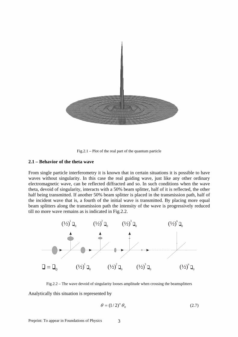
Fig.2.1 – Plot of the real part of the quantum particle

2.1 – Behavior of the theta wave From single particle interferometry it is known that in certain situations it is possible to have waves without singularity. In this case the real guiding wave, just like any other ordinary electromagnetic wave, can be reflected diffracted and so. In such conditions when the wave theta, devoid of singularity, interacts with a 50% beam splitter, half of it is reflected, the other half being transmitted. If another 50% beam splitter is placed in the transmission path, half of the incident wave that is, a fourth of the initial wave is transmitted. By placing more equal beam splitters along the transmission path the intensity of the wave is progressively reduced till no more wave remains as is indicated in Fig.2.2.

= 0 0(½)1

0(½)2

0(½)3

0(½)n

0(½)1

0(½)2

0(½)3

0(½)n

Fig.2.2 – The wave devoid of singularity looses amplitude when crossing the beamsplitters

Analytically this situation is represented by (2.7) 0)2/1( θθ n=


or, for a different generic attenuating coefficient t (2.8) 10,0 ≤≤= tt nθθthat is, , (9) ne µθθ −= 0 with tln−=µ . (2.10) In the case of a continuous homogeneous medium the discrete variable need to be changed by a continuous one , (2.11) xe µθθ −= 0 with µ standing for the average transmission factor. 2.2 – Behavior of the full wave Suppose now that we place a 50% beamsplitter in front of an incoming full wave φ , and that the singularity is transmitted. Next we place, in front of it, another equal beamsplitter, and, also in this case, consider that the singularity is transmitted. This process being continued as long as one wishes. What results shall be expected from this setup? We know that the singularityξ , being by its very nature indivisible, is either reflected or transmitted. The guiding wave in each beamsplitter gets its amplitude reduced by half. If this process of reducing amplitude keeps going on then, after a sufficient number of beamsplitters, the amplitude of the guiding wave will practically be zero. In such case we would be left with the singularity without the guiding wave. As a consequence de Broglie basic principle for the quantum physics, stating that any corpuscle possesses its own associated wave, would be broken. In order to avoid the breakdown of the whole conceptual structure of the quantum physics another more complex interacting process must be assumed. It is reasonable to assume that after having attained a minimum level, compatible with the said basic principle, the reduction process for the guiding wave stops. After that point on the amplitude of the guiding wave remains, for all practical purposes, constant. This state of minimum energy for the guiding wave corresponds to its fundamental state. If the amplitude of the guiding wave, from this point on, keeps constant, on average, it needs to take energy from the singularity. So, in each beamsplitter the singularity looses a very minute amount of energy to feed the guiding wave. This process is shown, schematically, in Fig.2.3.

0(½)1

0

0(½)2

0(½)k

0(½)k

⌧0

⌧0

⌧0

⌧0

⌧0

b1

´ ⌧0

b2

´

Fig.2.3 – Interacting process for the full wave


Analytically the whole process can be divided into two parts: The first with the singularity maintaining the energy constant, while the energy of the guiding wave decreases till attaining the fundamental energy level. The second when the singularity starts feeding energy to the guiding wave. For the guiding wave it reads

(2.10) ⎪⎩

⎪⎨⎧

=>=

≤=

constant,,

,

0

0

kknt

kntk

n

nn

θθ

θθ

and for the singularity

(2.11) ⎪⎩

⎪⎨⎧

>=

≤=

knb

knn ,'

,

0

0

ξξ

ξξ

with b’ standing for the attenuation factor for the singularity. In order to relate the parameter b’ with t it is necessary to recall the conservation of energy. In each transition the energy lost by the singularity equals the amount gained by the guiding wave. We know that

(2.12) ⎩⎨⎧

==

+

+

kk

kkbtξξθθ'1

1

with 0ξξ =k . (2.13) The energy lost by the guiding wave in each transition can be computed from (2.14) 22

12 |)1(||||| kkk t θθθθ −=−=∆ +

which must be compensated by the energy lost by the singularity (2.14’) 22

12 |)'1(||||| kkk b ξξξξ −=−=∆ +

that is, we must have ξθ ∆=∆ (2.15) or, explicitly kk tb θξ )1()'1( −=− , (2.16) which allows us to express the attenuation factor in terms of the damping constant of the theta wave

)1(1' tbk

k −−=ξθ (2.17’)

that is, recalling that kξξ =0

)1(1'0

tb k −−=ξθ . (2.17)

In such case, and naming the fundamental level of the guiding wave by kF θθ = , the attenuation for the singularity can be written


kntn

Fn ≥⎥

⎦

⎤⎢⎣

⎡−−= ,)1(1

00 ξ

θξξ , (2.18”)

or,

knent

n

F

≥=⎥⎦

⎤⎢⎣

⎡−−

,)1(1ln

00ξ

θ

ξξ (2.18’) that is, , (2.18) kne nb

n ≥= − ,0ξξ where the damping constant is given by

))1(1ln('ln0ξ

θFtbb −−−=−= . (2.19)

2.3 – Experimental Test It is possible to imagine a relatively easy experimental setup [4] to test the validity of the interacting process. For this it is necessary to take in consideration that the interacting process assumes that the loss of energy from the singularity to the guiding wave is, really, very small. This is a consequence of the fact that there is, as we shall see, an enormous difference between the energy of the singularity and the energy of the accompanying wave. The energy of this wave is so small that is unable to trigger the common quadratic detectors. In such case it is reasonable to suppose that under usual laboratory scale experiments the energy of the singularity remains, for all practical purposes, constant, even in the case when some minute part of it went to the guiding wave. The experimental setup is sketched in Fig.2.4,

sD

B1

B201

1

Fig.2.4 – Experimental setup for testing the photon interacting process

where we can see a modified Mach-Zehnder interferometer with 50% beamsplitters B1 and B2. Along both arms of the interferometer there are placed an equal number of beamsplitters with same transmission factor t. Let us now calculate the expected visibility, of the interference pattern, seen at the detector D. a) Orthodox approach Since the number of beamsplitters, in each arm of the interferometer, is equal, this leads to an overall absorbing effect, given by the A factor, at both the reflected and transmitted beams

01ψ and 02ψ . So we can write for the output beams


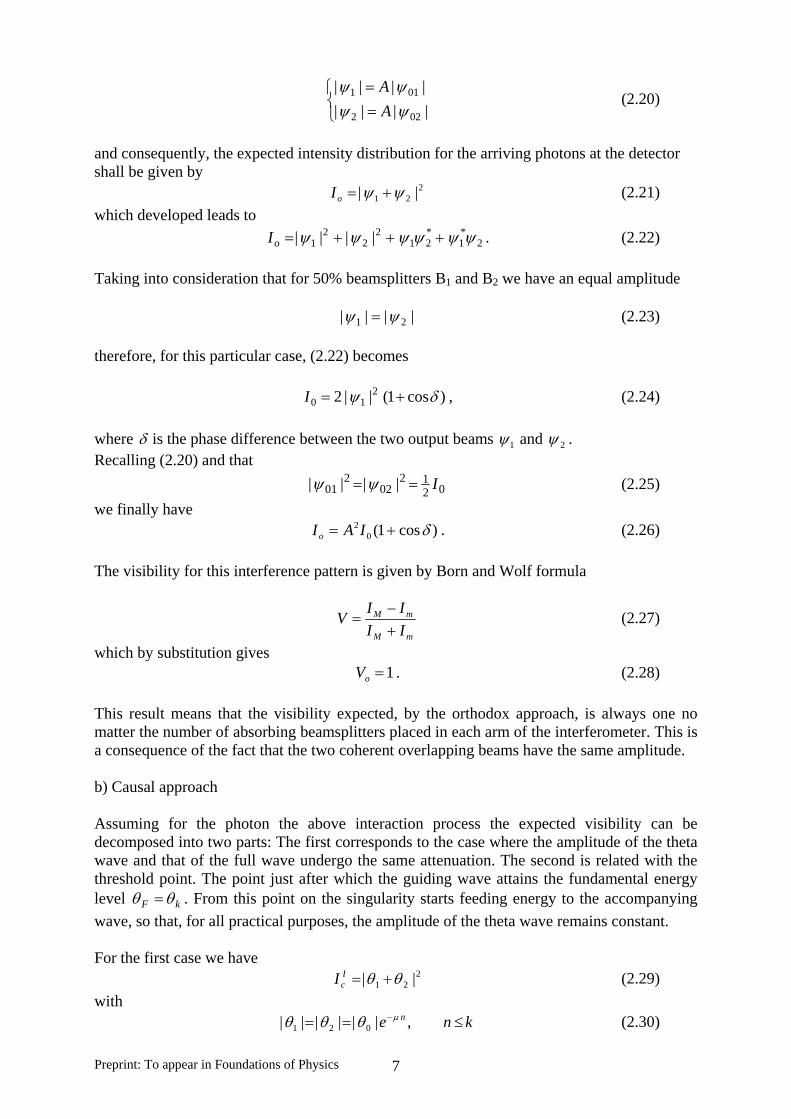
(2.20) ⎩⎨⎧

==

||||||||

022

011

ψψψψ

AA

and consequently, the expected intensity distribution for the arriving photons at the detector shall be given by (2.21) 2

21 || ψψ +=oIwhich developed leads to . (2.22) 2

*1

*21

22

21 |||| ψψψψψψ +++=oI

Taking into consideration that for 50% beamsplitters B1 and B2 we have an equal amplitude |||| 21 ψψ = (2.23) therefore, for this particular case, (2.22) becomes ) , (2.24) cos1(||2 2

10 δψ +=I where δ is the phase difference between the two output beams 1ψ and 2ψ . Recalling (2.20) and that 02

1202

201 |||| I== ψψ (2.25)

we finally have . (2.26) )cos1(0

2 δ+= IAIo

The visibility for this interference pattern is given by Born and Wolf formula

mM

mM

IIIIV

+−

= (2.27)

which by substitution gives 1=oV . (2.28) This result means that the visibility expected, by the orthodox approach, is always one no matter the number of absorbing beamsplitters placed in each arm of the interferometer. This is a consequence of the fact that the two coherent overlapping beams have the same amplitude. b) Causal approach Assuming for the photon the above interaction process the expected visibility can be decomposed into two parts: The first corresponds to the case where the amplitude of the theta wave and that of the full wave undergo the same attenuation. The second is related with the threshold point. The point just after which the guiding wave attains the fundamental energy level kF θθ = . From this point on the singularity starts feeding energy to the accompanying wave, so that, for all practical purposes, the amplitude of the theta wave remains constant. For the first case we have (2.29) 2

21 || θθ +=IcI

with (2.30) kne n ≤== − ,|||||| 021

µθθθ


giving by substitution into (2.29) a visibility equal to one . (2.30) 1=I

cVAfter the threshold level k we have

(2.31) const,02

01 =>⎪⎩

⎪⎨⎧

=

=−

−

kkne

ek

n

µ

µ

θθ

θθ

which means that the causal intensity , (2.32) 2

21 || θθ +=IIcI

for this part second part, gives by substitution (2.33) 2

00 || δµµ θθ iknIIc eeeI −− +=

that, after some calculation, leads to [ ] kneeI knII

c >−+= −− ,cosk)-(nsech1)(|| 2220 δµθ µµ . (2.34)

The visibility of this interference pattern is . (2.35) knknV II

c >−= ),(sechµ The plot of the visibilities predicted by the two different approaches is shown in Fig.2.5

k n

1

VI II

Fig.2.5 – Plot for the expected visibility: Dotted line orthodox approach. Solid line causal prediction

The visibility predicted by the orthodox approach is one in the two regions. The causal model in the first region predicts also a visibility one. Only in the second region the predictions are different. Contrary to the orthodox prediction of constant visibility one, the causal approach expects a decrease in the visibility attaining, eventually, a zero value. 3 – Causal interpretation of the cosmological redshift A causal explanation of the cosmological redshift without the Doppler effect was given in 1962 by de Broglie [1]. In his seminal paper de Broglie presents an alternative causal justification for the observable cosmological redshift in terms of his tired light model for the photon. Even if he did not elaborate explicitly the aging process for the photon, nevertheless his formula still stands.


The interacting process responsible for the aging of the photon results directly from the previous considerations. The discrete formula (2.18), derived for the case when the particle crosses the successive absorbing beamsplitters, can be generalized to include the continuous homogenous absorbing medium assuming the form . (3.1) ll be−= 0)( ξξ In this expression b stands for the mean amplitude attenuation factor of the medium and is the travelled distance.

l

Since 2||ξ∝E the expression for the energy decreasing, as the photon crosses the cosmic space, is therefore given by , (3.2) lBeEE −= 0

where B=2b is de Broglie cosmological constant standing for average aging coefficient. Recalling that νhE = we can also write , (3.3) lBe−= 0νν developing the exponential, and staying at the linear approximation, which is quite reasonable since de Broglie constant is very small, we have )1(0 lB−≅νν , or,

lB−≅−

0

0

ννν ,

which can also be written

00

, ννννν

−=∆−≅∆

lB . (3.4)

Recalling with de Broglie [1] that

000

, λλλνν

λλ

−=∆∆

−=∆ (3.5)

we have

lB≅∆

0λλ (3.6)

or, since in astronomy the relative wavelength difference is named by Z,

lBZ ≅∆

=0λλ (3.7)

and that Hubble law has the form

lcHZ = , (3.8)


with H being Hubble constant and c the velocity of light. In such conditions we have

cHB = , (3.9)

which shows that de Broglie average aging constant is given by Hubble constant divided by the constant c. Recalling that literature presents for the Hubble constant the value

, we get for de Broglie aging constant the figure 118106.1 −−×≈ sH . (3.10) 12610 −−= mB Now in order to estimate the distance of a cosmic light-emitting source, assuming, in a first approach, that the observable redshift is only due to the aging of the photon, we have only to use the expression BZ /≈l , (3.11) or . (3.11’) Z2610≈l As we have seen, starting from the causal model of de Broglie for the quantum particle, and from the inherent complex interaction process, it was possible to arrive directly, without any ad hoc hypothesis, to a natural explanation for the cosmological redshift, without need to postulate a hypothetical beginning for the universe. 4 – Ratio between the energy of the guiding wave and the singularity A first rough estimate of the ratio between the amplitude of the guiding wave, in the fundamental state, and the amplitude of the singularity can now be made. Since by (2.19) ))1(1ln(

0tb F −−−= ξ

θ and bB 2= we have ))1(1ln(2

0tB F −−−= ξ

θ , which means that

2/

0

1)1( BF et −−=−ξθ .

Remembering that , expanding the exponential, and staying at the linear approximation we have

12610 −−≅ mB

27

0

105)1( −×≈− tF

ξθ .

Assuming that each transition corresponds, in this case, to a relative large section of space it is reasonable to make the transition coefficient t relatively small. Therefore, under this assumption, we get a rough estimate

27

0

10−≈ξθ F

or, in terms of energy


54100

−≈ξ

θ

EE

F ,

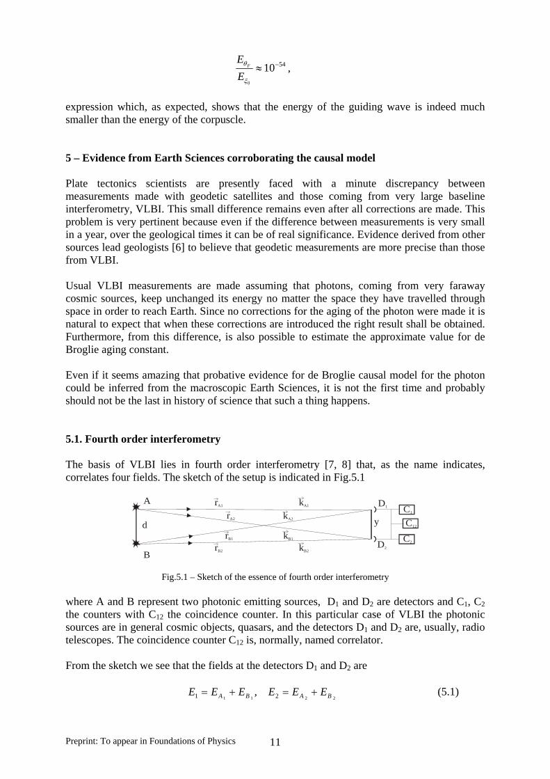
expression which, as expected, shows that the energy of the guiding wave is indeed much smaller than the energy of the corpuscle. 5 – Evidence from Earth Sciences corroborating the causal model Plate tectonics scientists are presently faced with a minute discrepancy between measurements made with geodetic satellites and those coming from very large baseline interferometry, VLBI. This small difference remains even after all corrections are made. This problem is very pertinent because even if the difference between measurements is very small in a year, over the geological times it can be of real significance. Evidence derived from other sources lead geologists [6] to believe that geodetic measurements are more precise than those from VLBI. Usual VLBI measurements are made assuming that photons, coming from very faraway cosmic sources, keep unchanged its energy no matter the space they have travelled through space in order to reach Earth. Since no corrections for the aging of the photon were made it is natural to expect that when these corrections are introduced the right result shall be obtained. Furthermore, from this difference, is also possible to estimate the approximate value for de Broglie aging constant. Even if it seems amazing that probative evidence for de Broglie causal model for the photon could be inferred from the macroscopic Earth Sciences, it is not the first time and probably should not be the last in history of science that such a thing happens. 5.1. Fourth order interferometry The basis of VLBI lies in fourth order interferometry [7, 8] that, as the name indicates, correlates four fields. The sketch of the setup is indicated in Fig.5.1

C1

D1

C2D2

C12yd

A

B

rA1

rB1

rB2

rA2

kA1

kA2

kB1

kB2

Fig.5.1 – Sketch of the essence of fourth order interferometry

where A and B represent two photonic emitting sources, D1 and D2 are detectors and C1, C2 the counters with C12 the coincidence counter. In this particular case of VLBI the photonic sources are in general cosmic objects, quasars, and the detectors D1 and D2 are, usually, radio telescopes. The coincidence counter C12 is, normally, named correlator. From the sketch we see that the fields at the detectors D1 and D2 are

2211 21 , BABA EEEEEE +=+= (5.1)


therefore, at a certain instant arbitrary of time, and emphasizing the spatial representation because of its intuitive nature, these fields, for the monochromatic approximation, can be written

⎪⎩

⎪⎨⎧

=

=

⎪⎩

⎪⎨⎧

=

=+

+

+

+

).(0

).(0

).(0

).(0

22

2

22

2

11

1

11

1

BBB

AAA

BBB

AAA

rkiBB

rkiAA

rkiBB

rkiAA

eEE

eEE

eEE

eEEϕ

ϕ

ϕ

ϕ

rr

rr

rr

rr

(5.2)

and by substitution into (5.1) the total fields at the detectors are

⎪⎩

⎪⎨⎧

+=

+=

++

++

).(0

).(02

).(0

).(01

2222

1111

BBBAAA

BBBAAA

rkiB

rkiA

rkiB

rkiA

eEeEE

eEeEEϕϕ

ϕϕ

rrrr

rrrr

(5.3)

to which correspond the intensities seen by the detectors

⎪⎪⎩

⎪⎪⎨

⎧

⎥⎦⎤

⎢⎣⎡ +++==

⎥⎦⎤

⎢⎣⎡ +++==

+−−+−

+−−+−

)..()..(*222

)..()..(*111

22222222

11111111

.

.

ϕϕ

ϕϕ

BBAABBAA

BBAABBAA

rkrkirkrkiBABA

rkrkirkrkiBABA

eeIIIIEEI

eeIIIIEEI

rrrrrrrr

rrrrrrrr

(5.4)

where we have made BA ϕϕϕ −= . (5.5) From these expressions it is possible to obtain the correlation intensity function measured at C12

⟩⟨= 2112 III (5.6) which explicitly reads

⟩⎥⎦⎤

⎢⎣⎡ ++

⎥⎦⎤

⎢⎣⎡ ++

⎥⎦⎤

⎢⎣⎡ +++

⎥⎦⎤

⎢⎣⎡ ++++⟨=

+−−−+−−

+−−+−+−−+

+−−+−

+−−+−

)....()....(

)2....()2....(

)..()..(

)..()..(212

2211221122112211

2211221122112211

22222222

11111111

)(

)()(

BBBBAAAABBBBAAAA

BBBBAAAABBBBAAAA

BBAABBAA

BBAABBAA

rkrkrkrkirkrkrkrkiBA

rkrkrkrkirkrkrkrkiBA

rkrkirkrkiBABA

rkrkirkrkiBABABA

eeII

eeII

eeIIII

eeIIIIIII

rrrrrrrrrrrrrrrr

rrrrrrrrrrrrrrrr

rrrrrrrr

rrrrrrrr

ϕϕ

ϕϕ

ϕϕ

(5.7)

Now assuming, as usual, that the light arriving at the two detectors is not correlated in phase all terms containing the phase difference in a long run average to zero. So, we simply got [ ])..()..(cos2)(

22112211

212 BBBBAAAABABA rkrkrkrkIIIII rrrrrrrr

−−−++= . (5.8) In order to further simplify the expression it is convenient to consider the case where III BA ≈≈ (5.9)


then, the coincidence intensity, that is, the cross correlation function assumes the habitual form )cos1(4 2

112 δ+= II (5.10)

with the modulating phase δ given by )..()..(

22112211 BBBBAAAA rkrkrkrk rrrrrrrr−−−=δ (5.11)

5.2. Orthodox Model In this approach it is assumed that the photon as it travels astronomical distances through the “empty” space, the subquantum medium, or the zero point field as is usually called, keeps always its energy unchanged. Therefore since the velocity of the light is constant we must write BBBAAA kkkkkk

rrrrrr====

2121, . (5.12)

By substitution into (5.11) we obtain for the phase predicted by the orthodox model )()(

2121 BBBAAAo rrkrrk rrrrrr−−−=δ . (5.13)

From Fig.5.1 we see that

⎪⎩

⎪⎨⎧

==−

==−

2

2

21

21

eyyrr

eyyrr

BB

AArrrr

rrrr

(5.14)

which means ykk BAo

rrr)( −=δ . (5.15)

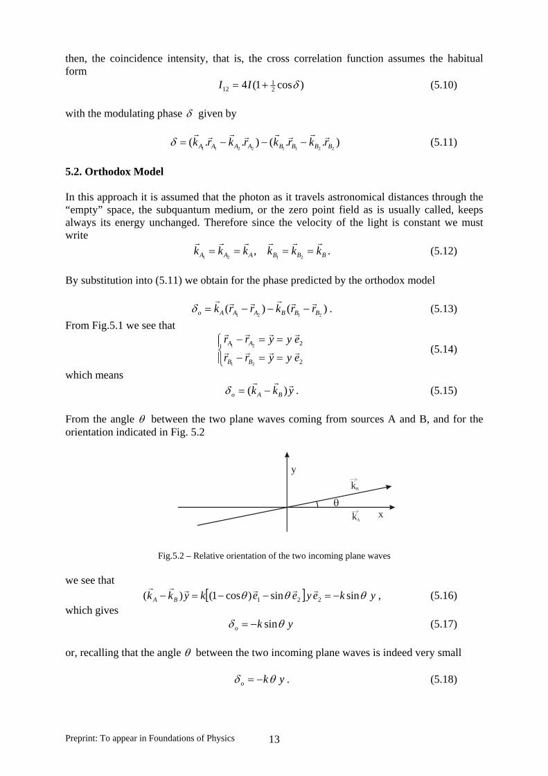
From the angle θ between the two plane waves coming from sources A and B, and for the orientation indicated in Fig. 5.2

y

xθ

kB

kA

Fig.5.2 – Relative orientation of the two incoming plane waves we see that [ ] ykeyeekykk BA θθθ sinsin)cos1()( 221 −=−−=−

rrrrrr, (5.16)

which gives yko θδ sin−= (5.17) or, recalling that the angle θ between the two incoming plane waves is indeed very small yko θδ −= . (5.18)


In this conditions the expected correlation function intensity I12, assuming no aging status for the photon so that it remains unchanged no matter the distance it travels through the space, is given by [ ])cos(14 2

112 ykII o θ+= . (5.19)

From the difference between the full maximum 0=δ and the minimum πδ = it is possible to get the approximate angular diameter θ of the cosmic object, which gives the customary formula

yo 2λθ = . (5.20)

Some times this expression is presented in the scientific literature [9] with a different multiplying constant resulting from considering the sources as circular apertures. In any case the expression remains essentially the same. By assuming that the angular diameter of the cosmic object is known then it is possible to determinate the distance between the two detectors which typically happen to be radiotelescopes. In such situation the distance between the two detectors, assuming, of course, that the angular diameter is known, is given by

θλ2

=oy . (5.21)

5.3. De Broglie causal approach Now assuming de Broglie local causal model for the photon important modifications need to be made in the calculations. From above we know that the change in energy of the photon as it travels through the subquantum medium, usually called in the in the orthodox literature by zero point field, can be described, as we have seen previously (3.2), by , (5.22) lBeEE −= 0

or in terms of frequency lBe−= 0νν , (5.23) recalling that the velocity c of the light is supposed constant, . (5.24) lBekk −= 0

In such circumstances, and in order to take into account the change in wavelength due to the aging of the photon it is necessary to write

⎪⎩

⎪⎨⎧

=

=

⎪⎩

⎪⎨⎧

=

=−

−

−

−

BrB

B

BrB

B

ArB

A

ArB

A

kekk

kekk

kekk

kekkB

B

A

A

ˆ

ˆ

ˆ

ˆ

2

2

1

1

2

2

1

1

0

0

0

0r

r

r

r

(5.25)

with

B

BB

A

AA k

kkkkk

rr

== ˆ,ˆ . (5.26)


The corrected phase, assuming the local causal aging model, is therefore )ˆˆ()ˆˆ(

2

2

1

1

2

2

1

10000 BB

rBBB

rBAA

rBAA

rBc rkekrkekrkekrkek BBAA rrrr

⋅−⋅−⋅−⋅= −−−−δ , (5.27) or [ ])(ˆ)(ˆ

21

212

2

12

1

1 )()(0 BB

rrBB

rBA

rrBAA

rBc rrekererkek BBBAAA rrrr

−−−= −−−−−−δ . (5.27’) In order to obtain a more manageable expression it is convenient to make the realistic approximation, which corresponds to assume a symmetric geometry l≈≈

21 BA rr , (5.28) with being the average distance traveled by the photon, from the cosmic object to the detectors D

l

1 and D2, and naming

2112; BBBAAA rrrr −=−= εε , (5.29)

the phase becomes [ ])(ˆ)(ˆ

21210 BBB

BAB

AAB

c rrekrerkek BArrrrl −−−= −−− εεδ (4.30)

or recalling that (5.31) lBekk −= 0

we have )()(

2121 BBB

BAB

AAc rrekrerk BArrrrrr

−−−= −− εεδ . (5.32) Taking in consideration Fig.5.3

yd

A

B

rA1

rB2

2AB re Aε−

1BB re Bε−

Aξ

BξyA

yB

Fig.5.3 – Graphic representation of the variables it is possible to write BBAAc ykyk rrrr

⋅−⋅=δ . (5.33) Naming by ξ the difference between the vectors and the corrected ones, we have

⎪⎩

⎪⎨⎧

−=−=

−=−=−−

−−

)1(

)1(

111

222

BB

AA

BBB

BBB

BAA

BAA

errer

errerεε

εε

ξ

ξrrrr

rrrr

(5.34)

From Fig.5.3 we see that BBAA yyyy ξξ

rrrrrr−=+= ; , (4.35)

so the corrected phase assumes the form


)()( BBAAc ykyk ξξδrrrrrr

−−+= (5.36) that is, by rearranging the terms BBAABAc kkykk ξξδ

rrrrrrr⋅+⋅+−= )( , (5.37)

or, recalling the previous calculations (5.15) and (5.18) we got BBAAc kkyk ξξθδ ++−= (5.38) and since it is reasonable to make BBAA kk ξξ

rr//ˆ;//ˆ . (5.39)

Because kkk BA == (5.40) we have )( BAc kyk ξξθδ ++−= (5.41) or by (5.34) . (5.42) ))1()1((

21

BA BB

BAc ererkyk εεθδ −− −+−+−=

In order to further simplify this expression it is convenient to recall the following approximations εεε ≈≈≈≈ BBA rr A and ,

21l , (5.43)

then (5.42) can be written (5.44) )1(2 εθδ B

c ekyk −−+−= l

or

⎥⎦⎤

⎢⎣⎡ −−−= − )1(2 ε

θθδ B

c eyk l . (5.45)

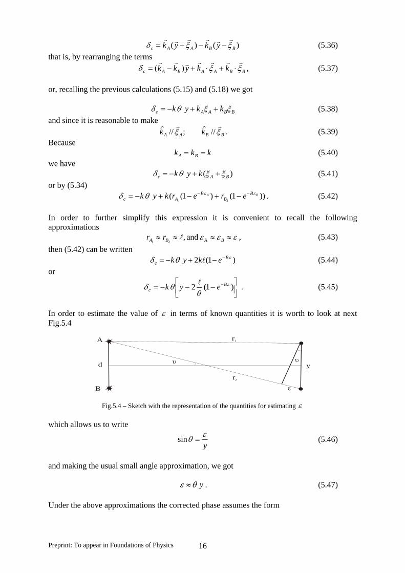
In order to estimate the value of ε in terms of known quantities it is worth to look at next Fig.5.4

yd

A

B

r1

r2

υ υ

ε

Fig.5.4 – Sketch with the representation of the quantities for estimating ε which allows us to write

yεθ =sin (5.46)

and making the usual small angle approximation, we got yθε ≈ . (5.47) Under the above approximations the corrected phase assumes the form


⎥⎦⎤

⎢⎣⎡ −−−= − )1(2 yB

c eyk θ

θθδ l , (5.48)

since the argument of the exponential is much less than one this expression can be further simplified giving )21( lBykc −−= θδ . (5.49) Finally, for correlated intensity function, taking in account the aging of the photon, we got under the simplificative approximations made [ ))21(cos(14 2

112 lBykII c −−+= θ ]. (5.50’)

or [ ))12(cos(14 2

112 −+= lBykII c θ ]. (5.50)

From the previous considerations we know that in order to make the concrete measurement we need to change the length y from zero, corresponding to a null phase, maximal visibility, to a of minimal visibility which corresponds to a phase value of π . That is πθ =− |12| lByk , (5.51) which gives

|12|

12 −

=lB

yc θλ , (5.52)

or, recalling the value predicted by the orthodox approach (4.21)

θλ2

=oy ,

we may write |12|

1−

=lB

yy oc , (5.53)

or co yBy |12| −= l . (5.53’) These expressions implies that the length we got with the usual VLBI method, yo, is different from the causal value yc, obtained assuming the aging model for the photon. Naturally if de Broglie aging constant approaches zero, 0≅B , the two predictions are precisely the same, . co yy ≅ It is worth to draw the attention that in these VLBI measurements, both without correction and with the aging correction for the light it is supposed that the true angular diameter of the cosmic object is known. This assumption is, as we are well aware, not entirely correct because the value of the angular diameter is also inferred from the theory. In the common approach it is given by

yo 2λθ = ,

which assumes that the distance between the two light sensors y is known. Assuming the aging model for the photon we have instead


|12|

12 −

=lByc

λθ , (5.54)

that depends also on de Broglie aging constant B and on the distance l . Now to estimate the value of de Broglie aging constant for the photon and compare it with the previous estimation it is convenient to know the approximate value for this small discrepancy between the two measurement processes. In order to do that it is necessary to get assistance from the Earth Sciences [10]. In such circumstances and quoting A. Ribeiro and L. Matias [6]: “The VLBI geodetic method gives results that are distinctly different from near-Earth geodetic methods (GPS, SLR, DORIS). Direct comparison between the different methods have not been investigated in a systematic way. Nevertheless there are studies that compare results of VLBI with plate kinematic models NUVEL-1 and NUVEL-1A, as well as results of near-Earth geodetic methods with these kinematic models. The plate kinematic model NUVEL-1 for relative plate motion was computed by DeMets et al. (1990) using a large set of tectonophysical measurements: spreading velocities measured from magnetic anomalies younger than 3 MA, young fracture zone azimuths and earthquake slip vectors. A recent revision of the magnetic time scale implied a revision of the velocity values and the relative model NUVEL-1A was defined (DeMets et al., 1994). In the NUVEL-1A model the velocity magnitudes were multiplied by a constant factor, 0.9562, giving 4.4% slower velocities than NUVEL-1. According to the same authors, this correction reduced the discrepancy between the tectonophysical model and the kinematic models derived by geodetic methods to only 2%, being the NUVEL-1A the faster. However, considering only the results provided by the VLBI method, Heki (1996) showed that this technique gave plate velocities 3.4% faster than NUVEL-1, that is, 7.8 % faster than NUVEL-1A. This means that, using NUVEL-1A as a reference, the VLBI method for estimating plate kinematics gives velocities that are 10 % faster (± a few %) than the other geodetic methods. Considering the length of a base line across the Pacific we can evaluate an order of magnitude of discrepancy between distances measured by VLBI and distances measured by near-Earth methods. For a base line of 5000 km and a relative plate velocity of 150 mm/year, 7% of plate velocity discrepancy means 1 cm of discrepancy over 1 year. This implies, a relative distance difference of 2x10-9 over the base line, with VLBI giving higher distances.” From this information we gather that experimental evidence tells us that , with y standing for the right distance. This implies

yyy co =≥

1|12| ≥−= lByyo , (5.55)

or , (5.56) 1≥lBwhich means that

112 ≥−= lByyo (5.57)

giving for the aging constant


)1(21

yyB o+=

l. (5.58)

This expression can be written in other form. Naming by ∆ the difference between the two predicted distances, we have ∆+=−=∆ yyyy oo ; , (5.59) which by substitution in (4.58) gives

σll 2

11+=B , (5.60)

with σ standing for the relative distance difference, y/∆=σ . Now since quasar distances from Earth can be from about 1025 m to 1026 m and that

we got by substitution in (60) 9102 −×≈σ , mB /10 26−≈ which perfectly agrees with the first estimated value, , for the mean aging constant assuming that the observable astronomical redshift is only due to the aging of the photon.

mB /10 26−≈

6 – Conclusion It was shown that not only the theoretical model for the photon is sound but even more it is capable, starting from first principles and without any ad hoc assumptions, to explain the cosmological redshift without need of a beginning for the universe as is assumed by the nowadays in fashion theory of the Big Bang of religious charisma. On the other hand convergence with results coming from unexpected and unsuspected source, as is Geology, indicates the correctness of the model to describe, in a first approach, the structure of the quantum particles. Furthermore it is worth to call the attention to the important fact that the causal model for the photon can be tested in laboratory scale experiments with controlled parameters. Acknowledgements: I dedicate this work to my dear friend Franco Selleri. Part of this work was the result of a very interesting idea with what the geologist A. Ribeiro challenged me. His idea was that probably the discrepancy between the two sets of geodetic measurements must, somehow, be explained by basic physical processes, namely by the aging model for the photon of de Broglie. For his idea, constant support, and helpful discussions I want to express him my many thanks. I want also to thank L. Matias for helpful discussions concerning the concrete geodynamic data. Finally I want to thank L. Mendes Victor for the given support, allowing me to stay at a place where the principal part of the present work was done. Part of this work was supported by FCT.


References 1 - L. de Broglie, Cahiers de Physique, 147(1962)425 2 - L. de Broglie, Comptes Rendus Acad. Sc. Paris, B, 263(1966)589 3 - J.R. Croca, Towards a nonlinear quantum physics, World Scientific, (Singapore, 2002) 4 - J.R. Croca, M. Ferrero, A. Garuccio and V.L. Lepore, Found. Phys. Lett. 10(1997)441;

J.R. Croca, Apeiron, 4(1997)41 5 - P. Kumar, Rev. Geophysics, 35(1997)385 6 - A. Ribeiro and L. Matias, Private communication 2002 7 - H. Paul, Rev. Mod. Physics, 58(1986)209 8 - Z.Y. Ou and L. Mandel, Phys. Rev. Lett. 62(1989)2941 9 - M. Born and E. Wolf, Principles of Optics, Pergamon Press, (New York, 1983) 10 - K. Heiki, J. Geophysical Research, 101, B2 (1996)3187; DeMets, C. R. G. Gordon, D. F.

Argus and S. Stein, Geophysics. J. Int.,101(1990) 425; DeMets, C. R. G. Gordon, D. F. Argus and S. Stein, Geoph. Res. Lett., 21(1994) 2191


DE BROGLIE TIRED LIGHT MODEL AND THE REALITY OF THE QUANTUM WAVES

Documents

Transcript of DE BROGLIE TIRED LIGHT MODEL AND THE REALITY OF THE QUANTUM WAVES