Day-ahead Management of Energy Sources and Storage in ...
17
*Corresponding author, e-mail: [email protected] Research Article GU J Sci32 (4): 1167-1183 (2019) DOI: 10.35378/gujs.512736 Gazi University Journal of Science http://dergipark.gov.tr/gujs Day-ahead Management of Energy Sources and Storage in Hybrid Microgrid to reduce Uncertainty Prakash Kumar K. 1,2 , Saravanan B. 2,* 1 Department of Technical Education, Government of Andhra Pradesh, Government Polytechnic for Women, Palamaner, India-517408. 2 Vellore Institute of Technology, Vellore, Tamil Nadu, India, 632 014. Highlights • An Energy Management Algorithm is proposed for day-ahead scheduling in a microgrid. • Optimization problem is framed to minimize the cost of power generation under DMO model. • Artificial Fish Swarm technique is used as a tool to solve the optimization part. • Several scenarios are drawn to treat uncertainty in Renewable Energy availability. ArticleInfo Abstract A day ahead management strategy is proposed in this article to schedule energy generators and storage in presence of Renewable Energy Sources under uncertainty conditions with an objective to optimize the cost of energy generation. Artificial Fish Swarm algorithm is used as optimization tool. The optimization problem is framed considering all the practical constraints of energy generators and storage units. The uncertainty of Renewable Energy Sources is treated with a proven uncertainty model and several scenarios are drawn for energy availability and demand. The proposed energy management algorithm is tested numerically on a grid connected microgrid hosting a group of hybrid energy sources and storage battery for day ahead scheduling under dynamic pricing and demand side management in one of the generated uncertainty scenarios. The obtained results show that the performance of Artificial Fish Swarm algorithm as an optimizing tool is validated and the proposed Energy Management System is found to optimize the cost of energy generation while matching the power generated with power required. Received:17/01/2019 Accepted:25/06/2019 Keywords Microgrid Uncertainty Storage Energy Management Day ahead scheduling 1. INTRODUCTION The economic research forecasts that the cost of energy generation from RESs will nose dive next decade in comparison with their conventional counterparts like coal [1]. In realization of these forecasts, solar generated electrical energy has witnessed a lowest bidding rate of 2.44 Rupees in India from a private producer [2]. It is comparatively much cheaper than conventional sources like nuclear or coal. Apart from cost of energy generation, the potency of solar generated energy in meeting the global energy needs with almost zero damage to the environment is yet another advantage. The sunshine rich parts of the world like Asia, Africa, and Australia etc have enough solar energy sources to meet a major share of global energy requirements. The idea of tapping solar and wind energy which are distributed sources by availability has encouraged the concept of connecting smaller and distributed generation sources to the utility grid at tail ends (distribution systems) at low and medium voltages levels. This lead to a whole new concept of autonomous microgrids [3]. The microgrids operate in either grid connected mode or in autonomous mode. The developments in microgrid enabling technologies like capacity building of DG units from a few kW to MW, efficient energy derivation methods from RESs, reducing costs of energy storage, availability of wide area controlling technologies like SCADA along with incentives offered by governments for renewable energy generation have grown so attractive that they can no more be overlooked by investment policy makers. The investment policies in energy market are being reframed to accommodate microgrids into the existing utility grid system and symptoms that conventional centralized generation concept of energy is slowly shifting towards the distributed generation concept are evident [4].
-
Upload
khangminh22 -
Category
Documents
-
view
3 -
download
0
Transcript of Day-ahead Management of Energy Sources and Storage in ...
*Corresponding author, e-mail: [email protected]
Research Article GU J Sci32 (4): 1167-1183 (2019) DOI: 10.35378/gujs.512736
Gazi University
Journal of Science
http://dergipark.gov.tr/gujs
Day-ahead Management of Energy Sources and Storage in Hybrid Microgrid
to reduce Uncertainty
Prakash Kumar K.1,2 , Saravanan B.2,*
1Department of Technical Education, Government of Andhra Pradesh, Government Polytechnic for Women, Palamaner, India-517408.
2Vellore Institute of Technology, Vellore, Tamil Nadu, India, 632 014.
Highlights • An Energy Management Algorithm is proposed for day-ahead scheduling in a microgrid.
• Optimization problem is framed to minimize the cost of power generation under DMO model.
• Artificial Fish Swarm technique is used as a tool to solve the optimization part.
• Several scenarios are drawn to treat uncertainty in Renewable Energy availability.
ArticleInfo
Abstract
A day ahead management strategy is proposed in this article to schedule energy generators and
storage in presence of Renewable Energy Sources under uncertainty conditions with an objective
to optimize the cost of energy generation. Artificial Fish Swarm algorithm is used as optimization
tool. The optimization problem is framed considering all the practical constraints of energy
generators and storage units. The uncertainty of Renewable Energy Sources is treated with a
proven uncertainty model and several scenarios are drawn for energy availability and demand.
The proposed energy management algorithm is tested numerically on a grid connected microgrid
hosting a group of hybrid energy sources and storage battery for day ahead scheduling under
dynamic pricing and demand side management in one of the generated uncertainty scenarios. The
obtained results show that the performance of Artificial Fish Swarm algorithm as an optimizing
tool is validated and the proposed Energy Management System is found to optimize the cost of
energy generation while matching the power generated with power required.
Received:17/01/2019
Accepted:25/06/2019
Keywords
Microgrid
Uncertainty
Storage Energy Management
Day ahead scheduling
1. INTRODUCTION
The economic research forecasts that the cost of energy generation from RESs will nose dive next decade
in comparison with their conventional counterparts like coal [1]. In realization of these forecasts, solar
generated electrical energy has witnessed a lowest bidding rate of 2.44 Rupees in India from a private
producer [2]. It is comparatively much cheaper than conventional sources like nuclear or coal. Apart from
cost of energy generation, the potency of solar generated energy in meeting the global energy needs with
almost zero damage to the environment is yet another advantage. The sunshine rich parts of the world like
Asia, Africa, and Australia etc have enough solar energy sources to meet a major share of global energy
requirements. The idea of tapping solar and wind energy which are distributed sources by availability has
encouraged the concept of connecting smaller and distributed generation sources to the utility grid at tail
ends (distribution systems) at low and medium voltages levels. This lead to a whole new concept of
autonomous microgrids [3]. The microgrids operate in either grid connected mode or in autonomous mode.
The developments in microgrid enabling technologies like capacity building of DG units from a few kW to
MW, efficient energy derivation methods from RESs, reducing costs of energy storage, availability of wide
area controlling technologies like SCADA along with incentives offered by governments for renewable
energy generation have grown so attractive that they can no more be overlooked by investment policy
makers. The investment policies in energy market are being reframed to accommodate microgrids into the
existing utility grid system and symptoms that conventional centralized generation concept of energy is
slowly shifting towards the distributed generation concept are evident [4].
1168 Prakash Kumar K, Saravanan B/ GU J Sci, 32(4): 1167-1183 (2019)
All the above advantages being on one side of the microgrids, they suffer from quite a few operation and
control difficulties. Uncertainty of energy availability from the RESs is one such serious setback, which
ultimately affects the reliability of the system, if not treated properly. The energy output from a RES
generator is not under the control of the microgrid operator. He can only curtail the generation in the event
of excess generation. A lot of research is inspired by the need to reduce the uncertainty of energy availability
from RESs and to balance the generation with the loads in the microgrids. The classical energy balance
techniques fall short in microgrid environment due to the uncertainty in generation and loads added with
bi-directional power flows, which add even more difficulty in energy balancing. Thanks to research, it has
come out with quite a few modern techniques modelled and tested to contain the uncertainty. Day ahead
scheduling using data mining, maintaining battery storage back-ups and spinning reserves, demand side
management tools like load shifting, load curtailing (load shedding under deficit generation), demand
response etc top the list. A sample of literature using the above energy balance techniques to solve various
types of objective functions include mixed integer linear programming problems [5-7], linear programming
problems [8]. Different types of linear programming techniques and nature inspired swarm intelligence
algorithms are employed to solve the problems of optimum energy exchange (charging/discharging)
schedules of batteries/storage facility [9-11]. All the above energy balancing techniques are from the
generation side. The other energy balancing techniques from demand side are also tested successfully, like
load shifting and shedding [12], demand response [13-16]. Load shedding being a technique used to manage
the constant power loads (They are either supplied with rated power or else completely disconnected), using
electric springs is a new technique to supply constant energy loads with reduced power [17]. Apart from
this quite a large number of models are proposed and tested to represent the uncertainty of energy
availability with the RES generators and the loads [18-21].
The problem of scheduling power generation sources and storage devices while optimizing the cost of
power generation from sources is considered in this article. The solution to the problem needs two aspects
to be solved. One is to find the optimal mix of generation from different sources to minimize the cost of
generation and the other part is to schedule the required power among generation sources following the
optimized mix as evaluated. Until late, the cost of power generation from renewable sources is considered
as zero on the pretext that they need zero expenditure towards the fuel and hence they are treated as non-
dispatchable sources [22,23]. This assumption is too remote from practical reality and simplifies the
optimization problem too much. A few works reported in literature have considered the cost of power
generation from renewable sources as non-zero. Authors in [24] have considered cost of generation from
wind and PV units as quadratic functions. Authors in [25] have proposed a new cost function for renewable
power generation by computing a penalty amount for differential power between actual powers generated
and forecasted power. This case is specifically proposed for the microgrid operators who do not have
sufficient facilities to store all the excess energy available with renewable sources. The penalty amount so
computed is made a component in computing the cost of renewable energy generation. The authors in [26]
put an end to general flow of concept in literature that the power generation from renewable sources in
uncontrollable. They have proposed an Automatic Generation Control strategy to control power generation
from wind farms.We have considered both the conventional and renewable generators in dispatchable
category with respective cost functions for both. The popular optimization techniques like GA and PSO,
which are the favourites in literature, suffer from serious drawbacks in terms of computational complexities
and time. More constrained the problem is, more will be these complexities. For instance, the process of
fine tuning the computational parameters like fitness normalization, mutation rate, crossover parameters
etc in GA is more trial and error based. Such complexities are quite lesser in number in Artificial Fish
Swarm (AFS) algorithm. Though it suffers from the disadvantage of not using the past experience of the
swarm members in evaluating the next step in search, AFS algorithm has the outweighing merits of higher
accuracy, lesser computational time, faster convergence, very few parameters to be tuned etc. As such, AFS
algorithm is used in this paper to find solution for the optimization part of the problem. The problem is
framed with an objective to reduce the cost of energy generation in presence of uncertain energy availability
from the RES generators under dynamic pricing of energy. A bunch of renewable and non-renewable
energy sources are considered along with battery back-up. The uncertainty with RESs energy availability
and loads is treated using a proven uncertainty model. The battery is charged from the excess energy
available and is used to back-up supply under deficit generation. The microgrid is operated in grid
connected mode with an upper limit for power drawl. The problem formulation is done with a view to

1169 Prakash Kumar K, Saravanan B/ GU J Sci, 32(4): 1167-1183 (2019)
include demand side management which allows load shedding under power shortage condition,
compensating the consumer for the inconvenience caused due to power disconnection. Artificial Fish
Swarm Algorithm is employed to work out the optimization part of the objective function. The problem is
solved over hourly intervals for 24 hours.
2. ARTIFICIAL FISH SWARM ALGORITHM
The fishes in a swarm are seen continuously changing their positions. For an observer, their movements
appear random and unsynchronized. But in reality, the fishes do it purposefully and with a high sense of
synchronization. They move continuously to adjust their position in synchronization to the path leading to
a location of their objective. Their objective could be anything like staying protected from a predator’s
attack, avoiding collision with neighbouring fellow fishes, finding a location where chances of finding food
is better etc. Such movements of the fishes are modelled and the AFS algorithm is framed [27]. It frames a
localized searching method for each of the individual artificial fish and each search ends with updating the
solution to obtain the best location for the objective chosen. Each individual fish in the swarm is termed as
artificial fish. Each instantaneous position that these artificial fishes occupy on their path to the objective
location, symbolizes a possible solution to the problem at hand. These instantaneous positions are modelled
differently for different objectives of movement by fish. The fishes exhibit different movement patterns for
different behaviours like random searching behaviour, trail following behaviour, preying, swarming and
mating behaviours etc. The AFS algorithm adopts these entire behaviours one after the other in its quest for
the optimum solution. The AFS algorithm can be summed up as follows.
Let the current location of an individual artificial fish be
𝑋𝑖 = (𝑥𝑖1, 𝑥𝑖2, … . . 𝑥𝑖𝑛), (1)
where 𝑖 signifies the number of control variables and 𝑛 signifies the total number of individual artificial
fishes living in the swarm.
Then the consistency of fulfilling its objective at the location will be
𝑌𝑖 = 𝑓(𝑋𝑖). (2)
On its way to the location where the consistency of fulfilling objective is best, the artificial fish alters its
position to a new location 𝑋𝑖∗which is given by
𝑋𝑖∗ = 𝑋𝑖 + 𝑟𝑎𝑛𝑑 ( ) ∗ 𝑠𝑡𝑒𝑝 ∗
𝑋𝑗−𝑋𝑖
‖𝑋𝑗−𝑋𝑖‖, (3)
where rand ( ) is any random number that lies between ‘0’ and ‘1’, step is the largest radial displacement
through which the fish can navigate in one move and 𝑋𝑗 is anyone of the calculated positions which exists
within the visual extent of the fish. The calculated position 𝑋𝑗 is a function of behaviour of the artificial
fish and it is different for different behaviours.
1. Chasing behaviour: In this behaviour, the artificial fish simply follows the fish in its front.
Condition is that the position of the neighbouring fish exists within its visual extent. In this
behaviour, the position 𝑋𝑗 is defined as
𝑋𝑗 = 𝑇ℎ𝑒 𝑝𝑜𝑠𝑖𝑡𝑖𝑜𝑛 𝑜𝑓 𝑡ℎ𝑒 𝑛𝑒𝑖𝑔ℎ𝑏𝑜𝑢𝑟 𝑓𝑖𝑠ℎ.
2. Swarming / gathering behaviour: In this behaviour the artificial fish tries to move close to the
centre of the swarm to ensure that it is surrounded by the fellow fishes in all directions to avoid
any potential attack/predator from outside. In this behaviour, the position 𝑋𝑗 is defined as 𝑋𝑗 =
𝑋𝑖 + 𝑟𝑎𝑛𝑑 ( ) ∗ 𝑠𝑡𝑒𝑝 ∗𝑋𝑐−𝑋𝑖
‖𝑋𝑐−𝑋𝑖‖, (4)
where the geometrical centre location of the swarm is denoted by 𝑋𝑐. 3. Foraging / Preying behaviour: In this behaviour, the artificial fish estimates the probability of
finding food at different locations either by vision or sense. It searches for a location with better
food consistency and directly moves in that direction. The position 𝑋𝑗 in this behaviour is defined
as
1170 Prakash Kumar K, Saravanan B/ GU J Sci, 32(4): 1167-1183 (2019)
𝑋𝑗 = 𝑋𝑖 + 𝑟𝑎𝑛𝑑 ( ) ∗ 𝑣𝑖𝑠𝑢𝑎𝑙. (5)
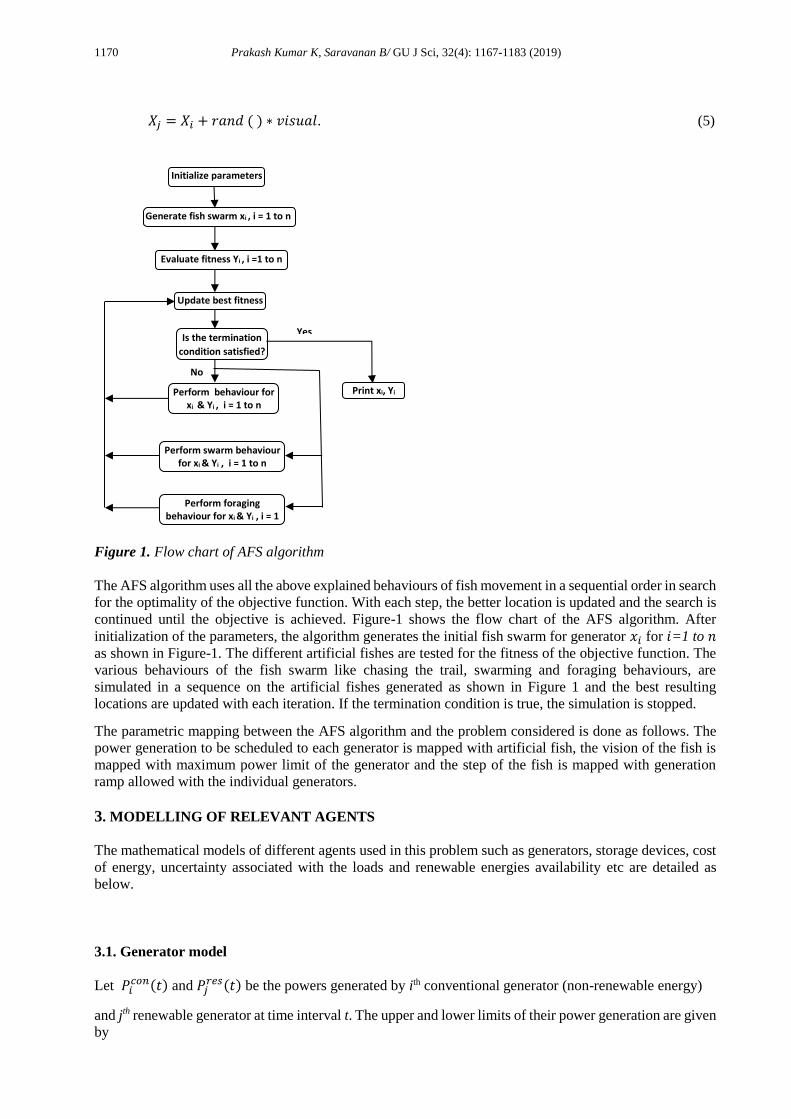
Figure 1. Flow chart of AFS algorithm
The AFS algorithm uses all the above explained behaviours of fish movement in a sequential order in search
for the optimality of the objective function. With each step, the better location is updated and the search is
continued until the objective is achieved. Figure-1 shows the flow chart of the AFS algorithm. After
initialization of the parameters, the algorithm generates the initial fish swarm for generator 𝑥𝑖 for 𝑖=1 to 𝑛
as shown in Figure-1. The different artificial fishes are tested for the fitness of the objective function. The
various behaviours of the fish swarm like chasing the trail, swarming and foraging behaviours, are
simulated in a sequence on the artificial fishes generated as shown in Figure 1 and the best resulting
locations are updated with each iteration. If the termination condition is true, the simulation is stopped.
The parametric mapping between the AFS algorithm and the problem considered is done as follows. The
power generation to be scheduled to each generator is mapped with artificial fish, the vision of the fish is
mapped with maximum power limit of the generator and the step of the fish is mapped with generation
ramp allowed with the individual generators.
3. MODELLING OF RELEVANT AGENTS
The mathematical models of different agents used in this problem such as generators, storage devices, cost
of energy, uncertainty associated with the loads and renewable energies availability etc are detailed as
below.
3.1. Generator model
Let 𝑃𝑖𝑐𝑜𝑛(𝑡) and 𝑃𝑗
𝑟𝑒𝑠(𝑡) be the powers generated by ith conventional generator (non-renewable energy)
and jth renewable generator at time interval t. The upper and lower limits of their power generation are given
by
Perform behaviour for xi & Yi , i = 1 to n
Perform swarm behaviour for xi & Yi , i = 1 to n
Perform foraging behaviour for xi & Yi , i = 1
to n
Initialize parameters
Generate fish swarm xi , i = 1 to n
Evaluate fitness Yi , i =1 to n
Update best fitness
Is the termination
condition satisfied?
Print xi, Yi
Yes
No
1171 Prakash Kumar K, Saravanan B/ GU J Sci, 32(4): 1167-1183 (2019)
𝑃𝑖𝑐𝑜𝑛𝑚𝑖𝑛 ≤ 𝑃𝑖
𝑐𝑜𝑛(𝑡) ≤ 𝑃𝑖𝑐𝑜𝑛𝑚𝑎𝑥 , 𝑡 ∈ 𝑇, 𝑖 ∈ 𝐼, (6)
𝑃𝑗𝑟𝑒𝑠𝑚𝑖𝑛 ≤ 𝑃𝑗
𝑟𝑒𝑠(𝑡) ≤ 𝑃𝑗𝑟𝑒𝑠𝑚𝑎𝑥 , 𝑡 ∈ 𝑇, 𝑗 ∈ 𝐽. (7)
3.2. Storage model
Battery storage is modelled as a distributed unit and their charging and discharging schedule is controlled
by the energy management system based on the following constraints.
Let 𝑃𝑘𝑠𝑡𝑔𝑐ℎ(𝑡), 𝑡 ∈ 𝑇, 𝑘 ∈ 𝐾 and 𝑃𝑘
𝑠𝑡𝑔𝑑𝑐ℎ(𝑡), 𝑡 ∈ 𝑇, 𝑘 ∈ 𝐾, be the charging and discharging powers
respectively.
Then the rates of charging and discharging are bound by upper and lower limits as in (8) and (9)
0 ≤ 𝑃𝑘𝑠𝑡𝑔𝑐ℎ(𝑡) ≤ 𝑃𝑘
𝑠𝑡𝑔𝑐ℎ𝑚𝑎𝑥 , 𝑡 ∈ 𝑇, 𝑘 ∈ 𝐾, (8)
0 ≤ 𝑃𝑘𝑠𝑡𝑔𝑑𝑐ℎ(𝑡) ≤ 𝑃𝑘
𝑠𝑡𝑔𝑑𝑐ℎ𝑚𝑎𝑥 , 𝑡 ∈ 𝑇, 𝑘 ∈ 𝐾, (9)
𝑆𝑜𝐶𝑘𝑚𝑖𝑛 ≤ 𝑆𝑜𝐶𝑘(𝑡) ≤ 𝑆𝑜𝐶𝑘
𝑚𝑎𝑥 , 𝑡 ∈ 𝑇, 𝑘 ∈ 𝐾, (10)
𝑆𝑜𝐶𝑘(𝑡 + 1) = 𝑆𝑜𝐶𝑘(𝑡) + 𝜂𝑘𝑃𝑘𝑠𝑡𝑔𝑐ℎ(𝑡), 𝑡 ∈ 𝑇, 𝑘 ∈ 𝐾, (11)
𝑆𝑜𝐶𝑘(𝑡 + 1) = 𝑆𝑜𝐶𝑘(𝑡) − 𝜂𝑘𝑃𝑘𝑠𝑡𝑔𝑑𝑐ℎ(𝑡), 𝑡 ∈ 𝑇, 𝑘 ∈ 𝐾. (12)
The magnitude of energy stored in the battery storage facility is expressed in terms of state of charge,
𝑆𝑜𝐶𝑘(𝑡) which could either be in terms of percentage of full charge or in terms of kWh remaining for
backup. It is convenient to use kWh remaining for back-up in the present case. The state of charge is bound
by upper and lower limits (10). The state of charge at any instant is given by (11) while charging and by
(12) while discharging, inclusive of charging and discharging efficiencies as noted in equations.
3.3. Load model
A constant power model is used for loads. In such models the loads are an aggregate of rated powers, which
should be supplied in full. A controllable/load shedding version of the model allows the energy
management system to either supply the load fully or disconnect it from the grid. The load in excess to total
power available with the microgrid cannot be supplied and is disconnected/ shed. Such load is termed as
load shed 𝐿𝑚𝑠ℎ𝑑(𝑡) [28]. The load shedding is allowed with compensation 𝐶𝑚
𝑠ℎ𝑑(𝑡) due to the energy user by
the utility operator for the inconvenience caused.
The Distribution Market Operator (DMO) model [29], which is used in the present work, restricts power
transactions between the utility grid and microgrid to a predetermined award, which is communicated to
the microgrid operator by the DMO one day in advance. The aim of this restriction is to reduce penetration
of uncertainty from microgrids into the utility grid. This award is binding on the microgrid operator and he
has to draw power from the utility grid without deviating from this award. Any deviation from the award
will be penalised. In other words, the DMO decides the upper and lower limits for power drawl from the
utility grid and utility grid is no more an infinite source. Under such conditions, if the load to be supplied
by the microgrid is more than the sum of all internal sources, storage and maximum grid power limit, the
excess load is disconnected and is termed as load shed.
3.4. Modelling of costs of energy
The business operation of microgrid involves various components towards the calculation of cost of energy
production. Such components which are considered in the present article may be summed up as follows.
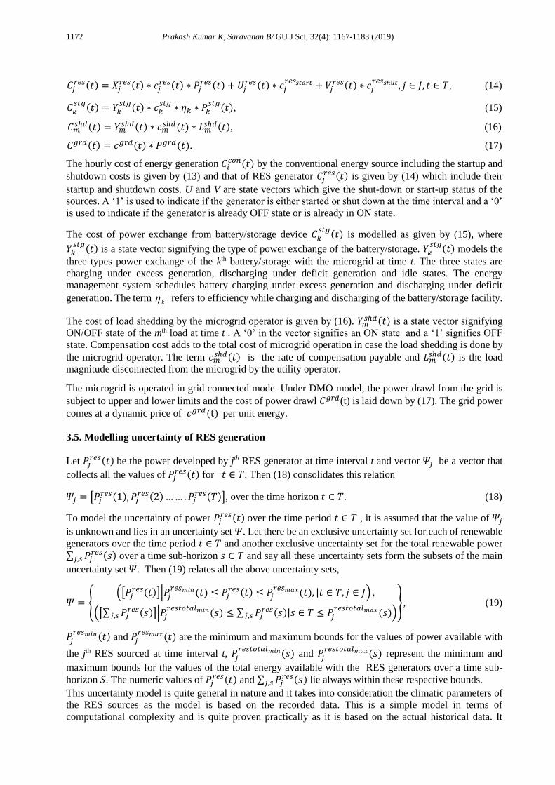
𝐶𝑖𝑐𝑜𝑛(𝑡) = 𝑋𝑖
𝑐𝑜𝑛(𝑡) ∗ 𝑐𝑖𝑐𝑜𝑛(𝑡) ∗ 𝑃𝑖
𝑐𝑜𝑛(𝑡) + 𝑈𝑖𝑐𝑜𝑛(𝑡) ∗ 𝑐𝑖
𝑐𝑜𝑛𝑠𝑡𝑎𝑟𝑡 + 𝑉𝑖𝑐𝑜𝑛(𝑡) ∗ 𝑐𝑖
𝑐𝑜𝑛𝑠ℎ𝑢𝑡 , 𝑖 ∈ 𝐼, 𝑡 ∈ 𝑇, (13)
1172 Prakash Kumar K, Saravanan B/ GU J Sci, 32(4): 1167-1183 (2019)
𝐶𝑗𝑟𝑒𝑠(𝑡) = 𝑋𝑗
𝑟𝑒𝑠(𝑡) ∗ 𝑐𝑗𝑟𝑒𝑠(𝑡) ∗ 𝑃𝑗
𝑟𝑒𝑠(𝑡) + 𝑈𝑗𝑟𝑒𝑠(𝑡) ∗ 𝑐𝑗
𝑟𝑒𝑠𝑠𝑡𝑎𝑟𝑡 + 𝑉𝑗𝑟𝑒𝑠(𝑡) ∗ 𝑐𝑗
𝑟𝑒𝑠𝑠ℎ𝑢𝑡 , 𝑗 ∈ 𝐽, 𝑡 ∈ 𝑇, (14)
𝐶𝑘𝑠𝑡𝑔(𝑡) = 𝑌𝑘
𝑠𝑡𝑔(𝑡) ∗ 𝑐𝑘𝑠𝑡𝑔
∗ 𝜂𝑘 ∗ 𝑃𝑘𝑠𝑡𝑔(𝑡), (15)
𝐶𝑚𝑠ℎ𝑑(𝑡) = 𝑌𝑚
𝑠ℎ𝑑(𝑡) ∗ 𝑐𝑚𝑠ℎ𝑑(𝑡) ∗ 𝐿𝑚
𝑠ℎ𝑑(𝑡), (16)
𝐶𝑔𝑟𝑑(𝑡) = 𝑐𝑔𝑟𝑑(𝑡) ∗ 𝑃𝑔𝑟𝑑(𝑡). (17)
The hourly cost of energy generation 𝐶𝑖𝑐𝑜𝑛(𝑡) by the conventional energy source including the startup and
shutdown costs is given by (13) and that of RES generator 𝐶𝑗𝑟𝑒𝑠(𝑡) is given by (14) which include their
startup and shutdown costs. U and V are state vectors which give the shut-down or start-up status of the
sources. A ‘1’ is used to indicate if the generator is either started or shut down at the time interval and a ‘0’
is used to indicate if the generator is already OFF state or is already in ON state.
The cost of power exchange from battery/storage device 𝐶𝑘𝑠𝑡𝑔(𝑡) is modelled as given by (15), where
𝑌𝑘𝑠𝑡𝑔(𝑡) is a state vector signifying the type of power exchange of the battery/storage. 𝑌𝑘
𝑠𝑡𝑔(𝑡) models the
three types power exchange of the kth battery/storage with the microgrid at time t. The three states are
charging under excess generation, discharging under deficit generation and idle states. The energy
management system schedules battery charging under excess generation and discharging under deficit
generation. The term k refers to efficiency while charging and discharging of the battery/storage facility.
The cost of load shedding by the microgrid operator is given by (16). 𝑌𝑚𝑠ℎ𝑑(𝑡) is a state vector signifying
ON/OFF state of the mth load at time t . A ‘0’ in the vector signifies an ON state and a ‘1’ signifies OFF
state. Compensation cost adds to the total cost of microgrid operation in case the load shedding is done by
the microgrid operator. The term 𝑐𝑚𝑠ℎ𝑑(𝑡) is the rate of compensation payable and 𝐿𝑚
𝑠ℎ𝑑(𝑡) is the load
magnitude disconnected from the microgrid by the utility operator.
The microgrid is operated in grid connected mode. Under DMO model, the power drawl from the grid is
subject to upper and lower limits and the cost of power drawl 𝐶𝑔𝑟𝑑(t) is laid down by (17). The grid power
comes at a dynamic price of 𝑐𝑔𝑟𝑑(t) per unit energy.
3.5. Modelling uncertainty of RES generation
Let 𝑃𝑗𝑟𝑒𝑠(𝑡) be the power developed by jth RES generator at time interval t and vector 𝛹𝑗 be a vector that
collects all the values of 𝑃𝑗𝑟𝑒𝑠(𝑡) for 𝑡 ∈ 𝑇. Then (18) consolidates this relation
𝛹𝑗 = [𝑃𝑗𝑟𝑒𝑠(1), 𝑃𝑗
𝑟𝑒𝑠(2)…… . 𝑃𝑗𝑟𝑒𝑠(𝑇)], over the time horizon 𝑡 ∈ 𝑇. (18)
To model the uncertainty of power 𝑃𝑗𝑟𝑒𝑠(𝑡) over the time period 𝑡 ∈ 𝑇 , it is assumed that the value of 𝛹𝑗
is unknown and lies in an uncertainty set 𝛹. Let there be an exclusive uncertainty set for each of renewable
generators over the time period 𝑡 ∈ 𝑇 and another exclusive uncertainty set for the total renewable power
∑ 𝑃𝑗𝑟𝑒𝑠(𝑠)𝑗,𝑠 over a time sub-horizon 𝑠 ∈ 𝑇 and say all these uncertainty sets form the subsets of the main
uncertainty set 𝛹. Then (19) relates all the above uncertainty sets,
𝛹 = {([𝑃𝑗
𝑟𝑒𝑠(𝑡)]|𝑃𝑗𝑟𝑒𝑠𝑚𝑖𝑛(𝑡) ≤ 𝑃𝑗
𝑟𝑒𝑠(𝑡) ≤ 𝑃𝑗𝑟𝑒𝑠𝑚𝑎𝑥(𝑡), |𝑡 ∈ 𝑇, 𝑗 ∈ 𝐽) ,
([∑ 𝑃𝑗𝑟𝑒𝑠(𝑠)𝑗,𝑠 ]|𝑃𝑗
𝑟𝑒𝑠𝑡𝑜𝑡𝑎𝑙𝑚𝑖𝑛(𝑠) ≤ ∑ 𝑃𝑗𝑟𝑒𝑠(𝑠)|𝑠 ∈ 𝑇𝑗,𝑠 ≤ 𝑃𝑗
𝑟𝑒𝑠𝑡𝑜𝑡𝑎𝑙𝑚𝑎𝑥(𝑠))}, (19)
𝑃𝑗𝑟𝑒𝑠𝑚𝑖𝑛(𝑡) and 𝑃𝑗
𝑟𝑒𝑠𝑚𝑎𝑥(𝑡) are the minimum and maximum bounds for the values of power available with
the jth RES sourced at time interval t, 𝑃𝑗𝑟𝑒𝑠𝑡𝑜𝑡𝑎𝑙𝑚𝑖𝑛(𝑠) and 𝑃𝑗
𝑟𝑒𝑠𝑡𝑜𝑡𝑎𝑙𝑚𝑎𝑥(𝑠) represent the minimum and
maximum bounds for the values of the total energy available with the RES generators over a time sub-
horizon 𝑆. The numeric values of 𝑃𝑗𝑟𝑒𝑠(𝑡) and ∑ 𝑃𝑗
𝑟𝑒𝑠(𝑠)𝑗,𝑠 lie always within these respective bounds.
This uncertainty model is quite general in nature and it takes into consideration the climatic parameters of
the RES sources as the model is based on the recorded data. This is a simple model in terms of
computational complexity and is quite proven practically as it is based on the actual historical data. It
1173 Prakash Kumar K, Saravanan B/ GU J Sci, 32(4): 1167-1183 (2019)
requires only the values of 𝑷𝒋𝒓𝒆𝒔𝒎𝒊𝒏(𝒕), 𝑷𝒋
𝒓𝒆𝒔𝒎𝒂𝒙(𝒕), 𝑷𝒋𝒓𝒆𝒔𝒕𝒐𝒕𝒂𝒍𝒎𝒊𝒏(𝒔) and 𝑷𝒋
𝒓𝒆𝒔𝒕𝒐𝒕𝒂𝒍𝒎𝒂𝒙(𝒔). Numeric values of these
terms can be estimated from historical data analysis using any of the data inference techniques reported in
literature [3].
4. MICROGRID PROBLEM FORMULATION
Minimization of energy generation cost being the prime objective of the microgrid utility operator, it can
be stated as in (20)
𝑚𝑖𝑛∑ ∑ 𝑓[𝑃𝑛(𝑡)]𝑇𝑡=1
𝑁𝑛=1 , (20)
where
𝑓[𝑃𝑛(𝑡)] =
{
∑ ∑ [𝑊𝑖
𝑐𝑜𝑛(𝑡) ∗ 𝑐𝑖𝑐𝑜𝑛(𝑡) ∗ 𝑃𝑖
𝑐𝑜𝑛(𝑡) + 𝑥𝑖 ∗ 𝑐𝑖𝑐𝑜𝑛𝑢𝑝 + 𝑦𝑖 ∗ 𝑐𝑖
𝑐𝑜𝑛𝑑𝑜𝑤𝑛]𝐼𝑖=1
𝑇𝑡=1
+∑ ∑ [𝑋𝑗𝑟𝑒𝑠(𝑡) ∗ 𝑐𝑗
𝑟𝑒𝑠(𝑡) ∗ 𝑃𝑗𝑟𝑒𝑠(𝑡) + 𝑥𝑗 ∗ 𝑐𝑗
𝑟𝑒𝑠𝑢𝑝 + 𝑦𝑖 ∗ 𝑐𝑗𝑟𝑒𝑠𝑑𝑜𝑤𝑛]
𝐽𝑗=1
𝑇𝑡=1
+∑ ∑ [𝑌𝑘𝑠𝑡𝑔(𝑡) ∗ 𝑐𝑘
𝑠𝑡𝑔(𝑡) ∗ 𝜂𝑘 ∗ 𝑃𝑘𝑠𝑡𝑔(𝑡)]𝐾
𝑘=1𝑇𝑡=1
+𝑐𝑔𝑟𝑑(𝑡) ∗ 𝑃𝑔𝑟𝑑(𝑡) + ∑ ∑ [𝑍𝑚𝑠ℎ𝑑(𝑡) ∗ 𝑐𝑚
𝑠ℎ𝑑(𝑡) ∗ 𝐿𝑚𝑠ℎ𝑑(𝑡)]𝑀
𝑚=1𝑇𝑡=1 ,
𝑖, 𝑗, 𝑘,𝑚 ∈ 𝑛, 𝑖 ∈ 𝐼, 𝑗 ∈ 𝐽, 𝑘 ∈ 𝐾,𝑚 ∈ 𝑀, 𝑡 ∈ 𝑇 }
, (21)
subject to the following constraints.
4.1. Power balance constraints
𝑃𝑔𝑒𝑛𝑒𝑟𝑎𝑡𝑒𝑑(𝑡) = 𝑃𝑟𝑒𝑞𝑢𝑖𝑟𝑒𝑑(𝑡),
where
𝑃𝑔𝑒𝑛𝑒𝑟𝑎𝑡𝑒𝑑(𝑡) = ∑ 𝑃𝑖𝑐𝑜𝑛𝐼
𝑖=1 (𝑡) + ∑ 𝑃𝑗𝑟𝑒𝑠𝐽
𝑗=1 (𝑡) + ∑ 𝑃𝑘𝑠𝑡𝑔𝑑𝑐ℎ𝐾
𝑘=1 (𝑡) + 𝑃𝑔𝑟𝑑(𝑡),
𝑃𝑟𝑒𝑞𝑢𝑖𝑟𝑒𝑑(𝑡) = ∑ [𝐿𝑚(𝑡) − 𝐿𝑚𝑠ℎ𝑒𝑑(𝑡)]𝑀
𝑚=1 + ∑ 𝑃𝑘𝑠𝑡𝑔𝑐ℎ𝐾
𝑘=1 (𝑡), 𝑖 ∈ 𝐼, 𝑗 ∈ 𝐽, 𝑘 ∈ 𝐾,𝑚 ∈ 𝑀, 𝑡 ∈ 𝑇. (22)
Equation (22) is the power balance equation.
4.2. Generator constraints
𝑃𝑖,𝑡𝑚𝑖𝑛𝑐𝑜𝑛 ≤ 𝑃𝑖,𝑡
𝑐𝑜𝑛 ≤ 𝑃𝑖,𝑡𝑚𝑎𝑥𝑐𝑜𝑛 , 𝑖 ∈ 𝐼, 𝑡 ∈ 𝑇, (23)
𝑃𝑗,𝑡𝑚𝑖𝑛𝑟𝑒𝑠 ≤ 𝑃𝑗,𝑡
𝑟𝑒𝑠 ≤ 𝑃𝑗,𝑡𝑚𝑎𝑥𝑟𝑒𝑠 , 𝑗 ∈ 𝐽, 𝑡 ∈ 𝑇. (24)
Equation (23) refers to minimum/maximum power generating limits of conventional generators whereas
(24) refers to that of RES generators.
4.3. Storage facility constraints
The limits of battery/storage power exchange with the microgrid while charging and discharging are
given by (25)
0 ≤ 𝑃𝑘𝑠𝑡𝑔𝑐ℎ(𝑡) ≤ 𝑃𝑘
𝑠𝑡𝑔𝑐ℎ𝑚𝑎𝑥 , 0 ≤ 𝑃𝑘𝑠𝑡𝑔𝑑𝑐ℎ(𝑡) ≤ 𝑃𝑘
𝑠𝑡𝑔𝑑𝑐ℎ𝑚𝑎𝑥 , 𝑘 ∈ 𝐾, 𝑡 ∈ 𝑇. (25)
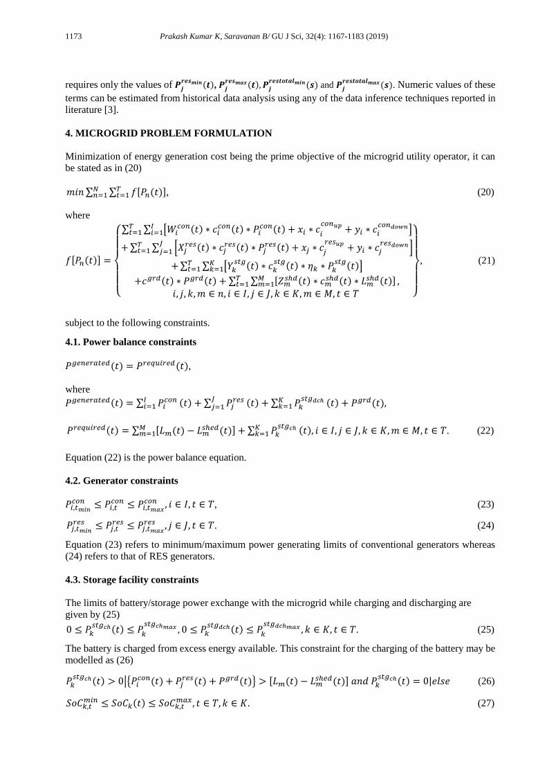
The battery is charged from excess energy available. This constraint for the charging of the battery may be
modelled as (26)
𝑃𝑘𝑠𝑡𝑔𝑐ℎ(𝑡) > 0|{𝑃𝑖
𝑐𝑜𝑛(𝑡) + 𝑃𝑗𝑟𝑒𝑠(𝑡) + 𝑃𝑔𝑟𝑑(𝑡)} > [𝐿𝑚(𝑡) − 𝐿𝑚
𝑠ℎ𝑒𝑑(𝑡)] 𝑎𝑛𝑑 𝑃𝑘𝑠𝑡𝑔𝑐ℎ(𝑡) = 0|𝑒𝑙𝑠𝑒 (26)
𝑆𝑜𝐶𝑘,𝑡𝑚𝑖𝑛 ≤ 𝑆𝑜𝐶𝑘(𝑡) ≤ 𝑆𝑜𝐶𝑘,𝑡
𝑚𝑎𝑥 , 𝑡 ∈ 𝑇, 𝑘 ∈ 𝐾. (27)
1174 Prakash Kumar K, Saravanan B/ GU J Sci, 32(4): 1167-1183 (2019)
Equation (27) restricts the state of charge of the battery/storage facility.
4.4. Grid power drawl constraints
𝑃𝑔𝑟𝑑(𝑡) ≤ 𝑃𝑔𝑟𝑑𝑚𝑎𝑥 . (28)
Equation (28) imposes limits on power drawl from the grid and restricts it to the DMO imposed award, as
explained in section 3.3.
5. ALGORITHM FOR PROPOSED ENERGY MANAGEMENT SYSTEM
The proposed algorithm for day ahead energy management is implemented in following steps.
1. Read data and initialize.
2. Generate scenarios of uncertainty for RES generators and loads.
3. For each scenario
a. If total generation available is more than loads
i. Find power required = load + Pcharge.
ii. Implement AFS algorithm and schedule generation.
iii. Charge the battery with excess power available and update state of charge.
b. If the total generation is less than loads
i. Find load shedding = load – (Sum of all generation available+ Pdischrge)
ii. Implement load shedding.
iii. Find power required = load-loadshedding
iv. Use all the available generation
v. Discharge the battery to meet load and update state of charge
4. Evaluate cost of generation
5. Save data and end.
The objective of the proposed Energy Management Algorithm (EMA) is to schedule the generation and
storage in a microgrid to reduce the effect of uncertainty in RES power availability and loads. Optimization
of cost of generation is only a part of proposed EMA. The proposed EMA calls the Artifical Fish Swarm
(AFS) algorithm when there is a chance to optimize the cost of generation in step 3.a. Optimization is
possible only during excess generation, i.e., when the generation is more than the load. On the other hand,
during deficit generation i.e., when the generation is less than the load, all the sources should be used and
hence there is no chance for optimization. After using all the generators to the full capacity, the EMA uses
storage and load shedding as options to match the load with generation in step 3.b of the proposed algorithm.
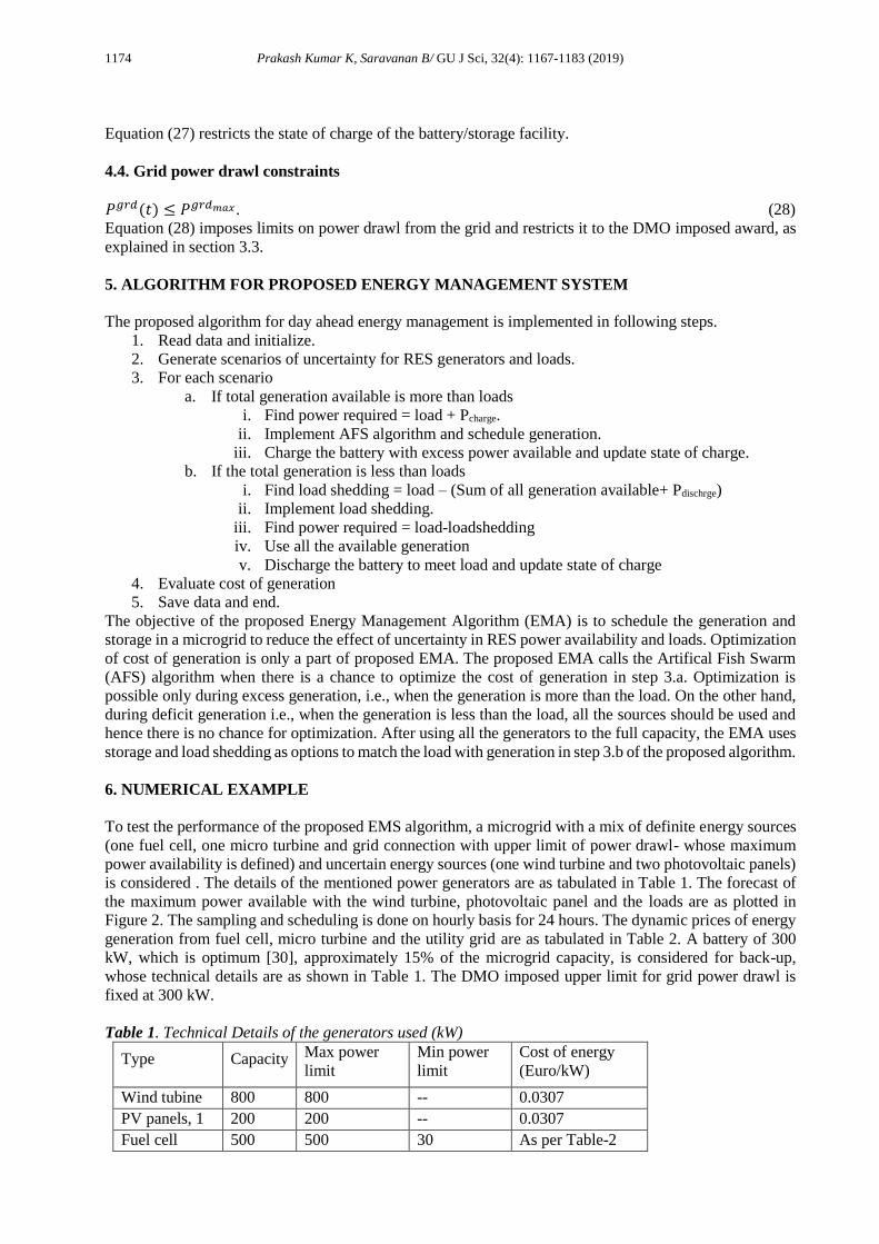
6. NUMERICAL EXAMPLE
To test the performance of the proposed EMS algorithm, a microgrid with a mix of definite energy sources
(one fuel cell, one micro turbine and grid connection with upper limit of power drawl- whose maximum
power availability is defined) and uncertain energy sources (one wind turbine and two photovoltaic panels)
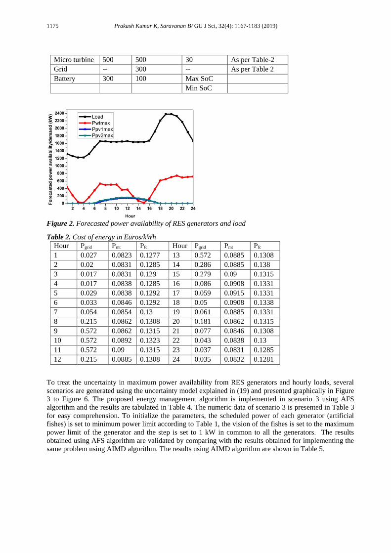
is considered . The details of the mentioned power generators are as tabulated in Table 1. The forecast of
the maximum power available with the wind turbine, photovoltaic panel and the loads are as plotted in
Figure 2. The sampling and scheduling is done on hourly basis for 24 hours. The dynamic prices of energy
generation from fuel cell, micro turbine and the utility grid are as tabulated in Table 2. A battery of 300
kW, which is optimum [30], approximately 15% of the microgrid capacity, is considered for back-up,
whose technical details are as shown in Table 1. The DMO imposed upper limit for grid power drawl is
fixed at 300 kW.
Table 1. Technical Details of the generators used (kW)
Type Capacity Max power
limit
Min power
limit
Cost of energy
(Euro/kW)
Wind tubine 800 800 -- 0.0307
PV panels, 1
and 2
200 200 -- 0.0307
Fuel cell 500 500 30 As per Table-2
1175 Prakash Kumar K, Saravanan B/ GU J Sci, 32(4): 1167-1183 (2019)
Micro turbine 500 500 30 As per Table-2
Grid -- 300 -- As per Table 2
Battery 300 100
(Charge/disch)
Max SoC
(300)
Min SoC
(30)
Figure 2. Forecasted power availability of RES generators and load
Table 2. Cost of energy in Euros/kWh
Hour Pgrid Pmt Pfc Hour Pgrid Pmt Pfc
1 0.027 0.0823 0.1277 13 0.572 0.0885 0.1308
2 0.02 0.0831 0.1285 14 0.286 0.0885 0.138
3 0.017 0.0831 0.129 15 0.279 0.09 0.1315
4 0.017 0.0838 0.1285 16 0.086 0.0908 0.1331
5 0.029 0.0838 0.1292 17 0.059 0.0915 0.1331
6 0.033 0.0846 0.1292 18 0.05 0.0908 0.1338
7 0.054 0.0854 0.13 19 0.061 0.0885 0.1331
8 0.215 0.0862 0.1308 20 0.181 0.0862 0.1315
9 0.572 0.0862 0.1315 21 0.077 0.0846 0.1308
10 0.572 0.0892 0.1323 22 0.043 0.0838 0.13
11 0.572 0.09 0.1315 23 0.037 0.0831 0.1285
12 0.215 0.0885 0.1308 24 0.035 0.0832 0.1281
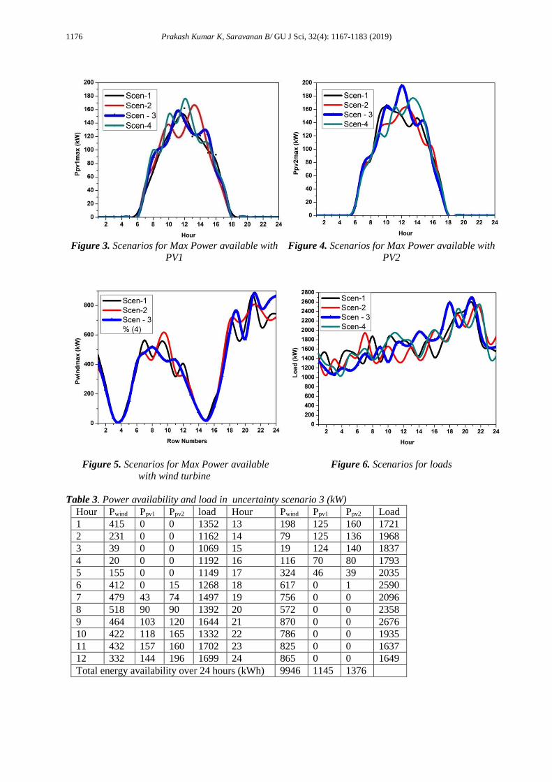
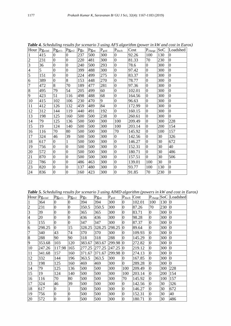
To treat the uncertainty in maximum power availability from RES generators and hourly loads, several
scenarios are generated using the uncertainty model explained in (19) and presented graphically in Figure
3 to Figure 6. The proposed energy management algorithm is implemented in scenario 3 using AFS
algorithm and the results are tabulated in Table 4. The numeric data of scenario 3 is presented in Table 3
for easy comprehension. To initialize the parameters, the scheduled power of each generator (artificial
fishes) is set to minimum power limit according to Table 1, the vision of the fishes is set to the maximum
power limit of the generator and the step is set to 1 kW in common to all the generators. The results
obtained using AFS algorithm are validated by comparing with the results obtained for implementing the
same problem using AIMD algorithm. The results using AIMD algorithm are shown in Table 5.
1176 Prakash Kumar K, Saravanan B/ GU J Sci, 32(4): 1167-1183 (2019)
Figure 3. Scenarios for Max Power available with
PV1
Figure 4. Scenarios for Max Power available with
PV2
Figure 5. Scenarios for Max Power available
with wind turbine
Figure 6. Scenarios for loads
Table 3. Power availability and load in uncertainty scenario 3 (kW)
Hour Pwind Ppv1 Ppv2 load Hour Pwind Ppv1 Ppv2 Load
1 415 0 0 1352 13 198 125 160 1721
2 231 0 0 1162 14 79 125 136 1968
3 39 0 0 1069 15 19 124 140 1837
4 20 0 0 1192 16 116 70 80 1793
5 155 0 0 1149 17 324 46 39 2035
6 412 0 15 1268 18 617 0 1 2590
7 479 43 74 1497 19 756 0 0 2096
8 518 90 90 1392 20 572 0 0 2358
9 464 103 120 1644 21 870 0 0 2676
10 422 118 165 1332 22 786 0 0 1935
11 432 157 160 1702 23 825 0 0 1637
12 332 144 196 1699 24 865 0 0 1649
Total energy availability over 24 hours (kWh) 9946 1145 1376
1177 Prakash Kumar K, Saravanan B/ GU J Sci, 32(4): 1167-1183 (2019)
Table 4. Scheduling results for scenario 3 using AFS algorithm (power in kW and cost in Euros)
Hour Pgwind Pgpv1. Pgpv2 Pgfc Pgmt Pgrid Pdisch Cost Pcharge SoC Loadshed
1 415 0 0 237 500 300 0 92.26 100 130 0
2 231 0 0 220 481 300 0 81.33 70 230 0
3 36 0 0 240 500 293 0 78.6 0 300 0
4 5 0 0 399 488 300 0 97.42 0 300 0
5 151 0 0 224 499 275 0 83.37 0 300 0
6 389 0 8 153 448 270 0 78.77 0 300 0
7 472 8 70 189 477 281 0 97.36 0 300 0
8 495 79 54 205 499 60 0 102.01 0 300 0
9 423 51 116 498 488 68 0 164.56 0 300 0
10 415 102 106 230 470 9 0 96.63 0 300 0
11 412 126 132 459 489 84 0 172.99 0 300 0
12 312 144 119 440 491 192 0 160.15 0 300 0
13 198 125 160 500 500 238 0 260.61 0 300 0
14 79 125 136 500 500 300 100 209.49 0 300 228
15 19 124 140 500 500 300 100 203.14 0 200 154
16 116 70 80 500 500 300 70 145.92 0 100 157
17 324 46 39 500 500 300 0 142.56 0 30 326
18 617 0 1 500 500 300 0 146.27 0 30 672
19 756 0 0 500 500 300 0 152.31 0 30 40
20 572 0 0 500 500 300 0 180.71 0 30 486
21 870 0 0 500 500 300 0 157.51 0 30 506
22 786 0 0 486 463 300 0 139.01 100 30 0
23 820 0 0 137 480 300 0 93.77 100 130 0
24 836 0 0 160 423 300 0 91.85 70 230 0
Table 5. Scheduling results for scenario 3 using AIMD algorithm (powers in kW and cost in Euros)
Hour Pgwind Pgpv1. Pgpv2 Pgfc Pgmt Pgrid Pdisch Cost Pcharge SoC Loadshed
1 364 0 0 394 394 300 0 102.01 100 130 0
2 231 0 0 350.5 350.5 300 0 87.26 70 230 0
3 39 0 0 365 365 300 0 83.71 0 300 0
4 20 0 0 436 436 300 0 98.28 0 300 0
5 155 0 0 347 347 300 0 87.37 0 300 0
6 298.25 0 15 328.25 328.25 298.25 0 89.64 0 300 0
7 340 43 74 370 370 300 0 109.93 0 300 0
8 288 90 90 318 318 288 0 145.29 0 300 0
9 353.68 103 120 383.67 383.67 299.98 0 272.82 0 300 0
10 247.26 117.98 165 277.25 277.25 247.25 0 219.12 0 300 0
11 341.68 157 160 371.67 371.67 299.98 0 274.13 0 300 0
12 332 144 196 363.5 363.5 300 0 167.85 0 300 0
13 198 125 160 469 469 300 0 289.28 0 300 0
14 79 125 136 500 500 300 100 209.49 0 300 228
15 19 124 140 500 500 300 100 203.14 0 200 154
16 116 70 80 500 500 300 70 145.92 0 100 157
17 324 46 39 500 500 300 0 142.56 0 30 326
18 617 0 1 500 500 300 0 146.27 0 30 672
19 756 0 0 500 500 300 0 152.31 0 30 40
20 572 0 0 500 500 300 0 180.71 0 30 486
1178 Prakash Kumar K, Saravanan B/ GU J Sci, 32(4): 1167-1183 (2019)
21 870 0 0 500 500 300 0 157.51 0 30 506
22 735 0 0 500 500 300 0 142.36 100 30 0
23 459 0 0 489 489 300 0 128.66 100 130 0
24 453 0 0 483 483 300 0 126.47 70 230 0
Figure 7. Scheduling results using AFS algorithm Figure 8. Scheduling results using AIMD algorithm
Figure 9. Comparison of cost of generation using AFS and AIMD algorithms
Figure 10. Battery power exchange Figure 11. State of charge of battery
1179 Prakash Kumar K, Saravanan B/ GU J Sci, 32(4): 1167-1183 (2019)
7. RESULTS AND DISCUSSIONS
The results of generation scheduling by implementing proposed algorithm for scenario-3 is presented in
Table 4 and that using AIMD algorithm in Table 5. The term Pg with suffix in the Tables 4 and 5 refers to
the power generation scheduled to the respective generators after implementing the proposed Energy
Management Algorithm. In either case, the fundamental constraint of energy balance as laid down by (19)
is verified and the power produced (Power produced=Power generated by conventional generators+Power
generated by renewable generators+Power obtained by battery discharge+Power drawn from grid, (22)] is
exactly matching the power required [Power required = Total load on microgrid-Load shed+Powre required
to charge battery, (22)] at each hour. A close comparison of Table 4 and Table 5 shows that AFS algorithm
is far better than AIMD algorithm in optimizing the cost of generation. For example at hour 1, the cost of
grid energy is the cheapest, followed by wind and PV power, micro turbine and fuel cell in sequence of
increasing cost of generation. During this hour, the proposed EMS using AFS algorithm is able to schedule
complete power available from cheaper sources (grid, wind turbine, PV panels, micro turbine) and use the
costliest source, i.e., fuel cell very sparingly. Whereas AIMD algorithm is unable to do the same. It is
scheduling equal powers to all the generators subject to min and max powers. For micro turbine and fuel
cell, the min powers are 30 kW (Table 1) and for wind turbine and PV panels, the min powers are zero.
Max powers available for wind turbine and PV panels are 415 kW,0 kW,0 kW (Table-3, uncertainty
scenario 3) during hour 1 and for micro turbine, fuel cell and grid it is 500 kW,500 kW and 300 kW
respectively (Table 1). At hour 1, AIMD algorithm is allocating equal power scheduling to wind (364 kW),
fuel cell (394-30 (min power) = 364 kW) and micro turbine (394-30 (min power) = 364 kW) and 300 kW
to grid as its maximum power limit is 300 kW. In other words, the AFS algorithm is able to choose the
cheaper sources and schedule more load to them compared to the costlier sources, whereas AIMD algorithm
is scheduling equal amounts of loads to all the sources available irrespective of their cost of energy
generation and that is the reason why there is a difference in cost of energy generation estimated by the two
algorithms. Similar scheduling is done for hours 1-13 and hours 22-24. During these hours, the demand is
less than the total power availability and hence the AFS algorithm is able to search for the most economic
mix of power generation from different sources. During the hours 14 -21, the demand is more than the total
power available, and hence both the algorithms are using entire power available, there is no choice of
selection of generators for scheduling and hence the cost estimation by both the algorithms is same. The
above discussion compares the performance of two tools used for optimization, i.e., AIMD algorithm and
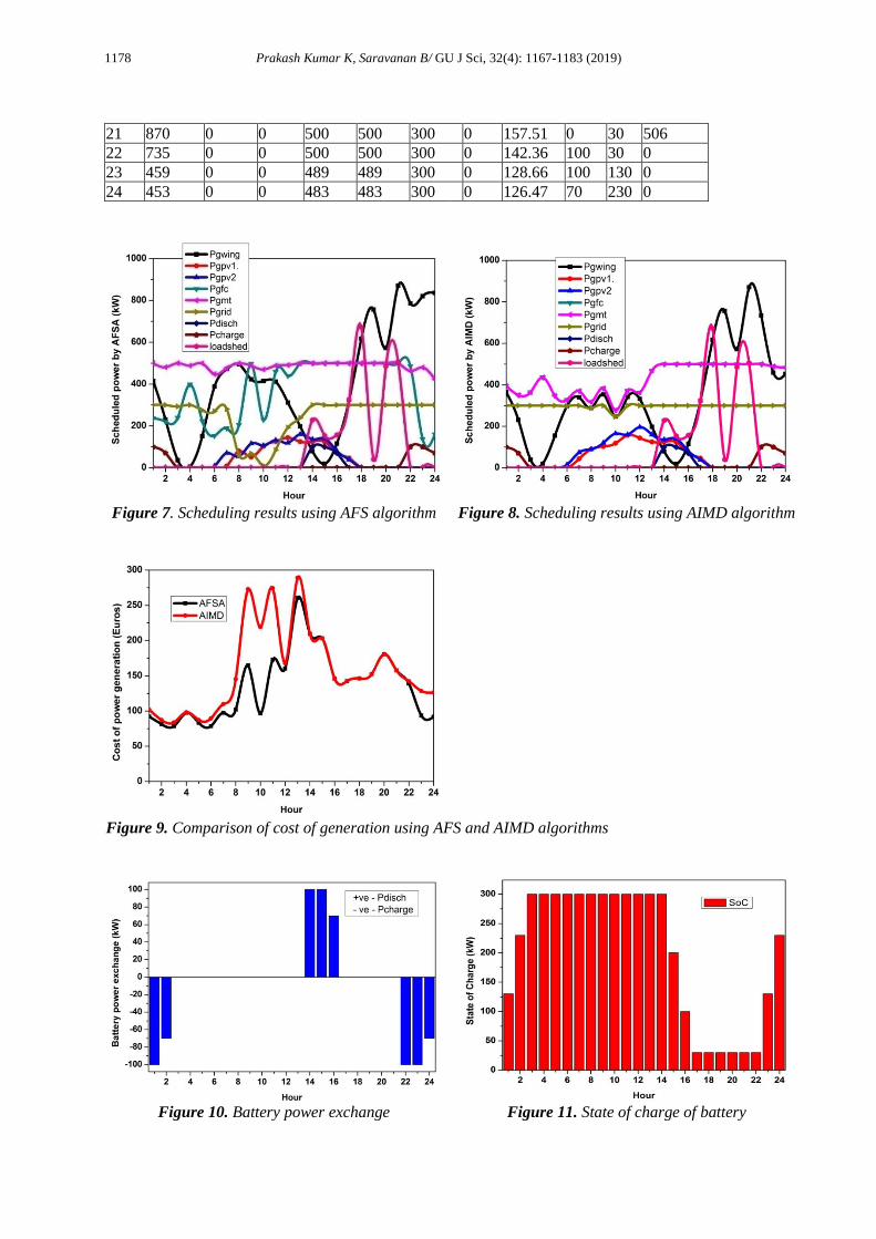
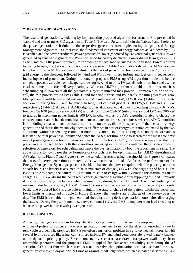
AFS algorithm. Figure 7 and Figure 8 show the scheduling results using two algorithms. Figure 9 compares
the costs of energy generation estimated by the two optimization tools. As far as the performance of the
Energy Management System proposed, it is able to balance the power required with the power generation
at each hour. The battery is assumed to be at min state of charge (30 kW) at the beginning of hour 1. The
EMS is able to charge the battery to its maximum state of charge without violating the maximum rate of
charge, i.e., 100kW, during the hours when excess generation is available after supplying the load. Similarly
it is able to discharge the battery when required, i.e., during hours 14,15 and 16 without violating the
maximum discharge rate, i.e., 100 kW. Figure 10 shows the hourly power exchange of the battery on hourly
basis. The proposed EMS is also able to maintain the state of charge of the battery within the upper and
lower limits as mentioned in Table 1. Figure 11 shows the hourly state of charge of the battery over the
day. The EMS is also able to implement load shedding during deficit generation hours, after discharging
the battery. During the peak hours, i.e., between hours 14-21, the EMS is implementing load shedding to
balance the power required with power generated.
8. CONCLUSIONS
An energy management system for day ahead energy planning in a microgrid is proposed in this article
with an objective to optimize the energy generation cost and to reduce the effect of uncertainty due to
renewable sources. The proposed EMS is tested on a numerical problem in a grid connected microgrid with
several hybrid sources like a fuel cell, a micro turbine, PV and wind generators along with battery backup
under dynamic pricing policy. Several uncertainty scenarios are drawn for power availability from
renewable generators and the proposed EMS is applied for day ahead scheduling considering the 3rd
scenario. AFS algorithm which is used as a tool to solve the optimization part, has estimated the total
generation cost over a day as 3228.9 Euros as against AIMD algorithm, which estimated the same as 3762
1180 Prakash Kumar K, Saravanan B/ GU J Sci, 32(4): 1167-1183 (2019)
Euros. The AFS algorithm is better optimizing the generation mix with a net saving of 16.5%. The proposed
EMS able to balance the generation with load at each interval. The main objective of the proposed EMS is
reducing the effect of uncertainty of renewable energy generation and it is well attained using battery
storage. The EMS is able to schedule battery storage during excess generation and discharge the battery
during deficit generation while maintaining the rate of power exchange and state of charge limits. The EMS
is also able to implement load shedding when there is no possibility to supply the demand in full during the
peak hours, i.e., between 14th to 21st hours.
CONFLICTS OF INTEREST
No conflict of interests was declared by the authors.
REFERENCES
[1] https://www.morganstanley.com/ideas/clean-energy-trump.html. (accessed on 25.12.2018).
[2] http://economictimes.indiatimes.com/industry /energy/ power/ solar-power-tariff-drops-to-
historic-low-at-rs-2-44-per-nit/articleshow/58649942.cm,(accessed on 25.12.2018).
[3] K. Prakash Kumar, B. Saravanan, “Recent techniques to model uncertainty in power generation
from renewable energy sources in microgrids”, J. Renew Sustain Energy Rev, 71, 348-58, (2017).
[4] Basu Ashoke Kumar, Chowdhury SP, Chowdhury S, Paul S. “Microgrids: energy management by
strategic deployment of DERs-A comprehensive review”, Renew Sustain Energy Rev 15, 4348–
56, (2011).
[5] El Bakari K, Kling WL., “Virtual power plant: Answer to increasing distributed generation”, IEEE
Proc, PES conf Innov Smartgrid Technol (Eur), 11-13, 1-6, (2010).
[6] K. Prakash Kumar, B. Saravanan and K.S.Swarup, “A two stage increase decrease algorithm to
optimize distributed generation in a virtual power plant”, Energy Procedia, 90, 276 – 82, (2016).
[7] GE Energy . Western wind and solar integration study [tech rep]. NREL (2010).
[8] Hawkes AD, Leach MA. “Modelling high level system design and unit commitment for a
microgrid”, Appl Energy, 86, 1253–65, (2009).
[9] Van der Kam M, van Sark W. “Smart charging of electric vehicles with photovoltaic power and
vehicle-to-grid technology in a microgrid; a case study”, Appl Energy, 152, 20–30, (2015).
[10] Zhang Z, Wang J, Wang X. “An improved charging/discharging strategy of lithium batteries
considering depreciation cost in day-ahead microgrid scheduling”, Energy Convers Manage, 105,
675–84, (2015).
[11] Mallol-Poyato R, Salcedo-Sanz S, Jimenez-Fernandez S, Diaz-Villar P. “Optimal discharge
scheduling of energy storage systems in MicroGrids based on hyperheuristics”, Renew Energy, 83,
13–24, (2015).
[12] Thillainathan Logenthiran , Dipti Srinivasan, Tan Zong Shun, “Demand side management in
smartgrid using heuristic optimization”, IEEE transaction on Smartgrid, 3, no.3, (2012).
[13] Zakariazadeh Alireza, Jadid Shahram, Siano Pierluigi. “Smart microgrid energy and reserve
scheduling with demand response using stochastic optimization”, Electr Power Energy Syst, 63,
523–33, (2014).
1181 Prakash Kumar K, Saravanan B/ GU J Sci, 32(4): 1167-1183 (2019)
[14] Montuori L, Alcazar-Ortega M, Alvarez-Bel C, Domijan A. “Integration of renewable energy in
microgrids coordinated with demand response resources: economic evaluation of a biomass
gasification plant by Homer Simulator”, Appl Energy, 132, 15–22, (2014).
[15] Mazidi M, Zakariazadeh A, Jadid S, Siano P. “Integrated scheduling of renewable generation and
demand response programs in a microgrid”, Energy Convers Manage, 86, 1118–27, (2014).
[16] Mohammadreza Mazidi, Hassan Monsef,Pierluigi Siano, “Robust day-ahead scheduling of smart
distribution networks considering demand response programs”, Applied Energy 178 (2016) 929–
942, (2016).
[17] Cherukuri, S. Hari Charan, and B. Saravanan. "A novel energy management algorithm for
reduction of main grid dependence in future smart grids using electric springs." Sustainable Energy
Technologies and Assessments 21, 1-12, (2017).
[18] Talari S, Yazdaninejad M, Haghifam M. “Stochastic-based scheduling of the microgrid operation
including wind turbines, photovoltaic cells, energystorages and responsive loads”, IET Gener
Transm Distrib, 9, 1498–509, (2015).
[19] Najibi F, Niknam T. “Stochastic scheduling of renewable micro-grids considering photovoltaic
source uncertainties”, Energy Convers Manage, 98, 484–99, (2015).
[20] Najibi F, Niknam T. “Stochastic scheduling of renewable micro-grids considering photovoltaic
source uncertainties”, Energy Convers Manage, 98, 484–99, (2015).
[21] Zakariazadeh A, Jadid S, Siano P. “Smart microgrid energy and reserve scheduling with demand
response using stochastic optimization”, Int J Electr Power Energy Syst, 63, 523–33, (2014).
[22] Yu Zhang, NikolaosGatsis, and Georgios B. Giannakis, “Robust Energy Management for
Microgrids With High-Penetration Renewables”, IEEE Transactions on Sustainable energy, 4,
No.4, (2013).
[23] Amin Khodaei, “Microgrid Optimal Scheduling With Multi-Period Islanding Constraints, IEEE
Trasactions on power systems”, 29,No.3, (2014).
[24] Emmanual Cristoni, Marco Raugi and Robert Shorten (2014), “Plug and Play distributed algorithm
for Optimized power Generation in a Microgrid”, IEEE Transactions on Smart Grid, 4, 2145-54,
(2014).
[25] Yaowang Li, Shihong Miao, Xing Luo, Jihong Wang, “Optimization scheduling model based on
source-load-energy storage coordination in power systems”, International Conference on
Automation and Computing. IEEE, 120–125, (2016).
[26] Zhigang Li, Wenchuan Wu, Boming Zhang, “Adjustable robust real-time power dispatch with
large-scale wind power integration”, IEEE Trans. Sustain. Energy, 6 (2), 357–68, (2015).
[27] Bo Xing, Wen Jing Gao, “Innovative computational intelligence: A rough guide to 134 clever
algorithms”, Springer International Publishing, Switzerland, (2014).
[28] K. Prakash Kumar, B. Saravanan, “Day ahead scheduling of generation and storage in a microgrid
considering demand side management”, Journal of Energy Storage, 21, 78–86, (2019).
[29] Sina Parhizi, Amin Khodaei, Mohammad Shahidehpour, “Market based verses Price based
microgrid optimal scheduling”, IEEE Trans on Smartgrids, 9(2), 615-23, (2018).
1182 Prakash Kumar K, Saravanan B/ GU J Sci, 32(4): 1167-1183 (2019)
[30] Braun B, Philipp B, Swierczynski S, Jozef MM, Diosi D, Robert R, Stroe S, Loan D. Teodorescu
T, Remus R. “Optimizing a hybrid energy storage system for a virtual power plant for improved
wind power generation: A case study for Denmark”, Proceedings of the 6th International
Renewable Energy Storage Conference and Exhibition, IRES, 1–9, (2011).
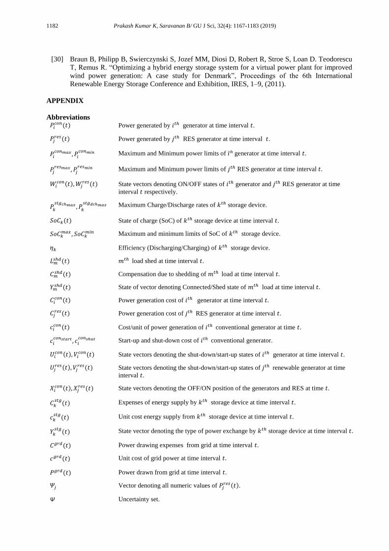
APPENDIX
Abbreviations 𝑃𝑖𝑐𝑜𝑛(𝑡) Power generated by 𝑖𝑡ℎ generator at time interval 𝑡.
𝑃𝑗𝑟𝑒𝑠(𝑡) Power generated by 𝑗𝑡ℎ RES generator at time interval 𝑡.
𝑃𝑖𝑐𝑜𝑛𝑚𝑎𝑥 , 𝑃𝑖
𝑐𝑜𝑛𝑚𝑖𝑛 Maximum and Minimum power limits of ith generator at time interval 𝑡.
𝑃𝑗𝑟𝑒𝑠𝑚𝑎𝑥 , 𝑃𝑗
𝑟𝑒𝑠𝑚𝑖𝑛 Maximum and Minimum power limits of 𝑗𝑡ℎ RES generator at time interval 𝑡.
𝑊𝑖𝑐𝑜𝑛(𝑡),𝑊𝑗
𝑟𝑒𝑠(𝑡) State vectors denoting ON/OFF states of 𝑖𝑡ℎ generator and 𝑗𝑡ℎ RES generator at time
interval 𝑡 respectively.
𝑃𝑘
𝑠𝑡𝑔𝑐ℎ𝑚𝑎𝑥 , 𝑃𝑘
𝑠𝑡𝑔𝑑𝑐ℎ𝑚𝑎𝑥
Maximum Charge/Discharge rates of 𝑘𝑡ℎ storage device.
𝑆𝑜𝐶𝑘(𝑡) State of charge (SoC) of 𝑘𝑡ℎ storage device at time interval 𝑡.
𝑆𝑜𝐶𝑘𝑚𝑎𝑥 , 𝑆𝑜𝐶𝑘
𝑚𝑖𝑛
Maximum and minimum limits of SoC of 𝑘𝑡ℎ storage device.
𝜂𝑘 Efficiency (Discharging/Charging) of 𝑘𝑡ℎ storage device.
𝐿𝑚𝑠ℎ𝑑(𝑡)
𝑚𝑡ℎ load shed at time interval 𝑡.
𝐶𝑚𝑠ℎ𝑑(𝑡)
Compensation due to shedding of 𝑚𝑡ℎ load at time interval 𝑡.
𝑌𝑚𝑠ℎ𝑑(𝑡)
State of vector denoting Connected/Shed state of 𝑚𝑡ℎ load at time interval 𝑡.
𝐶𝑖𝑐𝑜𝑛(𝑡)
Power generation cost of 𝑖𝑡ℎ generator at time interval 𝑡.
𝐶𝑗𝑟𝑒𝑠(𝑡)
Power generation cost of 𝑗𝑡ℎ RES generator at time interval 𝑡.
𝑐𝑖𝑐𝑜𝑛(𝑡)
Cost/unit of power generation of 𝑖𝑡ℎ conventional generator at time 𝑡.
𝑐𝑖𝑐𝑜𝑛𝑠𝑡𝑎𝑟𝑡 , 𝑐𝑖
𝑐𝑜𝑛𝑠ℎ𝑢𝑡
Start-up and shut-down cost of 𝑖𝑡ℎ conventional generator.
𝑈𝑖𝑐𝑜𝑛(𝑡), 𝑉𝑖
𝑐𝑜𝑛(𝑡)
State vectors denoting the shut-down/start-up states of 𝑖𝑡ℎ generator at time interval 𝑡.
𝑈𝑗𝑟𝑒𝑠(𝑡), 𝑉𝑗
𝑟𝑒𝑠(𝑡)
State vectors denoting the shut-down/start-up states of 𝑗𝑡ℎ renewable generator at time
interval 𝑡.
𝑋𝑖𝑐𝑜𝑛(𝑡), 𝑋𝑗
𝑟𝑒𝑠(𝑡)
State vectors denoting the OFF/ON position of the generators and RES at time 𝑡.
𝐶𝑘𝑠𝑡𝑔(𝑡)
Expenses of energy supply by 𝑘𝑡ℎ storage device at time interval 𝑡.
𝑐𝑘𝑠𝑡𝑔(𝑡)
Unit cost energy supply from 𝑘𝑡ℎ storage device at time interval 𝑡.
𝑌𝑘𝑠𝑡𝑔(𝑡)
State vector denoting the type of power exchange by 𝑘𝑡ℎ storage device at time interval 𝑡.
𝐶𝑔𝑟𝑑(𝑡)
Power drawing expenses from grid at time interval 𝑡.
𝑐𝑔𝑟𝑑(𝑡)
Unit cost of grid power at time interval 𝑡.
𝑃𝑔𝑟𝑑(𝑡)
Power drawn from grid at time interval 𝑡.
𝛹𝑗 Vector denoting all numeric values of 𝑃𝑗
𝑟𝑒𝑠(𝑡).
Ψ Uncertainty set.

1183 Prakash Kumar K, Saravanan B/ GU J Sci, 32(4): 1167-1183 (2019)
𝑃𝑗,𝑠𝑟𝑒𝑠𝑡𝑜𝑡𝑎𝑙𝑚𝑖𝑛 , 𝑃𝑗,𝑠
𝑟𝑒𝑠𝑡𝑜𝑡𝑎𝑙𝑚𝑎𝑥
Upper and lower limits for total energy availability with the 𝑗𝑡ℎ RES over a time sub-
horizon S.
t Time interval.
𝑃𝑖(𝑡) Power generated by 𝑖𝑡ℎ generator at time interval 𝑡.
𝑑(𝑡)
Demand at time interval 𝑡.
𝑃𝑖𝑚𝑎𝑥 , 𝑃𝑖𝑚𝑖𝑛 Generation limits of 𝑖𝑡ℎ generator.