Data-Driven and HVDC Control Methods to Enhance Power ...
286
General rights Copyright and moral rights for the publications made accessible in the public portal are retained by the authors and/or other copyright owners and it is a condition of accessing publications that users recognise and abide by the legal requirements associated with these rights. Users may download and print one copy of any publication from the public portal for the purpose of private study or research. You may not further distribute the material or use it for any profit-making activity or commercial gain You may freely distribute the URL identifying the publication in the public portal If you believe that this document breaches copyright please contact us providing details, and we will remove access to the work immediately and investigate your claim. Downloaded from orbit.dtu.dk on: Jul 24, 2022 Data-Driven and HVDC Control Methods to Enhance Power System Security Thams, Florian Publication date: 2018 Document Version Publisher's PDF, also known as Version of record Link back to DTU Orbit Citation (APA): Thams, F. (2018). Data-Driven and HVDC Control Methods to Enhance Power System Security. Technical University of Denmark.
-
Upload
khangminh22 -
Category
Documents
-
view
2 -
download
0
Transcript of Data-Driven and HVDC Control Methods to Enhance Power ...

General rights Copyright and moral rights for the publications made accessible in the public portal are retained by the authors and/or other copyright owners and it is a condition of accessing publications that users recognise and abide by the legal requirements associated with these rights.
Users may download and print one copy of any publication from the public portal for the purpose of private study or research.
You may not further distribute the material or use it for any profit-making activity or commercial gain
You may freely distribute the URL identifying the publication in the public portal If you believe that this document breaches copyright please contact us providing details, and we will remove access to the work immediately and investigate your claim.
Downloaded from orbit.dtu.dk on: Jul 24, 2022
Data-Driven and HVDC Control Methods to Enhance Power System Security
Thams, Florian
Publication date:2018
Document VersionPublisher's PDF, also known as Version of record
Link back to DTU Orbit
Citation (APA):Thams, F. (2018). Data-Driven and HVDC Control Methods to Enhance Power System Security. TechnicalUniversity of Denmark.

Florian Thams
Data-Driven and HVDC Control
Methods to Enhance Power System
Security
Dissertation, September 2018Kgs. Lyngby, Denmark


DANMARKS TEKNISKE UNIVERSITET
Center for Electric Power and Energy (CEE)DTU Electrical Engineering
Data-Driven and HVDC Control Methods to
Enhance Power System Security
Data-drevne og HVDC-kontrolmetoder til
forbedring af strømsystemets sikkerhed
Dissertation, by Florian Thams
Supervisors:
Associate Professor Spyros Chatzivasileiadis, Technical University of Denmark
Robert Eriksson, Swedish National Grid
Associate Professor Arne Hejde Nielsen, Technical University of Denmark
DTU - Technical University of Denmark, Kgs. Lyngby - September 2018

Data-Driven and HVDC Control Methods to Enhance Power System Security
This thesis was prepared by:Florian Thams
Supervisors:Associate Professor Spyros Chatzivasileiadis, Technical University of DenmarkRobert Eriksson, Swedish National GridAssociate Professor Arne Hejde Nielsen, Technical University of Denmark
Dissertation Examination Committee:Senior Researcher Nicolaos Cutululis (Chairman)Department of Wind Energy, Technical University of Denmark, Denmark
Professor Oriol Gomis-BellmuntCentre of Technological Innovation in Static Converters and Drives, Universitat Politècnica deCatalunya, Spain
Professor Louis WehenkelDepartment of Electrical Engineering and Computer Science, University of Liège, Belgium
Center for Electric Power and Energy (CEE)DTU Electrical EngineeringElektrovej, Building 325DK-2800 Kgs. LyngbyDenmark
Tel: (+45) 4525 3500Fax: (+45) 4588 6111E-mail: [email protected]
Release date: 30. September 2018
Edition: 1.0
Class: Internal
Field: Electrical Engineering
Remarks: The dissertation is presented to the Department of Electrical Engineeringof the Technical University of Denmark in partial fulfillment of the require-ments for the degree of Doctor of Philosophy.
Copyrights: ©Florian Thams, 2014– 2018
ISBN: 000-00-00000-00-0

To my family


PrefaceThis thesis is prepared at the Department of Electrical Engineering of the Technical Universityof Denmark in partial fulfillment of the requirements for acquiring the degree of Doctor ofPhilosophy in Engineering. The Ph.D. project was co-funded by the European Unions SeventhFramework Programme for Research, Technological Development and Demonstration under thegrant agreement no. 612748 and by the ForskEL-projekt 12264 Best Paths for DK.
This dissertation summarizes the work carried out by the author during his Ph.D. project. It startedon 1st June 2015, and it was completed on 30th September 2018. During this period, he was hiredby the Technical University of Denmark as a Ph.D. student at the Center for Electric Power andEnergy (CEE).
The thesis is composed of 8 chapters and 6 attached scientific papers, 5 of which have beenpeer-reviewed and published, whereas the remaining one is currently under review.
Florian Thams30. September 2018
i


AcknowledgementsI like to take this opportunity to thank Robert Eriksson for having accepted me as a PhD Studentat DTU and, for his support and feedback. I appreciate that even after leaving DTU, he took thetime and continued to supervise me and was available for discussions whenever needed. I wouldalso like to thank Spyros Chatzivasileiadis for ’taking me over’ when he joined DTU and, for hissupport and feedback. I appreciate that both, Spyros and Robert, gave me the freedom to exploredi↵erent research topics, encouraged me to try new things and gave their advice whenever needed.I would also like to thank Arne Hejde Nielsen for his support.
During my PhD studies I spent 5 months at ETH Zurich working with Gabriela Hug. I would liketo thank Gabriela for accepting me as guest researcher and, for her support and feedback duringthat time. Special thanks goes also to all PSL members, for the great time I had in Zurich.
I would also like to thank Lejla Halilbašic for the proof reading of parts of my thesis, the numerousdiscussions, and the great collaboration within the BestPaths project and beyond. I would alsolike to thank Andreas Venzke for our discussions and good collaboration. Special thanks goes toTheis Bo Rasmussen for helping me with the Danish abstract. Further, I would like to thank all mycolleagues for the entertaining discussions during lunch and co↵ee breaks.
Special thanks also goes to Nicolaos Cutululis, Oriol Gomis-Bellmunt and Louis Wehenkel foraccepting to be the examiners of this thesis. I highly appreciate the time they devoted in readingthe manuscript.
Finally, I’d like to thank my family and friends for their constant support.
Florian Thams
Kgs. Lyngby, Denmark, 30.09.2018
iii


Table of ContentsPreface i
Acknowledgements iii
Table of Contents v
Abstract ix
Resumé xi
Acronyms xiii
List of Figures xvii
List of Tables xxi
List of Symbols xxiii
1 Introduction 11.1 Background and Motivation . . . . . . . . . . . . . . . . . . . . . . . . . . . . . . . . 11.2 Contributions . . . . . . . . . . . . . . . . . . . . . . . . . . . . . . . . . . . . . . . . 31.3 Outline of the Thesis . . . . . . . . . . . . . . . . . . . . . . . . . . . . . . . . . . . . 41.4 List of Publications . . . . . . . . . . . . . . . . . . . . . . . . . . . . . . . . . . . . . 51.5 Division of Work between the Authors . . . . . . . . . . . . . . . . . . . . . . . . . . 6
2 Background 72.1 Introduction . . . . . . . . . . . . . . . . . . . . . . . . . . . . . . . . . . . . . . . . . 72.2 Definition of Important Concepts . . . . . . . . . . . . . . . . . . . . . . . . . . . . . 72.3 Power System Security Assessment . . . . . . . . . . . . . . . . . . . . . . . . . . . . 8
2.3.1 Power System Stability . . . . . . . . . . . . . . . . . . . . . . . . . . . . . . . 92.3.2 N-1 Criterion . . . . . . . . . . . . . . . . . . . . . . . . . . . . . . . . . . . . 10
2.4 Security Considerations in Market Clearing . . . . . . . . . . . . . . . . . . . . . . . 102.4.1 Transfer Capacity . . . . . . . . . . . . . . . . . . . . . . . . . . . . . . . . . . 102.4.2 Available Transfer Capacity (ATC) . . . . . . . . . . . . . . . . . . . . . . . . 112.4.3 Flow-Based Market Coupling (FBMC) . . . . . . . . . . . . . . . . . . . . . . 12
2.5 Supervised Machine Learning Methods . . . . . . . . . . . . . . . . . . . . . . . . . 132.5.1 Classification Tree . . . . . . . . . . . . . . . . . . . . . . . . . . . . . . . . . 132.5.2 Support Vector Machine . . . . . . . . . . . . . . . . . . . . . . . . . . . . . . 152.5.3 Ensemble Tree Algorithms . . . . . . . . . . . . . . . . . . . . . . . . . . . . . 152.5.4 Classifier Assessment . . . . . . . . . . . . . . . . . . . . . . . . . . . . . . . 16
2.6 Motivation for focusing on Data-driven Approaches and HVDC Transmission . . . 17
v

vi TABLE OF CONTENTS
2.6.1 Benefits of VSC-HVDC . . . . . . . . . . . . . . . . . . . . . . . . . . . . . . . 172.6.2 Benefits of the Use of Data . . . . . . . . . . . . . . . . . . . . . . . . . . . . . 18
2.7 Power System Modeling . . . . . . . . . . . . . . . . . . . . . . . . . . . . . . . . . . 182.7.1 Mathematical Model of a Multi-Machine System . . . . . . . . . . . . . . . . 182.7.2 Mathematical Model of a VSC based MT-HVDC Grid . . . . . . . . . . . . . 202.7.3 Mathematical Model of a Wind Farm with Doubly-Fed Induction Generators 272.7.4 System Linearization . . . . . . . . . . . . . . . . . . . . . . . . . . . . . . . . 292.7.5 Modeling of Contingencies . . . . . . . . . . . . . . . . . . . . . . . . . . . . 31
3 Development of Grid Expansion Scenarios for the European Power System: Scalabil-ity Analysis of AC and HVDC Technologies 333.1 Background . . . . . . . . . . . . . . . . . . . . . . . . . . . . . . . . . . . . . . . . . 333.2 Literature Review . . . . . . . . . . . . . . . . . . . . . . . . . . . . . . . . . . . . . . 343.3 Technologies developed within the BEST PATHS Project . . . . . . . . . . . . . . . 35
3.3.1 AC Technologies . . . . . . . . . . . . . . . . . . . . . . . . . . . . . . . . . . 353.3.2 DC Technolgies . . . . . . . . . . . . . . . . . . . . . . . . . . . . . . . . . . . 35
3.4 Contribution . . . . . . . . . . . . . . . . . . . . . . . . . . . . . . . . . . . . . . . . . 363.5 Development of the Business-as-Usual 2030 Scenario . . . . . . . . . . . . . . . . . 37
3.5.1 Adjusting Load and Generation Data to ENTSO-E Data for 2016 . . . . . . . 373.5.2 Including Load and Generation Projections for 2030 . . . . . . . . . . . . . . 40
3.6 Methodology for the Transmission Upgrade Scenarios . . . . . . . . . . . . . . . . . 403.6.1 AC Upgrade Scenario . . . . . . . . . . . . . . . . . . . . . . . . . . . . . . . 413.6.2 DC Upgrade Scenario . . . . . . . . . . . . . . . . . . . . . . . . . . . . . . . 423.6.3 Combined Upgrade Scenario . . . . . . . . . . . . . . . . . . . . . . . . . . . 44
3.7 Case Study - The European Transmission System . . . . . . . . . . . . . . . . . . . . 443.7.1 Performance Indicators of the Scalability Assessment . . . . . . . . . . . . . 453.7.2 Evaluation of the Business-as-Usual 2030 Scenario . . . . . . . . . . . . . . . 453.7.3 AC Upgrade Scenario . . . . . . . . . . . . . . . . . . . . . . . . . . . . . . . 473.7.4 DC Upgrade Scenario . . . . . . . . . . . . . . . . . . . . . . . . . . . . . . . 493.7.5 Combined Upgrade Scenario . . . . . . . . . . . . . . . . . . . . . . . . . . . 59
3.8 Conclusion . . . . . . . . . . . . . . . . . . . . . . . . . . . . . . . . . . . . . . . . . . 623.9 Future Work . . . . . . . . . . . . . . . . . . . . . . . . . . . . . . . . . . . . . . . . . 63
4 MT-HVDC Control Structures 654.1 Background . . . . . . . . . . . . . . . . . . . . . . . . . . . . . . . . . . . . . . . . . 654.2 Literature Review . . . . . . . . . . . . . . . . . . . . . . . . . . . . . . . . . . . . . . 664.3 Contributions . . . . . . . . . . . . . . . . . . . . . . . . . . . . . . . . . . . . . . . . 674.4 Classification of dc Voltage Droop Control Structures . . . . . . . . . . . . . . . . . 684.5 DC Voltage Droop Control Structures and its Impact on the Interaction Modes in
Interconnected AC-HVDC Systems . . . . . . . . . . . . . . . . . . . . . . . . . . . . 684.5.1 Methodology . . . . . . . . . . . . . . . . . . . . . . . . . . . . . . . . . . . . 694.5.2 Modeling particularities . . . . . . . . . . . . . . . . . . . . . . . . . . . . . . 704.5.3 Subsystem Definition . . . . . . . . . . . . . . . . . . . . . . . . . . . . . . . . 704.5.4 Case study . . . . . . . . . . . . . . . . . . . . . . . . . . . . . . . . . . . . . . 724.5.5 Discussion . . . . . . . . . . . . . . . . . . . . . . . . . . . . . . . . . . . . . . 75
4.6 Disturbance Attenuation of DC Voltage Droop Control Structures in a MT-HVDC Grid 76

TABLE OF CONTENTS vii
4.6.1 Methodology . . . . . . . . . . . . . . . . . . . . . . . . . . . . . . . . . . . . 774.6.2 Modeling particularities . . . . . . . . . . . . . . . . . . . . . . . . . . . . . . 794.6.3 Case study . . . . . . . . . . . . . . . . . . . . . . . . . . . . . . . . . . . . . . 794.6.4 Discussion . . . . . . . . . . . . . . . . . . . . . . . . . . . . . . . . . . . . . . 83
4.7 Interaction of Droop Control Structures and Its Inherent E↵ect on the Power TransferLimits in Multi-Terminal VSC-HVDC . . . . . . . . . . . . . . . . . . . . . . . . . . 834.7.1 Methodology . . . . . . . . . . . . . . . . . . . . . . . . . . . . . . . . . . . . 844.7.2 Modeling particularities . . . . . . . . . . . . . . . . . . . . . . . . . . . . . . 884.7.3 Case Study . . . . . . . . . . . . . . . . . . . . . . . . . . . . . . . . . . . . . . 884.7.4 Discussion . . . . . . . . . . . . . . . . . . . . . . . . . . . . . . . . . . . . . . 93
4.8 Multi-Vendor Interoperability . . . . . . . . . . . . . . . . . . . . . . . . . . . . . . . 944.8.1 Case Study . . . . . . . . . . . . . . . . . . . . . . . . . . . . . . . . . . . . . . 954.8.2 Discussion . . . . . . . . . . . . . . . . . . . . . . . . . . . . . . . . . . . . . . 95
4.9 Conclusion and Outlook . . . . . . . . . . . . . . . . . . . . . . . . . . . . . . . . . . 95
5 E�cient Database Generation for Data-driven Security Assessment of Power Systems 975.1 Background . . . . . . . . . . . . . . . . . . . . . . . . . . . . . . . . . . . . . . . . . 975.2 Definitions . . . . . . . . . . . . . . . . . . . . . . . . . . . . . . . . . . . . . . . . . . 985.3 Challenges of the Database Generation . . . . . . . . . . . . . . . . . . . . . . . . . . 995.4 Literature Review . . . . . . . . . . . . . . . . . . . . . . . . . . . . . . . . . . . . . . 1015.5 Contributions . . . . . . . . . . . . . . . . . . . . . . . . . . . . . . . . . . . . . . . . 1015.6 Methodology . . . . . . . . . . . . . . . . . . . . . . . . . . . . . . . . . . . . . . . . 102
5.6.1 Reducing the Search Space . . . . . . . . . . . . . . . . . . . . . . . . . . . . 1035.6.2 Directed Walks . . . . . . . . . . . . . . . . . . . . . . . . . . . . . . . . . . . 108
5.7 Case Studies . . . . . . . . . . . . . . . . . . . . . . . . . . . . . . . . . . . . . . . . . 1115.7.1 Small-Signal Model . . . . . . . . . . . . . . . . . . . . . . . . . . . . . . . . . 1115.7.2 IEEE 14 bus system . . . . . . . . . . . . . . . . . . . . . . . . . . . . . . . . . 1115.7.3 NESTA 162 bus system . . . . . . . . . . . . . . . . . . . . . . . . . . . . . . . 112
5.8 Conclusion and Outlook . . . . . . . . . . . . . . . . . . . . . . . . . . . . . . . . . . 113
6 Data-driven Methods for Market-clearing and Power System Operation 1156.1 Background . . . . . . . . . . . . . . . . . . . . . . . . . . . . . . . . . . . . . . . . . 1156.2 Literature Review . . . . . . . . . . . . . . . . . . . . . . . . . . . . . . . . . . . . . . 1176.3 Contributions . . . . . . . . . . . . . . . . . . . . . . . . . . . . . . . . . . . . . . . . 1186.4 Data-driven Small-Signal Stability and Preventive Security Constrained DC-OPF . 119
6.4.1 Methodology . . . . . . . . . . . . . . . . . . . . . . . . . . . . . . . . . . . . 1206.4.2 Database Generation . . . . . . . . . . . . . . . . . . . . . . . . . . . . . . . . 1216.4.3 Feature Selection and Knowledge Extraction . . . . . . . . . . . . . . . . . . 1216.4.4 OPF Implementation . . . . . . . . . . . . . . . . . . . . . . . . . . . . . . . . 1246.4.5 Case Study . . . . . . . . . . . . . . . . . . . . . . . . . . . . . . . . . . . . . . 1266.4.6 Discussion . . . . . . . . . . . . . . . . . . . . . . . . . . . . . . . . . . . . . . 131
6.5 Data-driven Small-Signal Stability and Preventive Security Constrained AC-OPF . 1316.5.1 Methodology . . . . . . . . . . . . . . . . . . . . . . . . . . . . . . . . . . . . 1326.5.2 Case Study . . . . . . . . . . . . . . . . . . . . . . . . . . . . . . . . . . . . . . 1366.5.3 Discussion . . . . . . . . . . . . . . . . . . . . . . . . . . . . . . . . . . . . . . 140

viii TABLE OF CONTENTS
6.6 Data-driven Small-Signal Stability and Preventive-Corrective Security ConstrainedDC-OPF . . . . . . . . . . . . . . . . . . . . . . . . . . . . . . . . . . . . . . . . . . . 1406.6.1 Methodology . . . . . . . . . . . . . . . . . . . . . . . . . . . . . . . . . . . . 1416.6.2 Database Generation . . . . . . . . . . . . . . . . . . . . . . . . . . . . . . . . 1416.6.3 OPF Implementation . . . . . . . . . . . . . . . . . . . . . . . . . . . . . . . . 1426.6.4 Feature Selection and Knowledge Extraction . . . . . . . . . . . . . . . . . . 1436.6.5 Case Study . . . . . . . . . . . . . . . . . . . . . . . . . . . . . . . . . . . . . . 1436.6.6 Discussion . . . . . . . . . . . . . . . . . . . . . . . . . . . . . . . . . . . . . . 146
6.7 Conclusion and Outlook . . . . . . . . . . . . . . . . . . . . . . . . . . . . . . . . . . 146
7 Data-driven Dynamic Stability Assessment based on Local Measurements 1477.1 Background . . . . . . . . . . . . . . . . . . . . . . . . . . . . . . . . . . . . . . . . . 1477.2 Literature Review . . . . . . . . . . . . . . . . . . . . . . . . . . . . . . . . . . . . . . 1497.3 Contributions . . . . . . . . . . . . . . . . . . . . . . . . . . . . . . . . . . . . . . . . 1507.4 Definitions . . . . . . . . . . . . . . . . . . . . . . . . . . . . . . . . . . . . . . . . . . 151
7.4.1 Definition of the extended Neighbourhood of a Strategic Node . . . . . . . 1517.4.2 Post-disturbance Measurement Window . . . . . . . . . . . . . . . . . . . . 151
7.5 Modeling . . . . . . . . . . . . . . . . . . . . . . . . . . . . . . . . . . . . . . . . . . . 1527.6 Methodology . . . . . . . . . . . . . . . . . . . . . . . . . . . . . . . . . . . . . . . . 153
7.6.1 Single Level Approach . . . . . . . . . . . . . . . . . . . . . . . . . . . . . . . 1537.6.2 Two-Level Approach . . . . . . . . . . . . . . . . . . . . . . . . . . . . . . . . 1547.6.3 Predictors . . . . . . . . . . . . . . . . . . . . . . . . . . . . . . . . . . . . . . 154
7.7 Case Study . . . . . . . . . . . . . . . . . . . . . . . . . . . . . . . . . . . . . . . . . . 1557.7.1 Single Level . . . . . . . . . . . . . . . . . . . . . . . . . . . . . . . . . . . . . 1567.7.2 Two-Level Approach . . . . . . . . . . . . . . . . . . . . . . . . . . . . . . . . 1567.7.3 Robustness Analysis . . . . . . . . . . . . . . . . . . . . . . . . . . . . . . . . 158
7.8 Conclusion and Outlook . . . . . . . . . . . . . . . . . . . . . . . . . . . . . . . . . . 159
8 Conclusion and Outlook 1618.1 Future work . . . . . . . . . . . . . . . . . . . . . . . . . . . . . . . . . . . . . . . . . 162
Bibliography 163
Appendix 179
Collection of relevant publications 187

AbstractThe development of High-Voltage Direct Current (HVDC) transmission based on Voltage SourceConverters (VSCs) and its advantages compared to HVDC based on Line Commutated Converter(LCC), such as black-start capability and the capability to supply weak grids, has increasedthe interest in HVDC technology in Europe. Moreover, it is seen as enabling technology forMulti-Terminal High-Voltage Direct Current (MT-HVDC) grids. As such a MT-HVDC grid wouldmost likely not be built at once in Europe but be developed by a step-wise integration of alreadyexisting on- and o↵shore inter-connectors, this raises potential multi-vendor interoperability issues.Furthermore, new methods are needed which take advantage of (i) the flexibility such a grid cano↵er and (ii) the high-resolution, real-time data available through the increasing deployment ofPhasor Measurement Units (PMUs) in order to enhance the system stability of the interconnectedAC-HVDC system.
This thesis covers five aspects of these developments: we investigate the potential of HVDCtransmission lines in Europe; we found that several new HVDC lines are indispensable in thefuture European transmission network to meet the renewable energy source (RES) integrationtargets of the European Union. Ideally, these lines must become parts of a MT-HVDC grid tominimize costs and increase reliability.
In order to enable an MT-HVDC network consisting of installations from multiple suppliers,we investigate potential multi-vendor interoperability issues and the impact of di↵erent controlstructures on the power system stability.
Further, with the ability to control active and reactive power independently within milliseconds,VSC-HVDC systems do not only introduce new challenges but also new opportunities, suchas controllable power flows and corrective control. Considering the increasing availability ofmeasurement data, and the recent advances in data-driven approaches, we develop methodsallowing us to enrich and use the available measurement data to increase power system security.As historical data often contain limited number of abnormal situations, simulation data arenecessary to accurately determine the security boundary. Therefore, we developed a modular andhighly scalable e�cient database generation method for data-driven security assessment of powersystems.
Moreover, using these databases, we take a more holistic view, and we combine the data-drivensecurity assessment with optimization for operations and markets. Thereby, we leverage theadvantages of the controlability of VSC-HVDC, the e�cient data generation and data-drivenmethods to minimize power system operation costs.
Finally, inspired by the development of the data-driven security assessment, we developed a firstproof-of-concept of how such methods can not only assess security, but also predict the criticalityof faults based on local measurements only without requiring communication. Ideally, such amethod could be developed into a local control support method for HVDC terminals enabling the
ix

x ABSTRACT
HVDC terminal potentially not only to react to measurements but act on stability predictions andthereby potentially prevent fast evolving short-term voltage stability problems.

ResuméUdviklingen af Voltage Source Converter (VSC) teknologi inden for jævnstrømsforbindelser(HVDC) og dets fordele sammenlignet med Line Commutated Converter (LCC) teknologi har øgetden Europæiske interessen i HVDC teknologi, bl.a. gennem mulighed for start fra dødt net ogforsyning af svage net. Derudover anses VSC teknologien som en muliggørelse af Multi-Terminaljævnstrømsforbindelser (MT-HVDC). Et MT-HVDC netværk vil højst sandsynligt ikke blive byggetsom en ny installation men snarere som en løbende sammensætning af eksisterende land- oghavbasered HVDC forbindelser. Dette medfører en potentiel udfordring i sammenspillet melleminstallationer fra forskellige leverandører. Yderligere er det nødvendigt at udvikle nye metoder derudnytter, (i) den fleksibilitet et MT-HVDC netværk kan tilbyde og (ii) den tilgængelige mængde afrealtids data fra et stigende antal af Phasor Measurement Units (PMUs). Disse metoder skal havesom mål at forbedre netværks stabiliteten i et sammenkoblet AC-HVDC net.
Denne afhandling dækker over fem dele af denne udvikling: Vi undersøger potentialet for HVDCforbindelser i Europa og identificerer adskillige forbindelser der i fremtiden er uundværlige for detEuropæiske transmissionsnet, hvis målene fra den Europæiske Union (EU) omkring omstillingentil vedvarende energi (VE) skal nås. Ideelt set skal de identificerede forbindelser blive del af etMT-HVDC netværk.
For at muliggøre et MT-HVDC netværk bestående af installationer fra flere leverandører, harvi undersøgt kompatibilitets vanskeligheder samt samspillet af forskellige kontrolstrukturersbetydning for stabiliteten af elnettet.
Med evnen til, indenfor millisekunder, at bestemme aktiv og reaktiv e↵ekt uafhængigt, vil VSC-HVDC forbindelser ikke blot skabe nye problemer men også nye muligheder. Disse inkludererpåvirkning af e↵ektstrømninger og udførelse fejlrettende styring. Som en reaktion på den øgededatamængde og udviklingen i den datadrevne tilgang til problemer, har vi udviklet metoder der kanudnytte den tilgængelige data og tilføre den værdi, som samlet kan forøge forsyningssikkerheden.På grund af den begrænsede repræsentation af unormale situation i historiske data, er brugen afsimulerings data nødvendig for at klarlægge de tilstedeværende sikkerhedsgrænser. Derfor har viudviklet en e↵ektiv metode til skabelse af databaser til datadreven sikkerhedsvurdering af elnet,som både er modulær og skalerbar.
Ved brug af de skabte databaser opnås et helhedsbillede, som vi bruger til at kombinere dendatadrevne sikkerhedsvurdering med optimeringsstrategier inden for elnet drift og markeder.Derved udnyttes fordelene i VSC-HVDC forbindelsers regulerbarhed, den e↵ektive skabelse afdatabaser samt datadrevne metoder til at minimere elnettets driftsomkostninger.
Endelig har vi, inspireret af udviklingen af den datadrevne sikkerhedsvurdering, udviklet enindledende proof-of-concept af hvordan denne slags metoder ydermere kan forudse kritiske fejludelukkende baseret på lokale målinger. Ideelt set kan sådan en metode blive videreudviklet til enlokal reguleringsmetode til understøttelse af HVDC terminaler. Derved kan HVDC terminalen
xi

xii RESUMÉ
potentielt set både reagere på målinger og samtidig på stabilitetsforudsigelser. Dette giver mulighedfor at forhindre en hurtig udbredelse af korttids spændings ustabilitet.

AcronymsAC Alternating Current
ANN Artificial Neuro Network
APTC Active Power Transfer Capability
ATC Available Transfer Capacity
BaU Business-as-Usual
BF Brute Force
CS Control Structure
ENTSO-E European Network of Transmission System Operators for Electricity
DW Directed Walk
DFIG Doubly-Fed Induction Generator
DLR Dynamic Line Rating
DSA Dynamic Security Assessment
DT Decision Tree
ELM Extreme Learning Machine
FACTS Flexible Alternating Current Transmission System
FBMC Flow-Based Market Coupling
FIDVR Fault Induced Delayed Voltage Recovery
GSC Grid Side Voltage Source Converter
HIC High Information Content
HTLS High Temperature Low Sag
HVDC High-Voltage Direct Current
ICT Information and Communication Technology
IPM Interior Point Method
IS Importance Sampling
ISO Independent System Operator
xiii

xiv RESUMÉ
LCC Line Commutated Converter
LS Load Shedding
LSTM Long Short-Term Memory
MILP Mixed-Integer Linear Programming
MIMO Multiple Input Multiple Output
MINLP Mixed-Integer Non-Linear Programming
MIP Mixed-Integer Programming
MISO Multiple Input Single Output
MISOCP Mixed-Integer Second Order Cone Program
MMC Modular Multilevel Converter
MT-HVDC Multi-Terminal High-Voltage Direct Current
NERC North American Electric Reliability Corporation
NLSDP Nonlinear Semi-Definite Programming
NSCOGI North Seas Countries O↵shore Grid Initiative
NSWPH North Sea Wind Power Hub
NTC Net Transfer Capacity
NTF Notified Transmission Flow
OPF Optimal Power Flow
PLL Phase Locked Loop
PMU Phasor Measurement Unit
PSS Power System Stabilizer
PTDF Power Transfer Distribution Factor
PTP Point-To-Point
RAM Remaining Available Margin
RES Renewable Energy Sources
SCADA Supervisory Control and Data Acquisition
SC-OPF Security-Constrained Optimal Power Flow
SISO Single Input Single Output
SOC Second Order Cone
SQP Sequential Quadratic Programming

xv
SRF Synchronous Reference Frame
SSSSC-OPF Small-Signal Stability Security Constrained Optimal Power Flow
SV Singular Value
SVM Support Vector Machine
SRF Synchronous Reference Frame
TEP Transmission Expansion Planning
TRM Transmission Reliability Margin
TSO Transmission System Operator
TTC Total Transfer Capacity
TYNDP Ten Year Network Development Plan
VSC Voltage Source Converter
WAMC Wide-Area Monitoring and Control
WFC Wind Farm Side Voltage Source Converter


List of Figures2.1 Classification of power system stability. Source: Adapted from [1]. . . . . . . . . . . . 9
2.2 Day-ahead principle using Net Transfer Capacity (NTC) and Available Transfer Capacity(ATC) in the Nordel-area. Source: [2]. . . . . . . . . . . . . . . . . . . . . . . . . . . . . 12
2.3 Comparison of the zonal market model of (a) the ATC model, (b) the FBMC model and(c) a visualisation of the resulting transfer limits. Source: Adapted from [3]. . . . . . . 13
2.4 Simple example of a decision tree and a visualization of partitioning the data set. . . . 14
2.5 Linear hyperplane of a SVM. . . . . . . . . . . . . . . . . . . . . . . . . . . . . . . . . . 15
2.6 Variability reduction using ensemble systems. Source: [4]. . . . . . . . . . . . . . . . . 16
2.7 Model of a Voltage Source Converter (VSC)-HVDC terminal connected to a single DCline. Source: [Pub. A]. . . . . . . . . . . . . . . . . . . . . . . . . . . . . . . . . . . . . . 21
2.8 DC cable models: a) classic fi-equivalent, b) approximation of frequency dependent fi
DC cable model. Source: Adapted from [5]. . . . . . . . . . . . . . . . . . . . . . . . . . 22
2.9 Control system - Grid Side Voltage Source Converter (GSC) and Wind Farm SideVoltage Source Converter (WFC) di↵er by outer controllers, GSCs di↵er by chosendroop Control Structure (CS). Source: [Pub. A]. . . . . . . . . . . . . . . . . . . . . . . 23
2.10 Phase Locked Loop. Source: [Pub. A]. . . . . . . . . . . . . . . . . . . . . . . . . . . . . 24
2.11 Active Damping of LC-Oscillations. Adapted from: [6]. . . . . . . . . . . . . . . . . . . 24
2.12 Analyzed DC voltage droop control structures. Source: [Pub. C]. . . . . . . . . . . . . 26
2.13 Double-Fed Induction Generator. Adapted from: [7]. . . . . . . . . . . . . . . . . . . . 27
2.14 Visualization of a (a) complete wind farm and (b) an equivalent wind farm. Adaptedfrom: [8] . . . . . . . . . . . . . . . . . . . . . . . . . . . . . . . . . . . . . . . . . . . . . 29
3.1 Schematic illustration of how the scalability assessment provides the bounds of thefuture European grid development. Source: [Pub. G]. . . . . . . . . . . . . . . . . . . . 36
3.2 Visualization of the disaggregation of the total load in net demand and RES productionon distribution level for the example of Germany. Source: [Pub. G] . . . . . . . . . . . 39
3.3 Impact of a congestion in the system on the merit-order curve. Source: [Pub. G]. . . . 41
3.4 Load and generation 2030. Source: [Pub. G]. . . . . . . . . . . . . . . . . . . . . . . . . 46
3.5 Available vs. dispatched power of the di↵erent RES. The dark areas represent RESspillage. Source: [Pub. G]. . . . . . . . . . . . . . . . . . . . . . . . . . . . . . . . . . . . 47
3.6 Renewable energy curtailment for each renewable generation category. Source: [Pub. G]. 48
3.7 Step 1 of the DC upgrade scenario. Source: [Pub. G]. . . . . . . . . . . . . . . . . . . . 50
3.8 Load duration curve of DC lines added during step 1 of the DC scalability assessment.Source: [Pub. G]. . . . . . . . . . . . . . . . . . . . . . . . . . . . . . . . . . . . . . . . . 51
3.9 Step 2 of the DC upgrade scenario. Lines added in step 1 are marked in black, whilelines added in step 2 are marked in blue. Source: [Pub. G]. . . . . . . . . . . . . . . . . 52
xvii

xviii List of Figures
3.10 Load duration curve of DC lines added during step 1 and 2 of the DC scalabilityassessment. Source: [Pub. G]. . . . . . . . . . . . . . . . . . . . . . . . . . . . . . . . . . 53
3.11 Step 3 of the DC upgrade scenario.Lines added in step 1 and step 2 are marked in blackand blue respectively, while lines added in step 3 are marked in green. Source: [Pub. G]. 54
3.12 Load duration curve of DC lines added during step 1-3 of the DC scalability assessment.Source: [Pub. G]. . . . . . . . . . . . . . . . . . . . . . . . . . . . . . . . . . . . . . . . . 55
3.13 Step 4 of the DC upgrade scenario.Lines added in step 1 and step 2 are marked in blackand blue respectively, while lines added in step 3 are marked in green. Lines added instep 4 are highlighted in orange. Source: [Pub. G]. . . . . . . . . . . . . . . . . . . . . . 56
3.14 Load duration curve of DC lines added during step 1-4 of the DC scalability assessment.Source: [Pub. G]. . . . . . . . . . . . . . . . . . . . . . . . . . . . . . . . . . . . . . . . . 57
3.15 Renewable energy penetration level for each step of DC upgrade. Source: [Pub. G]. . 573.16 Renewable energy curtailment for each renewable generation category. Source: [Pub. G]. 583.17 Development of the load shedding for each step of DC upgrade. Source: [Pub. G]. . . 583.18 Development of generation costs for each step of DC upgrade. Source: [Pub. G]. . . . 593.19 Annual generation cost (excl. cost of load shedding) and annual cost including load
shedding for AC, DC and combined upgrade scenarios. Source: [Pub. G]. . . . . . . . 603.20 Congestion level of the AC grid, RES penetration and total RES spillage for AC, DC
and combined upgrade scenarios. Source: [Pub. G]. . . . . . . . . . . . . . . . . . . . . 613.21 Schematic illustration of how the scalability assessment provides the bounds of the
future European grid development. Source: [Pub. G]. . . . . . . . . . . . . . . . . . . . 62
4.1 Generalized droop control structures. Source: [Pub. C]. . . . . . . . . . . . . . . . . . . 684.2 Splitting of the di↵erent subsystems. Adapted from: [Pub. D]. . . . . . . . . . . . . . . 704.3 Three terminal VSC-HVDC grid. Source: [9]. . . . . . . . . . . . . . . . . . . . . . . . . 724.4 Size of subset Sac,dc with respect to S in percent for the fast (black) and slow tuning
(red). The minimum damping ratio of the corresponding eigenvalues of subset Sac,dc isshown in percent in blue for the fast and in green for the slow tuning. Source: [Pub. D]. 73
4.5 Size of subset Sgsc with respect to S in percent for the fast (black) and slow tuning (red).The minimum damping ratio of the corresponding eigenvalues of subset Sgsc is shownin percent in blue for the fast and in green for the slow tuning. Source: [Pub. D]. . . . 75
4.6 Control structure of multi-terminal HVDC grid. Source: [Pub. C]. . . . . . . . . . . . . 774.7 Three terminal VSC-HVDC grid. Source: [9]. . . . . . . . . . . . . . . . . . . . . . . . . 794.8 Singular value representation of a) Ew(jÊ) (wind power input - dc voltage deviation)
for a fi-equivalent dc cable model and b) Ew(jÊ) for a ’frequency dependent fi’ cablemodel, c) Uuiq
r (jÊ)) (wind power input - current controller reference) for both modelsand d) the legend for all graphs. Source: [Pub. C]. . . . . . . . . . . . . . . . . . . . . . 81
4.9 Participation factor analysis of the complex pair of eigenvalues causing the resonancepeak in case of CS1(Vdc-Idc). Source: [Pub. C]. . . . . . . . . . . . . . . . . . . . . . . . 82
4.10 Visualization of the sensitivity of certain eigenvalues and the stability margin of aminimum damping ratio of 3%. The pole movement is shown for a variation of a) pwf
from 0 p.u. (blue) to 1 p.u. (red), b) kdroop from 0 (blue) to 0.1 (red) and c) kdroopgs2 from0 p.u. (blue) to 0.1 p.u. (red) for otherwise fixed values of pwf = 0 pu, kdroop = 0.1 p.u.
and kdroop,gs2 = 0.1 p.u.. Source: [Pub. A]. . . . . . . . . . . . . . . . . . . . . . . . . . 854.11 Visualization of the operation boundaries. Source: [Pub. A]. . . . . . . . . . . . . . . . 854.12 Flowchart of Methodology. Source: [Pub. A]. . . . . . . . . . . . . . . . . . . . . . . . . 86

List of Figures xix
4.13 Visualization of CS1(Vdc ≠ Idc) without PI controller. Source: [Pub. A]. . . . . . . . . . 884.14 Model of the dc grid. Source: [Pub. A]. . . . . . . . . . . . . . . . . . . . . . . . . . . . 884.15 Validation of the small signal model by a time domain simulation and comparison with
a non-linear model built in Matlab SimPowerSystems. (Response of a) vdc,gs1 and b)il,d to a 10% step in pú
wf ). Source: [Pub. A]. . . . . . . . . . . . . . . . . . . . . . . . . . 894.16 Active Power Transfer Capability (APTC) of a) GSC1 and b) the sum of both GSCs
(pgridside). Source: [Pub. A]. . . . . . . . . . . . . . . . . . . . . . . . . . . . . . . . . . . 904.17 Movement of the EV and the damping ratios for a variation of kdroop = 0 p.u. (blue) to
0.1 p.u. (red) in case both GSCs use CS3(Idc ≠ Vdc). Source: [Pub. A]. . . . . . . . . . . 94
5.1 Scatter plot of all possible operating points of two generators for a certain load profile.Operating points fulfilling the stability margin and outside the high information content(HIC) region (“x > 3.25%) are marked in blue, those not fulfilling the stability marginand outside HIC (“x < 2.75%) are marked in yellow. Operating points located in theHIC region (2.75% < “k < 3.25%) are marked in grey. Source: [Pub. B] . . . . . . . . . 100
5.2 Flowchart of the proposed methodology. Adapted from [Pub. B]. . . . . . . . . . . . . 1025.3 Comparison of an exemplary random and Latin hypercube sampling in two dimensions.
In contrast to random sampling, every row and column is samples using LHS (adaptedfrom [10]). . . . . . . . . . . . . . . . . . . . . . . . . . . . . . . . . . . . . . . . . . . . . 104
5.4 Search space reduction obtained by the proposed grid pruning algorithm for the IEEE14 bus system. Operating points within the structure formed by superimposed spheresare infeasible considering N-1 security. Source: [Pub. B]. . . . . . . . . . . . . . . . . . 106
5.5 Visualization of the graph extension. Node numbers are marked in red and edgeweights in black. . . . . . . . . . . . . . . . . . . . . . . . . . . . . . . . . . . . . . . . . . 107
5.6 Illustration of the Directed Walk (DW) through a two dimensional space using varyingstep sizes, –i, following the steepest descent of distance, d. Source: [Pub. B]. . . . . . 109
6.1 Proposed Methodology. Source: Adapted from [Pub. E]. . . . . . . . . . . . . . . . . . 1206.2 A simple example of a decision tree. Source: [Pub. E]. . . . . . . . . . . . . . . . . . . . 1236.3 IEEE 14 Bus System. Source: [11]. . . . . . . . . . . . . . . . . . . . . . . . . . . . . . . . 1256.4 Visualization of the location of the most critical eigenvalues in the N-1 security analysis
for the DC-OPF (black), Security-Constrained Optimal Power Flow (SC-OPF) usingthe classical dc approximation approach (red), SC-OPF using the less conservative dcapproximation approach (purple) and SC-OPF using the exact mapping approach. Thefaults corresponding to the critical eigenvalues are denoted in grey. The small signalmodels resembling the faults di↵er by the base case in that way that they considerthe disconnection of the corresponding elements. Any contingency not violating thestability margin requirement of 3% is neglected. Source: [Pub. E]. . . . . . . . . . . . . 128
6.5 Step size (d) of simulation needs to be chosen in a way that the area of stable operatingpoints (purple) is maximized while the area of uncertain/potentially stable operatingpoints (grey) which lies between stable (blue) and unstable (red) operating points isminimized. Source: [Pub. E]. . . . . . . . . . . . . . . . . . . . . . . . . . . . . . . . . . 128
6.6 Security domain of Flow-Based Market Coupling (FBMC) and Available TransferCapacity (ATC) [12]. ATCs are NTCs reduced by long-term capacity nominations.Source: [Pub. F]. . . . . . . . . . . . . . . . . . . . . . . . . . . . . . . . . . . . . . . . . 133
6.7 Illustrative example of non-convex space. Source: [Pub. F]. . . . . . . . . . . . . . . . . 134

xx List of Figures
6.8 Non-convex security domain of the DT as a function of the angle di↵erences along lines1 and 2. The blue shaded areas represent the stable regions defined by all DT branches.The darker the color, the more domains of di↵erent DT branches overlap. Note that theactual security domains covered by the di↵erent leaf nodes do not overlap and mighteven be disjoint, which however cannot be depicted by only two dimensions. Source:[Pub. F] . . . . . . . . . . . . . . . . . . . . . . . . . . . . . . . . . . . . . . . . . . . . . . 138
6.9 Visualization of redispatch and maximum convex security domain, which can becovered by one leaf node only. Source: [Pub. F] . . . . . . . . . . . . . . . . . . . . . . 139
6.10 Visualization of the di↵erence in data-point classification between preventive andcorrective control. . . . . . . . . . . . . . . . . . . . . . . . . . . . . . . . . . . . . . . . . 142
6.11 Visualization of the modified IEEE14Bus system. . . . . . . . . . . . . . . . . . . . . . . 144
7.1 Example of a voltage collapse scenario with the visualization of the post-disturbancemeasurement window and the NERC recommendation for under-voltage load shedding.148
7.2 Graph G. . . . . . . . . . . . . . . . . . . . . . . . . . . . . . . . . . . . . . . . . . . . . . 1517.3 Complex Load Model: ’CLODBL’. Adapted from: [13]. . . . . . . . . . . . . . . . . . . 1537.4 Two-Level Approach. . . . . . . . . . . . . . . . . . . . . . . . . . . . . . . . . . . . . . . 1547.5 IEEE 14 Bus System. Source: [Pub. E]. . . . . . . . . . . . . . . . . . . . . . . . . . . . . 1557.6 Accuracies of the single level and two-level approach. . . . . . . . . . . . . . . . . . . . 1567.7 Accuracies of di↵erent supervised machine learning methods for the second level (i.e.
di↵erent line faults) within the two-level approach. . . . . . . . . . . . . . . . . . . . . 1577.8 Accuracies of the supervised machine learning methods for specific faults after taking
line ’13-14’ o✏ine. . . . . . . . . . . . . . . . . . . . . . . . . . . . . . . . . . . . . . . . . 159

List of Tables3.1 Characteristics of European transmission network 2030. Source: [Pub. G]. . . . . . . . 443.2 Performance indicators of the scalability assessment. Source: [Pub. G]. . . . . . . . . . 453.3 Results of BaU 2030. Source: [Pub. G]. . . . . . . . . . . . . . . . . . . . . . . . . . . . . 463.4 Results of AC Scalability. Source: [Pub. G]. . . . . . . . . . . . . . . . . . . . . . . . . . 483.5 List of top ranked low-cost marginal generators in step 1. Source: [Pub. G]. . . . . . . 493.6 List of top ranked high-cost marginal generators in step 1. Source: [Pub. G]. . . . . . . 503.7 List of top ranked low-cost marginal generators in step 2. Source: [Pub. G]. . . . . . . 513.8 List of top ranked high-cost marginal generators in step 2. Source: [Pub. G]. . . . . . . 523.9 List of top ranked low-cost marginal generators in step 3. Source: [Pub. G]. . . . . . . 533.10 List of top ranked high-cost marginal generators in step 3. Source: [Pub. G] . . . . . . 543.11 List of top ranked low-cost marginal generators in step 4. Source: [Pub. G]. . . . . . . 553.12 List of top ranked high-cost marginal generators in step 4. Source: [Pub. G]. . . . . . . 55
4.1 Comparison of Maximum APTC of a single GSCs for various CSsRequirements: fulfilled, fulfilled but close to boundary, not fulfilled. Adaptedfrom: [Pub. A]. . . . . . . . . . . . . . . . . . . . . . . . . . . . . . . . . . . . . . . . . . 91
4.2 Participation Factor Analysis for Maximum APTC of a single GSCGSC1 + ac grid 1, GSC2 + ac grid 2, WFC +ac grid, dc grid. Adapted from: [Pub.
A]. . . . . . . . . . . . . . . . . . . . . . . . . . . . . . . . . . . . . . . . . . . . . . . . . . 914.3 Comparison of Maximum APTC of Sum of GSCs for various CSs
Requirements: fulfilled, fulfilled but close to boundary, not fulfilled. Adaptedfrom: [Pub. A]. . . . . . . . . . . . . . . . . . . . . . . . . . . . . . . . . . . . . . . . . . 92
4.4 Participation Factor Analysis for Maximum APTC of the Sum of both GSCsGSC1 + ac grid 1, GSC2 + ac grid 2, WFC +ac grid, dc grid. Adapted from: [Pub.
A]. . . . . . . . . . . . . . . . . . . . . . . . . . . . . . . . . . . . . . . . . . . . . . . . . . 934.5 Maximum APTC - Requirements: fulfilled. Source: [Pub. A]. . . . . . . . . . . . . . 95
5.1 Results: IEEE 14 Bus System. Source: [Pub. B]. . . . . . . . . . . . . . . . . . . . . . . 1125.2 Results: NESTA 162 Bus System. Source: [Pub. B] . . . . . . . . . . . . . . . . . . . . . 113
6.1 Results of standard DC-OPF and data-driven SC-OPF using di↵erent mapping ap-proaches. Source: [Pub. E]. . . . . . . . . . . . . . . . . . . . . . . . . . . . . . . . . . . 126
6.2 Database Analysis for di↵erent Step Sizes. Source: [Pub. E]. . . . . . . . . . . . . . . . 1296.3 Data-driven SC-OPF Results for di↵erent Step Sizes. Source: [Pub. E]. . . . . . . . . . 1306.4 Comparison of data-driven SC-OPF with standard DC-OPF, ATC limits and convex
limits extracted from the database representing flow-based market coupling . . . . . . 1306.5 Results of standard PSC-OPF and data-driven SC-OPF implemented as MINLP and
MISOCP. Adapted from: [Pub. F]. . . . . . . . . . . . . . . . . . . . . . . . . . . . . . . 137
xxi

xxii List of Tables
6.6 Comparison of data-driven preventive and preventive-corrective approaches. . . . . . 145
A.1 Net demand, RES energy and consumption per country 2016 . . . . . . . . . . . . . . . 181A.2 Net demand, RES energy and consumption per country 2030 . . . . . . . . . . . . . . . 181B.3 Base values of per unit system and parameters used in section 4.7. . . . . . . . . . . . . 182B.4 Parameters of the freq. dependent cable model used in section 4.5, 4.6 and 6.6 [14]. . . 182B.5 Base values of per unit system and parameters used in section 6.6. . . . . . . . . . . . . 183B.6 Parameters of the three terminal grid used in section 4.5 and 4.6. . . . . . . . . . . . . . 183C.7 Generator data for the IEEE 14 bus system adapted from [15] and used in chapter 5 & 6. 184C.8 Generator data for the NESTA 162 bus system adapted from [16] and used in chapter 5. 185C.9 Generator data for the NESTA 162 bus system adapted from [16] and used in chapter 5. 185D.10 DFIG parameters . . . . . . . . . . . . . . . . . . . . . . . . . . . . . . . . . . . . . . . . 186

List of SymbolsVariables used in the multi machine model (chapter 2)
–ik Angle of the ik-th entry of the network bus admittance matrix
”i Rotor angle of generator i
Asys System matrix
eÕgi
Transient voltage of generator i
igiCurrent of generator i
JAE Network algebraic Jacobian
Êi Rotor speed of generator i
Ês Synchronous rotor speed
Âd,qiMagnetic flux of generator i
di Additional damping Torque of generator i
efdiField voltage of generator i
hi Inertia constant of generator i
kAiAmplifier gain of generator i
kEiSelf-excited constant used for of generator i
kFiStabilizer gain used for of generator i
Ng Number of generators in the grid
NBus Number of buses in the grid
raiArmature resistance of generator i
rFiOutput of the stabilizer of generator i
Sacb Three-phase power base value
SEi(efdi
) Saturation function of generator i
tÕÕd0,q0i
Sub-transient time const. of d-/q-axis of gen. i
tÕd0,q0i
Transient time const. of d-/q-axis of generator i
tAiTime constant of the voltage regulator of gen. i
xxiii

xxiv List of Symbols
tEiExciter time constant of generator i
tFiTime constant of the stabilizer of generator i
tMiMechanical torque of generator i
V acb Phase-to-phase voltage base value
vi Bus Voltage of Bus i
vR,max Limit of the voltage regulator of generator i
vRiOutput of the voltage regulator of generator i
vrefiReference voltage of generator i
vs,i Signal of Power System Stabilizer (PSS) at gen i
xÕÕd,qi
Sub-transient reactance of gen. i in d-/q-axis
xÕd,qi
Transient reactance of generator i in d-/q-axis
xd,qiSynchronous reactance of gen. i in d-/q-axis
xliLeakage reactance of generator i in d-/q-axis
Yik Magnitude of the ik-th entry of the network bus admittance
Variables used in the MT-HVDC model and control structure analysis (chapter 2 & 4)
�ÊP LL AC grid frequency deviation
��P LL Phase angle deviation between the grid voltage and the orientation of the phase lockedloop
‘P LL Integrator state of the PLL
÷–,i Overall participation of each subsystem – in mode i
� Participation matrix
Ÿ Selectable threshold in percent
⁄ Eigenvalue
S– Set of interaction modes S–
‰ Integrator states of the outer controller of a VSC
“ Integrator states of the current controller of a VSC
�nki Normalized participation factors
„ Integrator states of damping controller of a VSC
Ew(s) System transfer function matrix - uncontrolled disturbances to outputs
idc,meas DC current considering measurement delay

List of Symbols xxv
ig AC grid current
il,meas Converter AC current considering measurement delay
il Converter AC current
ki,P LL Integrator Gain of the PLL controller
kp,P LL Proportional Gain of the PLL controller
pac,meas Active power measured on the AC side considering measurement delay
pdc,meas Active power measured on the DC side considering measurement delay
r Vector of reference values
Uuiqw (s) System transfer function matrix - uncontrolled disturbances to active current loop refer-
ences
uiq Active current loop references of the current loops of the di↵erent GSCs
vg AC grid voltage
vúAD Output signal of Active Damping Controller
vcv Converter AC voltage
vúcv Converter Output Voltage reference of a VSC
vdc,meas DC voltage considering measurement delay
vo,meas AC voltage at the filter considering measurement delay
vo AC voltage at the filter
vP LL,d/q Low-Pass Filter States of the PLL
wi Uncontrolled disturbances
y Vector of measurements values
zi Output measurements
Êb Base angular frequency
Êd Damped circular frequency
Êg Per unit grid frequency
ÊAD Cut-o↵ frequency of low-pass filter of a VSC
‡ Maximum singular value
‡(G(jÊ)) Maximum singular value of the transfer function G(jÊ)
�i Current error
�v Voltage error

xxvi List of Symbols
�P LL Actual voltage vector phase angle
’ Damping ratio
cdc,line Capacitances of DC lines
cdc DC capacitance of voltage source converter
cf Filter capacitance of VSC
dx,y Length of cable between VSC x and VSC y
Ew(jÊ) System transfer function matrix
iac AC current
idc,cv DC current at the voltage source converter
idc DC current
kAD Proportional gain of damping controller of a VSC
kdroop Droop parameter
kicd/q Integrator gain of the outer controller of a VSC
kic Integrator gain of the current controller of a VSC
kpcd/q Proportional gain of the outer controller of a VSC
kpc Proportional gain of the current controller of a VSC
ldc DC line inductance
ldc Inductance of DC lines in per unit
lf Filter inductance of VSC
lg Grid inductance of a Thévenin equivalent
púwf Active power reference value of the wind farm converter
pac Active power measured on the AC side of the converter
pdc Active power measured on the DC side of the converter
rdc DC line resistance
rf Filter resistance of VSC
rg Grid resistance of a Thévenin equivalent
vdc DC voltage
vúdc DC voltage set point
Variables used in the double-fed induction machine model (chapter 2)
is Stator current

List of Symbols xxvii
vr Rotor voltage
Ês Synchronous angle speed
eÕ
d Voltage behind transient reactance (d-axis)
eÕ
q Voltage behind transient reactance (q-axis)
htot Inertia constant of turbine and generator
k0 Coe�cient for maximum power production operation
ki1 Integrator gain (power regulator)
ki2 Integrator gain (rotor-side current regulator)
ki3 Integrator gain (grid voltage regulator)
kp1 Proportional gain (power regulator)
kp2 Proportional gain (rotor-side current regulator)
kp3 Proportional gain (grid voltage regulator)
lm Mutual inductance
lrr Rotor self-inductance
NW T Number of wind turbines
pref Active power control reference
ps Active power output
qref Specified reactive power reference
qs Reactive power at stator terminal
rr Rotor resistance
sr Rotor slip
tÕ
0 Rotor circuit time constant
te Electromagnetic torque
tm Wind torque
xs Stator reactance
xÕ
s Transient stator reactance
Zawt Equivalent impedance for the common network of the aggregated wind turbines in thecomplete wind farm
Ze Impedance of the equivalent wind farm
Zwt Wind turbine impedance

xxviii List of Symbols
Variables used in the gird expansion scenario development (chapter 3)
G(RES) Set of (renewable) generators
LAC Set of AC lines
N Set of nodes
cshed Cost of load shedding
cyear Installed generation capacities in a specific year
cg Marginal cost of generator g
CLAC Congestion level of the AC grid
EDLx Energy generated by the di↵erent RES types x on the distribution level
Econsumed,country(h) Hourly electricity consumption profiles of the di↵erent countries
E2016gx,country(h) Hourly energy generation profile of the RES type x in a specific country
E2016,fittedgx,DL,country(h) Hourly energy generation profile of the RES type x at the distribution level in a
specific country fitted to the data of 2016
E2016gx,DL,country(h) Hourly energy generation profile of the RES type x at the distribution level in a
specific country
E2016gi,x,country(h) Hourly energy generation profile of the RES type x in country i
Eg Annual energy produced by generator g
Emaxg Annual available energy of generator g
ehigh≠cost,i Indicator for the potential utilization of a HVDC line interconnecting the marginalgenerator i
elow≠cost,i Indicator for the potential utilization of a HVDC line interconnecting the marginalgenerator i
Enetdemand,country(h) Hourly net demand curves of the di↵erent countries
Eshedn Annual energy demand not supplied at node n
EDLx,country RES energy of type x generated at the distribution level in a specific country
hmarg,i Number of hours generator i is a marginal generator
Ncountry Number of nodes in the corresponding country
Pl,Node k,country Load values of the di↵erent nodes given in ENTSO-E’s grid model
Pmin,i Minimum generation capacity of generator i
up2030x,country Upscaling factor per generation type x on a per country basis
Variables used in the e�cient database generation method (chapter 5)
– Discretization interval

List of Symbols xxix
÷ Set of initialization points
� Set of contingencies
“ Security boundary
Ÿmax Maximum number of steps
� Number of di↵erent load profiles
⁄i Eigenvalue i
„i Right eigenvector associated with eigenvalue ⁄i
ÂTi Left eigenvector associated with eigenvalue ⁄i
Pmax Vector of generator maximum capacities
C Set of line outages
G Set of generator buses
N Set of buses
Òd(OPk) Gradient of d(OPk)
� Set of operating points in the vicinity of the security boundary “
Êi Imaginary part of eigenvalue i
P GiMaximum active power limits of generator i
QGiMaximum reactive power limits of generator i
V i Maximum bus voltage limits of bus i
� Set of all operating points
fli System parameter i
‡i Real part of eigenvalue i
P GiMinimum active power limits of generator i
QGi
Minimum reactive power limits of generator i
V i Minimum bus voltage limits of bus i
’i Damping ratio of eigenvalue i
A System matrix
d Distance from current OPk to security boundary “
f (k)ij,actual Active power flow of operating point OPk
f (k)max Maximum possible flow between global source and global sink node for OPk
NG Number of generators

xxx List of Symbols
OPk Operating point k
P ú Generation dispatch set-point
PDiActive power demand at bus i
QDiReactive power demand at bus i
R Radius around the operating point P ú that does not contain any points belonging to thenon-convex feasible region
W 0 Matrix representing the intact system state
Y c Bus admittance matrix for outage c
Variables used in the data-driven methods for market-clearing (chapter 6)
� Set of contingencies
Oac Set of ac operating points
N Set of buses
P Set of full paths representing the decision tree
◊i Voltage angle at bus i
Bnm Susceptance of the line between nodes n and m
cG,i Costs of generator i
cij Second Order Cone transformation variable
F minL,i Minimum line transfer limit of line i
F maxL,p Maximum line transfer limit of line i
Fnm Active power flow between nodes n and m
Gnm Conductance of the line between nodes n and m
In Set of nodes connected to node n
NB Number of buses
NG Number of generators
P i Active power generation of generator i
Qi Reactive power generation of generator i
sij Second Order Cone transformation variable
ui Second Order Cone transformation variable
Vi Voltage at bus i
yi Binary variable associated with path i

List of Symbols xxxi
yp Binary variable corresponding to the decision tree path
Variables used in the data-driven security assessment (chapter 2 & 7)
– Cost factor
c(T ) Accuracy of tree T
C–(T ) Cost-complexity metric
G(V, E) Graph G consisting of vertices V and edges E
NeV (G) Set of extended neighbours of a vertex V in a graph G
NV (G) Set of neighbours of a vertex V in a graph G
Pnm Active power flow between node n and m
Vy Voltage magnitude of node i
xnm Reactance of line between node n and m


CHAPTER1Introduction
1.1 Background and Motivation
Over the last decades, the operation of a power system faced new challenges following theliberalization of the energy market and the changes in the energy mix. The liberalization led to theinvolvement of more stakeholders and more competition [17]. The shift in generation towardsRenewable Energy Sources (RES) led the power system to be operated under increasingly stressedconditions. There are several reasons for that: the variability of the generation and the di�cultyof precise forecasts, a large number of newly developed generation sites leading to new loadflow patterns as well as high RES penetration in distribution grids causing potentially reversepower flows and voltage violations. At the same time, Transmission System Operators (TSOs)installed Flexible Alternating Current Transmission System (FACTS) devices enhancing flexibilityand power transfer capability of the system [18]. Many High-Voltage Direct Current (HVDC)transmission system projects are being developed and planned around the world enablingcontrollable bulk power transfer over long distances. Moreover, with the increasing deploymentof Phasor Measurement Units (PMUs) TSOs obtain high-resolution, real-time dynamic stateinformation of the power grid allowing the development of methods to monitor, predict andenhance the system stability in real-time.
As the system is operated under increasingly stressed conditions and closer to its securityboundaries, the TSOs are more often required to interfere with the initial market outcome, i.e. thepower plant dispatch, in order to ensure a secure operation of the network. The redispatchingmeasures, as these adjustments are called, consists mostly of readjusting the generation of singlepower plants or RES plants resulting in changed power flows complying with the determinedstability limits. Taking the example of Germany, the shift in generation in terms of type but alsolocation, i.e. from nuclear power plants located close to the load centers in the south/south-west ofGermany towards a high wind penetration in the north, far away from the load centers, combinedwith a delayed grid expansion to cope with the changed power flows, led to a more di�cult gridoperation scenario requiring significantly more costly redispatching measures by the TSOs (volumeof redispatched energy increased between between 2010 (306 GWh) and 2017 (18.455 GWh) byfactor 60; costs increased by factor 30 (13 Me vs. 396.5 Me) [19, 20]. However, it is important toemphasize here that simultaneously the cost of reimbursing down-regulated RES as well as the useof reserves increased significantly leading to overall costs of 1.4 Be in 2017 in Germany alone [19].
Looking in the future, following the Paris climate agreement [21] the trend of an increasing share ofRES will continue and even more challenges will appear due to the electrification of other sectorsas transport or heating [22]. This will confront the power system not only with a higher share ofvariable generation and a growing demand but will also provoke a higher variability of the loadrequiring a higher flexibility of the system. The limited acceptance of the European citizens for newtransmission lines demands a better utilization of existing assets. Still, additional grid capacity will
1

2 CHAPTER 1. INTRODUCTION
be required even with an optimal use of the existing grid [17]. With vast potential of wind energylocated o↵shore in the North Sea region, new transmission corridors between load and generationare required to harness this energy. While wind power plants are being built further from theshore, the use of Alternating Current (AC) technology to interconnect them with the continentbecomes less feasible. On the other hand, the transmission lines onshore could be built with HVACor HVDC technology. Recent project developments in Germany show, however, higher publicacceptance to new transmission corridors with an as small footprint as possible resulting in morecost intensive underground solutions [23] which are more suitable for long distances using HVDCtechnology [17]. HVDC o↵ers other benefits as well. Power flows on HVDC lines are controllableincreasing the grid flexibility and causing lower losses over long distances compared to AC. Thisled to an increasing interest in HVDC technology over the last decades.
A significant driver of this interest, in particular in Europe, was the appearance and developmentof HVDC transmission based on Voltage Source Converter (VSC) and its advantages compared toHVDC based on Line Commutated Converter (LCC). The black-start capability, the capability tosupply weak grids, the comparable small footprint and the ability to control active and reactivepower independently made this technology also feasible for o↵shore applications. Furthermore, itis seen as an enabler for Multi-Terminal High-Voltage Direct Current (MT-HVDC) grids allowingto interconnect several HVDC converters. In Europe, ten countries of the North sea region formedthe North Seas Countries O↵shore Grid Initiative (NSCOGI) in order to explore the best way toestablish an o↵shore HVDC grid [24]. More recently, the three TSOs TenneT TSO B.V., Energinetand TenneT TSO GmbH signed an agreement to investigate the development of an artificial islandin the North sea, the so called North Sea Wind Power Hub (NSWPH) [25]. Such an island wouldallow to harness the large o↵shore wind potential far away from the coasts serving as an energycollection point and would potentially be interconnected with the continent via several HVDClines. In China, two MT-HVDC grids have already been commissioned [17, 26].
Due to the little experience with MT-HVDC grids, the control, operation and potential interactionof such a MT-HVDC grid with the connected AC grids are open research questions. Moreover,new methods enhancing the grid stability by taking advantage of the flexibility such a grid cano↵er and the high-resolution, real-time data of the connected AC-grids are needed.
In light of these developments, this thesis develops methods to identify potential grid upgradescenarios and HVDC transmission corridors using a highly detailed European system modelof about 8000 nodes. Further, this work provides an in-depth analysis of di↵erent proposedcontrol structures for a potential MT-HVDC. Given the growing importance of multi-vendorinteroperability, our studies focused on di↵erent proposed DC voltage control structures and theirimpact on interactions between systems, stability and interoperability. Moreover, we propose amethodology enabling the assessment of the operation space of an arbitrary MT-HVDC consideringsmall-signal stability and other freely selectable requirements. Furthermore, this work developsmethods allowing us to enrich and use the increasing amount of available measurement data toincrease power system security. To this extent, we propose a highly scalable e�cient databasegeneration method to enrich historical data, as these data often lack information of all credibleabnormal situations. Through, simulation data we are able to accurately determine the securityboundary. Additionally, using data-driven methods on these simulation and measurement data,we extract the security boundary and incorporate it as constraints into the market clearing aimingto minimize redispatching actions and costs by considering more detailed security considerations

1.2. CONTRIBUTIONS 3
and the true non-convex feasible space. Moreover, we take the potential of HVDC corridors andMT-HVDC grids into account considering corrective control actions o↵ered by HVDC terminalswithin the market clearing enabling an even more cost-e�cient market-clearing. Finally, weinvestigate data-driven local control support methods enabling fast instability predictions withhigh accuracy based on local post-disturbance measurements. This method could support andenhance local control and protection systems enabling potentially fast local corrective controlactions.
1.2 Contributions
The main contributions of this thesis are:
• A classification and in-depth study of di↵erent DC voltage droop control structures proposedin literature. The disturbance rejection capability, the impact of the Control Structures (CSs)on interactions with connected AC grids and potential issues due to the interoperability ofdi↵erent CSs in a multi-vendor scenario have been analyzed.
• Development of a methodology for a stability analysis of di↵erent DC voltage droop controlimplementations. The methodology enables to determine the operation space of an arbitraryMT-HVDC grid.
• Development of a modular and highly scalable e�cient database generation method fordata-driven security assessment of power systems. As historical data often contain limitednumber of abnormal situations and therefore limited information on the actual securityboundary, simulation data are necessary to accurately determine the security boundary. Thismethod creates simulation data with high information content and outperforms existingapproaches requiring less than 10% of the time other methods require.
• Development of market-clearing algorithms which incorporate preventive / preventive-corrective security considerations. Using data-driven techniques, both small signal stabilityand steady-state security have been addressed and tractable decision rules in the form ofline flow limits have been derived from large databases obtained though an o✏ine securityassessment. The resulting constraints have been incorporated in the market clearing.
• Development of data-driven control support methods for HVDC terminals enabling fastinstability predictions with high accuracy based on using local measurement data only. Sucha control support method could support and enhance local control and protection systems byallowing the local controller not only to react to measurement but act in advance on accuratepredictions enabling potentially faster local corrective control actions.
• Development of methods to identify potential grid upgrade scenarios and HVDC transmissioncorridors maximizing social welfare and RES penetration in Europe using a highly detailedEuropean system model of about 8000 nodes.

4 CHAPTER 1. INTRODUCTION
1.3 Outline of the Thesis
This thesis is structured as follows:
Chapter 2: Background The motivation behind multi-terminal HVDC grids and the use of datato enhance system security is described. The basic power system modeling and stability conceptsused throughout the thesis are introduced.
Chapter 3: Development of Grid Expansion Scenarios for the European Power System: Scala-bility Analysis of AC and HVDC Technologies As part of the scalability assessment of theAC and HVDC technologies developed within BEST PATHS, grid expansion scenarios for theEuropean power system were investigated analyzing the RES integration potential of the di↵erenttechnologies developed within BEST PATHS.
Chapter 4: MT-HVDC Control Structures This chapter provides a classification of di↵erentDC voltage control structures proposed in literature. An in-depth comparison of the impact onsmall signal stability, disturbance rejection and the interaction level is performed. Furthermore,a methodology for a stability analysis of di↵erent DC voltage droop control implementationsdetermining the operation space of an arbitrary MT-HVDC grid is presented.
Chapter 5: E�cient Database Generation for Data-driven Security Assessment of Power Sys-tems A modular and highly scalable e�cient database generation method for data-drivensecurity assessment of power systems is presented. As historical data often contain limitednumber of abnormal situations, simulation data are necessary to accurately determine the securityboundary.
Chapter 6: Data-driven Methods for Market-clearing and Power System Operation Data-driven small-signal stability and preventive / preventive-corrective security-constrained optimalpower flow algorithms are presented. Using simulation data, we incorporate both small signalstability and steady-state security in form of line flow constraints into the market clearing algorithmaiming to maximize the feasible space and to minimize redispatching actions.
Chapter 7: Data-driven Control Support Methods A data-driven control support methodenabling fast instability predictions with high accuracy based on local post-disturbance measure-ments is presented. This method could support and enhance local control and protection systemsenabling potentially fast local corrective control actions.
Chapter 8: Conclusion and Outlook The key findings of this thesis are presented and anoutlook to future research directions is given.

1.4. LIST OF PUBLICATIONS 5
1.4 List of Publications
Over the course of the PhD project the following articles were published:
Journals
[Pub. A] F. Thams, R. Eriksson, and M. Molinas, “Interaction of Droop Control Structures andits Inherent E↵ect on the Power Transfer Limits in Multi- terminal VSC-HVDC,” IEEETransactions on Power Delivery, vol. 32, no. 1, pp. 182-192, 2017.
[Pub. B] F. Thams, A. Venzke, R. Eriksson, and S. Chatzivasileiadis, “E�cient Database Generationfor Data-driven Security Analysis of Power Systems,” IEEE Transactions of Power Systems,2018, under review.
Conferences
[Pub. C] F. Thams, S. Chatzivasileiadis, E. Prieto-Araujo, and R. Eriksson, “Disturbance Attenuationof DC Voltage Droop Control Structures in a Multi-Terminal HVDC Grid,” in Power Tech,Manchester, 2017.
[Pub. D] F. Thams, S. Chatzivasileiadis, and R. Eriksson, “DC Voltage Droop Control Structures andits Impact on the Interaction Modes in Interconnected AC-HVDC Systems,” in InternationalConference on Innovative Smart Grid Technologies (ISGT) Asia, Auckland, 2017.
[Pub. E] F. Thams, L. Halilbašic, P. Pinson, S. Chatzivasileiadis, and R. Eriksson, “Data-DrivenSecurity-Constrained OPF,” in 10th Bulk Power Systems Dynamics and Control Symposium- IREP, Espinho, 2017.
[Pub. F] L. Halilbašic, F. Thams, A. Venzke, S. Chatzivasileiadis, and P. Pinson, “Data-Driven Security-Constrained AC-OPF for Operations and Markets,” 20th Power Systems ComputationConference, Dublin, 2018.
Further Publications
[Pub. G] L. Halilbašic, F. Thams and S. Chatzivasileiadis, “BEST PATHS Deliverable 13.1: Technicaland economical scaling rules for the implementation of demo results,” Technical Report,Technical University of Denmark, 2018, under review.

6 CHAPTER 1. INTRODUCTION
1.5 Division of Work between the Authors
[Pub. A] F. Thams formulated the outline, and researched and wrote the paper under thesupervision of R. Eriksson. M. Molinas contributed with discussion on the content.
[Pub. B] F. Thams formulated the outline, and researched and wrote the paper under thesupervision of R. Eriksson and S. Chatzivasileiadis. A. Venzke contributed with the code andsection of the convex relaxation as well as with discussion on the content.
[Pub. C] F. Thams formulated the outline, and researched and wrote the paper under thesupervision of R. Eriksson and S. Chatzivasileiadis. E. Prieto-Araujo contributed with discussionon the content.
[Pub. D] F. Thams formulated the outline, and researched and wrote the paper under thesupervision of R. Eriksson and S. Chatzivasileiadis. E. Prieto-Araujo contributed with discussionon the content.
[Pub. E] F. Thams and L. Halilbašic formulated the outline and jointly wrote the articleunder the supervision of R. Eriksson, S. Chatzivasileiadis and P. Pinson. F. Thams developed themodel, created the database, and was responsible for the knowledge extraction while L. Halilbašicdeveloped the OPF formulation.
[Pub. F] L. Halilbašic formulated the outline and wrote the article under the supervision of S.Chatzivasileiadis and P. Pinson. F. Thams developed the model, created the database, and wasresponsible for the knowledge extraction while L. Halilbašic developed the OPF formulation andA. Venzke contributed with the convex relaxation formulation.
[Pub. G] F. Thams and L. Halilbašic formulated the outline and jointly wrote the report underthe supervision of S. Chatzivasileiadis and P. Pinson. The problem formulation and its solutionwere jointly and equally performed by L. Halilbašic and F. Thams.

CHAPTER2Background
This chapter provides background information on power system stability, power system security, securityconsiderations in market clearing, supervised machine learning methods and power system modeling withfocus on state-space modeling.
2.1 Introduction
With focus on HVDC control and data-driven methods, this thesis investigates potential benefitso↵ered by these methods within di↵erent aspects of power systems. These topics range froman high-level grid expansion scenario development over optimal power system operation andmarket-clearing algorithms to detailed low-level analyses of how specific methods impact theinteraction between and the stability of power systems. Moreover, by leveraging an e�cient datageneration method, we achieve to include detailed stability analyses and security considerationsinto high-level optimization problems used within power system operation and market-clearing.Therefore, this chapter provides the reader with an introduction to power system security, thedi↵erent types of power system stability and how power system security is currently taken intoaccount during market-clearing. Then, we introduce the di↵erent supervised learning methodsused within this thesis and we motivate the focus on HVDC and data-driven methods. Finally, thepower system models used in this thesis are introduced.
2.2 Definition of Important Concepts
Due to the tremendous importance of electricity in our society nowadays, the secure operation ofthe power system and, thus, the stability of the power system is crucial. It is, however, importantto distinguish between power system security, power system stability, the stability margin and thestability of an operating (equilibrium) point in a power system [27]:
• A set of equilibria is defined as stable if as a response to inputs or disturbances the systemmotion converges to the equilibrium set while the operating constraints are satisfied for allrelevant variables along the trajectory [1].
• The power system is considered as stable if the power system remains intact after beingsubject to a physical disturbance by regaining a state of operating equilibrium with mostsystem variables being bounded [1].
• The margin between the stability limit and the actual operating point of the power system isthen defined as the stability margin [27].
7

8 CHAPTER 2. BACKGROUND
• Power system security "refers to the degree of risk in its ability to survive imminentdisturbances (contingencies) without interruption of customer service. It relates to robustnessof the system to imminent disturbances and, hence, depends on the system operatingcondition as well as the contingent probability of disturbances. [...] System security can befurther distinguished from stability in terms of the resulting consequences. For example,two systems may both be stable with equal stability margins, but one may be relatively moresecure because the consequences of instability are less severe" [1].
Furthermore, with more and more complex control devices (e.g. HVDC links and FACTS devices)being installed to counteract the more stressed and uncertain operating conditions [28], it isimportant to distinguish between preventive security and preventive-corrective security in powersystem operation:
• Preventive security takes only preventive (i.e. pre-contingency) actions into account to ensurethat in the event of a contingency no limit will be violated and there exists a stable operatingpoint [29].
• Preventive-corrective security on the other hand considers both preventive and fast corrective(post-contingency) actions to ensure that in the event of a contingency no limit will be violatedand there exists a stable operating point [29].
Thus, the secure operation of a power system involves operating the power system in a stableoperating region consisting of a stable set of equilibria. Further, it usually involves the estimationof stability margins for the di↵erent types of (in)stability phenomena and a security assessment.
2.3 Power System Security Assessment
The power system security assessment is an important part of power system operation whichinvolves the evaluation of the security of the system as defined in the previous section. Thus, itdetermines the robustness of the power system to imminent disturbances and consists of twoimportant parts [1]:
• Static security analysis which consists of a post-disturbance system conditions analysisverifying that no equipment ratings or voltage constraints are violated [1].
• Dynamic security analysis which consists of the analysis of all di↵erent types of systemstability shown in Fig. 2.1 [1]. It involves the simulation of a number of contingencies todetermine the secure operating region in terms of the system dynamics [27].
Thus, for a secure operation of the power system, a clear understanding of the di↵erent types ofinstability and how they are interrelated is essential [1]. Hence, they are briefly introduced in thefollowing subsection.
Moreover, due to the importance of the power system and in order to guarantee the customersreliability although it is impossible to eliminate all potential faults, power systems are usuallyoperated according to various security criteria ensuring a su�cient security margin of thesystem [27]. One of these criteria is the N-1 criterion which is described after the introduction ofthe di↵erent types of power system stability.

2.3. POWER SYSTEM SECURITY ASSESSMENT 9
Power System Stability
Rotor angle stability
Frequency stability
Voltage stability
Power electronics
stability
Small signal
stabilityTransient stability
Small disturbance
voltage stability
Large disturbance
voltage stability
Short term
Short term
Long term
Figure 2.1: Classification of power system stability. Source: Adapted from [1].
2.3.1 Power System Stability
The authors of [1] divide power system stability into three types: rotor angle, frequency andvoltage stability. This classification is based on (i) the physical nature of the resulting mode ofinstability, (ii) the size of the disturbance and (iii) the time span taken into consideration [1]. Whilerotor angle stability is related to the ability of synchronous machines to remain in synchronismafter a disturbance, frequency stability is related to the ability of a power system to maintainsteady frequency after a disturbance resulting in imbalance between generation and load [1].Voltage stability, on the other hand, refers to the ability of a power system to maintain steadyvoltages at all buses in the system after a disturbance [1]. Thus, voltage instability describes thefailure of the power system to maintain/restore equilibrium between load demand and load supply.The instability is often driven by the loads, which tend to be restored after a disturbance by theaction of motor slip adjustment, distribution voltage regulators, tap-changing transformer, andthermostats [1].
Additionally, more recently with the increasing amount of power electronics in the system, a fourthtype of (in)stability driven by power electronics has been observed, e.g. at VSCs in weak gridconditions [30]. An overview is shown in Fig. 2.1.
This thesis focuses mainly on small-signal stability, for which the damping ratio usually serves asmetric used as stability margin. Usually, TSOs set certain threshold values of estimated dampingratios and operate the system in that way that the estimated damping ratio is over that threshold.While e.g. EirGrid uses a threshold of 5 % [31], Svenska kraftnät uses a threshold of 3 %. Themathematical background of small-signal stability and the damping ratio will be discussed afterthe introduction of the corresponding models in section 2.7.4.
In contrast to the remaining thesis, the work presented in Chapter 7 focuses on short-term voltagestability issues which are driven by fast recovering load components (e.g. induction motor) that tendto restore power consumption in the time scale of a second following a large disturbance [32]. Thestalling of induction motors has been identified as main reason for Fault Induced Delayed Voltage

10 CHAPTER 2. BACKGROUND
Recovery (FIDVR) which is the phenomenon whereby system voltage remains at significantlyreduced levels for several seconds after a transmission fault has been cleared [33]. FIDVR eventsare known to cause large amounts of bulk power system loads to trip on undervoltage potentiallycausing cascading events [34]. A FIDVR event is defined by North American Electric ReliabilityCorporation (NERC) as:
Fault-Induced Delayed Voltage Recovery - a voltage condition initiated by a fault andcharacterized by:
• Stalling of induction motors
• Initial voltage recovery after the clearing of a fault to less than 90 percent ofpre-contingency voltage
• Slow voltage recovery of more than two seconds to expected post-contingencysteady-state voltage levels
[35]
2.3.2 N-1 Criterion
The N-1 criterion defines that after occurrence of a single contingency, the elements remaining inoperation within a TSO’s control area are capable of accommodating the new operating situationwithout violating operational security limits [36].
2.4 Security Considerations in Market Clearing
As the European Union is striving for the completion of a liberalized single electricity market, theelectricity markets in Europe are gradually integrating [3]. As TSOs are responsible for a reliableoperation of their control area, they perform extensive contingency analyses using load flowcalculations in order to determine the available cross-border capacities, i.e. the transfer capacitiesof the tie-lines, which they provide to the market in order to include security considerations intothe day-ahead market clearing [2]. Until May 2015, this was mostly done using Available TransferCapacity (ATC) in Europe while today the Central Western European (CWE) day-ahead markets(i.e., Belgium, the Netherlands, France, Germany, Luxembourg and Austria) use a flow-basedapproach [3]. In the region Central Eastern Europe (CEE) the introduction of the Flow-BasedMarket Coupling (FBMC) is planned for 2019 [37].
Thus, the following subsection will briefly introduce the concept of transfer capacities whileafterwards the ATC method and the FBMC method are described which are used to incorporatedsecurity considerations into the market-clearing.
2.4.1 Transfer Capacity
Any power system has a maximum transfer capacity of electric power reflecting its ability totransmit power from one area to another over the available transmission lines [38]. This transfercapacity is limited by the physical and electrical characteristics of the transmission lines or theentire system. Thus, the knowledge and the enforcement of these limits is an important aspectto ensure a secure operation of the power system. However, the maximum transfer capacitiesare di�cult to determine in highly meshed interconnected power systems as they depend on the

2.4. SECURITY CONSIDERATIONS IN MARKET CLEARING 11
specific topology and the current operating condition, i.e. the maximum transfer capacity of aline may vary depending on whether another line has been taken o✏ine for e.g. maintenance,the current load level and which generators are currently dispatched. This is due to the fact thatmaximum transfer capacity of a line is bounded by one or more of the following limits dependingon which is currently the lowest. These limits have been defined by the North American ElectricReliability Council in [38] as follows:
Thermal Limits - Thermal limits establish the maximum amount of electrical currentthat a transmission line or electrical facility can conduct over a specified time periodbefore it sustains permanent damage by overheating or before it violates public safetyrequirements.
Voltage Limits - System voltages and changes in voltages must be maintained withinthe range of acceptable minimum and maximum limits. For example, minimum voltagelimits can establish the maximum amount of electric power that can be transferredwithout causing damage to the electric system or customer facilities. A widespreadcollapse of system voltage can result in a blackout of portions or all of the interconnectednetwork.
Stability Limits - The transmission network must be capable of surviving disturbancesthrough the transient and dynamic time periods (from milliseconds to several min-utes, respectively) following the disturbance. [...]. Immediately following a systemdisturbance, generators begin to oscillate relative to each other, causing fluctuations insystem frequency, line loadings, and system voltages. For the system to be stable, theoscillations must diminish as the electric systems attain a new, stable operating point.If a new, stable operating point is not quickly established, the generators will likely losesynchronism with one another, and all or a portion of the interconnected electric systemsmay become unstable. The results of generator instability may damage equipment andcause uncontrolled, widespread interruption of electric supply to customers. [38]
The test systems described in this thesis do not have thermal limits as limiting factor since thoseare comparably ’easy’ to determine. This thesis proposes methods to determine the maximumtransfer capacity (considering security requirements) as exact as possible using dynamic modelsand simulation data. By implementing the knowledge in optimization tools, this knowledge canbe considered at the market stage mitigating the need for costly redispatching actions.
Note that the terms transfer capacity (used by European Network of Transmission System Operatorsfor Electricity (ENTSO-E)) and (active power) transfer capability (used by NERC) are synonyms andcan be used interchangeably.
2.4.2 Available Transfer Capacity (ATC)
The ATC method uses a simplified grid model reducing all nodes within a zone to an equivalent node(Fig. 2.3a) and ATC calculations are based on assumptions on the eventual market outcome [3]. Theprocedure of determining the ATCs usually involves determining the Total Transfer Capacity (TTC)which is basically the maximum power that can be transferred through the tie-lines connectingthe TSO’s operating area and the adjacent operating areas [2]. As aforementioned, these TTCsare set by physical and electrical limitations as thermal limits, voltage limits and stability limits,

12 CHAPTER 2. BACKGROUND
Figure 2.2: Day-ahead principle using NTC and ATC in the Nordel-area. Source: [2].
however, without considering contingencies (i.e. N-1 security). Combined with the TransmissionReliability Margin (TRM), which basically covers the forecast uncertainties of the tie-line powerflows due to imperfect information from market players and unexpected real-time events (e.g.contingencies) [2], the Net Transfer Capacities (NTCs) can be determined as:
NTC = TTC ≠ TRM. (2.1)
Thus, the NTC value can be interpreted as "the expected maximum volume of generation thatcan be wheeled through the interface between the two systems, which does not lead to violationsof the network constraints in either systems, respecting some technical uncertainties on futurenetwork conditions" [2].
The ATC is then determined by considering also the Notified Transmission Flow (NTF), whichrelates to "the already occupied part of the NTC by the already accepted transfer contracts at thestudied time frame" [2]:
ATC = NTC ≠ NTF. (2.2)
The di↵erences between ATC, NTC, NTF, TRM and TTC are illustrated in Fig. 2.2.
The drawback of this concept is that the ATCs are determined beforehand independent of theactual operating point while the actual stability limits vary with the actual flows in the system.Moreover, the ATC limits are given as constant values representing linear cuts of the feasible space,as visualized in Fig. 2.3c, which do not reflect the true feasible space of the system, excludingparts of the true feasible space with potentially cheaper operating points. Finally, the ATCsare determined using ac power-flow simulations while the market clearing in Europe is basedon dc optimal power-flow simulations. In section 6.4.5, it is shown that by translating securityconsiderations from the ac to the dc space the inaccuracy may be increased causing either tooconservative or too loose limits requiring redispatching actions.
2.4.3 Flow-Based Market Coupling (FBMC)
In the FBMC, the physical transmission constraints are taken into account in the market clearing byusing an Optimal Power Flow (OPF) formulation with Power Transfer Distribution Factors (PTDFs)

2.5. SUPERVISED MACHINE LEARNING METHODS 13
Zone A
Zone BZone C
(a) Zonal market model (ATC)
Zone A
Zone BZone C
(b) Zonal market model(FBMC)
FBMC
ATCExport A to B
Export B to C
(c) Flow domain
Figure 2.3: Comparison of the zonal market model of (a) the ATC model, (b) the FBMC model and(c) a visualisation of the resulting transfer limits. Source: Adapted from [3].
considering the tie-lines and all critical lines in normal and N-1 state (Fig. 2.3b) [3]. The zonalPTDFs and the Remaining Available Margin (RAM) are determined by the TSOs. The zonal PTDFsare an approximation of the real physical characteristics of the (simplified) grid while the RAMis the line capacity that can be used in the day-ahead market. However, in order to be able tocalculate these parameters, the day-ahead market outcome has to be known already. Hence, it is acircular problem, in which the day-ahead market outcome has to be known to determine the FBMCparameters, and the FBMC parameters are needed to clear the day-ahead market outcome [3].Thus, the parameters are calculated in advance based on a forecast of the state of the electricitysystem and then communicated to the day-ahead market clearing algorithm [3].
The advantage of this approach is visualized in Fig. 2.3c. Here, the line limits are not constant butdepend on the operating point and are less conservative than with the ATC approach allowing amore e�cient operation of the power system. The weakness of this approach lies in the convexityof the determined security boundary, which depending on the system under investigation does notnecessarily reflect the true feasible space. This may cause the exclusion of feasible and potentiallycheaper operating points due to the fact that they are not part of the largest feasible convex space.Furthermore, the considered security limits are based on a simplified model focusing on tie-linesand the most critical lines and the parameters are calculated based on a forecast of the state of theelectricity system.
2.5 Supervised Machine Learning Methods
All data-driven methods used within this thesis can be classified as supervised machine learningmethods. In supervised learning, an algorithm is used to learn the mapping function from knowninput variables to a known output variable in order to predict the output for unseen inputs. Abrief introduction to the di↵erent methods used in this work is given in this subsection. For moredetails the interested reader is referred to [4, 39, 40]. After the description of the di↵erent methodsthe evaluation of the created classifiers are discussed.
2.5.1 Classification Tree
A classification tree is a subset of decision trees (DTs) where the decision outcome, called "targetvariable", can take a finite set of values. A introduction to DT theory for power systems can befound in [39].

14 CHAPTER 2. BACKGROUND
x1 z?
x2 y?
stable unstable
unstable
Yes
Yes No
No
x1
x2
z
y
stable
unstable
Figure 2.4: Simple example of a decision tree and a visualization of partitioning the data set.
The classification tree is used to reveal patterns of the interconnection between observed measure-ments (or artificially created signals) and target variables with the goal of using these patterns asdecision rules to predict the decision outcome of new observations. The measurements used asdecision variables are called ’predictors’ or ’features’. A simple example of a DT is shown in Fig.2.4. It contains nodes, branches and terminal decisions. At each node a test of a predictor splitsthe data set into subsets according to the test result. The branches connecting this node with thenodes one level below represent the possible test outcomes. The leaf nodes with terminal decisionsconstitute the final classification of the input observation [Pub. E]. This thesis uses the Statisticsand Machine Learning Toolbox in Matlab 2017b [41] applying the standard CART algorithm forthe creation of decision trees.
Splitting Criteria
The Statistics and Machine Learning Toolbox in Matlab 2017b [41] allows to choose between threedi↵erent splitting criteria. As we focus on binary classifications within this thesis, two options, i.e.the gini index and cross entropy / deviance reduction, are of main interest which we will brieflyintroduce here. For more details the reader is referred to the documentation of the toolbox [42].
In a node m, representing a region Rm with Nm observations the proportion of class k observationsin node m can be described as [40]:
pmk =1
Nm
ÿ
xiœRm
I(yi = k). (2.3)
The observations in node m can be classified to class k(m) by:
• Gini index:q
k ”=kÕ pmkpmkÕ =qK
k1pmk(1 ≠ pmk)
• Cross entropy or deviance: ≠qK
k=1 pmk log pmk.
Moreover, the Statistics and Machine Learning Toolbox allows to vary the costs of misclassifying adata point into a certain class. This allows to create rather conservative decisions trees aiming at -in the particular case of power system security - rather misclassifying more stable points as unstable(false negative misclassifications) while minimizing misclassifications of unstable points as stable(false positive misclassification).

2.5. SUPERVISED MACHINE LEARNING METHODS 15
Tree Pruning
In order to avoid over-fitting of the classifiers, i.e. to fit the classifier too closely to a particular setof data while reducing its generalization capability, the depth of decision trees can be controlled.Moreover, after growing a tree, it can be pruned, i.e. the size reduced, to mitigate the over-fitting.
There exist several di↵erent pruning approaches including top down (i.e. starting at the root) andbottom up (i.e. starting at the leaf nodes) methods. One of the most popular is cost-complexitypruning which aims at minimizing a cost-complexity metric C–(T ) = c(T ) + – ◊ |T | whichcombines the tree size |T | (complexity) and the accuracy (or error rate) c(T ) of the tree T for aselectable cost factor –. Thus, depending on the choice of – either complex and accurate or lesscomplex and less accurate trees are preferred. The optimal –, i.e. also the optimal subtree Ti, canbe determined by cross validation.
However, it is also possible to manually investigate the grown tree and prune specific nodes basedon test results.
2.5.2 Support Vector Machine
Support Vector Machine (SVM) is one of the most famous supervised machine learning methods.It classifies the data by finding the best hyperplane separating all data points of one class fromthose of the other class. The best hyperplane is determined based on the largest margin, i.e. themaximum width of the slab parallel to the hyperplane without interior data points [40] which isdetermined by an optimization problem. The basic idea for a two-dimensional problem is shownin Fig. 2.5. This example is using a linear classifier in the ideal case where the data points of thedi↵erent classes can be perfectly separated. However, in case simple hyperplanes are not a usefulsplitting criterion for the given data, nonlinear kernels (e.g. polynomial, cubic or radial) can be usedto transform the problem into some space S where the resulting classifiers are hypersurfaces [40].
2.5.3 Ensemble Tree Algorithms
Ensemble-based decision making is based on the idea of combining several classifiers with relativelyfixed bias to derive a decision by e.g. averaging their output [4]. Simply speaking: The intelligenceof the mass is used instead of the individual classifier, as illustrated in Fig. 2.6.
x1
x2 Margin
separating hyperplane
Figure 2.5: Linear hyperplane of a SVM.

16 CHAPTER 2. BACKGROUND1 Ensemble Learning 3
Feature 1
Fea
ture
2
Model 1 Model 2 Model 3
Ensemble decision boundary
Feature 1
Fea
ture
2
Feature 1
Fea
ture
2
Feature 1
Fea
ture
2Feature 1
Fea
ture
2
Fig. 1.1 Variability reduction using ensemble systems
The reduction of variability can be thought of as reducing high-frequency(high-variance) noise using a moving average filter, where each sample of thesignal is averaged by a neighbor of samples around it. Assuming that noise ineach sample is independent, the noise component is averaged out, whereas theinformation content that is common to all segments of the signal is unaffected by theaveraging operation. Increasing classifier accuracy using an ensemble of classifiersworks exactly the same way: assuming that classifiers make different errors on eachsample, but generally agree on their correct classifications, averaging the classifieroutputs reduces the error by averaging out the error components.
It is important to point out two issues here: first, in the context of ensemblesystems, there are many ways of combining ensemble members, of which averagingthe classifier outputs is only one method. We discuss different combination schemeslater in this chapter. Second, combining the classifier outputs does not necessarilylead to a classification performance that is guaranteed to be better than the bestclassifier in the ensemble. Rather, it reduces our likelihood of choosing a classifierwith a poor performance. After all, if we knew a priori which classifier wouldperform the best, we would only use that classifier and would not need to usean ensemble. A representative illustration of the variance reduction ability of theensemble of classifiers is shown in Fig. 1.1.
Figure 2.6: Variability reduction using ensemble systems. Source: [4].
A rich collection of ensemble tree classifiers has been developed, however, most of them arevariations of two examples: Bagging and Boosting. While both combine an ensemble of weaklearners using simple majority voting, they di↵er in the way the training sets of the weak learnersare chosen. In bagging, each instance has the same chance of being in each training set. In boosting,however, the training set for each subsequent weak learner is increasingly focused on misclassifiedinstances by previous classifiers [4].
While there exist countless di↵erent adaptations of ensemble tree algorithms, in this work weused three of the most popular ones: AdaBoost (short for Adaptive Boosting), LogitBoost andRUSBoost, i.e. three boosting examples. AdaBoost is the classical boosting algorithm, LogitBoost isan adaptation using a logistic regression model as cost function, while RUSBoost is an adaptation,which is expected to perform especially well for data-sets with skewed classes, i.e. uneven amountof samples for the di↵erent classes.
2.5.4 Classifier Assessment
In order to estimate the performance of the trained classifier, they need to be evaluated on datawhich has not been used during the training of the classifier. There exist di↵erent approaches tosplit the available data in training and test sets to create useful estimates of the performance of thecreated classifiers. Here, we focus on two methods used within this thesis: k-fold cross-validationand splitting into train and test sets.
Split into Train and Test Set
The simplest method to evaluate the performance of the trained classifiers is to split the data setinto a training and a test set. The classifier is trained on the training set and evaluated on thetest set. The size of the split depends on the size and the specifics of the data set. Given that the

2.6. MOTIVATION 17
classifier is only trained on part of the data, this method is suitable for very large data sets whereboth data sets, i.e. the training and the test set, are representative for the underlying problem [43].
K-fold Cross Validation
K-fold cross validation works by splitting the data set into k-parts (folds). The classifiers are trainedon k ≠ 1 folds with one held back on which the classifier is tested. This is repeated until eachpart of the data set has been held back and used to test the trained classifier. Thus, this methodleads to k di↵erent performance scores which are usually summarized by a mean and a standarddeviation [43].
2.6 Motivation for focusing on Data-driven Approaches and HVDCTransmission
The following subsections will shed light on why we focused on data-driven approaches andVSC-HVDC transmission.
2.6.1 Benefits of VSC-HVDC
HVDC transmission is in general used for economic reasons for bulk power transfer over longdistances due to lower line costs despite the converter stations being more costly than the acsubstations. The break-even distance depends on the rating and the distance and is usuallybetween 600 ≠ 800 km (overhead lines) [44] but in specific studies it can also be significantly shorter(310 km) [17].
Moreover, HVDC transmission has additional benefits compared to AC transmission, such as con-trollable power flows, a lower environmental impact, the capability to interconnect asynchronousareas and the possibility to use long (submarine) cables (> 200 km) for o↵shore wind farms [17].The break-even distance for submarine transmission depends on the rating and the number ofconductors and lies between 50 ≠ 200 km [17, 45].
A significant driver of this interest, in particular in Europe, was the appearance and developmentof HVDC transmission based on VSC and its advantages compared to HVDC based on LCC. Theblack-start capability, the capability to supply weak grids, the comparable small footprint and theability to control active and reactive power independently made this technology also feasible foro↵shore applications. The drawbacks are, however, higher costs, higher losses and lower powerratings at the moment [17, 46]. However, it is also seen as an enabler for MT-HVDC grids allowingto interconnect several HVDC converters. While in China two MT-HVDC grids have already beencommissioned [17, 26], there exists di↵erent initiatives investigating potential MT-HVDC in Europe.However, due to the little experience with MT-HVDC grids, the control, operation and potentialinteraction of such a MT-HVDC grid with the connected AC grids are open research questions.Moreover, new methods enhancing the grid stability by taking advantage of the flexibility such agrid can o↵er are needed, as each HVDC terminal is capable of performing fast corrective controlactions providing reactive power support and / or a rerouting of the active power flow.

18 CHAPTER 2. BACKGROUND
2.6.2 Benefits of the Use of Data
Power systems are one of the largest and most complex man-made nonlinear systems on earth,whose operation becomes increasingly challenging due to the shift in generation towards varyinggeneration in form of RES. At the same time, with the increasing deployment of PMUs, TSOsobtain high-resolution, real-time dynamic state information of the power grid. Although thesedata contain only limited information of abnormal situations, the data could be enriched withsimulation data, which is, however, a huge challenge by itself considering the complexity of thesystem (see section 5.3 for details). Nevertheless, such a database of measurement and simulationdata allows the development of methods to monitor, predict and enhance the system stabilityin real-time. The large amount of data already helps to increase TSO situational awareness inthe control center providing the TSOs with a better understanding of the actual stability limits,however, ideally, this knowledge could already be used within the market clearing leading to amore secure dispatch and reducing the need for costly re-dispatch.
Furthermore, real-time data could be used locally to support local control structures avoidingcommunication delay and enabling the controllers to act on accurate trajectory predictions basedon the most recent measurement data instead of just react to actual measurements. This couldpotentially enable fast(er) corrective control actions.
2.7 Power System Modeling
This section introduces the power systems models used within the thesis. First, a genericmathematical model of a classical multi-machine model is described which is used in chapter 5and 6. Then, a generic mathematical model of a MT-HVDC grid based on VSCs is presented whichis used in chapter 4 and 6. After the introduction of a model of a wind farm based on Double-FedInduction Generators (DFIGs) used in chapter 6, the concept of linearizing the derived state-spacemodels and the definitions of small-signal stability and participation factors are introduced. Finally,it is explained how contingencies are reflected in the corresponding models.
As the work in chapter 7 is not focusing on small-signal stability but short-term voltage stability,that work was performed using PSS/e and a more detailed load modeling approach. However,as the load modeling approach is not related to any other chapter, the corresponding model isdescribed within that chapter to improve the readability.
2.7.1 Mathematical Model of a Multi-Machine System
This section summarizes briefly the multi-machine model used in di↵erent sections of the thesis.For a more detailed description the interested reader is referred to [15, 47]. The model is denotedin a per-unit system using the three-phase ac power Sac
b and the phase-to-phase ac voltage V acb as
base values.
Several di↵erent kind of synchronous machine models have been proposed which can be distin-guished by the level of detail or the dynamic order of the model, respectively. A collection ofthe di↵erent models can be found in [15]. This thesis adapts the most common assumptions bymost power system books neglecting flux dynamics and considering rotor speed deviations tobe small as we are focusing on small-signal stability. Thus, a sixth order synchronous machinemodel (2.4)-(2.11) [47] with an Automatic Voltage Regulator (AVR) Type I ((2.13)-(2.15)) is used

2.7. POWER SYSTEM MODELING 19
throughout this thesis. All generators are additionally equipped with Power System Stabilizers(PSS) type 1 adding an additional state per generator (2.16). With an additional state for the busvoltage measurement delay (2.12) this leads to a state-space model of 11 · NG states, with NG
representing the number of generators in the grid. The small signal models were derived usingMathematica [48], the initialization and small signal analysis were carried out using Matpower6.0 [49] and Matlab 2017b [41]. Reactive power limits of the generators are enforced.
Thus, the multi-machine model can be described with 11 · NG di↵erential algebraic equations(2.4)-(2.16) and 4 · NG + 2 · NBus algebraic equations: 2 · NG equations defining stator fluxes(2.18)-(2.19), 2 · NG stator equations (2.20)-(2.21), and 2 · NBus network equations (2.22)-(2.23).NBus describes the number of buses in the power system.
d”i
dt= Êb(Êi ≠ Ês) (2.4)
dÊi
dt=
1
2hi(tMi
≠ Âdiig,qi
+ Âqiig,di
≠ di(Êi ≠ Ês)) (2.5)
deÕg,qi
dt= (≠eÕ
g,qi≠ (xdi
≠ xÕdi
)(ig,di≠ “d2i
ÂÕÕdi
(2.6)
≠ (1 ≠ “d1i)ig,di
+ “d2ieÕ
g,qi) + efdi
)/tÕd0i
(2.7)deÕ
g,di
dt= (≠eÕ
g,di≠ (xqi
≠ xÕqi
)(ig,qi≠ “q2i
ÂÕÕqi
(2.8)
≠ (1 ≠ “q1i)ig,qi
≠ “q2ieÕ
g,di))/tÕ
q0i(2.9)
dÂÕÕdi
dt= (≠ÂÕÕ
di+ eÕ
g,qi≠ (xÕ
di≠ xli
)ig,di)/tÕÕ
d0i(2.10)
dÂÕÕqi
dt= (≠ÂÕÕ
qi≠ eÕ
g,di≠ (xÕ
qi≠ xli
)ig,qi)/tÕÕ
q0i(2.11)
dvhi
dt=
vi ≠ vhi
tri
(2.12)
dvRi
dt=
kAi((vsi
+ vrefi) ≠ vhi
≠ rfi≠ kfi
tfi
efdi) ≠ vRi
tAi
(2.13)
drfi
dt= ≠rFi
tFi
≠ kFi
(tFi)2 efdi
(2.14)
defdi
dt= ≠kEi
+ sEi(efdi
)
tEi
efdi+
vRi
tEi
(2.15)
dv1i
dt= ≠ (kÊÊi + kppgen + kvvi + v1i
) /tÊ (2.16)
0 = kÊÊi + kppgen + kvvi + v1i≠ vsi
(2.17)
0 = Âdi+ xÕÕ
diig,di
≠ “d1ieÕ
g,qi≠ (1 ≠ “d1i
)ÂÕÕdi
(2.18)
0 = Âqi+ xÕÕ
qiig,qi
+ “q1ieÕ
g,di≠ (1 ≠ “q1i
)ÂÕÕqi
(2.19)
0 = rai· ig,di
+ Âqi+ vdi
(2.20)
0 = rai· ig,qi
≠ Âdi+ vqi
(2.21)
for i = 1, 2, 3, . . . , NG.and
0 = pGi+ pLi
(vi) ≠qn
k=1 vivkYik cos(◊i ≠ ◊k ≠ –ik) (2.22)
0 = qGi+ qLi
(vi) ≠qn
k=1 vivkYik sin(◊i ≠ ◊k ≠ –ik) (2.23)

20 CHAPTER 2. BACKGROUND
for i = 1, 2, 3, . . . , NG, NG + 1, . . . , NBus.with
pGi= ig,di
vi sin(”i ≠ ◊i) + ig,qivi cos(”i ≠ ◊i) (2.24)
qGi= ig,di
vi cos(”i ≠ ◊i) ≠ ig,qivi sin(”i ≠ ◊i) (2.25)
for i = 1, 2, 3, . . . , NG.The 11 · NG di↵erential algebraic equations and 4 · NG + 2 · NBus algebraic equations can becombined and rewritten in matrix notation as:
X = f(X, Y, U) (2.26)
0 = g1(X, Y) (2.27)
0 = g2(X, Y) (2.28)
with the state vector X = [XT1 XT
2 . . . XTNG
]T where Xi = [”i Êi eÕ
g,qieÕ
g,diÂÕÕ
diÂÕÕ
qivhi
vRirfi
efdiv1i
]T .
Y = [YCT YB
T]T
= [◊1 v1 . . . vNG
... ◊2 . . . ◊NBusvNG+1 . . . vNBus
]T is the set of algebraic variables
with YBT being the set of load-flow variables and YC
T representing the remaining algebraicvariables. The input vector is defined as U = [UT
1 UT2 . . . UT
NG]T with Ui = [vrefi
tMi]T . While
f(X, Y, U) denotes the 11 · NG di↵erential algebraic equations of the generators, g1(X, Y) denotesthe 2 · NG algebraic network equations corresponding to the buses where the generators areconnected to. g2(X, Y) denotes the 2 · (NBus ≠ NG) algebraic network equations corresponding tothe remaining buses.
After the introduction of the mathematical models of a VSC based MT-HVDC Grid and a windfarm, we will introduce the concept of linearizing such systems in matrix notation. Moreover, afew detailes of the linearization process of a multi-machine model will be briefly discussed. For adetailed description of the linearization process of a multi-machine model the interested reader isreferred to [47, 50].
2.7.2 Mathematical Model of a VSC based MT-HVDC Grid
Although recently the projects under development using HVDC based on VSCs tend to use mostlyModular Multilevel Converters (MMCs), most of the projects already commissioned use two-/ three- or multi-level VSCs. Due to the fact that a MT-HVDC will most likely not be built atonce but involve a step-wise integration of already existing on- and o↵shore interconnectors [51],this thesis will use a generic mathematical model of a VSC-HVDC terminal. All methodologiespresented in this thesis could, however, also be used with a mathematical model of a MMC. Thus,a general mathematical model of a VSC-HVDC terminal with simplified AC grid is presented inthis subsection. This model is based on the single VSC configuration introduced in [6]. In order todevelop a multi-terminal grid, an arbitrary number of those terminals and lines can be connected.
This model was used in [Pub. A], while a slightly di↵erent model [9] was used in [Pub. C] and[Pub. D] due to a collaboration with Eduardo Prieto-Araujo from the Universitat Politècnicade Catalunya. The di↵erences are highlighted in section 4.5.2. Thus, most parts of the modeldescription are taken from [Pub. A]. The dc cable model description is adjusted due to the factthat the later work did not only focus on fi-equivalent models but also took a frequency dependentfi cable model into account as described in subsection 2.7.2:

2.7. POWER SYSTEM MODELING 21
Figure 2.7: Model of a VSC-HVDC terminal connected to a single DC line. Source: [Pub. A].
Model Conventions
Upper case letters represent physical values of the electrical circuit, whereas lower case lettersdefine per unit quantities. The apparent power rating of the converter and the peak value ofthe rated phase voltage serve as base values for the used per unit system. The modelling of theelectrical system and the control of the AC-side will be presented in a Synchronous ReferenceFrame (SRF), using the amplitude-invariant Park Transformation. The d-axis voltage vector isaligned with the voltage vector, vo, at the corresponding filter capacitor, cf , and the q-axis is leadingthe d-axis by 90
¶ [52]. SRF equations will be noted in complex space vector notation according to
x = xd + j · xq. (2.29)
Electrical System
As shown in Fig. 2.7, a simplified but appropriate model for the analyses presented in the followingchapters is used. The focus on the outer control loop, as well as the emphasis on small-signalanalysis, justifies this simplification for a multi-terminal grid in order to minimize the largecomputational burden.
Electrical System on the AC side: As shown in Fig. 2.7, a simplified model of the AC gridis assumed, using an LC filter as the grid interface of the VSC and a Thévenin equivalentrepresentation of the grid. The state-space equations can be obtained as given below, where the perunit grid frequency is denoted as Êg and the base angular frequency as Êb [53, 54]. Considering theaforementioned model convention (vcv = vcv,d + jvcv,q), the equations are given as follows:
dil
dt=
Êb
lfvcv ≠ Êb
lfvo ≠
3rf Êb
lf+ j · ÊgÊb
4il (2.30)
dvo
dt=
Êb
cfil ≠ Êb
cfig ≠ j · ÊgÊbvo (2.31)
dig
dt=
Êb
lgvo ≠ Êb
lgvg ≠
3rgÊb
lg+ j · ÊgÊb
4ig (2.32)
The power balance between AC and DC side is given below. It is based on the assumption of anideal lossless average model for the converter.
vcv,d · il,d + vcv,q · il,q = vdc · idc,cv (2.33)
Electrical system on the DC side: Depending on the required model fidelity the DC cables canbe modeled either as fi-equivalent or as so-called frequency dependent fi-models.

22 CHAPTER 2. BACKGROUND
idc,jrdc,ij
idc,ij
ldc,ijidc,i
cdc,ivdc,icdc,j vdc,j
(a)
ccsvdc,i ccs vdc,j
rdc,z1ldc,z1
ldc,z3
ldc,z2 rdc,z2
rdc,z3gcs gcs
idc,jidc,i
(b)
Figure 2.8: DC cable models: a) classic fi-equivalent, b) approximation of frequency dependent fiDC cable model. Source: Adapted from [5].
fi-equivalent cable model: In this case, the lines are represented as single fi-equivalents.The cable resistance and inductance are modeled as single elements in series while the cablecapacitances, cdc,line, are incorporated in the DC capacitance of the corresponding converter, cdc,as given in (2.34).
cdc =cdc,line
2+ cdc,vsc (2.34)
It is worth to note that this is a simplified model, which can approximate only the lowest frequencyresonant peak of the cable [55]. But, on the other hand, D’Arco argues in [6], that this approachalso resembles the worst case scenario with respect to LC oscillations. This is due to the fact thatthe oscillatory e↵ects are condensed in a single frequency, instead of being spread on severalfrequencies as in a real cable. This modeling approach can also be justified by the results of [56],indicating that for an appropriate sizing of the capacitor the impedance seen by the VSC is almostidentical. The equations for the dynamics at the DC capacitors are given by:
dvdc
dt=
Êb
cdcidc,line ≠ Êb
cdcidc,cv (2.35)
Whereas the DC line dynamics according to the defined current flow are given by:
didc,line
dt=
Êb
ldcvdc,b ≠ Êb
ldcvdc ≠ Êbrdc
ldcidc,line (2.36)
Frequency dependent fi cable model: The ’frequency dependent fi’ cable model was intro-duced in [5]. The model, shown in Fig. 2.8b, is called ’frequency dependent fi’ since the additionalparallel branches are calculated to fit the frequency response of a wide-band cable model [14, 57].The equations for the dynamics at the DC capacitors are given by:
dvdc
dt=
Êb
cdc(idc,1 + idc,2 + idc,3) ≠ Êb
cdcidc,cv (2.37)
Whereas the DC line dynamics according to the defined current flow are given by:
didc,1dt
=Êb
ldc,z1vdc,b ≠ Êb
ldc,z1vdc ≠ Êbrdc,z1
ldc,z1idc,1 (2.38)
didc,2dt
=Êb
ldc,z2vdc,b ≠ Êb
ldc,z2vdc ≠ Êbrdc,z2
ldc,z2idc,2 (2.39)
didc,3dt
=Êb
ldc,z3vdc,b ≠ Êb
ldc,z3vdc ≠ Êbrdc,z3
ldc,z3idc,3 (2.40)

2.7. POWER SYSTEM MODELING 23
Figure 2.9: Control system - GSC and WFC di↵er by outer controllers, GSCs di↵er by chosen droopCS. Source: [Pub. A].
Control System
The control system consists of a damping controller against LC filter oscillations, a current controller,a Phase Locked Loop (PLL) and an outer controller. The outer control depends on the connectedAC grid, which is explained in more detail in the outer loop controller subsection. An overviewof the control system is given in Fig 2.9. The corresponding equations are given in the followingsubsections.
Phase Locked Loop (PLL): The VSC is assumed to be synchronized with the corresponding ACgrid through a PLL, modelled as shown in Fig. 2.10 [54, 58]. An inverse tangent function is usedon the low-pass filtered estimated phase voltages vP LL = vP LL,d + jvP LL,q to approximate theactual phase angle error ��v,P LL. Followed by a PI controller in order to derive the frequency ofthe tracked voltages. The corresponding equations are given as:
dvP LL
dt= ≠ÊLP,P LLvP LL + ÊLP,P LLvo (2.41)
d‘P LL
dt= tan
≠13
vP LL,q
vP LL,d
4(2.42)
d��v,P LL
dt= Êb�ÊP LL (2.43)
with ‘P LL representing the integrator state of the PI controller and ��P LL the phase angledeviation between the grid voltage, vg , and the orientation of the PLL. �ÊP LL describes the gridfrequency deviation. The deviation variables are necessary for the modeling of the PLL in the SRF.The actual voltage vector phase angle, �P LL, is needed for the transformation between stationaryand rotating reference frame.
In case the VSC is connected to a weak grid, the PLL which is commonly used for grid syn-chronization can negatively a↵ect the dynamic performance and stability range of the VSC. Thestability problems associated with the PLL are in general related to the influence of the converteroperation on the voltage measurements used for grid synchronization [59]. Di↵erent approacheshave been proposed to mitigate this problem as e.g. an impedance-conditioned PLL (IC-PLL) [59]

24 CHAPTER 2. BACKGROUND
or power-synchronization control [60] which introduces a power-balanced-based synchronizationmechanism similar to the operation principle of traditional synchronous machines. This thesis,however, focuses on situations where the grid connected to all VSCs is strong enough for the useof PLLs.
Active Damping of LC Filter Oscillations: An active damping of LC filter oscillations is im-plemented, based on injecting a component, vú
AD , to the converter output voltage, which is incounter-phase with the detected oscillations [61, 62].
vúAD = kAD (vo ≠ „) (2.44)d„
dt= ÊADvo ≠ ÊAD„ (2.45)
While ÊAD represents the cut-o↵ frequency and „ = „d + j„q the integrator states of the low-passfilter, kAD is used as tuning parameter depending on the dynamic response of the system. Thecontroller is visualized in Fig. 2.11.
Inner Current Control Loop: The inner current control is based on vector control in the syn-chronous reference frame, tuned by modulus optimum criterion [63]. Considering two conventionalPI controllers with decoupling terms and voltage feed-forward, the converter output voltagereference, vú
cv , can be defined as:
vúcv = kpc(iú
l ≠ il) + kic“ + jlf ÊP LLil + vo ≠ vúAD (2.46)
with “, kpc and kic representing the integrator state, the proportional and integral gain of the PIcontroller.
Figure 2.10: Phase Locked Loop. Source: [Pub. A].
!AD
s + !ADkAD
vo v⇤AD
- +�
Figure 2.11: Active Damping of LC-Oscillations. Adapted from: [6].

2.7. POWER SYSTEM MODELING 25
Outer loop controller: The outer loop control structure is the main di↵erence between theterminals. Here, a distinction is made between VSC terminals, which are supposed to take part inthe dc voltage control, and those which are not. The former are most likely connected to ratherstrong grids, hence those terminals are called Grid Side Converters (GSCs) in the following. Thelatter are most likely connected to rather weak grids, where the focus lies on maximizing thepower output as it is for wind farms, hence those are called Wind Farm Converters (WFCs) in thefollowing.
Wind farm converter (WFC): For a VSC terminal representing a wind farm, a conventionalactive power controller is providing the d-axis current reference. The q-axis reference is providedby an ac voltage controller. The equations are given as:
iúl,d,wf = kpcd,wf
!pú
wf ≠ pwf,ac
"+ kicd,wf ‰d,wf (2.47)
iúl,q,wf = kpcq,wf
!vú
o,d,wf ≠ vo,d,wf
"+ kicq,wf ‰q,wf (2.48)
with ‰d/q , kpcd/q and kicd/q representing the integrator state, the proportional and integral gain ofthe PI controller.
Grid side converter (GSC): The q-axis current reference for a VSC terminal connected to astrong grid is provided by a reactive power controller.
iúl,q,g = kpcq,g
!qú
g ≠ qg
"+ kicq,g‰q,g (2.49)
The d-axis current reference is provided by one of the various DC voltage droop controllers. Thedi↵erent types have been identified and categorized in section 4.4. They are shown in Fig. 2.12.The block diagrams of the corresponding droop controller indicate that these droop controllersdi↵er with respect to (i) power or current based droop implementations, (ii) the choice of thesecond variable (besides DC voltage): current / power measured on AC or DC side and (iii) thechoice on which variable the droop gain kdroop is applied, i.e. which variable is controlled in thefirst and which in the second loop.
The corresponding equations of those controllers are given in (2.51)-(2.58) in the order of CS 1 to 8.
CS1: iúl,d,g = kpcd,g
3vdc ≠ vú
dc
kdroop+ iú
dc ≠ idc
4(2.50)
+ kicd,g‰d,g (2.51)
CS2: iúl,d,g =
vdc ≠ vúdc
kdroop+ iú
ac (2.52)
CS3: iúl,d,g = kpcd,g ((iú
dc ≠ idc) · kdroop + vdc ≠ vúdc) (2.53)
+ kicd,g‰d,g
CS4: iúl,d,g = kpcd,g ((iú
ac ≠ iac) · kdroop + vdc ≠ vúdc) (2.54)
+ kicd,g‰d,g
CS5: iúl,d,g = kpcd,g
3vdc ≠ vú
dc
kdroop+ pú
dc ≠ pdc
4(2.55)
+ kicd,g‰d,g
CS6: iúl,d,g = kpcd,g
3vdc ≠ vú
dc
kdroop+ pú
ac ≠ pac
4(2.56)
+ kicd,g‰d,g

26 CHAPTER 2. BACKGROUND
CS7: iúl,d,g = kpcd,g ((pú
dc ≠ pdc) · kdroop + vdc ≠ vúdc) (2.57)
+ kicd,g‰d,g
CS8: iúl,d,g = kpcd,g ((pú
ac ≠ pac) · kdroop + vdc ≠ vúdc) (2.58)
+ kicd,g‰d,g
first loop second loop
PI+
-
1
kdroop,i
Idc
V⇤dc
Vdc
I⇤dc
++- i⇤
q
Control structure 1 (CS1)
(a) CS1(Vdc-Idc)- [55, 64–69]
first loop second loop
- + 1
kdroop,i
Vdc
V⇤dc
++ i⇤q
i⇤c,q
Control structure 2 (CS2)
(b) CS2 (Vdc-Iac) - [70, 71].
first loop second loop
PI+-
kdroop,iIdc
Vdc
V⇤dcI⇤
dc
++- i⇤q
Control structure 3 (CS3)
(c) CS3 (Idc-Vdc) - [72–74].
first loop second loop
PI-
- +ic,q
Vdc
V⇤dci⇤
c,q
++ i⇤q
kdroop,i
Control structure 4 (CS4)
(d) CS4 (Iac-Vdc) - [75].
first loop second loop
+- i⇤q
Vdc
V⇤dc
+P⇤
dc
-PI
Pdc
+1
kdroop,p
Control structure 5 (CS5)
(e) CS5 (Vdc-Pdc) - [76–79].
first loop second loop
- + i⇤q
Vdc
V⇤dc
+P⇤
ac
-PI
Pac
+1
kdroop,p
Control structure 6 (CS6)
(f) CS6 (Vdc-Pac) - [79].
first loop second loop
- + i⇤q
V⇤dc
Vdc
+Pdc -
PI
P⇤dc
+kdroop,p
Control structure 7 (CS7)
(g) CS7 (Pdc-Vdc) - [80, 81].
i⇤q
V⇤dc
Vdc
+PI
-kdroop,pPac
- + +P⇤
ac
first loop second loop
Control structure 8 (CS8)
(h) CS8 (Pac-Vdc) - [81].
Figure 2.12: Analyzed DC voltage droop control structures. Source: [Pub. C].

2.7. POWER SYSTEM MODELING 27
State Space Model
By combining the equations presented in the previous subsections, a MT-HVDC grid canbe modelled in a state space representation. The order of the model depends on the num-ber of terminals within the MT-HVDC, the chosen outer control structures, the number ofDC cables and the chosen DC cable model type. The state vector of each VSC is given asxV SC,i=[vo,d vo,q il,d il,q “d “q ‰d ‰q ig,d ig,q „d „q vpll,d vpll,q ‘P LL �� vdc]T , the state vector ofeach dc cable is given as xdc,pi,i=[idc]T for the classical fi model and xdc,freq,i=[idc,1 idc,2 idc,3]T
for the frequency dependent fi model respectively.
2.7.3 Mathematical Model of a Wind Farm with Doubly-Fed Induction Generators
This section presents a mathematical model of a DFIG as proposed in [7, 82–85]. The model neglectsthe stator transients and uses a one-mass model of the drive train [82]. It is visualized in Fig. 2.13.Given that a wind farm model consisting of full order models of every single wind turbine iscomputationally extremely demanding, it is common practice in power system stability studies touse simplified equivalent models. Thus, an aggregated model of a single DFIG wind turbine isused to represent a wind farm following the approach proposed in [86]. A wind farm based onDFIGs is used because this type of generator has one of the highest market shares resulting in ahigh frequency of occurrence in existing wind farms [87, 88].
The one-mass drive train model is given in (2.59) and the induction generator neglecting statortransients is given in (2.60)-(2.61) while the control loops of the back-to-back converter are given in(2.62)-(2.65). Corresponding algebraic equations are given in (2.66)-(2.69). The grid side converter
=
=~
~
Figure 2.13: Double-Fed Induction Generator. Adapted from: [7].

28 CHAPTER 2. BACKGROUND
is assumed to operate at unity power factor and the dc-link capacitor dynamics are neglected.
dsr
dt=
tm ≠ te
2htot(2.59)
deÕ
d
dt= srÊse
Õ
q ≠ Êslmlrr
vqr ≠ 1
tÕ0
(eÕ
d + (xs ≠ xÕ
s)iqs) (2.60)
deÕ
q
dt= ≠srÊse
Õ
d + Êslmlrr
vdr ≠ 1
tÕ0
(eÕ
q ≠ (xs ≠ xÕ
s)ids) (2.61)
dx1dt
= pref ≠ ps (2.62)
dx2dt
= kp1(pref ≠ ps) + ki1x1 ≠ iqr (2.63)
dx3dt
= qref ≠ qs (2.64)
dx4dt
= kp3(qref ≠ qs) + ki3x3 ≠ idr (2.65)
tm = ((k0 ú ((1 ≠ sr)3)/Ês) (2.66)
te =ps
Ês(2.67)
vqr = kp2(kp1(pref ≠ ps) + ki1x1 ≠ iqr) + ki2x2 + srÊslmids + srÊslrriqr (2.68)
vdr = kp2(kp3(qref ≠ qs) + ki3x3 ≠ idr) + ki2x4 ≠ srÊslmiqs ≠ srÊslrridr (2.69)
Combining these equations we obtain a state space model with the statesxDF IG = [sr, ed, eq, x1, x2, x3, x4]
T .
The equivalent wind farm model including the calculated equivalent impedance of the collectorsystem and the aggregated model of wind turbines is obtained following the approach proposedin [8, 89, 90] and visualized in Fig. 2.14. It is represented by the same complete model as theindividual wind turbines. Moreover, with this aggregated model we assume an equivalent windat every wind turbine of the wind farm. This is a simplified but appropriate assumption forlarge-scale power system steady-state analysis as the authors showed in [89]. For a wind farmconsisting of NW T equivalent wind turbines, equivalent parameters can be expressed as follows:
Seq =
NW Tÿ
j=1Sj = NW T · Sj (2.70)
Qref,eq =
NW Tÿ
j=1Qref,j (2.71)
The equivalent impedance is calculated in that way that the short-circuit impedance of theequivalent wind farm must be equal to the short-circuit impedance of the complete wind farm [8]:
Ze = Zawt ≠ Zwt
NW T(2.72)
where Zawt is the equivalent impedance for the common network of the aggregated wind turbinesand Zwt is the wind turbine impedance.

2.7. POWER SYSTEM MODELING 29
Feeder
Upcc
WT11
WT12
WT21
WT22
WT31
WT32
(a)
Feeder
Upcc
Ze
EWT
(b)
Figure 2.14: Visualization of a (a) complete wind farm and (b) an equivalent wind farm. Adaptedfrom: [8]
.
2.7.4 System Linearization
A set of nonlinear equations describing a dynamic system, such as a power system, can be expressedin vector matrix notations as [52]:
x = f(x, u) (2.73)
y = g(x, u) (2.74)
with x and u representing the state, respectively input vector.
Given an equilibrium point of this system, we have
x0 = f(x0, u0) = 0. (2.75)

30 CHAPTER 2. BACKGROUND
For small perturbations from the equilibrium the nonlinear functions f(x, u) can be expressed as
xi = xi0 + �xi = fi[(xi0 + �xi), (ui0 + �ui)]
= fi(x0, u0) +dfi
dx1�x1 + . . . +
dfi
dxn�xn
+dfi
du1�u1 + . . . +
dfi
dur�ur.
(2.76)
yj = yj0 + �yj = gj [(xj0 + �xj), (uj0 + �uj)]
= gj(x0, u0) +dgj
dx1�x1 + . . . +
dgj
dxn�xn
+dgj
du1�u1 + . . . +
dgj
dur�ur.
(2.77)
With xi0 = fi(x0, u0) and yj0 = gj(x0, u0), we obtain
�xi =dfi
dx1�x1 + . . . +
dfi
dxn�xn +
dfi
du1�u1 + . . . +
dfi
dur�ur (2.78)
�yj =dgj
dx1�x1 + . . . +
dgj
dxm�xm +
dgj
du1�u1 + . . . +
dgj
dur�ur (2.79)
with i = 1, . . . , n and j = 1, . . . , m. Thus, the linearized forms of (2.73)-(2.74) are
�x = A�x + B�u (2.80)
�y = C�x + D�u (2.81)
with A œ Rn ◊ R
n, B œ Rn ◊ R
r, C œ Rm ◊ R
m and D œ Rm ◊ R
r the known coe�cient matricesof the steady state linearization around x0 œ R
n.
Linearization process of the multi-machine model
For a detailed description of the linearization process a multi-machine model, the interested readeris referred to [50, 91]. Here, we will briefly summarize the main steps starting from the matrixnotation
X= f(X, Y, U) (2.82)
0 = g1(X, Y) (2.83)
0 = g2(X, Y) (2.84)
with the state vector X = [XT1 XT
2 . . . XTNG
]T where Xi = [”i Êi eÕ
g,qieÕ
g,diÂÕÕ
diÂÕÕ
qivhi
vRirfi
efdiv1i
]T .
Y = [YCT YB
T]T
= [◊1 v1 . . . vNG. . . ◊2 . . . ◊NBus
vNG+1 . . . vNBus]T is the set of algebraic vari-
ables with YBT being the set of load-flow variables and YC
T representing the remaining algebraicvariables. The input vector is defined as U = [UT
1 UT2 . . . UT
NG]T with Ui = [vrefi
tMi]T . While
f(X, Y, U) denotes the 11 · NG di↵erential algebraic equations of the generators, g1(X, Y) denotesthe 2 · NG algebraic network equations corresponding to the buses where the generators areconnected to. g2(X, Y) denotes the 2 · (NBus ≠ NG) algebraic network equations corresponding tothe remaining buses.
With A =df
dX, B1 =
df
dYC
, B2 =df
dYB
, E =df
dU, C1 =
dg1dX
, D11 =dg1
dYC
, D12 =dg1
dYB
, C2 =dg2dX
,D21 =
dg2dYC
, D22 =dg2
dYB
the notation of the linearized system is given as:S
WU�X
00
T
XV =
S
WUA B1 B2
C1D11D12
C2D21D22
T
XV
S
WU�X
�YC
�YB
T
XV +
S
WUE0
0
T
XV �U (2.85)

2.7. POWER SYSTEM MODELING 31
The system matrix Asys with dimension 11 · NG ◊ 11 · NG fulfilling the equation
�X = Asys�X + E�U (2.86)
can be obtained as:
Asys = A ≠ [B1 B2][JAE ]≠1
CC1
C2
D(2.87)
with
[JAE ] =
CD11 D12
D21 D22
D(2.88)
representing the network algebraic Jacobian.
In this work, the small-signal models are derived symbolically until equation (2.7.4), due to the factthat the symbolic inversion of the Jacobian given in (2.88) is computationally extremely demanding,if not impossible (for larger systems). The symbolic derivation enables us to initialize the modelfor every possible combination of load and generation using Matpower 6.0 [49].
Small Signal Stability
Small signal stability or small disturbance stability refers to the system’s ability to maintainsynchronism and steady state voltages under small disturbances [1]. It is based on Lyapunov’slinearized method [52] stating that a linear model A is asymptotically stable if all eigenvalues ⁄ ofA given by (2.89) have negative real parts.
(A ≠ ⁄I)� = 0 (2.89)
Each eigenvalue ⁄i = ai + ibi is commonly associated with a mode providing valuable informationon the system behavior. The damping of the ith mode is defined as:
’i =≠aia2
i + b2i
(2.90)
Participation Factors
The participation factors �ki measuring the relative participation of the k-th state variable in thei-th mode are determined by:
� = {�ki} = {�kilik} (2.91)
where �ki and lki are the k-th entry of the i-th right (�i œ Rnt ) respective left (li œ R
nt ) eigenvectorsof A. The normalized participation factors are defined as �
nki =
�ki
Î�iÎ . �i œ Rnt contains the
participation factors associated with mode i for all system states, whereas Î · Î denotes theL1-norm [52, 92].
2.7.5 Modeling of Contingencies
As the following chapters will present studies considering contingencies, we will briefly discusshow these are reflected by the small-signal model. In case of contingencies, the small-signal modelis adjusted by explicitly incorporating the outage of a single component. Thus, the multi-machine

32 CHAPTER 2. BACKGROUND
model of the base case, i.e. without any contingency, is adapted for every credible contingencyresulting in |�| + 1 di↵erent small signal models. Variable � represents the set of consideredcontingencies.
While line outages do not require explicit changes of the small-signal model, i.e. the use of thebase case in combination with the changed admittance matrix is su�cient to represent the outage,a bus outage requires an adaption of the matrices A, B, C, D. In particular, the rows and columnsof the matrices A, B, C, D corresponding to the specific bus need to be deleted.
In order to evaluate the N-1 security of the system, the small signal model is initialized for all �
operating points with a power flow of the base case. Then, the small signal model is adjustedfor the ncont di↵erent contingencies and the adjusted small signal models are initialized with ancorresponding ac power flow reflecting the post-disturbance system state of the correspondingcontingency. Then, the small signal stability is analyzed. The choice of the slack bus may di↵erbetween the contingencies considered. Ideally the distributed slack buses should be chosenaccording to the location of the primary reserves which balance the power mismatch in case of thespecific contingency, based on the experience of the TSO.

CHAPTER3Development of Grid Expansion
Scenarios for the European PowerSystem: Scalability Analysis of
AC and HVDC TechnologiesThis chapter describes the work performed within the EU-project BEST PATHS which has been publishedin [Pub. G]. As part of the scalability assessment of the BEST PATHS technologies, grid expansionscenarios for the European power system were developed analyzing the performance boundaries of thedi↵erent technologies developed within the project in terms of their RES integration potential. Thischapter is structured as follows: After a brief introduction and literature review, the di↵erent technologiesdeveloped within the project are introduced and the contributions of this work are highlighted. Then, thedevelopment of the Business-as-Usual 2030 scenario is described, followed by the di↵erent methodologiesused to determine the performance boundaries of the di↵erent technologies. In particular, we consider threedi↵erent methodologies to determine the di↵erent transmission upgrade scenarios: (i) only technologies forrepowering AC transmission lines (ii) extending the existing grid with DC transmission technology onlyand (iii) a combined approach. Finally, a case study is presented.
3.1 Background
Following the goal of the European Union to cut greenhouse gas emission by 80 ≠ 95 % by 2050,significant changes in the energy system can be expected. Besides energy e�ciency, the alreadyvisible shift towards renewable energy sources will be boosted demanding an almost emissionfree electricity production in 2050 [93]. In Europe, vast potential of wind energy is located in theNorth Sea region [94] due to the comparable high average wind speed. Due to higher capacityfactors of wind farms located o↵shore (40 ≠ 50[%] (o↵shore) vs 20 ≠ 30[%] (onshore) [95, 96]) andthe available onshore locations being restricted by limited social acceptance [97], more and moreo↵shore wind farms are being built [98]. The increasing generation capacity in the North sea region,far away from traditional load centers, e.g. in the south/south-west of Germany, requires alsoadditional transmission capacity, i.e. new transmission corridors, between load and generationenabling to harness this energy. Considering the forecasted electrification of sectors such astransport and heating [22] the power system will not only face more variability and uncertainty ofthe generation but also more variability and uncertainty of the load. The limited acceptance of theEuropean citizens for new transmission lines demands a higher flexibility of the power system anda better utilization of existing assets. However, additional grid capacity will be required even withan optimal use of the existing grid [17]. Recent project developments in Germany show higher
33

34 CHAPTER 3. DEVELOPMENT OF GRID EXPANSION SCENARIOS
public acceptance to new transmission corridors with an as small footprint as possible resultingin more cost intensive underground solutions [23] which for long distances are more suitable forHVDC technology [17].
ENTSO-E has recognized that significant transmission upgrades and expansions will be requiredto strengthen the power system and to keep pace with the climate goals of the EuropeanUnion. ENTSO-E started tackling the challenge through investments in new transmission projectsdeveloped within the framework of the Ten Year Network Development Plan (TYNDP) [22], whichprovides the most up to date reference for upcoming transmission investments in Europe [Pub.G]. This analysis requires a holistic approach taking into account the entire European transmissiongrid to evaluate the demand for grid reinforcements or a grid expansion considering the currentand projected power flows and limitations of the system. Moreover, the analysis has to assesswhich available technology is the most suitable for the specific application considering the specificconditions.
Thus, the EU-project BEST PATHS1 project was funded to develop novel transmission technologiesto increase the pan-European transmission network capacity and electric system flexibility. Theinvestigated technologies comprise Dynamic Line Rating (DLR) and High Temperature LowSag (HTLS) conductors, superconducting DC cables and the upgrade of existing and the buildingof new DC lines (overhead lines, underground or submarine cables) to even multi-terminalHVDC grids. The di↵erent technologies developed within the five demonstrations (DEMOs) areintroduced in Section 3.3.
The focus of this chapter is to assess the scalability of the novel transmission technologiesdeveloped within the BEST PATHS project and to analyze how they can contribute to higher levelsof renewable energy integration, social welfare and security of supply. Facilitating the assessmentof the performance boundaries of the di↵erent technologies, the analysis is split into a DC upgradeand an AC upgrade scenario. Based on this assessment, policy recommendations are developed.
3.2 Literature Review
Although, the focus of our work does not lie on investment cost optimality nor on an overall optimaltransmission expansion planning but on determining the performance boundaries of the developedtechnologies for a given generation and load development scenario, we still need to determinethe optimal grid expansion / grid reinforcement using the specific technology. Thus, this workstill lies in the domain of Transmission Expansion Planning (TEP). TEP is a large-scale, complexand nonlinear combinatorial problem of mixed integer nature which increases exponentially withsystem size [99]. The objective is to minimize investment and operational cost while satisfyingthe increasing demand and operational constraints such as generation output power or transferlimits of transmission lines. As one of the most important issues in power system planning, TEPhas been widely investigated as a non-detachable part of long-term power system planning [100].Di↵erent TEP problem formulations can be distinguished by several aspects such as the modeling(dc vs ac), the solving method (optimization vs heuristic) or considered constraints. The interestedreader is referred to [99–101] for a comprehensive literature review of existing methods. Here, weconcentrate on approaches focusing on large-scale TEP. Given the model size (¥ 8000 nodes) and
1BEST PATHS: “BEyond State-of-the-art Technologies for rePowering Ac corridors and multi-Terminal HVDC Systems”,www.bestpaths-project.eu, funded by the European Union

3.3. TECHNOLOGIES DEVELOPED WITHIN THE BEST PATHS PROJECT 35
the available simulation data (i.e. hourly demand and RES production profiles for a whole year),dc power flow modeling is the only viable option considering computational time.
Moreover, in [102], the authors emphasize that the application of optimization to solve large-scaleTEP is often unmanageable even with high-performance computing tools and that TSOs oftenresort to manual or partially manual approaches that rely on their intuition. As part of thee-HIGHWAYS 2050 project [103], they propose a reduce-expand-develop methodology which as a firststep consists of condensing most information of the system, i.e. among other things this includesnetwork reduction as well as a specific snapshot selection. As a second step, they optimize thegrid expansion at a zonal level before optimizing the grid expansion as a final step at a nodal level.In their case study, however, the most detailed network model used consists of 1025 nodes, i.e.¥ 1
8 of our system size, demanding a computational time of 37 h.
In [104], the authors propose a decomposition framework for solving large-scale transmissioncapacity expansion planning with security constraints under uncertainties. They present thecapability of their approach on a reduced ERCOT system with 3179 buses solving the problem inaround 2.8 days considering 10 scenarios.
An example for TEP in the context of cross-national regional planning is the TYNDP developed byENTSO-E every two years. It is an analysis of the electricity grid development in the coming tenyears considering the national TEPs. Grid bottlenecks are identified and used as candidates forgrid reinforcements. These candidates (and additional candidates submitted by third parties) areanalyzed in an extensive evaluation according to several criteria. However, the reinforcements areanalyzed individually and no optimization is performed [101].
3.3 Technologies developed within the BEST PATHS Project
The technologies developed within the BEST PATHS project are focusing either on repowering ACtransmission lines or on DC technology. Here, we briefly introduce the technologies:
3.3.1 AC Technologies
The technologies for repowering AC transmission lines developed within BEST PATHS focus onHTLS transmission lines and DLR, both of which can increase the transmission capacity of existinglines.
As we focus on the performance boundaries of these technologies, we sent out questionnairesto the demo leaders of the BEST PATHS technologies to collect data on the capabilities of thesetechnologies. The questionnaires revealed that DLR and HTLS can increase the transmissioncapacity of a line by up to 20% and 100%, respectively.
3.3.2 DC Technolgies
Four of the five demonstrations within the BestPaths project focus on DC technology:
• DEMO 1 aims on reducing risks of HVDC links connecting o↵shore wind farms.
• DEMO 2 focuses on multi-vendor interoperability.

36 CHAPTER 3. DEVELOPMENT OF GRID EXPANSION SCENARIOS
• DEMO 3 investigates potential upgrade scenarios of multi-terminal HVDC links with thespecific example of the SACOI link.
• DEMO 5 works on a prototype scale validation of the technical feasibility of integrating DCsuperconducting cable links within an AC meshed network.
We collected DEMO 1-3 within the DC scalability assessment, because given the aim of the study, aswell as the size of the test network, a clear separation between the demonstrators becomes infeasible.In fact, the combined success of all three demonstrators is a prerequisite for our assumption ofbeing able to up-scale single HVDC links to an pan-European network.
The superconducting cables developed within DEMO 5 are not considered in this study given thelimited length of the cables and their area of application being dense populated areas, which arerepresented as single nodes in the high-resolution European transmission grid model. Thus, thefollowing analysis also highlights the importance of multi-vendor interoperability for future griddevelopment plans, as it is seen as a prerequisite for the development of a pan-European network.Therefore, we will investigate potential multi-vendor interoperability issues in the next chapter.
3.4 Contribution
In contrast to existing work, this work determines the performance boundaries of the technologiesdeveloped within BEST PATHS for a given generation and load development scenario. Thatmeans, we developed methodologies to evaluate the maximum achievable RES penetration withthe di↵erent technologies for a given generation and load development scenario. We collectedthe di↵erent technologies developed within BEST PATHS in technologies aiming at repoweringexisting AC transmission lines and in DC technologies. For each of these technologies we determinethe performance boundaries as visualized in Fig. 3.1.
Hence, this work contributes with (i) a high-level analysis of a large-scale deployment of thetechnologies developed within BEST PATHS in the pan-European transmission network. Focusingon the capability of each BEST PATHS technology and not investment cost-optimality, (ii) theperformance boundaries of each technology are identified when applied on a pan-European scale asvisualized in Fig. 3.1. By using a 8,000 node model of the European system reflecting the expectedsystem topology of 2030, hourly wind, solar and generation profiles, and adopting the generationcapacity and demand projection of the EUCO30 scenario of the European Commission [105],
Figure 3.1: Schematic illustration of how the scalability assessment provides the bounds of thefuture European grid development. Source: [Pub. G].

3.5. DEVELOPMENT OF THE BUSINESS-AS-USUAL 2030 SCENARIO 37
(iii) a detailed picture of transmission bottlenecks in the year 2030 is obtained. (iv) A rigorousanalytical approach for the identification of new HVDC corridors is presented, which guaranteesthe maximum performance of each newly placed dc line, in term of increasing RES penetration,reducing RES curtailment and Load Shedding (LS), and decreasing generation. Moreover, (v)the dc grid expansion scenario is compared to a scenario focusing on the reinforcement of the acsystem and a combined upgrade scenario, i.e. dc grid expansion and ac reinforcement. Based onthis assessment, (vi) policy recommendations are developed.
3.5 Development of the Business-as-Usual 2030 Scenario
This thesis uses the data set developed within the framework of the deliverable “13.2 Definition andBuilding of BestPaths Scenario" led by CIRCE. The deliverable describes the development of theBusiness-as-Usual (BaU) data set using a combination of a grid model provided by the EuropeanNetwork of Transmission System Operators (ENTSO-E), the ten year network development plan2016 (TYNDP) [106] and data from the e-Highway 2050 project [103]. The load and generationdata for 2016 are based on ENTSO-E’s statistical factsheet [107] and ENTSO-E’s power statisticdata base [108], while the projections for 2030 are based on the EUCO30 scenario developed by theEuropean Commission [105]. The model development is out of the scope of this thesis, thereforethe interested reader is referred to the deliverable for more details. All results obtained from thesimulations and conclusions drawn from them are subject to these input data and dependent ontheir validity.
3.5.1 Adjusting Load and Generation Data to ENTSO-E Data for 2016
Due to the inclusion of the TYNDP projects, the data set already contains the transmission systemdata for 2030, while the load and generation data still corresponds to the year 2016. In order tofully represent a 2030 scenario, this data needs to be adjusted to consider the nuclear phase-out inGermany [109] as well as the projected increase in electricity consumption and installed capacityof renewable energy sources (RES) [22].
Furthermore, the data set developed within the framework of deliverable 13.2 consists of thenetwork model for voltage levels 220 kV and above. Thus, the connected loads at the transmissionbuses represent net demand at the di↵erent nodes and already consider (RES) generation at lowervoltage levels in the form of lower or negative demand. In Germany for example, 96 % of the windgeneration [110] and almost 100 % of the PV generation [111] is connected to the distribution grid,which means that this share of RES generation is not visible in the data set and only representedthrough lower net demand at the nodes. This also entails that the installed generation capacities inthe data set do not correspond to the o�cial values provided by ENTSO-E [107]. However, in orderto be able to upscale the load to projection levels for the year 2030, a more detailed di↵erentiationis required. Otherwise, the upscaling of RES and load could not consider the generation on thedistribution level.
To this end, this work takes the grid provided by CIRCE as basis and considers the RES sourcesin the data set as the share of RES connected to the transmission system. Then, using the powerstatistics database [108] and the ENTSO-E statistical factsheet [107], we derive the share of installedgeneration capacity on the transmission level by comparing the currently installed generationcapacity in the original data set (for each type of generation separately) with the actual totalinstalled capacity (given in [107]) on a per country basis. This gives us an estimate of how much

38 CHAPTER 3. DEVELOPMENT OF GRID EXPANSION SCENARIOS
energy is generated by the di↵erent generation types on the transmission and distribution level,respectively, which in turn allows us to determine the share of RES production in the net demand.Note that we do not assume any conventional generation on the distribution level but adjust theinstalled capacities of conventional generators on the transmission level (and thus, in the data set)to fully reflect the total installed capacity of conventional generation for each country individually.The data on electric energy generation and consumption per country are obtained from ENTSO-E’smonthly domestic values reports [108]. Combined with the hourly RES profiles given in CIRCE’sdata set, the energy E generated by the di↵erent RES types x on the distribution level (EDL
x ), whichis ’hidden’ in the net demand, can be computed per country as given in (3.1)-(3.2).
ECIRCEx,country =
8760ÿ
h=1
Ncountryÿ
i=1E2016
gi,x,country(h), (3.1)
EDLx,country = EENT SOE
x,country ≠ ECIRCEx,country, (3.2)
x œ � = {wind, solar, geo-thermal, hydro, bio fuel, other RES},
where Ncountry represents the number of nodes in the corresponding country. The net demandof the entire country Enetdemand,country is calculated by fitting the wind EDL
wind,country and solarenergy EDL
P V,country on the distribution level to wind and solar generation profiles taken, if available,from the CIRCE database or from [112–114], otherwise. If the data set already contains more thanone profile for a specific country, these profiles are interpolated and then fitted to the requiredenergy level:
E2016,fittedgx,DL,country(h) = E2016
gx,country(h) ·EDL
x,countryq8760h=1 E2016
gx,country(h)(3.3)
Generated energy from other RES sources in the distribution level (geothermal, hydro, bio-fuel,renewable waste, others [108]) is uniformly distributed over the whole year due to missing genera-tion profiles. The hourly net demand curves of the di↵erent countries Enetdemand,country(h) can becomputed by subtracting the di↵erent hourly distribution level profiles from the hourly electricityconsumption profile obtained from ENTSO-E’s power statistic data base Econsumed,country(h):
Enetdemand,country(h) = Econsumed,country(h) ≠|�|ÿ
x=1E2016,fitted
gx,DL,country(h) (3.4)
The total load of Germany as well as the net demand and the power produced by di↵erent RESsources on the distribution level over the course of a whole year is visualized in Fig. 3.2. Thecomputed net demand is distributed among the di↵erent nodes in the countries according to theload values Pl,Node k,country given in ENTSO-E’s grid model.
Enetdemand,Node k,country(h) = Enetdemand,country(h) · Pl,Node k,countryqNcountry
i=1 Pl,Node i,country
(3.5)
As pumped hydro power plants can either operate as generator or as a motor / load pumpingwater into a reservoir, the operation time of each of these operation modes need to be determined.This is due to the fact that the plants can only generate power as long as there is water in thereservoir and they can only pump water up as long there is space in the reservoir left. Given that a

3.5. DEVELOPMENT OF THE BUSINESS-AS-USUAL 2030 SCENARIO 39
Figure 3.2: Visualization of the disaggregation of the total load in net demand and RES productionon distribution level for the example of Germany. Source: [Pub. G]
detailed analysis would require time demanding sequential simulations with detailed reservoirsize modeling for each pump hydro plant, we use a simplified assumption in which pumpedhydro storage power plants are assumed to be able to operate annually for a limited number ofhours. This also enables parallelizing the simulations. We determine the number of hours duringwhich pumped hydro storage power plants are allowed to operate based on the actual generatedenergy provided in the ENTSO-E statistical factsheet for 2016 [107] and the installed pumpedhydro capacity per country. The hours are allocated to the periods with high demand and lowavailability of other renewable energy (i.e., wind and solar).
The electricity production of run-of-the-river and other hydro power plants depends on seasonalriver flows and reservoir/pondage limitations, which often prevent the hydro power plant fromoperating (at higher output levels). Hence, most hydro power plants are not always dispatchableto their maximum possible level. In order to consider these limitations, we reduce their installedcapacities, such that even when operating during each hour of the year at maximum capacity,their production would not exceed the observed hydro energy production in 2016 [107] on thetransmission level. The alternative approach to limit the number of operating hours as appliedto pumped hydro storages leads to a lot of infeasible hours due to the lack of su�cient basegeneration. Not changing the installed capacity of run-of-the-river and other hydro power plants(except for pumped storages) while considering them dispatchable throughout the entire year leadsto unrealistically high hydro production levels and would not reflect the actual 2016 productionlevels as listed by ENTSO-E. Therefore, we choose to adjust their installed capacity levels insteadwhile assuming them dispatchable during each hour of the year.
Following this approach, the RES penetration level can be evaluated accurately considering notonly the ’visible’ RES generation on the transmission level but also the ’hidden’ generation onthe distribution level. Furthermore, this approach allows us to (a) adjust the load and generationdata as accurately as possible to the ones given in the 2016 monthly domestic values reportsfrom ENTSO-E [108] and (b) better include 2030 load and generation projections, as shown in thefollowing section.

40 CHAPTER 3. DEVELOPMENT OF GRID EXPANSION SCENARIOS
3.5.2 Including Load and Generation Projections for 2030
The scenario for 2030 is based on the EUCO 2030 scenario developed by the European Commission[105]. The scenario reflects the achievements of the 2030 climate and energy targets as agreed bythe European Council in 2014 and includes an energy e�ciency target of 30 % [22]. This sectiondescribes the required upscaling of the load and the di↵erent RES generation sources.
ENTSO-E provides a detailed list of installed capacity projections per generation technology on aper country basis for the EUCO 2030 scenario [22]. We adjust the installed generation capacitiesin our data set c2016 to the projected levels for 2030 c2030 by determining an upscaling factor pergeneration type on a per country basis, up2030
x,country:
up2030x,country =
c2030x,country
c2016x,country
(3.6)
P 2030gx,node y,country(h) = up2030
x,country · P 2016gx,node y,country(h). (3.7)
Furthermore, the actual load within the net demand is also upscaled according to the givenvalues using the same approach. Finally, the installed capacity Pmax of all nuclear power plants inGermany is set to zero considering the planned nuclear phase-out.
Thus, this approach allows to fit the model as accurately as possible to the EUCO 2030 scenariodeveloped by the European Commission [105]. The data for 2016 and 2030 is given on a per countrybasis in the Appendix in Tables A.1 - A.2.
3.6 Methodology for the Transmission Upgrade Scenarios
Within this work, we consider three di↵erent methodologies to determine the di↵erent transmis-sion upgrade scenarios: (i) only technologies developed within BestPaths for repowering ACtransmission lines (ii) extending the existing grid with DC transmission technology only or (iii) acombined approach.
All transmission upgrade scenarios are performed for an entire year (i.e., 8760 hours) using DCoptimal power flow (DC-OPF) simulations and annual time series for load and renewable energygeneration. The DC-OPF is a linear optimization problem widely used in power system operationsand electricity market clearing, which minimizes total generation cost and thus, determines theoptimal active power generation dispatch, which satisfies all demand under consideration ofgenerator active power limits and active power line flow limits. Note that reactive power andtransmission losses are neglected. This simplification is, however, not expected to have a bigimpact. In fact, in [115], the authors compared the use of DC optimal power flow models with thefull AC system model to reveal congestion patterns and emphasized the good performance of theDC-OPF method while highlighting the speed advantage.
Despite the availability of su�cient generation capacities, line congestions might prevent to fullysupply all demand during certain hours of the year. Therefore, we include the possibility ofshedding load, which is a reasonable assumption given that it is common practice to disconnectcontracted industrial loads with own generation capabilities in case of a transmission capacityshortage. We minimize, however, the amount of unsupplied load by penalizing the correspondingvariable with a high cost in the objective function. This way, load shedding is only applied as a lastresort to ensure feasibility and thus, a guaranteed solution of the optimization problem.
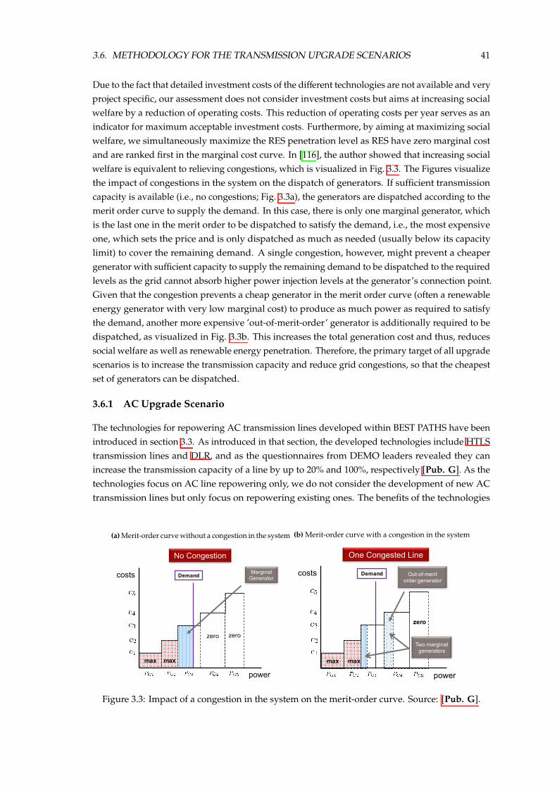
3.6. METHODOLOGY FOR THE TRANSMISSION UPGRADE SCENARIOS 41
Due to the fact that detailed investment costs of the di↵erent technologies are not available and veryproject specific, our assessment does not consider investment costs but aims at increasing socialwelfare by a reduction of operating costs. This reduction of operating costs per year serves as anindicator for maximum acceptable investment costs. Furthermore, by aiming at maximizing socialwelfare, we simultaneously maximize the RES penetration level as RES have zero marginal costand are ranked first in the marginal cost curve. In [116], the author showed that increasing socialwelfare is equivalent to relieving congestions, which is visualized in Fig. 3.3. The Figures visualizethe impact of congestions in the system on the dispatch of generators. If su�cient transmissioncapacity is available (i.e., no congestions; Fig. 3.3a), the generators are dispatched according to themerit order curve to supply the demand. In this case, there is only one marginal generator, whichis the last one in the merit order to be dispatched to satisfy the demand, i.e., the most expensiveone, which sets the price and is only dispatched as much as needed (usually below its capacitylimit) to cover the remaining demand. A single congestion, however, might prevent a cheapergenerator with su�cient capacity to supply the remaining demand to be dispatched to the requiredlevels as the grid cannot absorb higher power injection levels at the generator’s connection point.Given that the congestion prevents a cheap generator in the merit order curve (often a renewableenergy generator with very low marginal cost) to produce as much power as required to satisfythe demand, another more expensive ’out-of-merit-order’ generator is additionally required to bedispatched, as visualized in Fig. 3.3b. This increases the total generation cost and thus, reducessocial welfare as well as renewable energy penetration. Therefore, the primary target of all upgradescenarios is to increase the transmission capacity and reduce grid congestions, so that the cheapestset of generators can be dispatched.
3.6.1 AC Upgrade Scenario
The technologies for repowering AC transmission lines developed within BEST PATHS have beenintroduced in section 3.3. As introduced in that section, the developed technologies include HTLStransmission lines and DLR, and as the questionnaires from DEMO leaders revealed they canincrease the transmission capacity of a line by up to 20% and 100%, respectively [Pub. G]. As thetechnologies focus on AC line repowering only, we do not consider the development of new ACtransmission lines but only focus on repowering existing ones. The benefits of the technologies
(a) Merit-order curve without a congestion in the system
costs
power
max max
zero zero
Marginal GeneratorDemand
No Congestion
(b) Merit-order curve with a congestion in the system
costs
power
max max
zero
Demand
One Congested Line
Two marginal generators
Out-of-merit order generator
Figure 3.3: Impact of a congestion in the system on the merit-order curve. Source: [Pub. G].

42 CHAPTER 3. DEVELOPMENT OF GRID EXPANSION SCENARIOS
developed within the Best Paths project focusing on repowering AC lines are also constrained bythe capabilities of the substations, which are the determining factor for the improvement potentialof existing lines.
The optimal bound along the AC upgrade axis, which the Best Paths technologies could facilitate,are determined by allowing the flow on all transmission lines (i.e., not including transformers)to exceed the capacity limit by 100% and evaluate the required capacity increase ex-post. Anyrequired increase below 20% could be facilitated by both HTLS and DLR, while HTLS is the onlyupgrade option for increases above 20%.
Additionally, we perform two theoretical analyses serving as a benchmark for the 2030 ACgrid development. Fist, we analyze the theoretical bounds of using Best Paths technologies forrepowering AC lines but having no limitations imposed by transformers and substations (i.e.,leaving them unconstrained in the optimization problem). Secondly, we assume no limitation byneither AC lines nor transformers and substations at all (i.e., only considering the limitation of theDC lines). These analyses help to put the results of the analysis of the Best Paths technologies intocontext and serve as a benchmark for the 2030 AC grid development.
3.6.2 DC Upgrade Scenario
The technologies focusing on DC technology developed within BEST PATHS have been introducedin section 3.3. As discussed in that section, we collected them all within the DC scalabilityassessment except the superconducting cables, because given the aim of the study, as well as thesize of the test network, a clear separation between the demonstrators becomes infeasible. Thesuperconducting cables are not considered in this study given the limited length of the cables andtheir area of application being dense populated areas, which are represented as single nodes in thehigh-resolution European transmission grid model [Pub. G].
Within the DC Scalability assessment the focus lies on expanding the current European electricitynetwork by building new HVDC interconnections enabling controllable high power flows overlong distances with comparably low losses. Thus, besides o↵ering additional transmission capacityto relieve congestions, HVDC interconnections increase the controlability of the system enablingto route power directly from one specific node to the other allowing to circumvent congestionsin the vicinity of the low-cost marginal generator. Furthermore, HVDC interconnections allow ahigher integration of o↵shore wind energy, due to the fact that many locations located far awayfrom shore are only accessible by HVDC technology. Finally, additional transmission capacitywith controllable flows will enhance the trading capacity between the di↵erent countries which isexpected to result in significant cost reductions. However, due to the significant investment costfor new HVDC interconnections, every new line should carefully be planned in order to resultin a high utilization of the new asset and in an operating cost reduction which will make theinvestment feasible. Thus, even without taking all non-technical issues as e.g. social acceptance ofnew lines into account, the transmission expansion planing, or specifically in this case the problemof choosing the right location for new HVDC interconnections is not trivial considering the size ofthe European transmission network.
In [116], the author showed that increasing social welfare is synonymous to the relief of existingcongestions considering only energy costs. The author relate the number of congestions in anetwork to the number of marginal generators, i.e. generators which are dispatched neither at their

3.6. METHODOLOGY FOR THE TRANSMISSION UPGRADE SCENARIOS 43
minimum nor at the maximum limit. They prove that in any system an additional line connectinga low-cost marginal generator, i.e with a cost equal or lower than the system marginal cost, with ahigh-cost marginal generator, i.e. with a cost higher than the system marginal cost, will relieve atleast one congested line and enable the low-cost marginal generator to substitute the high-costmarginal generator and by that increase social welfare. Based on this observation the authorsdeveloped a methodology for HVDC placement for maximizing social welfare which is based onadding a line with the objective of setting the dispatch of the out-of-merit order generator to zero.
Following this approach, we adapt it to our system under investigation. We analyze a high-resolution European transmission grid model with varying production and demand over a timeframe of a whole year. Therefore, we observe varying congestions and marginal generators overthe year. We determine for every generator the number of hours (hmarg,i) it is neither producing atits minimum nor at its maximum limit. Within these hours, we determine the amount of energy itcould potentially produce additionally (in case of low-cost marginal generator) and the amount ofenergy we potentially need to substitute respectively (in case of a high-cost marginal generator).Finally, by combining these two features, i.e. the number of hours and the amount of energy ofthe marginal generator, we create two parameters elow≠cost,i and ehigh≠cost,i. These parametersdetermine the potential value for every generator i to be interconnected with an marginal-generatorof the opposite type (low-cost / high-cost). These parameters basically weight the amount of energyavailable / needed at the specific node with the proportion of time in which this energy is available/ needed. Hence, the factors are higher if the same amount of energy is available over many hourswithin a year compared to the case in which this energy is only available within a few hours ayear. Thus, these parameters serve as a good indicator for the potential utilization of a HVDC lineinterconnecting marginal generators:
hmarg,i = {h = 1, . . . , 8760 ’ P mini (h) < Pi(h) < P max
i (h)} (3.8)
elow≠cost,i =|hmarg,i|
8760·
|hmarg,i|ÿ
h=1(P max
i (hmarg,i(h)) ≠ Pi(hmarg,i(h))) (3.9)
ehigh≠cost,i =|hmarg,i|
8760·
|hmarg,i|ÿ
h=1
!Pi(hmarg,i(h)) ≠ P min
i (hmarg,i(h))"
(3.10)
As a result, parameter elow≠cost,i Ø ‘1 and ehigh≠cost,i Ø ‘2 justify the significant investment ofbuilding a new HVDC inter-connection between these marginal generators. After ranking themarginal generators according to elow≠cost and ehigh≠cost, we determine heuristically the topranked marginal generators to be interconnected based on the distance between them. Given thepotential large distances between low-cost and high-cost marginal generators, an inter-connectionof a low-cost and a high-cost marginal generator may be performed by inter-connecting anotherhigh-/low-cost marginal generator in between.
Thus, for example, in case we determine a low-cost marginal generator with a high elow≠cost,i
value in the North Sea. That means, this generator could produce significant more energy butis often curtailed. Further, we determine two high-cost marginal generators with comparablyhigh ehigh≠cost,i values, one in the North of Germany and one in the South of Germany. Thus,these generators are often dispatched with less than their maximum capacity (but above theirminimum capacity). Then, it is feasible to inter-connect the low-cost marginal generator with thehigh-cost marginal generator in the North because the currently curtailed energy of the low-costmarginal generator will substitute the energy produced by the more expensive high-cost marginal

44 CHAPTER 3. DEVELOPMENT OF GRID EXPANSION SCENARIOS
generator. Moreover, depending on the values of the parameters, it may be feasible to inter-connectthe high-cost marginal generator in the North with the high-cost marginal generator in the Southbecause (i) the available energy of the low-cost marginal generator may exceed the energy requiredto substitute the energy produced by the high-cost generator in the North allowing to transmitthe exceeding energy towards the South. (ii) The two high-cost marginal generators might bemarginal in di↵erent hours, i.e. in some hours the low-cost marginal generator could substitute thehigh-cost marginal generator in the North while in other hours the one in the South. (iii) In caseof potential cost di↵erences, the cheaper high-cost marginal generators can substitute the moreexpensive high-cost generator within hours in which the low-cost generator is not marginal.
The DC scalability assessment is performed step-wise in order to be able to react to changedpower-flows due to the added transmission capacity.
3.6.3 Combined Upgrade Scenario
The combined upgrade scenario is based on the DC upgrade scenario and examines potential im-provements for each stage of DC grid development by also upgrading the underlying AC grid.Similarly to the AC scalability assessment, we first evaluate the benefits of deploying the Best Pathstechnologies for AC line repowering at each step performed during the DC scalability analysis.We then look at the additional benefits to be gained when neglecting transformer limitations andin a third step, when neglecting the AC grid limitations as a whole. This allows us to assess theimpact of the added DC lines on the AC grid and the interactions between the two transmissionupgrade/expansion approaches.
3.7 Case Study - The European Transmission System
We perform the scalability assessment of the Best Paths technologies on a network model represent-ing the European transmission system in 2030. It includes impending transmission projects fromthe TYNDP 2016 to be commissioned before 2030 as well as projections for load and generationbased on the EUCO30 scenario. The AC grid of the network model consists of 7474 buses, 8787transmission lines, 1148 transformers, 1269 generators and 3361 loads. The DC system consistsof 72 point-to-point DC lines with 144 converters stations and 144 DC buses. There is no load orgeneration connected to the DC system. The generators are grouped in the following six categorieswith the number of generators belonging to the corresponding category indicated in parentheses:conventional (765), run-of-the-river hydro power plants and hydro reservoirs (87), pumped hydrostorage power plants (84), solar power plants (42), o↵shore wind generators (43) and onshore windgenerators (248). The data for (net) demand, renewable energy production on the distributionlevel (which is accounted for in the net demand) and maximum achievable RES penetration levelare listed in Table 3.1. The maximum RES penetration level is calculated based on the renewableenergy available from hydro, solar and wind generators and already accounts for the time periodsduring which renewable energy availability exceeds the demand and needs to be spilled in orderto maintain power balance across the entire network. The DC-OPF simulations are carried out onan hourly basis for a whole year (i.e., 8760 hours). Generator cost functions are assumed to be
Table 3.1: Characteristics of European transmission network 2030. Source: [Pub. G].
Net demand RES production in distribution Demand Max. RES penetration(TWh) (TWh) (TWh) (%)2733.10 786.60 3519.70 56.47

3.7. CASE STUDY - THE EUROPEAN TRANSMISSION SYSTEM 45
linear. Load shedding is penalized with 300 e/MWh, which is higher than the maximum cost ofgeneration (162.79 e/MWh) and thus, incentivizes to supply the load rather than to disconnect it.Note that the cost of LS is usually assumed much higher but in this case needs to be appropriatelyscaled as high values out of scale with the rest of the cost parameters might raise numerical issues.
3.7.1 Performance Indicators of the Scalability Assessment
The primary target of the scalability assessment is to increase the transmission capacity and reducegrid congestions, which in the context of this case study is equivalent to increasing social welfareand RES penetration levels. To this end, we use the key performance indicators (KPIs) definedin WP2 of the Best Paths project and listed in Table 3.2 for evaluating the results of the di↵erentupgrade scenarios.
3.7.2 Evaluation of the Business-as-Usual 2030 Scenario
The main results of the BaU2030 without any grid reinforcements are visualized in Figs. 3.4 and3.5. Fig. 3.4 shows the annual dispatch of the di↵erent generation categories and the amount ofload shedding. 22.35% of the demand is covered by distributed generation on lower voltage levels,while the remainder is covered by generators on the transmission level. The RES penetrationlevel reaches 52.84% and exceeds the penetration level of 50%, which has been projected by theEUCO30 scenario, mainly due to di↵erent modeling approaches. The EUCO30 projections havebeen evaluated using a high-level energy modeling approach based on a mixed complementarityproblem, which simultaneously accounts for several di↵erent energy objectives (such as energye�ciency targets etc.) and does not account for a high-resolution transmission grid model.Additionally, our assumption on the share of renewable energy generation in the transmissionand distribution systems might be another source causing discrepancies. 0.94% of the total load isshed due to grid congestions. Specifically, most of the LS occurs in Sweden, Norway and Finland(67.78%), where a simplified grid representation developed within the eHighway 2050 project isused and which consists primarily of DC lines, which exhibit a high congestion level due to large
Table 3.2: Performance indicators of the scalability assessment. Source: [Pub. G].
RES Penetration (%)Share of total load supplied by renewable energy sources:q
gœGRES EgqnœN
EDn
RES Curtailment (%)Share of available renewable energy not dispatched due to congestions:q
gœGRES Emax
g≠Egq
gœGRES Emaxg
Load Shedding (LS) (%)Share of energy demand not supplied due to congestions:q
nœNEshed
nqnœN
EDn
Generation Cost (e)Annual generation cost:q
gœG cg · Eg
Objective Function Value (e)Annual cost of generation and load shedding:q
gœG cg · Eg +q
nœN cshed · Eshedn
Eg Annual energy produced by generator g (MWh). Emax
gAnnual available energy of generator g (MWh).
Eshed
nAnnual energy demand not supplied at node n (MWh). ED
nAnnual energy demand at node n (MWh).
G(RES) Set of (renewable) generators. N Set of nodes.cg Marginal cost of generator g (e/MWh). cshed Cost of load shedding (e/MWh).

46 CHAPTER 3. DEVELOPMENT OF GRID EXPANSION SCENARIOS
exports of hydro and other renewable power to continental Europe. Most of the remaining LSoccurs in France (30.66%) due to AC grid congestions and particularly transformer congestions.
Fig. 3.5 depicts the dispatched renewable energy with respect to the available energy for eachrenewable generation category. The bottom subplot contains all sources of hydro power. Asexpected, solar power has a peak during the summer months whereas both o↵shore and onshorewind power are largely available during the winter months. Hydro power has a fairly constantgeneration profile due to our modeling assumptions of run-of-the-river power plants and hydroreservoirs described in section 3.5. Pumped hydro storages do not have a significant impact onthe hydro generation profile due to relatively low installed capacities supplying only 1.89% of thetotal load. The dark areas represent renewable energy curtailment, which amounts to 138.31 TWhor 12.10% of the total renewable energy available. It can be seen that there is still potential forincreased levels of RES penetration if the available renewable energy could be transported awayfrom where it is generated. Specifically, o↵shore wind farms and solar generators curtail 36.39%
and 15% of their available energy, respectively, which largely accounts for the gap between thecurrent RES penetration level and the maximum achievable of 56.47%. Table 3.3 lists the mainresults of the BaU2030 including the annual generation cost and the objective function value, whichadditionally to the generation cost also includes the cost of LS.
Figure 3.4: Load and generation 2030. Source: [Pub. G].
Table 3.3: Results of BaU 2030. Source: [Pub. G].
RES penetration RES curtailment LS Generation cost LS cost Obj. fct. value(%) (%) (%) (Be/a) (Be/a) (Be/a)
52.84 12.10 0.94 50.08 7.86 57.94

3.7. CASE STUDY - THE EUROPEAN TRANSMISSION SYSTEM 47
Figure 3.5: Available vs. dispatched power of the di↵erent RES. The dark areas represent RESspillage. Source: [Pub. G].
3.7.3 AC Upgrade Scenario
Grid congestions are the main cause for not being able to fully dispatch all renewable powerwhich is available. Within the AC scalability assessment we evaluate how Best Paths technologiesfor AC reinforcements could contribute to releasing congestions and thus, increasing both theRES penetration level and social welfare. Table 3.4 lists the main results, where BP reinforcementsdenotes the results considering transmission upgrades using Best Paths technologies for AC linerepowering only. BP reinforcements w/o transformer limits denotes the case using BP reinforcementsbut neglecting substation and transformer limitations which BP reinforcements do not upgrade. ACæ Œ represents the outermost bound on the AC upgrade axis without any AC grid limitations at all.
Load shedding remains unchanged in the BP reinforcements case as the increased levels of loadshedding in France are due to transformer congestions, while the load shedding in Scandinavia iscaused by congestions on DC lines, which remain largely una↵ected by AC grid reinforcements.This becomes apparent in the BP reinforcements w/o transformer limits scenario, where load sheddingin France is completely avoided and only remains in Scandinavia.
Fig. 3.6 shows the change in RES curtailment for each RES generation category individually. Solar,onshore wind and hydro power curtailment is decreased to a greater degree than o↵shore wind,which indicates that AC grid reinforcements alone cannot accommodate the available o↵shoreenergy and benefit mostly the dispatch of continental generation distributed throughout the ACgrid.
An increase in RES penetration level of 0.19 % can be achieved under the BP reinforcements scenario,while additionally 0.13 % can be added to that under the assumption of su�cient capacity in thesubstations. Note that transformer upgrades without any additional AC line repowerings cause anincrease in RES penetration of 0.15 % showing that transformer upgrades are not as e↵ective as theBP reinforcements, which alone achieve 0.19 %. However, in combination the e↵ect of both upgrademeasures are reinforced resulting in an increase of 0.5% to 53.34 %. The RES penetration level

48 CHAPTER 3. DEVELOPMENT OF GRID EXPANSION SCENARIOS
Table 3.4: Results of AC Scalability. Source: [Pub. G].
RES RES Load Gen. LS Obj. fct.pen. curtail. shedding cost cost value(%) (%) (%) (Be/a) (Be/a) (Be/a)
BP reinforcements 53.03 11.56 0.94 49.77 7.67 57.44BP reinforcements w/otransformer limits 53.34 10.82 0.63 48.70 5.19 53.89AC æ Œ 54.00 8.58 0.63 47.10 5.27 52.37
increases as expected through added transmission capacity but cannot exceed 54 % through ACgrid reinforcements only and thus, cannot reach the maximum possible penetration level. This andthe fact that most of the RES curtailment occurs o↵shore highlights the need for new transmissioncorridors, which will transport the power produced from remote o↵shore locations to consumptioncenters. Nonetheless, the BP reinforcements case results in annual generation cost savings of 310 Meat a required total transmission capacity increase of 11.83 GW distributed among 21 AC lines. Therequired increase corresponds to only 0.03 % of the current installed AC transmission capacity.
Figure 3.6: Renewable energy curtailment for each renewable generation category. Source: [Pub.G].

3.7. CASE STUDY - THE EUROPEAN TRANSMISSION SYSTEM 49
3.7.4 DC Upgrade Scenario
The DC upgrade scenario is developed in a step-wise approach allowing to account for the changein power flows due to the added transmission capacity. The development is stopped as soon aselow≠cost Æ ‘, which indicates that the highest ranked low-cost marginal generator does not o↵erenough spillage throughout the year to justify the significant investment costs of an additionalDC line. The following subsections will present the step-wise placement of the DC lines, whilethe main findings of all steps will be summarized in the last subsection as well as in Section 3.7.5,where we discuss the results of the combined upgrade scenario.
All lines are considered to be built as bipole with a total transmission capacity of 3 GW, which hasbeen identified as upper bound for HVDC interconections in Europe by the BestPaths partners.Based on the load duration curves obtained from the simulations the sizing of the lines canpotentially be improved afterwards.
Step 1
The first step of the DC scalability assessment uses the BaU 2030 scenario as base case to determinethe marginal generators (listed in Tab. 3.5 and Tab. 3.6). This list include the parameters hmarg,i.e. the number of hours the generators are marginal, and elow≠cost and ehigh≠cost, respectively, i.e.the parameters serving as a good indicator for the potential utilization of a HVDC line connectedto that node as introduced in Section 3.6.2. The added HVDC interconnections are visualizedin Fig. 3.7 (note that the connection points shown on the map is a rough approximation of theactual locations). The analysis of the BaU 2030 scenario already showed that the highest spillageof energy over the year can be observed at the o↵shore wind farms which is reflected by thetop ranked low-cost marginal generators. The high-cost marginal generators on the other handare located mainly in the UK / Scandinavia and Eastern Europe, i.e. far away from the low-costmarginal generators. Given the large distance between the o↵shore wind farms in the North seaand the high-cost marginal generators, two lower ranked low-cost marginal generators (’84NO’,’DK916183’) are taken as intermediate points allowing to transfer the generated power from theNorth sea to Sweden and Eastern Europe.
All added dc lines combined transfer 260.26 TWh over the whole year which corresponds to anaverage utilization of 71 %. This indicates a high usage of the assets and an increased tradingbetween the countries. The load duration curve of every added DC line is shown in Fig. 3.8. Mostof the new assets are used throughout the entire year at a high rate achieving average rates of Pdc Ø
Table 3.5: List of top ranked low-cost marginal generators in step 1. Source: [Pub. G].
Name Bus ID hmarg [h] Energy spillage [TWh] elow≠cost
’ES916537’ 2169 2627 21.79 6.53’o↵shore2’ 7465 6662 7.37 5.61’o↵shore3’ 7469 7008 5.72 4.58’o↵shore22’ 7466 6333 5.52 3.99’o↵shore14’ 7460 6681 4.84 3.69’o↵shore8’ 7474 6620 4.42 3.36’o↵shore5’ 7471 6671 4.05 3.13’o↵shore4’ 7470 6563 4.04 3.03’84NO’ 30 1999 0.28 0.06’DK916183’ 2046 619 0.48 0.034

50 CHAPTER 3. DEVELOPMENT OF GRID EXPANSION SCENARIOS
Table 3.6: List of top ranked high-cost marginal generators in step 1. Source: [Pub. G].
Name Bus ID hmarg [h] Energy production ehigh≠cost
of marg. gen. in hmarg
exceeding Pmin [TWh]’AC_95uk’ 78 4218 3.98 1.92’AC_92uk’ 67 1916 8.03 1.76’PL925636’ 6664 3832 3.33 1.45’AC_94uk’ 77 2066 5.39 1.27’AC_96IE’ 81 3336 3.10 1.18’BG911342’ 389 8712 0.86 0.86’74FI’ 1 8195 0.74 0.70’88SE’ 47 6542 0.91 0.68’CZ912108’ 652 1679 2.92 0.56’ES917371’ 2769 2310 1.22 0.32
60 % of the line rating. Only two lines (’88SE’-’74FI’ / ’o↵shore3’-’AC_95uk’) indicate a comparablelow usage with average usage rates of Pdc ¥ 40 % of the line rating. In these cases a lower linerating might be feasible considering potential cost reductions.
Figure 3.7: Step 1 of the DC upgrade scenario. Source: [Pub. G].

3.7. CASE STUDY - THE EUROPEAN TRANSMISSION SYSTEM 51
0 1000 2000 3000 4000 5000 6000 7000 8000 9000
Hours
offshore2-AC_95uk
offshore3-AC_95uk
offshore22-AC_92uk
offshore14-AC_92uk
offshore8-AC_94uk
offshore5-DK916183
offshore4-84NO
ES916537-ES917371
84NO-88SE
88SE-74FI
DK916183-PL925636
PL925636-CZ912108
CZ912108-BG911342
AC_96IE-AC_95uk>90%
80%-90%
70%-80%
60%-70%
50%-60%
40%-50%
30%-40%
20%-30%
10%-20%
<10%
Figure 3.8: Load duration curve of DC lines added during step 1 of the DC scalability assessment.Source: [Pub. G].
Step 2
The second step of the DC scalability assessment uses the simulation results of step 1 as basecase to determine the marginal generators (listed in Tab. 3.7 and Tab. 3.8). The added HVDCinterconnections are visualized in Fig. 3.9 (note that the connection points shown on the mapis a rough approximation of the actual locations). The top ranked low-cost marginal generatorsstill reflect the high spillage of energy at the o↵shore wind farms observed in the BaU 2030scenario. However, it is worth emphasizing that the spillage at the marginal generators of stage1 is significantly reduced and other o↵shore nodes are identified as marginal generators (withlower elow≠cost values). The majority of the high-cost marginal generators on the other hand arelocated in Eastern Europe, i.e. far away from the low-cost marginal generators. Given the largedistance between the o↵shore wind farms in the North sea and the high-cost marginal generatorsin Eastern Europe, the node ’PL925636’, in the previous step identified as high-cost marginalgenerator, serves as interconnection point between Denmark (’DK916155’) and the Czech Republic(’CZ912108’/’CZ911895’). All added dc lines (step 1 & 2) combined transfer 530.6 TWh over thewhole year which corresponds to an average utilization of 70 %. This indicates a high usage of theassets and an increased trading between the countries. The load duration curve of every added DCline is shown in Fig. 3.10. Note that the addition of ’o↵shore6’-’AC_92uk’ reduced the usage of thepreviously installed line ’o↵shore14’-’AC_92uk’. Thus, the installed capacity of those lines may beoptimized with respect to asset usage rate but this is out of the scope of this analysis. Furthermore,note that the low usage rate of the line ’o↵shore10’-’DK916155’ is not indicating its redundancy
Table 3.7: List of top ranked low-cost marginal generators in step 2. Source: [Pub. G].
Name Bus ID hmarg Energy spillage elow≠cost
’ES916537’ 2169 2575 20.35 5.74’o↵shore1’ 7457 6574 4.04 3.03’O↵shore11’ 6476 6500 3.73 2.77’o↵shore10’ 7458 6586 3.45 2.59’o↵shore6’ 7472 6669 3.40 2.59’o↵shore12’ 7459 6518 3.43 2.55’o↵shore7’ 7473 6682 3.55 2.71’o↵shore18’ 7464 6437 3.49 2.57’o↵shore17’ 7463 6493 3.32 2.46

52 CHAPTER 3. DEVELOPMENT OF GRID EXPANSION SCENARIOS
Table 3.8: List of top ranked high-cost marginal generators in step 2. Source: [Pub. G].
Name Bus ID hmarg [h] Energy production ehigh≠cost
of marg. gen. in hmarg
exceeding Pmin [TWh]’BG911091’ 373 6103 0.8913 0.6210’CZ912108’ 652 7371 0.7311 0.6152’ES917371’ 2769 1809 2.8493 0.5884’AC_92uk’ 67 1107 4.3101 0.5447’DK916155’ 2040 7713 0.2642 0.2326’HU922598’ 5.533 6374 0.3149 0.2291’CZ911895’ 596 4903 0.3129 0.1752’HU922547’ 5504 8601 0.1738 0.1706’PT925931’ 6794 8097 0.1817 0.1680’DK916424’ 2114 8290 0.1247 0.118
but it is due to insu�cient transmission capacity away from ’DK916155’ / ’PL925636’ / ’CZ912108’as indicated by the high usage of the corresponding lines and the following development steps ofthe dc upgrade scenario.
Figure 3.9: Step 2 of the DC upgrade scenario. Lines added in step 1 are marked in black, whilelines added in step 2 are marked in blue. Source: [Pub. G].

3.7. CASE STUDY - THE EUROPEAN TRANSMISSION SYSTEM 53
0 1000 2000 3000 4000 5000 6000 7000 8000 9000
Hours
offshore2-AC_95ukoffshore3-AC_95uk
offshore22-AC_92ukoffshore14-AC_92uk
offshore8-AC_94uk
offshore5-DK916183offshore4-84NO
ES916537-ES91737184NO-88SE
88SE-74FIDK916183-PL925636PL925636-CZ912108
CZ912108-BG911342AC_96IE-AC_95uk
ES916537-ES917371offshore1-DK916155Offshore11-AC_92uk
offshore10-DK916155offshore6-AC_92uk
ES916537-PT925931DK916155-PL925636offshore12-DK916155PL925636-CZ912108offshore7-DK916155
offshore18-DK916424offshore17-DK916424DK916424-PL925636PL925636-CZ911895
CZ911895-HU922598>90%
80%-90%
70%-80%
60%-70%
50%-60%
40%-50%
30%-40%
20%-30%
10%-20%
<10%
Figure 3.10: Load duration curve of DC lines added during step 1 and 2 of the DC scalabilityassessment. Source: [Pub. G].
Step 3
The third step of the DC scalability assessment uses the simulation results of step 2 as basecase to determine the marginal generators (listed in Tab. 3.9 and Tab. 3.10). The added HVDCinterconnections are visualized in Fig. 3.11 (note that the connection points shown on the map is arough approximation of the actual locations). The top ranked low-cost marginal generators stillreflect the high spillage of energy at the o↵shore wind farms observed in the BaU 2030 scenario.However, it is worth emphasizing that the spillage at the marginal generators of stage 1 & 2 issignificantly reduced and other o↵shore nodes are identified as marginal generators (with lowerelow≠cost values). Furthermore, note that the spillage at the spanish generator (’ES916537’) wassignificantly reduced from 21 TWh (BaU) to 16.8 TWh (step 2) (also indicated by high usage ofthe installed lines) but will be reduced further by adding additional transmission capacity. Thehigh-cost marginal generators on the other hand are located in Eastern Europe and South WesternEurope.
Given the large distance between the o↵shore wind farms in the North sea and the high-costmarginal generators in Eastern Europe the node ’DK916183’ previously identified as marginalgenerator node serves as interconnection point between the North sea and Eastern Europe. Alladded dc lines (step 1-3) combined transfer 938.3 TWh over the whole year which corresponds to
Table 3.9: List of top ranked low-cost marginal generators in step 3. Source: [Pub. G].
Name Bus ID hmarg Energy spillage elow≠cost
’ES916537’ 2169 2302 16.84 4.42’o↵shore15’ 7461 6654 2.972 2.26’O↵shore9’ 6478 6007 3.28 2.25’o↵shore16’ 7462 6674 2.90 2.21’O↵shore13’ 6477 6648 2.91 2.21’AC_96IE’ 81 830 0.7932 0.08’PT925871’ 6776 1119 0.52 0.066

54 CHAPTER 3. DEVELOPMENT OF GRID EXPANSION SCENARIOS
Table 3.10: List of top ranked high-cost marginal generators in step 3. Source: [Pub. G]
Name Bus ID hmarg [h] Energy production ehigh≠costof marg. gen. in hmargexceeding Pmin [TWh]
’BG911091’ 373 6834 0.66 0.51’ES917371’ 2769 1482 2.75 0.46’BG911342’ 389 8739 0.32 0.32’CZ912108’ 652 7712 0.34 0.30’AC_92uk’ 67 732 2.70 0.23’CZ912114’ 655 3061 0.46 0.16’PT925931’ 6794 8229 0.15 0.14’SK928311’ 7173 7260 0.15 0.12’ES916669’ 2266 6572 0.15 0.12’PL925276’ 6506 6197 0.16 0.11
an average utilization of 76.1 %. This indicates a high usage of the assets and an increased tradingbetween the countries. The load duration curve of every added DC line is shown in Fig. 3.12. Notethat the usage of ’o↵shore10’-’DK916155’ increased significantly due to the added transmissioncapacity.
Figure 3.11: Step 3 of the DC upgrade scenario.Lines added in step 1 and step 2 are marked inblack and blue respectively, while lines added in step 3 are marked in green. Source: [Pub. G].

3.7. CASE STUDY - THE EUROPEAN TRANSMISSION SYSTEM 55
0 1000 2000 3000 4000 5000 6000 7000 8000 9000
Hours
offshore2-AC_95ukoffshore3-AC_95uk
offshore22-AC_92ukoffshore14-AC_92uk
offshore8-AC_94ukoffshore5-DK916183
offshore4-84NOES916537-ES917371
84NO-88SE88SE-74FI
DK916183-PL925636PL925636-CZ912108
CZ912108-BG911342AC_96IE-AC_95uk
ES916537-ES917371offshore1-DK916155Offshore11-AC_92uk
offshore10-DK916155offshore6-AC_92uk
ES916537-PT925931DK916155-PL925636offshore12-DK916155PL925636-CZ912108offshore7-DK916155
offshore18-DK916424offshore17-DK916424DK916424-PL925636PL925636-CZ911895
CZ911895-HU922598ES916537-ES917371offshore15-AC_92uk
Offshore9-DK916183offshore16-DK916183Offshore13-DK916183
AC_96IE-AC_92ukPT925871-ES916669AC_92uk-offshore10
ES916537-PT925931ES917371-FR920572FR920662-ES916669
88SE-PL925276DK916183-PL925276
DK916183-88SEPL925276-CZ912108
CZ912108-BG911342PL925276-CZ912114
CZ912114-BG911091
>90%
80%-90%
70%-80%
60%-70%
50%-60%
40%-50%
30%-40%
20%-30%
10%-20%
<10%
Figure 3.12: Load duration curve of DC lines added during step 1-3 of the DC scalability assessment.Source: [Pub. G].
Step 4
The fourth step of the DC scalability assessment uses the simulation results of step 3 as basecase to determine the marginal generators (listed in Tab. 3.11 and Tab. 3.12). The added HVDCinterconnections are visualized in Fig. 3.13 (note that the connection points shown on the map is arough approximation of the actual locations). Note that the energy spillage is already significantlyreduced so that the last low-cost marginal generator listed in Tab. 3.11 only o↵ers 0.2 TWh incomparably few hours resulting in elow≠cost < ‘1 and is therefore not considered anymore.
All added dc lines (step 1-4) combined transfer 999.98 TWh over the whole year which correspondsto an average utilization of 76.22 %. This indicates a high usage of the assets and an increasedtrading between the countries. The load duration curve of every added DC line is shown in Fig.
Table 3.11: List of top ranked low-cost marginal generators in step 4. Source: [Pub. G].
Name Bus ID hmarg Energy spillage elow≠cost
’ES916537’ 2169 1622 8.790 1.627’FR920572’ 5139 928 1.815 0.192’FR918995’ 3775 823 0.195 0.018
Table 3.12: List of top ranked high-cost marginal generators in step 4. Source: [Pub. G].
Name Bus ID hmarg [h] Energy production ehigh≠cost
of marg. gen. in hmarg
exceeding Pmin [TWh]’ES917371’ 2769 1034 1.84 0.22’FR920662’ 5222 4485 0.24 0.12

56 CHAPTER 3. DEVELOPMENT OF GRID EXPANSION SCENARIOS
Figure 3.13: Step 4 of the DC upgrade scenario.Lines added in step 1 and step 2 are marked inblack and blue respectively, while lines added in step 3 are marked in green. Lines added in step 4are highlighted in orange. Source: [Pub. G].
3.14. Note that some lines connecting o↵shore nodes with the main grid (e.g. ’o↵shore3’-’AC_95uk’/ ’o↵shore8’-’AC_94uk’) show lower usage rates. The capacity for all connected lines of the specificnodes could be optimized, which is, however, out of the scope of this work.

3.7. CASE STUDY - THE EUROPEAN TRANSMISSION SYSTEM 57
0 1000 2000 3000 4000 5000 6000 7000 8000 9000
Hours
offshore2-AC_95ukoffshore3-AC_95uk
offshore22-AC_92ukoffshore14-AC_92uk
offshore8-AC_94ukoffshore5-DK916183
offshore4-84NOES916537-ES917371
84NO-88SE88SE-74FI
DK916183-PL925636PL925636-CZ912108
CZ912108-BG911342AC_96IE-AC_95uk
ES916537-ES917371offshore1-DK916155Offshore11-AC_92uk
offshore10-DK916155offshore6-AC_92uk
ES916537-PT925931DK916155-PL925636offshore12-DK916155PL925636-CZ912108offshore7-DK916155
offshore18-DK916424offshore17-DK916424DK916424-PL925636PL925636-CZ911895
CZ911895-HU922598ES916537-ES917371offshore15-AC_92uk
Offshore9-DK916183offshore16-DK916183Offshore13-DK916183
AC_96IE-AC_92ukPT925871-ES916669AC_92uk-offshore10
ES916537-PT925931ES917371-FR920572FR920662-ES916669
88SE-PL925276DK916183-PL925276
DK916183-88SEPL925276-CZ912108
CZ912108-BG911342PL925276-CZ912114
CZ912114-BG911091ES916537-ES917371FR920572-ES917371ES917371-FR920662
>90%
80%-90%
70%-80%
60%-70%
50%-60%
40%-50%
30%-40%
20%-30%
10%-20%
<10%
Figure 3.14: Load duration curve of DC lines added during step 1-4 of the DC scalability assessment.Source: [Pub. G].
Evaluation of the DC Upgrade Scenario
The previous subsections provided insights on which lines have been built and why,and visualized the utilization of the added lines. The following subsection discussesthe impact this grid development has on specific key performance indicators as therenewable energy penetration level, the curtailment of renewable energy sources, theenergy not served, and the operating costs.
The development of the RES penetration level is shown in Fig. 3.15 while the curtailment of each
BaU2030 DCScalability1 DCScalability2 DCScalability3 DCScalability4Penetration level 52.85 54.13 54.95 55.71 55.86Theoretical max 56.47 56.47 56.47 56.47 56.47
51
52
53
54
55
56
57
RESp
enetratio
nlevel[%]
Figure 3.15: Renewable energy penetration level for each step of DC upgrade. Source: [Pub. G].

58 CHAPTER 3. DEVELOPMENT OF GRID EXPANSION SCENARIOS
Figure 3.16: Renewable energy curtailment for each renewable generation category. Source: [Pub.G].
RES technology is shown in Fig. 3.16 with the BaU scenario as a base level. Fig. 3.15 shows thatthe RES penetration increases from 52.85 % up to 55.86 % in step 4 approaching the theoreticalmaximum of 56.47 % considering the theoretical maximum production of all RES sources. Asdiscussed in the previous subsections, most of the low-cost marginal generators are o↵shorewind farms located in the North sea region which is based on the fact that most spilled RESenergy is o↵shore wind energy as observed in the BaU scenario analysis. The e↵ect of establishinghigher transmission capacities from o↵shore locations to high-cost locations in Eastern Europeis well captured in Fig. 3.16 indicating the significant reduction of curtailment of o↵shore wind.Furthermore, Fig. 3.16 indicates the benefits of the added lines in South West Europe resulting inreductions of solar energy and onshore energy curtailment. Moreover, Fig. 3.16 indicates that,in particular in step 3, cheap o↵shore wind substitutes partially more expensive hydro powerplants. Note that during the selection of the high-cost marginal generators we neglected hydropower plants aiming to increase RES penetration. However, for every HVDC line connecting acheap marginal generator with an expensive marginal generator, the potential low-cost energyinjection at the expensive marginal generator node may exceed the energy required to completelysubstitute the expensive marginal generator. Therefore, the results show that the excess energymay additionally substitute hydro power plants located in the vicinity of the expensive marginalgenerator because hydro power plants have higher marginal costs. Although this reduces thegain in terms of RES penetration level, it still reduces the generation costs of the system, i.e. our
0.3
0.4
0.5
0.6
0.7
0.8
0.9
1
BaU2030 DCScalability1 DCScalability2 DCScalability3 DCScalability4
LoadShedding(%ofload)
Figure 3.17: Development of the load shedding for each step of DC upgrade. Source: [Pub. G].

3.7. CASE STUDY - THE EUROPEAN TRANSMISSION SYSTEM 59
BaU2030 DCScalability1 DCScalability2 DCScalability3 DCScalability4Annualgenerationcost 50.20 47.99 47.07 44.69 44.37
Objective functionvalue 57.94 53.95 53.02 47.99 47.64
40.0042.0044.0046.0048.0050.0052.0054.0056.0058.0060.00
Cost[B
€/a]
Figure 3.18: Development of generation costs for each step of DC upgrade. Source: [Pub. G].
objective function of the OPF.
Furthermore, a significant reduction of load shedding is achieved in particular due to the stepsbetween BaU - DC Scalability 1 and DC Scalability 2 - DC Scalability 3, as shown in Fig. 3.17. Thus,as it may have been expected, we show through our method that relieving congestions results in areduction of load shedding.
Although, a detailed cost-benefit analysis is out of the scope of this analysis, we briefly want todiscuss the potential generation cost reduction by a dc upgrade scenario. The generation costs ofthe European system as well as the objective function value for the di↵erent DC upgrade steps areshown in Fig. 3.18. A significant cost reduction can be achieved reducing the generation costsfrom 50.2 Be per year to 44.37 Be in step 4. This is a cost reduction of 11.61 %. The reduction ofload shedding is reflected by the objective function value curve approaching the generation costscurve. Considering a life-time of the required DC installations of approx. 30-40 years [117], the costsavings sum up to 233.2 Be (40 years) and considering the (not optimized) additionally installedHVDC capacity (150 GW) it resembles a break-even point for a potential investment decision of1.56 Be/ GW. However, considering a capacity optimization and a more realistic AC and DC griddevelopment, this factor can probably be further increased.
3.7.5 Combined Upgrade Scenario
Within the combined upgrade scenario we take a broader view on the AC and DC upgradepossibilities by combining the AC upgrades with each DC grid development stage. The mainresults of the AC, DC and combined upgrade scenarios are visualized and compared in Fig. 3.19 to3.20. Fig. 3.20 clearly shows that connecting more DC lines to the grid increases the congestionlevel of the AC grid as the grid tries to accommodate the increased injections from o↵shore windfarms. While DC lines do act as a congestion relief method [116] in some parts of the grid, theyalso increase the total amount of power flows in the underlying AC grid by allowing to supplypreviously disconnected load. We define the congestion level of the AC grid (CLAC ) based on thelines’ congestion duration T 100%
l throughout the year,
CLAC=
qlœLAC
T 100%l
8760|LAC | , (3.11)
where LAC represents the set of AC lines. Hence, the Best Paths technologies for repowering AClines can have a more profound impact in combination with a concurrent DC grid developmentand even more so with additional transformer upgrades than when deployed alone. The orange

60 CHAPTER 3. DEVELOPMENT OF GRID EXPANSION SCENARIOS
dot in the DC 4 grid development stage represents the highest grid development stage for the2030 network conditions developed within this case study, which can be facilitated by Best Pathstechnologies only. 56 AC lines europewide would require a total capacity increase of 63.62 GW,out of which 20 require an upgrade of less than 20 %. The RES penetration level is increased from52.85 % (BaU2030) to 56.06 % approaching the maximum possible level of 56.47 % as depicted inFig. 3.20. RES curtailment is significantly reduced from 12.10 % to 2.17 %, which can greatly a↵ectthe economics of renewable energy projects and increase the revenue of wind and solar energyprojects improving their competitiveness on the electricity market and possibly allowing for thediscontinuation of feed-in tari↵s and other subsidies. At the same time, the total cost (including thecost of load shedding) is reduced by 10.84 Be. Fig. 3.19 depicts the change in generation cost andthe change in objective function value (i.e., the cost of generation plus the cost of load shedding)for the di↵erent stages of grid development. Even though the objective function only considers afictitious value for load shedding, which at a value of 300 e/MW is still considered low, it is morerepresentative of the actual cost development and makes the di↵erent stages of grid development
Figure 3.19: Annual generation cost (excl. cost of load shedding) and annual cost including loadshedding for AC, DC and combined upgrade scenarios. Source: [Pub. G].

3.7. CASE STUDY - THE EUROPEAN TRANSMISSION SYSTEM 61
Figure 3.20: Congestion level of the AC grid, RES penetration and total RES spillage for AC, DCand combined upgrade scenarios. Source: [Pub. G].

62 CHAPTER 3. DEVELOPMENT OF GRID EXPANSION SCENARIOS
comparable to each other. This is due to the fact that unlike the generation costs, the objectivefunction value considers the same load level at each stage through either dispatched generationor load shedding. The generation cost, however, does not reflect the reduction in load sheddingfrom one stage to the next, which might lead to an increase in generation cost despite higher RESpenetration levels due to higher load levels that need to be supplied as becomes apparent throughthe increase in generation cost from DC 1 to DC 2. The objective function value still decreases,though. Load shedding is reduced by almost 60 % from 0.94 % to 0.39 % of the total load. Most ofthe remaining load shedding (i.e.,68.84 %) needs to be carried out in France, where the new DC lineconnections to Spain increase the stress on the already highly loaded transformers as discussed inSection 3.7.3. Nonetheless, load shedding is also reduced in France from 7.89 TWh to 7.33 TWh,which can be further improved with appropriate transformer upgrades.
3.8 Conclusion
We adapt the notion of optimality bounds from optimality theory, where relaxations (i.e., approxi-mations) can provide bounds on the optimal solution of NP-hard problems, to the context of thefuture European mixed AC/DC grid development. We consider the grid development for the ACand DC transmission technologies separately and evaluate their individual potential to relievecongestions, increase social welfare and contribute to a more renewable electricity supply. Thisapproach allows us to determine the bounds of the future European grid development as visualizedin Fig. 3.21. Our results show that congestions within the AC grid can be partially relieved usingtechnologies for repowering AC lines developed within the Best Paths project. However, wealso show that the positive impact of these Best Paths technologies is highly constrained by thetransformer limitations and that their benefits can be reinforced if they were deployed along withtransformer upgrades.
Given the RES development projections of the EUCO30 scenario, which considers a substantialincrease in o↵shore wind power capacity (11.7 GW in 2016 to 41 GW in 2030), a big share of theRES potential is not deployable without additional HVDC lines (or AC lines for o↵shore windfarms near shore). Therefore, the potential for improvements with AC reinforcements only isrelatively small given the mentioned EUCO30 assumptions. The benefits of the AC reinforcementsbecome more apparent when combining them with concurrent DC upgrades. In this way, thealready substantial increase in RES penetration level and reduction in cost achieved by placingnew HVDC transmission corridors can be further reinforced by relieving AC grid congestions in
Figure 3.21: Schematic illustration of how the scalability assessment provides the bounds of thefuture European grid development. Source: [Pub. G].

3.9. FUTURE WORK 63
the vicinity of the new injection points, which further reduces the annual cost by 4.2 Be (BestPathsAC reinforcements + transformer upgrades at DC Scalability step 4). 23.7 % of the total reductionin cost are related to the AC reinforcements. This also highlights that an optimal grid developmentwill consist of both AC reinforcements and new DC transmission assets. The study also emphasizesthe benefits of HVDC lines to reroute power flows from low-cost to high-cost marginal generatorsin a fully controllable way demonstrating their ability to substitute more expensive generators.Despite the fact that DC lines can reduce congestions in the underlying AC grid, additional ACreinforcements in the vicinity of their injection points are often required in case of increased powerinjections at that point. As a result, substituting larger expensive generators, which already inject asubstantial amount of power at their node, will require less AC reinforcements.
Thus, the following policy recommendation was developed:
New transmission lines based on HVDC technology are indispensable in the future Europeantransmission network, as they allow for highly flexible power transmission and the transport oflarge amounts of renewable energy from remote generation sites to load centers. At the sametime, reinforcements of the existing AC grid are necessary to accommodate increased injections ofHVDC lines. Thus, a coordinated upgrade of both AC and DC network is essential to achieve thefull potential of either technology.
3.9 Future Work
The future work in this area may include the improvement of the simplified system representingScandinavia and Great Britain. As the network model provided by ENTSO-E, did not include anydata for these systems, these models were taken from the e-HIGHWAYS 2050 project and consist ofvarious DC links.
Moreover, future work could focus on a more detailed representation of the pumped hydro storageplants and investigate the impact of potential upgrades of existing hydro plants to pumped hydrostorage plants, possibly while also considering other storage systems as e.g. power-to-gas.


CHAPTER4MT-HVDC Control Structures
Following our policy recommendation that new HVDC lines are indispensable in the future Europeantransmission system, this chapter deals with the challenges arising when such lines are potentiallyinterconnected to form a MT-HVDC grid. Due to the little experience with MT-HVDC grids, the control,operation and potential interaction of such a MT-HVDC grid with the connected AC grids are open researchquestions. Thus, this chapter investigates various dc voltage droop control structures in terms of stability,disturbance rejection and interaction with connected ac systems as well as multi-vendor interoperability. Amethodology is presented to determine the operating space of an arbitrary MT-HVDC system which is usedto compare the impact of the various dc voltage droop control structures on the power transfer capability.This chapter is structured as follows: First, the background of this chapter is discussed and a brief literaturereview is provided. Then, the contributions of this chapter are emphasized and the di↵erent dc voltage droopcontrol structures are classified in a simple framework, followed by a description of the work published in[Pub. A], [Pub. C], [Pub. D].
4.1 Background
So far most High-Voltage Direct Current (HVDC) systems have been built as Point-To-Point (PTP)connections. However, with the emergence of HVDC based on Voltage Source Converter (VSC)the development of Multi-Terminal High-Voltage Direct Current (MT-HVDC) is seen as a feasibleoption. A crucial aspect for the operation of such a large MT-HVDC is the operational reliability,since any malfunction could have a significant economic impact. In this perspective, it shouldbe avoided that the regulation of the dc voltage and the intertwined regulation of the powerflow between the terminals should rely on an approach where one single unit is assigned adominant role. Instead, a distributed control architecture where multiple units are activelyparticipating in the control of the dc voltage based on local measurements is preferable [75].Indeed, a decentralized architecture is inherently more robust against outages and more e↵ectivein case of power fluctuations that exceed the available control range of a single terminal [118].Several alternative strategies for distributed dc voltage control have been proposed in the technicalliterature. A common element in most of these control strategies is the presence of a dc voltagedroop mechanism [72, 76, 119, 120]. Despite that the general operating principle of dc droop isidentical for the di↵erent implementation schemes, the use of di↵erent control objectives anddi↵erent feedback signals can have significant impact on the dynamic performance and the stabilityproperties [75, 121]. Moreover, these di↵erences may also lead to di↵erent kind of interactionswith the connected ac grids which have already been observed for PTP-connections in di↵erentprojects (e.g. BorWin1 [122], INELFE [123]).
Furthermore, unlike in China, a MT-HVDC grid in Europe would most likely not be built at oncebut be developed by a step-wise integration of already existing on- and o↵shore interconnectors [51].This, however, would raise the question of the interoperability of HVDC systems from di↵erentvendors.
65

66 CHAPTER 4. MT-HVDC CONTROL STRUCTURES
4.2 Literature Review
Over the last decades, large projects and many publications have addressed the control of aMT-HVDC grid, its impact on the stability and the system interactions as well as potentialinteroperability issues.
The European HVDC Grid Study Group including Transmission System Operators (TSOs) aswell as vendors of HVDC technology was founded in 2010 to develop “Technical Guidelines forfirst HVDC Grids” including proposals to start standardization work [51]. Among other thingsthey concluded the necessity to study potential interactions between di↵erent converters andrecommended to apply vendor-specific parameter and control concepts to study the stability ofMT-HVDC systems [51]. They also stated that standardization of HVDC equipment as well ascontrol concepts and communication could enhance the development of MT-HVDC grids [51]. TheEuropean HVDC Grid Study Group identified dc voltage droop control and droop control withdeadband as suitable control concepts for MT-HVDC [51]. The applicability of droop control andits preference by vendors of HVDC technology is also proven by its use in the Nanao MT-HVDCgrid [26].
In technical literature several alternative droop control schemes have been proposed [55, 64–68, 70,72, 76, 119, 120, 124]. These dc droop implementations, however, are usually analyzed separatelyor by comparing only a few selected cases. In [125] for example, Vrana compares the generalprinciples and relation of power and current based droop schemes but does not consider droopcontrol methods using ac current or active power measured on the ac side. Haileselassie on theother hand di↵erentiates in [79] between active power measured on the ac and the dc side but doesnot consider any current based droop control methods. In 2018, 1-2 years after our studies, theauthors of [121] published a comparative study of five di↵erent droop control structures analyzingtheir impact on the relative stability, performance and robustness of the overall MT-HVDC system.Similar to our work they perform an eigenvalue analysis comparison, a multivariable frequencyresponse analysis of the di↵erent structures, and the impact of the cable modeling.
Similarly, interactions between converters or between converters and the connected ac grid havebeen studied, as e.g. by Beerten et al. in [92]. They investigate the influence of droop parameters(NB: not di↵erent kinds of droop control structures) and dc breaker inductors on the systeminteractions. In [126], Endegnanew et al. investigate interactions between asynchronous ac gridsin a hybrid ac/dc power system for a specific power based droop scheme. In [9, 127, 128], di↵erentdamping schemes have been proposed to mitigate observed harmonic stability problems causedby interactions between the converters and resonances from the system [122, 123]. In each case,however, a specific droop control scheme is used without analyzing which influence other optionscould potentially have. The final report of the MEDOW1 project (2013-2017) highlights the noveltyof harmonic instability problems due to AC/HVDC (converter) interactions in the power systemcommunity and emphasizes the need for detailed studies [129].
As one of the first initiatives, the EU-project BEST PATHS2 (2014-2018) focuses among otherthings on the HVDC-VSC multi-vendor interoperability. The main objective was to investigateconditions allowing a maximum of interoperability and contribute with recommendations to
1MEDOW: “Multi-terminal DC Grid for O↵shore Wind”, www.medow.engineering.cf.ac.uk, funded by the EuropeanUnion
2BEST PATHS: “BEyond State-of-the-art Technologies for rePowering Ac corridors and multi-Terminal HVDC Systems”,www.bestpaths-project.eu, funded by the European Union

4.3. CONTRIBUTIONS 67
the standardization of interoperability requirements for multi-vendor MT-HVDC grids. Expertsinvolved in the projects conclude that "the existing technology delivered by the main HVDCvendors is not directly interoperable" [130] and see "interoperability [of di↵erent vendors] as oneof the greatest challenge" [130] in the development of MT-HVDC grids. In fact, Olivier Despouysfrom RTE2 involved in the BEST PATHS1 project stated in May 2018 [130] that the main problemof investigating and improving multi-vendor interoperability is related to testing the interactionof potentially protected intellectual property of di↵erent vendors as e.g. control algorithmsdetermining the behaviour of the converters.
The on-going e↵orts of the European Union funding recently two new projects on MT-HVDC(PROMOTioN3 (2016-2019), InnoDC4 (2017-2021)) and the conclusions from previous projectsemphasize the importance of more detailed studies of the di↵erent Control Structures (CSs) andtheir potential interactions with each other in order to ensure the stability of future MT-HVDC.Although two MT-HVDC grids have been commissioned in China [17, 26], Olivier Despouysfrom RTE expects significant more di�culties in a European competitive market context withmultiple vendors, due to the fact that in China “a specific manufacturer was in charge of the wholecontrol and protection for all converters delivered by other suppliers” [130]. He does, however, notanticipate “this kind of set-up [as] the expected way forward in western countries where HVDC isa competitive market.”
4.3 Contributions
Several alternative droop control concepts have been proposed in the literature. It is, however, abusiness secret how each vendor has exactly set up its control scheme and experts identified theinteroperability of potentially di↵erent control concepts as key challenges for future MT-HVDCgrids. Furthermore, these dc droop implementations are usually analyzed separately or bycomparing only a few selected cases. Therefore, this work addresses the analysis and comparisonof di↵erent control schemes systematically, using a simple classification framework we proposedin [75]. Furthermore, this work contributes with
• an in-depth comparison of the impact of the di↵erent CSs on small signal stability, disturbancerejection, the interaction level and multi-vendor interoperability (section 4.5-4.8),
• the uncovering that limits frequently used in literature for CS analysis and tuning (e.g. [9, 69])are not su�cient to maintain the impact of specific disturbances within a certain boundary(section 4.6),
• a methodology for stability analysis of di↵erent dc voltage droop CSs determining theoperation space of an arbitrary MT-HVDC grid (section 4.7).
2RTE: Réseau de transport d’électricité3PROMOTioN: “PROgress on Meshed HVDC O↵shore Transmission Networks”, www.promotion-o↵shore.net, funded
by the European Union4InnoDC: “Innovative tools for o↵shore wind and direct current (dc) grids”, www.innodc.org, funded by the European
Union

68 CHAPTER 4. MT-HVDC CONTROL STRUCTURES
4.4 Classification of dc Voltage Droop Control Structures
In general, a droop control scheme introduces a linear relationship between two electrical variables.In the specific case of dc voltage droop control for MT-HVDC, the dc voltage is used in eachimplementation, so that the droop gain, kdroop, defines the deviation of Vdc for a variation of theother electric variable:
Vdc = V údc + kdroop(yú ≠ y) (4.1)
yú and V údc are the set points and Vdc, y are the measured electric variables respectively. The second
electric variable, y, can either represent the dc current, Idc, one component of the ac current, Iac,the active power measured on the dc side, Pdc, or the active power measured on the ac side, Pac.They can be categorized by two di↵erent types of generalized structures, depending on whetherthe dc voltage is used within the first loop (Type2 (Vdc-y)) or the second loop (Type1 (y-Vdc)) asshown in Fig. 4.1. This leads to a total of 8 di↵erent dc voltage droop control structures, shown inFig. 2.12. We introduced this classification first in [75].
+-
i⇤q
Vdc
V ⇤dc
+y⇤
-PI
y
+1
kdroop
first loop second loopfirst loop second loop
PI-
-+
y
Vdc
V ⇤dcy⇤
++ i⇤q
kdroop
Type 1 Type 2
Figure 4.1: Generalized droop control structures. Source: [Pub. C].
4.5 DC Voltage Droop Control Structures and its Impact on the InteractionModes in Interconnected AC-HVDC Systems
As a first step of the assessment of the di↵erent dc voltage droop control structures, we investigatehow the usage of the di↵erent structures impacts the interaction modes between the di↵erentsub-systems. That means, we analyze how the choice of the control structure influences the levelof interaction between the di↵erent converters and between the ac and the dc subsystem sinceit is preferred to have those systems as decoupled as possible to minimize a potential spread ofdisturbances from one system into the other. This work has been published in [Pub. D]. In [92],the authors analyze interaction modes and their sensitivity to droop parameters and dc breakerinductances in a MT-HVDC system. However, there does not exist an analysis of the impact of thevarious CSs on the interaction modes between di↵erent subsystems. Thus, it remains unknownwhether the choice of a certain CS results in an unfeasible stronger coupling of subsystems, asfor instance the dc and the ac subsystems. In general, it is preferred to have those systems asdecoupled as possible to minimize a potential spread of disturbances from one system into theother.
The contributions of this work include the following: First, an analysis of the quantitative andqualitative coupling between the di↵erent subsystems will be provided for two di↵erent tunings

4.5. DC VOLTAGE DROOP CSS AND ITS IMPACT ON THE INTERACTION MODES 69
of the converters, i.e. whether a certain CS imposes a higher degree of coupling reflected by ahigher percentage of interaction modes and whether this also influences the damping ratio of theinteraction modes. In particular, we will focus on the coupling between the dc and the ac systemsand the coupling between the di↵erent HVDC converters. We will show how a faster responsetime impacts the coupling of the di↵erent subsystems. Further, we will discuss how a generalizedfeedback influences the coupling of those subsystems.
4.5.1 Methodology
In order to evaluate how the choice of the CS influences the coupling of the di↵erent subsystems,a methodology, initially proposed in [92] to identify and analyze interaction modes betweenconverters in a HVDC system, is adapted [Pub. D].
Given a general linearized model of a HVDC system, which is composed of various subsystems forevery connected converter terminal and every HVDC cable, and the definition of the normalizedparticipation factors �
nki, as given in section 2.7.4, we define a criterion to distinguish between local
modes and interaction modes.
Here, interaction modes are defined as modes where at least two subsystems participate. Hence,local modes, on the other hand, are defined as modes where only a single subsystem participates.The vector �n
–,i œ Rn– contains all normalized participation factors associated with mode i for all
states of the subsystem –.
The overall participation of each subsystem – in mode i is defined as [92]:
÷–,i =Î�n
–,iÎÎ�n
i Î (4.2)
with Î · Î denoting the L1-norm. Focusing on interaction between specific subsystems I– a set ofinteraction modes S– can be defined as:
S–
= {i | ÷–,i Ø Ÿ, ’ – œ I–} (4.3)
with S– ™ S, the set of all modes, and Ÿ resembling a threshold chosen equal to 5%, following the
example in [92].
Here, two subsets of interaction modes are of particular interest:
• the interaction modes of the subset Sac,dc= {i | (÷dc,i Ø Ÿ) · ((÷ac1,i Ø Ÿ) ‚ · · · ‚ (÷acN ,i Ø
Ÿ)), ’ dc, acj œ Iac,dc}. That means interaction modes with participation of at least one of
the connected ac systems and the dc system, since it is preferred to have those systems asdecoupled as possible to minimize a potential spread of disturbances from one system intothe other.
• the interaction modes of the subset Sgsc= {i | (÷gsc1,i Ø Ÿ) · (÷gsc2,i Ø Ÿ) · · · · · (÷gscN ,i Ø
Ÿ), ’ gscj œ Igsc}, i.e. interaction modes between all Grid Side Voltage Source Converters
(GSCs), indicating the degree of coupling within the dc grid.
These two subsets will be evaluated quantitatively, i.e. how many of all modes show this type ofcoupling, and qualitatively, i.e. where are the corresponding eigenvalues located, how critical arethey and which states participate in particular?

70 CHAPTER 4. MT-HVDC CONTROL STRUCTURES
=
~ ~Cdc Vdc,gsc,n
Vc,n
Il,n LfRf
Cf
Ig,nLgRg Vg,n
Vo,n
AC subsystemGSC subsystem
AC Voltage Controller
Current Controller
Droop Controller
Vdc,n
yn
�
V ⇤
dc,n
y⇤n
�+
Un
U⇤n
+�
Iq⇤c,n
Id⇤c,n
� PLL
DC subsystem
Ccs Ccs
Rdc,z1Ldc,z1
Ldc,z3
Ldc,z2Rdc,z2
Rdc,z3Gcs Gcs
Idc,jIdc,i
Vdc,wf
Vo,n,meas
Il,n,meas
Figure 4.2: Splitting of the di↵erent subsystems. Adapted from: [Pub. D].
4.5.2 Modeling particularities
For the analysis of this section a slightly di↵erent generic MT-HVDC model derived in [9] wasused. The detailed state representation of this model is presented in the following subsectionwhere the model is divided into di↵erent subsystems. The main di↵erences to the model describedin section 2.7.2 are (i) the modeling is done in absolute values not in per-unit (ii) the absence ofthe active damping controllers, (iii) the use of ac voltage controllers instead of reactive powercontrollers, (iv) the introduction of measurement delays and (v) the use of di↵erent Phase LockedLoops (PLLs) based on [9], where the angle deviation is computed as
�P LL =Kp,P LLs + Ki,P LL
s2 + Vo,q,0Kp,P LLs + Vo,q,0Ki,P LLVo,d. (4.4)
Note that in this model the q-axis, not the d-axis, voltage vector is aligned with the voltage vector,Vo.
4.5.3 Subsystem Definition
This model is derived for every of the eight di↵erent droop control structures as well as for a casewith a generalized feedback signal which is described in detail below. Each of these models consistsof a number of three di↵erent kind of subsystems, shown in Fig. 4.2. Due to space limitations, thevariables are shown in complex space vector notation, i.e. for example Vo = Vo,q + jVo,d.
The ac subsystems are modeled as Thévenin equivalents with an LC-filter interface to the GSCs.Thus, the states corresponding to the ac subsystems, Iacj , with j = 1, . . . , N , are the following:
xac,j =
ËIg,d,j , Ig,q,j , Vo,d,j , Vo,q,j , Il,d,j , Il,q,j ,
Vo,d,meas,j , Vo,q,meas,j , Il,q,meas,j , Pac,meas,j
ÈT. (4.5)
Variables Ig,d/q,j , Il,d/q,j represent the grid current and the line current flowing through theconverter. Vo,d/q,j represents the voltage at the point of common coupling (PCC) and Vo,d/q,meas,j
the delayed voltage measurement at the PCC. Further, Pac,meas,j and Il,q,meas,j represent thedelayed active power measurement at the PCC and the delayed measurement of q- component ofthe current flowing though the converter used in the control loops.
The dc grid subsystem includes all dc cables, modelled as ’frequency dependent’ fi model wherethe additional parallel RL branches are calculated to fit the frequency response of a wide-bandcable model [5, 14]. In general, in a dc grid, wind farm side converters (WFC) work as grid forming

4.5. DC VOLTAGE DROOP CSS AND ITS IMPACT ON THE INTERACTION MODES 71
converters for the connected ac grid without controlling Vdc. Hence, due to the focus on the GSCcontrol WFCs can be simplified to dc current sources representing an uncontrolled disturbance forthe dc grid [9]. Thus, the states corresponding to the dc subsystem, Idc, are:
xdc =
ËIdc,z(l), Idc,z(l+1), Idc,z(l+2), · · · , Idc,z(3M≠2), Idc,z(3M≠1), Idc,z(3M), Idc,meas,l, · · · ,
Idc,meas,M , Vdc,wf,k, · · · , Vdc,wf,K
ÈT(4.6)
with Idc,z(l) - Idc,z(l+2) representing the currents in the di↵erent branches of the l = 1, · · · , M
di↵erent dc cables. Further, Idc,meas,l represents the delayed dc current measurements at the GSCs,shown in Fig. 4.2 as Idc,i. The variable Vdc,wf,k denotes the dc voltage at the k = 1, . . . , K WindFarm Side Voltage Source Converters (WFCs).
The GSCs are assumed to be synchronized to the ac grids through a PLL and operated withconventional current controllers in the Synchronous Reference Frame (SRF). As cascade controlrequires the speed of response to increase towards the inner loop, the internal loop is designed toachieve a fast response [63]. Thus, the current controllers of the GSCs are tuned by the InternalModel Control (IMC) technique designed to track references with a settling time of 10 ms [131].Saturation limits are included in the control scheme, in order not to exceed the maximum currentratings of the converters.
Both GSCs are assumed to use dc voltage droop control. the di↵erent structures have beenintroduced in section 2.7.2 and visualized in Fig. 2.12. Further, to better control the power sharingbetween the converters after a converter outage, the use of a generalized feedback signal usingcommunication between the GSCs has been proposed [132] as an alternative to the eight CSs usinglocal measurements only. The idea here is, to use a multiple-input feedback controller using allmeasured voltages deviations as inputs at every terminal, as given in:
S
WWWWU
�Idc,1
�Idc,2
...�Idc,N
T
XXXXV=
S
WWWWU
g11 g12 · · · g1N
g21 g22 · · · g2N
......
. . ....
gN1 gN2 · · · gNN
T
XXXXV
S
WWWWU
�Vdc,1
�Vdc,2
...�Vdc,N
T
XXXXV. (4.7)
Thus, G represents a matrix of droop gains interconnecting the current and voltage measurementsat the di↵erent terminals. In case all entries of the matrix are zero except the entries on the maindiagonal, this approach corresponds to the case where each droop controlled terminal uses CS1(Vdc-Idc). Then, each entry on the diagonal corresponds to the inverse of the droop gains, 1
kdroop
andthere is no generalized feedback. Otherwise, all matrix entries are determined by an optimizationproblem considering the line resistances. Hence, the proposed generalized feedback controlleris similar to CS1 (Vdc-Idc) but di↵ers by the fact that the generalized feedback controller usesmeasurements of all GSCs and additional corresponding droop gains.
A comparable performance of power and current based droop control structures and the generalizedfeedback controller is ensured by the following:
• The droop gains were chosen as kdroop,p =1
25V
kW as suggested in [9].
• The droop gains used within the power and current based droop controller should becomparable. Thus, the relation derived in [125] is used to determine the current based droop

72 CHAPTER 4. MT-HVDC CONTROL STRUCTURES
gains, kdroop,idc, that are equivalent to the power based droop gains, kdroop,p:
kdroop,idc=
V údc,j
1kdroop,p
≠ Iúdc,j
. (4.8)
The current based droop gain used for the CSs combining Vdc,j and Iac,j needs to be scaledadditionally, due to the higher range of Iac,j . However, due to the non-linearity of powerbased droop control, the approximation holds only for a small deviation of the voltage:
kdroop,iac=
Iúdc,j
Iúc,q,j
· kdroop,idc. (4.9)
• For a comparable performance of the generalized feedback control g11 and g22 are chosen as1
kdroop,i≠k
droop,i
2, while g12 and g21 are chosen as 1
kdroop,i/2 .
• For all droop control structures, we analyze two di↵erent tunings. Each of these tunings,is comparable for all droop control structure enabling comparability between the di↵erentstructures. We analyze two di↵erent tunings for each structure to show the impact of thetuning on the coupling of the di↵erent subsystems. The fast tuning leads to a fast rise time ofapprox. 17 ms and a settling time of approx. 60 ms with an overshoot of approx. 5 %. Theslow tuning leads to an over-damped response without overshoot, a rise time of approx.23 ms and a settling time of approx. 40 ms.
Only the response of CS2(Vdc-Iac) di↵ers, due to the absence of a PI controller (see Fig. 2.12), sincethe droop gain already serves as proportional controller connecting Vdc,j and Iq,j creating thenecessary reference variable for the current controller. Hence, the dynamics of CS2(Vdc-Iac) aredetermined by the current controller, which was tuned independently of the outer CS.
Thus, the GSC subsystems, Igscj , with j = 1, . . . , N , consist of the following states:
xgsc,j =
Ë‘d,j , ‘q,j , “d,j , “q,j , ‰d,j , ‰q,j , Vdc,j , Vdc,meas,j , Pdc,meas,j
ÈT(4.10)
with ‘d/q,j corresponding to the integrator state of the phase-locked loop (PLL). Variables “d/q,j
and ‰d/q,j represent the integrator states of the current and outer controllers. Vdc,j and Vdc,meas,j
represent the dc voltage at the converter and its delayed measurement. Further, Pdc,meas,j
represents the delayed active power measurement at the GSC.
4.5.4 Case study
A three terminal grid, shown in Fig. 4.3, is chosen to evaluate which impact has the choice of theCS on the coupling of the di↵erent subsystems. A WFC is connected over two submarine cables to
d1,3
d2,3
Figure 4.3: Three terminal VSC-HVDC grid. Source: [9].

4.5. DC VOLTAGE DROOP CSS AND ITS IMPACT ON THE INTERACTION MODES 73
two di↵erent GSCs on the shore. The length of both lines is assumed to be 100 km, parameters aretaken from [14]. Choosing the same droop control structure for both GSCs we obtain nine di↵erentscenarios (eight di↵erent droop CSs, one with generalized feedback). The parameters are given inthe appendix. The WFC is assumed to inject maximum power into the HVDC grid with an equalpower sharing between the converters. The linearized models are verified by equivalent non-linearmodels built in Matlab Simulink, which also provide the steady state initial values. As describedin the methodology, we focus on two subsets of interaction modes, in particular Sac,dc and S
gsc.
AC/DC Interactions
Fig. 4.4 shows the size of the subset of AC/DC Interactions modes Sac,dc with respect to the set ofall modes S in percent in black (fast tuning) and red (slow tuning) respectively. Further, it indicatesthe minimum damping ratio of the interaction modes in that subset in percent in blue (fast tuning)and green (slow tuning). The first observation is that the coupling of the dc and ac subsystems isa↵ected by the choice of the CS. In fact, depending on the CS and the tuning this subset includesbetween 11.8 % (CS7 (Pdc-Vdc) and CS8 (Pac-Vdc)) and 21.6 % (CS6 (Vdc-Pac))) of all modes in caseof the fast tuning. For the slow tuning it is spread between 0 % (CS3 (Idc-Vdc) and CS7 (Pdc-Vdc))and 13.7 % (CS8 (Pac-Vdc)), considering that there exists no di↵erent tuning for (CS2 (Vdc-Iac) dueto the fact that the CS does not include a PI-controller within the droop controller. Further, unlikeit might be intuitively expected the use of an ac measurement within the droop control structuredoes not necessarily lead to a higher degree of coupling. Further, Fig. 4.4 also indicates that thedamping ratio of the most critical eigenvalue of this subset di↵ers significantly for every CSs aswell as for the di↵erent tunings (between 16.4 % (CS6 (Vdc-Pac)) and 29.3 % (CS3 (Idc-Vdc)) for thefast tuning and between 15 % (CS8 (Pac-Vdc)) and 100 % (CS1 (Vdc-Idc)) for the slow tuning, CS2(Vdc-Iac): 14.8 %). This indicates that the choice and tuning of the CS does not only influence thedegree of coupling of the ac and dc grid, but also the damping of the disturbances, which canpotentially spread between the subsystems.
It is remarkable that for all CSs but CS8 (Pac-Vdc) an increased transient response (faster tuning)leads to a higher coupling and lower damping ratio, while it is the other way around for CS8(Pac-Vdc).
The analysis of the participation factors of the lowest damped modes indicates that CSs using theq-component of the ac current within the droop control structure (CS2 (Vdc-Iac) and CS4 (Iac-Vdc))
CS1 CS2 CS3 CS4 CS5 CS6 CS7 CS8 gen.F.0
10
20
30
40
50
60
70
80
90
100
Pe
rce
nt
[%]
Figure 4.4: Size of subset Sac,dc with respect to S in percent for the fast (black) and slow tuning(red). The minimum damping ratio of the corresponding eigenvalues of subset Sac,dc is shown inpercent in blue for the fast and in green for the slow tuning. Source: [Pub. D].

74 CHAPTER 4. MT-HVDC CONTROL STRUCTURES
create a stronger coupling between the outer control loops and therefore for specific modes astronger coupling between the dc and ac systems. The analysis shows that in this case the subsetIdc participates with ÷dc = 9.4 % (CS4 (Iac-Vdc) (fast tuning)) respectively ÷dc = 6.9 % (CS2 (Vdc-Iac)
in those modes which have a high participation of both ac voltage controllers and corresponding acstates, while in case other CSs are used the dc participation in these modes is Æ 2.2 % (fast tuning).
Further, it is worth mentioning that both CSs using the dc current (CS1 (Vdc-Idc) and CS3 (Idc-Vdc))lead to almost complete decoupling of the ac and dc systems in case of the slow tuning, i.e. thereexists no (CS3 (Idc-Vdc)), respectively only very few very well damped eigenvalues. Further, inthe fast tuning case, they lead to a medium coupling but all interaction modes are very welldamped. In fact, unlike the other CSs all eigenvalues but two corresponding to the interactionmodes have a damping ratio of 100 % and the two remaining ones have significant higher dampingratios (Ø 29 %) than the lowest damped eigenvalues corresponding to the interaction modes of allremaining CSs.
The impact of the generalized feedback controller can be evaluated by comparing the results of CS1(Vdc-Idc) with the scenario where both GSCs use the generalized feedback controller since they di↵eronly by the use of the measurement signals and additional corresponding droop gains as indicatedin section 4.5.3. Figure 4.4 shows that this leads to a slightly higher number of interaction modes(21.6 % to 17.7 % (fast tuning), 7.8 % to 2 % (slow tuning)), hence a higher coupling between thesubsystems as intuitively expected due to the communication between the converters. Further, inthe fast tuning case, it leads to a slightly higher damping of that aforementioned pair of eigenvalues31.6 % to 29.1 %.
Thus, considering that it is preferable to have the ac and dc grid as decoupled as possible withas well damped interaction modes as possible CS7 (Pdc-Vdc) shows the best properties. For theslow tuning it leads to a complete decoupled system while for the fast tuning it leads to the mostdecoupled system and a medium damping (together with CS8 (Pac-Vdc)). Further, CS3 (Idc-Vdc)leads to a complete decoupled system with the slow tuning as well. However, in case of the fasttuning a higher coupling of the system (with even though very well damped interaction modes)can be observed. Hence, the best results in particular for the slow tuning are observed for bothCSs, combining Vdc with dc variables and controlling Vdc in the second loop.
On the other hand, CS2 (Vdc-Iac) leads to a medium coupling of the systems (size of Sac,dc= 18.3 %
of S) and the lowest damping of the most critical interaction mode (14.8 %). However, consideringthat TSOs allow damping ratios as low as 3% in their systems, the values of all CSs are not critical interms of system security. Nevertheless, significant di↵erences between the CSs have been shown.
Converter Interactions
Fig. 4.5 shows the size of the subset Sgsc with respect to the set of all modes S in percent in black(fast tuning) and red (slow tuning) respectively. Further, it indicates the minimum damping ratioof the interaction modes in that subset in percent in blue (fast tuning) and green (slow tuning). Thefigure shows a high degree of coupling of the two converters and that also the degree of couplingbetween the di↵erent converters depends on the choice of the CS and the tuning, since the size ofthe subset Sgsc varies between 43.1 % (CS4 (Iac-Vdc) and CS6 (Vdc-Pac)) and 54.9 % (CS5 (Vdc-Pdc)and CS7 (Pdc-Vdc)) of S (fast tuning) and between 41.2 % (CS1 (Vdc-Idc) and CS3 (Idc-Vdc)) and54.9 % (CS5 (Vdc-Pdc)) of S. The choice of CS2 (Vdc-Iac) leads to 38.8 % of S being interaction modesof the subset Sgsc.

4.5. DC VOLTAGE DROOP CSS AND ITS IMPACT ON THE INTERACTION MODES 75
Further, it is shown that the choice of the CS and its tuning influences the degree of couplingbetween the converters and also how well those interaction modes are damped. The blue (fast) andgreen (slow) bars in Fig. 4.5 indicate minimum damping ratios between 3.3 % (CS4 (Iac-Vdc)) and10 % (CS6 (Vdc-Pac)) (fast) and between 10.1 % (CS7 (Pdc-Vdc)) and 14.3 % (CS8 (Pac-Vdc)) (slow),hence significant di↵erences and close to critical damping ratios for CS4 (Iac-Vdc). The choice ofCS2 (Vdc-Iac) leads to a minimum damping ratio of 5.4 %.
Thus, the best performing CS from the previous subset, CS7 (Pdc-Vdc), leads to a comparablymedium (slow) / high (fast) degree of coupling between the GSCs and a comparably low (slow) /medium (fast) level of damping ratio with respect to the other CSs. The second place, CS3 (Idc-Vdc),leads to a low (slow) /medium (fast) degree of coupling and comparably low (slow) /medium(fast) damping ratios.
The analysis of the participation factors of the least damped modes indicates that all least dampedmodes are related to the outer control loops (mostly ac voltage controllers) and the correspondingac variables. Thus, the previously observed stronger coupling between the outer control loops incase the q-component of the ac current is used within the droop control structure (CS2 (Vdc-Iac andCS4 (Iac-Vdc) (fast tuning)) also leads to a lower damping of the most critical interaction modes ofthe system. However, apart from this and the fact that CSs combining Idc with Vdc with a slowtuning lead to a comparably low degree of coupling of the GSCs, there is no clear tendency that aspecific combination of variables or order of control loops is better or worse in general within thissubset.
The generalized feedback leads to a higher degree of coupling (49 % to 45.1 %) as intuitivelyexpected due to communication between the converters, however, it does not improve the dampingof the most critical interaction mode.
4.5.5 Discussion
It has been shown that the choice of the CSs as well as the tuning influences the degree of couplingbetween the di↵erent subsystems. Further, a CS leading to a low degree of coupling of dc andac systems does not consequently also lead to a lower degree of coupling within the dc grid.
CS1 CS2 CS3 CS4 CS5 CS6 CS7 CS8 gen.F.0
10
20
30
40
50
60
Pe
rce
nt
[%]
Figure 4.5: Size of subset Sgsc with respect to S in percent for the fast (black) and slow tuning (red).The minimum damping ratio of the corresponding eigenvalues of subset Sgsc is shown in percentin blue for the fast and in green for the slow tuning. Source: [Pub. D].

76 CHAPTER 4. MT-HVDC CONTROL STRUCTURES
Additionally, a trade-o↵ between the degree of coupling of the subsystems, the damping of theinteraction modes and the response time of the converters was observed.
A CS controlling Vdc in the second loop and combining it with a second dc variable (Idc/Pdc) isespecially with a slow tuning preferable for decoupling the dc and ac subsystems. On the otherhand, a CS combining Vdc with Idc and a slow tuning leads to a comparably low degree of couplingwithin the dc grid. Thus, CS3 (Idc-Vdc) achieves overall the best results with a comparably slowtransient response. For a fast response the results are not as clear as for the slow response. In thatcase di↵erent CSs have advantages in di↵erent subsets. Considering the higher importance of thesubset Sac,dc, CS8 (Pac-Vdc) is a good candidate for a fast transient response, since it leads to themost decoupled dc and ac subsystems with a comparably medium damping ratio.
Finally, a generalized feedback increases the coupling of the subsystems and the damping ofspecific but not all interaction modes.
To sum up, the impact of the choice of the droop control structure and its tuning on the degree ofcoupling of di↵erent subsystems in an interconnected AC/MT-HVDC system has been analyzed. Ithas been highlighted that the choice of the droop control structure and its tuning influence thedegree of coupling of the dc grid with the connected ac grids as well as the degree of couplingbetween the GSCs. Moreover, it has been shown that the damping of these interaction modes alsodepends on the choice of the droop control structure and its tuning.
4.6 Disturbance Attenuation of DC Voltage Droop Control Structures in aMT-HVDC Grid
After the assessment of the impact on the interaction modes, we continue with an in-depth analysisof how well uncontrolled disturbances in the dc grid are damped using the di↵erent controlstructures. In a MT-HVDC grid, WFC usually do not participate in the dc voltage control but serveas grid forming units of the o↵shore collection grid, and thus can be interpreted as uncontrolleddisturbances for the dc grid, exporting as much power as available. The GSCs, on the other hand,use dc voltage droop control to control the dc voltage while balancing the active power. Thus, theGSCs continuously respond to the uncontrolled disturbances due to the wind-infeed fluctuations,ideally without violating any current or voltage limitations even in the worst case scenario. Thiswork investigates how well the di↵erent control structures perform in the worst case scenario andhow important a detailed dc cable modeling is. Moreover, we reveal that maximum singular valuelimits, frequently used in literature for Multiple Input Multiple Output (MIMO) analysis, are notsu�cient to prove that the impact of specific disturbances on analyzed outputs are within a certainboundary. The work presented in this section has been published in [Pub. C].
In this work, we adapt a methodology, proposed in [69]. Initially, the methodology was used toanalyse the multi-variable frequency response for one specific dc voltage droop CS. It was furtherextended in [9] using the methodology to design a droop controller using certain requirementsbased on maximum Singular Value (SV) limits. In our work, we adapt the methodology to comparethe disturbance attenuation of the di↵erent dc voltage droop control structures. This providesinsight on potential di↵erences between the CSs and the suitability of the di↵erent structures incombination with e.g. o↵shore nodes.
Thus, the contributions of this work include the following: (i) an analysis and comparison ofthe multi-variable frequency response of the eight di↵erent CSs is performed. Further, (ii) the

4.6. DISTURBANCE ATTENUATION OF DC VOLTAGE DROOP CS IN MT-HVDC 77
results for a frequency dependent and a conventional fi-equivalent dc cable model are compared,indicating how the usage of the latter might lead to overrated resonance peaks. The result isverified by a participation factor analysis of the eigenvalues corresponding to the resonance peaksin order to determine the origin of resonance peaks observed in the singular value representation.Finally, (iii) we point out that the maximum SV limits frequently used in literature (e.g. [9], [14])for MIMO analysis are not su�cient to prove that the impact of specific disturbances on analyzedoutputs is within a certain boundary. Due to the fact that these maximum SV limits implicitlyassume the same amplification at every output, it is necessary to verify them by a Multiple InputSingle Output (MISO) analysis of the transfer functions connecting the inputs with the highestamplified output [Pub. C].
This section is structured as follows: First, the methodology will be introduced, then the analyzedmodel will be presented followed by a discussion of the results.
4.6.1 Methodology
The methodology enables the analysis of the di↵erent dc voltage droop control structures consider-ing all the dynamics of a generic multi-terminal HVDC system. The control structure of a genericmulti-terminal HVDC system is illustrated in Fig. 4.6. The wind farms are assumed to control theac grid voltage and angle and to export all available active power. Thus their active power in-feedinto the dc grid is considered as uncontrolled disturbance for the distributed droop voltage controlscheme. Based on this scheme the closed loop transfer function matrices combining the convertersand both ac and dc grid dynamics can be calculated:
Ew(s) =z(s)
w(s)=
(�Vdc,1(s) · · · �Vdc,M (s))T
(Pwf,N+1(s) · · · Pwf,M (s))(4.11)
Uuiqw (s) =
uiq(s)
w(s)=
(iqúc,1(s) · · · iqú
c,N (s))T
(Pwf,N+1(s) · · · Pwf,M (s))(4.12)
where Ew(s) is the transfer function matrix relating the power induced into the HVDC grid by thewind farms, wi, with the dc voltage deviations at all terminals, zi. Indices k = 1 . . . N represent theGSCs, while k = N + 1 . . . M represent the connected wind farms. The transfer function matrixUuiq
w (s) relates accordingly the wind farm power, w, with uiq , the active current loop references ofthe current loops of the di↵erent GSCs.
The performance of the control structures is evaluated by analyzing the frequency response of thesystem transfer function matrices, using the singular values representation. The method can beunderstood as an expansion of the Bode frequency representation for multi-variable systems [9].The operation requirements, such as the desired power sharing among the di↵erent converters
DC grid uw = Pgs,n
GSVSCs Droop
Controller
Current Controller
AC Voltage Controller
z = �Vdc,n
Pwf,n
Vdc,n
yn
�
ydc
V ⇤
dc,n
y⇤n
�ygsvsc =
iac,n
Pac,n
�r
+�
Un
U⇤n+ �
uiq
eiq⇤c,n
id⇤c,n
Figure 4.6: Control structure of multi-terminal HVDC grid. Source: [Pub. C].

78 CHAPTER 4. MT-HVDC CONTROL STRUCTURES
controlling the DC voltage, the maximum voltage error allowed at the grid terminals and themaximum converter current ratings, can be transferred as gain boundaries in the multi-variablefrequency response of the overall system [69].
The singular value representation of the system transfer function matrix, Ew(s), can be obtained as:
‡i(Ew(jÊ)) =
Ò⁄i(ET
w(jÊ)Ew(jÊ)) (4.13)
where ⁄i is the i-eigenvalue of the matrix. The maximum SV ‡(Ew(jÊ)) indicates the maximumamplification of the corresponding inputs by the system seen from a specific output. Here, weanalyse which e↵ect the wind power input (w in Fig. 4.6) has on the dc voltage deviations (z) at allHVDC terminals.
As aforementioned, the operation requirements can be translated into gain boundaries of thesingular value frequency response. The energy of the error e, caused by any disturbance w ofbounded energy, is given by [9]:
maxv ”=0
ÎeÎ2ÎwÎ2
= maxʇ(Tew(jÊ)) (4.14)
where ÎeÎ22 =
seT e is the 2-norm of e. Thus, for instance ensuring that the e↵ects of a disturbance
w on the voltage error e is under defined limits can be expressed as ‡(Ew(jÊ)) is bounded at thefrequencies of interest [9].
In case a maximum voltage error of 10% (�v) of the nominal value at each terminal should not beexceeded, the maximum singular value ‡(Ew(jÊ)) can be derived as [9]:
‡(Ew(jÊ)) Æ Îz(jÊ)Î2Îw(jÊ)Î2
= 20 log10
Q
a
ÒqMk=1(Vdc,k · �v)2
ÒqMk=N+1 P 2
wf,k
R
b (4.15)
In addition, in [9] the authors derive the maximum gain the SV representation of the transferfunction Uuiq
r (jÊ) should not exceed. As given in (4.12), these transfer functions indicate theimpact of the wind power in-feed on the active current loop references of the di↵erent GSCs. Thismaximum gain corresponds to a maximum allowed current flowing through the GSCs of 110 %
(�i) of the nominal current value, il,n.
‡(Uuiqw (jÊ)) Æ Îuiq(jÊ)Î2
Îw(jÊ)Î2= 20 log10
Q
a
ÒqNk=1(il,n,k · �i)
2ÒqM
k=N+1 P 2wf,k
R
b (4.16)
However, by using the L2-norm these limits calculate the maximum energy of the error causedby the disturbances that would lead to a 10 % voltage deviation / 110 % nominal current at eachterminal. Hence, these limits assume implicitly that the deviation of the outputs is the same for alloutputs, i.e. in our case that the dc voltage deviation is the same at each terminal in the whole grid.However, this is not true and since the exact deviation at the less deviating terminals is not knownin advance it can therefore not be considered in the calculation. Therefore, we will show that it isnecessary to validate the results by analysing the transfer functions from the chosen disturbancesto that output which experiences the highest deviation. That means, to calculate the maximumerror, �, of the most deviating output by using ‡ of the MISO analysis one has to solve (4.15) and

4.6. DISTURBANCE ATTENUATION OF DC VOLTAGE DROOP CS IN MT-HVDC 79
(4.16) for � while neglecting the sum in the numerator considering only the single most deviatingoutput.
Extending the SV analysis, we analyzed the eigenvalues, ⁄i, in terms of their damping ratio, ’,and damped circular frequency, Êd, in order to determine those eigenvalues corresponding tothe resonance peaks in the SV representation. Then, we used the participation factor analysisdescribed in section 2.7.4 allowing us to determine the origin of the resonance peaks.
4.6.2 Modeling particularities
The modeling is done according to the generic MT-HVDC model described in section 4.5.2-4.5.3.The only di↵erences are that (i) a generalized feedback controller was not considered and that (ii)the tuning of the outer controllers is based on optimization based robust control techniques [133]determining the tuning of the controllers K(s) minimizing the HŒ norm ÎTw,ræy(K)ÎŒ, whereTw,ræy(K) denotes the closed loop transfer functions from the disturbance, w, respectively thereferences, r, to the measurements, y. A comparable tuning for a chosen settling time of 100 ms [131]was achieved using pre- and post-compensators.
Furthermore, this work compares the impact of two di↵erent dc line models. First, the results arediscussed for a conventional fi-equivalent model. As discussed in section 2.7.2, this is a simplifiedmodel, but it is considered appropriate, as D’Arco also argues in [6], since the chosen modelrepresents the worst case scenario with respect to LC oscillations [Pub. C]. In [14], however,the authors argue that for SV decomposition studies the conventional fi model is not su�cient.Therefore, in a second step, the results are compared to the case where a ’frequency dependentfi’ cable model is used. The model, introduced in section 2.7.2, is called ’frequency dependent fi’since the additional parallel branches are calculated to fit the frequency response of a wide-bandcable model [14, 57].
4.6.3 Case study
The analysis is performed for a three terminal grid shown in Fig. 4.7 for a scenario where bothGSCs use the same dc voltage droop control structure and the same droop gain values. Theparameters are given in the appendix. The results are compared for the di↵erent dc cable modelsand examined with a participation factor analysis in order to detect the origin of the resonancepeaks.
The wind farm is assumed to inject maximum power into the HVDC grid, since this leads to thehighest gains of the SV representation. Thus, it represents the worst case scenario. The linearized
d1,3
d2,3
Figure 4.7: Three terminal VSC-HVDC grid. Source: [9].

80 CHAPTER 4. MT-HVDC CONTROL STRUCTURES
model is verified by an equivalent non-linear model built in Matlab Simulink, which also providesthe steady state initial values.
The results of the SV analysis of Ew(jÊ) and Uuiqr (jÊ) for both dc cable models are shown in
Fig. 4.8. The maximum SV leading to a maximum of 10 % voltage deviation at each terminal(‡(Ew(jÊ))) and to maximum 110 % of the nominal current flowing through the GSCs (‡(Ew(jÊ)))can be calculated following (4.15)-(4.16):
‡(Ew(jÊ)) Æ 20 log10
Q
a
ÒqMk=1(Vdc,k · �v)2
ÒqMk=N+1 P 2
wf,k
R
b = 20 log10
A(
(4 · 105 · 0.1)2 · 3
700 · 106
B= ≠80.09 dB
(4.17)
‡(Uuiqw (jÊ)) Æ 20 log10
Q
a
ÒqNk=1(il,n,k · �i)
2ÒqM
k=N+1 P 2wf,k
R
b = 20 log10
A(1465.5 · 1.1)2 · 2
700 · 106
B= ≠109.74 dB
(4.18)
In order to visualize these limits and put them into context to the performance of the di↵erent CSs,we faded the area exceeding those limits gray in Fig. 4.8.
Cable model: conventional fi
The SV representations of Ew(jÊ) (Fig. 4.8a) are very similar for all CSs besides CS2(Vdc ≠ Iac),which, however, is the only droop control structure without a PI-controller. All CSs besidesCS2(Vdc ≠ Iac) exceed the limit of ≠80.09 dB already for Ê π 1 with values around ≠79.3 dB.CS2(Vdc ≠ Iac) stays at approx. ≠89 dB for Ê Æ 1. For higher frequencies the SV representationsof all CSs indicate a peak at a resonance frequency: CS2(Vdc ≠ Iac) at 145.5 rad/s (=23.2 Hz), allremaining CSs: at approx. 180 rad/s (=28.6 Hz). Here, all CSs exceed the limit with a maximum‡(Ew(jÊ)) of approx. ≠73.6 dB. Hence, all CSs would exceed the limit of a maximum dc voltagedeviation of 10% in case those frequencies are excited.
The SV representations of Uuiqr (jÊ) (Fig. 4.8c) show that all CSs achieve in steady state a ‡(Uuiq
r (jÊ))
of ≠110.8 dB. Thus, all CSs comply with the limit. However, similar to the previous analysis,the SV representations of Uuiq
r (jÊ) indicate a resonance peak for all CSs at the same resonancefrequencies leading to maximum SVs of ≠102.2 dB (CS2(Vdc ≠ Iac)) to ≠106.8 dB (all remainingCSs). Thus, none of the CSs complies with the limit for the whole frequency range.
The deviation from the results obtained in [9], where only CS6(Vdc-Pac) was analyzed, are due tothe varied cable length (here d1,3 = 200 km, d2,3 = 300 km instead of d1,3 = 100 km, d2,3 = 150 km)as well as the fact that the dc voltage deviation at the wind farm is also considered. Here, a smallerdroop gain would be necessary to comply with the derived limits. Hence, the analysis shows thatwith this cable model the choice of the droop gains is closely related to the length of the cables aswell as the capacitance size of the wind farm converter.
In the Single Input Single Output (SISO) case, the SV analysis is equivalent to the bode diagramof the corresponding transfer function. In the MIMO case, however, the maximum SV is themaximum gain for any input direction, hence the SV representation is not just the sum of the bodediagrams of the corresponding transfer functions. Nevertheless, it is possible to determine theeigenvalues causing the resonance peaks by examining the damped circular frequencies and ratiosof the corresponding transfer functions. The corresponding eigenvalues have been examined by a

4.6. DISTURBANCE ATTENUATION OF DC VOLTAGE DROOP CS IN MT-HVDC 81
10-5 100
Frequency (rad/s)
-90
-85
-80
-75Si
ngul
ar V
alue
s (d
B)
(a)(b)
100 102
Frequency (rad/s)
-112
-110
-108
-106
-104
-102
Sing
ular
Val
ues
(dB)
(c) (d)
Figure 4.8: Singular value representation of a) Ew(jÊ) (wind power input - dc voltage deviation)for a fi-equivalent dc cable model and b) Ew(jÊ) for a ’frequency dependent fi’ cable model, c)Uuiq
r (jÊ)) (wind power input - current controller reference) for both models and d) the legend forall graphs. Source: [Pub. C].
participation factor analysis in order to identify the source of the resonance peak. The analysis isdone for the case where both GSCs use CS1(Vdc-Idc). However, further analyses showed that theresults can be generalized for the remaining CSs.
The analyses showed that the resonance peak of CS1(Vdc-Idc) in Fig. 4.8a is related to a pair ofcomplex eigenvalues, with a damping ratio of 14.5 %. The participation factor analysis of this pairof complex eigenvalues causing the resonance peak is shown in Fig. 4.9. It indicates, that thepeak is mainly related to the dc voltage at the wind farm, Vdc,3, the currents in the dc lines, Idc,13
and Idc,23 as well as the dc voltage at GSC1, Vdc. Similar results with varying damping ratios areobtained for the analysis of the resonance peaks of the remaining GSCs. Hence, the resonancepeaks, i.e. the maximum possible amplifications of dc voltage oscillations, are always related to dcvalues at the wind farm. The results are also similar for the analysis of eigenvalues correspondingto the peaks of the SV representation of the transfer function matrix Uuiq
w (s), which resemblesthe control action. Hence, in contrast to the usual practice that the wind farm converter does

82 CHAPTER 4. MT-HVDC CONTROL STRUCTURES
Vdc Vdc3 Idc13 Idc23 States
0
10
20
30
40
Pa
rtic
ipa
tion
fa
cto
r (%
) Damp. ratio:14.5%
Figure 4.9: Participation factor analysis of the complex pair of eigenvalues causing the resonancepeak in case of CS1(Vdc-Idc). Source: [Pub. C].
not participate in the dc voltage control, the results indicate that a participation or an additionaldamping of dc voltage oscillations at this point could be feasible.
Cable model: frequency dependent fi
Compared with the conventional fi model, the frequency dependent fi model enables the droopcontrol structures to react faster without causing instability, which results in a better disturbanceattenuation. Hence, the results for Ew(jÊ) (Fig. 4.8b) indicate lower SVs for the whole frequencyrange for all CSs, however, with slightly bigger di↵erences between them. Still, in steady state, themaximum SVs of all CSs are comparable, with CS1(Vdc-Idc) achieving the lowest with ≠89.5 dB.The di↵erences are caused by the di↵erent tunings and the fact that (4.8) is only an approximationof the non-linear control behavior of active power and dc voltage [125].
For frequencies Ø 10rad
s , CS4(Iac-Vdc) achieves the lowest ‡(Ew(jÊ)) with ≠87.49 dB at a frequencyof 88 rad/s (=14 Hz). The highest maximum singular value is obtained by CS6(Vdc ≠ Pac) with≠85.7 dB, closely followed by CS2(Vdc-Iac) (≠85.99 dB) and CS5(Vdc-Pdc) (≠86.18 dB).
Although it seems, as if all CSs stay far below the 10 % voltage deviation limit (≠80.09 dB), it is notpossible to calculate the maximum dc voltage deviation from these dB values using (4.15), sincethe dc voltage deviation at each converter di↵ers. Assuming the same deviation for all outputs,as (4.15) and (4.16) do, a maximum deviation of 4.27 % (CS4(Iac-Vdc)) and 5.26 % (CS6(Vdc ≠ Pac))would be achieved. However, the deviations are not the same. In fact, the highest deviation can beobserved at the wind farm, due to the fact that there is no dc voltage control at this point and theinput is not damped by a cable. Hence, if we only consider the transfer function from wind powerinput to dc voltage deviation at the wind farm converter we can calculate a maximum voltagedeviation of 5.74 % (CS4(Iac-Vdc)) and 6.73 % (CS6(Vdc ≠ Pac)) using (4.15). Thus, in contrast towhat is implicitly assumed in (4.15) and (4.16), when deriving a maximum SV limit in the MIMOanalysis, it always needs to be considered that the output deviation might not be the same atevery output. Since the deviation at the less deviating terminals is not known in advance and cantherefore not be considered in the calculation, the transfer functions from the disturbances to thehighest deviating output (MISO analysis) should be analysed additionally in order to verify theresults.
The analysis of the control action, i.e. the SV representation of Uuiqw (jÊ) (Fig. 4.8c), for the various
CSs indicates small di↵erences between the di↵erent CSs. Here, only CS2(Vdc ≠ Iac) exceeds thelimit of ≠109.74 dB slightly. Although the remaining CSs do not exceed the limit, it is necessaryto analyse the transfer function from the wind power input to the highest deviating output, thecurrent reference at the converter station closest to the wind farm, GSC1. It indicates that only

4.7. INTERACTION OF CSS AND ITS EFFECT ON THE TRANSFER LIMITS IN MT-HVDC 83
CS4(Iac-Vdc) would comply with the boundary of max. 110 % of the nominal current flowingthrough GSC1. While - in case the frequencies corresponding to the resonance peaks are excited bythe input signal - the current exceeds from 111 % (CS5(Vdc-Pdc)) up to 120 % (CS8(Pac-Vdc)) of thenominal current for the remaining CSs.
Analysing the eigenvalues of CS1(Vdc-Idc), a complex pair of eigenvalues with similar participationfactors as the one leading to the resonance peak in the conventional fi model can be identifiedat the damping frequency of 327.44 rad/s (=52.1 Hz) with a damping ratio of 52.2 %. Hence, thedi↵erent dc cable parameters lead to a change in the resonance frequency and a significantly higherdamping.
4.6.4 Discussion
The results show that it is important to use a more accurate frequency dependent cable model as itallows to perform a more accurate design of the distributed droop voltage control.
Further, it was shown that the maximum dc voltage deviation depends on the chosen dc voltagedroop CS. In fact, for the topology chosen in the case study it can be minimized to 5.74 % by usingCS4(Iac ≠ Vdc) instead of 6.73 % with CS6(Vdc ≠ Pac), which would allow the operator to operatethe system closer to the nominal values, thus more e�ciently.
Only CS4(Iac ≠ Vdc) managed to comply also with the requirement of limiting the current flowingthrough the GSCs to 110% of the nominal current. The choice of a higher droop gain wouldallow all CSs to comply with that requirement, however, at the same time it would increase thedc voltage deviation. The e↵ect is the same for all CSs, hence, the di↵erences between them arecomparable for di↵erent droop gains. Finally, the need for MIMO analyses due to varying impactof the disturbance on the di↵erent HVDC terminals has been highlighted.
Thus, The impact of the various dc voltage droop control structures has been compared for twodi↵erent dc cable models. It was shown that the possible amplification of dc oscillations dependsup to a certain extent on the chosen dc voltage droop control structure. Finally, we showedthat the maximum singular value limits, frequently used in literature for MIMO analysis, is notsu�cient to prove that the impact of specific disturbances on analyzed outputs is within a certainboundary. In fact, it is necessary to verify them by an analysis of the transfer functions connectingthe disturbances with the highest deviating output (MISO analysis) due to an uneven impact ofthe disturbances on the di↵erent outputs.
4.7 Interaction of Droop Control Structures and Its Inherent E↵ect on thePower Transfer Limits in Multi-Terminal VSC-HVDC
After having assessed the response of the di↵erent control structures to uncontrolled disturbanceswithin the dc grid and the influence of the di↵erent control structures on the interaction modes, thiswork develops a methodology to determine the potential operation space of an arbitrary MT-HVDCfor selectable requirements (e.g. voltage / current limits or robustness against disturbances). Thework presented in this section has been published in [Pub. A]. The contributions enclose (i) amethodology enabling us to determine the potential operation space of an arbitrary MT-HVDC forfreely selectable requirements. Since this methodology is not limited to the usage of simplifiedThévenin equivalents as ac grid representation but could also be used with more detailed multi-machine models, it could be used for detailed grid expansion planing as well as for power system

84 CHAPTER 4. MT-HVDC CONTROL STRUCTURES
security studies. In fact, this methodology is adapted and developed further in section 6.6 allowingus to incorporate potential preventive and corrective control actions of HVDC terminals andsecurity considerations into market clearing.
In the case study of this chapter, the methodology is used (ii) for a stability analysis of di↵erentdroop control implementations. It is applied to analyze a MT-HVDC grid, which extends the workin [75], to emphasize the impact of di↵erent control structures [Pub. A]. In particular, the flexibilityagainst active power flow variations and robustness against disturbances will be compared andanalyzed for all the various implementations.
Additionally, (iii) the stability limits of the most promising configurations will be analyzed and thelimitations discussed in more detail. This will also provide further insight on how di↵erent droopcontrolled converters influence each other.
This work uses the general mathematical model described in section 2.7.2.
This section is structured as follows: After introducing the methodology, a case study of a threeterminal grid will be presented and the findings will be discussed.
4.7.1 Methodology
The operation space of an arbitrary MT-HVDC is defined by the safe operation range of theMT-HVDC in terms of the maximum active power and reactive power flows in the MT-HVDCgrid. The safe operation range is defined in this section as the set of operating points fulfillingthe requirements set by the user applying the method. Examples for these requirements, as e.g.voltage and current limits, will be introduced in the following subsection. In this study, we proposea methodology focusing on the active power transfer capability considering a variation of thepower sharing between the terminals, i.e. a variation of the droop gain. However, the methodologycan easily be adjusted to also include the reactive power capabilities and an arbitrary number ofterminals in an MT-HVDC grid.
The di↵erences between the various dc voltage droop controllers are analyzed in terms of activepower transfer capability as a function of the droop gains of the connected GSCs using droopcontrol. That means by using eigenvalue analysis, the eigenvalue movement is analyzed for avariation of the disturbances (= power injection at uncontrolled dc nodes /WFCs) and a variationof the droop gains. The sensitivity of certain eigenvalues for a variation of these parameters isshown in Fig. 4.10.
For each combination of these parameters, the nonlinear system is linearized and the steady stateis evaluated with respect to the chosen requirements for an acceptable operation point. Theserequirements can be chosen by the user applying the method and could include e.g. specificstability margins and / or current / voltage limitations. This analysis will basically result in aset of acceptable operation points, which are plotted with respect to the power transferred at aspecific terminal (see Fig. 4.11). The surfaces of this area of acceptable operation points in this plotillustrate the upper and lower boundary (both directions of power flow) of acceptable operationfor a specific combination of droop gains at each terminal. This set of acceptable operation pointsvaries with respect to the chosen requirements. In contrast to other publications using small signalanalysis, this methodology helps to determine the range of acceptable operation for a specificterminal within a multi-terminal grid for various control structures with all possible droop gain

4.7. INTERACTION OF CSS AND ITS EFFECT ON THE TRANSFER LIMITS IN MT-HVDC 85
(a) (b) (c)
Figure 4.10: Visualization of the sensitivity of certain eigenvalues and the stability margin of aminimum damping ratio of 3%. The pole movement is shown for a variation of a) pwf from 0 p.u.(blue) to 1 p.u. (red), b) kdroop from 0 (blue) to 0.1 (red) and c) kdroopgs2 from 0 p.u. (blue) to 0.1 p.u.(red) for otherwise fixed values of pwf = 0 pu, kdroop = 0.1 p.u. and kdroop,gs2 = 0.1 p.u.. Source:[Pub. A].
combinations and any arbitrary requirement. This operating range is expressed as a range ofpossible power flows at that terminal for a specific droop gain combination. Therefore, it is referredto as Active Power Transfer Capability (APTC) in the following.
Finally, the steady states at the boundary of the Active Power Transfer Capability (APTC) areanalyzed by a participation factor analysis, in order to identify the states associated with the modescausing the violation of a specific stability margin. This provides insight in determining the originof the boundary and identifies which part of the system is provoking the limit.
Here, this analysis is used to illustrate the focus of this work: revealing the impact of the choice ofthe droop control structure on the APTC for di↵erent exemplary requirements for an acceptableoperation point. Since the models di↵er only in terms of the droop control structures, this analysisallows to determine which e↵ect each control structure has on the APTC of each terminal and thewhole system. Further, it reveals which control structures are more beneficial than others in termsof the APTC. Additionally, in the planning phase of a multi-vendor MT-HVDC grid, probablyusing di↵erent kind of droop control structures, the analysis facilitates to determine more or lessbeneficial combinations of control structures. Moreover, by analyzing these boundaries along thevariation of the droop gains, it provides insight on how the choice of the droop gain values a↵ects
Figure 4.11: Visualization of the operation boundaries. Source: [Pub. A].

86 CHAPTER 4. MT-HVDC CONTROL STRUCTURES
the APTC during operation. Additionally, it indicates whether a certain ratio of the droop gainvalues may be beneficial for maximizing the APTC.
Flowchart of the Methodology
The methodology is shown in detail in Fig. 4.12, as an example for a three terminal model, as it isused in the case study. The methodology can, however, also be applied to other topologies, thevisualization of the APTC just becomes more challenging in case of a higher number of terminals.
The methodology can also be used to determine the operating space of an arbitrary MT-HVDCconsidering its reactive power capability by varying the reactive power set-points. Furthermore, insection 6.6, it is demonstrated how this methodology is used in combination with N-1 securityassessment to exploit the corrective control potential of HVDC terminals. Here, however, thefocus is on a variation of the power flow (pú
wf ) and the power sharing between the converters(kdroop/kdroop,gs2), allowing us to study the impact of di↵erent CSs on the APTC of the system.
First, a range of values for the droop gains, as well for the disturbance resembled by the powerinjection of the uncontrolled dc node, needs to be defined. Here, the values of the disturbances willdefine the power flow, while the droop gains will define the power sharing between the terminals.
Figure 4.12: Flowchart of Methodology. Source: [Pub. A].

4.7. INTERACTION OF CSS AND ITS EFFECT ON THE TRANSFER LIMITS IN MT-HVDC 87
In the case study, a value range of 0.0001 p.u. Æ kdroop Æ 0.1 p.u. and ≠2 p.u. Æ púwf Æ 2 p.u. was
chosen, however, the ranges can be chosen by the user applying the method according to theanalyzed system. Additionally, any arbitrary requirement for an acceptable operation point canbe chosen, which can include (several) stability margins and/or current/voltage requirements.Then, the first combination of values is chosen and the nonlinear system obtained from theaforementioned equations is linearized for the given inputs. It is analyzed whether the steadystate meets current and voltage limits and whether the eigenvalues satisfy the requirements ofvarious possible stability margins. Depending on the results, the operation points are savedcorrespondingly and the next combination of values is analyzed.
Requirements for an acceptable Operation Point
As aforementioned, any arbitrary requirement for an acceptable operation point can be chosenby the user applying the method. Since there are no grid codes or standardized requirementsfor acceptable operation points in MT-HVDC grids defined yet, in the case study the APTC isanalyzed for three possible requirements in order to investigate whether a certain requirement(current/voltage limit or stability margin) limits specific control structures more than others. Thethree requirements are:
Voltage and Current Limits: First, the APTC are analyzed only with respect to the current andvoltage limits. Here, these limits are chosen according to the Cigré B4 dc Grid test system, i.e. thedc voltage operational frame is assumed to be between 0.95 p.u. and 1.05 p.u., while the maximumcurrent in the dc cable is set to 2265 A [134].
Damping Ratio Ø 3%: A minimum damping ratio of 3% is required for all eigenvalues [135].
Maximum DC Voltage deviation of 5%: As we presented in section 4.6.1, the performance ofthe control structures can be analyzed by means of the singular value representation of the systemtransfer function matrices, Ew(jÊ). As aforementioned, the maximum singular value, ‡(G(jÊ)),indicates the maximum amplification of the corresponding inputs by the system seen from aspecific output. The analyzed inputs and outputs are the disturbance (wind power input) and thedc voltage errors at the GSCs. Thus, similarly as in section 4.6.1, we derive the maximum gainthe singular value representation should not exceed reflecting a specific maximum voltage error.Here, it is adapted to the per unit system and a maximum deviation of 5% at the GSCs is chosen asstability margin:
‡(Ew(0)) Æ Îe(0)Î2Îw(0)Î2
= 20 log10
3Ôegsc1 + egsc2
pwfc
4
= 20 log10
A(1 · 0.05)2 · 2
1
B= ≠23.01 dB (4.19)
As the previous case study investigated also the dc voltage error at the wind farms, a wider voltageerror was accepted (10%). In this case study, we narrowed our focus on the GSCs concentrating onthe di↵erences between the di↵erent droop control structures.

88 CHAPTER 4. MT-HVDC CONTROL STRUCTURES
first loop second loop
-+
i⇤dv⇤
dc
vdc
++
i⇤dc
⇥ p⇤÷
vdc vd
Control structure 1 (CS1)
1
kdroop
Figure 4.13: Visualization of CS1(Vdc ≠ Idc) without PI controller. Source: [Pub. A].
4.7.2 Modeling particularities
This work uses the model described in section 2.7.2. The only particularity is that this workfollows [75] in modeling CS1(Vdc ≠ Idc) as:
CS1: iúl,d,g =
1vdc≠vú
dc
kdroop
+ iúdc
2· vdc
vo,d, (4.20)
i.e. without a PI controller as visualized in Fig. 4.13.
4.7.3 Case Study
A symmetric three terminal grid is derived from the aforementioned model, as shown in Fig. 4.14(the ac sides are equal for all terminals as indicated by the ac system equivalent of the generalmodel). We chose a symmetric case study, because in this case, the same droop gain in bothconverters leads to an equal power sharing. Thus, it facilitates the comparison between the di↵erentCSs.
All used models are verified by time domain simulations with equivalent non-linear models builtin Matlab SimPowerSystems. The validation was performed by comparing di↵erent step responsesof the non-linear and the linearized models. Two validation plots are shown in Fig. 4.15.
The GSCs use each one of the eight di↵erent droop control structures. First, both GSCs use thesame CSs in order to detect the ones with highest APTC and highest damping ratios. Then, the
Figure 4.14: Model of the dc grid. Source: [Pub. A].

4.7. INTERACTION OF CSS AND ITS EFFECT ON THE TRANSFER LIMITS IN MT-HVDC 89
(a)(b)
Figure 4.15: Validation of the small signal model by a time domain simulation and comparisonwith a non-linear model built in Matlab SimPowerSystems. (Response of a) vdc,gs1 and b) il,d to a10% step in pú
wf ). Source: [Pub. A].
most promising ones are combined with each other in order to determine the most beneficialcombination of droop control structures. Each of these models consists of 52-54 states dependingon the dc voltage droop implementations used. All models have been derived using Maxima [136]as the symbolic derivation enables us to initialize the model for every possible operating point.
The analysis depends obviously on the given parameters and should therefore be selected asthey appear in the system. In this case study, the dc voltage reference values for both GSCs areset to 1 p.u., while the current and active power reference values of the GSCs are set to 0.1 p.u..The numerical values for the gains of the droop controller have been selected with respect tothe aforementioned reference values to ensure a comparable performance. In particular, if a PIcontroller is present, its tuning has been set to achieve a 5% overshoot for a 5% step in the dc voltagereference with a fast rise time of approx. 8 ms and a settling time of a few tens of milliseconds.Thus, it is chosen to be very fast compared to suggestions in the literature of up to few 100 ms [51]in order to approach the limits of the VSC. Additionally, a second tuning with a rise time in therange of tens of milliseconds and a settling time of 100 ms is used as reference case.
In order to ensure comparability but also not to be limited by the VSC representing the wind farm,the active damping of both GSCs are tuned equally, whereas a higher damping factor is chosen forthe WFC.
All parameter and base values are given in the appendix. The dc parameters are scaled into perunit by using the same base frequency as for the ac side, as shown in the appendix. This results inapparently high values for per unit inductance and capacitance, however, these parameters arecorresponding to a dc cable of about 67 km [6].
Note that this study was performed before the negative impact of the conventional fi cable modelwas identified and thus uses the conventional fi model. As aforementioned, it can be assumed asthe worst case scenario. The previous study also indicates that it negatively a↵ects the results forall CSs similarly and thus the results are still comparable. The methodology itself can be used withany kind of model.
Analysis of the Case where both GSCs use the same CS
In this scenario the same control structure is used at GSC1 and GSC2. This is done in order todetermine the operation ranges for each CS for the various requirements.

90 CHAPTER 4. MT-HVDC CONTROL STRUCTURES
(a) (b)
Figure 4.16: APTC of a) GSC1 and b) the sum of both GSCs (pgridside). Source: [Pub. A].
Below, the APTCs are given for the case where the only requirements considered are the systemstability (Re{⁄} Æ 0) and the voltage and current limits given in the subsection 4.7.1. The impactof the remaining requirements are discussed in the corresponding subsections and highlightedin the respective tables. The APTC of the case in which both GSCs use CS8(Pac ≠ Vdc) is shownin Fig. 4.16. Fig. 4.16a shows the maximum power transfer in both directions of one terminalfor all combinations of kdroop and kdroop,gs2. That means with the given current definition shownin Fig. 4.14, the upper surface resembles the inverter limit of that GSC while the lower surfaceresembles the rectifier limit of that GSC. The area between both surfaces is the area of stable andacceptable operation points. Thus, the APTC of a single terminal indicates for which power flowvariations a stable and acceptable operation can be achieved for that terminal for all droop gainvalue combinations. In the optimal case, each terminal should achieve an APTC Ø 2 p.u. for awide range of droop gain combinations in order to be able to withstand disturbances and powerflow variations up to its rated power in both power flow directions.
The APTC for the sum of both GSCs (pgridside), shown in Fig. 4.16b, indicates how much powercan be transferred from the WFC to the GSCs (upper limit) and how much could be transferredfrom both GSCs to an uncontrolled dc node (lower limit), i.e. to a converter not taking part in thedc voltage control. In this scenario, the WFC should be imagined as being connected to a weakgrid (e.g. small island) instead of a wind farm.
When analyzing the APTC of the various CSs, it is of main interest to find the maximum APTCvalue of a single terminal, i.e. for example for CS8(Pac ≠ Vdc) to determine the droop gaincombination where the range between the upper and lower limit is the highest in Fig. 4.16a.Further, it is of main interest to find the maximum APTC value for the whole pgridside (Tab. 4.1 &Tab. 4.3), since in the case of just maximizing the APTC of a single terminal the APTC of the secondterminal will be minimized at the same time, as shown in Fig. 4.16a (maximum at kdroop = 0.0001
and kdroop,gs2 = 0.1, but minimum at kdroop = 0.1 and kdroop,gs2 = 0.0001). Thus, the maximumAPTC for the whole pgridside is represented by the maximum range between the upper and lowerboundary in Fig. 4.16b.
Additionally, the eigenvalues with the lowest damping ratio at both limits have been analyzed inorder to determine possible limitations and di↵erences between the CSs (Tab. 4.2, Tab. 4.4).

4.7. INTERACTION OF CSS AND ITS EFFECT ON THE TRANSFER LIMITS IN MT-HVDC 91
Table 4.1: Comparison of Maximum APTC of a single GSCs for various CSsRequirements: fulfilled, fulfilled but close to boundary, not fulfilled. Adapted from: [Pub. A].
Fast Response Time Slow Response TimeControl Max Range Damping Ratio ‡(Ew(0)) Max Range Damping Ratio ‡(Ew(0))
Structure pgsc1 of lowest damped EV lower upper pgsc1 of lowest damped EV lower upperl. limit u. limit limit limit l. limit u. limit limit limit
CS1(Vdc ≠ Idc) 1.14 p.u. 0.14% 13.88% -46.1 dB -46.3 dBCS2(Vdc ≠ Iac) 1.17 p.u. 5.27% 0.02% -54.4 dB -54.5 dBCS3(Idc ≠ Vdc) 2.23 p.u. 6.86% 7.62% -51 dB -51.6 dB 2.23 p.u. 0.35% 6.19% -50.8 dB -51.4 dBCS4(Iac ≠ Vdc) 2.23 p.u. 7.26% 7.72% -51.4 dB -52 dB 2.16 p.u. 0.41% 6.14% -51.1 dB -51.8 dBCS5(Vdc ≠ Pdc) 1.34 p.u. 0.05% 13.1% -27.2 dB -27.4 dB 1.87 p.u. 0.03% 9.49% -30.5 dB -30.8 dBCS6(Vdc ≠ Pac) 1.38 p.u. 0.15% 15.41% -26 dB -26.3 dB 1.87 p.u. 0.08% 10.31% -30.5 dB -30.8 dBCS7(Pdc ≠ Vdc) 2.24 p.u. 8.6% 7.6% -51 dB -51.5 dB 2.24 p.u. 4.9% 6.7% -50.8 dB -51.4 dBCS8(Pac ≠ Vdc) 2.24 p.u. 6.8% 7.6% -51 dB -51.6 dB 2.24 p.u. 0.32% 6.15% -50.8 dB -51.4 dB
Both analyses have been carried out once for each investigated tuning in order to be able to pointout the consequences of a di↵erent tuning.
Analysis of the maximum APTC of a single terminal The results of the analysis of the maximumAPTC of a single terminal in the case both terminals use the same CS is given in Tab. 4.1. Theparticipation factor analysis of the lowest damped eigenvalues at both limits is given in Tab. 4.2.
The results indicate that the four CSs, where the dc voltage is controlled in the second loop,outperform the remaining CSs. That means, CS3(Idc ≠ Vdc), CS4(Pac ≠ Vdc), CS7(Pdc ≠ Vdc) andCS8(Pac ≠ Vdc) achieve a significantly larger APTC. Additionally, they achieve significantly lowermaximum singular values in steady state, ‡(Ew(0)). However, all CSs fulfill the requirements ofthe stability margin minimizing the voltage deviation (‡(Ew(0)) Ø ≠23.01 dB). The tables indicatefurther that the results are almost the same for the slow tuning.
For all CSs the APTC of a single terminal is maximized in case the di↵erence of the droop gainsis high, which minimizes the APTC of the second terminal at the same time, as shown abovein Fig. 4.16a. The reason for this is the current limit of 2265 A (= 0.755 p.u.), which limits thecurrent for each line and therefore makes it necessary to minimize the power transfer of the secondterminal, in order to transfer as much power as possible from the WFC through all three cablesto one specific terminal. This might make the results rather specific for this topology, however,the analysis still points out which CSs are capable of withstanding large droop gain deviations
Table 4.2: Participation Factor Analysis for Maximum APTC of a single GSCGSC1 + ac grid 1, GSC2 + ac grid 2, WFC +ac grid, dc grid. Adapted from: [Pub. A].
Fast Response TimeControl Highest participation factors of lowest damped EV
Structure lower limit upper limitCS1(Vdc ≠ Idc) 32% ig,d,g1 30% vo,d,g1 18% vo,q,g1 17% ig,q,g1 45% vo,q,g1 43% ig,q,g1 5% il,q,g1 3% ‰q,g1CS2(Vdc ≠ Iac) 50% il,d,g1 50% vdc,g1 37% ig,d,wf 26% vo,d,wf 11% ‰d,wf 8% vo,q,wf
CS3(Idc ≠ Vdc) 25% idc,wg2 22% vdc,w 21% vdc,g2 13% idc,wg1 31%vo,d,g1 26% ig,d,g1 17% vo,q,g1 16% ig,q,g1CS4(Iac ≠ Vdc) 24% idc,wg2 23% vdc,w 21% vdc,g2 13% idc,wg1 31%vo,d,g1 26% ig,d,g1 17% vo,q,g1 16% ig,q,g1CS5(Vdc ≠ Pdc) 39% ig,d,g1 29% vo,d,g1 10% vdc,g1 8% vo,q,g1 32% vo,d,g2 26% ig,d,g2 16% vo,q,g2 15% ig,q,g2CS6(Vdc ≠ Pac) 39% ig,d,g1 29% vo,d,g1 8% vdc,g1 8% vo,q,g1 32% vo,d,g2 25% ig,d,g2 18% vo,q,g2 16% ig,q,g2CS7(Pdc ≠ Vdc) 30% vo,q,g2 27% ig,q,g2 19% vo,d,g2 19% ig,d,g2 31% vo,d,g1 26% ig,d,g1 18% vo,q,g1 16% ig,q,g1CS8(Pac ≠ Vdc) 25% idc,wg2 23% vdc,w 21% vdc,g2 13% idc,wg2 31% vo,d,g1 26% id,g,g1 18% vo,q,g1 16% ig,q,g1
Slow Response TimeCS3(Idc ≠ Vdc) 23% vdc,w 23% idc,wg2 17% idc,wg1 16% vdc,g2 24% vdc,g1 24% idc,gg 23% vdc,g2 7% ‰d,g1CS4(Iac ≠ Vdc) 23% vdc,w 22% idc,wg2 17% idc,wg1 16% vdc,g2 23% idc,gg 23% vdc,g1 23% vdc,g2 7% ‰d,g1CS5(Vdc ≠ Pdc) 39% vdc,w 20% idc,wg1 12% idc,wg2 9% vdc,g2 38% vo,d,g1 27% ig,d,g1 10% vo,q,g1 9% ig,q,g1CS6(Vdc ≠ Pac) 39% vdc,w 20% idc,wg1 12% idc,wg2 9% vdc,g2 28% vo,d,g2 24% ig,d,g2 22% vo,q,g2 20% ig,q,g2CS7(Pdc ≠ Vdc) 34% vdc,g1 21% idc,wg1 11% vdc,w 11% ‰d,g1 34% vdc,g1 24% idc,wg1 12% vdc,w 11% ‰d,g1CS4(Pac ≠ Vdc) 23% idc,wg2 23% vdc,w 17% idc,wg1 16% vdc,g2 25% vdc,g1 24% idc,gg 23% vdc,g2 8% ‰d,g1

92 CHAPTER 4. MT-HVDC CONTROL STRUCTURES
within a MT-HVDC grid without leading to instability (in rectifier mode). This is indicated by thevery low damping ratios of the lowest damped eigenvalues at the lower limit for CS1(Vdc ≠ Idc),CS2(Vdc ≠ Iac), CS5(Vdc ≠ Pdc) and CS6(Vdc ≠ Pac), as shown in Tab. 4.2. This means further thatthe APTC of those CSs decreases further for a stability margin demanding a minimum dampingratio of 3%, which leads to an even bigger deviation between the highest and lowest APTC of thevarious CSs.
The participation factor analysis in Tab. 4.2 shows further which states have a participation inthe modes of those eigenvalues with the lowest damping ratio. In fact, in case of the fast tuning,the eigenvalues corresponding to the very low damping ratios at the lower limit (CS1(Vdc ≠ Idc),CS5(Vdc ≠ Pdc) & CS6(Vdc ≠ Pac)) are related to the GSC1, i.e. the GSC transferring as much poweras possible from the ac to the dc side. Hence, the instability is caused by the terminal and theconnected ac grid.
In case of the slower tuning, the damping ratios at the lower limit do not di↵er so much anymore,i.e. the ones of the better performing CSs decrease while the damping ratios of the remainingones remain low. Only CS7(Pdc ≠ Vdc) still fulfills the stability margin in this case. Further, withthe slower tuning, the lower limit is related to oscillation within the dc grid for all CSs, as theparticipation factor analysis indicates (Tab. 4.2). Thus, a faster tuning leads to better damped dcoscillations.
Analysis of the maximum APTC of the sum of both GSCs The results of the maximum APTCof all GSCs are given in Tab. 4.3. It is shown that CS3(Idc ≠ Vdc) and CS8(Pac ≠ Vdc) still outperformthe others in case of the fast tuning. While CS4(Iac ≠ Vdc) still achieves a comparable APTC,CS3(Idc ≠ Vdc) and CS8(Pac ≠ Vdc) achieve significant lower maximum singular values in steadystate, ‡(Ew(0)), i.e. smaller voltage deviation induced by a variation of the active power of theWFC.
The results indicate further that in order to maximize the APTC of all GSCs equal droop gains (orsmall deviations) are preferable, the only exception here is CS7(Pdc ≠ Vdc).
The analysis additionally shows that with slower tuning the maximum singular values of CS3(Idc ≠Vdc), CS4(Iac ≠ Vdc), CS7(Pdc ≠ Vdc) and CS8(Pac ≠ Vdc) decrease, while the ones of CS5(Vdc ≠ Pdc)and CS6(Vdc ≠ Pac) remain approximately constant. Further, with that tuning, the APTC ofCS5(Vdc ≠ Pdc), CS6(Vdc ≠ Pac) and CS7(Pdc ≠ Vdc) increase while the ones of CS3(Idc ≠ Vdc) andCS8(Pac ≠ Vdc) decrease, which brings the APTC of all CSs closer to each other. Hence, the variousCSs tend to favor di↵erent tunings / the impact of the tuning on the CSs varies for the di↵erent CSs.
Table 4.3: Comparison of Maximum APTC of Sum of GSCs for various CSsRequirements: fulfilled, fulfilled but close to boundary, not fulfilled. Adapted from: [Pub. A].
Fast Response Time Slow Response TimeControl Max Range Damping Ratio ‡(Ew(0)) Max Range Damping Ratio ‡(Ew(0))
Structure pgridside of lowest damped EV lower upper pgridside of lowest damped EV lower upperl. limit u. limit limit limit l. limit u. limit limit limit
CS1(Vdc ≠ Idc) 1.97 p.u. 0.23% 13.92% -26 dB -27.3 dBCS2(Vdc ≠ Iac) 1.95 p.u. 0.16% 0.19% -23.7 dB -24 dBCS3(Idc ≠ Vdc) 3.02 p.u. 6.19% 8.22% -61.3 dB -62 dB 2.9 p.u. 0.002% 5.8% -27.3 dB -29 dBCS4(Iac ≠ Vdc) 2.97 p.u. 8.98% 7.99% -36.6 dB -37.3 dB 2.97 p.u. 2.21% 5.87% -28.9 dB -29.6 dBCS5(Vdc ≠ Pdc) 2.48 p.u 0.06% 15.49% -26.4 dB -26.7 dB 2.76 p.u. 0.5% 11.12% -26.4 dB -26.7 dBCS6(Vdc ≠ Pac) 2.55 p.u 0.05% 17.04% -26.4 dB -26.7 dB 2.77 p.u. 0.03% 12.14% -26.5 dB -26.9 dBCS7(Pdc ≠ Vdc) 2.47 p.u 0.1% 9.2% -32 dB -32.3 dB 2.59 p.u. 0.07% 7.26% -28.8 dB -29.1 dBCS8(Pac ≠ Vdc) 3.02 p.u 6.7% 8.37% -53.5 dB -53.9 dB 2.97 p.u. 0.08% 5.6% -27.8 dB -28.2 dB

4.7. INTERACTION OF CSS AND ITS EFFECT ON THE TRANSFER LIMITS IN MT-HVDC 93
Table 4.4: Participation Factor Analysis for Maximum APTC of the Sum of both GSCsGSC1 + ac grid 1, GSC2 + ac grid 2, WFC +ac grid, dc grid. Adapted from: [Pub. A].
Fast Response TimeControl Highest participation factors of lowest damped EV
Structure lower limit upper limitCS1(Idc ≠ Pac) 37% ig,d,g1 30% vo,d,g1 11% vo,q,g1 10% ig,q,g1 45% vo,q,g2 42% ig,q,g1 5% il,q,g2 2% ‰q,g2CS2(Iac ≠ Pac) 46% vdc,w 24% idc,wg1 24% idc,wg2 2% vdc,g2 37% ig,d,wf 26% vo,d,wf 11% ‰d,wf 8% vo,q,wf
CS3(Idc ≠ Vdc) 26% vdc,w 15% ‰d,g1 15% ‰d,g2 11% vdc,g1 15%vo,d,g1 15% vo,d,g2 13% ig,d,g1 13% ig,q,g2CS4(Iac ≠ Vdc) 19% vdc,w 18% idc,wg1 17% vdc,g1 16% idc,wg2 29%vo,d,g2 25% ig,d,g2 19% vo,q,g2 17% ig,q,g2CS5(Vdc ≠ Pdc) 19%ig,d,g1 19% ig,d,g2 15% vo,d,g1 15% vo,d,g2 18% vo,q,g1 18% vo,q,g2 17% ig,q,g1 17% ig,q,g2CS6(Vdc ≠ Pac) 19% ig,d,g1 19% ig,d,g2 15% vo,d,g2 15% vo,d,g1 17% vo,q,g1 17% vo,q,g2 16% ig,q,g1 16% ig,q,g2CS7(Pdc ≠ Vdc) 34% ig,d,g2 31% vo,d,g2 16% vo,q,g2 14% ig,q,g2 32% vo,d,g1 26% ig,d,g1 17% vo,q,g1 15% ig,q,g1CS8(Pac ≠ Vdc) 25% vdc,w 15% ‰d,g1 15% ‰d,g2 11% vdc,g1 15% vo,d,g1 15% vo,d,g2 13% ig,d,g1 13% ig,d,g2
Slow Response TimeCS3(Idc ≠ Vdc) 23% vdc,w 19% idc,wg1 19% idc,wg2 13% vdc,g1 24% idc,gg 23% vdc,g1 23% vdc,g2 6% ‰d,g1CS4(Iac ≠ Vdc) 24% vdc,w 17% ‰d,g1 20% ‰d,g2 13% vdc,g1 24% idc,gg 24% vdc,g1 24% vdc,g2 7% ‰d,g2CS5(Vdc ≠ Pdc) 38% vdc,w 16% idc,wg1 16% idc,wg2 8% ‰d,g2 17% vo,d,g1 17% vo,d,g2 13% ig,d,g1 13% ig,d,g2CS6(Vdc ≠ Pac) 38% vdc,w 16% idc,wg1 16% idc,wg2 7% ‰d,g1 34% vo,d,g1 26% ig,d,g1 16% vo,q,g1 14% ig,q,g1CS7(Pdc ≠ Vdc) 37% ig,d,g2 32% vo,d,g2 12% vo,q,g2 11% ig,q,g2 34% vdc,g1 25% idc,wg1 13% vdc,w 10% ‰d,g1CS8(Pac ≠ Vdc) 21% vdc,w 19% idc,wg1 19% idc,wg2 14% vdc,g1 25% idc,gg 24% vdc,g1 24% vdc,g2 6% ‰d,g1
The damping ratios of the lowest damped eigenvalues, given in Tab. 4.4, indicate significantdi↵erence between the CSs. In fact, a stability margin demanding a minimum damping ratio of 3%with a fast tuning will further decrease the APTC of all CSs except CS3(Idc ≠ Vdc), CS4(Iac ≠ Vdc)and CS8(Pac ≠ Vdc). This will lead to even higher APTC deviation between the various CSs. Thelowest damped eigenvalues of the lower limit of all these three cases are related to the dc grid andthe droop controller. In all other cases (except CS2(Vdc ≠ Iac)) the lowest damped eigenvalues ofthe lower limit are related to ac values of either GSC1 or GSC2. Given the low damping ratios ofthose eigenvalues, for CS1(Vdc ≠ Idc), CS5(Vdc ≠ Pdc), CS6(Vdc ≠ Pac) and CS7(Pdc ≠ Vdc) the lowerlimit is caused by the ac side oscillations of one of the GSCs.
The lowest damped eigenvalues of the upper limit on the other hand have for all CSs a comparablehigh damping ratio, except for CS2(Vdc ≠ Iac), where the upper limit is apparently related tooscillations within the ac grid of the WFCs.
4.7.4 Discussion
Two important aspects of the APTC have been analyzed, first the maximization of power transferof a single terminal and then the maximization of APTC of the whole system. CS3(Idc ≠ Vdc),CS4(Iac ≠Vdc) and CS8(Pac ≠Vdc) outperform the remaining CSs in both aspects. In both cases, theyobtain wider APTC, higher damping ratios of the lowest damped eigenvalue, as well significantlower maximum singular values. Furthermore, the maximum APTC is only limited by the currentlimitations.
Additionally, we investigated the impact of the tuning of the converters on the ATPC. Therefore,two di↵erent tunings have been compared. The tuning hardly impacts the analysis of maximizingthe APTC of a single terminal, while the influence on the APTC between the WFC and the GSCs isnot negligible. It is obvious that a faster damping leads to better damped dc oscillations. Thisis indicated by the comparison of the eigenvalue movement for a variation of kdroop in Fig. 4.17.It is obvious that both pairs of complex eigenvalues with Im{⁄} ¥ ±400 are moved to regionswith higher damping ratio in the left half-plane. A participation factor analysis indicates that theseeigenvalues are related to dc states.

94 CHAPTER 4. MT-HVDC CONTROL STRUCTURES
(a) Slow Tuning (b) Fast Tuning
Figure 4.17: Movement of the EV and the damping ratios for a variation of kdroop = 0 p.u. (blue) to0.1 p.u. (red) in case both GSCs use CS3(Idc ≠ Vdc). Source: [Pub. A].
Further, it has been shown that all CSs are not limited by a set of maximum singular values. Thedamping ratio stability margin on the other hand is limiting specific CSs while others are fulfillingthis stability margin without further limitation of the APTC. Hence, in case of demanding aminimum damping ratio of 3%, the di↵erences between the APTC of the various CSs will be evenmore significant.
To sum up, a methodology to determine the operation range of an arbitrary MT-HVDC grid waspresented. The methodology allows to determine the active power transfer capability of singleterminals as well as the whole grid and e.g. how it is impacted by the choice of a specific CS ordi↵erent turnings. A case study was used to analyze the impact of the choice of di↵erent dc voltagedroop control structures and two di↵erent tunings on the APTC considering di↵erent stabilitymargins. It was shown that a fast tuning leads to better damping of dc oscillations. Further, it wasshown that three di↵erent CSs (CS3(Idc ≠ Vdc), CS4(Iac ≠ Vdc) and CS8(Pac ≠ Vdc)) outperform theremaining five. Between these three, the performance within the single terminal analysis is almostidentical. In the analysis of the maximum APTC of both GSCs, CS3(Idc ≠ Vdc) and CS8(Pac ≠ Vdc)achieve slightly higher ranges and lower voltage deviations.
4.8 Multi-Vendor InteroperabilityThe methodology presented in the previous section is also well suited to investigate potentialmulti-vendor interoperability issues. The di↵erent terminals can be modelled with di↵erent controlstructures and the operation spaces can be compared. Moreover, considering the analysis ofthe previous sections using the same models, the interaction level and frequency response canbe compared. Furthermore, since HVDC projects are very unique, and the topologies are veryproject-specific with a plug-and-play solution usually not existing, this methodology also allowsto investigate the operation space of specific topologies and could also be used within a securityassessment.
As it remains unknown which control structure each vendor is using, as an example we combinedthe best performing CSs from the previous analysis using the same topology. Thus, this casestudy represents a multi-vendor scenario. Hence, the results will reveal whether a combination ofdi↵erent CSs has a positive or negative impact on the operation space.
Ideally, in a real project, this methodology could be used by a third party using the specific modelsof the di↵erent vendors in order to identify potential interoperability issues for the specific projecttopology. In [130], Oliver Despouys from RTE suggests such an approach as a way to circumventany potential intellectual property theft threats which otherwise appear by demanding the vendorsto exchange their control algorithms to ensure interoperability.

4.9. CONCLUSION AND OUTLOOK 95
Table 4.5: Maximum APTC - Requirements: fulfilled. Source: [Pub. A].
Control Max Range ‡(Ew(0)) Low. Damp. RatioStructures pgridside l. limit u. limit l. limit u. limit
4 & 3 3.02 p.u. -61.33 dB -61.99 dB 6.2 % 8.2 %8 & 3 3.02 p.u. -53.5 dB -53.95 dB 6.7 % 8.4 %8 & 4 3.02 p.u. -61.33 dB -61.99 dB 6.2 % 8.2 %
4.8.1 Case Study
In order to determine the consequences of combining di↵erent CSs within one grid and findingthe most beneficial combination, the most promising CSs from the previous analysis have beencombined. Thus, GSC1 and GSC2 will use di↵erent droop control structures with the fast tuning inthe following. In particular, the combinations of CS3(Idc ≠ Vdc), CS4(Iac ≠ Vdc) and CS8(Pac ≠ Vdc)have been analyzed in detail, due to the most promising results in the previous section.
The analysis indicates that the results for a maximization of the APTC of the single terminal do notdi↵er from the previous analysis for the specific CSs. Thus, the focus is put on the maximization ofthe APTC of the whole system, the results are given in Tab. 4.5. All the three combinations fulfill allrequirements and achieve the same APTC. However, both combinations including CS4(Iac ≠ Vdc)achieve lower maximum singular values than the combination of CS8(Pac ≠ Vdc) & CS3(Idc ≠ Vdc),which leads to lower voltage deviation at the GSCs induced by a power variation of the WFC. Themaximum APTC of all these three combinations is limited by the current limit. Thus, with cablesenabling a higher current limit the APTC will be further increased. However, this does not implythat for other current limitations di↵erent combinations of CSs might be more beneficial, since inthe previous analysis it was already shown that these three CSs outperform the remaining onesalready with this current limit.
4.8.2 Discussion
The three best performing dc voltage droop control CSs from the previous case study have beencombined with each other in order to determine the most beneficial combination. It turns out thata combination of a control structure using the dc voltage and the ac current (CS4(Iac ≠ Vdc)) witheither a control structure using dc voltage and active power measured on the ac side (CS8(Pac ≠Vdc))or using dc voltage and dc current (CS3(Idc ≠ Vdc)) leads to even lower voltage deviation inducedby power variations of the wind farm. However, it is important to emphasize that additionalstudies are needed to verify the results for other topologies. The main contribution of this work isa methodology that can be used for such additional studies. In fact, the methodology does notonly allow to compare di↵erent CSs but allows to determine the operation space of any arbitraryMT-HVDC grid. This will be used in section 6.6 to determine the security boundaries of aninterconnected AC-HVDC system enabling us to include security considerations into power systemoperation and market clearing algorithms.
4.9 Conclusion and Outlook
The control of MT-HVDC grids has not been standardized yet and although vendors agree thatdc voltage droop control is a viable option, it is unknown what kind of control each vendor isexactly using. Given that a MT-HVDC grid in Europe will probably be developed in a step-wise

96 CHAPTER 4. MT-HVDC CONTROL STRUCTURES
approach integrating existing inter-connectors, multi-vendor interoperability will be required.Thus, the interoperability of di↵erent vendors has been identified as a key challenge. As a firststep, this work collected the di↵erent structures proposed in literature and developed a simplecategorization framework. Then, the benefits and drawbacks of the various CSs were analyzed indetail and a method capable of determining the operation space of an arbitrary MT-HVDC gridwas developed. This method has been used in a case study to analyze the impact of the di↵erentCSs on the APTC. Moreover, it has been revealed that limits frequently used in literature for CSanalysis and tuning (e.g. [9, 69]) are not su�cient to maintain the impact of specific disturbanceswithin a certain boundary and need to be verified by a MISO analysis of the highest amplifiedoutput.
The di↵erent studies have shown that the choice of the dc voltage droop CS has a significantimpact on the stability, disturbance rejection and interaction level between connected AC-HVDCsystems. It was shown that a dc voltage droop control structure using the dc voltage and the activepower measured on the ac side, (CS8(Pac ≠ Vdc)), leads to a comparable low-level of interactionsbetween the dc and ac subsystems. Thus, this structure separates those system as much as possiblemitigating the potential spread of disturbances from one system into the other. Moreover, thiskind of structure also maximizes the APTC of a MT-HVDC system. While, a combination of dcvoltage and ac current, (CS4(Iac ≠ Vdc)), also maximizes the APTC, it, moreover, maximized thedisturbance attenuation by a minimal dc voltage deviation in case of disturbances. However,compared to CS8(Pac ≠ Vdc), it leads to a slightly higher interaction level between the ac anddc system. Although, these studies focused on quite specific systems within the case studies,these observations are supported by the observations of the recently published study in [121].The authors conclude that two structures (almost) identical to CS4(Iac ≠ Vdc) and CS8(Pac ≠ Vdc)possess better stability and robustness than the other tested three structures (corresponding toCS3(Idc ≠ Vdc), CS6(Vdc ≠ Pac) and CS7(Pdc ≠ Vdc)).
Thus, the most beneficial CSs have been identified, however, it remains unknown what kind of CSeach vendor is using. Although, between the best performing CSs no interoperability issue wasidentified, it can not be ruled out that there exist potential interoperability problems between theimplementations of the di↵erent vendors. In fact, within the BestPaths project experts had accessto control replicas of di↵erent vendors and concluded that "the existing technology deliveredby the main HVDC vendors is not directly interoperable" [130]. Since the details are unknowndue to intellectual property interests of the di↵erent parties, it can only be speculated what thereason is. Given the presented studies, supported by the results of [121], it may either be related tointeroperability problems not visible within a study based on small-signal stability (e.g. requiringmore detailed electro-magnetic studies) or to a not optimal choice of the droop CS or it is related toadditional, not considered control features for e.g. protection purposes. Thus, future work shouldfocus on collaborations with di↵erent vendors and use control replicas of the vendors to be able tostudy potential interoperability issues in detail.

CHAPTER5E�cient Database Generation forData-driven Security Assessment
of Power SystemsAfter the development of the method enabling to determine the operation space of an MT-HVDC for givensecurity considerations, we extended our work to a more detailed representation of the ac grid. Motivatedby the idea to enhance power system security with data-driven methods, we quickly realized that first adatabase generation method capable of producing high-quality databases for large systems is required toenable data-driven security assessments. Therefore, this chapter deals with the development of an e�cientdatabase generation method for data-driven security assessment of power systems. This chapter is structuredas follows: First, the motivation for this work is discussed highlighting why such a method is needed andwhat the challenges are. Afterwards, a brief literature review is provided. Then, the contributions of thischapter are emphasized, followed by the description of the work published in [Pub. B].
5.1 Background
A fundamental function for both short-term and long-term power system operation is the securityassessment. TSOs need to balance the probability of system failure on a sub-hourly basis againstthe costs, and need to guarantee the security of supply in the long-term, having the requiredinfrastructure and operating practices in place. Moreover, TSOs are required to provide transfercapacities representing the bounds of a feasible system operation to the market. All thesefunctions require the assessment of thousands of possibilities with respect to load patterns,potential contingencies and active and reactive power generation ranges of generators leadingto a large-scale combinatorial problem already for small systems. Millions of possible operatingpoints violate operating constraints and lead to an insecure system, while millions satisfy alllimitations and ensure safe operation. For systems exceeding the size of a few buses, however, it isimpossible to assess all potential operating points, as the problem complexity explodes. Therefore,computationally e�cient methods are necessary to perform a fast and accurate Dynamic SecurityAssessment (DSA).
The DSA usually consists of several methods evaluating the di↵erent types of (in)stability, e.g.transient, small-signal, or voltage stability. Numerous approaches exist in the literature proposingmethods to assess or predict the di↵erent types of (in)stability. Recently, with the abundance ofdata from sensors, such as smart meters and Phasor Measurement Units (PMUs), machine learningapproaches have emerged showing promising results in tackling this problem [10, 137]. Due tothe high reliability of the power system operation, however, historical data are not su�cient totrain such techniques, as information related to the security boundary or insecure regions is oftenmissing. Thus, simulation data are necessary to fill this gap.
97

98 CHAPTER 5. EFFICIENT DATABASE GENERATION
This work deals with the fundamental problem that most of the DSA methods are confronted withbefore the implementation of any algorithm: the generation of the necessary data set which isrequired for the development of dynamic security classification approaches. As the quality of thisdata set directly impacts the achievable quality of any data-driven dynamic security classification, ahigh quality database is of significant importance. The database quality influences the data-drivendynamic security classification quality of any method because these tools try to generalize theknowledge they extract from the available data points. If the database, however, does only containa low percentage / a low number of operating points close to the security boundary, these tools willnot be able to identify the real security boundary. In contrast, depending on the available data set,these tools will determine a boundary which is either too conservative or too risky in categorizingthe operating points.
With this work we aim to propose a modular and scalable algorithm that can e�ciently focuson simulating operating points close to the security boundary allowing to identify the securityboundaries of large systems with data-driven tools in a computationally e�cient manner.
5.2 Definitions
Before carrying on with a description of the challenges of a database creation and our proposedmethodology, we define a set of terms that will be used throughout this work.
Security boundary
the boundary “ dividing the secure from the insecure region; (a) can correspond to a specificstability boundary, e.g. small-signal stability or voltage stability, (b) can represent a specific stabilitymargin, i.e. all operating points not satisfying the stability margin belong to the insecure region, (c)can be a combination of security indices, e.g. the intersection of operating points that are bothN-1 secure and small-signal stable. Note that our proposed method can apply to any securityboundary the user needs to consider.
HIC – High Information Content
the set � of operating points in the vicinity of the security boundary “, see (5.2) [138]. This is thesearch space of high interest for our methods as it separates the secure from insecure regions.
Infeasible Operating Points
in the remainder of this work, operating points, i.e. combinations of generator set-points and loadvalues, which either do not comply with the voltage requirements or for which there exist no powerflow solution are called infeasible. Naturally, all infeasible operating points are also insecure.
DW – Directed Walk
we use this term to denote the steepest descent path our algorithm follows, starting from a giveninitialization point, in order to arrive close to the security boundary.

5.3. CHALLENGES OF THE DATABASE GENERATION 99
5.3 Challenges of the Database Generation
Before describing the methodology in detail, we will briefly highlight the challenges of creating ahigh quality database for medium to large systems which suitable for data-driven approaches.There are two main challenges with the generation of such a database. First, the problem size. It iscomputationally impossible to assess all possible operating points for systems exceeding a fewtens of buses. Second, the information quality. Dynamic security assessment is a non-convex andhighly nonlinear problem. Generating an information-rich and not too large data set can lead toalgorithms that can be trained faster and achieve higher prediction accuracy.
Determining the secure region of a power system is an NP-hard problem. In an ideal situation, inorder to accurately determine the non-convex secure region we need to discretize the whole spaceof operating points with an as small interval as possible, and perform a security assessment for eachof those points. For a given system topology, this set consists primarily of all possible combinationsof generator and load setpoints (NB: if the system includes tap-changing transformers, and othercontrollable devices, the number of credible points increases geometrically). Thus, in a classicalbrute force approach, the number of points to be considered is given by:
|�| = � ·NG≠1Ÿ
i=1
1P Gi≠ P Gi
–+ 1
2, (5.1)
where NG is the number of generators i, P maxi and P min
i is their maximum and minimum capacity,– is the chosen discretization interval between the generation setpoints, and � represents thenumber of di↵erent load profiles.
For example, for the IEEE 14 bus system [49] with 5 generators and a discretization interval of– = 1 MW, a classical brute force approach requires |�| ¥ 2.5 · 10
6 operating points to be assessedfor a single load profile. It can be easily seen that security assessment of large systems can veryfast result in an intractable problem. For example, in the NESTA 162 bus system [139], a bruteforce approach would require the analysis of 7 · 10
29 points. It becomes clear that the e�cientdatabase generation is one of the major challenges for the implementation of data-driven toolsin power system security analysis. In this e↵ort, we need to balance the trade-o↵ between twopartially contradicting goals: keep the database as small as possible to minimize computationale↵ort, but contain enough data to determine the security boundary as accurately as possible. Tobetter illustrate our approach, in Fig. 5.1 we show all possible operating points of two generatorsfor a certain load profile in a system. Focusing on small-signal stability here, we define the securityboundary “ as a certain level of minimum damping ratio, which corresponds to our stability margin.All safe operating points, with a damping ratio above “, are plotted in blue, while operating pointsthat do not fulfill the stability margin are plotted in yellow. From Fig.5.1, it is obvious that if weare able to assess all points close to “, it is easy to classify the rest of the points. By that, the size ofthe required database can be significantly reduced. In the remainder of this chapter, we will callthe set of operating points in the vicinity of “ as the set of High Information Content (HIC), definedas follows:
� = {OPk œ � | “ ≠ µ < “k < “ + µ}, (5.2)
with “k denoting the value of the chosen stability margin for operating point OPk and µ representingan appropriate small value to let |�| be large enough to describe the desired security boundarywith su�cient accuracy. The value of µ depends on the chosen discretization interval in the vicinity

100 CHAPTER 5. EFFICIENT DATABASE GENERATION
of the boundary. In Fig. 5.1, the HIC set, i.e. all points OPk œ �, is visualized as the grey areasurrounding “. In this small example, we were able to assess all possible operating points andaccurately determine the HIC area. For large systems this is obviously not possible. As a result, inthe general case, the main challenge is to find the points OPk which belong to the HIC area |�|.
To put the di↵erence between |�| and |�| in perspective: for the small signal stability analysis ofthe IEEE 14 bus system, the classical brute force approach requires the analysis of |�| ¥ 2.5 · 10
6
operating points (OPs) for a single load profile. By assuming a required damping ratio of “ = 3 %,and µ = 0.25 %, the HIC set, defined as � = {OPk œ � | 2.75 % < “k < 3.25 %}, reduces theanalysis to only 1457 points (here, “ refers to the damping ratio of the lowest damped eigenvalue).In other words, by assessing only 0.06 % of all data points, we can accurately determine the wholesecure region of this example.
This small amount of operating points that are required to assess in order to determine the securityboundary has actually worked as an obstacle for one of the most popular approaches in previousworks: importance sampling. Importance sampling re-orients the sampling process towards adesired region of interest in the sampling space, while also preserving the probability distribution.Thus, it requires that the initial sampling points include su�cient knowledge about the desiredregion of interest. However, the smaller the proportion of the region of interest is in respect tothe entire multi-dimensional space, the larger the initial sample size needs to be to include asu�cient number of points within the desired region of interest. Therefore, the use of expertknowledge [138, 140, 141], regression models [10] or linear sensitivities [138] are proposed todetermine the desired region and reduce the search space. However, since this search spacereduction is based on a limited initial sample size, it entails the risk of either missing regions ofinterest not represented in the initial sample or requires a large initial sample which increases thecomputational burden. Similarly, expert knowledge has been used in previous works [138, 142] toreduce the burden of the N-1 security assessment to a few critical contingencies. Our proposedmethod does not require expert knowledge and avoids potential biases by not separating theknowledge extraction from the sampling procedure.
Figure 5.1: Scatter plot of all possible operating points of two generators for a certain loadprofile. Operating points fulfilling the stability margin and outside the high information content(HIC) region (“x > 3.25%) are marked in blue, those not fulfilling the stability margin andoutside HIC (“x < 2.75%) are marked in yellow. Operating points located in the HIC region(2.75% < “k < 3.25%) are marked in grey. Source: [Pub. B]

5.4. LITERATURE REVIEW 101
Note, that this has been an illustrative example to demonstrate the computational gains of focusingonly on the HIC area. In large systems, the main challenge is that it is not possible to know a prioriwhich points x belong to the HIC area �. Thus, finding the HIC region and focusing on simulatingpoints within that region is a major challenge which we will focus on later in this chapter.
5.4 Literature Review
The e↵orts to develop a systematic and computationally e�cient methodology to generate therequired database have been limited up to date: The aforementioned importance sampling basedmethods [10, 138, 143–145] are based on Monte-Carlo variance reduction (MCVR) technique,introducing a bias in the sampling process such that the representation of rare events increases inthe assessment phase.
In [140, 141], the authors use re-sampling techniques based on post-rule validation to enrich thedatabase with samples close to the boundary. In [142], the authors propose to enrich the databaseiteratively with additional points close to the security boundary by adding operating points athalf the distance of the already existing operating points at the security boundary. This, however,requires additional computation to enrich the previously generated database. In [146], M. Sun et al.propose a composite modelling approach using high dimensional historical data. I. Konstantelos etal. propose in [147] to use the variable truncation C-Vine method to model complex dependenciesextracted from historical measurement data. In [148], the authors provide an review of di↵erentmultivariate dependence modeling techniques, namely parametric, non-parametric and copulafunctions.
5.5 Contributions
This work leverages advancements in several di↵erent fields to propose a highly scalable, modular,and computationally e�cient method. Using properties derived from convex relaxation techniquesapplied on power systems, we drastically reduce the search space. Applying complex networktheory approaches, we identify the most critical contingencies boosting the e�ciency of our searchalgorithms. Based on steepest descent methods, we design the exploration algorithm in a highlyparallelizable fashion, and exploit parallel computing to reduce computation time. Comparedwith existing approaches, our method achieves a speed-up of 10 to 20 times, requiring less than10% of the time other approaches need to achieve the same results.
The contributions of this work are the following:
• We propose a computationally e�cient and highly scalable method to generate the requireddatasets for the training or testing of dynamic security assessment methods. Our approachrequires less than 10% of the time existing methods need for results of similar quality.
• Our method is modular and can accommodate several types of security boundaries, includ-ing transient stability and voltage stability. In this work, we demonstrate our approachconsidering the combination of N-1 security and small signal stability.
• Besides the database generation, the methodology we propose can be easily employed inreal-time operation, where computationally e�cient techniques are sought to explore thesecurity region in case of contingencies around the current operating point.

102 CHAPTER 5. EFFICIENT DATABASE GENERATION
5.6 Methodology
The Methodology is visualized in Fig. 5.2. We divide the proposed methodology in two mainparts. First, the search space reduction by the elimination of a large number of infeasible (andinsecure) operating points. Second, the directed walks: a steepest-descent based algorithm toexplore the search space and accurately determine the security boundary. During the search spacereduction, we exploit properties of convex relaxation techniques to discard large infeasible regions.In order to reduce the problem complexity, we employ complex network theory approaches whichallow us to identify the most critical contingencies. Finally, designing the directed walks as a
par
alle
lize
dfo
rea
chin
itia
liza
tion
poi
nt
Determine most critical contingency�i for current operating point
Determine step direction withsensitivity measure of �i for all Pi
Move towards dmin
Add them to the database
yes
noi � max ?
STOP
yes
yes
no
no
Determine step size ↵i
Section
5.6.1
Any OPswithin Pi + ↵
not visited andd+1 d ?
any otherOPs within
Pi + ↵
within ⌦?
Choose ⌘1 initializationpoints using latin hypercube sampling
Reduce search space by eliminating infeasibleOPs for base case and determine ⌘2 possibly
feasible initialization points using LHS
Determine 5 most critical contingenciesfor ⌘2 initialization points
Reduce search space by eliminating infeasibleOPs for base case and 5 most critical
contingencies and determine ⌘3 possiblyfeasible initialization points using LHS
allOPs in ⌦found?
Section
5.6.2
Figure 5.2: Flowchart of the proposed methodology. Adapted from [Pub. B].

5.6. METHODOLOGY 103
highly parallelizable algorithm, we use parallel computing capabilities to drastically reduce thecomputation time.
The di↵erent parts are described in detail in the following sections. Our algorithm starts byuniformly sampling the search space using the Latin Hypercube Sampling (LHS) method, togenerate initialization points for the subsequent steps (Section 5.6.1). Following that, we propose aconvex grid pruning algorithm, which also considers contingency constraints, to discard infeasibleregions and reduce the search space (Section 5.6.1). In Section 5.6.1, we leverage complex networktheory approaches to identify the most critical contingencies. The identified contingency set iscrucial both for the grid pruning algorithm, and for subsequent steps within the Directed Walks.After resampling the now significantly reduced search space, we use these samples as initializationpoints for the Directed Walk (DW) algorithm, described in Section 5.6.2. In order to achieve ane�cient database generation, the goal of the algorithm is to traverse as fast as possible large partsof the feasible (or infeasible) region, while carrying out a high number of evaluations inside theHIC region. This allows the algorithm to focus on the most relevant areas of the search space inorder to accurately determine the security boundary. The DWs are highly parallelizable, use avariable step size depending on their distance from the security boundary, and follow the directionof the steepest descent. Defining the secure region as the N-1 secure and small signal stable regionin our case studies, we demonstrate how our method outperforms existing importance samplingapproaches, achieving a 10 to 20 times speed-up.
5.6.1 Reducing the Search Space
Choice of Initialization Points
An initial set of operating points is necessary to start our computation procedure. Using the LatinHypercube Sampling (LHS), we sample the space of operating points to select the initializationpoints ÷. Besides the initialization points at the first stage, ÷1, our method requires the finerselection of initialization samples, ÷2 and ÷3 during the reduction of the search space in twosubsequent stages, as will be explained later. We use the same sampling procedure at all stages.The Latin hypercube sampling (LHS) aims to achieve a uniform distribution of samples across thewhole space. Dividing each dimension in subsections, LHS selects only one sample from eachsubsection of each parameter, while, at the same time, it maximizes the minimum distance betweenthe samples [10]. An even distribution of the initialization points over the multi-dimensionalspace is of high importance in order to increase the probability that our method does not missany infeasible region or any HIC region. The number of initialization points |÷| is a tuning factorwhich depends on the specific system under investigation. In general, quite sparse discretizationintervals are used for the search space reduction procedures in the first two stages of our approach,÷1≠2, while a more dense discretization interval is used for the directed walks at a later stage, ÷3.Suitable values are discussed in the case study. While LHS allows an even sampling, it is verycomputationally expensive for high-dimensional spaces and large numbers of initialization points.Thus, for larger systems there is a trade-o↵ between initial sampling and computation time, thatneeds to be considered. A comparison of LHS and random sampling is shown in Fig. 5.3.
Grid Pruning Algorithm For Search Space Reduction
Given the ÷1 initialization points from the first stage, the aim of this stage is to reduce the searchspace by eliminating infeasible operating regions. For that, we use a grid pruning algorithm

104 CHAPTER 5. EFFICIENT DATABASE GENERATION
Random samples LHS samples
Figure 5.3: Comparison of an exemplary random and Latin hypercube sampling in two dimensions.In contrast to random sampling, every row and column is samples using LHS (adapted from [10]).
which relies on the concept of convex relaxations. The algorithm is inspired by [149], where it wasdeveloped to compute the feasible space of small AC optimal power flow (OPF) problems. Inthis work, we introduce a grid pruning algorithm which determines infeasible operating regionsconsidering not only the intact system but also all N-1 contingencies.
Convex relaxations have been recently proposed to relax the non-convex AC-OPF to a semidefiniteprogram [150]. A corollary of that method is that the resulting semidefinite relaxation provides aninfeasibility certificate: If an initialization point is infeasible for the semidefinite relaxation, it isguaranteed to be infeasible for the non-convex AC-OPF problem. This property is used in our gridpruning algorithm.
The semidefinite relaxation introduces the matrix variable W to represent the product of real andimaginary parts of the complex bus voltages, (for more details the interested reader is referredto [150, 151]). Defining our notation, the investigated power grid consists of N buses, where Gis the set of generator buses. We consider a set of line outages C, where the first entry of set Ccorresponds to the intact system state. The following auxiliary variables are introduced for eachbus i œ N and outage c œ C:
Y ci := eie
Ti Y c (5.3)
Yci :=
1
2
CŸ{Y c
i + (Y ci )
T } ⁄{(Y ci )
T ≠ Y ci }
⁄{Y ci ≠ (Y c
i )T } Ÿ{Y c
i + (Y ci )
T }
D(5.4)
Yci :=
≠1
2
C⁄{Y c
i + (Y ci )
T } Ÿ{Y ci ≠ (Y c
i )T }
Ÿ{(Y ci )
T ≠ Y ci } ⁄{Y c
i + (Y ci )
T }
D(5.5)
Mi :=
CeieT
i 0
0 eieTi
D(5.6)
Matrix Y c denotes the bus admittance matrix of the power grid for outage c, and ei is the i-th basisvector. The initialization points ÷1 from stage A (see Section 5.6.1) correspond to both feasible andinfeasible operating points for the AC power flow. Given a set-point P ú for the generation dispatch(corresponding to initialization point ÷ú
1), (5.7) – (5.13) compute the minimum distance from P ú
to the closest feasible generation dispatch. Obviously, if P ú is a feasible generation dispatch, the

5.6. METHODOLOGY 105
minimum distance is zero.
minW c
Ûÿ
iœG(Tr{Y0
i W 0} + PDi≠ P ú
i )2 (5.7)
s.t. P GiÆ Tr{Yc
i W c} + PDiÆ P Gi
’i œ N ’c œ C (5.8)
QGi
Æ Tr{Yci W c} + QDi
Æ QGi’k œ N ’c œ C (5.9)
V 2i Æ Tr{MiW
c} Æ V2i ’i œ N ’c œ C (5.10)
W c ≤ 0 ’c œ C (5.11)
Tr{Yci W c} = Tr{Y0
i W 0} ’i œ G\{slack} ’c œ C (5.12)
Tr{MiWc} = Tr{MiW
0} ’k œ G ’c œ C (5.13)
The matrix variable W 0 refers to the intact system state. The terms P Gi, P Gi
, QGi
, QGiare the
maximum and minimum active and reactive power limits of the generator at bus i, respectively.The active and reactive power demand at bus i is denoted with the terms PDi
and QDi. The bus
voltages at each bus i are constrained by upper and lower bounds V i and V i. In case of an outage,the generator active power and voltage set-points remain fixed (5.12) – (5.13), as traditional N-1calculations do not consider corrective control. To reduce the computational complexity of thesemidefinite constraint (5.11), we apply a chordal decomposition according to [151] and enforcepositive semidefiniteness only for the maximum cliques of matrix W c. To obtain an objectivefunction linear in W 0, we introduce the auxiliary variable R and replace (5.7) with:
minW c,R
R (5.14)
s.t.Ûÿ
iœG(Tr{Y0
i W 0} + PDi≠ P ú
i )2 Æ R (5.15)
The convex optimization problem (5.8) – (5.15) guarantees that the hypersphere with radius R
around the operating point P ú does not contain any points belonging to the non-convex feasibleregion, considering both the intact system state and the contingencies in set C. Note that theobtained closest generation dispatch P 0
i = Tr{Y0i W 0} + PDi
is feasible in the relaxation but notnecessarily in the non-convex problem. Hence, with R we obtain a lower bound of the distance tothe closest feasible generation dispatch in the non-convex problem.
In a procedure similar to [152], we apply an iterative algorithm for the grid pruning: First, given ÷1
initialization points, we solve (5.8) – (5.15) without considering contingencies, i.e. C = {0}. Usingthe determined hyperspheres, we eliminate the infeasible operating regions and, using LHS, weresample the reduced search space to select a reduced set of initialization points ÷2. In the nextstage, given ÷2, we determine the five most critical contingencies (see section 5.6.1 for more details)and resolve (5.8) – (5.15). We remove all resulting infeasible regions from the set ÷2, and usingLHS we resample the remaining feasible region to determine the initialization set ÷3. The numberof considered contingencies is a trade-o↵ between the amount of obtained infeasible points andthe required computational time to solve the semidefinite relaxation.
As an example, we consider the IEEE 14 bus system in a scenario where all but three generators(Pgen2≠4) are fixed to specific values. Considering the five most critical contingencies, and using ourproposed convex grid pruning algorithm, the search space is reduced by 65.34 %. This is visualizedin Fig. 5.4; the colored area shows the discarded regions of infeasible points as determined by thesuperposition of the spheres.

106 CHAPTER 5. EFFICIENT DATABASE GENERATION
Figure 5.4: Search space reduction obtained by the proposed grid pruning algorithm for the IEEE 14bus system. Operating points within the structure formed by superimposed spheres are infeasibleconsidering N-1 security. Source: [Pub. B].
Determining the Most Critical Contingencies
From the definition of N-1 security criterion it follows that a single contingency su�ces to classifyan operating point as infeasible. Most of the unsafe operating points, however, belong to theinfeasible regions of several contingencies. As a result, focusing only on a limited number of criticalcontingencies, we can accurately determine a large part of the N-1 insecure region, thus reducingthe search space without the need to carry out a redundant number of computations for the wholecontingency set. This drastically decreases the computation time.
The goal of this section is to propose a methodology that determines the most critical contingencies,which can then be used both in the convex grid pruning algorithm (5.8) – (5.15), and in the stepdirection of the DWs in Section 5.6.2.
Classical N-1 contingency analyses including time-domain simulations are computationallydemanding. However, recent developments based on applying complex network theory in powersystems showed promising results in identifying vulnerable lines and nodes at a fraction of the timeusing e.g. the (extended) betweeness [153] or centrality based on maximum flow approaches [154].
Complex network theory studies the structural properties of complex systems based on statisticalphysics and graph theory. Graphs are simple models of complex systems, defined as a set ofvertices V connected by a subset of edges E. Mathematically, this can be represented as a graph,G = (V, E), where E is a subset of non-zero elements in the V ◊ V adjacency matrix [155]. Thegenerators / loads represent source respectively sink nodes. Since we focus on specific operatingpoints with specific power flow patterns, every edge has a direction leading to an directed graphGd.
The betweeness of a node in a network is defined as the number of shortest paths that pass throughit. Thus, it is a proxy for how much power each substation (node) is transmitting assuming thatpower is routed through the most direct path [153].
Similarly, the centrality index used in [154], and first proposed for power systems in [156, 157],refers to the portion of the flow passing through a specific edge in the network. Components with

5.6. METHODOLOGY 107
1
2
3
4 5
6
7
10.0
10.0
10.0
7.0
7.0
9.0 9.0
9.0
(a) Initial graph
1
2
3
4 5
6
7
10.0
10.0
10.0
7.0
7.0
9.0 9.0
9.0
15.0
15.0
10.0
5.0
12.0100
100 100
100
100
8
9
10
11
12
13
(b) Extended graph
Figure 5.5: Visualization of the graph extension. Node numbers are marked in red and edgeweights in black.
higher centrality have a higher impact on the vulnerability of the system, and thus have higherprobability to be critical contingencies. The index is based on a classical optimization problem incomplex network theory, known as maximum flow problem.
Similar to [154], we adopt an improved max-flow formulation for the power system problem,which includes vertex weights, and extends the graph with a single global source and a singleglobal sink node which has been visualized in Fig. 5.5. The initial graph is shown in Fig. 5.5a,while the extended graph is given in Fig. 5.5b. As a first step, the graph is extended in that waythat one additional node is added to the graph for every generator and every load. Each of thesenodes is connected with an edge to the corresponding node initially representing the bus of thecorresponding generator / load. The generator capacity, respectively the load size (active power),is chosen as the weight of the corresponding, newly introduced edge. All nodes and edges ofthe first step of the extension are marked blue in Fig. 5.5b. As a second step, two additionalnodes are introduced. The first one is connected to all previously introduced generator nodes,representing the global source node. The other one is connected to all previously introduced loadnodes, representing the global sink node. The weights of the newly introduced edges are chosen assignificantly higher than any other edge weight in order not to interfere with the maximum flowcalculations. All nodes and edges of the second step of the extension are marked red in Fig. 5.5b.
The improved max-flow formulation using the extended graph accounts for the net load andgeneration injections at every vertex, avoids line capacity violations resulting from the superpositionof di↵erent source-sink combinations, and decreases computation time. However, contrary to [154],we use a modified definition of the centrality index. While Fang et al. [154] analyze the mostcritical contingencies for all generation and demand patterns, we are interested in the most criticalcontingency for every specific load and generation profile, i.e. for every operating point OPk. Thus,

108 CHAPTER 5. EFFICIENT DATABASE GENERATION
for each operating point OPk we define the centrality index as:
C(k)ij = f (k)
ij,actual/f (k)max. (5.16)
where f (k)ij,actual, are the actual flows for that operating point OPk, and f (k)
max represents themaximum possible flow between global source and global sink node for the same case. Thus, atevery operating point OPk, the lines are ranked according to their contribution to the maximumflow in the system. The higher their centrality index is, the more vulnerable becomes the system incase they fail, and as a result they are placed higher in the list of most critical contingencies.
The case study includes a brief discussion about the performance of this vulnerability assessmentfor the investigated systems. Despite the drastic decrease in computation time and its general goodperformance, the proposed approach still includes approximations. As we will see in Section 5.6.2,we take all necessary steps to ensure that we have avoided any possible misclassification.
5.6.2 Directed Walks
Variable Step Size
As mentioned in Section 5.3, to achieve an e�cient database generation our focus is to assess asu�ciently high number of points inside the HIC area, while traverse the rest of the space fasterand with fewer evaluations. To do that, we propose to use a variable step size – depending onthe distance d of the operating point from the security boundary “. The distance d(OPk) of theoperating point under investigation is defined as:
d(OPk) = |“k ≠ “| , (5.17)
with “k being the stability index value for operating point OPk. Then, for OPk we define thevariable step size –k as follows:
–k =
Y____]
____[
‘1 · P max, if d(OPk) > d1
‘2 · P max, if d1 Ø d(OPk) > d2
‘3 · P max, if d2 Ø d(OPk) > d3
‘4 · P max, otherwise
, (5.18)
where Pmax is the vector of generator maximum capacities, ‘1≠4 are scalars, and for distances d1≠3
holds d1 > d2 > d3. Since the system is highly nonlinear (in our case study for example we aresearching for the minimum damping ratio considering N-1 security, i.e. � + 1 di↵erent nonlinearsystems superimposed), the exact step size required to reach the HIC region cannot be constantand determined a-priori. Thus, the step size is gradually reduced as we approach the securityboundary in order not to miss any points within the HIC region. This is illustrated in Fig. 5.6.
It follows that distances d1≠3 and the corresponding ‘1≠4 are tuning factors, to be chosen dependingon the desired speed, granularity, precision and given system size. Factors found useful for givensystems are discussed in the case study.
Determining the Step Direction
After identifying the step size, we need to determine the direction of the next step. Our goal is totraverse the feasible (or infeasible) region as fast as possible, and enter the HIC region. To do that,at every step we follow the steepest descent of the distance metric d(OPk), as shown in (5.19).
OPk+1 = OPk ≠ –k · Òd(OPk) (5.19)

5.6. METHODOLOGY 109
� = ⇣min
Im{�}
2-dim. subspace of multi-dim. space ofpotential generation patterns (remaining
dim. held constant for illustration)
OPinit
OPstep1
OPstep2
± d�
dPgen1
± d�
dPgen2
OPstep3
�min ⇣,OPinit
�min ⇣,OPstep1
�min ⇣,OPstep2
�min ⇣,OPstep3
step size ↵
�
↵1↵2 ↵3
Re{�}
dinit
dinit
dstep1
dstep2
Pgen2
Pgen1
OPs with
Eigenspace of all � + 1 analyzed systems (only lowestdamped (pair) of eigenvalues of all systems shown)
high informationcontent region
OPstep4�
OPssaved add.
Figure 5.6: Illustration of the Directed Walk (DW) through a two dimensional space using varyingstep sizes, –i, following the steepest descent of distance, d. Source: [Pub. B].
where –k is the step size for OPk, defined in (5.18), and Òd(OPk) is the gradient of d(OPk). As thedistance is a function of the chosen stability index, it is user specific and Òd(OPk) in the discretespace shall be determined by a suitable sensitivity measure, which di↵ers for di↵erent stabilityindices. If the focus is on voltage stability for example, the associated margin sensitivities could beused [158]. It is stressed that our method is suitable for any sensitivity capable of measuring thedistance to the chosen stability index. In the case studies of this work, we focus on small-signalstability and, as described in the next paragraph, we pick the damping ratio sensitivity as a suitablemeasure.
Normally, at every step k we should measure distance d for all N ≠ 1 contingencies, select theminimum of those distances and based on that, determine the next step size and direction. Havingthousands of initialization points ÷3 implies checking along all possible dimensions and N ≠ 1
contingencies at every step of thousands of directed walks. Beyond a certain system size, thisbecomes computationally intractable. Instead, we take advantage of the critical contingencyidentification procedure described in Section 5.6.1, and at every step we measure distance d
assuming the most critical contingency for OPk. This reduces the required analysis from � + 1
systems to one system, which drastically decreases the computation time. Following steps in thisprocedure, as described later, ensure that this approximation is su�cient and there is an accuratedetection of the security boundary as soon as we enter the HIC region.
Sensitivity Measure for Small-Signal Stability
We determine the step direction by the sensitivity of the damping ratio, ’, of the system representingthe most critical contingency, �i. This requires to compute the eigenvalue sensitivity which, inturn, depends on the state matrix A�i
(for more details about forming state matrix A the reader isreferred to [52]). Thus, the sensitivity of eigenvalue ⁄n to a system parameter fli is defined as
ˆ⁄n
ˆfli=
ÂTn
ˆA�i
ˆfli
„n
ÂTn „n
. (5.20)
ÂTn and „n are the left and right eigenvectors, respectively, associated with eigenvalue ⁄n [52].
Defining ⁄n = ‡n + jÊn, and with ’ =≠‡nÔ‡2
n+Ê2
n
, we can determine the damping ratio sensitivity,

110 CHAPTER 5. EFFICIENT DATABASE GENERATION
ˆ’n
ˆfli
as
ˆ’n
ˆfli=
ˆ
ˆfli
A≠‡n
‡2n + Ê2
n
B= Ên
(‡nˆÊn
ˆfli
≠ Ênˆ‡n
ˆfli
)
(‡2n + Ê2
n)32
. (5.21)
Due to the fact that the computation of ˆA�i
ˆfli
is extremely demanding, it is usually more e�cient todetermine the damping ratio sensitivity of ’ to fli by a small perturbation of fli. The whole processis illustrated in Fig. 5.6. The parameters fli correspond to the power dispatch of two generators.The DW is illustrated following the steepest descent of damping ratio considering the lowestdamped eigenvalue of the system representing the most critical contingency �i.
Parallelization of the Directed Walks
Directed Walks are easily parallelizable. In our case studies, we have used 80 cores of the DTUHPC cluster for this part of our simulations. To ensure an e�cient parallelization and not allowindividual processes take up unlimited time, we set a maximum number of steps of DWs, Ÿmax.The tuning of Ÿmax is discussed in the case studies in Section 5.7.
Entering the HIC region
As soon as a DW enters the HIC region, two additional processes take place. First, all pointssurrounding the current operating point are assessed as well, as they may be part of �. This isindicated in Fig. 5.6 by the yellow circles. Second, we allow the DW to move along only a singledimension (the dimension is still selected based on the steepest descent) and with the minimumstep size. This ensures that we collect as many points within the HIC region as possible.
Termination of the Directed Walks
Each DW terminates if the next step arrives at an operating point already existing in the database.The termination criterion excludes operating points that were collected as “surrounding points” ofa current step (see Section 5.6.2).
Full N-1 contingency check
After all DWs have been performed for every initialization point in parallel, we evaluate all safe(and almost safe) operating points in the database against all possible contingencies to ensurethat no violations occur. More formally, we assess all operating points in the final databasewith “k Ø “ ≠ µ for all remaining � systems to ensure that a possible false identification of themost critical contingency does not a↵ect the stability boundary detection. This allows us toguarantee a high level of accuracy in determining the security boundary. Despite, this being themost computationally expensive step of our method, accounting for over 50% of the requiredtime, in absence of expert knowledge this procedure is required for any method reported in theliterature [143, 144]. The di↵erence is, however, that our approach manages to discard a largevolume of not relevant data before this step, and, as a result, outperforms existing methods bybeing at least 10 to 20 times faster.
Final Set of Directed Walks
The maximum number of steps Ÿmax, although helpful for the e�cient parallelization of the DWs,may result in DWs that have not su�ciently explored the search space. In this final step, for any

5.7. CASE STUDIES 111
DWs that have reached Ÿmax while inside the HIC region, we perform an additional round of DWto explore as thoroughly as possible the HIC region. The final points from the previous roundserve as initialization points.
5.7 Case Studies
In the first case study, the e�cient database generation method is applied on the IEEE 14 bussystem. We measure the e�ciency improvement compared with the Brute Force (BF) approach, andwe demonstrate how our method outperforms importance sampling techniques. It is impossibleto carry out the comparison with the BF approach in larger systems, as BF becomes intractable. Inthe second case study, we demonstrate the scalability of our method to larger systems, such as theNESTA 162 bus system [139]. The case studies in this work use the combination of N-1 securityand small-signal stability for the definition of the security boundary. It should be stressed thoughthat the proposed methodology proposes a general framework and is applicable to a number ofother stability metrics or power system models.
5.7.1 Small-Signal Model
The sixth order synchronous machine model [47] with an Automatic Voltage Regulator (AVR)Type I introduced in Section 2.7.1 is used in this study. In case of the NESTA 162 bus system, allgenerators are addtionally equipped with Power System Stabilizers (PSS) type 1. The small signalmodels were derived using Mathematica, the initialization and small signal analysis were carriedout using Matpower 6.0 [49] and Matlab. Reactive power limits of the generators are enforced.Machine parameters are taken from [16] and given in the appendix.
5.7.2 IEEE 14 bus system
Carrying out the first case study on a small system, where the BF approach is still tractable, allowsus to verify that our method is capable of finding 100 % of the points belonging to the HIC region.To ensure comparability, all simulations used 20 cores of the DTU HPC cluster.
Network data is given in [49], machine parameters are given in the appendix. The consideredcontingencies include all line faults (except lines 7-8 and 6-131). Due to the BF approach, we knowthat 1457 operating points belong to the HIC set, i.e. with 2.75 % < ’ < 3.25 %. The grid pruningwithout considering any contingency does not reduce the search space in this case study; this isbecause all possible combinations of generation setpoints do not violate any limits for the givenload profile. Thus, ÷1 is chosen as 0 and we directly start with the contingency-constrained gridpruning considering the five most critical contingencies. Table 5.1 compares the performance of ourmethod with the BF approach and an Importance Sampling (IS) approach [143]. The BF approachis serving as the benchmark, because we know that this approach finds all OPs in the HIC region asit just analyzes all potential OPs. Thus, it allows us to show that our method is capable of findingall OPs in the HIC region in significantly less time than the BF and the IS approach. In fact, ourmethod is capable of creating a database including all points of interest in 3.77 min; that is 0.68 % of
1The IEEE 14-bus and the NESTA 162-bus systems, based on the available data, are not N ≠ 1 secure for all possiblecontingencies. The outage of those specific lines lead to violations (e.g. voltage limits, component overloadings, orsmall-signal instability) that no redispatching measure can mitigate. This would not have happened in a real system. Inorder not to end up with an empty set of operating points, and still use data publicly available, we choose to neglect theseoutages.

112 CHAPTER 5. EFFICIENT DATABASE GENERATION
Table 5.1: Results: IEEE 14 Bus System. Source: [Pub. B].
Required Time in % OPs in � Methodtime w.r.t. BF found ÷1 / ÷2 / ÷3 / Ÿmax
2.56 min 0.46 % 95.13 % DWs 0 / 200 / 2k / 10
2.99 min 0.54 % 98.9 % DWs 0 / 200 / 2k / 15
2.94 min 0.53 % 97.80 % DWs 0 / 200 / 2k / 20
3.77 min 0.68 % 100 % DWs 0 / 200 / 2k / 25
2.94 min 0.53 % 97.80 % DWs 0 / 200 / 1k / 20
3.48 min 0.74 % 99.93 % DWs 0 / 200 / 3k / 20
4.80 min 0.86 % 100 % DWs 0 / 200 / 5k / 20
37.0 min 6.66 % 100 % Importance Sampling (IS)556 min 100 % 100 % Brute Force (BF)
the time required by the BF approach (9.26 hours; 147 times faster). The proposed method is alsosignificantly faster (approx. 10 times) than an Importance Sampling approach (31.60 min).
One of the major advantages of our method is the drastic search space reduction through the gridpruning and the most critical contingency identification. In this case study, grid pruning eliminatedup to 70.13 % of all ¥ 2.5 · 10
6 potential operating points (the number varies based on the numberof initialization points). At the same time, performing every DW step for the single most criticalcontingency, we reduce the required assessment from � + 1 systems to 1 system. In larger systemsthe speed benefits will be even more pronounced, e.g. 14-bus: �+1 = 19 contingencies are reducedto 1 (most critical); 162-bus: � + 1 = 160 contingencies reduced to 1.
Table 5.1 also compares the method’s performance for di↵erent numbers of initialization points÷1≠3 and maximum number of DW steps Ÿmax. In this system, choosing a higher number ofmaximum steps instead of a higher number of initialization points leads to time savings. The sameholds in larger systems, as shown in Table 5.2.
In the highlighted case of Table 5.1, the required computation time for the di↵erent parts ofour method is split as follows: 26.67 % (60.31 s) for the grid pruning considering the 5 mostcritical contingencies (200 operating points); 53.1 % (120.12 s) for the Directed Walks; and 20.24 %(45.78 s) for the final N-1 check of all operating points. Grid pruning eliminates 1149 from the÷3 = 2000 initialization points, resulting in 851 feasible starting points for the DWs. The mostcritical contingency is detected correctly in 94.55 % of cases.
5.7.3 NESTA 162 bus system
A BF approach with a 1 MW step size for this system requires the assessment of 7.6 · 1029
operating points for a single load profile; this is computationally intractable. The set of consideredcontingencies includes 159 line faults1. To ensure comparability, all simulations for the 162-bussystem have been performed using 80 cores of the DTU HPC cluster.
Compared to the IEEE 14 bus system, the problem size (potential # of OPs) is 23 orders of magnitudelarger while the problem complexity (# of faults) increased 6.2 times. Table 5.2 presents the resultsof our method compared with an Importance Sampling approach [143]. As the BF approach forthis system is intractable, the exact number of points within the HIC region (set �) is unknown.Therefore, the focus here is on demonstrating that within similar time frames, our proposed methodis capable of finding substantially more unique operating points inside �. Indeed, our approach

5.8. CONCLUSION AND OUTLOOK 113
Table 5.2: Results: NESTA 162 Bus System. Source: [Pub. B]
Req. Unique Methodtime OPs in � ÷1 / ÷2 / ÷3 / Ÿmax
9.35 h 3118 Directed Walks 30k / 120k / 800k / 5
13.17 h 4166 Directed Walks 30k / 120k / 800k / 10
14.57 h 25046 Directed Walks 30k / 120k / 800k / 20
29.78 h 150790 Directed Walks 30k / 120k / 800k / 30
37.07 h 183295 Directed Walks 30k / 120k / 800k / 40
13.36 h 16587 Directed Walks 100k / 200k / 800k / 5
18.20 h 45040 Directed Walks 100k / 200k / 800k / 10
35.70 h 901 Importance Sampling (IS)
identifies approx. three orders of magnitude more HIC points that an Importance Samplingapproach (183’295 vs 901 points).
In the highlighted case of Table 5.2, the computation time is split as follows: 3.44 h (9.28 %) for LHS(3 stages), 1.85 h (4.98 %) for both stages of grid pruning, 7.04 h (18.98 %) for the DWs, and 24.75 h
(66.76 %) for the final N-1 check of all operating points of interest. This highlights that the mostcomputationally expensive part is the complete N-1 analysis and shows why our proposed methodis significantly faster than others: (i) we reduce the search space by eliminating infeasible N-1points through the grid pruning algorithm, (ii) we evaluate most points only for one contingencyand discard all with ’ < 2.75 %, and (iii) the method can largely be scheduled in parallel.
5.8 Conclusion and Outlook
This work proposes an e�cient database generation method that can accurately determine powersystem security boundaries, while drastically reducing computation time. Such databases arefundamental to any DSA method, as the information in historical data is not su�cient, containingvery few abnormal situations. This topic has not received the appropriate attention in the literature,with the few existing approaches proposing methods based on importance sampling.
Our approach is highly scalable, modular, and achieves drastic speed-ups compared with existingmethods. It is composed of two parts. First, the search space reduction, which quickly discardslarge infeasible regions leveraging advancements in convex relaxation techniques and complexnetwork theory approaches. Second, the “Directed Walks”, a highly parallelizable algorithm,which e�ciently explores the search space and can determine the security boundary with extremelyhigh accuracy. Using a number of initialization points, a variable step size, and based on a steepestdescent method, the “Directed Walk” algorithm traverses fast through large parts of feasible (orinfeasible) regions, while it focuses on the high information content area in the vicinity of thesecurity boundary. Our case studies on the IEEE 14-bus and the NESTA 162-bus system demonstratethe high scalability and excellent performance of our algorithm, being able to identify up to 100%of the discrete operating points around the security boundary, while achieving computationalspeed-ups of over 10 to 20 times, compared with an importance sampling approach. Our approachis modular, not dependent on the initial sampling set (as importance sampling is), and agnostic tothe security criteria used to define the security boundary. Criteria to be used include N-1 security,small-signal stability, voltage stability, or a combination of several of them. The method can findapplication in o↵-line security assessment, in real-time operation, and in machine learning and

114 CHAPTER 5. EFFICIENT DATABASE GENERATION
other data-driven applications, providing a computationally e�cient way to generate the requireddata for training and testing of new methods.
In future work, the methodology can be developed further in order to facilitate the generationof databases considering corrective control actions of HVDC terminals. The challenges arethreefold: (i) increasing complexity of the model, (ii) increasing problem size since each HVDCterminal adds two degrees of freedom with an wide operating range (¥ ±Pmax / ±Qmax) to theproblem. Moreover, (iii) an operating point cannot be classified by only evaluating the most criticalcontingency due to potential corrective control actions which complicates the operating pointclassification. This is described in more detail in Section 6.6.2. Although, the generation of such adatabase is in general possible with the proposed method, it would require an additional loopover operating ranges of the di↵erent HVDC terminals, i.e. adapting the method proposed inSection 4.7 to determine the operating space of MT-HVDC grids. This, however, could potentiallybe solved more elegantly and faster by developing the method further.

CHAPTER6Data-driven Methods for
Market-clearing and PowerSystem Operation
After the development of an e�cient database generation method enabling a data-driven power system securityassessment, such databases are used within this chapter to develop data-driven methods for market-clearingand power system operation. In particular, we include security considerations into optimal power flowalgorithms using data. This chapter is structured as follows: First, the background of this chapter is discussedand a brief literature review is provided. Then, the contributions of this chapter are emphasized, followed bya description of the work published in [Pub. E] and [Pub. F]. Finally, we bridge the gap to chapter 4 byincorporating corrective security into the market clearing considering corrective control actions of HVDCterminals.
6.1 Background
As a consequence of the change in the energy mix and the liberalization of the energy market, theEuropean power system is nowadays operated under increasingly stressed conditions. This isbased on several factors which are among others: increased competition, the higher variability dueto the more distributed generation and the di�culty of precise forecasts. As the system is operatedunder increasingly stressed conditions and closer to its security boundaries, the TransmissionSystem Operators (TSOs) are more often required to interfere with the initial market outcome, i.e.the power plant dispatch, in order to ensure a secure operation of the network. The redispatchingmeasures, as these adjustments are called, consists mostly of readjusting the generation of singlepower plants or RES plants resulting in changed power flows which comply with the determinedstability limits. Taking the example of Germany, the shift in generation in terms of type but alsolocation, i.e. from nuclear power plants located close to the load centers in the south/south-west ofGermany towards a high wind penetration in the north, far away from the load centers, combinedwith a delayed grid expansion to cope with the changed power flows, led to a more di�cult gridoperation scenario requiring significantly more costly redispatching measures by the TSOs (volumeof redispatched energy increased between between 2010 (306 GWh) and 2017 (18.455 GWh) byfactor 60; costs increased by factor 30 (13 Me vs. 396.5 Me) [19, 20]. However, it is importantto emphasize that simultaneously the cost of reimbursing down-regulated Renewable EnergySources (RES) as well as the use of reserves increased significantly leading to overall costs of 1.4 Be
in 2017 in Germany alone [19].
Nowadays, market-clearing processes and security assessment are separated in most electricitymarkets [159]. As introduced in section 2.4, the economic dispatch is determined by market
115

116 CHAPTER 6. DATA-DRIVEN METHODS FOR MARKET-CLEARING
operators in an auction based on Optimal Power Flow (OPF) algorithms considering only a fewlimitations. These limits are provided by the TSOs with focus on the transfer capacities of thetie-lines. While the Flow-Based Market Coupling (FBMC) improved the market clearing usingnot constant but linear convex limits (based on a simplified model) compared to the AvailableTransfer Capacity (ATC) approach, these convex limits still do not reflect the true feasible space ofthe system which is non-convex.
The actual physical bounds are determined by TSOs which are in charge of the secure and reliablesystem operation. Depending on the result of their detailed security assessment considering theirentire system and not only a few critical and tie-lines, TSOs carry out necessary redispatchingmeasures.
While in the example of Germany, the problem of missing transmission lines / transfer capacitybetween the north and south of Germany can not be solved by smarter algorithms, market-clearingprocesses which include more detailed security considerations and forecast uncertainties may stillbe able to reduce the need for costly redispatching measures leading directly to a feasible andsecure market outcome.
In order to optimally establish secure system operation, consider the whole true feasible spaceand avoid expensive redispatching actions, market-clearing processes need to account for moredetailed security considerations and use limits which actually reflect the true feasible space of thesystem. To this end, algorithms are required, which capture the security requirements imposed byTSOs while at the same time being scalable and rapidly deployable in market-clearing auctions.For TSOs, on the other hand, Security-Constrained Optimal Power Flows (SC-OPFs), i.e. OPFswhich explicitly account for security criteria, are an essential tool for the planning and real-timeoperation of their system [28]. Thus, SC-OPF is an important tool both for power system operationand market-clearing.
Following the distinction between preventive security and preventive-corrective security, intro-duced in section 2.3, preventive SC-OPFs identify optimal preventive control actions compliantwith the N-1 security criterion leading to an operating point at which the system is able to withstandthe loss of any major component without violating system constraints. However, in contrast topreventive-corrective SC-OPFs, preventive SC-OPFs do not consider the possibility of correctiveactions in post-contingency states, apart from those taking place automatically (e.g. active powerof generators participating in frequency control, secondary voltage control,...) [28].
Further, SC-OPFs can be distinguished by their application, by which kind of stability issuesthey consider, by the approach how they include stability constraints and by how many con-tingencies they consider [28]. Their application varies from the determination of the minimumnumber of control actions over identifying optimal redispatch actions to the identification of theoptimal dispatch in case of market applications. While in Europe market-dispatch relies on DCapproximations, the authors in [160] identified a security-constrained AC-OPF as "ultimate goal"for market software to be used by Independent System Operators (ISOs) across the US. Theyforesee up to 10 % cost savings worldwide based on improved modeling of voltage and stabilityconstraints leading to more realistic dispatch decisions and better market signals, whereas theyemphasize that the oversimplification of current software results in sub-optimal solutions [160].The implementation of Mixed-Integer Programming (MIP) in day-ahead and real-time markets inthe US already resulted in cost savings of half a billion dollars annually [161].

6.2. LITERATURE REVIEW 117
Major drawbacks of conventional SC-OPFs include the problem size and the negligence of stabilityrequirements [28]. The classical SC-OPF formulation just implicitly assumes that the system willnot lose stability after the occurrence of a contingency and (with or without post-contingencycorrective actions) will reach a viable steady-state [28]. However, since the system dynamicsare not modeled in the conventional SC-OPF, the assumptions are not verified. As the systemdynamics are based on di↵erential algebraic equations, they cannot be included in the OPF as linearor non-linear constraints in a straightforward way. Therefore, often linear heuristic constraintsderived after running time domain simulations are used. They, however, may lead to sub-optimalsolutions and generally require several iterations to refine the heuristic constraints [28]. Thus, theSC-OPF is usually formulated in a very conservative way leading potentially to sub-optimalityand undetected risk of instability [28].
As aforementioned, SC-OPFs can be further distinguished by the kind of stability they consider.This thesis focuses on Small-Signal Stability Security Constrained Optimal Power Flows (SSSSC-OPFs), i.e. SC-OPFs which consider N-1 security and ensure that the pre- and post-contingencystate is small-signal stable. In [162], the authors propose SSSSC-OPFs as commendable tool thatcan provide the complete redispatch information considering economic dispatch and technicalconstraints. They argue, that in contrast to SSSSC-OPFs, most commercial software such as PSS/eand NEPLAN only use particpation factors to perform o✏ine redispatching studies and cantherefore neither determine which generator should increase or decrease the generation nor howmuch generation should be dispatched. Thus, SSSSC-OPF seems like a good option. Solving aSSSSC-OPF problem is, however, in general very challenging because of the non-smooth nature ofthe small-signal stability constraint [162].
6.2 Literature Review
In literature several di↵erent methods have been proposed:
While an approach based on numerical eigenvalue sensitivity has been used in [163], the authorsin [159] use eigenvalue-sensitivities with respect to OPF decision variables to maintain tractabilityof small-signal stability constraints. Thus, they keep the small-signal stability constraint feasibleby successively solving SSSSC-OPF with Interior Point Method (IPM) [162]. However, the authorsconclude that the required computational e↵ort is a major challenge and the methods performpoorly when applied to larger systems.
An approximate singular value based IPM is proposed in [164] using the minimum singular valueof the modified full Jacobian matrix as stability index. The gradient of this index is, however,approximated by first-order Taylor series expansion and the Hessian is evaluated numerically byperturbing the gradients [162].
In [165], the authors use a closed-form eigenvalue sensitivity based IPM which however requirethe derivation and calculation of the second-order eigenvalue sensitivities essential for formingthe Hessian of the small-signal constraints. Thus, the authors also conclude that the requiredcomputational e↵ort is a major challenge and the methods perform poorly when applied to largersystems.
In [166], the authors use an explicit small-signal stability constraint based on Lyapunov theoremand a Nonlinear Semi-Definite Programming (NLSDP) formulation. This approach may, however,

118 CHAPTER 6. DATA-DRIVEN METHODS FOR MARKET-CLEARING
also be computationally problematic for large systems due to dense subsidiary semi-definite matrixvariables [162].
In [162], the authors propose an approach using closed-form eigenvalue sensitivity and SequentialQuadratic Programming (SQP) combined with gradient sampling. In contrast to all IPM methods,which cannot guarantee convergence of the problem, even locally, due to the non-smoothnessnature of the small-signal stability constraints [162], this methods achieves global convergence.The authors, however, do not consider N-1 security, thus reducing the problem size significantly.
In [167] a security boundary-constrained DC-OPF ensuring voltage and small-signal stabilityis proposed, where hyperplanes are used to linearly approximate the security boundary. Thus,operating points outside the convex space constructed by the hyperplanes are not considered inthe OPF.
Compared to these more conventional approaches where small-signal stability is considered usingsensitivities or hyperplanes, this thesis proposes to use data-driven approaches to determine theboundaries. While data-driven approaches have been used in power systems for online securityassessments using decision trees [141, 142, 144, 168–170] or multiway decision trees [171] foryears (an overview is given in [172]), the e↵orts to combine these approaches with a SC-OPF havebeen limited. In [173], the authors determine a online preventive control strategy accountingfor contingencies and transient stability. The security considerations are translated to generatorcapacity limits of the most critical generators, which are included as hard constraints in the OPF.This approach, however, restrains the market participants from bidding all their available capacityand imposes very conservative bounds, which can prevent the deployment of cheaper generationcapacity.
In [142], the authors propose also to translate the security considerations into generator capacitylimits. Additionally, they propose to decompose the security regions into several secure convexregions. In order to determine preventive and corrective control actions, they propose to solve theOPF problems sequentially for every convex set.
In [144], the authors translate also the security considerations into generator capacity limits toderive two kind of decision trees, one to identify potential security issues focusing on transientstability and the other to provide online decision support on allowed preventive control strategies.
6.3 Contributions
The contributions of this chapter include the development of market clearing algorithms whichincorporate both small-signal stability and N-1 security. First, a data-driven small-signal stabilityand preventive security constrained DC-OPF is developed which in contrast to previous workincorporates security and stability considerations and which does not limit any market participantin their bidding opportunities but does translate the security considerations into line flow limits.Di↵erent approaches to map the security considerations from the ac into the dc space are discussed.In contrast to current practices, we achieve less conservative limits and extend the feasible space tothe true non-convex feasible space. Thus, we relieve artificial market constraints which preventcertain market outcomes while ensuring a N-1 secure and small-signal stable dispatch mitigatingthe need for redispatching measures.
Second, the data-driven small-signal stability and preventive SC-OPF is developed further to anAC-OPF extending the applicability to power system operation. Used either in market clearing or

6.4. DATA-DRIVEN SSSPSC-DC-OPF 119
in power system operation for e.g. determining redispatching measures, the method incorporatesboth small-signal stability and N-1 security considerations translated into line flow limits. Moreimportantly, the method extends the feasible space represented in the SC-OPF compared toconventional methods, and can identify the global optimum as opposed to most previous work andtested Mixed-Integer Non-Linear Programming (MINLP) solvers. Furthermore, the approach wepropose significantly reduces computation time due to a decreased problem size, which we obtainby separating both the small-signal stability and N-1 security analysis from the online assessment.Instead, the analysis is performed o✏ine within the database creation / knowledge extraction.
Finally, we propose a data-driven small-signal stability and preventive-corrective security constraintDC-OPF. Thus, besides both small-signal stability and N-1 security, we incorporate also potentialfast corrective control actions by HVDC terminals into the market-clearing. Hence, we proposeto include corrective control actions, i.e. changes of the HVDC set-points, allowing for even lessconservative limits resulting in an even more cost-e�cient but still N-1 secure and small-signalstable dispatch.
6.4 Data-driven Small-Signal Stability and Preventive Security ConstrainedDC-OPF
In this work electricity market operations are unified with power system security considerations.Both small signal stability and steady-state security are addressed by using data-driven techniques.Tractable decision rules are derived in the form of line flow limits, and the resulting constraintsare incorporated in market clearing algorithms. The goal is to enlarge the feasible space of themarket clearing to a non convex region, thus minimizing redispatching actions, and instead allowthe market to determine the most cost-e�cient dispatch while considering all security constraints.
To maintain tractability of our approach we perform our security assessment o✏ine, in order todetermine stable and unstable operating regions. With the help of decision trees, we transform thisinformation to linear decision rules for line flow constraints. We propose conditional line transferlimits, which can accurately capture security considerations, while being less conservative thancurrent approaches. Our approach can be scalable for large systems, accounts explicitly for powersystem security, and enables the electricity market to identify a cost-e�cient dispatch avoidingredispatching actions. Furthermore, we investigate the impact of di↵erent mapping approachesbetween the security considerations determined using an ac power flow and the market clearingusing dc power flow algorithms.
Thus, the contribution of this section is a data-driven SC-OPF, which (a) incorporates the N-1criterion, (b) ensures small-signal stability and compliance with stability margins, (c) avoids thecomplex reformulation of small-signal stability constraints inside the OPF by incorporating decisionrules, (d) is applicable to large systems, (e) allows for a fast online solution as all computationrelated to the small-signal model is done o✏ine and (f) encapsulates all security considerationsfor the OPF in conditional transfer limits of the lines. Traditionally, transfer limits, which arecalculated by TSOs and provided to market operators, tend to be very conservative and can lead toan ine�cient use of the network. In this work, we derive conditional transfer limits in the form ofdecision rules, which can be easily incorporated in OPF algorithms using Mixed-Integer LinearProgramming (MILP) and allow the market to optimally decide on power flows which will alwaysguarantee power system security. Furthermore, this SC-OPF is not limited to market operation butit can also be used to minimize losses in the system or for other objectives.

120 CHAPTER 6. DATA-DRIVEN METHODS FOR MARKET-CLEARING
Start StartDatabase
of classified operation points
Yes
Derivation of small-signal
models
Sufficient SCADA and PMU data available?
Knowledge extraction
Feature selection
Implementationof decision
rules in OPF using MILP
Matching of SC-OPF and
Database
OnlineOffline
Simulation of base case model
Simulation of models resembling
contingencies
Section: 2.6.
Section: 6.4.3.1. Section: 6.4.3.2. Section: 6.4.4.2. Section: 6.4.4.3.
No
Challenges
Section: 5.2.Section: 6.4.2.
Database Generation Rules derivation OPF Implementation
SC-OPF
Section: 6.4.5.
Knowledge Source
Section: 6.4.5.4.
Minimize redispatch
Figure 6.1: Proposed Methodology. Source: Adapted from [Pub. E].
For this purpose, a large database of operating points is created using a small-signal model ofthe system. The operating points are evaluated for small-signal stability and classified accordingto their compliance with required stability margins and the N-1 security criterion. Decisiontree learning tools are then applied to derive decision rules suitable for implementation in OPFproblems, thereby reducing the complexity of the SC-OPF. This allows for a more detailedmodeling of the system given that all computations with respect to the small-signal model aredone o✏ine and not within the OPF. Less constraints are used compared to conventional SC-OPFs,which makes the method suitable for large systems.
The remainder of this section is organized as follows: An overview of the methodology to derivethe SC-OPF is given in section 6.4.1. The database creation is described in section 6.4.2, followedby a summary of the methodology for feature selection and knowledge extraction in section 6.4.3.Section 6.4.4 describes the implementation of small-signal stability constraints in an OPF problem,while the application of the proposed method is demonstrated in section 6.4.5. Finally, section6.4.6 concludes the work.
6.4.1 Methodology
The methodology to derive the data-driven preventive security constrained OPF is visualized in aflowchart in Fig. 6.1.
The first part consists of the data generation block. If available, data from Phasor MeasurementUnits (PMUs) could be used. Further, if Supervisory Control and Data Acquisition (SCADA)data is available a state estimator could be used to map the data into a power system modelto perform the required simulations. However, due to the unavailability of such data we useddata obtained by simulation of small-signal models in this work. The derivation of such modelsis described in section 2.7.1, while the consideration of N-1 security and the challenges of thedata generation are discussed in section 2.7.5 and section 5.3, respectively. The result of this firstpart of the methodology is a large database of operating points which are classified for the basecase as well as for credible contingencies. This is described in section 6.4.2. The second part ofthe methodology uses this database to derive rules, which can later be incorporated in the OPFformulation. The second part includes feature selection and knowledge extraction and is describedin section 6.4.4. The third part consists of implementing such rules in the OPF algorithm usingMILP (section 6.4.4). Finally, the SC-OPF is tested in a case study in section 6.4.5.

6.4. DATA-DRIVEN SSSPSC-DC-OPF 121
6.4.2 Database Generation
As shown in chapter 5, the IEEE 14 bus system is small enough to create a database using a classicalbrute force approach as database generation method. Here, we report on results from [Pub. E]which preceded the development of the method we proposed in chapter 5 and for this reasonthe brute force approach is used. However, as shown in chapter 5, we can generate an equallyhigh-quality database in significant less time with the method we proposed in chapter 5. As amatter of fact, the intractability of the brute force approach for larger systems which we realizedwhen carrying out this work is exactly what motivated us to develop the advanced method for ane�cient database generation that we reported in chapter 5.
Each operating point is examined for small signal stability for the base case as well as for all|�| contingencies considering the chosen stability margin and classified as fulfilling the stabilitymargin or not fulfilling the stability margin. � is defined as the set of considered contingencies. Theresults are saved in a database together with the necessary information of the operating point. Thenecessary information depends on the chosen mapping of the operating points between the ac anddc power flow and is described in more detail in section 6.4.3.
However, in case that PMU and SCADA data is available for all credible operating points, thedata could be used. In that case, noise reduction and data correction methods might be necessaryand the data needs to be analyzed with respect to the stability margin of the operating points.However, it is very likely that there does not exist data for all credible contingencies, thus additionalsimulations will be necessary. Hence, a state estimator could be used to map the SCADA data intoa power system model to perform additional simulations.
6.4.3 Feature Selection and Knowledge Extraction
After the database has been created, indicators need to be determined which are suitable todistinguish between operating points fulfilling the stability margin or not fulfilling the stability margin.These indicators are also called ’features’. In fact, the final accuracy of the data-driven SC-OPFdepends on how well these features are suited to classify the operating points and how well thesefeatures translate the security considerations from the ac space into the dc space of the marketclearing. Thus, determining the best features is key to obtain a low level of conservatism for theconstraints representing the security boundary. The knowledge extraction constitutes the final stepin the o✏ine derivation of the decision rules.
Feature Selection
The goal is to implement the derived security constraints in the market clearing. In order to avoidthe creation of constraints which target directly specific market participants by using constraintson specific generators as in previous works, we focus on deriving constraints on line flows. Thus,the goal is to incorporate all security considerations into conditional transfer limits, which providethe boundaries for the market and keep the complexity of the SC-OPF comparably low. Since lineflow constraints do not directly prevent any generator of producing at its limit (which indirectlycould of course happen), line flow constraints are less biased against certain market participantsand market interfering. In fact, line flow limits are well in line with current practices of transfercapacities.

122 CHAPTER 6. DATA-DRIVEN METHODS FOR MARKET-CLEARING
The transfer limits for the market-clearing are derived from the data obtained by using ac powerflow as initialization for the small signal models. Since market operations are usually based onlinearized dc power flow equations, the main issue here is to achieve a good mapping between theac power flow operating points and the dc power flow points. This mapping is needed due to thefact that for the same generation pattern the line flows in an ac power flow can di↵er (significantly)from the ones in a dc power flow depending on the voltages and angles in the system. Thus, abetter mapping of operating points leads to more accurate and less conservative line flow limits.
We focused on three di↵erent approaches to determine the active power transfer limits. Equation(6.1) shows the active power transfer over a line n ≠ m based on the full AC power flow equations.
Fnm = |Vn||Vm| (Gnm cos(◊n ≠ ◊m) + Bnmsin(◊n ≠ ◊m)) , (6.1)
where Fnm and Vn denote the active power flow between nodes n and m and the voltages at nodei, respectively. Gnm and Bnm correspond to the conductance and susceptance of the line.
Standard DC Approximation
• the resistance of the lines is very small compared to the reactance resulting in: G = 0 andBnm =
≠1xnm
• the angle di↵erence between adjacent nodes is small allowing for the sine to be replaced byits argument
• voltage magnitudes |Vn| are equal to 1 p.u..
The line flows are then given by:
Fnm =◊n ≠ ◊m
xnm. (6.2)
Less conservative approximation More accurate line flows can be computed if nodal voltagemagnitudes and the sine of the angle di↵erence are accounted for:
Fnm =|Vn||Vm| sin(◊n ≠ ◊m)
xnm. (6.3)
Exact Mapping of DC and AC operating points The most precise mapping of the dc and acoperating points has been achieved by incorporating the mapping into the data generation. Wederived the line losses of the ac power flow of each generation pattern and included them asadditional loads in a subsequent dc power flow. The losses are added to the nodes in the followingway:
PLoss,n =1
2·
ÿ
mœIn
1Fnm + Fmn
2, (6.4)
where Fnm and Fmn represent the line flows obtained from the ac power flow analysis and In
denotes the set of nodes connected to node n. The dc power flow is thus augmented by the lossapproximation of the corresponding ac power flow and the obtained line flows of the dc powerflow represent an exact mapping of operating points.

6.4. DATA-DRIVEN SSSPSC-DC-OPF 123
Knowledge Extraction
This work proposes classification trees as knowledge extraction/classification methods. A classifi-cation tree is a subset of decision trees (DT) where the decision outcome, called "target variable",can take a finite set of values. Decision Trees have been introduced in section 2.5.1. Within thegenerated databases containing all operating points, we distinguish between those "fulfilling thestability margin" and those "not fulfilling the stability margin". TSOs require stability margins toensure su�cient damping of oscillations. The classification tree is used to reveal patterns of theinterconnection between observation attributes and target variables with the goal of using thesepatterns as decision rules to predict the decision outcome of new observations. These attributes ofobservations used as decision variables are the previously introduced features. The use of a DTinstead of other data mining or machine learning techniques provides a better understanding ofthe entire system’s small-signal stability and what influence di↵erent parts of the system have.Moreover, we can define conditional transfer limits by using an appropriate feature selectionand associating all full Decision Tree (DT) paths from the root to the leaves with binary decisionvariables. The optimal dispatch is then chosen by allowing only one path to be activated.
Note that before training the DT, the database should be analyzed with respect to the potentialproblem of skewed classes, i.e. it needs to be examined whether one class ("fulfilling the stabilitymargin" / "not fulfilling the stability margin") is significantly over-represented compared to theother. If this is the case, three options exist: (a) limiting the number of the over-represented classby neglecting the appropriate amount of samples, (b) over-sampling the minority class or (c)raising the cost of misclassifying the minority class. While option (a) might leave out exactly themost important information close to the stability boundary, (b) degrades the learning speed dueto duplicate instances. Option (c) allows to introduce risk-aversion, which might lead to moreconservative and less cost-e�cient transfer limits. This however, can be improved through smallerstep sizes during the analysis described in section 5.3.
The DT is trained on a subset of the whole database, called training set A, as introduced in 2.5.4.The derived rules are tested using another subset B of the database with A fi B = ÿ. As the DTusing cross entropy as splitting criteria achieved higher accuracies in our study, we continued
F4�3 � �71.8 MW ?
F10�9 � �44.51 MW ?
F4�3 � �74.73 MW ?
Yes
Yes
YesNo
No
Yes
No
No
F8�7 � 11.77 MW ?
not fulfilling stability margin
fulfilling stability margin
not fulfilling stability margin
not fulfilling stability margin
not fulfilling stability margin
Figure 6.2: A simple example of a decision tree. Source: [Pub. E].

124 CHAPTER 6. DATA-DRIVEN METHODS FOR MARKET-CLEARING
working with that DT.
It is worth mentioning that although DTs achieve pretty high accuracies, there will always bemisclassifications, which in theory could cause unstable solutions of the proposed data-drivenSC-OPF. However, actions have been taken to minimize, if not completely avoid this threat. First,by increasing the cost for misclassifications of unstable cases (see section 2.5.1), we reduce themisclassifications in this direction. This, however, might also cause less cost-e�cient line flowlimits. Further, by choosing a certain stability margin and di↵erentiating between "fulfilling thestability margin" and "not fulfilling the stability margin", instead of "stable" and "unstable", wecan reduce the risk even further, since misclassifications do not necessarily lead to instability, butjust to lower stability margins than required - at least in all scenarios tested in this work. This isdiscussed in more detail in section 6.4.5.
Finally, in order to avoid over-fitting, the obtained trees need to be pruned appropriately. Thiswork applies a manual approach of pruning specific nodes according to test results using the OPF.
6.4.4 OPF Implementation
The network is modeled using a linear DC approximation as it is usually done in market applications.
Standard DC Optimal Power Flow (DC-OPF)
The objective function to be minimized represents the total generation cost (6.5). The optimizationproblem is formulated as follows:
minPG
NGÿ
i=1cG,iPG,i, (6.5)
s.t.NGÿ
i=1PG,i ≠
NBÿ
n=1PD,n = 0, (6.6)
≠ Fmax
LÆ PTDF ·
1PG ≠ PD
2Æ Fmax
L(6.7)
0 Æ PG Æ Pmax
G, (6.8)
where symbols in bold denote matrices or vectors. NG and NB refers to the number of generatorsand buses, respectively. Equality constraint (6.6) ensures balance between total generation andtotal demand. Demand PD is assumed to be inelastic and thus, not a decision variable. PowerTransfer Distribution Factors (PTDFs) are used to translate net injections into line flows, whichare constrained to their line flow limits F max
L,i in Eq. (6.7). Equation (6.8) constrains the generatoroutputs below capacity limits.
Security Constrained OPF (SC-OPF)
The SC-OPF ensuring N-1 security and small signal stability extends the standard DC-OPF byincluding additional constraints representing conditional line transfer limits, derived from thedecision tree in section 6.4.3. The DT is incorporated into the optimization using MILP. Each full

6.4. DATA-DRIVEN SSSPSC-DC-OPF 125
path p from the root to a leaf node is represented by a set of minimum and maximum line transferlimits Fmin
L,p and Fmax
L,p , respectively. Equation (6.7) is replaced by:
PTDF ·1
PG ≠ PD
2Æ Fmax
L,p yp + Fmax
L(1 ≠ yp) ’p œ P (6.9)
PTDF ·1
PG ≠ PD
2Ø Fmin
L,p yp ≠ Fmax
L(1 ≠ yp) ’p œ P, (6.10)
where P is the set of full paths representing the decision tree. Note that the conditional line transferlimits do not limit the flows symmetrically as in Eq. (6.7), i.e. the lower bound does not necessarilycorrespond to the negative upper bound. Each path is associated with a binary variable yp, which,if chosen, ensures the activation of the corresponding conditional line flow limits or otherwise,leaves the usual line flow limits unchanged. The number of binary variables corresponds to thenumber of leaf nodes in the DT. The choice of line limits to one path only is constrained throughq
p yp = 1.
Matching of SC-OPF and Database
In contrast to the operating points saved in the database, losses are not inherently considered inthe standard DC-OPF or SC-OPF described above. Thus, the operating points resulting from theOPFs need to be matched with the ones saved in the database by incorporating losses. Due to thefact that the optimal power flow is not known prior to delivering the line flow limits and the lineflows and losses vary depending on the generation pattern, an initial best guess of the optimaloperating point is crucial to achieve a good matching. By searching the database for the cheapestoperating point (assuming that costs are known a priori), which fulfills the stability margin andmeets the load level, we found a "best guess" operating point, whose losses were incorporated inthe standard DC-OPF and the SC-OPF according to (6.4). The losses of the "best guess" OP aredetermined through an ac power flow analysis. The DC-OPF and SC-OPF are thus augmented bya loss approximation and yield more realistic results.
Figure 6.3: IEEE 14 Bus System. Source: [11].

126 CHAPTER 6. DATA-DRIVEN METHODS FOR MARKET-CLEARING
Table 6.1: Results of standard DC-OPF and data-driven SC-OPF using di↵erent mapping approaches.Source: [Pub. E].
DC-OPF Best Guess SC-OPF SC-OPF SC-OPF(w. losses) (Data Based) (clas. DC) (less con. DC) (exact)
Dispatch (MW) 1. Run 2. Run 1. Run 2. Run 1. Run 2. Rung1 275.5509 183.73 165.962 165.262 176.535 176.297 184.106 184.127g2 0 55 60 60 60 60 60 60g3 0 27.5 26.603 26.671 22.51 22.616 24.628 24.906g4 0 2.5 16.17 15.687 9.689 9.582 0 0g5 0 0 0 0 0 0 0 0
Total Cost (e) 2755.5 2981.1 3091.63 3077.21 3022.56 3019.9 2960.48 2964.87Min. damping ratio (%) -20.33% 4.07% 9.73% 9.59% 6.59% 6.57% 2.98% 3.05%
Cost of Security (e) - 225.59 336.12 321.7 267.05 264.39 204.97 209.36
6.4.5 Case StudyThe proposed method ensuring small signal stability and N-1 security is applied to the IEEE 14bus test system shown in Fig. 6.3. All parameters are given in the appendix.
The small signal multi-machine model used in this work is described in section 2.7.1, neglecting,however, the Power System Stabilizers (PSSs) at every generator. It is worth emphasizing thatthe methodology is independent of the model and can be used with any model with any levelof detail. The small signal models were derived using Mathematica, the initialization and smallsignal analysis were carried out using Matlab and Matpower 6.0 [49]. All DC-OPF simulationswere carried out in Python using the Gurobi Optimizer [174].
A minimum damping ratio of 3% is chosen as stability margin. We chose to require the sameminimum damping ratio also for the steady states obtained after an outage of a single elementduring the N-1 security analysis. However, this could also be chosen di↵erently by e.g. allowinglower damping ratios after certain faults.
The system has been simulated for several load levels (±20%) and various step sizes between thegeneration patterns. Generator g1 has been chosen as the slack bus, also in all N-1 scenarios, dueto the small size of the other generators. Since the IEEE 14 Bus system is not N-1 stable, a fewcontingencies and reactive power limits could not be considered for the N-1 security assessment.All line faults have been considered except for a fault on the line connecting bus 1 and bus 2. Allbus faults have been analyzed, except for a fault at bus 1 and bus 2. These contingencies could notbe considered because either they lead to instability / violation of the AVR limits for any operatingpoint of the considered load patterns (bus 1) or the stable operating points are not stable for theremaining contingencies. Hence, this would leave us with an empty set of feasible operating pointsand therefore we had to neglect these contingencies.
First, we will compare the results of the novel data driven SC-OPF, when using di↵erent featuresfor mapping the operating points of ac and dc power flows. Then, we will investigate the impactof various step sizes between the generation patterns on the results of the data-driven SC-OPF, i.e.di↵erent accuracies and database sizes. Finally, we will discuss additional benefits of data-drivenapproaches.
Comparison between Standard DC-OPF and Data-driven SC-OPF using di↵erent MappingApproaches
The comparison between the data-driven SC-OPFs using di↵erent mapping approaches is doneusing a 2.5 MW step size during the data generation. Table 6.1 lists the results of both the standard

6.4. DATA-DRIVEN SSSPSC-DC-OPF 127
DC-OPF and the SC-OPF using di↵erent features of the database, in particular the three di↵erentmapping approaches described in section 6.4.3. Additionally, the database best guess operatingpoint is listed, which is used for determining the losses to be incorporated in the OPFs.
Table 6.1 shows that the standard DC-OPF fails to ensure N-1 security, since for this generationpattern the most critical pair of eigenvalues of the most critical fault in the N-1 security assessment(Fault at Bus 5) indicates a negative damping ratio, i.e. instability. The most critical eigenvalues ofthose faults in the N-1 security assessment violating the minimum required stability margin of 3%are shown in Fig. 6.4. It shows that all SC-OPFs ensure N-1 security of the system by a change ofthe generation pattern resulting in the most critical eigenvalues of the same faults being movedinto the left half-plane, i.e. in the safe area with a minimum damping ratio larger than the requiredstability margin.
The figure illustrates also that the operating points obtained by the SC-OPFs using di↵erentmapping approaches vary by their minimum damping ratio, which reflects the more conservativeline flow limits in case of both dc approximations compared with the exact mapping approach.These more conservative line flow limits lead consequently also to higher cost of security, asindicated in Tab. 6.1.
Finally, Tab. 6.1 indicates also the importance of the matching of operating points, i.e. theimportance of the best guess of power flow. While in the 1st run of the SC-OPFs the losses areimplemented according to the data based best guess, the 2nd run uses the result of the 1st run asinitial best guess. In this case, the loss distribution and therefore the line flows are more accurate,i.e. more comparable to dc power flows obtained in the data generation. Thus, the matching ofoperating points is improved which leads to better results in all cases.
Comparison of di↵erent Step Sizes between the analyzed Generation Patterns
Various aspects and results for the database generation of a SC-OPF comparing di↵erent step sizesused during data generation are shown in Tab. 6.2.
Obviously, following the simple brute force approach with constant step size between each analyzedgeneration pattern the database size grows as indicated in Eq. (5.1). However, as discussed insection 5.3 there exist improvement potential which we leveraged in the development of thee�cient database generation method presented in chapter 5. Further, the required simulation timeis related to the database size. It naturally increases with the number of operating points. Thedatabase was generated using 20 cores in parallel on the high performance computing farm atDTU.
The tree accuracy is also related to the available database size. In general, it should be easier todi↵erentiate between the case fulfilling the stability margin and not fulfilling the stability margin ifthere is a higher step size in between the analyzed generation patterns. This is reflected in Tab. 6.2by the decreasing number of false prediction with risk with increasing step size. False predictionswith risk are those predictions which falsely predict operating points not fulfilling the stabilitymargin as "fulfilling the stability margin". The results show that the chosen risk averse approach,discussed in section 6.4.3, which increases the costs of this kind of false predictions, works finesince the vast majority of false predictions is made in the other direction. This is indicated by thesmall percentage of these kind of false predictions within the total number of false predictions.

128 CHAPTER 6. DATA-DRIVEN METHODS FOR MARKET-CLEARING
Figure 6.4: Visualization of the location of the most critical eigenvalues in the N-1 security analysisfor the DC-OPF (black), SC-OPF using the classical dc approximation approach (red), SC-OPFusing the less conservative dc approximation approach (purple) and SC-OPF using the exactmapping approach. The faults corresponding to the critical eigenvalues are denoted in grey. Thesmall signal models resembling the faults di↵er by the base case in that way that they consider thedisconnection of the corresponding elements. Any contingency not violating the stability marginrequirement of 3% is neglected. Source: [Pub. E].
However, on the other hand there exists also less data for training which may decrease the treeaccuracy as indicated in Tab. 6.2. This also leads to potentially shorter trees represented by asmaller number of binary variables and a faster execution time, shown in Tab. 6.3.
Table 6.2 supports also the discussion in section 5.3 about the importance of the step size, in
Figure 6.5: Step size (d) of simulation needs to be chosen in a way that the area of stable operatingpoints (purple) is maximized while the area of uncertain/potentially stable operating points (grey)which lies between stable (blue) and unstable (red) operating points is minimized. Source: [Pub.E].

6.4. DATA-DRIVEN SSSPSC-DC-OPF 129
Table 6.2: Database Analysis for di↵erent Step Sizes. Source: [Pub. E].
step size 1 MW 2.5 MW 5 MW# operating points, � 2515396 75625 6084
Simulation time 8.17 h 15.11 min 1.29 min
Training setTree accuracy 99.86% 99.77% 98.9%
False prediction w. risk 55 1 0% of false pred. 1.54% 0.57% 0
Min. damp. ratio 2.89% 2.76% -of risky false pred.
Using database of other step sizes as test setTree accuracy 99.79% 99.03% 97.64%
False prediction w. risk 36 9111 13298% of false pred. 23.08% 37.34% 22.44%
Min. damp. ratio 2.73% 1.37% 0.82%of risky false pred.
particular close to the boundary. This is reflected by the significantly increasing number of riskyfalse predictions with increasing step size when the DTs are tested with the database of the otherstep sizes. Here, the DTs of 2.5 MW and 5 MW are tested on the 1 MW database while the 1 MW
DT is tested on the 2.5 MW database. It is shown that a wider step size in between the generationpatterns leads to potentially more and unsafer risky false predictions, as indicated by the increasingnumber of false predictions with risk and the decreasing minimum damping ratio of those falsepredictions.
However, the tree accuracy should not be confused with the cost e�ciency of the line flow limitsresembled by the generation costs. All SC-OPFs with the di↵erent step sizes lead to points fulfillingthe required stability margin. Here, we used two runs using the 1st run as initialization for the 2nd
run as described in the previous subsection.
Table 6.3 shows that in fact the SC-OPF using the widest step size leads to the cheapest operatingpoint. This is due to the wider uncertain area in between the analyzed operating points (asvisualized in Fig. 6.5) resulting in more relaxed line flow limits. However, the di↵erence is verysmall (max. 6.2e). It is important to emphasize that, although the widest step size achieves thebest performance in this particular scenario, smaller step sizes are safer as discussed before andindicated in Tab. 6.2.
Comparison with Available Transfer Capacity and Flow-Based Market Coupling
As already aforementioned and shown again in Tab. 6.4, a DC-OPF (with losses) leads to anoperating point which is not N-1 stable. Thus, redispatching would be necessary if a secureoperation of the power system is desired. Here, we compare the proposed SC-OPF with two otherapproaches used to include security into the market clearing.
First, we compare the proposed SC-OPF to a DC-OPF considering losses and using ATCs. In orderto compare the proposed method with current approaches, it is assumed that there is no capacityreserved for already accepted transfer contracts, thus the Net Transfer Capacities (NTCs) equal theATCs. Di↵erent ATCs ensuring a damping ratio of 3% have been tested and the least conservative

130 CHAPTER 6. DATA-DRIVEN METHODS FOR MARKET-CLEARING
Table 6.3: Data-driven SC-OPF Results for di↵erent Step Sizes. Source: [Pub. E].
Data-driven SC-OPFstep size 1 MW 2.5 MW 5 MWBin. var. 616 35 28
Exec. time 26.64s 1.08s 0.98sGeneration cost 2965.4e/h 2964.9e/h 2959.2e/h
Minimum margin 3.03% 3.05% 3.42%Generation (MW)
g1 187 193.50 183.3213g2 60 42.72 58.0360g3 18.7 24.73 27.46g4 3.7 0 0g5 0 0 0
and cheapest results have been obtained for a single limit of 37.09 MW for the line connecting bus2 and 3. It still leads to a comparably conservative and expensive operating point far away fromthe minimum required damping ratio. The proposed SC-OPF clearly outperforms the classicalATC approach.
Second, we compare the proposed SC-OPF to an approach where we determined the convex hullof the operating points with the minimum required damping ratio and derived linear constraintsfrom the convex hull implementing them into a DC-OPF considering losses. This, can be seen as avery detailed version of the flow-based market coupling where only tie-lines and critical lines areconsidered. Nevertheless, the results indicate that this approach also leads to more conservativelimits and higher costs than the proposed SC-OPF.
Thus, the enlargement of the feasible space, which will be discussed in more detail in section 6.5.2,allows to create less conservative limits and leads to a more cost e�cient market clearing.
Additional Benefit of the Data-driven Approach
Besides the possibility to deliver cost-e�cient line flow limits the data-driven approach providesthe additional benefit of serving as an easy accessible source of knowledge for the TSO whichcould be useful during normal operation but in particular during training of new employees.
Table 6.4: Comparison of data-driven SC-OPF with standard DC-OPF, ATC limits and convexlimits extracted from the database representing flow-based market coupling
DC-OPF ATC Convex SC-OPF(w. losses) limits limits (exact)
Dispatch (MW) 2. Rung1 275.5509 202.249 187.54 184.127g2 0 0 59.76 60g3 0 60 17.30 24.906g4 0 5.58 4.84 0g5 0 0 0 0
Total Cost (e) 2755.5 3020.1 2966.7 2964.87Min. damping ratio (%) -20.33% 7.15% 5.55% 3.05%
Cost of Security (e) - 264.64 211.16 209.36

6.5. DATA-DRIVEN SSSPSC-AC-OPF 131
First, similar as visualized in Fig. 6.4, the database enables the user to get an overview which faultsare the most critical for any operation point. Unlike for the specific generation pattern provided bythe DC-OPF this may only be a single fault.
Second, the use of a DT instead of other knowledge extraction methods provides the user withadditional knowledge about safe and unsafe line flows in the system which is easily to comprehendby human operators. By just visualizing the tree as e.g. in Fig. 6.2 the user is able to access thisvaluable comprehensive information, which would not be possible by most other knowledgeextraction methods, such as Artificial Neuro Networks (ANNs), which work mostly like a black-boxfrom the outside.
6.4.6 Discussion
A novel data-driven SC-OPF method ensuring small-signal stability has been proposed. It usesa small-signal model for data generation, and classification trees for the knowledge extraction.Conditional transfer limits in the form of decision rules are derived from the decision tree andimplemented in the OPF problem by means of MILP. We investigated the impact of di↵erentfeatures for the mapping of operating points from the ac to the dc space and emphasized specificaspects of this method, e.g. the importance of matching the operating points. Additionally, wediscussed the challenges of this method, such as the problems arising when using a wide step size(in particular at the stability boundary). Finally, we emphasized the additional benefits of thedata-driven approach as it serves as a source of knowledge of the system. The case study indicatesa good performance.
6.5 Data-driven Small-Signal Stability and Preventive Security ConstrainedAC-OPF
This section describes the work published in [Pub. F] extending the work described in the previoussection to an AC-OPF. Thus, it aims to bridge the gap between power system operation and markets.Using simulation data, we extract knowledge on system security using DTs and incorporate it intothe AC-OPF using MIP. Furthermore, we relax the non-convex AC power flow equations with aSecond Order Cone (SOC) relaxation and strengthen the relaxation using data. To our knowledge,this is the first SC-OPF formulated as a Mixed-Integer Second Order Cone Program (MISOCP)combining the advantages of convex MIP and data analytics. Besides allowing for a fast onlinesolution, this method extends the feasible space reflecting the non-convexity area of operation andincludes the true optimal solution.
Thus, the main contribution of this work is a data-driven small signal stability and preventivesecurity constrained AC-OPF (SSSPS-AC-OPF) algorithm formulated as a MISOCP. This methodincorporates the N-1 security criterion, small signal stability for the base case and all N-1contingencies. It is scalable, can be solved fast as all security considerations are computed o✏ine,and exploits the maturity of convex MIP solvers allowing to identify the optimal operating pointwithin a non-convex and possibly disjoint stability area. Potential users of this tool are:
• system operators using it as a security analysis tool for e.g. redispatch
• market operators aiming for optimal solutions considering security evaluations.
The main advantage of this approach is that it can be solved to global optimality where testednon-convex solvers fail and it mitigates the need for iterative contingency analyses currently usedby system operators.
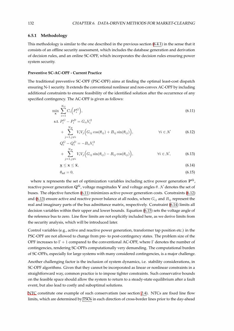
132 CHAPTER 6. DATA-DRIVEN METHODS FOR MARKET-CLEARING
6.5.1 Methodology
This methodology is similar to the one described in the previous section (6.4.1) in the sense that itconsists of an o✏ine security assessment, which includes the database generation and derivationof decision rules, and an online SC-OPF, which incorporates the decision rules ensuring powersystem security.
Preventive SC-AC-OPF - Current Practice
The traditional preventive SC-OPF (PSC-OPF) aims at finding the optimal least-cost dispatchensuring N-1 security. It extends the conventional nonlinear and non-convex AC-OPF by includingadditional constraints to ensure feasibility of the identified solution after the occurrence of anyspecified contingency. The AC-OPF is given as follows:
minx
NGÿ
i=1Ci
1P G
i
2, (6.11)
s.t. P Gi ≠ P D
i = GiiV2
i
+
NBÿ
j=1,j ”=i
ViVj
1Gij cos(◊ij) + Bij sin(◊ij)
2, ’i œ N (6.12)
QGi ≠ QD
i = ≠BiiV2
i
+
NBÿ
j=1,j ”=i
ViVj
1Gij sin(◊ij) ≠ Bij cos(◊ij)
2, ’i œ N , (6.13)
x Æ x Æ x, (6.14)
◊ref = 0, (6.15)
where x represents the set of optimization variables including active power generation PG,reactive power generation QG, voltage magnitudes V and voltage angles ◊. N denotes the set ofbuses. The objective function (6.11) minimizes active power generation costs. Constraints (6.12)and (6.13) ensure active and reactive power balance at all nodes, where Gij and Bij represent thereal and imaginary parts of the bus admittance matrix, respectively. Constraint (6.14) limits alldecision variables within their upper and lower bounds. Equation (6.15) sets the voltage angle ofthe reference bus to zero. Line flow limits are not explicitly included here, as we derive limits fromthe security analysis, which will be introduced later.
Control variables (e.g., active and reactive power generation, transformer tap position etc.) in thePSC-OPF are not allowed to change from pre- to post-contingency states. The problem size of theOPF increases to � + 1 compared to the conventional AC-OPF, where � denotes the number ofcontingencies, rendering SC-OPFs computationally very demanding. The computational burdenof SC-OPFs, especially for large systems with many considered contingencies, is a major challenge.
Another challenging factor is the inclusion of system dynamics, i.e. stability considerations, inSC-OPF algorithms. Given that they cannot be incorporated as linear or nonlinear constraints in astraightforward way, common practice is to impose tighter constraints. Such conservative boundson the feasible space should allow the system to return to a steady-state equilibrium after a faultevent, but also lead to costly and suboptimal solutions.
NTC constitute one example of such conservatism (see section 2.4). NTCs are fixed line flowlimits, which are determined by TSOs in each direction of cross-border lines prior to the day-ahead

6.5. DATA-DRIVEN SSSPSC-AC-OPF 133
Figure 6.6: Security domain of Flow-Based Market Coupling (FBMC) and Available TransferCapacity (ATC) [12]. ATCs are NTCs reduced by long-term capacity nominations. Source: [Pub.F].
market-clearing. Improvements towards a more accurate representation of the physical reality ofpower systems have been achieved by introducing FBMC, where a simplified European networkrepresentation is accounted for in the market-clearing. Critical branches (CBs) inside and betweenzones are identified, which could potentially be congested and limit the cross-border trade. AllCBs are represented through PTDF and instead of assuming only one fixed NTC value for eachcross-border line, all constraints imposed by the CBs are considered. Thus, a larger secure domain iso↵ered to the market compared to static NTC approaches as depicted in Fig. 6.6. The market is thenable to determine the optimal combination of commercial capacities between zones. Nonetheless,even flow based NTCs only capture one convex region of the entire feasible space and do notrepresent the non-convex reality of power system operations.
Improving the Preventive SC-AC-OPF Using Data
To address the challenges described above, we propose a data-driven approach to SC-AC-OPFs.
Database Generation As shown in chapter 5, the IEEE 14 bus system is small enough to create adatabase using a classical brute force approach as database generation method. Here, we report onresults from [Pub. F] which preceded the development of the method we proposed in chapter5 and for this reason the brute force approach is used. In order to achieve more detailed resultswe enriched the database with additional points close to the security boundary by running anadditional run of the brute force approach with an discretization interval/step size of 0.5 MW
focusing on the region close to the security boundary. However, as we discussed in 5.4, thisapproach proposed by Genc et al. in [142] requires additional computation to enrich the previouslygenerated database with important scenarios close to the security boundary. Thus, this workstrengthened our motivation to develop the advanced method for an e�cient database generationthat we reported in chapter 5. And as shown in chapter 5, we can generate an equally high-qualitydatabase in significant less time with the method we proposed in chapter 5.

134 CHAPTER 6. DATA-DRIVEN METHODS FOR MARKET-CLEARING
Feature Selection and Knowledge Extraction As this work deals with an AC-OPF, the featureselection process from the previous section needs to be adapted.
Compared with the previous work, here we need to consider that the security considerations aswell as the OPF are located in the AC space, i.e. we do not need a mapping from one space intothe other. Thus, based on the lessons learned from the previous section, we use voltage angledi↵erences ◊ij = ◊i ≠ ◊j along transmission lines as features to determine the security boundary.
As knowledge extraction method, this work continues to use decision trees which are trainedwith cross entropy as splitting criteria. We apply a manual approach of pruning specific nodesaccording to test results using the OPF.
Thus, each branch p of the DT contains a set of minimum and maximum voltage angle di↵erencesand leads to a di↵erent region of the feasibility space, one of which contains the least-cost, optimalsolution. A visual illustration of our approach is depicted in Fig. 6.7. Instead of defining boundsthat contain only one of the three stable regions depicted in the shades of blue, conditional rulesallow to capture the entire feasible region within the red frame.
OPF Implementation The DT is incorporated in the SC-OPF using Mixed-Integer Programming(MIP). Each full branch is associated with a binary variable yp, which if chosen, activates thecorresponding upper and lower bounds on angle di↵erences, or otherwise, leaves the originalbounds unchanged:
yp · ◊ij,p ≠ (1 ≠ yp) · ◊ij Æ ◊ij Æ yp · ◊ij,p + (1 ≠ yp) · ◊ij ,
’(i, j) œ L, ’p œ P. (6.16)
L and P denote the set of lines and DT branches/paths, respectively. Only one DT branch, i.e. oneset of minimum and maximum bounds on angle di↵erences, can be chosen, which is imposed byadding constraint
qpœP yp = 1.
The data-driven SC-OPF is thus formulated as a Mixed-Integer Non-linear Program (MINLP),which is a NP-hard problem. One of the main contributions of in this section is that we relaxthe non-convex AC power flow equations using a Second Order Cone relaxation and obtain aSC-OPF formulated as a Mixed-Integer Second Order Cone Program (MISOCP), which is a convexmixed-integer program that can be solved e�ciently by already existing solvers.
Figure 6.7: Illustrative example of non-convex space. Source: [Pub. F].

6.5. DATA-DRIVEN SSSPSC-AC-OPF 135
Relaxing the Data-driven SC-OPF
The SOC formulation of the OPF problem is based on [175], [176] and [177]. New variables areintroduced to capture the nonlinearities and non-convexities of the AC power flow equations: (a)ui := V 2
i , (b) cij := ViVj cos(◊ij) and (c) sij := ≠ViVj sin(◊ij). The AC-OPF is transformed fromthe space of x := {PG, QG, V, ◊} variables to the space of xSOC := {PG, QG, u, c, s} variablesand is given by:
minxSOC
NGÿ
i=1Ci
1P G
i
2(6.17)
s.t. P Gi ≠ P D
i = Giiui
+
NBÿ
j=1,j ”=i
1Gijcij ≠ Bijsij
2, ’i œ N (6.18)
QGi ≠ QD
i = ≠Biiui
≠NBÿ
j=1,j ”=i
1Gijsij + Bijcij
2, ’i œ N (6.19)
cij = cji, sij = ≠sji, ’(i, j) œ L (6.20)
c2ij + s2
ij = uiuj , ’(i, j) œ L (6.21)
Vi2 Æ ui Æ Vi
2, ’i œ N . (6.22)
Active and reactive power generation are constrained by their usual limits and are not explicitlymentioned. The non-convex quadratic equality constraint (6.21) is relaxed through a second-ordercone constraint: c2
ij + s2ij Æ uiuj . The SOC formulation of the OPF problem (6.17)-(6.22) is exact
for radial networks and the optimal voltage angles can be recovered by solving:
◊i ≠ ◊j = atan2(súji, cú
ij), ’(i, j) œ L, (6.23)
where ú indicates the optimal solution obtained from the SOC-OPF. For meshed networks theabove formulation is a strict relaxation, potentially resulting in solutions, which are infeasible forthe original AC-OPF [177]. Reintroducing voltage angle variables and constraint (6.23) in problem(6.17)-(6.22) would render the SOC formulation exact for meshed networks, but also non-convex.Various convex approximations of constraint (6.23) have been proposed [177], [175]. In this workwe use a sequential conic procedure as proposed in [175], where the arctan function is linearizedusing a Taylor series expansion.
Conditional bounds on voltage angles are introduced using binary variables as described in section6.5.1. Known limits on angle di↵erences can also be used to define bounds on the SOC variables cand s:
yp · tan(◊ij,p) · cij ≠ (1 ≠ yp) · tan(◊ij) · cij Æ sji,
’(i, j) œ L, ’p œ P, (6.24)
yp · tan(◊ij,p) · cij + (1 ≠ yp) · tan(◊ij) · cij Ø sji,
’(i, j) œ L, ’p œ P. (6.25)

136 CHAPTER 6. DATA-DRIVEN METHODS FOR MARKET-CLEARING
Otherwise, the SOC variables cij and sij are only constrained by their implied upper and lowerbounds ViVj and ≠ViVj , respectively, which in practice can be very loose. In order to tighten therelaxation, we determine minimum and maximum values of cij and sij along all lines (i, j) usingthe information from the generated database of operating points.
6.5.2 Case Study
We evaluate the performance of the proposed data-driven SC-OPF ensuring small-signal stabilityand N-1 security on a modified version of the IEEE 14 bus test system [11]. Our case studyconsists of three parts. First, we compare the convex MISOCP formulation of the algorithm toa data-driven MINLP implementation and a standard (i.e., not data-driven) preventive SC-OPF.Its low computational e↵ort makes the proposed MISOCP suitable for AC based market-clearingauctions as envisaged in the US. In Europe, however, electricity markets will probably continue torely on DC approximations. To this end, we show how the proposed method can also be usedby TSOs for optimizing redispatching actions in order to ensure N-1 security and small-signalstability after the market-clearing. Finally, we analyze how the data-driven approach coupled withMIP notably extends the feasible space of the OPF.
The network data is given in [178] with some modifications introduced in [Pub. E]. Note thatadditionally the voltage setpoints of generators 4 and 5 are changed to 1.02 p.u. and 1.01 p.u.,respectively, and the reactive power of generator 1 is limited within ±990 Mvar. The consideredcontingencies include the same as in the previous section (all except Bus 1 and 2, line 1-2).Additionally, a fault at Bus 6 is neglected because compared to the previous work the voltage limitsafter a contingency are tightened (0.94 p.u. Æ Vi Æ 1.06 p.u., ’ i œ N ). Note that the standardPSC-OPF does not incorporate stability considerations, but only extends the constraint set toaccount for the defined N-1 contingencies. Bus 1 with generator g1 has been chosen as the slack busfor the base case and all N-1 cases. A step size of 0.5 MW was chosen for discretizing the possibleoperating range and generating the database of operating points used for deriving the decisiontree. The minimum damping ratio of an operating point over the base case and all N-1 cases isused as a metric for small-signal stability. As usual in power system operation, we define a securitymargin by requiring a minimum damping ratio of 3 %. The derived DT contains 136 leaf nodes,out of which 74 point to operating regions, which are small-signal stable for the base case and allconsidered contingencies. Thus, 74 binary variables are used to define conditional constraintson voltage angle di↵erences along lines and incorporate the stable regions in the data-drivenSC-OPF. Note that 1.34 million operating points have been evaluated for this case study, fromwhich more than 88 000 fulfill the required minimum damping ratio. Three di↵erent load levels(base case, ±20%) have been considered. The voltage magnitude at generator buses is set to thecorresponding generator voltage setpoint in order to ensure an appropriate voltage profile, whichis fundamental to a secure system operation. The small-signal analysis was performed usingMatlab and Matpower 6.0 [49]. The data-driven SC-OPF based on MISOCP was implemented inPython using the Gurobi Optimizer. The standard preventive SC-OPF (i.e., NLP) and the MINLPimplementation of the data-driven SC-OPF were carried out in GAMS. The open-source solversBONMIN and COUENNE were used for the MINLPs, while CONOPT was used for the NLP.
Comparison of Preventive and Data-driven SC-OPFs
Table 6.5 lists the results of all three SC-OPF implementations. It can be observed that allimplementations based on decision trees result in operating points, which exhibit minimum

6.5. DATA-DRIVEN SSSPSC-AC-OPF 137
Table 6.5: Results of standard PSC-OPF and data-driven SC-OPF implemented as MINLP andMISOCP. Adapted from: [Pub. F].
Standard PSC-OPF Data-driven SC-OPF
NLP MINLP MISOCPCOUENNE BONMINCost (e/h) 3022.83 3445.09 3381.21 3365.95Runtime (s) 10.06 1000.16 96.16 5.58Iterations (-) - - - 4Min. damping ratio (%) unstable 3.27 2.97 2.53Leaf node (-) - 31 133 104
Dispatch P Q P Q P Q P Q(MW) (Mvar) (MW) (Mvar) (MW) (Mvar) (MW) (Mvar)
g1 168.20 5.30 106.86 16.37 108.15 16.76 109.89 16.44g2 60.00 50.00 52.19 38.08 60.00 37.55 60.00 37.97g3 39.39 21.51 60.00 10.93 60.00 11.65 60.00 11.79g4 0 6.91 25.00 0.40 25.00 0.74 25.00 0.82g5 0 4.81 19.33 3.72 10.61 4.01 8.98 4.09
damping ratios that are non-negative and are thus stable for the base case and all considered N-1contingencies. The solution of the standard PSC-OPF however is unstable for a fault at bus 5 andline 1-2, respectively. Thus, the identified preventive control actions do not fullfill the system’ssecurity requirements and would call for redispatching measures. As the PSC-OPF results in anoperating point, which does not reflect the small-signal stability requirements, its total cost is lowerthan the other solutions.
All three data-driven implementations result in di↵erent leaf nodes of the DT and thus in di↵erentregions of the feasible space with various degrees of conservatism. Higher damping ratios are alsoreflected by higher costs. All solutions include a stability margin, but only the most conservativeresult achieves a minimum damping ratio of more than 3 %. This can be explained by the factthat (a) the OPF is not limited to the specified discretization intervals of 0.5 MW, as used for thedatabase generation and (b) DTs are not 100 % accurate leading to missclassifications. For cases,where the minimum damping ratio is a hard constraint, higher values can be required whenderiving the DT in order to avoid violations. Fig. 6.8 illustrates the stable domain covered by allDT leaf nodes as a function of the angle di↵erences along lines 1 and 2. The rectangles indicatethe domains covered by the three di↵erent leaf nodes obtained from the data-driven SC-OPFimplementations with the location of the corresponding solution pointed out. It can be seen thatthe stable domain is non-convex and that safer operating points exhibiting higher damping ratiosare located further away from the stability boundary.
The known scalability issues of COUENNE [179], which is a global optimization solver, lead tosignificantly higher execution times compared to BONMIN, which employs heurisitic methods fornon-convex MINLPs. Also, the default settings for both solvers include a relative tolerance gapof 10 % terminating the computation as soon as a solution is found, which lies within 10 % of thetrue objective value. This explains the choice of di↵erent leaf nodes. However, even reducing thetolerance value does not change the outcome indicating that neither of the solvers is able to providethe best integer solution. The MISOCP is able to find the optimal integer solution, which has beenverified by manually imposing the bounds defined by each DT branch. Specifically, we solved 74AC-OPFs consecutively, one for each DT branch and imposed the corresponding bounds in orderto determine the DT branch, which contains the least-cost, optimal NLP solution. Leaf node 104actually contains the bounds, which result in the least-cost NLP solution. Notably, in this test case,the MISOCP relaxation is exact, i.e. its solution is feasible to the nonlinear, non-convex AC-OPF

138 CHAPTER 6. DATA-DRIVEN METHODS FOR MARKET-CLEARING
Figure 6.8: Non-convex security domain of the DT as a function of the angle di↵erences alonglines 1 and 2. The blue shaded areas represent the stable regions defined by all DT branches. Thedarker the color, the more domains of di↵erent DT branches overlap. Note that the actual securitydomains covered by the di↵erent leaf nodes do not overlap and might even be disjoint, whichhowever cannot be depicted by only two dimensions. Source: [Pub. F]
formulation and corresponds to the global optimum of the non-convex problem. Nonetheless,given that the MISOCP formulation is still a relaxation, identified solutions can be infeasible forthe original problem. Therefore, we propose to use the MISOCP primarily to identify the optimalDT branch and hence the linear bounds on the feasible space, such that the optimal solution isincluded. Once these are known and the feasible space has been reduced, the integer variablescan be omitted and a common AC-OPF (i.e., NLP) with the previously identified bounds onangle di↵erences imposed as linear constraints can be performed to identify feasible and securepreventive control actions. The MISOCP solution serves as a lower bound and can validate theoptimality of the AC-OPF solution.
Table 6.5 also outlines the savings in online computation time of the proposed SC-OPF method.The data-driven approach outperforms the usual PSC-OPF by more than 40 %, while at the sametime incorporating more security requirements. Naturally, the computation time depends on thesize of the DT and the number of binary variables used to represent it. Even though introducingbinaries increases the OPF complexity, this side e↵ect is o↵set by a signifincantly reduced overallsize of the SC-OPF. While the PSC-OPF increases 32-fold when considering 31 contingencies, theproposed data-driven approach inreases less than 4-fold for the same amount of contingencies. Asindicated by constraint (6.16), (2 ◊ NL ◊ NP + 1) additional constraints are added, where NL andNP denote the number of network lines and DT paths, respectively.
Furthermore, given that the problem is a convex MIP, which can be solved e�ciently by alreadyexisiting solvers that are able to handle up to a few thousand binaries, the amount of discretevariables is not expected to be an obstacle. The size of the DT is directly determined by the size ofthe dataset, which it is derived from. Hence, a more e�cient method to generate the database ofoperating points, appropriate pruning of the DT and techniques to decompose the data-drivenoptimization are aspects that require a deeper analysis and are promising approaches to enhancethe scalability performance of the method.

6.5. DATA-DRIVEN SSSPSC-AC-OPF 139
Figure 6.9: Visualization of redispatch and maximum convex security domain, which can becovered by one leaf node only. Source: [Pub. F]
Optimizing Redispatch
The method can be used by TSOs to identify optimal redispatching actions, where for example themarket-based day-ahead dispatch, if identified as unstable, is redirected through the DT to a securedomain. We have reformulated the MISOCP in order to optimize redispatching actions, assumingthat the costs of generator up- and down-regulation correspond to its marginal cost. Generatorsare assumed to be paid for up-regulation and charged for savings resulting from down-regulation.We have used the unstable solution of the standard PSC-OPF listed in Tab. 6.5 as an input to theredispatch and successfully shifted the operating point to leaf node 104. The cost of redispatchamounts to 343.12e, which corresponds to the original di↵erence in objective values between thePSC-OPF and MISOCP.
The MISOCP, if implemented at the market stage, could result in more than 10 % cost savings forthe system operator and better reflects the locational impact of stability requirements.
Enlarging the Feasible Space
The generated database contains 1.34 million operating points, out of which 6.57 % fulfill the 3 %
minimum damping ratio and define the feasible space of operation. We have evaluated howmuch of the entire stable region is covered by each individual leaf node, i.e. how many operatingpoints fulfill the constraints imposed by the corresponding DT branch. All leaf nodes cover intotal 99.91 % of the considered stability region, where leaf node 7 accounts for most of it, capturing77.78 % of the entire feasible space. The implied bounds of leaf node 7 are depicted in Fig. 6.9. Ifwe had considered the stability requirements in the OPF only by imposing bounds, which define aconvex space, as it is currently done in practice, we would have been able to capture at most 77.78 %
of the feasible space, thereby also missing the optimal solution as can be seen in Fig. 6.9. Thus, ourapproach to incorporate the information provided by the database in the optimization problemthrough binary variables allows us to enlarge the feasible space by more than 28 %, enclosing theremaining 22.13 %, which are covered by the DT.

140 CHAPTER 6. DATA-DRIVEN METHODS FOR MARKET-CLEARING
6.5.3 Discussion
In this section we propose a data-driven approach to preventive SC-OPF, which ensures N-1security and small-signal stability, it is scalable and uses decision trees to capture the non-convexand possibly disjoint space of stable operating points. We propose a new approach to translatedata, which operators usually already have available from dynamic simulations, and includethem in a simple way in an optimization framework. Binary variables are used to represent theknowledge extracted from the data giving rise to two levels of non-convexities: one that refers tothe integrality of the binary variables and another one that concerns the AC power flow equations.We eliminate the latter using a SOC relaxation and obtain a convex MISOCP. MISOCPs generalizeconvex mixed-integer quadratic programs, for which solvers have already reached a high level ofmaturity. The proposed method reduces the overall problem size by avoiding to explicitly includeall considered contingencies and incorporates stability requirements, both of which have beenmajor challenges in SC-OPFs. Finally, we have shown that by using data coupled with MIP in(SC-)OPFs we can enlarge the feasible space represented in the OPF by more than 28 %.
The relaxed data-driven SC-OPF can be used to determine the optimal bounds (i.e., the optimal DTbranch) on the feasible space, such that secure preventive control actions are ensured. Consideringthat the DT represents a non-convex operating space, identified preventive actions can be lessconservative than those determined by current approaches as described in section 6.5.1. The needfor iterative contingency analyses to indentify suitable control actions are alleviated. The MISOCPformulation of the SC-OPF can be used by market operators as a market-clearing tool due to itslow online computational e↵ort but also by TSOs to determine optimal redispatching actions andthe bounds on angle di↵erences, which allow accommodating the redispatch.
6.6 Data-driven Small-Signal Stability and Preventive-Corrective SecurityConstrained DC-OPF
This work extends the data-driven security constrained DC-OPF presented in section 6.4 byincorporating corrective control o↵ered by HVDC terminals. Moreover, it bridges the gap betweenthe chapter on Multi-Terminal High-Voltage Direct Current (MT-HVDC) control structures andthis chapter by adapting the methodology proposed in Section 4.7 to incorporate the flexibilityo↵ered by HVDC terminals into the security considerations already included in the previoussections. Considering corrective control by HVDC terminals already in the market-clearing allowsfor an even less conservative and more cost-e�cient dispatch while keeping all the benefits of thepresented data-driven security constrained DC-OPF, such as the incorporation of N-1 security andsmall-signal stability and the possibility of considering non-convex, possibly disjoint operatingspaces.
The additional challenges of including corrective control of High-Voltage Direct Current (HVDC)terminals are threefold. First, the size and complexity of the small-signal model increasessignificantly with every HVDC terminal. Second, every HVDC terminal adds two additionaldegrees of freedom with a wide range of potential values (¥ ±Pmax, ¥ ±Qmax) to the problemcomplicating the database generation by significantly increasing the number of potential operatingpoints. Finally, the benefit of corrective control, allowing HVDC terminals to change set-pointsin order to save the system in case of contingencies, complicates the data-point classification. Asthese challenges mainly concern the database generation and operating point classification, theyare described in more detail in section 6.6.2.

6.6. DATA-DRIVEN SSSPCSC-DC-OPF 141
6.6.1 Methodology
As this works extends the data-driven security constrained DC-OPF presented in section 6.4 weadapt the presented methodology. In order to include corrective control of HVDC terminals, themain changes lie in the database generation and the operating point classification.
6.6.2 Database Generation
In case of corrective control, the database generation faces the three aforementioned additionalchallenges: (i) increased small-signal stability model complexity leading to a higher computationtime. Given the model complexity of HVDC terminals, the size of the small-signal model increasesby approx. 20 states per terminal (depending on model fidelity of converter and dc cable). (ii)Two additional degrees of freedom per HVDC terminal increase the problem size significantly.Moreover, given the wide operating range of an HVDC terminal (¥ ±Pmax, ¥ ±Qmax), a singleHVDC terminal corresponds to a problem size increase of four generators. (iii) Increased complexityof operating point classification. The necessity to analyze potential corrective actions for everycontingency and every generation pattern (i.e. combination of generator outputs) complicates theoperating point classification. It is not enough anymore to know that a combination of generatoroutputs does not fulfill the security requirements for the most critical fault, because there couldpotentially exist another combination of HVDC set-points for which the combination of generatoroutputs fulfills the requirements for a specific contingency and another combination for anothercontingency. Thus, we basically need to extend the method proposed in Section 4.7 to determinethe operation boundaries of the HVDC terminals for the di↵erent network topologies and generatordispatches.
The complication of the operating point classification is visualized in Fig. 6.10. In case ofpreventive control, every generator set-point needs to be tested with every HVDC set-point forevery contingency. If this combination of generator and HVDC set-points fulfills the stabilityrequirements for every contingency, it is added to the set of ’set-points fulfilling the requirements’.If it does not fulfill the requirements for a single contingency, e.g. the most critical one, however, theremaining contingencies do not need to be evaluated to classify the operating point appropriately.
In case of corrective control, every combination of generator set-points needs also to be tested withevery HVDC set-point for every contingency. However, if there exists a combination of generatorset-points and HVDC set-points for which the stability requirements are fulfilled in the base case,the database needs to be evaluated whether there exists at least a single set of (possibly di↵erent)HVDC set-points fulfilling the stability requirements for the remaining contingencies. If thereexists at least one set of HVDC set-points for every contingency, the initial combination of generatorset-points and HVDC set-points can be added to the set of ’set-points fulfilling the requirements’.
An additional issue increasing the complexity of operating point classification is related tothe HVDC integration and the mapping between the ac and dc space. As the reactive powerset-points of the HVDC terminals are not part of the dc problem, a set of ac operating pointsOac, whose size depends on the discretization interval of the HVDC set-points, needs to bemapped into a single dc operating point. That means for example, that the operating pointsOPac = [Pg1 = 180 Pg2 = 0 Pg3 = 10 Pg4 = 10 Pg5 = 0 Pgwf
= 20 PgHV DC1 = ≠20 QHV DC1 =
±QHV DC,max QHV DC2 = ±QHV DC,max] œ Oac need to be mapped into a single dc operatingpoint. Moreover, these ac operating points di↵er by the losses occurring in the system, i.e. also

142 CHAPTER 6. DATA-DRIVEN METHODS FOR MARKET-CLEARING
Pick a combination ofgenerator outputs g1, . . . , gn
and HVDC set-pointsp1, q1, . . . , pn, qn
fulfillingstability
requirements forbase case and all n
contingencies?
fulfillingstability
requirements forthe base case?
fulfillingstability
requirements forcontingency 1?
add to setfulfilling stability
requirements
add to setnot fulfilling stability
requirements
Pick a combination ofgenerator outputs g1, . . . , gn
and HVDC set-pointsp1, q1, . . . , pn, qn
fulfillingstability
requirements forcontingency n?
Is there anyother combination of
HVDC set-pointsp1, q1, . . . , pn, qn
fulfillingrequirements?
Is there anyother combination of
HVDC set-pointsp1, q1, . . . , pn, qn
fulfillingrequirements?
add to setfulfilling stability
requirements
add to setnot fulfilling stability
requirements
Yes
Yes
Yes
Yes
Yes
Yes
No
No
No
NoNo
No
Preventive Control Corrective Control
Figure 6.10: Visualization of the di↵erence in data-point classification between preventive andcorrective control.
by the line flows which serve as predictors in our study, and also by their classification. To thisextent, we determine for every potential dc operating point whether there exists at least a singleOPac œ Oac allowing to classify it as fulfilling the requirements according to the preventive-corrective definition. Moreover, if there exists several OPac fulfilling the requirements (or allnot fulfilling the requirements) we need to map all these ac operating points into the single dcoperating point. Therefore, we average the corresponding lines flows in order to reduce memoryrequirements and classifier training time.
Thus, the database generation becomes significantly more complicated.
6.6.3 OPF Implementation
The OPF implementation remains the same as presented in 6.4.4. The implementation of theHVDC lines is realized in the form of virtual generators, i.e. two generators per HVDC line withPg,1 = ≠Pg,2. The losses of the HVDC line are considered as loads at the nodes of the virtualgenerators, evenly split between the nodes. Following the lessons learned from the previous

6.6. DATA-DRIVEN SSSPCSC-DC-OPF 143
sections, the losses of the DC lines are also approximated by an ac power flow of the best guess ofthe database using MatACDC [180].
6.6.4 Feature Selection and Knowledge Extraction
Following the lessons learned from previous work, which are presented in the case study in section6.4.5, this work uses as features the exact mapping of dc and ac operating points by augmentingthe dc power flow by the losses approximation of the corresponding ac-power flow. The detailsare presented in section 6.4.3.
Following the previous work, this work also uses decision trees as knowledge extraction method.
6.6.5 Case Study
We evaluate the performance of the data-driven small-signal stability and preventive-correctivesecurity constrained OPF by comparing it to a data-driven small-signal stability and preventivesecurity constrained OPF, which corresponds to the data-driven SC-DC-OPF presented in section6.4 with additionally considering HVDC lines and preventive control of HVDC terminals. Aswe have already shown in section 6.4.5 that our data-driven preventive SC-DC-OPF allows fora more cost e�cient dispatch than current approaches, such as ATC and FBMC, this case studydemonstrates that by considering the corrective control capabilities of HVDC terminals already inthe market-clearing, an even more cost e�cient dispatch can be obtained.
The IEEE 14 Bus system has been modified by integrating a HVDC line and a windfarm asvisualized in Fig. 6.11. The parameters are given in the appendix. The small-signal modelsof the multi-machine model, the HVDC transmission system and the Doubly-Fed InductionGenerator (DFIG) based wind farm have been introduced in section 2.7. The model has been builtusing Mathematica [48], as the symbolic derivation enables us to initialize the model for everypossible combination of load and generation using MatACDC [180]. The small signal analysis iscarried out using Matlab 2017b [41]. Reactive power limits of the generators are enforced. Note thatalthough a 100 MW wind farm is connected, the ac network is not capable of absorbing 100 MW atbus 17 at the given load level
qNB
i=1 PDi= 259 MW. Hence, it is a simplified example resembling
the problems currently observed in Germany. A comparable large installed wind power capacityis located in the north, while the load centers are in the south. Due to missing transmission linesfrom the north to the south because of delay in the project development, the wind power needsto be curtailed in case of high wind speeds. This setup allows us to show that our data-drivenapproach is capable of reducing the need for redispatching actions by incorporating the securityconsiderations and potential corrective control actions o↵ered by the HVDC terminals already inthe market-clearing.
Note that within the N-1 security analysis, the HVDC line has been neglected as HVDC point-to-point links are usually not considered as N-1 secure. All ac line faults have been considered exceptthose lines interconnecting the HVDC terminal with the ac grid / wind farm (line13-17 / line15-16)and line7-8.
As an extension of the e�cient database generation method proposed in chapter 5 which allows thecreation of databases considering corrective control is currently still under development, a bruteforce approach is used to enable the presentation of this small case study. Although a comparablywide grid discretization (i.e. a step size of 3 MW for the generators and 10 MW for the HVDC

144 CHAPTER 6. DATA-DRIVEN METHODS FOR MARKET-CLEARING
17
15
16
HVDC2
HVDC1
Figure 6.11: Visualization of the modified IEEE14Bus system.
set-points) was chosen, this requires the analysis of 173.3 · 106 data points with the brute force
approach. Considering also the increased model size and number of faults we consider per datapoint, the database generation takes ¥ 140 h using the brute force approach with 200 cores on theHPC cluster at DTU for a single load level. This emphasizes the need for the extension of oure�cient database generation method.
As a first step, both approaches, i.e. preventive security and the preventive-corrective securityapproach, can be compared by the size of the feasible space which becomes visible by an analysis ofthe database. Given the discretization and database reduction as described in Section 6.6.2, 392931dc operating points are obtained in the database. Just by comparing the amount of feasible pointsfor the preventive (13066, 3.33%) and the preventive-corrective (49640, 12.63%) case highlightsthe increase in feasible space obtained by considering corrective control actions o↵ered by HVDCterminals. However, it needs to be emphasized that - as for all small-signal stability OPFs - thetransition trajectory between the pre- and post-disturbance OPs is not considered and thus, itneeds to be verified that the transition trajectory does not violate any dynamic limits. However,as the potential pre- and post-disturbance OPs are collected within the database, the data-driven

6.6. DATA-DRIVEN SSSPCSC-DC-OPF 145
Table 6.6: Comparison of data-driven preventive and preventive-corrective approaches.
Pwind Æ Pwind,max Pwind Æ 10 MW
preventive corrective preventive correctiveDispatch (MW)
g1 106.8 133.0 166.2 218.8g2 60.0 60.0 60.0 20.4g3 60.0 28.7 7.6 17.0g4 13.6 25.0 25.0 6.0g5 12.1 0.0 3.6 0.0
gwf 20.0 25.8 10.0 10.0Total Cost (e) 3198.1 2948.6 3036.5 2807.7
Min. damping ratio (%) 7.3% 5.9% 8.9% 8.4%
approach also facilitates the time-domain verification. Ideally, the small-signal stability approachcould be supported by time-domain simulations verifying the transition trajectories already withinthe database generation.
The decision trees are created using Matlab 2017b [41] with the gini-index as splitting criteria. Weraise the cost for false positives by a factor 8, i.e. misclassifying an OP not complying with therequirements as stable. The initial accuracy using 5-fold cross-validation is for both approachesat 99.99 % with the only errors being false negative predictions. However, in order to mitigatethe over-fitting, we pruned step-wise singular nodes based on OPF results. Thus, in the end theaccuracy of the trees went significantly down to 96.68 % (preventive) and 89.45 % (preventive-corrective). Note, however, that also after the pruning zero false positives are detected, i.e. thewhole pruning made the trees a bit more conservative without increasing the risk of false positivemisclassifications.
Following the approach presented in section 6.4, we incorporate the system losses from a bestguess operating point found by searching in the database for the cost optimal solution of eachapproach.
The results of both approaches, once for Pwind = Pwind,max and once for Pwind = 10 MW are shownin Tab. 6.6. Both approaches find N-1 secure operating points, however, the preventive-correctivesecurity approach enlarges the feasible space and allows significant savings (7.8 % and 7.5 %,respectively) in both cases. Note that due to the small-signal stability considerations a maximumRES dispatch would not lead to the most cost e�cient solution which can be observed in Tab. 6.6.Especially the preventive-corrective SC-OPF would be able to determine even cheaper operatingpoints using less wind power, however, as RES are usually prioritized, high RES dispatch isenforced here. Still, as aforementioned the ac grid is not capable of absorbing Pwind,max but thepreventive-corrective security approach allows to maximize the RES dispatch compared to thepreventive approach. Considering the results presented in Section 6.4.5, more cost e�cient resultscould probably be achieved by using a database with smaller discretization intervals.
Thus, by incorporating security considerations and the corrective control capability of HVDCterminals into the market-clearing, a stable, cost e�cient dispatch is achieved and the need forredispatching actions is mitigated.

146 CHAPTER 6. DATA-DRIVEN METHODS FOR MARKET-CLEARING
6.6.6 Discussion
A data-driven small-signal stability and preventive-corrective security constrained DC-OPF hasbeen presented. Compared with a data-driven small-signal stability and preventive securityconstrained DC-OPF the feasible space is enlarged allowing for a more cost e�cient dispatch. Byensuring the small-signal stability and preventive(-corrective) security of the dispatched operatingpoints, the need for redispatch is mitigated. Potential corrective control policies can be extractedfrom the database.
6.7 Conclusion and Outlook
Data-driven methods for market-clearing and power system operation have been developedwhich allow for a more cost e�cient and secure dispatch determination by implementing moredetailed security considerations and extending the feasible space to the real non-convex space. Theproposed methods are scalable and computationally e�cient due to the fact that the N-1 securityand small-signal stability analysis is performed o✏ine. Tractable decision rules are extractedfrom the database enabling their implementation into OPF algorithms. Moreover, we took theincreasing interest in HVDC transmission in Europe into account and considered the benefits ofcorrective control o↵ered by HVDC terminals enabling an even more cost e�cient market-clearing.Further, the methods can potentially be used at di↵erent time horizons (e.g. day-ahead market,intra-day market or during operation). Case studies have highlighted the superior performance ofthe proposed methods compared to current approaches.
Although this work already shows promising results, we believe there exist a few opportunities toextend the proposed methods. (i) The database generation can be extended by adding time-domainsimulations. Besides the safe operating condition before and after the fault, as small-signal stabilityand security constrained OPF guarantee, the additional time-domain simulation would ensurethat the trajectory in between is also safe making it not only small-signal stable but transient andvoltage stable. The advantage of extending our method with time-domain simulation instead ofstarting from scratch is that the database can be used to determine a significant reduced size ofpre-disturbance states which need to be investigated.
Moreover, (ii) the proposed methods can be extended by including uncertainty within the OPFformulation by using chance constrains. So far the uncertainty of RES is separated from theproblem in the sense that we rely on a precise forecast. However, the next step is to include theuncertainty within the OPF allowing us to include more detailed probabilistic forecasts. Then,using chance constrains the data-driven OPF formulation could ensure that the dispatch woulde.g. with a violation probability of 5 % always be within the secure region.

CHAPTER7Data-driven Dynamic Stability
Assessment based on LocalMeasurements
After the successful application of data-driven methods on a system wide level, this work investigatespotential application on control level using local measurements only.
7.1 Background
In modern power systems voltage stability is an important issue since voltage instability hassignificantly contributed to some major blackouts around the world (e.g. USA-Canada blackout in2003 [181], southern Sweden/ eastern Denmark 2003 [182] and Italy blackout in 2003 [183]). TheIEEE and CIGRE joint task force defines ’voltage stability’ as the ability of a power system to sustainvoltage magnitudes at all buses after small or large disturbances [184]. Thus, voltage instabilitydescribes the failure of the power system to maintain/restore equilibrium between load demandand load supply. The instability is often driven by the loads, which tend to be restored after adisturbance by the action of motor slip adjustment, distribution voltage regulators, tap-changingtransformer, and thermostats [1].
Voltage stability can be classified in two categories: small disturbance and large disturbancevoltage stability. Further, based on the time frame of interest voltage stability can be distinguishedby short-term and long-term voltage stability. The long-term phenomena involves slower actingequipment, such as tap-changing transformers, thermostatically controlled loads, and generatorcurrent limiters [1]. The short-term voltage stability is driven by fast recovering load components(e.g. induction motor) that tend to restore power consumption in the time scale of a secondfollowing a large disturbance [32]. Due to the voltage dip, induction motors decelerate dramaticallyor may stall if the electrical torque cannot overcome the mechanical load. The behavior of themotors depends on the mechanical torque characteristics and the motor inertia. Stalling of a motornear the end of a feeder may cause the stalling of other motors [185]. As a consequence theydraw a very high reactive current at low power factor depressing the voltage magnitudes. Thestalling of induction motors has been identified as main reason for Fault Induced Delayed VoltageRecovery (FIDVR) which is the phenomenon whereby system voltage remains at significantlyreduced levels for several seconds after a transmission fault has been cleared [33]. In case loaddynamics attempt to restore power consumption beyond the capability of the transmission system,voltage collapse may occur due to excessive voltage deviation from normal permissible limits [1].Hence, the major challenges are that the systems transition from post-contingency to new operationpoint should not violate any dynamic limits and the new operation point needs to be stable [186].
147

148 CHAPTER 7. DATA-DRIVEN DYNAMIC STABILITY ASSESSMENT
Figure 7.1: Example of a voltage collapse scenario with the visualization of the post-disturbancemeasurement window and the NERC recommendation for under-voltage load shedding.
Dynamic voltage limits after a contingency required by di↵erent utilities are provided for examplein [187].
Since the short-term voltage instability is usually following a disturbance perturbing the systemstate away from equilibrium, the dynamics are complex making the voltage stability analysisa challenging problem [188]. The complexity of monitoring the voltage stability of the powersystem is further related to the system size, as well as the presence of various sources of parametricand modelling uncertainties in power system dynamics, which could cause unreliable stabilitypredictions [189].
The increasing penetration of induction motor loads (e.g., air-conditioners), as well as the moreintensive usage of the transmission system makes today’s power systems more vulnerable tothe short-term voltage instability [190]. At the same time, the increasing deployment of PhasorMeasurement Units (PMUs) has made it possible to obtain high-resolution, real-time dynamic stateinformation of the power grid. These measurements result in a large amount of data collectionof the system behavior enabling us to develop methods to monitor, predict, and enhance systemstability in real-time. In particular, as an accurate model is di�cult to establish as the operatingconditions constantly change. Although, PMUs allow the development of Wide-Area Monitoringand Control (WAMC) systems using numerous PMUs system-wide and communication to gatherall the data, the communication delay may prohibit WAMC systems to be e↵ective against short-termin voltage instability. In fact, in [191], the authors address the communication delays, whichinclude propagation delays, router queuing delays, data transmission delays and phasor dataconcentrators data aggregation delays, between the PMUs and the control actuator. The authorsdetermine delays between 50 ms and 78 ms depending on the Information and CommunicationTechnology (ICT) infrastructure configuration. However, they argue that the PMU data framelosses additionally need to be considered to obtain a robust WAMC system. In WAMC applicationsthe computation is performed with the most recent PMU data frames available, however, thesesdata frames would be outdated in case of data frame losses, since the most recent measurementssent by the PMU are lost during data transfer to the central control unit. Thus, data frame lossesinduce an additional time delay resulting in even higher average time delays between 172 ms and872 ms depending on the ICT configuration [191].
Thus, relying on communication comes with the risk of communication faults or loss, and introduces

7.2. LITERATURE REVIEW 149
a significant time delay between measurement and actuator which for certain faults could be toolarge to be acceptable. For instance, in case of potential load driven short-term voltage instability(or fast evolving transient instability) the time delay induced by communication between PMUsand a central control unit may limit the possibility of saving the system. In Fig. 7.1, the worst-caseWAMC time delay (not including communication loss) is visualized as blue, dashed line. It isworth noting that at the time instance of 872 ms after the fault, the WAMC does not even haveany post-disturbance measurements yet but has just received the measurements at the momentwhen the disturbance occurred. However, the voltages already violate the recommendation of theNorth American Electric Reliability Corporation (NERC) for under-voltage load shedding [192],visualized in Fig. 7.1 as red, dashed line. For this reason, most control and protection schemesare decentralized and based on local measurements. Among several examples, the control at theHVDC terminals, for instance, is usually based on PI-controllers reacting to the measured voltagemagnitude / active power.
7.2 Literature Review
While most research in short-term voltage stability uses classical fully populated dynamic models intime-domain simulations, mostly sped up by distributed architecture and earlier termination [193],there is less work done using a data driven approach. Nevertheless, it is possible to distinguishbetween two main di↵erent directions of research in the data driven short-term voltage stabilityanalysis:
• Approaches using mathematical functions as stability metrics
• Data-driven approaches using Artificial Intelligence (AI), Machine Learning (ML), and / orData Mining (DM)
The group of mathematical functions as stability metrics basically sums up approaches, whichdirectly apply certain methods involving specific mathematical functions on real-time measurement.In [194], the authors use a direct stability analysis based on transient energy functions. In[188, 195–197], the authors use the Lyapunov exponent as stability metric. By determining thesign of the Lyapunov exponent, the authors are able to determine whether the voltage trajectoriesdiverge/converge.
In [198], the authors describe a novel analytical method to analyze short-term voltage stabilityusing a transient PV-plane. This method was also already proposed to be used in a control structureto increase the dynamic voltage support capability of a photovoltaic systems [199].
In [200], the authors propose an index to detect voltage stability based on monitoring changes inactive power transferred to a weak area and the apparent conductance seen by the bus, whichis related to the Thévenin impedance matching approach that is frequently used for long-termvoltage stability assessment. They claim that an extension of this approach proposed to monitorlong-term voltage stability would make it possible to monitor short-term voltage stability.
Further, the use of singular value decomposition showed promising results for predicting long-termvoltage instability and also detecting topology changes [201].
On the other hand, there are many approaches using data-driven approaches. A review of themethods used at the di↵erent stages (i.e. Database Generation, Input and Output Definition,

150 CHAPTER 7. DATA-DRIVEN DYNAMIC STABILITY ASSESSMENT
Knowledge Extraction, Validation) is provided by Zhang et al. in [202]. Previous works mainlyused the knowledge of the measurements at all nodes in the system to enable a quite precisestability monitoring and prediction [168, 169, 203–207]. While several authors propose the useof Artificial Neuro Networks (ANNs) [208–211], other propose to use Support Vector Machine(SVM) methods [212–214] or Extreme Learning Machine (ELM) methods [215]. Other interestingapproaches are based on Decision Tree (DT), which might be more comprehensible for systemoperators [143, 169, 216–221].
In [222], the authors provide an extensive case study comparing the accuracy of detecting pre-emergency states of the power system for di↵erent learning techniques including various DT,SVM and ANN methods. The results indicate the best results for DT and SVM methods. Further,the authors emphasize the ability of DTs to uncover the intrinsic mechanism governing physicalprocesses, and to provide a clear description in terms of tractable system parameters as attractiveaspects compared to other machine learning approaches.However, such an approach requiresnumerous PMUs and relies on communication. Nevertheless, there has been very little workon data-driven methods using only local PMU measurements for stability assessment: Existingapproaches include the application of DTs for transformer protection [223], and for high impedancefault detection [224]. In [225], the authors propose a response-based DT approach for an out-of-steprelaying application. In [226], the authors use Long Short-Term Memory (LSTM) networks andSVM to predict the occurrence of faults based on measurement data.
7.3 Contributions
In contrast to these previous works, we raise the question whether we could enhance the systemperformance by supporting the local control of e.g. HVDC terminals with data-driven tools usinglocal post-disturbance data only. Given that it is possible to predict that the system will becomeunstable, or violate under-voltage load-shedding relay settings, before it becomes visible in thevoltage magnitude, the local control could act earlier avoiding load-shedding or even voltagecollapse. That means, while the voltages in Fig. 7.1 directly after the fault seem to recover, i.e.the voltage di↵erence between set-point and measurement actually decreases, the system is stillmoving towards collapse shortly afterwards. If it would be possible to predict the system instabilityright after the post-disturbance measurement window (shown in black, dashed lines in Fig. 7.1),relying only on local measurements, the system could potentially be saved by fast local correctivecontrol actions.
The contribution of this work is the first stage towards such a corrective control: the e�cientdata-driven early stability assessment of faults in the extended neighbourhood of a strategic nodewhich will later trigger appropriate early actions. Future work will focus on the complete design ofthe corrective control response to such events. Especially for faults that severely a↵ect the voltage,the focus on faults in the extended neighborhood of a strategic node is reasonable, due to thelimited, relatively local, impact of reactive power support.
This work includes the following contributions: (a) we propose two data-driven approaches ofassessing the system stability after faults in the extended neighbourhood of a strategic node usinglocal post-disturbance measurements only. First, a single-level approach is presented, then atwo-level approach is presented where the first-level classifier determines the fault location and thesecond-level classifier determines the criticality of that fault. Further, (b) we evaluate and comparethe accuracy of di↵erent supervised machine learning methods and (c) evaluate the robustness of

7.4. DEFINITIONS 151
these approaches against changes in the grid and the load configuration in a case study. Thus,compared with existing literature, this work focuses on local, data-driven approaches for stabilitypredictions which could be used to trigger early corrective control actions.
The remainder of this work is structured as follows: First, the underlying concepts of extendedneighborhood and post-disturbance measurements are introduced in detail, followed by a briefintroduction of the supervised machine learning methods. Then, the proposed approaches areintroduced. Finally, a case study is presented.
7.4 Definitions
The question is whether it is possible to assess and predict the system stability after faults inthe extended neighbourhood of a strategic node using a limited time-window of only localpost-disturbance measurements. Thus, let us first define the extended neighbourhood of thestrategic node, followed by a description of the limited time window of local post-disturbancemeasurements.
7.4.1 Definition of the extended Neighbourhood of a Strategic Node
For a graph G(V, E), where V is the set of vertices, and E is the set of edges, we define vertex 1 asstrategic node. Then, two vertices 1, 2 are adjacent or neighbours, if {1, 2} is an edge of G. The set ofneighbours of a vertex V in G is denoted by NV (G) [155].
If vertices 2, 3 are also neighbours, i.e. {2, 3} is an edge of G, then vertex 3 is an extended neighbourof vertex 1. The set of extended neighbours of a vertex v in G is denoted by Ne
v (G).
Thus, for the small example of graph G in Fig. 7.2, the set of neighbours of the strategic node 1 isN1(G) = {2, 4} with the connecting edges marked as red, dashed lines, while the set of extendedneighbours is Ne
1 (G) = {3, 5, 6, 7} with the connecting edges marked as blue, dotted lines.
7.4.2 Post-disturbance Measurement Window
Triggered by a fault and the characteristic subsequent drop of the voltage magnitude, the localmeasurements within a certain time-window are used as predictor variables and inputs for thesupervised machine learning methods described in the following subsections. Since we focus onfaults in the extended neighbourhood of the strategic node, the time window starts with one samplebefore the characteristic voltage magnitude drop and ends one sample after the characteristic riseof the voltage magnitude when the fault is cleared with a trip of the corresponding lines.
1
4 2 3
86
7
9
5
Figure 7.2: Graph G.

152 CHAPTER 7. DATA-DRIVEN DYNAMIC STABILITY ASSESSMENT
Thus, as shown in Fig. 7.1, at t = 1 s a line fault occurred in the extended neighbourhood of thestrategic node. The fault is cleared after 100 ms with a trip of the corresponding line. With asampling rate of the PMUs of 60 Hz, the time window between the first measurement and lastmeasurement used for the prediction lies between t = 0.9833 s and t = 1.125 s, shown in Fig. 7.1as black, dashed lines. If it is possible to assess a stability purely based on this limited localinformation, control actions can be initiated significantly faster than by a WAMC which has a timedelay of anywhere between 172 ms and 872 ms.
7.5 Modeling
As such fault measurements in form of real PMU data are rare if available at all, this work usesPSS/e as simulation tool to create the required data. As the complex dynamics of short-termvoltage instability a↵ect the analysis of the phenomena, time-domain simulations with a detailedmodeling of the load are required in order to analyze short-term voltage stability [185]. Followingsimilar studies, this work uses complex load models ’CLODBL’, shown in Fig. 7.3. A more detaileddescription is given in [227]. Note that the proposed methods are not limited to specific models ormodel parameters.
The CLOD model replaces the constant MVA, current, and impedance load with acomposition of loads as shown in [Fig. 7.3]. These loads consist of large and smallinduction motors, discharge lighting, constant MVA load, and a static load response.Also included are transformer saturation e↵ects and an equivalent distribution feederand transformer impedance. Some general comments and modeling considerations forthe CLOD model:
• The model assumes that the load bus voltage is 0.98 pu, and adjusts the transformertap ratio at initialization until that load bus voltage is attained.
• The motor curves for the large and small induction motor models are provided inthe instruction manual. These motors models represent large and small motorswith inertia constant H = 1.0 sec and H = 0.6 sec, respectively.
• The model does not consider single-phase induction motors such as residential airconditions.
• The distribution system equivalent modeled as (R+jX)/P0 represents the trans-former and/or feeder impedance; however, this does not represent shunt compen-sation at the substation or down the feeder.
• Under-load tap changing is not considered in the transformer model.
• Discharge lighting is modeled as constant current real part and imaginary partproportional to the voltage raised to 4.5 power. Voltage between 0.65-0.75 puexhibits a linear reduction. For any voltage less than 0.65 pu, the load is assumedextinguished (no load).
[227]
The configuration is chosen as suggested in [185] as 15 % large motors, 45 % small motors, 1 %
transformer exciting current, 20 % discharge lighting, 5 % constant power and 14 % remainingloads.

7.6. METHODOLOGY 153
M MV
IV
I Constant MVA
LargeMotors
SmallMotors
DischargeLighting
Transformer Saturation Remaining
Loads
P = PRO · V Kp
Q = QRO · V 2
P + jQTap
R + jX
P0
= Load MW in pu on system baseP0
Figure 7.3: Complex Load Model: ’CLODBL’. Adapted from: [13].
7.6 Methodology
The di↵erent supervised machine learning methods used in this work have been introduced insection 2.5. Here, we introduce the di↵erent data sets and point out two di↵erent approaches abouthow to apply these supervised machine learning methods.
For each fault we create a data set containing numerous scenarios using various load levels andgeneration patterns. A single scenario is defined as a set of local measurements at the strategicnode of a specific fault using a specific generation pattern and load level. The scenarios of eachof all the di↵erent faults are split into randomly chosen 80 % for the training set and 20 % for thetest set. Then, all training sets and all test sets of the di↵erent faults are accumulated to a globaltraining and a global test set. Thus, both global sets consist of an equal share of scenarios of all thedi↵erent considered faults.
The decision tree classifiers developed in this chapter are trained using the gini-index as splittingcriteria as introduced in section 2.5. Moreover, in order to avoid false positive classifications, i.e.unstable scenarios classified as stable, we raised the cost of these misclassifications. Cost-complexitypruning is used as pruning method minimizing C–(T ) = c(T ) + – ◊ |T | for a set of subtrees Tx
developed using cross-validation within the test set.
The SVM classifiers have been been trained with standardized data and auto kernel scaling, i.e.the software uses a heuristic procedure to select the scale value. The heuristic procedure usessubsampling [42].
7.6.1 Single Level Approach
In a single level approach, the described supervised machine learning methods are used to trainclassifiers on the global training set trying to distinguish acceptable scenarios from unacceptablescenarios according to specified criteria.

154 CHAPTER 7. DATA-DRIVEN DYNAMIC STABILITY ASSESSMENT
Aggregated Trainingset
Trainingset of fault 1…N
Supervised Machine
Learning (SML)
SML SML SML SML SML
fault location
fault 1 stable fault 1 unstable… … … … … …
fault N stable fault N unstable
1st Level
2nd Level
Figure 7.4: Two-Level Approach.
7.6.2 Two-Level Approach
The two-level approach is shown in Fig. 7.4. For the di↵erent machine learning methods, as afirst step, we use the global training set to train classifiers that are able to determine the faultlocation. Then, at a second step, we use the individual training sets of each fault in order to train asecond set of classifiers to distinguish between acceptable and unacceptable scenarios for eachfault individually.
Thus, while the single level approach leads to a single classifier (e.g. classification tree), thetwo-level approach results in N + 1 classifiers, with N being the number of considered faults. Theadvantage of this approach is that it leads to smaller trees with potentially higher accuracy sincedi↵erent predictors are important to determine the stability boundary or the location of the fault.
The disadvantage is that misclassifications of the fault location occurring at the first level, leadto the use of classifiers specialized at di↵erent fault locations in the second level. However, thecase study indicates that very high accuracies can be achieved for the first level classifiers and thateven first-level misclassified scenarios are classified correctly on the second level with quite highaccuracy. This is discussed in more detail in the case study.
7.6.3 Predictors
These methods consider local post-disturbance measurements only, i.e. we use the measurementsof voltage and current magnitudes, voltage and current phase angles and active power andreactive power flows on the connected lines within the post-disturbance measurement window.Additionally, based on the simplified power flow equations, we calculate an approximate voltagephase angle di↵erence of the strategic node and the neighbouring nodes:
�◊yz = arcsin
3Pyz · xyz
V 2y
4(7.1)
where Pyz is the active power flow between the strategic node y and the neighbouring node z, xyz
is the reactance of the corresponding line and Vy is the voltage magnitude at the strategic node.

7.7. CASE STUDY 155
Figure 7.5: IEEE 14 Bus System. Source: [Pub. E].
In addition to the local post-disturbance measurements, the global pre-disturbance steady statedata of the system is used, i.e. voltage magnitudes and voltage phase angles of all buses andthe phase angle di↵erences between the buses before the disturbance. Since the pre-disturbanceinformation of the system is not time critical, it is expected to be available e.g. through the SCADAsystem.
7.7 Case Study
The IEEE 14 Bus system, shown in Fig. 7.5, is used as test system. As we did not have PMUdata available, we created a large enough data set by running time-domain simulations of a largenumber of scenarios using PSS/e.
At buses 2 to 6, we use complex load models ’CLODBL’, shown in Fig. 7.3. The configuration ischosen as suggested in [185] as 15 % large motors, 45 % small motors, 1 % transformer excitingcurrent, 20 % discharge lighting, 5 % constant power and 14 % remaining loads. The remainingloads are modeled as constant power loads.
In this study, we chose bus 5 as strategic node and applied the data-driven dynamic stabilityassessment based only on local measurements. In general any bus could be selected. With bus 5being a very central node, with N5(G) = {1, 2, 4, 6} and Ne
5 (G) = {3, 7, 9, 11, 12, 13}, this choiceallows us to challenge the assessment with many di↵erent faults. Thus, we considered all linefaults of one of the lines directly connected to bus 5 (red lines) as well as those in the extendedneighborhood (blue lines). The line between bus 1 and bus 2 would in general be in the extendedneighborhood, however, this line appears to be very critical for the system, leading to mostlyunacceptable scenarios. Thus, this fault is very easy to predict leading to a very high accuracy.Hence, it was not considered in order not to overestimate the observed overall prediction accuracy.
We created simulation data for 12 contingencies, each for 441 di↵erent generation patterns (i.e.with Pgen,1 being the slack bus we vary the generator outputs between zero and Pmax in 10 MW
(Pgen,2/3) and 12.5 MW (Pgen,4/5) steps, respectively. Moreover, this is done at 13 di↵erent load

156 CHAPTER 7. DATA-DRIVEN DYNAMIC STABILITY ASSESSMENT
96.52 99.65 95.56 95.62 97.73 95.72 93.9596.30 97.73 93.10 93.58 94.99 80.89 72.0297.87 99.21 95.65 97.45 98.68 94.15 92.2597.53 94.15 61.63 75.87 60.30 97.21 95.8497.98 99.48 96.60 96.23 98.58 96.60 96.3196.19 99.56 96.22 95.32 97.92 96.77 95.56
line1-5 line2-3 line2-4 line2-5 line3-4 line4-5 line4-7
1st level two-level total single-level totalDT 98.82 96.75 95.79SVM (lin) 99.42 91.13 86.53SVM (cubic) 100.00 96.55 95.48AdaBoost 88.47 83.19 57.59RUSBoost 99.65 97.55 97.40LogitBoost 0.00 97.18 97.00
556065707580859095
100
Perc
enta
ge [%
]
Figure 7.6: Accuracies of the single level and two-level approach.
levels (between 70 % and 112.5 %). This results in total of over 63’000 scenarios and more than70 GB of raw data. For the robustness analysis in the second part of the case study over 20’000additional scenarios are created with the details given in that subsection.
The PMUs are assumed to provide 60 samples per second. We assumed that all line faults arecleared after 100 ms by tripping the corresponding line without re-closing it. Scenarios are declaredas unacceptable if the voltage trajectories fulfill the NERC recommendations for under voltageload-shedding settings. That means: After fault clearing, a minimum of 70% of nominal voltageshould be maintained at any bus and not fall below 80% for more than 40 cycles at load buses [192].
7.7.1 Single Level
The results for the di↵erent supervised machine learning approaches are shown in Fig. 7.6 inwhich the prediction accuracies of the test set for the single level approach are given in thelast column. The results indicate that quite high accuracies can be achieved using only localpost-disturbance measurements. Although the linear SVM and the AdaBoost ensemble achieveunacceptable accuracies of 57.6 % and 86.5 %, a single DT achieves 95.5 %, while the ensemblemethods LogitBoost and RUSBoost achieve even higher accuracies of 97 % and 97.4 %, respectively.
Thus, compared to literature where accuracies between 96 % and 99 % have been reported forapproaches using global measurements [171, 210, 219], we observe that we can achieve similaraccuracies with our single-level approach, based only on local measurements, as outlined in thiswork.
7.7.2 Two-Level Approach
The results of the two-level approach are shown in Fig. 7.6 as well and numerical values aregiven in the second column for just the 1st level and in the third column for both levels combined.The accuracies of the di↵erent supervised learning algorithms are given for the test set. SinceLogitBoost is not capable of classifying more than two classes, the best first level classifier (SVMcubic 100 % accuracy) was used within the first level, while the LogitBoost algorithm was used inthe second level to assess the stability of the di↵erent faults.

7.7. CASE STUDY 157
93.69 95.34 99.91 96.77 99.56 98.82 96.7584.62 87.16 99.21 93.11 99.30 99.42 91.1393.57 92.52 99.91 96.77 99.83 100.00 96.5595.84 95.25 67.54 98.17 68.76 88.47 83.1994.20 95.69 99.83 98.25 99.83 99.65 97.5593.57 95.78 99.83 98.08 99.65 0.00 97.18
line4-9 line5-6 line6-11 line6-12 line6-13 1stlevel two-leveltotal
line 1-5
line 2-3
line 2-4
line 2-5
line 3-4
line 4-5
line 4-7
line 4-9
line 5-6
line 6-11
line 6-12
line 6-13
DT 96.52 99.65 95.56 95.62 97.73 95.72 93.95 93.69 95.34 99.91 96.77 99.56SVM (lin) 96.30 97.73 93.10 93.58 94.99 80.89 72.02 84.62 87.16 99.21 93.11 99.30SVM (cubic) 97.87 99.21 95.65 97.45 98.68 94.15 92.25 93.57 92.52 99.91 96.77 99.83AdaBoost 97.53 94.15 61.63 75.87 60.30 97.21 95.84 95.84 95.25 67.54 98.17 68.76RUSBoost 97.98 99.48 96.60 96.23 98.58 96.60 96.31 94.20 95.69 99.83 98.25 99.83LogitBoost 96.19 99.56 96.22 95.32 97.92 96.77 95.56 93.57 95.78 99.83 98.08 99.65
6065707580859095100
Perc
enta
ge [%
]
Figure 7.7: Accuracies of di↵erent supervised machine learning methods for the second level (i.e.di↵erent line faults) within the two-level approach.
It is shown that very high accuracies can be achieved for the first level assessment, i.e. the faultlocation determination, with SVM cubic reaching 100 % accuracy. Only the AdaBoost methodachieves an unacceptable low accuracy of 88.5 %. It is worth mentioning that the misclassificationsof all methods are limited to the lines of the extended neighborhood. That means that the methodssometimes fail to distinguish between faults on those lines connecting extended neighbour nodesto the same neighbour node, since they share similar characteristics in the local measurements atthe strategic node. For example, faults on the lines between bus 6 and 11 and bus 6 and 12 aremisclassified as each other.
In order to raise the accuracy at the first level, we examined a modification to our approach. Byclustering these lines prone to misclassifications, i.e. those connecting extended neighbor busesto the same neighbor bus, accuracies of 100 % can be achieved with all methods. However, thiscame at the cost of reducing the accuracies of the second level assessment, resulting at the end in areduction of the overall assessment accuracy.
It is worth mentioning that, because the misclassification at the first level occurs only within smallgroups of specific faults, and these faults show similar characteristics in the local measurementsat the strategic node, the classifiers of each of these faults share also similarities. This allows toachieve a high accuracy of 95.3 % in the acceptable / unacceptable classification, even if due to themisclassification at the first level a classifier corresponding to a di↵erent fault is used.
The results of the second level assessment are shown for all supervised machine learning methodsin Fig. 7.7. It is shown that most methods (DT, SVM cubic, LogitBoost and RUSBoost) achieveaccuracies between 93 % and 99.9 %. It, is also shown that the accuracies vary quite noticeablyfor the di↵erent faults and the di↵erent supervised machine learning methods. Unlike one mightexpect, the accuracies of faults on lines not directly connected to the strategic node (bus 5) arenot lower compared to those on lines directly connected to it. Further, the performance of thesupervised machine learning methods varies for the di↵erent faults, i.e. that e.g. AdaBoostunderperforms for specific faults with very low accuracies of e.g. 60.3 % (fault on the line betweenbus 3 and 4), but at the same time AdaBoost outperforms the remaining methods for other faults:

158 CHAPTER 7. DATA-DRIVEN DYNAMIC STABILITY ASSESSMENT
e.g. 97.2 % (fault on the line 4-5). Thus, it is shown that it could be beneficial to choose di↵erentsupervised machine learning methods within the second level assessment in order to increase theoverall accuracy.
As indicated by the overall accuracies given in Fig. 7.6, it is shown that the overall accuracies canslightly be increased with the two-level assessment compared to the single level assessment whileat the same time reducing the size of the trees. Similar to the single level assessment the highestaccuracy can be achieved using the RUSBoost ensemble method with 97.6 % accuracy. However,in case we combine the best performing machine learning method of each fault we can furtherincrease the accuracy to 97.8 % using all di↵erent machine learning methods except SVM (lin) atleast once.
7.7.3 Robustness Analysis
One issue data-driven approaches are often criticized for is their robustness against changes in thesystem. Therefore, the following subsections analyze in detail how the approach reacts to changesin the grid, i.e. an outage of a line outside of the extended neighbourhood of the strategic node,and to changes of the load configuration.
Robustness against Changes in the Grid Topology
For the analysis of the robustness against changes in the grid topology, we change the system bytaking o✏ine the line between bus 13 and 14. This is a line that is not included in the stabilityassessment but that is directly connected to a bus œ Ne
5 (G). Thus, a rather high impact is expectedcompared to changes in the grid further away from the assessed region.
We created 110 scenarios for each of the same 13 load levels for each of the faults on the linesbetween the buses ’2-4’, ’4-5’, ’4-9’, ’5-6’, ’6-11’, ’6-12’, ’6-13’. These scenarios are tested with theclassifiers obtained with the initial grid status. The results are shown in Fig. 7.8. As expected theaccuracies of all second level classifiers decrease significantly, even the accuracies of the first levelclassifiers, i.e. the fault location detection is significantly lower. The single level classifiers showsimilar results.
Although this supports the criticism on data-driven tools, we believe this issue can be solved, atleast for changes in the grid. Since the SCADA system and state estimator will track potentialchanges in the grid, di↵erent classifiers could be trained for every outage which are then activatedin case changes in the grid are detected. This, however, remains to be tested.
Robustness against Changes in the Load Configuration
For the analysis of the robustness against changes in the load configuration, we created two newload configurations of all dynamic loads:
• configuration 1: 20 % large motors, 35 % small motors, 1 % transformer exciting current, 15 %
discharge lighting, 10 % constant power and 19 % remaining loads.
• configuration 2: 17.5 % large motors, 42.5 % small motors, 1 % transformer exciting current,17.5 % discharge lighting, 7.5 % constant power and 14 % remaining loads.

7.8. CONCLUSION AND OUTLOOK 159
We created 110 scenarios for the same 13 load levels for each of the faults on the lines between thebuses ’2-4’, ’4-5’, ’4-7’, ’5-6’ for each of both configurations. These scenarios are tested with theclassifiers obtained with the initial load configuration.
The analysis shows that the more the configuration di↵ers from the initial configuration theclassifier was trained with, the more the accuracy of the classifier decreases. That means that theresults for configuration 1 are worse than for configuration 2. The accuracy decrease is similarfor all supervised machine learning methods (¥ 5 ≠ 15 percentage points for configuration 2depending on the fault) except for SVM (cubic) which loses between 5 and 30 percentage points forconfiguration 2 depending on the fault. While the first level classifiers are not impacted by otherload configurations, the accuracy of the single level classifiers decreases similarly to the secondlevel classifiers.
Based on these results, new classifiers are trained using the initial training set enriched by theadditional scenarios of configuration 1. This provides an indication whether classifiers trainedfor a range of configurations (initial configuration + configuration 1) are capable of identifying aconfiguration somewhere within this range.
The results indicate that the accuracies are even lower compared to the previous analysis whichdemonstrates that additional predictors helping to distinguish between load configurations arenecessary. However, since this approach is supposed to learn from real PMU data and loadconfiguration changes follow mostly patterns through the day, the week and seasons of theyear [227], additional predictors as the time of the day, the weekday and the date will help todistinguish between them and therefore increase the accuracy compared to this simplified test.Thus, in a real system if the classifier is trained with seasonal measurement data, we believe theaccuracy would not necessarily decrease that much. This, however, remains to be tested.
7.8 Conclusion and Outlook
Two data-driven stability assessment methods based on local measurements have been proposedin this work. Compared to a wide-area monitoring and control system, these methods enable
Robustnessagainstgridchangeergebnisse
99.72 83.78 49.72 54.05 53.41 71.45 70.3497.76 88.95 75.31 65.14 62.33 49.97 55.8698.46 84.06 74.69 67.91 61.07 40.40 37.0194.19 56.99 46.71 54.61 46.66 71.45 72.7799.65 78.81 42.52 53.64 51.04 79.83 77.2099.65 83.92 44.34 53.71 48.61 71.38 85.03
2-3 line2-4 line4-5 line4-9 line5-6 line6-11 line6-12
CL2
98.51 90.73 85.33 79.21 89.33 99.34 84.6696.29 91.08 85.33 84.55 91.41 100.00 82.9697.55 90.66 75.83 60.43 86.63 100.00 70.2395.91 46.85 83.33 81.91 91.55 96.30 59.6698.74 91.37 83.88 79.97 91.82 99.13 87.0598.44 91.37 81.27 81.77 92.10 0.00 86.56
line 2-4
line 4-5
line 4-9
line 5-6
line 6-11
line 6-12
line 6-13
first level
single level
DT 83.78 49.72 54.05 53.41 71.45 70.34 83.02 81.00 63.70SVM (lin) 88.95 75.31 65.14 62.33 49.97 55.86 36.87 71.33 64.77SVM (cubic) 84.06 74.69 67.91 61.07 40.40 37.01 55.02 73.69 81.16AdaBoost 56.99 46.71 54.61 46.66 71.45 72.77 70.82 71.79 56.29RUSBoost 78.81 42.52 53.64 51.04 79.83 77.20 76.78 80.16 66.29LogitBoost 83.92 44.34 53.71 48.61 71.38 85.03 78.59 0.00 68.73
35455565758595
Perc
enta
ge [%
]
Figure 7.8: Accuracies of the supervised machine learning methods for specific faults after takingline ’13-14’ o✏ine.

160 CHAPTER 7. DATA-DRIVEN DYNAMIC STABILITY ASSESSMENT
control actions to be initiated significantly faster at similar prediction accuracies, with the two-levelapproach performing better than the single level approach.
Most of the tested methods demonstrated a very good performance, with four out of six methodsachieving accuracies over 96 %. The highest performance was achieved with SVM and ensemblemethods reaching accuracies up to 97.6 %.
Further, the robustness of the approaches against changes in the system topology and the loadconfiguration has been investigated. We observed that the performance, especially for somemethods, reduced below acceptable levels. However, we expect that communication with SCADA,or integration of the methods proposed in this work to a local state estimator, could help to maintaina robust good performance against topology changes. Concerning varying load configurations,additional predictors need to be considered. According to [227], loads follow typical (time related)patterns. If such information is included, higher accuracies for varying loads could potentially beachieved. Both assumptions still need to be verified in future work though.
Given that none of the data-driven methods achieves 100 % prediction accuracy in any scenario,these approaches could not completely replace local control and protection schemes. However,the proposed methods enable fast instability predictions with high accuracy based on local post-disturbance measurements even before a potential subsequent voltage collapse becomes visible inthe voltage magnitude. Thus, they indicate high potential to support and enhance local controland protection systems enabling potentially fast local corrective control actions.
While also literature shows that more complex machine learning methods are capable of achievinghigher accuracies, there is a trade-o↵ between performance and the ability for the user to intuitivelyinterpret the results. So, the first step towards an application of a data-driven methodology thatsupports and enhances local control is probably more likely to be based on an easily comprehensiblemachine learning method as for instance a decision tree which admittedly performs slightly worsebut enables a good understanding of the decision making process. Nevertheless, future workshould also investigate the performance of more complex machine learning methods as e.g. LSTMnetworks which have demonstrated good performance in predicting fault occurrences [226] orother fields as fault detection in railway applications [228] or sensor node fault detection in wirelesssensor networks [229].
As this study was just the first step towards a data-driven local support method enhancing powersystem stability, there are plenty of steps to take in future work. The methods have to be testedin larger systems, it has to be investigated how a potential instability prediction could exactlybe used within the control system of e.g. a HVDC terminal. Initial thoughts as changing theprioritization between active and reactive power enabling reactive power at the costs of a reductionof the active power transfer or determining an artificial optimal error trajectory as input to thevoltage controller enhancing its response need to be investigated in detail and developed furtherbased on the results. Thus, this work should be seen as an initial study towards an interestingstudy topic which potentially could enhance power system stability.

CHAPTER8Conclusion and Outlook
This thesis focused on important aspects of the integration of Multi-Terminal High-Voltage DirectCurrent (MT-HVDC) grids and the application of data-driven methods in power systems toincrease power system security. As a first step, we investigated the potential of AC and HVDClines in Europe; we found that several new HVDC lines are indispensable in the future Europeantransmission network to meet the renewable energy source (RES) integration targets of the EuropeanUnion. Ideally, these lines must become parts of a MT-HVDC grid in order to minimize costs andincrease reliability. Based on this study, we developed a policy recommendation highlighting thata coordinated upgrade of both AC and DC network is essential to achieve the full potential ofeither technology.
As such a MT-HVDC grid would most likely not be built at once by a single vendor but rather bedeveloped by a step-wise integration of already existing on- and o↵shore inter-connectors, weinvestigated potential multi-vendor interoperability issues and the impact of di↵erent controlstructures on power system stability. Following the in-depth analysis, two specific dc voltage droopcontrol structures are recommended based on their superior performance in the studies. Moreover,a methodology has been developed allowing to determine the operation space of an arbitraryMT-HVDC with freely selectable requirements. This methodology could be used by a third partyusing the specific models of di↵erent vendors in order to identify potential interoperability issuesfor specific project topologies. In [130], Oliver Despouys from RTE suggests such an approach as away to circumvent any potential intellectual property theft threads which otherwise appear bydemanding the vendors to exchange their control algorithms to ensure interoperability.
Considering that VSC-HVDC systems do not only introduce new challenges but also newopportunities, such preventive and corrective control. Taking also into account the increasingavailability of measurement data, and the recent advances in data-driven approaches, we developmethods allowing us to enrich and use the available measurement data to increase power systemsecurity. As historical data often contain limited number of abnormal situations, simulation dataare necessary to accurately determine the security boundary. Therefore, we developed a modularand e�cient database generation method for data-driven security assessment of power systemswhich is scalable to large systems and detailed models. Leveraging advancements in convexrelaxation techniques and complex network theory approaches, we develop a highly parallelizablealgorithm which e�ciently explores the search space and can determine the security boundarywith extremely high accuracy. Our approach is highly scalable, modular, and achieves drasticspeed-ups compared with existing methods.
Moreover, using the data, we take a more holistic view, and we combine the data-driven securityassessment with optimization for operations and markets. Thereby, we leverage advantages ofcontrolability of VSC-HVDC, e�cient data generation and data-driven methods to minimize powersystem operation costs. By deriving tractable decision rules from the databases, we implementsecurity considerations in the form of line flow limits in market-clearing and power system
161

162 CHAPTER 8. CONCLUSION AND OUTLOOK
operation algorithms. Our approach allows to enlarge the feasible space to the real non-convexfeasible space leading to more cost-e�cient still secure dispatch results mitigating redispatchingactions. Thus, we incorporate detailed small-signal stability and preventive-(corrective) securityconsiderations into market-clearing and power system operation methods. Case studies highlightthe superior performance of our methods compared to current approaches. Moreover, given thecapabilities of Mixed-Integer Linear Programming (MILP) solvers, these methods are scalable tomedium and large systems.
Finally, inspired by the development of the data-driven security assessment, we developed a firstproof-of-concept of how such methods can not only assess security, but also predict the criticalityof faults based on local measurements only without requiring communication. Ideally, such amethod could be developed into a local control support method for HVDC terminals enabling theHVDC terminal potentially not only to react to measurements but act on stability predictions andthereby potentially prevent fast evolving short-term voltage stability problems.
8.1 Future work
With increasing discussions of potential MT-HVDC grid developments in Europe, more researchis required on several di↵erent aspects for an optimal integration in daily operation of powersystems:
(i) Potential multi-vendor interoperability issues need to be investigated in detail, ideally usingcontrol replicas of the di↵erent vendors. Our proposed methodology could then be used by a thirdparty in order to identify potential interoperability issues for specific project topologies.
(ii) The flexibility and corrective control capability of a MT-HVDC grid should be explored.The proposed security constrained OPF methods should be developed further by incorporationuncertainty by using chance constrains. So far the uncertainty of RES is separated from the problemin that sense that we rely on a precise forecast. However, the next step is to include the uncertaintywithin the OPF allowing us to include more detailed probabilistic forecasts. Then, using chanceconstraints we could ensure that the dispatch is always secure for the given confidence intervals.Moreover, the databases should be enriched by time-domain simulations ensuring the feasibilityof the trajectory from pre-disturbance to post-disturbance state.
(iii) The proposed database generation method should be extended in order to incorporate HVDClines and allow to create databases considering corrective control actions. This would allow tocreate a case study of the data-driven preventive-corrective SC-OPF on a larger network.
(iv) The concept of enhancing control structures by data-driven control support methods shouldbe investigated in detail. Given the classification and prediction performance of machine learningapproaches, we foresee high potential in increasing the capabilities of control structures. As a firststep, we could imagine using the data-driven support methods for determining the optimal controlgains for the specific operating conditions. Finally, given increasing accuracies and generalizationcapabilities of machine learning methods, we could imagine that data-driven control supportmethods could enable control structures not only to react to measurements but act on (stability)predictions.

Bibliography[1] P. Kundur, J. Paserba, V. Ajjarapu, G. Andersson, A. Bose, C. Canizares, N. Hatziargyriou,
D. Hill, A. Stankovic, C. Taylor, T. Van Cutsem, and V. Vittal, “Definition and Classificationof Power System Stability,” IEEE Transactions on Power Systems, vol. 21, no. 3, pp. 1387–1401,2004.
[2] European Network of Transmission System Operators (ENTSO-E), “Net Transfer Capacities( NTC ) Available Transfer Capacities ( ATC ),” European Network of Transmission SystemOperators (ENTSO-E), Tech. Rep., 2000.
[3] K. Van den Bergh, J. Boury, and E. Delarue, “The Flow-Based Market Coupling in CentralWestern Europe: Concepts and definitions,” Electricity Journal, vol. 29, no. 1, pp. 24–29, 2016.[Online]. Available: http://dx.doi.org/10.1016/j.tej.2015.12.004
[4] C. Zhang and Y. Ma, Eds., Ensemble Machine Learning. Springer Science+Business Media,Inc., 2012.
[5] J. Beerten, S. D’Arco, and J. A. Suul, “Frequency-dependent cable modelling for small-signalstability analysis of VSC-HVDC systems,” IET Generation, Transmission & Distribution, vol. 10,no. 6, 2016.
[6] S. D’Arco, J. A. Suul, and M. Molinas, “Implementation and Analysis of a Control Scheme forDamping of Oscillations in VSC-based HVDC Grids,” in 16th International Power Electronicsand Motion Control Conference and Exposition, Antalya, Turkey 21-24, 2014, pp. 586–593.
[7] F. Mei, “Small - Signal Modelling and Analysis of Doubly - Fed Induction Generatorsin Wind Power,” Ph.D. dissertation, Impeial College London, 2008. [Online]. Available:https://spiral.imperial.ac.uk/handle/10044/1/4249
[8] L. M. Fernández, F. Jurado, and J. R. Saenz, “Aggregated dynamic model for wind farms withdoubly fed induction generator wind turbines,” Renewable Energy, vol. 33, no. 1, pp. 129–140,2008. [Online]. Available: http://linkinghub.elsevier.com/retrieve/pii/S0960148107000250
[9] E. Prieto-Araujo, A. Egea-Alvarez, S. F. Fekriasl, and O. Gomis-Bellmunt, “DC voltage droopcontrol design for multi-terminal HVDC systems considering AC and DC grid dynamics,”IEEE Transactions on Power Delivery, vol. 31, no. 2, pp. 575 – 585, 2015.
[10] R. Preece and J. V. Milanovic, “E�cient Estimation of the Probability of Small-DisturbanceInstability of Large Uncertain Power Systems,” IEEE Trans. on Power Systems, vol. 31, no. 2,pp. 1063–1072, 2016.
[11] S. Kodsi and C. Canizares, “Modeling and simulation of IEEE 14-bus system with FACTScontrollers,” University of Waterloo, Waterloo, Canada, Tech. Rep., 2003.
163

164 BIBLIOGRAPHY
[12] KUL Energy Institute, “Fact Sheet: Cross-border electricity trading - towards flow-basedmarket coupling,” KUL Energy Institute, no. February, pp. 1–5, 2015.
[13] Power Technologies Inc., “Chapter 19: Load Modeling,” Program Application Guide: VolumeII.
[14] S. Akkari, E. Prieto-Araujo, J. Dai, O. Gomis-Bellmunt, and X. Guillaud, “Impact of the DCcable models on the SVD analysis of a Multi-Terminal HVDC system,” in 19th Power SystemsComputation Conference (PSCC), Genoa, 2016, pp. 1–6.
[15] F. Milano, Power System Modelling and Scripting. Springer-Verlag Berlin Heidelberg, 2010.
[16] P. M. Anderson and A. A. Fouad, “Power Systems Control and Stability,” Ames, Iowa, USA,p. 464, 1977.
[17] D. V. Hertem, O. Gomis-Bellmunt, and J. Liang, Eds., HVDC grids: for o↵shore and supergrid ofthe future. Wiley-IEEE Press, 2016.
[18] S. Saeed, “A Snapshot of Flexible AC Transmission Systems (FACTS) Market in Europe,”Power Technology Research, Tech. Rep., 2018. [Online]. Available: https://powertechresearch.com/a-snapshot-of-flexible-ac-transmission-systems-facts-market-in-europe/
[19] Bundesnetzagentur, “Quartalsbericht zu Netz- und SystemsicherheitsmaßnahmenGesamtjahr und Viertes Quartal 2017,” Bundesnetzagentur für Elektrizität, Gas,Telekommunikation, Post und Eisenbahnen, Bonn, Tech. Rep., 2018. [Online].Available: https://www.bundesnetzagentur.de/SharedDocs/Downloads/DE/Allgemeines/Bundesnetzagentur/Publikationen/Berichte/2018/Quartalsbericht{_}Q4{_}Gesamt{_}2017.pdf?{_}{_}blob=publicationFile{&}v=3
[20] M. Laux, “Redispatch in Deutschland,” BDEW Bundesverband der Energie- undWasserwirtschaft e.V., Berlin, Tech. Rep., 2018. [Online]. Available: https://www.bdew.de/media/documents/Awh{_}20180212{_}Bericht{_}Redispatch{_}Stand{_}Februar-2018.pdf
[21] United Nations Framework Convention on Climate Change, “The Paris Agreement,” UnitedNations, Paris, Tech. Rep., 2015. [Online]. Available: https://treaties.un.org/doc/Treaties/2016/02/2016021506-03PM/Ch{_}XXVII-7-d.pdf
[22] European Network of Transmission System Operators (ENTSO-E), “TYNDP 2018 - ScenarioReport,” European Network of Transmission System Operators (ENTSO-E), Tech. Rep., 2018.[Online]. Available: https://www.entsoe.eu/Documents/TYNDPdocuments/TYNDP2018/Scenario{_}Report{_}2018{_}Final.pdf?Web=1
[23] 50Hertz Transmission GmbH, Amprion GmbH, TenneT TSO GmbH, andTransnetBW GmbH, “Hochspannungs-Gleich- strom-Übertragung | Netzentwick-lungsplan,” 2018. [Online]. Available: https://www.netzentwicklungsplan.de/de/wissen/hochspannungs-gleich-strom-uebertragung [Accessed: 2018-05-28]
[24] A. Orths, A. Hiorns, R. van Houtert, L. Fisher, and C. Fourment, “The European North SeasCountries’ O↵shore Grid initiative - The way forward,” 2012 IEEE Power & Energy SocietyGeneral Meeting. New Energy Horizons - Opportunities and Challenges, pp. 1–8, 2012.
https://powertechresearch.com/a-snapshot-of-flexible-ac-transmission-systems-facts-market-in-europe/

BIBLIOGRAPHY 165
[25] TenneT Holding B.V and TenneT TSO B.V., “Three TSOs sign agreement on NorthSea Wind Power Hub,” 2017. [Online]. Available: https://northseawindpowerhub.eu/23-march-2017-three-tsos-sign-agreement-on-north-sea-wind-power-hub/ [Accessed:2018-05-28]
[26] G. Bathurst and P. Bordignan, “Delivery of the Nan’ao Multi-terminal VSC-HVDC System,”in Cigré International Symposium - Across Borders - HVDC Systems and Market Integration, no.December 2013, Lund, 2015, pp. 1–12.
[27] R. Eriksson, “Coordinated Control of HVDC Links in Transmission Systems,” Ph.D. disserta-tion, KTH, 2011.
[28] F. Capitanescu, J. L. Martinez Ramos, P. Panciatici, D. Kirschen, A. Marano Marcolini,L. Platbrood, and L. Wehenkel, “State-of-the-art, challenges, and future trends in securityconstrained optimal power flow,” Electric Power Systems Research, vol. 81, no. 8, pp. 1731–1741,2011.
[29] F. Capitanescu, “Critical review of recent advances and further developments needed in ACoptimal power flow,” Electric Power Systems Research, vol. 136, pp. 57–68, 2016.
[30] T. V. Cutsem, “Instability of Voltage Source Converters in weak AC grid conditions : a casestudy,” in IEEE PES General Meeting, Chicago, USA, 2017, pp. 1–24.
[31] EirGrid, “Operating Security Standards,” EirGrid, Tech. Rep. April,2010. [Online]. Available: http://www.eirgridgroup.com/site-files/library/EirGrid/Operating-Security-Standards-December-2011.pdf
[32] C. D. Vournas, S. Member, and E. G. Potamianakis, “Investigation of Short-term VoltageStability Problems and Countermeasures,” in IEEE PES Power Systems Conference andExposition, New York, 2004, pp. 385 – 391.
[33] C. A. Baone, Y. Xu, and J. D. Kueck, “Local voltage support from distributed energy resourcesto prevent air conditioner motor stalling,” Innovative Smart Grid Technologies Conference, ISGT2010, pp. 1–6, 2010.
[34] Synchronized Measurement Subcommittee of North American Electric ReliabilityCorporation (NERC), “Fault Induced Delayed Voltage Recovery ( FIDVR ) Advisory,”North American Electric Reliability Corporation (NERC), Tech. Rep. July, 2014. [Online].Available: https://www.nerc.com/comm/PC/SynchronizedMeasurementSubcommittee/FIDVRAlert07-2015.pdf
[35] North American Electric Reliability Corporation - Transmission Issues Subcommittee andSystem Protection and Control Subcommittee, “A Technical Reference Paper Fault-InducedDelayed Voltage Recovery,” North American Electric Reliability Corporation, Tech. Rep.,2009.
[36] The European Commission, “COMMISSION REGULATION (EU) 2017/ 1485 -of 2 August 2017 - establishing a guideline on electricity transmission systemoperation,” The European Commission, Tech. Rep. 2, 2017. [Online]. Available:http://eur-lex.europa.eu/legal-content/EN/TXT/PDF/?uri=CELEX:32017R1485{&}from=EN
https://northseawindpowerhub.eu/23-march-2017-three-tsos-sign-agreement-on-north-sea-wind-power-hub/

166 BIBLIOGRAPHY
[37] Bundesnetzagentur, “Market Coupling - Kopplung der europäischen Stromgroßhandels-märkte,” 2016. [Online]. Available: https://www.bundesnetzagentur.de/DE/Sachgebiete/ElektrizitaetundGas/Unternehmen{_}Institutionen/HandelundVertrieb/EuropMarktkopplung/MarketCoupling.html [Accessed: 2018-08-12]
[38] NERC, “Available Transfer Capability Definitions and Determination,” North AmericanElectric Realiability Council, no. June, pp. 1–42, 1996.
[39] L. A. Wehenkel, Automatic Learning Techniques in Power Systems. Boston/London/Dordrecht:Kluwer Academic Publishers, 1998.
[40] T. Hastie, R. Tibshirani, and J. Friedman, The Elements of Statistical Learning, 2nd ed. SpringerScience+Business Media, Inc., 2009.
[41] The MathWorks Inc., “Matlab 2017b,” Natick, Massachusetts, United States.
[42] MathWorks, “Statistics and Machine Learning Toolbox,” 2018. [Online]. Available:https://se.mathworks.com/help/stats/index.html [Accessed: 2018-09-15]
[43] J. Brownlee, Machine Learning Mastery With Python, 1st ed., Melbourne, 2016. [Online].Available: https://machinelearningmastery.com/machine-learning-with-python/
[44] R. Eriksson, “On the centralized nonlinear control of HVDC systems using Lyapunov theory,”IEEE Transactions on Power Delivery, vol. 28, no. 2, pp. 1156–1163, 2013.
[45] ABB, “Economic and environmental advantages,” 2018. [Online]. Available: https://new.abb.com/systems/hvdc/why-hvdc/economic-and-environmental-advantages [Accessed:2018-09-15]
[46] O. E. Oni, K. I. Mbangula, and I. E. Davidson, “A Review of LCC-HVDC and VSC-HVDCTechnologies and Applications,” in 16th International Conference on Environment and ElectricalEngineering (EEEIC) IEEE, vol. 1, no. 3, Florence, 2016.
[47] P. Sauer and M. Pai, Power System Dynamics and Stability, M. Horton, Ed. New Jersey:Prentice-Hall, Inc., 1998.
[48] I. Wolfram Research, “Mathematica,” Champaign, Illinois, 2018.
[49] R. D. Zimmerman, C. E. Murillo-Sánchez, and R. J. Thomas, “MATPOWER: Steady-stateoperations, planning, and analysis tools for power systems research and education,” IEEETransactions on Power Systems, vol. 26, no. 1, pp. 12–19, 2011.
[50] D. Mondal, A. Chakrabarti, and A. Sengupta, Power System Small Signal StabilityAnalysis and Control, 1st ed. Academic Press 2014, 2014. [Online]. Available:http://linkinghub.elsevier.com/retrieve/pii/B9780128005729000056
[51] V. Akhmatov, M. Callavik, C. M. Franck, S. E. Rye, T. Ahndorf, M. K. Bucher, H. Muller,F. Schettler, and R. Wiget, “Technical guidelines and prestandardization work for first HVDCGrids,” IEEE Transactions on Power Delivery, vol. 29, no. 1, 2014.
[52] P. Kundur, Power system stability and control. McGraw-Hill Professional, 1994.

BIBLIOGRAPHY 167
[53] V. Blasko and V. Kaura, “A new mathematical model and control of a three-phase AC-DCvoltage source converter,” IEEE Transactions on Power Electronics, vol. 12, no. 1, pp. 116–123,1997.
[54] V. Kaura and V. Blasko, “Operation of a phase locked loop system under distorted utilityconditions,” IEEE Transactions on Industry Applications, vol. 33, no. 1, pp. 58–63, 1997.
[55] W. Wang, M. Barnes, and O. Marjanovic, “Droop control modelling and analysis of multi-terminal VSC-HVDC for o↵shore wind farms,” in 10th IET Int. Conf. on AC and DC PowerTransmission, Birmingham, 2012.
[56] C. Gavriluta, I. Candela, A. Luna, A. Gomez-Exposito, and P. Rodriguez, “HierarchicalControl of HV-MTDC Systems With Droop-Based Primary and OPF-Based Secondary,” IEEETransactions on Smart Grid, vol. 6, no. 3, pp. 1502–1510, 2015.
[57] O. Ramos-Leanos, J. L. Naredo, J. Mahseredjian, C. Dufour, J. A. Gutierrez-Robles, andI. Kocar, “A wideband line/cable model for real-time simulations of power system transients,”IEEE Transactions on Power Delivery, vol. 27, no. 4, pp. 2211–2218, 2012.
[58] H. Kolstad, Control of an Adjustable speed Hydro utilizing field programmable devices. Trondheim:Ph.D Dissertation, 2002.
[59] J. A. Suul, S. D’Arco, P. Rodríguez, and M. Molinas, “Impedance-compensated grid synchro-nisation for extending the stability range of weak grids with voltage source converters,” IETGeneration, Transmission & Distribution, vol. 10, no. 6, pp. 1315–1326, 2016.
[60] L. Zhang, “Modeling and Control of VSC-HVDC Links Connected to Weak AC Systems,”Ph.D. dissertation, KTH Royal Institute of Technology, 2010.
[61] M. Malinowski, M. P. Kazmierkowski, and S. Bernet, “New simple active damping ofresonance in three-phase PWM converter with LCL filter,” in IEEE International Conference onIndustrial Technology 2005. IEEE, 2005, pp. 861–865.
[62] O. Mo, M. Hernes, and K. Ljøkelsøy, “Active damping of oscillations in LC-filter for lineconnected , current controlled , PWM voltage source converters Keywords Basic controlsystem,” in Proc. of the 10th European Conference on Power Electronics and Applications, EPE2003, Toulouse, France, 2003, pp. 1–10.
[63] C. Bajracharya, M. Molinas, J. A. Suul, and T. Undeland, “Understanding of tuning techniquesof converter controllers for VSC-HVDC,” in Proceedings of the Nordic Workshop on Power andIndustrial Electronics, Espoo, Finland, 2008, p. 8.
[64] C. D. Barker and R. Whitehouse, “Autonomous converter control in a multi-terminal HVDCsystem,” in 9th IET International Conference on AC and DC Power Transmission, London, 2010,pp. 1–5.
[65] O. Gomis-Bellmunt, J. Liang, J. Ekanayake, and N. Jenkins, “Voltage-current characteristicsof multiterminal HVDC-VSC for o↵shore wind farms,” Elec.Power Syst. Research, vol. 81,no. 2, pp. 440–450, 2011.
[66] L. Xu, L. Yao, and M. Bazargan, “DC grid management of a multi-terminal HVDC transmissionsystem for large o↵shore wind farms,” in Int. Conf. on Sust. Power Gen. and Supply, 2009, pp.1–7.

168 BIBLIOGRAPHY
[67] F. D. Bianchi and O. Gomis-Bellmunt, “Droop control design for multi-terminal VSC-HVDCgrids based on LMI optimization,” in 50th IEEE Conf. on Decision and Control and Europ.Control Conf., Orlando, 2011.
[68] L. Xu and L. Yao, “DC voltage control and power dispatch of a multi-terminal HVDC systemfor integrating large o↵shore wind farms,” Renewable Power Generation, IET, vol. 5, no. 3, pp.223–233, 2011.
[69] E. Prieto-Araujo, F. D. Bianchi, A. Junyent-Ferre, and O. Gomis-Bellmunt, “Methodology forDroop Control Dynamic Analysis of Multiterminal VSC-HVDC Grids for O↵shore WindFarms,” IEEE Transactions on Power Delivery, vol. 26, no. 4, pp. 2476–2485, 2011.
[70] R. T. Pinto, S. Rodrigues, P. Bauer, and J. Pierik, “Operation and control of a multi-terminalDC network,” in IEEE ECCE Asia Downunder, Melbourne, 2013, pp. 474–480.
[71] Y. Chen, G. Damm, and A. Benchaib, “Multi-Time-Scale Stability Analysis and DesignConditions of a VSC Terminal with DC Voltage Droop Control for HVDC Networks,” in53rd IEEE Conference on Decision and Control, Los Angeles, CA, 2014.
[72] J. Liang, T. Jing, O. Gomis-Bellmunt, J. Ekanayake, and N. Jenkins, “Operation and Controlof Multiterminal HVDC Transmission for O↵shore Wind Farms,” IEEE Transactions on PowerDelivery, vol. 26, no. 4, pp. 2596–2604, 2011.
[73] B. K. Johnson, R. H. Lasseter, F. L. Alvarado, and R. Adapa, “Expandable multiterminal dcsystems based on voltage droop,” IEEE Transactions on Power Delivery, vol. 8, no. 4, 1993.
[74] S. Zhou, J. Liang, J. B. Ekanayake, and N. Jenkins, “Control of multi-terminal VSC-HVDCtransmission system for o↵shore wind power generation,” in 44th Int. Universities Power Eng.Conf., Glasgow, 2009.
[75] F. Thams, J. A. Suul, S. D’Arco, M. Molinas, and F. W. Fuchs, “Stability of DC Voltage DroopControllers in VSC HVDC Systems,” in PowerTech, Eindhoven 2015, Eindhoven, 2015.
[76] P. Rault, F. Colas, X. Guillaud, and S. Nguefeu, “Method for small signal stability analysis ofVSC-MTDC grids,” in IEEE Power and Energy Society General Meeting, San Diego, 2012.
[77] J. Dragon, L. Werner, and J. Hanson, “E↵ects of DC Voltage Droop Characteristics onContingency Behaviour of AC / DC Systems,” in 49th Int. Universities’ Power Eng. Conf.(UPEC), Cluj-Napoca, 2014.
[78] T. M. Haileselassie and K. Uhlen, “Impact of DC Line Voltage Drops on Power Flow of MTDCUsing Droop Control,” IEEE Transactions on Power Systems, vol. 27, no. 3, pp. 1441–1449, 2012.
[79] ——, “Precise control of power flow in multiterminal VSC-HVDCs using DC voltage droopcontrol,” in IEEE Power and Energy Society General Meeting, San Diego, 2012.
[80] ——, “Primary frequency control of remote grids connected by multi-terminal HVDC,” inIEEE Power and Energy Society General Meeting, Minneapolis, 2010, pp. 1–6.
[81] G. Stamatiou and M. Bongiorno, “Decentralized converter controller for multiterminalHVDC grids,” in 15th European Conference on Power Electronics and Applications (EPE), 2013,pp. 1–10.

BIBLIOGRAPHY 169
[82] F. Mei and B. C. Pal, “Modelling and small-signal analysis of a grid connected doubly-fed induction generator,” 2005 IEEE Power Engineering Society General Meeting, vol. 3, pp.2101–2108, 2005.
[83] B. Pal and F. Mei, “Modelling adequacy of the doubly fed induction generator for small-signalstability studies in power systems,” Renewable Power Generation, IET, vol. 2, no. 3, pp. 181–190,2008.
[84] F. Wu, X.-P. Zhang, K. Godfrey, and P. Ju, “Small signal stability analysis and optimalcontrol of a wind turbine with doubly fed induction generator,” Generation, Transmission &Distribution, IET, vol. 1, no. 5, pp. 751 – 760, 2007.
[85] J. Padron and A. Lorenzo, “Calculating Steady-State Operating Conditions for Doubly-FedInduction Generator Wind Turbines,” IEEE Transactions on Power Systems, vol. 25, no. 2, pp.922–928, 2010.
[86] H. Wang, Y. Zhang, and Q. Zhou, “Wind Farm Model with DFIG for Small Signal StabilityStudy,” in 4th International Conference on Electric Utility Deregulation and Restructuring andPower Technologies, 2011, pp. 303–307.
[87] J. Serrano-González and R. Lacal-Arántegui, “Technological evolution of onshore windturbines—a market-based analysis,” Wind Energy, vol. 19, pp. 2171–2187, 2016.
[88] Z. Zhang, A. Chen, A. Matveev, R. Nilssen, and A. Nysveen, “High-power generators foro↵shore wind turbines,” Energy Procedia, vol. 35, no. 1876, pp. 52–61, 2013.
[89] L. Fernández, C. García, J. Saenz, and F. Jurado, “Equivalent models of wind farms by usingaggregated wind turbines and equivalent winds,” Energy Conversion and Management, vol. 50,no. 3, pp. 691–704, 2009.
[90] A. Ellis and E. Muljadi, “Wind power plant representation in large-scale power flowsimulations in WECC,” in 2008 IEEE Power and Energy Society General Meeting - Conversionand Delivery of Electrical Energy in the 21st Century, vol. 87158, 2008, pp. 1–6.
[91] P. W. Sauer, M. A. Pai, and J. Chow, Power Systems Dynamics and Stability, 2nd ed. JohnWiley & Sons, Ltd Registered, 2018.
[92] J. Beerten, S. D Arco, and J. Suul, “Identification and Small-Signal Analysis of InteractionModes in VSC MTDC Systems,” IEEE Transactions on Power Delivery, vol. 31, no. 2, pp. 888 –897, 2016.
[93] European Commission, “Energy Roadmap 2050,” European Commission, Tech. Rep. April,2012. [Online]. Available: http://www.roadmap2050.eu/
[94] Aloys Nghiem and I. Pineda, “Wind Energy in Europe: Scenarios For 2030,” Wind Europe,Tech. Rep. September, 2017. [Online]. Available: https://windeurope.org/wp-content/uploads/files/about-wind/reports/Wind-energy-in-Europe-Scenarios-for-2030.pdf
[95] International Energy Agency, “IEA wind TCP 2016 Annual Report,” International EnergyAgency, Tech. Rep., 2016. [Online]. Available: https://community.ieawind.org/publications/ar

170 BIBLIOGRAPHY
[96] B. Chabot, “Onshore and O↵shore Wind Power Capacity Factors: How Much they Di↵erNow and in the Future? - A case study from Denmark,” Erneuerbare Energien, pp. 1–9, sep2013. [Online]. Available: https://www.erneuerbareenergien.de/files/smfiledata/3/1/7/2/7/1/V2BC37NhCFWindDK.pdf
[97] G. Ellis and G. Ferraro, “The social acceptance of wind energy Title: Socialacceptance of wind energy,” Joint Research Centre (JRC), Tech. Rep., 2016.[Online]. Available: http://publications.jrc.ec.europa.eu/repository/bitstream/JRC103743/jrc103743{_}2016.7095{_}src{_}en{_}socialacceptanceofwind{_}am-g�nal.pdf
[98] European Wind Energy Association, “The European o↵shore wind industry key 2015trends and statistics,” European Wind Energy Association, Tech. Rep. January, 2015.[Online]. Available: http://scholar.google.com/scholar?hl=en{&}btnG=Search{&}q=intitle:The+European+o↵shore+wind+industry+-+key+trends+and+statistics+2012{#}1
[99] Niharika, S. Verma, and V. Mukherjee, “Transmission expansion planning: A review,” 2016International Conference on Energy E�cient Technologies for Sustainability (ICEETS), pp. 350–355,2016.
[100] R. Hemmati, R. A. Hooshmand, and A. Khodabakhshian, “State-of-the-art of transmissionexpansion planning: Comprehensive review,” Renewable and Sustainable Energy Reviews,vol. 23, pp. 312–319, 2013.
[101] S. Lumbreras and A. Ramos, “The new challenges to transmission expansion planning.Survey of recent practice and literature review,” Electric Power Systems Research, vol. 134, pp.19–29, 2016.
[102] S. Lumbreras, A. Ramos, F. Banez-Chicharro, L. Olmos, P. Panciatici, C. Pache, and J. Maeght,“Large-scale transmission expansion planning: from zonal results to a nodal expansion plan,”IET Generation, Transmission & Distribution, vol. 11, no. 11, pp. 2778–2786, 2017.
[103] German Energy Agency, “e-Highway2050,” 2013. [Online]. Available: http://www.e-highway2050.eu/e-highway2050/ [Accessed: 2018-04-09]
[104] M. Majidi-Qadikolai and R. Baldick, “A Generalized Decomposition Framework for Large-Scale Transmission Expansion Planning,” IEEE Transactions on Power Systems, vol. 33, no. 2,pp. 1635–1649, 2018.
[105] E3M Lab/NTUA and IIASA, “Technical report on Member State resultsof the EUCO policy scenarios,” E3MLab & IIASA, Tech. Rep. Decem-ber, 2016. [Online]. Available: https://ec.europa.eu/energy/sites/ener/files/documents/20161219{_}-{_}technical{_}report{_}on{_}euco{_}scenarios{_}primes.pdf
[106] European Network of Transmission System Operators (ENTSO-E), “Ten YearNetwork Development Plan (TYNDP) 2016,” 2016. [Online]. Available: https://tyndp.entsoe.eu/2016/[accessedon10April2018] [Accessed: 2018-04-09]
[107] ——, “ENTSO-E Statistical Factsheet 2016,” 2018. [Online]. Available: https://docstore.entsoe.eu/Documents/Publications/Statistics/Factsheet/entsoe{_}sfs{_}2016{_}web.pdf [Accessed:2018-04-17]

BIBLIOGRAPHY 171
[108] ——, “Power Statistics - Montly Domestic Values,” 2016. [Online]. Available:https://www.entsoe.eu/data/power-stats/monthly-domestic/ [Accessed: 2018-04-09]
[109] The Federal Government, “Perspectives for Germany: Our Strategy for SustainableDevelopment (in English),” The Federal Government, Tech. Rep., 2002. [Online]. Available:https://m.bundesregierung.de/Content/EN/StatischeSeiten/Schwerpunkte/Nachhaltigkeit/Anlagen/perspektives-for-germany-langfassung.pdf?{_}{_}blob=publicationFile{&}v=1
[110] Bundesverband WindEnergie, “Bundesverband WindEnergie - Netze,” 2018. [Online].Available: https://www.wind-energie.de/themen/netze[accessedon10April2018] [Accessed:2018-04-09]
[111] Bundesverband Solarwirtschaft E.V., “Ausbau und Ertüchtigung des Niederspannungsnetzeszur Aufnahme großer Mengen an Photovoltaik,” Bundesverband Solarwirtschaft E.V.,Tech. Rep., 2012. [Online]. Available: https://www.solarwirtschaft.de/fileadmin/media/pdf/bsw{_}hintergr{_}netzausbau.pdf
[112] I. Sta↵ell and S. Pfenninger, “Using bias-corrected reanalysis to simulate current and futurewind power output,” Energy, vol. 114, pp. 1224–1239, 2016.
[113] S. Pfenninger and I. Sta↵ell, “Long-term patterns of European PV output using 30 years ofvalidated hourly reanalysis and satellite data,” Energy, vol. 114, pp. 1251–1265, 2016.
[114] ——, “Renewables.ninja,” 2015. [Online]. Available: https://www.renewables.ninja/[Accessed: 2018-04-17]
[115] T. Overbye, Xu Cheng, and Yan Sun, “A comparison of the AC and DC power flow modelsfor LMP calculations,” in 37th Annual Hawaii International Conference on System Sciences, 2004.Proceedings of the, 2004, p. 9 pp.
[116] S. Chatzivasileiadis, “Power System Planning and Operation Methods Integrating theControllability of HVDC,” Ph.D. dissertation, ETH Zurich, 2013. [Online]. Available:http://e-collection.library.ethz.ch/eserv/eth:7678/eth-7678-02.pdf
[117] ABB, “Introducing HVDC,” ABB, Tech. Rep., 2014. [Online]. Available: www.abb.com
[118] T. M. Haileselassie and K. Uhlen, “Power System Security in a Meshed North Sea HVDCGrid,” Proceedings of the IEEE, vol. 101, no. 4, pp. 978–990, 2013.
[119] T. K. Vrana, J. Beerten, R. Belmans, and O. B. Fosso, “A classification of DC node voltagecontrol methods for HVDC grids,” Electric Power Systems Research, vol. 103, pp. 137–144,2013.
[120] R. T. Pinto, S. F. Rodrigues, and P. Bauer, “Comparison of direct voltage control methods ofmulti-terminal DC (MTDC) networks through modular dynamic models,” in Proceedings of the2011-14th European Conference on Power Electronics and Applications (EPE 2011), Birmingham,2011.
[121] W. Wang, M. Barnes, and O. Marjanovic, “Stability Limitation and Analytical Evaluation ofVoltage Droop Controllers for VSC MTDC,” CSEE Journal of Power and Energy Systems, vol. 4,no. 2, pp. 238–249, 2018.

172 BIBLIOGRAPHY
[122] C. Buchhagen, C. Rauscher, A. Menze, and J. Jung, “BorWin1 - First Experiences withharmonic interactions in converter dominated grids,” International ETG Congress 2015; DieEnergiewende - Blueprints for the new energy age, pp. 27–33, 2015.
[123] H. Saad, “Performance Analysis of INELFE link with control replicas,” in Workshop of’Real-Time simulations to support installation and operation of HVDC/FACTS on transmission grids’durin Cigré Sessions 2016, 2016.
[124] T. M. Haileselassie, M. Molinas, and T. Undeland, “Multi-terminal VSC-HVDC system forintegration of o↵shore wind farms and green electrification of platforms in the North Sea,” inNordic Workshop on Power and Industrial Electronics (NORPIE/2008), Espoo, Finland, 2008, p. 8.
[125] T. K. Vrana, “System Design and Balancing Control of the North Sea Super Grid,” Ph.D.dissertation, NTNU, Trondheim, 2013.
[126] A. Endegnanew, J. Beerten, and K. Uhlen, “Dynamic interactions between asynchronousgrids interconnected through an MTDC system A.” in Cigré International Symposium - AcrossBorders - HVDC Systems and Market Integration, 2015.
[127] Y. Liu, A. Raza, K. Rouzbehi, B. Li, D. Xu, and B. Walliams, “Dynamic Resonance Analysisand Oscillation Damping of Multi-Terminal DC Grids,” IEEE Access, vol. 3536, no. c, 2017.
[128] A. Bayo-Salas, J. Beerten, E. Prieto-Araujo, O. Gomis-Bellmunt, and D. Van Hertem, “Mit-igation of harmonic interactions by the VSC-HVDC converter in variable networks,” IETConference Publications, vol. 2017, no. CP709, pp. 1–8, 2017.
[129] N. A. Cutululis, “Multi-terminal DC grid for o↵shore wind (MEDOW),” DTUWind Energy, Tech. Rep., 2018. [Online]. Available: http://orbit.dtu.dk/files/146792252/MEDOW{_}Final{_}Report{_}April2018.pdf
[130] R. Parsons, “Direct current grids: interoperability is a key factor for their development,”youris.com GEIE, pp. 1–2, 2018. [Online]. Available: https://euagenda.eu/publications/direct-current-grids-interoperability-is-a-key-factor-for-their-development [Accessed: 2018-06-14]
[131] H. Saad, X. Guillaud, J. Mahseredjian, S. Dennetiere, and S. Nguefeu, “MMC CapacitorVoltage Decoupling and Balancing Controls,” IEEE Transactions on Power Delivery, vol. 30,no. 2, pp. 704–712, 2014.
[132] J. Beerten, R. Eriksson, D. V. Hertem, and S. Member, “A New Approach to HVDC GridVoltage Control Based on Generalized State Feedback,” in Proceedings of 2014 IEEE PESGeneral Meeting, 2014, pp. 1–5.
[133] P. Apkarian, V. Bompart, and D. Noll, “Non-smooth structured control design with applicationto PID loop-shaping of a process,” Int. J. Robust Nonlinear Control, no. 17, 2007.
[134] T. K. Vrana, Y. Yang, D. Jovcic, S. Dennetière, J. Jardini, and H. Saad, “The CIGRE B4 DCGrid Test System,” Cigre, Tech. Rep., 2013.
[135] G. Pinares, L. B. Tjernberg, L. A. Tuan, C. Breitholtz, and A.-A. Edris, “On the analysis ofthe dc dynamics of multi-terminal VSC-HVDC systems using small signal modeling,” 2013IEEE Grenoble Conference, pp. 1–6, 2013.

BIBLIOGRAPHY 173
[136] Maxima CAS Development Team, “Maxima, a Computer Algebra System,” p. GNU GeneralPublic License (GPL), 2015.
[137] I. Konstantelos, G. Jamgotchian, S. Tindemans, P. Duchesne, S. Cole, C. Merckx, G. Strbac,and P. Panciatici, “Implementation of a Massively Parallel Dynamic Security AssessmentPlatform for Large-Scale Grids,” IEEE Transactions on Smart Grid, vol. 8, no. 3, pp. 1417–1426,2017.
[138] V. Krishnan, J. D. McCalley, S. Henry, and S. Issad, “E�cient database generation for decisiontree based power system security assessment,” IEEE Trans. on Power Systems, vol. 26, no. 4,pp. 2319–2327, 2011.
[139] C. Co↵rin, D. Gordon, and P. Scott, “NESTA, The NICTA Energy System Test Case Archive,”2014. [Online]. Available: http://arxiv.org/abs/1411.0359
[140] L. Wehenkel, M. Pavella, E. Euxibie, and B. Heilbronn, “Decision tree based transient stabilitymethod a case study,” IEEE Transactions on Power Systems, vol. 9, no. 1, pp. 459–469, 1994.
[141] N. Hatziargyriou, G. Contaxis, and N. Sideris, “A decision tree method for on-line steadystate security assessment,” IEEE Transactions on Power Systems, vol. 9, no. 2, pp. 1052–1061,1994.
[142] I. Genc, R. Diao, V. Vittal, S. Kolluri, and S. Mandal, “Decision tree-based preventive andcorrective control applications for dynamic security enhancement in power systems,” IEEETransactions on Power Systems, vol. 25, no. 3, pp. 1611–1619, 2010.
[143] C. Liu, Z. H. Rather, Z. Chen, C. L. Bak, and P. Thogersen, “Importance sampling baseddecision trees for security assessment and the corresponding preventive control schemes:The Danish case study,” in IEEE PowerTech, Grenoble, 2013, pp. 1–6.
[144] C. Liu, K. Sun, Z. Chen, Z. H. Rather, C. L. Bak, P. Thogersen, and P. Lund, “A SystematicApproach for Dynamic Security Assessment and the Corresponding Preventive ControlScheme Based on Decision Trees,” IEEE Transactions on Power Systems, vol. 29, no. 2, pp.717–730, 2014.
[145] C. Hamon, M. Perninge, and L. Söder, “An importance sampling technique for probabilisticsecurity assessment in power systems with large amounts of wind power,” Electric PowerSystems Research, vol. 131, pp. 11–18, 2016.
[146] M. Sun, I. Konstantelos, S. Tindemans, and G. Strbac, “Evaluating composite approachesto modelling high-dimensional stochastic variables in power systems,” 19th Power SystemsComputation Conference, 2016.
[147] I. Konstantelos, M. Sun, S. Tindemans, S. Issad, P. Panciatici, and G. Strbac, “Using VineCopulas to Generate Representative System States for Machine Learning,” IEEE Transactionson Power Systems, vol. PP, no. c, p. 1, 2018.
[148] E. Nuño Martinez, N. Cutululis, and P. Sørensen, “High dimensional dependence in powersystems: A review,” Renewable and Sustainable Energy Reviews, vol. 94, no. March 2017, pp.197–213, 2018. [Online]. Available: https://doi.org/10.1016/j.rser.2018.05.056

174 BIBLIOGRAPHY
[149] D. K. Molzahn, “Computing the Feasible Spaces of Optimal Power Flow Problems,” IEEETransactions on Power Systems, vol. 32, no. 6, pp. 4752–4763, 2017.
[150] J. Lavaei and S. H. Low, “Zero duality gap in optimal power flow problem,” IEEE Transactionson Power Systems, vol. 27, no. 1, pp. 92–107, 2012.
[151] D. K. Molzahn, J. T. Holzer, B. C. Lesieutre, and C. L. Demarco, “Implementation of a Large-Scale Optimal Power Flow Solver Based on Semidefinite Programming,” IEEE Transactionson Power Systems, vol. 28, no. 4, pp. 3987–3998, 2013.
[152] A. Venzke and S. Chatzivasileiadis, “Convex Relaxations of Security Constrained AC OptimalPower Flow under Uncertainty,” in Power Systems Computation Conference (PSCC), Dublin,Ireland, 2018.
[153] R. Albert, I. Albert, and G. L. Nakarado, “Structural Vulnerability of the North AmericanPower Grid,” Physical Review E - Statistical, Nonlinear, and Soft Matter Physics, vol. 69, no. 2,2004.
[154] J. Fang, C. Su, Z. Chen, H. Sun, and P. Lund, “Power System Structural VulnerabilityAssessment based on an Improved Maximum Flow Approach,” IEEE Transactions on SmartGrid, 2016.
[155] R. Diestel, Graph Theory, 5th ed. Springer-Verlag, 2016, vol. 173.
[156] A. Dwivedi, X. Yu, and P. Sokolowski, “Analyzing power network vulnerability withmaximum flow based centrality approach,” IEEE Int. Conf. on Industrial Informatics, pp.336–341, 2010.
[157] A. Dwivedi and X. Yu, “A maximum-flow-based complex network approach for powersystem vulnerability analysis,” IEEE Transactions on Industrial Informatics, vol. 9, no. 1, pp.81–88, 2013.
[158] S. Greene, I. Dobson, and F. L. Alvarado, “Sensitivity of the loading margin to voltagecollapse with respect to arbitrary parameters,” IEEE Transactions on Power Systems, vol. 12,no. 1, pp. 262–272, 1997.
[159] R. Zárate-Miñano, F. Milano, and A. J. Conejo, “An OPF methodology to ensure small-signalstability,” IEEE Transactions on Power Systems, vol. 26, no. 3, pp. 1050–1061, 2011.
[160] M. Cain, R. O’Neill, and A. Castillo, “History of Optimal Power Flow andFormulations,” Federal Energy Regulatory Comission, Tech. Rep. December, 2012. [Online].Available: http://www.ferc.gov/industries/electric/indus-act/market-planning/opf-papers/acopf-1-history-formulation-testing.pdf
[161] Federal Energy Regulatory Commission, “Recent ISO Software Enhancements and FutureSoftware and Modeling Plans,” Federal Energy Regulatory Commission, Tech. Rep., 2011.[Online]. Available: https://www.ferc.gov/industries/electric/indus-act/rto/rto-iso-soft-2011.pdf
[162] P. Li, J. Qi, J. Wang, H. Wei, X. Bai, and F. Qiu, “An SQP method combined with gradientsampling for small-signal stability constrained OPF,” IEEE Transactions on Power Systems,vol. 32, no. 3, pp. 2372–2381, 2017.

BIBLIOGRAPHY 175
[163] C. Y. Chung, L. Wang, F. Howell, and P. Kundur, “Generation Rescheduling Methods toImprove Power Transfer Capability Constrained by Small-Signal Stability,” IEEE Transactionson Power Systems, vol. 19, no. 1, pp. 524–530, 2004.
[164] S. K. Kodsi and C. A. Cañizares, “Application of a stability-constrained optimal power flowto tuning of oscillation controls in competitive electricity markets,” IEEE Transactions onPower Systems, vol. 22, no. 4, pp. 1944–1954, 2007.
[165] J. E. Condren and T. W. Gedra, “Expected-security-cost optimal power flow with small-signalstability constraints,” IEEE Transactions on Power Systems, vol. 21, no. 4, pp. 1736–1743, 2006.
[166] P. Li, B. Li, H. Wei, and Y. Yang, “Eigenvalue-optimisation-based optimal power flow withsmall-signal stability constraints,” IET Generation, Transmission & Distribution, vol. 7, no. 5,pp. 440–450, 2013.
[167] M. Chavez-Lugo, C. R. Fuerte-Esquivel, C. A. Canizares, and V. J. Gutierrez-Martinez,“Practical Security Boundary-Constrained DC Optimal Power Flow for Electricity Markets,”IEEE Transactions on Power Systems, vol. 31, no. 5, pp. 3358–3368, 2016.
[168] L. Wehenkel, “Decision tree approach to power systems security assessment,” Int. Journal ofElec. Power & Energy Systems, vol. 15, no. 1, pp. 13–36, 1993.
[169] K. Sun, “An Online Dynamic Security Assessment Scheme Using Phasor Measurements andDecision Trees,” IEEE Transactions on Power Systems, vol. 22, no. 4, pp. 1935–1943, 2007.
[170] E. Voumvoulakis, A. E. Gavoyiannis, and N. D. Hatziargyriou, “Decision trees for dynamicsecurity assessment and load shedding scheme,” in PES General Meeting, 2006. IEEE, no. 2,Montreal, Quebec, Canada, 2006, pp. 1–7.
[171] W. D. Oliveira, J. P. Vieira, U. H. Bezerra, D. A. Martins, and B. d. G. Rodrigues, “Powersystem security assessment for multiple contingencies using multiway decision tree,” ElectricPower Systems Research, vol. 148, pp. 264–272, 2017.
[172] C. Liu, Z. H. Rather, Z. Chen, and C. L. Bak, “An overview of decision tree applied to powersystems,” International Journal of Smart Grid and Clean Energy, pp. 413–419, 2013.
[173] Y. Xu, Z. Y. Dong, R. Zhang, and K. Po Wong, “A decision tree-based on-line preventivecontrol strategy for power system transient instability prevention,” International Journal ofSystems Science, vol. 45, no. 2, pp. 176–186, 2014.
[174] Gurobi Optimization, “Gurobi Optimizer Reference Manual,” 2015. [Online]. Available:http://www.gurobi.com
[175] R. A. Jabr, “A conic quadratic format for the load flow equations of meshed networks,” IEEETransactions on Power Systems, vol. 22, no. 4, pp. 2285–2286, 2007.
[176] A. G. Expösito and E. R. Ramos, “Reliable load flow technique for radial distributionnetworks,” IEEE Transactions on Power Systems, vol. 14, no. 3, pp. 1063–1069, 1999.
[177] B. Kocuk, S. S. Dey, and X. A. Sun, “New Formulation and Strong MISOCP Relaxations forAC Optimal Transmission Switching Problem,” IEEE Transactions on Power Systems, vol. 32,no. 6, pp. 4161–4170, 2017.

176 BIBLIOGRAPHY
[178] R. D. Zimmerman and C. E. Murillo-Sánchez, “MATPOWER 6.0 User’s Manual,” PowerSystems Engineering Research Center (PSerc), Tech. Rep., 2016. [Online]. Available:http://www.pserc.cornell.edu/matpower/manual.pdf
[179] H. Hijazi, C. Co↵rin, and P. V. Hentenryck, “Convex quadratic relaxations for mixed-integernonlinear programs in power systems,” Mathematical Programming Computation, vol. 9, no. 3,pp. 321–367, 2017.
[180] J. Beerten and R. Belmans, “Development of an open source power flow software for highvoltage direct current grids and hybrid AC/DC systems: MATACDC,” IET Generation,Transmission & Distribution, vol. 9, no. 10, pp. 966–974, 2015.
[181] U.S.-Canada Power System Outage Task Force, “Final Report on the August 14,2003 Blackout in the United States and Canada: Causes and Recommendations,”U.S.-Canada Power System Outage Task Force, Tech. Rep. April, 2004. [Online]. Available:https://www3.epa.gov/region1/npdes/merrimackstation/pdfs/ar/AR-1165.pdf
[182] S. Larsson and E. Ek, “The black-out in southern Sweden and eastern Denmark, 23 September,2003,” in IEEE Power Engineering Society General Meeting, 2004, pp. 1–5.
[183] A. Berizzi, “The Italian 2003 blackout,” IEEE Power Engineering Society General Meeting, 2004.,vol. 2, no. September, pp. 1673–1679, 2004.
[184] Power System Dynamic Performance Committee Power System Stability Subcommittee,“Voltage Stability Assessment : Concepts , Practices and Tools,” IEEE Power & Energy Society,Tech. Rep., 2002.
[185] J. A. D. De Leon and B. Kehrli, “The modeling requirements for short-term voltage stabilitystudies,” IEEE PES Power Systems Conference and Exposition (PSCE), pp. 582–588, 2006.
[186] A. Tiwari and V. Ajjarapu, “Addressing short term voltage stability problem - Part I:Challenges and plausible solution directions,” in Proceedings of the IEEE Power EngineeringSociety Transmission and Distribution Conference, Dallas, TX, USA, 2016, pp. 1–5.
[187] D. Shoup, J. Paserba, and C. Taylor, “A survey of current practices for transient voltagedip/sag criteria related to power system stability,” IEEE PES Power Systems Conference andExposition, 2004., pp. 1499–1506, 2005.
[188] S. Dasgupta, M. Paramasivam, U. Vaidya, and V. Ajjarapu, “PMU-based model-free approachfor short term voltage stability monitoring,” in IEEE Power and Energy Society General Meeting,San Diego, California, USA, 2012, pp. 1–8.
[189] ——, “PMU-Based Model-Free Approach for Real-Time Rotor Angle Monitoring,” IEEETransactions on Power Systems, vol. 30, no. 5, pp. 2818–2819, 2015.
[190] I. D. D. Leon, J.a. and C. Taylor, “Understanding and solving short-term voltage stabilityproblems,” in IEEE Power Engineering Society Summer Meeting,, vol. 2, San Diego, California,USA, 2002, pp. 745–752.
[191] K. Zhu and L. Nordström, “Design of wide-area damping systems based on the capabilitiesof the supporting information communication technology infrastructure,” IET Generation,Transmission Distribution, vol. 8, no. 4, pp. 640–650, 2014.
BIBLIOGRAPHY 177
[192] Transmission Issues Subcommittee of the North American Electric Reliability Council,“Guidelines for Developing an Under Voltage Load Shedding (UVLS) Evaluation Program,”North American Electric Reliability Council, Tech. Rep., 2006.
[193] R. Schainker, P. Miller, W. Dubbelday, P. Hirsch, and G. Zhang, “Real-Time Dynamic SecurityAssessment,” IEEE Power and Energy Magazine, vol. 4, no. 2, pp. 51–58, 2006.
[194] H.-D. Chang, C.-C. Chu, and G. Cauley, “Direct stability analysis of electric power systemsusing energy functions: theory, applications, and perspective,” Proceedings of the IEEE, vol. 83,no. 11, pp. 1497–1529, 1995.
[195] S. Dasgupta, M. Paramasivam, U. Vaidya, and V. Ajjarapu, “Real-time monitoring of short-term voltage stability using PMU data,” IEEE Transactions on Power Systems, vol. 28, no. 4, pp.3702–3711, 2013.
[196] A. Reddy, K. Ekmen, V. Ajjarapu, and U. Vaidya, “PMU based real-time short term voltagestability monitoring - Analysis and implementation on a real-time test bed,” 2014 NorthAmerican Power Symposium (NAPS), pp. 1–6, 2014.
[197] S. Vakili, Q. Zhao, and L. Tong, “Bayesian Quickest Short-term Voltage Instability Detectionin Power Systems,” in 54th IEEE Conference on Decision and Control (CDC), Osaka, Japan, 2015,pp. 7214–7219.
[198] K. Kawabe and K. Tanaka, “Analytical method for short-term voltage stability using thestability boundary in the P-V plane,” IEEE Transactions on Power Systems, vol. 29, no. 6, pp.3041–3047, 2014.
[199] K. Kawabe, Y. Ota, A. Yokoyama, and K. Tanaka, “Novel Dynamic Voltage Support Capabilityof Photovoltaic Systems for Improvement of Short-Term Voltage Stability in Power Systems,”IEEE Transactions on Power Systems, vol. PP, no. 99, 2016.
[200] C. D. Vournas, C. Lambrou, and P. Mandoulidis, “Voltage Stability Monitoring from aTransmission Bus PMU,” IEEE Transactions on Power Systems, vol. PP, no. 99, pp. 1–9, 2016.
[201] J. M. Lim and C. L. DeMarco, “SVD-Based Voltage Stability Assessment From PhasorMeasurement Unit Data,” IEEE Transactions on Power Systems, vol. 31, no. 4, pp. 2557–2565,2016.
[202] R. Zhang, H. K. Polytechnic, H. Kong, Y. Xu, Z. Y. Dong, K. Meng, and Z. Xu, “IntelligentSystems for Power System Dynamic Security Assessment : Review and Classification,” in 4thInternational Conference on Electric Utility Deregulation and Restructuring and Power Technologies(DRPT), Weihai, China, 2011, pp. 134–139.
[203] T. van Cutsem, L. Wehenkel, M. Pavella, B. Heilbronn, and M. Goubin, “Decision tree ap-proaches to voltage security assessment,” IEE Proc.- Generation, Transmission and Distribution,vol. 140, no. 3, p. 189, 1993.
[204] N. V. Tomin, V. G. Kurbatsky, D. N. Sidorov, and A. V. Zhukov, “Machine Learning Techniquesfor Power System Security Assessment,” IFAC-PapersOnLine, vol. 49, no. 27, pp. 445–450,2016.

178 BIBLIOGRAPHY
[205] K. Morison, X. Wang, A. Moshref, and A. Edris, “Identification of voltage control areas andreactive power reserve; An advancement in on-line voltage security assessment,” in IEEEPES GM: Conversion and Delivery of Elec. Energy in the 21st Century, 2008.
[206] J. Huang, A. Valette, M. Beaudoin, K. Morrison, A. Moshref, M. Provencher, and J. Sun,“An Intelligent System for Advanced Dynamic Security Assessment,” in Powercon 2002:International Conference on Power System Technology, vol. 1, 2002, pp. 220–224.
[207] Cigre Working Group C4.601, “Review of on-line dynamic security assessment tools andtechniques,” Cigre, Tech. Rep., 2007.
[208] D. Devaraj and J. Preetha Roselyn, “On-line voltage stability assessment using radial basisfunction network model with reduced input features,” International Journal of Electrical Powerand Energy Systems, vol. 33, no. 9, pp. 1550–1555, 2011.
[209] D. Q. Zhou, U. D. Annakkage, and A. D. Rajapakse, “Online Monitoring of Voltage StabilityMargin Using an Artificial Neural Network,” IEEE Transactions on Power Systems, vol. 25,no. 3, pp. 1566–1574, 2010.
[210] Y. Xu, R. Zhang, J. Zhao, Z. Y. Dong, D. Wang, H. Yang, and K. P. Wong, “AssessingShort-Term Voltage Stability of Electric Power Systems by a Hierarchical Intelligent System,”IEEE Trans. on Neural Networks and Learning Sys., vol. 27, no. 8, pp. 1686–1696, 2016.
[211] H. Shah, K. Verma, and M. Ieee, “PMU-ANN based Approach for Real Time Voltage StabilityMonitoring,” in 2016 IEEE 6th International Conference on Power Systems (ICPS), New Delhi,India, 2016, pp. 1–5.
[212] M. Mohammadi and G. B. Gharehpetian, “Application of multi-class support vector machinesfor power system on-line static security assessment using DT - Based feature and data selectionalgorithms,” Journal of Intelligent and Fuzzy Systems, vol. 20, no. 3, pp. 133–146, 2009.
[213] P. Duraipandy and D. Devaraj, “On-Line Voltage Stability Assessment using Least SquaresSupport Vector Machine with Reduced Input Features,” in International Conference onControl, Instrumentation, Communication and Computational Technologies (ICCICCT), no. January,Kumaracoil, Thuckalay Tamilnadu Kanyakumari District, India, 2014, pp. 1070–1074.
[214] J. Cepeda, J. L. Rueda, D. G. Colome, and I. Erlich, “Data-mining-based approach forpredicting the power system post-contingency dynamic vulnerability status,” InternationalTransactions on Electrical Energy Systems, vol. 36, no. E1, pp. 51–66, 2014.
[215] P. Duraipandy and D. Devaraj, “Extreme Learning Machine Approach for Real Time VoltageStability Monitoring in a Smart Grid System using Synchronized Phasor Measurements,”Journal of Electrical Engineering Technol., vol. 11, no. 6, pp. 1527–1534, 2016.
[216] H. Mohammadi, G. Khademi, D. Simon, and M. Dehghani, “Multi-Objective Optimizationof Decision Trees for Power System Voltage Security Assessment,” in Annual IEEE SystemsConference (SysCon), no. March, Orlando, Florida, 2016, pp. 1–6.
[217] A. Khatib, R. Nuqui, M. Ingram, and A. Phadke, “Real-time estimation of security fromvoltage collapse using synchronized phasor measurements,” IEEE Power Engineering SocietyGeneral Meeting, 2004., vol. 2, pp. 582–588, 2004.

BIBLIOGRAPHY 179
[218] R. Diao, K. Sun, V. Vittal, R. J. O’Keefe, M. R. Richardson, N. Bhatt, D. Stradford, and S. K.Sarawgi, “Decision tree-based online voltage security assessment using PMU measurements,”IEEE Transactions on Power Systems, vol. 24, no. 2, pp. 832–839, 2009.
[219] M. Beiraghi and A. M. Ranjbar, “Online Voltage Security Assessment Based on Wide-AreaMeasurements,” IEEE Transactions on Power Delivery, vol. 28, no. 2, pp. 989–997, 2013.
[220] S. M. Shahrtash and H. Khoshkhoo, “Fast online dynamic voltage instability prediction andvoltage stability classification,” IET Generation, Transmission & Distribution, vol. 8, no. 5, pp.957–965, 2014.
[221] I. Kamwa, S. Samantaray, and G. Joos, “Development of Rule-Based Classifiers for RapidStability Assessment of Wide-Area Post-Disturbance Records,” IEEE Transactions on PowerSystems, vol. 24, no. 1, pp. 258–270, 2009.
[222] V. Kurbatsky and N. Tomin, “Identification of Pre-Emergency States in the Electric PowerSystem on the Basis of Machine Learning Technologies,” in 12th World Congress on IntelligentControl and Automation (WCICA) June, no. 14, Guilin, China, 2016, pp. 378–383.
[223] Yong Sheng and S. Rovnyak, “Decision trees and wavelet analysis for power transformerprotection,” IEEE Transactions on Power Delivery, vol. 17, no. 2, pp. 429–433, 2002.
[224] Y. Sheng and S. M. Rovnyak, “Decision tree-based methodology for high impedance faultdetection,” IEEE Transactions on Power Delivery, vol. 19, no. 2, pp. 533–536, 2004.
[225] S. Rovnyak, G. Li, and K. Mei, “One-shot controls for preventing loss of synchronism,” inIEEE PES GM, vol. 4, 2003.
[226] S. Zhang, Y. Wang, M. Liu, and Z. Bao, “Data-Based Line Trip Fault Prediction in PowerSystems Using LSTM Networks and SVM,” IEEE Access, vol. 6, pp. 7675–7686, 2017.
[227] NERC, “Dynamic Load Modeling,” North American Electric Reliability Corporation (NERC),Tech. Rep. December, 2016.
[228] T. de Bruin, K. Verbert, and R. Babuska, “Railway Track Circuit Fault Diagnosis UsingRecurrent Neural Networks,” IEEE Transactions on Neural Networks and Learning Systems,vol. 28, no. 3, pp. 523–533, 2017.
[229] A. Moustapha and R. Selmic, “Wireless Sensor Network Modeling Using Modified RecurrentNeural Networks: Application to Fault Detection,” IEEE Transactions on Instrumentation andMeasurement, vol. 57, no. 5, pp. 981–988, 2008.


A.Ap
pend
ixA
.1D
ata
ofth
ePa
n-Eu
rope
anTr
ansm
issi
onSy
stem
in20
16an
d20
30
Tabl
eA
.1:N
etde
man
d,R
ESen
ergy
and
cons
umpt
ion
per
coun
try
2016
Cou
ntry
AT
BED
KFR
DE
HR
GR
HU
ITN
LPL
ESC
HU
KPT
SKBG
FISE
RO
NO
IEC
ZLU
RS
SIA
LM
EM
KBA
Tota
lC
onsu
mpt
ion
acco
rdin
gto
ENTS
O-E
(TW
h)69
.98
84.7
733
.87
478.
3350
4.38
17.5
551
.08
41.7
731
3.41
114.
2015
2.47
249.
6762
.59
374.
8149
.08
28.7
137
.59
84.7
913
8.88
53.4
313
1.86
26.8
465
.10
6.48
38.8
913
.76
7.09
3.23
7.08
12.3
532
62.4
2W
ind
ener
gyin
dist
ribu
tion
leve
l(TW
h)3.
840.
240.
000.
4750
.68
0.85
2.64
0.44
14.9
40.
006.
2735
.12
0.07
0.00
11.8
10.
001.
040.
000.
005.
400.
000.
000.
320.
080.
000.
000.
000.
000.
110.
0013
4.31
Sola
ren
ergy
indi
stri
butio
nle
vel(
TWh)
0.93
2.70
0.63
7.73
33.5
30.
063.
650.
0321
.55
1.54
0.12
12.9
50.
450.
000.
780.
551.
030.
000.
001.
590.
000.
002.
080.
100.
000.
240.
070.
000.
030.
0092
.34
Bio
fuel
ener
gyin
dist
ribu
tion
leve
l(TW
h)0.
003.
422.
984.
1340
.70
0.33
0.25
1.65
16.8
53.
477.
223.
400.
3213
.84
2.69
1.63
0.27
10.7
48.
980.
450.
000.
004.
200.
050.
000.
170.
000.
000.
040.
0012
7.78
Geo
ther
mal
indi
stri
butio
nle
vel(
TWh)
0.00
0.00
0.00
0.00
0.17
0.00
0.00
0.00
0.00
5.87
0.00
0.00
0.00
0.00
0.00
0.00
0.00
0.00
0.00
0.00
0.00
0.00
0.00
0.00
0.00
0.00
0.00
0.00
0.00
0.00
6.04
Ren
ewab
lew
aste
indi
stri
butio
nle
vel(
TWh)
0.00
1.21
1.40
2.34
4.97
0.00
0.00
0.40
2.41
0.00
0.00
0.79
0.64
0.08
0.00
0.00
0.00
0.00
1.23
0.00
0.00
0.06
0.00
0.00
0.00
0.00
0.00
0.00
0.00
0.00
15.5
3H
ydro
indi
stri
butio
nle
vel(
TWh)
15.8
50.
300.
0212
.09
20.9
04.
303.
470.
3038
.80
0.10
1.40
28.3
213
.20
4.50
12.5
91.
553.
500.
000.
0015
.44
0.00
0.00
2.00
0.12
0.00
4.40
0.00
0.00
1.60
3.40
188.
15O
ther
RES
indi
stri
butio
nle
vel(
TWh)
3.06
0.04
0.00
0.00
1.46
0.07
1.30
0.00
0.00
0.00
0.00
0.04
1.37
0.00
0.00
0.03
0.00
0.00
0.00
0.00
0.00
0.15
0.00
0.00
0.00
0.13
0.00
0.00
0.00
0.00
7.65
Net
dem
and
(TW
h)46
.31
76.8
628
.84
451.
5935
1.98
11.9
339
.77
38.9
521
8.86
103.
2313
7.45
169.
0646
.54
356.
4021
.21
24.9
531
.75
74.0
512
8.68
30.5
413
1.86
26.6
356
.50
6.12
38.8
98.
837.
023.
235.
318.
9426
82.2
4
Tabl
eA
.2:N
etde
man
d,R
ESen
ergy
and
cons
umpt
ion
per
coun
try
2030
Cou
ntry
AT
BED
KFR
DE
HR
GR
HU
ITN
LPL
ESC
HU
KPT
SKBG
FISE
RO
NO
IEC
ZLU
RS
SIA
LM
EM
KBA
Tota
lC
onsu
mpt
ion
acco
rdin
gto
ENTS
O-E
(TW
h)76
.92
95.5
639
.00
500.
8057
5.31
18.0
954
.76
42.3
131
6.55
118.
0818
4.86
273.
4072
.19
371.
2049
.39
32.7
333
.63
89.6
815
8.20
60.4
715
0.45
29.8
971
.32
8.14
43.2
515
.57
9.29
5.20
11.0
912
.55
3519
.84
Win
den
ergy
indi
stri
butio
nle
vel(
TWh)
3.84
0.24
0.00
0.47
50.6
80.
852.
640.
4414
.94
0.00
6.27
35.1
20.
070.
0011
.81
0.00
1.04
0.00
0.00
5.40
0.00
0.00
0.32
0.08
0.00
0.00
0.31
0.51
0.31
1.96
137.
28So
lar
ener
gyin
dist
ribu
tion
leve
l(TW
h)5.
896.
030.
637.
7333
.53
1.88
11.0
41.
1521
.55
4.48
0.76
12.9
50.
000.
003.
780.
701.
100.
020.
001.
590.
720.
022.
690.
340.
001.
510.
010.
000.
050.
0012
0.14
Bio
fuel
ener
gyin
dist
ribu
tion
leve
l(TW
h)0.
003.
367.
2715
.20
50.4
70.
001.
272.
1426
.28
19.1
818
.26
9.49
0.00
178.
522.
882.
250.
380.
009.
650.
830.
002.
010.
000.
180.
000.
480.
000.
000.
000.
0035
0.12
Hyd
roin
dist
ribu
tion
leve
l(TW
h)15
.85
3.50
0.02
12.0
975
.46
4.35
3.98
0.32
68.0
60.
105.
8134
.92
13.2
00.
0016
.19
1.55
5.53
0.00
0.00
15.4
44.
601.
823.
435.
898.
848.
776.
793.
011.
893.
3032
4.74
Oth
erR
ESin
dist
ribu
tion
leve
l(TW
h)6.
780.
000.
000.
040.
000.
090.
000.
000.
000.
000.
000.
000.
040.
000.
000.
000.
000.
040.
000.
000.
000.
000.
040.
000.
040.
000.
000.
040.
040.
007.
17N
etde
man
d(T
Wh)
44.5
782
.42
31.0
846
5.28
365.
1710
.91
35.8
338
.26
185.
7294
.32
153.
7618
0.91
58.8
819
2.69
14.7
428
.22
25.5
789
.62
148.
5437
.20
145.
1226
.04
64.8
41.
6434
.36
4.80
2.18
1.64
8.80
7.29
2580
.40
181

182 A. APPENDIX
A.2 Parameters of the MT-HVDC Models
Table B.3: Base values of per unit system and parameters used in section 4.7.
Parameter ValueRated voltage, VS,LL,RMS 220 kV
Rated power, Sb,gsvsc 1200 MVA
Rated power, Sb,wfvsc 2 · 1200 MVA
Rated dc voltage, Vdc 400 kV
Rated angular frequency, Êb 2fi50 s≠1
Base value for voltage definedas peak value of phase volt-age, Vb
Ò23 VS,LL,RMS
Base value for currents de-fined as peak value or ratedRMS, Ib
SbÔ3VS,LL,RMS
Base value for impedance, ZbVb
Ib
Base value for filter induc-tance, Lb
Zb
Êb
Base value for filter capaci-tance, Cb
1ÊbZb
Line resistance, R 0.011 �/km
Line inductance, L 2.615 mH/km
Line capacitance, C 0.1908 µF/km
Cable distances 67 km
Equivalent dc capacitor, cdc 4.2 p.u.Grid voltage, vg 1 p.u.Filter inductance, lf 0.08 p.u.Filter resistance, rf 0.003 p.u..Filter capacitance, cf 0.074 p.u.Grid inductance, lg 0.2 p.u.Grid resistance, rg 0.01 p.u.Reactive power reference, qú
0 p.u.Ac voltage reference, vú
o,d,wf 1 p.u.Low-Pass filter frequency,ÊAD
20 p.u.
Active damping parameter(GSVSCs), kad,gsvsc
0.2 p.u.
Active damping parameter(WFVSC), kad,wfvsc
1 p.u.
Table B.4: Parameters of the freq. dependent cable model used in section 4.5, 4.6 and 6.6 [14].
rdc,z1 = 1.1724 · 10≠1
�/km ldc,z1 = 2.2851 · 10≠4
H/km
rdc,z2 = 8.2072 · 10≠2
�/km ldc,z2 = 1.5522 · 10≠3
H/km
rdc,z3 = 1.1946 · 10≠2
�/km ldc,z3 = 3.2942 · 10≠3
H/km
gcs = 7.6333 · 10≠11
S/km ccs = 1.9083 · 10≠7
F/km

PARAMETERS OF THE MT-HVDC MODELS 183
Table B.5: Base values of per unit system and parameters used in section 6.6.
Parameter ValueRated voltage, VS,LL,RMS 345 kV
Rated power, Sb,gsvsc 100 MVA
Rated power, Sb,wfvsc 100 MVA
Rated dc voltage, Vdc 400 kV
Rated angular frequency, Êb 2fi50 s≠1
Base value for voltage definedas peak value of phase volt-age, Vb
Ò23 VS,LL,RMS
Base value for currents de-fined as peak value or ratedRMS, Ib
SbÔ3VS,LL,RMS
Base value for impedance, ZbVb
Ib
Base value for filter induc-tance, Lb
Zb
Êb
Base value for filter capaci-tance, Cb
1ÊbZb
Cable distances 100 km
Equivalent dc capacitor, cdc 4.2 p.u.Grid voltage, vg 1 p.u.Filter inductance, lf 0.1643 p.u.Filter resistance, rf 0.001 p.u..Filter capacitance, cf 0.0887 p.u.Grid inductance, lg 0.1121 p.u.Grid resistance, rg 0.0015 p.u.Low-Pass filter frequency,ÊAD
20 p.u.
Active damping parameter(GSVSCs), kad,gsvsc
1 p.u.
Active damping parameter(WFVSC), kad,wfvsc
1 p.u.
Table B.6: Parameters of the three terminal grid used in section 4.5 and 4.6.
Parameters Value UnitsGSC/WFC DC link capacitor cdc 150 µF
WFC rated power P3 700 MWReference voltage Eú 400 kV
Nominal power P1, P2 350 MWNominal voltage Vac 195 kVNominal frequency f 50 Hz
Short circuit ratio (SCR) 5 -Grid Thévenin Xn/Rn ratio 10 -
Coupling inductance Lc 0.2 puCoupling resistance Rc 0.01 pu
Capacitor filter impedance Xf 5.88 pu

184 A. APPENDIX
A.3 Parameters of the Multi-Machine Models
Table C.7: Generator data for the IEEE 14 bus system adapted from [15] and used in chapter 5 & 6.
Machine and AVR parametersParameters g1 g2 g3 g4 g5
MVA 615 60 60 25 25ra (pu) 0.0031 0.0031 0.0031 0.0041 0.0041H (s) 5.148 6.54 6.54 5.06 5.06
D (pu) 2 2 2 2 2xd (pu) 0.8979 1.05 1.05 1.25 1.25xÕ
d (pu) 0.2995 0.1850 0.1850 0.232 0.232xq (pu) 0.646 0.98 0.98 1.22 1.22xÕ
q (pu) 0.646 0.36 0.36 0.715 0.715xÕÕ
q (pu) 0.4 0.13 0.13 0.12 0.12xl (pu) 0.2396 0 0 0.134 0.134TÕ
do (s) 7.4 6.1 6.1 4.75 4.75TÕÕ
do (s) 0.03 0.04 0.04 0.06 0.06TÕ
qo (s) 0.31 0.3 0.3 1.5 1.5TÕÕ
qo (s) 0.033 0.099 0.099 0.21 0.21Ka 120 20 20 20 20
VRmax (pu) 9.9 2.05 1.7 2.2 2.2Ta (s) 0.02 0.02 0.02 0.02 0.02
Ke (pu) 1.0 1.0 1.0 1.0 1.0Te (s) 0.19 1.98 1.98 0.70 0.70Kf (s) 0.0012 0.001 0.001 0.001 0.001Tf (s) 1.0 1.0 1.0 1.0 1.0
Ae 0.0006 0.0006 0.0006 0.0006 0.0006Be (1/pu) 0.9 0.9 0.9 0.9 0.9
Economic dataclin (e/MWh) 10 12.5 15 17.5 20

PARAMETERS OF THE MULTI-MACHINE MODELS 185
Tabl
eC
.8:G
ener
ator
data
for
the
NES
TA16
2bu
ssy
stem
adap
ted
from
[16]
and
used
inch
apte
r5.
Mac
hine
,AV
Ran
dPS
Spa
ram
eter
sG
en.
MVA
tÕ do(s
)tÕÕ do
(s)
tÕ qo(s
)tÕÕ qo
(s)
h(s
)x d
(pu)
xÕ d(p
u)xÕÕ d
(pu)
x q(p
u)xÕ q
(pu)
xÕÕ q(p
u)x l
(pu)
“d,
1(p
u)“
d,2
(pu)
“q,
1(p
u)“
q,2
(pu)
r a(p
u)k A
t E(s
)k F
(s)
t F(s
)d
(pu)
v Rm
ax(p
u)v R
min
(pu)
g 112
170.
6341
0.00
410.
1446
0.11
9046
.980
00.
1631
0.03
330.
0271
0.15
770.
0955
0.02
710.
0220
0.45
1348
.555
10.
0694
12.6
614
0.00
0238
.546
90.
0014
0.00
00.
0048
2.0
60.8
409
-60.
8409
g 256
60.
8614
0.00
660.
1159
0.01
2713
.680
00.
4327
0.05
740.
0441
0.41
430.
1005
0.04
410.
0318
0.48
0520
.294
20.
1790
11.9
499
0.00
0941
.016
90.
0010
0.00
010.
2051
2.0
60.3
030
-60.
3030
g 312
820.
5813
0.00
380.
1326
0.01
0946
.980
00.
0150
0.03
050.
0248
0.14
460.
0875
0.02
480.
0202
0.45
1352
.969
20.
0694
13.8
124
0.00
0235
.334
70.
0013
0.00
000.
0044
2.0
55.7
708
-55.
7708
g 418
63.
7290
0.01
720.
2786
0.04
066.
3400
0.85
990.
1208
0.20
000.
8281
0.19
790.
2000
0.15
00-1
.712
3-9
2.88
801.
0438
-0.9
153
0.00
1413
.020
80.
0014
0.00
050.
0048
2.0
10.0
-10.
0g 5
180
2.39
000.
0134
0.21
670.
0316
6.34
000.
6688
0.09
400.
1556
0.64
410.
1539
0.15
560.
1167
-1.7
123
-119
.427
41.
0438
-1.1
768
0.00
1110
.127
30.
0014
0.00
040.
0048
2.0
7.77
78-7
.777
8g 6
1151
0.63
410.
0041
0.14
460.
1190
46.9
800
0.16
310.
0436
0.02
710.
1577
0.09
550.
0271
0.02
200.
2361
35.3
652
0.06
9412
.661
40.
0002
38.5
469
0.00
140.
0000
0.00
482.
060
.840
9-6
0.84
09g 7
148
3.58
310.
0403
1.24
990.
1817
4.31
001.
2808
0.24
920.
1800
1.26
660.
8133
0.18
000.
2775
3.44
5286
.403
9-0
.182
02.
2060
0.00
2814
5.82
520.
7933
0.00
030.
8333
2.0
30.4
543
-30.
4543
g 818
92.
3900
0.01
340.
2167
0.03
166.
3400
0.66
880.
0940
0.15
560.
6441
0.15
390.
1556
0.11
67-1
.712
3-1
19.4
274
1.04
38-1
.176
80.
0011
10.1
273
0.00
140.
0004
0.00
482.
07.
7778
-7.7
778
g 910
050.
5230
0.00
250.
0322
0.04
3033
.120
00.
0152
0.03
670.
0245
0.13
690.
0898
0.02
160.
0169
0.38
3831
.119
30.
0645
12.8
330
0.02
8331
.412
30.
0785
0.00
470.
0785
2.0
90.7
625
-90.
7625
g 10
2590
0.04
040.
0003
0.00
920.
1190
46.9
800
0.01
040.
0021
0.00
170.
0101
0.00
610.
0017
0.00
140.
4513
761.
4322
0.06
9419
8.55
360.
02.
4581
0.00
010.
00.
0003
2.0
3.87
97-3
.879
7g 1
159
10.
7831
0.00
600.
1054
0.11
9013
.680
00.
3934
0.05
220.
0401
0.37
660.
0914
0.04
010.
0289
0.48
0522
.323
60.
1790
13.1
449
0.00
0937
.288
10.
0009
0.00
010.
1865
2.0
54.8
209
-54.
8209
g 12
580
0.95
710.
0073
0.12
880.
1190
13.6
800
0.48
080.
0638
0.04
900.
4603
0.11
170.
0490
0.03
530.
4805
18.2
648
0.17
9010
.754
90.
0010
45.5
743
0.00
110.
0001
0.22
792.
067
.003
3-6
7.00
33
Tabl
eC
.9:G
ener
ator
data
for
the
NES
TA16
2bu
ssy
stem
adap
ted
from
[16]
and
used
inch
apte
r5.
Mac
hine
,AV
Ran
dPS
Spa
ram
eter
sG
en.
Ae
B e(1/p
u)t R
(s)
t A(s
)k E
(pu)
k Ê(p
u)k p
(pu)
k v(p
u)t Ê
(pu)
g 10.
0125
0.03
680.
0010
0.00
190.
0964
2.75
000.
0300
0.03
000.
0030
g 20.
0125
0.90
000.
001
0.07
330.
2051
2.75
000.
0300
0.03
000.
0030
g 30.
0115
0.03
370.
0010
0.00
170.
0884
2.75
000.
0300
0.03
000.
0030
g 40.
0007
0.71
530.
0010
0.10
420.
2051
2.75
000.
0300
0.03
000.
0030
g 50.
0005
0.55
630.
0010
0.08
100.
2051
2.75
000.
0300
0.03
000.
0030
g 60.
0125
0.03
680.
0010
0.00
190.
0964
2.75
000.
0300
0.03
000.
0030
g 70.
0022
1.21
890.
0010
0.04
170.
2051
2.75
000.
0300
0.03
000.
0030
g 80.
0005
0.55
630.
0010
0.08
100.
2051
2.75
000.
0300
0.03
000.
0030
g 90.
0001
0.12
200.
0010
0.01
490.
0785
10.7
500
0.03
000.
0300
0.00
30g 1
00.
0008
0.00
230.
0010
0.00
010.
0061
2.75
000.
0300
0.03
000.
0030
g 11
0.01
250.
9000
0.00
100.
0666
0.18
652.
7500
0.03
000.
0300
0.00
30g 1
20.
0125
0.90
000.
0010
0.08
140.
2279
2.75
000.
0300
0.03
000.
0030

186 A. APPENDIX
A.4 DFIG Parameters
Table D.10: DFIG parameters
DFIG parametersParameters Value
htot (s) 4.1tÕo (pu) 10
lm (pu) 4lÕs (pu) 1.01lmlrr (pu) 1.005 lÕs
kmrr (pu) lmlrr
ls (pu) lÕs ≠ lm · kmrrk0 (pu) 0.1018kp1 (pu) 0.6kp2 (pu) 0.27kp3 (pu) 1.48ki1 (pu) 80.4ki2 (pu) 5.1ki3 (pu) 219

Collection of relevant publicationsJournals
[Pub. A] F. Thams, R. Eriksson, and M. Molinas, “Interaction of Droop Control Structures andits Inherent E↵ect on the Power Transfer Limits in Multi- terminal VSC-HVDC,” IEEETransactions on Power Delivery, vol. 32, no. 1, pp. 182-192, 2017.
[Pub. B] F. Thams, A. Venzke, R. Eriksson, and S. Chatzivasileiadis, “E�cient Database Generationfor Data-driven Security Analysis of Power Systems,” IEEE Transactions of Power Systems,2018, under review.
Conferences
[Pub. C] F. Thams, S. Chatzivasileiadis, E. Prieto-Araujo, and R. Eriksson, “Disturbance Attenuationof DC Voltage Droop Control Structures in a Multi-Terminal HVDC Grid,” in Power Tech,Manchester, 2017.
[Pub. D] F. Thams, S. Chatzivasileiadis, and R. Eriksson, “DC Voltage Droop Control Structures andits Impact on the Interaction Modes in Interconnected AC-HVDC Systems,” in InternationalConference on Innovative Smart Grid Technologies (ISGT) Asia, Auckland, 2017.
[Pub. E] F. Thams, L. Halilbašic, P. Pinson, S. Chatzivasileiadis, and R. Eriksson, “Data-DrivenSecurity-Constrained OPF,” in 10th Bulk Power Systems Dynamics and Control Symposium- IREP, Espinho, 2017.
[Pub. F] L. Halilbašic, F. Thams, A. Venzke, S. Chatzivasileiadis, and P. Pinson, “Data-Driven Security-Constrained AC-OPF for Operations and Markets,” 20th Power Systems ComputationConference, Dublin, 2018.
Further Publications
[Pub. G] L. Halilbašic, F. Thams and S. Chatzivasileiadis, “BEST PATHS Deliverable 13.1: Technicaland economical scaling rules for the implementation of demo results,” Technical Report,Technical University of Denmark, 2018, under review.
187


[Pub. A] Interaction of Droop Control Structures andits Inherent E�ect on the Power Transfer Limits in
Multi- terminal VSC-HVDC.
189

1
Interaction of Droop Control Structures and itsInherent Effect on the Power Transfer Limits in
Multi-terminal VSC-HVDCF. Thams, Graduate Student Member, IEEE, R. Eriksson, Senior Member, IEEE, M. Molinas, Member, IEEE
Abstract—Future multi-terminal HVDC systems are expectedto utilize dc voltage droop controllers and several control struc-tures have been proposed in literature. This paper proposes amethodology to analyse the impact of various types of droopcontrol structures using small-signal stability analysis consideringall possible combinations of droop gains. The different controlstructures are evaluated by the active power transfer capabilityas a function of the droop gains, considering various possible sta-bility margins. This reveals the flexibility and robustness againstactive power flow variations, due to disturbances for all theimplementations. A case study analyzing a three terminal HVDCVSC-based grid with eight different kinds of droop controlschemes points out that three control structures outperform theremaining ones. Additionally, a multi-vendor case is consideredwhere the most beneficial combinations of control structures hasbeen combined in order to find the best performing combination.
Index Terms—Power system stability, Power transmission,stability, HVDC transmission, AC-DC power converters, Stabilityanalysis, Control system analysis, State-space methods
I. INTRODUCTION
THE rising number of offshore wind farm projects faraway from the coast, as well as the need to connect those
often remote RES to the major load centers, led to an increaseof interest in HVDC technology in the last decade. The firstcommercial application of HVDC transmission was built in1954 between Gotland and the Swedish mainland based onmercury valves [1]. Since then, most HVDC links based online commutated converters (LCC) were built in point-to-pointconnections besides few exceptions (e.g. in Sardinia-Corsica-Italy and Quebec New England [2]).The appearance and development of HVDC transmissionbased on voltage source converter (VSC) and its advantagescompared to HVDC based on LCC raised the interest inconnecting more than two terminals to a multi-terminal grid.These advantages include the capability of controlling activeand reactive power independently, the capability to supply
This project is co-funded by the European Unions Seventh FrameworkProgramme for Research, Technological Development and Demonstrationunder the grant agreement no. 612748.
F. Thams is with the Center of Electric Power and Energy (CEE), TechnicalUniversity of Denmark (DTU), DK-2800 Kgs. Lyngby, Denmark (e-mail:[email protected]).
Robert Eriksson was with the Center for Electric Power and Energy (CEE),Technical University of Denmark (DTU), DK-2800 Kgs. Lyngby, Denmark.He is now with the Swedish National Grid (e-mail: [email protected]).
M. Molinas is with the Department of Engineering Cybernetics, NorwegianUniversity of Science and Technology (NTNU), 7491 Trondheim, Norway (e-mail: [email protected]).
weak grids and especially the ease of achieving power flowreversal.In Europe, ten countries of the North sea region formed theNorth Seas Countries Offshore Grid Initiative (NSCOGI) inorder to explore the best way to establish an offshore HVDCgrid [3]. In China, however, two multi-terminal HVDC (MT-HVDC) grids have already been built [4], [5].Due to the little experience with multi-terminal grids, thecontrol of such a HVDC grid is an emerging research topic.The operational reliability is a crucial aspect due to thesignificant economic impact of any malfunction. In case of aMT-HVDC system it is preferable to have a distributed controlarchitecture, where multiple units are actively participating inthe control of the grid based on local measurements. This leadsto an inherently higher robustness against outages. Further,a distributed control architecture is more effective in caseof power fluctuations that exceed the available control rangeof a single terminal [6], [7]. This is reflected by the factthat the vendors participating in the European HVDC StudyGroup prefer droop control or droop control together withdeadband as control structure for distributed voltage control[8]. Additionally, the applicability of droop control is provenby its use in the Nanao MT-HVDC grid [4].In technical literature several alternative droop control schemeshave been proposed [6], [9]–[18], which have been categorizedin a simple framework in [19].The general operation principle for all the dc voltage droopimplementations is identical, i.e. each implementation containstwo control loops, in order to assume a linear relationshipbetween current respectively active power and dc voltage.However, it was shown that the choice of control objective forthe first respectively the second loop, as well as the tuning,has a significant impact on the dynamic performances and thestability properties. This is especially important to consider incase of a MT-HVDC grid built by different vendors.Although small-signal stability analysis has been carried out inMT-HVDC grids, a comparison of different dc voltage droopcontrol structures is still missing. To the best knowledge ofthe authors, there does not exist any analysis to determine themost beneficial and flexible control structure in the context ofa MT-HVDC grid yet. Further, there do not exist any studieson using different kinds of droop control structures within onegrid and their impact on each other.The contribution of this work encloses a methodology for astability analysis of different droop control implementations,regarding the active power transfer capability as a function
This is the author's version of an article that has been published in this journal. Changes were made to this version by the publisher prior to publication.The final version of record is available at http://dx.doi.org/10.1109/TPWRD.2016.2600028
Copyright (c) 2016 IEEE. Personal use is permitted. For any other purposes, permission must be obtained from the IEEE by emailing [email protected].

2
of the droop gains. This methodology is applied to analyse aMT-HVDC grid, which extends the work in [19], to emphasizethe impact of different control structures. In the study case theflexibility against active power flow variations and robustnessagainst disturbances will be compared and analyzed for all thevarious implementations.Additionally, the stability limits of the most promising config-urations will be analyzed and the limitations discussed in moredetail. This will also provide further insight on how differentdroop controlled converters influence each other. Moreover, incontrast to previous publications, this work will investigate theconsequences resulting from using different implementationssimultaneously at different converter stations.This paper is structured in four main parts. After the intro-duction a general model will be introduced and then the usedmethodology for analyzing the power transfer capability willbe explained. Finally, a case study of a three terminal grid willbe introduced and the findings will be discussed.
II. MATHEMATHICAL MODEL
A general mathematical model of a VSC-HVDC terminalwith simplified ac grid will be presented in the followingsections. This model is based on the single VSC configurationintroduced in [20]. In order to develop a multi-terminal grid,an arbitrary number of those terminals and lines can beconnected.
A. Model Conventions
Upper case letters represent physical values of the electricalcircuit, whereas lower case letters define per unit quantities.The apparent power rating of the converter and the peak valueof the rated phase voltage serve as base values for the usedper unit system. The modelling of the electrical system andthe control of the ac-side will be presented in a synchronousreference frame (SRF), using the amplitude-invariant ParkTransformation. The d-axis voltage vector is aligned with thevoltage vector, vo, at the corresponding filter capacitor, cf , andthe q-axis is leading the d-axis by 90� [1]. SRF equations willbe noted in complex space vector notation according to
x = xd + j · xq. (1)
B. Electrical System
As shown in Fig. 1, a simplified but appropriate model forthis analysis is used. The focus on the outer control loop, aswell as the emphasis on small signal analysis, justifies thissimplification for a multi-terminal grid in order to minimizethe large computational burden.
1) Electrical System on the AC Side: As shown in Fig. 1, asimplified model of the ac grid is assumed, using an LC filteras the grid interface of the VSC and a Thevenin equivalentrepresentation of the grid. The state-space equations can be
Fig. 1. Model of a VSC-HVDC terminal connected to a single dc line
obtained as given below, where the per unit grid frequency isdenoted as !g and the base angular frequency as !b [21], [22].
dildt
=!b
lfvcv � !b
lfvo �
�rf!b
lf+ j · !g!b
�il (2)
dvo
dt=
!b
cf
il � !b
cf
ig � j · !g!bvo (3)
digdt
=!b
lgvo � !b
lgvg �
�rg!b
lg+ j · !g!b
�ig (4)
The power balance between ac and dc side is given below. Itis based on the assumption of an ideal lossless average modelfor the converter.
vcv,d · il,d + vcv,q · il,q = vdc · idc,cv (5)
2) Electrical System on the DC Side: On the dc side,the lines are represented as single pi-equivalents, where thecapacitances are incorporated in the dc capacitance of thecorresponding converter, as given in (6).
cdc =cdc,line
2+ cdc,vsc (6)
It is worth to note that this is a simplified model, which canapproximate only the lowest frequency resonant peak of thecable [12]. But, on the other hand, D’Arco argues in [20], thisapproach also resembles the worst case scenario with respectto LC oscillations. This is due to the fact that the oscillatoryeffects are condensed in a single frequency, instead of beingspread on several frequencies as in a real cable. This modelingapproach can also be justified by the results of [23], indicatingthat for an appropriate sizing of the capacitor the impedance
Fig. 2. Control system GSVSC and WFVSC differ by outer controllers,GSVSCs differ by chosen droop control structure (CS)
This is the author's version of an article that has been published in this journal. Changes were made to this version by the publisher prior to publication.The final version of record is available at http://dx.doi.org/10.1109/TPWRD.2016.2600028
Copyright (c) 2016 IEEE. Personal use is permitted. For any other purposes, permission must be obtained from the IEEE by emailing [email protected].

3
seen by the VSC is almost identical. The equations for thedynamics at the dc capacitors are given by:
dvdc
dt=
!b
cdc
idc,line � !b
cdc
idc,cv (7)
Whereas the dc line dynamics according to the defined currentflow are given by:
didc,line
dt=
!b
ldc
vdc,b � !b
ldc
vdc � !brdc
ldc
idc,line (8)
C. Control System
The control system consists of an active damping of LCfilter oscillations for the ac side, a current controller, a PLL andan outer controller. The outer control depends on the connectedac grid, which is explained in more detail in the outer loopcontroller subsection. An overview of the control system isgiven in Fig 2. The corresponding equations are given in thefollowing subsections.
1) PLL: The VSC is assumed to be synchronized with thecorresponding ac grid through a PLL, modelled as shownin Fig. 3 [22], [24]. An inverse tangent function is usedon the low-pass filtered estimated phase voltages vPLL toapproximate the actual phase angle error ��v,PLL. Followedby a PI controller in order to derive the frequency of thetracked voltages. The corresponding equations are given as:
dvPLL
dt= �!LP,PLLvPLL + !LP,PLLvo (9)
d✏PLL
dt= tan�1
�vPLL,q
vPLL,d
�(10)
d��v,PLL
dt= !b�!PLL (11)
with ✏PLL representing the integrator state of the PI controllerand ��PLL the phase angle deviation between the grid volt-age, vg , and the orientation of the PLL. �!PLL describes thegrid frequency deviation. The deviation variables are necessaryfor the modeling of the PLL in the SRF. While the actualvoltage vector phase angle, �PLL, obtained, as shown in Fig.3, is needed for the transformation between stationary androtating reference frame.
Fig. 3. Phase Locked Loop
2) Active Damping of LC Filter Oscillations: An activedamping of LC filter oscillations is implemented, based oninjecting a component, v⇤
AD, to the converter output voltage,
which is in counter-phase with the detected oscillations [25],[26].
v⇤AD
= kAD (vo � �) (12)d�
dt= !ADvo � !AD� (13)
While !AD represents the cut-off frequency and � the in-tegrator states of the low-pass filter, kAD is used as tuningparameter depending on the dynamic response of the system.
3) Inner Current Control Loop: The inner current control isbased on vector control in the synchronous reference frame,tuned by modulus optimum criterion [27]. Considering twoconventional PI controllers with decoupling terms and voltagefeed-forward, the converter output voltage reference, v⇤
cv, can
be defined as:
v⇤cv
= kpc(i⇤l
� il) + kic� + jlf!PLLil + vo � v⇤AD
(14)
with �, kpc and kic representing the integrator state, theproportional and integral gain of the PI controller.
4) Outer Loop Controller: The outer loop control structureis the main difference between the terminals. Here, a distinc-tion is made between VSC terminals, which are supposed totake part in the dc voltage control, and those which are not.The former are most likely connected to rather strong grids,hence those terminals are called grid side VSC (GSVSC) inthe following. The latter is most likely connected to ratherweak grids, where the focus lies on maximizing the poweroutput as it is for wind farms, hence those are called wind farmVSC (WFVSC) in the following. This paper focuses on theouter loop control structure of the GSVSCs, in particular howdifferent droop control structures influence the power transferlimits of the whole system.
a) Wind Farm Converter (WFVSC): For a VSC termi-nal representing a wind farm, a conventional active powercontroller is providing the d-axis current reference. The q-axis reference is provided by an ac voltage controller. Theequations are given as:
i⇤l,d,wf
= kpcd,wf
�p⇤
wf� pwf,ac
�+ kicd,wf�d,wf (15)
i⇤l,q,wf
= kpcq,wf
�v⇤
o,d,wf� vo,d,wf
�+ kicq,wf�q,wf (16)
with �d/q , kpcd/q and kicd/q representing the integrator state,the proportional and integral gain of the PI controller.
b) Grid Side Converter (GSVSC): The q-axis currentreference for a VSC terminal connected to a strong grid isprovided by a reactive power controller.
i⇤l,q,g
= kpcq,g
�q⇤g
� qg
�+ kicq,g�q,g (17)
The d-axis current reference is provided by one of the variousdc voltage droop controllers, identified and categorized in [19]and shown in Fig. 4. The block diagrams of the correspondingdroop controller indicate that these droop controllers differregarding:
• power or current based droop implementations• the choice of the second variable (besides dc voltage):
current / power measured on ac or dc side• the choice on which variable the droop gain kdroop is
applied, i.e. which variable is controlled in the first andwhich in the second loop
This is the author's version of an article that has been published in this journal. Changes were made to this version by the publisher prior to publication.The final version of record is available at http://dx.doi.org/10.1109/TPWRD.2016.2600028
Copyright (c) 2016 IEEE. Personal use is permitted. For any other purposes, permission must be obtained from the IEEE by emailing [email protected].

4
first loop second loop
-+
i⇤dv⇤
dc
vdc
++
i⇤dc
⇥ p⇤÷
vdc vd
Control structure 1 (CS1)
1
kdroop
(a) Control Structure 1 - (18)Ref: [6], [12], [14], [15], [17], [18], [28]
first loop second loop
+ - 1
kdroop
vdc
v⇤dc
++ i⇤d
i⇤l,d
Control structure 2 (CS2)
(b) Control Structure 2 - (19)Ref: [16], [29], [30]
first loop second loop
PI-
+kdroopidc
vdc
v⇤dci⇤
dc
++- i⇤d
Control structure 3 (CS3)
(c) Control Structure 3 - (20)Ref: [10], [31], [32]
first loop second loop
PI+
- -il,d
vdc
v⇤dci⇤
l,d
++ i⇤d
kdroop
Control structure 4 (CS4)
(d) Control Structure 4 - (21)Ref: [19]
first loop second loop
-+ i⇤
dvdc
v⇤dc
+
p⇤dc
-PI
pdc
+1
kdroop
Control structure 5 (CS5)
(e) Control Structure 5 - (22)Ref: [11], [33]–[35]
first loop second loop
+ - i⇤dvdc
v⇤dc
+
p⇤ac
-PI
pac
+1
kdroop
Control structure 6 (CS6)
(f) Control Structure 6 - (23)Ref: [35]
first loop second loop
- + i⇤d
v⇤dc
vdc
+pdc
+PI
p⇤dc
-kdroop
Control structure 7 (CS7)
(g) Control Structure 7 - (24)Ref: [36], [37]
i⇤d
v⇤dc
vdc
-PI
+kdroop
pac- + +
p⇤ac
first loop second loop
Control structure 8 (CS8)
(h) Control Structure 8 - (25)Ref: [37]
Fig. 4. Analysed DC Voltage Droop Control Structures
The corresponding equations of those controllers are given in(18)-(25) in the order of control structure (CS) 1 to 8.
CS1: i⇤l,d,g
=
⇣vdc�v
�dc
kdroop+ i⇤
dc
⌘· vdc
vo,d
(18)
CS2: i⇤l,d,g
=vdc � v⇤
dc
kdroop
+ i⇤ac
(19)
CS3: i⇤l,d,g
= kpcd,g ((i⇤dc
� idc) · kdroop + vdc � v⇤dc
) (20)+ kicd,g�d,g
CS4: i⇤l,d,g
= kpcd,g ((i⇤ac
� iac) · kdroop + vdc � v⇤dc
) (21)+ kicd,g�d,g
CS5: i⇤l,d,g
= kpcd,g
�vdc � v⇤
dc
kdroop
+ p⇤dc
� pdc
�(22)
+ kicd,g�d,g
CS6: i⇤l,d,g
= kpcd,g
�vdc � v⇤
dc
kdroop
+ p⇤ac
� pac
�(23)
+ kicd,g�d,g
CS7: i⇤l,d,g
= kpcd,g ((p⇤dc
� pdc) · kdroop + vdc � v⇤dc
) (24)+ kicd,g�d,g
CS8: i⇤l,d,g
= kpcd,g ((p⇤ac
� pac) · kdroop + vdc � v⇤dc
) (25)+ kicd,g�d,g
III. METHODOLOGY
The differences between the various dc voltage droopcontrollers are analyzed in terms of active power transfercapability as a function of the droop gains of the connectedGSVSCs using droop control. That means by using eigenvalueanalysis, the eigenvalue movement is analyzed for a variationof the disturbances (= power injection at uncontrolled dc nodes/ WFVSCs) and a variation of the droop gains. The sensitivityof certain eigenvalues for a variation of these parameters isshown in Fig. 5. For each combination of these parameters, thenonlinear system is linearized and the steady state is evaluated
with respect to the chosen requirements for an acceptableoperation point. These requirements can be chosen by the userapplying the method and could include e.g. specific stabilitymargins and / or current / voltage limitations. This analysis willbasically result in a set of acceptable operation points, whichare plotted with respect to the power transferred at a specificterminal. The surfaces of this area of acceptable operationpoints in this plot illustrate the upper and lower boundary(both directions of power flow) of acceptable operation for aspecific combination of droop gains at each terminal. This setof acceptable operation points varies with respect to the chosenrequirements. In contrast to other publications using smallsignal analysis, this methodology helps to determine the rangeof acceptable operation for a specific terminal within a multi-terminal grid for various control structures with all possibledroop gain combinations and any arbitrary requirement. Thisoperating range is expressed as a range of possible powerflows at that terminal for a specific droop gain combination.Therefore, it is referred to as active power transfer capability(APTC) in the following.Finally, the steady states at the boundary of the APTC areanalyzed by a participation factor analysis, in order to identifythe states associated with the modes causing the violation of aspecific stability margin. This provides insight in determiningthe origin of the boundary and identifies which part of thesystem is provoking the limit.Here, this analysis is used to illustrate the focus of thispaper: revealing the impact of the choice of the droop controlstructure on the APTC for different exemplary requirementsfor an acceptable operation point. Since the models differonly in terms of the droop control structures, this analysisallows to determine which effect each control structure hason the APTC of each terminal and the whole system. Further,it reveals which control structures are more beneficial thanothers in terms of the APTC. Additionally, in the planningphase of a multi-vendor multi-terminal HVDC grid, probably
This is the author's version of an article that has been published in this journal. Changes were made to this version by the publisher prior to publication.The final version of record is available at http://dx.doi.org/10.1109/TPWRD.2016.2600028
Copyright (c) 2016 IEEE. Personal use is permitted. For any other purposes, permission must be obtained from the IEEE by emailing [email protected].

5
(a) (b) (c)
Fig. 5. Visualization of the sensitivity of certain eigenvalues and the stability margin of a minimum damping ratio of 3%. The pole movement is shown for avariation of a) pwf from 0 p.u. (blue) to 1 p.u. (red), b) kdroop from 0 (blue) to 0.1 (red) and c) kdroopgs2 from 0 p.u. (blue) to 0.1 p.u. (red) for otherwisefixed values of pwf = 0 pu, kdroop = 0.1 p.u. and kdroop,gs2 = 0.1 p.u.
using different kind of droop control structures, the analysisfacilitates to determine more or less beneficial combinationsof control structures. Moreover, by analyzing these boundariesalong the variation of the droop gains, it provides insighton how the choice of the droop gain values affects theAPTC during operation. Additionally, it indicates whether acertain ratio of the droop gain values may be beneficial formaximizing the APTC.
A. Flowchart of the Methodology
The methodology is shown in detail in Fig. 6, as an examplefor a three terminal model, as it is used in the case study. Themethodology can, however, also be applied to other topologies,the visualization of the APTC just becomes more challengingin case of a higher number of terminals.First, a range of values for the droop gains, as well for thedisturbance resembled by the power injection of the uncon-trolled dc node, needs to be defined. Here, the values of thedisturbances will define the power flow, while the droop gains
Fig. 6. Flowchart of Methodology
will define the power sharing between the terminals. In thecase study, a value range of 0.0001 p.u. kdroop 0.1 p.u.and �2 p.u. p⇤
wf 2 p.u. was chosen, however, the ranges
can be chosen by the user applying the method according tothe analyzed system. Additionally, any arbitrary requirementfor an acceptable operation point can be chosen, which caninclude (several) stability margins and/or current/voltage re-quirements. Then, the first combination of values is chosenand the nonlinear system obtained from the aforementionedequations is linearized for the given inputs. It is analyzedwhether the steady state meets current and voltage limits andwhether the eigenvalues satisfy the requirements of variouspossible stability margins. Depending on the results, the opera-tion points are saved correspondingly and the next combinationof values is analyzed.
B. Requirements for an acceptable Operation PointAs aforementioned any arbitrary requirement for an ac-
ceptable operation point can be chosen by the user applyingthe method. Since there are no grid codes or standardizedrequirements for acceptable operation points in MT-HVDCgrids defined yet, in the case study the APTC is analyzed forthree possible requirements in order to investigate whether acertain requirement (current/voltage limit or stability margin)limits specific control structures more than others.
1) Voltage and Current Limits: First, the APTC are an-alyzed only with respect to fulfill the current and voltagelimits. Here, these limits are chosen according to the CigreB4 DC Grid test system, i.e. the dc voltage operational frameis assumed to be between 0.95 p.u. and 1.05 p.u., while themaximum current in the dc cable is set to 2265 A [38].
2) Damping Ratio � 3%: A minimum damping ratio of3% is demanded for all eigenvalues [39].
3) Maximum DC Voltage deviation of 5%: The perfor-mance of the control structures can be analysed by meansof the singular value representation of the system transferfunction matrices, Ew(j!), according to [40]. The singularvalue representation can be obtained as:
�i(Ew(j!)) =q
�i(ETw
(j!)Ew(j!)) (26)
where �i is the i-eigenvalue of the matrix. The maximum sin-gular value, �(G(j!)), indicates the maximum amplificationof the corresponding inputs by the system seen from a specificoutput. The analysed inputs and outputs are the disturbance
This is the author's version of an article that has been published in this journal. Changes were made to this version by the publisher prior to publication.The final version of record is available at http://dx.doi.org/10.1109/TPWRD.2016.2600028
Copyright (c) 2016 IEEE. Personal use is permitted. For any other purposes, permission must be obtained from the IEEE by emailing [email protected].

6
(wind power input) and the dc voltage errors at the GSVSCs.In [40] the authors derive the maximum gain the singular valuerepresentation should not exceed, in case a maximum voltageerror of 10% of the nominal value at each terminal is assumed.Here, it is adapted to the per unit system and a maximumdeviation of 5% is chosen as stability margin:
�(Ew(0)) ke(0)k2
kw(0)k2= 20 log10
��egsvsc1 + egsvsc2
pwfvsc
�
= 20 log10
��(1 · 0.05)2 · 2
1
�= �23.01 dB
(27)
IV. CASE STUDY
A symmetric three terminal grid is derived from the afore-mentioned model, as shown in Fig. 8 (the ac sides are equalfor all terminals as indicated by the ac system equivalent ofthe general model).The GSVSCs use each one of the eight different droop controlstructures. First, both GSVSCs use the same CSs in orderto detect the ones with highest APTC and highest dampingratios. Then, the most promising ones are combined with eachother in order to determine the most beneficial combination ofdroop control structures. Each of these models consists of 52-54 states depending on the dc voltage droop implementationsused. All models have been derived using Maxima [41].The analysis depends obviously on the given parameters andshould therefore be selected as they appear in the system.In this case study, the dc voltage reference values for bothGSVSCs are set to 1 p.u., while the current and active powerreference values of the GSVSCs are set to 0.1 p.u.. Thenumerical values for the gains of the droop controller havebeen selected with respect to the aforementioned referencevalues to ensure comparable performances. In particular, if aPI controller is present, its tuning has been set to achieve a5% overshoot for a 5% step in the dc voltage reference with afast rise time of approx. 8 ms and a settling time of a few tensof milliseconds. Thus, it is chosen to be very fast compared tosuggestions in the literature of up to few 100 ms [8] in order toapproach the limits of the VSC. Additionally, a second tuningwith a rise time in the range of tens of milliseconds and asettling time of 100 ms is used as reference case.In order to ensure comparability but also not to be limited bythe VSC representing the wind farm, the active damping ofboth GSVSCs are tuned equally, whereas a higher dampingfactor is chosen for the WFVSC.All parameter and base values are given in appendix. The dcparameters are scaled into per unit by using the same basefrequency as for the ac side, as shown in appendix. Thisresults in apparently high values for per unit inductance andcapacitance, however, these parameters are corresponding to adc cable of about 67 km [20].All used models are verified by time domain simulations withequivalent non-linear models built in Matlab SimPowerSys-tems, two validation plots are shown in Fig. 7.
(a) (b)
Fig. 7. Validation of the small signal model by a time domain simulationand comparison with a non-linear model built in Matlab SimPowerSystems.(Response of a) vdc,gs1 and b) il,d to a 10% step in p⇤
wf ).
Fig. 8. Model of the dc grid
A. Analysis of the Case where both GSVSCs use the same CS
In this scenario the same control structure is used atGSVSC1 and GSVSC2. This is done in order to determine theoperation ranges for each CS for the various requirements.In the following the APTCs are given for the case wherethe only requirements considered are the system stability(Re{�} 0) and the voltage and current limits given in thesubsection III-B1. The impact of the remaining requirementsare discussed in the corresponding subsections and highlightedin the respective tables. The APTC of the case in which bothGSVSCs use CS 8 is shown in Fig. 9. Fig. 9a shows themaximum power transfer in both directions of one terminalfor all combinations of kdroop and kdroop,gs2. That meanswith the given current definition shown in Fig. 1, the uppersurface resembles the inverter limit of that GSVSC while thelower surface resembles the rectifier limit of that GSVSC.The area between both surfaces is the area of stable andacceptable operation points. Thus, the APTC of a single
(a) (b)
Fig. 9. APTC of a) GSVSC1 and b) the sum of both GSVSCs (pgridside)
This is the author's version of an article that has been published in this journal. Changes were made to this version by the publisher prior to publication.The final version of record is available at http://dx.doi.org/10.1109/TPWRD.2016.2600028
Copyright (c) 2016 IEEE. Personal use is permitted. For any other purposes, permission must be obtained from the IEEE by emailing [email protected].

7
TABLE ICOMPARISON OF MAXIMUM APTC OF A SINGLE GSVSC FOR VARIOUS CONTROL STRUCTURES
REQUIREMENTS: FULFILLED, FULFILLED BUT CLOSE TO BOUNDARY, NOT FULFILLED
Fast Response Time Slow Response TimeControl Max Range Damping Ratio �(Ew(0)) Max Range Damping Ratio �(Ew(0))
Structure pgsvsc1 of lowest damped EV lower upper pgsvsc1 of lowest damped EV lower upperl. limit u. limit limit limit l. limit u. limit limit limit
CS 1 1.14 p.u. 0.14% 13.88% -46.1 dB -46.3 dBCS 2 1.17 p.u. 5.27% 0.02% -54.4 dB -54.5 dBCS 3 2.23 p.u. 6.86% 7.62% -51 dB -51.6 dB 2.23 p.u. 0.35% 6.19% -50.8 dB -51.4 dBCS 4 2.23 p.u. 7.26% 7.72% -51.4 dB -52 dB 2.16 p.u. 0.41% 6.14% -51.1 dB -51.8 dBCS 5 1.34 p.u. 0.05% 13.1% -27.2 dB -27.4 dB 1.87 p.u. 0.03% 9.49% -30.5 dB -30.8 dBCS 6 1.38 p.u. 0.15% 15.41% -26 dB -26.3 dB 1.87 p.u. 0.08% 10.31% -30.5 dB -30.8 dBCS 7 2.24 p.u. 8.6% 7.6% -51 dB -51.5 dB 2.24 p.u. 4.9% 6.7% -50.8 dB -51.4 dBCS 8 2.24 p.u. 6.8% 7.6% -51 dB -51.6 dB 2.24 p.u. 0.32% 6.15% -50.8 dB -51.4 dB
terminal indicates for which power flow variations a stableand acceptable operation can be achieved for that terminal forall droop gain value combinations. In the optimal case, eachterminal should achieve an APTC � 2 p.u. for a wide rangeof droop gain combinations in order to be able to withstanddisturbances and power flow variations up to its rated powerin both power flow directions.The APTC for the sum of both GSVSCs (pgridside), shown inFig. 9b, indicates how much power can be transferred from theWFVSC to the GSVSCs (upper limit) and how much couldbe transferred from both GSVSCs to an uncontrolled dc node(lower limit). In this scenario the WFVSC should be imaginednot as wind farm, but as a weak grid not participating in thedc voltage control.When analyzing the APTC of the various CSs, it is ofmain interest to find the maximum APTC value of a singleterminal, i.e. exemplary for CS 8 to determine the droop gaincombination where the range between the upper and lowerlimit is the highest in Fig. 9a. Further, it is of main interest tofind the maximum APTC value for the whole pgridside (Tab.I & Tab. III), since in the case of just maximizing the APTCof a single terminal the APTC of the second terminal will beminimized at the same time, as shown in Fig. 9a (maximumat kdroop = 0.0001 and kdroop,gs2 = 0.1, but minimum atkdroop = 0.1 and kdroop,gs2 = 0.0001). Thus, the maximum
APTC for the whole pgridside is resembled by the maximumrange between the upper and lower boundary in Fig. 9b.Additionally, the eigenvalues with the lowest damping ratio atboth limits have been analyzed in order to determine possiblelimitations and differences between the CSs (Tab. II, Tab. IV).Both analyses have been carried out once for each investigatedtuning in order to be able to point out the consequences of adifferent tuning.
1) Analysis of the maximum APTC of a single terminal:The results of the analysis of the maximum APTC of a singleterminal in the case both terminals use the same CS is given inTab. I. The participation factor analysis of the lowest dampedeigenvalues at both limits is given in Tab. II.The results indicate that the four CSs, where the dc voltageis controlled in the second loop, outperform the remainingCSs. That means, CS 3, 4, 7 and 8 achieve a significant largerAPTC. Additionally, they achieve significant lower maximumsingular values in steady state, �(Ew(0)). However, all CSsfulfill the requirements of the stability margin minimizingthe voltage deviation (�(Ew(0)) � �23.01 dB). The resultsindicate further that the results are almost the same for theslow tuning.For all CSs the APTC of a single terminal is maximized in casethe difference of the droop gains is high, which minimizes theAPTC of the second terminal at the same time, as shown above
TABLE IIPARTICIPATION FACTOR ANALYSIS FOR MAXIMUM APTC OF A SINGLE GSVSC
GSVSC1 + AC GRID 1, GSVSC2 + AC GRID 2, WFVSC +AC GRID, DC GRID
Fast Response TimeControl Highest participation factors of lowest damped EV
Structure lower limit upper limitCS 1 32% ig,d,g1 30% vo,d,g1 18% vo,q,g1 17% ig,q,g1 45% vo,q,g1 43% ig,q,g1 5% il,q,g1 3% �q,g1CS 2 50% il,d,g1 50% vdc,g1 37% ig,d,wf 26% vo,d,wf 11% �d,wf 8% vo,q,wfCS 3 25% idc,wg2 22% vdc,w 21% vdc,g2 13% idc,wg1 31%vo,d,g1 26% ig,d,g1 17% vo,q,g1 16% ig,q,g1CS 4 24% idc,wg2 23% vdc,w 21% vdc,g2 13% idc,wg1 31%vo,d,g1 26% ig,d,g1 17% vo,q,g1 16% ig,q,g1CS 5 39% ig,d,g1 29% vo,d,g1 10% vdc,g1 8% vo,q,g1 32% vo,d,g2 26% ig,d,g2 16% vo,q,g2 15% ig,q,g2CS 6 39% ig,d,g1 29% vo,d,g1 8% vdc,g1 8% vo,q,g1 32% vo,d,g2 25% ig,d,g2 18% vo,q,g2 16% ig,q,g2CS 7 30% vo,q,g2 27% ig,q,g2 19% vo,d,g2 19% ig,d,g2 31% vo,d,g1 26% ig,d,g1 18% vo,q,g1 16% ig,q,g1CS 8 25% idc,wg2 23% vdc,w 21% vdc,g2 13% idc,wg2 31% vo,d,g1 26% id,g,g1 18% vo,q,g1 16% ig,q,g1
Slow Response TimeCS 3 23% vdc,w 23% idc,wg2 17% idc,wg1 16% vdc,g2 24% vdc,g1 24% idc,gg 23% vdc,g2 7% �d,g1CS 4 23% vdc,w 22% idc,wg2 17% idc,wg1 16% vdc,g2 23% idc,gg 23% vdc,g1 23% vdc,g2 7% �d,g1CS 5 39% vdc,w 20% idc,wg1 12% idc,wg2 9% vdc,g2 38% vo,d,g1 27% ig,d,g1 10% vo,q,g1 9% ig,q,g1CS 6 39% vdc,w 20% idc,wg1 12% idc,wg2 9% vdc,g2 28% vo,d,g2 24% ig,d,g2 22% vo,q,g2 20% ig,q,g2CS 7 34% vdc,g1 21% idc,wg1 11% vdc,w 11% �d,g1 34% vdc,g1 24% idc,wg1 12% vdc,w 11% �d,g1CS 8 23% idc,wg2 23% vdc,w 17% idc,wg1 16% vdc,g2 25% vdc,g1 24% idc,gg 23% vdc,g2 8% �d,g1
This is the author's version of an article that has been published in this journal. Changes were made to this version by the publisher prior to publication.The final version of record is available at http://dx.doi.org/10.1109/TPWRD.2016.2600028
Copyright (c) 2016 IEEE. Personal use is permitted. For any other purposes, permission must be obtained from the IEEE by emailing [email protected].

8
TABLE IIICOMPARISON OF MAXIMUM APTC OF SUM OF GSVSCS FOR VARIOUS CONTROL STRUCTURES
REQUIREMENTS: FULFILLED, FULFILLED BUT CLOSE TO BOUNDARY, NOT FULFILLED
Fast Response Time Slow Response TimeControl Max Range Damping Ratio �(Ew(0)) Max Range Damping Ratio �(Ew(0))
Structure pgridside of lowest damped EV lower upper pgridside of lowest damped EV lower upperl. limit u. limit limit limit l. limit u. limit limit limit
CS 1 1.97 p.u. 0.23% 13.92% -26 dB -27.3 dBCS 2 1.95 p.u. 0.16% 0.19% -23.7 dB -24 dBCS 3 3.02 p.u. 6.19% 8.22% -61.3 dB -62 dB 2.9 p.u. 0.002% 5.8% -27.3 dB -29 dBCS 4 2.97 p.u. 8.98% 7.99% -36.6 dB -37.3 dB 2.97 p.u. 2.21% 5.87% -28.9 dB -29.6 dBCS 5 2.48 p.u 0.06% 15.49% -26.4 dB -26.7 dB 2.76 p.u. 0.5% 11.12% -26.4 dB -26.7 dBCS 6 2.55 p.u 0.05% 17.04% -26.4 dB -26.7 dB 2.77 p.u. 0.03% 12.14% -26.5 dB -26.9 dBCS 7 2.47 p.u 0.1% 9.2% -32 dB -32.3 dB 2.59 p.u. 0.07% 7.26% -28.8 dB -29.1 dBCS 8 3.02 p.u 6.7% 8.37% -53.5 dB -53.9 dB 2.97 p.u. 0.08% 5.6% -27.8 dB -28.2 dB
in Fig. 9a. The reason for this is the current limit of 2265 A (=0.755 p.u.), which limits the current for each line and thereforemakes it necessary to minimize the power transfer of thesecond terminal, in order to transfer as much power as possiblefrom the WSVSC through all three cables to one specificterminal. This might make the results rather specific for thistopology, however, the analysis still points out which CSs arecapable of withstanding large droop gain deviations withina MT-HVDC grid without leading to instability (in rectifiermode). This is indicated by the very low damping ratios ofthe lowest damped eigenvalues at the lower limit for CS 1,2, 5 and 6, as shown in Tab. II. This means further that theAPTC of those CSs decreases further for a stability margindemanding a minimum damping ratio of 3%, which leads toan even bigger deviation between the highest and lowest APTCof the various CSs.The participation factor analysis in Tab. II shows further,which states have a participation in the modes of thoseeigenvalues with the lowest damping ratio. In fact, in caseof the fast tuning, the eigenvalues corresponding to the verylow damping ratios at the lower limit (CS 1, 5&6) are relatedto the GSVSC1, i.e. the GSVSC transferring as much poweras possible from the ac to the dc side. Hence, the instabilityis caused by the terminal and the connected ac grid.While in case of the slower tuning, the damping ratios at the
lower limit do not differ so much anymore, i.e. the ones ofthe better performing CSs decrease while the damping ratiosof the remaining ones remain low. Only CS 7 still fulfills thestability margin in this case. Further, with the slower tuning,the lower limit is related to oscillation within the dc grid forall CSs, as the participation factor analysis indicates (Tab. II).Thus, a faster tuning leads to better damped dc oscillations.
2) Analysis of the maximum APTC of the sum of bothGSVSCs: The results of the maximum APTC of all GSVSCsare given in Tab. III. It is shown that the CSs 3 and 8 stilloutperform the others in case of the fast tuning. While CS4 still achieves a comparable APTC, CS 3 and 8 achievesignificant lower maximum singular values in steady state,�(Ew(0)), i.e. smaller voltage deviation induced by a variationof the active power of the WFVSC.The results indicate further that in order to maximize theAPTC of all GSVSCs equal droop gains (or small deviations)are preferable, the only exception here is CS 7.The analysis additionally shows that with slower tuning themaximum singular values of CS 3, 4, 7 and 8 decrease, whilethe ones of CS 5 and 6 remain approximately constant. Further,with that tuning, the APTC of the CSs 5, 6 and 7 increasewhile the ones of 3 and 8 decrease, which brings the APTCof all CSs closer to each other. Hence, the various CSs tend tofavor different tunings / the impact of the tuning on the CSs
TABLE IVPARTICIPATION FACTOR ANALYSIS FOR MAXIMUM APTC OF THE SUM OF BOTH GSVSCS
GSVSC1 + AC GRID 1, GSVSC2 + AC GRID 2, WFVSC +AC GRID, DC GRID
Fast Response TimeControl Highest participation factors of lowest damped EV
Structure lower limit upper limitCS 1 37% ig,d,g1 30% vo,d,g1 11% vo,q,g1 10% ig,q,g1 45% vo,q,g2 42% ig,q,g1 5% il,q,g2 2% �q,g2CS 2 46% vdc,w 24% idc,wg1 24% idc,wg2 2% vdc,g2 37% ig,d,wf 26% vo,d,wf 11% �d,wf 8% vo,q,wfCS 3 26% vdc,w 15% �d,g1 15% �d,g2 11% vdc,g1 15%vo,d,g1 15% vo,d,g2 13% ig,d,g1 13% ig,q,g2CS 4 19% vdc,w 18% idc,wg1 17% vdc,g1 16% idc,wg2 29%vo,d,g2 25% ig,d,g2 19% vo,q,g2 17% ig,q,g2CS 5 19%ig,d,g1 19% ig,d,g2 15% vo,d,g1 15% vo,d,g2 18% vo,q,g1 18% vo,q,g2 17% ig,q,g1 17% ig,q,g2CS 6 19% ig,d,g1 19% ig,d,g2 15% vo,d,g2 15% vo,d,g1 17% vo,q,g1 17% vo,q,g2 16% ig,q,g1 16% ig,q,g2CS 7 34% ig,d,g2 31% vo,d,g2 16% vo,q,g2 14% ig,q,g2 32% vo,d,g1 26% ig,d,g1 17% vo,q,g1 15% ig,q,g1CS 8 25% vdc,w 15% �d,g1 15% �d,g2 11% vdc,g1 15% vo,d,g1 15% vo,d,g2 13% ig,d,g1 13% ig,d,g2
Slow Response TimeCS 3 23% vdc,w 19% idc,wg1 19% idc,wg2 13% vdc,g1 24% idc,gg 23% vdc,g1 23% vdc,g2 6% �d,g1CS 4 24% vdc,w 17% �d,g1 20% �d,g2 13% vdc,g1 24% idc,gg 24% vdc,g1 24% vdc,g2 7% �d,g2CS 5 38% vdc,w 16% idc,wg1 16% idc,wg2 8% �d,g2 17% vo,d,g1 17% vo,d,g2 13% ig,d,g1 13% ig,d,g2CS 6 38% vdc,w 16% idc,wg1 16% idc,wg2 7% �d,g1 34% vo,d,g1 26% ig,d,g1 16% vo,q,g1 14% ig,q,g1CS 7 37% ig,d,g2 32% vo,d,g2 12% vo,q,g2 11% ig,q,g2 34% vdc,g1 25% idc,wg1 13% vdc,w 10% �d,g1CS 8 21% vdc,w 19% idc,wg1 19% idc,wg2 14% vdc,g1 25% idc,gg 24% vdc,g1 24% vdc,g2 6% �d,g1
This is the author's version of an article that has been published in this journal. Changes were made to this version by the publisher prior to publication.The final version of record is available at http://dx.doi.org/10.1109/TPWRD.2016.2600028
Copyright (c) 2016 IEEE. Personal use is permitted. For any other purposes, permission must be obtained from the IEEE by emailing [email protected].

9
varies for the different CSs.The damping ratios of the lowest damped eigenvalues, givenin Tab. IV, indicate significant difference between the CSs.In fact, a stability margin demanding a minimum dampingratio of 3% with a fast tuning will further decrease the APTCof all CSs except 3, 4 and 8. This will lead to even higherAPTC deviation between the various CSs. The lowest dampedeigenvalues of the lower limit of all these three cases arerelated to the dc grid and the droop controller. Whereas inall other cases (except CS 2) the lowest damped eigenvaluesof the lower limit are related to ac values of either GSVSC1 orGSVSC2. Given the low damping ratios of those eigenvalues,for CSs 1, 5 ,6 and 7 the lower limit is caused by the ac sideoscillations of one of the GSVSCs.The lowest damped eigenvalues of the upper limit on theother hand have for all CSs a comparable high damping ratio,except for CS 2, where the upper limit is apparently relatedto oscillations within the ac grid of the WFVSC.
3) Conclusion for both GSVSCs using the same CS: Twoimportant aspects of the APTC have been analyzed, first themaximization of power transfer of a single terminal and thenthe maximization of APTC of the whole system. The CSs 3,4 and 8 outperform the remaining CSs in both aspects. Inboth cases, they obtain wider APTC, higher damping ratiosof the lowest damped eigenvalue, as well significant lowermaximum singular values. Furthermore, the maximum APTCis only limited by the current limitations.Additionally, the impact of two different tunings have beencompared. The tuning hardly impacts the analysis of maxi-mizing the APTC of a single terminal, while the influenceon the second analysis is not negligible. It is obvious that afaster damping leads to better damped dc oscillations. Thisis indicated by the comparison of the eigenvalue movementfor a variation of kdroop in Fig. 10. It is obvious that bothpairs of complex eigenvalues with Im{�} � ±400 are movedto regions with higher damping ratio in the left half-plane.A participation factor analysis indicates that these eigenvaluesare related to dc states.Further, it has been shown that all CSs are not limited by aset of maximum singular values. The damping ratio stabilitymargin on the other hand is limiting specific CSs while othersare fulfilling this stability margin without further limitation ofthe APTC. Hence, in case of demanding a minimum dampingratio of 3%, the differences between the APTC of the variousCSs will be even more significant.
(a) Slow Tuning (b) Fast Tuning
Fig. 10. Movement of the EV and the damping ratios for a variation ofkdroop = 0 p.u. (blue) to 0.1 p.u. (red) in case both GSVSCs use CS 3
TABLE VMAXIMUM APTC - REQUIREMENTS: FULFILLED
Control Max Range �(Ew(0)) Low. Damp. RatioStructures pgridside l. limit u. limit l. limit u. limit
4 & 3 3.02 p.u. -61.33 dB -61.99 dB 6.2 % 8.2 %8 & 3 3.02 p.u. -53.5 dB -53.95 dB 6.7 % 8.4 %8 & 4 3.02 p.u. -61.33 dB -61.99 dB 6.2 % 8.2 %
B. Analysis of the Case where both GSVSCs use different CSs
In order to determine the consequences of combining dif-ferent CSs within one grid and finding the most beneficialcombination, the most promising CSs from the previous anal-ysis have been combined. Thus, GSVSC1 and GSVSC2 willuse different droop control structures with the fast tuning inthe following. In particular, the combinations of CS 3, 4 and 8have been analyzed in detail, due to the most promising resultsin the previous section.The analysis indicates that the results for a maximizationof the APTC of the single terminal do not differ from theprevious analysis for the specific CSs. Thus, the focus isput on the maximization of the APTC of the whole system,the results are given in Tab. V. All the three combinationsfulfill all requirements and achieve the same APTC. However,both combinations including CS 4 achieve lower maximumsingular values than the combination of CS 8 & CS 3, whichleads to lower voltage deviation at the GSVSCs induced bya power variation of the WFVSC. The maximum APTC ofall these three combinations is limited by the current limit.Thus, with cables enabling a higher current limit the APTCwill be further increased. However, this does not imply that forother current limitations different combinations of CSs mightbe more beneficial, since in the previous analysis it was alreadyshown that these three CSs outperform the remaining oncealready with this current limit.
V. CONCLUSION
This paper presented a methodology to determine the activepower transfer capability of single terminals within a MTDCgrid. A case study was used to analyze deviations in theAPTC, considering different stability margins due to the use ofvarious dc voltage droop control structures and two differenttunings. It was shown that fast tuning leads to better dampingof dc oscillations. Further, it was shown that three differentCSs outperform the remaining five. These three have beencombined with each other in order to determine the mostbeneficial combination. In fact, a combination of a controlstructure using the dc voltage and the ac current (CS 4) witheither a control structure using dc voltage and active powermeasured on the ac side (CS 8) or using dc voltage and dccurrent (CS 3) leads to even lower voltage deviation inducedby power variations of the wind farm. However, additionalstudies are needed to verify the results for other topologies.
REFERENCES
[1] P. Kundur, N. J. Balu, and M. G. Lauby, Power system stability andcontrol. McGraw-Hill Professional, 1994.
This is the author's version of an article that has been published in this journal. Changes were made to this version by the publisher prior to publication.The final version of record is available at http://dx.doi.org/10.1109/TPWRD.2016.2600028
Copyright (c) 2016 IEEE. Personal use is permitted. For any other purposes, permission must be obtained from the IEEE by emailing [email protected].

10
[2] A. Y. Nilanjan Ray Chaudhuri, Balarko Chaudhuri, Rajat Majumder,Multi-Terminal Direct-Current Grids: Modeling, Analysis, and Control.Hoboken, New Jersey (USA): John Wiley & Sons, Inc., 2014.
[3] A. Orths, A. Hiorns, R. van Houtert, L. Fisher, and C. Fourment, “TheEuropean North Seas Countries’ Offshore Grid initiative - The wayforward,” 2012 IEEE Power & Energy Society General Meeting. NewEnergy Horizons - Opportunities and Challenges, pp. 1–8, 2012.
[4] G. Bathurst and P. Bordignan, “Delivery of the Nan’ao Multi-terminalVSC-HVDC System,” in Cigre International Symposium - Across Bor-ders - HVDC Systems and Market Integration, no. December 2013,Lund, 2015, pp. 1–12.
[5] L. I. Xuan, M. A. Yulong, Y. U. E. Bo, M. A. Weimin, and C. Dong,“Study on Discharge Characteristics of DC System in Zhoushan Multi-Terminal VSC-HVDC Transmission Project,” in Cigre InternationalSymposium - Across Borders - HVDC Systems and Market Integration,Lund, 2015.
[6] C. D. Barker and R. Whitehouse, “Autonomous converter control in amulti-terminal HVDC system,” in 9th IET International Conference onAC and DC Power Transmission, 2010. London: IET, 2010, pp. 1–5.
[7] T. M. Haileselassie and K. Uhlen, “Power System Security in a MeshedNorth Sea HVDC Grid,” Proceedings of the IEEE, vol. 101, no. 4, pp.978–990, 2013.
[8] V. Akhmatov, M. Callavik, C. M. Franck, S. E. Rye, T. Ahndorf, M. K.Bucher, H. Muller, F. Schettler, and R. Wiget, “Technical guidelines andprestandardization work for first HVDC Grids,” IEEE Transactions onPower Delivery, vol. 29, no. 1, 2014.
[9] R. T. Pinto, S. F. Rodrigues, and P. Bauer, “Comparison of direct volt-age control methods of multi-terminal DC (MTDC) networks throughmodular dynamic models,” in Proceedings of the 2011-14th EuropeanConference on Power Electronics and Applications (EPE 2011), Birm-ingham, 2011.
[10] J. Liang, T. Jing, O. Gomis-Bellmunt, J. Ekanayake, and N. Jenkins,“Operation and Control of Multiterminal HVDC Transmission for Off-shore Wind Farms,” IEEE Transactions on Power Delivery, vol. 26,no. 4, pp. 2596–2604, 2011.
[11] P. Rault, F. Colas, X. Guillaud, and S. Nguefeu, “Method for smallsignal stability analysis of VSC-MTDC grids,” 2012 IEEE Power andEnergy Society General Meeting, 2012.
[12] W. Wang, M. Barnes, and O. Marjanovic, “Droop control modellingand analysis of multi-terminal VSC-HVDC for offshore wind farms,” in10th IET International Conference on AC and DC Power Transmission,2012, pp. 1–6.
[13] T. M. Haileselassie and M. Molinas, “Multi-terminal VSC-HVDC sys-tem for integration of offshore wind farms and green electrificationof platforms in the North Sea,” in Nordic Workshop on Power andIndustrial Electronics (NORPIE/2008), 2008.
[14] O. Gomis-Bellmunt, J. Liang, J. Ekanayake, and N. Jenkins, “Voltage-current characteristics of multiterminal HVDC-VSC for offshore windfarms,” Electric Power Systems Research, vol. 81, no. 2, pp. 440–450,2011.
[15] L. Xu, L. Yao, and M. Bazargan, “DC grid management of a multi-terminal HVDC transmission system for large offshore wind farms,” inInternational Conference on Sustainable Power Generation and Supply,2009. IEEE, 2009, pp. 1–7.
[16] R. T. Pinto, S. Rodrigues, P. Bauer, and J. Pierik, “Operation and controlof a multi-terminal DC network,” IEEE ECCE Asia Downunder 2013,pp. 474–480, 2013.
[17] F. D. Bianchi and O. Gomis-Bellmunt, “Droop control design for multi-terminal VSC-HVDC grids based on LMI optimization,” in 50th IEEEConference on Decision and Control and European Control Conference,2011, pp. 4823–4828.
[18] L. Xu and L. Yao, “DC voltage control and power dispatch of amulti-terminal HVDC system for integrating large offshore wind farms,”Renewable Power Generation, IET, vol. 5, no. 3, pp. 223–233, 2011.
[19] F. Thams, J. A. Suul, S. D’Arco, M. Molinas, and F. W. Fuchs,“Stability of DC Voltage Droop Controllers in VSC HVDC Systems,”in PowerTech, Eindhoven 2015, Eindhoven, 2015.
[20] S. D’Arco, J. A. Suul, and M. Molinas, “Implementation and Analysisof a Control Scheme for Damping of Oscillations in VSC-based HVDCGrids,” in 16th International Power Electronics and Motion ControlConference and Exposition, Antalya, Turkey 21-24, 2014, pp. 586–593.
[21] V. Blasko and V. Kaura, “A new mathematical model and control ofa three-phase AC-DC voltage source converter,” IEEE Transactions onPower Electronics, vol. 12, no. 1, pp. 116–123, 1997.
[22] V. Kaura and V. Blasko, “Operation of a phase locked loop systemunder distorted utility conditions,” IEEE Transactions on Industry Ap-plications, vol. 33, no. 1, pp. 58–63, 1997.
[23] C. Gavriluta, I. Candela, A. Luna, A. Gomez-Exposito, and P. Rodriguez,“Hierarchical Control of HV-MTDC Systems With Droop-Based Pri-mary and OPF-Based Secondary,” IEEE Transactions on Smart Grid,vol. 6, no. 3, pp. 1502–1510, 2015.
[24] H. Kolstad, Control of an Adjustable speed Hydro utilizing field pro-grammable devices. Trondheim: Ph.D Dissertation, 2002.
[25] M. Malinowski, M. P. Kazmierkowski, and S. Bernet, “New simpleactive damping of resonance in three-phase PWM converter with LCLfilter,” in IEEE International Conference on Industrial Technology 2005.IEEE, 2005, pp. 861–865.
[26] O. Mo, M. Hernes, and K. Ljøkelsøy, “Active damping of oscillationsin LC-filter for line connected, current controlled, PWM voltage sourceconverters,” in 10th European Conference on Power Electronics andApplications 2003, 2003.
[27] C. Bajracharya, M. Molinas, and J. A. Suul, “Understanding of tuningtechniques of converter controllers for VSC-HVDC,” in Proceedings ofthe Nordic Workshop on Power and Industrial Electronics, 2008.
[28] E. Prieto-Araujo, F. D. Bianchi, A. Junyent-Ferre, and O. Gomis-Bellmunt, “Methodology for Droop Control Dynamic Analysis ofMultiterminal VSC-HVDC Grids for Offshore Wind Farms,” IEEETransactions on Power Delivery, vol. 26, no. 4, pp. 2476–2485, 2011.
[29] R. L. Hendriks, G. C. Paap, and W. L. Kling, “Control of a multiter-minal VSC transmission scheme for connecting offshore wind farms,”European Wind Energy Conference, 2007.
[30] Y. Chen, G. Damm, and A. Benchaib, “Multi-Time-Scale StabilityAnalysis and Design Conditions of a VSC Terminal with DC VoltageDroop Control for HVDC Networks,” in 53rd IEEE Conference onDecision and Control, Los Angeles, CA, 2014.
[31] B. K. Johnson, R. H. Lasseter, F. L. Alvarado, and R. Adapa, “Ex-pandable multiterminal dc systems based on voltage droop,” IEEETransactions on Power Delivery, vol. 8, no. 4, 1993.
[32] S. Zhou, J. Liang, J. B. Ekanayake, and N. Jenkins, “Control of multi-terminal VSC-HVDC transmission system for offshore wind powergeneration,” in Proceedings of the 44th International Universities PowerEngineering Conference , 2009, 2009.
[33] J. Dragon, L. Werner, and J. Hanson, “Effects of DC Voltage DroopCharacteristics on Contingency Behaviour of AC / DC Systems,” in49th International Universities’ Power Engineering Conference (UPEC),Cluj-Napoca, 2014.
[34] T. M. Haileselassie and K. Uhlen, “Impact of DC Line Voltage Dropson Power Flow of MTDC Using Droop Control,” IEEE Transactions onPower Systems, vol. 27, no. 3, pp. 1441–1449, 2012.
[35] ——, “Precise control of power flow in multiterminal VSC-HVDCsusing DC voltage droop control,” 2012 IEEE Power and Energy SocietyGeneral Meeting, pp. 1–9, 2012.
[36] ——, “Primary frequency control of remote grids connected by multi-terminal HVDC,” Power and Energy Society General Meeting, 2010IEEE, pp. 1–6, 2010.
[37] G. Stamatiou and M. Bongiorno, “Decentralized converter controller formultiterminal HVDC grids,” in 15th European Conference on PowerElectronics and Applications (EPE), 2013. IEEE, 2013, pp. 1–10.
[38] T. K. Vrana, Y. Yang, D. Jovcic, S. Dennetiere, J. Jardini, and H. Saad,“The CIGRE B4 DC Grid Test System,” Cigre, Tech. Rep., 2013.
[39] G. Pinares, L. B. Tjernberg, L. A. Tuan, C. Breitholtz, and A.-A. Edris,“On the analysis of the dc dynamics of multi-terminal VSC-HVDCsystems using small signal modeling,” 2013 IEEE Grenoble Conference,pp. 1–6, 2013.
[40] E. Prieto-Araujo, A. Egea-Alvarez, S. F. Fekriasl, and O. Gomis-Bellmunt, “DC voltage droop control design for multi-terminal HVDCsystems considering AC and DC grid dynamics,” IEEE Transactions onPower Delivery, vol. 31, no. 2, pp. 575 – 585, 2015.
[41] Maxima CAS Development Team, “Maxima, a Computer AlgebraSystem,” p. GNU General Public License (GPL), 2015.
This is the author's version of an article that has been published in this journal. Changes were made to this version by the publisher prior to publication.The final version of record is available at http://dx.doi.org/10.1109/TPWRD.2016.2600028
Copyright (c) 2016 IEEE. Personal use is permitted. For any other purposes, permission must be obtained from the IEEE by emailing [email protected].

11
APPENDIX
TABLE VIBASE VALUES OF PER UNIT SYSTEM AND PARAMETERS
Parameter ValueRated voltage, VS,LL,RMS 220 kV
Rated power, Sb,gsvsc 1200 MVA
Rated power, Sb,wfvsc 2 · 1200 MVA
Rated dc voltage, Vdc 400 kV
Rated angular frequency, !b 2⇡50 s�1
Base value for voltage defined as peakvalue of phase voltage, Vb
�23VS,LL,RMS
Base value for currents defined as peakvalue or rated RMS, Ib
Sb�3VS,LL,RMS
Base value for impedance, ZbVbIb
Base value for filter inductance, LbZb�b
Base value for filter capacitance, Cb1
�bZbLine resistance, R 0.011 ⌦/km
Line inductance, L 2.615 mH/km
Line capacitance, C 0.1908 µF/km
Cable distances 67 km
Equivalent dc capacitor, cdc 4.2 p.u.Grid voltage, vg 1 p.u.Filter inductance, lf 0.08 p.u.Filter resistance, rf 0.003 p.u..Filter capacitance, cf 0.074 p.u.Grid inductance, lg 0.2 p.u.Grid resistance, rg 0.01 p.u.Reactive power reference, q⇤
0 p.u.Ac voltage reference, v⇤
o,d,wf 1 p.u.Low-Pass filter frequency, !AD 20 p.u.Active damping parameter (GSVSCs),kad,gsvsc
0.2 p.u.
Active damping parameter (WFVSC),kad,wfvsc
1 p.u.
Florian Thams received the B.Sc. and M.Sc. inBusiness Administration and Engineering from theChristan Albrechts University of Kiel, Germany, in2012 and 2015, respectively. From February 15 toJune 15 he joined the Center of Electric Powerand Energy at the Technical University of Denmark(DTU) as Research Assistant. Currently he is pur-suing his PhD at the same institute working withinthe EU BestPath project.
Robert Eriksson Robert Eriksson (M06) receivedhis M.Sc. and Ph.D. degrees in electrical engineer-ing from the KTH Royal Institute of Technology,Stockholm, Sweden, in 2005 and 2011, respectively.He held a position as Associate Professor with theCenter for Electric Power and Energy (CEE), DTUTechnical University of Denmark between 2013 and2015. He is currently employed by the SwedishNational Grid, focusing on research and develop-ment, at the Department of Market and Systemdevelopment. His research interests include power
system dynamics and stability, HVDC systems, dc grids, and automaticcontrol.
Marta Molinas Marta Molinas (M’94) received theDiploma degree in electromechanical engineeringfrom the National University of Asuncion, Asuncion,Paraguay, in 1992; the Master of Engineering degreefrom Ryukyu University, Japan, in 1997; and theDoctor of Engineering degree from the Tokyo Insti-tute of Technology, Tokyo, Japan, in 2000. She wasa Guest Researcher with the University of Padova,Padova, Italy, during 1998. From 2004 to 2007, shewas a Postdoctoral Researcher with the NorwegianUniversity of Science and Technology (NTNU) and
from 2008-2014 she has been professor at the Department of ElectricPower Engineering at the same university. She is currently Professor at theDepartment of Engineering Cybernetics, NTNU. Her research interests includestability of power electronics systems, harmonics, instantaneous frequency,and non-stationary signals from the human and the machine. She is AssociateEditor for the IEEE Journal JESTPE, IEEE PELS Transactions and Editorof the IEEE Transactions on Energy Conversion. Dr. Molinas has been anAdCom Member of the IEEE Power Electronics Society from 2009 to 2011.
This is the author's version of an article that has been published in this journal. Changes were made to this version by the publisher prior to publication.The final version of record is available at http://dx.doi.org/10.1109/TPWRD.2016.2600028
Copyright (c) 2016 IEEE. Personal use is permitted. For any other purposes, permission must be obtained from the IEEE by emailing [email protected].

[Pub. B] E�cient Database Generation forData-driven Security Assessment of Power Systems.
201

IEEE TRANSACTIONS ON POWER SYSTEMS , VOL. X, NO. X, 1
Efficient Database Generation for Data-drivenSecurity Assessment of Power Systems
Florian Thams, Student Member, IEEE, Andreas Venzke, Student Member, IEEE,Robert Eriksson, Senior Member, IEEE, Spyros Chatzivasileiadis, Senior Member, IEEE
Abstract—Power system security assessment methods requirelarge datasets of operating points to train or test their per-formance. As historical data often contain limited number ofabnormal situations, simulation data are necessary to accuratelydetermine the security boundary. Generating such a database isan extremely demanding task, which becomes intractable evenfor small system sizes. This paper proposes a modular and highlyscalable algorithm for computationally efficient database gener-ation. Using convex relaxation techniques and complex networktheory, we discard large infeasible regions and drastically reducethe search space. We explore the remaining space by a highlyparallelizable algorithm and substantially decrease computationtime. Our method accommodates numerous definitions of powersystem security. Here we focus on the combination of N-1 securityand small-signal stability. Demonstrating our algorithm on IEEE14-bus and NESTA 162-bus systems, we show how it outperformsexisting approaches requiring less than 10% of the time othermethods require.
Index Terms—Convex relaxation, data-driven, power systemanalysis, small-signal stability
I. INTRODUCTION
SECURITY assessment is a fundamental function for bothshort-term and long-term power system operation. Op-
erators need to eliminate any probability of system failureon a sub-hourly basis, and need to guarantee the securityof supply in the long-term, having the required infrastructureand operating practices in place. All these functions requirethe assessment of thousands of possibilities with respect toload patterns, system topology, power generation, and theassociated uncertainty which is taking up a more profoundrole with the increased integration of renewable energy sources(RES). Millions of possible operating points violate operatingconstraints and lead to an insecure system, while millionssatisfy all limitations and ensure safe operation. For systemsexceeding the size of a few buses it is impossible to assess thetotal number of operating points, as the problem complexityexplodes. Therefore, computationally efficient methods arenecessary to perform a fast and accurate dynamic securityassessment.
Numerous approaches exist in the literature proposing meth-ods to assess or predict different types of instability, e.g.transient, small-signal, or voltage instability. Recently, withthe abundance of data from sensors, such as smart meters andphasor measurement units, machine learning approaches haveemerged showing promising results in tackling this problem
F. Thams, A. Venzke, and S. Chatzivasileiadis are with the Center forElectric Power and Energy (CEE), Technical University of Denmark (DTU),Kgs. Lyngby, Denmark. E-mail: {fltha, andven, spchatz} @elektro.dtu.dk.
R. Eriksson is with the Department of Market and System Development,Svenska kraftnät, Sundbyberg, Sweden. E-mail: [email protected]
[1]–[4]. Due to the high reliability of the power system oper-ation, however, historical data are not sufficient to train suchtechniques, as information related to the security boundary orinsecure regions is often missing. For that, simulation data arenecessary.
This paper deals with the fundamental problem that mostof the dynamic security assessment (DSA) methods are con-fronted with before the implementation of any algorithm: thegeneration of the necessary dataset which is required for thedevelopment of dynamic security classification approaches.With this work we aim to propose a modular and scalablealgorithm that can map the secure and insecure regions,and identify the security boundaries of large systems in acomputationally efficient manner.
There are two main challenges with the generation of sucha database. First, the problem size. It is computationallyimpossible to assess all possible operating points for systemsexceeding a few tens of buses. Second, the information quality.Dynamic security assessment is a non-convex and highlynonlinear problem. Generating an information-rich and not toolarge dataset can lead to algorithms that can be trained fasterand achieve higher prediction accuracy.
The efforts to develop a systematic and computationally effi-cient methodology to generate the required database have beenlimited up to date. In [5], [6] re-sampling techniques based onpost-rule validation were used to enrich the database with sam-ples close to the boundary. Genc et al. [7] propose to enrich thedatabase iteratively with additional points close to the securityboundary by adding operating points at half the distance of thealready existing operating points at the stability boundary. In[2], [8]–[11], the authors propose to use importance samplingmethods based on Monte-Carlo variance reduction (MCVR)technique, introducing a bias in the sampling process such thatthe representation of rare events increases in the assessmentphase. In [12], the authors propose a composite modellingapproach using high dimensional historical data.
This work leverages advancements in several different fieldsto propose a highly scalable, modular, and computationallyefficient method. Using properties derived from convex re-laxation techniques applied on power systems, we drasticallyreduce the search space. Applying complex network theoryapproaches, we identify the most critical contingencies boost-ing the efficiency of our search algorithms. Based on steepestdescent methods, we design the exploration algorithm in ahighly parallelizable fashion, and exploit parallel computing toreduce computation time. Compared with existing approaches,our method achieves a speed-up of 10 to 20 times, requiringless than 10% of the time other approaches need to achievethe same results.

IEEE TRANSACTIONS ON POWER SYSTEMS , VOL. X, NO. X, 2
The contributions of this work are the following:• We propose a computationally efficient and highly scal-
able method to generate the required datasets for the train-ing or testing of dynamic security assessment methods.Our approach requires less than 10% of the time existingmethods need for results of similar quality.
• Our method is modular and can accommodate severaltypes of security boundaries, including transient stabilityand voltage stability. In this paper, we demonstrate ourapproach considering the combination of N-1 security andsmall signal stability.
• Besides the database generation, the methodology wepropose can be easily employed in real-time operation,where computationally efficient techniques are soughtto explore the security region in case of contingenciesaround the current operating point.
The remainder of this paper is organized as follows: First,a set of terms are defined in Section II. In Section III, wedescribe the challenges of the database generation for data-driven security analysis. Section IV provides an overviewof the methodology, which we detail in the two subsequentsections. Section V describes how we reduce the search space,while Section VI describes the highly parallelizable explo-ration of the remaining space. We demonstrate our methodsin Section VII. Section VIII concludes the paper.
II. DEFINITIONS
1) Security boundary: the boundary � dividing the securefrom the insecure region; (a) can correspond to a specific sta-bility boundary, e.g. small-signal stability or voltage stability,(b) can represent a specific stability margin, i.e. all operatingpoints not satisfying the stability margin belong to the insecureregion, (c) can be a combination of security indices, e.g. theintersection of operating points that are both N-1 secure andsmall-signal stable. Note that our proposed method can applyto any security boundary the user needs to consider.
2) HIC – High Information Content: the set ⌦ of operatingpoints in the vicinity of the security boundary �, see (2) [10].This is the search space of high interest for our methods as itseparates the secure from insecure regions.
3) DW – Directed Walk: we use this term to denote thesteepest descent path our algorithm follows, starting from agiven initialization point, in order to arrive close to the securityboundary.
III. CHALLENGES OF THE DATABASE GENERATION
Determining the secure region of a power system is an NP-hard problem. In an ideal situation, in order to accuratelydetermine the non-convex secure region we need to discretizethe whole space of operating points with an as small intervalas possible, and perform a security assessment for each ofthose points. For a given system topology, this set consistsprimarily of all possible combinations of generator and loadsetpoints (NB: if the system includes tap-changing transform-ers, and other controllable devices, the number of crediblepoints increases geometrically). Thus, in a classical brute forceapproach, the number of points to be considered is given by:
| | = ⇤ ·NG�1÷i=1
⇣ Pmaxi � Pmin
i
↵+ 1
⌘, (1)
where NG is the number of generators i, Pmaxi and Pmin
iis their maximum and minimum capacity, ↵ is the chosendiscretization interval between the generation setpoints, and ⇤represents the number of different load profiles. For example,for the IEEE 14 bus system [13] with 5 generators and adiscretization interval of ↵ = 1 MW, a classical brute forceapproach requires | | ⇡ 2.5 · 106 operating points to beassessed for a single load profile. It can be easily seen thatsecurity assessment of large systems can very fast resultin an intractable problem. For example, in the NESTA 162bus system [14], a brute force approach would require theanalysis of 7 · 1029 points. It becomes clear that the efficientdatabase generation is one of the major challenges for theimplementation of data-driven tools in power system securityanalysis. In this effort, we need to balance the trade-offbetween two partially contradicting goals: keep the database assmall as possible to minimize computational effort, but containenough data to determine the security boundary as accuratelyas possible. To better illustrate our approach, in Fig. 1 we showall possible operating points of two generators for a certainload profile in a system. Focusing on small-signal stabilityhere, we define the security boundary � as a certain level ofminimum damping ratio, which corresponds to our stabilitymargin. All safe operating points, with a damping ratio below�, are plotted in blue, while operating points that do not fulfillthe stability margin are plotted in yellow. From Fig.1, it isobvious that if we are able to assess all points close to �,it is easy to classify the rest of the points. By that, the sizeof the required database can be significantly reduced. In theremainder of this paper, we will call the set of operating pointsin the vicinity of � as the set of high information content(HIC), defined as follows:
⌦ = {OPk 2 | � � µ < �k < � + µ}, (2)
with �k denoting the value of the chosen stability margin foroperating point OPk and µ representing an appropriate smallvalue to let |⌦| be large enough to describe the desired securityboundary with sufficient accuracy. The value of µ dependson the chosen discretization interval in the vicinity of theboundary. In Fig. 1, the HIC set, i.e. all points OPk 2 ⌦,is visualized as the grey area surrounding �. In this smallexample, we were able to assess all possible operating pointsand accurately determine the HIC area. For large systems thisis obviously not possible. As a result, in the general case, themain challenge is to find the points OPk which belong to theHIC area |⌦|.
To put the difference between | | and |⌦| in perspective:for the small signal stability analysis of the IEEE 14 bus
Fig. 1. Scatter plot of all possible operating points of two generators for acertain load profile. Operating points fulfilling the stability margin and outsidethe high information content (HIC) region (�k > 3.25%) are marked in blue,those not fulfilling the stability margin and outside HIC (�k < 2.75%) aremarked in yellow. Operating points located in the HIC region (2.75% < �x <3.25%) are marked in grey.

IEEE TRANSACTIONS ON POWER SYSTEMS , VOL. X, NO. X, 3
system, the classical brute force approach requires the analysisof | | ⇡ 2.5 · 106 operating points (OPs) for a single loadprofile. By assuming a required damping ratio of � = 3 %, andµ = 0.25 %, the HIC set, defined as ⌦ = {OPk 2 | 2.75 % <�k < 3.25 %}, reduces the analysis to only 1457 points (here,� refers to the damping ratio of the lowest damped eigenvalue).In other words, by assessing only 0.06 % of all data points,we can accurately determine the whole secure region of thisexample.
This small amount of required operating points to assesshas actually worked as an obstacle for one of the mostpopular approaches in previous works: importance sampling.Importance sampling re-orients the sampling process towardsa desired region of interest in the sampling space, whilealso preserving the probability distribution. Thus, it requiresthat the initial sampling points include sufficient knowledgeabout the desired region of interest. However, the smallerthe proportion of the region of interest is in respect to theentire multi-dimensional space, the larger the initial samplesize needs to be to include a sufficient number of pointswithin the desired region of interest. Therefore, the use ofexpert knowledge [5], [6], [10], regression models [2] or linearsensitivities [10] are proposed to determine the desired regionand reduce the search space. However, since this search spacereduction is based on a limited initial sample size, it entailsthe risk of either missing regions of interest not representedin the initial sample or requires a large initial sample whichincreases computational burden. Furthermore, previous works[7], [10] often use expert knowledge to reduce the burden ofthe N-1 security assessment to a few critical contingencies.Our proposed method does not require expert knowledgeand avoids potential biases by not separating the knowledgeextraction from the sampling procedure.
IV. METHODOLOGY
We divide the proposed methodology in two main parts.First, the search space reduction by the elimination of alarge number of infeasible (and insecure) operating points.Second, the directed walks: a steepest-descent based algorithmto explore the search space and accurately determine thesecurity boundary. During the search space reduction, weexploit properties of convex relaxation techniques to discardlarge infeasible regions. In order to reduce the problemcomplexity, we employ complex network theory approacheswhich allow us to identify the most critical contingencies.Finally, designing the directed walks as a highly parallelizablealgorithm, we use parallel computing capabilities to drasticallyreduce the computation time.
The different parts are described in detail in the followingsections. Our algorithm starts by uniformly sampling thesearch space using the Latin Hypercube Sampling (LHS)method, to generate initialization points for the subsequentsteps (Section V-A). Following that, we propose a convexgrid pruning algorithm, which also considers contingencyconstraints, to discard infeasible regions and reduce the searchspace (Section V-B). In Section V-C, we leverage complexnetwork theory approaches to identify the most critical contin-gencies. The identified contingency set is crucial both for thegrid pruning algorithm, and for subsequent steps within the Di-rected Walks. After resampling the now significantly reduced
search space, we use these samples as initialization points forthe Directed Walk (DW) algorithm, described in Section VI.In order to achieve an efficient database generation, the goalof the algorithm is to traverse as fast as possible large parts ofthe feasible (or infeasible) region, while carrying out a highnumber of evaluations inside the HIC region. This allows thealgorithm to focus on the most relevant areas of the searchspace in order to accurately determine the security boundary.The DWs are highly parallelizable, use a variable step sizedepending on their distance from the security boundary, andfollow the direction of the steepest descent. Defining the secureregion as the N-1 secure and small signal stable region in ourcase studies, we demonstrate how our method outperformsexisting importance sampling approaches, achieving a 10 to20 times speed-up.
V. REDUCING THE SEARCH SPACE
A. Choice of Initialization Points
An initial set of operating points is necessary to start ourcomputation procedure. Using the Latin Hypercube Sampling(LHS), we sample the space of operating points to selectthe initialization points ⌘. Besides the initialization points atthe first stage, ⌘1, our method requires the finer selection ofinitialization samples, ⌘2 and ⌘3 during the reduction of thesearch space in two subsequent stages, as will be explainedlater. We use the same sampling procedure at all stages. TheLatin hypercube sampling (LHS) aims to achieve a uniformdistribution of samples across the whole space. Dividing eachdimension in subsections, LHS selects only one sample fromeach subsection of each parameter, while, at the same time,it maximizes the minimum distance between the samples [2].An even distribution of the initialization points over the multi-dimensional space is of high importance in order to increasethe probability that our method does not miss any infeasibleregion or any HIC region. The number of initialization points|⌘ | is a tuning factor which depends on the specific systemunder investigation. In general, quite sparse discretizationintervals are used for the search space reduction proceduresin the first two stages of our approach, ⌘1�2, while a moredense discretization interval is used for the directed walks at alater stage, ⌘3. Suitable values are discussed in the case study.While LHS allows an even sampling, it is very computationallyexpensive for high-dimensional spaces and large numbers ofinitialization points. Thus, for larger systems there is a trade-off between initial sampling and computation time, that needsto be considered.
B. Grid Pruning Algorithm For Search Space Reduction
Given the ⌘1 initialization points from the first stage, theaim of this stage is to reduce the search space by elimi-nating infeasible operating regions. For that, we use a gridpruning algorithm which relies on the concept of convexrelaxations. The algorithm is inspired by [15], where it wasdeveloped to compute the feasible space of small AC optimalpower flow (OPF) problems. In this work, we introduce agrid pruning algorithm which determines infeasible operatingregions considering not only the intact system but also all N-1contingencies.

IEEE TRANSACTIONS ON POWER SYSTEMS , VOL. X, NO. X, 4
Convex relaxations have been recently proposed to relax thenon-convex AC-OPF to a semidefinite program [16]. A corol-lary of that method is that the resulting semidefinite relaxationprovides an infeasibility certificate: If an initialization point isinfeasible for the semidefinite relaxation, it is guaranteed to beinfeasible for the non-convex AC-OPF problem. This propertyis used in our grid pruning algorithm.
The semidefinite relaxation introduces the matrix variableW to represent the product of real and imaginary parts of thecomplex bus voltages, (for more details the interested reader isreferred to [16], [17]). Defining our notation, the investigatedpower grid consists of N buses, where G is the set of generatorbuses. We consider a set of line outages C, where the first entryof set C corresponds to the intact system state. The followingauxiliary variables are introduced for each bus i 2 N andoutage c 2 C:
Y ci := eieTi Y c (3)
Yci := 1
2
<{Y c
i + (Y ci )T } ={(Y c
i )T � Y ci }
={Y ci � (Y c
i )T } <{Y ci + (Y c
i )T }
�(4)
Yci := �1
2
={Y c
i + (Y ci )T } <{Y c
i � (Y ci )T }
<{(Y ci )T � Y c
i } ={Y ci + (Y c
i )T }
�(5)
Mi :=eieTi 0
0 eieTi
�(6)
Matrix Y c denotes the bus admittance matrix of the power gridfor outage c, and ei is the i-th basis vector. The initializationpoints ⌘1 from stage A (see Section V-A) correspond to bothfeasible and infeasible operating points for the AC powerflow. Given a set-point P⇤ for the generation dispatch (cor-responding to initialization point ⌘⇤1), (7) – (13) compute theminimum distance from P⇤ to the closest feasible generationdispatch. Obviously, if P⇤ is a feasible generation dispatch,the minimum distance is zero.
minW c
s’i2G
(Tr{Y0i W0} + PDi � P⇤
i )2 (7)
s.t. PGi Tr{Yc
i Wc} + PDi PGi 8i 2 N 8c 2 C (8)
QGi
Tr{Yci Wc} +QDi QGi
8k 2 N 8c 2 C (9)
V2i Tr{MiWc} V
2i 8i 2 N 8c 2 C (10)
Wc ⌫ 0 8c 2 C (11)Tr{Yc
i Wc} = Tr{Y0i W
0} 8i 2 G\{slack} 8c 2 C (12)Tr{MiWc} = Tr{MiW0} 8k 2 G 8c 2 C (13)
The matrix variable W0 refers to the intact system state. Theterms PGi
, PGi , QGi
, QGiare the maximum and minimum
active and reactive power limits of the generator at bus i,respectively. The active and reactive power demand at bus i isdenoted with the terms PDi and QDi . The bus voltages at eachbus i are constrained by upper and lower bounds V i and V i . Incase of an outage, the generator active power and voltage set-points remain fixed (12) – (13), as traditional N-1 calculationsdo not consider corrective control. To reduce the computationalcomplexity of the semidefinite constraint (11), we apply achordal decomposition according to [17] and enforce positivesemidefiniteness only for the maximum cliques of matrix Wc .
Fig. 2. Search space reduction obtained by the proposed grid pruningalgorithm for the IEEE 14 bus system. Operating points within the structureformed by superimposed spheres are infeasible considering N-1 security.
To obtain an objective function linear in W0, we introduce theauxiliary variable R and replace (7) with:
minW c,R
R (14)
s.t.s’
i2G(Tr{Y0
i W0} + PDi � P⇤i )2 R (15)
The convex optimization problem (8) – (15) guarantees thatthe hypersphere with radius R around the operating pointP⇤ does not contain any points belonging to the non-convexfeasible region, considering both the intact system state andthe contingencies in set C. Note that the obtained closestgeneration dispatch P0
i = Tr{Y0i W
0} + PDi is feasible inthe relaxation but not necessarily in the non-convex problem.Hence, with R we obtain a lower bound of the distance tothe closest feasible generation dispatch in the non-convexproblem.
In a procedure similar to [18], we apply an iterative algo-rithm for the grid pruning: First, given ⌘1 initialization points,we solve (8) – (15) without considering contingencies, i.e.C = {0}. Using the determined hyperspheres, we eliminatethe infeasible operating regions and, using LHS, we resamplethe reduced search space to select a reduced set of initializationpoints ⌘2. In the next stage, given ⌘2, we determine the fivemost critical contingencies (see section V-C for more details)and resolve (8) – (15). We remove all resulting infeasibleregions from the set ⌘2, and using LHS we resample theremaining feasible region to determine the initialization set ⌘3.The number of considered contingencies is a trade-off betweenthe amount of obtained infeasible points and the requiredcomputational time to solve the semidefinite relaxation.
As an example, we consider the IEEE 14 bus systemin a scenario where all but three generators (Pgen2�4) arefixed to specific values. Considering the five most criticalcontingencies, and using our proposed convex grid pruningalgorithm, the search space is reduced by 65.34 %. This isvisualized in Fig. 2; the colored area shows the discardedregions of infeasible points as determined by the superpositionof the spheres.
C. Determining the Most Critical ContingenciesFrom the definition of N-1 security criterion it follows that
a single contingency suffices to classify an operating pointas infeasible. Most of the unsafe operating points, however,belong to the infeasible regions of several contingencies.

IEEE TRANSACTIONS ON POWER SYSTEMS , VOL. X, NO. X, 5
As a result, focusing only on a limited number of criticalcontingencies, we can accurately determine a large part of theN-1 insecure region, thus reducing the search space withoutthe need to carry out a redundant number of computationsfor the whole contingency set. This drastically decreases thecomputation time.
The goal of this section is to propose a methodology thatdetermines the most critical contingencies, which can thenbe used both in the convex grid pruning algorithm (8) –(15), and in the step direction of the DWs in Section VI-2.While classical N-1 analyses are computationally demanding,recent approaches based on complex network theory showedpromising results while requiring a fraction of that time. Refs.[19], [20] propose fast identification of vulnerable lines andnodes, using concepts such as the (extended) betweenness orthe centrality index.
The centrality index used in [20], and first proposed forpower systems in [21], [22], is based on a classical optimiza-tion problem in complex network theory, known as maximumflow problem. The index refers to the portion of the flowpassing through a specific edge in the network. Componentswith higher centrality have a higher impact on the vulnerabilityof the system, and thus have higher probability to be criticalcontingencies.
Similar to [20], we adopt an improved max-flow formulationfor the power system problem, which includes vertex weights,and extends the graph with a single global source and a singleglobal sink node. The improved formulation accounts for thenet load and generation injections at every vertex, avoids linecapacity violations resulting from the superposition of differentsource-sink combinations, and decreases computation time.Contrary to [20], however, we use a modified definition ofthe centrality index. While Fang et al. [20] analyze the mostcritical contingencies for all generation and demand patterns,we are interested in the most critical contingency for everyspecific load and generation profile, i.e. for every operatingpoint OPk . Thus, for each operating point OPk we define thecentrality index as:
C(k)i j = f (k)i j,actual/ f (k)max . (16)
where f (k)i j,actual , are the actual flows for that operating pointOPk , and f (k)max represents the maximum possible flow betweenglobal source and global sink node for the same case. Thus,at every operating point OPk , the lines are ranked accordingto their contribution to the maximum flow in the system. Thehigher their centrality index is, the more vulnerable becomesthe system in case they fail, and as a result they are placedhigher in the list of most critical contingencies.
The case study includes a brief discussion about the per-formance of this vulnerability assessment for the investigatedsystems. Despite the drastic decrease in computation timeand its general good performance, the proposed approach stillincludes approximations. As we will see in Sections VI-7–VI-8, we take all necessary steps to ensure that we haveavoided any possible misclassification.
VI. DIRECTED WALKS
1) Variable Step Size: As mentioned in Section III, toachieve an efficient database generation our focus is to assess
a sufficiently high number of points inside the HIC area, whiletraverse the rest of the space faster and with fewer evaluations.To do that, we propose to use a variable step size ↵ dependingon the distance d of the operating point from the securityboundary �. The distance d(OPk) of the operating point underinvestigation is defined as:
d(OPk) = |�k � � | , (17)
with �k being the stability index value for operating pointOPk . Then, for OPk we define the variable step size ↵k asfollows:
↵k =
8>>><>>>:
✏1 · Pmax, if d(OPk) > d1✏2 · Pmax, if d1 � d(OPk) > d2✏3 · Pmax, if d2 � d(OPk) > d3✏4 · Pmax, otherwise
, (18)
where Pmax is the vector of generator maximum capacities,✏1�4 are scalars, and for distances d1�3 holds d1 > d2 > d3.Since the system is highly nonlinear (in our case study forexample we are searching for the minimum damping ratioconsidering N-1 security, i.e. �+1 different nonlinear systemssuperimposed), the exact step size required to reach the HICregion cannot be constant and determined a-priori. Thus, thestep size is gradually reduced as we approach the securityboundary in order not to miss any points within the HICregion. This is illustrated in Fig. 3.
It follows that distances d1�3 and the corresponding ✏1�4 aretuning factors, to be chosen depending on the desired speed,granularity, precision and given system size. Factors founduseful for given systems are discussed in the case study.
2) Determining the Step Direction: After identifying thestep size, we need to determine the direction of the next step.Our goal is to traverse the feasible (or infeasible) region as fastas possible, and enter the HIC region. To do that, at every stepwe follow the steepest descent of the distance metric d(OPk),as shown in (19).
OPk+1 = OPk � ↵k · rd(OPk) (19)
where ↵k is the step size for OPk , defined in (18), andrd(OPk) is the gradient of d(OPk). As the distance is afunction of the chosen stability index, it is user specific andrd(OPk) in the discrete space shall be determined by a suit-able sensitivity measure, which differs for different stabilityindices. If the focus is on voltage stability for example, theassociated margin sensitivities could be used [23]. It is stressedthat our method is suitable for any sensitivity capable ofmeasuring the distance to the chosen stability index. In thecase studies of this paper, we focus on small-signal stabilityand, as described in the next paragraph, we pick the dampingratio sensitivity as a suitable measure.
Normally, at every step k we should measure distance dfor all N � 1 contingencies, select the minimum of thosedistances and based on that, determine the next step size anddirection. Having thousands of initialization points ⌘3 implieschecking along all possible dimensions and N�1 contingenciesat every step of thousands of directed walks. Beyond a certainsystem size, this becomes computationally intractable. Instead,we take advantage of the critical contingency identificationprocedure described in Section V-C, and at every step wemeasure distance d assuming the most critical contingency for

IEEE TRANSACTIONS ON POWER SYSTEMS , VOL. X, NO. X, 6
Fig. 3. Illustration of the Directed Walk (DW) through a two dimensional space using varying step sizes, ↵i , following the steepest descent of distance, d.
OPk . This reduces the required analysis from �+1 systems toone system, which drastically decreases the computation time.Following steps in this procedure, as described later, ensurethat this approximation is sufficient and there is an accuratedetection of the security boundary as soon as we enter theHIC region.
3) Sensitivity Measure for Small-Signal Stability: We deter-mine the step direction by the sensitivity of the damping ratio,⇣ , of the system representing the most critical contingency, �i .This requires to compute the eigenvalue sensitivity which, inturn, depends on the state matrix A�i (for more details aboutforming state matrix A the reader is referred to [24]). Thus,the sensitivity of eigenvalue �n to a system parameter ⇢i isdefined as
@�n@⇢i= Tn
@A�i@⇢i
�n
Tn �n
. (20)
Tn and �n are the left and right eigenvectors, respectively,
associated with eigenvalue �n [24]. Defining �n = �n + j!n,and with ⇣ = ��np
�2n+!
2n
, we can determine the damping ratio
sensitivity, @⇣n@⇢i
as
@⇣n@⇢i=
@
@⇢i
��np�2n + !
2n
!= !n
(�n@!n@⇢i
� !n@�n@⇢i
)
(�2n + !
2n)
32. (21)
Due to the fact that the computation of@A�i@⇢i
is extremelydemanding, it is usually more efficient to determine thedamping ratio sensitivity of ⇣ to ⇢i by a small perturbation of⇢i . The whole process is illustrated in Fig. 3. The parameters⇢i correspond to the power dispatch of two generators. TheDW is illustrated following the steepest descent of dampingratio considering the lowest damped eigenvalue of the systemrepresenting the most critical contingency �i .
4) Parallelization of the Directed Walks: Directed Walksare easily parallelizable. In our case studies, we have used 80cores of the DTU HPC cluster for this part of our simulations.To ensure an efficient parallelization and not allow individualprocesses take up unlimited time, we set a maximum numberof steps of DWs, max . The tuning of max is discussed in thecase studies in Section VII.
5) Entering the HIC region: As soon as a DW enters theHIC region, two additional processes take place. First, allpoints surrounding the current operating point are assessed aswell, as they may be part of ⌦. This is indicated in Fig. 3 by
the yellow circles. Second, we allow the DW to move alongonly a single dimension (the dimension is still selected basedon the steepest descent) and with the minimum step size. Thisensures that we collect as many points within the HIC regionas possible.
6) Termination of the Directed Walks: Each DW terminatesif the next step arrives at an operating point already existingin the database. The termination criterion excludes operatingpoints that were collected as “surrounding points” of a currentstep (see Section VI-5).
7) Full N-1 contingency check: After all DWs have beenperformed for every initialization point in parallel, we evaluateall safe (and almost safe) operating points in the databaseagainst all possible contingencies to ensure that no violationsoccur. More formally, we assess all operating points in thefinal database with �k � � � µ for all remaining � systems toensure that a possible false identification of the most criticalcontingency does not affect the stability boundary detection.This allows us to guarantee a high level of accuracy indetermining the security boundary. Despite, this being the mostcomputationally expensive step of our method, accounting forover 50% of the required time, in absence of expert knowledgethis procedure is required for any method reported in theliterature [8], [9]. The difference is, however, that our approachmanages to discard a large volume of not relevant data beforethis step, and, as a result, outperforms existing methods bybeing at least 10 to 20 times faster.
8) Final Set of Directed Walks: The maximum number ofsteps max , although helpful for the efficient parallelization ofthe DWs, may result in DWs that have not sufficiently exploredthe search space. In this final step, for any DWs that havereached max while inside the HIC region, we perform anadditional round of DW to explore as thoroughly as possiblethe HIC region. The final points from the previous round serveas initialization points.
VII. CASE STUDIES
In the first case study, the efficient database generationmethod is applied on the IEEE 14 bus system. We measurethe efficiency improvement compared with the brute force ap-proach (BF), and we demonstrate how our method outperformsimportance sampling techniques. It is impossible to carry outthe comparison with the BF approach in larger systems, as BFbecomes intractable. In the second case study, we demonstratethe scalability of our method to larger systems, such as the

IEEE TRANSACTIONS ON POWER SYSTEMS , VOL. X, NO. X, 7
TABLE IRESULTS: IEEE 14 BUS SYSTEM
Required Time in % OPs in ⌦ Methodtime w.r.t. BF found ⌘1 / ⌘2 / ⌘3 / max
2.56 min 0.46 % 95.13 % DWs 0 / 200 / 2k / 102.99 min 0.54 % 98.9 % DWs 0 / 200 / 2k / 152.94 min 0.53 % 97.80 % DWs 0 / 200 / 2k / 203.77 min 0.68 % 100 % DWs 0 / 200 / 2k / 252.94 min 0.53 % 97.80 % DWs 0 / 200 / 1k / 203.48 min 0.74 % 99.93 % DWs 0 / 200 / 3k / 204.80 min 0.86 % 100 % DWs 0 / 200 / 5k / 2037.0 min 6.66 % 100 % Importance Sampling (IS)556 min 100 % 100 % Brute Force (BF)
NESTA 162 bus system [14]. The case studies in this paperuse the combination of N-1 security and small-signal stabilityfor the definition of the security boundary. It should be stressedthough that the proposed methodology proposes a generalframework and is applicable to a number of other stabilitymetrics or power system models.
A. Small-Signal ModelA sixth order synchronous machine model [25] with an
Automatic Voltage Regulator (AVR) Type I (3 states) is usedin this study. With an additional state for the bus voltagemeasurement delay this leads to a state-space model of 10 ·NG
states, with NG representing the number of generators in thegrid. In case of the NESTA 162 bus system, all generatorsare addtionally equipped with Power System Stabilizers (PSS)type 1 adding an additional state per generator. The small sig-nal models were derived using Mathematica, the initializationand small signal analysis were carried out using Matpower6.0 [13] and Matlab. Reactive power limits of the generatorsare enforced. For a detailed description of the derivation of amulti-machine model, the interested reader is referred to [26].Machine parameters are taken from [27].
B. IEEE 14 bus systemCarrying out the first case study on a small system, where
the BF approach is still tractable, allows us to verify that ourmethod is capable of finding 100 % of the points belonging tothe HIC region. To ensure comparability, all simulations used20 cores of the DTU HPC cluster.
Network data is given in [13], machine parameters aregiven in [3]. The considered contingencies include all linefaults (except lines 7-8 and 6-131). Due to the BF approach,we know that 1457 operating points belong to the HIC set,i.e. with 2.75 % < ⇣ < 3.25 %. The grid pruning withoutconsidering any contingency does not reduce the search spacein this case study; this is because all possible combinationsof generation setpoints do not violate any limits for the givenload profile. Thus, ⌘1 is chosen as 0 and we directly start withthe contingency-constrained grid pruning considering the fivemost critical contingencies. Table I compares the performanceof our method with the BF approach and an ImportanceSampling (IS) approach [8]. Our method is capable of creatinga database including all points of interest in 3.77 min; that is
1The IEEE 14-bus and the NESTA 162-bus systems, based on the availabledata, are not N � 1 secure for all possible contingencies. The outage of thosespecific lines lead to violations (e.g. voltage limits, component overloadings,or small-signal instability) that no redispatching measure can mitigate. Thiswould not have happened in a real system. In order not to end up with anempty set of operating points, and still use data publicly available, we chooseto neglect these outages.
0.68 % of the time required by the BF approach (9.26 hours;147 times faster). The proposed method is also significantlyfaster (approx. 10 times) than an Importance Sampling ap-proach (31.60 min).
One of the major advantages of our method is the drasticsearch space reduction through the grid pruning and the mostcritical contingency identification. In this case study, gridpruning eliminated up to 70.13 % of all ⇡ 2.5 · 106 potentialoperating points (the number varies based on the number ofinitialization points). At the same time, performing every DWstep for the single most critical contingency, we reduce therequired assessment from �+ 1 systems to 1 system. In largersystems the speed benefits will be even more pronounced,e.g. 14-bus: � + 1 = 19 contingencies are reduced to 1 (mostcritical); 162-bus: � + 1 = 160 contingencies reduced to 1.
Table I also compares the method’s performance for differ-ent numbers of initialization points ⌘1�3 and maximum numberof DW steps max . In this system, choosing a higher numberof maximum steps instead of a higher number of initializationpoints leads to time savings. The same holds in larger systems,as shown in Table II.
In the highlighted case of Table I, the required computationtime for the different parts of our method is split as follows:26.67 % (60.31 s) for the grid pruning considering the 5 mostcritical contingencies (200 operating points); 53.1 % (120.12 s)for the Directed Walks; and 20.24 % (45.78 s) for the finalN-1 check of all operating points. Grid pruning eliminates1149 from the ⌘3 = 2000 initialization points, resulting in851 feasible starting points for the DWs. The most criticalcontingency is detected correctly in 94.55 % of cases.
C. NESTA 162 bus systemA BF approach with a 1 MW step size for this system
requires the assessment of 7.6 · 1029 operating points for asingle load profile; this is computationally intractable. Theset of considered contingencies includes 159 line faults1. Toensure comparability, all simulations for the 162-bus systemhave been performed using 80 cores of the DTU HPC cluster.
Compared to the IEEE 14 bus system, the problem size(potential # of OPs) is 23 orders of magnitude larger whilethe problem complexity (# of faults) increased 6.2 times.Table II presents the results of our method compared with anImportance Sampling approach [8]. As the BF approach forthis system is intractable, the exact number of points within theHIC region (set ⌦) is unknown. Therefore, the focus here is ondemonstrating that within similar time frames, our proposedmethod is capable of finding substantially more unique oper-ating points inside ⌦. Indeed, our approach identifies approx.three orders of magnitude more HIC points that an ImportanceSampling approach (183’295 vs 901 points).
In the highlighted case of Table II, the computation timeis split as follows: 3.44 h (9.28 %) for LHS (3 stages), 1.85 h(4.98 %) for both stages of grid pruning, 7.04 h (18.98 %) forthe DWs, and 24.75 h (66.76 %) for the final N-1 check ofall operating points of interest. This highlights that the mostcomputationally expensive part is the complete N-1 analysisand shows why our proposed method is significantly fasterthan others: (i) we reduce the search space by eliminatinginfeasible N-1 points through the grid pruning algorithm, (ii)we evaluate most points only for one contingency and discard

IEEE TRANSACTIONS ON POWER SYSTEMS , VOL. X, NO. X, 8
TABLE IIRESULTS: NESTA 162 BUS SYSTEM
Req. Unique Methodtime OPs in ⌦ ⌘1 / ⌘2 / ⌘3 / max
9.35 h 3118 Directed Walks 30k / 120k / 800k / 513.17 h 4166 Directed Walks 30k / 120k / 800k / 1014.57 h 25046 Directed Walks 30k / 120k / 800k / 2029.78 h 150790 Directed Walks 30k / 120k / 800k / 3037.07 h 183295 Directed Walks 30k / 120k / 800k / 4013.36 h 16587 Directed Walks 100k / 200k / 800k / 518.20 h 45040 Directed Walks 100k / 200k / 800k / 1035.70 h 901 Importance Sampling (IS)
all with ⇣ < 2.75 %, and (iii) the method can largely bescheduled in parallel.
VIII. CONCLUSIONS
This work proposes an efficient database generation methodthat can accurately determine power system security bound-aries, while drastically reducing computation time. Suchdatabases are fundamental to any DSA method, as the in-formation in historical data is not sufficient, containing veryfew abnormal situations. This topic has not received theappropriate attention in the literature, with the few existingapproaches proposing methods based on importance sampling.
Our approach is highly scalable, modular, and achievesdrastic speed-ups compared with existing methods. It iscomposed of two parts. First, the search space reduction,which quickly discards large infeasible regions leveragingadvancements in convex relaxation techniques and complexnetwork theory approaches. Second, the “Directed Walks”,a highly parallelizable algorithm, which efficiently exploresthe search space and can determine the security boundarywith extremely high accuracy. Using a number of initializationpoints, a variable step size, and based on a steepest descentmethod, the “Directed Walk” algorithm traverses fast throughlarge parts of feasible (or infeasible) regions, while it focuseson the high information content area in the vicinity of thesecurity boundary. Our case studies on the IEEE 14-bus andthe NESTA 162-bus system demonstrate the high scalabilityand excellent performance of our algorithm, being able toidentify up to 100% of the operating points around thesecurity boundary, while achieving computational speed-upsof over 10 to 20 times, compared with an importance samplingapproach. Our approach is modular, not dependent on theinitial sampling set (as importance sampling is), and agnosticto the security criteria used to define the security boundary.Criteria to be used include N-1 security, small-signal stability,voltage stability, or a combination of several of them. Themethod can find application in off-line security assessment, inreal-time operation, and in machine learning and other data-driven applications, providing a computationally efficient wayto generate the required data for training and testing of newmethods.
IX. ACKNOWLEDGEMENTSThis work has been supported by the EU-FP7 Project “Best Paths”, grant
agreement no. 612748, and by the Danish ForskEL project “Best Paths forDK”, grant agreement 12264.
REFERENCES
[1] I. Konstantelos, G. Jamgotchian, S. Tindemans, P. Duchesne, S. Cole,C. Merckx, G. Strbac, and P. Panciatici, “Implementation of a MassivelyParallel Dynamic Security Assessment Platform for Large-Scale Grids,”IEEE Transactions on Smart Grid, vol. 8, no. 3, pp. 1417–1426, 2017.
[2] R. Preece and J. V. Milanovic, “Efficient Estimation of the Probabilityof Small-Disturbance Instability of Large Uncertain Power Systems,”IEEE Trans. on Power Systems, vol. 31, no. 2, pp. 1063–1072, 2016.
[3] F. Thams, L. Halilbašic, P. Pinson, S. Chatzivasileiadis, and R. Eriksson,“Data-Driven Security-Constrained OPF,” in 10th Bulk Power SystemsDynamics and Control Symposium - IREP, Espinho, 2017, pp. 1–10.
[4] L. Halilbašic, F. Thams, A. Venzke, S. Chatzivasileiadis, and P. Pinson,“Data-driven Security-Constrained AC-OPF for Operations and Mar-kets,” in XX Power Systems Computation Conference, Dublin, 2018.
[5] L. Wehenkel, M. Pavella, E. Euxibie, and B. Heilbronn, “Decision treebased transient stability method a case study,” IEEE Transactions onPower Systems, vol. 9, no. 1, pp. 459–469, 1994.
[6] N. Hatziargyriou, G. Contaxis, and N. Sideris, “A decision tree methodfor on-line steady state security assessment,” IEEE Transactions onPower Systems, vol. 9, no. 2, pp. 1052–1061, 1994.
[7] I. Genc, R. Diao, V. Vittal, S. Kolluri, and S. Mandal, “Decision tree-based preventive and corrective control applications for dynamic securityenhancement in power systems,” IEEE Transactions on Power Systems,vol. 25, no. 3, pp. 1611–1619, 2010.
[8] C. Liu, Z. H. Rather, Z. Chen, C. L. Bak, and P. Thogersen, “Impor-tance sampling based decision trees for security assessment and thecorresponding preventive control schemes: The Danish case study,” inIEEE PowerTech, Grenoble, 2013, pp. 1–6.
[9] C. Liu, K. Sun, Z. Rather, Z. Chen, C. Bak, P. Thogersen, andP. Lund, “A systematic approach for dynamic security assessment andthe corresponding preventive control scheme based on decision trees,”IEEE Transactions on Power Systems, vol. 29, no. 2, 2014.
[10] V. Krishnan, J. D. McCalley, S. Henry, and S. Issad, “Efficient databasegeneration for decision tree based power system security assessment,”IEEE Trans. on Power Systems, vol. 26, no. 4, pp. 2319–2327, 2011.
[11] C. Hamon, M. Perninge, and L. Söder, “An importance samplingtechnique for probabilistic security assessment in power systems withlarge amounts of wind power,” Electric Power Systems Research, vol.131, pp. 11–18, 2016.
[12] M. Sun, I. Konstantelos, S. Tindemans, and G. Strbac, “Evaluating com-posite approaches to modelling high-dimensional stochastic variables inpower systems,” 19th Power Systems Computation Conference, 2016.
[13] R. D. Zimmerman, C. E. Murillo-Sánchez, and R. J. Thomas, “MAT-POWER: Steady-state operations, planning, and analysis tools for powersystems research and education,” IEEE Transactions on Power Systems,vol. 26, no. 1, pp. 12–19, 2011.
[14] C. Coffrin, D. Gordon, and P. Scott, “NESTA, The NICTA EnergySystem Test Case Archive,” pp. 1–26, 2014. [Online]. Available:http://arxiv.org/abs/1411.0359
[15] D. K. Molzahn, “Computing the Feasible Spaces of Optimal Power FlowProblems,” IEEE Transactions on Power Systems, vol. 32, no. 6, pp.4752–4763, 2017.
[16] J. Lavaei and S. H. Low, “Zero duality gap in optimal power flowproblem,” IEEE Transactions on Power Systems, vol. 27, no. 1, pp.92–107, 2012.
[17] D. K. Molzahn, J. T. Holzer, B. C. Lesieutre, and C. L. Demarco,“Implementation of a Large-Scale Optimal Power Flow Solver Basedon Semidefinite Programming,” IEEE Transactions on Power Systems,vol. 28, no. 4, pp. 3987–3998, 2013.
[18] A. Venzke and S. Chatzivasileiadis, “Convex Relaxations of SecurityConstrained AC Optimal Power Flow under Uncertainty,” in PowerSystems Computation Conference (PSCC) 2018, June 2018.
[19] R. Albert, I. Albert, and G. L. Nakarado, “Structural Vulnerability of theNorth American Power Grid,” Physical Review E - Statistical, Nonlinear,and Soft Matter Physics, vol. 69, no. 2, 2004.
[20] J. Fang, C. Su, Z. Chen, H. Sun, and P. Lund, “Power SystemStructural Vulnerability Assessment based on an Improved MaximumFlow Approach,” IEEE Transactions on Smart Grid, 2016.
[21] A. Dwivedi, X. Yu, and P. Sokolowski, “Analyzing power networkvulnerability with maximum flow based centrality approach,” IEEE Int.Conf. on Industrial Informatics, pp. 336–341, 2010.
[22] A. Dwivedi and X. Yu, “A maximum-flow-based complex networkapproach for power system vulnerability analysis,” IEEE Transactionson Industrial Informatics, vol. 9, no. 1, pp. 81–88, 2013.
[23] S. Greene, I. Dobson, and F. L. Alvarado, “Sensitivity of the loadingmargin to voltage collapse with respect to arbitrary parameters,” IEEETransactions on Power Systems, vol. 12, no. 1, pp. 262–272, 1997.
[24] P. Kundur, Power system stability and control. McGraw-Hill Profes-sional, 1994.
[25] P. Sauer and M. Pai, Power System Dynamics and Stability, M. Horton,Ed. New Jersey: Prentice-Hall, Inc., 1998.
[26] F. Milano, Power System Modelling and Scripting. Springer-VerlagBerlin Heidelberg, 2010.
[27] P. M. Anderson and A. A. Fouad, “Power Systems Control and Stability,”Ames, Iowa, USA, p. 464, 1977.


[Pub. C] Disturbance Attenuation of DC VoltageDroop Control Structures in a Multi-Terminal HVDC
Grid.
211

Disturbance Attenuation of DC Voltage DroopControl Structures in a Multi-Terminal HVDC GridFlorian Thams and Spyros Chatzivasileiadis
Center for Electric Power and Energy (CEE)Technical University of Denmark
{fltha} / {spchatz} @elektro.dtu.dk
Eduardo Prieto-AraujoCITCEA-UPC
Universitat Politecnica de [email protected]
Robert ErikssonMarket and System Development
Svenska [email protected]
Abstract—DC voltage droop control is seen as the preferredcontrol structure for primary voltage control of future multi-terminal HVDC systems. Different droop control structureshave been proposed in literature which can be classified ineight categories. This paper contributes to an analysis of thedisturbance rejection of these droop control structures. Theapproach is based on multi-variable frequency response analysiswhere both ac and dc grid dynamics are incorporated. Inparticular, the amplification of dc voltage oscillations due towind power variations is analyzed using singular value analysis.Further, the impact of dc cable modeling on the results isdiscussed. In addition, it is shown that the maximum singularvalue limits, frequently used in literature for MIMO-analysis, arenot sufficient to prove that the impact of certain disturbances onanalyzed outputs is within a certain boundary. It is necessaryto verify the results by a multiple input single output analysisof the transfer functions connecting the inputs with the highestamplified output.
Index Terms—HVDC transmission, Wind energy integration,Control system analysis, State-space methods
I. INTRODUCTION
The present trend of developing offshore wind farms withincreasing distance from shore raised the interest in HVDCbased on voltage source converters (VSC). VSC-HVDC en-tails several advantages compared to HVDC based on line-commutated converters such as smaller converter size or thecapability to supply weak grids. Further, the ease of changingrapidly the power direction and enabling parallel connectionsmakes VSC-HVDC the most appropriate technology for amulti-terminal HVDC (MT-HVDC) grid. However, only a fewmulti-terminal VSC-HVDC systems have been built world-wide while many ideas and projects have been proposed [1].
Due to the very little experience with MT-HVDC grids,there is no standardization of the control structure for suchgrids yet. It is acknowledged in academia and industry that itis preferable to have a distributed control architecture [2], as itmakes the grid more resilient against the significant impact ofany single malfunction. Thus, it is preferable to have multipleunits actively participating in the control of the dc grid voltageinstead of having it controlled by a single converter. One of thepreferred control structures, enabling power sharing betweenseveral converters, is dc voltage droop control. In technical
This work is co-funded by the European Unions Seventh FrameworkProgramme for Research, Technological Development and Demonstrationunder the grant agreement no. 612748.
literature, however, several alternative droop control schemeshave been discussed [3]–[22]. Here, we collect them all andevaluate their performance by their disturbance attenuation.
In general, a droop control scheme introduces a linearrelationship between two electrical variables. In the specificcase of dc voltage droop control for MT-HVDC, the dc voltageis used in each implementation, so that the droop gain, kdroop,defines the deviation of Vdc for a variation of the other electricvariable:
Vdc = V ⇤dc
+ kdroop(y⇤ � y) (1)
y⇤ and V ⇤dc
are the set points and Vdc, y are the measuredelectric variables respectively. The second electric variable, y,can either represent the dc current, Idc, one component of theac current, Iac, the active power measured on the dc side, Pdc,or the active power measured on the ac side, Pac. They canbe categorized by two different types of generalized structures,depending on whether the dc voltage is used within the firstloop (Type2 (Vdc-y)) or the second loop (Type1 (y-Vdc)) asshown in Fig. 1. This leads to a total of 8 different dc voltagedroop control structures, shown in Fig. 2.
In [9] a methodology was proposed to analyse the multi-variable frequency response for one specific dc voltage droopcontrol structure (CS). This work was extended in [23] usingthe methodology to design a droop controller using certainrequirements based on maximum singular value (SV) limits.However, to the knowledge of the authors no previous work isdone on analysing and comparing the performance of all thedifferent CSs in terms of multi-variable frequency response.
The contributions of this paper include the following: First,we perform an analysis and comparison of the multi-variablefrequency response of the eight different CSs. Second, wecompare the results for a frequency dependent and a conven-tional ⇡-equivalent dc cable model indicating how the usageof the latter might lead to overrated resonance peaks. Wealso perform a participation factor analysis of the eigenvalues
+-
i⇤q
Vdc
V ⇤dc
+y⇤
-PI
y
+1
kdroop
first loop second loopfirst loop second loop
PI-
-+
y
Vdc
V ⇤dcy⇤
++ i⇤q
kdroop
Type 1 Type 2
Fig. 1. Generalized droop control structures.

first loop second loop
PI+
-
1
kdroop,i
Idc
V ⇤dc
Vdc
I⇤dc
++- i⇤q
Control structure 1
(a) CS1 (Vdc-Idc) - [3]–[9].
first loop second loop
- + 1
kdroop,iVdc
V ⇤dc
++ i⇤q
i⇤c,q
Control structure 2
(b) CS2 (Vdc-Iac) - [10], [11].
first loop second loop
PI+
-kdroop,iIdc
Vdc
V ⇤dcI⇤
dc
++- i⇤
q
Control structure 3
(c) CS3 (Idc-Vdc) - [12]–[14].
first loop second loop
PI-
- +ic,q
Vdc
V ⇤dci⇤
c,q
++ i⇤q
kdroop,i
Control structure 4
(d) CS4 (Iac-Vdc) - [15].
first loop second loop
+- i⇤
qVdc
V ⇤dc
+
P ⇤dc
-PI
Pdc
+1
kdroop,p
Control structure 5
(e) CS5 (Vdc-Pdc) - [17]–[20].
first loop second loop
- + i⇤qVdc
V ⇤dc
+
P ⇤ac
-PI
Pac
+1
kdroop,p
Control structure 6
(f) CS6 (Vdc-Pac) - [20].
first loop second loop
- + i⇤q
V ⇤dc
Vdc
+Pdc -
PI
P ⇤dc
+kdroop,p
Control structure 7
(g) CS7 (Pdc-Vdc) - [21], [22].
i⇤q
V ⇤dc
Vdc
+PI
-kdroop,pPac
-+
+
P ⇤ac
first loop second loop
Control structure 8
(h) CS8 (Pac-Vdc) - [22].
Fig. 2. Analysed dc voltage droop control structures.
corresponding to the resonance peaks in order to determinethe origin of resonance peaks observed in the singular valuerepresentation. Third, we point out that the maximum SV lim-its frequently used for multiple input multiple output (MIMO)analysis in literature (e.g. [23], [24]) are not sufficient to provethat the impact of specific disturbances on analyzed outputs iswithin a certain boundary. Due to the fact that these maximumSV limits implicitly assume the same amplification at everyoutput, it is necessary to verify them by a multiple input singleoutput (MISO) analysis of the transfer functions connectingthe inputs with the highest amplified output.
This paper is structured as follows: First, the methodologywill be introduced, then the analyzed model will be presentedfollowed by a discussion of the results.
II. METHODOLOGY
The methodology enables the analysis of the different dcvoltage droop control structures considering all the dynamicsof a generic multi-terminal HVDC system. The control struc-ture of a generic multi-terminal HVDC system is illustratedin Fig. 3. The wind farms are assumed to control the ac gridvoltage and angle and to export all available active power.Thus their active power in-feed into the dc grid is consideredas uncontrolled disturbance for the distributed droop voltagecontrol scheme. Based on this scheme the closed loop transferfunction matrices combining the converters and both ac anddc grid dynamics can be calculated:
Ew(s) =z(s)
w(s)=
(�Vdc,1(s) · · · �Vdc,M (s))T
(Pwf,N+1(s) · · · Pwf,M (s))(2)
Uuiq
w(s) =
uiq(s)
w(s)=
(iq⇤c,1(s) · · · iq⇤
c,N(s))T
(Pwf,N+1(s) · · · Pwf,M (s))(3)
where Ew(s) is the transfer function matrix relating thepower induced into the HVDC grid by the wind farms,wi, with the dc voltage deviations at all terminals, zi, withk = 1 . . . N representing the grid side converters (GSCs) whilek = N + 1 . . . M resemble the connected wind farms. Thetransfer function matrix Uuiq
w(s) relates accordingly the wind
farm power, w, with uiq , the active current loop references ofthe current loops of the different GSCs.
DC grid uw = Pgs,n
GSVSCs Droop
Controller
Current Controller
AC Voltage Controller
z = �Vdc,n
Pwf,n
Vdc,n
yn
�
ydc
V ⇤
dc,n
y⇤n
�ygsvsc =
iac,n
Pac,n
�r
+�
Un
U⇤n+ �
uiq
eiq⇤c,n
id⇤c,n
Fig. 3. Control structure of multi-terminal HVDC grid.
The performance of the control structures is analysed bymeans of the singular value representation of the systemtransfer function matrix, Ew(s), which can be obtained as:
�i(Ew(j!)) =q
�i(ETw(j!)Ew(j!)) (4)
where �i is the i-eigenvalue of the matrix. The maximumSV �(Ew(j!)) indicates the maximum amplification of thecorresponding inputs by the system seen from a specificoutput. Here, we analyse which effect the wind power input(w in Fig. 3) has on the dc voltage deviations (z) at all HVDCterminals. Thus, according to [23], in case a maximum voltageerror of 10% (✏v) of the nominal value at each terminal shouldnot be exceeded, the maximum singular value �(Ew(j!)) canbe derived as:
�(Ew(j!)) kz(j!)k2
kw(j!)k2= 20 log10
0
@
qPM
k=1(Vdc,k · ✏v)2qP
M
k=N+1 P 2wf,k
1
A
(5)
In addition, in [23] the authors derive the maximum gainthe SV representation of the transfer function Uuiq
r(j!) should
not exceed. As given in (3), these transfer functions indicatethe impact of the wind power in-feed on the active currentloop references of the different GSCs. This maximum gaincorresponds to a maximum allowed current flowing through

the GSCs of 110 % (✏i) of the nominal current value, in.
�(Uuiq
w(j!)) kuiq(j!)k2
kw(j!)k2= 20 log10
0
@
qPN
k=1(in,k · ✏i)2qP
M
k=N+1 P 2wf,k
1
A
(6)
However, by using the L2-norm these limits calculate themaximum energy of the error caused by the disturbances thatwould lead to a 10 % voltage deviation / 110 % nominal currentat each terminal. Hence, these limits assume implicitly thatthe deviation of the outputs is the same for all outputs, i.e.e.g. the dc voltage deviation is the same at each terminalin the whole grid. However, this is not true and since theexact deviation at the less deviating terminals is not known inadvance it can therefore not be considered in the calculation.Therefore, we will show that it is necessary to validate theresults by analysing the transfer functions from the chosendisturbances to that output which experiences the highestdeviation. That means, to calculate the maximum error, ✏, ofthe most deviating output by using � of the MISO analysisto solve (5) and (6) for ✏ while neglecting the sum in thenumerator considering only the single most deviating output.
Extending the SV analysis, we analyzed the eigenvalues,�i, in terms of their damping ratio, ⇣, and damped circularfrequency, !d, in order to determine those eigenvalues cor-responding to the resonance peaks in the SV representation.Then, we derived the participation matrix, �, enabling us todetect the participation factor, �ki, of the k-state in the i-thmode [25]:
� = {�ki} = {vkilik} (7)
where vki and lki are the k-th entry of the i-th right (vi)respective left (li) eigenvectors of A. Hence, the participationfactor analysis allows to determine the origin of the resonancepeaks.
III. MODELING
The modeling is done according to the generic multi-terminal grid derived in [23]. A three terminal grid is usedas case study with two GSCs connected by LC filters to twodifferent equivalent ac grids, modeled as Thevenin equivalent.An overview is shown in Fig. 4. The GSCs are assumed tobe synchronized to the ac grids through a Phase Locked Loop(PLL) and operated with conventional current controllers in theSynchronous Reference Frame (SRF). The current controllersof the GSCs are tuned by the Internal Model Control (IMC)technique designed to track references with a settling time
d1,3
d2,3
Fig. 4. Three terminal VSC-HVDC grid [23].
of 10 ms [26]. Saturation limits are included in the controlscheme, in order not to exceed the maximum current ratingsof the converters. Both GSCs are assumed to use one of theeight dc voltage droop control structures, shown in Fig. 2.In order to achieve a comparable performance of power andcurrent based droop control structures, the following is done:
• The droop gains were chosen as kdroop,p = 125
VkW as
suggested in [23].• The droop gains used within the power and current based
droop controller should be comparable. Thus, the relationderived in [27] and given in (8) is used to determine thecurrent based droop gains, kdroop,idc , that are equivalent tothe power based droop gains, kdroop,p. The current baseddroop gain used for the CSs combining Vdc and Iac needsto be scaled additionally (9), due to the higher range of Iac.However, due to the non-linearity of power based droopcontrol, the approximation holds only for a small deviationof the voltage.
kdroop,idc =V ⇤
dc
1kdroop,p
� I⇤dc
(8)
kdroop,iac =I⇤dc
i⇤c,q
· kdroop,idc (9)
• The tuning of the outer controllers is based on opti-mization based robust control techniques [28] determiningthe tuning of the controllers K(s) minimizing the H1norm
��Tw,r!y(K)k1 , where Tw,r!y(K) denotes theclosed loop transfer functions from the disturbance, w,respectively the references, r, to the measurements, y. Acomparable tuning for a chosen settling time of 100 ms[26] was achieved using pre- and post-compensators.
Only the response of CS2(Vdc-Iac) differs, due to theabsence of a PI controller, since the droop gain already servesas proportional controller connecting Vdc and iq creating thenecessary reference variable for the current controller. Hence,the dynamics of CS2(Vdc-Iac) are determined by the currentcontroller, which was tuned independently of the outer CS.
The impact of two different dc line models are compared.First, the results are discussed for a conventional ⇡-equivalentmodel from the Cigre B4 DC grid test system, in which thecapacitors at both ends are the results of incorporating allcapacitors connected in parallel. This is a simplified model,but it is considered appropriate, as D’Arco also argues in[29], since the chosen model represents the worst casescenario with respect to LC oscillations. This is due to thefact that the oscillatory effects are condensed in a singlefrequency, instead of being spread on several frequencies as
ccsvdc,i ccs vdc,j
rdc,z1ldc,z1
ldc,z3
ldc,z2 rdc,z2
rdc,z3gcs gcs
idc,jidc,i
Fig. 5. Approximation of frequency dependent ⇡ dc cable model [30].

10-5 100
Frequency (rad/s)
-90
-85
-80
-75
Sing
ular
Val
ues
(dB)
(a) (b)
100 102
Frequency (rad/s)
-112
-110
-108
-106
-104
-102
Sing
ular
Val
ues
(dB)
(c) (d)
Fig. 6. Singular value representation of a) Ew(j!) (wind power input - dc voltage deviation) for a ⇡-equivalent dc cable model and b) Ew(j!) for a’frequency dependent ⇡’ cable model, c) Uuiq
r (j!)) (wind power input - current controller reference) for both models and d) the legend for all graphs.
in a real cable. The model parameters are chosen accordingto [23]. In [24], however, the authors argue that for SVDstudies the conventional ⇡ model may not be accurate enough.Therefore, in a second step, the results are compared to thecase where a ’frequency dependent ⇡’ cable model, introducedin [30], is implemented. The model, shown in Fig. 5, is called’frequency dependent ⇡’ since the additional parallel branchesare calculated to fit the frequency response of a wide-bandcable model [24], [31].
IV. CASE STUDY
The analysis is performed for a scenario where both GSCsuse the same dc voltage droop control structure and the samedroop gain values. The results are compared for the differentdc cable models and examined with a participation factoranalysis in order to detect the origin of the resonance peaks.
The wind farm is assumed to inject maximum power intothe HVDC grid, since this leads to the highest gains of the SVrepresentation. Thus, it represents the worst case scenario. Thelinearized model is verified by an equivalent non-linear modelbuilt in Matlab Simulink, which also provides the steady stateinitial values.
The results of the SV analysis of Ew(j!) and Uuiqr
(j!) forboth dc cable models are shown in Fig. 6. The maximum SVleading to a max. of 10 % voltage deviation at each terminaland to max. 110 % of the nominal current flowing through theGSCs have been calculated as �(Ew(j!)) �80.09 dB and�(Uuiq
w(j!)) �109.74 dB. The area exceeding those limits
has been faded gray in Fig. 6.
A. Cable model: conventional ⇡
The SV representations of Ew(j!) (Fig. 6a) are very similarfor all CSs besides CS2(Vdc � Iac), which, however, is theonly droop control structure without a PI-controller. All CSsbesides CS2(Vdc �Iac) exceed the limit of �80.09 dB alreadyfor ! ⌧ 1 with values around �79.3 dB. CS2(Vdc � Iac)stays at approx. �89 dB for ! 1. For higher frequenciesthe SV representations of all CSs indicate a peak at a reso-nance frequency: CS2(Vdc � Iac) at 145.5 rad/s (=23.2 Hz),all remaining CSs: at approx. 180 rad/s (=28.6 Hz). Here,all CSs exceed the limit with a maximum �(Ew(j!)) of
approx. �73.6 dB. Hence, all CSs would exceed the limitof a maximum dc voltage deviation of 10% in case thosefrequencies are excited.
The SV representations of Uuiqr
(j!) (Fig. 6c) show thatall CSs achieve in steady state a �(Uuiq
r(j!)) of �110.8 dB.
Thus, all CSs comply with the limit. However, similar to theprevious analysis, the SV representations of Uuiq
r(j!) indicate
a resonance peak for all CSs at the same resonance frequenciesleading to maximum SVs of �102.2 dB (CS2(Vdc � Iac))to �106.8 dB (all remaining CSs). Thus, none of the CSscomplies with the limit for the whole frequency range.
The deviation from the results obtained in [23], whereonly CS6(Vdc-Pac) was analyzed, are due to the varied cablelength (here d1,3 = 200 km, d2,3 = 300 km instead ofd1,3 = 100 km, d2,3 = 150 km) as well as the fact that the dcvoltage deviation at the wind farm is also considered. Here,a smaller droop gain would be necessary to comply with thederived limits. Hence, the analysis shows that with this cablemodel the choice of the droop gains is closely related to thelength of the cables as well as the capacitance size of the windfarm converter.
In the SISO case, the SV analysis is equivalent to thebode diagram of the corresponding transfer function. In theMIMO case, however, the maximum SV is the maximumgain for any input direction, hence the SV representation isnot just the sum of the bode diagrams of the correspondingtransfer functions. Nevertheless, it is possible to determinethe eigenvalues causing the resonance peaks by examining thedamped circular frequencies and ratios of the correspondingtransfer functions. The corresponding eigenvalues have beenexamined by a participation factor analysis in order to identifythe source of the resonance peak. The analysis is done for thecase where both GSCs use CS1(Vdc-Idc). However, furtheranalyses showed that the results can be generalized for theremaining CSs.
The analyses showed that the resonance peak of CS1(Vdc-Idc) in Fig. 6a is related to a pair of complex eigenvalues, witha damping ratio of 14.5 %. The participation factor analysis ofthis pair of complex eigenvalues causing the resonance peakis shown in Fig. 7. It indicates, that the peak is mainly relatedto the dc voltage at the wind farm, Vdc,3, the currents in the

Vdc Vdc3 Idc13 Idc23 States
0
10
20
30
40
Pa
rtic
ipa
tion
fa
cto
r (%
) Damp. ratio:14.5%
Fig. 7. Participation factor analysis of the complex pair of eigenvalues causingthe resonance peak in case of CS1(Vdc-Idc).
dc lines, Idc,13 and Idc,23 as well as the dc voltage at GSC1,Vdc. Similar results with varying damping ratios are obtainedfor the analysis of the resonance peaks of the remainingCSs. Hence, the resonance peaks, i.e. the maximum possibleamplifications of dc voltage oscillations, are always related todc values at the wind farm. The results are also similar for theanalysis of eigenvalues corresponding to the peaks of the SVrepresentation of the transfer function matrix Uuiq
w(s), which
resembles the control action. Hence, in contrast to the usualpractice that the wind farm converter does not participate inthe dc voltage control, the results indicate that a participationor an additional damping of dc voltage oscillations at this pointcould be feasible.
B. Cable model: frequency dependent ⇡
The frequency dependent ⇡ model enables the droop controlstructures to react faster without causing instability, whichresults in a better disturbance attenuation. Hence, the resultsfor Ew(j!) (Fig. 6b) indicate lower SVs for the wholefrequency range for all CSs, however, with slightly biggerdifferences between them. While in steady state, the maximumSVs of all CSs are comparable, with CS1(Vdc-Idc) achievingthe lowest with �89.5 dB. The differences are caused by thedifferent tunings and the fact that (8) is only an approximationof the non-linear control behavior of active power and dcvoltage [27].
For frequencies � 10 rads , CS4(Iac-Vdc) achieves the low-
est �(Ew(j!)) with �87.49 dB at a frequency of 88 rad/s(=14 Hz). The highest maximum singular value is obtained byCS6(Vdc �Pac) with �85.7 dB, closely followed by CS2(Vdc-Iac) (�85.99 dB) and CS5(Vdc-Pdc) (�86.18 dB).
Although it seems, as if all CSs stay far below the 10 %voltage deviation limit (�80.09 dB), it is not possible to cal-culate the maximum dc voltage deviation from these dB valuesusing (5), since the dc voltage deviation at each converterdiffers. Assuming the same deviation for all outputs, as (5)and (6) do, a maximum deviation of 4.27 % (CS4(Iac-Vdc))and 5.26 % (CS6(Vdc � Pac)) would be achieved. However,the deviations are not the same, in fact, the highest deviationcan be observed at the wind farm, due to the fact that there isno dc voltage control at this point and the input is not dampedby a cable. Hence, if we only consider the transfer functionfrom wind power input to dc voltage deviation at the windfarm converter we can calculate a maximum voltage deviationof 5.74 % (CS4(Iac-Vdc)) and 6.73 % (CS6(Vdc � Pac)) using(5). Thus, in contrast to what is implicitly assumed in (5) and(6), when deriving a maximum SV limit in the MIMO analysis,it always needs to be considered that the output deviation
might not be the same at every output. Since the deviationat the less deviating terminals is not known in advance andcan therefore not be considered in the calculation, the transferfunctions from the disturbances to the highest deviating output(MISO analysis) should be analysed additionally in order toverify the results.
The analysis of the control action, i.e. the SV representationof Uuiq
w(j!) (Fig. 6c), for the various CSs indicates small
differences between the different CSs. Here, only CS2(Vdc �Iac) exceeds the limit of �109.74 dB slightly. Although theremaining CSs do not exceed the limit, it is necessary toanalyse the transfer function from the wind power input to thehighest deviating output, the current reference at the converterstation closest to the wind farm, GSC1. It indicates that onlyCS4(Iac-Vdc) would comply with the boundary of max. 110 %of the nominal current flowing through GSC1. While - incase the frequencies corresponding to the resonance peaks areexcited by the input signal - the current exceeds from 111 %(CS5(Vdc-Pdc)) up to 120 % (CS8(Pac-Vdc)) of the nominalcurrent for the remaining CSs.
Analysing the eigenvalues of CS1(Vdc-Idc), a complex pairof eigenvalues with similar participation factors as the oneleading to the resonance peak in the conventional ⇡ modelcan be identified at the damping frequency of 327.44 rad/s(=52.1 Hz) with a damping ratio of 52.2 %. Hence, the dif-ferent dc cable parameters lead to a change in the resonancefrequency and a significantly higher damping.
C. DiscussionThe results show that it is important to use a more accurate
frequency dependent cable model as it allows to perform amore accurate design of the distributed droop voltage control.
Further, it was shown that the maximum dc voltage devia-tion depends on the chosen dc voltage droop CS. In fact, forthe topology chosen in the case study it can be minimizedto 5.74 % by using CS4(Iac � Vdc) instead of 6.73 % withCS6(Vdc � Pac), which would allow the operator to operatethe system closer to the nominal values, thus more efficiently.
Only CS4(Iac � Vdc) managed to comply also with therequirement of limiting the current flowing through the GSCsto 110% of the nominal current. The choice of a higher droopgain would allow all CSs to comply with that requirement,however, at the same time it would increase the dc voltagedeviation. The effect is the same for all CSs, hence, thedifferences between them are comparable for different droopgains. Finally, the need for MISO analyses due to varyingimpact of the disturbance on the different HVDC terminalshas been highlighted.
V. CONCLUSION
The impact of the various dc voltage droop control struc-tures has been compared for two different dc cable models. Itwas shown that the possible amplification of dc oscillationsdepends up to a certain extent on the chosen dc voltagedroop control structure. Finally, we showed that the maximumsingular value limits, frequently used in literature for MIMO

analysis, is not sufficient to prove that the impact of specificdisturbances on analyzed outputs is within a certain boundary.In fact, it is necessary to verify them by an analysis of thetransfer functions connecting the disturbances with the highestdeviating output (MISO analysis) due to an uneven impact ofthe disturbances on the different outputs.
REFERENCES
[1] D. V. Hertem, O. Gomis-Bellmunt, and J. Liang, Eds., HVDC grids: foroffshore and supergrid of the future. Wiley-IEEE Press, 2016.
[2] V. Akhmatov, M. Callavik, C. M. Franck, S. E. Rye, T. Ahndorf, M. K.Bucher, H. Muller, F. Schettler, and R. Wiget, “Technical guidelines andprestandardization work for first HVDC Grids,” IEEE Transactions onPower Delivery, vol. 29, no. 1, 2014.
[3] C. D. Barker and R. Whitehouse, “Autonomous converter control in amulti-terminal HVDC system,” in 9th IET International Conference onAC and DC Power Transmission, London, 2010, pp. 1–5.
[4] W. Wang, M. Barnes, and O. Marjanovic, “Droop control modelling andanalysis of multi-terminal VSC-HVDC for offshore wind farms,” in 10thIET Int. Conf. on AC and DC Power Transmission, Birmingham, 2012.
[5] O. Gomis-Bellmunt, J. Liang, J. Ekanayake, and N. Jenkins, “Voltage-current characteristics of multiterminal HVDC-VSC for offshore windfarms,” Elec.Power Syst. Research, vol. 81, no. 2, pp. 440–450, 2011.
[6] L. Xu, L. Yao, and M. Bazargan, “DC grid management of a multi-terminal HVDC transmission system for large offshore wind farms,” inInt. Conf. on Sust. Power Gen. and Supply, 2009, pp. 1–7.
[7] F. D. Bianchi and O. Gomis-Bellmunt, “Droop control design for multi-terminal VSC-HVDC grids based on LMI optimization,” in 50th IEEEConf. on Decision and Control and Europ. Control Conf., Orlando, 2011.
[8] L. Xu and L. Yao, “DC voltage control and power dispatch of amulti-terminal HVDC system for integrating large offshore wind farms,”Renewable Power Generation, IET, vol. 5, no. 3, pp. 223–233, 2011.
[9] E. Prieto-Araujo, F. D. Bianchi, A. Junyent-Ferre, and O. Gomis-Bellmunt, “Methodology for Droop Control Dynamic Analysis ofMultiterminal VSC-HVDC Grids for Offshore Wind Farms,” IEEETransactions on Power Delivery, vol. 26, no. 4, pp. 2476–2485, 2011.
[10] R. T. Pinto, S. Rodrigues, P. Bauer, and J. Pierik, “Operation and controlof a multi-terminal DC network,” in IEEE ECCE Asia Downunder,Melbourne, 2013, pp. 474–480.
[11] Y. Chen, G. Damm, and A. Benchaib, “Multi-Time-Scale StabilityAnalysis and Design Conditions of a VSC Terminal with DC VoltageDroop Control for HVDC Networks,” in 53rd IEEE Conference onDecision and Control, Los Angeles, CA, 2014.
[12] J. Liang, T. Jing, O. Gomis-Bellmunt, J. Ekanayake, and N. Jenkins,“Operation and Control of Multiterminal HVDC Transmission for Off-shore Wind Farms,” IEEE Transactions on Power Delivery, vol. 26,no. 4, pp. 2596–2604, 2011.
[13] B. K. Johnson, R. H. Lasseter, F. L. Alvarado, and R. Adapa, “Ex-pandable multiterminal dc systems based on voltage droop,” IEEETransactions on Power Delivery, vol. 8, no. 4, 1993.
[14] S. Zhou, J. Liang, J. B. Ekanayake, and N. Jenkins, “Control of multi-terminal VSC-HVDC transmission system for offshore wind powergeneration,” in 44th Int. Universities Power Eng. Conf., Glasgow, 2009.
[15] F. Thams, J. A. Suul, S. D’Arco, M. Molinas, and F. W. Fuchs,“Stability of DC Voltage Droop Controllers in VSC HVDC Systems,”in PowerTech, Eindhoven 2015, Eindhoven, 2015.
[16] F. Thams, R. Eriksson, and M. Molinas, “Interaction of Droop ControlStructures and its Inherent Effect on the Power Transfer Limits in Multi-terminal VSC-HVDC,” IEEE Transactions on Power Delivery, vol. 32,no. 1, pp. 182–192, 2017.
[17] P. Rault, F. Colas, X. Guillaud, and S. Nguefeu, “Method for small signalstability analysis of VSC-MTDC grids,” in IEEE Power and EnergySociety General Meeting, San Diego, 2012.
[18] J. Dragon, L. Werner, and J. Hanson, “Effects of DC Voltage DroopCharacteristics on Contingency Behaviour of AC / DC Systems,” in49th Int. Universities’ Power Eng. Conf. (UPEC), Cluj-Napoca, 2014.
[19] T. M. Haileselassie and K. Uhlen, “Impact of DC Line Voltage Dropson Power Flow of MTDC Using Droop Control,” IEEE Transactions onPower Systems, vol. 27, no. 3, pp. 1441–1449, 2012.
[20] T. M. Haileselassie and K. Uhlen, “Precise control of power flow inmultiterminal VSC-HVDCs using DC voltage droop control,” in IEEEPower and Energy Society General Meeting, San Diego, 2012.
[21] T. M. Haileselassie and K. Uhlen, “Primary frequency control of remotegrids connected by multi-terminal HVDC,” in IEEE Power and EnergySociety General Meeting, Minneapolis, 2010, pp. 1–6.
[22] G. Stamatiou and M. Bongiorno, “Decentralized converter controller formultiterminal HVDC grids,” in 15th European Conference on PowerElectronics and Applications (EPE), 2013, pp. 1–10.
[23] E. Prieto-Araujo, A. Egea-Alvarez, S. F. Fekriasl, and O. Gomis-Bellmunt, “DC voltage droop control design for multi-terminal HVDCsystems considering AC and DC grid dynamics,” IEEE Transactions onPower Delivery, vol. 31, no. 2, pp. 575 – 585, 2015.
[24] S. Akkari, E. Prieto-Araujo, J. Dai, O. Gomis-Bellmunt, and X. Guillaud,“Impact of the DC cable models on the SVD analysis of a Multi-Terminal HVDC system,” in 19th Power Systems Computation Con-ference (PSCC), Genoa, 2016, pp. 1–6.
[25] I. J. Perez-Arriaga, G. C. Verghese, and F. C. Schweppe, “SelectiveModal Analysis with Applications to Electric Power Systems, Part I:Heuristic Introduction,” IEEE Power Engineering Review, vol. PER-2,no. 9, pp. 29–30, 1982.
[26] H. Saad, X. Guillaud, J. Mahseredjian, S. Dennetiere, and S. Nguefeu,“MMC Capacitor Voltage Decoupling and Balancing Controls,” IEEETransactions on Power Delivery, vol. 30, no. 2, pp. 704–712, 2014.
[27] T. K. Vrana, “System Design and Balancing Control of the North SeaSuper Grid,” Ph.D. dissertation, NTNU, Trondheim, 2013.
[28] P. Apkarian, V. Bompart, and D. Noll, “Non-smooth structured controldesign with application to PID loop-shaping of a process,” Int. J. RobustNonlinear Control, no. 17, 2007.
[29] S. D’Arco, J. A. Suul, and M. Molinas, “Implementation and Analysisof a Control Scheme for Damping of Oscillations in VSC-based HVDCGrids,” in 16th International Power Electronics and Motion ControlConference and Exposition, Antalya, Turkey 21-24, 2014, pp. 586–593.
[30] J. Beerten, S. D’Arco, and J. A. Suul, “Frequency-dependent cablemodelling for small-signal stability analysis of VSC-HVDC systems,”IET Generation, Transmission & Distribution, vol. 10, no. 6, 2016.
[31] O. Ramos-Leanos, J. L. Naredo, J. Mahseredjian, C. Dufour, J. A.Gutierrez-Robles, and I. Kocar, “A wideband line/cable model for real-time simulations of power system transients,” IEEE Transactions onPower Delivery, vol. 27, no. 4, pp. 2211–2218, 2012.
[32] T. K. Vrana, Y. Yang, D. Jovcic, S. Dennetiere, J. Jardini, and H. Saad,“The CIGRE B4 DC Grid Test System,” Cigre, Tech. Rep., 2013.
[33] L. Zhang, “Modeling and control of VSC-HVDC links connected toweak AC systems,” Ph.D. dissertation, 2010.
APPENDIX
TABLE IPARAMETERS OF THE THREE-TERMINAL DC GRID. CIGRE B4
DC GRID TEST SYSTEM [32] AND AC GRIDS [33]
Parameters Value UnitsLine resistance rdc 0.0095 ⌦/kmLine inductance ldc 2.112 mH/kmLine capacitance ccs 0.1906 µF/kmCable distance d13 200 kmCable distance d23 300 km
GSC/WFC DC link capacitor cdc 150 µFWFC rated power P3 700 MWReference voltage E⇤ 400 kV
Nominal power P1, P2 350 MWNominal voltage Vac 195 kVNominal frequency f 50 Hz
Short circuit ratio (SCR) 5 -Grid Thevenin Xn/Rn ratio 10 -
Coupling inductance Lc 0.2 puCoupling resistance Rc 0.01 pu
Capacitor filter impedance Xf 5.88 pu
TABLE IIPARAMETERS OF THE FREQ. DEPENDENT CABLE MODEL [24]
rdc,z1 = 1.1724 · 10�1
⌦/km ldc,z1 = 2.2851 · 10�4
H/km
rdc,z2 = 8.2072 · 10�2
⌦/km ldc,z2 = 1.5522 · 10�3
H/km
rdc,z3 = 1.1946 · 10�2
⌦/km ldc,z3 = 3.2942 · 10�3
H/km
gcs = 7.6333 · 10�11
S/km ccs = 1.9083 · 10�7
F/km


[Pub. D] DC Voltage Droop Control Structures andits Impact on the Interaction Modes in Interconnected
AC-HVDC Systems.
219

DC Voltage Droop Control Structures and itsImpact on the Interaction Modes in Interconnected
AC-HVDC SystemsFlorian Thams and Spyros Chatzivasileiadis
Center for Electric Power and Energy (CEE)Technical University of Denmark
{fltha} / {spchatz} @elektro.dtu.dk
Robert ErikssonMarket and System Development
Svenska [email protected]
Abstract—Different dc voltage droop control structures forfuture multi-terminal HVDC systems have been proposed inliterature. This paper contributes to the evaluation of thosestructures by an analysis of their impact on the couplingof the interconnected subsystems. In particular, the modes ofthe systems are classified in different subsets according tothe participation of the various subsystems. Those subsets arethen evaluated qualitatively and quantitatively indicating whichimpact the choice of the droop control structure has on the degreeof coupling between the connected ac and dc systems respectivelythe different HVDC converters. The lowest damped interactionmodes of the different subsets are analyzed in more detail.
Index Terms—HVDC transmission, Wind energy integration,Control system analysis, State-space methods
I. INTRODUCTION
The increasing interest in renewable energy sources, oftenbuilt far away from load centers, also raised interest in HVDCtechnology as enabler for long distance bulk power transmis-sion. In particular, HVDC based on voltage source converter(VSC) is acknowledged as the appropriate technology for gridconnection of offshore wind parks far away from the coast.Several advantages, such as the capability to support weakgrids and the smaller converter size compared to HVDC basedon line-commutated converter (LCC), makes it the preferredtechnology for this use case. Further, with VSC-HVDC tech-nology enabling multi-terminal HVDC (MT-HVDC) systems,researchers started to think about larger overlay-grids, allowingthe interconnection of different asynchronous areas, even aglobal grid [1]. However, so far only a few multi-terminalVSC-HVDC systems have been built worldwide [2]. Sinceeven on a smaller scale such an MT-HVDC grid would mostlikely not be built at once but be developed by step-wiseintegration of already existing on- and offshore interconnec-tors, this would raise the question of the interoperabilityof HVDC systems from different vendors using potentiallydifferent control structures. Furthermore, such a system couldpotentially connect widely dispersed parts of the power system
This work is co-funded by the European Unions Seventh FrameworkProgramme for Research, Technological Development and Demonstrationunder the grant agreement no. 612748 and by the ForskEL-projekt 12264Best Paths for DK.
and even asynchronous systems demanding a carefully evalu-ation of potential interactions between converters in order toavoid potential propagation of disturbances between differentsubsystems.
The little experience with MT-HVDC systems is also thereason for the lacking standardization of the control structurefor such grids. In academia and industry it is acknowledgedthat it is preferable to have a distributed control architectureto make the grid more resilient against the significant impactof any single malfunction. However, while different controlschemes have been proposed, it remains unknown whichcontrol structure exactly each vendor is using. While one of thepreferred options by academia and industry for the control ofthe grid side converters (GSCs) is dc voltage droop control [3],several alternative droop control schemes have been discussedin technical literature [4]–[19]. The different dc voltage droopcontrol structures (CS) have been categorized and analyzed interms of their inherent effect on the power transfer capability[15] and in terms of their disturbance attenuation [20]. Fur-ther, in [21] the authors analyze interaction modes and theirsensitivity to droop gains and dc breaker inductances in a MT-HVDC system. However, to the best knowledge of the authors,there does not exist an analysis of the impact of the variousCSs on the interaction modes between different subsystems.Thus, it remains unknown whether the choice of a certain CSresults in an unfeasible stronger coupling of subsystems, asfor instance the dc and the ac subsystems. In general, it ispreferred to have those systems as decoupled as possible tominimize a potential spread of disturbances from one systeminto the other.
The contributions of this paper include the following: First,an analysis of the quantitative and qualitative coupling be-tween the different subsystems will be provided for two differ-ent tunings of the converters, i.e. whether a certain CS imposesa higher degree of coupling reflected by a higher percentageof interaction modes and whether this also influences thedamping ratio of the interaction modes. In particular, we willfocus on the coupling between the dc and the ac systemsand the coupling between the different HVDC converters. Wewill show how an increased transient response impacts thecoupling of the different subsystems. Further, we will discuss

Fig. 1. Splitting of the different subsystems.
how a generalized feedback influences the coupling of thosesubsystems.
II. METHODOLOGY
In [21], the authors propose a methodology to identify andanalyze interaction modes between converters in a HVDCsystem. Here, we adapt the strategy to evaluate how the choiceof the CS influences the coupling of the different subsystems:
Given a general linearized model of a HVDC system,which is composed of various subsystems for every connectedconverter terminal and HVDC cable:
x = Ax + Bu, x(0) = x0 (1)
with x 2 Rn being the state vector and u 2 Rm the inputvector. A 2 Rn ⇥ Rn and B 2 Rn ⇥ Rm are the knowncoefficient matrices of the steady state linearization aroundx0 2 Rn.
First, a criterion is defined to distinguish between localmodes and interaction modes. Here, interaction modes aredefined as modes where at least two subsystems participate.Thus, the participation factors �ki measuring the relativeparticipation of the k-th state variable in the i-th mode aredetermined by:
� = {�ki} = {vkilik} (2)
where vki and lki are the k-th entry of the i-th right (vi 2 Rnt )respective left (li 2 Rnt ) eigenvectors of A. Then, �n
ki= �ki
k�ikare the normalized participation factors. While �i 2 Rnt
contains the participation factors associated with mode i forall system states, k·k denotes the L1-norm [21]. Further,the vector �n
↵,i2 Rn↵ contains all normalized participation
factors associated with mode i for all states of the subsystem↵.
The overall participation for each subsystem ↵ in mode i isdefined as [21]:
⌘↵,i =k�n
↵,ik
k�n
ik (3)
with k·k denoting the L1-norm. Focusing on interaction be-tween specific subsystems I↵ a set of interaction modes S↵
can be defined as:
S↵ = {i | ⌘↵,i � �, 8 ↵ 2 I↵} (4)
with S↵ ✓ S, the set of all modes, and � resembling athreshold chosen as 5% following the example in [21].
Here, two subsets of interaction modes are of particularinterest:
• the interaction modes of the subset Sac,dc = {i | (⌘dc,i ��) ^ ((⌘ac1,i � �) _ · · · _ (⌘acN ,i � �)), 8 dc, acj 2Iac,dc}. That means interaction modes with participationof at least one of the connected ac systems and the dcsystem, since it is preferred to have those systems asdecoupled as possible to minimize a potential spread ofdisturbances from one system into the other.
• the interaction modes of the subset Sgsc = {i | (⌘gsc1,i ��) ^ (⌘gsc2,i � �) ^ · · · ^ (⌘gscN ,i � �), 8 gscj 2 Igsc},i.e. interaction modes between all GSCs, indicating thedegree of coupling within the dc grid.
These two subsets will be evaluated quantitatively, i.e. howmany of all modes show this type of coupling, and quali-tatively, i.e. where are the corresponding eigenvalues located,how critical are they and which states participate in particular?
III. MODELING
The modeling is done according to the generic MT-HVDCmodel derived in [22]. Each model consists of a number ofthree different kind of subsystems, shown in Fig. 1.
The ac subsystems are modeled as Thevenin equivalentwith an LC-filter interface to the GSCs. Thus, the statescorresponding to the ac subsystems, Iacj , with j = 1, . . . , N ,are the following:
xac,j =⇥ig,d,j ig,q,j vo,d,j vo,q,j il,d,j il,q,j
vo,d,meas,j vo,q,meas,j il,q,meas,j Pac,meas,j
⇤. (5)
Variables ig,d/q,j , il,d/q,j represent the grid current and theline current flowing through the converter. While vo,d/q,j
represents the voltage at the point of common coupling (PCC),vo,d/q,meas,j resembles the delayed voltage measurement atthe PCC. Further, Pac,meas,j and il,q,meas,j represent thedelayed active power measurement at the PCC and the delayedmeasurement of q- component of the current flowing thoughthe converter used in the control loops.
The dc grid subsystem includes all dc cables, modelled as’frequency dependent’ ⇡ model where the additional parallelRL branches are calculated to fit the frequency response ofa wide-band cable model [24], [25]. The model is illustratedin Fig. 1. In general, in a dc grid wind farm side converters(WFC) work as grid forming converter for the connected acgrid without controlling Vdc. Hence, due to the focus on theGSC control WFCs can be simplified to dc current sources

first loop second loop
PI+
-
1
kdroop,i
Idc
V⇤dc
Vdc
I⇤dc
++- i⇤
q
Control structure 1 (CS1)
(a) CS1 (Vdc-Idc) - [4]–[8].
first loop second loop
- + 1
kdroop,i
Vdc
V⇤dc
++ i⇤q
i⇤c,q
Control structure 2 (CS2)
(b) CS2 (Vdc-Iac) - [9], [10].
first loop second loop
PI+-
kdroop,iIdc
Vdc
V⇤dcI⇤
dc
++- i⇤q
Control structure 3 (CS3)
(c) CS3 (Idc-Vdc) - [11]–[13].
first loop second loop
PI-
- +ic,q
Vdc
V⇤dci⇤
c,q
++ i⇤q
kdroop,i
Control structure 4 (CS4)
(d) CS4 (Iac-Vdc) - [14].
first loop second loop
+- i⇤q
Vdc
V⇤dc
+P⇤
dc
-PI
Pdc
+1
kdroop,p
Control structure 5 (CS5)
(e) CS5 (Vdc-Pdc) - [16], [17].
first loop second loop
- + i⇤q
Vdc
V⇤dc
+P⇤
ac
-PI
Pac
+1
kdroop,p
Control structure 6 (CS6)
(f) CS6 (Vdc-Pac) - [23].
first loop second loop
- + i⇤q
V⇤dc
Vdc
+Pdc -
PI
P⇤dc
+kdroop,p
Control structure 7 (CS7)
(g) CS7 (Pdc-Vdc) - [18], [19].
i⇤q
V⇤dc
Vdc
+PI
-kdroop,pPac
- + +P⇤
ac
first loop second loop
Control structure 8 (CS8)
(h) CS8 (Pac-Vdc) - [19].
Fig. 2. Analyzed dc voltage droop control structures [20].
representing an uncontrolled disturbance for the dc grid [22].Thus, the states corresponding to the dc subsystem, Idc, are:
xdc =⇥Idc,z(l) Idc,z(l+1) Idc,z(l+2) · · · Idc,z(3M�2)
Idc,z(3M�1) Idc,z(3M) Idc,meas,l · · · Idc,meas,M
Vdc,wf,k · · · Vdc,wf,K
⇤(6)
with Idc,z(l) - Idc,z(l+2) representing the currents in the differ-ent branches of the l = 1, · · · , M different dc cables. Further,Idc,meas,l represents the delayed dc current measurements atthe GSCs, shown in Fig. 1 as Idc,i. The variable Vdc,wf,k
denotes the dc voltage at the k = 1, . . . , K WFCs.The GSCs are assumed to be synchronized to the ac
grids through a Phase Locked Loop (PLL) and operated withconventional current controllers in the Synchronous ReferenceFrame (SRF). The current controllers of the GSCs are tuned bythe Internal Model Control (IMC) technique designed to trackreferences with a settling time of 10 ms [26]. Saturation limitsare included in the control scheme, in order not to exceed themaximum current ratings of the converters.
Both GSCs are assumed to use dc voltage droop control. Ingeneral, dc voltage droop control introduces a linear relation-ship between the dc voltage and a second electric variable, sothat the droop gain, kdroop, defines the deviation of Vdc,j fora variation of the other electric variable:
Vdc,j = V ⇤dc,j
+ kdroop(y⇤j
� yj) (7)
y⇤j
and V ⇤dc,j
are the set points and Vdc,j , yj are the measuredelectric variables respectively. The second electric variable, yj ,can either represent the dc current, Idc,j , one component ofthe ac current, Iac,j , the active power measured on the dc side,Pdc,j , or the active power measured on the ac side, Pac,j [20].Depending on whether the dc voltage is controlled in the firstor the second loop this leads to a total of 8 different dc voltagedroop control structures, shown in Fig. 2.
Further, to better control the power sharing between theconverters after a converter outage the use of a generalizedfeedback signal using communication between the GSCs hasbeen proposed [27] as an alternative to the eight CSs usinglocal measurements only. The idea here is, to use a multiple-input feedback controller using all measured voltages devia-
tions as inputs at every terminal, as given in:2
6664
�Idc,1
�Idc,2
...�Idc,N
3
7775=
2
6664
g11 g12 · · · g1N
g21 g22 · · · g2N
......
. . ....
gN1 gN2 · · · gNN
3
7775
2
6664
�Vdc,1
�Vdc,2
...�Vdc,N
3
7775(8)
with gxy corresponding to the inverse of the droop gains,1
kdroop. Here, however, they are determined by an optimization
problem considering the line resistances. Hence, the proposedgeneralized feedback controller is similar to CS1 (Vdc-Idc) butdiffers by the fact that the generalized feedback controller usesmeasurements of all GSCs and additional corresponding droopgains.
A comparable performance of power and current baseddroop control structures and the generalized feedback con-troller is ensured by the following:
• The droop gains were chosen as kdroop,p = 125
VkW as
suggested in [22].• The droop gains used within the power and current based
droop controller should be comparable. Thus, the relationderived in [28] is used to determine the current baseddroop gains, kdroop,idc , that are equivalent to the powerbased droop gains, kdroop,p:
kdroop,idc =V ⇤
dc,j
1kdroop,p
� I⇤dc,j
. (9)
The current based droop gain used for the CSs combiningVdc,j and Iac,j needs to be scaled additionally, due to thehigher range of Iac,j . However, due to the non-linearity ofpower based droop control, the approximation holds onlyfor a small deviation of the voltage:
kdroop,iac =I⇤dc,j
i⇤c,q,j
· kdroop,idc . (10)
• For a comparable performance of the generalized feedbackcontrol g11 and g22 are chosen as 1
kdroop,i�kdroop,i
2
, while
g12 and g21 are chosen as 1kdroop,i/2 .
• Two different for all droop control structures comparabletunings are chosen to show the impact of the tuning on thecoupling of the different subsystems. The fast tuning leads

to a fast rise time of approx. 17 ms and a settling time ofapprox. 60 ms with an overshoot of approx. 5% . The slowtuning is reflected by an over-damped response withoutovershoot, a rise time of approx. 23 ms and a settling timeof approx. 40 ms.
Only the response of CS2(Vdc-Iac) differs, due to the absenceof a PI controller, since the droop gain already serves asproportional controller connecting Vdc,j and iq,j creating thenecessary reference variable for the current controller. Hence,the dynamics of CS2(Vdc-Iac) are determined by the currentcontroller, which was tuned independently of the outer CS.
Thus, the GSC subystems, Igscj , with j = 1, . . . , N , consistof the following states:
xgsc,j =⇥plld,j pllq,j �d,j �q,j d,j q,j
Vdc,j Vdc,meas,j Pdc,meas,j
⇤(11)
with plld/q,j corresponding to the integrator state of the phase-locked loop (PLL). While �d/q,j and d/q,j represent theintegrator states of the current, respective outer controllers,Vdc,j and Vdc,meas,j represent the dc voltage at the converterand its delayed measurement. Further, Pdc,meas,j representsthe delayed active power measurement at the GSC.
IV. CASE STUDY
A three terminal grid, shown in Fig. 3, is chosen to evaluatewhich impact has the choice of the CS on the coupling of thedifferent subsystems. The length of both lines is assumed to be100 km, parameters are taken from [25]. Choosing the samedroop control structure for both GSCs we obtain nine differentscenarios (eight different droop CSs, one with generalizedfeedback). The parameters are given in the appendix. TheWFC is assumed to inject maximum power into the HVDCgrid with an equal power sharing between the converters. Thelinearized models are verified by equivalent non-linear modelsbuilt in Matlab Simulink, which also provide the steady stateinitial values. As described in the methodology, we focus ontwo subsets of interaction modes, in particular Sac,dc and Sgsc.
A. Subset: AC/DC InteractionsFig. 4 shows the size of the subset Sac,dc with respect to
the set of all modes S in percent in black (fast tuning) and red(slow tuning) respectively. Further, it indicates the minimumdamping ratio of the interaction modes in that subset inpercent in blue (fast tuning) and green (slow tuning). The firstobservation is that the coupling of the dc and ac subsystemsis affected by the choice of the CS. In fact, depending on theCS and the tuning this subset includes between 11.8 % (CS7(Pdc-Vdc) and CS8 (Pac-Vdc)) and 21.6 % (CS6 (Vdc-Pac)))
d1,3
d2,3
Fig. 3. Three terminal VSC-HVDC grid [22].
of all modes in case of the fast tuning. For the slow tuningit is spread between 0 % (CS3 (Idc-Vdc) and CS7 (Pdc-Vdc))and 13.7 % (CS8 (Pac-Vdc)), considering that there exists nodifferent tuning for (CS2 (Vdc-Iac) due to the fact that the CSdoes not include a PI-controller within the droop controller.Further, unlike it might be intuitively expected the use of anac measurement within the droop control structure does notnecessarily lead to a higher degree of coupling. Further, Fig.4 also indicates that the damping ratio of the most criticaleigenvalue of this subset differs significantly for every CSsas well as for the different tunings (between 16.4 % (CS6(Vdc-Pac)) and 29.3 % (CS3 (Idc-Vdc)) for the fast tuning andbetween 15 % (CS8 (Pac-Vdc)) and 100 % (CS1 (Vdc-Idc)) forthe slow tuning, CS2 (Vdc-Iac): 14.8 %). This indicates thatnot only the degree of coupling of the ac and dc grid dependson the choice and tuning of the CS, but also how well dampeddisturbances potentially spread between the subsystems.
It is remarkable that for all CSs but CS8 (Pac-Vdc) anincreased transient response (faster tuning) leads to a highercoupling and lower damping ratio, while it is the other wayaround for CS8 (Pac-Vdc).
The analysis of the participation factors of the lowestdamped modes indicates that CSs using the q-component ofthe ac current within the droop control structure (CS2 (Vdc-Iac) and CS4 (Iac-Vdc)) create a stronger coupling between theouter control loops and therefore for specific modes a strongercoupling between the dc and ac systems. The analysis showsthat in this case the subset Idc participates with ⌘dc = 9.4 %(CS4 (Iac-Vdc) (fast tuning)) respectively ⌘dc = 6.9 % (CS2(Vdc-Iac) in those modes which have a high participation ofboth ac voltage controllers and corresponding ac states, whilein case other CSs are used the dc participation in these modesis 2.2 % (fast tuning).
Further, it is worth to mention that both CSs using thedc current (CS1 (Vdc-Idc) and CS3 (Idc-Vdc)) lead to almostcomplete decoupling of the ac and dc systems in case of theslow tuning, i.e. there exists no (CS3 (Idc-Vdc)), respectivelyonly very few very well damped eigenvalues. Further, in thefast tuning case, they lead to a medium coupling but allinteraction modes are very well damped. In fact, unlike tothe other CSs all eigenvalues but two corresponding to theinteraction modes have a damping ratio of 100 % and the
CS1 CS2 CS3 CS4 CS5 CS6 CS7 CS8 gen.F.0
10
20
30
40
50
60
70
80
90
100
Pe
rce
nt
[%]
Fig. 4. Size of subset Sac,dc with respect to S in percent for the fast (black)and slow tuning (red). The minimum damping ratio of the correspondingeigenvalues of subset Sac,dc is shown in percent in blue for the fast and ingreen for the slow tuning.

two remaining ones have significant higher damping ratios(� 29 %) than the lowest damped eigenvalues correspondingto the interaction modes of all remaining CSs.
The impact of the generalized feedback controller can beevaluated by comparing the results of CS1 (Vdc-Idc) withthe scenario where both GSCs use the generalized feedbackcontroller since they differ only by the use of the measurementsignals and additional corresponding droop gains as indicatedin III. Figure 4 shows that this leads to a slightly higher num-ber of interaction modes (21.6 % to 17.7 % (fast tuning), 7.8 %to 2 % (slow tuning)), hence a higher coupling between thesubsystems as intuitively expected due to the communicationbetween the converters. Further, in the fast tuning case, it leadsto a slightly higher damping of that aforementioned pair ofeigenvalues 31.6 % to 29.1 %.
Thus, considering that it is preferable to have the ac and dcgrid as decoupled as possible with as well damped interactionmodes as possible CS7 (Pdc-Vdc) shows the best properties.For the slow tuning it leads to a complete decoupled systemwhile for the fast tuning it leads to the most decoupledsystem and a medium damping (together with CS8 (Pac-Vdc)).Further, CS3 (Idc-Vdc) leads to a complete decoupled systemwith the slow tuning as well. However, in case of the fasttuning a higher coupling of the system (with even though verywell damped interaction modes) can be observed. Hence, thebest results in particular for the slow tuning are observed forboth CSs, combining Vdc with dc variables and controlling Vdc
in the second loop.On the other hand, CS2 (Vdc-Iac) leads to a medium
coupling of the systems (size of Sac,dc= 18.3 % of S) and thelowest damping of the most critical interaction mode (14.8 %).However, considering that TSOs allow damping ratios as lowas 3% in their systems, the values of all CSs are not critical interms of system security. Nevertheless, significant differencesbetween the CSs have been shown.
B. Subset: Converter InteractionsFig. 5 shows the size of the subset Sgsc with respect to the
set of all modes S in percent in black (fast tuning) and red(slow tuning) respectively. Further, it indicates the minimumdamping ratio of the interaction modes in that subset in percentin blue (fast tuning) and green (slow tuning). The figure showsa high degree of coupling of the two converters and thatalso the degree of coupling between the different convertersdepends on the choice of the CS and the tuning, since thesize of the subset Sgsc varies between 43.1 % (CS4 (Iac-Vdc)and CS6 (Vdc-Pac)) and 54.9 % (CS5 (Vdc-Pdc) and CS7 (Pdc-Vdc)) of S (fast tuning) and between 41.2 % (CS1 (Vdc-Idc)and CS3 (Idc-Vdc)) and 54.9 % (CS5 (Vdc-Pdc)) of S. Thechoice of CS2 (Vdc-Iac) leads to 38.8 % of all modes havinga participation of at least 5 % of both converters.
Further, it is shown that not only the degree of couplingdepends on the chosen CS and its damping but also howwell those interaction modes are damped. The blue (fast) andgreen (slow) bars in Fig. 5 indicate minimum damping ratiosbetween 3.3 % (CS4 (Iac-Vdc)) and 10 % (CS6 (Vdc-Pac))
(fast) and between 10.1 % (CS7 (Pdc-Vdc)) and 14.3 % (CS8(Pac-Vdc)) (slow), hence significant differences and close tocritical damping ratios for CS4 (Iac-Vdc). The choice of CS2(Vdc-Iac) leads to a minimum damping ratio of 5.4 %.
Thus, the best performing CS from the previous subset, CS7(Pdc-Vdc), leads to a comparably medium (slow) / high (fast)degree of coupling between the GSCs and a comparably low(slow) / medium (fast) level of damping ratio with respect tothe other CSs. The second place, CS3 (Idc-Vdc), leads to a low(slow) / medium (fast) degree of coupling and comparably low(slow) / medium (fast) damping ratios.
The analysis of the participation factors of the lowestdamped modes indicates that all lowest damped modes arerelated to the outer control loops (mostly ac voltage con-trollers) and the corresponding ac variables. Thus, the previousobserved stronger coupling between the outer control loops incase the q-component of the ac current is used within thedroop control structure (CS2 (Vdc-Iac and CS4 (Iac-Vdc) (fasttuning)) also leads to a lower damping of the most criticalinteraction modes of the system. However, apart from thisand the fact that CSs combining Idc with Vdc with a slowtuning lead to a comparably low degree of coupling of theGSCs, there is no clear tendency that a specific combinationof variables or order of control loops is better or worse ingeneral within this subsets.
The generalized feedback leads to a higher degree ofcoupling (49 % to 45.1 %) as intuitively expected due tocommunication between the converters, however, it does notimprove the damping of the most critical interaction mode.
C. Discussion
It has been shown that the choice of the CSs as well as thetuning influences the degree of coupling between the differentsubsystems. Further, a CS leading to a low degree of couplingof dc and ac systems does not consequently also lead to alower degree of coupling within the dc grid. Additionally, atrade-off between the degree of coupling of the subsystems,the damping of the interaction modes and the response timeof the converters was observed.
A CS controlling Vdc in the second loop and combining it
CS1 CS2 CS3 CS4 CS5 CS6 CS7 CS8 gen.F.0
10
20
30
40
50
60
Pe
rce
nt
[%]
Fig. 5. Size of subset Sgsc with respect to S in percent for the fast (black)and slow tuning (red). The minimum damping ratio of the correspondingeigenvalues of subset Sgsc is shown in percent in blue for the fast and ingreen for the slow tuning.

with a second dc variable (Idc/Pdc) is in particular with a slowtuning preferable for a decoupling of the dc and ac subsystems.On the other hand, a CS combining Vdc with Idc and a slowtuning leads to a comparably low degree of coupling withinthe dc grid. Thus, CS3 (Idc-Vdc) achieves overall the bestresults with a comparably slow transient response. For a fastresponse the results are not as clear as for the slow responsewith different CSs having advantages in different subsets.Considering the higher importance of the subset Sac,dc, CS8(Pac-Vdc) is a good candidate for a fast transient response,since it leads to the most decoupled dc and ac subsystemswith a comparably medium damping ratio.
Finally, a generalized feedback increases the coupling of thesubsystems and the damping of specific but not all interactionmodes.
V. CONCLUSION
This paper presented an analysis of the impact the choice ofthe droop control structure and its tuning have on the degreeof coupling of different subsystems in an interconnectedAC/MT-HVDC system. It was shown that the choice of thedroop control structure and its tuning influence the degree ofcoupling of the dc grid with the connected ac grids as wellas the degree of coupling between the GSCs. Further, it alsoinfluences how well the corresponding interaction modes aredamped.
REFERENCES
[1] S. Chatzivasileiadis, D. Ernst, and G. Andersson, “The Global Grid,”Renewable Energy, vol. 57, pp. 372–383, 2013.
[2] D. V. Hertem, O. Gomis-Bellmunt, and J. Liang, Eds., HVDC grids: foroffshore and supergrid of the future. Wiley-IEEE Press, 2016.
[3] V. Akhmatov, M. Callavik, C. M. Franck, S. E. Rye, T. Ahndorf, M. K.Bucher, H. Muller, F. Schettler, and R. Wiget, “Technical guidelines andprestandardization work for first HVDC Grids,” IEEE Transactions onPower Delivery, vol. 29, no. 1, 2014.
[4] C. D. Barker and R. Whitehouse, “Autonomous converter control in amulti-terminal HVDC system,” in 9th IET International Conference onAC and DC Power Transmission, London, 2010, pp. 1–5.
[5] W. Wang, M. Barnes, and O. Marjanovic, “Droop control modelling andanalysis of multi-terminal VSC-HVDC for offshore wind farms,” in 10thIET Int. Conf. on AC and DC Power Transmission, Birmingham, 2012.
[6] O. Gomis-Bellmunt, J. Liang, J. Ekanayake, and N. Jenkins, “Voltage-current characteristics of multiterminal HVDC-VSC for offshore windfarms,” Elec.Power Syst. Research, vol. 81, no. 2, pp. 440–450, 2011.
[7] L. Xu, L. Yao, and M. Bazargan, “DC grid management of a multi-terminal HVDC transmission system for large offshore wind farms,” inInt. Conf. on Sust. Power Gen. and Supply, 2009, pp. 1–7.
[8] F. D. Bianchi and O. Gomis-Bellmunt, “Droop control design for multi-terminal VSC-HVDC grids based on LMI optimization,” in 50th IEEEConf. on Decision and Control and Europ. Control Conf., Orlando, 2011.
[9] R. T. Pinto, S. Rodrigues, P. Bauer, and J. Pierik, “Operation and controlof a multi-terminal DC network,” in IEEE ECCE Asia Downunder,Melbourne, 2013, pp. 474–480.
[10] Y. Chen, G. Damm, and A. Benchaib, “Multi-Time-Scale StabilityAnalysis and Design Conditions of a VSC Terminal with DC VoltageDroop Control for HVDC Networks,” in 53rd IEEE Conference onDecision and Control, Los Angeles, CA, 2014.
[11] J. Liang, T. Jing, O. Gomis-Bellmunt, J. Ekanayake, and N. Jenkins,“Operation and Control of Multiterminal HVDC Transmission for Off-shore Wind Farms,” IEEE Transactions on Power Delivery, vol. 26,no. 4, pp. 2596–2604, 2011.
[12] B. K. Johnson, R. H. Lasseter, F. L. Alvarado, and R. Adapa, “Ex-pandable multiterminal dc systems based on voltage droop,” IEEETransactions on Power Delivery, vol. 8, no. 4, 1993.
[13] S. Zhou, J. Liang, J. B. Ekanayake, and N. Jenkins, “Control of multi-terminal VSC-HVDC transmission system for offshore wind powergeneration,” in 44th Int. Universities Power Eng. Conf., Glasgow, 2009.
[14] F. Thams, J. A. Suul, S. D’Arco, M. Molinas, and F. W. Fuchs,“Stability of DC Voltage Droop Controllers in VSC HVDC Systems,”in PowerTech, Eindhoven 2015, Eindhoven, 2015.
[15] F. Thams, R. Eriksson, and M. Molinas, “Interaction of Droop ControlStructures and its Inherent Effect on the Power Transfer Limits in Multi-terminal VSC-HVDC,” IEEE Transactions on Power Delivery, vol. 32,no. 1, pp. 182–192, 2017.
[16] P. Rault, F. Colas, X. Guillaud, and S. Nguefeu, “Method for small signalstability analysis of VSC-MTDC grids,” in IEEE Power and EnergySociety General Meeting, San Diego, 2012.
[17] T. M. Haileselassie and K. Uhlen, “Impact of DC Line Voltage Dropson Power Flow of MTDC Using Droop Control,” IEEE Transactions onPower Systems, vol. 27, no. 3, pp. 1441–1449, 2012.
[18] T. M. Haileselassie and K. Uhlen, “Primary frequency control of remotegrids connected by multi-terminal HVDC,” in IEEE Power and EnergySociety General Meeting, Minneapolis, 2010, pp. 1–6.
[19] G. Stamatiou and M. Bongiorno, “Decentralized converter controller formultiterminal HVDC grids,” in 15th European Conference on PowerElectronics and Applications (EPE), 2013, pp. 1–10.
[20] F. Thams, S. Chatzivasileiadis, E. Prieto-Araujo, and R. Eriksson,“Disturbance Attenuation of DC Voltage Droop Control Structures ina Multi-Terminal HVDC Grid,” in PowerTech, Manchester, 2017.
[21] J. Beerten, S. D Arco, and J. Suul, “Identification and Small-SignalAnalysis of Interaction Modes in VSC MTDC Systems,” IEEE Trans-actions on Power Delivery, vol. 8977, no. c, pp. 1–1, 2015.
[22] E. Prieto-Araujo, A. Egea-Alvarez, S. F. Fekriasl, and O. Gomis-Bellmunt, “DC voltage droop control design for multi-terminal HVDCsystems considering AC and DC grid dynamics,” IEEE Transactions onPower Delivery, vol. 31, no. 2, pp. 575 – 585, 2015.
[23] T. M. Haileselassie and K. Uhlen, “Precise control of power flow inmultiterminal VSC-HVDCs using DC voltage droop control,” in IEEEPower and Energy Society General Meeting, San Diego, 2012.
[24] J. Beerten, S. D’Arco, and J. A. Suul, “Frequency-dependent cablemodelling for small-signal stability analysis of VSC-HVDC systems,”IET Generation, Transmission & Distribution, vol. 10, no. 6, 2016.
[25] S. Akkari, E. Prieto-Araujo, J. Dai, O. Gomis-Bellmunt, and X. Guillaud,“Impact of the DC cable models on the SVD analysis of a Multi-Terminal HVDC system,” in 19th Power Systems Computation Con-ference (PSCC), Genoa, 2016, pp. 1–6.
[26] H. Saad, X. Guillaud, J. Mahseredjian, S. Dennetiere, and S. Nguefeu,“MMC Capacitor Voltage Decoupling and Balancing Controls,” IEEETransactions on Power Delivery, vol. 30, no. 2, pp. 704–712, 2014.
[27] J. Beerten, R. Eriksson, D. V. Hertem, and S. Member, “A NewApproach to HVDC Grid Voltage Control Based on Generalized StateFeedback,” pp. 1–5, 2014.
[28] T. K. Vrana, “System Design and Balancing Control of the North SeaSuper Grid,” Ph.D. dissertation, NTNU, Trondheim, 2013.
[29] T. K. Vrana, Y. Yang, D. Jovcic, S. Dennetiere, J. Jardini, and H. Saad,“The CIGRE B4 DC Grid Test System,” Cigre, Tech. Rep., 2013.
[30] L. Zhang, “Modeling and control of VSC-HVDC links connected toweak AC systems,” Ph.D. dissertation, 2010.
APPENDIX
TABLE IPARAMETERS OF THE THREE-TERMINAL DC GRID. CIGRE B4
DC GRID TEST SYSTEM [29] AND AC GRIDS [30]
Parameters Value UnitsGSC/WFC DC link capacitor cdc 150 µF
WFC rated power P3 700 MWReference voltage E⇤ 400 kV
Nominal power P1, P2 350 MWNominal voltage Vac 195 kVNominal frequency f 50 Hz
Short circuit ratio (SCR) 5 -Grid Thevenin Xn/Rn ratio 10 -
Coupling inductance Lc 0.2 puCoupling resistance Rc 0.01 pu
Capacitor filter impedance Xf 5.88 pu


[Pub. E] Data-Driven Security-Constrained OPF.
227

Data-Driven Security-Constrained OPFFlorian Thams, Lejla Halilbašic, Pierre Pinson, and Spyros Chatzivasileiadis
Center for Electric Power and Energy (CEE)Technical University of Denmark (DTU)
Kgs. Lyngby, DenmarkEmail: {fltha, lhal, ppin, spchatz} @elektro.dtu.dk
Robert ErikssonMarket and System Development
Svenska kraftnätSundbyberg, [email protected]
Abstract—In this paper we unify electricity market operationswith power system security considerations. Using data-driventechniques, we address both small signal stability and steady-statesecurity, derive tractable decision rules in the form of line flowlimits, and incorporate the resulting constraints in market clear-ing algorithms. Our goal is to minimize redispatching actions,and instead allow the market to determine the most cost-efficientdispatch while considering all security constraints. To maintaintractability of our approach we perform our security assessmentoffline, examining large datasets, both from measurements andsimulations, in order to determine stable and unstable operatingregions. With the help of decision trees, we transform thisinformation to linear decision rules for line flow constraints. Wepropose conditional line transfer limits, which can accuratelycapture security considerations, while being less conservativethan current approaches. Our approach can be scalable forlarge systems, accounts explicitly for power system security, andenables the electricity market to identify a cost-efficient dispatchavoiding redispatching actions. We demonstrate the performanceof our method in a case study.
I. INTRODUCTION
Market-clearing processes and security assessment are sep-arated in most electricity markets [1]. Market operators deter-mine the economic dispatch in an auction based on OptimalPower Flow algorithms (OPFs) considering only a few physi-cal limitations, such as generation and line flow limits. Trans-mission System Operators (TSOs), in charge of the secure andreliable system operation, determine actual physical boundsand carry out necessary redispatching measures. In order tooptimally establish secure system operation and avoid expen-sive redispatching actions, market-clearing processes need toaccount for security considerations. To this end, algorithms arerequired, which capture the security requirements imposed byTSOs while at the same time being scalable and rapidly de-ployable in market-clearing auctions. We propose conditionalline transfer limits as preventive security measures, which areoptimally chosen in market-clearing auctions.
Security requirements include the N-1 criterion and stabilitymargins. The N-1 criterion guarantees safe system operationeven after the outage of any single component, while thestability margin ensures that oscillations caused by small dis-turbances are sufficiently damped. Security-Constrained OPFalgorithms (SC-OPFs), i.e. OPFs which explicitly account forsecurity criteria, have primarily focused on the N-1 criterion.Constraints, which for example ensure small-signal stability,are based on differential algebraic equations and cannot be
included in the OPF as linear or non-linear constraints in astraightforward way. The authors in [1] and [2] use eigenvalue-sensitivities with respect to OPF decision variables to maintaintractability of small-signal stability constraints. However, bothpapers conclude that the required computational effort is amajor challenge and the methods perform poorly when appliedto larger systems. Additionally, compared to this paper, themethod developed in [1] determines only the optimal redis-patching action of the TSO and does not incorporate small-signal stability constraints in market-clearing auctions. Anonline preventive control strategy accounting for contingenciesand transient stability was developed in [3]. The securityconsiderations are translated to generator capacity limits of themost critical generators, which are included as hard constraintsin the OPF. This approach, however, does not allow themarket participants to bid all their available capacity andimposes very conservative bounds, which can prevent thedeployment of cheaper generation capacity. In [4] a securityboundary-constrained DC-OPF ensuring voltage and small-signal stability is proposed, where hyperplanes are used tolinearly approximate the security boundary. Thus, operatingpoints outside the convex space constructed by the hyperplanesare not considered in the OPF.
The contribution of this paper is a data-driven SC-OPF,which (a) incorporates the N-1 criterion, (b) ensures small-signal stability and compliance with stability margins, (c)avoids the complex reformulation of small-signal stabilityconstraints inside the OPF by incorporating decision rules,(d) is applicable to large systems, (e) allows for a fast onlinesolution as all computation related to the small-signal modelis done offline and (f) encapsulates all security considera-tions for the OPF in conditional transfer limits of the lines.Traditionally, transfer limits, which are calculated by TSOsand provided to market operators, tend to be very robust andcan lead to an inefficient use of the network. In this paper,we derive conditional transfer limits in the form of decisionrules, which can be easily incorporated in OPF algorithmsusing Mixed Integer Linear Programming (MILP) and allowthe market to optimally decide on power flows which willalways guarantee power system security. Furthermore, this SC-OPF is not limited to market operation but it can also be usedto minimize losses in the system or for other objectives.
For this purpose, a large database of operating points is cre-ated using a small-signal model of the system. The operating

Start StartDatabase
of classified operation points
Yes
Derivation of small-signal
models
Sufficient SCADA and PMU data available?
Knowledge extraction
Feature selection
Implementationof decision
rules in OPF using MILP
Matching of SC-OPF and
Database
OnlineOffline
Simulation of base case model
Simulation of models resembling
contingencies
Section: IV.
Section: V.B.
Section: VI.A. Section: VI.B. Section: VII.B Section: VII.C
No
Challenges
Section: V.C.Database Generation Rules derivation OPF Implementation
Section: V.A.
Section: V.
SC-OPF
Section: VIII.A/B
Knowledge Source
Section: VIII.C
Fig. 1. Proposed Methodology.
points are evaluated for small-signal stability and classifiedaccording to their compliance with required stability marginsand the N-1 security criterion. Decision tree learning toolsare then applied to derive decision rules suitable for imple-mentation in OPF problems, thereby reducing the complexityof the SC-OPF. This allows for a more detailed modeling ofthe system given that all computations with respect to thesmall-signal model are done offline and not within the OPF.Less constraints are used compared to conventional SC-OPFs,which makes the method suitable for large systems.
The remainder of this paper is organized as follows: Sec-tion II introduces small-signal stability. An overview of themethodology to derive the SC-OPF is given in section III.The small-signal model and database creation are described insection IV and V, followed by a summary of the methodologyfor feature selection and knowledge extraction in section VI.Section VII describes the implementation of small-signal sta-bility constraints in an OPF problem, while the application ofthe proposed method is demonstrated in section VIII. Finally,section IX concludes the paper.
II. SMALL-SIGNAL STABILITY
Small-signal stability assessment belongs to standard prac-tice for almost all power system operators. In [5], a joint Cigreand IEEE Task Force defines small-signal rotor angle stabilityas the ability of a power system to maintain synchronism undersmall disturbances. They conclude that small-signal (or smalldisturbance) stability depends on the initial operating pointand that nowadays instability is usually a result of insufficientdamping of oscillations.
Small-signal instability is associated with one or morecomplex eigenvalues, whose real parts become positive [1].Usually, TSOs determine a certain stability margin in termsof minimum damping ratio which should not be violated atany time to ensure a secure operation of the system.
Although power system stabilizers (PSS) and other dampingcontrollers have been proposed and shown to be effectivein improving small-signal stability, the authors of [6] arguethat it is usually not possible to design a damping controllerfor all possible operating conditions, which makes additional
remedial measures necessary. Thus, an OPF considering small-signal stability constraints may be an efficient way to avoidsuch operating conditions and therefore small-signal stabilityproblems.
III. METHOD
The methodology to derive the data-driven SC-OPF pro-posed in this paper is shown as a flowchart in Fig. 1.
The first part consists of the data generation block. Ifavailable, data from phasor measurement units (PMUs) couldbe used. Further, if SCADA data is available a state estimatorcould be used to map the data into a power system modelto perform the required simulations. However, due to theunavailability of such data we used data obtained by simulationof small-signal models in this paper. The derivation of suchmodels is described in section IV, while the considerationof N-1 security and the challenges of the data generationare discussed in the following subsections. The result of thisfirst part of the methodology is a large database of operatingpoints which are classified for the base case as well as forcredible contingencies. This is described in section V. Thesecond part of the methodology uses this database to deriverules, which can later be incorporated in the OPF formulation.The second part includes feature selection and knowledgeextraction and is described in section VI. The third partconsists of implementing such rules in the OPF algorithmusing MILP (section VII). Finally, the SC-OPF is tested ina case study in section VIII.
IV. MODELING
In order to create a database of possible operating pointsfor which we can perform a small-signal stability assessment,we first need to derive a small-signal model.
A sixth order synchronous machine model [7] with anAutomatic Voltage Regulator (AVR) Type I (3 states) is usedin this study. With an additional state for the bus voltagedelay this leads to a state-space model of 10m states, withNG representing the number of generators in the grid. Themodel is based on the following assumptions without loss ofgenerality:• Stator and network transients are neglected.
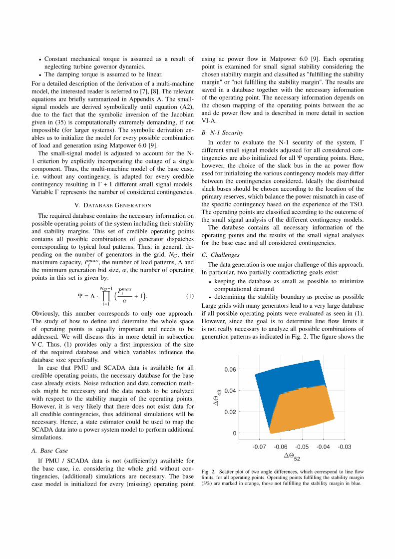
• Constant mechanical torque is assumed as a result ofneglecting turbine governor dynamics.
• The damping torque is assumed to be linear.For a detailed description of the derivation of a multi-machinemodel, the interested reader is referred to [7], [8]. The relevantequations are briefly summarized in Appendix A. The small-signal models are derived symbolically until equation (A2),due to the fact that the symbolic inversion of the Jacobiangiven in (35) is computationally extremely demanding, if notimpossible (for larger systems). The symbolic derivation en-ables us to initialize the model for every possible combinationof load and generation using Matpower 6.0 [9].
The small-signal model is adjusted to account for the N-1 criterion by explicitly incorporating the outage of a singlecomponent. Thus, the multi-machine model of the base case,i.e. without any contingency, is adapted for every crediblecontingency resulting in � + 1 different small signal models.Variable � represents the number of considered contingencies.
V. DATABASE GENERATION
The required database contains the necessary information onpossible operating points of the system including their stabilityand stability margins. This set of credible operating pointscontains all possible combinations of generator dispatchescorresponding to typical load patterns. Thus, in general, de-pending on the number of generators in the grid, NG , theirmaximum capacity, Pmax
i , the number of load patterns, ⇤ andthe minimum generation bid size, ↵, the number of operatingpoints in this set is given by:
= ⇤ ·NG�1Y
i=1
⇣Pmaxi
↵+ 1⌘. (1)
Obviously, this number corresponds to only one approach.The study of how to define and determine the whole spaceof operating points is equally important and needs to beaddressed. We will discuss this in more detail in subsectionV-C. Thus, (1) provides only a first impression of the sizeof the required database and which variables influence thedatabase size specifically.
In case that PMU and SCADA data is available for allcredible operating points, the necessary database for the basecase already exists. Noise reduction and data correction meth-ods might be necessary and the data needs to be analyzedwith respect to the stability margin of the operating points.However, it is very likely that there does not exist data forall credible contingencies, thus additional simulations will benecessary. Hence, a state estimator could be used to map theSCADA data into a power system model to perform additionalsimulations.
A. Base Case
If PMU / SCADA data is not (sufficiently) available forthe base case, i.e. considering the whole grid without con-tingencies, (additional) simulations are necessary. The basecase model is initialized for every (missing) operating point
using ac power flow in Matpower 6.0 [9]. Each operatingpoint is examined for small signal stability considering thechosen stability margin and classified as "fulfilling the stabilitymargin" or "not fulfilling the stability margin". The results aresaved in a database together with the necessary informationof the operating point. The necessary information depends onthe chosen mapping of the operating points between the acand dc power flow and is described in more detail in sectionVI-A.
B. N-1 SecurityIn order to evaluate the N-1 security of the system, �
different small signal models adjusted for all considered con-tingencies are also initialized for all operating points. Here,however, the choice of the slack bus in the ac power flowused for initializing the various contingency models may differbetween the contingencies considered. Ideally the distributedslack buses should be chosen according to the location of theprimary reserves, which balance the power mismatch in case ofthe specific contingency based on the experience of the TSO.The operating points are classified according to the outcome ofthe small signal analysis of the different contingency models.
The database contains all necessary information of theoperating points and the results of the small signal analysesfor the base case and all considered contingencies.
C. ChallengesThe data generation is one major challenge of this approach.
In particular, two partially contradicting goals exist:• keeping the database as small as possible to minimize
computational demand• determining the stability boundary as precise as possible
Large grids with many generators lead to a very large databaseif all possible operating points were evaluated as seen in (1).However, since the goal is to determine line flow limits itis not really necessary to analyze all possible combinations ofgeneration patterns as indicated in Fig. 2. The figure shows the
-0.07 -0.06 -0.05 -0.04 -0.03
52
0
0.02
0.04
0.06
43
Fig. 2. Scatter plot of two angle differences, which correspond to line flowlimits, for all operating points. Operating points fulfilling the stability margin(3%) are marked in orange, those not fulfilling the stability margin in blue.

Fig. 3. Step size (d) of simulation needs to be chosen in a way that thearea of stable operating points (purple) is maximized while the area ofuncertain/potentially stable operating points (grey) which lies between stable(blue) and unstable (red) operating points is minimized.
area of operating points fulfilling the stability margin (orange)and the area of operating points not fulfilling the stabilitymargin (blue). Thus, by focusing on the stability boundaryand neglecting operating points far away from the boundarythe database can be reduced. This can be achieved by e.g. usingthe existing knowledge of experienced engineers at TSOs.
Furthermore, we want to determine the stability boundaryas accurately as possible, in order to provide the most cost-efficient line flow limits without increasing risk. Thus, in thearea around the stability boundaries the step size between theoperating points should be smaller than the minimum bid sizeleading to an even larger database. Hence, the appropriatedistance between the different simulated operating points isan important issue. It was shown in [10] that eigenvaluesassociated with Hopf bifurcations vary smoothly with respectto power changes. Nonetheless, Fig. 3 indicates that it isimportant, in particular at the boundary, to find the step sized of active power variation �P, which minimizes the area ofnot simulated operating points (i.e., grey area), whose stabilityis uncertain. Smaller distances lead to a larger data sampleand are computationally more demanding, whereas largerdistances lead to inaccuracies and potentially higher costs dueto more conservative boundaries. The computational efficiencydepends on the method used for the database generation,including the appropriate choice of operating points to beanalyzed. Although carried out offline, the database generationmay represent a major obstacle. In future work we plan oninvestigating methods to minimize the computational demandwithout losing accuracy.
VI. FEATURE SELECTION AND KNOWLEDGE EXTRACTION
The creation of the database is followed by the featureselection, which determines the level of conservatism of theline flow limits. The knowledge extraction constitutes the finalstep in the offline derivation of the decision rules.
A. Feature Selection
In order to be able to substitute simulation data with PMUdata in the future, only easily accessible variables should be
considered as inputs. The goal is to incorporate all securityconsiderations into conditional transfer limits, which providethe boundaries for the market and keep the complexity of theSC-OPF comparably low.
The transfer limits for the market-clearing are derived fromthe data obtained by using ac power flow as initialization forthe small signal models. Since market operations are usuallybased on linearized dc power flow equations, the main issuehere is to achieve a good mapping between the ac power flowoperating points and the dc power flow points. This mappingis needed due to the fact that for the same generation patternthe line flows in an ac power flow can differ (significantly)from the ones in a dc power flow depending on the voltagesand angles in the system. Thus, a better mapping of operatingpoints leads to more accurate and less conservative line flowlimits.
We focused on three different approaches to determine theactive power transfer limits. Eq. (2) shows the active powertransfer over a line n � m based on the full AC power flowequations.
Fnm = |Vn | |Vm | (Gnm cos(✓n � ✓m) + Bnmsin(✓n � ✓m)) , (2)
where Fnm and Vn denote the active power flow between nodesn and m and the voltages at node i, respectively. Gnm and Bnm
correspond to the conductance and susceptance of the line.1) Standard DC Approximation: The standard dc approxi-
mation is based on the following assumptions:• the resistance of the lines is very small compared to the
reactance resulting in: G = 0 and Bnm =�1xnm
• the angle difference between adjacent nodes is smallallowing for the sine to be replaced by its argument
• voltage magnitudes |Vn | are equal to 1 p.u..The line flows are then given by:
Fnm =✓n � ✓m
xnm. (3)
2) Less conservative approximation: More accurate lineflows can be computed if nodal voltage magnitudes and thesine of the angle difference are accounted for:
Fnm =|Vn | |Vm | sin(✓n � ✓m)
xnm. (4)
3) Exact Mapping of DC and AC operating points: Themost precise mapping of the dc and ac operating points hasbeen achieved by incorporating the mapping into the datageneration. We derived the line losses of the ac power flow ofeach generation pattern and included them as additional loadsin a subsequent dc power flow. The losses are added to thenodes in the following way:
PLoss,n =12 ·X
m2In
⇣Fnm + Fmn
⌘, (5)
where Fnm and Fmn represent the line flows obtained fromthe ac power flow analysis and In denotes the set of nodesconnected to node n. The dc power flow is thus augmentedby the loss approximation of the corresponding ac power flow

and the obtained line flows of the dc power flow represent anexact mapping of operating points.
B. Knowledge ExtractionThis paper proposes classification trees as knowledge ex-
traction/classification methods. A classification tree is a subsetof decision trees (DT) where the decision outcome, called"target variable", can take a finite set of values. A completeintroduction to DT theory for power systems can be found in[11]. Within the generated databases containing all operatingpoints, we distinguish between those "fulfilling the stabilitymargin" and those "not fulfilling the stability margin". TSOsrequire stability margins to ensure sufficient damping of os-cillations. The classification tree is used to reveal patterns ofthe interconnection between observation attributes and targetvariables with the goal of using these patterns as decision rulesto predict the decision outcome of new observations. Theseattributes of observations used as decision variables are called"predictors". A simple example of a DT is shown in Fig. 4. Itcontains nodes, branches and terminal decisions. At each nodea test of a predictor splits the data set into subsets accordingto the test result. The branches connecting this node with thenodes one level below represent the possible test outcomes.The leaf nodes with terminal decisions constitute the finalclassification of the input observation. The use of a DT insteadof other data mining or machine learning techniques providesa better understanding of the entire system’s small-signalstability and what influence different parts of the system have.Moreover, we can define conditional transfer limits by using anappropriate feature selection and associating all full DT pathsfrom the root to the leaves with binary decision variables. Theoptimal dispatch is then chosen by allowing only one path tobe activated.
Note that before training the DT, the database should be an-alyzed with respect to the potential problem of skewed classes,i.e. it needs to be examined whether one class ("fulfillingthe stability margin" / "not fulfilling the stability margin") is
F4�3 � �71.8 MW ?
F10�9 � �44.51 MW ?
F4�3 � �74.73 MW ?
Yes
Yes
YesNo
No
Yes
No
No
F8�7 � 11.77 MW ?
not fulfilling stability margin
fulfilling stability margin
not fulfilling stability margin
not fulfilling stability margin
not fulfilling stability margin
Fig. 4. A simple example of a decision tree
significantly over-represented compared to the other. If this isthe case, three options exist: (a) limiting the number of theover-represented class by neglecting the appropriate amountof samples, (b) over-sampling the minority class or (c) raisingthe cost of misclassifying the minority class. While option (a)might leave out exactly the most important information closeto the stability boundary, (b) degrades the learning speed dueto duplicate instances. Option (c) allows to introduce risk-aversion, which might lead to more conservative and lesscost-efficient transfer limits. This however, can be improvedthrough smaller step sizes during the analysis described inV-C.
The DT is trained using a subset of the whole database,called training set A. The derived rules are tested using anothersubset B of the database with A [ B = ;.
It is worth mentioning that although DTs achieve pretty highaccuracies, there will always be misclassifications, which intheory could cause unstable solutions of the proposed data-driven SC-OPF. However, actions have been taken to mini-mize, if not completely avoid this threat. First, by increasingthe cost for misclassifications of unstable cases we reduce themisclassifications in this direction. This, however, might alsocause less cost-efficient line flow limits. Further, by choosing acertain stability margin and differentiating between "fulfillingthe stability margin" and "not fulfilling the stability margin",instead of "stable" and "unstable", we can reduce the riskeven further, since misclassifications do not necessarily leadto instability, but just to lower stability margins than required- at least in all scenarios tested in this paper. This is discussedin more detail in section VIII-B.
Finally, in order to avoid over-fitting, the obtained trees needto be pruned appropriately. Different pruning techniques willbe investigated in future work.
VII. OPF IMPLEMENTATION
As usual in market applications, the network is modeledusing a linear DC approximation.
A. Standard DC Optimal Power Flow (DC-OPF)The objective function to be minimized represents the total
generation cost (6). The optimization problem is formulatedas follows:
minPG
NGX
i=1cG,iPG,i, (6)
s.t.NGX
i=1PG,i �
NBX
n=1PD,n = 0, (7)
� FmaxL PTDF ·
⇣PG � PD
⌘ Fmax
L (8)
0 PG PmaxG , (9)
where symbols in bold denote matrices or vectors. NG andNB refers to the number of generators and buses, respectively.Equality constraint (7) ensures balance between total genera-tion and total demand. Demand PD is assumed to be inelasticand thus, not a decision variable. Power Transfer Distribution

Factors (PTDF) are used to translate net injections into lineflows, which are constrained to their line flow limits Fmax
L,i inEq. (8). Eq. (9) constrains the generator outputs below capacitylimits.
B. Security Constrained OPF (SC-OPF)
The SC-OPF ensuring N-1 security and small signal stabilityextends the standard DC-OPF by including additional con-straints representing conditional line transfer limits, derivedfrom the decision tree in Section VI-B. The DT is incorporatedinto the optimization using Mixed Integer Linear Programming(MILP). Each full path p from the root to a leaf node isrepresented by a set of minimum and maximum line transferlimits Fmin
L,p and FmaxL,p , respectively. Eq. (8) is replaced by:
PTDF ·⇣PG � PD
⌘ Fmax
L,p yp + FmaxL (1 � yp) 8p 2 P (10)
PTDF ·⇣PG � PD
⌘� Fmin
L,p yp � FmaxL (1 � yp) 8p 2 P, (11)
where P is the set of full paths representing the decisiontree. Note that the conditional line transfer limits do not limitthe flows symmetrically as in Eq. (8), i.e. the lower bounddoes not necessarily correspond to the negative upper bound.Each path is associated with a binary variable yp , which, ifchosen, ensures the activation of the corresponding conditionalline flow limits or otherwise, leaves the usual line flow limitsunchanged. The number of binary variables corresponds to thenumber of leaf nodes in the DT. The choice of line limits toone path only is constrained through
Pp yp = 1.
C. Matching of SC-OPF and Database
In contrast to the operating points saved in the database,losses are not inherently considered in the standard DC-OPF orSC-OPF described above. Thus, the operating points resultingfrom the OPFs need to be matched with the ones saved inthe database by incorporating losses. Due to the fact that theoptimal power flow is not known prior to delivering the lineflow limits and the line flows and losses vary depending on thegeneration pattern, an initial best guess of the optimal operat-ing point is crucial to achieve a good matching. By searchingthe database for the cheapest operating point (assuming thatcosts are known a priori), which fulfills the stability marginand meets the load level, we found a "best guess" operatingpoint, whose losses were incorporated in the standard DC-OPF and the SC-OPF according to (5). The losses of the"best guess" OP are determined through an ac power flowanalysis. The DC-OPF and SC-OPF are thus augmented by aloss approximation and yield more realistic results.
VIII. CASE STUDY
The proposed method ensuring small signal stability and N-1 security is applied to the IEEE 14 bus test system shown inFig. 5. All parameters are given in the appendix.
The small signal models were derived using Mathematica,the initialization and small signal analysis were carried outusing Matlab and Matpower 6.0 [13]. All DC-OPF simulationswere carried out in Python using the Gurobi Optimizer [14].
A minimum damping ratio of 3% is chosen as stabilitymargin. We chose to require the same minimum damping ratioalso for the steady states obtained after an outage of a singleelement during the N-1 security analysis. However, this couldalso be chosen differently by e.g. allowing lower dampingratios after certain faults.
The system has been simulated for several load levels(±20%) and various step sizes between the generation patterns.Generator g1 has been chosen as the slack bus, also in all N-1scenarios, due to the small size of the other generators. Sincethe IEEE 14 Bus system is not N-1 stable, a few contingenciesand reactive power limits could not be considered for the N-1 security assessment. All line faults have been consideredexcept for a fault on the line connecting bus 1 and bus 2. Allbus faults have been analyzed, except for a fault at bus 1 andbus 2. These contingencies could not be considered becauseeither they lead to instability / violation of the AVR limits forany operating point of the considered load patterns (bus 1)or the stable operating points are not stable for the remainingcontingencies. Hence, this would leave us with an empty setof feasible operating points and therefore we had to neglectthese contingencies.
First, we will compare the results of the novel data drivenSC-OPF, when using different features for mapping the op-erating points of ac and dc power flows. Then, we willinvestigate the impact of various step sizes between thegeneration patterns on the results of the data-driven SC-OPF,i.e. different accuracies and database sizes. Finally, we willdiscuss additional benefits of data-driven approaches.
A. Comparison between Standard DC-OPF and Data-drivenSC-OPF using different Mapping Approaches
The comparison between the data-driven SC-OPFs usingdifferent mapping approaches is done using a 2.5 MW stepsize during the data generation. Table I lists the results of both
Fig. 5. IEEE 14 Bus System [12].

TABLE IRESULTS OF STANDARD DC-OPF AND DATA-DRIVEN SC-OPF USING DIFFERENT MAPPING APPROACHES
DC-OPF Best Guess SC-OPF SC-OPF SC-OPF(w. losses) (Data Based) (clas. DC) (less con. DC) (exact)
Dispatch (MW) 1. Run 2. Run 1. Run 2. Run 1. Run 2. Rung1 275.5509 183.73 165.962 165.262 176.535 176.297 184.106 184.127g2 0 55 60 60 60 60 60 60g3 0 27.5 26.603 26.671 22.51 22.616 24.628 24.906g4 0 2.5 16.17 15.687 9.689 9.582 0 0g5 0 0 0 0 0 0 0 0
Total Cost (e) 2755.5 2981.1 3091.63 3077.21 3022.56 3019.9 2960.48 2964.87Min. damping ratio (%) -20.33% 4.07% 9.73% 9.59% 6.59% 6.57% 2.98% 3.05%
Cost of Security (e) - 225.59 336.12 321.7 267.05 264.39 204.97 209.36
the standard DC-OPF and the SC-OPF using different featuresof the database, in particular the three different mappingapproaches described in VI-A. Additionally, the database bestguess operating point is listed, which is used for determiningthe losses to be incorporated in the OPFs.
Table I shows that the standard DC-OPF fails to ensure N-1 security, since for this generation pattern the most criticalpair of eigenvalues of the most critical fault in the N-1 securityassessment (Fault at Bus 5) indicates a negative damping ratio,i.e. instability. The most critical eigenvalues of those faults inthe N-1 security assessment violating the minimum requiredstability margin of 3% are shown in Fig. 6. It shows that allSC-OPFs ensure N-1 security of the system by a change ofthe generation pattern resulting in the most critical eigenvaluesof the same faults being moved into the left half-plane, i.e. inthe safe area with a minimum damping ratio larger than therequired stability margin.
The figure visualizes also that the operating points obtainedby the SC-OPFs using different mapping approaches varyby their minimum damping ratio, which reflects the moreconservative line flow limits in case of both dc approximationscompared with the exact mapping approach. These moreconservative line flow limits lead consequently also to highercost of security, as indicated in Tab. I.
Finally, Tab. I indicates also the importance of the matchingof operating points, i.e. the importance of the best guess ofpower flow. While in the 1st run column of the SC-OPFsthe losses are implemented according to the data based bestguess, the 2nd run uses the result of the 1st run as initial bestguess. In this case, the loss distribution and therefore the lineflows are more accurate, i.e. more comparable to dc powerflows obtained in the data generation. Thus, the matching ofoperating points is improved which leads to better results inall cases.
B. Comparison of different Step Sizes between the analyzedGeneration Patterns
Table II shows various aspects and results for the databasegeneration of a SC-OPF comparing different step sizes usedduring data generation.
Obviously, following the simple approach with constant stepsize between each analyzed generation pattern the databasesize grows as indicated in (1). However, as discussed in V-C
there exist improvement potential on which we will focus infuture work. Further, the required simulation time is relatedto the database size. It naturally increases with the number ofoperating points. The database was generated using 20 coresin parallel on the high performance computing farm at DTU.
The tree accuracy is also related to the available databasesize. In general, it should be easier to differentiate betweenthe case fulfilling the stability margin and not fulfilling thestability margin if there is a higher step size in betweenthe analyzed generation patterns. This is reflected in Tab. IIby the decreasing number of false prediction with risk withincreasing step size. False predictions with risk are thosepredictions which falsely predict operating points not fulfillingthe stability margin as "fulfilling the stability margin". Theresults show that the chosen risk averse approach, discussedin section VI-B, which increases the costs of this kind offalse predictions, works fine since the vast majority of falsepredictions is made in the other direction. This is indicated bythe small percentage of these kind of false predictions withinthe total number of false predictions.
However, on the other hand there exists also less data fortraining which may decrease the tree accuracy as indicated inTab. II. This also leads to potentially shorter trees resembledby a smaller number of binary variables and a faster executiontime, shown in Tab. III.
Table II supports also the discussion in section V-C aboutthe importance of the step size, in particular close to theboundary. This is reflected by the significantly increasingnumber of risky false predictions with increasing step sizewhen the DTs are tested with the database of the other stepsizes. Here, the DTs of 2.5 MW and 5 MW are tested onthe 1 MW database while the 1 MW DT is tested on the2.5 MW database. It is shown that a wider step size in betweenthe generation patterns leads to potentially more and unsaferrisky false predictions, as indicated by the increasing numberof false predictions with risk and the decreasing minimumdamping ratio of those false predictions.
However, the tree accuracy should not be confused withthe cost efficiency of the line flow limits resembled by thegeneration costs. All SC-OPFs with the different step sizeslead to points fulfilling the required stability margin. Here, weused two runs using the 1st run as initialization for the 2nd runas described in the previous subsection.

Fig. 6. Visualization of the location of the most critical eigenvalues in the N-1 security analysis for the DC-OPF (black), SC-OPF using the classical dcapproximation approach (red), SC-OPF using the less conservative dc approximation approach (purple) and SC-OPF using the exact mapping approach. Thefaults corresponding to the critical eigenvalues are denoted in grey. The small signal models resembling the faults differ by the base case in that way thatthey consider the disconnection of the corresponding elements. Any contingency not violating the stability margin requirement of 3% is neglected.
TABLE IIDATABASE ANALYSIS FOR DIFFERENT STEP SIZES
step size 1 MW 2.5 MW 5 MW# operating points, 2515396 75625 6084
Simulation time 8.17 h 15.11 min 1.29 min
Training setTree accuracy 99.86% 99.77% 98.9%
False prediction w. risk 55 1 0% of false pred. 1.54% 0.57% 0Min. damp. ratio 2.89% 2.76% -of risky false pred.
Using database of other step sizes as test setTree accuracy 99.79% 99.03% 97.64%
False prediction w. risk 36 9111 13298% of false pred. 23.08% 37.34% 22.44%Min. damp. ratio 2.73% 1.37% 0.82%of risky false pred.
Table III shows that in fact the SC-OPF using the widest stepsize leads to the cheapest operating point. This is due to thewider uncertain area in between the analyzed operating points(see Fig. 3) resulting in more relaxed line flow limits. However,the difference is very small (max. 6.2e). It is important toemphasize that, although the widest step size achieves the bestperformance in this particular scenario, smaller step sizes aresafer as discussed before and indicated in Tab. II.
TABLE IIIDATA-DRIVEN SC-OPF RESULTS FOR DIFFERENT STEP SIZES
Data-driven SC-OPFstep size 1 MW 2.5 MW 5 MWBin. var. 616 35 28
Exec. time 26.64s 1.08s 0.98sGeneration cost 2965.4e/h 2964.9e/h 2959.2e/h
Minimum margin 3.03% 3.05% 3.42%Generation (MW)
g1 187 193.50 183.3213g2 60 42.72 58.0360g3 18.7 24.73 27.46g4 3.7 0 0g5 0 0 0
C. Additional Benefit of the Data-driven Approach
Besides the possibility to deliver cost-efficient line flowlimits the data-driven approach provides the additional benefitof serving as an easy accessible source of knowledge for theTSO which could be useful during normal operation but inparticular during training of new employees.
First, similar as visualized in Fig. 6, the database enables theuser to get an overview which faults are the most critical forany operation point. Unlike for the specific generation patternprovided by the DC-OPF this may only be a single fault.
Second, the use of a DT instead of other knowledge extrac-tion methods provides the user with additional comprehensibleknowledge about safe and unsafe line flows in the system. Byjust visualizing the tree as e.g. in Fig. 4 the user is able to

access this valuable comprehensive information, which wouldnot be possible by most other knowledge extraction methods,which work mostly like a black-box from the outside.
IX. CONCLUSION
A novel data-driven SC-OPF method ensuring small-signalstability has been proposed. It uses a small-signal model fordata generation, and classification trees for the knowledgeextraction. Conditional transfer limits in the form of decisionrules are derived from the decision tree and implemented inthe OPF problem by means of Mixed Integer Linear Program-ming. We investigated the impact of different features for themapping of operating points from the ac to the dc space andemphasized specific aspects of this method, e.g. the importanceof matching the operating points. Additionally, we discussedthe challenges of this method, such as the problems arisingwhen using a wide step size (in particular at the stabilityboundary). Finally, we emphasized the additional benefits ofthe data-driven approach as it serves as a source of knowledgeof the system. The case study indicates a good performance.
ACKNOWLEDGMENT
This work is supported by the EU project Best Paths underthe 7th Framework Programme, Grant Agreement No. 612748and by the ForskEL-projekt 12264 Best Paths for DK.
APPENDIX
A. Small-Signal Model1) Notation:
↵ik Angle of the ik-th entry of the network busadmittance matrix.
�i Rotor angle of generator i.!i Rotor speed of generator i.!s Synchronous rotor speed.⌦ Base synchronous frequency. d,qi Magnetic flux of generator i.Di Additional damping Torque of generator i.e0d,qi Transient voltage of generator i in d-/q-axis.e f di Field voltage of generator i.Hi Inertia constant of generator i.id,q Current of generator i in d-/q-axis.KAi Amplifier gain of generator i.KEi Self-excited constant used for of generator i.KFi Stabilizer gain used for of generator i.m Number of machines.n Number of buses.rFi Output of the stabilizer of generator i.rai Armature resistance of generator i.SEi (E f di ) Saturation function of generator i.TAi Time constant of the voltage regulator of gen. i.T 0d0,q0i Transient time const. of d-/q-axis of generator i.T 00d0,q0i Sub-transient time const. of d-/q-axis of gen. i.TEi Exciter time constant of generator i.TFi Time constant of the stabilizer of generator i.TMi Mechanical torque of generator i.vre fi Reference voltage of generator i.
vRi Output of the voltage regulator of generator i.vR,max Limit of the voltage regulator of generator i.x 0d,qi Transient reactance of generator i in d-/q-axis.xli Leakage reactance of generator i in d-/q-axis.xd,qi Synchronous reactance of gen. i in d-/q-axis.x 00d,qi Sub-transient reactance of gen. i in d-/q-axis.Yik Magnitude of the ik-th entry of the network bus
admittance matrix.2) Model: The multi-machine model can be described
with 10m differential algebraic equations (12)-(23) and 6malgebraic equations: 2m equations defining stator fluxes (24)-(25), 2m stator equations (26)-(27), and 2n network equations(28)-(29). For a more detailed desciption the interested readeris referred to [8].
d�idt= ⌦(!i � !s) (12)
d!i
dt=
12Hi
⇣TMi � d,iiq,i + q,iid,i � Di (!i � !s)
⌘(13)
de0qidt= (�e0qi � (xdi � x 0di )(idi � �d2,i
00d,i (14)
� (1 � �d1,i)id,i + �d2,ie0q,i) + e f di )/T0d0i (15)
de0didt= (�e0di � (xqi � x 0qi )(iqi � �q2,i
00q,i (16)
� (1 � �q1,i)iq,i + �q2,ie0d,i))/T 0q0i (17)d 00di
dt= (� 00d,i + e0q,i � (x 0d,i � xl,i)id,i)/T 00d0,i (18)
d 00qidt= (� 00q,i + e0d,i � (x 0q,i � xl,i)iq,i)/T 00q0,i (19)
dvhidt=
vb,i � vh,iTr,i
(20)
dvRi
dt=
KAi (vre f ,i � vh,i � r f ,i � K f , i
Tf , ie f di ) � vRi
TAi
(21)
drFi
dt= � rFi
TFi
� KFi
(TFi )2 e f di (22)
de f di
dt= �KEi + SEi (e f di )
TEi
e f di +vRi
TEi
(23)
0 = d,i + x 00d,iid,i � �d1,ie0q,i � (1 � �d1,i) 00d,i (24)0 = q,i + x 00q,iiq,i + �q1,ie0d,i � (1 � �q1,i) 00q,i (25)0 = ra,i + id,i + q,i + vd,i (26)0 = ra,i + iq,i � d,i + vq,i (27)
for i = 1, 2, 3, . . . ,m.and
0 = PGi + PLi (Vi) �Pn
k=1 ViVkYik cos(✓i � ✓k � ↵ik ) (28)0 = QGi +QLi (Vi) �
Pnk=1 ViVkYik sin(✓i � ✓k � ↵ik ) (29)
for i = 1, 2, 3, . . . ,m,m + 1, . . . , n.with
PGi = IdiVi sin(�i � ✓i) + IqiVi cos(�i � ✓i) (30)QGi = IdiVi cos(�i � ✓i) � IqiVi sin(�i � ✓i) (31)

for i = 1, 2, 3, . . . ,m.The equations can be combined, linearized and rewritten inmatrix notation as:
2666664�X00
3777775=
2666664A B1 B2C1 D11 D12C2 D21 D22
37777752666664�X�Z1�Z2
3777775+
2666664E100
3777775�U (32)
with X = [XT1 , . . . ,XT
m]T andXi = [�i !i e0qi e0di
0d,i
0q,i vh,i vRi rFi e f di ]T including
the machine state variables and �Z1 = [✓1 vb,1 . . . vb,m]Tincluding the voltage angle of the slack bus as well asthe voltage magnitudes of the generator buses. �Z2 =[✓2 . . . ✓n vb,m+1 . . . vb,n]T includes the voltage angles of theremaining buses and the voltage magnitudes of the load buses.The system matrix Asys with dimension 10m x 10m fulfillingthe equation
�X = Asys�X + E�U (33)
can be obtained as:
Asys = A � [B1 B2][JAE ]�1"C1C2
#(34)
with
[JAE ] =
"D11 D12D21 D22
#(35)
representing the network algebraic Jacobian.
B. Parameters
TABLE IVGENERATOR DATA ADAPTED FROM [8]
Machine and AVR parametersParameters g1 g2 g3 g4 g5
MVA 615 60 60 25 25ra (pu) 0.0031 0.0031 0.0031 0.0041 0.0041H (s) 5.148 6.54 6.54 5.06 5.06
D (pu) 2 2 2 2 2xd (pu) 0.8979 1.05 1.05 1.25 1.25x0d (pu) 0.2995 0.1850 0.1850 0.232 0.232xq (pu) 0.646 0.98 0.98 1.22 1.22x0q (pu) 0.646 0.36 0.36 0.715 0.715x00q (pu) 0.4 0.13 0.13 0.12 0.12xl (pu) 0.2396 0 0 0.134 0.134T0do (s) 7.4 6.1 6.1 4.75 4.75T00do (s) 0.03 0.04 0.04 0.06 0.06T0qo (s) 0.31 0.3 0.3 1.5 1.5T00qo (s) 0.033 0.099 0.099 0.21 0.21
Ka 120 20 20 20 20VRmax (pu) 9.9 2.05 1.7 2.2 2.2
Ta (s) 0.02 0.02 0.02 0.02 0.02Ke (pu) 1.0 1.0 1.0 1.0 1.0Te (s) 0.19 1.98 1.98 0.70 0.70Kf (s) 0.0012 0.001 0.001 0.001 0.001Tf (s) 1.0 1.0 1.0 1.0 1.0
Ae 0.0006 0.0006 0.0006 0.0006 0.0006Be (1/pu) 0.9 0.9 0.9 0.9 0.9
Economic dataclin (e/MWh) 10 12.5 15 17.5 20
REFERENCES
[1] R. Zárate-Miñano, F. Milano, and A. J. Conejo, “An OPF Methodologyto Ensure Small-Signal Stability,” IEEE Transactions on Power Systems,vol. 26, no. 3, pp. 1050–1061, 2011.
[2] J. E. Condren and T. W. Gedra, “Expected-Security-Cost Optimal PowerFlow With Small-Signal Stability Constraints,” IEEE Transactions onPower Systems, vol. 21, no. 4, pp. 1736–1743, 2006.
[3] Y. Xu, Z. Y. Dong, R. Zhang, and K. P. Wong, “A DecisionTree-Based Online Preventive Control Strategy for Power SystemTransient Instability Prevention,” International Journal of SystemsScience, vol. 45, no. 2, pp. 176–186, 2014. [Online]. Available:http://dx.doi.org/10.1080/00207721.2011.626906
[4] M. Chávez-Lugo, C. R. Fuerte-Esquivel, C. A. Canizares, and V. J.Gutierrez-Martinez, “Practical Security Boundary-Constrained DC Op-timal Power Flow for Electricity Markets,” IEEE Transactions on PowerSystems, vol. 31, no. 5, pp. 3358–3368, Sept 2016.
[5] P. Kundur, J. Paserba, V. Ajjarapu, G. Andersson, A. Bose, C. Canizares,N. Hatziargyriou, D. Hill, A. Stankovic, C. Taylor, T. Van Cutsem, andV. Vittal, “Definition and Classification of Power System Stability,” IEEETransactions on Power Systems, vol. 21, no. 3, pp. 1387–1401, 2004.
[6] C. Y. Chung, L. Wang, F. Howell, and P. Kundur, “GenerationRescheduling Methods to Improve Power Transfer Capability Con-strained by Small-Signal Stability,” IEEE Transactions on Power Sys-tems, vol. 19, no. 1, pp. 524–530, 2004.
[7] P. Sauer and M. Pai, Power System Dynamics and Stability, M. Horton,Ed. New Jersey: Prentice-Hall, Inc., 1998.
[8] F. Milano, Power System Modelling and Scripting. Springer-VerlagBerlin Heidelberg, 2010, no. 1.
[9] R. D. Zimmerman, C. E. Murillo-sánchez, R. J. Thomas, L. Fellow,and A. M. Atpower, “MATPOWER : Steady-State Operations , SystemsResearch and Education,” Power, vol. 26, no. 1, pp. 12–19, 2011.
[10] C. A. Cañizares, N. Mithulananthan, and F. Milano, “Linear PerformanceIndices to Predict Oscillatory Stability Problems in Power Systems,”IEEE Transactions on Power Systems, vol. 19, no. 2, pp. 1104–1114,2004.
[11] L. A. Wehenkel, Automatic Learning Techniques in Power Systems.Boston/London/Dordrecht: Kluwer Academic Publishers, 1998.
[12] S. Kodsi and C. Canizares, “Modeling and Simulation of IEEE 14-Bus System with FACTS Controllers,” University of Waterloo, Waterloo,Canada, Tech. Rep., 2003.
[13] R. D. Zimmerman, C. E. Murillo-Sanchez, and R. J. Thomas, “Mat-power: Steady-state operations, planning, and analysis tools for powersystems research and education,” IEEE Transactions on Power Systems,vol. 26, no. 1, pp. 12–19, Feb 2011.
[14] Gurobi Optimization, “Gurobi Optimizer Reference Manual,” 2015.[Online]. Available: http://www.gurobi.com


[Pub. F] Data-driven Security-Constrained AC-OPFfor Operations and Markets.
239

Data-driven Security-Constrained AC-OPF forOperations and Markets
Lejla Halilbasic, Florian Thams, Andreas Venzke, Spyros Chatzivasileiadis, Pierre PinsonCenter for Electric Power and Energy
Technical University of DenmarkKongens Lyngby, Denmark
{lhal, fltha, andven, spchatz, ppin}@elektro.dtu.dk
Abstract—In this paper, we propose a data-driven preventivesecurity-constrained AC optimal power flow (SC-OPF), whichensures small-signal stability and N-1 security. Our approachcan be used by both system and market operators for optimizingredispatch or AC based market-clearing auctions. We derivedecision trees from large datasets of operating points, whichcapture all security requirements and allow to define tractabledecision rules that are implemented in the SC-OPF using mixed-integer nonlinear programming (MINLP). We propose a second-order cone relaxation for the non-convex MINLP, which allowsus to translate the non-convex and possibly disjoint feasiblespace of secure system operation to a convex mixed-integerOPF formulation. Our case study shows that the proposedapproach increases the feasible space represented in the SC-OPF compared to conventional methods, can identify the globaloptimum as opposed to tested MINLP solvers and significantlyreduces computation time due to a decreased problem size.
Index Terms—Security-constrained OPF, small-signal stability,convex relaxation, mixed-integer non-linear programming.
I. INTRODUCTION
The Security-Constrained Optimal Power Flow (SC-OPF) isan important tool for power system operation and planning inorder to maintain power system security. The SC-OPF identi-fies optimal preventive control actions compliant with the N-1criterion, which ensure that the system can withstand the lossof any major component without violating system constraints.To this end, the constraint set of the conventional OPF isextended to include all considered contingency scenarios. TheSC-OPF can be applied at different planning stages to eitherdetermine an optimal and N-1 secure dispatch or to identifyoptimal redispatching actions closer to real-time. SC-OPFs arenon-linear and non-convex problems with both continuous anddiscrete variables. A major drawback of conventional SC-OPFalgorithms is the problem size and the negligence of stabilityrequirements [1], which cannot be expressed as linear or non-linear constraints and are therefore difficult to incorporatein a straightforward way. We address both challenges byusing a data-driven approach to preventive SC-OPF, whichis computationally tractable and based on decision trees thatcapture all N-1 and small-signal stability considerations. We
This work is supported by the European project BEST PATHS, Grant No.612748, and the ForskEL-project 12264 BestPaths for DK.
extend our previous work in [2] to an AC-OPF context with theintention to bridge the gap between power system operationand markets. We incorporate the knowledge extracted from thedata in the OPF using convex Mixed-Integer Programming(MIP) and relax the non-convex AC power flow equationsthrough a Second Order Cone (SOC) relaxation. We furtheruse the data to strengthen the relaxation. To the authors’knowledge, this is the first SC-OPF formulated as a Mixed-Integer Second Order Cone Program (MISOCP). Our approachcombines the advantages of convex MIP and data analytics andallows for a fast online solution. It extends the feasible spacein order to reflect the true non-convex area of operation andincludes the true optimal solution.
Research in SC-OPF algorithms has primarly investigatedthe N-1 security criterion and the reduction of the associatedcomputational burden, while less focus has been put on sta-bility requirements. However, only enforcing the N-1 criteriondoes not necessarily guarantee stability and hence, feasiblityof the solution. In order to translate small-signal stabilityconstraints to an OPF context, eigenvalue-sensitivities withrespect to OPF decision variables are used in [3] and [4].However, the required computational effort and the scalabilityof the proposed methods are still major challenges. In [5]hyperplanes are used to approximate the security boundaryand are incorporated in a DC-OPF. Operating points outsidethe convex space constructed by the hyperplanes are neglectedthough, increasing the likelihood of missing the optimal solu-tion.
The authors in [6] have identified the Security-ConstrainedAC-OPF as the “ultimate goal” for market software to beused by Independent System Operators (ISO) across the US.They outline the oversimplification of current software, oftenrequiring operator intervention and resulting in suboptimalsolutions due to inaccurate ISO models, which only useestimates for reactive power and voltage constraints. Improvedmodeling of voltage and stability constraints can lead to morerealistic dispatch decisions and better market signals, resultingin up to 10% cost savings worldwide [7]. The relative amountof potential savings will increase over the course of the comingdecades due to the ongoing electrification of the entire energyindustry. Electricity market participants in the US are alreadysaving over half a billion dollars annually as a result of theimplementation of MIP in day-ahead and real-time markets

[8]. Due to significant improvements since the 1990s, MIPhas been widely applied accross various industries, increasingexpertise, which only reinforces further development of MIPapproaches.
SOCP has gained increased attention for power systemapplications as it is computationally less demanding thanother relaxations, such as Semi-Definite Programming (SDP).Furthermore, it can be extended to mixed-integer problems,where the SDP relaxation fails even on small scales. MISOCPhas been introduced for OPF problems incorporating optimaltransmission switching and capacitor placement in [9] and[10]. The challenge in SOCP for OPF problems lies inconvexifying the coupling contraint between voltage anglesand SOC variables, which are introduced to remove the non-convexities arising from the AC power flow equations. Severalstrengthening techniques have been proposed in [9] and [10],which significantly contribute to the advancement of MISOCPfor real-life applications. However, these techniques still do notachieve to avoid optimality gaps and can be computationallydemanding, negating the benefit of convex MIP solvers.
The main contribution of this work is a data-driven SC-OPF algorithm formulated as a MISOCP, which (a) can beused by system operators as a security analysis tool (e.g., forredispatch), (b) can be used by market operators, approachingthe “ultimate goal” for market software [6], (c) incorporatesthe N-1 security criterion, (d) ensures small-signal stabilityfor the base case and all considered contingencies, (e) isscalable, (f) exploits the maturity of convex MIP solversin order to identify the optimal operating point within anon-convex and possibly disjoint stability area, (g) can besolved fast, as all computation related to the small-signalstability assessment and N-1 criterion is done offline and theOPF problem size is significantly decreased, (h) uses data tostregthen the relaxation, (i) can be solved to global optimalitywhere tested non-convex solvers fail and (j) alleviates the needfor iterative contingency analyses, which are currently used bysystem operators to define the boundaries of the secure systemspace.
The remainder of this paper is organized as follows: SectionII describes the proposed methodology including the deriva-tion of decision rules from data and focuses mainly on theincorporation of those rules in nonlinear and non-convex SC-OPF algorithms. Section III presents results from a case study.Section IV concludes and gives an outlook on future work.
II. METHOD
Our approach consists of an offline security assessment,which includes the database generation and derivation ofdecision rules, and an online SC-OPF, which incorporates thedecision rules ensuring power system security. The databasegeneration, stability analysis and knowledge extraction havebeen discussed in more detail in our previous work [2] and wewill only highlight the main features here. This work focusesmainly on the implementation of the decision rules in AC-OPFalgorithms and applications of the proposed method.
�✓4�3 � �12.28� ?
�✓10�9 � �3.76� ?
�✓4�3 � �12.78� ?
Yes
Yes
YesNo
No
Yes
No
No
�✓8�7 � �2.07� ?
unstablestable
stable
unstable
unstable
Figure 1. A simple illustrative decision tree.
A. Offline Security Assessment
A large database of operating points is created for variousload levels based on AC power flow calculations. All possiblegeneration patterns corresponding to the specified load levelsare evaluated using specified step sizes to discretize the spaceof possible dispatch combinations. In order to perform thesmall-signal stability assessment of the simulated operatingpoints, small-signal models are derived for the base case andall considered contingencies. A database is generated, whichcontains the operating points together with the information onwhether they are stable or unstable. Challenges related to thecomputational demand of the database generation, the appro-priate choice of discretization intervals and the determinationof the stability boundary have been addressed in [2]. Ongoingwork focuses on further improvements.
Once the database is generated, decision rules based onappropriate features, that need to be selected, can be derivedfor the OPF, which will lead the solution to a stable op-erating region. These features have to be easily accessiblein an AC-OPF formulation to allow for a fast online com-putation. Voltage angle differences along transmission linesare explicitly modeled in both the security analysis and theAC-OPF, representing coupling variables. Among the testedfeatures, they have proven to most efficiently capture allsecurity requirements and are thus chosen as features for theknowledge extraction (i.e., the derivation of the decision rules).Additionally, if approximations of the OPF are used, which donot explicitly model voltage angles, angle differences can betranslated to line capacity limits using appropriate mappingstrategies as explained in [2]. We employ decision trees (DTs)as the knowledge extraction method, as they are comprehen-sible and easy to interpret for the operator. They are trainedbased on the selected features. Moreover, the conditional rulesdefined by the DT can be directly incorporated through binaryvariables in an optimization problem. A simple illustrativeexample is shown in Fig. 1.
We refer to our previous work for details on the small-signal models, the DT generation including the reduction ofmislassifications and the dependence of the DT accuracy onthe database size/discretization [2].

B. Preventive SC-OPF - Current PracticeThe traditional preventive SC-OPF (PSC-OPF) aims at
finding the optimal least-cost dispatch ensuring N-1 security.It extends the conventional nonlinear and non-convex AC-OPF by including additional constraints to ensure feasibilityof the identified solution after the occurrence of any specifiedcontingency. The AC-OPF is given as follows:
minx
NGX
i=1
Ci
⇣PG
i
⌘, (1)
s.t. PG
i� PD
i= GiiV
2i
+NBX
j=1,j 6=i
ViVj
⇣Gij cos(✓ij) + Bij sin(✓ij)
⌘, 8i 2 N
(2)QG
i� QD
i= �BiiV
2i
+NBX
j=1,j 6=i
ViVj
⇣Gij sin(✓ij) � Bij cos(✓ij)
⌘, 8i 2 N ,
(3)x x x, (4)✓ref = 0, (5)
where x represents the set of optimization variables includingactive power generation PG, reactive power generation QG,voltage magnitudes V and voltage angles ✓. N denotes theset of buses. The objective function (1) minimizes activepower generation costs. Constraints (2) and (3) ensure activeand reactive power balance at all nodes, where Gij and Bij
represent the real and imaginary parts of the bus admittancematrix, respectively. Constraint (4) limits all decision variableswithin their upper and lower bounds. Equation (5) sets thevoltage angle of the reference bus to zero. Line flow limitsare not explicitly included here, as we derive limits from thesecurity analysis, which will be introduced later.
Control variables (e.g., active and reactive power genera-tion, transformer tap position etc.) in the PSC-OPF are notallowed to change from pre- to post-contingency states. Theproblem size of the OPF increases to Nc + 1 comparedto the conventional AC-OPF, where Nc denotes the numberof contingencies, rendering SC-OPFs computationally verydemanding. The computational burden of SC-OPFs, especiallyfor large systems with many considered contingencies, is amajor challenge. Another challenging factor is the inclusionof system dynamics, i.e. stability considerations, in SC-OPFalgorithms. Given that they cannot be incorporated as linearor nonlinear constraints in a straightforward way, commonpractice is to impose tighter constraints. Such conservativebounds on the feasible space should allow the system to returnto a steady-state equilibrium after a fault event, but also leadto costly and suboptimal solutions.
Net Transfer Capacities (NTC) constitute one example ofsuch conservatism. NTCs are maximum cross-zonal capaci-ties available for trade on the day-ahead market, which arederived based on the N-1 security criterion, accounting for
Figure 2. Security domain of Flow-Based Market Coupling (FBMC) andAvailable Transfer Capacity (ATC) [12]. ATCs are NTCs reduced by long-term capacity nominations.
thermal and stability limitations [11]. NTCs are fixed line flowlimits, which are determined by transmission system operators(TSOs) in each direction of cross-border lines prior to the day-ahead market-clearing. Improvements towards a more accuraterepresentation of the physical reality of power systems havebeen achieved by introducing Flow-Based Market Coupling(FBMC), where a simplified European network representationis accounted for in the market-clearing. Critical branches(CBs) inside of and between zones are identified, which couldpotentially be congested and limit the cross-border trade.All CBs are represented through Power Transfer DistributionFactors (PTDFs) and instead of assuming only one fixed NTCvalue for each cross-border line, all constraints imposed bythe CBs are considered. Thus, a larger secure domain isoffered to the market compared to static NTC approaches asdepicted in Fig. 2. The market is then able to determine theoptimal combination of commercial capacities between zones.Nonetheless, even flow based NTCs only capture one convexregion of the entire feasible space and do not represent thenon-convex reality of power system operations.
C. Improving the Preventive SC-OPF Using Data
To address the challenges described above, we propose adata-driven approach to SC-OPFs, which we introduced inprevious work [2]. Non-convex and discontinous feasibilityspaces are captured using decision trees, which define con-ditional constraints on appropriate decision variables, such asvoltage angle differences ✓ij = ✓i � ✓j along transmissionlines. Each branch p of the DT contains a set of minimum andmaximum voltage angle differences and leads to a differentregion of the feasibility space, one of which contains the least-cost, optimal solution. A visual illustration of our approach isdepicted in Fig. 3. Instead of defining bounds that containonly one of the three stable regions depicted in the shadesof blue, conditional rules allow to capture the entire feasibleregion within the red frame. The DT is incorporated in theSC-OPF using Mixed-Integer Programming (MIP). Each fullbranch is associated with a binary variable yp, which ifchosen, activates the corresponding upper and lower boundson angle differences, or otherwise, leaves the original boundsunchanged:

Figure 3. Illustrative example of non-convex space.
yp · ✓ij,p � (1 � yp) · ✓ij ✓ij yp · ✓ij,p + (1 � yp) · ✓ij ,
8(i, j) 2 L, 8p 2 P. (6)
L and P denote the set of lines and DT branches/paths,respectively. Only one DT branch, i.e. one set of minimumand maximum bounds on angle differences, can be chosen,which is imposed by adding constraint
Pp2P yp = 1.
The data-driven SC-OPF is thus formulated as a Mixed-Integer Non-linear Program (MINLP), which is a NP-hardproblem. One of the main contributions of this paper is that werelax the non-convex AC power flow equations using a SecondOrder Cone relaxation and obtain a SC-OPF formulated asa Mixed-Integer Second Order Cone Program (MISOCP),which is a convex mixed-integer program that can be solvedefficiently by already existing solvers.
D. Relaxing the Data-driven SC-OPFThe SOC formulation of the OPF problem is based on
[13], [14] and [9]. New variables are introduced to capturethe nonlinearities and non-convexities of the AC power flowequations: (a) ui := V 2
i, (b) cij := ViVj cos(✓ij) and (c)
sij := �ViVj sin(✓ij). The AC-OPF is transformed from thespace of x := {PG,QG,V, ✓} variables to the space ofxSOC := {PG,QG,u, c, s} variables and is given by:
minxSOC
NGX
i=1
Ci
⇣PG
i
⌘(7)
s.t. PG
i� PD
i= Giiui
+NBX
j=1,j 6=i
⇣Gijcij � Bijsij
⌘, 8i 2 N (8)
QG
i� QD
i= �Biiui
�NBX
j=1,j 6=i
⇣Gijsij + Bijcij
⌘, 8i 2 N (9)
cij = cji, sij = �sji, 8(i, j) 2 L (10)c2ij
+ s2ij
= uiuj , 8(i, j) 2 L (11)
Vi2 ui Vi
2, 8i 2 N . (12)
Active and reactive power generation are constrained by theirusual limits and are not explicitly mentioned. The non-convexquadratic equality constraint (11) is relaxed through a second-order cone constraint: c2
ij+ s2
ij uiuj . The SOC formulation
of the OPF problem (7)-(12) is exact for radial networks andthe optimal voltage angles can be recovered by solving:
✓i � ✓j = atan2(s⇤ji
, c⇤ij
), 8(i, j) 2 L, (13)
where ⇤ indicates the optimal solution obtained from theSOC-OPF. For meshed networks the above formulation is astrict relaxation, potentially resulting in solutions, which areinfeasible for the original AC-OPF [9]. Reintroducing voltageangle variables and constraint (13) in problem (7)-(12) wouldrender the SOC formulation exact for meshed networks, butalso non-convex. Various convex approximations of constraint(13) have been proposed [9], [13]. In this paper we use asequential conic procedure as proposed in [13], where thearctan function is linearized using a Taylor series expansion.
Conditional bounds on voltage angles are introduced usingbinary variables as described in Section II-C. Known limitson angle differences can also be used to define bounds on theSOC variables c and s:
yp · tan(✓ij,p) · cij � (1 � yp) · tan(✓ij) · cij sji,
8(i, j) 2 L, 8p 2 P, (14)
yp · tan(✓ij,p) · cij + (1 � yp) · tan(✓ij) · cij � sji,
8(i, j) 2 L, 8p 2 P. (15)
Otherwise, the SOC variables cij and sij are only constrainedby their implied upper and lower bounds ±ViVj , which inpractice can be very loose. In order to tighten the relaxation,we determine the values for cij and sij along all lines (i, j)for each operating point in the generated database and extracttheir minimum and maximum values to obtain tighter variablebounds.
III. CASE STUDY
We evaluate the performance of the proposed data-drivenSC-OPF ensuring small-signal stability and N-1 security ona modified version of the IEEE 14 bus test system [15].Our case study consists of three parts. First, we compare theconvex MISOCP formulation of the algorithm to a data-drivenMINLP implementation and a standard (i.e., not data-driven)preventive SC-OPF. Its low computational effort makes theproposed MISOCP suitable for AC based market-clearing auc-tions as envisaged in the US. In Europe, however, electricitymarkets will probably continue to rely on DC approximations.To this end, we show how the proposed method can also beused by TSOs for optimizing redispatching actions in order toensure N-1 security and small-signal stability after the market-clearing. Finally, we analyze how the data-driven approachcoupled with MIP notably extends the feasible space of theOPF.
The network data is given in [16] with some modificationsintroduced in [2]. Note that additionally the voltage setpointsof generators 4 and 5 are changed to 1.02 p.u. and 1.01p.u., respectively, and the reactive power of generator 1 islimited within ±990 Mvar. The considered contingenciesinclude all line and bus faults, except for faults at buses 1,

2 and 6. These would lead to either instability/AVR limitviolations or operating points, which are unstable for theremaining contingencies. Note that the standard PSC-OPFdoes not incorporate stability considerations, but only extendsthe constraint set to account for the defined N-1 contingencies.Bus 1 with generator g1 has been chosen as the slack busfor the base case and all N-1 cases. A step size of 0.5 MWwas chosen for discretizing the possible operating range andgenerating the database of operating points used for derivingthe decision tree. See [2] for a comparison of test cases withdifferent discretization intervals. The minimum damping ratioof an operating point over the base case and all N-1 cases isused as a metric for small-signal stability. As usual in powersystem operation, we define a security margin by requiring aminimum damping ratio of 3%. The derived DT contains 136leaf nodes, out of which 74 point to operating regions, whichare small-signal stable for the base case and all consideredcontingencies. Thus, 74 binary variables are used to defineconditional constraints on voltage angle differences along linesand incorporate the stable regions in the data-driven SC-OPF.Note that 1.34 million operating points have been evaluatedfor this case study, from which more than 88 000 fulfill therequired minimum damping ratio. We derive the DT based onthree different load levels (base case, ±20%). The data-drivenSC-OPF was performed for all three levels seperately. Giventhat they showed very similar results, we present our results forthe base case only. The voltage magnitude at generator busesis set to the corresponding generator voltage setpoint in orderto ensure an appropriate voltage profile, which is fundamentalto a secure system operation.
The small-signal analysis was performed using Matlab andMatpower 6.0 [16]. The MISOCP was implemented in Pythonusing the Gurobi Optimizer. The standard PSC-OPF (i.e.,NLP) and the MINLP implementation of the data-driven SC-OPF were carried out in GAMS. BONMIN and COUENNEwere used for solving the MINLPs, while CONOPT was usedfor the NLP.
A. Comparison of Preventive and Data-driven SC-OPFs
Table I lists the results of all three SC-OPF implementations.It can be observed that all implementations based on decisiontrees result in operating points, which exhibit minimum damp-ing ratios that are non-negative and are thus stable for the basecase and all considered N-1 contingencies. The solution of thestandard PSC-OPF however is unstable for a fault at bus 5 andline 1-2, respectively. Thus, the identified preventive controlactions do not fullfill the system’s security requirements andwould call for redispatching measures. As the PSC-OPF resultsin an operating point, which does not reflect the small-signalstability requirements, its total cost is lower than the othersolutions. All three data-driven implementations result in dif-ferent leaf nodes of the DT and thus in different regions of thefeasible space with various degrees of conservatism. Higherdamping ratios are also reflected by higher costs. All solutionsinclude a stability margin, but only the most conservative resultachieves a minimum damping ratio of more than 3%. This can
Figure 4. Non-convex security domain of the DT as a function of the angledifferences along lines 1 and 2. The blue shaded areas represent the stableregions defined by all DT branches. The darker the color, the more domains ofdifferent DT branches overlap. Note that the actual security domains coveredby the different leaf nodes do not overlap and might even be disjoint, whichhowever cannot be depicted by only two dimensions.
be explained by the fact that (a) the OPF is not limited to thespecified discretization intervals of 0.5 MW, as used for thedatabase generation and (b) DTs are not 100% accurate leadingto missclassifications. For cases, where the minimum dampingratio is a hard constraint, higher values can be required whenderiving the DT in order to avoid violations. Fig. 4 illustratesthe stable domain covered by all DT leaf nodes as a functionof the angle differences along lines 1 and 2. The rectanglesindicate the domains covered by the three different leaf nodesobtained from the data-driven SC-OPF implementations withthe location of the corresponding solution pointed out. It canbe seen that the stable domain is non-convex and that saferoperating points exhibiting higher damping ratios are locatedfurther away from the stability boundary.
The known scalability issues of COUENNE [10], which is aglobal optimization solver, lead to significantly higher execu-tion times compared to BONMIN, which employs heurisiticmethods for non-convex MINLPs. Also, the default settingsfor both solvers include a relative tolerance gap of 10%terminating the computation as soon as a solution is found,which lies within 10% of the true objective value. Thisexplains the choice of different leaf nodes. However, evenreducing the tolerance value does not change the outcomeindicating that neither of the solvers is able to provide thebest integer solution. The MISOCP is able to find the optimalinteger solution, which has been verified by manually impos-ing the bounds defined by each DT branch. Specifically, wesolved 74 AC-OPFs consecutively, one for each DT branchand imposed the corresponding bounds in order to determinethe DT branch, which contains the least-cost, optimal NLPsolution. Leaf node 104 actually contains the bounds, whichresult in the least-cost NLP solution. Notably, in this testcase, the MISOCP relaxation is exact, i.e. its solution isfeasible to the nonlinear, non-convex AC-OPF formulation andcorresponds to the global optimum of the non-convex problem.

TABLE IRESULTS OF STANDARD PSC-OPF AND DATA-DRIVEN SC-OPF IMPLEMENTED AS MINLP AND MISOCP.
Standard PSC-OPF Data-driven SC-OPFNLP MINLP MISOCPCOUENNE BONMIN
Cost (e/h) 3022.83 3445.09 3381.21 3365.95Runtime (s) 10.06 1000.16 96.16 5.58Iterations* (-) - - - 4Min. damping ratio (%) unstable 3.27 2.97 2.53Leaf node (-) - 31 133 104
* The number of iterations refers to the sequential conic algorithm used to approximate constraint (13) with a chosen convergence tolerance of 10�6.
Nonetheless, given that the MISOCP formulation is still arelaxation, identified solutions can be infeasible for the originalproblem. Therefore, we propose to use the MISOCP primarilyto identify the optimal DT branch and hence the linearbounds on the feasible space, such that the optimal solutionis included. Once these are known and the feasible spacehas been reduced, the integer variables can be omitted anda common AC-OPF (i.e., NLP) with the previously identifiedbounds on angle differences imposed as linear constraints canbe performed to identify feasible and secure preventive controlactions. The MISOCP solution serves as a lower bound andcan validate the optimality of the AC-OPF solution.
Table I also outlines the savings in online computation timeof the proposed SC-OPF method. The data-driven approachoutperforms the usual PSC-OPF by more than 40%, whileat the same time incorporating more security requirements.Naturally, the computation time depends on the size of the DTand the number of binary variables used to represent it. Eventhough introducing binaries increases the OPF complexity,this side effect is offset by a significantly reduced overallsize of the SC-OPF. While the PSC-OPF increases 32-foldwhen considering 31 contingencies, the proposed data-drivenapproach increases less than 4-fold for the same amount ofcontingencies. As indicated by constraint (6), (2 ⇥ NL ⇥NP + 1) additional linear inequality constraints are added,where NL and NP denote the number of network lines andDT paths, respectively. Hence, the complexity of the resultingMISOCP is primarily determined by the NL SOC constraintsc2ij
+ s2ij
uiuj and the NP binary variables.Furthermore, given that the problem is a convex MIP, which
can be solved efficiently by already existing solvers that areable to handle up to a few thousand binaries, the amount ofdiscrete variables is not expected to be an obstacle. Whilesolvers for MISOCPs have not yet reached the maturity ofMILP solvers, recent work has demonstrated how generalconvex MIPs can be solved to global optimality by a se-quence of MILPs using polyhedral outer approximations andcontinuous convex programs [17]. Large-scale instances of asimilar type of problem class with up to 3000 binary variablesand quadratic constraints have successfully been solved in[18] using state-of-the-art solvers and employing heuristicmethods. The size of the DT is directly determined by thesize of the dataset, which it is derived from. Hence, a moreefficient method to generate the database of operating points,appropriate pruning of the DT and techniques to decomposethe data-driven optimization are aspects that require a deeper
Figure 5. Visualization of redispatch and maximum convex security domain,which can be covered by one leaf node only.
analysis and are promising approaches to enhance the scala-bility performance of the method. One approach already usedin the industry would be to focus only on the most criticalN-1 contingencies and angle differences.
B. Optimizing RedispatchThe method can be used by TSOs to identify optimal
redispatching actions, where for example the market-basedday-ahead dispatch, if identified as unstable, is redirectedthrough the DT to a secure domain. We have reformulated theMISOCP in order to optimize redispatching actions, assumingthat the costs of generator up- and down-regulation correspondto its marginal cost. Generators are assumed to be paid forup-regulation and charged for savings resulting from down-regulation. We have used the unstable solution of the standardPSC-OPF listed in Table I as an input to the redispatch andsuccessfully shifted the operating point to leaf node 104. Thecost of redispatch amounts to 343.12e, which corresponds tothe original difference in objective values between the PSC-OPF and MISOCP. The MISOCP, if implemented at the marketstage, could result in more than 10% cost savings for thesystem operator and better reflects the locational impact ofstability requirements.
C. Enlarging the Feasible SpaceThe generated database contains 1.34 million operating
points, out of which 6.57% fulfill the 3% minimum damping

ratio and define the feasible space of operation. We haveevaluated how much of the entire stable region is covered byeach individual leaf node, i.e. how many operating points fulfillthe constraints imposed by the corresponding DT branch. Allleaf nodes cover in total 99.91% of the considered stabilityregion, where leaf node 7 accounts for most of it, capturing77.78% of the entire feasible space. The implied bounds of leafnode 7 are depicted in Fig. 5. If we had considered the stabilityrequirements in the OPF only by imposing bounds, whichdefine a convex space, as it is currently done in practice, wewould have been able to capture at most 77.78% of the feasiblespace, thereby also missing the optimal solution as can be seenin Fig. 5. Thus, our approach to incorporate the informationprovided by the database in the optimization problem throughbinary variables allows us to enlarge the feasible space bymore than 28%, enclosing the remaining 22.13%, which arecovered by the DT.
IV. CONCLUSION AND FUTURE WORK
In this paper we propose a data-driven approach to pre-ventive SC-OPF, which ensures N-1 security and small-signalstability and uses decision trees to capture the non-convex andpossibly disjoint space of stable operating points. We proposea new approach to translate data, which operators usuallyalready have available from dynamic simulations, and includethem in a simple way in an optimization framework. Binaryvariables are used to represent the knowledge extracted fromthe data giving rise to two levels of non-convexities: one thatrefers to the integrality of the binary variables and anotherone that concerns the AC power flow equations. We eliminatethe latter using a SOC relaxation and obtain a convex MIS-OCP. MISOCPs generalize convex mixed-integer quadraticprograms, for which solvers have already reached a highlevel of maturity. The proposed method reduces the overallproblem size by avoiding to explicitly include all consideredcontingencies and incorporates stability requirements, both ofwhich have been major challenges in SC-OPFs. Finally, wehave shown that by using data coupled with MIP in (SC-)OPFswe can enlarge the feasible space represented in the OPF bymore than 28%.
The relaxed data-driven SC-OPF can be used to determinethe optimal bounds (i.e., the optimal DT branch) on thefeasible space, such that secure preventive control actions areensured. Considering that the DT represents a non-convexoperating space, identified preventive actions can be lessconservative than those determined by current approaches. Theneed for iterative contingency analyses to identify suitablecontrol actions is alleviated. The MISOCP formulation ofthe SC-OPF can be used by market operators as a market-clearing tool due to its low online computational effort butalso by TSOs to determine optimal redispatching actions andthe bounds on angle differences, which allow accommodatingthe redispatch.
In future work, we are planning to: (a) include uncertaintiesand corrective control policies for relaxed OPFs, which wedeveloped in [19], (b) exploit the decomposable structure of
the MISOCP to separate discrete and continuous variables andapply decomposition techniques with convergence guaranteesresulting from the convex problem properties, (c) improvethe database generation and determination of the stabilityboundary, which directly determines the DT size and (d) applythe method to larger systems.
REFERENCES
[1] F. Capitanescu, J. M. Ramos, P. Panciatici, D. Kirschen, A. M. Mar-colini, L. Platbrood, and L. Wehenkel, “State-of-the-art, challenges, andfuture trends in security constrained optimal power flow,” Electric PowerSystems Research, vol. 81, no. 8, pp. 1731 – 1741, 2011.
[2] F. Thams, L. Halilbasic, P. Pinson, S. Chatzivasileiadis, and R. Eriksson,“Data-Driven Security-Constrained OPF,” 10th IREP Symposium - BulkPower Systems Dynamics and Control, 2017.
[3] R. Zarate-Minano, F. Milano, and A. J. Conejo, “An OPF Methodologyto Ensure Small-Signal Stability,” IEEE Transactions on Power Systems,vol. 26, no. 3, pp. 1050–1061, 2011.
[4] J. E. Condren and T. W. Gedra, “Expected-Security-Cost Optimal PowerFlow With Small-Signal Stability Constraints,” IEEE Transactions onPower Systems, vol. 21, no. 4, pp. 1736–1743, 2006.
[5] M. Chavez-Lugo, C. R. Fuerte-Esquivel, C. A. Canizares, and V. J.Gutierrez-Martinez, “Practical Security Boundary-Constrained DC Op-timal Power Flow for Electricity Markets,” IEEE Transactions on PowerSystems, vol. 31, no. 5, pp. 3358–3368, Sept 2016.
[6] M. B. Cain, R. P. O’Neill, and A. Castillo, “History of Optimal PowerFlow and Formulations - Optimal Power Flow Paper 1,” 2012.[Online]. Available: https://www.ferc.gov/industries/electric/indus-act/market-planning/opf-papers/acopf-1-history-formulation-testing.pdf
[7] FERC Joint Boards on Security Constrained Economic Dispatch,“Study and Recommendations Regarding Security ConstrainedEconomic Dispatch (SCED) in the Northeast by the JointBoard on Economic Dispatch for the Northeast Region,” 2006.[Online]. Available: https://www.ferc.gov/industries/electric/indus-act/joint-boards/south-recom.pdf
[8] FERC Staff, “Recent ISO Software Enhancementsand Future Modeling Plans,” 2011. [Online]. Avail-able: https://www.ferc.gov/industries/electric/indus-act/rto/rto-iso-soft-2011.pdf
[9] B. Kocuk, S. S. Dey, and X. Sun, “New Formulation and Strong MIS-OCP Relaxations for AC Optimal Transmission Switching Problem,”IEEE Transactions on Power Systems, 2017, (in press).
[10] H. Hijazi, C. Coffrin, and P. V. Hentenryck, “Convex Quadratic Re-laxations for Mixed-Integer Nonlinear Programs in Power Systems,”NICTA, Tech. Rep., 2013.
[11] ENTSO-E, “Principles for Determining the Transfer Capacities in theNordic Power Market,” 2017.
[12] KU Leuven Energy Institute, “EI Fact Sheet: Cross-border ElectrcityTrading: Towards Flow-based Market Coupling,” 2015. [Online].Available: http://set.kuleuven.be/ei/factsheets
[13] R. A. Jabr, “A Conic Quadratic Format for the Load Flow Equationsof Meshed Networks,” IEEE Transactions on Power Systems, vol. 22,no. 4, pp. 2285–2286, Nov 2007.
[14] A. G. Esposito and E. R. Ramos, “Reliable Load Flow Technique forRadial Distribution Networks,” IEEE Transactions on Power Systems,vol. 14, no. 3, pp. 1063–1069, Aug 1999.
[15] S. Kodsi and C. Canizares, “Modeling and Simulation of IEEE 14-Bus System with FACTS Controllers,” University of Waterloo, Waterloo,Canada, Tech. Rep., 2003.
[16] R. D. Zimmerman, C. E. Murillo-Sanchez, and R. J. Thomas, “MAT-POWER: Steady-State Operations, Planning, and Analysis Tools forPower Systems Research and Education,” IEEE Transactions on PowerSystems, vol. 26, no. 1, pp. 12–19, Feb 2011.
[17] M. Lubin, E. Yamangil, R. Bent, and J. P. Vielma, “Polyhedral approxi-mation in mixed-integer convex optimization,” ArXiv e-prints, Jul. 2016.
[18] A. Bley, A. M. Gleixner, T. Koch, and S. Vigerske, “Comparing MIQCPSolvers to a Specialised Algorithm for Mine Production Scheduling,” inModeling, Simulation and Optimization of Complex Processes. Berlin,Heidelberg: Springer Berlin Heidelberg, 2012, pp. 25–39.
[19] A. Venzke, L. Halilbasic, U. Markovic, G. Hug, and S. Chatzivasileiadis,“Convex Relaxations of Chance Constrained AC Optimal Power Flow,”IEEE Transactions on Power Systems, 2017, (in press).

Department of Electrical Engineering
Center for Electric Power and Energy (CEE)Technical University of DenmarkElektrovej, Building 325DK-2800 Kgs. LyngbyDenmark
www.elektro.dtu.dk/cee
Tel: (+45) 45 25 35 00Fax: (+45) 45 88 61 11E-mail: [email protected]