D3.7 Detailed Processing Model FIRE CCI
114
fire_cci D3.7 Detailed Processing Model (DPM) Version 2 Project Name ESA CCI ECV Fire Disturbance (fire_cci) Contract N° 4000101779/10/I-NB Project Manager Arnd Berns-Silva Last Change Date 08/09/2014 Version 2.2 State Final Author Bernardo Mota, Jose Miguel Cardoso Pereira, Duarte Oom, Itziar Alonso, Andrew Bradley, Kevin Tansey, Thomas Krauß, Kurt Günther, Rupert Müller, Veronika Gstaiger Document Ref: Fire_cci_Ph3_ISA_D3_7_DPM_v2_2 Document Type: Public
Transcript of D3.7 Detailed Processing Model FIRE CCI

fire_cci
D3.7 Detailed Processing Model (DPM) Version 2
Project Name ESA CCI ECV Fire Disturbance (fire_cci)
Contract N° 4000101779/10/I-NB
Project Manager Arnd Berns-Silva
Last Change Date 08/09/2014
Version 2.2
State Final
Author Bernardo Mota, Jose Miguel Cardoso Pereira, Duarte Oom, Itziar Alonso, Andrew Bradley, Kevin Tansey, Thomas Krauß, Kurt Günther, Rupert Müller, Veronika Gstaiger
Document Ref: Fire_cci_Ph3_ISA_D3_7_DPM_v2_2
Document Type: Public

fire_cci
Doc. No.:Fire_cci_Ph3_ISA_D3_7_DPM_v2_2
Issue/Rev-No.: 2.2
D3.7 Detailed Processing Models Version 2 Page II
Project Partners
Distribution
Affiliation Name Address Copies
ESA-ECSAT Stephen Plummer (ESA – ECSAT) [email protected] electronic copy
Project Team Emilio Chuvieco, (UAH)
Itziar Alonso-Canas (UAH)
Stijn Hantson (UAH)
Marc Padilla Parellada (UAH)
Dante Corti (UAH)
Arnd Berns-Silva(GAF)
Christopher Sandow (GAF)
Stefan Saradeth (GAF)
Jose Miguel Pereira (ISA)
Duare Oom (ISA)
Gerardo López Saldaña (ISA)
Kevin Tansey (UL)
Andrew Bradley
Oscar Pérez (GMV)
Luis Gutiérrez (GMV)
Ignacio García Gil (GMV)
Andreas Müller (DLR)
Martin Bachmann (DLR)
Martin Habermeyer (DLR)
Kurt Guenther (DLR)
Veronika Gstaiger (DLR)
Eric Borg (DLR)
Martin Schultz (JÜLICH)
Angelika Heil (JÜLICH)
Florent Mouillot (IRD)
Julien Ruff (IRD)
Philippe Ciais (LSCE)
Patricia Cadule (LSCE)
Chao Yue (LSCE)
martin.habermeyer@dlr
electronic copy
Prime Contractor/
Scientific Lead
- UAH - University of Alcalá de Henares (Spain)
Project Management - GAF AG (Germany)
System Engineering Partners - GMV - Aerospace & Defence (Spain)
- DLR - GermanAerospace Centre (Germany)
Earth Observation Partners - ISA - Instituto Superior de Agronomia (Portugal)
- UL - University of Leicester (United Kingdom)
- DLR - GermanAerospace Centre (Germany)
Climate Modelling Partners - IRD-CNRS - L’Institut de Recherche pour le Développement - Centre National de la
RechercheScientifique (France)
- JÜLICH - Forschungszentrum Jülich GmbH (Germany)
- LSCE - Laboratoire des Sciences du Climat et l’Environnement (France)

fire_cci
Doc. No.:Fire_cci_Ph3_ISA_D3_7_DPM_v2_2
Issue/Rev-No.: 2.2
D3.7 Detailed Processing Models Version 2 Page III
Summary
This document is the Detailed Processing Model Document, version 2, for the fire_cci project. It
provides a structured and environment-independent description of the computer programming
algorithms.
Affiliation/Function Name Date
Prepared ISA, UAH, UL, DLR Andrew Bradley, Kurt Günther, Rupert Müller, Thomas Krauß, Bernardo Mota, Duarte Oom, Itziar Alonso,
17/09/2013
14/10/2013
22/10/2013
05/09/2014
Reviewed GAF Arnd Berns-Silva 08/09/2014
Authorized UAH/ Prime Contractor Emilio Chuvieco
Accepted ESA/ Project Manager Stephen Plummer
Signatures
Name Date Signature
Signature of authorisation and overall approval Emilio Chuvieco
Signature of acceptance by ESA Stephen Plummer
Document Status Sheet
Issue Date Details
1.0 12/07/2012 First Document Issue
1.1 27/11/2012 Addressing ESA comments according to CCI-FIRE-EOPS-MM-12-0048
2.0 25/09/2013 Final Processing Model of prototype; Addressing ESA comments according to CCI-FIRE-EOPS-MM-13-0025.pdf
2.1 16/01/2014 Addressing ESA comments according to CCI-FIRE-EOPS-MM-13-0040.pdf
2.2 08/09/2014 Addressing ESA comments according to CCI-FIRE-EOPS-MM-14-0015.pdf
Document Change Record
# Date Request Location Details
1.1 07/12/2012 DLR Section 3.2 Amended
Section 3.3 Separate workflow for test sites and global processing introduced
Section 3.4.1 Amended
Section 3.4.2 Figure 4 updated
Section 3.6.2 Figure 6 updated
Section 3.7.2 Figure 7 introduced
Section 3.8.1 Figure 8 introduced
Section 3.8.2 Figure 9 updated
ISA Section 4.3.1 Figure 11 updated
Section 4.3.5 Sections 4.3.5.1 and 4.3.5.2 introduced
Section 4.3.6 Sections 4.3.6.1 and 4.3.6.2 introduced
Section 4.3.7 Sections 4.3.7.1 and 4.3.7.2 introduced
Section 4.3.8 Sections 4.3.8.1 and 4.3.8.2 introduced
Section 4.3.9 Sections 4.3.7.1 and 4.3.9.2 introduced

fire_cci
Doc. No.:Fire_cci_Ph3_ISA_D3_7_DPM_v2_2
Issue/Rev-No.: 2.2
D3.7 Detailed Processing Models Version 2 Page IV
Section 5.3.1 Figure 19 updated
Section 5.3.5 Section 5.3.5.1 and 5.3.5.2 introduced
Section 5.3.6 Section 5.3.6.1 and 5.3.6.2 introduced
Section 5.3.7 Section 5.3.7.1 and 5.3.7.2 introduced
Section 5.3.8 Section 5.3.8.1 and 5.3.8.2 introduced
Section 5.3.9 Section 5.3.9.1 and 5.3.9.2 introduced
Section 5.3.10 Section 5.3.10.1 and 5.3.10.2 introduced
UAH Section 6.1 Figure 26 updated
Section 6.2 Referring to pre-processing described in section 3
Section 6.3 Figure 27 updated
Section 6.4.2 Figure 28 updated
Section 6.5.2 Figure 29/30 updated, Figure 31 introduced
Section 6.6.2 Figure 32/33 updated
Section 6.7.2 Figure 34 updated
Section 6.8.2 Figure 35 updated
Section 6.9 Post-processing introduced
UL Section 7.1 Figure 36 introduced
Section 7.3.2 Introducing the 2nd Merge step and Figure 37
Section 7.3.5 Updating and amending “Processing steps”
Section 7.3.5.1 Figure 38 introduced
Section 7.3.5.2 Figure 39 introduced
Section 7.3.5.3 Figure 40 introduced
Section 7.3.5.4 Figure 41 introduced
GAF Section 1.3 Description of symbols introduced; Reference to respective algorithm theoretical base documents applied
Whole document Typos and layout consistency
2.0
11/10/2013
DLR
Section 2
Text modified as response to ESA comments;
Figure 2 modified
Section 3 Text modified as response to ESA comments
Section 3.3 Figure 2 and 3 modified
Section 3.4.2 Figure 4 modified
Section 3.6.2 Figure 6 modified
Section 3.6.5 Including land-water masking pseudo code
Section 3.7.2 Figure 7 modified
Section 3.8.1 Figure 8 modified
Section 3.8.2 Figure 9 modified
Section 3.8.5 Including atmosphere correction pseudo code
Section 4.2
Amendment of pre-processing description;
Updating Figure 10
Section 4.3
Adapting overview description;
Modifying Figure 11;
Modifying Equations 4.3 – 4.7
Adapting Tables 2 and 3
Section 4.3.5 Adapting overview description;
Section 4.3.7
Restructured and text amendment; Adapting pseudo-code; Figure 14 modified;
Section 4.3.8
Introducing “Spatial p_scoring”, overview and pseudo-code description; Figure 15 modified;
Section 4.3.9 Pseudo-code description modified;
Section 5.1 Restructured and text adapted/amended

fire_cci
Doc. No.:Fire_cci_Ph3_ISA_D3_7_DPM_v2_2
Issue/Rev-No.: 2.2
D3.7 Detailed Processing Models Version 2 Page V
Section 5.2 Amendment of pre-processing description
Section 5.3
Adapting overview description; Figure 19 modified; Modifying Equations 4.3 – 4.7; Adapting Tables 4 and 5; Figure 21 modified;
Figure 22 introduced; Introducing processing step 5 – Spatial p_scoring; Figure 24 introduced;
UAH Section 6.1 Figure 27 adapted
Section 6.3 Figure 28 adapted
Section 6.4 Description amended; Figure 29 adapted
Section 6.5 Overview description modified;
Figures 30, 31, 32 adapated
Section 6.6 Figures 33, 34, 35 adapted
Section 6.10 Equations 6.1 – 6.3 modified and adapted
Section 6.11
Burnable tile function introduced; Build component function modified; BA detection function modified; Region growing function modified;
UL Section 7 Restructured, modified and adapted
Section 7.2 Adapted
Section 7.3.1 Figure 38 adapted
Section 7.3.2 Restructured; Figure 39 modified
Section 7.3.3 Table 6 extended
Section 7.3.4 Table 7 modified and extended
Section 7.3.5
Adapting processing steps 1 - 6, pseudo-code and functions upgraded;
Figure 40 modified;
Figure 41 modified;
Figure 42 modified;
Figure 43 modified;
Figure 44 modified;
2.1
16/01/2014
DLR
ISA
UAH
Section 1
Section 2
Section 3
Section 3.7
Section 3.8
Section 4.2
Section 4.3
Section 4.3.5
Section 4.3.6
Section 4.3.7 – 4.3.9
Section 5
Section 5.1
Section 5.2
Section 6.1
Section 6.4
Section 6.5
Section 6.6
Section 6.7
Section 6.8
Section 6.9
Section 6.11
Section 6.12
Rephrasing
Text modified as response to ESA comments
Text modified as response to ESA comments
Inserting more details in the pseudocode of masking
Changes in Figure 8
Updating Reference
Figure 11 updated; Table 2 updated;
Further remarks
Text restructured and rephrased
Rephrasing
Restructured; section on time series filtering in previous release discarded;
Rephrased
Figure 18 updated;
Restructured; Figure 20 upgraded;
Figure 21 upgraded;
Figures 22, 23 and 24 upgraded;
Figures 25, 26 and 27 upgraded;
Figure 28 upgraded;
Figure 29 upgraded;
Introducing output layers
Introducing list of variables

fire_cci
Doc. No.:Fire_cci_Ph3_ISA_D3_7_DPM_v2_2
Issue/Rev-No.: 2.2
D3.7 Detailed Processing Models Version 2 Page VI
UL
Section 7
Section 7.2
Section 7.3
Section 7.3.1
Section 7.3.2
Section 7.3.3
Section 7.3.5.1
Section 7.3.5.2
Section 7.3.5.3
Section 7.3.5.4
Section 7.3.5.5
Section 8
Introducing list of parameters
Rephrasing
Introducing confidence and uncertainty screening
Rephrasing and restructuring; updating index of functions;
Updating Figure 31
Updating logical flow, Updating Figure 32
Updating Table 6
Rephrasing and updating Figure 33
Updated description and restructuring processing part 1.2; Figure 34 updated; introducing Functions 7.4, 7.5, 7.7, 7.8
Updated description and restructuring processing part 1.3; Figure 35 updated; amending Function 7.11; integration of Function 7.4
Updated description and restructuring processing part 1.4; Figure 36 updated; introducing “Standard error of total burned area”; Function 7.16, 7.18, 7.19 updated
Updating description; introducing Figure 37
Updating References
2.2
08/09/2014
ISA
Section 3.1
Section 4
Section 5.1
Section 5.2
Section 5.3
Section 5.3.2
Section 5.3.3
Section 5.3.4
Section 5.4.5
Section 6.3.6
Section 6.3.7
Section 6.3.8
Section 6.3.9
Section 6.6.2
Section 6.7.2
Section 6.11
Section 7.3.1
Section 7.3.2
Section 7.3.4
Section 7.3.5
Section 7.3.5.2
Section 7.3.5.3
Section 7.3.5.
Section 7.3.5.5
Whole document
Discarding note on test sites
Note that AATSR processing is not applied in the global BA production
Text rephrasing
Upgrading text and Figure 11
Text rephrasing
Introducing Eq.4.8 Normalization of distances to ideal and anti-ideal points
Updating Table 4
Updating Table 5
Introducing – Maxima/Minima time series extraction
Upgrade of Scale Estimate
Upgraded and rephrased
Upgraded and rephrased
Upgraded and rephrased
Figure 26 updated
Figure 29 updated
Table 4, description of variable “Lon” updated
Updated; Figure 31 updated
Paragraph P1.5 updated
Table 7 updated
Introducing new c-shell script.
Processing updated; Function 7.5 updated
Updated
Updated; Function 7.19 updated, introducing 2nd c-shell script
Introducing 3rd c-shell script; Figure 37 updated; Cancelling layer stack
Typo / grammar correction and rephrasing; Updating references

fire_cci
Doc. No.:Fire_cci_Ph3_ISA_D3_7_DPM_v2_2
Issue/Rev-No.: 2.2
D3.7 Detailed Processing Models Version 2 Page VII
Table of Contents 1 Executive Summary ...................................................................................................................... 1
1.1 Scope ..................................................................................................................................................... 1 1.2 Purpose .................................................................................................................................................. 1 1.3 Organisation .......................................................................................................................................... 1
2 Processing Chain Overview .......................................................................................................... 2 3 Pre-Processing chain ..................................................................................................................... 4
3.1 Introduction ........................................................................................................................................... 4 3.2 Data preparation .................................................................................................................................... 4 3.3 Pre-processing chain overview .............................................................................................................. 4 3.4 Algorithm– Geometric Correction ......................................................................................................... 8
3.4.1 Overview .......................................................................................................................................... 8 3.4.2 Logical Flow .................................................................................................................................... 8 3.4.3 List of Variables ............................................................................................................................. 10 3.4.4 Processing step 1: Extraction of DEM ........................................................................................... 10 3.4.5 Processing step 2: Extraction of reference image ........................................................................... 10 3.4.6 Processing step 3: Transformation of A to T .................................................................................. 10 3.4.7 Processing step 4: Image-to-image matching ................................................................................. 10 3.4.8 Processing step 5: Iterative least-square-matching until sub-pixel accuracy .................................. 10 3.4.9 Processing step 6: Inverse Transformation back to A .................................................................... 10 3.4.10 Processing step 7: Selection of GCPs and ICPs ............................................................................. 10 3.4.11 Processing step 8: Estimation of affine transformation .................................................................. 10 3.4.12 Processing step 9: Calculation of deviations to measured ICPs ..................................................... 10 3.4.13 Processing step 10: Applying affine transformation to complete geolayer .................................... 10
3.5 Algorithm – ortho-rectification ............................................................................................................ 11 3.5.1 Overview ........................................................................................................................................ 11 3.5.2 Logical Flow .................................................................................................................................. 11 3.5.3 Processing Step 1: Splitting of image ............................................................................................. 11 3.5.4 Processing Step 2: Bounding Box .................................................................................................. 11 3.5.5 Processing Step 3: Resampling of image layer .............................................................................. 11 3.5.6 Processing Step 4: Resampling of flag layer .................................................................................. 12 3.5.7 Processing Step 5: Joining of Image .............................................................................................. 12
3.6 Algorithm – Water masking ................................................................................................................ 13 3.6.1 Overview ........................................................................................................................................ 13 3.6.2 Logical Flow .................................................................................................................................. 13 3.6.3 List of Variables ............................................................................................................................. 15 3.6.4 Processing steps ............................................................................................................................. 15 3.6.5 Processing step ............................................................................................................................... 15
3.7 Algorithm – Cloud, snow/ice, haze and spectral shadow masking ...................................................... 16 3.7.1 Overview ........................................................................................................................................ 16 3.7.2 Logical Flow .................................................................................................................................. 16 3.7.3 List of Variables ............................................................................................................................. 19 3.7.4 Processing step ............................................................................................................................... 19
3.8 Algorithm – atmospheric correction .................................................................................................... 25 3.8.1 Overview ........................................................................................................................................ 25 3.8.2 Logical Flow .................................................................................................................................. 27 3.8.3 Equations ........................................................................................................................................ 29 3.8.4 List of Variables ............................................................................................................................. 29 3.8.5 Processing steps ............................................................................................................................. 29
4 (A)ATSR Burnt Area Processing Chain .................................................................................... 31 4.1 Introduction ......................................................................................................................................... 31 4.2 Pre-processing ..................................................................................................................................... 31 4.3 Overview ............................................................................................................................................. 32
4.3.1 Logical Flow .................................................................................................................................. 32 4.3.2 Equations and functions ................................................................................................................. 34 4.3.3 List of variables .............................................................................................................................. 35 4.3.4 List of parameters ........................................................................................................................... 35 4.3.5 Step 1 - Data extraction, Cloud, Water mask and Quality Control flagging and observational
statistics .......................................................................................................................................... 36 4.3.6 Step 2 - Time-series filtering .......................................................................................................... 37

fire_cci
Doc. No.:Fire_cci_Ph3_ISA_D3_7_DPM_v2_2
Issue/Rev-No.: 2.2
D3.7 Detailed Processing Models Version 2 Page VIII
4.3.7 Step 3 - Change point detection and ranking .................................................................................. 38 4.3.8 Step 4 - Spatial p_scoring ............................................................................................................... 40 4.3.9 Step 5 - Spatial probability revision - MRF segmentation ............................................................. 41
4.4 Post-processing .................................................................................................................................... 42 5 SPOT-VEGETATION Burnt Area Processing Chain ............................................................. 43
5.1 Introduction ......................................................................................................................................... 43 5.2 Pre-processing ..................................................................................................................................... 43 5.3 Overview ............................................................................................................................................. 44 5.4 Logical Flow ........................................................................................................................................ 44
5.4.1 Equations and functions ................................................................................................................. 46 5.4.2 List of variables .............................................................................................................................. 47 5.4.3 List of parameters ........................................................................................................................... 47 5.4.4 Step 1 - Data extraction, Cloud, Water mask and Quality Control flagging and observational
statistics .......................................................................................................................................... 48 5.4.5 Step 2- Maxima/Minima time series extraction ............................................................................. 49 5.4.6 Step 3 - Time-series filtering .......................................................................................................... 50 5.4.7 Step 3 - Change point detection and ranking .................................................................................. 51 5.4.8 Step 4 - Spatial p_scoring ............................................................................................................... 54 5.4.9 Step 5 - Spatial probability revision - MRF segmentation ............................................................. 55
5.5 Post-processing .................................................................................................................................... 57 6 MERIS Burnt Area Processing Chain ....................................................................................... 58
6.1 Key Principles of the Algorithm .......................................................................................................... 58 6.2 Pre-processing ..................................................................................................................................... 59 6.3 Processing Chain ................................................................................................................................. 59 6.4 Data Filtering ....................................................................................................................................... 59
6.4.1 Overview ........................................................................................................................................ 59 6.4.2 Logical flow ................................................................................................................................... 59
6.5 Build Composites ................................................................................................................................ 60 6.5.1 Overview ........................................................................................................................................ 60 6.5.2 Logical flow ................................................................................................................................... 61
6.6 BA Detection ....................................................................................................................................... 62 6.6.1 Overview ........................................................................................................................................ 62 6.6.2 Logical flow ................................................................................................................................... 62
6.7 Compute Layers ................................................................................................................................... 64 6.7.1 Overview ........................................................................................................................................ 64 6.7.2 Logical flow ................................................................................................................................... 64
6.8 BA Monthly product ............................................................................................................................ 65 6.8.1 Overview ........................................................................................................................................ 65 6.8.2 Logical flow ................................................................................................................................... 65
6.9 Post Processing .................................................................................................................................... 66 6.10 Equations ............................................................................................................................................. 66 6.11 List of variables ................................................................................................................................... 67 6.12 List of parameters ................................................................................................................................ 67 6.13 Computer Programme in Pseudo-Code ............................................................................................... 68
6.13.1 Data Filtering ................................................................................................................................. 68 6.13.2 Build Components .......................................................................................................................... 69 6.13.3 BA Detection .................................................................................................................................. 70 6.13.4 Compute Layers ............................................................................................................................. 71 6.13.5 BA Monthly Product and Format Conversion ................................................................................ 72
7 Product Merging Processing Chain ........................................................................................... 73 7.1 Introduction ......................................................................................................................................... 73 7.2 Pre-processing and preparation ............................................................................................................ 73 7.3 Algorithm ............................................................................................................................................ 73
7.3.1 Overview ........................................................................................................................................ 73 7.3.2 Logical flow ................................................................................................................................... 74 7.3.3 List of variables .............................................................................................................................. 76 7.3.4 List of parameters ........................................................................................................................... 76 7.3.5 Processing steps ............................................................................................................................. 77
8 References .................................................................................................................................. 103

fire_cci
Doc. No.:Fire_cci_Ph3_ISA_D3_7_DPM_v2_2
Issue/Rev-No.: 2.2
D3.7 Detailed Processing Models Version 2 Page IX
List of Figures
Figure 1: Data flow and processing chains involved in fire_cci global processing ................................................ 3 Figure 2: Workflow for the test site pre-processing of (A)ATSR, MERIS and VGT data ..................................... 6 Figure 3: Workflow for the global pre-processing of (A)ATSR, MERIS and VGT data ....................................... 7 Figure 4: Geometric transformation of polygons (triangles) from the input image grid to the output image grid
using the transformation of the geo-layer. For test-site images this approach is applied for all sensor
data. For global processing, only (A)ATSR data are processed in this way. ......................................... 9 Figure 5: Geometric transformation of polygons (triangles) from the input image grid to the output image grid
using the information of the geolayer ................................................................................................... 12 Figure 6: Work flow of land-water masking process for test-site and global processing. There is no difference in
land-water masking for test-site or global processing .......................................................................... 14 Figure 7: Fuzzy operator Fdn, Fhi and Fup ........................................................................................................... 17 Figure 8: Work flow of cloud, snow/ice, haze and spectral shadow masking for test-site and global processing.
Input for the masking procedure is geo-referenced data ...................................................................... 18 Figure 9: General workflow for the atmospheric correction using ATCOR-WS .................................................. 26 Figure 10: Logical flow chart of the combined atmospheric and topographic correction ..................................... 28 Figure 11: (A)ATSR ASCII initial file example ................................................................................................... 31 Figure 12: Flow diagram of the (A)ATSR BA processing chain .......................................................................... 33 Figure 13: Flow diagram of step 1 - Data extraction, Cloud, Water mask and Quality Control flagging and
observational statistics ......................................................................................................................... 36 Figure 14: Flow diagram of step 2 - Time-series filtering .................................................................................... 37 Figure 15: Flow diagram of step 3 - Change point detection and ranking ............................................................ 39 Figure 16: Flow diagram of step 4 –z_scoring ...................................................................................................... 40 Figure 17: DIMACS format file example ............................................................................................................. 41 Figure 18: Flow diagram of step 5 - MRF segmentation ...................................................................................... 42 Figure 19: VGT ASCII initial file example........................................................................................................... 43 Figure 20: Flow diagram of the VGT BA processing chain.................................................................................. 45 Figure 21: Flow diagram of step 1 - Data extraction, Cloud, Water mask and Quality Control flagging and
observational statistics ......................................................................................................................... 49 Figure 22: Flow diagram of step 2 and 3 – Maxima/Minima time series extraction and filtering ........................ 50 Figure 23: Flow diagram of step 2 - Time-series filtering .................................................................................... 51 Figure 24: Flow diagram of step 3 - Change point detection and ranking ............................................................ 53 Figure 25: Flow diagram of step 4 –z_scoring ...................................................................................................... 55 Figure 26: DIMACS format file example ............................................................................................................. 56 Figure 27: Flow diagram of step 5 - MRF segmentation ...................................................................................... 57 Figure 28: Algorithm general flow........................................................................................................................ 58 Figure 29: Data filtering logical flow .................................................................................................................... 60 Figure 30: Build composites logical flow ............................................................................................................. 61 Figure 31: NIR composite logical flow ................................................................................................................. 61 Figure 32: GEMI logical flow ............................................................................................................................... 62 Figure 33: BA detection logical flow .................................................................................................................... 63 Figure 34: Identify seeds logical flow ................................................................................................................... 63 Figure 35: Region growing logical flow ............................................................................................................... 64 Figure 36: Compute layers logical flow ................................................................................................................ 65 Figure 37: BA monthly product and format conversion logical flow ................................................................... 65 Figure 38: Overview of the inputs and outputs to the data processing chain P1 ................................................... 73 Figure 39: Overview of the component parts of the processing chain P1 ............................................................. 75 Figure 40: Preparation of datasets P1.1 ................................................................................................................. 79 Figure 41: The processing steps for the primary merge at 1/120°, P1.2 ................................................................ 81 Figure 42: Processing steps for the secondary merge, P1.3 .................................................................................. 88 Figure 43: Processing steps for the generation of the pixel product, P1.4 ............................................................ 93 Figure 44: Processing steps for the grid product, P1.5 ........................................................................................ 101

fire_cci
Doc. No.:Fire_cci_Ph3_ISA_D3_7_DPM_v2_2
Issue/Rev-No.: 2.2
D3.7 Detailed Processing Models Version 2 Page X
List of Tables Table 1: Description of symbols applied in flow charts .......................................................................................... 2 Table 2: Variables used in the (A)ATSR BA processing chain ............................................................................ 35 Table 3: Parameters set in the (A)ATSR BA processing chain ............................................................................. 35 Table 4: Variables used in the VGT BA processing chain .................................................................................... 47 Table 5: Parameters set in the VGT BA processing chain .................................................................................... 47 Table 6: Variables in the MERIS BA processing chain ........................................................................................ 67 Table 7: Parameters set in the MERIS BA processing chain ................................................................................ 67 Table 8: Variables in the merged product chain .................................................................................................... 76 Table 9: Parameters set in the merge processing chain ......................................................................................... 77

fire_cci
Doc. No.:Fire_cci_Ph3_ISA_D3_7_DPM_v2_2
Issue/Rev-No.: 2.2
D3.7 Detailed Processing Models Version 2 Page XI
List of Abbreviations
AATSR
ACL
AMORGOS
Advanced Along-Track Scanning Radiometer
Average Confidence Level
Accurate MERIS Ortho-Rectified Geo-location Operational Software
AOI
AOT
ATBD
ATCOR-WS
Area of interest
Aerosol Optical Thickness
Algorithm Theoretical Basis Document
Atmospheric Correction and haze Reduction for Wide field Sensors
ASTER Advanced Spaceborne Thermal Emission and Reflection Radiometer
ASTER-GDEM ASTER Global Digital Elevation Map
BAS Burned Area Status,
BEAM Name of an open source platform for viewing, analysing and processing of
remote sensing raster data
CON Confidence Level
DEM Digital Elevation Model
DIMAP Digital Image Map (format for SPOT products, introduced for the SPOT 5)
ENVISAT ENVIronmentalSATellite
FRS Full Resolution, full Swath
GAF Name of a German company
GCP Ground Control Point
GDAL Geospatial Data Abstraction Library
GLS2000 Global Land Survey 2000
GlobCover Global land cover based on MERIS data
ICP Independent Control Point
INIA Instituto Nacional de Investigación y Tecnología Agraria y Alimentaria
IRD L'Institut de recherche pour le développement
LDC Last clear DeteCtion prior to burn
LSCE Laboratoire des Sciences du Climat et l'Environnement
lwmd1
lwmd2
lwms
dynamic land-water mask, processes in step 1
dynamic land-water mask, processes in step 2
land water mask, static
MERIS Medium Resolution Imaging Spectrometer, on board of ENVISAT
MAD Median absolute deviation.
MAP-MRF Maximum A Posteriori – Markov Random Field
MODIS MODerate Resolution Imaging Spectrometer (on board of TERRA and AQUA)
NDSI Normalised Difference Snow Index
NDVI Normalised Difference Vegetation Index
NetCDF Network Common Data Form
NIR Near Infra-Red
NOC Number of Cloud Observations
NOS Number of Sensor Observations
NOV Number of Valid Observations
PELT Pruned Exact Linear Time
RM Repeated Median
RR Reduced Resolution
SPOT
SRTM
Système Pour l’Observation de la Terre
Shuttle Radar Topography Mission
SWBD SRTM Water Body Data
SWIR Short Wave Infra-Red
UAH University of Alcalá de Henares
UL University of Leicester
VEGETATION CNES Earth observation sensor onboard SPOT-4/5 (VGT)

fire_cci
Doc. No.:Fire_cci_Ph3_ISA_D3_7_DPM_v2_2
Issue/Rev-No.: 2.2
D3.7 Detailed Processing Model Version 2 Page 1
1 Executive Summary
1.1 Scope
This document is the Detailed Processing Model document for the full fire_cci burned area product
processing chain. It covers the VGT/(A)ATSR/MERIS pre-processing, as defined in ATBD I
(Bachmann et al. 2014), burned area classification algorithms for all sensors and burned area map
merging, as defined in ATBD II (Pereira et al. 2014) and ATBD III (Bradley and Tansey 2014). The
input and output products generated by the processing chain covered in this document are described in
Input Output Data Definition document (Krauß et al. 2013). All the processing is in compliance with
the System Interface Definition & Processor Guidelines Document (Krauß et al. 2014).
This document takes the elements of the ATBDs and describes
• Key principles of the algorithms.
• Top-down decomposition of its composition of the software into its components.
• Detailed list and description of the variables used in the mathematical equations.
• Computer pseudo-code
1.2 Purpose
The Detailed Processing Model shall serve as an implementation-independent description of the data
processing to be performed within the fire_cci data processing. It describes all processing steps in
terms of algorithms, functions and data structures required for the generation of the final products. As
such it is intended to serve as:
• a functional requirements specification for the data processing modules.
• a basis for the estimate of the computation resources requirements for the data processing.
1.3 Organisation
This document includes the following sections:
Section 1: Introduction gives the scope, purpose, reference and applicable documents and list of
acronyms, notations and conventions used in this document.
Section 2: Overview gives a brief overview of the processing steps described in this document.
Section 3: Pre-processing describes the processing steps required to generate the atmospheric
corrected data products which serves as input product for the Cloud and water masking and
BA classification.
Section 4: Describes in detail the processing steps required to generate the VGT based burned area
product.
Section 5: Describes in detail the processing steps required to generate the ATSR2/AATSR based
burned area product.
Section 6: Describes in detail the processing steps required to generate the MERIS based burned area
product.
Section 7: Describes in detail the processing steps for the data merging and generation of the pixels
and grid based products.
A detailed description of all algorithms developed and equations applied are documented in the
respective Algorithm Theoretical Base Documents I, II and III (Bachmann et al. 2014, Pereira et al.
2014, Bradley and Tansey 2014).

fire_cci
Doc. No.:Fire_cci_Ph3_ISA_D3_7_DPM_v2_2
Issue/Rev-No.: 2.2
D3.7 Detailed Processing Model Version 2 Page 2
Table 1: Description of symbols applied in flow charts
Symbol Meaning
Something that is put in or put out, i.e. a data product, auxiliary data,
parameters, etc.
A process (a process is doing something that usually involves more
than a subroutine)
A subroutine/procedure/function (a subroutine is a simple process,
usually the implementation of an equation)
A Boolean decision
Input /Output database/repository
A line indicating the direction of flow
In the sections where pseudo-code is needed, all the code is in italic, enclosed between C-style
comment delimiters, /* */, and with shaded background.
2 Processing Chain Overview
The main purpose of fire_cci processor chain is the development of a global burned area product based
on the integration of the 3 burned area classifications based on the AATSR/ATSR2, MERIS and
SPOT-VEGETATION sensors. The processing chain, intended to be fully automatic is divided into 3
main steps (Figure 1): Data pre-processing, Burned Area (BA) classification and BA product merging.
Two end products are delivered. The first end product is based on the requirements of the climate user
modelling group. This product is a global map of each time step. The second end product is a pixel-
based BA map representing each continent.

fire_cci
Doc. No.:Fire_cci_Ph3_ISA_D3_7_DPM_v2_2
Issue/Rev-No.: 2.2
D3.7 Detailed Processing Model Version 2 Page 3
Figure 1: Data flow and processing chains involved in fire_cci global processing
The pre-processing chain imports level1B MERIS, ATSR2 and AATSR data and S1 SPOT-
VEGETATION daily data, performs geometric and radiometric correction, merges images into daily
composites and produces cloud-, haze-, snow-, shadow- and water-masks and additional layers of
information to be passed on to the following step. The BA classification runs each sensor specific
burned area classification algorithm and produces burned area maps, confidence, temporal uncertainty
and observational statistics that are passed to the following step. The last step merges the MERIS,
ATSR2/AATSR and SPOT-VEGETATION BA classifications into two different output formats,
pixel-based and grid-based product.

fire_cci
Doc. No.:Fire_cci_Ph3_ISA_D3_7_DPM_v2_2
Issue/Rev-No.: 2.2
D3.7 Detailed Processing Model Version 2 Page 4
3 Pre-Processing chain
3.1 Introduction
The global pre-processing chain uses original level-1B satellite data from MERIS-FRS, and
(A)ATSR) or level 2 satellite data from VGT.
The pre-processing performs following tasks:
Importing satellite data to standardised formats (including all relevant metadata)
Image-to-image correlation to a reference (Landsat) for generation of ground control points
Correction of sensor model or geo-layer included in original data using the ground control
points
Ortho-rectification of the original input imagery to the required output projection and
resolution
Derivation of a cloud mask containing fuzzy probabilities for topographic and cloud shadow,
snow/ice and haze
Derivation of a water mask containing a static and a dynamic water mask
Atmospheric correction of the ortho-rectified images
Exporting all relevant images in the requested output format
Depending on the purpose (AOI processing vs. global processing) and the input data (which sensor)
some parts are handled differently as described below in detail.
The pre-processing chain is designed for automated mass data processing without manual interaction.
For this many parameters can be tuned for optimisation of the result.
3.2 Data preparation
The data preparation for the pre-processing chain includes the provision of the required input data for
the processor. In case of the global pre-processing simply all images have to be copied as archives (zip
or tar.gz) to a directory accessible by all processing nodes.
In case of the test site processing the input data intended for processing has to be tailed to the area of
interest (AOI) prior ingestion. This is done by calling “cuttestsites” for each scene. This programme
uses the tools “geochildgen” and “pconvert” from Brockmann Consult for extracting the areas of
interest in turn for each test site from an original scene and converts the results to BEAM DIMAP
format which are used as input for the pre-processing chain.
For global pre-processing of (A)ATSR L1b data, full paths of are read and then processed. For global
pre-processing of MERIS-FRS data each segment of a path is read and processed. For global VGT
pre-processing, the daily global maps are tailored to 10° x 10° tiles.
3.3 Pre-processing chain overview
The pre-processing consists of the geo-correction, ortho-rectification, cloud masking, snow/ice
masking, haze masking, water masking and atmospheric correction including image and data handling.
These steps are described in detail later and in the ATBD I v2.2 (Bachmann et al. 2014). The logical
work flow of the different pre-processing steps for test site processing is illustrated in Figure 2, and for
global processing in Figure 3.

fire_cci
Doc. No.:Fire_cci_Ph3_ISA_D3_7_DPM_v2_2
Issue/Rev-No.: 2.2
D3.7 Detailed Processing Model Version 2 Page 5
The following abbreviations apply for special branches:
Processing type:
G=global processing
T=AOI/test site processing
Sensor:
A=ATSR2/AATSR
M=MERIS FRS and RR
V=SPOT Vegetation
Import to standardized format (all sensors)
if G and M: call AMORGOS (PO ID ACR GS 0003, 2007) for correction of the
original data prior to import
if G: split to small, overlapping tiles (M: 1,500 px by 1,500 px, A: 500 px by 800 px,
V: 1,100 px by 1,100 px)
for all tiles do:
Retrieve DEM data from database (SRTM, >60°/<-60°: ASTER-GDEM V2 for test
site processing; GETASSE for global processing)
if T or A:
Retrieve reference data from database
Project imported image coarse to reference using corners
Apply matching
Correct geolayer
Otherwise:
(if G and M: geo-correction already done using AMORGOS)
if G and V: no geo-correction performed since input is already worldwide
daily composite
Ortho-rectify image using DEM and geolayer
Generate static and dynamic water-mask
Generate cloud/shadow/snow/haze mask
if A or M: apply atmospheric correction using ATCOR-WS
Move sun and scan-angle layers to images
if T: cut all results to requested AOI
if G: grid all results to requested worldwide gridding
collect and export all needed data

fire_cci
Doc. No.:Fire_cci_Ph3_ISA_D3_7_DPM_v2_2
Issue/Rev-No.: 2.2
D3.7 Detailed Processing Model Version 2 Page 6
Figure 2: Workflow for the test site pre-processing of (A)ATSR, MERIS and VGT data

fire_cci
Doc. No.:Fire_cci_Ph3_ISA_D3_7_DPM_v2_2
Issue/Rev-No.: 2.2
D3.7 Detailed Processing Model Version 2 Page 7
Figure 3: Workflow for the global pre-processing of (A)ATSR, MERIS and VGT data

fire_cci
Doc. No.:Fire_cci_Ph3_ISA_D3_7_DPM_v2_2
Issue/Rev-No.: 2.2
D3.7 Detailed Processing Model Version 2 Page 8
3.4 Algorithm– Geometric Correction
3.4.1 Overview
In the geometric correction step the coarse geo-referenced scenes given by a geolayer are corrected
using existing ground control points. In fire_cci the geometric correction is applied in case of test site
processing for all sensors while in case of global processing it is applied for ATSR2 and AATSR data.
For global processing MERIS data is already geometrically corrected during import using the
Accurate MERIS Ortho-Rectified Geo-location Operational Software (AMORGOS; PO ID ACR GS
0003, 2007). AMORGOS carries out geometric correction based on orbit and attitude data as well as a
Digital Elevation Model (GETASSE) without the need for ground control points. According to the
AMORGOS Software user manual (PO ID ACR GS 0003, 2007) the following calculation is
performed. “For each MERIS sample, an ortho-geolocation algorithm computes the first intersection
between the pixel’s line of sight and the Earth surface, represented by interpolation of the
GETASSE30 high resolution Digital Elevation Model (DEM) cells elevations on top of the reference
ellipsoid. Line of sight is determined using its pointing vector expressed relative to the satellite, the
satellite location, and attitude that are in turn determined from appropriate Orbit and Attitude files
using the appropriate CFI routines. Location of the intersection is expressed as longitude, geodetic
latitude, and geodetic attitude.”
The accuracy of this approach for geo-location is better than 80 m RMSE and better than 52 m for co-
registration (Arino et al. 2007)
3.4.2 Logical Flow
The work flow for the geometrical correction is shown in Figure 4.

fire_cci
Doc. No.:Fire_cci_Ph3_ISA_D3_7_DPM_v2_2
Issue/Rev-No.: 2.2
D3.7 Detailed Processing Model Version 2 Page 9
Figure 4: Geometric transformation of polygons (triangles) from the input image grid to the output image
grid using the transformation of the geo-layer. For test-site images this approach is applied for all sensor
data. For global processing, only (A)ATSR data are processed in this way.
fire_cci
Doc. No.:Fire_cci_Ph3_ISA_D3_7_DPM_v2_2
Issue/Rev-No.: 2.2
D3.7 Detailed Processing Model Version 2 Page 10
3.4.3 List of Variables
Bold names (e.g. A) denoting images in capitals, point lists as p, transformations as a or c and other
individual variables as lower case letters.
3.4.4 Processing step 1: Extraction of DEM
Extract for each imported image/tile A a digital elevation model D fitting the data and including an
additional extent of about 100 km from a database containing the SRTM DEM for latitudes between -
60°N and 60°S degree and the ASTER GDEM V2 for higher/lower latitudes. For global pre-
processing GETASSE is used as DEM.
3.4.5 Processing step 2: Extraction of reference image
Extract for each imported image/tile A a reference image R fitting the data and including an additional
extent of about 100 km from a database containing a worldwide Landsat reference of panchromatic
images allowing an absolute accuracy of CE90 below 50 m. The additional extent of about 100 km is
selected as typical margin in order to allow inaccuracies in geo-location of A.
3.4.6 Processing step 3: Transformation of A to T
Do a coarse affine transformation a of the imported image A onto R as T.
3.4.7 Processing step 4: Image-to-image matching
Create a window based image-to-image-matching T and R providing matching points p of accuracy of
about one pixel.
3.4.8 Processing step 5: Iterative least-square-matching until sub-pixel accuracy
Do a local least squares matching for each of the points p on T and R providing p' with a sub pixel
accuracy of about 0.1 pixels.
3.4.9 Processing step 6: Inverse Transformation back to A
Apply the inverse affine transformation aT to the R-pixel-coordinates in points p' transposing them
back to A.
3.4.10 Processing step 7: Selection of GCPs and ICPs
Grid points p' over a 25x25 grid over A selecting the best matched point for each grid cell as ground
control point (GCP) and all others as independent control points (ICP). Select for each GCP/ICP the
height from D at its geo position; now each GCP/ICP consists of a set of (x, y, h, lon, lat) denoting x,
y as pixel coordinates in A, h the height at lon, lat extracted from D and lon,lat from the reference
image R.
3.4.11 Processing step 8: Estimation of affine transformation
Estimate a local affine transformation c of the geolayer in A to fit on all GCPs.
3.4.12 Processing step 9: Calculation of deviations to measured ICPs
Calculate the deviations of the affine transformed geolayer to the measured ICPs as RMSE values.
3.4.13 Processing step 10: Applying affine transformation to complete geolayer
Apply the affine transformation c to all coordinates in the geolayer.

fire_cci
Doc. No.:Fire_cci_Ph3_ISA_D3_7_DPM_v2_2
Issue/Rev-No.: 2.2
D3.7 Detailed Processing Model Version 2 Page 11
3.5 Algorithm – ortho-rectification
A detailed description of the algorithms developed and applied is documented in the ATBD I v2.2
(Bachmann et al. 2014).
3.5.1 Overview
The ortho-rectification creates from an original image containing a geolayer an image in a requested
geographic projection and resolution by projecting each pixel of the original image to the position
given in the geolayer and interpolating correctly.
Images consist of optical data and congruent flag layers, which have to be resampled in a different
way. The optical image data are resampled using bilinear interpolation, which has to be shown as a
well resampling technique with spectral error minimizing properties (Schläpfer et al. 2007). For the
flag layers the Nearest Neighbour resampling has to be applied in order not to destroy the semantic
pixel values.
3.5.2 Logical Flow
The logical flow of the pre-processing step ortho-rectification is described in bullets instead of a flow
diagram.
Split image to image-layers and flag-layers
For each image layer:
◦ Estimate bounding box of resulting image in requested projection
◦ for each pixel at requested resolution in this bounding box:
▪ search neighbours to this coordinate in x and y direction (x should be interpreted as
column and y as line) and interpolate bilinear the corresponding values in the original
image
For each flag layer:
◦ Estimate bounding box of resulting image in requested projection
◦ for each pixel at requested resolution in this bounding box:
▪ search nearest point in geolayer and take the corresponding value from the original
image
Join ortho-rectified image-layers and flag-layers again in same order
3.5.3 Processing Step 1: Splitting of image
Split the image into sensed image layers and the flag layers, because of different processing
afterwards.
3.5.4 Processing Step 2: Bounding Box
Calculate bounding box based on the geolayer information for the output image (valid for sensed
image and flag image layer).
3.5.5 Processing Step 3: Resampling of image layer
Transform triangles from the input image grid to the output image grid according to the values given
in the geolayer. Fill resulting triangle in the output grid with bilinear interpolated values from the three
grey values at the position of the input image. The output image grid is defined by the requested pixel
size given in metre or degree depending on the used map projection. Only locations inside the
bounding box are processed.

fire_cci
Doc. No.:Fire_cci_Ph3_ISA_D3_7_DPM_v2_2
Issue/Rev-No.: 2.2
D3.7 Detailed Processing Model Version 2 Page 12
3.5.6 Processing Step 4: Resampling of flag layer
Transform triangles from the input image grid to the output image grid according to the values given
in the geolayer. Fill resulting triangle in the output grid with nearest neighbour values from the three
grey values at the position of the input image. The output image grid is defined by the requested pixel
size given in metre or degree depending on the used map projection. Only locations inside the
bounding box are processed.
Figure 5: Geometric transformation of polygons (triangles) from the input image grid to the output image
grid using the information of the geolayer
3.5.7 Processing Step 5: Joining of Image
Join image layer and flag layer of the output image according to the input image layout.
PixelPixel
Input Pixel GridOutput Pixel Grid

fire_cci
Doc. No.:Fire_cci_Ph3_ISA_D3_7_DPM_v2_2
Issue/Rev-No.: 2.2
D3.7 Detailed Processing Model Version 2 Page 13
3.6 Algorithm – Water masking
A detailed description of the water masking algorithms developed and applied is documented in the
ATBD I v2.2 (Bachmann et al. 2014).
3.6.1 Overview
For generating the final water mask intermediate water masks are calculated based on the ortho-
rectified images: first a static water mask and second two dynamic water masks are developed. For the
static water mask the SRTM Water Body Data (SWBD) is used which can be applied for all areas
from 60°N to 60°S. For all other regions the GSHHS water mask is applied. Both data sets are
imported as shape files. A precise geo-referencing of both the ortho-rectified images and the imported
shape files is mandatory for generating the final water mask.
3.6.2 Logical Flow
The work flow of the water masking is presented in Figure 6.
The following steps are performed:
For each ortho-rectified image O:
create an empty image fitting to the ortho-rectified image but with higher resolution s
For all water polygons touching within bounding box of the image
write a binary mask for all pixels inside
scale resulting image down by s averaging all s x s pixels as static water mask WS
Feed O and WS to generation of dynamic water mask WD
Join WS and WD as channel 1 and 2 to water mask WM

fire_cci
Doc. No.:Fire_cci_Ph3_ISA_D3_7_DPM_v2_2
Issue/Rev-No.: 2.2
D3.7 Detailed Processing Model Version 2 Page 14
Figure 6: Work flow of land-water masking process for test-site and global processing. There is no
difference in land-water masking for test-site or global processing

fire_cci
Doc. No.:Fire_cci_Ph3_ISA_D3_7_DPM_v2_2
Issue/Rev-No.: 2.2
D3.7 Detailed Processing Model Version 2 Page 15
3.6.3 List of Variables
The reflectances of the different sensors are input for the water masking algorithms. In addition, the
coordinates of each pixel (lat/long) are used for the co-registration of the satellite data with the static
masks.
The variables for the water masking are:
lwms: land water mask static as intermediate output
lwmd1: land water mask dynamic 1
lwmd2: land water mask dynamic 2
lwmCAT: final land water mask as output
3.6.4 Processing steps
The processing steps are visualised in Figure 6. Our new approach is based on the determination and
use of mean values representative for regional water bodies. Therefore, the pre-processing of a scene
or a full path needs a sub setting of the complete input-data set in well-defined frames. Three
processing steps can be defined as:
First, a static land-water mask is overlaid to each frame. A precise geo-location of each frame is
mandatory. The result of step 1 is a mask of the percentage water content of each pixel. With regard to
the dynamical behaviour of the water body the identified water pixels are used only as static
candidates for water.
The second step is the classification of water pixels using the static water pixels a training set. The
result of the second step is the identification of water pixels or in principle all dark pixels which are
assigned as dynamic candidates for water pixels.
The third and final processing step of the land-water masking algorithm is the data fusion of the results
of the first and second steps. The data fusion is based at first on the reliability of the identified water
objects in the static as well as in the dynamic masks on regional level. Corresponding water pixels are
assigned as stable water pixels within a new resulting mask of the Fusion Processor. Using the spectral
characteristics of these stable water pixels result in the mean water spectrum representative for the
frame under investigation (DySLEM). In the next step of the Fusion Processor the spectrum of all
static water pixels not identified as stable is tested using the mean spectrum including an off-set. When
the pixels of static mask are accepted as water pixel based on the mean spectrum as reference they are
included in the final water mask. In the last step of the Fusion Processor all pixels assigned as dynamic
candidates are investigated applying thresholds for single bands, band ratios and band differences. The
dynamic candidates are a result of the spectral classification of the second step and not identified in
the static mask. The accepted dynamic candidates are finally assigned as water pixels in the Fusion
Processor and represent temporal water bodies.
3.6.5 Processing step
The processing steps for the land-water masking are performed as shown in the pseudo code:
/*
# cmmakewatermask creates an watermask layer OWM containing 8 bit values denoting
# band 1: amount of water mask in the corresponding pixel of ortho image
# band 2: different water classes (dynamic water classes)
# get water subpixel values from 0 (no water) to 255 (100 % water
Import ortho image
call csmakewatermask
#csmakewatermask generates a water density mask from a given image using different approaches:
# - first all SRTM watermask tiles between -60...60 degree latitude will be sampled
# -second below -60 and above 60 degree latitude GSHHS watermask tiles will be sampled
if input file latitude < 60°N and > 60°S then

fire_cci
Doc. No.:Fire_cci_Ph3_ISA_D3_7_DPM_v2_2
Issue/Rev-No.: 2.2
D3.7 Detailed Processing Model Version 2 Page 16
searching SRTM tiles for the input image
creating list of available and needed .shp-files
joining all .shp-files
rasterizing shapes to image
calculating stable watermask for ortho image and SRTM coverage
writing watermask also as vector layer
else
getting GSHHS coverage
rasterizing shapes to image
calculating stable watermask for ortho image and GSHHS coverage
writing watermask also as vector layer
endif
generate stable water pixel mask (lwms) for input image
call csmakedynwatermask
generate dynamic water mask 1 (lwmd1)
generate dynamic water mask 2 (lwmd2)
calculating stable water pixels (lwmd1 && lwmd2 &&lwms>60% == class.1)
calculating mean spectrum for stable water pixels
exclude class.1 pixels from static water mask (reduced static mask)
look for pixels with mean spectrum in reduced static mask == class.2
exclude class.1 pixel from dynamic water mask 1 and 2 (reduced dynamic mask)
look for pixels with mean spectrum in reduced dynamic mask == class.3
look for pixels which fulfil additional spectral criteria in reduced dynamic mask
== class.4
combining static and dynamic watermask to two layers product
*/
3.7 Algorithm – Cloud, snow/ice, haze and spectral shadow masking
A detailed description of the cloud, snow/ice, haze and spectral shadow masking algorithms developed
and applied is documented in the ATBD I 2.2 (Bachmann et al. 2014).
3.7.1 Overview
In this step the cloud, snow/ice, haze and spectral shadow masks are calculated for the ortho-rectified
image. The masking of topographic shadow is performed later in the ATCOR-WS processing step.
3.7.2 Logical Flow
The logical flow of the cloud, snow/ice, haze and spectral shadow masking is shown in Figure 8. Each
mask contains a continuous value from 0 to 100, indicating a confidence value as described in ATBD-
I-pre-processing.
The logical flow of the pre-processing steps “masking” is described in bullets of a flow diagram.
For each ortho-rectified image O:
◦ Select for each sensor the appropriate wavelengths for the cloud, snow/ice, shadow and haze
masking algorithms and calculate the new, additional bands as e.g. “bright” or “flat”
◦ According to the sensor choose appropriate cloud, snow/ice, haze and shadow masking
algorithm

fire_cci
Doc. No.:Fire_cci_Ph3_ISA_D3_7_DPM_v2_2
Issue/Rev-No.: 2.2
D3.7 Detailed Processing Model Version 2 Page 17
◦ For each pixel:
▪ Calculate fuzzy properties for cloud, snow/ice, shadow and haze
▪ In the case of SPOT-VEGETATION: copy flag geometrical shadow from flag layer of
ortho-rectified image as fifth channel to cloud mask
▪ Write mask image CM with the bands “cloud”, “snow/ice”, “shadow” and “haze”
The fuzzy based rules used for the masking algorithms are defined as (see Figure 7):
◦ Fuzzy_up: Fup 𝑐,𝑑(𝑥) = {
0 𝑖𝑓 𝑥 < 𝑐𝑥−𝑐
𝑑−𝑐 𝑖𝑓 𝑐 ≤ 𝑥 ≤ 𝑑
1 𝑖𝑓 𝑥 > 𝑑
◦ Fuzzy down: Fdn 𝑎,𝑏(𝑥) = {
0 𝑖𝑓 𝑥 < 𝑎𝑏−𝑥
𝑏−𝑎 𝑖𝑓 𝑎 ≤ 𝑥 ≤ 𝑏
1 𝑖𝑓 𝑥 > 𝑏
◦ Fuzzy high: Fhi 𝑎,𝑏,𝑐,𝑑(𝑥) =
{
0 𝑖𝑓 𝑥 < 𝑎𝑥−𝑎
𝑏−𝑎 𝑖𝑓 𝑎 ≤ 𝑥 ≤ 𝑏
1 𝑖𝑓 𝑏 ≤ 𝑥 ≤ 𝑐 𝑑−𝑥
𝑑−𝑐 𝑖𝑓 𝑐 ≤ 𝑥 ≤ 𝑑
0 𝑖𝑓 𝑥 > 𝑑
Fuzzy low: Flo 𝑎,𝑏,𝑐,𝑑(𝑥) = 1 − Fhi 𝑎,𝑏,𝑐,𝑑(𝑥)
◦ Fuzzy and: Fand(a,b,…) = min(a,b,…)
Figure 7: Fuzzy operator Fdn, Fhi and Fup

fire_cci
Doc. No.:Fire_cci_Ph3_ISA_D3_7_DPM_v2_2
Issue/Rev-No.: 2.2
D3.7 Detailed Processing Model Version 2 Page 18
Figure 8: Work flow of cloud, snow/ice, haze and spectral shadow masking for test-site and global
processing. Input for the masking procedure is geo-referenced data

fire_cci
Doc. No.:Fire_cci_Ph3_ISA_D3_7_DPM_v2_2
Issue/Rev-No.: 2.2
D3.7 Detailed Processing Model Version 2 Page 19
3.7.3 List of Variables
The variables for masking cloud, snow/ice and haze are the reflectances of the different sensors as
well as the thermal channel for (A)ATSR.
Variables which are used for the different masks in intermediate steps are:
NDSI: Normalised difference snow index (all sensors)
Mean: The mean value for the visible and NIR bands (all sensors)
Std: The standard deviation of the mean (all sensors)
Bright: Ratio of the square of the mean and the standard deviation (all sensors)
Flat: Ratio of standard deviation to mean (only for MERIS)
Fuzzy_bright: Fuzzy value based on the variable bright (all sensors)
Fuzzy_flat: Fuzzy value based on the variable flat (only for MERIS)
Fuzzy_ndsi: Fuzzy value based on the variable ndsi (all sensors)
Fuzzy_temp: Fuzzy value based on the variable temperature (only for (A)ATSR)
Fuzzy_mean4dark: Fuzzy value based on the variable mean (all sensors)
Fuzzy_bright4haze: Fuzzy value based on the variable bright (all sensors)
The output variables for the masks are:
Fuzzy_snow: Fuzzy value based on the variables fuzzy_bright, fuzzy_ndsi and fuzzy_temp
(only for (A)ATSR)
Fuzzy_snow: Fuzzy value based on the variables fuzzy_bright and fuzzy_ndsi (for VGT and
MERIS))
Fuzzy_cloud: Fuzzy value based on the variables fuzzy_mean4dark and fuzzy_bright (for
(A)ATSR and VGT)
Fuzzy_cloud: Fuzzy value based on the variables fuzzy_bright and fuzzy_flat (only for
MERIS)
Fuzzy_haze: Fuzzy value based on the variables fuzzy_snow, fuzzy_bright4haze,
fuzzy_mean4dark (for all sensors)
3.7.4 Processing step
The generation of the different masks is performed on a pixel by pixel step. All calculations are done
in matrix operation for reducing computation time.
For (A)ATSR the following calculations are necessary, shown as an example of pixel by pixel
calculation:
/*
For all pixel do
calculate mean
Input: TOA reflectances at 555nm, 659 nm and 865nm
- Calculate the mean value of the input reflectances
Output: mean
calculate std
Input: TOA reflectances at 555nm, 659nm and 865nm, mean
- Calculate the standard deviation of the input reflectances
Output: std
calculate bright
Input: mean, std
- Calculate the ratio of pow(mean,2) to std
Output: bright
calculate ndsi

fire_cci
Doc. No.:Fire_cci_Ph3_ISA_D3_7_DPM_v2_2
Issue/Rev-No.: 2.2
D3.7 Detailed Processing Model Version 2 Page 20
Input: TOA reflectances at 555nm and 1610nm
- Calculate the difference of TOA reflectances at 555nm minus TOA reflectances at
1610nm
- Calculate the sum of TOA reflectances at 555nm and TOA reflectances at 1610nm
- Divide the difference by the sum
Output: ndsi
calculate fuzzy_bright
Input: bright,
threshold_low=0.1,
threshold_high=2.0
- Apply Fup to bright using threshold_low and threshold_high
Output: fuzzy_bright
calculate fuzzy_ndsi
Input : ndsi
threshold_low=0.3
threshold_high=0.6
- Apply Fup to ndsi using threshold_low and threshold_high
Output: fuzzy_ndsi
calculate fuzzy_temp
Input: Brightness temperature at 11µm
threshold_low=250
threshold_high=300
- Apply Fup to brightness temperature using threshold_low and threshold_high
Output: fuzzy_temp
calculate fuzzy_snow
Input: fuzzy_bright
fuzzy_temp
fuzzy_ndsi
land_flag
std
- Calculate the mean of fuzzy_bright, fuzzy_temp and fuzzy_ndsi if pixel is( land_flag
& std <0.13 & std > 0.005)
Output: fuzzy_snow
calculate fuzzy_mean4dark
Input: mean
threshold_low=0.15
threshold_high=0.25
- Apply Fdn to mean using threshold_low and threshold_high
Output: fuzzy_mean4dark
calculate fuzzy_cloud
Input: fuzzy_bright
fuzzy_mean4dark
fuzzy_snow
- Calculate !fuzzy_mean4dark
- Calculate mean of !fuzzy_mean4dark and fuzzy_bright if pixel is (fuzzy_snow < 0.9)
Output: fuzzy_cloud
calculate bright4haze
Input: bright
threshold_low1=0.7
threshold_high1=1.0
threshold_low2=2.0
threshold_high2=2.3
- Apply Fhi to bright using threshold_low1, threshold_high1, threshold_low2 and
threshold_high2
Output: fuzzy_bright4haze

fire_cci
Doc. No.:Fire_cci_Ph3_ISA_D3_7_DPM_v2_2
Issue/Rev-No.: 2.2
D3.7 Detailed Processing Model Version 2 Page 21
calculate fuzzy_haze
Input: fuzzy_snow
fuzzy_bright4haze
fuzzy_mean4dark
soil_flag
- Calculate !fuzzy_snow
- Calculate !mean4dark
- Calculate mean of !fuzzy_snow, !fuzzy_mean4dark and Fuzzy_bright4haze if pixel is
!soil_flag
Output: fuzzy_haze
calculate shadow
Input: TOA reflectances at 865nm
TOA reflectances at 1610nm
threshold_865_low1=0.035
threshold_865_high1 = 0.045
threshold_865_high2=0.1
threshold_865_low2=0.14
threshold_1610_low= 017
threshold_1610_high=0.23
land_flag
- Calculate temp1 = Fhi of TOA reflectances at 865nm
- Calculate temp2 = Fdn of TOA reflectances at 1610nm
- Calculate Fand of temp1 and temp2 if pixel is land_flag
Output: shadow
end d
*/
For MERIS the following calculations are necessary:
/*
For all pixels do
calculate mean
Input: All TOA reflectances except band 11 and band 15
- Calculate the mean value of the input reflectances
Output: mean
calculate std
Input: All TOA reflectances except band 11 and band 15, mean
- Calculate the standard deviation of the input reflectances
Output: std
calculate bright
Input: mean
std
- Calculate the ratio of pow(mean,2) to std
Output: bright
calculate ndsi
Input: TOA reflectances at 865nm and 890nm
- Calculate the difference of TOA reflectances at 865nm minus TOA reflectances at
890nm
- Calculate the sum of TOA reflectances at 865nm and TOA reflectances at 890nm
- Divide the difference by the sum
Output: ndsi
calculate flat

fire_cci
Doc. No.:Fire_cci_Ph3_ISA_D3_7_DPM_v2_2
Issue/Rev-No.: 2.2
D3.7 Detailed Processing Model Version 2 Page 22
Input: mean
std
- Calculate the ratio of std to mean
Output: flat
calculate fuzzy_bright
Input: bright
threshold_low=1.0
threshold_high=2.0
- Apply Fup to bright using threshold_low and threshold_high
Output: fuzzy_bright
calculate fuzzy_ndsi
Input : ndsi
threshold_low=0.005
threshold_high=0.01
- Apply Fup to ndsi using threshold_low and threshold_high
Output: fuzzy_ndsi
calculate fuzzy_flat
Input: flat
threshold_low=0.1
threshold_high=0.2
- Apply Fdn to flat using threshold_low and threshold_high
Output: fuzzy_flat
calculate fuzzy_snow
Input: fuzzy_bright
fuzzy_flat
fuzzy_ndsi
- Calculate the mean of the input data
Output: fuzzy_snow
calculate fuzzy_mean4dark
Input: mean
threshold_low=0.15
threshold_high=0.25
- Apply Fdn to mean using threshold_low and threshold_high
Output: fuzzy_mean4dark
calculate soil
Input: TOA reflectances at 510nm, 560nm 665nm, 680nm, 753nm and 778nm
- Check if TOA reflectances increase monotonically towards the red
- If TOA reflectances increase monotonically then 1 else 0
Output: soil_flag
calculate fuzzy_cloud
Input: fuzzy_bright
fuzzy_ndsi
fuzzy_flat
- Calculate mean of fuzzy_flat and fuzzy_bright if pixel is (fuzzy_snow < 0.9 & !soil)
Output: fuzzy_cloud
calculate bright4haze
Input: bright
threshold_low1=0.2
threshold_high1=0.8
threshold_low2=1.0
threshold_high2=2.0
- Apply Fhi to bright using threshold_low1, threshold_high1, threshold_low2 and
threshold_high2
Output: fuzzy_bright4haze

fire_cci
Doc. No.:Fire_cci_Ph3_ISA_D3_7_DPM_v2_2
Issue/Rev-No.: 2.2
D3.7 Detailed Processing Model Version 2 Page 23
calculate fuzzy_haze
Input: fuzzy_snow
fuzzy_bright4haze
fuzzy_mean4dark
soil_flag
- Calculate !fuzzy_snow
- Calculate !mean4dark
- Calculate mean of !fuzzy_snow, !fuzzy_mean4dark and fuzzy_bright4haze if pixel is
!soil_flag
Output: fuzzy_haze
calculate shadow
Input: TOA reflectances at 865nm
threshold_865_low1=0.035
threshold_865_high1 = 0.045
threshold_865_high2=0.1
threshold_865_low2=0.14
land_flag
- Calculate Fhi of TOA reflectances at 865nm if pixel is land_flag
Output: shadow
end do
*/
For VGT the following calculations are necessary:
/*
For all pixels do
calculate mean
Input: BOA reflectances at 450nm, 645nm and 835nm
- Calculate the mean value of the input reflectances
Output: mean
calculate std
Input: BOA reflectances at 450nm, 645nm and 835nm, mean
- Calculate the standard deviation of the input reflectances
Output: std
calculate bright
Input: mean
std
- Calculate the ratio of pow(mean,2) and std
Output: bright
calculate ndsi
Input: BOA reflectances at 450nm and 1665nm
- Calculate the difference of BOA reflectances at 450nm minus BOA reflectances at
1665nm
- Calculate the sum of BOA reflectances at 450nm and BOA reflectances at 1665nm
- Divide the difference by the sum
Output: ndsi
calculate ndvi
Input: BOA reflectances at 645nm and 835nm
- Calculate difference between BOA reflectances at 835nm and 645nm
- Calculate sum of BOA reflectances at 835nm and 645nm
- Calculated ratio of difference to sum
Output: ndvi

fire_cci
Doc. No.:Fire_cci_Ph3_ISA_D3_7_DPM_v2_2
Issue/Rev-No.: 2.2
D3.7 Detailed Processing Model Version 2 Page 24
calculate fuzzy_bright
Input: bright
threshold_low=0.1
threshold_high=2.0
- Apply Fup to bright using threshold_low and threshold_high
Output: fuzzy_bright
calculate fuzzy_ndsi
Input : ndsi
threshold_low=0.3
threshold_high=0.6
- Apply Fup to ndsi using threshold_low and threshold_high
Output: fuzzy_ndsi
calculate fuzzy_ndvi
Input: ndvi
threshold_low=-0.01
threshold_high=0.0
- Apply Ddn to ndvi using threshold_low and threshold_high
Output: fuzzy_ndvi
calculate fuzzy_snow
Input: fuzzy_bright
fuzzy_ndsi
fuzzy_ndvi
- Calculate the mean of fuzzy_bright and three times fuzzy_ndsi if pixel is fuzzy_ndvi
Output: fuzzy_snow
calculate fuzzy_mean4dark
Input: mean
threshold_low=0.15
threshold_high=0.25
- Apply Fdn to mean using threshold_low and threshold_high
Output: fuzzy_mean4dark
calculate fuzzy_cloud
Input: fuzzy_bright
fuzzy_snow
fuzzy_mean4dark
- Calculate !fuzzy_snow
- Calculate !mean4dark
- Calculate mean of !fuzzy_snow, !fluzzy_mean4dark and 4 times fuzzy_bright if pixel
is (fuzzy_snow < 0.9)
Output: fuzzy_cloud
calculate bright4haze
Input: bright
threshold_low1=0.7
threshold_high1=1.0
threshold_low2=2.0
threshold_high2=2.3
- Apply Fhi to bright using threshold_low1, threshold_high1, threshold_low2 and
threshold_high2
Output: fuzzy_bright4haze
calculate fuzzy_haze
Input: fuzzy_snow
fuzzy_bright4haze
fuzzy_mean4dark
- Calculate !fuzzy_snow
- Calculate !mean4dark

fire_cci
Doc. No.:Fire_cci_Ph3_ISA_D3_7_DPM_v2_2
Issue/Rev-No.: 2.2
D3.7 Detailed Processing Model Version 2 Page 25
- Calculate mean of !fuzzy_snow, !fuzzy_mean4dark and fuzzy_bright4haze if pixel is
(fuzzy_cloud < 0.9)
Output: fuzzy_haze
calculate shadow
Input: TOA reflectances at 835nm
TOA reflectances at 1665nm
threshold_835_low1=0.035
threshold_835_high1 = 0.045
threshold_835_high2=0.1
threshold_835_low2=0.14
threshold_1665_low= 017
threshold_1665_high=0.23
land_flag
- Calculate temp1 = Fhi of TOA reflectances at 835nm
- Calculate temp2 = Fdn of TOA reflectances at 1665nm
- Calculate Fand of temp1 and temp2 if pixel is land_flag
Output: shadow
end for j
end for i
*/
3.8 Algorithm – atmospheric correction
3.8.1 Overview
In the case of ATSR2, AATSR or MERIS the atmospheric correction using ATCOR-WS is applied to
the ortho-rectified images O creating the atmospheric corrected images Q. In the case of SPOT
VEGETATION already atmospheric corrected images serve as input and so the images are already on
the same processing level after ortho-rectification.

fire_cci
Doc. No.:Fire_cci_Ph3_ISA_D3_7_DPM_v2_2
Issue/Rev-No.: 2.2
D3.7 Detailed Processing Model Version 2 Page 26
Figure 9: General workflow for the atmospheric correction using ATCOR-WS

fire_cci
Doc. No.:Fire_cci_Ph3_ISA_D3_7_DPM_v2_2
Issue/Rev-No.: 2.2
D3.7 Detailed Processing Model Version 2 Page 27
3.8.2 Logical Flow
For each ortho-rectified image O:
o Transform DEM D to OD fitting exactly on O
o Import OWM and OCM to combine them a haze-cloud-water-mask HCW
o Convert O, OD and HCW to format required by ATCOR-WS (BSQ conversion)
o Call ATCOR-WS modules:
aspslp: This module is a necessary precursor for the topographic correction part of
ATCOR-WS where aspect/slope are calculated based on the DEM D used. For global
processing, GETASSE is used as DEM.
shadow: This module is also a necessary precursor for the topographic correction part
of ATCOR-WS where the shadow is calculated based on the DEM D used. A ray
tracing method is applied using the DEM D and the solar zenith and azimuth angles of
each pixel.
atcor_wfov: This module includes the atmospheric and topographic correction (see the
logical flow chart in the next figure).
o Reconvert the atmospherically corrected image of ATCOR-WS to the standard format as
Q.
First, some consistency checks are performed on metadata. The valid range of the sun zenith angle
must be greater than or equal 0 and less than 70 degrees. The range of the view angle must be greater
or equal than 0 and less than 50 degrees. Finally it is checked if for the sensor under investigation a
spectral band is available to derive the water vapour content (as e.g. for MERIS). In the next step the
scene is partitioned into small cells of 30 km x 60 km (across-track / along-track) to interpolate the
radiative transfer functions from the off-line calculated LUTs on a per-cell basis. The LUTs are
calculated using MODTRAN. Next, the cloud, snow/ice, haze and spectral shadow mask and the water
masks are read, followed by the aerosol optical thickness (AOT at 550 nm) retrieval based on dark
reference areas (dense, dark vegetation DDV and water). For MERIS the water vapour map is
calculated, for (A)ATSR a fixed water vapour column is assumed as specified in the input metadata
(for more information please refer to the ATBD-I-Pre-processing (Bachmann et al. 2014)).
The reflectance retrieval consists of two steps: the first one calculates the surface reflectance including
topographic compensation on the basis of the small cells, the second step accounts for the adjacency
effect. In the latter case, the radiative transfer functions are evaluated for nadir to reduce the execution
time. This is justified because the adjacency effect is a small second-order effect for coarse spatial
resolution imagery.

fire_cci
Doc. No.:Fire_cci_Ph3_ISA_D3_7_DPM_v2_2
Issue/Rev-No.: 2.2
D3.7 Detailed Processing Model Version 2 Page 28
Figure 10: Logical flow chart of the combined atmospheric and topographic correction

fire_cci
Doc. No.:Fire_cci_Ph3_ISA_D3_7_DPM_v2_2
Issue/Rev-No.: 2.2
D3.7 Detailed Processing Model Version 2 Page 29
3.8.3 Equations
A detailed description of the equations used in ATCOR-WS can be found in Richter (2010) and in the
ATBD-I (Bachmann et al. 2014).
3.8.4 List of Variables
The list of variables used in ATCOR-WS can be found in Richter (2010) and in the ATBD-I-pre-
processing (Bachmann et al. 2014).
3.8.5 Processing steps
The different processing steps for running ATCOR-WS can be found in Richter (2010) and in the
ATBD-I (Bachmann et al. 2014).
The processing of the atmospheric correction is performed on a pixel by pixel step. All calculations
are done as matrix operations to reduce computation time.
The following processing steps are necessary, shown as an example of pixel by pixel calculation:
/*
# Algorithm AEROSOL
# input: pixel p with b bands
# output: pixel q containing the aerosol parameter as
# aerosol type
# aerosol optical thickness (AOT)
if p is valid and ddv : calculate AOT@550
if p is valid and not-ddv : calculate <AOT@550>
if p is valid : smooth AOT@550 using 3 km x 3 km window
return AOT@550
*/
/*
# Algorithm WATER VAPOUR
# input: pixel p with b bands (14 and 15 for MERIS)
# output: pixel q containing the water vapour content (scale factor: 1000)
if p is valid : calculate WV
return WV
*/

fire_cci
Doc. No.:Fire_cci_Ph3_ISA_D3_7_DPM_v2_2
Issue/Rev-No.: 2.2
D3.7 Detailed Processing Model Version 2 Page 30
/*
# Algorithm ATMOSPHERIC CORRECTION
# input: pixel p with b bands
# aerosol model
# AOT@550
# DEM (slope and aspect)
# Water vapour
# output: pixel q containing surface reflectance for each band
if p is valid :
for each band b do
read AOT@550
if water vapour band available read water vapour
read DEM related files
read AOT@550- and WV-dependent LUT
calculate surface reflectance
return surface reflectance
else
return surface reflectance ==NaN
endif
*/

fire_cci
Doc. No.:Fire_cci_Ph3_ISA_D3_7_DPM_v2_2
Issue/Rev-No.: 2.2
D3.7 Detailed Processing Model Version 2 Page 31
4 (A)ATSR Burnt Area Processing Chain
4.1 Introduction
This section describes in detail the processing steps to generate the burned area (BA) product based on
the (A)ATSR sensor imagery. Our version of the BA processing algorithm was mainly written in the
Python 2.7 (http://www.python.org) language calling several open-source libraries, which are
specified in the next sections, but it can be written in any programming language has long as the
library requirements are met. Due to its high processing speed, the processing chain also includes the
use of a compiled C++ programme, also calling open source libraries, to evaluate the computational
demanding spatial probability revision. The (A)ATSR processor has been implemented and applied
for specific areas within selected regions, but is not implemented in the production of the global BA
products.
4.2 Pre-processing
The initial step of the burned area processing chain is data uploading. Extraction of data from the daily
files and upload info into memory was designed to limit the frequency of I/O operations and occupy
the least possible RAM memory, to allow multi-core processing on single machine. A single ASCII
file (Figure 11) is required for each run, containing all the necessary parameters and the directory
names of the sequential daily files (produced in the data pre-processing, section 3), and the auxiliary
fire-season reference cell map and the corresponding Look Up Table (LUT) weights.
These fire-season related files were based on results obtained, externally to the project, by Benali et al.
(2013) by adjusting modal and bimodal circular frequency distributions to 1 degree spatial and 10 day
temporal aggregations of the screened MODIS thermal anomalies product (MCD14ML) by Oom and
Pereira, (2013). The reference file consists on a global map at 1km spatial resolution where each pixel
contains a reference number corresponding to an individual 1 degree global cell. The map is in Plate-
Carré projection, deserts and water bodies pixels are classified by in GlobCover 2005
(http://due.esrin.esa.int/globcover/) are set to 0, so that they are recognized by the algorithm as pixels
not to process. For each reference number in the map there is a corresponding line in the LUT file with
the corresponding fire season temporal weighs. In total, this look up table has 360 x 180 lines,
corresponding to the possible 1 degree cells and 37 columns, related to the 10 day composite period,
containing the seasonal weights that were obtained by the normalised adjustments performed by
Benali et al. (2013).
2008 - year
8 - line
19 - column
351 - number Observations
/home/bmota/Datasets/Satelite/ATS/L8C19/2008/ - path
/home/bmota/CCI_fire/Fire_Season/ - path
ATS_20080102_0000
ATS_20080103_0000
ATS_20080104_0000
ATS_20080105_0000
ATS_20080106_0000
ATS_20080107_0000
ATS_20080108_0000
ATS_20080109_0000
ATS_20080110_0000
ATS_20080111_0000
ATS_20080112_0000
ATS_20080113_0000
ATS_20080114_0000
ATS_20080115_0000
ATS_20080116_0000
ATS_20080117_0000
ATS_20080118_0000
ATS_20080119_0000
ATS_20080120_0000
..
.
Figure 11: (A)ATSR ASCII initial file example

fire_cci
Doc. No.:Fire_cci_Ph3_ISA_D3_7_DPM_v2_2
Issue/Rev-No.: 2.2
D3.7 Detailed Processing Model Version 2 Page 32
4.3 Overview
The BA algorithm loads all the available annual reflectance images of the NIR channel, applies the
water and cloud masks to filter invalid surface observations (all derived from the pre-processing
stage), for each pixel extracts the time series and applies a filter to remove spikes. It then detects
significant changes in mean NIR time-series and scores them according to a calculated distance based
on its attributes to an idealized potential fire event. For each pixel, the change point with the lowest
rank is then re-scaled according to the spatial context and used to build a graph. This graph is then
segmented between the burned and unburned. The last post-processing step is information aggregation
into monthly composites.
4.3.1 Logical Flow
The logical flow of the (A)ATSR burned area processing steps is illustrated in Figure 12.

fire_cci
Doc. No.:Fire_cci_Ph3_ISA_D3_7_DPM_v2_2
Issue/Rev-No.: 2.2
D3.7 Detailed Processing Model Version 2 Page 33
Figure 12: Flow diagram of the (A)ATSR BA processing chain

fire_cci
Doc. No.:Fire_cci_Ph3_ISA_D3_7_DPM_v2_2
Issue/Rev-No.: 2.2
D3.7 Detailed Processing Model Version 2 Page 34
4.3.2 Equations and functions
The equations applied in the burned area processing chain are listed below.
Eq.4.1-Robust filter function (R function)
Yt_fil ←robust.filter(Yt, trend, width, scale, outlier, shiftd, p, adapt, max. width, extrapolate)
Eq.4.2-Change point detection function (R function)
Y, Yt← cpt.mean(Yt_fil,penalty,method)
Eq.4.3-Neighbour pixel connection flow velocity function
diffDdiff
Dv
diffD
=xxvmax_)
max_1(*0
max_0
),( 21
Eq.4.4-Density of observations
tt
t
tj j
SS
y=tDensity
1
1
Eq.4.5-Logit function
Logit(p) = | 100*p / (1-p) |
Eq.4.6-Normalization based on the maximum
minmax
max
xx
xx=xNorm i
i
Eq.4.7-Normalization based on the minimum
minmax
min
xx
xx=xNorm i
i

fire_cci
Doc. No.:Fire_cci_Ph3_ISA_D3_7_DPM_v2_2
Issue/Rev-No.: 2.2
D3.7 Detailed Processing Model Version 2 Page 35
4.3.3 List of variables
Table 2: Variables used in the (A)ATSR BA processing chain
Variables
y1:n = (y1, . . . , yn) Time series of NIR reflectance
ytm = Time series of local minima NIR reflectance
ytM = Time series of local maxima NIR reflectance
ytmin = Time series of local minima NIR channels reflectance without spurious turning points
ytmin_fil = Time series of local minima NIR channels reflectance despiked
daytm = Time series of associated Julian dates for ytm
daytM= Time series of associated Julian dates for ytM
daytmin = Time series of associated Julian dates for ytmin
daytmin_fil = Time series of associated Julian dates for ytmin_fil
NIRi,j,t=NIR channel observations, where i and j represent the spatial location and temporal location
yt_fil = Time series of local minima despiked (NIR reflectance)
dayt_fil = Time series of associated Julian dates for yt_fil
S= Change point segments of mean NIR reflectance
decres= NIR reflectance decrease between consecutive segments
po_ref= Post change point NIR mean reflectance segment
sea_w= Change point fire-season weight
decres= NIR reflectance decrease between consecutive segments
po_dst_min= Post change point segment reflectance difference to the time-series minimum
dst= Euclidian distance to an idealised fire event point
4.3.4 List of parameters
Table 3: Parameters set in the (A)ATSR BA processing chain
Parameter value
min_diff_cutoff 0.02
max_refl_cutoff 0.4
mask_cl_thres 75
mask_wt_thres 75
min_obs_req 25
min_score 0.2
max_score 0.6
max_diff 20
den_thres 0.2
po_thres 5
v0 0.9
mean_p_score=(max_p_score-min_p_score)/2 0.5

fire_cci
Doc. No.:Fire_cci_Ph3_ISA_D3_7_DPM_v2_2
Issue/Rev-No.: 2.2
D3.7 Detailed Processing Model Version 2 Page 36
4.3.5 Step 1 - Data extraction, Cloud, Water mask and Quality Control flagging and
observational statistics
4.3.5.1 Overview
The processing chain is design to minimise I/O operations and memory usage. To achieve this, data
are read and simultaneously validated to be stored into memory. For each daily atmosphere corrected
reflectance Q.1: NIR channel and the Quality control layers, both the OWM: static and dynamic layers
and the OWM: cloud, cloud shadow, haze and snow are read using the python GDAL library and pixel
validation is performed by flagging invalid pixels where cloud/haze/ice/shadow and water masks
exceed the corresponding mask_cl_thres and mask_wt_thres levels, and where the quality layer
identifies pixels with any radiometric problems. For each day the NIR channel and flags are stored in
memory in a 3D matrix, NIRi,j,t, where i,j represent the location within the tile/scene and t is the
seasonal observation. Simultaneously, imagery dates are extracted from the directory names and
converted into Julian dates.
In addition, for each valid pixel, cloudy and the total observation frequencies are calculated and split
into monthly layers and saved into a temporary binary file to be read at the post-processing stage
(section 4.10). The total number of observations is provided by the frequency a pixel is observed with
surface reflectance, the number of valid observations is determined by the number of untagged
observations and the cloudy observations is provided by the frequency of pixels flagged as cloud.
In order to save processing time, pixels located over water bodies or desert land-surface with no fuel
are flagged and not processed. This information is provided by the auxiliary reference file (section 4.2)
identified by the value 0 and pixels are assigned a value of 0. In order to proceed to the next steps a
minimum number of observations is required (min_obs_req). If this number is not satisfied the pixel is
flagged and not processed, and information is passed on to the post-processing stage.
4.3.5.2 Logical flow
Figure 13: Flow diagram of step 1 - Data extraction, Cloud, Water mask and Quality Control flagging and
observational statistics
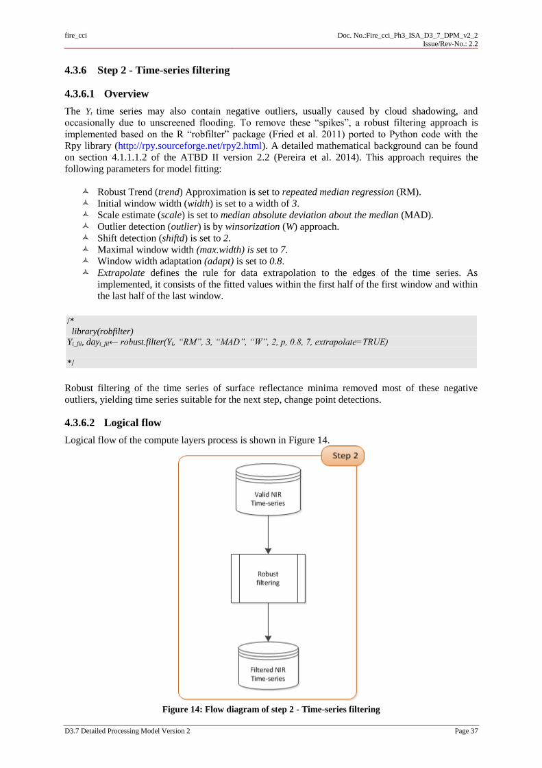
fire_cci
Doc. No.:Fire_cci_Ph3_ISA_D3_7_DPM_v2_2
Issue/Rev-No.: 2.2
D3.7 Detailed Processing Model Version 2 Page 37
4.3.6 Step 2 - Time-series filtering
4.3.6.1 Overview
The Yt time series may also contain negative outliers, usually caused by cloud shadowing, and
occasionally due to unscreened flooding. To remove these “spikes”, a robust filtering approach is
implemented based on the R “robfilter” package (Fried et al. 2011) ported to Python code with the
Rpy library (http://rpy.sourceforge.net/rpy2.html). A detailed mathematical background can be found
on section 4.1.1.1.2 of the ATBD II version 2.2 (Pereira et al. 2014). This approach requires the
following parameters for model fitting:
Robust Trend (trend) Approximation is set to repeated median regression (RM).
Initial window width (width) is set to a width of 3.
Scale estimate (scale) is set to median absolute deviation about the median (MAD).
Outlier detection (outlier) is by winsorization (W) approach.
Shift detection (shiftd) is set to 2.
Maximal window width (max.width) is set to 7.
Window width adaptation (adapt) is set to 0.8.
Extrapolate defines the rule for data extrapolation to the edges of the time series. As
implemented, it consists of the fitted values within the first half of the first window and within
the last half of the last window.
/*
library(robfilter)
Yt_fil, dayt_fil← robust.filter(Yt, “RM”, 3, “MAD”, “W”, 2, p, 0.8, 7, extrapolate=TRUE)
*/
Robust filtering of the time series of surface reflectance minima removed most of these negative
outliers, yielding time series suitable for the next step, change point detections.
4.3.6.2 Logical flow
Logical flow of the compute layers process is shown in Figure 14.
Figure 14: Flow diagram of step 2 - Time-series filtering

fire_cci
Doc. No.:Fire_cci_Ph3_ISA_D3_7_DPM_v2_2
Issue/Rev-No.: 2.2
D3.7 Detailed Processing Model Version 2 Page 38
4.3.7 Step 3 - Change point detection and ranking
4.3.7.1 Overview
Detections of points where a change in mean occurred depends on two options, a choice of criteria to
optimise and an optimisation algorithm. The Pruned Exact Linear Time (PELT) algorithm proposed by
Killick et al. (2012) produces exact optimisation of change-point segmentations in linear
computational time. The mathematical description and background of PELT is given in ATBD II v2.2
(Pereira et al. 2014), and the function is available in the R “changepoint” package (Killick and Eckley,
2010) which can easily be ported to Python code with the Rpy library
(http://rpy.sourceforge.net/rpy2.html). The function is parameterised by the following settings:
Change point method (method) is set to PELT.
Penalty (penalty) used is set to SIC.
/*
library(changepoint)
S, St ← cpt.mean(Ytmin_fil,”SIC”,”PELT”)
*/
This approach may yield several change points per pixel / time series, and per season, since the mean
value of NIR reflectance data varies not only in response to burning, but also due to other events. Each
change point is scored according to their likelihood of representing a burned area. Compromise
programming is the technique chosen to perform temporal change point selection of the potential burn
event. For all change points, only the ones representing reflectance decrease and pre and post change
point segment observation density above den_thres are considered. Density is determined by dividing
the number of observations by the temporal extent in each segment (eq. 4.4). For each considered
change point its attributes are determined. These are the mean segment reflectance decrease, the post-
change point segment reflectance, the difference between the post-change point segment reflectance
and time-series minima and the associated seasonal weight for the corresponding 10-day time step
(column) obtained from the auxiliary LUT.
/*
for i=1 to Si
if Si+1 –Si >0 and Density(Si ) >den_thresand Density(Si+1 ) >den_thres
decresi=Si+1 –Si
po_refi=Si+1
sea_wi=LUT(pixel_reference(line,column), St)
po_dst_min=Si+1- n=jjymin:1
*/
For the seasonal weight attribute, the mean segment reflectance decrease attribute and the difference
between the post-change point segment reflectance and time-series minima, normalization in relation
to the maximum observed value is performed according to eq. 4.6and for the post change mean
reflectance attribute, based on its minimum observed value according to eq. 4.7.
Change point ranking is determined by the Euclidian distance to an idealised point determined by the
attribute values that best describe a possible burn event, i.e., the biggest reflectance decrease, the
highest seasonal weight, the lowest difference of the post segment reflectance to the minimum and the
lowest post segment reflectance.

fire_cci
Doc. No.:Fire_cci_Ph3_ISA_D3_7_DPM_v2_2
Issue/Rev-No.: 2.2
D3.7 Detailed Processing Model Version 2 Page 39
/*
for i=1 to decres
dsti=sqrt((Norm(po_refi)-min(Norm(po_refi)))2+
(Norm(sea_wi)-max(Norm(sea_wi)))2+
(Norm(po_dst_mini)-min(Norm((po_dst_mini)))2+
(Norm(decresi)-min(Norm(decresi)))2)
*/
The change point with the highest rank, i.e., the lowest distance is selected to be included in a four
layer composite containing the change point post reflectance, seasonal weight, reflectance decrease,
associated dates and the difference in days to the previous valid observation. The first three layers are
passed on to the spatial rescaling and z-score determination (next section) and the last layer is passed
on to the post-processing (section 4.4) to be included in the final product format.
/*
po_refmin_dist,sea_wmin_dst, decresmin_dst,DOYdst_min, DOY_lagdst_min= min_select(dst, St)
*/
4.3.7.2 Logical flow
Logical flow of the compute layers process is shown in Figure 15.
Figure 15: Flow diagram of step 3 - Change point detection and ranking

fire_cci
Doc. No.:Fire_cci_Ph3_ISA_D3_7_DPM_v2_2
Issue/Rev-No.: 2.2
D3.7 Detailed Processing Model Version 2 Page 40
4.3.8 Step 4 - Spatial p_scoring
4.3.8.1 Overview
Spatial attribute rescaling serves to determine each pixel z_score based on its attributes. As for the
previous section compromise programming is the technique chosen to perform this operation but now
in a spatial context. For all the pixels, only the ones representing reflectance decrease below max_diff
and post reflectance above po_thres are considered to avoid residual atmospheric contaminated pixels
and water bodies. For each considered pixel, the attributes are: the mean segment reflectance decrease,
the post-change point segment reflectance, and the associated seasonal weight. These are normalised
following the same rule as in the previous section.
The scores are determined by the Euclidian distance to an idealised point determined by the attribute
values found in the spatial frame that best describe a possible burn event, i.e., the biggest reflectance
decrease, the highest seasonal weight, the lowest post segment reflectance.
/*
for i=1 to number of considered pixels
if decresi<max_diff and po_refi>po_thres
dsti=sqrt((Norm(po_refi)-min(Norm(po_refi)))2+
(Norm(sea_wi)-max(Norm(sea_wi)))2+
(Norm(decresi)-min(Norm(decresi)))2)
z_score=1-dsti
*/
The z_scores with the highest and lowest values are selected to rescale the z_scores into p_scores, by
normalizing between the observed range. The p_scores and associated dates, for the considered pixels,
are passed on to the next section. All pixels that are not considered are flagged and are classified as
unburned in the post-processing phase
4.3.8.2 Logical flow
Logical flow of the compute layers process is shown in Figure 16.
Figure 16: Flow diagram of step 4 –z_scoring

fire_cci
Doc. No.:Fire_cci_Ph3_ISA_D3_7_DPM_v2_2
Issue/Rev-No.: 2.2
D3.7 Detailed Processing Model Version 2 Page 41
4.3.9 Step 5 - Spatial probability revision - MRF segmentation
4.3.9.1 Overview
The previous steps of the algorithm lead to a characterization of each pixel of the image through two
variables: p_score and detection dates. The high p-scores detection dates are used in the Markov
random field image segmentation. The algorithm is a standard image processing algorithm that solves
the maximum a posteriori – Markov random field (MAP-MRF) problem, which arises in image
segmentation or image restoration. The MAP-MRF problem can be converted into finding a minimum
cut in a certain graph. In this case there are only two classes (burned and unburned) and the Boykov
Kolmogorov algorithm (Boykov and Kolmogorov, 2004) is used. For more mathematical background
and details refer to ATBD II v2.2 (Pereira et al. 2014). Pixels with no computed p_score and
associated dates and pixels flagged as “unburned” by the fire season mask (defined in previous
section) are not revised. The remaining pixels are classified according to their relation to their 4
neighbour pixels (by dates) and to their relation to an ideal “burned” or “unburned” pixel (by z-
scores).
To build the graph, each pixel (graph vertex) and its relation with other pixels (graph edges) has to be
set in a table of adjacencies in DIMACS format and saved on in an ASCII file temp_flow.dat.
// c Use a DIMACS network flow file example.
//
// c The total flow:
// s 0 t 2013
// c flow values:
// f 0 6 3
// f 0 1 6
// f 0 2 4
// f 1 5 1
// f 1 0 0
// f 1 3 5
// f 2 4 4
// f 2 3 0
// ...
Figure 17: DIMACS format file example
Each line of the file contains a pixel connection (edges) and its flow capacity. The capacities pixels are
calculated by applying the Logit function to v(x1,x2) calculated between two neighbour pixels. The
connection of each pixel with the ideal unburned (vertex 0) or burned (vertex n+1) is determined by
the p_score. If p_scoremax is lower/higher than the mean_score, the pixel is connected to the
“unburned”/”burned” ideal pixel and its capacity is determined by applying the Logit function to the p-
scores.
/*
for unflagged pixels
edge connections to ideal vertexes
if p_scoremax<mean_zscore
edge source = vertex 0
edge target = vertex(pixels)
edge capacity = Logit(p-score(p_score))
if p_scoremax>=mean_zscore
edge source = vertex(pixels)
edge target = vertex(N+1)
edge capacity = Logit(p-score(z-score))
edge connections between pixels
edge source = vertex(pixel A)
edge target = vertex(pixel B)
edge capacity = Logit(v(A,B))

fire_cci
Doc. No.:Fire_cci_Ph3_ISA_D3_7_DPM_v2_2
Issue/Rev-No.: 2.2
D3.7 Detailed Processing Model Version 2 Page 42
*/
This temporary ASCII file is read by a C++ programme (Min_Cut.cpp) that solves the minimum
source/sink-cut problem from the unburned source (vertex 0) and the burned sink (vertex N+1) by
applying the Boykov Kolmogorov algorithm available in the Boost C++ libraries
(http://www.boost.org/). The assigned class of each pixel (vertex) is stored in a binary file where
unburned pixels take value 0 and burned pixels take value 1.
4.3.9.2 Logical flow
Logical flow of the compute layers process is shown in Figure 18.
Figure 18: Flow diagram of step 5 - MRF segmentation
4.4 Post-processing
The final step is set to combine all the layer information necessary as stated in the IODD. The first
layer - burned Julian date - is determined by the date layer and contains only for pixels classified as
burned from the previous section (section 4.3.9). Water or unprocessed pixels are attributed the date -1
and for the unburned pixels the date 0. For layer two - the confidence level - the p-scores calculated in
the previous section are used and flagged with -1 for the water and unprocessed pixels. In layer three -
time since last clear detection - the information is passed from section 4.3.7 and set only for the pixels
classified as burned. The remaining unburned pixels have value 0 and the water and unprocessed
pixels have value -1. Layers 1-3 are splinted into monthly time frames. Water or unprocessed pixels
are replicated on all the monthly files and the burned pixels are distributed according to the date of
occurrence.
In the remaining three layers (4-6) - number of valid observations to classify, number of observations
covered by the sensor and the number of observations with cloud cover – contain information passed
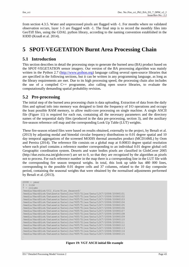
fire_cci
Doc. No.:Fire_cci_Ph3_ISA_D3_7_DPM_v2_2
Issue/Rev-No.: 2.2
D3.7 Detailed Processing Model Version 2 Page 43
from section 4.3.5. Water and unprocessed pixels are flagged with -1. For months where no validated
observation occurs, layer 1-3 are flagged with -1. The final step is to record the monthly files into
GeoTiff files, using the GDAL python library, according to the naming convention established in the
IODD (Krauß et al. 2014).
5 SPOT-VEGETATION Burnt Area Processing Chain
5.1 Introduction
This section describes in detail the processing steps to generate the burned area (BA) product based on
the SPOT-VEGETATION sensor imagery. Our version of the BA processing algorithm was mainly
written in the Python 2.7 (http://www.python.org) language calling several open-source libraries that
are specified in the following sections, but it can be written in any programming language, as long as
the library requirements are met. Due to its high processing speed, the processing chain also includes
the use of a compiled C++ programme, also calling open source libraries, to evaluate the
computationally demanding spatial probability revision.
5.2 Pre-processing
The initial step of the burned area processing chain is data uploading. Extraction of data from the daily
files and upload info into memory was designed to limit the frequency of I/O operations and occupy
the least possible RAM memory, to allow multi-core processing on single machine. A single ASCII
file (Figure 11) is required for each run, containing all the necessary parameters and the directory
names of the sequential daily files (produced in the data pre-processing, section 3), and the auxiliary
fire-season reference cell map and the corresponding Look Up Table (LUT) weights.
These fire-season related files were based on results obtained, externally to the project, by Benali et al.
(2013) by adjusting modal and bimodal circular frequency distributions to 0.01 degree spatial and 10
day temporal aggregations of the screened MODIS thermal anomalies product (MCD14ML) by Oom
and Pereira (2014). The reference file consists on a global map at 0.00833 degree spatial resolution
where each pixel contains a reference number corresponding to an individual 0.01 degree global cell
Geographic coordination system. Deserts and water bodies pixels are classified in GlobCover 2005
(http://due.esrin.esa.int/globcover/) are set to 0, so that they are recognized by the algorithm as pixels
not to process. For each reference number in the map there is a corresponding line in the LUT file with
the corresponding fire season temporal weighs. In total, this look up table has 480 000 lines,
corresponding to the possible 0.01 degree cells and 37 columns, related to the 10 day composite
period, containing the seasonal weights that were obtained by the normalised adjustments performed
by Benali et al. (2013).
2008 - year
3 - line
7 - column
/media/HardDisk/CCI_fire/Fire_Season6/
/media/HardDisk/Datasets/Satelite/VGT/Tiles/Data/L3C7/2008/20080101
/media/HardDisk/Datasets/Satelite/VGT/Tiles/Data/L3C7/2008/20080102
/media/HardDisk/Datasets/Satelite/VGT/Tiles/Data/L3C7/2008/20080103
/media/HardDisk/Datasets/Satelite/VGT/Tiles/Data/L3C7/2008/20080104
/media/HardDisk/Datasets/Satelite/VGT/Tiles/Data/L3C7/2008/20080105
/media/HardDisk/Datasets/Satelite/VGT/Tiles/Data/L3C7/2008/20080106
/media/HardDisk/Datasets/Satelite/VGT/Tiles/Data/L3C7/2008/20080107
/media/HardDisk/Datasets/Satelite/VGT/Tiles/Data/L3C7/2008/20080108
/media/HardDisk/Datasets/Satelite/VGT/Tiles/Data/L3C7/2008/20080109
/media/HardDisk/Datasets/Satelite/VGT/Tiles/Data/L3C7/2008/20080110
/media/HardDisk/Datasets/Satelite/VGT/Tiles/Data/L3C7/2008/20080111
/media/HardDisk/Datasets/Satelite/VGT/Tiles/Data/L3C7/2008/20080112
/media/HardDisk/Datasets/Satelite/VGT/Tiles/Data/L3C7/2008/20080113
/media/HardDisk/Datasets/Satelite/VGT/Tiles/Data/L3C7/2008/20080114
/media/HardDisk/Datasets/Satelite/VGT/Tiles/Data/L3C7/2008/20080115
..
.
Figure 19: VGT ASCII initial file example

fire_cci
Doc. No.:Fire_cci_Ph3_ISA_D3_7_DPM_v2_2
Issue/Rev-No.: 2.2
D3.7 Detailed Processing Model Version 2 Page 44
5.3 Overview
The BA algorithm loads all the available annual reflectance images of the NIR channel, plus the last
month of the previous year and the first month of the following year. After loading the data, the
algorithm applies the water and cloud masks to each pixel, masking out invalid surface observations
(all derived from the pre-processing stage), extracts the time series and applies a filter to remove
spikes. It then detects significant changes in mean NIR time-series and scores them according to a
calculated distance based on its attributes to an idealized potential fire event. For each pixel, the
change point with the lowest rank is then re-scaled according to the spatial context and used to build a
graph. This graph is then segmented between the burned and unburned. The last post-processing step
is information aggregation into monthly composites.
5.4 Logical Flow
The logical flow of the VGT burned area processing steps is illustrated in Figure 20.

fire_cci
Doc. No.:Fire_cci_Ph3_ISA_D3_7_DPM_v2_2
Issue/Rev-No.: 2.2
D3.7 Detailed Processing Model Version 2 Page 45
Figure 20: Flow diagram of the VGT BA processing chain

fire_cci
Doc. No.:Fire_cci_Ph3_ISA_D3_7_DPM_v2_2
Issue/Rev-No.: 2.2
D3.7 Detailed Processing Model Version 2 Page 46
5.4.1 Equations and functions
The equations applied in the burned area processing chain are listed below.
Eq.4.1-Robust filter function (R function)
Yt_fil ←robust.filter(Yt, trend, width, scale, outlier, shiftd, p, adapt, max.width, extrapolate)
Eq.4.2-Change point detection function (R function)
Y, Yt← cpt.mean(Yt_fil,penalty,method)
Eq.4.3-Neighbour pixel connection flow velocity function
diffDdiff
Dv
diffD
=xxvmax_)
max_1(*0
max_0
),( 21
Eq.4.4-Density of observations
tt
t
tj j
SS
y=tDensity
1
1
Eq.4.5-Logit function
Logit(p) = | 100*p / (1-p) |
Eq.4.6-Normalization based on the maximum
minmax
max
xx
xx=xNorm i
i
Eq.4.7-Normalization based on the minimum
minmax
min
xx
xx=xNorm i
i
Eq.4.8-Normalization of distances to ideal and anti-ideal points
Di+DaiDi=pscore /

fire_cci
Doc. No.:Fire_cci_Ph3_ISA_D3_7_DPM_v2_2
Issue/Rev-No.: 2.2
D3.7 Detailed Processing Model Version 2 Page 47
5.4.2 List of variables
Table 4: Variables used in the VGT BA processing chain
Variables
y1:n = (y1, . . . , yn) Time series of NIR reflectance
ytm = Time series of local minima NIR reflectance
ytM = Time series of local maxima NIR reflectance
ytmin = Time series of local minima NIR channels reflectance without spurious turning points
ytmin_fil = Time series of local minima NIR channels reflectance despiked
daytm = Time series of associated Julian dates for ytm
daytM= Time series of associated Julian dates for ytM
daytmin = Time series of associated Julian dates for ytmin
daytmin_fil = Time series of associated Julian dates for ytmin_fil
NIRi,j,t=NIR channel observations, where i and j represent the spatial location and temporal location
yt_fil = Time series of local minima despiked (NIR reflectance)
dayt_fil = Time series of associated Julian dates for yt_fil
S= Change point segments of mean NIR reflectance
day S= Time series of associated Julian dates for S
decres= NIR reflectance decrease between consecutive segments (𝑆𝑖+1̅̅ ̅̅ ̅ − 𝑆�̅�)
po_ref= Post change point NIR mean reflectance segment (𝑆𝑖+1̅̅ ̅̅ ̅)
pre_NIR= Reflectance observations in the pre change point
po_NIR= Reflectance observations in the post change point
half_temp_range=half of the time-lag in time series ((lastdate-1st date)/2)
sea_w= Change point fire-season weight
dst_time= Euclidean distance to an idealised fire event point (time series stage)
dst_space= Euclidean distance to an idealised fire event point (space stage)
dst_space_ideal= Euclidean distance to an idealised regional group of points (space stage)
dst_space_a-ideal= orthogonal distances to a constant vale (space stage)
5.4.3 List of parameters
Table 5: Parameters set in the VGT BA processing chain
Parameter value
min_diff_cutoff 0.02
max_refl_cutoff 0.4
mask_cl_thres 75
mask_wt_thres 75
min_obs_req 60
min_obs_min 35

fire_cci
Doc. No.:Fire_cci_Ph3_ISA_D3_7_DPM_v2_2
Issue/Rev-No.: 2.2
D3.7 Detailed Processing Model Version 2 Page 48
Parameter value
max_slope 0.4
min_score 0.2
max_score 0.6
max_diff 0.2
den_thres 0.1
decres_min 0.02
po_max 0.2
num_observ 3
v0 0.9
mean_p_score = (max_p_score-min_p_score)/2 0.5
5.4.4 Step 1 - Data extraction, Cloud, Water mask and Quality Control flagging and
observational statistics
5.4.4.1 Overview
The processing chain is design to minimise I/O operations and memory usage. To achieve this, data
are read and simultaneously validated to be stored into memory. For each daily atmosphere corrected
reflectance Q.1: NIR channel and the Quality control layers, both the OWM: static and dynamic layers
and the OWM: cloud, cloud shadow, haze and snow are read using the python GDAL library and pixel
validation is performed by flagging invalid pixels where cloud/haze/ice/shadow and water masks
exceed the corresponding mask_cl_thres and mask_wt_thres levels, and where the quality layer
identifies pixels with any radiometric problems. For each day the NIR channel and flags are stored in
memory in a 3D matrix, NIRi,j,t, where i,j represent the location within the tile/scene and t is the
seasonal observation. Simultaneously, imagery dates are extracted from the directory names and
converted into Julian dates.
In addition, for each valid pixel, cloudy and the total observation frequencies are calculated and split
into monthly layers and saved into a temporary binary file to be read at the post-processing stage. The
total number of observations is provided by the frequency a pixel is observed with surface reflectance,
the number of valid observations is determined by the number of untagged observations and the
cloudy observations is provided by the frequency of pixels flagged as cloud.
In order to save processing time, pixels located over water bodies or desert land-surface with no fuel
are flagged and not processed. This information is provided by the auxiliary reference file identified
by the value 0 and pixels are assigned a value of 0. In order to proceed to the next steps a minimum
number of observations is required (min_obs_req). If this number is not satisfied the pixel is flagged
and not processed, and information is passed on to the post-processing stage.

fire_cci
Doc. No.:Fire_cci_Ph3_ISA_D3_7_DPM_v2_2
Issue/Rev-No.: 2.2
D3.7 Detailed Processing Model Version 2 Page 49
5.4.4.2 Logical flow
Figure 21: Flow diagram of step 1 - Data extraction, Cloud, Water mask and Quality Control flagging and
observational statistics
5.4.5 Step 2- Maxima/Minima time series extraction
5.4.5.1.1 Overview
Extracting local minima from a time series of observations y1:n of reflectance data entails a series of
steps:
1 Identify of “turning points” i.e. the local minimum, ytm, and local maximum, ytM if its two
adjacent neighbours are smaller or larger (Kugiumtzis and Tsimpiris, 2010). Time series edges
are extended by replicating the second value prior to the first and performing the same
corresponding operation for opposite edge, the n observation.
2 Remove from the series all yt that are not turning points.
3 Calculate a time series of first-order differences and remove all turning points that differ from
one of its immediate neighbours less than the min_diff_cutoff reflectance units. This process
need to consider which of the series, ytm or ytM, starts and which ends.
4 Retain only the local minima and remove from the series those ytm values above the
max_refl_cutoff reflectance units.

fire_cci
Doc. No.:Fire_cci_Ph3_ISA_D3_7_DPM_v2_2
Issue/Rev-No.: 2.2
D3.7 Detailed Processing Model Version 2 Page 50
5.4.5.2 Logical flow
Logical flow of the compute layers process is shown in Figure 22.
Figure 22: Flow diagram of step 2 and 3 – Maxima/Minima time series extraction and filtering
/*
for i=1 to lines
for j=1 to columns
Yt, dayt = validate_observations(NIRi,j,t)
ytm,ytM,daytm,daytM= find_envelopes(Yt, dayt )
ytmin,daytmin= remove_barbs( ytm,ytM,daytm,daytM, min_diff_cutoff)
end for
end for
*/
5.4.6 Step 3 - Time-series filtering
5.4.6.1 Overview
The Yt time series may also contain negative outliers, usually caused by cloud shadowing, and
occasionally due to unscreened flooding. To remove these “spikes”, a robust filtering approach is
implemented based on the R “robfilter” package (Fried et al. 2011) ported to Python code with the
Rpy library (http://rpy.sourceforge.net/rpy2.html). A detailed mathematical background can be found
on section 4.2.1.1.2 of the ATBD II version 2.2 (Pereira et al. 2014). This approach requires the
following parameters for model fitting:
Robust Trend (trend) Approximation is set to repeated median regression (RM).
Initial window width (width) is set to a width of 3.
Scale estimate (scale) is set to to Rousseeuw’s and Croux’ (1993) on scale estimator (QN) .
Outlier detection (outlier) is by winsorization (W) approach.
Shift detection (shiftd) is set to 2.
Maximal window width (max.width) is set to 7.
Window width adaptation (adapt) is set to 0.8.
Extrapolate defines the rule for data extrapolation to the edges of the time series. As
implemented, it consists of the fitted values within the first half of the first window and within
the last half of the last window.

fire_cci
Doc. No.:Fire_cci_Ph3_ISA_D3_7_DPM_v2_2
Issue/Rev-No.: 2.2
D3.7 Detailed Processing Model Version 2 Page 51
/*
# robfilter R package
library(robfilter)
Yt_fil, dayt_fil← robust.filter(Yt, “RM”, 3, “QN”, “W”, 2, p, 0.8, 7, extrapolate=TRUE)
*/
Robust filtering of the time series of surface reflectance minima removed most of these negative
outliers, yielding time series suitable for the next step, change point detection.
5.4.6.2 Logical flow
Logical flow of the compute layers process is shown in Figure 23.
Figure 23: Flow diagram of step 2 - Time-series filtering
5.4.7 Step 3 - Change point detection and ranking
5.4.7.1 Overview
Detections of points where a change in mean occurred depends on two options, a choice of criteria to
optimise and an optimisation algorithm. The Pruned Exact Linear Time (PELT) algorithm proposed by
Killick et al. (2012) produces exact optimisation of change-point segmentations in linear
computational time. The mathematical description and background of PELT is given in ATBD II v2.2
(Pereira et al. 2014), and the function is available in the R “changepoint” package (Killick and Eckley,
2010) which can easily be ported to Python code with the Rpy library
(http://rpy.sourceforge.net/rpy2.html). The function is parameterised by the following settings:
Change point method (method) is set to PELT
Penalty (penalty) used is set to SIC

fire_cci
Doc. No.:Fire_cci_Ph3_ISA_D3_7_DPM_v2_2
Issue/Rev-No.: 2.2
D3.7 Detailed Processing Model Version 2 Page 52
/*
# changepoint R package
library(changepoint)
S, St ← cpt.mean(Ytmin_fil,”SIC”,”PELT”)
*/
This approach may yield several change points per pixel / time series, and per season, since the mean
value of NIR reflectance data varies not only in response to burning, but also due to other events. Each
change point is scored according to their likelihood of representing a burned area. Compromise
programming is the technique chosen to perform temporal change point selection of the potential burn
event. Each change point detected by PELT has to comply with each and every of the following
criteria, before it is considered apt for scoring (see Table 4):
- decres < 0
- decres < | max_diff |
- po_ref < po_thres
- Density(Si ) > den_thres , Density is determined by dividing the number of observations by the
temporal extent in each segment (eq. 4.4).
- Density(Si+1 ) > den_thres
- po_ref < min{po_NIR} +0.005
- Slope of the linear fit to the po_NIR observations in the post CP segment < max_slope
- Time lag between the CP dates of two lowest po_ref values in time series < half_temp_range.
- Number of observations prior to first CP and/or after the last CP > num_observ.
The attributes mean segment reflectance decrease decres=(𝑆𝑖+1̅̅ ̅̅ ̅ − 𝑆�̅�), the post-change point segment
reflectance po_ref=(𝑆𝑖+1̅̅ ̅̅ ̅), and the associated seasonal weight for the corresponding 10-day time step
(column) obtained from the auxiliary LUT (sea_w). Each change point satisfying these requirements is
calculated and used for scoring and selecting the best (most likely to represent a burn event) CP in
each time series
/*
for i=1 to Si # for all the change points, selectif Si+1 –Si <0 and Si+1 –Si <abs(max_diff) and po_ref < po_thres
and Density(Si ) >den_thres and Density(Si+1 ) ..>den_thres
and 𝑆𝑖+1̅̅ ̅̅ ̅ < min{po_NIR} +0.005 and 0<Slope (po_NIR (Si)) <max_slope
and t < half_temp_range
and Number of observations prior to first CP and/or after the last CP > num_observ
endif
end for
decresi=𝑆𝑖+1̅̅ ̅̅ ̅ − 𝑆�̅�
po_refi=𝑆𝑖+1̅̅ ̅̅ ̅
sea_wi=LUT(pixel_reference(line,column), St)
*/
For the seasonal weight attribute and the mean segment reflectance decrease attribute, normalization is
performed according to eq. 4.7 and for the post change mean reflectance attribute, according to eq. 4.6.
Change point ranking is determined by the Euclidean distance to an ideal point determined by the best
attribute values that characterise a possible burn event, i.e., the largest reflectance decrease, the highest
seasonal weight, and the lowest post fire segment reflectance. All data are rescaled such that the most
desirable score of each variable is assigned a value of 1, i.e. the ideal point is a vector [1, 1, 1]
/*
for i=1 to all the change point selected calculate the Euclidean distance

fire_cci
Doc. No.:Fire_cci_Ph3_ISA_D3_7_DPM_v2_2
Issue/Rev-No.: 2.2
D3.7 Detailed Processing Model Version 2 Page 53
dst_po_ref= 0.332*(1-(Norm(po_refi)))2
dst_sea_w= 0.332*(1-(Norm(sea_wi)))2
dst_decres= 0.332*(1-(Norm(decresi))))2
# calculate Euclidean distance
dst_tempi=sqrt(dst_po_refi+ dst_sea_wi+ dst_decresi)
end for
*/
The change point with the highest rank, i.e., the lowest distance to the ideal is selected to be included
in a four layer composite containing the change point post reflectance, seasonal weight, reflectance
decrease, all the associated dates and the difference in days to the previous valid observation. The first
three layers are passed on to the spatial rescaling and z-score determination (next section) and the last
layer is passed on to the post-processing (section 4.4) to be included in the final product format.
/*
po_refmin_dist_temp,sea_wmin_dst_temp, decresmin_dst_temp,DOYdst_temp__min, DOY_lagdst_temp_min= min_select(dst_temp, St)
*/
5.4.7.2 Logical flow
Logical flow of the compute layers process is shown in Figure 24.
Figure 24: Flow diagram of step 3 - Change point detection and ranking

fire_cci
Doc. No.:Fire_cci_Ph3_ISA_D3_7_DPM_v2_2
Issue/Rev-No.: 2.2
D3.7 Detailed Processing Model Version 2 Page 54
5.4.8 Step 4 - Spatial p_scoring
5.4.8.1 Overview
Spatial attribute rescaling serves to determine each pixel pscore (burning probability) based on its
attributes. As for the previous section compromise programming is the technique chosen to perform
this operation but now in a spatial context. For each change point out of each time series (only one per
pixel) the scoring attributes are: mean segment reflectance decrease, post-change point segment
reflectance, and associated seasonal weight.
Global-scale scoring of the candidate change points from each time series/pixel relies on the
calculation of Euclidean distances to an ideal and to an anti-ideal, which are represented by sets of
points, rather than by single points. The ideal set contains one point/site/year from 9 of the 10 project
regional study sites (Borneo was excluded due to lack of appropriate data), representing the most
paradigmatic examples of fire-affected pixels, in terms of the non-rescaled variables mean segment
reflectance decrease, the post-change point segment reflectance, and the associated seasonal weight.
The convex hull of this set of ideal points was determined and distances between the change point
selected from each time series/pixel and the ideal set are calculated. The distance to the nearest point
in the convex hull is selected (minimum distance) as the distance to the ideal set, according to a
mathematical definition of distance between a point and a set of points. Distances to an anti-ideal set
were also calculated for each pixel as the shortest of the orthogonal distances to a constant vale of
decres_min and po_max, respectively for mean segment reflectance decrease and post-change point
segment reflectance. Finally, for each timeseries/pixel, the distances to the ideal (Dii) and anti-ideal
(Daii) sets were combined as eq. 4.8 to achieve the p-scores.
/* for each of considered change point selected CP i
#distance to ideal
for each ideal point j (1 to 11)
#distance of each pixel to the eleven(j) points dst_po_refij=po_ref(CPi)-pointj
dst_sea_wij=dst_sea_w(CPi)-pointj
dst_decresij=decres(CPi)-pointj
dst_space_ideali=sqrt((0.332 *(dst_po_refij)2)+( 0.332 *(dst_sea_wij)2)+ ( 0.342
*(dst_decresij)2) Dii=min {dst_space_ideal}
end for
#distance to anti-ideal
for each anti-ideal constant value max_diff and po_thres
#distance of each pixel to the max_diff
dst_decresij=decres(CPi)- max_diff
dst_sea_wij=dst_sea_w(CPi)-0 #anti-ideal for seasonal weight is zero
dst_po_refij=po_ref(CPi) #keeps the value
#distance of each pixel to the po_thres
dst_decresij=decres(CPi) #keeps the value
dst_sea_wij=dst_sea_w(CPi) -0 #anti-ideal for seasonal weight is zero
dst_po_refij=po_ref(CPi) -po_thres
dst_space_a-ideali=sqrt((0.332 *(dst_po_refij)2)+( 0.332 *(dst_sea_wij)2)+ ( 0.342
*(dst_decresij)2)
Daii=min {dst_space_a-ideal}
*/

fire_cci
Doc. No.:Fire_cci_Ph3_ISA_D3_7_DPM_v2_2
Issue/Rev-No.: 2.2
D3.7 Detailed Processing Model Version 2 Page 55
The p_scores and associated dates, for the considered pixels, are passed on to the next section. All
pixels that are not considered are flagged and are classified as unburned in the post-processing phase
5.4.8.2 Logical flow
Logical flow of the compute layers process is shown in Figure 25.
Figure 25: Flow diagram of step 4 –z_scoring
5.4.9 Step 5 - Spatial probability revision - MRF segmentation
5.4.9.1 Overview
The previous steps of the algorithm lead to a characterization of each pixel of the image through two
variables: p_score and detection dates. The high p-scores detection dates are used in the Markov
random field image segmentation. The algorithm is a standard image processing algorithm that solves
the maximum a posteriori – Markov random field (MAP-MRF) problem, which arises in image
segmentation or image restoration. The MAP-MRF problem can be converted into finding a minimum
cut in a certain graph. In this case there are only two classes (burned and unburned) and the Boykov
Kolmogorov algorithm (Boykov and Kolmogorov, 2004) is used. For more mathematical background
and details refer to ATBD II v2.2 (Pereira et al. 2014). Pixels with no computed p_score and
associated dates and pixels flagged as “unburned” by the fire season mask (defined in previous
section) are not revised. The remaining pixels are classified according to their relation to their 4
neighbour pixels (by dates) and to their relation to an ideal “burned” or “unburned” pixel (by z-
scores).
To build the graph, each pixel (graph vertex) and its relation with other pixels (graph edges) has to be
set in a table of adjacencies in DIMACS format and saved in an ASCII file temp_flow.dat.

fire_cci
Doc. No.:Fire_cci_Ph3_ISA_D3_7_DPM_v2_2
Issue/Rev-No.: 2.2
D3.7 Detailed Processing Model Version 2 Page 56
// c Use a DIMACS network flow file example.
//
// c The total flow:
// s 0 t 2013
// c flow values:
// f 0 6 3
// f 0 1 6
// f 0 2 4
// f 1 5 1
// f 1 0 0
// f 1 3 5
// f 2 4 4
// f 2 3 0
// ...
Figure 26: DIMACS format file example
Each line of the file contains a pixel connection (edges) and its flow capacity. The capacities pixels are
calculated by applying the Logit function to v(x1,x2) calculated between two neighbour pixels. The
connection of each pixel with the ideal unburned (vertex 0) or burned (vertex n+1) is determined by
the p_score. If p_score is lower/higher than the mean_score, the pixel is connected to the
“unburned”/”burned” ideal pixel and its capacity is determined by applying the Logit function to the p-
scores.
/*
for unflagged pixels
edge connections to ideal vertexes
if p_score<mean_zscore
edge source = vertex 0
edge target = vertex(pixels)
edge capacity = Logit (p_score)
if p_score>=mean_zscore
edge source = vertex(pixels)
edge target = vertex(N+1)
edge capacity = Logit( (p_score)
edge connections between pixels
edge source = vertex(pixel A)
edge target = vertex(pixel B)
edge capacity = Logit(v(A,B))
*/
This temporary ASCII file is read by a C++ programme (max_flow.cpp) that solves the minimum
source/sink-cut problem from the unburned source (vertex 0) and the burned sink (vertex N+1) by
applying the Boykov Kolmogorov algorithm available in the Boost C++ libraries
(http://www.boost.org/). The assigned class of each pixel (vertex) is stored in a binary file where
unburned pixels take value 0 and burned pixels take value 1.
5.4.9.2 Logical flow
Logical flow of the compute layers process is shown in Figure 27.

fire_cci
Doc. No.:Fire_cci_Ph3_ISA_D3_7_DPM_v2_2
Issue/Rev-No.: 2.2
D3.7 Detailed Processing Model Version 2 Page 57
Figure 27: Flow diagram of step 5 - MRF segmentation
5.5 Post-processing
The final step is set to combine all the layer information necessary as stated in the IODD (Krauß et al.
2014). The first layer - burned Julian date - is determined by the date layer and contains only pixels
classified as burned from the previous section. Water or unprocessed pixels are attributed the date -1
and for the unburned pixels the date 0. For layer two - the confidence level - the p-scores calculated in
the previous section are used and flagged with -1 for the water and unprocessed pixels. In layer three -
time since last clear detection - the information is passed from section 5.3.7 and set only for the pixels
classified as burned. The remaining unburned pixels have value 0 and the water and unprocessed
pixels have value -1. Layers 1-3 are splinted into monthly time frames. Water or unprocessed pixels
are replicated on all the monthly files and the burned pixels are distributed according to the date of
occurrence.
The remaining three layers (4-6) - number of valid observations to classify, number of observations
covered by the sensor and the number of observations with cloud cover – contain information passed
from section 5.3.5. Water and unprocessed pixels are flagged with -1. For months where no validated
observation occurs, layer 1-3 are flagged with -1. The final step is to record the monthly files into
GeoTiff files, using the GDAL python library, according to the naming convention established in the
IODD (Krauß et al. 2014).

fire_cci
Doc. No.:Fire_cci_Ph3_ISA_D3_7_DPM_v2_2
Issue/Rev-No.: 2.2
D3.7 Detailed Processing Model Version 2 Page 58
6 MERIS Burnt Area Processing Chain
6.1 Key Principles of the Algorithm
The MERIS BA algorithm detects burned areas on a global scale, based on the use of MERIS
reflectance bands, spectral indices calculation, post-fire and multi-temporal discrimination, in synergy
with hotspot locations (as determined using MODIS middle- and thermal-infrared bands). A general
flow of the algorithm can be seen in Figure 28.
The BA algorithm for MERIS has been tailored according to the data characteristics (lack of SWIR,
temporal noise…). Spectral reflectance and mask auxiliary data are used to obtain a series of monthly
spectral index composites. BA detection is performed in a two phase process: the first one detects seed
pixels, while the second one applies a contextual criterion around these seed pixels.
Input data to the algorithm is: spatial distribution of active fires for burned area detection, MERIS
reflectance bands 8 and 10, together with their auxiliary information (water, cloud, shadow, haze and
snow masks) and information on burnable/not burnable areas extracted from a land cover map
(GlobCover 2005). Details on the BA algorithm can be found in the ATBD II v2.2 (Pereira et al.
2014).
Figure 28: Algorithm general flow
fire_cci
Doc. No.:Fire_cci_Ph3_ISA_D3_7_DPM_v2_2
Issue/Rev-No.: 2.2
D3.7 Detailed Processing Model Version 2 Page 59
6.2 Pre-processing
Before running the MERIS BA algorithm MERIS data must have been pre-processed as described in
section 3.
6.3 Processing Chain
The 5 main processes of the algorithm are:
- Data filtering: information needed for the specific tile in process is extracted from all
input data.
- Build composites: a set of variables and matrices needed to perform the proper BA
detection is computed within this process.
- BA detection: seed identification and region growing, together with confidence levels are
obtained in this process.
- Compute layers: separation of yearly product obtained from the BA detection process into
monthly products and calculation of other variables needed for the merged product are
performed here.
- BA monthly product: data obtained on the previous steps is assembled to obtain the BA
monthly product 6 layers.
Each one of these 5 main processes is further detailed in the following sections.
6.4 Data Filtering
6.4.1 Overview
This step of the algorithm is in charge of selecting all relevant data that are needed in the BA
algorithm. There are 2 main tasks included in this process. First step is to look for the burnable file
that corresponds to the tile that is being processed. If the tile is not burnable the process stops here and
continues with the next tile.
- Valid images: this task looks for the reflectances GeoTiff file. If the file is found, the
corresponding filename (that contains the date of the image) is saved in the variable
valid_images.
- HS: selects from all Hot Spots available in the MOD 014 product the ones in the
geographical tile and year that is being processed, saving the information in the variable
HS.
6.4.2 Logical flow
The logical flow for the data filtering is shown in Figure 29.

fire_cci
Doc. No.:Fire_cci_Ph3_ISA_D3_7_DPM_v2_2
Issue/Rev-No.: 2.2
D3.7 Detailed Processing Model Version 2 Page 60
Figure 29: Data filtering logical flow
6.5 Build Composites
6.5.1 Overview
In this process the different matrices that are the input to the BA algorithm are obtained. It is
performed in 5 steps:
- HS-matrix: this task computes the distance from each pixel to a HS. The value of the HS
closest to the pixel is assigned to the pixel, obtaining with this procedure the Thiessen
polygons.
- NIR composite: this process looks for the lowest 3 NIR values every 2 months and assigns
to each pixel the NIR value that is closest in date to the HS matrix, from the set of 3
lowest NIR values.
- HS_density_monthly: obtains HS density matrices (3x3 and 9x9) for each month.
- GEMI: computes the GEMI monthly composites and finds the annual maximum value of
this index.
- Minimum NIR_HS: obtains the lowest NIR value around the HS pixels.

fire_cci
Doc. No.:Fire_cci_Ph3_ISA_D3_7_DPM_v2_2
Issue/Rev-No.: 2.2
D3.7 Detailed Processing Model Version 2 Page 61
6.5.2 Logical flow
The logical flows for the process build composites, NIR composite and GEMI are shown in Figure 30,
Figure 31 and Figure 32, respectively.
Figure 30: Build composites logical flow
Figure 31: NIR composite logical flow

fire_cci
Doc. No.:Fire_cci_Ph3_ISA_D3_7_DPM_v2_2
Issue/Rev-No.: 2.2
D3.7 Detailed Processing Model Version 2 Page 62
Figure 32: GEMI logical flow
6.6 BA Detection
6.6.1 Overview
In this process, the estimation of burned areas is performed. There are 3 main steps:
- Identify seeds: seed pixels are obtained from the HS information previously filtered.
Percentile curves of burned and unburned pixels are built and thresholds defined to
discriminate between burned and unburned pixels.
- Region growing: new thresholds are used (see ATBD II) for the NIR and differenceGEMI
composites to identify burned and unburned pixels. Pixels are classified as burned if the
neighbours to a seed pixel have higher values than the threshold. The threshold is defined
taking into account the value found in the seed pixel.
- Confidence levels: probability rules are applied to compute confidence levels on the burned
pixels. Probabilities of burning and not burning are set (0.5). Conditional probabilities are
computed. Confidence level is obtained with the probability of a pixel having burned given
the fact that the pixel has a particular NIR value (obtained from the composite) ((P(B/NIR)
see Equation 6.2 in section 6.9)
6.6.2 Logical flow
The Logical flow for the overall BA detection process is shown in Figure 33. The Logical flow of the
seed and region growing process are shown in Figure 34 and Figure 35.

fire_cci
Doc. No.:Fire_cci_Ph3_ISA_D3_7_DPM_v2_2
Issue/Rev-No.: 2.2
D3.7 Detailed Processing Model Version 2 Page 63
Figure 33: BA detection logical flow
Figure 34: Identify seeds logical flow

fire_cci
Doc. No.:Fire_cci_Ph3_ISA_D3_7_DPM_v2_2
Issue/Rev-No.: 2.2
D3.7 Detailed Processing Model Version 2 Page 64
Figure 35: Region growing logical flow
6.7 Compute Layers
6.7.1 Overview
In this process, the layers needed to obtain the final product are computed. It is performed in 3 steps:
- Convert_BA_ product:in order to obtain the BA product a yearly composite is built, with the
BA detected for each month. In this process, yearly values are separated into 12 months to
prepare the product to be delivered to the merging algorithm chain.
- Previous_observation: this process looks for the last valid image before the burnt, and counts
the number of days in between.
- Valid_all_cloud observations: this process counts the number of valid observations per pixel
and month, considering a 30 % threshold for cloud, shadow and snow, and 40 % for haze. It
also counts the number of images that were acquired by the sensor per pixel per month and the
number of images that were covered by more than 30 % of cloud and 40 % of haze per pixel
per month.
6.7.2 Logical flow
Logical flow of the compute layers process is shown in Figure 36.

fire_cci
Doc. No.:Fire_cci_Ph3_ISA_D3_7_DPM_v2_2
Issue/Rev-No.: 2.2
D3.7 Detailed Processing Model Version 2 Page 65
Figure 36: Compute layers logical flow
6.8 BA Monthly product
6.8.1 Overview
In the last process of the algorithm the variables obtained in the previous tasks are assembled. This
process is performed in 1 step:
- Group_layers: all the information obtained from the previous block is grouped by month and the 6
layers of the product are created.
6.8.2 Logical flow
Figure 37: BA monthly product and format conversion logical flow

fire_cci
Doc. No.:Fire_cci_Ph3_ISA_D3_7_DPM_v2_2
Issue/Rev-No.: 2.2
D3.7 Detailed Processing Model Version 2 Page 66
6.9 Post Processing
In this step the BA monthly product in .mat format is converted to the GeoTiff output format.The
output product is divided in 6 different layers:
- Layer 1: BA state
o Burned = Julian date of burn (1-365)
o Water mask = -1
o Not burned = 0
o Non–observed = -4
- Layer 2: Confidence level: 0-100%
- Layer 3: Time since last clear detection: number of days between the detection and the
previous valid image.
- Layer 4: Number of valid observations to classify (days)
- Layer 5: Number of observations covered by the sensor (days)
- Layer 6: Number of observations with cloud cover (days)
6.10 Equations
The equations applied through the BA algorithm are listed below.
Eq.6.1 - GEMI index
R
RGEMI
1
125,0)25,01(*
5,0
)*5,0()*5,1()(*2 22
RIR
RIRRIR
Eq.6.1 - Confidence level
Confidence level calculation is based on the Bayes’ theorem:
PBcondBmax=100 * (PBmaxcondB * PB) / (PBmaxcondB * PB + PBmaxcondU * PU);
Where:
- P(B/NIR) = probability of having burned given the fact that it has a particular NIR value
- P(NIR/B) = probability of observing a certain value of NIR knowing that it has burned
- P(NIR/U) = probability of observing a certain NIR value knowing that it has not burned
- PB = 0.5 = a priori probability of burning
- PU = 0.5 = a priori probability of not burning
Eq.6.3 - Thiessen polygons
Where:
- is a space with a distance function d,
- K is a set of indices
- (Pk)k ϵK is a tuple of non-empty subsets in the space
- Rk is the region associated to the Pk set of points in X whose distance to Pk is not greater
than the distance to the other Pj sites
- (Rk)k ϵK is the Thiessen diagram.

fire_cci
Doc. No.:Fire_cci_Ph3_ISA_D3_7_DPM_v2_2
Issue/Rev-No.: 2.2
D3.7 Detailed Processing Model Version 2 Page 67
6.11 List of variables
A list of variables used in the BA MERIS processing chain is detailed in Table 6.
Table 6: Variables in the MERIS BA processing chain
Variable Description
Year Time series of years to process
Path 1 Root path to data directories
Path 2 Root path intermediate variables
Path 3 Root path to HS auxiliary files
Path 4 Root path to Land cover auxiliary files
Path 5 Root path to output file
HS MOD14 product information
Lat Latitude of the tile to process
Lon Longitude of the tile year to process
Valid_images Valid images for the specific tile and year
Thiessen Matrix obtained with HS information
NIR-HS GEMI-HS, jul Composites containing the MERIS reflectances and Julian dates
associated
HS dens HS Density matrices (3 x 3, 9 x 9)
Seeds Pixels identified as burned in the seed phase
BA Pixels identified as burned after the growing phase
CL Confidence level relative to the BA pixels
Previous Previous valid observation before the burn detection date
Valid Number of valid observations over a pixel
All Total number of observations over a pixel
Cloud Number of cloudy observations over a pixel
Threshold 1 Threshold identified to filter the seeds
Threshold 2 Threshold identified to filter the pixels in the growing phase
6.12 List of parameters
A list of parameters is used through the BA MERIS processing. They are detailed in Table 7.
Table 7: Parameters set in the MERIS BA processing chain
Parameter value
Cloud threshold 30
Haze threshold 40
Snow threshold 30
Shadow threshold 30
Growing GEMI 0.9

fire_cci
Doc. No.:Fire_cci_Ph3_ISA_D3_7_DPM_v2_2
Issue/Rev-No.: 2.2
D3.7 Detailed Processing Model Version 2 Page 68
6.13 Computer Programme in Pseudo-Code
The main script is the only one to interact with the user. Its pseudo code is as follows: /*
begin
Year = ask user for the year to process
for i = 1:number of tiles
call data filtering
call build composites
call BA detection
call compute layers
call monthly product
end for
end
*/
6.13.1 Data Filtering
Input: MERIS data, MOD 14, latitude, longitude of the tile and year to process
Output: valid images, HS
- Valid_images function: /*
Begin
Create path to folder with year indicated, latitude and longitude of the file being processed
for i=1:files in the folder year/tile
open file
if result open = -1
next file
else
valid_images = file_id
endif
end for
End
*/
- Burnable tile function: /*
Begin
Create path to folder with year indicated, latitude and longitude of the file being processed
open file
if result open = -1
go to the next tile
endif
End
*/
- HS function: /*
Begin
Create path to folder with year indicated, latitude and longitude of the file being processed
load MODIS_014 for the specified year
select lat long information
HS = selected information
End
*/

fire_cci
Doc. No.:Fire_cci_Ph3_ISA_D3_7_DPM_v2_2
Issue/Rev-No.: 2.2
D3.7 Detailed Processing Model Version 2 Page 69
6.13.2 Build Components
Input: valid_images, MERIS bands 8, 10 and masks, HS
Output: Thiessen matrix, NIR-HS, DAY, GEMI-HS, GEMImax, HS density matrices,
minimum NIR.
- HS_matrix function: */
Begin
for i = 1:raws
for j=1:columns
dist = Euclidean distance from pixel to HS
pix = mindistHS
end for
end for:
End
*/
- NIR composite: */
Begin
for i = 1:365
find NIRmin1NIRmin2NIRmin3, jul1, jul2,jul3
end
find closest juliandate to the Thiessen matrix
End
*/
- GEMI: /*
Begin
for i = 1: valid_images
GEMI = call compute-GEMI
ifGEMI>GEMImax
GEMImax = GEMI
end if
end for
End
*/
- HS density monthly function: /*
Begin
for i=1:12
identify monthly HS
build 3x3 and 9x9 density matrices
end for
End
*/

fire_cci
Doc. No.:Fire_cci_Ph3_ISA_D3_7_DPM_v2_2
Issue/Rev-No.: 2.2
D3.7 Detailed Processing Model Version 2 Page 70
- Minimum NIR HS: /*
Begin
for i=1:12
for j = 1:8
if NIR value<NIR-HS
NIR-HS = NIRvalue;
End if
End for
End for
End
*/
6.13.3 BA Detection
Input: HS, NIR-HS, DAY, GEMI, GEMImax, minimumNIR, HS densitymatrices
Output: yearly BA, CL
- Identify_seeds function: /*
Begin
burn = minimimum NIR
unburn = HSdensitymatrices==0;
build percentile curves
identify threshold
Verify conditions:
NIR < threshold1
1 burned pixel in 9x9 matrix
NIRmonth-NIRmonth-2 >0
If conditions verified
Add neigbourpixel(i,j) to burn
end if
seeds = burn*DAY
End
*/
- Region growing function: /*
Begin
burn = seed
while (length (burn)>0)
for i = -1:1
for j = -1:1
Verify conditions:
NIR-HSneighbour<threshold2
DiffGEMIneighbour< 0.9*DifGEMIseed
If conditions verified
Add neigbourpixel(i,j) to burn
end if
end for
end for
end while
Jul_burn = burn*DAY
End
*/

fire_cci
Doc. No.:Fire_cci_Ph3_ISA_D3_7_DPM_v2_2
Issue/Rev-No.: 2.2
D3.7 Detailed Processing Model Version 2 Page 71
- Confidence_level function: /*
Begin
PB = PU = 0.5
PB = PU = 0.5
Compute PB(NIR/B), PB(NIR/U)
PB(B/NIR)=100 * (PB(NIR/B)* PB) ./
(PB(NIR/B)* PB + PB(NIR/U) * PU);
CL(jul_burn) = PB(B/NIR)
End
*/
6.13.4 Compute Layers
Input: yearly BA, CL, valid_images
Output: monthly BA, monthly CL, previous, valid, all, cloud
- Convert function: /*
Begin
for i = 1:12
month = find dates in BA related to the i month
CL_month = save values for pixels found on line 2
end for
End
*/
- Previous function: /*
Begin
found = 0
counter = 0
for i = 1:12
valid_images
dates =BA(i)
for i = 1:length (dates)
date = dates(i)
position = find image related to date in valid_images
while ( found ==0 & counter <31)
Open the previous image to the one indicated by position in valid_images
Counter = date of the image opened - date
if (cloud<30 & shadow<30 &snow<30 & haze<40% &counter<31)
Datefound = date of the image opened
found=1
else
Position = position -1
previous = date-datefound
End
*/

fire_cci
Doc. No.:Fire_cci_Ph3_ISA_D3_7_DPM_v2_2
Issue/Rev-No.: 2.2
D3.7 Detailed Processing Model Version 2 Page 72
- Valid_all_cloud function: /*
Begin
valid =0
all = 0
cloud = 0
for i = 1:12
for j = 1: valid_images(month(i))
all = all+1
Masks related to each image will be checked
if (cloud<30 & shadow<30 &snow<30 & haze<40%)
valid = valid+1
end if
if (cloud>=30&haze>=40)
cloud = cloud+1
end if
end for
end for
End
*/
6.13.5 BA Monthly Product and Format Conversion
Input: monthly BA, monthly CL, previous, valid, all, cloud
Output: BA monthly product
- Group layers function: /*
Begin
for i = 1:12
BA_layer1 = monthly BA(i)
BA_layer2= monthly CL(i)
BA_layer3 = previous (i)
BA_layer4 = valid (i)
BA_layer5= all(i)
BA_layer6 = cloud (i)
end for
End
*/
- Format conversion function: /*
Begin
for i = 1:12
BA_monthly(i) = call geotiff (BA(i))
end for
End
*/

fire_cci
Doc. No.:Fire_cci_Ph3_ISA_D3_7_DPM_v2_2
Issue/Rev-No.: 2.2
D3.7 Detailed Processing Model Version 2 Page 73
7 Product Merging Processing Chain
7.1 Introduction
This section describes the processing chain for the BA merging. The merging chain ingests all the BA
products produced as 10 by 10 degree tiles in sections 4, 5 and 6, and produces the global grid product
at 0.5 degree resolution with 22 attributes (or layers) and the pixel product at 1/120 degree prior to the
availability of MERIS data and 1/360 degree with MERIS data mosaicked into six global sub sets
containing 4 attributes (or layers).
7.2 Pre-processing and preparation
BA data described in sections 4.4, 5.5 and 6.2 must be available as 10 by 10 degree tiles.
Each 10 by 10 degree tile must have a land cover map at 1/120 and 1/360 degree resolution.
A formatted text file indicating years and months to be processed must be completed.
Thresholds for confidence and uncertainty screening for each land cover must be entered into the
processing script.
7.3 Algorithm
7.3.1 Overview
The processing chain P1 (Figure 38) uses three c-shell scripts. The first calls a series of C programmes
to process each 10 by 10 degree global tile of monthly burned area data from each of the BA products
from section 4, 5, and 6. The second and third scripts create the final global grid and pixel products.
There is also a separate reference text file read by the c-shell showing which years and months to
process. The c script loads several (free) software modules, Python, R, GDAL and NetCDF and
defines the parameters and variables required to process a 10 by 10 degree tile. The first c shell script
has 5 stages (Figure 39). The second and third c shell script mosaics the tiles to form the pixel and grid
products to the product specification format. Details of these stages are described in the logical flow
section (Section 7.3.2).
Figure 38: Overview of the inputs and outputs to the data processing chain P1

fire_cci
Doc. No.:Fire_cci_Ph3_ISA_D3_7_DPM_v2_2
Issue/Rev-No.: 2.2
D3.7 Detailed Processing Model Version 2 Page 74
7.3.2 Logical flow
The processing chain (Figure 39) inside the merge processor follows this sequence:
1. Data preparation, extraction of the BA datasets P1.1 (section 7.3.5.1);
2. The first merge 1/120°, resolution screened when no MERIS data P1.2 (section 7.3.5.2);
3. The second merge 1/360°,resolution always screened P1.3 (section 7.3.5.3);
4. Aggregation of the pixel product to the final grid product, P1.4 (section 7.3.5.4).
5. Update and mosaicking the global sub tiles, P1.5 (section 7.3.5.5)
P1.1: The BA products are first split into their constituent layers, burned area status (BAS), confidence
level (CON) and number of valid observations (NOV).
P1.2: The 1/120 degree AATSR, ATSR and SPOT VGT data are merged. Data is processed to show
sensor combinations detecting the burn (SC), earliest Julian Date of detection (JD), highest confidence
level (CL) and land cover burned (LC). If there is no MERIS data single sensor observations are
performance screened using the confidence level thresholds where one sensor detects a burned area
(based on BA algorithm performance per land cover). After the merge a further screening is applied
using thresholds derived from a moving window that calculates the probability (uncertainty) that a
pixel detected by one sensor burned within its neighbourhood.
P1.3: The second merge operates when 1/360 degree MERIS data are available. Data from P1.2 are
resampled to 1/360 degree and data are processed to show sensor combinations detecting the burn
(SC), earliest Julian Date of detection (JD), highest confidence level (CL) and land cover burned (LC).
As with P1.2 sensor observations are performance screened using the confidence level thresholds
where one sensor detects a burned area (based on BA algorithm performance per land cover). After the
merge a further screening is applied using thresholds derived from a moving window that calculates
the probability (uncertainty) that a pixel detected by one sensor burned within its neighbourhood.
P1.4: The pixel level product is aggregated to the 0.5 degree cell calculating the sum of burned area
(ASB), the standard error of burned area (SEB), the percentage of clear observations (PCO), the
number of patches (NOP) and the area of each of 18 land covers that was burned (LCn).
P1.5: In the second and their c-shell scripts, the 10 by 10 degree tiles are mosaicked into the product
specification.

fire_cci
Doc. No.:Fire_cci_Ph3_ISA_D3_7_DPM_v2_2
Issue/Rev-No.: 2.2
D3.7 Detailed Processing Model Version 2 Page 75
Figure 39: Overview of the component parts of the processing chain P1

fire_cci
Doc. No.:Fire_cci_Ph3_ISA_D3_7_DPM_v2_2
Issue/Rev-No.: 2.2
D3.7 Detailed Processing Model Version 2 Page 76
7.3.3 List of variables
A list of variables is used in the merge processing chain:
Dates to process in the monthly time series;
The root directories to the source code and the processing directories.
Screening flags for single sensor burn detection
Table 8: Variables in the merged product chain
Variable Description
Year time series of years to process
Month time series of months to process
root_path root path to data directories
bin_path root path to executable files
python_path Root path to Python executable and reference files
lut_conf_ats[n] ATSR confidence threshold (1 value for [n] land cover type)
lut_conf_at2[n] ATSR2 confidence threshold (1 value for [n] land cover type)
lut_conf_vgt[n] VGT confidence threshold (1 value for [n] land cover type)
lut_conf_mer[n] MERIS confidence threshold (1 value for [n] land cover type)
lut_unc_ats[n] ATSR uncertainty threshold (1 value for [n] land cover type)
lut_unc_at2[n] ATSR2 uncertainty threshold (1 value for [n] land cover type)
lut_unc_vgt[n] VGT uncertainty threshold (1 value for [n] land cover type)
lut_unc_mer[n] MERIS uncertainty threshold (1 value for [n] land cover type)
7.3.4 List of parameters
A list of parameters for each global tile is shown in Table 7, these parameters define:
Dimensions of the 1/120, 1/360 and 0.5 degree 10 by 10 degree tile
The coordinate system and top left coordinates of the 10 by 10 degree tile and global subset
Dimensions of the global subset at 1/120, 1/360 and 0.5 degree;
Position of 10 by 10 degree tiles in the global grid at 1/120, 1/360 and 0.5 degree resolutions
Dates to process

fire_cci
Doc. No.:Fire_cci_Ph3_ISA_D3_7_DPM_v2_2
Issue/Rev-No.: 2.2
D3.7 Detailed Processing Model Version 2 Page 77
Table 9: Parameters set in the merge processing chain
Parameters Source Represents
pixels Fixed 1200 Number of pixels at 1/120° resolution
lines Fixed 1200 Number of lines at 1/120° resolution
pixels_meris Fixed 3600 Number of pixels at 1/360° resolution
lines_meris Fixed 3600 Number of lines at 1/360° resolution
Grid_pixels_02* Fixed 20 Number of pixels at 0.5° resolution
Grid_lines_02* Fixed 20 Number of lines at 0.5° resolution
dd_tl_lat ‘L’ ‘C’ ref from tile name Top left latitude of tile
dd_tl_lon ‘L’ ‘C’ ref from tile name Top left longitude of tile
ga_y ‘L’ ‘C’ ref from tile name Y position in global grid at 0.5° resolution
ga_x ‘L’ ‘C’ ref from tile name X position in global grid at 0.5° resolution
sub_y ‘L’ ‘C’ ref from tile name Y position in global grid at 1/120° resolution
sub_x ‘L’ ‘C’ ref from tile name X position in global grid at 1/120° resolution
subm_y ‘L’ ‘C’ ref from tile name Y position in global grid at 1/360° resolution
subm_x ‘L’ ‘C’ ref from tile name X position in global grid at 1/360° resolution
y_proc Set within the script Year being processed
m_proc Set within the script Year being processed
*file naming convention _02 = reciprocal of 0.5
7.3.5 Processing steps
The c shell script has hardcoded pre-set root paths to the processing and executable directories. There
are lines of code to load the Python, R, GDAL and NetCDF modules (specific commands may vary
according to the platform being used) some parameters are also hard coded into the script and some
parameters are calculated from a c script that uses the reference of the tile in the file name. A text file
is also read which provides the years /months to be processed.
The c shell script is called with the following syntax:
#######################################################"
echo " ESA CCI Fire ECV shell script: cci_global_merge_processor.csh"
echo " Copyright University of Leicester 2014"
echo " Code built by Andrew Bradley / Kevin Tansey"
echo " Contact person: [email protected]"
echo " #######################################################"
echo ""
echo " Syntax: cci_global_merge_processor.csh <site_y>,<site_x>,<Processor flag (0 = Merge, 1 =
MERIS ONLY, 2 = VGT ONLY)>"
echo " <Site_y e.g. L11C30 = 11>"
echo " <Site_x e.g. L11C30 = 30>"
echo " <Generate which product (0 = Merge, 1 = MERIS ONLY, 2 = VGT ONLY)>"
echo ""
exit(0)
endif

fire_cci
Doc. No.:Fire_cci_Ph3_ISA_D3_7_DPM_v2_2
Issue/Rev-No.: 2.2
D3.7 Detailed Processing Model Version 2 Page 78
The full time series must be processed completely for each of the first three parts before moving onto
the next part, e.g. the data extraction, primary merge and secondary merge (<3>, <4> and <5>). If this
procedure is not followed then double counts between products are not identified correctly. After
completing the processing the second c script is run to complete the pixel product (one for each global
sub set) which mosaics the 10 by 10 degree tiles into the global sub sets.
Each of the parts are described in the following sections using these abbreviations:
GRID = Grid product
PIXEL = Pixel product
SC = Sensor Combinations
JD = Julian Day
CL= Confidence Level
LC = Land cover
NOV = Number of Valid Observations
ASB = Aggregate Sum Burned
ASE = Aggregate Standard Error
NOP = Number of patches
FOP = Fraction of Observed Pixels
ASLn = Aggregate Sum Land cover n burned
t - 0 = current month
t - 1 = previous month
7.3.5.1 Processing part 1.1: Data preparation
The first step is to extract location and position details of the tile being processed using Function 7.1
cci_tile_attributes.c. This function reads the reference of the tile name e.g. L10 and C20 from the c
shell command: >cci_global_tiles.csh 10 20 1 0 0 0 0 0. The function cci_tile_attributes contains an
array of look up values for L and C corresponding to latitude and longitude. The upper left latitude and
longitude are calculated along with the corresponding x and y, position of the tile as if it was part of
the final 0.5 degree global grid. Each value is written to a text file which is then read and the value is
assigned to a variable in the c shell script. This function also calculates the corresponding x, y position
for a 1/120 and 1/360 degree resolution global pixel product. These latter values are not used in the
first shell script and assist in the mosaicking of the global sub tiles Part 1.5.
Function 7.1 cci_tile_attributes
Input value: L_coord
Input value: C_coord
Output file: top left lat
Output file: top left long
Output file: Coordinate of y in global grid product @ 0.5 degree resolution
Output file: Coordinate of x in global grid product @ 0.5 degree resolution
Output file: Coordinate of y in a global pixel grid @ 1/120 degree resolution
Output file: Coordinate of x in a global pixel grid @ 1/120 degree resolution
Output file: Coordinate of y in a global pixel grid @ 1/360 degree resolution
Output file: Coordinate of x in a global pixel grid @ 1/360 degree resolution
The script loops through the years and months provided in the date text file and searches for the
corresponding GeoTiffs in the data archive. When found the data is reformatted into separate layers in
using a GDAL function, creating the layers Burned area state (BAS), Confidence level (CON),
Number of valid pixels (NOV) and Number of surface observations (NOS).If there are no files for a
particular year then the processor creates blank files that pass through the processing chain without
influencing the merging (Function 7.2 cci_create_raster). At this point the variable meris_switch is set
from 0 to 1 if the year is greater than 2002 when MERIS data are available. This switch determines
whether to skip or apply the secondary merge later in the processing. If the meris_switch is on and

fire_cci
Doc. No.:Fire_cci_Ph3_ISA_D3_7_DPM_v2_2
Issue/Rev-No.: 2.2
D3.7 Detailed Processing Model Version 2 Page 79
there are no MERIS data e.g. a missing month of data then blank MERIS files will be created. Land
cover maps are supplied at 1/120° to 1/360° resolution in the .hdr format (Figure 40).
Function 7.2 cci_ create_raster
output file: new raster (byte/integer/float)
input value: pixels (integer)
input value: lines (integer)
input value: bytes per pixel e.g. 1, 2 or 4 (integer)
input value: value for the raster e.g. 0-255 (integer)
Figure 40: Preparation of datasets P1.1
P1.1 Extraction of data
/*
gdal_translate -b x -of ENVI<filename.tif><filename_layer>
*/
Where:
x = band in the GeoTiff
layer= BAS-Burned area state, CON-Confidence level, NOV- Number of valid pixels, NOS- Number of surface
observations
The files are then written to monthly directories.

fire_cci
Doc. No.:Fire_cci_Ph3_ISA_D3_7_DPM_v2_2
Issue/Rev-No.: 2.2
D3.7 Detailed Processing Model Version 2 Page 80
7.3.5.2 Processing part 1.2: 1/120° resolution merge
In this stage, P1.2, the AATSR, ATSR and SPOT vegetation data are merged as they are 1/120° resolution datasets. The processing steps (Figure 41) are described. When processing begins for the
first time a blank data set is created for the previous month (function 7.1). A land cover map, currently
GlobCover (which will eventually be land_cover_cci) is used for the landcover map. During the
merging double counts between the previous month merge and current month data are tested for
(function 7.4). This may be when the data in the current month double counts a late burn from the
previous month which has a lagged date because of obscured observation of the surface or long
overpass intervals. The check involves comparing the results of the merging of the previous month (t –
1) to data of the current month (t + 0). If a duplicate burn is found, the burn is deleted from the current
month (t + 0) and the sensor combinations, and confidence levels are revised in the previous month (t -
1).
At this stage if there is no MERIS (1/360°) BA product a screening of occasions where single sensor
BA observations occur is made using different thresholds for different sensors for different land
covers. A threshold (TH) of CL (CLTH) and PB (PBTH) was identified, globally and for each land cover
(LC), for each fire_cci intermediate product and the final Pixel Product such that TH minimized the
bias (B) of the BA estimates. B ( 11 pp ) is computed from the error matrix. THs were found by
iteration on the calibration dataset. For example, for CL, all product pixels with a value higher than a
potential CL were classified as burned and unburned otherwise, and from that reclassification B was
computed. B was computed for all possible CL and the CLTH selected was the one that produced the
lowest B. This was done in a similar way for PB. CL is not available and PB is constant for pixels
classified as unburned. Hence, the identification of a TH is only applicable when the product itself
(without applying any TH) overestimates. If the product overestimates, there are too many pixels
classified as burned. If the product underestimates, there are too many pixels classified as unburned.
As pixels classified as unburned have no CL values and have a constant PB value, no potential pixels
can be identified for reclassifying them, from unburned to burned. A temporary data set is then created
which ‘maps’ the thresholds according to the land cover. This map is compared to the merged data set
and if the confidence level is below the calculated threshold all BA data (JD, SC, CL and LC) are
excluded from the merge.
A second contextual screen is then applied again looking at single sensor detections but this time
examining the probability (uncertainty) that the pixel burned given that the surrounding pixels burned.
The BA and CL are stacked and passed through a python programme to calculate BA uncertainty. The
uncertainty of the BA estimates on the Pixel Product is expressed in probabilistic terms, as the
probability that a pixel is really burnt (PB). Errors were measured using reference data derived at the
10 Study Sites and regression analysis was used to generate the uncertainty quantification models. For
the Pixel Product a logistic regression was calibrated for pixels classified as burned. The explicative
variables were the Confidence Level (CL) and the number of neighbour pixels classified as burned, in
a 9x9 moving window (NEI). CL and NEI values are not available for pixels classified as unburned,
for those, the PB was estimated from the ratio between the number of pixels classified as unburned by
the product but burned by the reference data and the number of pixels classified as unburned by the
product. The uncertainty is then compared to the uncertainty thresholds and the JD, CL, SC and LC is
removed (screened) if the uncertainty is below the threshold.
The 10 by 10 degree tiles are then passed on to the global sub tile processing P1.5 (section 7.3.5.5)
The resolution 1/120°, or 1/360°depends on the meris_switch.

fire_cci
Doc. No.:Fire_cci_Ph3_ISA_D3_7_DPM_v2_2
Issue/Rev-No.: 2.2
D3.7 Detailed Processing Model Version 2 Page 81
Figure 41: The processing steps for the primary merge at 1/120°, P1.2

fire_cci
Doc. No.:Fire_cci_Ph3_ISA_D3_7_DPM_v2_2
Issue/Rev-No.: 2.2
D3.7 Detailed Processing Model Version 2 Page 82
Firstly the script checks for the existence of AATSR, ATSR or SPOT data for the previous month (t-1)
If NO:
A blank dummy file is created (function 7.2) where BAS=0, CON=0, LDC=0, NOV=0, NOS=0,
NOC=0. This ensures that data files are available to pass through the merging function. The missing
data is reported to a text file. The YES condition is now satisfied.
Function 7.2 cci_ create_raster
output file: new raster (byte/integer/float)
input value: pixels (integer)
input value: lines (integer)
input value: bytes per pixel e.g. 1, 2 or 4 (integer)
input value: value for the raster e.g. 0-255 (integer)
If YES
Merge the burned area data sets
If there is MERIS data then call cci_primary_merge_check (function 7.3).
If there is no MERIS data then create the confidence level maps cci_create_data_screen (function 7.4)
then call cci_primary_merge_check_conf2 (function 7.5).
Function 7.3 cci_primary_merge_check
input file: sensor x JD (integer)
input file: sensor y JD (integer)
input file: sensor z JD (integer)
input file: sensor x CL (integer)
input file: sensor y CL (integer)
input file: sensor z CL (integer)
input file: LC map 1km (byte)
input file: primary merged JD t - 1 (integer)
input file:primary merged CL t - 1 (integer)
input file: primary merged SC t - 1 (integer)
input file: primary merged LC t - 1 (byte)
output file: merged output JD t + 0 (integer)
output file: merged output CL t + 0 (integer)
output file: merged output SC t + 0 (integer)
output file: Land cover of burned area t + 0 (byte)
output file: primary merged output JD revised t - 1 (integer)
output file: primary merged output CL revised t - 1 (integer)
output file: primary merged output SC revised t - 1 (integer)
output file: primary merged Land cover of burned area t - 1 (byte)
output file: check for overlap (integer)
input value: pixels (integer)
input value: lines (integer)
Function 7.3 does the following:
/*
If JD > 0 for all sensors
Then: SC = 12, JD = earliest JD, CL = highest confidence, LC = Globcover class
If JD > 0 for SPOT/ATSR sensors
Then: SC = 4, JD = earliest JD, CL = highest confidence, LC = Globcover class
If JD > 0 for SPOT/ATSR-2 sensors
Then: SC = 10, JD = earliest JD, CL = highest confidence, LC = Globcover class
If JD > 0 for ATSR/ATSR-2 sensors
Then: SC = 9, JD = earliest JD, CL = highest confidence, LC = Globcover class

fire_cci
Doc. No.:Fire_cci_Ph3_ISA_D3_7_DPM_v2_2
Issue/Rev-No.: 2.2
D3.7 Detailed Processing Model Version 2 Page 83
If JD > 0 for ATSR (or SPOT or ATSR-2)
Then: SC = 1 (2 or 8), JD = ATSR (SPOT or ATSR-2) JD, CL = ATSR (SPOTor ATSR-2) confidence, LC =
Globcover class
Check for double counts:
If JD > 0 for month t-1 and t+0
Then:
t+0, SC = 0, JD = 0, CL = 0, LC = 0
t-1, SC = revised, CL = revised
Write out t+0 and t-1, SC, JD, CL, LC
*/
Where SC= sensor combinations, JD = Julian day, CL = confidence level, LC =land cover
Function 7.4 cci_create_screen(confidence or uncertainty)
input file: land cover map (byte)
input data: pixels (integer)
input data: lines (integer)
output file: screen for sensor (w OR x OR y OR z)
input data: threshold for sensor (w OR x OR y OR z) for land cover type 1
input data: threshold for sensor (w OR x OR y OR z) for land cover type 2
input data: thresholdfor sensor (w OR x OR y OR z) for land cover type 3
input data: thresholdfor sensor (w OR x OR y OR z) for land cover type 4
input data: thresholdfor sensor (w OR x OR y OR z) for land cover type 5
input data: thresholdfor sensor (w OR x OR y OR z) for land cover type 6
input data: thresholdfor sensor (w OR x OR y OR z) for land cover type 7
input data: thresholdfor sensor (w OR x OR y OR z) for land cover type 8
input data: thresholdfor sensor (w OR x OR y OR z) for land cover type 9
input data: threshold for sensor (w OR x OR y OR z) for land cover type 10
input data: thresholdfor sensor (w OR x OR y OR z) for land cover type 11
input data: thresholdfor sensor (w OR x OR y OR z) for land cover type 12
input data: thresholdfor sensor (w OR x OR y OR z) for land cover type 13
input data: thresholdfor sensor (w OR x OR y OR z) for land cover type 14
input data: thresholdfor sensor (w OR x OR y OR z) for land cover type 15
input data: thresholdfor sensor (w OR x OR y OR z) for land cover type 16
input data: thresholdfor sensor (w OR x OR y OR z) for land cover type 17
input data: thresholdfor sensor (w OR x OR y OR z) for land cover type 18
input data: thresholdfor sensor (w OR x OR y OR z) for land cover type 19
input data: thresholdfor sensor (w OR x OR y OR z) for land cover type 20
input data: thresholdfor sensor (w OR x OR y OR z) for land cover type 21
input data: thresholdfor sensor (w OR x OR y OR z) for land cover type 22
input data: threshold for sensor (w OR x OR y OR z) for land cover type 23
Function 7.4 does the following:
/*
When LC = n
Confidence(uncertainty) screen = lut_confidence(uncertainty)_sensor[n]
*/

fire_cci
Doc. No.:Fire_cci_Ph3_ISA_D3_7_DPM_v2_2
Issue/Rev-No.: 2.2
D3.7 Detailed Processing Model Version 2 Page 84
Function 7.5 cci_primary_merge_check_conf2
input file: sensor x JD (integer)
input file: sensor y JD (integer)
input file: sensor z JD (integer)
input file: sensor x CL (integer)
input file: sensor y CL (integer)
input file: sensor z CL (integer)
input file: LC map 1km (byte)
input file: primary merged JD t - 1 (integer)
input file:primary merged CL t - 1 (integer)
input file: primary merged SC t - 1 (integer)
input file: primary merged LC t - 1 (byte)
input file: confidence threshold mask sensor x (integer)
input file:confidence threshold mask sensor y (integer)
input file: confidence threshold mask sensor z (integer)
output file: merged output JD t + 0 (integer)
output file: merged output CL t + 0 (integer)
output file: merged output SC t + 0 (integer)
output file: Land cover of burned area t + 0 (byte)
output file: primary merged output JD revised t - 1 (integer)
output file: primary merged output CL revised t - 1 (integer)
output file: primary merged output SC revised t - 1 (integer)
output file: primary merged Land cover of burned area t - 1 (byte)
output file: check for overlap (integer)
input value: pixels (integer)
input value: lines (integer)
Function 7.5 does the following:
/*
If JD > 0 for all sensors
Then: SC = 12, JD = earliest JD, CL = highest confidence, LC = Globcover class
If JD > 0 for SPOT/ATSR sensors
Then: SC = 4, JD = earliest JD, CL = highest confidence, LC = Globcover class
If JD > 0 for SPOT/ATSR-2 sensors
Then: SC = 10, JD = earliest JD, CL = highest confidence, LC = Globcover class
If JD > 0 for ATSR/ATSR-2 sensors
Then: SC = 9, JD = earliest JD, CL = highest confidence, LC = Globcover class
If JD > 0 for ATSR (or SPOT or ATSR-2) AND CL > CL threshold
Then: SC = 1 (2 or 8), JD = ATSR (SPOT or ATSR-2) JD, CL = ATSR (SPOTor ATSR-2) confidence, LC =
Globcover class
Check for double counts:
If JD > 0 for month t-1 and t+0
Then:
t+0, SC = 0, JD = 0, CL = 0, LC = 0
t-1, SC = revised, CL = revised
Write out t+0 and t-1, SC, JD, CL, LC
*/
Where SC= sensor combinations, JD = Julian day, CL = confidence level, LC =land cover
The land cover map is changed from byte to integer so it can be stacked by GDAL (Function 7.6)

fire_cci
Doc. No.:Fire_cci_Ph3_ISA_D3_7_DPM_v2_2
Issue/Rev-No.: 2.2
D3.7 Detailed Processing Model Version 2 Page 85
Function 7.6 cci_char2int
input file: LC product (byte)
output file: LC product (integer)
input value: pixels
inputvalue:lines
These data files are then stacked to a .vrt file and converted to the GeoTiff format with GDAL, P1.4.2.
Prior to the stacking a header file must be created using cci_create_envi_header (function 7.7).
Function 7.7cci_make_envi_header
input value: pixels (integer)
input value: lines (integer)
input value: data type (integer)
input value: top_left_lon (integer)
input value: top_left_lat (integer)
input value: pixel_size (integer)
input value: UTM zone(integer)
input value: Hemisphere(integer)
input value: image name (string)
Once JD, SC, CL and LC are stacked into a GeoTiff the file is called by the python code (Function
7.8) and the uncertainty layer is calculated. The uncertainty layer is then converted from a GeoTiff to
ENVI format using a GDAL function.
Function 7.8PredictUnc_pixelproduct.py
input data: path to code
input data: path to input data directory
input data: data input flag (e.g. PixelProduct)
output data: path to output file
input data: optional land cover
/*: BAp = f(gpcl,gpnei) if pixel is classified as “burned”
BAp = Uaunburned if pixel is classified as “unburned”
Where: f Logistic Generalized Linear Model
BAp burned area proportion in the reference data
gpcl confidence level of the merged product
gpnei number of neighbour burnt pixels in a 9x9 window
landcover Globcover ID
Uaunburned User accuracy for the unburned category
*/
A mask indicating where single sensor detections should be revised is created using the performance
look up and the land cover map (function 7.4 cci_create_screen).
Function 7.4 cci_create_screen(confidence or uncertainty)
input file: land cover map (byte)
input data: pixels (integer)
input data: lines (integer)
output file: screen for sensor (w OR x OR y OR z)
input data: threshold for sensor (w OR x OR y OR z) for land cover type 1
input data: threshold for sensor (w OR x OR y OR z) for land cover type 2
input data: thresholdfor sensor (w OR x OR y OR z) for land cover type 3
input data: thresholdfor sensor (w OR x OR y OR z) for land cover type 4

fire_cci
Doc. No.:Fire_cci_Ph3_ISA_D3_7_DPM_v2_2
Issue/Rev-No.: 2.2
D3.7 Detailed Processing Model Version 2 Page 86
input data: thresholdfor sensor (w OR x OR y OR z) for land cover type 5
input data: thresholdfor sensor (w OR x OR y OR z) for land cover type 6
input data: thresholdfor sensor (w OR x OR y OR z) for land cover type 7
input data: thresholdfor sensor (w OR x OR y OR z) for land cover type 8
input data: thresholdfor sensor (w OR x OR y OR z) for land cover type 9
input data: threshold for sensor (w OR x OR y OR z) for land cover type 10
input data: thresholdfor sensor (w OR x OR y OR z) for land cover type 11
input data: thresholdfor sensor (w OR x OR y OR z) for land cover type 12
input data: thresholdfor sensor (w OR x OR y OR z) for land cover type 13
input data: thresholdfor sensor (w OR x OR y OR z) for land cover type 14
input data: thresholdfor sensor (w OR x OR y OR z) for land cover type 15
input data: thresholdfor sensor (w OR x OR y OR z) for land cover type 16
input data: thresholdfor sensor (w OR x OR y OR z) for land cover type 17
input data: thresholdfor sensor (w OR x OR y OR z) for land cover type 18
input data: thresholdfor sensor (w OR x OR y OR z) for land cover type 19
input data: thresholdfor sensor (w OR x OR y OR z) for land cover type 20
input data: thresholdfor sensor (w OR x OR y OR z) for land cover type 21
input data: thresholdfor sensor (w OR x OR y OR z) for land cover type 22
input data: threshold for sensor (w OR x OR y OR z) for land cover type 23
Function 7.4 does the following:
/*
When LC = n
Confidence(uncertainty) screen = lut_confidence(uncertainty)_sensor[n]
*/
The mask and uncertainty later are then used to remove data and revise the JD, SC, CL and LC
(function 7.9 cci_pix_unc_screen).
Function 7.9cci_pix_unc_screen2
input file: merged SC
input file: merged JD
input file: merged CL
input file: merged uncertainty
input file: merged LC
input file: ATSR screen
input file: ATSR2 screen
input file: VGT screen
input file: MERIS screen
ouput file: revised CS
ouput file: revised JD
ouput file: Revised CL
ouput file: Revised LC
input data: pixels
input data: lines
The revised JD, SC, CL and LC are then passed to P1.5, (section 7.3.5.5) and mosaicked into the
global subtiles. The results are also passed to the GRID merge procedure which includes calculation of
standard error of burned area Part 1.4 (section 7.3.5.4).
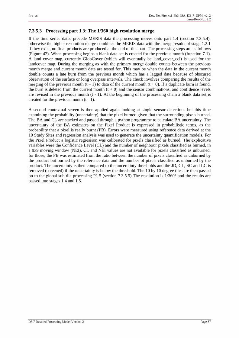
fire_cci
Doc. No.:Fire_cci_Ph3_ISA_D3_7_DPM_v2_2
Issue/Rev-No.: 2.2
D3.7 Detailed Processing Model Version 2 Page 87
7.3.5.3 Processing part 1.3: The 1/360 high resolution merge
If the time series dates precede MERIS data the processing moves onto part 1.4 (section 7.3.5.4),
otherwise the higher resolution merge combines the MERIS data with the merge results of stage 1.2.1
if they exist, no final products are produced at the end of this part. The processing steps are as follows
(Figure 42). When processing begins a blank data set is created for the previous month (function 7.1).
A land cover map, currently GlobCover (which will eventually be land_cover_cci) is used for the
landcover map. During the merging as with the primary merge double counts between the previous
month merge and current month data are tested for. This may be when the data in the current month
double counts a late burn from the previous month which has a lagged date because of obscured
observation of the surface or long overpass intervals. The check involves comparing the results of the
merging of the previous month (t – 1) to data of the current month (t + 0). If a duplicate burn is found,
the burn is deleted from the current month (t + 0) and the sensor combinations, and confidence levels
are revised in the previous month (t - 1). At the beginning of the processing chain a blank data set is
created for the previous month (t - 1).
A second contextual screen is then applied again looking at single sensor detections but this time
examining the probability (uncertainty) that the pixel burned given that the surrounding pixels burned.
The BA and CL are stacked and passed through a python programme to calculate BA uncertainty. The
uncertainty of the BA estimates on the Pixel Product is expressed in probabilistic terms, as the
probability that a pixel is really burnt (PB). Errors were measured using reference data derived at the
10 Study Sites and regression analysis was used to generate the uncertainty quantification models. For
the Pixel Product a logistic regression was calibrated for pixels classified as burned. The explicative
variables were the Confidence Level (CL) and the number of neighbour pixels classified as burned, in
a 9x9 moving window (NEI). CL and NEI values are not available for pixels classified as unburned,
for those, the PB was estimated from the ratio between the number of pixels classified as unburned by
the product but burned by the reference data and the number of pixels classified as unburned by the
product. The uncertainty is then compared to the uncertainty thresholds and the JD, CL, SC and LC is
removed (screened) if the uncertainty is below the threshold. The 10 by 10 degree tiles are then passed
on to the global sub tile processing P1.5 (section 7.3.5.5) The resolution is 1/360° and the results are
passed into stages 1.4 and 1.5.

fire_cci
Doc. No.:Fire_cci_Ph3_ISA_D3_7_DPM_v2_2
Issue/Rev-No.: 2.2
D3.7 Detailed Processing Model Version 2 Page 88
Figure 42: Processing steps for the secondary merge, P1.3

fire_cci
Doc. No.:Fire_cci_Ph3_ISA_D3_7_DPM_v2_2
Issue/Rev-No.: 2.2
D3.7 Detailed Processing Model Version 2 Page 89
The module begins by checking the meris_switch, 1 = YES, 0 = NO.
If NO:
The processing continues to stage 4.
If YES:
Continue
Then the script checks for the existence of MERIS data from the previous month (t-1)
If NO:
A blank dummy file is created (function 7.2) where BAS=0, CON=0, NOV=0, this ensures that data
files are available to pass through the merging function. The missing data are reported to a text file.
The YES condition is now satisfied.
Function 7.2 cci_ create_raster
output file: new raster (byte/integer/float)
input value: pixels (integer)
input value: lines (integer)
input value: bytes per pixel e.g. 1, 2 or 4 (integer)
input value: value for the raster e.g. 0-255 (integer)
If YES:
The 1/120° data sets are resampled to the equivalent MERIS resolution 1/360°. This is done with
cci_dissaggregation(function 7.10).
Function 7.10 cci_dis-aggregation / cci_dis-aggregation_char*
input file: data to resample (short integer / character*)
output file: data at higher resolution (short integer / character*)
input value: pixels (integer)
input value: lines (integer)
input value: number of pixels to disaggregate to (integer)
Then the data files are passed into the second merge function, cci_secondary_merge_check (function
7.11).
Function 7.11 cci_secondary_merge_check_conf
input file: primary merged product 1/360 SC (integer)
input file: primary merged product 1/360 JD (integer)
input file: primary merged product 1/360 CL (integer)
input file: MERIS product 1/360 JD (integer)
input file: MERIS product 1/360 CL (integer)
input file: LC product 1/360 (char)
input file: secondary merged SC t - 1 (integer)
input file: secondary merged JD t - 1 (integer)
input file: secondary merged CL t - 1 (integer)
input file: secondary merged LC t - 1 (byte)
input file: confidence threshold mask sensor w (integer)
input file:confidence threshold mask sensor x (integer)
input file: confidence threshold mask sensor y (integer)
input file: confidence threshold mask sensor z (integer)
output file: secondary merged SC t + 0 (integer)
output file: secondary merged JD t + 0 (integer)
output file: secondary merged CL t + 0 (integer)
output file: secondary merged LC t + 0 (char)
output file: secondary merged SC revised t - 1 (integer)
output file: secondary merged JD revised t - 1 (integer)
output file: secondary merged CL revised t - 1(integer)

fire_cci
Doc. No.:Fire_cci_Ph3_ISA_D3_7_DPM_v2_2
Issue/Rev-No.: 2.2
D3.7 Detailed Processing Model Version 2 Page 90
output file: secondary merged LC revised t - 1 (char)
output file: check for overlap (integer)
input value: pixels (integer)
input value: lines (integer)
The function then revises the merged data:
/*
IF JD = 0 for MERIS and SC > 0 for first merge
THEN SC = SC for first merge (1 OR 2 OR 4 OR 8 OR 9 OR 10 OR 12), JD = JD for first merge, CL = CL for
first merge, LC = globcover class for first merge
IF JD > 0 for MERIS AND SC = 1 OR 2 OR 4 OR 8 OR 9 OR 10 OR 12 for first merge
THEN SC = 5 OR 6 OR 7 OR 11 OR 13 OR 14 OR 15, JD = earliest JD, CL = highest confidence, LC =
globcover class
IF JD > 0 for MERIS AND SC = 0 for first merge
THEN SC = 3, JD = MERIS JD, CL = MERIS confidence, LC = globcover class
Check for double counts:
If JD > 0 for month t-1 and t+0
Then:
t+0, SC = 0, JD = 0, CL = 0, LC = 0
t-1, SC = revised, CL = revised
Write out t+0 and t-1, SC, JD, CL, LC
*/
Where SC= sensor combinations, JD = Julian day, CL = confidence level, LC =land cover
The land cover map is changed from character to byte so it can be stacked by GDAL (Function 7.6)
Function 7.6 cci_char2int
input file: LC product (byte)
output file: LC product (integer)
input value: pixels
inputvalue:lines
These data files are then stacked to a .vrt file and converted to the GeoTiff format with GDAL, P1.4.2.
Prior to the stacking a header file must be created using cci_create_envi_header (function 7.7).
Function 7.7cci_make_envi_header
input value: pixels (integer)
input value: lines (integer)
input value: data type (integer)
input value: top_left_lon (integer)
input value: top_left_lat (integer)
input value: pixel_size (integer)
input value: UTM zone(integer)
input value: Hemisphere(integer)
input value: image name (string)
Once JD, SC, CL and LC are stacked into a GeoTiff the file is called by the python code (Function
7.8) and the uncertainty layer is calculated. The uncertainty layer is then converted from a GeoTiff to
ENVI format using a GDAL function.

fire_cci
Doc. No.:Fire_cci_Ph3_ISA_D3_7_DPM_v2_2
Issue/Rev-No.: 2.2
D3.7 Detailed Processing Model Version 2 Page 91
Function 7.8PredictUnc_pixelproduct.py
input data: path to code
input data: path to input data directory
input data: data input flag (e.g. PixelProduct)
output data: path to output file
input data: optional land cover
/* BAp = f(gpcl,gpnei) if pixel is classified as “burned”
BAp = Uaunburned if pixel is classified as “unburned”
Where: f Logistic Generalized Linear Model
BAp burned area proportion in the reference data
gpcl confidence level of the merged product
gpnei number of neighbor burnt pixels in a 9x9 window
landcover Globcover ID
Uaunburned User accuracy for the unburned category
*/
A mask indicating where single sensor detections should be revised is created using the performance
look up and the land cover map (function 7.4 cci_create_screen).
Function 7.4 cci_create_screen(confidence or uncertainty)
input file: land cover map (byte)
input data: pixels (integer)
input data: lines (integer)
output file: screen for sensor (w OR x OR y OR z)
input data: threshold for sensor (w OR x OR y OR z) for land cover type 1
input data: threshold for sensor (w OR x OR y OR z) for land cover type 2
input data: thresholdfor sensor (w OR x OR y OR z) for land cover type 3
input data: thresholdfor sensor (w OR x OR y OR z) for land cover type 4
input data: thresholdfor sensor (w OR x OR y OR z) for land cover type 5
input data: thresholdfor sensor (w OR x OR y OR z) for land cover type 6
input data: thresholdfor sensor (w OR x OR y OR z) for land cover type 7
input data: thresholdfor sensor (w OR x OR y OR z) for land cover type 8
input data: thresholdfor sensor (w OR x OR y OR z) for land cover type 9
input data: threshold for sensor (w OR x OR y OR z) for land cover type 10
input data: thresholdfor sensor (w OR x OR y OR z) for land cover type 11
input data: thresholdfor sensor (w OR x OR y OR z) for land cover type 12
input data: thresholdfor sensor (w OR x OR y OR z) for land cover type 13
input data: thresholdfor sensor (w OR x OR y OR z) for land cover type 14
input data: thresholdfor sensor (w OR x OR y OR z) for land cover type 15
input data: thresholdfor sensor (w OR x OR y OR z) for land cover type 16
input data: thresholdfor sensor (w OR x OR y OR z) for land cover type 17
input data: thresholdfor sensor (w OR x OR y OR z) for land cover type 18
input data: thresholdfor sensor (w OR x OR y OR z) for land cover type 19
input data: thresholdfor sensor (w OR x OR y OR z) for land cover type 20
input data: thresholdfor sensor (w OR x OR y OR z) for land cover type 21
input data: thresholdfor sensor (w OR x OR y OR z) for land cover type 22
input data: threshold for sensor (w OR x OR y OR z) for land cover type 23
fire_cci
Doc. No.:Fire_cci_Ph3_ISA_D3_7_DPM_v2_2
Issue/Rev-No.: 2.2
D3.7 Detailed Processing Model Version 2 Page 92
Function 7.4 does the following:
/*
When LC = n
Confidence(uncertainty) screen = lut_confidence(uncertainty)_sensor[n]
*/
Where the uncertainty value is below the threshold the JD, SC, CL and LC are reset to zero as they are
no longer considered as burned area (function 7.9 cci_pix_unc_screen3).
Function 7.9cci_pix_unc_screen3
input file: merged SC
input file: merged JD
input file: merged CL
input file: merged uncertainty
input file: merged LC
input file: ATSR screen
input file: ATSR2 screen
input file: VGT screen
input file: MERIS screen
ouput file: revised CS
ouput file: revised JD
ouput file: Revised CL
ouput file: Revised LC
output file: screened data check
input data: pixels
input data: lines
7.3.5.4 Processing part 1.4: Aggregation and generation of the tiled GRID product
In this part P1.4 the 10 by 10 degree merged tiles are used to calculate the final GRID product
attributes and are aggregated and written to a global file in the NetCDF format (Figure 43). The
meris_switch determines if the final product is 1/120 degree or 1/360 degree. All input data are split
into half months prior to calculations (function 7.12 cci_split_month) except for the NOV data which
is received as half monthly summaries directly from the BA algorithm.

fire_cci
Doc. No.:Fire_cci_Ph3_ISA_D3_7_DPM_v2_2
Issue/Rev-No.: 2.2
D3.7 Detailed Processing Model Version 2 Page 93
Figure 43: Processing steps for the generation of the pixel product, P1.4

fire_cci
Doc. No.:Fire_cci_Ph3_ISA_D3_7_DPM_v2_2
Issue/Rev-No.: 2.2
D3.7 Detailed Processing Model Version 2 Page 94
Function 7.12cci_split_month
input file: merged JD (integer)
input file:merged CL (integer)
input file: merged LC (integer)
input file:merged CL (integer)
output file: JD first half of month (integer)
output file: CL first half of month (integer)
output file: LC first half of month (integer)
output file: JD second half of month (integer)
output file: CL second half of month (integer)
output file: LC second half of month (integer)
Input data: pixels
Input data: lines
Sum of total burned area and burned area per and cover (P1.4.1)
The total area burned and the total area burned per land cover are calculated (Function 7.13
cci_aggregation_grid_PSD), these are the source for layers 1 and 5-22 of the final grid product. A
reference file with the total area in m2 is also created and used along with the burned area sum to
calculate the standard error (see standard error explanation).
Function 7.13 cci_aggregation_grid_PSD
input file: merged JD 1/120 or 1/360 (integer)
input file: merged CL 1/120 or 1/360 (integer)
input file: merged LC 1/120 or 1/360 (byte)
output file: layer 1 aggregated ASB file (m2), GRID product 0.5 deg (float)
output file: aggregated CL - currently not required 0.5 deg (float)
output file: aggregated CL - standard deviation file, currently not required 0.5 deg (float)
output file: layer 5 aggregated ASL1 GRID product (float)
output file: layer 6 aggregated ASL2 GRID product (float)
output file: layer 7 aggregated ASL3 GRID product (float)
output file: layer 8 aggregated ASL4 GRID product (float)
output file: layer 9 aggregated ASL5 GRID product (float)
output file: layer 10 aggregated ASL6 GRID product (float)
output file: layer 11 aggregated ASL7 GRID product (float)
output file: layer 12 aggregated ASL8 GRID product (float)
output file: layer 13 aggregated ASL9 GRID product (float)
output file: layer 14 aggregated ASL10 GRID product (float)
output file: layer 15 aggregated ASL11 GRID product (float)
output file: layer 16 aggregated ASL12 GRID product (float)
output file: layer 17 aggregated ASL13 GRID product (float)
output file: layer 18 aggregated ASL14 GRID product (float)
output file: layer 19 aggregated ASL15 GRID product (float)
output file: layer 20 aggregated ASL16 GRID product (float)
output file: layer 21 aggregated ASL17 GRID product (float)
output file: layer 22 aggregated ASL18 GRID product (float)
output file: total cell area (m2) 1/120 or 1/360 0.5 degree cell (float)
input value: pixels (integer)
input value: lines (integer)
input value: sensor resolution, metres (integer)
input value: window size, pixels (integer)

fire_cci
Doc. No.:Fire_cci_Ph3_ISA_D3_7_DPM_v2_2
Issue/Rev-No.: 2.2
D3.7 Detailed Processing Model Version 2 Page 95
/*
FOR k
IF JD > 0 (i.e. burned pixel)
THEN
ASB = total pixels burned (equation 7.1)
Equation 7.1 Sum of burned area:
SBk= ∑ 𝐵𝐴𝑖𝑗
Where, BA = area of burned pixel, k = grid cell and i j are coordinates of individual pixels.
*/
Standard error, of total burned area (P1.4.2)
For the Grid Product, uncertainty is expressed as a standard error, similarly as in the GFED product.
The standard error is calculated using the sum of the burned area per 0.5 degree cell and the total area
of each 0.5 degree cell. Errors were measured using reference data derived at the 10 Study Sites and
regression analysis was used to generate the uncertainty quantification models. The uncertainty of the
Grid Product was expressed as the standard error of the BA proportion estimated by the product (SEp
and EBAp respectively) in each grid cell i. A linear regression model was calibrated to model SEp:
EBApEpS i 10ˆˆˆ
whereβ0 and β1 are the parameters estimated through maximum likelihood methods.
First header files are created for these layers (Function 7.7 cci_create_envi_header) and these two files
are stacked using GDAL (see function explanation) to provide the correct format for a python
programme to ingest the data files (function 7.14 PredictUnc_gridproduct_py).
Function 7.14PredictUnc_gridproduct.py
input data: path to code
input data: data input flag (e.g. PixelProduct)
input data: path to input data directory
output data: path to output file
/*
Prediction functions
AEO = f(BApG)
Where: AEO = Absolute error observed
f = linear model
BApG = burned area proportion in the grid product
*/
The output file is then converted from GeoTiff to ENVI format using GDAL functions. This output
forms the basis of layer 2, standard error, in the final GRID product.
Number of patches (F1.4.3)
This is layer 4 of the GRID product. Three sequential programmes are run to create and count burned
area patches within each 0.5 degree cell. The procedure is as follows:
1) Vertical segmentation (function 7.15 cci_tile_seg). In this function the adjacent JD detections
are coalesced into larger burned area segments to reduce the number of JD patches into fewer
burned area segments. If adjacent to a burned pixel the right hand pixel and/or the pixel in the
row above are assigned the same reference value taken as the Julian Day value. The process
creates vertically striped patches.

fire_cci
Doc. No.:Fire_cci_Ph3_ISA_D3_7_DPM_v2_2
Issue/Rev-No.: 2.2
D3.7 Detailed Processing Model Version 2 Page 96
Function 7.15 cci_tile_seg
input file: primary / secondary merged JD (integer)
output file: segmented patches (integer)
input value: window size, pixels e.g. 56 / 560 (integer)
input value: pixels (integer)
input value: lines (integer)
/*
//loop around each cell
FOR k
FOR i
FOR j
//Assign same value to right adjacent pixels
If (JD > 0 pixelij AND JD > 0 in pixeli+1j) THEN value pixeli+1j = value pixelij
//Assign same value as row above adjacent pixels
If (JD > 0 pixelij and JD > 0 pixelij-1) THEN value pixelij = pixelij-1
*/
Where k = grid cell, I = columns, j = rows
2) Merging of the segments. Each of the segments are then coalesced and numbered into distinct
and discrete burned (function 7.16 cci_tile_morph). An iterative search and merge of adjacent
segments (equivalent to 4 neighbours) is applied. The programme works by searching for
adjacent segments, when adjacent segments are found all pixels in both segments are assigned
the same id and creates one patch. The programme then checks if other segments are adjacent
to this one, if not then the programme searches for the next segment id and repeats the
process. Each new patch is tagged with a different numerical id. When all the segments have
been assigned to patches the results are passed to step 3.
Function 7.16 cci_tile_morph
input file: segmented patches (integer)
output file: morphed patches (integer)
inputvalue: window size, pixels e.g. 56 / 560 (integer)
input value: pixels
input value: lines
/*
FOR k
// Find maximum (max) and minimum (min) values per cell k assigned in cci_seg (function 7.8),
FOR i
FOR j
//e.g. for max:
If value pixelij> max, max = value pixelij
If value pixelij< min, min = value pixelij (when value pixelij> 0)
//Find the adjacent segments
//Cover all possible adjacent segment values by iterating between the max and min values
FOR min to max
FOR i
FOR j
//Find pixels that are in adjacent segments, then assign the first segment value to the adjacent segment
if value pixelij> 0 and pixeli+1j > 0, value pixeli+1j = value pixelij
// then assign all pixels in the adjacent segment with the first segment value
IF valulepixeli+nj+nEQ value pixelij THEN
valuepixeli+nj+n= valuepixelij
//Now check if the merged segment is adjacent to another segment (min->max)
FALSE
Look for next case of two adjacent segments.
*/
Where k = grid cell, I = columns, j = rows
fire_cci
Doc. No.:Fire_cci_Ph3_ISA_D3_7_DPM_v2_2
Issue/Rev-No.: 2.2
D3.7 Detailed Processing Model Version 2 Page 97
3) Calculation of number of patches, cci_patch_stat_area (function 7.17). This function searches
for unique patch reference numbers, when a new reference number is found a value of 1 is
added to a counter.
Function 7.17 cci_tile_patch_stat_area
input file: morphed patches (integer)
output file: number of patches (float)
output file: number of patches (integer)
input value: resolution 1/120 1/360 (integer)
input value: pixels (integer)
input value: lines (integer)
input value: resolution 1/120 1/360 (integer)
input value: grid dims (60 /180) (integer)
input value: top left latitude (integer)
/*
//loop around each cell
FOR k
//Loop through possible patch values (min to max)
FOR m = min to max
FOR i
FOR j
IF value pixel = m
Patch count = patch count + 1
Fraction of observed area (P1.4.4)
This is the source of layer 3 of the GRID product. For this layer the algorithm works out the
proportion of area in a 0.5 degree grid cell that has never been observed during the month or discarded
from the burned area processing due to contamination by cloud, haze, snow, topographic shadow or if
data was flagged as unsuitable for burned area detection. It considers data from all sensors available in
each time step. This information extracted from the layer containing the number of valid observations
(NOV). There are two steps, firstly identify unobserved pixels and water then secondly aggregate to
the 0.5 degree cell.
In the first step, the NOV layer for each BA product is read. Each pixel indicates how many times the
pixel was observed in the time period. If the number is greater than 1 in any NOV data set then the
pixel is flagged as being observed. If the number is less than 1 in all of the NOV data sets then the
pixel is flagged as not being observed. Water pixels are flagged as -1 and not considered as land
surface to observe (function 7.18 cci_merge_nsno). If there is no BA data for any one of the four
sensors, a blank files is created and passed thorugh the algorithm. The meris_switch determines which
resolution the data set is created at.
Function 7.18cci_merge_nsno
input file: Sensor w NOV 1/120 or 1/360 (integer)
input file: Sensor x NOV 1/120 or 1/360 (integer)
input file: Sensor y NOV 1/120 or 1/360 (integer)
input file: Sensor z NOV 1/120 or 1/360 (integer)
input file: Sensor w BS 1/120 or 1/360 (integer)
input file: Sensor x BS 1/120 or 1/360 (integer)
input file: Sensor y BS 1/120 or 1/360 (integer)
input file: Sensor z BS 1/120 or 1/360 (integer)
output file: NSNO t + 0 all 1/120 or 1/360 (integer)
input value: pixels (integer)
input value: lines (integer)

fire_cci
Doc. No.:Fire_cci_Ph3_ISA_D3_7_DPM_v2_2
Issue/Rev-No.: 2.2
D3.7 Detailed Processing Model Version 2 Page 98
/*
FOR i
FOR j
IF sensor x OR sensor y OR sensor x > 0, then surface = observed
IF sensor x OR sensor y OR sensor x = -1, then surface = water
*/
Where, i = columns, j = rows
In the second step, the results of Step 1 are corrected for area and aggregated to 0.5 degrees and the
proportion of valid observations is calculated from the NOV layer, whilst allowing for areas that are
taken up as water. This accounts for land area where pixels were either not observed or deemed
unsuitable for processing (i.e. data discarded as unsuitable due to clouds, bad pixel data). The value is
calculated as percentage, function 7.19 cci_aggregation_nsno_area_16.
Function 7.19 cci_aggregation_nsno_area_16
input file: NOV t + 0 (integer)
output file: ANS GRID product (integer)
input value: pixels (integer)
input value: lines (integer)
input value: sensor_res, 1/120 or 1/360 (integer)
input value: window_size, pixels e.g. 60 / 180 (integer)
/*
FOR k
FOR i
FOR j
%valid surface observationsk = (NOV_countk/(pixel area in gridk - water_area in gridk))*100)
Equation 7.4 Percentage of valid observations
VOk = (𝑣k/(𝑐k−𝑤k))∗100
Where VO = number of valid observations, k = grid cell, v = total area of valid pixels, c = total area of pixels in
cell, w = total area of water pixels in cell
*/
Where i = columns, j = rows, k = grid cell
Create the output format (F1.4.5)
The final step in part 5 is to combine the results of the 10 by 10 degree tiles into a global file. This is
undertaken in the second c-shell script.
#######################################################"
echo " ESA CCI Fire ECV shell script: cci_global_grid_processor.csh"
echo " Copyright University of Leicester 2014"
echo " Code built by Andrew Bradley / Kevin Tansey"
echo " Contact person: [email protected]"
echo " #######################################################"
echo ""
echo " Syntax: cci_global_grid_processor.csh <year>,<month>,<Processor flag (0 = Merge, 1 =
MERIS ONLY, 2 = VGT ONLY)>"
echo " set year"
echo " set month"
echo " Generate which product (0 = Merge, 1 = MERIS ONLY, 2 = VGT ONLY)"

fire_cci
Doc. No.:Fire_cci_Ph3_ISA_D3_7_DPM_v2_2
Issue/Rev-No.: 2.2
D3.7 Detailed Processing Model Version 2 Page 99
echo ""
exit(0)
endif
This is done by creating a master global tile for each layer for each half month (function 7.2 cci_create
raster). The 10 by 10 degree tiles are then mosaicked into a temporary global layer (function 7.20
cci_global_mosaic_float) and the global layers are then combined into a single net CDF file (function
7.21 cci_create_NetCDF_grid). The temporary global layer replaces the master global file and the next
10 by 10 degree tile is mosaicked into it.
Function 7.2 cci_ create_raster
output file: new raster (byte/integer/float)
input value: pixels (integer)
input value: lines (integer)
input value: bytes per pixel e.g. 1, 2 or 4 (integer)
input value: value for the raster e.g. 0-255 (integer)
Function 7.20 cci_ global mosaic float /cci_ global mosaic int*
input file: global raster for one layer of GRID product (float/integer)
input value: pixel dims for global 0.5 degree data set (integer)
input value: lines dims for global 0.5 degree data set (integer)
input value: bytes per pixel e.g. 1, 2 or 4 (integer)
input value: value for the raster e.g. 0-255 (integer)
input value: x position of 10 by 10 degree tile in the global 0.5 degree data set (integer)
input value: y position of 10 by 10 degree tile in the global 0.5 degree data set (integer)
output file: temporary mosaicked raster for one layer of GRID product (float/integer)
*for number of patches cci_global_mosaic_int is used.
Function 7.21cci_create_NetCDF
input file: GRID layer 1 ASB (float)
input file: GRID layer 2 ASE (float)
input file: GRID layer 3 FOB (float)
input file: GRID layer 4 NOP (integer)
input file: GRID layer 5 ASL1 (float)
input file: GRID layer 6 ASL2 (float)
input file: GRID layer 7 ASL3 (float)
input file: GRID layer 8 ASL4 (float)
input file: GRID layer 9 ASL5 (float)
input file: GRID layer 10 ASL6 (float)
input file: GRID layer 11 ASL7 (float)
input file: GRID layer 12 ASL8 (float)
input file: GRID layer 13 ASL9 (float)
input file: GRID layer 14 ASL10 (float)
input file: GRID layer 15 ASL11 (float)
input file: GRID layer 16 ASL12 (float)
input file: GRID layer 17 ASL13 (float)
input file: GRID layer 18 ASL14 (float)
input file: GRID layer 19 ASL15 (float)
input file: GRID layer 20 ASL16 (float)
input file: GRID layer 21 ASL17 (float)
input file: GRID layer 22 ASL18 (float)
input character: output file name (char)
input value: x dims for global 0.5 degree data set (integer)
input value: y dims for global 0.5 degree data set (integer)

fire_cci
Doc. No.:Fire_cci_Ph3_ISA_D3_7_DPM_v2_2
Issue/Rev-No.: 2.2
D3.7 Detailed Processing Model Version 2 Page 100
input value: top left longitude *100 of global 0.5 degree data set (integer)
input value: top left latitude * 100of global 0.5 degree data set (integer)
input value: cell size *100 (integer)
Metadata for the final function is written into the attributes of the NetCDF files.
7.3.5.5 Processing part 1.5: Mosaicking the global sub tiles into the pixel product
The third c-shell produces the global sub tiles for the pixel product.
#######################################################"
echo " ESA CCI Fire ECV shell script: cci_global_pixel_processor.csh"
echo " Copyright University of Leicester 2012"
echo " Code built by Andrew Bradley / Kevin Tansey"
echo " Contact person: [email protected]"
echo " #######################################################"
echo ""
echo " Syntax: cci_global_pixel_processor.csh <zone>,<year>,<month>,<Processor flag (0 =
Merge, 1 = MERIS ONLY, 2 = VGT ONLY)>"
echo " zone N America = 1, S America = 2, Europe = 4, Asia = 5,Africa = 6, Australia = 8"
echo " set year"
echo " set month"
echo " Generate which product (0 = Merge, 1 = MERIS ONLY, 2 = VGT ONLY)"
Each of the 6 sub areas has a separate script with the same generic format. These scripts also require
the input dates text file and variable values for root_path and bin_path. In each script dimensions for
1/120 and 1/360 are included and selected according to the value of the meris_switch, these values
represent:
Number of pixels / lines in a global data set made of 10 degree tiles
Number of pixels / lines in the global subset with whole 10 degree tiles
x, y coordinates of the 10 degree sub tile in a global data set of 10 degree tiles
x, y coordinates of the 10 degree tile in the global sub set with 10 degree tiles
Number of pixels / lines to clip from sub set with whole 10 degree tiles to match the exact
dimensions of the subsets defined in the PSD (sub tile dimensions are not multiples of 10 degrees
and need to be clipped)
Resolution of cells (10 -8)
Using results of section 7.3.5.2 or section 7.3.5.3 the revised JD, SC, UNC_CL and LC are mosaicked
into the global subtile areas and stacked into the final tiff format (Figure 44).
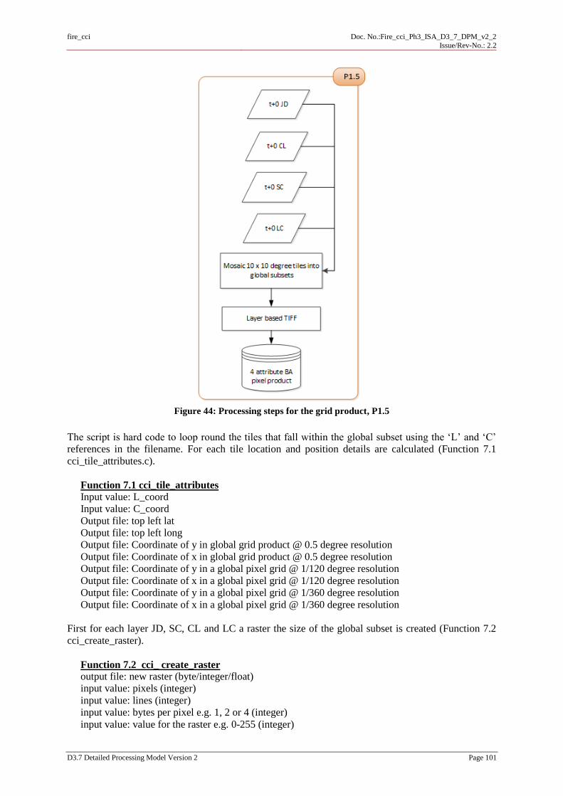
fire_cci
Doc. No.:Fire_cci_Ph3_ISA_D3_7_DPM_v2_2
Issue/Rev-No.: 2.2
D3.7 Detailed Processing Model Version 2 Page 101
Figure 44: Processing steps for the grid product, P1.5
The script is hard code to loop round the tiles that fall within the global subset using the ‘L’ and ‘C’
references in the filename. For each tile location and position details are calculated (Function 7.1
cci_tile_attributes.c).
Function 7.1 cci_tile_attributes
Input value: L_coord
Input value: C_coord
Output file: top left lat
Output file: top left long
Output file: Coordinate of y in global grid product @ 0.5 degree resolution
Output file: Coordinate of x in global grid product @ 0.5 degree resolution
Output file: Coordinate of y in a global pixel grid @ 1/120 degree resolution
Output file: Coordinate of x in a global pixel grid @ 1/120 degree resolution
Output file: Coordinate of y in a global pixel grid @ 1/360 degree resolution
Output file: Coordinate of x in a global pixel grid @ 1/360 degree resolution
First for each layer JD, SC, CL and LC a raster the size of the global subset is created (Function 7.2
cci_create_raster).
Function 7.2 cci_ create_raster
output file: new raster (byte/integer/float)
input value: pixels (integer)
input value: lines (integer)
input value: bytes per pixel e.g. 1, 2 or 4 (integer)
input value: value for the raster e.g. 0-255 (integer)

fire_cci
Doc. No.:Fire_cci_Ph3_ISA_D3_7_DPM_v2_2
Issue/Rev-No.: 2.2
D3.7 Detailed Processing Model Version 2 Page 102
Each 10 by 10 tile is then mosaicked into the global subset (Function 7.22)
Function 7.22cci_global_mosaic_shortint
input file: global sub tile (integer)
input value: Pixels of global sub tile (integer)
input value: Lines of global sub tile (integer)
input value: Offset of pixels in global sub tile relative to global coordinates (integer)
input value: Offset of lines in global sub tile relative to global coordinates (integer)
input file:10 by 10 degree tile mosaic into global sub tile
input value: Pixels of 10 by 10 degree sub tile
input value: Lines of 10 by 10 degree sub tile
input value:Offset of pixels in 10 by 10 tile relative to global coordinates (integer)
input value:Offset of lines in 10 by 10 tile relative to global coordinates (integer)
output file: global sub tile mosaicked with 10 by 10 degree tile (integer)
When the mosaic has been completed the global sub tile is clipped to the dimension stated in the PSD
(Function 7.23) for each of the JD, SC, CL and LC.
Function 7.23 cci_snip
input file: file to resize (char/integer/float)
output file: resized file (char/integer/float)
input value: pixels (integer)
input value: lines (integer)
input value: x_start (integer)
input value: y_start (integer)
input value: x_size (integer)
input value: y_size (integer)
input value: bytes_to_skip (integer)
These data files (JD, SC, CL and LC) are then converted to a .vrt file and then to aGeoTiff format with
GDAL, P1.4.2. Prior to the stacking a header file must be created using cci_create_envi_header
(function 7.7).
Function 7.7cci_make_envi_header
input value: pixels (integer)
input value: lines (integer)
input value: data type (integer)
input value: top_left_lon (integer)
input value: top_left_lat (integer)
input value: pixel_size (integer)
input value: UTM zone(integer)
input value: Hemisphere(integer)
input value: image name (string)
/*
gdalbuildvrt -separate –overwrite<SC><JD><CL ><LC><filename.vrt>
gdal_translate -ot Int16 -of GTiff<filename.vrt><filename.tiff>*/
Where:
Where SC= sensor combinations, JD = Julian day, CL = confidence level, LC =land cover
A generic metadata file is then copied from a source directory into the same directory as the stack. The
PIXEL product is completed.

fire_cci
Doc. No.:Fire_cci_Ph3_ISA_D3_7_DPM_v2_2
Issue/Rev-No.: 2.2
D3.7 Detailed Processing Model Version 2 Page 103
8 References Bachmann, M., Borg, E., Fichtelmann, B., Günther, K., Krauß, T., Müller, A., Müller, R., Richter, R.
(2014). ESA CCI ECV Fire Disturbance, Algorithm Theoretical Basis Document – Volume I– Pre-
processing, Fire_cci_Ph2_DLR_D3_6_1_ATBD_I_v2_2.pdf, (https://www.esa-fire-
cci.org/webfm_send/734)
Benali A., Mota B., Pereira J.M.C., Oom D., Carvalhais N. (2013), ’Global patterns of vegetation fire
seasonality’. (EGU2013-11632) EGU General Assembly, Vienna, April 7-12, 2013
Bradley, A. & Tansey, K. (2014). ESA CCI ECV Fire Disturbance, Algorithm Theoretical Basis
Document Volume III BA Merging: Fire_cci_Ph3_UL_D3_6_3_ATBD_III_v2_3.pdf,
https://www.esa-fire-cci.org/
Boykov, Y., Kolmogorov,V. (2004). An experimental comparison of min-cut/max-flow algorithms for
energy minimization in vision.IEEE Transactions on Pattern Analysis and Machine Intelligence,
26(9): 1124 -1137.
Chuvieco, E., Calado T., Oliva P., (2014). ESA CCI ECV Fire Disturbance - Product Specification
Document, Fire_cci_Ph2_UAH_D1_2_PSD_v4_3.pdf, https://www.esa-fire-cci.org/
Fried, R., Schettlingerand, K.,Borowski, M. (2011). Robust Time Series Filters. R packageversion 3.0,
http://CRAN.R-project.org/package=robfilter.
Killick, R.,Eckley, I. A. (2010). R package- changepoint: Analysis of Changepoint Models. Lancaster
University, Lancaster, UK.
Killick, R., Fearnhead, P., Eckley, I. A. (2012). Optimal detection of changepoints with a linear
computational cost.In Submission.
Krauß, T., Günther, K., Bachmann, M. Alonso, I., Calado, T., Bradley, A., Pereira, J.M., Mota, B.,
Gstaiger, V. (2012). ESA CCI ECV Fire Disturbance, System Interface Definition and Processor
Guidelines, Fire_cci_Ph2_DLR_D3_1_1_SIDPG_v1_2.pdf, https://www.esa-fire-cci.org
Krauß, T., Gstaiger, V., Günther, K., Bradley, A. Alonso, I., Mota, B. (2014). ESA CCI ECV Fire
Disturbance, Input-Output Data Definition, Version 1. Fire_cci_Ph3_DLR_D3_8_IODD_v2_2.pdf,
https://www.esa-fire-cci.org
Kugiumtzis, D., Tsimpiris, A. (2010). Measures of Analysis of Time Series (MATS): A MATLAB
toolkit for computation of multiple measures on time series data bases. Journal of Statistical Software,
33(5): 1-30.
Oom, D., J.M.C. Pereira (2013). Spatial autocorrelation in global vegetation fires: exploratory analysis
of screened MODIS hotspot data. International Journal of Earth Observation and Geoinformation. 21:
326–340.
Pereira, J.M., Mota, B.,Alonso, I., Calado, T.,Oliva, P., Gonzalez-Alonso, F., (2014). ESA CCI ECV
Fire Disturbance, Algorithm Theoretical Basis Document – Volume II,
Fire_cci_Ph3_ISA_D3_6_2_ATBD_II_v2_2.pdf, https://www.esa-fire-cci.org/
PO-ID-ACR-GS-0003, “The AMORGOS MERIS CFI Software User Manual and Interface Control
Document”, prepared by L. Bourg and F. Etanchaud, (2007). Available online (Last access:
24/02/2012): http://earth.esa.int/envisat/services/amorgos/download/Amorgos_ICD-SUM_3.0a.pdf
Richter, R. (2010). Atmospheric/Topographic Correction for Satellite Imagery, User Guide, Version
7.1, January 2010, DLR, Remote Sensing Data Sensor, DLR-IB 565-01 /10
Schläpfer, D., Nieke, J., Itten, K.I. (2007). Spatial PSF Nonuniformity Effects in Airborne Pushbroom
Imaging Spectrometry Data.IEEE Transactions on Geoscience and Remote Sensing, 45(2): 458-468.