D2.1 Semantically enriched socio-mobility patterns and social ...
140
1 Project funded by the Eurpean Community under the Information and Communication Technologies Programme - Contract ICT-FP7-280733 D2.1 Semantically enriched socio-mobility patterns and social network models: preliminary results DATA science for SIMulating the era of electric vehicles www.datasim-fp7.eu Project details Project reference: 270833 Status: Execution Programme acronym: FP7-ICT (FET Open) Subprogramme area: ICT-2009.8.0 Future and Emerging Technologies Contract type: Collaborative project (generic) Consortium details Coordinator: 1. (UHasselt) Universiteit Hasselt Partners: 2. (CNR) Consiglio Nazionale delle Ricerche 3. (BME) Budapesti Muszaki es Gazdasagtudomanyi Egyetem 4. (Fraunhofer) Fraunhofer-Gesellschaft zur Foerdering der Angewandten Forschung E.V 5. (UPM) Universidad Politecnica de Madrid 6. (VITO) Vlaamse Instelling voor Technologisch Onderzoek N.V. 7. (IIT) Technion – Israel Institute of Technology 8. (UPRC) University of Piraeus Research Center 9. (HU) University of Haifa Contact details Prof. dr. Davy Janssens Universiteit Hasselt– Transportation Research Institute (IMOB) Fuction in DATA SIM: Person in charge of scientific and technical/technological aspects Address: Wetenschapspark 5 bus 6 | 3590 Diepenbeek | Belgium Tel.: +32 (0)11 26 91 28 Fax: +32 (0)11 26 91 99 E-mail: [email protected] URL: www.imob.uhasselt.be Deliverable details Work Package WP2 Deliverable: Semantically enriched socio-mobility patterns and social network models: preliminary results Dissemination level: PU/CO Nature: R Contractual Date of Delivery: 31.08.2012 Actual Date of Delivery: 31.08.2012 Total number of pages: 140 Authors: F. Giannotti, G. Andrienko, B. Furletti, C. Koerner, F. Liu, M. Nanni, L. Pappalardo, D. Pedreschi, N. Pelekis, C. Renso, S. Rinzivillo, Abstract This report presents the work pursued in the first year of the project by the participants of WP2. The document presents the scientific background and the state of the art of the main topics of the workpackage, an overview of the work done by the partners and the scientific achievements reached in this first year, and a presentation of the short/medium term research plan of the workpackge.
-
Upload
khangminh22 -
Category
Documents
-
view
0 -
download
0
Transcript of D2.1 Semantically enriched socio-mobility patterns and social ...
1
Project funded by the Eurpean Community under the Information and Communication Technologies Programme - Contract ICT-FP7-280733
D2.1 Semantically enriched socio-mobility patterns and social network models:
preliminary results DATA science for SIMulating the era of electric vehicles
www.datasim-fp7.eu
Project details
Project reference: 270833 Status: Execution Programme acronym: FP7-ICT (FET Open) Subprogramme area: ICT-2009.8.0 Future and Emerging Technologies Contract type: Collaborative project (generic)
Consortium details
Coordinator: 1. (UHasselt) Universiteit Hasselt Partners: 2. (CNR) Consiglio Nazionale delle Ricerche
3. (BME) Budapesti Muszaki es Gazdasagtudomanyi Egyetem 4. (Fraunhofer) Fraunhofer-Gesellschaft zur Foerdering der Angewandten Forschung E.V 5. (UPM) Universidad Politecnica de Madrid 6. (VITO) Vlaamse Instelling voor Technologisch Onderzoek N.V. 7. (IIT) Technion – Israel Institute of Technology 8. (UPRC) University of Piraeus Research Center 9. (HU) University of Haifa
Contact details
Prof. dr. Davy Janssens Universiteit Hasselt– Transportation Research Institute (IMOB) Fuction in DATA SIM: Person in charge of scientific and technical/technological aspects Address: Wetenschapspark 5 bus 6 | 3590 Diepenbeek | Belgium Tel.: +32 (0)11 26 91 28 Fax: +32 (0)11 26 91 99 E-mail: [email protected] URL: www.imob.uhasselt.be
Deliverable details
Work Package WP2 Deliverable: Semantically enriched socio-mobility patterns and social network models: preliminary results Dissemination level: PU/CO Nature: R Contractual Date of Delivery: 31.08.2012 Actual Date of Delivery: 31.08.2012 Total number of pages: 140 Authors: F. Giannotti, G. Andrienko, B. Furletti, C. Koerner, F. Liu, M. Nanni, L. Pappalardo, D. Pedreschi, N. Pelekis, C. Renso, S. Rinzivillo,
Abstract This report presents the work pursued in the first year of the project by the participants of WP2. The document presents the scientific background and the state of the art of the main topics of the workpackage, an overview of the work done by the partners and the scientific achievements reached in this first year, and a presentation of the short/medium term research plan of the workpackge.

2
Project funded by the Eurpean Community under the Information and Communication Technologies Programme - Contract ICT-FP7-280733
Copyright
This report is DATASIM Consortium 2012. Its duplication is restricted to the personal use within the consortium and the European Commission.
www.datasim-fp7.eu

Contents
1 Semantically enriched socio-mobility patterns and social networkmodels: preliminary results 41.1 Scientific Pillars: State of Art . . . . . . . . . . . . . . . . . . 6
1.1.1 Mobility Data Mining . . . . . . . . . . . . . . . . . . . 61.1.2 Semantic Enrichment of Movement Data . . . . . . . . 71.1.3 Mobility Network Science . . . . . . . . . . . . . . . . 9
1.2 First Year Achievements . . . . . . . . . . . . . . . . . . . . . 101.2.1 Individual Patterns . . . . . . . . . . . . . . . . . . . . 111.2.2 Collective Patterns . . . . . . . . . . . . . . . . . . . . 201.2.3 Global Models and Complex Systems . . . . . . . . . . 24
1.3 Directions for Future Research . . . . . . . . . . . . . . . . . . 251.3.1 Diaries and Activity Extraction . . . . . . . . . . . . . 261.3.2 Scaling Radiation Model . . . . . . . . . . . . . . . . . 261.3.3 Diffusion Model for Car Pooling Adoption . . . . . . . 271.3.4 Consolidation of Mobility Patterns on Large Scale . . . 27
A Mobility Data Mining 34
B Visual analytics of movement: a rich palette of techniques toenable understanding 60
C Understaning human mobility using Mobility Data Mining 93
D Mobility and Network Science 118
3

Chapter 1
Semantically enrichedsocio-mobility patterns andsocial network models:preliminary results
This report presents the work pursued in the first year of the project bythe participants of WP2, entitled Big data driven theories of mobility demand.The objective of the workpackage is to develop a novel data-driven theory ofhuman mobility based on the exploitation of semantically enriched mobilitydata. The extracted patterns and models will be exploited within WP3 to en-hance the capabilities of actual simulators by considering also the individualmotivations and social interactions among mobile agents.
The workpackage is organized into four tasks:
• Task 2.1: Person-based constrained trajectory mining based onGPS data. The objective of this task is to demonstrate how the combi-nation of network science with data mining within a uniform analyti-cal framework is able to develop macro-micro models of human mobil-ity and achieve an unprecedented explanatory and predictive power.
• Task 2.2: Semantic enrichment of mined trajectories. This taskwill investigate a semantic enrichment and reasoning process to char-acterize movement data with domain-dependent behaviour definition.The discovered mobility models and patterns will be expressed interms of realistic semantics of movements. The semantic annota-tion/reconstruction of mobility patterns will be based on the mobility
4

and social networking data, and the socio-demographic data providedby WP1.
• Task 2.3: Social network mining. In this task we plan to analyzethe topological and the dynamical properties of the social network ofusers, to the purpose of better characterizing the mobility behavioursof sub-populations on the basis of their social relations. The analyticalof network science bring into the project another semantic dimensionwhich may contribute at better understanding the mobility behaviourat society-wide scale.
• Task 2.4: Knowledge transition to Simulator. This task will in-tegrate the patterns, models of the previous tasks to blend the be-havioural and semantic description of individual traveler into the novelagent-based simulation system developed in WP3, which is able toevaluate policy and behaviourally reasoning on a country-wide scale.
During this first year of the project, the participants of the WP2 collabo-rated to three main activities:
• Collective exploration of the state of the art in the fields related to thetasks of the workpackage;
• Concrete exploration of some research directions and preliminary re-sults;
• Definition of shared research activities among the partner of the WP2.
The report is organized into three parts, each covering one of the threeactivities above. In Section 1.1 we present the state of the art of the threescientific pillars of WP2: (i) mobility data mining; (ii) semantic enrichmentof movement data; (iii) mobility networks science. Section 1.2 presents thescientific achievements of the first year by showing a classification of theactivities according to three families of patterns and models: individual pat-terns, collective patterns and global laws. Section 1.3 concludes the reportand provide a roadmap for the collaborative research activities of workpack-age for the next year.
Papers refereed within the report are available for the reviewers at theURL http://kdd.isti.cnr.it/datasim/dlv2.1/ (Project Officer will pro-vide login/password to access to the website).
5

1.1 Scientific Pillars: State of Art
The state of the art related to the activities of WP2 is structured into threesections corresponding to the three scientific cornerstones of the workpack-age. The content of each of these sections is based on a series of bookchapters that has been developed by the partners of this consortium thatparticipate also to the Coordination Action MODAP project. The book titledMobility Data: Modeling, Management, and Understanding discusses differ-ent facets of mobility data, like spatio-temporal data modeling, data aggre-gation and warehousing, data analysis, and basic definitions and state-of-the-art concepts and techniques. One peculiarity of the book is to use aconsistent framework that facilitates understanding of all different facets.The learning objective is to enable readers to understand the many issuesat hand and identify the application and research perspectives targeted bythe development of mobility data. The book chapters present in an intro-ductory language the state of the art of these three topics, without assumingany prior knowledge in mobility data management. As a result of the effortfor the book, we include in the next sections three extended abstract of thechapters. The actual contents of the chapters are part of this deliverableand they are included in appendix. To avoid copyright infringements ,theappendix are restricted within the project consortium.
Each section presents also relevant papers of the project consortium thatcan be useful to better understand the context and scientific background ofthese three cornerstones.
1.1.1 Mobility Data Mining
In this section we present a taxonomy of methods for the analysis of move-ment data based on two main approaches: an approach based on analyticalmethods and algorithms that instantiate an instance of the knowledge dis-covery process; a second approach combines the analytical methods withinteractive visual techniques to enable and promote human understandingof the data and human reasoning about the data.
The chapter Mobility Data Analysis [11] (see Chapter A) provides a gen-eral overview of the literature for the instantiation of the knowledge dis-covery process to the context of trajectory and mobility data. The specificcontext requires special attention when the general KDD process is instan-tiated to a scenario with data with a complex structure, since the searchspace for interesting solutions may be orders of magnitudes larger than aclassical relational dataset. Moreover, mobility data represents a set of very
6
complex phenomena where a single local event may have broader influenceon the global status of the traffic. With this premises, the chapter presentsa taxonomy of mobility data mining methods defined over the kind of pat-terns or models extracted, in particular local patterns and global models.Another important aspect on mobility data is the distinction between indi-vidual habits and collective behaviors. The latter perspective on mobility datamining approaches is the central activity of the work in DATASIM and it willbe discussed deeply in Section 1.2, where recent research achievements arepresented.
The chapter Visual analytics of movement: a rich palette of techniques toenable understanding [1] (see Chapter B) gives an overview of the existingvisual analytics methods for analyzing movement data. The chapter focuseson four different approaches to focus on movement data: on the individualtrajectories as wholes; on portions of the trajectories to highlight relevantvariations in movement; on aggregation and distribution of multiple move-ments; on the relationship between the movement and its context.
1.1.2 Semantic Enrichment of Movement Data
The state of the art on semantic enrichment is structured into three contribu-tions. One is a survey accepted for publication at ACM Computing Surveyswhich presents the state of the art on semantic trajectories modelling andanalysis, thus including the specific task of semantic erichment intendedboth as contruction of semantic trajectories and as annotation of raw tra-jectories with semantic information. A second contribution goes more indetails on the semantic enrichement intended as an enriched knowledgeprocess over raw trajectory data. The steps of this process can be seen assemantic enrichment with the objective of the better comprehension of hu-man mobility. The third contribution presents a proposal to understand andmanage complex, global, socially interactive systems, with a focus on sus-tainability and resilience, as planned and designed in the Future ICT Project.A brief abstract of these three contribution are below, while the full versionof the book chapter is available in appendinx.
The survey [14] entitled Semantic Trajectories Modeling and Analysisaims at summarizing the main approaches in the literature for the semantictrajectory recent research. The survey is structured in sections that presentthe process of semantic trajectory definition, trajectory behavior, trajectorytransformations, and behavior inference and privacy issues. In particular,after three introductory sections about main definitions used in the paper, asection on the trajectory pre-processing techniques is followed by a semantic
7

enrichment part where approaches for annotating trajectories with semanticinformation are detailed. Later, the paper focuses on the data mining meth-ods used to infer behavior from large sets of mobility data and eventuallya section devoted to the privacy issues on (semantic) trajectories concludesthe survey.
Semantic enrichment of trajectory refers to a process which attaches se-mantic information to raw trajectory data. This broad concept covers severaltecnniques going from the annotation of raw data with information comingfrom application domain data sources (e.g. metadata, surveys, etc) to theautomatic inference of semantic information from the data itself. In partic-ular, the book chapter on Mobility data understanding [15] (see Chapter C)focuses mainly on the Knowledge Discovery process as a way to infer se-mantic information on trajectory data. As we can see, the chapter presentsa semantic enrichment KDD process where each step of the process enablesthe understanding of different aspects of the data related to an applicationdomain. We base our presentation on M-Atlas, a system which supports thesemantic ernichement KDD process on mobility data. After presenting thecore concepts of the system and the tools for basic statistics on the mobil-ity data, we show tasks like data preparation - a context-driven preparationof data for mining or data validation where the mobility dataset is evalu-ated against an application domain knowledge that acts as a ground truth.This latter step allows to establish if, and at which degree, the dataset tobe analyses is representative of the real world and therefore the results ofthe analysis are still valid in the real world. Other presented techniquesinclude progressive clustering and parameter tuning. The second part ofthe chapter is more semantic oriented, since it focuses on the discovery oftrajectory behavior which are illustrated by means of examples a mobilityknowledge discovery process. Mobility behavior like StuckedInTrafficJamand Commuter are discovered in data using a combination of moning tech-niques. In these examples we introduce also the use of ontologies whichimplement a deductive step in the KDD process. Indeed, this step basedon the ontology reasoning further enriches mobility data with pre-definedbehavior classes based on the trajectory features.
In [10] it is presented a sustainable system implementing the SocialSensing and Semantic Enrichment of digital breadcrumbs (i.e. digital tracks).These simple forms of data, collected for many different purposes, containhistorical and collective information of very basic human actions. To makesuch breadcrumbs usable for analysis it is needed to inject back the con-textual knowledge of human action that got lost during sensing. There isthe attempt to add context information to raw data by augmenting, tagging,
8

and/or classifying data in relationship to dictionaries and/or other referencesources. An advanced vision of semantic enrichment is that of a system thatcontinuously and automatically enriches its own understanding of the con-text and content of the data it is receiving, by comparing it to its existingknowledge base and then building increasingly smarter classifiers upon thatstore. More generally, the overall repertoire of semantic enrichment needsto be adaptive with respect to the continuous progress of sensing devices, toimprove its capability to map human behavior along multiple dimensions,and to become increasingly intelligent with use, by incorporating machinelearning techniques.
1.1.3 Mobility Network Science
The chapter Combining human mobility and network science [9] (see Chap-ter D) provides a review of some of the important findings on human mobil-ity and network science, from empirical observations and scaling propertiesto generative and predictive models. The chapter is structured into threeparts. The first part presents the fundamental models for motion availablein the literature. The overview starts with the presentation of Brownianmotion based on the observartions of the botanist Robert Brown, who for-mulated the hypothesis that the motion is the result of a random walk with anormal distribution for the position at time t, with the variance proportionalto t. Some animal movements, however, do not obey this law and theypresent occasional jumps of very long distance. This variation of randomwalk model is better approximated by the Levy-flight model which modelsmovement as a sequence of interleaved brownian motion and occasionallong jumps according to a normal distribution. Since these models are notsufficient to model human movements, new models were provided capableof modeling long jumps as a power law distribution. The second part of thechapter introduces the basic concepts of network science, introducing thereader to the main network models used, like random graph, small-worknetworks, and scale-free network. The last part presents an overview ofthe combination of mobility and network science and it shows how eachdimension influences the other one.
Recent activities within the project have explored the opportunities ofusing community discovery algorithms to analyze human mobility. Theseapproaches are presented in details in Section 1.2. The survey A Classi-cation for Community Discovery Methods in Complex Networks [7] by CNRprovides an extensive overview on community discovery problem, organiz-ing the contribution of the literature according to the notion of community
9

adopted.
1.2 First Year Achievements
The broad diffusion of location aware technologies like GPS sensors andGSM devices provides the opportunity for a social microscope to observehuman movements in details. These data provide accurate spatial as wellas temporal information on movement patterns, allowing the travel behav-ior of individuals to be monitored automatically, offering a potential solu-tion to the challenges associated with conventional travel surveys. However,large raw movement data are often semantically poor and they require novelmethods to infer richer semantic information about mobility behaviors andactivities of people. To this purpose we have explored how implicit seman-tics can be extracted automatically by this kind of data exploiting automaticmobility data analysis and user interaction and interpretation.
One of the main objective of the project is the combination of micro- andmacro-laws of human mobility. Exploiting the big data available, we havenow an unprecedented possibility to analyze quantitatively the behaviourof human systems with the methods of statistical physics and data min-ing. Thanks to the recent developments in the statistical physics of complexnetworks, a series of theoretical, computational and analytical frameworksare now available: concepts like centrality of nodes and robustness of thestructure have been quantified and tested in a variety of situations. Sim-ilarly, the area of mobility data mining has gained remarkable insight inextracting models describing collective mobility behaviour out of humantrajectories. A goal of this workpackage is to find a synthesis between thistwo approaches: macro-laws of human mobility focus on asymptotic prop-erties providing relative simple models that depends on a small number ofparameters; micro-laws emerging from mobility data mining enable us todiscover the statistically significant sub-populations where complexity dis-appears and regular behaviour appears.
In order for the patterns and models to be incorporated within the sim-ulator, it is necessary that the extracted knowledge would be semanticallyenriched with purpose and activities of people. The semantic annotationof mobility patterns should exploit both the mobility and social networkingdata and the contextual information of people whereabouts, like sociode-mographic and geographic data as described in deliverable 1.1 from WP1.
The scientific activity of the workpackage is organized into three cate-gories, according to the type of patterns and model extracted:
10

• individual patterns concentrate on personal history and highlight rele-vant behaviors and activities of each moving person;
• collective patterns loose the details of the single user and they focus onthe phenomena emerging from people moving together in a territory;
• global models and complex system define the general rules of mobilityat a large scale and they bridge the first two kinds of patterns.
1.2.1 Individual Patterns
The point of view of individual patterns is given by the personal movementhistory of each individual, with the objective of indentify relevant patterns.In particular, this research activity is tailored at indentifiy three types ofindividual patterns, that are detailed below.
Extraction of individual mobility profile
One of the basis for our research on this topic is the definition of a user’smobility profile [20]. The daily mobility of each user can be essentially sum-marized by a set of single trips that the user performs during the day. Whentrying to extract a mobility profile of users, our interest is in the trips thatare part of their habits, therefore neglecting occasional variations that di-vert from their typical behavior. Therefore in order to identify the individualmobility profiles of users from their GPS traces, the following steps will beperformed - see Figure 1.1:
1. divide the whole history of the user into trips (Figure 1.1(a))
2. group trips that are similar, discarding the outliers (Figure 1.1(b))
3. from each group, extract a set of representative trips, to be used asmobility profiles (Figure 1.1(c)).
Mobility Profile
Trips The history of a user is represented by the set of points in spaceand time recorded by their mobility device:
Definition 1.2.1 (User history). The user history is defined as an orderedsequence of spatio-temporal points H = 〈p1 . . . pn〉 where pi = (x, y, t) andx, y are spatial coordinates and t is an absolute timepoint.
11

(a) (b) (c)
Figure 1.1: Mobility profile extraction process: (a) trip identification; (b)group detection/outlier removal; (c) selection of representative mobilityprofiles.
Figure 1.2: Trajectories of a user and the corresponding groups and routinesextracted (A and B). Of the 30 trips, 11 are part of group A, and 12 of groupB, while the remaining 7 are noise. The two routines are spatially similar,yet move in opposite directions (points represent the end of trips), i.e., south(A) vs. north (B).
12

This continuous stream of information contains different trips made bythe user, therefore in order to distinguish between them we need to detectwhen a user stops for a while in a place. This point in the stream willcorrespond to the end of a trip and the beginning of the next one. We adopta heuristic-based approach for the detection of the stops. Thus we look forpoints that change only in time; i.e. they keep the same spatial position fora certain amount of time quantified by the temporal threshold thstop
temporal.Specularly, a spatial threshold thstop
spatial is used to remove both the noiseintroduced by the imprecision of the device and the small movements thatare of no interest for a particular analysis.
We indicate with S = 〈S1 . . . St〉 the set of all stops over H. Once wehave found the stops in the users history we can identify the trips:Definition 1.2.2 (Trip). A trip is defined as a subsequence T of the user’shistory H between two consecutive stops in the ordered set S or between astop and the first/last point of H (i.e., p1 or pn).
The set of extracted trips T = 〈T1 . . . Tc〉 in Fig. 1.1(a), are the basicsteps to create the user mobility profile. Notice that the thresholds thstop
spatial
and thstoptemporal are the knobs for expressing specific analytical requirements.
Trip Groups Our objective is to use the set of trips of an individualuser to find his routine behaviors. We do this by grouping together similartrips based on concepts of spatial distance and temporal alignment, withcorresponding thresholds for both the spatial and temporal components ofthe trips. In order to be defined as routine, a behavior needs to be supportedby a significant number of similar trips. The above ideas are formalized asfollows:Definition 1.2.3 (Trip Group). Given a set of trips T , spatial and temporalthresholds thgroup
spatial and thgrouptemporal, a spatial distance function δ : T 2 → R
and a temporal alignment constraint α : T 2×R → B between pairs of trips,and a minimum support threshold thgroup
support, a trip group for T is defined asa subset of trips g ⊆ T such that:
1. ∀t1, t2 ∈ g.δ(t1, t2) ≤ thgroupspatial ∧ α(t1, t2, th
grouptemporal);
2. |g| ≥ thgroupsupport.
Condition 1 requires that the trips in a group are approximately co-located, both in space and time, while condition 2 requires that the group issufficiently large. Again, the thresholds are the knobs that the analyst willprogressively tune the extraction process with.
13

Mobility Profile Each group obtained in the previous step representsthe typical mobility habit of a user, i.e., one of his routine movements. Herewe summarize the whole group by choosing the central element of such agroup:
Definition 1.2.4 (Routine). Given a trip group g and the distance function δused to compute it, its routine is defined as the medoid of the set, i.e.:
routine(g, δ) = arg mint∈g
∑t′∈g\{t}
δ(t, t′)
Notice that the temporal alignment is always satisfied over each pair oftrips in a group, therefore the alignment relation α does not appear in thedefinition. Now we are ready to define the users mobility profile.
Definition 1.2.5 (Mobility Profile). Given a set of trip groups G of a user andthe distance function δ used to compute them, the user’s mobility profile isdefined as his corresponding set of routines:
profile(G, δ) = {routine(g, δ) | g ∈ G}
Mobility Profile Construction The definitions provided in the previ-ous section were kept generic w.r.t. the distance function δ. Different choicescan satisfy different needs, possibly both conceptually (which criteria definea good group/routine assignment) and pragmatically (for instance, simplercriteria might be preferred for the sake of scalability). Obviously, the re-sults obtained by different instantiations can vary greatly. Hence the crucialpoint is the selection of groups of trajectories. Our proposal is to use a clus-tering method to carry out this task. We choose a clustering algorithm fortrajectories consisting of two steps. First, a density-based clustering is per-formed, thus removing noisy elements and producing dense – yet, possiblyextensive – clusters. Secondly, each cluster is split through a bisection k-medoid procedure. Such method splits the dataset into two parts throughk-medoid (a variant of k-means) with k = 2, then the same splitting pro-cess is recursively applied to each sub-group. Recursion stops when eachresulting sub-cluster is compact enough to fit within a distance threshold ofits medoid, by removing sub-clusters that are too small. The bisection k-medoid procedure guarantees that requirements 1 and 2 of Definition 1.2.3are satisfied. The clustering method adopted is parametric w.r.t. a repertoireof similarity functions, that includes: Ends and Starts functions, comparingtrajectories by considering only their last (respectively, first) points; Routesimilarity, comparing the paths followed by trajectories from a purely spatial
14

viewpoint (time is not considered); Synchronized route similarity, similar toRoute similarity but considering also time.
The definition of mobility profile enables a proactive carpooling appli-cation scenario where the profiles of a set of participants are extracted andthen analyzed to find matching profiles. The matched profiles are candi-dates for sharing the car to perform the movements they have in common.Using an extensive dataset of GPS traces from private vehicles we find thatapprox. 70% of individuals have a matching profiles with another person,thus potentially allowing the reduction of circulating vehicles by 30%. Thisfeasibility experiment has also been extended on movement data with aspatial granularity comparable to GSM data, providing acceptable perfor-mances.
This kind of online service for matching commuter profiles is helpfulin order for the carpooling service to be successful, due to the large com-munity involved. Such service is necessary but not sufficient because car-pooling requires rerouting and activity rescheduling along with candidatematching. We advise to introduce services of this kind using a two step pro-cess [5]: (1) an agent- based simulation is used to investigate opportunitiesand inhibitors and (2) online matching is made available. We explored thechallenges to build the model and in particular investigated possibilities toderive the data required for commuter behavior modeling from big data(such as GSM, GPS and/or Bluetooth).
Mobility Diaries Mobility profiles portrait the systematic mobility and donot consider occasional movement of an user. To compensate this approach,we extend the analysis of individual mobility to derive a pattern capable ofmodeling both occasional and systematic movement of an user. Precisely, weare studying an analytical process with the objective of extracting a mobilitydiary for an individual.
A Mobility Diary MD for a user u is a characterization of the movementsof a user on the basis of his/her sequence of stops and trips. A MobilityDiary can be represented as a model that determine the location of a userin a given time interval Tj = [t1, t2]. Formally, a Mobility Diary model for auser u can be described as a probability function Pu(Li‖Tj) that assign thelikelihood of the user u to be in the location Li in the time interval Tj . Theprocess to extract a mobility diary consists of the following steps:
1. the mobility history of a user is divided into trips and stops;
2. the stops are aggregated by spatial similarity to derive a set of relevantlocations;
15

Figure 1.3: Clustering of stop points for a single user. (left) Trajectories(drawn with red line) of a user and their corresponding locations (circlesfilled in green). (right) Details of a set of locations of the same user.
3. the movement of the user is generalized according to his/her relevantlocations.
The first step is similar to the initial step in the procedure to extractmobility profiles. In the second step, a spatial generalization step is appliedto the stop points, by associating a set of points in a neighborhood to alocation: all the points are generalized according to a threshold δ, i.e. a setof points are clustered if the maximum distance between any two points inthe cluster is within δ. This kind of generalization enable us to representeach cluster with a compact notation consisting of the centroid of the pointsin the cluster and the radius of the set r (where r ≤ δ). To cluster thestops, we adopted the bisecting k-medoids procedure as explained above.Figure 1.3 shows the locations extracted from the trajecories of a singleuser.
The set of locations for a user u enables the description of the movementof the user in terms of the sequence of movements from one location to thesuccessive one. Such a sequence is characterized by the time spent by theuser in each location and by the time intervals in which the user is movingto change her location. From the actual locations we obtain a very precisedescription of the position of the user along time. However, such descriptionis too detailed for a practical use. Instead, we want to extract a model thatwould describe the typical behavior of the user in a cyclic time interval, e.g.during a day. The Mobility Model is intended precisely for this abstraction.Given a time interval T , the complete history of user’s locations is condensedin T , by computing the probability of the user to be observed in a given
16

Figure 1.4: Mobility diary of an user by locations. (Left) A gantt represen-tation of the locations of a user during a specific time interval: the rangeaxis contains the list of visited locations in descending order of frequency;the domain axis represents the time dimension; a bar represents the stopof the user in the location for the corresponding amount of time. (Right)Summarization of the mobility of the user in a single day representation:the chart represent the most probable location of the user at a given time ofthe day. It is evident, in this example, the daily routine of the trip to work,the trip to go back home for lunch and then the return to work.
location at a time instant t ∈ T . To simplify the presentation, hereafter weconsider a day as the time interval T and a time granularity of one hour;the probability of the position of the user is expressed as the probability offinding the user in a location in a give hour of the day.
For example, Figure 1.4 shows the result of the extraction process. OnFigure 1.4(Right) the location visited by a user are represented as a ganttchart: the rows represent the different location in order of frequency de-scending, and the columns represent the time line. On the Figure 1.4(Left)the movements of the user have been condensed in a single day and thedifferent curves represent the probability of the user to be in that locationat that time.
Despite the Mobility Diary is a compact representation of a typical dayof a user, there exists a model for each user observed in the input dataset.Thus, it is necessary to analyze the extracted Mobility Diaries in order tofind similarities and regularities in the data. Moreover, the Mobility Diaryrefer to a set of location that have a validity for the single user. What ismissing is a semantic enrichment of such location in order to be able tocompare the location of a user with the locations of the other ones. Theactivity extraction process is described in details in the following section.
17

Extraction of individual activities
The extraction and exploitation of activities is a central topic in the objec-tives of the workpackage. During the first year several activities have beenactivated by the partners to explore this semantic enrichment. We presenthere the activity that are still in progress and that have produced prelimi-nary papers that are under review or are going to be submitted in the nextmonths.
The general approach is to exploit traditional survey data collected withthe corresponding GPS traces. A proposal from IMOB (submitted to theJournal of the Transportation Research Board) consists in a decision tree-based model that considers activity start times and activity durations. Twomodels, i.e. a predicted probability distribution and a point predictionmodel, are derived from a decision tree classification. Two types of data isbeing used, namely paper-and-pencil activity-travel diary data as the train-ing/validation set and corresponding GPS data as the test set.An accuracyof 74% is achieved when training the tree. The accuracy of the model forthe validation set, i.e. 72.5%, shows that over fitting is minimal. Whenapplying the model to the GPS test set, the performance is approx. 76% ac-curate. The models constructed indicate the importance of time informationin the semantic enrichment process. The contribution of this study towardsfuture data collection is promising in that it enables researchers to automat-ically infer activities solely from activity start time and duration informationobtained from GPS data.
A similar approach has also been studied for phone calling data (sub-mitted to Journal of Expert Systems with Applications). IMOB is exploringan integration between machine learning algorithms and the characteris-tics of underlying activity-travel behavior which originates the movementtraces. Resulted from the nature of how activity and related travel deci-sions are made in daily life, humans follow a high degree of spatial andtemporal regularities as well as sequential orders in activity-travel patterns.The annotation process consists of four steps. First, we define a set of com-prehensive temporal variables characterizing each calling location; featureselection techniques are then applied to choose the most effective variablesin the second step. Next, a set of state-of-the-art classifiers including Sup-port Vector Machine, Logistic Regression, Decision Tree, and Random Forestare employed to build classification models, and an additional ensemble ofthe above model results is also tested. Finally, the inference performanceis further enhanced by a post processing algorithm based on sequential in-formation. Using calling location data collected from 80 peoples real life
18

over more than a year, we evaluated our approach via a set of extensive ex-periments. Based on the ensemble of the individual classifiers, we achievedprediction accuracy of 69.7%. Furthermore, using the post processing al-gorithm, the performance obtained a 7% improvement. The experiment re-sults demonstrate the feasibility to infer activities using information drawnfrom calling locations. The advantage of using this annotation approach isthat it does not depend on additional sensor data and geographic details,the data collection cost is low and the results are generic to be deployed toother areas. Both the methodology and data requirement needed to applythis method are fairly simple.
The activity recognition task is also explored by taking advantage of theMobility Diary model proposed by CNR. Since a Mobility Diary for an useru is a concise representation of his/her mobility we can reason about theinternal characteristics of this model and its relationships with the context.In particular, a Mobility Diary model can be represented as a network wherenodes correspond to locations and edges correspond to travels between twolocations. In this phase it is crucial to attach semantic information both tothe nodes and to the edges. To achieve this objective, we are exploring amachine learning approach exploiting the survey data provided by IMOB(see Deliverable 1.1 from WP1). Each user provides two source of informa-tion: a GPS trace collected by a PDA device and a paper-and-pencil surveywhere he/she declares all the movements performed and the related activi-ties. Our proposed approach consists in extracting two Mobility Diaries fromthese sources of information and to exploit their correspondences to extendthe semantic knowledge from the survey to the GPS traces. Our objectiveis to characterize the labeling in terms of features of the Mobility Diary ex-tracted from GPS data. The candidate features that have been explored sofar includes: duration time in a location, starting time from a location, out-degree of a location, frequency of an edges, and other attributes that relatesto relevant network measures of the network derived by the Mobility Di-ary. The expected outcome of this process is a classifier capable of relatingcharacteristics of the Mobility Diary to semantic concepts.
Extraction of individual points of interest
Meaningful information can be derived by means of interactive visual anal-ysis performed by a human expert; however, this is only possible for dataabout a small number of people. A recent proposal by Fraunhofer [3] hasbeen accepted for presentation at “GeoVisual Analytics, Time to Focus onTime” Workshop @ GIScience (18 September 2012, Columbus OH, USA). It
19

proposes an approach that allows scaling to large datasets reflecting move-ments of numerous people. It includes extracting stops, clustering them foridentifying personal places of interest (POIs), and creating temporal signa-tures of the POIs characterizing the temporal distribution of the stops withrespect to the daily and weekly time cycles and the time line. The analystcan give meanings to selected POIs based on their temporal signatures (i.e.,classify them as home, work, etc.), and then POIs with similar signaturescan be classified automatically. The possibilities for interactive visual se-mantic analysis are demonstrated by example of GSM and GPS data. GPSdata allow inferring richer semantic information but only temporal signa-tures may be insufficient for interpreting short stops. This work serves abase to develop an intelligent system that learns how to classify personalplaces and trips while a human analyst visually analyzes and semanticallyannotates selected portions of movement data.
1.2.2 Collective Patterns
Collective patterns highlight relevant behaviors that result from the con-tribution of groups of individual movements. In this case the resolutionof the individual (his/her history and habits) is ignored. An example ofthis approach is the analysis of mobility data to detect groups of vehiclethat present critical spatio-temporal characteristics, like for example slowmovement. With this objective, sets of objects, or parts of their movements,are grouped together according to similar spatio-temporal characteristicsexploiting mobility data mining methods (see Chapter A). It is worth not-ing how this approach is relevant to provide semantics and interpretation tomobility patterns provided by the data mining methods, as required by Task2.2.
We organize the activities in this context according to the different typesof aggregations that we extract.
Characteristic behaviors
Individual patterns observable through GSM data are analyzed in [8] byCNR to identify groups of users with similar individual profiles. The pro-posed analytical method exploits the individual movement habits to seg-ment a population of mobile phone users into profiles, namely residents,commuters, and visitors. The proposed method is structured into two phases.First, the user behavior observed through calling logs is aggregated into a
20

temporal profile, i.e. a succinct representation of the calling and move-ment habits of each user. Secondly, the profiles are analyzed by a combi-nation of domain expert rules and clustering based techniques to identifysubgroups with common characteristics. The experiments show that theproposed method is capable of automatically distinguish the profiles of resi-dent, commuters and occasional visitors to a city and to highlight emergingbehavior that were not initially considered by the domain experts.
Significant movements
The emerging of mobility patterns represents an example of bottom-up ap-proach to semantic enrichment. When several individuals perform similarbehaviors it is possible for the analyst to infer useful knowledge from thisphenomena. A typical example is the identification of traffic jams. For in-stance, the work Traffic Jams Detection Using Flock Mining [12] by CNR pro-vides an application scenario of the flock algorithm to the detection of trafficjams. In this scenario, the extracted flocks are analyzed with a two-step ap-proach to select only those that are potential traffic jams. The raw resultof the algorithm is a set of patterns where different object travel coherentlytogether. However, not all the candidate flocks can be considered trafficjam. Thus, the work provides a basic definition of a traffic jam in terms ofrelative average speed in an area and compares each candidate flock withthe expected speed. This comparison is used to distinguish regions wheretypically objects move slowly from those where slow movement is rare. Thisclassification step explores a semantic enrichment approach where move-ment characteristics and background knowledge are combined.
UPRC has been investigated efficient solution for tackling the problemsof sub-trajectory clustering and outlier detection in Moving Object Databases(MOD). The proposed methodology relies on a voting-and-segmentationphase that segments trajectories of moving objects according to local den-sity and trajectory similarity criteria, a sampling phase that selects the topvoted sub-trajectories that will be used as seeds for the clustering process,and a clustering phase that is driven by the sampling set of the originaldataset, which groups the sub-trajectories of the MOD into clusters, also de-tecting outliers. The proposed solution, called S2T-Clustering (for sampling-based sub-trajectory clustering) is boosted by an efficient index mechanismthat speeds up the overall process, also allowing S2T-Clustering to be effi-ciently registered as a query operator in a real MOD engine. The previousmentioned indexing techniques will be the kernel to support the BIG datachallenges raised in DATASIM. Obviously, given the above characteristics,
21

S2T-Clustering is also related with the activities of WP1. More details aboutthis line of research are provided in the activity report of WP1.
Significant places
The joint work of CNR and Fraunhofer From movement tracks through eventsto places: Extracting and characterizing significant places from mobility data[2] generalizes the previous approach by relaxing the spatio-temporal con-straints to identify relevant movement events. The work proposes a visualanalytical procedure aimed at determining significant places on the basis ofcertain types of events occurring repeatedly in movement data. The pro-cedure consists of four major steps: (1) extraction of relevant events fromtrajectories by queries involving diverse instant, interval, and cumulativecharacteristics of the movement and relations between the moving objectsand elements of the spatio-temporal context; (2) density- based clusteringof the events by spatial positions, temporal positions, movement directionsand, possibly, other attributes, which may be done in two stages for aneffective removal of noise and getting clear clusters; (3) spatio-temporalaggregation of events and trajectories by the extracted places; and (4) anal-ysis of the aggregated data. The proposed procedure was applied on twodistinct movement datasets: a set of GPS traced vehicles with the objectiveof detecting traffic jams in a metropolitan area and a set of air traffic routesto extract relevant landing and take-off patterns along time. The work re-ceived the Best Paper Award and extended version has been submitted to theIEEE Transactions on Visualization and Computer Graphics (TVCG) Journaland it is under review at the moment.
The approach of combining interactive visual techniques with computa-tional methods from machine learning and statistics is extended and gen-eralize in the work A visual analytics framework for spatio-temporal anal-ysis and modelling [4] by Fraunhofer. Clustering methods and interactivetechniques are used to group spatially referenced time series (TS) of nu-meric values by similarity. Statistical methods for time series modelling arethen applied to representative TS derived from the groups of similar TS.The framework includes interactive visual interfaces to a library of mod-elling methods supporting the selection of a suitable method, adjustment ofmodel parameters, and evaluation of the models obtained. The models canbe externally stored, communicated, and used for prediction and in furthercomputational analyses. From the visual analytics perspective, the frame-work suggests a way to externalize spatio-temporal patterns emerging inthe mind of the analyst as a result of interactive visual analysis: the patterns
22

are represented in the form of computer-processable and reusable models.From the statistical analysis perspective, the framework demonstrates howtime series analysis and modelling can be supported by interactive visualinterfaces, particularly, in a case of numerous TS that are hard to analyseindividually. From the application perspective, the framework suggests away to analyse large numbers of spatial TS with the use of well-establishedstatistical methods for time series analysis.
Significant Areas
A distinctive feature of the previous two approaches is the transformation ofmobility data into a different form of data, respectively events and time se-ries. This approach of extracting different representation of knowledge frommobility data is also exploited to take advantage of network based analysis.The bases of this approach have been presented in Chapter D. In the follow-ing we present two novel approaches of this paradigm applied to the analysisof collective mobility behavior that are are orthogonal to Task 2.2 and Task2.3. The two approaches are based on the extraction of a complex networkfrom mobility data and on the analysis of these networks by means of com-munity discovery methods. The paper Discovering the Geographical Bordersof Human Mobility [17] by CNR proposes a general method to determinethe influence of social and mobility behavior over a specific geographicalarea in order to evaluate to what extent the current administrative bordersrepresent the real basin of human movement. In this work mobility datais generalized over a tessellation of the space to produce a graph model-ing of mobility demand: nodes of the graph represent the places and thelink between any two nodes is weighted with the directed flow of move-ment between the two. Once the mobility network has been extracted, acommunity discovery algorithm is able to partition the nodes, and hencethe geography, into zone with a high internal mobility w.r.t the mobilitytowards other zones. Since the spatial resolution influences the extractedmobility network, the work Optimal Spatial Resolution for the Analysis ofHuman Mobility [16] by CNR explores the previous approach by consider-ing several spatial resolution provided by a series of regular grid partitions.Each spatial generalization is analyzed by extracting the corresponding mo-bility network and by evaluating several network statistics borrowed fromnetwork science.
In [6] by CNR the nodes of the graph represent the points of interestand the links are weighted according to the number of trajectories passingthrough them. The objective is to identify communities of places based on
23

the mobility of the citizens. For example, the bridge communities highlighta mobility that tend to cross the city to visit places which can be far away,while the overlap communities show different mobility behavior associatedto the same places.
1.2.3 Global Models and Complex Systems
Radiation Model
Introduced in its contemporary form in 1946, but with roots that go backto the eighteenth century, the gravity law is the prevailing framework withwhich to predict population movement, cargo shipping volume and inter-city phone calls, as well as bilateral trade flows between nations. Despiteits widespread use, it relies on adjustable parameters that vary from regionto region and suffers from known analytic inconsistencies. In [18] we in-troduce a stochastic process capturing local mobility decisions that helps usanalytically derive commuting and mobility fluxes that require as input onlyinformation on the population distribution. The resulting radiation modelpredicts mobility patterns in good agreement with mobility and transportpatterns observed in a wide range of phenomena, from long-term migra-tion patterns to communication volume between different regions. Givenits parameter-free nature, the model can be applied in areas where we lackprevious mobility measurements, significantly improving the predictive ac-curacy of most of the phenomena affected by mobility and transport pro-cesses.
Starting from this model, in [19] we showed how models of humanmobility are derivable within the framework of the radiation model. A uni-fied continuous approach is used for computing the probability to observea trip to any region. Fluxes among all areas, defined by a generic spatialsubdivision, are computed and are shown to lead to previously proposedmodels, like the intervening opportunities model, or new models, like thehigh expectations model, depending on the benefit distribution. Compari-son with observational data offered by commuting trips extracted from theUS census data set shows the validity of such models. Finally, we discussthe advantages of the continuum approach, we illustrate the fluxes’ additiv-ity property, and we use our theoretical framework to derive some specialcases of gravity models from first principles. These findings suggest that thecomplex topological features observed in large mobility and transportationnetworks may be the result of a simple stochastic process taking place on aninhomogeneous landscape.
24

Scaling the general law of human mobility
General laws on human mobility are based on large mobile phone datasets.In our project and in our current research activity we extensively used ve-hicular GPS traces to sense the movement of people. Clearly, the observedGPS vehicles covers a smaller population w.r.t. the devices observed by thecellular network but provide a very precise spatial position. Moreover, theGPS traces are limited to car travels and do not allow to sense the move-ment of people once they have parked their car. It is therefore legitimate toinvestigate to what extent the previous models apply to GPS data, which de-viations are observed, and which new analytical opportunities are providedby the finer spatio-temporal granularity. On the other hand, it is compulsoryto investigate to what extent our GPS data are representative of the overallvehicular mobility, in order to generalize the validity of our findings. Thepaper [13] shows two evidences of the statistical validity of our dataset:first, the known human mobility models can be refined to deal with car mo-bility, and second, the available GPS data can indeed be used as a faithfulproxy of car mobility.
Human Mobility and Social Ties
One of the founding ideas of the DATASIM project is the evidence that themobility is a complex phenomenon that has strong relationship with themotivation of people to perform some activities. Indeed, such activities arestrongly influenced by the social links with people around us. Starting fromthese premises, in [21] we investigated to what extent do individual mobil-ity patterns shape and impact the social network. In this work, by followingdaily trajectories and communication records of 6 Million mobile phone sub-scribers, we address this problem for the first time, through both empiricalanalysis and predictive models. We find that the similarity between two in-dividuals’ movements strongly correlates with their proximity in their socialnetwork. We further investigate how the predictive power hidden in suchcorrelations can be exploited to address the challenging problem of deter-mining which new links will develop in a social network on the base of theobservation of the individual mobility.
1.3 Directions for Future Research
The research directions in the short/middle terms origin from the work inprogress described in Section 1.2 and they take advantage from the expertise
25

of each participant of the WP2.
1.3.1 Diaries and Activity Extraction
Starting from the preliminary work on Mobility Diaries, we plan to extendthe approach by stressing the semantic enrichment phase of the model. Thesemantic information involved in the enrichment process can be obtained bya top-down or a bottom-up method. Top down indicates a method to collectand summarize all the available information sources from the applicationdomain (e.g. the geo-objects that a trajectory crosses, personal informationcoming form questionnaires, etc) with the objective of annotating the trajec-tories. With bottom up we indicate all the methods used to infer knowledgefrom data. The more challenging methods form a research point of vieware the bottom-up: inferring knowledge from data. For example, the homeand work places of individuals can be inferred as the most frequent loca-tions observed in a large number of Mobility Diaries, thus exploiting thefrequency measure of the model to derive a semantic interpretation. IMOB,CNR and Fraunhofer are collaborating to provide method for semantic in-terpretation of movement data by exploiting automatic methods and visualanalytics techniques and combinations of the two.
1.3.2 Scaling Radiation Model
The radiation model has been formulated and applied to predict OD com-muting matrices at mesoscopic scales, i.e. at the municipality/county level,whose average size is 50 km. Recent studies have shown that its applica-tion at the regional scale, where the average location size is 5 km, is moreproblematic since some of the simplifying assumptions used at larger scalescease to be valid.
CNR and BME are collaborating to apply the radiation model at the re-gional scale to reproduce the observed Origin-Destination (OD) matricesextracted from GPS traces. IMOB and BME are performing a similar activ-ity by exploiting OD matrices available from the transportation models. Wedo a systematic study of the various formulations and assumptions of themodels belonging to the radiation models family. In particular we considerthe high expectations model and the intervening opportunities model, bothhaving one free parameter, and we will test their performances consideringtwo kinds of distance measures, the first being the usual Euclidean distance,the second being the average travel time between the two locations. Once
26

the best performing model has been identified, we plan to adopt it to fore-cast mobility flux and to enable the simulation of future mobility scenariosaccording to what-if hypotheses.
1.3.3 Diffusion Model for Car Pooling Adoption
We intend to study the diffusion models underlying the adoption of innova-tive behavior, with particular attention to the carpooling scenario. In fact,besides the intrinsic difficulty of adopting carpooling as a means for trans-portation for systematic mobility needs, due to the the competition withother modalities (public transport, private cars, etc.), there is also a factorof social influence, in terms of missing examples in the social neighborhoodto imitate, or to a negative perception of carpooling. Therefore, as wit-nessed in the social science research on the diffusion of innovation, thereis probably an influence model that plays here, in that a cascading adop-tion of carpooling cannot be expected only as a result of reasoned choice ofcost/benefits, but also as an effect of reaching a threshold of social neigh-bors that adopt carpooling and foster imitation in their communities. Whatis a realistic diffusion model for car pooling? What is a critical thresholdthat may cause cascading adoption? How to discover a set of promisinginnovators that may trigger a successful diffusion process? How can weleverage the social network and the network of compatible mobility needsto design a successful diffusion process? We plan to study along these lines,trying to overcome the difficulty of lacking adoption data from real carpool-ing experiments; to this purpose, we shall consider both simulations basedon real mobility profiles, as studied during the first year of the project, andreal data from different scenarios of innovation diffusion, such as the dataon Skype users available at BME on both the adoption of services and thesocial relations. Joint research of CNR and BME.
1.3.4 Consolidation of Mobility Patterns on Large Scale
The activities of pattern and model extraction will be further experimentedin the second year of the project. In particular, we plan to follow two direc-tions: (i) extend the method and techniques to the large scale by exploitingthe datasets available in the project and presented in Deliverable 1.1 ofWP1; (ii) selection of patterns useful for the simulator. For example, the ac-tivity on diaries extraction and activity learning have shown how crucial is aprecise labeling of activities, by means of ad-hoc devices and mobile applica-tions capable of assisting the user to provide valid interpretation for his/her
27

own travels. To this purpose, we are planning to set up a crowdsourcingexperiment by recruiting a set of volunteers equipped with a smartphone onwhich should be installed a social/mobile-sensing application, like for ex-ample the SPARROW tool developed by IMOB and presented in Deliverable1.1.
28

Bibliography
[1] G. Andrienko and N. Andrienko. Visual analytics of movement: a richpalette of techniques to enable understanding. In C. Renso, S. Spac-capietra, and E. Zimanyi, editors, Mobility Data: Modeling, Manage-ment, and Understanding. 2013, to appear.
[2] G. Andrienko, N. Andrienko, C. Hurter, S. Rinzivillo, and S. Wrobel.From movement tracks through events to places: Extracting and char-acterizing significant places from mobility data. In Visual AnalyticsScience and Technology (VAST), 2011 IEEE Conference on, pages 161–170, oct. 2011.
[3] G. Andrienko, N. Andrienko, A-M Olteanu Raimond, J. Symanzik, andC. Ziemlicki. Towards extracting semantics from movement data byvisual analytics approaches. In accepted for presentation at “GeoVisualAnalytics, Time to Focus on Time”, Workshop at GIScience, 2012.
[4] N. Andrienko and G. Andrienko. A visual analytics framework forspatio-temporal analysis and modelling. Data Mining and KnowledgeDiscovery, pages 1–29. 10.1007/s10618-012-0285-7.
[5] T. Bellemans, S. Bothe, S. Cho, F. Giannotti, Davy Janssens, L. Knapen,C. Korner, M. May, M. Nanni, D. Pedreschi, H. Stangeb, R. Trasarti, A-U-Haque Yasara, and G. Wets. An agent-based model to evaluate car-pooling at large manufacturing plants. In Proceedings of the 1st Inter-national Workshop on Agent-based Mobility, Traffic and TransportationModels, Methodologies and Applications, 2012.
[6] I. R. Brilhante, M. Berlingerio, R. Trasarti, C. Renso, J.A. de Macedo,and M. A. Casanova. Cometogether: discovering communities ofplaces in mobility data. In Proceedings of the 13th International Confer-ence on Mobile Data Management. July 23-26, 2012, Bengaluru, India.,2012.
29

[7] M. Coscia, F. Giannotti, and D. Pedreschi. A classification for commu-nity discovery methods in complex networks. Statistical Analysis andData Mining, 4(5):512–546, 2011.
[8] B. Furletti, L. Gabrielli, C. Renso, and S. Rinzivillo. Identifying usersprofiles from mobile calls habits. In Proceedings of the ACM SIGKDDInternational Workshop on Urban Computing, UrbComp ’12, pages 17–24, New York, NY, USA, 2012. ACM.
[9] F. Giannotti, L. Pappalardo, D. Pedreschi, and D. Wang. Mobility andnetwork science. In C. Renso, S. Spaccapietra, and E. Zimanyi, editors,Mobility Data: Modeling, Management, and Understanding. 2013, toappear.
[10] F. Giannotti, D. Pedreschi, S. Pentland, P. Lukowicz, D. Kossmann,J. Crowley, and D. Helbing. A planetary nervous system for socialmining and collective awareness. European Journal of Physics, 2012,to appear.
[11] M. Nanni. Mobility data mining. In C. Renso, S. Spaccapietra, andE. Zimanyi, editors, Mobility Data: Modeling, Management, and Under-standing. 2013, to appear.
[12] R. Ong, F. Pinelli, R. Trasarti, M. Nanni, C. Renso, S. Rinzivillo, andF. Giannotti. Traffic jams detection using flock mining. In ECML/PKDD(3), pages 650–653, 2011.
[13] L. Pappalardo, S. Rinzivillo, Z. Qu, D. Pedreschi, and F. Giannotti. Un-derstanding the patterns of car travels. European Journal of Physics,2012, to appear.
[14] C. Parent, S. Spaccapietra, C. Renso, G. Andrienko, N. Andrienko,V. Bogorny, M.L. Damiani, A. Gkoulalas-Divanis A, J.A. Macedo,N. Pelekis, Y. Theodoridis, and Z. Yan. Semantic trajectories model-ing and analysis. ACM Computing Surveys, 2012, to appear. to appear.
[15] C. Renso and R. Trasarti. Understaning human mobility using mobilitydata mining. In C. Renso, S. Spaccapietra, and E. Zimanyi, editors,Mobility Data: Modeling, Management, and Understanding. 2013, toappear.
[16] S. Rinzivillo, M. Coscia, D. Pedreschi, and F. Giannotti. Optimal spa-tial resolution for the analysis of human mobility. In Proceedings of
30

the 2012 IEEE/ACM International Conference on Advances in Social Net-works Analysis and Mining (ASONAM 2012), 2012.
[17] S. Rinzivillo, S. Mainardi, F. Pezzoni, M. Coscia, D. Pedreschi, andF. Giannotti. Discovering the geographical borders of human mobility.KI - Knstliche Intelligenz, 26:253–260, 2012.
[18] F. Simini, M. C. Gonzalez, A Maritan, and A-L Barabasi. A universalmodel for mobility and migration patterns. Nature, 484, 2012.
[19] F. Simini, A. Maritan, and Z. Neda. Continuum approach for a class ofmobility models. arXiv:1206.4359v1, 2012.
[20] R. Trasarti, F. Pinelli, M. Nanni, and F. Giannotti. Mining mobilityuser profiles for car pooling. In Proceedings of the 17th ACM SIGKDDinternational conference on Knowledge discovery and data mining, KDD’11, pages 1190–1198, New York, NY, USA, 2011. ACM.
[21] D. Wang, D. Pedreschi, C. Song, F. Giannotti, and A.-L. Barabasi. Hu-man mobility, social ties, and link prediction. In Proceedings of the17th ACM SIGKDD International Conference on Knowledge Discoveryand Data Mining, KDD ’11, pages 1100–1108, New York, NY, USA,2011. ACM.
31

1
Project funded by the Eurpean Community under the Information and Communication Technologies Programme - Contract ICT-FP7-280733
D2.1 Semantically enriched socio-mobility patterns and social network models: preliminary results - APPENDIXES
DATA science for SIMulating the era of electric vehicles www.datasim-fp7.eu
Project details
Project reference: 270833 Status: Execution Programme acronym: FP7-ICT (FET Open) Subprogramme area: ICT-2009.8.0 Future and Emerging Technologies Contract type: Collaborative project (generic)
Consortium details
Coordinator: 1. (UHasselt) Universiteit Hasselt Partners: 2. (CNR) Consiglio Nazionale delle Ricerche
3. (BME) Budapesti Muszaki es Gazdasagtudomanyi Egyetem 4. (Fraunhofer) Fraunhofer-Gesellschaft zur Foerdering der Angewandten Forschung E.V 5. (UPM) Universidad Politecnica de Madrid 6. (VITO) Vlaamse Instelling voor Technologisch Onderzoek N.V. 7. (IIT) Technion – Israel Institute of Technology 8. (UPRC) University of Piraeus Research Center 9. (HU) University of Haifa
Contact details
Prof. dr. Davy Janssens Universiteit Hasselt– Transportation Research Institute (IMOB) Fuction in DATA SIM: Person in charge of scientific and technical/technological aspects Address: Wetenschapspark 5 bus 6 | 3590 Diepenbeek | Belgium Tel.: +32 (0)11 26 91 28 Fax: +32 (0)11 26 91 99 E-mail: [email protected] URL: www.imob.uhasselt.be
Deliverable details
Work Package WP2 Deliverable: Semantically enriched socio-mobility patterns and social network models: preliminary results Dissemination level: CO Nature: R Contractual Date of Delivery: 31.08.2012 Actual Date of Delivery: 31.08.2012 Authors: F. Giannotti, G. Andrienko, B. Furletti, C. Koerner, F. Liu, M. Nanni, L. Pappalardo, D. Pedreschi, N. Pelekis, C. Renso, S. Rinzivillo,
Abstract This part of the Deliverable contains material protected by copyrights. Thus the dissemination of the appendixes is restricted to use within the consortium and the European Commission.

2
Project funded by the Eurpean Community under the Information and Communication Technologies Programme - Contract ICT-FP7-280733
Copyright
This report is DATASIM Consortium 2012. Its duplication is restricted to the personal use within the consortium and the European Commission.
www.datasim-fp7.eu

Appendix A
Mobility Data Mining
Author : Mirco Nanni
Book : Mobility Data: Modeling, Management, and Understanding
Editors : Chiara Renso, Stefano Spaccapietra, and Esteban Zimanyi
Year : 2013, to appear
34

1
Mobility data miningMirco Nannia
Abstract
Analyzing huge amount of mobility data in the form of trajectories isa challenging task. This chapter presents a summary of the potential-ities, main issues and current solutions to the problem of extractinguseful knowledge out of mobility data. The most important trajectorydata mining techniques are introduced, including methods for detectingfrequent and sequential patterns as well as clustering.
1.1 Introduction
What is mobility data mining. The trajectories of a moving objectare a powerful summary for its activity related to mobility. As seen inprevious chapters, such information can be queried in order to retrievethose trajectories (and the objects that own them) that respond to somegiven search criteria, for instance following a predefined interesting be-havior. However, when massive information is available, we might beable to move a step forward and ask that such “interesting behaviors”automatically emerge from the data. That is precisely the domain ex-plored by mobility data mining.
Moving from queries to data mining essentially consists in adding de-grees of freedom to the search process that the algorithms perform. Forinstance, a query might consist in searching those trajectories that atsome point perform the following sequence of maneuvers: abrupt slowdown, U-turn and finally accelerate. One possible corresponding data
a KDD Lab, ISTI-CNR, Pisa, Italy

2 Mobility data mining
mining task, instead, might require to discover which sequences of ma-neuvers are performed frequently in the database of trajectories. Then,the output sequences obtained might contain also the slow-down → U-turn → accelerate example mentioned above. To perform this data min-ing process the user needs to specify the general structure of the behav-iors he/she searches (sequences), what kind of elements they can contain(the set of maneuvers to consider, as well as a precise way to locate agiven maneuver within a trajectory), and a criterion to select “inter-esting” behaviors – in our example, the user wants only behaviors thatappear frequently in the data.
The several forms and variants of existing analysis tasks that belongto mobility data mining cannot be easily categorized into a set of fixedclasses. However, it is possible to recognize a few simple dimensions alongwhich to locate the different analysis methods. In the following we willmention two of them, that will be also used later as guidelines duringthe presentation of analysis examples.
Local patterns vs. global models. The example of behavior illus-trated at the beginning of this section is representative of a class ofmining methods, called local patterns or, in most contexts, simply pat-terns. The key point of local patterns is the aim of identifying behaviorsand regularities that involve only a (potentially small) subset of trajecto-ries, and that describe only a (potentially small) part of each trajectoryinvolved.
The complementary class of mining methods is called global models, orsimply models. Their objective is to provide a general characterizationof the whole dataset of trajectories, thus going towards the definitionof general laws that regulate the data, rather than spotting interestingyet isolated phenomena. For instance, we will see later mining tasksaimed to define a global subdivision of all trajectories into homogeneousgroups, as well as tasks aimed to discover rules able to predict the futureevolution of a trajectory (i.e., the next locations it will visit).
Mining individual habits vs. mining collective behaviors. Arelevant aspect to consider when analyzing trajectory data is the factthat in general multiple trajectories can be produced by the same mov-ing object. Depending on how we deal with this association, we canobtain analysis with rather different objectives. Two basic (and mostinteresting) approaches are the following:
• mining individual habits: the mobility mining methods are applied on

1.2 Local trajectory patterns/behaviors 3
the trajectories of a single moving object, thus obtaining a set of out-put patterns or models for each object. This way, the behaviors weextract describe salient aspects of the individual, such as movementsthat it repeats often (i.e., it repeated them in several distinct trajec-tories) or a general classification of its trips (i.e., each trajectory isput in a class);
• mining collective behaviors: all moving objects are analyzed together,and the analysis takes into consideration the owner of each trajectory.This way, the behaviors we extract describe aspects that are significantfor the collectivity, and not only for a single individual.
Note on terminology. The notion of (local) trajectory pattern intro-duced above is substantially equivalent to that of “trajectory behavior”defined in previous chapters. The two notions originate from differentcommunities and simply reflect different perspectives of the same sub-ject: the data management view (where “trajectory behavior” originates)focuses more on determining who is associated to each behavior; the datamining view, on the contrary, is more focused on what are the interestingbehaviors.
In the rest of the chapter we will provide an overview of the problemsand methods available in the mobility data mining field. For obviousreasons of space, the discussion will not cover exhaustively the availableliterature on the subject, and instead will propose some representativeexamples of the various topics. The presentation will mainly follow thedistinction between local patterns and global models introduced above.
1.2 Local trajectory patterns/behaviors
The mobility data mining literature offers several examples of trajectorypatterns that can be discovered from trajectory data. Despite this widevariety, most proposals actually respect two basic rules: first, a pattern isinteresting (and therefore extracted) only if it is frequent, and thereforeit involves (or appears in) several trajectories; second, a pattern mustdescribe the movement in space of the objects involved, and not onlyaspatial or highly abstracted spatial features.
While the spatial component of patterns is a rather fixed component,the temporal one (also intrinsic in trajectory data) can be treated inseveral different ways, and we will use this differentiation to better orga-nize the presentation. Then, while a trajectory pattern always describes

4 Mobility data mining
a behavior that is followed by several moving objects, we can choosewhether they should do so together (i.e., at the same time instants), indifferent moments yet with same timings (i.e., there can be a time shiftbetween the moving objects), or in any way, with no constraints on time.
Using absolute time or Groups that move together. One of thebasic questions that arise when analyzing moving objects trajectories isthe following:
Are there groups of objects that move together for some time?
For instance, in the realm of animal monitoring such kind of patternswould help to identify possible aggregations, such as herds or simplefamilies, as well as predator-prey relations. In human mobility, similarpatterns might indicate groups of people moving together on purposeor forced by external factors, e.g. a traffic jam, where cars are forced tostay close to each other for a long time period.
Obviously, the larger are the groups and the longer is the period theystay together, the higher is the likelihood that the observed phenomenonis significant and not a pure coincidence. For instance, if two membersof a population of zebras under monitoring happen to move close toeach other for a short time, that can be seen as a random encounter.However, if dozens of zebras are observed together for several hours, wecan safely assume that they form a herd or something is happening thatforces them to keep together.
The simplest form of trajectory pattern in literature that exactly an-swers the question posed above is the trajectory flock. As the name sug-gests, a flock is a group of moving objects that satisfy three constraints:
• a spatial proximity constraint: within the whole duration of the flock,all its members must be located within a disk of radius r – possiblya different one at each time instant, i.e. the disk moves to follow theflock;
• a minimum duration constraint: the flock duration must be at least ktime units;
• a frequency constraint: the flock must contain at least m members.
Figure 1.1(left) shows an abstract example of flock, where three tra-jectories meet at some point (at the fifth time unit), keep close to eachother for some time (four consecutive time units) and then separate(ninth time unit). If, for instance, the constraints chosen by the user arethe radius r used in the figure to draw the circles, a minimum duration

1.2 Local trajectory patterns/behaviors 5
Figure 1.1 Visual representation of a trajectory flock (left) and sam-ple result on a real dataset: the left part represents the trajectoriesinvolved, the right part a zoom on the segments that form the flock
of four time units (or less) and a minimum size of three members, thenthe common movement shown in the figure will be recognized as a flock.
Figure 1.1(right) shows an example extracted from a real dataset thatcontains GPS tracks of tourists in a recreational park (DwingelderveldNational Park, in Netherland). The leftmost section of the figure depictsthe three trajectories that were involved in the flock, while the rightmostone shows (a zoom with) only the segments of trajectories that createthe flock. As we can see, in this example a flock is a local pattern, bothin the sense of involving only a small subset of trajectories (three, in ourcase), and in the sense of describing an interesting yet relatively smallsegment of the whole life of the trajectories involved.
The general concepts of moving together or forming a group are imple-mented by the flocks framework in the simplest way possible: the objectsare required to be very close to each other during all the duration of theflock. However, a group might appear also under different conditions.One of these alternatives is to require that at each timestamp the objectsform a cluster – thus borrowing ideas and methods from the clusteringliterature. A notable example are moving clusters, a form of pattern thatat each time stamp groups objects by means of density-based clustering.Such approach can be summarized in the following points:
• first, all objects that have a large number of neighbors are labeled ascore objects; among the remaining objects, those that are neighborsof core objects are labeled as border objects; the remaining objects arelabeled as noise;
• second, core objects are grouped into clusters in such a way that eachpair of neighboring core objects fall in the same cluster. Essentially,clusters are computed as transitive closure of the neighbor relation;

6 Mobility data mining
• finally, border objects are assigned to the same cluster of their neigh-boring core objects1, while noise is discarded.
The neighbors of an object are all the objects at a distance not largerthan a threshold r, and the minimum number of neighbors requiredto make an object a core object is also a parameter m. Therefore, wecan see that a core object and its neighbors approximately satisfy thecloseness requirements of a flock – more exactly, these where densityrequirements. The step forward here is that multiple compact groups canbe merged together if they are adjacent (see the second step), in orderto form larger ones. Beside their sheer size, the groups formed throughthis process can also have a relatively large extension (therefore not allpairs of objects in the cluster will be close to each other, because theyactually are neighbors of neighbors of neighbors. . . ) and an arbitraryshape. In several contexts this can be useful, for instance in analyzingvehicle trajectories, since the road network simply forces large groupsof cars to distribute along the roads (therefore creating a cluster withsnake-like shape) instead of freely agglomerate around a center (whichwould instead yield a compact, spherical-shape cluster).
A second, interesting feature that characterizes moving clusters is thefact that the population of objects involved in the pattern can gradu-ally change along the time: the only strict requirements are that at eachtimestamp a (spatial dense) cluster exists, and that when moving froma timestamp to the consecutive one the population shared by the corre-sponding spatial clusters is larger than a given fraction (a parameter ofthe method). A simple example of pattern that illustrates this point isshown in Figure 1.2: at each time slice a dense cluster is found, formedby three objects, and any pair of consecutive clusters share two overthree objects. This way, moving clusters that last a long time, mighteven start from a set of objects and end into a completely different (pos-sibly disjoint) set. In our example, only one object permanently belongsto the moving cluster. In some sense, the pattern is not strictly relatedto a population that generates it. The purpose of the pattern becomes todescribe phenomena that happen in the population, not to find a groupof individuals that do something peculiar consistently together.
One element of rigidity that affects both the patterns illustrated sofar is the fact that they describe continuous portions of time. For in-
1 Notice that a border object might have two or more neighboring core objectsbelonging to different clusters. In this case one of them is chosen through anyarbitrary criterion.

1.2 Local trajectory patterns/behaviors 7
Figure 1.2 Visual example of a moving cluster over three time units
stance, if a herd that usually moves compactly gets dispersed for a shorttime (for instance due to an attack by predators) and then recovers itscompactness, both flocks and moving clusters will generally result intotwo different and disconnected patterns – the before and the after thetemporary dispersion. One possible way to avoid this loss of informa-tion consists in allowing interruptions in the patterns, i.e., timestampswhere the spatial cohesion of the group disappears. In the literature wecan find a solution of this kind, known as swarm patterns. Swarms area general form of patterns that generalize flocks and moving clusters,since any spatial clustering method can be applied at the level of singletimestamp, and then spatial clusters belonging to different timestampsare linked (in case they share an appropriate fraction of population)regardless of their temporal distance.
Using relative time. In some contexts, the moving objects we areexamining might act in a similar way, even if they are not together. Forinstance, similar daily routines might lead several individuals to drivetheir car along the same routes, even if they leave home at very differenthours of the day. Or, tourists that visit a city in different days of the yearmight actually visit it in the same way – for instance by visiting the sameplaces in the same order and spending approximately the same amountof time on them – because they simply share interests and attitude. Thisleads to a new category of questions, which can be well represented bythe following:
Are there groups of objects that perform some sequence of movements,with similar timings though possibly in completely different moments?
Patterns like flocks and moving clusters can provide some answers tothe question, but usually it is a small set, since it is limited to movementsthat happen synchronously among all objects involved. The questionposed above involves a much weaker constraint on the temporal dimen-sion of the problem, and therefore might allow many more answers. In

8 Mobility data mining
the following we will present one example of pattern that goes in thisdirection and extracts spatio-temporal behaviors that are followed byseveral objects, but allowing any arbitrary time shift between them.
Trajectory patterns (or T-Patterns) are defined as sequences of spatiallocations with typical transition times, such as the following two:
Railway Station15min−→ Castle Square2h15min−→ Museum
Railway Station10min−→ Middle Bridge10min−→ Campus
For instance, the first pattern might represent the typical behavior oftourists that rapidly reach a major attraction from the railway stationand spend there about two hours before getting to the adjacent museum.The second pattern, instead, might be related to students that reach theuniversity campus from the station by passing through the mandatorypassage on the central bridge over the river. A graphical example is alsoprovided in Figure 1.3(left).
The two key points that characterize trajectory patterns are the fol-lowing: first, they do not specify any particular route among two consec-utive regions described: instead, a typical travel time is specified, whichapproximates the (similar) travel time of each individual trajectory rep-resented by the pattern; second, the individual trajectories aggregatedin a pattern need not to be simultaneous, since the only requirementto join the pattern is to visit the same sequence of places with similartransition times, even if they start at different absolute times.
Trajectory patterns are parametric on three main parameters: the setof spatial regions to be used to form patterns, i.e., the spatial extensionof “Railway Station” and any other place considered relevant for theanalysis2; the minimum support threshold, corresponding to the mini-mum size of the population that contributes to form the pattern (theparameter m for flocks); and a time tolerance threshold τ , that deter-mines the way transition times are aggregated: transition times thatdiffer less than τ will be considered compatible, and therefore can bejoined to form a common typical transition time.
Figure 1.3(right) depicts an example of trajectory pattern on vehicledata describing the movements of a fleet of trucks. The pattern showsthat there exists a consistent flow of vehicles from region A to region B,
2 Actually, the algorithmic tool provided in literature to extract trajectorypatterns also contains heuristics to automatically define such regions, but ingeneral the domain expert might want to do it maually in order to better exploitits knowledge or to better focus the analysis, or both.

1.2 Local trajectory patterns/behaviors 9
Figure 1.3 Visual representation of a trajectory pattern (left) andsample result on a real dataset (right)
and then back to region C, close to the origin. Also, the time taken tomove from region A to region B (t1 in the figure) is around ten timeslarger then the transition time from B to C. That might suggest, forinstance, that the first part of the pattern describes a set of deliveriesperformed by the trucks, while the second part describes the fast returnto the base.
Not using time. In many cases it is interesting to understand if thereare typical routes followed by significant portions of the population, i.e.:
Are there groups of objects that perform a common route (or segmentof route), regardless of when and how fast they move?
That means, for instance, that we are interested in what path anindividual follows, but not the hour of the day he/she does it, nor thetransportation means adopted: cars, bicycles, pedestrians and peopleon the bus might follow the same path yet at very different speeds,resulting in different relative times. Also notice that we are interestedhere in routes that might be just a small part of a longer trip of theindividual.
The mobility data mining literature provides a few definitions of pat-terns that can answer to the question given above. In particular, we willbriefly summarize one of the earliest proposals appeared, at that timenamed generically as spatio-temporal sequential pattern (in contrast, thetrend in recent times is to assign elaborate and sonorous names to anynew form of pattern or model).
The basic idea, also depicted in Figure 1.4, consists of two steps3:first, segments of trajectories are grouped based on their distance anddirection, in such a way that each group is well described by a single rep-
3 The original proposal of this pattern considers a single, long input trajectory.However, the same concepts can be easily extended to multiple trajectories.

10 Mobility data mining
Figure 1.4 Visual representation of a spatio-temporal sequential pat-tern
resentative segment (see the two thick segments in the figure); second,consecutive segments are joined to form the pattern. Frequent sequencesare then outputted as sequences of rectangles such that their width quan-tifies the average distance between each segment and the points in thetrajectory it covers. Figure 1.4 depicts a simple pattern of this kind,formed of two segments and corresponding rectangles. In particular, itis possible to see how the second part of the pattern is tighter than thefirst one, i.e., the trajectory segments it represents are more compact.
1.3 Global trajectory models
A common need in data analysis at large is to understand which are thelaws and rules that drive the behavior of the objects under monitoring.In the context of mobility data mining we refer to such laws and rulesas (global) trajectory models, and in this area we can recognize threeimportant representative classes of problems: dividing trajectories intohomogeneous groups; learning rules to label any arbitrary trajectorywith some tag, to be chosen among a set of predefined classes; predictingwhere an arbitrary trajectory will move next. In the following we willintroduce and discuss each of them.
Trajectory clustering. In data mining, clustering is defined as thetask of creating groups of objects that are similar to each other, whilekeeping separated those that are much different. In most cases, the finalresult of clustering is a partitioning of the input objects into groups,called clusters, which means that all objects are assigned to a cluster,and clusters are mutually disjoint. However, exceptions to this generaldefinition exists and are relatively common.
While the data mining literature is extremely rich of clustering meth-

1.3 Global trajectory models 11
ods for simple data types, such as numerical vectors or tuples of a rela-tional database, moving to the realm of trajectory makes it difficult todirectly apply them. The problem is, trajectories are complex objects,and many traditional clustering methods are tightly bound to the simpleand standard data type they were developed for. In most cases, to usethem we need to adapt the existing methods or even to re-implementtheir basic ideas in a completely new, trajectory-oriented way. We willsee next some solutions that try to reuse as much as possible existingmethods and frameworks; then, we will discuss a few clustering methodsthat were tailored around trajectory data since the beginning.
Generic methods with trajectory distances. Several clustering methodsin the data mining literature are actually clustering schemata that can beapplied to any data type, provided that a notion of similarity or distancebetween objects is given. For this reason, they are commonly referred toas distance-based methods. The key point is that such methods do notlook at the inner structure of data, and simply try to create groups thatexhibit small distances between its members. All the knowledge aboutthe structure of the data and their semantics is encapsulated in thedistance function provided, which summarizes this knowledge throughsingle numerical values – the distances between pairs of objects; the algo-rithm itself, then, combines such summaries to form groups by followingsome specific strategy.
To give an idea of the range of alternative clustering schemata avail-able in literature, we mentioned three very common ones: k-means, hi-erarchical clustering, density-based clustering.
K-means tries to partition all input objects into k clusters, where k isa parameter given by the user. The method starts from a random par-titioning and then performs several iterations to progressively refine it.During an iteration, k-means first computes a centroid for each cluster,i.e., a representative object that lies in the perfect center of the clus-ter4), then re-assigns each object to the centroid that is closest to it.Such iterative process stops when convergence (perfect or approximate)is reached.
Hierarchical clustering methods try to organize objects in a multi-level structure of clusters and sub-clusters. The idea is that under tightproximity requirements, several small and specific clusters might be ob-
4 Notice that such object is a new one, computed from those in the cluster.Therefore, some level of understanding of the data structure is needed, here.When that is not possible, usually a variant is applied, called k-medoid thatselects the most central object of the cluster as representative.
12 Mobility data mining
tained, while loosening the requirements some clusters might be mergedtogether into larger and more general ones. For instance, agglomerativemethods start from a set of extremely small clusters – one singleton foreach input object – and iteratively selects and merge together the pairof clusters that are most similar. At each iteration, then, the number ofclusters decreases of one unit, and the process ends when only one hugecluster is obtained, containing all objects. The final output will be a datastructure called dendogram, represented as a tree where each singletoncluster is a leaf, and each cluster is a node having as children the twosub-clusters that originated it through merging.
Finally, density-based clustering, as already introduced in Section 1.2,is aimed to form maximal, crowded (i.e., dense) groups of objects, thusnot limiting the cluster extension or its shape and, in some cases, puttingtogether also couples of very dissimilar objects.
How to choose the appropriate clustering method? While no strictrule can exist, a general hint consists in paying attention to some ba-sic characteristics of the data and the expected characteristics of theoutput. For instance, if we expect that our data should form compactclusters of spherical shapes (i.e., they should agglomerate around somecenters of attractions), then k-means is a good candidate, especially ifthe dataset is large – k-means is known to be very efficient. However, theuser should know the number k of clusters to be found in the data, or atleast some reasonable guess. That can be avoided with hierarchical, ag-glomerative algorithms, since the dendograms they produce synthesizethe results that can be obtained for all possible values of k, from 1 to N(the number of input objects). The choice of the most appealing k can bepostponed after the computation, and be supported by an examinationof the dendogram. However, hierarchical clustering is usually expensive(efficient variants exist, yet introducing other factors to be evaluated), soit is not a good option with large datasets. Finally, density-based meth-ods apparently does not suffer of any of the issues mentioned above, andis also more robust to noisy data, yet the resulting clusters will usuallyhave an arbitrary shape and size – a feature that might be unacceptablein some contexts, and extremely useful in others.
Depending on the analysis task that the user wants to perform, oncethe clustering schema to be adopted has been selected, he/she needsto choose the most appropriate similarity function, i.e., the numericalmeasure that quantifies how much two trajectories look similar. Therange of possible choices is virtually unlimited. The examples that can
1.3 Global trajectory models 13
be found in the literature include the following, approximately sorted inincreasing order of complexity:
• spatial starts, ends, or both: two trajectories are compared based onlyon their starting points (the origin of the trip), or the ending point(the final destination of the trip), or a combination of them. Thedistance between the trajectories, then, reduces to the spatial distancebetween two points. When both starts and ends are considered, thesum or average of their respective distances is computed. The outputof a clustering based on these distances will generally put togethertrajectories that start or end in similar places, regardless of whenthey do start/end and what happens in the rest of the trajectory;
• spatial route: in this case, the spatial shape of the trajectory is consid-ered, and two trajectories that follow a similar path (though possiblyat different times and with different speeds) from start to end, willresult in a low distance.
• spatio-temporal route: in this case, also the time is considered, there-fore two trajectories will be similar when they approximately movetogether throughout their life.
Obviously, the selection of the clustering schema and the selectionof the distance function might also be performed in the opposite order.Indeed, in some cases the choice of the distance to adopt is relatively easyor even enforced by the specific application, in which case the selectionof the distance is performed first.
Figure 1.5(right) shows an example of result obtained by a specificcombination of schema and distance, namely a density-based clusteringalgorithm using the spatial route distance described above. Differentclusters are plotted with different colors. The dataset used in the examplecontains trajectories of vehicles in Tuscany, Italy, also plotted on the leftof the figure.
trajectory-oriented clustering methods. A complementary approach toclustering, as opposed to the distance-based solutions described so far,consists in algorithms that try to better exploit the nature and innerstructure of trajectory data. From a technical point of view, that usuallytranslates to deeply re-adapt some existing solution in order to accom-modate the characteristics of trajectory data.
One important family of solutions makes use of standard probabilisticmodeling tools. A very early example was provided by mixture models-based clustering of trajectories. The basic idea is not dissimilar from

14 Mobility data mining
Figure 1.5 Sample trajectory clustering on a real dataset, obtainedusing a density-based clustering schema, and a spatial route distancefunction
k-means: we assume that the data actually forms a set of k groups, andeach group can be summarized by means of a representative object. Thedifference is that now the representative is a probability distribution oftrajectories that fits well with the trajectories in its cluster. The keypoint in this approach, obviously, is exactly how a probability distribu-tion of trajectories can be defined (and fitted on a dataset). In short,the solution adopted computes a central representative trajectory plus arandom Gaussian noise around it. The closeness of a trajectory from thecluster center, then, is simply computed as its likelihood, i.e., the prob-ability that it was generated from the central trajectory adding someGaussian noise. Another well-known statistical tool often adopted whendealing with trajectories are Hidden Markov Models (HMMs). The basicapproach, here, consists in modeling a trajectory as a sequence of transi-tions between spatial areas. Then, a cluster of trajectories is modeled bymeans of a Markov model (i.e. the set of transition probabilities betweenall possible pairs of regions) that better fits the trajectories. Moreover,the precise position that a trajectory is expected to occupy within eachspatial region is also modeled through a probability distribution. Theclustering problem, then, consists in finding a set of HMMs (the clus-ters), such that each of them fits well with a subset of the trajectories.
Other examples of trajectory-oriented clustering methods can arise byadding novel dimensions to the clustering problem. For instance, in theliterature it was investigated the problem of finding clusters by means ofa distance-based clustering method (a distance-based one, more exactly,though a similar process might be easily replicated for other approaches)when it is not known in advance the time interval to consider for clus-
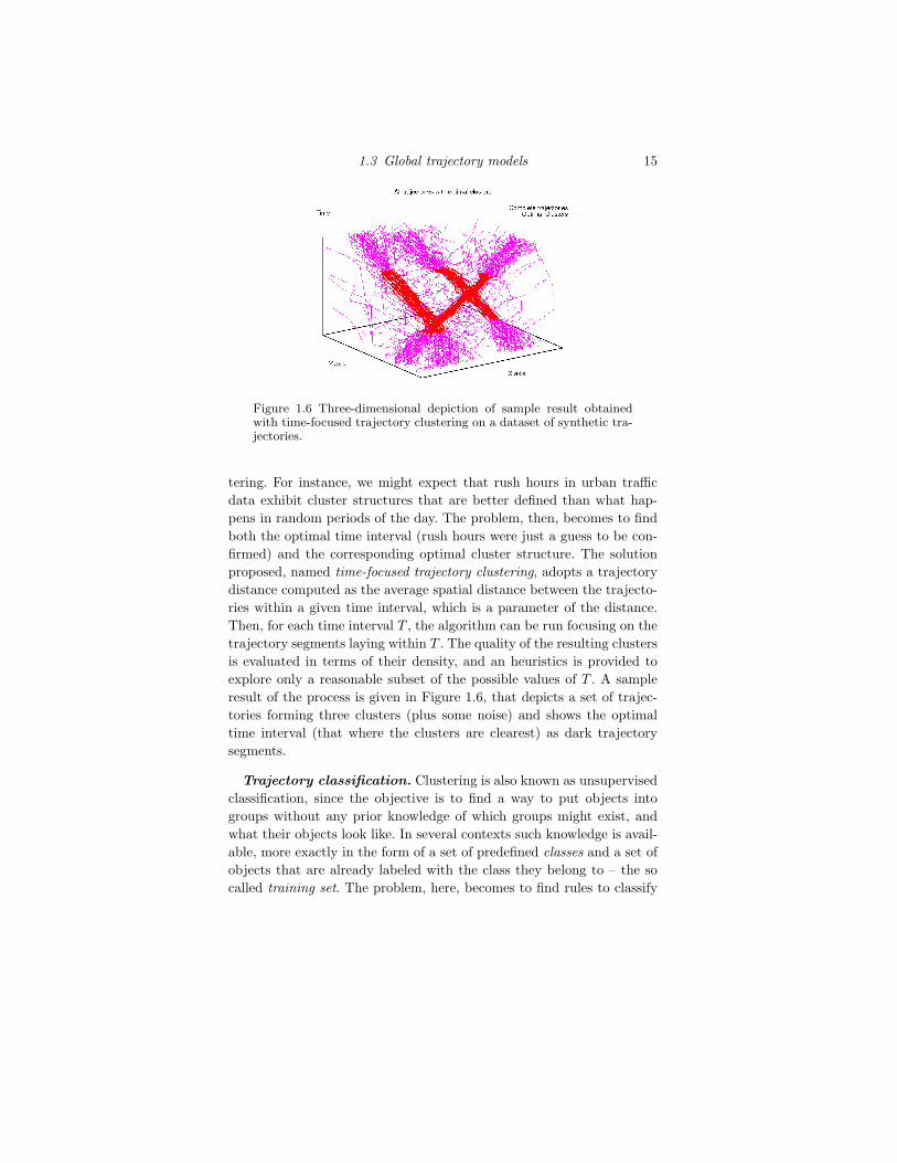
1.3 Global trajectory models 15
Figure 1.6 Three-dimensional depiction of sample result obtainedwith time-focused trajectory clustering on a dataset of synthetic tra-jectories.
tering. For instance, we might expect that rush hours in urban trafficdata exhibit cluster structures that are better defined than what hap-pens in random periods of the day. The problem, then, becomes to findboth the optimal time interval (rush hours were just a guess to be con-firmed) and the corresponding optimal cluster structure. The solutionproposed, named time-focused trajectory clustering, adopts a trajectorydistance computed as the average spatial distance between the trajecto-ries within a given time interval, which is a parameter of the distance.Then, for each time interval T , the algorithm can be run focusing on thetrajectory segments laying within T . The quality of the resulting clustersis evaluated in terms of their density, and an heuristics is provided toexplore only a reasonable subset of the possible values of T . A sampleresult of the process is given in Figure 1.6, that depicts a set of trajec-tories forming three clusters (plus some noise) and shows the optimaltime interval (that where the clusters are clearest) as dark trajectorysegments.
Trajectory classification. Clustering is also known as unsupervisedclassification, since the objective is to find a way to put objects intogroups without any prior knowledge of which groups might exist, andwhat their objects look like. In several contexts such knowledge is avail-able, more exactly in the form of a set of predefined classes and a set ofobjects that are already labeled with the class they belong to – the socalled training set. The problem, here, becomes to find rules to classify

16 Mobility data mining
new objects in a way that is coherent with the prior knowledge, i.e. theyfit well with the training set. For instance, we might have access to a setof vehicle trajectories that were manually labeled with the vehicle type(car, truck, motorbike), and we would like to find a way to automaticallylabel an other, much larger set of new trajectories.
The simplest solution to the problem is the so called k-nearest neigh-bors (kNN) approach: instead of inferring any classification rule, it di-rectly compares each new trajectory t against the training set, and findsthe k labeled trajectories that are closest to t. The most popular labelamong the neighbors is then assigned also to t. The assumption is thatthe more similar are two trajectories, the more likely they belong tothe same class. Obviously, everything revolves around a proper choicefor the similarity measure applied, which should be as much coherentas possible with the classification problem at hand. As an example, wecan expect that a similarity function which takes into consideration theacceleration of objects will recognize well the vehicle type – the lighterthe vehicle, the easier is to reach high accelerations. On the contrary, ameasure based only on the places visited might perform worse.
The same idea is also applied in several sampling-based solutions tothe clustering problem: when the dataset is too large to process, one ap-proach consists in randomly sampling a small subset of trajectories, andcomputing clusters on them. Then, all others trajectories are assigned tothe cluster (i.e., classified) with a kNN approach or by comparing themagainst the centroid of each cluster.
Approaching the problem from a different viewpoint, each class in-volved in the classification problem could be modeled through a prob-abilistic model that is fitted to the available trajectories in the class.Then, each new trajectory can be assigned to the class whose modelmost likely generated it. Similarly to what we have seen with clustering,hidden Markov models are a common choice to do it. As compared toclustering, the problem is now simplified, since the association trajecto-ries↔ classes is known apriori. Behind the probabilistic framework theyoperate in, HMMs essentially aggregate trajectories based on their over-all shape, again assuming that similar trajectories have better chancesof belonging to the same class.
The final way to classify trajectories we will see, is based on a tradi-tional two-steps approach: first extract a set of discriminative featuresby a preliminary analysis of the trajectories; then, use such features –

1.3 Global trajectory models 17
that can be expressed as a database tuple or a vector – to train anyexistent standard classification model for vector/relational data.
The first step requires to understand which characteristics of the tra-jectories appear to better predict which class each trajectory belongs to.One straightforward approach might consist in calculating a predefinedset of measures expected to be informative enough for the task. For in-stance, aggregates such as average speed of the trajectory, its length,duration, average acceleration and diameter of the covered region mightbe used. Other, more sophisticated, solutions might instead try to ex-tract finer aspects of the movement, tuned to calculate only the mostuseful ones. A proposal of this kind can be find in literature with thename TraClass, which heavily relies on a trajectory clustering step.
TraClass is based on a fundamental observation: in several (if notmost) cases, the features that best discriminate trajectory classes arerelated to a small part of the overall trajectory. All approaches men-tioned so far, on the contrary, uniquely consider overall characteristics– that includes HMM-based solutions, since each model must fit wholetrajectories. Single, short-duration events hidden in the long life of atrajectory might then be lost in the process. TraClass tries to fill in thegap by extracting a set of trajectory behaviors (which, we recall, lookfor local behaviors rather than overall descriptions of full trajectories).The basic tool adopted is trajectory segmentation and the clustering ofsuch segments to form movement patterns.
TraClass works at two levels: regions and trajectory segments. At thefirst one, it extracts higher-level features based on the regions of spacethat trajectories visited, without using movement patterns; at the secondone, lower-level trajectory-based features are computed, using movementpatterns. The extraction phase is made more effective by evaluating thediscriminative power of the regions and patterns under construction. Forinstance, a frequent movement that is performed by trajectories of allclasses will be not useful for classification (knowing that a trajectory con-tains such pattern does not help in guessing the right class to associateto it); on the contrary, a slightly less frequent pattern that is mostly fol-lowed by trajectories of a single class is a very promising feature. In theproposed framework, trajectory partitioning makes discriminative partsof trajectories identifiable, and the two types of patterns collaborate tobetter characterize trajectories.
Once a vector of features has been computed for each trajectory, wecan choose any generic, vector-based classification algorithm. One rep-resentative (and easy to grasp) example are decision trees. The resulting

18 Mobility data mining
Figure 1.7 Sample decision tree on regions and patterns.
classification model has the structure of a tree, whose internal nodesrepresent tests on the features of the object to classify, and the leavesindicate the class to associate to the objects. Figure 1.7 shows a fictitiousexample based on TraClass features, with two classes: positive (P) andnegative (N). When a new trajectory needs to be classified, the test onthe root (the top circle) is performed on it. In the example, if the trajec-tory actually visits region A, then we move to the left child of the rootand continue the evaluation from there, otherwise we move to the rightchild. In the first case, we have now to test whether the trajectory fol-lows pattern X: in case of positive answer, the trajectory is labeled with“class P”, otherwise with “class N”. The classification process proceedsin a similar way when different outcomes are obtained, always startingfrom the root and descending through a path till a leaf is reached, whichprovides the label prediction. Another way to read a decision tree is asa set of decision rules, one for each path from root to leaf, such as “If(Visit region A) AND (Follow patter X) THEN Class P”.
Trajectory location prediction. Trajectory classification can beseen as the problem of predicting a categorical variable related to atrajectory. However, prediction is most naturally related to the tempo-ral evolution of variables. Since the basic aspect of objects in the contextof trajectory is their location, predicting their future position appearsto be a problem of primary interest.
The modeling tools that are able to model the sequential evolution

1.3 Global trajectory models 19
of the objects they describe, are good candidates for a predictive usage.Indeed, once a trajectory has been associated to the most likely model(for instance by choosing one of the k HMMs combined in a mixture-model, as described for the clustering problem), such model can be run tosimulate the most likely next steps. In most cases we can apply the sameremarks discussed earlier in this section for classification: if the modelis based on an overall summary of the behavior of a set of trajectories,most likely it will not be able to capture local events, even though theirappearance is highly correlated with a future behavior – in our case, thenext location.
In literature it can be found an approach called WhereNext, that worksin a way not too dissimilar from the one followed by TraClass for theclassification problem. WhereNext acts in three main steps:
• first, a set of local patterns is extracted from data, to be used asconcise representations of interesting behaviors of moving objects;
• second, the local patterns extracted in the previous step are combinedtogether, to form a so called Prediction tree;
• finally, the global model is used to predict the future location of amoving object, by means of an ad hoc concept of distance to find thebest matching pattern and to predict the next movement location.
The patterns used to model relevant behaviors are trajectory patterns,already presented in Section 1.2. Therefore, they are expressed as se-quences of regions, plus temporal information in terms of time of tran-sition between each consecutive pair of regions. Such patterns are com-bined into a tree structure similar to a prefix-tree: the root of the treeis a dummy node, whose children are all regions that appear as startingpoint of some pattern. Then, successive children of the tree are built byadding consecutive regions in each pattern, labeling the edge that con-nects two regions with the corresponding transition times found in theoriginal trajectory patters. Each root-to-node path corresponds to a tra-jectory pattern, and root-to-leaf paths correspond to maximal patterns.Figure 1.8 shows a sample prediction tree, condensing 12 patterns, 7 ofwhich are maximal.
When a new trajectory is presented, its most recent segment is com-pared against the regions represented in the tree, looking for the bestmatch among the root-to-node paths. For instance, Figure 1.8 depictsthe case where the last part of the trajectory visits region A followedby region B after a delay between 9 and 15 time units. The match isdepicted by the red sequence. Then, the model finds that the matched

20 Mobility data mining
Figure 1.8 Sample Prediction tree produced by WhereNext.
sequence is a prefix of a longer pattern, and so it suggests as likely con-tinuation region E (marked in green in the figure), to be reached after adelay between 10 and 56 time units.
WhereNext has a few characteristic features that distinguish it frommost alternative approaches: first, the next location prediction is equippedalso with a temporal delay; second, if no good match is found betweennew trajectories and prediction tree, no prediction is provided, whilemost standard approaches always output a suggestion, even if it has anextremely low confidence; finally, the location prediction occurs in termsof regions and not single spatial points, although the center of the regioncan be returned if a single point is required by the specific application.
1.4 Conclusion
We conclude this chapter with a few notes on the topics presented andsome of the open questions in mobility data mining research.
Summary. Mobility data mining, as many other instantiations of thegeneral data mining paradigm into specific contexts, brings with itselfthe general categorization of problems and methods it inherited fromstandard data mining. In particular, the three main categories – fre-quent patterns, clustering and classification – appear again. However,some specificities of trajectory data emerged and stimulated the devel-opment of new approaches. In particular, the complexity of the data,joining temporal and spatial information, greatly increases the searchspace of most interesting problems, such as finding patterns or discov-

1.4 Conclusion 21
ering discriminative spatio-temporal features for classification or predic-tion problems.
Open questions. One aspect of mobility data mining that the readermight have guessed by reading this chapter is the fact that it still lacks anoverall, comprehensive and clear theoretical framework. Such a frame-work should be able to accommodate existing problems and solutionsproposed in literature, as well as clarify the relations between them.Some examples of efforts in this direction exist in literature, and we alsoreported a few of them – for instance, the relation between local tra-jectory patterns and global trajectory classification models, and theirability to grasp different, complementary kinds of discriminatory fea-tures of trajectory data; or the relations between some of the variousforms of trajectory pattern. However, such cases are rather isolated, andat the present, providing an integrated view of methods and issues isstill a largely unexplored part of the research field.
Another important point in mobility data mining is the fact that sev-eral data sources might provide information about the same mobilityphenomena coming from different viewpoints. Each data source usuallyhas distinctive characteristics, strong points and limitations, and theirintegration might help in overcoming the limits of each of them. For in-stance, vehicle GPS data are usually very detailed in space (i.e., spatialuncertainty is small) and time (frequency of data acquisition is rela-tively high), yet it is inherently limited to the vehicles that are involvedin the data collection process; instead, mobile phone service providersare able to collect information about mobility of all their customers, andthrough the collaboration of a few providers it is possible to cover theactivity of very large portions of the real population. One example arecall detail records (CDRs), that describe the cell towers that served eachcall performed by each phone, together with its timestamp. CDRs allowto build mobility trajectories for each customer served. However, suchtrajectories are very sparse (one point corresponds to a call, which areusually not so frequent) and spatially rough (a point actually representsthe whole area served by the cell tower). Activities that try to com-bine these two data sources are appearing nowadays, with the aim ofimproving the representativity of GPS data through the extremely highpenetration of the (spatially and temporally poor) CDR data.
Finally, so far, our discussion has always implicitly assumed that thetrajectory data were analyzed off-line and in a centralized setting, i.e.,by first collecting all data in a single database and then analyzing them.

22 Mobility data mining
However, mobility data are usually massive and arrive as a continuousstream from the data source(s). Massiveness and streaming nature ofdata leads, at a large scale, to make it impossible to collect them in acentralized database, and therefore analysis methods need to be devel-oped that exploit appropriate technologies, such as distributed databases(a paradigm where data are distributed along several data centers, to bequeried to obtain the data needed for each specific analysis or compu-tation step), distributed computation (several nodes with computationpowers collaborate to analyze data) and streaming-oriented computa-tion (essentially aimed to perform computation by looking at the inputdata only once).
1.5 Bibliographic Notes
As mentioned at the beginning of the chapter, the literature on mobilitydata mining is rather extensive – especially for such a young field – andheterogeneous. Attempting an exhaustive discussion of existing problemsand proposals would require much more space and would be beyond ourpurposes as well. In the following, we will provide an essential list ofbibliographic references for the reader, including those describing themethods cited in the chapter and a few pointers for further readings.
The original definition of flock patterns required that the group ofobjects meet at a single time instant and have the same direction ofmovement. Successive variants introduced the temporal duration con-straint, also adopted in this chapter, starting from Gudmundsson et al.(2004). Moving clusters were defined by Kalnis et al. (2005), providedwith a few heuristics for incrementally computing the interesting pat-terns, while spatio-temporal sequential patterns appeared in Cao et al.(2005).
Trajectory patterns were introduced by Giannotti et al. (2007), andlater were exploited in building WhereNext – a location prediction methodby Monreale et al. (2009) – as well as in several application works.
One rich source for a library of trajecory distances – to be used withingeneric clustering algorithms – is provided by Pelekis et al. (2007). Sev-eral references exist for standard (distance-based) clustering schema thatcan be applied to trajectory data, including basic introductions to datamining such as Tan et al. (2005).
Model-based approaches to trajectory clustering can be found in sev-

1.5 Bibliographic Notes 23
eral, isolated papers, especially on specific application domains (videosurveillance, animal tracking, etc.). The mixture-models trajectory clus-tering described in this chapter was first introduced in Gaffney andSmyth (1999), later extended to include time shifts. Hidden MarkovModels-based approaches can be found, for instance, in Mlich and Chme-lar (2008).
Time-focused clustering, an extension of density-based clustering fortrajectories, was presented in Nanni and Pedreschi (2006).
The TraClass framework for trajectory classification was introducedin Lee et al. (2008), mainly based on previous works of the same authorson trajectory segmentation and clustering.
Finally, a few sources already exist for deeper exploring the subject ofdata mining on trajectory data, including the book by Giannotti and Pe-dreschi (2008), which contains a chapter on spatio-temporal data mining,and the book chapter on spatio-temporal clustering by Kisilevich et al.(2010).

References
Cao, H., Mamoulis, N., and Cheung, D. W. 2005. Mining Frequent Spatio-temporal Sequential Patterns. Pages 82–89 of: Proceedings of the 5thInternational Conference on Data Mining (ICDM’05). IEEE.
Gaffney, S., and Smyth, P. 1999. Trajectory Clustering with Mixture of Re-gression Models. Pages 63–72 of: Proceedings of the 5th InternationalConference on Knowledge Discovery and Data Mining (KDD’99). ACM.
Giannotti, F., Nanni, M., Pedreschi, D., and Pinelli, F. 2007. TrajectoryPattern Mining. In: Proceedings of the 13th International Conference onKnowledge Discovery and Data Mining (KDD’07). ACM.
Giannotti, Fosca, and Pedreschi, Dino (eds). 2008. Mobility, Data Mining andPrivacy - Geographic Knowledge Discovery. Springer.
Gudmundsson, J., van Kreveld, M. J., and Speckmann, B. 2004. Efficientdetection of motion patterns in spatio-temporal data sets. Pages 250–257 of: Proceedings of the 12th International Workshop on GeographicInformation Systems (GIS’04). ACM.
Kalnis, P., Mamoulis, N., and Bakiras, S. 2005. On Discovering Moving Clus-ters in Spatio-temporal Data. Pages 364–381 of: Proceedings of 9th In-ternational Symposium on Spatial and Temporal Databases (SSTD’05).Springer.
Kisilevich, Slava, Mansmann, Florian, Nanni, Mirco, and Rinzivillo, Salvatore.2010. Spatio-temporal clustering. Pages 855–874 of: Data Mining andKnowledge Discovery Handbook.
Lee, Jae-Gil, Han, Jiawei, Li, Xiaolei, and Gonzalez, Hector. 2008. TraClass:trajectory classification using hierarchical region-based and trajectory-based clustering. Proc. VLDB Endow., 1(August), 1081–1094.
Mlich, Jozef, and Chmelar, Petr. 2008. Trajectory classification based on Hid-den Markov Models. Pages 101–105 of: Proceedings of 18th InternationalConference on Computer Graphics and Vision. Lomonosov Moscow StateUniversity.
Monreale, Anna, Pinelli, Fabio, Trasarti, Roberto, and Giannotti, Fosca. 2009.WhereNext: a location predictor on trajectory pattern mining. Pages637–646 of: Proceedings of the 15th ACM SIGKDD international confer-

References 25
ence on Knowledge discovery and data mining. KDD ’09. New York, NY,USA: ACM.
Nanni, Mirco, and Pedreschi, Dino. 2006. Time-focused clustering of trajec-tories of moving objects. J. Intell. Inf. Syst., 27(November), 267–289.
Pelekis, Nikos, Kopanakis, Ioannis, Marketos, Gerasimos, Ntoutsi, Irene, An-drienko, Gennady, and Theodoridis, Yannis. 2007. Similarity Search inTrajectory Databases. Pages 129–140 of: Proceedings of the 14th Inter-national Symposium on Temporal Representation and Reasoning. Wash-ington, DC, USA: IEEE Computer Society.
Tan, Pang-Ning, Steinbach, Michael, and Kumar, Vipin. 2005. Introductionto Data Mining. Addison-Wesley.

Appendix B
Visual analytics of movement:a rich palette of techniques toenable understanding
Author : Gennady Andrienko, Natalia Andrienko
Book : Mobility Data: Modeling, Management, and Understanding
Editors : Chiara Renso, Stefano Spaccapietra, and Esteban Zimanyi
Year : 2013, to appear
60

1
Visual analytics of movement: a rich paletteof techniques to enable understanding
1.1 Introduction
Visual analytics develops knowledge, methods, and technologies that ex-ploit and combine the strengths of human and electronic data processing(Keim et al., 2008). Technically, visual analytics combines interactivevisual techniques with algorithms for computational data analysis. Thekey role of the visual techniques is to enable and promote human un-
derstanding of the data and human reasoning about the data, which arenecessary, in particular, for choosing appropriate computational meth-ods and steering their work. Visual analytics approaches are appliedto data and problems for which there are (yet) no purely automaticmethods. By enabling human understanding, reasoning, and use of priorknowledge and experiences, visual analytics can help the analyst to findsuitable ways for data analysis and problem solving, which, possibly, canlater be fully or partly automated. In this way, visual analytics can drivethe development and adaptation of computational analysis and learningalgorithms.
Visualization is particularly essential for analyzing phenomena andprocesses unfolding in geographical space. Since the heterogeneity ofthe space and the variety of properties and relationships occurring in itcannot be adequately represented for fully automatic processing, explo-ration and analysis of geospatial data and the derivation of knowledgefrom it needs to rely upon the human analyst’s sense of the space andplace, tacit knowledge of their inherent properties and relationships, andspace/place-related experiences. This applies, among others, to move-ment data.
To support understanding and analysis of movement, visual analyt-ics researchers leverage the legacy of cartography, with its established

4Visual analytics of movement: a rich palette of techniques to enable understanding
techniques for representing movements of tribes, armies, explorers, hur-ricanes, etc., time geography (a branch of human geography), with itsrevolutionary idea of considering space and time as dimensions of a uni-fied continuum (space-time cube) and representation of behaviours ofindividuals as paths in this continuum, information visualization, withits techniques for user-display interaction supporting exploratory dataanalysis, and geovisualization, with its interactive maps and associatedmethods enabling exploration of spatial information.
This chapter gives a glimpse of the variety of the existing visual an-alytics methods for analyzing movement data. We group the methodsinto four categories according to the analysis focus:
1. Looking at trajectories: The focus is on trajectories of moving objectsconsidered as wholes. The methods support exploration of the spatialand temporal properties of individual trajectories and comparison ofseveral or multiple trajectories.
2. Looking inside trajectories: The focus is on variation of movementcharacteristics along trajectories. Trajectories are considered at thelevel of segments and points. The methods support detecting andlocating segments with particular movement characteristics and se-quences of segments representing particular local patterns of individ-ual movement.
3. Bird’s-eye view on movement: The focus is on the distribution ofmultiple movements in space and time. Individual movements arenot of interest; generalization and aggregation are used to uncoveroverall spatio-temporal patterns.
4. Investigating movement in context: The focus is on relations and in-teractions between moving objects and the environment (context) inwhich they move, including various kinds of spatial, temporal, andspatio-temporal objects and phenomena. Movement data are ana-lyzed together with other data describing the context. Computationaltechniques are used to detect occurrences of specific kinds of relationsor interactions and visual methods support overall and detailed ex-ploration of these occurrences.
We demonstrate the capabilities of the visual analytics by examplesusing a dataset consisting of GPS tracks of 17,241 cars collected duringone week in Milan (Italy). The data were provided by Comune di Milano(Municipality of Milan).

1.2 Looking at trajectories 5
1.2 Looking at trajectories
In this section, we consider, first, the techniques for visual representationof trajectories and interaction with the representations, second, the useof clustering methods for comparative studies of multiple trajectories,and, third, the time transformations supporting exploration of tempo-ral properties of trajectories and comparison of dynamic properties ofmultiple trajectories.
1.2.1 Visualizing trajectories
The most common types of display for the visualization of movements ofdiscrete entities are static and animated maps and interactive space-timecube (STC) with linear symbols representing trajectories. When multi-ple trajectories are shown, the displays may su↵er from visual clutterand occlusions. The drawback of STC, besides occlusion, is distortion ofboth space and time due to projection. It is also quite limited with re-spect to the length of the time interval that can be e↵ectively explored.To compensate for these limitations, map and STC displays are oftencomplemented with other types of graphs and diagrams.
Common interaction techniques facilitating visual exploration of tra-jectories and related data include manipulations of the view (zooming,shifting, rotation, changing the visibility and rendering order of di↵erentinformation layers, changing opacity levels, etc.), manipulations of thedata representation (selection of attributes to represent and visual en-coding of their values, e.g. by colouring or line thickness), manipulationsof the content (selection or filtering of the objects that will be shown),and interactions with display elements (e.g. access to detailed informa-tion by mouse pointing, highlighting, selection of objects to explore inother views, etc.). Multiple co-existing displays are visually linked byusing consistent visual encodings (e.g. same colours) and exhibit coor-dinated behaviours by simultaneous consistent reaction to various userinteractions.
Figure 1.1 gives examples of map and STC displays and demonstratessome basic interaction techniques. The map in Figure 1.1A shows a sub-set of the Milan dataset consisting of 8206 trajectories that began onWednesday, 4th of April 2007. To make the map legible, the trajectorylines are drawn with only 5% opacity. A temporal filter, as in Figure1.1C, can be used to limit the map view to showing only the positionsand movements within a selected time interval. Thus, the display state in

6Visual analytics of movement: a rich palette of techniques to enable understanding
Figure 1.1 A: 8206 trajectories of cars are shown on a map as linesdrawn with 5% opacity. B: The map shows only positions and move-ments from a 30-minutes time interval selected by means of a tem-poral filter (C). D: A space-time cube (STC) shows a subset of tra-jectories selected by means of a spatial filter (E).
Figure 1.1B corresponds to the 30-minutes time interval from 06:30 till07:00. The time filter can also be used for map animation: the limitingtime interval is moved (automatically or interactively) forward or back-ward in time making the map and other displays dynamically updatetheir content according to the current start and end of the interval.
Figure 1.1B also demonstrates the access to various attributes associ-

1.2 Looking at trajectories 7
ated with a trajectory, such as start and end time, number of positions,length, duration, etc. When the mouse cursor points on a trajectory line,the attributes of this trajectory are shown in a pop-up window as wellas the time when the car was in the position at the cursor.
Figure 1.1D demonstrates the space-time cube (STC) display wheretwo dimensions represent the space and the third dimension time. Thetime axis is oriented from the bottom of the cube, where the base mapis shown, to the top. When all trajectories are included in the STC,the view is illegible due to overplotting. In our example, the STC shows63 trajectories selected by means of a spatial filter (Figure 1.1E). Forthe filter, we have outlined on the map two areas on the northwest andsoutheast of the city and set the filter so that only the trajectories thatvisited both areas in the given order are visible. There are also manyother interactive techniques for data querying and filtering, e.g., the onessuggested by Bouvier and Oates (2008) and (Guo et al., 2011).
1.2.2 Clustering of trajectories
Clustering is a popular technique used in visual analytics for handlinglarge amounts of data. Clustering should not be considered as a stan-dalone analysis method whose outcomes can be immediately used forwhatever purposes. An essential part of the analysis is interpretation ofthe clusters by a human analyst; only in this way they acquire meaningand value. To enable the interpretation, the results of clustering need tobe appropriately presented to the analyst. Visual and interactive tech-niques play here a key role. Visual analytics usually does not invent newclustering methods but wraps existing ones in interactive visual inter-faces supporting not only inspection and interpretation but often alsointeractive refinement of clustering results.
Trajectories of moving objects are quite complex spatio-temporal con-structs. Their potentially relevant characteristics include the geometricshape of the path, its position in space, the life span, and the dynam-ics, i.e. the way in which the spatial location, speed, direction and otherpoint-related attributes of the movement change over time. Clustering oftrajectories requires appropriate distance (dissimilarity) functions whichcould properly deal with these non-trivial properties. However, creatinga single function accounting for all properties would not be reasonable.On the one hand, not all characteristics of trajectories may be simulta-neously relevant in practical analysis tasks. On the other hand, clusters

8Visual analytics of movement: a rich palette of techniques to enable understanding
produced by means of such a universal function would be very di�cultto interpret.
A more reasonable approach is to give the analyst a set of relativelysimple distance functions dealing with di↵erent properties of trajectoriesand provide the possibility to combine them in the process of analysis.The simplest and most intuitive way is to do the analysis in a sequence ofsteps. In each step, clustering with a single distance function is appliedeither to the whole set of trajectories or to one or more of the clustersobtained in the preceding steps. If the purpose and work principle ofeach distance function is clear to the analyst, the clusters obtained ineach step are easy to interpret by tracking the history of their derivation.Step by step, the analyst progressively refines his/her understanding ofthe data. New analytical questions arise as an outcome of the previousanalysis and determine the further steps. The whole process is called”progressive clustering” (Rinzivillo et al., 2008).
There is an implementation of the density-based clustering algorithmOPTICS in which the process of building clusters is separated from mea-suring the distances between the objects. This allows clustering with theuse of diverse distance functions. Hence, the procedure of progressiveclustering is done as follows: The user chooses a suitable distance func-tion and applies the clustering tool first to the whole set of trajectories.Then the user interactively selects one or more clusters and applies theclustering algorithm to this subset using a di↵erent distance functionor di↵erent parameter settings. The latter step is iterated. In this way,the user may (a) refine clustering results, (b) combine several distancefunctions di↵ering in semantics, and (c) gradually build comprehensiveunderstanding of di↵erent aspects of the trajectories.
The procedure of progressive clustering is illustrated in Figure 1.2.The first image (A) shows the result of clustering of the same subsetof the car trajectories as in Figure 1 using the distance function ”com-mon destinations”, which compares the spatial positions of the ends oftrajectories. From the 8206 trajectories, 4385 have been grouped into80 density-based clusters and 3821 treated as noise. Figure 1.2B showsthe clusters without the noise. We have selected the biggest cluster con-sisting of 590 trajectories that end on the northwest (Figure 1.2C) andapplied clustering with the distance function ”route similarity” to it.This distance function compares the routes followed by the moving ob-jects. Figure 1.2D presents the 18 clusters we have obtained; the noiseconsisting of 171 trajectories is hidden. The largest cluster (in red) con-sists of 116 trajectories going from the city centre and the next largest

1.2 Looking at trajectories 9
Figure 1.2 Interactive progressive clustering of trajectories. A: Thecar trajectories have been clustered according to the destinations. B:The noise is hidden. C: One of the clusters is selected. C: Clusteringby route similarity has been applied to the selected cluster; the noiseis hidden. D: The clusters by route similarity are shown in an STC.

10Visual analytics of movement: a rich palette of techniques to enable understanding
cluster (in orange) consists of 104 trajectories going from the northeastalong the northern motorway. The orange cluster and the yellow cluster(68 trajectories) going from the southeast along the motorway on thesouth and west are, evidently, trajectories of transit cars. The clusters byroute similarity are also shown in the STC in Figure 1.2E. This displayinvolves time transformation, which is discussed in the next subsection.
1.2.3 Transforming times in trajectories
Comparison of dynamic properties of trajectories using STC, time graph,or other temporal displays is di�cult when the trajectories are distantin time, because their representations are located far from each otherin a display. This problem can be solved or alleviated by transformingtimes in trajectories. Two classes of time transformations are possible:
1. Transformations based on temporal cycles. Depending on the dataand application, trajectories can be projected in time onto a singleyear / season / month / week / day etc. This allows the user touncover and study movement patterns related to temporal cycles,e.g., find typical routes taken in the morning and see their di↵erencesfrom the routes taken in the evening.
2. Transformations with respect to the individual lifelines of trajecto-ries. Trajectories can be shifted in time to a common start time or acommon end time. This facilitates the comparison of dynamic prop-erties of the trajectories (particularly, spatially similar trajectories),for example, the dynamics of the speed. Aligning both the start andend times supports comparison of internal dynamics in trajectoriesirrespective of the average movement speed.
An example of time-transformed trajectories is shown in Figure 1.2E.The STC shows the route-based clusters of car trajectories ending onthe northwest. The times in the trajectories have been transformed sothat all trajectories have a common end time. This allows us to see that,although the routes within each cluster are similar, the dynamics of themovement may di↵er greatly. The speeds can be judged from the slopesof the lines. Fast movement is manifested by slightly inclined lines (whichmeans more distance travelled in less time) while steep lines signify slowmovement. Vertical line segments mean staying in the same place. In theSTC in Figure 1.2 we can very clearly observe the movement dynamics inthe red cluster: the cars moved slowly while being in the city centre butcould move fast after reaching the diagonal motorway. The orange cluster

1.3 Looking inside trajectories: attributes, events and patterns 11
is divided in two parts. One part consists of nearly straight slightly tiltedlines indicating uniformly high speed along the whole route. The otherpart consists of trajectories with steep segments at the beginning. Thismeans that there were times when the movement in the eastern partof the northern motorway was obstructed and the cars could not reachhigh speed. We can interactively select the trajectories with the steepsegments and find out the times of the obstructed tra�c: from about 06till 13 o’clock; the most di�cult situation was after 10:30. Making suchobservations could be hardly possible with the trajectories positioned inthe STC according to their original times.
1.3 Looking inside trajectories: attributes, events
and patterns
The methods described in the previous section deal with trajectories aswholes, i.e., treat them as atomic objects. Here we consider the meth-ods operating on the level of points and segments of trajectories. Theyvisualize and analyze the variation of movement characteristics (speed,direction, etc.) and other dynamic attributes associated with trajectorypositions or segments. The most obvious way to visualize position-relatedattributes is by dividing the lines or bands representing trajectories ona map or in a 3D display into segments and varying the appearance ofthese segments. Attribute values are usually represented by colouring orshading of the segments.
Position-related dynamic attributes can also be visualized in separatetemporal displays such as time graph or time bars display. An exam-ple of a time bars display is given in Figure 1.3A. The horizontal axisrepresents time. Each trajectory is represented by a horizontal bar suchthat its horizontal position and length correspond to the start time andduration of the trajectory. Note that temporal zooming has been ap-plied: a selected interval from 06:30 till 12:00 is stretched to the fullavailable width. The vertical dimension is used to arrange the bars,which can be sorted based on one or more attributes of the trajectories(start time in our example). Colouring of bar segments encodes valuesof some user-selected dynamic attribute associated with the positionsin the trajectories. This may be an existing (measured) attribute or anattribute derived from the position records, i.e., coordinates and times.Examples of such derivable attributes are speed, acceleration, direction,etc. To represent attribute values by colours, the value range is divided

12Visual analytics of movement: a rich palette of techniques to enable understanding
Figure 1.3 A: A time bars display shows the speeds by colour-coding.Mouse-pointing highlights the trajectory and marks the pointed po-sition in a map (B). C: Trajectory segments are filtered according tothe speed values. D: Only the segments satisfying the filter are visi-ble on the map. E: Low speed events have been extracted from thetrajectories according to the segment filter. F: Density-based spatio-temporal clusters of the low speed events are shown in a space-timecube. G: A scatterplot shows the times (horizontal dimension) andmovement directions (vertical dimension) of the low speed events.
into intervals and each interval is assigned a distinct colour or shade.In Figure 1.3A, shades of red and green represent speed values; red isused for low speeds and green for high. The legend on the left explainsthe colour coding. Interactive linking between displays allows the userto relate attribute values to the spatial context: when the mouse cursor

1.3 Looking inside trajectories: attributes, events and patterns 13
points on some element within the time bars display, the correspondingspatial position is marked in the map by crossing horizontal and verticallines and the trajectory containing it is highlighted (Figure 1.3B). Inthis example we see that the car whose trajectory is highlighted movedat 06:54 on the northeast with the speed 1.2km/h.
The use of this kind of dynamic link is limited to exploration of one ora few particular trajectories. To investigate position-related dynamic at-tributes in a large number of trajectories, the analyst can apply filteringof trajectory segments according to attribute values. Figure 1.3(C-D)illustrates how such filtering can be done in a highly interactive way.The colour legend on the left of the time bars display is simultaneouslya filtering device: the user can switch o↵ and on the visibility of anyvalue interval by clicking on the corresponding coloured rectangle in thelegend. In Figure 1.3C, the user has switched o↵ all intervals except forthat with the speeds from 0 to 5km/h. As a result, the trajectory seg-ments with the speed values higher than 5km/h have been hidden. Thefilter a↵ects not only the time bars display but also the map (Figure1.3D). It is possible to combine several segment filters based on valuesof di↵erent attributes.
The points satisfying filter conditions can be extracted from the tra-jectories into a separate dataset (information layer) consisting of spatialevents, i.e., objects located in space and time. This dataset can be vi-sualized and analyzed independently from the original trajectories orin combination with them. In Figure 1.3E, the yellow circles represent19339 spatial events constructed from the points of the car trajectorieswhere the speeds did not exceed 5km/h. The filtering of the trajectorysegments has been cancelled so that the whole trajectory lines are againvisible. As could be expected, there are many low speed events in thecentre of the city. However, there are also visible concentrations of suchevents in many places on the motorways and their entrances/exits. Theseevents are very probable to have occurred due to tra�c congestions.
To investigate when and where tra�c congestions occurred, we applydensity-based clustering to the set of extracted events in order to findspatio-temporal clusters of low speed events. We look for dense spatio-temporal clusters because standalone low speed events may be unrelatedto tra�c jams. The distance function we use is spatio-temporal distancebetween events. The STC in Figure 1.3F displays the clusters we haveobtained; the noise (15554 events) is hidden. The clusters are colouredaccording to the geographical positions. We see a vertically extendedcluster in light green on the east of the city. More precisely, it is located at

14Visual analytics of movement: a rich palette of techniques to enable understanding
the Linate airport. Most probably, the reason for these low speed eventsis not tra�c congestions but car parking or disembarking/embarking ofpassengers. The clusters in the other locations are more probable to berelated to tra�c jams. Some clusters on the northwest (blue) and north-east (cyan) are quite extended spatially, which means that the tra�cwas obstructed on long parts of the roads. The existence times of theclusters can be more conveniently seen in a two-dimensional display likethe scatterplot in Figure 1.3G, where the times of the events (horizon-tal axis) are plotted against the movement directions. It is possible toselect the clusters one by one and see when they occurred and in whichdirection the cars were moving. For instance, two large clusters of slowmovement westwards occurred on the far northeast in the time intervals05:38-06:50 and 10:20-12:44.
Generally, there are many possible ways how events extracted fromtrajectories can be further analyzed and used. Interested readers are re-ferred to papers (Andrienko et al., 2011b) and (Andrienko et al., 2011c).
1.4 Bird’s-eye on movement: generalization and
aggregation
Generalization and aggregation enables an overall view of the spatial andtemporal distribution of multiple movements, which is hard to gain fromdisplays showing individual trajectories. Besides, aggregation is helpfulin dealing with large amounts of data. There are two major groups ofanalysis tasks supported by aggregation:
• Investigation of the presence of moving objects in di↵erent locationsin space and the temporal variation of the presence.
• Investigation of the flows (aggregate movements) of moving objectsbetween spatial locations and the temporal variation of the flows.
1.4.1 Analyzing presence and density
Presence of moving objects in a location during some time interval canbe characterized in terms of the count of di↵erent objects that visitedthe location, the count of the visits (some objects might visit the loca-tion more than once), and the total time spent in the location. Besides,statistics of various attributes describing the objects, their movements,

1.4 Bird’s-eye on movement: generalization and aggregation 15
Figure 1.4 A,B: Car tracks aggregated in a continuous density surface(A) and by discrete grid cells (B). C: STC shows the variation of carpresence over a day in the most visited cells. D: The cells clusteredby similarity of the presence time series shown on a time graph in(E). F: Hourly time intervals clustered by similarity of the spatialdistributions of car presence, which are summarized in (G).
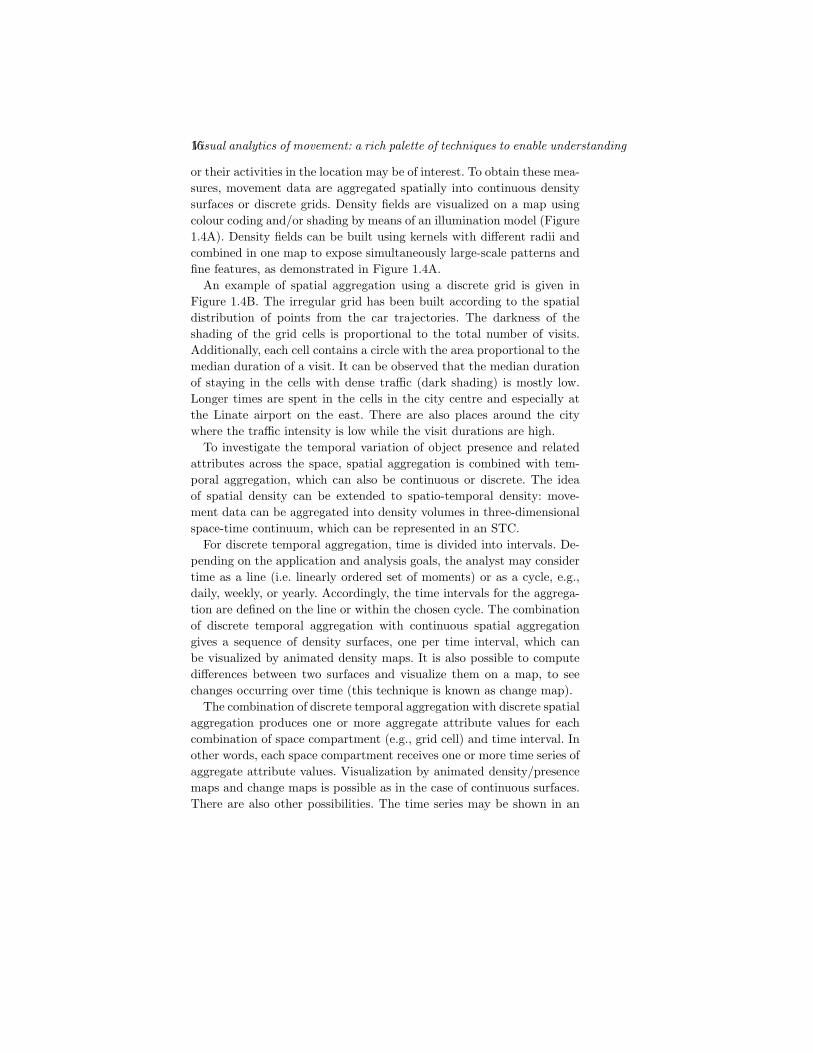
16Visual analytics of movement: a rich palette of techniques to enable understanding
or their activities in the location may be of interest. To obtain these mea-sures, movement data are aggregated spatially into continuous densitysurfaces or discrete grids. Density fields are visualized on a map usingcolour coding and/or shading by means of an illumination model (Figure1.4A). Density fields can be built using kernels with di↵erent radii andcombined in one map to expose simultaneously large-scale patterns andfine features, as demonstrated in Figure 1.4A.
An example of spatial aggregation using a discrete grid is given inFigure 1.4B. The irregular grid has been built according to the spatialdistribution of points from the car trajectories. The darkness of theshading of the grid cells is proportional to the total number of visits.Additionally, each cell contains a circle with the area proportional to themedian duration of a visit. It can be observed that the median durationof staying in the cells with dense tra�c (dark shading) is mostly low.Longer times are spent in the cells in the city centre and especially atthe Linate airport on the east. There are also places around the citywhere the tra�c intensity is low while the visit durations are high.
To investigate the temporal variation of object presence and relatedattributes across the space, spatial aggregation is combined with tem-poral aggregation, which can also be continuous or discrete. The ideaof spatial density can be extended to spatio-temporal density: move-ment data can be aggregated into density volumes in three-dimensionalspace-time continuum, which can be represented in an STC.
For discrete temporal aggregation, time is divided into intervals. De-pending on the application and analysis goals, the analyst may considertime as a line (i.e. linearly ordered set of moments) or as a cycle, e.g.,daily, weekly, or yearly. Accordingly, the time intervals for the aggrega-tion are defined on the line or within the chosen cycle. The combinationof discrete temporal aggregation with continuous spatial aggregationgives a sequence of density surfaces, one per time interval, which canbe visualized by animated density maps. It is also possible to computedi↵erences between two surfaces and visualize them on a map, to seechanges occurring over time (this technique is known as change map).
The combination of discrete temporal aggregation with discrete spatialaggregation produces one or more aggregate attribute values for eachcombination of space compartment (e.g., grid cell) and time interval. Inother words, each space compartment receives one or more time series ofaggregate attribute values. Visualization by animated density/presencemaps and change maps is possible as in the case of continuous surfaces.There are also other possibilities. The time series may be shown in an

1.4 Bird’s-eye on movement: generalization and aggregation 17
STC by proportionally sized or shaded or coloured symbols, which arevertically aligned above the locations; Figure 1.4C gives an example; thecolour legend is given in the lower right corner of Figure 1.4. Occlusion ofsymbols is often a serious problem in such a display; therefore, we haveapplied interactive filtering so that only the data for the most intensivelyvisited cells (1000 or more visits per day) are visible.
When the number of the space compartments is big and time seriesare long, it may be di�cult to explore the spatio-temporal distributionof object presence using only visual and interactive techniques. It is rea-sonable to cluster the compartments by similarity of the respective timeseries and analyze the temporal variation cluster-wise, i.e., investigatethe attribute dynamics within the clusters and do comparisons betweenclusters. Figure 1.4D demonstrates the outcome of k-means clustering ofgrid cells according to the time series of car presence obtained by aggre-gating the car movement data from the whole time period of one weekby hourly intervals (hence, the time series consist of 168 time steps).Distinct colours have been assigned to the clusters and used for paintingthe cells on the map. The same colours are used for drawing the timeseries lines on the time graph in Figure 1.4E. The colours are chosenby projecting the cluster centroids onto a two-dimensional continuouscolour map; hence, clusters with close centroids receive similar coloursand, vice versa, high di↵erence in colours signifies much dissimilaritybetween the clusters. Figure 1.4E shows a prominent periodic variationof car presence in the grid cells over the week. Interactive tools allow usto select the clusters one by one or pairs of clusters for comparison andsee only these clusters on the displays. We find out that the clusters dif-fer mainly in the value magnitudes and not in the temporal patterns ofvalue variation, with the exception of the bright red and orange clusters.The value ranges in these clusters are very close. The main di↵erence isthat the red cluster has higher values in the afternoons of Sunday andSaturday. This may have something to do with people spending theirleisure time near lakes, which are located to the north from the city.
Spatially referenced time series is one of two possible views on a re-sult of discrete spatio-temporal aggregation. The other possibility is toconsider the aggregates as a temporal sequence of spatial situations. Theterm ’spatial situation’ denotes spatial distribution of aggregate valuesof one or more attributes in one time interval. Thus, in our example,there are 168 spatial situations each corresponding to one of the hourlyintervals within the week. Temporal variation of spatial situations canalso be investigated by means of clustering. In this case, the spatial sit-

18Visual analytics of movement: a rich palette of techniques to enable understanding
uations are considered as feature vectors characterizing di↵erent timeintervals. Clustering groups the time intervals by similarity of these fea-ture vectors.
In Figure 1.4F, we have applied k-means clustering to the 168 spa-tial situations in terms of car presence and built a time mosaic displaywhere each hourly interval is represented by a square. As in the previouscase, di↵erent colours have been assigned to the clusters. The squares inthe time mosaic are painted in these colours. The squares are arrangedso that the columns, from left to right, correspond to the days, fromSunday (the first day in our dataset) to Saturday, and the rows corre-spond to the hours of the day, from 0 on the top to 23 in the bottom.We see that the working days (columns 2-6) have quite similar patternsof colouring, which means similarity of the daily variations of the sit-uations. The patterns on Sunday (column 1) and Saturday (column 7)are di↵erent. The multi-map display in Figure 1.4G shows summarizedspatial situations: each small map represents the mean presence valuesin the respective time cluster (the colour coding is the same as in theSTC in Figure 1.4C; see the legend in the lower right corner). It is seenthat the shades of cyan, which occur in the night hours, correspond tovery low car presence over the city and the shades of red, which occurin the working days from 5 till 17 o’clock, to high presence, especiallyon the belt roads around the city. Red also occurs in the afternoon ofSunday (from 15 till 17) and in the morning of Saturday (from 8 till 9).
To deal with very large amounts of movement data, possibly, not fit-ting in RAM, discrete spatio-temporal aggregation can be done within adatabase or data warehouse. The aggregates can then be loaded in RAMfor visualization and interactive analysis.
1.4.2 Tracing flows
In the previous section, we have considered spatial aggregation of move-ment data by locations (space compartments). Another way of spatialaggregation is by pairs of locations: for two locations A and B, the moves(transitions) from A to B are summarized. This can result in such ag-gregate attributes as number of transitions, number of di↵erent objectsthat moved from A to B, statistics of the speed, transition duration, etc.The term ”flow” is often used to refer to aggregated movements betweenlocations. The respective amount of movement, that is, count of movingobjects or count of transitions, may be called ”flow magnitude”.
There are two possible ways to aggregate trajectories into flows. As-

1.4 Bird’s-eye on movement: generalization and aggregation 19
suming that each trajectory represents a full trip of a moving objectfrom some origin to some destination, the trajectories can be aggregatedby origin-destination pairs, ignoring the intermediate locations. A well-known representation of the resulting aggregates is origin-destinationmatrix (OD matrix) where the rows and columns correspond to the lo-cations and the cells contain aggregate values. OD matrices are oftenrepresented graphically as matrices with shaded or coloured cells. Therows and columns can be automatically or interactively reordered foruncovering connectivity patterns such as clusters of strongly connectedlocations and ”hubs”, i.e., locations strongly connected to many others.A disadvantage of the matrix display is the lack of spatial context.
Another way to visualize flows is flow map where flows are repre-sented by straight or curved lines or arrows connecting locations; theflow magnitudes are represented by proportional widths and/or colour-ing or shading of the symbols. Since lines or arrows may connect not onlyneighbouring locations but any two locations at any distance, massiveintersections and occlusions of the symbols may occur, which makes themap illegible. Several approaches that have been suggested for reducingthe display clutter either involve high information loss (e.g. due to fil-tering or low opacity of lesser flows) or work well only for special cases(e.g., for showing flows from one or two locations).
The other possible way of transforming trajectories to flows is to rep-resent each trajectory as a sequence of transitions between all visitedlocations along the path and aggregate the transitions from all trajec-tories. Movement data having su�ciently fine temporal granularity orallowing interpolation between known positions may be aggregated sothat only neighbouring locations (adjacent spatial compartments) arelinked by flows. Such flows can be represented on a flow map withoutintersections and occlusions of the flow symbols. To summarize move-ment data in this way, the space can be tessellated into larger or smallercompartments, e.g., using the method suggested in (Andrienko and An-drienko, 2011), to achieve higher or lower degree of generalization andabstraction. This is illustrated in Figure 1.5A-C. The same trajectoriesof cars (a one-day subset from Wednesday) have been aggregated intoflows using fine, medium, and coarse territory tessellations. The flowsare represented by ”half-arrow” symbols, to distinguish movements be-tween the same locations in the opposite directions. Minor flows havebeen hidden to improve the display legibility; see the legends below themaps. The exact values of the flow magnitudes and other flow-relatedattributes can be accessed through mouse-pointing on the flow symbols.

20Visual analytics of movement: a rich palette of techniques to enable understanding
Figure 1.5 A,B,C: Flow maps based on fine, medium, and coarseterritory divisions obtained automatically. D,E: Clustering of flowsbased on the time series of flow magnitudes. F: Flows between pre-defined regions. G: Investigation of movements between the regionsover time adjusted to individual lifetimes of the trajectories.
Flow maps can also be built using predefined locations or space parti-tioning, as demonstrated in Figure 1.5F, where the flow map is builtbased on a division of the territory of Milan into 13 geographic regions.

1.4 Bird’s-eye on movement: generalization and aggregation 21
Flow maps can serve as expressive visual summaries of clusters ofsimilar trajectories. To obtain such summaries, aggregation is appliedseparately to each cluster.
When movement data are aggregated into flows by time intervals, theresult is time series of flow magnitudes. These can be visualized by an-imated flow maps or by combining flow maps with temporal displayssuch as a time graph. Flows may be clustered by similarity of the re-spective time series (Figure 1.5D,E) and the temporal variation analyzedcluster-wise, as was suggested for time series of presence indicators inthe previous section. Note that the spatial patterns visible on the mapand the periodic patterns of flow variation visible on the time graphare similar to those that we observed for the presence (Figure 1.4D,E).However, we see that symmetric flows (i.e., flows between the same lo-cations in opposite directions) may have di↵erent patterns of temporalvariation. Thus, on the east and south of the city symmetric flow sym-bols are coloured in blue and in magenta, i.e., the respective time seriesbelong to di↵erent clusters. The flows in the magenta cluster achievehigher magnitudes in the afternoons of all days, except Friday (day 6).
Aggregation of movement data into transitions between locations doesnot allow investigation of paths and movement behaviors where morethan two locations are visited. The visualization technique demonstratedin Figure 1.5G aggregates trajectories in such a way that movement be-haviors can be traced (Bremm et al. (2011)). This is an abstract displaywhere the horizontal axis represents time and colours represent di↵erentlocations. The map in Figure 1.5F shows the geographic regions of Milanfilled in di↵erent colours. The same colours are used in Figure 1.5G.
In this example, we investigate the movements of 4634 cars who spentat least 6 hours on the territory under study on Wednesday (i.e., wehave selected the trajectories with the duration of at least 6 hours); theflow map in Figure 1.5F summarizes the movements of these cars. Thetrajectories have been aligned in time to common start and end times,as mentioned in section 1.2.3. The resulting time units are thousandths(also called ’per mill’) of the total trajectory duration. Then the trans-formed time has been divided into 50 intervals of the length 20 per mills,or 2 percents. The temporal display in Figure 1.5G represents time in-tervals by vertical bars divided into coloured segments proportionally tothe number of cars that visited the regions in these intervals. Aggregatedtransitions between the regions are represented by bands drawn betweenthe bars. The widths of the bands are proportional to the counts of theobjects that moved. Gradient colouring is applied to the bands so that

22Visual analytics of movement: a rich palette of techniques to enable understanding
the left end is painted in the colour of the origin location and the rightend in the colour of the destination location.
The coloured bars are shown not for all time intervals but for a subsetof intervals selected interactively or automatically. In our example, wehave selected the first 3 intervals, the last 3 intervals, and each 10th in-terval (i.e., 100 per mills, 200 per mills, and so on). The small rectanglesat the bottom of the display represent all time intervals. The greyscaleshading encodes the amount of change in each interval with respect tothe previous interval, i.e., how many objects moved to di↵erent loca-tions. We can observe that the most intensive movements of the selectedcars occurred in the first 2% and in the last 2% of the total trajectorylifetime. Between the time intervals 100 and 900 the cars mostly stayedin the same regions. The most visited region was centre. There werehigher presence and more movements in the northern part of the citythan in the southern part. The most intensive flows at the beginning ofthe trips were to the centre and inner northeast and at the end to theouter northeast.
By interacting with the display, it is possible to explore not only di-rect transitions between locations but also longer sequences of visitedlocations. When the user clicks on a bar segment, the movements ofthe corresponding subset of objects are highlighted in the display (i.e.,shown by brighter colours). It is possible to see which locations werevisited and when. Thus, we can learn that from the 994 cars that werein the centre in the interval 500 (i.e., in the middle of the trip time) 489cars were in this region during the whole time and the remaining carscame to the centre mainly from the northeast (133), southwest (132),northwest (74) and southeast (62) in the first 2% of the time. At theend, these cars moved back. Analogously, the user can click on bandsconnecting segments to select the objects participating in the respectivetransitions and trace their movements.
1.5 Investigation of movement in context
The spatio-temporal context of the movement includes the propertiesof di↵erent locations (e.g., land cover or road type) and di↵erent times(e.g. day or night, working day or weekend) and various spatial, tempo-ral, and spatio-temporal objects a↵ecting and/or being a↵ected by themovement. The methods discussed so far seem to deal with movementdata alone and not address the context of the movement, at least in an

1.5 Investigation of movement in context 23
explicit way. However, the context is always involved in the process of in-terpreting what is seen on visual displays. Thus, the analyst always triesto relate visible spatial patterns to the spatial context (e.g., the highestcar tra�c density is on motorways) and visible temporal patterns to thetemporal context (e.g., the tra�c decreases on weekends).
Cartographic map is a very important provider of information aboutspatial context; therefore, maps are essential in analyzing movementdata. It is not very usual although possible to include information abouttemporal context in temporal displays such as time graph. Space-timecube may show spatio-temporal context, but occlusions and projectione↵ects often complicate the analysis. Besides the context items thatare explicitly represented on visual displays, the analyst also takes rel-evant context information from his/her background knowledge. Visualdisplays, especially maps, help the analyst in doing this since things thatare shown can facilitate recall of related things from analyst’s mind. Af-ter noticing a probable relationship between an observed pattern andsome context item, or group of items, or type of items, the analyst maywish to check it, which can be supported by interactive visual tools.
The analyst may not only attend to the movement context for inter-preting results of previously done analysis. It may also be a primary goalof analysis to detect and investigate particular relationships between themovement and a certain specific context item or group of items. For ex-ample, the goal may be to investigate how cars move on motorways or intra�c congestions. To do the analysis, one may need special techniquesthat support focussing on the context items and relationships of interest.
Position records in movement data may include some context infor-mation, but this is rarely the case. In any case, movement data cannotinclude all possible context information. Typically, the source of relevantcontext information is one or more additional datasets describing someaspect(s) of the movement context. We shall shortly call such data ”con-text data”. Context data may result from previous analyses of movementdata. In our previous examples we have demonstrated derivation of spa-tial events, event clusters, as well as classes (clusters) of locations andof time moments. Such derived data can be considered as context dataand used in further analysis of movement data.
The general approach is to derive contextual attributes for trajectorypositions by joint processing of movement data and context data andthen visualize the attributes to observe patterns and determine relation-ships. The derived attributes may characterize the environment (suchas weather conditions) at the positions of the moving objects or rela-

24Visual analytics of movement: a rich palette of techniques to enable understanding
tions (such as spatial distance) between the positions and context itemsin focus. Values of these attributes are defined, as a rule, for all tra-jectory positions. The analyst looks for correlations, dependencies, or,more generally, stable or frequent correspondences between the contex-tual attributes and movement attributes.
Besides stable relationships between movement and its context, theanalyst may also be interested in transitory spatial, temporal, and spatio-temporal relationships occurring between moving objects and contextitems during the movement and lasting for limited time. This includes,in particular, relative movements of two or more moving objects such asapproaching, meeting, passing, following, etc., and relative movementswith respect to other kinds of spatial objects. Such occurrent relation-ships can be regarded as spatial events since they exist only at certainpositions in space and in time.
Many types of relationships can be expressed in terms of spatialand/or temporal distances. This includes proximity between moving ob-jects, visiting of certain locations or types of locations, being in spatio-temporal neighbourhood of a spatial event, etc. Spatial and/or temporaldistances from moving objects to context items can be computed andattached to trajectory positions as new attributes, which can be visual-ized and/or used in further analyses. Particularly, they can be used forfiltering and event extraction as described in section 1.3.
As an example of analyzing movement in context, we shall investigatehow the speed of car movement on motorways is related to the distancesbetween the cars. Hence, there are two aspects of the movement contextwe are interested in: type of location (specifically, motorway) and othercars (specifically, distances to them). The distances between the cars canbe determined directly from the trajectory data; no additional data areneeded. This can be done using a computational procedure that finds foreach trajectory position the closest position in another trajectory withina given time window, e.g., of 1 minute length (from -30 to +30 secondswith respect to the time of the current position).
The location types could be taken from an additional dataset describ-ing the streets; however, we have no such dataset for Milan. We shalldemonstrate the use of previously derived data. Earlier we have made atessellation of the territory (Figure 1.4); moreover, the clustering accord-ing to the temporal variation of the car presence (Figure 1.4D) separatesquite well the cells on motorways from the other cells. We create a suit-able classification of the cells, as in Figure 1.6D, by editing the clusters.Here the yellow filling corresponds to the cells on motorways. We select

1.5 Investigation of movement in context 25
Figure 1.6 A,B,C: Frequency distributions of car speeds on motor-ways in di↵erent ranges of distance to the nearest neighbour car:below 20m (A), 20-50m (B), over 50m (C). D: Trajectory segmentson or near motorways selected by means of segment filter. E: Spatio-temporal clusters of low speed events on motorways where the dis-tance to the nearest neighbour is 10m or less. Yellow shapes repre-sent spatio-temporal convex hulls of the clusters. F: Trajectories thatpassed through one of the convex hulls are selected by filtering. G:The selected trajectories and respective low speed events in a STC.
this class of cells and compute the distances from the trajectory posi-tions to the selected cells; for each position the nearest cell is taken.The computed distances are attached to the position records as a newattribute, which can now be used for filtering. By filtering, we extract
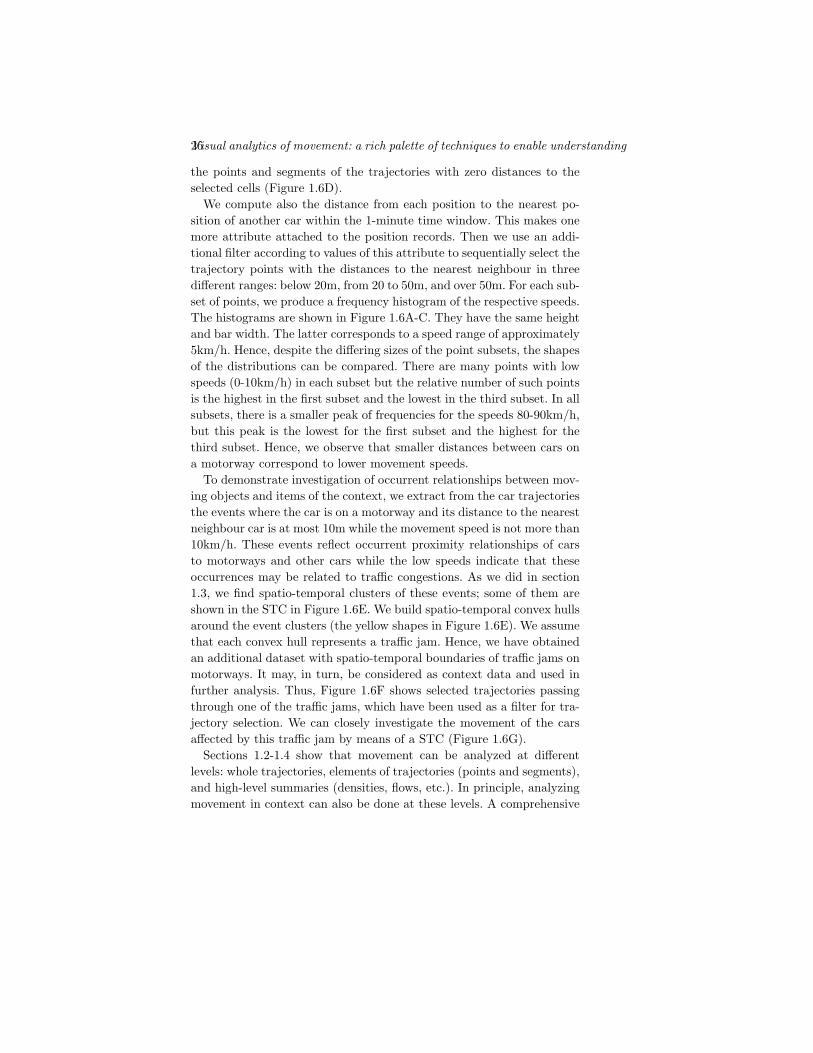
26Visual analytics of movement: a rich palette of techniques to enable understanding
the points and segments of the trajectories with zero distances to theselected cells (Figure 1.6D).
We compute also the distance from each position to the nearest po-sition of another car within the 1-minute time window. This makes onemore attribute attached to the position records. Then we use an addi-tional filter according to values of this attribute to sequentially select thetrajectory points with the distances to the nearest neighbour in threedi↵erent ranges: below 20m, from 20 to 50m, and over 50m. For each sub-set of points, we produce a frequency histogram of the respective speeds.The histograms are shown in Figure 1.6A-C. They have the same heightand bar width. The latter corresponds to a speed range of approximately5km/h. Hence, despite the di↵ering sizes of the point subsets, the shapesof the distributions can be compared. There are many points with lowspeeds (0-10km/h) in each subset but the relative number of such pointsis the highest in the first subset and the lowest in the third subset. In allsubsets, there is a smaller peak of frequencies for the speeds 80-90km/h,but this peak is the lowest for the first subset and the highest for thethird subset. Hence, we observe that smaller distances between cars ona motorway correspond to lower movement speeds.
To demonstrate investigation of occurrent relationships between mov-ing objects and items of the context, we extract from the car trajectoriesthe events where the car is on a motorway and its distance to the nearestneighbour car is at most 10m while the movement speed is not more than10km/h. These events reflect occurrent proximity relationships of carsto motorways and other cars while the low speeds indicate that theseoccurrences may be related to tra�c congestions. As we did in section1.3, we find spatio-temporal clusters of these events; some of them areshown in the STC in Figure 1.6E. We build spatio-temporal convex hullsaround the event clusters (the yellow shapes in Figure 1.6E). We assumethat each convex hull represents a tra�c jam. Hence, we have obtainedan additional dataset with spatio-temporal boundaries of tra�c jams onmotorways. It may, in turn, be considered as context data and used infurther analysis. Thus, Figure 1.6F shows selected trajectories passingthrough one of the tra�c jams, which have been used as a filter for tra-jectory selection. We can closely investigate the movement of the carsa↵ected by this tra�c jam by means of a STC (Figure 1.6G).
Sections 1.2-1.4 show that movement can be analyzed at di↵erentlevels: whole trajectories, elements of trajectories (points and segments),and high-level summaries (densities, flows, etc.). In principle, analyzingmovement in context can also be done at these levels. A comprehensive
1.6 Recommended reading 27
set of visual analytics methods addressing all these levels and di↵erenttypes of context items does not exist yet, which necessitates furtherresearch in this direction.
1.6 Recommended reading
Keim et al. (2008) give a general definition of visual analytics and de-scribe the scope of this research field. Andrienko et al. (2011a) suggest aconceptual framework defining the concepts of movement data, trajec-tories, and events, and possible relationships between moving objects,locations, and times. It shows that movement data hold valuable infor-mation not only about the moving objects but also about properties ofspace and time and about events and processes occurring in space andtime. To uncover various types of information hidden in movement data,it is necessary to consider the data from di↵erent perspectives and toperform a variety of analytical tasks. The paper defines the possible fociand tasks in analyzing movement data. Furthermore, it defines genericclasses of analytical techniques and links the types of tasks to the classesof techniques that can support fulfilling them. The techniques include vi-sualizations, data transformations, and computational analysis methodsdeveloped in several areas: visualization and visual analytics, geographicinformation science, database research, and data mining.
Readers interested in visualization of trajectories and techniques forinteraction with the displays can be referred to the papers by Kaplerand Wright (2005) describing a nice implementation of space-time cube,Bouvier and Oates (2008) suggesting original interaction techniques formarking moving objects on an animated display and tracing their move-ments, and Guo et al. (2011) showing the use of several coordinateddisplays and interactive query techniques specifically designed for trajec-tories, such as sketching for finding trajectories with particular shapes.
Rinzivillo et al. (2008) talk about visually supported progressive clus-tering of trajectories. The paper argues for the use of diverse distancefunctions addressing di↵erent properties of trajectories, describes severaldistance functions, and demonstrates the use of progressive clustering byexample.
The papers Andrienko et al. (2011b) and Andrienko et al. (2011c) referto ”looking inside trajectories” (section 1.3). The first paper describesvisual displays that show temporal variation of dynamic attributes as-sociated with trajectory positions. The second paper gives a structured

28Visual analytics of movement: a rich palette of techniques to enable understanding
list of position-related attributes that can be computationally derivedfrom movement data alone and from a combination of movement dataand context data. These attributes characterize either the movement it-self or possible relationships between the moving objects and the move-ment context. Both papers deal with extraction of spatial events frommovement data. The first paper introduces a conceptual model wheremovement is considered as a composition of spatial events of diversetypes and extents in space and time. Spatial and temporal relations oc-cur between movement events and elements of the spatial and temporalcontexts. The model gives a ground to a generic approach based on ex-traction of interesting events from trajectories and treating the eventsas independent objects. The paper also describes interactive techniquesfor extracting events from trajectories. The second paper focuses moreon the use of extracted events in further analysis. Thus, it considersdensity-based clustering of movement-related events, which accounts fortheir positions in space and time, movement directions, and, possibly,other attributes. The clustering allows extraction of meaningful places.The further analysis involves spatio-temporal aggregation of events ortrajectories using the extracted places.
Andrienko and Andrienko (2010) give an illustrated survey of the ag-gregation methods used for movement data and the visualization tech-niques applicable to the results of the aggregation. These methods andtechniques are also presented in a more formal way by Andrienko et al.(2011a). Willems et al. (2009) describe aggregation of trajectories into acontinuous density surface using a specially designed kernel density esti-mation method, which involves interpolation between consecutive trajec-tory points taking into account the speed and acceleration. Density fieldsbuilt using kernels with di↵erent radii can be combined into one field toexpose simultaneously large-scale patterns and fine features. Andrienkoand Andrienko (2011) suggest a method for tessellation of a territoryused for discrete spatial aggregation of movement data and generationof expressive visual summaries in the form of flow maps. The methoddivides a territory into convex polygons of desired size on the basis ofthe spatial distribution of characteristic points extracted from trajec-tories. It uses a special algorithm for spatial clustering of points thatproduces clusters of user-specified spatial extent (radius). Depending onthe chosen radius, the data can be aggregated at di↵erent spatial scalesfor achieving lower or higher degree of generalization and abstraction.
An example of visualization of flows between locations in the form oforigin-destination matrix can be found in the paper by (Guo, 2007). The

1.7 Conclusion 29
rows and columns can be automatically or interactively reordered foruncovering connectivity patterns such as clusters of strongly connectedlocations and ”hubs”, i.e., locations strongly connected to many others.
To deal with very large amounts of movement data, possibly, not fit-ting in RAM, discrete spatio-temporal aggregation can be done withina database or a data warehouse as described by (Ra↵aeta et al., 2011).Only aggregated data are loaded in RAM for visualization and interac-tive analysis. Using roll-up and drill-down operators of the warehouse,the analyst may vary the level of aggregation.
1.7 Conclusion
Movement data link together space, time, and objects positioned in spaceand time. They hold valuable and multifaceted information about mov-ing objects, properties of space and time as well as events and processesoccurring in space and time. Visual analytics has developed a wide va-riety of methods and tools for analysis of movement data, which allowan analyst to look at the data from di↵erent perspectives and performdiverse analytical tasks. Visual displays and interactive techniques areoften combined with computational processing, which, in particular, al-lows analysis of larger amounts of data than it would be possible withpurely visual methods. Visual analytics leverages methods and tools de-veloped in other areas related to data analytics, particularly, statistics,machine learning, and geographic information science. The main goal ofvisual analytics is to enable human understanding and reasoning. Wehave demonstrated by examples how understanding of various aspectsof movement is gained by viewing visual displays and interacting withthem, possibly, after appropriate data transformations and/or compu-tational derivation of additional data.


References
Andrienko, G., and Andrienko, N. 2010. General Framework for Using Ag-gregation in Visual Exploration of Movement Data. The Cartographic
Journal, 47(1), 22–40.
Andrienko, G., Andrienko, N., Bak, P., Keim, D., Kisilevich, S., and Wrobel, S.2011a. A conceptual framework and taxonomy of techniques for analyzingmovement. Journal of Visual Languages & Computing, 22(3), 213–232.
Andrienko, G., Andrienko, N., and Heurich, M. 2011b. An event-based concep-tual model for context-aware movement analysis. International Journal
of Geographical Information Science, 25(9), 1347–1370.
Andrienko, G., Andrienko, N., Hurter, C., Rinzivillo, S., and Wrobel, S. 2011c.From Movement Tracks through Events to Places: Extracting and Char-acterizing Significant Places from Mobility Data. Pages 161–170 of: IEEE
Conference on Visual Analytics Science and Technology, VAST 2011.IEEE.
Andrienko, N., and Andrienko, G. 2011. Spatial generalization and aggregationof massive movement data. IEEE Transactions on Visualization and
Computer Graphics, 17(2), 205–219.
Bouvier, D.J., and Oates, B. 2008. Evacuation Traces Mini Challenge award:Innovative trace visualization. Staining for information discovery. Pages219–220 of: IEEE Symposium on Visual Analytics Science and Technol-
ogy, VAST 2008. IEEE.
Bremm, S., Andrienko, G., Andrienko, N., Schreck, T., and Landesberger, T.2011. Interactive Analysis of Object Group Changes over Time. Pages41–44 of: EuroVA International Workshop on Visual Analytics. Euro-graphics. Peer-reviewed short paper.
Guo, D. 2007. Visual analytics of spatial interaction patterns for pandemicdecision support. International Journal of Geographical Information Sci-
ence, 21, 859–877.
Guo, H., Wang, Z., Yu, B., Zhao, H., and Yuan, X. 2011. TripVista: Triple Per-spective Visual Trajectory Analytics and its application on microscopictra�c data at a road intersection. Pages 163 –170 of: Pacific Visualization
Symposium (PacificVis), 2011 IEEE.

32 References
Kapler, T., and Wright, W. 2005. GeoTime information visualization. Infor-
mation Visualization, 4(2), 136–146.Keim, D., Andrienko, G., Fekete, J.-D., Carsten, G., Kohlhammer, J., and
Melancon, G. 2008. Visual Analytics: Definition, Process, and Challenges.Chap. 7, pages 154–175 of: Kerren, A., Stasko, J., Fekete, J.-D., andNorth, C. (eds), Information Visualization. Lecture Notes in ComputerScience, vol. 4950. Berlin, Heidelberg: Springer Berlin / Heidelberg.
Ra↵aeta, A., Leonardi, L., Marketos, G., Andrienko, G., Andrienko, N., Frent-zos, E., Giatrakos, N., Orlando, S., Pelekis, N., Roncato, A., and Silvestri,C. 2011. Visual Mobility Analysis using T-Warehouse. International
Journal of Data Warehousing & Mining, 7(1), 1–23.Rinzivillo, S., Pedreschi, D., Nanni, M., Giannotti, F., Andrienko, N., and
Andrienko, G. 2008. Visually driven analysis of movement data by pro-gressive clustering. Information Visualization, 7(3-4), 225–239.
Willems, N., Van De Wetering, H., and Van Wijk, J.J. 2009. Visualization ofvessel movements. Computer Graphics Forum, 28(3), 959–966.

Author index
Peterson, K., 36
Tranah, D.A., 36
Young, P.D.F., 36

Subject index
di↵raction, 36
force
hydrodynamic, 36
interactive, 36
Appendix C
Understaning human mobilityusing Mobility Data Mining
Authors : Chiara Renso, Roberto Trasarti
Book : Mobility Data: Modeling, Management, and Understanding
Editors : Chiara Renso, Stefano Spaccapietra, and Esteban Zimanyi
Year : 2013, to appear
93

1
Understaning human mobility using MobilityData Mining
Chiara Renso, Roberto Trasarti1
1.1 The Mobility Knowledge Discovery Process
There is an old saying that says ”Knowledge is power”. This is partic-ularly true in the Mobility field where knowledge can be rephrased inhow, when, where, and why objects move?. This knowledge gives to auser - who could be any mobility related expert, from a tra�c manager,to a urban planner, or to an ethologist studying the animal behavior- a great power in terms of deployment of the analysis results in ef-fective decision-making. For example, a tra�c manager could improvetra�c sustainability in a city, or an ethologist could finally get a deepunderstanding of how a given animal behaves within his habitat.
The mobility data mining research field has seen a growing interestin the last few year - as already stated in Chapter 6 - providing sev-eral algorithms and techniques tailored on trajectory data. However, acommon problem of these techniques is that the knowledge producedby the mining step is generally, not actionable in the sense that it isnot really applicable to the application domain. The lack of semanticsof the extracted patterns makes the interpretation task far from obvi-ous. This problem, commonly recognized in the data mining literature,is particularly significant in mobility data mining, where the complex-ity of the data themselves, together with the extreme multifariousnessof the mobility application requirements makes the knowledge discoveryeven more challenging. The interestingness evaluation of the discovered
1ISTI-CNR, Pisa, Italy
4 Understaning human mobility using Mobility Data Mining
movement patterns makes sometimes the KDD process a mere academicapplication, useless in the reality. A way to close the gap between the”KDD knowledge” and the ”application actionable knowledge” is to re-inforce the KDD process with tools capable to easily manage the stepsintegrated with new elements focussed on the semantic aspect for animproved data and patterns understanding. This results in a number oftechniques, tailored on mobility data, aimed at enriching the steps of theknowledge discovery process with the final objective of getting meaningfrom movement data.
It is worth noticing that most of the methods to compute trajectorypatterns, as illustrated in the previous chapter, are focused on the geo-metric properties of the trajectory. However, just discovering geometrictrajectory patterns can be of limited interest since it lacks the necessarysemantics to be fully understood by the domain expert user. For exam-ple, assume that a cluster is found on a trajectory dataset representingpeople movements in a city: this pattern represents how people is mov-ing, not why, or the reason for the movement. The reason why entitiesmove needs a deeper understanding of the movement based on the con-text semantics, or context knowledge -also called background knowledge.For example, we can discover that this particular movement happeneddue to a football match, or that the cluster represents tourists visitingattraction points a city. The conceptual lift from finding how movementhappened to understanding why entities are moving in that way, needsan improved knowledge discovery process tailored on mobility data char-acteristics and possibly enriched with contextual semantic information.
We believe that mobility understanding encompasses the whole dis-covery process, from pre-processing step, to the data mining and thepatterns interpretation performed during the post-processing step. Forthis reason this chapter is centered on approaches devoted at improvingthe understanding of mobility data and patterns with the final objectiveof giving insights of why the movement happens. These range from datapreprocessing techniques, to mining to post processing where contextualknowledge have a primary role. We introduce these techniques accom-panied by a system that supports the whole mobility knowledge discov-ery process, called M-Atlas. M-Atlas provides the basic components forsupporting the discovery steps from data pre-processing to mining topost-processing. We are introducing the system as a specific instance ofa mobility knowledge discovery support systems highlighting the stepsthat allows to infer the new knowledge from trajectory data, possiblycombined with contextual knowledge. Particularly, we highlight the im-

1.2 The M-Atlas system 5
portance of the pre-processing step, is to get a better perception of thevalues and the knowledge embedded in the data, and thus driving themining task accordingly. During the mining and post-processing phasesthe context knowledge has a major role since it is explicitly consideredto get an interpretation of the patterns in terms of mobility knowledge.Therefore, we present the core concepts of the M-Atlas system illustrat-ing some basic statistics techniques for the mobility data understandingincluding tasks like data preparation for a context-driven preparation ofdata for mining or data validation where the mobility dataset is evalu-ated against an application domain knowledge that acts as a ”groundtruth”. This latter step allows to establish if, and at which degree, thedataset to be analyses is representative of the real world and thereforethe results of the analysis are still valid in the real world. Other tech-niques include progressive clustering and parameter tuning. The secondpart of the chapter focuses on trajectory behavior as already introducedin Chapter 1 illustrated by means of examples a mobility knowledgediscovery process that extracts trajectory behavior like ”StuckedInTraf-ficJam” and ”Commuter”.
1.2 The M-Atlas system
M-Atlas2 is a running system developed to handle all the steps of themobility knowledge discovery process providing a SQL-based data min-ing query language. In other words, it is a querying and mining systemcentered onto the concept of trajectory. Besides the mechanisms for stor-ing and querying trajectory data, M-Atlas has mechanisms for miningtrajectory patterns and models that, in turn, can be stored and queried.The basic design choice is compositionality, i.e., querying and mining oftrajectory data, patterns and models may be freely combined, in orderto provide the expressive power needed to master the complexity of themobility knowledge discovery process. The conceptual model behind M-Atlas views the knowledge discovery process as the interaction betweentwo conceptual worlds: the data world and the model world. The formeris a set of entities to be mined, trajectories in our case; the latter is a setof models and patterns extracted from the data, representing the resultof mining tasks. Two kinds of operators connect the two worlds: themining operators, and the entailment operators. Mining operators map
2Available for download at the URL: http://m-atlas.eu

6 Understaning human mobility using Mobility Data Mining
data into models, or patterns, while entailment operators map models,patterns and data into the data that satisfy the property expressed inthe given model or pattern. This view supports compositionally, sincedata can be mapped onto models and vice versa, coherently with in-ductive databases vision introduce by Mannila. Another design choiceof the system is that all entities are represented in the object-relationaldata model, which is more suitable to tackle the structural complexityof spatio-temporal data compared to the standard tabular data.
The M-Atlas system is equipped with a graphical user interface and aset of interactive graphical tools allowing the user to navigate the dataand model easily. This has the advantage of making the tool usable bydomain expert users to get full advantage of their domain expertise. Eachinteraction of the analyst with the interface is compiled into a sequenceof M-Atlas queries which can be retrieved at any moment to describe orreview the entire process. Alternatively, an expert data miner analystcan directly submit queries to the M-Atlas engine, to exploit its fullexpressiveness.
Using a data mining algorithm in a knowledge discovery process is nota straightforward process: in fact usually it’s di�cult even for an expertanalyst user to choose the right algorithm and setup all the parameters inorder to extract meaningful and useful patterns. This is especially truein mobility domain due to the complexity of the data under analysisas well as the applications requirements. For this reason, the extractedbehavior can be meaninful only if a proper mobility knowledge discoveryprocess has been set up.
In this section we introduce a set of techniques, demonstrated withexamples using M-Atlas, that drive a user through the mobility knowl-edge discovery process by optimizing the data analysis and tuning theparameters setting. The techniques introduced here have been tailoredon the case of mobility data, although they can be applied to generaldata mining.
1.2.1 Data Preprocessing
In this section we present some data preprocessing techniques useful inthe mobility knowledge discovery, illustrating them through the use ofM-Atlas.
Data validation. Data validation is a necessary step to measure how

1.2 The M-Atlas system 7
much the trajectory dataset we are going to analyze is consistent andrepresentative of the real world phenomena. Here we consider the dataalready cleaned and reconstructed as described in Chapter 2. However,the reconstruction step does not eliminate all the possible imperfectionsin the data and errors at higher level may still exist. This is due tobias in the data (e.g. tracking only a certain category of the users) ortechnological problems (i.e. an area where the devices don’t work) thatcan still produce unusual and unwanted e↵ects on the analysis results.To asses the significance of a dataset as a proxy of the real mobilityphenomena within a certain area, the trajectory dataset can be com-pared against a ”ground truth” such as survey data or other forms of”a-priori” knowledge. However, an important issue to be considered inthis comparison is the population of these two dataset. For example,considering the dataset coming from a set of private cars, this coversonly vehicular movements, whereas surveys usually include all the kindof movement like pedestrians and public transportation. Second, the au-tomatic collection procedure and the cleaning step applied for the cardataset ensures that all movements are correctly captured, whereas sur-veys leave space to omissions or distortions. Finally, the data providesno explicit semantic information about the purpose of movements, likethe final destination, and profiles of the citizens involved, whereas sur-veys explicitly collect this information. A significant di↵erences hold alsofor the size of the sample which can alter the reality represented in thedataset. A method that can help to understand if the data is consistentto the ground truth is to replicate a statistic analysis. This phase of theanalysis is crucial since only after assessing the correspondence of thepreliminary analysis results with the ground truth, we can proceed withthe mobility knowledge discovery following steps having the guaranteethat the results will represent real mobility patterns. In the chapter 11dedicated to Car Tra�c we will see an example of this validation processon the Milano dataset.
Data reconstruction and data preparation: As explained in theprevious chapter, the data mining algorithms apply to the concept oftrajectory: but which trajectory definition?It is simply the ordered se-quence of observations of the user’s history? Or a subsequence represent-ing the movements between stops? And how to define and compute astop? Answering to this questions is crucial and a↵ects deeply the resultsof the knowledge discovery process. For example, if we are interested in

8 Understaning human mobility using Mobility Data Mining
frequent paths followed by a certain number of users we need to considerT-Pattern applied to the whole user history as single trajectory, so thatthe support of a single pattern will be the number of users that followthat path. Alternatively, if we are interested in the usage of certain fre-quent paths then we do not need to distinguish between distinct users.As a consequence, the concept of trajectory to be mined become thesubsequences of users trajectories delimited by two stops as described inchapter 2. There are several ways of reconstructing trajectories consid-ering di↵erent constraints and thresholds thus leading to di↵erent setsof trajectories. In M-Atlas we can perform this operation with the Dataconstructor statement :e
CREATE DATA <trajectory_table> BUILDING MOVING_POINTS
FROM (SELECT userid, longitude, latitude, timepoint
FROM <raw_observation_table>
ORDER BY userid, datetime)
SET MOVING_POINT.<constraint_name> = <value> AND ...
The syntax of queries in M-Atlas extends the standard SQL. In thisquery we see a CREATE DATA operation to build a new kind of data tobe stored in the database. As we can see, a new trajectory table is builtfrom the raw observations using trajectory reconstruction parametersexpressed in the constraints. Some examples of constraint names areMAX TIME GAP or MAX SPEED which realize the two constraintsdescribed in chapter 2. These values depend on the application and theirvalues have to be carefully chose since they a↵ect all the subsequentanalysis. Examples are MAX TIME GAP = 30 min or MAX SPEED =5 km/h to cut trajectories where there is a temporal gap of 30 minutesor a max speed of 5 km per hour, respectively.
Data manipulation: before the execution of a data mining algorithmthe analyst can manipulate (e.g. selecting the data in a particular areaor period) or transform the data (e.g. anonymizing it). For this reasonthe system integrates a rich set of spatio-temporal primitives and trans-formations. To better understand what are the relation statements andtransformation statements two examples are presented: the first one isthe relation between a trajectories table and a temporal period tableswhich computes the temporal distribution of the movements:
CREATE RELATION <relation_table> USING INTERSECT
FROM (SELECT t.id, t.object, p.id, p.object

1.2 The M-Atlas system 9
FROM <trajectories_table> t,
<time_periods_table> p)
The objective of this query is to create a new table where the trajectoriesare intersected with a temporal period. This is useful in the analysisprocess when the data to be mined have to be selected based on spaceand/or time as in the example above. In general for this kind of operationall the spatio-temporal operators embedded into the system - such as theINTERSECT - assume a di↵erent meaning according to the types ofdata on which they are applied. In this example, a temporal intersectionis used. However, the same operator, like INTERSECT, between twotrajectories becomes a spatio-temporal intersection. This means thatthe operation returns true when the two moving users are in the sameplace at the same time. This is completely tansparent to the user.
The second example is a transformation operation which builds a newset of trajectories to be mined. A classical example is the anonymizationof trajectories, where the initial dataset is tranformed in order to guar-antee the k-anonymity. This realizes the anonymization operation thatis described in chapter 10:
CREATE TRANSFORMATION <trans_table> USING K-ANONYMITY
FROM (SELECT * FROM <trajectories_table> t)
SET K-ANONIMITY.K = <k_value>
In this case the only parameter is K, but di↵erent algorithms may haveother parameters to specify.
1.2.2 Data Mining
Naturally, the mining step applies the mining algorithm. However, sev-eral actions can be taken during the mining step in order to make theknowledge discovery more e↵ective. Moreover, models can be furthermanipulated and combined.Data mining step: the mining step is the core step of the process andconsists in the execution the algorithms, as for example the ones pre-sented in chapter 6. M-Atlas realizes this step with a Mining statement :
CREATE MODEL <model_table> MINE AS <mining_algorithm_name>
FROM (SELECT t.id, t.object
FROM <trajectories_table> t)
SET <mining_algorithm_name>.<param>= <value> AND ...

10 Understaning human mobility using Mobility Data Mining
As we can see, this statement create a new model as the result of amining task specifying the mining algorithm to execute on a selectionof trajectories where the algorithm is to be applied (identified by theSELECT statement). The SET component allows to set the algorithmparameters.
Mining a Data Sample. Applying a data mining algorithm on a largetrajectory dataset may be extremely time and memory consuming mak-ing the direct application of the algorithm to the entire dataset notpossible due the time or memory limitation. This problem can be solvedusing the data mining algorithms presented in chapter 6 in combina-tion with data sampling techniques. In general,sampling the data is atechnique to reduce the size of the data without altering the statisticalproperties.
The data can be sampled using semantic criteria such as dividing thedata using the a spatial or temporal characteristics of the trajectories.Whatever sampling technique is chosen by the analyst, the importantissue is to maintain the consistency of the data or, at least, understandexactly the bias introduced since this may strongly a↵ect the extractedpatterns.
An example of random sampling realized in M-Atlas is expressed asfollow:
CREATE MODEL <model_table> MINE AS <mining_algorithm_name>
FROM (SELECT t.id, t.object
FROM <trajectories_table> t
ORDER BY RANDOM()
LIMIT 20%)
SET <mining_algorithm_name>.<param>= <value> AND ...
We notice here the RANDOM keyword that allows to reorder trajecotrieson a random way selecting only ythe 20
Model Manipulation: Similarly to the trajectory data, the models re-sulting form the mining step can be stored and manipulated to producean useful and meaningful representation of the trajectories behaviors.For this reason, the relation statements and the transformation state-ments can be used also on models. In particular, M-Atlas provides arelation which is a bridge between data and models called entails whichidentifies the data which support a model, realized with the followingquery:

1.2 The M-Atlas system 11
CREATE RELATION <relation_table> USING ENTAILS
FROM (SELECT t.id, t.object, m.id, m.object
FROM <trajectories_table> t, <models_table> m)
Notice the use of ENTAILS keyword in the query. The idea is toapply the entails operation to the join between trajectories and extractedmodels specified in the SELECT statement. This relation is crucial inthe knowledge discovery process since it to allow the interaction of theprocess building complex progressive queries between data and modelswhere models are progressively mined and combined with data. Thisprocedure is illustrated in the following.
Progressive Mining. As described in previous sections, the knowledgediscovery process is not a straightforward sequence where a single run ofdata mining algorithm can perform the whole understanding task. Theiterative and interactive aspects are crucial to get a real understanding ofthe data and extracted patters. The progressive mining technique is theconcatenation of a series of mining algorithms which restrict, at each steptheir constraints removing the not interesting data or noise. In Figure1.1 a graphical representation of the process is shown, at each step themodel are extracted and the data supporting them are reused in order toapply a more strict version of the mining algorithm. An example of thistechnique can be applied to the T-Clustering algorithm both reducingthe allowed distance between trajectories or choosing di↵erent distancefunctions which become more precise at each level: e.g. Starting points,Route similarity and then Synchronized route similarity. In M-Atlas eachstep of this technique is realized as a sequence of two kinds of queries: amining query to perform the clustering step and and a relation query torealize the entails operation, i.e. the selection of trajectories satisfyingthe cluster definition. This is depicted below:
CREATE MODEL <model_table> MINE AS T-CLUSTERING
FROM (SELECT t.id, t.object
FROM <trajectories_table> t)
SET T-CLUSTERING.METHOD = <distance function> AND ...
CREATE RELATION <relation_table> USING ENTAILS
FROM (SELECT t.id, t.object, m.id, m.object
FROM <trajectories_table> t, <model_table> m
WHERE m.id<>’noise’)

12 Understaning human mobility using Mobility Data Mining
Figure 1.1 The process of extracting knowledge from the data usingthe progressive mining technique restricting the constraint at eachlevel.
The first query performs a clustering task on all trajectories. Thefollowing query uses the resulting model table representing the clusteringand the original trajectories dataset to find trajectories that belong tosome clustering thus excluding the noise - here specified by the ”noise”ID. It is important to notice that in every step the classification of thenoise can be both unsupervised, e.g. the T-Clustering, or supervised bythe user which individually selects the interesting patterns extracted inthe last data mining execution.
In chapter 11 we will see an example of use of this technique on theMilano dataset.
Tuning the parameters. Tuning the parameters of the data miningalgorithm is not easy since usually it needs several tentatives in orderto evaluate the results and adjust the parameters values accordingly. Ingeneral, we must consider two aspects when dealing with the parameterssettings: (i) the number of patterns and (ii) the usefulness of the pat-terns. Usually the objective of the analyst is to find a small set of usefuland meaningful patterns. Finding a good value for the parameters thatguarantees this result is highly arduous. However, some techniques maybe used to guess a reasonable value. Essentially, the idea is to progres-

1.2 The M-Atlas system 13
sively adjust the parameters values based on the characteristics of theresulting patterns. As an example, let us consider the T-Pattern algo-rithm presented in Chapter 6, although similar methodology may be usedfor other algorithms. It is worth recalling that the parameters are thesupport threshold, the time tolerance and the initial set of regions. Thetable below depicts the method to adjust the parameters based on theanalysis of the the mining results. The objective is to iterate the miningtask with di↵erent parameters values toward the objective consideringthe characteristics of the resulting patterns. Therefore, depending on theresulting set of patterns an action must be taken as summarized below:
Small and contains useful patterns. In this case the objective ofthe analyst is reached.
Too big or the algorithm is not terminating. In this case the sup-port threshold probably is too low and too many regions becomefrequent, leading to an explosion of patterns. There are threepossible solution: (i) try to increment the support threshold,(ii) check the set of region in order to reduce them or (iii) raisethe time tolerance so more pattern will be merged together.
Small but time intervals are trivial. The time tolerance is too highand make the pattern too inclusive leading to trivial ones. Weneed to lower the time tolerance.
Small but the sequences of regions are trivial. In this case the sup-port threshold is too high and the real patterns are hidden inthe data or the set of regions is not meaningful. Some regionscan be divided into subregions leading to a di↵erentiation in theresulting patterns.
When a reasonable result is obtained, the analyst can apply a pruningin the post-precessing phase in order to remove some of the patternsconsidering additional properties such as the length of the pattern (i.e.the number of regions in a T-pattern).
The problem of finding a good initial parameters configuration is alsoworth a discussion: the analyst can simply start from a reasonable or ran-dom set of thresholds and then start tuning the parameters as describedabove. Another smarter possibility is a parameter estimation performedconsidering the critical steps of the algorithm. Consider again the ba-sic step of the T-Pattern algorithm: the detection of frequent regions inthe area under analysis makes the support threshold the most influentparameter for the whole process. We present a heuristics data-driven

14 Understaning human mobility using Mobility Data Mining
1
10
100
1000
10000
0 100 200 300 400 500 600 700 800 900 1000
Num
ber o
f mov
emen
ts
Grid cells
Cumulative distribution of movements in space
0 0.1 0.2 0.3 0.4 0.5 0.6 0.7 0.8 0.9
1
0 1000 2000 3000 4000 5000 6000 7000
Freq
uenc
y
Time
Cumulative distribution of transition times
0 0.05
0.1 0.15
0.2 0.25
0 50 100 150 200 250 300
Figure 1.2 Cumulative frequency distribution of trajectories in space:the plot proposes a ranked list of three candidate values for the T-Pattern support threshold (13, 24, 82) based on detected points ofsignificant slope variation (left.) Cumulative distribution of transitiontimes between each pair of points in each trajectory (right).
method to estimate the value for this threshold. This is based on the cu-mulative frequency distribution of trajectories in the spatial grid cells.An example on the Milano dataset is shown in Figure 1.2(left). Thepoints of significant slope change in this distribution are the best can-didates for the support threshold, because these points separate groupsof grid cells that have a rather uniform frequency internally, while thefrequency between the di↵erent groups is very di↵erent.
Another crucial parameter for the extraction of T-Pattern is the timetolerance ⌧ . In Figure 1.2(right) we plot all the time distances for everypossible pair of points in each trajectory. These represent all the possibletransition time candidates in the T-Pattern mining algorithm. The sharpsteps in the zoomed inset are the artifact of the average sampling rate, ⇡33 seconds. This is the minimum admissible value for the ⌧ parameter.We note that with a high value of ⌧ the T-pattern computation aggres-sively merges the transition times. For instance, with a 130 seconds the10% of transition times are merged. An adequate candidate for the ⌧parameter is around the 50th percentile (14 minutes) and, in any case,between the 10th and the 90th percentiles (2 minutes - 45 minutes). Thefrequency distribution of trajectories in M-Atlas is realized computingthe intersection between the spatial grid and the set of trajectories asspecified in the following query:
CREATE RELATION intersection_table USING INTERSECT
FROM (SELECT t.id, t.object, s.id, s.object
FROM <trajectories_table> t, <grid_cells> s)
and grouping the result by the cells. Here we see the use of the RE-

1.2 The M-Atlas system 15
LATION query with the INTERSECT operation that here applies totrajectories and spatial objects. Once the presence of trajectories in thespatial cells is computed by this query, a frequency distribution has to becomputed. Therefore, the cumulative and the identification of the slopescan be done using the mathematical functions provided by standardSQL.
1.2.3 Data Post-Processing
Post-processing refers to the set of operations that can be done oncethe mining step have been performed that refers to the evaluation orinterestingness of the extracted patterns. The result of this steps maytrigger a new iteration of the knoweldge discovery process. The validationof the patterns aims at measuring how much the extracted patterns arevalid and not just ramdom results. The patterns interpretation task,instead, is more semantics in the sense that aims at interpret the patternsin the light of a domain knowledge.
Patterns Validation. The validation of a set of discovered mobilitypatterns can be very arduous since the useful patterns are usually notthe already known or are trivial behaviors. Comparing the result withdomain knowledge like a survey (when available) can be useful to val-idate the knowledge discovery methodology although not appropriatefor validating the discovered patterns. In other words, the patterns needan interpretation step which can be done with the participation of thedomain expert user or exploiting some form of contextual informationwhich proves the real usefullnes and interestingness of the patterns.
Although the direct assistance of the domain expert in the validationof patterns remain the optimal solution, it is in practice not easy to re-alize due to the general di�cult availability of domain experts. However,there are alternative methods to evaluate some properties of the set ofpatterns which can be used to help the interpretation. Here, we presenttwo examples which are general and valid for the patterns described inthe previous chapter.
The first example is to study the stability of a set of extracted patternsover time. When a pattern happens to be stable over time this meansit probably reflects a common behavior in the reality. The idea is tocompute the patterns with the same parameters values for several timeslots (i.e. several weeks or days). If a pattern has the same relative

16 Understaning human mobility using Mobility Data Mining
support for all the temporal intervals, it means that the pattern is stableand this confirms the patterns as a regular behavior and not an exceptionthat happened only occasionally.
A similar approach is to study the evolution of the patterns over time.This can be done extracting the patterns in di↵erent time intervals (e.g.days or weeks) and then try to match them in order to build the evolu-tion of the pattern through time. This is useful to understand how thepatterns temporally evolve. Although similar to the previous case, thismethod is more di�cult to realize since a distance measure has to bedefined over patterns. Considering for example the T-Flock algorithm:we can discover a set of patterns in the first day P = {p1, p2} and asecond set of patterns in the second day P 0 = {p0
1, p02, p
03}. In order to
match and compare them we need to define a distance measures f(p, p0)between them to link together the closest patterns. Due to the complex-ity of the flock definition, finding a suitable distance measure is not atrivial task. Once we have built the evolution of the patterns over timewe can understand when the patterns remain similar, when and howthey change, or when they disappear.
Patterns Interpretation. The intrinsic di�culty of behavior extrac-tion lies in the need of integrating into the discovery process the con-textual knowledge. We define contextual knowledge any kind of informa-tion that is not only geometric and that have some relation with themobility data. Examples of contextual knowledge are: the geographi-cal environment where the objects move (e.g. hotels, roads, parks), anynon-geometric moving object feature (e.g. the age of the tracked per-son), or the application-specific concepts and behavior (e.g. goal of themovement or predefined behavior like commuting, shopping or tourist).
Application domain knowledge may be globally represented by for-mally encoding it into a knowledge representation structure such as anontology which can be used to represent the main concepts of the applica-tion. Formal ontologies are described by languages which are formal andmachine readable. They often include reasoning facilities that supportthe automatic processing of that knowledge. Standards like DescriptionLogics (DL) provide deductive inference system based on a formal wellfounded semantics. The basic components of DL are suitable to rep-resent concepts, properties, and instances. Complex expressions, calledaxioms, can be used to implicitly define new concepts. Combining on-tologies with data mining is an intricate, challenging and growing re-

1.3 Finding Behavior from Trajectory Data 17
search field. Besides, in the case of mobility, additional di�culties dueto the complexity of the managed data and patterns make this combina-tion even more arduous. The lack of primitive spatio-temporal ontologyrepresentation and reasoning mechanisms is the major obstacle for thesuccessfully development of this trend.
Some recent proposals are making the first steps in this direction in-volving contextual knowledge in the form of ontologies. An interestingfeature of combining data mining with ontologies in the knowledge dis-covery process is the possibility of integrating deduction and inductionaspects. The inductive power of the data mining, extracting patternsfrom data (bottom-up) is enriched with the possibility to deductively in-fer additional information based on some application domain knowledge(top-down). This combination allows to classify the mobility patterns, asextracted from the mining step, into the application knowledge conceptsencoded in the ontology. An example of this induction - deduction com-bination is the framework Athena, an extension of M-Atlas that is anattempt to exploit ontologies in the mobility knowledge discovery pro-cess. Athena represents application domain knowledge into an ontologywhere axioms define the behavior we want to find in the data. There-fore a classification of the extracted pattern into predefined behavior isperformed directly by the ontology reasoning engine. An example of theuse of Athena is reported in the following section.
1.3 Finding Behavior from Trajectory Data
The objective of the mobility KDD process is to give an understanding ofmovement data, starting from the statistical analysis the gives indicationon the properties of the dataset, to the extraction of local patterns andglobal models that show the hidden correlations of the geometric aspectsof the trajectories. However, these steps alone are may be not enoughfor a proper understanding and interpretation of mobility data in termsof movement behavior.
The main outcome of a mobility knowledge disovery process is toextract behavior from raw trajectory data. In the following, we reportsome examples of interesting trajectory behavior. Later we will showhow they can be extracted using the introduced methodology M-Atlasmethodology.
Spatio-Temporal Behaviors: these behaviors are characterized by

18 Understaning human mobility using Mobility Data Mining
the geometric properties of the trajectories. They can be individual orcollective. Examples of individual spatio-temporal behavior are:
Residence: A trajectory shows the Residence behavior within the areaA for the time interval I if during the whole time interval I allits spatio-temporal positions are located inside the area A.
SystematicMovement: A trajectory represents a systematic move-ment if it entails a frequent movement pattern of the user overa time period.
Examples of collective spatio-temporal behavior are:
Flock: A set of trajectories shows the Flock behavior during a giventime interval T when all the trajectories of the set stay closeto each other during the time interval T. Or more precisely: ateach instant t of the time interval T there is a circle such that1) its radius is smaller than a given threshold, and 2) it containsthe positions at t of all the trajectories.
Convergence: (also called Encounter) A set of trajectories shows theConvergence behavior if every trajectory of the set roughly passesby the same point at the same instant.
Leadership: Let S be a set of trajectories showing the Flock behavior.A trajectory T of S shows the Leadership behavior during somegiven time interval if during the time interval, each time theflock S moves, T is ahead of the other trajectories of the flockS.
Semantic Behaviors: these behaviors are identified by semanticproperties of the trajectories. Some examples are listed below. Again,we can distinguish between individual or collective behaviors. Individualbehaviors include Home, Work, HomeToWork, Commuter as depictedbelow:
Home: is the most frequent place where the user’s trajectories are res-ident.
Work: is the second most frequent place where the user’s trajectoriesare resident.
HomeToWork: A trajectory shows the HomeToWork behavior if: Thetrajectory starts in the Home place and ends in the Work place.
CommuterMovement: A trajectory which is a SystematicMovementand a HomeToWork where the Home is ”outside” the city urbanarea and the Work is ”inside” or viceversa.

1.3 Finding Behavior from Trajectory Data 19
Examples of collective semantic behaviors are StuckInTra�cJam, Eventand TouristGuide as described below:
StuckInTra�cJam: A car trajectory shows the StuckInTra�cJam be-havior if it is part of a Flock where the speed is always lowerthan 1/4 of the free speed in that area.
Events: A public place where several trajectories Converge and thenReside for a time interval I.
Tourist Guide: a pedestrian trajectory which is a SystematicMove-ment starting from a place labeled as ”information center” whichbecome Leader of a group of trajectories.
To translate the behavior definitions as composition of the three KDDsteps we show how this can be done in the M-Atlas system for the Stuck-InTra�cJam behavior. Consider a table called Observations containingthe raw points collected by the GPS devices for all the users. This tableis composed by four columns: ¡userID, lon, lat, timestamp¿. The firstM-Atlas query represents the Pre-Processing step which builds thetrajectories according to the spatio-temporal constraints of 3 hours and50 meters respectively. This is done to cut the movement of the users intotrips describing real activities and thus avoiding the long stops duringthe night or during the working time.
CREATE DATA Trajectories AS MOVING_POINTS
FROM (SELECT t.userID, t.lon, t.lat, t.timestamp
FROM Observations)
SET MOVING_POINTS.MAX_TIME_GAP = 3 hours AND
MOVING_POINTS.MAX_SPACE_GAP = 50 meters
the result is a table called Trajectories with the three columns ¡userID,trajID, trajectory¿. We can notice here as trajectory becomes a data typeinto the system. After the data preparation step we can start execut-ing the data mining taks. Using the T-Flock algorithm described inChapter 6 we want to obtain the groups composed by at least 10 carswith a maximal distance of 20 meters between them for a time periodof at least 5 minutes. These parameters have been chosen as a reason-able approximation of what a tra�c jam represents. However, it reallydepends on the application and the analyzed city. Bigger cities requireslarger parameters to be identified as really tra�c jams.
CREATE MODEL Flocks USING T-FLOCK
FROM (SELECT trajID, trajectory FROM Trajectories)
20 Understaning human mobility using Mobility Data Mining
SET T-FLOCK.MIN_SUPPORT = 10 AND
T-FLOCK.MAX_SPACE_GAP = 20 meters AND
T-FLOCK.MIN_DURATION = 5 minutes
Once again, the result is a table called Flocks where the patterns arestored. At this point we can move to the post-processing step. Thereare two things that need to be done in order to complete the process: (i)compute the free speed in the area of each flock; (ii) selecting only theflock with a speed lower than 1/4 of the computed free speed. For thefirst task, we use the spatial transformation Intersection between theT-Flock pattern and a trajectory:
CREATE TRANSFORMATION SubTrajectories USING INTERSECTION
FROM (SELECT flockID, flock FROM Flocks),
(SELECT trajID, trajectory FROM Trajectories)
SET INTERSECTION.ONLY_SPATIAL = true
The resulting table SubTrajectories contains the parts of trajectorieswhich intersect only the spatial component of the Flock: in other wordwe are considering the whole set of vehicles which pass in that area inthe period of analysis. From this set of sub-trajectories we extract theaverage speed as na estimation of the free speed:
CREATE TRANSFORMATION FreeSpeeds USING STATISTICS
FROM (SELECT flockID, trajID, trajectory
FROM SubTrajectories)
The result is a table of statistics for each trajectory in the source table(including the average speed). The second task is computing the speedof the Flocks to compare it to the free speed. We see the use of theTRANSFORMATION statement followed by a CREATE TABLE.
CREATE TRANSFORMATION FlockSpeeds USING STATISTICS
FROM (SELECT flockID, flock FROM Flocks)
CREATE TABLE TrafficJams AS
SELECT f.flockID, f.flock
FROM FlockSpeeds s, Flocks f, FreeSpeeds fs
WHERE s.flockID = f.flockID AND
s.flockID = fs.FLOCK ID AND
s.avg_speed <= fs.avg_speed*.25
Once identified the tra�c jams, we can retrieve the trajectories of theusers which are stucked using the Entail relation predicate:

1.3 Finding Behavior from Trajectory Data 21
Figure 1.3 The process of extracting Tra�c Jams from the data. (a)Using the T-Flock algorithm all the candidates are extracted; (b)The patterns are colored based on ratio between their speed and thefree speed in the same area (Blue¿1, Red¡1); (c) The patterns with aspeed lower than 1/4 of the free speed.
CREATE RELATION StuckInTrafficJam USING ENTAIL
FROM (SELECT flockID, flock FROM TrafficJams),
(SELECT userID, trajID, trajectory)
The obtained table contains the set of trajectories of the users whichare part of a tra�c jam (identified by flockID). In Figure 1.3 we visualizesome of the steps visualized on the map. However, it is important tonotice how tstep does not finish analysis. In fact, the selected trajectoriescan be further analyzed to determine, for example, the reasons of thetra�c jams. An example is to merge the StuckInTra�cJam with theCommuterMovement to discover a possible relations of Tra�c jam withthe commuting behavior.
Another way to get semantic behavior from trajectories analysis is touse automatic tools which build the process from an high level repre-sentation of the knowledge. An example of this induction - deductioncombination is the framework Athena, an extension of M-Atlas that isan attempt to exploit ontologies in the mobility knowledge discoveryprocess. Athena represents application domain knowledge into an on-tology where axioms define the behavior we want to find in the data.For example, the Commuter behavior can be defined in an axiom as atrajectory moving from outside the city in the morning, stopping a longtime in the city center, then moving back from center to the outside inthe afternoon. The commuter behavior is a special case of HomeToWorkwhere the Home is outside the city and Work is inside the city. Fur-thermore, the mapping between the trajectories, patterns and the ontol-ogy is formalized so that the trajectories, the mobility patterns and the

22 Understaning human mobility using Mobility Data Mining
Figure 1.4 The ontology used in the Athena system in order to dis-cover HomeToWork behavior
geographical knowledge become instances in the ontology. A reasoningengine is run in order to classify patterns and trajectories into the appro-priate behavior as defined by the axioms (e.g. the trajectories satisfyingthe HomeToWork behavior).
In Fig.1.4 we present an example of the ontology definition for theHomeToWork behavior, this is used by the system. Moreover, a specialfunction called SEMANTIC(object) is defined in M-Atlas returning allthe ontology classes in which the object is classified. Therefore, with thequery:
SELECT t.id, t.object
FROM trajectories t
WHERE ’HomeToWork behavior’ in SEMANTIC(t.trajectory)
we obtain all the trajectories which are classified as HomeToWork. Atthis point the user can combine the results with a concept of inside areaand outside area of the city contained in a table called areas to extractthe CommuterMovement using the following query:
CREATE TABLE CommuterMovement AS
SELECT t.trajId, t.trajectory
FROM trajectories t, areas a, areas a2
WHERE ’HomeToWork behavior’ in SEMANTIC(t.trajectory)

1.3 Finding Behavior from Trajectory Data 23
Figure 1.5 The trajectories obtained from the Commuter movement
analysis.
AND ’Systematic movement’ in SEMANTIC(t.trajectory)
AND ST_contains(ST_PointN(trajectory,first), a.area)
AND ST_contains(ST_PointN(trajectory,last), a2.area)
AND a.label = ’outside’ and a2.label = ’inside’
where the ST contains3 is a spatial predicate which checks if a pointis contained in a specific area. In Fig.1.5 we show an example of theresulting trajectories. Similarly to the Tra�c Jam analysis we can finallycombine the two analyses obtaining the commuters which are stuck in atra�c jam:
e
SELECT sj.userID, sj.flock
FROM CommuterMovement cm, StuckInTrafficJam sj
WHERE cm.trajID = sj.trajID
This section introduced a step by step KDD process for mobility un-derstanding by using examples from the use of the M-Atlas system. Wehave shown how specific techniques have to be applied to each step in or-der to find meaningful behaviors. We also have pointed out the possibil-
3This function and the other used in the query are inherit from PostGIS
extension and can be used directly in the M-Atlas system, even if they consider
only the spatial component of the geometries.

24 Understaning human mobility using Mobility Data Mining
ity of using ontologies for the pattern postprocessing where applicationdomain knowledge is explicitly represented into the process. However,the main message derived from this experience in extracting behaviorfrom data is that data mining alone - even when applied to trajectorydata - is not enough to transform data into knowledge. This is a complexprocess that must take into account contextual knowledge. Although wemade an attempt to propose a systematic process to get behavior formdata, we have to highlight the fact that currently the several proposalsin the literature that are making their first steps into this field and morework have to be carried out to organize and standardize a real mobilityknowledge discovery process.
1.4 Final Remarks
Although the lack of space does not allows a comprehensive and ex-haustive coverage of the several issues related to the mobility data un-serstanding, we believe that the techniques proposed in this chaptercould give the reader a first feeling of the di�culties and the possibleapproaches to cope with this challenging aspect. Having a tool that com-prehensively supports each step of the mobility knowledge discovery isan essential requirement for extracting meaningful patterns. Enrichingthe Mobility KDD process with contextual knowledge makes a furtherstep towards to proper understanding of the mobility knowledge hiddenin the movement data. However, this topic is taking its first steps in theresearch as a direct consequence of the broad interest that mobility datamining has seen in the last few years. However, very often the proposedsolutions are still unorganized ad-hoc solutions for the individual casesand they lack a systematic vision. For this reason we believe that a lot ofwork has still to be done in defining methodical approaches for mobilityunderstanding.
1.5 Bibliographic Notes
The Knowledge Discovery Process has been firstly introduced in [4] forthe relational case where the main KDD steps are presented and dis-cussed.
The M-Atlas system has been used to run the experiments used asillustrating examples in the chapter. This tool is extensively illustrated

1.5 Bibliographic Notes 25
in [5]. Here, the experiments have been run on two GPS datasets: theMilano dataset and the Pisa dataset. In the latter case vehicles trajecto-ries have been collected for 5 weeks covering the whole Pisa province. Asurvey on dataset sampling techniques is presented in the book [7] whileprogressive clustering on trajectory data is introduced in paper [6].
An alternative approach for mining semantic trajectories representedas sequences of stops and moves with frequent and sequential patternshas been presented in [1] where trajectories are first pre-processed thenstandard relational data mining techniques are applied. Although itssimplicity, this has been the first approach facing the problem of miningsemantic trajectories. The Athena system and the induction - deductionframework has been firstly presented in [2] and deepened in [3] where ex-periments on two trajectories datasets representing cars and pedestrianshas been reported.

References
[1] L. O. Alvares et al. A model for enriching trajectories with semanticgeographical information. In GIS, page 22, 2007.
[2] Miriam Baglioni, Jose Macedo, Chiara Renso, Roberto Trasarti, and Mon-ica Wachowicz. Towards semantic intepretation of movement data. InAGILE Conference, 2009.
[3] Miriam Baglioni, Jose Macedo, Chiara Renso, Roberto Trasarti, and Mon-ica Wachowicz. How you move reveals who you are: understanding humanbehavior by analyzing trajectory data. to appear.
[4] U.M. Fayyad, G. Piatetsky-Shapiro, and P. Smyth. From data mining toknowledge discovery: an overview. In Advances in knowledge discovery and
data mining, pages 1,34, 1996.[5] Fosca Giannotti, Mirco Nanni, Dino Pedreschi, Fabio Pinelli, Chiara
Renso, Salvatore Rinzivillo, and Roberto Trasarti. Unveiling the complex-ity of human mobility by querying and mining massive trajectory data.VLDB J., 20(5):695–719, 2011.
[6] Salvatore Rinzivillo, Dino Pedreschi, Mirco Nanni, Fosca Giannotti, Na-talia V. Andrienko, and Gennady L. Andrienko. Visually driven analysisof movement data by progressive clustering. Information Visualization,7(3-4):225–239, 2008.
[7] Richard L. Schea↵er, III William Mendenhall, R. Lyman Ott, and KennethGerow. Elementary survey sampling. Richard Stratton, 2005.

Appendix D
Mobility and Network Science
Authors : Fosca Giannotti, Luca Pappalardo, Dino Pedreschi, Dashun Wang
Book : Mobility Data: Modeling, Management, and Understanding
Editors : Chiara Renso, Stefano Spaccapietra, and Esteban Zimanyi
Year : 2013, to appear
118

8
Combining human mobility and network
science
Fosca Giannotti, Luca Pappalardo, Dino Pedreschi, Dashun Wang
Fueled by a wealth of data collected by a wide range of high-throughputtools and technologies, advances in human mobility and network sciencehave rapidly proliferated during the past decade, impacting in a mean-ingful fashion a wide array of disciplines, from physics and computerscience to cell biology and economics. Indeed, technology has inundatedus with huge amounts of information about human activity patterns,o↵ering access to patterns of human behavior at an unprecedented levelof details. These large-scale datasets, o↵ering objective description onhuman activity patterns, have started to reshape, and are expected tofundamentally alter, our discussions on quantifying and understandinghuman behavior, from mobility patterns to their interactions.
Indeed, the data windfall have brought together researchers from di-verse backgrounds to quantify, model, and predict patterns of humanactivities. Human mobility, aiming at quantifying and modeling humanmovements, has attracted particular interest in recent years, partly dueto its crucial role in various domains, from urban planning and virusspreading to emergency response. On the other hand, much e↵ort hasbeen devoted to understanding the interconnectedness of individuals,i.e., how people interact and exchange information with others. Fueledby advances in human mobility and social networks, the interplay be-tween these two aspects starts to emerge as a new focus in our journeyof understanding human behavior.
The aim of this chapter is to review some of the important findingson human mobility and network science, from empirical observationsand scaling properties to generative and predictive models. We will alsodiscuss some recent advances on the interplay between human mobilityand social networks.

8.1 Models of human mobility
We live in an era in which understanding individual mobility patternsis of fundamental importance for epidemic preventions and urban andtransportation planning. Yet, human movements are inherently massive,dynamical, and complex. Indeed, on one hand, aided by modern trans-portation technologies, we can now travel to any place on the globe injust a day or two. On the other hand, while the mobility of our fellowspecies is mainly governed by mating needs and food resources, humanmobility is fundamentally driven by ourselves, from job-imposed restric-tions and family related programs to involvement in routine and socialactivities. Therefore, quantifying the regularities and singularities be-hind human movements had remained as a often elusive goal. Thanksto the availability of large-scale datasets generated by various domainsof modern technologies, ranging from registration of dollar bills to mo-bile phone services and GPS devices to location based websites, we havewitnessed a proliferation of studies on human mobility.
In this section, we will start from the most fundamental models formotions, rooting back to the 19th century. We will then describe severalempirical observations of human mobility and the new generation ofmobility models, presenting to what extent real human mobility patternsdeviate from those expected from simple di↵usion processes.
8.1.1 Motion models: Brownian motion and Levy flights
In 1827, while he was studying sexual relations of plants, botanist RobertBrown noticed that granules contained in grains of pollen were in con-stant motion, and that this motion was not caused by currents in thefluid or evaporation. He thought at first that they were jiggling aroundbecause they were alive or because of the organic nature of the matter.So, he did the same experiment with dead organic and inorganic matterfinding there was just as much jiggling. The movement evidently hadnothing to do with the substance ever being alive or dead, and this lefthim and his contemporaries with a puzzling question: What is this mys-terious perpetuum motion that keeps the pollen moving?A possible explanation for the so-called Brownian motiona, is that allthe molecules in the fluid are in vigorous motion, and these tiny gran-ules are moved around by this constant battering from all sides as the
a The first observation of Brownian motion was reported in 1785 by the Dutchphysician Jan Ingenhaysz. However, Brown was the first to discover the ubiquityof the phenomenon.

fluid molecules bounced o↵. Imagine we are in the middle of a crowdand there is a big balloon. As the individuals move around, they pushthe balloon from all directions: sometimes the balloon will move to theleft, occasionally to the right, overall displaying a random, jittery mo-tion like paths in Figure 8.1. A particle of pollen behaves like a reallyhuge balloon in the midst of a dense crowd.
Figure 8.1 Some examples of Brownian motions.
Such atomic-molecular thesis was guessed by Einstein, who in 1905published a theoretical analysis of Brownian motion and showed thatthe mean distance reached by particles from the first collision point mustgrow with the square root of time. It means, for example, that after 4seconds, the distance is only twice (
p4 = 2) the one found after a second,
and not four times as insight would suggest. Einstein’s calculations wereconfirmed experimentally in 1908 by physicist Jean Baptiste Perrin, whoconvinced even the most skeptical about the validity of atomic-molecularhypothesis.
Before Einstein, Louis Bachelier derived indipendently several math-ematical properties of Brownian motion, including the equation for theprobability P (x, t) for the position x of a Brownian random walker attime t, when the walker starts as the origin at time t = 0. The equationfor P (x, t) in one dimension is given by the di↵usion equation, with aGaussian solution. Therefore, a Brownian motion is basically a random

walk with a normal distribution for the position of the random walkerafter a time t, with the variance proportional to t. It means that randomwalkers tend to travel roughly the same distance between sightings.
However, there are situations in which equations for Brownian motionare no longer applicable. An example occurs if the jumps are of very largedistances: this is the case of some animal movements. Measurements onalbatrosses, monkeys and marine predators, suggested that animal tra-jectories are di↵erent from the Brownian motion, and they are betterapproximated by the so-called Levy-flight. The French mathematicianPaul Levy investigated in the 1930’s the mathematics of random walkswith infinite moments. A random walk of N steps is a sum of N indipen-dent and identically distributed random variables with mean µ = 0 andvariance �
2, that is S
N
= X1 +X2 + . . .+X
N
. Levy posed the followingquestion: when the probability distribution P
N
(x) of the sum of N stepshave a similar form as the probability distribution of a single step p(x)?For walks with finite jump variances, the central limit theorem impliesthat the overall probability P
N
(x) is a Gaussian. For infinite variancerandom walks, the Fourier transform of p(x) has the form p(k) = e
�|k|�
with � < 2. The Gaussian distribution (Brownian motion case) corre-sponds to � = 2, and the Cauchy distribution corresponds to � = 1.Therefore Levy-flights are a generalization of Brownian motions (Figure8.2).
When the absolute value of x is large, p(x) is approximately |x|�(1��),which implies that the second moment of p(x) is infinite when � < 2.This means that there is no characteristic size for the random walkjumps, except in the Gaussian case of � = 2. It is just this absence of acharacteristic size the makes Levy random walks scale-invariant fractals.
8.1.2 Human mobility patterns
Are human movements similar to those of grains of pollen, followinga Brownian motion, or are they governed by Levy-flight, like marinepredators and monkeys? Or do they follow their own laws? To answerabove questions, we need to observe humans under a microscope, likePerrin observed atoms and was able to experimentally confirm Einstein’stheory. The technological era, at last, allows us to track human mobil-ity and to test models, thanks to the exploding prevalence of mobilephones, GPS, and other handheld devices. Such devices are our socialmicroscopes.
In 2006, Dirk Brockmann and his colleagues proposed using the geo-

Figure 8.2 Brownian motion (black curve) is describe as a randomwalk in which all the steps give the same contribution. Levy-flight(red curve) occurs when the trip is dominated by a few very largesteps.
graphic circulation of bank notes in the United States as proxy for hu-man tra�c, based on the idea that individuals transport money as theytravel. They analyzed data collected at the largest online bill-trackingWebsite www.wheresgeorge.com, and found that most bills remain inthe vicinity of their initial entry, yet a small but a significant numberhave traversed distances of the order of the size of USA (Figure 8.3), con-sistent with the intuitive notion that short trips occur more frequentlythat long ones. Brockmann’s team calculated that the probabilty P (r)of a bank note traversing a distance r follows a power law:
P (r) ⇠ r
�(1+�) (8.1)
with an exponent � ⇡ 0.6. Moreover, they found that the typical distanceX(t) from the initial starting point as a function of time is a power law:
X(t) / t
1/�
. (8.2)
As we know, for Brownian motion the distance X(t) scales accordingto the square-root law. For a power law the variance diverge for ex-ponents � < 2 and it implies that bank note dispersal lacks a typicallength scale resembling Levy-flights. Levy-flights are superdi↵usive; they

Figure 8.3 Short time trajectories of dollar bills in the United States.Lines connect origin and destination locations of bank notes thattraveled for less than a week.
disperse faster than ordinary random walks. This discovery was a majorbreakthrough in understanding human mobility on global scales. In lightof this discovery, in dispersal humans are similar to animals.However, our intuition suggests that we do not move completely ran-dom. There are regularities in our lives: most of us have a home, a work,an hobby. These activities necessarily shape our trajectories. Instead, ifwe do follow a pure Levy flight we rarely find our way back home, butour position increasingly moves away from the initial one.
To further investigate human mobility patterns, in 2008 Barabasi andhis team analyzed the trajectory of 100,000 anonymized mobile phoneusers whose position is tracked for a six-month period. Contrary to bills,mobile phones are carried by the same individual during his daily rou-tine, o↵ering the best proxy to capture individual human trajectories.An immediate result of the research was that the distribution of dis-placements �r between user’s positions at consecutive calls is well ap-proximated by a truncated power-law:
P (�r) = (�r + �r0)��
exp(��r/) (8.3)
with exponent � = 1.75 ± 0.15, �r0 = 1.5 km and some cuto↵ values. Such equation suggests that human motion follows a truncated Levy-flight, apparently confirming in a certain way observations on bank notes.However, di↵erences from randomness emerge from other measures. Thedistribution P (r
g
) of radius of gyration r
g
, the characteristic distance

travelled by a user when observed up to time t, also follows a powerlaw, in contrast with random walks (Figure 8.4, left). So, most peopleusually travel in close vicinity to their home location, while a few fre-quently make long journeys. Furthermore, the probability F
pt
(t) that auser returns to the position where he was first observed after t hoursshows several peaks at 24 h, 48 h and 72 h (Figure 8.4, right), capturingthe recurrence and temporal periodicity inherent to human mobility.
Figure 8.4 The distribution P (rg
) of the radius of gyration measuredfor the users. The solid line represents a similar truncated power-lawfit. The dotted, dashed and dot-dashed curves show P (r
g
) obtainedfrom random walk, pure and truncated Levy flights models. The pic-ture on the right shows that the prominent peaks capture the ten-dency of humans to return regularly to the locations they visited be-fore, in contrast with the smooth asymptotic behaviour (solid line),predicted for random walks.
The most important result was the finding that, after appropriate rescal-ing aiming to remove the anisotropy and the r
g
dependence, all individ-uals seem to follow tha same universal probability distribution �(x, y)that an individual is in a given position (x, y) (Figure 8.5 b). Individualsdisplay significant regularity, returning to a few highly frequented loca-tions, such as home or work. This regularity does not apply to the banknotes: a bill always follows the trajectory of its current owner; that is,dollar bills di↵use, but humans do not.
Song et al. extended the experiment to a larger dataset and measuredthe distribution of the visiting time (the interval �t a user spends atone location). The resulting curve is well approximated by a truncatedpower-law with an exponent � = 0.8 ± 0.1 and a cuto↵ of �t = 17 h,witch the authors connected with the typical awake period of humans.The number of distinct location S(t) visited by humans is sublinear in

Figure 8.5 a, The probability density function �(x, y) of finding amobile phone user in a location (x, y) in the user’s intrinsic referenceframe. The three plots, from left to right, were generated for 10, 000users with: r
g
3, 20 r
g
30 and rg > 100 km. The trajecto-ries become more anisotropic as r
g
increases. b, After scaling eachposition, the resulting probability distribution has approximately thesame shape for each group.
time, well approximated by S(t) ⇠ t
µ with µ = 0.6±0.02, that indicatesa decreasing tendency of people to visit previously unvisited locations.Moreover, the visitation frequency, that is the probability f of a user tovisit a given location, is rather uneven, resulting in a Zipf-like visitationfrequency distribution P (f) ⇠ f
�(1+1/⇣).
8.1.3 Predictability of human mobility
What is the role of randomness in human behavior and to what degree ishuman behavior predictable? This question is crucial, because the quan-tification of the interplay between the predictable and the unforeseeableis very important in a range of applications. From predicting the spreadof human and electronic viruses to city planning and resource manage-ment in mobile communications, our ability to foresee the whereaboutsand mobility of individuals can help us to improve or save human lives.
In 2009, Song et al. provided a quantitative evaluation of the limitsin predictability for human walks, using a 3-month-long mobile phonedataset of about 50, 000 individuals. The authors defined three entropymeasures: the random entropy S
rand
i
in the case of location visited with

equal probability; the entropy S
unc
i
that depends only on frequenciesof visits; and the real entropy S
i
that considers the probability of find-ing particular time-ordered subsequences in the trajectory. To charac-terize the predictability across the user population, they determinedthese three entropies per each user i, and calculated the distributionsP (Srand
i
), P (Sunc
i
) and P (Si
), i.e. the frequency of entropy values. Asshown in Figure 8.6A, P (S
i
) has a peak in S = 0.8 indicating that thereal uncertainty in a typical user’s whereabouts is 20.8 ⇡ 1.74. It meansthat a user who chooses randomly his or her next location could be foundon average in two locations. A big di↵erence emerges in respect to therandom entropy, for which the peak at S = 6 implies 26 ⇡ 64 locations.
Figure 8.6 (A) The distribution of the entropies S, S
rand and S
unc
across 45, 000 users. (B) The distribution of ⇧max, ⇧rand and ⇧unc
across all users. (C). The dependence of ⇧max on the user’s radiusof gyration r
g
. For r
g
> 10 km, ⇧max is largely indipendent of r
g
.(D). The fraction of time a user spends in the top n most visited
locations, the resulting measure ⇧ representing an upper bound ofpredictability ⇧max.
To represent the fundamental limit for each individual’s predictability,Song et al. defined the probability ⇧ that an appropriate algorithm canpredict correctly the user’s future whereabouts. If a user with entropyS moves between N locations, then his predictability is bounded by themaximal predictability ⇧max(S, N). For a user with ⇧max = 0.2, thismeans that, no matter how good the predictive algorithm is, only in the
20% of the time can we hope to predict his whereabouts. They deter-mined ⇧max separately for each user and found that the distributionP (⇧max) is peaked around ⇧max ⇡ 0.93. Figure 8.6B highlights that⇧rand and ⇧unc are instead ine↵ective predictive tools.
Despite the apparent randomness of the individual’s trajectories, ina historical record of the daily mobility pattern of the users there is apotential 93% average predictability in user mobility, an exceptionallyhigh value rooted in the inherent regularity of human behavior. The mostsuprising is the lack of variability in predictability across the population,obtained by explored impact of home, language groups, population den-sity and rural versus urban environment. Although the population hasan inherent eterogeneity, the maximal predictability ⇧max varies verylittle, there are no users whose predictability would be under 80%.
Since, knowing the history of a person’s movements, we can poten-tially foresee his current location with extremely high success probabil-ity. Advanced data mining and knowledge discovery techniques can beused to find patterns in a structure and regularity in human mobility.Several classes of pattern could be of interest, within a KDDb process.A reasonable classification of human mobility pattern is in temporal,social and spatial patterns. At a temporal level, human movements canbe periodic (very regular and repetitive trajectories), aperiodic (frequentreturns without strict regularity) and sporadic (unrepeated walks in newsites). Think about, respectively, daily travels to work and home, week-end travel to friends’ homes, and una tantum holidays all over the world.We can also consider predictability in the context of patterns observed inthe structure of trajectories. Depending on di↵erent spatial and temporalscales, we can imagine centric movements (home town and neighboringcities), orbits (from home, to work or gym) or completely random move-ments. Finally, social aspect is a driving force that define our mobilitybehavior, as well. Knowing social surroundings helps predict person’slocation, because substantial part of our free time is usually spent withour friends. In this case we have three main patterns: meetings (thegoal is to meet social contacts), group trips (organized movements), andindividual trips. Figure 8.7, summarize above classification.
b Knowledge Discovery in Databases

Figure 8.7 Patterns in human mobility traces.
8.2 Introduction to network science
Network science is a truly interdisciplinary field that examines the inter-connections among diverse physical, engineered, information, biological,cognitive, semantic and social systems.A network has a very flexible definition: it is a set of nodes connected bylinks. In mathematical terms a network is represented by a graph, a pairof sets G = {V, E}, where V is a set of n nodes and E is a set of edgesthat connects elements of V . According to the definition, any systemwith coupled elements can be represented as a network. Therefore, weare surrounded by networks.The scientific studies of networks have their roots back to the Eighteenthcentury when the legendary mathematician Leonhard Euler solved thefamous Seven Bridges of Konigsberg problem. In his short paper of 1736,he inadvertently started the immense branch of graph theory, the basisfor our thinking about networks. The field of graph theory continued todevelop, and specific networks like regular and disordered lattices weremain objects of study in physics and natural sciences up to the end ofthe 20th century. However, most natural and artificial networks, fromthe Internet to biological and social networks, does not resemble lattices.
Random graphs
In the twentieth century an important breakthrough has been the theoryof random graphs, introduced by Solomono↵ and Rapoport and indepen-dently by Erdos and Renyi. In their seminal paper, the latters defineda random graph G
n,m
as n labeled nodes connected by m edges, chosen

randomly from the n(n�1)/2 possible edges. All possible graphs with n
nodes and m edges form a probability space in which every realizationis equiprobable. In an alternative and equivalent definition of a randomgraph G
n,p
, we start with n nodes, every pair of nodes being connectedwith probability p. Figure 8.8 shows three random graphs from di↵er-ent choices of p. Studies in random graph theory showed some major
p = 0 p = 0.1 p = 0.2
Figure 8.8 The Erdos Renyi model.
outcomes: the degree distribution follows a Poisson distribution; ran-dom graphs tend to have small diameters and the diameter is similarto the average path length (we say random networks have the small-
world e↵ect); most nodes are assigned approximately the same numberof nodes, so nodes with a significantly larger or smaller degree are rare;if the mean degree hki = pn < 1 then a random graph is typically com-posed by isolated trees, yet at hki = 1, a phase transition occurs, and agiant component emerges.The random graph theory has dominated scientific thinking about net-works since 1959 and it was the first attempt to describe networks incommunication and life sciences. Erdos and Renyi described networks ascompletely random. However, our insight suggests that behind a com-plex system there is an underlying network with nonrandom topology.Measurements of real world networks made at the end of last centuryconfirmed this intuition and showed that real networks di↵er from ran-dom graphs in several characteristics.
Small-world Network
In 1998, Watts and Strogatz analyzed the neural network of the wormC. elegans, the collaboration graphs of film actors and the western U.S.power grid, and found that these systems do resemble random graph in

L
actual
L
random
C
actual
C
random
Film actors 3.65 2.99 0.79 0.00027Power grid 18.7 12.4 0.080 0.005C. elegans 2.65 2.25 0.28 0.05
Table 8.1 Characteristic path length L and clustering coe�cient C for
three real networks, compared to random graphs with the same number
of vertices (n) and average number of edges per vertex (k).
having small characteristic path lengths, but at the same time preservea high clustering coe�cient, contradicting predictions from random net-work theory (Table 8.1). They called them ‘small-world ’ networks, inanalogy to the famous small-world phenomenon discovered in the sixtiesby sociologist Stanley Milgram, a wonder also popularly known as six
degrees of separation thanks to a play by John Guare. In a primary paperof 1967, Milgram decided to see whether in the “small-world experience”(an unknown person we meet, knows a person we know) there was moreto the phenomenon than just anecdotes. He described an experimentin which he asked Midwestern volunteers to send packages to strangersin Boston. The midwesterners were not allowed to mail the packagesdirectly but had to relay them through personal contacts. Milgram re-ported that the average number of intermediaries for completed chainswas as low as 5.5. The highly clustered nature of networks was guessedin social context by Granovetter, who argued that the network behindour society consists of small, fully connected circles of friends connectedby strong ties. Weak ties connect the members of these cliques to theiracquaintances, who have strong ties to their own friends. Recently, boththe “small-world e↵ect” and the clustered nature was discovered in alarge number of natural and artificial networks like the WWW, the In-ternet, food webs, cellular networks, scientific collaboration networks, inthe neural network of worm C. elegans, in email contacts networks, inthe Messenger contacts network. These findings suggest that pioneeringresults of Milgram and Granovetter are pervasive in networks, in natureand technology.
With the aim of creating a model that fits the observed characteristics,Watts and Strogatz defined the small-world model, also commonlyknown as Watts-Strogatz (WS) Model. The intuition behind the WSmodel is to start from a regular network, for instance a ring, in whicheach node is connected to its k nearest neighbors (figure 8.9 (a)). The

(a) (b) (c)
Figure 8.9 The rewiring procedure. (a) A one-dimensional regularnetwork with n = 16 nodes and connections between all nodes pairsseparated by k = 2 or fewer lattice spacing. (b) A small-world net-work created by rewiring a random fraction p of the edges. (c) Avariation of the model by Newman and Watts without rewiring, inwhich edge are added.
small-world model is then created by taking each edge in turn and, withprobability p, moving one end of that edge to a new location chosenuniformly at random from the lattice, except that no double edges orself-edges are ever created (figure 8.9 (b)). In a variation of this model,there is no rewiring, but a few extra link are added, connecting randomlyselected nodes.When p = 0, we have a regular lattice, with a very high clusteringcoe�cient and large average path length. When p = 1, every edge isrewired and we have a random graph, with small-world e↵ect, and verylow clustering. Between these two extremes 0 < p < 1, there exists awide region for which the model has both low path lengths and highclustering (figure 8.10).
Watts and Strogatz quantified structural properties of small-worldnetworks by their characteristic path length L(p) and clustering coe�-cient C(p). They found that there is a broad interval of p over whichL(p) is almost as small as L
random
, and yet C(p) � C
random
. The intro-duction of shortcut links connects nodes that would otherwise be muchfarther apart than L
random
. For small p, each shortcut has a highly non-linear e↵ect on L, reducing the distance not just between the pair ofnodes that it connects, but between their immediate neighbourhoods,neighbourhoods of neighbourhoods and so on. By contrast, an edge re-moved from a clustered neighbourhood to make a shortcut has, at most,a linear e↵ect on C; hence C(p) remains practically unchanged for smallp even though L(p) drops dramatically. The important implication here

Regular Small-world Random
p = 0 p = 1Increasing randomness
Figure 8.10 Variations in the small-world model at di↵erent p rates.
is that at the local level (as reflected by C(p)), the transition to a smallworld is almost undetectable (figure 8.11).
Figure 8.11 Variation of L(p) and C(p) with the probabilty p.
Scale-Free Network
Despite their simplicity, models from random network theory have con-siderable predictive power, explaining for example the small world phe-nomenon. Yet their success raises fundamental questions: Are real net-works truly random? What is the topological structure of networks in thereal world? As data regarding wiring diagrams of real systems startedbeing collected by computer programs in late 1990s, such topologicalinformation became increasingly available to address these questions.

Exploiting these large databases, researchers found that the topology ofthese large networks, spanning from the internet and WWW to scientificcitations and actor collaborations, exihibites the ‘scale-free’ property, ahighly reproducible pattern not accounted for by any existing models.That is, the degree distribution of the network P (k), the probability thatnodes have degree k, follows a power law P (k) ⇠ k
�� , in contrast to Pois-son distribution predicted by Erdos-Renyi model. This result indicatesthat real networks are rather heterogeneous: most nodes in the networkhave very low degree, while there are a notable number of nodes witha large number of connections. Think about Yahoo! for the Web, ATPprotein for metabolic networks, Heathrow for air tra�c network, an im-portant person for social networks. To explain the possible origin of theobserved scale-free feature, Barabasi and Albert introduced a dynamicalmodel, commonly known as Barabasi-Albert (BA) model, by incorporat-ing two generic ingredients: growth and preferential attachment (figure8.12). Imagine an initial network of a small number of nodes m0. Ateach time step we add a new node with m edges that link the node to m
di↵erent vertices already present in the network. The probability that anew node will be connected to node i depends on the connectivity k
i
ofthat node. After t time steps the model leads to a network with t + m0
nodes and mt edges. This network evolves into a scale-invariant statewith the probability that a node has k edges following a power law withexponent � = 3.
It is perhaps safe to say that the discovery of scale free networkstriggered an explosion of research activities following its birth and laidthe foundation of the emerging field of network science, for the reasonsmainly as the following. First and foremost, the scale free property is re-markably pervasive in real-world networks. Indeed, many real networks,such as the WWW, Internet backbone, metabolic reaction networks,co-authorship networks, most social networks like email communicationnetwork, and the phone call graph, share this common feature in theirarchitectures. Second, a series of findings have shown the unique and crit-ical role in which network topology, i.e., the scale free property, plays. Forinstance, Romualdo Pastor-Satorras and Alessandro Vespignani showedthat on a scale-free network the epidemic threshold for spreading pro-cesses converges to zero, indicating even the weakest virus could surviveand pan out in reality. Shlomo Havlin and his collaborators showed thatscale free networks are exceptional robust to random failure of nodes,but at the same time vulnerable to targeted attacked. These findings,

consequences of the scale-freeness, are making real impact in not onlyscience and industry but also policy making.
Figure 8.12 The Barabasi-Albert model. Starting from two connectednodes (top left), in each panel a new node (the white one) is added tothe network. When deciding where to link, new nodes prefer to attachto the more connected ones. A few highly connected hubs emerge.
8.3 Combining human mobility and network science
8.3.1 Interplay between human mobility and social
networks
The interplay between human mobility and social networks is a centralpoint in current research on human dynamics. On one hand, despite theproclaimed “end of geography” and the myth of living in a global vil-lage with a bordless society, several works argued that with the Internetrevolution the importance of geographic proximity has dramatically in-creased. For instance, several findings analyzed the probability of friend-ship in Facebook or emails as a function of distance and confirmed themore cosmopolitan nature of people living in metropolitan areas and thatthe volume of electronic communications is inversely proportional to ge-ographic distance, following a Power Law. Thus, geographical locationsand human mobility clearly influences the underlying social network.The fact of living in a big city or in a small rural town, the presence ofroads, harbors and airports, determines the ease of moving and thus thestructure of the social contacts.On the other hand, human mobility itself may be shaped by social re-lationships, because people may be more likely to visit places that theirfriends and people similar to them visited in the past. For example,strong ties with people living in other cities, as in the case of emigrants,could might encourage a person to travel frequently to hometown.
The study of the interaction of social network and mobility needs

large-scale society-wide data that simultaneously capture the dynami-cal information on individual movements and social interplays. Mobilephone networks and location-based online social networks (LBSN) arevery useful in this sense, because provide at the same time temporalinformation and social contacts (see Chapter 16).
Wang et al. presented a data mining approach to the question of towhat extent individual mobility patterns shape and impact the socialnetwork. Following the trajectories and communication patterns of ap-proximately 6 Million mobile phone users over three months, they de-fined three group of similarity measures: mobile-homophily (similarityin trajectories), network proximity (distance in the call graph) and tiestrength (number of calls between two users). Exploring the correlationbetween these measures, researchers descovered that they strongly corre-late with each other. The more similar two user’s mobility patterns are,the higher is the chance that they have close proximity in the social net-work, as well as the higher is the intensity of their interactions. Startingfrom these results, they designed a link prediction experiment, construct-ing the entire repertoire of both supervised and unsupervised classifiers,based either on network and/or mobility quantities. Results showed thatmobility on their own carry high predictive power, complarable to that ofnetwork proximity measures. By combining both mobility and networkmeasures, in the supervised case authors obtained that only approxi-mately one fourth of the predicted new links were false positives, andonly one third of the actual links were missed by the predictor (Figure8.13).
Leskovec et al. investigated the interaction of the person’s social net-work structure and their mobility using datasets that capture humanmovements from Gowalla, Brightkite and phone location trace data.Since they uncovered a surprising increase of the e↵ect of distant friendson an individual’s mobility, they tried to understand if friendships in-fluence where people travel, or if it is more traveling that influencesand shapes social networks. In order to measure the degree of causalityin each direction, they downloaded the Gowalla social network at twodi↵erent time points t1 and t2, three months apart. Considering friend-ships at time t1, they calculated a set of checkins C
a
that occurred aftertime t1 and quantified the influence of sociality on future movements bymeasuring what fraction of them occurred within the vicinity of friend’shomes. Similarly, researchers examined the influence of mobility on cre-ating new social ties by examining a set of checkins C
b
before time t1
and counted the fractions of checkins led to creation of new friendships.

Figure 8.13 Precision of the best supervised classifiers found overincreasing fractions of missing links (used to balance the positiveand negative class), using only network measures, and combinationof both.
They found that whereas there is, on average, a 61% probability that auser will visit a home of an existing friend, the probability that a checkinwill lead to a new friendship is only 24%. Such results were confirmedin phone call data, with the influence of friendship on individual’s mo-bility about 2.5 times greater than the influence of mobility on creatingfriendships. Moreover, data also display a strong dependency betweenprobability of friendship and trajectory similarity, suggesting the thereis a strong presence of social and geographical homophily.
The most interesting aspect of such main findings in the interplay be-tween sociality and mobility, is that they can be used to develop a modelof human mobility dynamics combining the periodic daily movementpatterns with the social movement e↵ects coming from the friendshipnetwork.
8.3.2 Combining network science and data mining
Social mining pushes towards the convergence of the complementarystrengths and weaknesses of network science and data. The former isaimed at discovering the global models of complex social phenomena, bymeans of statistical macro-laws governing basic quantities, which showthe behavioral diversity in society at large. Data mining is aimed at dis-covering local patterns of complex social phenomena, by means of micro-laws governing behavioral similarity or regularities in sub-populations.

Figure 8.14 The GPS trajectories of tens of thousand cars observedfor one week in the city of Milan, Italy, and the power-law distributionof users radius of gyration and travel length (left); the work-homecommuting patterns mined from the previous dataset by trajectoryclustering and the normal distribution of travel length within eachdiscovered pattern (right).
The dualistic approach is illustrated in Figure 8.14. In the overall setof individual movements across a large city we observe a huge diversity:while most travels are short, a small but significant fragment of trav-els are extraordinarily long; therefore, we observe a long-tailed, scale-free distribution of quantities such as the travel length and the usersradius of gyration. Mobility data mining can automatically discovertravel patterns corresponding to set of travellers with similar mobil-ity: in such sub-populations the global diversity vanishes and similarbehaviour emerges. The above dual scenario of global diversity (whosemanifestation is the emergence of scale-free distributions) and local regu-larity (within clusters, or behavioural profiles) is perceived today as thesignature of social phenomena, and seems to represent a foundationaltenet of computational social sciences. Although network science anddata mining emerged from di↵erent scientific communities using largelydi↵erent tools, we need to reconcile the macro vision of the first withthe micro vision of the second within a unifying theoretical framework,because each can benefit from the other and together have the potentialto support realistic and accurate models for prediction and simulationof social phenomena.

8.4 Bibliographic notes
Erdos and Renyi (1959) is the seminal paper that introduced randomgraphs. The famous small-world model was presented in Watts andStrogatz (1998), while the first argumentations on the small-world phe-nomenon and the cliquishness nature of society, can be found respec-tively in Milgram (1967) and Granovetter (1973). The scale-free modelwas introduced firstly in Barabasi and Albert (1999).
The analysis of human mobility based on dollar movements can befound in Brockmann et al (2006). In Gonzalez et al (2008), are de-scribed the mobility patterns discovered by analyzing a rich mobilephone dataset, a work later extended in Song et al (2010). Limits onpredictability of human mobility are presented in Song et al (2009),while Karamshuk et al (2011) classifies mobility patterns in temporal,social and spatial dimensions. Wang et al (2011) presents a data miningapproach to the question of to what extent individual mobility patternsshape and impact the social network. In Leskovec et al (2011), authorsinvestigate the interactions between social network and mobility by an-alyzing datasets from location based social network and a mobile phonenetwork.

References
P. Erdos and A. Renyi, On random graphs, i. Publicationes Mathematicae(Debrecen), 6:290-297, 1959.
D. J. Watts and S. H. Strogatz, Collective dynamics of ’small-world’ networks,Nature 393, 440 (1998).
S. Milgram, The small world problem, Psychol. Today 2, 6067 (1967).M. S. Granovetter, The strength of weak ties, America Journal of Sociology,
Volume 78, Issue 6 (May, 1973), 1360-1380.A. L. Barabasi, R. Albert, Emergence of Scaling in Random Networks, Science
286, 509 (1999).D. Brockmann, L. Hufnagel, T. Geisel, The scaling laws of human travel, Na-
ture 439, 462465 (2006).M. C. Gonzalez, C. A. Hidalgo, A. L. Barabasi, Understanding human mobility
patterns, Nature 454, 779-782 (2008).C. Song, T. Koren, P. Wang, A. L. Barabasi, Modelling the scaling properties
of human mobility, Nature Physics, 2010C. Song, Z. Qu, N. Blumm, A. L. Barabasi, Limits of Predictability in Human
Mobility, Science 327, 1018-1021 (2009)D. Karamshuk, C. Boldrini, M. Conti, A. Passarella, Human mobility models
for opportunistic networks, IEEE Communication Magazine, May 2011D. Wang, D. Pedreschi, C. Song, F. Giannotti, A. L. Barabasi, Human Mobil-
ity, Social Ties, and Link Prediction, KDD 2011.E. Cho, S. A. Myers, J. Leskovec, Friendship and Mobility: user movement in
location-based social networks, KDD 2011.