FTUAM-00/10; IFT-UAM/CSIC-00-18, DAMTP-2000-42

CAB-IB 2405300, CERN-TH/2000-127, hep-th/0005067

D-Branes at Singularities : A Bottom-Up

Approach to the String Embedding of the

Standard Model

G. Aldazabal1, L. E. Ibanez2, F. Quevedo3 and A. M. Uranga4

1 Instituto Balseiro, CNEA, Centro Atomico Bariloche,8400 S.C. de Bariloche, and CONICET, Argentina.

2 Departamento de Fısica Teorica C-XI and Instituto de Fısica Teorica C-XVI,Universidad Autonoma de Madrid, Cantoblanco, 28049 Madrid, Spain.

3 DAMTP, Wilberforce Road, Cambridge, CB3 0WA, England.4 Theory Division, CERN, CH-1211 Geneva 23, Switzerland.

We propose a bottom-up approach to the building of particle physics models from string

theory. Our building blocks are Type II D-branes which we combine appropriately to re-

produce desirable features of a particle theory model: 1) Chirality ; 2) Standard Model

group ; 3) N = 1 or N = 0 supersymmetry ; 4) Three quark-lepton generations. We

start such a program by studying configurations of D = 10, Type IIB D3-branes located

at singularities. We study in detail the case of ZZN N = 1, 0 orbifold singularities leading

to the SM group or some left-right symmetric extension. In general, tadpole cancellation

conditions require the presence of additional branes, e.g. D7-branes. For the N = 1 super-

symmetric case the unique twist leading to three quark-lepton generations is ZZ3, predicting

sin2 θW = 3/14 = 0.21. The models obtained are the simplest semirealistic string models

ever built. In the non-supersymmetric case there is a three-generation model for each ZZN ,

N > 4, but the Weinberg angle is in general too small. One can obtain a large class of D = 4

compact models by considering the above structure embedded into a Calabi Yau compactifi-

cation. We explicitly construct examples of such compact models using ZZ3 toroidal orbifolds

and orientifolds, and discuss their properties. In these examples, global cancellation of RR

charge may be achieved by adding anti-branes stuck at the fixed points, leading to models

with hidden sector gravity-induced supersymmetry breaking. More general frameworks, like

F-theory compactifications, allow completely N = 1 supersymmetric embeddings of our local

structures, as we show in an explicit example.

1 Introduction

One of the important motivations in favour of string theory in the mid-eighties was the

fact that it seemed to include in principle all the ingredients required to embed the

observed standard model (SM) physics inside a fully unified theory with gravity. The

standard approach when trying to embed the standard model into string theory has

traditionally been an top-down approach. One starts from a string theory like e.g. the

E8 ×E8 heterotic and reduces the number of dimensions, supersymmetries and the gauge

group by an appropriate compactification leading to a massless spectrum as similar as

possible to the SM. The paradigm of this approach [1] has been the compactification of

the E8 × E8 heterotic on a CY manifold with Euler characteristic χ = ±6, leading to a

three-generation E6 model. Further gauge symmetry breaking may be achieved e.g. by

the addition of Wilson lines [2] and a final breakdown of D = 4, N = 1 supersymmetry

is assumed to take place due to some field-theoretical non-perturbative effects [3]. Other

constructions using compact orbifolds or fermionic string models follow essentially the

same philosophy [4].

Although since 1995 our view of string theory has substantially changed, the concrete

attempts to embed the SM into string theory have essentially followed the same traditional

approach. This is the case for instance in the construction of a M-theory compactifications

on CY×S1/Z2 [5, 6], or of F-theory compactifications on Calabi-Yau (CY) four-folds

[7, 8], leading to new non-perturbative heterotic compactifications. This is still a top-

down approach in which matching of the observed low-energy physics is expected to be

achieved by searching among the myriads of CY three- or four-folds till we find the correct

vacuum 1.

The traditional top-down approach is in principle a reasonable possibility but it does

not exploit fully some of the lessons we have learnt about string theory in recent years,

most prominently the fundamental role played by different classes of p-branes (e.g. D-

branes) in the structure of the full theory, and the important fact that they localize

gauge interactions on their worldvolume without any need for compactification at this

level. It also requires an exact knowledge of the complete geography of the compact extra

dimensions (e.g. the internal CY space) in order to obtain the final effective action for

massless modes.

We know that, for example, Type IIB D3-branes have gauge theories with matter

fields living in their worldvolume. These fields are localized in the four-dimensional

1For recent attempts at semirealistic model building based on Type IIB orientifolds see refs. [9, 10,

11, 12, 13, 14, 15].

1

world-volume, and their nature and behaviour depends only on the local structure of

the string configuration in the vicinity of that four-dimensional subspace. Thus, as far

as gauge interactions are concerned, it seems that the most sensible approach should be

to look for D-brane configurations with world volume field theories resembling as much

as possible the SM field theory, even before any compactification of the six transverse

dimensions. Following this idea, in the present article we propose a bottom-up approach

to the embedding of the SM physics into string theory. Instead of looking for particular

CY compactifications of a D = 10, 11, 12 dimensional structure down to four-dimensions

we propose to proceed in two steps:

i) Look for local configurations of D-branes with worldvolume theories resembling

the SM as much as possible. In particular we should search for a gauge group SU(3) ×SU(2) × U(1) but also for the presence of three chiral quark-lepton generations. Asking

also for D = 4 N = 1 unbroken supersymmetry may be optional, depending on what

our assumptions about what solves the hierarchy problem are. At this level the theory

needs no compactification and the D-branes may be embedded in the full 10-dimensional

Minkowski space. On the other hand, gravity still remains ten-dimensional, and hence

this cannot be the whole story.

ii) The above local D-brane configuration may in general be part of a larger global

model. In particular, if the six transverse dimensions are now compactified, one can in

general obtain appropriate four-dimensional gravity with Planck mass proportional to the

compactification radii.

This two-step process is illustrated in Figure 1. An important point to realize is that,

although taking the first step i.e. finding a ‘SM brane configuration’ may be relatively

very restricted, the second step may be done possibly in myriads of manners. Some

properties of the effective Lagrangian (e.g. the gauge group, the number of generations,

the normalization of coupling constants) will depend only on the local structure of the

D-brane configuration. Hence many phenomenological questions can be addressed already

at the level of step i). On the other hand, other properties, like some Yukawa couplings

and Kahler metrics, will be dependent on the structure of the full global model.

In this paper we present the first specific realizations of this bottom-up approach. We

believe that the results are very promising and lead to new avenues for the understanding

of particle theory applications of string theory. In particular, and concerning the two step

bottom-up approach described above we find that:

i) One can obtain simple configurations of Type IIB D3, D7 branes with world-volume

theories remarkably close to the SM (or some left-right symmetric generalizations). They

2

D3

i)

X

D3

ii)

CY3

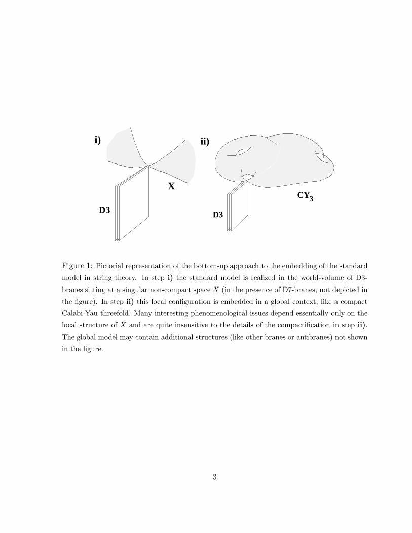
Figure 1: Pictorial representation of the bottom-up approach to the embedding of the standard

model in string theory. In step i) the standard model is realized in the world-volume of D3-

branes sitting at a singular non-compact space X (in the presence of D7-branes, not depicted in

the figure). In step ii) this local configuration is embedded in a global context, like a compact

Calabi-Yau threefold. Many interesting phenomenological issues depend essentially only on the

local structure of X and are quite insensitive to the details of the compactification in step ii).

The global model may contain additional structures (like other branes or antibranes) not shown

in the figure.

3

correspond to collections of D3/D7 branes located at orbifold singularities. The presence

of additional branes beyond D3-branes (i.e. D7-branes) is dictated by tadpole cancellation

conditions. Finding three quark-lepton generations and N = 1 SUSY turns out to be quite

restrictive leading essentially to IC3/ZZ3 singularities or some variations (including related

models with discrete torsion, ZZ3 orbifolds of the conifold singularity, or a non-abelian

orbifold singularity based on the discrete group ∆27). In these models extra gauged

U(1)’s with triangle anomalies (cured by a generalized Green-Schwarz mechanism) are

generically present but decouple at low energies. The appearance of the weak hypercharge

U(1)Y in these models is particularly elegant, corresponding to a unique universal linear

combination which is always anomaly-free and yields the SM hypercharge assignments

automatically. In the case of non-supersymmetric ZZN orbifold singularities, three quark-

lepton generations may be obtained for any N > 4, but the resulting weak angle tends to

be too small.

ii) These local ‘SM configurations’ may be embedded into compact models yielding

correct D=4 gravity. We construct specific compact Type IIB orbifold and orientifold

models which contain subsectors given by the realistic D-brane configurations discussed

above. In order to cancel global tadpoles (i.e, the total untwisted RR D-brane charges) one

can add anti-D3 and/or anti-D7 branes. These antibranes are stuck at orbifold fixed points

(in order to ensure stability against brane-antibrane annihilation) and lead to models

with hidden sector gravity-induced supersymmetry breaking. Other compact models with

unbroken D = 4 N = 1 supersymmetry may be easily obtained in the more general

framework of F-theory compactifications, and we construct an specific example of this

type. In this approach the embedding of SM physics into F-theory is quite different

from those followed previously: the interesting physics resides on D3-branes, rather than

D7-branes.

As we comment above, some properties of the low-energy physics of the compact

models will only depend on the local D3-brane configuration. That is for example the case

of hypercharge normalization. The D-brane configurations leading to unbroken N = 1

SUSY predict a tree-level value for the weak angle sin2 θW = 3/14 = 0.215, different

from the SU(5) standard result 3/8. This is compatible with standard logarithmic gauge

coupling unification if the string scale is of order Ms ∝ 1011 GeV, as we discuss in the

text. Other phenomenological aspects like Yukawa couplings depend not only on the

singularity structure, but also on the particular form of the compactification. Notice in

this respect that although the physics of the D3-branes will be dominated by the presence

of the singularity, the D7-branes wrap subspaces in the compact space and are therefore

4

more sensitive to its global structure.

The structure of this paper is as follows. In the following chapter we present some

general results which will be needed in the remaining sections. We describe the general

massless spectrum and couplings of Type IIB D3- and D7-branes on Abelian orbifold

singularities, both for the N = 1 and N = 0 cases. We also discuss the consistency

conditions of these configurations (cancellation of RR twisted tadpoles), as well as the

appearance of non-anomalous U(1) gauge symmetries in this class of theories. In chapter

3 we apply the formalism discussed in chapter 2 to the search of realistic three-generation

D-brane configurations sitting on IR6/ZZN singularities. We present specific simple N = 1

models leading to the SM gauge group with three quark-lepton generations. We also

present an alternative SU(3) × SU(2)L × SU(2)R × U(1)B−L three generation model.

We also discuss the case of non-SUSY ZZN singularities and present an specific three

generation non-SUSY model based on a ZZ5 singularity.

Finally, we discuss different generalizations yielding also three quark-lepton genera-

tions. In particular we discuss orbifold singularities with discrete torsion, models based on

non-abelian orbifolds, as well as some models based on certain non-orbifold singularities.

Although the massless spectrum of these new possibilities is very similar to the models

based on the ZZ3 singularity, some aspects like Yukawa couplings get modified, which may

be interesting phenomenologically. We argue that locating the D3-branes on an orientifold

(rather than orbifold) point does not lead to standard model configurations and hence

is not very promising. Finally we discuss non-supersymmetric models constructed using

branes and antibranes.

In chapter 4 we proceed to the second step in our approach and embed the realistic

D3/D7 configurations found in the previous chapters into a compact space. We present

examples based on type IIB orbifolds and orientifolds. As we mentioned above, in this

models the global RR charges may be canceled by the addition of anti-D-branes which

are trapped at the fixed points. Some of these models are T-dual to the models recently

studied in [13, 15]. We also discuss the construction of models with unbroken D = 4,

N = 1 SUSY by considering F-theory compactifications with the SM embedded on D3-

branes, and construct an specific example. In chapter 5 we briefly discuss some general

phenomenological questions, like gauge coupling unification and Yukawa couplings. We

leave our final comments and outlook for chapter 6. In order not to obstruct continuity

in the reading with many details, we have five appendices. The first four give the details

of each of the generalizations mentioned in section 3.6. The last appendix deals with the

issue of T -duality on some of the compact models in Section 4.

5

2 Three-Branes and Seven-Branes at Abelian Orb-

ifold Singularities

In this section we introduce the basic formalism to compute the spectrum and interactions

on the world-volume of D3-branes at IR6/ZZN singularities 2. These have been discussed

in [16, 17, 18, 19, 20], but our treatment is more general in that we allow the presence

of D7-branes. We also discuss several aspects of these field theories, to be used in the

remaining sections.

Before entering the construction, we would like to explain our interest in placing the

D3-branes on top of singularities. The reason is that D3-branes sitting at smooth points in

the transverse dimensions lead to N = 4 supersymmetric field theories. The only known

way to achieve chirality in this framework is to locate the D3-branes at singularities, the

simplest examples being IR6/ZZN orbifold singularities. Another important point in our

approach is that we embed all gauge interactions in D3-branes. Our motivation for this is

the fact that the appearance of SM fermions in three copies is difficult to achieve if color

and weak interactions live in e.g. D3- and D7- branes, respectively (as will be manifest

from the general spectra below).

2.1 Brane Spectrum

We start by considering the case of a generic, not necessarily supersymmetric, singularity.

Later on we discuss the specific N = 0 non supersymmetric and N = 1 supersymmetric

realizations. Consider a set of D3-branes at a IR6/Γ singularity with Γ ⊂ SU(4) where,

for simplicity, we take Γ = ZZN . Before the projection, the world-volume field theory on

the D3-branes is a N = 4 supersymmetric U(N) gauge theory. In N = 1 language, it

contains U(N) vector multiplets, and three adjoint chiral multiplets Φr, r = 1, 2, 3, with

interactions determined by the superpotential

W =∑r,s,t

εrst Tr (ΦrΦsΦt) (2.1)

In terms of component fields, the theory contains U(N) gauge bosons, four adjoint

fermions transforming in the 4 of the SU(4)R N = 4 R-symmetry group, and six ad-

joint real scalar fields transforming in the 6.

The ZZN action on fermions is given by a matrix

R4 = diag (e2πia1/N , e2πia2/N , e2πia3/N , e2πia4/N) (2.2)

2Other cases, like ZZN × ZZM orbifolds can be studied analogously, and we will skip their discussion.

6

with a1 + a2 + a3 + a4 = 0 mod N . The action of ZZN on scalars can be obtained from

the definition of the action on the 4, and it is given by the matrix

R6 = diag (e2πib1/N , e−2πib1/N , e2πib2/N , e−2πib2/N , e2πib3/N , e−2πib3/N) (2.3)

with b1 = a2 + a3, b2 = a1 + a3, b3 = a1 + a2. Scalars can be complexified, the action

on them being then given by Resc = diag (e2πib1/N , e2πib2/N , e2πib3/N ). Notice that, since

scalars have the interpretation of brane coordinates in the transverse space, eq. (2.3)

defines the action of ZZN on IR6 required to form the quotient IR6/ZZN .

The action of the ZZN generator θ must be embedded on the Chan-Paton indices. In

order to be more specific we consider the general embedding given by the matrix

γθ,3 = diag (In0 , e2πi/N In1 , . . . , e

2πi(N−1)/N InN−1) (2.4)

where In is the n × n unit matrix. The theory on D3-branes at the IR6/ZZN singularity

is obtained by keeping the states invariant under the combined (geometrical plus Chan-

Paton) ZZN action [16, 17]. World-volume gauge bosons correspond to open string states

in the NS sector, of the form λψµ

− 12

|0〉, with µ along the D3-brane world-volume, and λ

the Chan-Paton wavefunction. The projection for gauge bosons is then given by

λ = γθ,3 λ γ−1θ,3 (2.5)

The projection for each of the three complex scalars, λΨr− 1

2

|0〉 (with r = 1, 2, 3 labeling a

complex plane transverse to the D3-brane) is

λ = e−2πibr/N γθ,3 λ γ−1θ,3 (2.6)

The four fermions in the D3-brane world-volume, labeled by α = 1, . . . , 4 are described by

string states in the R sector, of the form λ|s1, s2, s3, s4〉, with si = ±12

and∑

i si = odd.

The projection for left-handed fermions, s4 = −12, leads to

λ = e2πiaα/Nγθ,3λγ−1θ,3 (2.7)

The final spectrum in the 33 sector is

Vectors∏N−1

i=0 U(ni)

Complex Scalars∑3

r=1

∑N−1i=0 (ni, ni−br)

Fermions∑4

α=1

∑N−1i=0 (ni, ni+aα) (2.8)

where subindices will be understood modulo N throughout the paper. The interactions

are obtained by keeping the surviving fields in the interactions of the original N = 4

7

theory. Notice that the spectrum is, generically, non supersymmetric. Instead, when

b1 + b2 + b3 = 0, we have a4 = 0 and the ZZN action is in SU(3). This case corresponds

to a supersymmetric singularity. The fermions with α = 4 transforming in the adjoint

representation of U(ni) become gauginos, while the other fermions transform in the same

bifundamental representations as the complex scalars. The different fields fill out complete

vector and chiral multiplets of N = 1 supersymmetry.

In general, we would also like to include D7-branes in the configuration. Let us

center on D7-branes transverse to the third complex plane Y3, denoted D73-branes in

what follows. Open strings in the 373 and 733 sectors contribute new fields in the D3-

brane world-volume. In the R sector, there are fermion zero modes in the NN and DD

directions Y4, Y3. Such states are labeled by λ|s3; s4〉, with s3 = s4 = ±12, where s4 defines

the spacetime chirality. The projection for left-handed fermions s4 = −12

are

λ373 = eiπb3/Nγθ,3λγ−1θ,73

, λ733 = eiπb3/Nγθ,73λγ−1θ,3 (2.9)

Scalars arise from the NS sector, which contains fermion zero modes in the DN directions

(Y1, Y2). States are labeled as λ|s1, s2〉, with s1 = s2 = ±1/2. The projections for λ|12, 1

2〉

are

λ373 = e−iπ(b1+b2)/Nγθ,3λγ−1θ,73

, λ733 = e−iπ(b1+b2)/Nγθ,73λγ−1θ,3 (2.10)

We can give the resulting spectrum quite explicitly. Let us consider the Chan-Paton

embedding

γθ,73 = diag ( Iu0 , e2πi/N Iu1 , . . . , e

2πi(N−1)/N IuN−1) for b3 = even (2.11)

γθ,73 = diag (eπi 1N Iu0 , e

2πi 3N Iu1, . . . , e

2πi 2N−1N IuN−1

) for b3 = odd

The resulting spectrum is

b3 = even → Fermions∑N−1

i=0 [ (ni, ui+ 12b3

) + (ui, ni+ 12b3

) ]

Complex Scalars∑N−1

i=0 [ (ni, ui− 12(b1+b2)) + (ui, ni− 1

2(b1+b2)

) ]

b3 = odd → Fermions∑N−1

i=0 [ (ni, ui+ 12(b3−1)) + (ui, ni+ 1

2(b3+1)) ]

Complex Scalars∑N−1

i=0 [ (ni, ui− 12(b1+b2+1)) + (ui, ni− 1

2(b1+b2−1)) ]

(2.12)

The computation is identical for other D7r-branes, transverse to the rth complex plane,

i.e. with world-volume defined by the equation Yr = 0. Notice that for a general twist,

D7-branes with world-volume∑3

r=1 βrYr = 0, with arbitrary complex coefficients βr, are

not consistent with the orbifold action (more precisely, they are not invariant under the

orbifold action, and suitable ZZN images should be included). For twists with several

equal eigenvalues, such D7-branes are possible (see footnote 3).

8

Notice that in the non-compact setting, fields in the 77 sector are non-dynamical from

the viewpoint of the D3-brane world-volume field theory. For instance, 77 gauge groups

correspond to global symmetries, and 77 scalars act as parameters of the D3-brane field

theory. Only after compactification of the transverse space, as in the models discussed in

Section 4, 77 fields become four-dimensional, and should be treated on an equal footing

with 33 and 37, 73 fields.

We conclude this section by restricting the above results to the case of singularities

IC3/ZZN preserving N = 1 supersymmetry on the D3-brane world-volume. That is, for

a4 = 0, and hence a1 + a2 + a3 = 0 modN . The spectrum is given by

33 Vector mult.∏N−1

i=0 U(ni)

Chiral mult.∑N−1

i=0

∑3r=1(ni, ni+ar)

373, 733 Chiral mult.∑N−1

i=0 [ (ni, ui− 12a3

) + (ui, ni− 12a3

) ] a3 even∑N−1i=0 [ (ni, ui− 1

2(a3+1)) + (ui, ni− 1

2(a3−1)) ] a3 odd

(2.13)

We will denote Φri,i+ar

the 33 chiral multiplet in the representation (ni, ni+ar). We also

denote (assuming a3 = even for concreteness) Φ(373)

i,i− 12a3

, Φ(733)

i,i− 12a3

the 373 and 733 chiral

multiplets in the (ni, ui− 12a3

), (ui, ni− 12a3

). With this notation, the interactions are encoded

in the superpotential

W =3∑

r,s,t=1

εrst Tr ( Φri,i+ar

Φsi+ar ,i+ar+as

Φti+ar+as,i ) +

N−1∑i=0

Tr ( Φ3i,i+a3

Φ(373)

i+a3,i+ 12a3

Φ(733)

i+ 12a3,i

)

2.2 Anomaly and Tadpole Cancellation

With the fermionic spectrum at hand we can proceed to compute non-abelian anoma-

lies and establish the constraints for consistent anomaly-free theories. Moreover, such

constraints can be rephrased in terms of twisted tadpole cancellation conditions [21, 22].

Let us address the computation of the non-abelian anomaly for SU(ni), in a case with

D7r-branes, r = 1, 2, 3. Let us assume br = even for concreteness, and denote by urj the

number of entries with phase e2πij/N in γθ,7r . The SU(nj) non-abelian anomaly cancella-

tion conditions are

4∑α=1

(ni+aα − ni−aα) +3∑

r=1

(uri+ 1

2br− ur

i− 12br

) = 0 (2.14)

These conditions are equivalent to the consistency conditions of the string theory config-

uration, namely cancellation of RR twisted tadpoles. To make this explicit, we use

nj = 1N

∑Nk=1 e

−2πi kj/NTr γθk,3 ; urj = 1

N

∑Nk=1 e

−2πi kj/NTr γθk,7r(2.15)

9

and substitute in (2.14). We obtain

2i

N

N∑k=1

e−2πi jk/N [4∑

α=1

sin(2πkaα/N)Tr γθk,3 +3∑

r=1

sin(πkbr/2)Tr γθk,7r] = 0 (2.16)

Using the identity

4∑α=1

sin(2πkaα/N) = 43∏

r=1

sin(πkbr/N) (2.17)

the Fourier-transformed anomaly cancellation condition is recast as

[3∏

r=1

2 sin(πkbr/N) ] Tr γθk,3 +3∑

r=1

2 sin(πkbr/N) Tr γθk,7r= 0 (2.18)

These are in fact the twisted tadpole cancellation conditions. Notice that the contributions

from the different disk diagrams are weighted by suitable sine factors, which arise from

integration over the string center of mass in NN directions.

2.3 Structure of U(1) Anomalies and Non-anomalous U(1)’s

An important property of systems of D3-branes at singularities leading to chiral world-

volume theories is the existence of mixed U(1)-nonabelian gauge anomalies. These field

theory anomalies are canceled by a generalized Green-Schwarz mechanism mediated by

closed string twisted modes [23] (see [24, 16, 25] for a similar mechanism in six dimensions).

Consider the generically non-supersymmetric field theory constructed from D3- and

D7r-branes at a ZZN singularity, with spectrum given in (2.8), (2.12). Assuming br = even

for concreteness, the mixed anomaly between the jth U(1) (that within U(nj)) and SU(nl)

is

Ajl =1

2nj

4∑α=1

(δl,j+aα − δl,j−aα) +1

2δj,l[

4∑α=1

(nj+aα − nj−aα) +3∑

r=1

(urj− 1

2br− ur

j+ 12br

) ]

The anomaly is not present if nj or nl vanish. After using the cancellation of cubic non-

abelian anomalies (2.14) (i.e. the tadpole cancellation conditions), the remaining piece is

given by

Ajl =1

2nj

4∑α=1

(δl,j+aα − δl,j−aα) (2.19)

This anomaly can be rewritten as

Ajl =−i2N

N−1∑k=1

[nj exp(2iπ kj/N) exp(−2iπkl/N)3∏

α=1

2 sin(πkbr/N) ] (2.20)

10

which makes the factorized structure of the anomaly explicit. The anomaly is canceled by

exchange of closed string twisted modes [23], which have suitable couplings to the gauge

fields on the D-brane world-volume [16, 17, 26, 27].

An important fact is that anomalous U(1)’s get a tree-level mass of the order of the

string scale [28], and therefore do not appear in the low-energy field theory dynamics on

the D3-brane world-volume. It is therefore interesting to discuss the existence of non-

anomalous U(1)’s and their structure. Concretely, we consider linear combinations of the

U(1) generators

Qc =N−1∑j=0

cjQnj

nj(2.21)

(we take cj = 0 if nj = 0). The condition for U(1)’s free of Qc −SU(nl)2 anomalies reads

1

2

4∑α=1

N−1∑j=0

cj(δl,j+aα − δl,j−aα) =4∑

α=1

(cl−aα − cl+aα) = 0 (2.22)

for all l = 0, . . . N − 1. It is clear that cj = const. lead to an anomaly free combination

Qdiag. =N−1∑i=0

Qni

ni(2.23)

This generically non-anomalous U(1) plays a prominent role in the realistic models of

Section 3. In general (2.22) gives N − 1 independent conditions for the N unknowns

cj , and (2.23) is the only non-trivial solution (as long as no nj vanishes). In certain

cases, however, the number of independent equations may be smaller, and additional

non-anomalous U(1)’s appear. In order to compute the number of independent equations

we rewrite the unknowns cj in terms of the new variables rk =∑N−1

j=0 e2iπkj/Ncj. The

original variables are given by

cj =1

N

N−1∑k=0

e−2πikj/Nrk. (2.24)

By replacing in (2.22) above we find∑4

α=1 sin(2πkaα/N)rk = 0 and, by using the identity

(2.17) we obtain

[3∏

r=1

sin(πkbr/N) ] rk = 0 (2.25)

Thus, we have managed to diagonalize the matrix corresponding to eq. (2.22). We see

that, besides the diagonal solution (corresponding to ri = 0 for i = 0. . . . , N − 1) other

non trivial solutions are possible whenever there exist twists θk that leave, at least, one

unrotated direction. In other words, the rank of the matrix is given by the number of

twists rotating all complex planes. It is possible to describe explicitly the non-anomalous

11

U(1)’s, as follows. Let us consider a ZZM subgroup, generated by a certain twist θp,

leaving e.g. the third complex plane fixed, hence pa1 = −pa2 and pa3 = −pa4. For each

value of I = 1, . . . ,M − 1, there is one non-anomalous U(1), defined by cj = δpj,I. This

satisfies the condition (2.22) by a cancellation of contributions from different values of

α. Hence we obtain one additional non-anomalous U(1) per twist leaving some complex

plane fixed 3.

Let us consider some explicit examples. For instance, for ZZ3 with twist v = 13(1, 1,−2),

equation (2.22) leads to b0 = b1 = b2 and the only anomaly free combination is (2.23).

Consequently, it is not possible to have an anomaly free U(1), unless all ni 6= 0. This will

always be the case for ZZN orbifold actions (supersymmetric or not) without twists with

fixed planes. Consequently, and as we discuss further in section 3, if we are interested

in gauge groups similar to the Standard Model one, with an anomaly free (hypercharge)

U(1), then all ni’s in (2.4) should be non vanishing.

The situation is different when subgroups with fixed planes exist. For instance, con-

sider the ZZ6 ≡ 16(1, 1,−2) example. The 33 spectrum reads

U(n0) × U(n1) × U(n2) × U(n3) × U(n4) × U(n5) × U(n6)

2[(n0, n1) + (n1, n2) + (n2, n3) + (n3, n4) + (n4, n5) + (n5, n0) + (n3, n0)] (2.26)

+(n0, n4) + (n2, n0) + (n4, n2) + (n1, n5) + (n3, n1) + (n5, n3) (2.27)

and the anomaly matrix (2.19) is given by

2Tαβij =

0 2n0 −n0 0 n0 −2n0

−2n1 0 2n1 −n1 0 n1

n2 −2n2 0 2n2 −n2 0

0 n3 −2n3 0 2n3 −n3

−n4 0 n4 −2n4 0 2n4

2n5 −n5 0 n5 −2n5 0

(2.28)

The search for anomaly-free combinations leads to eq.(2.22) above, which has two non-

trivial independent solutions. In fact, (2.24) becomes ci = r0 + (−1)ir3, namely c0 =

c2 = c4 and c1 = c3 = c5 indicating that two anomaly-free abelian factors can be present.

In particular, by choosing n1 = n3 = n5 = 0 and n4 = 3, n2 = 2, n0 = 1 we obtain

a field theory with Standard Model group SU(3) × SU(2) × U(1) and one generation

3There are arguments suggesting these additional non-anomalous U(1)’s are nevertheless massive due

to their mixing with closed string twisted modes [65]. This observation however, would not change our

analysis in the following sections, since our model building involves only the diagonal combination (2.23),

for which such mixing vanishes.

12

(3, 2)1/6 + (1, 2)1/2 + (3, 1)−2/3, with subscripts giving U(1) charges (fields in a suitable

37 sector should complete this to a full SM generation).

3 Particle Models from Branes at Singularities

In this Section we discuss the embedding of the Standard Model (and related Left-Right

symmetric extensions) in systems of D3-branes at IC3/ZZN singularities, with ZZN ⊂ SU(3).

We also discuss possible extensions to more general cases.

3.1 Number of Generations and Hypercharge

Let us start by recalling the structure of the field theory on D3-branes at a IC3/ZZN

singularity, defined by the twist v = (a1, a2, a3)/N . It has N = 1 supersymmetry, and

the following field content: there are vector multiplets with gauge group∏N−1

i=0 U(ni), and

3N N = 1 chiral multiplets Φri,i+ar

, i = 0, . . . , N − 1, r = 1, 2, 3, transforming in the

representation (ni, ni+ar). The interactions are encoded in the superpotential

W = εrst Tr (Φri,i+ar

Φsi+ar ,i+ar+as

Φti+ar+as,i). (3.1)

In general, the configurations will also include D7-branes, but for the moment we center

of general features in the 33 sector.

We are interested in constructing theories similar to the standard model or some

simple extension thereof. In particular, we will be interested in constructing models which

explicitly contain an SU(3) × SU(2) factor, to account for color and weak interactions.

Besides simplicity, this choice has the additional advantage (discussed in detail below)

that a non-anomalous U(1) leading to correct hypercharge assignments arises naturally.

Hence we consider models in which two factors, which without loss of generality we

take U(n0) and U(nj), are actually U(3), U(2). Since the matter content contains only

bi-fundamental representations, the number of generations is given by the number of left-

handed quarks, i.e. fields in the representation (3, 2). This is given by the number of

twist eigenvalues ar equal to j (minus the number of ar equal to −j), which is obviously

at most three, this maximum value occurring only for the IC3/ZZ3 singularity, with twist

v = (1, 1,−2)/3. For this reason, this singularity will play a prominent role in our

forthcoming models.

Before centering on that concrete case, it will be useful to analyze the issue of hy-

percharge. In order to obtain a theory with standard model gauge group, one needs the

presence of at least one non-anomalous U(1) to play the role of hypercharge. Happily, our

13

analysis in section 2.3 has shown that, as long as no ni vanishes, D3-branes at singularities

always have at least one non-anomalous U(1) generated by Qdiag in (2.23). Therefore,

a possibility to obtain the standard model gauge group, with no additional non-abelian

factors would be to consider models with group 4 U(3)× U(2) × U(1)N−2. In the generic

case, only the diagonal combination

Qdiag = −(

1

3Q3 +

1

2Q2 +

N−2∑s=1

Q(s)1

)(3.2)

will be non-anomalous (the overall minus sign is included for later convenience). In a

generic orbifold all other N − 1 additional U(1) factors will be anomalous and therefore

massive, with mass of the order of the string scale. Of course, the fact that we have

a non-anomalous U(1) does not guarantee it has the right properties of hypercharge.

Quite surprisingly this is precisely the case for (3.2). For instance, fields transforming in

the (3, 2) representation have Qdiag charge −13

+ 12

= 16, as corresponds to left-handed

quarks. Fields transforming in the (3, 1) (necessarily with charge −1 under one of the

Q(s)1 generators) have a Qdiag. charge −1

3+ 1 = −2

3, as corresponds to right-handed U

quarks, etc. Analysis of the complete spectrum requires information about the D7-brane

sector, and is postponed until the construction of explicit examples in section 3.3. Notice

that correct hypercharge assignments would not be obtained had our starting point been

e.g. SU(4) × SU(2), hence our interest in the SU(3) × SU(2) structure.

It is worth noticing that normalization of this hypercharge U(1) depends on N . In fact,

by normalizing U(n) generators such that TrT 2a = 1

2the normalization of Y generator is

fixed to be

k1 = 5/3 + 2(N − 2) (3.3)

This amounts to a dependence on N in the Weinberg angle, namely

sin2 θW =1

k1 + 1=

3

6N − 4(3.4)

Thus the weak angle decreases as N increases. Notice that the SU(5) result 3/8 is

only obtained for a Z2 singularity. However in that case the (33) spectrum is necessarily

vector-like and hence one cannot reproduce the SM spectrum.

We will also be interested in constructing left-right symmetric extensions of the stan-

dard model. In particular, we consider gauge groups with a factor SU(3) × SU(2)L ×4Such choice for the Chan-Paton embedding for D3-branes leads in general to non-vanishing tadpoles,

which can be canceled by the introduction of D7-branes. We leave their discussion for the explicit

examples below.

14

SU(2)R, which are obtained by choosing suitable values for three of the entries ni in the

Chan-Paton embedding. As above, the corresponding tadpole must be canceled by addi-

tional D7-branes, whose details we postpone for the moment. The number of generations

is again given by the number of representations (3, 2, 1), and is equal to three only for

the ZZ3 orbifold.

To reproduce hypercharge after the breaking of the right-handed SU(2) factor, an

essential ingredient is the existence of a non-anomalous (B−L) U(1) in the theory. In order

to obtain at least one non-anomalous U(1) in the D3-branes, we are led to consider models

with group U(3) × U(2) × U(2) × U(1)N−3. Generically, only the diagonal combination

Qdiag = −2

(1

3Q(3) +

1

2Q(2L) +

1

2Q(2R) +

N−3∑s=1

Q(1)s

)(3.5)

(the overall factor is included for convenience) is non-anomalous. Interestingly, the charges

under this non-anomalous U(1) turn out to have the correct B−L structure. For instance,

fields transforming in the (3, 2, 1) or (3, 1, 2) representations have Qdiag charge is −2(13−

12) = 1

3, correct for quark fields. Again, the discussion for the complete spectrum is

postponed to the explicit examples in section 3.4.

Notice, as above, that normalization of B−L generator is N dependent and leads to

kB−L = 8/3 + 8(N − 2). Since hypercharge is given by Y = −T 3R + QB−L (with T 3

R

the diagonal generator of SU(2)R) the values (3.3) and, thus, (3.4) are reobtained for

hypercharge normalization and Weinberg angle.

We find it is quite remarkable that the seemingly complicated hypercharge structure

in the standard model is easily accomplished by the structure of the diagonal U(1) in this

class of orbifold models.

We conclude by remarking that in cases with additional non-anomalous U(1)’s Qc

(2.21), they could be used as hypercharge or B−L generators, as long as the U(1) factors

in U(3) and U(2) belong to the corresponding linear combination in Qc (as in the ZZ6

example in section 2.3). However, since the presence of these U(1)’s is not generic, we

will not analyze this possibility in detail. Moreover, they are not present in the case of

ZZ3 singularity, which is the only candidate to produce three-generation models.

3.2 Generalities for IC3/ZZ3

In the following we construct some explicit examples of standard model or left-right

symmetric theories based on the IC3/ZZ3 singularity. This is the most attractive case,

since it leads naturally to three-family models. It also illustrates the general technology

involved in model building using branes at singularities.

15

Consider a set of D3-branes and D7r-branes at a IC3/ZZ3 orbifold singularity, generated

by the twist v = 13(1, 1,−2). Its action on the Chan-Paton factors is in general given by

the matrices

γθ,3 = diag (In0, αIn2 , α2In3) ; γθ,71 = −diag (Iu1

0, αIu1

2, α2Iu1

3)

γθ,73 = diag (Iu30, αIu3

1, α2Iu3

2) ; γθ,72 = −diag (Iu2

0, αIu2

2, α2Iu2

3)

(3.6)

with α = e2πi/3. The notation, slightly different from that in section 2.1, is more conve-

nient for IC3/ZZ3.

The full spectrum is given by

33 U(n0) × U(n1) × U(n2)

3 [(n0, n1) + (n1, n2) + (n2, n0) ]

37r, 7r3 (n0, ur1) + (n1, u

r2) + (n2, u

r0)+

+(ur0, n1) + (ur

1, n2) + (ur2, n0)

(3.7)

The superpotential 5 terms are

W =2∑

i=0

3∑r,s,t=1

εrstTr (Φri,i+1Φ

si+1,i+2Φ

ti+2,i) +

2∑i=0

3∑r=1

Tr (Φri,i+1Φ

37ri+1,i+2Φ

7r3i+2,i) (3.8)

The twisted tadpole cancellation conditions are

Tr γθ,73 − Tr γθ,71 − Tr γθ,72 + 3Tr γθ,3 = 0 (3.9)

where the relative signs, coming from the sine prefactors, cancel those in the definitions

in (3.6), hence it is consistent to ignore both. Eqs (3.9) are equivalent to the non-abelian

anomaly cancellation conditions.

3.3 Standard Model and Branes at IC3/ZZ3 Singularity

Following the general arguments in section 3.1, the strategy to obtain a field theory with

standard model gauge group from the ZZ3 singularity is to choose a D3-brane Chan-Paton

embedding

γθ,3 = diag (I3, αI2, α2I1) (3.10)

The simplest way to satisfy the tadpole conditions (3.9) is to introduce only one set of D7-

branes, e.g. D73-branes, with Chan-Paton embedding u30 = 0, u1

0 = 3, u20 = 6. The gauge

5It is possible to consider the generic case of D7β-branes, with world-volume defined by∑

r βrYr = 0,

which preserve the N = 1 supersymmetry of the configuration for arbitrary complex βr [29]. The 37β,

7β3 spectra are as above, but the superpotential is W =∑

i

∑r βrTr (ΦrΦ37β

Φ7β3), with fields from a

single mixed sector coupling to 33 fields from all complex planes.

16

2Y

3

1

Y

Y

3 D72 3 D73

3 D71

SMX

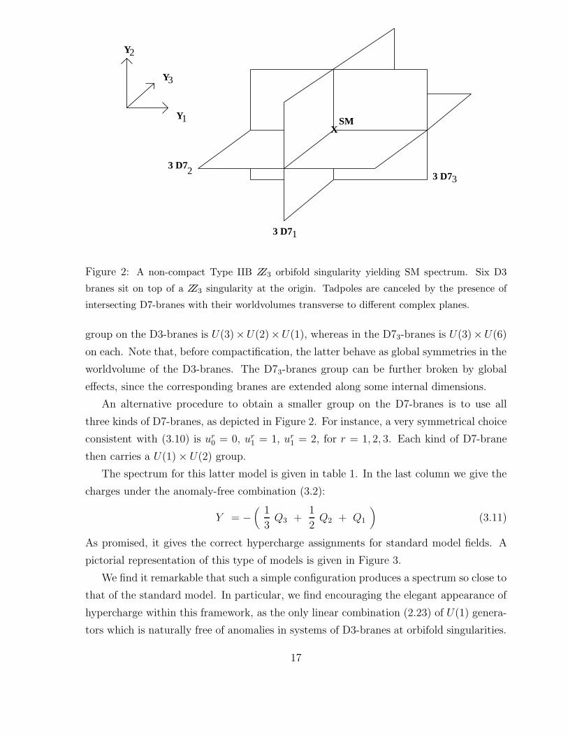
Figure 2: A non-compact Type IIB ZZ3 orbifold singularity yielding SM spectrum. Six D3

branes sit on top of a ZZ3 singularity at the origin. Tadpoles are canceled by the presence of

intersecting D7-branes with their worldvolumes transverse to different complex planes.

group on the D3-branes is U(3)×U(2)×U(1), whereas in the D73-branes is U(3)×U(6)

on each. Note that, before compactification, the latter behave as global symmetries in the

worldvolume of the D3-branes. The D73-branes group can be further broken by global

effects, since the corresponding branes are extended along some internal dimensions.

An alternative procedure to obtain a smaller group on the D7-branes is to use all

three kinds of D7-branes, as depicted in Figure 2. For instance, a very symmetrical choice

consistent with (3.10) is ur0 = 0, ur

1 = 1, ur1 = 2, for r = 1, 2, 3. Each kind of D7-brane

then carries a U(1) × U(2) group.

The spectrum for this latter model is given in table 1. In the last column we give the

charges under the anomaly-free combination (3.2):

Y = −(

1

3Q3 +

1

2Q2 + Q1

)(3.11)

As promised, it gives the correct hypercharge assignments for standard model fields. A

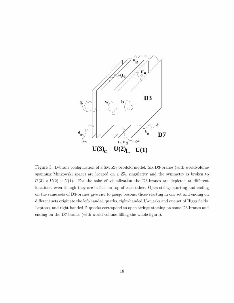
pictorial representation of this type of models is given in Figure 3.

We find it remarkable that such a simple configuration produces a spectrum so close to

that of the standard model. In particular, we find encouraging the elegant appearance of

hypercharge within this framework, as the only linear combination (2.23) of U(1) genera-

tors which is naturally free of anomalies in systems of D3-branes at orbifold singularities.

17

uR

U(3)c

g

u

RE

w

H

b

LQ

R

D3

U(1)U(2)L

d

dL, H

D7

Figure 3: D-brane configuration of a SM ZZ3 orbifold model. Six D3-branes (with worldvolume

spanning Minkowski space) are located on a ZZ3 singularity and the symmetry is broken to

U(3) × U(2) × U(1). For the sake of visualization the D3-branes are depicted at different

locations, even though they are in fact on top of each other. Open strings starting and ending

on the same sets of D3-branes give rise to gauge bosons; those starting in one set and ending on

different sets originate the left-handed quarks, right-handed U-quarks and one set of Higgs fields.

Leptons, and right-handed D-quarks correspond to open strings starting on some D3-branes and

ending on the D7-branes (with world-volume filling the whole figure).

18

Matter fields Q3 Q2 Q1 Qur1

Qur2

Y

33 sector

3(3, 2) 1 -1 0 0 0 1/6

3(3, 1) -1 0 1 0 0 -2/3

3(1, 2) 0 1 -1 0 0 1/2

37r sector

(3, 1) 1 0 0 -1 0 -1/3

(3, 1; 2′) -1 0 0 0 1 1/3

(1, 2; 2′) 0 1 0 0 -1 -1/2

(1, 1; 1′) 0 0 -1 1 0 1

7r7r sector

3(1; 2)′ 0 0 0 1 -1 0

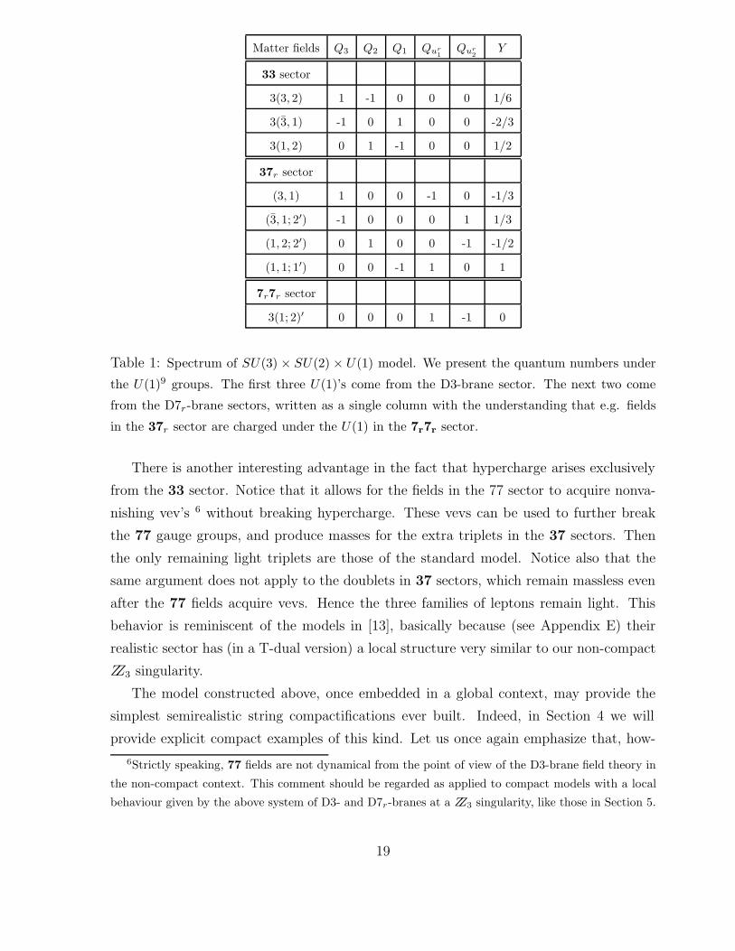
Table 1: Spectrum of SU(3) × SU(2) × U(1) model. We present the quantum numbers under

the U(1)9 groups. The first three U(1)’s come from the D3-brane sector. The next two come

from the D7r-brane sectors, written as a single column with the understanding that e.g. fields

in the 37r sector are charged under the U(1) in the 7r7r sector.

There is another interesting advantage in the fact that hypercharge arises exclusively

from the 33 sector. Notice that it allows for the fields in the 77 sector to acquire nonva-

nishing vev’s 6 without breaking hypercharge. These vevs can be used to further break

the 77 gauge groups, and produce masses for the extra triplets in the 37 sectors. Then

the only remaining light triplets are those of the standard model. Notice also that the

same argument does not apply to the doublets in 37 sectors, which remain massless even

after the 77 fields acquire vevs. Hence the three families of leptons remain light. This

behavior is reminiscent of the models in [13], basically because (see Appendix E) their

realistic sector has (in a T-dual version) a local structure very similar to our non-compact

ZZ3 singularity.

The model constructed above, once embedded in a global context, may provide the

simplest semirealistic string compactifications ever built. Indeed, in Section 4 we will

provide explicit compact examples of this kind. Let us once again emphasize that, how-

6Strictly speaking, 77 fields are not dynamical from the point of view of the D3-brane field theory in

the non-compact context. This comment should be regarded as applied to compact models with a local

behaviour given by the above system of D3- and D7r-branes at a ZZ3 singularity, like those in Section 5.

19

ever, many properties of the resulting theory will be independent of the particular global

structure used to achieve the compactification, and can be studied in the non-compact

version presented above, as we do in Section 5.

3.4 Left-Right Symmetric Models and the IC3/ZZ3 Singularity

One may use a similar approach to construct three-generation models with left-right

symmetric gauge group. Following the arguments in section 3.1, we consider the D3-

brane Chan-Paton embedding

γθ,3 = diag (I3, αI2, α2I2) (3.12)

The corresponding tadpoles can be canceled for instance by D7r-branes, r = 1, 2, 3 with

the symmetric choice ur0 = 0, ur

1 = ur2 = 1. The gauge group on D3-branes is U(3) ×

U(2)L × U(2)R, while each set of D7r-branes contains U(1)2. As explained above, the

combination (3.5)

QB−L = −2(

1

3Q3 +

1

2QL +

1

2QR

)(3.13)

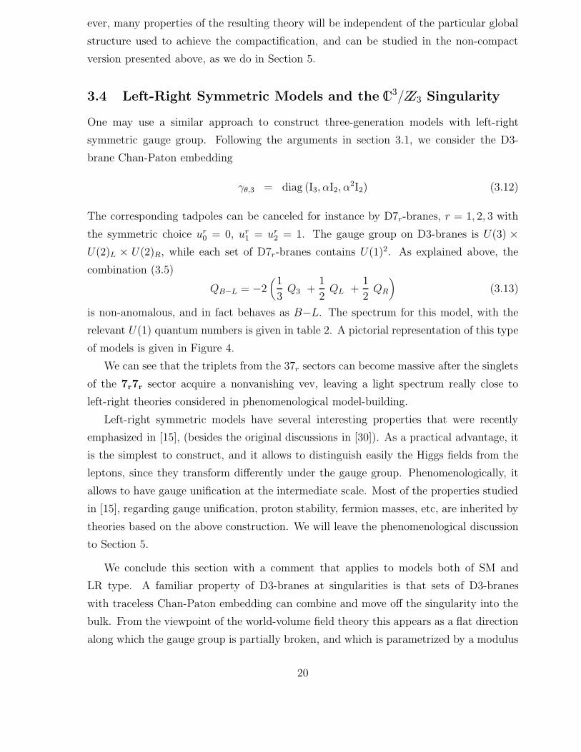
is non-anomalous, and in fact behaves as B−L. The spectrum for this model, with the

relevant U(1) quantum numbers is given in table 2. A pictorial representation of this type

of models is given in Figure 4.

We can see that the triplets from the 37r sectors can become massive after the singlets

of the 7r7r sector acquire a nonvanishing vev, leaving a light spectrum really close to

left-right theories considered in phenomenological model-building.

Left-right symmetric models have several interesting properties that were recently

emphasized in [15], (besides the original discussions in [30]). As a practical advantage, it

is the simplest to construct, and it allows to distinguish easily the Higgs fields from the

leptons, since they transform differently under the gauge group. Phenomenologically, it

allows to have gauge unification at the intermediate scale. Most of the properties studied

in [15], regarding gauge unification, proton stability, fermion masses, etc, are inherited by

theories based on the above construction. We will leave the phenomenological discussion

to Section 5.

We conclude this section with a comment that applies to models both of SM and

LR type. A familiar property of D3-branes at singularities is that sets of D3-branes

with traceless Chan-Paton embedding can combine and move off the singularity into the

bulk. From the viewpoint of the world-volume field theory this appears as a flat direction

along which the gauge group is partially broken, and which is parametrized by a modulus

20

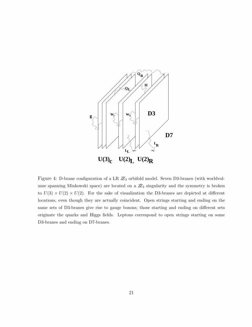
LL

w

QLH

U(3)c U(2)L

wRL

QR

LR

U(2)R

D3g

D7

Figure 4: D-brane configuration of a LR ZZ3 orbifold model. Seven D3-branes (with worldvol-

ume spanning Minkowski space) are located on a ZZ3 singularity and the symmetry is broken

to U(3) × U(2) × U(2). For the sake of visualization the D3-branes are depicted at different

locations, even though they are actually coincident. Open strings starting and ending on the

same sets of D3-branes give rise to gauge bosons; those starting and ending on different sets

originate the quarks and Higgs fields. Leptons correspond to open strings starting on some

D3-branes and ending on D7-branes.

21

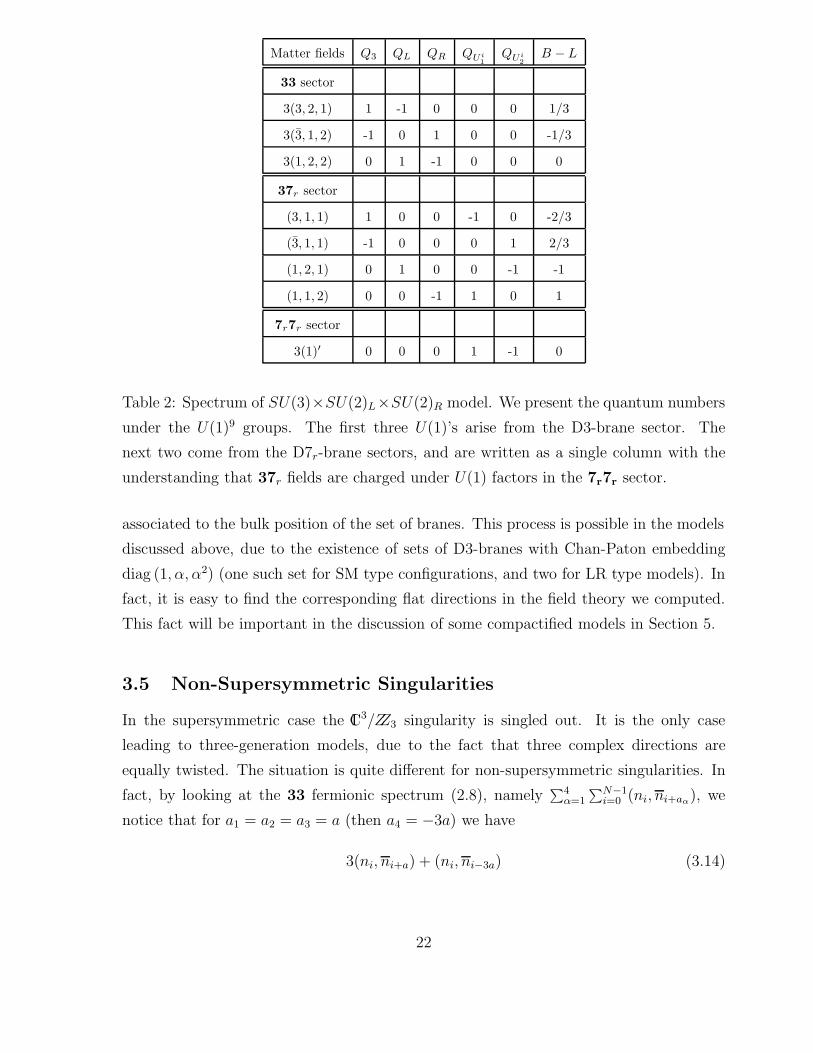
Matter fields Q3 QL QR QUi1

QUi2

B − L

33 sector

3(3, 2, 1) 1 -1 0 0 0 1/3

3(3, 1, 2) -1 0 1 0 0 -1/3

3(1, 2, 2) 0 1 -1 0 0 0

37r sector

(3, 1, 1) 1 0 0 -1 0 -2/3

(3, 1, 1) -1 0 0 0 1 2/3

(1, 2, 1) 0 1 0 0 -1 -1

(1, 1, 2) 0 0 -1 1 0 1

7r7r sector

3(1)′ 0 0 0 1 -1 0

Table 2: Spectrum of SU(3)×SU(2)L×SU(2)R model. We present the quantum numbers

under the U(1)9 groups. The first three U(1)’s arise from the D3-brane sector. The

next two come from the D7r-brane sectors, and are written as a single column with the

understanding that 37r fields are charged under U(1) factors in the 7r7r sector.

associated to the bulk position of the set of branes. This process is possible in the models

discussed above, due to the existence of sets of D3-branes with Chan-Paton embedding

diag (1, α, α2) (one such set for SM type configurations, and two for LR type models). In

fact, it is easy to find the corresponding flat directions in the field theory we computed.

This fact will be important in the discussion of some compactified models in Section 5.

3.5 Non-Supersymmetric Singularities

In the supersymmetric case the IC3/ZZ3 singularity is singled out. It is the only case

leading to three-generation models, due to the fact that three complex directions are

equally twisted. The situation is quite different for non-supersymmetric singularities. In

fact, by looking at the 33 fermionic spectrum (2.8), namely∑4

α=1

∑N−1i=0 (ni, ni+aα), we

notice that for a1 = a2 = a3 = a (then a4 = −3a) we have

3(ni, ni+a) + (ni, ni−3a) (3.14)

22

and therefore a potential triplication. This singularities are therefore well-suited for model

building of non-supersymmetric realistic spectra. We would like to point out that, despite

the lack of supersymmetry, these models do not contain tachyons, neither in open nor in

closed (untwisted or twisted) string sectors.

Without loss of generality we can choose a = 1 7 corresponding to ZZN twist given by

(1, 1, 1,−3)/N . Thus, we observe that N = 2 leads to non-chiral theories, N = 4 to four-

generation models, while each model with N ≥ 5 leads to three-generations models. For

instance, by choosing n0 = 3, n1 = 2 and ni = 1 for i = 3, . . . , N − 1, a Standard Model

gauge group SU(3) × SU(2) × U(1)Y × U(1)N−1 is found with 33 fermions transforming

as

3[(3, 2)1/6 + (3, 1)−2/3 + (1, 2)1/2] + (N − 3) singlets. (3.15)

Thus, we obtain three generations of left-handed quarks and right-handed U type quarks.

Since such a matter content is anomalous, extra contributions coming from D7-branes are

expected to complete the spectrum to the three generations of SM quarks and leptons.

Notice that presence of D7-branes only produce fundamentals of 33 groups in 37 + 73

sectors and therefore the number of generations is not altered.

Interestingly enough, the correct SM hypercharge assignments above correspond to

the anomaly-free diagonal U(1) combination (2.23)

Y = −Qdiag = − 1

3Qn0 +

1

2Qn1 +

N−1∑j=3

Qnj

(3.16)

Hence hypercharge can arise by the same mechanism discussed in section 3.1 for super-

symmetric models.

It is interesting to study the Weinberg angle prediction for these models. The com-

putation follows that in section 3.1, leading to the result (3.4), which gives sin2 θW =

0.214, 0.115... for N = 3, N = 5, . . . respectively. Hence we see that, even though many

non-supersymmetric singularities lead to three-generation models, in general they yield

too low values of the Weinberg angle. It is interesting that the value gets worse as the

order of the singularity increases, suggesting that simple configurations are better suited

to reproduce realistic particle models.

A ZZ5 example

As a concrete example of the above discussion let us consider the ZZ5 singularity acting

on the 4 with twist (a1, a2, a3, a4) = (1, 1, 1,−3). Hence the action on the 6 is given by

7For a ZZN singularity, we must have gcd(a, N) = 1, hence there exists p such that pa = 1 mod N ,

and we may choose θp to generate ZZN . This only implies a harmless redefinition on the ni’s in γθ,3.

23

(b1, b2, b3) = (2, 2, 2). The general D3-brane Chan-Paton matrix has the form

γθ,3 = diag (In0, αIn1, α2In2 , α

3In3 , α4In4) (3.17)

with α = e2πi/5. Anomaly/tadpole cancellation conditions require

4(α− α4)Tr γθ,3 +3∑

r=1

γθ,7r = 0 (3.18)

and, therefore, D7-branes must be added. Let us consider the case with only D73-branes,

with Chan-Paton action

γθ,73 = diag (Iu0 , αIu1, α2Iu2, α

3Iu3 , α4Iu4) (3.19)

The massless spectrum reads

33 Vectors U(n0) × U(n1) × U(n2) × U(n3) × U(n4)

Fermions 3[(n0, n1) + (n1, n2) + (n2, n3) + (n3, n4) + (n4, n0)] +

(n0, n2) + (n1, n3) + (n2, n4) + (n3, n0) + (n4, n1)]

Cmplx.Sc. 3[(n0, n3) + (n1, n4) + (n2, n0) + (n3, n1) + (n4, n2), ]

373 Fermions (n0, u1) + (n1, u2) + (n2, u3) + (n3, u4) + (n4, u0)

Cmplx.Sc. (n0, u3) + (n1, u4) + (n2, u0) + (n3, u1) + (n4, u2)

733 Fermions (u0, n1) + (u1, n2) + (u2, n3) + (u3, n4) + (u4, n0)

Cmplx.Sc. (u0, n3) + (u1, n4) + (u2, n0) + (u3, n1) + (u4, n2)

where ni, ui’s are constrained by (3.18).

To be more specific, let us build up a Left-Right model, by choosing n0 = 3, n1 = n4 =

2 and n2 = n3 = 1, which leads to a gauge group SU(3) × SU(2) × SU(2) × U(1)B−L ×[U(1)5]. The choice u0 = 0, u1 = 3, u2 = u3 = 7, u4 = 3 ensures tadpole cancellation.

The B−L charge is provided by the anomaly-free diagonal combination (2.23). From the

generic spectrum above we find 33 fermions transform, under LR group as

3[(3, 2, 1) 13

+ (1, 2, 1)1 + (1, 1, 1)0 + (1, 1, 2)−1 + (3, 1, 2)− 13]

(3, 1, 1) 43

+ (3, 1, 1)− 43

+ (1, 2, 1)+1 + (1, 1, 2)−1 + (1, 2, 2)0 (3.20)

while scalars live in

3[(3, 1, 1) 43

+ (3, 1, 1)− 43

+ (1, 2, 1)−1 + (1, 1, 2)−1 + (1, 2, 2)0]

24

Fermions in 37 +73 sectors transform as

(3, 1, 1; 3, 1, 1, 1)− 23

+ (3, 1, 1; 1, 1, 1, 3) 23+

+(1, 2, 1; 1, 7, 1, 1)−1 + (1, 1, 2; 1, 1, 7, 1)1 + +LR singlets (3.21)

while scalars do as

(3, 1, 1; 1, 1, 7, 1)− 23

+ (1, 2, 1; 1, 1, 1, 3)−1 + (1, 1, 2; 1, 7, 1, 1)−1 +

+(1, 1, 2; 3, 1, 1, 1)1 + (3, 1, 1; 1, 7, 1, 1) 23

+ (1, 2, 1; 1, 1, 7, 1)1 + L − R singlets(3.22)

We obtain three quark-lepton families from the 33 sector. The remaining fields, vector-like

with respect to the LR group could acquire masses by breaking of the 77 groups.

3.6 Other Possibilities

It is interesting to compare the kind of models we have constructed, using abelian orbifold

singularities, with the field theories arising from D3-branes at more complicated singular-

ities. In this section we discuss some relevant cases. The details for the construction of

the corresponding field theories can be found in appendices A, B, C and D.

3.6.1 Orbifold Singularities with Discrete Torsion

Orbifold singularities IC3/(ZZM1×ZZM2) lead to different models depending on their discrete

torsion. In appendix A we review the field theory on singularities IC3/(ZZN ×ZZM ×ZZM),

with ZZN twist (a1, a2, a3)/N , and discrete torsion e2πi/M between the ZZM twists. The

final spectrum on the D3-brane world-volume is identical to that of the IC3/ZZN singularity

(2.13), but the superpotential is modified to (A.5).

Hence it follows that the phenomenologically most interesting models in this class are

those obtained from the ZZ3 orbifold by a further ZZM × ZZM projection with discrete

torsion. The resulting spectrum coincides with (3.7), and can lead to three-generation

SM or LR models. The superpotential in the 33 sector is modified to

W = Tr [ Φ1i,i+1Φ

2i+1,i+2Φ

3i+2,i] − e2πi 1

M Tr [Φ1i,i+1Φ

3i+1,i+2Φ

2i+2,i ] (3.23)

Since the spectra we obtain from such singularities are identical to those in the simpler

case of IC3/ZZ3, we may question the interest of these models. They have two possible

applications we would like to mention. The first, explored in section 5, is that discrete

torsion enters as a new parameter that modifies the superpotential of the theory, and

25

therefore the pattern of Yukawa couplings in phenomenological models. The second ap-

plication is related to the process of moving branes off the singularity into the bulk, a

phenomenon that, as discussed in Section 3 can take place in the realistic models there

constructed. In ZZN ×ZZM ×ZZM singularities with discrete torsion, the process can also

occur, but the minimum number of branes allowed to move into the bulk is NM2. In

particular, in SM theories constructed from the IC3/(ZZ3 × ZZM × ZZM) singularity, there

are only six D3-branes with traceless Chan-Paton embedding, so motion into the bulk

is forbidden for M ≥ 2. For LR models, motion into the bulk of the twelve traceless

D3-branes is forbidden for M ≥ 3. In fact, the trapping is only partial, since branes are

still allowed to move along planes fixed under some ZZM twist [31]. This partial trapping

will be exploited in section 4.1 in the construction of certain compact models.

3.6.2 Non-Abelian Orbifold Singularities

We may also consider the field theories on D3-branes at non-abelian orbifold singularities.

The rules to compute the spectrum, along with the relevant notation, are reviewed in

Appendix B. They allow to search for phenomenologically interesting spectra. The clas-

sification of non-abelian discrete subgroups of SU(3) and several aspects of the resulting

field theories have been explored in [32, 33]. An important feature in trying to embed

the standard model in such field theories is that of triplication of families. Seemingly

there is no non-abelian singularity where the spectrum appears in three identical copies.

A milder requirement with a chance of leading to phenomenological models would be the

appearance of three copies of at least one representation, i.e. a3ij = 3 for suitable i 6= j.

Going through the explicit tables in [32] there is one group with this property, ∆3n2 for

n = 3, on which we center in what follows. The 33 spectrum 8 for this case is

∏9i=1 U(ni) × U(n10) × U(n11)∑9

i=1(ni, n10) + 3 (n10, n11) +∑9

i=1(n11, ni) (3.24)

If the triplicated representation is chosen to give left-handed quarks, a potentially

interesting choice is given by ni = 1, n10 = 3, n11 = 2. However, and due to the additional

factors ri (in our case ri = 1 for i = 1, . . . , 9, r10 = r11 = 3) in (B.4), the diagonal

combination does not lead to correct hypercharge assignments. Besides (B.4) there are

eight non-anomalous U(1)’s given by combinations Qc =∑9

i=1 ciQni+Qn10 + 3

2Qn11 , with∑9

i=1 ci = 9. The charge structure under the combination c1 = c2 = c3 = 3, ci = 0 for

8The gauge group in page 16 of [32] corresponds to the particular case of Chan-Paton embedding

given by the regular representation. Here we consider a general choice.

26

i = 4, . . . , 9 is particularly interesting. We obtain

SU(3) × SU(2) × U(1) (×U(1)8 )

3(3, 2)1/6 + 3(1, 2)1/2 + 6(1, 2)−1/2 + 3(3, 1)−2/3 + 6(3, 1)1/3 (3.25)

Hence, the spectrum under this U(1) contains fields present in the standard model, and

with the possibility of leading to three net copies (if suitable 37, 73 sectors are considered),

even though they would still be distinguished by their charges under the additional U(1)’s.

It is conceivable that this model leads to phenomenologically interesting field theories by

breaking the additional U(1) symmetries at a large enough scale. However, it is easy

to see that the Weinberg angle, which, taking into account (B.3), is still given by (3.4)

where now N = 11, is exceedingly too small sin2 θW = 3/62. Nevertheless we hope the

model is illustrative on the type of field theory spectra one can achieve using non-abelian

singularities.

3.6.3 Non-Orbifold Singularities

In appendix C we discuss the construction of field theories on D3-branes at some non-

orbifold singularities, which is in general rather involved. We also discuss that a promising

spectrum is obtained from a partial blow-up of a ZZ3 quotient of the conifold. The general

spectrum is given in (C.7), (C.9). There are several possibilities to construct phenomeno-

logically interesting spectra from this field theory. For the purpose of illustration, let us

consider one example with n2 = 3, n0 = 2, n′1 = 2, n′

1 = 1 and v2 = 1, x2 = 3, x3 = 5 (all

others vanishing). This choice leads to the spectrum

SU(3) × SU(2) × SU(2) × U(1)diag × U(1)′

33 3(3, 2, 1) 13

+ (3, 1, 1)− 43

+ 2(3, 1, 2)− 13

+ (1, 2, 2)0 + 2(1, 2, 1)1 + (1, 1, 2)−1

37, 73 (3, 1, 1; 1, 1)− 23

+ (1, 1, 1; 1, 1)2 + (3, 1, 1; 3, 1)− 23+

(1, 1, 2; 3, 1)1 + (1, 2, 1; 1, 5)−1 + (3, 1, 1; 1, 5) 23

(3.26)

with subindices giving charges under U(1)diag. We obtain three net generations, but the

right-handed quarks have a different embedding into the left-right symmetry: whereas two

generations of right-handed quarks are standard SU(2)R doublets the other generation

are SU(2)R singlets. Notice that an interesting property this model illustrates is that

one can achieve three quark-lepton generations without triplication of the (1, 2, 2) Higgs

multiplets. This could be useful in order to suppress flavour changing neutral currents for

these models.

27

3.6.4 Orientifold Singularities

There is another kind of singularities that arises naturally in string theory, which we refer

to as orientifold singularities. They arise from usual geometric singularities which are

also fixed under an action Ωg, where Ω reverses the world-sheet orientation, and g is an

order two geometric action. Orientifolds were initially considered in [34] and have recently

received further attention [35, 36, 37].

Starting with the field theory on a set of D3-branes at a usual singularity, the main

effect of the orientifold projection is to impose a ZZ2 identification on the fields. Most

examples in the literature deal with orientifolds of orbifolds singularities [38, 23], on which

we center in the following (see [39] for orientifold of some simple non-orbifols singulari-

ties). To be concrete, we consider orientifolds of IC3/ZZN singularities with odd N [23].

The spectrum before the orientifold projection is given in (2.13). This configuration can

be modded out by ΩR1R2R3(−1)FL (where Rr acts as Yr → −Yr, and FL is left-handed

world-sheet fermion number), preserving N = 1 supersymmetry. The action of the ori-

entifold projection on the 33 spectrum amounts to identifying the gauge groups U(ni)

and U(n−i), in such a way (due to world-sheet orientation reversal) that the fundamental

representation ni is identified with the anti-fundamental n−i. Consequently, there is an

identification of the chiral multiplet Φri,i+ar

and Φr−i−ar ,−i. Finally, since Ω exchanges the

open string endpoints, 37r fields Φ(37r)

i,i− 12br

map to 7r3 fields Φ7r3N−i+ 1

2br ,N−i

.

Notice that the gauge group U(n0) is mapped to itself and, similarly, chiral multiplets

Φri,i+ar

are mapped to themselves if i + ar = N − i. There exist two possible orientifold

projections, denoted ‘SO’ and ‘Sp’, differing in the prescription of these cases. The SO

projection projects the U(n0) factor down to SO(n0), and the bi-fundamental Φri,i+ar

(=

Φri,−i) to the two-index antisymmetric representation of the final U(ni). The Sp projection

chooses instead USp(n0), and two-index symmetric representations.

It is easy to realize that D3-branes at orientifold singularities will suffer from a generic

difficulty in yielding realistic spectra. The problem lies in the fact that the orientifold

projection removes from the spectrum the diagonal U(1) (2.23) (as is obvious, since the

U(1) in U(n0) is automatically lost), which was crucial in obtaining correct hypercharge

in our models in section 3.

For illustration, we can check explicitly that, in the only candidate to yield three-

family models, the orientifold of the IC3/ZZ3 singularity, no realistic spectra arise. The

general 33 spectrum for this orientifold (choosing, say the SO projection) is

SO(n0) × U(n1)

28

3 [ (n0, n1) + (1, 12n1(n1 − 1)) ] (3.27)

The U(1) factor is anomalous, with anomaly canceled by a GS mechanism [23].

A seemingly interesting possibility would be SO(3)× U(3) ' SU(3) × SU(2) × U(1).

However, the U(1) factor does not provide correct hypercharge assignments. Moreover,

it is anomalous and therefore not even present in the low-energy theory. A second pos-

sibility, yielding a Pati-Salam model SO(4) × U(4) ' SU(2) × SU(2) × SU(4) × U(1)

is unfortunately vector-like. In fact, the most realistic spectrum one can construct is

obtained for n0 = 1, n1 = 5, yielding a U(5) (actually SU(5)) gauge theory with chiral

multiplets in three copies of 5 + 10. This GUT-like theory, which constitutes a subsector

in a compact model considered in [10], does not however contain Higgs fields to trigger

breaking to the standard model group.

We hope this brief discussion suffices to support our general impression that orien-

tifold singularities yield, in general, field theories relatively less promising than orbifold

singularities.

3.6.5 Non-Supersymmetric Models from Antibranes

We would like to conclude this section by considering a further set of field theories,

obtained by considering branes and antibranes at singularities. The rules to compute the

spectrum are reviewed in Appendix C. For simplicity we center on systems of branes and

antibranes at IC3/ZZN singularities, with ZZN ⊂ SU(3), even though the class of models

is clearly more general. Notice that, due to the presence of branes and antibranes, the

resulting field theories will be non-supersymmetric. Let us turn to the discussion of the

generic features to be expected in embedding the standard model in this type of D3/D3

systems.

The first possibility we would like to consider is the case with the standard model

embedded on D3- and D3-branes. From (D.1), tachyons arise whenever the Chan-Paton

embedding matrices γθ,3, γθ,3 have some common eigenvalue. Denoting nj, mj the number

of eigenvalues e2πij/N in γθ,3, γθ,3, tachyons are avoided only if one considers models

where ni vanishes when mi is non-zero, and vice-versa. This corresponds, for instance, to

embedding SU(3) in the D3-branes and SU(2) in the D3-branes.

One immediate difficulty is manifest already at this level, regarding the appearance of

hypercharge. As we remark in Appendix D, it is a simple exercise to extend the analysis of

U(1) anomalies of section 2.3 to the case with antibranes, with the result that (generically)

there are two non-anomalous diagonal combinations (2.23) if no ni, mi vanish. But this

case is excluded by the requirement of absence of tachyons. Hence tachyon-free models

29

lack the diagonal linear combination of U(1)’s and in general fail to produce correct

hypercharge. It is still possible that in certain models, suitable tachyon-free choices of ni,

mi may produce hypercharge out of non-diagonal additional U(1)’s. Instead of exploring

this direction (which in any case would not be available in the only three-family case of

the IC3/ZZ3 singularity), we turn to a different possibility.

An alternative consists in embedding the standard model in, say D3-branes, but to

satisfy the tadpole cancellation conditions using D7-branes (and possibly D7-branes as

well). The resulting models are closely related to those in Section 3, differing from them

only in the existence of 37, 73 sectors. Let us consider a particular example, with a set

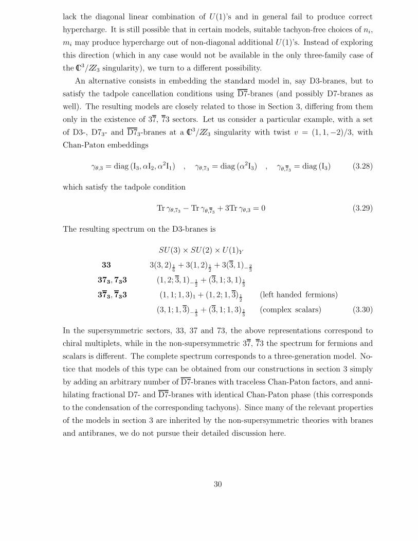
of D3-, D73- and D73-branes at a IC3/ZZ3 singularity with twist v = (1, 1,−2)/3, with

Chan-Paton embeddings

γθ,3 = diag (I3, αI2, α2I1) , γθ,73 = diag (α2I3) , γθ,73

= diag (I3) (3.28)

which satisfy the tadpole condition

Tr γθ,73 − Tr γθ,73+ 3Tr γθ,3 = 0 (3.29)

The resulting spectrum on the D3-branes is

SU(3) × SU(2) × U(1)Y

33 3(3, 2) 16

+ 3(1, 2) 12

+ 3(3, 1)− 23

373, 733 (1, 2; 3, 1)− 12

+ (3, 1; 3, 1) 13

373, 733 (1, 1; 1, 3)1 + (1, 2; 1, 3) 12

(left handed fermions)

(3, 1; 1, 3)− 13

+ (3, 1; 1, 3) 13

(complex scalars) (3.30)

In the supersymmetric sectors, 33, 37 and 73, the above representations correspond to

chiral multiplets, while in the non-supersymmetric 37, 73 the spectrum for fermions and

scalars is different. The complete spectrum corresponds to a three-generation model. No-

tice that models of this type can be obtained from our constructions in section 3 simply

by adding an arbitrary number of D7-branes with traceless Chan-Paton factors, and anni-

hilating fractional D7- and D7-branes with identical Chan-Paton phase (this corresponds

to the condensation of the corresponding tachyons). Since many of the relevant properties

of the models in section 3 are inherited by the non-supersymmetric theories with branes

and antibranes, we do not pursue their detailed discussion here.

30

4 Embedding into a Compact Space

As discussed in the introduction, even though SM gauge interactions propagate only

within the D3-branes even in the non-compact setup, gravity remains ten-dimensional. In

order to reproduce correct four-dimensional gravity the transverse space must be compact.

In this section we present several simple string compactifications which include the local

structures studied in section 3, as particular subsectors.

Since these local structures contain D3- and D7-branes, the corresponding RR charges

must be cancelled in the compact space. A simple possibility is to cancel these charges by

including antibranes (denoted D3-, D7-branes) in the configuration. General rules to avoid

tachyons and instabilities against brane-antibrane annihilation have been provided in [12]

(see [40, 14] for related models), which we exploit in section 4.1 to construct compact

models based on toroidal orbifolds. A second possibility is to use orientifold planes. In

section 4.2 we provide toroidal orientifolds without D3-branes, the D3-brane charge being

cancelled by orientifold 3-planes (O3-planes). All of the above models contain some kind of

antibranes, breaking supersymmetry in a hidden sector lying within the compactification

space. It may be possible to find completely supersymmetric embeddings of our local

structure by using toroidal orientifolds including O3- and O7-planes, even though we

have not found such examples within the class of toroidal abelian orientifolds. This

is hardly surprising, since this class is rather restricted. We argue that suitable N = 1

supersymmetric compactifications of our local structures exist in more general frameworks,

like compactification on curved spaces. In fact, in section 4.3 we present an explicit F-

theory compactification of this type.

4.1 Inside a Compact Type IIB Orbifold

A simple family of Calabi-Yau compactifications with singularities is given by toroidal

orbifolds T 6/ZZN . The twist ZZN is constrained to act cristalographycally, and a list

of the possibilities preserving supersymmetry is given in [41]. Several such orbifolds

include IC3/ZZ3 singularities, the simplest being T 6/ZZ3, with 27 singularities arising from

fixed points of ZZ3. Parameterizing the three two-tori in T 6 by zr, r = 1, 2, 3, with

zr ' zr +1 ' zr + e2πi/3, the 27 fixed points are located at (z1, z2, z3) with zr = 0, 1√3eπi/6,

1√3e−πi/6. For simplicity, we denote these values by 0, +1, −1 in what follows. We now

present several compact versions of the models in section 3, based on this orbifold.

31

4.1.1 Simple Examples

The simplest possibility, in order to embed the local structures of section 3 in a compact

orbifold, is to consider models with only one type of D7-brane. We will also consider

the addition of Wilson lines, a modification which, being a global rather than a local

phenomenon, was not available in the non-compact case. We first construct an example

of a left-right symmetric model, which illustrates the general technique, and then briefly

mention the construction of a model with standard model group.

A Left-Right Symmetric Model

Consider a compact T 6/ZZ3 orbifold, and locate seven D3-branes with

γθ,3 = diag (I3, αI2, α2I2) (4.1)

at the origin. To cancel twisted tadpoles at the origin we will add six D71-branes at the

origin in the first complex plane, with Chan-Paton embedding

γθ,7 = diag (αI3, α2I3) (4.2)

The local structure around the origin is exactly as in the LR models studied in section 3.4,

hence the final model will automatically contain a SU(3)× SU(2)L × SU(2)R ×U(1)B−L

gauge group, with three quark-lepton generations. That one can make this statement at

such an early stage in the construction of the model is the main virtue of the bottom-up

approach we are presenting. In the following, we simply discuss how to complete the

model satisfying the string consistency conditions, and will not bother computing the

detailed spectrum from the additional sectors.

The choice (4.2) cancels the twisted tadpoles at the origin. But the worldvolume of

these D71-branes also overlap with other eight fixed points (0, n, p), where n, p = 0,±1,

so we will also have to ensure twisted tadpole cancellation at them. A simple option

would be to add one single D3-brane with γθ,3 = 1 at each. However we consider the

following more interesting possibility, which in addition breaks the (too large) D71-brane

U(3) × U(3) gauge group. Consider adding a Wilson line e.g. along the second complex

plane, and acting on seven-branes as

γW,7 = diag (I1, αI1, α2I1, I1, αI1, α

2I1) (4.3)

The D71-brane gauge group is broken down to U(1)6 (some of which will actually be

anomalous and therefore not really present). The fixed points (0,±1, p), p = 0,±1 feel

32

3YY1

Y2

16 D7 6 D71

LR

**

*

**

*

**

*

0

0

0

0

0

0

LR

**

*

**

*

**

*

0

0

0

0

0

0

0

0

0

0

0

0

0

0

0

x

x

1 = +1 1 = 0 1 = - 1 Y Y Y

Figure 5: A compact Type IIB T 6/ZZ3 orbifold model with a LR subsector. The points marked

(0) correspond to fixed points without D3-branes; those marked (∗) contain anti-D3-branes and

those marked (x) have D3-branes located on them. Seven D3-branes, leading to a LR model of

the type studied in section 3.4, reside at the origin. The overall RR charge cancels.

the presence of the Wilson line [42, 37], hence the D71 contribution to twisted tadpoles is

given by tr γθ,7γW,7 or tr γθ,7γ2W,7, which vanish. Hence twisted tadpole cancellation does

not require any additional branes at those fixed points. On the other hand the points

(0, 0,±1) do not feel the presence of the Wilson line and require e.g. the presence of one

D3-brane with γθ,3 = 1 on each of them to achieve tadpole cancellation 9.

The above configuration has a total of nine D3-branes and six D71-branes. The sim-

plest possibility to cancel untwisted tadpoles is to locate six D71-branes at a different

point, say Y1 = 1, in the first complex dimension, with the same Chan-Paton twist matrix

(4.2). Twisted and untwisted tadpoles are cancelled by adding one D3-brane at each of

the nine fixed points (1, m, p), m, p = 0,±1, with Chan-Paton embedding γθ,3 = diag (I1).

The number of branes minus that of antibranes vanishes. The complete configuration is

schematically depicted in Figure 5

A comment on the stability of this brane configuration is in order. In this compact

configuration the D7-branes and D7-branes are trapped at the singular points, which they

9An amusing possibility is to add, instead of these single D3-branes, ‘new brane-worlds’ of seven

3-branes with (4.1), so that the model contains three different but analogous universes.

33

cannot leave. The flat directions associated to motions into the bulk are not present in

their world-volume field theory. Moreover such motions would violate the twisted tadpole

cancellation conditions. Hence, these objects cannot leave the fixed points and annihilate

each other into the vacuum. On the other hand, groups of three D3-branes in the LR

subsector may in principle abandon the origin and travel into the bulk in ZZ3-invariant

configurations, attracted by the D3-branes living at the fixed points (1, m, p). Eventually

the D3-branes could reach the D3-branes, and partial brane-antibrane annihilation would

follow. This annihilation cannot be complete, since again the tadpole cancellation condi-

tions would be violated. Since the complete configuration is non-supersymmetric, a more

detailed analysis of the forces involved would be needed to find out whether the emission

of D3-branes from the origin to the bulk is actually dynamically preferred or not, but

we expect this specific model to suffer from such instability. On the other hand, as we

will argue below, there are other ways to embed the set of SM or LR D3-branes into a

compact space in which brane-antibrane annihilation is not possible.

One Standard-like Model

From the above construction, it is clear how to construct a compact orbifold model

with an SM subsector, as we sketch in the following. We place the six D3-branes at the

origin with

γθ,3 = diag (I3, αI2, α2I1) (4.4)

and nine D71-branes with

γθ,7 = diag (αI3, α2I6) (4.5)

The local structure at the origin is of the type considered in section 3.3, and will lead to

a three-generation SU(3)×SU(2)L ×U(1)Y subsector. In order to break the U(3)×U(6)

D71-brane gauge group, we add a Wilson line along the second complex plane, with

γW,7 = diag (I1, αI1, α2I1, I2, αI2, α

2I2) (4.6)

which break the D71-brane gauge group to U(2)3 × U(1)3. Again, the fixed points

(0,±1, p), p = 0,±1, feel the Wilson lines and receive no contribution to twisted tad-

poles, hence do not require the presence of D3-branes. On the other hand the fixed points

(0, 0,±1) require additional D3-branes for tadpole cancellation. The simplest option is to

add three 3-branes at each of these with γθ,3 = diag (I2, αI1).

Let us add nine D71-branes at e.g. Y1 = +1, with

γθ,7 = diag (I3, αI3, α2I3). (4.7)

34

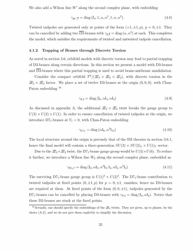
We also add a Wilson line W ′ along the second complex plane, with embedding

γW ′,7 = diag (I3, 1, α, α2, 1, α, α2). (4.8)

Twisted tadpoles are generated only at points of the form (+1,±1, p), p = 0,±1. They

can be cancelled by adding two D3-branes with γθ,3 = diag (α, α2) at each. This completes

the model, which satisfies the requirements of twisted and untwisted tadpole cancellation.

4.1.2 Trapping of Branes through Discrete Torsion

As noted in section 3.6, orbifold models with discrete torsion may lead to partial trapping

of D3-branes along certain directions. In this section we present a model with D3-branes

and D3-branes where this partial trapping is used to avoid brane-antibrane annihilation.

Consider the compact orbifold T 6/(ZZ3 × ZZ2 × ZZ2), with discrete torsion in the

ZZ2 × ZZ2 factor. We place a set of twelve D3-branes at the origin (0, 0, 0), with Chan-

Paton embedding 10

γθ,3 = diag (I6, αI4, αI2) (4.9)

As discussed in appendix A, the additional ZZ2 × ZZ2 twist breaks the gauge group to

U(3) × U(2) × U(1). In order to ensure cancellation of twisted tadpoles at the origin, we

introduce D71-branes at Y1 = 0, with Chan-Paton embedding

γθ,71 = diag (αI6, α2I12) (4.10)

The local structure around the origin is precisely that of the SM theories in section 3.6.1,

hence the final model will contain a three-generation SU(3) × SU(2)L × U(1)Y sector.

Due to the ZZ2×ZZ2 twist, the D71-brane gauge group would be U(3)×U(6). To reduce

it further, we introduce a Wilson line W2 along the second complex plane, embedded as

γW2,7 = diag (I2, αI2, α2I2; I4, αI4, α

2I4) (4.11)

The surviving D71-brane gauge group is U(1)3 × U(2)3. The D71-brane contribution to

twisted tadpoles at fixed points (0,±1, p) for p = 0,±1, vanishes, hence no D3-branes

are required at them. At fixed points of the form (0, 0,±1), tadpoles generated by the

D71-branes can be cancelled by placing D3-branes with γθ,3 = diag (I4, αI2). Notice that

these D3-branes are stuck at the fixed points.

10Actually, one should specify the embeddings of the ZZ2 twists. They are given, up to phases, by the

choice (A.2), and we do not give them explicitly to simplify the discussion.

35

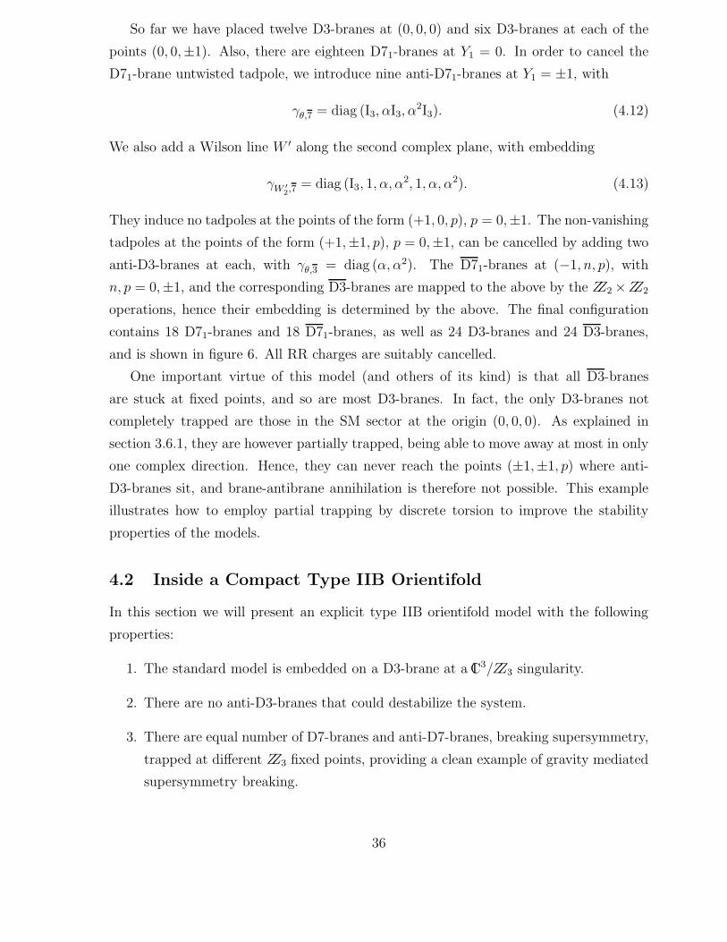
So far we have placed twelve D3-branes at (0, 0, 0) and six D3-branes at each of the

points (0, 0,±1). Also, there are eighteen D71-branes at Y1 = 0. In order to cancel the

D71-brane untwisted tadpole, we introduce nine anti-D71-branes at Y1 = ±1, with

γθ,7 = diag (I3, αI3, α2I3). (4.12)

We also add a Wilson line W ′ along the second complex plane, with embedding

γW ′2,7 = diag (I3, 1, α, α

2, 1, α, α2). (4.13)

They induce no tadpoles at the points of the form (+1, 0, p), p = 0,±1. The non-vanishing

tadpoles at the points of the form (+1,±1, p), p = 0,±1, can be cancelled by adding two

anti-D3-branes at each, with γθ,3 = diag (α, α2). The D71-branes at (−1, n, p), with

n, p = 0,±1, and the corresponding D3-branes are mapped to the above by the ZZ2 ×ZZ2

operations, hence their embedding is determined by the above. The final configuration

contains 18 D71-branes and 18 D71-branes, as well as 24 D3-branes and 24 D3-branes,

and is shown in figure 6. All RR charges are suitably cancelled.

One important virtue of this model (and others of its kind) is that all D3-branes

are stuck at fixed points, and so are most D3-branes. In fact, the only D3-branes not

completely trapped are those in the SM sector at the origin (0, 0, 0). As explained in

section 3.6.1, they are however partially trapped, being able to move away at most in only

one complex direction. Hence, they can never reach the points (±1,±1, p) where anti-

D3-branes sit, and brane-antibrane annihilation is therefore not possible. This example

illustrates how to employ partial trapping by discrete torsion to improve the stability

properties of the models.

4.2 Inside a Compact Type IIB Orientifold

In this section we will present an explicit type IIB orientifold model with the following

properties:

1. The standard model is embedded on a D3-brane at a IC3/ZZ3 singularity.

2. There are no anti-D3-branes that could destabilize the system.

3. There are equal number of D7-branes and anti-D7-branes, breaking supersymmetry,

trapped at different ZZ3 fixed points, providing a clean example of gravity mediated

supersymmetry breaking.

36

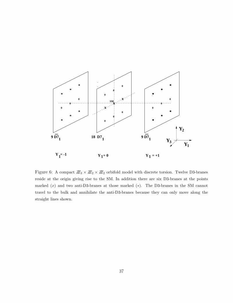
Y1

Y2

Y3

**

*

**

*

**

*

**

*

x0

0

0

0

0

0

0

0

0

0

0

**

*

**

*x

x

1 1= 0 1 = +1

SM

Y = -1 Y Y

18 D719 D7 9 D71 1

0

Figure 6: A compact ZZ3 × ZZ2 × ZZ2 orbifold model with discrete torsion. Twelve D3-branes

reside at the origin giving rise to the SM. In addition there are six D3-branes at the points

marked (x) and two anti-D3-branes at those marked (∗). The D3-branes in the SM cannot

travel to the bulk and annihilate the anti-D3-branes because they can only move along the

straight lines shown.

37

Models of this type are similar to the ones constructed in [13, 15] (based on the general

framework in [12], see also [14]), but in those cases the standard model was inside a higher

dimensional brane (D7 or D9-brane) and supersymmetry was broken by the presence of

lower dimensional anti-branes (D3- or D5-branes). Furthermore those examples did not

include models where all the anti-branes were completely trapped, and it was left as a

dynamical question if the configuration was stable. The class of models we are going to

present succeeds in trapping all antibranes. Nevertheless, it is well known that T -dualizing

these models with respect to the different extra dimensions we should get to models where

the standard model is embedded into D7 or D9-branes and therefore models like those

considered in [13, 15]. We will then find the T duals of these models which happen to be

complicated versions of the models in [13, 15] in terms of several Wilson lines. We will

submit the reader to the appendices where we discuss in detail the T duality between the

models of this section and those of [13].

4.2.1 Explicit Models

As an illustration to this class of models let us consider in detail the following orientifold

of the T 6/ZZ3 orbifold. The orientifold action is Ω(−1)FL R1 R2 R3 with Ri reflection on

the ith plane. There are 64 orientifold three-planes (O3-planes), which are localized at

points in the internal space. To cancel their RR charge we need a total of 32 D3 branes.

We will distribute them among the 27 orbifold fixed points (m,n, p), m,n, p = 0,±1. We

will also introduce an equal number of D7 and D7-branes. Among these 27 points, only

the origin (0, 0, 0) is fixed under the orientifold action, hence it is an orientifold singularity,

of the type mentioned in section 3.6.4. The cancellation of tadpoles at this point requires

3 Tr γθ,3 + (Tr γθ,7 − Tr γθ,7) = −12 (4.14)

As shown in appendix C, this orientifold singularity is not suitable to incorporate the

standard model. Fortunately, ZZ3 fixed points other than the origin are not fixed under

the orientifold action, and therefore are IC3/ZZ3 orbifold singularities, which we may employ

to embed local configurations as those in section 3.3.

The strategy is then to concentrate at an orbifold point different from the origin, say

(0, 1, 0) where we want to have the standard model (its ZZ2 mirror image (0,−1, 0) will

have identical spectrum). We choose a suitable twist matrix for the D3 branes such as

that in section 3.3. At these points the tadpole condition is simply:

Tr γθ,7 − Tr γθ,7 + 3Tr γθ,3 = 0 (4.15)

38

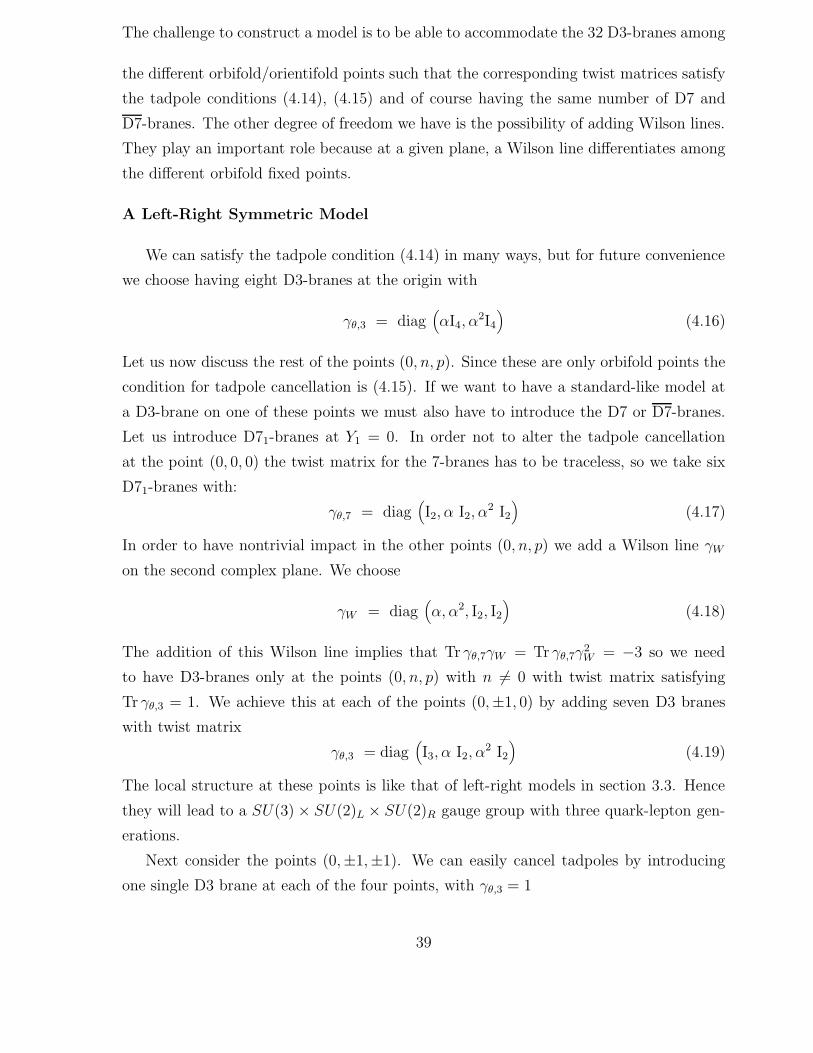
The challenge to construct a model is to be able to accommodate the 32 D3-branes among

the different orbifold/orientifold points such that the corresponding twist matrices satisfy

the tadpole conditions (4.14), (4.15) and of course having the same number of D7 and

D7-branes. The other degree of freedom we have is the possibility of adding Wilson lines.

They play an important role because at a given plane, a Wilson line differentiates among

the different orbifold fixed points.

A Left-Right Symmetric Model

We can satisfy the tadpole condition (4.14) in many ways, but for future convenience

we choose having eight D3-branes at the origin with

γθ,3 = diag(αI4, α

2I4)

(4.16)

Let us now discuss the rest of the points (0, n, p). Since these are only orbifold points the

condition for tadpole cancellation is (4.15). If we want to have a standard-like model at

a D3-brane on one of these points we must also have to introduce the D7 or D7-branes.

Let us introduce D71-branes at Y1 = 0. In order not to alter the tadpole cancellation

at the point (0, 0, 0) the twist matrix for the 7-branes has to be traceless, so we take six

D71-branes with:

γθ,7 = diag(I2, α I2, α

2 I2)

(4.17)

In order to have nontrivial impact in the other points (0, n, p) we add a Wilson line γW

on the second complex plane. We choose

γW = diag(α, α2, I2, I2

)(4.18)

The addition of this Wilson line implies that Tr γθ,7γW = Tr γθ,7γ2W = −3 so we need

to have D3-branes only at the points (0, n, p) with n 6= 0 with twist matrix satisfying

Tr γθ,3 = 1. We achieve this at each of the points (0,±1, 0) by adding seven D3 branes

with twist matrix

γθ,3 = diag(I3, α I2, α

2 I2)

(4.19)

The local structure at these points is like that of left-right models in section 3.3. Hence

they will lead to a SU(3) × SU(2)L × SU(2)R gauge group with three quark-lepton gen-

erations.

Next consider the points (0,±1,±1). We can easily cancel tadpoles by introducing

one single D3 brane at each of the four points, with γθ,3 = 1

39

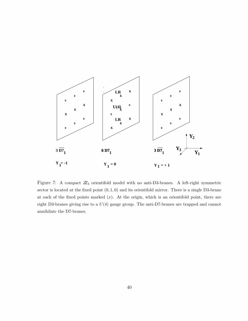
Y1

Y2

Y33 D71 1

LR

U(4)

1Y = -1

LR

0

0

0

0

0

0

0

x

x

xx

x

x

x0

6 D76 D71

1 = 0 1 = + 1

0

0

0

0

0

0

xx

x

xx

x

Y Y

3 D73 D7

Figure 7: A compact ZZ3 orientifold model with no anti-D3-branes. A left-right symmetric

sector is located at the fixed point (0, 1, 0) and its orientifold mirror. There is a single D3-brane

at each of the fixed points marked (x). At the origin, which is an orientifold point, there are

eight D3-branes giving rise to a U(4) gauge group. The anti-D7-branes are trapped and cannot

annihilate the D7-branes.

40

Finally we have to consider the points (m,n, p) with m 6= 0. So far we have six D71-

branes and 8 + 7 + 7 + 4 = 26 D3-branes. Therefore we need to introduce six more D3

branes to complete 32, and six D7-branes. We can easily achieve this by locating three

D71-branes at Y1 = ±1 with twist matrix and Wilson lines given by

γθ,7 = I3 γW 7 =(1, α, α2

)(4.20)

We then have Tr γθ,7γW ,7 = Tr γθ,7γ2W ,7 = 0 and do not need to add D3 branes at the points

(1,±1, p). At the points (1, 0, p) we can put a single D3-brane with γθ,3 = 1, canceling

the tadpoles from γθ,7. At the points (−1, n, p) we have a similar structure, consistently

with the orientifold projection. In total, we have added precisely the six D7-branes and

six D3-branes, as needed for consistency.

Since this model provides an interesting example of a realistic compactification with

gravity mediated supersymmetry breaking, we give some details on the computation of

the spectrum in the visible sector.

The D7-branes, with Chan-Paton embedding (4.17) would (before the orientifold pro-

jection) lead to a group U(2)3 with matter in three copies of (2, 2, 1) + (1, 2, 2) + (2, 1, 2).

The Wilson line (4.18) breaks the gauge symmetry to U(1)2 × U(2) × U(2) with matter

in three copies of (2, 2) with zero charge under the U(1)2. A simple way to read the

spectrum is by using the shift vectors defined in the Cartan-Weyl basis (in analogy with

[37]) for the twist matrix and Wilson line which in this case are:

V70 =1

3(0, 0, 1, 1,−1,−1)

W70 =1

3(1, 1, 0, 0, 0, 0) (4.21)

We keep states of the form P = (1,−1, 0, ...) (and permutations) satisfying PV = 1/3

and PW = 0. The orientifold projection identifies two pairs of groups and further breaks

the symmetry to U(1) × U(2) with the simple matter consisting of three singlets (anti-

symmetrics of SU(2)) with charge +2 under the U(1) inside U(2).

The D3-branes at the origin, with Chan-Paton embedding (4.16) lead, before the

orientifold projection, to an U(4) × U(4) gauge group with matter on three copies of

(4, 4). After the orientifold projection this becomes a single U(4) group with matter on

three copies of a 6. For states in the 37 sector for D3-branes at the origin, we use the

extended shift vector

V =1

3(1, 1, 1, 1,−1,−1,−1,−1)⊗ V70 (4.22)

41

with the first eight entries corresponding to the original U(4)2 on the D3-branes. We then

keep the vectors 11 P = (−1, 0, · · · ; 1, 0, · · ·) satisfying P V = 1/3. We obtain the matter

fields transforming as (4, 2)0 + (4, 1)1 + (4, 1)−1 under the final U(4) × U(2) × U(1).

For D3-branes at (0,±1, 0) the Chan-Paton twist is (4.19), we obtain the spectrum of

the LR model. The gauge group is U(3)×U(2)×U(2), with two anomalous U(1)’s being

actually massive, and the diagonal combination giving B−L. In the 33 sector, we obtain

matter fields

33 sector:

3 [(3, 2, 1) + (1, 2, 2) + (3, 1, 2)] (4.23)

These can be explicitly seen by using the effective shift vector V3 = 13(0, 0, 0, 1, 1,−1,−1).

For matter in 37, 73 sectors, the gauge quantum numbers are easily computed by con-

sidering the shift vectors V3⊗(V7±W7), and keeping the state vectors P = (−1, 0, · · ·0)⊗(1, 0 · · · , 0) and permutations for the 37 sector, and the opposite sign for the 73 sector.

We get:

37 sector:

(3, 1, 1; 1)−1 + (3, 1, 1; 2)0 + (1, 2, 1; 1)1 + (1, 2, 1; 2)0 (4.24)

73 sector:

(3, 1, 1; 1)1 + (3, 1, 1; 2)0 + (1, 1, 2; 1)1 + (1, 1, 2; 2)0 (4.25)

The orientifold projection map the sets of branes at (0, 1, 0) and (0,−1, 0) to each other,

so only one copy of the LR model is obtained. Notice that these sector contain some

extra vector-like chiral fields beyond those obtained in section 3.4. Six pairs of colour

triplets will in general become massive once (7i7i) states get vevs. The remaining extra

vector-like fields beyond the leptons transform like (3, 1, 1) + (1, 2, 1) + (1, 1, 2) + h.c.. As

discussed in chapter 6, the presence of extra SU(2)R doublets is in fact welcome in order

to give rise of the required SU(2)R gauge symmetry breaking.

For D3-branes at fixed points (0,±1,±1), with γθ,3 = 1, we have one U(1) gauge

group, with no 33 matter, at each brane. The orientifold projection relates two pairs of

these points reducing the group to U(1)2. The matter on each of these two 37 sectors can

be easily computed as above (shift vector 0 ⊗ V7) and transforms as 1−1,1 + 20,1 under

the (U(2) × U(1))×U(1) (where the first U(1) arises from D7-branes and the second one

from D3-branes). The 73 sector gives multiplets 1−1,−1 + 20,−1.

11The 73 sector would have the opposite relative signs between the D7 and D3 branes; but it is identified

to the 37 sector by the orientifold projection and need not be considered independently.

42

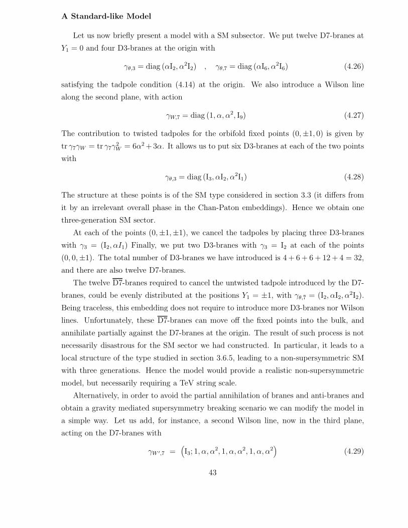
A Standard-like Model

Let us now briefly present a model with a SM subsector. We put twelve D7-branes at

Y1 = 0 and four D3-branes at the origin with

γθ,3 = diag (αI2, α2I2) , γθ,7 = diag (αI6, α

2I6) (4.26)

satisfying the tadpole condition (4.14) at the origin. We also introduce a Wilson line

along the second plane, with action

γW,7 = diag (1, α, α2, I9) (4.27)

The contribution to twisted tadpoles for the orbifold fixed points (0,±1, 0) is given by

tr γ7γW = tr γ7γ2W = 6α2 +3α. It allows us to put six D3-branes at each of the two points

with

γθ,3 = diag (I3, αI2, α2I1) (4.28)

The structure at these points is of the SM type considered in section 3.3 (it differs from

it by an irrelevant overall phase in the Chan-Paton embeddings). Hence we obtain one

three-generation SM sector.

At each of the points (0,±1,±1), we cancel the tadpoles by placing three D3-branes

with γ3 = (I2, αI1) Finally, we put two D3-branes with γ3 = I2 at each of the points

(0, 0,±1). The total number of D3-branes we have introduced is 4 + 6 + 6 + 12 + 4 = 32,

and there are also twelve D7-branes.

The twelve D7-branes required to cancel the untwisted tadpole introduced by the D7-

branes, could be evenly distributed at the positions Y1 = ±1, with γθ,7 = (I2, αI2, α2I2).

Being traceless, this embedding does not require to introduce more D3-branes nor Wilson

lines. Unfortunately, these D7-branes can move off the fixed points into the bulk, and

annihilate partially against the D7-branes at the origin. The result of such process is not

necessarily disastrous for the SM sector we had constructed. In particular, it leads to a

local structure of the type studied in section 3.6.5, leading to a non-supersymmetric SM

with three generations. Hence the model would provide a realistic non-supersymmetric

model, but necessarily requiring a TeV string scale.

Alternatively, in order to avoid the partial annihilation of branes and anti-branes and

obtain a gravity mediated supersymmetry breaking scenario we can modify the model in

a simple way. Let us add, for instance, a second Wilson line, now in the third plane,

acting on the D7-branes with

γW ′,7 =(I3; 1, α, α

2, 1, α, α2, 1, α, α2)

(4.29)

43

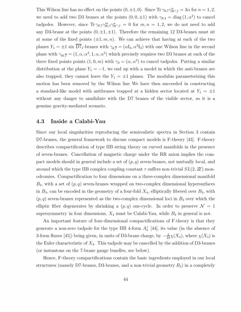
This Wilson line has no effect on the points (0,±1, 0). Since Tr γθ,7γnW ′,7 = 3α for n = 1, 2,

we need to add two D3 branes at the points (0, 0,±1) with γθ,3 = diag (1, α2) to cancel

tadpoles. However, since Tr γθ,7γmW,7γ

nW ′,7 = 0 for m,n = 1, 2, we do not need to add

any D3-brane at the points (0,±1,±1). Therefore the remaining 12 D3-branes must sit

at some of the fixed points (±1, m, n). We can achieve that having at each of the two

planes Y1 = ±1 six D71-branes with γθ,7 = (αI3, α2I3) with one Wilson line in the second

plane with γW,7 = (1, α, α2, 1, α, α2) which precisely requires two D3 branes at each of the

three fixed points points (1, 0, m) with γ3 = (α, α2) to cancel tadpoles. Putting a similar

distribution at the plane Y1 = −1, we end up with a model in which the anti-branes are

also trapped, they cannot leave the Y1 = ±1 planes. The modulus parameterizing this

motion has been removed by the Wilson line We have then succeeded in constructing

a standard-like model with antibranes trapped at a hidden sector located at Y1 = ±1

without any danger to annihilate with the D7 branes of the visible sector, so it is a

genuine gravity-mediated scenario.

4.3 Inside a Calabi-Yau

Since our local singularities reproducing the semirealistic spectra in Section 3 contain

D7-branes, the general framework to discuss compact models is F-theory [43]. F-theory

describes compactification of type IIB string theory on curved manifolds in the presence

of seven-branes. Cancellation of magnetic charge under the RR axion implies the com-

pact models should in general include a set of (p, q) seven-branes, not mutually local, and

around which the type IIB complex coupling constant τ suffers non-trivial SL(2, ZZ) mon-

odromies. Compactification to four dimensions on a three-complex dimensional manifold

B3, with a set of (p, q) seven-branes wrapped on two-complex dimensional hypersurfaces

in B3, can be encoded in the geometry of a four-fold X4, elliptically fibered over B3, with

(p, q) seven-branes represented as the two-complex dimensional loci in B3 over which the

elliptic fiber degenerates by shrinking a (p, q) one-cycle. In order to preserve N = 1

supersymmetry in four dimensions, X4 must be Calabi-Yau, while B3 in general is not.

An important feature of four-dimensional compactifications of F-theory is that they

generate a non-zero tadpole for the type IIB 4-form A+4 [44], its value (in the absence of

3-form fluxes [45]) being given, in units of D3-brane charge, by − 124χ(X4), where χ(X4) is

the Euler characteristic ofX4. This tadpole may be cancelled by the addition of D3-branes

(or instantons on the 7-brane gauge bundles, see below).

Hence, F-theory compactifications contain the basic ingredients employed in our local

structures (namely D7-branes, D3-branes, and a non-trivial geometry B3) in a completely

44

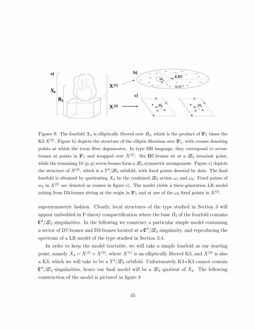
X (2)

X (1)

4X

B3ω 2 ω 2

ω 1

(p,q) 7

6 D7a) b)

c)

Figure 8: The fourfold X4 is elliptically fibered over B3, which is the product of IP1 times the

K3 X(2). Figure b) depicts the structure of the elliptic fibration over IP1, with crosses denoting

points at which the torus fiber degenerates. In type IIB language, they correspond to seven-

branes at points in IP1 and wrapped over X(2). Six D7-branes sit at a ZZ3 invariant point,

while the remaining 18 (p, q) seven-branes form a ZZ3 symmetric arrangement. Figure c) depicts

the structure of X(2), which is a T 4/ZZ3 orbifold, with fixed points denoted by dots. The final

fourfold is obtained by quotienting X4 by the combined ZZ3 action ω1 and ω2. Fixed points of

w2 in X(2) are denoted as crosses in figure c). The model yields a three-generation LR model

arising from D3-branes sitting at the origin in IP1 and at one of the ω2 fixed points in X(2).

supersymmetric fashion. Clearly, local structures of the type studied in Section 3 will

appear embedded in F-theory compactification where the base B3 of the fourfold contains

IC3/ZZ3 singularities. In the following we construct a particular simple model containing

a sector of D7-branes and D3-branes located at a IC3/ZZ3 singularity, and reproducing the

spectrum of a LR model of the type studied in Section 3.4.

In order to keep the model tractable, we will take a simple fourfold as our starting

point, namely X4 = X(1) ×X(2), where X(1) is an elliptically fibered K3, and X(2) is also

a K3, which we will take to be a T 4/ZZ3 orbifold. Unfortunately K3×K3 cannot contain

IC3/ZZ3 singularities, hence our final model will be a ZZ3 quotient of X4. The following

construction of the model is pictured in figure 8

45

Let us start by describing X4. The K3 manifold X(1) is a fibration of T 2 over a IP1,

which can be defined in the Weierstrass form

y2 = x3 + f8(z, w)x+ g12(z, w) (4.30)

where x, y parameterize T 2, and [z, w] are projective coordinates in IP1. The functions

f8, g12 are of degree 8 and 12 respectively in their arguments. The elliptic fibration

degenerates at the 24 points [z, w] given by zeroes of the discriminant

δ24 = 4f8(z, w)3 + 27g12(z, w)2 (4.31)

These degenerations signal the presence of 24 (p, q) seven-branes sitting at a point in

IP1 and wrapping X(2) completely. We will be interested in a particular family of K3

manifolds, containing six coincident D7-branes sitting at z = 0. Geometrically, we require

the fibration (4.30) to have an I6 Kodaira type degeneration [46] at z = 0, meaning f8

and g12 are non-zero at z = 0, but δ24 vanishes as z6. We will be more explicit below.

For X4 = K3×K3, χ(X4) = 24×24, and the compactification leads to an A+4 -tadpole

of −24 units. It will be useful to rederive this result from a different point of view. On

the world-volume M7 of each seven-brane (of any (p, q) type) there exist couplings

− 1

24

∫M7

R ∧R ∧ A+4 +

∫M7

F ∧ F ∧A+4 (4.32)

where R is the Ricci tensor of the induced curvature, and F is the field strength tensor

for the world-volume gauge fields. In the absence of world-volume gauge instantons the

second term drops, and the contribution of the first for each seven-brane wrapped on the

K3 X(2) (recall χ(K3) =∫K3R ∧ R = 24) is − ∫M4

A+4 , where M4 is four-dimensional

spacetime. Namely, we get an A+4 -tadpole of −1 for each of the 24 seven-branes in the

model, hence a total tadpole of −24. This tadpole can be cancelled by adding 24 D3-

branes sitting at a point in B3 = IP1×X(2), or by turning on instantons on the seven-brane

gauge bundles.

We will be interested in considering X(2) in the T 4/ZZ3 orbifold limit. We start with

T 4 parametrized by two coordinates z1, z2 with identifications zi ' zi + 1, zi ' zi + e2πi/3

(we set the radii to unity for the sake of simplicity), and mod out by the ZZ3 action

θ : z1 → e2πi/3z1 , z2 → e−2πi/3z2 (4.33)

The quotient is a K3 manifold, flat everywhere except at the nine fixed points of θ (located

at points (z1, z2) with z1, z2 = 0, 13(1 + eπi/3) or 1

3(eπi/3 + e2πi/3)), which descend to

singularities IC2/ZZ3 in the quotient. The curvature is concentrated at those points, and

46

gives a contribution of∫C2/Z3

R ∧ R = 8/3 at each. Hence the −1 A+4 -tadpole at each

seven-brane is split in nine −1/9 A+4 -tadpole, arising from the nine points IC2/ZZ3 wrapped

by the seven-brane world-volume. There are no contributions from world-volume gauge

instantons if the gauge bundle over these IC2/ZZ3 is trivial; in more familiar terms, if the

ZZ3 action is embedded trivially on the seven-brane indices. Given this θ-embedding, one

may worry about twisted tadpoles. However, since the ZZ3 twist leaves fixed the complete

IP1, such tadpoles receive contributions from all seven-branes, and they cancel by the same

reason the overall axion RR-charge cancels, namely by cancellation among contributions

of different (p, q) seven-branes.

As mentioned above, in order to obtain IC3/ZZ3 singularities we are forced to con-

sider a quotient of the four-fold X4 considered above, by ZZ3, with generator ω acting

simultaneously on IP1 and X(2). We choose the action of ω on IP1 to be given by

ω1 : z → e2πi/3z , w → w (4.34)

For the configuration to be invariant under this action, the K3 X(1) must be given by

(4.30) with the functions f8, g12 depending only on z3

f8(z, w) = Aw8 +Bz3w5 + Cz6w2

g12(z, w) = Dw12 + Ez3w9 + Fz6w6 +Gz9w3 +Hz12 (4.35)

The requirement that there are six D7-branes at z = 0 amounts to the vanishing of the

coefficients of order 1 and z3 in δ24

4A3 + 27D2 = 0 , 12A2B + 54DE = 0 (4.36)

It will be convenient to require no seven-branes to be present at [z, w] = [1, 0], hence we

require H 6= 0. The configuration we have constructed therefore contains six D7-branes at

z = 0, and the remaining 18 seven-branes distributed on IP1 in a ZZ3 symmetric fashion.

Notice that not only the locations, but the (p, q) types of these seven-branes are consistent

with the symmetry, since the F-theory K3 X(1) is ZZ3 invariant. Also, notice that no (p, q)

seven-branes (other than the six at z = 0) are fixed under ω.

We have to specify also the action of ω on X2, which we take to be

ω2 : z1 → e2πi/3z1 +1

3(1 + eπi/3) , z2 → e2πi/3z2 + 1

3(1 + eπi/3) (4.37)

(The shifts have been included to avoid ω-fixed points to coincide with θ-fixed points).

That this is a symmetry of X(2) = T 4/ZZ3 follows from the fact that ω2 is a symmetry of

T 4, and that it commutes with the action θ (4.33) required to form T 4/ZZ3. The action

47

ω2 has nine fixed points in T 4, given by points (z1, z2) with zi = 13eπi/3, 1

3(1 + 2eπi/3),

13(e2πi/3 + 2eπi/3). The action of θ maps them to each other so that in the quotient they

yield just three singular points. Similarly, ω2 maps the nine fixed points of θ to each

other, so that in the quotient they give rise to just three singularities. Notice that in the

final model the T 4 is modded out by θ and ω2, and consequently by all other twists they

generate. In this respect it is important to notice that θω2 and θ2ω2 (and their inverses)

are freely acting due to the shifts in (4.37), and do not generate new singularities.

The final model is obtained by quotienting IP1 × X(2) by ω, the combined action of

(4.34), (4.37). One can see that it preserves N = 1 supersymmetry in the quotient by

noticing that the holomorphic 4-form in X4, given by (dx/y)(dz/w)dz1dz2 is invariant,

hence the quotient is still a four-fold. Notice that the fixed points of ω correspond to

[z, w] = [0, 1], [1, 0] in IP1 times the three fixed points in X(2).

We must also specify the action of ω on the seven-branes. For the (p, q) seven-branes

at z 6= 0, the action is fully specified by the geometrical action in ω1. The six D7-branes

at z = 0, sit at a fixed point of ω, and hence may suffer a non-trivial action on their

Chan-Paton indices, which we choose to be given by

γω,7 = diag (e2πi 13 I3, e

2πi 23 I3) (4.38)

This amounts to choosing a non-trivial U(6) bundle on D7-brane world-volume. This will

lead to a non-zero contribution to world-volume instanton number, and hence influence

the computation of the A+4 -tadpole in the quotient. Moreover, the embedding (4.38) also

leads to non-zero ω-twisted tadpoles which must be properly cancelled.

Let us turn to the computation of the A+4 tadpole. Since the ω action has fixed

points, the Euler characteristic of the quotient four-fold is not simply χ(X4)/3. Direct

computation seems rather involved, hence we prefer to compute the A+4 tadpole by using

the seven-brane world-volume couplings (4.32). The 18 (p, q) seven-branes at z 6= 0 are

not invariant under ω, hence their world-volume R∧R contribution comes only from the

nine θ-fixed points, yielding a total A+4 tadpole of −18. This is reduced to −6 by the ω

action (equivalently, the 18 seven-branes in X4 descend to just six in the quotient by ω).

The six D7-branes at z = 0 sit at a ω fixed point, hence their R ∧ R coupling receives

contributions from three IC2/ZZ3 (from nine θ-fixed ω-identified points), and three IC2/ZZ3

(from nine ω-fixed θ-identified points). The total contribution is − 124× 8

3×3×2×6 = −4.

There is a further contribution, from the instanton number of the nontrivial bundle implied

by (4.38). This can be computed (see [25, 47] for a discussion of instanton numbers for

orbifold spaces) to be +1 per IC3/ZZ3 generated by ω, yielding an overall contribution

48

+3 to the A+4 tadpole. Hence, the total A+

4 tadpole in the model is −7, and one must

introduce 7 D3-branes (as counted in the quotient) to achieve a consistent model.

Recall that the choice of the twist (4.38) generates non-zero ω-twisted tadpoles at the

nine fixed points of ω2 (three in the quotient), at z = 0. Happily, these are IC3/ZZ3 fixed

points of the type studied in section 3.2, for which the twisted tadpole condition reads

Tr γω,7 + 3Tr γω,3 = 0 (4.39)

The tadpoles are easily cancelled by choosing γω,3 = (I3, e2πi 1

3 I2, e2πi 2

3 I2) at three of them

(one after the θ-identification) and γθ,3 = I1 at six (two in the quotient by θ). This

employs 3 D3-branes (as counted in the quotient) out of the 7 we had available. The

remaining 4 can be placed at a generic, smooth, point in the quotient (so that they would

be described by 4 × 3 × 3 in the covering space of the θ and ω actions).

This concludes the construction of the model. We have succeeded in constructing a

N = 1 supersymmetric compact model with a local singularity of the form IC3/ZZ3, on

which D3-branes and D7-branes sit. This local structure is of the kind considered in

section 3.4, and leads to a left-right symmetric model SU(3)×SU(2)×SU(2)×U(1)B−L

with three generations of standard model particles. Notice that in this concrete example

the D7-brane gauge group is relatively large, but it should not be difficult to modify the

construction (for instance, by adding Wilson lines on T 4) to reduce it. We prefer not to

complicate the discussion for the moment.

We would like to conclude with a remark. F-theory model building (see e.g. [7]) has

centered on embedding the standard model gauge group on the seven-branes, while D3-

branes are basically a useless sector. In our framework, the situation is inverted, with the

D3-branes playing the main role, even if seven-branes also contribute to the spectrum. One

particular advantage of our alternative embedding, which we have stressed throughout the

paper, is that the relevant sector can be determined by using just the local behaviour of

the compactification manifold. In this respect it is clear that many other consistent

supersymmetric embeddings of our local structures may be achieved by considering more

general four-folds with IC3/ZZ3 singularities on the base, on which D3-branes and D7-branes

(with gauge bundles locally reproducing the required monodromy) are located.

5 Some Phenomenological Aspects

Obtaining SU(3)×SU(2)L×U(1)Y (or its left-right symmetric extension SU(3)×SU(2)L×SU(2)R ×U(1)B−L) and three quark-lepton generations in a simple manner is already re-

markable. However we would like also to know if the class of models discussed in the

49

previous sections is sufficiently rich to accommodate other important phenomenological

features like gauge coupling unification, a hierarchical structure of quark/lepton masses

and proton stability. In this chapter we would like to address these issues. Let us make

clear from the beginning that we do not intend here to give a full account of these questions

but rather to evaluate the phenomenological potential of these models without compro-

mising ourselves with a particular one.

We will limit ourselves to the case of models obtained from D-branes at N = 1

supersymmetric singularities. As already remarked above, some properties like number of

generations, gauge group and gauge coupling normalization will mostly be controlled by

the local D-brane configurations introduced in section 3. On the other hand other aspects

like some Yukawa couplings or the N = 1 Kahler metrics will be in general dependent on

the particular compact space chosen in order to embed the realistic D-brane set. Thus,

for example, the Kahler metric of the matter fields will in general be different for an

embedding inside a compact ZZ3 orbifold compared to an embedding inside an F-theory

model. Thus, the complete effective action will certainly depend on the specific model.

We will try to discuss certain features which seem generic among the class of models

considered in the previous chapters. In particular, that is the case of the question of

gauge coupling unification. We will also study some aspects of the Yukawa couplings

both in the SM and LR type of models. As a general conclusion we believe that the

structure of the models seems to be sufficiently rich to be able to accommodate the main

phenomenological patterns of the fermion mass spectrum. Finally, we comment on the

structure of mass scales and in particular the value of the string scale Ms that should be

considered in these constructions. Since this depends on the compactification scale, the

choice of Ms is also model dependent.

i) Gauge Coupling Unification

This question obviously depends on whether we are considering a SM like the one

considered in section 3.3 or a left-right symmetric model as in section 3.4. As we will

see, from the gauge coupling unification point of view the left-right models look more

interesting. Let us consider first the case of the SM. As mentioned in section 3, the tree-

level gauge coupling constants at the string scale Ms are in the ratios g23 : g2

2 : g21 = 1 :

1 : 11/3. The one-loop running between the weak scale MZ and the string scale Ms is

governed by the equations

sin2 θW (MZ) = 314

(1 + 11

6πα(MZ) (b2 − 3

11b1) log( Ms

MZ))

50

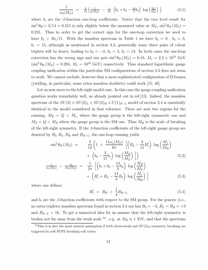
1

α3(MZ)= 3

14

(1

α(MZ )− 1

2π

(b1 + b2 − 14

3b3)

log(

Ms

MZ

) )(5.1)

where bi are the β-function one-loop coefficients. Notice that the tree level result for

sin2 θW = 3/14 = 0.215 is only slightly below the measured value at MZ , sin2 θW (MZ) =

0.231. Thus in order to get the correct sign for the one-loop correction we need to

have b2 > 3b1/11. With the massless spectrum in Table 1 we have b3 = 0 , b2 = 3,

b1 = 15, although as mentioned in section 3.3, generically some three pairs of colour

triplets will be heavy, leading to b3 = −3, b2 = 3, b1 = 13. In both cases the one-loop

correction has the wrong sign and one gets sin2 θW (MZ) = 0.18, Ms = 2.2 × 1015 GeV

(sin2 θW (MZ) = 0.204, Ms = 1010 GeV) respectively. Thus standard logarithmic gauge

coupling unification within the particular SM configurations of section 3.3 does not seem

to work. We cannot exclude, however that a more sophisticated configuration of D-branes

(yielding, in particular, some extra massless doublets) could work [15, 48].

Let us now move to the left-right model case. In this case the gauge coupling unification

question works remarkably well, as already pointed out in ref.[15]. Indeed, the massless

spectrum of the SU(3) × SU(2)L × SU(2)R × U(1)B−L model of section 3.4 is essentially

identical to the model considered in that reference. There are now two regions for the

running, MR < Q < Ms, where the gauge group is the left-right symmetric one and

MZ < Q < MR where the gauge group is the SM one. Thus MR is the scale of breaking

of the left-right symmetry. If the β-function coefficients of the left-right gauge group are

denoted by B3, BL, BR and BB−L, the one-loop running yields

sin2 θW (MZ) =3

14

(1 +

11αe(MZ)

6π

[(BL − 3

11B′

1

)log

(Ms

MR

)

+(b2 − 3

11b1

)log

(MR

MZ

) ])(5.2)

1αe(MZ )

− 143α3(MZ )

=1

2π

[(b1 + b2 − 14

3b3

)log

(MR

MZ

)

+(B′

1 +BL − 14

3B3

)log

(Ms

MR

) ](5.3)

where one defines

B′1 = BR +

1

4BB−L (5.4)

and bi are the β-function coefficients with respect to the SM group. For the generic (i.e.,

no extra triplets) massless spectrum found in section 3.4 one has B3 = −3, BL = BR = +3

and BB−L = 16. To get a numerical idea let us assume that the left-right symmetry is

broken not far away from the weak scale 12 , e.g. at MR ∝ 1 TeV, and that the spectrum

12This is in fact the most natural assumption if both electroweak and SU(2)R symmetry breaking are

triggered by soft SUSY-breaking soft terms.

51

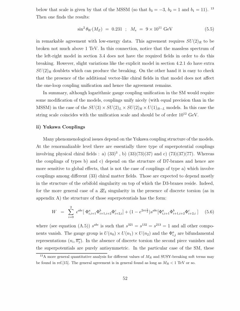
below that scale is given by that of the MSSM (so that b3 = −3, b2 = 1 and b1 = 11). 13

Then one finds the results:

sin2 θW (MZ) = 0.231 ; Ms = 9 × 1011 GeV (5.5)

in remarkable agreement with low-energy data. This agreement requires SU(2)R to be

broken not much above 1 TeV. In this connection, notice that the massless spectrum of

the left-right model in section 3.4 does not have the required fields in order to do this

breaking. However, slight variations like the explicit model in section 4.2.1 do have extra

SU(2)R doublets which can produce the breaking. On the other hand it is easy to check

that the presence of the additional vector-like chiral fields in that model does not affect

the one-loop coupling unification and hence the agreement remains.

In summary, although logarithmic gauge coupling unification in the SM would require

some modification of the models, couplings unify nicely (with equal precision than in the

MSSM) in the case of the SU(3)× SU(2)L × SU(2)R ×U(1)B−L models. In this case the

string scale coincides with the unification scale and should be of order 1012 GeV.

ii) Yukawa Couplings

Many phenomenological issues depend on the Yukawa coupling structure of the models.

At the renormalizable level there are essentially three type of superpotential couplings

involving physical chiral fields : a) (33)3 , b) (33)(73)(37) and c) (73)(37)(77). Whereas

the couplings of types b) and c) depend on the structure of D7-branes and hence are

more sensitive to global effects, that is not the case of couplings of type a) which involve

couplings among different (33) chiral matter fields. Those are expected to depend mostly

in the structure of the orbifold singularity on top of which the D3-branes reside. Indeed,

for the more general case of a ZZ3 singularity in the presence of discrete torsion (as in

appendix A) the structure of those superpotentials has the form:

W =2∑

i=0

εabc[ Φai,i+1Φ

bi+1,i+2Φ

ci+2,i] + (1 − e2πi 1

3 )sabc[Φai,i+1Φ

bi+1,i+2Φ

ci+2,i ] (5.6)

where (see equation (A.5)) sabc is such that s321 = s132 = s213 = 1 and all other compo-

nents vanish. The gauge group is U(n0) × U(n1) × U(n2) and the Φai,j are bifundamental

representations (ni, nj). In the absence of discrete torsion the second piece vanishes and

the superpotentials are purely antisymmetric. In the particular case of the SM, these

13A more general quantitative analysis for different values of MR and SUSY-breaking soft terms may

be found in ref.[15]. The general agreement is in general found as long as MR < 1 TeV or so.

52

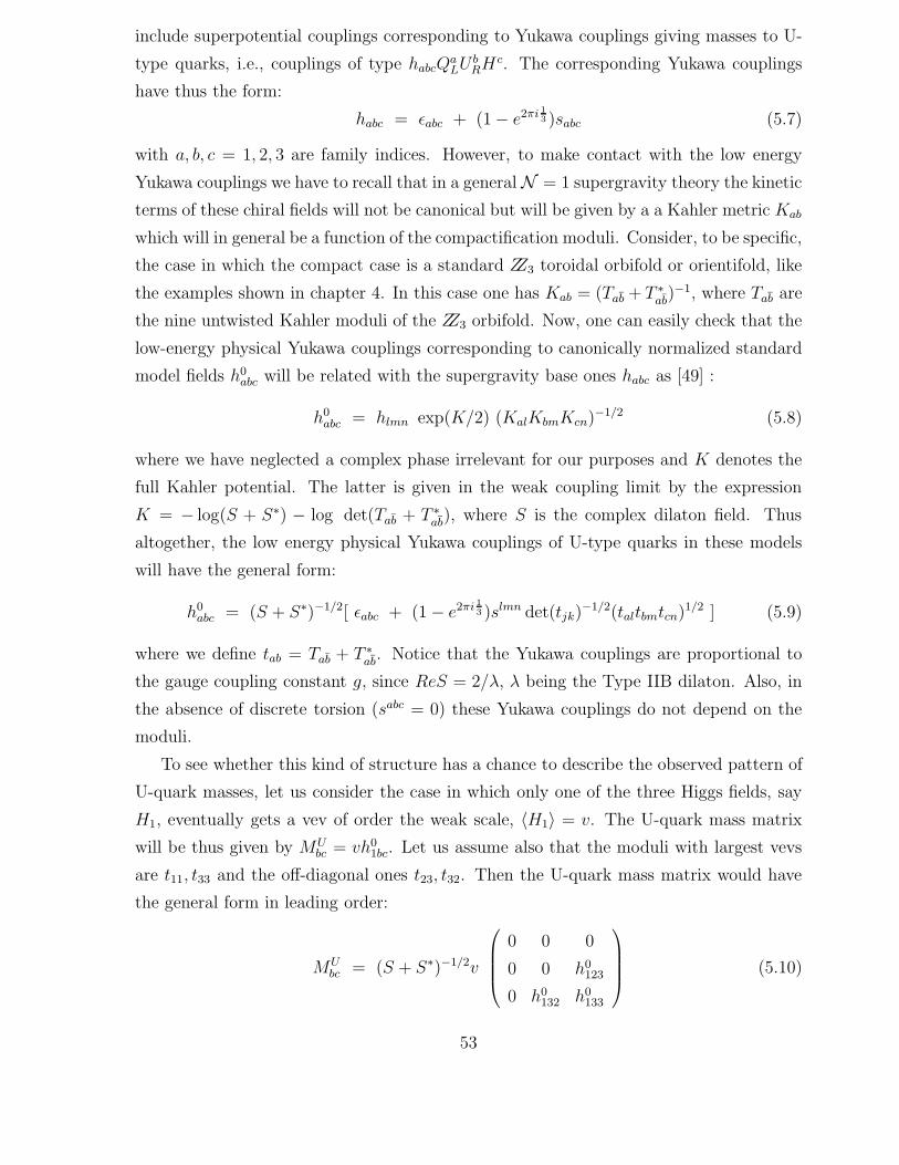
include superpotential couplings corresponding to Yukawa couplings giving masses to U-

type quarks, i.e., couplings of type habcQaLU

bRH

c. The corresponding Yukawa couplings

have thus the form:

habc = εabc + (1 − e2πi 13 )sabc (5.7)

with a, b, c = 1, 2, 3 are family indices. However, to make contact with the low energy

Yukawa couplings we have to recall that in a general N = 1 supergravity theory the kinetic

terms of these chiral fields will not be canonical but will be given by a a Kahler metric Kab

which will in general be a function of the compactification moduli. Consider, to be specific,

the case in which the compact case is a standard ZZ3 toroidal orbifold or orientifold, like

the examples shown in chapter 4. In this case one has Kab = (Tab + T ∗ab)

−1, where Tab are

the nine untwisted Kahler moduli of the ZZ3 orbifold. Now, one can easily check that the

low-energy physical Yukawa couplings corresponding to canonically normalized standard

model fields h0abc will be related with the supergravity base ones habc as [49] :

h0abc = hlmn exp(K/2) (KalKbmKcn)−1/2 (5.8)

where we have neglected a complex phase irrelevant for our purposes and K denotes the

full Kahler potential. The latter is given in the weak coupling limit by the expression

K = − log(S + S∗) − log det(Tab + T ∗ab), where S is the complex dilaton field. Thus

altogether, the low energy physical Yukawa couplings of U-type quarks in these models

will have the general form:

h0abc = (S + S∗)−1/2[ εabc + (1 − e2πi 1

3 )slmn det(tjk)−1/2(taltbmtcn)1/2 ] (5.9)

where we define tab = Tab + T ∗ab. Notice that the Yukawa couplings are proportional to

the gauge coupling constant g, since ReS = 2/λ, λ being the Type IIB dilaton. Also, in

the absence of discrete torsion (sabc = 0) these Yukawa couplings do not depend on the

moduli.

To see whether this kind of structure has a chance to describe the observed pattern of

U-quark masses, let us consider the case in which only one of the three Higgs fields, say

H1, eventually gets a vev of order the weak scale, 〈H1〉 = v. The U-quark mass matrix

will be thus given by MUbc = vh0

1bc. Let us assume also that the moduli with largest vevs

are t11, t33 and the off-diagonal ones t23, t32. Then the U-quark mass matrix would have

the general form in leading order:

MUbc = (S + S∗)−1/2v

0 0 0

0 0 h0123

0 h0132 h0

133

(5.10)

53

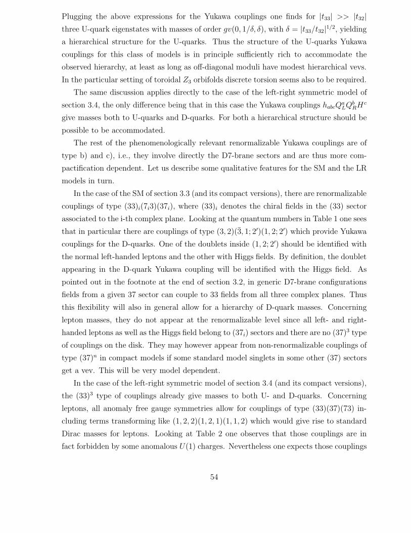
Plugging the above expressions for the Yukawa couplings one finds for |t33| >> |t32|three U-quark eigenstates with masses of order gv(0, 1/δ, δ), with δ = |t33/t32|1/2, yielding

a hierarchical structure for the U-quarks. Thus the structure of the U-quarks Yukawa

couplings for this class of models is in principle sufficiently rich to accommodate the

observed hierarchy, at least as long as off-diagonal moduli have modest hierarchical vevs.

In the particular setting of toroidal Z3 orbifolds discrete torsion seems also to be required.

The same discussion applies directly to the case of the left-right symmetric model of

section 3.4, the only difference being that in this case the Yukawa couplings habcQaLQ

bRH

c

give masses both to U-quarks and D-quarks. For both a hierarchical structure should be

possible to be accommodated.

The rest of the phenomenologically relevant renormalizable Yukawa couplings are of

type b) and c), i.e., they involve directly the D7-brane sectors and are thus more com-

pactification dependent. Let us describe some qualitative features for the SM and the LR

models in turn.

In the case of the SM of section 3.3 (and its compact versions), there are renormalizable

couplings of type (33)i(7i3)(37i), where (33)i denotes the chiral fields in the (33) sector

associated to the i-th complex plane. Looking at the quantum numbers in Table 1 one sees

that in particular there are couplings of type (3, 2)(3, 1; 2′)(1, 2; 2′) which provide Yukawa

couplings for the D-quarks. One of the doublets inside (1, 2; 2′) should be identified with

the normal left-handed leptons and the other with Higgs fields. By definition, the doublet

appearing in the D-quark Yukawa coupling will be identified with the Higgs field. As

pointed out in the footnote at the end of section 3.2, in generic D7-brane configurations

fields from a given 37 sector can couple to 33 fields from all three complex planes. Thus

this flexibility will also in general allow for a hierarchy of D-quark masses. Concerning

lepton masses, they do not appear at the renormalizable level since all left- and right-

handed leptons as well as the Higgs field belong to (37i) sectors and there are no (37)3 type

of couplings on the disk. They may however appear from non-renormalizable couplings of

type (37)n in compact models if some standard model singlets in some other (37) sectors

get a vev. This will be very model dependent.

In the case of the left-right symmetric model of section 3.4 (and its compact versions),

the (33)3 type of couplings already give masses to both U- and D-quarks. Concerning

leptons, all anomaly free gauge symmetries allow for couplings of type (33)(37)(73) in-

cluding terms transforming like (1, 2, 2)(1, 2, 1)(1, 1, 2) which would give rise to standard

Dirac masses for leptons. Looking at Table 2 one observes that those couplings are in

fact forbidden by some anomalous U(1) charges. Nevertheless one expects those couplings

54

to be present once appropriate twisted closed string insertions (which are charged under

anomalous U(1)’s) are made [15]. Again, for different geometrical configurations of D7-

branes there will be enough flexibility to obtain a hierarchy of Yukawa couplings also for

leptons.

In the case of the left-right model we also have to worry about neutrino masses. Gener-

ically they will get Dirac masses of the order of the charged lepton masses. However, once

SU(2)R symmetry-breaking takes place through the vevs of the extra SU(2)R doublets

discussed above, the right-handed neutrinos may combine with some singlets in (7i7j)

sectors and get masses of order MR. We will not give details here which would be very

model dependent. Let us note however that the effective left-handed neutrino masses

would thus be of order m2l /MR, where ml are the neutrino Dirac masses. For values of

ml of order the electron mass and MR of order 1 TeV, they would have masses of order 1

eV, compatible with experimental bounds.

Let us finally comment about proton stability in these schemes. This is an important

question if, as seems to be indicated by gauge coupling unification, the string scale is

chosen to be well below the Planck mass (e.g. at scales of order 1012 GeV or below).

Since for this question higher dimensional operators are in principle important, it is not

possible to make model independent statements about sufficient proton stability. We

would like to underline however, that from this point of view the left-right symmetric

models seem more promising since the symmetry B−L is gauged and hence dimension

four baryon or lepton violating operators are forbidden to start with. Furthermore, B/L-

violating dimension 5 operators like F-terms of the form QLQLQLL (which respect B−L)

are of type (33)3(73) and hence are forbidden on the disk. In fact, it was shown in ref.

[15], that in a left-right model analogous to the compact orientifold of chapter 5, the

proton is absolutely stable due to the presence of induced baryon and lepton parity ZZ2

symmetries. Thus we believe that, at least in the left-right class of models, a sufficiently

stable proton may naturally be achieved.

iii) String Scale versus Planck Mass

In our approach, four-dimensional gravity arises once we embed our SM or LR D-brane

systems into a finite compact space. The precise relationship between the string scale Ms

and four-dimensional Planck scale Mp will depend on the compactification. In toroidal

orbifold compactifications with factorized two-tori they are related by

Mp =2√

2M4s

λM1M2M3(5.11)

55

where Mi are the compactification mass scales of the three tori. Thus, as is well known

[5, 50, 51, 52], values for Ms much below the Planck scale may be possible if some of

the compact dimensions are very large. Until we get a handle on the dynamics fixing

the radii, the value of the string scale is only constrained by accelerator limits to be

Ms > 1 TeV or so. In particular, one can accommodate intermediate scale values [53, 54]

of order Ms ∝ 1010−1012 GeV, as suggested by the logarithmic gauge coupling unification

arguments above.

Similar qualitative statements can be made concerning the Planck versus string scales

in F-theory models with the SM sector living on the world-volume of D3-branes, like those

discussed in chapter 5. Thus, e.g. one can match the observed size of the Planck scale by

making very large the volume of the base P1 in the first K3 X(1), while maintaining the

volume of the second K3, X(2) of order the string scale.

It is quite interesting to remark that such intermediate values for the string scale turn

out to be also suggested in a completely independent manner in models [13, 15] containing

anti-branes like the orientifolds in chapter 5. Indeed, in those models supersymmetry is

broken at the string scale Ms due to the presence of anti-D7-branes. However the physical

SM or LR sectors are away from these antibranes in the Y1 transverse dimension. Let us

suppose that e.g. one has M2,M3 = Ms and M1 = M2s /(λMp) so that one obtains the

correct Planck scale. This means taking very large Y1 radii which will also mean that

the susy-breaking effects from the anti-D7-branes will be felt in a Planck mass suppressed

manner in the visible SM world. Thus one expects effective SUSY-breaking contributions

of order M2s /Mp in the SM sector. If Ms is of order 1010 − 1012 GeV, then these SUSY-

breaking contributions would be of order the weak scale, as required. The structure of

these models would be very similar to hidden-sector supersymmetry-breaking models, the

main difference being that in the present case the string and SUSY-breaking scales do

coincide.

Let us also comment that the approach here presented is also consistent with low (i.e.

1-10 TeV) string scale scenarios [51, 52] , just by choosing larger compact radii. In these

cases an alternative understanding of the gauge coupling unification problem should be

found.

Finally the F -theory constructions of the previous section allows for the possibility of

a more standard scenario. Being supersymmetric, we do not have to identify the string

scale with the supersymmetry breaking scale. We may in principle conceive models of

this type for which the string scale is closer to the Planck or GUT scales. The left-right

symmetric model presented in that section still requires unification at the intermediate

56

scale but in general, achieving or not gauge coupling unification will clearly depend on

the spectrum of each model.

6 Final Comments and Outlook

We have presented what we consider to be the first steps on a new way to deal with

string model building. The fact that D3-brane worlds can appear naturally on type

IIB strings suggests that looking directly to the physics on these D3-branes may tell us

many interesting phenomenological aspects that depend very weakly on the details of the

compactified space. This is so since only gravitational strength interactions feel the extra

dimensions.

It is remarkable how easy is to obtain realistic models from this approach and how

powerful the structure of singularities turn out to be in order to achieve interesting phe-

nomenological properties, such as the number of families, the ubiquity of hypercharge and

the value of Weinberg’s angle. For instance a concrete prediction of the class of models

considered is that the number of families does not exceed 3 for supersymmetric models

and 4 for non-supersymmetric ones. The reason being essentially the N = 4 symmetry

underlying the 33 spectrum, which limits the number of replicated fermions after the

orbifold projection. This is a very small (and realistic) number compared with more stan-

dard compactifications in which the number of families depends on the topology of the

compact manifold and is naturally very large.

It is worth remarking that the consideration of the non-compact models constructed

here may have an importance per se. At present there is increasing interest on non-

compact extra dimensions raised after the work of Randall and Sundrum [55] . It would

be tempting to speculate that a similar mechanism to localize gravity on the D3-branes

may be present in models similar to ours. However it is not clear if this could be achievable.

Furthermore, during the past few years, non-compact brane models were used in order to

obtain information on the dynamics of gauge theories from the structure of branes. Much

work has been done in this direction, [56], although most of the activity was based on

extended supersymmetric models and non-chiral N = 1 models. Chiral theories were con-

structed in [57], and seen to be related to theories on D3-branes at singularities [20]. Our

models extend this program by addressing (and actually succeeding in) the construction

of realistic models using brane configurations.

Independent of these issues, the fact that in compact models we have been able to

obtain realistic N = 0 and N = 1 models from type IIB strings at singularities may be the

57

most important concrete result of this work. We have explored several mechanisms and

generalizations to current model building, each of them deserving further study. The new

approach, while sharing some of the good properties of the constructions of [13, 15] (gauge

unification, supersymmetry breaking, proton stability), has several clear advantages over

previous discussions, besides the fact that it is more general: from the stability of the

models, by trapping anti-branes avoiding brane/anti-brane annihilation, to the inclusion

of new degrees of freedom, such as discrete torsion, which allow more flexibility on the

structure of fermion masses and helps to stabilize the models.

A scenario with intermediate fundamental scale is clearly favoured by the non su-

persymmetric models which can also have gauge coupling unification at the same scale,

especially in the case of the left-right symmetric models. On the other hand, the fact

that we have also obtained quasi-realistic N = 1 supersymmetric models allows for the

possibility of realistic scenarios with fundamental scales as large as the Planck or GUT

scales. It is worth pointing out however that, as usual in string theory, grand unified gauge

models do not seem to appear naturally in this scheme, whereas the standard model and

its left-right symmetric extension are very easy to obtain.

There are clearly many avenues that deserve to be explored in the future, starting

from our approach. Probably the most pressing one being the understanding of moduli

and dilaton stabilization after supersymmetry breaking and the corresponding value of

the vacuum energy.

Acknowledgements

We thank M. Cvetic, S. Franco, M. Klein, P. Langacker, J. Maldacena, B. Ovrut,

M. Plumacher and R. Rabadan for useful discussions. A. M. U. thanks the Department

of Applied Mathematics and Theoretical Physics of Cambridge University, and the De-

partment of Physics and Astronomy of University of Pennsylvania for hospitality, and

M. Gonzalez for encouragement and support. G. A. thanks the High Energy Theory

Group of Harvard University for hospitality. This work has been partially supported by

CICYT (Spain), the European Commission (grant ERBFMRX-CT96-0045) and PPARC.

G.A work is partially supported by ANPCyT grant 03-03403.

58

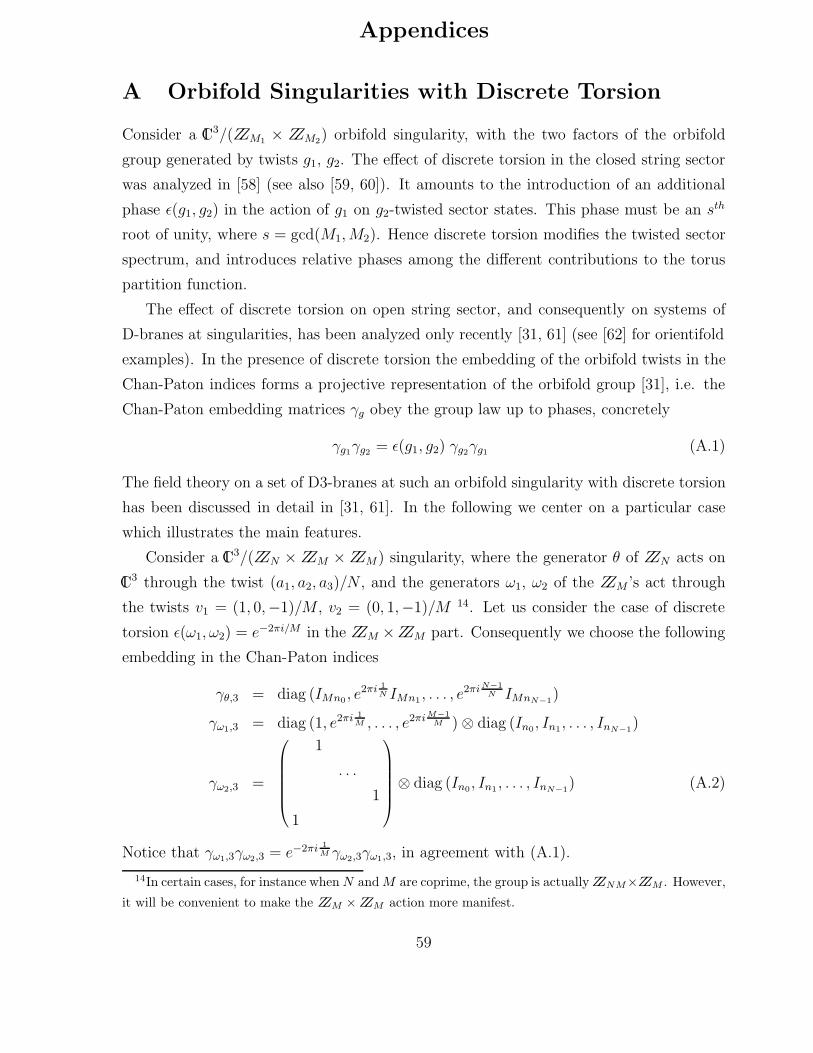
Appendices

A Orbifold Singularities with Discrete Torsion

Consider a IC3/(ZZM1 × ZZM2) orbifold singularity, with the two factors of the orbifold

group generated by twists g1, g2. The effect of discrete torsion in the closed string sector

was analyzed in [58] (see also [59, 60]). It amounts to the introduction of an additional

phase ε(g1, g2) in the action of g1 on g2-twisted sector states. This phase must be an sth

root of unity, where s = gcd(M1,M2). Hence discrete torsion modifies the twisted sector

spectrum, and introduces relative phases among the different contributions to the torus

partition function.

The effect of discrete torsion on open string sector, and consequently on systems of

D-branes at singularities, has been analyzed only recently [31, 61] (see [62] for orientifold

examples). In the presence of discrete torsion the embedding of the orbifold twists in the

Chan-Paton indices forms a projective representation of the orbifold group [31], i.e. the

Chan-Paton embedding matrices γg obey the group law up to phases, concretely

γg1γg2 = ε(g1, g2) γg2γg1 (A.1)

The field theory on a set of D3-branes at such an orbifold singularity with discrete torsion

has been discussed in detail in [31, 61]. In the following we center on a particular case

which illustrates the main features.

Consider a IC3/(ZZN × ZZM × ZZM) singularity, where the generator θ of ZZN acts on

IC3 through the twist (a1, a2, a3)/N , and the generators ω1, ω2 of the ZZM ’s act through

the twists v1 = (1, 0,−1)/M , v2 = (0, 1,−1)/M 14. Let us consider the case of discrete

torsion ε(ω1, ω2) = e−2πi/M in the ZZM ×ZZM part. Consequently we choose the following

embedding in the Chan-Paton indices

γθ,3 = diag (IMn0 , e2πi 1

N IMn1 , . . . , e2πi N−1

N IMnN−1)

γω1,3 = diag (1, e2πi 1M , . . . , e2πi M−1

M ) ⊗ diag (In0, In1, . . . , InN−1)

γω2,3 =

1

. . .

1

1

⊗ diag (In0, In1 , . . . , InN−1

) (A.2)

Notice that γω1,3γω2,3 = e−2πi 1M γω2,3γω1,3, in agreement with (A.1).

14In certain cases, for instance when N and M are coprime, the group is actually ZZNM×ZZM . However,

it will be convenient to make the ZZM × ZZM action more manifest.

59

The spectrum is obtained after imposing the projections

Vector λ = γθ,3λγ−1θ,3 λ = γω1,3λγ

−1ω1,3 λ = γω2,3λγ

−1ω2,3

Chiral1 λ = e2πia1N γθ,3λγ

−1θ,3 λ = e2πi 1

M γω1,3λγ−1ω1,3 λ = γω2,3λγ

−1ω2,3

Chiral2 λ = e2πia2N γθ,3λγ

−1θ,3 λ = γω1,3λγ

−1ω1,3 λ = e2πi 1

M γω2,3λγ−1ω2,3

Chiral3 λ = e2πia3N γθ,3λγ

−1θ,3 λ = e−2πi 1

M γω1,3λγ−1ω1,3 λ = e−2πi 1

M γω2,3λγ−1ω2,3

(A.3)

The projection process is relatively simple. For vector multiplets, the θ projection yields

a gauge group∏N−1

i=0 U(Mni). The ω1 projection splits it into∏N−1

i=0 U(n1)N . Finally, the

ω2 action identifies the different gauge factors with equal rank, leaving a remaining gauge

group∏N−1

i=0 U(ni). Proceeding analogously, the complete spectrum is

Vector∏N−1

i=0 U(ni)

Chiral∑3

r=1

∑N−1i=0 (ni, ni+ar) (A.4)

Notice this is identical to the spectrum of the IC3/ZZN singularity with twist (a1, a2, a3)/N ,

in section 2.1 or 3.1. However, the effect of the additional ZZM × ZZM twist and of the

discrete torsion are manifest in the superpotential, which reads

W = Tr [Φ1i,i+a1

Φ2i+a1,i+a1+a2

Φ3i+a1+a2,i − e−2πi 1

M Φ1i,i+a1

Φ3i+a1,i+a1+a3

Φ2i+a1+a3,i](A.5)

which differs from the 33 piece in (3.1).

We spare the reader the detailed discussion of the introduction of D7-branes in the

configuration. The resulting spectrum is identical to that obtained for ZZN singularities

in Section 3.1.

Notice that, since the twists ω1, ω2 have traceless Chan-Paton embeddings, the corre-

sponding disk tadpoles vanish. The only constraints on the integers ni arise from cancel-

lation of tadpoles in ZZN twisted sectors. The corresponding conditions are those for ZZN

singularities (as expected, since they are basically the anomaly cancellation conditions).

B Non-Abelian Orbifolds

The rules to compute the spectrum of D3-branes at non-abelian orbifold singularities have

been discussed in [63] for Γ ⊂ SU(2), and generalized in [19]. In the following we center

on N = 1 supersymmetric field theories in the case Γ ⊂ SU(3), studied in detail in [32, 33]

(see [64] for the general case Γ ⊂ SU(4)).

The computation of the spectrum is just a natural group-theoretical generalization

of the abelian case. Let Rii=1,...,N denote the irreducible representations of Γ, with

60

N the number of conjugacy classes of Γ. We are interested in the field theory on a set

of D3-branes at a IC3/Γ singularity, where the action of Γ on IC3 is specified by a three-

dimensional representation R(3), and its action on the D3-brane Chan-Paton indices is

given by a representation RCP , which decomposes as

RCP =N∑

i=1

niRi (B.1)

The field theory on D3-branes at IC3/Γ is obtained by projecting the field theory on D3-

branes on IC3 onto states invariant under the combined (geometric plus Chan-Paton) action

of Γ. The resulting gauge group 15 is∏N

i=1 U(ni). There are also a3ij chiral multiplets in the

(ni, nj) representation, where the adjacency matrix a3ij is defined by the decomposition

R(3) ⊗Ri =N∑

j=1

a3ijRj (B.2)

The superpotential is obtained by substituting the surviving chiral multiplets Φij in the

N = 4 superpotential (2.1), but we will not need it explicitly.

An important observation is that the gauge couplings for the different factors are not

equal in field theories from non-abelian orbifolds. The gauge coupling for the ith group is

given by [19]

τi =riτ

|Γ| (B.3)

with ri = dim Ri, and τ an overall value independent of i.

The analysis of U(1) anomalies has not been performed in the literature, but can be

easily generalized from the abelian case 16. Assuming the 37, 73 sectors contribute a set

of bifundamental multiplets which cancel the non-abelian anomaly in the 33 sector, the

mixed Qni-SU(nj)

2 anomaly reduces to Aij = 12ni(a

(3)ij − a

(3)ji ). It is possible to check that

the diagonal combination

Qdiag =N∑

i=1

ri

niQni

(B.4)

15In the literature on D-branes on non-abelian orbifold, the representation RCP is usually taken to be k

copies of the regular representation, ni = kdim Ri, which satisfies tadpole cancellation conditions without

the need of additional branes. We will consider more general choices of ni, with the understanding that

additional D7-branes will cancel the corresponding tadpoles. Unfortunately, the inclusion of D7-branes

has not been discussed in the literature, hence we will not be explicit about the 37 sector in our models,

and simply assume it provides additional chiral multiplets to cancel gauge theory anomalies from the 33

sector.16We thank A. Hanany for conversations on this point.

61

is automatically non-anomalous. Also, as long as no ni vanishes, there is one additional

non-anomalous U(1)’s for each non-trivial conjugacy classes leaving some complex plane

invariant. An important difference with respect to the abelian case is that, due to the

presence of the factors ri above, the structure SU(3)×SU(2) does not in general guarantee

the correct hypercharge assignments for the non-anomalous U(1)’s.

C Non-Orbifold Singularities

In this section we briefly discuss systems of D3-branes at non-orbifold singularities. The

only known systematic approach to construct the world-volume field theory is to realize

the non-orbifold singularity as a partial resolution of a suitable orbifold singularity [65]17. However, the identification of the field-theory interpretation of the partial blowing-up

is very involved beyond the simplest examples [65, 71, 72]. Consequently, it is difficult to

make general statements about the phenomenological potential of these systems.

We would like to center on a particular family of singularities, which can be constructed

as orbifolds of the conifold singularity [68] (see also [73]), and their partial blow-ups. They

have potential interest since generically they lead to chiral N = 1 supersymmetric field

theories on the world-volume of D3-branes, and include abelian orbifold singularities as

particular cases. Moreover, they have a T-dual representation in terms of configurations

of NS-fivebranes and D5-branes, known as ‘brane diamonds’ [74], generalizing the brane

box constructions in [57, 20], which allow a systematic search of interesting field theories

within this class.

Instead of extending on such analysis, we point out that the only singularity in this

family, leading to full triplication of chiral multiplet content in the 33 sector is in fact

the IC3/ZZ3 singularity. A milder requirement would be to have triplication not for the

full 33 sector, but at least for some representation. Besides the ZZ3 orbifold, there is only

one singularity in this family fulfilling this milder requirement. Let us briefly discuss its

construction.

Consider the conifold, given by the hypersurface xy = zw in IC4. The field theory on

D3-branes at a conifold was determined in [66]. The gauge group is U(N1) × U(N2) and

there are chiral multiplets A1, A2 in the ( , ), and B1, B2 in the ( , ). There is also a

17Alternative approaches include the direct construction of field theories with the right symmetries and

the correct moduli space [66, 67], and the use of T-duality [68, 69] to configurations of NS-branes and

D4-branes [70, 56].

62

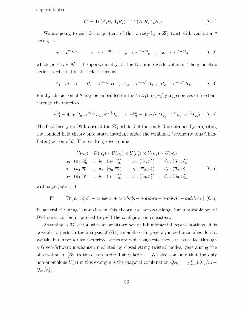
superpotential

W = Tr (A1B1A2B2) − Tr (A1B2A2B1) (C.1)

We are going to consider a quotient of this variety by a ZZ3 twist with generator θ

acting as

x→ e2πi/3x ; z → e2πi/3z ; y → e−2πi/3y ; w → e−2πi/3w (C.2)

which preserves N = 1 supersymmetry on the D3-brane world-volume. The geometric

action is reflected in the field theory as

A1 → eπiA1 ; B1 → e−πi/3B1 ; A2 → e−πi/3A2 ; B2 → e−πi/3B2 (C.3)

Finally, the action of θ may be embedded on the U(N1), U(N2) gauge degrees of freedom,

through the matrices

γ(1)θ,3 = diag (In0, e

2πi 13 In1 , e

2πi 23 In2) ; γ

(2)θ,3 = diag (eπiIn′

0, eπi 5

3 In′1, eπi 1

3 In′2) (C.4)

The field theory on D3-branes at the ZZ3 orbifold of the conifold is obtained by projecting

the conifold field theory onto states invariant under the combined (geometric plus Chan-

Paton) action of θ. The resulting spectrum is

U(n0) × U(n′0) × U(n1) × U(n′

1) × U(n2) × U(n′2)

a0 : (n0, n′0) , b2 : (n2, n

′0) , c0 : (n1, n

′0) , d0 : (n1, n

′0)

a1 : (n1, n′1) , b0 : (n0, n

′1) , c1 : (n2, n

′1) , d1 : (n2, n

′1)

a2 : (n1, n′1) , b1 : (n1, n

′2) , c2 : (n0, n

′2) , d2 : (n0, n

′2)

(C.5)

with superpotential

W = Tr [ a0c0b1d2 − a0d0b1c2 + a1c1b2d0 − a1d1b2c0 + a2c2b0d1 − a2d2b0c1 ] (C.6)

In general the gauge anomalies in this theory are non-vanishing, but a suitable set of

D7-branes can be introduced to yield the configuration consistent.

Assuming a 37 sector with an arbitrary set of bifundamental representations, it is

possible to perform the analysis of U(1) anomalies. In general, mixed anomalies do not

vanish, but have a nice factorized structure which suggests they are cancelled through

a Green-Schwarz mechanism mediated by closed string twisted modes, generalizing the

observation in [23] to these non-orbifold singularities. We also conclude that the only

non-anomalous U(1) in this example is the diagonal combination Qdiag =∑2

i=0(Qni/ni +

Qn′i/n′

i).

63

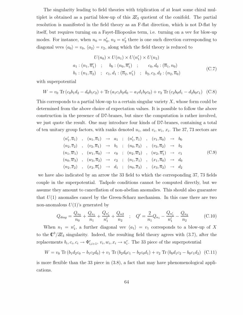
The singularity leading to field theories with triplication of at least some chiral mul-

tiplet is obtained as a partial blow-up of this ZZ3 quotient of the conifold. The partial

resolution is manifested in the field theory as an F-flat direction, which is not D-flat by

itself, but requires turning on a Fayet-Illiopoulos term, i.e. turning on a vev for blow-up

modes. For instance, when n0 = n′0, n2 = n′

2 there is one such direction corresponding to

diagonal vevs 〈a0〉 = v0, 〈a2〉 = v2, along which the field theory is reduced to

U(n0) × U(n1) × U(n′1) × U(n2)

a1 : (n1, n′1) ; b0 : (n0, n

′1) ; c0, d0 : (n1, n0)

b1 : (n1, n2) ; c1, d1 : (n2, n′1) ; b2, c2, d2 : (n2, n0)

(C.7)

with superpotential

W = v0 Tr (c0b1d2 − d0b1c2) + Tr (a1c1b2d0 − a1d1b2c0) + v2 Tr (c2b0d1 − d2b0c1) (C.8)

This corresponds to a partial blow-up to a certain singular variety X, whose form could be

determined from the above choice of expectation values. It is possible to follow the above

construction in the presence of D7-branes, but since the computation is rather involved,

we just quote the result. One may introduce four kinds of D7-branes, containing a total

of ten unitary group factors, with ranks denoted u1, and vi, wi, xi. The 37, 73 sectors are

(n′1, u1) , (u1, n1) → a1 ; (n′

1, v1) , (v1, n0) → b0

(n2, v2) , (v2, n1) → b1 ; (n0, v3) , (v3, n2) → b2

(n1, w1) , (w1, n0) → c0 ; (n2, w2) , (w2, n′1) → c1

(n0, w3) , (w3, n2) → c2 ; (n1, x1) , (x1, n0) → d0

(n2, x2) , (x2, n′1) → d1 ; (n0, x3) , (x3, n2) → d2

(C.9)

we have also indicated by an arrow the 33 field to which the corresponding 37, 73 fields

couple in the superpotential. Tadpole conditions cannot be computed directly, but we

assume they amount to cancellation of non-abelian anomalies. This should also guarantee

that U(1) anomalies cancel by the Green-Scharz mechanism. In this case there are two

non-anomalous U(1)’s generated by

Qdiag =Qn0

n0+Qn1

n1+Qn′

1

n′1

+Qn2

n2; Q′ =

2

n1Qn1 −

Qn′1

n′1

− Qn2

n2(C.10)

When n1 = n′1, a further diagonal vev 〈a1〉 = v1 corresponds to a blow-up of X

to the IC3/ZZ3 singularity. Indeed, the resulting field theory agrees with (3.7), after the

replacements bi, ci, ci → Φri,i+1, vi, wi, xi → ur

i . The 33 piece of the superpotential

W = v0 Tr (b1d2c0 − b1c2d0) + v1 Tr (b2d0c1 − b2c0d1) + v2 Tr (b0d1c2 − b0c1d2) (C.11)

is more flexible than the 33 piece in (3.8), a fact that may have phenomenological appli-

cations.

64

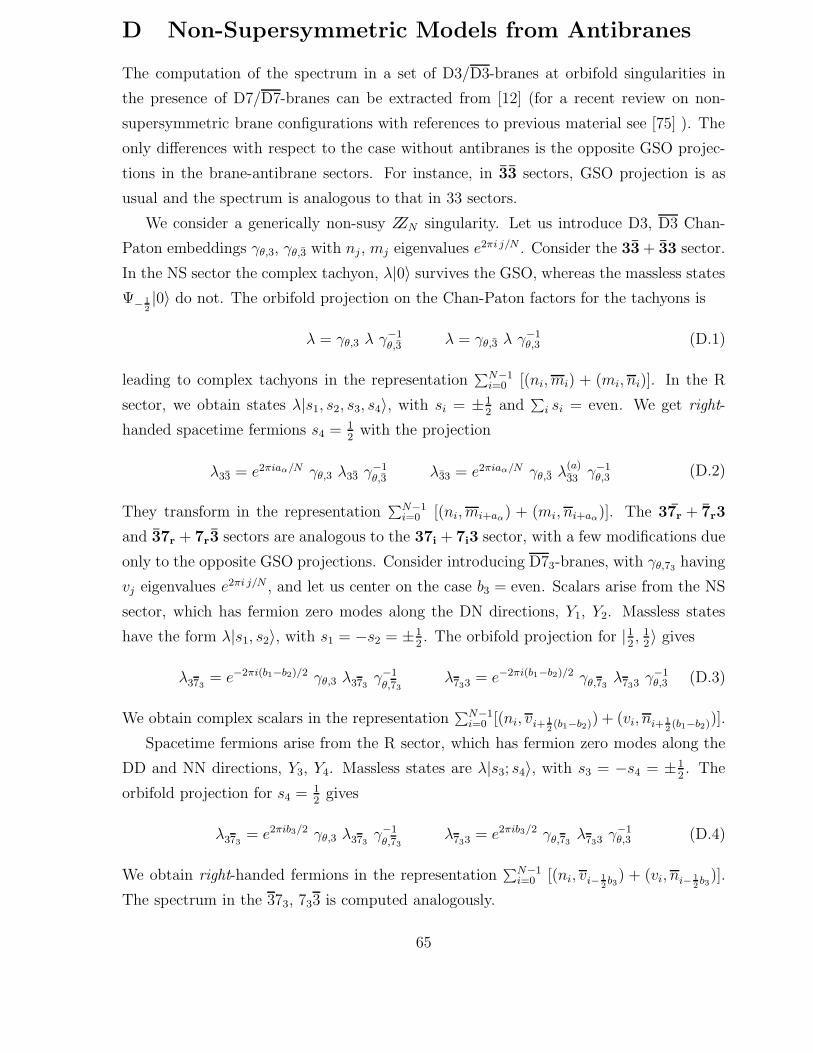
D Non-Supersymmetric Models from Antibranes

The computation of the spectrum in a set of D3/D3-branes at orbifold singularities in

the presence of D7/D7-branes can be extracted from [12] (for a recent review on non-

supersymmetric brane configurations with references to previous material see [75] ). The

only differences with respect to the case without antibranes is the opposite GSO projec-

tions in the brane-antibrane sectors. For instance, in 33 sectors, GSO projection is as

usual and the spectrum is analogous to that in 33 sectors.

We consider a generically non-susy ZZN singularity. Let us introduce D3, D3 Chan-

Paton embeddings γθ,3, γθ,3 with nj , mj eigenvalues e2πi j/N . Consider the 33 + 33 sector.

In the NS sector the complex tachyon, λ|0〉 survives the GSO, whereas the massless states

Ψ− 12|0〉 do not. The orbifold projection on the Chan-Paton factors for the tachyons is

λ = γθ,3 λ γ−1θ,3 λ = γθ,3 λ γ

−1θ,3 (D.1)

leading to complex tachyons in the representation∑N−1

i=0 [(ni, mi) + (mi, ni)]. In the R

sector, we obtain states λ|s1, s2, s3, s4〉, with si = ±12

and∑

i si = even. We get right-

handed spacetime fermions s4 = 12

with the projection

λ33 = e2πiaα/N γθ,3 λ33 γ−1θ,3 λ33 = e2πiaα/N γθ,3 λ

(a)33 γ−1

θ,3 (D.2)

They transform in the representation∑N−1

i=0 [(ni, mi+aα) + (mi, ni+aα)]. The 37r + 7r3

and 37r + 7r3 sectors are analogous to the 37i + 7i3 sector, with a few modifications due

only to the opposite GSO projections. Consider introducing D73-branes, with γθ,73 having

vj eigenvalues e2πi j/N , and let us center on the case b3 = even. Scalars arise from the NS

sector, which has fermion zero modes along the DN directions, Y1, Y2. Massless states

have the form λ|s1, s2〉, with s1 = −s2 = ±12. The orbifold projection for |1

2, 1

2〉 gives

λ373= e−2πi(b1−b2)/2 γθ,3 λ373

γ−1θ,73

λ733 = e−2πi(b1−b2)/2 γθ,73λ733 γ

−1θ,3 (D.3)

We obtain complex scalars in the representation∑N−1

i=0 [(ni, vi+ 12(b1−b2)) + (vi, ni+ 1

2(b1−b2))].

Spacetime fermions arise from the R sector, which has fermion zero modes along the

DD and NN directions, Y3, Y4. Massless states are λ|s3; s4〉, with s3 = −s4 = ±12. The

orbifold projection for s4 = 12

gives

λ373= e2πib3/2 γθ,3 λ373

γ−1θ,73

λ733 = e2πib3/2 γθ,73λ733

γ−1θ,3 (D.4)

We obtain right-handed fermions in the representation∑N−1

i=0 [(ni, vi− 12b3

) + (vi, ni− 12b3

)].

The spectrum in the 373, 733 is computed analogously.

65

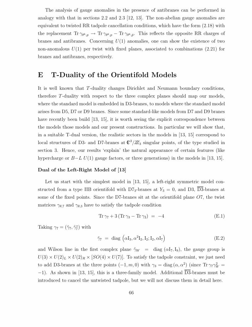
The analysis of gauge anomalies in the presence of antibranes can be performed in

analogy with that in sections 2.2 and 2.3 [12, 13]. The non-abelian gauge anomalies are

equivalent to twisted RR tadpole cancellation conditions, which have the form (2.18) with

the replacement Tr γθk,p → Tr γθk,p − Tr γθk,p. This reflects the opposite RR charges of

branes and antibranes. Concerning U(1) anomalies, one can show the existence of two

non-anomalous U(1) per twist with fixed planes, associated to combinations (2.21) for

branes and antibranes, respectively.

E T-Duality of the Orientifold Models

It is well known that T -duality changes Dirichlet and Neumann boundary conditions,

therefore T -duality with respect to the three complex planes should map our models,

where the standard model is embedded in D3-branes, to models where the standard model

arises from D5, D7 or D9 branes. Since some standard-like models from D7 and D9 branes

have recently been build [13, 15], it is worth seeing the explicit correspondence between

the models those models and our present constructions. In particular we will show that,

in a suitable T-dual version, the realistic sectors in the models in [13, 15] correspond to

local structures of D3- and D7-branes at IC3/ZZ3 singular points, of the type studied in

section 3. Hence, our results ‘explain’ the natural appearance of certain features (like

hypercharge or B−L U(1) gauge factors, or three generations) in the models in [13, 15].

Dual of the Left-Right Model of [13]

Let us start with the simplest model in [13, 15], a left-right symmetric model con-

structed from a type IIB orientifold with D73-branes at Y3 = 0, and D3, D3-branes at

some of the fixed points. Since the D7-branes sit at the orientifold plane O7, the twist

matrices γθ,7 and γθ,3 have to satisfy the tadpole condition

Tr γ7 + 3 (Tr γ3 − Tr γ3) = −4 (E.1)

Taking γ7 = (γ7, γ∗7) with

γ7 = diag(αI3, α

2I2, I2; I2, αI7)

(E.2)

and Wilson line in the first complex plane γW = diag (αI7, I9), the gauge group is

U(3) × U(2)L × U(2)R × [SO(4) × U(7)]. To satisfy the tadpole constraint, we just need

to add D3-branes at the three points (−1, m, 0) with γ3 = diag (α, α2) (since Tr γ7γ2W =

−1). As shown in [13, 15], this is a three-family model. Additional D3-branes must be

introduced to cancel the untwisted tadpole, but we will not discuss them in detail here.

66

To find the dual of this model in the approach of the present paper we have to dualize

with respect to the first two complex planes so that the D73-branes become D3-branes

and viceversa. Also under T -duality Wilson lines become displacement of the branes,

although the explicit mapping is rather involved. The best strategy in the present case is

to construct the model explicitly.

Since the Wilson lines above only affect the 14 entries leading to the LR model, these

correspond to the D3-branes that sit outside the origin in the T-dual version. Therefore

we consider 18 D3-branes at the origin, with twist matrix γθ,3 = (γ3, γ∗3) and

γ3 = diag (I2, αI7) (E.3)

This should correspond to the ‘hidden’ part of the original model (last entries in (E.2),

and indeed it leads to an SO(4) × U(7) gauge group. Since the origin is an O3-plane,

the tadpole condition is (4.14). Since Tr γ3 = −3 we can cancel tadpoles introducing six

D7-branes at Y3 = 0 with γθ,7 = diag (αI3, α2I3).

After introducing these D7-branes, we have to worry about tadpole cancellation at the

other fixed points in the Y1, Y2 planes, given by (4.15). At the points (±1, 0, 0) (mapped

into each other under the orientifold action (−1)F ΩR1R2R3) we can put seven D3-branes

on each, with twist matrix

γθ,3 = diag(I3, αI2, α

2I2)

(E.4)

giving rise to a three-generation SU(3) × SU(2)L × SU(2)R × U(1)B−L LR model of the

type studied in section 3.4.

Notice that we have introduced 18 D3-branes at the origin and 7 + 7 = 14 at the

(±1, 0, 0) points, already saturating the total number of allowed D3-branes (32). There-

fore, twisted tadpoles at the remaining fixed points should cancel without additional

D3-branes. This can be achieved by introducing a Wilson line in the Y2 direction (hence

not affecting the points (m, 0, 0)) , such that Tr γ7γW = Tr γ7γ2W = 0. The right choice is

γW = diag(1, α, α2; 1, α2, α

)(E.5)

Therefore we do not have to introduce D3-branes at any of the six fixed points (m,±1, 0).

Notice also that this Wilson line breaks the D7-brane gauge group U(3) to U(1)3, as in

the original model. The appearance of this Wilson line in the dual model reflects the fact

that in the original model the six D3-branes were distributed among three different fixed

points.

The last consistency requirement is to have an equal number of D7- and D7-branes.

To satisfy it, we put three anti-D7-branes with γ7 = (1, α, α2) at the two mirror locations

67

Y3 = ±1. Since this matrix is traceless there is no need to add more D3-branes to cancel

tadpoles. These anti-branes can move freely in the Y3 direction. Moreover, it is possible

to turn on continuous Wilson lines along their world-volume, i.e. the directions Y1, Y2.

This corresponds to possibility of moving the D3-branes in the original model in the three

complex dimensions of the bulk. They are naturally dual to the anti D3-branes of the

original model.

A Variant Left-Right Orientifold Model and its Dual

Let us consider a variant left-right orientifold model slightly different from the one in

section 4. We satisfy the tadpole equations (4.14) at the origin by having 12 D7-branes

and 4 D3-branes with:

γ7 =(αI6, α

2I6), γ3 =

(α, α2, α, α2

)(E.6)

In the second plane, we add a Wilson line:

γW =(1, α, α2, I3, 1, α, α

2, I3)

(E.7)

Since Tr γ7γW = Tr γ7γ2W = −3 we can put a left-right model at each of the points

(0,±1, 0) in terms of 7 D3-branes with

γ3 =(I3, αI2, α

2I2)

(E.8)

satisfying the tadpole condition (4.15). In order to minimize the number of D3-branes

needed to cancel tadpoles (so we do not exceed 32) it is convenient to add a second Wilson

line now in the third plane:

γ′W =(I3, 1, α, α

2, I3, 1, α, α2)

(E.9)

Since Tr γ7γ′W = Tr γ7γ

′2W = −3 we can cancel tadpoles at the points (0, 0,±1) by putting

just one single D3-brane on each with γ3 = 1. The advantage of adding the second

Wilson line is that at the points (0,±1,±1) there is no need to add any D3-brane because

Tr γ7γmWγ

′nW = 0 for m,n = 1, 2. Therefore we have at the plane Y1 = 0 12 D7-branes and

a total of 4 + 7 + 7 + 1 + 1 = 20 D3-branes.

At each of the planes Y1 = ±1 we have to put 6 D7-branes and 6 D3-branes distributed

on the fixed points (±1, m, n). We achieve tadpole cancellation by having:

γ7 =(αI3, α

2I3), γW =

(1, α, α2, 1, α, α2

)(E.10)

68

So we have Tr γ7 = −3 and can cancel tadpoles at the points (±1, 0, m) adding 2 D3-branes

at each point with γ3 = (α, α2). This saturates the number of D3-branes (20+2×6 = 32)

which is OK since at the points (±1,±1, m) there is no need to add D3-branes since

Tr γ7γW = Tr γ7γ2W = 0.

We can easily see that the gauge group coming from the D3-branes is [U(3)×U(2)L ×U(2)R] × U(2) × U(1)7 whereas from the D7-branes is simply U(1)12. The full spectrum

may be computed following the same lines as the left-right model of section 4.

In order to find the T dual of this model, in the formalism of [13] we know that at the

plane Y1 = 0 we should have 20 D7 branes and 12 D3 branes. To obtain the same gauge

group as the model above we choose:

γ7 =(αI3, α

2I2, I2, αI2, α2), γW = (αI7, I2, α) . (E.11)

Since Tr γ7 = −4 and Tr γ7γW = Tr γ7γ2W = −1 we cancel tadpoles by having 2 D3-branes

at each of the 6 points (0,±1, m) with γ3 = (α, α2).

At each of the planes Y1 = ±1 we put 6 D7-branes with:

γ7 = αI3 , γW =(1, α, α2

)(E.12)

Since Tr γ7 = −3 and Tr γ7γW = Tr γ7γ2W = 0 we cancel tadpoles by adding 2 anti D3

branes at each of the points (±1, 0, n).

We can then see that there is an explicit D3/D7 duality among the two models indi-

cating that they are T dual of each other. In both cases anti-branes are trapped, as in the

orientifold models of section 4.2 providing good examples of gravity mediated supersym-

metry breaking. One of the positive points about this left-right model is that the extra

gauge symmetries are essentially abelian, and most of the U(1) symmetries get broken by

the Green-Schwarz mechanism.

69

References

[1] P. Candelas, G. Horowitz, A. Strominger, E. Witten, Nucl. Phys. B258 (1985) 46.

[2] E. Witten, Nucl. Phys. B258 (1985) 75 ;

J. Breit, B. Ovrut, G. Segre, Phys. Lett. B158 (1985) 33.

[3] J.P. Derendinger, L.E. Ibanez, H.P. Nilles, Phys. Lett. B155 (1985) 65; M. Dine, R.

Rohm, N. Seiberg, E. Witten, Phys. Lett. B156 (1985) 55.

[4] For reviews on perturbative heterotic model building see e.g.:

F. Quevedo, hep-ph/9707434; hep-th/9603074 ;

J.D. Lykken, hep-th/9607144 ;

Z. Kakushadze, S.-H.H. Tye, hep-th/9512155.

[5] E. Witten, Nucl. Phys. B471 (1996) 135.

[6] R. Donagi, A. Lukas, B. Ovrut, D. Waldram, JHEP 9905 (1999) 018, hep-th/9811168;

JHEP 9906 (1999) 034, hep-th/9901009;

R. Donagi, B. Ovrut, T. Pantev, D. Waldram, hep-th/9912208; hep-th/0001101;

Z. Lalak, S. Pokorski, S. Thomas, Nucl. Phys. B549 (1999) 63, hep-ph/9807503.

[7] B. Andreas, G. Curio, A. Klemm, hep-th/9903052;

B. Andreas, JHEP 9901(1999)011, hep-th/9802202;

G. Curio, Phys. Lett. B435 (1998) 39, hep-th/9803224;

P. Berglund, P. Mayr, Adv.Theor.Math.Phys. 2 (1999) 1307, hep-th/9811217.

[8] M. Lynker, R. Schimmrigk, A. Wisskirchen, Nucl. Phys. B550 (1999) 123, hep-

th/9812195.

[9] Z. Kakushadze, Phys. Lett. B434 (1998) 269, hep-th/9804110; Phys. Rev. D58 (1998)

101901, hep-th/9806044;

Z. Kakushadze, S.H. Tye, Phys. Rev. D58 (1998) 126001, hep-th/9806143;

M. Cvetic, M. Plumacher, J. Wang, JHEP 0004(2000)004, hep-th/9911021.

[10] J. Lykken, E. Poppitz, S. Trivedi, Nucl. Phys. B543 (1999) 105, hep-th/9806080.

[11] G. Shiu, S.H. Tye, Phys. Rev. D58 (1998) 106007, hep-th/9805157;

L.E. Ibanez, C. Munoz, S. Rigolin, Nucl. Phys. B553 (1999) 43, hep-ph/9812397;

I. Antoniadis, E. Kiritsis, T. Tomaras, hep-ph/0004214.

70

[12] G. Aldazabal, A. M. Uranga, JHEP 9910 (1999) 024, hep-th/9908072.

[13] G. Aldazabal, L. E. Ibanez, F. Quevedo, JHEP 0001 (2000) 031, hep-th/9909172.

[14] I. Antoniadis, E. Dudas, A. Sagnotti, Phys. Lett. B464 (1999) 38, hep-th/9908023;

C. Angelantonj, I. Antoniadis, G. D’Apollonio, E. Dudas, A. Sagnotti, hep-

th/9911081.

[15] G. Aldazabal, L. E. Ibanez, F. Quevedo, hep-ph/0001083.

[16] M. R. Douglas, G. Moore, hep-th/9603167.

[17] M. R. Douglas, B. R. Greene, D. R. Morrison, Nucl. Phys. B506 (1997) 84, hep-

th/9704151.

[18] S. Kachru, E. Silverstein, Phys. Rev. Lett. 80 (1998) 4855, hep-th/9802183.

[19] A. Lawrence, N. Nekrasov, C. Vafa, NPB53398199, hep-th/9803015.

[20] A. Hanany, A. M. Uranga, JHEP 9805 (1998) 013, hep-th/9805139.

[21] R. G. Leigh, M. Rozali, Phys. Rev. D59 (1999) 026004, hep-th/9807082.

[22] G. Aldazabal, D. Badagnani, L. E. Ibanez, A. M. Uranga, JHEP 9906 (1999) 031,

hep-th/9904071.

[23] L. E. Ibanez, R. Rabadan, A. M. Uranga, Nucl. Phys. B542 (1999) 112, hep-

th/9808139.

[24] A. Sagnotti, Phys. Lett. B294 (1992) 196, hep-th/9210127.

M. Berkooz, R. G. Leigh, J. Polchinski, J. H. Schwarz, N. Seiberg, E. Witten, Nucl.

Phys. B475 (1996) 115, hep-th/9605184.

[25] K. Intriligator, Nucl. Phys. B496 (1997) 177, hep-th/9702038.

[26] I. Antoniadis, C. Bachas, E. Dudas, Nucl. Phys. B560 (1999) 93, hep-th/9906039.

[27] C. Scrucca, M. Serone, JHEP 9912 (1999) 024, hep-th/9912108.

[28] E. Poppitz, Nucl. Phys. B542 (1999) 31, hep-th/9810010.

[29] M. Berkooz, M. R. Douglas, R. G. Leigh, Nucl. Phys. B480 (1996) 265, hep-

th/9606139.

71

[30] J.C. Pati, A. Salam, Phys. Rev. D10 (1974) 275;

R. Mohapatra, J.C. Pati, Phys. Rev. D11 (1974) 566;

G. Senjanovic, R. Mohapatra, Phys. Rev. D12 (1975) 1502.

[31] M. R. Douglas, hep-th/9807235; M. R. Douglas, B. Fiol, hep-th/9903031.

[32] A. Hanany, Y. -H. He, JHEP 9902 (1999) 013, hep-th/9811183.

[33] B. R. Greene, C. I. Lazaroiu, M. Raugas, Nucl. Phys. B553 (1999) 711, hep-

th/9811201; T. Muto, JHEP 9902 (1999) 008, hep-th/9811258.

[34] A. Sagnotti, in Cargese 87, Strings on Orbifolds, ed. G. Mack et al. (Pergamon Press,

1988) p. 521;

P. Horava, Nucl. Phys. B327 (1989) 461; Phys. Lett. B231 (1989) 251;

J. Dai, R. Leigh, J. Polchinski, Mod. Phys. Lett. A4 (1989) 2073;

R. Leigh, Mod. Phys. Lett. A4 (1989) 2767;

G. Pradisi, A. Sagnotti, Phys. Lett. B216 (1989) 59 ;

M. Bianchi, A. Sagnotti, Phys. Lett. B247 (1990) 517.

[35] E. Gimon, J. Polchinski, Phys.Rev. D54 (1996) 1667, hep-th/9601038.

E. Gimon, C. Johnson, Nucl. Phys. B477 (1996) 715, hep-th/9604129;

A. Dabholkar, J. Park, Nucl. Phys. B477 (1996) 701, hep-th/9604178.

[36] M. Berkooz, R. G. Leigh, Nucl. Phys. B483 (1997) 187, hep-th/9605049.

C. Angelantonj, M. Bianchi, G. Pradisi, A. Sagnotti, Ya.S. Stanev, Phys. Lett. B385

(1996) 96, hep-th/9606169.

Z. Kakushadze, Nucl. Phys. B512 (1998) 221 , hep-th/9704059;

Z. Kakushadze, G. Shiu, Phys. Rev. D56 (1997) 3686 , hep-th/9705163;

Z. Kakushadze, G. Shiu, Nucl. Phys. B520 (1998) 75 , hep-th/9706051;

G. Zwart, hep-th/9708040.

L.E. Ibanez, hep-th/9802103.

[37] G. Aldazabal, A. Font, L.E. Ibanez, G. Violero, Nucl. Phys. B536 (1998) 29, hep-

th/9804026.

[38] Z. Kakushadze, Nucl. Phys. B529 (1998) 157, hep-th/9803214; Phys. Rev. D58 (1998)

106003, hep-th/9804184.

[39] J. Park, R. Rabadan, A. M. Uranga, Nucl. Phys. B570(2000)38, hep-th/9907086.

[40] S. Sugimoto, Prog. Theor. Phys. 102 (1999) 685, hep-th/9905159.

72

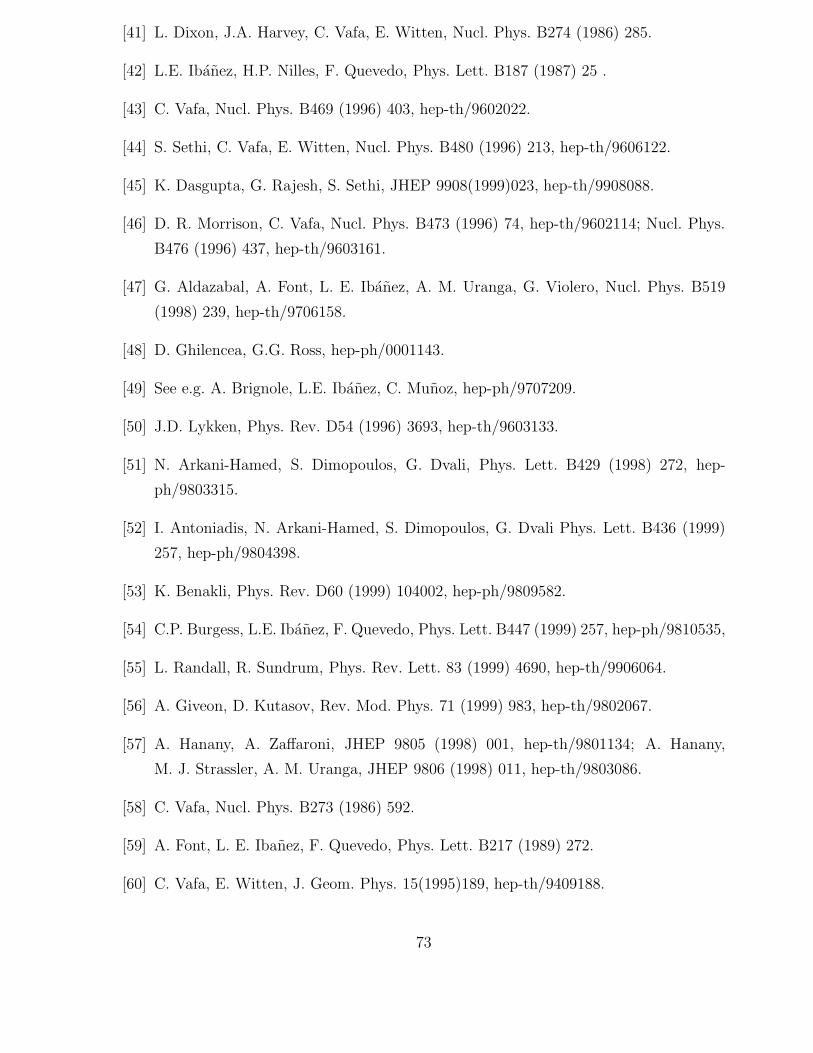
[41] L. Dixon, J.A. Harvey, C. Vafa, E. Witten, Nucl. Phys. B274 (1986) 285.

[42] L.E. Ibanez, H.P. Nilles, F. Quevedo, Phys. Lett. B187 (1987) 25 .

[43] C. Vafa, Nucl. Phys. B469 (1996) 403, hep-th/9602022.

[44] S. Sethi, C. Vafa, E. Witten, Nucl. Phys. B480 (1996) 213, hep-th/9606122.

[45] K. Dasgupta, G. Rajesh, S. Sethi, JHEP 9908(1999)023, hep-th/9908088.

[46] D. R. Morrison, C. Vafa, Nucl. Phys. B473 (1996) 74, hep-th/9602114; Nucl. Phys.

B476 (1996) 437, hep-th/9603161.

[47] G. Aldazabal, A. Font, L. E. Ibanez, A. M. Uranga, G. Violero, Nucl. Phys. B519

(1998) 239, hep-th/9706158.

[48] D. Ghilencea, G.G. Ross, hep-ph/0001143.

[49] See e.g. A. Brignole, L.E. Ibanez, C. Munoz, hep-ph/9707209.

[50] J.D. Lykken, Phys. Rev. D54 (1996) 3693, hep-th/9603133.

[51] N. Arkani-Hamed, S. Dimopoulos, G. Dvali, Phys. Lett. B429 (1998) 272, hep-

ph/9803315.

[52] I. Antoniadis, N. Arkani-Hamed, S. Dimopoulos, G. Dvali Phys. Lett. B436 (1999)

257, hep-ph/9804398.

[53] K. Benakli, Phys. Rev. D60 (1999) 104002, hep-ph/9809582.

[54] C.P. Burgess, L.E. Ibanez, F. Quevedo, Phys. Lett. B447 (1999) 257, hep-ph/9810535,

[55] L. Randall, R. Sundrum, Phys. Rev. Lett. 83 (1999) 4690, hep-th/9906064.

[56] A. Giveon, D. Kutasov, Rev. Mod. Phys. 71 (1999) 983, hep-th/9802067.

[57] A. Hanany, A. Zaffaroni, JHEP 9805 (1998) 001, hep-th/9801134; A. Hanany,

M. J. Strassler, A. M. Uranga, JHEP 9806 (1998) 011, hep-th/9803086.

[58] C. Vafa, Nucl. Phys. B273 (1986) 592.

[59] A. Font, L. E. Ibanez, F. Quevedo, Phys. Lett. B217 (1989) 272.

[60] C. Vafa, E. Witten, J. Geom. Phys. 15(1995)189, hep-th/9409188.

73

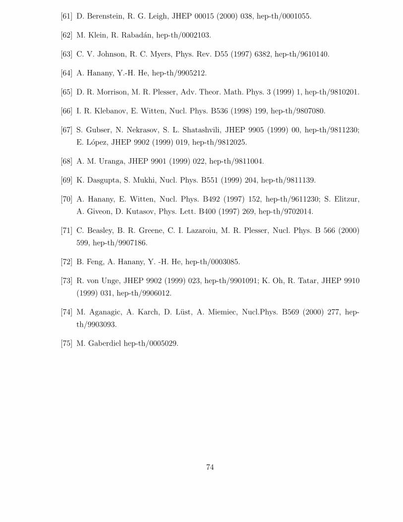
[61] D. Berenstein, R. G. Leigh, JHEP 00015 (2000) 038, hep-th/0001055.

[62] M. Klein, R. Rabadan, hep-th/0002103.

[63] C. V. Johnson, R. C. Myers, Phys. Rev. D55 (1997) 6382, hep-th/9610140.

[64] A. Hanany, Y.-H. He, hep-th/9905212.

[65] D. R. Morrison, M. R. Plesser, Adv. Theor. Math. Phys. 3 (1999) 1, hep-th/9810201.

[66] I. R. Klebanov, E. Witten, Nucl. Phys. B536 (1998) 199, hep-th/9807080.

[67] S. Gubser, N. Nekrasov, S. L. Shatashvili, JHEP 9905 (1999) 00, hep-th/9811230;

E. Lopez, JHEP 9902 (1999) 019, hep-th/9812025.

[68] A. M. Uranga, JHEP 9901 (1999) 022, hep-th/9811004.

[69] K. Dasgupta, S. Mukhi, Nucl. Phys. B551 (1999) 204, hep-th/9811139.

[70] A. Hanany, E. Witten, Nucl. Phys. B492 (1997) 152, hep-th/9611230; S. Elitzur,

A. Giveon, D. Kutasov, Phys. Lett. B400 (1997) 269, hep-th/9702014.

[71] C. Beasley, B. R. Greene, C. I. Lazaroiu, M. R. Plesser, Nucl. Phys. B 566 (2000)

599, hep-th/9907186.

[72] B. Feng, A. Hanany, Y. -H. He, hep-th/0003085.

[73] R. von Unge, JHEP 9902 (1999) 023, hep-th/9901091; K. Oh, R. Tatar, JHEP 9910

(1999) 031, hep-th/9906012.

[74] M. Aganagic, A. Karch, D. Lust, A. Miemiec, Nucl.Phys. B569 (2000) 277, hep-

th/9903093.

[75] M. Gaberdiel hep-th/0005029.

74