Currency-translated foreign equity options: The American case

CURRENCY-TRANSLATED FOREIGN EQUITY OPTIONS: THE AMERICAN CASE

Klaus Bjerre Toft and Eric S. Reinert

INTRODUCTION

As increasing numbers ofinvestors adopt global investment strategies they demand tools that make it possible to isolate and control sources of risk in international investments. Many of these risk factors are difficult to quantify and even harder to hedge. Uncertainty about the effects of central bank interventions and foreign expropriation is difficult to model in a systematic !'ashion. Other related factors such as currency risk under floating rate regimes and equity risk in local currency are easier to identify and manage if certain simplifying assumptions are made. In this paper we price four varieties of American currency-translated foreign equity options which help investors manage different types of risk associated with inter-

•Department of Finance, Graduate School of Business, University of Texas at Austin

tVice President, UBS Securities, Global Equity Derivatives

Advances In Futures and Options Reaearch, Volume 9, pages 233-164. Copyrlghl Cl 1997 by JAi Prest Inc. All rights of reproduction in IDY form reserved. ISBN: 0-7623-0125-2

233

234 KLAUS BJERRE TOFf and ERIC S. REINER

national equity investments. 1 Although techniques to price American currencytranslated foreign equity options exist.2 we show that all four varieties of options can be valued as if they were standard American options on a single underlying asset. Further, the local risk measures such as deltas, gammas, and so on can be obtained from the corresponding quantities for a standard American option.

Payoff definitions for the four different currency-translated foreign equity options are shown in Table 1. The exercise value of each option depends on both the foreign equity index and the foreign exchange rate.

A potential client for these options is an investor who either possesses or wishes to gain exposure to a foreign equity market. However, varying market outlooks and risk preferences will cause him to choose different payoffs. For example, consider an investor who holds neutral to bullish views on the performance of the foreign currency but is concerned about potential losses in the foreign equity's value measured in its own currency units. A long position in a foreign equity put with striking price in foreign currency (option type 1) provides a natural way to control losses measured in foreign currency. This option does not limit losses measured with respect to the investor's consumption numeraire, the domestic currency. Another investor may be indifferent to the level of the foreign index measured in foreign currency units. Instead, he is interested in protecting the value of his foreign equity investment in his own currency. Alternatively, he may be concerned with downside risk from both the equity and currency exposure. For him, a foreign equity put struck in domestic currency (option type 2) may be an appropriate hedging device. The third investor wants to protect himself against losses in the foreign index measured in foreign currency. He does not, however, want to bear any exchange-rate risk, even at the cost of giving up any currency appreciation. Thus, if the foreign index drops below the foreign strike, he wants the right to sell the index and get the strike in exchange, where the values of both the index and the strike are translated into the domestic currency at a fixed exchange rate. In essence, this investor wants to combine a foreign equity option with a quantity-adjusting currency forward which guarantees the exchange rate on the option's payoff. For this investor, the q uanto (option type 3) may be an appropriate hedging tool. Finally,

Table 1. Currency-translated Foreign Equity Options

This table shows the payoffs of the four different currency-translated foreign equity options analyzed in this paper. X denotes the foreign exchange rate, !f is the value of foreign equity measured in foreign currency, and Xis a constant multiplier or predetermined exchange rate. All options considered in this paper are American.

Option Type Call

Type 1 X max[Sf - Kf, OJ Type 2 max[SfX- K, 0) Type 3 X max[Sf -Kf, Ol Type 4 Sf max[X - K, O}

Put

X max[Kf - sf, OJ max[K - S tx, OJ X max{Kf - sf, OJ sf max[K - X, OJ

Currency-Translated Foreign Equity Options 235

the last investor cannot bear significant currency losses on his foreign equity investment. On the other hand he is willing to take full responsibility for fluctuations in the underlying equity index itself. This investor would likely be interested in the equity-Jinked foreign currency option (option type 4), where currency losses are controlled, but no protection against changes in foreign equity value is provided

A complete set of valuation formulas for the European counterparts to' the contracts considered in this paper is contained in Reiner ( 1992). Similar results are obtained by Derman, Karasinski, and Wecker ( 1990), Wei (l 992), Dravid, Richardson, and Sun (l 993), Gruca and Ritchken (l 993 ), and extended to stochastic interest rates by Wei (l 995).3 The research on American currency-translated foreign equity options is more fragmented. However, previously they have been analyzed by Ziemba (1991), Shaw, Thorp, and Ziemba (1995), Dravid, Richardson, and Sun (1993), Wei (1994), and more recently by Huang, Subrahmanyarn, and Yu (1996).

We focus on general pricing' arguments relating to American currency-translated foreign equity options. First, we show that the pricing problem for all four option types can be reduced to that for an American option on a single underlying asset. Consequently, each can be valued using a standard technique such as the Cox, Ross, and Rubinstein (1979) algorithm.4 Our pricing results, therefore, extend those of Reiner ( 1992) to American options.

We evaluate each of the American currency-translated foreign equity options by carefully 'choosing appropriate numeraires. For example, option type 2 is most easily evaluated when both the option value function and the state variables are denominated in domestic currency. For option type 1, however, it is convenient to measure option values and state variables in terms of foreign currency units. This change of numeraire, coupled with the properties of the PDE and its boundary condition, allows us to simplify the pricing PDE into one expressed as a function of a single state variable. 5

The applied nwneraire change is a special case of a general result presented in the Appendix. Result 1 in the Appendix shows that it is possible to transform an (n + 1)-dimensional pricing PDE with both option value and state variables denominated in one numeraire (i.e., domestic currency) into a pricing PDE with option value and state variables expressed in terms of another numeraire (i.e., foreign currency). This nwneraire change does not alter the structure of the PDE, but it changes the PDE 's coefficients. A corollary to this result shows that the replication portfolio is independent of the choice of numeraire. A similar result is derived by Geman, Karoui, and Rochet(l995).6

For other types of options such as option type 3 (the quanto) and type 4, the reduction in dimensionality is obtained by denominating option value and state variables in different numeraires. The PDE transformation we use to price the quanto option is an application of another general result derived in the Appendix. Result 2 in the Appendix transforms an (n + !)-dimensional pricing PDE with option value and state variables denominated in a single numeraire into a pricing PDE with the state variables expressed in other-possibly multiple--numeraires.

236 KLAUS BJERRE TOFT and ERIC S. REINER

This numeraire change again leaves the structure of the PDE unaltered, but modifies the PDE's coefficients. It is this change ofnumeraire that allows us to reduce the dimensionality of the pricing PDE for quanto-type option structures.

Finally, we use the pricing results to derive hedge parameters for the four option types in terms of the corresponding values for a single-asset American option. This allows us to use hedge ratios and sensitivities computed by a one-factor American optibn pricing algorithm to detennine the corresponding quantities for the twofactor pricing problems considered in this paper.

The remainder of the paper is organized as follows. The second section deriv~ and discusses the pricing results. This section also relates the pricing results to the general transformations perfonned in the Appendix. The third section derives a complete set of hedge parameters, and the final section summarizes our results.

THE PRICING RESULTS

Valuation of derivative securities written on assets denominated in several currencies can be obscured by payoff functions that depend on variables in different denominations. For currency-translated foreign equity options of types I and 2 the valuation problem can be greatly simplified by denominating option values and state variables in terms of a single numeraire. This change of numeraire immediately transforms the pricing problem to a point where standard techniques can be used for valuation and hedging purposes. Options of types 3 and 4, on the other hand, are most easily priced when the option value and state variables are denominated in different numeraires.

Assumptions

The contingent claims considered in this section are specified in terms of two state variables: a foreign exchange rate,X, and the value of foreign stock, sf, where Xis the domestic currency value of a unit of foreign currency and sf is expressed in units of foreign currency. 7 Both assets are traded continuously and are assumed to follow geometric Brownian motions,

(I)

and

dX = ( T) - r1 )Xdt + cr ~dro j.J). (2)

sf has a total continuously compounded mean rate of return µ and a proportional payout rate o. The corresponding parameters for the exchange rateXare Tl and rt Uncertainty is introduced by IDsf(t) and roj_t) which are correlated stan~~ Brownian motions defined on a complete probability space (0, ~ ~. The volatthties of and correlation between the two price processes are expressed as constants


(as'• crxi and Psi ,x) but the analysis herein is easily extended to volatilities expressed as well-behaved deterministic functions of time. Risk-free bonds are traded in both the foreign and the domestic economies; the domestic and foreign risk-free interest rates, r and rp are assumed to be constants, although our treatment is also easily generalized to the situation where they are bounded deterministic functions of time. The foreign stock price, sf, is denominated in foreign currency units (FC per share), whereas the exchange rate, X, is the price of one unit of foreign currency in domestic currency units (DC per FC). The payoffs of all of the options considered in this paper may be expressed in terms of these price processes. However, for the purposes of pricing and hedging it is often more convenient to express these payoffs as functions of variables traded in the same economy; the equivalent martingale measure and the accompanying risk-neutral asset price processes can be written down immediately when all state variables are expressed in the same denomination.

For the foreign investor the traded currency or exchange rate is given by l/X, which we shall denote xt (this process is in units of FC per DC). The process Xf is completely described by the process for X as8

d)(f = (rr ri + a})Xf dt + axrXI droxr(t),

where rox(t) =-rox1(1), and ax! = ax- Finally, for the domestic investor the traded equity is not Sf, but S = S/)(. The price process for S, denominated in domestic currency units, is given by

The two underlying state variables are now expressed in both domestic and foreign currency units and equivalent martingale measures can readily be constructed with respect to both numeraires.

All option values considered in this paper are initially expressed as functions of both asset price variables and time. To simplify notation, dependence on the state variables is often omitted, that is, C = C(t) = C(sf (t), X(t), t). Early exercise is modeled by separating the state space into a continuation and an early exercise region. Let the semi-open set C (sf, X, t) e ~"'2 >< (0, T) denote the continuation region, that is, if (sf, X, t) e C(Sf, X, t), then C(sf, X, t) is greater than the early exercise value. When (Sf,x, t) leaves the continuation region, the option is exercised, and C(Sl,X, t) is defined by the option's payoff function. Let te denote the first time the state variables leave the continuation region, that is, te = inf{i > 0 : cst.x. t) ~ C). The early exercise region may be specified in terms of any combination of the variables that span the state space. However, optimal early exercise must be the same no matter what denomination is used. Otherwise, the value of the contingent claim differs for investors located in different economies; this contradicts the law of one price.


Foreign Equity Options with Foreign Strike

We now evaluate the simplest of the four currency-translated foreign equity options, the foreign equity option with foreign strike. This option's payoff is

C(Sf(t,),X(t,), t,) =X(t,.)max[Sf(te)-Kf, OJ.

The law of one price implies that the value of this option in the domestic economy, C(t), equals the value in the foreign economy translated back into domestic currency at the prevailing exchange rate, that is, cf (t)X(t); otherwise arbitrage opportunities exist. The payoff in the foreign economy, ct (t,.) = C(t,.)>:f (t.,). is given by

Cf(Sf(t,), t,.) = max[Sf (t,)-Kf, O].

Note that the value of the option in the foreign economy does not depend on the exchange rate; all payoffs are expressed in foreign currency units, and the exchange rate does not appear anywhere in the payoff definitions. Under the equivalent martingale measure in the foreign economy the foreign index, sf(t), is lognormally distributed and fully described by its initial value Sf(O) and the stochastic differential equation

dsf = (r1 - o)Sf dt + a51Sf dro ~(t),

where ro ;t(t) is a new standard Brownian motion obtained from Girsanov's theorem. The valuation problem in the foreign economy is the well-known free boundary problem from the theory of American options. This can be solved using any suitable numerical procedure such as Cox, Ross, and Rubinstein's binomial approximation to the value of an American option on a dividend paying stock.

Let AC(S, K, r, o, a, 't) denote this American call option value where S, K, r, 5, a, and 'tare dummy arguments for the underlying asset price, strike, continuously compounded interest rate, continuously compounded dividend yield, volatility, and time to maturity, respectively. The value of the foreign equity option in the foreign economy is

Cf(t) =AC(Sf (t), Kl, r1, o, a51, T- t).

The value in the domestic economy equals, by the law of one price, the value in the foreign economy multiplied by the exchange rate,X. Using homogeneity in the first and second arguments of an American option's value leads to the first proposition.

Proposition 1. Under this paper's assumptions the value of an American foreign equity call struck in foreign currency is

C(t) = AC(Sf (t)X(t). KfX(t), rp o, as1, T- t).

Correspondingly, the value of an American foreign equity put struck in foreign currency is

Cwrrency-'Iranslated Foreign Equity Options 239

P(t) = AP(Sl(t)X(t), KfX(t), rf' 6, as1, T- t).

The r.esult for the put 's value follows directly by changing the form of the boundary condition and repeating the argument.

The above pricing result was obtained by denominating option value and state variables in foreign currency units. Alternatively, the option value, pricing PDE, boundary condition, and state variables could have been denominated in domestic currency units, and subsequently transformed into corresponding quantities de· nominated in foreign currency units. We perform this type of transformation of the pricing PDE and boundary conditions with option value and state variables den~minated in one numeraire into one with value and state variables denominated in another numeraire in the Appendix for a general pricing PDE with n state variables. For option type I this transformation, coupled with the fact that the transfonned boundary condition and PDE are invariant to changes in the value of foreign currency which leave the value of foreign equity (Sf) unchanged, results in pricing formulas identical to those of Proposition 1.

Foreign Equity Options with Domestic Strike

In the previous section we demonstrated how a few arguments simplified the valuation ofa foreign equity option with a foreign strike. In this section equally simple arguments are used to value a foreign equity option struck in domestic currency. The exercise cash flow from a foreign equity option with domestic strike is given by

C(Sf (te), X(t,), t,) =max[ Sf (t,)X(t,.) - K, O].

The valuation of this type of option is particularly simple. From a domestic investor's perspective the value of foreign stock is sf ( t)X(t), previously defined as S(t). This is the traded asset in the domestic economy. The payout rate on this asset remains 15. Under the equivalent martingale measure in the domestic economy, the continuously compounded mean growth rate of S(t) is (r - 15) with a total mean rate of return of r. The volatility of the traded a8set, S(t), is obtained by Ito's lemma as

a5= "a2st+ a}+2Ps'.Ps'ax.9

Consequently, the option isa standard American option on an asset with payout rate o and volatility as

Proposition 2. Under this paper's assumptions the value of an American foreign equity call struck in domestic currency is

C(t) = AC(Sf (t)X(t), K, r, 6, aSt T- t).

where

240 KLAUS BJERRE TOF'f and ERIC S. REINER

0 s = '\/a2s1+ a}+ 2Ps',x0 s'0 x·

Correspondingly, the value of an American foreign equity put struck in domestic currency is

P(t) = AP(Sf(t)X(t), K, r, o, as, T- t).

Most of the parameters in this fonnula can be observed in or inferred from the marketplace. In particular, if foreign equity and foreign currency options are traded in liquid and competitive markets, implied volatilities can be used as input parameters. 10 Only the correlation between the foreign index and the exchange rate needs to be estimated. Alternatively, one could consider the domestic value of foreign stock to be the primitive input variable, and therefore estimate and use the parameter as directly in the valuation model.

Foreign Equity' Options with Foreign Strike and Fixed Exchange Rate

The foreign equity option with payoff translated back into domestic currency at a fixed exchange rate (a quanta) is slightly more complicated to evaluate. The quanto's payoff in domestic currency is defined as

(4)

where Xis a DC per FC denominated constant. The left-hand side of {4) is denominated in domestic currency. However, the payoff on the right-hand side is specified in terms of s', a security that is traded in foreign-not domesticcurrency.

To price a derivative asset in domestic currency, we begin with the fundamental PDE and boundary conditions expressed in tenns of domestically traded assets. The PDE is given by:

C,+ (r- o)SC5 + (r-r1)XCx

1--22 1.-22 +1¢.sS Cs,s+ Ps • .r:sscrxSXCs.x+2¢.0' Cx.x=rC,

(5)

while the payoff must be rewritten as:

C(S(te), X(te), t11) = X max [S(te) - Kl, o] . X(te)

At this point we observe that the PDE (5) and the modified boundary condition are homogeneous under transformations of Sand X which leave st unchanged. Consequently, we may derive a new fundamental PDE for the valuation of domestically denominated payoffs which depend only on the foreign denominated asset sf. We write

Currency-Translated Foreign Equity Options

C(S,X, t)= {sf =f, 1).

Finding partial derivatives

C,=C1,

I Cs.s= xi cs'.s'•

2sf (sf)2

Cx.x= xi Ct+ x2 Cs1,s1.

I Cs= xcsr.

s' Cx=- xCsf,

and substituting these into the fundamental PDE results in:

c, + (rF c5 ~ Ps'.Jfls'ax)Sf C5.r+ f a~r(sf)2C5t,st= rC,

241

with boundary condition given by the right hand side of(4), which only depends on Sf. 11 Finally, adding and subtracting rs! C 51 on the left-hand side of the PDE yields:

This is the fundamental PDE for a contingent claim on a single underlying asset with interest rate rand dividend yield c5 + r - r1+ Ps'. JP 5.ra x subject to the boundary condition (4).

Ifwe examine (6), we see that Sf has the same risk-neutral drift it would have in the foreign economy, but with an additional term in the covariance rate of the returns of Sf and X. We can understand how this comes about by considering how we would protect the domestic value of a share of foreign stock from changes in the exchange rate. We must first recognize that the share carries an exchange rate exposure equal to its price. To offset this exposure over the next instant of time, we borrow Sf units of the foreign currency. We invest the proceeds in domestic bonds. The instantaneous retwn on our portfolio is given by

The terms in this equation represent the domestic value of the share of stock's capital appreciation, dividend payouts, capital losses on the short currency position, interest paid in the foreign currency, and interest earned on domestic lending. Applying Ito's lemma and substituting equations (2) and (3) into (7), we find that the instantaneous return simplifies to


In addition to the net return and the dividends paid on sf during the interval dt, we earn the net proceeds (r - rf)Sf Xdt of lending the stock's value in domestic currency and borrowing it in foreign currency. Holding the foreign share realizes the effect of any correlation between movements in sf and X, while the currency hedge does not; this is the reason for the appearance of the Psl,.Psto xSf Xdt term. lfthere existed a traded asset worth Sf in domestic currency at all times, that asset would realize neither the gains nor the losses of the dynamic strategy outlined here. For there to be no arbitrage opportunities given the price processes for the foreign traded sf and the exchange rate x, the domestically traded sf must pay dividends at a proportional rate equal to (o +r- rf+ Ps' • .Ps"'x)·

We have reduced the two-asset valuation problem to one in a single asset variable. Hence, the resulting free boundary problem for C is precisely that for a standard American option on sf as if it were a domestically traded asset with a modified dividend yield. This leads to our third proposition.

Proposition 3. Under this paper's assumptions the value of an American foreign equity call struck in foreign currency, translated back at a guaranteed exchange rate is

Correspondingly, the value of an American foreign equity put struck in foreign currency, translated back at a guaranteed exchange rate is

Proposition 3 was obtained by transforming the pricing problem with option value, PDE, state variables, and boundary condition denominated in a single consistent numeraire (domestic currency) into one with option value denominated in domestic currency but with the value of foreign equity denominated in foreign currency units. Since the boundary condition and the PDE are invariant to changes in the value of foreign currency which leave the value of foreign equity (Sf) unchanged, the PDE's dimension is reduced by one. The employed PDE transformation is a special case of the one presented in Result 2 of the Appendix. This result shows that the structure of a pricing PDE with n state variables does not change when one or multiple state variables have numeraires different from that of the option value. However, the coefficients of the PDE change to reflect the numeraire change. For example, the coefficient of the first-orderterm sf oC/ oSf in the pricing PDE for the quanto option equals the payout rate on sf•s numeraire asset (r) less the payout rate on foreign equity Oi) less the covariance rate between sf and X (p s' .XO sfO x)•

Currency-'Il'anslated Foreign Equity Options 243

Equity-Linked Foreign Currency Options

An equity-linked foreign currency option is evaluated in the same way as a quanto. Again, the key to the problem is to express all values in tenns of assets traded in one economy. The structure of the boundary condition can then be used to simplify the fundamental PDE. To begin, the payoff of the equity-linked foreign currency option in domestic currency is given by

(8)

This is written as a function of assets not traded in the same economy. Next, translate the payoff into foreign currency units:

f I Sf(t,) C (S (t,), X{t"), t.) = -( -) max[X(t.,) - K, O],

XI t.,

and rewrite it in tenns of foreign traded assets:

The exercise cash flow is now transfonned into that of a currency put multiplied by sf (t,); this is homogeneous in the foreign stock price. Since the fundamental PDE is also unaltered by changes in the stock price, the value of the option in the foreign economy can be written as

Finding the partial derivatives

cf=sfnf I t'

C{t,sr=O,

C{1,;1= SfH1x1.x1,

C~::Hf.

C1x1=SfH'x1,

Cfr,s'= Hy, and substituting these into the fundamental PDE, dividing by sf, and adding and subtracting fJXfHy on the left-hand side yields:

H{ + [o - (o + r- rr Ps' .,rta81axlJJXfHfr+ t a2x1(Xf)2H{1,x1= oH'. (9)

with the boundary condition

Hf(Xf(IJ, t") = max[l - KXf(t,), O].

It is helpful to interpret the simplifications we have obtained. The payoff (8) can be understood as that of an option to exchange K units of quantoed equity for the domestic value of a foreign share. Since the payoff and the fundamental PDE in

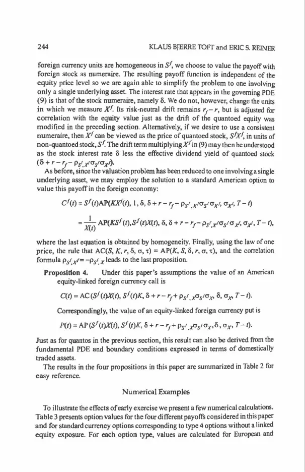
244 KLAUS BJERRE TOIT and ERIC S. REINER

foreign currency units are homogeneous in Sf, we choose to value the payoff with foreign stock as numeraire. The resulting payoff function is independent of the equity price level so we are again able to simplify the problem to one involving only a single underlying asset. The interest rate that appears in the governing PDE (9) is that of the stock numeraire, namely a. We do not, however, change the units in which we measure XI. Its risk-neutral drift remains r1- r, but is adjusted for correlation with the equity value just as the drift of the quantoed equity was modified in the preceding section. Alternatively, if we desire to use a consistent numeraire, then xt can be viewed as the price of quantoed stock, six!, in units of non-quantoed stock, Sf. The drift term multiplyingXI in (9) may then be understood as the stock interest rate a less the effective dividend yield of quantoed stock (B + r - rr Ps1.,x1c:Js'crx1).

As before, since the valuation problem has been reduced to one involving a single underlying asset, we may employ the solution to a standard American option to value this payoff in the foreign economy:

Cf(t) = sl(t)AP(KXf(t), l, &, o + r- r1- p51,x1CJ51CJx1, axi, T-t)

=-1-AP(KSl(t),Sl(t)X(t), &, o + r- rr Ps'.xlasfax', CJxf, T- t), X(t) ·

where the last equation is obtained by homogeneity. Finally, using the law of one price, the rule that AC(S, K, r, o, cr, T) = AP(K, S, o, r, a, T), and the correlation formula Ps1.x'= -Ps', x leads to the last proposition.

Proposidon 4. Under this paper's assumptions the value of an American equity-linked foreign currency call is

C(t) = AC(Sf(t)X(t), Sl(t)K,o +r-r1+ p51.x051ax, a, aX> T-t).

Correspondingly, the value of an equity-linked foreign currency put is

P(t) = AP(SI (t)X(t), sf (t)K, o + r- r1+ Ps'.x'Jslax,5, ax, T- t).

Just as for quantos in the previous section, this result can also be derived from the fundamental PDE and boundary conditions expressed in terms of domestically traded assets.

The results in the four propositions in this paper are summarized in Table 2 for easy reference.

Numerical Examples

To illustrate the effects of early exercise we present a few numerical calculations. Table 3 presents option values for the four different payoffs considered in this paper and for standard currency options corresponding to type 4 options without a linked equity exposure. For each option type, values are calculated for European and


Table 2. Summary of Valuation Results

This table shows the parameter substitutions that must be made to evaluate the four types of currency-translated foreign equity options considered in this paper as standard American options. lie11= r.11=li + r-r,+ Ps~XCSsfox and o~ = a~f + aJc + 2p5t,xa5tox.

Option Type Asset Strike Interest Riite Dividend Yield Volatility

Typel stx Fix 'f 1> a1 Type2 SfX K Ii as Type 3 stx I<fx lie11 atj iype4 stx gK relf o ox

American calls and puts. The parameter values are selected to illustrate the environment faced by a German investor interested in currency-translated foreign equity options on the Nikkei index. The value of the foreign index is 20,000 yen per share with a dividend yield of I percent per year. Since the correlation between the yen-denominated Nikkei index and the exchange rate in DM per yen varies over time, we calculate option values using correlations equal to-0.5, 0.0, and 0.5. The exchange rate is assumed to be 0.015 DM per yen. The volatility of the foreign index is 20 percent per year, and the exchange rate volatility is 15 percent per year. The Japanese and German term structures of interest rates are assumed to be flat

Table3. Numerical Examples

Values of the four opticn types considered in this paper. To facilitate the analysis of option type 4, values of a standard currency option on a notional amount of one index unit are listed as option type 5. g = 20,000 yen/index unit, X = 0.015 DM/yen, r = 0.06;;{ = 0.02, Ii = 0.01, a5! = 0.2, and ax = 0.15. All options are at-the-money and have one year 1 to maturity. The calculated effective volatilities o, for type 2 options are 18.0%, 25.0%, and 30.4% for Psf,x values of --0.5, 0.0, and 0.5, respectively. The corresponding values of lieff and r elf are 0,035, 0.050, and 0.065.

Calls Puts

Option Type Exercise I>= --0.5 p= 0.0 p=0.5 p =--0.5 p=O.O p=0.5

Typel European 25.05 25.05 25.05 22.09 22.09 22.09 American 25.05 25.05 25.05 22.38 22.38 22.38

Type2 European 28.85 36.64 42.74 14.36 22.15 28.25 American 28.85 36.64 42.74 15.98 23.79 29.91



Type5 European 23.61 23.61 23.61 U.08 12.08 1208 American 23.61 23.61 23.61 13.40 13.40 13.40


with yields of 2 and 6 percent per year, respectively. Finally, the options have a maturity of one year and the striking prices are constructed such that all options are at-the-money.

For option type I, the foreign equity option, the DM values are independent of the correlation. The dividend yield on the Nikkei is not large enough to imply a sizable early exercise premium for the American call options. For the puts, the early exercise premium is positive but, as expected for a small interest rate-dividend yield differential, not very large.

Values for the foreign equity option with a domestic strike, option type 2, are highly sensitive to correlations between the Nikkei index and the exchange rate. A larger correlation implies a higher effective volatility; this translates directly into higher option values. Since the domestic risk-free interest rate is 6 percent per year and the dividend yield is I percent per annum, the optimal exercise boundary lies far from the strike level. Consequently, the possibility of early exercise does not result in a significantly higher value for the American call option. However, American put option values are substantially higher than those of the corresponding European options. This result is in contrast to that for option type I and comes from the greater difference between the domestic interest rate and the dividend yield.

The tabulated quanto values (option type 3) illustrate two interesting results. First, the value of the quanto call is decreasing in the correlation. This follows directly from the higher effective dividend yield. Second, when the correlation between the Nikkei and the exchange rate is 0.5, the early exercise premium for the American call is quite significant. This is also caused by a high effective dividend yield of 6.5 percent per year, which implies that the option, if exercised at all, will be exercised early. When the correlation is -0.S, the early exercise feature has a much less pronounced value (in this case, the effective dividend yield is 3.5 percent per year). The opposite effects are observed for quanto puts. Indeed for a correlation of0.5 the early exercise premium is quite small because the effective dividend yield is greater than the interest rate. This results in a positive probability that the put will be held to maturity since the limiting value of the early exercise boundary as I-+

Tis rldctr= 92.3 percent of the strike level. Comparison of the valuation results for type 3 options to those of types I and 2

is also instructive. It is simpler to begin with the domestic strike options. Except for the cases of strong negative correlation, Ps'.x= -0.5,. between stock and exchange rate returns, American and European quanto calls and puts are significantly less valuable than their type 2 counterparts. This is the case because the effective volatilities a5 for options with domestic strikes are substantially greater than the stock volatility a51; this illustrates the point that quantos possess optionality only with respect to the foreign stock price and not also with respect to the exchange rate as do options of type 2. For Ps',x values of 0.0 and 0.5, O's is equal to 25.0 percent and 30.4 percent, respectively. In contrast, when Ps' x equals--0.5, as takes on the value of 18.0 percent, which is smaller than O'sf. For this correlation value, the type 2 calls remain more valuable than those of type 3 because the effect


of a lower volatility is more than offset by that of the difference between the dividend yields S = 0.01 for the fonner and Serr= 0.035 for the latter. Indeed, this explains why the difference between type 2 and type 3 call values is always more positive than for puts. This difference rises with Ps',x as 3err increases. For puts at the lowest correlation value, both volatility and dividend effects combine to make type 3 options more valuable than type 2 options.

Comparison of quanto values to those of foreign strike options also requires consideration of two effects. The first is that of the interest rate differential r - '!" In changing from the payoff of type I to that of type 3, this differential appears m two ways. The first is the change in the rate used to discount the strike from r1 to r. The second is the addition of r - r1 to the dividend yield to obtain aell' (neglecting correlation). These combine to make both quanto calls and puts less valuable than their type I equivalents for most of the market parameters considered here. 12 The second e'ffect to be considered in comparing type 1 and type 3 option values is that of correlation. Since an increase in Ps',x increases 3eft' while leaving the interest rate used for discounting unchanged, positive correlations will raise the values of quanto puts and lower those of quanto calls from the values of type I options. The opposite results hold for negative values of Ps'.x- For correlations of such magnitudes as those considered in Table 3, this effect can be large enough to dominate that of the interest rate differential.

The correlations of most indexes with exchange rates are small. Consequently, the two considerations faced by an investor who wishes to purchase a foreign equity option are the effective volatility (as' versus cr5) and the interest rate/effective dividend yield (r1 versus rA> versus Serr>· Since a5 is always greater than O's' for positive or small negative correlations, the cost of the currency protection afforded by type 2 options can sometimes be prohibitive. In contrast, type 3 options also provide a fonn of protection against adverse currency moves without altering the underlying volatility. If the interest rate differential r - r1 is positive, both considerations work to lower the premium faced by an investor; this helps explain the exceptional popularity of quanto options on indexes in countries with low interest rates with payoffs in higher interest rate currencies.

The values of options of type 4 (equity-linked foreign currency options) display effects similar to those seen for quantos. Here, however, call prices are increasing and put prices are decreasing in Ps' X' This is the case because increases in the correlation raise the effective interest rate. Since the dividend yield is small, early exercise opportunities for calls of type 4 are quite limited. The puts, however, display an increasing early exercise premium in Ps',x since larger values of 'err provide a disincentive to delaying exercise. It is also instructive to compare our type 4 results to those labeled type 5, standard currency options on a notional amount equal to the spot value of one index unit. For zero correlation, all type 4 values arc slightly greater than the corresponding type 5 quantities. This is the case because in changing from a currency option with fixed notional to one with equity-linked notional both the domestic and foreign interest rates are reduced by

248 KLAUS BJERRE TOFI' and ERIC S. REINER

rf- S. Consequently, both call and put values are larger by a factor of '-'rtiXT-1>. The corresponding American options are also more valuable than their type 5 counterparts, but by a smaller factor. 13 Since the standard currency option values are independent of the correlation, the effect of varying p on the difference between type 4 and type 5 prices is entirely explained by the correlation dependence of the former.

SENSITIVITIES AND HEDGE PARAMETERS

To discuss the sensitivities of currency-translated foreign equity options to changes in the input parameters, we assume the availability of an American option evaluation procedure which, in addition to a value, provides the user with precise first and second derivatives with respect to the underlying asset value and first derivatives with respect to all other parameters.

The hedging problem can be approached from the perspective of either a foreign or a domestic book runner. The resulting hedge portfolio does not depend on the route taken to derive the deltas. The Appendix shows that this result holds for derivative securities with payoffs that depend on multiple state variables.

If one takes the perspective of the domestic hedger, one simply writes the value in domestic units as a function of the traded assets in the domestic economy (S =sf X, and X) and applies the chain rule for partial derivatives. This gives the quantities of foreign stock and currency from which the domestic cash holding may then be derived.

Alternatively, one can use the value function expressed in terms of foreign currency units. The partial derivatives with respect to the foreign index level, sf, and the price of domestic currency in the foreign economy, xi, yield the holdings of foreign stock and domestic currency (foreign currency from the perspective of the foreign hedger). The foreign currency holding (domestic from the foreign perspective) is detennined from the price of the option in foreign currency and the value of the foreign stock and domestic currency holdings.

To illustrate the derivation of the hedge portfolio we will use option type 3, the quanto, as an example. Recall that the assets traded in the domestic economy are S =sf X and X and rewrite the value of the quanta as a function of assets traded in the domestic economy

C(t) =AC XX, Kl X, r, deff' ersl, T- t . (six- - )

The number of foreign shares in the hedge portfolio is defined as the partial derivative of the value function with respect to sf X,

C = oC(t) -~AC s- o(SfX) - X s•


where ACs is the partial derivative with respect to the underlying asset obtained from a standard American option price calculator.

The foreign cash in the hedge portfolio is given by

c =acct> =-six Ac x ax x s·

This implies that the currency exposure obtained from the long position in the foreign asset must be exactly offset with a short foreign currency position. Consequently, a correctly adjusted quanto hedge has no net currency exposure. Finally, the last component of the hedge portfolio, the domestic cash holding, equals the domestic value of the option. This portfolio precisely parallels the dynamic hedging strategy for quantoed equity outlined in an earlier section.

The gammas and cross-gammas are derived from the above deltas as

x-2 Cs.s= .xzACs.s•

x sli2 Cs,x= - x2 ACs- x2 ACs.s•

six (SfX)2

Cx,x=2 xi AC5+~ACs.s•

where ACs.,s is the second partial derivative of the AC value with respect to the underlying asset. For hedging purposes, we are also concerned with the sensitivities to changes in volatilities and correlation in addition to sensitivities to shifts in the domestic and foreign interest rates and the dividend yield on the foreign asset. The former are important if the hedger wishes to use other options to offset volatility and correlation risk. The latter are useful in matching durations of the three exposures into which the option value is decomposed. Although the input volatility parameter for the quanto is CJ sf, the volatility of foreign currency and the correlation between the foreign asset and the exchange rate enter into the pricing relationship in the form of an adjustment to the dividend yield. Consequently, the sensitivities to the volatilities and the correlation are

where AC., and ACti are the partial derivatives of the AC-value with respect to the volatility and the dividend yield, respectively. Finally, the sensitivities to changes


in the domestic and foreign interest rate and the dividend yield on the foreign asset are given by

The time decay of the quanto can be taken directly from the American option calculator.

Table 4 summarizes the substitutions that must be made to convert the output parameters from a valuation model for American options into sensitivities used to hedge the four types of currency-linked foreign equity options.

Table 4. Summary of Hedging Results

11lis table shows the transformations of a standard American option's (AO) sensitivities that must be made to calculate the corresponding sensitivities of the four types of currencytranslated foreign equity options considered in this paper:. Sensitivity Type 1 T!fpe 2

Cs AOs A Os

Cx AO x--sfAOs

0

Cs.s AOs,s AOs,s

Cs,x -sfAOs,s 0

Cx,x (Sf)2A0s.s 0

Co sf A00 ( ast+ Psl.x"x ) AO., ~f + ai + 2p5~xtJsfax

c.,x 0 ( ax+PsfxCsf ) AO ' " aV + ai + 2pst ,xastax

CPsf)I 0 ( axesf ) AO., ~f + ai + 2p5t ,xastax

c, 0 AO,

c,, AO, 0

C5 A06 A05

c, A01 A01

(continued on next page)

Crmency-11-anslated Foreign Equity Options 251

Table4. (Continued)

S..liirity ~3 'JY1¥4

Cs x - 1-AO XAOs sfx

Cx - 5: AOs

AO ---x+SfAOs

Cs.s Xi x'2 AOs,s

0

Cs.x x !fx2 AO A Os -if. A05 - x'2 AOs.s ---+-

sfx'2 x Cx.x stx <s'xr

2}(TA05+~A05.s AO Sf f

2X2"-2 XA05 + s AOs.s

Casf AOo + Psf ,xoxAD& Ps~x.GxAO,

Cox Psf,xastA<Ja AOo + Psl.xasfAO,

CPsf.x asfOxA06 crsfOxAOr

C, AO.+A06 AO,

c., -A011 -AO,

c,, A06 AO,+AOg

Ci A01 AO,

Together, Tables 2 and4 show how to use a standard one-factor American option pricing model to price and hedge four types of currency-translated foreign equity options: First, use Table 2 to compute the input parameters. Second, input these numbers into a standard American option pricing routine which computes an option value and a set of hedge parameters. Finally, use this set of hedge parameters and the results presented in Table 4 to compute hedge parameters for the four types of currency-translated foreign equity options.

CONCLUSIONS

Evaluation procedures for four different types of currency-translated foreign equity ortions with payoffs expressed as functions of two underlying price variables simplify to well-known American option pricing problems with one asset variable. The key to solving the first two problems is to write the values and payoffs as functions of state variables expressed in the same currency units. After this


transfonnation, the pricing problem for the foreign equity option struck in either domestic or foreign currency is a standard American option pricing problem.

The last two option types considered in this paper, the quanto and the equitylinked foreign currency option, require further simplification. Using properties of the option payoffs and the general PDEs satisfied by derivative securities in the domestic and foreign economies, the last two pricing problems also simplify to standard pricing problems in one state variable. A single-factor American option pricing model such as that of Cox, Ross, and Rubinstein (1979) may therefore be used to value and hedge all four types of currency-translated foreign equity options.

ACKNOWLEDGMENT

The authors would like to thank Hua He and William Keirstead for their valuable comments. All remaining errors are the authors' responsibility. The first author gratefully acknowledges financial support from the Danish Social Science Research Council, grant no. 14-6076.

NOTES

I • Al least three of the contract types have been or are traded on exchanges. For a survey, see Dravid, Richardson, and Sun ( 1993), and Zuraclc, Lim, and Young (1990).

2. See discussion below. 3. See also Babbel and Eisenberg ( 1993) for a related analysis. 4. Alternative-and more efficient-American option pricing algorithms exist. For a survey and

numerical comparisons see Broadie and Detemple (1996). 5. Otherauthon have used numeraire changes to simplify option valuation problems. Merton ( 1973)

extends the Black-Scholes ( 1973) model lo a stochastic interest rate environment by using a uro-coupon bond as numeraire. Margrabe (1978) changes the numeraire to a risky asset in order to detennine the value of an option to exchange one risky asset for another. Other examples of convenient numeraire changes are contained in Harrison and Kreps (1979), Rubinstein (1991), Jamshidian (1996), Flesaker and Hughston ( 1996), and Koc:ie ( 1997).

6. Geman, Karoui, and Rochel (1995) construct a martingale measure for asset price processes denominated in a numeraire different from that used to construct the original martingale measure.

7. Quantities denominated in foreign currency units (e.g., Danish kroner for a U.S.-bl!sed investor) are represented with a superscript f. Asset prices in domestic currency units (e.g., dollars for a U.S. investor) arc represented without a superscript.

8. Apply Ito's lemma. 9. Technically, it is slightly more involved than just applying Ito's lenuna. One must also define a

new Brownian motion from (3) as

asfCJls/(t) + axCJl,rlt) (1)5(1) = 2 •

VaSf + ai-+ 2ps',~sfax

Using this new Brownian motion, the volatility of the traded asset is given by as. It is e&5Y to verify that tbis process is indeed a standard Brownian motion. Finally, using Girsanov's tbeorem to construct the equivalent martingale measure does not change the volatility of the underlying asset.

I 0. Here, we ignore a set of interesting issues caused by the volatility smile. 11. Rigorously, for each of the payoffs analyud in this paper we also require suitable restrictions

on the limiting behaviorofC(·,., ·)as each asset price which appears as an independent variable in the

Currency-'Iranslated Foreign Equity Options 253

governing PDE approaches 0 and +<io. In practice, the forms taken by these restrictions and their behavior under the transformations performed here are trivial.

12. Since equity-currencycorrelations are often small, this explains the often-encountered fonnula for European options:

(Quanto value) = e(rrr)(T- r)('fype 1 value).

This relation holds for p = 0.0 for both calls and puts since the argwnents of the cumulative normal distribution functions in Merton's ( 1973) fonn of the Black-Scholes formula are unaltered by addition of the same quantity to both the interest rate and the dividend yield. Alternatively, the fixed exchange rate X may be set at the fon11ard price xe<•- rj*.T- •>, yielding a quanto value equal to that of the corresponding type I option. for American-style exercise, the interest rate differential has a similar but reduced effect. To see this, we first note that the risk-neutral drift of the quantoed equity price process is unaffected by the interest rate differential. However, since the present value of any exercise ea&h flow is affected by the change in discounting rates, the value of the option and the optimal exercise strategy will change accordingly. Only if all exercise is restricted to maturity will the effect be as great as that in the fonnula above.

13. Just as for quantos, we may introduce heuristics for the pricing of equity-linked foreign exchange options if correlation effects are negligible. Analysis analogous to that in the preceding note demonstrates that since foreign and domestic rates are both reduced by r1- II, the arguments of the cumulative nonnal distribution function in Merton's ( 1973) version of the Black-Scholes formula are unaltered by linking a currency option to a floating equity amount when Ps'.x= 0. Thus, we may write

(Type 4 value)= t1C'r S)(T- t)('fype S value).

For most indexes, this implies that equity-linked foreign exchange options arc slightly more expensive than standard options. An alternative viewpoint is that a type 4 European option has the same value as that of a type S option on a foreign currency notional amount equal to the forward price of a share of stock. This analog to the "quanto effect" will also be smaller in magnitude for American options since optimal early exercise reduces the impact of the foreign stock's risk-neutral drift rate on the present value of any payouts.

APPENDIX

We examine the properties of the fundamental pricing PDE for derivative securities under changes in the numeraire for both the independent and dependent assets. We obtain two general results that are applicable to the pricing problems considered in the main text of this paper.

Our first result demonstrates that if the units of measurement for all prices are transferred from one consistent numeraire to another, the form of the fundamental PDE is unaltered but the coefficients of the various terms in the equation are changed to correspond to risk-neutral asset price processes in the new price units. This ensures that valuation of a derivative security yields consistent pricing and hedging results in any numeraire. The numeraire change used to value option type 2 is a special case of the transformation performed in the proof of our first result.

Our second result generalizes and complements the first result to allow for changes in price units from one consistent nwneraire for all assets to different numeraires for each underlying asset, as long as the full set of original prices can


be recovered from the transformed set. Again, the form of the fundamental PDE does not change, but the coefficients take on fonns representing the "quantoing" of the individual underlying asset prices into their new numeraires. The proof of this second result relies on a generalization of the transformations presented in the section in the main text that values quanto options.

Result 1. Numeraire Invariance Theorem. The structure of the pricing PDE is invariant to changes in numeraire.

We begin our proof by considering an n + l asset economy consisting of n risky assets and a numeraire asset "0." The stochastic processes for the asset prices measured with respect to this numeraire are assumed to be

dS? = (µ?- d;)S?dt + cr ?s?dro? 'Vi e {O, n}.

Here, the superscripts 0 on S;• µ1, and cr; indicate that each of these 'quantities is measured with respect to the chosen numeraire. The process for asset O is represented by sg = I, o~ = 0, and µg = d0. The quantity d0 can be interpreted as the riskless interest or payout rate on asset 0. The ro? are standard Brownian motions with correlation matrix p00 whose elements are given by

doordroJ=p~dt.

Again, the superscript zeros indicate correlations expressed in tenns of asset i's and j's returns both measured in numeraire zero.

The fundamental PDE for the numeraire-zero price of a derivative asset C given this system of asset price returns is

corresponding to the set of risk-neutral asset price processes

dS? = (d0 - d1)S?dt + cr ?srdro ~ 'Vi e {0, n} .

We introduce (as a matter of notational convenience):

0 " 0 ac =Co-"'s0 ac. as0 - ~ 1 as?

0 }•I J

The economic interpretation of this definition is that the number ofunits (or "delta") of the numeraire asset in the replicating portfolio for C is given by the value of C, less the holdings of the risky assets. Hence, we may rewrite the fundamental PDE as

Cu"ency-Translllted Foreign Equity Options 255

We now evaluate the effect of a change of numeraire from asset 0 to some other asset k e { l , n}. The value of asset j measured in numeraire k is given by

S1c-~-sos1c j - SO - j O• le

while the value of the contingent claim measured in numeraire zero can be rewritten as

C 0 (sr, t)"" ct (S~, r)S2"" ctcs? IS~, r)S2,

where we use C0(S?, t) as short notation for C0(S?, ••. , S~, t). We now use the above identities to transform the fundamental pricing PDE expressed in terms of numeraire zero into one expressed in terms ofnumeraire Jc.

We proceed by expressing OC018t, 8C0 /oSr, and iJ2C0 !asrasJ in terms of asset prices and their derivatives relative to numeraire k. We begin with the first-order derivatives:


o(SJIS~), as2 o

1.s, 1~k

n k

- ck - "' st ac - ~ j ~·

j"'O J

j-lr.

We note that this derived result for the "delta" with respect to the new numeraire asset is consistent with our definition for the old numeraire. To complete our analysis of the first-order derivatives, we evaluate

These fonnulas lead naturally to the following corollary:

Corollary 1. Deltas are independent ofnumeraire.

This follows directly because 011r formulas for the first partial derivative of the option price with respect to the state variables are independent of our choice of numeraire. This implies that the dynamic hedge portfolio for any option is independent of the frame of reference in which its value is determined.

The second-order derivatives are given by

&c0cs?. 1)

as;asJ.

a [ac* cs? 1s~.1>]j 1 a2ck = asJ. · asJ ,.1, '*1' = s2 as;asJ. ;

Vj ' ~O.k

Currency-'Iranslated Foreign Equity Options 257

and

I ~ k k <f'-C:* = s0 £..J s1 sl as~as•. ·

k j,/-'I J j

j,j#k

Note that these formulas allow the gammas of an option in the old numeraire to be expressed in tenn of the gammas in the new numeraire. Unlike the deltas. option gammas are not numeraire-independent. We now substitute these results into the numeraire zero PDE:

Each of the summations over i andj may begin at zero instead of one since the corresponding tenns consist of finite quantities multiplied by ag. Collecting and rearranging terms leads to:


In this form, the PDE represents the evolution of the option value with state variables denominated in numeraire k, but with covariances expressed with respect to numeraire zero. If we now consider the covariances of the processes for s* and Sk. I

}"

dS:dsJ = d(S~ I si)d(sJ IS~)

= s:sj(a~dro?- a2dro'f><aJdwJ- a~dro~)

_ sks*[ oo o o oo o o oo o o c 0,.2] - i 1 Pva1a1 -P;1t.cr1ak-Pjkaia1 + a 4J dt,

we can identify the bracketed tenns as the numeraire-k covariance rate

kk k It. piJa1a1,

where

a:= V(a't)2 - 2p::'o~a~ + (o~2 • Consequently, the numeraire-k PDE takes the form:

It. n It. n ~~

ac "'"' It. ac 1 "'"' u * • • 1 a-l.-· iii= L.... d~, as~ -2 L.... pija,ais,si as~as~ i=IJ I i,fa<J I J

I.fa/<

The corresponding risk-neutral price processes are:

dS~ = (d1t. - d1)S:dt +a :s:dw:

where

dro :dw J = p tkdt

and aZ and p:f for each i ;ie k may be identified as zero from the above formulas. The above result shows that in a multi-asset Black-Scholes economy the choice

of numeraire is arbitrary. The validity of the hedging argument and the existence of a risk-neutral measure for pricing in any one numeraire suffice to assure their validity and existence in any other numeraire.

Sometimes, however, it is desirable to value options whose payoffs are not written in terms of asset prices denominated in identical numeraires. As our analyses of the quanto and the equity-linked foreign currency option show, the need to keep track of underlying asset prices in a consistent set of units is at best inconvenient

Currency-'Iranslated Fortign Equity Options 259

and at worst confusing. Indeed, for those two payoffs the primary obstacle to obtaining pricing results is the fact that the price variables in the payoff fonnulas are expressed with respect to different numeraires than the payoff itself. By re-expressing the option value and asset prices in tenns of different numeraires, we were able to reduce the number of relevant state variables to the point where standard single asset pricing techniques could be applied. We want to generalize this approach fully. Our generalization to an arbitrary mixture of numeraires is contained in Result 2:

Result 2. Numeraire Scrambling Theorem. The structure of the pricing PDE is unchanged when state variables are denominated in numeraires different from that of the contingent claim.

Since we explicitly wish to track the numeraire asset we begin with the fundamental PDE in numerai~e-zero:

Our next step is to express each of the risky asset prices in tenns of a nearly arbitrary numeraire chosen from S1, i e { 0, n}. We transfonn the space of underlying assets from {S?, '>;Ii e {O, n}} to {Sg; S;<i) = s?1s~il' '>;Ii e { 1, n}. /(i) e {O, n} }. In other words, the values of assets i e { 1, n} can be measured in units of any of the other assets.

We require this transfonnation to be nonsingular so that {1;<1'} fully spans the price space {S? }. Intuitively, this means that all prices in the old numeraire can be recovered from the values expressed in the new numeraire. The condition is satisfied if then by n matrix Twith elements TiJ given by

TIJ = l(l"!/l - l<l(•FIJ' i,j e { 1, n}

is of full rank. For example, this excludes the possibility of choosing an asset as numeraire for itself.

To identify the fonn taken by the fundamental PDE we must again evaluate the partial derivatives in terms of the new spanning variables. Denoting dependencies on the original set by {O} and on the new set by {/},we find

0c101 _ ac1,1 ar - ar

and

ac101 asy

260 KLAUS BJERRE TOIT and ERIC S. REINER

The latter formula shows that the deltas of the individual underlying assets may be expressed as the first derivative with respect to the corresponding new state variable (scaled by the value of its numeraire), less the scaled sensitivities with respect to each of the new state variables in which the asset serves as numeraire.

Second-order derivatives are given by

&C(o1 asJas;

'Vj,j' "#. 0

n -.20 " "20 I cl(I) v-C 111 _!_ " l(il <TC 111

- so -·~o. L I<1uw·r1 as~>as'J'> - s?S!. .. £... t<1<r;.,~1 as~l)as~n 1ur J ;:1 1 , 1 1u > r-i , 1

Substituting the above expressions into the fundamental PDE, we find:

0 ,, 0 ,, aco ac 111 o " o [_1_ ac 111 _!_ " 1c;i :.:::..1!.l.J

81 = doC Ill - ~(do - ~)S; so oSf.11 - S~ £... 1(11.iFJf; QS(<•1 .f-) f(J) J J i~I I

Currency-Translated foreign Equity Options 261

Collecting and rearranging terms leads to

" 0 2 o _ .l ~ s1V>s1<./> c 111 ><

2 L..J 1 1 aS!J)as«l> J.J'~I J I

- .l ~ /(J) iv> a2c;a x 2 L..J 81 'Sp I(}) ,.j( i'J iJS, 8.:D' j,J'=I J J


where the final equation is obtained because p~ and cr~ equal zero. In this fonn the PDE represents the evolution of the option value with covariances measured in numeraire-zero, but with state variable ~· j E { 1, n} expressed in terms of numeraire S11 n. Ifwe consider the covariance between the processes for S~Ul and

0 v• 1 SIU)'

dS}'1ds7(j) = d(SJ; st1)ds7(})

= s;v)s~Ul<aJroJ- crt1drot1XaJ(j)drot~

= s;(f)st{P;lpJat1- Ca7(})>2] dt,

then we can identify the terms inside square brackets as the covariance rate between asset} measured in numeraire /lj) and asset JU) measured in numeraire zero, that is,

p'Jncr Jl(;1a 7(})·

Finally, consider the covariance between ~1 and Sj./>:

dSJ/(j)dSjlCf> = d(SJ I st»dCSJ.! s7~

= SJ'1S1jl1CaJdroJ- a7uf1ro?0.;xaJ,droJ. - a~ndroL·~

S/(;1s"''f oo o o oo o o oo o o oo -1l o ld = J jY Lpii.aJa J' - PJIU'laJal(j') - p J'l(J)crJ.a/U) + Piuiit.ncri(J)all.J'ljt.

Here, the tenn inside the square brackets may be identified as the covariance rate between asset} and)' when the values of these assets are measured in numeraires /{j) and /lj'), that is,

IU'IU ') l(i) 11.J 'l Pjj• cr1 aJ' •

These observations allow us to rewrite the PDE with state variables denominated in arbitrary numeraires as:

"'Co " aco ~ 0 "'"' l(J) .:::::.m. [ /{j)O /(J) 0 J ot = doC II} - £..,,SJ aS,Ul dl(J) - ~ - Pj!Ulcri al(})

J=I J

11 iflCO - .!. """ 1!J> 19'> 111 l(l-;(/) /(}) I(}')

2 £... 1 'I o#oS!/l PJJ' al aJ' • j ,}'==I 'j J

We have thus shown that the structure of the PDE with state variables denominated in arbitrary numeraires is identical to that of the PDE expressed in terms of a single consistent numeraire, but with coefficients altered by the "quantoing" process. For example, consider the coefficient of the term involving the first partial

Cunmcy-1Tanslated Foreign Equity Options 26.3

derivative with respect to as.Set} measured in numeraire /(J). This coefficient equals the difference between the payout rates of the numeraire asset and asset j, dl(Jl - d, less the covariance rate between the value of asset j measured in num.erairi-l(J) and the value of the numeraire asset /(J) measured in numeraire-zero. This covariance term only appears when the state variable is "quantoed" into a numeraire different from that of the option value. If asset zero is the numeraire for state variablej, then the covariance term is zero and the term's coefficient simplifies tod0 -~.

REFERENCES

Babbel, D.F., and L.K. Eisenberg. 1993. "Quantity-Adjusting Options and Forward Contracts." Journal of Financial Engineering 2: 89--126.

Black, F., and M. Scholes. 1973. "fhc Pricing of Options and Corporate Liabilities." Journal of Political Economy 81 : 637-654.

Broadie, M., and J. Detemple. 1996. "American Option Valuation: New Bounds, Approximations. and a Comi>arison of Existing Methods." Review of Financial Studies 9: 1211-1250.

Co~. J.C., S. Ross, and M. Rubinstein. 1979. "Option Pricing: A Simplified Approach." Journal of Financial Economics 7: 229-263.

Dcnnan, E., P. Karasinski, and J.S. Wecker. 1990. "Understanding Guaranteed Exchange-Rate Contracts in Foreign Stock Investments." Working Paper, Goldman Sachs International Equity Strategies.

Dravid, A., M. Richardson, and T. Sun. 1993. "Pricing Foreign Index Contingent Claims: An Application to Nikkei Index Warrants." The Journal of Derivatives 1: 3J-5 I .

Flesaker, B.,and L. Hughston. 1996. "Positive Interest." Rislc 9(1): 46-49. Geman, H., N.E. Karoui, and J. Rochel. 1995. "Changes ofNumerairc, Changes of Probability Measure

and Option Pricing." Journal of Applied Probability 32: 443-458. Gnica, E., and P. Ritchken. 1993. "Exchange Traded Foreign Warrants." Advances in Futures and

· Option.s Research 6: 5>-66. Harrison, J.M., and D.M. Kreps. 1979. "Martingales and Arbitrage in Multiperiod Securities Markets."

Journal of Economic Theory 20: 381-408. Huang, J., M.G. Subrahmanyam, and G.G. Yu. 1996. "Pricing and Hedging American Options: A

Recursive Integration Method." The Review of Financial Studies 9: 277-300. Jamshidian, F. 1996. "Libor and Swap Market Models and Measures." Working Paper, Sakura Global

Capital. Koci¢, A. 1997. "Numeraire Invariance and Generalized Risk Neutral Valuation." Pp. 157-176 in

Advances in Futures and Options Research, Vol. 9, edited by P. Ritchken. Greenwich, CT: JAi Press.

Margrabe, W. 1978. "The Value of an Option to Exchange One Asset for Another." The Jountal of Finance 33: 177-186.

Merton, R.C. 1973. ''The Theory of Rational Option Pricing." Bell Journal of Economics and Manage-ment Science 4: 141-183.

Reiner, E. 1992. "Quante Mechanics." Rislc 5(3): 59--63. RubinSlein, M. 1991. "One for Another." Rislc 4(7): 30-32. Rumsey, J. 1991. "Pricing Cross-Currency Options." 1he Journal of Futures Markets II: 89--93. Shaw, J., E.O. Thorp, and W.T. Ziemba. 1995. "Risk Arbitrage in the Nikkei Put Warrant Market of

1989--1990." Applied Mathematical Finance 2: 24J-27 I. Wei, J.Z. 1992. "Pricing Nikkei Put Warrants." Multinational Financial Management 2: 45-75. Wei, J.Z. 1994. "Pricing Forward Contracts and Options on Foreign Assets." Handbook of Derivative

Instruments (2nd ed.).


Wei, J.Z. 1995. "Pricing Options on Foreign Assets when Interest Rates are Stochastic." Pp. 67~9 in A d!Jances in International Banking and Finance, Volume I, edited by J. Khoury. Greenwich, CT: JAi Press Inc.

Ziemba, W.T. 1991. "Japanese Stock Index Options and Warrants." Presentation given at the Berkeley Program in Finance, September 23.

Zurack, M.A., B. Lim, and V. Young. 1990. "Japanese Stock Index Contracts Come to the United States." Working Paper, Goldman Sachs Stock Index Research.

Currency-translated foreign equity options: The American case

Documents

Transcript of Currency-translated foreign equity options: The American case