
Cumhuriyet Science Journal (CSJ) - DergiPark
199
-
Upload
khangminh22 -
Category
Documents
-
view
0 -
download
0
Transcript of Cumhuriyet Science Journal (CSJ) - DergiPark
ISSN: 2587-2680
e-ISSN:2587-246X
Period: Quarterly Founded: 2002
Publisher: Cumhuriyet
University
Cumhuriyet Science Journal (CSJ)
Derginin Eski Adı: Cumhuriyet Üniversitesi Fen-Edebiyat Fakültesi Fen Bilimleri Dergisi
Eski ISSN: 1300-1949
Baş Editör / Editor-in-Chief:
Prof. Dr. İdris ZORLUTUNA
Yazı İşleri Müdürü/ Managing Editor:
Assoc. Prof. Dr. Adil ELİK
Editörler / Editors:
Prof. Dr. Baki KESKİN
Assoc. Prof. Dr. Adil ELİK
Assoc. Prof. Dr. Nilüfer TOPSAKAL
Assoc. Prof. Dr. Serkan AKKOYUN
Assoc. Prof. Dr. Hülya KURŞUN
Assoc. Prof. Dr. Birnur AKKAYA
Assoc. Prof. Dr. Halil İbrahim ULUSOY
Akademik Dizin / Abstracted/Indexed in
Ulakbim TR-Dizin
Akademik Dizin
Arastirmax Bilimsel Yayın İndeksi
Bielefeld Academic Search Engine (BASE)
Directory of Open Access Journals (DOAJ)
Directory of Research Journal Indexing (DRJI)
Google Scholar
Index Copernicus
Research Gate
Thomson Reuters Zoological
WorldCat
CUMHURİYET SCIENCE JOURNAL
Section Editors:
Prof. Dr. Sezai ELAGÖZ
Assoc. Prof. Dr. Muhammet BEKÇİ
Assoc. Prof. Dr. Duran KARAKAŞ
Assoc. Prof. Dr. Yaşar ÇAKMAK
Assoc. Prof. Dr. Sevgi DURNA DAŞTAN
Editorial Board:
Prof. Dr. Mustafa SOYLAK (Erciyes University)
Prof. Dr. Münevver SÖKMEN (KGTU)
Prof. Dr. Hüseyin MERDAN (TOBB ETU)
Prof. Dr. Chuan Fu Yang (Nanjing University of Science and
Technology)
Prof. Dr. Mehmet AKKURT (Erciyes University)
Prof. Dr. Mustafa KAVUTÇU (Gazi University)
Prof. Dr. Abuzar KABIR (International Forensic Research Institute)
Prof. Dr. Mustafa TÜZEN (GOP University)
Prof. Dr. Ali Fazıl YENİDÜNYA (Cumhuriyet University)
Prof. Dr. Songül KAYA MERDAN (METU)
Prof. Dr. Yeşim SAĞ AÇIKEL (Hacettepe University)
Prof. Dr. Mehmet ŞİMŞİR (Cumhuriyet University)
Prof. Dr. Atalay SÖKMEN (KGTU)
Prof. Dr. Marcello LOCATELLI (University "G. d'Annunzio" of
Chieti-Pescara)
Dr. Ricardo I. JELDRES (Universitad de Antofagasta)
Prof. Dr. Mustafa YILDIRIM (Cumhuriyet University)
Assoc. Prof. Dr. Ali DELİCEOĞLU (Erciyes University)
Assoc. Prof. Dr. Tuncay BAYRAM (KATU)
Assoc. Prof. Dr. Gökhan KOÇAK (Erciyes University)
Dr. Francois VOS (The University of Queensland)
Proofreader:
Assoc. Prof. Dr. Koray SAYIN
Assist. Prof. Dr. Yener ÜNAL
Assist. Prof. Dr. Tuğba MERT
Layout Editors:
Research Assistant Esra Merve YILDIRIM
Copyeditors:
Research Assistant Özgür İNCE
Research Assistant Doğa Can SERTBAŞ
Secretariat-Communication:
Research Assistant Hacı Ahmet KARADAŞ
Publication Type. Peer Reviewed Journal
Cite Type: Cumhuriyet Sci. J.
Contact Information
Faculty of Science Cumhuriyet University 58140
Sivas- TURKEY
Phone: +90(346)2191010-1522
Fax: +90(346)2191186
e-mail: [email protected]
http://dergipark.gov.tr/csj
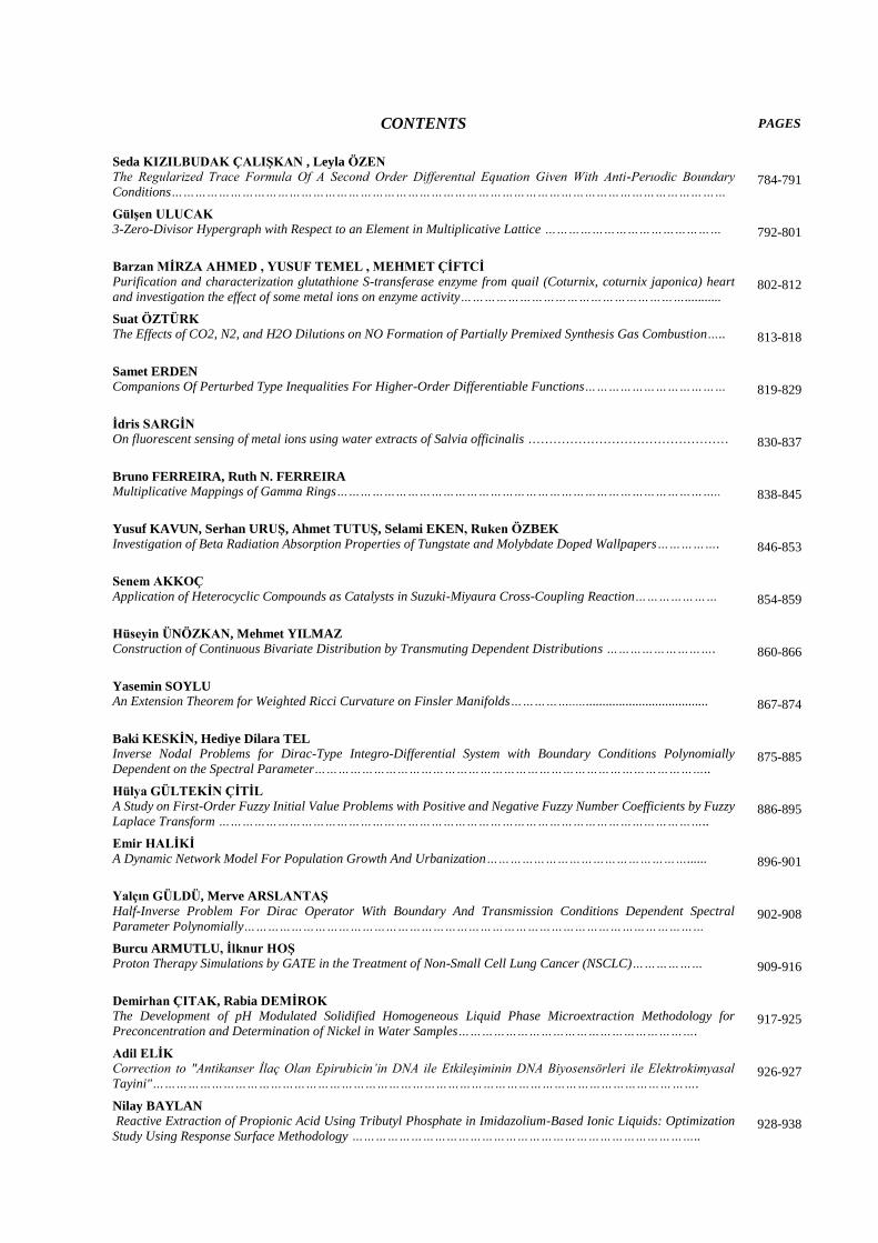
CONTENTS PAGES
Seda KIZILBUDAK ÇALIŞKAN , Leyla ÖZEN
The Regularized Trace Formula Of A Second Order Differentıal Equation Given With Anti-Perıodic Boundary
Conditions…………………………………………………………………………………………………………………………… 784-791
Gülşen ULUCAK
3-Zero-Divisor Hypergraph with Respect to an Element in Multiplicative Lattice ……………………………………… 792-801
Barzan MİRZA AHMED , YUSUF TEMEL , MEHMET ÇİFTCİ
Purification and characterization glutathione S-transferase enzyme from quail (Coturnix, coturnix japonica) heart
and investigation the effect of some metal ions on enzyme activity…………………………………………………........... 802-812
Suat ÖZTÜRK
The Effects of CO2, N2, and H2O Dilutions on NO Formation of Partially Premixed Synthesis Gas Combustion….. 813-818
Samet ERDEN
Companions Of Perturbed Type Inequalities For Higher-Order Differentiable Functions……………………………… 819-829
İdris SARGİN
On fluorescent sensing of metal ions using water extracts of Salvia officinalis ………………………………………… 830-837
Bruno FERREIRA, Ruth N. FERREIRA
Multiplicative Mappings of Gamma Rings…………………………………………………………………………………….. 838-845
Yusuf KAVUN, Serhan URUŞ, Ahmet TUTUŞ, Selami EKEN, Ruken ÖZBEK
Investigation of Beta Radiation Absorption Properties of Tungstate and Molybdate Doped Wallpapers……………. 846-853
Senem AKKOÇ
Application of Heterocyclic Compounds as Catalysts in Suzuki-Miyaura Cross-Coupling Reaction………………… 854-859
Hüseyin ÜNÖZKAN, Mehmet YILMAZ
Construction of Continuous Bivariate Distribution by Transmuting Dependent Distributions ………………………. 860-866
Yasemin SOYLU
An Extension Theorem for Weighted Ricci Curvature on Finsler Manifolds…………….......................................... 867-874
Baki KESKİN, Hediye Dilara TEL
Inverse Nodal Problems for Dirac-Type Integro-Differential System with Boundary Conditions Polynomially
Dependent on the Spectral Parameter……………………………………………………………………………………….. 875-885
Hülya GÜLTEKİN ÇİTİL
A Study on First-Order Fuzzy Initial Value Problems with Positive and Negative Fuzzy Number Coefficients by Fuzzy
Laplace Transform …………………………………………………………………………………………………………….. 886-895
Emir HALİKİ
A Dynamic Network Model For Population Growth And Urbanization……………………………………………...... 896-901
Yalçın GÜLDÜ, Merve ARSLANTAŞ
Half-Inverse Problem For Dirac Operator With Boundary And Transmission Conditions Dependent Spectral
Parameter Polynomially……………………………………………………………………………………………………… 902-908
Burcu ARMUTLU, İlknur HOŞ
Proton Therapy Simulations by GATE in the Treatment of Non-Small Cell Lung Cancer (NSCLC)……………… 909-916
Demirhan ÇITAK, Rabia DEMİROK
The Development of pH Modulated Solidified Homogeneous Liquid Phase Microextraction Methodology for
Preconcentration and Determination of Nickel in Water Samples……………………………………………………. 917-925
Adil ELİK
Correction to "Antikanser İlaç Olan Epirubicin’in DNA ile Etkileşiminin DNA Biyosensörleri ile Elektrokimyasal
Tayini"…………………………………………………………………………………………………………………………. 926-927
Nilay BAYLAN
Reactive Extraction of Propionic Acid Using Tributyl Phosphate in Imidazolium-Based Ionic Liquids: Optimization
Study Using Response Surface Methodology …………………………………………………………………………….. 928-938

Molham MOSHANTAT , Saeid KARAMZADEH
CT and MRI Medical Image Fusion Using Discrete Wavelet Transform………………………………………………. 939-945
Hülya KURŞUN
Correlation of the entrainment factor with frother types and their mixtures in the column flotation……………... 946-957
Umut TOSUN
Comparative Analysis of the Feature Extraction Performance of Augmented Reality Algorithms……………….. 958-966
Z. Seba KESKİN , Nevcihan GÜRSOY
Investıgatıon of Natural Mycoflora and Aflatoxin Formation in Hazelnuts and Products………………………... 967-977
Cumhuriyet Science Journal
CSJ
e-ISSN: 2587-246X
ISSN: 2587-2680 Cumhuriyet Sci. J., Vol.40-4 (2019) 784-791
* Corresponding author. Email address: [email protected]
http://dergipark.gov.tr/csj ©2016 Faculty of Science, Sivas Cumhuriyet University
The Regularized Trace Formula Of A Second Order Differentıal Equation
Given With Anti-Perıodic Boundary Conditions
Seda KIZILBUDAK ÇALIŞKAN 1 Leyla ÖZEN 1
1 Yıldız Technical University, Faculty of Arts and Science, Department of Mathematics, (34210), Davutpaşa,
İstanbul,TURKEY
Received: 09.11.2018; Accepted: 24.10.2019 http://dx.doi.org/10.17776/csj.480810
Abstract. In this study, we examined the formula of the regularized trace of the self-adjoint operator which is
formed by
ℓ(𝑦) = −𝑦′′ + 𝑝(𝑥)𝑦
differential expression and
𝑦(0) + 𝑦(𝜋) = 0
𝑦′(0) + 𝑦′(𝜋) = 0
anti-periodic boundary condition.
Keywords: Regularized trace, Eigenvalues, Eigen functions.
Ters Periyodik Sınır Koşulları İle Verilmiş İkinci Mertebeden
Diferansiyel Denklemin Düzenli İz Formülü
Özet. Bu çalışmada,
ℓ(𝑦) = −𝑦′′ + 𝑝(𝑥)𝑦
diferansiyel ifadesi ve
𝑦(0) + 𝑦(𝜋) = 0
𝑦′(0) + 𝑦′(𝜋) = 0
ters periyodik sınır koşulları ile oluşturulmuş kendine eş operatörün düzenli iz formülü incelenmiştir.
Anahtar Kelimeler: Düzenli iz, Öz değer, Öz fonksiyon.
1. INTRODUCTION
𝑝(𝑥) is a real valued, continuous function in[0, 𝜋], 𝐿0 and 𝐿 get two self-adjoint operators generated by
the following expressions
ℓ0(𝑦) = −𝑦′′
and
ℓ(𝑦) = −𝑦′′ + 𝑝(𝑥)𝑦 (1)
Çalışkan, Özen / Cumhuriyet Sci. J., Vol.40-4 (2019) 784-791
with the same boundary conditions
𝑦(0) + 𝑦(𝜋) = 0
𝑦′(0) + 𝑦′(𝜋) = 0 (2)
respectively, in the space 𝐿2[0, 𝜋]. The spectrum of operator 𝐿0 coincides with the set (2𝑛 + 1)2𝑛=0∞ .
Every point of the spectrum is an eigenvalue with multiplicity two.
Let
𝜇𝑘 = 𝑘2, 𝑖𝑓 𝑘 𝑖𝑠 𝑜𝑑𝑑
(𝑘 − 1)2, 𝑖𝑓 𝑘 𝑖𝑠 𝑒𝑣𝑒𝑛 (𝑘 = 1,2, … )
is the eigenvalues of operator 𝐿0 and
𝜓1 = √2
𝜋sin 𝑥 , 𝜓2 = √
2
𝜋cos 𝑥 , 𝜓3 = √
2
𝜋sin 3𝑥, 𝜓4 = √
2
𝜋cos 3𝑥, …
are the orthonormal eigenfunctions corresponding to this eigenvalues.
Also we showed the eigenvalues of operator 𝐿 by 𝜆1 ≤ 𝜆2 ≤ 𝜆3 ≤ ⋯ ≤ 𝜆𝑘 ≤ ⋯ and corresponding
orthonormal eigenfunctions by 𝜑0, 𝜑1, 𝜑2, … , 𝜑𝑘 , …
In this study, we obtained a formula for the sum of series by Dikii's method,
∑(𝜆𝑛 − 𝜇𝑛)
∞
𝑛=1
which is called the formula of regularized trace of operator 𝐿.
The regularized trace theory, which was first examined by Gelfand and Levitan and they derived the
formula of regularized trace for the Sturm-Liouville operator [1], attracted the attention of many authors.
Dikii [2] provided and developed Gelfand and Levitan's formulas by their own method. Later, Levitan [6]
suggested one more method for computing the traces of the Sturm–Liouville operator. There are numerous
investigations on the calculation of the regularized trace of differential operator equations [3-17].
2. CALCULATION
Let us show the following equation
lim𝑁→∞
∑[(𝜑𝑛, 𝐿𝜑𝑛) − (𝜓𝑛, 𝐿𝜓𝑛)]
𝑁
𝑛=1
= 0 (3)
which will be used later. For this we consider the transfer matrix (𝑢𝑖𝑘)𝑖,𝑘=1∞ from the orthonormal basis
𝜑𝑘 to orthonormal basis 𝜓𝑘 as in [2] :
𝜓𝑘 = ∑ 𝑢𝑖𝑘𝜑𝑖 (𝑘 = 1,2, … )
∞
𝑖=1
785

Çalışkan, Özen / Cumhuriyet Sci. J., Vol.40-4 (2019) 784-791
where 𝑢𝑖𝑘 = (𝜑𝑖 , 𝜓𝑘) and (𝑢𝑖𝑘)𝑖,𝑘=1∞ are the unitary matrix, that is
∑ 𝑢𝑖𝑘2
∞
𝑖=1
= 1 (𝑘 = 1,2, … )
Let us give some limitations for 𝑢𝑖𝑘 . It is clear that
𝐿𝜓𝑘 = 𝜇𝑘𝜓𝑘 + 𝑝𝜓𝑘 (4)
If we multiply both side of equality (4) by 𝜑𝑖 we obtain
(𝐿𝜓𝑘 , 𝜑𝑖) = (𝜇𝑘𝜓𝑘, 𝜑𝑖) + (𝑝𝜓𝑘, 𝜑𝑖)
Or
𝜆𝑖(𝜓𝑘 , 𝜑𝑖) = 𝜇𝑘(𝜓𝑘, 𝜑𝑖) + (𝑝𝜓𝑘 , 𝜑𝑖)
and
(𝜆𝑖 − 𝜇𝑘)(𝜓𝑘, 𝜑𝑖) = (𝑝𝜓𝑘 , 𝜑𝑖)
.
With respect to [2] taking the square of both sides of the last equality and summing from 1 to ∞ respect
to 𝑖 we obtain
∑(𝜆𝑖 − 𝜇𝑘)2(𝜓𝑘 , 𝜑𝑖)2
∞
𝑖=1
= ∑(𝑝𝜓𝑘 , 𝜑𝑖)
∞
𝑖=1
= ‖𝑝𝜓𝑘‖2 = ∫ [𝑝(𝑥)𝜓𝑘(𝑥)]2𝑑𝑥 ≤ 𝑝02
𝜋
0
(5)
where 𝑝0 = 𝑚𝑎𝑥0≤𝑥≤𝜋|𝑝(𝑥)|.
Suppose that the following conditions hold:
1. For the eigenvalues and the eigenfunctions of the 𝐿 operator holds the asymptotic formulas
𝜆𝑘 = 𝜇𝑘 + 𝑂 (1
𝑘) , 𝜑𝑘 = 𝜓𝑘 + 𝑂 (
1
𝑘) [10].
2. ∫ 𝑝(𝑥) 𝑑𝑥 = 0 .𝜋
0
Hence
∑ (𝜆𝑖 − 𝜇𝑘)2𝑢𝑖𝑘2
∞
𝑖=𝑁+1
< 𝐶 (𝐶 = 𝑐𝑜𝑛𝑠𝑡. ) (𝑘 < 𝑁) . (6)
We will use condition 1 in the inequalities we will obtain.
Obviously,
∑ (𝜆𝑖 − 𝜇𝑘)𝑢𝑖𝑘2
∞
𝑖=𝑁+1
< 𝐶 ⇒ ∑ (𝜆𝑖 − 𝜇𝑘)(𝜆𝑖 − 𝜆𝑘)𝑢𝑖𝑘2
∞
𝑖=𝑁+1
< 𝐶
⇒ ∑ (𝜆𝑖 − 𝜆𝑘)2𝑢𝑖𝑘2
∞
𝑖=𝑁+1
< 𝐶
786
Çalışkan, Özen / Cumhuriyet Sci. J., Vol.40-4 (2019) 784-791
is obtained for all integer 𝑁 from equation (6)
And we obtain
∑ (𝜆𝑖 − 𝜆𝑘)𝑢𝑖𝑘2
∞
𝑖=𝑁+1
≤𝐶
𝜆𝑁+1 − 𝜇𝑘 (𝑘 < 𝑁). (7)
Now let us prove the equation (3).
(𝜓𝑘 , 𝐿𝜓𝑘) = (∑ 𝑢𝑖𝑘𝜑𝑖
∞
𝑖=1
, ∑ 𝜆𝑖𝑢𝑖𝑘𝜑𝑖
∞
𝑖=1
) = ∑ 𝜆𝑖𝑢𝑖𝑘2
∞
𝑖=1
If we take the sum on k from 1 to 𝑁 on both sides of this equation we get
∑(𝜓𝑘 , 𝐿𝜓𝑘)
𝑁
𝑘=1
= ∑ ∑ 𝜆𝑖𝑢𝑖𝑘2
∞
𝑖=1
.
𝑁
𝑘=1
Since ∑ 𝑢𝑘𝑖2 = 1∞
𝑖=1 we get
∑(𝜑𝑘 , 𝐿𝜑𝑘)
𝑁
𝑘=1
= ∑ 𝜆𝑘
𝑁
𝑘=1
= ∑ ∑ 𝜆𝑘𝑢𝑘𝑖2
∞
𝑖=1
𝑁
𝑘=1
So now we need to prove
lim𝑁→∞
(∑ ∑ 𝜆𝑖𝑢𝑖𝑘2
∞
𝑖=1
𝑁
𝑘=1
− ∑ ∑ 𝜆𝑘𝑢𝑘𝑖2
∞
𝑖=1
𝑁
𝑘=1
) = 0. (8)
∑ ∑ 𝜆𝑖𝑢𝑖𝑘2
∞
𝑖=1
𝑁
𝑘=1
− ∑ ∑ 𝜆𝑘𝑢𝑘𝑖2 = ∑ ∑ (𝜆𝑖 − 𝜆𝑘)𝑢𝑖𝑘
2
∞
𝑖=𝑁+1
𝑁
𝑘=1
+
∞
𝑖=1
𝑁
𝑘=1
∑ ∑ 𝜆𝑘(𝑢𝑖𝑘2 − 𝑢𝑘𝑖
2 ).
∞
𝑖=𝑁+1
𝑁
𝑘=1
(9)
Let us calculate first sum on the right side of equality (9). For convenience while let 𝑁 + 1 be even
number then we have
∑ ∑ (𝜆𝑖 − 𝜆𝑘)𝑢𝑖𝑘2
∞
𝑖=𝑁+1
𝑁
𝑘=1
= ∑ ∑ (𝜆𝑖 − 𝜆𝑘)𝑢𝑖𝑘2
∞
𝑖=𝑁+1
𝑁−1
𝑘=1
+ (𝜆𝑁+1 − 𝜆𝑁)𝑢(𝑁+1)𝑁2 + ∑ (𝜆𝑖 − 𝜆𝑁)𝑢𝑖𝑁
2
∞
𝑖=𝑁+2
(10)
Let us calculate first and third sum on the right side of equality (10) by inequality (7), for 𝑁 → ∞
∑ ∑ (𝜆𝑖 − 𝜆𝑘)𝑢𝑖𝑘2
∞
𝑖=𝑁+1
𝑁
𝑘=1
<1
4𝑁+
1
2(𝑁 + 1)[ln
𝑁2 + 𝑁
𝑁 − 1] → 0 (11)
and
787
Çalışkan, Özen / Cumhuriyet Sci. J., Vol.40-4 (2019) 784-791
∑ (𝜆𝑖 − 𝜆𝑁)𝑢𝑖𝑁2
∞
𝑖=𝑁+2
≤𝐶
𝜆𝑁+2 − 𝜇𝑁≤
𝐶
4𝑁 + 4 → 0 (12)
Now we shall calculate the second term on the right side of equality (10) when 𝑁 → ∞. Suppose that
𝑁 + 1 is even , we have
(𝜆𝑁+1 − 𝜆𝑁)𝑢(𝑁+1)𝑁2 ≤ 𝑁2 + 𝑂 (
1
𝑁 + 1) − 𝑁2 − 𝑂 (
1
𝑁) → 0 (𝑁 → ∞) (13)
In this way, for even number 𝑁 + 1 from the expressions (10), (11), (12) and (13) we have
lim𝑁→∞
∑ ∑ (𝜆𝑖 − 𝜆𝑘)𝑢𝑖𝑘2
∞
𝑖=𝑁+1
𝑁
𝑘=1
= 0. (14)
Formula (14) can also calculated for odd number 𝑁 + 1.
Now we shall calculate second sum on the right side of equality (9).
𝑢𝑖𝑘 + 𝑢𝑘𝑖 = (𝜑𝑖, 𝜓𝑘) + (𝜑𝑘 , 𝜓𝑖) = −(𝜑𝑖 − 𝜓𝑖, 𝜑𝑘 − 𝜓𝑘) (15)
By equality (15) and condition 1., we have
|𝑢𝑖𝑘 + 𝑢𝑘𝑖| ≤ ‖𝜑𝑖 − 𝜓𝑖‖ ‖𝜑𝑘 − 𝜓𝑘‖ <𝐶
𝑖𝑘 . (16)
According to Cauchy-Schwarz inequality we have
∑ (𝜆𝑖 − 𝜇𝑘)
∞
𝑖=𝑁+1
|𝑢𝑖𝑘2 − 𝑢𝑘𝑖
2 | = ∑ (𝜆𝑖 − 𝜇𝑘)
∞
𝑖=𝑁+1
|𝑢𝑖𝑘 − 𝑢𝑘𝑖||𝑢𝑖𝑘 + 𝑢𝑘𝑖|
≤ √ ∑ |𝑢𝑖𝑘 − 𝑢𝑘𝑖|2
∞
𝑖=𝑁+1
√ ∑ (𝜆𝑖 − 𝜇𝑘)2|𝑢𝑖𝑘 − 𝑢𝑘𝑖|2
∞
𝑖=𝑁+1
<𝐶
(𝑘 − 1)√𝑁 + 1 . (17)
Hence
∑ |𝑢𝑖𝑘2 − 𝑢𝑘𝑖
2 |
∞
𝑖=𝑁+1
<𝐶
(𝑘 − 1)√𝑁 + 1[𝑁2 − (𝑘 − 1)2] (18)
Now we shall evaluate the second sum on the right side of equality (9),
∑ 𝜆𝑘 ∑ |𝑢𝑖𝑘2 − 𝑢𝑘𝑖
2 |
∞
𝑖=𝑁+1
𝑁
𝑘=1
= 𝜆𝑁 ∑ |𝑢𝑖𝑁2 − 𝑢𝑁𝑖
2 |
∞
𝑖=𝑁+1
+ ∑ 𝜆𝑘 ∑ |𝑢𝑖𝑘2 − 𝑢𝑘𝑖
2 |
∞
𝑖=𝑁+1
𝑁−1
𝑘=1
788

Çalışkan, Özen / Cumhuriyet Sci. J., Vol.40-4 (2019) 784-791
= 𝜆𝑁|𝑢𝑁+1𝑁2 − 𝑢𝑁𝑁+1
2 | + 𝜆𝑁 ∑ |𝑢𝑖𝑁2 − 𝑢𝑁𝑖
2 |
∞
𝑖=𝑁+2
+ ∑ 𝜆𝑘 ∑ |𝑢𝑖𝑘2 − 𝑢𝑘𝑖
2 |
∞
𝑖=𝑁+1
𝑁−1
𝑘=1
(19)
By inequality (16) we have
𝜆𝑁|𝑢𝑁+1𝑁2 − 𝑢𝑁𝑁+1
2 | = 𝜆𝑁|𝑢𝑁+1𝑁 − 𝑢𝑁𝑁+1||𝑢𝑁+1𝑁 + 𝑢𝑁𝑁+1|
<𝐶𝑁2
𝑁2(𝑁 + 1)2 |𝑢𝑁+1𝑁 − 𝑢𝑁𝑁+1| → 0 (𝑁 → ∞) (20)
By the expression (18) we evaluate the second and third sum on the right side of equality (19)
𝜆𝑁 ∑ |𝑢𝑖𝑁2 − 𝑢𝑁𝑖
2 |
∞
𝑖=𝑁+2
<𝐶𝑁2
(𝑁 − 1)√𝑁 + 2[(𝑁 + 2)2 − (𝑁 + 1)2]→ ∞ (𝑁 → ∞) (21)
and
∑ 𝜆𝑘 ∑ |𝑢𝑖𝑘2 − 𝑢𝑘𝑖
2 |
∞
𝑖=𝑁+1
𝑁−1
𝑘=1
<𝐶𝑁
√𝑁 + 1∑
1
𝑁2 − (𝑘 − 1)2
𝑁
𝑘=2
~𝐶ln 𝑁
√𝑁→ 0 (𝑁 → ∞). (22)
From the expressions (19), (20),(21) and (22) we have
lim𝑁→∞
∑ ∑ 𝜆𝑘(𝑢𝑖𝑘2 − 𝑢𝑘𝑖
2 )
∞
𝑖=𝑁+1
=
𝑁
𝑘=1
0 (23)
Thus from the expressions (9), (14), and (23) we obtain formula (8). Therefore formula (3) have proved.
3. CONCLUSION
(𝜑𝑘 , 𝐿𝜑𝑘) = 𝜆𝑘 and (𝜓𝑘 , 𝐿𝜓𝑘) = 𝜇𝑘 + (𝜓𝑘 , 𝑝𝜓𝑘).
If we use these into formula (3) then we obtain
∑[(𝜓𝑘 , 𝐿𝜓𝑘) − (𝜑𝑘 , 𝐿𝜑𝑘)] =
𝑁
𝑘=1
∑(𝜇𝑘 − 𝜆𝑘)
𝑁
𝑘=1
+ ∑(𝜓𝑘 , 𝑝𝜓𝑘)
𝑁
𝑘=1
→ 0 , (𝑁 → ∞). (24)
Now we shall calculate
lim𝑁→∞
∑(𝜓𝑘, 𝑝𝜓𝑘).
𝑁
𝑘=1
According to condition 2. we have for even number 𝑁
789
Çalışkan, Özen / Cumhuriyet Sci. J., Vol.40-4 (2019) 784-791
∑(𝜓𝑘 , 𝑝𝜓𝑘)
𝑁
𝑘=1
=1
𝜋∫ 𝑝(𝑥)
𝜋
0
𝑑𝑥 +𝑁
𝜋∫ 𝑝(𝑥)
𝜋
0
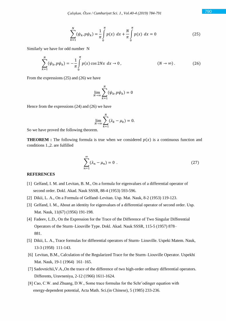
𝑑𝑥 = 0 (25)
Similarly we have for odd number N
∑(𝜓𝑘, 𝑝𝜓𝑘)
𝑁
𝑘=1
= −1
𝜋∫ 𝑝(𝑥)
𝜋
0
cos 2𝑁𝑥 𝑑𝑥 → 0 , (𝑁 → ∞) . (26)
From the expressions (25) and (26) we have
lim𝑁→∞
∑(𝜓𝑘, 𝑝𝜓𝑘)
𝑁
𝑘=1
= 0
Hence from the expressions (24) and (26) we have
lim𝑁→∞
∑(𝜆𝑘 − 𝜇𝑘)
𝑁
𝑘=1
= 0.
So we have proved the following theorem.
THEOREM : The following formula is true when we considered 𝑝(𝑥) is a continuous function and
conditions 1.,2. are fulfilled
∑(𝜆𝑛 − 𝜇𝑛)
∞
𝑛=1
= 0 . (27)
REFERENCES
[1] Gelfand, I. M. and Levitan, B. M., On a formula for eigenvalues of a differential operator of
second order. Dokl. Akad. Nauk SSSR, 88-4 (1953) 593-596.
[2] Dikii, L. A., On a Formula of Gelfand–Levitan. Usp. Mat. Nauk, 8-2 (1953) 119-123.
[3] Gelfand, I. M., About an identity for eigenvalues of a differential operator of second order. Usp.
Mat. Nauk, 11(67) (1956) 191-198.
[4] Fadeev, L.D., On the Expression for the Trace of the Difference of Two Singular Differential
Operators of the Sturm–Liouville Type. Dokl. Akad. Nauk SSSR, 115-5 (1957) 878–
881.
[5] Dikii, L. A., Trace formulas for differential operators of Sturm- Liouville. Uspeki Matem. Nauk,
13-3 (1958) 111-143.
[6] Levitan, B.M., Calculation of the Regularized Trace for the Sturm–Liouville Operator. Uspekhi
Mat. Nauk, 19-1 (1964) 161–165.
[7] Sadovnichii,V.A.,On the trace of the difference of two high-order ordinary differential operators.
Differents, Uravneniya, 2-12 (1966) 1611-1624.
[8] Cao, C.W. and Zhuang, D.W., Some trace formulas for the Schr¨odinger equation with
energy-dependent potential, Acta Math. Sci.(in Chinese), 5 (1985) 233-236.
790
Çalışkan, Özen / Cumhuriyet Sci. J., Vol.40-4 (2019) 784-791
[9] Bayramoğlu, M., On the regularized trace formula of th differential equation with unbounded
Coefficient. Spectral Theory and Its Applications, 7 (1987) 15-40.
[10] Lax P. D., Trace formulas for the Schroeding operator. Commun. Pure Appl. Math.,
47- 4 (1994) 503-512.
[11] Papanicolaou, V.G., Trace formulas and the behavior of large eigenvalues, SIAM J.
Math. Anal., 26 (1995), 218-237.
[12] Adıgüzelov, E. E., Baykal, O. and Bayramov, A., On the spectrum and regularized trace of the
Sturm-Liouville problem with spectral parameter on the boundary condition and with the operator
coefficient. International Journal of Differential Equations and Applications, 2-3
(2001) 317-333.
[13] Savchuk, A.M., Shkalikov, A.A., Trace formula for Sturm-Liouville Operators with Singular
Potentials. Mathematical Notes, 69-3 (2001).
[14] Bayramov, A., Öztürk Uslu, S. and Kızılbudak Çalışkan, S., On the trace formula of second
order differential equation given with non-seperable boundary conditions. Sigma Journal of
Engineering and Natural Sciences, 4 (2005) 57-64.
[15] Guliyev, N.J., The regularized trace formula for the Sturm-Liouville equation with spectral
parameter in the boundary condition. Proceedins of IMM of NAS of Azerbaijan, 22 (2005)
99-102.
[16] Sadovnichii, V.A. and Podol’skii, V.E., Traces of Differential Operators. Differential Equ-
ations, 45- 4 (2009) 477-493
[17] Wang, Y.P., Koyunbakan H. and Yang, C.F., A Trace Formula for Integro-differential
Operators on the Finite Interval, Acta Mathematicae Applicatae Sinica (English Series)
33-1 (2017) 141-146.
791
Cumhuriyet Science Journal
CSJ
e-ISSN: 2587-246X
ISSN: 2587-2680 Cumhuriyet Sci. J., Vol.40-4 (2019) 792-801
* Corresponding author. Email address: [email protected]
http://dergipark.gov.tr/csj ©2016 Faculty of Science, Sivas Cumhuriyet University
3-Zero-Divisor Hypergraph with Respect to an Element in Multiplicative
Lattice
Gülşen ULUCAK 1
1 Department of Mathematics, Gebze Technical University, P.K 41400, Gebze-Kocaeli, TURKEY
Received: 19.11.2018; Accepted: 23.10.2019 http://dx.doi.org/10.17776/csj.485085
Abstract. Let 𝐿 be a multiplicative lattice and 𝑧 be a proper element of 𝐿. We introduce the 3-zero-divisor
hypergraph of 𝐿 with respect to 𝑧 which is a hypergraph whose vertices are elements of the set
𝑥1 ∈ 𝐿 − 𝑧|𝑥1𝑥2𝑥3 ≤ 𝑧 ⇒ 𝑥1𝑥2 ≰ 𝑧, 𝑥2𝑥3 ≰ 𝑧 𝑎𝑛𝑑 𝑥1𝑥3 ≰ 𝑧
𝑓𝑜𝑟 𝑠𝑜𝑚𝑒 𝑥2, 𝑥3 ∈ 𝐿 − 𝑧 where distinct vertices 𝑥1, 𝑥2 and 𝑥3 are
adjacent, that is, 𝑥1, 𝑥2, 𝑥3 is a hyperedge if and only if 𝑥1𝑥2𝑥3 ≤ 𝑧 ⇒ 𝑥1𝑥2 ≰ 𝑧, 𝑥2𝑥3 ≰ 𝑧 𝑎𝑛𝑑 𝑥1𝑥3 ≰ 𝑧.
Throughout this paper, the hypergraph is denoted by 𝐻3(𝐿, 𝑧). We investigate many properties of the hypergraph
over a multiplicative lattice. Moreover, we find a lower bound of diameter of 𝐻3(𝐿, 𝑧) and obtain that 𝐻3(𝐿, 𝑧)
is connected.
Keywords: 3-Zero-Divisor Hypergraph, Complete n-partite Hypergraph.
Çarpımsal Kafeslerde Bir Eleman ile İlgili 3-lü Sıfır Bölen Hipergrafı
Özet. 𝐿 bir çarpımsal kafes ve 𝑧, 𝐿 nin bir has elemanı olsun. 𝑧 ile ilgili 𝐿 nin 3-lü sıfır bölen hipergrafını tanıttık
öyle ki bu hipergrafın köşeleri𝑥1 ∈ 𝐿 − 𝑧|𝑥1𝑥2𝑥3 ≤ 𝑧 ⇒ 𝑥1𝑥2 ≰ 𝑧, 𝑥2𝑥3 ≰ 𝑧 𝑣𝑒 𝑥1𝑥3 ≰ 𝑧
ℎ𝑒𝑟ℎ𝑎𝑛𝑔𝑖 𝑥2, 𝑥3 ∈ 𝐿 − 𝑧 𝑖ç𝑖𝑛 kümesinin
elemanlarıdır ki burada 𝑥1, 𝑥2 ve 𝑥3 komşudur, yani, 𝑥1, 𝑥2, 𝑥3 bu hipergarfın bir hiperkenarıdır ancak ve
ancak 𝑥1𝑥2𝑥3 ≤ 𝑧 ⇒ 𝑥1𝑥2 ≰ 𝑧, 𝑥2𝑥3 ≰ 𝑧 𝑣𝑒 𝑥1𝑥3 ≰ 𝑧. Bu çalışma boyunca, bu hipergrafı 𝐻3(𝐿, 𝑧) ile
göstereceğiz. Çarpımsal bir kafes üzerinde bu hipergrafın birçok özelliğini araştırdık. Ayrıca, 𝐻3(𝐿, 𝑧) nin
diametresinin bir alt sınırını bulduk ve bu hipergrafın bağlantılı olduğunu gösterdik.
Anahtar Kelimeler: 3-lü Sıfır Bölen Hipergraf, n-parçalı Tam Hipergraf.
1. INTRODUCTION
A complete lattice 𝐿 is called multiplicative lattice if there exists a commutative, associative,
completely join distributive product on the lattice with the compact greatest element 1𝐿, which is
the multiplicative identity, and the least element 0𝐿. It can be easily seen that 𝐿/𝑎 = 𝑏 ∈ 𝐿|𝑎 ≤
𝑏 is a multiplicative lattice with the product 𝑥 ∘ 𝑦 = 𝑥𝑦 ∨ 𝑎 where 𝐿 is multiplicative lattice and
𝑎 ∈ 𝐿. Note that 0𝐿/𝑧 = 𝑧. D.D. Anderson and the current authors have studied on multiplicative
lattices in a series of articles [1-4]. An element 𝑎 ∈ 𝐿 is said to be proper if 𝑎 < 1𝐿. A proper element
𝑝 ∈ 𝐿 is called a prime element if 𝑎𝑏 ≤ 𝑝 implies 𝑎 ≤ 𝑝 or 𝑏 ≤ 𝑝, where 𝑎, 𝑏 ∈ 𝐿. Then 𝑝 is called
2-absorbing element of 𝐿 if 𝑥1𝑥2𝑥3 ≤ 𝑝 for some 𝑥1, 𝑥2 and 𝑥3 in L, then 𝑥1𝑥2 ≤ 𝑝 or 𝑥1𝑥3 ≤ 𝑝 or
𝑥2𝑥3 ≤ 𝑝.
Let a finite set 𝑉 be a vertex set and 𝐸(𝑉) = (𝑢, 𝑣)|𝑢, 𝑣 ∈ 𝑉, 𝑢 ≠ 𝑣. A pairwise 𝐺 = (𝑉, 𝐸) is
called a graph on 𝑉 where 𝐸 ⊆ 𝐸(𝑉). The elements of 𝑉 are the vertices of 𝐺, and those of 𝐸 the
Ulucak / Cumhuriyet Sci. J., Vol.40-4 (2019) 792-801
edges of 𝐺. Consider that the edges (𝑥, 𝑦) and (𝑦, 𝑥) denote the same edge (For more information,
see [3-8].
A hypergraph 𝐻 is a pair (𝑉, 𝐸) of disjoint sets, where the elements of 𝐸 are nonempty subsets of
𝑉. The elements of 𝑉 are called the vertices of 𝐻 and the elements of 𝐸 are called the hyperedges of
𝐻. If the size of any hyperedge 𝑒 in the hypergraph 𝐻 is 𝑛, then 𝐻 is called 𝑛-uniform hypergraph.
Let 𝐻 be an 𝑛-uniform hypergraph. An alternating sequence of distinct vertices and hyperedges is
called a path with the form 𝑣1, 𝑒1, 𝑣2, 𝑒2, … , 𝑣𝑚 such that 𝑣𝑖 , 𝑣𝑖+1 are in 𝑒𝑖 for all 1 ≤ 𝑖 ≤ 𝑚 − 1.
The length of a path is the number of hyperedges of it. The distance 𝑑(𝑥, 𝑦) between two vertices 𝑥
and 𝑦 of 𝐻 is the length of the shortest path from 𝑥 to 𝑦. If no such path between 𝑥 and 𝑦 exists, then
𝑑(𝑥, 𝑦) = ∞. The diameter 𝑑𝑖𝑎𝑚(𝐻) of 𝐻 is the greatest distance between any two vertices. The
hypergraph 𝐻 is said to be connected if 𝑑𝑖𝑎𝑚(𝐻) < ∞. A cycle in a hypergraph 𝐻 is an alternating
sequence of distinct vertices and hyperedges of the form 𝑣1, 𝑒1, 𝑣2, 𝑒2, … , 𝑣𝑚, 𝑒𝑚, 𝑣1 such that
𝑣𝑖, 𝑣𝑖+1 ∈ 𝑒𝑖 and 𝑣𝑚, 𝑣1 ∈ 𝑒𝑚 for all 1 ≤ 𝑖 ≤ 𝑚. The girth 𝑔𝑟(𝐻) of a hypergraph 𝐻 containing a
cycle is the smallest size of the length of cycles of 𝐻. (For more information, see [5]). A hypergraph
𝐻 is called trivial if it has a single vertex and also it is called empty if it has no hyperedges.
The concept of a zero-divisor graph of a commutative ring was first introduced in [6]. Let 𝑅 be a
commutative ring and 𝑘 ≥ 2 be an integer. A nonzero nonunit element 𝑥1 in 𝑅 is said to be a 𝑘-zero-
divisor in 𝑅 if there are 𝑘 − 1 distinct nonunit elements 𝑥2, 𝑥3, … , 𝑥𝑘 in 𝑅 different from 𝑥1 such
that 𝑥1𝑥2𝑥3 … 𝑥𝑘 = 0 and the product of no elements of any proper subset of 𝐴 = 𝑥1, 𝑥2,𝑥3, … , 𝑥𝑘
is zero. The set of 𝑘-zero divisor elements of 𝑅 is denoted by 𝑍𝑘(𝑅). Let 𝐼 be a proper ideal of 𝑅.
The 3-zero-divisor hypergraph of 𝑅 with respect to 𝐼, denoted by 𝐻3(𝑅, 𝐼), is the hypergraph whose
vertices are the set 𝑥1 ∈ 𝑅\𝐼|𝑥1𝑥2𝑥3 ∈ 𝐼 𝑓𝑜𝑟 𝑠𝑜𝑚𝑒 𝑥2, 𝑥3 ∈ 𝑅\𝐼 𝑠𝑢𝑐ℎ 𝑡ℎ𝑎𝑡 𝑥1𝑥2 ∉ 𝐼, 𝑥2𝑥3 ∉
𝐼 𝑎𝑛𝑑 𝑥1𝑥3 ∉ 𝐼 where distinct vertices 𝑥1, 𝑥2 and 𝑥3 are adjacent if and only if 𝑥1𝑥2𝑥3 ∈ 𝐼, 𝑥1𝑥2 ∉
𝐼, 𝑥2𝑥3 ∉ 𝐼 𝑎𝑛𝑑 𝑥1𝑥3 ∉ 𝐼 (See [9]). Let 𝐼 be a proper ideal of 𝑅. Recall that 𝐼 is called a 2-absorbing
ideal of 𝑅 if 𝑥1𝑥2𝑥3 ∈ 𝐼 for some 𝑥1, 𝑥2 and 𝑥3 in 𝑅, then 𝑥1𝑥2 ∈ 𝐼 or 𝑥2𝑥3 ∈ 𝐼 or 𝑥1𝑥3 ∈ 𝐼 (For
more information, see [10]). Hence 𝐻3(𝑅, 𝐼) is not empty if and only if 𝐼 is not a 2-absorbing ideal
of 𝑅 (see Proposition 1 in [9]).
Let 𝑧 be a proper element of 𝐿. A proper element 𝑎1 of 𝐿 is called 𝑛-zero divisor element with respect
to 𝑧 in 𝐿 if there are 𝑛 − 1 distinct elements 𝑎2, 𝑎3, … , 𝑎𝑛 in 𝐿 different from 𝑎1 such that
𝑎2𝑎3 … 𝑎𝑛 ≤ 𝑧 and the product of no elements of any proper subset of 𝐴 = 𝑎1, 𝑎2,, … , 𝑎𝑛 is less
than or equals to 𝑧. The set of all 𝑛-zero divisor element with respect to 𝑧 in 𝐿 is denoted by 𝑍𝑛(𝐿, 𝑧).
For example, consider the lattice of ideals of ℤ, 𝐿 = Ι(ℤ) the set of all ideals of ℤ. The ideal (2) is
a 3-zero-divisor with respect to (8) in 𝐿 since (2)(3)(6) ⊆ (8), and the product of no elements of
any proper subset of (2), (3), (6) is contained by (8).
Throughout this paper, we assume that a lattice 𝐿 is a multiplicative lattice. Let 𝑧 be a proper element
of 𝐿. The 3-zero-divisor hyper-graph of 𝐿 with respect to 𝑧, denoted by 𝐻3(𝐿, 𝑧), is a hypergraph
whose vertices are elements of the set
𝑥1 ∈ 𝐿 − 𝑧|𝑥1𝑥2𝑥3 ≤ 𝑧 ⇒ 𝑥1𝑥2 ≰ 𝑧, 𝑥2𝑥3 ≰ 𝑧 𝑎𝑛𝑑 𝑥1𝑥3 ≰ 𝑧
𝑓𝑜𝑟 𝑠𝑜𝑚𝑒 𝑥2, 𝑥3 ∈ 𝐿 − 𝑧 such that distinct vertices 𝑥1, 𝑥2
and 𝑥3 are adjacent, that is, 𝑥1, 𝑥2, 𝑥3 is a hyperedge if and only if 𝑥1𝑥2𝑥3 ≤ 𝑧 ⇒ 𝑥1𝑥2 ≰ 𝑧,
𝑥2𝑥3 ≰ 𝑧 𝑎𝑛𝑑 𝑥1𝑥3 ≰ 𝑧. It can be seen that 𝐻3(𝐿, 𝑧) is a 3-uniform hypergraph. In this paper, we
show that 𝐻3(𝐿, 𝑧) is empty if and only if 𝑧 is a 2-absorbing element of 𝐿 and also, 𝐻3(𝐿/𝑧) is empty
793
Ulucak / Cumhuriyet Sci. J., Vol.40-4 (2019) 792-801
hypergraph if and only if 𝐻3(𝐿, 𝑧) is empty hypergraph. Then we give that 𝐻3(𝐿, 𝑧) is connected
and 𝑑𝑖𝑎𝑚(𝐻3(𝐿, 𝑧)) ≤ 4. Additionally, we show that 𝐻3(𝐿, 𝑧) is a complete 3-partite hypergraph if
𝑝1, 𝑝2 and 𝑝3 are prime elements of 𝐿 and 𝑧 = 𝑝1 ∧ 𝑝2 ∧ 𝑝3 ≠ 0𝐿 and the converse is true if 𝐿 is
reduced lattice. Finally, we see that 𝐻3(𝐿, 𝑧) has no cut-point.
2. ZERO DIVISOR HYPERGRAPH H_3 (L,z) WITH RESPECT TO z
Definition 1. Let 𝑧 be a proper element of 𝐿. The 3-zero-divisor hypergraph of 𝐿 with respect to 𝑧
is a hypergraph whose vertices are elements of the set
𝑥1 ∈ 𝐿 − 𝑧|𝑥1𝑥2𝑥3 ≤ 𝑧 ⇒ 𝑥1𝑥2 ≰ 𝑧, 𝑥2𝑥3 ≰ 𝑧 𝑎𝑛𝑑 𝑥1𝑥3 ≰ 𝑧
𝑓𝑜𝑟 𝑠𝑜𝑚𝑒 𝑥2, 𝑥3 ∈ 𝐿 − 𝑧. Also, distinct vertices 𝑥1, 𝑥2 and
𝑥3 are adjacent, that is, 𝑥1, 𝑥2, 𝑥3 is a hyperedge if and only if 𝑥1𝑥2𝑥3 ≤ 𝑧 ⇒ 𝑥1𝑥2 ≰ 𝑧, 𝑥2𝑥3 ≰
𝑧 𝑎𝑛𝑑 𝑥1𝑥3 ≰ 𝑧. Throughout this paper, the hypergraph is denoted by 𝐻3(𝐿, 𝑧).
Let 𝑧 = 0𝐿. Then it is clear that 𝐻3(𝐿) = 𝐻3(𝐿, 0𝐿) is the hypergraph whose vertices are elements
of the set𝑥1 ∈ 𝑍3(𝐿)|𝑥1𝑥2𝑥3 = 0𝐿 ⇒ 𝑥1𝑥2 ≠ 0𝐿 , 𝑥2𝑥3 ≠ 0𝐿 𝑎𝑛𝑑 𝑥1𝑥3 ≠ 0𝐿
𝑓𝑜𝑟 𝑠𝑜𝑚𝑒 𝑥2, 𝑥3 ∈ 𝑍3(𝐿) where distinct
vertices 𝑥1, 𝑥2 and 𝑥3 are adjacent if and only if 𝑥1𝑥2𝑥3 = 0𝐿 ⇒ 𝑥1𝑥2 ≠ 0𝐿 , 𝑥2𝑥3 ≠ 0𝐿 𝑎𝑛𝑑 𝑥1𝑥3 ≠
0𝐿.
The hypergraphs 𝐻3(𝑅) in [5] and 𝐻3(𝑅, 𝐼) in [10], which are defined on a commutative ring 𝑅 and
a proper ideal 𝐼 of 𝑅, are examples for the hypergraph 𝐻3(𝐿, 𝑧).
We obtain the following results with the above definition and the definition of 2-absorbing element
in 𝐿.
Proposition 1. Let 𝑧 be a proper element of 𝐿. Then the following statements hold:
1) 𝐻3(𝐿, 𝑧) is empty hypergraph if and only if 𝑧 is a 2-absorbing element of 𝐿.
2) 𝐻3(𝐿/ 𝑧) is empty hypergraph if and only if 𝐻3(𝐿, 𝑧) is empty hypergraph.
Proof. 1). (⇒): Let 𝐻3(𝐿, 𝑧) be empty hypergraph. Suppose that 𝑧 is not a 2-absorbing element of
𝐿. Take 𝑥1𝑥2𝑥3 ≤ 𝑧 for some 𝑥1, 𝑥2, 𝑥3 ∈ 𝐿. Then we get 𝑥1𝑥2 ≰ 𝑧, 𝑥2𝑥3 ≰ 𝑧 and 𝑥1𝑥3 ≰ 𝑧. Hence
𝑒 = 𝑥1, 𝑥2, 𝑥3 is a hyperedge of 𝐻3(𝐿, 𝑧), a contradiction.
(⇐): It is obvious.
2). (⇒): Assume that 𝐻3(𝐿, 𝑧) is not an empty hypergraph. Then it has a hyperedge 𝑒 = 𝑥1, 𝑥2, 𝑥3.
Consider 𝑥1 ∨ 𝑧, 𝑥2 ∨ 𝑧, 𝑥3 ∨ 𝑧 ∈ 𝐿/𝑧. It is clear that 𝑥1 ∨ 𝑧, 𝑥2 ∨ 𝑧, 𝑥3 ∨ 𝑧 are different from 𝑧. Then
we have that (𝑥1 ∨ 𝑧)(𝑥2 ∨ 𝑧)(𝑥3 ∨ 𝑧) = 0𝐿/𝑧, (𝑥1 ∨ 𝑧)(𝑥2 ∨ 𝑧) ≠ 0𝐿/𝑧, (𝑥2 ∨ 𝑧)(𝑥3 ∨ 𝑧) ≠ 0𝐿/𝑧
and (𝑥1 ∨ 𝑧)(𝑥3 ∨ 𝑧) ≠ 0𝐿/𝑧. Thus 𝑒′ = 𝑥1 ∨ 𝑧, 𝑥2 ∨ 𝑧, 𝑥3 ∨ 𝑧 is a hyperedge of 𝐻3(𝐿/ 𝑧), a
contradiction.
(⇐): Let 𝐻3(𝐿/ 𝑧) be not an empty hypergraph. Then it has a hyperedge 𝑒 = 𝑦1, 𝑦2, 𝑦3 for some
𝑦1, 𝑦2, 𝑦3 ∈ 𝑉(𝐻3(𝐿/ 𝑧)). Then 𝑦1 ∘ 𝑦2 ∘ 𝑦3 = 0𝐿/𝑧, that is, 𝑦1𝑦2𝑦3 ≤ 𝑧 and since 𝑦1 ∘ 𝑦2, 𝑦2 ∘ 𝑦3
and 𝑦1 ∘ 𝑦3 are different from 0𝐿/𝑧, then 𝑦1𝑦2, 𝑦2𝑦3, 𝑦1𝑦3 ≰ 𝑧. Therefore, 𝑒 = 𝑦1, 𝑦2, 𝑦3 is a
hyperedge of 𝐻3(𝐿, 𝑧), a contradiction.
794
Ulucak / Cumhuriyet Sci. J., Vol.40-4 (2019) 792-801
Theorem 1. Let 𝐻3(𝐿, 𝑧) be a 3-zero-divisor hypergraph of 𝐿 with respect to 𝑧. If 𝑥2 ≰ 𝑧 for each
3-zero-divisor 𝑥 ∈ 𝐿 with respect to 𝑧, then 𝐻3(𝐿, 𝑧) is connected and 𝑑𝑖𝑎𝑚(𝐻3(𝐿, 𝑧)) ≤ 4.
Furthermore, if 𝐻3(𝐿, 𝑧) has a cycle, then 𝑔𝑟(𝐻3(𝐿, 𝑧)) ≤ 9.
Proof. Let 𝑒1 = 𝑥1, 𝑥2, 𝑥3 and 𝑒2 = 𝑦1, 𝑦2, 𝑦3 be hyperedges of 𝐻3(𝐿, 𝑧). If 𝑒1 ∩ 𝑒2 ≠ ∅, the
proof is completed. Assume that 𝑒1 ∩ 𝑒2 = ∅. We show that there are hyperedges 𝑒3, 𝑒4 such that
they satisfy one of the followings:
(1) 𝒆𝟑 ∩ 𝒆𝟏 ≠ ∅, 𝒆𝟑 ∩ 𝒆𝟐 ≠ ∅
(2) 𝑒3 ∩ 𝑒1 ≠ ∅, 𝑒4 ∩ 𝑒2 ≠ ∅, 𝑒4 ∩ 𝑒3 ≠ ∅
Assume that 𝐺 is the partite graph such that 𝑉(𝐺) = 𝑒1 ∪ 𝑒𝟐 and 𝑥𝑖𝑦𝑗 ∈ 𝐸(𝐺) if and only if 𝑥𝑖𝑦𝑗 ≤
𝑧.
Assume that 𝐺 has two isolated vertices such that one is in 𝑒1 and the other is in 𝑒2. Let 𝑑𝑒𝑔𝐺(𝑥3) =
𝑑𝑒𝑔𝐺(𝑦3) = 0. Suppose that there is 𝑎 ∈ 𝑥1, 𝑥2, 𝑦1, 𝑦2 where 𝑥3𝑦3𝑎 ≤ 𝑧. Then 𝑒3 = 𝑥3, 𝑦3, 𝑎 is
a hyperedge which holds the condition (1). Let the case not satisfy. If 𝑥3𝑦3 ∉ 𝑥1, 𝑥2, 𝑦1, 𝑦2, then
𝑒3 = 𝑥1, 𝑥2, 𝑥3𝑦3 and 𝑒4 = 𝑦1, 𝑦2, 𝑥3𝑦3 are two hyperedges which satisfy the condition (2). In
the contrary case, without loss of generality (wlog.), suppose that 𝑥3𝑦3 = 𝑥1. Hence 𝑒3 =
𝑥1, 𝑦1, 𝑦2 is a hyperedge satisfying the condition (1). Consequently, 𝐻3(𝐿, 𝑧) is connected. Now,
we show that 𝑑𝑖𝑎𝑚(𝐻3(𝐿, 𝑧)) ≤ 4. We consider the number of edges 𝐺 for the rest of the proof.
Case 1. Assume that |𝐸(𝐺)| ≤ 2. Then 𝐺 has two isolated vertices such that one is in 𝑒1 and the
other is in 𝑒2.
Case 2. Let |𝐸(𝐺)| = 3. Take account of the next four different subcases for this case:
Case 2.1: Let 𝑑𝑒𝑔𝐺(𝑎) = 1 for each vertex 𝑎 of 𝐺. Assume that 𝐸(𝐺) = 𝑥1𝑦1, 𝑥2𝑦2, 𝑥3𝑦3. We
consider 𝑥1, 𝑥2𝑦3, 𝑦1 ∨ 𝑦2. If 𝑥1 = 𝑥2𝑦3, then 𝑥1𝑦2 = 𝑥2𝑦3𝑦2 ≤ 𝑧, a contradiction. If 𝑥1 = 𝑦1 ∨
𝑦2, then 𝑦1𝑥2𝑥3 ≤ 𝑧. Thus 𝑒3 = 𝑦1, 𝑥2, 𝑥3 satisfies the condition (1). If 𝑦1 ∨ 𝑦2 = 𝑥2𝑦3, then
𝑥1𝑦2𝑥3 ≤ 𝑧 and so the condition (1) is satisfied for 𝑒3 = 𝑥1, 𝑦2, 𝑥3. On the contrary, reconsider
𝑒3 = 𝑥1, 𝑥2𝑦3, 𝑦1 ∨ 𝑦2. If 𝑒3 is not a hyperedge, then 𝑥1𝑥2𝑦3 ≤ 𝑧 or 𝑥2𝑦3(𝑦1 ∨ 𝑦2) ≤ 𝑧, that is,
𝑥2𝑦3𝑦1 ≤ 𝑧. Then 𝑒′3 = 𝑥1, 𝑥2, 𝑦3 is a hyperedge satisfying the condition (1) or 𝑒′4 = 𝑥2, 𝑦3, 𝑥1
is a hyperedge satisfying the condition (1). Let 𝑒3 = 𝑥1, 𝑥2𝑦3, 𝑦1 ∨ 𝑦2 be a hyperedge. In a similar
way, we consider 𝑦1, 𝑥2𝑦3, 𝑥1 ∨ 𝑥3. If 𝑒4 is not a hyperedge, then 𝑦1𝑥2𝑦3 ≤ 𝑧 or 𝑥2𝑦3(𝑥1 ∨ 𝑥3) ≤
𝑧, that is, 𝑥2𝑦3𝑥1 ≤ 𝑧. Then 𝑒′′3 = 𝑦1, 𝑥2, 𝑦3 is a hyperedge satisfying the condition (1) or 𝑒′′4 =
𝑥2, 𝑦3, 𝑥1 is a hyperedge satisfying the condition (1). Assume that 𝑒4 = 𝑦1, 𝑥2𝑦3, 𝑥1 ∨ 𝑥3 is a
hyperedge. Then we have two hyperedges 𝑒3 = 𝑥1, 𝑥2𝑦3, 𝑦1 ∨ 𝑦2 and 𝑒4 = 𝑦1, 𝑥2𝑦3, 𝑥1 ∨ 𝑥3
with 𝑒3 and 𝑒4 satisfying the condition (2).
Case 2.2. Let 𝑑𝑒𝑔𝐺(𝑎) = 1 for only an element 𝑎 of 𝐺. Wlog., suppose that 𝐸(𝐺) =
𝑥1𝑦1, 𝑥1𝑦2, 𝑥2𝑦3. We consider 𝑥2, 𝑥3𝑦1, 𝑥1 ∨ 𝑦3. If 𝑥2 = 𝑥3𝑦1, then 𝑥1𝑥2 ≤ 𝑧, is a contradiction.
If 𝑥2 = 𝑥1 ∨ 𝑦3, then 𝑥2𝑦2𝑦1 ≤ 𝑧 and so the condition (1) is satisfied for 𝑒3 = 𝑥2, 𝑦2, 𝑦1. If 𝑥1 ∨
𝑦3 = 𝑥3𝑦1, then 𝑥3𝑦1𝑦2𝑦1 ≤ 𝑧. In the circumstances, if 𝑥3 = 𝑦1𝑦2, then 𝑥1𝑥3 ≤ 𝑧, a contradiction.
If 𝑦1 = 𝑦1𝑦2, then 𝑦1𝑦3 ≤ 𝑧, a contradiction. Hence, the condition (1) holds for 𝑒3 = 𝑥3, 𝑦1𝑦2, 𝑦1.
Let the above conditions not hold. If 𝑒3 = 𝑥2, 𝑥3𝑦1, 𝑥1 ∨ 𝑦3 is not a hyperedge, then 𝑥2𝑥3𝑦1 ≤ 𝑧
or 𝑥3𝑦1(𝑥1 ∨ 𝑦3) ≤ 𝑧, that is, 𝑥3𝑦1𝑦3 ≤ 𝑧. Then 𝑒′3 = 𝑥2, 𝑥3, 𝑦1 is a hyperedge satisfying the
condition (1) or 𝑒′4 = 𝑥3, 𝑦1, 𝑦3 is a hyperedge satisfying the condition (1). Suppose that 𝑒3 =
795
Ulucak / Cumhuriyet Sci. J., Vol.40-4 (2019) 792-801
𝑥2, 𝑥3𝑦1, 𝑥1 ∨ 𝑦3 is a hyperedge. Now, similarly we consider 𝑦2, 𝑥3𝑦1, 𝑦3. If 𝑒4 = 𝑦2, 𝑥3𝑦1, 𝑦3
is not a hyperedge, then 𝑦2𝑥3𝑦1 ≤ 𝑧 or 𝑥3𝑦1𝑦3 ≤ 𝑧. Then 𝑒′′3 = 𝑦2, 𝑥3, 𝑦1 is a hyperedge
satisfying the condition (1) or 𝑒′4 = 𝑥3, 𝑦1, 𝑦3 is a hyperedge satisfying the condition (1). Let
𝑦2, 𝑥3𝑦1, 𝑥1 ∨ 𝑦3 be a hyperedge. Then we obtain two hyperedges 𝑒3 = 𝑥2, 𝑥3𝑦1, 𝑥1 ∨ 𝑦3 and
𝑒4 = 𝑦2, 𝑥3𝑦1, 𝑦3 with 𝑒3 and 𝑒4 satisfying the condition.
Case 2.3. Let 𝑑𝑒𝑔𝐺(𝑎) = 𝑑𝑒𝑔𝐺(𝑏) = 2 for 𝑎, 𝑏 ∈ 𝑉 (𝐺). Wlog., suppose that 𝐸(𝐺) =
𝑥1𝑦1, 𝑥1𝑦2, 𝑥2𝑦2. Then 𝑑𝑒𝑔𝐺(𝑥3) = 𝑑𝑒𝑔𝐺(𝑦3) = 0 and so the proof is completed.
Case 2.4. Let 𝑑𝑒𝑔𝐺(𝑎) = 3 for only one element 𝑎 of 𝐺. Wlog., suppose that 𝐸(𝐺) =
𝑥1𝑦1, 𝑥1𝑦2, 𝑥1𝑦3. Let 𝑥12𝑥2 ≰ 𝑧. Consider 𝑥1𝑥2 ∨ 𝑦1, 𝑥1, 𝑥3. If 𝑥1𝑥2 ∨ 𝑦1 = 𝑥1, then 𝑦2𝑦1 ≤ 𝑧,
a contradiction. If 𝑥1𝑥2 ∨ 𝑦1 = 𝑥3, then 𝑥3𝑦3𝑦2 ≤ 𝑧, a contradiction. Hence 𝑒3 = 𝑥3, 𝑦2, 𝑦3 is a
hyperedge satisfying the condition (1). In the other case, 𝑒3 = 𝑥1𝑥2 ∨ 𝑦1, 𝑥1, 𝑥3 is a hyperedge. In
a similar way, we consider 𝑥1𝑥2 ∨ 𝑦1, 𝑦2, 𝑦3. Then we have a hyperedge 𝑒3 which satisfies the
condition (1) or 𝑒4 = 𝑥1𝑥2 ∨ 𝑦1, 𝑦2, 𝑦3 is a hyperedge with 𝑒3 and 𝑒4 satisfying the condition (2).
Let 𝑥12𝑥2 ≤ 𝑧. We consider 𝑥1 ∨ 𝑦1, 𝑥1, 𝑥2. If 𝑥1 ∨ 𝑦1 = 𝑥2, then 𝑥2𝑦3𝑦2 ≤ 𝑧, a contradiction.
Thus 𝑒3 = 𝑥1 ∨ 𝑦1, 𝑥1, 𝑥2 is a hyperedge. In a similar way, we consider 𝑥1 ∨ 𝑦1, 𝑦2, 𝑦3. Then we
have a hyperedge 𝑒3 which satisfies the condition (1) or 𝑒4 = 𝑥1𝑥2 ∨ 𝑦1, 𝑦2, 𝑦3 is a hyperedge with
𝑒3 and 𝑒4 satisfying the condition (2).
Case 3. Assume that |𝐸(𝐺)| = 4. Consider four different subcases for this case:
Case 3.1. Let 𝑑𝑒𝑔𝐺(𝑎) = 3 for only one element 𝑎 of 𝐺. Wlog., suppose that 𝐸(𝐺) =
𝑥1𝑦1, 𝑥1𝑦2, 𝑥1𝑦3, 𝑥2𝑦3. We consider 𝑥3𝑦1, 𝑥2, 𝑥1 ∨ 𝑦3. If 𝑥3𝑦1 = 𝑥2, then 𝑥3𝑦3𝑦1 ≤ 𝑧, a
contradiction. Thus 𝑒3 = 𝑥3, 𝑦1, 𝑦3 is a hyperedge which holds (1). If 𝑥3𝑦1 = 𝑥1 ∨ 𝑦3, then 𝑥12 ≤
𝑧, is a contradiction. If 𝑥2 = 𝑥1 ∨ 𝑦3, then 𝑦32 ≤ 𝑧, a contradiction. In the other condition, consider
again 𝑒3 = 𝑥3𝑦1, 𝑥2, 𝑥1 ∨ 𝑦3. If 𝑒3 = 𝑥3𝑦1, 𝑥2, 𝑥1 ∨ 𝑦3 is not a hyperedge, then 𝑥2𝑥3𝑦1 ≤ 𝑧 or
𝑥3𝑦1(𝑥1 ∨ 𝑦3) ≤ 𝑧, that is, 𝑥3𝑦1𝑦3 ≤ 𝑧. Then 𝑒′3 = 𝑥2, 𝑥3, 𝑦1 is a hyperedge satisfying the
condition (1) or 𝑒′4 = 𝑥3, 𝑦1, 𝑦3 is a hyperedge satisfying the condition (1). Assume that 𝑒3 =
𝑥3𝑦1, 𝑥2, 𝑥1 ∨ 𝑦3 is a hyperedge. In a similar way, we consider 𝑥3𝑦1, 𝑦2, 𝑦3. If 𝑒4 =
𝑥3𝑦1, 𝑦2, 𝑦3 is not a hyperedge, then 𝑥3𝑦1𝑦2 ≤ 𝑧 or 𝑥3𝑦1𝑦3 ≤ 𝑧. Then 𝑒′′3 = 𝑦2, 𝑥3, 𝑦1 is a
hyperedge satisfying the condition (1) or 𝑒′4 = 𝑥3, 𝑦1, 𝑦3 is a hyperedge satisfying the condition
(1). Suppose that 𝑒4 = 𝑥3𝑦1, 𝑦2, 𝑦3 is a hyperedge. Then we get two hyperedges 𝑒3 =
𝑥3𝑦1, 𝑥2, 𝑥1 ∨ 𝑦3. and 𝑒4 = 𝑥3𝑦1, 𝑦2, 𝑦3 with 𝑒3 and 𝑒4 satisfying the condition (2).
Case 3.2. Assume that the degree of four vertices of 𝐺 equals to two. Wlog., presume that 𝐸(𝐺) =
𝑥1𝑦1, 𝑥1𝑦2, 𝑥2𝑦1, 𝑥2𝑦2. Then 𝑑𝑒𝑔𝐺(𝑥3) = 𝑑𝑒𝑔𝐺(𝑦3) = 0 and so the proof is completed.
Case 3.3. Suppose that the degree of three vertices of 𝐺 is two. Wlog. assume that 𝐸(𝐺) =
𝑥1𝑦1, 𝑥1𝑦2, 𝑥2𝑦2, 𝑥2𝑦3. We consider 𝑥3𝑦3, 𝑥1, 𝑥2. If 𝑥3𝑦3 = 𝑥1 or 𝑥3𝑦3 = 𝑥2, then 𝑥3𝑦3𝑦2 ≤ 𝑧
and so (1) is satisfied for a hyperedge 𝑒3 = 𝑥3, 𝑦2, 𝑦3. In the other case, let us view 𝑒3 =
𝑥3𝑦3, 𝑥1, 𝑥2. If 𝑒3 = 𝑥3𝑦3, 𝑥1, 𝑥2 is not a hyperedge, then 𝑥3𝑦3𝑥1 ≤ 𝑧 or 𝑥3𝑦3𝑥2 ≤ 𝑧. Then 𝑒′3 =
𝑥3, 𝑦3, 𝑥1 is a hyperedge satisfying the condition (1) or 𝑒′4 = 𝑥3, 𝑦3, 𝑥2 is a hyperedge satisfying
the condition (1). Let 𝑒3 = 𝑥3𝑦3, 𝑥1, 𝑥2 be a hyperedge. In a similar way, we consider
𝑥3𝑦3, 𝑦1, 𝑦2. If 𝑒4 = 𝑥3𝑦3, 𝑦1, 𝑦2 is not a hyperedge, then 𝑥3𝑦3𝑦1 ≤ 𝑧 or 𝑥3𝑦3𝑦2 ≤ 𝑧. Then
𝑒′′3 = 𝑥3, 𝑦3, 𝑦1 is a hyperedge satisfying the condition (1) or 𝑒′′4 = 𝑥3, 𝑦3, 𝑦2 is a hyperedge
796
Ulucak / Cumhuriyet Sci. J., Vol.40-4 (2019) 792-801
satisfying the condition (1). Let 𝑒4 = 𝑥3𝑦3, 𝑦1, 𝑦2 be a hyperedge. Then we get two hyperedges
𝑒3 = 𝑥3𝑦3, 𝑥1, 𝑥2 and 𝑒4 = 𝑥3𝑦3, 𝑦1, 𝑦2 with 𝑒3 and 𝑒4 satisfying the condition (2).
Case 3.4. Let 𝑑𝑒𝑔𝐺(𝑎) = 𝑑𝑒𝑔𝐺(𝑏) = 2 for 𝑎, 𝑏 ∈ 𝑉 (𝐺). Then, we have two different cases and we
can choose one of these sets 𝐸(𝐺) = 𝑥1𝑦1, 𝑥1𝑦2, 𝑥2𝑦2, 𝑥3𝑦3 and 𝐸(𝐺) = 𝑥1𝑦1, 𝑥1𝑦2, 𝑥2𝑦3, 𝑥3𝑦3.
In the first choice, we consider 𝑥3𝑦1, 𝑥2, 𝑥1 ∨ 𝑦2. If 𝑥3𝑦1 = 𝑥2, then 𝑥3𝑦1𝑦2 ≤ 𝑧 and so 𝑒3 =
𝑥3, 𝑦1, 𝑦2 is an edge satisfying (1). If 𝑥3𝑦1 = 𝑥1 ∨ 𝑦2, then 𝑥12 ≤ 𝑧, a contradiction. If 𝑥2 = 𝑥1 ∨
𝑦2, then 𝑦22 ≤ 𝑧, is a contradiction. In the other case, consider 𝑒3 = 𝑥3𝑦1, 𝑥2, 𝑥1 ∨ 𝑦2. If 𝑒3 =
𝑥3𝑦1, 𝑥2, 𝑥1 ∨ 𝑦2 is not a hyperedge, then 𝑥3𝑦1𝑥2 ≤ 𝑧 or 𝑥3𝑦1(𝑥1 ∨ 𝑦2) ≤ 𝑧, that is, 𝑥3𝑦1𝑦2 ≤ 𝑧.
Then 𝑒′′3 = 𝑥3, 𝑦1, 𝑦2 is a hyperedge satisfying the condition (1) or 𝑒′′4 = 𝑥3, 𝑦1, 𝑦3 is a
hyperedge satisfying the condition (1). Let 𝑒4 = 𝑥3𝑦1, 𝑦2, 𝑦3 be a hyperedge. Then we get two
hyperedges 𝑒3 = 𝑥3𝑦1, 𝑥2, 𝑥1 ∨ 𝑦2 and 𝑒4 = 𝑥3𝑦1, 𝑦2, 𝑦3 with 𝑒3 and 𝑒4 satisfying the condition
(2).
In a similar manner, we consider 𝑥1 ∨ 𝑦1, 𝑥2, 𝑥3 and 𝑥1 ∨ 𝑦1, 𝑦2, 𝑦3 for the second choice. Hence,
we have a hyperedge 𝑒3 which holds (1) or two hyperedges 𝑒3 and 𝑒4 which hold the condition (2).
Case 4. Assume that |𝐸(𝐺)| = 5. Consider four different subcases for this case:
Case 4.1. Wlog. assume that 𝐸(𝐺) = 𝑥1𝑦1, 𝑥1𝑦2, 𝑥1𝑦3, 𝑥2𝑦1, 𝑥2𝑦2. We consider 𝑥3𝑦3, 𝑥2, 𝑥1 ∨
𝑦2. If 𝑥3𝑦3 = 𝑥2, then 𝑥3𝑦3𝑥2 ≤ 𝑧, and so the condition (1) is satisfied for a hyperedge 𝑒3 =
𝑥2, 𝑥3, 𝑦3. If 𝑥3𝑦3 = 𝑥1 ∨ 𝑦2, then 𝑥12 ≤ 𝑧, a contradiction. If 𝑥2 = 𝑥1 ∨ 𝑦2, then 𝑦1𝑦2 ≤ 𝑧,
yielding a contradiction. On the other hand, 𝑒3 = 𝑥3𝑦3, 𝑥2, 𝑥1 ∨ 𝑦2 is a edge in 𝐺. In a similar way,
we consider 𝑥3𝑦3, 𝑦1, 𝑦2. If 𝑒4 = 𝑥3𝑦3, 𝑦1, 𝑦2 is not a hyperedge, then 𝑥3𝑦3𝑦1 ≤ 𝑧 or 𝑥3𝑦3𝑦2 ≤
𝑧. Then 𝑒′′3 = 𝑥3, 𝑦3, 𝑦1 is a hyperedge satisfying the condition (1) or 𝑒′′4 = 𝑥3, 𝑦3, 𝑦2 is a
hyperedge satisfying the condition (1). Let 𝑒4 = 𝑥3𝑦3, 𝑦1, 𝑦2 be a hyperedge. Then we get two
hyperedges 𝑒3 = 𝑥3𝑦3, 𝑥2, 𝑥1 ∨ 𝑦2 and 𝑒4 = 𝑥3𝑦3, 𝑦1, 𝑦2 with 𝑒3 and 𝑒4 satisfying the condition
(2).
Case 4.2. Wlog., presume that 𝐸(𝐺) = 𝑥1𝑦1, 𝑥1𝑦2, 𝑥1𝑦3, 𝑥2𝑦1, 𝑥3𝑦2. We consider 𝑥1 ∨
𝑦1, 𝑥2, 𝑦2. If 𝑥1 ∨ 𝑦1 = 𝑥2, then 𝑦12 ≤ 𝑧, is a contradiction. If 𝑥1 ∨ 𝑦1 = 𝑦2, then 𝑥1
2 ≤ 𝑧, is a
contradiction. In the following situations, 𝑒3 = 𝑥1 ∨ 𝑦1, 𝑥2, 𝑥3𝑦3 is a hyperedge of 𝐺 satisfying
(1).
Case 4.3. Wlog., presume that 𝐸(𝐺) = 𝑥1𝑦1, 𝑥1𝑦2, 𝑥1𝑦3, 𝑥2𝑦1, 𝑥3𝑦2. We consider 𝑥1 ∨
𝑦1, 𝑥2, 𝑦2. If 𝑥1 ∨ 𝑦1 = 𝑥2 then 𝑦12 ≤ 𝑧, is a contradiction. If 𝑥1 ∨ 𝑦1 = 𝑦2 then 𝑥2𝑥3𝑦2 ≤ 𝑧. Thus
𝑒3 = 𝑥2, 𝑥3, 𝑦2 is a hyperedge satisfying (1). In the other case, 𝑒3 = 𝑥1 ∨ 𝑦1, 𝑥2, 𝑦2 is a
hyperedge satisfying (1).
Case 4.4. Wlog., let 𝐸(𝐺) = 𝑥1𝑦1, 𝑥1𝑦2, 𝑥2𝑦1, 𝑥2𝑦2, 𝑥3𝑦3. We consider 𝑥3 ∨ 𝑦1, 𝑥1, 𝑦3. If 𝑥3 ∨
𝑦1 = 𝑥1 or 𝑥3 ∨ 𝑦1 = 𝑦3, then 𝑥1𝑥2𝑦3 ≤ 𝑧. Then 𝑒3 = 𝑥1, 𝑥2, 𝑦3 is a hyperedge satisfying the
condition (1). In the other case, 𝑒3 = 𝑥3 ∨ 𝑦1, 𝑥1, 𝑦3 is a hyperedge satisfying the condition (1).
Case 4.5. Wlog., presume that 𝐸(𝐺) = 𝑥1𝑦1, 𝑥1𝑦2, 𝑥2𝑦2, 𝑥2𝑦3, 𝑥3𝑦3. We consider 𝑥1 ∨
𝑦2, 𝑥2, 𝑦1. If 𝑥1 ∨ 𝑦2 = 𝑥2, then 𝑦22 ≤ 𝑧, is a contradiction. If 𝑥1 ∨ 𝑦2 = 𝑦1, then 𝑥1
2 ≤ 𝑧, is a
contradiction. Then 𝑒3 = 𝑥1 ∨ 𝑦2, 𝑥2, 𝑦1 is a hyperedge satisfying the condition (1).
797
Ulucak / Cumhuriyet Sci. J., Vol.40-4 (2019) 792-801
Case 5. Let |𝐸(𝐺)| = 6. Consider three different subcases for this case:
Case 5.1. Wlog., presume that 𝐸(𝐺) = 𝑥1𝑦1, 𝑥1𝑦2, 𝑥1𝑦3, 𝑥2𝑦1, 𝑥2𝑦2, 𝑥3𝑦1.
We consider 𝑥1 ∨ 𝑦1, 𝑥2, 𝑥3 and 𝑥1 ∨ 𝑦1, 𝑦2, 𝑦3. If 𝑥1 ∨ 𝑦1 = 𝑥2, then 𝑦1𝑦2 ≤ 𝑧, a contradiction.
If 𝑥1 ∨ 𝑦1 = 𝑥3, then 𝑦12 ≤ 𝑧, is a contradiction. If 𝑥1 ∨ 𝑦1 = 𝑦2 or 𝑥1 ∨ 𝑦1 = 𝑦3, then 𝑥1
2 ≤ 𝑧, is
a contradiction. Thus 𝑒3 = 𝑥1 ∨ 𝑦1, 𝑥2, 𝑥3 and 𝑒4 = 𝑥1 ∨ 𝑦1, 𝑦2, 𝑦3 are hyperedges satisfying the
condition (2).
Case 5.2. Wlog., presume that 𝐸(𝐺) = 𝑥1𝑦1, 𝑥1𝑦2, 𝑥1𝑦3, 𝑥2𝑦1, 𝑥2𝑦2, 𝑥3𝑦3.
We consider 𝑥1 ∨ 𝑦3, 𝑥3, 𝑦1. If 𝑥1 ∨ 𝑦3 = 𝑥3, then 𝑦32 ≤ 𝑧, is a contradiction. If 𝑥1 ∨ 𝑦3 = 𝑦1,
then 𝑥12 ≤ 𝑧, is a contradiction. Thus 𝑒3 = 𝑥1 ∨ 𝑦3, 𝑥3, 𝑦1 is a hyperedge satisfying the condition
(1).
Case 5.3. Wlog., presume that 𝐸(𝐺) = 𝑥1𝑦1, 𝑥1𝑦3, 𝑥2𝑦1, 𝑥2𝑦2, 𝑥3𝑦2, 𝑥3𝑦3. We consider 𝑥1 ∨
𝑦3, 𝑥3, 𝑦1. If 𝑥1 ∨ 𝑦3 = 𝑥3, then 𝑦32 ≤ 𝑧, is a contradiction. If 𝑥1 ∨ 𝑦3 = 𝑦1, then 𝑥1
2 ≤ 𝑧, is a
contradiction. Thus 𝑒3 = 𝑥1 ∨ 𝑦3, 𝑥3, 𝑦1 is a hyperedge satisfying the condition (1).
Case 6. If 7 ≤ |𝐸(𝐺)| ≤ 9, then we have two vertices which are degree three in 𝑒1 and the other in
𝑒2. We suppose that 𝑑𝑒𝑔𝐺(𝑥1) = 𝑑𝑒𝑔𝐺(𝑦1) = 3. We consider 𝑥1 ∨ 𝑦1, 𝑥2, 𝑥3 and 𝑥1 ∨ 𝑦1, 𝑦2, 𝑦3.
If 𝑥1 ∨ 𝑦1 = 𝑥2 or 𝑥1 ∨ 𝑦1 = 𝑥3, then 𝑦12 ≤ 𝑧, is a contradiction. If 𝑥1 ∨ 𝑦1 = 𝑦2 or 𝑥1 ∨ 𝑦1 = 𝑦3,
then 𝑥12 ≤ 𝑧, is a contradiction. Hence 𝑒3 = 𝑥1 ∨ 𝑦1, 𝑥2, 𝑥3 and 𝑒4 = 𝑥1 ∨ 𝑦1, 𝑦2, 𝑦3 are
hyperedges satisfying the condition (2).
By the fact that 𝑔𝑟(𝐻3(𝐿, 𝑧)) ≤ 2𝑑𝑖𝑎𝑚(𝐻3(𝐿, 𝑧)) + 1, we have that 𝑔𝑟(𝐻3(𝐿, 𝑧)) ≤ 9.
2.1. Complete 3-Partıte Hypergraph
Definition 2. [10] A hypergraph 𝐻 is called an 𝑛-partite if the vertex set 𝑉 can be partitioned into
disjoint subsets 𝑉1, 𝑉2, … , 𝑉𝑛 of 𝑉 such that a hyperedge in the hyperedge set 𝐸 composes of a choice
of completely one vertex from each subset of 𝑉. Also, a hypergraph 𝐻 is called a complete 𝑛-partite
hypergraph if the vertex set 𝑉 can be partitioned into disjoint subsets 𝑉1, 𝑉2, … , 𝑉𝑛 of 𝑉 and each
element of 𝑉𝑖 for each 1 ≤ 𝑖 ≤ 𝑛 creates a hyperedge of 𝐻.
Proposition 2. Let 𝐻3(𝐿, 𝑧) be a complete 3-partite hypergraph.
If 𝑥𝑦 ≤ 𝑧, then 𝑥 and 𝑦 are contained by same subset 𝑉𝑖 for some 𝑖 ∈ 1,2,3.
Proof. Let 𝐻3(𝐿, 𝑧) has disjoint subsets 𝑉1, 𝑉2, 𝑉3 which are partitions of the vertex set 𝑉. Let 𝑎 be
a vertex with 𝑥𝑦𝑎 ≤ 𝑧. Without loss of generality, assume that 𝑥 ∈ 𝑉1 and 𝑎 ∈ 𝑉2. Then 𝑒 = 𝑥, 𝑦, 𝑎
is not a hyperedge in 𝐻3(𝐿, 𝑧) by our assumption. If 𝑦 ∈ 𝑉3, then 𝑒 is a hyperedge since 𝐻3(𝐿, 𝑧) is
a complete 3-partite hypergraph, a contradiction. If 𝑦 ∈ 𝑉2, then there is a vertex 𝑏 ∈ 𝑉3 such that
𝑒′ = 𝑥, 𝑦, 𝑏. But this contradicts the fact that 𝑥𝑦 ≤ 𝑧. Therefore, 𝑦 must be in 𝑉1.
Theorem 2. Let 𝑧 be a proper element of 𝐿. Then the following statements hold:
(1) If 𝑝1, 𝑝2 and 𝑝3 are prime elements of 𝐿 and 𝑧 = 𝑝1 ∧ 𝑝2 ∧ 𝑝3 ≠ 0𝐿, then 𝐻3(𝐿, 𝑧) is a complete
3-partite hypergraph.
798
Ulucak / Cumhuriyet Sci. J., Vol.40-4 (2019) 792-801
(2) Let 𝑎2 ≤ 𝑧 for every 3-zero-divisor 𝑎 ∈ 𝐿 with respect to 𝑧 and 𝐻3(𝐿, 𝑧) be a complete 3-
partite hypergraph over the reduced lattice 𝐿. Then there exist prime elements 𝑝1, 𝑝2 and 𝑝3 of 𝐿
such that 𝑝1 ∧ 𝑝2 ∧ 𝑝3 ≤ 𝑧.
Proof. (1). Let 𝑒 = 𝑎, 𝑏, 𝑐 be a hyperedge of 𝐻3(𝐿, 𝑧). Then 𝑎𝑏𝑐 ≤ 𝑧 = 𝑝1 ∧ 𝑝2 ∧ 𝑝3, that is,
𝑎𝑏𝑐 ≤ 𝑝1, 𝑝2, 𝑝3. Since 𝑝𝑖 is a prime element for any 𝑖 ∈ 1,2,3, then 𝑎 ≤ 𝑝1 or 𝑏 ≤ 𝑝1 or 𝑐 ≤
𝑝1 and 𝑎 ≤ 𝑝2 or 𝑏 ≤ 𝑝2 or 𝑐 ≤ 𝑝2 and 𝑎 ≤ 𝑝3 or 𝑏 ≤ 𝑝3 or 𝑐 ≤ 𝑝3. Additionally, 𝑎𝑏 ≰ 𝑝𝑖 and
𝑏𝑐 ≰ 𝑝𝑗 and 𝑎𝑐 ≰ 𝑝𝑘 for some 𝑖, 𝑗, 𝑘 ∈ 1,2,3 since 𝑎𝑏, 𝑏𝑐, 𝑎𝑐 ≰ 𝑧 = 𝑝1 ∧ 𝑝2 ∧ 𝑝3. Wlog., we
assume 𝑎𝑏 ≰ 𝑝1. Then 𝑎 ≰ 𝑝1 and 𝑏 ≰ 𝑝1. Thus, we have 𝑐 ≤ 𝑝1. Indeed, if 𝑎𝑐 ≰ 𝑝1, then 𝑏 ≤
𝑝1, a contradiction. In a similar manner, suppose that 𝑎𝑐 ≰ 𝑝2. Then 𝑎 ≰ 𝑝2 and 𝑐 ≰ 𝑝2. Thus,
this yields 𝑏 ≤ 𝑝2. Indeed, if 𝑏𝑐 ≰ 𝑝1, then 𝑎 ≤ 𝑝1, a contradiction and if 𝑏𝑐 ≰ 𝑝2, then 𝑎 ≤ 𝑝2,
a contradiction. Thus, it must be 𝑏𝑐 ≰ 𝑝3. Then, we get 𝑎 ≤ 𝑝3. We assume that 𝑎 ≤ 𝑝3 and 𝑎 ≰
𝑝1, 𝑝2, 𝑏 ≤ 𝑝2 and 𝑏 ≰ 𝑝1, 𝑝3 and 𝑐 ≤ 𝑝1 and 𝑐 ≰ 𝑝2, 𝑝3. Consequently, 𝐻3(𝐿, 𝑧) is a complete
3-partite hypergraph with parts 𝑉𝑖 for any 𝑖 ∈ 1,2,3 whose vertices must be only less than or
equal to 𝑝𝑖.
(2). Let 𝐻3(𝐿, 𝑧) be a complete 3-partite hypergraph and it has parts 𝑉1, 𝑉2 and 𝑉3. Set 𝑝1 = 𝑉1 ∨
𝑧, 𝑝2 = 𝑉2 ∨ 𝑧 and 𝑝3 = 𝑉3 ∨ 𝑧. Then 𝑥1𝑥2𝑥3 ≤ 𝑧 for every 𝑥𝑖 ≤ 𝑝𝑖 for any 𝑖 ∈ 1,2,3. It is clear
that (⋁ 𝑥1𝑥1∈𝑉1)(⋁ 𝑥2𝑥2∈𝑉2
)(⋁ 𝑥3𝑥3∈𝑉3) ∨ 𝑧 ≤ 𝑧, that is, 𝑝1𝑝2𝑝3 ≤ 𝑧 since 𝐿 is a multiplicative
lattice. As 𝐿 is reduced, then 𝑝1 ∧ 𝑝2 ∧ 𝑝3 ≤ 𝑧. We assume that 𝑝1 is not a prime element of 𝐿,
that is, 𝑎𝑏 ≤ 𝑝1 and 𝑎, 𝑏 ≰ 𝑝1 for some 𝑎, 𝑏 ∈ 𝐿. Since 𝑎𝑏 ≤ 𝑝1 = 𝑉1 ∨ 𝑧 then 𝑎𝑏 ≤ 𝑧 or 𝑎𝑏 ∈
𝑉1. We have three cases for this assumption.
Case 1. Let 𝑎𝑏 ∈ 𝑉1 and 𝑎𝑏 ≤ 𝑧. This contradicts the definition of vertex set of 𝐻3(𝐿, 𝑧).
Case 2. Let 𝑎𝑏 ∈ 𝑉1 and 𝑎𝑏 ≰ 𝑧. Since 𝑎𝑏 ∈ 𝑉1 and 𝑎 ∉ 𝑉1, then 𝑎 ∈ 𝑉2 or 𝑎 ∈ 𝑉3. Wlog.,
assume that 𝑎 ∈ 𝑉2. So, 𝑎𝑏, 𝑎, 𝑐 must be a hyperedge of 𝐻3(𝐿, 𝑧) for any 𝑐 ∈ 𝑉3. However,
since 𝑎2 ≤ 𝑧 for every 3-zero-divisor 𝑎 ∈ 𝐿, then 𝑎2𝑏 ≤ 𝑧, contradiction.
Case 3. Let 𝑎𝑏 ∉ 𝑉1 and 𝑎𝑏 ≤ 𝑧. By Proposition 2, 𝑎 and 𝑏 must be in the same 𝑉𝑖 for any 𝑖 =
2, 3. Wlog., let 𝑎, 𝑏 ∈ 𝑉2. Then, 𝑥𝑎𝑦 ≤ 𝑧, 𝑥𝑎 ≰ 𝑧, 𝑥𝑦 ≰ 𝑧, 𝑎𝑦 ≰ 𝑧 and 𝑥𝑏𝑦 ≤ 𝑧, 𝑥𝑏 ≰ 𝑧, 𝑥𝑦 ≰
𝑧, 𝑏𝑦 ≰ 𝑧 for some 𝑥 ∈ 𝑉1 and 𝑦 ∈ 𝑉3. By Proposition 2, we obtain that 𝑥𝑎 ∈ 𝑉3, 𝑥𝑏 ∈ 𝑉3, 𝑎𝑦 ∈
𝑉1, 𝑏𝑦 ∈ 𝑉1. Therefore, 𝑎𝑦, 𝑏, 𝑥𝑎 must be a hyperedge, since 𝐻3(𝐿, 𝑧) is a complete 3-partite
hypergraph. However, 𝑎2𝑦𝑥 ≤ 𝑧 for 𝑎2 ≤ 𝑧, contradiction. We have a contradiction for each
cases. Therefore, 𝑎 or 𝑏 must be less than or equal to 𝑝1. Similarly, it can be seen that 𝑝2 and 𝑝3
are prime elements in 𝐿.
2.2. Cut Points and Bridge of 𝑯𝟑(𝑳, 𝒛)
Definition 3. [6] A vertex 𝑎 of a connected graph 𝐺 is called a cut-point of 𝐺 if there are vertices
𝑥 and 𝑦 of 𝐺 with 𝑎 ≠ 𝑥 and 𝑎 ≠ 𝑦 such that 𝑎 is in every path which is from 𝑥 to 𝑦.
Theorem 3. Let 𝑧 ∈ 𝐿 and 𝑆 = 𝑢 ∈ 𝐿|𝑢 ≤ 𝑧 𝑎𝑛𝑑 𝑢 ≰ 𝑎. If 𝑆 ≠ ∅, then 𝑎 is not a cut-point in
𝐻3(𝐿, 𝑧).
799

Ulucak / Cumhuriyet Sci. J., Vol.40-4 (2019) 792-801
Proof. Let 𝑎 be in every path which is from 𝑥 to 𝑦 with 𝑎 ≠ 𝑥 and 𝑎 ≠ 𝑦. We know that 𝑑(𝑥, 𝑦) =
2, 3 or 4 by Theorem 1. Consider 𝑎 ∨ 𝑢. Note that it is a vertex in 𝐻3(𝐿, 𝑧) which is different
from 𝑎. We consider the following cases:
Case 1. Let 𝑑(𝑥, 𝑦) = 2. Then there are two hyperedges 𝑒1 = 𝑥, 𝑎, 𝑐1 and 𝑒2 = 𝑎, 𝑦, 𝑐2 for
some vertices 𝑐1, 𝑐2 in 𝐻3(𝐿, 𝑧) such that 𝑥−𝑒1𝑎−𝑒2
𝑦 is a path. Consider 𝑒′1 = 𝑥, 𝑎 ∨ 𝑢, 𝑐1 and
𝑒′2 = 𝑎 ∨ 𝑢, 𝑦, 𝑐2.
Let 𝑎 ∨ 𝑢 ≠ 𝑥, 𝑎 ∨ 𝑢 ≠ 𝑦 and 𝑎 ∨ 𝑢 ≠ 𝑐𝑖 for 𝑖 ∈ 1,2. It is easily seen that 𝑒′1 and 𝑒′2 are two
hyperedges such that 𝑥−𝑒′1𝑎 ∨ 𝑢−𝑒′2
𝑦 is a path.
i.If 𝑎 ∨ 𝑢 = 𝑥 or 𝑎 ∨ 𝑢 = 𝑦, then 𝑥 and 𝑦 are adjacent.
ii.Consider 𝑎 ∨ 𝑢 = 𝑐1 or 𝑎 ∨ 𝑢 = 𝑐2. Wlog., assume that 𝑎 ∨ 𝑢 = 𝑐1. Then 𝑒′′1 = 𝑥, 𝑎 ∨ 𝑢, 𝑎
and 𝑒′2 = 𝑎 ∨ 𝑢, 𝑦, 𝑐2 are two hyperedges such that 𝑥−𝑒′′1𝑎 ∨ 𝑢−𝑒′2
𝑦 is a path.
Thus 𝑎 is not a cut point.
Case 2. Let 𝑑(𝑥, 𝑦) = 3. Then there are three hyperedges 𝑒1 = 𝑥, 𝑎, 𝑐1 and 𝑒2 = 𝑎, 𝑏, 𝑐2 and
𝑒3 = 𝑏, 𝑦, 𝑐3 for some vertices 𝑏, 𝑐1, 𝑐2, 𝑐3 in 𝐻3(𝐿, 𝑧) such that 𝑥−𝑒1𝑎−𝑒2
𝑏−𝑒3𝑦 is a path. If
𝑎 ∨ 𝑢 is different from each of 𝑥, 𝑏 and 𝑐𝑖 for 𝑖 ∈ 1,2,3, then there is a path from 𝑥 to 𝑦 which
does not contain 𝑎. Now, we consider other situations.
i. Let 𝑎 ∨ 𝑢 = 𝑥. Then consider 𝑒′2 = 𝑎 ∨ 𝑢, 𝑏, 𝑐2 and 𝑒3. Note that there is a path 𝑎 ∨
𝑢−𝑒′2𝑏−𝑒3
𝑦. Thus 𝑎 is not a cut point.
ii. Let 𝑎 ∨ 𝑢 = 𝑏. Consider 𝑒′1 = 𝑥, 𝑎 ∨ 𝑢, 𝑐1 and 𝑒3. Clearly, there is a path 𝑥−𝑒′1𝑎 ∨
𝑢−𝑒3𝑦. Hence 𝑎 is not a cut point.
iii. Let 𝑎 ∨ 𝑢 = 𝑦. Consider 𝑒′1 = 𝑥, 𝑎 ∨ 𝑢, 𝑐1. Thus 𝑥 and 𝑦 are adjacent. Hence 𝑎 is not a
cut point.
iv. 𝑎 ∨ 𝑢 = 𝑐𝑖 for 𝑖 ∈ 1,2. It can be seen in a similar way in Case 1 (ii).
v. Let 𝑎 ∨ 𝑢 = 𝑐3. Consider 𝑒′3 = 𝑏, 𝑦, 𝑎 ∨ 𝑢 and 𝑒′1 = 𝑥, 𝑎 ∨ 𝑢, 𝑐1. Then there is a path
such that 𝑥−𝑒′1𝑎−𝑒′3
𝑦.
Case 3. Let 𝑑(𝑥, 𝑦) = 4. Then there are four hyperedges 𝑒1 = 𝑥, 𝑎, 𝑐1 and 𝑒2 = 𝑎, 𝑏, 𝑐2,
𝑒3 = 𝑏, 𝑐, 𝑐3 and 𝑒4 = 𝑐, 𝑦, 𝑐4 for some vertices 𝑏, 𝑐, 𝑐1, 𝑐2, 𝑐3, 𝑐4 in 𝐻3(𝐿, 𝑧) such that
𝑥−𝑒1𝑎−𝑒2
𝑏−𝑒3𝑦−𝑒4
𝑐 is a path. If 𝑎 ∨ 𝑢 is different from each of 𝑥, 𝑏, 𝑐, 𝑦 and 𝑐𝑖 for 𝑖 ∈
1,2,3,4, then there is a path from 𝑥 to 𝑦 which does not contain 𝑎. Now, we consider other
situations.
i. Let 𝑎 ∨ 𝑢 = 𝑥. Now, consider 𝑒′2 = 𝑎 ∨ 𝑢, 𝑏, 𝑐2. Then note that 𝑒′2 is a hyperedge and
there is a path 𝑎 ∨ 𝑢−𝑒′2𝑏−𝑒3
𝑐−𝑒4𝑦.
ii. Let 𝑎 ∨ 𝑢 = 𝑏 Consider 𝑒′1 = 𝑥, 𝑎 ∨ 𝑢, 𝑐1 and 𝑒′3 = 𝑎 ∨ 𝑢, 𝑐, 𝑐3. Then note that 𝑒′1 and
𝑒′3 are two hyperedges and there is a path x−𝑒′1𝑎 ∨ 𝑢−𝑒′3
𝑐−𝑒4𝑦.
iii. Let 𝑎 ∨ 𝑢 = 𝑐. Consider 𝑒′1 = 𝑥, 𝑎 ∨ 𝑢, 𝑐1 and 𝑒′4 = 𝑎 ∨ 𝑢, 𝑦, 𝑐4. Then note that 𝑒′4 is
a hyperedge and there is a path x−𝑒′1𝑎 ∨ 𝑢−𝑒′4
𝑦.
iv. Let 𝑎 ∨ 𝑢 = 𝑦. Consider 𝑒′1 = 𝑥, 𝑎 ∨ 𝑢, 𝑐1. Note that 𝑒′1 is a hyperedge and 𝑥 and 𝑦 are
adjacent.
iv. Let 𝑎 ∨ 𝑢 = 𝑐𝑖 for 𝑖 ∈ 1,2. It can be seen in a similar way in Case 1 (ii).
800
Ulucak / Cumhuriyet Sci. J., Vol.40-4 (2019) 792-801
v. Let 𝑎 ∨ 𝑢 = 𝑐𝑖 for 𝑖 ∈ 3,4. It can be seen in a similar way in Case 2 (v).
We obtain the following result by the previous theorem.
Corollary 1. Let 𝑎 be a vertex in 𝐻3(𝐿, 𝑧) and 𝑧 ≰ 𝑎. Then 𝑎 is not a cut-point of 𝐻3(𝐿, 𝑧).
Proposition 3. If 𝐻3(𝐿, 𝑧) is connected, then 𝐻3(𝐿, 𝑧) has not any bridge.
Proof. Let 𝑒 = 𝑎, 𝑏, 𝑐 be a bridge of 𝐻3(𝐿, 𝑧). Then 𝐻3(𝐿, 𝑧) is disconnected if 𝑒 is omitted in
hypergraph. Take an element 𝑦 with 0𝐿 ≠ 𝑦 ≰ 𝑧. Then 𝑎 ∨ 𝑦, 𝑏 ∨ 𝑦, 𝑐 ∨ 𝑦 ≰ 𝑧. Also each of 𝑒1 =
𝑎 ∨ 𝑦, 𝑏, 𝑐, 𝑒2 = 𝑎, 𝑏 ∨ 𝑦, 𝑐 and 𝑒3 = 𝑎, 𝑏, 𝑐 ∨ 𝑦 is a hyperedge. Thus, there is a cycle
𝑎−𝑒3𝑏−𝑒1
𝑐−𝑒2𝑎. Indeed if 𝑒 is omitted in hypergraph, 𝐻3(𝐿, 𝑧) is connected. Thus, 𝐻3(𝐿, 𝑧) has
not any bridge.
REFERENCES
[1] Jayaram C. and Johnson E.W., Some Results on Almost Principal Element Lattices, Period.
Math. Hungar, 31 (1995) 33-42.
[2] Anderson D.D., Abstract Commutative Ideal Theory without Chain Condition, Algebra
Universalis, 6 (1976) 131-145.
[3] Anderson D.F. and Livingston P.S., The Zero Divisor of a Commutative Ring, J. of Algebra,
(1999) 434-447.
[4] Dilworth R.P., Abstract Commutative Ideal Theory, Pacific Journal of Mathematics 12 (1962)
481-498.
[5] Eslahchi Ch. and Rahimi A.M., The k-Zero-Divisor Hypergraph of a Commutative Ring, Int.
J. Math. Math. Sci. Art. 50875 (2007) 15.
[6] Beck I., Coloring of Commutative Rings, J. of Algebra, (1988) 208-226.
[7] Selvakumar K. and Ramanathana V., Classification of non-Local Rings with Genus One 3-
zero-divisor Hypergraphs, Comm. Algebra, (2016) 275-284.
[8] Akbari S. and Mohammadian A., On the Zero-Divisor Graph of a Commutative Ring, J.
Algebra, (2004) 847-855.
[9] Elele A.B. and Ulucak G., 3-Zero-Divisor Hypergraph Regarding an Ideal, 7 th International
Conference on Modeling, Simulation, and Applied Optimization (ICMSAO), 2017.
[10] Badawi A., On 2-absorbing Ideals of Commutative Rings, Bull. Austral. Math. Soc.,75
(2007) 417-429.
801
Cumhuriyet Science Journal
CSJ
e-ISSN: 2587-246X
ISSN: 2587-2680 Cumhuriyet Sci. J., Vol.40-4 (2019) 802-812
* Corresponding author. Email address: [email protected]
http://dergipark.gov.tr/csj ©2019 Faculty of Science, Sivas Cumhuriyet University
Purification and characterization glutathione S-transferase enzyme from
quail (Coturnix, coturnix japonica) heart and investigation the effect of some
metal ions on enzyme activity
Barzan Mirza AHMED1 , Yusuf TEMEL2 , Mehmet ÇİFTCİ1,*
1Bingol University, Department of Chemistry, Arts and Science Faculty, Bingol, TURKEY
2Bingol University, Solhan Vocational School of Health Services, Bingol, TURKEY
Received: 12.12.2018; Accepted: 13.05.2019 http://dx.doi.org/10.17776/csj.496122
Abstract. In this study glutathione S-transferase enzyme (EC: 2.5.1.18) from the heart of japonica quail was
purified with 34.0 EU/mg specific activity, 10.44% purification yield and 78.29 purification folds and
characterized. Purification processes are consist of three steps, firstly homogenate was prepared, and then
ammonium sulfate precipitation was performed and finally glutathione-agarose gel affinity column
chromatography was performed. To check the purity of GST enzyme used SDS-PAGE method. Then the M.W
calculated at approximately 26.3 kDa by SDS-PAGE method. Enzymatic activity was determined
spectrofotometrically according to Beutler`s method at 340 nm. Also characterizations study carry out, and the
results obtained are stability-pH = 9.0 in Tris/HCL buffer, optimum pH = 8.0 in Tris/HCl buffer, optimum
temperature 60 °C, optimum ionic strength was 1.2 M in Tris/HCl buffer. And kinetic studies performed for
GST enzyme purified from quail heart by used both glutathione and 1-chloro 2,4-dinitrobenzen as substrate.
KM and Vmax values are determined as 1.642 mM and 0.502 EU/mL respectively for GSH substrate and 3.880
mM and 0.588 EU/mL respectively for CDNB substrate. In addition, the effect of some metal ions (Cu2+, Cd2+,
Fe2+, Fe3+ Zn2+, Ag+, Co2+, and Ti1+) were investigated on the GST enzyme activity in vitro.
Keywords: Quail, Heart, Glutathione S-transferase, Purification, Characterizations, Metal Ions.
Glutatyon S-transferaz enziminin Japon bıldırcın (Coturnix, coturnix
japonica) yürek dokusundan saflaştırılması, karakterizasyonu ve bazı metal
iyonlarının enzim aktivitesi üzerine etkilerinin araştırılması
Özet. Bu çalışmada japon bıldırcın yürek dokusundan glutatyon S-transferaz enzimi (EC: 2.5.1.18) 34.0 EU/mg
spesifik aktivite ile % 10.44 verimle ve 78.29 kat saflaştırılmıştır. Saflaştırma işlemi üç aşamada
gerçekleştirilmiştir. Bu aşamalar homojenatın hazırlanması, amonyum sülfat çöktürmesi ve glutatyon-agaroz
jel afinite kolon kromatografisinden oluşmaktadır. Bıldırcın yürek dokusu GST enziminin saflığını test etmek
için SDS-PAGE yöntemi kullanılmıştır. Daha sonra SDS-PAGE yöntemi ile enzimin alt birimlerinin molekül
kütlesi yaklaşık olarak 26.3 kDa olarak hesaplanmıştır. Enzimatik aktivite 340 nm'de Beutler yöntemine göre
spektrofotometrik olarak belirlenmiştir. Yapılan karakterizasyon çalışmalarında enzyme ait optimum pH
Tris/HCl tamponu pH = 8.0, stabil pH Tris / HCL tamponu pH = 9.0, optimum sıcaklık 60 °C, optimum iyonik
şiddeet Tris/HCl tamponu 1.2 M olarak bulunmuştur. GST enzimi substrat olarak hem glutatyon hem de 1-kloro
2,4-dinitrobenzen kullanmaktadır. Yapılan kinetik çalışmalarda GST enzimi için KM ve Vmax değerleri, GSH
substratı için sırasıyla 3.880 mM ve 0.588 EU/mL, CDNB substrat için sırasıyla 1.642 mM ve 0.502 EU/mL
Ahmed et. al / Cumhuriyet Sci. J., Vol.40-4 (2019) 802-812
bulunmuştur. Buna ek olarak bazı metal iyonlarının (Cu2+, Cd2+, Fe2+, Fe3+ Zn2+, Ag+, Co2+ ve Ti1+) GST enzim
aktivitesi üzerine in vitro etkileri araştırılmıştır.
Anahtar Kelimeler: Bıldırcın, Yürek, Glutatyon S-Transferaz, Karakterizasyon, Metal iyonları.
1. INTRODUCTION
Glutathione S-transeferase (GST-EC: 2.5.1.18)
isozymes consist of approximately 223 amino acids
are ubiquitously distributed from the nature, can be
detect in both prokaryotes and eukaryotes [1].
Being found in organism as diverse as microbes,
insect, plants, fish, birds and mammals [2-3]. These
cellular detoxification enzymes exist mostly from
kidney and liver as well as intestine also present in
other tissue such as heart, brain and erythrocyte.
GST isoenzymes protect the cell against the
harmful effects of toxic chemicals. GST
isoenzymes are important antioxidant enzymes that
protect cells from the toxic effects of reactive
oxygen species (ROS) by detoxifying exogenous
and endogenous substances [4]. Transferase
enzymes catalyze different types of reactions.
Some of these enzymes can catalyze the
conjugation of the reduced glutathione (GSH) with
compounds containing the electrophilic center.
This reaction takes place with the formation of a
thioether bond between the GSH and the
xenobiotic sulfur atom [5]. A number of GST
isoenzymes reveal some GSH-dependent catalytic
activities, such as reduction of organic
hydroperoxides6, and isomerization of different
types unsaturated compounds [7].
GSTs can catalysis the conjugation of glutathione
to different electrophiles and reverse conjugation
of various electrophiles compounds with
glutathione [8]. By lowering activation energy and
increase speed of conjugation that participates in
deprotonation of GSH to GS by a tyrosine residue
in which as the base catalyst function. The first
step from the mercapturic acid pathway is the
glutathione conjugation due to elimination of
xenobiotic compounds. Evolved GSH by GSTs and
are abundant throughout most life forms. Because
of GST response of detoxifying both endogenously
and exogenously derived toxic compounds [9].
GST isoenzymes are divided into two distinct
super-family members: the cytosolic family
members and membrane bound microsomal based
upon the similarity of amino acid sequence. In
which five classes are cytosolic (designated α, μ, π,
θ, and κ), so two are membrane-band. The cytosolic
family of GSTs are subject to genetic significantly
polymorphisms in human populations [10].
Glutathione S-tansferase GSTs have been purified
and characterized from different sources such as rat
brain cytosol [11], humane kidney [12], human
placental tissues [13], and rainbow trout
hepatocytes [14], liver of the freshwater fish
Monopterus albus [15], rat liver [16], turkey liver
[17], muscle tissue of Van Lake fish [18] and quail
liver [19]. There have been used different
techniques such as the affinity, ion exchange,
hydrophobic, and gel filtration chromatography to
purification.
Nowadays from the world our environmental was
contaminated and polluted through the metal
refuses, agriculture practice, industrials,
commercials waste and human activity every day.
In which any substances such as (drugs, metal ions,
poisons, etc.) form in vivo and in vitro of the living
organism cell can inhibition or activation of
enzymes. Living organisms are exposed to heavy
metals in nature. Nowadays, the toxic effects of
heavy metals on living things have been intensively
studied by researchers, and this has become a
central research area in the toxicological field [20-
22], So far, there were not found any encountered
study on the purification and characterization
glutathione S-tanasferase from the heart tissue of
japanese quail and the effect of (Cu2+, Cd2+, Fe2+,
Fe3+ Zn2+, Ag+, Co2+, and Ti+) metal ions on the
quail heart GST activity.
The objective of this study was purification and
characterization of GST enzyme from the quail
heart and investigation of the any possible effects
of metal ions on enzyme activity in vitro.
2. MATERIALS AND METHODS
2.1. Materials
Ammonium sulfate, sodium chloride, sodium
hydroxide, potassium phosphate, EDTA ethylene
diamine tetra acetic acid, Tris (Trihydroxy methyl
amino methane), isopropanol, β-mercaptoethanol,
803
Ahmed et. al / Cumhuriyet Sci. J., Vol.40-4 (2019) 802-812
acrylamide, TEMED (N, N, N, N
tetramethylethylenediamine), hydrochloric acid,
phosphoric acid, glycerin, ethanol, methanol,
acetic acid, GSH, glutathione-agarose gel (Sigma
company), bromothymol blue, sodium acetate,
potassium hydroxide, glycine amino acid and
trichloroacetic acid (Merck company), SDS
(sodium dodecyl sulfate), Commasie Brilliant Blue
G-250, Commasie Brilliant Blue R-250 (Fishcer
Scientific), Ammonium persulfate (Chem Solute
Bio).
2.2. Methods
2.2.1. Preparation of homogenate
The quail heard tissues were supplied fresh from
the Bingol University application farm. It was
frozen in deep freeze at -20 °C. In the experiments,
the frozen heart 4 g was cut into small pieces and
suspended in 12 mL of homogenate buffer (50 mM
Tris-HCl pH = 7.5) by homoginezer after that the
suspention was centrifuged at 13,000 rpm for one
hour and perciptate was discarded. These processes
carry out at +4 °C.
2.2.2. Activity determination
Enzyme activity was determined according to
Habig method [32].
2.2.3. Ammonium sulfate precipitation
Solid ammonium sulfate precipitation was
performed at 0% -20%, 30%, 40%, 50%, 60%,
70%, 80%, 90% and 100% to homogenate and the
settling interval was determined. According to the
method was performed by Green and Hughes [33].
2.2.4. Glutathione agarose affinity column
chromatography
Weighted 1 gram of dry glutathione agarose gel
and washed by distillated water for some times to
remove impurities also dissolved gel in 200 mL
distillated water or equilibration buffer and kept it
overnight between 2 ºC and 4 ºC. The gel was
swollen, the swollen gelatin air was removed by
used water tromp then put into the (1 x 10 cm)
column and packed via closed system. The column
was equilibrate with 10 mM KH2PO4, 150 mM
NaCl (pH = 7.4) and sample applied to the
glutathione-agarose affinity column. Then the
column was washed with 10 mM KH2PO4, 0.1M
KCl, pH = 8.0, until absorbance difference 0.05 at
340nm by spectrofometrically and then gradient
elution was performed in 50 mM Tris-HCl and
1.25-10 mM GSH, pH = 9.5, finally the eluates
were collected.
2.2.5. Protein determination
Quantitative protein was determined at 595 nm
spectrophotometrically by used bovine serum
albumin as a standard according to Bradford 1976
method [34].
2.2.6. Sodium dodecyl sulfate polyacrylamide
gel electrophoresis (SDS-PAGE)
To control the purity of the GST enzyme, (SDS-
PAGE) was performed at 3% to 15%. According to
the Laemmli procedure. Also GST molar mass was
determined according to the Laemmli method [35].
2.2.7. Determination optimum pH
To determine the optimal pH of the GST enzyme,
two different buffers system were used; potassium
phosphate with pHs 5.5 to 8.0 and Tris/HCl with
pHs 7.5 to 9.0. With appropriate substrate solution,
the GST enzyme activity was determined at 340 nm
by spectrophotometrically.
2.2.8. Stable pH determination
To determine the GST enzyme pH-stable, two
different buffers system were used; potassium
phosphate with pHs 5.5 to 8.0 and Tris/HCl with
pHs 7.5 to 9.0. The GST enzyme activity measured
at 340 nm by spectrofotometrically. % activity
were found as against time (days) at 24 hour
intervals for 7 days under optimal conditions.
2.2.9. Optimum ionic strength determination
To determine the optimum ionic strength the GST
enzyme, two different buffers system were used;
KH2PO4 prepared with 0.1-1.0 M and Tris /HCl
prepared with 0.1-1.4 M with the pH = 8.0 for all
solutions. The GST enzyme activity was measured
for each solution at 340 nm by
spectrofotometrically.
2.2.10. Optimum temperature determination
To determine optimum temperature of GST
enzyme was used water bath. The GST enzyme
activity was measured increased temperatures at
10, 20, 30, 40, 50, 60, 70, 75 and 80 °C,
respectively.
804
Ahmed et. al / Cumhuriyet Sci. J., Vol.40-4 (2019) 802-812
2.2.11. Kinetic study
To determine the KM and Vmax values for GSH and
CDNB substrates of GST enzyme, the enzyme
activity was measured. In this process used at 5
different concentrations of CDNB and constant
GSH concentration. Lineweaver-Burk graph
plotted with the obtain data. The values of KM and
Vmax for CDNB substrate were determined by
Lineweaver-Burk graph. In the same way, activity
measurement with 5 different concentrations of
GSH and constant CDNB concentration. Activity
measurements was performed under optimal
condition [36].
2.2.12. In vitro effects of metal ions
The following concentrations of metal ions
selected for this study; Ag+ (0.05 - 1.0 mM), Cu2+
(0.1 - 1.0 mM), Cd2+ (1.0 - 7.5 mM), Fe2+ (0.05 -
1.5 mM ), Fe3+ (0.001 - 0.007 mM), Co2+ (0.5 - 2.5
mM), Zn2+ (0.5 - 5.0 mM), Ti+ (1 - 7 mM) and Pb2+
(0.25 - 1.5 mM) were added to the reaction
medium, and GST enzyme activity was measured.
The absence of metal ions was used as a control
(100% activity). Activity (%) - metal ion
concentration graph plotted, to determine the IC50
value which is the inhibitor concentration to reduce
enzyme activity by half. To determine Ki values, 5
different (GSH) substrate concentrations (0.2, 0.5,
1.0, 2.0, 3.0 mM) and 3 different inhibitor (metal
ions) solutions Cu2+, Ag+ and Cd2+ were added to
the reaction cuvette. Lineweaver-Burk graphs (1/V
vs 1/[S]) were drawn and Ki constant were
calculated.
3. RESULTS
The GST enzyme was purified from the quail heart
with the 34.0 EU/mg specific activity, 10.44%
purification yield and 78.29 purification folds. The
purity of the quail heart GST enzyme was checked
by SDS-PAGE (Figure 1). The molecular weight of
GST enzyme was determined as approximately
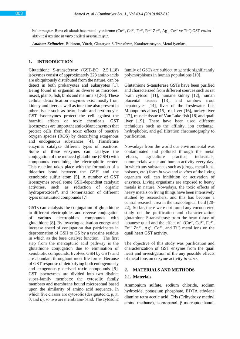
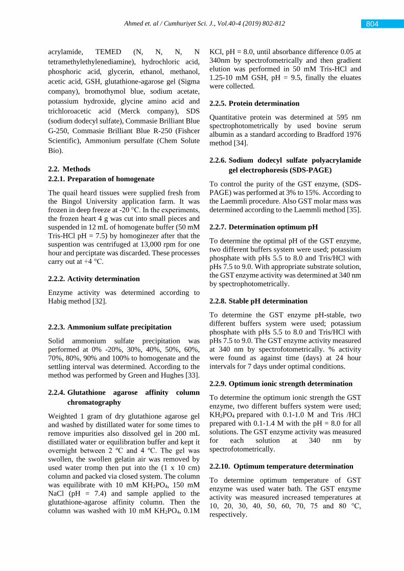
26.3 kDa by SDS-PAGE method (Figure 2).
Figure 1. SDS-PAGE photograph: show a single band
of GST enzyme.
Figure 2. Rf-log M.W calibration curve to determine
M.W of GST enzyme.
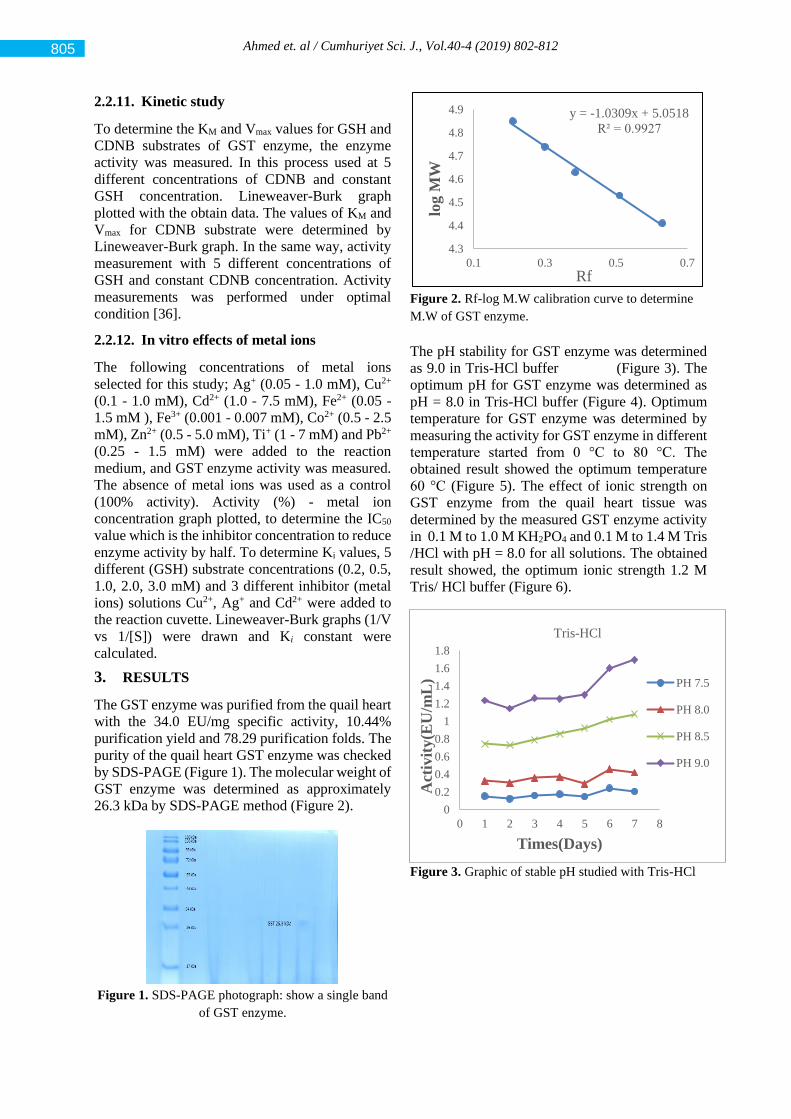
The pH stability for GST enzyme was determined
as 9.0 in Tris-HCl buffer (Figure 3). The
optimum pH for GST enzyme was determined as
pH = 8.0 in Tris-HCl buffer (Figure 4). Optimum
temperature for GST enzyme was determined by
measuring the activity for GST enzyme in different
temperature started from 0 °C to 80 °C. The
obtained result showed the optimum temperature
60 °C (Figure 5). The effect of ionic strength on
GST enzyme from the quail heart tissue was
determined by the measured GST enzyme activity
in 0.1 M to 1.0 M KH2PO4 and 0.1 M to 1.4 M Tris
/HCl with pH = 8.0 for all solutions. The obtained
result showed, the optimum ionic strength 1.2 M
Tris/ HCl buffer (Figure 6).
Figure 3. Graphic of stable pH studied with Tris-HCl
y = -1.0309x + 5.0518
R² = 0.9927
4.3
4.4
4.5
4.6
4.7
4.8
4.9
0.1 0.3 0.5 0.7
log M
W
Rf
0
0.2
0.4
0.6
0.8
1
1.2
1.4
1.6
1.8
0 1 2 3 4 5 6 7 8
Act
ivit
y(E
U/m
L)
Times(Days)
Tris-HCl
PH 7.5
PH 8.0
PH 8.5
PH 9.0
805
Ahmed et. al / Cumhuriyet Sci. J., Vol.40-4 (2019) 802-812
Figure 4. The graphic of optimum pH results.
Figure. 5. Result of optimum temperature.
Figure 6. The results of optimum ionic strength
(KH2PO4 and Tris-HCl buffer).
In addition enzyme kinetic study was performed to
determine KM and Vmax for glutathione S-
transferase purified from the quail heart tissues,
and by using both GSH and CDNB as substrate.
The results obtained are 1.642 mM and 0.502
EU/mL respectively for GSH substrate (Figure 7),
and 3.880 mM and 0.588 EU/mL respectively for
CDNB substrate (Figure 8).
Figure 7. Lineweaver-Burk graphic with five different
[GSH].
Figure 8. Lineweaver-Burk graphic with five different
[CDNB].
The effect of metal ions on the GST enzyme
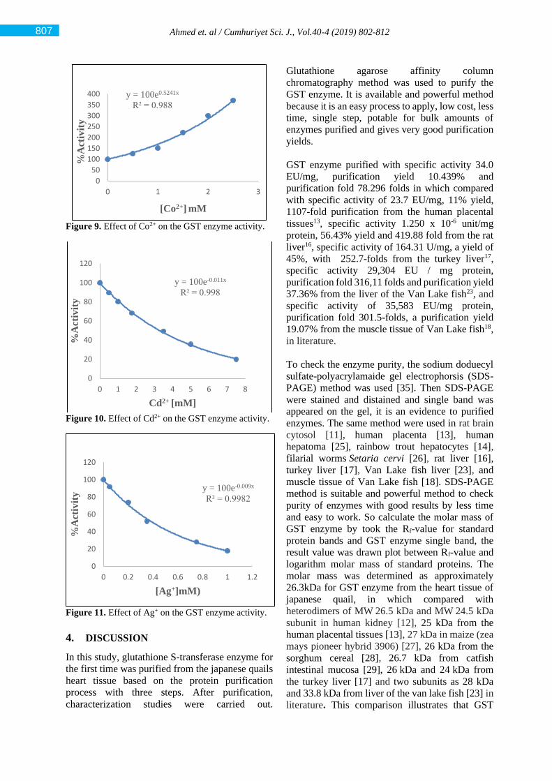
activity were determined. Results show that Co2+,
Fe2+, Fe3+, Ti+, Zn2+ metal ions increased GST
enzyme activity. Those metal ions indicated
activator for GST enzyme, (an example Co2+ ion,
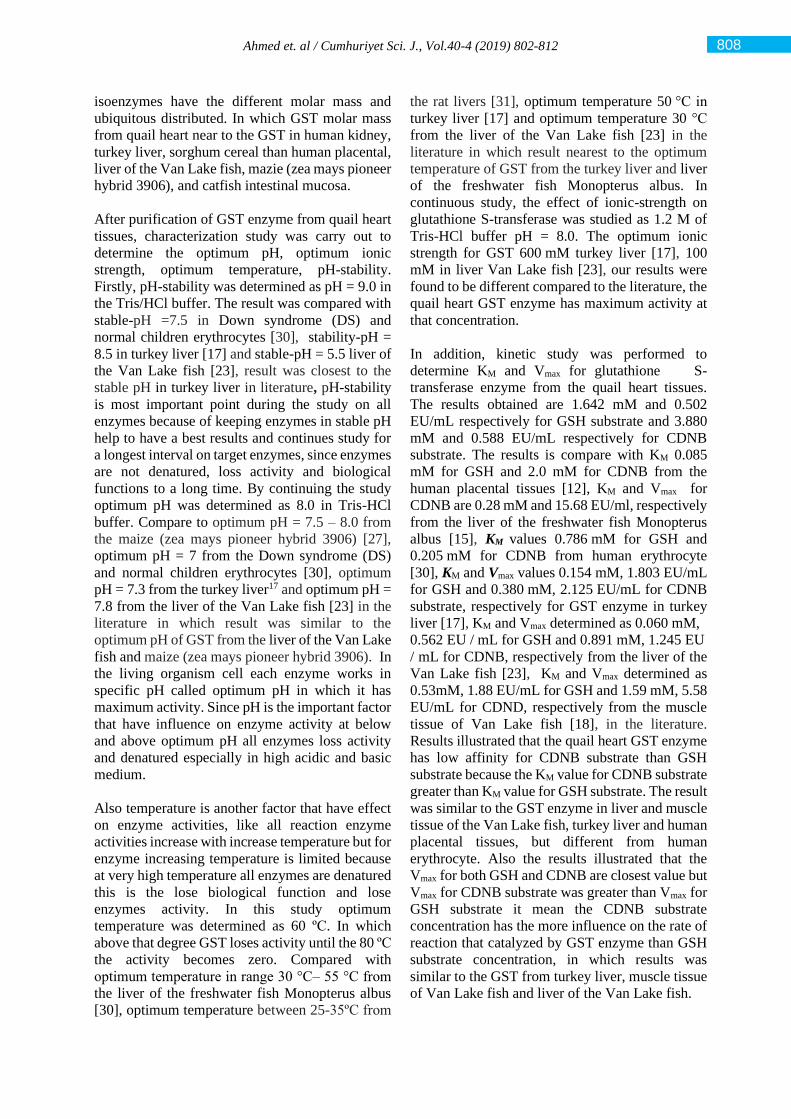
Figure 9), But Cd2+, Cu2+, Ag+ have negative effect
on the GST enzyme cause the decreased enzyme
activity, that indicated those are inhibitors for GST
enzyme from quail heart (Figure 10, Figure 11).
0
0.5
1
1.5
2
2.5
3
3.5
5 6 7 8 9 10
Act
ivit
y(E
U/m
L)
pH
Optimum pH
KH2PO4
Tris-HCl
0
0.2
0.4
0.6
0.8
1
0 10 20 30 40 50 60 70 80 90
Act
ivit
y(E
U/m
L)
Temprature °C
Optimum Temprature
0
0.4
0.8
1.2
1.6
0 0.4 0.8 1.2 1.6
Act
ivit
y(E
U/m
L)
Concetration M
Ionic strength
KH2PO4
Tris-HCl
y = 3.2678x + 1.9899
R² = 0.9954
0
1
2
3
4
5
6
7
8
9
-1 -0.5 0 0.5 1 1.5 2 2.5
1/V
1/[GSH]mM
y = 6.5895x + 1.6982
R² = 0.9748
0
1
2
3
4
5
6
7
8
-0.4 -0.2 0 0.2 0.4 0.6 0.8 1
1/V
1/[CDNB]mM
806
Ahmed et. al / Cumhuriyet Sci. J., Vol.40-4 (2019) 802-812
Figure 9. Effect of Co2+ on the GST enzyme activity.
Figure 10. Effect of Cd2+ on the GST enzyme activity.
Figure 11. Effect of Ag+ on the GST enzyme activity.
4. DISCUSSION
In this study, glutathione S-transferase enzyme for
the first time was purified from the japanese quails
heart tissue based on the protein purification
process with three steps. After purification,
characterization studies were carried out.
Glutathione agarose affinity column
chromatography method was used to purify the
GST enzyme. It is available and powerful method
because it is an easy process to apply, low cost, less
time, single step, potable for bulk amounts of
enzymes purified and gives very good purification
yields.
GST enzyme purified with specific activity 34.0
EU/mg, purification yield 10.439% and
purification fold 78.296 folds in which compared
with specific activity of 23.7 EU/mg, 11% yield,
1107-fold purification from the human placental
tissues13, specific activity 1.250 x 10⁻⁶ unit/mg
protein, 56.43% yield and 419.88 fold from the rat
liver16, specific activity of 164.31 U/mg, a yield of
45%, with 252.7-folds from the turkey liver17,
specific activity 29,304 EU / mg protein,
purification fold 316,11 folds and purification yield
37.36% from the liver of the Van Lake fish23, and
specific activity of 35,583 EU/mg protein,
purification fold 301.5-folds, a purification yield
19.07% from the muscle tissue of Van Lake fish18,
in literature.
To check the enzyme purity, the sodium doduecyl
sulfate-polyacrylamaide gel electrophorsis (SDS-
PAGE) method was used [35]. Then SDS-PAGE
were stained and distained and single band was
appeared on the gel, it is an evidence to purified
enzymes. The same method were used in rat brain
cytosol [11], human placenta [13], human
hepatoma [25], rainbow trout hepatocytes [14],
filarial worms Setaria cervi [26], rat liver [16],
turkey liver [17], Van Lake fish liver [23], and
muscle tissue of Van Lake fish [18]. SDS-PAGE
method is suitable and powerful method to check
purity of enzymes with good results by less time
and easy to work. So calculate the molar mass of
GST enzyme by took the Rf-value for standard
protein bands and GST enzyme single band, the
result value was drawn plot between Rf-value and
logarithm molar mass of standard proteins. The
molar mass was determined as approximately
26.3kDa for GST enzyme from the heart tissue of
japanese quail, in which compared with
heterodimers of MW 26.5 kDa and MW 24.5 kDa
subunit in human kidney [12], 25 kDa from the
human placental tissues [13], 27 kDa in maize (zea
mays pioneer hybrid 3906) [27], 26 kDa from the
sorghum cereal [28], 26.7 kDa from catfish
intestinal mucosa [29], 26 kDa and 24 kDa from
the turkey liver [17] and two subunits as 28 kDa
and 33.8 kDa from liver of the van lake fish [23] in
literature. This comparison illustrates that GST
y = 100e0.5241x
R² = 0.988
0
50
100
150
200
250
300
350
400
0 1 2 3
%A
ctiv
ity
[Co2+] mM
y = 100e-0.011x
R² = 0.998
0
20
40
60
80
100
120
0 1 2 3 4 5 6 7 8
%A
ctiv
ity
Cd2+ [mM]
y = 100e-0.009x
R² = 0.9982
0
20
40
60
80
100
120
0 0.2 0.4 0.6 0.8 1 1.2
%A
ctiv
ity
[Ag+]mM)
807
Ahmed et. al / Cumhuriyet Sci. J., Vol.40-4 (2019) 802-812
isoenzymes have the different molar mass and
ubiquitous distributed. In which GST molar mass
from quail heart near to the GST in human kidney,
turkey liver, sorghum cereal than human placental,
liver of the Van Lake fish, mazie (zea mays pioneer
hybrid 3906), and catfish intestinal mucosa.
After purification of GST enzyme from quail heart
tissues, characterization study was carry out to
determine the optimum pH, optimum ionic
strength, optimum temperature, pH-stability.
Firstly, pH-stability was determined as pH = 9.0 in
the Tris/HCl buffer. The result was compared with
stable-pH =7.5 in Down syndrome (DS) and
normal children erythrocytes [30], stability-pH =
8.5 in turkey liver [17] and stable-pH = 5.5 liver of
the Van Lake fish [23], result was closest to the
stable pH in turkey liver in literature, pH-stability
is most important point during the study on all
enzymes because of keeping enzymes in stable pH
help to have a best results and continues study for
a longest interval on target enzymes, since enzymes
are not denatured, loss activity and biological
functions to a long time. By continuing the study
optimum pH was determined as 8.0 in Tris-HCl
buffer. Compare to optimum pH = 7.5 – 8.0 from
the maize (zea mays pioneer hybrid 3906) [27],
optimum pH = 7 from the Down syndrome (DS)
and normal children erythrocytes [30], optimum
pH = 7.3 from the turkey liver17 and optimum pH =
7.8 from the liver of the Van Lake fish [23] in the
literature in which result was similar to the
optimum pH of GST from the liver of the Van Lake
fish and maize (zea mays pioneer hybrid 3906). In
the living organism cell each enzyme works in
specific pH called optimum pH in which it has
maximum activity. Since pH is the important factor
that have influence on enzyme activity at below
and above optimum pH all enzymes loss activity
and denatured especially in high acidic and basic
medium.
Also temperature is another factor that have effect
on enzyme activities, like all reaction enzyme
activities increase with increase temperature but for
enzyme increasing temperature is limited because
at very high temperature all enzymes are denatured
this is the lose biological function and lose
enzymes activity. In this study optimum
temperature was determined as 60 ºC. In which
above that degree GST loses activity until the 80 ºC
the activity becomes zero. Compared with
optimum temperature in range 30 °C– 55 °C from
the liver of the freshwater fish Monopterus albus
[30], optimum temperature between 25-35ºC from
the rat livers [31], optimum temperature 50 °C in
turkey liver [17] and optimum temperature 30 °C
from the liver of the Van Lake fish [23] in the
literature in which result nearest to the optimum
temperature of GST from the turkey liver and liver
of the freshwater fish Monopterus albus. In
continuous study, the effect of ionic-strength on
glutathione S-transferase was studied as 1.2 M of
Tris-HCl buffer pH = 8.0. The optimum ionic
strength for GST 600 mM turkey liver [17], 100
mM in liver Van Lake fish [23], our results were
found to be different compared to the literature, the
quail heart GST enzyme has maximum activity at
that concentration.
In addition, kinetic study was performed to
determine KM and Vmax for glutathione S-
transferase enzyme from the quail heart tissues.
The results obtained are 1.642 mM and 0.502
EU/mL respectively for GSH substrate and 3.880
mM and 0.588 EU/mL respectively for CDNB
substrate. The results is compare with KM 0.085
mM for GSH and 2.0 mM for CDNB from the
human placental tissues [12], KM and Vmax for
CDNB are 0.28 mM and 15.68 EU/ml, respectively
from the liver of the freshwater fish Monopterus
albus [15], KM values 0.786 mM for GSH and
0.205 mM for CDNB from human erythrocyte
[30], KM and Vmax values 0.154 mM, 1.803 EU/mL
for GSH and 0.380 mM, 2.125 EU/mL for CDNB
substrate, respectively for GST enzyme in turkey
liver [17], KM and Vmax determined as 0.060 mM,
0.562 EU / mL for GSH and 0.891 mM, 1.245 EU
/ mL for CDNB, respectively from the liver of the
Van Lake fish [23], KM and Vmax determined as
0.53mM, 1.88 EU/mL for GSH and 1.59 mM, 5.58
EU/mL for CDND, respectively from the muscle
tissue of Van Lake fish [18], in the literature.
Results illustrated that the quail heart GST enzyme
has low affinity for CDNB substrate than GSH
substrate because the KM value for CDNB substrate
greater than KM value for GSH substrate. The result
was similar to the GST enzyme in liver and muscle
tissue of the Van Lake fish, turkey liver and human
placental tissues, but different from human
erythrocyte. Also the results illustrated that the
Vmax for both GSH and CDNB are closest value but
Vmax for CDNB substrate was greater than Vmax for
GSH substrate it mean the CDNB substrate
concentration has the more influence on the rate of
reaction that catalyzed by GST enzyme than GSH
substrate concentration, in which results was
similar to the GST from turkey liver, muscle tissue
of Van Lake fish and liver of the Van Lake fish.
808
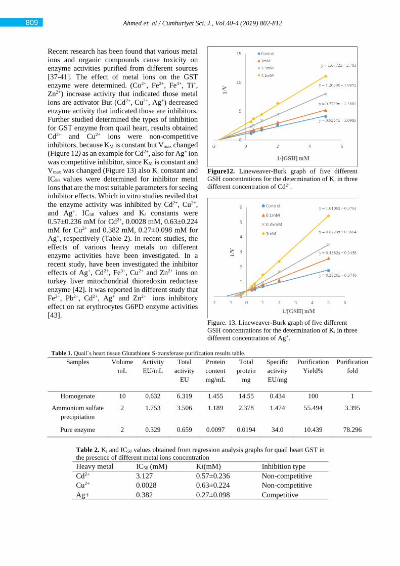
Ahmed et. al / Cumhuriyet Sci. J., Vol.40-4 (2019) 802-812
Recent research has been found that various metal
ions and organic compounds cause toxicity on
enzyme activities purified from different sources
[37-41]. The effect of metal ions on the GST
enzyme were determined. (Co2+, Fe2+, Fe3+, Ti+,
Zn2+) increase activity that indicated those metal
ions are activator But (Cd2+, Cu2+, Ag+) decreased
enzyme activity that indicated those are inhibitors.
Further studied determined the types of inhibition
for GST enzyme from quail heart, results obtained
Cd2+ and Cu2+ ions were non-competitive
inhibitors, because KM is constant but Vmax changed
(Figure 12) as an example for Cd2+, also for Ag+ ion
was competitive inhibitor, since KM is constant and
Vmax was changed (Figure 13) also Ki constant and
IC50 values were determined for inhibitor metal
ions that are the most suitable parameters for seeing
inhibitor effects. Which in vitro studies reviled that
the enzyme activity was inhibited by Cd2+, Cu2+,
and Ag+. IC50 values and Ki constants were
0.57±0.236 mM for Cd2+, 0.0028 mM, 0.63±0.224
mM for Cu2+ and 0.382 mM, 0.27±0.098 mM for
Ag+, respectively (Table 2). In recent studies, the
effects of various heavy metals on different
enzyme activities have been investigated. In a
recent study, have been investigated the inhibitor
effects of Ag+, Cd2+, Fe3+, Cu2+ and Zn2+ ions on
turkey liver mitochondrial thioredoxin reductase
enzyme [42]. it was reported in different study that
Fe2+, Pb2+, Cd2+, Ag+ and Zn2+ ions inhibitory
effect on rat erythrocytes G6PD enzyme activities
[43].
Figure12. Lineweaver-Burk graph of five different
GSH concentrations for the determination of Ki in three
different concentration of Cd2+.
Figure. 13. Lineweaver-Burk graph of five different
GSH concentrations for the determination of Ki in three
different concentration of Ag+.
Table 1. Quail`s heart tissue Glutathione S-transferase purification results table.
Samples Volume
mL
Activity
EU/mL
Total
activity
EU
Protein
content
mg/mL
Total
protein
mg
Specific
activity
EU/mg
Purification
Yield%
Purification
fold
Homogenate 10 0.632 6.319 1.455 14.55 0.434 100 1
Ammonium sulfate
precipitation
2 1.753 3.506 1.189 2.378 1.474 55.494 3.395
Pure enzyme 2 0.329 0.659 0.0097 0.0194 34.0 10.439 78.296
Table 2. Ki and IC50 values obtained from regression analysis graphs for quail heart GST in
the presence of different metal ions concentration
Heavy metal IC50 (mM) Ki(mM) Inhibition type
Cd2+ 3.127 0.57±0.236 Non-competitive
Cu2+ 0.0028 0.63±0.224 Non-competitive
Ag+ 0.382 0.27±0.098 Competitive
809
Ahmed et. al / Cumhuriyet Sci. J., Vol.40-4 (2019) 802-812
5. CONCLUSION
In this study, glutathione S-transferase enzyme for
the first time was purified from the japanese quails
heart tissue based on the protein purification
process with three steps. After purification,
characterization studies were carried out. In
addition the effect of metal ions on the GST
enzyme activity were determined. Our study
showed that Co2+, Fe2+, Fe3+, Ti+, Zn2+ metal ions
increased GST enzyme activity, while Cd2+, Cu2+
and Ag+ ions had an inhibitory effect on enzyme
activity.
REFERENCES
[1] Booth J., Boyland E., Sims A.P., An enzyme
from rat liver catalysing conjugations with
glutathione, Biochem. J., 79 (1961) 516-
524.
[2] Sherratt P.H., Hayes J., Glutathione S-
Transferases Enzyme System That
Metabolise Drugs and Other
Xenobiotics. Chichester, UK ., (2001) 1-
578.
[3] Hayes J.D., Pulford D.J., The glutathione S-
transferase supergene family: regulation of
GST and the contribution of the lsoenzymes
to cancer chemoprotection and drug
resistance, part I. Critic. Rev. Biochem. Mol.
Biol., 30 (1995) 445-520.
[4] George S.G., Enzymology and molecular
biology of phase II xenobiotic-conjugating
enzymes in fish, Aquatic Toxicol. (1994)
37-85.
[5] Mannervik B., Alin P., Guthenbergg C.,
Jensson H., Tahir M.K., Warholm M.,
Jornvall H., Identification of three classes of
cytosolic glutathione transferase common to
several mammalian species: correlation
between structural data and enzymatic
properties, Proceed National Acad. Sci USA
82 (1985) 7202-206.
[6] Ketterer B., Meyer D.J, Taylor J.B., Pemble
S., Coles B., Fraser G., GSTs and protection
against oxidative stress. In Glutathione
S.Transferase and Drug Resistance, Taylor
Francis Bristol, 1990; pp 97-109.
[7] Benson A.M., Talalay P., Keen J.H., Jakoby
W.B., Relationship between the soluble
glutathione-dependent delta 5-3-ketosteroid
isomerase and the glutathione S-transferases
of the liver, Proceed National Acad. Sci., 74
(1977) 158-162.
[8] Yu S.J., Insect glutathione S-transferases,
Zoological Studies, 35-1 (1996) 9-19.
[9] Cancado G.M., De Rosa V.E., Fernandez
J.H., Maron L.G., Jorge R.A., Menossi M.,
Glutathione S-transferase and aluminum
toxicity in maize, Functional Plant. Biol., 32
(2005) 1045–1055.
[10] Townsend D.M., Tew K.D., The role of
glutathione-S-transferase in anti-cancer drug
resistance, Oncogene 22 (2003) 7369-7375.
[11] Senjo M., Ishibashi T., Purification and
characterization of glutathione S-transferase
from rat brain cytosol identification of four
isozymes and evidence for absence of the Ya
subunit, Biomed. Res., 7 (1986) 19-26.
[12] Singh S.V., Leal T., Ansari G.A., Awasthi
Y.C., Purification and characterization of
glutathione S-transferases of human
kidney, Biochem. J., 246 (1987) 179-186.
[13] Kwak S.J, Park S.C., Purification and
Characterization of Glutathione S-
transferase π from Human Placental Tissues,
Seoul J. Med., 29 (1988) 107-118.
[14] Riol M.M., Valinas M.N., Fernandez M.G.,
Lopez M.P., Glutathione S-transferases from
rainbow trout liver and freshly isolated
hepatocytes: purification and
characterization, Comp. Biochem. Physiol
Part C: Toxicol. Pharmacol., 128 (2001)
227-235.
[15] Huang Q., Liang L., Wei T., Zhang D., Zeng
Q.Y., Purification and partial
characterization of glutathione transferase
from the teleost Monopterus albus. Comp
Biochem Physiol Part C: Toxicol Pharmacol
147 (2008) 96-100.
[16] Jassim H.A., Ameen F.Z., Al-Jumaily
E.F.A., Isolation And Purification Of
Glutathione S-Transferasefrom Rat Liver, J
Al-Nahrain Univ. Sci., 12 (2009) 137-144.
[17] Akkemik E., Taser P., Bayindir A., Budak
H., Ciftci M., Purification and
characterization of glutathione S-transferase
810
Ahmed et. al / Cumhuriyet Sci. J., Vol.40-4 (2019) 802-812
from turkey liver and inhibition effects of
some metal ions on enzyme activity,
Environ. Toxicol. Pharmacol. 34 (2012)
888-894.
[18] Aksoy M., Ozaslan M., Kufrevioglu O.,
Purification of glutathione S-transferase
from Van Lake fish (Chalcalburnus tarichii
Pallas) muscle and investigation of some
metal ions effect on enzyme activity. J
Enzyme Inhib. Med. Chem. 31 (2016) 546-
550.
[19] Temel Y., Koçyigit U.M., Taysı M.Ş.,
Gökalp F., Gürdere M.B., Budak Y., Çiftci
M., Purification of glutathione S‐transferase
enzyme from quail liver tissue and inhibition
effects of (3aR, 4S, 7R, 7aS)‐2‐(4‐((E)‐3‐
(aryl) acryloyl) phenyl)‐3a, 4, 7, 7a‐
tetrahydro‐1H‐4, 7‐methanoisoindole‐1, 3
(2H)‐dione derivatives on the enzyme
activity, J. Biochem. Mol. Toxicol. 32
(2018) e22034.
[20] Krewski D., Yokel R.A., Nieboer E.,
Borchelt D., Cohen J., Harry J., Rondeau V.,
Human health risk assessment for
aluminium, aluminium oxide, and
aluminium hydroxide, J. Toxicol. Environ.
Health Part B 10 (2007) 1-269.
[21] Kucuk M., Gulcin I., Purification and
characterization of the carbonic anhydrase
enzyme from Black Sea trout (Salmo trutta
Labrax Coruhensis) kidney and inhibition
effects of some metal ions on enzyme
activity, Environ. Toxicol. Pharm. 44 (2016)
134-139.
[22] Verstraeten S.V., Aimo L., Oteiza P.I.,
Aluminium and lead: molecular mechanisms
of brain toxicity, Arch. Toxicol., 82 (2008)
789-802.
[23] Ozaslan M.S., Ciftci M., Purification of
glutathione S-transferase from Van Lake
fish (Chalcalburnus tarichii Pallas) liver and
investigation of some metal ions effect on
enzyme activity. J. Enzyme İnhib. Med.
Chem., 31 (2014) 546-550.
[24] Laemmli U.K., Cleavage of structural
proteins during assembly of head of
bacteriophage T4. Nature 227 (1970) 680–
85.
[25] Dierickx P.J., Purification and
characterization of glutathione S-transferase
from the human hepatoma derived
PLC/PRF/5 cell line, Biomed. Res., 10
(1989) 301-306.
[26] Ahmad R., Srivastava A. K., Walter R.D.,
Purification and biochemical
characterization of cytosolic glutathione-S-
transferase from filarial worms Setaria
cervi, Comp. Biochem. Physiology Part B:
Biochem. Mol. Biol., 151 (2008) 237-245.
[27] Fuerst E.P., Irzyk G.P., Miller K.D., Partial
characterization of glutathione S-transferase
isozymes induced by the herbicide safener
benoxacor in maize, Plant Physiol. 102
(1993) 795-802.
[28] Gronwald J.W., Plaisance K.L., Isolation
and Characterization of Glutathione S-
Transferase Isozymes from Sorghum, Plant
Physiol. 17-1(1998) 877-892.
[29] Gadagbui B.K., James M.O., Activities of
affinity-isolated glutathione S-transferase
(GST) from channel catfish whole intestine,
Aquatic Toxicol., 49 (2000) 27-37.
[30] Hamed R.R., Maharem T.M., Abdel-Meguid
N., Sabry G.M., Abdalla A.M., Guneidy
R.A., Purification and biochemical
characterization of glutathione S-transferase
from Down syndrome and normal children
erythrocytes: A comparative study, Res.
Develop. disabilities 32 (2011) 1470-1482.
[31] Lebda M., Taha N., Noeman S., Korshom
M., El-Wahab Mandour, A. Purification and
Characterization of Glutathione-S-
Transferase from Rat′ s Liver: Effect of
Carbon Tetrachloride and Camel′ s Milk, J.
Chromat. Separation Techniq, 3-4 (2012) 2-
8.
[32] Habig W.H., Pabst M.J., Jakoby W.B.,
Glutathione S-transferases the first
enzymatic step in mercapturic acid
formation, J. Biol. Chem. 249 (1974) 7130-
7139.
[33] Wingfield P., Protein precipitation using
ammonium sulfate, Current Prot. Prot. Sci.,
53 (2001) A- 3F.
[34] Bradford M.M., Rapid and sensitive method
for the quantitation of microgram
811
Ahmed et. al / Cumhuriyet Sci. J., Vol.40-4 (2019) 802-812
quantities of protein utilizing the principle of
protein-dye binding, Anal. Biochem., 72
(1976) 248-254.
[35] Laemmli D.K., Cleavage of structural
proteins during in assembly of the heat of
bacteriophage T4. Nature London, 227
(1970) 680-685.
[36] Lineweaver H., Burk D., The determination
of enzyme dissocation constants, J. Am.
Chem. Soc., 56-3 (1934) 57-685.
[37] Temel Y., Bengü A.Ş., Akkoyun H.T.,
Akkoyun M.B., Çiftci M., Effect of
astaxanthin and aluminum chloride on
erythrocyte G6PD and 6PGD enzyme
activities in vivo and on erythrocyte G6PD
in vitro in rats, J. Biochem. Mol. Tox. 31
(2017) e21954.
[38] Ceylan M., Kocyigit U.M., Usta N.C.,
Gürbüzlü B., Temel Y., Alwasel S.H.,
Gulcin I., Synthesis, carbonic anhydrase I
and II iso enzymes inhibition properties, and
antibacterial activities of novel tetralone-
based 1,4-benzothiazepine deriva tives, J.
Biochem. Mol. Tox. 31 (2017) e21872.
[39] Bayındır S., Ayna A., Temel Y., Çiftci M.,
The synthesis of new oxindoles as analogs of
natural product 3,3'-bis(indolyl)oxindole
and in vitro evaluation for enzyme activity
of G6PD and 6PGD, Turk. J. Chem. 42
(2018) 332- 345.
[40] Bayindir S., Temel Y., Ayna A., Ciftci M.,
The synthesis of N‐benzoylindoles as
inhibitors of rat erythrocyte glucose‐6‐
phosphate dehydrogenase and 6‐
phosphogluconate dehydrogenase, J.
Biochem. Mol. Tox. 32 (2018) e22193.
[41] Temel Y., Taher S.S.M., Hamza M.A.,
Shafeeq I.H., Koçyiğit U.M., Çiftci M.,
Investigation of the Inhibition Effects of
Some Metal Ions on Glutathione Reductase
Enzyme From Japanese Quail (Coturnix
coturnix japonica) Liver, Cumhuriyet Sci. J.
39 (2018) 3679-687.
[42] Temel Y., Küfrevioğlu Ö.İ., Çiftci M.,
Investigation of the effects of purification
and characterization of turkey (Meleagris
gallopavo) liver mitochondrial thioredoxin
reductase enzyme and some metal ions on
enzyme activity, Turk. J. Chem. 41 (2017)
48-60.
[43] Temel Y. and Kocyigit U.M., Purification of
glucose-6-phosphate dehydrogenase from
rat (Rattus norvegicus) erythrocytes and
inhibition effects of some metal ions on
enzyme activity, J. Biochem. Mol. Tox. 31
(2017) e21927.
812

Cumhuriyet Science Journal
CSJ
e-ISSN: 2587-246X
ISSN: 2587-2680 Cumhuriyet Sci. J., Vol.40-4 (2019) 813-818
* Corresponding author. Email address: [email protected]
http://dergipark.gov.tr/csj ©2019 Faculty of Science, Sivas Cumhuriyet University
The Effects of CO2, N2, and H2O Dilutions on NO Formation of Partially
Premixed Synthesis Gas Combustion
Suat OZTURK1,*
1Department of Electronic and Automation, Zonguldak Vocational School, Zonguldak Bulent Ecevit University,
Zonguldak, Turkey
Received: 21.03.2019; Accepted: 11.11.2019 http://dx.doi.org/10.17776/csj.543130
Abstract. One of the main methods to decrease NO emission during the combustion of gases is the use of
diluents. This study is interested in the effects of CO2, N2, and H2O dilutions in the adiabatic, turbulent, partially
premixed combustion of synthesis gas. The amounts of NO emissions are computationally determined. The
results show that NO maximizes at 1.39 of equivalence ratio under humid burning air conditions. The best
reductive effect on NO emissions indicates H2O dilution followed by CO2 and N2. The increase in the dilution
rates gradationally reduces NO. The rising pressure enhances NO emissions with/without diluters. The
increasing inlet air and premixed mixture temperatures raises NO.
Keywords: Synthesis gas, partially premixed, combustion, nitrogen oxide.
Kısmi Önkarışımlı Sentez Gazı Yanmasının NO Oluşumu Üzerinde CO2, N2
ve H2O Seyreltmelerinin Etkileri
Özet. Gazların yakılmasında NO emisyonunu azaltmak için ana metodlardan biri seyrelticilerin kullanımıdır.
Bu çalışma sentez gazının adyabatik, turbülanslı, kısmi önkarışımlı yanmasında CO2, N2 ve H2O
seyreltmelerinin etkileri ile ilgilenmektedir. NO emisyonlarının miktarları hesaplamalı olarak saptanmıştır.
Sonuçlar, nemli yakma havası şartlarında, NO’in, 1.39 ekivalans oranında maksimize olduğunu göstermektedir.
NO emisyonları üzerinde en iyi azaltıcı etkiyi CO2 ve N2 tarafından takip edilen H2O seyrelticisi göstermektedir.
Seyreltici oranlarındaki artış derecesel olarak NO’i azaltmaktadır. Yükselen basınç seyreltili veya seyreltisiz
NO emisyonlarını artırmaktadır. Artan hava ve önkarıştırılmış karışım giriş sıcaklıkları NO’i yükseltmektedir.
Anahtar Kelimeler:, Sentez gazı, kısmi karışımlı, yanma, nitrojen oksit.
1. INTRODUCTION
Synthesis gas (syngas) is a product obtained by
gasification process from coal, tire, biomass, or
steam reforming from natural gas. It generally
consists of different components as H2, CH4, CO,
CO2, H2O, N2, H2S, NH3, and COS depending on
fuel source what it is derived of. Synthesis gas is
utilized in industrial furnace and high efficiency
gas turbines for power generation after post
gasification process removing H2S and other
unwanted contaminants. Its wide presence and
appropriate combustion characteristics makes
synthesis gas a conspicuous option among gas fuels
[1, 2].
NOx emissions forming because of high
temperature reactions of N2 and O2 in burning air
and fuel also continue to be an environmental
problem as a pollutant for synthesis gas
combustion. NOx is the sum of mostly NO and NO2
from greenhouse gases and countries take common
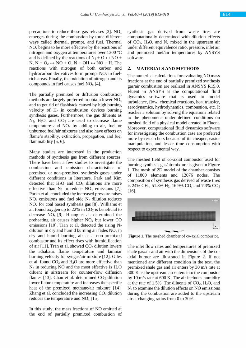
Ozturk / Cumhuriyet Sci. J., Vol.40-4 (2019) 813-818
precautions to reduce these gas releases [3]. NOx
emerges during the combustion by three different
ways called thermal, prompt, and fuel. Thermal
NOx begins to be more effective by the reactions of
nitrogen and oxygen at temperatures over 1300 oC
and is defined by the reactions of N2 + O ↔ NO +
N, N + O2 ↔ NO + O, N + OH ↔ NO + H. The
reactions with nitrogen of both carbon and
hydrocarbon derivatives form prompt NOx in fuel-
rich areas. Finally, the oxidation of nitrogen and its
compounds in fuel causes fuel NOx [4].
The partially premixed or diffusion combustion
methods are largely preferred to obtain lower NOx
and to get rid of flashback caused by high burning
velocity of H2 in combustion devices burning
synthesis gases. Furthermore, the gas diluents as
N2, H2O, and CO2 are used to decrease flame
temperature and NOx by adding to air, fuel or
unburned fuel/air mixtures and also have effects on
flame’s stability, extinction, propagation, and fuel
flammability [5, 6].
Many studies are interested in the production
methods of synthesis gas from different sources.
There have been a few studies to investigate the
combustion and emission characteristics of
premixed or non-premixed synthesis gases under
different conditions in literature. Park and Kim
detected that H2O and CO2 dilutions are more
effective than N2 to reduce NOx emissions [7].
Parka et al. concluded the increased pressure raises
NOx emissions and fuel side N2 dilution reduces
NOx for coal based synthesis gas [8]. Williams et
al. found oxygen up to 22% in CO2 is beneficial to
decrease NOx [9]. Huang et al. determined the
preheating air causes higher NOx but lower CO
emissions [10]. Tian et al. detected the rising N2
dilution in dry and humid burning air fades NOx in
dry and humid burning air at a non-premixed
combustor and its effect rises with humidification
of air [11]. Tran et al. showed CO2 dilution lowers
the adiabatic flame temperature and laminar
burning velocity for syngas/air mixture [12]. Giles
et al. found CO2 and H2O are more effective than
N2 in reducing NO and the most effective is H2O
diluent in airstream for counter-flow diffusion
flames [13]. Chan et al. determined CO2 dilution
lower flame temperature and increases the specific
heat of the premixed methane/air mixture [14].
Zhang et al. concluded the increasing CO2 dilution
reduces the temperature and NOx [15].
In this study, the mass fractions of NO emitted at
the end of partially premixed combustion of
synthesis gas derived from waste tires are
computationally determined with dilution effects
of CO2, H2O, and N2 mixed in the upstream air
under different equivalence ratio, pressure, inlet air
and premixed fuel/air temperatures by ANSYS
software.
2. MATERIALS AND METHODS
The numerical calculations for evaluating NO mass
fractions at the end of partially premixed synthesis
gas/air combustion are realized in ANSYS R15.0.
Fluent in ANSYS is the computational fluid
dynamics software that is used to model
turbulence, flow, chemical reactions, heat transfer,
aerodynamics, hydrodynamics, combustion, etc. It
reaches a solution by solving the equations related
to the phenomena under defined conditions on
meshed field of a physical model created in Fluent.
Moreover, computational fluid dynamics software
for investigating the combustion case are preferred
more by researchers because of its cheaper, easier
manipulation, and lesser time consumption with
respect to experimental way.
The meshed field of co-axial combustor used for
burning synthesis gas/air mixture is given in Figure
1. The mesh of 2D model of the chamber consists
of 11800 elements and 12076 nodes. The
composition of synthesis gas derived of waste tires
is 24% CH4, 51.8% H2, 16.9% CO, and 7.3% CO2
[16].
Figure 1. The meshed chamber of co-axial combustor.
The inlet flow rates and temperatures of premixed
shale gas/air and air with the dimensions of the co-
axial burner are illustrated in Figure 2. If not
mentioned any different condition in the text, the
premixed shale gas and air enters by 30 m/s rate at
300 K as the upstream air enters into the combustor
by 10 m/s rate at 600 K. The air includes humidity
at the rate of 1.5%. The diluents of CO2, H2O, and
N2 to examine the dilution effects on NO emissions
during the combustion are added to the upstream
air at changing ratios from 0 to 30%.
814
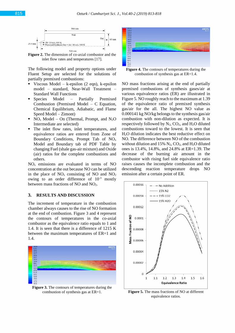
Ozturk / Cumhuriyet Sci. J., Vol.40-2 (2019) 813-818
Figure 2. The dimension of co-axial combustor and the
inlet flow rates and temperatures [17].
The following model and property options under
Fluent Setup are selected for the solutions of
partially premixed combustions:
Viscous Model – k-epsilon (2 eqn), k-epsilon
model – standard, Near-Wall Treatment –
Standard Wall Functions
Species Model – Partially Premixed
Combustion (Premixed Model – C Equation,
Chemical Equilibrium, Adiabatic, and Flame
Speed Model – Zimont)
NOx Model – On (Thermal, Prompt, and N2O
Intermediate are selected)
The inlet flow rates, inlet temperatures, and
equivalence ratios are entered from Zone of
Boundary Conditions, Prompt Tab of NOx
Model and Boundary tab of PDF Table by
changing Fuel (shale gas-air mixture) and Oxide
(air) ratios for the complete combustions and
others.
NOx emissions are evaluated in terms of NO
concentration at the out because NO can be utilized
in the place of NOx consisting of NO and NO2
owing to an order difference of 10-3 mostly
between mass fractions of NO and NO2.
3. RESULTS AND DISCUSSION
The increment of temperature in the combustion
chamber always causes to the rise of NO formation
at the end of combustion. Figure 3 and 4 represent
the contours of temperatures in the co-axial
combustor as the equivalence ratio equals to 1 and
1.4. It is seen that there is a difference of 1215 K
between the maximum temperatures of ER=1 and
1.4.
Figure 3. The contours of temperatures during the
combustion of synthesis gas at ER=1.
Figure 4. The contours of temperatures during the
combustion of synthesis gas at ER=1.4.
NO mass fractions arising at the end of partially
premixed combustions of synthesis gases/air at
various equivalence ratios (ER) are illustrated in
Figure 5. NO roughly reach to the maximum at 1.39
of the equivalence ratio of premixed synthesis
gas/air for the all. The highest NO value as
0.000141 kg NO/kg belongs to the synthesis gas/air
combustion with non-dilution as expected. It is
respectively followed by N2, CO2, and H2O diluted
combustions toward to the lowest. It is seen that
H2O dilution indicates the best reductive effect on
NO. The difference between NO of the combustion
without dilution and 15% N2, CO2, and H2O diluted
ones is 13.4%, 14.8%, and 24.8% at ER=1.39. The
decrease of the burning air amount in the
combustor with rising fuel side equivalence ratio
raises causes the incomplete combustion and the
descending reaction temperature drops NO
emission after a certain point of ER.
Figure 5. The mass fractions of NO at different
equivalence ratios.
815
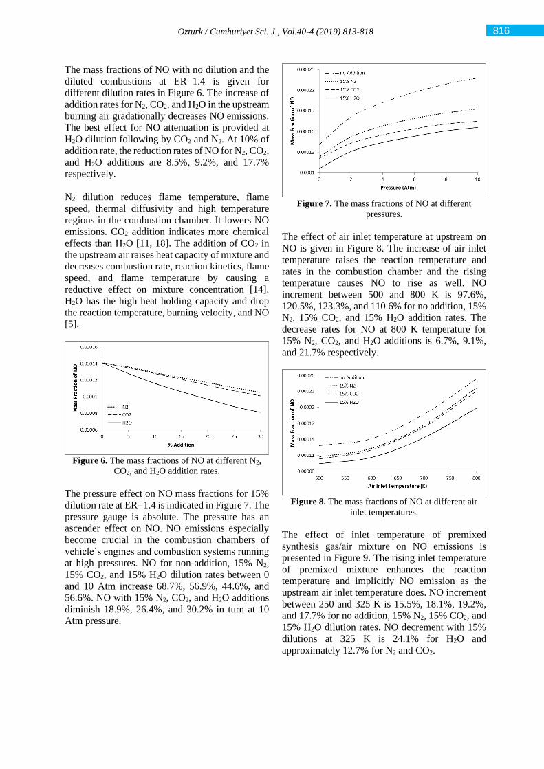
Ozturk / Cumhuriyet Sci. J., Vol.40-4 (2019) 813-818
The mass fractions of NO with no dilution and the
diluted combustions at ER=1.4 is given for
different dilution rates in Figure 6. The increase of
addition rates for N2, CO2, and H2O in the upstream
burning air gradationally decreases NO emissions.
The best effect for NO attenuation is provided at
H2O dilution following by CO2 and N2. At 10% of
addition rate, the reduction rates of NO for N2, CO2,
and H2O additions are 8.5%, 9.2%, and 17.7%
respectively.
N2 dilution reduces flame temperature, flame
speed, thermal diffusivity and high temperature
regions in the combustion chamber. It lowers NO
emissions. CO2 addition indicates more chemical
effects than H2O [11, 18]. The addition of CO2 in
the upstream air raises heat capacity of mixture and
decreases combustion rate, reaction kinetics, flame
speed, and flame temperature by causing a
reductive effect on mixture concentration [14].
H2O has the high heat holding capacity and drop
the reaction temperature, burning velocity, and NO
[5].
Figure 6. The mass fractions of NO at different N2,
CO2, and H2O addition rates.
The pressure effect on NO mass fractions for 15%
dilution rate at ER=1.4 is indicated in Figure 7. The
pressure gauge is absolute. The pressure has an
ascender effect on NO. NO emissions especially
become crucial in the combustion chambers of
vehicle’s engines and combustion systems running
at high pressures. NO for non-addition, 15% N2,
15% CO2, and 15% H2O dilution rates between 0
and 10 Atm increase 68.7%, 56.9%, 44.6%, and
56.6%. NO with 15% N2, CO2, and H2O additions
diminish 18.9%, 26.4%, and 30.2% in turn at 10
Atm pressure.
Figure 7. The mass fractions of NO at different
pressures.
The effect of air inlet temperature at upstream on
NO is given in Figure 8. The increase of air inlet
temperature raises the reaction temperature and
rates in the combustion chamber and the rising
temperature causes NO to rise as well. NO
increment between 500 and 800 K is 97.6%,
120.5%, 123.3%, and 110.6% for no addition, 15%
N2, 15% CO2, and 15% H2O addition rates. The
decrease rates for NO at 800 K temperature for
15% N2, CO2, and H2O additions is 6.7%, 9.1%,
and 21.7% respectively.
Figure 8. The mass fractions of NO at different air
inlet temperatures.
The effect of inlet temperature of premixed
synthesis gas/air mixture on NO emissions is
presented in Figure 9. The rising inlet temperature
of premixed mixture enhances the reaction
temperature and implicitly NO emission as the
upstream air inlet temperature does. NO increment
between 250 and 325 K is 15.5%, 18.1%, 19.2%,
and 17.7% for no addition, 15% N2, 15% CO2, and
15% H2O dilution rates. NO decrement with 15%
dilutions at 325 K is 24.1% for H2O and
approximately 12.7% for N2 and CO2.
816
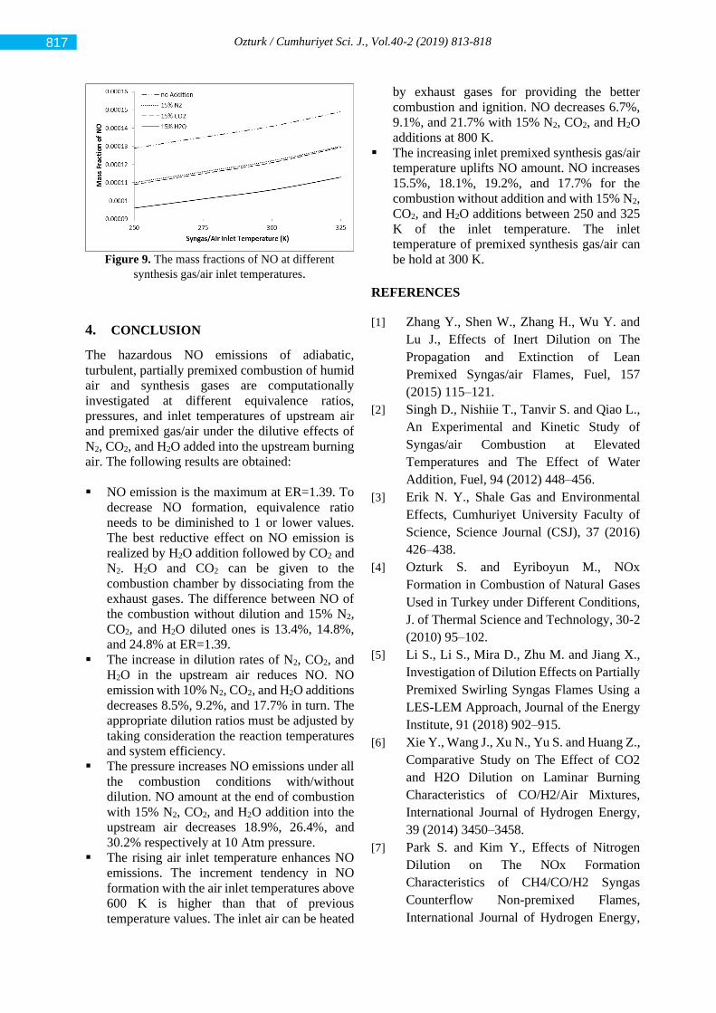
Ozturk / Cumhuriyet Sci. J., Vol.40-2 (2019) 813-818
Figure 9. The mass fractions of NO at different
synthesis gas/air inlet temperatures.
4. CONCLUSION
The hazardous NO emissions of adiabatic,
turbulent, partially premixed combustion of humid
air and synthesis gases are computationally
investigated at different equivalence ratios,
pressures, and inlet temperatures of upstream air
and premixed gas/air under the dilutive effects of
N2, CO2, and H2O added into the upstream burning
air. The following results are obtained:
NO emission is the maximum at ER=1.39. To
decrease NO formation, equivalence ratio
needs to be diminished to 1 or lower values.
The best reductive effect on NO emission is
realized by H2O addition followed by CO2 and
N2. H2O and CO2 can be given to the
combustion chamber by dissociating from the
exhaust gases. The difference between NO of
the combustion without dilution and 15% N2,
CO2, and H2O diluted ones is 13.4%, 14.8%,
and 24.8% at ER=1.39.
The increase in dilution rates of N2, CO2, and
H2O in the upstream air reduces NO. NO
emission with 10% N2, CO2, and H2O additions
decreases 8.5%, 9.2%, and 17.7% in turn. The
appropriate dilution ratios must be adjusted by
taking consideration the reaction temperatures
and system efficiency.
The pressure increases NO emissions under all
the combustion conditions with/without
dilution. NO amount at the end of combustion
with 15% N2, CO2, and H2O addition into the
upstream air decreases 18.9%, 26.4%, and
30.2% respectively at 10 Atm pressure.
The rising air inlet temperature enhances NO
emissions. The increment tendency in NO
formation with the air inlet temperatures above
600 K is higher than that of previous
temperature values. The inlet air can be heated
by exhaust gases for providing the better
combustion and ignition. NO decreases 6.7%,
9.1%, and 21.7% with 15% N2, CO2, and H2O
additions at 800 K.
The increasing inlet premixed synthesis gas/air
temperature uplifts NO amount. NO increases
15.5%, 18.1%, 19.2%, and 17.7% for the
combustion without addition and with 15% N2,
CO2, and H2O additions between 250 and 325
K of the inlet temperature. The inlet
temperature of premixed synthesis gas/air can
be hold at 300 K.
REFERENCES
[1] Zhang Y., Shen W., Zhang H., Wu Y. and
Lu J., Effects of Inert Dilution on The
Propagation and Extinction of Lean
Premixed Syngas/air Flames, Fuel, 157
(2015) 115–121.
[2] Singh D., Nishiie T., Tanvir S. and Qiao L.,
An Experimental and Kinetic Study of
Syngas/air Combustion at Elevated
Temperatures and The Effect of Water
Addition, Fuel, 94 (2012) 448–456.
[3] Erik N. Y., Shale Gas and Environmental
Effects, Cumhuriyet University Faculty of
Science, Science Journal (CSJ), 37 (2016)
426–438.
[4] Ozturk S. and Eyriboyun M., NOx
Formation in Combustion of Natural Gases
Used in Turkey under Different Conditions,
J. of Thermal Science and Technology, 30-2
(2010) 95–102.
[5] Li S., Li S., Mira D., Zhu M. and Jiang X.,
Investigation of Dilution Effects on Partially
Premixed Swirling Syngas Flames Using a
LES-LEM Approach, Journal of the Energy
Institute, 91 (2018) 902–915.
[6] Xie Y., Wang J., Xu N., Yu S. and Huang Z.,
Comparative Study on The Effect of CO2
and H2O Dilution on Laminar Burning
Characteristics of CO/H2/Air Mixtures,
International Journal of Hydrogen Energy,
39 (2014) 3450–3458.
[7] Park S. and Kim Y., Effects of Nitrogen
Dilution on The NOx Formation
Characteristics of CH4/CO/H2 Syngas
Counterflow Non-premixed Flames,
International Journal of Hydrogen Energy,
817
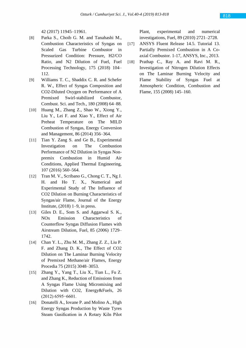
Ozturk / Cumhuriyet Sci. J., Vol.40-4 (2019) 813-818
42 (2017) 11945–11961.
[8] Parka S., Choib G. M. and Tanahashi M.,
Combustion Characteristics of Syngas on
Scaled Gas Turbine Combustor in
Pressurized Condition: Pressure, H2/CO
Ratio, and N2 Dilution of Fuel, Fuel
Processing Technology, 175 (2018) 104–
112.
[9] Williams T. C., Shaddix C. R. and Schefer
R. W., Effect of Syngas Composition and
CO2-Diluted Oxygen on Performance of A
Premixed Swirl-stabilized Combustor,
Combust. Sci. and Tech., 180 (2008) 64–88.
[10] Huang M., Zhang Z., Shao W., Xiong Y.,
Liu Y., Lei F. and Xiao Y., Effect of Air
Preheat Temperature on The MILD
Combustion of Syngas, Energy Conversion
and Management, 86 (2014) 356–364.
[11] Tian Y. Zang S. and Ge B., Experimental
Investigation on The Combustion
Performance of N2 Dilution in Syngas Non-
premix Combustion in Humid Air
Conditions, Applied Thermal Engineering,
107 (2016) 560–564.
[12] Tran M. V., Scribano G., Chong C. T., Ng J.
H. and Ho T. X., Numerical and
Experimental Study of The Influence of
CO2 Dilution on Burning Characteristics of
Syngas/air Flame, Journal of the Energy
Institute, (2018) 1–9, in press.
[13] Giles D. E., Som S. and Aggarwal S. K.,
NOx Emission Characteristics of
Counterflow Syngas Diffusion Flames with
Airstream Dilution, Fuel, 85 (2006) 1729–
1742.
[14] Chan Y. L., Zhu M. M., Zhang Z. Z., Liu P.
F. and Zhang D. K., The Effect of CO2
Dilution on The Laminar Burning Velocity
of Premixed Methane/air Flames, Energy
Procedia 75 (2015) 3048–3053.
[15] Zhang Y., Yang T., Liu X., Tian L., Fu Z.
and Zhang K., Reduction of Emissions from
A Syngas Flame Using Micromixing and
Dilution with CO2, Energy&Fuels, 26
(2012) 6595−6601.
[16] Donatelli A., Iovane P. and Molino A., High
Energy Syngas Production by Waste Tyres
Steam Gasification in A Rotary Kiln Pilot
Plant, experimental and numerical
investigations, Fuel, 89 (2010) 2721–2728.
[17] ANSYS Fluent Release 14.5. Tutorial 13.
Partially Premixed Combustion in A Co-
axial Combustor. 1-17, ANSYS, Inc., 2013.
[18] Prathap C., Ray A. and Ravi M. R.,
Investigation of Nitrogen Dilution Effects
on The Laminar Burning Velocity and
Flame Stability of Syngas Fuel at
Atmospheric Condition, Combustion and
Flame, 155 (2008) 145–160.
818

Cumhuriyet Science Journal
CSJ
e-ISSN: 2587-246X
ISSN: 2587-2680 Cumhuriyet Sci. J., Vol.40-4 (2019) 819-829
* Corresponding author. Email address: [email protected]
http://dergipark.gov.tr/csj ©2016 Faculty of Science, Sivas Cumhuriyet University
Companions Of Perturbed Type Inequalities For Higher-Order
Differentiable Functions
Samet ERDEN 1
1 Department of Mathematics, Faculty of Science, Bartın University, Bartın-TURKEY
Received: 13.06.2019; Accepted: 24.10.2019 http://dx.doi.org/10.17776/csj.577459
Abstract. First of all, a novel inequality of Hadamard's type for functions higher order derivatives of which
are convex is developed. It is also presented midpoint type results. Afterward, Ostrowski type inequalities for
mappings whose derivatives are either Lipschitzian or Hölder continuous with are established. Furthermore,
links between results given in the earlier paper and our outcomes are examined.
Keywords: Convex Functions, Lipschitz Continuity, Ostrowski's Inequality, Hermite-Hadamard inequality.
Yüksek Mertebeden Diferensiyellenebilir Fonksiyonlar için Perturbe
Tipli Eşitsizliklerin Geliştirilmiş Durumları
Özet. Bu çalışmada, ilk olarak yüksek mertebeden türevleri konveks olan fonksiyonlar için Hadamard tipli
yeni bir eşitsizlik geliştirilmiş ve aynı zamanda bu eşitsizliğin orta nokta tarzındaki sonuçları sunulmuştur.
Daha sonra, n. mertebeden türevleri ya Lipschitzyan ya da ]1,0( olmak üzere − Hölder sürekli olan
fonksiyonlar için Ostrowski tipli eşitsizlikler kurulmuştur. Bulunanlara ek olarak, bizim sonuçlarımız ile
önceki makalelerde sunulmuş eşitsizlikler arasındaki bağlantılar incelenmiştir.
Anahtar Kelimeler: Konveks Fonksiyonlar, Lipschitzyan Süreklilik, Ostrowski Eşitsizliği, Hermite-
Hadamard Eşitsizliği.
1. INTRODUCTION
The main purpose of the mathematical inequalities is to determine lower and upper bounds to
mathematical expressions whose values are unknown exactly. So, inequality theory plays an
important role in many areas of modern mathematics. Hermite-Hadamard inequality, introduced by
C. Hermite and J. Hadamard but first published by Hadamard [1] in 1893, is one of the most
significant inequalities in the literature because it gives an estimate of the mean value of a convex
function. This inequality expresses that if R→If : is a convex function on the interval of real
numbers and ba, are elements of I with ,ba then we have the chain of inequalities.
.2
)()()(
1
2
bfafdxxf
ab
baf
b
a
+
−
+ (1)
Another important inequality, published by Ostrowski [2] in 1938, is Ostrowski inequality obtained
by using functions first derivatives of which are bound. This inequality is stated as follows:

Erden / Cumhuriyet Sci. J., Vol.40-4 (2019) 819-829
Let R,: →baf be a differentiable mapping on ( )ba, whose derivative ( ) R,: → baf
is bounded on ( ),,ba i.e. ( )
.)(sup:,
=
tff
bat
Then, we have the inequality
( )( )
( ) ,4
1)(
1)(
2
2
2
+
−
−
−+
−− fab
ab
xdttf
abxf
bab
a
(2)
for all bax , . The constant 41 is the best possible.
These two inequalities have attracted many researchers due to its wide application areas. A large
number of authors have devoted their effort to observed different generalizations, refined,
counterparts and extensions of (1) and (2) for various classes of mappings. In particular, some
generalizations of the inequalities (1) and (2) for differentiable, twice differentiable and higher-
order differentiable mappings are studied. For instance, Sarikaya and Set derived some novel
Ostrowski type results for twice differentiable functions by using a new Montgomery type
identity in [3]. Moreover, results similar to Ostrowski's inequality are provided for functions
second derivatives of which are bounded in [4] and [5]. On the other side, an extension of the
inequality (1) for twice differentiable functions is presented by Farissi et al. in reference [6].
The interested mathematicians focused on perturbed type inequalities which give more general
and more extensive outcomes of (1) and (2). In [7], the author developed an identity to establish
some inequalities of perturbed Ostrowski type for absolutely continuous as follows.
Theorem 1. Let C,: →baf be an absolutely continuous on ba, and .,bax Then,
for any )(1 x and )(2 x complex numbers, we have
( ) ( )
( )( ) ( ) dttf
abxaxxxb
abxf
dtxtfbtab
dtxtfatab
b
a
b
x
x
a
)(1
)()(2
1)(
)()(1
)()(1
1
2
2
2
21
−−−−−
−+=
−−−
+−−−
where the integrals in the left hand side are taken in the Lebesgue sense.
Afterward, researchers worked on perturbed inequalities for twice differentiable functions in [8]
and [9].
We note that there are cases when first and second-order derivatives are not enough to solve
certain mathematical issues. Hence, some researchers observed integral inequalities for higher-
order differentiable mappings. As an illustration, authors provided some generalizations of
Ostrowski type results for mappings higher-order derivatives are elements of pLL ,1
or L in
[10], [11] and [12]. What is more, results that are higher order generalizations of Hermite-
Hadamard inequality are deduced in [13] and [14]. In [15], Ozdemir and Yildiz examined
midpoint formula related to (1) for higher order differentiable functions. In [16], Erden gave
perturbed inequalities for mappings n .th derivatives of which are of bounded variation. In
addition, it is presented some perturbed type integral inequalities for functions whose higher-
order derivatives are either convex or Lipschitzian in [17].
820
Erden / Cumhuriyet Sci. J., Vol.40-4 (2019) 819-829
In [18] and [19], Dragomir observed companions of Perturbed Ostrowski type inequalities for
absolutely continuous functions. In [20], Erden established the following equality for −n times
differentiable functions so as to refined Ostrowski type inequalities. He also investigated new
quadrature rules to capture more effective results than the previous.
Lemma 1. Let R,: →baf be a −n time differentiable function on ( ).,ba Then, for any
3,2,1),( =ixi complex numbers and all ,,2baax + we have the identity
( )
( )
( ) ( )( )
( ) ( )
( ) ,)(12!1
)(11
!1)(1)(),:(
)()(!
)()(2!
1)()(
!
1
2
1
31
3
)(
2
)(
1
)(
dttfxba
n
x
n
axxxxnfS
dtxtfn
bt
dtxtfba
tn
dtxtfn
at
b
a
n
n
n
nn
n
nb
xba
n
nxba
x
n
nx
a
−+
−
+
+−+−
+
−−+−=
−−
+
−
+−+−
−
+
+
−+
−+
(3)
where ),:( xnfS is defined by
( ) ( ) ( ) ( ) ( ) ( ) ( ) .)1(
),:(
1
2
1
!1
111
0
)()(1 +++
+
−+−+−−
=
−−+−=+ kbakk
k
xfxbafn
k
xax
xnfSkkkn (4)
In [21], Kashif et al. developed new results of Ostrowski type for functions thn. derivatives of
which are element of either baL ,1 or baL ,2 by means of three-step kernel. Moreover,
Qayyum et al. improved more comprehensive Ostrowski type results whose special cases give
inequalities presented in the previous studies for functions having a five-step kernel in [22].
Both works also presented new efficient quadrature rules which can use to find the approximate
value of expressions values of which cannot be calculated exactly.
In this study, our purpose is to establish new inequalities for mappings higher order derivatives
of which are absolutely continuous. By utilizing the above equality, some companions of
perturbed inequality for mappings higher order derivatives of which are either convex or
Lipschitzian are examined. Results given in previous articles were recaptured when we gave
specific values to the inequalities obtained in this work.
2. INEQUALITIES FOR CONVEX FUNCTIONS
Convex functions have become a cornerstone in many fields of Mathematics. Specifically, these
type functions are a lot used in the inequality theory and optimization problems. The most
famous of the inequalities obtained by using convex functions is Hermite-Hadamard inequality.
Furthermore, midpoint and trapezoidal type results which are related to Hermite-Hadamard
inequality plays an important role in a large number of areas of Mathematics. Now, we recall
some definitions and properties concerning the convex functions which will use to establish our
new results.
821

Erden / Cumhuriyet Sci. J., Vol.40-4 (2019) 819-829
Supposing that I is an interval of real number with interior .I Also, R:)1( →− In be a
convex function on .I In this case, )1( −n is continuous on
I and possess finite left and right
derivatives at each point of .I Furthermore, if i and j are element of I and ,ji then
),()()()( )()()()( jjii nnnn
+−+− and this situation shows that both )(n
− and
)(n
+ are
non-decreasing functions on .I A convex function is well known to must be differentiable
apart from at most countably many points.
We note that the sub differential of convex function )1( −n indicated by
)1( − n is the set of all
functions −→ ,: I such that ( ) RI satisfied the condition
( ) ( )mmimi nn −+ −− )()( )1()1(
for any ., Imi In this circumstance, if )1( −n is convex on ,I then
)1( − n isn't empty, )(n
− ,
)1()( −
+ nn and if is element of ,)1( − n then
( ) )()( )()( iii nn
+−
for any .Ii Specifically, is a nondecreasing mapping. Also, we must state that
)()1( nn = − if f is differentiable and convex on .I
Theorem 2. Let R,: →baf be n times differentiable function on ( ),,ba and let n be
odd number. If )1( −nf is a convex function with the lateral derivatives )()( af n
+ and )()( bf n
− ,
then one has the inequality
( ) ( ) ( ) ( )
( )
( )( ) 1
)()(
1
1)()(1
0
!1
)()(
2)1(
!1
1
)(
++−
+
+−
=
−
+
−+
−
+−+−
+
−+−+
nnn
k
kkkkkn
k
b
a
axn
afbf
xba
axk
xfxbaf
dttf
for any .,2
baax +
Proof. If we take ),()( )(
1 afx n
+= ( ) )()(,)( )(
32
)(
2 bfxfx nban
−+
+ == in the equality (3),
since n is odd number, then, for any ,,2baax + we possess the identity
( ) ( ) ( ) ( )
( )
( )( ) dttfax
n
bfaf
xba
axk
xfxbaf
b
a
nnn
k
kkkkkn
k
)(!1
)()(
2)1(
!1
1
1)()(
1
1)()(1
0
−−+
−−
−
+−+−
+
−+−+
+−+
+
+−
=
822

Erden / Cumhuriyet Sci. J., Vol.40-4 (2019) 819-829
( ) ( )
dtba
ftba
tn
dtbftn
btdtaft
n
at
n
nxba
x
n
nb
xba
n
nx
a
+−
+−+
−−
+−−
=
+
−+
−
−+
+
2)(
2!
1
)()(!
)()(!
)(
)()(
where ,)1( − nf because is equal to )(nf almost everywhere on .,ba
Let x be an element of ( ).,2
baa + One has
( ) 0)()( )( −− + aftat nn
for any xat , and
02
)(2
)(
+−
+− +
baft
bat n
n
for any xbaat −+ , . Also, as n is odd number, we have
( ) 0)()()( −− − tbftb nn
for any bxbat ,−+ . Hence, the desired inequality is proved.
Corollary 1. Under the sane assumptions of Theorem 2 with ,2
bax += then the following
inequality hold:
( ) ( )
( )
( )
1)()(
1)(
1
1
0
2!1
)()(
2!12
11)(
+
+−
+
+
−
=
−
+
−+
−
+
+
−+
nnn
kk
k
kn
k
b
a
ab
n
afbf
abba
fk
dttf
which is a midpoint type inequality for mappings whose higher order derivatives are convex.
Corollary 2. Under all the all conditions of the Theorem 2, if we choose ,4
3 bax += one has the
result
( ) ( ) ( ) ( )
( )
( ).
4!1
)()(
)1(1!14
1
)(
1)()(
1
1
43)(
43)(1
0
+
+−
+
+
++−
=
−
+
−+
−−++
−+
nnn
kk
k
bakkbakn
k
b
a
ab
n
afbf
abk
ff
dttf
Remark 1. If we take 1=n in the inequality presented in the theorem 2, we have
823

Erden / Cumhuriyet Sci. J., Vol.40-4 (2019) 819-829
( ) ( )
( )2)()(
2
1
2
1)(
1
axab
afbf
xfxbafdttfab
b
a
−
−
−+
+−+−
+
−
which was proved by Dragomir in [19].
3. SOME RESULTS FOR LIPSCHITZIAN DERIVATIVES
Lipschitz continuity, which was called after Rudolf Lipschitz, is a more consistent form of
uniform continuity. We began with the definition of Lipschitz continuity to this section.
R,: →ba is said to be Lipschitzian , if there exists a real constant 0M such that
srMsr −− )()(
for any .,, basr
A recent companion inequality for mappings whose higher order derivatives are Lipschitzian is
provided in the following theorem.
Theorem 3. Let R: →If be a n times differentiable function on I and ., Iba If the
n th derivative R:)( →If n is Lipschitzian with the constants 21 , MM and 3M on
xbaxxa −+,,, and bxba ,−+ respectively, then, for all x in ,, 2baa + we have
( ) ( )( )
( ) ( )
( )
( )( ) ( )
2
2
2
31
1
)(
1
)()(
22!
2
!2
)(122!1
11
!1)(1)(),:(
++
+
+
−
+
++
+
−+
−+
−
+
+
+
−+−
+
−−+−+−
nn
b
a
n
n
n
n
n
nnn
xba
nnM
n
axMM
dttfxbaba
fn
n
axxbafxfxnfS
where ),:( xnfS is defined as in (4).
Proof. Should we write ),()( xf n ( )
2
)( banf + and )()( xbaf n −+ in place of ),(1 x )(2 x
and )(3 x in the equality (3) respectively, because of the triangle inequality, then we possess
the outcome
( ) ( )( )
( ) ( )
( ) dttfxbaba
fn
n
axxbafxfxnfS
b
a
n
n
n
n
n
nnn
)(122!1
11
!1)(1)(),:(
1
)(
1
)()(
−+
−
+
+
+
−+−
+
−−+−+−
+
+
(5)
824

Erden / Cumhuriyet Sci. J., Vol.40-4 (2019) 819-829
( ) ( )
.2
)(2!
1
)()(!
)()(!
)()(
)()()()(
dtba
ftfba
tn
dtxbaftfn
tbdtxftf
n
at
nn
nxba
x
nn
nb
xba
nn
nx
a
+−
+−+
−+−−
+−−
−+
−+
Seeing that C:)( →If n is Lipschitzian with the constant 1M on ,, xa we get
( )
( )( )
( )( )
.!2!
)()(!
2
11
)()(
+
−=−
−
−−
+
n
axMdttx
n
atM
dtxftfn
at
nnx
a
nn
nx
a
Similarly, if the other two integrals in the right-hand side of (5) are observed, then the desired
result can easily be obtained.
Corollary 3. Let R: →If be a n times differentiable function on I and ., Iba
Also, let ( ).,bax If the n th derivative R:)( →If n is Lipschitzian with the constant M
on ba, , then one has
( ) ( )( )
( ) ( )
( )
( )( ) ( )
−
+++−
+
−+
−
+
+
+
−+−
+
−−+−+−
+
+
+
+
2
2
1
)(
1
)()(
21
!2
2
)(122!1
11
!1)(1)(),:(
n
n
b
a
n
n
n
n
n
nnn
xba
naxn
M
dttfxbaba
fn
n
axxbafxfxnfS
(6)
for any ., 2baax +
Remark 2. If we take 1=n in (6), the inequality (6) becomes
( )
( ) ,2
23
)()()(2
1
)()(2
1
3
3
2)()(
−
++−
−−−+−−
−++
xba
axM
dttfaxxbafxf
xbafxf
b
a
nn
which is provided by Dragomir in [19].
Furthermore, it can be derived trapezoidal and midpoint type inequalities by choosing ax =
and 2bax += in the above results.
825

Erden / Cumhuriyet Sci. J., Vol.40-4 (2019) 819-829
Now, we deal with another result acquired by using a more comprehensive condition than
Lipschitz continuity in the next theorem.
Theorem 4. Let R: →If be a n time differentiable function on I and ., Iba
If the conditions
( )atLaftf nn −− 1
)()( )()( for any ),, xat (7)
( )xbaxtba
tLba
ftf nn −++
−
+− ,any for
22)( 2
)()(
(8)
and
( ) )xattbLbftf nn ,any for )()( 3
)()( −−
(9)
are satisfied for 1,, − and ,0,, 321 LLL then, for any ,,2baax + we have the
inequality
( ) ( )( )
( ) ( )
( )
( )( )
( )( )
( )
1
2
1
3
1
1
1
)(
1
)()(
21
2
!
1!1!
)(122!1
11
!1)(1)(),:(
++
++++
+
+
−
+
+++
++
−+
++
−
−+
−
+
+
+
−+−
+
−−+−
n
nn
b
a
n
n
n
n
n
nnn
xba
nn
L
n
ax
n
L
n
ax
n
L
dttfxbaba
fn
n
axbfafxnfS
(10)
where ),:( xnfS is as shown in (4).
Proof. We take absolute value of both sides of the equality (3) for ),()( )(
1 afx n=
( ) )()(,)( )(
32
)(
2 bfxfx nban == + , due to the well-known triangle inequality, we get the
inequality
( ) ( )( )
( ) ( )
( ) )(122!1
11
!1)(1)(),:(
1
)(
1
)()(
tfxbaba
fn
n
axbfafxnfS
b
a
n
n
n
n
n
nnn
−+
−
+
+
+
−+−
+
−−+−
+
+
(11)
( ) ( )
.2
)(2!
1
)()(!
)()(!
)()(
)()()()(
dtba
ftfba
tn
dtbftfn
tbdtaftf
n
at
nn
nxba
x
nn
nb
xba
nn
nx
a
+−
+−+
−−
+−−
−+
−+
Now, should we calculate the first integral given in right hand side of the above inequality by
826

Erden / Cumhuriyet Sci. J., Vol.40-4 (2019) 819-829
utilizing the property (7), we possess
( ) ( )( )
( )( )
.!1
!)()(
!
1
1
1
)()(
nn
axL
dtatn
atLdtaftf
n
at
n
nx
a
nn
nx
a
++
−=
−−
−−
++
If we substitute the resulting inequalities in (11) after having estimated the other two integrals
by using the properties (8) and (9), we can easily find the desired inequality (10) which finishes
the proof.
In particular, if we take in consideration Hölder condition that is a generalization of the
Lipschitzian, then we can express a new result as follows.
Corollary 4. Let R: →If be a n time differentiable function on I and ., Iba If the
n th derivative )(nf is − Hölder type on ,,ba then we have the inequality
srKsfrf nn −− )()( )()(
for any ,,, basr where ( 1,0r and 0H . In this case, the following inequality holds:
( ) ( )( )
( ) ( )
( )
( )( )
−
++−
++
−+
−
+
+
+
−+−
+
−−+−
++
++
+
+
1
1
1
)(
1
)()(
2!1
2
)(122!1
11
!1)(1)(),:(
n
n
b
a
n
n
n
n
n
nnn
xba
axn
K
n
dttfxbaba
fn
n
axbfafxnfS
for any ., 2baax + Specifically, if we suppose that
)(nf is Lipschitzian with the constant
0K or if we take 1= in the above result, then, for any ,,2baax + we get
( ) ( )( )
( ) ( )
( )
( )( ) ,
2!2
2
)(122!1
11
!1)(1)(),:(
2
2
1
)(
1
)()(
−
++−
+
−+
−
+
+
+
−+−
+
−−+−
+
+
+
+
n
n
b
a
n
n
n
n
n
nnn
xba
axn
L
n
dttfxbaba
fn
n
axbfafxnfS
(12)
where ),:( xnfS is as given in (4).
Remark 3. If we choose 1=n in (12), the inequality (12) reduce to the result
827
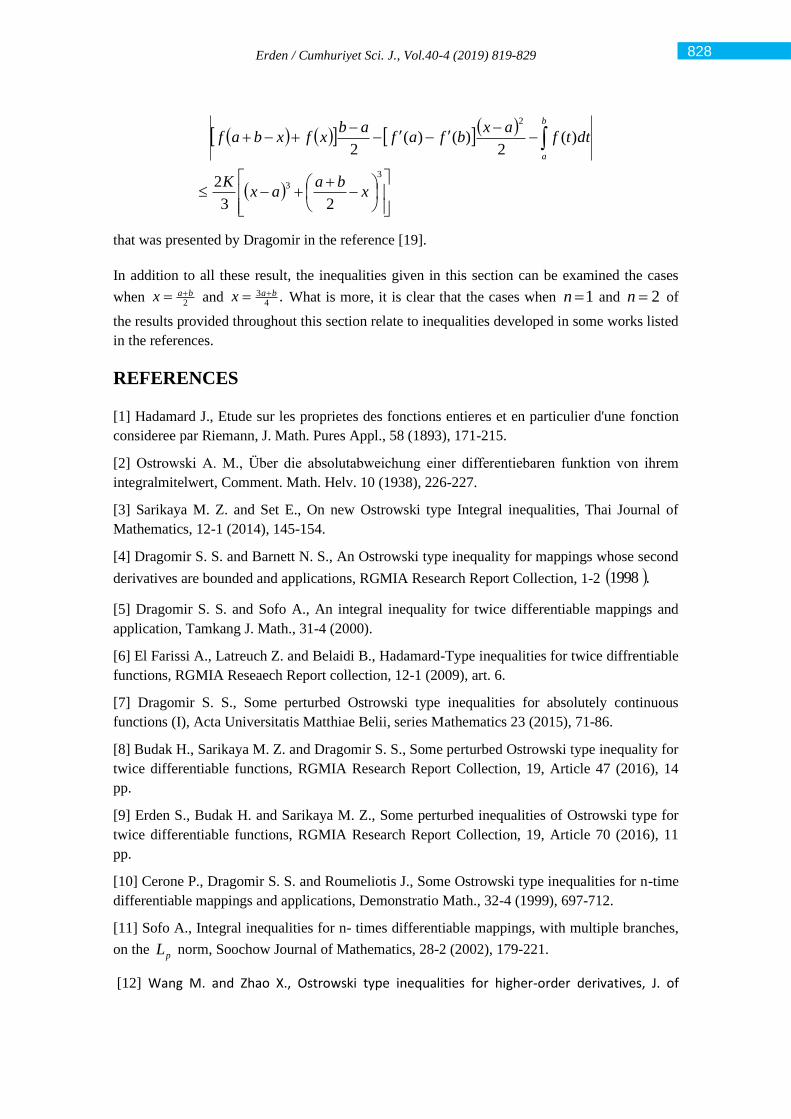
Erden / Cumhuriyet Sci. J., Vol.40-4 (2019) 819-829
( ) ( ) ( )
( )
−
++−
−−
−−−
+−+
3
3
2
23
2
)(2
)()(2
xba
axK
dttfax
bfafab
xfxbaf
b
a
that was presented by Dragomir in the reference [19].
In addition to all these result, the inequalities given in this section can be examined the cases
when 2bax += and .
43 bax += What is more, it is clear that the cases when 1=n and 2=n of
the results provided throughout this section relate to inequalities developed in some works listed
in the references.
REFERENCES
[1] Hadamard J., Etude sur les proprietes des fonctions entieres et en particulier d'une fonction
consideree par Riemann, J. Math. Pures Appl., 58 (1893), 171-215.
[2] Ostrowski A. M., Über die absolutabweichung einer differentiebaren funktion von ihrem
integralmitelwert, Comment. Math. Helv. 10 (1938), 226-227.
[3] Sarikaya M. Z. and Set E., On new Ostrowski type Integral inequalities, Thai Journal of
Mathematics, 12-1 (2014), 145-154.
[4] Dragomir S. S. and Barnett N. S., An Ostrowski type inequality for mappings whose second
derivatives are bounded and applications, RGMIA Research Report Collection, 1-2 ( ).1998
[5] Dragomir S. S. and Sofo A., An integral inequality for twice differentiable mappings and
application, Tamkang J. Math., 31-4 (2000).
[6] El Farissi A., Latreuch Z. and Belaidi B., Hadamard-Type inequalities for twice diffrentiable
functions, RGMIA Reseaech Report collection, 12-1 (2009), art. 6.
[7] Dragomir S. S., Some perturbed Ostrowski type inequalities for absolutely continuous
functions (I), Acta Universitatis Matthiae Belii, series Mathematics 23 (2015), 71-86.
[8] Budak H., Sarikaya M. Z. and Dragomir S. S., Some perturbed Ostrowski type inequality for
twice differentiable functions, RGMIA Research Report Collection, 19, Article 47 (2016), 14
pp.
[9] Erden S., Budak H. and Sarikaya M. Z., Some perturbed inequalities of Ostrowski type for
twice differentiable functions, RGMIA Research Report Collection, 19, Article 70 (2016), 11
pp.
[10] Cerone P., Dragomir S. S. and Roumeliotis J., Some Ostrowski type inequalities for n-time
differentiable mappings and applications, Demonstratio Math., 32-4 (1999), 697-712.
[11] Sofo A., Integral inequalities for n- times differentiable mappings, with multiple branches,
on the pL norm, Soochow Journal of Mathematics, 28-2 (2002), 179-221.
[12] Wang M. and Zhao X., Ostrowski type inequalities for higher-order derivatives, J. of
828 828
Erden / Cumhuriyet Sci. J., Vol.40-4 (2019) 819-829
Inequalities and App., Vol. 2009, Article ID 162689 (2009), 8 p.
[13] Latif M. A. and Dragomir S.S., On Hermite-Hadamard type integral inequalities for n-
times differentiable Log-Preinvex functions, Filomat, 29-7 (2015), 1651--1661.
[14] Latif M. A.,, and Dragomir S.S., Generalization of Hermite-Hadamard type inequalities for
n-times differentiable functions which are s-preinvex in the second sense with applications,
Hacettepe J. of Math. and Stat., 44-4 (2015), 389-853.
[15] Özdemir M. E. and Yıldız Ç., A new generalization of the midpoint formula for n -time
differentiable mappings which are convex, arXiv:1404.5128v1, (2014).
[16] Erden S., Some perturbed inequalities of Ostrowski type for funtions whose n th
derivatives are of bounded, Iranian Journal of Mathematical Sciences and Informatics, in press,
(2019).
[17] Erden S., New perturbed inequalities for functions whose higher degree derivatives are
absolutely continuous, Konuralp Journal of Mathematics, 7-2, (2019), 371-379.
[18] Dragomir S. S., Perturbed Companions of Ostrowski's Inequality for Absolutely
Continuous Functions (I), Analele Universitatii de Vest, Timisoara Seria Matematica -
Informatica, LIV (1) (2016), 119- 138.
[19] Dragomir S. S., Perturbed Companions of Ostrowski's Inequality for Absolutely
Continuous Functions (II), RGMIA Research Report Collection, 17, Article 19 (2014) 11 pp.
[20] Erden S., Refined Inequalities of Perturbed Ostrowski type for higher order absolutely
continuous functions and applications, Submitted, (2019).
[21] Kashif A. R., Shoib M. and Latif M. A., Improved version of perturbed Ostrowski type
inequalities for n-times di erentiable mappings with three-step kernel and its application, J.
Nonlinear Sci. Appl. 9 (2016), 3319-3332.
[22] Qayyum A., Shoaib M. and Faye I., On new refinements and applications of
efficient quadrature rules using n -times differentiable mappings, J. Computational
Analysis abd Applicaions, 23-4 (2017), 723-739.
829
Cumhuriyet Science Journal
CSJ
e-ISSN: 2587-246X
ISSN: 2587-2680 Cumhuriyet Sci. J., Vol.40-4 (2019) 830-837
* Corresponding author. Email address: [email protected]
http://dergipark.gov.tr/csj ©2019 Faculty of Science, Sivas Cumhuriyet University
On fluorescent sensing of metal ions using water extracts of Salvia officinalis
Idris SARGIN1,*
1 Department of Biochemistry, Faculty of Science, Selcuk University, 42075 Konya, Turkey
Received: 02.07.2019; Accepted: 14.11.2019 http://dx.doi.org/10.17776/csj.585503
Abstract. Sensing of metal ions using fluorometric tools has wide applications in chemical, biological and
environmental analysis. Plant phytochemicals, like flavonoids, exhibit intense fluorescence upon excitation by
UV light. Leaves sage (Salvia officinalis), which is rich in polyphenolic and flavonoids compounds, were
extracted using Soxhlet and microwave-assisted extractors. The extraction methods led to variations in the
phytochemical composition of the extracts, which in turn affected their interaction with metal ions. Despite the
variations in the composition, both of the extracts gave high fluorescence emissions when excited at 365 nm.
Variations in fluorescence emissions of the extracts were studied in upon addition of each metal ion; i.e., Li+,
Na+, K+, Cs+, Be2+, Mg2+, Sr2+, Ba2+, Al3+, Tl3+, Ge4+, Sn4+, Pb2+, Sb3+, Bi3+, Se4+, Cu2+, Ag+, Zn2+, Cd2+, Ti4+,
Cr3+, Cr6+, Mo6+, W6+, Mn2+, Fe3+, Ni2+, Co2+ and Pd2+. When they were added into the Soxhlet extract, some
ions (Cr3+, Pb2+, Co2+) induced intense fluorescence and some (Ge4+, Mg2+, K+, Na+) ions quenched the
fluorescence emission. As for microwave-assisted extract, the addition of Sr2+, Mg2+ and Co2+ ions enhanced
the fluorescence emission of the extract, but Fe3+, Be2+ and Cs+ lowered the fluorescence intensity. However,
the results of the study should be considered as introductory and further selectivity and sensitivity studies should
be done for each extract if they are used for sensing of metal ions. Yet, this study demonstrated that sage extracts
has a potential for fluorescent sensing of certain metal ions.
Keywords: Sage; Flavonoid; Metal ion sensing; Soxhlet extraction; Microwave irradiation.
Salvia officinalis'in su özütlerini kullanarak metal iyonlarının floresanla
algılanması
Özet. Metal iyonlarının florometrik araçlar kullanarak algılanması kimyasal, biyolojik ve çevresel analizlerde
geniş uygulamalara sahiptir. Flavonoidler gibi bitki fitokimyasalları, UV ışığı ile uyarıldıklarında yoğun
floresans ışıma yaparlar. Polifenolik bileşikler ve flavonoidler bakımından zengin olan adaçayı (Salvia
officinalis) yaprakları Soxhlet ve mikrodalga ekstraktörler kullanılarak özütlendi. Ekstraksiyon yöntemleri,
özütlerin fitokimyasal kompozisyonunda değişikliklere neden olmuştur, bu da metal iyonlarıyla etkileşimlerini
etkilemiştir. Kompozisyondaki değişikliklere rağmen, özütlerin her ikisi de 365 nm'de uyarıldığında yüksek
floresans emisyonu vermiştir. Özütlerin floresans emisyonundaki değişmeler her bir iyonun ilave edilmesiyle
çalışıldı; Li+, Na+, K+, Cs+, Be2+, Mg2+, Sr2+, Ba2+, Al3+, Tl3+, Ge4+, Sn4+, Pb2+, Sb3+, Bi3+, Se4+, Cu2+, Ag+, Zn2+,
Cd2+, Ti4+, Cr3+, Cr6+, Mo6+, W6+, Mn2+, Fe3+, Ni2+, Co2+ ve Pd2+. Soxhlet özütüne ilave edildiğinde, bazı iyonlar
(Cr3+, Pb2+, Co2+) yoğun floresansa neden olmuş, bazı (Ge4+, Mg2+, K+, Na+) iyonlar ise floresans emisyonunu
söndürmüştür. Mikrodalga destekli özütte, Sr2+, Mg2+ ve Co2+'nın ilavesi, özütün floresans emisyonunu arttırdı,
ancak Fe3+, Be2+ ve Cs+ floresan şiddetini düşürdü. Bununla birlikte, çalışmanın sonuçları giriş niteliğinde
olarak değerlendirilmeli ve metal iyonlarını algılamak için kullanılacaksa her özüt için seçicilik ve duyarlılık
çalışmaları yapılmalıdır. Yine de, bu çalışma adaçayı özütlerinin belirli metal iyonlarının floresan algılama
potansiyelinin olduğunu göstermiştir.
Anahtar Kelimeler: Adaçayı; Flavonoid; Metal iyonu algılama; Soxhlet ekstraksiyonu; Mikrodalga ışınlaması.
Sargin / Cumhuriyet Sci. J., Vol.40-4 (2019) 830-837
1. INTRODUCTION
Extracts from plants have been subject of intensive
studies because of their wide range of
pharmacological activities. Sage (Salvia
officinalis) is a medicinal and herbal plant [1]. Its
biological activities are attributed to its phenolic
compounds including carnosic acid, carnosol,
rosmarinic acid, diterpenes, triterpenes and
flavonoids [2, 3].
Apart from therapeutic activities and physiological
importance [4], flavonoids, one group of the active
ingredients in S. officinalis extracts, also display
important characteristics [5]. These polyphenolic
phytochemicals emit brilliant fluorescence when
excited by UV light [6].
Detection of metal ions using fluorescence
spectrometry is a simple and powerful technique in
analytical chemistry. Designing fluorescent and
water-soluble chemosensors for sensing metal ions
in aqueous environments is of importance. Water-
soluble and natural fluorescent chemosensors are
needed for detection of metal ions by fluorescence
spectrometry [7, 8].
Natural compounds as fluorescent probes for metal
ions have attracted considerable attention in the
past few years. For example, a plant alkaloid
berberine was isolated from the stems of Mahonia
leschenaultti and then used for detection of Ag+ ion
[9]. In one study natural Isorhamnetin from Ginkgo
leaves was applied for determination of Cu2+ in
samples from rivers, lakes, vegetables and fruits
[10]. In another study, a simple and green
analytical procedure based on chlorophyll a was
developed by Gao and et al., (2006) [11]. The
authors reported the extraction and purification of
chlorophyll a from the leaves of pea and use of
chlorophyll a fluorometric detection of Hg2+ ion. A
more recent study by Ahmad et al., (2018) reported
that flavonoid containing methanolic extract of
Corchorus depressus could be used as a
spectrofluorometric assay for the detection of
Benzo[a]pyrene [12]. Flavonoids also display
affinity for metal ions by forming metal–flavonoids
complexes. Flavonoids are able to form fluorescent
chelates with a variety of metal ions [13].
This study aimed to test whether it is possible to
develop a simple, cheap and fast
spectrofluorometric chemosensor based on the
water extract of common sage (S. officinalis) for
detection of metal ions. In the study, two extraction
procedures were used to see the effect of the
extraction method on the composition of the S.
officinalis extracts; the Soxhlet extraction and
microwave-assisted extraction. Both extracts
exhibited high fluorescence emission when excited
by UV light despite the variations in their
compositions. The change in the fluorescence
intensity of the extracts was tested for 30 metal
ions; Li+, Na+, K+, Cs+, Be2+, Mg2+, Sr2+, Ba2+, Al3+,
Tl3+, Ge4+, Sn4+, Pb2+, Sb3+, Bi3+, Se4+, Cu2+, Ag+,
Zn2+, Cd2+, Ti4+, Cr3+, Cr6+, Mo6+, W6+, Mn2+, Fe3+,
Ni2+, Co2+, Pd2+.
2. MATERIALS AND METHODS
2.1. Preparation of S. officinalis extracts
Commercially available, dry sage (Salvia
officinalis) was obtained from a local supplier. Dry
aerial parts of S. officinalis were ground to powder
using a commercial blender. Two extraction
procedures were followed; Soxhlet extraction [14]
and microwave-assisted extraction [15]. In Soxhlet
extraction, 5.0 g of S. officinalis in a cellulose
thimble was placed in the extractor and a flaks with
300 mL of ultrapure water (ELGA, PURELAB
Option-Q) was fitted to the assembly. The
extraction bed was heated at 80°C for 24 h. In
microwave-assisted extraction, 5.0 g of S.
officinalis powder in 300 mL of ultrapure water
was microwave-irradiated at 400 W for 30 min in a
MARS CEM microwave oven. The Soxhlet and
microwave extracts were filtered using a filter
paper (Whatman, No: 42), transferred into the glass
flasks sealed with aluminium foil and stored at 4°C
in dark (To protect from direct sunlight, the vessels
were covered with aluminium foil). The pH of the
Soxhlet and microwave extracts was measured as
5.13 and 5.67.
2.2. Flavonoid and phenolic content of the
Soxhlet and microwave-assisted extracts
of S. officinalis
Analysis of the flavonoid and phenolic content of
the Soxhlet and the microwave extracts was done
using high-performance liquid chromatography
(Shimadzu HPLC-DAD) [5, 16]. The HPLC
working conditions were as follows: Detector:
DAD detector, max = 278 nm; auto sampler: SIL–
10AD vp; system controller: SCL-10Avp; pump:
LC-10ADvp; degasser: DGU-14A; column oven:
CTO-10Avp; column: Agilent Eclipse XDB-C18,
250x4.60 mm, 5 µ; mobile phase: A: 3% acetic
acid, B: methanol; flow rate: 0.8 mL min−1; column
temperature: 300 °C; injection volume: 20 µL.
831
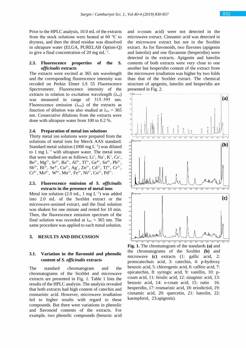
Sargin / Cumhuriyet Sci. J., Vol.40-4 (2019) 830-837
Prior to the HPLC analysis, 10.0 mL of the extracts
from the stock solutions were heated at 60 °C to
dryness, and then the dried residue was dissolved
in ultrapure water (ELGA, PURELAB Option-Q)
to give a final concentration of 20 mg mL−1.
2.3. Fluorescence properties of the S.
officinalis extracts
The extracts were excited at 365 nm wavelength
and the corresponding fluorescence intensity was
recoded on Perkin Elmer LS 55 Fluorescence
Spectrometer. Fluorescence intensity of the
extracts in relation to excitation wavelength (λex)
was measured in range of 315‒395 nm.
Fluorescence emission (λem) of the extracts as
function of dilution was also studied at λex = 365
nm. Consecutive dilutions from the extracts were
done with ultrapure water from 100 to 0.2 %.
2.4. Preparation of metal ion solutions
Thirty metal ion solutions were prepared from the
solutions of metal ions for Merck AAS standard.
Standard metal solution (1000 mg L−1) was diluted
to 1 mg L−1 with ultrapure water. The metal ions
that were studied are as follows; Li+, Na+, K+, Cs+,
Be2+, Mg2+, Sr2+, Ba2+, Al3+, Tl3+, Ge4+, Sn4+, Pb2+,
Sb3+, Bi3+, Se4+, Cu2+, Ag+, Zn2+, Cd2+, Ti4+, Cr3+,
Cr6+, Mo6+, W6+, Mn2+, Fe3+, Ni2+, Co2+, Pd2+.
2.5. Fluorescence emission of S. officinalis
extracts in the presence of metal ions
Metal ion solution (2.0 mL, 1 mg L−1) was added
into 2.0 mL of the Soxhlet extract or the
microwave-assisted extract, and the final solution
was shaken for one minute and rested for 10 min.
Then, the fluorescence emission spectrum of the
final solution was recorded at λex = 365 nm. The
same procedure was applied to each metal solution.
3. RESULTS AND DISCUSSION
3.1. Variation in the flavonoid and phenolic
content of S. officinalis extracts
The standard chromatogram and the
chromatograms of the Soxhlet and microwave
extracts are presented in Fig. 1. Table 1 lists the
results of the HPLC analysis. The analysis revealed
that both extracts had high content of catechin and
rosmarinic acid. However, microwave irradiation
led to higher results with regard to these
compounds. But there were variations in phenolic
and flavonoid contents of the extracts. For
example, two phenolic compounds (benzoic acid
and o-coum acid) were not detected in the
microwave extract. Cinnamic acid was detected in
the microwave extract but not in the Soxhlet
extract. As for flavonoids, two flavones (apigenin
and luteolin) and one flavanone (hesperidin) were
detected in the extracts. Apigenin and luteolin
contents of both extracts were very close to one
another but hesperidin content of the extract from
the microwave irradiation was higher by two folds
than that of the Soxhlet extract. The chemical
structure of apigenin, luteolin and hesperidin are
presented in Fig. 2.
Fig. 1. The chromatogram of the standards (a) and
the chromatograms of the Soxhlet (b) and
microwave (c) extracts (1: gallic acid, 2:
protocatechuic acid, 3: catechin, 4: p-hydroxy
benzoic acid, 5: chlorogenic acid, 6: caffeic acid, 7:
epicatechin, 8: syringic acid, 9: vanillin, 10: p-
coum acid, 11: ferulic acid, 12: sinapinic acid, 13:
benzoic acid, 14: o-coum acid, 15: rutin 16:
hesperidin, 17: rosmarinic acid, 18: eriodictiol, 19:
cinnamic acid, 20: quercetin, 21: luteolin, 22:
kaempferol, 23:apigenin).
832
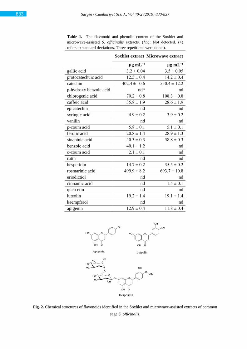
Sargin / Cumhuriyet Sci. J., Vol.40-2 (2019) 830-837
Table 1. The flavonoid and phenolic content of the Soxhlet and
microwave-assisted S. officinalis extracts. (*nd: Not detected. (±)
refers to standard deviations. Three repetitions were done.).
Soxhlet extract Microwave extract
µg mL−1 µg mL−1
gallic acid 3.2 ± 0.04 3.5 ± 0.05
protocatechuic acid 12.5 ± 0.4 14.2 ± 0.4
catechin 402.4 ± 10.6 550.4 ± 12.2
p-hydroxy benzoic acid nd* nd
chlorogenic acid 70.2 ± 0.8 108.3 ± 0.8
caffeic acid 35.8 ± 1.9 28.6 ± 1.9
epicatechin nd nd
syringic acid 4.9 ± 0.2 3.9 ± 0.2
vanilin nd nd
p-coum acid 5.8 ± 0.1 5.1 ± 0.1
ferulic acid 20.8 ± 1.4 28.9 ± 1.3
sinapinic acid 40.3 ± 0.3 58.8 ± 0.3
benzoic acid 40.1 ± 1.2 nd
o-coum acid 2.1 ± 0.1 nd
rutin nd nd
hesperidin 14.7 ± 0.2 35.5 ± 0.2
rosmarinic acid 499.9 ± 8.2 693.7 ± 10.8
eriodictiol nd nd
cinnamic acid nd 1.5 ± 0.1
quercetin nd nd
luteolin 19.2 ± 1.4 19.1 ± 1.4
kaempferol nd nd
apigenin 12.9 ± 0.4 11.8 ± 0.4
Fig. 2. Chemical structures of flavonoids identified in the Soxhlet and microwave-assisted extracts of common
sage S. officinalis.
833
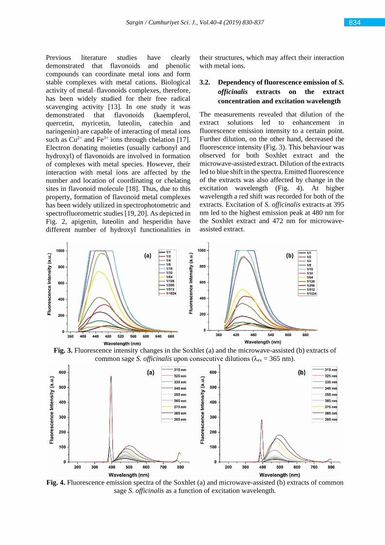
Sargin / Cumhuriyet Sci. J., Vol.40-4 (2019) 830-837
Previous literature studies have clearly
demonstrated that flavonoids and phenolic
compounds can coordinate metal ions and form
stable complexes with metal cations. Biological
activity of metal–flavonoids complexes, therefore,
has been widely studied for their free radical
scavenging activity [13]. In one study it was
demonstrated that flavonoids (kaempferol,
quercetin, myricetin, luteolin, catechin and
naringenin) are capable of interacting of metal ions
such as Cu2+ and Fe3+ ions through chelation [17].
Electron donating moieties (usually carbonyl and
hydroxyl) of flavonoids are involved in formation
of complexes with metal species. However, their
interaction with metal ions are affected by the
number and location of coordinating or chelating
sites in flavonoid molecule [18]. Thus, due to this
property, formation of flavonoid metal complexes
has been widely utilized in spectrophotometric and
spectrofluorometric studies [19, 20]. As depicted in
Fig. 2, apigenin, luteolin and hesperidin have
different number of hydroxyl functionalities in
their structures, which may affect their interaction
with metal ions.
3.2. Dependency of fluorescence emission of S.
officinalis extracts on the extract
concentration and excitation wavelength
The measurements revealed that dilution of the
extract solutions led to enhancement in
fluorescence emission intensity to a certain point.
Further dilution, on the other hand, decreased the
fluorescence intensity (Fig. 3). This behaviour was
observed for both Soxhlet extract and the
microwave-assisted extract. Dilution of the extracts
led to blue shift in the spectra. Emitted fluorescence
of the extracts was also affected by change in the
excitation wavelength (Fig. 4). At higher
wavelength a red shift was recorded for both of the
extracts. Excitation of S. officinalis extracts at 395
nm led to the highest emission peak at 480 nm for
the Soxhlet extract and 472 nm for microwave-
assisted extract.
Fig. 3. Fluorescence intensity changes in the Soxhlet (a) and the microwave-assisted (b) extracts of
common sage S. officinalis upon consecutive dilutions (λex = 365 nm).
Fig. 4. Fluorescence emission spectra of the Soxhlet (a) and microwave-assisted (b) extracts of common
sage S. officinalis as a function of excitation wavelength.
834
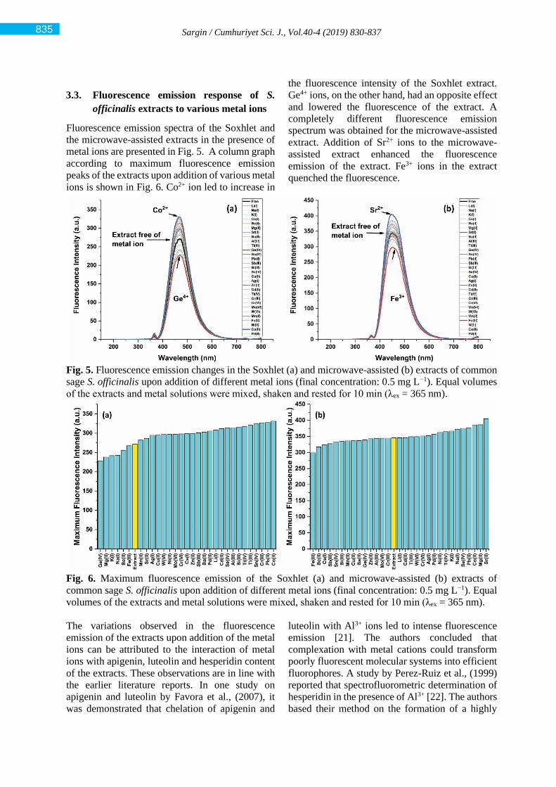
Sargin / Cumhuriyet Sci. J., Vol.40-4 (2019) 830-837
3.3. Fluorescence emission response of S.
officinalis extracts to various metal ions
Fluorescence emission spectra of the Soxhlet and
the microwave-assisted extracts in the presence of
metal ions are presented in Fig. 5. A column graph
according to maximum fluorescence emission
peaks of the extracts upon addition of various metal
ions is shown in Fig. 6. Co2+ ion led to increase in
the fluorescence intensity of the Soxhlet extract.
Ge4+ ions, on the other hand, had an opposite effect
and lowered the fluorescence of the extract. A
completely different fluorescence emission
spectrum was obtained for the microwave-assisted
extract. Addition of Sr2+ ions to the microwave-
assisted extract enhanced the fluorescence
emission of the extract. Fe3+ ions in the extract
quenched the fluorescence.
Fig. 5. Fluorescence emission changes in the Soxhlet (a) and microwave-assisted (b) extracts of common
sage S. officinalis upon addition of different metal ions (final concentration: 0.5 mg L−1). Equal volumes
of the extracts and metal solutions were mixed, shaken and rested for 10 min (λex = 365 nm).
Fig. 6. Maximum fluorescence emission of the Soxhlet (a) and microwave-assisted (b) extracts of
common sage S. officinalis upon addition of different metal ions (final concentration: 0.5 mg L−1). Equal
volumes of the extracts and metal solutions were mixed, shaken and rested for 10 min (λex = 365 nm).
The variations observed in the fluorescence
emission of the extracts upon addition of the metal
ions can be attributed to the interaction of metal
ions with apigenin, luteolin and hesperidin content
of the extracts. These observations are in line with
the earlier literature reports. In one study on
apigenin and luteolin by Favora et al., (2007), it
was demonstrated that chelation of apigenin and
luteolin with Al3+ ions led to intense fluorescence
emission [21]. The authors concluded that
complexation with metal cations could transform
poorly fluorescent molecular systems into efficient
fluorophores. A study by Perez-Ruiz et al., (1999)
reported that spectrofluorometric determination of
hesperidin in the presence of Al3+ [22]. The authors
based their method on the formation of a highly
835

Sargin / Cumhuriyet Sci. J., Vol.40-4 (2019) 830-837
fluorescent complex between hesperidin molecule
and Al3+ ion. Yet, in some studies contradictory
results were also reported. For example, in a recent
study the authors concluded that presence of Fe3+,
Cu2+, Mg2+, Mn2+, Zn2+ and Ca2+ ions did not have
obvious effect on the interaction of apigenin with
bovine serum albumin [23].
3.4. Turn-on fluorescence sensing of Co2+
using the Soxhlet extract of S. officinalis
The microwave extract exhibited the significant
fluorescence intensity at presence of Co2+ ion.
Therefore, the fluorescence response of the Soxhlet
extract to Co2+ was studied further as a model ion
(Fig. 7). In the experiments, the final concentration
of the extract was adjusted to 50%, Co2+ ion
solutions were added into the extract solutions,
shaken for one minute and rested for 10 min. The
lowest concentration of Co2+ ion that gave obvious
fluorescence emission intensity was found to be 0.2
mg L−1.
Fig. 7. Fluorescence emission spectra of the
Soxhlet extract of S. officinalis as a function of
Co2+ concentration.
4. CONCLUSION
This study revealed that the flavonoid and phenolic
content of S. officinalis extract is highly dependent
on the extraction method and parameters that are
followed during an extraction procedure. Upon
excitation by UV light, the Soxhlet and the
microwave-assisted extracts emitted brilliant
fluorescence, which can be attributed to the
presence flavonoids (apigenin, luteolin and
hesperidin). The extraction method greatly affected
the content of the extracts by giving different
HPLC profiles. Numerous previous studies have
demonstrated clearly that flavonoid and phenolic
molecules from plant extracts are capable of
interacting with metal ions through chelation or
complex formation. This study, however, aimed to
find out whether it was possible to use plant
extracts with high flavonoid contents for
fluorescent sensing of metal ions. As the chemical
contents of plant extracts are highly dependent on
the solvent type and extraction procedure, in the
study two different methods were followed for
water extraction of S. officinalis. Due to the
variation of their composition, the extracts showed
different interaction with 30 metal ions including
alkaline, alkaline earth and transition metal ions.
The result of the study with Co2+ was encouraging;
the Soxhlet extract was sensitive to Co2+ ion
concentration of 0.2 mg L−1. However, further
studies are still needed to clarify the phenomena.
The extracts can be used as simple, fast and low-
cost turn-on fluorescence method for detection of,
for example, Co2+ and Sr2+ ions; or for a turn-off
fluorescence method for signalling of Ge4+ and Fe3+
ions; yet, this study should be considered as an
introductory study. Therefore, preliminary studies
were not done to optimize the conditions for each
ion. Especially, in case of Co2+, Sr2+, Ge4+ and Fe3+
ions optimization conditions have to be
investigated in a more detailed manner if sage
extracts are used in any analytical metal sensing
study. In future studies phytochemicals of sage
plant can be extracted using different methods and
the extracts can be tested in fluorescent sensing
applications of metal ions.
REFERENCES
[1] Ghorbani A., Esmaeilizadeh M.,
Pharmacological properties of Salvia officinalis
and its components, J. Tradit. Complem. Med.,
7(2017) 433-440.
[2] Durling N.E., Catchpole O.J., Grey J.B., Webby
R.F., Mitchell K.A., Foo L.Y., Perry N.B.,
Extraction of phenolics and essential oil from
dried sage (Salvia officinalis) using ethanol–
water mixtures, Food. Chem., 101(2007) 1417-
1424.
[3] Ollanketo M., Peltoketo A., Hartonen K.,
Hiltunen R., Riekkola M.-L., Extraction of sage
(Salvia officinalis L.) by pressurized hot water
and conventional methods: Antioxidant activity
of the extracts, Eur. Food. Res. Technol.,
215(2002) 158-163.
[4] de Rijke E., Out P., Niessen W.M.A., Ariese F.,
Gooijer C., Brinkman U.A.T., Analytical
836
Sargin / Cumhuriyet Sci. J., Vol.40-2 (2019) 830-837
separation and detection methods for
flavonoids, J. Chromatogr. A, 1112(2006) 31-
63.
[5] Lu Y., Foo L.Y., Flavonoid and phenolic
glycosides from Salvia officinalis,
Phytochemistry, 55(2000) 263-267.
[6] Havsteen B.H., The biochemistry and medical
significance of the flavonoids, Pharmacol.
Therapeut., 96(2002) 67-202.
[7] Formica M., Fusi V., Giorgi L., Micheloni M.,
New fluorescent chemosensors for metal ions in
solution, Coordin. Chem. Rev., 256(2012) 170-
192.
[8] Jeong Y., Yoon J., Recent progress on
fluorescent chemosensors for metal ions, Inorg.
Chim. Acta, 381(2012) 2-14.
[9] Affrose A., Parveen S.D.S., Kumar B.S.,
Pitchumani K., Selective sensing of silver ion
using berberine, a naturally occurring plant
alkaloid, Sensor. Actuat. B-Chem., 206(2015)
170-175.
[10] Yang S., Jiang W., Zhao F., Xu L., Xu Y., Gao
B., Sun H., Du L., Tang Y., Cao F., A highly
sensitive and selective fluorescent sensor for
detection of copper ions based on natural
Isorhamnetin from ginkgo leaves, Sensor.
Actuat. B-Chem., 236(2016) 386-391.
[11] Gao S., Tan G., Yuan H., Xiao D., Choi
M.M.F., A Simple fluorometric method using
Chlorophyll A for determination of Hg2+ ion,
Microchim. Acta, 153(2006) 159-162.
[12] Ahmad W., Rana N.F., Riaz S., Ahmad N.M.,
Hameed M., Naeem A., Tahir R., Chemical
sensing of Benzo [a] pyrene using Corchorus
depressus fluorescent flavonoids, Nat. Prod.
Res., 32(2018) 968-971.
[13] Malešev D., Kuntić V., Investigation of metal-
flavonoid chelates and the determination of
flavonoids via metal-flavonoid complexing
reactions, J. Serbian Chem. Soc., 72(2007) 921-
939.
[14] Veličković D., Milenović D., Ristić M.,
Veljković V., Kinetics of ultrasonic extraction
of extractive substances from garden (Salvia
officinalis L.) and glutinous (Salvia glutinosa
L.) sage. Ultrason. Sonochem., 13(2006) 150-
156.
[15] Putnik P., Kovačević D.B., Penić M., Fegeš M.,
Dragović-Uzelac V., Microwave-assisted
extraction (MAE) of dalmatian sage leaves for
the optimal yield of polyphenols: HPLC-DAD
identification and quantification, Food Anal.
Method., 2016;9:2385-94.
[16] Kontogianni VG, Tomic G, Nikolic I,
Nerantzaki AA, Sayyad N, Stosic-Grujicic S,
Stojanovic I., Gerothanassis I.P., Tzakos A.G.,
Phytochemical profile of Rosmarinus
officinalis and Salvia officinalis extracts and
correlation to their antioxidant and anti-
proliferative activity. Food Chem. 136(2013)
120-129.
[17] Fernandez M.T., Mira M.L., Florencio M.H.,
Jennings K.R., Iron and copper chelation by
flavonoids: An electrospray mass spectrometry
study, J. Inorg. Biochem., 92(2002) 105-111.
[18] Kasprzak M.M., Erxleben A., Ochocki J.,
Properties and applications of flavonoid metal
complexes, RSC Adv., 5(2015) 45853-45877.
[19] Samsonowicz M., Regulska E., Spectroscopic
study of molecular structure, antioxidant
activity and biological effects of metal
hydroxyflavonol complexes, Spectrochim. Acta
A, 173(2017) 757-771.
[20] Özbek N., Alp H., Çelik G., Ak T., Çağılcı O.C.,
Yaylı N., Ocak U., Ocak M., A simple
spectrofluorimetric method for iron
determination with a chalcone-based Schiff
base, J. Fluoresc. 27(2017) 635-641.
[21] Favaro G., Clementi C., Romani A.,
Vickackaite V., Acidichromism and
ionochromism of luteolin and apigenin, the
main components of the naturally occurring
yellow weld: A spectrophotometric and
fluorimetric study, J. Fluoresc., 17(2007) 707-
714.
[22] Perez-Ruiz T., Martinez-Lozano C., Tomas V.,
Fenoll J., Spectrofluorometric determination of
hesperidin by manual and flow-injection
methods, Fresenius J. Anal. Chem., 364(1999)
279-283.
[23] Bi S., Yan L., Pang B., Wang Y., Investigation
of three flavonoids binding to bovine serum
albumin using molecular fluorescence
technique, J. Lumin., 132(2012) 132-140.
837
Cumhuriyet Science Journal
CSJ
e-ISSN: 2587-246X
ISSN: 2587-2680 Cumhuriyet Sci. J., Vol.40-4 (2019) 838-845
* Corresponding author. Email address: [email protected]
http://dergipark.gov.tr/csj ©2016 Faculty of Science, Sivas Cumhuriyet University
Multiplicative Mappings of Gamma Rings
Bruno L. M. FERREİRA 1* , Ruth N. FERREİRA 1
1 Federal Technological University of Paraná,Professora Laura Pacheco Bastos Avenue, 800,
85053-510, Guarapuava, Brazil.
Received: 15.07.2019; Accepted: 04.11.2019 http://dx.doi.org/10.17776/csj.592101
Abstract. Let 𝔐𝑖 and Γ𝑖 (𝑖 = 1,2) be abelian groups such that 𝔐𝑖 is a Γ𝑖-ring. An ordered pair (𝜑, 𝜙) of
mappings is called a multiplicative isomorphism of 𝔐1 onto 𝔐2 if they satisfy the following properties: (i) 𝜑
is a bijective mapping from 𝔐1 onto 𝔐2, (ii) 𝜙 is a bijective mapping from Γ1 onto Γ2 and (iii) 𝜑(𝑥𝛾𝑦) =𝜑(𝑥)𝜙(𝛾)𝜑(𝑦) for every 𝑥, 𝑦 ∈ 𝔐1 and 𝛾 ∈ Γ1. We say that the ordered pair (𝜑, 𝜙) of mappings is additive
when 𝜑(𝑥 + 𝑦) = 𝜑(𝑥) + 𝜑(𝑦), for all 𝑥, 𝑦 ∈ 𝔐1. In this paper we establish conditions on 𝔐1 that assures that
(𝜑, 𝜙) is additive.
Keywords: Multiplicative mappings, Additivity, Gamma rings.
Gamma Halkalarında Çarpımsal Dönüşümler
Özet. 𝔐𝑖 ve Γ𝑖 (𝑖 = 1,2) değiştirmeli grup ve 𝔐𝑖 bir Γ𝑖-halka olsun. Aşağıdaki özellikler sağlanırsa
dönüşümlerin (𝜑, 𝜙) sıralı ikilisine 𝔐1 den 𝔐2 üzerine çarpımsal izomorfizm denir: (i) 𝜑, 𝔐1 den 𝔐2, üzerine
bijektif dönüşümdür. (ii) 𝜙, Γ1 den Γ2 üzerine bijektif dönüşümdür. (iii) Her 𝑥, 𝑦 ∈ 𝔐1 ve 𝛾 ∈ Γ1.için 𝜑(𝑥𝛾𝑦) =𝜑(𝑥)𝜙(𝛾)𝜑(𝑦) dir ve Her 𝑥, 𝑦 ∈ 𝔐1 için 𝜑(𝑥 + 𝑦) = 𝜑(𝑥) + 𝜑(𝑦), olduğunda dönüşümlerin (𝜑, 𝜙) sıralı
ikilisine toplamsaldır denir. Bu makalede 𝔐1 üzerinde (𝜑, 𝜙) nin toplamsallığını garanti edecek koşulları
vereceğiz.
Anahtar Kelimeler: Çarpımsal dönüşümleri, Toplamsallık, Gamma halkaları.
2010 Mathematics Subject Classification. 16Y99
1. INTRODUCTION AND PRELIMINARIES
N. Nobusawa [1] introduced the concept of a -ring which is called the -ring in the sense of
Nobusawa. He obtained an analogue of the Wedderburn’s Theorem for -rings with minimum
condition on left ideals. W. E. Barnes [2] gave the definition of a -ring as a generalization of a ring
and he also developed some other concepts of -rings such as -homomorphism, prime and primary
ideals, m-systems etc. -rings are closely related to others ternary structures as ternary algebras,
associative triple systems and associative pairs, which have been extensively studied see [3], [4] and
[5].
Let and be two abelian groups. If there exists a mapping (the image of
is denoted by where and ). We call a -ring if the following
conditions are satisfied:
1.

Ferreira, Ferreira / Cumhuriyet Sci. J., Vol.40-4 (2019) 838-845
2.
3.
4.
for all and
A nonzero element is called a multiplicative -identity of or -unity element (for some
) if for all . A nonzero element is called a -idempotent (for
some ) if and a nontrivial -idempotent if it is a -idempotent different from
multiplicative -identity element of .
Let and be two abelian groups such that is a -ring and a nontrivial -idempotent.
Let us consider and two -additive maps verifying the conditions
and . Let us denote ,
, , and suppose
for all and . Then and
, for all and , allowing us to write and as
a direct sum of subgroups where
called Peirce decomposition of relative to , satisfying the multiplicative relations:
1. ;
2. if .
For the reader interested in the Peirce decomposition of -rings we indicate [6]. If and are
subsets of a -ring and we denote the subset of consisting of all finite sums of
the form where and . A right ideal (resp., left ideal) of a -ring
is an additive subgroup of such that (resp., ). If is both a right and a left
ideal of , then we say that is an ideal or two-side ideal of .
An ideal of a -ring is called prime if for any ideals , implies that
or . A -ring is said to be prime if the zero ideal is prime.
Theorem 1.1 [7, Theorem 4] If is a -ring, the following conditions are equivalent:
1. is a prime -ring;
2. if and , then or .
Let and be abelian groups such that is a -ring . An ordered pair
of mappings is called a multiplicative isomorphism of onto if they satisfy the
following properties:
1. is a bijective mapping from onto ;
2. is a bijective mapping from onto ;
3. for all and .
We say that a multiplicative isomorphism of onto is additive when
for all
2. GAMMA RINGS AND THE MULTIPLICATIVE ISOMORPHISMS
The study of the question of when a multiplicative isomorphism is additive has become an active
research area in associative ring theory. In this case, one often tries to establish conditions on the ring
839
Ferreira, Ferreira / Cumhuriyet Sci. J., Vol.40-4 (2019) 838-845
which assures the additivity of every multiplicative isomorphism defined on it. The first result in this
direction is due to Martindale III [8] who obtained a pioneer result in 1969, where in his condition
requires that the ring possesses idempotents. In recent papers [9],[10] Ferreira has studied the
additivity of elementary maps and multiplicative derivation on Gamma rings. This motivated us in the
present paper we investigate the problem of when a multiplicative isomorphism is additive for the
class of gamma rings.
Let us state our main theorem.
Theorem 2.1 Let be a -ring containing a family of nontrivial -idempotents
which satisfies:
1. If is such that then ;
2. If is such that for all then (and hence implies
);
3. For each and if then
Then any multiplicative isomorphism of onto an arbitrary gamma ring is additive.
The following lemmas have the same hypotheses of Theorem 2.1 and we need these lemmas for
the proof of this theorem. Thus, let us consider a nontrivial -idempotent of
and .
Lemma 2.1
Proof. Since is onto, we can choose such that Thus
Lemma 2.2
Proof. First assume that and Since is onto, let be an element of
such that . For arbitrary and we have
Hence In a similar way, for we get
that It follows that
(1)
where . Next, for arbitraries and we
have
840
Ferreira, Ferreira / Cumhuriyet Sci. J., Vol.40-4 (2019) 838-845
which implies In a similar way, we get that
Hence
(2)
where , by condition (i) of the Theorem. From (1) and (2), we
have , where , which implies
and resulting in by condition (i) of the Theorem.
Now assume that and Again, we may find an element of such that
For arbitraries and we have
It follows that In a similar way, for arbitraries and
we get that This implies
(3)
where . Next, for arbitraries and we
have
It follows that In a similar way, for arbitraries and
we get that which implies
(4)
where , by condition (i) of the Theorem. From (3) and (4) we have
which implies resulting in
by condition (ii) of the Theorem.
Similarly, we prove the remaining cases.
Lemma 2.3
Proof. First, let us note that
.
841

Ferreira, Ferreira / Cumhuriyet Sci. J., Vol.40-4 (2019) 838-845
Hence
, by Lemma 2.2.
Lemma 2.4 is additive on .
Proof. Let and choose such that ,
where . For an arbitrary we have
which implies . It follows that . In a similar
way, for an arbitrary we get that .
Hence
(5)
where . Now, for an arbitrary element we
have
, by Lemma 2.3. It follows that Next, for an arbitrary
element we have
, by Lemma 2.2. It follows that . Hence
(6)
where , by condition (i) of the Theorem. From (5) and (6) we have
which implies and resulting in
, by condition (i) of the Theorem.
Lemma 2.5 is additive on
842

Ferreira, Ferreira / Cumhuriyet Sci. J., Vol.40-4 (2019) 838-845
Proof. Let and choose such that ,
where . Firstly, let us note that
It follows that which results in Similarly, we prove that
.This implies which leads to . Next, for an arbitrary element
, applying Lemma 2.4 we get that
which implies and
resulting in . It follows that
(7)
where , by condition (i) of the Theorem.
From (7) we have which implies
. It follows that , that is,
By condition (iii) of the Theorem we conclude that .
Lemma 2.6 is additive on .
843

Ferreira, Ferreira / Cumhuriyet Sci. J., Vol.40-4 (2019) 838-845
Proof. Let and be arbitrary elements and let us write
and . It follows that
and
. Hence, by Peirce decomposition properties of
and making use of the Lemmas 2.2, 2.4 and 2.5, we can see that
holds true, as desired.
Proof of Theorem 2.1. Suppose that and choose such that
. Since is additive on for all , by Lemma 2.6, then for an
arbitrary element and elements we have
844
Ferreira, Ferreira / Cumhuriyet Sci. J., Vol.40-4 (2019) 838-845
Hence which results in
for all . From condition (ii) of the Theorem, we conclude that . This shows
that is additive on .
Corollary 2.1 Let be a prime -ring containing a -idempotent ( need not have a -
identity element), where . Suppose , two -
additive maps such that , , for all , and
if we denote , , ,
, then for all and . Then
any multiplicative isomorphism of onto an arbitrary gamma ring is additive.
Proof. The result follows directly from the Theorem 2.1.
Corollary 2.2 Let be a prime -ring containing a -idempotent and a -unity element,
where . Then any multiplicative isomorphism of onto an arbitrary gamma
ring is additive.
REFERENCES
[1] N. Nobusawa, On a generalization of the ring theory, Osaka J. Math., 1 (1964) 81-89.
[2] W. E. Barnes, On the gamma Nobusawa, Pacific J. Math., 18 (1966) 411-422.
[3] M.R. Hestenes, On a ternary algebra, Scripta Math., 29 (1973) 253-272.
[4] O. Loos, Assoziative Triplesysteme, Manuscripta Math., 7 (1972) 103-112.
[5] W.G. Lister, Ternary rings, Trans. Amer. Math. Soc., 154 (1971) 37-55.
[6] R. N. Mukherjee Some results on Γ-rings, Indian J. pure appl. Math., 34 (2003) 991-994.
[7] S. Kyuno, On prime gamma rings, Pacific J. Math., 75 (1978) 185-190.
[8] W. S. Martindale III, When are multiplicative mappings additive?, Proc. Amer. Math. Soc.,
21 (1969) 695-698.
[9] B. L. M. Ferreira, Multiplicative derivation of gamma rings, Algebra, Groups and
Geometries, 34 (2017) 401-406.
[10] B. L. M. Ferreira, Additivity of elementary maps on gamma ring, Extracta Mathematicae,
34 (2019) 61-76.
845
Cumhuriyet Science Journal
CSJ
e-ISSN: 2587-246X
ISSN: 2587-2680 Cumhuriyet Sci. J., Vol.40-4 (2019) 846-853
* Corresponding author. Email address: [email protected]
http://dergipark.gov.tr/csj ©2016 Faculty of Science, Sivas Cumhuriyet University
Investigation of Beta Radiation Absorption Properties of Tungstate and
Molybdate Doped Wallpapers
Yusuf KAVUN 1* Serkan URUŞ 2 , Ahmet TUTUŞ 3 , Selami EKEN 4 ,
Ruken ÖZBEK 2
1,*Kahramanmaras Sutcu Imam Univ, Vocational School of Health Services, Dept. of Medica Imaging
Techniques, 46100, Kahramanmaras, Turkey
2 Kahramanmaras Sutcu Imam Univ, Dept. Chemistry, 46100, Kahramanmaras, Turkey
3 Kahramanmaras Sutcu Imam Univ, Fac Forestry, Dept Forest Ind. Engineering, Kahramanmaras, Turkey
4Kahramanmaras Sutcu Imam Univ, Fac Med, Dept Rad. Oncology, 46100, Kahramanmaras, Turkey
Received: 03.08.2019; Accepted: 25.11.2019 http://dx.doi.org/10.17776/csj.600967
Abstract. It is very important that the shielding material used in radiation treatment and imaging centers can
effectively protect against radiation and that this material is cost-effective. Therefore, studies are underway on
the development of different types of shielding materials. In this study, radiation absorption properties of
sodium tungstate (Na2WO4) and sodium molybdate (Na2MoO4) coated wall papers were investigated. The
beta radiation absorption properties of these elements which are applied on wall papers in different densities
(100% precipitated calcium carbonate (PCC), 2.5 g, 5 g, and 7.5 g amounts of Na2WO4 and Na2MoO4 and
various thicknesses (0.172-0.258 mm) were investigated. The wallpapers were irradiated with 4 MeV-energized
electrons and measurements were taken with the PTW brand electron detector. The linear absorption
coefficients of the wallpapers were obtained and half value layer (HVL) and one-tenth value layer (TVL) were
calculated from these results. According to the results, it is observed that the beta radiation absorption properties
of these wallpapers increase as the density of Na2WO4 and Na2MoO4 increases and as the coating thickness
increases in the coating materials used to cover the surface of the wallpapers.
Keywords: Wallpaper, Radiation shielding, Attenuation coefficient, Na2WO4, Na2MoO4.
Tungstat ve Molibdat Katkılı Duvar Kâğıtlarının Beta Radyasyon
Absorbsiyon Özelliklerinin İncelenmesi
Özet. Radyasyonla tedavi ve görüntüleme merkezlerinde kullanılan zırhlama materyalinin etkin bir şekilde
radyasyona karşı koruma sağlaması ve bu malzemenin düşük maliyetli olması çok önemlidir. Bu nedenle faklı
zırhlama materyallerinin geliştirilmesi üzerinde çalışmalar devam etmektedir. Bu çalışmada, farklı yüzdelerde
sodyum tungstat (Na2WO4) ve sodyum molibdat (Na2MoO4) ile kaplanmış duvar kâğıtlarının beta radyasyon
soğurma özellikleri araştırılmıştır. Duvar kâğıtları üzerine farklı yoğunluklarda (% 100 çöktürülmüş kalsiyum
karbonat (PCC), 2.5 gr, 5 gr, ve 7.5 gr.) Na2WO4 ve Na2MoO4 kaplanarak (0.172-0.258 mm aralığında) duvar
kağıtlarının radyasyon soğurma özellikleri incelenmiştir. 4 MeV enerjili elektronlar ile kâğıtlar ışınlanmış ve
PTW marka elektron detektörü ile ölçümler alınmıştır. Duvar kâğıtlarının lineer soğurma katsayıları elde
edilerek bu sonuçlardan yarı değer kalınlığı (HVL) ve onda bir değer kalınlığı (TVL) hesaplanmıştır. Elde edilen
sonuçlara göre duvar kâğıtlarının yüzeyini kaplamak için kullanılan kaplama materyallerinde Na2WO4 ve
Na2MoO4 yoğunluğu arttıkça ve kaplama kalınlığı arttıkça bu kâğıtların beta radyasyonu soğurma
özelliklerinin arttığı görülmektedir.
Anahtar Kelimeler: Duvar kâğıdı, Radyasyon zırhlama, Soğurma katsayısı, Na2WO4, Na2MoO4.

Kavun et. al. / Cumhuriyet Sci. J., Vol.40-4 (2019) 846-853
1. INTRODUCTION
The use of radiation in the diagnosis and treatment of diseases and use in medical applications has been
widely used. While technologically developed the diagnosis and imaging using radiation, it has some risks
during application of radiation in treatment centers [1]. Therefore, radiation treatment centers have to take
various precautions against any radiation leakage that may occur. Effective shielding during the various
radiological applications is the first of these measures [2]. The various materials have been placed between
a source and the target may affect the amount of radiation delivered from the source to the target [3]. The
type of radiation-emitting substance, the released particle and energy level change the material to be used
in shielding [4-6]. For example, Plexi glass is an effective way for the shielding against for Beta particles,
X-ray and gamma ray. Radiation-protective materials are often used in hospitals, clinics, and dental
practices to protect the patients and staffs from direct and secondary radiation during diagnostic imaging
[7]. The radiation permeability depends on the structure of the protective materials [8].
In controlled and uncontrolled areas, the effective shielding can be designed to meet the recommended
effective dose limits for staff and patients. These designs can be varied according to the characteristics of
the devices to be used in the application and have certain standards [9]. Such as, while selecting the type
of the material to form the shielding walls, it is assumed that the closest interaction must be the closest
0.3 m distance from the wall. In addition, the effective dose limits for the staff that are exposed to radiation
are evaluated monthly in order to control the effectiveness of shielding [7]. In this study, as shown in
figure 1, the beta radiation absorption properties of sodium tungstate (Na2WO4) and sodium molybdate
(Na2MoO4) doped wallpaper samples were investigated. The beta radiation shielding properties of these
doped wall paper samples in different densities and thicknesses were investigated.
Figure 1. An example of Na2WO4 and Na2MoO4 doped wallpaper
2. MATERIALS AND METHODS
Within the scope of this research, 85 grams of wall papers were obtained from the market and used.
Mixtures of sodium tungstate (Na2WO4) and sodium molybdate (Na2MoO4) salts (100% precipitated
calcium carbonate (PCC), 2.5 gr., 5 gr., and 7.5 gr. of Na2WO4 and Na2MoO4) were applied on the surface
of the wallpapers. The prepared wallpapers placed between solid phantoms using 4 MeV energy electrons
were irradiated. VARIAN brand [9] linear accelerator was used for irradiation and PTW [10] brand
electron detector was used for dose measurements. As can be seen in Figure 2, samples were placed at a
distance of 100 cm from the gantry and the detector was placed just below the samples. Measurements
were made in triplicate for each sample.
847
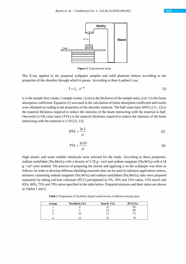
Kavun et. al. / Cumhuriyet Sci. J., Vol.40-4 (2019) 846-853
Figure 2. Experimental setup
The X-ray applied to the prepared wallpaper samples and solid phantom behave according to the
properties of the absorber through which it passes. According to Beer-Lambert Law;
0. tI I e −= (1)
I0 is the sample-free counts, I sample counts, t (cm) is the thickness of the sample and (cm-1) is the linear
absorption coefficient. Equation (1) was used in the calculation of linear absorption coefficient and results
were obtained according to the properties of the absorber material. The half value layer (HVL) [11, 12] is
the material thickness required to reduce the intensity of the beam interacting with the material in half.
One-tenth (1/10) value layer (TVL) is the material thickness required to reduce the intensity of the beam
interacting with the material to 1/10 [12, 13].
ln 2
HVL
= (2)
ln10
TVL
= (3)
High atomic and water soluble chemicals were selected for the study. According to these properties,
sodium molybdate (Na2MoO4) with a density of 3.78 g / cm3 and sodium tungstate (Na2WO4) with 4.18
g / cm3 were studied. The process of preparing the mortar and applying it on the wallpaper was done as
follows: In order to develop different shielding materials that can be used in radiation application centers,
mixtures containing sodium tungstate (Na2WO4) and sodium molybdate (Na2MoO4) salts were prepared
separately by taking calcium carbonate (PCC) precipitated in 5%, 10% and 15% ratios, 15% starch and
85%, 80%, 75% and 70% ratios specified in the table below. Prepared mixtures and their ratios are shown
in Tables 1 and 2.
Table 1. Preparation of Na2MoO4 doped coated mortar at different mixing ratios
Group Na2MoO4 (%) Starch (%) PCC(%)
1 0 15 85
2 5 15 80
3 10 15 75
4 15 15 70
848

Kavun et. al. / Cumhuriyet Sci. J., Vol.40-4 (2019) 846-853
Table 2. Preparation of Na2WO4 doped coated mortar at different mixing ratios
3. RESULTS AND DISCUSSION
The main purpose of shielding in radiation treatment centers is to prevent the radiation released from the
linear accelerator out of the treatment room as much as possible. This equivalent radiation dose is 0.02
mSv per week, except in public and uncontrolled areas [13]. The energy and amount of radiation
interacting with the material determine the quality of material in shielding. HVL represents the material
thickness required to reduce the amount of radiation to half and TVL to one tenth. The linear absorption
coefficients, HVL and TVL values were calculated by applying 4 MeV energy electrons shown in Table
5. The HVL values of sodium molybdate (Na2MoO4) applied wallpaper samples having different densities
ranged from the range of 16.91 to 115.52. The TVL values were between 9.36 and 383.76. The HVL
values for sodium tungstate (Na2WO4) were between 14.44 and 63.01. The TVL values varied between
47.97 and 209.33. Figures 4 and 5 show the attenuation coefficient values applied 4 MeV energy electrons
to the wallpaper samples doped with sodium molybdate (Na2MoO4) and sodium tungstate (Na2WO4). It
was observed that the attenuation coefficient values increased depending on the thickness of the
wallpapers doped with 3, 6 and 9 layers of material with different thicknesses. Accordingly, Figure 3 and
4 show the variation of HVL and TVL values. Figure 5 shows the comparison of HVL and TVL values
obtained by using (2) and (3) equations. In Table 6, HVL and TVL values of concrete, steel and lead
obtained at different energies used as radiation shielding materials in some radiotherapy centers are given.
As shown in this table 6, lead has the lowest HVL and TVL values while concrete has the highest values.
when in table 6 the HVL and TVL values of some materials values are compared with the Na2MoO4 and
Na2WO4 in Table 5, it can be seen in table 5 that the values we obtained have higher HVL and TVL
values. Accordingly, it is understood that these materials are not suitable for shielding use alone.
Table 3. Thickness and linear attenuation coefficient vales of wallpapers doped with sodium molybdate (Na2MoO4)
Table 4. Thickness and linear attenuation coefficient vales of wallpapers coated with sodium tungstat (Na2WO4)
Layer
PCC
Thick.(
mm)
µ(cm-1)
2.5 gr
Thick.
(mm)
µ(cm-1)
5.0 gr
Thick.
(mm)
µ(cm-1)
7.5 gr
Thick.
(mm)
µ(cm-1)
3 0.186 0.044 0.212 0.017 0.208 0.014 0.209 0.011
6 0.192 0.046 0.223 0.024 0.236 0.018 0.226 0.021
9 0.197 0.048 0.230 0.027 0.258 0.026 0.243 0.025
Group Na2WO4 (%) Starch (%) PCC (%)
1 0 15 85
2 5 15 80
3 10 15 75
4 15 15 70
Layer
PCC
Thick.
(mm)
µ(cm-1)
2.5 gr
Thick.
(mm)
µ(cm-1)
5.0 gr
Thick.
(mm)
µ(cm-1)
7.5 gr
Thick.
(mm)
µ(cm-1)
3 0.172 0.021 0.199 0.006 0.197 0.013 0.183 0.009
6 0.181 0.029 0.225 0.011 0.213 0.020 0.213 0.023
9 0.184 0.041 0.246 0.017 0.235 0.023 0.241 0.028
849
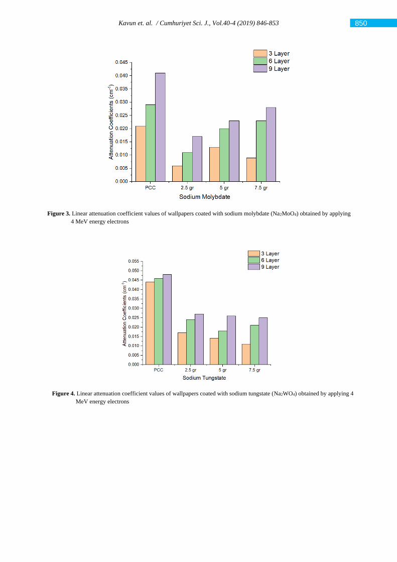
Kavun et. al. / Cumhuriyet Sci. J., Vol.40-4 (2019) 846-853
Figure 3. Linear attenuation coefficient values of wallpapers coated with sodium molybdate (Na2MoO4) obtained by applying
4 MeV energy electrons
Figure 4. Linear attenuation coefficient values of wallpapers coated with sodium tungstate (Na2WO4) obtained by applying 4
MeV energy electrons
850
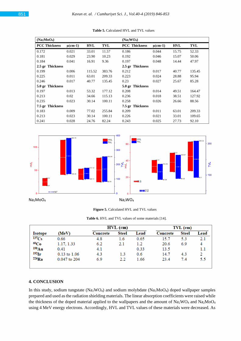
Kavun et. al. / Cumhuriyet Sci. J., Vol.40-4 (2019) 846-853
Table 5. Calculated HVL and TVL values
(Na2MoO4) (Na2WO4)
PCC Thickness µ(cm-1) HVL TVL PCC Thickness µ(cm-1) HVL TVL
0.172 0.021 33.01 11.57 0.186 0.044 15.75 52.33
0.181 0.029 23.90 10.23 0.192 0.046 15.07 50.06
0.184 0.041 16.91 9.36 0.197 0.048 14.44 47.97
2.5 gr Thickness 2.5 gr Thickness 0.199 0.006 115.52 383.76 0.212 0.017 40.77 135.45
0.225 0.011 63.01 209.33 0.223 0.024 28.88 95.94
0.246 0.017 40.77 135.45 0.23 0.027 25.67 85.28
5.0 gr Thickness 5.0 gr Thickness 0.197 0.013 53.32 177.12 0.208 0.014 49.51 164.47
0.213 0.02 34.66 115.13 0.236 0.018 38.51 127.92
0.235 0.023 30.14 100.11 0.258 0.026 26.66 88.56
7.5 gr Thickness 7.5 gr Thickness 0.183 0.009 77.02 255.84 0.209 0.011 63.01 209.33
0.213 0.023 30.14 100.11 0.226 0.021 33.01 109.65
0.241 0.028 24.76 82.24 0.243 0.025 27.73 92.10
Na2MoO4 Na2WO4
Figure 5. Calculated HVL and TVL values
Table 6. HVL and TVL values of some materials [14].
4. CONCLUSION
In this study, sodium tungstate (Na2WO4) and sodium molybdate (Na2MoO4) doped wallpaper samples
prepared and used as the radiation shielding materials. The linear absorption coefficients were raised while
the thickness of the doped material applied to the wallpapers and the amount of Na2WO4 and Na2MoO4
using 4 MeV energy electrons. Accordingly, HVL and TVL values of these materials were decreased. As
851
Kavun et. al. / Cumhuriyet Sci. J., Vol.40-4 (2019) 846-853
understood from these results, beta radiation permeability decreases with increasing amount of sodium
tungstate and sodium molybdate. Therefore, sodium tungstate (Na2WO4) and sodium molybdate
(Na2MoO4) salts can be used in radiation treatment by mixing together with other materials in the radiation
treatment centers that require radiation shielding or in many areas where beta radiation is applied. These
materials are not sufficient for use alone. Because, the obtained HVL-TVL values of sodium tungstate
(Na2WO4) and sodium molybdate (Na2MoO4) were high when compared to the literature [14] (table 6).
A successful shielding can be achieved when these materials are used in conjunction with low HVL and
TVL materials in the future studies.
Na2WO4 and Na2MoO4 salts are used in different agent such as paints, textiles, plastics, crops, cleaning
washings and pesticides [15]. As seen in the applications, it can be said that these compounds can be
stable in the air having moisture. Nevertheless, to preserve the properties of these materials, it is suitable
to coat the wallpaper surface with a coating material. Also, radiation treatment centers should be well
ventilated and preserve against moisture. In addition, the chemical properties of the wallpaper surfaces
can be preserved for a long time by coating them with materials such as gel or paint.
REFERENCES
[1] Köklü, N., Effects of Radiation on Human Health and Its Applıcatıon Fıelds in Medıcal, Master Thesis,
Selçuk University, Institute of Science, 2006.
[2] Martin J. E., Physics for Radiation Protection: A Handbook”, 2nd ed., Weinheim, WILEY-VCH
Verlag GmbH & Co. KGaA, 2006.
[3] Aggrey-Smith S., Preko K., Owusu F. W., and Amoako J. K., Study of Radiation Shielding Properties
of selected Tropical Wood Species for X-rays in the 50-150 keV Range, Journal of Science and
Technology 4 (2016) 1-8.
[4] Abrath, F. G., Bello, J., and Purdy, J. A., Attenuation of Primary and Scatter Radiation in Concrete
and Steel for 18 MeV X-Rays from a Clinac-20 Linear Accelerator., Health Physics, 45(5) (1983) 969-
73.
[5] Barish, R. J., Evaluation of a New High-Density Shielding Material., Health Physics, 64(4) (1993)
412-6.
[6] Al-Affan, I. A. M., Estimation of the Dose at the Maze Entrance for X-Rays from Radiotherapy Linear
Accelerators, Med. Phys., 27(1) (2000) 231-8.
[7] Çatak M.N., Shielding Linear Accelerator Devices According to NCRP–151 Report, Master Thesis,
Ankara University, Institute of Science, 2012.
[8] Tel, E. Sarpun, İ. H., Şahan, M., Bulbul A. and Özgen, M., Analysis of Dose—Thickness Interaction
with X-Rays Energy of 6 and 18 MeV for Beech Wooden Materials, Journal of Physical Science and
Application, 7(2) (2017) 42-45.
[9] VARİAN, Varian Medical Systems, Clinac, On-Board Imager and Rapidarc, Are Registered
Trademarks, And Exact and Laserguard Are Trademarks of Varian Medical Systems, Inc. 2012.
[10] PTW-Freiburg and Ptw-New York: Advanced Markus, Bragg Peak, Curıementor, Dıamentor,
Farmer, Markus, Nomex, Octavıus, Pin Point, Roos, Trufıx, 2017.
[11] Agar, O., et al., An extensive investigation on gamma ray shielding features of Pd/Ag-based alloys.
Nuclear Engineering and Technology, 51(3) (2019) 853-859.
852

Kavun et. al. / Cumhuriyet Sci. J., Vol.40-4 (2019) 846-853
[12] Akkaş A., Determination of the Tenth and Half Value Layer Thickness of Concretes with Different
Densities, Acta Physica Polonica A, 129 (2016) 770-772.
[13] Kavaz, E., et al., The Mass stopping power/projected range and nuclear shielding behaviors of
barium bismuth borate glasses and influence of cerium oxide. Ceramics International, 45(12) (2019)
15348-15357.
[14] Safety Reports Series, Radiation Protection in the Design of Radiotherapy Facilities, IAEA, Vienna,
No. 47, (2006), ISBN 92–0–100505–9.
[15] EPA Chemical and Products Database (CPDat),
Adres:https://comptox.epa.gov/dashboard/dsstoxdb/results?search=DTXSID2052788#exposure.
Retrieved November 18, 2019.
853
Cumhuriyet Science Journal
CSJ
e-ISSN: 2587-246X
ISSN: 2587-2680 Cumhuriyet Sci. J., Vol.40-4 (2019) 854-859
* Corresponding author. Email address: [email protected], [email protected]
http://dergipark.gov.tr/csj ©2019 Faculty of Science, Sivas Cumhuriyet University
Application of Heterocyclic Compounds as Catalysts in Suzuki-Miyaura
Cross-Coupling Reaction
Senem AKKOÇ1,*
1 Süleyman Demirel University, Faculty of Pharmacy, Department of Basic Pharmaceutical Sciences, 32260,
Isparta, Turkey
Received: ?; Accepted: ? http://dx.doi.org/10.17776/csj.613060
Abstract. Four different benzimidazolium salts (1-4) were prepared in three steps at 80 oC and their structures
were elucidated using spectroscopic methods. The compounds (1-4) obtained were tested in in situ medium as
catalyst in the carbon-carbon (C-C) bond formation reactions of two different boronic acid derivatives with
various aryl halides in the presence of palladium acetate (PdOAc)2 and sodium tertiarybutoxide (NaOBut) as a
base. With this reaction, four coupling products (5-8) were synthesized in different yields ranging from 11 to
93%. Compound 2 from the carbene precursors tested in the Suzuki-Miyaura cross-coupling reaction was found
to be a more effective catalyst candidate than others.
Keywords: Suzuki-Miyaura coupling reaction, Benzimidazolium salt, Catalyst.
Suzuki-Miyaura Çapraz Eşleşme Reaksiyonunda Katalizör Olarak
Heterosiklik Bileşiklerin Uygulanması
Özet. Dört farklı benzimidazolyum tuzu (1-4) üç basamakta 80 oC de hazırlandı ve yapıları spektroskopik
yöntemler kullanılarak aydınlatıldı. Elde edilen bileşikler (1-4), palladyum asetat (PdOAc)2 ve bir baz olarak
sodyum tersiyerbütoksitin (NaOBut) varlığında iki farklı boronik asit türevi ile farklı aril halojenürlerin karbon-
karbon (C-C) bağ oluşum reaksiyonlarında katalizör olarak in situ ortamda test edildi. Bu reaksiyon ile dört
eşleşme ürünü (5-8) %11 ile %93 arasında değişen farklı verimlerde sentezlendi. Suzuki-Miyaura çapraz
eşleşme reaksiyonunda test edilen karben öncüllerinden bileşik 2 diğerlerinden daha etkili bir katalizör adayı
olduğu bulundu.
Anahtar Kelimeler: Suzuki-Miyaura eşleşme reaksiyonu, Benzimidazolyum tuzu, Katalizör.
1. INTRODUCTION
Compounds containing benzimidazole nucleus
demonstrate a wide variety of biological activity
properties such as anticancer, antitubercular
antimicrobial, antifungal, antioxidant, antidiabetic
and etc [1-13]. On the other hand, heterocyclic
benzimidazole derivatives have different
application area and can be used as catalysts [14-
16] and sensors [17, 18]. Therefore,
benzimidazoles and their derivatives are consumed
in large quantities in the chemical, medical and
biological industries. So, they are among the most
frequently synthesized heterocyclic compounds in
the research studies, too.
Many chemicals used in pharmaceutical and
agricultural chemistry have C-C (carbon-carbon)
and C-N (carbon-nitrogen) bonds. Therefore, the
formation reactions of these bonds are used in the
synthesis of many organic materials of industrial
importance [19]. Suzuki-Miyaura, Mizoroki-Heck,
Sonogashira-Hagihara, Stille, Negishi, Kumada-
Tamao-Corriu and Hiyama cross-coupling
reactions are important C-C bond formation
reactions (Scheme 1).
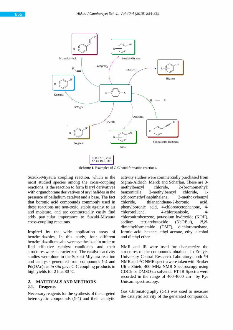
Akkoc / Cumhuriyet Sci. J., Vol.40-4 (2019) 854-859
R R
R'
R
Ar
R'
R
ArR
R'
R
R'
R
R'
Mizoroki-Heck Suzuki-Miyaura
Sonogashira-Hagihara
Stille
Hiyama
Negishi
Kumada
R, R'= Aril, VinilX= Cl, Br, I, OTf
R'H
ArB(OH)2
ArSnBu3
R'MgBr
R'ZnBr
R'Si(OR)3
XR
R'
Scheme 1. Examples of C-C bond formation reactions.
Suzuki-Miyaura coupling reaction, which is the
most studied species among the cross-coupling
reactions, is the reaction to form biaryl derivatives
with organoborane derivatives of aryl halides in the
presence of palladium catalyst and a base. The fact
that boronic acid compounds commonly used in
these reactions are non-toxic, stable against to air
and moisture, and are commercially easily find
adds particular importance to Suzuki-Miyaura
cross-coupling reactions.
Inspired by the wide application areas of
benzimidazoles, in this study, four different
benzimidazolium salts were synthesized in order to
find effective catalyst candidates and their
structures were characterized. The catalytic activity
studies were done in the Suzuki-Miyaura reaction
and catalysts generated from compounds 1-4 and
Pd(OAc)2 as in situ gave C-C coupling products in
high yields for 2 h at 80 oC.
2. MATERIALS AND METHODS
2.1. Reagents
Necessary reagents for the synthesis of the targeted
heterocyclic compounds (1-4) and their catalytic
activity studies were commercially purchased from
Sigma-Aldrich, Merck and Scharlau. These are 3-
methylbenzyl chloride, 2-(bromomethyl)
benzonitrile, 2-methylbenzyl chloride, 1-
(chloromethyl)naphthalene, 3-methoxybenzyl
chloride, thianaphthene-2-boronic acid,
phenylboronic acid, 4-chloroacetophenone, 4-
chlorotoluene, 4-chloroanisole, 4-
chloronitrobenzene, potassium hydroxide (KOH),
sodium tertiarybutoxide (NaOBut), N,N-
dimethylformamide (DMF), dichloromethane,
formic acid, hexane, ethyl acetate, ethyl alcohol
and diethyl ether.
NMR and IR were used for characterize the
structures of the compounds obtained. In Erciyes
University Central Research Laboratory, both 1H
NMR and 13C NMR spectra were taken with Bruker
Ultra Shield 400 MHz NMR Spectroscopy using
CDCl3 or DMSO-d6 solvents. FT-IR Spectra were
recorded in the range of 400-4000 cm-1 by Pye
Unicam spectroscopy.
Gas Chromatography (GC) was used to measure
the catalytic activity of the generated compounds.
855

Akkoc / Cumhuriyet Sci. J., Vol.40-4 (2019) 854-859
This was carried out by the SHIMADZU-2010 Plus
(Kyoto, Japan) with a ROSTEK packed stainless
steel column with a length and ID of 2.0 M, 2.0 mm
respectively, was used with high purity nitrogen at
a flow rate of 40 mL/min as a carrier gas and a
flame ionization detector (FID) set at a temperature
of 320 oC with an injection port temperature of 300 oC. Additionally, thermo Trace GC
(Massachusetts, ABD) with Finnigan Polaris Q ion
trap mass spectrometer in positive ion EI mode
(GC-MS) was used to identify the catalytic activity
results of some compounds in Suzuki-Miyaura
coupling reaction. The instrument settings were
used as injection port: 300 oC, injection type: split
(1:20), injection volume: 1 μL (sample dissolved in
1 mL CH2Cl2 diluted 1:2), GC column: Zebron
ZB5ms 30 m x 0.25 mm ID x 0.25 µm film
thickness, carrier gas: helium (1.3 mL/min), oven
program: 40 oC, hold 3 minutes, 12 oC/min ramp to
300 oC, hold 5 minutes, transfer line: 280 oC, MS
temperature: 240 oC, EI electron energy: 70 eV,
MS range: 46-650 m/z (3 minute solvent delay).
2.2. Synthesized benzimidazolium salts, 1-4
Four benzimidazolium salts (1-4) were prepared
easily and economically according to the literature
procedures [20] (Scheme 2) and their structures
were characterized using different spectroscopic
methods [20].
N
N
NC
Cl-
4
N
N
NC
Cl-
2
N
N
NC
Cl-
1
N
N
NC
Cl-
O
3
Scheme 2. The open structures of the synthesized
benzimidazolium salts 1-4.
2.3. Experimental protocol for the Suzuki-
Miyaura coupling reaction
The catalytic activity studies were done according
to the protocols in the literature [15, 16, 21].
Briefly, benzimidazolium salts (2-5), Pd(OAc)2
(0.1 mmol), aryl chlorides (1 mmol), boronic acid
derivatives (1.5 mmol) and NaOBut (2 mmol) as
base in DMF/H2O (1:1) mixture as solvents were
added to a 25 mL Schleng tube. The reaction was
conducted at 80 oC for 2 h. After the specified
period of time completed, the reaction temperature
was dropped to room temperature. Ethyl acetate
and hexane (1:5) were added on this reaction
mixture and it mixed at rapidly. The two phases
formed were separated and MgSO4 was added to
the organic phase for removing water. The products
were purified with flash column chromatography
using 5 mL of hexane and 1 mL of ethyl acetate as
solvents. Final products were analyzed using GC.
3. RESULTS AND DISCUSSION
Catalytic activities of the compounds (1-4) were
tested in Suzuki-Miyaura reaction. For this,
benzimidazolium salt (1-4), Pd(OAc)2, aryl
chloride, phenylboronic acid/tianaphthene-2-
boronic acid and NaOBut were used. The reaction
was carried out in DMF/H2O mixture at 80 oC with
heating for two hours. At the end of the this time (2
h), the waited product (5-8) was purified by column
chromatography and analyzed using GC. The
results obtained are presented in Table 1.
In the presence of catalysts synthesized from 1-
4/Pd(OAc)2, various Suzuki-Miyaura coupling
products (5-8) were obtained from the reaction of
4-chloronitrobenzene, 4-chloroanisole or 4-
chlorotoluene with phenylboronic acid and 4-
chloroacetophenone with tianaften-2-boronic acid.
These are 1-phenyl-4-nitrobenzene (5), 1-phenyl-
4-methoxybenzene (6), 1-phenyl-4-methylbenzene
(7) and 1-(4-(benzo[b]thiophen-2-yl)phenyl
ethanone (8). It is seen that from Table 1 the
reaction yields of the Suzuki-Miyaura coupling
products are between 11 and 93% and their
conversions are among 11 and 98%.
The product 1-phenyl-4-nitrobenzene (5), formed
from the coupling of phenylboronic acid with 4-
chloronitrobenzene, was obtained in 27% yield
using ligand 1 (Table 1, Entry 1) (Figure 1).
856
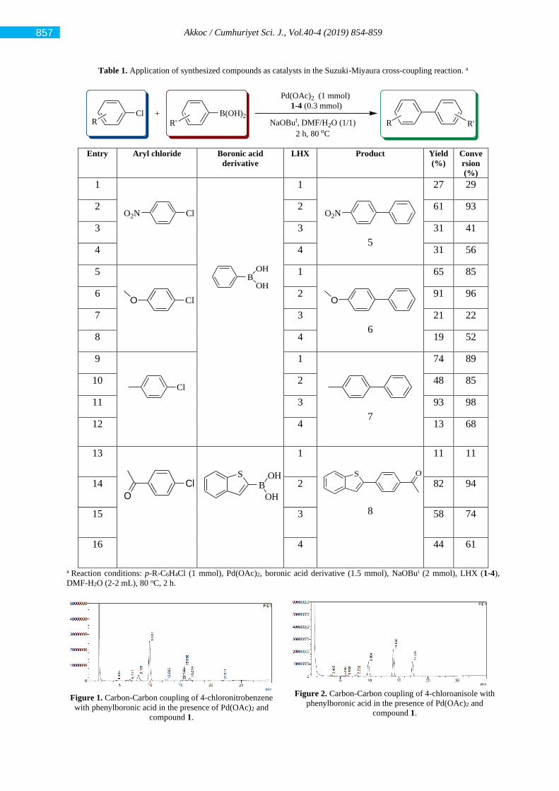
Akkoc / Cumhuriyet Sci. J., Vol.40-4 (2019) 854-859
Table 1. Application of synthesized compounds as catalysts in the Suzuki-Miyaura cross-coupling reaction. a
Cl
Pd(OAc)2 (1 mmol)
1-4 (0.3 mmol)
NaOBut, DMF/H2O (1/1)
2 h, 80 oC
+ B(OH)2R R' R'R
Entry Aryl chloride Boronic acid
derivative
LHX Product Yield
(%)
Conve
rsion
(%)
1
ClO2N
BOH
OH
1
O2N
5
27 29
2 2 61 93
3 3 31 41
4 4 31 56
5
ClO
1
O
6
65 85
6 2 91 96
7 3 21 22
8 4 19 52
9
Cl
1
7
74 89
10 2 48 85
11 3 93 98
12 4 13 68
13
Cl
O
S
BOH
OH
1
S O
8
11 11
14 2 82 94
15 3 58 74
16 4 44 61
a Reaction conditions: p-R-C6H4Cl (1 mmol), Pd(OAc)2, boronic acid derivative (1.5 mmol), NaOBut (2 mmol), LHX (1-4),
DMF-H2O (2-2 mL), 80 oC, 2 h.
Figure 1. Carbon-Carbon coupling of 4-chloronitrobenzene
with phenylboronic acid in the presence of Pd(OAc)2 and
compound 1.
Figure 2. Carbon-Carbon coupling of 4-chloroanisole with
phenylboronic acid in the presence of Pd(OAc)2 and
compound 1.
857
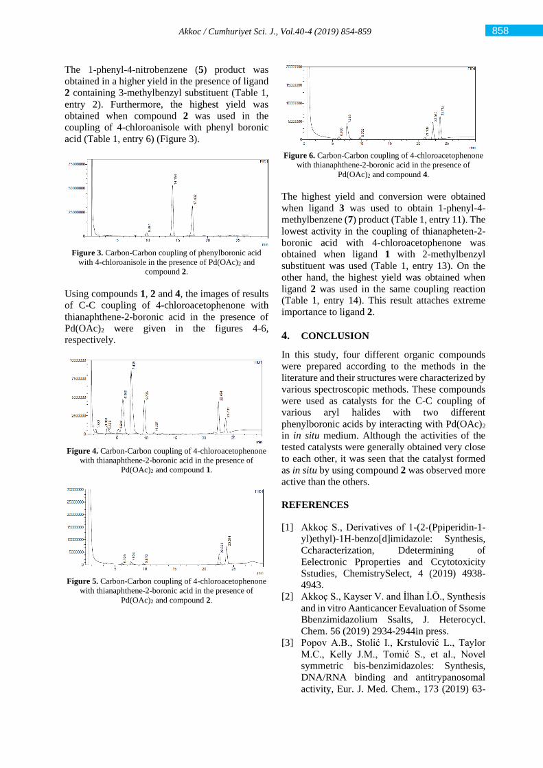
Akkoc / Cumhuriyet Sci. J., Vol.40-4 (2019) 854-859
The 1-phenyl-4-nitrobenzene (5) product was
obtained in a higher yield in the presence of ligand
2 containing 3-methylbenzyl substituent (Table 1,
entry 2). Furthermore, the highest yield was
obtained when compound 2 was used in the
coupling of 4-chloroanisole with phenyl boronic
acid (Table 1, entry 6) (Figure 3).
Figure 3. Carbon-Carbon coupling of phenylboronic acid
with 4-chloroanisole in the presence of Pd(OAc)2 and
compound 2.
Using compounds 1, 2 and 4, the images of results
of C-C coupling of 4-chloroacetophenone with
thianaphthene-2-boronic acid in the presence of
Pd(OAc)2 were given in the figures 4-6,
respectively.
Figure 4. Carbon-Carbon coupling of 4-chloroacetophenone
with thianaphthene-2-boronic acid in the presence of
Pd(OAc)2 and compound 1.
Figure 5. Carbon-Carbon coupling of 4-chloroacetophenone
with thianaphthene-2-boronic acid in the presence of
Pd(OAc)2 and compound 2.
Figure 6. Carbon-Carbon coupling of 4-chloroacetophenone
with thianaphthene-2-boronic acid in the presence of
Pd(OAc)2 and compound 4.
The highest yield and conversion were obtained
when ligand 3 was used to obtain 1-phenyl-4-
methylbenzene (7) product (Table 1, entry 11). The
lowest activity in the coupling of thianapheten-2-
boronic acid with 4-chloroacetophenone was
obtained when ligand 1 with 2-methylbenzyl
substituent was used (Table 1, entry 13). On the
other hand, the highest yield was obtained when
ligand 2 was used in the same coupling reaction
(Table 1, entry 14). This result attaches extreme
importance to ligand 2.
4. CONCLUSION
In this study, four different organic compounds
were prepared according to the methods in the
literature and their structures were characterized by
various spectroscopic methods. These compounds
were used as catalysts for the C-C coupling of
various aryl halides with two different
phenylboronic acids by interacting with Pd(OAc)2
in in situ medium. Although the activities of the
tested catalysts were generally obtained very close
to each other, it was seen that the catalyst formed
as in situ by using compound 2 was observed more
active than the others.
REFERENCES
[1] Akkoç S., Derivatives of 1-(2-(Ppiperidin-1-
yl)ethyl)-1H-benzo[d]imidazole: Synthesis,
Ccharacterization, Ddetermining of
Eelectronic Pproperties and Ccytotoxicity
Sstudies, ChemistrySelect, 4 (2019) 4938-
4943.
[2] Akkoç S., Kayser V. and İlhan İ.Ö., Synthesis
and in vitro Aanticancer Eevaluation of Ssome
Bbenzimidazolium Ssalts, J. Heterocycl.
Chem. 56 (2019) 2934-2944in press.
[3] Popov A.B., Stolić I., Krstulović L., Taylor
M.C., Kelly J.M., Tomić S., et al., Novel
symmetric bis-benzimidazoles: Synthesis,
DNA/RNA binding and antitrypanosomal
activity, Eur. J. Med. Chem., 173 (2019) 63-
858
Akkoc / Cumhuriyet Sci. J., Vol.40-4 (2019) 854-859
75.
[4] Zaman K., Rahim F., Taha M., Ullah H.,
Wadood A., Nawaz M., et al., Synthesis, in
vitro urease inhibitory potential and molecular
docking study of Benzimidazole analogues,
Bioorg. Chem. 89 (2019) 103024.
[5] Sadaf H., Imtiaz ud D., Fettouhi M., Fazal A.,
Ahmad S., Farooqi B.A., et al., Synthesis,
crystal structures and biological activities of
palladium(II) complexes of benzimidazole
and 2-methylbenzimidazole. Polyhedron,
(2019).
[6] Fang Y., Zhou H., Gu Q. and Xu J., Synthesis
and evaluation of tetrahydroisoquinoline-
benzimidazole hybrids as multifunctional
agents for the treatment of Alzheimer's
disease, Eur. J. Med. Chem., 167 (2019) 133-
145.
[7] Keri R.S., Rajappa C.K., Patil S.A. and
Nagaraja B.M., Benzimidazole-core as an
antimycobacterial agent, Pharmacol. Rep., 68
(2016)1254-1265.
[8] Akkoç S., Antiproliferative activities of 2-
hydroxyethyl substituted benzimidazolium
salts and their palladium complexes against
human cancerous cell lines, Synth. Commun.,
49 (2019) 2903-2914.
[9] Gök Y., Akkoç S., Çelikal Ö.Ö., Özdemir İ.
and Günal S., In vitro antimicrobial studies of
naphthalen-1-ylmethyl substituted silver N-
heterocyclic carbene complexes, Arabian J.
Chem., (2015).
[10] Singh I., Luxami V. and Paul K., Effective
synthesis of benzimidazoles-imidazo[1,2-
a]pyrazine conjugates: A comparative study
of mono-and bis-benzimidazoles for
antitumor activity, Eur. J. Med. Chem. 180
(2019) 546-561.
[11] Menteşe E., Emirik M. and Sökmen B.B.,
Design, molecular docking and synthesis of
novel 5,6-dichloro-2-methyl-1H-
benzimidazole derivatives as potential urease
enzyme inhibitors, Bioorg. Chem., 86
(2019)151-158.
[12] Babkov D.A., Zhukowskaya O.N., Borisov
A.V., Babkova V.A., Sokolova E.V.,
Brigadirova A.A., et al., Towards multi-target
antidiabetic agents: Discovery of biphenyl-
benzimidazole conjugates as AMPK
activators, Bioorg. Med. Chem. Lett. 29
(2019) 2443-2447.
[13] Mohanty S.K., Khuntia A., Yellasubbaiah N.,
Ayyanna C., Naga Sudha B. and Harika M.S.,
Design, synthesis of novel azo derivatives of
benzimidazole as potent antibacterial and anti
tubercular agents, Beni-Suef Uni. J. Bas.
Appl. Sci. 7 (2018) 646-651.
[14] Fukutake T., Wada K., Yu H., Hosokawa S.
and Feng Q., Development of titania-
supported iridium catalysts with excellent
low-temperature activities for the synthesis of
benzimidazoles via hydrogen transfer, Mol.
Catal. 477 (2019) 110550.
[15] Akkoç S., Gök Y., lhan l.Ö. and Kayser V., In
situ Ggeneration of Eefficient Ppalladium N-
heterocyclic Ccarbene Ccatalysts Uusing
Bbenzimidazolium Ssalts for the Suzuki-
Miyaura Ccross-coupling Rreaction, Curr.
Org. Synth., 13 (2016) 761-766.
[16] Akkoç S., Özer İlhan İ., Gök Y. and Kayser
V., Carbon-carbon bond formation catalyzed
by PEPPSI Pd-NHC, Inorg. Chim. Acta, 461
(2017) 52-56.
[17] Suman G.R., Bubbly S.G., Gudennavar S.B.
and Gayathri V., Benzimidazole and
benzothiazole conjugated Schiff base as
fluorescent sensors for Al3+ and Zn2+, J.
Photochem. Photobiol., A, 382 (2019)
111947.
[18] Suman G.R., Bubbly S.G. and Gudennavar
S.B., Benzimidazole and benzothiazole
fluorophores with large Stokes shift and
intense sky-blue emission in aggregation as
Al3+ and Pb2+ sensors, J. Lumin. 215 (2019)
116688.
[19] Weissermel K. and Arpe H-J., Industrial
Organic Chemistry, Weinheim. 2008.
[20] Akkoç S., Kayser V., İlhan İ.Ö., Hibbs D.E.,
Gök Y., Williams P.A., et al., New
compounds based on a benzimidazole
nucleus: synthesis, characterization and
cytotoxic activity against breast and colon
cancer cell lines, J. Organomet. Chem. 839
(2017) 98-107.
[21] Aslan H.G., Akkoç S., Kökbudak Z. and
Aydın L., Synthesis, characterization, and
antimicrobial and catalytic activity of a new
Schiff base and its metal(II) complexes, J.
Iran. Chem. Soc. 14 (2017) 2263-2273.
859
Cumhuriyet Science Journal
CSJ
e-ISSN: 2587-246X
ISSN: 2587-2680 Cumhuriyet Sci. J., Vol.40-4 (2019) 860-866
* Corresponding author. Email address: [email protected]
http://dergipark.gov.tr/csj ©2016 Faculty of Science, Sivas Cumhuriyet University
Construction of Continuous Bivariate Distribution by Transmuting
Dependent Distribution
Hüseyin ÜNÖZKAN 1 , Mehmet YILMAZ 2*
1 Ankara University, Graduate School of Natural and Applied Science, Department of Statistics, Turkey
2 Ankara University, Faculty of Science, Department of Statistics, 06100, Ankara, Turkey
Received: 10.09.2019; Accepted: 02.10.2019 http://dx.doi.org/10.17776/csj.618236
Abstract. In this study, a new bivariate distribution family is introduced by adding an appropriate term to
independent class. By choosing a base distribution which is negatively dependent from the same marginals we
derive a new distribution around the product of marginals, i.e. independent class of distribution. We note that
the new distribution has additional parameter which would provide additional flexibility in applications. The
joint probability density, joint reliability and reversed hazard rate functions of the new bivariate distribution are
obtained. Furthermore, we obtain lower and upper bounds of Spearman’s correlation coefficient. Two example
are given to illustrate this family. This new bivariate continuous distribution can make more appropriate
modeling of some data sets in terms of the Spearman rank coefficient.
Keywords: Transmuted bivariate distribution, Dependence, Bivariate distribution, Spearman’s Rho correlation
coefficient, Fréchet bounds.
Bağımlı Dağılım Fonksiyonunun Dönüştürülmesi ile İki Boyutlu Sürekli
Dağılım Fonksiyonu Oluşturulması
Özet. Bu çalışmada, bağımsız dağılım fonksiyonuna uygun bir terim eklenerek yeni bir iki boyutlu dağılım
fonksiyonu tanıtılmıştır. Bu yeni dağılım karmaşık bir yapıda değildir. Aynı marjinallere sahip dağılım
fonksiyonları sınıfından bir temel dağılım seçilerek, bağımsız dağılım fonksiyonu etrafında yeni dağılım
türetilmiştir. Bu yeni dağılımın fazladan bir parametresi olup, uygulama alanlarında modelleme esnasında
esneklik sağlayacağı düşünülmektedir. Bu yeni iki boyutlu dağılımın ortak olasılık yoğunluk fonksiyonu, ortak
güvenirlilik fonksiyonu ve ters bozulma oranı fonksiyonu elde edilmiştir. Bunun yanı sıra, bu metot ile elde
edilen yeni dağılım fonksiyonunun Spearman Sıra Korelasyonu katsayısı bakımından biraz daha esneklik
kazandırabileceği söylenebilir.
Anahtar Kelimeler: Dönüştürülmüş iki boyutlu dağılım, Bağımlılık, İki boyutlu dağılım, Spearman sıra
korelasyonu, Fréchet sınırları.
1. INTRODUCTION
In both statistical theory and practice, univariate models are sometimes insufficient to explain random
phenomena. Bivariate distributions are very important in modeling dependent random quantities in many
different areas. We need to construct a joint distribution with specific marginals and higher or lower
correlations. Dolati and Ubeda-Flores [1] introduced a method based on the choice of pairs of order
statistics of the marginal distributions. Lai and Xie [2] studied on construction of continuous bivariate
distributions that possesses the Positive Quadrant Dependence property. According to similar work of [2],
[3] introduces some conditions for negatively dependent families. Inspired by these studies, we desire to
propose a simpler but useful model. After giving the necessary conditions to construct a new distribution,
Ünözkan, Yılmaz / Cumhuriyet Sci. J., Vol.40-4 (2019) 860-866
Spearman's rank correlation coefficient is calculated on two illustrative examples and the usefulness of
this family is discussed. Furthermore, some reliability properties are studied for this family.
Let (𝑋1, 𝑌1) and (𝑋2, 𝑌2) be two independent vectors of random variables with common distribution
function 𝐻(𝑥, 𝑦). Note that, 𝐻(𝑥, 𝑦) belongs to the distribution family ℱ(𝐹, 𝐺) where 𝐹 and 𝐺 denote
respectively marginals of 𝑋 and Y. Let 𝑋(1), 𝑋(2) and 𝑌(1), 𝑌(2) be their corresponding order statistics.
According to [4], consider the random vector
(𝑍1, 𝑍2) = (𝑋(1), 𝑌(2)),with probability 1/2
(𝑋(2), 𝑌(1)), with probability 1/2.
Then the distribution of (𝑍1, 𝑍2) is given by
𝐻1(𝑥, 𝑦) = 𝐻(𝑥, 𝑦)[1 − (𝑥, 𝑦)], (1)
where (𝑥, 𝑦) denotes survival function of (𝑋, 𝑌) i.e., 𝑃𝑟(𝑋 > 𝑥, 𝑌 > 𝑦). If we consider the random
vector
(𝑇1, 𝑇2) = (𝑋(1), 𝑌(1)),with probability 1/2
(𝑋(2), 𝑌(2)), with probability 1/2.
Then the distribution function of (𝑇1, 𝑇2) is given by
𝐻2(𝑥, 𝑦) = 𝐹(𝑥)𝐺(𝑦) + 𝐻(𝑥, 𝑦)(𝑥, 𝑦). (2)
If we look at the equations (1) and (2) immediately, it is possible to say that the model formed by obtaining
a mixture of 𝐻1 and 𝐻2 is not a simple structure. With this in mind, our contribution is to propose a simpler
model. According to eq. (2.1) and and the conditions (2.2)-(2.4) of Han (2011) [3], the following
assumption is sufficient for our purpose: Suppose that 𝜓(𝑥, 𝑦) = −𝐻(𝑥, 𝑦)(𝑥, 𝑦). Then we have a
function defined as 𝐻1∗(𝑥, 𝑦) = 𝐹(𝑥)𝐺(𝑦) + 𝜓(𝑥, 𝑦). For subsequent discussions, following theorem
explains the necessity of having negative dependence (or independence) condition on 𝐻(𝑥, 𝑦).
Theorem1. Let 𝐻(𝑥, 𝑦) be a distribution function belongs to the distribution family ℱ(𝐹, 𝐺) which is
differentiable on ℝ2 and ℎ(𝑥, 𝑦) =𝜕2𝐻(𝑥,𝑦)
𝜕𝑥𝜕𝑦 denote the joint probability density function. Then
𝐻1∗(𝑥, 𝑦) = 𝐹(𝑥)𝐺(𝑦) − 𝐻(𝑥, 𝑦)(𝑥, 𝑦) is a distribution function if 𝐻(𝑥, 𝑦) ≤ 𝐹(𝑥)𝐺(𝑦), for all (𝑥, 𝑦) ∈
ℝ2 (or 𝐻(𝑥, 𝑦) = 𝐹(𝑥)𝐺(𝑦), for all (𝑥, 𝑦) ∈ ℝ2).
Proof. Multivariate distribution function must satisfy following properties (see, Barlow and Proschan,
1975, Chapter 5), [4]:
(P1)
lim𝑥→∞
𝐹(𝑥)𝐺(𝑦) − 𝐻(𝑥, 𝑦)(𝑥, 𝑦) = 𝐺(𝑦),
lim𝑦→∞
𝐹(𝑥)𝐺(𝑦) − 𝐻(𝑥, 𝑦)(𝑥, 𝑦) = 𝐹(𝑥),
lim𝑥∧𝑦→∞
𝐹(𝑥)𝐺(𝑦) − 𝐻(𝑥, 𝑦)(𝑥, 𝑦) = 1.
(P2) 𝜕𝐻1
∗(𝑥,𝑦)
𝜕𝑥≥ 0 and
𝜕𝐻1∗(𝑥,𝑦)
𝜕𝑦≥ 0. For the simplicity 𝑓𝑥 =
𝑑𝐹(𝑥)
𝑑𝑥 and 𝑔𝑦 =
𝑑𝐺(𝑦)
𝑑𝑦. Then
861
Ünözkan, Yılmaz / Cumhuriyet Sci. J., Vol.40-4 (2019) 860-866
𝜕𝐻1∗(𝑥, 𝑦)
𝜕𝑥= 𝑓𝑥𝐺(𝑦) −
𝜕𝐻(𝑥, 𝑦)
𝜕𝑥(𝑥, 𝑦) − 𝐻(𝑥, 𝑦)
𝜕(𝑥, 𝑦)
𝜕𝑥
= 𝑓𝑥(𝐺(𝑦) − 𝑃𝑟(𝑌 ≤ 𝑦|𝑋 = 𝑥)(𝑥, 𝑦) + 𝐻(𝑥, 𝑦)𝑃𝑟(𝑌 > 𝑦|𝑋 = 𝑥))
Now, by noting that negatively dependence implies 𝑃𝑟(𝑌 ≤ 𝑦|𝑋 = 𝑥) ≤ 𝐺(𝑦), then we have
𝜕𝐻1∗(𝑥, 𝑦)
𝜕𝑥≥ 𝑓𝑥(𝑃𝑟(𝑌 ≤ 𝑦|𝑋 = 𝑥)[1 − (𝑥, 𝑦)] + 𝐻(𝑥, 𝑦)𝑃𝑟(𝑌 > 𝑦|𝑋 = 𝑥))
≥ 0.
Obviously, 𝜕𝐻1
∗(𝑥,𝑦)
𝜕𝑦≥ 0.
(P3) 𝜕2𝐻1
∗(𝑥,𝑦)
𝜕𝑥𝜕𝑦≥ 0. For the simplicity, let ℎ0 = 𝑓(𝑥)𝑔(𝑦), 𝐻0 = 𝐹(𝑥)𝐺(𝑦) and ℎ𝑥𝑦 =
𝜕2𝐻(𝑥,𝑦)
𝜕𝑥𝜕𝑦. Then
𝜕2𝐻1∗(𝑥, 𝑦)
𝜕𝑥𝜕𝑦= ℎ0 − ℎ𝑥𝑦[𝐻(𝑥, 𝑦) + (𝑥, 𝑦)] −
𝜕𝐻(𝑥, 𝑦)
𝜕𝑥
𝜕(𝑥, 𝑦)
𝜕𝑦−𝜕𝐻(𝑥, 𝑦)
𝜕𝑦
𝜕(𝑥, 𝑦)
𝜕𝑥.
Now, according to Domma (2011) [5], by noting that negative dependence implies both ℎ𝑥𝑦𝐻(𝑥, 𝑦) ≤𝜕𝐻(𝑥,𝑦)
𝜕𝑥
𝜕𝐻(𝑥,𝑦)
𝜕𝑦 and ℎ𝑥𝑦(𝑥, 𝑦) ≤
𝜕(𝑥,𝑦)
𝜕𝑥
𝜕(𝑥,𝑦)
𝜕𝑦. Hence, we have
𝜕2𝐻1∗(𝑥, 𝑦)
𝜕𝑥𝜕𝑦≥ ℎ0 − [
𝜕𝐻(𝑥, 𝑦)
𝜕𝑥+𝜕(𝑥, 𝑦)
𝜕𝑥] [𝜕𝐻(𝑥, 𝑦)
𝜕𝑦+𝜕(𝑥, 𝑦)
𝜕𝑦].
By considering 𝜕(𝑥,𝑦)
𝜕𝑥= −𝑓𝑥 +
𝜕𝐻(𝑥,𝑦)
𝜕𝑥 and
𝜕(𝑥,𝑦)
𝜕𝑦= −𝑓𝑦 +
𝜕𝐻(𝑥,𝑦)
𝜕𝑦, the expressions in square brackets
are rewritten as ℎ0 − 2𝑓𝑦𝜕𝐻(𝑥,𝑦)
𝜕𝑥− 2𝑓𝑥
𝜕𝐻(𝑥,𝑦)
𝜕𝑦+ 4
𝜕𝐻(𝑥,𝑦)
𝜕𝑥
𝜕𝐻(𝑥,𝑦)
𝜕𝑦. After some simplification, the above
inequality becomes:
𝜕2𝐻1∗(𝑥, 𝑦)
𝜕𝑥𝜕𝑦≥ 2
𝜕𝐻(𝑥, 𝑦)
𝜕𝑥(𝑓𝑦 −
𝜕𝐻(𝑥, 𝑦)
𝜕𝑦) + 2
𝜕𝐻(𝑥, 𝑦)
𝜕𝑦(𝑓𝑥 −
𝜕𝐻(𝑥, 𝑦)
𝜕𝑥)
≥ 0.
This completes the proof.
According to Therorem1, by assuming 𝐻(𝑥, 𝑦) be negatively dependent or independent, we can define a
new pairs of random variables 𝑈 and 𝑉 as below:
(𝑈, 𝑉) = (𝑇1, 𝑇2 ), with probability 𝛼(𝑍1
∗, 𝑍2∗ ), with probability 1 − 𝛼,
where (𝑍1∗, 𝑍2
∗ ) is distributed as 𝐻1∗. Hence, the distribution of (𝑈, 𝑉) is given by
𝐹(𝑥, 𝑦) = 𝑃𝑟(𝑈 ≤ 𝑥, 𝑉 ≤ 𝑦 ) = 𝛼𝐻2(𝑥, 𝑦) + (1 − 𝛼)𝐻1∗(𝑥, 𝑦)
= 𝐹(𝑥)𝐺(𝑦) + (2𝛼 − 1)𝐻(𝑥, 𝑦)(𝑥, 𝑦). (3)
By letting 𝜆 = 2𝛼 − 1, where 𝜆 ∈ [−1,1], eq. (3) can be rewritten as
𝐹(𝑥, 𝑦) = 𝐹(𝑥)𝐺(𝑦) + 𝜆𝐻(𝑥, 𝑦)(𝑥, 𝑦). (4)
λ = 0 indicates 𝐹 = 𝐹(𝑥)𝐺(𝑦), 𝜆 = −1 indicates that 𝐹 is negatively dependent and 𝜆 = 1 indicates that
𝐹 is positively dependent. Note that, if 𝐻(𝑥, 𝑦) = 𝐹(𝑥)𝐺(𝑦), 𝐹 indicates well-known bivariate
distribution which is called as Farlie-Gumbel-Morgenstern distribution (see, [6] and [7]).
862

Ünözkan, Yılmaz / Cumhuriyet Sci. J., Vol.40-4 (2019) 860-866
We need the survival and probability density function for subsequent discussions. These functions are
respectively given by
(𝑥, 𝑦) = (𝑥)(𝑦) + 𝜆𝐻(𝑥, 𝑦)(𝑥, 𝑦)
and
𝑓(𝑥, 𝑦) = 𝑓(𝑥)𝑔(𝑦) + 𝜆ℎ(𝑥, 𝑦)[(𝑥, 𝑦) + 𝐻(𝑥, 𝑦)] − λ𝑘(𝑥, 𝑦),
where 𝑘(𝑥, 𝑦) = 𝑃𝑟(𝑋 ≤ 𝑥|𝑌 = 𝑦)𝑃𝑟(𝑌 > 𝑦|𝑋 = 𝑥) + 𝑃𝑟(𝑋 > 𝑥|𝑌 = 𝑦)𝑃𝑟(𝑌 ≤ 𝑦|𝑋 = 𝑥).
2. REVERSED HAZARD RATE OF THE NEW FAMILY OF BIVARIATE DISTRIBUTION
The bivariate reversed hazard is defined by Bismi [8] as 𝑟𝑣(𝑥, 𝑦) = 𝑓( 𝑥, 𝑦)/𝐹(𝑥, 𝑦). Furthermore, the
bivariate hazard rate function defined by Basu [9] as 𝑟(𝑥, 𝑦) = 𝑓( 𝑥, 𝑦)/(𝑥, 𝑦). Analogously to the
hazard gradient by Johnson and Kotz [10], Roy [11] defined the bivariate reversed hazard rate
and the bivariate hazard rate as follows: 𝒓𝒗1,2(𝑥, 𝑦) = (𝑟𝑣1(𝑥, 𝑦), 𝑟𝑣2(𝑥, 𝑦)), where
𝑟𝑣1(𝑥, 𝑦) =𝜕𝑙𝑜𝑔𝐹(𝑥, 𝑦)
𝜕𝑥, 𝑟𝑣2(𝑥, 𝑦) =
𝜕𝑙𝑜𝑔𝐹(𝑥, 𝑦)
𝜕𝑦,
and 𝒓1,2(𝑥, 𝑦) = (𝑟1(𝑥, 𝑦), 𝑟2(𝑥, 𝑦)), where
𝑟1(𝑥, 𝑦) =−𝜕𝑙𝑜𝑔(𝑥, 𝑦)
𝜕𝑥, 𝑟2(𝑥, 𝑦) =
−𝜕𝑙𝑜𝑔(𝑥, 𝑦)
𝜕𝑦.
Reversed hazard rate gradients of 𝐹(𝑥, 𝑦) given by eq. (4) are as follows:
𝑟𝑣1(𝑥, 𝑦) = 𝑤(𝑥, 𝑦, 𝜆)𝑟𝑣1(𝑥,∞) + (1 − 𝑤(𝑥, 𝑦, 𝜆)) (𝑟𝑣1𝐻(𝑥, 𝑦) − 𝑟1𝐻(𝑥, 𝑦)) ,
𝑟𝑣2(𝑥, 𝑦) = 𝑤(𝑥, 𝑦, 𝜆)𝑟𝑣2(∞, 𝑦) + (1 − 𝑤(𝑥, 𝑦, 𝜆)) (𝑟𝑣2𝐻(𝑥, 𝑦) − 𝑟2𝐻(𝑥, 𝑦)).
Accordingly, after some simplifications, bivariate reversed hazard rate can be given by
𝑟𝑣(𝑥, 𝑦) = 𝑤(𝑥, 𝑦, 𝜆)𝑟𝑣1(𝑥,∞)𝑟𝑣2(∞, 𝑦) + (1 − 𝑤(𝑥, 𝑦, 𝜆))(𝑟𝑣𝐻(𝑥, 𝑦) + 𝑟𝐻(𝑥, 𝑦))
−(1 − 𝑤(𝑥, 𝑦, 𝜆))[𝑟𝑣1𝐻(𝑥, 𝑦)𝑟2𝐻(𝑥, 𝑦) + 𝑟𝑣2𝐻(𝑥, 𝑦)𝑟1𝐻(𝑥, 𝑦)],
where 𝑤(𝑥, 𝑦, 𝜆) =𝐹(𝑥)𝐺(𝑦)
𝐹(𝑥)𝐺(𝑦)+𝜆𝐻(𝑥,𝑦)(𝑥,𝑦).
3. LOWER AND UPPER BOUNDS ON SPEARMAN’S RHO MEASURE FOR THE NEW
FAMILY OF BIVARIATE DISTRIBUTION
This section deals with obtaining bounds for the bivariate distribution family given by the eq. (4).
According to Hoeffding [12] and Fréchet [13], for any bivariate distribution belonging to ℱ(𝐹, 𝐺) contains
Fréchet a lower bound and an upper bound. These bounds are respectively defined as
𝐹−(𝑥, 𝑦) = max𝐹(𝑥) + 𝐺(𝑦) − 1,0 (5)
𝐹+(𝑥, 𝑦) = min𝐹(𝑥), 𝐺(𝑦). (6)
For 𝐹 ∈ ℱ(𝐹, 𝐺), Spearman’s rho can be expressed as
𝜌𝑠(𝑋, 𝑌) = 12 ∫ ∫𝐹(𝑥, 𝑦) − 𝐹(𝑥)𝐺(𝑦)𝑑𝐺(𝑦)𝑑𝐹(𝑥)
ℝℝ
(7)
863
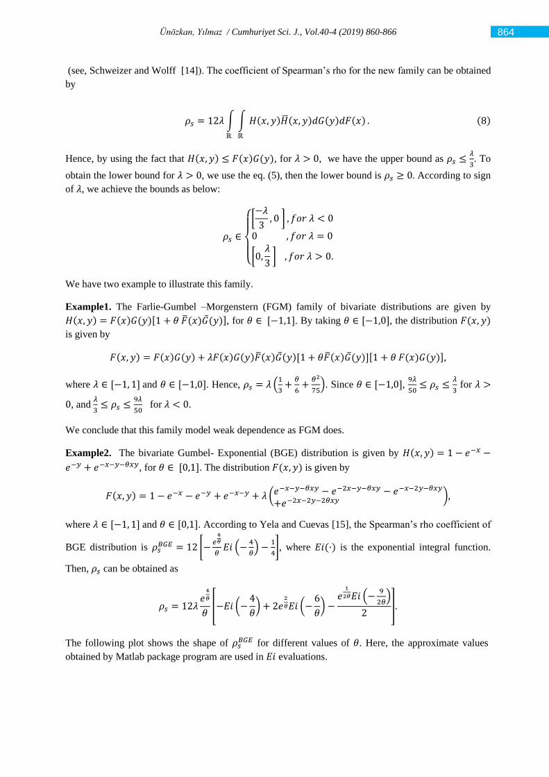
Ünözkan, Yılmaz / Cumhuriyet Sci. J., Vol.40-4 (2019) 860-866
(see, Schweizer and Wolff [14]). The coefficient of Spearman’s rho for the new family can be obtained
by
𝜌𝑠 = 12𝜆 ∫ ∫ 𝐻(𝑥, 𝑦)(𝑥, 𝑦)𝑑𝐺(𝑦)𝑑𝐹(𝑥)
ℝℝ
. (8)
Hence, by using the fact that 𝐻(𝑥, 𝑦) ≤ 𝐹(𝑥)𝐺(𝑦), for 𝜆 > 0, we have the upper bound as 𝜌𝑠 ≤𝜆
3. To
obtain the lower bound for 𝜆 > 0, we use the eq. (5), then the lower bound is 𝜌𝑠 ≥ 0. According to sign
of 𝜆, we achieve the bounds as below:
𝜌𝑠 ∈
[−𝜆
3, 0 ] , 𝑓𝑜𝑟 𝜆 < 0
0 , 𝑓𝑜𝑟 𝜆 = 0
[0,𝜆
3 ] , 𝑓𝑜𝑟 𝜆 > 0.
We have two example to illustrate this family.
Example1. The Farlie-Gumbel –Morgenstern (FGM) family of bivariate distributions are given by
𝐻(𝑥, 𝑦) = 𝐹(𝑥)𝐺(𝑦)[1 + 𝜃 (𝑥)(𝑦)], for 𝜃 ∈ [−1,1]. By taking 𝜃 ∈ [−1,0], the distribution 𝐹(𝑥, 𝑦)
is given by
𝐹(𝑥, 𝑦) = 𝐹(𝑥)𝐺(𝑦) + 𝜆𝐹(𝑥)𝐺(𝑦)(𝑥)(𝑦)[1 + 𝜃(𝑥)(𝑦)][1 + 𝜃 𝐹(𝑥)𝐺(𝑦)],
where 𝜆 ∈ [−1, 1] and 𝜃 ∈ [−1,0]. Hence, 𝜌𝑠 = 𝜆 (1
3+𝜃
6+𝜃2
75). Since 𝜃 ∈ [−1,0],
9𝜆
50≤ 𝜌𝑠 ≤
𝜆
3 for 𝜆 >
0, and 𝜆
3≤ 𝜌𝑠 ≤
9𝜆
50 for 𝜆 < 0.
We conclude that this family model weak dependence as FGM does.
Example2. The bivariate Gumbel- Exponential (BGE) distribution is given by 𝐻(𝑥, 𝑦) = 1 − 𝑒−𝑥 −
𝑒−𝑦 + 𝑒−𝑥−𝑦−𝜃𝑥𝑦, for 𝜃 ∈ [0,1]. The distribution 𝐹(𝑥, 𝑦) is given by
𝐹(𝑥, 𝑦) = 1 − 𝑒−𝑥 − 𝑒−𝑦 + 𝑒−𝑥−𝑦 + 𝜆 (𝑒−𝑥−𝑦−𝜃𝑥𝑦 − 𝑒−2𝑥−𝑦−𝜃𝑥𝑦 − 𝑒−𝑥−2𝑦−𝜃𝑥𝑦
+𝑒−2𝑥−2𝑦−2𝜃𝑥𝑦),
where 𝜆 ∈ [−1, 1] and 𝜃 ∈ [0,1]. According to Yela and Cuevas [15], the Spearman’s rho coefficient of
BGE distribution is 𝜌𝑠𝐵𝐺𝐸 = 12 [−
𝑒4𝜃
𝜃𝐸𝑖 (−
4
𝜃) −
1
4], where 𝐸𝑖(·) is the exponential integral function.
Then, 𝜌𝑠 can be obtained as
𝜌𝑠 = 12𝜆𝑒4
𝜃
𝜃[−𝐸𝑖 (−
4
𝜃) + 2𝑒
2
𝜃𝐸𝑖 (−6
𝜃) −
𝑒1
2𝜃𝐸𝑖 (−9
2𝜃)
2].
The following plot shows the shape of 𝜌𝑠𝐵𝐺𝐸 for different values of 𝜃. Here, the approximate values
obtained by Matlab package program are used in 𝐸𝑖 evaluations.
864
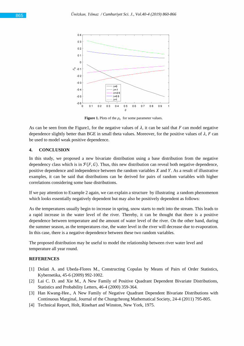
Ünözkan, Yılmaz / Cumhuriyet Sci. J., Vol.40-4 (2019) 860-866
Figure 1. Plots of the 𝜌𝑠 for some parameter values.
As can be seen from the Figure1, for the negative values of 𝜆, it can be said that 𝐹 can model negative
dependence slightly better than BGE in small theta values. Moreover, for the positive values of 𝜆, 𝐹 can
be used to model weak positive dependence.
4. CONCLUSION
In this study, we proposed a new bivariate distribution using a base distribution from the negative
dependency class which is in ℱ(𝐹, 𝐺). Thus, this new distribution can reveal both negative dependence,
positive dependence and independence between the random variables 𝑋 and 𝑌. As a result of illustrative
examples, it can be said that distributions can be derived for pairs of random variables with higher
correlations considering some base distributions.
If we pay attention to Example 2 again, we can explain a structure by illustrating a random phenomenon
which looks essentially negatively dependent but may also be positively dependent as follows:
As the temperatures usually begin to increase in spring, snow starts to melt into the stream. This leads to
a rapid increase in the water level of the river. Thereby, it can be thought that there is a positive
dependence between temperature and the amount of water level of the river. On the other hand, during
the summer season, as the temperatures rise, the water level in the river will decrease due to evaporation.
In this case, there is a negative dependence between these two random variables.
The proposed distribution may be useful to model the relationship between river water level and
temperature all year round.
REFERENCES
[1] Dolati A. and Ubeda-Flores M., Constructing Copulas by Means of Pairs of Order Statistics,
Kybernetika, 45-6 (2009) 992-1002.
[2] Lai C. D. and Xie M., A New Family of Positive Quadrant Dependent Bivariate Distributions,
Statistics and Probability Letters, 46-4 (2000) 359-364.
[3] Han Kwang-Hee., A New Family of Negative Quadrant Dependent Bivariate Distributions with
Continuous Marginal, Journal of the Chungcheong Mathematical Society, 24-4 (2011) 795-805.
[4] Technical Report, Holt, Rinehart and Winston, New York, 1975.
865
Ünözkan, Yılmaz / Cumhuriyet Sci. J., Vol.40-4 (2019) 860-866
[5] Domma F., Bivariate Reversed Hazard Rate, Notions, and Measures of Dependence and their
Relationships, Communications in Statistics - Theory and Methods, 40-6 (2011) 989-999, DOI:
10.1080/03610920903511777.
[6] Farlie D., The Performance of Some Correlation Coefficients for a General Bivariate Distribution,
Biometrika, 47-3/4 (1960) 307-323.
[7] Gumbel E. J., Bivariate Exponential Distributions, Journal of the American Statistical Association,
55-292 (1960) 698-707.
[8] Bismi G., Bivariate Burr Distributions, unpublished PhD Thesis, Cochin University of Science and
Technology, 2005.
[9] Basu A.P., Bivariate Failure Rate, Journal of the American Statistical Association, 66 (1971) 103–
104.
[10] Johnson N. L. and Kotz S., A Vector Multivariate Hazard Rate, Journal of Multivariate Analysis, 5-
1 (1975) 53-66.
[11] Roy D., A Characterization of Model Approach for Generating Bivariate Life Distributions Using
Reversed Hazard Rates, Journal of Japan Statistical Society, 32-2 (2002) 239–245.
[12] Hoeffding W., Masstabinvariante Korrelationstheorie, Schriften des Mathematischen Instituts und
Instituts fur Angewandte Mathematik der Universitat Berlin, 5 (1940) 181-233.
[13] Fréchet M., Sur Les Tableaux de Corrélation Dont Les marges Sont Donnees, Annales de
l’Université de Lyon, Sciences, 4 (1951) 13–84.
[14] Schweizer B. and Wolff E., On Nonparametric Measures of Dependence for Random Variables, The
Annals of Statistics, 9-4 (1981) 879-885.
[15] Yela P.J. and Cuevas T.J.R., Estimating the Gumbel-Barnett Copula Parameter of Dependence,
Revista Colombiana de Estadística, 41-1 (2018) 53-73.
866
Cumhuriyet Science Journal
CSJ
e-ISSN: 2587-246X
ISSN: 2587-2680 Cumhuriyet Sci. J., Vol.40-4 (2019) 867-874
* Corresponding author. Email address: [email protected]
http://dergipark.gov.tr/csj ©2016 Faculty of Science, Sivas Cumhuriyet University
An Extension Theorem for Weighted Ricci Curvature on Finsler Manifolds
Yasemin SOYLU 1
1 University of Giresun, Department of Mathematics, Giresun, Turkey
Received: 11.09.2019; Accepted: 19.12.2019 http://dx.doi.org/10.17776/csj.618537
Abstract. Let (𝑀, 𝐹) be a forward complete and connected Finsler manifold of dimensional 𝑛 ≥ 2. In this
study, we extend Wan’s extension theorem in Riemannian manifolds to Finsler manifolds by using the weighted
Ricci curvature R𝑖𝑐𝑁 bounded below. The proof of theorem is obtained by the Laplacian comparison theorem
on Finsler manifolds and the excess function.
Keywords: Distance function, Finsler manifold, Weighted Ricci curvature.
Finsler Manifoldlar Üzerinde Ağırlıklı Ricci Eğriliği İçin Bir Genişleme
Teoremi
Özet. (M,F) tam ve bağlantılı n≥2 boyutlu bir Finsler manifold olsun. Bu çalışmada aşağıdan sınırlı
R𝑖𝑐𝑁 ağırlıklı Ricci eğriliği yardımıyla Wan’ın Riemann manifoldlarında elde ettiği genişleme teoremi Finsler
manifoldlara genişletilmiştir. Teoremin ispatı Finsler manifoldlar üzerindeki Laplasyan karşılaştırma teoremi
ve excess fonksiyonu kullanılarak elde edilmiştir.
Anahtar Kelimeler: Uzaklık fonksiyonu, Finsler manifold, Ağırlıklı Ricci eğriliği.
1. INTRODUCTION
Finsler geometry includes analogues for many of the natural objects in Riemannian geometry. It is just
Riemannian geometry without quadratic restriction. The recent works have shown that some results in
Riemannian geometry have been extended to the Finsler setting. For example in this scope, the reader is
referred to [1, 2, 3] and references therein.
In the Riemannian case, in [4], Myers obtained a compactness theorem. The theorem of Myers concludes
that if R𝑖𝑐 ≥ (𝑛 − 1)𝐾 > 0, then d𝑖𝑎𝑚(𝑀) ≤ 𝜋/√𝐾. Later, Calabi [5] extended this theorem as follows:
Theorem 1. Let M be a complete and connected n-dimensional Riemannian manifold with non-negative
Ricci curvature. Suppose there exists a point po ∈ M such that every geodesic ray γ(t) issuing from po
satisfies
limsup𝑘→∞
(∫𝑘
0R𝑖𝑐(𝑠)1/2𝑑𝑠 − 1/2ln(𝑘)) = ∞, (1)
then manifold is compact.
In [6] Cheeger-Gromov-Taylor have proved the following result:

Soylu / Cumhuriyet Sci. J., Vol.40-4 (2019) 867-874
Theorem 2. Let Mn be a complete and connected Riemannian manifold. If there exist o ∈ M and r0, ν >
0 such that
R𝑖𝑐(𝑥) ≥(𝑛−1)(
1
4+𝜈2)
𝑟2 (2)
holds for all r(x) ≥ r0 > 0, then M is compact and the diameter is bounded from above by diamo(M) <
r0eπ/ν, where r is distance function defined with respect to fixed point o ∈ M.
The idea of their proof relies on studying carefully the index form or the second variation.
Recently, Wan [7] gave a complementary extension of Calabi and Cheeger-Gromov-Taylor’s theorems
by showing that the manifold has no ray issuing from some point.
Theorem 3. Let (M, g) be a complete n-dimensional Riemannian manifold and satisfy
R𝑖𝑐 ≥𝐻(𝑛,ℓ,𝜔)
(𝑟+𝜔)ℓ (3)
for all r ≥ 0, ω > 0 and ℓ ≥ 2, where r is a distance function r(x) = d(x, o) with respect to a fixed point
o ∈ M and H is a constant depending on n, ℓ and ω. Then manifold is compact. Here H can be chosen to
equal to (n − 1).ωℓ−2.(ℓ−1)ℓ
(ℓ−2)ℓ−2 for ℓ > 2 and (n − 1). (1 +
ω
ε), ε > 0 for ℓ = 2.
Qui [8] used the idea of Wan, by using the excess function and 𝑉-Laplacian comparison theorem, he
derived an extension of Bonnet– Myers type theorem with the Bakry–Emery Ricci curvature R𝑖𝑐𝑉:=
R𝑖𝑐 −1
2𝐿𝑉𝑔. Also, he showed that when the vector field 𝑉 is the gradient of some smooth function 𝑓 on
𝑀, i.e., 𝑉 = ∇𝑓, if R𝑖𝑐𝑉 has a positive lower bound and |𝑓| is bounded, then manifold is compact.
Moreover, for the 𝑚-Bakry-Emery Ricci curvature R𝑖𝑐𝑉𝑚:= R𝑖𝑐 −
1
2𝐿𝑉𝑔 −
1
𝑚−𝑛𝑉∗⊗𝑉∗, he obtained a
compactness theorem by using a similar method as in the proof of Wan.
Also, these type theorems and other calculations in Riemannian geometry has been generalized in various
direction by a lot of authors [9, 10, 11, 12] and references therein.
Motivated by the above studies, in this paper we will prove the corresponding Wan’s above theorem, for
the weighted Ricci curvature R𝑖𝑐𝑁 on Finsler manifolds. In particular, we will use the Laplacian
comparison theorem on Finsler manifolds and the excess function. Our main result is as follows:
Theorem 4. Let (M, F, dμ) be a forward complete and connected Finsler manifold of dimension n with
arbitrary volume form and let r be the distance function r(x) = d(x, o) with respect to a fixed point o ∈
M. Suppose that the weighted Ricci curvature
R𝑖𝑐𝑁:= R𝑖𝑐∞ −𝑆2
𝑁−𝑛≥ 𝐴𝜓(𝑟) (4)
for all N ∈ (n,∞) and A is a constant depending on ψ and N. Then
• Manifold is compact,
• Let ϵ and δ be positive arbitrary constants. Then A can be chosen as (N−1
ϵ)(∫
∞
ϵψ(s)ds)−1 + δ.
868

Soylu / Cumhuriyet Sci. J., Vol.40-4 (2019) 867-874
Remark 5. If we choose ψ =1
r2 and ψ =
1
(r+1)2, then Theorem 4 becomes Theorem 2 and Theorem 3 in
[13], respectively.
Remark 6. If ψ satisfies ∫∞
ϵψ(s)ds = ∞, then A can be chosen as an arbitrary positive real number.
Choose 𝜓 =1
(𝑟+𝜔)ℓ such that ℓ ∈ ℝ and 𝜔 > 0. So we can obtain the following result:
Corollary 7. Let (M, F, dμ) be a forward complete and connected Finsler manifold of dimension n with
arbitrary volume form and let r be the distance function r(x) = d(x, o) with respect to a fixed point o ∈
M. Suppose that the weighted Ricci curvature
R𝑖𝑐𝑁 ≥𝐵(𝑛,ℓ,𝜔)
(𝑟+𝜔)ℓ (5)
for all r ≥ 0 and ω > 0, where r is a distance function r(x) = d(x, o) with respect to a fixed point o ∈ M
and B is a positive constant depending on N, ℓ and ω. Then manifold is compact. Here B can be chosen
to equal to
• (𝑁 − 1). 𝜔ℓ−2.(ℓ−1)ℓ
(ℓ−2)ℓ−2+ 𝛿 for ℓ > 2,
• (𝑁−1)(ℓ−1)
𝜖. (𝜔 + 𝜖)ℓ−1 + 𝛿 for 1 < ℓ ≤ 2,
• an arbitrary positive real number for ℓ ≤ 1
(𝜖, 𝛿 are positive constants).
Additionally, if R𝑖𝑐𝑁 ≥ 𝛿 > 0, we can rescale the metric such that δ is bigger than the right hand of (5).
So manifold is compact (see [13]). By taking 𝜓 ≡ 𝑐𝑜𝑛𝑠𝑡𝑎𝑛𝑡 in Theorem 4 we have
Corollary 8. Let (M, F, dμ) be a forward complete and connected Finsler manifold of dimension n with
arbitrary volume form. Assume that RicN ≥ (N − 1)C, C > 0, then manifold is compact and the diameter
has an upper bound.
The proof of Corollary 8 is almost the same steps of Theorem 2 in [13]. So, it may be omitted here.
Now, we review below a summary of the basic concepts associated with the Finsler geometry.
2. FINSLER GEOMETRY
Let M be a differentiable n-manifold and TM be the tangent bundle on M, where TxM is tangent space at
x ∈ M. Set T0M = TM\0. Let π: TM → M be the natural projection and (x, y) be a point of TM such that
x ∈ M and y ∈ TxM.
Definition 9. A Finsler metric F: TM → [0,∞) is a 𝒞∞-Finsler structure of M with the following
conditions:
1. F is 𝒞∞ on T0M (Regularity),
2. F(x, λy) = λF(x, y) for all λ > 0 (Positive homogeneity),
3. The n × n Hessian matrix
869
Soylu / Cumhuriyet Sci. J., Vol.40-4 (2019) 867-874
gij: =1
2[F2]yiyj (6)
is positive-definite at every point of T0M (Strong convexity).
The pair (M, F) is called a Finsler manifold.
The Chern curvature RV for vectors fields X, Y, Z ∈ TxM\0 is defined by
RV(X, Y)Z: = ∇XV∇Y
VZ − ∇YV∇X
VZ − ∇[X,Y]V Z. (7)
In the Riemannian case this curvature does not depend on V and coincides with the Riemannian curvature
tensor. The flag curvature is defined as follows:
K(V,W):=gV(R
V(V,W)W,V)
gV(V,V)gV(W,W)−gV(V,W)2, (8)
where V,W ∈ TxM\0 are linearly independent vectors. Then the Ricci curvature of V (as the trace of the
flag curvature) is given as
Ric(V):= ∑n−1i=1 K(V, Ei), (9)
where E1, E2, . . . , En−1, V/F(V) is an orthonormal basis of TxM with respect to gV, namely gV(Ei, Ej) =
δij and gV(V, Ei) = 0 for all i, j = 1, . . . , n − 1.
Let dμ = σF(x)dx1dx2. . . dxn be the volume form on M. For a vector V ∈ TxM\0,
τ(x, V):= ln√det(gij(x,V))
σF(x) (10)
is a scalar function on TxM\0 which is called the distortion of (M, F, dμ). We say that the distortion τ is
a 𝒞∞-function, if M is a Riemannian manifold. Setting
S(x, V):=d
dt(τ(γ(t), γ(t)))|t=0, (11)
where γ is the geodesic with γ(0) = x, γ(0) = V. S(x, λV) = λS(x, V) for all λ > 0. S is a scalar function
on TxM\0 which is called the S-curvature. From the definition, it seems that the S-curvature measures
the rate of change in the distortion along geodesics in the direction V ∈ TxM.
For all N ∈ (n,∞), we define the weighted Ricci curvature of (M, F, dμ) as follows (see [1]):
RicN(W):= Ric(W) + S(W) −
S(W)2
N − n,
Ric∞(W):= Ric(W) + S(W),
Ricn(W) ∶= Ric + S(W), if S(W) = 0−∞ otherwise.
Also RicN(βW):= β2RicN(W) for β > 0.
870
Soylu / Cumhuriyet Sci. J., Vol.40-4 (2019) 867-874
We say that (M, F) is forward complete if each geodesic γ: [0, ℓ] → M is extended to a geodesic on [0,∞),
in other words, if exponential map is defined on whole TM. Then the Hopf-Rinow theorem gives that
every pair of points in M can be joined by a minimal geodesic.
The Legendre transformation ℒ: TM → T∗M is defined as
ℒ(Z): = gZ(Z, . ), Z ∈ T0M,0 Z = 0.
For a smooth function h:M → ℝ, the gradient vector of h at x ∈ M is defined as ∇h(x):= ℒ−1(dh).
Given a smooth vector field Z = Zi ∂/ ∂xi on M, the divergence of Z with respect to an arbitrary volume
form dμ = eφdx1dx2. . . dxn is defined by
divZ:= ∑ni=1 (∂Zi
∂xi+ Zi
∂φ
∂xi). (12)
Then we define the Finsler-Laplacian of h by Δh:= div(∇h) = div(ℒ−1(dh)).
Let U = x ∈ M:∇u|x ≠ 0. The Hessian of u on U is defined by follows:
H(u)(V,W):= VW(u) − ∇V∇uW(u), ∀ V,W ∈ TM|U.
We know that H(u) is symmetric, and it can be rewritten as
H(u)(V,W) = g∇u(∇V∇u∇u,W).
The following lemma will be very useful in the proofs of our main results (see [14]).
Lemma 10. Let (M, F, dμ) be a Finsler n-manifold, and u:M → R a smooth function on M. Then on U =
x ∈ M:∇u|x ≠ 0 we have
Δu = ∑i H(u)(Ei, Ei) − S(∇u):= tr∇uH(u) − S(∇u), (13)
where E1, E2, . . . , En is a local g∇u-orthonormal frame on U.
Finally, define revesibility λ:= λ(M, F) as follows:
λ: = supx∈M,y∈TM\0
F(x,−y)
F(x,y). (14)
It is clear that λ ∈ [1,∞], and λ = 1 if and only if (M, F) is called reversible.
3. THE PROOF OF THE MAIN RESULT
Let (𝑀, 𝐹, 𝑑𝜇) be a Finsler manifold of dimensional 𝑛 and 𝑟(𝑥) = 𝑑(𝑜, 𝑥) be a distance function with
respect to a fixed point 𝑜 ∈ 𝑀. It is well known that 𝑟 is only smooth on 𝑀 − (𝐶𝑜 ∪ 𝑜) where 𝐶𝑜 is the
cut locus of the point 𝑜 ∈ 𝑀. We assume that 𝜎 is a minimal unit speed geodesic segment. We have ∇𝑟 =
𝜎′(𝑡) in the adapted coordinates with respect to the 𝑟, and the distance function 𝑟 satisfies 𝐹(∇𝑟) = 1 for
all 𝑝 ∈ 𝑀 − (𝐶𝑜 ∪ 𝑜) (see [15]). On the other hand, using the Finsler metric we obtain a weighted
Riemannian metric 𝑔∇𝑟. Thus we apply the Riemannian calculation for 𝑔∇𝑟 (on 𝑀− (𝐶𝑜 ∪ 𝑜)).
In order to prove the Theorem 4 we first give an upper estimate for the Laplacian of the distance function
𝑟(𝑥) = 𝑑(𝑜, 𝑥).
871
Soylu / Cumhuriyet Sci. J., Vol.40-4 (2019) 867-874
Lemma 11. [16] If RicN ≥ 0 for N ∈ (n,∞), then the Laplacian of the distance function r(x) = d(o, x) from any given point o ∈ M can be estimated as follows:
Δ𝑟 ≤𝑁−1
𝑟 (15)
in the sense of distributions on M\o.
Now, we can prove our main theorem using the above notations.
Proof of Theorem 4. Let σ(t) be a unit speed ray starting from a fixed point o ∈ M with σ(0) = o. For
every t > 0, Δr(γ(t)) denotes the Finsler-Laplacian of distance function r from a fixed point o ∈ M. It
satisfies F(∇r) = 1. In the Finsler case, recall that the Bochner-Weitzenböck formula [17] for a smooth
function u ∈ 𝒞∞(M)
0 = Δ∇𝑢 (𝐹(∇𝑢)2
2) = R𝑖𝑐∞(∇𝑢) + 𝐷(Δ𝑢)(∇𝑢)+∥ ∇
2𝑢 ∥𝐻𝑆(∇𝑢)2 . (16)
From the Bochner formula applied to distance function 𝑟 and by Lemma 10, we have, on 𝑀− (𝐶𝑝 ∪ 𝑝),
0 = R𝑖𝑐∞(∇𝑟) + 𝐷(Δ𝑟)(∇𝑟)+∥ ∇2𝑟 ∥𝐻𝑆(∇𝑟)
2
≥ R𝑖𝑐∞(∇𝑟) + 𝑔∇𝑟(∇∇𝑟Δ𝑟, ∇𝑟) +
1
𝑛−1(𝑡𝑟∇𝑟H𝑒𝑠𝑠𝑟)
2
= R𝑖𝑐∞(∇𝑟) + 𝑔∇𝑟(∇∇𝑟Δ𝑟, ∇𝑟) +
(Δ𝑟+𝑆(∇𝑟))2
𝑛−1. (17)
Using the basic inequality
(𝑥 + 𝑧)2 ≥1
𝜈+1𝑥2 −
1
𝜈𝑧2
holding for all real numbers 𝑥, 𝑧 and positive real number 𝜈, we have
(Δ𝑟+𝑆(∇𝑟))2
𝑛−1≥
(Δ𝑟)2
(𝑛−1)(𝜈+1)−(𝑆(∇𝑟))2
(𝑛−1)𝜈. (18)
In the case where 𝑁 > 𝑛, taking 𝜈 =𝑁−𝑛
𝑛−1> 0, (17) yields
0 ≥ R𝑖𝑐∞(∇𝑟) + 𝑔∇𝑟(∇∇𝑟Δ𝑟, ∇𝑟) +
(Δ𝑟)2
𝑁−1−(𝑆(∇𝑟))2
𝑁−𝑛
= R𝑖𝑐𝑁(∇𝑟) +𝜕
𝜕𝑟(Δ𝑟) +
(Δ𝑟)2
𝑁−1. (19)
Integrating the inequality (19) over the interval [𝜖, 𝑡], we get
0 ≥ ∫𝑡
𝜖R𝑖𝑐𝑁(∇𝑟)𝑑𝑠 + Δ𝑟(𝑡) − Δ𝑟(𝜖) +
1
𝑁−1∫𝑡
𝜖(Δ𝑟)2𝑑𝑠 (20)
for any 𝜖 > 0. Because R𝑖𝑐𝑁 ≥ 𝐴𝜓(𝑟) > 0, by Lemma 11, we have Δ𝑟(𝜎(𝑡)) ≤𝑁−1
𝑡.
Now, let 𝑟1(𝑥) = 𝑑(𝑜, 𝑥) and 𝑟2(𝑥) = 𝑑(𝜎(𝑗), 𝑥). We can think of the excess function 𝑒 as
𝑒(𝑥): = 𝑑(𝑜, 𝑥) + 𝑑(𝜎(𝑗), 𝑥) − 𝑗, (21)
which measures how much the triangle inequality fails to be an equality. By the triangle inequality, we
have 𝑒(𝑥) ≥ 0 and 𝑒(𝜎(𝑡)) = 0 for 0 ≤ 𝑡 ≤ 𝑗. Thus
872

Soylu / Cumhuriyet Sci. J., Vol.40-4 (2019) 867-874
Δ𝑒(𝜎(𝑡)) = Δ𝑑(𝑜, 𝜎(𝑡)) + Δ𝑑(𝜎(𝑗), 𝜎(𝑡)) ≥ 0. (22)
From here, we have
Δ𝑟(𝜎(𝑡)) = Δ𝑑(𝜎(0), 𝜎(𝑡)) ≥ −Δ𝑑(𝜎(𝑗), 𝜎(𝑡)) ≥ −𝑛−1
𝑗−𝑡. (23)
By taking 𝑗 → ∞ in the above inequality, we obtain Δ𝑟(𝜎(𝑡)) ≥ 0 and therefore we have
0 ≤ Δ𝑟(𝜎(𝑡)) ≤𝑁−1
𝑡. (24)
From (20), (24) and the assumption of Theorem 4, we have
0 ≤1
𝑁−1∫𝑡
𝜖(Δ𝑟)2𝑑𝑠 ≤
𝑁−1
𝜖− ∫
𝑡
𝜖𝐴𝜓(𝑠)𝑑𝑠 (25)
We observe that this is a contradiction if 𝐴 is very large (see [7]). So manifold must be compact. Now we
calculate the 𝐴 constant we need. By taking 𝑡 → ∞ and solving . The term
𝑁−1
𝜖− 𝐴∫
∞
𝜖𝜓(𝑠)𝑑𝑠 ≤ 0, (26)
we get
𝐴 ≥ (𝑁−1
𝜖) (∫
∞
𝜖𝜓(𝑠)𝑑𝑠)
−1. (27)
This allows to choose 𝐴 = (𝑁−1
𝜖) (∫
∞
𝜖𝜓(𝑠)𝑑𝑠)
−1+ 𝛿 for any 𝛿 > 0. Therefore theorem holds.
Proof of the Corollary 7. If we take 𝐴 = 𝐵(𝑛, ℓ,𝜔) and 𝜓(𝑠) =1
(𝑟+𝜔)ℓ in the proof of the Theorem 4,
then we have
0 ≤1
𝑁−1∫𝑡
𝜖(Δ𝑟)2𝑑𝑠 ≤
𝑁−1
𝜖− ∫
𝑡
𝜖
𝐵(𝑛,ℓ,𝜔)
(𝑠+𝜔)ℓ𝑑𝑠
=𝑁−1
𝜖−
𝐵
ℓ−1[
1
(𝜖+𝜔)ℓ−1−
1
(𝑡+𝜔)ℓ−1] (28)
from the inequality (25). Let 𝑡 → ∞. So we get
𝐵 ≥ (𝑁 − 1)(ℓ − 1)(𝜖+𝜔)ℓ−1
𝜖. (29)
The term (𝜖+𝜔)ℓ−1
𝜖 attains its minimal value when 𝜖 =
𝜔
ℓ−2 for ℓ > 2. Inserting 𝜖 =
𝜔
ℓ−2 into the above
inequality, we have (𝑁 − 1). 𝜔ℓ−2.(ℓ−1)ℓ
(ℓ−2)ℓ−2+ 𝛿, 𝛿 > 0. It is easy to see that (𝑖𝑖) for 1 < ℓ ≤ 2 and (𝑖𝑖𝑖)
for ℓ ≤ 1.
REFERENCES
[1] Ohta S., Finsler interpolation inequalities, Calc. Var. Partial Differ. Equ., 36 (2009) 211-249.
[2] Wu B., A note on the generalized Myers theorem for Finsler manifolds, Bull. Korean Math.
Soc., 50 (2013) 833–837.
873

Soylu / Cumhuriyet Sci. J., Vol.40-4 (2019) 867-874
[3] Yin S., Two compactness theorems on Finsler manifolds with positive weighted Ricci curvature,
Results Math., 72 (2017) 319–327.
[4] Myers S.B., Riemannian manifolds with positive mean curvature, Duke Math. J., 8-2 (1941) 401-404.
[5] Calabi E., On Ricci curvature and geodesics, Duke Math. J., 34 (1967) 667–676.
[6] Cheeger J., Gromov M. and Taylor M., Finite propagation speed, kernel estimates for functions of the
Laplace operator, and the geometry of complete Riemannian manifolds, J. Differ. Geom., 17-1 (1982)
15-53.
[7] Wan J., An extension of Bonnet–Myers theorem, Math. Z., 291 (2019) 195–197.
[8] Qui H., Extensions of Bonnet-Myers’ type theorems with the Bakry-Emery Ricci curvature,
https://arxiv.org/abs/1905.01452, (2019).
[9] Lott J., Some geometric properties of the Bakry-Emery-Ricci Tensor, Comment. Math. Helv., 78
(2003) 865-883.
[10] Wei G. and Wylie W., Comparison geometry for the Bakry-Emery-Ricci tensor, J. Differential
Geom., 83 (2009) 337-405.
[11] Deshmukh S. and Al-Solamy F.R., Conformal vector fields on a Riemannian manifold, Balkan J.
Geom. Appl., 19 (2014) 86-93.
[12] Eker S., The Bochner Vanishing Theorems on the Conformal Killing Vector Fields, TWMS J. App.
Eng. Math., 9-1 Special Issue (2019) 114-120.
[13] Soylu Y., Upper Bounds on the Diameter for Finsler Manifolds with Weighted Ricci Curvature,
Miskolc Math. Notes, 19-2 (2018) 1173-1184.
[14] Wu B. and Xin Y., Comparison theorems in Finsler geometry and their applications, Math. Ann.,
337 (2007) 177–196.
[15] Shen Z., Lectures on Finsler Geometry, World Scientific, Singapore, 2001.
[16] Ohta S. and Sturm K.T., Heat flow on Finsler manifolds, Commun. Pure Appl. Math., 62 (2009)
1386-1433.
[17] Ohta S. and Sturm K.T., Bochner-Weitzenböck formula and Li-Yau estimates on Finsler manifolds,
Adv. Math., 252 (2014) 429-448.
874
Cumhuriyet ScienceJournal
CSJ
e-ISSN: 2587-246X
ISSN: 2587-2680 Cumhuriyet Sci. J.,Vol.40-4(2019) 875-885
* Corresponding author. Email address: [email protected]
http://dergipark.gov.tr/csj ©2016 Faculty of Science, Cumhuriyet University
Inverse Nodal Problems for Dirac-Type Integro-Differential System with
Boundary Conditions Polynomially Dependent on the Spectral Parameter
Baki KESKİN 1* H. Dilara TEL2
1,2 Sivas Cumhuriyet University Faculty of Science Department of Mathematics, Sivas, TURKEY
Received:16.09.2019; Accepted: 30.12.2019 http://dx.doi.org/10.17776/csj.620668
Abstract. In this work, we study the inverse nodal problem for Dirac type integro-differential operator with
the boundary conditions dependent spectral parameter polynomially. We prove that dense subset of the nodal
points determines the coefficients of differential part of operator and gives partial information for integral part
of it.
Keywords: Dirac operator, integro-differential operators, inverse nodal problem, parameter dependent boundary
conditions.
Sınır Koşulları Spektral Parametreye Polinom Şeklinde Bağlı Olan Dirac
Tipli İntegro-Diferansiyel Sistemi İçin Ters Nodal Problemler
Özet. Bu çalışmada sınır koşulunun spektral parametreye polinom şeklinde bağlı olduğu Dirac tipli integro
diferansiyel operatörü ele aldık ve nodal noktaların yoğun bir alt kümesinin operatörün diferansiyel kısmının
katsayılarını belirlediğini, integral parçası için de kısmi bilgi verdiğini gösterdik.
Anahtar Kelimeler: Dirac operatörü, integro diferansiyel operator, ters nodal problem, parametreye bağlı sınır
koşulu.
1. INTRODUCTION
We consider the following boundary value problem L(Ω, M, a1, a2, b1, b2), generated by the Dirac-type
integro-differential system
𝐵𝑌′(𝑥) + 𝛺(𝑥)𝑌(𝑥) + ∫ 𝑀(𝑥, 𝑡)𝑌(𝑡)𝑑𝑡
𝑥
0
= 𝜆𝑌(𝑥), 𝑥 ∈ (0, 𝜋) (1)
with the spectral parameter dependent boundary conditions
𝑎₁(𝜆)𝑦₁(0) + 𝑎₂(𝜆)𝑦₂(0) = 0𝑏₁(𝜆)𝑦₁(𝜋) + 𝑏₂(𝜆)𝑦₂(𝜋) = 0
(2)
Keskin, Tel / Cumhuriyet Sci. J.,Vol.40-4(2019) 875-885
where 𝑎𝑣(𝜆) = ∑ 𝑎𝑣𝑘𝜆𝑘𝑠𝑣𝑘=0 and 𝑏𝑣(𝜆) = ∑ 𝑏𝑣𝑘𝜆𝑘𝑟𝑣
𝑘=0 , (𝑣 = 1,2) are monic polynomial with real
cofficients; 𝑎1(𝜆) and 𝑎2(𝜆) have no common zeros and same for 𝑏1(𝜆) and 𝑏2(𝜆) , 𝜆 is the spectral
parameter, 𝐵 = (0 1
−1 0), 𝛺(𝑥) = (
𝑉(𝑥) + 𝑚 00 𝑉(𝑥) − 𝑚
), 𝑀(𝑥, 𝑡) = (𝜒₁₁(𝑥, 𝑡) 𝜒₁₂(𝑥, 𝑡)𝜒₂₁(𝑥, 𝑡) 𝜒₂₂(𝑥, 𝑡)
), 𝑌(𝑥) =
(𝑦₁(𝑥)𝑦₂(𝑥)
), 𝛺(𝑥) and 𝑀(𝑥, 𝑡) are real-valued functions in the class of 𝑊21(0, 𝜋) where 𝑚 is a real constant.
Throughout this paper, we denote 𝑝(𝑥) = 𝑉(𝑥) + 𝑚, 𝑟(𝑥) = 𝑉(𝑥) − 𝑚.
Inverse nodal problems were first proposed and solved for Sturm-Liouville operator by McLaughlin in 1988
[1]. In this study, it has been shown that a dense subset of zeros of eigenfunctions, called nodal points,
uniquelly determines the potential of the Sturm Liouville operator. In 1989, Hald and McLaughlin gave
some numerical schemes for reconstructing potential from nodal points for more general boundary
conditions [2]. In 1997 Yang gave an algorithm to determine the coefficients of operator for the inverse
nodal Sturm-Liouville problem [3]. Inverse nodal problems have been addressed by various researchers in
several papers for different operators [4], [5], [6], [7], [8], [9], [10], [11] and [12]. The inverse nodal
problems for Dirac operators with various boundary conditions have been studied and shown that the dense
subsets of nodal points which are the first components of the eigenfunctions determines the coefficients of
discussed operator by Yang C-F, Huang Z-Y [13]; Yang C-F, Pivovarchik VN [14] and Guo Y, Wei Y
[15].
In recent years, perturbation of a differential operator by a Volterra type integral operator, namely the
integro-differential operator has acquired significant popularity and major attention from several authors
and take significant place in the literature [16], [17], [18], [19] 𝑎𝑛𝑑 [20]. Integro-differential operators are
nonlocal, and therefore they are more difficult for investigation, than local ones. New methods for solution
of these problems are being developed. For Sturm-Liouville type integro-differential operators, there exist
some studies about inverse problems but there is very little study for Dirac type integro-differential
operators. The inverse nodal problem for Dirac type integro-differential operators was first studied by [21].
In their study, it is shown that the coefficients of the differential part of the operator can be determined by
using nodal points and nodal points also gives the partial information about integral part. In [22] the authors
considered boundary conditions depend on the spectral parameter linearly. In our study, we deal with an
inverse nodal problem of reconstructing the Dirac type integro-differential operators with the spectral
parameter in the boundary conditions polynomially. We have obtained asymptotic estimates of the solutions,
eigenvalues and nodal points of considered problem. We have proved that the operator can be reconstructed
by given dense subset of the nodal points.
2. MAIN RESULTS
Let 𝜑(𝑥, 𝜆) = (𝜑₁(𝑥, 𝜆)𝜑2(𝑥, 𝜆)
) be the solution of (1) under the the initial condition 𝜑(0, 𝜆) = (𝑎₂(𝜆)
−𝑎₁(𝜆)) . It is
easy to see that this solution is an entire function of λ for each fixed 𝑥 and 𝑡. One can easily verify that the
function 𝜑(𝑥, 𝜆) satisfies
𝜑1(𝑥, 𝜆) = 𝑎₁(𝜆)𝑠𝑖𝑛𝜆𝑥 + 𝑎₂(𝜆)𝑐𝑜𝑠𝜆𝑥
876
Keskin, Tel / Cumhuriyet Sci. J.,Vol.40-4(2019) 875-885
+ ∫ 𝑝(𝑡)𝜑1(𝑡)𝑠𝑖𝑛𝜆(𝑥 − 𝑡)𝑑𝑡 + ∫ 𝑟(𝑡)𝜑2(𝑡)𝑐𝑜𝑠𝜆(𝑥 − 𝑡)𝑑𝑡
𝑥
0
𝑥
0
+ ∫ ∫𝑀11(𝑡, 𝜉)𝜑₁(𝜉) + 𝑀₁₂(𝑡, 𝜉)𝜑₂(𝜉)𝑠𝑖𝑛𝜆(𝑥 − 𝑡)𝑑𝜉𝑑𝑡
𝑡
0
𝑥
0
+ ∫ ∫𝑀21(𝑡, 𝜉)𝜑₁(𝜉) + 𝑀12𝑡, 𝜉)𝜑₂(𝜉)𝑐𝑜𝑠𝜆(𝑥 − 𝑡)𝑑𝜉𝑑𝑡
𝑡
0
𝑥
0
𝜑2(𝑥, 𝜆) = −𝑎₁(𝜆)𝑐𝑜𝑠𝜆𝑥 + 𝑎₂(𝜆)(𝜆)𝑠𝑖𝑛𝜆𝑥
− ∫ 𝑝(𝑡)𝜑1(𝑡)𝑐𝑜𝑠𝜆(𝑥 − 𝑡)𝑑𝑡
𝑥
0
+ ∫ 𝑟(𝑡)𝜑2(𝑡)𝑠𝑖𝑛𝜆(𝑡 − 𝑥)𝑑𝑡
𝑥
0
− ∫ ∫𝑀11(𝑡, 𝜉)𝜑₁(𝜉) + 𝑀12(𝑡, 𝜉)𝜑₂(𝜉)𝑐𝑜𝑠𝜆(𝑥 − 𝑡)𝑑𝜉𝑑𝑡
𝑡
0
𝑥
0
+ ∫ ∫𝑀21(𝑡, 𝜉)𝜑₁(𝜉) + 𝑀12𝑡, 𝜉)𝜑₂(𝜉)𝑠𝑖𝑛𝜆(𝑥 − 𝑡)𝑑𝜉𝑑𝑡
𝑡
0
𝑥
0
Theorem1. The functions 𝜑1(𝑥, 𝜆) and 𝜑2(𝑥, 𝜆) have the following asymptotic expansions:
𝜑1(𝑥, 𝜆) = 𝑎1(𝜆)𝑠𝑖𝑛[𝜆𝑥 − 𝑤(𝑥)] + 𝑎2(𝜆)𝑐𝑜𝑠[𝜆𝑥 − 𝑤(𝑥)] (3)
+𝑎₁(𝜆)𝑚
𝜆𝑠𝑖𝑛[𝜆𝑥 − 𝑤(𝑥)] −
𝑎₁(𝜆)𝑚²𝑥
2𝜆𝑐𝑜𝑠[𝜆𝑥 − 𝑤(𝑥)]
+𝑎₂(𝜆)𝑚²𝑥
2𝜆𝑠𝑖𝑛[𝜆𝑥 − 𝑤(𝑥)] −
𝑎₁(𝜆)
2𝜆𝐾(𝑥)𝑠𝑖𝑛[𝜆𝑥 − 𝑤(𝑥)]
−𝑎₂(𝜆)
2𝜆𝐾(𝑥)𝑐𝑜𝑠[𝜆𝑥 − 𝑤(𝑥)] +
𝑎₁(𝜆)
2𝜆𝐿(𝑥)𝑐𝑜𝑠[𝜆𝑥 − 𝑤(𝑥)]
−𝑎₂(𝜆)
2𝜆𝐿(𝑥)𝑠𝑖𝑛[𝜆𝑥 − 𝑤(𝑥)] + 𝑜 (
𝑒|𝜏|𝑥
𝜆1−𝑠)
𝜑₂(𝑥, 𝜆) = −𝑎₁(𝜆)𝑐𝑜𝑠[𝜆𝑥 − 𝑤(𝑥)] + 𝑎₂(𝜆)𝑠𝑖𝑛[𝜆𝑥 − 𝑤(𝑥)] (4)
−𝑎₂(𝜆)𝑚
𝜆𝑠𝑖𝑛[𝜆𝑥 − 𝑤(𝑥)] −
𝑎₁(𝜆)𝑚²𝑥
2𝜆𝑠𝑖𝑛[𝜆𝑥 − 𝑤(𝑥)]
−𝑎₂(𝜆)𝑚²𝑥
2𝜆𝑐𝑜𝑠[𝜆𝑥 − 𝑤(𝑥)] +
𝑎₁(𝜆)
2𝜆𝐾(𝑥)𝑐𝑜𝑠[𝜆𝑥 − 𝑤(𝑥)]
877
Keskin, Tel / Cumhuriyet Sci. J.,Vol.40-4(2019) 875-885
−𝑎₂(𝜆)
2𝜆𝐾(𝑥)𝑠𝑖𝑛[𝜆𝑥 − 𝑤(𝑥)] +
𝑎₁(𝜆)
2𝜆𝐿(𝑥)𝑠𝑖𝑛[𝜆𝑥 − 𝑤(𝑥)]
+𝑎₂(𝜆)
2𝜆𝐿(𝑥)𝑐𝑜𝑠[𝜆𝑥 − 𝑤(𝑥)] + 𝑜 (
𝑒|𝜏|𝑥
𝜆1−𝑠)
for sufficiently large |λ|, uniformly in 𝑥, where, 𝑤(𝑥) =1
2∫ (𝑝(𝑡) + 𝑟(𝑡))𝑑𝑡
𝑥
0,
𝐾(𝑥) = ∫ (𝑀11(𝑡, 𝑡) + 𝑀22(𝑡, 𝑡))𝑑𝑡𝑥
0, 𝐿(𝑥) = ∫ (𝑀12(𝑡, 𝑡) − 𝑀21(𝑡, 𝑡))𝑑𝑡
𝑥
0 and 𝜏 = 𝐼𝑚𝜆
Proof To apply the method of successive approximations to (4) and (5), put
𝜑1,0(𝑥, 𝜆) = 𝑎₁(𝜆)𝑠𝑖𝑛𝜆𝑥 + 𝑎₂(𝜆)𝑐𝑜𝑠𝜆𝑥
𝜑2,0(𝑥, 𝜆) = −𝑎₁(𝜆)𝑐𝑜𝑠𝜆𝑥 + 𝑎₂(𝜆)𝑠𝑖𝑛𝜆𝑥
𝜑1,𝑛+1(𝑥, 𝜆) = ∫ 𝑝(𝑡)𝜑1,𝑛(𝑡)𝑠𝑖𝑛𝜆(𝑥 − 𝑡)𝑑𝑡
𝑥
0
+ ∫ 𝑟(𝑡)𝜑2,𝑛(𝑡)𝑐𝑜𝑠𝜆(𝑥 − 𝑡)𝑑𝑡
𝑥
0
+ ∫ ∫𝑀11(𝑡, 𝜉)𝜑1,𝑛(𝜉) + 𝑀₁₂(𝑡, 𝜉)𝜑2,𝑛(𝜉)𝑠𝑖𝑛𝜆(𝑥 − 𝑡)𝑑𝜉𝑑𝑡
𝑡
0
𝑥
0
+ ∫ ∫𝑀21(𝑡, 𝜉)𝜑1,𝑛(𝜉) + 𝑀22(𝑡, 𝜉)𝜑2,𝑛(𝜉)𝑐𝑜𝑠𝜆(𝑥 − 𝑡)𝑑𝜉𝑑𝑡
𝑡
0
𝑥
0
𝜑2,𝑛+1(𝑥, 𝜆) = − ∫ 𝑝(𝑡)𝜑1,𝑛(𝑡)𝑐𝑜𝑠𝜆(𝑥 − 𝑡)𝑑𝑡
𝑥
0
+ ∫ 𝑟(𝑡)𝜑2,𝑛(𝑡)𝑠𝑖𝑛𝜆(𝑡 − 𝑥)𝑑𝑡
𝑥
0
− ∫ ∫𝑀11(𝑡, 𝜉)𝜑1,𝑛(𝜉) + 𝑀₁₂(𝑡, 𝜉)𝜑2,𝑛(𝜉)𝑐𝑜𝑠𝜆(𝑥 − 𝑡)𝑑𝜉𝑑𝑡
𝑡
0
𝑥
0
+ ∫ ∫𝑀21(𝑡, 𝜉)𝜑1,𝑛(𝜉) + 𝑀22𝑡, 𝜉)𝜑2,𝑛(𝜉)𝑠𝑖𝑛𝜆(𝑥 − 𝑡)𝑑𝜉𝑑𝑡
𝑡
0
𝑥
0
Then we have
𝜑1,1(𝑥, 𝜆) = −𝑎₁(𝜆)𝑤(𝑥)𝑐𝑜𝑠𝜆𝑥 + 𝑎₂(𝜆)𝑤(𝑥)𝑠𝑖𝑛𝜆𝑥
+𝑎₁(𝜆)𝑚
𝜆𝑠𝑖𝑛𝜆𝑥 −
𝑎₁(𝜆)
2𝜆𝐾(𝑥)𝑠𝑖𝑛𝜆𝑥
+𝑎₁(𝜆)
2𝜆𝐿(𝑥)𝑐𝑜𝑠𝜆𝑥 −
𝑎2(𝜆)
2𝜆𝐾(𝑥)𝑐𝑜𝑠𝜆𝑥
878
Keskin, Tel / Cumhuriyet Sci. J.,Vol.40-4(2019) 875-885
−𝑎2(𝜆)
2𝜆𝐿(𝑥)𝑠𝑖𝑛𝜆𝑥 + 𝑜 (
𝑒|𝜏|𝑥
𝜆1−𝑠)
𝜑2,1(𝑥, 𝜆) = −𝑎₁(𝜆)𝑤(𝑥)𝑠𝑖𝑛𝜆𝑥 − 𝑎₂(𝜆)𝑤(𝑥)𝑐𝑜𝑠𝜆𝑥
−𝑎2(𝜆)𝑚
𝜆𝑠𝑖𝑛𝜆𝑥 +
𝑎₁(𝜆)
2𝜆𝐾(𝑥)𝑐𝑜𝑠𝜆𝑥
+𝑎₁(𝜆)
2𝜆𝐿(𝑥)𝑠𝑖𝑛𝜆𝑥 −
𝑎2(𝜆)
2𝜆𝐾(𝑥)𝑠𝑖𝑛𝜆𝑥
+𝑎2(𝜆)
2𝜆𝐿(𝑥)𝑐𝑜𝑠𝜆𝑥 + 𝑜 (
𝑒|𝜏|𝑥
𝜆1−𝑠)
and for n ∈ ℤ⁺
𝜑1,2𝑛+1(𝑥, 𝜆) = (−1)𝑛+1𝑎₁(𝜆)𝑤2𝑛+1(𝑥)
(2𝑛 + 1)!𝑐𝑜𝑠𝜆𝑥 + (−1)𝑛𝑎₂(𝜆)
𝑤2𝑛+1(𝑥)
(2𝑛 + 1)!𝑠𝑖𝑛𝜆𝑥
+(−1)𝑛𝑎1(𝜆)𝑚
𝜆
𝑤2𝑛(𝑥)
(2𝑛)!𝑠𝑖𝑛𝜆𝑥 + (−1)𝑛
𝑎1(𝜆)𝑚2𝑥
2𝜆
𝑤2𝑛−1(𝑥)
(2𝑛 − 1)!𝑠𝑖𝑛𝜆𝑥
+(−1)𝑛𝑎2(𝜆)𝑚2𝑥
2𝜆
𝑤2𝑛−1(𝑥)
(2𝑛 − 1)!𝑐𝑜𝑠𝜆𝑥 + (−1)𝑛+1
𝑎1(𝜆)
2𝜆
𝑤2𝑛(𝑥)
(2𝑛)!𝐾(𝑥)𝑠𝑖𝑛𝜆𝑥
+(−1)𝑛+1𝑎2(𝜆)
2𝜆
𝑤2𝑛(𝑥)
(2𝑛)!𝐾(𝑥)𝑐𝑜𝑠𝜆𝑥 + (−1)𝑛
𝑎1(𝜆)
2𝜆
𝑤2𝑛(𝑥)
(2𝑛)!𝐿(𝑥)𝑐𝑜𝑠𝜆𝑥
+(−1)𝑛+1𝑎2(𝜆)
2𝜆
𝑤2𝑛(𝑥)
(2𝑛)!𝐿(𝑥)𝑠𝑖𝑛𝜆𝑥 + 𝑜 (
𝑒|𝜏|𝑥
𝜆1−𝑠)
𝜑1,2𝑛(𝑥, 𝜆) = (−1)𝑛𝑤2𝑛(𝑥)
(2𝑛)!𝑠𝑖𝑛𝜆𝑥 + (−1)𝑛
𝑤2𝑛(𝑥)
(2𝑛)!𝑐𝑜𝑠𝜆𝑥
+(−1)𝑛𝑎1(𝜆)𝑚
𝜆
𝑤2𝑛−1(𝑥)
(2𝑛 − 1)!𝑐𝑜𝑠𝜆𝑥 + (−1)𝑛
𝑎1(𝜆)𝑚2𝑥
2𝜆
𝑤2𝑛−2(𝑥)
(2𝑛 − 2)!𝑐𝑜𝑠𝜆𝑥
+(−1)𝑛+1𝑎2(𝜆)𝑚2𝑥
2𝜆
𝑤2𝑛−2(𝑥)
(2𝑛 − 2)!𝑠𝑖𝑛𝜆𝑥 + (−1)𝑛+1
𝑎1(𝜆)
2𝜆
𝑤2𝑛−1(𝑥)
(2𝑛 − 1)!𝐾(𝑥)𝑐𝑜𝑠𝜆𝑥
+(−1)ⁿ𝑎2(𝜆)
2𝜆
𝑤2𝑛−1(𝑥)
(2𝑛 − 1)!𝐾(𝑥)𝑠𝑖𝑛𝜆𝑥 + (−1)𝑛+1
𝑎1(𝜆)
2𝜆
𝑤2𝑛−1(𝑥)
(2𝑛 − 1)!𝐿(𝑥)𝑠𝑖𝑛𝜆𝑥
+(−1)ⁿ+1𝑎2(𝜆)
2𝜆
𝑤2𝑛−1(𝑥)
(2𝑛 − 1)!𝐿(𝑥)𝑐𝑜𝑠𝜆𝑥 + 𝑜 (
𝑒|𝜏|𝑥
𝜆1−𝑠)
𝜑2,2𝑛+1(𝑥, 𝜆) = (−1)𝑛+1𝑤2𝑛+1(𝑥)
(2𝑛 + 1)!𝑠𝑖𝑛𝜆𝑥 + (−1)𝑛+1
𝑤2𝑛+1(𝑥)
(2𝑛 + 1)!𝑐𝑜𝑠𝜆𝑥
879
Keskin, Tel / Cumhuriyet Sci. J.,Vol.40-4(2019) 875-885
+(−1)𝑛+1𝑎2(𝜆)𝑚
𝜆
𝑤2𝑛(𝑥)
(2𝑛)!𝑠𝑖𝑛𝜆𝑥 + (−1)𝑛+1
𝑎1(𝜆)𝑚2𝑥
2𝜆
𝑤2𝑛−1(𝑥)
(2𝑛 − 1)!𝑐𝑜𝑠𝜆𝑥
+(−1)𝑛𝑎2(𝜆)𝑚2𝑥
2𝜆
𝑤2𝑛−1(𝑥)
(2𝑛 − 1)!𝑠𝑖𝑛𝜆𝑥 + (−1)𝑛
𝑎1(𝜆)
2𝜆
𝑤2𝑛(𝑥)
(2𝑛)!𝐾(𝑥)𝑐𝑜𝑠𝜆𝑥
+(−1)𝑛+1𝑎2(𝜆)
2𝜆
𝑤2𝑛(𝑥)
(2𝑛)!𝐾(𝑥)𝑠𝑖𝑛𝜆𝑥 + (−1)𝑛
𝑎1(𝜆)
2𝜆
𝑤2𝑛(𝑥)
(2𝑛)!𝐿(𝑥)𝑠𝑖𝑛𝜆𝑥
+(−1)𝑛𝑎2(𝜆)
2𝜆
𝑤2𝑛(𝑥)
(2𝑛)!𝐿(𝑥)𝑐𝑜𝑠𝜆𝑥 + 𝑜 (
𝑒|𝜏|𝑥
𝜆1−𝑠)
𝜑2,2𝑛(𝑥, 𝜆) = (−1)𝑛+1𝑎1(𝜆)𝑤2𝑛(𝑥)
(2𝑛)!𝑐𝑜𝑠𝜆𝑥 + (−1)𝑛𝑎2(𝜆)
𝑤2𝑛(𝑥)
(2𝑛)!𝑠𝑖𝑛𝜆𝑥
+(−1)𝑛+1𝑎2(𝜆)𝑚
𝜆
𝑤2𝑛−1(𝑥)
(2𝑛 − 1)!𝑐𝑜𝑠𝜆𝑥 + (−1)𝑛
𝑎1(𝜆)𝑚2𝑥
2𝜆
𝑤2𝑛−2(𝑥)
(2𝑛 − 2)!𝑠𝑖𝑛𝜆𝑥
+(−1)𝑛𝑎2(𝜆)𝑚2𝑥
2𝜆
𝑤2𝑛−2(𝑥)
(2𝑛 − 2)!𝑐𝑜𝑠𝜆𝑥 + (−1)𝑛+1
𝑎1(𝜆)
2𝜆
𝑤2𝑛−1(𝑥)
(2𝑛 − 1)!𝐾(𝑥)𝑠𝑖𝑛𝜆𝑥
+(−1)𝑛+1𝑎2(𝜆)
2𝜆
𝑤2𝑛−1(𝑥)
(2𝑛 − 1)!𝐾(𝑥)𝑐𝑜𝑠𝜆𝑥 + (−1)𝑛
𝑎1(𝜆)
2𝜆
𝑤2𝑛−1(𝑥)
(2𝑛 − 1)!𝐿(𝑥)𝑐𝑜𝑠𝜆𝑥
+(−1)𝑛+1𝑎2(𝜆)
2𝜆
𝑤2𝑛−1(𝑥)
(2𝑛 − 1)!𝐿(𝑥)𝑠𝑖𝑛𝜆𝑥 + 𝑜 (
𝑒|𝜏|𝑥
𝜆1−𝑠)
for sufficiently large |λ|, uniformly inx. Hence, the proof of the theorem1 is completed by successive
approximations method.
For defineteness, below we suppose 𝑠1 = 𝑠2 = 𝑠 and 𝑟1 = 𝑟2 = 𝑟 . The other cases can be treated
similarly.
Define the entire function Δ(λ) by
𝛥(𝜆) = 𝑏₁(𝜆)𝜑₁(𝜋, 𝜆) + 𝑏₂(𝜆)𝜑₂(𝜋, 𝜆), (5)
this function is called the characteristic function of the problem (1)-(3) and the zeros 𝜆𝑛𝑛∈ℤ. (counting
with algebraic multipicities) coincide with the eigenvalues of the problem (1)-(3). The spectrum of the
considered problem consist of eigenvalues 𝜆𝑛𝑛∈ℤ up to 𝑜(𝑛−1). From (3) and (4), we get the
characteristic function Δ(λ) has the following asymptotic relation for sufficiently large |λ|,
𝛥(𝜆) = 𝜆𝑠+𝑟2𝑠𝑖𝑛(𝜆𝜋 − 𝑤(𝜋)) −𝑚²𝜋
𝜆𝑐𝑜𝑠(𝜆𝜋 − 𝑤(𝜋)) (6)
+𝐿(𝜋)
𝜆𝑐𝑜𝑠(𝜆𝜋 − 𝑤(𝜋)) −
𝐾(𝜋)
𝜆𝑠𝑖𝑛(𝜆𝜋 − 𝑤(𝜋)) + 𝑜 (
𝑒|𝜏|𝜋
𝜆)
880
Keskin, Tel / Cumhuriyet Sci. J.,Vol.40-4(2019) 875-885
Using this asymptotic relation, for sufficiently large 𝑛 > 0, we get
𝜆𝑛 = 𝑛 − 𝑟 − 𝑠 +𝑤(𝜋)
𝜋+
𝑚²−𝐿(𝜋)
2𝑛+ 𝑜 (
1
𝑛) (7)
Similarly, for n ≥ 1,
𝜆−𝑛 = −𝑛 +𝑤(𝜋)
𝜋−
𝑚²−𝐿(𝜋)
2𝑛+ 𝑜 (
1
𝑛) (8)
Denote the algebraic multiplicity of 𝜆𝑛 ∈ ℤ by ρ𝑛 , then by virtue of (7) and (8) we have ρ𝑛 = 1, for
sufficiently large |𝑛| .
Theorem2. For sufficiently large |𝑛|, the first component 𝜑₁(𝑥, 𝜆𝑛)of the eigenfunction 𝜑(𝑥, 𝜆𝑛) has
exactly 𝑛 − 𝑟 − 𝑠 nodes 𝑥𝑛𝑗 (𝑗 = 0, … , 𝑛 − 𝑟 − 𝑠 − 1 ) in the interval (0, 𝜋) i.e.,
0<𝑥𝑛0 < 𝑥𝑛
1 < ⋯ < 𝑥𝑛𝑛−𝑟−𝑠−1<π. The numbers 𝑥𝑛
𝑗 satisfy the following asymptotic formula:
𝑥𝑛𝑗 =
𝑗𝜋
𝑛 − 𝑟 − 𝑠+
𝑤(𝑥𝑛𝑗) − 1
𝑛 − 𝑟 − 𝑠−
𝑤(𝜋)
(𝑛 − 𝑟 − 𝑠)𝜋
𝑗𝜋
𝑛 − 𝑟 − 𝑠
−(𝑤(𝑥𝑛
𝑗) − 1)𝑤(𝜋)
(𝑛 − 𝑟 − 𝑠)²𝜋+
𝑚 + 𝑚²𝑥𝑛𝑗 − 𝐿(𝑥𝑛
𝑗)
(𝑛 − 𝑟 − 𝑠)²+ 𝑂 (
1
𝑛³)
Proof From (3), we can write
𝜑1(𝑥, 𝜆𝑛) = 𝑎1(𝜆𝑛)𝑠𝑖𝑛[𝜆𝑛𝑥 − 𝑤(𝑥)] + 𝑎₂(𝜆𝑛)𝑐𝑜𝑠[𝜆𝑛𝑥 − 𝑤(𝑥)]
+𝑎₁(𝜆𝑛)𝑚
𝜆𝑛𝑠𝑖𝑛[𝜆𝑛𝑥 − 𝑤(𝑥)] −
𝑎₁(𝜆𝑛)𝑚²𝑥
2𝜆𝑛𝑐𝑜𝑠[𝜆𝑛𝑥 − 𝑤(𝑥)]
+𝑎₂(𝜆𝑛)𝑚²𝑥
2𝜆𝑛𝑠𝑖𝑛[𝜆𝑛𝑥 − 𝑤(𝑥)] −
𝑎₁(𝜆𝑛)
2𝜆𝑛𝐾(𝑥)𝑠𝑖𝑛[𝜆𝑛𝑥 − 𝑤(𝑥)]
−𝑎₂(𝜆𝑛)
2𝜆𝑛𝐾(𝑥)𝑐𝑜𝑠[𝜆𝑛𝑥 − 𝑤(𝑥)] +
𝑎₁(𝜆𝑛)
2𝜆𝑛𝐿(𝑥)𝑐𝑜𝑠[𝜆𝑛𝑥 − 𝑤(𝑥)]
−𝑎₂(𝜆𝑛)
2𝜆𝑛𝐿(𝑥)𝑠𝑖𝑛[𝜆𝑛𝑥 − 𝑤(𝑥)] + 𝑜 (
𝑒|𝜏|𝑥
𝜆1−𝑠)
which is equivalent to
𝜑1(𝑥, 𝜆𝑛) = (𝜆𝑛)𝑠sin[𝜆𝑛𝑥 − 𝑤(𝑥)] + cos[𝜆𝑛𝑥 − 𝑤(𝑥)] +𝑚
𝜆𝑛sin[𝜆𝑛𝑥 − 𝑤(𝑥)]]
−𝑚2𝑥
2𝜆𝑛𝑐𝑜𝑠[𝜆𝑛𝑥 − 𝑤(𝑥)] +
𝑚2𝑥
2𝜆𝑛𝑠𝑖𝑛[𝜆𝑛𝑥 − 𝑤(𝑥)]
−1
2𝜆𝑛𝐾(𝑥)𝑠𝑖𝑛[𝜆𝑛𝑥 − 𝑤(𝑥)] −
1
2𝜆𝑛𝐾(𝑥)𝑐𝑜𝑠[𝜆𝑛𝑥 − 𝑤(𝑥)]
881

Keskin, Tel / Cumhuriyet Sci. J.,Vol.40-4(2019) 875-885
+1
2𝜆𝑛𝐿(𝑥)𝑐𝑜𝑠[𝜆𝑛𝑥 − 𝑤(𝑥)] −
1
2𝜆𝑛𝐿(𝑥)𝑠𝑖𝑛[𝜆𝑛𝑥 − 𝑤(𝑥)] + 𝑜 (
𝑒|𝜏|𝑥
𝜆𝑛)
for sufficiently large |n|. From 𝜑1(𝑥𝑛𝑗, 𝜆𝑛) = 0, we get
𝑠𝑖𝑛[𝜆𝑛𝑥𝑛𝑗 − 𝑤(𝑥𝑛
𝑗)] + 𝑐𝑜𝑠[𝜆𝑛𝑥𝑛𝑗 − 𝑤(𝑥𝑛
𝑗)] +𝑚
𝜆𝑛𝑠𝑖𝑛[𝜆𝑛𝑥𝑛
𝑗 − 𝑤(𝑥𝑛𝑗)]
−𝑚2𝑥𝑛
𝑗
2𝜆𝑛𝑐𝑜𝑠[𝜆𝑛𝑥𝑛
𝑗 − 𝑤(𝑥𝑛𝑗)] +
𝑚2𝑥𝑛𝑗
2𝜆𝑛𝑠𝑖𝑛[𝜆𝑛𝑥𝑛
𝑗 − 𝑤(𝑥𝑛𝑗)]
−1
2𝜆𝑛𝐾(𝑥𝑛
𝑗)𝑠𝑖𝑛[𝜆𝑛𝑥𝑛𝑗 − 𝑤(𝑥𝑛
𝑗)] −1
2𝜆𝑛𝐾(𝑥𝑛
𝑗)𝑐𝑜𝑠[𝜆𝑛𝑥𝑛𝑗 − 𝑤(𝑥𝑛
𝑗)]
+1
2𝜆𝑛𝐿(𝑥𝑛
𝑗)𝑐𝑜𝑠[𝜆𝑛𝑥𝑛𝑗 − 𝑤(𝑥𝑛
𝑗)] −1
2𝜆𝑛𝐿(𝑥𝑛
𝑗)𝑠𝑖𝑛[𝜆𝑛𝑥𝑛𝑗 − 𝑤(𝑥𝑛
𝑗)] + 𝑜 (𝑒|𝜏|𝑥
𝜆𝑛) = 0
divide both sides by 𝑐𝑜𝑠[𝜆𝑛𝑥𝑛𝑗 − 𝑤(𝑥𝑛
𝑗), we get
𝑡𝑎𝑛[𝜆𝑛𝑥𝑛𝑗 − 𝑤(𝑥𝑛
𝑗)] + 1 +𝑚
𝜆𝑛𝑡𝑎𝑛[𝜆𝑛𝑥𝑛
𝑗 − 𝑤(𝑥𝑛𝑗)] −
𝑚2𝑥𝑛𝑗
2𝜆𝑛
+𝑚²𝑥𝑛
𝑗
2𝜆𝑛𝑡𝑎𝑛[𝜆𝑛𝑥𝑛
𝑗 − 𝑤(𝑥𝑛𝑗)] −
1
2𝜆𝑛𝐾(𝑥𝑛
𝑗)𝑡𝑎𝑛[𝜆𝑛𝑥𝑛𝑗 − 𝑤(𝑥𝑛
𝑗)] −1
2𝜆𝑛𝐾(𝑥𝑛
𝑗)
+1
2𝜆𝑛𝐿(𝑥𝑛
𝑗) −1
2𝜆𝑛𝐿(𝑥𝑛
𝑗)𝑡𝑎𝑛[𝜆𝑛𝑥𝑛𝑗 − 𝑤(𝑥𝑛
𝑗)] + 𝑜 (𝑒|𝜏|𝑥
𝜆𝑛) = 0,
then, we get
𝑡𝑎𝑛[𝜆𝑛𝑥𝑛𝑗 − 𝑤(𝑥𝑛
𝑗)] = (1 +𝑚
𝜆𝑛+
𝑚²𝑥𝑛𝑗
2𝜆𝑛−
𝐾(𝑥𝑛𝑗)
2𝜆𝑛−
𝐿(𝑥𝑛𝑗)
2𝜆𝑛)
−1
×
× (−1 +𝑚²𝑥𝑛
𝑗
2𝜆𝑛+
𝐾(𝑥𝑛𝑗)
2𝜆𝑛−
𝐿(𝑥𝑛𝑗)
2𝜆𝑛+ 𝑜 (
𝑒|𝜏|𝑥
𝜆𝑛)),
Taylor formula for the function arctangent yields
𝑥𝑛𝑗 =
1
𝜆𝑛(𝑗𝜋 + 𝑤(𝑥𝑛
𝑗) − 1 +𝑚
𝜆𝑛+
𝑚²𝑥𝑛𝑗
𝜆𝑛−
𝐿(𝑥𝑛𝑗)
𝜆𝑛+ 𝑜 (
1
𝜆𝑛)).
If we put
𝜆𝑛−1 =
1
𝑛 − 𝑟 − 𝑠1 −
𝑤(𝜋)
(𝑛 − 𝑟 − 𝑠)𝜋+ 𝑜 (
1
𝑛) ;
1
𝜆𝑛2 =
1
(𝑛 − 𝑟 − 𝑠)2 1 −2𝑤(𝜋)
(𝑛 − 𝑟 − 𝑠)𝜋+ 𝑜 (
1
𝑛)
then we get
882

Keskin, Tel / Cumhuriyet Sci. J.,Vol.40-4(2019) 875-885
𝑥𝑛𝑗 =
𝑗𝜋
𝑛 − 𝑟 − 𝑠+
𝑤(𝑥𝑛𝑗) − 1
𝑛 − 𝑟 − 𝑠−
𝑤(𝜋)
(𝑛 − 𝑟 − 𝑠)𝜋
𝑗𝜋
𝑛 − 𝑟 − 𝑠
−(𝑤(𝑥𝑛
𝑗) − 1)𝑤(𝜋)
(𝑛 − 𝑟 − 𝑠)2𝜋+
𝑚 + 𝑚²𝑥𝑛𝑗 − 𝐿(𝑥𝑛
𝑗)
(𝑛 − 𝑟 − 𝑠)2+ 𝑂 (
1
𝑛3)
Fix x ∈ (0, π). Let X be the set of nodal points. One can choose a sequence 𝑥𝑛𝑗 ⊂ 𝑋 such that
𝑥𝑛𝑗converges to x. Then the following limits are exist and finite:
𝑓(𝑥): = lim|𝑛|→∞
(𝑥𝑛𝑗 −
𝑗𝜋
𝑛−𝑟−𝑠) (𝑛 − 𝑟 − 𝑠) = 𝑤(𝑥𝑛
𝑗) − 1 +𝑤(𝜋)
𝜋𝑥 (9)
and
𝑔(𝑥): = lim|𝑛|→∞
(𝑥𝑛𝑗 −
𝑗𝜋
𝑛−𝑟−𝑠−
𝑤(𝑥𝑛𝑗)−1
𝑛−𝑟−𝑠+
𝑤(𝜋)
(𝑛−𝑟−𝑠)𝜋
𝑗𝜋
𝑛−𝑟−𝑠) (𝑛 − 𝑟 − 𝑠)2 (10)
= −(𝑤(𝑥𝑛
𝑗) − 1)𝑤(𝜋)
𝜋+ 𝑚 + 𝑚²𝑥𝑛
𝑗 − 𝐿(𝑥𝑛𝑗)
Now, we can formulate the following uniqueness theorem and establish a constructive procedure for
reconstructing the potantial of the considered problem. Without loss of generality, we assume
𝐿(𝜋) = ∫ (𝜒₁₂(𝑡, 𝑡) − 𝜒₂₁(𝑡, 𝑡))𝑑𝑡𝜋
0
= 0
Theorem3. The given dense subset of nodal set X uniquely determines the potential V(x) of the problem,
the function 𝐿′(𝑥) = 𝜒12(𝑥, 𝑥) − 𝜒21(𝑥, 𝑥) of the partial imformation of the integral part, a.e. on (0, 𝜋).
Moreover, 𝑉(𝑥), 𝐿′(𝑥) , and 𝑚 can be constructed by the following algorithm:
(1) fix 𝑥 ∈ (0, 𝜋) , choose a sequence (𝑥𝑛𝑗(𝑛)) ⊂ X such that lim
|𝑛|→∞𝑥𝑛
𝑗(𝑛) = 𝑥;
(2) find the function 𝑓(𝑥) via (9) and calculate
𝑤(𝜋) =𝑓(𝜋) + 1
2
𝑉(𝑥) = 𝑓′(𝑥) −𝑓(𝜋) + 1
2𝜋
(3) find the function 𝑔(𝑥) via (10) and calculate
𝑚 = 𝑔(0) −𝑓(𝜋) + 1
2𝜋
𝐿′(𝑥) = −𝑔′(𝑥) −𝑉(𝑥)
𝜋+ 𝑚²
Acknowledgement: The work was supported by grants from CUBAP (F-568)
883
Keskin, Tel / Cumhuriyet Sci. J.,Vol.40-4(2019) 875-885
REFERENCES
[1] J.R. McLaughlin, Inverse spectral theory using nodal points as data a uniqueness result, J.
Diff. Eq. 73 (1988) 354-362.
[2] O.H. Hald, J.R. McLaughlin, Solutions of inverse nodal problems, Inv. Prob. 5 (1989) 307-
347.
[3] X-F Yang, A solution of the nodal problem, Inverse Problems, 13 (1997) 203-213.
[4] P.J. Browne, B.D. Sleeman, Inverse nodal problem for Sturm-Liouville equation with
eigenparameter depend boundary conditions, Inverse Problems 12 (1996) 377-381.
[5] S.A. Buterin, C.T. Shieh, Inverse nodal problem for differential pencils, Appl. Math. Lett.
22, (2009) 1240-1247.
[6] S.A. Buterin, C.T. Shieh, Incomplete inverse spectral and nodal problems for differential
pencil. Results Math. 62 (2012) 167-179.
[7] Y.H. Cheng, C-K. Law and J. Tsay, Remarks on a new inverse nodal problem, J. Math. Anal.
Appl. 248 (2000) 145-155.
[8] C.K. Law, C.L. Shen and C.F. Yang, The Inverse Nodal Problem on the Smoothness of the
Potential Function, Inverse Problems, 15-1 (1999) 253-263 (Erratum, Inverse Problems, 17
(2001) 361-363.
[9] A.S. Ozkan, B. Keskin, Inverse Nodal Problems for Sturm-Liouville Equation with
EigenparameterDependent Boundary and Jump Conditions, Inverse Problems in Science and
Engineering, 23-8 (2015) 1306-1312.
[10] C-T Shieh, V.A. Yurko, Inverse nodal and inverse spectral problems for discontinuous
boundary value problems, J. Math. Anal. Appl. 347 (2008) 266-272.
[11] C-F Yang, Xiao-Ping Yang, Inverse nodal problems for the Sturm-Liouville equation with
polynomially dependent on the eigenparameter, Inverse Problems in Science and
Engineering, 19-7 (2011) 951-961.
[12] C-F Yang, Inverse nodal problems of discontinuous Sturm-Liouville operator, J. Differential
Equations, 254 (2013) 1992-2014.
[13] C-F Yang, Z-Y.Huang, Reconstruction of the Dirac operator from nodal data. Integr. Equ.
Oper. Theory 66 (2010) 539-551.
884
Keskin, Tel / Cumhuriyet Sci. J.,Vol.40-4(2019) 875-885
[14] C-F Yang, V.N. Pivovarchik, : Inverse nodal problem for Dirac system with spectral
parameter in boundary conditions. Complex Anal. Oper. Theory 7 (2013) 1211-1230.
[15] Y. Guo, Y. Wei, Inverse Nodal Problem for Dirac Equations with Boundary Conditions
Polynomially Dependent on the Spectral Parameter, Results. Math. 67 (2015) 95--110.
[16] S.A. Buterin, On an Inverse Spectral Problem for a Convolution Integro-Differential
Operator, Results in Mathematics, 50 (2007) 173-181.
[17] S.A. Buterin, The Inverse Problem of Recovering the Volterra Convolution Operator from
the Incomplete Spectrum of its Rank-One Perturbation, Inverse Problems, 22 (2006) 2223--
2236.
[18] G. Freiling, V.A. Yurko, Inverse Sturm--Liouville Problems and their Applications, Nova
Science, New York, 2001.
[19] Y.V. Kuryshova, Inverse Spectral Problem for Integro-Differential Operators, Mathematical
Notes, 81-6 (2007) 767-777.
[20] B.Wu, J. Yu, Uniqueness of an Inverse Problem for an Integro-Differential Equation Related
to the Basset Problem, Boundary Value Problems, 229 (2014).
[21] B. Keskin A. S. Ozkan, Inverse nodal problems for Dirac-type integro-differential operators,
J. Differential Equations. 263 (2017) 8838--8847
[22] B. Keskin, H. D. Tel, Reconstruction of the Dirac-Type Integro-Differential Operator From
Nodal Data, Numerical Functional Analysis and Optimization, 39-11 (2018) 1208–1220.
885
Cumhuriyet Science Journal
CSJ
e-ISSN: 2587-246X
ISSN: 2587-2680 Cumhuriyet Sci. J., Vol.40-4 (2019) 886-895
* Corresponding author. Email address: [email protected]
http://dergipark.gov.tr/csj ©2016 Faculty of Science, Sivas Cumhuriyet University
A Study on First-Order Fuzzy Initial Value Problems with Positive and
Negative Fuzzy Number Coefficients by Fuzzy Laplace Transform
Hülya GÜLTEKİN ÇİTİL
Department of Mathematics, Faculty of Arts and Sciences, Giresun University, Giresun, Turkey.
Received: 14.10.2019; Accepted: 21.11.2019 http://dx.doi.org/10.17776/csj.632770
Abstract. In this paper, fuzzy initial value problems for first-order fuzzy differential equations with positive
and negative fuzzy number coefficients are studied by fuzzy Laplace transform. Solutions are found under the
approach of generalized differentiability. Examples are solved. Figures of the solutions are drawn using the
Mathematica program. Finally, conclusions are given.
Keywords: Fuzzy Initial Value Problem, Generalized Differentiability, Fuzzy Laplace Transform, Positive and
Negative Fuzzy Numbers.
Fuzzy Laplace Dönüşümüyle Pozitif ve Negatif Fuzzy Sayı Katsayılı
Birinci-Mertebe Fuzzy Başlangıç Değer Problemleri Üzerine Bir
Çalışma
Özet. Bu çalışmada, fuzzy Laplace dönüşümüyle pozitif ve negatif fuzzy sayı katsayılı birinci-mertebe fuzzy
diferansiyel denklemler için fuzzy başlangıç değer problemleri çalışıldı. Çözümler genelleştirilmiş
diferansiyellenebilirlik yaklaşımı altında bulundu. Örnekler çözüldü. Çözümlerin şekilleri Mathematica
programı kullanarak çizildi. Son olarak, sonuçlar verildi.
Anahtar Kelimeler Fuzzy Başlangıç Değer Problem, Genelleştirilmiş Diferansiyellenebilirlik, Fuzzy Laplace
Dönüşüm, Pozitif ve Negatif Fuzzy Sayılar.
1. INTRODUCTION
The topic of fuzzy differential equations has been rapidly grown in current years. The term of ‘‘fuzzy
differetial equation’’ was introduced by Kandel and Byatt [1]. The fuzzy differential equations are
extensively used in applied mathematics, physics and engineering. Many researchers study fuzzy
differential equation with different approach. The first approach is on the Zadeh’s extenciple [2]. The
second approach is differential inclusion [3]. The third approach is Hukuhara derivative [4-5] or
generalized derivative [6-8].
Fuzzy Laplace transform is very useful to solve fuzzy differential equation. In many papers, fuzzy Laplace
transform was studied [9-11].
This paper is on solutions of fuzzy initial value problems for first-order fuzzy differential equations with
positive and negative fuzzy number coefficients by fuzzy Laplace transform.

Çitil / Cumhuriyet Sci. J., Vol.40-4 (2019) 886-895
Definition 1.1 [12] A fuzzy number is a function 𝑢: ℝ → [0,1] satisfying the following properties:
𝑢 is normal, 𝑢 is convex fuzzy set, 𝑢 is upper s
emi-continuous on ℝ and 𝑐𝑙𝑥 ∈ ℝ|𝑢(𝑥) > 0 is compact, where 𝑐𝑙 denotes the closure of a subset.
Let ℝ𝐹 be the space of fuzzy numbers.
Definition 1.2 [12] Let be 𝑢 ∈ ℝ𝐹. The 𝛼-level set of 𝑢 is [𝑢]𝛼 = 𝑥 ∈ ℝ|𝑢(𝑥) ≥ 𝛼, 0 < 𝛼 ≤ 1.
If 𝛼 = 0, the support of 𝑢 is [𝑢]0 = 𝑐𝑙𝑥 ∈ ℝ|𝑢(𝑥) > 0.
Definition 1.3 [13] A fuzzy number 𝑢 in parametric form is a pair [𝑢𝛼, 𝑢𝛼] of functions 𝑢𝛼 , 𝑢𝛼, 0 ≤ 𝛼 ≤ 1,
which satisfy the following requirements:
1. 𝑢𝛼 is bounded non-decreasing left-continuous in (0,1], right-continuous at 𝛼 = 0.
2. 𝑢𝛼 is bounded non-increasing left-continuous in (0,1] , right-continuous at 𝛼 = 0.
3. 𝑢𝛼 ≤ 𝑢𝛼, 0 ≤ 𝛼 ≤ 1.
Definition 1.4 [14] A fuzzy number 𝑢 is called positive (negative), denoted by 𝑢 > 0 (𝑢 < 0), if its
membership function 𝑢(𝑥) satisfies 𝑢(𝑥) = 0, ∀𝑥 < 0 (𝑥 > 0).
Definition 1.5 [12] If 𝐴 is a symmetric triangular number with support [𝑎, 𝑎], the 𝛼-level set of 𝐴 is
[𝐴]𝛼 = [𝑎 + (𝑎−𝑎
2) 𝛼, 𝑎 − (
𝑎−𝑎
2) 𝛼].
Definition 1.6 [15] Let be 𝑢, 𝑣 ∈ ℝ𝐹, [𝑢]𝛼 = [𝑢𝛼 , 𝑢𝛼], [𝑣]𝛼 = [𝑣𝛼 , 𝑣𝛼], the product 𝑢. 𝑣 is defined by
[𝑢. 𝑣]𝛼 = [𝑢]𝛼 . [𝑣]𝛼 , ∀𝛼 ∈ [0,1],
where
[𝑢]𝛼 . [𝑣]𝛼 = [𝑢𝛼, 𝑢𝛼][𝑣𝛼, 𝑣𝛼] = [𝑤𝛼 , 𝑤𝛼],
𝑤𝛼 = 𝑚𝑖𝑛𝑢𝛼𝑣𝛼 , 𝑢𝛼𝑣𝛼, 𝑢𝛼𝑣𝛼, 𝑢𝛼𝑣𝛼, 𝑤𝛼 = 𝑚𝑎𝑥𝑢𝛼𝑣𝛼, 𝑢𝛼𝑣𝛼, 𝑢𝛼𝑣𝛼, 𝑢𝛼𝑣𝛼.
Definition 1.7 [16] Let be 𝑢, 𝑣 ∈ ℝ𝐹. If there exists 𝑤 ∈ ℝ𝐹 such that 𝑢 = 𝑣 + 𝑤 then 𝑤 is called the H-
difference of 𝑢 and 𝑣 and it is denoted 𝑢 ⊝ 𝑣.
Definition 1.8 [16] Let be 𝑓: [𝑎, 𝑏] ⟶ ℝ𝐹 and 𝑡0 ∈ [𝑎, 𝑏]. If there exists 𝑓′(𝑡0) ∈ ℝ𝐹 such that for all
ℎ > 0 sufficiently small, ∃𝑓(𝑡0 + ℎ) ⊝ 𝑓(𝑡0), 𝑓(𝑡0) ⊝ 𝑓(𝑡0 − ℎ) and the limits hold
limℎ⟶0
𝑓(𝑡0 + ℎ) ⊝ 𝑓(𝑡0)
ℎ= lim
ℎ⟶0
𝑓(𝑡0) ⊝ 𝑓(𝑡0 − ℎ)
ℎ= 𝑓′(𝑡0),
𝑓 is (1)-differentiable at 𝑡0. If there exists 𝑓′(𝑡0) ∈ ℝ𝐹 such that for all ℎ > 0 sufficiently small, ∃𝑓(𝑡0) ⊝
𝑓(𝑡0 + ℎ), 𝑓(𝑡0 − ℎ) ⊝ 𝑓(𝑡0) and the limits hold
limℎ⟶0
𝑓(𝑡0) ⊝ 𝑓(𝑡0 + ℎ)
−ℎ= lim
ℎ⟶0
𝑓(𝑡0 − ℎ) ⊝ 𝑓(𝑡0)
−ℎ= 𝑓′(𝑡0),
𝑓 is (2)-differentiable.
Definition 1.9 [13] The fuzzy Laplace transform of fuzzy function 𝑓 is
887

Çitil / Cumhuriyet Sci. J., Vol.40-4 (2019) 886-895
𝐹(𝑠) = 𝐿(𝑓(𝑡)) = ∫ 𝑒−𝑠𝑡∞
0
𝑓(𝑡)𝑑𝑡 = [ lim𝜌⟶∞
∫ 𝑒−𝑠𝑡𝜌
0
𝑓(𝑡)𝑑𝑡 , lim𝜌⟶∞
∫ 𝑒−𝑠𝑡𝜌
0
𝑓(𝑡)𝑑𝑡].
𝐹(𝑠, 𝛼) = 𝐿([𝑓(𝑡)]𝛼) = [𝐿 (𝑓𝛼(𝑡)) , 𝐿 (𝑓𝛼
(𝑡))],
𝐿 (𝑓𝛼(𝑡)) = ∫ 𝑒−𝑠𝑡∞
0
𝑓𝛼(𝑡)𝑑𝑡 = lim𝜌⟶∞
∫ 𝑒−𝑠𝑡𝜌
0
𝑓𝛼(𝑡)𝑑𝑡,
𝐿 (𝑓𝛼
(𝑡)) = ∫ 𝑒−𝑠𝑡∞
0
𝑓𝛼
(𝑡)𝑑𝑡 = lim𝜌⟶∞
∫ 𝑒−𝑠𝑡𝜌
0
𝑓𝛼
(𝑡)𝑑𝑡.
Theorem 1.1 [9] Let 𝑓′(𝑡) be an integrable fuzzy function and 𝑓(𝑡) is primitive of 𝑓′(𝑡) on (0, ∞].
1. If 𝑓 is (1)-differentiable, 𝐿(𝑓′(𝑡)) = 𝑠𝐿(𝑓(𝑡)) ⊝ 𝑓(0).
2. If 𝑓 is (2)-differentiable, 𝐿(𝑓′(𝑡)) = (−𝑓(0)) ⊝ (−𝑠𝐿(𝑓(𝑡))).
2. RESULTS AND DISCUSSION
Consider the fuzzy problem
𝑢′(𝑡) + [𝜇]𝛼𝑢(𝑡) = [𝜌]𝛼 , 𝑡 > 0 (1)
u(0) = [𝜔]𝛼, (2)
by the fuzzy Laplace transform, where [𝜇]𝛼 = [𝜇𝛼, 𝜇𝛼], [𝜌]𝛼 = [𝜌𝛼 , 𝜌𝛼] , [𝜔]𝛼 = [𝜔𝛼 , 𝜔𝛼] are
symmetric triangular fuzzy numbers and 𝑢(𝑡) is positive fuzzy function. In this paper, (i) solution means
that 𝑢 is (i)-differentiable, i=1,2.
I) The case of positive fuzzy number coefficient
Let be [𝜇]𝛼 = [𝜇𝛼 , 𝜇𝛼] positive fuzzy number.
1) Let be 𝑢 (1)-differentiable. Then, using the fuzzy Laplace transform, from the fuzzy differential
equation (1)
𝑠𝐿(𝑢(𝑡)) ⊝ 𝑢(0) + [𝜇]𝛼𝐿(𝑢(𝑡)) = 𝐿([𝜌]𝛼)
is obtained. Using the Hukuhara difference and fuzzy arithmetic, we have
𝑠𝐿 (𝑢𝛼(𝑡)) − 𝑢𝛼(0) + 𝜇𝛼𝐿 (𝑢𝛼(𝑡)) = 𝐿 (𝜌𝛼),
𝑠𝐿(𝑢𝛼(𝑡)) − 𝑠𝑢𝛼(0) + 𝜇𝛼𝐿(𝑢𝛼(𝑡)) = 𝐿(𝜌𝛼).
Also, using the initial condition (2), we obtain
𝐿 (𝑢𝛼(𝑡)) =𝜌𝛼
𝑠 (𝑠 + 𝜇𝛼)+
𝜔𝛼
𝑠 + 𝜇𝛼,
𝐿(𝑢𝛼(𝑡)) =𝜌𝛼
𝑠(𝑠 + 𝜇𝛼)+
𝜔𝛼
𝑠 + 𝜇𝛼
.
888

Çitil / Cumhuriyet Sci. J., Vol.40-4 (2019) 886-895
Taking the inverse Laplace transform of this equations, (1) solution is obtained as
𝑢𝛼(𝑡) = 𝑒−𝜇𝛼𝑡 (𝜔𝛼 −𝜌𝛼
𝜇𝛼) +
𝜌𝛼
𝜇𝛼,
𝑢𝛼(𝑡) = 𝑒−𝜇𝛼𝑡 (𝜔𝛼 −𝜌𝛼
𝜇𝛼
) +𝜌𝛼
𝜇𝛼
,
[𝑢(𝑡)]𝛼 = [𝑢𝛼(𝑡), 𝑢𝛼(𝑡)].
2) Let be 𝑢 (2)-differentiable. Using the fuzzy Laplace transform, from the fuzzy differential equation (1)
−𝑢(0) ⊝ (−𝑠𝐿(𝑢(𝑡))) + [𝜇]𝛼𝐿(𝑢(𝑡)) = 𝐿([𝜌]𝛼),
that is, the equations
−𝑢𝛼(0) + 𝑠𝐿(𝑢𝛼(𝑡)) + 𝜇𝛼𝐿 (𝑢𝛼(𝑡)) = 𝐿 (𝜌𝛼),
−𝑢𝛼(0) + 𝑠𝐿 (𝑢𝛼(𝑡)) + 𝜇𝛼𝐿(𝑢𝛼(𝑡)) = 𝐿(𝜌𝛼)
are obtained. From this, we have
𝑠𝐿(𝑢𝛼(𝑡)) + 𝜇𝛼𝐿 (𝑢𝛼(𝑡)) =𝜌𝛼
𝑠+ 𝜔𝛼 (3)
𝑠𝐿 (𝑢𝛼(𝑡)) + 𝜇𝛼𝐿(𝑢𝛼(𝑡)) =𝜌𝛼
𝑠+ 𝜔𝛼 . (4)
If 𝐿(𝑢𝛼(𝑡)) in the equation (4) is replaced by the equation (3),
𝐿 (𝑢𝛼(𝑡)) = (𝜌𝛼 − 𝜇𝛼𝜔𝛼) (1
𝑠2 − 𝜇𝛼𝜇𝛼
) + 𝜔𝛼 (𝑠
𝑠2 − 𝜇𝛼𝜇𝛼
) −𝜌𝛼𝜇𝛼
𝑠 (𝑠2 − 𝜇𝛼𝜇𝛼)
is obtained. Taking the inverse Laplace transform of this equation, the lower solution is obtained as
𝑢𝛼(𝑡) =(𝜌𝛼 − 𝜇𝛼𝜔𝛼)
√𝜇𝛼𝜇𝛼
𝑠𝑖𝑛 (√𝜇𝛼𝜇𝛼𝑡) + 𝜔𝛼𝑐𝑜𝑠 (√𝜇𝛼𝜇𝛼𝑡) −𝜌𝛼
𝜇𝛼(
𝑒√𝜇𝛼𝜇𝛼𝑡
+ 𝑒−√𝜇𝛼𝜇𝛼𝑡
2− 1).
Similarly, the upper solution is obtained as
𝑢𝛼(𝑡) =(𝜌𝛼 − 𝜇𝛼𝜔𝛼)
√𝜇𝛼𝜇𝛼
𝑠𝑖𝑛 (√𝜇𝛼𝜇𝛼𝑡) + 𝜔𝛼𝑐𝑜𝑠 (√𝜇𝛼𝜇𝛼𝑡) −𝜌𝛼
𝜇𝛼
(𝑒
√𝜇𝛼𝜇𝛼𝑡+ 𝑒
−√𝜇𝛼𝜇𝛼𝑡
2− 1).
Example 2.1 Consider the fuzzy initial value problem
𝑢′(𝑡) + [1]𝛼𝑢(𝑡) = [2]𝛼 , 𝑡 > 0 (5)
u(0) = [1]𝛼, (6)
using the fuzzy Laplace transform, where [1]𝛼 = [𝛼, 2 − 𝛼], [2]𝛼 = [1 + 𝛼, 3 − 𝛼].
889
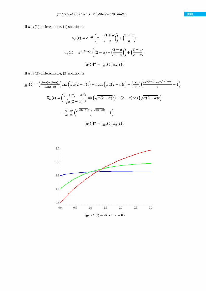
Çitil / Cumhuriyet Sci. J., Vol.40-4 (2019) 886-895
If 𝑢 is (1)-differentiable, (1) solution is
𝑢𝛼(𝑡) = 𝑒−𝛼𝑡 (𝛼 − (1 + 𝛼
𝛼)) + (
1 + 𝛼
𝛼),
𝑢𝛼(𝑡) = 𝑒−(2−𝛼)𝑡 ((2 − 𝛼) − (3 − 𝛼
2 − 𝛼)) + (
3 − 𝛼
2 − 𝛼),
[𝑢(𝑡)]𝛼 = [𝑢𝛼(𝑡), 𝑢𝛼(𝑡)].
If 𝑢 is (2)-differentiable, (2) solution is
𝑢𝛼(𝑡) = ((3−𝛼)−(2−𝛼)2
√𝛼(2−𝛼)) 𝑠𝑖𝑛 (√𝛼(2 − 𝛼)𝑡) + 𝛼𝑐𝑜𝑠 (√𝛼(2 − 𝛼)𝑡) − (
1+𝛼
𝛼) (
𝑒√𝛼(2−𝛼)𝑡+𝑒−√𝛼(2−𝛼)𝑡
2− 1),
𝑢𝛼(𝑡) = ((1 + 𝛼) − 𝛼2
√𝛼(2 − 𝛼)) 𝑠𝑖𝑛 (√𝛼(2 − 𝛼)𝑡) + (2 − 𝛼)𝑐𝑜𝑠 (√𝛼(2 − 𝛼)𝑡)
− (3−𝛼
2−𝛼) (
𝑒√𝛼(2−𝛼)𝑡+𝑒−√𝛼(2−𝛼)𝑡
2− 1),
[𝑢(𝑡)]𝛼 = [𝑢𝛼(𝑡), 𝑢𝛼(𝑡)].
Figure 1 (1) solution for 𝛼 = 0.5
0.0 0.5 1.0 1.5 2.0 2.5 3.0
0.5
1.0
1.5
2.0
2.5
890
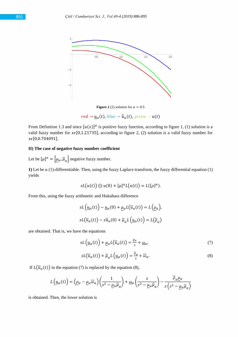
Çitil / Cumhuriyet Sci. J., Vol.40-4 (2019) 886-895
Figure 2 (2) solution for 𝛼 = 0.5
𝑟𝑒𝑑 → 𝑢𝛼(𝑡), 𝑏𝑙𝑢𝑒 → 𝑢𝛼(𝑡), 𝑔𝑟𝑒𝑒𝑛 → 𝑢(𝑡)
From Definition 1.3 and since [𝑢(𝑥)]𝛼 is positive fuzzy function, according to figure 1, (1) solution is a
valid fuzzy number for 𝑥𝜖[0,1.21735], according to figure 2, (2) solution is a valid fuzzy number for
𝑥𝜖[0,0.704091].
II) The case of negative fuzzy number coefficient
Let be [𝜇]𝛼 = [𝜇𝛼 , 𝜇𝛼] negative fuzzy number.
1) Let be 𝑢 (1)-differentiable. Then, using the fuzzy Laplace transform, the fuzzy differential equation (1)
yields
𝑠𝐿(𝑢(𝑡)) ⊝ 𝑢(0) + [𝜇]𝛼𝐿(𝑢(𝑡)) = 𝐿([𝜌]𝛼).
From this, using the fuzzy arithmetic and Hukuhara difference
𝑠𝐿 (𝑢𝛼(𝑡)) − 𝑢𝛼(0) + 𝜇𝛼𝐿(𝑢𝛼(𝑡)) = 𝐿 (𝜌𝛼),
𝑠𝐿(𝑢𝛼(𝑡)) − 𝑠𝑢𝛼(0) + 𝜇𝛼𝐿 (𝑢𝛼(𝑡)) = 𝐿(𝜌𝛼)
are obtained. That is, we have the equations
𝑠𝐿 (𝑢𝛼(𝑡)) + 𝜇𝛼𝐿(𝑢𝛼(𝑡)) =𝜌𝛼
𝑠+ 𝜔𝛼 , (7)
𝑠𝐿(𝑢𝛼(𝑡)) + 𝜇𝛼𝐿 (𝑢𝛼(𝑡)) =𝜌𝛼
𝑠+ 𝜔𝛼 . (8)
If 𝐿(𝑢𝛼(𝑡)) in the equation (7) is replaced by the equation (8),
𝐿 (𝑢𝛼(𝑡)) = (𝜌𝛼 − 𝜇𝛼𝜔𝛼) (1
𝑠2 − 𝜇𝛼𝜇𝛼
) + 𝜔𝛼 (𝑠
𝑠2 − 𝜇𝛼𝜇𝛼
) −𝜌𝛼𝜇𝛼
𝑠 (𝑠2 − 𝜇𝛼𝜇𝛼)
is obtained. Then, the lower solution is
0.5 1.0 1.5 2.0
4
2
2
891

Çitil / Cumhuriyet Sci. J., Vol.40-4 (2019) 886-895
𝑢𝛼(𝑡) =(𝜌𝛼 − 𝜇𝛼𝜔𝛼)
√𝜇𝛼𝜇𝛼
𝑠𝑖𝑛 (√𝜇𝛼𝜇𝛼𝑡) + 𝜔𝛼𝑐𝑜𝑠 (√𝜇𝛼𝜇𝛼𝑡) −𝜌𝛼
𝜇𝛼
(𝑒
√𝜇𝛼𝜇𝛼𝑡+ 𝑒
−√𝜇𝛼𝜇𝛼𝑡
2− 1).
Similarly, upper solution is
𝑢𝛼(𝑡) =(𝜌𝛼 − 𝜇𝛼𝜔𝛼)
√𝜇𝛼𝜇𝛼
𝑠𝑖𝑛 (√𝜇𝛼𝜇𝛼𝑡) + 𝜔𝛼𝑐𝑜𝑠 (√𝜇𝛼𝜇𝛼𝑡) −𝜌𝛼
𝜇𝛼(
𝑒√𝜇𝛼𝜇𝛼𝑡
+ 𝑒−√𝜇𝛼𝜇𝛼𝑡
2− 1).
2) Let be 𝑢 (2)-differentiable. Then, using the fuzzy Laplace transform, from the fuzzy differential
equation (1)
−𝑢(0) ⊝ (−𝑠𝐿(𝑢(𝑡))) + [𝜇]𝛼𝐿(𝑢(𝑡)) = 𝐿([𝜌]𝛼),
that is,
−𝑢𝛼(0) + 𝑠𝐿(𝑢𝛼(𝑡)) + 𝜇𝛼𝐿(𝑢𝛼(𝑡)) = 𝐿 (𝜌𝛼),
−𝑢𝛼(0) + 𝑠𝐿 (𝑢𝛼(𝑡)) + 𝜇𝛼𝐿 (𝑢𝛼(𝑡)) = 𝐿(𝜌𝛼)
are obtained. From this, we have
𝐿 (𝑢𝛼(𝑡)) =𝜌𝛼
𝑠(𝑠 + 𝜇𝛼)+
𝜔𝛼
𝑠 + 𝜇𝛼
,
𝐿(𝑢𝛼(𝑡)) =𝜌𝛼
𝑠 (𝑠 + 𝜇𝛼)+
𝜔𝛼
𝑠 + 𝜇𝛼.
Then, (2) solution is obtained as
𝑢𝛼(𝑡) = 𝑒−𝜇𝛼𝑡 (𝜔𝛼 −𝜌𝛼
𝜇𝛼
) +𝜌𝛼
𝜇𝛼
,
𝑢𝛼(𝑡) = 𝑒−𝜇𝛼𝑡 (𝜔𝛼 −𝜌𝛼
𝜇𝛼) +
𝜌𝛼
𝜇𝛼,
[𝑢(𝑡)]𝛼 = [𝑢𝛼(𝑡), 𝑢𝛼(𝑡)].
Example 2.2 Consider the fuzzy initial value problem
𝑢′(𝑡) + [−1]𝛼𝑢(𝑡) = [2]𝛼 , 𝑡 > 0 (9)
𝑢(0) = [1]𝛼, (10)
using the fuzzy Laplace transform, where
[−1]𝛼 = [−2 + 𝛼, −𝛼], [1]𝛼 = [𝛼, 2 − 𝛼], [2]𝛼 = [1 + 𝛼, 3 − 𝛼].
892
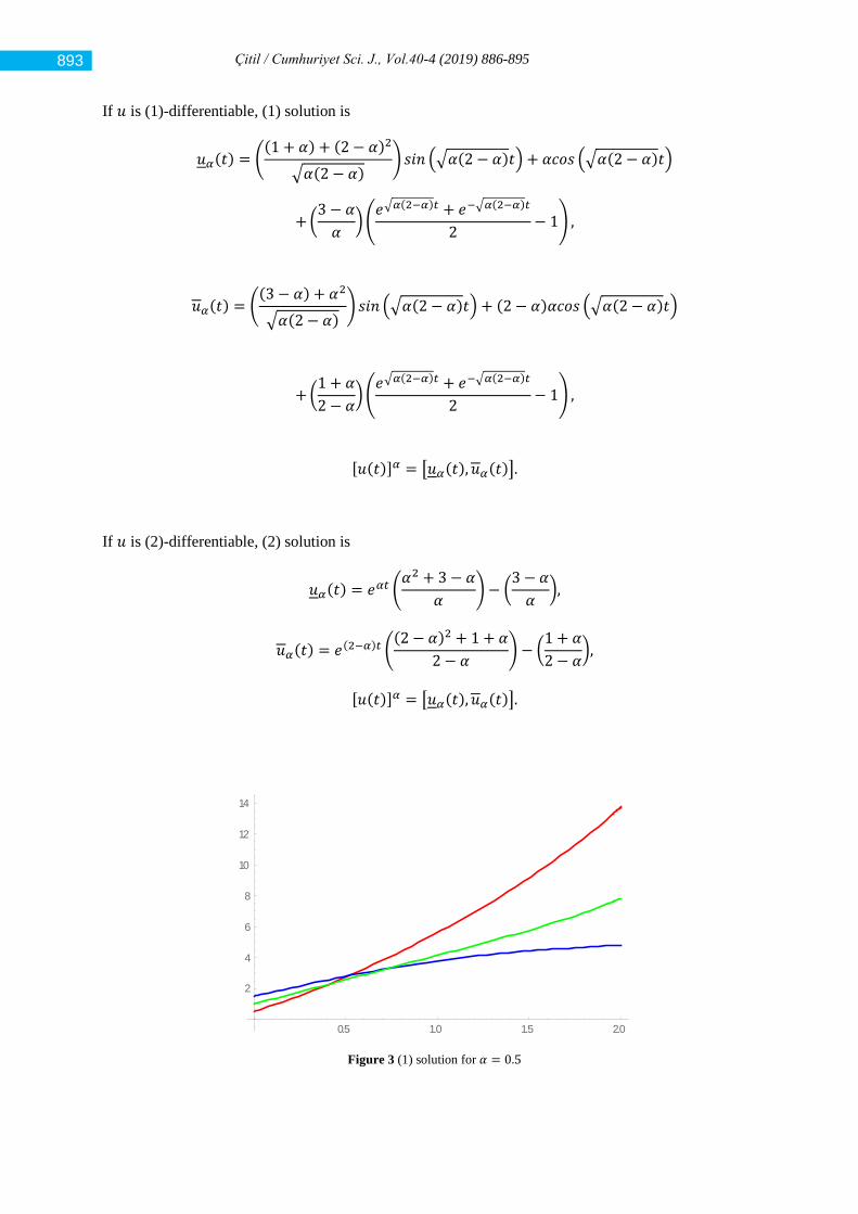
Çitil / Cumhuriyet Sci. J., Vol.40-4 (2019) 886-895
If 𝑢 is (1)-differentiable, (1) solution is
𝑢𝛼(𝑡) = ((1 + 𝛼) + (2 − 𝛼)2
√𝛼(2 − 𝛼)) 𝑠𝑖𝑛 (√𝛼(2 − 𝛼)𝑡) + 𝛼𝑐𝑜𝑠 (√𝛼(2 − 𝛼)𝑡)
+ (3 − 𝛼
𝛼) (
𝑒√𝛼(2−𝛼)𝑡 + 𝑒−√𝛼(2−𝛼)𝑡
2− 1) ,
𝑢𝛼(𝑡) = ((3 − 𝛼) + 𝛼2
√𝛼(2 − 𝛼)) 𝑠𝑖𝑛 (√𝛼(2 − 𝛼)𝑡) + (2 − 𝛼)𝛼𝑐𝑜𝑠 (√𝛼(2 − 𝛼)𝑡)
+ (1 + 𝛼
2 − 𝛼) (
𝑒√𝛼(2−𝛼)𝑡 + 𝑒−√𝛼(2−𝛼)𝑡
2− 1) ,
[𝑢(𝑡)]𝛼 = [𝑢𝛼(𝑡), 𝑢𝛼(𝑡)].
If 𝑢 is (2)-differentiable, (2) solution is
𝑢𝛼(𝑡) = 𝑒𝛼𝑡 (𝛼2 + 3 − 𝛼
𝛼) − (
3 − 𝛼
𝛼),
𝑢𝛼(𝑡) = 𝑒(2−𝛼)𝑡 ((2 − 𝛼)2 + 1 + 𝛼
2 − 𝛼) − (
1 + 𝛼
2 − 𝛼),
[𝑢(𝑡)]𝛼 = [𝑢𝛼(𝑡), 𝑢𝛼(𝑡)].
Figure 3 (1) solution for 𝛼 = 0.5
0.5 1.0 1.5 2.0
2
4
6
8
10
12
14
893
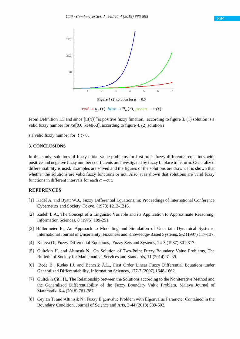
Çitil / Cumhuriyet Sci. J., Vol.40-4 (2019) 886-895
Figure 4 (2) solution for 𝛼 = 0.5
𝑟𝑒𝑑 → 𝑢𝛼(𝑡), 𝑏𝑙𝑢𝑒 → 𝑢𝛼(𝑡), 𝑔𝑟𝑒𝑒𝑛 → 𝑢(𝑡)
From Definition 1.3 and since [𝑢(𝑥)]𝛼is positive fuzzy function, according to figure 3, (1) solution is a
valid fuzzy number for 𝑥𝜖[0,0.514863], according to figure 4, (2) solution i
s a valid fuzzy number for 𝑡 > 0.
3. CONCLUSIONS
In this study, solutions of fuzzy initial value problems for first-order fuzzy differential equations with
positive and negative fuzzy number coefficients are investigated by fuzzy Laplace transform. Generalized
differentiability is used. Examples are solved and the figures of the solutions are drawn. It is shown that
whether the solutions are valid fuzzy functions or not. Also, it is shown that solutions are valid fuzzy
functions in different intervals for each 𝛼 −cut.
REFERENCES
[1] Kadel A. and Byatt W.J., Fuzzy Differential Equations, in: Proceedings of International Conference
Cybernetics and Society, Tokyo, (1978) 1213-1216.
[2] Zadeh L.A., The Concept of a Linguistic Variable and its Application to Approximate Reasoning,
Information Sciences, 8 (1975) 199-251.
[3] Hüllermeier E., An Approach to Modelling and Simulation of Uncertain Dynamical Systems,
International Journal of Uncertainty, Fuzziness and Knowledge-Based Systems, 5-2 (1997) 117-137.
[4] Kaleva O., Fuzzy Differential Equations, Fuzzy Sets and Systems, 24-3 (1987) 301-317.
[5] Gültekin H. and Altınışık N., On Solution of Two-Point Fuzzy Boundary Value Problems, The
Bulletin of Society for Mathematical Services and Standards, 11 (2014) 31-39.
[6] Bede B., Rudas I.J. and Bencsik A.L., First Order Linear Fuzzy Differential Equations under
Generalized Differentiability, Information Sciences, 177-7 (2007) 1648-1662.
[7] Gültekin Çitil H., The Relationship between the Solutions according to the Noniterative Method and
the Generalized Differentiability of the Fuzzy Boundary Value Problem, Malaya Journal of
Matematik, 6-4 (2018) 781-787.
[8] Ceylan T. and Altınışık N., Fuzzy Eigenvalue Problem with Eigenvalue Parameter Contained in the
Boundary Condition, Journal of Science and Arts, 3-44 (2018) 589-602.
1 2 3 4 5 6 7
500
1000
1500
894
Çitil / Cumhuriyet Sci. J., Vol.40-4 (2019) 886-895
[9] Allahviranloo T. and Barkhordari Ahmadi M., Fuzzy Laplace Transforms, Soft Computing, 14-3
(2010) 235-243.
[10] Patel K.R. and Desai N.B., Solution of Fuzzy Initial Value Problems by Fuzzy Laplace Transform,
Kalpa Publications in Computing, 2 (2017) 25-37.
[11] Patel K.R. and Desai N.B., Solution of Variable Coefficient Fuzzy Differential Equations by Fuzzy
Laplace Transform, International Journal on Recent and Innovation Trends in Computing and
Communication, 5-6 (2017) 927-942.
[12] Liu H.-K., Comparison Results of Two-Point Fuzzy Boundary Value Problems, International Journal
of Computational and Mathematical Sciences, 5-1 (2011) 1-7.
[13] Salahshour S. and Allahviranloo T., Applications of Fuzzy Laplace Transforms, Soft Computing,
17-1 (2013) 145-158.
[14] Shirin S. and Saha G.K., A New Computational Methodology to Find Appropriate Solutions of Fuzzy
Equations, Mathematical Theory and Modeling, 2-1 (2011) 1-10.
[15] Lakshmikantham V. and Mohapatra R.N., Theory of Fuzzy Differential Equations and Inclusions,
Taylor and Francis, London, New York, 2003.
[16] Khastan A. and Nieto J.J., A Boundary Value Problem for Second Order Fuzzy Differential
Equations, Nonlinear Analysis: Theory, Methods and Applications, 72-9-10 (2010) 3583-3593.
895
Cumhuriyet Science Journal
CSJ
e-ISSN: 2587-246X
ISSN: 2587-2680 Cumhuriyet Sci. J., Vol.40-4 (2019) 896-901
* Corresponding author. Email address: [email protected]
http://dergipark.gov.tr/csj ©2016 Faculty of Science, Sivas Cumhuriyet University
A Dynamic Network Model For Population Growth And Urbanization
Emir HALİKİ 1*
1 EgeUniversity, Faculty of Science, Department of Physics, Izmir, Turkey
Received: 14.10.2019; Accepted: 08.12.2019 http://dx.doi.org/10.17776/csj.632996
Abstract. Dynamic networks imply those states of which change over time and such changes are generally
associated with the topology of a network. Dynamic models are currently needed for numerous systems which
could be defined as a network model. Those related to the propagation of living organisms are also a typical
example. The study has examined a sample space which has been defined in the network topology of human
population as the way in which it will spread with population growth and correlated with various variables in
the modeled dynamic network.
Keywords: Network, Population growth, Logistic differential equation, Connected component, Clustering
coefficient, Correlation.
Nüfus Artışı ve Kentleşme İçin Dinamik Bir Ağ Modeli
Özet. Dinamik ağlar, zaman içinde değişiklik gösteren durumları belirtmekte ve bu değişiklikler genellikle bir
ağın topolojisi ile ilişkilendirilmektedir. Ağ modeli olarak tanımlanabilecek birçok sistem için dinamik
modellere ihtiyaç duyulmaktadır. Canlı organizmaların yayılması ile ilgili olanlar da bu duruma bir örnektir.
Çalışmada insan nüfusunun ağ topolojisi tanımlanarak ile bir örnek uzay oluşturulmuş, nüfus artışı ile içerisinde
nasıl bir yayılma görüleceği araştırılmış ve nüfus büyümesinin modellenen dinamik ağdaki çeşitli değişkenler
ile aralarındaki korelasyonlar incelenmiştir.
Anahtar Kelimeler: Dönüştürülmüş iki boyutlu dağılım, Bağımlılık, İki boyutlu dağılım, Spearman sıra
korelasyonu, Fréchet sınırları.
1. INTRODUCTION
When the human population was still small and when people were constantly moving from one place to
another, the abandonment of the land on which they grew plants and lived was not a problem for the
nature yet. However, the idea that nature had to be conquered developed later and people pass on to
expansionist form of life [1]. By far the most important factor in this sense originated from the transition
to settlement. So sufficient was settlement instead of immigration for sources that existing land was
preserved with inevitable expansion to the new soils. It is known that Neolithic people first passed to
settlement approximately 12500 years ago [2,3]. It was the major factors which played a significant role
in the related transition that agricultural development, climatic changes and husbandry of animals
occurred. Although it is still obscure whether those reasons triggered population growth or population
growth lead to those reasons, it is a fact that population growth accelerated use up of present sources in a
place and necessitated people to expand to new lands, which is currently going on.

Haliki / Cumhuriyet Sci. J., Vol.40-4 (2019) 896-901
Expansion of regions by human being under the settlement principle has caused the cities to be made up
of districts and countries to be composed of cities [4]. Increasingly growing population and urbanization
leads to construction shifting to rural areas and expansion is in the form of construction across natural
zones by transforming them into increased settlement. Various predictions and dynamic models have been
thus far developed on the growth and spread of countless plant and animal populations [5,6] while those
on spreading human population are far cry from being sufficient [7,8].
The present study has modeled the human expansion accompanied by population growth using a network
model to finally examine its correlation of several variables with it. A fictitious region has been defined,
separated into a certain number of nodes and a precessor pattern is created in such a way that no nodes
are connected with each other (disconnected graph) first and then a random starting node has been selected
where the population first began to proliferate and urbanized in a sense with the identification of the
location and linking a new node to the preceeding ones over time. In conclusion, the correlation between
population growth and some characteristics of the growing network has been shown and the conclusions
presented in the section of results and discussion.
2. MATERIALS AND METHODS
A population-related differential equation to indicate the two important concepts namely, ecology and
epidemiology are as follows;
= (𝑟 − 𝑑)𝑁, (1)
where 𝑁 is the number of individuals 𝑟 birth rate and 𝑑 death. If 𝑟 > 𝑑 the population continues to grow
indefinitely. In a real environment, any growth in the population will hit constraints such as in running
out of nutrients or physical space, which suggests the concept of carrying capacity and a more proper
population growth could be given by the logistic equation [9] below;
= 𝑟𝑁 (1 −
𝑁
𝜅), (2)
where 𝜅 is the carrying capacity. When 𝑁 increases, the rate of growth decreases. As 𝑁 = 𝜅, growth of
the population stops. For any initial population 𝑁0, solution of eq. 2 is presented as follows;
𝑁(𝑡) =
𝜅𝑁0𝑒𝑟𝑡
𝜅 + 𝑁0(𝑒𝑟𝑡 − 1)
(3)
with 𝑁0 being the initial population. As time passes, the population converges to its carrying capacity.
Once it has reached it, growth stops. However, there may be occasional dynamic limits for the carrying
capacity [10]. Ecological carrying capacity is suitable for non-human beings whereas it does not always
apply to human beings, because economy, environment, culture and demography are involved [11].
Nevertheless, an average carrying capacity can be determined in order to acquire fundamental approaches
to population dynamics [12,13].
The region of population distribution in the developed model as a pattern composed of 36 nodes, each of
which corresponds to a zone likely to be occupied on a possible settlement map. The network growth has
been defined as expanding 2-D graph distribution which represents a graph with 𝑛 nodes uniformly
distributed over a plane. Edges between nodes have been determined by distance 𝑑. The simulation
exhibits that the 𝑑 value in the network changes proportionally with the increasing population by the
continuous logistic equation. The initial population for population growth model is 100 individuals and
897
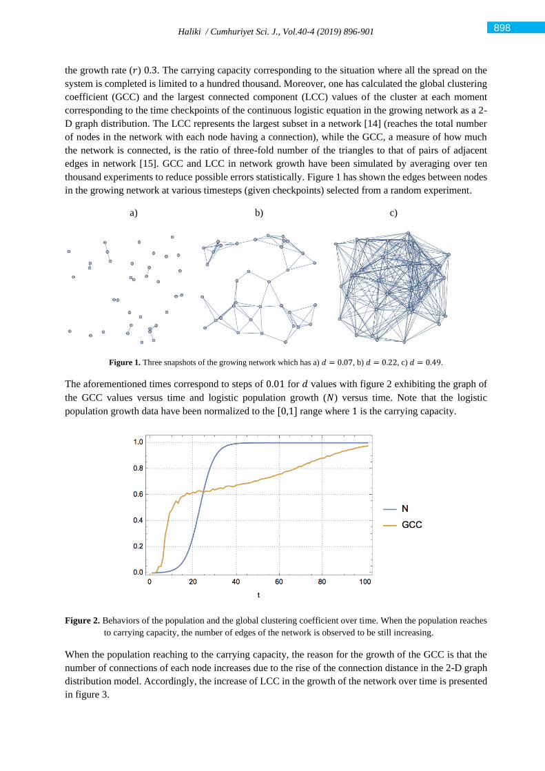
Haliki / Cumhuriyet Sci. J., Vol.40-4 (2019) 896-901
the growth rate (𝑟) 0.3. The carrying capacity corresponding to the situation where all the spread on the
system is completed is limited to a hundred thousand. Moreover, one has calculated the global clustering
coefficient (GCC) and the largest connected component (LCC) values of the cluster at each moment
corresponding to the time checkpoints of the continuous logistic equation in the growing network as a 2-
D graph distribution. The LCC represents the largest subset in a network [14] (reaches the total number
of nodes in the network with each node having a connection), while the GCC, a measure of how much
the network is connected, is the ratio of three-fold number of the triangles to that of pairs of adjacent
edges in network [15]. GCC and LCC in network growth have been simulated by averaging over ten
thousand experiments to reduce possible errors statistically. Figure 1 has shown the edges between nodes
in the growing network at various timesteps (given checkpoints) selected from a random experiment.
a) b) c)
Figure 1. Three snapshots of the growing network which has a) 𝑑 = 0.07, b) 𝑑 = 0.22, c) 𝑑 = 0.49.
The aforementioned times correspond to steps of 0.01 for 𝑑 values with figure 2 exhibiting the graph of
the GCC values versus time and logistic population growth (𝑁) versus time. Note that the logistic
population growth data have been normalized to the [0,1] range where 1 is the carrying capacity.
Figure 2. Behaviors of the population and the global clustering coefficient over time. When the population reaches
to carrying capacity, the number of edges of the network is observed to be still increasing.
When the population reaching to the carrying capacity, the reason for the growth of the GCC is that the
number of connections of each node increases due to the rise of the connection distance in the 2-D graph
distribution model. Accordingly, the increase of LCC in the growth of the network over time is presented
in figure 3.
898
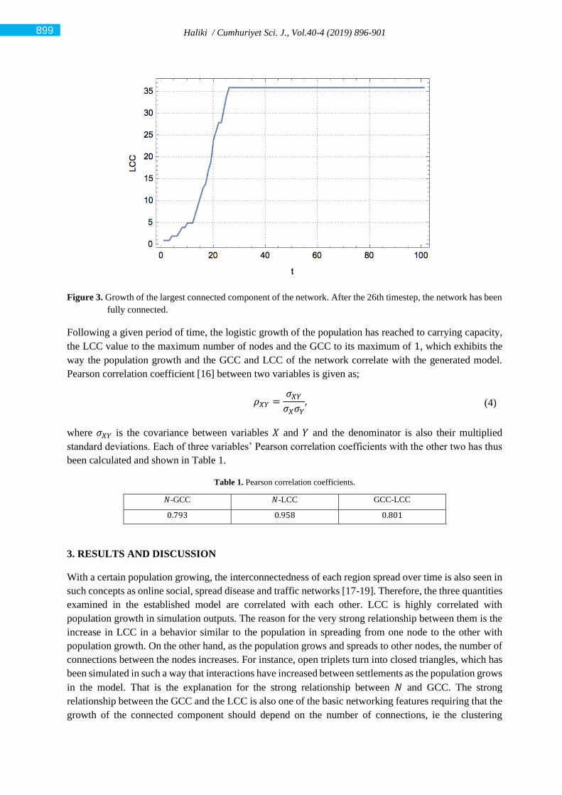
Haliki / Cumhuriyet Sci. J., Vol.40-4 (2019) 896-901
Figure 3. Growth of the largest connected component of the network. After the 26th timestep, the network has been
fully connected.
Following a given period of time, the logistic growth of the population has reached to carrying capacity,
the LCC value to the maximum number of nodes and the GCC to its maximum of 1, which exhibits the
way the population growth and the GCC and LCC of the network correlate with the generated model.
Pearson correlation coefficient [16] between two variables is given as;
𝜌𝑋𝑌 =𝜎𝑋𝑌𝜎𝑋𝜎𝑌
, (4)
where 𝜎𝑋𝑌 is the covariance between variables 𝑋 and 𝑌 and the denominator is also their multiplied
standard deviations. Each of three variables’ Pearson correlation coefficients with the other two has thus
been calculated and shown in Table 1.
Table 1. Pearson correlation coefficients.
𝑁-GCC 𝑁-LCC GCC-LCC
0.793 0.958 0.801
3. RESULTS AND DISCUSSION
With a certain population growing, the interconnectedness of each region spread over time is also seen in
such concepts as online social, spread disease and traffic networks [17-19]. Therefore, the three quantities
examined in the established model are correlated with each other. LCC is highly correlated with
population growth in simulation outputs. The reason for the very strong relationship between them is the
increase in LCC in a behavior similar to the population in spreading from one node to the other with
population growth. On the other hand, as the population grows and spreads to other nodes, the number of
connections between the nodes increases. For instance, open triplets turn into closed triangles, which has
been simulated in such a way that interactions have increased between settlements as the population grows
in the model. That is the explanation for the strong relationship between 𝑁 and GCC. The strong
relationship between the GCC and the LCC is also one of the basic networking features requiring that the
growth of the connected component should depend on the number of connections, ie the clustering
899
Haliki / Cumhuriyet Sci. J., Vol.40-4 (2019) 896-901
coefficient [20]. They have become well correlated since the network grew from a single point in the 2-
D graph distribution-based model.
The present knowledge of the world is often determined by geographical maps. In the developed model,
a possible settlement on a given map has been divided into units (nodes) and extrapolated from the initial
node to the others with the population. In order that the model to should show some similarity to the
reality, the number of connections has continued to increase even if the carrying capacity has been reached
in order to make the settlement area completely connected to each other. If different components of a
human population is to have heterogeneous requirements, estimates of total carrying capacity based on a
single formula could not be accurate. Similarly, it is possible that different parts of the global human
population would have heterogeneous needs as well. Therefore, the developed model may seem to be
simplified in terms of the increase of the human population and its limitation to a certain area. However,
in future studies, carrying capacity, a variable of equations such as logistic growth, could be rendered
more dynamic by having multiple variables within itself.
REFERENCES
[1] Goudie A. S., Human impact on the natural environment, 8th ed., Wiley: Hoboken, NJ, USA, 2018.
[2] Kuijt I. J., People and space in early agricultural villages: exploring daily lives, community size, and
architecture in the Late Pre-Pottery Neolithic, Anthropol. Archaeol., 19 (2000) 75-102.
[3] Putterman L., Agriculture, diffusion and development: ripple effects of the neolithic revolution,
Economica, 75 (2008) 729-748.
[4] Dickinson R. E., City and region: a geographical interpretation, Taylor&Francis: Oxfordshire, UK,
1998.
[5] Clark J. S., Lewis M., McLachlan J. S., HilleRisLambers J., Estimating population spread: what can
we forecast and how well?, Ecology, 84 (2003) 1979-1988.
[6] Haydon D. T., Morales J. M., Yott A., Jenkins D. A., Rosatte R., Fryxell J. M. P., Socially informed
random walks: incorporating group dynamics into models of population spread and growth, Roy. Soc.
B. Biol. Sci., 275 (2008) 1101-1109.
[7] Wittemyer G., Elsen P., Bean W. T., Burton A. C. O., Brashares J. S., Accelerated human population
growth at protected area edges, Science, 321 (2008) 123-126.
[8] Bongaarts J., Human population growth and the demographic transition, Philos. T. Roy. Soc. B., 364
(2009) 2985-2990.
[9] Nowak M. A., Evolutionary dynamics, Harvard University Press: London, UK, 2006.
[10] Meyer P. S., Ausubel J. H., Carrying capacity: a model with logistically varying limits, Technol.
Forecast. Soc., 61 (1999) 209-214.
[11] Cohen J. E., Population growth and earth's human carrying capacity, Science, 269 (1995) 341-346.
[12] Graymore M. L., Sipe N. G., Rickson R. E., Sustaining human carrying capacity: a tool for regional
sustainability assessment, Ecol. Econ., 69 (2010) 459-468.
[13] Hopfenberg R., Human carrying capacity is determined by food availability, Popul. Environ., 25
(2003) 109-117.
[14] Yang X., Megson G. M., Tang Y. Y., Xing Y., Largest connected component of a star graph with
faulty vertices, Int. J. Comput. Math., 85 (2008) 1771-1778.
900

Haliki / Cumhuriyet Sci. J., Vol.40-4 (2019) 896-901
[15] Soffer S. N., Vazquez A., Network clustering coefficient without degree-correlation biases, Phys.
Rev. E., 71 (2005) 057101.
[16] Benesty J., Chen J., Huang Y., Cohen I., Pearson correlation coefficient. In Noise reduction in speech
processing, Springer: Berlin, Heidelberg, 2009.
[17] Centola D., The spread of behavior in an online social network experiment, Science, 329 (2010)
1194-1197.
[18] Jeger M. J., Pautasso M., Holdenrieder O., Shaw M. W., Modelling disease spread and control in
networks: implications for plant sciences, New Phytol., 174 (2007) 279-297.
[19] Coclite G. M., Garavello M., Piccoli B., Traffic flow on a road network, SIAM J. Math. Anal., 36
(2005) 1862-1886.
[20] Serrano M. Á., Boguná M., Percolation and epidemic thresholds in clustered networks, Phys. Rev.
Lett., 97 (2006) 088701.
901
Cumhuriyet Science Journal
CSJ
e-ISSN: 2587-246X
ISSN: 2587-2680 Cumhuriyet Sci. J., Vol.40-4 (2019) 902-908
* Corresponding author. Email address: [email protected]
http://dergipark.gov.tr/csj ©2016 Faculty of Science, Sivas Cumhuriyet University
Half-Inverse Problem For Dirac Operator With Boundary And
Transmission Conditions Dependent Spectral Parameter Polynomially
Merve ARSLANTAŞ 1 , Yalçın GÜLDÜ 1*
1 Department of Mathematics, Faculty of Science, Cumhuriyet University 58140
Sivas, TURKEY
Received: 25.10.2019; Accepted: 18.12.2019 http://dx.doi.org/10.17776/csj.637861
Abstract. In this paper, half-inverse problem is considered for Dirac equations with boundary and finite number
of transmission conditions depending polynomially on the spectral parameter, if the potential is given over the
half of the considered interval and if one spectrum is known then, potential function Ω(x) on the whole interval
and the other coefficients of the considered problem can be determined uniquely.
Keywords: Dirac equations, Transmission conditions, Spectral parameter.
Sınır ve Süreksizlik Koşulları Spektral Parametreye Polinom Olarak
Bağlı Dirac Operatörü İçin Yarı-Ters Problem
Özet. Bu makalede, sınır koşulları ve sonlu sayıda süreksizlik koşulları spektral parametreye polinom olarak
bağlı Dirac denklemleri için yarı-ters problem ele alınmış olup, yarı aralıkta Ω(x) potansiyel fonksiyonu
biliniyorken, bir spektruma göre, aralığın tamamında Ω(x) potansiyel fonksiyonu ile ele alınan problemin
katsayılarının tek olarak belirlendiği gösterilmiştir.
Anahtar Kelimeler: Dirac denklemler, Süreksizlik koşulları, Spektral parametre.
1. INTRODUCTION
Inverse problems of spectral analysis compose of retrieving operators from their spectral characteristics.
For this reason, inverse spectral theory is so significant research subject in mathematics, physics,
mechanics, electronics, geophysics and other branches of natural sciences.
Half-inverse problem for a Dirac operator consists in reconstruction of the operator from its spectrum and
known potential in the half-interval. Half inverse problem was first studied by Hochstadt and Lieberman
in 1978[1]. In study of [2],by one boundary condition and potential which is known on half the interval,
the potential and other boundary condition are uniquely determined. After that, these results have been
used to lots of works[3-12].
On the other hand, in 1973 Walter [13] and in 1977 Fulton [14] studied the Sturm-Liouville problem with
boundary conditions dependent on spectral parameter linearly. Then, inverse problems for some classes
of differential operators depending on the eigenvalue-parameter linearly or nonlinearly on boundary and
also transmission conditions were studied in various papers[15-33].
The main result of this paper is that if the potential function Ω(x) is known over the half the interval
and one spectrum is given, then coefficients of the following problem can be uniquely determined.

Arslantaş, Güldü / Cumhuriyet Sci. J., Vol.40-4 (2019) 902-908
In this study, we concern the boundary value problem L generated by the following system of Dirac
equations
𝑙[𝑌(𝑥)] ≔ 𝐵𝑌′(𝑥) + Ω(x)Y(x) = 𝜆𝑌(𝑥) (1)
with the boundary conditions
𝑙1𝑦 ≔ 𝑎2(𝜆)𝑦2(𝑎) − 𝑎1(𝜆)𝑦1(𝑎) = 0 (2)
𝑙2𝑦 ≔ 𝑏2(𝜆)𝑦2(𝑏) − 𝑏1(𝜆)𝑦1(𝑏) = 0 (3)
and the transmission conditions
𝑈𝑖(𝑦) ≔ 𝑦1(𝜉𝑖 + 0) − 𝜃𝑖𝑦1(𝜉𝑖 − 0) = 0
𝑉𝑖(𝑦) ≔ 𝑦2(𝜉𝑖 + 0) − 𝜃𝑖−1𝑦2(𝜉𝑖 − 0) − 𝛾𝑖(𝜆)𝑦1(𝜉𝑖 − 0) = 0
𝑖 = 1, 𝑛 (4)
where 𝐵 = (0 1
−1 0), Ω(x) = (
𝑝(𝑥) 𝑞(𝑥)𝑞(𝑥) 𝑟(𝑥)
), 𝑌(𝑥) = (𝑦1(𝑥)𝑦2(𝑥)
), 𝑝(𝑥), 𝑞(𝑥) and 𝑟(𝑥) are real valued
functions in 𝐿2(𝑎, 𝑏), 𝝀 is a spectral parameter, 𝑎𝑖(𝜆), 𝑏𝑖(𝜆), (𝑖 = 1,2) and 𝛾𝑖(𝜆) (𝑖 = 1, 𝑛 ) are
polynomial with real cofficients and no common zeros, 𝜉𝑖𝜖(𝑎, 𝑏) (𝑖 = 1, 𝑛 ), 𝜃𝑖𝜖ℝ+,
𝑎1(𝜆) = ∑ 𝑎𝑘1𝜆𝑘𝑚1𝑘=0 , 𝑎2(𝜆) = ∑ 𝑎𝑘2𝜆𝑘𝑚2
𝑘=0 , 𝑏1(𝜆) = ∑ 𝑏𝑘1𝜆𝑘𝑚3𝑘=0 , 𝑏2(𝜆) = ∑ 𝑏𝑘2𝜆𝑘𝑚4
𝑘=0 and
𝛾𝑖(𝜆)=∑ 𝛾𝑘𝑖𝜆𝑘𝑟𝑖𝑘=0 , 𝑓(𝜆) =
𝑏1(𝜆)
𝑏2(𝜆) , 𝑚𝑎 = 𝑚𝑎𝑥𝑚1, 𝑚2, 𝑚𝑏 = 𝑚𝑎𝑥𝑚3, 𝑚4,
𝑟 = 𝑚𝑎𝑥1≤𝑖≤𝑛𝑑𝑒𝑔 𝛾𝑖(𝜆).
2. UNIQUENESS THEOREM
Theorem: Suppose
𝜆𝑛 = 𝑛 , 𝑎𝑖(𝜆) = 𝑖(𝜆) (𝑖 = 1,2), Ω(x) = Ω(x) on [𝑎,𝑎+𝑏
2] and 𝑈𝑖 = 𝑖 , 𝑉𝑖 = 𝑖 for all 𝑖 = 1, 𝑛 with
𝜉𝑖 ≤𝑎+𝑏
2 for 𝑑𝑒𝑔𝑎2(𝜆) > 𝑑𝑒𝑔𝑎1(𝜆)
if 𝑑𝑒𝑔𝑏2(𝜆) > 𝑑𝑒𝑔𝑏1(𝜆) 𝑚2 > 𝑚4 + ∑ 𝑟𝑖𝑛𝑖=1
if 𝑑𝑒𝑔𝑏1(𝜆) > 𝑑𝑒𝑔𝑏2(𝜆) 𝑚2 > 𝑚3 + ∑ 𝑟𝑖𝑛𝑖=1
if 𝑑𝑒𝑔𝑏1(𝜆) = 𝑑𝑒𝑔𝑏2(𝜆) 𝑚2 > 𝑚𝑏 + ∑ 𝑟𝑖𝑛𝑖=1 .
Then Ω(x) = Ω(x) almost everywhere on [𝑎, 𝑏], 𝑓(𝜆) = 𝑓(𝜆) and 𝜃𝑖 = 𝑖, 𝛾𝑖(𝜆) = 𝑖(𝜆), 𝜉𝑖 = 𝜉𝑖 for
𝑖 = 1, 𝑛 .
We need the following lemma, before we prove this theorem.
Lemma: If 𝜆∗ is the zero of the polynomial 𝑎2(𝜆) with multiplicities 𝑚𝜆∗ then 𝜆∗ is also the zero of the
entire function
𝐶𝜓1(𝑎, 𝜆) − 1(𝑎, 𝜆)
with at least multiplicities 𝑚𝜆∗.
Proof: Δ(𝜆) = 𝑎1(𝜆)𝜓1(𝑎, 𝜆) − 𝑎2(𝜆)𝜓2(𝑎, 𝜆) and (𝜆) = 𝑎1(𝜆)1(𝑎, 𝜆) − 𝑎2(𝜆)2(𝑎, 𝜆).
903

Arslantaş, Güldü / Cumhuriyet Sci. J., Vol.40-4 (2019) 902-908
If 𝜆∗ is the zero of the polynomial 𝑎2(𝜆) with multiplicities 𝑚𝜆∗ at that time we attain
Δ(𝜆∗) = 𝑎1(𝜆∗)𝜓1(𝑎, 𝜆∗) and (𝜆∗) = 𝑎1(𝜆∗)1(𝑎, 𝜆∗).
On the other hand, since (𝜆) and Δ(𝜆) are both entire in 𝜆, by Hadamard's factorization theorem we
can (𝜆) = 𝐶Δ(𝜆). Then
0 = 𝐶Δ(𝜆∗) − (𝜆∗)= 𝑎1(𝜆∗)[𝐶𝜓1(𝑎, 𝜆∗) − 1(𝑎, 𝜆∗)].
Since 𝑎1(𝜆) and 𝑎2(𝜆) do not have common zeros, we have
𝐶𝜓1(𝑎, 𝜆∗) − 1(𝑎, 𝜆∗) = 0.
Now, inductively, if for all 0 ≤ 𝑠 < 𝑘 ≤ 𝑚𝜆∗ − 1 there holds
𝑑𝑠
𝑑𝜆𝑠 [𝐶𝜓1(𝑎, 𝜆) − 1(𝑎, 𝜆)]|𝜆=𝜆∗
=0
then we will prove that
𝑑𝑘
𝑑𝜆𝑘 [𝐶𝜓1(𝑎, 𝜆) − 1(𝑎, 𝜆)]|𝜆=𝜆∗
=0.
𝑑𝑘
𝑑𝜆𝑘Δ(𝜆) =
𝑑𝑘
𝑑𝜆𝑘[𝑎1(𝜆)𝜓1(𝑎, 𝜆) − 𝑎2(𝜆)𝜓2(𝑎, 𝜆)]
= ∑ (𝑘𝑡
) [𝑑𝑡
𝑑𝜆𝑡 𝑎1(𝜆)𝑑𝑘−𝑡
𝑑𝜆𝑘−𝑡 𝜓1(𝑎, 𝜆) −𝑑𝑡
𝑑𝜆𝑡 𝑎2(𝜆)𝑑𝑘−𝑡
𝑑𝜆𝑘−𝑡 𝜓2(𝑎, 𝜆)]𝑘𝑡=0
𝑑𝑘
𝑑𝜆𝑘Δ(𝜆)|
𝜆=𝜆∗
= ∑ (𝑘𝑡
)𝑑𝑡
𝑑𝜆𝑡𝑎1(𝜆)|
𝜆=𝜆∗
𝑑𝑘−𝑡
𝑑𝜆𝑘−𝑡𝜓1(𝑎, 𝜆)|
𝜆=𝜆∗
𝑘
𝑡=0
𝑑𝑘
𝑑𝜆𝑘Δ(𝜆)|
𝜆=𝜆∗
= ∑ (𝑘𝑡
)𝑑𝑡
𝑑𝜆𝑡𝑎1(𝜆)|
𝜆=𝜆∗
𝑑𝑘−𝑡
𝑑𝜆𝑘−𝑡1(𝑎, 𝜆)|
𝜆=𝜆∗
𝑘
𝑡=0
From the last two equations we have
𝑑𝑘
𝑑𝜆𝑘 [𝐶Δ(𝜆) − Δ(𝜆)]|𝜆=𝜆∗
= ∑ (𝑘𝑡
)𝑑𝑡
𝑑𝜆𝑡 𝑎1(𝜆)|𝜆=𝜆∗
𝑑𝑘−𝑡
𝑑𝜆𝑘−𝑡 [𝐶𝜓1(𝑎, 𝜆) − 1(𝑎, 𝜆)]|𝜆=𝜆∗
𝑘𝑡=0 .
Since
𝐶Δ(𝜆) − (𝜆)=0
∑ (𝑘𝑡
)𝑑𝑡
𝑑𝜆𝑡𝑎1(𝜆)|
𝜆=𝜆∗
𝑑𝑘−𝑡
𝑑𝜆𝑘−𝑡 [𝐶𝜓1(𝑎, 𝜆) − 1(𝑎, 𝜆)]|𝜆=𝜆∗
= 0.
𝑘
𝑡=0
Since for all 0 ≤ 𝑠 < 𝑘
𝑑𝑠
𝑑𝜆𝑠 [𝐶𝜓1(𝑎, 𝜆) − 1(𝑎, 𝜆)]|𝜆=𝜆∗
=0
we have
904

Arslantaş, Güldü / Cumhuriyet Sci. J., Vol.40-4 (2019) 902-908
𝑎1(𝜆∗)𝑑𝑘
𝑑𝜆𝑘 [𝐶𝜓1(𝑎, 𝜆) − 1(𝑎, 𝜆)]|𝜆=𝜆∗
=0.
Since 𝑎1(𝜆∗) we obtain
𝑑𝑘
𝑑𝜆𝑘 [𝐶𝜓1(𝑎, 𝜆) − 1(𝑎, 𝜆)]|𝜆=𝜆∗
=0.
Lemma is proved.
If 𝑎1(𝜆) ≡ 0 and 𝑎2(𝜆) ≡ 1 are taken in the boundary condition, since 𝑀(𝜆) = −𝜓1(𝑎,𝜆)
Δ(𝜆) and
Δ(𝜆) = 𝑎1(𝜆)𝜓1(𝑎, 𝜆) − 𝑎2(𝜆)𝜓2(𝑎, 𝜆) = −𝜓2(𝑎, 𝜆)
𝑀0(𝜆) ≔𝜓1(𝑎, 𝜆)
𝜓2(𝑎, 𝜆)
obtained.
Remark 1: For the problem 𝐿 given by the conditions 𝑎1(𝜆) ≡ 0 and 𝑎2(𝜆) ≡ 1 if 𝑀0(𝜆) = 0(𝜆)
then Ω(x) = Ω(x) almost everywhere on [𝑎, 𝑏], 𝑓(𝜆) = 𝑓(𝜆) and for each 𝑖 = 1, 𝑛 𝜃𝑖 = 𝑖,
𝛾𝑖(𝜆) = 𝑖(𝜆), 𝜉𝑖 = 𝜉𝑖 applies.
Remark 2: For the Dirac operator given in the interval [𝑎+𝑏
2, 𝑏] with equation (1), 𝑦2 (
𝑎+𝑏
2) = 0 and the
transmission conditions (4), from the above Remark 1; 𝑀0(𝜆) determines the function Ω(x) and 𝜃𝑖,
𝛾𝑖(𝜆), 𝜉𝑖 for 𝑖 = 1, 𝑛 as one on [𝑎+𝑏
2, 𝑏].
Proof of Theorem : We only prove the case when 𝜉𝑖 ≠𝑎+𝑏
2 for all 𝑖. The argument of the case when
𝜉𝑖 =𝑎+𝑏
2 for some 𝑖 is similar. Using Lagrange identity we have
∫ (1(𝑥, 𝜆), 2(𝑥, 𝜆)) (Ω(x) − Ω(x)) (𝜓1(𝑥, 𝜆)
𝜓2(𝑥, 𝜆))
𝑎+𝑏
2
𝑎
𝑑𝑥
+[1(𝑥, 𝜆)𝜓2(𝑥, 𝜆) − 2(𝑥, 𝜆)𝜓1(𝑥, 𝜆)]|𝑎
𝑎+𝑏
2
For all 𝑖 satisfying 𝜉𝑖 <𝑎+𝑏
2
[1(𝑥, 𝜆)𝜓2(𝑥, 𝜆) − 2(𝑥, 𝜆)𝜓1(𝑥, 𝜆)]|𝜉𝑖−0
𝜉𝑖+0= 0
Together with Ω(x) = Ω(x) for a.e. [𝑎,𝑎+𝑏
2] we have
1 (𝑎 + 𝑏
2, 𝜆) 𝜓2 (
𝑎 + 𝑏
2, 𝜆) − 2 (
𝑎 + 𝑏
2, 𝜆) 𝜓1 (
𝑎 + 𝑏
2, 𝜆)
= 1(𝑎, 𝜆)𝜓2(𝑎, 𝜆) − 2(𝑎, 𝜆)𝜓1(𝑎, 𝜆).
Since
905

Arslantaş, Güldü / Cumhuriyet Sci. J., Vol.40-4 (2019) 902-908
(𝜆) = 𝐶Δ(𝜆), Δ(𝜆) = 𝑎1(𝜆)𝜓1(𝑎, 𝜆) − 𝑎2(𝜆)𝜓2(𝑎, 𝜆) and (𝜆) = 𝑎1(𝜆)1(𝑎, 𝜆) − 𝑎2(𝜆)2(𝑎, 𝜆)
we get
1(𝑎, 𝜆)𝜓2(𝑎, 𝜆) − 2(𝑎, 𝜆)𝜓1(𝑎, 𝜆) = Δ(𝜆)𝐶𝜓1(𝑎, 𝜆) − 1(𝑎, 𝜆)
𝑎2(𝜆)
Denote
Τ(𝜆): =G(𝜆)
Δ(𝜆)
=1 (
𝑎+𝑏
2, 𝜆) 𝜓2 (
𝑎+𝑏
2, 𝜆) − 2 (
𝑎+𝑏
2, 𝜆) 𝜓1 (
𝑎+𝑏
2, 𝜆)
Δ(𝜆)
The function Τ(𝜆) is entire in ℂ. From the assumption that 𝜆𝑛 = 𝑛 and the term of the characteristic
function Δ(𝜆) it is easy to infer that
if 𝑑𝑒𝑔𝑏2(𝜆) > 𝑑𝑒𝑔𝑏1(𝜆) 𝑚4 = 4
if 𝑑𝑒𝑔𝑏1(𝜆) > 𝑑𝑒𝑔𝑏2(𝜆) 𝑚3 = 3
if 𝑑𝑒𝑔𝑏1(𝜆) = 𝑑𝑒𝑔𝑏2(𝜆) 𝑚𝑏 = 𝑏.
From the following inequalities
|Δ(𝜆)| ≥ 𝐶𝛿|𝜆|𝑚2+𝑚4+𝐴𝑒𝑥𝑝|𝐼𝑚𝜆|(𝑏 − 𝑎), 𝑑𝑒𝑔𝑏2(𝜆) > 𝑑𝑒𝑔𝑏1(𝜆)
|Δ(𝜆)| ≥ 𝐶𝛿|𝜆|𝑚2+𝑚3+𝐴𝑒𝑥𝑝|𝐼𝑚𝜆|(𝑏 − 𝑎), 𝑑𝑒𝑔𝑏1(𝜆) > 𝑑𝑒𝑔𝑏2(𝜆)
|Δ(𝜆)| ≥ 𝐶𝛿|𝜆|𝑚2+𝑚𝑏+𝐴𝑒𝑥𝑝|𝐼𝑚𝜆|(𝑏 − 𝑎), 𝑑𝑒𝑔𝑏1(𝜆) = 𝑑𝑒𝑔𝑏2(𝜆)
and the asymptotic formulas of the functions 𝜓𝑖(𝑥, 𝜆), (𝑖 = 1,2) for all intervals (𝜉𝑖, 𝜉𝑖+1), (𝑖 = 0, 𝑛 )
and Phragmen-Lindelöf theorem, for all 𝜆 we get Τ(𝜆) ≡ 0.
Because of G(𝜆) ≡ 0 it yields
1 (𝑎 + 𝑏
2, 𝜆) 𝜓2 (
𝑎 + 𝑏
2, 𝜆) − 2 (
𝑎 + 𝑏
2, 𝜆) 𝜓1 (
𝑎 + 𝑏
2, 𝜆) = 0
which is equivalent to
𝜓1 (𝑎+𝑏
2, 𝜆)
𝜓2 (𝑎+𝑏
2, 𝜆)
=1 (
𝑎+𝑏
2, 𝜆)
2 (𝑎+𝑏
2, 𝜆)
.
From Remark 1 and Remark 2, proof of this theorem is finished.
Acknowledgement: The work was supported by grants from CUBAP (F-543).
REFERENCES
[1] Hochstadt, H., Lieberman, B., An inverse Surm-Liouville Problem with mixed given data, Siam J.
Appl. Math., 34 -4 (1978) 676-680.
906
Arslantaş, Güldü / Cumhuriyet Sci. J., Vol.40-4 (2019) 902-908
[2] Hald, O. H., Discontiuous inverse eigenvalue problems, Comm. Pure Appl. Math., 37 (1984) 539-
577.
[3] Buterin, S., On half inverse problem for differential pencils with the spectral parameter in boundary
conditions, Tamkang J. Math. , 42 (2011) 355-364.
[4] Özkan, A. S., Half inverse problem for a class of differential operator with eigenvalue dependent
boundary and jump conditions, Journal of Advanced Research in Applied Mathematics, 4 (2011) 43-
49.
[5] Özkan, A. S., Half-inverse Sturm-Liouville problem with boundary and discontinuity conditions
dependent on the spectral parameter, Inverse Problems in Science and Engineering. 22-5 (2013) 848-
859.
[6] Sakhnovich, L., Half inverse problems on the finite interval, Inverse Probl., 17 (2001) 527-532.
[7] Wang, YP., Inverse problems for Sturm-Liouville operators with interior discontinuities and boundary
conditions dependent on the spectral parameter, Math. Methods Appl. Sci., 36 (2013) 857-868.
[8] Yang, C-Fu., Uniqueness theorems for differential pencils with eigenparameter boundary conditions
and transmission conditions, 255 (2013) 2615-2635.
[9] Yang, C-Fu., Inverse problems for Dirac equations polynomially depending on the spectral parameter,
Applicable Analysis, (2015).
[10] Yang, C-Fu. (2011). Hochstadt-Lieberman theorem for Dirac operator with eigenparameter
dependent boundary conditions, Nonlinear Anal. Ser. A: Theory Methods Appl., 74 (2011) 2475-
2484.
[11] Yang, C-Fu., Determination of Dirac operator with eigenparameter dependent boundary conditions
from interior spectral data, Inv. Probl. Sci. Eng., 20 (2012) 351-369.
[12] Yang, C-Fu, Huang Z-You., A half-inverse problem with eigenparameter dependent boundary
conditions, Numer. Func. Anal. Opt. , 31 (2010) 754-762.
[13] Walter, J., Regular eigenvalue problems with eigenvalue parameter in the boundary conditions, Math
Z., 133 (1973) 301-312.
[14] Fulton, C. T. (1977). Two-point boundary value problems with eigenvalue parameter contained in
the boundary conditions, Proc. R. Soc. Edinburgh, A77 (1977) 293-308.
[15] Amirov, R. Kh.; Keskin, B.; Özkan, A. S., Direct and inverse problems for the Dirac operator with
spectral parameter linearly contained in boundary condition., Ukrainian Math. J., 61-9 (2009) 1365-
1379.
[16] Binding, P. A.; Browne, P. J.; Watson, B. A., Inverse spectral problems for Sturm--Liouville
equations with eigenparameter dependent boundary conditions, J. London Math. Soc. 62 (2000) 161-
-182.
[17] Binding, P. A.; Browne, P. J.; Watson, B. A., Equivalence of inverse Sturm--Liouville problems with
boundary conditions rationally dependent on the eigenparameter, J. Math. Anal. Appl. 291 (2004)
246-261.
[18] Binding, P. A.; Browne, P. J.; Seddighi, Sturm-Liouville problems with eigenparameter
dependent boundary conditions, Proc. Edinb. Math. Soc. 37-2 (1993) 57-72.
[19] Browne, P. J.; Sleeman, B. D., A uniqueness theorem for inverse eigenparameter
dependent Sturm-Liouville problems, Inverse Problem, 13 (1997) 1453-1462.
907
Arslantaş, Güldü / Cumhuriyet Sci. J., Vol.40-4 (2019) 902-908
[20] Chernozhukova, A.; Freiling, G., A uniqueness theorem for the boundary value problems with non-
linear dependence on the spectral parameter in the boundary conditions, Inverse Problems in Science
and Engineering, 17-6 (2009) 777-785.
[21] Freiling, G.; Yurko, V. A., Inverse problems for Sturm-Liouville equations with boundary conditions
polynomially dependent on the spectral parameter. Inverse Problems 26-5 (2010) 17.
[22] Gasymov, M. G.; Levitan, B. M., The Inverse Problem for the Dirac System, Dokl. Akad. Nauk SSR,
167 (1966) 967-970.
[23] Gasymov, M. G., The inverse scattering problem for a system of Dirac equations of order 2n. Dokl.
Akad. Nauk SSSR 169 (1966) 1037-1040 (Russian); 11 676-678.
[24] Gasymov, M. G.; Dzhabiev, T. T., On the Determination of the Dirac System from Two Spectra,
Transactions of the Summer School on Spectral Theory Operator, Baku/ELM., (1975) 46-71.
[25] Guliyev, N. J., Inverse eigenvalue problems for Sturm-Liouville equations with spectral parameter
linearly contained in one of the boundary conditions. Inverse Problems 21-4 (2005) 1315-1330.
[26] Guseinov, IM., On the representation of Jost solutions of a system of Dirac differential equations
with discontinuous coefficients, Izv. Akad. Nauk Azerb. SSR., 5 (1999) 41-45.
[27] Güldü, Y., On discontinuous Dirac operator with eigenparameter dependent boundary and two
transmission conditions. Bound. Value Probl., (2016) 135- 19.
[28] Keskin, B., Inverse spectral problems for impulsive Dirac operators with spectral parameters
contained in the boundary and discontinuity conditions polynomially, Neural Comput&Applic. ,23
(2013) 1329-1333.
[29] Keskin, B., Inverse problems for impulsive Dirac operators with spectral parameters contained in the
boundary and multitransfer conditions, Math. Methods in Applied Sciences, (2013) 38.
[30] Mennicken, R.; Schmid, H., Shkalikov, A. A., On the eigenvalue accumulation of Sturm-Liouville
problems depending nonlinearly on the spectral parameter, Math. Nachr., 189 (1998) 157-170.
[31] Schmid, H.; Tretter, C., Singular Dirac systems and Sturm-Liouville problems nonlinear in the
spectral parameter, J. Differ. Eqns., 181-2 (2002) 511-542.
[32] Yurko, V. A., Boundary value problems with a parameter in the boundary conditions, Izv. Akad.
Nauk Armyan. SSR, Ser. Mat., 19-5 (1984) 398-409.
[33] Yurko, V. A. (2000). An inverse problem for pencils of differential operators, Mat Sbornik, 191-10
(2000) 137-158.
908
Cumhuriyet Science Journal
CSJ
e-ISSN: 2587-246X
ISSN: 2587-2680 Cumhuriyet Sci. J., Vol.40-4 (2019) 909-916
* Corresponding author. Email address: [email protected]
http://dergipark.gov.tr/csj ©2016 Faculty of Science, Sivas Cumhuriyet University
Proton Therapy Simulations by GATE in the Treatment of Non-Small Cell
Lung Cancer (NSCLC)
Burcu ARMUTLU 1 , İlknur HOŞ2*
1 Istanbul Aydın University, Graduate Education Institute, Health Physics, 34295, Istanbul, Turkey
2 Istanbul Aydın University, Application and Research Center For Advanced Studies, 34295, Istanbul, Turkey
Received: 30.10.2019; Accepted: 22.11.2019 http://dx.doi.org/10.17776/csj.640079
Abstract. Lung cancer is one of the leading causes of cancer - related deaths. Recently, radiotherapy is being
used extensively for the treatment of patients suffering from cancer. Proton therapy is a very suitable form of
radiation therapy for tumors that occur in the vicinity of critical tissues such as lung, due to the unique
characteristics of the protons used in the treatment. In this study, a geometry model with lung, heart, tumor and
bone structures in a water phantom is modeled with the Monte Carlo simulation tool vGATE, version of 7.2.
With this simulation, the accumulated dose are calculated for each organ.
Keywords: GATE, Monte Carlo, Lung cancer, Proton therapy
Küçük Hücreli Olmayan Akciğer Kanseri (KHDAK) Tedavisinde
GATE ile Proton Tedavi Simülasyonları
Özet. Akciğer kanseri, kansere bağlı ölümlerde ilk sırada yer almaktadır. Günümüzde kanser hastalarını tedavi
etmek amacıyla yaygın bir şekilde radyoterapi kullanılmaktadır. Proton tedavisi, tedavide kullanılan protonların
benzersiz karakteristik özelliklerinden dolayı akciğer gibi kritik dokuların yakınında oluşan tümörler için
oldukça uygun bir radyasyon tedavisi şeklidir. Bu çalışmada, Monte Carlo simülasyon aracı GATE (vGATE
7.2) ile bir su fantomu içerisinde akciğerler, kalp, tümör ve kemik yapıların bulunduğu bir geometri
modellenmiştir. Bu benzetim ile organların aldığı dozlar hesaplanmıştır.
Anahtar Kelimeler GATE, Monte Carlo, Akciğer kanseri, Proton terapi
1. INTRODUCTION
According to the case records over the world in 2018, lung and breast cancer is the most common cancer.
For all cancers in Turkey in 2018, a total of 210 537 new cases and 116 710 deaths have been reported.
34 703 (16.5%) of these new cases reported as lung cancer [1].
The history of radiation therapy begins in 1895 when Rontgen discovered X-ray [2]. The existence of the
proton was first introduced by Ernest Rutherford in 1919 and the first cyclotron was built in 1930 by E.
O. Lawrence [3]. In 1946, Robert Wilson, from Harvard University, made the first suggestion that the use
of accelerated protons should be considered [3,4] for radiation therapy. In 1954, the first patient
applications were reported, and in 1955 he treated the patients with protons for the first time with Tobias
and his colleagues at the Lawrence Berkeley Laboratory [3,5]. Following this, clinical treatments were
started at Harvard University MGH (Massachusetts General Hospital) in USA and Uppsala University in
Sweden. Hospital-based proton therapy began in 1990 at Loma Linda University, and by the end of 2008,
Hoş, Armutlu / Cumhuriyet Sci. J., Vol.40-4 (2018) 909-916
approximately 13,000 patients were treated [6]. Currently, there are a total of 99 particle treatment centers
in the world since 1954, of which 86 are protons and 13 are carbon-ions. Furthermore, 43 treatment centers
are under construction and 24 treatment centers are under planning [7].
Radiation therapy is an important component in the treatment applications for non-small cell lung cancer
(NSCLC), either alone or in combination with chemotherapy and surgery [8]. The aim of radiation therapy
is to protect the normal tissues around the tumor as much as possible while delivering required radiation
dose to the tumor. However, radiation causes certain side effects and secondary cancer risk in healthy
tissues around the tumor. Compared to photons considering accumulated the dose throughout the tissue
and exit dose, protons show a maximum dose accumulation (Bragg peak) at the desired tissue depth due
to their characteristic properties, followed by a sharp dose reduction with very little exit dose. This
dosimetric difference of proton treatment is a good treatment option especially for lung cancer that is
close to critical structures such as adjacent lung, esophagus, heart, spinal cord, main airways, vessels, as
it provides an unnecessary dose reduction to critical organs [9-12]. Proton beam therapy (PBT) has also
emerged as a potential solution to improve clinical outcomes such as isolated local recurrence, toxicity
and life expectancy in modern photon radiation techniques in both early and locally advanced disease [8].
Recently, the popularity of Monte Carlo (MC) techniques in the field of medical physics has increased
rapidly especially for proton therapy. MC simulations are important tools in the design and commissioning
of clinical facilities that provide a detailed description of the beam line and distribution system and can
also potentially be used to simulate the entire Proton Therapy System [13-16]. MC uses basic laws of
physics to determine the probability distributions of individual interactions of photons and particles. As
the number of simulated particles increases, the accuracy of predicting their dispersion increases, but the
computational time is prolonged in a prohibitive manner. The dose distribution is calculated by the
accumulation of ionizing events in the boxes (voxels) causing the accumulation of energy in the medium.
MC is the most accurate method of calculating dose distribution in a patient, despite uncertainties in
calculation time. Sample plans with MC simulation have shown improvements in dose calculation
accuracy, particularly at the interfaces of heterogeneous tissues and in the lung where particle imbalance
may occur under certain conditions [3]. Furthermore, beam data simulated with MC can be used as input
data to the clinical commercial treatment planning systems [17]. This can greatly improve the
commissioning efficiency of the Proton Therapy system.
GATE (OpenGATE Collab.) is an open source software developed jointly by the world's leading medical
physics laboratories, which simulates medical physics using the Geant4 code library. It supports output
formats such as GATE, ROOT, ASCII, ECAT7 and LMF, which are commonly used for modeling,
optimization and algorithm generation [18].
Geant4 is a toolkit that provides a comprehensive software package including the passage of particles
through matter and their interactions with matter. Geant4 can handle complex geometries efficiently and
compactly and allows visualization of the geometry and particle tracks through a variety of interfaces. Its
areas of application include high energy, nuclear and accelerator physics, studies in medical and space
science [19-20].
There are recent studies have been performed using the Geant4 simulation program to simulate the proton
beam line and compare the simulation data with the experimental data. The first study is done by Hong
Qi Tan and his friends by using the GEANT4 toolkit and MC simulations for the preliminary preparation
of a new Proton Therapy Center, scheduled to open in Singapore in 2020 [21]. They have shown the
energy-range comparison of the measured data the simulation for different energies and data showed
compatibility is observed. A second study published by Shane Mesko and Daniel Gomez is a review of
treatment options, proton doses, and outcomes for patients with non-small cell lung cancer at different
stages such as early stage, locally advanced stage, relapse and postoperative NSCLC radiation [8]. This
910
Hoş, Armutlu / Cumhuriyet Sci. J., Vol.40-4 (2018) 909-916
paper conclude that proton therapy provides higher survival, better local control and less toxicity than
photon radiation therapy. A paper, by Cirrone and his friends, reported proton ranges and Bragg peaks
obtained from different materials (water, aluminum, copper and PMMA) in the energy range of 10-62
MeV [22]. Another study done by Cirrone and friends presents the treatment of the patients with ocular
melanoma lesions of different stages using an energy of 62 MeV at the first Italian protontherapy facility
called CATANA. The preliminary results were very similar to the treatment of uveal melanoma via
hadrons reported in the literature, despite limited follow-up time, and showed a high percentage of tumor
response with limited acute and subacute toxicity and visual outcome compared to previsions [23].
In our paper, we will report the Bragg peaks and deposited dose in the organs filled with proper materials
by using vGATE. We first summarize the geometry of phantom contains lungs, heart, bones and tumor.
Then Bragg peaks are shown for each organ and tumor. Later accumulated dose values are given, and
results are discussed.
2. GEOMETRY DEFINITION and SIMULATION of BEAM LINE
All the relative results presented in this article and in the simulation of proton beam were obtained using
QGSP_BERT_HP_EMY as the Reference Physics List. In this study, the vGATE7.2 version of GATE
was used [18].
This study is primarily intended to demonstrate the proton beam, from the proton source defined in the
simulation, dose distribution in the organs we positioned. ‘Pencil Beam Scanning’ (PBS) rays were used
as proton source. Pencil beam scanning is a perfect and efficient proton beam delivery method for both
traditional and Intensity Modulated Proton Therapy (IMPT) techniques. Its major advantage is not
requiring any site-specific equipment such as scattering foils, field openings and physical range
compensators, and that subsequent areas are automatically transmitted without the need to enter the
treatment room [3]. The source was positioned at 13 0 -25 cm inside the world volume, described in next
paragraph, to suit the tumor position.
As shown schematically in Figure 1, a world volume is defined, and a water phantom is placed at the
center of this volume. A bone, right and left lungs, a spherical tumor with a radius of 1 cm inside the left
lung, an ellipsoid heart, and a second bone were identified, respectively, according to their distance from
the source into the water phantom. The simulated phantom, we use, is obtained by developing a sample
which makes a range-dose comparison in water using a source of pencil beam scanning of the proton
beam defined in a heterogeneous phantom (water, bones, lung). The size of simulated heart inside the
phantom is determined using an average adult heart shape [24]. The lung parameters described in our
study are decided by using inputs from ref [25]. This reference paper aims to determine lung sizes and
volume ranges using computed tomography (CT) images to contribute to the development of the body
phantom for a human. Muscle was selected as tumor material and tumor is placed in the left lung at the
coordinates of 0.0 0.0 -6.0 cm. Tissues for each organ are defined in GATE as muscle, lung and bone
materials. The heart with the material of muscle is placed in the phantom at 2.0 -3.0 2.0 cm. The size and
positioning of each geometry are shown in Table 1. When the geometry formed, a schematic view is
created to see the geometry. In Figure 1 left image shows lateral view (in the x direction), while right
image represents the view from the z-axis. From the first image (left in Figure 1) one can see bone, lung,
tumor within the lung, heart and second bone, respectively. When the geometry is viewed from the back,
it is observed that the tumor is defined correctly in the left lung and the heart is between the two lungs
along the z-axis. The source is positioned perpendicular to the phantom material (z-direction) and
irradiated in this manner. 99 MeV proton energy is used to reach the target depth and 2.14×10⁷ particles
are delivered to get the ~4 Gy dose (around one fraction out of 70 Gy [8]).
911
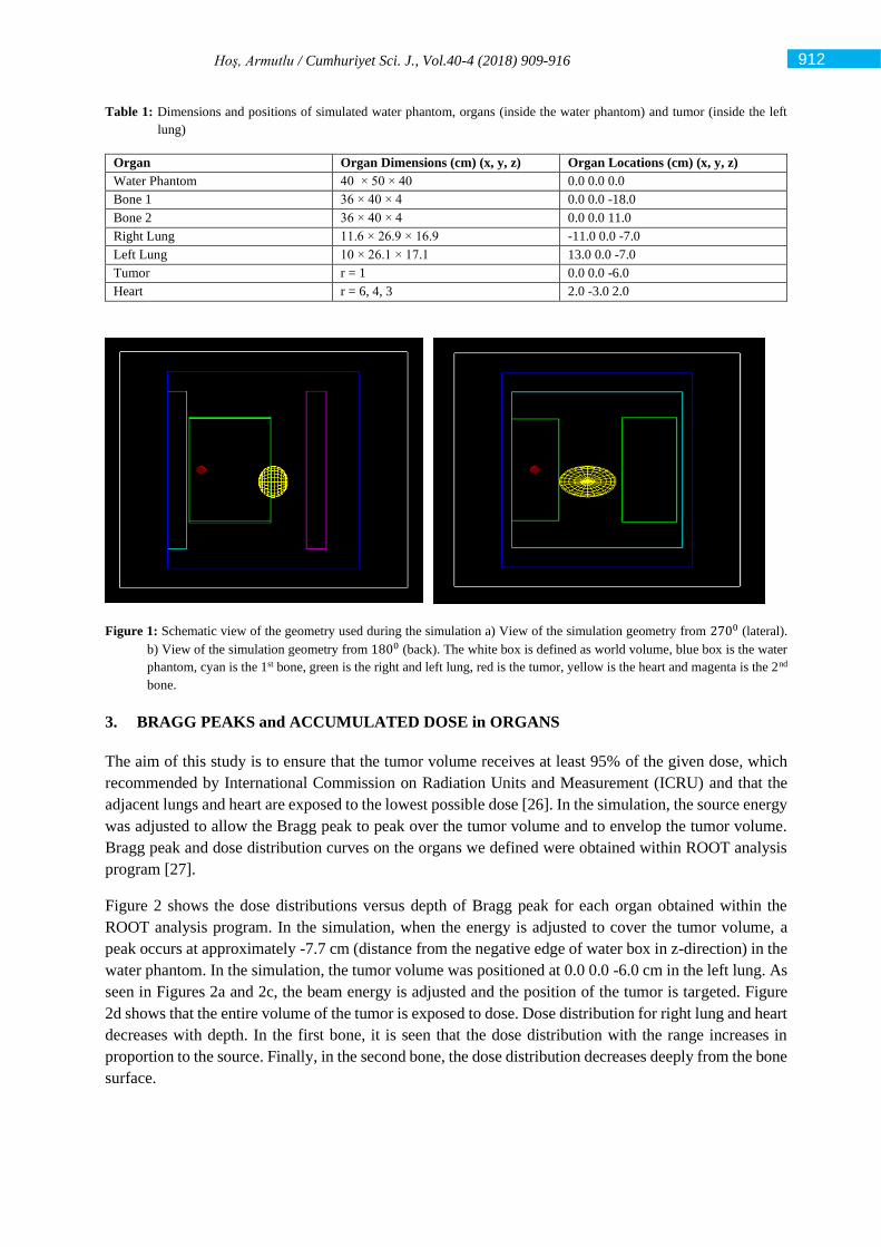
Hoş, Armutlu / Cumhuriyet Sci. J., Vol.40-4 (2018) 909-916
Table 1: Dimensions and positions of simulated water phantom, organs (inside the water phantom) and tumor (inside the left
lung)
Organ Organ Dimensions (cm) (x, y, z) Organ Locations (cm) (x, y, z)
Water Phantom 40 × 50 × 40 0.0 0.0 0.0
Bone 1 36 × 40 × 4 0.0 0.0 -18.0
Bone 2 36 × 40 × 4 0.0 0.0 11.0
Right Lung 11.6 × 26.9 × 16.9 -11.0 0.0 -7.0
Left Lung 10 × 26.1 × 17.1 13.0 0.0 -7.0
Tumor r = 1 0.0 0.0 -6.0
Heart r = 6, 4, 3 2.0 -3.0 2.0
Figure 1: Schematic view of the geometry used during the simulation a) View of the simulation geometry from 2700 (lateral).
b) View of the simulation geometry from 1800 (back). The white box is defined as world volume, blue box is the water
phantom, cyan is the 1st bone, green is the right and left lung, red is the tumor, yellow is the heart and magenta is the 2nd
bone.
3. BRAGG PEAKS and ACCUMULATED DOSE in ORGANS
The aim of this study is to ensure that the tumor volume receives at least 95% of the given dose, which
recommended by International Commission on Radiation Units and Measurement (ICRU) and that the
adjacent lungs and heart are exposed to the lowest possible dose [26]. In the simulation, the source energy
was adjusted to allow the Bragg peak to peak over the tumor volume and to envelop the tumor volume.
Bragg peak and dose distribution curves on the organs we defined were obtained within ROOT analysis
program [27].
Figure 2 shows the dose distributions versus depth of Bragg peak for each organ obtained within the
ROOT analysis program. In the simulation, when the energy is adjusted to cover the tumor volume, a
peak occurs at approximately -7.7 cm (distance from the negative edge of water box in z-direction) in the
water phantom. In the simulation, the tumor volume was positioned at 0.0 0.0 -6.0 cm in the left lung. As
seen in Figures 2a and 2c, the beam energy is adjusted and the position of the tumor is targeted. Figure
2d shows that the entire volume of the tumor is exposed to dose. Dose distribution for right lung and heart
decreases with depth. In the first bone, it is seen that the dose distribution with the range increases in
proportion to the source. Finally, in the second bone, the dose distribution decreases deeply from the bone
surface.
912
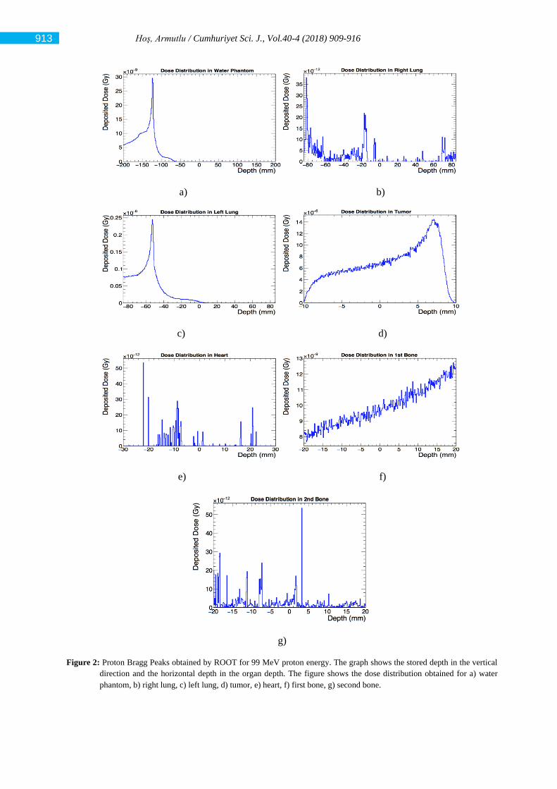
Hoş, Armutlu / Cumhuriyet Sci. J., Vol.40-4 (2018) 909-916
a) b)
c) d)
e) f)
g)
Figure 2: Proton Bragg Peaks obtained by ROOT for 99 MeV proton energy. The graph shows the stored depth in the vertical
direction and the horizontal depth in the organ depth. The figure shows the dose distribution obtained for a) water
phantom, b) right lung, c) left lung, d) tumor, e) heart, f) first bone, g) second bone.
913
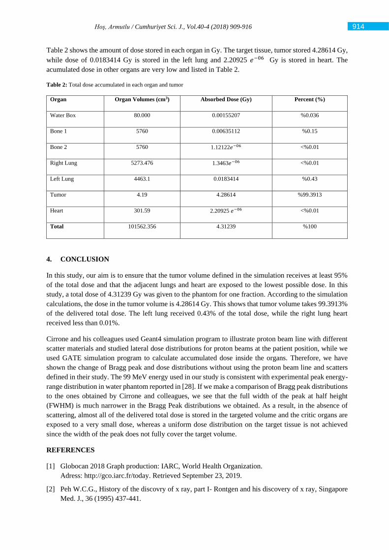
Hoş, Armutlu / Cumhuriyet Sci. J., Vol.40-4 (2018) 909-916
Table 2 shows the amount of dose stored in each organ in Gy. The target tissue, tumor stored 4.28614 Gy,
while dose of 0.0183414 Gy is stored in the left lung and 2.20925 𝑒−06 Gy is stored in heart. The
acumulated dose in other organs are very low and listed in Table 2.
Table 2: Total dose accumulated in each organ and tumor
Organ
Organ Volumes (cm3) Absorbed Dose (Gy) Percent (%)
Water Box 80.000 0.00155207
%0.036
Bone 1 5760 0.00635112
%0.15
Bone 2 5760
1.12122𝑒−06 <%0.01
Right Lung 5273.476
1.3463𝑒−06 <%0.01
Left Lung 4463.1
0.0183414 %0.43
Tumor 4.19
4.28614 %99.3913
Heart 301.59
2.20925 𝑒−06 <%0.01
Total 101562.356 4.31239 %100
4. CONCLUSION
In this study, our aim is to ensure that the tumor volume defined in the simulation receives at least 95%
of the total dose and that the adjacent lungs and heart are exposed to the lowest possible dose. In this
study, a total dose of 4.31239 Gy was given to the phantom for one fraction. According to the simulation
calculations, the dose in the tumor volume is 4.28614 Gy. This shows that tumor volume takes 99.3913%
of the delivered total dose. The left lung received 0.43% of the total dose, while the right lung heart
received less than 0.01%.
Cirrone and his colleagues used Geant4 simulation program to illustrate proton beam line with different
scatter materials and studied lateral dose distributions for proton beams at the patient position, while we
used GATE simulation program to calculate accumulated dose inside the organs. Therefore, we have
shown the change of Bragg peak and dose distributions without using the proton beam line and scatters
defined in their study. The 99 MeV energy used in our study is consistent with experimental peak energy-
range distribution in water phantom reported in [28]. If we make a comparison of Bragg peak distributions
to the ones obtained by Cirrone and colleagues, we see that the full width of the peak at half height
(FWHM) is much narrower in the Bragg Peak distributions we obtained. As a result, in the absence of
scattering, almost all of the delivered total dose is stored in the targeted volume and the critic organs are
exposed to a very small dose, whereas a uniform dose distribution on the target tissue is not achieved
since the width of the peak does not fully cover the target volume.
REFERENCES
[1] Globocan 2018 Graph production: IARC, World Health Organization.
Adress: http://gco.iarc.fr/today. Retrieved September 23, 2019.
[2] Peh W.C.G., History of the discovry of x ray, part I- Rontgen and his discovery of x ray, Singapore
Med. J., 36 (1995) 437-441.
914
Hoş, Armutlu / Cumhuriyet Sci. J., Vol.40-4 (2018) 909-916
[3] Khan M.F., Gibbons J.P., (2014), Khan’s The Physics of Radiation Therapy (Fifth Edition), Lippin-
cott Williams & Wilkins, Philadelphia, USA: LWW.com
[4] Wilson R.R., Radiological use of fast protons, Radiology, 47 (1946) 487-491.
[5] Lawrence J.H., Tobias C.A., Born J.L., Mccombs R.K., Roberts J.E., Anger H.O., Lowbeer B.V.,
Huggıns C.B., Pituitary irradiation with high energy proton beams: a preliminary report, Cancer Res.,
18-2 (1958) 121-34.
[6] Gragoudas E., Li W., Goitein M., Lane A.M., Munzenrider J.E., Egan K.M., Evidence-based
estimates of outcome in patients irradiated for intraocular melanoma, Arch Ophthalmol 10-12 (2002)
1665-71.
[7] Particle Therapy Co-Operative Group (PTCOG) - An organisation for those interested in proton,
light ion and heavy charged particle radiotherapy. Adress:https://www.ptcog.ch/index.php/facilities-
in-operatio. Retrieved September 30, 2019.
[8] Mesko S., Gomez D., Proton Therapy in Non-small Cell Lung Cancer, Curr. Treat. Options in
Oncol., 19-12 (2018) 76. doi: https://doi.org/ 10.1007/s11864-018-0588-z.
[9] Cozzi L., Fogliata A., Lomax A., Bolsi A., A treatment planning comparison of 3D conformal
therapy, intensity modulated photon therapy and proton therapy for treatment of advanced head and
neck tumours, Radiother Oncol., 61-3 (2001) 287–297.
[10] Macdonald O.K., Kruse J.J., Miller J.M., Garces Y.I., Brown P.D., Miller R.C., Foote R.L., Proton
beam radiotherapy versus three-dimensional conformal stereotactic body radiotherapy in primary
peripheral, early-stage non-small-cell lung carcinoma: a comparative dosimetric analysis, Int J
Radiation Oncol. Biol. Phys., 75-3 (2009) 950–958.
[11] Kadoya N., Obata Y., Kato T., Kagiya M., Nakamura T., Tomoda T., Takada T., Takayama K.,
Fuwa N., Dose-volume comparison of proton radiotherapy and stereotactic body radiotherapy for
non-small cell lung cancer, Int J Radiat Oncol Biol Phys., 79 (2011) 1225–31.
[12] Roelofs E., Engelsman M., Rasch C., Persoon L., Quamhiyeh S., Ruysscher D.D., Verhaegen F.,
Pijls J.M., Lambin P., Rococo consortium, Results of a multicentric in silico clinical trial
(ROCOCO): comparing radiotherapy with photons and protons for non-small cell lung cancer, J
Thorac Oncol., 7-1 (2012) 165–76. doi: 10.1097 / JTO.0b013e31823529fc.
[13] Paganetti H., Jiang H., Lee S.Y., Kooy H.M., Accurate Monte Carlo simulations for nozzle design,
commissioning and quality assurance for a proton radiation therapy facility, Med. Phys., 31-7 (2004)
2107–2118. doi: https://doi.org/10.1118/1.1762792.
[14] Van Goethem M.J., Van Der Meer R., Reist H.W., Schippers J.M., Geant4 simulations of proton
beam transport through a carbon or beryllium degrader and following a beam line, Phys. Med. Biol.,
7-54 (2009) 5831–5846. doi:https://doi.org/10.1088/0031-9155/54/ 19/011.
[15] Aso T., Kimura A., Tanaka S., Yoshida H., Kanematsu N., Sasaki T., Akagi T., Verification of the
Dose Distributions With GEANT4 Simulation for Proton Therapy, IEEE Transactions on Nuclear
Science, 52-4 (2005) 896–901. doi: https://doi.org/10. 1109/tns.2005.852697.
[16] Allison J., Amako K., Araujo H., Apotolakis J., Geant4 developments and applications, IEEE
Trans.Nucl.Sci., 53-1 (2006) 270-278.
[17] Clasie B., Depauw N., Fransen M., Gom C., Panahandeh H.R., Seco J., et al.: Golden beam data for
proton pencil-beam scanning. Phys. Med. Biol. 57-5 (2012). doi:https://doi.org/10.1088/ 0031-
9155/57/5/1147.
[18] Users Guide V7.2 From GATE collaborative documentation wiki. Adress:
http://www.opengatecollaboration.org/sites/default/files/GATE-UsersGuideV7.2.pdf. Retrieved
September 13, 2019.
915
Hoş, Armutlu / Cumhuriyet Sci. J., Vol.40-4 (2018) 909-916
[19] Agostinelli S., Allison J., Amako K. al, Apostolakis J., Araujo H., Arce P., Asai M., Axen D.,
Banerjee S., Barrand G., GEANT4—a simulation toolkit, Nucl. instruments methods Phys. Res. Sect.
A Accel. Spectrometers, Detect. Assoc. Equip., 506 (2003) 250–303.
[20] GEANT4 a simulation toolkit. Adress: https://geant4.web.cern.ch/. Retrieved: November 19, 2019.
[21] Tan H.Q., Phua J.H., Tan L., Ang K.W., Lee J., Bettiol A.A., Geant4 Simulation for Commissioning
of Proton Therapy Centre, World Congress on Medical Physics and Biomedical Engineering 2018,
IFMBE Proceedings, 68-1 (2018) 583-587. doi:https://doi.org/10.1007/978-981-10-9035-6_108.
[22] Cirrone G.A.P., Cuttone G., Nigro S.L., Guatelli S., Mascialino B., Pia M.G., Raffaele L., Russo G.,
Implementation of a New Monte Carlo GEANT4 Simulation Tool for the Development of a Proton
Therapy Beam Line and Verification of the Related Dose Distributions, IEEE Transactions on
Nuclear Science, 52-1 (2005) 262-265. doi:10.1109/TNS.2004.843140.
[23] Cirrone, G.A.P., Cuttone, G., D. Battaglia L., Calabbretta L., Celona F., Di R., Lojacono P.,
Maggiore M., Mongelli V., Nigro L.S., Piazza L.A.C., Patti V.I., Raffaele L., Re M., Rifuggiato D.,
Russo G.,Sabini M.G, Salamone V., Valastro L.M., A 62 MeV Proton beam for the treatment of
ocular melanoma at Laboratori Nazionali del Sud-INFN (CATANIA), IEEE Nuclear Science
Symposium. Conference Record, 5 (2003) 3658-3662.
doi:https://doi.org/10.1109/NSSMIC.2003.1352701.
[24] Gray H., Gray’s Anatom, 39th ed. Londo: Churchill; (2005) 997-1003.
[25] Kramer G.H., Capello K., Bearrs B., Lauzon A., Normandeau L., Linear dimensions and volumes of
human lungs obtained from CT images. Health Phys., 102-4 (2012) 378-83.
doi:10.1097/HP.0b013e31823a13f1.
[26] International Commission on Radiation Units and Measurement)(ICRU). Adress:https://icru.org/.
Retrieved September 13, 2019.
[27] Rene B. and Fons R., ROOT An Object Oriented Data Analysis Framework, Proceedings
AIHENP'96 Workshop, Lausanne, Nucl. Inst. & Meth. in Phys. Res. A., 389 (1997) 81-86.
[28] Rinecker Proton Therapy Center Third Annual Report Establishing Proton Cancer Therapy in
Europe. Adress: https://www.rptc.de/en/information/latest-news/progress-reports/news-progress-
reports-detail/rinecker-proton-therapy-center-third-annual-report-establishing-proton-cancer-
therapy-in-europe.html. Retrieved September 10 (2019).
916

Cumhuriyet Science Journal
CSJ
e-ISSN: 2587-246X
ISSN: 2587-2680 Cumhuriyet Sci. J., Vol.40-4 (2019) 917-925
* Corresponding author. Email address: [email protected]
http://dergipark.gov.tr/csj ©2019 Faculty of Science, Sivas Cumhuriyet University
The Development of pH Modulated Solidified Homogeneous Liquid Phase
Microextraction Methodology for Preconcentration and Determination of
Nickel in Water Samples
Demirhan ÇITAK 1,* , Rabia DEMİROK 1
1 Tokat Gaziosmanpaşa University, Faculty of Science and Arts, Chemistry Department, 60250 Tokat, Turkey
Received: 04.11.2019; Accepted: 19.12.2019 http://dx.doi.org/10.17776/csj.642319
Abstract. In this work, a new, fast and green pH assisted solidified homogeneous liquid phase microextraction
method (pH-MS-HLPME) was developed. Initially, the complex formation of Ni-1-Phenylthiosemicarbazide
(Ni-PTC) and the dissolution of the extraction solvent (caprylic acid) in water were achieved by addition of
NaOH. After base addition caprylic acid (CA) become completely soluble as sodium caprylate in model
solution. The phase separation of extraction solvent was accessed by addition of HCl. The analyse of nickel
concentrations was carried out by micro-sampler adapted flame atomic absorption spectrometer. Under
optimized parameters, linear range (10.0-450 μg L-1), detection limit (3.2 μg L-1), limit of quantification (10.0
μg L-1), relative standard deviation (2.0 %), relative error (-3.9 %), and preconcentration factor (45) were
calculated, respectively. Finally, the developed pH-MS -HLPME methodology was successfully applied to LGC
6010 hard drinking water (CRM) and some water samples.
Keywords: Nickel, pH, liquid phase microextraction, drinking water samples, microsampler system.
Su Örneklerinde Nikelin Zenginleştirilmesi ve Tayini için pH Modülasyonlu
Katılaştırılmış Homojen Sıvı Faz Mikroekstraksiyon Metodunun
Geliştirilmesi
Özet. Bu çalışmada yeni, hızlı ve yeşil bir pH destekli katılaştırılmış homojen sıvı faz mikroekstraksiyon
metodu (pH-MS-HLPME) geliştirildi. İlk olarak, Ni-1-feniltiyosemikarbazit (Ni-PTC) kompleksinin oluşumu
ve ekstraksiyon çözücüsünün (kaprilik asit) su içinde çözülmesi, NaOH ilave edilerek sağlandı. Baz ilave
edildikten sonra kaprilik asit (CA), model çözeltide sodyum kaprilat halinde tamamen çözünür hale geldi.
Ekstraksiyon çözücüsü fazının ayrılması HC1 ilavesiyle gerçekleştirildi. Nikel konsantrasyonlarının tayini,
mikro örnekleyici uyarlanmış alevli atomik absorpsiyon spektrometresi ile gerçekleştirildi. Optimize edilmiş
parametreler altında, doğrusal çalışma aralığı (10.0-450 μg L-1), gözlenebilme sınırı (3.2 μg L-1), tayin sınırı
(10.0 μg L-1), bağıl standart sapma (% 2.0), bağıl hata (-3.9 %) zenginleştirme faktörü (45) hesaplandı. Son
olarak, geliştirilen pH-SFO-HLPME yöntemi LGC 6010 sert içme suyu standard referans maddesine ve bazı su
örneklerine başarıyla uygulandı.
Anahtar Kelimeler: Nikel, pH, sıvı faz mikroekstraksiyon, içme suları, mikro örnek verici sistem.
1. INTRODUCTION
Nickel is widely used industrial element for
making many products such as batteries, coins,
keys, cooking equipments and cell phones etc. In
addition, natural waters, foods, fruits and
vegetables include trace amount of nickel and
nickel compounds. It is also very important for
Çıtak, Demirok / Cumhuriyet Sci. J., Vol.40-4 (2019) 917-925
hormonal activity and lipid metabolism [1–4].
However, the excessive amount uptake of nickel
can cause cancer, allergic skin problems and
psychological disorders. Because of these harmful
effects determination of nickel is an essential
obligation for analytical chemists. Many modern
instrumental methods like inductively coupled
plasma mass spectrometry (ICP-MS), inductively
coupled plasma optical emission spectrometry
(ICP-OES, electrothermal atomic absorption
spectrometry (ETAAS), flame atomic absorption
spectrometry (FAAS) can be used for
determination of nickel in various samples. FAAS
is the most favourable and used technique when it
is compared to the other spectroanalytical
techniques. However, for sensitive and reliable
determination of nickel a sample pretreatment
procedure is needed before FAAS measurements
[5–9].
The aim of many analytic chemists is to develop
high- performance, away from environmental
pollution and matrix effects, less time consuming
and economically feasible sample pretreatment
methods. Nowadays, the popularity of liquid phase
microextraciton (LPME) methods is increasing day
by day when we compare with the other sample
pretreatment methods. LPME was presented as a
simpler and cheaper alternative to conventional
liquid-liquid extraction in 1990s [10–12]. Many
kinds of modified LPME techniques were reported
in literature for separation and preconcentration of
metals [13–18] such as dispersive liquid–liquid
microextraction (DLLME) [19], single-drop
microextraction (SDME) [20–22], hollow-fiber
liquid-phase microextraction (HF-LPME) [23,24],
solidification of floating organic droplets liquid
phase microextraction (SFO-LPME) [25,26].
The use of two types of solvent (disperser and
extraction solvent) at DLLME, the instability of the
extraction solvent drop at SDME, the use of
expensive membranes at HF-LPME restrict the
application of these methods [27]. Among these
techniques, SFO-LPME draws more attention due
to advantages such as easy removal of extraction
solvent, use of less toxic extraction solvents and
simplicity [28]. In this technique usually a low
toxic extraction solvent with appropriate melting
point (near room temperature) is mixed with a
disperser solvent and injected into water sample for
providing short extraction time and fast mass
transfer. After phase separation by centrifugation,
the sample tubes are placed in an ice bath for
solidification of organic drop floats on the surface.
The solidified organic drop including analyte
removed with a spatula to a conical tube than the
melted extraction solvent introduced to appropriate
analytic techniques [29–31].
The aim of this work was to develop a modified
SFO-LPME called pH modulated solidified
homogeneous liquid phase microextraction (pH-
MS-HLPME) method for determination of nickel.
The concentration levels of nickel in various water
samples were determined by microsampler adapted
flame atomic absorption spectrometer. This
method offers more green and economic alternative
when compared to the other SFO-LPME methods.
Because the dissolution of the extraction solvent
(caprylic acid) and complex formation of Ni-1-
Phenylthiosemicarbazide (Ni-PTC) was achieved
by using any disperser solvent and buffer solution.
Both were achieved by addition of appropriate
amount of NaOH-HCl.
2. EXPERIMENTAL
2.1 Instruments and chemicals
A hand made micro-sampler adapted Perkin-Elmer
Analyst 700 (Norwalk, CT, USA) atomic
absorption spectrometer was used for Ni (II)
determination. The operation conditions of FAAS
were chosen according to manufacturer guides. A
Sartorius pp-15 (Gottingen, Germany) model pH
meter with glass-electrode and a Nüve NF 200
(Ankara, Turkey) model centrifuge were used for
pH measuring and centrifuging test solutions,
respectively.
All chemicals used during the pH-MS-HLPME
were analytical reagent grade. Caprylic acid, 1-
phenylthiosemicarbazide were purchased from
Merck chemical company (Darmstadt, Germany).
0.1 % (w/v) PTC solution was prepared daily by
dissolving in methanol. Sodium hydroxide and
hydrochloric acid (E. Merck, Darmstadt, Germany)
solutions at various concentrations were prepared
by dissolving appropriate amount in deionized
water. 1000 mg L-1 Ni (II) standard solution were
prepared from Ni(NO3)2.6H2O (Sigma-Aldrich)
and nickel solutions at other concentrations for test
solutions were prepared by diluting from 1000 mg
L-1 Ni (II) standard solution.
2.2 pH-MS-HLPME procedure
130 µL CA was added to conical test tube
containing 9 mL test solution (containing 30 µg L-
1 Ni(II), 1 ml PTC from 0.1 %) by a micropipette .
Than 1.0 mL NaOH (1 mol L-1) was added to test
918
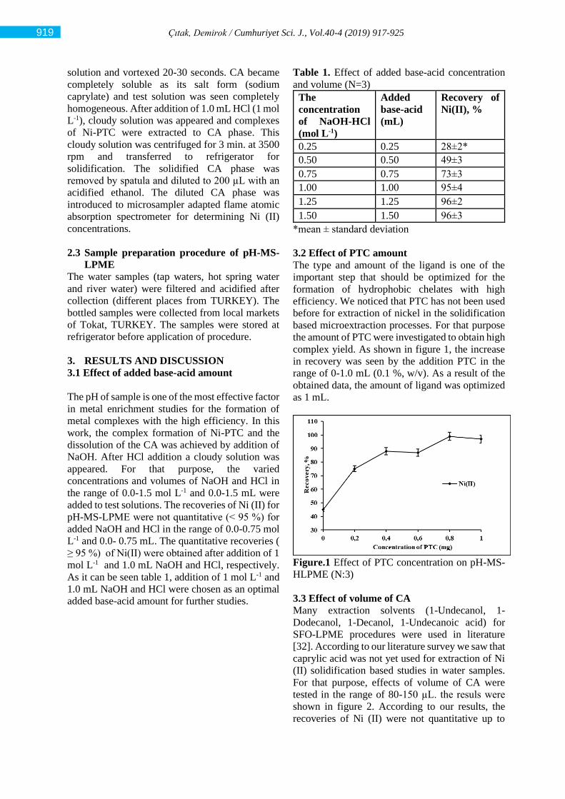
Çıtak, Demirok / Cumhuriyet Sci. J., Vol.40-4 (2019) 917-925
solution and vortexed 20-30 seconds. CA became
completely soluble as its salt form (sodium
caprylate) and test solution was seen completely
homogeneous. After addition of 1.0 mL HCl (1 mol
L-1), cloudy solution was appeared and complexes
of Ni-PTC were extracted to CA phase. This
cloudy solution was centrifuged for 3 min. at 3500
rpm and transferred to refrigerator for
solidification. The solidified CA phase was
removed by spatula and diluted to 200 µL with an
acidified ethanol. The diluted CA phase was
introduced to microsampler adapted flame atomic
absorption spectrometer for determining Ni (II)
concentrations.
2.3 Sample preparation procedure of pH-MS-
LPME
The water samples (tap waters, hot spring water
and river water) were filtered and acidified after
collection (different places from TURKEY). The
bottled samples were collected from local markets
of Tokat, TURKEY. The samples were stored at
refrigerator before application of procedure.
3. RESULTS AND DISCUSSION
3.1 Effect of added base-acid amount
The pH of sample is one of the most effective factor
in metal enrichment studies for the formation of
metal complexes with the high efficiency. In this
work, the complex formation of Ni-PTC and the
dissolution of the CA was achieved by addition of
NaOH. After HCl addition a cloudy solution was
appeared. For that purpose, the varied
concentrations and volumes of NaOH and HCl in
the range of 0.0-1.5 mol L-1 and 0.0-1.5 mL were
added to test solutions. The recoveries of Ni (II) for
pH-MS-LPME were not quantitative (˂ 95 %) for
added NaOH and HCl in the range of 0.0-0.75 mol
L-1 and 0.0- 0.75 mL. The quantitative recoveries (
≥ 95 %) of Ni(II) were obtained after addition of 1
mol L-1 and 1.0 mL NaOH and HCl, respectively.
As it can be seen table 1, addition of 1 mol L-1 and
1.0 mL NaOH and HCl were chosen as an optimal
added base-acid amount for further studies.
Table 1. Effect of added base-acid concentration
and volume (N=3)
The
concentration
of NaOH-HCl
(mol L-1)
Added
base-acid
(mL)
Recovery of
Ni(II), %
0.25 0.25 28±2*
0.50 0.50 49±3
0.75 0.75 73±3
1.00 1.00 95±4
1.25 1.25 96±2
1.50 1.50 96±3
*mean ± standard deviation
3.2 Effect of PTC amount
The type and amount of the ligand is one of the
important step that should be optimized for the
formation of hydrophobic chelates with high
efficiency. We noticed that PTC has not been used
before for extraction of nickel in the solidification
based microextraction processes. For that purpose
the amount of PTC were investigated to obtain high
complex yield. As shown in figure 1, the increase
in recovery was seen by the addition PTC in the
range of 0-1.0 mL (0.1 %, w/v). As a result of the
obtained data, the amount of ligand was optimized
as 1 mL.
Figure.1 Effect of PTC concentration on pH-MS-
HLPME (N:3)
3.3 Effect of volume of CA
Many extraction solvents (1-Undecanol, 1-
Dodecanol, 1-Decanol, 1-Undecanoic acid) for
SFO-LPME procedures were used in literature
[32]. According to our literature survey we saw that
caprylic acid was not yet used for extraction of Ni
(II) solidification based studies in water samples.
For that purpose, effects of volume of CA were
tested in the range of 80-150 µL. the resuls were
shown in figure 2. According to our results, the
recoveries of Ni (II) were not quantitative up to
919

Çıtak, Demirok / Cumhuriyet Sci. J., Vol.40-4 (2019) 917-925
volume 120 µL. It was quantitative in the range of
120-130 µL. After volume of 130 µL a decrease
was seen. Therefore 130 µL CA volume was
chosen for other experimental parameters.
Figure.2 Effect of volume of CA (N:3)
3.4 Optimization of the other experimental
parameters
The mixing time is an important parameter that
plays a major role for increasing the extraction
efficiency and reducing the extraction time. The
effective mixing of the aqueous and organic phases
is very important to ensure the mass transfer of the
solution. The mass transfer coefficient of the
aqueous phase increases with increasing mixing
ratio. Therefore, in this study, the effects of shaking
and centrifugation times on recovery rates of 1 to 5
minutes were examined. As it can be seen from
figure 3, it was found that the best recovery was
achieved the 20-30 seconds vortex time and 3
minute centrifugation time for the experimental
conditions and all of the studies were completed at
this time period.
Figure 3. The effects of vortex and centrifugation
and vortex time on recovery Ni (II) (N:3)
The increase in the ratio of the aqueous phase
volume to the organic phase will increase the
preconcentration factor, but this can reduce the
extraction efficiency in a given extraction time.
The effects of sample volume on the recovery of Ni
(II) were investigated in the range of 8-14 mL in
this study. The results are shown in figure 4. The
recovery of 95 % and higher than 95 % was
achieved between 8-9 mL. Therefore, the sample
volume was chosen as 9 mL. In addition, the final
volume was completed with 1M HNO3 (in ethanol)
to 200 mL before the analysis step.
Figure 4. The effect of sample volume on pH-MS-
HLPME (N:3)
3.5 Effect of interferences on pH-MS-HLPME
Some components which can be present in the
water samples may interfere and cause negative or
positive errors during the preconcentraiton studies.
Therefore, the effects of some ions in different
concentrations and types were investigated for pH-
MS-HLPME technique. The results (table 2.)
showed that ions had no effect until added
concentrations. It demonstrates that our pH-MS-
HLPME method was applicable for water samples.
Table 2. Effect of interferes on pH-MS-HLPME
(N=3)
Ion Interference/metal
ratio
Recovery of
Ni(II),%
Na+ 400 99±3*
K+ 500 96±2
Ca2+ 200 96±2
Mg2+ 200 99±4
Cl- 800 102±3
NO3- 500 102±5
SO42- 500 96±3
PO43- 600 103±3
* mean ± standard deviation
920
Çıtak, Demirok / Cumhuriyet Sci. J., Vol.40-4 (2019) 917-925
3.5 Analytical performance criteria of the
proposed method
To evaluate analytical performance criteria of the
proposed method, limit of detection, calibration
curve equation, linear range, reproducibility and
preconcentration factor were calculated under
optimized conditions. The limit of detection (3Sb,
Sb is the standard deviation of ten replicates of the
blank measurement) and limit of quantification
(10Sb) were found as 3.2 μg L-1 and 10 μg L-1,
respectively. The linear range was found as 10.0-
450 μg L-1. The calibration curve equation was
A=1.73x10⁻²C + 3.2x10⁻³ (r2=0.9993). The
reproducibility defined as relative standard
deviation (R.S.D.) was calculated as 2.0 % after
application (N=11) of pH-MS-LPME to model
solutions containing 30 μg L−1 of Ni (II). The
preconcentration factor of 45 was calculated from
the ratio of the highest sample volume (9 mL) to
final completed volume (200 µL).
3.6 Accuracy and application of optimized pH-
MS-HLPME
In order to test the accuracy of the developed
method, the method was applied to standard
reference material (LGC 6010 hard drinking
water). The experimental obtained value was found
49 ± 2 µg L-1 and the certificate value was 51 µg L-
1. The values of SRM shoved that pH-MS-HLPME
method was found to be applicable to water
samples. The relative error was calculated as -3.9
%.
Also, the developed method was applied to two
different tap water samples, river water, hot spring
water, sea water and 7 different bottled water
samples purchased from local markets in Tokat city
(TURKEY) for the determination of Ni (II). The
obtained results were given in Table 3. together
with the recoveries. The recovery values were
quantitative. The results of pH-MS-HLPME
shoved that the method was applicable for the
determination of Ni (II) in natural and bottled water
samples.
3.7 Comparison of pH-MS-HLPME with the
other solidification based microextraction
methods in literature
The developed pH-MS-HLPME was compared
with some SFODME based studies for
preconcentration of Ni (II) in the literature (Table
4). In many DLLME and SFODME studies, a
disperser solvent was often used to mix the
extraction solvent in the samples. However, the
dissolution of the extraction solvent, the formation
of the Ni-PTC complex and the phase separation of
extraction solvent were carried out only with the
addition of NaOH-HCl in our study. This showed
that the developed method reduces use of the
amount of organic toxic solvent during the sample
preparation step and because of this reason, the
developed pH-MS-HLPME was a more
environmentally and economically efficient
method.
921
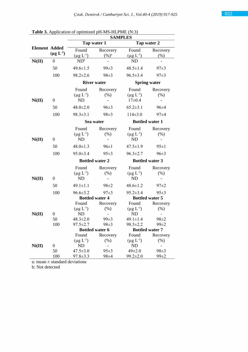
Çıtak, Demirok / Cumhuriyet Sci. J., Vol.40-4 (2019) 917-925
Table 3. Application of optimized pH-MS-HLPME (N:3)
Element
Added
(µg L-1)
SAMPLES
Tap water 1 Tap water 2
Found
(µg L-1)
Recovery
(%)a
Found
(µg L-1)
Recovery
(%)
Ni(II) 0 NDb - ND -
50 49.6±1.5 99±3 48.5±1.4 97±3
100 98.2±2.6 98±3 96.5±3.4 97±3
River water Spring water
Found
(µg L-1)
Recovery
(%)
Found
(µg L-1)
Recovery
(%)
Ni(II) 0 ND - 17±0.4 -
50 48.0±2.0 96±3 65.2±3.1 96±4
100 98.3±3.1 98±3 114±3.0 97±4
Sea water Bottled water 1
Found
(µg L-1)
Recovery
(%)
Found
(µg L-1)
Recovery
(%)
Ni(II) 0 ND - ND -
50 48.0±1.3 96±1 47.5±1.9 95±1
100 95.0±3.4 95±3 96.3±2.7 96±3
Bottled water 2 Bottled water 3
Found
(µg L-1)
Recovery
(%)
Found
(µg L-1)
Recovery
(%)
Ni(II) 0 ND - ND -
50 49.1±1.1 98±2 48.6±1.2 97±2
100 96.6±3.2 97±3 95.2±3.4 95±3
Bottled water 4 Bottled water 5
Found
(µg L-1)
Recovery
(%)
Found
(µg L-1)
Recovery
(%)
Ni(II) 0 ND - ND -
50 48.3±2.0 99±3 49.1±1.4 98±2
100 97.5±2.7 98±3 98.5±2.2 99±2
Bottled water 6 Bottled water 7
Found
(µg L-1)
Recovery
(%)
Found
(µg L-1)
Recovery
(%)
Ni(II) 0 ND - ND -
50 47.5±3.0 95±3 49±2.0 98±3
100 97.8±3.3 98±4 99.2±2.0 99±2
a: mean ± standard deviations
b: Not detected
922
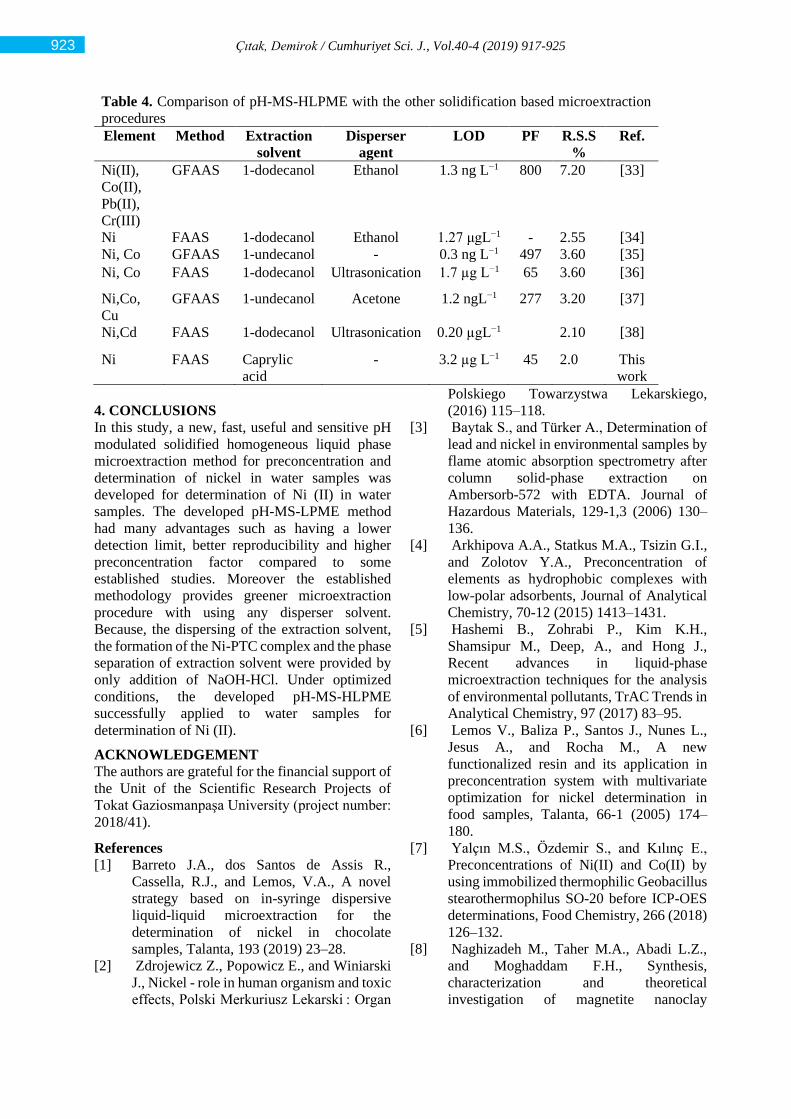
Çıtak, Demirok / Cumhuriyet Sci. J., Vol.40-4 (2019) 917-925
4. CONCLUSIONS
In this study, a new, fast, useful and sensitive pH
modulated solidified homogeneous liquid phase
microextraction method for preconcentration and
determination of nickel in water samples was
developed for determination of Ni (II) in water
samples. The developed pH-MS-LPME method
had many advantages such as having a lower
detection limit, better reproducibility and higher
preconcentration factor compared to some
established studies. Moreover the established
methodology provides greener microextraction
procedure with using any disperser solvent.
Because, the dispersing of the extraction solvent,
the formation of the Ni-PTC complex and the phase
separation of extraction solvent were provided by
only addition of NaOH-HCl. Under optimized
conditions, the developed pH-MS-HLPME
successfully applied to water samples for
determination of Ni (II).
ACKNOWLEDGEMENT
The authors are grateful for the financial support of
the Unit of the Scientific Research Projects of
Tokat Gaziosmanpaşa University (project number:
2018/41).
References
[1] Barreto J.A., dos Santos de Assis R.,
Cassella, R.J., and Lemos, V.A., A novel
strategy based on in-syringe dispersive
liquid-liquid microextraction for the
determination of nickel in chocolate
samples, Talanta, 193 (2019) 23–28.
[2] Zdrojewicz Z., Popowicz E., and Winiarski
J., Nickel - role in human organism and toxic
effects, Polski Merkuriusz Lekarski : Organ
Polskiego Towarzystwa Lekarskiego,
(2016) 115–118.
[3] Baytak S., and Türker A., Determination of
lead and nickel in environmental samples by
flame atomic absorption spectrometry after
column solid-phase extraction on
Ambersorb-572 with EDTA. Journal of
Hazardous Materials, 129-1,3 (2006) 130–
136.
[4] Arkhipova A.A., Statkus M.A., Tsizin G.I.,
and Zolotov Y.A., Preconcentration of
elements as hydrophobic complexes with
low-polar adsorbents, Journal of Analytical
Chemistry, 70-12 (2015) 1413–1431.
[5] Hashemi B., Zohrabi P., Kim K.H.,
Shamsipur M., Deep, A., and Hong J.,
Recent advances in liquid-phase
microextraction techniques for the analysis
of environmental pollutants, TrAC Trends in
Analytical Chemistry, 97 (2017) 83–95.
[6] Lemos V., Baliza P., Santos J., Nunes L.,
Jesus A., and Rocha M., A new
functionalized resin and its application in
preconcentration system with multivariate
optimization for nickel determination in
food samples, Talanta, 66-1 (2005) 174–
180.
[7] Yalçın M.S., Özdemir S., and Kılınç E.,
Preconcentrations of Ni(II) and Co(II) by
using immobilized thermophilic Geobacillus
stearothermophilus SO-20 before ICP-OES
determinations, Food Chemistry, 266 (2018)
126–132.
[8] Naghizadeh M., Taher M.A., Abadi L.Z.,
and Moghaddam F.H., Synthesis,
characterization and theoretical
investigation of magnetite nanoclay
Table 4. Comparison of pH-MS-HLPME with the other solidification based microextraction
procedures
Element Method Extraction
solvent
Disperser
agent
LOD PF R.S.S
%
Ref.
Ni(II),
Co(II),
Pb(II),
Cr(III)
GFAAS 1-dodecanol Ethanol
1.3 ng L−1 800 7.20 [33]
Ni FAAS 1-dodecanol Ethanol 1.27 μgL−1 - 2.55 [34]
Ni, Co GFAAS 1-undecanol - 0.3 ng L−1 497 3.60 [35]
Ni, Co FAAS 1-dodecanol Ultrasonication 1.7 µg L−1 65 3.60 [36]
Ni,Co,
Cu
GFAAS 1-undecanol Acetone 1.2 ngL−1 277 3.20 [37]
Ni,Cd FAAS 1-dodecanol Ultrasonication 0.20 µgL−1 2.10 [38]
Ni FAAS Caprylic
acid
- 3.2 µg L−1 45 2.0 This
work
923
Çıtak, Demirok / Cumhuriyet Sci. J., Vol.40-4 (2019) 917-925
modified as a new nanocomposite for
simultaneous preconcentration of lead and
nickel prior to ETAAS determination,
Environmental Nanotechnology,
Monitoring & Management, 7 (2017) 46–56.
[9] ALOthman Z.A., Habila M.A., Yilmaz E.,
Soylak M., and Alfadul S.M., Ultrasonic
supramolecular microextration of nickel (II)
as N,N′-Dihydroxy-1,2-cyclohexanediimine
chelates from water, tobacco and fertilizer
samples before FAAS determination,
Journal of Molecular Liquids, 221 (2016)
773–777.
[10] He Y. and Lee H.K., Liquid-Phase
Microextraction in a Single Drop of Organic
Solvent by Using a Conventional
Microsyringe. Analytical Chemistry, 69-22
(1997) 4634–4640.
[11] Rykowska I., Ziemblińska J., and Nowak I.,
Modern approaches in dispersive liquid-
liquid microextraction (DLLME) based on
ionic liquids: A review, Journal of Molecular
Liquids, 259 (2018) 319–339.
[12] De Almeida O.N., Luzardo F.H.M.,
Amorim F.A.C., Velasco F.G., and
González L.N., Use of fiberglass support in
the application of dried-spot technique with
dispersion liquid-liquid microextraction for
the determination of Co, Cr, Cu, Ni and Pb
by Energy Dispersive X-Ray Fluorescence
Spectrometry, Spectrochimica Acta Part B:
Atomic Spectroscopy, 150 (2018) 92–98.
[13] Kocot K., Pytlakowska K., Zawisza B., and
Sitko R., How to detect metal species
preconcentrated by microextraction
techniques, TrAC Trends in Analytical
Chemistry, 82 (2016) 412–424.
[14] Giakisikli G. and Anthemidis A.N., An
automatic stirring-assisted liquid–liquid
microextraction system based on lab-in-
syringe platform for on-line atomic
spectrometric determination of trace metals,
Talanta, 166 (2017) 364–368.
[15] Habila M.A., Yilmaz E., ALOthman Z.A.,
and Soylak M., Combination of dispersive
liquid–liquid microextraction and
multivariate optimization for separation-
enrichment of traces lead by flame atomic
absorption spectrometry, Journal of
Industrial and Engineering Chemistry, 37
(2016) 306–311.
[16] Zhang S., Chen B., He M., and Hu B.,
Switchable solvent based liquid phase
microextraction of trace lead and cadmium
from environmental and biological samples
prior to graphite furnace atomic absorption
spectrometry detection, Microchemical
Journal, 139 (2018) 380–385.
[17] Biata N.R., Nyaba L., Ramontja J., Mketo
N., and Nomngongo P.N., Determination of
antimony and tin in beverages using
inductively coupled plasma-optical emission
spectrometry after ultrasound-assisted ionic
liquid dispersive liquid-liquid phase
microextraction, Food Chemistry, 237
(2017) 904–911.
[18] Khazaeli E., Haddadi H., Zargar B.,
Hatamie A., and Semnani A., Ni(II) analysis
in food and environmental samples by
liquid-liquid microextraction combined with
electro-thermal atomic absorption
spectrometry, Microchemical Journal, 133
(2017) 311–319.
[19] Altunay N., Yıldırım E., and Gürkan R.,
Extraction and preconcentration of trace Al
and Cr from vegetable samples by vortex-
assisted ionic liquid-based dispersive liquid–
liquid microextraction prior to atomic
absorption spectrometric determination,
Food Chemistry, 245 (2018) 586–594.
[20] Manzoori J.L., Amjadi M., and
Abulhassani, J., Ultra-trace determination of
lead in water and food samples by using
ionic liquid-based single drop
microextraction-electrothermal atomic
absorption spectrometry, Analytica Chimica
Acta, 644-1,2 (2009) 48–52.
[21] Xia L., Li, X., Wu Y., Hu B., and Chen R.,
Ionic liquids based single drop
microextraction combined with
electrothermal vaporization inductively
coupled plasma mass spectrometry for
determination of Co, Hg and Pb in biological
and environmental samples. Spectrochimica
Acta Part B: Atomic Spectroscopy, 63-11
(2008) 1290–1296.
[22] Dadfarnia S., and Haji Shabani A.M.,
Recent development in liquid phase
microextraction for determination of trace
level concentration of metals—A review,
Analytica Chimica Acta, 658-2 (2010) 107–
119.
[23] Jiang H., Hu B., Chen B., and Xia L.,
Hollow fiber liquid phase microextraction
combined with electrothermal atomic
absorption spectrometry for the speciation of
arsenic (III) and arsenic (V) in fresh waters
and human hair extracts, Analytica Chimica
Acta, 634-1 (2009) 15–21.
[24] Ghambarian M., Yamini Y., and Esrafili A.,
924

Çıtak, Demirok / Cumhuriyet Sci. J., Vol.40-4 (2019) 917-925
Developments in hollow fiber based liquid-
phase microextraction: principles and
applications, Microchimica Acta, 177-3
(2012) 271–294.
[25] Shamsipur M., Ramezani M., and Miran
Beigi A.A., Floating Organic Drop
Microextraction Combined with
Electrothermal Atomic Absorption
Spectrometry for Trace Determination of
Cobalt in Oil Refining Wastewaters, Energy
Sources, Part A: Recovery, Utilization, and
Environmental Effects, 37-11 (2015) 1164–
1171.
[26] Mohammadi S.Z., Sheibani A., Abdollahi
F., and Shahsavani E., Speciation of Tl(III)
and Tl(I) in hair samples by dispersive
liquid–liquid microextraction based on
solidification of floating organic droplet
prior to flame atomic absorption
spectrometry determination, Arabian
Journal of Chemistry, 9 (2016) 1510–S1515.
[27] Haji Shabani A.M., Dadfarnia S., and
Nozohor M., Indirect spectrophotometric
determination of ultra trace amounts of
selenium based on dispersive liquid–liquid
microextraction–solidified floating organic
drop, Spectrochimica Acta Part A:
Molecular and Biomolecular Spectroscopy,
116 (2013) 1–5.
[28] Karadaş, C., and Kara, D., Dispersive
liquid–liquid microextraction based on
solidification of floating organic drop for
preconcentration and determination of trace
amounts of copper by flame atomic
absorption spectrometry, Food Chemistry,
220 (2017) 242–248.
[29] Mohamadi M., and Mostafavi A., A novel
solidified floating organic drop
microextraction based on ultrasound-
dispersion for separation and
preconcentration of palladium in aqueous
samples. Talanta, 81-2 (2010) 309–313.
[30] Pérez-Outeiral J., Millán E., and Garcia-
Arrona, R., Determination of phthalates in
food simulants and liquid samples using
ultrasound-assisted dispersive liquid–liquid
microextraction followed by solidification
of floating organic drop, Food Control, 62
(2016) 171–177.
[31] Pelit F.O. and Yengin Ç., Application of
solidified floating organic drop
microextraction method for biomonitoring
of chlorpyrifos and its oxon metabolite in
urine samples, Journal of Chromatography
B, 949–950 (2014) 109–114.
[32] Mansour F.R. and Danielson N.D.,
Solidification of floating organic droplet in
dispersive liquid-liquid microextraction as a
green analytical tool, Talanta, 170 (2017)
22–35.
[33] Mirzaei M., Behzadi M., Abadi N.M., and
Beizaei A., Simultaneous
separation/preconcentration of ultra trace
heavy metals in industrial wastewaters by
dispersive liquid–liquid microextraction
based on solidification of floating organic
drop prior to determination by graphite
furnace atomic absorption spectrometer
Journal of Hazardous Materials, 186-3
(2011) 1739–1743.
[34] Wang Y., Zhang J., Zhao B., Du X., Ma J.,
and Li J., Development of Dispersive
Liquid–Liquid Microextraction Based on
Solidification of Floating Organic Drop for
the Determination of Trace Nickel,
Biological Trace Element Research, 144-3
(2011) 1381–1393.
[35] Bidabadi M.S., Dadfarnia S., and Shabani
A.M.H., Solidified floating organic drop
microextraction (SFODME) for
simultaneous separation/preconcentration
and determination of cobalt and nickel by
graphite furnace atomic absorption
spectrometry (GFAAS), Journal of
Hazardous Materials, 166-1 (2009) 291–
296.
[36] Arpa Ç. and Arıdaşır I., Ultrasound assisted
ion pair based surfactant-enhanced liquid–
liquid microextraction with solidification of
floating organic drop combined with flame
atomic absorption spectrometry for
preconcentration and determination of
nickel and cobalt ions in vegeta, Food
Chemistry, 284 (2019) 16–22.
[37] Amirkavei M., Dadfarnia S., and Shabani
A.M.H., Dispersive liquid-liquid
microextraction based on solidification of
floating organic drop for simultaneous
separation/preconcentration of nickel, cobalt
and copper prior to determination by
electrothermal atomic absorption
spectrometry. Química Nova, 36-1 (2013)
63–68.
[38] Ezoddin M., Taghizadeh T., and Majidi B.,
Ultrasound-assisted surfactant-enhanced
emulsification microextraction for the
determination of Cd and Ni in tea and water
samples. Environmental Technology, 35-19
(2014) 2401–2409.
925
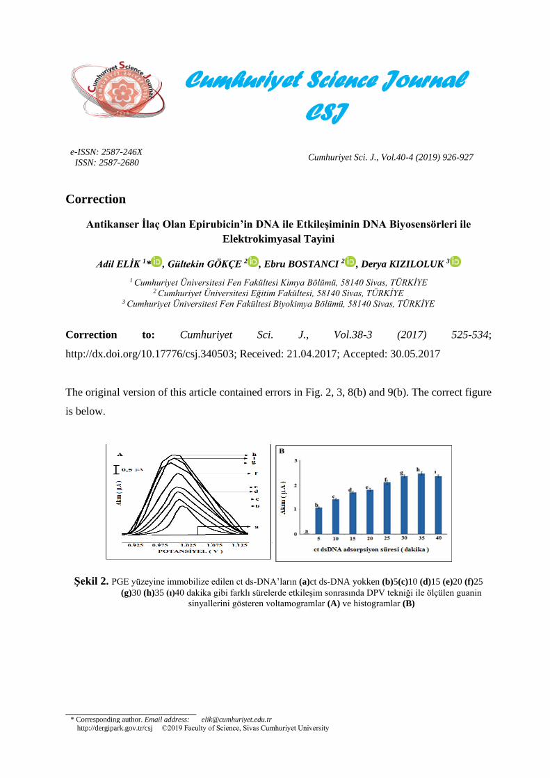
Cumhuriyet Science Journal
CSJ
e-ISSN: 2587-246X
ISSN: 2587-2680 Cumhuriyet Sci. J., Vol.40-4 (2019) 926-927
* Corresponding author. Email address: [email protected]
http://dergipark.gov.tr/csj ©2019 Faculty of Science, Sivas Cumhuriyet University
Correction
Antikanser İlaç Olan Epirubicin’in DNA ile Etkileşiminin DNA Biyosensörleri ile
Elektrokimyasal Tayini
Adil ELİK 1* , Gültekin GÖKÇE 2 , Ebru BOSTANCI 2 , Derya KIZILOLUK 3
1 Cumhuriyet Üniversitesi Fen Fakültesi Kimya Bölümü, 58140 Sivas, TÜRKİYE
2 Cumhuriyet Üniversitesi Eğitim Fakültesi, 58140 Sivas, TÜRKİYE
3 Cumhuriyet Üniversitesi Fen Fakültesi Biyokimya Bölümü, 58140 Sivas, TÜRKİYE
Correction to: Cumhuriyet Sci. J., Vol.38-3 (2017) 525-534;
http://dx.doi.org/10.17776/csj.340503; Received: 21.04.2017; Accepted: 30.05.2017
The original version of this article contained errors in Fig. 2, 3, 8(b) and 9(b). The correct figure
is below.
Şekil 2. PGE yüzeyine immobilize edilen ct ds-DNA’ların (a)ct ds-DNA yokken (b)5(c)10 (d)15 (e)20 (f)25
(g)30 (h)35 (ı)40 dakika gibi farklı sürelerde etkileşim sonrasında DPV tekniği ile ölçülen guanin
sinyallerini gösteren voltamogramlar (A) ve histogramlar (B)
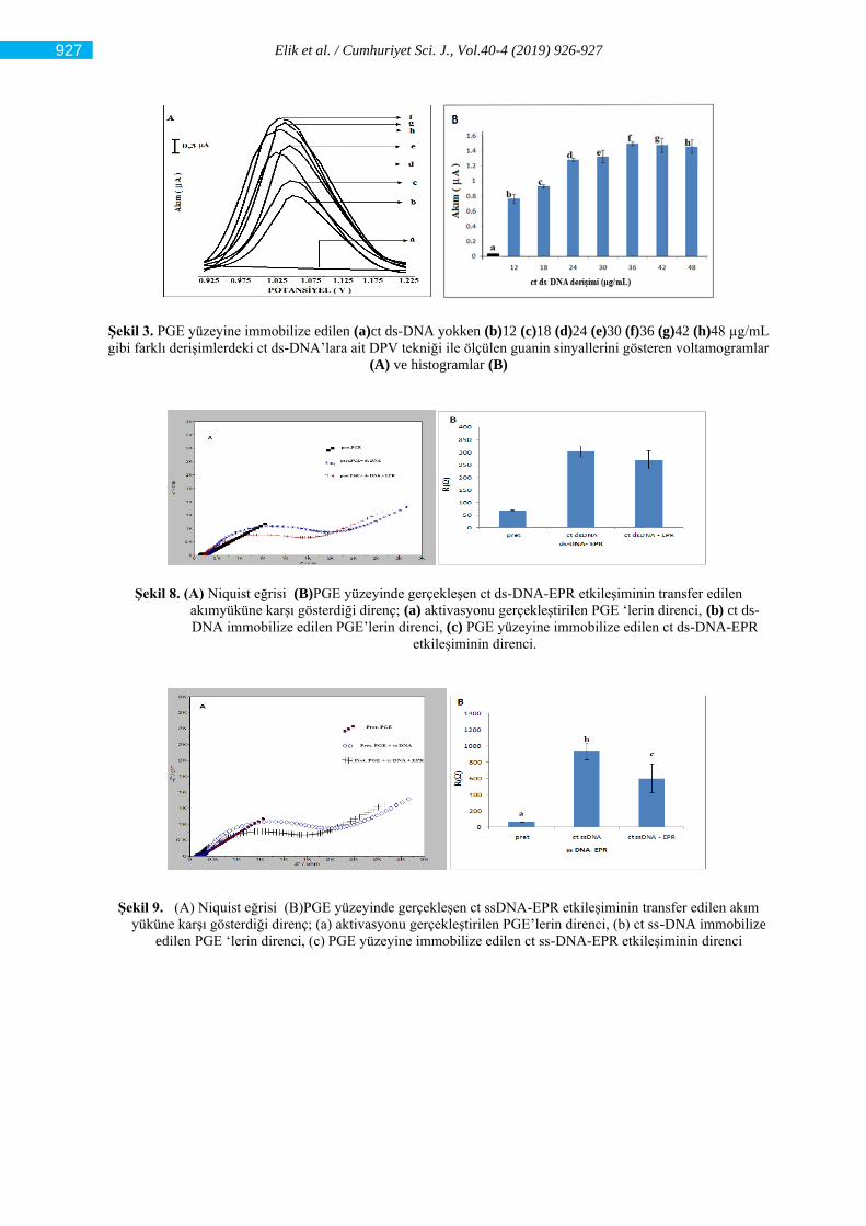
Elik et al. / Cumhuriyet Sci. J., Vol.40-4 (2019) 926-927
Şekil 3. PGE yüzeyine immobilize edilen (a)ct ds-DNA yokken (b)12 (c)18 (d)24 (e)30 (f)36 (g)42 (h)48 µg/mL
gibi farklı derişimlerdeki ct ds-DNA’lara ait DPV tekniği ile ölçülen guanin sinyallerini gösteren voltamogramlar
(A) ve histogramlar (B)
Şekil 8. (A) Niquist eğrisi (B)PGE yüzeyinde gerçekleşen ct ds-DNA-EPR etkileşiminin transfer edilen
akımyüküne karşı gösterdiği direnç; (a) aktivasyonu gerçekleştirilen PGE ‘lerin direnci, (b) ct ds-
DNA immobilize edilen PGE’lerin direnci, (c) PGE yüzeyine immobilize edilen ct ds-DNA-EPR
etkileşiminin direnci.
Şekil 9. (A) Niquist eğrisi (B)PGE yüzeyinde gerçekleşen ct ssDNA-EPR etkileşiminin transfer edilen akım
yüküne karşı gösterdiği direnç; (a) aktivasyonu gerçekleştirilen PGE’lerin direnci, (b) ct ss-DNA immobilize
edilen PGE ‘lerin direnci, (c) PGE yüzeyine immobilize edilen ct ss-DNA-EPR etkileşiminin direnci
927
Cumhuriyet Science Journal
CSJ
e-ISSN: 2587-246X
ISSN: 2587-2680 Cumhuriyet Sci. J., Vol.40-4 (2019) 917-925
* Corresponding author. Email address: [email protected]
http://dergipark.gov.tr/csj ©2019 Faculty of Science, Sivas Cumhuriyet University
Reactive Extraction of Propionic Acid Using Tributyl Phosphate in
Imidazolium-Based Ionic Liquids: Optimization Study Using Response
Surface Methodology
Nilay BAYLAN 1,*
1 Department of Chemical Engineering, İstanbul University-Cerrahpaşa, Avcılar 34320, İstanbul, Turkey
Received: 04.07.2019; Accepted: 12.10.2019 http://dx.doi.org/10.17776/csj.586822
Abstract. In this work, the reactive extraction of propionic acid from aqueous solutions using imidazolium-
based ionic liquids was examined. Ionic liquids, 1-butyl-3-methylimidazolium
bis(trifluoromethylsulfonyl)imide ([BMIM][Tf2N]), and 1-butyl-3-methylimidazolium hexafluorophosphate
([BMIM][PF6]) were utilized as diluents. Tributyl phosphate (TBP) as an extractant in ionic liquids was used.
D-optimal design based on the response surface methodology (RSM) has been exerted to specify the effect of
different variables on the reactive extraction process. Initial propionic acid concentration (2-10% w/w),
extractant (TBP) concentration (0-3.00 mol.L-1) and temperature (25-45 ) were chosen as numerical variables,
and type of ionic liquid was chosen as a categorical variable. Extraction efficiency, selected as a dependent
variable, was calculated from the experimental data. In addition to, the model equation for the extraction
efficiency was created. The optimum extraction conditions were obtained as the initial propionic acid
concentration of approximately 5% (w/w), TBP concentration in ionic liquids of 3 mol.L-1 and temperature of
45C. Under these conditions, the values of extraction efficiency were determined as 85.64% for [BMIM][PF6],
and 81.91% for [BMIM][Tf2N]. This study has indicated that the systems of TBP in ionic liquids is an efficient
and green reactive extraction method for the removal of propionic acid from the aqueous media.
Keywords: Propionic acid, Imidazolium-Based Ionic Liquids, Tributyl phosphate, Reactive extraction,
Response surface methodology.
İmidazolyum Bazlı İyonik Sıvılarda Trıbutil Fosfat Kullanarak Propyonik
Asitin Reaktif Ekstraksiyonu: Yanıt Yüzey Metodolojisi İle Optimizasyon
Çalışması
Özet. Bu çalışmada, propiyonik asidin sulu çözeltilerden imidazolyum bazlı iyonik sıvılar kullanılarak reaktif
ekstraksiyonu incelenmiştir. İyonik sıvılar, 1-butil-3-metil imidazolyum bis(triflorometilsülfonil)imid
([BMIM][Tf2N]), ve 1-butil-3-metil imidazolyum hekzaflorofosfat ([BMIM][PF6]) seyreltici olarak
kullanılmıştır. İyonik sıvılarda ekstraktan olarak tributil fosfat (TBP) kullanılmıştır. Farklı değişkenlerin reaktif
ekstraksiyon işlemi üzerindeki etkisini belirlemek için yanıt yüzey metodolojisi (RSM) temelli D-optimal
tasarım kullanılmıştır. Başlangıç propiyonik asit konsantrasyonu (ağırlıkça % 2-10), ekstraktan (TBP)
konsantrasyonu (0-3.00 mol.L-1) ve sıcaklık (25-45 ) sayısal değişkenler olarak, ve iyonik sıvı türü ise
kategorik değişken olarak seçilmiştir. Bağımlı değişken olarak seçilen ekstraksiyon etkinliği deneysel
verilerden yararlanarak hesaplanmıştır. Ayrıca, ekstraksiyon etkinliği için model denklem oluşturulmuştur.
Optimum ekstraksiyon koşulları, yaklaşık %5 (ağ/ağ) başlangıç propiyonik asit konsantrasyonu, 3 mol.L-1
iyonik sıvılar içerisinde TBP konsantrasyonu ve 45 °C sıcaklık olarak elde edildi. Bu koşullar altında,
ekstraksiyon etkinliği değerleri [BMIM][PF6] için %85.64 ve [BMIM][Tf2N] için %81.91 olarak belirlenmiştir.
Baylan / Cumhuriyet Sci. J., Vol.40-4 (2019) 928-938
Bu çalışma, iyonik sıvılar içerisindeki TBP sistemlerinin, propiyonik asidin sulu ortamdan uzaklaştırılması için
verimli ve yeşil reaktif ekstraksiyon yöntemi olduğunu göstermiştir.
Anahtar Kelimeler: Propiyonik asit, İmidazolyum Bazlı İyonik Sıvılar, Tributil fosfat, Reaktif ekstraksiyon,
Yanıt yüzey Metodolojisi.
1. INTRODUCTION
Propionic acid has large amount of using in
different chemical applications and industries.
Especially it is widely used in production of
cellulose plastics, ester solvents, perfume bases,
arthritis drugs, herbicides, and plasticizers. Also, it
is utilized to prevent the growth of mold and rope
in cakes and breads in food industry and it is used
as mold preventives in hay and silage [1].
Propionic acid is generally obtained by the
fermentation process and is acquired not only as a
single product, but as by-product with aqueous
solutions. The by-product formation is a major
problem that reduces the production efficiency. It
must be removed from the fermentation broths for
the continuous fermentation process. [2, 3]. Hence,
the removal of propionic acid from waste streams
or aqueous media or fermentation broths has great
importance.
A variety of separation methods such as solvent
extraction [4, 5], electrodialysis [6], reverse
osmosis [7], adsorption [8-10], ion exchange [11],
membrane system [12] are utilized for the removal
of propionic acid from aqueous media. In addition
to these methods, reactive extraction is commonly
used for the propionic acid removal from aqueous
media or fermentation broths or industrial
wastewaters [13-15].
Reactive extraction can be defined as a process in
which solvent extraction occurs simultaneously
with the chemical complexation [16]. The removal
of carboxylic acid by reactive extraction from
aqueous solutions ensures a higher distribution
coefficient and removal yield [17]. Aliphatic
amines such as trioctylamine (TOA), tributylamine
(TBA), and organophosphorous compounds like
tributyl phosphate (TBP), trioctylphosphine oxide
(TOPO), are broadly utilized as extractants for the
removal carboxylic acids from aqueous. These
extractants exhibit a high selectivity and solvent
capacity [16]. The traditional organic solvents,
such as alcohols, aliphatic hydrocarbons, ketones,
ethers, are frequently used as diluents in the
reactive extraction process [18].
Ionic liquids are organic molten salts which
composed of specific anions and cations. Anions
can be composed of organic or inorganic groups
like bis (trifluoromethanesulfonyl) imide,
hexafluorophosphate, tris
(trifluoromethylsulfonyl) methyl,
tetrafluoroborate, halides, acetate and nitrate.
Cations are composed of organic groups like
pyrrolidinium, ammonium pyridinium, sulfonium,
phosphonium and imidazolium. Ionic liquids have
negligible vapor pressure, and so they do not
contribute to the atmosphere. Ionic liquids are non-
flammable, good thermal stability, recyclable and
good solubility for diverse compounds.
Considering the substantial features of ionic
liquids, they are also entitled “green solvents”.
They have received great interest as an alternative
to traditional solvents in many applications [19,
20].
Reactive extraction systems investigated in the
literature for the uptake of propionic acid from
aqueous solutions are summarized in Table 1. As
shown in Table 1, the traditional organic solvents
have been tested for the removal of propionic acid
by reactive extraction. Nevertheless, these organic
solvents cause environmental pollution due to they
have toxic, volatile and flammable features.
Therefore, the search for environmentally friendly
solvent has emerged in the extraction. In this
regard, ionic liquids have attention as alternative
green solvents for the extraction processes instead
of the traditional solvents [21].
Response surface methodology (RSM) is a
technique consisting of mathematical and
statistical methods used to determine the relation
between independent variables and response,
construct an experimental plan, build the model
equation and specify the optimal conditions for
response. RSM gives the minimum number of
experiments that the maximum information about
process behavior can be detected. Factorial Design,
Box-Behnken, Central Composite and D-optimal
designs are experimental design methods mostly
used in RSM [36-38].
In this study, the use of imidazolium-based ionic
liquids were investigated in the reactive extraction
of propionic acid. TBP was utilized as an extractant
in ionic liquids. D-optimal design based on RSM
929
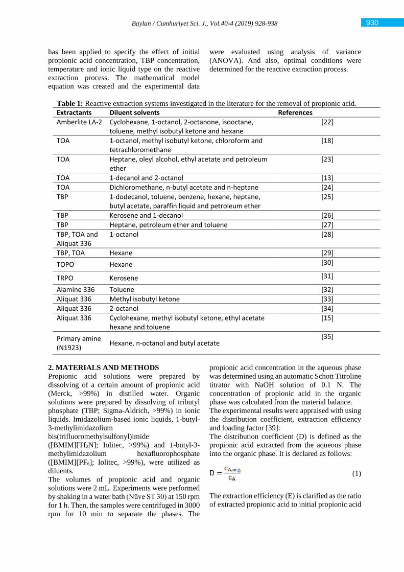
Baylan / Cumhuriyet Sci. J., Vol.40-4 (2019) 928-938
has been applied to specify the effect of initial
propionic acid concentration, TBP concentration,
temperature and ionic liquid type on the reactive
extraction process. The mathematical model
equation was created and the experimental data
were evaluated using analysis of variance
(ANOVA). And also, optimal conditions were
determined for the reactive extraction process.
Table 1: Reactive extraction systems investigated in the literature for the removal of propionic acid. Extractants Diluent solvents References
Amberlite LA-2 Cyclohexane, 1-octanol, 2-octanone, isooctane, toluene, methyl isobutyl ketone and hexane
[22]
TOA
1-octanol, methyl isobutyl ketone, chloroform and tetrachloromethane
[18]
TOA Heptane, oleyl alcohol, ethyl acetate and petroleum ether
[23]
TOA 1-decanol and 2-octanol [13]
TOA Dichloromethane, n‐butyl acetate and n‐heptane [24]
TBP 1-dodecanol, toluene, benzene, hexane, heptane, butyl acetate, paraffin liquid and petroleum ether
[25]
TBP Kerosene and 1-decanol [26]
TBP Heptane, petroleum ether and toluene [27]
TBP, TOA and Aliquat 336
1-octanol [28]
TBP, TOA Hexane [29]
TOPO Hexane [30]
TRPO Kerosene [31]
Alamine 336 Toluene [32]
Aliquat 336 Methyl isobutyl ketone [33]
Aliquat 336 2-octanol [34]
Aliquat 336 Cyclohexane, methyl isobutyl ketone, ethyl acetate hexane and toluene
[15]
Primary amine (N1923)
Hexane, n-octanol and butyl acetate [35]
2. MATERIALS AND METHODS
Propionic acid solutions were prepared by
dissolving of a certain amount of propionic acid
(Merck, >99%) in distilled water. Organic
solutions were prepared by dissolving of tributyl
phosphate (TBP; Sigma-Aldrich, >99%) in ionic
liquids. Imidazolium-based ionic liquids, 1-butyl-
3-methylimidazolium
bis(trifluoromethylsulfonyl)imide
([BMIM][Tf2N]; Iolitec, >99%) and 1-butyl-3-
methylimidazolium hexafluorophosphate
([BMIM][PF6]; Iolitec, >99%), were utilized as
diluents.
The volumes of propionic acid and organic
solutions were 2 mL. Experiments were performed
by shaking in a water bath (Nüve ST 30) at 150 rpm
for 1 h. Then, the samples were centrifuged in 3000
rpm for 10 min to separate the phases. The
propionic acid concentration in the aqueous phase
was determined using an automatic Schott Titroline
titrator with NaOH solution of 0.1 N. The
concentration of propionic acid in the organic
phase was calculated from the material balance.
The experimental results were appraised with using
the distribution coefficient, extraction efficiency
and loading factor [39]:
The distribution coefficient (D) is defined as the
propionic acid extracted from the aqueous phase
into the organic phase. It is declared as follows:
(1)
The extraction efficiency (E) is clarified as the ratio
of extracted propionic acid to initial propionic acid
930
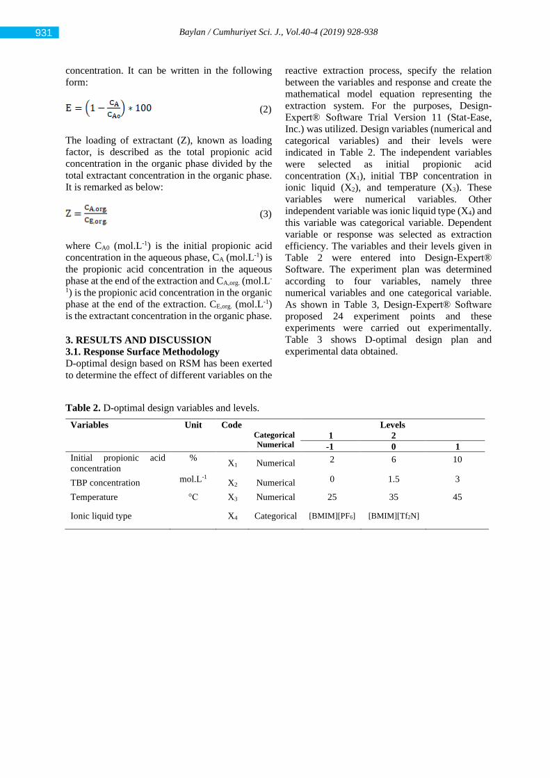
Baylan / Cumhuriyet Sci. J., Vol.40-4 (2019) 928-938
concentration. It can be written in the following
form:
(2)
The loading of extractant (Z), known as loading
factor, is described as the total propionic acid
concentration in the organic phase divided by the
total extractant concentration in the organic phase.
It is remarked as below:
(3)
where CA0 (mol.L-1) is the initial propionic acid
concentration in the aqueous phase, CA (mol.L-1) is
the propionic acid concentration in the aqueous
phase at the end of the extraction and CA,org. (mol.L-
1) is the propionic acid concentration in the organic
phase at the end of the extraction. CE,org. (mol.L-1)
is the extractant concentration in the organic phase. 3. RESULTS AND DISCUSSION 3.1. Response Surface Methodology
D-optimal design based on RSM has been exerted
to determine the effect of different variables on the
reactive extraction process, specify the relation
between the variables and response and create the
mathematical model equation representing the
extraction system. For the purposes, Design-
Expert® Software Trial Version 11 (Stat-Ease,
Inc.) was utilized. Design variables (numerical and
categorical variables) and their levels were
indicated in Table 2. The independent variables
were selected as initial propionic acid
concentration (X1), initial TBP concentration in
ionic liquid (X2), and temperature (X3). These
variables were numerical variables. Other
independent variable was ionic liquid type (X4) and
this variable was categorical variable. Dependent
variable or response was selected as extraction
efficiency. The variables and their levels given in
Table 2 were entered into Design-Expert®
Software. The experiment plan was determined
according to four variables, namely three
numerical variables and one categorical variable.
As shown in Table 3, Design-Expert® Software
proposed 24 experiment points and these
experiments were carried out experimentally.
Table 3 shows D-optimal design plan and
experimental data obtained.
Table 2. D-optimal design variables and levels.
Variables Unit Code Categorical
Numerical
Levels
1 2
-1 0 1
Initial propionic acid
concentration
% X1 Numerical 2 6 10
TBP concentration mol.L-1 X2 Numerical 0 1.5 3
Temperature °C X3 Numerical 25 35 45
Ionic liquid type
X4 Categorical [BMIM][PF6] [BMIM][Tf2N]
931
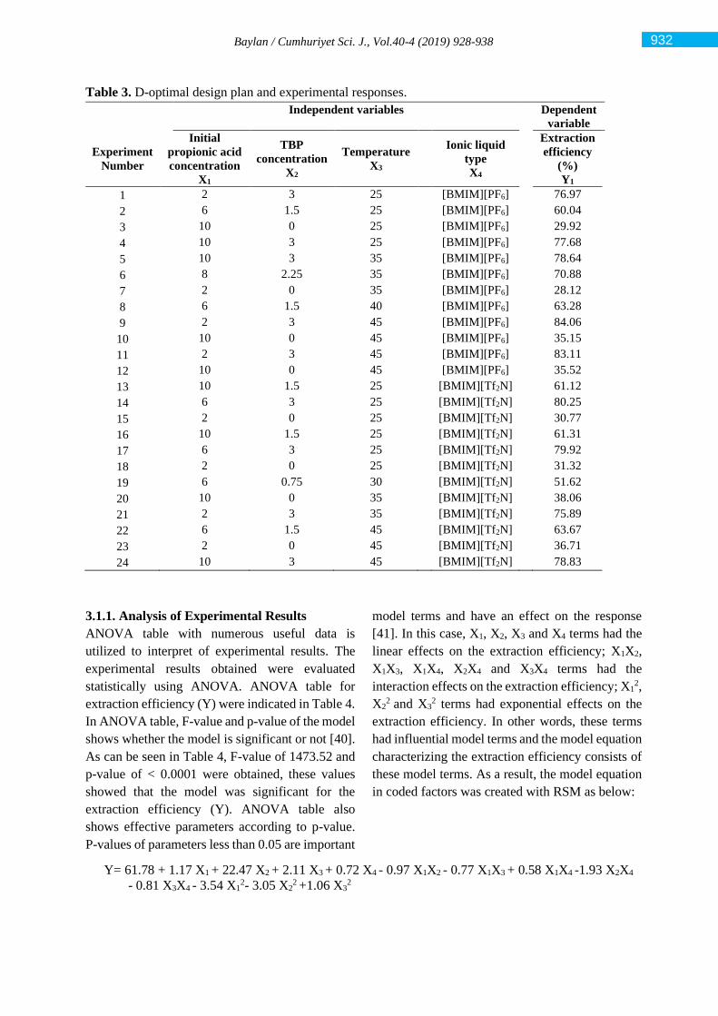
Baylan / Cumhuriyet Sci. J., Vol.40-4 (2019) 928-938
Table 3. D-optimal design plan and experimental responses.
Independent variables Dependent
variable
Experiment
Number
Initial
propionic acid
concentration
X1
TBP
concentration
X2
Temperature
X3
Ionic liquid
type
X4
Extraction
efficiency
(%)
Y1
1 2 3 25 [BMIM][PF6] 76.97
2 6 1.5 25 [BMIM][PF6] 60.04
3 10 0 25 [BMIM][PF6] 29.92
4 10 3 25 [BMIM][PF6] 77.68
5 10 3 35 [BMIM][PF6] 78.64
6 8 2.25 35 [BMIM][PF6] 70.88
7 2 0 35 [BMIM][PF6] 28.12
8 6 1.5 40 [BMIM][PF6] 63.28
9 2 3 45 [BMIM][PF6] 84.06
10 10 0 45 [BMIM][PF6] 35.15
11 2 3 45 [BMIM][PF6] 83.11
12 10 0 45 [BMIM][PF6] 35.52
13 10 1.5 25 [BMIM][Tf2N] 61.12
14 6 3 25 [BMIM][Tf2N] 80.25
15 2 0 25 [BMIM][Tf2N] 30.77
16 10 1.5 25 [BMIM][Tf2N] 61.31
17 6 3 25 [BMIM][Tf2N] 79.92
18 2 0 25 [BMIM][Tf2N] 31.32
19 6 0.75 30 [BMIM][Tf2N] 51.62
20 10 0 35 [BMIM][Tf2N] 38.06
21 2 3 35 [BMIM][Tf2N] 75.89
22 6 1.5 45 [BMIM][Tf2N] 63.67
23 2 0 45 [BMIM][Tf2N] 36.71
24 10 3 45 [BMIM][Tf2N] 78.83
3.1.1. Analysis of Experimental Results
ANOVA table with numerous useful data is
utilized to interpret of experimental results. The
experimental results obtained were evaluated
statistically using ANOVA. ANOVA table for
extraction efficiency (Y) were indicated in Table 4.
In ANOVA table, F-value and p-value of the model
shows whether the model is significant or not [40].
As can be seen in Table 4, F-value of 1473.52 and
p-value of < 0.0001 were obtained, these values
showed that the model was significant for the
extraction efficiency (Y). ANOVA table also
shows effective parameters according to p-value.
P-values of parameters less than 0.05 are important
model terms and have an effect on the response
[41]. In this case, X1, X2, X3 and X4 terms had the
linear effects on the extraction efficiency; X1X2,
X1X3, X1X4, X2X4 and X3X4 terms had the
interaction effects on the extraction efficiency; X12,
X22 and X3
2 terms had exponential effects on the
extraction efficiency. In other words, these terms
had influential model terms and the model equation
characterizing the extraction efficiency consists of
these model terms. As a result, the model equation
in coded factors was created with RSM as below:
Y= 61.78 + 1.17 X1 + 22.47 X2 + 2.11 X3 + 0.72 X4 - 0.97 X1X2 - 0.77 X1X3 + 0.58 X1X4 -1.93 X2X4
- 0.81 X3X4 - 3.54 X12- 3.05 X2
2 +1.06 X32
932
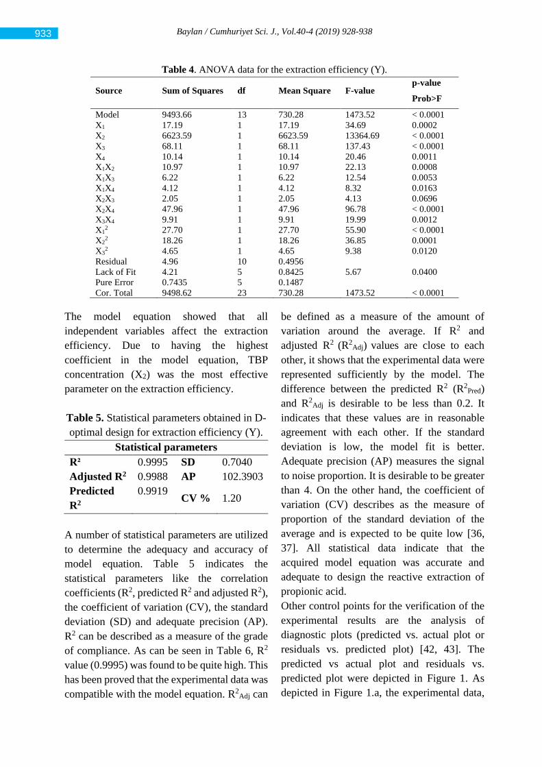
Baylan / Cumhuriyet Sci. J., Vol.40-4 (2019) 928-938
Table 4. ANOVA data for the extraction efficiency (Y).
Source Sum of Squares df Mean Square F-value p-value
Prob>F
Model 9493.66 13 730.28 1473.52 < 0.0001
X1 17.19 1 17.19 34.69 0.0002
X2 6623.59 1 6623.59 13364.69 < 0.0001
X3 68.11 1 68.11 137.43 < 0.0001
X4 10.14 1 10.14 20.46 0.0011
X1X2 10.97 1 10.97 22.13 0.0008
X1X3 6.22 1 6.22 12.54 0.0053
X1X4 4.12 1 4.12 8.32 0.0163
X2X3 2.05 1 2.05 4.13 0.0696
X2X4 47.96 1 47.96 96.78 < 0.0001
X3X4 9.91 1 9.91 19.99 0.0012
X12 27.70 1 27.70 55.90 < 0.0001
X22 18.26 1 18.26 36.85 0.0001
X32 4.65 1 4.65 9.38 0.0120
Residual 4.96 10 0.4956
Lack of Fit 4.21 5 0.8425 5.67 0.0400
Pure Error 0.7435 5 0.1487
Cor. Total 9498.62 23 730.28 1473.52 < 0.0001
The model equation showed that all
independent variables affect the extraction
efficiency. Due to having the highest
coefficient in the model equation, TBP
concentration (X2) was the most effective
parameter on the extraction efficiency.
Table 5. Statistical parameters obtained in D-
optimal design for extraction efficiency (Y).
Statistical parameters
R² 0.9995 SD 0.7040
Adjusted R2 0.9988 AP 102.3903
Predicted
R2
0.9919 CV % 1.20
A number of statistical parameters are utilized
to determine the adequacy and accuracy of
model equation. Table 5 indicates the
statistical parameters like the correlation
coefficients (R2, predicted R2 and adjusted R2),
the coefficient of variation (CV), the standard
deviation (SD) and adequate precision (AP).
R2 can be described as a measure of the grade
of compliance. As can be seen in Table 6, R2
value (0.9995) was found to be quite high. This
has been proved that the experimental data was
compatible with the model equation. R2Adj can
be defined as a measure of the amount of
variation around the average. If R2 and
adjusted R2 (R2Adj) values are close to each
other, it shows that the experimental data were
represented sufficiently by the model. The
difference between the predicted R2 (R2Pred)
and R2Adj is desirable to be less than 0.2. It
indicates that these values are in reasonable
agreement with each other. If the standard
deviation is low, the model fit is better.
Adequate precision (AP) measures the signal
to noise proportion. It is desirable to be greater
than 4. On the other hand, the coefficient of
variation (CV) describes as the measure of
proportion of the standard deviation of the
average and is expected to be quite low [36,
37]. All statistical data indicate that the
acquired model equation was accurate and
adequate to design the reactive extraction of
propionic acid.
Other control points for the verification of the
experimental results are the analysis of
diagnostic plots (predicted vs. actual plot or
residuals vs. predicted plot) [42, 43]. The
predicted vs actual plot and residuals vs.
predicted plot were depicted in Figure 1. As
depicted in Figure 1.a, the experimental data,
933
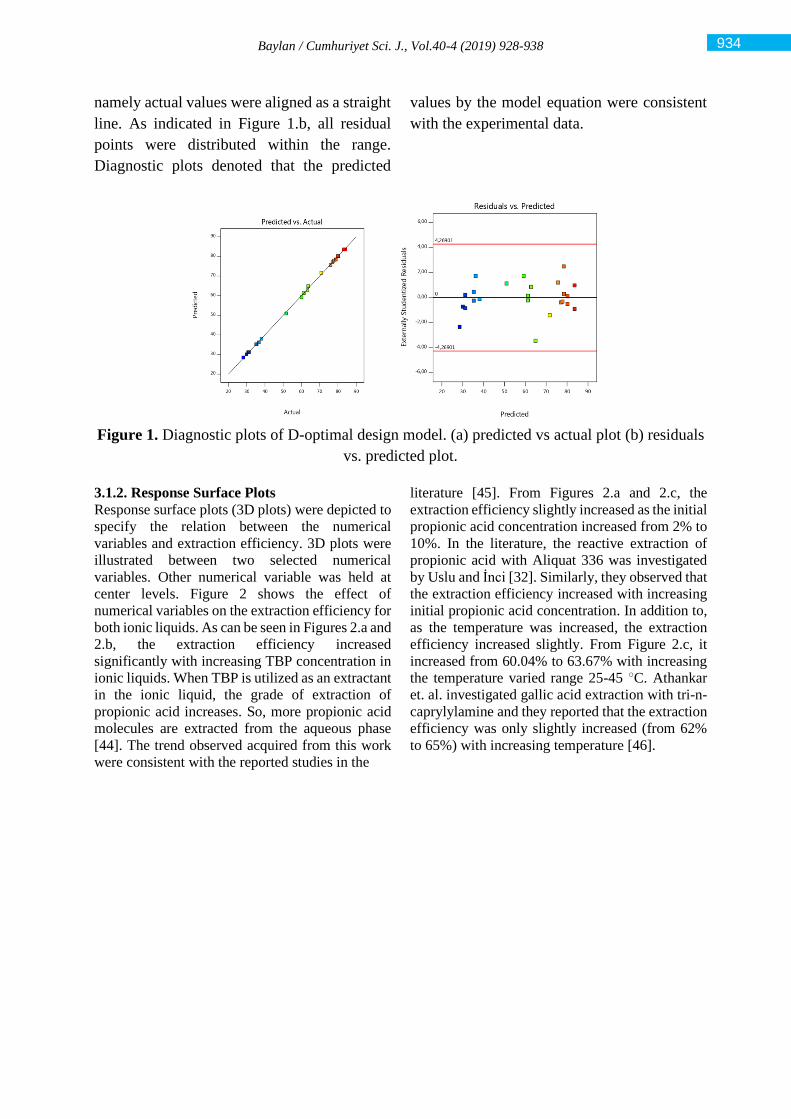
Baylan / Cumhuriyet Sci. J., Vol.40-4 (2019) 928-938
namely actual values were aligned as a straight
line. As indicated in Figure 1.b, all residual
points were distributed within the range.
Diagnostic plots denoted that the predicted
values by the model equation were consistent
with the experimental data.
Figure 1. Diagnostic plots of D-optimal design model. (a) predicted vs actual plot (b) residuals
vs. predicted plot.
3.1.2. Response Surface Plots
Response surface plots (3D plots) were depicted to
specify the relation between the numerical
variables and extraction efficiency. 3D plots were
illustrated between two selected numerical
variables. Other numerical variable was held at
center levels. Figure 2 shows the effect of
numerical variables on the extraction efficiency for
both ionic liquids. As can be seen in Figures 2.a and
2.b, the extraction efficiency increased
significantly with increasing TBP concentration in
ionic liquids. When TBP is utilized as an extractant
in the ionic liquid, the grade of extraction of
propionic acid increases. So, more propionic acid
molecules are extracted from the aqueous phase
[44]. The trend observed acquired from this work
were consistent with the reported studies in the
literature [45]. From Figures 2.a and 2.c, the
extraction efficiency slightly increased as the initial
propionic acid concentration increased from 2% to
10%. In the literature, the reactive extraction of
propionic acid with Aliquat 336 was investigated
by Uslu and İnci [32]. Similarly, they observed that
the extraction efficiency increased with increasing
initial propionic acid concentration. In addition to,
as the temperature was increased, the extraction
efficiency increased slightly. From Figure 2.c, it
increased from 60.04% to 63.67% with increasing
the temperature varied range 25-45 C. Athankar
et. al. investigated gallic acid extraction with tri-n-
caprylylamine and they reported that the extraction
efficiency was only slightly increased (from 62%
to 65%) with increasing temperature [46].
934
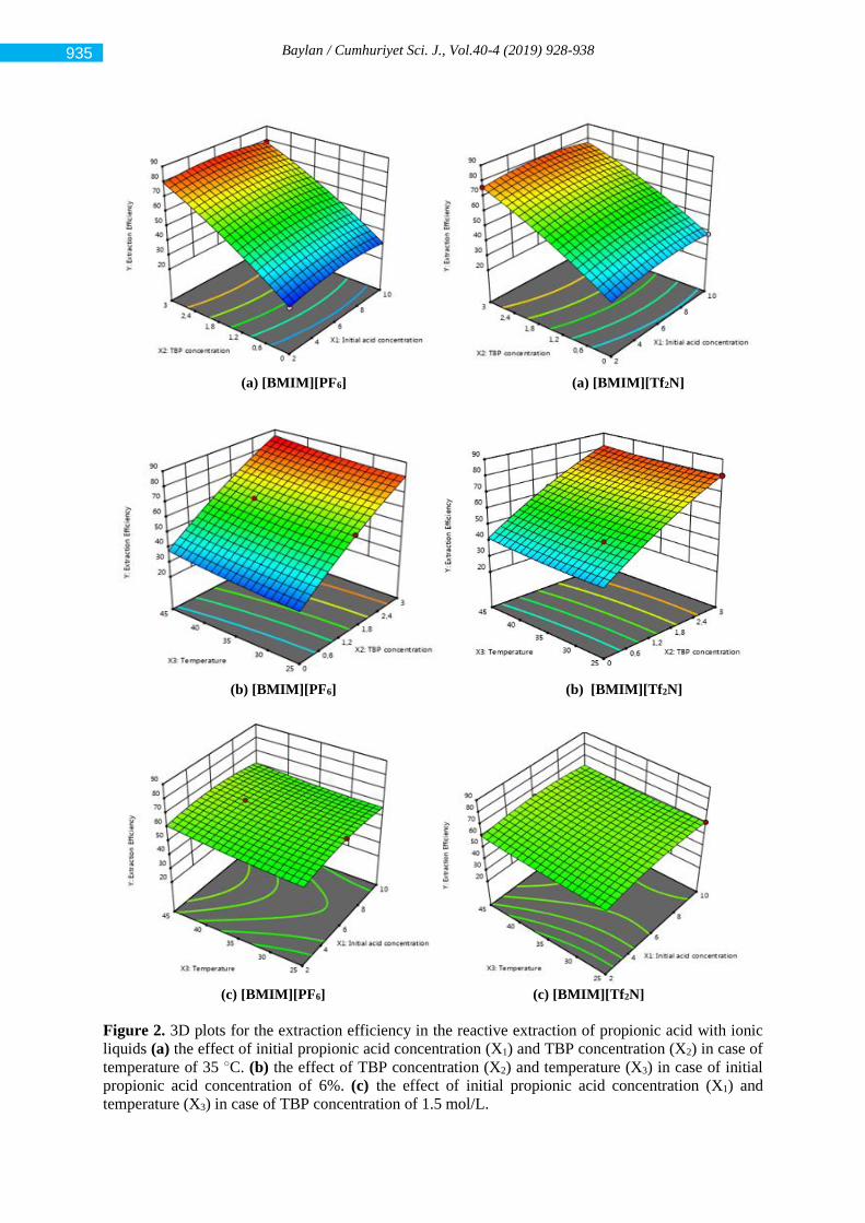
Baylan / Cumhuriyet Sci. J., Vol.40-4 (2019) 928-938
(a) [BMIM][PF6] (a) [BMIM][Tf2N]
(b) [BMIM][PF6] (b) [BMIM][Tf2N]
(c) [BMIM][PF6] (c) [BMIM][Tf2N]
Figure 2. 3D plots for the extraction efficiency in the reactive extraction of propionic acid with ionic
liquids (a) the effect of initial propionic acid concentration (X1) and TBP concentration (X2) in case of
temperature of 35 C. (b) the effect of TBP concentration (X2) and temperature (X3) in case of initial
propionic acid concentration of 6%. (c) the effect of initial propionic acid concentration (X1) and
temperature (X3) in case of TBP concentration of 1.5 mol/L.
935
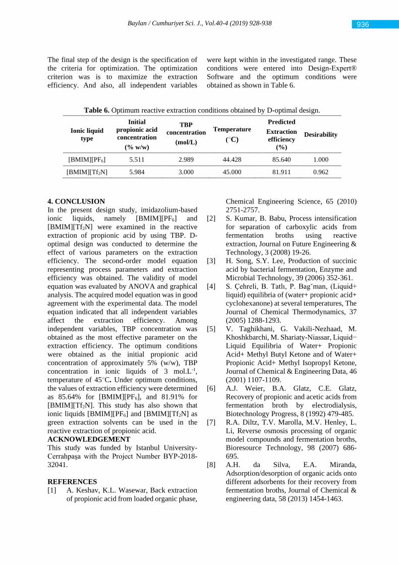
Baylan / Cumhuriyet Sci. J., Vol.40-4 (2019) 928-938
The final step of the design is the specification of
the criteria for optimization. The optimization
criterion was is to maximize the extraction
efficiency. And also, all independent variables
were kept within in the investigated range. These
conditions were entered into Design-Expert®
Software and the optimum conditions were
obtained as shown in Table 6.
Table 6. Optimum reactive extraction conditions obtained by D-optimal design.
Ionic liquid
type
Initial
propionic acid
concentration
(% w/w)
TBP
concentration
(mol/L)
Temperature
(C)
Predicted
Extraction
efficiency
(%)
Desirability
[BMIM][PF6] 5.511 2.989 44.428 85.640 1.000
[BMIM][Tf2N] 5.984 3.000 45.000 81.911 0.962
4. CONCLUSION
In the present design study, imidazolium-based
ionic liquids, namely [BMIM][PF6] and
[BMIM][Tf2N] were examined in the reactive
extraction of propionic acid by using TBP. D-
optimal design was conducted to determine the
effect of various parameters on the extraction
efficiency. The second-order model equation
representing process parameters and extraction
efficiency was obtained. The validity of model
equation was evaluated by ANOVA and graphical
analysis. The acquired model equation was in good
agreement with the experimental data. The model
equation indicated that all independent variables
affect the extraction efficiency. Among
independent variables, TBP concentration was
obtained as the most effective parameter on the
extraction efficiency. The optimum conditions
were obtained as the initial propionic acid
concentration of approximately 5% (w/w), TBP
concentration in ionic liquids of 3 mol.L-1,
temperature of 45C. Under optimum conditions,
the values of extraction efficiency were determined
as 85.64% for [BMIM][PF6], and 81.91% for
[BMIM][Tf2N]. This study has also shown that
ionic liquids [BMIM][PF6] and [BMIM][Tf2N] as
green extraction solvents can be used in the
reactive extraction of propionic acid.
ACKNOWLEDGEMENT
This study was funded by Istanbul University-
Cerrahpaşa with the Project Number BYP-2018-
32041.
REFERENCES
[1] A. Keshav, K.L. Wasewar, Back extraction
of propionic acid from loaded organic phase,
Chemical Engineering Science, 65 (2010)
2751-2757.
[2] S. Kumar, B. Babu, Process intensification
for separation of carboxylic acids from
fermentation broths using reactive
extraction, Journal on Future Engineering &
Technology, 3 (2008) 19-26.
[3] H. Song, S.Y. Lee, Production of succinic
acid by bacterial fermentation, Enzyme and
Microbial Technology, 39 (2006) 352-361.
[4] S. Çehreli, B. Tatlı, P. Bagˇman, (Liquid+
liquid) equilibria of (water+ propionic acid+
cyclohexanone) at several temperatures, The
Journal of Chemical Thermodynamics, 37
(2005) 1288-1293.
[5] V. Taghikhani, G. Vakili-Nezhaad, M.
Khoshkbarchi, M. Shariaty-Niassar, Liquid−
Liquid Equilibria of Water+ Propionic
Acid+ Methyl Butyl Ketone and of Water+
Propionic Acid+ Methyl Isopropyl Ketone,
Journal of Chemical & Engineering Data, 46
(2001) 1107-1109.
[6] A.J. Weier, B.A. Glatz, C.E. Glatz,
Recovery of propionic and acetic acids from
fermentation broth by electrodialysis,
Biotechnology Progress, 8 (1992) 479-485.
[7] R.A. Diltz, T.V. Marolla, M.V. Henley, L.
Li, Reverse osmosis processing of organic
model compounds and fermentation broths,
Bioresource Technology, 98 (2007) 686-
695.
[8] A.H. da Silva, E.A. Miranda,
Adsorption/desorption of organic acids onto
different adsorbents for their recovery from
fermentation broths, Journal of Chemical &
engineering data, 58 (2013) 1454-1463.
936
Baylan / Cumhuriyet Sci. J., Vol.40-4 (2019) 928-938
[9] A. Freitas, M. Mendes, G. Coelho,
Thermodynamic study of fatty acids
adsorption on different adsorbents, The
Journal of Chemical Thermodynamics, 39
(2007) 1027-1037.
[10] İ. İnci, Ş.S. Bayazit, H. Uslu, Investigation
of adsorption equilibrium and kinetics of
propionic acid and glyoxylic acid from
aqueous solution by alumina, Journal of
Chemical & Engineering Data, 56 (2011)
3301-3308.
[11] H. Uslu, İ. İnci, S.S. Bayazit, G.K. Demir,
Comparison of solid− liquid equilibrium
data for the adsorption of propionic acid and
tartaric acid from aqueous solution onto
Amberlite IRA-67, Industrial & Engineering
Chemistry Research, 48 (2009) 7767-7772.
[12] R. Wodzki, J. Nowaczyk, M. Kujawski,
Separation of propionic and acetic acid by
pertraction in a multimembrane hybrid
system, Separation and Purification
Technology, 21 (2000) 39-54.
[13] A. Keshav, K.L. Wasewar, S. Chand,
Reactive extraction of propionic acid using
tri-n-octylamine, Chemical Engineering
Communications, 197 (2009) 606-626.
[14] S. Kumar, D. Datta, B. Babu, Estimation of
equilibrium parameters using differential
evolution in reactive extraction of propionic
acid by tri-n-butyl phosphate, Chemical
Engineering and Processing: Process
Intensification, 50 (2011) 614-622.
[15] H. Uslu, İ. İnci, (Liquid+ liquid) equilibria
of the (water+ propionic acid+ Aliquat 336+
organic solvents) at T= 298.15 K, The
Journal of Chemical Thermodynamics, 39
(2007) 804-809.
[16] M. Rodriguez, S. Luque, J. Alvarez, J. Coca,
Extractive ultrafiltration for the removal of
valeric acid, Journal of Membrane Science,
120 (1996) 35-43.
[17] M.O. Ruiz, J.L. Cabezas, I. Escudero, J.
Coca, Valeric Acid Extraction with Tri‐N‐
butyl Phosphate Impregnated in a
Macroporous Resin. I. Equilibrium and
Mass Transfer Rates, Separation Science
and Technology, 39 (2005) 77-95.
[18] Z. Li, W. Qin, Y. Dai, Liquid− liquid
equilibria of acetic, propionic, butyric, and
valeric acids with trioctylamine as
extractant, Journal of Chemical &
Engineering Data, 47 (2002) 843-848.
[19] K. Ghandi, A review of ionic liquids, their
limits and applications, Green and
Sustainable Chemistry, 4 (2014) 44-53.
[20] K. Mikami, Green reaction media in organic
synthesis, Wiley Online Library, 2005.
[21] L. Sprakel, B. Schuur, Solvent developments
for liquid-liquid extraction of carboxylic
acids in perspective, Separation and
Purification Technology, 211 (2019) 935-
957.
[22] Y.S. Aşçı, İ. İnci, Extraction equilibria of
propionic acid from aqueous solutions by
Amberlite LA-2 in diluent solvents,
Chemical Engineering Journal, 155 (2009)
784-788.
[23] A. Keshav, K.L. Wasewar, S. Chand,
Extraction of propionic acid with tri-n-octyl
amine in different diluents, Separation and
Purification Technology, 63 (2008) 179-
183.
[24] A.I. Galaction, A. Carlescu, M. Turnea, D.
Caşcaval, Direct Extraction of Propionic
Acid from Propionibacterium
acidipropionici Broths with Tri‐n‐
octylamine, Chemical Engineering &
Technology, 35 (2012) 1657-1663.
[25] A. Keshav, S. Chand, K.L. Wasewar,
Equilibrium studies for extraction of
propionic acid using tri-n-butyl phosphate in
different solvents, Journal of Chemical &
Engineering Data, 53 (2008) 1424-1430.
[26] S. Kumar, D. Datta, B. Babu, Differential
evolution approach for reactive extraction of
propionic acid using tri-n-butyl phosphate
(TBP) in kerosene and 1-decanol, Materials
and Manufacturing Processes, 26 (2011)
1222-1228.
[27] A. Keshav, K.L. Wasewar, S. Chand,
Recovery of propionic acid from an aqueous
stream by reactive extraction: Effect of
diluents, Desalination, 244 (2009) 12-23.
[28] A. Keshav, K.L. Wasewar, S. Chand,
Extraction of propionic acid using different
extractants (tri-n-butylphosphate, tri-n-
octylamine, and Aliquat 336), Industrial &
Engineering Chemistry Research, 47 (2008)
6192-6196.
[29] M. Matsumoto, T. Otono, K. Kondo,
Synergistic extraction of organic acids with
tri-n-octylamine and tri-n-butylphosphate,
Separation and Purification Technology, 24
(2001) 337-342.
[30] A. Keshav, K.L. Wasewar, S. Chand,
Equilibrium and Kinetics of the Extraction
of Propionic Acid Using Tri‐n‐
Octylphosphineoxide, Chemical
Engineering & Technology: Industrial
Chemistry‐Plant Equipment‐Process
937
Baylan / Cumhuriyet Sci. J., Vol.40-4 (2019) 928-938
Engineering‐Biotechnology, 31 (2008)
1290-1295.
[31] Y. Wang, Y. Li, Y. Li, J. Wang, Z. Li, Y.
Dai, Extraction equilibria of
monocarboxylic acids with
trialkylphosphine oxide, Journal of
Chemical & Engineering Data, 46 (2001)
831-837.
[32] H. Uslu, Linear solvation energy
relationship (LSER) Modeling and kinetic
studies on propionic acid reactive extraction
using Alamine 336 in a toluene solution,
Industrial & Engineering Chemistry
Research, 45 (2006) 5788-5795.
[33] A. Keshav, K.L. Wasewar, S. Chand,
Reactive extraction of propionic acid using
Aliquat 336 in MIBK: Linear solvation
energy relationship (LSER) modeling and
kinetics study, Journal of Scientific and
Industrial Research 2009; 68: 708-713.
[34] A. Keshav, K. Wasewar, S. Chand, H. Uslu,
Reactive extraction of propionic acid using
Aliquat-336 in 2-octanol: Linear solvation
energy relationship (LSER) modeling and
kinetics study, Chemical and Biochemical
Engineering Quarterly, 24 (2010) 67-73.
[35] K. Wang, Z. Chang, Y. Ma, C. Lei, S. Jin, Y.
Wu, I. Mahmood, C. Hua, H. Liu,
Equilibrium study on reactive extraction of
propionic acid with N1923 in different
diluents, Fluid Phase Equilibria, 278 (2009)
103-108.
[36] N. Baylan, S. Çehreli, Ionic liquids as bulk
liquid membranes on levulinic acid removal:
A design study, Journal of Molecular
Liquids, 266 (2018) 299-308.
[37] N. Baylan, S. Çehreli, Removal of acetic
acid from aqueous solutions using bulk ionic
liquid membranes: A transport and
experimental design study, Separation and
Purification Technology, 224 (2019) 51-61.
[38] D. Granato, V.M. de Araújo Calado, The use
and importance of design of experiments
(DOE) in process modelling in food science
and technology, Mathematical and statistical
methods in food science and technology, 1
(2014) 1-18.
[39] İ. İnci, Linear solvation energy relationship
modeling and kinetic studies on reactive
extraction of succinic acid by
tridodecylamine dissolved in MIBK,
Biotechnology Progress, 23 (2007) 1171-
1179.
[40] C.-C. Chen, K.-T. Chiang, C.-C. Chou, Y.-
C. Liao, The use of D-optimal design for
modeling and analyzing the vibration and
surface roughness in the precision turning
with a diamond cutting tool, The
International Journal of Advanced
Manufacturing Technology, 54 (2011) 465-
478.
[41] M.D. Turan, Statistical Approach to Mineral
Engineering and Optimization,
Contributions to Mineralization,
IntechOpen, 2018.
[42] A. Asghar, A. Raman, A. Aziz, W.M.A.W.
Daud, A comparison of central composite
design and Taguchi method for optimizing
Fenton process, The Scientific World
Journal, 2014 (2014) 1-14.
[43] T. Rajmohan, K. Palanikumar, Modeling
and analysis of performances in drilling
hybrid metal matrix composites using D-
optimal design, The International Journal of
Advanced Manufacturing Technology, 64
(2013) 1249-1261.
[44] M. Djas, M. Henczka, Reactive extraction of
carboxylic acids using organic solvents and
supercritical fluids: a review, Separation and
Purification Technology, 201 (2018) 106-
119.
[45] K.L. Wasewar, D. Shende, A. Keshav,
Reactive extraction of itaconic acid using tri‐
n‐butyl phosphate and aliquat 336 in
sunflower oil as a non‐toxic diluent, Journal
of Chemical Technology & Biotechnology,
86 (2011) 319-323.
[46] K.K. Athankar, K.L. Wasewar, M.N.
Varma, D.Z. Shende, Reactive extraction of
gallic acid with tri-n-caprylylamine, New
Journal of Chemistry, 40 (2016) 2413-2417.
938
Cumhuriyet Science Journal
CSJ
e-ISSN: 2587-246X
ISSN: 2587-2680 Cumhuriyet Sci. J., Vol.40-4 (2019) 939-945
* Corresponding author. Email address: [email protected]
http://dergipark.gov.tr/csj ©2016 Faculty of Science, Sivas Cumhuriyet University
CT and MRI Medical Image Fusion Using Discrete Wavelet Transform
Molham Moshantat 1 , Saeid Karamzadeh2 *
1 Electrical and Electronics Engineering, Istanbul Aydın University, Istanbul, TURKEY
2 Electrical and Electronics Engineering Department, Faculty of Engineering and Natural Sciences, Bahçeşehir
University, Istanbul, TURKEY
Received: 04.04.2019; Accepted: 24.05.2019 http://dx.doi.org/10.17776/csj.549192
Abstract. In these days, using medical image is very important in hospitals. These medical images give a lot
of data about human body for example Computed Tomography (CT) identifies the bone structure, Magnetic
Resonance Image (MRI) image gives information about tissue data, Positron on Emission Tomography (PET)
and Single photon release computed tomography (SPECT) give human body functionality data. but these
images can't give clear data image for disease diagnosis and treatment planning. So, these different modality
complementary data for effective disease analysis is required. In this work we fused two images (CT and MRI)
by using discrete wavelet transform then applied this transform on all types of wavelets (haar, Daubechies,
Mexican Hat, Symlets, Morlet, Shannon).
Keywords: Image fusion, DWT, PSNR, IDWT, CT, MRI, Entropy.
Ayrık Dalgacık Dönüşümü ile CT ve MRI Medikal Görüntü Füzyonu
Özet. Günümüzde medikal görüntülerin teşhis ve tedavide büyük bir rol oynadığı aşikardır. Daha fazla bilgi
taşıyan ve birden fazla görüntünün füzyonundan ulaşan bir görüntü bu sürece katkı sağlayacaktır. Bu çalışmada
ise, CT ve MRI görüntülerinin füzyonu için, literatürde bilinen en iyi füzyon yöntemlerinden bir olan dalgacık
dönüşümü uygulanmıştır. Farklı dalgacık dönüşümleri kullanılıp sonuçları sunulmuştur. Çıkan sonuçların
karşılaştırılması için entropi ve sinyal, gürültü oranı (SNR) ölçülüp verilmiştir.
Anahtar Kelimeler: Dalgacık Dönüşümü, Görüntü Füzyonu, Entropi.
1. INTRODUCTION
These days, with the accelerate advancement in
high-technology and contemporary
instrumentation, medical imaging is now an
essential part of a high number of applications,
such as diagnosis, research, and treatment, for
medical examination, just one sort of image might
not be enough to supply accurate clinical
prerequisite for doctors. Consequently, the
combination of this multi-modal medical images is
required [1]. Medical imaging provides many
modes of images information for the clinical
examination including CT, X-ray, DSA, MRI,
PET, SPECT etc. Different medical images have
different features, which may provide structural
knowledge of distinct organs. By way of instance,
CT (Computed tomography) and MRI (Magnetic
resonance image) with high spatial resolution
might offer anatomical construction info of organs.
Thus, an assortment of imaging to get the exact
same organ, they're contradictory but interrelated
and complementary. As a result, the right image
fusion of distinct features becomes an urgent
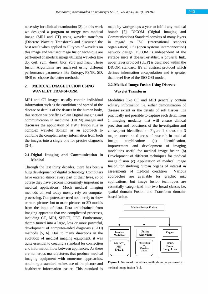
Moshantat, Karamzadeh / Cumhuriyet Sci. J., Vol.40-4 (2019) 939-945
necessity for clinical examination [2]. in this work
we designed a program to merge two medical
image (MRI and CT) using wavelet transform
(Discrete Wavelet Transform) and discussed the
best result when applied to all types of wavelets on
this image and we used image fusion technique are
performed on medical image utilizing wavelets like
db, coif, sym, dmey, bior, rbio and haar. These
fusion Algorithms are analyzed using different
performance parameters like Entropy, PSNR, SD,
SNR to choose the better methods.
2. MEDICAL IMAGE FUSION USING
WAVELET TRANSFORM
MRI and CT images usually contain individual
information such as the condition and spread of the
disease or details of the tissues in the human body,
this section we briefly explain Digital imaging and
communication in medicine (DICM) images and
discusses the application of DWT fusion rule in
complex wavelet domain as an approach to
combine the complementary information from both
the images into a single one for precise diagnosis
[3-4].
2.1. Digital Imaging and Communication in
Medical
Through the last thirty decades, there has been a
huge development of digital technology. Computers
have entered almost every part of their lives, so of
course they have become increasingly important in
medical applications. Much medical imaging
methods utilized today mostly rely on computer
processing. Computers are used not merely to show
or store pictures but to make pictures or 3D models
from the input of data. Data are obtained from
imaging apparatus that use complicated processes,
including CT, MRI, SPECT, PET. Furthermore,
there's turned into a large, less or more powerful,
development of computer-aided diagnosis (CAD)
methods [5, 6]. Due to many directions in the
evolution of medical imaging equipment, it was
quite essential to creating a standard for connection
and information flow between appliances. As there
are numerous manufacturers that produce medical
imaging equipment with numerous approaches,
obtaining a standard makes use of the picture and
healthcare information easier. This standard is
made by workgroups a year to fulfill any medical
branch [7]. DICOM (Digital Imaging and
Communication) Standard consists of many layers
in regard to ISO (international standers
organization) OSI (open systems interconnection)
network design. DICOM is independent of the
surface since it doesn't establish a physical link.
upper layer protocol (ULP) is described within the
DICOM standard. It's an abstract protocol which
defines information encapsulation and is greater
than level five of the ISO OSI model.
2.2. Medical Image Fusion Using Discrete
Wavelet Transform
Modalities like CT and MRI generally contain
solitary information i.e. either demonstration of
disease extent or the details of soft tissues. It's
practically not possible to capture each detail from
1 imaging modality that will ensure clinical
precision and robustness of the investigation and
consequent identification. Figure 1 shows the 3
major concentrated areas of research in medical
image combination: (a) Identification,
improvement and development of imaging
modalities useful for medical image fusion (b)
Development of different techniques for medical
image fusion (c) Application of medical image
fusion for studying human organs of interest in
assessments of medical condition Various
approaches are available for graphic mix
applications, but image fusion techniques are
essentially categorized into two broad classes i.e.
spatial domain Fusion and Transform domain-
based fusion.
Figure 1: Nature of modalities, methods and organs used in
medical image fusion [11].
940

Moshantat, Karamzadeh / Cumhuriyet Sci. J., Vol.40-4 (2019) 939-945
The first idea and concept of wavelet-based
multiresolution analysis came from Mallat. A
wavelet transform is a mathematical tool which
could detect local attributes in a signal process.
Additionally, it may be utilized to segregate two
dimensional (2D) signs like 2D gray-scale image
signals into various varying levels for
multiresolution analysis. Wavelet transform has
been heavily utilized in several locations, including
texture analysis, data compression, feature
detection, and image fusion.
In one dimension (1D) the basic idea of the DWT
is to represent the signal as a superposition of wave
lets. Suppose that a discrete signal is represented by
f(t) the wavelet decomposition is then defined as
𝑓(𝑡) = ∑ 𝑐𝑚,𝑛 𝜓𝑚,𝑛(𝑡)𝑚,𝑛 (1)
Where 𝜓𝑚, 𝑛 (𝑡) = 2−𝑚/2 𝜓 [2−𝑚 𝑡 − 𝑛] and m
and n are integers. Wavelet transform for image
fusion the schematic diagram for wavelet based
fusion techniques is shown in figure 2.
Figure 2: Wavelet Transform on a signal [10].
In all wavelet-based image fusion techniques the
wavelet transforms W of the two registered input
images are computed and these transforms are
combined using some kind of fusion rule Ø. This is
given by equation (2) below:
𝐼(𝑥, 𝑦) = 𝑤−1(𝜙 (𝑊(𝐼1(𝑥, 𝑦)), 𝑊(𝐼2(𝑥, 𝑦))) (2)
where W-1 is the inverse discrete wavelet
transform (IDWT).
Generally, the fundamental idea of image fusion
based on wavelet transform would be to execute a
multiresolution decomposition on every source
image; the coefficients of the low-frequency band
and high-frequency bands are subsequently
performed with a particular mix rule. Following
that, the fused image is accessed by doing the
inverse DWT (IDWT) for its corresponding
combined wavelet coefficients [8, 9].
2.3. Algorithm:
Following algorithm has been developed and
implemented in MATLAB software:
1. Read the image I1 and find its size.
2. Read the second image I2 and find its size.
3. Compute and match the size if not same, make it
same.
4. The indexed image should be DICOM.
5. Perform multilevel wavelet decomposition using
any wavelet (haar, db, bior…). Generate the
coefficient matrices of the level-three
approximation and horizontal, vertical and
diagonal details.
6. Now fuse the wavelet coefficients using discrete
wavelet transform.
7.Generate a final matrix of fused wavelet
coefficients.
8. Compute the inverse wavelet transform to get
the fused image.
9. Finally compute the entropy, SD, PSNR, SNR
and display the results
The block diagram for image fusion is shown in
figure 3.
3. RESULT AND DISCUSSION
PERFORMANCE ANALYSIS
This paper aims to present a new algorithm to
improve the quality of multimodality medical
image fusion using discrete wavelet transform
(DWT) approach. performance of fusion is
calculated on the basis of entropy, SD and PSNR.
The total processing time and the results
demonstrate the effectiveness of fusion scheme
based on wavelet transform. MRI and CT images
are taken as source images (figure 4). MATLAB is
used for the simulation.
941
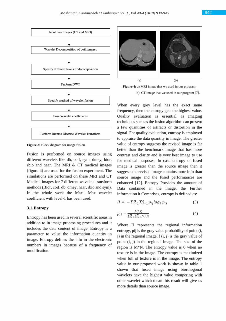
Moshantat, Karamzadeh / Cumhuriyet Sci. J., Vol.40-4 (2019) 939-945
Figure 3: Block diagram for image fusion.
Fusion is performed on source images using
different wavelets like db, coif, sym, dmey, bior,
rbio and haar. The MRI & CT medical images
(figure 4) are used for the fusion experiment. The
simulations are performed on these MRI and CT
Medical images for 7 different wavelets transform
methods (Bior, coif, db, dmey, haar, rbio and sym).
In the whole work the Max– Max wavelet
coefficient with level-1 has been used.
3.1. Entropy
Entropy has been used in several scientific areas in
addition to in image processing procedures and it
includes the data content of image. Entropy is a
parameter to value the information quantity in
image. Entropy defines the info in the electronic
numbers in images because of a frequency of
modification.
(a) (b)
Figure 4: a) MRI image that we used in our program,
b): CT image that we used in our program [7].
When every grey level has the exact same
frequency, then the entropy gets the highest value.
Quality evaluation is essential as Imaging
techniques such as the fusion algorithm can present
a few quantities of artifacts or distortion in the
signal. For quality evaluation, entropy is employed
to appraise the data quantity in image. The greater
value of entropy suggests the revised image is far
better than the benchmark image that has more
contrast and clarity and is your best image to use
for medical purposes. In case entropy of fused
image is greater than the source image then it
suggests the revised image contains more info than
source image and the fused performances are
enhanced [12]. Entropy Provides the amount of
Data contained in the image, the Further
information it Comprises, entropy is defined as:
𝐻 = − ∑ ∑ 𝑝𝑖𝑗𝑙𝑜𝑔2 𝑝𝑖𝑗 𝑁𝑗=1
𝑀𝑖=1 (3)
𝑝𝑖𝑗 =𝑓(𝑖,𝑗)
∑ ∑ 𝑓(𝑖,𝑗)𝑁𝑖=1
𝑀𝑖=1
(4)
Where H represents the regional information
entropy, pij is the gray value probability of point (i,
j) in the regional image, f (i, j) is the gray value of
point (i, j) in the regional image. The size of the
region is M*N. The entropy value is 0 when no
texture is in the image. The entropy is maximized
when full of texture is in the image. The entropy
value in our proposed work is shown in table 1
shown that fused image using biorthogonal
wavelets have the highest value compering with
other wavelet which mean this result will give us
more details than source image.
942
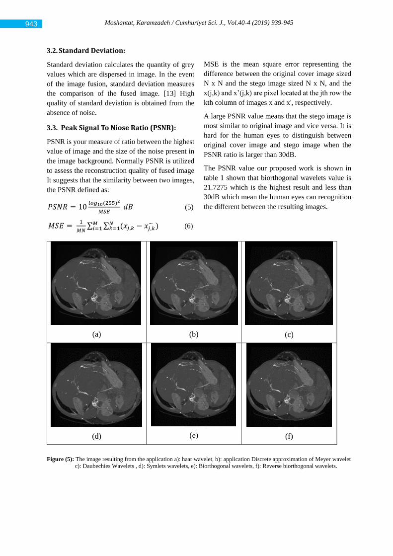
Moshantat, Karamzadeh / Cumhuriyet Sci. J., Vol.40-4 (2019) 939-945
3.2. Standard Deviation:
Standard deviation calculates the quantity of grey
values which are dispersed in image. In the event
of the image fusion, standard deviation measures
the comparison of the fused image. [13] High
quality of standard deviation is obtained from the
absence of noise.
3.3. Peak Signal To Niose Ratio (PSNR):
PSNR is your measure of ratio between the highest
value of image and the size of the noise present in
the image background. Normally PSNR is utilized
to assess the reconstruction quality of fused image
It suggests that the similarity between two images,
the PSNR defined as:
𝑃𝑆𝑁𝑅 = 10𝑙𝑜𝑔10(255)2
𝑀𝑆𝐸 𝑑𝐵 (5)
𝑀𝑆𝐸 = 1
𝑀𝑁∑ ∑ (𝑥𝑗,𝑘 − 𝑥𝑗,𝑘
~ )𝑁𝑘=1
𝑀𝑖=1 (6)
MSE is the mean square error representing the
difference between the original cover image sized
N x N and the stego image sized N x N, and the
x(j,k) and x’(j,k) are pixel located at the jth row the
kth column of images x and x', respectively.
A large PSNR value means that the stego image is
most similar to original image and vice versa. It is
hard for the human eyes to distinguish between
original cover image and stego image when the
PSNR ratio is larger than 30dB.
The PSNR value our proposed work is shown in
table 1 shown that biorthogonal wavelets value is
21.7275 which is the highest result and less than
30dB which mean the human eyes can recognition
the different between the resulting images.
Figure (5): The image resulting from the application a): haar wavelet, b): application Discrete approximation of Meyer wavelet
c): Daubechies Wavelets , d): Symlets wavelets, e): Biorthogonal wavelets, f): Reverse biorthogonal wavelets.
(a)
(b)
(c)
(d)
(e)
(f)
943
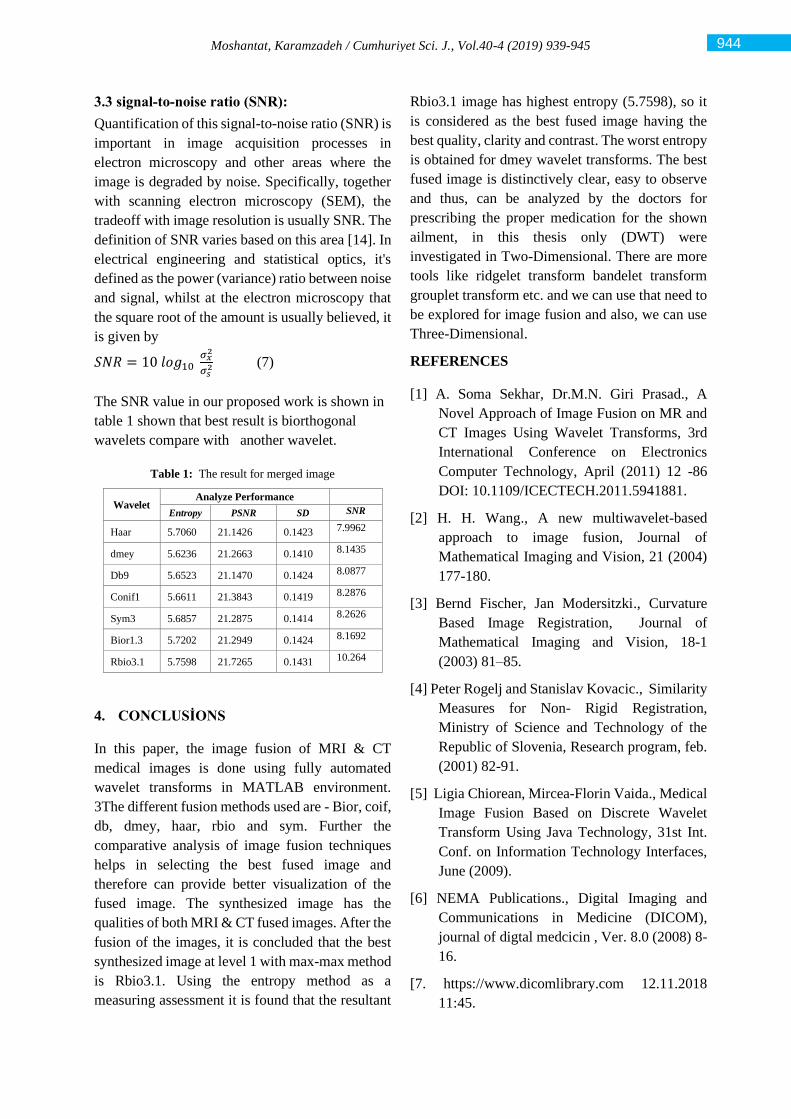
Moshantat, Karamzadeh / Cumhuriyet Sci. J., Vol.40-4 (2019) 939-945
3.3 signal-to-noise ratio (SNR):
Quantification of this signal-to-noise ratio (SNR) is
important in image acquisition processes in
electron microscopy and other areas where the
image is degraded by noise. Specifically, together
with scanning electron microscopy (SEM), the
tradeoff with image resolution is usually SNR. The
definition of SNR varies based on this area [14]. In
electrical engineering and statistical optics, it's
defined as the power (variance) ratio between noise
and signal, whilst at the electron microscopy that
the square root of the amount is usually believed, it
is given by
𝑆𝑁𝑅 = 10 𝑙𝑜𝑔10 𝜎𝑥
2
𝜎𝑠2 (7)
The SNR value in our proposed work is shown in
table 1 shown that best result is biorthogonal
wavelets compare with another wavelet.
Table 1: The result for merged image
Wavelet Analyze Performance
Entropy PSNR SD SNR
Haar 5.7060 21.1426 0.1423 7.9962
dmey 5.6236 21.2663 0.1410 8.1435
Db9 5.6523 21.1470 0.1424 8.0877
Conif1 5.6611 21.3843 0.1419 8.2876
Sym3 5.6857 21.2875 0.1414 8.2626
Bior1.3 5.7202 21.2949 0.1424 8.1692
Rbio3.1 5.7598 21.7265 0.1431 10.264
4. CONCLUSİONS
In this paper, the image fusion of MRI & CT
medical images is done using fully automated
wavelet transforms in MATLAB environment.
3The different fusion methods used are - Bior, coif,
db, dmey, haar, rbio and sym. Further the
comparative analysis of image fusion techniques
helps in selecting the best fused image and
therefore can provide better visualization of the
fused image. The synthesized image has the
qualities of both MRI & CT fused images. After the
fusion of the images, it is concluded that the best
synthesized image at level 1 with max-max method
is Rbio3.1. Using the entropy method as a
measuring assessment it is found that the resultant
Rbio3.1 image has highest entropy (5.7598), so it
is considered as the best fused image having the
best quality, clarity and contrast. The worst entropy
is obtained for dmey wavelet transforms. The best
fused image is distinctively clear, easy to observe
and thus, can be analyzed by the doctors for
prescribing the proper medication for the shown
ailment, in this thesis only (DWT) were
investigated in Two-Dimensional. There are more
tools like ridgelet transform bandelet transform
grouplet transform etc. and we can use that need to
be explored for image fusion and also, we can use
Three-Dimensional.
REFERENCES
[1] A. Soma Sekhar, Dr.M.N. Giri Prasad., A
Novel Approach of Image Fusion on MR and
CT Images Using Wavelet Transforms, 3rd
International Conference on Electronics
Computer Technology, April (2011) 12 -86
DOI: 10.1109/ICECTECH.2011.5941881.
[2] H. H. Wang., A new multiwavelet-based
approach to image fusion, Journal of
Mathematical Imaging and Vision, 21 (2004)
177-180.
[3] Bernd Fischer, Jan Modersitzki., Curvature
Based Image Registration, Journal of
Mathematical Imaging and Vision, 18-1
(2003) 81–85.
[4] Peter Rogelj and Stanislav Kovacic., Similarity
Measures for Non- Rigid Registration,
Ministry of Science and Technology of the
Republic of Slovenia, Research program, feb.
(2001) 82-91.
[5] Ligia Chiorean, Mircea-Florin Vaida., Medical
Image Fusion Based on Discrete Wavelet
Transform Using Java Technology, 31st Int.
Conf. on Information Technology Interfaces,
June (2009).
[6] NEMA Publications., Digital Imaging and
Communications in Medicine (DICOM),
journal of digtal medcicin , Ver. 8.0 (2008) 8-
16.
[7. https://www.dicomlibrary.com 12.11.2018
11:45.
944

Moshantat, Karamzadeh / Cumhuriyet Sci. J., Vol.40-4 (2019) 939-945
[8] M. Hub, M.L. Kessler, and C.P. Karger., A
stochastic approach to estimate the
uncertainty involved in B-spline image
registration, MedImg, 28-11 (2009) 1708–
1716.
[9] J.V.Chapnick, M.E.Noz, G.Q. Maguire,
E.L.Kramer, J.J.Sanger, B.A.Birnbaum,
A.J.Megibow., Techniques of Multimodality
Image Registration, Proceedings of the IEEE
nineteenth Annual North East
Bioengineeering conference, 18-19 March
(1993) 221-222.
[10] J. B. Antoine Maintz and Max A. Viergever.,
A Survey of Medical Image Registration,
Medical Image Analysis 2-1 (1998) 1-36.
[11] Brown Gottesfeld L., A survey of image
Registration Techniques, ACM Computing
surveys, 24-4 (1992) 325-376.
[12] Rahul S.Shınde, Altaaf O.Mulani., Bıomedıcal
Image Fusıon Usıng Wavelet Transform, 2-10
(2015) 50-53.
[13] P. A. Van Den Elsen, E. J. D. Pol and M. A.
Viergever., Medical image matching: a review
with classification, IEEE Engineering in
medicine and biology, march (1993) 26-39.
[14] Pelizzari CA, Chen GTY, Spelbring DR,
Weichselbaum RR, Chen CT. Accurate 3-
dimensional registration of CT, PET, and/or
MR images of the brain. J Comput Assist
Tomogr, Jan-Feb. (1989) 13-20.
945
Cumhuriyet Science Journal
CSJ
e-ISSN: 2587-246X
ISSN: 2587-2680 Cumhuriyet Sci. J., Vol.40-4 (2019) 946-957
* Corresponding author. Email address: [email protected], [email protected]
http://dergipark.gov.tr/csj ©2016 Faculty of Science, Sivas Cumhuriyet University
Correlation of the entrainment factor with frother types and their mixtures
in the column flotation
Hulya KURŞUN1,*
1 Department of Material and Metallurgical Engineering, Sivas Cumhuriyet University, TR-58140 Sivas, Turkey
Received: 16.09.2019; Accepted: 11.11.2019 http://dx.doi.org/10.17776/csj.620798
Abstract. In flotation, entrainment is a mechanical mass transfer process and it is based on the changes
depending on the establishment of linear relationship between water and solid recovery. The present paper
presents results obtained in investigating the effect of frother mixture concentrations on the entrainment of fine
particles’ during the column flotation. The aim of the present study was to investigate more specifically the
relationship between the recovery via entrainment of a range of different hydrophilic calcite particles. For this,
to determine entrainment factor of fine particle was used a mixture of artificial ore (celestite/calcite; 1:1). The
results showed that the frother mixtures had important effect on the grade and recovery, superficial air rate, gas
hold-up and entrainment of fine gangue particles. Entrainment factors for frother mixtures were compared in
flotation column. Kirjaveinen (1989) model was used for explaining the specific entrainment factor (Pi) of
hydrophilic particles and it has been observed that this model supports the results of this study. This, together
with the increased recovery, resulted in higher celestite grades of valuable mineral recovered to the concentrate
when using the frother mixtures (Pine Oil+MIBC).
Keywords: Entrainment, Column flotation, Frothers, Celestite, Calcite.
Sürüklenme faktörünün kolon flotasyonunda kullanılan köpürtücü tür ve
karışımlarıyla ilişkisi
Özet. Flotasyonda, su ile taşınım mekanik bir kütle transfer işlemidir ve katı-su kazanımı arasında doğrusal bir
ilişki kurulmasına bağlı değişim gösterir. Bu çalışmada, kolon flotasyonunda ince tanelerin sürüklenmesi
üzerine farklı miktarlarda köpürtücü karışımlarının etkisi incelenmektedir. Çalışmanın amacı, hidrofilik kalsit
tanelerinin sürüklenmesi yoluyla geri kazanım arasındaki ilişkiyi daha spesifik olarak incelemektir. İnce
tanelerin sürüklenme faktörünü belirlemek için yapay cevher karışımı (selestit / kalsit; 1: 1) kullanılmıştır.
Deneysel sonuçlar, köpürtücü karışımlarının tenör-verim, yüzeysel hava hızı, gaz tutunumu ve ince gang
tanelerinin sürüklenmesi üzerinde önemli bir etkiye sahip olduğunu göstermiştir. Farklı tür ve miktarlarda
köpürtücü karışımları için sürüklenme faktörleri, kolon flotasyonunda karşılaştırılmıştır. Hidrofilik tanelerin
spesifik sürüklenme faktörünü (Pi) açıklamak için Kirjaveinen (1989) modeli kullanılmış ve bu modelin bu
çalışmanın sonuçlarını desteklediği görülmüştür. Çamyağı + MIBC köpürtücü karışımı kullanıldığında,
konsantrede verim artmış ve daha yüksek tenörlü selestit konsantresi elde edilmiştir.
Anahtar Kelimeler: Su ile taşınım, Kolon flotasyonu, Köpürtücüler, Selestit, Kalsit
1. INTRODUCTION
In entrainment, particles suspended in the water
between bubbles enter froth zone from the
collection zone and are conducted to the
concentrate. Both hydrophobic and hydrophilic
mineral particles in pulp can experience
entrainment. Entrainment is widely accepted to be
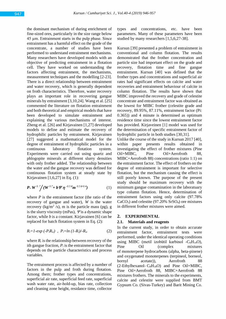
Kursun / Cumhuriyet Sci. J., Vol.40-4 (2019) 946-957
the dominant mechanism of during enrichment of
fine-sized ores, particularly in the size range below
45 µm. Entrainment starts in the pulp phase. Since
entrainment has a harmful effect on the grade of the
concentrate, a number of studies have been
performed to understand entrainment mechanisms.
Many researchers have developed models with an
objective of predicting entrainment in a flotation
cell. They have worked on understanding the
factors affecting entrainment, the mechanisms,
measurement techniques and the modelling [2-23].
There is a direct relationship between entrainment
and water recovery, which is generally dependent
on froth characteristics. Therefore, water recovery
plays an important role in recovering gangue
minerals by entrainment [3,10,24]. Wang et al. [25]
commented the literature on flotation entrainment
and both theoretical and empirical models that have
been developed to simulate entrainment and
explaining the various mechanisms of interest.
Zheng et al. [26] and Kirjavainen [1,27] developed
models to define and estimate the recovery of
hydrophilic particles by entrainment. Kirjavainen
[27] suggested a mathematical model for the
degree of entrainment of hydrophilic particles in a
continuous laboratory flotation system.
Experiments were carried out using quartz and
phlogopite minerals at different slurry densities
with only frother added. The relationship between
the water and the gangue recovery was defined for
continuous flotation system at steady state by
Kirjavainen [1,6,27] in Eq. (1):
P= W 0. 7 (W 0.7+ b -0.5m 0.5-0.4) (1)
where P is the entrainment factor (the ratio of the
recovery of gangue and water), W is the water
recovery (kg/m2 /s), m is the particle mass (pg), g
is the slurry viscosity (mPas), is a dynamic shape
factor, while b is a constant. Kirjavainen [6] can be
replaced for batch flotation system in Eq. (2):
Ri=1-exp (-PiRw) , Pi=ln (1-Ri)/-Rw (2)
where Ri is the relationship between recovery of the
ith gangue fraction, Pi is the entrainment factor that
depends on the particle characteristics and process
variables.
The entrainment process is affected by a number of
factors in the pulp and froth during flotation.
Among them; frother types and concentrations,
superficial air rate, superficial feed rate, superficial
wash water rate, air-hold-up, bias rate, collection
and cleaning zone height, residance time, collector
types and concentrations, etc. have been
parameters. Many of these parameters have been
studied by many researchers [1,5,6,27-38].
Kursun [39] presented a problem of entrainment in
conventional and column flotation. The results
demonstrated that the frother concentration and
particle size had important effect on the grade and
recovery, flotation time and fine gangue
entrainment. Kursun [40] was defined that the
frother types and concentrations and superficial air
rates had significant effects on calcite and water
recoveries and entrainment behaviour of calcite in
column flotation. The results have shown that
MIBC improved the recovery and grade of celestite
concentrate and entrainment factor was obtained as
the lowest for MIBC frother (celestite grade and
recovery, 89.95%, 87.11%, entrainment factor (Pi:
0.365)) and 4 minute is determined as optimum
residence time since the lowest entrainment factor
has provided. Kirjaveinen [1] model was used for
the determination of specific entrainment factor of
hydrophilic particle in both studies [30,31].
Unlike the course of the study in Kursun 2017 [40],
within paper presents results obtained in
investigating the effect of frother mixtures (Pine
Oil+MIBC, Pine Oil+Aerofroth 88,
MIBC+Aerofroth 88) concentrations (ratio 1:1) on
the entrainment factor. The effect of frothers on the
degree of entrainment is important for selective
flotation, but the mechanism causing the effect is
still poorly known. The purpose of the present
study should be maximum recovery with the
minimum gangue contamination in the laboratuary
type column flotation. Hence, determination of
entrainment factors using only calcite (97.78%
CaCO3) and celestite (97.20% SrSO4) ore mixtures
in different frother mixtures were aimed.
2. EXPERIMENTAL
2.1. Materials and reagents
In the current study, in order to obtain accurate
entrainment factor, entrainment tests were
performed, under the identical operating conditions
using MIBC (metil izobütil karbinol -C6H14O),
Pine Oil (complex mixtures
of monoterpene hydrocarbons (alpha, beta-pinene)
and oxygenated monoterpenes (terpineol, borneol,
bornyl acetate)), Aerofroth 88
(2-Ethylhexanol- C8H18O) and Pine Oil+MIBC,
Pine Oil+Aerofroth 88, MIBC+Aerofroth 88
mixtures frothers. The minerals to the experiments,
calcite and celestite were supplied from BMT
Gypsum Co. (Sivas-Turkey) and Barit Mining Co.
947
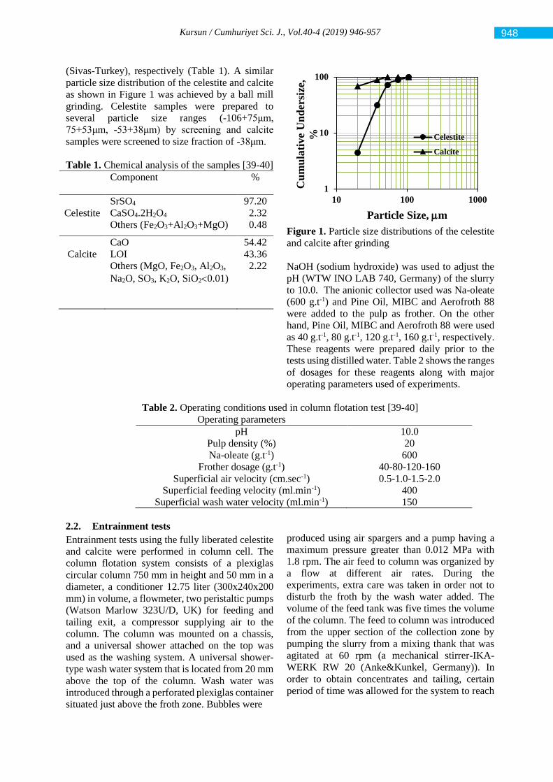
Kursun / Cumhuriyet Sci. J., Vol.40-4 (2019) 946-957
(Sivas-Turkey), respectively (Table 1). A similar
particle size distribution of the celestite and calcite
as shown in Figure 1 was achieved by a ball mill
grinding. Celestite samples were prepared to
several particle size ranges (-106+75μm,
75+53μm, -53+38μm) by screening and calcite
samples were screened to size fraction of -38μm.
Table 1. Chemical analysis of the samples [39-40]
Component %
Celestite
SrSO4
CaSO4.2H2O4
Others (Fe2O3+Al2O3+MgO)
97.20
2.32
0.48
Calcite
CaO
LOI
Others (MgO, Fe2O3, Al2O3,
Na2O, SO3, K2O, SiO20.01)
54.42
43.36
2.22
Figure 1. Particle size distributions of the celestite
and calcite after grinding
NaOH (sodium hydroxide) was used to adjust the
pH (WTW INO LAB 740, Germany) of the slurry
to 10.0. The anionic collector used was Na-oleate
(600 g.t-1) and Pine Oil, MIBC and Aerofroth 88
were added to the pulp as frother. On the other
hand, Pine Oil, MIBC and Aerofroth 88 were used
as 40 g.t-1, 80 g.t-1, 120 g.t-1, 160 g.t-1, respectively.
These reagents were prepared daily prior to the
tests using distilled water. Table 2 shows the ranges
of dosages for these reagents along with major
operating parameters used of experiments.
Table 2. Operating conditions used in column flotation test [39-40]
Operating parameters
pH 10.0
Pulp density (%) 20
Na-oleate (g.t-1) 600
Frother dosage (g.t-1) 40-80-120-160
Superficial air velocity (cm.sec-1) 0.5-1.0-1.5-2.0
Superficial feeding velocity (ml.min-1) 400
Superficial wash water velocity (ml.min-1) 150
2.2. Entrainment tests
Entrainment tests using the fully liberated celestite
and calcite were performed in column cell. The
column flotation system consists of a plexiglas
circular column 750 mm in height and 50 mm in a
diameter, a conditioner 12.75 liter (300x240x200
mm) in volume, a flowmeter, two peristaltic pumps
(Watson Marlow 323U/D, UK) for feeding and
tailing exit, a compressor supplying air to the
column. The column was mounted on a chassis,
and a universal shower attached on the top was
used as the washing system. A universal shower-
type wash water system that is located from 20 mm
above the top of the column. Wash water was
introduced through a perforated plexiglas container
situated just above the froth zone. Bubbles were
produced using air spargers and a pump having a
maximum pressure greater than 0.012 MPa with
1.8 rpm. The air feed to column was organized by
a flow at different air rates. During the
experiments, extra care was taken in order not to
disturb the froth by the wash water added. The
volume of the feed tank was five times the volume
of the column. The feed to column was introduced
from the upper section of the collection zone by
pumping the slurry from a mixing thank that was
agitated at 60 rpm (a mechanical stirrer-IKA-
WERK RW 20 (Anke&Kunkel, Germany)). In
order to obtain concentrates and tailing, certain
period of time was allowed for the system to reach
1
10
100
10 100 1000
Cu
mu
lati
ve
Un
der
size
,
%
Particle Size, mm
Celestite
Calcite
948
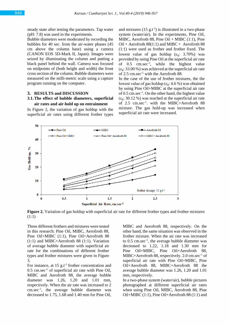
Kursun / Cumhuriyet Sci. J., Vol.40-4 (2019) 946-957
steady state after testing the parameters. Tap water
(pH: 7.8) was used in the experiments.
Bubble diameters were moderated by recording the
bubbles for 40 sec. from the air-water phases (45
cm above the column base) using a camera
(CANON EOS 5D-Mark II, Japan). Images were
seized by illuminating the column and putting a
black panel behind the wall. Camera was focused
on midpoints of (both height and width) the front
cross section of the column. Bubble diameters were
measured on the milli-metric scale using a capture
program running on the computer.
3. RESULTS and DISCUSSION
3.1. The effect of bubble diameters, superficial
air rates and air-hold up on entrainment
In Figure 2, the variation of gas holdup with the
superficial air rates using different frother types
and mixtures (15 g.t-1) is illustrated in a two-phase
system (water/air). In the experiments, Pine Oil,
MIBC, Aerofroth 88, Pine Oil + MIBC (1:1), Pine
Oil + Aerofroth 88(1:1) and MIBC + Aerofroth 88
(1:1) were used as frother and frother fixed. The
lowest value of gas holdup (g: 3.70%) was
provided by using Pine Oil at the superficial air rate
of 0.5 cm.sec-1, while the highest value
(εg: 33.00 %) was achieved at the superficial air rate
of 2.5 cm.sec-1 with the Aerofroth 88.
In the case of the use of frother mixtures, the the
lowest value of gas holdup (εg: 4.6 %) was obtained
by using Pine Oil+MIBC at the superficial air rate
of 0.5 cm.sec-1. On the other hand, the highest value
(εg: 30.12 %) was reached at the superficial air rate
of 2.5 cm.sec-1. with the MIBC+Aerofroth 88
mixture. The gas hold-up was increased when
superficial air rate were increased.
Figure 2. Variation of gas holdup with superficial air rate for different frother types and frother mixtures
(1:1)
Three different frothers and mixtures were tested
in this research: Pine Oil, MIBC, Aerofroth 88,
Pine Oil+MIBC (1:1), Pine Oil+Aerofroth 88
(1:1) and MIBC+Aerofroth 88 (1:1). Variation
of average bubble diameter with superficial air
rate for the combinations of different frother
types and frother mixtures were given in Figure
3.
For instance, at 15 g.t-1 frother concentration and
0.5 cm.sec-1 of superficial air rate with Pine Oil,
MIBC and Aerofroth 88, the average bubble
diameter was 1.26, 1.20 and 1.01 mm,
respectively. When the air rate was increased to 2
cm.sec-1, the average bubble diameter was
decreased to 1.75, 1.68 and 1.40 mm for Pine Oil,
MIBC and Aerofroth 88, respectively. On the
other hand, the same situation was observed in the
frother mixture. When the air rate was increased
to 0.5 cm.sec-1, the average bubble diameter was
decreased to 1.22, 1.18 and 1.30 mm for
Pine Oil+MIBC, Pine Oil+Aerofroth 88,
MIBC+Aerofroth 88, respectively. 2.0 cm.sec-1 of
superficial air rate with Pine Oil+MIBC, Pine
Oil+Aerofroth 88, MIBC+Aerofroth 88 the
average bubble diameter was 1.26, 1.20 and 1.01
mm, respectively.
In a two-phase system (water/air), bubble pictures
photographed at different superficial air rates
when using Pine Oil, MIBC, Aerofroth 88, Pine
Oil+MIBC (1:1), Pine Oil+Aerofroth 88 (1:1) and
949
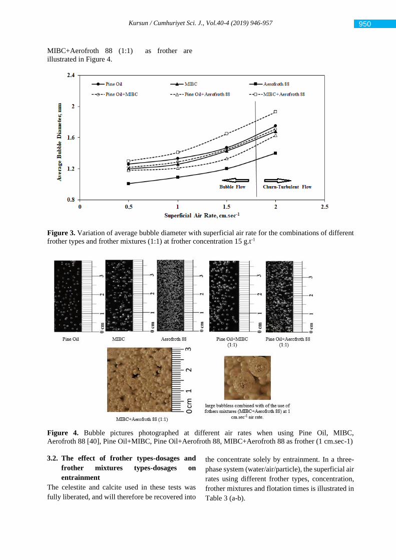
Kursun / Cumhuriyet Sci. J., Vol.40-4 (2019) 946-957
MIBC+Aerofroth 88 (1:1) as frother are
illustrated in Figure 4.
Figure 3. Variation of average bubble diameter with superficial air rate for the combinations of different
frother types and frother mixtures (1:1) at frother concentration 15 g.t-1
Figure 4. Bubble pictures photographed at different air rates when using Pine Oil, MIBC,
Aerofroth 88 [40], Pine Oil+MIBC, Pine Oil+Aerofroth 88, MIBC+Aerofroth 88 as frother (1 cm.sec-1)
3.2. The effect of frother types-dosages and
frother mixtures types-dosages on
entrainment
The celestite and calcite used in these tests was
fully liberated, and will therefore be recovered into
the concentrate solely by entrainment. In a three-
phase system (water/air/particle), the superficial air
rates using different frother types, concentration,
frother mixtures and flotation times is illustrated in
Table 3 (a-b).
950
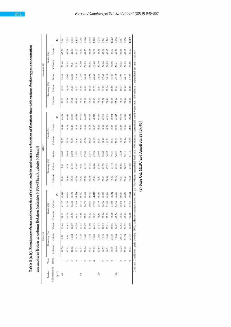
Kursun / Cumhuriyet Sci. J., Vol.40-4 (2019) 946-957
951
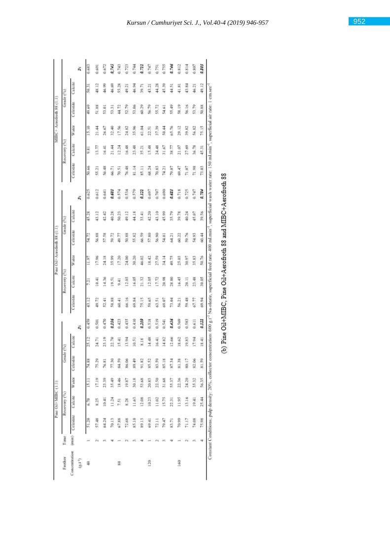
Kursun / Cumhuriyet Sci. J., Vol.40-4 (2019) 946-957
952
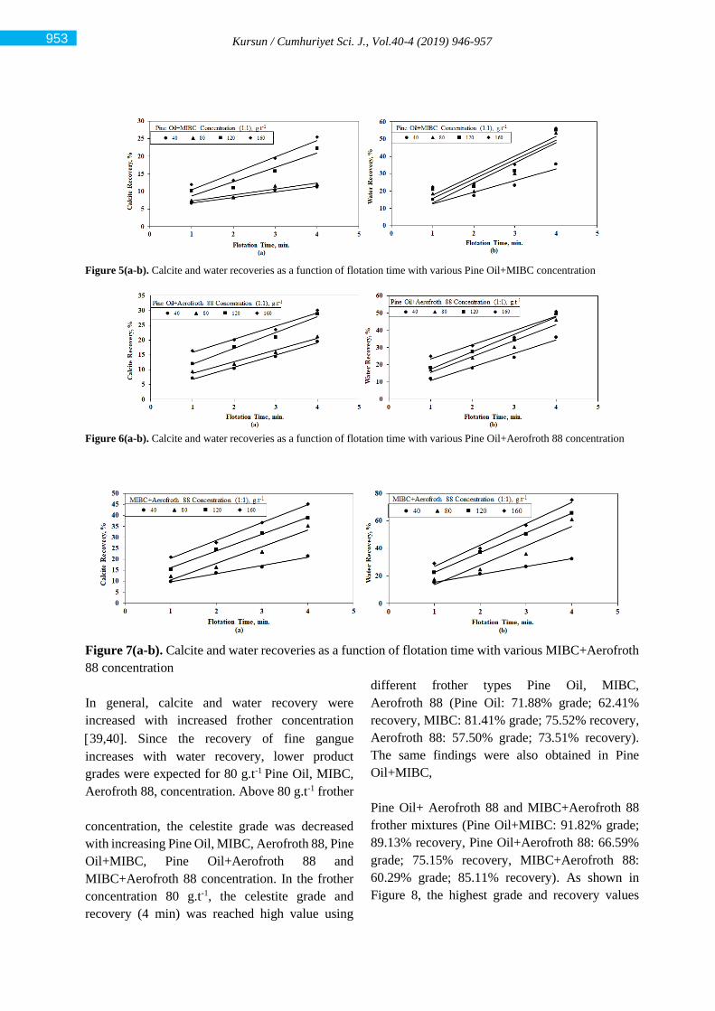
Kursun / Cumhuriyet Sci. J., Vol.40-4 (2019) 946-957
Figure 5(a-b). Calcite and water recoveries as a function of flotation time with various Pine Oil+MIBC concentration
Figure 6(a-b). Calcite and water recoveries as a function of flotation time with various Pine Oil+Aerofroth 88 concentration
Figure 7(a-b). Calcite and water recoveries as a function of flotation time with various MIBC+Aerofroth
88 concentration
In general, calcite and water recovery were
increased with increased frother concentration
39,40]. Since the recovery of fine gangue
increases with water recovery, lower product
grades were expected for 80 g.t-1 Pine Oil, MIBC,
Aerofroth 88, concentration. Above 80 g.t-1 frother
concentration, the celestite grade was decreased
with increasing Pine Oil, MIBC, Aerofroth 88, Pine
Oil+MIBC, Pine Oil+Aerofroth 88 and
MIBC+Aerofroth 88 concentration. In the frother
concentration 80 g.t-1, the celestite grade and
recovery (4 min) was reached high value using
different frother types Pine Oil, MIBC,
Aerofroth 88 (Pine Oil: 71.88% grade; 62.41%
recovery, MIBC: 81.41% grade; 75.52% recovery,
Aerofroth 88: 57.50% grade; 73.51% recovery).
The same findings were also obtained in Pine
Oil+MIBC,
Pine Oil+ Aerofroth 88 and MIBC+Aerofroth 88
frother mixtures (Pine Oil+MIBC: 91.82% grade;
89.13% recovery, Pine Oil+Aerofroth 88: 66.59%
grade; 75.15% recovery, MIBC+Aerofroth 88:
60.29% grade; 85.11% recovery). As shown in
Figure 8, the highest grade and recovery values
953
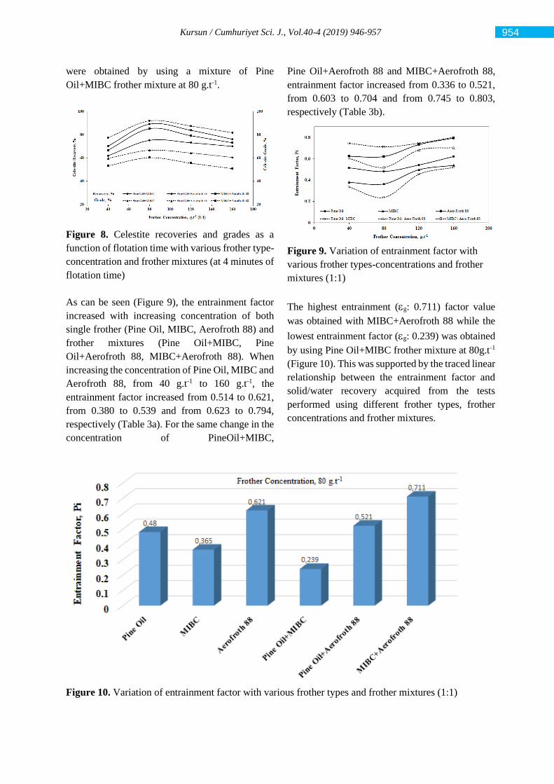
Kursun / Cumhuriyet Sci. J., Vol.40-4 (2019) 946-957
were obtained by using a mixture of Pine
Oil+MIBC frother mixture at 80 g.t-1.
Figure 8. Celestite recoveries and grades as a
function of flotation time with various frother type-
concentration and frother mixtures (at 4 minutes of
flotation time)
As can be seen (Figure 9), the entrainment factor
increased with increasing concentration of both
single frother (Pine Oil, MIBC, Aerofroth 88) and
frother mixtures (Pine Oil+MIBC, Pine
Oil+Aerofroth 88, MIBC+Aerofroth 88). When
increasing the concentration of Pine Oil, MIBC and
Aerofroth 88, from 40 g.t-1 to 160 g.t-1, the
entrainment factor increased from 0.514 to 0.621,
from 0.380 to 0.539 and from 0.623 to 0.794,
respectively (Table 3a). For the same change in the
concentration of PineOil+MIBC,
Pine Oil+Aerofroth 88 and MIBC+Aerofroth 88,
entrainment factor increased from 0.336 to 0.521,
from 0.603 to 0.704 and from 0.745 to 0.803,
respectively (Table 3b).
Figure 9. Variation of entrainment factor with
various frother types-concentrations and frother
mixtures (1:1)
The highest entrainment (g: 0.711) factor value
was obtained with MIBC+Aerofroth 88 while the
lowest entrainment factor (g: 0.239) was obtained
by using Pine Oil+MIBC frother mixture at 80g.t-1
(Figure 10). This was supported by the traced linear
relationship between the entrainment factor and
solid/water recovery acquired from the tests
performed using different frother types, frother
concentrations and frother mixtures.
Figure 10. Variation of entrainment factor with various frother types and frother mixtures (1:1)
954
Kursun / Cumhuriyet Sci. J., Vol.40-4 (2019) 946-957
4. CONCLUSION
The column flotation experiment was performed
using a mixture of liberated celestite as the valuable
mineral and as the gangue mineral calcite, to
indicate the primary factors affecting the
entrainment factor. The obtained experimental
results performed allow the following conclusions
to be drawn:
. Superficial air rates, air hold-up and frother
concentrate are three parameters that directly
effective each other. When superficial air rate and
the frother concentration were increased, the
bubble diameter was decreased. Above a certain
superficial air rate value, bubbly flow conditions
were destroyed and turbulence flow conditions
were formed producing large bubbles. When
frother concentration was increased, bubble size
was demonstrate to decrease importantly at the
pulp/froth interface, which resulted in an increase
in gas holdup (εg).
. In the MIBC Aerofroth 88 frother mixture, small
bubbles collided in the pulp/froth interface and
occured form large bubbles. In this case, bubbly
flow conditions were lost and churn-turbulent flow
conditions prevailed accompanied by large
bubbles. This case, the amount of particles that can
overcome the downward gravitational force to be
recovered by the entrainment mechanism to the
final concentrate increased, and the entrainment
factor increased. As a result, the concentrate was
contaminated by fine calcite minerals.
This was explained by the observed linear
relationship between the entrainment factor and
liquid velocity at the pulp/froth interface obtained
from the tests performed using different frother
types and concentrations. It has been seen that there
is a linear relationship between calcite and water
recoveries. Beside, the type, concentration and
mixture of frother had exceptional effect on calcite.
The recovery was increased, but the selectivity was
decreased. The lowest entrainment factor was
obtained with 80 g.t-1 of frother concentration for
Pine Oil+ MIBC frother mixture (g: 0.239).
. Experimental results show that the entrainment
factor varied significantly frother type, frother
concentration and frother mixture. The recovery of
calcite by entrainment was affected by
Pine Oil+MIBC, Pine Oil+Aerofroth 88 and
MIBC+Aerofroth 88 frother mixture. These results
suggest that the frother types, frother concentration
and frother mixtures at the flotation is a key factor
which affects the entrainment factor. Kirjaveinen
Model’s 1 has been seen supported the results of
this study.
REFERENCES
[1] Kirjavainen V.M., Application of a
probability model for the entrainment of
hydrophilic particles in froth flotation. Int. J.
of Miner. Process., 27 (1) (1989) 63–74.
[2] Jowett, A., Gangue mineral contamination
of froth, Brazilian J. of Chem. Eng. 2:5
(1966) 330–333.
[3] Johnson, N.W., MC Kee D.J., Lynch A.J.,
Flotation rates of non-sulphide minerals in
chalcopyrite processes, Trans. of the
American Inst. of Mining, Metall. and
Petrol. Eng., 256 (1974) 204–226.
[4] Bisshop J.P and White M.E., Study of
particle entrainment in flotation froths.
Trans. of the Inst. of Mining and Metall.
Section C: Miner. Process. and Extract.
Metall., 85 (1976) 191– 194.
[5] Smith P.G. and Warren L.J., Entrainment of
particles into flotation froths, Miner.
Process. and Extract. Metall. Rev. 5 (1989),
123–145.
[6] Kirjavainen V.M., Review and analysis of
factors controlling the mechanical flotation
of gangue minerals. Int. J. of Miner. Process.
46 (1996) 21– 34.
[7] Savassi O.N., Alexander J.P., Franzidis J.-
P., Manlapig E.V., An empirical model for
entrainment in industrial flotation plants,
Min. Eng., 11 (3) (1998) 243–256.
[8] Zheng X., Franzidis J.P., Johnson N.W., An
evaluation of different models of water
recovery in flotation, Miner. Eng., 19 (2006)
871–882.
[9] Yianatos J.B., Contreras F., Díaz F.,
Villanueva A., Direct measurement of
entrainment in large flotation cells, Powder
Technol., 189 (2009) 42–47.
[10] Yianatos J. and Contreras F., Particle
entrainment model for industrial cells,
Powder Technol. 197 (2010) 260–267.
[11] Konopacka Z. and Drzymala J., Types of
particles recovery-water recovery
entrainment plots useful in flotation
research, Adsorption, 16 (2010) 313–320.
[12] Warren L.J., Determination of the
contributions of true flotation and
entrainment in batch flotation test, Int. J. of
Miner. Process., 14 (1985) 33–34.
[13] Ross V.E., Flotation and entrainment of
955
Kursun / Cumhuriyet Sci. J., Vol.40-4 (2019) 946-957
particles during batch flotation, Miner. Eng.,
3(3/ 4) (1990) 254–256.
[14] Wang L., Runge K., Peng Y., Vos C., An
empirical model for the degree of
entrainment in froth flotation based on
particle size and density, Miner. Eng., 98
(2016) 187–193.
[15] Wang L., Peng Y., Runge K., The
mechanism responsible for the effect of
frothers on the degree of entrainment in
laboratory batch flotation, Miner. Eng., 100
(2017) 124–131.
[16] Wiese J., Becker M., Yorath G., O’Connor
C., An investigation into the relationship
between particle shape and entrainment,
Miner. Eng., 83 (2015) 211–216.
[17] Wiese J. and Harris P., The effect of frother
type and dosage on flotation performance in
the presence of high depressant
concentrations, Miner. Eng. 36– 38 (2012)
204–210.
[18] Wiese J.G. and O'Connor C.T., An
investigation into the relative role of particle
size, particle shape and froth behaviour on
the entrainment of chromite, Int. J. of Miner.
Process., 156 (2016) 127–133.
[19] McFadzean B., Marozva T., Wiese J.,
Flotation frother mixtures: Decoupling the
sub-processes of froth stability, froth
recovery and entrainment, Miner. Eng., 85
(2016) 72–79.
[20] Little L., Wiese J., Becker M., Mainza A.,
Ross V., Investigating the effects of particle
shape on chromite entrainment at a platinum
concentrator, Miner. Eng., 96–97 (2016) 46–
52.
[21] Lima N.P., de Souza Pinto T.C., Tavares
A.C., Sweet J., The entrainment effect on the
performance of iron ore reverse flotation,
Miner. Eng. 96–97 (2016) 53–58.
[22] Neethling S.J. and Cilliers J.J.. The
entrainment factor in froth flotation: Model
for particle size and other operating
parameter effects, Int. J. Miner. Process., 93
(2009) 141–148
[23] Mao Y., Peng Y., Bu X., Xie G., Wu E., Xia
W., Effect of ultrasound on the true flotation
of lignite and its entrainment behavior, Part
A: Recovery, Utilization, and
Environmental Effects, Energy Sources, 40
(8) (2018) 940–950
[24] Neethling S.J., Lee H.T, Cilliers J.J., Simple
relationships for predicting the recovery of
liquid from flowing foams and froths, Miner.
Eng., 16 (2003) 1123–1130.
[25] Wang L., Peng Y., Runge K., Bradshaw D.
A review of entrainment: Mechanisms,
contributing factors and modelling in
flotation, Miner. Eng., 70 (2015) 77-91.
[26] Zheng X., Johnson N.W., Franzidis J.P.,
Modelling of entrainment in industrial
flotation cells: water recovery and degree of
entrainment, Miner. Eng., 19 (2006) 1191–
1203.
[27] Kirjavainen V.M., Mathematical model for
the entrainment hydrophilic particles in froth
flotation, Int. J. of Miner. Process., 35 (1992)
1–11
[28] Maachar A. and Dobby G.S., Measurement
of feed water recovery and entrainment
solids recovery in flotation columns,
Canadian Metall. Quarterly, 31 (3) (1992)
167–172.
[29] Tao D., Luttrell G.H., Yoon R.H., A
parametric study of froth stability and its
effect on column flotation of fine particles,
Int. J. Miner. Process., 59 (2000) 25–43.
[30] Liang L., Tan J., Li B., Xie G., Reducing
quartz entrainment infine coalflotation by
polyaluminumchloride, Fuel, 235 (2019)
150-157.
[31] Tuteja R. K., Spottıswood D. J., Mısra V. N.,
Column parameters: Their effect on
entrainment in froth, Miner. Eng., 8 (1995)
1359–1368.
[32] Rahal K., Manlapig E., Franzidis J.-P.,
Effect of frother type and concentration on
the water recovery and entrainment recovery
relationship, Miner. & Metall. Process.,
18(3) (2001) 138–141.
[33] Johnson N.W., A Review of the entrainment
mechanism and its modelling in ındustrial
flotation processes. Proceedings-Centenary
of Flotation Symposium, Brisbane, 2005,5
Australia.
[34] Yianatos J., Contreras F., Díaz F.,
Villanueva A., Direct measurement of
entrainment in large flotation cells, Powder
Technol., 189 (2009) 42–47.
[35] Nguyen A.V. and Schulze H.J., Colloidal
science of flotation. Surfactant Science
Series, 118. Marcel Dekker Inc. New York,
(2004) 709–775.
[36] Kursun H., Influence of superficial air rate
on entrainment in column flotation, J. of
Eng. and Earth Sci., 2(1) (2017) 8-16
[37] Runge K., Laboratory flotation testing – an
essential tool for ore characterisation.
Flotation plant optimisation: A metallurgical
guide to identifying and solving problems in
956

Kursun / Cumhuriyet Sci. J., Vol.40-4 (2019) 946-957
flotation plants, 16. Australasian Inst. of
Mining and Metall. Spectrum Series,
Carlton, Vic, (2010) 55–173.
[38] Shabalala N.Z.P., Harris M., Leal Filho L.S.,
Deglon D.A., Effect of slurry rheology on
gas dispersion in a pilot-scale mechanical
flotation cell, Miner. Eng., 24 (2011) 1448–
1453.
[39] Kursun H., Effect of fine particles’
entrainment on conventional and column
flotation, Particulate Sci. and Technol. 32
(2014) 251–256.
[40] Kursun H., The influence of frother types
and concentrations on fine particles’
entrainment using column flotation, Sep.
Sci. and Technol., 4 (2017) 722–731.
957
Cumhuriyet Science Journal
CSJ
e-ISSN: 2587-246X
ISSN: 2587-2680 Cumhuriyet Sci. J., Vol.40-4 (2019) 958-966
* Corresponding author. Email address: [email protected]
http://dergipark.gov.tr/csj ©2016 Faculty of Science, Sivas Cumhuriyet University
Comparative Analysis of the Feature Extraction Performance of
Augmented Reality Algorithms
Umut TOSUN1*
1 Alanya Alaaddin Keykubat University, Faculty of Engineering, Department of Computer Engineering, Alanya,
TURKEY
Received: 25.10.2019; Accepted: 21.11.2019 http://dx.doi.org/10.17776/csj.638297
Abstract. The algorithms that extract keypoints and descriptors in augmented reality applications are getting
more and more important in terms of performance. Criterions like time and correct matching of points gain
more impact according to the type of application. In this paper, the performance of the algorithms used to
identify an image using keypoint and descriptor extraction is studied. In the context of this research, main
criterion like the number of keypoints and descriptors that the algorithms extract, algorithm execution time, and
the quality of keypoints and descriptors extracted are considered as the performance metrics. Same data stacks
were used for obtaining comparison results. In addition to comparisons for a group of well-known augmented
reality applications, the best performing algorithms for varying applications were also suggested. C++ language
and OpenCV library were used for the implementation of the augmented reality algorithms compared.
Keywords: Augmented Reality, Image Processing, Key Point, Descriptor.
Artırılmış Gerçeklik Algoritmalarının Öznitelik Çıkarma
Performanslarının Karşılaştırmalı Analizi
Özet. Artırılmış gerçeklik uygulamalarında kullanılan anahtar nokta ve öznitelik çıkaran algoritmalar
performansları açısından önem teşkil etmektedirler. Uygulamanın türüne göre zaman, noktaların doğru
eşleşmesi gibi kriterler önem kazanmaktadır. Bu makalede artırılmış gerçeklik uygulamalarında kullanılan ve
bir resmi tanımak amacı ile resim üzerinde anahtar nokta ve öznitelik bulunması için uygulanan algoritmaların
performansları incelenmiştir. Çalışma kapsamında, algoritmaların çıkarabildiği anahtar nokta sayısı, öznitelik
sayısı, algoritmanın çalışması sırasında geçen süre, iki resmin eşleştirilmesi sırasında çıkartılan anahtar nokta
ve özniteliklerin kaliteleri gibi ana kriterler incelenmiştir. Karşılaştırma sonuçlarının elde edilmesinde, aynı
veri kümeleri kullanılmıştır. Bu çalışmada, iyi bilinen bir grup artırılmış gerçeklik algoritması incelenerek
performanslarının karşılaştırılmasının yanında, farklı uygulamalar için kullanılabilecek algoritmalar hakkında
da önerilerde bulunulmuştur. Artırılmış gerçeklik algoritmalarının karşılaştırılması için C++ dili ve OpenCV
kütüphaneleri kullanılmıştır.
Anahtar Kelimeler Artırılmış Gerçeklik, Görüntü İşleme, Anahtar Nokta, Öznitelik.
1. INTRODUCTION
Augmented reality is the result of combining real
data and computer generated sound, images,
graphics and location information in the world
we live in. [1]. In other words, it is the
enrichment of reality with virtual data in
computer environment [2, 3]. Various methods
Tosun / Cumhuriyet Sci. J., Vol.40-4 (2019) 958-966
are used to recognize the actual images in the
virtual environment. In order to recognize an
image from the real world, there are qualified
points on the image.
Descriptors of a feature are extracted with
respect to some of the basic properties of this
point (pixels) and other points around it. The dots
on the image that have the feature value for that
image are then used for virtual recognition of this
image. Thus, in the virtual environment, a person
has the values of the picture that they want to be
recognized. The user can compare the picture
that he has previously extracted and wanted to
recognize with the other pictures taken from the
camera. A “threshold" value should be
determined during the matching phase.
Otherwise, if the features taken from the camera
and extracted from a picture that we do not want
to recognize actually match the features of the
picture that is intended to be recognized, a wrong
match will be made. After setting the threshold
value, it is possible to match the image to be
recognized with the images taken from the
camera. One of the methods used to extract key
points and features on the image is the Oriented
Fast and Rotated Brief (ORB) algorithm [4].
ORB is a binary algorithm. Within the scope of
this paper, one of the reasons why ORB
algorithm is compared with other methods is the
opinion that it is faster than basic algorithms in
the literature which extract some key points and
features. The fact that ORB is based on binary
descriptor and that pairing between two pictures
happens while performing matching, supports
the idea that it is faster than other methods.
In the literature, fps (frame per second), the
number of key points extracted on one image, the
number of features extracted on one image and
the number of features matched correctly
between the two images are used to compare the
algorithms used in the extraction of key points
and features [5-10]. This work will be based on
the criteria mentioned. At the end of this study,
the algorithms used for augmented reality an
developed for the recognition of an image will be
compared and their performance will be
benchmarked. At the end of the study, the
algorithms used for augmented reality and
developed for the recognition of an image will be
compared and their performance will be
benchmarked. Moreover, some suggestions on
the usage areas will be made.
2. COMPARED ALGORITHMS
Keypoint is a pixel that has a specific meaning on
an image. In calculating the key point, various
algorithms can be applied depending on the type
of application. The ORB algorithm [4] uses the
FAST [11, 12] algorithm in the background when
calculating the key points on the image. The
FAST algorithm basically calculates the key
points by targeting the corners on the image.
There may be many meaningless pixels on the
picture. These insignificant pixels cause loss of
performance within augmented reality.
Therefore, it is important to identify and process
key points. However, in some cases, key points
may not make sense alone. Feature values should
be calculated while matching the key points on
the picture taken from the real world with the
picture that is required to be recognized within
the context of augmented reality. Thus, when
pairing the two images, more accurate matches
can be made with the feature values of the key
points extracted from the objects to be
recognized.
Feature can be defined as scalable and observable
information obtained from the image [13, 14].
Feature extraction removes a significant set of
features by discarding unnecessary information
[15]. Feature extraction aims to reduce
processing time by reducing the size of high-
dimensional data. Using this data as it is in image
processing applications increases processing
complexity. Feature extraction is an important
part of augmented reality applications in terms of
application performance [16]. It aims to increase
the recognition success by expressing the
information of the pattern in the smallest
dimension with the most prominent features [17].
Dimension reduction is performed by extracting
unnecessary information that is irrelevant to the
pattern and obtaining specific properties. This
process aims to create a more selective set by
959
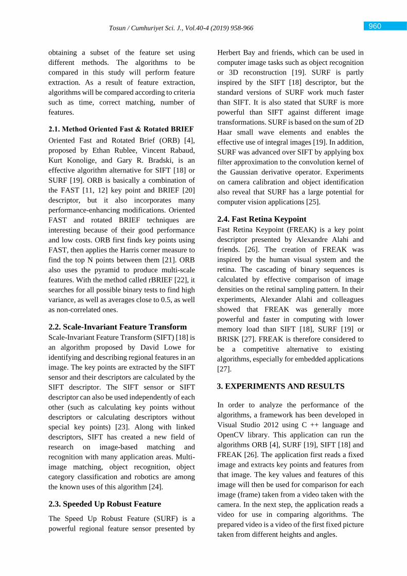
Tosun / Cumhuriyet Sci. J., Vol.40-4 (2019) 958-966
obtaining a subset of the feature set using
different methods. The algorithms to be
compared in this study will perform feature
extraction. As a result of feature extraction,
algorithms will be compared according to criteria
such as time, correct matching, number of
features.
2.1. Method Oriented Fast & Rotated BRIEF
Oriented Fast and Rotated Brief (ORB) [4],
proposed by Ethan Rublee, Vincent Rabaud,
Kurt Konolige, and Gary R. Bradski, is an
effective algorithm alternative for SIFT [18] or
SURF [19]. ORB is basically a combination of
the FAST [11, 12] key point and BRIEF [20]
descriptor, but it also incorporates many
performance-enhancing modifications. Oriented
FAST and rotated BRIEF techniques are
interesting because of their good performance
and low costs. ORB first finds key points using
FAST, then applies the Harris corner measure to
find the top N points between them [21]. ORB
also uses the pyramid to produce multi-scale
features. With the method called rBRIEF [22], it
searches for all possible binary tests to find high
variance, as well as averages close to 0.5, as well
as non-correlated ones.
2.2. Scale-Invariant Feature Transform
Scale-Invariant Feature Transform (SIFT) [18] is
an algorithm proposed by David Lowe for
identifying and describing regional features in an
image. The key points are extracted by the SIFT
sensor and their descriptors are calculated by the
SIFT descriptor. The SIFT sensor or SIFT
descriptor can also be used independently of each
other (such as calculating key points without
descriptors or calculating descriptors without
special key points) [23]. Along with linked
descriptors, SIFT has created a new field of
research on image-based matching and
recognition with many application areas. Multi-
image matching, object recognition, object
category classification and robotics are among
the known uses of this algorithm [24].
2.3. Speeded Up Robust Feature
The Speed Up Robust Feature (SURF) is a
powerful regional feature sensor presented by
Herbert Bay and friends, which can be used in
computer image tasks such as object recognition
or 3D reconstruction [19]. SURF is partly
inspired by the SIFT [18] descriptor, but the
standard versions of SURF work much faster
than SIFT. It is also stated that SURF is more
powerful than SIFT against different image
transformations. SURF is based on the sum of 2D
Haar small wave elements and enables the
effective use of integral images [19]. In addition,
SURF was advanced over SIFT by applying box
filter approximation to the convolution kernel of
the Gaussian derivative operator. Experiments
on camera calibration and object identification
also reveal that SURF has a large potential for
computer vision applications [25].
2.4. Fast Retina Keypoint
Fast Retina Keypoint (FREAK) is a key point
descriptor presented by Alexandre Alahi and
friends. [26]. The creation of FREAK was
inspired by the human visual system and the
retina. The cascading of binary sequences is
calculated by effective comparison of image
densities on the retinal sampling pattern. In their
experiments, Alexander Alahi and colleagues
showed that FREAK was generally more
powerful and faster in computing with lower
memory load than SIFT [18], SURF [19] or
BRISK [27]. FREAK is therefore considered to
be a competitive alternative to existing
algorithms, especially for embedded applications
[27].
3. EXPERIMENTS AND RESULTS
In order to analyze the performance of the
algorithms, a framework has been developed in
Visual Studio 2012 using C ++ language and
OpenCV library. This application can run the
algorithms ORB [4], SURF [19], SIFT [18] and
FREAK [26]. The application first reads a fixed
image and extracts key points and features from
that image. The key values and features of this
image will then be used for comparison for each
image (frame) taken from a video taken with the
camera. In the next step, the application reads a
video for use in comparing algorithms. The
prepared video is a video of the first fixed picture
taken from different heights and angles.
960
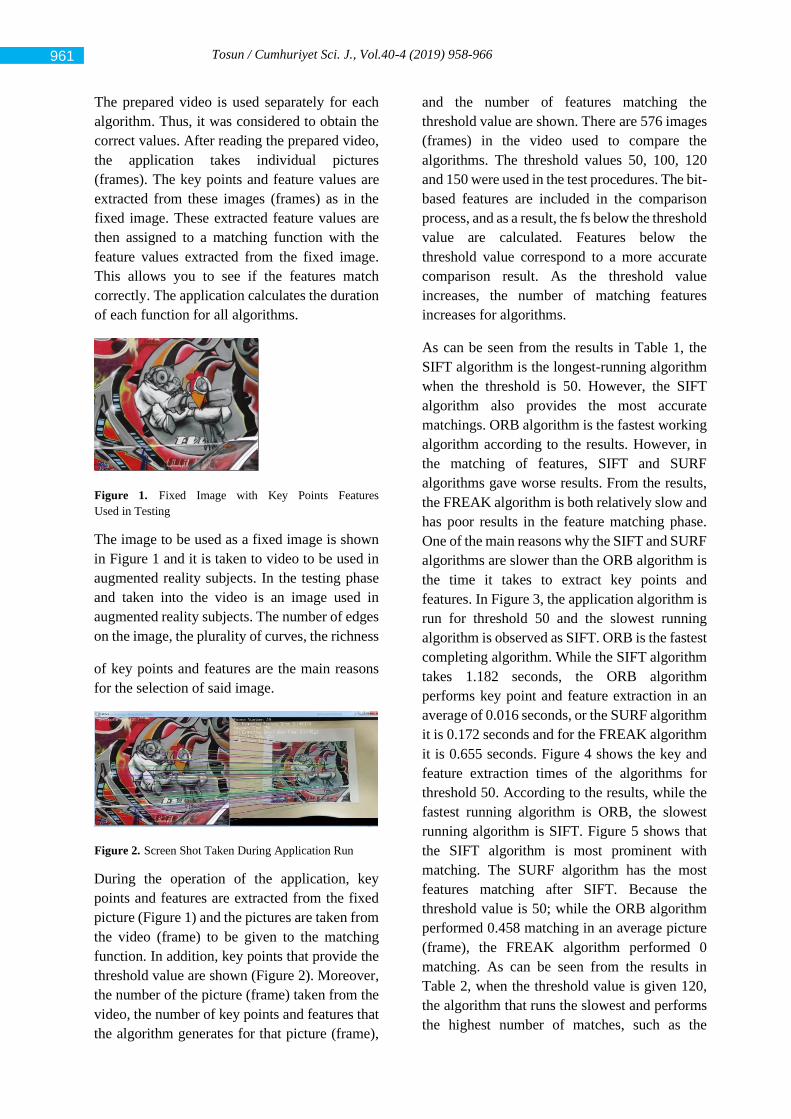
Tosun / Cumhuriyet Sci. J., Vol.40-4 (2019) 958-966
The prepared video is used separately for each
algorithm. Thus, it was considered to obtain the
correct values. After reading the prepared video,
the application takes individual pictures
(frames). The key points and feature values are
extracted from these images (frames) as in the
fixed image. These extracted feature values are
then assigned to a matching function with the
feature values extracted from the fixed image.
This allows you to see if the features match
correctly. The application calculates the duration
of each function for all algorithms.
Figure 1. Fixed Image with Key Points Features
Used in Testing
The image to be used as a fixed image is shown
in Figure 1 and it is taken to video to be used in
augmented reality subjects. In the testing phase
and taken into the video is an image used in
augmented reality subjects. The number of edges
on the image, the plurality of curves, the richness
of key points and features are the main reasons
for the selection of said image.
Figure 2. Screen Shot Taken During Application Run
During the operation of the application, key
points and features are extracted from the fixed
picture (Figure 1) and the pictures are taken from
the video (frame) to be given to the matching
function. In addition, key points that provide the
threshold value are shown (Figure 2). Moreover,
the number of the picture (frame) taken from the
video, the number of key points and features that
the algorithm generates for that picture (frame),
and the number of features matching the
threshold value are shown. There are 576 images
(frames) in the video used to compare the
algorithms. The threshold values 50, 100, 120
and 150 were used in the test procedures. The bit-
based features are included in the comparison
process, and as a result, the fs below the threshold
value are calculated. Features below the
threshold value correspond to a more accurate
comparison result. As the threshold value
increases, the number of matching features
increases for algorithms.
As can be seen from the results in Table 1, the
SIFT algorithm is the longest-running algorithm
when the threshold is 50. However, the SIFT
algorithm also provides the most accurate
matchings. ORB algorithm is the fastest working
algorithm according to the results. However, in
the matching of features, SIFT and SURF
algorithms gave worse results. From the results,
the FREAK algorithm is both relatively slow and
has poor results in the feature matching phase.
One of the main reasons why the SIFT and SURF
algorithms are slower than the ORB algorithm is
the time it takes to extract key points and
features. In Figure 3, the application algorithm is
run for threshold 50 and the slowest running
algorithm is observed as SIFT. ORB is the fastest
completing algorithm. While the SIFT algorithm
takes 1.182 seconds, the ORB algorithm
performs key point and feature extraction in an
average of 0.016 seconds, or the SURF algorithm
it is 0.172 seconds and for the FREAK algorithm
it is 0.655 seconds. Figure 4 shows the key and
feature extraction times of the algorithms for
threshold 50. According to the results, while the
fastest running algorithm is ORB, the slowest
running algorithm is SIFT. Figure 5 shows that
the SIFT algorithm is most prominent with
matching. The SURF algorithm has the most
features matching after SIFT. Because the
threshold value is 50; while the ORB algorithm
performed 0.458 matching in an average picture
(frame), the FREAK algorithm performed 0
matching. As can be seen from the results in
Table 2, when the threshold value is given 120,
the algorithm that runs the slowest and performs
the highest number of matches, such as the
961
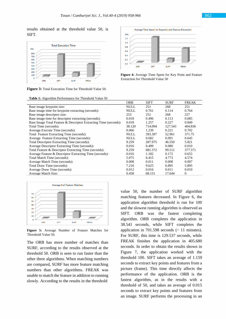
Tosun / Cumhuriyet Sci. J., Vol.40-4 (2019) 958-966
results obtained at the threshold value 50, is
SIFT.
Figure 3: Total Execution Time for Threshold Value 50.
Figure 5: Average Number of Feature Matches for
Threshold Value 50.
The ORB has more number of matches than
SURF, according to the results observed at the
threshold 50. ORB is seen to run faster than the
other three algorithms. When matching numbers
are compared, SURF has more feature matching
numbers than other algorithms. FREAK was
unable to match the feature in addition to running
slowly. According to the results in the threshold
Figure 4: Average Time Spent for Key Point and Feature
Extraction for Threshold Value 50
value 50, the number of SURF algorithm
matching features decreased. In Figure 6, the
application algorithm threshold is run for 100
and the slowest running algorithm is observed as
SIFT. ORB was the fastest completing
algorithm. ORB completes the application in
38.541 seconds, while SIFT completes the
application in 701.598 seconds (~ 11 minutes).
For SURF, this time is 129.537 seconds, while
FREAK finishes the application in 405.680
seconds. In order to obtain the results shown in
Figure 7, the application worked with the
threshold 100. SIFT takes an average of 1.159
seconds to extract key points and features from a
picture (frame). This time directly affects the
performance of the application. ORB is the
fastest algorithm, as in the results with a
threshold of 50, and takes an average of 0.015
seconds to extract key points and features from
an image. SURF performs the processing in an
Table 1: Algorithm Performance for Threshold Value 50
ORB SIFT SURF FREAK
Base image keypoint size:
Base image time for keypoint extracting (seconds):
Base image descriptor size:
Base image time for descriptor extracting (seconds):
Base Image Total Feature & Descriptor Extracting Time (seconds):
Total Time (seconds):
Average Execute Time (seconds):
Total Feature Extracting Time (seconds):
Average Feature Extracting Time (seconds):
Total Descriptor Extracting Time (seconds):
Average Descriptor Extracting Time (seconds):
Total Feature & Descriptor Extracting Time (seconds):
Average Feature & Descriptor Extracting Time (seconds):
Total Match Time (seconds):
Average Match Time (seconds):
Total Draw Time (seconds):
Average Draw Time (seconds):
Average Match Size:
NULL 251 268 251
NULL 0.761 0.114 0.764
253
0.018
0.018
38.120
0.066
NULL
NULL
9.259
0.016
9.259
0.016
5.075
0.008
7.216
0.012
0.458
251
0.496
1.257
714.094
1.239
393.397
0.682
287.975
0.499
681.372
1.182
6.415
0.011
9.625
0.016
68.151
268
0.113
0.227
127.543
0.221
52.961
0.091
46.550
0.080
99.511
0.172
4.773
0.008
6.895
0.011
17.644
227
0.085
0.849
404.836
0.702
371.75
0.645
5.821
0.010
377.571
0.655
4.574
0.007
5.895
0.010
0
962
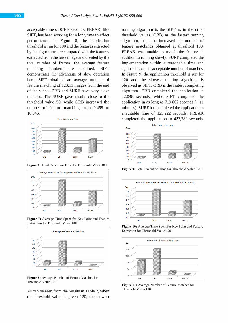
Tosun / Cumhuriyet Sci. J., Vol.40-4 (2019) 958-966
acceptable time of 0.169 seconds. FREAK, like
SIFT, has been working for a long time to affect
performance. In Figure 8, the application
threshold is run for 100 and the features extracted
by the algorithms are compared with the features
extracted from the base image and divided by the
total number of frames, the average feature
matching numbers are obtained. SIFT
demonstrates the advantage of slow operation
here. SIFT obtained an average number of
feature matching of 123.11 images from the end
of the video. ORB and SURF have very close
matches. The SURF gave results close to the
threshold value 50, while ORB increased the
number of feature matching from 0.458 to
18.946.
Figure 6: Total Execution Time for Threshold Value 100.
Figure 7: Average Time Spent for Key Point and Feature
Extraction for Threshold Value 100
Figure 8: Average Number of Feature Matches for
Threshold Value 100
As can be seen from the results in Table 2, when
the threshold value is given 120, the slowest
running algorithm is the SIFT as in the other
threshold values. ORB, as the fastest running
algorithm, has also increased the number of
feature matchings obtained at threshold 100.
FREAK was unable to match the feature in
addition to running slowly. SURF completed the
implementation within a reasonable time and
again achieved an acceptable number of matches.
In Figure 9, the application threshold is run for
120 and the slowest running algorithm is
observed as SIFT. ORB is the fastest completing
algorithm. ORB completed the application in
42,048 seconds, while SIFT completed the
application in as long as 719.802 seconds (~ 11
minutes). SURF has completed the application in
a suitable time of 125.222 seconds. FREAK
completed the application in 423,282 seconds.
Figure 9: Total Execution Time for Threshold Value 120.
Figure 10: Average Time Spent for Key Point and Feature
Extraction for Threshold Value 120
Figure 11: Average Number of Feature Matches for
Threshold Value 120
963
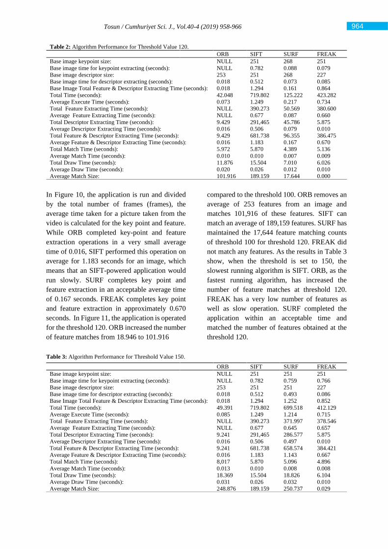
Tosun / Cumhuriyet Sci. J., Vol.40-4 (2019) 958-966
In Figure 10, the application is run and divided
by the total number of frames (frames), the
average time taken for a picture taken from the
video is calculated for the key point and feature.
While ORB completed key-point and feature
extraction operations in a very small average
time of 0.016, SIFT performed this operation on
average for 1.183 seconds for an image, which
means that an SIFT-powered application would
run slowly. SURF completes key point and
feature extraction in an acceptable average time
of 0.167 seconds. FREAK completes key point
and feature extraction in approximately 0.670
seconds. In Figure 11, the application is operated
for the threshold 120. ORB increased the number
of feature matches from 18.946 to 101.916
compared to the threshold 100. ORB removes an
average of 253 features from an image and
matches 101,916 of these features. SIFT can
match an average of 189,159 features. SURF has
maintained the 17,644 feature matching counts
of threshold 100 for threshold 120. FREAK did
not match any features. As the results in Table 3
show, when the threshold is set to 150, the
slowest running algorithm is SIFT. ORB, as the
fastest running algorithm, has increased the
number of feature matches at threshold 120.
FREAK has a very low number of features as
well as slow operation. SURF completed the
application within an acceptable time and
matched the number of features obtained at the
threshold 120.
Table 3: Algorithm Performance for Threshold Value 150.
Table 2: Algorithm Performance for Threshold Value 120.
ORB SIFT SURF FREAK
Base image keypoint size:
Base image time for keypoint extracting (seconds):
Base image descriptor size:
Base image time for descriptor extracting (seconds):
Base Image Total Feature & Descriptor Extracting Time (seconds):
Total Time (seconds):
Average Execute Time (seconds):
Total Feature Extracting Time (seconds):
Average Feature Extracting Time (seconds):
Total Descriptor Extracting Time (seconds):
Average Descriptor Extracting Time (seconds):
Total Feature & Descriptor Extracting Time (seconds):
Average Feature & Descriptor Extracting Time (seconds):
Total Match Time (seconds):
Average Match Time (seconds):
Total Draw Time (seconds):
Average Draw Time (seconds):
Average Match Size:
NULL 251 268 251
NULL 0.782 0.088 0.079
253
0.018
0.018
42.048
0.073
NULL
NULL
9.429
0.016
9.429
0.016
5.972
0.010
11.876
0.020
101.916
251
0.512
1.294
719.802
1.249
390.273
0.677
291,465
0.506
681.738
1.183
5.870
0.010
15.504
0.026
189.159
268
0.073
0.161
125.222
0.217
50.569
0.087
45.786
0.079
96.355
0.167
4.389
0.007
7.010
0.012
17.644
227
0.085
0.864
423.282
0.734
380.600
0.660
5.875
0.010
386.475
0.670
5.136
0.009
6.026
0.010
0.000
ORB SIFT SURF FREAK
Base image keypoint size:
Base image time for keypoint extracting (seconds):
Base image descriptor size:
Base image time for descriptor extracting (seconds):
Base Image Total Feature & Descriptor Extracting Time (seconds):
Total Time (seconds):
Average Execute Time (seconds):
Total Feature Extracting Time (seconds):
Average Feature Extracting Time (seconds):
Total Descriptor Extracting Time (seconds):
Average Descriptor Extracting Time (seconds):
Total Feature & Descriptor Extracting Time (seconds):
Average Feature & Descriptor Extracting Time (seconds):
Total Match Time (seconds):
Average Match Time (seconds):
Total Draw Time (seconds):
Average Draw Time (seconds):
Average Match Size:
NULL 251 251 251
NULL 0.782 0.759 0.766
253
0.018
0.018
49.391
0.085
NULL
NULL
9.241
0.016
9.241
0.016
8,017
0.013
18.369
0.031
248.876
251
0.512
1.294
719.802
1.249
390.273
0.677
291,465
0.506
681.738
1.183
5.870
0.010
15.504
0.026
189.159
251
0.493
1.252
699.518
1.214
371.997
0.645
286.577
0.497
658.574
1.143
5.096
0.008
18.826
0.032
250.737
227
0.086
0.852
412.129
0.715
378.546
0.657
5.875
0.010
384.421
0.667
4.896
0.008
6.104
0.010
0.029
964
Tosun / Cumhuriyet Sci. J., Vol.40-4 (2019) 958-966
4. CONCLUSIONS
According to the results obtained, ORB is the
fastest working algorithm. SIFT has the highest
value in feature extraction criteria. Increasing the
threshold value causes the fall of feature matching
quality. In other words, increasing the threshold
value causes the number of matching features
generated by the algorithms to increase. As a result
of this work, it was observed that SIFT and SURF
performed more accurate feature matches. ORB
has better results than the other three algorithms in
terms of FPS (frame per second) time. In addition
to being a slow algorithm like SIFT, FREAK is not
successful in feature matching. Although SURF is
relatively slow compared to ORB, it cannot provide
feature matches such as SIFT. If it is an application
where the simultaneous pictures taken from a
camera are processed or pictures taken from a
video are processed; extracting features for each
image may cause a slowdown. If the desired
number of features is matched on the picture, the
feature may not be matched again on the next
picture to be processed. Instead, features matched
in the previous picture can be given to the follow-
up phase depending on the type of application;
thus, time can be saved as the follow-up phase runs
faster than the feature matching phase. At this
point, it is important to note that the key points that
are processed as a result of feature matching during
the follow-up phase are correctly matched key
points. As a result, ORB works faster than the other
three algorithms compared, and fewer features
match with SIFT and SURF. Algorithm selection
with respect to the application area of the
augmented reality application to be implemented
would be beneficial. For example, if a mobile
application is to be realized, time will be an
important criterion and ORB will give a good
performance in this regard. SIFT or SURF will be
more appropriate in high performance applications
where time is not critical and correct feature
matching is more important.
REFERENCES
[1] Graham M., Zook M., and Boulton A.,
Augmented Reality in Urban Places: contested
content and the duplicity of code, Trans. Inst.
Br. Geogr., 38-3 (2013) 464-479.
[2] Steuer J., Defining Virtual Reality:
Dimensions Determining Telepresence, J.
Commun., 42-4 (1992) 73-93.
[3] If You’re Not Seeing Data You’re Not Seeing,
Wired.https://www.wired.com/2009/08/augm
ented-reality/. Retrieved October 25 (2009).
[4] Rublee E., Rabaud V., Konolige K., and
Bradski G., ORB An Efficient Alternative to
SIFT or SURF, Proceedings of 7th IEEE
International Conference on Computer Vision,
(2011) 2564-2571.
[5] Wagner D., Reitmayr G., Mulloni A.,
Drummond T., and Schmalstieg D., Pose
Tracking from Natural Features on Mobile
Phones, Proceedings of 7th IEEE and ACM
International Symposium on Mixed and
Augmented Reality, (2008) 125-134.
[6] Wagner D., Schmalstieg D., and Bischof H.,
Multiple Target Detection and Tracking with
Guaranteed Framerates on Mobile Phones,
International Symposium on Mixed and
Augmented Reality, (2009) 57-64.
[7] Wagner D., Mulloni A., Langlotz T., and
Schmalstieg D., Real-Time Panoramic
Mapping and Tracking on Mobile Phones,
Proceedings of IEEE Virtual Reality, (2010)
211-218.
[8] Klein G. and Murray D., Parallel Tracking and
Mapping on a Camera Phone, Proceedings of
8th IEEE International Symposium on Mixed
and Augmented Reality, (2009) 83-86.
[9] Ta D. N., Chen W. C., Gelfand N., and Pulli
K., SURFTrac: Efficient Tracking and
Continuous Object Recognition using Local
Feature Descriptors, IEEE Computer Society
Conference on Computer Vision and Pattern
Recognition, (2009) 2937-2944.
[10] Takacs G., Chandrasekhar V., Tsai S., Chen
D., Grzeszczuk R., and Girod B., Rotation-
invariant fast features for large-scale
recognition and real-time tracking, Signal
Process. Image, 28-4 (2013) 334-34.
[11] Rosten E. and Drummond T., Machine
learning for high-speed corner detection,
European Conference on Computer Vision,
(2006) 430-443 .
[12] Rosten E., Porter R., and Drummond T., Faster
and better: A machine learning approach to
corner detection, IEEE T. Pattern Anal., 32-1
(2010) 105–119.
[13] Trzcinski T., Christoudias M., Lepetit V., and
Fua P., Learning Image Descriptors with the
965
Tosun / Cumhuriyet Sci. J., Vol.40-4 (2019) 958-966
Boosting-Trick, Advances in Neural
Information Processing Systems, (2012) 1-9.
[14] Winder S. and Brown M., Learning Local
Image Descriptors, IEEE Conference on
Computer Vision and Pattern Recognition,
(2007) 1-8.
[15] Brown M., Hua G., and Winder S.,
Discriminative Learning of Local Image
Descriptors, IEEE T. Pattern Anal., 33-1
(2011) 43-57.
[16] Ke Y. and Sukthankar R., PCA-SIFT: A More
Distinctive Representation for Local Image
Descriptors, IEEE Computer Society
Conference on Computer Vision and Pattern
Recognition, (2004) 506-514.
[17] Simonyan K., Vedali A., and Zisserman A.,
Descriptor Learning Using Convex
Optimisation, European Conference on
Computer Vision (2012), 243-256.
[18] Lowe D. G., Distinctive Image Features from
Scale-Invariant Keypoints, Int. J. Comput.
Vis., 60-2 (2004) 91-110.
[19] Bay H., Ess A., Tuytelaars T., and Gool L.V.,
Speeded-Up Robust Features (SURF),
Comput. Vis. Image Und., 110-3 (2008), 346-
359.
[20] Calonder M,, Lepetit V, Strecha C, and Fua P.
Brief: Binary Robust Independent Elementary
Features, European Conference on Computer
Vision, Heraklion, (2010) 778-792.
[21] Harris C. and Stephens M., A combined corner
and edge detector, Fourth Alvey Vision
Conference, (1988) 147-151.
[22] Huang W., Wu L. D., Song H. C., and Wei Y.
M. “RBRIEF: a robust descriptor based on
random binary comparisons”. IET Comput.
Vis,, 7-1 (2013) 29-35.
[23] Scale Invariant FeatureTransform,
Scholarpedia.http://www.scholarpedia.org/art
icle/SIFT. Retrieved October 18, 2013.
[24] Scale Invariant Feature Transform (SIFT),
VLFeat. http://www.vlfeat.org/api/sift.html.
Retrieved October 18, 2013.
[25] Schaeffer C., A Comparison of Keypoint
Descriptors in the Context of Pedestrian
Detection: FREAK vs. SURF vs. BRISK
(2013).
[26] Alahi A., Ortiz R., and Vandergheynst P.,
FREAK: Fast Retina Keypoint, Proceedings of
the IEEE Computer Society Conference on
Computer Vision and Pattern Recognition,
(2012) 510-517.
[27] Leutenegger S., Chli M., and Siegwart R. Y.,
BRISK: Binary Robust invariant scalable
keypoints, Proceedings of the IEEE
International Conference on Computer Vision,
(2011) 2548-2555.
966

Cumhuriyet Science Journal
CSJ
e-ISSN: 2587-246X
ISSN: 2587-2680 Cumhuriyet Sci. J., Vol.40-4 (2019) 967-977
* Corresponding author. Email address: [email protected], [email protected]
http://dergipark.gov.tr/csj ©2019 Faculty of Science, Sivas Cumhuriyet University
Investıgatıon of Natural Mycoflora and Aflatoxin Formation in Hazelnuts
and Products
Z. Seba KESKIN 1 , Nevcihan GURSOY 2
1 Cumhuriyet University, Yildizeli Vocational School, Department of Food Technology Sivas / TURKEY
2 Cumhuriyet University, Faculty of Engineering, Dept. of Food Engineering, Sivas/TURKEY
Received: 08.11.2019; Accepted: 11.12.2019 http://dx.doi.org/10.17776/csj.644503
Abstract. In this study, natural mycoflora of 30 raw and 50 roasted hazelnut, 20 hazelnut paste and 50 inner
membrane samples and their total aflatoxin contents were determined. In mycological isolations, 1.8-2.56% of
Aspergillus flavus and 42.7-65.44% of A. niger were determined in the raw hazelnut samples. A. flavus (2.2-
12.2%) and A. niger (33.3-74.5%) were also detected in roasted hazelnut, while the percentages of these
microorganisms in hazelnut paste samples were 0-13.1% and 43.5-100.0%, respectively. The ratio of A. flavus
and A. niger in inner membranes was found to be 2.6-16.2% and 44.6-89.4%, respectively. Aflatoxin analysis
showed that the levels of aflatoxin were 2.11–10.03 ppb in raw hazelnut, 0.1–4.04 ppb in roasted hazelnut, 0.2-
6.02 ppb in hazelnut paste samples and 0.7-38.2 ppb in inner membrane samples. While only one of the raw
hazelnut, roasted hazelnut and hazelnut paste samples had toxin above the legal limit, 100% of the inner
membrane samples showed different levels of aflatoxin contamination. Since there is no limitation in the
Turkish Food Codex on hazelnut inner membrane, the amount of aflatoxin, which is higher than 10 ppb in 25
of the samples, was considered to be high contamination. Kruskal Wallis and Mann Whitney U analyses were
used for statistical evaluation of the samples. There was a significant difference in aflatoxin formation and
moisture content between the samples in different groups (p <0.05).
Keywords: Aflatoxin, hazelnut, hazelnut products, mycoflora.
Fındık ve Fındık Ürünlerinde Doğal Olarak Oluşan Mikoflora İle
Aflatoksin Oluşumlarinin Araştirilmasi
Özet. Bu çalışmada, 30 çiğ, 50 kavrulmuş fındık, 20 ezme ve 50 iç zar örneğinde oluşan doğal mikoflora ve
toplam aflatoksin içerikleri belirlenmiştir. Yapılan mikolojik izolasyonlarda çiğ fındıkta %1,8-2,56 Aspergillus
flavus, %42,7-65,44 A. niger; kavrulmuş fındıkta %2,2-12,2 A. flavus, %33,3-74,5 A. niger; ezme örneklerinde
%0-13,1 A. flavus, %43,5-100 A. niger; iç zarda ise %2,6-16,2 A.flavus, %44,6-89,4 A. niger belirlenmiştir.
Aflatoksin analizlerinde çiğ fındıkta 2.11–10.03 ppb, kavrulmuş fındıkta 0,1–4,04 ppb, ezme örneklerinde 0,2-
6,02 ppb ve iç zar örneklerinde ise 0,7-38,2 ppb seviyelerinde aflatoksin içerikleri saptanmıştır. Çiğ fındık,
kavrulmuş fındık ve ezme örneklerinin sadece 1’inde yasal sınırın üzerinde toksin içeriği bulunurken, iç zar
örneklerinin % 100’ ünde değişik seviyelerde aflatoksin bulaşıklığı bulunmuştur. Fındık iç zarı ile ilgili Türk
Gıda Kodeksinde bir sınırlama olmadığı için örneklerin 25’ in de 10 ppb ‘den yüksek olan aflatoksin oluşumları
yüksek bulaşıklık olarak değerlendirilmiştir. Çalışılan örneklerin istatistikî değerlendirmelerinde Kruskal
Wallis ve Mann Whitney U analizleri kullanılmıştır. Farklı gruplardaki örnekler arasında aflatoksin oluşumu
ve nem içerikleri arasındaki değişim istatistiki açıdan önemli bulunmuştur (p<0.05).
Anahtar Kelimeler: Aflatoksin, fındık, fındık ürünleri, mikoflora.

Keskin,Gürsoy / Cumhuriyet Sci. J., Vol.40-4 (2019) 967-977
1. INTRODUCTION
Hazelnut (Corylus avellana L.) forms the basis for
the more important commercial cultivars and is
belonging to Betulaceae family. The hazelnut
(Corylus avellana L.) forms the more important
commercial cultivars. C. maxima and C. colurna
(Turkish hazel) are also common others. Hazelnut
is grown in the Blacksea Region of Turkey,
especially in Trabzon, Ordu, Giresun and
Akçakoca. Although vary depending on the year,
Turkey ranks the first in the world with
approximately 600 thousand tonnes of hazelnut
production [1].
Hazelnut is a food rich in proteins, lipids,
carbohydrates, vitamins, minerals, dietary fibers,
tocopherols, phytosterols and phenolic compounds
[2,3]. Monounsaturated fatty acids (especially oleic
acid) and polyunsaturated fatty acids in hazelnut
have been reported to have beneficial effects on
human health [3]. Hazelnut oil has been found to
reduce cholesterol levels in the blood [4]. Hazelnut
contains tocopherols, phytosterols, squalene and
phenolic compounds that help prevent chronic
diseases such as cancer and cardiovascular diseases
[5,6].
There are biological, chemical and microbiological
factors limiting hazelnut production. The most
important microbiological factors limiting hazelnut
production are fungal contamination and
aflatoxins, one of the metabolites produced by
these fungi. Aflatoxins are secondary metabolites
produced by Aspergillus species. To date, more
than 20 different aflatoxins have been reported.
However, B1, B2, G1, G2 were reported to be four
naturally occurring main forms. A. flavus produces
only AFB1 and B2, while A. parasiticus produces
AFB1, B2, G1 and G2 [7-9].
Aflatoxins produced by Aspergillus spp. in field
conditions, transportation, processing and storage
can be found in oilseeds such as nuts, pistachios,
peanuts, almonds, sunflowers, in cereals and cereal
products, pulses, spices, milk, dairy products, meat,
meat products and animal products such as eggs
[10-12].
Aflatoxins have been reported to have several
effects on human and animal health such as
mutagenic, carcinogenic, teratogenic (embryonal
damage), tremorgenic (problems of tremor and
reflex loss), hemoralgic (tissue and organs bleeding
problems), dermatitic (skin lesions), hepatoxic
(liver damage), nephrotoxic (kidney system
damage), and neurotoxic (nervous system damage)
[13-15]. Aflatoxins are known to be the most
effective hepatocarcinogen in many animal
species. In many countries, aflatoxins are included
in the class 1A carcinogens by the International
Organization for Cancer Research, since there is a
positive correlation between consumption of
aflatoxin-contaminated food and an increased risk
of liver cancer [16].
The maximum limits of aflatoxins in many
foodstuffs have been established and published in
each country. In order to protect public health,
importing countries, especially the European
Union countries, aim to reduce the legal values of
aflatoxins to zero in risky products. To this end,
aflatoxin B1 limit in many countries has been
reduced from 5 ppb to 2 ppb and the total aflatoxin
(B1+B2+G1+G2) in hazelnuts has been reduced
from 10 ppb to 4 ppb (Commission Regulation EC
No 194/97). In the Turkish Food Codex, the total
aflatoxin content in hazelnut and its products is
determined to be 10 ppb and Aflatoxin B1 content
is maximum 5 ppb [17,18].
As mentioned above, although vary depending on
the year, Turkey ranks first in the world with
approximately 600 thousand tonnes of hazelnut
production [1]. In addition, Aflatoxin
contamination is one of the most important
problems in hazelnut and hazelnut products. Due to
the aflatoxin values in nuts exported by Turkey are
sometimes above the legal limits, these products
are rejected by the countries, which leads to huge
economic losses. Additionally, producers and
industrialists are struggling economically, Turkey's
reputation in foreign trade is damaged and
marketing problems arise.
After the occurrence of aflatoxin, which is a
problem in food all over the world, they cannot be
controlled [19-21].Therefore, the most effective
method for the formation of aflatoxins produced by
fungi is to harvest, dry, store and process food
under conditions that reduce the risk of
contamination and limit the development of fungi.
These conditions can only be achieved by
determining the natural mycoflora that is formed in
the product and can cause toxin formation.
In this study, it was aimed to determine the
naturally occurring mycoflora in raw hazelnut,
968
Keskin,Gürsoy / Cumhuriyet Sci. J., Vol.40-4 (2019) 967-977
roasted hazelnut, hazelnut paste and hazelnut inner
membrane and to investigate the total aflatoxin
formation in these products.
2. MATERIALS AND METHODS
2.1. Supply of Hazelnut Samples
The samples used in the study were obtained from
various factories and retail stores in Trabzon, Ordu,
Giresun and Akçakoca regions where hazelnut
production is intense in the Blacksearegion. In the
sampling, raw hazelnut (n = 30), roasted hazelnut
(n = 50), hazelnut paste (n = 20), and inner
membrane (n = 50) samples were used. The
hazelnut samples were provided immediately after
harvest, the inner membrane samples were
obtained during the drying period and the hazelnut
paste samples were provided during the processing
stages of the product. Samples were brought to the
laboratory under appropriate conditions and kept in
labelled cloth bags and refrigerated at 4 C until
tested.
2.2. Determination of Moisture Content of
Samples
The moisture content of the hazelnut, hazelnut
paste and membrane samples used in the study was
determined by a precision balance and halogen
lamp moisture analyzer according to the method
reported by Bakker [22]. 5.0 ± 0.1 g of raw and
roasted hazelnut samples were taken and shredded
in hand blender and moisture contents were
determined at 140 C. In order to determine the
moisture content of hazelnut membrane and
hazelnut paste samples, 1 g of each sample was
weighed directly without any process and
evaluated according Özkaya [23] equation (1).
%Moisture content:
01
1
MM
MM
−
− (1)
M0: Weight of continer (Tare) (g)
M: Weight of the container and sample after drying
M1 : Weight of sample with container
2.3. Mycological Isolations
Raw hazelnut, roasted hazelnut and inner
membrane samples were sterilized with 2.0% (v/v)
NaOCl solution and washed with distilled water.
After surface sterilization, of dried hazelnut,
roasted hazelnut and inner membrane samples,
hazelnut paste samples were added directly to
Potato Dextrose Agar (PDA). After surface
sterilization was performed, raw hazelnut, roasted
hazelnut and inner membrane samples were dried
and then planted in PDA while surface sterilization
process was not applied for the cultivation of
hazelnut paste samples. A total of 100 plantings
were made for each sample using 10 petri dishes.
Cultivated petri dishes were incubated at 24 C for
4-5 days and thus colony development was
ensured. At the end of incubation, the fungal
colonies were differentiated based on macroscopic
criteria such as size, colour, surface or overhead
development, and colonies showing different
growth were purified by classifying as Fusarium
(F1, F2,…), Aspergillus (A1, A2, …) and
Penicillium (P1, P2,…).
After purification, single spore isolation was made
on water and Czapek Dox Agar. Single spore
isolates were incubated at 25 °C for 7 days by
transferring them to a suitable growth medium.
Cultures were examined under microscope during
the incubation and general morphological
definitions were made, colony number and
characteristics were recorded.
Specific diagnostic keys have been used for the
fungi species identified intensively as a result of
mycological isolations. While the diagnostic keys
developed by Raper and Fennel [24] and Samson
and Pitt [25] is used for the identification of
Aspergillus species, Penicillum species were
identified according to the diagnostic keys of
Samson et al. [26] and Pitt [27]. In identifying
Fusarium and other species, diagnostic key
developed by Barnett and Hunter [28] was used.
In species identification of fungi; growth rates at
certain temperatures (colony diameter and
properties), overhead mycelium formation (colour
and structure), the presence or absence of
chlamidospores, sporodosium development, fialitic
properties, conidial cap (color and shape), conidial
sequencing, colony colours, presence or absence of
sclerotes, and presence of macro and micro conidia
were evaluated.
2.4. Aflatoxin Analysis
CD-ELISA (Competitive Direct Enzyme-Linked
Immuno Sorbent Assay) method was used to
investigate the total amount of aflatoxin in raw
hazelnut, roasted hazelnut, inner membrane and
hazelnut paste samples. 5 different aflatoxin
standards were used in CD-ELISA at 0, 1, 2, 4 and
8 ppb levels. Samples were prepared and extracted
according to the procedure of Neogen Veratox®.
CD-ELISA results were obtained by reading at 650
nm in a microwell reader. Veratox Software for
Windows, Log/Logit and Single Test Format v3.02
software were used to calculate the toxin values in
ppb.
969
Keskin,Gürsoy / Cumhuriyet Sci. J., Vol.40-4 (2019) 967-977
3. RESULTS AND DISCUSSION
Moisture measurement analyzes were carried out to
determine how moisture content of raw hazelnut,
roasted hazelnut, inner membrane and hazelnut
paste affect natural mycoflora and aflatoxin
formation in these samples.
The moisture content of samples obtained from
Trabzon, Ordu, Giresun and Akçakoca regions are
given in Figure 1.
Figure 1. Moisture content of samples obtained
from different regions
As can be seen from Figure 1, the moisture values
of the raw hazelnuts were determined as 3.88-
4.56%. It is recommended that the maximum
moisture content in raw hazelnuts should be max.
4.5% [29]. It was observed that the moisture values
of our samples were close to or higher than the
recommended maximum value. Aluç and Aluç [30]
found the moisture values of 186 Akcakoca, 177
Ordu and 160 Giresun raw hazelnut samples to be
4.2-6.8%. According to meteorological data, the
rainfall of the 4 regions is approximately 61.6-75.9
mm per year. Samples of raw nuts with the highest
moisture content were obtained from Ordu region.
This is due to the fact that the average annual
rainfall in the Ordu region is generally higher than
the other three regions.
As a result of mycological isolation of raw
hazelnut, roasted hazelnut, hazelnut paste and inner
membrane samples, Aspergillus species were
observed as the most dominant fungal ones.
Natural mycoflora determined as a result of
mycological isolations in samples obtained from
different regions is presented in Table 1 and Figure
2. Aspergillus and Penicillium species are
predominant in the studies conducted on the
determination of raw and roasted hazelnut
mycoflora, however, Rhizopus, Fusarium,
Cladosporium, Trichothecium, Mucor, Alternaria
and Trichoderma species have also been reported
to be isolated [31, 32]. No studies have been found
in the literature on the determination of mycoflora
in hazelnut paste and inner membrane samples.
a. A. flavus from raw nuts; b. A. niger from roasted nuts; c. Fusarium spp. from hazelnut butter; d. Penicillium spp. from the
inner membrane; e. Trichoderma spp. from raw nuts; f. A. flavus from roasted hazelnuts; g. Fusarium spp. from hazelneut butter;
h. A. niger isolated from the inner membrane ı. A. flavus from raw nuts; j. Fusarium spp. from roasted hazelnuts; k.Trichoderma
spp. isolated hazelnut butter; l. Penicillium spp. isolated from inner membrane; m. Tricoderma spp. from raw nuts; n. A. flavus
from roasted hazelnuts; o. A. niger from hazelneut butter; p. Tricoderma spp. from the inner membrane.
Figure 2. Isolated fungal species from sample groups.
970

Keskin,Gürsoy / Cumhuriyet Sci. J., Vol.40-4 (2019) 967-977
Table 1. Natural mycoflora determined as a result
Regions
Sample
Type Fungus Species % Isolation
Regions
Sample
Type Fungus Species % Isolation
Tra
bzo
n
Raw
Aspergillus 68.0
Ord
u
Raw
Aspergillus 63.0
Penicillium 19.2 Penicillium
23.3
Rhizopus 12.8 Rhizopus 9.4
Roast
ed
Aspergillus 57.8 Fusarium
2.6
Penicillium 26.6 Trichoderma
1.7
Fusarium 8.4
Roast
ed
Aspergillus 44.5
Alternaria 4.6 Penicillium
33.5
Rhizopus 2.6 Fusarium
16.5
Bu
tter
Aspergillus 50.3 Rhizopus 5.5
Penicillium 43.5
Bu
tter
Aspergillus 51.0
Fusarium 6.2 Penicillium
20.6
İnn
er M
emb
ran
e Aspergillus 60.6 Rhizopus
18.0
Penicillium 33.0 Fusarium
10.4
Rhizopus 4.0
İnn
er
Mem
b.
Aspergillus 95.0
Trichoderma 1.4 Penicillium
4.4
Gir
esu
n
Raw
Aspergillus 45.0 Rhizopus 0.6
Penicillium 21.0
Ak
çak
oca
Raw
Aspergillus 54.2
Rhizopus 21.0 Penicillium
14.6
Fusarium 13.0 Rhizopus 14.6
Roast
ed
Aspergillus 78.5 Fusarium
8.3
Penicillium 17.5 Trichoderma
8.3
Fusarium 4.0
Roast
ed
Aspergillus 45.2
Bu
tter
Aspergillus 63.7 Rhizopus 27.0
Penicillium 23.7 Penicillium
18.3
Trichoderma 10,0 Fusarium 9.5
Rhizopus 2,0
Bu
tter
Aspergillus 81.3
Fusarium 0,6 Penicillium
18.7
İnn
er M
emb
ran
e Aspergillus 4.8
İnn
er M
emb
ran
e
Aspergillus 85.1
Penicillium 34.4 Penicillium
9.3
Trichoderma 12.2 Trichoderma
4.7
Rhizopus 5.6 Rhizopus 0.9
971

Keskin,Gürsoy / Cumhuriyet Sci. J., Vol.40-4 (2019) 967-977
Figure 3. Fungus genus isolated from raw and roasted hazelnut samples.
Mycoflora in raw hazelnut was determined to be
45-68% of Aspergillus spp., 14.6-23.3% of
Penicillium spp., 9.4-21% of Rhizopus spp., 2.6-
13.0% of Fusarium spp., and 1.7-8.3% of
Trichoderma spp. These ratios were found to be as
follows in the mycoflora of roasted hazelnuts: 44.5-
78.5% Aspergillus spp., 17.5-33.5% Penicillium
spp., 2.6-27.0% Rhizopus spp., 4.0-16.5%
Fusarium spp., 0.0-4.0% Alternaria spp. (Figure
3).
Various studies on the determination of natural
microflora in raw and roasted hazelnuts yield
similar results to the present study. In these studies,
although Aspergillus and Penicillium species were
dominant, Rhizopus, Fusarium, Cladosporium,
Trichothecium, Mucor, Alternaria and
Trichoderma species were also isolated [31-34].
Aspergillus spp. was found to be high in natural
mycoflora of raw and roasted hazelnuts in many
studies [35-37].Other fungi genus and their
proportions isolated from raw nuts are as follows:
12.8-23.3% Rhizopus spp., 9.4-19.2% Penicillium
spp., 2.6-13% Fusarium spp. and 1.7-8.3%
Trichoderma spp. According to a study carried out
by Demir et al. [38] on 30 raw hazelnut samples,
the most commonly isolated fungi genus have been
reported as follows: 2.2- 100.0% Aspergillus spp.,
4.0-67.4% Penicillium, 2.0-62.0% Rhizopus, 2.0-
82.0% Mucor and 2.0-56.0% other fungus genera.
Simsek et al. [39], identified 96.6% Aspergillus
spp., 93.3% Penicillium, 96.6% Rhizopus and
83.3% Mucor in 30 hazelnut samples obtained
from Giresun. It is thought that the reason of high
observation of the Aspergillus spp. in many of our
samples is that the hazelnut was exposed to fungal
contamination in the tree and during harvest.
Furthermore, this indicates that although the
product is harvested early and the shell forms a
protective layer, there is a risk of contamination
from cracks that may occur during harvest. In
addition, high moisture content of hazelnut
growing areas is one of the important factors that
promote the development of Aspergillus spp.
According to our literature search could ascertain,
no study is available on natural mycoflora formed
in hazelnut inner membrane and hazelnut paste.
However, it is thought that the data obtained from
this study will serve as an example for other
scientific studies in the future. As can be seen from
Figure 4, 47.8-95.0% Aspergillus spp., 4.4-34.4%
Penicillium spp., 1.4- 12.2% Trichoderma spp.,
and 0.6-4.0% Rhizopus spp. was determined in the
inner membranes of hazelnuts samples collected
from 4 regions. Unidentified fungi species were
ignored. From hazelnut paste samples, 50.3-81.3%
Aspergillus spp., 18.7-43.5% Penicillium spp., 2.0-
18.0% Rhizopus spp., 0.0-10.0% Trichoderma spp.
and 0.6-10.4% Fusarium spp. were isolated.
Although Aspergillus spp. species that can
synthesize aflatoxin in hazelnut paste samples are
different according to regions, they have been
isolated and identified as the most dominant
species in the present study by 50.3-81.3%.
Penicillium, Rhizopus, Fusarium and Trichoderma
strains were isolated in 18.7-43.5%, 2.0-18.0%,
0.6-10.4% and 0.0-10.0%, respectively in
mycoflora of hazelnut paste samples.
972
Keskin,Gürsoy / Cumhuriyet Sci. J., Vol.40-4 (2019) 967-977
Figure 4. Fungus genus isolated from hazelnut paste and inner membrane samples.
The high rate of Aspergillus spp. species in most of
our samples suggests that hazelnut is exposed to
fungal contamination in the tree and during harvest.
This is because the development of Aspergillus
spp. species in shelled hazelnuts starts on the
surface of the shell when it is still in the tree, and it
can increase during the contact of the product with
the soil and harvesting. Aspergillus spp. are not
seen in shelled hazelnuts that come into contact
with the ground, while A. flavus-parasiticus
develops in the hazelnut which is damaged in the
outer shells [31]. This is because the hard shell of
hazelnut is a good protector against fungal
contamination and bacteria.
50% of the total 150 raw hazelnuts, roasted
hazelnuts, hazelnut paste and inner membranes,
aflatoxin contamination was found to be at levels
of 0.1-38.2 ppb. Aflatoxin levels of 2.11-10.03 ppb
were determined in 9 of 30 raw hazelnut samples
and only one sample had aflatoxin content above
the legal limit. Aflatoxin contamination (14.0%)
and aflatoxin levels (0.1-4.04 ppb) were below the
legal limit in roasted hazelnut samples (Table 2).
Table 2. Toxin contents and contamination rates determined in the samples
Sample
Number
of
Samples
Aflatoxin
(ppb)
Contaminated
Samples
Exceeding
Legal Limit %
Contamination
Raw 30 2,11-10,03 9 1 30
Roasted 50 0,1-4,04 7 - 14
Hazelnut
Butter
20 0,2-6,02 9 - 45
Inner
Membran
50 0,7-38,2 50 25 100
As a result of statistical evaluations between the
moisture contents and aflatoxin formation of 4
different hazelnut samples obtained from different
regions, the relationship between moisture content
and aflatoxin formation was found to be significant
(p<0.05) (Figure 5).
973
Keskin,Gürsoy / Cumhuriyet Sci. J., Vol.40-4 (2019) 967-977
Figure 5. The relationship between moisture content and aflatoxin formation.
While the amount of aflatoxin was found to be 30%
in the studied hazelnut samples, in only one of the
samples obtained from 4 regions, total aflatoxin
levels exceeded 10 ppb, which is the legal limit of
aflatoxin determined by the Turkish Food Codex.
Aycicek et al. [40] have studied the total aflatoxin
levels in raw hazelnuts. According to this study,
only one of 51 raw hazelnut samples has been
reported to exceed this legal limit. Especially in
raw hazelnut samples, high moisture content and
therefore aflatoxin content were detected in high
rainfall areas, indicating that climatic data play an
important role. Aluç and Aluç [30] determined the
levels of aflatoxins in raw nuts obtained from
Akçakoca, Ordu and Giresun. In 10 of 186 lots raw
nuts from Akcakoca region B1 = 2.66-75.08 ppb,
total = 4.77-78.93 ppb, 20 of 160 lots raw nuts from
Giresun region B1 = 2.17-75.68 ppb, total = 4.34-
150, 08 ppb, and 16 of 177 lots raw nuts from Ordu
region B1 = 2.1-29.44 ppb, total = 3.61-135.51 ppb
aflatoxin contamination. Due to the high rainfall in
the regions where raw hazelnuts are grown, factors
such as high moisture values and the fact that
hazelnuts are not fully developed while in the tree
cause aflatoxin formation. In addition, mistakes
made during the production, processing and
storage stages lead to an increase in the amount of
aflatoxin.
Aflatoxin was determined in 7 of the 50 roasted
hazelnut samples and total amount of aflatoxin was
between 0.1-4.04 ppb. The amount of aflatoxin
found in the samples was found to be below the
legal limit specified in the Turkish Food Codex.
Heperkan [31] has investigated the mycotoxins in
foods and their importance in terms of our country.
In this study, 140 samples obtained from Ordu,
Giresun and Tirebolu in Blacksearegion were
examined and aflatoxin was determined in 5 of 25
hazelnut samples. Deabes and Al-Habib [34]
reported that Aspergillus species, which are
capable of producing aflatoxin, were predominant
in mycoflora of hazelnut samples and aflatoxin
levels were found to be between 41-55 ppb.
Aflatoxin content was found to be 14.0% in roasted
hazelnut samples. This value was found to be lower
than in raw hazelnut. Raw nuts are more risky in
terms of aflatoxin, while roasted nuts are more
stable [41]. The reason for this is that some fungi
in the mycoflora become ineffective and the
moisture content decreases as a result of heat
treatments applied to roasted hazelnuts. Because
fungal contamination is more common due to the
high rate of free water required for the development
of fungi. In addition, as the fat content of the
products increases, the rate of mold and aflatoxin
increase [42].
In a study, aflatoxin levels were investigated in
hazelnuts. Aspergillus species capable of
producing aflatoxin in the mycoflora of hazelnut
samples analyzed have been reported to be
predominant and aflatoxin levels vary between 41-
55 ppb [34].
In a study investigating natural mycoflora and
aflatoxin contamination in 25 raw and 25 roasted
hazelnut samples, aflatoxin contamination was
reported in 33 (66%) of 50 hazelnut samples at 0.1–
155 ppb levels. In this study, aflatoxin formation
above the legal limit was determined at 14.2-155
ppb levels in 2 raw and 6 roasted hazelnut samples
[32].
Baltacı et al. [43], have collected samples during 3
years from companies exporting raw and roasted
hazelnuts. According to the results of this study,
0
10
20
30
40
50
60
70
80
90
100
Raw Roasted Paste Inner
membrane
Moisture
Aflatoxin
974
Keskin,Gürsoy / Cumhuriyet Sci. J., Vol.40-4 (2019) 967-977
aflatoxin levels were found to be between 0.02-
78.98 ppb in 3188 samples. It was determined that
3147 of these samples had aflatoxin below the legal
limits and 41 of them were well above the legal
limits.
The amount of aflatoxin was found to be 100% in
hazelnut inner membrane. It is noteworthy that
aflatoxin levels reach a high rate of 0.7-38.2 ppb.
However, since there is no limitation of aflatoxin
in the inner membrane in Turkish Food Codex, our
samples could not be evaluated in this respect.
Hazelnut membrane is a thin and brown perisperm
layer that completely encapsulates the hazelnut
grain and is released as a by-product during
roasting process. The antioxidant capacity of
hazelnut membrane is high and it is also considered
as dietary fiber [44,45]. In the Blacksearegion,
hazelnut inner membrane is used for different
purposes such as animal feed and soil fertilizer. The
absence of a legal limitation for aflatoxin
contamination in the hazelnut membrane is highly
risky for the health. Therefore, it is thought that it
should be controlled with legal restrictions. While
studies have been conducted to determine whether
the hard shell protects the hazelnut against fungal
contamination and thus aflatoxin formation, there
is not enough work on the inner membrane.
However, in a study by Özer [46] the aflatoxin
content of the membrane was examined after
roasting and peeling of the hazelnuts. In addition to
natural contaminated hazelnuts, hazelnuts were
artificially contaminated with Aspergillus flavus to
contain aflatoxin at levels 10 and 20 ppb.
According to the data obtained from the study,
roasting, manual separating, mechanical separating
and membrane peeling were found to reduce
aflatoxin contamination and Aflatoxin B1 content
in hazelnuts. Aflatoxin B1 level before the first
roasting process was 11.28 ppb. this value was
found to be 11.11 ppb after roasting. This value
decreased to 0.23 ppb after peeling of the
membrane. In the membrane, Aflatoxin B1 (12.71
ppb) was reported to be higher than hazelnut. It has
been reported that aflatoxin is concentrated in the
membrane and damaged hazelnuts and the average
reduction in aflatoxin contamination after
operations is reported to be 98%.
Aflatoxin levels of 0.2-6.02 ppb were determined
in 9 of 20 hazelnut paste samples used in the study.
Although the rate of aflatoxin contamination in the
samples was 45%, none of them exceeded the legal
limit specified in the Turkish Food Codex (max.5
ppb for aflatoxin B1, max. 10 ppb for total
aflatoxin). Vural et al. [47] examined 180 hazelnut
paste samples consumed in Istanbul in terms of
aflatoxin B1 and total aflatoxin and found that
6.59% of the samples exceeded the legally
acceptable maximum level. Günşen and
Büyükyörük [48] reported that there were an
average of 1076.5 ± 194.4 ppb aflatoxin B1 in 25
cocoa hazelnut paste obtained from various
markets in Bursa. Yu et al., [49] reported that the
majority of aflatoxins are better produced by fungi
in glucose, fructose-containing media. It is thought
that hazelnut, which is a good substrate for
Aspergillus species and sugar added as an additive
in hazelnut paste may have increased aflatoxin
production in hazelnut paste. The rate of
contamination in the hazelnut paste analysed
cannot be ignored. This situation makes us think
that businesses producing hazelnut paste, which is
a food consumed especially by young people and
children, should be more careful in hazelnut intake,
operational hygiene and storage.
4. CONCLUSION
The weather in the Black Sea region is rainy and
continuously the harvesting season is very humid,
increasing the risk of Aflatoxins contamination.
Fungal contamination and consequently aflatoxins
formation can occur in hazelnuts, at pre-harvest,
harvest, during post-harvest applications and also
in storage. According to this study results indicate
that, although the risk of aflatoxin formation is
present in hazelnuts and products, the most
important stages to prevent aflatoxin occurrence
are harvesting and drying methods including
storage.
ACKNOWLEDGMENTS
This study was accepted by the Institute of Science
and Technology of Sivas Cumhuriyet University
and supported financially by the Scientific
Research Council of Sivas Cumhuriyet University
(CUBAP M-434).
REFERENCES
[1] TUIK., Agricultural production values.
www.tuik.gov.tr (2016). (Access date:
09/09/2018).
[2] Alasavar C., Shahidi F., Liyanapathirana
C.M., Oshima T., Turkish Tombul Hazelnut
(Corylus Avellena L.) 1. Compositional
Characteristics, Journal of Agricultural and
Food Chemistry, 51(2003) 3790–3796.
975

Keskin,Gürsoy / Cumhuriyet Sci. J., Vol.40-4 (2019) 967-977
[3] Alasalvar C, Amaral JS, Shahidi F..
Functional lipid characteristics of Turkish
Tombul hazelnut (Corylus avellana L.). J
Agric Food Chem. 54 (2006) 10117–10183.
[4] Durak I., Köksal I., Kacmaz M.,
Büyükkocak S., Cimen B.M.Y., Ozturk
H.S., Hazelnut supplementation enhances
plasma antioxidant potential and lowers
plasma cholesterol levels. Clinica Chimica
Acta. 284 (1999) 113–115.
[5] Maguire L.S., O’Sullvian S.M., Galvin K.,
O’Connor T.P., Brien N.M., Fatty acid
profile, tocopherol, squalene, and
phytosterol content of walnut, almonds,
peanuts, hazelnuts, and macadamia nut. Int J
Food Sci. 3 (2004) 171–178.
[6] Shahidi F., Alasalvar C., Liyana-Patharina
C.M., Antioxidant and phytochemicals in
hazelnut kernel (Corylus avellana L.) and
hazelnut by-products. J Agric Food Chem.
55 (2007) 1212–1220.
[7] Quillien J.F., Mycotoxins. (2002)
http://www.fevia.be/pdf/20pagers/synth/my
cotoxins.pdf.
[8] Hussain I., and Anwar J., A study on
contamination of aflatoxin M1 in raw milk in
the Punjab province of Pakistan. Food
Control 19 (2008) 393–395.
[9] Samuel M.S., Sivaramakrishna A., Mehta,
A., Degradation and detoxification of
aflatoxin B1 by Pseudomonas putida. Int.
Biodeterioration and Biodegradation, 86
(2014) 202-209.
[10] Bullerman L.B., Schroeder L. L., Park K.Y.,
Formation and Control of Mycotoxins in
Food, Journal of Food Protection, 47 (1984)
637-646.
[11] Severns D. E., Clements M. J., Lambert R.
J., and White D. G., Comparison of
Aspergillus ear rot and aflatoxin
contamination in grain of high oil and
normal oil corn hybrids. J. Food Prot. 66
(2003) 637–643.
[12] Alsuhaibani, A.M.A., Effects of Storage
Periods and Temperature on Mold
Prevalence and Aflatoxin Contamination in
Nuts. Pak. J. Nutr., 17 (2018) 219-227.
[13] Amaike S.A., and Keller N.P., Aspergillus
flavus. Annu.Rev.Phytopath. 49 (2011)107–
133.
[14] Kensler T.W., Roebuck B.D., Wogan G.N.,
and Groopman J.D., Aflatoxin: a 50-year
odyssey of mechanistic and translational
toxicology. Toxicol.Sci.120 (2011) 28–48.
[15] Roze L.V., Hong S.Y., and Linz J.E.,
Aflatoxin biosynthesis: current frontiers.
Annu. Rev. Food Sci.Technol.4 (2013) 293–
311.
[16] IARC., Some Naturally Occurring
Substances: Food Items and Constituents,
Heterocyclic Aromatic Amines and
Mycotoxins, in IARC Monographs on The
Evaluation of Carcinogenic Risks to
Humans, 56 (1993) 489–521.
[17] Afsah-Hejri L., Jinap S., Arzandeh S.,
Mirhosseini H., Optimization of HPLC
conditions for quantitative analysis of
aflatoxins in contaminated peanut. Food
Control, 22 (2011) 381-388.
[18] Ding X., Peiwu L., Bai Y., Zhou H.,
Aflatoxin B1 in post-harvest peanuts and
dietary risk in China. Food Control, 23
(2012) 143-148.
[19] Chen Y.C., Liao C.D., Lin H.Y., Chiueh
L.C., Survey of aflatoxin contamination in
peanut products in Taiwan from 1997 to
2011. Journal of Food and Drug Analysis, 21
(2013) 247-252.
[20] Torres A.M., Barros G.G.. Palacios S.A.
Chulze S.N., Battilani P., Review on pre-
and post-harvest management of peanuts to
minimize aflatoxin contamination. Food
Research International, 62 (2014) 11-19.
[21] Kumar P., Dipendra K.M., Madhu K., Tapan
K.M., and Sang G.K., Aflatoxins: A Global
Concern for Food Safety, Human Health and
Their Management. Frontiers in
Microbiology, 2 (7) (2017) 2170.
[22] Bakker F.W., Grains and Grain Quality.
CIGR Handbook of Agricultural
Engineering, Volume IV Agro-Processing
Engineering. The American Society of
Agricult. Eng. (1999) 1-3.
[23] Özkaya H., Analitik Gıda Kalite Kontrolü,
Ankara Üniv. Ziraat Fak. Yay. 108 s.,
Ankara.
[24] Raper K.B. and Fennell, D.I., The Genus
Aspergillus. Robert E. Krieger Publishing
Company Huntington, New York, (1977)
686.
[25] Samson R.A. and Pitt I.J., Modern Concepts
in Penicillium and Aspergillus
Classification, NATO ASI Series, Plenum
Press, New York and London, 185 (1990)
478.
[26] Samson R.A, Stolk A.C., Hadlock R.,
Revision of The Subsection Fasciculata of
Penicillium and Some Allied Species, Stud.
Mycol. Baarn, 11 (1976) 1-47.
976
Keskin,Gürsoy / Cumhuriyet Sci. J., Vol.40-4 (2019) 967-977
[27] Pitt J.I. A Laboratory Guide to Common
Penicillium Species, Food Science,
Australia, Mycologia, 93 (2000) 689–703.
[28] Barnet H.L. and Hunter B.B., Illustrated
Genera of Imperfect Fungi, Third Edition,
Burgess Publishing Company (1997).
[29] Çetin Ö., Nazlı B., Bostan K., Alperden İ.,
Depolamanın Çiğ İç Fındığın Kalitesi
Üzerine Etkileri, İst. Vet. Fak. Der., 26
(2000) 413-419.
[30] Aluç M., Aluç S., Akçakoca, Ordu ve
Giresun Yörelerinde Yetiştirilen Fındıklarda
Aflatoksin Düzeyinin Belirlenmesi Üzerine
Bir Çalışma, Ulusal Mikotoksin
Sempozyumu. İstanbul (2003) 60-67.
[31] Heperkan D., The Importance of
Mycotoxins and a Brief History of
Mycotoxin Studies in Turkey, The Bulletin
İstanbul Tech. Uni.,54 (2003) 18-27.
[32] Gürsoy, N., Çiğ ve Kavrulmuş Fındıklardaki
Mikoflora ve Aflatoksin Bulaşıklıklarının
Değerlendirilmesi, Türkiye 10. Gıda
Kongresi (2008) Erzurum.
[33] Jimenez M., Mateo R., Quero, A., Huerta T.,
Hernandez E., Mycotoxins and
Mycotoxigenic Moulds in Nuts and
Sunflower Seeds for Human Consumption,
Mycopathologia,115 (1991) 121-7.
[34] Deabes M,. and Al- Habib R., Toxigenic
Fungi and Aflatoxin Associated to Nuts in
Saudi Arabia, Journal of American Science,
7 (2011) 658-665.
[35] Gürses M., Mycoflora and Aflatoxin
Content of Hazelnuts, Walnuts, Peanuts,
Almonds and Roasted Chickpeas (Leblebi)
Sold in Turkey, J. of Food Properties, 9
(2006) 39-399.
[36] Ostadrahimi A., Ashrafnejad F., Kazemi A.,
Sargheini N., Mahdavi R., Farshchian M.,
Aflatoxin in raw and salt-roasted nuts
(pistachios, peanuts and walnuts) sold in
markets of Tabriz, İran. Jundishapur. J
Microbiol. 7 (2014) 8674.
[37] Abdel Hafez A.I.I., Saber S.M., Mycoflora
and Mycotoxin of Hazelnut (Corylus
Avellana L.) and Walnut (Juglans Regia L.)
Seeds in Egypt, 148 (1993) 137-147.
[38] Demir C., Şimşek O., Hamzacebi H .,
Fındıkta Küf Florası ve Aflatoksin
Oluşumlarının Araştırılması. Gıda 22 (2002)
291-295.
[39] Şimşek O., Arici M., Demir C., Mycoflora
of Hazelnut ( Corylus avellana L.) and
Aflatoxin Content in Hazelnut Kernels
Artifically Infected with Aspergillus
parasiticus, Food Science and Technology,
46 (2002) 194-196.
[40] Ayçiçek H., Aksoy A., Saygı S.,
Determination of Aflatoxin Levels in Some
Dairy and Food Products Which Consumed
in Ankara, Turkey, Food Control, 16 (2005)
263-266.
[41] Sanchis V., Quilez M. L., Viladrich R.,
Vinas I., Canela R., Hazelnuts as Possible
Substrate for Aflatoxin Production, Journal
Food Protection, 51 (1988) 289-292.
[42] Reddy M.J., Shetty H.S., Role of Seed
Lipids in Aspergillus parasiticus Growth and
Aflatoxin Production, Journal of the Science
of Food and Agriculture, 59 (1992) 177 -
181.
[43] Baltaci C., İlyasoğlu H., Cavrar S., Aflatoxin
levels in raw and processed hazelnuts in
Turkey. Food Additives and Contaminants:
Part B 5 (2012) 83–86
[44] Çöpür Y., Tozluoglu A., Özkan M.,
Evaluating pretreatment techniques for
converting hazelnut husks to bioethanol.
Bioresource Technology, 129 (2013) 182–
90.
[45] Velioğlu S.D., Güner K.G., Velioğlu H.M.,
Çelikyurt G., Fındık Zarının Fırıncılık
Ürünlerinde Kullanımı. Journal of Tekirdag
Agricultural Faculty, 14 (2017) 34-38.
[46] Özer H., Fındıklara Uygulanan Fiziksel ve
Isıl Süreçlerde Aflatoksinler Üzerinde
Etkisi, Doktora Tezi, Yıldız Teknik
Üniversitesi Fen Bilimleri Enstitüsü,
İstanbul (2009) 119.
[47] Vural A., Çakmak Ö., Erkan M. E., Aydın A.
İstanbul Bölgesinde Tüketime Sunulan
Fındık Ezmelerinde Aflatoksin Düzeylerinin
Belirlenmesi, II. Ulusal Mikotoksin
Sempozyumu Bildiriler Kitabı (2005) 178.
[48] Günşen U. and Büyükyörük I., Aflatoxins in
Retail Food Products in Bursa, Turkey,
Veterinary and Human Toxicology, 44
(2002) 289–290.
[49] [49] Yu J., Chang, P.K., Bhatnagar, D.,
Cleveland, T.E., Cloning of a sugar
utilization gene cluster in Aspergillus
parasiticus. Biochim. Biophys. Acta 1493
(2000) 211–214.
977