CS PDO en

Journal of Mathematical Sciences, Vol. 172, No. 4, 2011

ON THE SPECTRUM OF THE ALGEBRA OF SINGULARINTEGRAL OPERATORS WITH DISCONTINUITIES INSYMBOLS IN MOMENTA AND COORDINATES

V. Kasatkin

St. Petersburg State University28, Universitetskii pr., Petrodvorets, St. Petersburg 198504, Russia

[email protected] UDC 517.9

We study the C∗-algebra B generated in L2(R) by operators of multiplication by func-

tions with finitely many discontinuities of the first kind and by convolution operators

with the Fourier transforms of such functions. The algebra B is represented as the

restricted direct sum A1 ⊕C A2. We express the spectrum of the restricted direct sum

in terms of the spectra of its summands. This result is used to express the spectrum

of the algebra B in terms of the spectra of A1 and A2. We describe all equivalence

classes of irreducible representations of the algebra B, the topology on the spectrum of

this algebra, and solving composition series. We discuss the abstract index group of the

quotient algebra B by the ideal of compact operators and by the ideal comB generated

by the commutators of elements of the algebra B. Bibliography: 14 titles.

1 Introduction. Results

We denote by B(H) the C∗-algebra of bounded linear operators in a Hilbert space H and

by K(H) the ideal of compact operators. We set K = K(L2(R)). Let R be the one-point

compactification of the real axis, and let X be an arbitrary subset of R. We consider the C∗-subalgebra ΠXC(R) of B(L2(R)) consisting of the operators of multiplication by c that have

the left and right limits c(x−) and c(x+) at each point x ∈ X and are continuous at each point

x ∈ R \X. For such a function the set of its discontinuities (i.e., points, where c(x−) �= c(x+))

is at most countable. Let F be the Fourier transform:

Fu(x) =1√2π

∫

R

e−ixyu(y)dy. (1.1)

Let X, X ⊂ R. The goal of this paper is to study the algebra B(X, X) generated in B(L2(R))

by the subalgebra ΠXC(R) and the subalgebra

F∗(ΠXC(R))def= {FsF−1 | s ∈ ΠXC(R)}. (1.2)

Translated from Problems in Mathematical Analysis 53, January 2011, pp. 49–94.

1072-3374/11/1724-0477 c© 2011 Springer Science+Business Media, Inc.

477

We recall that the spectrum of a C∗-algebra is the set of equivalence classes of its irreducible

representations, equipped with the Jacobson topology. Following [1], we say that a C∗-algebraB is solvable if there exists a composition series

{0} = J−1 ⊂ J0 ⊂ · · · ⊂ Jl = B, (1.3)

consisting of ideals Jj , j = −1, . . . , l, such that there exists an isomorphism

Jj/Jj−1 � C0(Ωj)⊗K(Hj) (1.4)

for j = 0, . . . , l, where Ωj are locally compact Hausdorff spaces. Moreover, the series (1.3) is

said to be solving and the number l is called its length. A solving series of an algebra B is said

to be minimal if B has no solving series of less length.

An operator a ∈ B(H) is called a Fredholm operator if its kernel ker a is finite-dimensional,

the image is closed, and the orthogonal complement coker a of this image has finite dimension.

An operator a ∈ B(H) is a Fredholm operator if and only if its equivalence class is invertible in

B(H)/K(H). The Fredholm index of a Fredholm operator is the integer

ind a = dimker a− dim coker a.

The equality

ind(a+K(H)) = ind a

defines the Fredholm index on the set Inv(B(H)/K(H)) of invertible elements of the quotient

algebra which is constant on its connected components.

By the abstract index group of a unital C∗-algebra B we mean the group Λ(B) of connected

components of the group Inv(B) of invertible elements of the algebra B. If B is a subalgebra

of B(H)/K(H), then there exists a homomorphism Λ(B) → Z associating with the Fredholm

index an element of the abstract index group.

The algebra A (X) is simpler than B(X, X) and is generated in B(L2(R)) by the algebra

ΠXC(R) and the Cauchy integral

(Su)(x) =1

πi

∫

R

u(y)dy

y − x. (1.5)

The algebra A (X) and similar algebras were studied in [2, 3].

In [4, Section 7], the family of operators of algebra B(R,R) of the form

n∑j=1

cjF−1sjF,

where cj , sj ∈ ΠRC(R), was treated. In particular, a matrix-valued function, called the symbol,

was introduced. In terms of this function, with the help of the tools of localizing classes, a

criterion and a formula for index were obtained in [5]. In fact, the symbols introduced in [4]

realize irreducible representations of the algebra B(R, R)/K , although they were not interpreted

in such a way. We also note that, in [4], the operators in Lp(R), p ∈ (1,∞), were considered.

In [6], the algebra B(R, R)/K was studied by means of C∗-algebras. In particular, the ideals

Ix,y of the algebra B(R, R) generated by c ∈ C(R) such that c(x) = 0 and also operators of the

478

form F−1sF , where s ∈ C(R), s(y) = 0, were introduced. The quotient algebras B(R, R)/Ix,y

were described in [6]. On the basis of the results obtained, the essential spectrum of elements

of the algebra B(R, R) was described there. Furthermore, a criterion was obtained and the

Fredholm index was computed for operators of algebra B(R, R) of the form

Op(a)f(x) =1√2π

∫

R

a(x, y)eixyFf(y) dy

satisfying some additional condition. Although the considerations in [6] do not concern the list

of all irreducible representations of the algebra B(R, R), however, in fact, such a list is presented

there.

In this paper, we find all irreducible representations of the algebra B(X, X) (in terms slightly

different from those used in [4, 6]), describe the Jacobson topology on the set of these repre-

sentations, find the minimal solving series, and describe the algebra of symbols, isomorphic to

B(X, X)/K , and its abstract index group, and obtain a formula for the Fredholm index of

elements of B(X, X).

In this paper, we propose an approach based on ideas quite different from the ideas used

in [4, 6]. We use the localization principle for computing the (already known) spectrum of the

algebra A (X), whereas to study the algebra B(X, X), we use, instead of localizing classes as

in [4] and the localization principle as in [6], the formula

B(X, X)/K � A1 ⊕Cn A2,

where the right-hand side contains the restricted direct sum of algebras A1 and A2. The number

n ∈ {1, 2, 4} and the algebras A1 and A2 depend on the sets X and X, but, in all cases, the

structure of these algebras is simpler than that of the algebra B(X, X)/K . For arbitrary

C∗-algebras A1 and A2 the restricted direct sum

A1 ⊕C A2 = {(a1, a2) | a1 ∈ A1, a2 ∈ A2, p1(a1) = p2(a2)}is defined provided that a C∗-algebra C and a homomorphism p1,2 : A1,2 → C are given. The

notion of the restricted direct sum was systematically used in [7], but its spectrum was not

considered there. We show that the spectrum of the restricted direct sum is described by the

formula

(A1 ⊕C A2) = A1 � CA2. (1.6)

We derive this formula in Section 2. Owing to formula (1.6), we can express the spectrum of the

algebra B(X, X)/K in terms of the spectra of the algebras A1 and A2, which can be assumed

to be known.

The author thanks B. A. Plamenevskii for statement of the problem.

1.1 Formulation of the results

We formulate the results in the case X, X � ∞, X �= {∞}. Instead of B(X, X), we write

B. The equivalence class of an element a by an ideal I is denoted by [a]. For x ∈ R we denote

by Ix(X) the ideal of the algebra A (X) generated by c ∈ C(R) such that c(x) = 0. We set

Ifin =⋂x∈R

Ix(X).

479

This ideal and the quotient algebra A /Ifin are studied in Subsection 4.5.

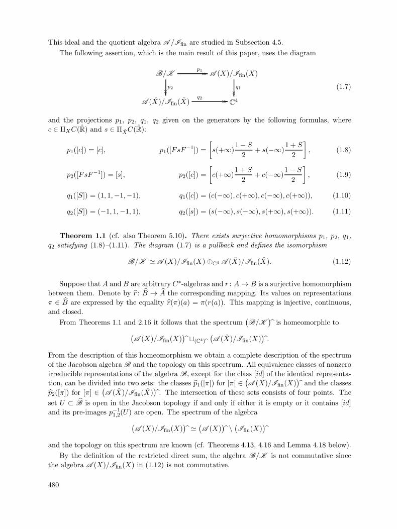
The following assertion, which is the main result of this paper, uses the diagram

B/Kp1 ��

p2��

A (X)/Ifin(X)

q1��

A (X)/Ifin(X)q2 ��

C4

(1.7)

and the projections p1, p2, q1, q2 given on the generators by the following formulas, where

c ∈ ΠXC(R) and s ∈ ΠXC(R):

p1([c]) = [c], p1([FsF−1]) =

[s(+∞)

1− S

2+ s(−∞)

1 + S

2

], (1.8)

p2([FsF−1]) = [s], p2([c]) =

[c(+∞)

1 + S

2+ c(−∞)

1 − S

2

], (1.9)

q1([S]) = (1, 1,−1,−1), q1([c]) = (c(−∞), c(+∞), c(−∞), c(+∞)), (1.10)

q2([S]) = (−1, 1,−1, 1), q2([s]) = (s(−∞), s(−∞), s(+∞), s(+∞)). (1.11)

Theorem 1.1 (cf. also Theorem 5.10). There exists surjective homomorphisms p1, p2, q1,

q2 satisfying (1.8)–(1.11). The diagram (1.7) is a pullback and defines the isomorphism

B/K � A (X)/Ifin(X) ⊕C4 A (X)/Ifin(X). (1.12)

Suppose that A and B are arbitrary C∗-algebras and r : A→ B is a surjective homomorphism

between them. Denote by r : B → A the corresponding mapping. Its values on representations

π ∈ B are expressed by the equality r(π)(a) = π(r(a)). This mapping is injective, continuous,

and closed.

From Theorems 1.1 and 2.16 it follows that the spectrum(B/K

)is homeomorphic to

(A (X)/Ifin(X)

) �(C4)

(A (X)/Ifin(X)

).

From the description of this homeomorphism we obtain a complete description of the spectrum

of the Jacobson algebra B and the topology on this spectrum. All equivalence classes of nonzero

irreducible representations of the algebra B, except for the class [id] of the identical representa-

tion, can be divided into two sets: the classes p1([π]) for [π] ∈(A (X)/Ifin(X)

)and the classes

p2([π]) for [π] ∈ (A (X)/Ifin(X)). The intersection of these sets consists of four points. The

set U ⊂ B is open in the Jacobson topology if and only if either it is empty or it contains [id]

and its pre-images p−11,2(U) are open. The spectrum of the algebra

(A (X)/Ifin(X)

) � (A (X)) \ (Ifin(X)

)

and the topology on this spectrum are known (cf. Theorems 4.13, 4.16 and Lemma 4.18 below).

By the definition of the restricted direct sum, the algebra B/K is not commutative since

the algebra A (X)/Ifin(X) in (1.12) is not commutative.

480

In Proposition 4.20, there is a homomorphism that maps the algebra A (X)/Ifin(X) to the

isomorphic algebra S(A (X)/Ifin(X)

)of matrix-valued functions. Therefore, we can describe

a similar algebra SB that is isomorphic to the algebra B/K . We denote by com(B) the ideal

generated by the commutators [a, b] = ab − ba of elements of the algebra B and by (B)k the

subspace of the spectrum of the algebra B consisting of all k-dimensional representations of this

spectrum. Using the isomorphism

B(X, X)/K � SB,

it is easy to see that the minimal solving series of the algebra B has the form

{0} ⊂ K ⊂ com(B) ⊂ B.

Moreover,

B/ com(B) � C((B)1),

com(B)/K � C0((B)2)⊗K(C2).

We recall that the abstract index group of an arbitrary unital C∗-algebra A is the group

Λ(A) whose elements are connected components of the group InvA of invertible elements of

the algebra A. It is equal to the quotient group Λ(A) = Inv(A)/(Inv(A))0, where (Inv(A))0is the connected component of identity of the group Inv(A). In this case, Λ(B/ comB) is

isomorphic to {0} and Λ(B/K ) is isomorphic to Z. The element of Z corresponding, under the

last isomorphism, to the connected component [b] of an element b ∈ B/K is denoted by ΛInd b.

The Fredholm index is denoted by ind b. On a dense set in Inv(B/K ), the Fredhom index can

be defined by the formula

ind b = ΛInd b =1

2πi

∫

( B)1

d lnU(π) +1

2πi

∫

( B)2

d ln detU(π), (1.13)

where U is the element of the algebra of symbols SB corresponding to b ∈ Inv(B/K ). Since

ΛInd and ind are locally constant, formula (1.13) is sufficient for defining them on the entire

Inv(B/K ).

In the general case (with other X, X) ΛInd b ∈ Zk, k ∈ {0, 1, 2}, it suffices to know ΛInd b

for computing ind b, but the converse assertion is not in general true.

1.2 Structure of the paper

In Section 2, we collect facts concerning restricted direct sums and introduce a mapping of

the spectra spec i and p corresponding to the homomorphisms i and p. In Subsection 2.2, we

prove formula (1.6).

In Subsection 3.1, we study the algebra A0 generated in B(L2(R)) by the operator of multi-

plication by the Heaviside function θ and the Cauchy integral S given by formula (1.5). Using

the Mellin transform, we show that A0 is isomorphic to the algebra S0 of continuous matrix-

valued functions on the axis that have diagonal limits at ±∞. In Subsection 3.2, we introduce

and describe the algebra ΠXC(R) of discontinuous functions on R = R ∪ {∞}. In Subsection

3.3, we formulate sufficient conditions for the compactness of commutators [c, FsF−1].

481

In Section 4, we present some known results concerning the algebra A = A (X) in formu-

lations convenient for our purposes. In Subsection 4.1, we prove that the algebra is irreducible

and contains the ideal K . The localization principle can be applied to the algebra A , which

means that the spectrum of the algebra A can be written in the form

A = {[id]} ∪⋃x∈R

(A /Ix) . (1.14)

The local algebras A /Ix are obtained by the definitions which are not convenient for our

purpose, namely, as the quotient algebras of the algebra A defined by its generators by the

ideal which is also defined by its generators. In Subsection 4.2, we describe a method for

computing such a quotient algebra, i.e., we construct isomorphic quotient algebras admitting

a more convenient description. We complete Subsection 4.2 by applying this method to the

computation of A /Ix. In this case, the method is to choose a family of homomorphisms

ϕn : A → B(L2(R)) such that the mapping ϕ : A → B(L2(R)) : a �→ s-limϕn(a) is defined

and is a homomorphism with kernel Ix. Then the algebra A /Ix is isomorphic to the image

of this homomorphism. For x ∈ X this image is isomorphic to A0, and for x /∈ X the image

coincides with the family of operators of the form α + βS (α, β ∈ C) and is isomorphic to C2.

From (1.14) and the description of the spectrum of local algebras we find the spectrum of the

algebra A /K . The notation is introduced in Subsection 4.3. For any element a of the algebra

A /K we define a function, called the symbol, on the spectrum (A /K ) � π �→ π(a) of the

operator a. We denote by Φ a mapping that with each element of the algebra A /K associates

its symbol. The image of this mapping is denoted by SA and is called the algebra of symbols.

The main result in Subsection 4.3 is Theorem 4.15 which explicitly describes the algebra SA .

Based on this theorem, we describe in Subsection 4.4 the Jacobson topology on the spectrum of

the algebra A /K . In Subsection 4.5, we prove assertions concerning ideals of the algebra A .

These assertions will be useful when we apply the results of Sections 2 and 4 to the algebra B.

In Section 5, we study the algebra B = B(X, X). In Subsection 5.1, we prove that B is

irreducible and contains the ideal K . In the remaining part of Subsection 5.1, we describe the

ideals of the algebra B. In Subsection 5.2, we obtain the formula

B(R, R)/K � A (R)/Ifin(R)⊕C4 A (R)/Ifin(R). (1.15)

Based on this formula, we prove (cf. Theorem 5.10 which is the main result of Subsection 5.3) a

similar formula for B(X, X) with other X and X (cf. formula (5.28)). Subsection 5.4 contains

some consequences of Theorem 5.10: the description of the spectrum of the algebra B/K and

topology there, an isomorphism Φ between B/K and the algebra of symbolsSB whose elements

are functions on the spectrum of the algebra B/K . Finally, we write out the solving series of

the algebra B.

In Section 6, we describe the abstract index group Λ(B/K ) of the algebra B/K . Subsection

6.1 contains the main definitions and general facts concerning the Fredholm index, the abstract

index group, and connections between them. In Subsection 6.2, we prove Lemma 6.7 which is the

main tool for describing Λ(B/K ). The description depends on the pair of sets X, X ⊂ R. All

such pairs are divided into three groups. We compute the isomorphism ΛInd: Λ(SB) → Zk and

derive a formula for the Fredholm index of operators of the algebra B in Subsections 6.3–6.5. In

Subsection 6.6, we show that the abstract index group Λ(B/ comB) for comB �= K consists

of a single element.

482

2 Spectrum of the Restricted Direct Sum of C∗-Algebras

Throughout the section, we assume that all algebras under consideration are C∗-algebras andall homomorphisms between the algebras are *-homomorphisms. We often omit the symbols C∗

and * in the notation.

Definition 2.1. Let A1, A2, C be algebras, and let δ1 : A1 → C and δ2 : A2 → C be

homomorphisms. The restricted direct sum of the algebras A1 and A2 is the algebra

A1 ⊕C A2def= {(a1, a2) ∈ A1 ⊕A2 | δ1(a1) = δ2(a2)}.

In this section, we collect some assertions about restricted direct sums which will be used in

the paper. The main goal of this section is Theorem 2.16 which expresses the spectrum of the

restricted direct sum in terms of the spectra of its summands.

2.1 Pullbacks and Pushouts

In this section, we collect necessary definitions and results of cathegory theory. Then we

formulate Theorem 2.9 and Proposition 2.10 which are reformulations of the corresponding

assertions in [7] adapted for our purposes.

We introduce the notion of a pullback in the cathegory of C∗-algebras whose morphisms

are ∗-homomorphisms and the notion of a pushout in the cathegory of topological spaces whose

morphisms are continuous mappings.

Definition 2.2. A commutative diagram of C∗-algebras

Bβ2 ��

β1

��

A2

δ2��

A1 δ1�� C

(2.1)

is called a pullback if for any algebra D equipped with morphisms γ1 and γ2 such that the

diagram

Dγ2 ��

γ1��

A2

δ2��

A1 δ1�� C

(2.2)

is commutative there exists a unique morphism γ : D → B such that γ1 = β1 ◦γ and γ2 = β2 ◦γ.The algebra B is called a vertex of the pullback (2.1). Pairs of morphisms γ1 and γ2 such that

the diagram (2.2) is commutative are called coherent.

Definition 2.3. A commutative diagram of topological spaces

Y X2f2��

X1

f1

��

Zg1��

g2

��

(2.3)

483

is called a pushout if for any topological space V equipped with morphisms h1 and h2 such that

the diagram

V X2h2��

X1

h1

��

Zg1��

g2

��

(2.4)

is commutative there exists a unique morphism h : Y → V such that h1 = h◦f1 and h2 = h◦f2.The space Y is called a vertex of the pushout (2.3). Pairs of morphisms h1 and h2 such that

the diagram (2.4) is commutative are called coherent.

The assertions about the uniqueness of pullback and pushout are known in cathegory theory.

Proposition 2.4 (uniqueness of a pullback). Let

Bβ2 ��

β1

��

A2

δ2��

A1 δ1�� C

and

B˜β2 ��

˜β1

��

A2

δ2��

A1 δ1�� C

(2.5)

be pullbacks. Then there exists a unique isomorphism σ : B → B such that the following diagram

is commutative:

B

β2

��

β1

��

σ �� B

˜β2

��

˜β1

��

A1 δ1�� C A2 .δ2

��

(2.6)

Proposition 2.5 (uniqueness of a pushout). Let

Y X2f2��

X1

f1

��

Zg1��

g2

��

and

Y X2

˜f2��

X1

˜f1

��

Zg1��

g2

��(2.7)

be pushouts. Then there exists a unique isomorphism h : Y → Y such that the following diagram

is commutative:

Y Yh��

X1

f1

��

˜f1

��Zg1

��g2

�� X2 .

f2

��˜f2

��

(2.8)

484

The following assertion describes a pushout vertex.

Proposition 2.6 (isomorphism between a pushout vertex and gluing of topological spaces).

A vertex Y of the pushout (2.3) is isomorphic to the quotient space of the disjoint union X1�X2

by the equivalence relation ∼ generated by {g1(z) ∼ g2(z)}z∈Z .

This quotient space, denoted by X1 �Z X2, is obtained by gluing the topological spaces X1

and X2 along the space Z. We show that an assertion similar to Proposition 2.6 is also valid

for a pullback of C∗-algebras. We consider only the case where the morphisms δ1 and δ2 of the

pullaback 1 are surjective.

Lemma 2.7. We consider a square of the form (2.1). Suppose that the morphisms δ1 and

δ2 are surjective and the following conditions hold:

(1) the morphisms β1 and β2 are surjective,

(2) ker β1 ∩ ker β2 = {0},(3) ker(δ1 ◦ β1) = ker β1 + ker β2.

Then (2.1) is a pullback.

Proof. It suffices to verify that for any C∗-algebra D and any pair of coherent morphisms

γ1 : D → A1 and γ2 : D → A2 there exists a unique mapping γ : D → B such that

γ1 = β1 ◦ γ,γ2 = β2 ◦ γ.

(2.9)

For this purpose, we consider an arbitrary d ∈ D. By condition (1), the homomorphisms β1 and

β2 are surjective. Therefore, there exist b1, b2 ∈ B such that β1(b1) = γ1(d) and β2(b2) = γ2(d).

Let g = δ1 ◦ β1. We have

g(b1) = δ1(β1(b1)) = δ1(γ1(d)) = δ2(γ2(d)) = δ2(β2(b2)) = g(b2).

Hence b2 − b1 ∈ ker g. By (3), there exist b2 ∈ ker β1 and b1 ∈ ker β2 such that

b2 − b1 = b2 − b1. (2.10)

We set b = b1 + b2. Then b = b2 + b1. We have

β1(b) = β1(b1) + β1(b2) = γ1(d) + 0 = γ1(d),

β2(b) = β2(b2) + β2(b1) = γ2(d) + 0 = γ2(d).

Therefore,β1(b) = γ1(d),

β2(b) = γ2(d).(2.11)

Furthermore, for a fixed d ∈ D there exists only one element b ∈ B satisfying relations (2.11).

Indeed, assume that b also satisfies (2.11). Then b − b belongs to the kernel of β1 and to the

kernel of β2 as well. By condition (2), we have b− b = 0.

485

Since there exists a unique element b ∈ B satisfying (2.11), there is a unique mapping

γ : D → B such thatγ1(d) = β1(γ(d)),

γ2(d) = β2(γ(d)).(2.12)

It remains to show that the mapping γ is a *-homomorphism. From (2.12) we find that for

i = 1, 2 and d1, d2 ∈ D

γi(d1 + d2) = γi(d1) + γi(d2) = βi(γ(d1)) + βi(γ(d2)) = βi(γ(d1) + γ(d2)).

Since γ is uniquely defined, we have γ(d1 + d2) = γ(d1)+ γ(d2). Similarly, γ(d1d2) = γ(d1)γ(d2)

and γ(d∗) = (γ(d))∗.

Proposition 2.8. Suppose that the homomorphisms p1 and p2 in the square

A1 ⊕C A2p2 ��

p1��

A2

δ2��

A1 δ1�� C

(2.13)

are determined by natural projections to the components of the direct sum and the homomor-

phisms δ1 and δ2 are surjective. Then (2.13) is a pullback.

Proof. We show that the diagram (2.13) satisfies conditions (1)–(3) in Lemma 2.7. Let us

check that the mapping p1 is surjective. Consider an arbitrary element a1 ∈ A1. Since δ2 is

surjective, we can find an element a2 ∈ A2 such that δ2(a2) = δ1(a1). Then (a1, a2) ∈ B and

a1 = p1(a1, a2). Since a1 was chosen arbitrarily, p1 is surjective. In a similar way, we can check

that p2 is surjective.

Conditions (2) and (3) follow from the equalities

ker p1 = {(0, a2) | a2 ∈ A2, δ2(a2) = 0},ker p2 = {(a1, 0) | a1 ∈ A1, δ1(a1) = 0},ker(δ1 ◦ p1) = {(a1, a2) | a1 ∈ A1, a2 ∈ A2, δ1(a1) = 0, δ2(a2) = 0}.

The proposition is proved.

From this result and Proposition 2.4 it follows that any pullback (2.1) with surjective δ1 and

δ2 coincides, up to an isomorphism, with the pullback (2.1).

Theorem 2.9. Suppose that the morphisms δ1 and δ2 in the commutative diagram

Bβ2 ��

β1

��

A2

δ2��

A1 δ1�� C

(2.14)

are surjective. This diagram is a pullback if and only if the following conditions hold:

486

(1) the morphisms β1 and β2 are surjective,

(2) ker β1 ∩ ker β2 = {0},(3) ker(δ1 ◦ β1) = ker β1 + ker β2.

Proof. By Lemma 2.7, conditions (1)–(3) imply that (2.1) is a pullback.

To check the converse assertion, we consider an arbitrary pullback (2.1) with surjective δ1,

δ2 and the pullback (2.13). From Proposition 2.4 it follows that there exists an isomorphism

σ : B → A such that βi = pi ◦ σ. Conditions (1)–(3) for βi are obtained from similar conditions

for pi, which follow from Proposition 2.8.

The following assertion is used in the proof of the assertion that the square is a pullback (cf.

Subsection 5.2).

Proposition 2.10. The diagram of C∗-algebras

A/(I ∩ J) ��

��

A/I

��A/J �� A/(I + J) ,

(2.15)

where all the mappings are standard projections, is a pullback for any C∗-algebra A and its closed

ideals I and J .

Proof. We note that

I/(I ∩ J) ∩ J/(I ∩ J) = {0},(I + J)/(I ∩ J) = I/(I ∩ J) + J/(I ∩ J).

Therefore, conditions (1)–(3) in Theorem 2.9 are satisfied. Consequently, (2.15) is a pullback.

2.2 Mappings of spectra

Definition 2.11. Let i : I ↪→ A be an injective homomorphism of C∗-algebras whose image

is an ideal of the C∗-algebra A. If π : I → B(H) is an irreducible representation of the algebra

I, then spec i(π) denotes a unique irreducible representation of the algebra A such that the

following diagram is commutative:

I� � i ��

π��

A

spec i(π)��

��

�

B(H).

We denote by spec i the embedding of spectra I ↪→ A that sends the class [π] of the irreducible

representation π of the algebra I to the class spec i([π])def= [spec i(π)].

487

Definition 2.12. Let p : A � B be a surjective homomorphism of C∗-algebras. If π : B →B(H) is an irreducible representation of the algebra B, then p(π) denotes a unique irreducible

representation of the algebra A such that the following diagram is commutative:

A

p(π) ��

��

�p �� B

π��

B(H).

We denote by p the embedding B ↪→ A sending the class [π] of the irreducible representation

π of the algebra B to the class p([π])def= [p(π)].

Remark 2.13. By [8, Subsection 5.5], these mappings are well defined, are continuous, and

are homeomorphisms onto their images. The mapping spec i is open and p is closed. Further-

more, if the sequence

0 �� I� � i �� A

p �� B �� 0

is exact, then the images of the mappings spec i and p are complements of each other in A.

Proposition 2.14. Suppose that one of the following diagrams is commutative:

(2.16)

Assume also that the images of i and l (if they are indicated in the diagram) are ideals. Then

the corresponding diagram in (2.17) is defined and is commutative:

(2.17)

Proof. The assertions of the lemma for different diagrams in (2.16) are proved in a similar

way. Therefore, we consider only the third diagram in (2.16). By assumption, the image i(I)

is an ideal of the algebra A. Therefore, the image p(i(I)) is an ideal of the algebra B. On the

other hand,

j(J) = j(q(I)) = p(i(I)).

488

Hence the image of the homomorphism j is an ideal of the algebra B and all the mappings in

the corresponding diagram in (2.17) are defined.

We write ϕ for spec i ◦ p and ψ for q ◦ spec j. The commutativity of the diagrams in (2.17)

follows from the equality ϕ = ψ. We show that the corresponding mappings of irreducible

representations coincide. These mappings are denoted by ϕ and ψ.

Let π : J → B(H) be an irreducible representation of an ideal J , and let u ∈ I. We prove

that

ϕ(π)(i(u)) = ψ(π)(i(u)).

Indeed,

ϕ(π)(i(u)) = spec i(p(π))(i(u)) = p(π)(u) = π(p(u)),

ψ(π)(i(u)) = q(spec j(π))(i(u)) = spec j(π)(q(i(u))) = spec j(π)(j(p(u))) = π(p(u)).

Since u is arbitrary, ϕ(π) and ψ(π) coincide on the image of i.

We use the fact that an irreducible representation of an ideal is extended to an irreducible

representation of the entire algebra in a unique way. In our case, by the definition of spec i,

the restriction of the representation ϕ(π) to i(I) is irreducible and coincides with the restricted

representation ψ(π). Therefore, ϕ(π) = ψ(π). Since π is arbitrary, we have ϕ = ψ.

Theorem 2.15. Let

(2.18)

be a pullback of C∗-algebras. Then

(2.19)

is a pushout.

Proof. We consider the commutative diagram

(2.20)

489

Here, i1,2 are standard embeddings of ker δ1,2 ⊂ A1,2 in A1,2. The embedding j2 : ker δ2 → B

is defined due to the universal property of the pullaback (2.18), regarded as a unique mapping

such that β2 ◦ j2 = i2 and β1 ◦ j2 = 0. Similarly, the equalities β1 ◦ j1 = i1 and β2 ◦ j1 = 0

define the *-homomorphism j1. It is easy to see that the diagram (2.20) is commutative. The

mappings j1 and j2 are injective because the compositions i1 = β1 ◦ j1 and i2 = β2 ◦ j2 are

injective.

It is obvious that the first and third rows of this diagram are short exact sequences. Let

us prove that the second row is also an exact sequence, i.e., j1(ker δ1) = ker β2. The inclusion

j1(ker δ1) ⊂ ker β2 follows from the definition of j1. To verify the inverse inclusion, we define

an homomorphism j : ker β2 → B by the equality j(b) = j1(β1(b)). To verify that it is well

defined, it suffices to note that β1(b) ∈ ker δ1. This relation holds since the right lower square

in the diagram (2.20) is commutative. We show that the homomorphism j coincides with the

identical embedding i of the ideal ker β2 in B. This fact follows from the equalities β1 ◦j = β1 ◦i,β2 ◦ j = 0 = β2 ◦ i and the universal property of a pullback. Thus, we have proved that any

element b ∈ ker β2 is equal to i(b) = j(b) = j1(β1(b)) and, consequently, belongs to the image of

j1. Similarly, all the columns of this diagram are short exact sequences.

We consider the diagram of topological spaces

(2.21)

It is commutative because of the commutativity of (2.20) and Proposition 2.14. According to

Remark 2.13, the images of embeddings β1 and spec j2 do not intersect and their union yields

the entire B. Therefore,

B = β1(A1) ∪ β2(A2).

To show that the right lower square in the diagram (2.21) is a pushout, we consider an

arbitrary topological spaceX and a continuous mapping f1,2 : A1,2 → X such that f1◦δ1 = f2◦δ2.We show that there exists a unique continuous mapping f : B → X such that

f1 = f ◦ β1,

f2 = f ◦ β2.(2.22)

Since

β1(A1) ∪ β2(A2) = B,

the mapping f is uniquely found from (2.22).

Let us show that this notion is well defined. Let b = β1(a1) = β2(a2). By Remark 2.13,

the element a2 belongs either to the image of spec i2 or to the image of δ2. The first variant

is impossible since, in this case, b should belong to the image of spec j2, which contradicts the

490

equality b = β1(a1) in view of Remark 2.13. Thus, a2 = δ2(c) for some c ∈ C. Since the left

lower square in this diagram is commutative, we have β1(a1) = β1(δ1(c)) and, consequently,

a1 = δ1(c). Therefore,

f1(a1) = f1(δ1(c)) = f2(δ2(c)) = f2(a2)

and, consequently, f is well defined.

Let us prove the continuity of f . We choose a closed subset U of X and show that f−1(V )

is closed. We have

f−1(V ) =(f−1(V ) ∩ β1(A1)

)∪(f−1(V ) ∩ β2(A2)

)= β1(f

−11 (V )) ∪ β2(f−12 (V )).

The mapping f1 is continuous. Therefore, the set f−11 (V ) is closed. Since β1 is a homeomorphism

to its closed image, β1(f−11 (V )) is also closed. Similarly, β2(f

−12 (V )) is closed. Therefore, the

union f−1(V ) is also closed.

Theorem 2.15 can be reformulated as follows.

Theorem 2.16. Suppose that A1, A2, and C are algebras and δ1,2 : A1,2 � C are injective

homomorphisms. Then the following canonical isomorphism holds:

(A1 ⊕C A2) � A1 � CA2, (2.23)

defined in the sense of Propositions 2.5 and 2.6 by the pushout

(2.24)

Proof. We consider the diagram

(2.25)

where p1 and p2 are the standard projections. By Proposition 2.8, it is a pullback. By Theorem

2.15, the square (2.24) is a pushout. On the other hand, by Proposition 2.6, the square

(2.26)

491

is also a pushout. By Proposition 2.5, we have the homeomorphism

σ : A1 ⊕C A2 → A1 � C A2. (2.27)

The theorem is proved.

3 Auxiliary Algebras and Compactness of Commutators

3.1 Algebra generated by two projections

Let F be the Fourier transform L2(R) → L2(R) defined on a dense set in L2(R) by the

equality

Fu(p) =1√2π

∫

R

e−ipxu(x)dx. (3.1)

Denote by F∗ the homomorphism of the algebra B(L2(R)) given by the equality

F∗b = FbF−1. (3.2)

In this subsection, we study the algebra A0 generated by the operators θ and S in B(L2(R)),

where θ is the operator of multiplication by a function θ that is equal to 1 for positive values of

variable and vanishes for negative ones, whereas S = −F∗ sgn, wheresgn(x) = 2θ(x)− 1

is the sign function. The operator S can be written in the explicit form:

Su(x) =1

πiv.p.

∫

R

u(y)dy

y − x. (3.3)

For a more convenient description of the algebra, we use the Mellin transform M which acts as

a unitary operator from L2(R) to L2(R)⊕ L2(R) and is given by the formula

Mu(λ) =1√2π

∞∫

0

x−12+iλ

(u(x)

u(−x))dx

or

M = F−1N,

where

Nu(t) = et/2

(u(et)

u(−et)

)

and the Fourier transform is applied in the componentwise sense. LetM∗ be the homomorphism

defined by the equality M∗b = MbM−1. Denote by S0 the image M∗(A0) of the algebra A0.

This algebra is generated by the operators of multiplication M∗(θ) and M∗(S) by the matrices

M∗(θ)(λ) =

(1 0

0 0

),

M∗(S)(λ) =

(− th(πλ) i/ ch(πλ)

−i/ ch(πλ) th(πλ)

).

(3.4)

492

It is easy to verify that the algebra generated by these matrix-valued functions coincides with

the algebra of all continuous functions having diagonal matrix limits as λ→ ±∞. The spectrum

of this algebra consists of points λ in the real axis and four points corresponding to the limits

of diagonal entries of the matrix as λ→ ±∞.

3.2 Algebra of piecewise continuous functions

Let R = R∪{∞} be the one-point compactification of the real axis, and let X be an arbitrary

subset of R. Denote by ΠXC(R) the C∗-algebra generated in L∞(R) by functions continuous on

R, except possibly for finitely many points of the set X where discontinuous of the first kind are

allowed. We identify such functions with operators of multiplication and thereby assume that

ΠXC(R) is a subalgebra of B(L2(R)). For x ∈ R we write ΠxC(R) instead of Π{x}C(R). We

explicitly describe the algebra ΠXC(R) and its spectrum. We begin with the notation.

For c ∈ L∞(R), x ∈ R, we denote by c(x±) the limit limy→x± c(y). Note that for connected

subsets of R the notation 〈a, b〉 is usually used, where a < b and the round or square brackets

should be written instead of the angular brackets. To unify the consideration of connected

subsets of R, we will write 〈a,∞) instead of 〈a,+∞) and (∞, b〉 instead of (−∞, b〉. We also

write the square brackets for ∞; moreover, for a > b we set 〈a, b〉 def= 〈a,∞] ∪ (∞, b〉. Let

I = 〈a, b〉 ⊂ R. We set

ΠXIdef= (I \X) ∪ {x− | x ∈ I ∩X,x �= a} ∪ {x+ | x ∈ I ∩X,x �= b}.

Similarly,

ΠXRdef= (R \X) ∪ {x−, x+ | x ∈ R ∩X}.

We set

ΠX∅def= ∅.

We introduce the topology on ΠX R with the base of sets of ΠXI, where I runs all the intervals,

half-intervals, and segments such that their closed endpoints belong to the set X.

The following theorem describes the algebra ΠXC(R). We note that for X = R the first

assertion immediately follows from [4, Lemma 2.9].

Theorem 3.1.

(1) The set of elements of the algebra ΠXC(R) coincides with the set of functions that are

continuous outside X and possess the left and right limits at each point x ∈ X.

(2) For any c ∈ ΠXC(R) and ε > 0 the inequality |c(x+) − c(x−)| > ε can be valid only for

finitely many points x ∈ X.

(3) The spectrum of the algebra ΠXC(R) is homeomorphic to ΠXR.

Proof. Denote by ΠXC(R) the set mentioned in assertion (1) and verify that this set is a

C∗-algebra. We note that this set is invariant under addition, multiplication, and involution. It

remains to check that it is closed. Suppose that a sequence of functions cn in ΠXC(R) converges

to c. Then there exists limn→∞ cn(y) uniform with respect to y ∈ R. Hence the following limits

exist:

c(x±) = limy→x± c(y) = lim

y→x± limn→∞ cn(y) = lim

n→∞ limy→x± cn(y) = lim

n→∞ cn(x±)

493

for x ∈ X and limy→x

c(y) for x ∈ R \X. Therefore, c ∈ ΠXC(R).

We begin with assertion (2) for c ∈ ΠXC(R). Let ε > 0. The existence of limy→x± c(y) for any

x ∈ R implies the existence of a neighborhood Ix of x such that

|c(y+)− c(y−)| � ε

for all y ∈ Ix \ {x}. In particular, the number of points y ∈ Ix where |c(y+) − c(y−)| > ε is

finite. The sets Ix cover the compact set R. Therefore, the set {y ∈ R | |c(y+)− c(y−)| > ε} is

also finite.

We prove that ΠX R is compact. Let ΠXR be covered by a family of sets {ΠXI}I∈I in the

above-described base of topology. Then for x ∈ X we have

x+ ∈⋃I∈I

ΠXI, x− ∈⋃I∈I

ΠXI,

which implies that some interval containing x is contained in the union of at most two sets in

I. The last assertion is also valid for x ∈ R \X. These intervals cover R and, consequently, we

can extract a finite subcovering. Then the union of ΠXI corresponding to I ∈ I yields a finite

covering of ΠXR.

We note that for any function c ∈ ΠX R its values c(x) are defined at all points x ∈ ΠX R.

Thus, c can be identified with a function ΠXR → C. One can immediately check that the

obtained function is continuous. Taking into account this identification, we have the following

embeddings of C∗-algebras:

ΠXC(R) ⊂ ΠXC(R) ⊂ C(ΠXR).

The first embedding contains the identity and separates points of the space ΠXR. Therefore, by

the Stone–Weierstrass theorem, these algebras coincide. In particular, assertion (1) is proved.

Assertion (2) was checked for c ∈ ΠXC(R) and thereby for c ∈ ΠXC(R). As is known, any com-

pact topological space is homeomorphic to the spectrum of the algebra of continuous functions

defined on this space. Applying this fact to the space ΠX R, we obtain assertion (3).

In the sequel, we identify ΠXC(R) and C(ΠX R).

3.3 Compactness of commutators

We note that, by the inclusion

ΠXC(R) ⊂ B(L2(R)),

the homomorphism F∗ defined by formula (3.2) can be applied to elements s ∈ ΠXC(R).

Theorem 3.2. In each of the following cases, the commutator [c, F∗(s)] is compact:

(1) c ∈ C(R), s ∈ ΠRC(R)

(2) c ∈ ΠRC(R), s ∈ C(R)

(3) c ∈ Π∞C(R), s ∈ Π∞C(R)

The proof of assertions (1) and (2) can be found in [5], and the proof of assertion (3) is

contained in [9].

494

4 Algebra of Singular Integral Operators with Discontinuities

in Coordinates

We fix an arbitrary set X ⊂ R and call it the coordinate set where discontinuity is allowed.

Denote by K the algebra of compact operators in L2(R). This subsection is devoted to the

study of the algebra A generated by functions in ΠXC(R) and the operator S.1) The main

goal of this section is the proof of Theorems 4.13, 4.15, and 4.16. Theorem 4.13 describes the

spectrum of the algebra A /K , Theorem 4.15 deals with the algebra of matrix-valued functions,

isomorphic to the algebra A /K , and Theorem 4.16 concerns the Jacobson topology on the

spectrum (A /K ) .

4.1 Localization in the algebra A

To justify the possibility to apply the localization principle (Theorem 4.7), we first prove

that the algebra A is irreducible. In the following assertions, all the equalities and inclusions

of sets are understood up to a set of zero measure. Denote by χU the characteristic function of

a set U . We use the notation cL = {cl | l ∈ L}, where L is a set of elements l for which the

product cl is defined. For example, if (X, dμ) is a space with measure and U is a measurable

subset of X, then χUL2(X, dμ) is the space of functions in L2(X, dμ) vanishing outside U .

Lemma 4.1. Assume that μ is a σ-finite measure on the set R and Y is a closed subspace

of L2(R, dμ). Then the following assertions are equivalent.

(1) Y = χUL2(R, dμ) for some μ-measurable U ⊂ R.

(2) For all u ∈ Y, v ⊥ Y the supports 2) of u and v do not intersect.

Proof. The implication (1) ⇒ (2) is obvious. Let us verify the implication (2) ⇒ (1).

Assume that assertion (2) is true. We check assertion (1) by constructing a set U . Since μ is

σ-finite, the set R is divided into at most countable number of disjoint sets Rk of finite measure.

To determine the set U , we put

U =⋃k

Uk,∞, Uk,l =

l⋃i=1

(suppuk,i ∩Rk),

where uk,i ∈ Y are found by the following inductive procedure: uk,i is an arbitrary function in

Y such that μ((suppuk,i ∩ Rk) \ Uk,i−1) differs from its maximal value (over all uk,i in Y ) by

at most two times; Uk,0 = ∅. By the above construction, for any k and u ∈ Y the intersection

suppu ∩ Rk belongs to Uk,∞ and, consequently, the support of any u ∈ Y is contained in U ,

which proves Y ⊂ χUL2(R, dμ).

Let Y �= χUL2(R, dμ). Consider an arbitrary nonzero function v ∈ χUL

2(R, dμ) � Y . Since

v ⊥ Y and uk,l ∈ Y , their supports do not intersect. On the other hand, by construction, U

belongs to the union of supports of uk,l, which implies that supp v is contained in the union of

supports of uk,l and, consequently, intersects at least one of them.

1) The definitions of ΠXC(R) and S are given at the beginning of Subsection 3.2 and in (3.3) respectively.2) By the support we mean the set of points where the function is not equal to zero.

495

Proposition 4.2. Any reducing subspace of the algebra C(R) has the form χUL2(R) for

some measurable U ⊂ R.

Proof. Let Y be a reducing subspace of the algebra C(R). By Lemma 4.1, it suffices to

prove that for any u ∈ Y and v ⊥ Y their supports do not intersect. Suppose that u and v are

functions in these spaces such that their supports intersect. Then uv differs from zero and there

is a measurable set V1 ⊂ R such that (χV1u, v) �= 0. Since V1 can be approximated by open sets

as precisely as desired, we can take an open set V2 such that (χV2u, v) �= 0. Using the absolute

continuity of the Lebesgue integral, we take a compact set V3 ⊂ V2 such that

∫

V 2\V 3

|uv| dx < |(χV2u, v)| .

Let c : R → [0, 1] be a continuous function such that c = 1 on V3 and c = 0 outside V2. Then

cu ∈ Y and, consequently, (cu, v) = 0. However, on the other hand,

|(cu, v) − (χV2u, v)| �∫

V 2\V 3

|uv| dx < |(χV2u, v)| .

We arrive at a contradiction.

Proposition 4.3. The algebra A is irreducible.

Proof. We consider a reducing subspace Y of the algebra A . By Proposition 4.2, it has the

form χUL2(R). It remains to prove that the set U coincides with ∅ or R. Let U be nonempty.

Consider an arbitrary interval I intersecting U and a function u that is equal to 1 on I ∩U and

vanishes at the remaining points. By construction, u ∈ Y . Therefore, iπSu ∈ Y . For any x /∈ Ithe integrand in the integral

iπSu(x) =

∫

I∩U

dy

y − x

is of constant sign. Consequently, the integral differs from zero. Hence R \ I ⊂ suppu ⊂ U .

Since I is arbitrary, we have U = R.

Recall that K denotes the ideal of compact operators K(L2(R)) of B(L2(R).

Proposition 4.4. K ⊂ A .

Proof. It is known (cf., for example, [8, Theorem 2.4.9] or [10, Corollary 4.1.10]) that if the

image π(A) : A → B(H) of an irreducible representation of the algebra A contains at least one

nonzero compact operator, then K(H) ⊂ π(A). Thus, we need to check that the algebra Acontains at least one nonzero compact operator. We consider an arbitrary non-constant function

c ∈ C(R). The commutator [c, S] with kernel

1

πi

c(x) − c(y)

y − x

differs from zero. By Theorem 3.2, it is compact.

496

We recall that Propositions 4.3 and 4.4 imply that any nonzero ideal of the algebra Acontains the ideal of compact operators. This fact takes place owing to the following known

assertion (we supply the proof of this assertion for the convenience of the reader).

Proposition 4.5. Suppose that the ideal K(H) of compact operators on the Hilbert space

H is contained in an irreducible algebra B ⊂ B(H). Then K(H) is contained in any nonzero

ideal of the algebra B.

Proof. We consider a nonzero ideal J ⊂ B. As is known, the restriction of any irreducible

representation to the ideal either is equal to zero or is irreducible. The identical representation,

restricted to the ideal J cannot be zero and, consequently, it is irreducible. It suffices to show

that the ideal J contains at least one nonzero compact operator. We consider j ∈ J, j �= 0.

Then there is u ∈ H such that ju �= 0. Denote by Pu the projection onto the space Cu. This

projection is compact and, consequently, belongs to B. The operator jPu differs from zero,

belongs to J , and is compact.

Definition 4.6. We introduce the ideal Ix generated in A by continuous functions in C(R)

vanishing at x ∈ R.

The localization principle was used by Simonenko, Douglas, Dynin, Plamenevskii and Senich-

kin (cf. [11]). In this paper, we use the localization principle in the following form.

Theorem 4.7. Let A be the C∗-subalgebra of the algebra B(H) of bounded operators, and

let C be its commutative subalgebra containing the identity operator. Assume that for all c ∈ C

and a ∈ A the commutator [a, c] is compact. Then

A = {[id]} ∪⋃x∈ C

(A/Jx) .

Lemma 4.8. The spectrum of the algebra A is equal to

{[id]} ∪⋃x∈R

(A /Ix) .

Proof. We apply the localization principle (Theorem 4.7). For the localizing algebra C we

take the algebra C(R). The compactness of the commutator [c, a] for c ∈ C(R), a ∈ A follows

from Theorem 3.2.

Proposition 4.9. For any x ∈ X the isomorphism ϕx : A /Ix → S0 holds, where S0 is the

algebra of matrix-valued functions on the real axis defined in Subsection 3.1. The values of the

isomorphism ϕx on the equivalence classes of the generators of the algebra A take the form

ϕx(c+ Ix) =

(c(x+) 0

0 c(x−)

)for c ∈ ΠXC(R),

ϕx(S + Ix) =

( − th(πλ) i/ ch(πλ)


).

(4.1)

497

For any x /∈ X the isomorphism ϕx : A /Ix → C2 holds. In this case, the values of the

isomorphism on the generators take the form

ϕx(c) = (c(x), c(x)),

ϕx(S) = (−1, 1).(4.2)

This assertion is proved in the following subsection.

4.2 Description of local algebras

The following method is useful for computing local algebras. The idea of the method is

taken from the proof of Proposition 2.1.5 in [12]. Assume that we need to compute the quotient

algebra A/J , where the ideal J (regarded as the closed ideal of the algebra A) is given by the

set of its generator J and the algebra itself (regarded as a Banach algebra) is given by the set

of generators A ∪ J .To find these quotient algebras, we choose a family of homomorphisms ϕn : A→ B(H) and

define a mapping ϕ : A→ B(H) by the equality ϕ(a) = s-limn

ϕn(a) on elements where the limit

exists. Moreover, the mapping ϕ must satisfy the following conditions:

(i) ϕ is defined on J and vanishes on J ,

(ii) ϕ is defined on A,

(iii) for any finite combination p formed from elements of A by addition, multiplication, and

involution the following inequality holds: ϕ(p) � ‖p+ J‖.

As shown in Lemma 4.11, ϕ is a *-homomorphism defined on the entire algebra A and its

kernel coincides with the ideal J . Therefore, the quotient algebra A/J is isomorphic to the

image ϕ(A) generated by ϕ(a) for a ∈ A.

Owing to the following lemma, we can simplify the verification of conditions (i) and (ii)

Lemma 4.10.

(1) Let for every a ∈ J the limits limnϕn(a)u vanish for all u in a dense subset of the Hilbert

space H (such sets can be different for different a). Then condition (i) is satisfied.

(2) Assume that for every a ∈ A the limits limnϕn(a)u exist for all u in a dense subset of the

Hilbert space H (such sets can be different for different a). Then condition (ii) is satisfied.

Proof. Both assertions will be proved simultaneously. Assume that a ∈ J if we prove

assertion (1), and a ∈ A if we prove assertion (2). By condition, limnϕn(a)u exists for all u in

some dense subset U of the space H. We prove that this limit exists on the entire space H. For

this purpose it suffices to show that for all u ∈ H the sequence ϕn(a)u is a Cauchy sequence.

Consider an arbitrary ε > 0 and u0 ∈ U such that

‖a‖ ‖u− u0‖ < ε/3.

498

Since ϕn(a)u0 is a Cauchy sequence, from the above inequality for sufficiently large n and m we

have

‖ϕn(a)u− ϕm(a)u‖ � ‖ϕn(a)u− ϕn(a)u0‖+ ‖ϕn(a)u0 − ϕm(a)u0‖+ ‖ϕm(a)u0 − ϕm(a)u‖� ‖a‖ ‖u− u0‖+ ‖ϕn(a)u0 − ϕm(a)u0‖+ ‖a‖ ‖u0 − u‖< ε/3 + ε/3 + ε/3 = ε.

The existence of s-limn

ϕn(a) follows because B(H) is strongly complete. In the case a ∈ J ,

from the assumptions of the lemma we find that the limit operator vanishes on a dense set and,

consequently, is the zero operator.

Lemma 4.11. If conditions (i)–(iii) are satisfied, then the mapping ϕ is a *-homomorphism;

moreover, kerϕ = J .

Proof. The linearity of ϕ follows from its definition. It suffice to prove the following prop-

erties:

(1) ϕ(ab) = ϕ(a)ϕ(b) for all a, b ∈ Dom(ϕ),

(2) Dom(ϕ) = A,

(3) ϕ(a∗) = (ϕ(a))∗ for all a ∈ Dom(ϕ),

(4) ker(ϕ) = J .

Let us prove property (1). We recall that the product of operators is continuous in the sense

of the strong convergence. Assume that

ϕ(a) = s-limn

ϕn(a) and ϕ(b) = s-limn

ϕn(b).

Then the strong continuity of the product implies the existence of the limit

ϕ(ab) = s-limn

ϕn(ab)

and the equality

ϕ(ab) = ϕ(a)ϕ(b).

Consider property (2). As was already established, Dom(ϕ) is a subalgebra of A. Since

Dom(ϕ) contains A and J generating A (regarded as a Banach algebra), in order to prove

Dom(ϕ) = A it suffices to show that Dom(ϕ) is closed. Let am be a sequence of elements

in Dom(ϕ), and let am → a ∈ A. Then ϕn(am) converges to ϕn(a) as m → ∞. Since the

homomorphisms ϕn do not increase the norms, ϕn(am) converges uniformly with respect to

n. By the continuity of the strong limit with respect to the uniform convergence, the limit

ϕ(a) = s-limn

ϕn(a) exists and is equal to limmϕ(am).

To prove property (3), we check the equality

s-limn

ϕn(a∗) = (s-lim

nϕn(a))

∗.

499

By property (2), the left-hand and right-hand sides of this equality are defined. Therefore, it

suffices to check this equality for weak limits. But this assertion is valid since the weak limit

and *-homomorphisms ϕn are invariant under involutions.

Finally, we prove property (4). We note that J ⊂ ker(ϕ) follows from the fact that ker(ϕ)

is a closed ideal containing J . Therefore, the mapping Φ: A/J → B(H) given by the equality

Φ(a+ J) = ϕ(a) is well defined. We show that Φ is injective. It suffices to prove that ‖Φ(a)‖ �‖a‖ on a dense set in A/J . For such a set we take the image under the standard projection

A → A/J of the set of finite combinations described in (iii) since the required inequality is

formulated in this condition.

Proof of Proposition 4.9. We apply the above method to the algebra A . We reduce the

consideration of the case of an arbitrary point x ∈ R to the case x = 0. For this purpose,

let us look how the algebra A changes under the change of variables. Suppose that a mapping

f : R → R is continuous, bijective and has the derivative f ′(x) which is defined, continuous and is

not equal to zero everywhere, except possibly for finitely many points. Then the inverse mapping

f−1 possesses the same properties. We define the corresponding operator Ef : L2(R) → L2(R)

by the equality

Efu(x) =√

|f ′(x)|u(f(x)).It is easy to verify that it is unitary and (Ef )

−1 = Ef−1 . We consider the corresponding

automorphism (Ef )∗ of the algebra B(L2(H)) given by the equality

(Ef )∗(a) = Efa(Ef )−1.

If a is the operator of multiplication by a(x), then (Ef )∗(a) is the operator of multiplication by

a(f(x)).

It is easy to check that if f(x) = (αx+ β)/(γx + δ) and αδ − βγ > 0, then (Ef )∗ sends theoperator S to the operator (Ef )∗(S) = S, the algebra A = A (X) to the algebra (Ef )∗(A (X)) =

A (f(X)), and the ideal Ix = Ix(X) to the ideal (Ef )∗(Ix(X)) = If(x)(f(X)). We note that

for any point x0 ∈ R it is possible to find f such that f(x0) = 0. Therefore, it suffices to prove

the assertion for x = 0.

Now, we compute the ideal A /I0. For J we take the set of functions c ∈ ΠXC(R) vanishing

at 0, i.e., c(0−) = c(0+) = 0. For A we take the operator S for 0 /∈ X and the pair {S, θ} for

0 ∈ X, where θ is the Heaviside function.

We note that an arbitrary function c ∈ ΠXC(R) can be represented as the sum of three

terms (c(0+) − c(0−))θ, c(0−)S2, and a function vanishing at 0. Therefore, A ∪ J generates a

Banach algebra A . Finally, we set ϕn = (Ex �→x/n)∗.Let us check (i)–(iii). We note that (ii) and (iii) are valid because ϕn(S) = S and ϕn(θ) = θ.

To prove (i), we use (4.10) which asserts that it suffices to verify the equality limnϕn(c)u = 0

for elements u in a dense subset of L2(R). For such a subset we take the set of compactly

supported functions. For c ∈ J and any ε > 0 there is an interval containing 0, where c < ε.

Then (ϕn(c)u)(x) = c(x/n)u(x) and the required convergence follows from the fact that for

sufficiently large n the inequality |c(x/n)| < ε holds on the support of u.

Thus, A /I0 is isomorphic to the image of the algebra A under the mapping ϕ. For x /∈ X

the image of the algebra A is generated by the operator S and is isomorphic to C2 since S2 = 1.

For x ∈ X this image is generated by the operators θ and S and, consequently, it coincides with

500

the algebra A0 considered in Subsection 3.1. Formulas for the images of basis elements indicated

in the formulation of this assertion are obtained from (3.4).

4.3 Spectrum and the algebra of symbols

Using the isomorphism ϕx in Proposition 4.9, we describe some representations of the algebra

A . Suppose that x ∈ X and a ∈ A . Then ϕx(a + Ix) ∈ S0 is a matrix-valued function. For

λ ∈ R ∪ {−∞,∞} we define the π(x, λ) of the algebra A by the equality

π(x, λ)(a) = ϕx(a+ Ix)(λ).

Entries of the matrix π(x, λ)(a) are denoted by (π(x, λ)(a))α,β , where α, β ∈ {“+”, “−”}. Usingthe equality (4.1) in Proposition 4.9, we find

π(x, λ)(c) =

(c(x+) 0

0 c(x−)

)for c ∈ ΠXC(R), (4.3)

π(x, λ)(S) =M∗(S)(λ) =( − th(πλ) i/ ch(πλ)


). (4.4)

We recall that the matrix-valued function M∗(S) was introduced in Subsection 3.1. Suppose

that x /∈ X and a ∈ A . Then ϕx(a+ Ix) ∈ C2. The components of this vector are denoted by

π±(x)(a). From the equality (4.2) in Proposition 4.9 we find

π±(x)(c) = c(x) for c ∈ ΠXC(R),

π±(x)(S) = ±1.(4.5)

The identity 2×2-matrix is denoted by Id2. The representations π(x, λ) for x /∈ X, λ ∈ R ∪{−∞,+∞} are defined by the formula

π(x, λ)(a) =π+(x)(a) − π−(x)(a)

2M∗(S)(λ) +

π+(x)(a) + π−(x)(a)2

Id2, (4.6)

and the representations π±(x±) for x ∈ X are defined by the formula

πα(xβ)(a) = π(x,−αβ∞)β,β(a), α, β ∈ {“+”, “−”}. (4.7)

In this case, (4.3) and (4.4) hold for all x ∈ R, whereas (4.5) holds for all x ∈ ΠX R.

The ideal K is contained in all the ideals Ix. Therefore, the above representations annihilate

K and can be regarded as representations of the quotient algebras A /K for which we preserve

the notation π(x, λ), π±(x).

Remark 4.12. The above representations introduced for different X agree: if a ∈ A (X1)∩A (X2), then π(x, λ)(a) is independent of the choice of a set X under consideration. It suffices

to verify this assertion for X2 = R: for the remaining X2 it follows by transitivity. For X2 = R

501

we have X1 ⊂ X2 and A (X1) ⊂ A (X2). The set X does not occur explicitly in formulas (4.3),

(4.4), and (4.5). Therefore, the restriction of the representation of the algebra A (X2) to the

algebra A (X1) coincides with the representation in A (X1) on the basis elements of the algebra

A (X1). Hence they also coincide on A (X1).

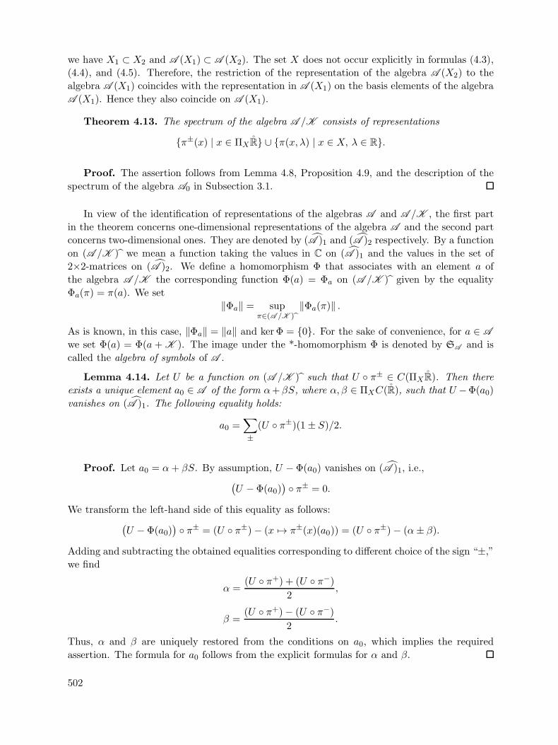
Theorem 4.13. The spectrum of the algebra A /K consists of representations

{π±(x) | x ∈ ΠX R} ∪ {π(x, λ) | x ∈ X, λ ∈ R}.

Proof. The assertion follows from Lemma 4.8, Proposition 4.9, and the description of the

spectrum of the algebra A0 in Subsection 3.1.

In view of the identification of representations of the algebras A and A /K , the first part

in the theorem concerns one-dimensional representations of the algebra A and the second part

concerns two-dimensional ones. They are denoted by (A )1 and (A )2 respectively. By a function

on (A /K ) we mean a function taking the values in C on (A )1 and the values in the set of

2×2-matrices on (A )2. We define a homomorphism Φ that associates with an element a of

the algebra A /K the corresponding function Φ(a) = Φa on (A /K ) given by the equality

Φa(π) = π(a). We set

‖Φa‖ = supπ∈(A /K )

‖Φa(π)‖ .

As is known, in this case, ‖Φa‖ = ‖a‖ and ker Φ = {0}. For the sake of convenience, for a ∈ Awe set Φ(a) = Φ(a + K ). The image under the *-homomorphism Φ is denoted by SA and is

called the algebra of symbols of A .

Lemma 4.14. Let U be a function on (A /K ) such that U ◦ π± ∈ C(ΠX R). Then there

exists a unique element a0 ∈ A of the form α+βS, where α, β ∈ ΠXC(R), such that U −Φ(a0)

vanishes on (A )1. The following equality holds:

a0 =∑±

(U ◦ π±)(1± S)/2.

Proof. Let a0 = α+ βS. By assumption, U −Φ(a0) vanishes on (A )1, i.e.,(U −Φ(a0)

) ◦ π± = 0.

We transform the left-hand side of this equality as follows:(U − Φ(a0)

) ◦ π± = (U ◦ π±)− (x �→ π±(x)(a0)) = (U ◦ π±)− (α± β).

Adding and subtracting the obtained equalities corresponding to different choice of the sign “±,”

we find

α =(U ◦ π+) + (U ◦ π−)

2,

β =(U ◦ π+)− (U ◦ π−)

2.

Thus, α and β are uniquely restored from the conditions on a0, which implies the required

assertion. The formula for a0 follows from the explicit formulas for α and β.

502

Theorem 4.15. In the image of SA under the *-homomorphism Φ, there are only those

functions U that satisfy the following conditions.

(1) U ◦ π± ∈ C(ΠX R).

(2) For each x ∈ R the function λ �→ U(π(x, λ)) is continuous (for λ ∈ R) and there exists

limλ→±∞

U(π(x, λ)) =

(U(π∓(x+)) 0

0 U(π±(x−))

). (4.8)

(3) Let a0 ∈ A be the element in Lemma 4.14 corresponding to U . The function (x, λ) �→(U − Φa0)(π(x, λ) defined on the locally compact space X × R, where X is equipped with

the discrete topology and R is equipped with the usual topology on the real axis, converges

to zero at infinity. In other words, for any ε > 0 the following set is finite:

{x ∈ X | sup

λ‖(U − Φa0)(π(x, λ))‖ > ε

}. (4.9)

Proof. 1◦. We show that (1)–(3) hold on SA . The algebra SA is generated by ΦS and Φc

for c ∈ ΠXC(R). From (4.3), (4.4), (4.5) and the equality Φa(π) = π(a) we find

Φc(π±(x)) = c(x), Φc(π(x, λ)) =

(c(x+) 0

0 c(x−)

), (4.10)

ΦS(π±(x)) = ±1, ΦS(π(x, λ)) =M∗(S)(λ) =



). (4.11)

These formulas show that Φc and ΦS satisfy conditions (1) and (2). These conditions are

preserved under taking the sum, product and involution and the limit passage. Therefore, these

conditions also hold on the entire algebra.

We turn to condition (3). We show that it holds on the ideal J of the algebra SA generated

by the commutators [Φc,ΦS] for c ∈ ΠXC(R). We note that U(π±(x)) = 0 for U ∈ J, x ∈ ΠX R

and, consequently, a0 = 0.

We begin with U = [Φc,ΦS]. Let ε > 0. By Theorem 3.1, the set

{x ∈ X | ‖c(x+)− c(x−)‖ > ε/2}

is finite. If an element x ∈ X does not belong to this set, then

∥∥[Φc,ΦS ](π(x, λ)

)∥∥ =∥∥[(c(x+)− c(x−)

)M∗(θ) + c(x−)Id2,M∗(S)(λ)

]∥∥=∥∥[(c(x+)− c(x−)

)M∗(θ),M∗(S)(λ)

]∥∥� 2 ‖c(x+)− c(x−)‖ ‖M∗(θ)‖ ‖M∗(S)‖ � ε. (4.12)

Thus, condition (3) holds for U = [Φc,ΦS ]. It is clear that it also holds on the entire ideal J .

We prove that any element U of the algebra SA is represented as

U = ΦcΦS +Φs + V, (4.13)

503

where c, s ∈ ΠXC(R) and V ∈ J . For this purpose, we consider the quotient algebra SA /J .

Since the generators Φc and ΦS commute modulo J , their product is equivalent modulo J to an

element of the form ΦcΦS or Φs. Therefore, any combination of generators is equivalent to the

sum ΦcΦS +Φs. The representation (4.13) follows from the closedness of such sums.

Now, for arbitrary U ∈ SA we have the representation (4.13). From this representation it

follows that a0 = cS + s and U − Φa0 = V . Therefore, condition (3) for U is obtained from the

same condition (3) for V .

2◦. We show that any function U satisfying (1)–(3) belongs to SA . For this purpose, it

suffices to show that V = U − Φa0 belongs to SA . By (3), for any ε > 0 everywhere, except

possibly for finitely many points xi, we have

supλ

‖V (π(x, λ))‖ < ε.

Therefore, finite sums of functions Vi coinciding with V for x = xi and vanishing for the re-

maining x approximate V as precisely as desired. Thus, it suffices to verify that V ∈ SA for

functions V taking nonzero values only at one value of x = x0 ∈ X. Using again the closeness

of SA , we assume that V (π(x0, ·)) is compactly supported.

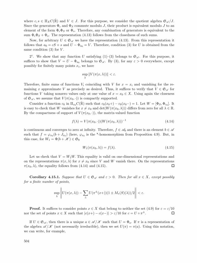
Consider a function c0 in Πx0C(R) such that c0(x0+)− c0(x0−) = 1. Let W = [ΦS ,Φc0 ]. It

is easy to check thatW vanishes for x �= x0 and det(W (π(x0, λ))) differs from zero for all λ ∈ R.

By the compactness of support of V (π(x0, ·)), the matrix-valued function

f(λ) = V (π(x0, ·))(W (π(x0, λ)))−1 (4.14)

is continuous and converges to zero at infinity. Therefore, f ∈ A0 and there is an element b ∈ A

such that f = ϕx0(b + Jx0) (here, ϕx0 is the *-homomorphism from Proposition 4.9). But, in

this case, for W1 = Φ(b+ K ) ∈ S0

W1(π(x0, λ)) = f(λ). (4.15)

Let us check that V = W1W. This equality is valid on one-dimensional representations and

on the representations π(x, λ) for x �= x0 since V and W vanish there. On the representations

π(x0, λ), the equality follows from (4.14) and (4.15).

Corollary 4.15.1. Suppose that U ∈ SA and ε > 0. Then for all x ∈ X, except possibly

for a finite number of points,

supλ

∥∥∥∥∥U(π(x, λ)) −∑±U(π±(x+))(1 ±M∗(S)(λ))/2

∥∥∥∥∥ < ε.

Proof. It suffices to consider points x ∈ X that belong to neither the set (4.9) for ε = ε/10

nor the set of points x ∈ X such that |c(x+)− c(x−)| > ε/10 for c = U ◦ π±.

If U ∈ SA , then there is a unique a ∈ A /K such that U = Φa. If π is a representation of

the algebra A /K (not necessarily irreducible), then we set U(π) = π(a). Using this notation,

we can write, for example,

504

U(π(x,±∞)) =

(U(π∓(x+)) 0

0 U(π±(x−))

).

If U(π±(x+)) = U(π±(x−)) for x ∈ X, then U(π±(x)) denotes their common value.

4.4 Jacobson topology on the spectrum

We describe the Jacobson topology on the spectrum of the algebra A /K by describing the

fundamental system of neighborhoods of points of this spectrum. We recall that the definition

of ΠXI for intervals, half-intervals, and segments I ⊂ R is given in Subsection 3.2.

Suppose that x ∈ X and J ⊂ R is an interval. We set

Vx0,Jdef= {π(x0, λ) | λ ∈ J} . (4.16)

Let α ∈ {“+”, “−”}, and let I be an interval in R. We set

V αI

def= {πα(x) | x ∈ ΠXI} ∪ {π(x, λ) | x ∈ I ∩X,λ ∈ R} . (4.17)

Suppose that x0 ∈ X, α, β ∈ {“+”, “−”}, I ⊂ R is a half-interval with the closed endpoint x0such that x0β ∈ ΠXI and J ⊂ R is a semi-infinite interval going to αβ∞. We set

V αI,x0β,J

def= {πα(x) | x ∈ ΠXI}∪{π(x, λ) | x ∈ I ∩X \ {x0}, λ ∈ R}∪{π(x0, λ) | λ ∈ J} . (4.18)

Theorem 4.16.

(1) For points π(x0, λ0) with x0 ∈ X, λ0 ∈ R the fundamental system of neighborhoods consists

of the sets Vx0,J with J � λ0.

(2) For points πα(x0) with x0 ∈ R \X, α ∈ {“+”, “−”} the fundamental system of neighbor-

hoods consists of the sets V αI with I � x0.

(3) For points πα(x0β) with x0 ∈ X, α, β ∈ {“+”, “−”} the fundamental system of neighbor-

hoods consists of the sets V αI,x0β,J

.

Proof. We note that the base of the Jacobson topology on (A /K ) is formed by the set

NUdef= {π | U(π) �= 0}, U ∈ SA . (4.19)

Let us check that any interval Vx0,J is open in the Jacobson topology. We consider a con-

tinuous matrix-valued function on the line {π(x0, λ), λ ∈ R} that is different from zero only on

this interval and converges to zero at infinity and extend this function by zero to (A /K ) . By

Theorem 4.15, the function obtained U belongs to SA . Since Vx0,J = NU , the set Vx0,J is open.

By Theorem 4.15, the restriction of any function U ∈ SA to {π(x0, λ), λ ∈ R} is continuous.

Therefore, on any set NU containing the point π(x0, λ0) there is an interval of the form Vx0,J .

Consider neighborhoods of the second kind. Let us check that the V αI is open. We choose

a function c ∈ C(R) such that I = {x ∈ R | c(x) �= 0} and note that V αI = NU for U =

Φ([c(1 + αS)/2]).

505

Let x0 �= X, α ∈ {“+”, “−”}. We show that for any U ∈ SA such that U(πα(x0)) �= 0 the

set NU contains V αI for some I � x0. We set ε = |U(πα(x0))| /3. If I ⊂ R is a sufficiently small

neighborhood of x0, then for x ∈ ΠXI

|U(πα(x))| > 2ε.

By Corollary 4.15.1, decreasing the neighborhood I if necessary, for x ∈ I ∩X,λ ∈ R we have

‖U(π(x, λ))‖ > −ε+∥∥∥∥U(π+(x))

1 + S

2+ U(π−(x))

1 − S

2

∥∥∥∥= −ε+max

(U(π+(x)), U(π−(x))

)

> −ε+ 2ε > 0. (4.20)

Finally, we consider neighborhoods of the third kind. Let us check that the set V αI,x0β,J

is

open. We choose a function c ∈ Πx0C(R) such that the equality c(x) = 0 holds for those and

only those x ∈ ΠX R for which x /∈ ΠXJ . We set U1 = Φ([c(1 + αS)/2]). Let U be a function

that can differ from U1 only on the line {π(x0, λ) | λ ∈ R} and is continuous on this line;

moreover, it has the same limits as U1, as λ → ±∞, and is different from the zero matrix only

if λ ∈ J . Such a function exists since the set J is open and contains a neighborhood of infinity

where limλ→±∞

U1(π(x0, λ)) is not equal to zero. Under the passage from U1 to U , none of the

assumptions of Theorem 4.15 fails. Therefore, U ∈ SA . By construction, V αI,x0β,J

= NU .

If U is different from zero at πα(x0β), the set NU contains a set of the form V αI,x0β,J

. This

assertion is proved in the same way as a similar assertion for V αI .

4.5 Quotient algebra A /Ifin

We introduce the ideal Ifin of the algebra A by the equality

Ifin =⋂x∈R

Ix. (4.21)

There is a one-to-one correspondence between the set of ideals of an algebra and the set of

closed subsets of its spectrum. The ideal corresponding to such a subset consists of operators

that are sent to zero by all representations in this subset. The proof of these assertions can be

found in [8, Section 5.4]. Since any representation of the algebra SA is obtained by computing a

function at a point, all its ideals have the form {U ∈ SA | U |S = 0}, where S is a closed subset

of (A /K ) . For the sake of simplicity, we identify representations of the algebra SA with the

corresponding points.

Lemma 4.17. The following assertions hold.

(1) For x /∈ X the ideal Φ(Ix) coincides with the set of functions U ∈ SA vanishing at π±(x).

(2) For x ∈ X the ideal Φ(Ix) coincides with the set of functions U ∈ SA vanishing at the

points πα(xβ) with α, β ∈ {“+”, “−”} and at the points π(x, λ) with λ ∈ R.

506

Proof. By the definition of the ideal Ix, the set of points described in the lemma coin-

cides with the set of representations vanishing on Ix. Taking into account this correspondence

between ideals and closed subsets of the spectrum, we arrive at the assertion of the lemma.

Lemma 4.18. The following assertions hold.

(1) If ∞ /∈ X, then the ideal Φ(Ifin) coincides with {0}.(2) If ∞ ∈ X, then the ideal Φ(Ifin) coincides with the ideal of functions of the algebra SA

that vanish outside the set {π(∞, λ) | λ ∈ R}.

Proof. The assertions immediately follows from the definition of the ideal Ifin, Lemma 4.17,

and the following assertion which can be directly derived from [8, Section 5.4]. Suppose that

Iα is a family of ideals of some C∗-algebra and Sα is the closed subset of the spectrum of this

algebra associated with Iα. Then the intersection of ideals Iα corresponds to the closure of the

union of sets Sα.

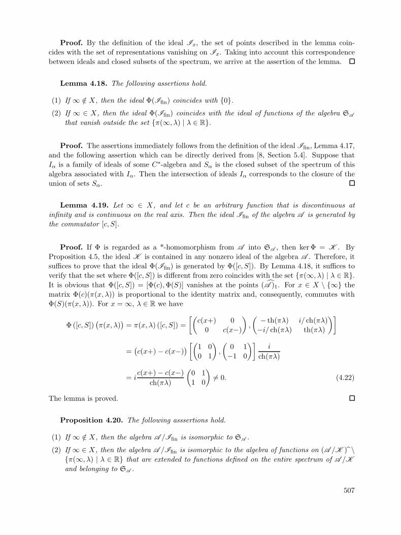
Lemma 4.19. Let ∞ ∈ X, and let c be an arbitrary function that is discontinuous at

infinity and is continuous on the real axis. Then the ideal Ifin of the algebra A is generated by

the commutator [c, S].

Proof. If Φ is regarded as a *-homomorphism from A into SA , then kerΦ = K . By

Proposition 4.5, the ideal K is contained in any nonzero ideal of the algebra A . Therefore, it

suffices to prove that the ideal Φ(Ifin) is generated by Φ([c, S]). By Lemma 4.18, it suffices to

verify that the set where Φ([c, S]) is different from zero coincides with the set {π(∞, λ) | λ ∈ R}.It is obvious that Φ([c, S]) = [Φ(c),Φ(S)] vanishes at the points (A )1. For x ∈ X \ {∞} the

matrix Φ(c)(π(x, λ)) is proportional to the identity matrix and, consequently, commutes with

Φ(S)(π(x, λ)). For x = ∞, λ ∈ R we have

Φ ([c, S])(π(x, λ)

)= π(x, λ) ([c, S]) =

[(c(x+) 0

0 c(x−)

),



)]

=(c(x+)− c(x−)

) [(1 0

0 1

),

(0 1

−1 0

)]i

ch(πλ)

= ic(x+)− c(x−)

ch(πλ)

(0 1

1 0

)�= 0. (4.22)

The lemma is proved.

Proposition 4.20. The following asssertions hold.

(1) If ∞ /∈ X, then the algebra A /Ifin is isomorphic to SA .

(2) If ∞ ∈ X, then the algebra A /Ifin is isomorphic to the algebra of functions on (A /K ) \{π(∞, λ) | λ ∈ R} that are extended to functions defined on the entire spectrum of A /Kand belonging to SA .

507

It suffices to take into account the isomorphism A /Ifin � Φ(A )/Φ(Ifin) and Lemma 4.18.

Lemma 4.21. Suppose that x ∈ R and Un ⊂ R is a contracting sequence of intervals with

intersection {x}, and ψn : R → [0, 1] is a sequence of continuous functions such that ψn = 1

outside Un and ψn(x) = 0. Then ψn is an approximate identity of the ideal Ix.

Proof. For each n the multiplication operator ψn is a positive element of the ideal Ix and

ψn � 1. To prove that the sequence ψn is an approximate identity of the ideal Ix, we verify the

following equality for all l ∈ Ix:

limn→∞ l(1− ψn) = 0. (4.23)

We begin with the equality (4.23) for l ∈ K . Since the right-hand side of (4.23) is linear in l

and the estimate ‖l(1− ψn)‖ � ‖l‖ holds, if suffices to verify this equality on the total set 3) in

K . For such a set we take the set of one-dimensional operators v⊗w∗ defined for v,w ∈ L2(R)

by the equality (v ⊗ w∗)f = (f,w)v. Then

(v ⊗ w∗)(1− ψn) = v ⊗ ((1 − ψn)w)∗ → 0

since (1− ψn)w → 0 in L2(R). For l ∈ K the equality (4.23) is proved.

Now, we pass to the case l ∈ Ix. As in the previous case, we can check 4.23 on a total set in

Ix. For such a set we take the set of products a1ca2, where a1 and a2 are arbitrary elements of

the algebra A and the function c : R → C is continuous and vanishes in a neighborhood of the

point x. The element a1ca2 can be represented as a1[c, a2] + a1a2c. By Theorem 3.2, the first

term is compact and, in this case, the equality (4.23) is already proved. For the second term the

equality (4.23) is valid since for some n the support of c is contained in Un and, consequently,

c(1− ψn) = 0.

Lemma 4.22. For any X ⊂ R and x ∈ R

A (X) ∩ Ix(R) = Ix(X).

Proof. We choose ψn as in Lemma 4.21 and write the ideal Ix(X) in the form

Ix(X) = {l ∈ A (X) | l(1− ψn) → 0 for n→ ∞}

and the ideal Ix(R) in the form

Ix(R) = {l ∈ A (R) | l(1− ψn) → 0 for n→ ∞}.

The assertion of the lemma follows from these equalities and the inclusion A (X) ⊂ A (R).

Lemma 4.23. A (X) ∩ Ifin(R) = Ifin(X) for any X ⊂ R.

3) A set S is said to be total in a Banach space X if linear combinations of elements in S are dense in X.

508

Proof. Using the definition of the ideal Ifin and Lemma 4.22, we find

A (X) ∩ Ifin(R) = A (X) ∩(⋂x∈R

Ix(R))

=⋂x∈R

(A (X) ∩ Ix(R)

)=⋂x∈R

Ix(X) = Ifin(X).


Lemma 4.24. ΠXC(R) ∩ Ifin(R) = {0} for any X ⊂ R.

Proof. We consider x ∈ R and choose ψn as in Lemma 4.21. We write

ΠXC(R) ∩ Ix(R) = ΠXC(R) ∩ {l ∈ A (R) | l(1− ψn) → 0 as n→ ∞}= {l ∈ ΠXC(R) | l(1− ψn) → 0 as n→ ∞}= {l ∈ ΠXC(R) | l(x) = 0}.

Using the definition of the ideal Ifin and the above equality, we find

ΠXC(R) ∩ Ifin(R) = ΠXC(R) ∩(⋂

x∈RIx(R)

)

=⋂x∈R

(ΠXC(R) ∩ Ix(R)

)

=⋂x∈R

{l ∈ ΠXC(R) | l(x) = 0}

= {l ∈ ΠXC(R) | ∀x ∈ R l(x) = 0} = {0}.


5 Algebra of Singular Integral Operators with Discontinuities

in Momenta and Coordinates

We fix an arbitrary pair of sets X, X ⊂ R. In this section. we study the algebra B = B(X, X)

generated in B(L2(R)) by the subalgebras ΠXC(R) and F∗(ΠXC(R)) (the homomorphism F∗is defined by the equality F∗b = FbF−1).

5.1 Ideals of the algebra B

Proposition 5.1. The algebra B(X, X) is irreducible.

509

Proof. Let Y be a reducing subspace of the algebra B(X, X). By Proposition 4.2, it has

the form χUL2(R), where χU is the characteristic function of a set U ⊂ R. We prove that U

coincides, up to a set of zero measure, with either ∅ or R. Let U be nonempty. Then there is

a nonzero nonnegative function u ∈ L2(R) supported in U . We consider an arbitrary positive

function g in the Schwartz class S(R). Then the function s =√2πF−1g is continuous on R and,

consequently, the operator F∗(s) belongs to the algebra B(X, X). But, in this case, the support

of F∗(s)u lies in U . On the other hand, this support coincides with R since

F∗(s)u =

∫

R

g(x− y)u(y)dy > 0.

The proposition is proved.

Proposition 5.2. K ⊂ B(X, X).

Proof. As is known (cf., for example, [8, Theorem 2.4.9] or [10, Corollary 4.1.10]), if the

image π(A) : A → B(H) of an irreducible representation of A contains at least one nonzero

compact operator, then K(H) ⊂ π(A). Thus, we need to verify that the algebra B contains at

least one nonzero compact operator. We consider the commutator [c, F∗(s)], where c and s are

continuous functions on R. By Theorem 3.2, it is compact. We show that it is possible to choose

c and s such that [c, F∗(s)] �= 0. For this purpose, we consider a positive function u ∈ L2(R)

and choose s equal to√2πF−1g, where a positive function g belongs to the Schwartz class, and

for c we take a nonzero nonnegative function with compact support. Then cF∗(s)u = 0 outside

the support of c and F∗(s)cu > 0 on the entire real axis.

In Subsection 4.1, we introduced the ideal Ix of the algebra A generated by functions that

are continuous in R and vanish at the point x ∈ R. In a similar way, we introduce the ideals Jx

generated by the same functions of the algebra B = B(X, X) and the ideals Jx generated by

the operators F∗(s), where s ∈ C(R), s(x) = 0. The following lemma describes the action of the

homomorphism F∗ on the algebra B(X, X). From this lemma and other assertions for the ideals

Jx we automatically obtain similar assertions for the ideals Jx. We set −X def= {−x | x ∈ X}.

The following assertion follows from the definitions of the algebra B(X, X) and mapping F∗.

Lemma 5.3. Under the isomorphism F∗ : B(X, X) → B(−X,X), the ideals Jx(X, X) and

J (X, X) are transformed to the ideals Jx(−X,X) and J−x(−X,X) respectively.

Lemma 5.4. Suppose that ψn : R → [0, 1] is a sequence of continuous functions and ψn = 1

on [−n, n], ψn(∞) = 0. Then ψn is an approximate identity of the ideal J∞.

The proof of Lemma 5.4 is obtained from the proof of Lemma 4.21 with replacing A by B,

I by J , x by ∞, and Un by R \ [−n, n].Lemma 5.5. J∞ ∩ J∞ = K .

Proof. By Propositions 4.5, 5.1 and 5.2, the ideal of compact operators is contained in each

of the ideals J and J . Let us check the inverse inclusion.

Let j be an arbitrary element of J∞ ∪ J∞. By Lemmas 5.4 and 5.3,

510

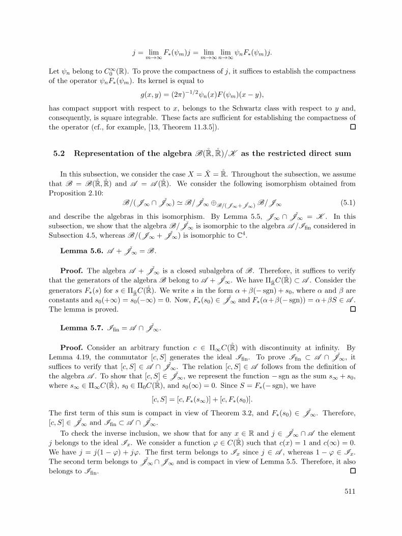
j = limm→∞F∗(ψm)j = lim

m→∞ limn→∞ψnF∗(ψm)j.

Let ψn belong to C∞0 (R). To prove the compactness of j, it suffices to establish the compactness

of the operator ψnF∗(ψm). Its kernel is equal to

g(x, y) = (2π)−1/2ψn(x)F (ψm)(x− y),

has compact support with respect to x, belongs to the Schwartz class with respect to y and,

consequently, is square integrable. These facts are sufficient for establishing the compactness of

the operator (cf., for example, [13, Theorem 11.3.5]).

5.2 Representation of the algebra B(R, R)/K as the restricted direct sum

In this subsection, we consider the case X = X = R. Throughout the subsection, we assume

that B = B(R, R) and A = A (R). We consider the following isomorphism obtained from

Proposition 2.10:

B/(J∞ ∩ J∞) � B/J∞ ⊕B/(J∞+J∞) B/J∞ (5.1)

and describe the algebras in this isomorphism. By Lemma 5.5, J∞ ∩ J∞ = K . In this

subsection, we show that the algebra B/J∞ is isomorphic to the algebra A /Ifin considered in

Subsection 4.5, whereas B/(J∞ + J∞) is isomorphic to C4.

Lemma 5.6. A + J∞ = B.

Proof. The algebra A + J∞ is a closed subalgebra of B. Therefore, it suffices to verify

that the generators of the algebra B belong to A + J∞. We have ΠRC(R) ⊂ A . Consider the

generators F∗(s) for s ∈ ΠRC(R). We write s in the form α+ β(− sgn) + s0, where α and β are

constants and s0(+∞) = s0(−∞) = 0. Now, F∗(s0) ∈ J∞ and F∗(α+β(− sgn)) = α+βS ∈ A .


Lemma 5.7. Ifin = A ∩ J∞.

Proof. Consider an arbitrary function c ∈ Π∞C(R) with discontinuity at infinity. By

Lemma 4.19, the commutator [c, S] generates the ideal Ifin. To prove Ifin ⊂ A ∩ J∞, it

suffices to verify that [c, S] ∈ A ∩ J∞. The relation [c, S] ∈ A follows from the definition of

the algebra A . To show that [c, S] ∈ J∞, we represent the function − sgn as the sum s∞ + s0,

where s∞ ∈ Π∞C(R), s0 ∈ Π0C(R), and s0(∞) = 0. Since S = F∗(− sgn), we have

[c, S] = [c, F∗(s∞)] + [c, F∗(s0)].

The first term of this sum is compact in view of Theorem 3.2, and F∗(s0) ∈ J∞. Therefore,

[c, S] ∈ J∞ and Ifin ⊂ A ∩ J∞.To check the inverse inclusion, we show that for any x ∈ R and j ∈ J∞ ∩ A the element

j belongs to the ideal Ix. We consider a function ϕ ∈ C(R) such that c(x) = 1 and c(∞) = 0.

We have j = j(1 − ϕ) + jϕ. The first term belongs to Ix since j ∈ A , whereas 1 − ϕ ∈ Ix.

The second term belongs to J∞∩J∞ and is compact in view of Lemma 5.5. Therefore, it also

belongs to Ifin.

511

Lemma 5.8. B/J∞ � A /Ifin.

Proof. We have B/J∞ = (A + J∞)/J∞ � A /(A ∩ J∞) = A /Ifin.

The equivalence class of an element a modulo some ideal is denoted by [a]. The following

assertion is the main result of this section. Consider the diagram

B/Kp ��

p��

A /Ifin

q��

A /Ifin q�� C4 .

(5.2)

The surjective homomorphisms p, p, q, q are described by the following assertions:

(1) any element b ∈ B admits the representation b = a+ j with some a ∈ A , j ∈ J∞; for any

such a representation p(b+ K ) = a+ Ifin,

(2) if b ∈ B, then p(b+ K ) = p(F−1∗ (b) + K ),

(3) if a ∈ A , then q([a]) = (π+(−∞)(a), π+(+∞)(a), π−(−∞)(a), π−(+∞)(a)),

(4) if a ∈ A , then F∗(a) admits a representation in the form a+ j with some a ∈ A , j ∈ J∞;for any such a representation q([a]) = q([a]),

(4′) if a ∈ A , then q([a]) = (π−(−∞)(a), π+(−∞)(a), π−(+∞)(a), π+(+∞)(a)).

The values of the homomorphisms p, p, q, q on the generators are described by the following

equalities, where c and s are arbitrary elements of ΠRC(R):

p([c]) = [c], (5.3)

p([F∗(s)]) =[s(+∞)

1− S

2+ s(−∞)

1 + S

2

], (5.4)

p([c]) =

[c(+∞)

1 + S

2+ c(−∞)

1− S

2

], (5.5)

p([F∗(s)]) = [s], (5.6)

q([c]) = (c(−∞), c(+∞), c(−∞), c(+∞)), (5.7)

q([S]) = (1, 1,−1,−1), (5.8)

q([c]) = (c(−∞), c(−∞), c(+∞), c(+∞)), (5.9)

q([S]) = (−1, 1,−1, 1). (5.10)

Theorem 5.9. The following isomorphism holds:

B/K � A /Ifin ⊕C4 A /Ifin, (5.11)

defined in the sense of Propositions 2.4 and 2.8 by the diagram (5.2), which is a pullback. For

the homomorphisms p, p, q, and q in this diagram assertions (1)–(4′) and formulas (5.3)–(5.10)

hold.

512

Proof. We consider the commutative diagram

B/(J∞ ∩ J∞)r ��

r��

B/J∞

t��

f : [a+j] �→[a] �� A /Ifin[a]← �[a]

��

h��

B/J∞t ��

F−1∗��

B/(J∞ + J∞)g ��

F−1∗��

A /(I∞ + Ifin)��

ϕ

��

B/J∞

F∗

��

t ��

f

��

B/(J∞ + J∞)

F∗

��

g

��A /Ifin

��

h �� A /(I∞ + Ifin)

��

ϕ ��C4 .

(5.12)

The mappings r, r, t, t, h are the standard projections. The left upper square is a pullback

by Proposition 2.10. The isomorphisms, denoted by F∗ and F−1∗ in the diagram, are obtained

by omitting the isomorphisms F∗ and F−1∗ from the algebra B to the quotient algebras B/J∞,B/J∞, and B/(J∞ + J∞).

Let us describe the right upper square coinciding with the left lower square in the diagram.

Here, f denotes the isomorphism from Lemma 5.8. To compute its value on the equivalence

class [b] = b+ J∞, we take a representative a in the algebra A , which exists in view of Lemma

5.6. Then f([b]) = [a]. The isomorphism g is obtained by omitting the isomorphism f to the

quotient algebra

B/(J∞ + J∞) � (B/J∞)/((J∞ + J∞)/J∞

).

To verify that it is well defined, we check the equality

f((J∞ + J∞)/J∞

)= (I∞ + Ifin)/Ifin. (5.13)

The right-hand side is a subset of the left-hand side. Indeed, I∞ ⊂ J∞ and Ifin ⊂ J∞.Therefore, for any j in I∞ + Ifin

f(j + J∞) = j + Ifin.

Let us prove the inverse inclusion. We note that any equivalence class in (J∞+ J∞)/J∞ has

the form j + J∞ for some j ∈ J∞. We choose ψn as in Lemma 5.4 and write

f([j]) = f([limnψnj]) = lim

nf([ψn])f([j]) = lim

n(ψn + Ifin)f([j]).

Thus, f([j]) is the limit of elements of the ideal (I∞ + Ifin)/Ifin of the algebra A /Ifin and,

consequently, belongs to it. Therefore, the isomorphism g is well defined and the right upper

square (consequently, the left lower square) in the diagram (5.12) is commutative.

To define the mapping ϕ, we consider an isomorphism Φ between the algebra A and the

corresponding algebra of symbols SA . Using the correspondence between ideals of the algebra

SA and closed subsets of (A /K ) , we associate with the ideal Φ(I∞ + Ifin) the set

(A /K ) \ {π+(−∞), π+(+∞), π−(−∞), π−(+∞)}.

513

Thus, the spectrum of the algebra A /(I∞+Ifin) is isomorphic to SA /Φ(I∞ +Ifin), consists

of four one-dimensional representations and, consequently, the algebra itself is isomorphic to C4.

We denote by ϕ the isomorphism defined by the formula

ϕ([a]) = (π+(−∞)(a), π+(+∞)(a), π−(−∞)(a), π−(+∞)(a)) for a ∈ A . (5.14)

We denote by ϕ the isomorphism making the right lower square in the diagram (5.12) commu-

tative. It is obvious that this isomorphism is given by the formula

ϕ = ϕ ◦ g ◦ F∗ ◦ g−1.To simplify the description of this isomorphism, we note that ϕ ◦ ϕ−1 is an isomorphism of the

algebra C4. All such isomorphisms are permutations of components of C4. In order to determine

which of 24 permutations is ϕ◦ϕ−1, we compute the values of ϕ and ϕ on the equivalence classes

of elements sgn and S of the algebra A :

ϕ([sgn]) = (−1, 1,−1, 1), ϕ([S]) = (1, 1,−1,−1), (5.15)

ϕ([sgn]) = (−1,−1, 1, 1), ϕ([S]) = (−1, 1,−1, 1). (5.16)

Hence

ϕ([a]) = (π−(−∞)(a), π+(−∞)(a), π−(+∞)(a), π+(+∞)(a)) for a ∈ A .

To obtain the diagram (5.2) from the diagram (5.12), it suffices to eliminate all the algebras,

except possibly for algebras at the corners of the diagram, by replacing the homomorphisms

with the compositions: p = f ◦ r, p = f ◦ F−1∗ ◦ r, q = ϕ ◦ h, q = ϕ ◦ h. The diagram (5.2)

coincides, up to an isomorphic algebra, with the left upper square in the diagram (5.12) and,

therefore, is a pullback.

Assertions (1)–(4′) describing the homomorphisms p, p, q, q in (5.2) are obtained from the

above description of the homomorphisms in the diagram (5.12). The values on the generators

are obtained from these descriptions.

5.3 Representation of the algebra B(X, X)/K as the restricted direct sum

In Subsection 5.2, we considered the algebra B(R, R)/K . Now, we assume that X, X ⊂ R

are arbitrary. To formulate the following assertion, we need the diagram

B(X, X)/Kp1 ��

p2��

A1

q1��

A2 q2�� Cn .

(5.17)

The algebras A1, A2, number n and projections p1, p2, q1, q2 depend on the sets X and X

in the following way.

1◦. If X, X � ∞, then A1 = A (X)/Ifin(X), A2 = A (X)/Ifin(X), n = 4; the projections

p1 and p2 take the form

514

p1([F∗(s)]) =[s(+∞)

1− S

2+ s(−∞)

1 + S

2

], p1([c]) = [c], (5.18)

p2([c]) =

[c(+∞)

1 + S

2+ c(−∞)

1− S

2

], p2([F∗(s)]) = [s], (5.19)

where [c], [F∗(s)] are the generators of B(X, X)/K ; the projection q1 of A (X)/Ifin(X) is given

by the formulas

q1([c]) = (c(−∞), c(+∞), c(−∞), c(+∞)),

q1([S]) = (1, 1,−1,−1),(5.20)

where c ∈ ΠXC(R); the projection q2 onto the generators [c] of the algebra A (X)/Ifin(X) is

defined by the formulas

q2([c]) = (c(−∞), c(−∞), c(+∞), c(+∞)),

q2([S]) = (−1, 1,−1, 1),(5.21)

where c ∈ pXC(R).

2◦. If X � ∞, X �� ∞, then A1 = ΠXC(R), A2 = A (X)/Ifin(X), n = 2; the projection p1on the generators of B(X, X)/K has the form

p1([F∗(s)]) = s(∞),

p1([c]) = c,(5.22)

and the projection p2 is defined by (5.19); further,

q1(c) = (c(−∞), c(+∞)),

q2([c]) = (c(∞), c(∞)),

q2([S]) = (−1, 1).

(5.23)

3◦. If X �� ∞, X � ∞, then A1 = A (X)/Ifin(X), A2 = ΠXC(R), n = 2; the projection p2on the generators of B(X, X)/K has the form

p2([c]) = c(∞),

p2([F∗(s)]) = s,(5.24)

and the projection p1 is defined by (5.18); further,

q1([c]) = (c(∞), c(∞)),

q1([S]) = (1,−1),

q2(c) = (c(−∞), c(∞)).

(5.25)

515

4◦. If X, X �� ∞, then A1 = ΠXC(R), A2 = ΠXC(R), n = 1; the projections p1, p2, q1, and

q2 take the form

p1([c]) = c, p1([F∗(s)]) = s(∞), q1(c) = c(∞), (5.26)

p2([c]) = c(∞), p2([F∗(s)]) = s, q2(c) = c(∞). (5.27)

Theorem 5.10. The following isomorphism holds:

B(X, X)/K � A1 ⊕Cn A2, (5.28)

defined in the sense of Propositions 2.4 and 2.8 by the diagram (5.2), which is a pullback. The

homomorphisms p1, p2, q1, q2 are well defined and are given on the generators by the above

formulas.

Proof. By Theorem 5.9, the diagram

B(R, R)/Kp ��

p��

A (R)/Ifin(R)

q

��A (R)/Ifin(R) q

�� C4

(5.29)

is a pullback. Therefore, by Theorem 2.9, the following assertions hold:

(1) the homomorphisms p and p are surjective,

(2) ker p ∩ ker p = {0},(3) ker(q ◦ p) = ker p+ ker p.

We consider the diagram obtained from (5.29) by passing to subalgebras and restricting the

homomorphisms:

B(X, X)/Kp0 ��

p0��

p(B(X, X)/K )

q0��

p(B(X, X)/K )q0

�� (q ◦ p)(B(X, X)/K).

(5.30)

We show that it is also a pullback. By Theorem 2.9, it suffices to verify the following conditions:

(1′) the homomorphisms p0 and p0 are surjective,

(2′) ker p0 ∩ ker p0 = {0},(3′) ker(q0 ◦ p0) = ker p0 + ker p0.

Condition (1′) holds because of the construction of the diagram (5.30), and (2′) follows

from (2). Consider assertion (3′). The embedding ker(q0 ◦ p0) ⊃ ker p0 + ker p0 holds because

516

the diagram (5.30) is commutative. To check the inverse inclusion, we write the left-hand and

right-hand sides in the form

ker(p ◦ q) ∩ (B(X, X)/K) ⊂ ker p ∩ (B(X, X)/K

)+ ker p ∩ (B(X, X)/K

).

Using the diagram (5.12), we find the values of ker(p ◦ q), ker p, ker q:((

J∞(R, R) + J∞(R, R))/K

)∩ (B(X, X)/K

)(J∞(R, R)/K

) ∩ (B(X, X)/K)+(J∞(R, R)/K

) ∩ (B(X, X)/K). (5.31)

Below, [·] denotes the equivalence class modulo the ideal K . Consider l ∈ J∞(R, R) and

j ∈ J∞(R, R) such that [l] + [j] ∈ B(X, X)/K . We show that [l] + [j] belongs to the right-

hand side of (5.31). By Lemma 5.4, the approximate identity ψn of the ideal J∞(R, R) can be

taken in the algebra B(X, X). By Lemma 5.5, [ψnl] = 0. Therefore,

[ψn]([l] + [j]

)= [ψnj] → [j], n→ ∞,

which implies [j] ∈ B(X, X)/K . Using [l] + [j] ∈ B(X, X)/K , we find [l] ∈ B(X, X)/K .

Therefore, [l]+[j] belongs to the right-hand side of (5.31) which means that (5.30) is a pullback.

To compute the algebras p(B(X, X)/K

), p(B(X, X)/K

), and (q ◦ p)(B(X, X)/K

), we

note that the algebra B(X, X)/K is generated by [c] for c ∈ ΠXC(R) and [F∗(s)] for s ∈ΠXC(R). Therefore, their images are generated by the images of [c] and [F∗(s)].

In the case ∞ ∈ X, formulas (5.3) and (5.4) describing the values of the homomorphism

p on the generators imply that the algebra p(B(X, X)/K

)is generated in A (R)/Ifin(R) by

[c], c ∈ ΠXC(R) and [S]. Hence

p(B(X, X)/K

)=(A (X) + Ifin(R)

)/Ifin(R) � A (X)/

(A (X) ∩ Ifin(R)

)= A (X)/Ifin(X).

Here, we used Lemma 4.23.

In the case ∞ /∈ X, the algebra p(B(X, X)/K

)is generated by [c], c ∈ ΠXC(R). Therefore,

p(B(X, X)/K

)=(ΠXC(R) + Ifin(R)

)/Ifin(R)

� ΠXC(R)/(ΠXC(R) ∩ Ifin(R)

)= ΠXC(R)/{0} = ΠXC(R).

Here, we used Lemma 4.24.

Thus, for any X, X we obtain the isomorphism p(B(X, X)/K

) � A1. Using this result

and Lemma 5.3, we have

p(B(X, X)/K

)= p((F−1∗ B(X,−X)

)/K

)� A2.

Based on the known image p(B(X, X)/K

), we can compute the image (q◦p)(B(X, X)/K

)with the help of formulas (5.7) and (5.8). Replacing the algebras of the pullback (5.30) with

isomorphic algebras A1, A2, and Cn, we find the required pullback (5.17). The isomorphism

(5.28) is obtained from Proposition 2.4, and the formulas for the homomorphisms p1, p2, q1, q2follow from formulas (5.3)–(5.10) and the description of the above-obtained isomorphisms.

517

5.4 Consequences

To prove the following assertion, one can apply Theorem 2.16 to the diagram (5.17) which

is a pullback in view of Theorem 5.10.

Theorem 5.11. In the notation of Theorem 5.10, the following homeomorphism holds:

(B(X, X)/K

) � A1 �(Cn) A2, (5.32)

defined in the sense of Propositions 2.5 and 2.6 by the pushout

(B(X, X)/K ) A1��

p1��

A1

��

p2

��

(Cn) .��q2��

��

q1

��

(5.33)

The set of classes of one-dimensional and two-dimensional representations of the algebra Bis denoted by (B)1 and (B)2 respectively. Then

B = {[id]} ∪ (B)2 ∪ (B)1.

Replacing in (5.28) the algebras A1 and A2 with isomorphic algebras, we obtain the isomorphism

Ψ: B/K → SB, where the algebra SB consists of functions on the spectrum of B/K .

Using the description of p1, p2, q1, q1 and the spectra of algebras A (X)/Ifin(X), ΠXC(R),

one can obtain from Theorem 5.10 a complete list of nonzero irreducible representations of the

algebra B(X, X)/K and compute the values of these representations on the generators. In the

formulas below, c is an arbitrary element of ΠXC(R) and s belongs to ΠXC(R). In the case

X, X � ∞, the list is as follows:

1. The representations p1(π±(x)), x ∈ ΠXR,

p1(π±(x)

)([c]) = c(x),

p1(π±(x)

)([F∗(s)]) = s(∓∞).

(5.34)

2. The representations p1(π(x, λ)), x ∈ X \ {∞},

p1(π(x, λ)

)([c]) =

(c(x+) 0

0 c(x−)

), (5.35)

p1(π(x, λ)

)([F∗(s)]) =

s(−∞) + s(+∞)

2Id2 +

s(−∞)− s(+∞)

2M∗(S)(λ). (5.36)

3. The representations p2(π±(x)), x ∈ ΠXR,

p2(π±(x)

)([c]) = c(±∞),

p2(π±(x)

)([F∗(s)]) = s(x).

(5.37)

518

4. The representations p2(π(x, λ)), x ∈ X \ {∞},

p2(π(x, λ)

)([c]) =

c(+∞) + c(−∞)

2Id2 +

c(+∞)− c(−∞)

2M∗(S)(λ), (5.38)

p2(π(x, λ)

)([F∗(s)]) =

(s(x+) 0

0 s(x−)

). (5.39)

Some representations are listed twice, namely:

p1(π+(−∞)) = p2(π

−(−∞)),

p1(π+(+∞)) = p2(π

+(−∞)),

p1(π−(−∞)) = p2(π

−(+∞)),

p1(π−(+∞)) = p2(π

+(+∞)).(5.40)

In the case X �� ∞, X � ∞, the list is as follows:

1. The representations p1(π±(x)), x ∈ ΠXR, satisfying (5.34).

2. The representations p1(π(x, λ)), x ∈ X \ {∞}, satisfying (5.35) and (5.36) hold.

3. The representations p2(x), x ∈ ΠXR,

p2(x)([c]) = c(∞),

p2(x)([F∗(s)]) = s(x).(5.41)

Here, the following representations are listed twice:

p1(π+(∞)) = p2(−∞), p1(π

−(∞)) = p2(+∞). (5.42)

In the case X, X �� ∞, irreducible representations of the algebra B(X, X)/K are the repre-

sentations p2(x), x ∈ ΠXR, satisfying (5.41) and the representations p1(x), x ∈ ΠXR, satisfying

p1(x)([c]) = c(x),

p1(x)([F∗(s)]) = s(∞).(5.43)

Moreover, p1(∞) = p2(∞).

The algebra B(X, X) is not commutative if and only if at least one of the algebras A1 or

A2 is not commutative. The algebra A1, as well as the algebra A2, is not commutative only

if it coincides with A (X)/Ifin(X) for X /∈ {∅, {∞}}. Therefore, the algebra B(X, X) is not

commutative if and only if one of the sets X or X contains ∞ and the other contains at least

one element different from ∞. We list the cases where the algebra B is commutative.

1. X, X �� ∞. In this case, B(X, X)/K � ΠXC(R)⊕C ΠXC(R).

2. One of the sets X or X is empty. For the sake of definiteness, let X be nonempty. We

also assume that X � ∞ (otherwise, we are in the above situation). Then B(X, X)/K �A (∅)/K ⊕C2 ΠXC(R).

519

3. X = X = {∞}. Then B(X, X)/K � A ({∞})/Ifin({∞}) ⊕C4 A ({∞})/Ifin({∞}), i.e.,it is isomorphic to the algebra C(S1) of continuous functions on the circle S1.

Such cases are referred to as “commutative.”

We denote by com(B) the closed ideal of the algebra B generated by commutators. In the

“commtative” case, it coincides with K .

Theorem 5.12. The algebra B is solvable. In the “commutative” case, the minimal solving

series has length 1 and can be taken in the form {0} ⊂ K ⊂ B. In the “noncommutative” case,

the minimal solving series has length 2 and can be taken in the form

{0} ⊂ K ⊂ com(B) ⊂ B;

moreover,

B/ com(B) � C((B)1),

com(B)/K � C0((B)2)⊗K(C2).(5.44)

Proof. A solving series cannot be shorter. because, in the “commutative” case, B possesses

representations of two different dimensions, whereas, in the “noncommutative” case, it has repre-

sentations of three different dimensions. The isomorphisms (5.44) hold since B/K � SB.

6 Abstract Index Group and the Fredholm Index of Operators

6.1 Introduction

Definition 6.1 (cf. [14, Definition 2.10]). Let A be a unital C∗-algebra. We denote by

Inv(A) the group of invertible elements of A and by Inv(A)0 the connected component of identity.

By the abstract index group of A we mean the quotient group

Λ(A)def= Inv(A)/ Inv(A)0.

In this subsection, we prove that there exists an isomorphism ΛInd: Λ(B/K ) → Zk, where

k ∈ {0, 1, 2} depends on the choice of the sets X and X. We also write out a formula for

computing the corresponding locally constant homomorphism ΛInd: Inv(SB) → Zk such that

the following diagram is commutative:

Λ(B/K )ΛInd ��

Zk

Inv(B/K )

��

Ψ �� InvSB .

ΛInd

��

(6.1)

As we show below, these formulas can be used for computing the Fredholm index of operators

of the algebra B. We recall that an operator b ∈ B(H) is Fredholm if its kernel ker b = {u ∈ H |b(u) = 0} is finite-dimensional, the image is closed, and the orthogonal complement of this image

(denoted by coker b) has finite dimension. The Fredholm index of an operator b is the number

520

ind b = dimker b − dim coker b. The product ab of Fredholm operators is a Fredholm operator

and ind(ab) = ind a+ind b. By the Atkinson theorem, the operator b ∈ B(H) is Fredholm if and

only if the operator b+K(H) is invertible in the quotient algebra B(H)/K(H). The Fredholm

index is unchanged if we add a compact term.

These facts allow us to find the Fredholm index on the set Inv(B(H)/K(H)) of all invertible

elements of the quotient algebra. The Fredholm index is constant on connected components of

Inv(B(H)/K(H)) and, consequently, is omitted to ΛInd(B(H)/K(H)). The above assertions

can be found, for example, in [8, Section 1.4]. The obtained mapping is the group isomorphism

ind: ΛInd(B(H)/K(H)) → Z (cf., for example, [14, Theorems 5.35 and 5.36]).

Remark 6.2. The mapping ind is constant on connected components of Inv(B(H)/K(H))

and, consequently, on components of Inv(B/K ). Hence it is possible to introduce a mapping

ind: Λ(B/K ) → Z, and for a ∈ Inv(B/K ) the value ind a is uniquely determined by the value

of ΛInd a. In other words, there exists a homomorphism Δ: Zk → Z such that the following

diagram is commutative:

Inv(B/K )ΛInd ��

ind�� Zk

Δ

��Z .

(6.2)

To compute the homomorphism Δ, it suffices to determine ind on the elements of Inv(B/K )

corresponding to the generators of Λ(B/K ) � Zk. For this purpose, we need the following

assertion [5, Theorem IV.7.3].

Lemma 6.3. Suppose that c, s ∈ C(R) and c − s, c + s do not vanish at any point of R.

Then

ind(c+ sS) =1

2πi

∫

R

d lnc− s

c+ s. (6.3)

6.2 Technical description of SB

The space (B)1 for any X, X is formed, up to a homeomorphism, by gluing finitely many

copies of ΠY R (possibly, with different Y ⊂ R)m in particular, at ∞ for ∞ /∈ Y and at ±∞ for

∞ ∈ Y .

Definition 6.4. Let i : ΠY R → (B)1 be an embedding, and let y ∈ Y \ {∞}. We set

i(y)def= {i(y−), i(y+)}

and call i(y) a discontinuity point in (B)1. We say that U ∈ SB is discontinuous at a point

i(y) if U(i(y+)) �= U(i(y−)); otherwise, we assume that U(i(y)) is defined and is equal to the

common value U(i(y+)) and U(i(y−)).

The space (B)2 consists of lines parametrized by λ ∈ R. Passing to the closure of this line,

we should add four points: elements of two discontinuity points in (B)1.

521

Definition 6.5. Let i : R → (B)2 be a parametrization of some line in (B)2. We say that

U ∈ SB has the standard form on this line if for some α, β ∈ C

U(i(λ)) = αId2 + βM∗(S)(λ). (6.4)

We denote by Z the set of functions U ∈ SB that have only finitely many discontinuities

in (B)1 and have the standard form on all lines in (B)2, except possibly for a finite number of

them.

We note that the set Z is dense in SB. This fact follows from the expressions of the algebra

SB via the algebras ΠY C(R), SA and similar assertions for these two algebras following from

Theorems 3.1 and 4.15. Any connected component of Inv(SB) is open and, consequently, there

is a function in Z in this component. We note that the function (6.4) is invertible for all λ if and

only if its limit values as λ→ ±∞ are invertible, i.e., if the values of this functions are different

from zero at corresponding points in (B)1.

The main tool for constructing the isomorphism ΛInd is Lemma 6.7 below. In the proof of

this lemma, the following known assertion is used.

Lemma 6.6. The fundamental group π1(GL(n,C)) is isomorphic to Z. This isomorphism

sends the equivalence class of path γ : [0, 1] → GL(n,C) to the number of rotations of det(γ(t))

around 0, given by the formula

1

2πi

1∫

0

ddet(γ(t)).

We choose an arbitrary function U1 in Inv(SB) ∩ Z and consider some line in (B)2. We

describe a procedure for transforming continuously the function U1 to the standard form on

this line. We introduce the local coordinates in a neighborhood of the closure of this line and

parametrize the line by ξ = th(λ). The values of U1 on this line are described by a continuous

function u1 that is defined on the segment [−1, 1] and takes the values in the set of 2×2-matrices;

moreover, its values are diagonal matrices at the endpoints of this segment. A neighborhood of

the closure of the line is taken so small that, on lines in (B)2 intersecting the neighborhood, the

function U1 has the standard form and is uniquely restored from its values on (B)1. The values

of the function on two parts of (B)1 adjoining to the line are defined by the pair (g1, h1) of

functions given on an interval (−ε, ε) that are continuous everywhere in this interval expect for

the point 0, where a discontinuity of the first kind is admissible. We choose a parametrization

such that

u1(−1) =

(g1(0+) 0

0 h1(0−)

), u1(1) =

(h1(0+) 0

0 g1(0−)

). (6.5)

Lemma 6.7. There exists a function U ∈ Inv(SB)∩Z that is described in the local coordi-

nates by the functions u, g, h and

1) U and U1 belong to the same connected component of Inv(SB),

2) U and U1 coincide outside the neighborhood under consideration,

3) g and h are continuous,

522

4) U has the standard form on all lines in (B)2 intersecting the neighborhood.

5)

ε∫

−εd ln g(x) = 2πin + ln(g1(ε)/g1(−ε)), where n is any given integer.

Proof. The proof is divided into four steps. Technical details are omitted.

Step 1. We continuously transform u1, g1, h1 to u2, g2, h2 so that g2 = g1, h2 = h1,

u2(ξ) = u1(−1) for ξ < −0.1, u2(ξ) = u1(10ξ) for ξ ∈ [−0.1, 0.1], and u2(ξ) = u1(1) for ξ > 0.1.

Now, u2 on [−1,−0.1] and [0.1, 1] is diagonal and constant.

Step 2. We continuously change the diagonal elements u2 on these segments keeping un-

changed their values at the endpoints so that the resulting function u3 coincides with the identity

matrix on less segments [−0.9,−0.2] and [0.2, 0.9]. Moreover, the diagonal elements on [−1,−0.9]

and [0.9, 1] make the same number of rotations around 0 as in the segments [−0.2,−0.1] and

[0.1, 0.2] respectively, but in the opposite direction. The fractional part of the rotation number

is uniquely determined by the values of diagonal u2 at the points −1,−0.1, 0.1, 1, whereas the

integer part can be chosen arbitrarily. At this step, the functions g and h remain unchanged.

Step 3. Stretching, we obtain the following functions, where y ∈ [0, 1]:

u4(y) = u3(0.5y), u4(−y) = u3(−0.5y),

g4(ε(−0.5 + 0.5y)) = (u3)22(1− 0.5y), g4(ε(0.5 − 0.5y)) = (u3)11(−1 + 0.5y),

g4(ε(−1 + 0.5y)) = g3(ε(−1 + y)), g4(ε(1 − 0.5y)) = g3(ε(1− y)),

h4(ε(0.5 − 0.5y)) = (u3)11(1− 0.5y), h4(ε(−0.5 + 0.5y)) = (u3)22(−1 + 0.5y),

h4(ε(1 − 0.5y)) = h3(ε(1 − y)), h4(ε(−1 + 0.5y)) = h3(ε(−1 + y)).

Choosing the number of rotations around 0 in a suitable way at Step 2, one can obtain the

desired valueε∫

−εd ln g4(x).

This result depends only on (u3)11(ξ) for ξ < 0 and (u3)22(ξ) for ξ > 0. Specifying the number of

rotations of (u3)11(ξ) for ξ > 0 and (u3)22(ξ) for ξ < 0 around 0, we finally achieve the situation

where the number of rotations of det u4(ξ) around 0 is equal to zero.

Step 4. By Lemma 6.6, the element u4 ∈ C([−1, 1],GL(2,C)) regarded as a loop in GL(2,C)

is homotopic to the trivial loop u5 defined by the equality u5(ξ) = Id2.

6.3 Case X, X � ∞

In this case, the algebra B has the form

B � A (X)/Ifin(X)⊕C4 A (X)/Ifin(X).

523

We note that the spectrum of the algebra B consists of a square some points of which are

bisected (i.e., some points are replaced with pairs of points in the sense of Definition 6.4) and

lines in (B)2 intertwining pairs of opposite bisected points (cf. Theorem 5.11 and 4.16 and also

the list of irreducible representations, p. 518). Using Lemma 6.7, one can show that, in each

connected component of Inv(SA ), there is a function that has the standard form on all lines

in (B)2 and has no discontinuities on (B)1. There is a one-to-one correspondence between the

set of such functions and the functions on the square (with the values in C \ {0}). As is known,the connected components of this set are parametrized by the number of rotations of a function

around 0 when the variable goes along the square, i.e.,

1

2πi

∫

( B)1

d ln(U(π)), (6.6)

where the integral over (B)1 is defined by the formula∫

( B)1

db(π)def=

∫

R

db(p1(π−(x)))−

∫

R

db(p1(π+(x)))+

∫

R

db(p2(π−(x)))−

∫

R

db(p2(π+(x))). (6.7)

If b has finitely many discontinuities, the integrals on the right-hand side of (6.7) are understood

as the sum of integrals over segments containing no discontinuities of b. Otherwise, the integral

on the left-hand side of (6.7) is undefinite.

To describe the homomorphism ΛInd: Inv(SB) → Z, we extend the notion of the “rotation

number” to Inv(SB). For this purpose, we define the integral over (B)2 by the following formula

(the integrals on the right-hand side are taken with respect to λ):∫

( B)2

db(π)def=∑x∈X

∫

R

db(p1(π(x, λ))) +∑x∈X

∫

R

db(p2(π(x, λ))). (6.8)

The integral on the left-hand side of (6.8) is assumed to be defined for all complex-valued

functions b that are continuous on the line in (B)2 and are constant on all such lines (except

possibly for finitely many such lines).

We define ΛInd on U ∈ Inv(SB) ∩ Z by the formula

ΛInd(U)def=

1

2πi

( ∫

( B)1

d ln(U(π)) +

∫

( B)2

d ln(det(U(π)))

). (6.9)

It is well defined since the function ln(U(π)) has finitely many discontinuities on (B)1 and the

function det(U(π)) is constant on the lines where U has the standard form and is continuous on

the remaining lines.

Lemma 6.8. The mapping ΛInd defined by formula (6.9) is continuous. Let U,U1, U2 ∈Inv(SB) ∩ Z. The following relations hold.

(1) ΛInd(1SB) = 0,

524

(2) ΛInd(U1U2) = ΛInd(U1) + ΛInd(U2),

(3) ΛInd(U−1) = −ΛInd(U),

(4) the mapping ΛInd is locally constant,

(5) ΛInd(U) ∈ Z.

The mapping ΛInd can be extended by continuity to the entire Inv(SB) in such a way that

assertions (1)–(5) remain valid.

Proof. Assertions (1)–(3) immediately follow from (6.9). Let us prove assertion (4). Let

U1 ∈ Inv(SB) ∩ Z, ε = 0.1∥∥U−11

∥∥−1. It suffices to verify that for any U2 ∈ Inv(SB) ∩ Z such

that ‖U2 − U1‖ < ε

ΛInd(U1) = ΛInd(U2).

Let U = U1U−12 . By assertion (2), it suffices to verify that ΛInd(U) = 0. We have

‖U − 1SB‖ =

∥∥U1(U1 + (U2 − U1))−1 − 1SB

∥∥=∥∥(1SB

+ (U2 − U1)U−11 )−1 − 1SB

∥∥

�∞∑i=1

∥∥(U2 − U1)U−11

∥∥i �∞∑i=1

0.1i = 1/9. (6.10)

Therefore, the values of U on (B)1 and the eigenvalues of U on (B)2 differ from 1 by a number

at most 1/9. By the definition of Z, the function U has the form different from the standard one

only on finitely many lines in (B)2. Let ψi be a function in SB such that ψi has the standard

form on all lines in (B)2, ψi = Id2 on the ith line in (B)2, where U has a “nonstandard” form,

ψi = 0 outside some neighborhood of this line, ψi(π) ∈ [0, 1] for π ∈ (B)1, and for π ∈ (B)2

ψi(π) = α(π)Id2,

where α(π) ∈ [0, 1]. We also assume that the above-described neighborhoods corresponding to

different i do not intersect. We represent U in the form

U = V0∏i

Vi, where Vi = 1SB+ ψi(U − 1SB

). (6.11)

At each point of (B/K ) , only one of Vi may differ from 1SB. Furthermore,

‖Vi − 1SB‖ � 1/9.

Therefore,

‖V0 − 1SB‖ � 1/4.

In an expression of the form (6.9) for ΛIndV0, the integral over (B)2 vanishes and, in the integral

over (B)1,

|V0(π)− 1| � 1/4.

Consequently, V0(π) cannot make any rotation around 0. Hence ΛIndV0 = 0.

525

We prove that ΛIndVi = 0. The function Vi has a form different from the standard one

only on a single line in (B)2. For the sake of definiteness, we assume that this is the line

{p1(π(x, λ)) | λ ∈ R} (the line {p2(π(x, λ)) | λ ∈ R} is treated in a similar way). Using the

principal branch of logarithm (in the integrals in (6.9) for U = Vi the expression under the

logarithm sign always has positive real part), we find

ΛInd(Vi) = ln(Vi(p1(π−(x−)))) − ln(Vi(p1(π

−(x+))))

+ ln(Vi(p1(π+(x+)))) − ln(Vi(p1(π

+(x−))))

+ ln(det(Vi(p1(π(x,+∞))))

) − ln(det(Vi(p1(π(x,−∞))))

). (6.12)

The right-hand side of (6.12) vanishes by formula (4.7) connecting the representations π(x,±∞)

and π±(x±).

Assertion (5) follows from (4), the density of ΛInd in Inv(SB), and the existence of an

element of the standard form in each connected component of Inv(SB) on all lines in (B)2(for such an element the integral over (B)2 vanishes and the integral over (B)1 is equal to an

integer). Arguing in the same way as in the proof of (4), we can extend ΛInd, which is locally

constant in a sufficiently small neighborhood of any point U ∈ Inv(SB), to Inv(SB). Assertions

(1)–(5) for the extended mapping are established by limit passage.

Lemma 6.9. The mapping ΛInd: Λ(SB) → Z : [U ] �→ ΛInd(U) is well defined and is a

group isomorphism.

Proof. By Lemma 6.8, the mapping ΛInd: Inv(SB) → Z is a group homomorphism, con-

stant on connected components of Inv(SB). Hence the homomorphism ΛInd: Λ(SB) → Z is

well defined. To show that ΛInd is an isomorphism, we show that the set of elements with

constant index is connected. In each connected component of this set, there is a function U

taking the standard form on all lines in (B)2, and the index of this function coincides with the

number of twistings described at the beginning of Subsection 6.3. In this case, the function U

can be interpreted as an invertible function on the square with a given number of twistings. The

set of such functions is connected. Therefore, the original set is also connected.

Lemma 6.10. ind(b) = ΛInd(Ψ(b)) for any b ∈ Inv(B/K

).

Proof. We choose c, s ∈ C(R) such that c(∞) = 1, s(∞) = 0, the functions c + s and

c − s are different from zero on R and make 0 and 1 rotations around 0 respectively. Then

ind(c + sS) = 1 by Lemma 6.3 and ΛInd(Ψ(c + sS)) = 1 by (6.9). It remains to take into

account Remark 6.2.

6.4 Cases X �� ∞, X � ∞ and X � ∞, X �� ∞

By Lemma 5.3, the algebra B(X, X) is isomorphic to the algebra B(−X,X). Therefore, we

can consider only the case X �� ∞, X � ∞. We recall that

B/K � A (X)/Ifin ⊕C2 ΠXC(R).

526

Lemma 6.11. In each connected component of Inv(SB), there is at least one function U

satisfying the following conditions:

(1) there are no discontinuity points of U in (B)1,

(2) U has the standard form on each line in (B)2,

(3) U is identically equal to 1 on p2(ΠXR),

(4) U(p1(π+(x))) = 1 for X �= ∅ and any x ∈ ΠXR.

Proof. We fix a connected component of Inv(SB) and consider a function U1 ∈ Z in this

component. Using Lemma 6.7, we continuously transform U1 to a function U2 that has the

standard form on all lines in (B)2. In the case X �= ∅, we can assume that

∫

R

d ln(U2(p1(π+(x)))) = 0.

Using continuous transformations, we pass to a function U3 having no discontinuity points of

the form p2(π(x)), x ∈ R. Since the function U3 has the standard form on all lines in (B)2, it

is uniquely restored from its values on (B)1. Furthermore, U3 has no discontinuities in (B)1and, consequently, it is uniquely described by the nonzero function in the space obtained from

(B)1 by “gluing” together elements of discontinuity points (cf. Definition 6.4). This space

is homeomorphic to a pair of circles joined by a segment. Therefore, U3 can be continuously

transformed to a function U4 that is equal to 1 on this segment. This means that the lemma

is proved in the case X = ∅. In the case X �= ∅, the number of rotations of U3 on one of the

circles is equal to zero, and one can require that the function U4 is identically equal to 1 on this

circle.

As in the case of the integral over (B)1 introduced in 6.3, we introduce the integral over

(A )1: ∫

( A )1,±

db(π) =

∫

R

db(p1(π+(x))). (6.13)

The integral on the left-hand side of (6.13) is assumed to be defined if the function b has finitely

many discontinuity points. We set

∫

( A )1

db(π) =

∫

( A )1,−

db(π) −∫

( A )1,+

db(π). (6.14)

The integral over (A )2 is defined by the equality

∫

( A )2

db(π)def=∑x∈X

∫

R

db(p1(π(x, λ))). (6.15)

For U ∈ Inv(SB) ∩ Z we set

527

ΛInd(U)def=

⎧⎪⎪⎪⎪⎪⎪⎪⎪⎨⎪⎪⎪⎪⎪⎪⎪⎪⎩

1

2πi

( ∫

( A )1

d ln(U(π)) +

∫

( A )2

d ln(det(U(π)))

), X �= ∅,

1

2πi

( ∫

( A )1,+

d ln(U(π)),

∫

( A )1,−

d ln(U(π))

), X = ∅.

(6.16)

We set k = 1 for X �= ∅ and k = 2 for X = ∅. As in Lemmas 6.8 and 6.9, we can prove the

following assertions.

Lemma 6.12. ΛInd can be extended to the entire Inv(SB). The extended mapping satisfies

the following relations:

(1) ΛInd(1SB) = 0,

(2) ΛInd(U1U2) = ΛInd(U1) + ΛInd(U2),

(3) ΛInd(U−1) = −ΛInd(U),

(4) ΛInd is locally constant,

(5) ΛInd(U) ∈ Zk.

Lemma 6.13. The mapping ΛInd: Λ(SB) → Zk : [U ] �→ ΛInd(U) is well defined and is a

group isomorphism.

Lemma 6.14. For any b ∈ Inv(B/K

)

ind(b) = Δ(ΛInd(Ψ(b))),

where the homomorphism Δ: Zk → Z is defined by the formula Δ(n) = n for k = 1 and the

formula Δ(n1, n2) = n2 − n1 for k = 2.

Proof. Consider an arbitrary pair of integers n1, n2 and an operator of the form c + sS,

where c, s ∈ C(R) are such that c(∞) = 1, s(∞) = 0, and

1

2πi

∫

R

(c+ s)(x)dx = n1,1

2πi

∫

R

(c− s)(x)dx = n2. (6.17)

From (6.3) it follows that the Fredholm index of the operator c + sS is equal to n2 − n1. For

X �= ∅, using (6.16), we find

ΛInd(Ψ([c+ sS])) = n2 − n1.

For X = ∅, in view of (6.16), we find

ΛInd(Ψ([c+ sS])) = (n1, n2).

To complete the proof, it remains to apply Remark 6.2.

528

6.5 Case X, X �� ∞

In this case, the algebra B/K is commutative and

B/K � ΠXC(R)⊕C ΠXC(R) ={(c, s) | c ∈ ΠXC(R), s ∈ ΠXC(R), c(∞) = s(∞)

}. (6.18)

Denote by B the right-hand side of (6.18).

Lemma 6.15. The Fredholm index of all elements in Inv(B/K ) is equal to 0.

Proof. Let b ∈ Inv(B/K ). Under the isomorphism (6.18), an element b corresponds to

the element (c, s) of the algebra B. We have (c, s) = (1/c(∞))(c, 1)(1, s), which implies b =

[(1/c(∞))cF∗(s)] and ind b = − ind(c(∞)) + ind(c) + ind(F∗s) = 0.

We consider a homomorphism

ϕ : (C \ {0}) × Inv(B) → Inv(ΠXC(R))× Inv(ΠXC(R))

given by the equality

ϕ(α, (c, s)) = (c, sα/c(∞)).

Then

ϕ−1(c, s) = (s(∞), (c, sc(∞)/s(∞)).

It is clear that ϕ is an isomorphism of topological groups. Since the group C \ {0} is connected,

we have

Λ(B) � Λ(ΠXC(R))× Λ(ΠXC(R)).

It is easy to verify that

Λ(ΠXC(R)) �⎧⎨⎩Z, X = ∅

{0}, X �= ∅.(6.19)

In the case X = ∅, the isomorphism (6.19) has the form

ΛInd([c]) = ΛInd(c) =1

2πi

∫

R

d ln(c(x)).

Therefore,

Λ(Inv(B/K )) � Λ(Inv(B)) �

⎧⎪⎪⎪⎪⎨⎪⎪⎪⎪⎩

Z× Z, (X = ∅, X = ∅),

Z, (X �= ∅, X = ∅),

Z, (X = ∅, X �= ∅),

{0}, (X �= ∅, X �= ∅),

and the isomorphism ΛInd: Inv(B) → Zk is defined by the formula

ΛInd(c, s) =

⎧⎪⎪⎪⎪⎨⎪⎪⎪⎪⎩

(ΛInd(c),ΛInd(s)), (X = ∅, X = ∅),

ΛInd(s), (X �= ∅, X = ∅),

ΛInd(c), (X = ∅, X �= ∅),

{0}, (X �= ∅, X �= ∅).

529

6.6 Abstract index group of the quotient algebra B/ comB

In the “commutative” case comB = K , the group Λ(B/ comB) coincides with Λ(B/K ) (cf.

Subsections 6.3–6.5). As is shown below, in the remaining cases, Inv(B/ comB) is connected.

Therefore, Λ(B/ comB) � {0}.Lemma 6.16. The mapping Inv(SB) � U �→ [U ] ∈ Inv(SB/ comB) is surjective.

Proof. Assume that

U ∈ SB, [U ] ∈ Inv(SB/ com(B)).

We set ε =∥∥[U ]−1

∥∥−1. Thenε = inf

π∈( B)1

|U(π)| .

By Corollary 4.15.1, on each line π : R → (B)2, except possibly for finitely many lines,∥∥∥U(π(λ)) − U(λ)

∥∥∥ < ε,

where

U(λ) = U(π1)(1 +M∗(S)(λ))/2 + U(π2)(1−M∗(S)(λ))/2,

π1 and π2 are points in (B)1 depending on π. We have

∥∥∥(U(λ)−1)∥∥∥ = 1/min(|U(π1)| , |U(π2)|) � 1/ε.

Therefore, the matrix

U(π(λ)) = (1 + (U (λ))−1(U(π(λ)) − U(λ)))U (λ)−1

in invertible. Let V be a function coinciding with U on (B)1 and on all lines in (B)2, except

possibly for finitely many lines, We assume that, on each remaining line, the function V is equal

to a continuous invertible matrix-valued function so that V is continuous on the closure of this

line. Since none of the assumptions of Theorem 4.15 fails, we have V ∈ SA . The function V

is invertible since all its values are invertible. By construction, U and V coincide on (B)1 and,

consequently, [U ] = [V ].

Proposition 6.17. If comB �= K , then Inv(B/ comB) is connected and

Λ(B/ comB) � {0}.

Proof. It suffices to verify that the group Inv(SB/ comSB) is connected. By Lemma 6.16,

any element of this group has the form [U ] for some U ∈ Inv(SB). By Lemma 6.9 in the

case X, X � ∞ and Lemma 6.13 in the cases X �� ∞, X � ∞ and X � ∞, X �� ∞, we can

assert that the function U can be continuously transformed to any function U1 ∈ SB such

that ΛInd(U1) = ΛInd(U). We consider a function U1 ∈ Inv(SB) that is identically equal to

1 on (B)1 and is different from the identity matrix only on one line in (B)2. The values of

U1 on this line are chosen in such a way that ΛInd(U1) = ΛInd(U). It remains to note that

[U1] = [1SB].

530

Acknowledgement

The work was financially supported by the Russian Foundation for Basic Research (grant

No. 09–01–00191).

References

1. A. Dynin, “Inversion problem for singular integral operators: C∗-approach,” Proc. Natl.Acad. Sci. USA 75, No. 10, 4668–4670 (1978).

2. B. A. Plamenevskii and G. V. Rozenblyum, “Topological characteristics of the algebra ofsingular integral operators on the circle, with discontinuous symbols” [in Russian], AlgebraAnal 3, No. 5, 155–167 (1991); English transl.: St. Petersbg. Math. J. 3, No. 5, 1089-1101(1992).

3. B. A. Plamenevskii and V. N. Senichkin, “On C∗-algebras of singular integral operatorswith discontinuous coefficients on a complex contour. I. II” [in Russian], Izv. Vyssh. Uchebn.Zaved., Mat., No. 1(260), 25–33 (1984); Ibid., No. 4(263), 37–46 (1984); English transl.:Sov. Math. 28, No. 1, 28-37 (1984); Ibid., 28, No. 4, 47-58 (1984).

4. R. V. Dudacheva, Integral Convolution Equations with discontinuous Presymbols, SingularIntegral Equations with Fixed Singularities, and Their Applications to Problems in Me-chanics [in Russian], Metsniereba, Tbilisi (1979).

5. I. Ts. Gokhberg and N. Ya. Krupnik, Introduction to the Theory of One-DimensionalSingular Integral Operators [in Russian], Shtintsa, Kishinev (1973).

6. S. C. Power, “Fredholm theory of piecewise continuous Fourier integral operators on Hilbertspace,” J. Operator Theory 7, 51–60 (1982).

7. G. K. Pedersen, “Pullback and pushout constructions in C∗-algebra theory,” J. Funct.Anal. 167, 243–344 (1999).

8. G. J. Murphy, C∗-Algebras and Operator Theory, Academic Press, Boston, MA etc. (1990).

9. H. O. Cordes, “On compactness of commutators of multiplications and convolutions, andboundedness of pseudodifferential operators,” J. Funct. Anal. 18, 115–131 (1975).

10. J. Dixmier, Les C∗-algebres et leurs representations [in French], Gauthier-Villars, Paris(1969).

11. B. A. Plamenevskii and V. N. Senichkin, “Solvable operator algebras” [in Russian], AlgebraAnal. 6, No. 5, 1–87 (1994); English transl.: St. Petersbg. Math. J. 6, No. 5, 895–968 (1995).

12. B. A. Plamenevskii, Pseudodifferential Operators on Piecewise Smooth Manifolds, TamaraRozhkovskaya Publisher, Novosibirsk (2010).

13. M. Sh. Birman and M. Z. Solomyak, Spectral Theory of Selfadjoint Operators in HilbertSpace [in Russian], Leningr. Univ. Press, Leningr. (1980); English transl.: Kluwer Acad.Publ., Dordrecht etc. (1987).

14. R. G. Douglas, Banach Algebra Techniques in Operator Theory, Academic Press, New Yorketc. (1972).

Submitted on October 11, 2010

531

CS PDO en

Documents

Transcript of CS PDO en