Department of Computer Science

Thomas Borchert

Code Profiling

Static Code Analysis

Computer Science E-level thesis (30hp)

Date: 08-01-23 Supervisor: Donald F. Ross Examiner: Thijs J. Holleboom Serial Number: E2008:01

Karlstads universitet 651 88 Karlstad

Tfn 054-700 10 00 Fax 054-700 14 60

Information@kau.se www.kau.se

Code Profiling

Static Code Analysis

Thomas Borchert

© 2008 The author and Karlstad University

This report is submitted in partial fulfilment of the requirements for the

Master’s degree in Computer Science. All material in this report which is

not my own work has been identified and no material is included for which

a degree has previously been conferred.

Thomas Borchert

Approved, January 23rd, 2008

Advisor: Donald F. Ross

Examiner: Thijs Jan Holleboom

iii

Abstract

Capturing the quality of software and detecting sections for further scrutiny within are of high

interest for industry as well as for education. Project managers request quality reports in

order to evaluate the current status and to initiate appropriate improvement actions and

teachers feel the need of detecting students which need extra attention and help in certain

programming aspects. By means of software measurement software characteristics can be

quantified and the produced measures analyzed to gain an understanding about the

underlying software quality.

In this study, the technique of code profiling (being the activity of creating a summary of

distinctive characteristics of software code) was inspected, formulized and conducted by

means of a sample group of 19 industry and 37 student programs. When software projects are

analyzed by means of software measurements, a considerable amount of data is produced.

The task is to organize the data and draw meaningful information from the measures

produced, quickly and without high expenses.

The results of this study indicated that code profiling can be a useful technique for quick

program comparisons and continuous quality observations with several application scenarios

in both industry and education.

Keywords: code profile, static code analysis, software metrics

iv

v

Acknowledgements

My first and foremost thanks go to my dissertation supervisor Dr. Donald F. Ross at Karlstad

University for the guidance he provided. His suggestions were not only found helpful for the

project but also for the life to come. While conducting this research, I was sustained by the

love, support, understanding and encouragement of my girlfriend and especially my parents

and two siblings who I thank most gratefully. Through out this large and long lasting project,

several up and downs were encountered and the people close to me helped me through the

rough times and provided me with the support needed. At this point, I take the chance and

thank all people directly or indirectly involved in the completion of this research. It has been

an interesting and very beneficial journey for me.

vi

vii

Contents

1 Introduction ....................................................................................................................... 1 1.1 The project ................................................................................................................. 2

1.2 Methodology.............................................................................................................. 3

1.3 Motivation.................................................................................................................. 3

1.4 Organization .............................................................................................................. 5

2 Background........................................................................................................................ 6 2.1 Terminology .............................................................................................................. 6

2.2 Software measurement............................................................................................... 8 2.2.1 The history and development of software measurement .......................................................... 8 2.2.2 Reasons for software measurement........................................................................................ 11 2.2.3 Problems and issues of software measurement ...................................................................... 12 2.2.4 Software measurement applied .............................................................................................. 13 2.2.5 Application in education ........................................................................................................ 15

2.3 Software metrics ...................................................................................................... 17 2.3.1 Static source code metrics ...................................................................................................... 17 2.3.2 Dynamic source code metrics ................................................................................................ 17

2.4 Software measures: Tools to produce them............................................................. 17

2.5 Summary.................................................................................................................. 18

3 Software measurement: Code analysis.......................................................................... 19 3.1 Introduction.............................................................................................................. 19

3.2 Measurement theory ................................................................................................ 19 3.2.1 Introduction to measurement theory ...................................................................................... 19 3.2.2 Measurement scales for code analysis ................................................................................... 21 3.2.3 Software measurement error and inaccuracy ......................................................................... 22

3.3 Software entity code ................................................................................................ 23 3.3.1 Code attributes ....................................................................................................................... 24

3.4 Measuring code complexity..................................................................................... 25 3.4.1 Different perspectives on software complexity...................................................................... 25 3.4.2 Psychological/cognitive complexity ...................................................................................... 27 3.4.3 Internal code/product complexity........................................................................................... 27

3.5 Code complexity vs. code distribution .................................................................... 29

3.6 Summary.................................................................................................................. 31

viii

4 Software metrics: Static code metrics ........................................................................... 32 4.1 Introduction.............................................................................................................. 32

4.2 Program size ............................................................................................................ 32 4.2.1 Lines of code.......................................................................................................................... 32 4.2.2 Number of constructs ............................................................................................................. 33 4.2.3 Comments and examples........................................................................................................ 34

4.3 Code distribution ..................................................................................................... 35 4.3.1 Measuring code distribution................................................................................................... 35 4.3.2 Code distribution metrics ....................................................................................................... 35 4.3.3 Summary ................................................................................................................................ 36

4.4 Halstead code complexity........................................................................................ 36 4.4.1 Halstead’s software science ................................................................................................... 36 4.4.2 Halstead’s complexity metrics ............................................................................................... 37 4.4.3 Comments on the Halstead metrics ........................................................................................ 38

4.5 Control flow complexity.......................................................................................... 38 4.5.1 Simple control flow metrics ................................................................................................... 38 4.5.2 Cyclomatic and Essential Complexity ................................................................................... 39 4.5.3 Comments on the control flow complexity metrics ............................................................... 41

4.6 Code maintainability................................................................................................ 41 4.6.1 Comment Rate........................................................................................................................ 42 4.6.2 Maintainability Index (MI) .................................................................................................... 42 4.6.3 Maintainability Index summarized......................................................................................... 43

4.7 Object oriented metrics............................................................................................ 44 4.7.1 Chidamber and Kemerer metrics (CK) .................................................................................. 44 4.7.2 The MOOD metrics set .......................................................................................................... 46 4.7.3 Henry and Kafura metrics ...................................................................................................... 49 4.7.4 Other OO metrics ................................................................................................................... 50

4.8 Summary.................................................................................................................. 51

5 Software measurement tools: Static code analysis ....................................................... 52 5.1 Introduction.............................................................................................................. 52

5.2 List of tools .............................................................................................................. 52 5.2.1 CCCC..................................................................................................................................... 53 5.2.2 CMT....................................................................................................................................... 54 5.2.3 Essential Metrics .................................................................................................................... 54 5.2.4 Logiscope............................................................................................................................... 54 5.2.5 SourceMonitor ....................................................................................................................... 55

5.3 Tool comparison ...................................................................................................... 55 5.3.1 Tools in detail: Usage and the metrics supported................................................................... 55 5.3.2 How the original metrics are implemented ............................................................................ 60 5.3.3 How to compare the results.................................................................................................... 61

5.4 Difficulties experienced while comparing the tools ................................................ 62

5.5 Summary.................................................................................................................. 63

6 Code analysis: Measuring............................................................................................... 64 6.1 Introduction.............................................................................................................. 64

6.2 Metrics of interest .................................................................................................... 64 6.2.1 Metrics interpretation ............................................................................................................. 64 6.2.2 Metrics combination .............................................................................................................. 66

ix

6.3 Measurement stage description................................................................................ 67 6.3.1 Measurement tools used......................................................................................................... 67 6.3.2 The choice of tool for each metric ......................................................................................... 67 6.3.3 The set of source programs measured .................................................................................... 69 6.3.4 Code measurement preparations ............................................................................................ 73 6.3.5 The code measurements performed........................................................................................ 74

6.4 Expected differences................................................................................................ 75 6.4.1 Students vs. industry .............................................................................................................. 75 6.4.2 Open source vs. closed source ............................................................................................... 76 6.4.3 Expected measurement results ............................................................................................... 77

6.5 Summary.................................................................................................................. 77

7 Code analysis: Measure interpretation ......................................................................... 78 7.1 Introduction.............................................................................................................. 78

7.2 Program size ............................................................................................................ 79 7.2.1 Measurement results .............................................................................................................. 79 7.2.2 Definition revisions and correlations ..................................................................................... 79 7.2.3 Defining lines of code size groups ......................................................................................... 80

7.3 Code distribution ..................................................................................................... 82 7.3.1 Measure ranges and measure outliers..................................................................................... 82 7.3.2 A closer look and measure combination ................................................................................ 84 7.3.3 The big picture ....................................................................................................................... 85

7.4 Textual code complexity.......................................................................................... 87 7.4.1 Problematic aspects................................................................................................................ 87 7.4.2 Results & normalisations ....................................................................................................... 87 7.4.3 Result interpretation............................................................................................................... 89 7.4.4 Control flow complexity results............................................................................................. 90 7.4.5 Individual differences............................................................................................................. 91 7.4.6 The importance of measure combination ............................................................................... 92

7.5 Maintainability......................................................................................................... 92 7.5.1 Maintainability measure results ............................................................................................. 92 7.5.2 Investigating group outliers.................................................................................................... 93 7.5.3 Interpretation.......................................................................................................................... 94

7.6 Object oriented aspects ............................................................................................ 94 7.6.1 Information flow and object coupling.................................................................................... 95 7.6.2 Inheritance and polymorphism............................................................................................... 96 7.6.3 Is high good or bad?............................................................................................................... 96

7.7 Individual comparisons............................................................................................ 97 7.7.1 Group differences summarized .............................................................................................. 97 7.7.2 Individual comparison: BonForum vs. FitNesse.................................................................... 97 7.7.3 Creating an individual code profile ...................................................................................... 101

7.8 Summary................................................................................................................ 101

8 Code profiling ................................................................................................................ 102 8.1 Introduction............................................................................................................ 102

8.2 Reasoning and usage.............................................................................................. 102 8.2.1 For industry.......................................................................................................................... 103 8.2.2 For education........................................................................................................................ 104

8.3 The code profile ..................................................................................................... 104 8.3.1 Defining areas of importance ............................................................................................... 104

x

8.3.2 Selecting metrics of importance........................................................................................... 105 8.3.3 Defining measure intervals .................................................................................................. 106 8.3.4 Profile visualisation.............................................................................................................. 107 8.3.5 Profile revision..................................................................................................................... 108

8.4 Profiling the programs ........................................................................................... 109 8.4.1 BonForum vs. FitNesse........................................................................................................ 109 8.4.2 Student vs. Student............................................................................................................... 111 8.4.3 General comparison ............................................................................................................. 112

8.5 Profile drawbacks .................................................................................................. 112

8.6 Summary................................................................................................................ 112

9 Conclusion...................................................................................................................... 114 9.1 Review ................................................................................................................... 114

9.2 Project evaluation .................................................................................................. 114

9.3 Future Work........................................................................................................... 118

10 References ...................................................................................................................... 119

11 Appendix ........................................................................................................................ 125 A.1 Software measurement process.............................................................................. 125

A.2 Measurement result tables ..................................................................................... 126 A.2.1 List of software metrics applied ........................................................................................... 126 A.2.2 Program size & code distribution......................................................................................... 127 A.2.3 Textual code complexity and code maintainability.............................................................. 128 A.2.4 Structural code complexity .................................................................................................. 129 A.2.5 Object oriented aspects ........................................................................................................ 130

A.3 Measurement result diagrams ................................................................................ 131 A.3.1 Line diagrams....................................................................................................................... 131 A.3.2 Scatter plots.......................................................................................................................... 141

A.4 Program profiles .................................................................................................... 142 A.4.1 Metric information ............................................................................................................... 142 A.4.2 Kiviat diagrams (competitive measures).............................................................................. 143 A.4.3 Program profiles (full view)................................................................................................. 148

A.5 Measurement tools screenshots ............................................................................. 176 A.5.1 CCCC................................................................................................................................... 176 A.5.2 CMT (CMT++ / CMTJava) ................................................................................................. 177 A.5.3 SourceMonitor ..................................................................................................................... 178 A.5.4 Essential Metrics .................................................................................................................. 179 A.5.5 Logiscope............................................................................................................................. 180

xi

List of Figures

Figure 1.1: The dissertation project .................................................................................... 2

Figure 1.2: Dissertation organization.................................................................................. 5

Figure 2.1: Measurement, Metrics and Measures ............................................................... 7

Figure 2.2: Software Measurement domains .................................................................... 14

Figure 2.3: Core entities for the products domain............................................................. 14

Figure 3.1: Examples of software entities [1] ................................................................... 23

Figure 3.2: Classification of software complexity ............................................................ 26

Figure 3.3: Code distribution example.............................................................................. 29

Figure 4.1: Control flow.................................................................................................... 39

Figure 4.2: Tree reduction [51] ......................................................................................... 41

Figure 6.1: Tool selection process .................................................................................... 67

Figure 6.2: Measurement stage ......................................................................................... 73

Figure 6.3: Database tables ............................................................................................... 74

Figure 7.1: Industry NCLOC groups ................................................................................ 81

Figure 7.2: Student NCLOC values .................................................................................. 81

Figure 7.3: Industry NCLOC per file (avg, max).............................................................. 83

Figure 7.4: Code distribution charts on file scope (5, 6, 14, 19)....................................... 86

Figure 7.5: Halstead Volume results (industry & student) ............................................... 88

Figure 7.6: Halstead Effort results (industry & student)................................................... 89

Figure 7.7: BP and ECC_N for D.CC ............................................................................... 92

Figure 7.8: Maintainability Index results .......................................................................... 93

Figure 7.9: Comment rate results ...................................................................................... 93

Figure 7.10: Information flow D.OODM.......................................................................... 95

Figure 7.11: File scope code distribution (BonForum vs. FitNesse) ................................ 98

Figure 7.12: Method scope code distribution (BonForum vs. FitNesse) .......................... 98

Figure 7.13: Textual code complexity (BonForum vs. FitNesse)..................................... 99

Figure 7.14: ECC file & method scope (BonForum vs. FitNesse) ................................... 99

xiii

Figure 7.15: Branch percentage & nesting level (BonForum vs. FitNesse) ................... 100

Figure 7.16: ECC_N and Maintainability Index (BonForum vs. FitNesse) ................... 100

Figure 8.1: Code profiling illustrated.............................................................................. 103

Figure 8.2: Examples for data visualization.................................................................... 107

Figure 8.3: Example kiviat diagram................................................................................ 107

Figure 8.4: Profile layout explanation............................................................................. 108

Figure 8.5: Kiviat diagram section example ................................................................... 110

Figure 8.6: kiviat diagrams for course D.CC_L4............................................................ 111

xiv

List of tables

Table 3.1: Scale types ....................................................................................................... 22

Table 4.1: Program size example ...................................................................................... 35

Table 5.1: Static code analysis tools list ........................................................................... 53

Table 5.2: Tools' metric support........................................................................................ 59

Table 6.1: Metrics interpretation....................................................................................... 65

Table 6.2: Tools and metrics selection.............................................................................. 68

Table 7.1: List of programs measured............................................................................... 78

Table 7.2: Different program sizes.................................................................................... 79

Table 7.3: Correlations with the total_LOC measures...................................................... 80

Table 7.4: Correlations7, NCLOC, #STAT, HN ............................................................... 80

Table 7.5: Code distribution measure ranges (file scope)................................................. 82

Table 7.6: Code distribution measure ranges (method scope) .......................................... 83

Table 7.7: Program size (ID 5,6,14,19)............................................................................. 84

Table 7.8: Code distribution sample group (file scope) .................................................... 84

Table 7.9: Code distribution sample group (method scope) ............................................. 85

Table 7.10: ECC range measures (industry & student)..................................................... 90

Table 7.11: BP, NBD, ECC_N range measures (industry & student) .............................. 90

Table 7.12: Control flow complexity results (5, 6, 40, 45) ............................................... 91

Table 7.13: MI measure comparison (6, 14) ..................................................................... 94

Table 7.14: Information flow and object coupling measure ranges.................................. 95

Table 7.15: File scope code distribution (BonForum vs. FitNesse).................................. 98

Table 7.16: Method scope code distribution (BonForum vs. FitNesse) ........................... 98

Table 8.1: List of comparative metrics ........................................................................... 108

xv

1 Introduction

In industry, with increasing demands for shorter turnaround in constructing and programming

computer systems, it is important to quickly identify the parts of a system which may need

further scrutiny in order to improve the system. One technique to achieve this is code

profiling i.e. using a selection of metrics to build a description, or profile, of the program.

This in turn requires tools to produce software measures, each of which is a value for a given

metric, for example the number of lines of code, Cyclomatic Complexity and Maintainability

Index. These measures may then be combined to produce a profile of the program. In this

project the goal is to produce a static profile for a given program i.e. measures derived from

the program text. This profiling technique may also be applied to student programs in order to

detect those students who may need extra help in laboratory assignments. Finally, the profiles

for both student and industry programs may be compared in order to ascertain whether the

teaching of programming in the university environment is actually preparing the student for

industrial scale programming. This project has been undertaken in two parts: (i) an

investigation into available tools for software measurement and (ii) a study of how such

measures may be combined to produce a profile for a single program.

1

1.1 The project

In this dissertation, the feasibility of using software measurement for both industry and

computer science education is examined. The preparations as well as the measurement

process required are explained and the use of code profile generation in order to compare

student programs is discussed. Figure 1.1 gives an overview of the project.

Code profiles (individual comparisons)

code measures

Student A

Student BStudent CIndustry A

x x x x x xx x x x x x

x x x x x x

Student program A

Student program B

Student program C

Industry program A

Industry program B

Industry program C

group comparisons

x x x x x x

source

codesource

codesource

codesource

code

source

codesource

codesource

codesource

code

Group of industry programs (programs A-C)

Group of student programs (programs A-C)

Software measurement

tools

Measure code

characteristics

Create overviews

of code characteristics

Figure 1.1: The dissertation project

2

1.2 Methodology

In this study a quantitative research methodology was followed. The first step was to

undertake a literature study in the area of software measurement followed by a survey of

software metrics for static code analysis. The next step was a survey of the available tools for

producing software measures and the suitability of these tools for this project. The third step

was to select industry and student programs as a test sample and derive a number of software

measures for each program. Finally, a study was undertaken on how these measures could be

combined to create a profile for each program.

1.3 Motivation

The motivation for this dissertation can be summarized by the following key questions:

(1) Is it useful to perform static software measures on programs for use in education and

industry?

(2) How does student source code differ from industry source code and are students

prepared for industrial scale programming?

(3) Is student code profiling feasible as a means of quick program comparison?

The first question suggests a deeper view into and understanding of the discipline of

software measurement. When performed, additional questions might arise such as:

• Which software metrics are available and useful for the analysis of source code?

• Which software measurement tools are available and how do they differ?

• Are the measures produced by different tools comparable?

In order to answer the second question, not only an understanding of software measurement is

required, but also knowledge about the general differences between the two areas (student vs.

industry programming). Here subsidiary questions similar to the following might be asked:

• What code characteristics can be compared?

• When may code be defined as complex, and what does complex in this sense mean?

The third and last key question raises another set of subsidiary questions:

• What is a code profile?

• What is needed for a code profile?

• Can code profiling be used to improve the students’ awareness of programming?

3

These three main questions and their subsidiary questions will be considered and answered

in the course of this dissertation project. The following sections present the way in which the

reader will be directed through the dissertation and the questions presented.

4

1.4 Organization

This section gives an overview on the

organization of the dissertation. The

dissertation can be viewed as consisting of

two parts. Part 1 describes the generation of

the measures and part 2 the analysis of these

measures. The first part of the dissertation

is divided as follows (see Figure 1.2):

Chapter 2 presents an introduction and

background to software measurement as

well as the terminology used in this

dissertation. Chapter 3 serves as a more

detailed background of code analysis within

the area of software measurement; special

focus is placed on software complexity.

Chapter 4 presents and discusses the survey

of software metrics for static code analysis.

Chapter 5 gives a survey of software

measurement tools available. In addition, a

Cod

e m

easu

rem

ent

and

Prof

ile g

ener

atio

n

Bac

kgro

und

and

liter

atur

e st

udy

Software measurementChapter 2

Code analysis Measurement theory and

Code complexity

Chapter 3

Survey of static code

metrics

Chapter 4

Comparison of software

measurement tools

Chapter 5

Comparison of software

measurement tools

Chapter 5

The Measurementspreparations and

realizations

Chapter 6

Results presentation,

interpretation, and group comparisons

Chapter 7

Results presentation,

interpretation, and group comparisons

Chapter 7

Code Profilingdefinition, generation

and comparison of the profiles

Chapter 8

Code Profilingdefinition, generation

and comparison of the profiles

Chapter 8

ConclusionChapter 9

ConclusionChapter 9

Part A: MeasurementPart B: Analysis

Student Code Profiling: Static code analysis

Figure 1.2: Dissertation organization

selection of tools is compared in terms of usability and applicability for this study. Chapter 6

deals the student and industry code measurements themselves and the preparations for them.

Next to the introduction of the program sample selection a discussion about the student vs.

industry issue is presented.

Part two of this dissertation is presented in Chapters 7, and 8. In Chapter 7 the code

measurement results are presented, discussed and analyzed. Furthermore, group differences

are pointed out and individual comparisons made. The profile generation and comparison is

discussed and analyzed in Chapter 8. Here the profile defined is illustrated by comparing two

programs, for which the results were to a great extent discussed in the chapter before. Chapter

9 evaluates and reviews the methodology used and the problems experienced, as well as the

outcome produced.

In the Appendix Measurement results and profiles generated can be found.

5

2 Background

A more comprehensive understanding of the area of software measurement is required, before

specific static code analysis can be discussed in detail. In this chapter a description of

software measurement is presented and general information on the topic and the related tasks

is given.

2.1 Terminology

The first set of terms consists of measurement, metrics, and measures. Before understanding

these terms in the context of software measurement, some definitions are presented:

• “Measurement is the process by which numbers or symbols are assigned to attributes

of entities in the real world in such a way as to describe them according to clearly

defined rules.” [1]

It should be noted at this point that an entity is any object, either real or abstract,

whose characteristics can be described, and captured as attributes [2].

• “Metrics are a system of parameters or ways of quantitative and periodic assessment

of a process that is to be measured, along with the procedures to carry out such

measurement and the procedures for the interpretation of the assessment in the light of

previous or comparable assessments” [3].

• A Measure is

“a basis for comparison; a reference point against which other things can be

evaluated; they set the measure for all subsequent work” [4]

“how much there is of something that you can measure” [4]

These terms are quite clear in literature. The terms software measurement and software

metrics, however, are often used interchangeably [5]. In this paper the understanding of

software measurement as being the process of quantifying selected characteristics of software

entities with the goal of gathering meaningful information about these entities, is followed.

How the selected characteristics are quantified is determined by the software metrics used in

the measurement process. Applying a software metric results in a measure for the

characteristic which subsequently must be interpreted. The measure produced is a value that

can be used as the basis for comparison. Information can be retrieved through the

interpretation of the software measures. The first set of terms stands in this dissertation for the

6

code measurements and represents a combination of software measurement, metrics and

measures (see Figure 2.1).

Software

Entities

Source

CodeSoftware Metrics

Software

Measures

Software Measurement: Code Analysis

1. apply 2. retrieve

Figure 2.1: Measurement, Metrics and Measures

The second set of terms consists of information and profile. The measures produced and the

metrics applied in the first part of this dissertation require to be understood in order to gain

information about the measures produced. What does the term information actually mean? A

general definition says that:

• “Information is the result of processing, manipulating and organizing data in a way

that adds to the knowledge of the person receiving it.” [6]

Within the context of software measurement, information is knowledge about software

entities together with the understanding of associated software attributes and their

characteristics. In other words information is retrieved when the measure for the attribute is

interpreted. In this dissertation, the focus is on gaining an understanding of code

characteristics. As indicated, the information gained is analyzed to profile the programming

ability and style of students.

A profile is “a formal summary or analysis of data, often in the form of a graph or table,

representing distinctive features or characteristics” [7].

The information about selected code characteristics will be summarized and stored in a

code profile for a particular program.

7

2.2 Software measurement

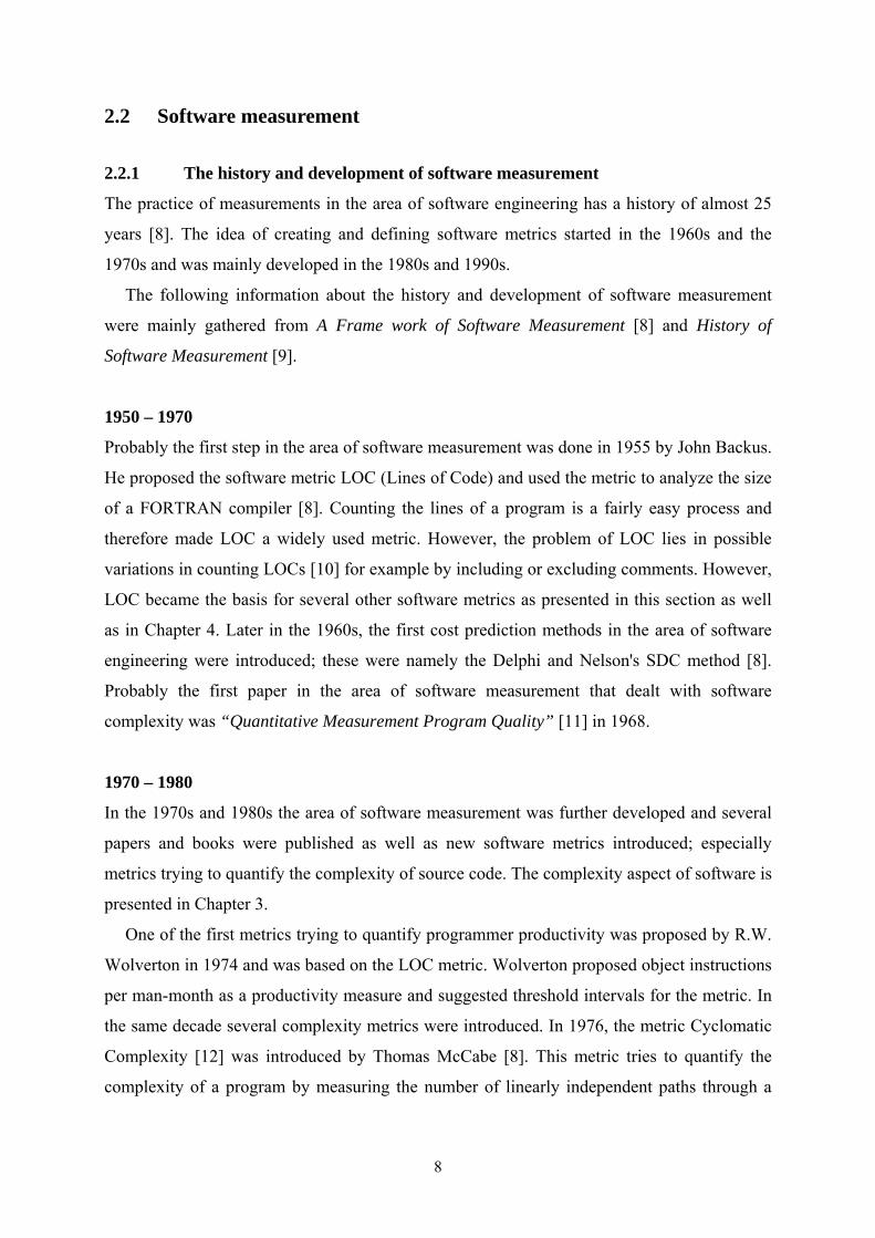
2.2.1 The history and development of software measurement

The practice of measurements in the area of software engineering has a history of almost 25

years [8]. The idea of creating and defining software metrics started in the 1960s and the

1970s and was mainly developed in the 1980s and 1990s.

The following information about the history and development of software measurement

were mainly gathered from A Frame work of Software Measurement [8] and History of

Software Measurement [9].

1950 – 1970

Probably the first step in the area of software measurement was done in 1955 by John Backus.

He proposed the software metric LOC (Lines of Code) and used the metric to analyze the size

of a FORTRAN compiler [8]. Counting the lines of a program is a fairly easy process and

therefore made LOC a widely used metric. However, the problem of LOC lies in possible

variations in counting LOCs [10] for example by including or excluding comments. However,

LOC became the basis for several other software metrics as presented in this section as well

as in Chapter 4. Later in the 1960s, the first cost prediction methods in the area of software

engineering were introduced; these were namely the Delphi and Nelson's SDC method [8].

Probably the first paper in the area of software measurement that dealt with software

complexity was “Quantitative Measurement Program Quality” [11] in 1968.

1970 – 1980

In the 1970s and 1980s the area of software measurement was further developed and several

papers and books were published as well as new software metrics introduced; especially

metrics trying to quantify the complexity of source code. The complexity aspect of software is

presented in Chapter 3.

One of the first metrics trying to quantify programmer productivity was proposed by R.W.

Wolverton in 1974 and was based on the LOC metric. Wolverton proposed object instructions

per man-month as a productivity measure and suggested threshold intervals for the metric. In

the same decade several complexity metrics were introduced. In 1976, the metric Cyclomatic

Complexity [12] was introduced by Thomas McCabe [8]. This metric tries to quantify the

complexity of a program by measuring the number of linearly independent paths through a

8

program. The Cyclomatic Complexity metric is still widely in use and is discussed further in

Chapter 4.

One year later, Maurice Halstead [13] introduced a set of metrics targeting a program’s

complexity; especially the computational complexity [14]. Halstead based the metrics on

operators and operands count within the source code of a program as explained in his book

“Elements of Software Science” [13]. Several companies, including IBM and General Motors,

have used this metric set in their software measurement processes. Today the Halstead metrics

are still widely in use, including Halstead Length, Volume, Difficulty and Effort which are the

most common. Further complexity metrics were introduced by Hecht in 1977 and by McClure

in 1978 [9].

The first book which focussed entirely on software measurement was “Software Metrics”

by Tom Gilb, was published in 1976 [9]. Also in the 1970s, the terms software physics and

software science were introduced in order to construct computer programs systematically. The

former was proposed by Kolence in 1975 and the latter was proposed by Halstead in 1977 in

the previously mentioned book “Elements of Software Science” [13].

Then in the late 1970s (1979), Alan Albrecht introduced his idea of function points at IBM

[8]. The Function-Point metric captured the size of a system based on the functionality

provided to the user in order to quantify the application development productivity.

1980 – 1990

Also in the 1980s several complexity metrics were introduced, including Ruston’s flowchart

metric [8], which describes a program’s flowchart with the help of the flowchart’s elements

and underlying structure. In 1981 Harrison et al [8] introduced metrics to determine the

nesting level of flow graphs. One year later Troy et al defined a set of metrics, which tried to

quantify modularity, size, complexity, cohesion and coupling of a program [8].

In addition to the Function Point method from 1979, another widely spread cost estimation

metric with the COCOMO (Constructive Cost Model) [15] was introduced two years later in

1981. The COCOMO, based on the Metric LOC, estimates the number of man-months it will

take to finish a software product. A further cost estimation metric is the Bang metric was

proposed by DeMarco six years later [9].

In 1984, NASA was one of the first institutions to begin with software measurement. In the

same year the metric GQM (Goal Question Metric) was developed by Victor Basili and the

NASA Software Engineering Laboratory. GQM is a approach to establish a goal-driven

9

measurement system for software development applicable to applied to all life-cycle products,

processes, and resources [16] [1] .

In 1987, Grady and Castwell established the first company wide metric program at Hewlett

Packard and published their findings in [17].

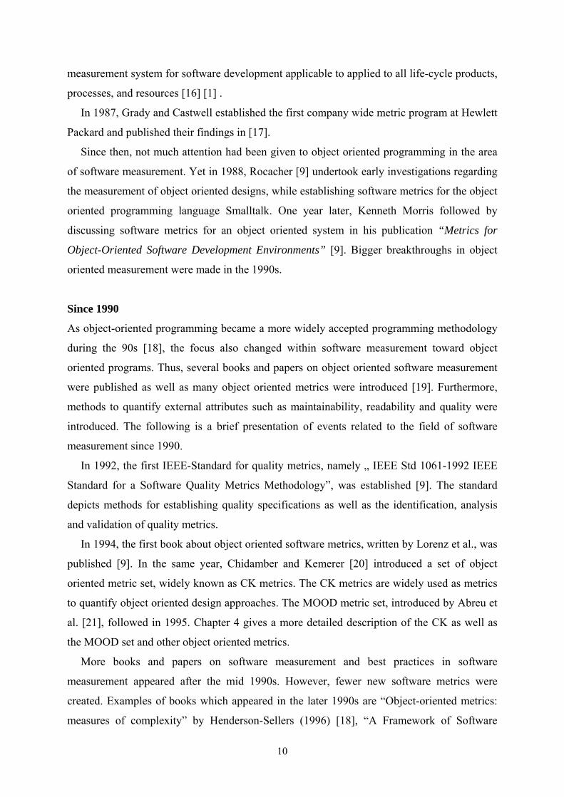
Since then, not much attention had been given to object oriented programming in the area

of software measurement. Yet in 1988, Rocacher [9] undertook early investigations regarding

the measurement of object oriented designs, while establishing software metrics for the object

oriented programming language Smalltalk. One year later, Kenneth Morris followed by

discussing software metrics for an object oriented system in his publication “Metrics for

Object-Oriented Software Development Environments” [9]. Bigger breakthroughs in object

oriented measurement were made in the 1990s.

Since 1990

As object-oriented programming became a more widely accepted programming methodology

during the 90s [18], the focus also changed within software measurement toward object

oriented programs. Thus, several books and papers on object oriented software measurement

were published as well as many object oriented metrics were introduced [19]. Furthermore,

methods to quantify external attributes such as maintainability, readability and quality were

introduced. The following is a brief presentation of events related to the field of software

measurement since 1990.

In 1992, the first IEEE-Standard for quality metrics, namely „ IEEE Std 1061-1992 IEEE

Standard for a Software Quality Metrics Methodology”, was established [9]. The standard

depicts methods for establishing quality specifications as well as the identification, analysis

and validation of quality metrics.

In 1994, the first book about object oriented software metrics, written by Lorenz et al., was

published [9]. In the same year, Chidamber and Kemerer [20] introduced a set of object

oriented metric set, widely known as CK metrics. The CK metrics are widely used as metrics

to quantify object oriented design approaches. The MOOD metric set, introduced by Abreu et

al. [21], followed in 1995. Chapter 4 gives a more detailed description of the CK as well as

the MOOD set and other object oriented metrics.

More books and papers on software measurement and best practices in software

measurement appeared after the mid 1990s. However, fewer new software metrics were

created. Examples of books which appeared in the later 1990s are “Object-oriented metrics:

measures of complexity” by Henderson-Sellers (1996) [18], “A Framework of Software

10

Measurement” by Zuse (1997) [8] and especially “Software Metrics: A Rigorous Approach”

by Fenton (second edition 1997) [1]. Despite new approaches in the 1980s and 1990s, many

of the metrics applied in industry were established in the 1970s [22].

2.2.2 Reasons for software measurement

There are several reasons for using software measurement in practice. The key benefits of

software measurement can be classified as follows [16]:

• Understanding

• Evaluation Control [1]

• Prediction

• Improvement

According to Fenton [1], the categories evaluation and prediction can be combined to

control and control is essential to any important activity.

“We must control our projects, not just run them” [1]

However, only ongoing software projects require control. A completed project will not

change in state and therefore does not need to be controlled, but may be compared to other

projects. Since the final source code (as entity code) itself and not its creation processes is the

central point in this dissertation, the main focus lies on the aspects of understanding and

improvement of software.

Before knowing how to improve an attribute (where to go), we first need to understand the

meaning of the attribute and its current characteristics (where we are).

“If you don’t know where you are a map won’t help” [23]

In the context of measuring source code, understanding is defined here as to gain

meaningful information about code attributes (as illustrated in Figure 2.2). With the

understanding of the code characteristics within their current states, areas of improvement

[16] can be identified and threshold intervals which should be met can be defined. Threshold

intervals define a value range in which the measures should occur.

11

2.2.3 Problems and issues of software measurement

The major problems and issues in the field of software measurement can be pointed out as

follows:

• Interpretation of measures

Each measure produced on its own does not give us more than a single value. It requires

education and experience to make software measures useful [2]. Furthermore, information

regarding the context in which the measures were produced is needed [8]. For this project,

the measure of cyclomatic complexity of a student program might have a value x.

However this measure has to be interpreted in the context of the program size, since a

longer program is more likely to be more complex, before information about the

complexity can be retrieved. This point is further discussed in Chapter 3.

• Scale types

Care has to be taken about the scale types involved. According to measurement theory

[24], every scale type has a different set of applicable statistics. E.g. the set of statistics for

the interval scale does not include multiplication. Therefore saying today’s temperature is

twice as hot as yesterday’s is not a valid statement for Fahrenheit and Celsius, which are

based on the interval scale [1] (see Chapter 3). This means in the context of software

measurement that comparing and analyzing the measures produced has to be done with

caution. More information about measurement scale types are presented in Section 3.2.2.

• Lack of specific standards

According to Munson [2], the biggest problem in the field of software measurement, for

each measured object, is the lack of standards.

“NIST1 is not motivated to establish standards in the field

of software measurement.”

Therefore, measures retrieved for the same software entity are not comparable unless

additional information about the way they were quantified is available and the methods

are identified as equivalent. This means for this project, that the tools have to be compared

by analyzing which of the software measures are produced in the same manner.

12

• Issues of people measures

With software measurement the productivity of programmers can be measured. However,

judging a programmer’s performance by the use of a metric (such as LOC/hour) can be

seen as unethical [2]. Furthermore, the outcome can be influenced by the programmer

measured. For example, the programmer writes unnecessary LOC to increase the measure

for his productivity. Since not the students but their code is of interest, this does not

represent a problem in this dissertation project.

• Reliable and valid data

Gathering measures is not sufficient in order to obtain reliable measurement results, since

the way the data are collected and analyzed has a great influence on the outcome. As M.J.

Moroney (1950) said:

“Data should be collected with a clear purpose in mind. Not only a clear purpose

but a clear idea as to the precise way in which they will be analyzed so as to yield

the desired information.”

In this dissertation, the purpose of data collection is to gain information about the size,

structure, complexity and quality of the available source code.

2.2.4 Software measurement applied

Section 2.2.1 presented the history and development of Software Measurement. In that

section, the reasons for Software Measurement and the related problems were illustrated. This

section focuses on the application of software measurement; the domains, their entities, and

the measurement process itself.

Software measurement domains (and their entities)

Software entities can be classified into product entities, process entities and resource entities

[1]. Since software measurement tries to quantify software entities, the areas of application

can be categorized correspondingly as displayed in Figure 2.2. Further examples for software

entities can be seen in Figure 2.2.

1 National Institute of Standards and Technology

13

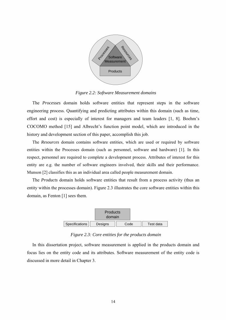
SoftwareMeasurement

Products

ResourcesProc

esse

s

Figure 2.2: Software Measurement domains

The Processes domain holds software entities that represent steps in the software

engineering process. Quantifying and predicting attributes within this domain (such as time,

effort and cost) is especially of interest for managers and team leaders [1, 8]. Boehm’s

COCOMO method [15] and Albrecht’s function point model, which are introduced in the

history and development section of this paper, accomplish this job.

The Resources domain contains software entities, which are used or required by software

entities within the Processes domain (such as personnel, software and hardware) [1]. In this

respect, personnel are required to complete a development process. Attributes of interest for this

entity are e.g. the number of software engineers involved, their skills and their performance.

Munson [2] classifies this as an individual area called people measurement domain.

The Products domain holds software entities that result from a process activity (thus an

entity within the processes domain). Figure 2.3 illustrates the core software entities within this

domain, as Fenton [1] sees them.

Productsdomain

Designs CodeSpecifications Test data

Figure 2.3: Core entities for the products domain

In this dissertation project, software measurement is applied in the products domain and

focus lies on the entity code and its attributes. Software measurement of the entity code is

discussed in more detail in Chapter 3.

14

The measurement process

The term software measurement process can be defined as follows:

“That portion of the software process that provides for the identification, definition,

collection, and analysis of measures that are used to understand, evaluate, predict, or control

software processes or products.” [25]

According to McAndrews [25], the software measurement process can be split into the four

activities: planning, collecting data, analyzing data and evolving the process. During the

planning a purpose and a plan for measuring has to be defined. Furthermore the software

entities and attributes of interest have to be identified and suitable software metrics selected or

new ones defined. During the data collecting phase the selected metrics are applied manually

or by the use of software measurement tools [26]. Software measurement tools are discussed

later in Section 2.4 and in Chapter 5. The measures/data produced are then analyzed with

regard to the measurement goals defined.

In this dissertation the measurement process is split into two stages, namely a measurement

stage and an analysis stage. The measurement stage includes the planning, preparations for

code measurements and the code measurements themselves. In the analysis stage, the

measures produced are analyzed and interpreted for later use in code profiling.

2.2.5 Application in education

Despite its age and its application in industry, the discipline of software measurement is not

often used for the education sector [27]. Some of the related studies about the application of

software measurement in education were found as follows:

• Using Verilog LOGISCOPE to analyze student programs [28]

This paper (published in 1998) describes the application of a software measurement tool to

measure student programs. The results of analyzing programs are given to show the

diversity of results. In addition a discussion on how the software measurement tool can be

used to help students improve their programming and help instructors evaluate student

programs better is presented.

• A case study of the static analysis of the quality of novice student programs [27]

In this paper (published in 1999) builds up on the paper listed above. The authors used a

software measurement tool and sample student programs to affirm that static code analysis

15

is a viable methodology for assessing student work. Further work is considered by the

author to help to confirm the study’s results and their practical application.

• Static analysis of students' Java programs [29]

This paper (published in 2004) introduces framework for a static analysis. According to

the author this framework can be used to give beginning students practice in writing better

programs and to help in the program grading process. The framework suggests both

software metrics and relative comparison to evaluate the quality of students’ programs.

• Student portfolios and software quality metrics in computer science education [30]

This paper (published in 2006) discusses the usage of student program collections

(portfolios) to conduct long term studies of student performance, quantitative curriculum

and course assessment, and prevention of forms of cheating. The authors suggest the use

of quality software metrics to analyze the portfolios, however only requirements for those

are outlined.

16

2.3 Software metrics

As indicated in Section 2.1 software metrics are instruments applied within the software

measurement process to quantify attributes of software entities. Each software metric holds

information about its targeted attribute(s) as well as how the metric can be applied to quantify

the attribute(s). Thus, software metrics are specific defined instruments for targeting an

attribute of a software entity and explains the application of the metric within a software

measurement process. For example, LOC is a metric that targets the source code size (length)

attribute. As will be explained below in Chapter 4, LOC quantifies the size by counting the

lines of code. In this dissertation project, the focus is on the source code and source code

attributes. Source code metrics can be further classified as follows:

2.3.1 Static source code metrics

Static code metrics attempt to quantify source code attributes from the program text [2, 31].

Such metrics may quantify control flow graphs, data flows and possible data ranges. Static

source code metrics are further reviewed in Chapter 4.

2.3.2 Dynamic source code metrics

Dynamic source code metrics quantify characteristics of a running system and how it interacts

with other processes. Compared with the usage of static source code metrics, the measurement

of a running system is rather resource consuming due to the massive data overhead. However,

dynamic source code metrics represent a great help in error detection, security aspects and

program interaction [2].

2.4 Software measures: Tools to produce them

There is a large number software measurement tools available [32], most of which are

commercial. Some of the available tools focus on a specific area of software measurement,

such as software process or resource measurement. In this dissertation, the focus lies on tools

suitable for static code analysis. A more detailed description of software measurement tools is

given in Chapter 5.

17

2.5 Summary

In conclusion, software measurement is the process of applying software metrics with the goal

of quantifying specified attributes of software entities to gain meaningful information about

the entity itself. The main advantages of software measurement are control, understanding and

improvement. The disadvantages are the lack of standards and the experience required in

order to gain meaningful information. Software measurement tools exist to simplify and

automate the application of software metrics within the software measurement process.

18

3 Software measurement: Code analysis

3.1 Introduction

In order to measure software, the basic theory about measurement theory has to be known and

understood. Section 3.2 presents a short introduction and aspects of interest. Since the

analysis of source code is the major aspect in this dissertation project, a deeper look at the

entity code and its attributes is presented in Section 3.3. One frequently discussed and

difficult quantifiable attribute is complexity [5]. The measurement of code complexity and the

term software complexity itself are discussed in Section 3.4.

3.2 Measurement theory

Measurement theory is a branch of applied mathematics and defines a theoretical basis for

measurement. According to Zuse [8], the major advantages of measurement theory are

hypotheses about reality, empirical investigations of measures produced, and the

understanding of the real world through an interpretation of numerical properties.

3.2.1 Introduction to measurement theory

As with other measurement disciplines, software measurement also requires to be based on

measurement theory [33]. For the area of software measurement, measurement theory holds

the following [8]: (1) clear definitions of terminology, (2) strong basis for software metrics,

(3) criteria for experimentation, (4) conditions for validating software metrics and (5) criteria

for measurement scales. Henderson-Sellers [18] points out, that measurement theory in

addition introduces an understanding of variances, intervals, and types of errors in the

measurement data through the use of statistics and probabilities.

In the literature, measurement theory for software measurement has been discussed in

much detail. For this dissertation, the works of Zuse [8], Fenton [1] and Henderson-Sellers

[18] were used to gain an understanding of the aspects of measurement theory for software

measurement. In the following sections, key aspects of measurement theory are briefly

presented:

19

• Empirical relations

The aspect of empirical relations deals with the intuitive or empirical understanding of

relationships of objects in the real world. The relationships can be expressed in a

formal relationship system [18]. For example, one might observe the relation of two

people in terms of height. The comparisons “taller than”, “smaller than”, etc. are

empirical relations for height [1]. If a term, such as complexity or quality, has different

meanings to different people, then defining a formal relationship system becomes

close to impossible [1, 18]. The difficulty of measuring software complexity is further

discussed in Section 3.4.

• Rules of mapping

There are different approaches for mapping an attribute from the real world to a

mathematical system. The mapping has to follow specific rules to make the measures

reproducible as well as comparable [1]. As an example, several approaches for

quantifying the size of a software system exist however these measures are not

comparable unless clear information is presented about the way the measures were

produced.

• Scale types

Differences in mapping can limit the possible ways of analysing a given measure [1,

8]. Measurement scale types exist to help identify the level of statistics applicable.

The different scale types are further discussed in Section 3.2.2.

• Direct and indirect measurement

Measurement theory categorizes measures into direct and indirect measures [1]. Direct

measurement of an attribute does not depend on the mapping of any other attribute.

Whereas, indirect measurement of an attribute is measurement which involves the

measurement of one or several other attributes. The same classification applies for

software metrics.

• Validity and reliability of measurement

Measurement theory helps to validate the transformation of abstract mapping concepts

into operational mapping definitions and prove the definitions’ reliability [34, 35].

20

This means that software metrics definitions can be inspected and validated

mathematically. However, “theory and practice are travelling very different roads on

the topic of software metrics “ [36]. The theoretical validation of software metrics is

often neglected [18, 34]. Several software metrics (such as Cyclomatic Complexity)

exist without theoretical proof but with analytical analyses verifying the concept [18].

Furthermore, Henderson-Sellers [18] complains that the number of experiments

performed are often not sufficient and the underlying experiment context is too narrow.

According to Zuse, theory and the application of statistics should be combined for

validating software metrics [8].

• Measurement error and inaccuracy

Measurement errors result in deviations of the measures produced from the true values

in the real world [34, 37]. Measurement error and inaccuracy in software measurement

is further discussed in Section 3.2.3.

3.2.2 Measurement scales for code analysis

Measurement theory provides conditions for applying statistics to the measures produced. The

measures as well as the mappings used to produce the measures can be connected to certain

scale levels. This is important for understanding which analyses are appropriate for

underlying measurement data [8]. Different scale types allow a different set of applicable

statistical methods. In Table 3.1 the scale types are divided into nominal, ordinal, interval,

ratio and absolute scale types. The scale types are each successively supersets of the

preceding sets of scales. The set of defined relations and thereby the applicable analyses

increase for each such superset [1]. The classification into scale types helps to understand

which kinds of measurements may be used to derive meaningful results. Stating that a

software project is twice as big as another, by using the number of lines of code (absolute

scale), is valid. However, stating that a project is twice as complex with regard to the

measures produced is problematic, since complexity measures may be defined on an interval

scale [1].

21

(all)detected errorsCounts number of occurences. Valid values are zero and positive integers.

Absolutef(x) = x

(above),ratio

length, massThe ratio scale enhances the interval scale by starting with a zero element, which itself represents the absence of the attribute being measured.

Ratiof(x) = ax (a>0)

(above),difference

temperatureUses ordered categories, as the ordinal, and in addition preservesthe gap size between the groups.

Intervalf(x) = ax+b (a>0)

(above),bigger smaller

user ratingsA extension to the nominal scale,as it provides a ordering of the categories.

Ordinalordered classes

equivalencecolors, fruitsA set of classes or categories, in which the observed elements are placed.

Nominalclasses

Defined relationsExamplesScale definitionScale type

(all)detected errorsCounts number of occurences. Valid values are zero and positive integers.

Absolutef(x) = x

(above),ratio

length, massThe ratio scale enhances the interval scale by starting with a zero element, which itself represents the absence of the attribute being measured.

Ratiof(x) = ax (a>0)

(above),difference

temperatureUses ordered categories, as the ordinal, and in addition preservesthe gap size between the groups.

Intervalf(x) = ax+b (a>0)

(above),bigger smaller

user ratingsA extension to the nominal scale,as it provides a ordering of the categories.

Ordinalordered classes

equivalencecolors, fruitsA set of classes or categories, in which the observed elements are placed.

Nominalclasses

Defined relationsExamplesScale definitionScale type

Table 3.1: Scale types

In this dissertation the interest lies in the static analysis of source code. Therefore the

restriction to metrics that produce measures on interval scales seems advisable. The nominal

and ordinal scales, as shown in Table 3.1, would seem less suited to the required types of

analyses needed to for this project (such as the arithmetic average).

3.2.3 Software measurement error and inaccuracy

Errors may occur during measurement, even in simple measurements [23, 37]. Software

measurement error concerns the deviation and inaccuracy of software measures produced

from the actual software characteristics in the real world. Several classifications for

measurement errors exist [34, 37] and in this dissertation a classification into instrumental

measurement errors and personal errors is made. Instrumental measurement errors are caused

by imperfections in the measurement instrument used during the measurement process.

Possible instrumental measurement errors in this dissertation project caused by the

measurement tools encountered during the measurement process are discussed in Chapter 5.

Personal errors are caused by human mistakes during the measurement process. These

errors can include improper selection of software metrics, the incorrect adjustment and

application of measurement tools as well as incorrect interpretation of the measures produced.

The metric selection for this dissertation project is discussed in Chapters 5 and 6.

Measurement results and the interpretation of these follow in Chapter 7.

22

Measurements are highly dependent on the instruments used and on the accuracy these

provide [24, 36, 37]. For software measurement the inaccuracy of available software metrics

is an often discussed topic. Some software attributes are harder to quantify more accurately

than others. Software complexity for example is difficult to quantify [5, 33] because this

software attribute is influenced by several other not always ascertainable factors. The factors

themselves can further depend on other aspects, thus making the intended attribute difficult to

quantify. The problem of quantifying software complexity and the accuracy of software

metrics is further discussed in Section 3.4.

3.3 Software entity code

Software entities can be classified into the three software measurement domains presented in

Figure 3.1. Each software entity has specific attributes, which are of interest for the

measurement. According to Fenton [1], attributes of software attributes can be classified into

internal and external attributes. Internal attributes can be measured directly through its entity,

whereas external attributes are measured through the entities environment. For external

attributes the behaviour is of interest rather than the entity itself [1]. Figure 3.1 shows a list of

example software entities and their corresponding attributes.

reliability, usability, maintainability,

complexity, portability, readability,...

size, reuse, modularity, coupling,cohesiveness, functionality,

algorithmic complexity, control-flow structuredness,…

Code

comprehensibility, …size, correctness, syntactic…Specification

Internal

productivity, experience, intelligence,…age, pricePersonnel

Resources

quality, cost, stability,…time, effort, number of requirement changes,…

Constructing specification

Processes

Products

External

ATTRIBUTES ENTITIES

reliability, usability, maintainability,

complexity, portability, readability,...

size, reuse, modularity, coupling,cohesiveness, functionality,

algorithmic complexity, control-flow structuredness,…

Code

comprehensibility, …size, correctness, syntactic…Specification

Internal

productivity, experience, intelligence,…age, pricePersonnel

Resources

quality, cost, stability,…time, effort, number of requirement changes,…

Constructing specification

Processes

Products

External

ATTRIBUTES ENTITIES

Figure 3.1: Examples of software entities [1]

23

Source code is the software product created with the combination of software entities from the

processes and resources domain. It consists of a sequence of statements and/or declarations

written in one or several programming languages. Source code represents the implementation

of a software program. In this dissertation project, the code attributes of different software

projects are analyzed to gain meaningful information about the different code characteristics.

3.3.1 Code attributes

Code attributes represent characteristic traits of the source code and will be also classified into

internal and external.

Internal code attributes

Internal code attributes hold information about the code itself. The following internal

attributes are of special interest for this project: size, modularity, coupling, cohesion, control-

flow and other internal aspects that are involved in the structure of the source code. Several

software metrics exist to quantify these attributes. The measurement of internal code attributes

can be performed objectively [18] due to their independence from other software entities.

LOC e.g. is a software metric that quantifies the internal attribute size of the software entity

code. As further explained in Chapter 4, LOC quantifies the size by counting the lines of

code.

External code attributes

External code attributes hold information about the code and the code behaviour or

characteristics within its environment [1]. These attributes require to be quantified with

regards to how the code relates to other entities [1]. Thus, external code attributes are difficult

to grasp and since in this dissertation project only the source code itself is analyzed are

external attributes not directly of interest. In this dissertation only the code maintainability, as

external attribute, is considered.

24

3.4 Measuring code complexity

Since software complexity was found to be one major contributing factor to the cost of

developing and maintaining software [12, 15, 38], the interest in quantifying this

characteristic / software attribute arose after the 1970s [18, 39, 40] and a number of

complexity metrics have been proposed [5]. In order to measure the complexity the

researchers first had to understand what software complexity is and means. However, here the

definitions differ in the software engineering literature, indicating that the aspects of software

complexity are not yet fully understood

3.4.1 Different perspectives on software complexity

In the software engineering literature a number of definitions for software complexity are

given [5, 18, 41].

For Evangelisti [5] software complexity is “the degree of complication of a system or

system component, determined by such factors as the number and intricacy of

interfaces, the number and intricacy of conditional branches, the degree of nesting, and

the types of data structures”

Basili [18] defined software complexity as “a measure of resources expended by a

system (human or other) while interacting with a piece of software to perform a given

task”.

IEEE [42] defines software complexity as “the degree to which a system or component

has a design or implementation that is difficult to understand and verify”

For Zuse [5] software complexity is “the difficulty to maintain, change and understand

software. It deals with the psychological complexity of programs” [5].

Thus the definition of the term software complexity is difficult to specify precisely, but can

we still measure the complexity of software? Fenton states that quantifying complexity into a

single measure is close to impossible or equally difficult as finding the “holy grail” [33].

Instead complexity metrics focus on certain aspects of complexity, what complexity consists

of and what influences the complexity of a system. However, since the term itself is unclear,

25

opinions differ in the software engineering literature also with regard to different aspects of

software complexity.

Fenton classified the aspects of complexity into 4 areas: problem complexity, algorithmic

complexity2, structural complexity and cognitive complexity (cognitive complexity is further

discussed in Section 3.4.2) [1]. Jones [43] lists 20 different aspects of software complexity.

Here the approach from Henderson-Sellers [18] is discussed in more detail. He classified

software complexity as depicted in Figure 3.2 using the following three aspects.

Computational complexity is concerned with the complexity of the computation in terms

of required time and hardware resources [18, 43]. Algorithms which are difficult to

understand do not necessarily have to be computationally complex [34].

Psychological complexity is related to the difficulty of understanding the software

program. This aspect of software complexity is also referred to as cognitive complexity and is

further discussed in Section 3.4.2.

Representational complexity deals with the tradeoffs between graphical and textual

notations for unambiguous representations of the software system, its environment and the

system interactions within [18].

External

attributes

Complexity

Computationalcomplexity

Psychologicalcomplexity

Representationalcomplexity

Problemcomplexity

Programmercharacteristics

ProductComplexity

=(Structuralcomplexity)

Is-a-kind-of relationship

Is-composed-of relationship

Source: Henderson-Sellers96

Internal

attribute

External

attributes

Complexity

Computationalcomplexity

Psychologicalcomplexity

Representationalcomplexity

Problemcomplexity

Programmercharacteristics

ProductComplexity

=(Structuralcomplexity)

Is-a-kind-of relationship

Is-composed-of relationship

Source: Henderson-Sellers96

Internal

attribute

Figure 3.2: Classification of software complexity

26

Henderson-Sellers considered Zuse’s view [5] in this approach to software complexity

(presented above) and introduces the psychological complexity as a major aspect in software

complexity. As shown in Figure 3.2, psychological complexity now consists of the individual

programmer characteristics as well as problem complexity and structural complexity. The

latter two were perceived in other publications (such as [1] and [43]) as direct components of

software complexity. A model for code complexity applied to product complexity as an

internal attribute is presented in Section 3.4.3.

3.4.2 Psychological/cognitive complexity

Psychological (cognitive) complexity refers to the difficulty for a person/programmer of

understanding and verifying a software product [5, 18]. This complexity aspect is thus highly

dependent on the difficulty of the underlying problem, the product complexity including

software characteristics (such as size, control flow and coupling) and the programmer

characteristics [18].

Problem complexity refers to the difficulty of the underlying problem. It is assumed that

complex problems are more difficult for a person/programmer to comprehend than simple

ones. This type of complexity is not controllable and difficult to measure. In this dissertation

project, the complexity of the underlying problem is classified in terms of class level of the

student. It is assumed that A-level courses provide easier problems than D-level courses.

Product complexity (structural complexity) is concerned with the structure of the software

program. Structural complexity is frequently discussed in the software engineering literature

[1, 18, 40] and, as it is essential to this dissertation project, will be presented in more detail in

the following section.

Programmer characteristics deal with the individual programmer traits that are involved

when performing tasks on software products. Quantifying the programmer characteristics is

difficult, especially without adding subjective bias [18].

3.4.3 Internal code/product complexity

The structure of a program is measurable through internal attributes of the software code

(such as size and coupling). Several metrics [5], called structural complexity metrics, have

been proposed in order to achieve this goal. In the software engineering literature, structural

2 Algorithmic complexity deals with the difficulty of implementing a problem solving algorithm

27

complexity is often referred to as product complexity [1, 18, 34], as the complexity of the

product (source code) is highly dependent on the underlying structure. A complex structure

makes it more difficult to understand and maintain a software product. The proposed

structural complexity metrics offer monitoring of structural complexity through the

assessment of a variety of structural aspects. These aspects and thereby the metrics

themselves can be classified as follows: size, logical structure, data structure, cohesion,

coupling and information flow [18]. Through the combination of these metrics a prediction

for the product complexity can be made [44]. However, they ought to be interpreted as

indicators. [18, 33]. Chapter 4 presents software metrics that capture structural aspects of the

source code. Thus e.g., the LOC metric measures the size of a program and the software

metric Cyclomatic Complexity is used to quantify the complexity of the underlying logical

structure.

28

3.5 Code complexity vs. code distribution

In this dissertation the term code distribution is understood as the way the source code of a

program, as a whole, is organised over a number of files, classes, and methods. As an

example, a program’s code can be placed in a single method within one file, whereas for the

same program, in a different code distribution approach, the code may be distributed over

several methods within different programming files. Figure 3.3 illustrates this point further.

Method1...............

Method1...............

Method1......

Method2......

Method1......

Method2......

PROGRAM‘S SOURCE CODE

A single file withone very large method

Method1......

Method2......

....................

............................................................Method1......

Method2......

A single file in wich the code is split over several methods

A few single files withseveral large methods

Many files withmany small methods

Extract of possible code distribution approaches

Figure 3.3: Code distribution example

Which code distribution is the most suitable, is highly dependent on the project, the

programming language used, and the environment [10]. Thus, there is no clearly defined

optimal approach for the textual code length of methods, classes, and files. Nevertheless,

different views about an ideal length exist in the software engineering literature [10, 45]. In

this dissertation the discussion about a possible ideal or maximum size (length) is not of

interest. What is of interest is the actual choice of size and code distribution. Before the

relationship between code distribution and code complexity is further explained, two

important issues about the code distribution require to be considered:

29

(1) Long3 files, classes, and methods (with regard to their size, e.g. lines of code) are

potentially difficult to understand [46]. With regard to the capabilities of the human

brain, it is easier to understand small pieces of information rather than the full story at

once [46]. However, to be able to sub-divide information into suitable pieces, a

reasonable overview of the information must be constructed. As an example, scientific

books and papers are organised into several chapters and sections. Thus, the authors

present the full information in pre-selected units of information, helping the readers to

follow their argument. How difficult a chapter or section (or a piece of source code) is

to follow and understand also depends on the reader and is thus somewhat subjective.

(2) Using a large number of files, classes, and methods can help to divide the information

(a program’ source code) into smaller and more easily manageable pieces. The higher

this number is the lower the average textual length of the individual pieces will be; thus

resulting in small, easy to understand sections of code. However, the more files, classes

and methods used, the harder the organisation of the program will become. By this is

meant that if code is distributed over just one file, the programmers responsible for

maintaining the system know exactly where to look for the code. When a program

consists of a large number of files, the task of finding a particular source code file,

might not be so easy and will be highly dependent on how the files are managed

(subdirectories and labelling). A large number of classes will most likely result in a

design, which is difficult to understand. Similarly with a large number of methods

within a file or a class.

In summary, a balance between section length and manageability should be found. Long

code sections are considered less desirable, but on the other hand, short sections may not

always provide an ideal solution [47]. However, to understand the underlying complexity of a

code section, the actual code distribution i.e. the organisation of the code between classes and

files, has to be known beforehand.

For this dissertation, this last point is of great importance, and thus will be discussed in

more detail. Complexity metrics measure particular quantifiable aspects of the source code,

and store the quantity measured in a measure for a particular program, file, class or method.

Thus, a measure produced can be defined for program, file, class, or method scope. To

understand the individual measure, the measure has to be seen in relation to the environment

3 At which point a file, class, or method is to be considered as long is difficult to decide [47]. As stated above,

the goal of the code distribution aspect in this dissertation is not to define an optimal length, but to understand which code distribution is used for a particular program.

30

of the related scope. By just looking at the weight measure of a unknown person, for example,

you will see a value, but to grasp the meaning of the weight measure for this particular person,

you most likely either see him/her in person or consider his/her height, age, and gender

measures. Thus, you are consulting the person’s other physical characteristics.

The same goes for complexity measure of a program (in the example above replaced by the

weight measure for a person). Just seeing a value of 500 for this complexity measure will not

tell us much, unless we either look at the program in detail or consider other measures

describing the program scope environment.

A program’s code distribution can be seen as analogous to the person’s height information

in this matter

3.6 Summary

Aspects of measurement theory and, internal and external code attributes are all part of the

foundation for later chapters. The definition and meaning of a particular software metric has

to be kept in mind when the measure produced are interpreted. One difficult to measure

internal attribute is code complexity. The code complexity can not be captured in a single

measure [1, 33]. To describe the underlying complexity, software metrics targeting different

aspects of software complexity should be combined. Furthermore aspects about the code

distribution of a program require to be considered when complexity measures are interpreted.

31

4 Software metrics: Static code metrics

This chapter gives an overview of existing static code metrics. Furthermore, the important

software metrics for this study are explained and discussed. Not all metrics listed will be

applied in the later code measurements (see in Chapter 6 Table 6.1 for an overview of the

metrics used).

4.1 Introduction

This section illustrates the most common software metrics in the area of static code analysis.

As well as illustrating the metrics, the areas of application and the advantages and

disadvantages were taken into consideration. In addition, some examples are provided to

clarify these metrics in more detail.

Static code metrics are applied to quantify attributes of source code before run-time; such

attributes are size, reuse, coupling, complexity. See Figure 3.1 for further examples. Basic and

derived metrics are presented and discussed in this chapter. Basic software metrics are

directly applied; whereas computed software metrics are derived using existing basic software

metrics.

4.2 Program size

These metrics include the lines of code including comments (LOC), lines of code excluding

comments (NCLOC), number of statements, operands and operators.

4.2.1 Lines of code

Lines of code metrics count the number of lines in a program. However, some lines might be

of more interest than others with regard to the measurement purpose [1, 10]; i.e. lines of code

may need to be further classified.

The content of one physical line of code can be classified as follows [1]:

o Blank line (line with no content)

o Comment line

o Statement line4

4 A statement can be a data declaration, a data definition, a simple statement, or a compound statement.

32

Line of code metrics can therefore focus on a set of aspects of this content classification.

For example the line of code metric CLOC (Comment Lines of Code) focuses only on

comment lines, whereas NCLOC (Non-Comment Lines of Code) focuses only on lines

containing statements. In this way, several useful metrics can be defined and the following

section presents them as well as their usage. A defined standard for measuring the lines of

code does not exist [43].

The general positive aspects of the lines of code metrics can be seen as follows. When

applied, they can give a quick overview of the size of a program. Furthermore, like other

countable metrics, lines of code metrics are easy to compute and to apply. In addition, lines of

code metrics are not restricted by programming language.

However, when applying lines of code metrics, it is important to know that the complexity

of a program is not considered.

Physical lines of code (LOC)

LOC counts all lines with no regard to their content. The advantage of LOC is that it is

easy to understand. [10].

Non-comment lines of code (NCLOC)

The metric NCLOC counts lines that are not blank and not comment lines. NLOC is also

called eLOC (for effective lines of code).

Comment lines of code (CLOC)

The metric CLOC counts only lines of code that contain one or more comments. The

quality of the comments is not considered. An interesting derived measure in this context

is the comment rate (CLOC/LOC) which is described later in Section 4.6.1.

4.2.2 Number of constructs

The program size can also be measured in terms of number of programming constructs used

within the code. The number of constructs is independent of the number of lines since several

constructs may appear on one line for example writing several statements on one line.

Numer of statements (#STAT)

The metric #STAT counts the total number of statements in the program. Since one

source code line may contain several statements, the number of statements may be higher

33

than the number of non comment lines of code (NCLOC) [1]. Counting the number of

statements in the code is not as straight forward as counting the lines of code. Here it

depends on how a statement is defined.

Number of operators (N1)

Operators are all keywords of a programming language (such as while, for, and switch)

and symbols, which represent an action.

Number of operands (N2)

Operands are all code items which represent data (such as variables, constants).

Halstead program length (HL)

The Halstead program length is one of the linguistic software metrics5 introduced by

Maurice Halstead in 1977. The so called Halstead software science metrics were created

in order to measure the program size (which is discussed in this section) and the textual

code complexity (see Section 4.3) [2, 13].

The Halstead length (HL) is based on counting the total number of operators (N1) and

operands (N2). Halstead introduced the Halstead length of a program as an estimation of

the length of the program excluding comments as an alternative to NCLOC [13]. The

metric definition is as follows:

21 NNHL +=

As such HL is thus a well defined metric, defined in terms of the number of instances of

operands and operators used. [48] [1] [14].

4.2.3 Comments and examples

Program size metrics (especially the lines of code metrics) are widespread and accepted. Care

must be taken when a lines of code metric is discussed, to distinguish between LOC, NCLOC

and CLOC. The lines of code metrics are a reasonable indicator for a program’s size and also

offer potential for derived metrics. Following is an example (Table 4.1) to illustrate how the

different program size metrics vary in the measures produced.

5 Linguistic metrics are quantifying properties of program or specification text without the text’s semantics. For

example : lines of code, number of statements, number of unique operators

34

LOC NCLOC CLOC #STAT HL

// switches the values of two integers 1 1

function switch(int &a, &b) { 1 1 1 7

Int tmp; 1 1 1 2

tmp = a; a = b; b = tmp; // switch values 1 1 1 3 9

} 1 1 1

5 4 2 5 19

Table 4.1: Program size example

4.3 Code distribution

Section 3.5 illustrated the importance of considering the code distribution aspects for the

interpretation of measures produced. This section gives a brief overview on how the code

distribution can be quantified.

4.3.1 Measuring code distribution

The code distribution of a program can be measured by considering the size (i.e. length) of the

individual files, classes and methods together with the number of these files, classes and

methods. The files, classes and methods are considered to be program/code sections in the

program, which hold parts of the code. The following metrics measure for a program section

group defined (e.g. all methods) the code distribution among these code sections defined.

4.3.2 Code distribution metrics

Number of program sections

The Number of program sections metrics count the number of specific program sections in

a program. Within this group of metrics are the following metrics:

• The number of file (#files)

• The number of classes (#classes)

• The number of methods (#methods)

Combined with the program size metrics, these metrics can give information about the

organisation of the underlying program. For example, LOC/#files gives the average lines

of code per file. A pathological case is the monolithic program i.e. all the code is in one

file.

35

Size per program section

The size per program section metrics measure the size (length) for particular code sections

(such as methods). As size metric, one of the program size metrics listed can be selected.

For example the Statements per method metric measures the number of statements in a

method. Here, extremely long methods can be difficult to comprehend. Refer back to

Section 3.5 for a discussion on code distribution aspects.

4.3.3 Summary

The code distribution metrics are simple to understand and compute. In order to understand

the code distribution of a program, more than the average values (e.g. average LOC per file)

require to be considered.

4.4 Halstead code complexity

4.4.1 Halstead’s software science

The software science metrics, introduced by Halstead in 1977, were created as means of

quantitatifying the complexity of a program [2, 13]. As linguistic software metrics6, however,

the Halstead metrics were found not to capture the complexity of a program, but the textual

complexity of the code [14].

The Halstead software metrics are a good example of how a set of derived metrics can be

created from a set of simple metrics. Halstead bases his software metrics on counting the

number of operators and operands (see Section 4.2.2.). Halstead further classified into total

and distinct number of operators and operands. The four resulting simple metrics are as

follows [14, 48]:

n1 : number of distinct operators

n2 : number of distinct operands

N1 : number of actual operators

N2 : number of actual operands

In the following section the Halstead software science metrics are explained. The Halstead

program length (HL) was previously introduced in Section 4.2.2)

6 Linguistic metrics are quantifying properties of program or specification text without the text’s semantics. For

example : lines of code, number of statements, number of unique operators

36

4.4.2 Halstead’s complexity metrics

Halstead vocabulary (Hvoc)

The Halstead vocabulary is an indicator for vocabulary size of a program. It is calculated

as the sum of the number of unique operators and operands [13].

21 nnHvoc +=

A small program vocabulary can indicate two possible aspects. (1) In the program

measures, the same operands and operators are used frequently, thus making the program

less complicated to understand. (2) The program measured uses a small number of

operands and operators, as it is small in program size, which consequently results in a

small program vocabulary.

Halstead Volume (HV)

Halstead's volume (HV) metric was intended by Halstead to measure the volume of a

program.[48]. For the computation of HV, the number of operations performed and

operands handled are considered [1]. The computation of V is performed as follows.

)(log* 2 HvocHLV =

The Halstead volume is a “count of the number of mental comparisons required to

generate a program” [13]. Halstead believed that the Halstead volume indicates the size of

any implemented algorithm.

Halstead Difficulty (HD)

The program difficulty was intended to measure the difficulty to implement the program

[13].

N2 * n2) / (n1 * 0.5 n2) * (2 / N2) * (n1 HD ==

Halstead Effort (HE)

According to Halstead [13], the program effort, as the ratio of program volume and

program level, represents the number of mental decisions (effort) required for the

implementation of the program.

HV * HD HE =

37

4.4.3 Comments on the Halstead metrics

Halstead’s software science metrics are based on countable measures and therefore can be

computed easily. However, the rules for identifying operators and operands have to be

determined for every programming language. The Halstead difficulty and effort have been

much discussed [48]. Halstead intended them as complexity metrics, but they have been under

severe criticism since their publication. The main criticism is that the measurements show

lexical and textual complexity rather than structural or logical complexity (for more on

complexity see Chapter 3.4). Some authors [14, 49] argue that when the drawbacks are known

and accounted for, the Halstead software science metrics can deliver good results.

4.5 Control flow complexity

4.5.1 Simple control flow metrics

The metrics presented help in later experiments, in combination with the complexity metrics

(such as CC or Halstead difficulty), to gain information about the structure and complexity of

a program.

Nested block depth (NBD)

The nested block depth metric measures the depth of conditional nesting in a method or

module. The nesting depth is indicated by the width of the methods/modules flow graph

(see Figure 4.1). Therefore the metric is an indicator of complex control flow within the

program. Deeply nested conditional statements increases the conceptual complexity of the

code and are more likely to be error-prone [38].

Brach percentage (BP)

This metric considers the percentage of statements that cause a break in the sequential

execution (i.e. creating a branch in the programs flow graph) over all statements (#STAT).

A high branch percentage indicates a complex control flow within the program.

38

4.5.2 Cyclomatic and Essential Complexity

Cyclomatic Complexity (CC)

The Cyclomatic Complexity, which was introduced by Thomas McCabe in 1976 [12],

measures the structural complexity of a module by counting the number of linearly-

independent paths through the program module. Cyclomatic Complexity is sometimes

referred to as McCabe complexity or simply as program complexity. For a flow graph F,

the Cyclomatic Complexity is calculated from the number of arcs (e) and the number of

nodes (n) as follows:

2 n - e V(F) +=

In a given flow graph example shown in Figure 4.1, we

have 8 edges and 7 nodes. The Cyclomatic Complexity for

this flow graph is calculated as follows:

3 2 7 - 8 v(F) CC2 n - e v(F) CC=+==

+==

The number of linearly-independent paths through the

module can be clearly captured with flow graphs. Another

way of calculating the Cyclomatic Complexity for a

module is to count the number of single/multiway

decisions, which in program languages are indicated by

keywords (such as if and switch). In Figure 4.1, the

intersections illustrate the decision points, which in the

source code is presented through if – else constructs.

Figure 4.1: Control flow

Because of CC’s simple computation and the ability to indicate how difficult a module

will be to test or maintain, it is widely used and used it several software measurement

tools [1].

The key benefits of Cyclomatic Complexity can be seen as following [5, 50]:

• The metric is independent of source code layout and only loosely bound to the

programming language used, as different single/multiway decision statements (such as

if, case, switch) might be available. The decision making constructs are common

among programming languages but the naming (e.g. switch and case) of these can

differ.

39

• As the cyclomatic number indicates the number of independent paths through the

program module, CC itself represents the minimal number of tests needed to confirm a

program’s preconditions [51][34].

The disadvantage of this metric is that the CC metric gives no representation of

relationships between methods. Thus, the metric does not show coherence and coupling of

methodss [5].

According to van Doren [52], CC finds its areas of application in code development

risk analysis, change risk analysis in maintenance, test planning, and reengineering. When

it comes to threshold values for CC, McCabe suggested the value of 10 to be a good

indicator for when a module might need to be reviewed [1]. In 1994, Grady concluded that

the CC value for a module under maintenance should not exceed 15 [1].

Extended Cyclomatic Complexity (ECC)

This metric is an extension of the McCabe Cyclomatic Complexity metric. ECC extends

the original CC metric by including Boolean operators in the decision count [53]. I.e. the

value of ECC is always higher or equal to the CC value of a module measured. Regarding

the computation of ECC, the general CC computation is extended by increasing the

complexity count whenever a Boolean operator (And, Or, Xor, Not) is found within a

conditional statement (see Cyclomatic Complexity). In software measurement tools

Extended Cyclomatic Complexity is often used (see Chapter 5) instead of the CC metric,

since a Boolean operator increases [51] the internal complexity of a branch. E.g. the same

complexity level can be achieved through sub-dividing the code into sub-conditions

without Boolean operators.

Essential Complexity (EC)

In 1977, McCabe [12] proposed another complexity metric named Essential Complexity

metric [1]. The essential complexity metric measures the level of structured logic in a

program [1, 51, 52]. For the computation of EC, the Cyclomatic Complexity of program’s

reduced flow graph is evaluated. For the control flow graph reduction, structured

programming primitives (sequential, selection and iteration nodes) are removed until the

graph cannot be reduced further [12, 51]. I.e. the reduced flow graph will not produce a

higher CC value then the original flow graph, having EC always less or equal to CC.

Thereby the definition of EC looks as follows:

40

EC = CC – m = v(F) – m

Where m is the number of subgraphs (in the control graph) with sole entry and exit points

[1, 12]. Figure 4.2 illustrates a control flow graph reduction to a single statement in the

essential complexity computation process. I.e. the corresponding program sequence can be

reduced to a program of unit complexity [54].

Figure 4.2: Tree reduction [51]

Not all control flow graphs can be reduced in the same manner. Further, McCabe [51]

states that even primitive constructs containing module calls can be removed. At this point

only a brief introduction to the essential complexity is presented. For further readings on

the topic please see the McCabe literature listed under Chapter 10, especially [51].

4.5.3 Comments on the control flow complexity metrics

Further complexity measures have been designed especially for object oriented designs. These

are discussed in Section 4.7. So, several complexity metrics that try to quantify software

complexity exist. However, as Fenton [33] and other authors [8] have expressed, the

complexity metrics have to be treated with caution. The metrics presented can be used as

indicators of program complexity, thus, should not be used alone as a basis for the general

complexity of a system. Laird [34] states that complexity metrics can be more helpful when

used in combination. In Chapter 3.4 software complexity is discussed in more detail.

4.6 Code maintainability

Code maintainability is, as Sommerville [38] sees it, a code attribute that characterizes how

easy existing source code can be modified to provide new or changed functionality, correct

41

faults, improve performance, or adapt to a changed environment. According to ISO 9126, can

maintainability be classified into the attributes stability, analyzability, changeability and

testability. Since software products should preferably stay maintainable [55], there have been

several attempts to quantify the maintainability of a software system. The most widely spread

software metric trying to quantify the maintainability is the Maintainability Index which is

presented in 4.6.2 [56].

4.6.1 Comment Rate

The Comment Rate (CR) metric measures the ratio between the number of physical lines,

LOC, and CLOC and therefore gives an indicator of how much the source code is

commented. A high comment rate can be beneficial in terms of code maintainability, however

the quality and usefulness of the code has to be considered to determine this. The Comment

Rate does not quantify the quality of the comments but the quantity, thus has to be treated

with care, when the code maintainability is analyzed.

4.6.2 Maintainability Index (MI)

The Maintainability Index (MI) was introduced by Dr. Paul W. Oman [49] in 1992 as a

predictor of maintainability. The MI has been subject of several studies [53, 56, 57], which

state a high correlation between a system’s maintainability and the MI value. Furthermore, the

MI metric is still today a widely used indicator for maintainability [53]. Oman combined in

the MI the following four widely used unrelated software metrics [56]:

The average Halstead Volume (Avg_HV) per program section (e.g. file, class, ..)

The average Extended Cyclomatic Complexity (Avg_ECC) per program section

The average number of lines of code (Avg_LOC) per program section

The percentage of comment lines (CR) per program section

These metrics are discussed in detail in preceding subsections of this chapter.

The Maintainability Index is defined as

) CR) * (2.4 sin( * 50

) avg_LOC ln( * 16.2 - avg_ECC * 0.23 -

) avg_HV ln( * 5.2 - 171 MI

+

=

42

According to [56, 57] the computation of the CR (Comment Rate) in the MI metric is

optional. A general understanding is that good commented code is easier to maintain, however

the CR does not indicate the quality of the comments written. The coefficients used in the

definition were derived throughout numerous calibration tests of the MI metric [56]. On

application of the MI metric, measures typically range from 100 to -200 [53]. Here the higher

the MI value, the more maintainable [53, 56, 57] a system is considered to be.

The advantages of MI:

The calculation of the MI metric is considered simple and straightforward [56]. In

addition, through the combination of the McCabe and Halstead metrics, the MI targets

individual aspects of software complexity (structural & lexical complexity).

The disadvantages of MI:

Since the MI is derived from three or optional four unrelated metrics, a change in value

in the MI requires examination of all the metrics used in the derivation to furnish a

explanation for the change [57]. In object oriented systems the possibility of a high number

of methods with low complexity (e.g. getter & setter) may affect the MI via the ECC. The

use of an average Extended Cyclomatic Complexity can result in flawed outcomes [57].

4.6.3 Maintainability Index summarized

As van Doren [56] states, there have been several attempts to quantify software

maintainability. MI is a good approach to do so as it tries to quantify a program's

maintainability through the combination of widely-used and commonly-available metrics. The

main drawback of MI, as it produces a composite measure, is problem of identifying the

particular cause for a value change.

43

4.7 Object oriented metrics

The metrics presented in this section were designed to fit the object oriented software

approaches. The work of Chidamber and Kemerer [20] is a widely used and frequently cited

[58] set of object oriented metrics. In addition, the MOOD metrics set from Abreu [21] is

presented and discussed. More object oriented metrics exist and are briefly mentioned.

However, for a more complete picture [59], [60] and [18] are suggested.

4.7.1 Chidamber and Kemerer metrics (CK)

The metrics set introduced by Chidamber and Kemerer [20]. In 1994 considers structural

characteristics and design of object oriented programs and is considered one of the most

widely spread OO metrics [59]. The CK metrics set contains six metrics which are presented

and discussed below:

Weighted Method per Class (WMC)

This metric measures the total complexity of a class. For this, the number of methods and

the complexity level of the methods involved are considered. The authors state that the

number of methods and the complexity of these are indicators for the time and effort

required to develop and maintain the class [20]. The WMC metric is calculated as follows:

∑ ==

n

1i ic WMC

Here ci is equivalent to the complexity of the respective method and n the total number

of methods involved. To construct the WMC metric flexible, the authors intentionally did

not specify a method for computing the complexity ci and thereby left the users to choose

the best fitting approach [20]. The available software measurement tools use the

Cyclomatic Complexity metric (CC) for computing the complexity of the methods.

However other static complexity metrics could be used instead (e.g. ECC) [18]. A high

value of the WMC metric indicates a class which should be redesigned into smaller

classes [20] [18].

Depth of Inheritance Tree (DIT)

The Depth of the Inheritance Tree (DIT) is defined as the longest path from the current

node back to the root of the tree [20]. With a growing inheritance tree, more classes are

involved, the design complexity as a whole grows and it becomes more difficult to

44

calculate the behaviour of a class [59]. A lower DIT value is worthwhile, however a low

average DIT value may suggest the presence of little reuse by inheritance [58].

Number of Children (NOC)

The Number of Children metric measures the level of reuse in a system by counting the

numbers of immediate subclasses of a defined object in the class hierarchy. A growing

NOC value indicates a higher level of reuse. However, the higher the NOC value the

higher the amount of testing required due to the increase in class responsibilities [59].

Coupling between Object classes (CBO)

For each object this metric returns the number of objects to which it is coupled. Two

objects are seen to be coupled if object methods or instance variables are used from each

other. High coupling between classes complicates the reuse of these modules, since the

classes will require exactly the same conditions in the new system and are thereby limited

in maintainability and reusability. The CBO value should be kept low, since higher values

indicate more testing effort [59].

Response for a Class (RFC)

The RFC metric measures the number of called methods plus the number of class owned

methods. The RFC measure reveals the maximum number of methods which can be

invoked through a message to an object of this class [20]. A high value is an indicator for

high class design complexity [59] and lower values indicate higher reusability due to

greater polymorphism.

Lack of cohesion in Methods (LCOM)

The LCOM metric measures the lack of cohesion within a class by evaluating the

dissimilarities between methods of a class. A high dissimilarity between methods

indicates that the class fulfils different purposes and should be divided into several

subclasses. In addition to the lack of cohesion, the metric is intended by [20] to reveal the

complexity of a class and the design quality of the system [61]. CK defined the LCOM

metric as follows [20]:

|P| - |Q| , if |P| < |Q| LCOM = 0, otherwise

where

45

P = all disjoint attribute sets used by class methods

Q = all not disjoint attribute sets used by class methods

However, since the introduction of LCOM, the metric has been under severe criticism

and other definitions for LCOM have been proposed. Two suggestions for LCOM by

Henry & Li and Henderson-Sellers will be presented later in this chapter.

4.7.1.1 CK summary

The CK metrics present the headstone for object oriented design metrics and are the basis for

several other OO metrics, some of which will be presented subsequently in this chapter.

Regarding the criticism on the six CK metrics, WCM and LCOM have emerged as the most

criticised [1]. The WMC’s advantage of leaving the metric adjustable regarding the

complexity method used can be seen as a disadvantage from the point of view of lack of

precise description, since CK does not indicate which complexity metric to use [58]. In

addition, the complexity metrics used need to be adapted to object oriented design

approaches. Henderson-Sellers [18] points out that setter and getter methods can bias the

WMC metric by considerably lowering the mean complexity measure if a non OO complexity

metric is applied, for example the Cyclomatic Complexity (CC). Setter methods are methods

with no other purpose than setting a value or state of a class property. Getter methods are used

for retrieving a class property. Additionally, [62] highlights that the WMC description

altogether lacks the differentiation about which metrics should be considered in the WMC.

Regarding the NOC value, Reißing [62] and Sarker [59] point out the ambiguity of striving

for a high or low value. Both high and low values have drawbacks. The LCOM metric was

criticized heavily and has been target for many suggestions for improvement, because the

version proposed by Chidamer and Kemerer does not react sensitively enough to cases of high

cohesion and lacks coverage of special cohesion cases [18].

4.7.2 The MOOD metrics set

The MOOD (Metrics for Object Oriented Design) metrics set developed by Abreu et at. [21]

can be categorized into the four object oriented paradigms namely encapsulation, inheritance,

coupling and polymorphism [63]. Abreu based the six software metrics in the MOOD metric

set on two key elements of object oriented programming: object methods (M) and object

attributes (A). Furthermore, the visibility (visible/invisible) of methods and attributes outside

the class is considered [21]. The six Abreu metrics (MHF, AHF, MIF, AIF, POF and COF)

are presented below.

46

4.7.2.1 Encapsulation

The MHF and AHF metrics measure the invisibility of methods and attributes in classes.

The invisibility of a method/attribute is the percentage of the classes/(total number of classes)

from which the method/attribute is not visible [58].

Method Hiding Factor (MHF)

The MHF metric measures the invisibility of methods in all classes (TC).

∑

∑ ∑

=

= =

−= TC

j jd

TC

i

CM

mmi

CM

MVMHF

id

1

1

)(

1

)(

))(1(, where

1

),(_)( 1

−=∑ =

TC

CMvisibleisMV

TC

j jmimi

Md (Ci) = the number of all methods defined in the classi

A MHF measure of 0% indicates that all methods are defined as visible, whereas a

MHF measure of 100% indicates that all methods are hidden. The latter scenario provides

little functionality, since the classes in the system cannot communicate well with each

other [59].

Attribute Hiding Factor (AHF)

The AHF metric computation is very similar to MHF. Instead of hidden methods in a

classi, hidden attributes in a classi are considered. Thus, the AHF metric measures the

invisibility of attributes in all classes (TC).

∑

∑ ∑

=

= =

−= TC

j jd

TC

i

CA

mmi

CA

AVAHF

id

1

1

)(

1

)(

))(1(, where

1

),(_)( 1

−=∑ =

TC

CAvisibleisAV

TC

j jmimi

According to object oriented design principles, attributes should be kept hidden

within a class [55] Therefore, the AHF measure is expected to be high, indicating high

attribute invisibility.

4.7.2.2 Inheritance

The MIF and AIF metric measure the inheritance level in a system.

Method Inheritance Factor (MIF)

The MIF metric is computed through the number of inherited methods (Minh) in all

classes (TC) and indicates the percentage of inherited methods in a system.

47

∑∑

=

== TC

i ia

TC

i ii

CM

CMMIF

1

1

)(

)(

Ma (Ci) = the number of all methods in the classi

Ma (Ci) = Md (Ci) + Minh (Ci)

Attribute Inheritance Factor (AIF)

The AIF metric is computed through the number of inherited attributes (Ainh) in all

classes (TC) and indicates the percentage of inherited methods in a system.

∑∑

=

== TC

i ia

TC

i ii

CA

CAAIF

1

1

)(

)(

Aa (Ci) = the number of all attributes in the classi

Aa (Ci) = Ad (Ci) + Ainh (Ci)

4.7.2.3 Polymorphism

Polymorphism can be measured as degree of overriding in the inheritance tree.

Polymorphism Factor (PF)

The PF metric is computed as the number of methods that redefine inherited methods

divided by the actual number of possible different polymorphic situations. The PF is

defined as follows:

[ ]∑∑

=

=

×= TC

i iin

TC

i io

CDCCM

CMPOF

1

1

)()(

)(

Mn (Ci) = the number of new methods defined in classi

Mo (Ci) = the number of overriding methods in classi

DC (Ci) = the descendants count in Ci

TC = total number of classes

4.7.2.4 Coupling

Coupling Factor (CF)

The CF metric measures the coupling degree excluding inheritance coupling. The

computation is done as follows:

[ ]TCTC

CCclientisCOF

TC

i

TC

j ji

−=∑ ∑= =

21 1

),(_,

48

where ⎭⎬⎫

⎩⎨⎧ ≠∧⇒

=otherwise

CsCcCsCifCCclientis c

sc 01

),(_

The numerator represents the actual number of couplings not attributable to

inheritance. TC is defined as the total number of classes. The denominator is computed

as the maximum number of couplings with TC classes. The CF measures can vary

between 0 and 1. High values indicate a very high coupling degree and should be

avoided [59].

4.7.2.5 MOOD Summary

The MOOD metrics have become an accepted object oriented metrics set. They cover the

object oriented aspects of encapsulation, inheritance, coupling and polymorphism. Studies

indicate that the metrics are valid [58, 59, 63] and that only minor problems, such as the

imprecise definition of the concept “attribute”, exist [63].

4.7.3 Henry and Kafura metrics

In 1981 Henry and Kafura introduced metrics of intermodule coupling [18].

4.7.3.1 Fan-in

The Fan-in (Informational fan-in) metric measures the fan-in of a module. The fan-

in of a module A is the number of modules that pass control into module A.

4.7.3.2 Fan-out

The Fan-out metric measures the number of the number of modules that are called

by a given module.

4.7.3.3 Information Flow

The Information Flow metric, which was proposed as structural complexity metric,

is derived from a modules fan-in and fan-out measures. The metric is calculated as

the square of the product of the fan-in and fan-out of a single module.

4.7.3.4 Summary

High values for Fan-out indicates a high complexity of a certain module due to the

control logic needed to coordinate the called methods/modules [38]. A high value

for Fan-in indicates the particular module is tightly coupled to the system. Tight

coupling should be avoided if possible, since in a tightly coupled system a single

module change will result in changes to other modules [38].

49

4.7.4 Other OO metrics

More OO metrics have been proposed but are not as widely spread and analyzed as the CK

and MOOD set [58], and are therefore are not discussed in detail.

4.7.4.1 Li and Henry

Li and Henry reused five of the six Chidamber and Kemerer metrics and introduced five new

metrics. These five new metrics are listed below:

Message Passing Coupling (MPC)

Data Abstraction Coupling (DAC)

The Number of Methods (NOM)

The number of semicolons (SIZE1)

The number of properties (SIZE2)

4.7.4.2 Chen and Lu

Chen and Lu developed an object oriented metric set in 1993 which mainly focuses on class

complexity [58]. These metrics are the follwing:

Operation Complexity (OpCom)

Operation argument complexity (OAC)

Attribute complexity (AC)

Reuse (Re)

Operation coupling (OpCpl)

Class coupling (ClCpl)

Cohesion (Coh)

Class hierarchy (CH)

4.7.4.3 Moreau and Dominick

Message vocabulary size (MVS)

Inheritance complexity (IC)

Message domain size (MDS)

4.7.4.4 Abbott, Korson and McGreggor

Interaction level (IL) Interface size (IS)

4.7.4.5 Hitz and Montazeri

Object Level Coupling (OLC) Class Level Coupling (CLC)

50

4.8 Summary

The Cyclomatic Complexity (CC) and the Halstead complexity (HC) metrics are important

contributions to the area of software measurement, but should be used be used in combination

with other metrics to provide a context in which these two metrics (CC, HC) may be

interpreted.

A wide variety of object oriented metrics have been designed to quantify aspects of object

oriented systems. The CK metric set focuses on class hierarchy, complexity, coupling and

cohesion. Whereas, the MOOD metric set focuses on encapsulation, inheritance, message

passing and polymorphism within the system level. Other object oriented metrics that have

not been discussed in this chapter, can be reviewed in [18, 19, 58-62].

51

5 Software measurement tools: Static code analysis

This chapter presents the results from the survey of available static code analysis conducted.

A list of available software measurement tools is presented as well as an analysis and

comparison of these tools in order to select the tools used in this study.

5.1 Introduction

Several commercial and open source software measurement tools are available, but the

majority of the static code analysis tools were found to mainly focus on one specific

programming language. Since the implementation of software metrics can differ [2] from one

tool to another, the application of several tools for the same metric should be avoided. For this

project, tools supporting the analysis of C, C++ and Java programs were required. The

following section presents a list of available software measurement tools which focus on code

analysis.

5.2 List of tools

Many static code analysis tools exist, both commercial and non commercial. The following

list of tools was created during the software measurement tool survey, presenting an overview

on the number and the names of the tools available. The tools were found with the help of

internet search engines, wikipedia and ‘http://www.testingfaqs.org’.

A-C

AccVerify SE for FrontPage, Aivosto Project Analyzer, ASSENT, Axivion Bauhaus Suite,

Ccount, CCCC, Cleanscape LintPlus, ClearMaker, CMT++/CMTjava, CodeCompanion,

CodeReports, CodeSurfer, Coverity Prevent and Extend

D-K DeepCover, Dependency Walker, Discover, Eclipse Metrics, Enerjy CQ2, ES1, ES2,

Flawfinder, floppy/fflow, ftnchek, FxCop, Hindsight/SQA, HP_Mas, Jtest, JHawk, JMetric,

JDepend, Jstyle, Klocwork K7, Krakatau, Essential Metrics

52

L-P LDRA Testbed (static analysis), Lind, Logiscope, Malpas, McCabe QA, METRIC, Metrics

Tools, NStatic, Optimal Advisor, ParaSoft CodeWizard, Project Analyzer, PC-lint/FlexeLint,

PC-Metric, PMD, PolySpace, Plum Hall SQS

Q-Z

QStudio for Java Pro, RSM (Resource Standard Metrics), Safer C Toolset, SCLC, SDMetrics,

SemmleCode, Splint, SofAudit, SourceMonitor, SSW Code Auditor, STATIC, Team in a

Box, Together ControlCenter

Table 5.1: Static code analysis tools list

Since the above list is long, only a handful of tools were considered for the tool comparison.

Here, the tools which passed the given requirements were examined closer. These

requirements included the programming languages, the metrics supported, the reliability and

the availability. Only tools with C, C++ and Java support were of interest. A mix of software

measurement tools can bias the measures produced for different programming languages (as

indicated in Section 5.1), thus one tool should cover all three selected programming

languages. In addition, the measures produced should be reliable. Thus, the metric

computation was expected to come close to originally intended metric definition (listed in

Chapter 4). Moreover, for commercial software measurement tools, a sufficient trial version

was expected to be available on request.

Finally three commercial and two non commercial software measurement tools were

selected based on the requirements listed. In the following sections the selected tools, namely

CCCC, CMT, Essential Metrics, Logiscope and SourceMonitor, are introduced. In Section 5.3

the tools are analyzed and compared with regard to the metrics support, the metrics

implementation, reliability, and usage.

5.2.1 CCCC

CCCC (C and C++ Code Counter) is a free software measurement tool for static code

analysis. Tim Littlefair [35] developed the tool as a part of his PhD software metric project in

2001 [64]. Since then, it has been under continuous maintenance and is available through the

open source development and download repository SourceForge.net. The programming

53

languages supported by CCCC are C, C++ and Java. Earlier versions of CCCC also provided

Ada (83, 95) programming language support. This static source code analysis tool supports a

variety of software metrics including LOC, Cyclomatic Complexity and metrics proposed by

Chidamber & Kemerer and Henry & Kafura. The tool can be found at

http://cccc.sourceforge.net/.

5.2.2 CMT

The commercial software measurement toolset CMT (Complexity Measurement Tool),

containing the tools CMT++ and CMTjava, is a product of the company Testwell and is

distributed through Verisoft. These tools are intended for static source code analysis and

mainly focus on code complexity metrics (such as the Halstead metrics or Cyclomatic

Complexity). CMT++ supports the analysis of C and C++ programs and CMTjava similarly

supports java programs. The traditional software metrics implemented are CC, MI, Halstead

metrics and LOC metrics. The tools are advertised as being able to measure many thousand

source lines per second. More Information about the tool can be found at the Testwell website

at http://www.testwell.fi/.

5.2.3 Essential Metrics

Essential Metrics is a commercial command line software measurement tool which is

distributed through Power Software (“http://www.powersoftware.com/”). Essential Metrics

supports the static analysis of C, C++ and Java source code. As well as traditional software

metrics, such as LOC and Cyclomatic Complexity, Essential Metrics also supports several

object oriented metrics (such as the CK and MOOD metrics). More Information about the tool

can be obtained from the company website at http://www.powersoftware.com/em/. As well as

Essential Metrics, Power Software also offers five other products that are intended for

software measurement (such as tools for software project measurement).

5.2.4 Logiscope

Telelogic Logiscope is a commercial software package developed for software quality

assurance. Static and dynamic complexity analysis of software code can be performed and a

wide variety of software metrics (over 40) are supported in Logiscope. As graphical software

measurement tool Logiscope supports metrics for C, C++, Java and Ada. Furthermore,

54

functions for new custom software metrics can be defined. This tool was provided by

Telelogic as a trial version for this dissertation. More information about the tool can be

gathered on the Telelogic website at http://www.telelogic.com/.

5.2.5 SourceMonitor

The freeware tool SourceMonitor by Campwood Software is a graphical software

measurement tool with focus on static code analysis comparison and code review. This means

SM provides functionality for comparing source code versions via checkpoints. Additionally,

SourceMonitor supports a wide variety of programming languages including C, C++, C#,

Java, VB.NET, Delphi, Visual Basic (VB6) and HTML. The measures produced may be

graphed, printed, or exported and analyzed through diagrams. However, only a small selection

of software metrics is supported by SourceMonitor. The tool can be found at

http://www.campwoodsw.com/.

5.3 Tool comparison

After the introduction to the selected tools in the previous section, a more detailed

examination is presented in this section. Here, the focus lies on the metrics support, the

metrics implementation, reliability, and usage.

5.3.1 Tools in detail: Usage and the metrics supported

CCCC (version 3.1.4)

The documentation provides a section for the metrics description and a separate section for

the metric computation. In addition, the documentation explains the application of the

command line tool as well as the options available. However, since CCCC is a command line

tool, extra time for understanding and adjusting to its usage was required. Once comfortable

with the tool, various programs can be measured in one command line. As an open source

project, CCCC was intended to be platform-independent and still is; however a windows

installer has been added to remove the duty of compiling from the user. The results produced

by running CCCC are exported as HTML and xml files. The output in the html file is well

structured and colours indicate measures outwith specified boundaries. As briefly mentioned

in Section 5.2, CCCC also provides object oriented metrics from Chidamber & Kemerer (CK)

and Henry & Kafura besides the LOC and CC metrics. However, the CK metrics set

supported is not complete, since the RFC and LCOM metrics have not been implemented in

55

the static code analysis tool at present. The Henry & Kafura metrics implemented are: Fan-in,

Fan-out, and Information flow.

CMT (version 4.1)

CMT++ and CMTjava (version 2.1) are alike in their usage. The difference between the two

tools lies in the programming languages supported. Due to the different programming

languages, different programming constructs have to be taken into account. For example, the

‘#define’ construct in C and C++ is not valid for Java which results in minor differences in

the metric computation. The differences however, can also be found in tools which combine

the analysis of Java, C, and C++. The graphical user interface (GUI) provided (please see the

Appendix for screenshots) is very clear and the functionality is self-explanatory. The GUI is,

compared to other evaluated software measurement tools like Logiscope or SourceMonitor,

rather simple, and due to this simplicity further reading of the documentation is not required.

Several report types are supported in CMT, and in this project, the xml output has been used.

The xml output file is structured clearly and logical names are used to label the measures

produced. A disadvantage of CMT is that it does not display results using graphs and

diagrams. On the other hand this deficiency is acceptable, regarding the simplicity of the

tools. Furthermore, the graphs required can be build manually (e.g. in excel) from the output

files. The full name of CMT (Complexity Measurement Tool) indicates the integration of

complexity metrics. However, the tool does not take into consideration the complexity of

object oriented designs. Neither CK and Mood, nor HK metrics are implemented. The metrics

covered are: LOCs, Halstead, block depth, CC and MI. Table 5.2 presents the metrics support

in more detail.

Essential Metrics (version 1.2)

The available documentation for Essential Metrics is somewhat insufficient. The

documentation provided after installing the software is available in the form of a 46-line long

README text file, most of which is used for company contact information and

acknowledgments. The essential point in the README file is to explain how to create a file

list via the DOS dir command. Since more emphasis was placed on how the product can be

licensed, the user needs to figure out the application of the command line tool through trial

and error approaches. Information and a detailed guide for licensing the software can be found

both online on the company website as well as in the installation path of Essential Metrics.

56

Once the use of the tool has been mastered, the lack of progress messages becomes

noticeable. When running the tool, no information is given about which source code file is

currently being processed or which metric is applied; the command line screen stays almost

blank. Only a short start text and three characters are shown (“abc”), for which the intended

meaning is unknown. The lack of error message coverage of the tool is also quite noticeable;

however, this aspect is more discussed in Section 5.4.

Compared to the other tools analyzed, Essential Metrics supports a wide variety of

software metrics. These range from LOC and comment ratio to Halstead metrics and

Cyclomatic Complexity to the object oriented metric sets CK and MOOD. However, the

Henry and Kafura metrics are not implemented. Table 5.1 presents which metrics in detail are

supported by Essential Metrics.

The tool does not provide an option for selecting which metrics should be applied and

therefore all metrics are applied automatically. This can create unnecessarily complex output-

files. The results can be stored in html, xml, or csv file format.

Logiscope (version 6.2.30)

As indicated in the previous section, Telelogic Logiscope is a graphical software

measurement package. The graphical user interface was found to support ease of use.

However, not all computed metrics are accessible over the GUI (e.g. object oriented metrics

are not displayed). Additionally, measuring several projects via the GUI is very time

consuming. Therefore, the usage of the provided command line tools is of interest. The full

functionality of each command line tool is explained in separate documentation.

The information about the tools is extensive and the variety of metrics supported is not

clearly explained. Unfortunately, the list of metrics supported and information regarding the

metrics is not available through the company’s official webpage. Whereas, for the other

software measurement tools evaluated, the software metrics supported were mostly listed on

the specific company website and sufficient information about the product was given.

After getting acquainted with Telelogic and its command line tools, it was noted that the

metrics supported were different for different programming languages. Thus, for C++ and

Java, both being object oriented programming languages, a major difference in metric support

was detected. This meant in detail that the object oriented metrics described in Chapter 4

(such as CK and MOOD) were supported for C++, but not for Java. This difference resulted

in reconsidering the tools application for the code measurements planned.

57

SourceMonitor (version 2.3.6.1)

The build-in Documentation in SourceMonitor explains the metric computation for the

different programming languages supported. Each metric is mentioned in a small paragraph.

In addition, chapters on “Getting started”, explanation of the user interface, and how to export

the data are provided. All in all, the documentation is complete, but the computation could

have been explained in more detail. The metric implementation is not entirely clear and

therefore test scenarios are required.

Another drawback of the tool is that object oriented metrics are not fully supported. By

this, is meant that neither the CK nor the MOOD metrics are included and the ones which are,

only barely capture OO design aspects. The two OO metrics included are the number of

classes and interfaces and the number of methods per class. The metrics which are supported

mainly focus on flow graphs and can be classified into complexity (cyclomatic complexity)

and branch level (nested block depth) metrics. Regarding complexity aspects, the following

measures can be produced:

• The line number of the most complex method, the name of the most complex

method, the maximum complexity and the average complexity

All complexity measures produced are not based on the CC metric as the SM

documentation indicates, but actually on the ECC metric (as later shown in Section 5.3.2). For

the branch level the following measures are producible:

• The percentage of branch statements, the line number of the deepest block, the

maximum block depth and the average block depth

In addition, some more measures such as the lines of code in a program are included (see

Table 5.2 for a complete list).

58

CCCC CMT Source Monitor

Essential Metrics Logiscope

LOC Lines Of Code - + + + +NCLOC Non Comment LOC + + - + -#STAT Number of Statements - - + - +HL Halstead Length - + - + +# Files Number of Files - - + + +# Methods Number of Methods + - + + +

Hvoc Halstead Vocabulary - + - + +HV Halstead Volume - + - + +HD Halstead Difficulty - + - + +HE Halstead Effort - + - + +

NBD Nested Block Depth - + + - +BP Branch Percentage - - + - +CC Cyclomatic Complexity - - - + +ECC Extended CC + + + - -ESC Essential Complexity - - - - -

CR Comment Rate + - + + -MI Maintainability Index - + - + -

WMC Weighted Methods + - - + +DIT Depth of Inheritance Tree + - - + +NOC Number Of Children + - - + +CBO Coupling Between Objects + - - + +RFC Response for a class - - - + -LCOM Lack of cohesion - - - + +MHF, AHF Hiding factor - - - + +/-MIF, AIF Inheritance factor - - - + +/-PF Polymorphism factor - - - + +/-CF Coupling factor - - - + +/-FI Fan-in + - - - -FO Fan-out + - - - -IF4 IFlow + - - - -

+ The tool does support the metric

- The tool does not support the metric

+/- Metric is for ether C++ or Java not supported

Legend:

Program size & Code distribution

Textual code complexity

Control flow complexity

Maintainability

Object Orientation

Table 5.2: Tools' metric support

59

5.3.2 How the original metrics are implemented

In this section a brief overview is given on the interpretation and implementation metrics

provided by these tools. If a software metric can be applied by several tools, the tool chosen is

that which computes the metric in the manner closest to the definition given in Chapter 4. Due

to difficulties experienced, Essential Metrics and Telelogic Logiscope are not included in this

comparison (more detail on this issue is presented in Section 5.4.). In order for the measures

produced to be comparable, the same tool must be used.

In the following paragraphs, the metrics implementation is analyzed and compared. With

regard to the LOC metrics, SourceMonitor and CMT produce different results. CMT and

SourceMonitor produced different results for measuring the lines of code in a program.

Although, one might expect that different tools count the number of physical lines of a

program in the same way, this was found not to be the case. For a set of programs, lower

values were produced in some cases by CMT and in other cases by SourceMonitor. Neither

the documentation nor test cases revealed the source of the differences.

Both CCCC and CMT support the NCLOC metric, though CCCC counts per module rather

than per file and not all lines are considered during the measurement.

The computation of the cyclomatic complexity needs also to be reviewed in more detail.

The tools’ product-feature lists indicate that the tools support the Cyclomatic Complexity

(CC) metric. However, on closer inspection it was revealed that they actually have the

Extended Cyclomatic Complexity (ECC) metric implemented. This feature is not necessarily

a drawback, but it has to be known before the measures are interpreted. Once again, as

indicated in Chapter 4, the difference between ECC and CC is that ECC considers Boolean

operators in the decision count, whereas CC does not. For the three tools mentioned (CCCC,

CMT and SourceMonitor), the Extended Cyclomatic Complexity is implemented as follows:

- if statements increase the complexity count by 1

- boolean operations increase the count by 1

- for and while loop increase the count by 1

- switch statements and switch cases increase the count by 1,

however CMT does not increase the count for switch default cases

- methods increase the count by 1, however not for CCCC

- else statements do not increase the count, however in SourceMonitor they

increase the count by 1

60

Within the scope of a file, CMT computes the Extended Cyclomatic Complexity as follows:

∑=−+=

methods

i imethodECCECCscopefile #

11)(1

Using this method, getter and setter functions (with intentionally low complexity) do not

influence the complexity measure.

Only CMT supports the application of the Halstead metrics. The implementations of

Halstead length, vocabulary, volume, difficulty, level and effort, which all rely on the

operator and operand count, follow the equations presented in Chapter 4. Tokens in the

following categories are all counted as operands by CMT: identifiers, type names, type

specifiers, constants. Tokens in the following categories are all counted as operators by CMT:

storage class specifiers, type qualifiers, and operators (+,-, &&, {,}…}, reserved words, pre-

processors directives.

CMT has the Maintainability Index implemented according to the definition presented (see

Chapter 4). On file-level CMT does not calculate the MI measures via the averages of its

participating modules as suspected, but directly through averaged file-level V, ECC, and LOC

measures. If the module count is zero the number 1 is taken as average divider for the three

stated metrics.

The WMC metric is interpreted and implemented by CCCC as the number of methods in

the class. Thereby the integrated complexity function in this tool (see 4.7.1) is not represented

by the cyclomatic complexity of the method but by the value of 1. Since this interpretation

does not seem to be that useful, this metric will not be used for the code measurements.

Other metric implementations will not be discussed further at this point. The

documentation provided by the tool can be consulted for further understanding.

5.3.3 How to compare the results

Since the software measurement tools listed, computed the software metrics differently, only

one specific tool per metric was chosen for all three programming languages. Using different

tools for the same metric can result in different measures. In this dissertation, the application

and interpretation of these metrics were of interest rather than the reasons for computational

differences. Therefore, the most suitable software measurement tool for each metric was

selected at the author’s discretion. The list, explaining the metrics tool selection, is given in

the measurement description in Table 6.2.

61

5.4 Difficulties experienced while comparing the tools

During the tool comparison, difficulties with the Essential Metrics and Logiscope tools were

experienced. In this section these problems are presented.

Essential Metrics worked as advertised for smaller software projects, such as the test code

examples and the students’ code. However, for six of the larger code programs measured

(7Zip, Emule, FileZilla, Gimp, Miranda and VIM) the tool did not complete the code

measurements. For these larger projects, the tool became literally ‘stuck’ (see the Appendix

for the screenshots in A.5.4) and no measures were produced. Other software measurement

tools required only a few seconds, whereas Essential Metrics was not finished after several

hours. The problem was not system dependent, because the same problem occurred on other

computers. Since the insufficient support for process and error message handling (see Section

5.3.1) did not help in finding the source of the problem, the issue was brought up with the

vendor. However, the vendor did not show much interest in fixing the problem and a later

request for a debug mode version (displaying encountered problems) of the tool was left

unanswered. Therefore, the decision was made to omit the tool from the later code

measurements and to forgo the metrics supported.

Also with the Logiscope tool, difficulties were encountered. These difficulties were related

to a lack of clarity in the vendor product description. The initial tool selection was made due

to the wide variety of software metrics and the programming language support as well as to

previous studies [28] in which the tool has been used .

The product description did not distinguish between the metric support for Java and C++,

neither on the official website nor in the PDF product description (which was available for

download). Therefore, the author assumed that metric support for the two object oriented

programming languages C++ and Java were very similar with regard to the available object

oriented metrics. That this was not the case is indicated in Table 5.2. The difference was

discovered while studying the manuals provided. The manuals did not state this difference

directly, but the missing software metrics were simply not listed in the Java manual. As one of

the requirements for this dissertation was to avoid the mixing software measurement tools for

different programming languages (see Section 5.1) the Logiscope tool was not selected for the

later code measurements.

62

5.5 Summary

As presented in this chapter, a large number of software measurement tools exist. The

analysis and comparison of the selected tools indicated a difference in the metric

implementation and in the metric sets supported. Three software measurement tools, namely

CCCC, CMT and SourceMonitor, were found helpful for this dissertation project and were

used for the student and industry code measurements. For the measurements, one of the tools

was selected for each software metric of interest. The selection process is described in the

following chapter.

63

6 Code analysis: Measuring

To avoid any misconception at this point, the distinction made in Chapter 3 between the

measurement process, the measurement stage and the individual code measurements is

reiterated. The measurement process is split up into two parts, the measurement stage and the

analysis stage. This chapter is about the measurement stage, and thus deals with the

preparations taken for the code measurements as well as with the individual code

measurements themselves.

The following chapter will then deal with the second part of the measurement process, the

measure analysis. There, the code measurement results are presented and analyzed.

6.1 Introduction

In preparation for the measurement, software metrics of interest were selected. This selection

and the metric interpretation for this dissertation project are discussed in Section 6.2. Then in

Section 6.3, the measurement stage is described. The first part of Section 6.3 summarises the

tool selection process performed and explains the metric tools assignment taken. Additionally,

the different code programs measured (sample programs) are briefly introduced. The later

sections of 6.3 then describe the preparatory steps required, as well as present a brief

summary of the code measurements. Expected differences between students, open source and

closed code are discussed and expectations with regard to the results are presented.

6.2 Metrics of interest

Chapter 4 gave a broad overview on what software metrics are available. This section presents

the metrics of interest for the code measurements performed and explains the metrics

interpretation. Furthermore, aspects about metrics combinations are considered.

6.2.1 Metrics interpretation

Software metrics are in the best case only indicators for a particular code attribute [1] and

therefore cannot describe this attribute fully, thus interpretations of the measures produced

should not be over emphasized. Table 6.1 lists the metrics of interest and explains how low

and high values for the measures produced will be interpreted in this dissertation.

64

Low values indicate Software metrics High values indicate

small project LOC, NCLOC large project

small project that is based on few

statements / operators and operands

HN, #Stat large projects based on many

statements / operators and operands

code is distributed over a small

number of files. For big projects this

should be avoided.

#Files code distributed over a large number

of files

the program actions are based on a

small number of methods. For big

projects this should be avoided

#Methods the program actions are based on a

large number of methods.

small underlying functionality HVoc large underlying token vocabulary

low textual complexity HV, HL, HD, HE high textual complexity

simple control flow structure of the

program

NBD wide control flow structure

simple control flow structure of the

program

BP complex control flow throughout the

program

method contains a simple control flow ECC per method method contains a complex control

flow

the file is small and contains a simple

control flow

ECC per file the file is presumably big and / or

complex

rather difficult to maintain MI rather easy to maintain

code is not highly commented CR code is commented, but the comment

quality is unknown

low polymorphism DIT complex inheritance tree

low polymorphism NOC high polymorphism but maybe too

complex inheritance tree

low coupling and thus flexible to

requirement changes

CBO high coupling, changes might be

difficult to perform

low communication within the

program

IFlow high communication and thus

coupling of programming parts

(modules)

Table 6.1: Metrics interpretation

When the measures produced are analysed, metric combinations have to be considered to

fully understand a measure produced. For many software metrics, just looking at a single

65

measure will not tell you much other than the value itself. It is important to understand what

caused the measure to be high or low. Recall the person’s weight example from Chapter 3,

where not only the weight but also the size and age measures are required for the

interpretation of the weight measure. This metric combination aspect is discussed further in

the next section.

6.2.2 Metrics combination

As seen in Chapter 4, software metrics can be combined pre application to form new metrics

(such as the MI which is a combination of LOC, HV and ECC) [56] or to normalise existing

metrics (such as dividing HE by NCLOC) [65].

Post metrics application, the metric measures produced can be combined to understand

those aspects which influenced the measures in reaching a specific value and thus understand

what this value indicates. The possible combinations of post application metric performed in

this dissertation are discussed in the list below.

• When considering the ECC measures produced, the size measures for a particular

program section indicate whether the ECC has a high value due to control flow

complexity or due to length. In addition, the branch percentage (BP), nested block

depth (NDB) and Cyclomatic Complexity must be combined to understand the

underlying control flow complexity.

• Similar to the ECC metric, the textual code complexity metrics also can be combined

with the size metrics by using normalization. Long program sections are likely to result

in a higher textual code value, simply because they hold more text. Thus, the Halstead

Difficulty, normalized by the size metric NCLOC, can indicate how high the textual

code complexity is per line.

• The Maintainability Index (MI) can be combined with the metrics it is derived from to

understand why a certain value of a MI measure was produced. For example, a low MI

measure can indicate low code maintainability. In order to understand which aspect

requires improvement, analysing each of the composite metrics of the MI can help in

determining the reason.

• When average measures (such as the average extended CC per file) are used, the code

distribution (see Section 3.5) plays an important role for understanding these average

measures. An average value alone is not enough to determine whether a value is high

or low.

66

6.3 Measurement stage description

This section takes a closer look at the steps taken before the individual code measurements

were performed.

6.3.1 Measurement tools used

Before the metrics of interest were applied, suitable software measurement tools were

selected. The tool comparison and selection is described in Chapter 5 and now in a

summarized form displayed in Figure 6.1 below.

Softwaremeasurement

tools

CCCC

CMT

EM

SM

Logiscope

test &compare

CCCC

CMT

SM

TOOLS

selected for the code measurements

filter

Requirements:availability, reliability,

metric & language support

Requirements:reasonable metric implementation,

applicable for the selected code programs

Softwaremeasurement

tools

CCCC

CMT

EM

SM

Logiscope

test &compare

CCCC

CMT

SM

CCCC

CMT

SM

TOOLS

selected for the code measurements

filter

Requirements:availability, reliability,

metric & language support

Requirements:reasonable metric implementation,

applicable for the selected code programs

Figure 6.1: Tool selection process

A wide variety of software measurement tools is available. After filtering by and testing

for the requirements (see Chapter 5), the tools CCCC, CMT and SourceMonitor were selected

for the code measurements. Since, as depicted in Table 5.2, the tools supported a common set

of metrics, one of the 3 tools was chosen for each software metric. This choice is presented in

the following section.

6.3.2 The choice of tool for each metric

The table below (Table 6.2) shows the selected tool/metric pairing. The specific decisions, for

or against a tool metric combination, are presented and discussed.

67

CCCC CMT Source Monitor

LOC Lines Of Code - + +NCLOC Non Comment LOC + + -#STAT Number of Statements - - +HL Halstead Length - + -# Files Number of Files - +* +# Methods Number of Methods - +* +

Hvoc Halstead Vocabulary - + -HV Halstead Volume - + -HD Halstead Difficulty - + -HE Halstead Effort - + -

NBD Nested Block Depth - + +BP Branch Percentage - - +ECC Extended CC + + +

CR Comment Rate + +* +MI Maintainability Index - + -

DIT Depth of Inheritance Tree + - -NOC Number Of Children + - -CBO Coupling Between Objects + - -FI Fan-in + - -FO Fan-out + - -IF4 IFlow + - -

Metrics

Control flow complexity

Maintainability

Object Orientation

Textual code complexity

Program size & Code distribution

Legend:

+ The tool does support the metric

- The tool does not support the metric

+* Tool's output used for computation

+ This tool is selected for the metric

Table 6.2: Tools and metrics selection

For the measure of NCLOC, the CMT tool was chosen over CCCC. Since the majority of

metrics were computed per file and method rather than per module, the idea was to leave

room for later metric combinations (see Chapter 5). The #Files, #Methods metrics were

applied with CMT. As only CMT out of the three tools selected supports the Halstead metrics

and the Maintainability Index, the decision was simple. The same was the case for CCCC and

the object oriented metrics. The ECC metric was computed by CMT as the implementation

68

came close to the original definition (see Chapter 5). For the Cyclomatic Complexity, CMT

was selected, since the other tools were not as suitable with regard to the metric computation

(see Section 5.3.2).

6.3.3 The set of source programs measured

For the code measurement, several software programs were selected. These can be

categorized into student, open source and closed source programs.

The student programs were collected from volunteer students at Karlstad University. Their

code was made anonymous and thus is referred to as for example: Student1 code. The

university courses, for which the code was produced, range from A- (first year) to D-level

(final year) courses. One of the student courses (OODM – Object Oriented Design Methods)

especially focused on the design and program structure of the student programs. Thus extra

attention will be given to measurement result difference between this and the other courses in

Chapter 7. The following is a brief introduction to the different courses.

First year course (A-Level)

• A.OOPJ (Object Oriented Programming with Java)

The course gives elementary mechanisms for object oriented programming (such as

inheritance, polymorphism, cohesion and data abstraction). Additionally object oriented

design and design patterns are introduced.

Measured: 5 different java lab assignments from the same student

Second year course (B-Level)

• B.OS (Operating System)

This course describes the elementary principles of how an operating system is constructed

and functions and how the principles are implemented in today’s operating systems.

Measured: 5 different lab assignments programmed in C by a single student

Third year course (C-Level)

• C.PL (Programming languages)

The course provides an awareness of different kinds of programming languages as well as

an understanding of how syntax and semantics are described. The course further aims to

give a deeper knowledge of imperative languages and their design. The functional, logic

and object-oriented paradigms are introduced.

69

Measured: 7 programs from different students, implemented for the same lab assignment

The task in this single lab assignment was to implement a program that can parse code

using a given grammar (a reduced Pascal grammar). For the lab, the students had the

choice of using C or C++. Four out of the seven programs are written in C++, the other

three in C.

Fourth year courses (D-level)

• D.CC (Compiler Construction)

The goals of the course are to give an introduction to programming languages and

compiler implementation. A background in the history and development of computer

languages and compiler construction theory is presented. Further course goals are the

construction and implementation of a compiler for a simpler imperative language.

Measured: 15 programs from 4 students and the course teacher for 3 lab assignments

The task for the first lab was to implement a recursive descent parser with symbol table

support and basic syntax and semantic error handling. Lab2 built on Lab1 and required the

students to add the functionality of generating 3 address code (3ac) or stack machine code

to their programs. The final lab assignment was to implement an interpreter for the in lab2

produced 3ac or stack machine code.

• D.OODM – Object Oriented Design Methods

The goal of this course was to teach object oriented design methods and patterns, as well

as their practical application to the students. Several design patterns, such as singleton,

factory, decorator, composite, etc. were discussed in great detail.

Measured: 5 java programs from different students for the same lab assignment

The lab assignment was to design and implement a game factory to configure and arrange

board games (such as chess and checkers). In this lab assignment special attention had to

be given to the design and in the course presented design patterns (such as abstract

factory, singleton and factory method)

The open source code was collected via the open source code development and download

repository Sourceforge (http://www.sourceforge.net). The selection was made in accordance

to the number of previous downloads and the programming language used to implement the

project. High download frequency counts were seen as rough indicators for good and typical

open source projects with several developers involved. For each programming language six

70

open source projects were selected. Two of the 18 projects were selected, since a previous

software measurement study distinguished them as “good” and “bad” regarding their design

and programming background [65]. These are namely FitNesse and BonForum. The open

source programs are presented sorted by programming language. The following programs

descriptions were gathered through Sourceforge and [65].

C Projects:

• GIMP – version 2.2.15

GIMP (GNU Image Manipulation Program)

is a raster graphics editor, which is used to

process digital graphics and photographs.

• Miranda – version 0.6.8

Miranda is an instant messenger with support

for multiple protocols including AIM, Jabber,

ICQ, IRC, MSN, Yahoo.

• Null Webmail – version 0.9.0

Null Webmail is POP3/SMTP Webmail

Common Gateway Interface.

• Panda – version 0.5.4

Panda is A PDF generation application

programming interface.

• SDCC – version 2.7.0

SDCC (Small Device C Compiler) is

an ANSI - C compiler.

• VIM – version 7.1

VIM is a text editor, which originated

from ‘vi’ one of the standard text

editors on UNIX systems.

C++ projects:

• 7-Zip – version 4.5.3

7-Zip is a file archiver tool with support of

several compression formats (including 7z,

ZIP, RAR, ARJ, and so on…)

• DiskCleaner – version 1.5.7

DiskCleaner is a tool to free disk space that is

used by temporary files (such as temporary

system files and internet cookies and cache).

• FileZilla – version 3.0.1

FileZilla is a file transfer protocol and

simple file transfer protocol client for

Windows.

• HexView – version unknown

HexView is a standalone multiple

document hexadecimal viewer for

windows that can display and print a

file as a hex dump.

71

• eMule – version 0.4.7.c

eMule is a filesharing client which is based

on the eDonkey2000 network.

• Notepad++ – version 4.2.2

Notepad++ is a source code editor and

intended as windows Notepad re-

placement.

Java projects:

• BonForum – version 0.5.2

BonForum is a chat application, that was

developed for technology demonstration

purposes as part of the book “XML, XSLT,

Java and JSP” and not much attention was

given to design and implementation [65].

• FitNesse – version 20050301

FitNesse is a software development colla-

boration tool, that is administrated by Robert

Cecile Martin, an author of several books in

the area of object oriented design patterns

and design principles, and CEO of a

worldwide acting company specialist in

object-oriented programming and software

design consulting. [65]

• HTML Unit – version 1.13

HTML Unit is a unit testing frame-work

intended for html based web site testing.

• JSS – version 0.1

Java Internet Spreadsheet is a

spreadsheet application intended for

online use.

• JSettlers – version 1.0.6

Java Settlers is a web-based version of

the board game ‘Settlers of Catan’.

JSettlers was developed as part of a

doctor degree dissertation in the area

of artificial intelligence.

• Nekohtml – version 0.95

NekoHTML is a simple HTML

scanner and tag balancer that enables

application programmers to parse

HTML documents and access the

information using standard XML

interfaces.

The industry code (closed source code) was collected at Sogeti Sverige AB in Karlstad.

Sogeti, as a wholly owned subsidiary of Cap Gemini, is a consultancy specialized in local

professional IT services with locations in 13 different countries and revenue of EUR 1,309

million in 2006. The measured source code belongs to project Production Planing System

(PPS). As the name indicates, the system can be used for production planning. The program is

written in Java and will be referred to as CS.PPS (closed source production planning system)

in this dissertation.

72

6.3.4 Code measurement preparations

For each of the above mentioned software programs the software metrics of interest (see

Section 6.2) had to be applied and the measurement data be properly stored for later

comparison. Since three different software measurement tools were used, the analysis could

not be done with the tools itself but the sets of measures produced needed to be exported and

then united in order to facilitate comparison (Figure 6.2).

DBSource

programs

Source

programs

CCCC

CMT

SM

Sets of

Measurement stage

measure produce

Using the tools to..

VBAand

export

unify

into

measures

Figure 6.2: Measurement stage

In order to automate the collection of the individual code measurements and the measure

export, batch files were implemented that triggered the tools’ measurement processes with the

specific measurement options. Thus, the code measurements were easily reproducible.

In order to unite the measures exported, Visual Basic Application modules were created

that read the data into an MS Access database. Since more than one software measurement

tool was used, the export file layout had to be considered and covered by the implemented

import modules as well. In addition, as the export file layout also differed depending on the

programming language measured, the VBA modules were adjusted further. This last step,

however, was not initially expected to be required. The previous setups steps can be

figuratively followed by means of Figure 6.2.

73

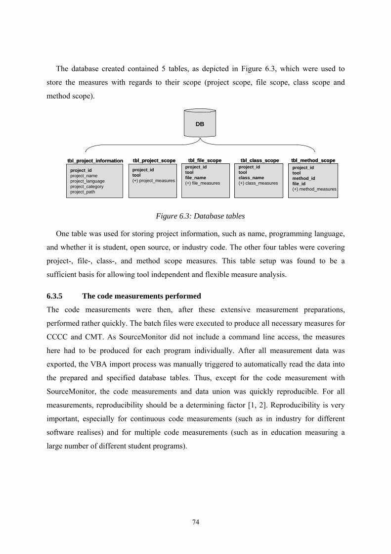
The database created contained 5 tables, as depicted in Figure 6.3, which were used to

store the measures with regards to their scope (project scope, file scope, class scope and

method scope).

DB

project_idproject_nameproject_languageproject_categoryproject_path

tbl_project_information

project_idproject_nameproject_languageproject_categoryproject_path

tbl_project_information

project_idtool(+) project_measures

tbl_project_scope

project_idtool(+) project_measures

tbl_project_scopeproject_idtoolclass_name(+) class_measures

tbl_class_scopeproject_idtoolclass_name(+) class_measures

tbl_class_scopeproject_idtoolfile_name(+) file_measures

tbl_file_scopeproject_idtoolfile_name(+) file_measures

tbl_file_scopeproject_idtoolmethod_idfile_id(+) method_measures

tbl_method_scopeproject_idtoolmethod_idfile_id(+) method_measures

tbl_method_scope

Figure 6.3: Database tables

One table was used for storing project information, such as name, programming language,

and whether it is student, open source, or industry code. The other four tables were covering

project-, file-, class-, and method scope measures. This table setup was found to be a

sufficient basis for allowing tool independent and flexible measure analysis.

6.3.5 The code measurements performed

The code measurements were then, after these extensive measurement preparations,

performed rather quickly. The batch files were executed to produce all necessary measures for

CCCC and CMT. As SourceMonitor did not include a command line access, the measures

here had to be produced for each program individually. After all measurement data was

exported, the VBA import process was manually triggered to automatically read the data into

the prepared and specified database tables. Thus, except for the code measurement with

SourceMonitor, the code measurements and data union was quickly reproducible. For all

measurements, reproducibility should be a determining factor [1, 2]. Reproducibility is very

important, especially for continuous code measurements (such as in industry for different

software realises) and for multiple code measurements (such as in education measuring a

large number of different student programs).

74

6.4 Expected differences

Before taking a look at the empirical differences in Chapter 7, let us consider expected

differences between the different areas of student programming, open source programming

and industry programming.

6.4.1 Students vs. industry

One immediately noticeable difference is that computer science students deal with smaller

projects and problems than professionals do in industry [66]. According to [66], programmers

and software engineers should get involved in bigger programming projects during their

education to gain necessary experience for industrial scale programming.

Not only the size of the programs produced differs but also the way the two groups of

programmers approach problems. Students tend to use a trial and error approach [67]. In order

to learn a programming language, this method is initially very effective, however students

tend to use this method for too long [67]. This means that students tend to use insufficient

time to analyze the underlying problem and design a solution [68], but start programming

right away. If no clear plan towards the solution is known beforehand, more time is needed to

implement the program, as new problems are encountered. Thus the program is updated in an

ad hoc manner to solve the current problem or difficulty. This not only results in low

productivity [69] but also most likely results in complex and poor code structure [29] and

program design [70].

Without a good design and simple implementation, the code maintenance can become

difficult [70], as the solution is likely to be too specialized on a specific problem [69].

According to [69], students are usually not graded on program structure, program design and

code readability, but it “is expected that design effort and quality will indirectly benefit

students, with better (more accurate) programs and reduced time spent on projects” [69].

However a majority of graduate students still cannot create good program designs [70]. Next

to a good design, code readability and maintainability are required factors in industry.

Students tend not to focus enough on the readability [71] and maintainability aspects of their

code [70, 72] and rather direct their efforts towards creating a correct program [72].

Common poor programming practices among students can be listed as follows [29, 72]:

• Too many loop and conditional statements

• Not enough methods

• Use of global variables rather than parameters to a method

• Use of too many parameters for a single function

75

• Too large methods

• Improper identifier-naming

• Unused variables

• Perform unnecessary checking with Boolean expression

• Un-initialised variables

• Inappropriate access modifiers

Some of these programming practices can be identified in the code with the software metrics

used in this dissertation. More on this aspect, however, will be presented in Section 6.5.

6.4.2 Open source vs. closed source

Open Source Software is computer software whose source code is freely available together

with the executable program (e.g. via sourceforge). Furthermore, OSS includes a license

allowing anyone to modify and redistribute the software [73]. As stated by Aberdour [74],

OSS projects are characterized by highly distributed teams of volunteer programmers who

contribute to and maintain the existing code and write documentation for the product [75].

Advocates of OSS argue that through the open available source code, reliability and

security are increased as more pairs of eyes are reviewing the code; thus finding errors and

bugs [76]. An additional benefit of the potentially unlimited number of people involved is

seen in the inevitable requirement of modular, self-contained and self explanatory code [73,

76] which itself would result in high readability, maintainability and flexibility of the program

[76].

The disadvantages of OSS development lie in the area of task coordination. [74]. Here,

Stamelos [73] and Berry [76] find that OSS projects can suffer from weak project

management and development processes which are not well defined. This is reflected by

activities such as system testing and documentation, which are often ignored [73], improper

requirement definition performed by the programmers themselves, no formal risk assessment

process, too much effort dedicated to programming rather than a detailed design [73, 76].

Despite differences in the development processes and quality assurance, is it seen that OSS

and CSS are comparable in terms of software quality [74, 76] and also in terms of structural

code quality [73].

In this dissertation project, the single industry project will be placed in the same group as

the OSS projects for the later code measurement.

76

6.4.3 Expected measurement results

With regard to the different project backgrounds and the expected differences between

student, open source and closed source code, several assumptions about the expected

measurement results can be made. In what intervals will the results lie and what are the major

differences between the three areas are typical questions.

Since students have to deal with rather small problems compared to the ones in industry

[66], it is expected that the program size measures for the latter are clearly higher. It is

expected that the student projects will be within the range of 100 lines to 5000 lines of code.

Whereas, the OSS and CSS projects are expected to range from 4000 lines and upward.

The potentially poor programming practices present among students, might be reflected by

high NLOC per method measures (large methods) and high NBD, BP, ECC measures (not

enough methods, and to many loop and conditional statements). With regard to the design of

student programs, the CBO measure might indicate too tight coupling.

For the open source projects high Maintainability Index measures are expected, since the

code (indicated in Section 6.4.2) is supposedly self-contained and self explanatory. However,

all in all the differences between OSS and CSS should not be highly noticeable as the two are

comparable (see Section 4.4.2). If major differences are found, then no solid conclusions

should be drawn from these, as only a single CSS project was available for this dissertation

project. Here the difference between student and industry code is more of interest.

6.5 Summary

When applying different software measurement tools for code measurements, special

attention has to be paid to the aggregation of the data produced and the automation of the code

measurements. Without any automation in the code measurements the results are costly to

produce and reproduce for single and especially multiple programs. Certainly teachers and

tutors would prefer running the code measurements for all selected students via a single click,

rather than performing the code measurement for each student individually.

As presented in this chapter, the areas of student, open source and closed source show

disparities. The following chapter will take a closer look on whether these differences are

reflected by the code measurement results.

77

7 Code analysis: Measure interpretation

7.1 Introduction

At this point, the programs introduced in Chapter 6 are presented in summarized and

numbered form. The industry projects, which are sorted by programming language, are

numbered from 1 to 19 (the closed source program from Sogeti is listed last in this group).

The student programs, which are sorted by course level (A-D) and course name, range from

the number 20 to 56. Rather than the full program titles, the program numbers are used in the

diagrams in this chapter (Table 7.1 represents a look-up table in this matter).

Industry Programs Student Programs

ID Program name Lan ID Program name Lan ID Program name Lan

01 GIMP C 20 A.OOPJ Java 39 D.CC_L2_st2 C 02 Miranda C 21 A.OOPJ Java 40 D.CC_L2_st3 C 03 NullWebmail C 22 A.OOPJ Java 41 D.CC_L2_st4 C 04 Panda C 23 A.OOPJ Java 42 D.CC_L3_teacher C 05 SDCC C 24 A.OOPJ Java 43 D.CC_L3_st1 C 06 VIM C 25 B.OS_L1_st1 C 44 D.CC_L3_st2 C 07 7-Zip C++ 26 B.OS_L2_st1 C 45 D.CC_L3_st3 C 08 DiskCleaner C++ 27 B.OS_L3_st1 C 46 D.CC_L3_st4 C 09 Emule C++ 28 B.OS_L4_st1 C 47 D.CC_L4_teacher C 10 FileZilla C++ 29 B.OS_L5_st1 C 48 D.CC_L4_st1 C 11 HexView C++ 30 C.PL_L1_st1 C+ 49 D.CC_L4_st2 C 12 Notepad++ C++ 31 C.PL_L1_st2 C 50 D.CC_L4_st3 Java 13 BonForum Java 32 C.PL_L1_st3 C 51 D.CC_L4_st4 Java 14 FitNesse Java 33 C.PL_L1_st4 C+ 52 D.OODM_L4_st1 Java 15 HTML Unit Java 34 C.PL_L1_st5 C+ 53 D.OODM_L4_st2 Java 16 NekoHTML Java 35 C.PL_L1_st6 C 54 D.OODM_L4_st3 Java 17 Jsettlers Java 36 C.PL_L1_st7 C++ 55 D.OODM_L4_st4 Java 18 JSS Java 37 D.CC_L2_teac C 56 D.OODM_L4_st5 Java 19 Sogeti.PPS Java 38 D.CC_L2_st1 C

Table 7.1: List of programs measured

78

7.2 Program size

The program size was measured in terms of lines of code, number of statements and number

of tokens (operands and operators).

7.2.1 Measurement results

The lines of code (both LOC and NCLOC), the number of statements (#STAT) and the

Halstead length (HL) indicate the size of the programs. The following table (Table 7.2)

illustrates the results for these aspects.

Total values Total values Open Source LOC NCLOC #STAT HL Closed Source LOC NCLOC #STAT HLHexView 1856 1121 721 5131 CS.PPS 120778 76338 65109 493258JSS 3029 1198 1762 8521 DiskCleaner 7470 5430 3765 25748 BonForum *8584 4077 3086 21545 Average Values for the course NullWebmail 9912 8925 6961 63583 Student LOC NCLOC #STAT HLNekoHTML 11482 6478 4890 34247 B.OS 228 172 123 760Panda *26049 13848 6706 148989 D.CC 869 673 585 3438Miranda 34029 28823 23892 196620 C.PL 886 679 562 3416FitNesse 35347 27122 20399 138937 A.OOPJ **1034 578 382 2513HTML Unit *42482 14188 11203 70533 D.OODM *1487 594 449 2855Notepad++ 48233 35677 27285 195363 JSettlers 56768 30724 20801 154519 FileZilla 112208 81934 58600 450582 * -> LOC values pushed up by a high CR > 40% 7-Zip 117789 95889 64469 469066 ** -> percent of blank lines ~10% and CR ~ 30% SDCC 207690 144892 96970 757764 CR = comment rate Emule 221641 169635 124427 947371 VIM 320531 239693 123416 1111573 GIMP 732157 526279 290981 2755645

Table 7.2: Different program sizes

The measures in Table 7.2 are sorted in ascending order by the LOC column. For the open

source programs, a major difference between lowest (1856, HexView) and highest (732157,

GIMP) LOC measure was detected. The student code measures are presented grouped by the

course for which they were produced. They lie in the same size range and their highest

average LOC measure is below the lowest LOC measure found in the industry group.

7.2.2 Definition revisions and correlations

The observed measures for NCLOC and #STAT follow the ascending order of the LOC

measures (see the scatter charts in Appendix A.3.2). While this relationship will in general be

79

expected to be true, it need not necessarily hold in all cases, for example when (say) 90% of

the program text is composed of comments. Note that the LOC value is highly influenced by

the number of blank lines and the comment rate (see Chapter 4) which itself differs from

programmer to programmer and from program to program. The correlation values in Table

7.3 confirm that the trend depends on the range measured. Student programs which have a

much lower LOC value show less correlation with the other program size metrics than the

larger Industry programs.

total_NCLOC total_#STAT total_HL

Student 0,811 0,741 0,783

Industry 0,997 0,989 0,997

ALL 0,999 0,991 0,998

Table 7.3: Correlations7 with the total_LOC measures

The other three program size metrics show a high correlation for small and large ranged

groups (see Table 7.4). Since a statement is a collection of operands and operators [2], the

Halstead length (as the total number of operands and operators in the code, see Chapter 4)

correlates to the total number of statements (see Table 7.4 and scatter plot in the Appendix).

Both #STAT and HL, however, are dependent on the programming language used by their

definition (see Chapter 4). By definition NCLOC is not dependent on the programming

language used, as the metric counts non comment lines of code rather than language specific

constructs.

NCLOC vs. #STAT NCLOC vs. HL #STAT vs. HL

Student 0,969 0,952 0,958

Industry 0,991 0,997 0,994

ALL 0,992 0,998 0,995

Table 7.4: Correlations7, NCLOC, #STAT, HN

7.2.3 Defining lines of code size groups

Since for the industry programs the range of the program size measures is rather large, a

division into size groups seemed reasonable. For this dissertation the author finds the NCLOC

metric the most suitable. NCLOC was chosen over LOC, #STAT and HN since this metric is

not affected by the comment rate and its computation is not affected by the programming

language used.

7 Spearman correlation

80

The industry programs were divided into the following three groups: small, medium and

large.

• The small group contains programs with a NLOC measure < 10.0000

• The medium group ranges from 10.000 NCLOC to 100.000 NLCOC

• The large group contains the programs above 100.000 NCLOC

small: total_NCLOC

01000

20003000

400050006000

70008000

900010000

11 18 13 8 16 3

medium: total_NCLOC

010000

2000030000

400005000060000

7000080000

90000100000

4 15 14 2 17 12 19 10 7

large: total_NCLOC

0

100000

200000

300000

400000

500000

600000

5 9 6 1

ID → ID →

ID →

Figure 7.1: Industry NCLOC groups

Since the program size measures for the student programs lie within a much tighter range, the

programs are not sub-divided into size groups. The values for these programs can be seen in

Figure 7.2 below.

Student: total_NCLOC

0

200

400

600

800

1000

1200

1400

27 28 36 47 23 43 56 22 55 41 44 46 24

ID →

Figure 7.2: Student NCLOC values

81

7.3 Code distribution

As discussed in Chapter 3 (Section 3.5), program source code can be distributed in several

ways among files, classes and methods. In this section, the results for the code distribution

metrics are presented and discussed. The code distribution is presented and discussed for a set

of sample programs. The complete set of measures is given in Appendix A.3.

7.3.1 Measure ranges and measure outliers

Table 7.5 presents the ranges measured for the code distribution measures in file scope.

NCLOC measures per file

average max min #files

Group From to from to from to from to

Student 17 960 52 960 4 960 1 29

Small 70 307 230 2298 1 33 15 58

Medium 55 294 386 16786 1 10 70 915

Large 255 2282 4723 16512 0 2 104 2036

Table 7.5: Code distribution measure ranges (file scope)

Both the average and minimum NCLOC measures per file seem rather high for the student

group, when compared to the ranges of the three industry groups. These high values belong to

the same student program (D.CC_L3_st3) which only consists of one file; thus the average,

min, max and total measures per file are equal for this particular program. This example

indicates the importance of combining measures to understand their meaning. When looking

at a single measure, other measures should be used to gain an understanding of what this

value indicates (more on this aspect is presented in the next section and Section 7.4.6).

The number of files used increases noticeably for larger programs. However, as indicated

in Chapter 3.5, this need not necessarily have to be the case.

The maximum NCLOC measures per file for both the large and the medium length group

were unexpectedly high. Figure 7.3 illustrates these aspects further. In the next section

(Section 7.3.2) the outliers are investigated in more detail.

82

Industry: avg_file_NCLOC (ordered by total_NCLOC)

0

500

1000

1500

2000

2500

11 18 13 8 16 3 4 15 14 2 17 12 19 10 7 5 9 6 1

small medium large

Industry: max_file_NCLOC (ordered by total_NCLOC)

0

2000

4000

6000

8000

10000

12000

14000

16000

18000

11 18 13 8 16 3 4 15 14 2 17 12 19 10 7 5 9 6 1

small medium large

ID → ID →

Figure 7.3: Industry NCLOC per file (avg, max)

Figure 7.3 shows that three of the programs measured have source files with more than

10000 non comment lines of code. Understanding the content of such a programming file can

possibly be rather difficult (see Chapter 3.5 for the discussion on length per file).

The measures for the method scope show values within a similarly high range. Before

these measures are discussed, the full measure ranges are presented in Table 7.6.

NCLOC measures per method

average max min #methods

Group From to from to from to from to

Student 4.1 49.7 23 131 1 10 3 100

Small 13.5 39,8 112 505 1 4 66 414

Medium 6.1 37.0 86 1691 1 2 261 4279

Large 23.4 33.4 922 2326 1 2 1592 14795

Table 7.6: Code distribution measure ranges (method scope)

The average NCLOC measures for the method scope lie within similar ranges for the four

groups (see the corresponding charts in the appendix A.3 for more detail). As with the number

of files, the number of methods also increases for each size groups (small vs. medium vs.

large). The maximum method size measures indicate the use of methods which are

presumably too large. Here, 9 out of the 19 industry programs have at least one method with a

code length above 700 NCLOC. Three out of the 19 have at least one method with a code

length above 1600 NCLOC. As stated in Chapter 3.5, defining a clear optimal length or limit

is difficult; however methods with a NCLOC measure above 700 should evidently be

refactored. A programmer would need to read 46 to 77 screen pages (if 30 to 50 lines fit on

one page) to see the full content of the longest method measured (2326 NLOC long in

83

program 9). Understanding this content would be a totally different task (see chapter 3 for the

discussion on code distribution and optimal method and file size).

The class scope has been left out in this presentation, since the measures produced for the

code distribution were very similar to the measures produced on file scope. One class is stored

in one file and a file does not contain more than one class except for a few cases.

Since the individual code distributions can not be captured by the measure ranges

presented, a closer look at individual example programs will be taken in the following section.

7.3.2 A closer look and measure combination

When comparing different programs or program versions, the code distribution can help to

identify problem areas. In this matter, the results for the C level course C.PL showed

interesting results in terms of number of files. Two of the student programs differed greatly

from the course average of 10 files. Student1 of the C.PL course decided to keep all his code

in a single file, whereas Student5 divided his code over 22 files. As stated in Chapter 3,

defining an optimal code distribution for a program is difficult. However, when a group of

programs designed for the same problem differ greatly, it is advisable to double check with

the programmers (in this case the two students) to understand what they did and why.

In order to grasp the code distribution of a program, the measures produced must be

combined. Just looking at single measures (like the number of files) is useful to capture the

group outliers, but does not indicate much about the individual code distribution.

At this point a set of sample programs will be used to show the differences in code

distribution. The three file size outliers from Figure 7.3 and the program FitNesse (ID 14) are

used as samples in this matter. Let us now consider the combined code distribution measures

in Table 7.8 and Table 7.9 together with the total program size measures in Table 7.7.

SDCC (5) VIM (6) FitNesse (14) CS.PPS (19)

Total_NCLOC 144,892 239,693 27,122 76,338

Table 7.7: Program size (ID 5,6,14,19)

NCLOC measures per file

ID Mean median max min stdev #files

5 728 123 11,077 1 1,681 199

6 2,282 1420 16,512 1 2,714 104

14 55 37 386 4 54 493

19 207 88 16,786 3 925 368

Table 7.8: Code distribution sample group (file scope)

84

NCLOC measures per method

ID Mean median max min stdev #methods

5 33,4 17 1763 1 58,38 3874

6 25,9 13 1070 1 50,87 1592

14 7,5 6 86 1 5,00 3254

19 17,1 4 716 1 42,15 4279

Table 7.9: Code distribution sample group (method scope)

Combined, the measures help build a picture about the actual code distribution. Thus,

program 5 and 6 with respect to program size, have rather few files and consequently a high

average file length. Especially program 6 consists of mainly long files (average per file of

2,282 NCLOC and mean per file of 1,420 NCLOC). In method scope, both programs seem to

have a couple of very long methods, but the majority of methods lie within a fairly narrow

range. Program 19 shows a similar code distribution for file and method scope (a few very

long file and methods, but the majority short). For the FitNesse (program 14) the code for

both file and method scopes lies within a fairly narrow range with low values.

It is very important to understand the underlying code distribution scenario for the

interpretation of other measures produced as we will find out later.

7.3.3 The big picture

As described in the previous section, a variety of measures have to be combined in order to

understand the code distribution of an underlying program. It would be an advantage to have a

single measure describing a program’s code distribution. However, the more information is

combined in a single measure, the greater is the risk of loss of information about particular

aspects [8]. Even with looking at 6 measures per scope, not all aspects of the code distribution

are considered. In order to see the distribution to the full extent, either the individual files and

lengths of methods or the graphical representation of these lengths should be inspected.

Below in Figure 7.4 this is done for the four sample programs, for which the code

distribution measures were presented in detail.

85

SDCC (5)

0

500

1000

1500

2000

1 51 101 151

files →

VIM (6)

0

500

1000

1500

2000

1 51 101

files → FitNesse (14)

0

500

1000

1500

2000

1 101 201 301 401

files →

S.PPS (19)

0

500

1000

1500

2000

1 101 201 301

files →

NC

LOC

→

ID →

NC

LOC

→

Figure 7.4: Code distribution charts on file scope (5, 6, 14, 19)

The charts combined with the measures produced capture the different code distributions.

In the following sections the code distribution of a program will be used for understanding

and explaining the value of particular measures. Measures (such as complexity measures)

have to be combined with the information about the underlying measure scope, in a similar

way to considering a person’s physical aspects (such as height, age and gender) before any

decision is made, i.e. whether a certain weight measure is too high, low or acceptable.

86

7.4 Textual code complexity

Selected examples of the textual code complexity measures produced will be displayed in this

section. See the corresponding section in the appendix (A.2.3) for a full view on the textual

code complexity measures.

7.4.1 Problematic aspects

The total measure for the Halstead vocabulary (total_Hvoc), as the sum over all file Hvoc

measures, is not useful for this dissertation since the information about the actual vocabulary

size gets lost through summing up. By this is meant that the vocabulary for a program (by

Halstead defined as the distinct number of operands and operators) will contain double entries

when several presumably non disjunctive vocabularies are joined. This is not due to an error

in the metric definition, but to deficiencies in the software measurement tool applied.

For the total Halstead Difficulty (total_HD) a similar aspect came to light. The more files

the code was distributed over, the higher the total_HD measures found. However, since the

overall number of operands and operators is independent to the number of files used, this

should not be the case. Thus, a similar problem as for the total_Hvoc was experienced.

To what extent the total formation of the HV and HE measures biased the corresponding

total values is not clear8. Here, however, no strong indicators for a measure distortion were

found. Nevertheless the total values of these should be treated with care.

The mean values are highly dependent on the code distribution aspects. Programs with a

high mean program size showed high textual code complexity measures. Here again, the trend

is especially due to the high size range of the underlying program sample.

7.4.2 Results & normalisations

In this section the total values of HV and HE will be presented and discussed. Furthermore,

as suggested by [14] and [65], the total values for the textual code complexity measures will

be presented in combination with the underlying code size; thus normalized.

8 As described in chapter 4 the Halstead Difficulty (HD) and Halstead Effort (HE) metrics are based on the

Halstead vocabulary aspects. However, the total measures produced for these metrics are not affected by the total_Hvoc. Even though the total measures are again the sum of the file scope measures, the computation for these file scope measures was performed on the file scope level as well, thus unbiased Halstead vocabulary measures were applied.

87

small: HV_N, total_HV

0

100000

200000

300000

400000

500000

600000

11 18 13 8 16 30

10

20

30

40

50

60

70

80

90

total_HV HV_N

medium: HV_N, total_HV

0

500000

10000001500000

2000000

2500000

3000000

35000004000000

4500000

5000000

4 15 14 2 17 12 19 10 70

10

20

30

40

50

60

70

80

90

total_HV HV_N

large: HV_N, total_HV

0

5000000

10000000

15000000

20000000

25000000

5 9 6 10

10

20

30

40

50

60

70

80

90

total_HV HV_N

Student: HV_N, total_HV

0

10000

20000

30000

40000

50000

60000

0

10

20

30

40

50

60

70

80

90

total_HV HV_N

Figure 7.5: Halstead Volume results (industry & student)

Figure 7.5 displays the total_HV measures combined with the normalized values (HV_N9)

and ordered by the program size (NCLOC value). The different program size groups show

clear range disparities for the total values measured. However the normalized values range

between 19.2 and 80.6 (or 57.7 if the one outlier is ignored) for all groups displayed. Another

observation is that, for the large group just a minimal fluctuation of the normalized measure

can be noticed. Since only 4 programs are in the group, this might be due to coincidence. Also

possible is that for very large programs, the normalized measure runs towards a constant

value. However, this will not be analyzed at this point and thus will be left for future work.

The normalized Halstead Effort measures9, on the other hand, show a very high fluctuation

and range (from 19.9 to 10,103.5) for the group of small programs such as the student

programs. The industry programs fluctuate less and less with increasing program size (small:

43.3 - 276.6, medium: 2 - 59.9 [without program 4: 582.3], large: 7.2 – 101.4). The

comparison between student and industry programs in this matter is depicted in Figure 7.6.

9 The Halstead measures were normalized by dividing the underlying NCLOC measure.

88

Student: HE_N, total_HE

0

1000000

2000000

3000000

4000000

5000000

6000000

7000000

8000000

9000000

10000000

-200

300

800

1300

1800

2300

2800

3300

3800

4300

4800

total_HE HE_N

Industry: HE_N, total_HE

0

1000000000

2000000000

3000000000

4000000000

5000000000

6000000000

7000000000

8000000000

11 18 13 8 16 3 4 15 14 2 17 12 19 10 7 5 9 6 1-200

300

8001300

1800

2300

2800

3300

38004300

4800

total_HE HE_N

Figure 7.6: Halstead Effort results (industry & student)

7.4.3 Result interpretation

As described above, the normalized Halstead Volume measures lie within a tight range and

seems for this specific set of programs to be independent of program size and the number of

files. Since the HV metric is intended to measure the information content of a program (see

Chapter 4) the normalized Halstead Volume could be interpreted as compactness and density

of the information content per lines of code. Whether this is a valid conclusion may be shown

by later program comparisons (presented in Section 7.7.2).

89

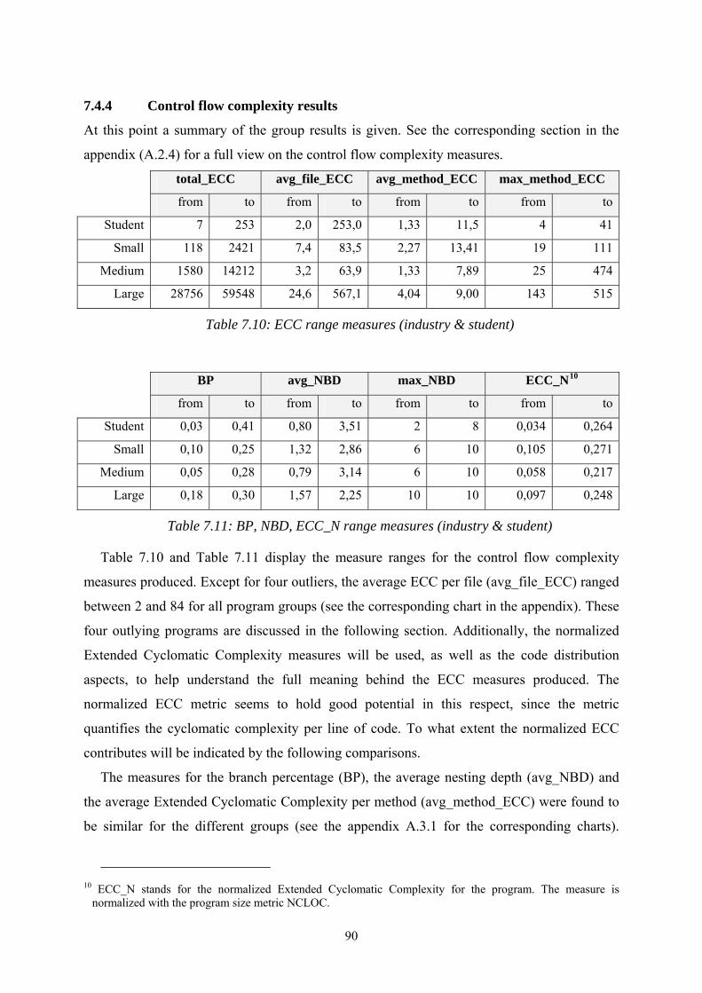
7.4.4 Control flow complexity results

At this point a summary of the group results is given. See the corresponding section in the

appendix (A.2.4) for a full view on the control flow complexity measures.

total_ECC avg_file_ECC avg_method_ECC max_method_ECC

from to from to from to from to

Student 7 253 2,0 253,0 1,33 11,5 4 41

Small 118 2421 7,4 83,5 2,27 13,41 19 111

Medium 1580 14212 3,2 63,9 1,33 7,89 25 474

Large 28756 59548 24,6 567,1 4,04 9,00 143 515

Table 7.10: ECC range measures (industry & student)

BP avg_NBD max_NBD ECC_N10

from to from to from to from to

Student 0,03 0,41 0,80 3,51 2 8 0,034 0,264

Small 0,10 0,25 1,32 2,86 6 10 0,105 0,271

Medium 0,05 0,28 0,79 3,14 6 10 0,058 0,217

Large 0,18 0,30 1,57 2,25 10 10 0,097 0,248

Table 7.11: BP, NBD, ECC_N range measures (industry & student)

Table 7.10 and Table 7.11 display the measure ranges for the control flow complexity

measures produced. Except for four outliers, the average ECC per file (avg_file_ECC) ranged

between 2 and 84 for all program groups (see the corresponding chart in the appendix). These

four outlying programs are discussed in the following section. Additionally, the normalized

Extended Cyclomatic Complexity measures will be used, as well as the code distribution

aspects, to help understand the full meaning behind the ECC measures produced. The

normalized ECC metric seems to hold good potential in this respect, since the metric

quantifies the cyclomatic complexity per line of code. To what extent the normalized ECC

contributes will be indicated by the following comparisons.

The measures for the branch percentage (BP), the average nesting depth (avg_NBD) and

the average Extended Cyclomatic Complexity per method (avg_method_ECC) were found to

be similar for the different groups (see the appendix A.3.1 for the corresponding charts).

10 ECC_N stands for the normalized Extended Cyclomatic Complexity for the program. The measure is

normalized with the program size metric NCLOC.

90

However, the programs require to be compared on an individual basis in order to explore the

full potential behind the measures.

7.4.5 Individual differences

No large group differences were noted for the structural complexity measures produced, apart

from increasing total_ECC measures, which as total measures are related to program size

groups. Thus, at this point, the comparison level is moved to the level of individual programs.

The four outliers for the average file ECC measures mentioned in Section 7.4.4, are two

student programs (ID 40 and 45) and two industry programs (ID 5 and 6). These student

programs were written for the course D.CC by the same student (student 3). The industry

programs, which are written in C, both belong to the size group large and namely are, SDCC

and VIM. The code distributions for programs SDCC (5) and VIM (6) were already

presented in Section 7.3.2; thus their high average file ECC, resulted most likely from their

long code length per file. For the two student programs a similar situation was found (the

average textual code length per file was high). In order to better understand these high ECC

values, Table 7.12 presents measures used for the interpretation.

ID Avg_file_NCLOC Avg_file_ECC ECC_N BP Avg_NBD

5 728 161 0,22 0,30 2,19

6 2,282 567 0,25 0,28 2,25

40 557 147 0,26 0,33 1,24

45 960 253 0,26 0,33 1,54

Table 7.12: Control flow complexity results (5, 6, 40, 45)

With this table (Table 7.12) and the ranges measured (Table 7.11), it becomes clear that the

high average file ECC measures are not just caused by long code files. Both the branch

percentage and the normalized ECC measures have high values. Even though the average

nesting block depth measures seem still acceptable for the two student programs, the other

two measures (BP and ECC_N) indicate a very complex control flow throughout the program.

As the student programs are rather short, a very detailed look at the full source code was

possible. The programs indeed show a very complex control flow. The majority of the other

students in the course, managed to hold the BP and ECC_N values significantly lower (see

Figure 7.7). Program 48, however shows similar results and an even higher branch

91

percentage. Due to a relatively low average file ECC (=46), this program was not detected

before. Thus to find the outliers, all aspects require to be considered and combined.

Course D.CC

0,1

0,15

0,2

0,25

0,3

0,35

0,4

0,45

37 38 39 40 41 42 43 44 45 46 47 48 49 50 51

avg_BPECC_N

ID →

Figure 7.7: BP and ECC_N for D.CC

7.4.6 The importance of measure combination

As the previous section reveals, measures produced have to be combined to understand their

full potential. The measures should not only be combined with the code distribution aspects,

but also with measures which quantify the same code characteristic (such as the control flow

complexity) in a different approach. The measures require to be viewed from different angles

to understand their meaning for the particular program [44].

7.5 Maintainability

In this section the results for the Maintainability Index (MI) and the comment rate (CR) are

presented and discussed.

7.5.1 Maintainability measure results

The Maintainability Index metric, as pointed out in Chapter 4, measures the maintainability of

a program. High measures indicate a good maintainability whereas low measures indicate the

opposite [56]. The results for the program selection are presented in the line diagrams below

(Figure 7.8).

92

Industry: avg_MI

0

20

40

60

80

100

120

1 2 3 4 5 6 7 8 9 10 11 12 13 14 15 16 17 18 19

Student: avg_MI

0

20

40

60

80

100

120

20 22 24 26 28 30 32 34 36 38 40 42 44 46 48 50 52 54 56

ID → ID →

Figure 7.8: Maintainability Index results

Another definition (see Chapter 4) for the Maintainability Index includes the comment

rate. Thus the comment rate results are presented (Figure 7.9) but are not used to draw

conclusions about the maintainability of particular programs. Although, a well documented

code can be easy to maintain [56], the comment rate does not convey the quality of the

comments found in a program code.

Industry: avg_CR

0

0,1

0,2

0,3

0,4

0,5

0,6

1 2 3 4 5 6 7 8 9 10 11 12 13 14 15 16 17 18 19

Student: avg_CR

0

0,1

0,2

0,3

0,4

0,5

0,6

20 22 24 26 28 30 32 34 36 38 40 42 44 46 48 50 52 54 56ID → ID →

Figure 7.9: Comment rate results

As seen above in Figure 7.8, the MI measures ranged from 65 to 104 for student programs

and from 24 to 107 (small: 54 - 87, medium: 52 - 107, large: 24 -75) for the industry

programs. For the group of student programs the majority (89%) showed results above an MI

measure of 80, whereas in the group of industry programs only 42% went above this value.

The next section takes a closer look at the outlying measures seen in Figure 7.8 (program 6

and 14).

7.5.2 Investigating group outliers

For the individual investigation two extreme points within the group of industry programs

were chosen. The industry programs are VIM (ID: 6, MI: 24.0) and FitNesse (ID: 14, MI:

93

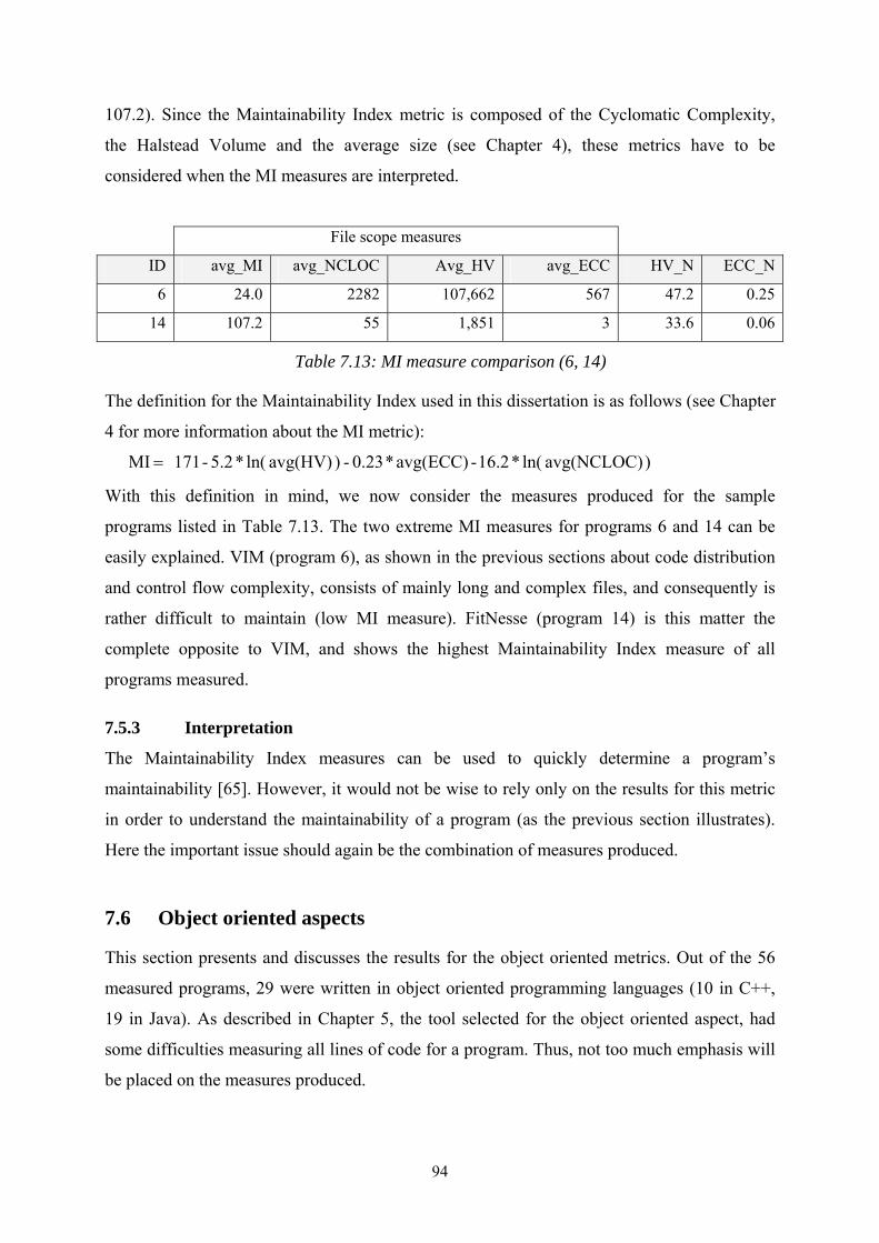
107.2). Since the Maintainability Index metric is composed of the Cyclomatic Complexity,

the Halstead Volume and the average size (see Chapter 4), these metrics have to be

considered when the MI measures are interpreted.

File scope measures

ID avg_MI avg_NCLOC Avg_HV avg_ECC HV_N ECC_N

6 24.0 2282 107,662 567 47.2 0.25

14 107.2 55 1,851 3 33.6 0.06

Table 7.13: MI measure comparison (6, 14)

The definition for the Maintainability Index used in this dissertation is as follows (see Chapter

4 for more information about the MI metric):

) avg(NCLOC) ln( * 16.2 - avg(ECC) * 0.23 - ) avg(HV) ln( * 5.2 - 171 MI =

With this definition in mind, we now consider the measures produced for the sample

programs listed in Table 7.13. The two extreme MI measures for programs 6 and 14 can be

easily explained. VIM (program 6), as shown in the previous sections about code distribution

and control flow complexity, consists of mainly long and complex files, and consequently is

rather difficult to maintain (low MI measure). FitNesse (program 14) is this matter the

complete opposite to VIM, and shows the highest Maintainability Index measure of all

programs measured.

7.5.3 Interpretation

The Maintainability Index measures can be used to quickly determine a program’s

maintainability [65]. However, it would not be wise to rely only on the results for this metric

in order to understand the maintainability of a program (as the previous section illustrates).

Here the important issue should again be the combination of measures produced.

7.6 Object oriented aspects

This section presents and discusses the results for the object oriented metrics. Out of the 56

measured programs, 29 were written in object oriented programming languages (10 in C++,

19 in Java). As described in Chapter 5, the tool selected for the object oriented aspect, had

some difficulties measuring all lines of code for a program. Thus, not too much emphasis will

be placed on the measures produced.

94

7.6.1 Information flow and object coupling

For the information flow and object coupling the following result ranges were measured:

Total Mean Max

Group From to from to from to

Student 0 6061 0 275 0 3136

Small 0 11699 0 111 0 9216

Medium 37098 6775496 116 21441 9216 6285049 IFlo

w

Large 783824 783824 1139 1139 492804 492804

Student 6 192 1 5 3 18

Small 42 500 1 4 6 30

Medium 952 4120 5 7 43 312 CB

O

Large 4734 4734 6 6 122 122

Table 7.14: Information flow and object coupling measure ranges

How much information should flow, is unknown and highly related to the program task

and problem size. The information flow measures produced can, however, help to filter out

students who might have to reconsider their program design (see Figure 7.10 left and right,

and for example program 56 which exhibits high values for those measures) and compare

different programs for the same task with each other. In order to compare two independent

programs, the information flow value requires to be normalized (similarly to the ECC_N and

HV_N), but the question here is which denominator should be chosen.

D.OODM: total_IF

0

1000

2000

3000

4000

5000

6000

7000

52 53 54 55 56

D.OODM: avg_IF

0

50

100

150

200

250

300

52 53 54 55 56ID → ID →

Figure 7.10: Information flow D.OODM

Similar to the IF measures, the measures produced with the CBO metric, should be

compared within a group of programs written for the same problem. Otherwise, understanding

which measures are too high becomes very difficult.

95

7.6.2 Inheritance and polymorphism

The DIT (Depth of the Inheritance Tree) metric was found to present no valuable information

for this particular set of programs (student and industry programs). The corresponding line

diagram charts are to be found in the appendix A.3.1. Also, the Uppsala study [65] did not

find the metric that useful for their set of programs. The depth of the inheritance tree ranged

from 0 to 7 for the programs measured. Thus, no clear indicators for a too long and complex

inheritance tree were found. Often programs have only an indirectly deep inheritance tree, due

to the reuse of existing libraries (such as Java libraries). However these libraries are not and

also should not be considered in the DIT metric [65].

The NOC metric, similar to the DIT metric, did not produce useful measures for the set of

programs measured in this dissertation. The industry programs were found to have a high

number of children, but this is very likely for extremely large programs.

7.6.3 Is high good or bad?

One problem for most object oriented measures produced in this dissertation was that

without analyzing the programs in depth (meaning understanding and mentally reconstructing

the underlying object oriented design), the measures do not provide much information.

Whether a measure is high or low can at this point only be identified by comparing this

particular measure to measures of programs which were created for the same task (such as

student programs for the same assignment).

96

7.7 Individual comparisons

In this section, the comparison is made from a group view down to individual programs. In

order to conclude the group view comparison, the group results from the previous sections in

Chapter 7 are presented in summarized form.

7.7.1 Group differences summarized

The results from the Student vs. Industry comparison revealed major differences in the

program size and code distribution. The average non comment lines of code per program was

583 NCLOC for the student and 79,593 NCLOC for the industry programs. With regard to the

number of files and methods the code was distributed over, these numbers differed greatly as

well. Besides these, also the maximum values of lines per file and per method showed large

differences between the two groups.

Apart from these major differences, a few minor differences were found in three of the

other code characteristic areas. Here the textual code complexity, the control flow complexity

(in terms of nesting block depth) and the maintainability results differed slightly for the

industry and student programs measured. Since in both groups good and not so good

candidate programs were found, the comparison will be made at the individual level.

Considering the programming languages used, the differences can be summarized as

follows:

With regard to the code distribution, the java programs showed the same tendencies in

code as the C++ programs. The results for the programs written in C indicate longer files and

methods than the object oriented languages. Nevertheless, just because the language is object

oriented does not mean the programmers follow this paradigm [77]. Thus for Java and C++,

similar long cases were found. In general, the Java programs measured showed especially

good results for the Maintainability Index (which however is influenced by the code

distribution aspect). Apart from these characteristics, no major differences were spotted.

7.7.2 Individual comparison: BonForum vs. FitNesse

In this section the measures produced are combined in full detail for the two industry

programs BonForum and FitNesse. Even though they differ in program size (BonForum: 8584

NCLOC, FitNesse: 35347 NCLOC), the two programs may be compared.

97

NCLOC measures per file

Program max min mean median stdev #files

BonForum 1287 9 239,82 100 367,00 17

FitNesse 386 4 55,01 37 53,96 493

Table 7.15: File scope code distribution (BonForum vs. FitNesse)

BonForum

0

500

1000

1500

1 5 9 13 17

FitNesse

0

500

1000

1500

1 124 247 370 493files

lines

files

lines

Figure 7.11: File scope code distribution (BonForum vs. FitNesse)

It is important to notice for the following charts that, BonForum contains 3 files above than

500 NCLOC, whereas the remaining 14 files are below 250 NCLOC (see Table 7.15 and

Figure 7.11). For FitNesse only a small number of files (<10) are slightly above 250 non

comment lines of code.

NCLOC measures per method

Program max min mean median stdev #methods

BonForum 505 3 21,8 9 50,34 180

FitNesse 86 1 7,5 6 5,00 3254

Table 7.16: Method scope code distribution (BonForum vs. FitNesse)

BonForum

0102030405060708090

100

1 180methods

lines

FitNesse

0102030405060708090

100

1 3254methods

lines

Figure 7.12: Method scope code distribution (BonForum vs. FitNesse)

As Table 7.16 and Figure 7.12 indicate, BonForum has on average methods which are

almost 3 times longer than FitNesse. About one quarter of BonForum’s methods are longer

than 20 non comment lines of code. The code distribution on file and method scope requires

to be considered for the following measure comparisons.

98

avg_File_HV

0

2000

4000

6000

8000

10000

12000

BonForum FitNesse

HV_N

0

5

10

15

20

25

30

35

40

45

50

BonForum FitNesse

Figure 7.13: Textual code complexity (BonForum vs. FitNesse)

The average Halstead Volume per file is about 5 times larger for BonForum (see Figure

7.13 left), but this result has to be seen in relation to the number of lines per file, as the code

distribution differs greatly. Also, since the normalized Halstead Volume is higher (see the

right chart in see Figure 7.13), the results suggest that FitNesse has a lower textual code

complexity.

0

50

100

150

200

250

BonForum FitNesse

avg_File_ECC max_File_ECC

file scope

0

20

40

60

80

100

120

BonForum FitNesse

avg_method_ECC max_method_ECC

method scope

Figure 7.14: ECC file & method scope (BonForum vs. FitNesse)

The control flow complexity measures (ECC measures, BP and NBD presented in Figure

7.14, Figure 7.15 and Figure 7.16) require to be combined to obtain an overview of the

underlying control flow. The average file and method complexity was found to be high for

BonForum, but since the code distribution affected the measures, the normalized ECC

measure had to be taken into consideration as well.

99

avg_BP

0

0,05

0,1

0,15

0,2

0,25

0,3

BonForum FitNesse0

2

4

6

8

10

12

BonForum FitNesse

avg_BDL max_BDL

Figure 7.15: Branch percentage & nesting level (BonForum vs. FitNesse)

The Branch Percentage (BP) and the nesting block depth confirm the difference in control

flow complexity for the two programs. Thus, together the charts indicate a much more

complex control flow for BonForum than for FitNesse. Besides the control flow complexity,

also the Maintainability Index is noticeably lower for BonForum (see the right chart in Figure

7.16). FitNesse reached the best Maintainability Index results among all programs measured.

ECC_N

0

0,05

0,1

0,15

0,2

BonForum FitNesse

avg_MI

0

20

40

60

80

100

120

BonForum FitNesse

Figure 7.16: ECC_N and Maintainability Index (BonForum vs. FitNesse)

A previous study [65] of BonForum and FitNesse, indicated a poor object oriented design

quality for BonForum and good object oriented design quality for FitNesse. The measures

produced show that this difference in quality is not just to be found for the design but also for

the source code. Here, BonForum was behind FitNesse in all aspects measured.

100

7.7.3 Creating an individual code profile

As seen in the previous section (7.7.2), comparing measures for two or more projects can be

an extensive task. A better solution might be to generate a code profile for each program,

which allows the programs to be compared quickly and easily. The next chapter deals with

this aspect of generating a code profile for the programs. The programs BonForum and

FitNesse can help understand a good choice of profile metrics, since the two programs have

now been discussed in detail.

7.8 Summary

When software projects are analyzed by means of software measurements, a considerable

amount of data is produced. The task here is to organize the data and draw meaningful

information from the measures produced [8]. At this point, the importance of measure

combination should be reviewed. Measures produced need to be combined, as illustrated in

this chapter, to avoid drawing hasty decisions about a particular code characteristic measured.

101

8 Code profiling

This chapter deals with the generation of code profiles in general and for the programs

measured.

8.1 Introduction

As suggested in Chapter 7, the comparison should be brought to the individual level due to

large amounts of data produced. In Section 7.7.2, this individual comparison was illustrated

by the example BonForum vs. FitNesse. Even if only two programs are compared, the

comparison is not simple and the number of measures, tables and charts can still feel

overwhelming. The creation of code profiles can improve the comparison process, as a

summary of data is compared rather than the full number of measures produced (in this

dissertation, for each program 66 measures were produced).

Before the topic of code profiling is discussed in more depth, the definition of profile listed

in Chapter 2 is presented again:

A profile is “a formal summary or analysis of data, often in the form of a graph or table,

representing distinctive features or characteristics” [7].

Thus code profiling is the activity of creating a formal summary of distinctive characteristics

of a program’s source code. A literature survey revealed that mostly data concerning the

(dynamic) performance of software is profiled such as in [53] and [78], rather than the static

characteristics of the code. Nevertheless in this dissertation the static code characteristics

(such as the control flow complexity) are profiled.

8.2 Reasoning and usage

A program code profile can help to present a quick overview about code characteristics.

Instead of reviewing a large number of measures, a reduced set of summarizing measures can

be sufficient to determine whether changes have to be made. If the code profile indicates

problematic code characteristics, these particular characteristics can be inspected further by

consulting the remaining measures, which were not included in the profile, or by going

directly to the source code level (see Figure 8.1).

102

source

code

code measurescode

profile

further inspection

further inspection

formal

summary

code

analysis

overviewquantificationthe entity

source

codesource

code

code measurescode

profile

further inspection

further inspection

formal

summary

code

analysis

overviewquantificationthe entity

Figure 8.1: Code profiling illustrated

Several scenarios of application seem reasonable for both industry and education. Four of

these scenarios are presented in the following sections.

8.2.1 For industry

Scenario 1:

The use of code profiles allows a quick comparison of different releases for the same

program. A code profile for a particular program could be generated each time a new release

is made. Over time, when the current release profile indicates a large change compared to the

previous profiles the areas of change can be inspected and through refactoring adjusted. Thus

the program profile history will be stored, and used in order to have a deeper basis for

answering questions similar to the following ones:

• Did the project code become more complex, when the last change was made?

• Is a trend visible? Does the maintainability become better or worse?

• If worse, then why and how can it be improved?

Scenario 2

Before acquiring a new software product, the source code can quickly be checked in terms of

maintainability. As the code of the software is possibly unknown beforehand, a profile can

give a quick overview about the code characteristics. If the profile indicates a very complex

source code, an alternative product with better maintainability aspects might be considered

instead.

103

8.2.2 For education

Scenario 1:

Profiles for different student programs in the same course can be compared. When one profile

is significantly different to the ones of the other student programs, the code of this particular

program should be inspected further. Inspecting all student programs in detail is rarely

performed and the more students who are in course, the more difficult it becomes to conduct.

With code profiles, students who might need help can be detected rather quickly, without

having the teacher look through all student programs in detail.

Scenario 2:

Every time a student hands in a programming assignment a code profile for the particular

program can be generated. These profiles can then according to date and course level be

stored in a profile portfolio for the student. This way the student’s programming improvement

can be tracked from the first year assignments to the final year assignments. Whether the

profile indicate better programs over the years would be interesting to see.

8.3 The code profile

8.3.1 Defining areas of importance

In this dissertation the following areas of code characteristics will be considered for the code

profiling:

• Code distribution

• Textual code complexity

• Control flow complexity

• Maintainability aspects

Since the results for the object oriented metrics applied in this dissertation were not found

very useful for the underlying program, these metrics will be covered to a lesser extent in the

code profiles. The maintainability aspects can be seen as combination of code distribution

textual code complexity and control graph complexity (the MI metric covers these three

areas).

104

8.3.2 Selecting metrics of importance

In this section, two sets of metrics (comparative and descriptive) will be presented and

discussed. A distinction was made to guarantee a low complexity of the profile and thus

allowing a quick comparison of two individual profiles. The measures for the comparative

metrics (comparative measures) will receive, as means of comparison, the main attention in

the profile. When anomalies in those measures are detected, the measures for the descriptive

metrics (descriptive measures) can be consulted to further interpret the program’s code

characteristics.

Since the student and industry programs differ greatly in their textual length, the

comparative metrics where chosen to be program length independent. In detail, 8 comparative

metrics were selected11. The selected comparative metrics cover the defined areas of

importance and are listed and explained below:

• Code distribution

o Since it is difficult to say which code distribution is to be preferred for a single

program (see Chapter 3), the metrics are more to be seen as supportive metrics

and thus are mostly within the set of descriptive metrics. Nevertheless, one

adjusted code distribution metric was included: the lines of code per method.

The average lines per method were not measured, but instead the percentage of

large methods determined by the number of non comment lines of code used.

This adjusted metric was labelled:

- LPM>X (Lines per Method greater than a defined limit)

• Textual code complexity

o As representative for the textual code complexity the normalized Halstead

Volume (see Section 7.4) was chosen:

- HV_N (normalized Halstead Volume | code distribution independent)

• Control flow complexity

o The control flow complexity was measured through the branch percentage, the

nesting block level and the Extended Cyclomatic Complexity (ECC). As

Chapter 7 shows these three aspects require to be combined to grasp the

complexity of the control flow. Here 5 representative metrics were selected

(from which one was adjusted similar to LPM>X):

11 Any number of comparative metrics can be chosen. The number 8 was found to be a good balance between

high granularity and lucidity.

105

- avg_BP (average Branch Percentage)

- avg_NBD (average Nesting Block Depth)

- ECC_N (normalized ECC | code distribution independent)

- avg_file_ECC (average ECC per file | file scope code distribution dependent)

- ECC>X (percentage of methods with an ECC above X | method scope code

distribution dependent)

• Maintainability

o The maintainability aspects are covered in the set of primary metrics by the

combination of the metrics above and the Maintainability Index (MI).

- MI (Maintainability Index | file scope code distribution dependent)

The set of descriptive metrics cover code the textual length of a program and more aspects of

the above stated four code characteristic areas (such as code distribution and control flow).

Additionally, object oriented aspects are integrated in form of the coupling between object

metric. The full list of descriptive metrics can be found in the corresponding section of the

appendix (see A.4.1).

8.3.3 Defining measure intervals

The two newly defined metrics (LPM>X, and ECC>X) are required to be adjusted further, as

the value of X was not set. For LPM, this value was set to 20 and for ECC to 10.

Consequently, methods fulfilling the following conditions were counted:

• Lines per method > 20

• ECC per method > 10

As discussed in Chapter 3, no clear understanding about how many lines a method should

have exists. In this dissertation, methods with a length above 20 NCLOC are not essentially

considered to be fault prone and do not require to be redesigned without consulting other

measures beforehand. However, knowing the percentage of long methods in a program can

improve understanding about the code distribution and thus supports the interpretation of

other metrics (such as ECC>X).

Long methods are not essentially complex [51]. Thus, the complexity measures for a

method have to be considered together with the method length. For the complexity per

method (i.e. ECC per method) the counting limit of 10 was chosen in conformance with the

selected LPM limit.

106

8.3.4 Profile visualisation

The visualisation of measurement data has been well researched, thus several different

visualization methods exist [79], [80]. Figure 8.2 displays two out of many of those methods

within the area of software measurement.

Multivariate visualization of

fan-in and code smell

3D perspective visualization with

15 metrics per component

Source: [79] Source: [80]

Figure 8.2: Examples for data visualization

In this dissertation, a rather less complex visualisation form is chosen. When comparing the

profiles of different students in class, a very detailed profile can reduce the clarity and

usability. Thus, here the ease of comparison and simplicity is chosen over the granularity

level of the representation.

The measures for the comparative metrics will be visualized by using a kiviat diagram

(also called spider or radar diagram), which is presented in Figure 8.3. The file scope code

distribution will be presented in visualized form as well (see 7.3.3). The measures for other

descriptive metrics will be listed in textual form next to the kiviat diagram.

Kiviat (or Spider) diagram 1

2

3

4

5

6

7

8

Figure 8.3: Example kiviat diagram

6 Therefore, the layout for the code profile in this dissertation is a combination of literal and

figurative elements. A brief explanation of the profile layout follows in the next section.

107

8.3.5 Profile revision

Figure 8.4 shows the layout selected and explains the different sections briefly

Programming languageProgram lengthComment RateMaintainabilityTextual code compl.File complexityMethod complexityAverage nestingMaximal nestingBranch PercentageMaximal coupling

Number of filesLines per file (avg)Lines per file (max)Number of methodsLines per method (avg)Lines per method (max)

^MI 0.33 ^ECC_N 0.33 ECC>10 0.17 ^BP 0.39^HV_N 0.36 ^ECC_F 0.26 LPM>20 0.35 ^NBD 0.29

Diagram data

22.1

1.20

07

29498

C

Code distribution

0

Program name (ID)

56.6171.89

0.0928,823

30892

1,215

Program summary

100.28

2.657.89

63.90

1,041

^MI

^HV_N

^ECC_F

LPM>20

ECC>10

^BP

^ECC_N

^NBD

0

200

400

600

800

1000

1200

1400

1 11 21 31 41 51 61 71 81 91

prof

ile c

reat

ed o

n

Program summary:

descriptive measures

Visual presentation

of the comparitive

measures (Kiviat)

Code distribution aspects

(literal and figurative

presentation)

Kiviat data

Figure 8.4: Profile layout explanation

Six of the comparative metrics were normalized and renamed (these are indicated with a

‘^’ symbol), for the purpose of display (the new computation can be found in Appendix

A.4.1). In order to keep the original values, the measures for these adjusted metrics were

included in the program summary section (see Figure 8.4). In this way the adjusted

Maintainability Index12 (^MI) is used for the kiviat diagram and the kiviat data section,

whereas the original MI measure is included in the project summary. Table 8.1 gives a brief

overview of the selected primary metrics (adjusted and not adjusted).

Name description name description

^MI Maintainability Index ^BP Branch percentage

^HV_N Normalized Halstead Volume ^ECC_N Normalized Extended CC

^NBD Nesting Block Depth per file LPM>20 Lines (NCLOC) per method > 20

^ECC_F Cyclomatic complexity per file ECC>10 Extended CC per method > 10

Table 8.1: List of comparative metrics

The measures for these comparative metrics are presented as surface on the kiviat diagram. In

terms of interpretation, single spikes on the kiviat diagram indicate possible problems in

particular code characteristics (such as textual code complexity). Here the smaller the area on

kiviat diagram (face) the better the program code. The code distribution aspects are displayed

in figurative and literal form in the bottom right corner.

12 The Maintainability Index did not only required to be adjusted due to the measure range, but also was reversed

as for this metric originally high values indicate a good maintainability and low values a poor maintainability [57].

108

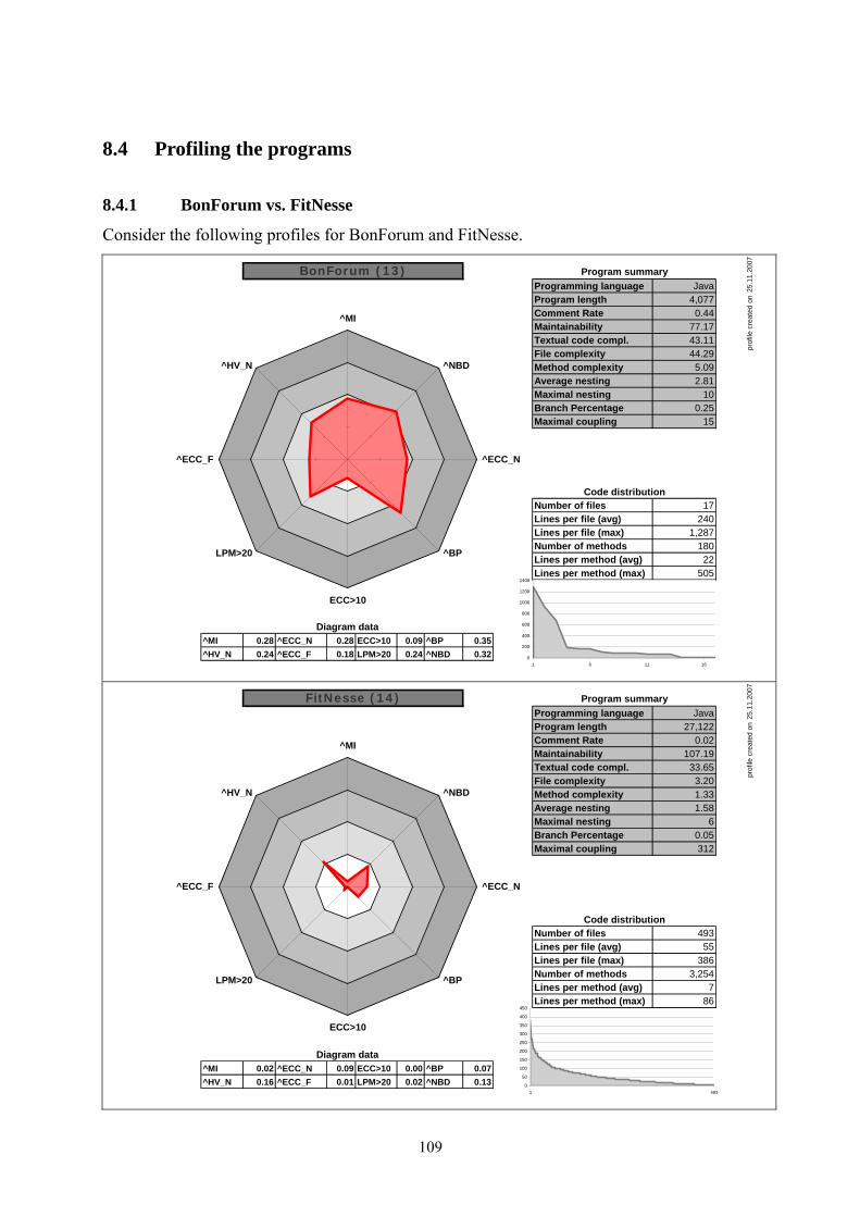
8.4 Profiling the programs

8.4.1 BonForum vs. FitNesse

Consider the following profiles for BonForum and FitNesse.

Programming languageProgram lengthComment RateMaintainabilityTextual code compl.File complexityMethod complexityAverage nestingMaximal nestingBranch PercentageMaximal coupling

Number of filesLines per file (avg)Lines per file (max)Number of methodsLines per method (avg)Lines per method (max)

^MI 0.28 ^ECC_N 0.28 ECC>10 0.09 ^BP 0.35^HV_N 0.24 ^ECC_F 0.18 LPM>20 0.24 ^NBD 0.32

Diagram data

25.1

1.20

07

24017

Java

Code distribution

15

BonForum (13)

43.1177.17

0.444,077

22180

1,287

Program summary

100.25

2.815.09

44.29

505

^MI

^NBD

^ECC_N

^BP

ECC>10

LPM>20

^ECC_F

^HV_N

0

200

400

600

800

1000

1200

1400

1 6 11 16

prof

ile c

reat

ed o

n

Programming languageProgram lengthComment RateMaintainabilityTextual code compl.File complexityMethod complexityAverage nestingMaximal nestingBranch PercentageMaximal coupling

Number of filesLines per file (avg)Lines per file (max)Number of methodsLines per method (avg)Lines per method (max)

^MI 0.02 ^ECC_N 0.09 ECC>10 0.00 ^BP 0.07^HV_N 0.16 ^ECC_F 0.01 LPM>20 0.02 ^NBD 0.13

Diagram data

25.1

1.20

07

55493

Java

Code distribution

312

FitNesse (14)

33.65107.19

0.0227,122

73,254

386

Program summary

60.05

1.581.333.20

86

^MI

^NBD

^ECC_N

^BP

ECC>10

LPM>20

^ECC_F

^HV_N

0

50

100

150

200

250

300

350

400

450

1 493

prof

ile c

reat

ed o

n

109

A detailed comparison between the programs BonForum and FitNesse was performed in

Chapter 7. At this point, with the differences of the two programs in mind, the profile

generation can be examined.

The first immediately visible difference between the two profiles is the size of the shaded

area on the kiviat diagram (surface), thus indicating an overall worse outcome for the program

BonForum. The surface is in all 8 directions (the eight selected comparative metrics) bigger

than the surface for FitNesse. The following sectors on the surface should to be viewed in

combination as these can quickly reveal information about the code characteristics (see Figure

8.5):

^MI

^NBD

^ECC_N

^BP

ECC>10

LPM>20

^ECC_F

^HV_N

Sector 1

Sector 2

Sector 3 Sector 1:

Control flow complexity

Sector 2:

Code distribution

Control flow complexity

Sector 3:

Textual code complexity

^MI

^NBD

^ECC_N

^BP

ECC>10

LPM>20

^ECC_F

^HV_N

Sector 1

Sector 2

Sector 3 Sector 1:

Control flow complexity

Sector 2:

Code distribution

Control flow complexity

Sector 3:

Textual code complexity

Figure 8.5: Kiviat diagram section example

• Sector 1 (^MI - ^BP) presents the control flow complexity measured independent

from the code distribution

• Sector 2 (^BP - ^ECC_F) represents a combination of code distribution and control

flow complexity

• Sector 3 (^ECC_F - ^MI) shows the textual code complexity of the program

With regard to the information in these 3 sectors and the two program profiles, the conclusion

about these programs which was drawn in the previous chapter, can quickly be confirmed. In

the following section the elements within the three sections will be considered closer.

110

8.4.2 Student vs. Student

In Figure 8.6, the kiviat diagrams are shown for the programs of the course D.CC and

programming assignment L4. The full code profiles are presented in the corresponding section

in Appendix A.4.2.

Student 1 (C) Student 2 (C) Student 3 (Java)

^MI

^NBD

^ECC_N

^BP

ECC>10

LPM>20

^ECC_F

^HV_N

^MI

^NBD

^ECC_N

^BP

ECC>10

LPM>20

^ECC_F

^HV_N

^MI

^NBD

^ECC_N

^BP

ECC>10

LPM>20

^ECC_F

^HV_N

Student 4 (Java) Teacher (C)

^MI

^NBD

^ECC_N

^BP

ECC>10

LPM>20

^ECC_F

^HV_N

^MI

^NBD

^ECC_N

^BP

ECC>10

LPM>20

^ECC_F

^HV_N

Figure 8.6: kiviat diagrams for course D.CC_L4

The kiviat surfaces spike out for student 1 and 3. The code from student 1 in particular

shows a high control flow complexity. The results for Student 3’s program indicate overall

high values for the textual code complexity and the control flow complexity. As the teacher

version indicates, the programming assignment required a rather complex control flow.

Nevertheless, Student 2 and 4 showed, with this in mind, good results. The spike in the

bottom right corner (LPM>20) for Student 2 together with the minimal value for the method

complexity (ECC>10) indicate that the code is distributed over predominantly long but rather

non complex methods. In conclusion, the 5 kiviat diagrams can be compared quickly; and the

comparison points to further inspection of the programs of Student 1 and 3, by considering the

full code profile (1), the full measures (2), and finally the code itself (3) (see Figure 8.1).

111

8.4.3 General comparison

The course, in which the design and implementation was graded (D.OODM), the code

profiles show, compared to the other profiles generated, good results. These programs were

written in Java. That Java programs do not necessarily produce good profiles is shown by the

BonForum vs. FitNesse comparison.

When comparing the industry with the student programs (see Appendices A.4.2 and

A.4.3), no clear group difference is visible. Both large and small kiviat surfaces can be found

among student and industry programs. As indicated in Chapter 7, the difference is mostly to

be found in the areas of program size and code distribution.

8.5 Profile drawbacks

Code profiles allow a quick overview about code characteristics, as pointed out in Section 8.2.

However, as not the source code itself, but only a set of metrics quantifying code

characteristics are considered, the profiles should not be over emphasized. When a set of

metrics is chosen, a balance between high granularity level and clarity has to be found. A

profile high in granularity can capture more aspects about the code, but will be lacking in ease

of comparison and analysis.

In this dissertation, four areas of importance were selected (see Section 8.3.1); the object

oriented aspects were not included in the group of comparable metrics. Thus, the profile does

not indicate possible issues in the design, but focuses more on the implementation and the

code itself.

8.6 Summary

For code profiling several application scenarios seem reasonable, in both education and

industry. The definition of a code profile is straight forward, though several decisions (such as

the granularity level, the areas of importance, and the metrics of choice) have to be made in

the definition process. The programs profiled in this dissertation show, with regards to their

area (education vs. industry), that apart from program size and code distribution, there were

only minor differences. However, the profiles generated were used to find individual

differences. Here, the results found through a detailed result analysis of the industry programs

BonForum and FitNesse (see 7.7.2), were confirmed by the profiles generated for these two

programs. In conclusion, using code profiles to quickly compare (without an intensive and in

112

depth measure analysis) software programs in terms of code characteristics was found to be

very reasonable.

113

9 Conclusion

In this chapter conclusions from the theoretical and practical part of this dissertation are

presented together with suggestions for related studies and future work.

9.1 Review

In this dissertation, a survey on software metrics and software measurement tools was

conducted. A set of tools was selected and compared in terms of metric support,

implementation and interpretation. Three tools (CCCC, CMT and SourceMonitor), which

fulfilled previously defined requirements, were used for measuring student and industry

programs with regard to the source code characteristics. The measures produced were

compared and analyzed in terms of programming language groups, textual length groups, area

groups (student vs. education) and individually. Since an individual comparison was found to

be quite an extensive task, the idea of code profiling was used and implemented to reduce the

complexity from the individual program comparisons (such as BonForum vs. FitNesse).

Finally, the student and industry code profiles generated were for a subset of programs which

were discussed and analyzed in detail.

9.2 Project evaluation

In the first part of the evaluation, the three key questions of the dissertation are answered and

the goal achievement evaluated. The following section discusses problematic aspects during

the dissertation and proposes suggestions for related work within this area.

(1) Is it useful to perform software measurements in software engineering education?

Yes, the project and the source code measurements involved show that software measurement

in education is useful. The software measurement process can be, as experienced, realized in

almost fully automated form, thus allowing the investigator to quickly produce and to

reproduce measurement results for a group of students. Nevertheless, the preparations for an

automated software measurement system can be extensive. Especially when different software

measurement tools are used, extra effort is needed to unify the measurement results. Learning

114

to understand what the measures produced indicate and how these should be interpreted is

feasible, though practical experience is needed.

• Which software metrics are available and useful for the analysis of source code?

The survey conducted (see Chapter 4) illustrates that a variety of software metrics can be used

and applied in the software measurement process to measure code characteristics. In this

dissertation the metrics were classified into the following six areas of code characteristics:

1. Program size

2. Code distribution

3. Textual code complexity

4. Control flow complexity

5. Code maintainability

6. Object oriented aspects

Here no single metrics were found to be useful for the analysis of source code but instead a

combination of several metrics (such as control flow complexity metrics supported by code

distribution metrics). A distinction between code distribution (how the source code is

distributed over a number of files and methods) dependent and independent metrics was

made. While interpreting measures produced by the former, code distribution aspects have to

be considered. One area of code characteristics (namely object oriented aspects) was found

not to be particularly useful for this dissertation and the profile generation, since determining

whether a measure produced is too high or low was found to be very difficult for this area;

especially if the program and the program design is not known.

The variety of software metrics available can be an issue; using and applying software

metrics just because these are available can result in an overwhelming amount of data

(measures) produced [2]. Depending on the scope level of interest one single metric can result

in a handful of measures for one particular program measured (measures for program scope,

file scope, class scope, and method scope).

• Which software measurement tools are available and how do they differ?

The survey of software measurement tools in the area of static code analysis conducted

(presented in Chapter 5) points out that here a great variety also exists. For the tools surveyed,

a difference in programming language support as well as in software metric support was

noted. No clearly defined set of metrics was observed; each tool vendor defined their own set

of interest.

115

None of the chosen tools presented a metrics set covering the list of metrics selected, thus

a combination of tools was used. For further studies in the same area, the selection of a single

tool is however advisable, since the measure unification process can present an extensive task

which should be avoided if possible. The issue is that the tools export the measures produced

in different formats, as no clear standard exists.

• Are the measures produced by different tools comparable?

The interpretation and computation of a single metric was found to differ somewhat from tool

to tool. Thus, even for small programs noticeable differences in the values of the measures

produced were found. The quality of the tools’ documentation varied. In this dissertation, the

creation and application of test cases was found useful to determine the metric

implementation and the tool’s documentation was rather seen as support in this area. A

difference in metric computation results in comparison problems. Measures produced by

different tools require to be transformed before any comparison. For instance, one has to

transform Fahrenheit measures to Celsius measures or visa versa, for making valid

comparisons of temperatures. As the metric computation can be difficult to grasp and also

differ from tool to tool (see chapter 5), measure comparisons became very difficult and almost

meaningless. In order to avoid these problematic aspects, each metric was computed by just

one tool for all three programming languages.

(2) How does student source code differ from industry source code? Are students

prepared for industrial size programming?

Since the set of source samples was small (56 programs) and not completely randomly chosen

(it was acquired from what was available), this question is difficult to answer. For the set of

sample programs, complex and non complex cases were found for both industry and student

programs. A large difference was nevertheless found in the program size and code

distribution. Thus the idea that students in software engineering education rarely face

industrial scale problems was supported. Here the student assignments considered dealt with

the creation of new solutions rather than with the maintenance of existing ones. Since the

development of larger software system takes several months to years, students never become,

when not assigned with maintenance aspects, involved with the life cycle process of these

systems in their courses. The dilemma is that university courses are generally short and thus

do not allow large scale assignments. Nevertheless, different computer science courses could

be coordinated to have students work on the same large scale program in different courses.

One course can focus on the design aspects, another on the program extension, yet another

116

one on the program maintenance and quality assurance. This way the students become closely

familiar with the system and gain experience with and understanding of large scale programs.

• What code characteristics can be compared?

A variety of code characteristics (such as size) can be compared. The set of these is

depending on the software metrics used.

• When is a code complex, and what does complex in this sense mean?

The definition of the term complex is difficult to specify precisely. Chapter 3 illustrated that

different views about the related aspect of code complexity exist in the software measurement

literature. Thus, it is not easy to determine what code complexity actually means. In this

dissertation, code complexity was measured in terms of the control flow complexity and the

textual code complexity.

(3) Is student code profiling feasible in means of quick program comparison?

For the set of programs samples, code profiling was found useful for observing a program’s

code characteristics and for means of quick program comparison. The profiles generated are

to be seen as overview of the program’s program size, code distribution, textual code

complexity, control flow complexity, and maintainability. Once the preparations for the

profile generation are completed, the profile generation itself is literally one click away; thus

allowing such use in the education sector. Teachers and tutors can quickly browse over and

compare student profiles on the fly, or save them for later comparison. In order to understand

the profiles generated, surface patterns require to be interpreted. Since the profile

visualization was chosen to be rather simple and immediate, the understanding and

interpretation of the profiles can be taught quickly. Furthermore the profiles can be used to for

different programming language, as the measures and profiles generated for programs of

different programming languages were found to be comparable. Nevertheless, code

distribution tendencies of the different programming languages should be noted.

• What is a code profile?

A code profile is in this dissertation defined as a formal summary of distinctive

characteristics of a program source code.

117

• What is needed for a code profile?

In order to profile code, code characteristics of interest and software metrics which can

quantify these require to be defined. In addition, a form of representation has to be selected

and a balance between granularity level and overview be found.

• Can code profiling be used to improve the students programming knowledge?

Since the students were not measured continuously in this dissertation, this question can not

be answered to the full extent at this point. However, since the results indicate the possibility

of quick program comparisons, it seems reasonable that code profiling can used to determine

areas which can be improved.

9.3 Future Work

With regard to future work the following aspects can be noted:

A continuous measurement and profiling of student programs may be started in order to

collect historical data and analyse which code characteristic areas showed improvement. Once

problematic and well understood areas are detected, teaching can be adjusted accordingly.

Since only a small set of sample programs (56 programs) were used, a study on student

code and industry code differences may be conducted on much larger scale.

Another interesting aspect may be, to further investigate the use of object oriented metrics

for code profiling. Due to difficulties experienced with the tools, the set of object oriented

metrics applied was reduced and the ones which could be used were found not that useful for

this study. The difficulties experienced with the tools as well as with the tool selection point

out that a project regarding the creation of a software measurement tool for education may be

of interest. The support for all taught programming languages and the automated generation

of code profile could be seen as possible requirement for this tool.

118

10 References

[1] N. E. Fenton and S. L. Pfleeger, Software Metrics: A Rigorous & Practical Approach. Boston 1997.

[2] J. C. Munson, Software Engineering Measurement. Boca Raton, FL: Auerbach Publications, 2003.

[3] Wikipedia, “Metrics,” http://www.wikipedia.org/Metrics, accessed 2007-06-10.

[4] Die-net, “Measure,” http://dict.die.net/measure/, accessed 2007-06-10.

[5] H. Zuse, Software Complexity: Measures and Methods. New York: Walter de Gruyter, 1991.

[6] Wikipedia, “Information,” http://www.wikipedia.org/Information, accessed 2007-06-10.

[7] TheFreeDictionary, “Profile,” http://www.thefreedictionary.com/profile, accessed 2007-11-13.

[8] H. Zuse, A Framework of Software Measurement. Berlin: Walter de Gruyter, 1998.

[9] H. Zuse, “History of Software Measurement,” 14. September 1995, http://irb.cs.tu-berlin.de/~zuse/metrics/3-hist.html, accessed 2007-06-01.

[10] S. H. Khan, Metrics and Models in Software Quality Engineering. Addison-Wesley Professional, 2002.

[11] R. J. Rubey and R. D. Hartwick, “Quantitative measurement program quality,” in ACM, National Computer Conference, pp. 671-677, 1968.

[12] T. J. McCabe, “A Complexity Measure,” IEEE Transactions on Software Engineering, vol. 2, pp. 308-320, 1976.

[13] M. H. Halstead, Elements of Software Science. New York: Elsevier, 1977.

[14] E. v. Doren, “Halstead Complexity Measures,” January 1997, http://www.sei.cmu.edu/str/descriptions/halstead_body.html, accessed 2007-06-01.

[15] B. W. Boehm, Clark, et al., Software Cost Estimation with Cocomo II with Cdrom. Upper Saddle River, NJ, USA: Prentice Hall PTR, 2000.

[16] R. E. Park, W. B. Goethert,W.A.Florac, “Goal-Driven Software Measurement – A Guidebook,” 1996.

[17] R. B. Grady and D. L. Caswell, Software Metrics: Establishing a Company-Wide Program. Upper Saddle River, NJ, USA: Prentice-Hall, Inc, 1987.

119

[18] B. Henderson-Sellers, Object-Oriented Metrics: Measures of Complexity. Upper Saddle River, N.J.: Prentice Hall, pp. 234, 1996.

[19] S. Purao and V. Vaishnavi, “Product metrics for object-oriented systems,” ACM Comput. Surv., vol. 35, pp. 191-221, 2003.

[20] S. R. Chidamber and C. F. Kemerer, “A Metrics Suite for Object Oriented Design,” IEEE Tansactions on Software Engineering 20, pp. 476 – 493, 1994.

[21] F. B. Abreu, “The MOOD metrics set,” in ECOOP'95, 1995,

[22] N. E. Fenton and M. Neil, “Software Metrics: Successes, Failures and New Directions,” Journal of Systems and Software, vol. 47, pp. 149-157, 1999.

[23] C. R. Pandian, Software Metrics: A Guide to Planning, Analysis, and Application. Boca Raton, FL, USA: Auerbach Publishers, 2003.

[24] Lionel Briand, Khaled El Emam,Sandro Morasca, “On the application of measurement theory in software engineering,” International Software Engineering Research Network, Tech. Rep. #ISERN-95-04, 1996.

[25] D. R. McAndrews, “Establishing a software measurement process,” Software Engineering Institute, Tech. Rep. CMU/SEI-93-TR-16, 1993.

[26] W. A. Florac, R. E. Park and et al., “Practical software measurement: Measuring for process management and improvement,” Tech. Rep. CMU/SEI-97-HB-003, 1997.

[27] S. A. Mengel and Y. Yerramilli, “A case study of the static analysis of the quality of novice student programs,” ACM SIGCSE Bulletin, vol. 31, pp. 78-82, 1999.

[28] S. A. Mengel and J. Ulans, “Using Verilog LOGISCOPE to analyze student programs,” Frontiers in Education Conference, 1998. FIE '98. 28th Annual, vol. 3, pp. 1213-1218, 1998.

[29] N. Truong, P. Roe and P. Bancroft, “Static analysis of students' Java programs,” in ACE '04: The sixth conference on Australasian computing education, pp. 317-325, 2004.

[30] A. L. Patton and M. McGill, “Student portfolios and software quality metrics in computer science education,” Journal of Computing Sciences in Colleges, vol. 21, pp. 42-48, 2006.

[31] Wikipedia, “Static code analysis,” http://en.wikipedia.org/wiki/Static_code_analysis, accessed 2007-07-10.

[32] P. Pohjolainen, “Software testing Tools,” Department of Computer Science and Applied Mathematics, University of Kuopio, 2002.

[33] N. Fenton, “Software Measurement: A Necessary Scientific Basis,” IEEE Trans. Software Eng., vol. 20, pp. 199-206, 1994.

120

[34] L. M. Laird and M. C. Brennan, Software Measurement and Estimation: A Practical Approach (Quantitative Software Engineering Series). Wiley-IEEE Computer Society Pr, 2006.

[35] T. Littlefair, “An Investigation into the Use of Software Code Metrics in the Industrial Software Development Environment,” Ph.D. thesis, 2001.

[36] R. L. Glass, “The relationship between theory and practice in software engineering,” Commun ACM, vol. 39, pp. 11-13, 1996.

[37] S. Rabinovich, Measurement Errors and Uncertainties: Theory and Practice. Springer, 2005.

[38] I. Sommerville, Software Engineering. 7th ed., Pearson Addison Wesley, 2004.

[39] L. Arockiam, U. L. Stanislaus, P. D. Sheba and Kasmir Raja, S. V., "An analysis of method complexity of object-oriented system using statistical techniques," in Conference Proceeding SMEF 2005, 2005.

[40] D. P. Tegarden, S. D. Sheetz and D. E. Monarchi, “A software complexity model of object-oriented systems,” Decis. Support Syst., vol. 13, pp. 241-262, 1995.

[41] A. Abran, M. Lopez and N. Habra, “An analysis of the McCabe cyclomatic complexity number,” in IWSM Proceedings, Berlin, 2004.

[42] IEEE Computer Society, “IEEE Glossary of Software Engineering Terminology,” 1990.

[43] C. Jones, Applied Software Measurement: Assuring Productivity and Quality. 2nd ed., New York: McGraw-Hill, pp. 618, 1997.

[44] M. Bauer, “Analyzing software systems using combinations of metrics,” in Proceedings of the ECOOP Workshop on Experiences in Object-Oriented Re-Engineering, 1999,

[45] K. E. Emam, S. Benlarbi, N. Goel, W. Melo, H. Lounis and S. N. Rai, “The Optimal Class Size for Object-Oriented Software,” IEEE Trans. Softw. Eng., vol. 28, pp. 494-509, 2002.

[46] T. Klemola, "A cognitive model for complexity metrics," in 4th International ECOOP Workshop on Quantitative Approaches in Object-Oriented Software Engineering, 2000.

[47] S. McConnell, Code Complete, Second Edition. Redmond, WA, USA: Microsoft Press, 2004.

[48] H. Zuse, “Resolving the Mysteries of the Halstead Measures,” Metrikon 2005 - Software-Messung in Der Praxis, 2005.

[49] P. Oman, “HP-MAS: A tool for software maintainability, software engineering,” Moscow, ID: Test Laboratory, University of Idaho, Tech. Rep. (#91-08-TR), 1991.

121

[50] E. Li, “On the cyclomatic metric of program complexity,” California Polytechnic State University School of Buisness, Quality DATA PROCESSING, 1987.

[51] A. H. Watson and T. J. McCabe, “Structured testing: A testing methodology using the cyclomatic complexity metric,” National Institute of Standards and Technology, 1996.

[52] E. v. Doren, “Cyclomatic Complexity,” January 1997, http://www.sei.cmu.edu/str/descriptions/cyclomatic.html, accessed 2007-06-01.

[53] D. Spinellis, Code Quality: The Open Source Perspective. Addison Wesley, 2006.

[54] A. Krusko, “Complexity analysis of real time software: using software complexity metrics to improve the quality of real-time-software,” MS.c thesis, Department of Numerical Analysis and Computer Science, Royal Institute of Technology, Sweden, vol. 04032, pp. 90, 2004.

[55] R. S. Pressman, Software Engineering: A Practitioner's Approach. 5th ed., Boston: McGraw-Hill, pp. 860, 2001.

[56] E. v. Doren, “Maintainability Index Technique for Measuring Program Maintainability,” January 1997, http://www.sei.cmu.edu/str/descriptions/mitmpm.html, accessed 2007-06-01.

[57] T. Kuipers and J. Visser, “Maintainability index revisited,” in 11th European Conference on Software Maintenance and Reengineering, 2007.

[58] J. R. Abounader and D. A. Lamb, “A data model for object oriented design metrics,” Department of Computing and Information Science Queen's University, Kingston, Ontario, Canada, Tech. Rep. ISSN-0836-0227-1997-409, 1997.

[59] M. Sarker, “An overview of Object Oriented Design Metrics,” MS.c thesis, Department of Computer Science, Umeå University, Sweden, 2005.

[60] Xenos, M. et al., “Object oriented metrics – A survey,” in Proceedings of the FESMA 2000, Federation of European Software Measurement Associations, 2000,

[61] R. Harrison, S. J. Counsell and R. V. Nithi, “An Investigation into the Applicability and Validity of Object-Oriented Design Metrics,” Empirical Software Engineering: An International Journal, vol. 3, pp. 255-273, 1998.

[62] R. Reißing, “Towards a model for object-oriented design measurement,” in 5th International ECOOP Workshop on Quantitative Approaches in Object-Oriented Software Engineering, 2001.

[63] R. Harrison, S. J. Counsell and R. V. Nithi, “An Evaluation of the MOOD Set of Object-Oriented Software Metrics,” IEEE Trans. Software Eng., vol. 24, pp. 491-496, 1998.

[64] Information Society and Media, “Software quality observatory for open source software,” Tech. Rep. IST-2005-33331, 2007.

122

[65] M. Andersson and P. Vestergren, “Object-Oriented Design Quality Metrics,” MS.c thesis, Computing Science Department, Uppsala University, Sweden, 2004.

[66] N. Clark, “Evaluating student teams developing unique industry projects,” in ACE '05: Proceedings of the 7th Australasian Conference on Computing Education, pp. 21-30, 2005.

[67] S. H. Edwards, "Using software testing to move students from trial-and-error to reflection-in-action," SIGCSE Bull, vol. 36, pp. 26-30, 2004.

[68] J. Tenenberg, S. Fincher, et al., “Students Designing Software: a Multi-National, Multi-Institutional Study,” Informatics in Education, vol. 4, pp. 143-162, 2005.

[69] J. B. Raley, “Factors affecting the programming performance of computer science students,” MS.c thesis, Computer Science, Virginia Polytechnic Institute and State University, Blacksburg, Va., 1996.

[70] A. Eckerdal, R. McCartney, J. E. Mostrom, M. Ratcliffe and C. Zander, “Can graduating students design software systems?” in SIGCSE '06: Proceedings of the 37th SIGCSE Technical Symposium on Computer Science Education, pp. 403-407, 2006.

[71] G. T. Leavens, A. L. Baker, V. Honavar, S. Lavalle and G. Prabhu, “Programming is Writing: Why Student Programs must be Carefully Evaluated,” Mathematics and Computer Education, vol. 32, pp. 284-295, 1998.

[72] P. Relf, “Achieving software quality through source code readability,” in QUALCON 2004: Quality - the Key to Organisational Prosperity, 2004.

[73] I. Stamelos, L. Angelis, A. Oikonomou and G. L. Bleris, “Code quality analysis in open source software development,” Information Systems Journal 12, pp. 43-60, 2002.

[74] M. Aberdour, “Achieving Quality in Open Source Software,” IEEE Software, vol. 24, pp. 58-64, 2007.

[75] A. MacCormack, J. Rusnak and C. Y. Baldwin, “Exploring the Structure of Complex Software Designs: An Empirical Study of Open Source and Proprietary Code,” Manage. Sci., vol. 52, pp. 1015-1030, 2006.

[76] D. Berry, “Open source software,” Parliamentary Office of Science and Technology, vol. Number 242, London, 2005.

[77] S. R. Schach, Object-Oriented and Classical Software Engineering. McGraw-Hill Pub. Co, 2001.

[78] A. Kent, Encyclopedia of Computer Science and Technology. CRC, 1997.

[79] D. Holten, R. Vliegen and van Wijk, Jarke J., “Visualization of software metrics using computer graphics techniques,” in Proceedings of the 12th Annual Conference of the Advanced School for Computing and Imaging, 2006,

123

[80] M. Termeer, C. F. J. Lange, A. Telea and M. R. V. Chaudron, “Visual exploration of combined architectural and metric information.” in VISSOFT, pp. 21-26, 2005.

124

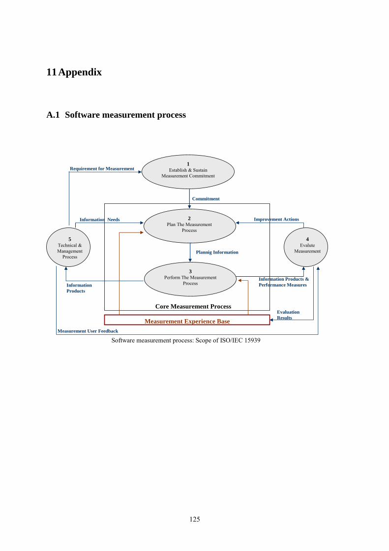
11 Appendix

A.1 Software measurement process

1Establish & Sustain

Measurement Commitment

2Plan The Measurement

Process

3Perform The Measurement

Process

4Evalute

Measurement

5Technical & Management

Process

Commitment

Plannig Information

Requirement for Measurement

Information Needs Improvement Actions

Core Measurement Process

Measurement Experience Base

Information Products & Performance MeasuresInformation

Products

Evaluation Results

Measurement User Feedback

Software measurement process: Scope of ISO/IEC 15939

125

A.2 Measurement result tables

A.2.1 List of software metrics applied

Scope applied in… Abb. Full name Program File Class Method

LOC (Physical) Lines of Code X X X NCLOC Non Comment Lines of Code X X X X #STAT Number of statements X X X HL Halstead Length X X LPM Lines (of code) per Method X X SPM Statements per Method X X #files Number of files X #methods Number of methods X X LPM>20 Percentage of methods with LPM bigger than 20 X Hvoc Halstead vocabulary X X HV Halstead Volume X X HD Halstead Difficulty X X HE Halstead Effort X X HV_N Normalized Halstead Volume X HE_N Normalized Halstead Effort X CR Comment Rate X X MI Maintainability Index (without comments) X X MIwc Maintainability Index (with comments) X X NBD Nesting Block Depth X X X BP Branch Percentage X X ECC Extended Cyclomatic Complexity X X X X ECC_N Normalized ECC X ECC>8 Percentage of methods with ECC bigger than 8 X ECC>10 Percentage of methods with ECC bigger than 10 X WMC Weighted Methods per Class X X DIT Depth of Inheritance Tree X X NOC Number of Children X X CBO Coupling Between Objects X X FI Fan In X X FO Fan Out X X IF4 Information Flow X X

126

A.2.2 Program size & code distribution pi

dla

nna

me

tota

l_LO

Cto

tal_

NC

LOC

tota

l_#S

TAT

tota

l_H

Lav

g_N

CLO

Cm

in_N

CLO

Cm

ax_N

CLO

Cst

dev_

NC

LOC

avg_

HL

avg_

LOC

avg_

#STA

Tav

g_LP

Mm

ax_L

PM#f

iles

#met

hods

LPM

>20

1C

GIM

P73

2157

5262

7929

0981

2755

645

255.

12

5586

429.

9513

35.7

435

4.89

141.

0427

.78

922

2063

1479

50.

422

CM

irand

a34

029

2882

323

892

1966

2029

4.11

112

1523

6.92

2006

.32

347.

2324

3.79

30.0

110

4198

892

0.35

3C

Nul

lWeb

mai

l99

1289

2569

6163

583

307.

7533

918

250.

0421

92.5

134

1.79

240.

0339

.78

255

2917

90.

584

CPa

nda

2604

913

848

6706

1489

8919

7.82

118

9528

4.21

2128

.41

372.

1295

.818

.90

326

7026

10.

225

CSD

CC

2076

9014

4892

9697

075

7764

728.

11

1107

716

81.2

638

07.8

510

43.6

648

7.28

33.4

417

6319

938

740.

446

CVI

M32

0531

2396

9312

3416

1111

573

2282

.79

016

512

2713

.82

1058

6.4

3082

.02

1186

.69

25.8

610

7010

415

920.

317

C++

7-Zi

p11

7789

9588

964

469

4690

6610

4.34

113

7616

9.52

510.

412

8.73

70.4

519

.93

459

915

4063

0.25

8C

++D

iskC

lean

er74

7054

3037

6525

748

93.6

21

824

158.

9444

3.93

128.

7964

.91

21.5

313

458

216

0.32

9C

++Em

ule

2216

4116

9635

1244

2794

7371

258.

190

4723

472.

1814

41.9

633

7.86

189.

6723

.37

2326

656

6395

0.28

10C

++Fi

leZi

lla11

2208

8193

458

600

4505

8227

8.68

149

2259

5.32

1532

.59

381.

6519

9.31

29.9

416

9129

418

810.

3411

C++

Hex

View

1856

1121

721

5131

70.0

61

528

127.

3232

0.68

116

45.0

614

.47

112

1666

0.23

12C

++N

otep

ad++

4823

335

677

2728

519

5363

251.

242

5711

591.

5113

75.7

933

9.66

192.

1437

.02

1444

142

893

0.45

13Ja

vaBo

nFor

um85

8440

7730

8621

545

239.

829

1287

367.

0112

67.3

550

4.94

181.

5221

.81

505

1718

00.

2414

Java

FitN

esse

3534

727

122

2039

913

8937

55.0

14

386

53.9

628

1.81

71.6

941

.37

7.45

8649

332

540.

0215

Java

HTM

L_U

nit

4248

214

188

1120

370

533

65.0

83

843

117.

3332

3.54

194.

8751

.38

6.08

9621

821

560.

0516

Java

Nek

oHTM

L11

482

6478

4890

3424

722

3.37

522

9843

1.68

1180

.93

395.

9316

8.62

13.5

418

129

414

0.17

17Ja

vaJs

ettle

rs56

768

3072

420

801

1545

1920

7.59

1034

6549

8.15

1044

.04

383.

5614

0.54

17.2

713

3814

816

820.

1718

Java

JSS

3029

1198

1762

8521

79.8

610

230

73.4

656

8.06

201.

9311

7.46

17.4

915

715

950.

2719

Java

CS.

PPS

1207

7876

338

6510

949

3258

207.

443

1678

692

5.08

1340

.37

328.

217

6.92

17.1

371

636

842

790.

2220

Java

A.O

OPJ

_L1_

st1

265

172

9652

986

2814

482

.02

264.

513

2.5

4810

.19

442

160.

0621

Java

A.O

OPJ

_L2_

st1

758

502

298

1868

100.

412

302

119.

5637

3.6

151.

659

.613

.94

535

340.

2622

Java

A.O

OPJ

_L3_

st1

1206

586

387

2921

58.6

715

839

.40

292.

112

0.6

38.7

6.63

2310

810.

0123

Java

A.O

OPJ

_L4_

st1

918

318

341

1358

39.7

523

5512

.43

169.

7570

.61

26.2

39.

2823

1329

0.07

24Ja

vaA.

OO

PJ_L

5_st

120

2111

4878

652

1854

.66

714

831

.66

248.

4796

.23

37.4

210

.40

4321

970.

1425

CB.

OS_

L1_s

t118

312

080

407

407

6830

.81

135.

6661

26.6

615

.17

363

60.

1726

CB.

OS_

L2_s

t130

619

716

974

649

.25

4554

4.03

186.

576

.542

.25

11.4

225

412

0.08

27C

B.O

S_L3

_st1

7652

4229

852

5252

-29

876

4214

.33

261

30.

3328

CB.

OS_

L4_s

t121

919

013

297

719

019

019

0-

977

219

132

35.4

094

15

0.40

29C

B.O

S_L5

_st1

358

301

193

1373

301

301

301

-13

7335

819

349

.67

921

60.

6730

C++

C.P

L_L1

_st1

1084

763

620

3884

54.5

828

169

.52

277.

4277

.42

44.2

812

.30

5414

540.

1131

CC

.PL_

L1_s

t298

369

256

429

7362

.910

259

77.9

827

0.27

89.3

651

.27

14.9

451

1134

0.24

32C

C.P

L_L1

_st3

837

652

549

3435

163

1742

719

0.04

858.

7520

9.25

137.

2519

.83

131

429

0.24

33C

++C

.PL_

L1_s

t410

2578

069

442

6065

1218

853

.16

355

85.4

157

.83

10.3

446

1265

0.11

34C

++C

.PL_

L1_s

t513

2610

5890

053

1848

.09

626

059

.78

241.

7260

.27

40.9

10.0

312

322

930.

0935

CC

.PL_

L1_s

t655

647

938

125

0895

.817

259

100.

2550

1.6

111.

276

.28.

0436

545

0.04

36C

++C

.PL_

L1_s

t739

233

122

715

3233

133

133

1-

1532

392

227

13.8

746

123

0.22

37C

D.C

C_L

2_te

ache

r13

3288

483

148

0817

6.8

563

326

2.43

961.

626

6.4

166.

29.

4838

575

0.12

38C

D.C

C_L

2_st

162

052

638

620

1752

652

652

6-

2017

620

386

18.0

440

128

0.39

39C

D.C

C_L

2_st

282

568

958

631

5313

7.8

656

023

8.44

630.

616

511

7.2

17.6

340

535

0.34

40C

D.C

C_L

2_st

362

555

754

920

2655

755

755

7-

2026

625

549

8.69

351

580.

0941

CD

.CC

_L2_

st4

986

755

662

4097

377.

580

675

420.

7320

48.5

493

331

14.7

935

242

0.29

42C

D.C

C_L

3_te

ache

r15

9610

8910

1059

5421

7.8

583

835

2.18

1190

.831

9.2

202

9.61

425

940.

1443

CD

.CC

_L3_

st1

620

526

386

2017

526

526

526

-20

1762

038

618

.04

401

280.

3944

CD

.CC

_L3_

st2

1091

883

761

4498

176.

66

716

304.

6489

9.6

218.

215

2.2

18.4

948

543

0.37

45C

D.C

C_L

3_st

310

5996

088

340

0796

096

096

0-

4007

1059

883

14.9

392

159

0.25

46C

D.C

C_L

3_st

413

7410

4488

359

0114

9.14

966

123

2.59

843

196.

2812

6.14

15.6

341

752

0.29

47C

D.C

C_L

4_te

ache

r62

044

837

523

1944

844

844

8-

2319

620

375

12.3

950

131

0.16

48C

D.C

C_L

4_st

144

036

330

421

1918

1.5

118

245

89.8

010

59.5

220

152

19.5

353

217

0.29

49C

D.C

C_L

4_st

258

747

538

325

8115

8.33

4329

912

9.87

860.

3319

5.66

127.

6615

.73

463

260.

3550

Java

D.C

C_L

4_st

354

036

533

628

5836

536

536

5-

2858

540

336

19.3

911

71

180.

3351

Java

D.C

C_L

4_st

471

652

843

532

1475

.42

1520

769

.71

459.

1410

2.28

62.1

411

.80

777

410.

1252

Java

D.O

OD

M_L

4_st

113

7667

640

125

8330

.72

712

629

.69

117.

462

.54

18.2

26.

7726

2287

0.05

53Ja

vaD

.OO

DM

_L4_

st2

1368

500

450

2594

17.2

44

6115

.82

89.4

447

.17

15.5

14.

1423

2910

00.

0154

Java

D.O

OD

M_L

4_st

318

5855

848

832

3421

.46

775

17.7

812

4.38

71.4

618

.76

4.79

2926

100

0.03

55Ja

vaD

.OO

DM

_L4_

st4

1448

684

481

2781

23.5

85

9422

.85

95.8

949

.93

16.5

87.

7867

2977

0.13

56Ja

vaD

.OO

DM

_L4_

st5

1386

552

427

3085

29.0

511

150

31.3

016

2.36

72.9

422

.47

4.99

3019

980.

06

127

A.2.3 Textual code complexity and code maintainability V

pid

lan

nam

eto

tal_

Hvo

cav

g_H

voc

tota

l_H

avg_

HV

tota

l_H

Dav

g_H

Dto

tal_

HE

avg_

HE

HE_

NH

V_N

avg_

CR

avg_

MI

stde

v_M

Iav

g_M

Iwc

1C

GIM

P28

3860

137.

5922

4480

6910

881.

2795

796

46.4

377

7806

2667

3770

267.

914

779.

3542

.65

0.12

73.9

415

.72

105.

252

CM

irand

a23

453

239.

3116

3159

716

648.

9472

0173

.47

1691

1006

217

2561

2.9

5867

.19

56.6

10.

0971

.89

18.9

697

.79

3C

Nul

lWeb

mai

l65

2422

4.96

5153

6217

771.

123

7982

.03

6465

3276

2229

423.

372

44.0

657

.74

0.16

54.3

719

.90

81.7

54

CPa

nda

1118

815

9.82

1115

848

1594

0.68

3380

48.2

856

4495

518

8064

221.

740

763.

6980

.58

0.41

52.4

536

.94

90.8

45

CSD

CC

4636

823

372

3271

236

345.

2815

393

77.3

523

7354

4889

1192

7361

.316

381.

4849

.92

0.19

75.0

121

.65

103.

476

CVI

M75

169

715.

8911

3045

7610

7662

.62

1401

313

3.45

2552

9867

9424

3141

59.9

1065

1.07

47.1

60.

2023

.96

45.0

556

.81

7C

++7-

Zip

8077

387

.89

3545

186

3857

.65

3073

733

.44

3478

7745

737

8539

.136

27.9

236

.97

0.07

90.7

623

.64

109.

478

C++

Dis

kCle

aner

4917

84.7

719

3799

3341

.36

1413

24.3

613

6220

3623

4862

.725

08.6

635

.69

0.12

87.4

419

.87

113.

319

C++

Emul

e12

6459

192.

4783

0728

712

644.

2732

321

49.1

910

5652

4874

1608

104.

862

28.2

248

.97

0.14

75.2

619

.49

104.

7510

C++

File

Zilla

6085

620

6.99

4039

110

1373

8.46

1275

143

.37

5538

3933

418

8380

7.3

6759

.58

49.3

00.

1663

.78

25.5

098

.23

11C

++H

exVi

ew11

5772

.31

3822

223

88.8

732

820

.50

3012

977

1883

11.1

2687

.76

34.1

00.

2686

.81

13.9

012

6.81

12C

++N

otep

ad++

2544

817

9.21

1726

844

1216

0.87

6768

47.6

621

4834

473

1512

918.

860

21.6

548

.40

0.12

69.4

819

.94

99.0

413

Java

BonF

orum

2459

144.

6417

5778

1033

9.88

793

46.6

419

1698

4611

2763

8.0

4701

.95

43.1

10.

4477

.17

20.3

411

4.23

14Ja

vaFi

tNes

se31

875

64.6

591

2566

1851

.04

9000

18.2

526

3153

9353

378.

197

0.26

33.6

50.

0210

7.19

10.5

210

9.02

15Ja

vaH

TML_

Uni

t14

540

66.6

951

0462

2341

.56

4096

18.7

825

0853

2311

5070

.317

68.0

735

.98

0.53

101.

728.

2814

5.99

16Ja

vaN

ekoH

TML

3919

135.

1328

1373

9702

.51

1400

48.2

733

0384

7411

3925

7.7

5100

.10

43.4

40.

3287

.58

17.3

412

8.48

17Ja

vaJs

ettle

rs14

687

99.2

312

9869

787

74.9

756

7738

.35

1891

1060

812

7777

4.4

6155

.14

42.2

70.

3095

.56

14.7

413

5.70

18Ja

vaJS

S15

2810

1.86

6093

840

62.5

345

030

.00

2908

658

1939

10.5

2427

.93

50.8

70.

2576

.53

10.5

611

1.80

19Ja

vaC

S.PP

S52

302

142.

1243

7117

811

878.

215

403

41.8

569

3377

956

1884

179.

290

83.0

057

.26

0.20

80.2

624

.84

103.

9820

Java

A.O

OPJ

_L1_

st1

118

5933

0816

5447

23.5

011

4137

5706

8.5

663.

5919

.23

0.26

102.

5013

.44

140.

0021

Java

A.O

OPJ

_L2_

st1

327

65.4

1276

525

5314

428

.80

6730

4213

4608

.413

40.7

225

.43

0.25

97.2

010

.71

136.

8022

Java

A.O

OPJ

_L3_

st1

608

60.8

1820

518

20.5

186

18.6

049

0289

4902

8.9

836.

6731

.07

0.37

101.

907.

0313

9.10

23Ja

vaA.

OO

PJ_L

4_st

147

859

.75

8171

1021

.37

134

16.7

514

7749

1846

8.6

464.

6225

.69

0.30

93.8

75.

3013

2.75

24Ja

vaA.

OO

PJ_L

5_st

113

1162

.42

3234

515

40.2

342

720

.33

7915

7137

693.

968

9.52

28.1

80.

3091

.76

11.9

213

0.19

25C

B.O

S_L1

_st1

139

46.3

324

3381

145

15.0

058

424

1947

4.7

486.

8720

.28

0.26

89.3

317

.16

126.

3326

CB.

OS_

L2_s

t120

551

.25

4243

1060

.75

6817

.00

7325

418

313.

537

1.85

21.5

40.

1487

.50

1.91

115.

5027

CB.

OS_

L3_s

t171

7118

3318

3335

35.0

065

039

6503

9.0

1250

.75

35.2

50.

2185

.00

-11

7.00

28C

B.O

S_L4

_st1

102

102

6519

6519

7878

.00

5095

9450

9594

.026

82.0

734

.31

0.00

71.0

0-

78.0

029

CB.

OS_

L5_s

t179

7986

5586

5515

615

6.00

1350

194

1350

194.

044

85.6

928

.75

0.09

65.0

0-

87.0

030

C++

C.P

L_L1

_st1

790

56.4

224

827

1773

.35

384

27.4

212

4310

088

792.

916

29.2

332

.54

0.14

82.5

711

.93

109.

1431

CC

.PL_

L1_s

t264

658

.72

1917

817

43.4

524

422

.18

7193

3465

394.

010

39.5

027

.71

0.09

82.6

312

.77

105.

7232

CC

.PL_

L1_s

t343

010

7.5

2563

864

09.5

194

48.5

027

0676

067

6690

.041

51.4

739

.32

0.03

82.2

514

.38

90.7

533

C++

C.P

L_L1

_st4

789

65.7

527

265

2272

.08

394

32.8

313

5232

211

2693

.517

33.7

534

.96

0.10

85.5

014

.90

102.

6634

C++

C.P

L_L1

_st5

1186

53.9

3431

115

59.5

960

727

.59

1874

811

8521

8.7

1772

.03

32.4

30.

1093

.59

15.1

511

4.00

35C

C.P

L_L1

_st6

409

81.8

1728

834

57.6

160

32.0

097

0672

1941

34.4

2026

.46

36.0

90.

0088

.40

14.6

094

.60

36C

++C

.PL_

L1_s

t714

314

310

969

1096

985

85.0

093

6159

9361

59.0

2828

.27

33.1

40.

0092

.00

-99

.00

37C

D.C

C_L

2_te

ache

r66

313

2.6

3876

777

53.4

122

24.4

019

8221

439

6442

.822

42.3

243

.85

0.14

89.0

014

.02

123.

2038

CD

.CC

_L2_

st1

205

205

1549

015

490

8282

.00

1263

944

1263

944.

024

02.9

429

.45

0.02

87.0

0-

100.

0039

CD

.CC

_L2_

st2

447

89.4

2415

748

31.4

133

26.6

013

0480

926

0961

.818

93.7

735

.06

0.05

93.4

013

.81

101.

2040

CD

.CC

_L2_

st3

231

231

1590

815

908

2727

.00

4273

5442

7354

.076

7.24

28.5

60.

0110

3.00

-11

2.00

41C

D.C

C_L

2_st

445

722

8.5

3376

316

881.

511

356

.50

3204

983

1602

491.

542

45.0

144

.72

0.10

70.5

021

.92

94.5

042

CD

.CC

_L3_

teac

her

783

156.

650

412

1008

2.4

146

29.2

035

9107

571

8215

.032

97.5

946

.29

0.13

89.4

014

.01

123.

4043

CD

.CC

_L3_

st1

205

205

1549

015

490

8282

.00

1263

944

1263

944.

024

02.9

429

.45

0.02

87.0

0-

100.

0044

CD

.CC

_L3_

st2

532

106.

435

949

7189

.817

835

.60

3042

870

6085

74.0

3446

.06

40.7

10.

0591

.60

16.6

198

.80

45C

D.C

C_L

3_st

334

234

233

730

3373

085

85.0

028

6266

028

6266

0.0

2981

.94

35.1

40.

0890

.00

-11

2.00

46C

D.C

C_L

3_st

478

611

2.28

4609

665

85.1

421

931

.28

3766

006

5380

00.9

3607

.29

44.1

50.

0981

.42

15.9

010

0.42

47C

D.C

C_L

4_te

ache

r25

925

918

591

1859

185

85.0

015

8725

615

8725

6.0

3542

.98

41.5

00.

1289

.00

-11

5.00

48C

D.C

C_L

4_st

126

613

314

988

7494

136

68.0

010

6379

653

1898

.029

30.5

741

.29

0.11

83.0

05.

6610

0.50

49C

D.C

C_L

4_st

234

011

3.33

1822

660

75.3

315

451

.33

1220

358

4067

86.0

2569

.17

38.3

70.

0581

.66

14.0

193

.33

50Ja

vaD

.CC

_L4_

st3

148

148

2060

520

605

179

179.

0036

8778

636

8778

6.0

1010

3.52

56.4

50.

0079

.00

-84

.00

51Ja

vaD

.CC

_L4_

st4

486

69.4

221

166

3023

.71

245

35.0

012

7661

318

2373

.324

17.8

340

.09

0.13

98.0

013

.89

124.

0052

Java

D.O

OD

M_L

4_st

172

933

.13

1467

466

736

116

.40

4683

4921

288.

669

2.82

21.7

10.

4510

0.50

5.89

144.

9553

Java

D.O

OD

M_L

4_st

285

929

.62

1398

748

2.31

345

11.8

928

8701

9955

.257

7.40

27.9

70.

4310

4.20

8.58

148.

0054

Java

D.O

OD

M_L

4_st

395

936

.88

1830

670

4.07

387

14.8

846

6933

1795

9.0

836.

8032

.81

0.55

98.8

47.

6114

5.42

55Ja

vaD

.OO

DM

_L4_

st4

806

27.7

915

161

522.

7938

613

.31

4397

3415

163.

264

2.89

22.1

70.

3810

0.24

10.4

014

2.96

56Ja

vaD

.OO

DM

_L4_

st5

792

41.6

818

016

948.

2136

119

.00

6382

2433

590.

711

56.2

032

.64

0.48

104.

948.

2815

0.00

128

A.2.4 Structural code complexity

pid

lan

nam

eav

g_N

BD

max

_NB

Dav

g_B

Pav

g_m

etho

d_EC

Cm

ax_m

etho

d_EC

Cto

tal_

ECC

avg_

File

_EC

Cm

ax_F

ile_E

CC

stde

v_EC

CEC

C_N

ECC

>8EC

C>1

01

CG

IMP

1.57

100.

184.

0414

350

842

24.6

490

152

.53

0.10

0.11

0.08

2C

Mira

nda

2.65

100.

287.

8927

762

6363

.931

361

.35

0.22

0.22

0.17

3C

Nul

lWeb

mai

l1.

848

0.23

13.4

111

124

2183

.48

306

89.6

60.

270.

420.

384

CPa

nda

0.79

100.

073.

1551

1751

25.0

132

656

.21

0.13

0.09

0.07

5C

SDC

C2.

1910

0.30

8.99

466

3204

316

1.02

2259

367.

280.

220.

280.

226

CVI

M2.

2510

0.28

6.56

352

5954

856

7.12

3582

721.

560.

250.

180.

147

C++

7-Zi

p1.

6510

0.19

3.96

9414

212

15.4

627

830

.36

0.15

0.10

0.08

8C

++D

iskC

lean

er1.

658

0.18

3.85

2272

112

.43

131

23.2

90.

130.

120.

099

C++

Emul

e2.

0310

0.21

5.18

515

2875

643

.76

1284

105.

340.

170.

130.

1010

C++

File

Zilla

1.71

100.

176.

5047

411

932

40.5

812

4812

5.35

0.15

0.18

0.15

11C

++H

exVi

ew1.

326

0.15

2.27

1911

87.

3759

14.1

40.

110.

030.

0312

C++

Not

epad

++2.

2910

0.25

7.25

268

5836

41.0

911

9812

3.12

0.16

0.21

0.15

13Ja

vaBo

nFor

um2.

8110

0.25

5.09

104

753

44.2

921

968

.05

0.18

0.11

0.09

14Ja

vaFi

tNes

se1.

586

0.05

1.33

4015

803.

241

4.40

0.06

0.00

0.00

15Ja

vaH

TML_

Uni

t1.

778

0.13

1.64

2516

007.

3315

716

.96

0.11

0.01

0.01

16Ja

vaN

ekoH

TML

2.86

100.

213.

8144

1205

41.5

555

710

4.08

0.19

0.11

0.07

17Ja

vaJs

ettle

rs3.

1410

0.22

3.59

386

4506

30.4

461

392

.57

0.15

0.06

0.05

18Ja

vaJS

S2.

578

0.10

3.37

2017

711

.844

11.6

60.

150.

110.

0819

Java

CS.

PPS

2.61

100.

102.

8572

8256

22.4

313

6981

.21

0.11

0.06

0.04

20Ja

vaA.

OO

PJ_L

1_st

12.

215

0.31

2.00

1018

917

11.3

10.

100.

060.

0021

Java

A.O

OPJ

_L2_

st1

2.56

80.

242.

4413

5410

.836

14.7

90.

110.

030.

0322

Java

A.O

OPJ

_L3_

st1

1.56

50.

031.

124

202

72.

160.

030.

000.

0023

Java

A.O

OPJ

_L4_

st1

1.6

40.

091.

664

273.

377

1.77

0.08

0.00

0.00

24Ja

vaA.

OO

PJ_L

5_st

11.

926

0.11

1.84

810

24.

8516

4.05

0.09

0.00

0.00

25C

B.O

S_L1

_st1

0.88

30.

163.

339

175.

6613

6.35

0.14

0.17

0.00

26C

B.O

S_L2

_st1

0.8

20.

072.

085

174.

255

0.50

0.09

0.00

0.00

27C

B.O

S_L3

_st1

1.02

30.

143.

005

77

7-

0.13

0.00

0.00

28C

B.O

S_L4

_st1

2.02

60.

227.

4019

3333

33-

0.17

0.20

0.20

29C

B.O

S_L5

_st1

3.51

70.

2810

.50

1958

5858

-0.

190.

500.

5030

C++

C.P

L_L1

_st1

1.22

40.

162.

7810

118

8.42

5313

.73

0.15

0.02

0.00

31C

C.P

L_L1

_st2

1.14

40.

214.

1515

124

11.2

759

18.2

20.

180.

090.

0932

CC

.PL_

L1_s

t31.

656

0.22

4.90

4111

929

.75

6526

.89

0.18

0.10

0.10

33C

++C

.PL_

L1_s

t41.

145

0.13

2.48

1811

49.

543

12.7

50.

150.

020.

0234

C++

C.P

L_L1

_st5

1.34

50.

192.

6526

187

8.5

6114

.98

0.18

0.02

0.02

35C

C.P

L_L1

_st6

1.06

40.

192.

3810

6913

.837

15.9

40.

140.

020.

0036

C++

C.P

L_L1

_st7

1.5

50.

183.

2611

5454

54-

0.16

0.04

0.04

37C

D.C

C_L

2_te

ache

r1.

235

0.20

3.07

1316

032

132

56.5

80.

180.

040.

0138

CD

.CC

_L2_

st1

1.61

40.

243.

7911

7979

79-

0.15

0.04

0.04

39C

D.C

C_L

2_st

21.

364

0.28

4.89

1014

328

.612

352

.97

0.21

0.14

0.00

40C

D.C

C_L

2_st

31.

243

0.33

3.41

914

714

714

7-

0.26

0.03

0.00

41C

D.C

C_L

2_st

41.

594

0.31

4.93

3316

884

166

115.

970.

220.

100.

0742

CD

.CC

_L3_

teac

her

1.2

50.

182.

7613

170

3414

261

.00

0.16

0.03

0.01

43C

D.C

C_L

3_st

11.

614

0.24

3.79

1179

7979

-0.

150.

040.

0444

CD

.CC

_L3_

st2

1.37

40.

234.

5313

159

31.8

135

58.0

40.

180.

140.

0945

CD

.CC

_L3_

st3

1.54

50.

335.

1725

253

253

253

-0.

260.

150.

1446

CD

.CC

_L3_

st4

1.54

40.

264.

6534

201

28.7

115

857

.86

0.19

0.10

0.06

47C

D.C

C_L

4_te

ache

r1.

324

0.26

3.55

1680

8080

-0.

180.

100.

0648

CD

.CC

_L4_

st1

1.83

50.

416.

2919

9246

471.

410.

250.

240.

1849

CD

.CC

_L4_

st2

1.16

30.

173.

4219

6722

.33

4521

.59

0.14

0.04

0.04

50Ja

vaD

.CC

_L4_

st3

2.97

70.

184.

6737

6767

67-

0.18

0.06

0.06

51Ja

vaD

.CC

_L4_

st4

2.12

50.

142.

6825

7610

.85

3913

.17

0.14

0.02

0.02

52Ja

vaD

.OO

DM

_L4_

st1

1.85

50.

241.

779

894.

0417

5.01

0.13

0.01

0.00

53Ja

vaD

.OO

DM

_L4_

st2

1.51

50.

141.

5721

862.

9624

4.58

0.17

0.01

0.01

54Ja

vaD

.OO

DM

_L4_

st3

1.48

50.

101.

477

732.

810

2.28

0.13

0.00

0.00

55Ja

vaD

.OO

DM

_L4_

st4

2.09

60.

192.

2925

128

4.41

337.

620.

190.

060.

0456

Java

D.O

OD

M_L

4_st

51.

796

0.18

1.84

3010

15.

3132

9.53

0.18

0.02

0.01

129

A.2.5 Object oriented aspects pi

dla

nna

me

tota

l_W

MC

avg_

WM

Cto

tal_

DIT

avg_

DIT

max

_DIT

tota

l_N

OC

avg_

NO

Cm

ax_N

OC

tota

l_C

BO

avg_

CB

Om

ax_C

BO

tota

l_FI

/FO

avg_

FI/F

Om

ax_F

Im

ax_F

Oto

tal_

IFav

g_IF

max

_IF

1C

GIM

P13

024

230

00

00

00

00

00

00

00

02

CM

irand

a68

014

00

00

00

00

00

00

00

00

3C

Nul

lWeb

mai

l35

911

90

00

00

00

00

00

00

00

04

CPa

nda

517

70

00

00

00

00

00

00

00

05

CSD

CC

2520

504

00

00

00

00

00

00

00

00

6C

VIM

472

50

00

00

00

00

00

00

00

07

C++

7-Zi

p38

156

219

04

323

071

3530

512

417

652

124

5381

5041

1358

4044

968

C++

Dis

kCle

aner

144

57

01

70

442

16

210

66

00

09

C++

Emul

e68

379

250

06

213

016

4734

612

223

673

122

3878

3824

1139

4928

0410

C++

File

Zilla

4674

1411

40

291

021

1624

564

812

264

3737

098

116

9216

11C

++H

exVi

ew59

18

01

80

254

18

270

38

00

012

C++

Not

epad

++14

347

101

03

640

2095

25

4347

62

4339

3736

519

811

664

13Ja

vaBo

nFor

um18

03

130

113

04

154

315

771

1511

2850

6019

3614

Java

FitN

esse

3237

569

01

646

60

6941

207

312

2060

331

215

2808

403

4833

1703

025

15Ja

vaH

TML_

Uni

t21

646

661

27

214

046

2348

718

411

743

184

3067

7549

621

441

6285

049

16Ja

vaN

ekoH

TML

362

337

03

270

650

04

3025

02

3025

1169

911

192

1617

Java

Jset

tlers

1674

719

90

215

50

7015

827

110

791

311

072

3215

7014

6882

944

18Ja

vaJS

S10

01

170

117

06

190

314

951

108

2112

3916

0019

Java

CS.

PPS

4220

848

30

329

80

175

3144

622

215

723

222

5850

4280

310

249

4120

900

20Ja

vaA.

OO

PJ_L

1_st

116

20

00

00

010

13

50

13

40

421

Java

A.O

OPJ

_L2_

st1

343

00

00

00

222

411

13

49

04

22Ja

vaA.

OO

PJ_L

3_st

182

411

02

80

484

412

422

1012

428

2525

623

Java

A.O

OPJ

_L4_

st1

311

60

113

03

843

1142

14

1037

817

144

24Ja

vaA.

OO

PJ_L

5_st

198

213

02

150

519

24

1396

213

1310

1322

576

25C

B.O

S_L1

_st1

55

00

00

00

00

00

00

00

00

26C

B.O

S_L2

_st1

66

00

00

00

00

00

00

00

00

27C

B.O

S_L3

_st1

33

00

00

00

00

00

00

00

00

28C

B.O

S_L4

_st1

55

00

00

00

00

00

00

00

00

29C

B.O

S_L5

_st1

66

00

00

00

00

00

00

00

00

30C

++C

.PL_

L1_s

t156

50

00

00

028

27

141

47

191

931

CC

.PL_

L1_s

t234

340

00

00

00

00

00

00

00

032

CC

.PL_

L1_s

t329

290

00

00

00

00

00

00

00

033

C++

C.P

L_L1

_st4

626

00

00

00

242

512

13

535

316

34C

++C

.PL_

L1_s

t578

70

00

00

028

27

141

54

124

1210

035

CC

.PL_

L1_s

t644

440

00

00

00

00

00

00

00

036

C++

C.P

L_L1

_st7

224

00

00

00

81

44

01

40

00

37C

D.C

C_L

2_te

ache

r75

750

00

00

00

00

00

00

00

038

CD

.CC

_L2_

st1

2814

00

00

00

00

00

00

00

00

39C

D.C

C_L

2_st

26

60

00

00

00

00

00

00

00

040

CD

.CC

_L2_

st3

1111

00

00

00

00

00

00

00

00

41C

D.C

C_L

2_st

441

410

00

00

00

00

00

00

00

042

CD

.CC

_L3_

teac

her

9494

00

00

00

00

00

00

00

00

43C

D.C

C_L

3_st

128

140

00

00

00

00

00

00

00

044

CD

.CC

_L3_

st2

2525

00

00

00

00

00

00

00

00

45C

D.C

C_L

3_st

311

110

00

00

00

00

00

00

00

046

CD

.CC

_L3_

st4

5454

00

00

00

00

00

00

00

00

47C

D.C

C_L

4_te

ache

r31

310

00

00

00

00

00

00

00

048

CD

.CC

_L4_

st1

1717

00

00

00

00

00

00

00

00

49C

D.C

C_L

4_st

213

130

00

00

00

00

00

00

00

050

Java

D.C

C_L

4_st

318

40

00

00

06

13

30

13

00

051

Java

D.C

C_L

4_st

441

30

00

00

046

47

232

56

216

1964

52Ja

vaD

.OO

DM

_L4_

st1

692

150

115

07

112

413

562

117

1089

4048

453

Java

D.O

OD

M_L

4_st

210

12

370

323

06

172

415

862

158

5712

146

2025

54Ja

vaD

.OO

DM

_L4_

st3

872

190

119

07

150

312

751

117

1469

3710

2455

Java

D.O

OD

M_L

4_st

477

236

12

230

613

64

1568

215

527

0982

1600

56Ja

vaD

.OO

DM

_L4_

st5

984

120

112

04

130

518

652

146

6061

275

3136

130

A.3 Measurement result diagrams

A.3.1 Line diagrams

Industry: total_LOC

0

100000

200000

300000

400000

500000

600000

700000

800000

1 2 3 4 5 6 7 8 9 10 11 12 13 14 15 16 17 18 19

Student: total_LOC

0

500

1000

1500

2000

2500

20 22 24 26 28 30 32 34 36 38 40 42 44 46 48 50 52 54 56

Student: total_NCLOC

0

200

400

600

800

1000

1200

1400

20 22 24 26 28 30 32 34 36 38 40 42 44 46 48 50 52 54 56

Industry: total_NCLOC

0

100000

200000

300000

400000

500000

600000

1 2 3 4 5 6 7 8 9 10 11 12 13 14 15 16 17 18 19

Industry: total_#STAT

0

50000

100000

150000

200000

250000

300000

350000

1 2 3 4 5 6 7 8 9 10 11 12 13 14 15 16 17 18 19

Student: total_#STAT

0

200

400

600

800

1000

1200

20 22 24 26 28 30 32 34 36 38 40 42 44 46 48 50 52 54 56

131

Industry: total_HL

0

500000

1000000

1500000

2000000

2500000

3000000

1 2 3 4 5 6 7 8 9 10 11 12 13 14 15 16 17 18 19

Student: total_HL

0

1000

2000

3000

4000

5000

6000

7000

20 22 24 26 28 30 32 34 36 38 40 42 44 46 48 50 52 54 56

Industry: avg_NCLOC

0

500

1000

1500

2000

2500

1 2 3 4 5 6 7 8 9 10 11 12 13 14 15 16 17 18 19

Student: avg_NCLOC

0

200

400

600

800

1000

1200

20 22 24 26 28 30 32 34 36 38 40 42 44 46 48 50 52 54 56

Industry: min_NCLOC

0

5

10

15

20

25

30

35

1 2 3 4 5 6 7 8 9 10 11 12 13 14 15 16 17 18 19

Student: min_NCLOC

0

200

400

600

800

1000

1200

20 22 24 26 28 30 32 34 36 38 40 42 44 46 48 50 52 54 56

Industry: max_NCLOC

0

2000

4000

6000

8000

10000

12000

14000

16000

18000

1 2 3 4 5 6 7 8 9 10 11 12 13 14 15 16 17 18 19

Student: max_NCLOC

0

200

400

600

800

1000

1200

20 22 24 26 28 30 32 34 36 38 40 42 44 46 48 50 52 54 56

132

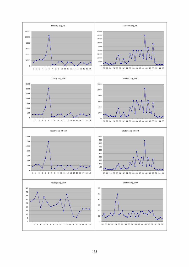
Industry: avg_HL

0

2000

4000

6000

8000

10000

12000

1 2 3 4 5 6 7 8 9 10 11 12 13 14 15 16 17 18 19

Student: avg_HL

0

500

1000

1500

2000

2500

3000

3500

4000

4500

20 22 24 26 28 30 32 34 36 38 40 42 44 46 48 50 52 54 56

Industry: avg_LOC

0

500

1000

1500

2000

2500

3000

3500

1 2 3 4 5 6 7 8 9 10 11 12 13 14 15 16 17 18 19

Student: avg_LOC

0

200

400

600

800

1000

1200

20 22 24 26 28 30 32 34 36 38 40 42 44 46 48 50 52 54 56

Industry: avg_#STAT

0

200

400

600

800

1000

1200

1400

1 2 3 4 5 6 7 8 9 10 11 12 13 14 15 16 17 18 19

Student: avg_#STAT

0

100

200

300

400

500

600

700

800

900

1000

20 22 24 26 28 30 32 34 36 38 40 42 44 46 48 50 52 54 56

Industry: avg_LPM

0

5

10

15

20

25

30

35

40

45

1 2 3 4 5 6 7 8 9 10 11 12 13 14 15 16 17 18 19

Student: avg_LPM

0

10

20

30

40

50

60

20 22 24 26 28 30 32 34 36 38 40 42 44 46 48 50 52 54 56

133

Industry: max_LPM

0

500

1000

1500

2000

2500

1 2 3 4 5 6 7 8 9 10 11 12 13 14 15 16 17 18 19

Student: max_LPM

0

20

40

60

80

100

120

140

20 22 24 26 28 30 32 34 36 38 40 42 44 46 48 50 52 54 56

Industry: LPM>20

0

0.1

0.2

0.3

0.4

0.5

0.6

0.7

1 2 3 4 5 6 7 8 9 10 11 12 13 14 15 16 17 18 19

Student: LPM>20

0

0.1

0.2

0.3

0.4

0.5

0.6

0.7

20 22 24 26 28 30 32 34 36 38 40 42 44 46 48 50 52 54 56

Industry: #files

0

500

1000

1500

2000

2500

1 2 3 4 5 6 7 8 9 10 11 12 13 14 15 16 17 18 19

Student: #files

0

5

10

15

20

25

30

35

20 22 24 26 28 30 32 34 36 38 40 42 44 46 48 50 52 54 56

Industry: #methods

0

2000

4000

6000

8000

10000

12000

14000

16000

1 2 3 4 5 6 7 8 9 10 11 12 13 14 15 16 17 18 19

Student: #methods

0

20

40

60

80

100

120

20 22 24 26 28 30 32 34 36 38 40 42 44 46 48 50 52 54 56

134

Industry: total_Hvoc

0

50000

100000

150000

200000

250000

300000

1 2 3 4 5 6 7 8 9 10 11 12 13 14 15 16 17 18 19

Student: total_Hvoc

0

200

400

600

800

1000

1200

1400

20 22 24 26 28 30 32 34 36 38 40 42 44 46 48 50 52 54 56

Industry: avg_Hvoc

0

100

200

300

400

500

600

700

800

1 2 3 4 5 6 7 8 9 10 11 12 13 14 15 16 17 18 19

Student: avg_Hvoc

0

50

100

150

200

250

300

350

400

20 22 24 26 28 30 32 34 36 38 40 42 44 46 48 50 52 54 56

Industry: total_HV

0

5000000

10000000

15000000

20000000

25000000

1 2 3 4 5 6 7 8 9 10 11 12 13 14 15 16 17 18 19

Student: total_HV

0

10000

20000

30000

40000

50000

60000

20 22 24 26 28 30 32 34 36 38 40 42 44 46 48 50 52 54 56

Industry: avg_HV

0

20000

40000

60000

80000

100000

120000

1 2 3 4 5 6 7 8 9 10 11 12 13 14 15 16 17 18 19

Student: avg_HV

0

5000

10000

15000

20000

25000

30000

35000

40000

20 22 24 26 28 30 32 34 36 38 40 42 44 46 48 50 52 54 56

135

Industry: total_HD

0

20000

40000

60000

80000

100000

120000

1 2 3 4 5 6 7 8 9 10 11 12 13 14 15 16 17 18 19

Student: total_HD

0

100

200

300

400

500

600

700

20 22 24 26 28 30 32 34 36 38 40 42 44 46 48 50 52 54 56

Industry: avg_HD

0

20

40

60

80

100

120

140

160

1 2 3 4 5 6 7 8 9 10 11 12 13 14 15 16 17 18 19

Student: avg_HD

0

20

40

60

80

100

120

140

160

180

200

20 22 24 26 28 30 32 34 36 38 40 42 44 46 48 50 52 54 56

Industry: total_HE

0

1000000000

2000000000

3000000000

4000000000

5000000000

6000000000

7000000000

8000000000

9000000000

1 2 3 4 5 6 7 8 9 10 11 12 13 14 15 16 17 18 19

Student: total_HE

0

500000

1000000

1500000

2000000

2500000

3000000

3500000

4000000

20 22 24 26 28 30 32 34 36 38 40 42 44 46 48 50 52 54 56

Industry: avg_HE

0

5000000

10000000

15000000

20000000

25000000

30000000

1 2 3 4 5 6 7 8 9 10 11 12 13 14 15 16 17 18 19

Student: avg_HE

0

500000

1000000

1500000

2000000

2500000

3000000

3500000

4000000

20 22 24 26 28 30 32 34 36 38 40 42 44 46 48 50 52 54 56

136

Industry: HV_N

0

10

20

30

40

50

60

70

80

90

1 2 3 4 5 6 7 8 9 10 11 12 13 14 15 16 17 18 19

Student: HV_N

0

10

20

30

40

50

60

20 22 24 26 28 30 32 34 36 38 40 42 44 46 48 50 52 54 56

Industry: HE_N

0

5000

10000

15000

20000

25000

30000

35000

40000

45000

1 2 3 4 5 6 7 8 9 10 11 12 13 14 15 16 17 18 19

Student: HE_N

0

2000

4000

6000

8000

10000

12000

20 22 24 26 28 30 32 34 36 38 40 42 44 46 48 50 52 54 56

Industry: avg_NBD

0

0.5

1

1.5

2

2.5

3

3.5

1 2 3 4 5 6 7 8 9 10 11 12 13 14 15 16 17 18 19

Student: avg_NBD

0

0.5

1

1.5

2

2.5

3

3.5

4

20 22 24 26 28 30 32 34 36 38 40 42 44 46 48 50 52 54 56

Industry: max_NBD

0

2

4

6

8

10

12

1 2 3 4 5 6 7 8 9 10 11 12 13 14 15 16 17 18 19

Student: max_NBD

0

2

4

6

8

10

12

20 22 24 26 28 30 32 34 36 38 40 42 44 46 48 50 52 54 56

137

Industry: avg_BP

0

0.05

0.1

0.15

0.2

0.25

0.3

0.35

0.4

0.45

1 2 3 4 5 6 7 8 9 10 11 12 13 14 15 16 17 18 19

Student: avg_BP

0

0.05

0.1

0.15

0.2

0.25

0.3

0.35

0.4

0.45

20 22 24 26 28 30 32 34 36 38 40 42 44 46 48 50 52 54 56

Industry: avg_method_ECC

0

2

4

6

8

10

12

14

16

1 2 3 4 5 6 7 8 9 10 11 12 13 14 15 16 17 18 19

Student: avg_method_ECC

0

2

4

6

8

10

12

14

16

20 22 24 26 28 30 32 34 36 38 40 42 44 46 48 50 52 54 56

Industry: max_method_ECC

0

100

200

300

400

500

600

1 2 3 4 5 6 7 8 9 10 11 12 13 14 15 16 17 18 19

Student: max_method_ECC

0

20

40

60

80

100

20 22 24 26 28 30 32 34 36 38 40 42 44 46 48 50 52 54 56

Industry: avg_File_ECC

0

100

200

300

400

500

600

1 2 3 4 5 6 7 8 9 10 11 12 13 14 15 16 17 18 19

Student: avg_File_ECC

0

50

100

150

200

250

300

20 22 24 26 28 30 32 34 36 38 40 42 44 46 48 50 52 54 56

138

Industry: max_File_ECC

0

500

1000

1500

2000

2500

3000

3500

4000

1 2 3 4 5 6 7 8 9 10 11 12 13 14 15 16 17 18 19

Student: max_File_ECC

0

50

100

150

200

250

300

20 22 24 26 28 30 32 34 36 38 40 42 44 46 48 50 52 54 56

Industry: total_ECC

0

10000

20000

30000

40000

50000

60000

70000

1 2 3 4 5 6 7 8 9 10 11 12 13 14 15 16 17 18 19

Student: total_ECC

0

50

100

150

200

250

300

20 22 24 26 28 30 32 34 36 38 40 42 44 46 48 50 52 54 56

Industry: ECC_N

0

0.05

0.1

0.15

0.2

0.25

0.3

1 2 3 4 5 6 7 8 9 10 11 12 13 14 15 16 17 18 19

Student: ECC_N

0

0.05

0.1

0.15

0.2

0.25

0.3

20 22 24 26 28 30 32 34 36 38 40 42 44 46 48 50 52 54 56

Industry: ECC>8

0

0.1

0.2

0.3

0.4

0.5

1 2 3 4 5 6 7 8 9 10 11 12 13 14 15 16 17 18 19

Student: ECC>8

0

0.05

0.1

0.15

0.2

0.25

0.3

0.35

0.4

0.45

0.5

20 22 24 26 28 30 32 34 36 38 40 42 44 46 48 50 52 54 56

139

Industry: ECC>10

0

0.1

0.2

0.3

0.4

0.5

1 2 3 4 5 6 7 8 9 10 11 12 13 14 15 16 17 18 19

Student: ECC>10

0

0.05

0.1

0.15

0.2

0.25

0.3

0.35

0.4

0.45

0.5

20 22 24 26 28 30 32 34 36 38 40 42 44 46 48 50 52 54 56

Industry: avg_CR

0

0.1

0.2

0.3

0.4

0.5

0.6

1 2 3 4 5 6 7 8 9 10 11 12 13 14 15 16 17 18 19

Student: avg_CR

0

0.1

0.2

0.3

0.4

0.5

0.6

20 22 24 26 28 30 32 34 36 38 40 42 44 46 48 50 52 54 56

Industry: avg_MI

0

20

40

60

80

100

120

1 2 3 4 5 6 7 8 9 10 11 12 13 14 15 16 17 18 19

Student: avg_MI

0

20

40

60

80

100

120

20 22 24 26 28 30 32 34 36 38 40 42 44 46 48 50 52 54 56

Industry: total_CBO

0

500

1000

1500

2000

2500

3000

3500

4000

4500

5000

1 2 3 4 5 6 7 8 9 10 11 12 13 14 15 16 17 18 19

Student: total_CBO

0

50

100

150

200

250

20 22 24 26 28 30 32 34 36 38 40 42 44 46 48 50 52 54 56

140

A.3.2 Scatter plots

ALL: total_LOC (x-axis) vs. total_NCLOC (y-axis)

0

100000

200000

300000

400000

500000

600000

0 100000 200000 300000 400000 500000 600000 700000 800000

Student: total_LOC (x-axis) vs. total_NCLOC (y-axis)

0

200

400

600

800

1000

1200

1400

0 500 1000 1500 2000 2500

ALL: total_NCLOC (x-axis) vs. total_#STAT (y-axis)

0

50000

100000

150000

200000

250000

300000

350000

0 100000 200000 300000 400000 500000 600000

Student: total_NCLOC (x-axis) vs. total_#STAT (y-axis)

0

200

400

600

800

1000

1200

0 200 400 600 800 1000 1200 1400

ALL: avg_BP (x-axis) vs. ECC_N (y-axis)

0

0.05

0.1

0.15

0.2

0.25

0.3

0.35

0.4

0.45

0 10 20 30 40 50 60

Student: avg_BP (x-axis) vs. ECC_N (y-axis)

0

0.05

0.1

0.15

0.2

0.25

0.3

0.35

0.4

0.45

0 5 10 15 20 25 30 35 40

total_NCLOC(x-axis) vs. Total_ECC(y-axis) for each file

-500

0

500

1000

1500

2000

2500

3000

3500

4000

0 2000 4000 6000 8000 10000 12000 14000 16000 18000

141

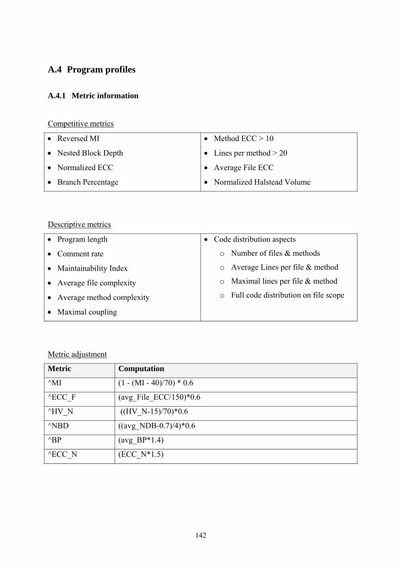
A.4 Program profiles

A.4.1 Metric information

Competitive metrics

• Reversed MI

• Nested Block Depth

• Normalized ECC

• Branch Percentage

• Method ECC > 10

• Lines per method > 20

• Average File ECC

• Normalized Halstead Volume

Descriptive metrics

• Program length

• Comment rate

• Maintainability Index

• Average file complexity

• Average method complexity

• Maximal coupling

• Code distribution aspects

o Number of files & methods

o Average Lines per file & method

o Maximal lines per file & method

o Full code distribution on file scope

Metric adjustment

Metric Computation

^MI (1 - (MI - 40)/70) * 0.6

^ECC_F (avg_File_ECC/150)*0.6

^HV_N ((HV_N-15)/70)*0.6

^NBD ((avg_NDB-0.7)/4)*0.6

^BP (avg_BP*1.4)

^ECC_N (ECC_N*1.5)

142

A.4.2 Kiviat diagrams (competitive measures)

1. Gimp (C) 2. Miranda (C) 3. NullWebmail (C)

^M I

^NBD

^E CC_N

^BP

E CC>10

LP M >20

^E CC_F

^HV _N

4. Panda (C) 5. SDCC (C) 6. VIM (C)

^M I

^NBD

^E CC_N

^BP

E CC>10

LP M >20

^E CC_F

^HV _N

7. 7-Zip (C++) 8. DiskCleaner (C++) 9. Emule (C++)

^M I

^NBD

^E CC_N

^BP

E CC>10

LP M >20

^E CC_F

^HV _N

10. FileZilla (C++) 11. HexView (C++) 12. Notepad++ (C++)

^M I

^NBD

^E CC_N

^BP

E CC>10

LP M >20

^E CC_F

^HV _N

^M

^NBD

^E CC_N

^BP

E CC>10

LP M >20

^E CC_F

^HV _N

I ^M

^NBD

^E CC_N

^BP

E CC>10

LP M >20

^E CC_F

^HV _N

I

^M I

^NBD

^E CC_N

^BP

E CC>10

LP M >20

^E CC_F

^HV _N

^M

^NBD

^E CC_N

^BP

E CC>10

LP M >20

^E CC_F

^HV _N

I

^M I

^NBD

^E CC_N

^BP

E CC>10

LP M >20

^E CC_F

^HV _N

^M

^NBD

^E CC_N

^BP

E CC>10

LP M >20

^E CC_F

^HV _N

I

^M I

^NBD

^E CC_N

^BP

E CC>10

LP M >20

^E CC_F

^HV _N

^M

^NBD

^E CC_N

^BP

E CC>10

LP M >20

^E CC_F

^HV _N

I

143

13. BonForum (Java) 14. FitNesse (Java) 15. HTML_Unit (Java)

^M I

^NBD

^E CC_N

^BP

E CC>10

LP M >20

^E CC_F

^HV _N

16. NekoHTML (Java) 17. Jsettlers (Java) 18. JSS (Java)

^M I

^NBD

^E CC_N

^BP

E CC>10

LP M >20

^E CC_F

^HV _N

19. CS.PPS (Java)

^M I

^NBD

^E CC_N

^BP

E CC>10

LP M >20

^E CC_F

^HV _N

20. A.OOPJ_L1_st1 21. A.OOPJ_L2_st1 22. A.OOPJ_L3_st1

^M I

^NBD

^E CC_N

^BP

E CC>10

LP M >20

^E CC_F

^HV _N

^M I

^NBD

^E CC_N

^BP

E CC>10

LP M >20

^E CC_F

^HV _N

^M

^NBD

^E CC_N

^BP

E CC>10

LP M >20

^E CC_F

^HV _N

I

^M I

^NBD

^E CC_N

^BP

E CC>10

LP M >20

^E CC_F

^HV _N

^M

^NBD

^E CC_N

^BP

E CC>10

LP M >20

^E CC_F

^HV _N

I

^M I

^NBD

^E CC_N

^BP

E CC>10

LP M >20

^E CC_F

^HV _N

^M

^NBD

^E CC_N

^BP

E CC>10

LP M >20

^E CC_F

^HV _N

I

144

23. A.OOPJ_L4_st1 24. A.OOPJ_L5_st1 25. B.OS_L1_st1

^M I

^NBD

^E CC_N

^BP

E CC>10

LP M >20

^E CC_F

^HV _N

26. B.OS_L2_st1 27. B.OS_L3_st1 28. B.OS_L4_st1

^M I

^NBD

^E CC_N

^BP

E CC>10

LP M >20

^E CC_F

^HV _N

29. B.OS_L5_st1 30. C.PL_L1_st1 31. C.PL_L1_st2

^M I

^NBD

^E CC_N

^BP

E CC>10

LP M >20

^E CC_F

^HV _N

32. C.PL_L1_st3 33. C.PL_L1_st4 34. C.PL_L1_st5

^M I

^NBD

^E CC_N

^BP

E CC>10

LP M >20

^E CC_F

^HV _N

^M I

^NBD

^E CC_N

^BP

E CC>10

LP M >20

^E CC_F

^HV _N

^M

^NBD

^E CC_N

^BP

E CC>10

LP M >20

^E CC_F

^HV _N

I

^M I

^NBD

^E CC_N

^BP

E CC>10

LP M >20

^E CC_F

^HV _N

^M

^NBD

^E CC_N

^BP

E CC>10

LP M >20

^E CC_F

^HV _N

I

^M I

^NBD

^E CC_N

^BP

E CC>10

LP M >20

^E CC_F

^HV _N

^M

^NBD

^E CC_N

^BP

E CC>10

LP M >20

^E CC_F

^HV _N

I

^M I

^NBD

^E CC_N

^BP

E CC>10

LP M >20

^E CC_F

^HV _N

^M

^NBD

^E CC_N

^BP

E CC>10

LP M >20

^E CC_F

^HV _N

I

145

35. C.PL_L1_st6 36. C.PL_L1_st7 37. D.CC_L2_teacher

^M I

^NBD

^E CC_N

^BP

E CC>10

LP M >20

^E CC_F

^HV _N

38. D.CC_L2_st1 39. D.CC_L2_st2 40. D.CC_L2_st3

^M I

^NBD

^E CC_N

^BP

E CC>10

LP M >20

^E CC_F

^HV _N

41. D.CC_L2_st4 42. D.CC_L3_teacher 43. D.CC_L3_st1

^M I

^NBD

^E CC_N

^BP

E CC>10

LP M >20

^E CC_F

^HV _N

44. D.CC_L3_st2 45. D.CC_L3_st3 46. D.CC_L3_st4

^M I

^NBD

^E CC_N

^BP

E CC>10

LP M >20

^E CC_F

^HV _N

^M I

^NBD

^E CC_N

^BP

E CC>10

LP M >20

^E CC_F

^HV _N

^M

^NBD

^E CC_N

^BP

E CC>10

LP M >20

^E CC_F

^HV _N

I

^M I

^NBD

^E CC_N

^BP

E CC>10

LP M >20

^E CC_F

^HV _N

^M

^NBD

^E CC_N

^BP

E CC>10

LP M >20

^E CC_F

^HV _N

I

^M I

^NBD

^E CC_N

^BP

E CC>10

LP M >20

^E CC_F

^HV _N

^M

^NBD

^E CC_N

^BP

E CC>10

LP M >20

^E CC_F

^HV _N

I

^M I

^NBD

^E CC_N

^BP

E CC>10

LP M >20

^E CC_F

^HV _N

^M

^NBD

^E CC_N

^BP

E CC>10

LP M >20

^E CC_F

^HV _N

I

146

47. D.CC_L4_teacher 48. D.CC_L4_st1 49. D.CC_L4_st2

^M I

^NBD

^E CC_N

^BP

E CC>10

LP M >20

^E CC_F

^HV _N

50. D.CC_L4_st3 51. D.CC_L4_st4 52 D.OODM_L4_st1

^M I

^NBD

^E CC_N

^BP

E CC>10

LP M >20

^E CC_F

^HV _N

53 D.OODM_L4_st2 54 D.OODM_L4_st3 55 D.OODM_L4_st4

^M I

^NBD

^E CC_N

^BP

E CC>10

LP M >20

^E CC_F

^HV _N

56 D.OODM_L4_st5

^M I

^NBD

^E CC_N

^BP

E CC>10

LP M >20

^E CC_F

^HV _N

^M I

^NBD

^E CC_N

^BP

E CC>10

LP M >20

^E CC_F

^HV _N

^M

^NBD

^E CC_N

^BP

E CC>10

LP M >20

^E CC_F

^HV _N

I

^M I

^NBD

^E CC_N

^BP

E CC>10

LP M >20

^E CC_F

^HV _N

^M

^NBD

^E CC_N

^BP

E CC>10

LP M >20

^E CC_F

^HV _N

I

^M I

^NBD

^E CC_N

^BP

E CC>10

LP M >20

^E CC_F

^HV _N

^M

^NBD

^E CC_N

^BP

E CC>10

LP M >20

^E CC_F

^HV _N

I

147

A.4.3 Program profiles (full view)

Programming languageProgram lengthComment RateMaintainabilityTextual code compl.File complexityMethod complexityAverage nestingMaximal nestingBranch PercentageMaximal coupling

Number of filesLines per file (avg)Lines per file (max)Number of methodsLines per method (avg)Lines per method (max)

^MI 0.31 ^ECC_N 0.14 ECC>10 0.08 ^BP 0.25^HV_N 0.24 ^ECC_F 0.10 LPM>20 0.42 ^NBD 0.13

Diagram data

07.1

2.20

07

2552,063

C

Code distribution

0

GIMP (1)

42.6573.940.12

526,279

2814,7955,586

Program summary

100.18

1.574.04

24.64

922

^MI

^NBD

^ECC_N

^BP

ECC>10

LPM>20

^ECC_F

^HV_N

0

1000

2000

3000

4000

5000

6000

1 2063

prof

ile c

reat

ed o

n

Programming languageProgram lengthComment RateMaintainabilityTextual code compl.File complexityMethod complexityAverage nestingMaximal nestingBranch PercentageMaximal coupling

Number of filesLines per file (avg)Lines per file (max)Number of methodsLines per method (avg)Lines per method (max)

^MI 0.33 ^ECC_N 0.33 ECC>10 0.17 ^BP 0.39^HV_N 0.36 ^ECC_F 0.26 LPM>20 0.35 ^NBD 0.29

Diagram data

07.1

2.20

07

29498

C

Code distribution

0

Miranda (2)

56.6171.890.09

28,823

30892

1,215

Program summary

100.28

2.657.89

63.90

1,041

^MI

^NBD

^ECC_N

^BP

ECC>10

LPM>20

^ECC_F

^HV_N

0

200

400

600

800

1000

1200

1400

1 11 21 31 41 51 61 71 81 91

prof

ile c

reat

ed o

n

148

Programming languageProgram lengthComment RateMaintainabilityTextual code compl.File complexityMethod complexityAverage nestingMaximal nestingBranch PercentageMaximal coupling

Number of filesLines per file (avg)Lines per file (max)Number of methodsLines per method (avg)Lines per method (max)

^MI 0.48 ^ECC_N 0.41 ECC>10 0.38 ^BP 0.32^HV_N 0.37 ^ECC_F 0.33 LPM>20 0.58 ^NBD 0.17

Diagram data

07.1

2.20

07

30829

C

Code distribution

0

NullWebmail (3)

57.7454.370.16

8,925

40179918

Program summary

80.23

1.8413.4183.48

255

^MI

^NBD

^ECC_N

^BP

ECC>10

LPM>20

^ECC_F

^HV_N

0100200300400500600700800900

1000

1 6 11 16 21 26

prof

ile c

reat

ed o

n

Programming languageProgram lengthComment RateMaintainabilityTextual code compl.File complexityMethod complexityAverage nestingMaximal nestingBranch PercentageMaximal coupling

Number of filesLines per file (avg)Lines per file (max)Number of methodsLines per method (avg)Lines per method (max)

^MI 0.49 ^ECC_N 0.19 ECC>10 0.07 ^BP 0.10^HV_N 0.56 ^ECC_F 0.10 LPM>20 0.22 ^NBD 0.01

Diagram data

07.1

2.20

07

19870

C

Code distribution

0

Panda (4)

80.5852.450.41

13,848

19261

1,895

Program summary

100.07

0.793.15

25.01

326

^MI

^NBD

^ECC_N

^BP

ECC>10

LPM>20

^ECC_F

^HV_N

0200400600800

100012001400160018002000

1 11 21 31 41 51 61

prof

ile c

reat

ed o

n

149

Programming languageProgram lengthComment RateMaintainabilityTextual code compl.File complexityMethod complexityAverage nestingMaximal nestingBranch PercentageMaximal coupling

Number of filesLines per file (avg)Lines per file (max)Number of methodsLines per method (avg)Lines per method (max)

^MI 0.30 ^ECC_N 0.33 ECC>10 0.22 ^BP 0.42^HV_N 0.30 ^ECC_F 0.64 LPM>20 0.44 ^NBD 0.22

Diagram data

07.1

2.20

07

728199

C

Code distribution

0

SDCC (5)

49.9275.010.19

144,892

333,874

11,077

Program summary

100.30

2.198.99

161.02

1,763

^MI

^NBD

^ECC_N

^BP

ECC>10

LPM>20

^ECC_F

^HV_N

0

2000

4000

6000

8000

10000

12000

1 199

prof

ile c

reat

ed o

n

Programming languageProgram lengthComment RateMaintainabilityTextual code compl.File complexityMethod complexityAverage nestingMaximal nestingBranch PercentageMaximal coupling

Number of filesLines per file (avg)Lines per file (max)Number of methodsLines per method (avg)Lines per method (max)

^MI 0.74 ^ECC_N 0.37 ECC>10 0.14 ^BP 0.39^HV_N 0.28 ^ECC_F 2.27 LPM>20 0.31 ^NBD 0.23

Diagram data

07.1

2.20

07

2,283104

C

Code distribution

0

VIM (6)

47.1623.960.20

239,693

261,592

16,512

Program summary

100.28

2.256.56

567.12

1,070

^MI

^NBD

^ECC_N

^BP

ECC>10

LPM>20

^ECC_F

^HV_N

0

2000

4000

6000

8000

10000

12000

14000

16000

18000

1 105

prof

ile c

reat

ed o

n

150

Programming languageProgram lengthComment RateMaintainabilityTextual code compl.File complexityMethod complexityAverage nestingMaximal nestingBranch PercentageMaximal coupling

Number of filesLines per file (avg)Lines per file (max)Number of methodsLines per method (avg)Lines per method (max)

^MI 0.16 ^ECC_N 0.22 ECC>10 0.08 ^BP 0.27^HV_N 0.19 ^ECC_F 0.06 LPM>20 0.25 ^NBD 0.14

Diagram data

07.1

2.20

07

104915

C++

Code distribution

124

7-Zip (7)

36.9790.760.07

95,889

204,0631,376

Program summary

100.19

1.653.96

15.46

459

^MI

^NBD

^ECC_N

^BP

ECC>10

LPM>20

^ECC_F

^HV_N

0

200

400

600

800

1000

1200

1400

1600

1 919

prof

ile c

reat

ed o

n

Programming languageProgram lengthComment RateMaintainabilityTextual code compl.File complexityMethod complexityAverage nestingMaximal nestingBranch PercentageMaximal coupling

Number of filesLines per file (avg)Lines per file (max)Number of methodsLines per method (avg)Lines per method (max)

^MI 0.19 ^ECC_N 0.20 ECC>10 0.09 ^BP 0.25^HV_N 0.18 ^ECC_F 0.05 LPM>20 0.32 ^NBD 0.14

Diagram data

07.1

2.20

07

9458

C++

Code distribution

6

DiskCleaner (8)

35.6987.440.12

5,430

22216824

Program summary

80.18

1.653.85

12.43

134

^MI

^NBD

^ECC_N

^BP

ECC>10

LPM>20

^ECC_F

^HV_N

0

100

200

300

400

500

600

700

800

900

1 11 21 31 41 51

prof

ile c

reat

ed o

n

151

Programming languageProgram lengthComment RateMaintainabilityTextual code compl.File complexityMethod complexityAverage nestingMaximal nestingBranch PercentageMaximal coupling

Number of filesLines per file (avg)Lines per file (max)Number of methodsLines per method (avg)Lines per method (max)

^MI 0.30 ^ECC_N 0.25 ECC>10 0.10 ^BP 0.29^HV_N 0.29 ^ECC_F 0.18 LPM>20 0.28 ^NBD 0.20

Diagram data

07.1

2.20

07

258656

C++

Code distribution

122

Emule (9)

48.9775.260.14

169,635

236,3954,723

Program summary

100.21

2.035.18

43.76

2,326

^MI

^NBD

^ECC_N

^BP

ECC>10

LPM>20

^ECC_F

^HV_N

0500

100015002000250030003500400045005000

1 657

prof

ile c

reat

ed o

n

Programming languageProgram lengthComment RateMaintainabilityTextual code compl.File complexityMethod complexityAverage nestingMaximal nestingBranch PercentageMaximal coupling

Number of filesLines per file (avg)Lines per file (max)Number of methodsLines per method (avg)Lines per method (max)

^MI 0.40 ^ECC_N 0.22 ECC>10 0.15 ^BP 0.24^HV_N 0.29 ^ECC_F 0.16 LPM>20 0.34 ^NBD 0.15

Diagram data

07.1

2.20

07

279294

C++

Code distribution

64

FileZilla (10)

49.3063.780.16

81,934

301,8814,922

Program summary

100.17

1.716.50

40.58

1,691

^MI

^NBD

^ECC_N

^BP

ECC>10

LPM>20

^ECC_F

^HV_N

0

1000

2000

3000

4000

5000

6000

1 294

prof

ile c

reat

ed o

n

152

Programming languageProgram lengthComment RateMaintainabilityTextual code compl.File complexityMethod complexityAverage nestingMaximal nestingBranch PercentageMaximal coupling

Number of filesLines per file (avg)Lines per file (max)Number of methodsLines per method (avg)Lines per method (max)

^MI 0.20 ^ECC_N 0.16 ECC>10 0.03 ^BP 0.21^HV_N 0.16 ^ECC_F 0.03 LPM>20 0.23 ^NBD 0.09

Diagram data

07.1

2.20

07

7016

C++

Code distribution

8

HexView (11)

34.1086.810.26

1,121

1466

528

Program summary

60.15

1.322.277.37

112

^MI

^NBD

^ECC_N

^BP

ECC>10

LPM>20

^ECC_F

^HV_N

0

100

200

300

400

500

600

1 6 11 16

prof

ile c

reat

ed o

n

Programming languageProgram lengthComment RateMaintainabilityTextual code compl.File complexityMethod complexityAverage nestingMaximal nestingBranch PercentageMaximal coupling

Number of filesLines per file (avg)Lines per file (max)Number of methodsLines per method (avg)Lines per method (max)

^MI 0.35 ^ECC_N 0.25 ECC>10 0.15 ^BP 0.35^HV_N 0.29 ^ECC_F 0.16 LPM>20 0.45 ^NBD 0.24

Diagram data

07.1

2.20

07

251142

C++

Code distribution

43

Notepad++ (12)

48.4069.480.12

35,677

37893

5,711

Program summary

100.25

2.297.25

41.09

1,444

^MI

^NBD

^ECC_N

^BP

ECC>10

LPM>20

^ECC_F

^HV_N

0

1000

2000

3000

4000

5000

6000

1 142

prof

ile c

reat

ed o

n

153

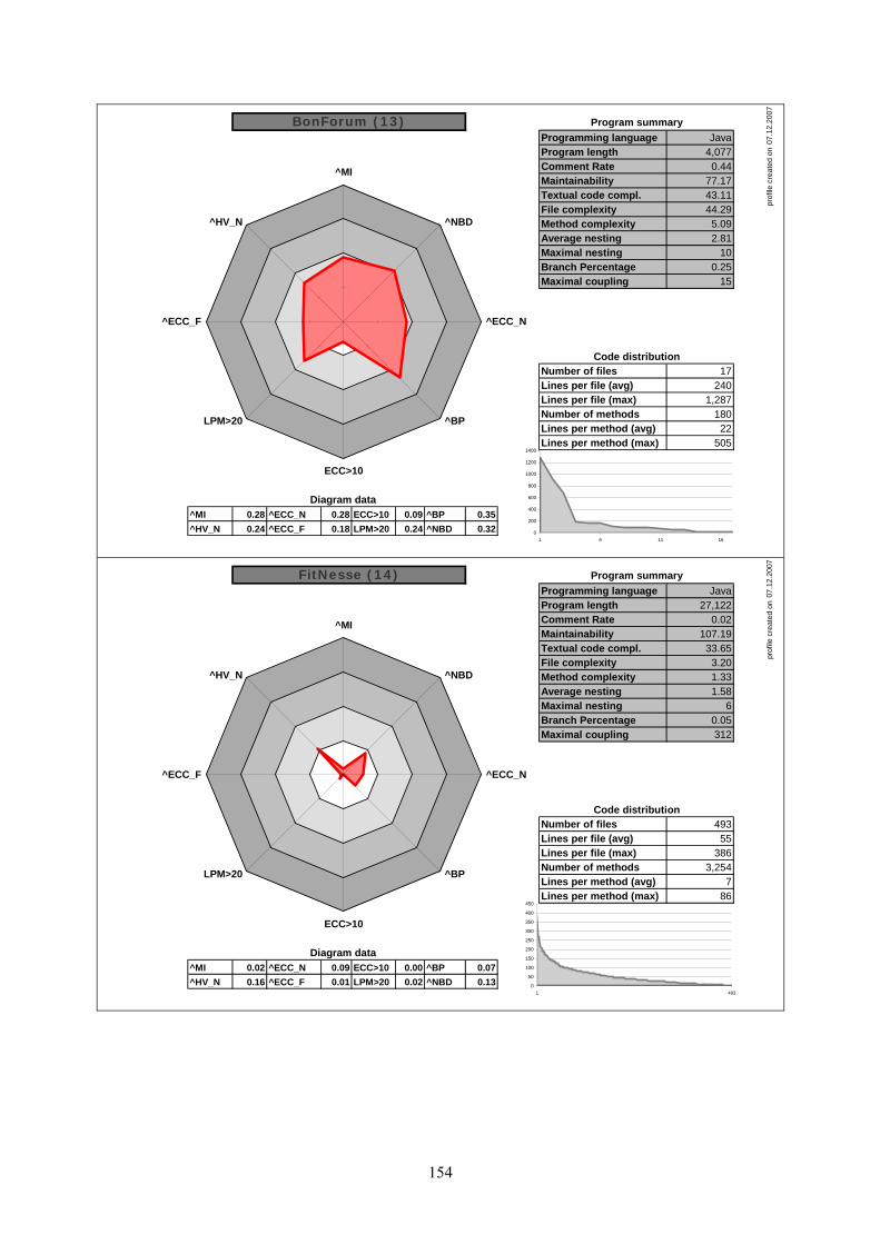
Programming languageProgram lengthComment RateMaintainabilityTextual code compl.File complexityMethod complexityAverage nestingMaximal nestingBranch PercentageMaximal coupling

Number of filesLines per file (avg)Lines per file (max)Number of methodsLines per method (avg)Lines per method (max)

^MI 0.28 ^ECC_N 0.28 ECC>10 0.09 ^BP 0.35^HV_N 0.24 ^ECC_F 0.18 LPM>20 0.24 ^NBD 0.32

Diagram data

07.1

2.20

07

24017

Java

Code distribution

15

BonForum (13)

43.1177.170.44

4,077

22180

1,287

Program summary

100.25

2.815.09

44.29

505

^MI

^NBD

^ECC_N

^BP

ECC>10

LPM>20

^ECC_F

^HV_N

0

200

400

600

800

1000

1200

1400

1 6 11 16

prof

ile c

reat

ed o

n

Programming languageProgram lengthComment RateMaintainabilityTextual code compl.File complexityMethod complexityAverage nestingMaximal nestingBranch PercentageMaximal coupling

Number of filesLines per file (avg)Lines per file (max)Number of methodsLines per method (avg)Lines per method (max)

^MI 0.02 ^ECC_N 0.09 ECC>10 0.00 ^BP 0.07^HV_N 0.16 ^ECC_F 0.01 LPM>20 0.02 ^NBD 0.13

Diagram data

07.1

2.20

07

55493

Java

Code distribution

312

FitNesse (14)

33.65107.19

0.0227,122

73,254

386

Program summary

60.05

1.581.333.20

86

^MI

^NBD

^ECC_N

^BP

ECC>10

LPM>20

^ECC_F

^HV_N

0

50

100

150

200

250

300

350

400

450

1 493

prof

ile c

reat

ed o

n

154

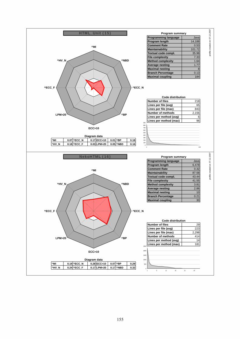
Programming languageProgram lengthComment RateMaintainabilityTextual code compl.File complexityMethod complexityAverage nestingMaximal nestingBranch PercentageMaximal coupling

Number of filesLines per file (avg)Lines per file (max)Number of methodsLines per method (avg)Lines per method (max)

^MI 0.07 ^ECC_N 0.17 ECC>10 0.01 ^BP 0.18^HV_N 0.18 ^ECC_F 0.03 LPM>20 0.05 ^NBD 0.16

Diagram data

07.1

2.20

07

65218

Java

Code distribution

184

HTML_Unit (15)

35.98101.72

0.5314,188

62,156

843

Program summary

80.13

1.771.647.33

96

^MI

^NBD

^ECC_N

^BP

ECC>10

LPM>20

^ECC_F

^HV_N

0

100

200

300

400

500

600

700

800

900

1 218

prof

ile c

reat

ed o

n

Programming languageProgram lengthComment RateMaintainabilityTextual code compl.File complexityMethod complexityAverage nestingMaximal nestingBranch PercentageMaximal coupling

Number of filesLines per file (avg)Lines per file (max)Number of methodsLines per method (avg)Lines per method (max)

^MI 0.19 ^ECC_N 0.28 ECC>10 0.07 ^BP 0.29^HV_N 0.24 ^ECC_F 0.17 LPM>20 0.17 ^NBD 0.32

Diagram data

07.1

2.20

07

22329

Java

Code distribution

30

NekoHTML (16)

43.4487.580.32

6,478

14414

2,298

Program summary

100.21

2.863.81

41.55

181

^MI

^NBD

^ECC_N

^BP

ECC>10

LPM>20

^ECC_F

^HV_N

0

500

1000

1500

2000

2500

1 6 11 16 21 26

prof

ile c

reat

ed o

n

155

Programming languageProgram lengthComment RateMaintainabilityTextual code compl.File complexityMethod complexityAverage nestingMaximal nestingBranch PercentageMaximal coupling

Number of filesLines per file (avg)Lines per file (max)Number of methodsLines per method (avg)Lines per method (max)

^MI 0.12 ^ECC_N 0.22 ECC>10 0.05 ^BP 0.31^HV_N 0.23 ^ECC_F 0.12 LPM>20 0.17 ^NBD 0.37

Diagram data

07.1

2.20

07

208148

Java

Code distribution

110

Jsettlers (17)

42.2795.560.30

30,724

171,6823,465

Program summary

100.22

3.143.59

30.44

1,338

^MI

^NBD

^ECC_N

^BP

ECC>10

LPM>20

^ECC_F

^HV_N

0

500

1000

1500

2000

2500

3000

3500

4000

1 148

prof

ile c

reat

ed o

n

Programming languageProgram lengthComment RateMaintainabilityTextual code compl.File complexityMethod complexityAverage nestingMaximal nestingBranch PercentageMaximal coupling

Number of filesLines per file (avg)Lines per file (max)Number of methodsLines per method (avg)Lines per method (max)

^MI 0.29 ^ECC_N 0.22 ECC>10 0.08 ^BP 0.14^HV_N 0.31 ^ECC_F 0.05 LPM>20 0.27 ^NBD 0.28

Diagram data

07.1

2.20

07

8015

Java

Code distribution

14

JSS (18)

50.8776.530.25

1,198

1795

230

Program summary

80.10

2.573.37

11.80

157

^MI

^NBD

^ECC_N

^BP

ECC>10

LPM>20

^ECC_F

^HV_N

0

50

100

150

200

250

1 6 11

prof

ile c

reat

ed o

n

156

Programming languageProgram lengthComment RateMaintainabilityTextual code compl.File complexityMethod complexityAverage nestingMaximal nestingBranch PercentageMaximal coupling

Number of filesLines per file (avg)Lines per file (max)Number of methodsLines per method (avg)Lines per method (max)

^MI 0.25 ^ECC_N 0.16 ECC>10 0.04 ^BP 0.14^HV_N 0.36 ^ECC_F 0.09 LPM>20 0.22 ^NBD 0.29

Diagram data

07.1

2.20

07

207368

Java

Code distribution

222

CS.PPS (19)

57.2680.260.20

76,338

174,279

16,786

Program summary

100.10

2.612.85

22.43

716

^MI

^NBD

^ECC_N

^BP

ECC>10

LPM>20

^ECC_F

^HV_N

0

2000

4000

6000

8000

10000

12000

14000

16000

18000

1 368

prof

ile c

reat

ed o

n

Programming languageProgram lengthComment RateMaintainabilityTextual code compl.File complexityMethod complexityAverage nestingMaximal nestingBranch PercentageMaximal coupling

Number of filesLines per file (avg)Lines per file (max)Number of methodsLines per method (avg)Lines per method (max)

^MI 0.06 ^ECC_N 0.16 ECC>10 0.00 ^BP 0.43^HV_N 0.04 ^ECC_F 0.04 LPM>20 0.06 ^NBD 0.23

Diagram data

07.1

2.20

07

862

Java

Code distribution

3

A.OOPJ_L1_st1 (20)

19.23102.50

0.26172

1016

144

Program summary

50.31

2.212.009.00

44

^MI

^NBD

^ECC_N

^BP

ECC>10

LPM>20

^ECC_F

^HV_N

0

20

40

60

80

100

120

140

160

1 2

prof

ile c

reat

ed o

n

157

Programming languageProgram lengthComment RateMaintainabilityTextual code compl.File complexityMethod complexityAverage nestingMaximal nestingBranch PercentageMaximal coupling

Number of filesLines per file (avg)Lines per file (max)Number of methodsLines per method (avg)Lines per method (max)

^MI 0.11 ^ECC_N 0.16 ECC>10 0.03 ^BP 0.34^HV_N 0.09 ^ECC_F 0.04 LPM>20 0.26 ^NBD 0.28

Diagram data

07.1

2.20

07

1005

Java

Code distribution

4

A.OOPJ_L2_st1 (21)

25.4397.200.25502

1434

302

Program summary

80.24

2.562.44

10.80

53

^MI

^NBD

^ECC_N

^BP

ECC>10

LPM>20

^ECC_F

^HV_N

0

50

100

150

200

250

300

350

1 2 3 4 5

prof

ile c

reat

ed o

n

Programming languageProgram lengthComment RateMaintainabilityTextual code compl.File complexityMethod complexityAverage nestingMaximal nestingBranch PercentageMaximal coupling

Number of filesLines per file (avg)Lines per file (max)Number of methodsLines per method (avg)Lines per method (max)

^MI 0.07 ^ECC_N 0.05 ECC>10 0.00 ^BP 0.04^HV_N 0.14 ^ECC_F 0.01 LPM>20 0.01 ^NBD 0.13

Diagram data

07.1

2.20

07

5910

Java

Code distribution

12

A.OOPJ_L3_st1 (22)

31.07101.90

0.37586

781

158

Program summary

50.03

1.561.122.00

23

^MI

^NBD

^ECC_N

^BP

ECC>10

LPM>20

^ECC_F

^HV_N

0

20

40

60

80

100

120

140

160

180

1 6

prof

ile c

reat

ed o

n

158

Programming languageProgram lengthComment RateMaintainabilityTextual code compl.File complexityMethod complexityAverage nestingMaximal nestingBranch PercentageMaximal coupling

Number of filesLines per file (avg)Lines per file (max)Number of methodsLines per method (avg)Lines per method (max)

^MI 0.14 ^ECC_N 0.13 ECC>10 0.00 ^BP 0.13^HV_N 0.09 ^ECC_F 0.01 LPM>20 0.07 ^NBD 0.14

Diagram data

07.1

2.20

07

4013

Java

Code distribution

11

A.OOPJ_L4_st1 (23)

25.6993.870.30318

92955

Program summary

40.09

1.601.663.37

23

^MI

^NBD

^ECC_N

^BP

ECC>10

LPM>20

^ECC_F

^HV_N

0

10

20

30

40

50

60

1 2 3 4 5 6 7 8

prof

ile c

reat

ed o

n

Programming languageProgram lengthComment RateMaintainabilityTextual code compl.File complexityMethod complexityAverage nestingMaximal nestingBranch PercentageMaximal coupling

Number of filesLines per file (avg)Lines per file (max)Number of methodsLines per method (avg)Lines per method (max)

^MI 0.16 ^ECC_N 0.13 ECC>10 0.00 ^BP 0.15^HV_N 0.11 ^ECC_F 0.02 LPM>20 0.14 ^NBD 0.18

Diagram data

07.1

2.20

07

5521

Java

Code distribution

13

A.OOPJ_L5_st1 (24)

28.1891.760.30

1,148

1097

148

Program summary

60.11

1.921.844.85

43

^MI

^NBD

^ECC_N

^BP

ECC>10

LPM>20

^ECC_F

^HV_N

0

20

40

60

80

100

120

140

160

1 6 11 16 21

prof

ile c

reat

ed o

n

159

Programming languageProgram lengthComment RateMaintainabilityTextual code compl.File complexityMethod complexityAverage nestingMaximal nestingBranch PercentageMaximal coupling

Number of filesLines per file (avg)Lines per file (max)Number of methodsLines per method (avg)Lines per method (max)

^MI 0.18 ^ECC_N 0.21 ECC>10 0.00 ^BP 0.22^HV_N 0.05 ^ECC_F 0.02 LPM>20 0.17 ^NBD 0.03

Diagram data

07.1

2.20

07

403

C

Code distribution

0

B.OS_L1_st1 (25)

20.2889.330.26120

156

68

Program summary

30.16

0.883.335.66

36

^MI

^NBD

^ECC_N

^BP

ECC>10

LPM>20

^ECC_F

^HV_N

0

10

20

30

40

50

60

70

80

1 2 3

prof

ile c

reat

ed o

n

Programming languageProgram lengthComment RateMaintainabilityTextual code compl.File complexityMethod complexityAverage nestingMaximal nestingBranch PercentageMaximal coupling

Number of filesLines per file (avg)Lines per file (max)Number of methodsLines per method (avg)Lines per method (max)

^MI 0.19 ^ECC_N 0.13 ECC>10 0.00 ^BP 0.10^HV_N 0.06 ^ECC_F 0.02 LPM>20 0.08 ^NBD 0.02

Diagram data

07.1

2.20

07

494

C

Code distribution

0

B.OS_L2_st1 (26)

21.5487.500.14197

111254

Program summary

20.07

0.802.084.25

25

^MI

^NBD

^ECC_N

^BP

ECC>10

LPM>20

^ECC_F

^HV_N

0

10

20

30

40

50

60

1 2 3 4

prof

ile c

reat

ed o

n

160

Programming languageProgram lengthComment RateMaintainabilityTextual code compl.File complexityMethod complexityAverage nestingMaximal nestingBranch PercentageMaximal coupling

Number of filesLines per file (avg)Lines per file (max)Number of methodsLines per method (avg)Lines per method (max)

^MI 0.33 ^ECC_N 0.26 ECC>10 0.20 ^BP 0.31^HV_N 0.17 ^ECC_F 0.13 LPM>20 0.40 ^NBD 0.20

Diagram data

07.1

2.20

07

1901

C

Code distribution

0

B.OS_L4_st1 (28)

34.3171.000.00190

355

190

Program summary

60.22

2.027.40

33.00

94

^MI

^NBD

^ECC_N

^BP

ECC>10

LPM>20

^ECC_F

^HV_N

020406080

100120140160180200

1

prof

ile c

reat

ed o

n

161

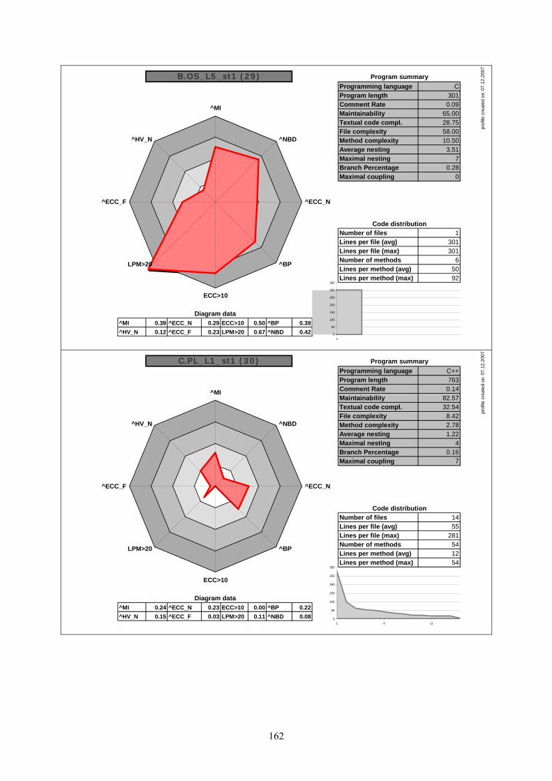
Programming languageProgram lengthComment RateMaintainabilityTextual code compl.File complexityMethod complexityAverage nestingMaximal nestingBranch PercentageMaximal coupling

Number of filesLines per file (avg)Lines per file (max)Number of methodsLines per method (avg)Lines per method (max)

^MI 0.39 ^ECC_N 0.29 ECC>10 0.50 ^BP 0.39^HV_N 0.12 ^ECC_F 0.23 LPM>20 0.67 ^NBD 0.42

Diagram data

07.1

2.20

07

3011

C

Code distribution

0

B.OS_L5_st1 (29)

28.7565.000.09301

506

301

Program summary

70.28

3.5110.5058.00

92

^MI

^NBD

^ECC_N

^BP

ECC>10

LPM>20

^ECC_F

^HV_N

0

50

100

150

200

250

300

350

1

prof

ile c

reat

ed o

n

Programming languageProgram lengthComment RateMaintainabilityTextual code compl.File complexityMethod complexityAverage nestingMaximal nestingBranch PercentageMaximal coupling

Number of filesLines per file (avg)Lines per file (max)Number of methodsLines per method (avg)Lines per method (max)

^MI 0.24 ^ECC_N 0.23 ECC>10 0.00 ^BP 0.22^HV_N 0.15 ^ECC_F 0.03 LPM>20 0.11 ^NBD 0.08

Diagram data

07.1

2.20

07

5514

C++

Code distribution

7

C.PL_L1_st1 (30)

32.5482.570.14763

1254

281

Program summary

40.16

1.222.788.42

54

^MI

^NBD

^ECC_N

^BP

ECC>10

LPM>20

^ECC_F

^HV_N

0

50

100

150

200

250

300

1 6 11

prof

ile c

reat

ed o

n

162

Programming languageProgram lengthComment RateMaintainabilityTextual code compl.File complexityMethod complexityAverage nestingMaximal nestingBranch PercentageMaximal coupling

Number of filesLines per file (avg)Lines per file (max)Number of methodsLines per method (avg)Lines per method (max)

^MI 0.23 ^ECC_N 0.27 ECC>10 0.09 ^BP 0.29^HV_N 0.11 ^ECC_F 0.05 LPM>20 0.24 ^NBD 0.07

Diagram data

07.1

2.20

07

6311

C

Code distribution

0

C.PL_L1_st2 (31)

27.7182.630.09692

1534

259

Program summary

40.21

1.144.15

11.27

51

^MI

^NBD

^ECC_N

^BP

ECC>10

LPM>20

^ECC_F

^HV_N

0

50

100

150

200

250

300

1 6 1

prof

ile c

reat

ed o

n

1

Programming languageProgram lengthComment RateMaintainabilityTextual code compl.File complexityMethod complexityAverage nestingMaximal nestingBranch PercentageMaximal coupling

Number of filesLines per file (avg)Lines per file (max)Number of methodsLines per method (avg)Lines per method (max)

^MI 0.24 ^ECC_N 0.27 ECC>10 0.10 ^BP 0.31^HV_N 0.21 ^ECC_F 0.12 LPM>20 0.24 ^NBD 0.14

Diagram data

07.1

2.20

07

1634

C

Code distribution

0

C.PL_L1_st3 (32)

39.3282.250.03652

2029

427

Program summary

60.22

1.654.90

29.75

131

^MI

^NBD

^ECC_N

^BP

ECC>10

LPM>20

^ECC_F

^HV_N

0

50

100

150

200

250

300

350

400

450

1 2 3 4

prof

ile c

reat

ed o

n

163

Programming languageProgram lengthComment RateMaintainabilityTextual code compl.File complexityMethod complexityAverage nestingMaximal nestingBranch PercentageMaximal coupling

Number of filesLines per file (avg)Lines per file (max)Number of methodsLines per method (avg)Lines per method (max)

^MI 0.21 ^ECC_N 0.22 ECC>10 0.02 ^BP 0.18^HV_N 0.17 ^ECC_F 0.04 LPM>20 0.11 ^NBD 0.07

Diagram data

07.1

2.20

07

6512

C++

Code distribution

5

C.PL_L1_st4 (33)

34.9685.500.10780

1065

188

Program summary

50.13

1.142.489.50

46

^MI

^NBD

^ECC_N

^BP

ECC>10

LPM>20

^ECC_F

^HV_N

020406080

100120140160180200

1 6 11

prof

ile c

reat

ed o

n

Programming languageProgram lengthComment RateMaintainabilityTextual code compl.File complexityMethod complexityAverage nestingMaximal nestingBranch PercentageMaximal coupling

Number of filesLines per file (avg)Lines per file (max)Number of methodsLines per method (avg)Lines per method (max)

^MI 0.14 ^ECC_N 0.27 ECC>10 0.02 ^BP 0.27^HV_N 0.15 ^ECC_F 0.03 LPM>20 0.09 ^NBD 0.10

Diagram data

07.1

2.20

07

4822

C++

Code distribution

7

C.PL_L1_st5 (34)

32.4393.590.10

1,058

1093

260

Program summary

50.19

1.342.658.50

123

^MI

^NBD

^ECC_N

^BP

ECC>10

LPM>20

^ECC_F

^HV_N

0

50

100

150

200

250

300

1 6 11 16 21

prof

ile c

reat

ed o

n

164

Programming languageProgram lengthComment RateMaintainabilityTextual code compl.File complexityMethod complexityAverage nestingMaximal nestingBranch PercentageMaximal coupling

Number of filesLines per file (avg)Lines per file (max)Number of methodsLines per method (avg)Lines per method (max)

^MI 0.19 ^ECC_N 0.22 ECC>10 0.00 ^BP 0.27^HV_N 0.18 ^ECC_F 0.06 LPM>20 0.04 ^NBD 0.05

Diagram data

07.1

2.20

07

965

C

Code distribution

0

C.PL_L1_st6 (35)

36.0988.400.00479

845

259

Program summary

40.19

1.062.38

13.80

36

^MI

^NBD

^ECC_N

^BP

ECC>10

LPM>20

^ECC_F

^HV_N

0

50

100

150

200

250

300

1 2 3 4 5

prof

ile c

reat

ed o

n

Programming languageProgram lengthComment RateMaintainabilityTextual code compl.File complexityMethod complexityAverage nestingMaximal nestingBranch PercentageMaximal coupling

Number of filesLines per file (avg)Lines per file (max)Number of methodsLines per method (avg)Lines per method (max)

^MI 0.15 ^ECC_N 0.24 ECC>10 0.04 ^BP 0.25^HV_N 0.16 ^ECC_F 0.22 LPM>20 0.22 ^NBD 0.12

Diagram data

07.1

2.20

07

3311

C++

Code distribution

4

C.PL_L1_st7 (36)

33.1492.000.00331

1423

331

Program summary

50.18

1.503.26

54.00

46

^MI

^NBD

^ECC_N

^BP

ECC>10

LPM>20

^ECC_F

^HV_N

0

50

100

150

200

250

300

350

1

prof

ile c

reat

ed o

n

165

Programming languageProgram lengthComment RateMaintainabilityTextual code compl.File complexityMethod complexityAverage nestingMaximal nestingBranch PercentageMaximal coupling

Number of filesLines per file (avg)Lines per file (max)Number of methodsLines per method (avg)Lines per method (max)

^MI 0.18 ^ECC_N 0.27 ECC>10 0.01 ^BP 0.28^HV_N 0.25 ^ECC_F 0.13 LPM>20 0.12 ^NBD 0.08

Diagram data

07.1

2.20

07

1775

C

Code distribution

0

D.CC_L2_teacher (37)

43.8589.000.14884

975

633

Program summary

50.20

1.233.07

32.00

38

^MI

^NBD

^ECC_N

^BP

ECC>10

LPM>20

^ECC_F

^HV_N

0

100

200

300

400

500

600

700

1 2 3 4 5

prof

ile c

reat

ed o

n

Programming languageProgram lengthComment RateMaintainabilityTextual code compl.File complexityMethod complexityAverage nestingMaximal nestingBranch PercentageMaximal coupling

Number of filesLines per file (avg)Lines per file (max)Number of methodsLines per method (avg)Lines per method (max)

^MI 0.20 ^ECC_N 0.23 ECC>10 0.04 ^BP 0.34^HV_N 0.12 ^ECC_F 0.32 LPM>20 0.39 ^NBD 0.14

Diagram data

07.1

2.20

07

5261

C

Code distribution

0

D.CC_L2_st1 (38)

29.4587.000.02526

1828

526

Program summary

40.24

1.613.79

79.00

40

^MI

^NBD

^ECC_N

^BP

ECC>10

LPM>20

^ECC_F

^HV_N

0

100

200

300

400

500

600

1

prof

ile c

reat

ed o

n

166

Programming languageProgram lengthComment RateMaintainabilityTextual code compl.File complexityMethod complexityAverage nestingMaximal nestingBranch PercentageMaximal coupling

Number of filesLines per file (avg)Lines per file (max)Number of methodsLines per method (avg)Lines per method (max)

^MI 0.14 ^ECC_N 0.31 ECC>10 0.00 ^BP 0.39^HV_N 0.17 ^ECC_F 0.11 LPM>20 0.34 ^NBD 0.10

Diagram data

07.1

2.20

07

1385

C

Code distribution

0

D.CC_L2_st2 (39)

35.0693.400.05689

1835

560

Program summary

40.28

1.364.89

28.60

40

^MI

^NBD

^ECC_N

^BP

ECC>10

LPM>20

^ECC_F

^HV_N

0

100

200

300

400

500

600

1 2 3 4 5

prof

ile c

reat

ed o

n

Programming languageProgram lengthComment RateMaintainabilityTextual code compl.File complexityMethod complexityAverage nestingMaximal nestingBranch PercentageMaximal coupling

Number of filesLines per file (avg)Lines per file (max)Number of methodsLines per method (avg)Lines per method (max)

^MI 0.06 ^ECC_N 0.40 ECC>10 0.00 ^BP 0.46^HV_N 0.12 ^ECC_F 0.59 LPM>20 0.09 ^NBD 0.08

Diagram data

07.1

2.20

07

5571

C

Code distribution

0

D.CC_L2_st3 (40)

28.56103.00

0.01557

958

557

Program summary

30.33

1.243.41

147.00

35

^MI

^NBD

^ECC_N

^BP

ECC>10

LPM>20

^ECC_F

^HV_N

0

100

200

300

400

500

600

1

prof

ile c

reat

ed o

n

167

Programming languageProgram lengthComment RateMaintainabilityTextual code compl.File complexityMethod complexityAverage nestingMaximal nestingBranch PercentageMaximal coupling

Number of filesLines per file (avg)Lines per file (max)Number of methodsLines per method (avg)Lines per method (max)

^MI 0.34 ^ECC_N 0.33 ECC>10 0.07 ^BP 0.43^HV_N 0.25 ^ECC_F 0.34 LPM>20 0.29 ^NBD 0.13

Diagram data

07.1

2.20

07

3782

C

Code distribution

0

D.CC_L2_st4 (41)

44.7270.500.10755

1542

675

Program summary

40.31

1.594.93

84.00

35

^MI

^NBD

^ECC_N

^BP

ECC>10

LPM>20

^ECC_F

^HV_N

0

100

200

300

400

500

600

700

800

1 2

prof

ile c

reat

ed o

n

Programming languageProgram lengthComment RateMaintainabilityTextual code compl.File complexityMethod complexityAverage nestingMaximal nestingBranch PercentageMaximal coupling

Number of filesLines per file (avg)Lines per file (max)Number of methodsLines per method (avg)Lines per method (max)

^MI 0.18 ^ECC_N 0.23 ECC>10 0.01 ^BP 0.25^HV_N 0.27 ^ECC_F 0.14 LPM>20 0.14 ^NBD 0.08

Diagram data

07.1

2.20

07

2185

C

Code distribution

0

D.CC_L3_teacher (42)

46.2989.400.13

1,089

1094

838

Program summary

50.18

1.202.76

34.00

42

^MI

^NBD

^ECC_N

^BP

ECC>10

LPM>20

^ECC_F

^HV_N

0

100

200

300

400

500

600

700

800

900

1 2 3 4 5

prof

ile c

reat

ed o

n

168

Programming languageProgram lengthComment RateMaintainabilityTextual code compl.File complexityMethod complexityAverage nestingMaximal nestingBranch PercentageMaximal coupling

Number of filesLines per file (avg)Lines per file (max)Number of methodsLines per method (avg)Lines per method (max)

^MI 0.20 ^ECC_N 0.23 ECC>10 0.04 ^BP 0.34^HV_N 0.12 ^ECC_F 0.32 LPM>20 0.39 ^NBD 0.14

Diagram data

07.1

2.20

07

5261

C

Code distribution

0

D.CC_L3_st1 (43)

29.4587.000.02526

1828

526

Program summary

40.24

1.613.79

79.00

40

^MI

^NBD

^ECC_N

^BP

ECC>10

LPM>20

^ECC_F

^HV_N

0

100

200

300

400

500

600

1

prof

ile c

reat

ed o

n

Programming languageProgram lengthComment RateMaintainabilityTextual code compl.File complexityMethod complexityAverage nestingMaximal nestingBranch PercentageMaximal coupling

Number of filesLines per file (avg)Lines per file (max)Number of methodsLines per method (avg)Lines per method (max)

^MI 0.16 ^ECC_N 0.27 ECC>10 0.09 ^BP 0.32^HV_N 0.22 ^ECC_F 0.13 LPM>20 0.37 ^NBD 0.10

Diagram data

07.1

2.20

07

1775

C

Code distribution

0

D.CC_L3_st2 (44)

40.7191.600.05883

1843

716

Program summary

40.23

1.374.53

31.80

48

^MI

^NBD

^ECC_N

^BP

ECC>10

LPM>20

^ECC_F

^HV_N

0

100

200

300

400

500

600

700

800

1 2 3 4 5

prof

ile c

reat

ed o

n

169

Programming languageProgram lengthComment RateMaintainabilityTextual code compl.File complexityMethod complexityAverage nestingMaximal nestingBranch PercentageMaximal coupling

Number of filesLines per file (avg)Lines per file (max)Number of methodsLines per method (avg)Lines per method (max)

^MI 0.17 ^ECC_N 0.40 ECC>10 0.14 ^BP 0.46^HV_N 0.17 ^ECC_F 1.01 LPM>20 0.25 ^NBD 0.13

Diagram data

07.1

2.20

07

9601

C

Code distribution

0

D.CC_L3_st3 (45)

35.1490.000.08960

1559

960

Program summary

50.33

1.545.17

253.00

92

^MI

^NBD

^ECC_N

^BP

ECC>10

LPM>20

^ECC_F

^HV_N

0

200

400

600

800

1000

1200

1

prof

ile c

reat

ed o

n

Programming languageProgram lengthComment RateMaintainabilityTextual code compl.File complexityMethod complexityAverage nestingMaximal nestingBranch PercentageMaximal coupling

Number of filesLines per file (avg)Lines per file (max)Number of methodsLines per method (avg)Lines per method (max)

^MI 0.24 ^ECC_N 0.29 ECC>10 0.06 ^BP 0.36^HV_N 0.25 ^ECC_F 0.11 LPM>20 0.29 ^NBD 0.13

Diagram data

07.1

2.20

07

1497

C

Code distribution

0

D.CC_L3_st4 (46)

44.1581.420.09

1,044

1652

661

Program summary

40.26

1.544.65

28.71

41

^MI

^NBD

^ECC_N

^BP

ECC>10

LPM>20

^ECC_F

^HV_N

0

100

200

300

400

500

600

700

1 2 3 4 5 6 7

prof

ile c

reat

ed o

n

170

Programming languageProgram lengthComment RateMaintainabilityTextual code compl.File complexityMethod complexityAverage nestingMaximal nestingBranch PercentageMaximal coupling

Number of filesLines per file (avg)Lines per file (max)Number of methodsLines per method (avg)Lines per method (max)

^MI 0.18 ^ECC_N 0.27 ECC>10 0.06 ^BP 0.36^HV_N 0.23 ^ECC_F 0.32 LPM>20 0.16 ^NBD 0.09

Diagram data

07.1

2.20

07

4481

C

Code distribution

0

D.CC_L4_teacher (47)

41.5089.000.12448

1231

448

Program summary

40.26

1.323.55

80.00

50

^MI

^NBD

^ECC_N

^BP

ECC>10

LPM>20

^ECC_F

^HV_N

050

100150200250300350400450500

1

prof

ile c

reat

ed o

n

Programming languageProgram lengthComment RateMaintainabilityTextual code compl.File complexityMethod complexityAverage nestingMaximal nestingBranch PercentageMaximal coupling

Number of filesLines per file (avg)Lines per file (max)Number of methodsLines per method (avg)Lines per method (max)

^MI 0.23 ^ECC_N 0.38 ECC>10 0.18 ^BP 0.57^HV_N 0.23 ^ECC_F 0.18 LPM>20 0.29 ^NBD 0.17

Diagram data

07.1

2.20

07

1822

C

Code distribution

0

D.CC_L4_st1 (48)

41.2983.000.11363

2017

245

Program summary

50.41

1.836.29

46.00

53

^MI

^NBD

^ECC_N

^BP

ECC>10

LPM>20

^ECC_F

^HV_N

0

50

100

150

200

250

300

1 2

prof

ile c

reat

ed o

n

171

Programming languageProgram lengthComment RateMaintainabilityTextual code compl.File complexityMethod complexityAverage nestingMaximal nestingBranch PercentageMaximal coupling

Number of filesLines per file (avg)Lines per file (max)Number of methodsLines per method (avg)Lines per method (max)

^MI 0.24 ^ECC_N 0.21 ECC>10 0.04 ^BP 0.24^HV_N 0.20 ^ECC_F 0.09 LPM>20 0.35 ^NBD 0.07

Diagram data

07.1

2.20

07

1583

C

Code distribution

0

D.CC_L4_st2 (49)

38.3781.660.05475

1626

299

Program summary

30.17

1.163.42

22.33

46

^MI

^NBD

^ECC_N

^BP

ECC>10

LPM>20

^ECC_F

^HV_N

0

50

100

150

200

250

300

350

1 2

prof

ile c

reat

ed o

n

3

Programming languageProgram lengthComment RateMaintainabilityTextual code compl.File complexityMethod complexityAverage nestingMaximal nestingBranch PercentageMaximal coupling

Number of filesLines per file (avg)Lines per file (max)Number of methodsLines per method (avg)Lines per method (max)

^MI 0.27 ^ECC_N 0.28 ECC>10 0.06 ^BP 0.25^HV_N 0.36 ^ECC_F 0.27 LPM>20 0.33 ^NBD 0.34

Diagram data

07.1

2.20

07

3651

Java

Code distribution

3

D.CC_L4_st3 (50)

56.4579.000.00365

1918

365

Program summary

70.18

2.974.67

67.00

117

^MI

^NBD

^ECC_N

^BP

ECC>10

LPM>20

^ECC_F

^HV_N

0

50

100

150

200

250

300

350

400

1

prof

ile c

reat

ed o

n

172

Programming languageProgram lengthComment RateMaintainabilityTextual code compl.File complexityMethod complexityAverage nestingMaximal nestingBranch PercentageMaximal coupling

Number of filesLines per file (avg)Lines per file (max)Number of methodsLines per method (avg)Lines per method (max)

^MI 0.10 ^ECC_N 0.22 ECC>10 0.02 ^BP 0.20^HV_N 0.22 ^ECC_F 0.04 LPM>20 0.12 ^NBD 0.21

Diagram data

07.1

2.20

07

757

Java

Code distribution

7

D.CC_L4_st4 (51)

40.0998.000.13528

1241

207

Program summary

50.14

2.122.68

10.85

77

^MI

^NBD

^ECC_N

^BP

ECC>10

LPM>20

^ECC_F

^HV_N

0

50

100

150

200

250

1 2 3 4 5 6 7

prof

ile c

reat

ed o

n

Programming languageProgram lengthComment RateMaintainabilityTextual code compl.File complexityMethod complexityAverage nestingMaximal nestingBranch PercentageMaximal coupling

Number of filesLines per file (avg)Lines per file (max)Number of methodsLines per method (avg)Lines per method (max)

^MI 0.08 ^ECC_N 0.20 ECC>10 0.00 ^BP 0.34^HV_N 0.06 ^ECC_F 0.02 LPM>20 0.05 ^NBD 0.17

Diagram data

07.1

2.20

07

3122

Java

Code distribution

13

D.OODM_L4_st1 (52)

21.71100.50

0.45676

787

126

Program summary

50.24

1.851.774.04

26

^MI

^NBD

^ECC_N

^BP

ECC>10

LPM>20

^ECC_F

^HV_N

0

20

40

60

80

100

120

140

1 6 11 16 21

prof

ile c

reat

ed o

n

173

Programming languageProgram lengthComment RateMaintainabilityTextual code compl.File complexityMethod complexityAverage nestingMaximal nestingBranch PercentageMaximal coupling

Number of filesLines per file (avg)Lines per file (max)Number of methodsLines per method (avg)Lines per method (max)

^MI 0.05 ^ECC_N 0.26 ECC>10 0.01 ^BP 0.20^HV_N 0.11 ^ECC_F 0.01 LPM>20 0.01 ^NBD 0.12

Diagram data

07.1

2.20

07

1729

Java

Code distribution

15

D.OODM_L4_st2 (53)

27.97104.20

0.43500

410061

Program summary

50.14

1.511.572.96

23

^MI

^NBD

^ECC_N

^BP

ECC>10

LPM>20

^ECC_F

^HV_N

0

10

20

30

40

50

60

70

1 6 11 16 21 26

prof

ile c

reat

ed o

n

Programming languageProgram lengthComment RateMaintainabilityTextual code compl.File complexityMethod complexityAverage nestingMaximal nestingBranch PercentageMaximal coupling

Number of filesLines per file (avg)Lines per file (max)Number of methodsLines per method (avg)Lines per method (max)

^MI 0.10 ^ECC_N 0.20 ECC>10 0.00 ^BP 0.14^HV_N 0.15 ^ECC_F 0.01 LPM>20 0.03 ^NBD 0.12

Diagram data

07.1

2.20

07

2126

Java

Code distribution

12

D.OODM_L4_st3 (54)

32.8198.840.55558

510075

Program summary

50.10

1.481.472.80

29

^MI

^NBD

^ECC_N

^BP

ECC>10

LPM>20

^ECC_F

^HV_N

0

10

20

30

40

50

60

70

80

1 6 11 16 21 26

prof

ile c

reat

ed o

n

174

Programming languageProgram lengthComment RateMaintainabilityTextual code compl.File complexityMethod complexityAverage nestingMaximal nestingBranch PercentageMaximal coupling

Number of filesLines per file (avg)Lines per file (max)Number of methodsLines per method (avg)Lines per method (max)

^MI 0.08 ^ECC_N 0.28 ECC>10 0.04 ^BP 0.27^HV_N 0.06 ^ECC_F 0.02 LPM>20 0.13 ^NBD 0.21

Diagram data

07.1

2.20

07

2429

Java

Code distribution

15

D.OODM_L4_st4 (55)

22.17100.24

0.38684

87794

Program summary

60.19

2.092.294.41

67

^MI

^NBD

^ECC_N

^BP

ECC>10

LPM>20

^ECC_F

^HV_N

0102030405060708090

100

1 6 11 16 21 26

prof

ile c

reat

ed o

n

Programming languageProgram lengthComment RateMaintainabilityTextual code compl.File complexityMethod complexityAverage nestingMaximal nestingBranch PercentageMaximal coupling

Number of filesLines per file (avg)Lines per file (max)Number of methodsLines per method (avg)Lines per method (max)

^MI 0.04 ^ECC_N 0.27 ECC>10 0.01 ^BP 0.25^HV_N 0.15 ^ECC_F 0.02 LPM>20 0.06 ^NBD 0.16

Diagram data

07.1

2.20

07

2919

Java

Code distribution

18

D.OODM_L4_st5 (56)

32.64104.94

0.48552

598

150

Program summary

60.18

1.791.845.31

30

^MI

^NBD

^ECC_N

^BP

ECC>10

LPM>20

^ECC_F

^HV_N

0

20

40

60

80

100

120

140

160

1 6 11 16

prof

ile c

reat

ed o

n

175

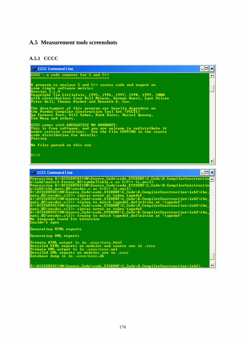
A.5 Measurement tools screenshots

A.5.1 CCCC

176

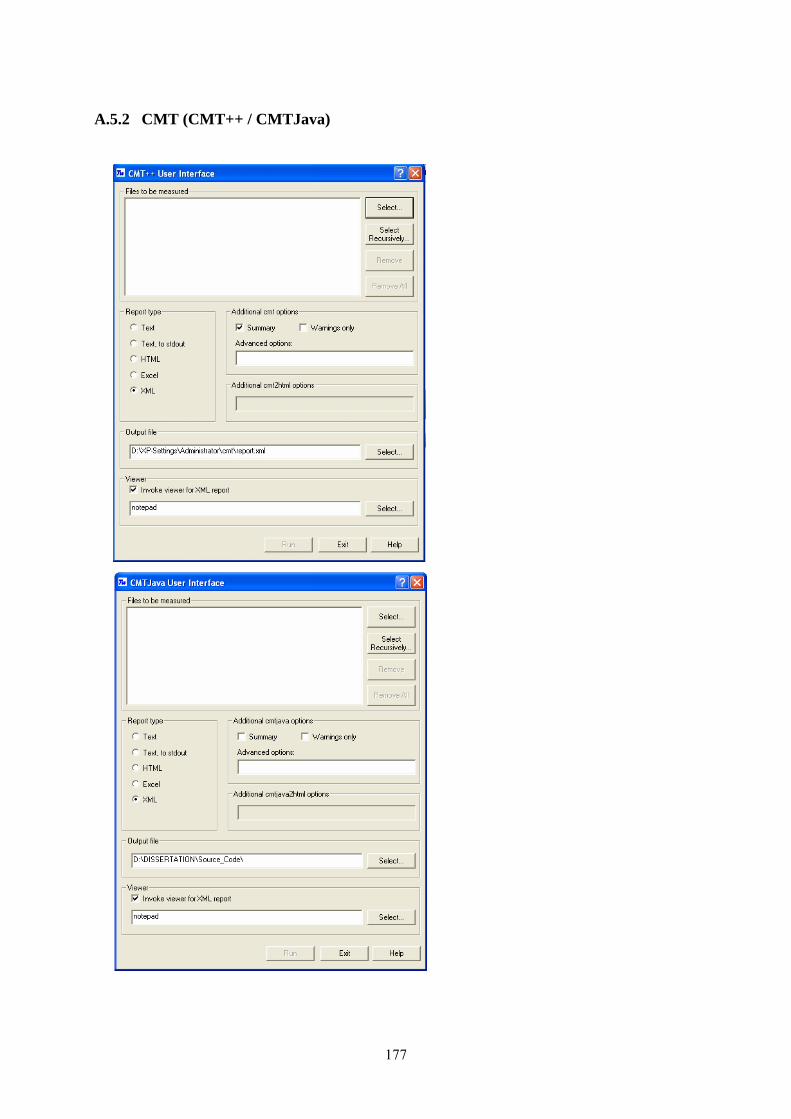
A.5.2 CMT (CMT++ / CMTJava)

177

A.5.3 SourceMonitor

178

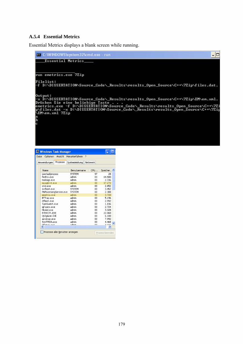
A.5.4 Essential Metrics

Essential Metrics displays a blank screen while running.

179

A.5.5 Logiscope

180