Crum_10782178.pdf - Mountain Scholar

T-2337

AN APPLICATION OF A PROGRAM EVALUATION

AND REVIEW TECHNIQUE MODEL

FOR THE INTRODUCTION OF A NEW PACKAGED

CONSUMER GOOD

byLester L. Crum

CLOSED RESERVE

ARTHUR LAKES LIBRARYCOLOR/ D«j .: COL oi MINES

ProQuest Number: 10782178

All rights reserved

INFORMATION TO ALL USERS The quality of this reproduction is dependent upon the quality of the copy submitted.

In the unlikely event that the author did not send a com p le te manuscript and there are missing pages, these will be noted. Also, if material had to be removed,

a note will indicate the deletion.

uestProQuest 10782178

Published by ProQuest LLC(2018). Copyright of the Dissertation is held by the Author.

All rights reserved.This work is protected against unauthorized copying under Title 17, United States C ode

Microform Edition © ProQuest LLC.

ProQuest LLC.789 East Eisenhower Parkway

P.O. Box 1346 Ann Arbor, Ml 48106- 1346

T-2337

This Thesis 1s submitted to the Faculty and the Board of Trustees

of the Colorado School of Mines 1n partial fu lfillm ent of the require

ments for the deqree of Master of Science, Mineral Economics.

Golden, Colorado

Date: Juhn JL3 , 19_gp

Slqned:Lester L Crum, Student

Golden, Colorado

Date: Juh e U » 19To

Approved: /&&>/<, tR.E.D. Woolsey, Thesis Advisor

- ttfoo/sa.)Tsey, hRobert E.D. WooTsd̂ , Head

Department of Mineral Economics

11

T-2337

ABSTRACT

This thesis demonstrates the use of a special type of

network analysis known as PERT (program evaluation and re

view technique) to ensure the precise planned timing of a

new product introduction. New consumer products which

have large volume fluctuations monthly or seasonally re

quire the introduction to occur at the optimum point to

achieve the highest potential market share. Timing is

also critical in the expected profitability of a new prod

uct: the purchase, installation, and operation of all

capital equipment with the shortest lead time before prod

uct distribution and customer sales realize higher returns

on the invested capital.

The analysis of the new product by means of the PERT

network indicated a zero probability of the project meet

ing the time schedule before the peak volume of the plan

ned year. Consequently, the project manager presented and

received acceptance from the senior management of the com

pany to reschedule the new product introduction for the

following year. The new time schedules drastically improved the odds of the project achieving the projected

profits and market share.

i i i

T-2337

CONTENTS

LIST OF ILLUSTRATIONS..................................... v

LIST OF T A B L E S ..................................... . . . vi

ACKNOWLEDGEMENTS .......................................... vii

INTRODUCTION................. 1

I. LITERATURE SURVEY.................................... 4

Critical Path Analysis.......................... 4

Networks............................................ 10

Deterministic Approach. . . .................... 16

Stocastic Approach................................. 23

II. PERT METHODOLOGY......................................2 5

Approximating the Beta Distribution ........... 25

Early and Late Time for an Event.................. 28

Probability of a Scheduled Event.................. 31

III. NEW PRODUCT EVALUATION . ........................... 36

Problem Statement ............................... 36

Solution Approach and Network ................. 37

R e s u l t s............. 42

IV. SENSITIVITY ANALYSIS: ACTIVITY AND NETWORK BASED. 46

Activity Based Errors . .........................46

Network Based Errors............................... 50

Epilogue............... 52

iv

T-2337

APPENDIX

A. Area Under Normal Curve. ................. 56

B. Input D a t a ............................................. 57

C. Input Activity Discriptions. ...................... 71

D. Output R e sults.........................................79

BIBLIOGRAPHY.......... 86

ILLUSTRATIONS

Figure

1 Gantt Chart of Job Processing Times .............. 6

2 Gantt Chart of Job Processing Times .............. 7

3 Project Network of Budgeting Process................ 15

4 Typical Job Duration Time-Cost Relationships. . . 18

5 Network Example - C P M ................................19

6 Time-Cost Trade-off for CPM Example .............. 20

7 Possible Forms of the Beta Distribution............ 27

8 Sample Network.........................................29

9 Nugget Activity Flow Network......................... 41

10 Alternative Distributions to the B e t a .............. 48

11 The Alternative Nugget Activity Chart ........... 53

v

T-2337

TABLES

1 Job Processing Times............................. 5

2 Budget Project.....................................14

3 Sample Network Event Calculations ................ 30

4 Sample Network Expected Values (T )2and Variences («r)..............................34

5 Sample Network Probabilities..................... 34

6 Nugget's Critical Path and Expected Probabilities 45

7 Comparison of Parallel Activity Paths ........... 51

8 Discription of the Alternative Activities . . . . 5 4

vi

T-2337

ACKNOWLEDGEMENTS

Writing an acceptable thesis has more than fulfilled my

expectation of frustration. The mechanics and revisions of

some sentences became a word by word construction process

which pushed the range of emotional and thought processes

to deeper thresholds of pain. Fortunately, two things kept

me going and in retrospect, made the task anything but

grim. First, the realization that most of my future prob

lem solving efforts will not require a thesis format for

communication purposes, which ensures I'll continue to en

joy my work. And second, the experience of accomplishing a

goal in which the encouragement of a few people turned a

shared frustration into one of fun. Thanks to my parents

Evelyn T. and Lester W. Crum who encouraged me while com

pleting this the si s as they have throughout the learning

experience of life. If a thesis is a learning exper

ience, then these two people have made my goal directed

life a master thesis.

I would like to thank each member of my thesis com

mittee for giving me a permanent impression which has ex

panded my knowledge and application of Operations Research. Thanks to Dr. Liernert, my first undergraduate

professor in Operations Research, whose hard work and en

thusiasm for Operations Research inspired my study in this

vi i

T-2337

discipline; to Dr. Stermole, who gave added meaning to

Benjamin Franklin's statement, "Remember that time is

money," by demonstrating the importance of the time value

of money; and most of all to my thesis advisor, Dr. R.E.D.

Woolsey, whose advice in problem solving approaches was,

"Do the simple things first."

Also, I'd like to thank J. Robert Copper who gave me

the opportunity and support to address and solve the prob

lem illustrated in this thesis. And finally, to my con

fidante, Karen Carlson, ' who typed and proof read each

draft of this thesis, my sincere appreciation.

vi i i

T-2337 1

INTRODUCTION

The corporate objective to increase revenues is common

to most firms. The increasing dollar sales is an indica

tion of a firms vitality to generate and sustain profits.

To increase total revenues, a firm must maximize the

effectiveness of pricing, advertising, promotions, and

distribution for current products and by adding new prod

ucts to the current product mix. For existing products,

revenue growth becomes an in-depth analysis of pricing and

volume relationships. If product demand is elastic, a re

duced pric'e will increase total revenue, while products

with inelastic demand will increase total revenue with an

increase in price. In the case of new products, market

share penetration for that product’s target market indi

cates the expected increase in sales to the firm.

The new products, besides increasing the revenue base

through additions to the number of products for sale, also

serve to replace the marginally economic products. The

latter function, replacing uneconomical products, is the

most important for new products. Manufactured products,

whether industrial, consumer durable, or non-durable, have

a product life cycle: introductory stage, growth stage,

maturity stage, and declining stage (1). Thus, the

backbone of the corporation then becomes the efforts to

T-2337 2

introduce new products for those in the declining stages

as additions and possible replacements in the currentproduct mix.

The firm's emphasis between new products and existing

products is weighted for the existing products. Here the

human and capital resources in the functional areas of

forecasting, procurement, marketing, manufacturing, dis

tribution, and sales are in place. Also, management can

plan pricing strategies to maximize profits having some

historical basis to forecast the future.

New products, by their non-existence, require a dif

ferent planning and management control within and between

functional areas than the mix of current products. Any

time delays to bring a new product into the product mix

represent foregone revenues and profits for the corpora

tion. The opportunity costs of poor planning and sched

uling of new products are in the millions of dollars for

delays as short as six months. For example, a consumer

goods manufacturer of non-durable goods will experience

seasonality for the various products demanded. Due to

this cyclical demand, the timing of the new product intro

duction should be just before the annual peak demand (2). At the peak of the demand cycle the new product will ex

perience more first time purchases. The larger number of

first time purchases provides a higher probability of

T-2337 3

repeat purchases (3). Therefore, the mature stage market

share for a new product is a partial function of the num

ber of first time purchases. A firm will delay until the

following demand peak if there are any delays in the new

products introduction. There are examples where the lost

profits for a year have reduced the product’s expected

return on investment to the point where the project is

stopped indefinitely.

The purpose of this paper is to illustrate a manage

ment control tool, program evaluation and review technique

(PERT), for a new product introduction. The objective of

the analysis is to provide a means for planning and man

aging activities within and between functional areas and

specifically determine the probability of meeting a sched

uled new product introduction for the peak demand period.

T-2337 4

I. LITERATURE SURVEY

CPA

Program Evaluation and Review Technique is one of a

family of planning and scheduling techniques known gener

ally as critical path analysis (CPA). Plans and schedules

have long been the tools which management has employed to

accomplish the difficult task of coordinating the efforts

of many diverse activities towards a common goal. Ide

ally, a plan is a document that states the manner and

order in which the various tasks of an operation are to be

accomplished before the operation begins. Schedules are

plans that have been fitted to the calendar in order to

meet an established objective date. The plan tells each

component of the organization what is expected of it and

the schedule tells it when it must be accomplished. By

comparing what is accomplished with what was directed,

progress towards the objective can be evaluated and reme

dial action taken if required. Most of the traditional

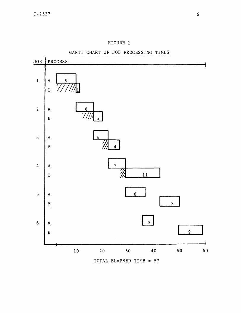
scheduling techniques are based on the GANTT or bar chart

which have been in common use for over 50 years (4, 5).An example of two Gantt charts depicting the elapsed times

for six jobs consisting of two technologically ordered

processes (process A must precede B) listed in Table 1

follows (5).

T-2337 5

TABLE 1

JOB PROCESSING TIMES

JOB A B

1 9 1

2 8 3

3 5 4

4 7 11

5 6 8

6 2 9

A = Processing time on machine A

B = Processing time in machine B

T-2337 6

FIGURE 1

GANTT CHART OF JOB PROCESSING TIMESJOB PROCESS

A

B 7/m

AB

A

B

AB

A

B

2 A 8

B 'ini,3

%7 I 11

□10 20 30 40 50 60

TOTAL ELAPSED TIME = 57

T-2337 7

Figure 2 shows a collapsed version of the preceding Gantt

Chart.

FIGURE 2

GANTT CHART OF JOB PROCESSING TIMES

9 8 5 7 6 2m M <y//t 11 8 9

T-2337 8

Although these techniques are valuable tools for

scheduling small projects, their use is limited and detri

mental to scheduling of large scale operations. In par

ticular, the bar chart fails to delineate complex inter

actions and relationships which exist among the project

events. In addition, they do not lend themselves to mech

anization through the use of a high speed electronic com

puter. Hence, the developement of CPA as a management

control tool enabled large and complex tasks to be system

atically planned and scheduled. Ideally, CPA functions to

( 6 ):

1. Facilitate the establishment of realistic objectives, initially, so that the likelihood of their timely achievement is good.

2. Monitor the progress of the project and alert management to potential danger areas, on an exception basis, far enough in advance of their occurrence to permit corrective action to be taken with minimum cost and disrupt ion.

3. Provide a vehicle for selecting the optimum course of action from among the several alternatives on a quantitative basis and in accordance with objective criteria when such action is indicated.

CPA was initially used in the construction industry

but is presently finding widespread usage in the defense

industries especially the segments concerned with the

development of aircraft missiles and spacecraft (6). It

has also been successfully employed in the chemical and

petroleum refinery industries and the outlook is that it

T-2337 9

will eventually find application in many other areas, par

ticularly those engaged in project type activities. Among

the many operations that may be classed as projects, are

heavy construction, facilities maintenance, ship building,

and the research and development phase of military weapons

systems acquisitions (7, 8). The organizations engaged in

these operations tend to have several things in common.

The following are of particular interest (9):

1. The end products of each operation are few in number.

2. Each operation is composed of a large number of serial and parallel jobs.

3. All of the jobs are directed toward a common objective event.

4. A significant amount of uncertainty existsregarding the exact manner in which the objective is to be accomplished, how long it will take, and how much it will cost.

The degree of uncertainty will vary with each operation depending upon such factors as the state of the technology employed and the number of times similar operations havebeen performed in the past. In general, theeffects of this uncertainty are quite noticeable when contrasted to production type activities where the operation reaches a steady state and the uncertainty is relatively low.

5. Different jobs are done by different organizations which have difficulty communicatingwith each other.

T-2337 10

NETWORKS

The main idea underlining CPA is the characterization

of a project as a network of inter-related events. The

use of a network or flow diagram as a model of the proj

ect's technological precedence relationship is the one

common element that all CPA family of techniques has in common (10). The network represents all the activity

paths or chains of events that must be accomplished before

achieving the project's objective. The most time restric

tive of these is called the critical path (11). Manage

ment's attention is focused on those activities which form

the critical path. A delay of any one of these activities

means the project's completion will be extended. For this

reason, the term critical path analysis (CPA) has been

given to this family of techniques (12).

The flow diagram or network used as the project model

is an outgrowth of the flow graph technique which has been

used for some time in systems engineering activities (13).

Systems have long been described by mathematical models in

the form of equations. However, the set of equations that

suffices to describe the behavior of a system, fails to portray the structure of the whole system in a readily

comprehended form. Each equation reveals only one com

ponent of that structure and conventional notation does

little to connect these pieces into a coherent whole.

T-2337 11

The flow graph diagram evolved to overcome these

deficiencies. They provided a visual and concise

description of the systems structure that was capable of

being manipulated and solved. "These later operations are

governed by a straight forward set of rules so that one

flow graph is the equivalent of an entire set of equations

(14)

Much work has been done in this field, particularly in

regard to the solution of networks (15, 16, 17). A proj

ect characterized as a network will show the inter-rela

tionship and sequential order of events which must be ac

complished to achieve the desired objective by a certain

date. An event initiates or marks the beginning of an

activity and another event signals the completion of that

activity (18). An event is separated from other events by

jobs or activities which consume time and resources. A

job can not begin until the preceding event has been

accomplished and the succeeding event can not occur until

the jobs which precede it are completed. Certain jobs in

a project must be accomplished in a serial fashion and

others may be accomplished concurrently. Thus, a given event may depend on the completion of two or more jobs.

Generally, it can be expected that one of these parallel

preceding jobs will require more time to complete than its

companions. Similarity, certain events will require more

T-2337 12

time to achieve than others. The particular sequence of

events which represents the most rigorous time constraint

for accomplishing the objective are the critical events/

and comprise the critical path (19). Thus, the critical

path consists of those elements that can not be delayed

without incurring an equivalent delay of the project com

pletion date.

There may be more than one critical path depending

upon the urgency of the project and the degree to which

each job is compressed. A measure of this compression is

the amount of float or slack which a job contains (19).

Float is the difference between the maximal amount of time

available to do a job as prescribed by the schedule and

the time required to do the job utilizing a given level of

resources and without regard to its predecessors or suc

cessors. Float normally has a positive value for non-

critical jobs and zero for those on the critical path.

The project network can be formed in several ways.

One of these is to start at the end or objective event and

work backwards in time in. a step-by-step fashion deter

mining what work must be performed in order to achieve a

given event. Another approach is to list all the jobs

having a bearing on the project and to determine their

precedent relationships before diagramming. A simplified

example illustrates the approach which starts with

T-2337 13

precedence relationships before diagramming (20). The

project is to determine the next year’s operating budget

for a large manufacturing firm. To accomplish this proj

ect the following jobs or activities need to be per

formed :

1. Salesmen must provide unit sales estimatesto the sales and production managers;

2. the Sales manager estimates the market pricefrom the forecast and submits this to thefinance officer;

3. the Production manager schedules the unitsfor production, forwarding the schedule to account ing;

4. the Accounting manager determines the costsof production for the finance officer; and

5. the Financial officer prepares the finalbudget from the sales and accounting departments inputs which is submitted to the president of the company.

Before diagramming, the order in which the jobs have to be

completed before others can be started must be identi

fied. In this example, the sales forecast must be done

before any other activity. The market pricing and produc

tion scheduling follow directly from the sales forecast

which is referred to as the immediate predecessor. Simi

larity, the production schedule is the immediate predecessor for costing the production; the sales pricing and

costing of production are immediate predecessors to thei*

budget preparation. Table 2 summarizes this information.

T-2337 14

TABLE 2

BUDGET PROJECT

JOB DESCRIPTION DEPARTMENT PREDECESSOR

1 Forecasting unit sales Sales

2 Pricing sales Sales 1

3 Preparing production schedules

Manufacturing 1

4 Costing the production Account ing 3

5 Preparing the budget Treasurer 2, 4

Figure 3 shows the project graph or network for the bud

geting projects. Jobs are shown as arrows leading from

one circle on the graph to another. The circles are

called nodes or events (21).

T-2337 15

FIGURE 3

PROJECT NETWORK OF BUDGETING PROCESS

►

No matter which one of the several approaches is usedin the construction of the project network, two essential

steps are found. First, determine precisely those activi

ties that must precede and follow each job and those that

must be performed concurrently. Second, diagram those

relationships without regard to the time duration of the

job. Each job is represented by an arrow which indicates

the direction of the flow of work but whose length has no

significance. Each event is represented by a circle,square or other geometric shape and appears as a nodeformed by the confluence of two or more arrows (22). In

particular, event nodes are identified by numbers assigned

in a variety of ways depending upon the characteristics of

T-2337 16

the computer program employed. Job arrows may be identi

fied by a letter or by the combination of numbers assigned to the events that precede and succede each event. In

addition to the internal work restraints, external re

straints such as deliveries of basic data, equipment,

material and other factors over which management has

little control should be shown. Thus, the project network

represents a completely stated plan, together, with the

environment in which it must be carried out (23).

DETERMINISTIC APPROACH

All CPA approaches use a network to depict and solve

the scheduling problems of a project. It is at this point

that the major difference in the various CPA techniques is

noted. The time certainty or uncertainty of the job

activities in a project determines whether the input data

will be probabilistic or deterministic. When the tech

nology being employed is well established and the degree

of uncertainty is relatively low, the use of deterministic

input data is used (24). In these cases, the operations

of the proposed project have been performed many times in

the past and the job durations are known and can be deter

mined to a reasonably high degree of accuracy.

T-2337 17

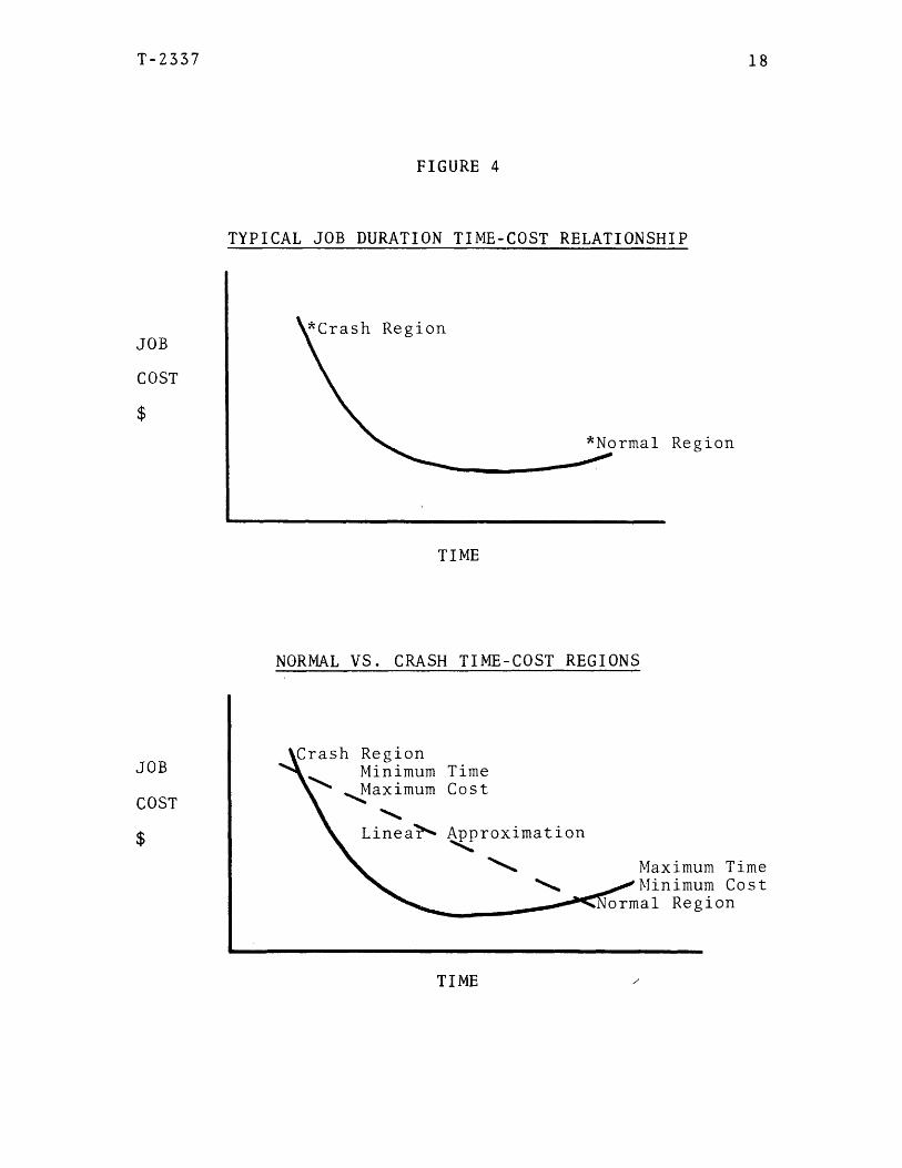
When the job duration is known or can be accurately

estimated the associated costs of performing that job is

likely to be known to the same degree of precision. The

two quantities of time and cost very inversely to one

another as shown in Figure 4 (25). Usually, there is some

region where cost is at a minimum and in which management

elects to operate in order to meet its objectives. This

is known as the normal cost and the associated job dura

tion is the normal time to do the job. For critical path

analysis this is the maximum time to do a job as shown in

the same figure. There is also a minimum time to perform

a given job which can be achieved by expending more re

sources in the form of labor, equipment, and materials.

This is referred to as the crash time and the associated

crash cost is the maximum cost for the project. The crash

cost is the total incremental expense from reducing the

activities’ completion times. Between these limits many

other job time-cost relationships exist and are available

for computing schedules as either simple linear or piece-

wise linear representation of the time-cost curve (26).

The original CPM model assumed that the time-cost trade

off for an individual activity is linear with a negative

or zero slope as in Figure 4. The steeper the slope of

the line the higher the cost of expediting the activity;

crashing the job time at no additional cost represents a

line with zero slope or a horzontal line.

T-2337 18

FIGURE 4

TYPICAL JOB DURATION TIME-COST RELATIONSHIP

JOB

COST

$

TIME

NORMAL VS. CRASH TIME-COST REGIONS

JOB

COST

$

TIME

Irash RegionMinimum Time Maximum Cost

Lineai*^ ApproximationMaximum Time Minimum Cost

ormal Region

*Crash Region

*Normal Region

T-2337 19

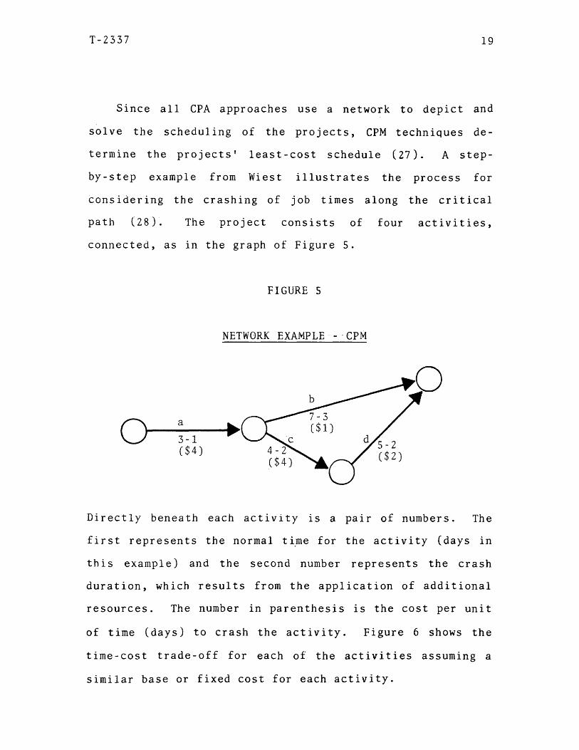
Since all CPA approaches use a network to depict and

solve the scheduling of the projects, CPM techniques de

termine the projects' least-cost schedule (27). A step-

by-step example from Wiest illustrates the process for

considering the crashing of job times along the critical

path (28). The project consists of four activities,

connected, as in the graph of Figure 5.

FIGURE 5

NETWORK EXAMPLE - CPM

($i)C$4) ($2)($4)

Directly beneath each activity is a pair of numbers. The

first represents the normal time for the activity (days in

this example) and the second number represents the crash

duration, which results from the application of additional

resources. The number in parenthesis is the cost per unit

of time (days) to crash the activity. Figure 6 shows the

time-cost trade-off for each of the activities assuming a

similar base or fixed cost for each activity.

T-2337 20

FIGURE 6

TIME-COST TRADE-OFF FOR CPM EXAMPLE

Activity a Activity b

10987654321

Slope=l

DAYS

10

Slope=4

s

DAYS

Activity c Activity d

10Slope=4

s

DAYS

10987654321

Slope=2

DAYS

T-2337 21

The critical path for this example network is a-c-d which

is a total of twelve days. Assuming the fixed expenses

for the project are time related at $4.50 per day, then

the incremental total cost of the schedule is $54:

Total cost = cost of crashing + cost of overhead = 0 + (12 days)($4.50)= $54.00.

Since activity d has the smallest time-cost trade-off

(slope = 2) on the critical path and the path a-b has two days of slack, the cost of reducing activity d by two days

is calculated:

Total cost = cost of crashing + cost of overhead= (2 days)($2) + (10 days)($4.50)= $49.00.

There are now two critical paths, a-b and a-c-d each

with ten days total time for the project. To reduce the

project schedule further, activities b and c, b and d, or

a must be evaluated. Because activities b and d have the

smallest combined time-cost trade-off ($3), each activity

is reduced one day. Activity d can be reduced to a mini

mum total of two days: the two days reduction at the

first step plus the one day at this point reduces the five

day schedule to the minimum. The total cost for the nine

day schedule is as follows:Total cost = cost of crashing + cost of overhead

= (1 day)($l) + (3 days)($2) + (9 days)($4.50)= $47.50.

T-2337 22

The remaining alternatives for reduction are activity

a or activity b and c. Activity a is the least expensive

($4) compared to activities b and c expense ($5). Activ

ity a can be reduced two days to its’ one day minimum for

a seven day schedule which costs-out to $46.50:

Total cost = cost of crashing + cost of overhead= (2 days)($4) + (1 day)($l) + (3 days)($2)

+ (7 days)($4.50)= $46.50.

The seven day schedule is the least-cost for this

project. Activities b and c can be reduced further but

the cost of crashing will exceed the saving from overhead

expenses.

The preceding process is described as an exhaustive

search procedure because each possible alternative action

of each step of the solution must be evaluated. For proj

ects larger than the example presented, this procedure be

comes more and more difficult to evaluate by a manual

technique. Fortunately there are a number of computer

software packages that handle deterministic inputs of time

and cost. The majority of these techniques are referred

to as Critical Path Methods (CPM) (29). Further develop

ments since 1962 reflect the addition of software programs

incorporating deterministic as well as probabilistic in

puts (30). The next section discusses the approach to

probabilistic time inputs.

T-2337 23

STOCHASTIC APPROACH

The approach to those projects having job times which

are unknown but can be estimated to a reasonable degree of

accuracy are the projects whose job duration uses a proba

bilistic approach. Program Evaluation and Review Tech

nique (PERT) is a CPA application which uses a stochastic

approach to the job activities and to the likelihood of

meeting scheduled completion dates (31). Early in 1958 an

operations research team began an investigation of CPA

techniques for use in evaluating the progress of the U. S.

Navy’s Polaris Fleet Balistic Missile Program (32). Mem

bers of this team included a management consulting firm,

Lockheed Missiles and Space Division, the prime contractor

for the weapons system, and the Navy’s special project

office which was charged with management of the program.

From this investigation came the CPA approach known widely

as PERT. The original application involved 23 networks

connected by some 3,000 job activities that provided con

tinuous appraisal of the project’s validity in terms of

plans and schedules (33). The successful use of PERT in

the Polaris Missile program lead the navy to use PERT inits Eagle Air to Air Missile project and to the aircraft

carrier which was to carry the Eagle Missile. Therefore,

the development and the successful use of PERT as a man

agement control tool had its beginning in the U. S. Navy's

T-2337 24

complex weapons development program. Since 1958, PERT has

experienced a rapid and diverse application. This is due

to the ease of adapting PERT to project type activities

where the technology is new and developing and the uncer

tainty of activities time is indefinite. These projects

are generally representative of old as well as new tech

nological ventures of production. For these cases the

PERT method determines the probability of meeting sched

uled deadlines from estimates made of the approximate

range of the job durations (34).

T-2337 25

II. PERT METHODOLOGY

The first step in the application of PERT is to

develop a network representing the activities of the pro

ject plan. Next a time estimate for each activity's dura

tion is made. Due to the uncertainty in estimating dura

tion times for developmental and research type projects,

PERT assumes the probable duration of an activity is

Beta-distributed. The choice of the Beta distribution

fulfilled three properties that would be postulated for an

actual activity distribution: unimodal, continuous, and

two nonnegative abscissa intercepts (35).

APPROXIMATING THE BETA DISTRIBUTION

The scientist, engineer or manager directly concerned

with the performance of the activity provides these esti

mates :

1. The optimistic estimate of time, symbol a.

2. The most likely estimate of time, symbol m.

3. The pessimistic estimate of time, symbol b.

The PERT literature (36) defines these time estimates as follows:

1. Optimistic time: the resultant duration ifeverything goes better than expected; usually depends upon a breakthrough of some kind. Basically, fewer than 1% of similiarjobs would be completed in less time.

T-2337 26

2. Most likely time: the resultant duration ifeverything goes as expected.

3. Pessimistic time: the duration required ifeverything goes wrong. Fewer than 1% ofsimiliar jobs would exceed this time.

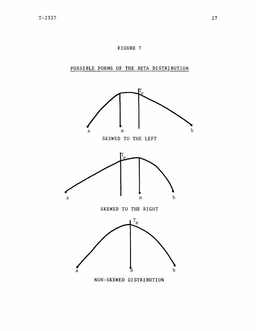
The three time estimates are used to calculate an expected

time, symbol T ;rr. a + 4m + be 6

Te is a linear approximation of the mean for the beta distribution with the probability density function

f(t) = K • (t-a) «(b-t) . The end points, a and b; and the

exponents, e*6- and , must be specified to determine a

unique beta distribution. The optimistic and pessimistic

times are used to specify a and b. The most likely time

is the value used as the mode of the distribution. This

value and the assumption that the standard deviation of

~ the distribution is 1/6 of its range, - l/6(b-a), deter

mines the two parameters and (37). These two

parameters (o* ) also determines the value of the func

tion defining the constant K. The theory of T is to

divide the uncertainty by assuming a 50 percent chance of

being right. The value of Tg would approximately split

the area under the density function into two equal parts(35). This is also true for values of a, b, and m which

determine distributions skewed to the left, skewed to the

right, or non-skewed (figure 7) (38).

T-2337 27

FIGURE 7

POSSIBLE FORMS OF THE BETA DISTRIBUTION

SKEWED TO THE LEFT

SKEWED TO THE RIGHT

NON-SKEWED DISTRIBUTION

T-2337 28

EARLY AND LATE TIME FOR AN EVENT The third step in applying PERT is to calculate the

earliest and latest times which an event may begin. The

earliest time is defined as the time at which the event

will occur if all preceding activities are started as

early as possible; the latest time for an event is the

latest time an event can begin without delaying the com

pletion of the project beyond its earliest time. For

those events that have more than one path of activities

leading toward (or from) them, the earliest time (or

latest time) is calculated from the one path having the

maximum (or minimum) of the total T0 1 s leading to (or

from) that event (39). For example, in the following net

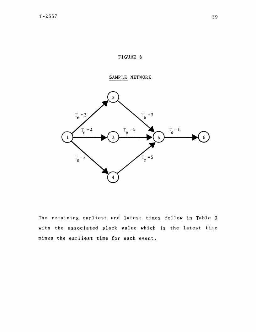
work (figure 8), there are three paths leading to event

number five. The three paths to event five and the

expected times of each are: © , Q), (j) = 6; © > @ > © = 8;

a n d © , © , (s) = 10. The earliest time is taken from the

path with the maximum expected time (T = 10) which is

the path consisting of events©, (4), © .

T-2337 29

FIGURE 8

SAMPLE NETWORK

= 4 ►0 — ►©

The remaining earliest and latest times follow in Table 3

with the associated slack value which is the latest time

minus the earliest time for each event.

T-2337 30

TABLE 3

SAMPLE NETWORK EVENT CALCULATIONS

EVENT EARLIEST TIME LATEST TIME SLACK

6 © ©© ® = i 6 © = 16 0

5 © © © = 10 © © = 1 0 0

4 ' © © - 5 ©©© ‘ 5 0

3 © © = 4 © @ © = 6 2

2 ® @ = 3 © © © = 7 4

1 oII© © © ©© = o 0

T-2337 31

The critical path is identified as those events having

zero slack. If the time unit for the expected value,

Te> is days, the path of events Q), Q), (j)> © totalling sixteen days represents the critical path. Any delay for

an activity along this path will delay the project. A

delay of two days on the pathQ^), (J) or a delay of four days

on the path (T^ Q ) will not delay the project beyond the

original sixteen days schedule.

PROBABILITY OF A SCHEDULED EVENT

The fourth and final step of the PERT application is

calculating the expected probability of an event beginning

when scheduled. PERT’S last assumption is the statistical

independence of all activity’s time in the project (40).

Therefore, the sum of the expected times, which determines

the earliest times and the associated times for the stan

dard deviation, tend toward a normal distribution accord

ing to the central limit theorem. The expected time,

Tg , and the standard deviations, , are from a betadistribution but the distribution of their sum still tend

toward normality. The central limit theorem states (41):

Let the random variables , X£> ...., Xn

be independent with means u, . u„........ u .1 * 2 * * n ’2 2respectively, and associated variance 2 *2. . • • , cs~ • The random variable Z .’ n n

T-2337 32

/ _ Xfc ~ £-1 -/n

under certain regularity conditions is approxi

mately normally distributed with zero mean and

unit variance.

The transformed cumulative density function for the normal

distribution where Z = (y-u)/^- is:2

- ooVZrr

The table of values in Appendix A is used to calculate the

probability of an event starting later than scheduled.

Appendix A is entered with K = (b-u)/^- andCO ~2̂

I

, _ / /n<

d ’z

which is the area (probability) under the normal curve of

a normal random variable being greater than K<*-=(42). Due

to the symmetry of the normal distribution, the value 1 -

gives the probability of being less than K^c • Referring

back to the Zn formula, the variables x^, u^,2and <5 * ̂ are interpreted as follows:

x^= The scheduled start date for event i wherethe start of the project is on day numberone.

ui= The (largest) sum of the Te 1s for theactivities whose path (paths) leads to event i.

2«*i= The sum of the activity variances for thecorresponding Te ’s leading to event i.

T-2337 33

Returning to the preceding example, if the scheduled start

time for each activity is based on the most likely time

estimates leading up to each activity, event six has a 16%

probability of meeting its’ schedule. The two events 2

and 3 have the highest probability of meeting their

schedule, 50% and 77%, respectively. The remaining proba

bilities are shown in the following tables 4 and 5.

T-2337 34

TABLE 4

SAMPLE NETWORK EXPECTED VALUES (Te), AND VARIANCES (^ )

EVENTOPTIMUMESTIMATE

MOSTLIKELYESTIMATE

PESSIMISTICESTIMATE T*

5 to 6 4 6 8 6 .44

2 to 5 1 3 5 3 .44

3 to 5 2 4 6 4 .44

4 to 5 4 5 6 5 .11

1 to 2 2 3 4 3 .11

1 to 3 2 3 10 4 1.78

1 to 4 3 4 7 5 .44

TABLE 5

SAMPLE NETWORK PROBABILITIES

EVENTEARLIEST TIME*

SCHEDULE PROBABILITYT* ..6 16 .99 15 .16-

5 10 .55 9 .09

4 5 .44 4 .07

3 4 1.78 3 .77

2 3 .11 3 .50

1 0 0.00 - -

*Earliest time (Te , <ar^) correspond to the definitions of 14 and ^ 2 ̂ 0n the preceding page.

T-2337 35

In summary, the PERT methodology consists of four steps:

1. Develop the projects activity flow network.

2. Obtain the relevant time estimates for each act ivi ty.

3. Calculate the earliest and latest time estimate for each event in the project.

4. Calculate the probability of an event beginning on schedule.

T-2337 36

III. NEW PRODUCT EVALUATION

PROBLEM STATEMENT

The PERT example to follow was used to resolve the

problem situation of a new product that had advanced to

the last stages of development before commercialization.

This example is the first time in the company's history

that PERT was used as a planning or as a problem solving technique related to new product introductions. Despite

the fact that personnel in the functional areas of market

research, research and development (R§D), and engineering

were familiar, in varying degrees, with PERT; the market

ing department is ultimately responsible for all stages of

new product development. Unfortunately, the marketing

personnel and specifically the New Product marketing mana

ger's low level of confidence in a new quantitative tech

nique (PERT) was understandable. This confidence level is

a particular reflection of the operating and organiza

tional structure of this company: the marketing depart

ment will defer to the experts (operations research, en

gineering, research and development, market research,

etc.) as the major source of evaluation while maintaining the final approval on all recommendations. Therefore, the

marketing department provides the primary initiative and

management in developing, assimulating, and presenting

T-2337 37

recommendations and programs for upper management’s evalu

ation. After approvals are granted, the marketing depart

ment holds the major responsibility for implementation.

The manager responsible for the commercialization

phase for this new product (for proprietary reasons the

product will be referred to as Nugget) presented hisproblem as follows:

Nugget has failed to reach the manufacturing volumes from line tests indicating that the production plants can not fill a national distribution pipeline. Reaching national distribution before the start of the bake season (October) is the marketing strategy approved by senior management. If the manufacturing and R§D problems which have been resolved and those still pending can not be implemented before September the sales and creative activities will be stopped andintroduction will be scheduled for next year.

It is critical to know the odds of success in meeting the planned start ship date. The risk of introducing Nugget into only a limited number of markets is the reaction of competitors introducing new products which would absorb enough volume the next bake season to jeopardize the current and projected profits of the product. In essence there must be enough product produced in September to distribute nationally this year with the contingency plan to delay and introduce the next year.

SOLUTION APPROACH AND NETWORK The proposed solution was to derive a PERT chart

depicting the remaining activities for the Nugget intro

duction and estimate the probability of the project

T-2337 38

meeting the scheduled start ship date. The application of

PERT involved the following steps: list all the jobs or

activities that have to be carried out to complete the

program; assign to each job the estimated time required to

perform it; logically arrange the jobs which are sequen

tial and/or concurrent; sum the time for those jobs that

must be performed consecutively; determine the critical

path; and, calculate the probability of the expected time

meeting the scheduled time for each activity on the criti

cal path.

The marketing manager did not know in total the jobs,

time duration nor precedence relationship for the commer

cialization activities in the Nugget project. This has

been the norm, rather than exception, for all new product

development because a large number of new product ideas

progress through the first stages of development: screen

ing, feasibility, and development, but very few are

approved for commercialization development.

During the first three stages of development, (screen

ing, feasibility, and development), the marketing depart

ment works directly with the R§D department. The personnel in marketing solicits, generates, and segments new product ideas while the R§D personnel will assess the pre

liminary feasibilities for formulations, packaging, and

manufacturing. This information is incorporated into a

T-2337 39

preliminary economic evaluation that if approved leads in

to the beginning of the development phase. R§D will fin

alize the technical plans for process and package design

in the development phase while the market research and

marketing departments continue product and consumer evalu

ations forming the marketing position and branding for the

product. It is at this point that data collection begins

for the finalized capital appropriations needed to bring

the project to commercialization.

Interviews with the marketing people supplied the

background information which represented the stage the

Nugget project had progressed to as of a year ago. At

that time, January, upper management. authorized the Nugget

project to proceeed to the final commercialization phase.

Usually, the first step after the commercialization

approval is the submittal of a package and graphics con

cept by a marketing manager. Simultaneously, the R§D and

operations departments develop a preliminary manufacturing

plan covering the design of the facilities and instal

lations. The problems which developed from that point

were related to the failure of the test equipment to perform at required processing speeds. For the remaining

months of that year, issues of ingredients, formulas, and

equipment were addressed. As of the first of September,

preliminary shelf-life tests indicated the Nugget project

T-2337 40

was again ready to begin the first step of commercializa

tion. One year was spent resolving problems just to bring

the Nugget project to the development point that upper

management believed it to be last September. The network

in figure 9 shows the flow of activities leading up to the

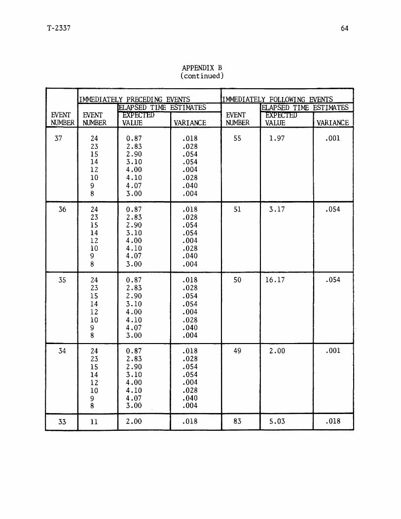
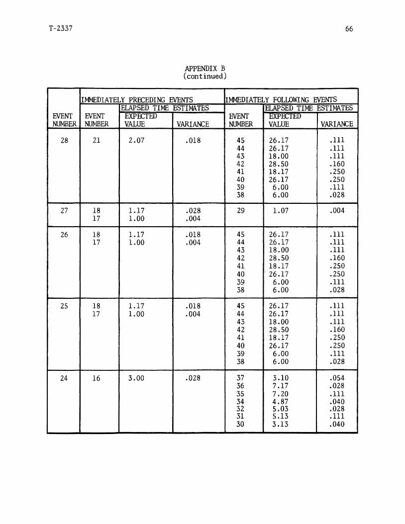
next- scheduled start production. Appendix B contains the

detailed time estimates and precedence relationships

(those activities which precede or may begin concurrently

to one another) for the network shown in figure 9, and

follow the format used by Hillier and Lieberman (43). The

descriptions of the activities are listed in Appendix C.

Time estimates, which are in weeks or a fraction of a five

day week, and precedence relationships were supplied by a

group engineer from the functional area of processing and

from packaging. These two groups of engineers formed a

manufacturing plan using the resolved inputs from market

ing and R$D which reflected changes in the flavor consid

erations, package design and the desired scale of opera

tion. Against this identified manufacturing plan - which

was approved for validity by manufacturing, as well as,

R§D departments - the scheduled time table from the marketing department was finally imposed and evaluated.

T- 2337 42

RESULTS

A time limit of six weeks was imposed for determining

the odds of starting the product production by the first

of September. With that fact in mind, the objective was

to avoid wasting time identifying people and departments

responsible for past failures and the tendency of such

groups and departments to postulate what can not be accom

plished. The approach was to identify those activities which must be successfully accomplished between now and

September (approximately 9 months), assuming all technical

process and product problems had been resolved. The pre

ceding assumption reduced the number of detailed activi

ties each technician identified. Sometimes a certain

group of activities are considered as one activity. ’’This

interpretation may be quite desirable, especially when all

the activities in the group are technologically ordered

and can be considered to form a small project in it’s own

right (44).” For example, the testing and debugging of a

case packing machine may take a week under normal condi

tions. For the Nugget project, the case packing machine

was a new model and required a new set-up configuration;

consequently, the manufacturing and testing steps were not explicitly identified but the increase in the time esti

mates for manufacturing and testing were made. A total of

one hundred and forty-six activities (figure 9) were

T- 2337 4.3

identified as those necessary to bring Nugget to a factory

production state. Approval of the identified activities,

their associated precedence relation to each other and the

time estimates, (optimistic, most likely, and pessimistic)

were given by the departments of manufacturing, R§D, and

market ing.

The network represents the tasks (excluding advertis

ing and sales activities) that a marketing manager must

monitor for one year to assure production begins on sched

ule. The output of results are given in appendix D:

Hillier and Lieberman format (45). The critical path for

the network consists of the following activities which

have a zero slack time: 4, 5 , 21 , 28 , 42 , 54 , 112 , 125,

126, 118, and 146. This is also one of the paths with the

least control because the construction of the cartoner,

activity number 42, is contracted to an outside equipment

manufacturer. The contract represented the earliest pos

sible delivery date from all the bids submitted.

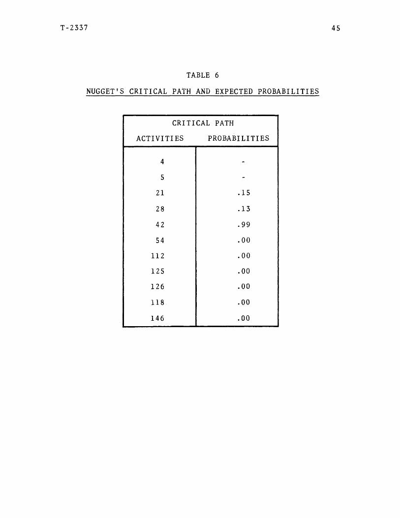
Associated with the critical path are the probabili

ties of the earliest start times beginning on the schedule

assigned by senior management asserting that production start by the first of September. Table 6 is a list of the network activities having a zero slack (critical path) and

the probability of each beginning on schedule.

T-2337 44

The probability of the Nugget project having product

available in all major national markets before the start

of the current bake season is zero. The activity (number

42) which delays the schedule is the design and construc

tion of the cartoner. As mentioned previously, the con

struction of the cartoner is performed by outside contrac

tors. The information from the PERT analysis was incor

porated in the negotiation of a new delivery date on the

new capital equipment which saved the company the cost of

paying for unproductive equipment.

T-2337 45

TABLE 6

NUGGET’S CRITICAL PATH AND EXPECTED PROBABILITIES

CRITICAL PATH ACTIVITIES PROBABILITIES

4 -

5 -

21 .15

28 .13

42 .99

54 .00

112 .00

125 .00

126 .00

118 .00

146 .00

T-2337 46

IV. SENSITIVITY ANALYSIS: ACTIVITY AND NETWORK BASED

The error implications in establishing a critical path

and the associated probabilities of these activities

beginning on schedule assume that the network is correct.

The activity precedence relationships and time estimates

are made by the managers and engineers most directly con

cerned with the performance of those tasks. Therefore, a

unique network representation is identified and possible

variation in the result is a factor of activity estimates

or the network configuration (46).

ACTIVITY BASED ERRORS

There are three possible activity time errors in esti

mating the mean and standard deviation: the deviation for

an activity duration which is not beta-distributed; the

error using the PERT approximation formula for the mean

and standard deviation for a beta-distribution; and the

implication of errors made by the managers, engineers and

scientists in the optimistic, most likely, and pessimistic

time estimates.MacCrimmon and Ryavec (46) considered two extreme dis

tributions, quasi-uniform and quasi-delta, as two extreme

functions to determine the extent and direction of errors

T-2337 47

in using the beta function. This is shown in figure 10

(46). Even though the true distribution of an activity is

not known, the possibility exists that the distribution of

an activity is not beta-distributed. The uniform and

delta distributions conform to the three properties of the

beta-distribution: unimodal, continuous, and having two

non-negative abscissa intercepts; and structured to give

bounds on possible errors on the mean and standard devi

ation by using the beta-distribution. The authors (46)

state that the possible error in the mean activity time

(T ) is a function of the mode and if the mode is near

the endpoint of the distribution (a and b values) the

error could be as much as 33 percent. Associated with the

mean error was a 17 percent absolute worst error in the

standard deviation for this case. Similar error results

were noted in using the approximating formulas for the

mean and standard deviation in the beta-distribution (46).

The additive effect of these two types of errors on

the estimating of the mean and standard deviation activity

time is cancelled by the negative and positive direction

of the error values. The ranges of the activity durations

and the skewness of the activity distributions are addi

tional factors which would lower the error of the expected

worst case.

T-2337 48

FIGURE 10

ALTERNATIVE DISTRIBUTIONS TO THE BETA

t)

Delta

BetaUniform

t1

T-2337 49

The last type of error relating to an activity's time

is the estimation error given for the optimistic, most

likely, and pessimistic activity times. To evaluate this

case an assumption was specified on the extent of the

range of the errors for the time estimates (46):

80% optimistic time 1.10

90% most likely time 1.10

90% pessimistic time 1.20

The results for this case is an absolute error in the mean

and standard deviation respectively:

Maximum mean error = 1/60 (a+4m+b)/(b-a)

Maximum standard deviation error = 1/30 (b+a)/(b-a)

In summary these three factors previously mentioned can

each cause an error of 30 and 15 percent of the range,

respectively, for the activity time's mean and standard

deviation. Since some degree of cancellation can be

expected to occur when all the activities are combined in a network, and the cases considered are extreme, the

errors may be reduced from the 30 and 15 percent to 5 or

10 percent (46).

T-2337 50

As the probability of beginning the production runs as

scheduled was zero, the three types of activity errors was

analyzed for those activities along the critical path.

This was to verify any change in the probability assuming

the errors reduced the expected activity completion time

by the guidelines of 30 percent for the mean and 10 per

cent for the variance. The finding was still a zero prob

ability of meeting a 52 week start production schedule.

At best, if the sum of the optimistic times were achieved

for each activity on the critical path, the probability of

meeting the scheduled production dates is .1 percent. The

.1 percent estimate is the best improvement to expect con

sidering the types of errors previously discussed.

NETWORK BASED ERRORS

There may also be error introduced into the calcula

tion of the early start probability times due to the con

figuration of the network. The calculated mean of an

activity path will be understated and the calculated

standard deviation overstated if parallel paths in the

network are present; where parallel paths are defined as

paths not having a common activity between them. Follow

ing is the table which summarizes the results which

MacCrimmon and Ryavec (46) (table 7) observed for parallel

paths having a mean duration very close to the mean dura

tion of the critical path.

T-2337 51

TABLE 7

COMPARISON OF PARALLEL ACTIVITY PATHS

RATIO OF LENGTHS_____ 1/1 3/4 1/2 1/4

Percent error of PERT from -17% - 8% -0.5% -0.0%actual mean

Percent error of PERT from +39% +23% +4.0% +0.0%actual standard deviation

/

Table 7 implies that if there is a path through a network

that is longer than any other path, the remaining paths do

not have an effect on the project completion time distri

bution in spite of the parallel effect (46). For the

longest path in this case, the central limit theorem is

applied: the mean and standard deviation is summed to

arrive at the project mean and standard deviation.

To examine the effect of parallel paths in the Nugget

network, the early start times on all paths were compared

to the duration on the critical path up to event number

128 which is 53.50 weeks. The next largest mean duration

of an event leading into event 117 or 118 is event number

124 which is 44.6 weeks. The ratio of event 124 to 128 is.83 indicating a mean error of approximately -12% and an

error in the standard deviation of approximately + 31%.

T-2337 52

The effect on the Z value by making the preceding correc

tions is to reduce the probability below that of the orig

inal results. Therefore, the optimistic probability of

0.1% is reduced back to zero for this network. In sum

mary, to assume the worst possible error cases effecting

the specific activities and the possible errors due to

parallel activities paths, the best possible improvement

for the probability of the production beginning on time is from 0.0 to 0.1 percent.

EPILOGUE

The product manager presented the result of the Nugget

PERT analysis to the senior management committee. Their

directive was to stop all contract negotiations, and to

develop a time table which would ensure Nugget's success

ful introduction for the following year.

The Gantt chart which follows on the next page (figure

11) is the basis for the new time schedule. The first

series of activities represents the critical path from the

point where the negotiations were terminated. The remain

ing series of activities (table 8) represents the activi

ties which marketing and sales will follow in the next

year's Nugget project.

T-2337 54

TABLE 8

DISCRIPTION OF THE ALTERNATIVE ACTIVITIES

EVENT NUMBER DESCRIPTION

174 Start advertising.173 ASI results.172 16MM ASI.171 Delivery to the factory.170 Start selling to the trade.169 Kraft district meeting.168 Review first proof.167 Produce TV.166 ASI results.165 Kraft management presentations.164 Order package.163 Turn over final keylines.162 Prepare and review sales promotion

presentations.161 Animated ASI160 Animated production.159 Approve copy to go to animated.158 Order and receive sales materials.157 Final review of story board creation to

all of management.156 Review story board creative.155 Keyline ready for samples.154 Review final promotional plan.153 Start creative copy.152 Start sales promotion development work.151 Start package design.150 Written marketing plan.149 Agency strategy development and

presentation.148 Volume forecasts by market.147 Contract package design firm.

APPENDICES

T-23 37 56

APPENDIX A

AREAS UNDER THE NORMAL CURVE FROM K«c TO O O

P (normal - K dx= <*-

K *

oo .01 .02 .03 .04 .05 .06 .07 .08 .09

0.0 .5000 .4960 .4920 .4880 .4840 .4801 .4761 .4721 .4681 .46410.1 .4602 .4562 .4522 .4483 .4443 .4404 .4364 .4325 .4286 .42470.2 .4207 .4168 .4129 .4090 .4052 .4013 .3974 .3936 .3897 .38590.3 .3821 .3783 .3745 .3707 .3669 .3632 .3594 .3557 .3520 .34830.4 .3446 .3409 .3372 .3336 .3300 .3264 .3228 .3192 .3156 .3121

0.5 .3085 .3050 .3015 .2981 .2946 .2912 .2877 .2843 .2810 .27760.6 .2743 .2709 .2676 .2643 .2611 .2578 .2546 .2514 .2483 .24510.7 .2420 .2389 .2358 .2327 .2296 .2266 .2236 .2206 .2177 .21480.8 .2119 .2090 .2061 .2033 .2005 .1977 .1949 .1922 .1894 .18670.9 .1841 .1814 .1788 .1762 .1736 .1711 .1685 .1660 .1635 .1611

1.0 .1587 .1562 .1539 .1515 .1492 .1469 .1446 .1423 .1401 .13791.1 .1357 .1335 .1314 .1292 .1271 .1251 .1230 .1210 .1190 .11701.2 .1151 .1131 .1112 .1093 .1075 .1056 .1038 .1020 .1003 .09851.3 .0968 .0951 .0934 .0918 .0901 .0885 .0869 .0853 .0838 .08231.4 .0808 .0793 .0778 .0764 .0749 .0735 .0721 .0708 .0694 .0681

1.5 .0668 .0655 .0643 .0630 .0618 .0606 .0594 .0582 .0571 .05591.6 .0548 .0537 .0526 .0516 .0505 .0495 .0485 .0475 .0465 .04551.7 .0446 .0436 .0427 .0418 .0409 .0401 .0392 .0384 .0375 .03671.8 .0359 .0351 .0344 .0336 .0329 .0322 .0314 .0307 .0301 .02941.9 .0287 .0281 .0274 .0268 .0262 .0256 .0250 .0244 .0239 .0233

2.0 .0228 .0222 .0217 .0212 .0207 .0202 .0197 .0192 .0188 .01832.1 .0179 .0174 .0170 .0166 .0162 .0158 .0154 .0150 .0146 .01432.2 .0139 .0136 .0132 .0129 .0125 .0122 .0119 .0116 .0113 .01102.3 .0107 .0104 .0102 .00990 .00964 .00939 .00914 .00889 .00866 .008422.4 .00820 .00798 .00776 .00755 .00734 .00714 .00695 .00676 .00657 .00639

2.5 .00621 .00604 .00587 .00570 .00554 .00539 .00523 .00508 .00494 .004802.6 .00466 .00453 .00440 .00427 .00415 .00402 .00391 .00379 .00368 .003572.7 .00347 .00336 .00326 .00317 .00307 .00298 .00289 .00280 .00272 .002642.8 .00256 .00248 .00240 .00233 .00226 .00219 .00212 .00205 .00199 .001932.9 .00187 .00181 .00175 .00169 .00164 .00159 .00154 .00149 .00144 .00139

Kcs .0 .1 .2 .3 .4 .5 .6 .7 .8 .9

3 .00135 •03968 .03687 .03483 .0^337 .0^233 .0^159 .03108 .04723 .044814 .04317 .04207 .04133 .05854 .05541 .05340 .05211 .0s130 .06793 .064795 .06287 .06170 .07996 .07579 .07335 .07190 .07107 .08599 .08332 .081826 .09987 •09530 .09282 .09149 .010777 .010402 .010206 .010104 -011523 .0^260

T-2337 57

APPENDIX B

INPUT DATA

EVENTNUMBER

IMMEDIATELY PRECEDING EVENTS IMMEDIATELY FOLLOWING EVENTS

EVENTNUMBER

ELAPSED TIME ESTIMATESEVENTNUMBER

ELAPSED TIME ESTIMATESEXPECTEDVALUE VARIANCE

EXPECTEDVALUE VARIANCE

146 118 3.07 .160

145 144 3.00 .018 117 2.00 .028

144 106 8.00 .054 145 2.07 .018

143 142 3.00 .010 118 3.07 .160

142 141 3.10 .018 143 2.10 .004

141 107 4.50 .040 142 3.00 .010

140 139 3.00 .010 118 3.07 .160139 138 3.10 .018 140 2.03 .004

138 109 4.93 .028 139 3.00 .010

137 136 1.00 .004 118 3.07 .160

136 135 2.07 .018 137 2.00 .004

135 110 1.00 .004 136 1.00 .004

134 133 0.97 .010 117 2.00 .028

133 132 2.00 .010 134 2.00 .004

132 111 1.00 .004 133 0.97 .010

131 120 1.00 .004 118 3.07 .160130 129 2.00 .101 131 2.00 .018'129 90

1133.031.00

.004

.010130 1.00 .004

128 127 2.53 .010 118 3.07 .160

127 126 0.50 .004 128 1.97 .004

T-2337 58

APPENDIX B(continued)

EVENTNUMBER


EVENTNUMBER




126 125 1.00 .010 127 2.53 .010

125 112 1.97 .010 126 0.50 .004

124 123 3.00 .018 118 3.07 .160

123 98 3.00 .018 124 2.07 .010

122 121 2.00 .028 118 3.07 .160

121 120 1.03 .010 122 2.10 .028

120 119 1.00 .010 121 2.00 .028

119 97 1.93 .018 120 1.03 .010

118 143 2.10 .004 146 4.00 .010140 2.03 .004137 2.00 .004131 2.00 .018128 1.97 .004124 2.07 .010122 2.10 .028117 2.00 .028

117 145 2.07 .018 118 3.07 .160134 2.00 .004116 1.97 .010108 2.07 .018101 3.00 .01086 2.97 .01084 3.00 .01881 2.93 .01080 3.00 .02877 2.00 .01074 4.00 .02863 1.90 .01862 11.10 .054

116 115 0.97 .018 117 2.00 .028

T-2337 59


IMMEDIATELY PRECEDING EVENTS IMMEDIATELY FOLLOWING EVENTSELAPSED TIME ESTIMATES ELAPSED TIME ESTIMATES

EVENTNUMBER

EVENTNUMBER


EVENTNUMBER


115 1146439

1.0012.006.00

.010

.250

.11

116 1.97 .010

114 94 1.97 .004 115 0.97 .018

113 54 11.63 .009 129 2.00 .010

112 54 11.63 .009 125 1.00 .010

111 102 2.00 .004 132 2.00 .010

110 103 2.00 .004 135 2.07 .018

109 104 2.50 .010 138 3.10 .018108 105 2.80 .018 117 2.00 .028

107 92 2.50 .010 141 3.10 .018

106 91 4.55 .028 144 3.00 .018

105 69 8.00 .028 108 2.07 .018

104 68 3.00 .004 109 4.93 .028

103 45 26.17 .111 110 1.00 .004

102 44 26.17 .111 111 1.00 .004

101 100 2.90 .018 117 2.00 .028

100 99 2.00 .028 101 3.00 .010

99 87 2.10 .028 100 2.90 .018

98 96 4.00 .010 123 3.00 .018

97 40 26.17 .250 119 1.00 .010

T-2337 60



EVENTNUMBER

EVENTNUMBER


EVENTNUMBER


96 95 0.93 .018 98 3.00 .018

95 87 2.10 .028 96 4.00 .010

94 93 3.00 .028 114 1.00 .010

93 40 26.17 .250 94 1.97 .004

92 91 4.55 .028 107 4.50 .040

91 70 1.50 .018 10692

8.002.50

.054

.010

90 89 2.00 .001 113 1.00 .010

89 88 2.10 .028 90 3.03 .004

88 43 18.00 .111 89 2.00 .001

87 65 2.10 .028 9995

2.000.93

.028

.018

86 85 4.03 .018 117 2.00 .02885 50 16.17 .054 86 2.97 .01084 83 5.03 .018 117 2.00 .028

83 8233

12.0019.00

.028

.25084 3.00 .018

82 49 2.00 .001 83 5.03 .018

81 78 4.10 .018 117 2.00 .02880 79 2.93 .004 117 2.00 .028

79 59 8.93 .028 80 3.00 .028

78 60 14.00 .054 81 2.93 .010

T-2337 61


EVENTNUMBER


EVENTNUMBER




77 76 3.00 .028 117 2.00 .028

76 75 4.93 .018 77 2.00 .01075 55 9.17 .028 76 3.00 .02874 73 3.90 .028 117 2.00 .02873 72

712.901.93

.018

.00474 4.00 .028

72 30 3.13 .040 73 3.90 .028

71 30 3.13 .040 73 3.90 .028

70 46 9.63 .040 91 4.55 .028

69 68 3.00 .004 105 2.80 .018

68 67 4.07 .018 10469

2.508.00

.010

.02867 66 2.10 .028 * 68 3.00 .004

66 22 8.60 .028 67 4.07 .018

65 41 18.17 .250 87 2.10 .028

64 53 2.00 .001 115 0.97 .018

63 52 1.97 .001 117 2.00 .028

62 61 2.00 .028 117 2.00 .02861 51 3.17 .054 62 11.10 .05460 48 3.00 .004 78 4.10 .018

59 58 0.93 .004 79 2.93 .004

T-2337 62



EVENTNUMBER

EVENTNUMBER


EVENTNUMBER


58 57 4.07 .018 59 8.93 .028

57 56 4.00 .018 58 0.93 .004

56 47 3.00 .004 57 4.07 .018

55 47 3.00 .004 75 4.93 .018

54 42 28.50 .160 113112

1.001.97

.010

.010

53 38 6.00 .028 64 12.00 .250

52 37 3.10 .054 63 1.90 .018

51 36 7.17 .028 61 2.00 .028

50 35 7.20 .111 85 4.03 .018

49 34 4.87 .040 82 12.00 .028

48 32 5.03 .028 60 14.00 .054

47 31 5.13 .111 5655

4.009.17

.018

.028

46 7 10.07 .160 70 1.50 .018

45 292826252019

1.073.133.003.002.932.93

.004

.018

.028

.028

.018

.018

103 2.00 .004

44 292826252019

1.073.133.003.002.932.93

.004

.018

.028

.028

.018

.018

102 2.00 .004

T-2337 63


EVENTNUMBER


EVENTNUMBER



EXPJatttlbVALUE VARIANCE

43 29 1.07 .004 88 2.10 .02828 3.13 .01826 3.00 .02825 3.00 .02820 2.93 .01819 2.93 ' .018

42 29 1.07 .004 54 11.63 .00928 3.13 .01826 3.00 .02825 3.00 - .02820 2.93 .01819 2.93 .018

41 29 1.07 .004 65 2.10 .02828 3.13 .01826 3.00 .02825 3.00 .02820 2.93 .01819 2.93 .018

40 29 1.07 .004 97 1.93 .01828 3.13 .018 93 3.00 .02826 3.00 .02825 3.00 .02820 2.93 .01819 2.93 .018

39 29 1.07 .004 115 0.97 .01828 3.13 .01826 3.00 .02825 3.00 .02820 2.93 .01819 2.93 .018

38 292826252019

1.073.133.003.002.932.93

.004

.018

.028

.028

.018

.018

53 2.00 .001

T-2337 64


EVENTNUMBER


EVENTNUMBER


ELAPSED TIME ESTIMATESEXPECtfii)VALUE VARIANCE


37 24 0.87 .018 55 1.97 .00123 2.83 .02815 2.90 .05414 3.10 .05412 4.00 .00410 4.10 .0289 4.07 .0408 3.00 .004

36 24 0.87 .018 51 3.17 .05423 2.83 .02815 2.90 .05414 3.10 .05412 4.00 .00410 4.10 .0289 4.07 .0408 3.00 .004

35 24 0.87 .018 50 16.17 .05423 2.83 .02815 2.90 .05414 3.10 .05412 4.00 .00410 4.10 .0289 4.07 .0408 3.00 .004

34 24 0.87 .018 49 2.00 .00123 2.83 .02815 2.90 .05414 3.10 .05412 4.00 .00410 4.10 .0289 4.07 .0408 3.00 .004

33 11 2.00 .018 83 5.03 .018

T-2337 65


EVENTNUMBER


EVENTNUMBER


ELAPSED TIME ESTIMATESEXPECTEl)VALUE VARIANCE


32 24 0.87 .018 48 3.00 .00423 2.83 .02815 2.90 .05414 3.10 .05412 4.00 .00410 4.10 .0289 4.07 .0408 3.00 .004

31 24 0.87 .018 47 3.00 .00423 2.83 .02815 2.90 .05414 3.10 .05412 4.00 .00410 4.10 .0289 4.07 .0408 3.00 .004

30 24 0.87 .018 72 2.90 .01823 2.83 .028 71 1.93 .00415 2.90 .05414 3.10 .05412 4.00 .00410 4.10 .0289 4.07 .0408 3.00 .004

29 27 0.93 .004 4544434241403938

26.1726.17 18.00 28.5018.1726.17 6.00 6.00

.111

.111

.111

.160

.250

.250

.111

.028

T-2337 66


EVENTNUMBER


EVENTNUMBER




28 21 2.07 .018 45 26.17 .11144 26.17 .11143 18.00 .11142 28.50 .16041 18.17 .25040 26.17 .25039 6.00 .11138 6.00 .028

27 18 1.17 .028 29 1.07 .00417 1.00 .004

26 18 1.17 .018 45 26.17 .11117 1.00 .004 44 26.17 .111

43 18.00 .11142 28.50 .16041 18.17 .25040 ' 26.17 .25039 6.00 .11138 6.00 .028

25 18 1.17 .018 45 26.17 .11117 1.00 .004 44 26.17 .111

43 18.00 .11142 28.50 .16041 18.17 .25040 26.17 .25039 6.00 .11138 6.00 .028

24 16 3.00 .028 37363534323130

3.107.177.204.875.035.133.13

.054

.028

.111

.040

.028

.111

.040

T-2337 67


EVENTNUMBER


EVENTNUMBER

ELAPSED TIME ESTIMATES ELAPSED TIME ESTIMATESEXPECTEDVALUE VARIANCE

EVENTNUMBER


23 13 2.07 .004 37 3,10 .05436 7.17 .02835 7.20 .11134 4.87 .04032 5.03 .02831 5.13 .11130 3.13 .040

22 6 2.50 .028 66 2.10 .028

21 5 2.17 .028 28 3.13 .0184 2.17 .028

20 5 2.17 .028 45 26.17 .1114 2.17 .028 44 26.17 .111

43 18.00 .11142 28.50 .16041 18.17 .25040 26.17 .25039 6.00 .11138 6.00 .028

19 5 2.17 .028 45 26.17 .1114 2.17 .028 44 26.17 .111

43 18.00 .11142 28.50 .16041 „ 18.17 .25040 26.17 .25039 6.00 .11138 6.00 .028

18 54

2.172.17

.028

.028272625

0.933.003.00

.004

.028

.02817 3 1.00 .028 27

2625

0.933.003.00

.004

.028

.028

T-2337 68



EVENT EVENT EXPECTED EVENT EXPECTEDNUMBER NUMBER VALUE VARIANCE NUMBER VALUE VARIANCE

16 2 2.00 .004 24 0.87 .0181 2.00 .004

15 2 2.00 .004 37 3.10 .0541 2.00 .004 36 7.17 .028

35 7.20 .11134 4.87 .04032 5.03 .02831 5.13 .11130 3.13 .040

14 2 2.00 .004 37 3.10 .0541 2.00 .004 36 7.17 .028

35 7.20 .11134 4.87 .04032 5.03 .02831 5.13 .11130 3.13 .040

13 2 2.00 .004 23 2.83 .0281 2.00 .004

12 2 2.00 .004 37 3.10 .0541 2.00 .004 36 7.17 .028

35 7.20 .11134 4.87 .04032 5.03 .02831 5.13 .11130 3.13 .040

11 2 2.00 .004 33 19.00 .2501 2.00 .004

10 2 2.00 .004 37 3.10 .0541 2.00 .004 36 7.17 .028

35 7.20 .11134 4.87 .04032 5.03 .02831 5.13 .11130 3.13 .040

T-2337 69



EVENT EVENT EXPECTED EVENT EXPECTEDNUMBER NUMBER VALUE VARIANCE NUMBER VALUE VARIANCE

9 2 2.00 .004 37 3.10 .0541 2.00 .004 36 7.17 .028

35 7.20 .11134 4.87 .04032 5.03 .02831 5.13 .11130 3.13 .040

8 2 2.00 .004 37 3.10 .0541 2.00 .004 36 7.17 .028

35 7.20 .11134 4.87 .04032 5.03 .02831 5.13 .11130 3.13 .040

7 46 9.63 .040

6 22 8.60 .028

5 21 2.07 .01820 2.93 .01819 2.93 .01818 1.17 .028

4 21 2.07 .01820 2.93 .01819 2.93 .01818 1.17 .028

3 17 1.00 .004

T-2337 70



EVENT EVENT Expected EVENT ExpectedNUMBER NUMBER VALUE VARIANCE NUMBER value VARIANCE

2 16 3.00 .02815 2.90 .05414 3.10 .05413 2.07 .00412 4.00 .00411 2.00 .01810 4.10 .0289 4.07 .0408 3.00 .004

1 16 3.00 .02815 2.90 .05414 3.10 .05413 2.07 .00412 4.00 .00411 2.00 .01810 4.10 .0289 4.07 .0408 3.00 .004

T-2337 71

APPENDIX C INPUT ACTIVITY DISCRETIONS

EVENT NUMBER DESCRIPTION____________________________________

146 Start 4 week product run to build inventory.

145 Test runs of folder at N. A.

144 Install and hook-up next folder at N. A.

143 Test run second unit folder at N. A.

142 Ship and install folder at N. A.

141 Manufacture samples for shelf-life test -S. V.

140 Test run second unit sheeter at N. A.

139 Ship and install second unit at N. A.

138 Manufacture samples to inspection at S. V.

137 Test run of palletizer.

136 Make electrical hook-up for palletizer.

135 Install palletizer.

134 Check out running of case packer.

133 Make electrical hook-ups for case packers.

132 Install case packer.

131 Check out entire cartoner operation at N. A.

130 Electrical hook-up of cartoner at N.A.129 Install cartoner at N. A.

128 Check out entire cartoner operation at S. V.

127 Install electrical hook-ups.

T-2337 72

APPENDIX C(cont inued)


126 Install cartoner.

125 Deliver cartoner to S. V.124 Check out sheeter at N. A.

123 Ship and install sheeter - N. A.

122 Check out pouch operation.

121 Connect electrical hook-ups.

120 Install pouch machine at N. A.

119 Deliver pouch machine to N. A.

118 In plant shakedowns.

117 All plants and lines final check out.

116 Electrical hook-up of pouch machine.

115 Install pouch machine at S. V.

114 Deliver pouch machine to S. V.

113 Deliver cartoner to N. A.

112 Test and modify cartoner.

Ill Deliver case packer.

110 Deliver palletizer.109 Synchronize test: dough, sheeter, folder

at S. V.

108 Check out slipsheeter operation - N. A.

107 Synchronize test: dough, sheeter - S. V.

T-2337 73

APPENDIX C

(cont inued)


106 Order and construct folder for N. A.

105 Install and hook-up slipsheeter at N. A.104 Hand feed test case packer with folder.

103 Test palletizer.

102 Test case packers.

101 Check out of sheeter at N. A.

100 Install second unit sheeter at N. A.

99 Shop test second unit sheeter send to N. A.

98 Manufacture samples from slipsheeter - S. V.

97 Test second pouch machine.

96 Test slipsheeter at S. V.

95 Machine adjustments for slipsheeter - S. V.

94 Test first poucher machine.

93 Make modification changes to poucher.

92 Hand feed test with slipsheeter at S. V.

91 Install and hand feed test at S. V.

90 Test run poucher and cartoner.89 Make electrical hook-ups for poucher and

carton loader.

88 Deliver and install pouch and carton loader.

87 Install first sheeter unit at S. V.

T-2337 74

APPENDIX C

(cont inued)


86 Check out bulk flour system.

85 Install bulk flour system.

84 Check out liquid lard system.

83 Install liquid lard system.

82 Deliver liquid lard system.

81 Check out flour cooling system.

80 Ship samples to N. A. for Q. A. comparison.

79 Manufacture samples.

78 Install flour cooling system.

77 In place testing of water and alcoholsystem.

76 Install water and alcohol system.

75 Layout water color and alcohol system.

74 Start-up of old cookie line.

73 Relocate cookie line.

72 Remove and install electrical hook-ups.

71 Remove dinner roll line.

70 Shop test folder and ship to S. V.69 Order, construct, ship second unit to N. A.

68 Hand feed test slipsheeter at S. V.

67 Install at S. V. - slipsheeter.

T-2337 75

APPENDIX C

(cont inued)

EVENT NUMBER DESCRIPTION__________________________________

66 Shop test and ship to S. V. - slipsheeter.

65 Shop test and ship to S. V. - packagesheeter.

64 Deliver construction equipment - packaging.

63 Contact supplier if required.

62 Start construction.

61 Award contract.

60 Deliver - flour cooling system.

59 Test with dough sheeter.

58 Mix review session - management.

57 Test and optimize mix process.

56 Install mixers at S. V. plant.

55 Install mixers at N. A. plant.

54 Deliver cartoner.

53 Order construction equipment.

52 Investment project analysis - review.

51 Submit bids for building modifications.

50 Delivery time - bulk flour system.49 Order equipment - liquid lard system.

48 Order equipment - flour cooling system.

47 Order equipment - mix systems - N. A. andS. V.

T-2337 76

APPENDIX C

(continued)


46 Construct folder prototype.

45 Order palletizer.

44 Order case packer.

43 Cyber design pouch out-feed and cartonloader in-feed.

42 Design and construct cartoners (contracted).

41 Construct sheeter.

40 Design and construct poucher (contracted).

39 Final packaging layout.

38 Final construction system design.

37 Final cost estimates - processing.

36 Building design.

35 Final design - bulk flour.

34 Final design for liquid lard.

33 Construct liquid shortening tanks and pads.

32 Final design flour cooling.

31 Final design of mix system.

30 Electrical design - dinner roll and cookie1ines.

29 Place in preliminary production schedule.

28 Final sheeter specifications.

27 Order carton and poucher.

T-2337 77

APPENDIX C

(continued)


26 Preliminary package layout.

25 Preliminary control system design.

24 Investment project analysis - update.

23 Final process flow approval.

22 Construct prototype for slipsheeter.

21 Select sheeter.

20 Final packaging ground rules.

19 Final packaging equipment specifications.

18 Select cartoner and other equipment.

17 Appropriation requests for investmentanalysis.

16 Investment project analysis first estimate.

15 Final process ground rules.

14 Final process design - liquid vs. plastic.

13 Preliminary process flow configuration.

12 Preliminary process design - bulk flour.

11 Order liquid tanks.

10 Preliminary process design liquidshortening.

9 Preliminary process design flour cooling.

8 Preliminary process design mix system.

T-2337 78

APPENDIX C

(cont inued)

EVENT NUMBER DESCRIPTION________________________

7 Design folder.

6 Design slipsheeter.

5 Preliminary packaging system ground rules.

4 Preliminary packaging equipment criteria.3 Investment project analysis - processing.

2 Processing system ground rules.

1 Preliminary process design criteria.

T-2337 79

APPENDIX D OUTPUT RESULTS

EVENT

EARLIEST TIME ...TSraSTTIHE..

SLACKORIGINALSCHEDULE

PROBABILITY



146 58.54 .431 58.54 0 0 52 .00

145 36.75 .318 51.40 .206 14.65 38 .99

144 33.75 .300 48.40 .224 14.65 35 .99143 38.85 .324 51.37 .192 12.52 40 .98142 35.85 .314 48.37 .202 12.52 37 .98

141 32.75 .296 45.27 .220 12.52 34 .99

140 33.80 • .172 53.44 .164 19.64 35 .99

139 30.80 .162 50.44 .174 19.64 32 .99

138 27.70 .144 47.34 .192 19.64 29 .99

137 39.61 .205 53.47 .164 13.86 40 .81

136 38.61 .201 52.47 .168 13.86 39 .81

135 36.54 .183 50.40 .186 13.86 37 .86134 39.51 .203 53.47 .164 13.96 40 .86

133 38.54 .193 52.50 .174 13.96 39 .85

132 36.54 .183 50.50 .184 13.96 38 .99

131 51.50 .257 53.47 .178 1.97 47 .00

130 50.50 .253 52.47 .182 1.97 46 .00

129 48.50 .243 50.47 .192 1.97 45 .00128 53.50 .267 53.50 .164 0.0 47 .00

127 50.97 .257 50.97 .174 0.0 46 .00

126 50.47 .253 50.47 .178 0.0 45.5 .00

T-2337 80

APPENDIX D(continued)

EVENT

EARLIEST TIME LATENT TIME


PROBABILITY



125 49.47 .243 49.47 .188 0.0 45 .00

124 44.60 .426 53.40 .170 8.80 44 .18123 41.60 .408 50.40 .188 8.80 42 .74122 39.50 .380 53.37 .188 13.87 40 .79121 37.50 .352 51.37 .216 13.87 38 .80120 36.47 .342 50.34 .226 13.87 37 .82119 35.47 .332 49.34 .236 13.87 36 .82

118 55.47 .271 55.47 .160 0.0 49 .00117 42.45 .384 53.47 .188 11.02 47 .99

116 40.48 .374 51.50 .198 11.02 41 .80

115 39.51 .356 50.53 .216 11.02 40 .79114 38.51 .346 49.53 .226 11.02 39 .80

113 47.50 .233 49.47 .202 1.97 44 oo

112 47.50 .233 47.50 .198 0.0 44 .00

111 35.54 .179 49.50 .188 13.96 36 .86

110 35.54 .179 49.40 .190 13.86 36 .86

109 22.77 .116 42.41 .220 19.64 24 .99

108 31.07 .152 51.40 .206 20.33 32 .99107 28.25 .256 40.77 .260 12.52 30 .99

106 25.75 .246 40.40 .278 14.65 27 .99

105 28.27 .134 48.60 .224 20.33 29 .98

T-2337 81


EVENT

EARLIEST TIME LATEST Tl'm


PROBABILITY



104 20.27 .106 39.91 .230 19.64 21 .99

103 33.54 .175 47.40 .194 13.86 33 .10

102 33.54 .175 47.50 .192 13.96 34 .86

101 34.64 .416 50.47 .198 15.83 36 .98

100 31.74 .398 47.57 .216 15.83 32 .66

99 29.74 .370 45.57 .244 15.83 30 .67

98 34.67 .398 47.40 .206 12.73 35 .70

97 33.54 .314 47.41 .254 13.87 34 .79

96 30.67 .388 43.40 .216 12.73 31 .70

95 29.74 .370 42.47 .234 12.73 30 .67

94 36.54 .342 47.56 .230 11.02 37 .79

93 33.54 .314 44.56 .258 11.02 34 .79

92 25.75 .246 38.27 .270 12.52 27 .99

91 21.20 .218 33.72 .298 12.52 22 .96

90 29.47 .204 46.44 .206 16.97 31 .99

89 27.47 .203 44.44 .207 16.97 29 .99

88 25.37 .175 42.34 .235 16.97 27 .99

87 27.64 .342 40.37 .262 12.73 28 .73

86 34.30 .219 50.50 .198 16.20 35 .93

85 30.27 .201 46.47 .216 16.20 31 .99

84 30.80 .123 50.47 .206 19.67 31 .72

T-2337 82


EVENTEARLIEST TIME LATEST TIME


PROBABILITY



83 25.77 .105 45.44 .224 19.67 26 .7682 13.77 .077 33.44 .252 19.67 14 .8081 33.03 .140 50.54 .198 17.51 34 .9980 35.89 .223 50.47 .216 14.58 37 .99

79 32.96 .219 47.54 .220 14.58 34 .9978 28.93 .122 46.44 .216 17.51 30 .9977 32.13 .225 51.47 .198 19.34 33 .9776 29.13 .197 48.47 .226 19.34 30 .9875 •24.20 .179 43.54 .244 19.34 25 .97

74 16.83 .122 49.47 .216 32.64 21 .99

73 12.93 .094 45.57 .244 32.64 17 .99

72 10.03 .076 42.67 .262 32.64 15 .99

71 10.03 .076 43.64 .248 33.61 15 .99

70 19.70 .200 32.22 .316 12.52 20 .75

69 20.27 .106 40.60 .252 20.33 21 .99

68 17.27 .102 36.91 .234 19.64 18 .99

67 13.20 .084 32.84 .252 19,64 14 .99

66 11.10 .056 30.74 .280 19.64 12 .99

65 25.54 .314 38.27 .290 12.73 26 .79

64 15.37 .093 38.53 .466 23.16 16 .98

63 11.97 .091 51.57 .206 39.60 12 .54

T-2337 83


EVENT

EARLIEST TIME LATEST tiMeORIGINALSCHEDULE

PROBABILITY


EXPECTEDVALUE VARIANCE SLACK

62 19.24 .146 42.37 .242 23.13 20 .86

61 17.24 .118 40.37 .270 23.13 18 .99

60 14.93 .068 32.44 .270 17.51 15 .6159 24.03 .191 38.61 .248 14.58 24 .2558 23.10 .187 37.68 .252 14.58 23 .41

57 19.03 .169 33.61 .270 14.58 19 .47

56 15.03 .151 29.61 .288 14.58 15 .22

55 15.03 .151 34.37 .272 19.34 15 .22

54 35.87 .224 35.87 .211 0.0 34 .00

53 13.37 .092 36.53 .467 23.16 14 .98

52 10.00 .090 49.60 .207 39.60 10 .50

51 14.07 .064 37.20 .324 23.13 15 .9950 14.10 .147 30.30 .270 16.20 15 .9949 11.77 .076 31.44 .253 19.67 12 .80

48 11.93 .064 29.44 .274 17.51 12 .6147 12.03 .147 26.61 .292 14.58 12 .22

46 10.07 .160 22.59 .356 12.52 11 .99

45 7.37 .064 21.23 .305 13.86 6 .9944 7.37 .064 21.33 .303 13.96 6 .99

43 7.37 .064 24.34 .346 16.97 6 .99

42 7.37 .064 7.37 .371 0.0 6 .99

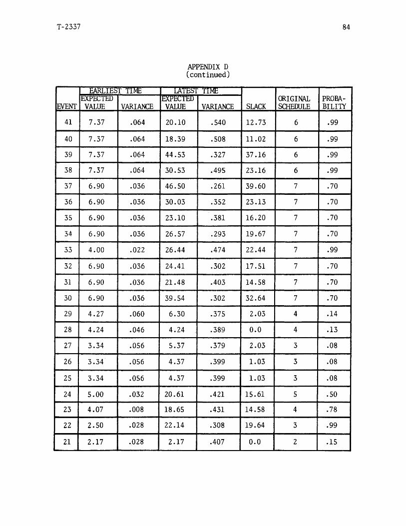
T-2337 84


EVENT

EARLIEST TIME LATENT M M ESLACK

ORIGINALSCHEDULE

PROBABILITY



41 7.37 .064 20.10 .540 12.73 6 .99

40 7.37 .064 18.39 .508 11.02 6 .9939 7.37 .064 44.53 .327 37.16 6 .9938 7.37 .064 30.53 .495 23.16 6 .9937 6.90 .036 46.50 .261 39.60 7 .70

36 6.90 .036 30.03 .352 23.13 7 .70

35 6.90 .036 23.10 .381 16.20 7 .70

34 6.90 .036 26.57 .293 19.67 7 .70

33 4.00 .022 26.44 .474 22.44 7 .99

32 6.90 .036 24.41 .302 17.51 7 .70

31 6.90 .036 21.48 .403 14.58 7 .70

30 6.90 .036 39.54 .302 32.64 7 .70

29 4.27 .060 6.30 .375 2.03 4 .14

28 4.24 .046 4.24 .389 0.0 4 .13

27 3.34 .056 5.37 .379 2.03 3 .08

26 3.34 .056 4.37 .399 1.03 3 .08

25 3.34 .056 4.37 .399 1.03 3 .08

24 5.00 .032 20.61 .421 15.61 5 .5023 4.07 .008 18.65 .431 14.58 4 .78

22 2.50 .028 22.14 .308 19.64 3 .99

21 2.17 .028 2.17 .407 0.0 2 .15

T-2337 85


EVENT

EARLIEST TIME LATEST TIME


PROBABILITY



20 2.17 .028 4.44 .389 2.27 2 .15

19 2.17 .028 4.44 .389 2.27 2 .1518 2.17 .028 3.20 .427 1.03 2 .1517 1.00 .028 3.37 .403 2.31 1 .50

16 2.00 .004 17.61 .449 15.61 2 .50

15 2.00 .004 18.58 .457 16.38 2 .50

14 2.00 .004 18.38 .457 16.38 2 .50

13 2.00 .004 16.58 .435 14.58 2 .50

12 2.00 .004 17.48 .407 15.48 2 .50

11 2.00 .004 24.44 .492 22.44 2 .50

10 2.00 .004 17.38 .431 15.38 2 .50

9 2.00 .004 17.41 .443 15.41 2 .50

8 2.00 .004 18.48 .407 16.48 2 .50

7 0.0 0 12.52 .516 12.52 - -

6 0.0 0 19.64 .336 19.64 - -

5 0.0 0 0.0 .435 0.0 - -

4 0.0 0 0.0 .435 0.0 - -

3 0.0 0 2.37 .431 2.37 - -

2 0.0 0 14.58 .439 14.58 - -

1 0.0 0 14.58 .439 14.58 - -

T-2337 86

BIBLIOGRAPHY

References Cited

( 1) The PIMS Program Selected Finding, The Strategic

Planning Insitiute, pp. 18-20, (1977).

( 2) Speeches Describing Hendry Marketing Support Sys

tem, Speaking of Hendry, The Hendry Corpor

ation, (1976).

( 3) Ibid., pp. 115-116.

( 4) Clark, R. W., An Introduction to Critical Path

Analysis, Research Paper Stanford Univeristy,

pp. 1-39, (1961).

( 5) Woolsey, R.E.D., and Swanson, H.S., Operations

Research For Immediate Application - A Quick

and Dirty Manual, New York, Harber § Row, pp.

12-13, (1975).

( 6) Kelley, J. E. Jr., Critical-Path Planning and

Scheduling: Mathematical Basis, Operations

Research, Vol. 9, pp. 296-300, (1961).

( 7) Woolsey and Swanson, op. cit., pp. 129-135

( 8) Kelley, loc. cit.( 9) Clark, loc. cit.

(10) Kelley, loc. cit.

T-2337 87

(11) Hillier, F. S., and Lieberman, G. J., Introduction

to Operations Research, San Francisco, Holden-

Day, pp. 225-235, (1967).

(12) Clark, loc. cit.

(13) Huggins, W. H., Flow-Graph Representation of Systems,

Operations Research and Systems Engineering,

Ed. by Flagle, Huggins and Roy, Baltimore,

John Hopkins Press, (1960).

(14 ) Ibid., p . 9.

(15) Mason, S. J., Feedback Theory: Some Properties of

Signal Flow-Graphs, Proceedings of the IRE,

Vol. 41, pp. 1144-11566, (1953).

(16) Mason, S. J, Feedback Theory: Further Properties of

Signal Flow-Graphs, Proceedings of the IRE,

Vol. 44, pp. 920-926, (1956).

(17) Fulkerson, D. R., Increasing the Capacity of a

Network: The Parametric Budget Problem,

Management Science, Vol. 5, pp. 472-483,

(1959).

(18) Woolsey and Swanson, loc. cit.

(19) Hillier and Lieberman, loc. cit.(20) Wiest, J.E., and Levy, F.R., A Management Guide to

PERT/CPM: With GERT/PDM/DCPM and Other Net

works, New Jersey, Prentice-Hall, pp. 5-12,

(1977 ).

T-2337 88

(21) Woolsey and Swanson, loc. cit.

(22) Hillier and Lieberman, loc. cit.

(23) Kelley, loc. cit.

(24) Walker, M. R., and Sayer, J. S., Project Planning

and Scheduling, Report 6959, E. I. DuPont de

Nemours and Co., Delware, (1959).

(25) Clark, loc. cit.

(26) Kelley, J. E., Jr., and Walker, M. R., The Critical

Path Method of Planning and Scheduling, Case

Histories Presented at the 12th Annual Meeting

of the Systems and Procedures Association,

Toronto, pp. 403-411, (1960).

(27) Wiest and Levy, op. cit., pp. 62-73.

(28) Ibid.

(29) Multiple Access Limited, Project Management and Con

trol System, Ontario, Don Mills, p. 1, (1973)

(30) Wiest and Levy, op. cit., p. 80.

(31) Martino, R. L., Critical Path Networks, New York,

Gordon and Breach, p. 48, (1968).


(33) Malcom, Roseboom, Clark, and Frazar, Application of aTechnique for Research and Development Program

Evaluation, Operations Research, Vol. 7, pp.

646-649, (1959).


T-2337 89

(35) MacCrimmon, K. R., and Ryavec, C. A., An Analytical

Study of the PERT Assumptions, Operations

Research, Vol. 12, pp. 16-37, (1964).

(36) Martino, loc. cit.

(37) MacCrimmon and Ryavec, loc. cit.

(38) Martino, op. cit., p. 50.



(41) Hillier and Lieberman, op. cit.,(42) Ibid . , pp. 44-47 .

(43) Ibid. , pp. 225-235 .

(44) Kelley and Walker, op. cit., pp.

(45) Hillier and Lieberman. loc. cit.


Crum_10782178.pdf - Mountain Scholar

Documents

Transcript of Crum_10782178.pdf - Mountain Scholar