Cross-Domain Visual Matching via Generalized Similarity ...

IEEE TRANSACTIONS ON PATTERN ANALYSIS AND MACHINE INTELLIGENCE 1

Cross-Domain Visual Matching via GeneralizedSimilarity Measure and Feature Learning

Liang Lin, Guangrun Wang, Wangmeng Zuo, Xiangchu Feng, and Lei Zhang

Abstract—Cross-domain visual data matching is one of the fundamental problems in many real-world vision tasks, e.g., matchingpersons across ID photos and surveillance videos. Conventional approaches to this problem usually involves two steps: i) projectingsamples from different domains into a common space, and ii) computing (dis-)similarity in this space based on a certain distance. Inthis paper, we present a novel pairwise similarity measure that advances existing models by i) expanding traditional linear projectionsinto affine transformations and ii) fusing affine Mahalanobis distance and Cosine similarity by a data-driven combination. Moreover, weunify our similarity measure with feature representation learning via deep convolutional neural networks. Specifically, we incorporatethe similarity measure matrix into the deep architecture, enabling an end-to-end way of model optimization. We extensively evaluateour generalized similarity model in several challenging cross-domain matching tasks: person re-identification under different views andface verification over different modalities (i.e., faces from still images and videos, older and younger faces, and sketch and photoportraits). The experimental results demonstrate superior performance of our model over other state-of-the-art methods.

Index Terms—Similarity model, Cross-domain matching, Person verification, Deep learning.

F

1 INTRODUCTION1

V ISUAL similarity matching is arguably considered as2

one of the most fundamental problems in computer3

vision and pattern recognition, and this problem becomes4

more challenging when dealing with cross-domain data. For5

example, in still-video face retrieval, a newly rising task in6

visual surveillance, faces from still images captured under a7

constrained environment are utilized as the queries to find8

the matches of the same identity in unconstrained videos.9

Age-invariant and sketch-photo face verification tasks are10

also examples of cross-domain image matching. Some ex-11

amples in these applications are shown in Figure 1.12

Conventional approaches (e.g., canonical correlation13

analysis [1] and partial least square regression [2]) for cross-14

domain matching usually follow a procedure of two steps:15

1) Samples from different modalities are first projected into16

a common space by learning a transformation. One may17

simplify the computation by assuming that these cross18

domain samples share the same projection.19

2) A certain distance is then utilized for measuring the20

similarity/disimilarity in the projection space. Usually21

Euclidean distance or inner product are used.22

Suppose that x and y are two samples of different23

modalities, and U and V are two projection matrices ap-24

plied on x and y, respectively. Ux and Vy are usually25

formulated as linear similarity transformations mainly for26

• L. Lin and G. Wang are with School of Data and Computer Science, SunYat-sen University, Guangzhou, P. R. China. Email: [email protected];[email protected].

• W. Zuo is with School of Computer Science and Technology, HarbinInstitute of Technology, Harbin, P. R. China. Email: [email protected].

• X. Feng is with School of Math. and Statistics, Xidian University, Xi’an,P. R. China. Email: [email protected].

• L. Zhang is with Dept. of Computing, The Hong Kong PolytechnicUniversity, Hong Kong. Email: [email protected].

(a)(a) (b)(b)

(c) (d)(c)(c) (d)(d)

Fig. 1: Typical examples of matching cross-domain visualdata. (a) Faces from still images and vidoes. (b) Front- andside-view persons. (c) Older and younger faces. (d) Photoand sketch faces.

the convenience of optimization. A similarity transforma- 27

tion has a good property of preserving the shape of an 28

object that goes through this transformation, but it is limited 29

in capturing complex deformations that usually exist in 30

various real problems, e.g., translation, shearing, and their 31

compositions. On the other hand, Mahalanobis distance, 32

Cosine similarity, and their combination have been widely 33


studied in the research of similarity metric learning, but it34

remains less investigated on how to unify feature learning35

and similarity learning, in particular, how to combine Ma-36

halanobis distance with Cosine similarity and integrate the37

distance metric with deep neural networks for end-to-end38

learning.39

To address the above issues, in this work we present40

a more general similarity measure and unify it with deep41

convolutional representation learning. One of the key inno-42

vations is that we generalize the existing similarity models43

from two aspects. First, we extend the similarity transforma-44

tions Ux and Vy to the affine transformations by adding a45

translation vector into them, i.e., replacing Ux and Vy with46

LAx + a and LBy + b, respectively. Affine transformation47

is a generalization of similarity transformation without the48

requirement of preserving the original point in a linear49

space, and it is able to capture more complex deforma-50

tions. Second, unlike the traditional approaches choosing51

either Mahalanobis distance or Cosine similarity, we com-52

bine these two measures under the affine transformation.53

This combination is realized in a data-driven fashion, as54

discussed in the Appendix, resulting in a novel generalized55

similarity measure, defined as:56

S(x,y) = [xT yT 1]

A C dCT B edT eT f

xy1

, (1)

where sub-matrices A and B are positive semi-definite,57

representing the self-correlations of the samples in their own58

domains, and C is a correlation matrix crossing the two59

domains.60

Figure 2 intuitively explains the idea1. In this example, it61

is observed that Euclidean distance under the linear trans-62

formation, as (a) illustrates, can be regarded as a special case63

of our model with A = UTU, B = VTV, C = −UTV,64

d = 0, e = 0, and f = 0. Our similarity model can be65

viewed as a generalization of several recent metric learning66

models [3] [4]. Experimental results validate that the intro-67

duction of (d, e, f) and more flexible setting on (A,B,C)68

do improve the matching performance significantly.69

Another innovation of this work is that we unify feature70

representation learning and similarity measure learning. In71

literature, most of the existing models are performed in72

the original data space or in a pre-defined feature space,73

that is, the feature extraction and the similarity measure74

are studied separately. These methods may have several75

drawbacks in practice. For example, the similarity models76

heavily rely on feature engineering and thus lack of gen-77

erality when handling problems under different scenarios.78

Moreover, the interaction between the feature represen-79

tations and similarity measures is ignored or simplified,80

thus limiting their performances. Meanwhile, deep learning,81

especially the Convolutional Neural Network (CNN), has82

demonstrated its effectiveness on learning discriminative83

features from raw data and benefited to build end-to-end84

learning frameworks. Motivated by these works, we build85

1. Figure 2 does not imply that our model geometrically aligns twosamples to be matched. Using this example we emphasize the superi-ority of the affine transformation over the traditional linear similaritytransformation on capturing pattern variations in the feature space.

(a)

(b)

Fig. 2: Illustration of the generalized similarity model. Con-ventional approaches project data by simply using the linearsimilarity transformations (i.e., U and V), as illustrated in(a), where Euclidean distance is applied as the distancemetric. As illustrated in (b), we improve existing models byi) expanding the traditional linear similarity transformationinto an affine transformation and ii) fusing Mahalanobisdistance and Cosine similarity. One can see that the casein (a) is a simplified version of our model. Please refer toAppendix section for the deduction details.

a deep architecture to integrate our similarity measure with 86

the CNN-based feature representation learning. Our archi- 87

tecture takes raw images of different modalities as the inputs 88

and automatically produce their representations by sequen- 89

tially stacking shared sub-network upon domain-specific 90

subnetworks. Upon these layers, we further incorporate the 91

components of our similarity measure by stimulating them 92

with several appended structured neural network layers. 93

The feature learning and the similarity model learning are 94

thus integrated for end-to-end optimization. 95

In sum, this paper makes three main contributions to 96

cross-domain similarity measure learning. 97

• First, it presents a generic similarity measure by general- 98

izing the traditional linear projection and distance metrics 99

into a unified formulation. Our model can be viewed 100

as a generalization of several existing similarity learning 101

models. 102

• Second, it integrates feature learning and similarity mea- 103

sure learning by building an end-to-end deep architecture 104

of neural networks. Our deep architecture effectively im- 105

proves the adaptability of learning with data of different 106

modalities. 107

• Third, we extensively evaluate our framework on four 108

challenging tasks of cross-domain visual matching: per- 109

son re-identification across views2, and face verification 110

under different modalities (i.e., faces from still images and 111

videos, older and younger faces, and sketch and photo 112

portraits). The experimental results show that our similar- 113

ity model outperforms other state-of-the-arts in three of 114

2. Person re-identification is arguably a cross-domain matching prob-lem. We introduce it in our experiments since this problem has beenreceiving increasing attentions recently.


the four tasks and achieves the second best performance115

in the other one.116

The rest of the paper is organized as follows. Section 2117

reviews related work. Section 3 introduces our generalized118

similarity model and discusses its connections to existing119

works. Section 4 presents the proposed deep neural network120

architecture and the learning algorithm in Section 4.2. The121

experimental results, comparisons and ablation studies are122

presented in Section 5. Section 6 concludes the paper.123

2 RELATED WORK124

In literature, to cope with the cross-domain matching of125

visual data, one can learn a common space for different126

domains. CCA [1] learns the common space via maximizing127

cross-view correlation, while PLS [2] is learned via maximiz-128

ing cross-view covariance. Coupled information-theoretic129

encoding is proposed to maximize the mutual information130

[5]. Another conventional strategy is to synthesize samples131

from the input domain into the other domain. Rather than132

learning the mapping between two domains in the data133

space, dictionary learning [6] [7] can be used to alleviate134

cross-domain heterogeneity, and semi-coupled dictionary135

learning (SCDL [7]) is proposed to model the relationship136

on the sparse coding vectors from the two domains. Duan et137

al. proposed another framework called domain adaptation138

machine (DAM) [8] for multiple source domain adaption139

but they need a set of pre-trained base classifiers.140

Various discriminative common space approaches have141

been developed by utilizing the label information. Super-142

vised information can be employed by the Rayleigh quotient143

[1], treating the label as the common space [9], or employing144

the max-margin rule [10]. Using the SCDL framework, struc-145

tured group sparsity was adopted to utilize the label infor-146

mation [6]. Generalization of discriminative common space147

to multiview was also studied [11]. Kan et al. proposed a148

multiview discriminant analysis (MvDA [12]) method to149

obtain a common space for multiple views by optimizing150

both inter-view and intra-view Rayleigh quotient. In [13], a151

method to learn shape models using local curve segments152

with multiple types of distance metrics was proposed.153

Moreover, for most existing multiview analysis methods,154

the target is defined based on the standard inner product155

or distance between the samples in the feature space. In156

the field of metric learning, several generalized similarity /157

distance measures have been studied to improve recognition158

performance. In [4] [14], the generalized distance / simi-159

larity measures are formulated as the difference between160

the distance component and the similarity component to161

take into account both cross inner product term and two162

norm terms. Li et al. [3] adopted the second-order decision163

function as distance measure without considering the pos-164

itive semi-definite (PSD) constraint. Chang and Yeung [15]165

suggested an approach to learn locally smooth metrics using166

local affine transformations while preserving the topological167

structure of the original data. These distance / similarity168

measures, however, were developed for matching samples169

from the same domain, and they cannot be directly applied170

to cross domain data matching.171

To extend traditional single-domain metric learning,172

Mignon and Jurie [16] suggested a cross-modal metric learn-173

ing (CMML) model, which learns domain-specific transfor- 174

mations based on a generalized logistic loss. Zhai et al. 175

[17] incorporated the joint graph regularization with the 176

heterogeneous metric learning model to improve the cross- 177

media retrieval accuracy. In [16], [17], Euclidean distance is 178

adopted to measure the dissimilarity in the latent space. In- 179

stead of explicitly learning domain-specific transformations, 180

Kang et al. [18] learned a low rank matrix to parameterize 181

the cross-modal similarity measure by the accelerated prox- 182

imal gradient (APG) algorithm. However, these methods 183

are mainly based on the common similarity or distance 184

measures and none of them addresses the feature learning 185

problem under the cross-domain scenarios. 186

Instead of using hand-crafted features, learning feature 187

representations and contextual relations with deep neu- 188

ral networks, especially the convolutional neural network 189

(CNN) [19], has shown great potential in various pattern 190

recognition tasks such as object recognition [20] and seman- 191

tic segmentation [21]. Significant performance gains have 192

also been achieved in face recognition [22] and person re- 193

identification [23] [24] [25] [26], mainly attributed to the 194

progress in deep learning. Recently, several deep CNN- 195

based models have been explored for similarity matching 196

and learning. For example, Andrew et al. [27] proposed a 197

multi-layer CCA model consisting of several stacked non- 198

linear transformations. Li et al. [28] learned filter pairs via 199

deep networks to handle misalignment, photometric and 200

geometric transforms, and achieved promising results for 201

the person re-identification task. Wang et al. [29] learned 202

fine-grained image similarity with deep ranking model. Yi 203

et al. [30] presented a deep metric learning approach by 204

generalizing the Siamese CNN. Ahmed et al. [25] proposed 205

a deep convolutional architecture to measure the similarity 206

between a pair of pedestrian images. Besides the shared 207

convolutional layers, their network also includes a neigh- 208

borhood difference layer and a patch summary layer to 209

compute cross-input neighborhood differences. Chen et al. 210

[26] proposed a deep ranking framework to learn the joint 211

representation of an image pair and return the similarity 212

score directly, in which the similarity model is replaced by 213

full connection layers. 214

Our deep model is partially motivated by the above 215

works, and we target on a more powerful solution of cross- 216

domain visual matching by incorporating a generalized 217

similarity function into deep neural networks. Moreover, 218

our network architecture is different from existing works, 219

leading to new state-of-the-art results on several challenging 220

person verification and recognition tasks. 221

3 GENERALIZED SIMILARITY MODEL 222

In this section, we first introduce the formulation of our 223

deep generalized similarity model and then discuss the con- 224

nections between our model and existing similarity learning 225

methods. 226

3.1 Model Formulation 227

According to the discussion in Section 1, our generalized 228

similarity measure extends the traditional linear projection 229

and integrates Mahalanobis distance and Cosine similarity 230


into a generic form, as shown in Eqn. (1). As we derive in the231

Appendix, A and B in our similarity measure are positive232

semi-definite but C does not obey this constraint. Hence, we233

can further factorize A, B and C, as:234

A = LATLA,

B = LBTLB,

C = −LxC

TLyC.

(2)

Moreover, our model extracts feature representation (i.e.,235

f1(x) and f2(y)) from the raw input data by utilizing the236

CNNs. Incorporating the feature representation and the237

above matrix factorization into Eqn. (1), we can thus have238

the following similarity model:239

S(x,y) = S(f1(x), f2(y)) (3)

= [f1(x)T f2(y)

T 1]

A C dCT B edT eT f

f1(x)f2(y)1

= ∥LAf1(x)∥2 + ∥LBf2(y)∥2 + 2dT f1(x)

− 2(LxCf1(x))

T (LyCf2(y))+2eT f2(y)+f.

Specifically, LAf1(x), LxCf1(x), d

T f1(x) can be regarded240

as the similarity components for x, while LBf2(y), LyCf2(y),241

dT f2(y) accordingly for y. These similarity components are242

modeled as the weights that connect neurons of the last two243

layers. For example, a portion of output activations repre-244

sents LAf1(x) by taking f1(x) as the input and multiplying245

the corresponding weights LA. In the following, we discuss246

the formulation of our similarity learning.247

The objective of our similarity learning is to seek a248

function S(x,y) that satisfies a set of similarity/disimilarity249

constraints. Instead of learning similarity function on hand-250

crafted feature space, we take the raw data as input, and251

introduce a deep similarity learning framework to integrate252

nonlinear feature learning and generalized similarity learn-253

ing. Recall that our deep generalized similarity model is254

in Eqn. (1). (f1(x), f2(y)) are the feature representations for255

samples of different modalities, and we use W to indicate256

their parameters. We denote Φ = (LA,LB,LxC,L

yC,d, e, f)257

as the similarity components for sample matching. Note that258

S(x,y) is asymmetric, i.e., S(x,y) = S(y,x). This is rea-259

sonable for cross-domain matching, because the similarity260

components are domain-specific.261

Assume that D = (xi,yi, ℓi)Ni=1 is a training set262

of cross-domain sample pairs, where xi,yi denotes the263

ith pair, and ℓi denotes the corresponding label of xi,yi264

indicating whether xi and yi are from the same class:265

ℓi = ℓ(xi,yi) =

−1, c(x) = c(y)1, otherwise , (4)

where c(x) denotes the class label of the sample x. An ideal266

deep similarity model is expected to satisfy the following267

constraints:268

S(xi,yi)

< −1, if ℓi = −1≥ 1, otherwise (5)

for any xi,yi.269

Note that the feasible solution that satisfies the above270

constraints may not exist. To avoid this scenario, we relax271

the hard constraints in Eqn. (5) by introducing a hinge-like 272

loss: 273

G(W,Φ) =N∑i=1

(1− ℓiS(xi,yi))+. (6)

To improve the stability of the solution, some regularizers 274

are further introduced, resulting in our deep similarity 275

learning model: 276

(W, Φ) = arg minW,Φ

N∑i=1

(1− ℓiS(xi,yi))+ +Ψ(W,Φ), (7)

where Ψ(W,Φ) = λ∥W∥2+µ∥Φ∥2 denotes the regularizer 277

on the parameters of the feature representation and gener- 278

alized similarity models. 279

3.2 Connection with Existing Models 280

Our generalized similarity learning model is a generaliza- 281

tion of many existing metric learning models, while they 282

can be treated as special cases of our model by imposing 283

some extra constraints on (A,B,C,d, e, f). 284

Conventional similarity model usually is defined as 285

SM(x,y) = xTMy, and this form is equivalent to our 286

model, when A = B = 0, C = 12M, d = e = 0, and 287

f = 0. Similarly, the Mahalanobis distance DM(x,y) = 288

(x − y)TM(x − y) is also regarded as a special case of our 289

model, when A = B = M, C = −M, d = e = 0, and 290

f = 0. 291

In the following, we connect our similarity model to two 292

state-of-the-art similarity learning methods, i.e., LADF [3] 293

and Joint Bayesian [4]. 294

In [3], Li et al. proposed to learn a decision func- 295

tion that jointly models a distance metric and a locally 296

adaptive thresholding rule, and the so-called LADF (i.e., 297

Locally-Adaptive Decision Function) is formulated as a 298

second-order large-margin regularization problem. Specif- 299

ically, LADF is defined as: 300

F (x,y)=xTAx+yTAy+2xTCy+dT (x+y)+f. (8)

One can observe that F (x,y) = S(x,y) when we set B = A 301

and e = d in our model. 302

It should be noted that LADF treats x and y using the 303

same metrics, i.e., A for both xTAx and yTAy, and d for 304

dTx and dTy. Such a model is reasonable for matching 305

samples with the same modality, but may be unsuitable for 306

cross-domain matching where x and y are with different 307

modalities. Compared with LADF, our model uses A and d 308

to calculate xTAx and dTx, and uses B and e to calculate 309

yTBy and eTy, making our model more effective for cross- 310

domain matching. 311

In [4], Chen et al. extended the classical Bayesian face 312

model by learning a joint distributions (i.e., intra-person 313

and extra-person variations) of sample pairs. Their decision 314

function is posed as the following form: 315

J(x,y) = xTAx+yTAy − 2xTGy. (9)

Note that the similarity metric model proposed in [14] also 316

adopted such a form. Interestingly, this decision function 317

is also a special variant of our model by setting B = A, 318

C = −G, d = 0, e = 0, and f = 0. 319


200×3×180×130

20×3×180×130 5×5 Conv + ReLU + 3×3 MaxPool

5×5 Conv +ReLU +3×3 MaxPool FC FC

f2(y)

f1(x)

LBf2(y)

LCf2(y)

eTf2(y)

y

LAf1(x)

LCf1(x)

dTf1(x)

x

200×32×30×21

220×32×9×6

220×400

x

y

Concate Slice

20×801

200×801

Domain-specific sub-network Similarity sub-network

g1(x)

g2(y)

5×5 Conv + ReLU + 3×3 MaxPool

220×400

200×400

20×400

FC

FC

20×32×30×21

Shared sub-network

Fig. 3: Deep architecture of our similarity model. This architecture is comprised of three parts: domain-specific sub-network,shared sub-network and similarity sub-network. The first two parts extract feature representations from samples of differentdomains, which are built upon a number of convolutional layers, max-pooling operations and fully-connected layers. Thesimilarity sub-network includes two structured fully-connected layers that incorporate the similarity components in Eqn.(3).

In summary, our similarity model can be regarded as the320

generalization of many existing cross-domain matching and321

metric learning models, and it is more flexible and suitable322

for cross-domain visual data matching.323

4 JOINT SIMILARITY AND FEATURE LEARNING324

In this section, we introduce our deep architecture that325

integrates the generalized similarity measure with convo-326

lutional feature representation learning.327

4.1 Deep Architecture328

As discussed above, our model defined in Eqn. (7) jointly329

handles similarity function learning and feature learning.330

This integration is achieved by building a deep architecture331

of convolutional neural networks, which is illustrated in332

Figure 3. It is worth mentioning that our architecture is333

able to handle the input samples of different modalities with334

unequal numbers, e.g., 20 samples of x and 200 samples of335

y are fed into the network in a way of batch processing.336

From left to right in Figure 3, two domain-specific sub-337

networks g1(x) and g2(y) are applied to the samples of338

two different modalities, respectively. Then, the outputs339

of g1(x) and g2(y) are concatenated into a shared sub-340

network f(·). We make a superposition of g1(x) and g2(y)341

to feed f(·). At the output of f(·), the feature representations342

of the two samples are extracted separately as f1(x) and343

f2(y), which is indicated by the slice operator in Figure 3.344

Finally, these learned feature representations are utilized in345

the structured fully-connected layers that incorporate the346

similarity components defined in Eqn. (3). In the following,347

we introduce the detailed setting of the three sub-networks.348

Domain-specific sub-network. We separate two349

branches of neural networks to handle the samples from350

different domains. Each network branch includes one351

convolutional layer with 3 filters of size 5 × 5 and the352

stride step of 2 pixels. The rectified nonlinear activation is353

utilized. Then, we follow by a one max-pooling operation354

with size of 3× 3 and its stride step is set as 3 pixels.355

Shared sub-network. For this component, we stack one 356

convolutional layer and two fully-connected layers. The 357

convolutional layer contains 32 filters of size 5 × 5 and the 358

filter stride step is set as 1 pixel. The kernel size of the max- 359

pooling operation is 3 × 3 and its stride step is 3 pixels. 360

The output vectors of the two fully-connected layers are 361

of 400 dimensions. We further normalize the output of the 362

second fully-connected layer before it is fed to the next sub- 363

network. 364

Similarity sub-network. A slice operator is first applied 365

in this sub-network, which partitions the vectors into two 366

groups corresponding to the two domains. For the example 367

in Figure 3, 220 vectors are grouped into two sets, i.e., 368

f1(x) and f2(y), with size of 20 and 200, respectively. 369

f1(x) and f2(y) are both of 400 dimensions. Then, f1(x) 370

and f2(y) are fed to two branches of neural network, and 371

each branch includes a fully-connected layer. We divide the 372

activations of these two layers into six parts according to 373

the six similarity components. As is shown in Figure 3, 374

in the top branch the neural layer connects to f1(x) and 375

outputs LAf1(x), LxCf1(x), and dT f1(x), respectively. In 376

the bottom branch, the layer outputs LBf2(y), LyCf2(y), and 377

eT f2(y), respectively, by connecting to f2(y). In this way, 378

the similarity measure is tightly integrated with the feature 379

representations, and they can be jointly optimized during 380

the model training. Note that f is a parameter of the gen- 381

eralized similarity measure in Eqn. (1). Experiments show 382

that the value of f only affects the learning convergence 383

rather than the matching performance. Thus we empirically 384

set f = −1.9 in our experiments. 385

In the deep architecture, we can observe that the similar- 386

ity components of x and those of y do not interact to each 387

other by the factorization until the final aggregation calcula- 388

tion, that is, computing the components of x is independent 389

of y. This leads to a good property of efficient matching. In 390

particular, for each sample stored in a database, we can pre- 391

computed its feature representation and the corresponding 392

similarity components, and the similarity matching in the 393

testing stage will be very fast. 394


4.2 Model Training395

In this section, we discuss the learning method for our396

similarity model training. To avoid loading all images into397

memory, we use the mini-batch learning approach, that is,398

in each training iteration, a subset of the image pairs are fed399

into the neural network for model optimization.400

For notation simplicity in discussing the learning algo-401

rithm, we start by introducing the following definitions:402

x∆= [ LAf1(x) Lx

Cf1(x) dT f1(x) ]T

y∆= [ LBf2(y) Ly

Cf2(y) eT f2(y) ]T,

(10)

where x and y denote the output layer’s activations of the403

samples x and y. Prior to incorporating Eqn. (10) into the404

similarity model in Eqn. (3), we introduce three transforma-405

tion matrices (using Matlab representation):406

P1 =[Ir×r 0r×(r+1)

],

P2 =[0r×r Ir×r 0r×1

],

p3 =[01×2r 11×1

]T,

(11)

where r equals to the dimension of the output of shared407

neural network (i.e., the dimension of f(x) and f(y)), an I408

indicates the identity matrix. Then, our similarity model can409

be re-written as:410

S(x,y) = (P1x)TP1x+ (P1y)

TP1y − 2(P2x)

TP2y

+2pT3 x+ 2pT

3 y + f.(12)

Incorporating Eqn. (12) into the loss function Eqn. (6),411

we have the following objective:412

G(W,Φ;D)

=N∑i=1 1− ℓi [ (P1xi)

TP1xi + (P1yi)TP1yi−

2(P2xi)TP2yi + 2pT

3 xi + 2pT3 yi + f ] +

, (13)

where the summation term denotes the hinge-like loss for413

the cross domain sample pair xi, yi, N is the total number414

of pairs, W represents the feature representation of different415

domains and Φ represents the similarity model. W and Φ416

are both embedded as weights connecting neurons of layers417

in our deep neural network model, as Figure 3 illustrates.418

The objective function in Eqn. (13) is defined in sample-419

pair-based form. To optimize it using SGD, one should ap-420

ply a certain scheme to generate mini-batches of the sample421

pairs, which usually costs much computation and memory.422

Note that the sample pairs in training set D are constructed423

from the original set of samples from different modalities424

Z = X, Y, where X = x1, ...,xj , ...,xMx and425

Y = y1, ...,yj , ...,yMy. The superscript denotes the sam-426

ple index in the original training set, e.g., xj ∈ X =427

x1, ...,xj , ...,xMx and yj ∈ Y = y1, ...,yj , ...,yMy,428

while the subscript denotes the index of sample pairs, e.g.,429

xi ∈ xi,yi ∈ D. Mx and My denote the total number of430

samples from different domains. Without loss of generality,431

we define zj = xj and zMx+j = yj . For each pair xi,yi432

in D, we have zji,1 = xi and zji,2 = yi with 1 ≤ ji,1 ≤ Mx433

and Mx + 1 ≤ ji,2 ≤ Mz(= Mx +My). And we also have434

zji,1 = xi and zji,2 = yi.435

Therefore, we rewrite Eqn. (13) in a sample-based form:436

L(W,Φ;Z)

=N∑i=1 1− ℓi [ (P1z

ji,1)TP1zji,1 + (P1z

ji,2)TP1zji,2−

2(P2zji,1)TP2z

ji,2 + 2pT3 z

ji,1 + 2pT3 z

ji,2 + f ] +

,

(14)Given Ω = (W,Φ), the loss function in Eqn. (7) can also be 437

rewritten in the sample-based form: 438

H(Ω) = L(Ω;Z) + Ψ(Ω). (15)

The objective in Eqn. (15) can be optimized by the mini- 439

batch back propagation algorithm. Specifically, we update 440

the parameters by gradient descent: 441

Ω = Ω− α∂

∂ΩH(Ω), (16)

where α denotes the learning rate. The key problem of 442

solving the above equation is calculating ∂∂ΩL(Ω). As is 443

discussed in [31], there are two ways to this end, i.e., pair- 444

based gradient descent and sample-based gradient descent. 445

Here we adopt the latter to reduce the requirements on 446

computation and memory cost. 447

Suppose a mini-batch of training samples 448

zj1,x , ..., zjnx,x , zj1,y , ..., zjny,y from the original set 449

Z , where 1 ≤ ji,x ≤ Mx and Mx + 1 ≤ ji,y ≤ Mz. 450

Following the chain rule, calculating the gradient for all 451

pairs of samples is equivalent to summing up the gradient 452

for each sample, 453

∂

∂ΩL(Ω) =

∑j

∂L

∂zj∂zj

∂Ω, (17)

where j can be either ji,x or ji,y. 454

Using zji,x as an example, we first introduce an in- 455

dicator function 1zji,x (zji,y) before calculating the partial 456

derivative of output layer activation for each sample ∂L∂zji,x

. 457

Specifically, we define 1zji,x (zji,y) = 1 when zji,x , zji,y 458

is a sample pair and ℓji,x,ji,y S(zji,x , zji,y) < 1. Otherwise 459

we let 1zji,x (zji,y) = 0. ℓji,x,ji,y , indicating where zji,x and 460

zji,y are from the same class. With 1zji,x (zji,y), the gradient 461

of ˜zji,x can be written as 462

∂L

∂zji,x=−

∑ji,y

21zji,x (zji,y)ℓji,x,ji,y(P

T1 P1z

ji,x−PT2 P2z

ji,y+p3).

(18)The calculation of ∂L

∂zji,ycan be conducted in a similar way. 463

The algorithm of calculating the partial derivative of output 464

layer activation for each sample is shown in Algorithm 1. 465

Note that all the three sub-networks in our deep ar- 466

chitecture are differentiable. We can easily use the back- 467

propagation procedure [19] to compute the partial deriva- 468

tives with respect to the hidden layers and model pa- 469

rameters Ω. We summarize the overall procedure of deep 470

generalized similarity measure learning in Algorithm 2. 471

If all the possible pairs are used in training, the sample- 472

based form allows us to generate nx × ny sample pairs 473

from a mini-batch of nx + ny. On the other hand, the 474

sample-pair-based form may require 2nxny samples or less 475

to generate nx × ny sample pairs. In gradient compu- 476

tation, from Eqn. (18), for each sample we only require 477

calculating PT1 P1z

ji,x once and PT2 P2z

ji,y ny times in the 478

sample-based form. While in the sample-pair-based form, 479

PT1 P1z

ji,x and PT2 P2z

ji,y should be computed nx and ny 480


Algorithm 1 Calculate the derivative of the output layer’sactivation for each sample

Input:The output layer’s activation for all samples

Output:The partial derivatives of output layer’s activation forall the samples

1: for each sample zj do2: Initialize the partner setMj containing the sample zj

withMj = ∅;3: for each pair xi,yi do4: if pair xi,yi contains the sample zj then5: if pair xi,yi satisfies ℓiS(xi,yi) < 1 then6: Mi ← Mi, the corresponding partner of zj in

xi,yi;7: end if8: end if9: end for

10: Compute the derivatives for the sample zj with allthe partners in Mj , and sum these derivatives to bethe desired partial derivative for sample zj ’s outputlayer’s activation using Eqn. (18);

11: end for

times, respectively. In sum, the sample-based form generally481

results in less computation and memory cost.482

Algorithm 2 Generalized Similarity Learning

Input:Training set, initialized parameters W and Φ, learningrate α, t← 0

Output:Network parameters W and Φ

1: while t <= T do2: Sample training pairs D;3: Feed the sampled images into the network;4: Perform a feed-forward pass for all the samples and

compute the net activations for each sample zi;5: Compute the partial derivative of the output layer’s

activation for each sample by Algorithm 1.6: Compute the partial derivatives of the hidden layers’

activations for each sample following the chain rule;7: Compute the desired gradients ∂

∂ΩH(Ω) using theback-propagation procedure;

8: Update the parameters using Eqn. (16);9: end while

Batch Process Implementation. Suppose that the train-483

ing image set is divided into K categories, each of which484

contains O1 images from the first domain and O2 images485

from the second domain. Thus we can obtain a maximum486

number (K × O1) × (K × O2) of pairwise samples, which487

is quadratically more than the number of source images488

K × (O1 + O2). In real application, since the number of489

stored images may reach millions, it is impossible to load490

all the data for network training. To overcome this problem,491

we implement our learning algorithm in a batch-process492

manner. Specifically, in each iteration, only a small subset493

of cross domain image pairs are generated and fed to494

the network for training. According to our massive ex- 495

periments, randomly generating image pairs is infeasible, 496

which may cause the image distribution over the special 497

batch becoming scattered, making valid training samples 498

for a certain category very few and degenerating the model. 499

Besides, images in any pair are almost impossible to come 500

from the same class, making the positive samples very 501

few. In order to overcome this problem, an effective cross 502

domain image pair generation scheme is adopted to train 503

our generalized similarity model. For each round, we first 504

randomly choose K instance categories. For each category, a 505

number of O1 images first domain and a number of O2 from 506

second domain are randomly selected. For each selected 507

images in first domain, we randomly take samples from the 508

second domain and the proportions of positive and negative 509

samples are equal. In this way, images distributed over the 510

generated samples are relatively centralized and the model 511

will effectively converge. 512

5 EXPERIMENTS 513

In this section, we apply our similarity model in four rep- 514

resentative tasks of matching cross-domain visual data and 515

adopt several benchmark datasets for evaluation: i) person 516

re-identification under different views on CUHK03 [28] and 517

CUHK01 [32] datasets; ii) age-invariant face recognition on 518

MORPH [33], CACD [34] and CACD-VS [35] datasets; 519

iii) sketch-to-photo face matching on CUFS dataset [36]; 520

iv) face verification over still-video domains on COX face 521

dataset [37]. On all these tasks, state-of-the-art methods are 522

employed to compare with our model. 523

Experimental setting. Mini-batch learning is adopted in 524

our experiments to save memory cost. In each task, we 525

randomly select a batch of sample from the original training 526

set to generate a number of pairs (e.g., 4800). The initial 527

parameters of the convolutional and the full connection 528

layers are set by two zero-mean Gaussian Distributions, 529

whose standard deviations are 0.01 and 0.001 respectively. 530

Other specific settings to different tasks are included in the 531

following sub-sections. 532

In addition, ablation studies are presented to reveal the 533

benefit of each main component of our method, e.g., the 534

generalized similarity measure and the joint optimization 535

of CNN feature representation and metric model. We also 536

implement several variants of our method by simplifying 537

the similarity measures for comparison. 538

5.1 Person Re-identification 539

Person re-identification, aiming at matching pedestrian im- 540

ages across multiple non-overlapped cameras, has attracted 541

increasing attentions in surveillance. Despite that consider- 542

able efforts have been made, it is still an open problem due 543

to the dramatic variations caused by viewpoint and pose 544

changes. To evaluate this task, CUHK03 [28] dataset and 545

CUHK01 [32] dataset are adopted in our experiments. 546

CUHK03 dataset [28] is one of the largest databases for 547

person re-identification. It contains 14,096 images of 1,467 548

pedestrians collected from 5 different pairs of camera views. 549

Each person is observed by two disjoint camera views and 550

has an average of 4.8 images in each view. We follow the 551


rank

5 10 15 20 25 30

identification r

ate

0

0.2

0.4

0.6

0.8

1

5.64%Euclid

20.65%DFPNN

54.74%IDLA

5.53%ITML

14.17%KISSME

13.51%LDM

7.29%LMNN

10.42%RANK

5.6%SDALF

8.76%eSDC

22.0%DRSCH

32.7%KML

58.4%Ours

(a) CUHK03

rank

5 10 15 20 25 30

identification r

ate

0

0.2

0.4

0.6

0.8

1

10.52%Euclid

27.87%FPNN

65.00%IDLA

17.10%ITML

29.40%KISSME

26.45%LDM

21.17%LMNN

20.61%RANK

9.9%SDALF

22.82%eSDC

34.30%LMLF

66.50%Ours

(b) CUHK01

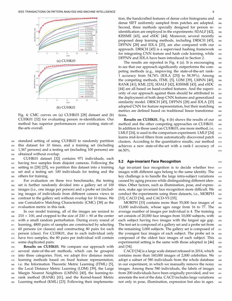
Fig. 4: CMC curves on (a) CUHK03 [28] dataset and (b)CUHK01 [32] for evaluating person re-identification. Ourmethod has superior performances over existing state-of-the-arts overall.

standard setting of using CUHK03 to randomly partition552

this dataset for 10 times, and a training set (including553

1,367 persons) and a testing set (including 100 persons) are554

obtained without overlap.555

CUHK01 dataset [32] contains 971 individuals, each556

having two samples from disjoint cameras. Following the557

setting in [28] [25], we partition this dataset into a training558

set and a testing set: 100 individuals for testing and the559

others for training.560

For evaluation on these two benchmarks, the testing561

set is further randomly divided into a gallery set of 100562

images (i.e., one image per person) and a probe set (includ-563

ing images of individuals from different camera views in564

contrast to the gallery set) without overlap for 10 times. We565

use Cumulative Matching Characteristic (CMC) [38] as the566

evaluation metric in this task.567

In our model training, all of the images are resized to568

250× 100, and cropped to the size of 230× 80 at the center569

with a small random perturbation. During every round of570

learning, 4800 pairs of samples are constructed by selecting571

60 persons (or classes) and constructing 80 pairs for each572

person (class). For CUHK01, due to each individual only573

have two samples, the 80 pairs per individual will contain574

some duplicated pairs.575

Results on CUHK03. We compare our approach with576

several state-of-the-art methods, which can be grouped577

into three categories. First, we adopt five distance metric578

learning methods based on fixed feature representation,579

i.e. the Information Theoretic Metric Learning (ITML) [5],580

the Local Distance Metric Learning (LDM) [39], the Large581

Margin Nearest Neighbors (LMNN) [40], the learning-to-582

rank method (RANK) [41], and the Kernel-based Metric583

Learning method (KML) [23]. Following their implementa-584

tion, the handcrafted features of dense color histograms and 585

dense SIFT uniformly sampled from patches are adopted. 586

Second, three methods specially designed for person re- 587

identification are employed in the experiments: SDALF [42], 588

KISSME [43], and eSDC [44]. Moreover, several recently 589

proposed deep learning methods, including DRSCH [45], 590

DFPNN [28] and IDLA [25], are also compared with our 591

approach. DRSCH [45] is a supervised hashing framework 592

for integrating CNN feature and hash code learning, while 593

DFPNN and IDLA have been introduced in Section 2. 594

The results are reported in Fig. 4 (a). It is encouraging 595

to see that our approach significantly outperforms the com- 596

peting methods (e.g., improving the state-of-the-art rank- 597

1 accuracy from 54.74% (IDLA [25]) to 58.39%). Among 598

the competing methods, ITML [5], LDM [39], LMNN [40], 599

RANK [41], KML [23], SDALF [42], KISSME [43], and eSDC 600

[44] are all based on hand-crafted features. And the superi- 601

ority of our approach against them should be attributed to 602

the deployment of both deep CNN features and generalized 603

similarity model. DRSCH [45], DFPNN [28] and IDLA [25] 604

adopted CNN for feature representation, but their matching 605

metrics are defined based on traditional linear transforma- 606

tions. 607

Results on CUHK01. Fig. 4 (b) shows the results of our 608

method and the other competing approaches on CUHK01. 609

In addition to those used on CUHK03, one more method, i.e. 610

LMLF [24], is used in the comparison experiment. LMLF [24] 611

learns mid-level filters from automatically discovered patch 612

clusters. According to the quantitative results, our method 613

achieves a new state-of-the-art with a rank-1 accuracy of 614

66.50%. 615

5.2 Age-invariant Face Recognition 616

Age invariant face recognition is to decide whether two 617

images with different ages belong to the same identity. The 618

key challenge is to handle the large intra-subject variations 619

caused by aging process while distinguishing different iden- 620

tities. Other factors, such as illumination, pose, and expres- 621

sion, make age invariant face recognition more difficult. We 622

conduct the experiments using three datasets, i.e., MORPH 623

[33], CACD [34], and CACD-VS [35]. 624

MORPH [33] contains more than 55,000 face images of 625

13,000 individuals, whose ages range from 16 to 77. The 626

average number of images per individual is 4. The training 627

set consists of 20,000 face images from 10,000 subjects, with 628

each subject having two images with the largest age gap. 629

The test set is composed of a gallery set and a probe set from 630

the remaining 3,000 subjects. The gallery set is composed of 631

the youngest face images of each subject. The probe set is 632

composed of the oldest face images of each subject. This 633

experimental setting is the same with those adopted in [46] 634

and [34]. 635

CACD [34] is a large scale dataset released in 2014, which 636

contains more than 160,000 images of 2,000 celebrities. We 637

adopt a subset of 580 individuals from the whole database 638

in our experiment, in which we manually remove the noisy 639

images. Among these 580 individuals, the labels of images 640

from 200 individuals have been originally provided, and we 641

annotate the rest of the data. CACD includes large variations 642

not only in pose, illumination, expression but also in ages. 643


2004−2006 2007−2009 2010−20120.5

0.55

0.6

0.65

0.7

0.75

MAP

HFA

CARC

Deepface

Ours−1

Ours−2

Fig. 5: The retrieval performances on CACD dataset forage-invariant face recognition. Ours-1 and Ours-2 are ourmethod, while the latter uses more training samples.

TABLE 1: Experimental results for age-invariant face recog-nition.

(a) Recognition rates on the MORPH dataset.Method Recognition rateTDBN [48] 60%3D Aging Model [50] 79.8%MFDA [49] 83.9%HFA [46] 91.1%CARC [34] 92.8%Ours 94.4%

(b) Verification accuracy on the CACD-VS dataset.Method verification accuracyHD-LBP [51] 81.6%HFA [46] 84.4%CARC [34] 87.6%Deepface [52] 85.4%Ours 89.8%

Based on CACD, a verification subset called CACD-VS [35]644

is further developed, which contains 2,000 positive pairs645

and 2,000 negative pairs. The setting and testing protocol of646

CACD-VS are similar to the well-known LFW benchmark647

[47], except that CACD-VS contains much more samples for648

each person.649

All of the images are resized to 200 × 150. For data650

augmentation, images are cropped to the size of 180×130 at651

the center with a small random perturbation when feeding652

to the neural network. Sample-based mini-batch setting is653

adopted, and 4,800 pairs are constructed for each iteration.654

Results on MORPH. We compare our method with sev-655

eral state-of-the-art methods, including topological dynamic656

Bayesian network (TDBN) [48], cross-age reference coding657

(CARC) [34], probabilistic hidden factor analysis (HFA) [46],658

multi-feature discriminant analysis (MFDA) [49] and 3D659

aging model [50]. The results are reported in Table 1(a).660

Thanks to the use of CNN representation and generalized661

similarity measure, our method achieves the recognition662

rate of 94.35%, and significantly outperforms the competing663

methods.664

Results on CACD. On this dataset, the protocol is to665

retrieve face images of the same individual from gallery sets666

by using a probe set, where the age gap between probe face667

images and gallery face images is large. Following the ex-668

perimental setting in [34], we set up 4 gallery sets according669

to the years when the photos were taken: [2004 − 2006],670

[2007− 2009], [2010− 2012], and [2013]. And we use the set671

of [2013] as the probe set to search for matches in the rest672

of three sets. We introduce several state-of-the-art methods673

for comparison, including CARC [34], HFA [46] and one 674

deep learning based method, Deepface [52]. The results of 675

CARC [34] and HFA [46] are borrowed from their papers. 676

The results of Deepface [52] and our approach (i.e., Ours- 677

1) are implemented based on the 200 originally annotated 678

individuals, where 160 samples are used for model training. 679

From the quantitative results reported in Figure 5, our 680

model achieves superior performances over the competing 681

methods. Furthermore, we also report the result of our 682

method (i.e., Ours-2) by using images of 500 individuals as 683

training samples. One can see that, the performance of our 684

model can be further improved by increasing training data. 685

Results on CACD-VS. Following the setting in [35], we 686

further evaluate our approach by conducting the general 687

face verification experiment. Specifically, for all of the com- 688

peting methods, we train the models on CACD and test on 689

CACD-VS, and the optimal threshold value for matching 690

is obtained by exhaustive search. The results produced by 691

our methods and the others (i.e., CARC [34], HFA [46], HD- 692

LBP [51] and Deepface [52]) are reported in Table 1 (b). It 693

is worth mentioning that our method improves the state-of- 694

the-art recognition rate from 87.6% (by CARC [34] [52]) to 695

89.8%. Thanks to the introduction of generalized similarity 696

measure our approach achieves higher verification accuracy 697

than Deepface. Note that an explicit face alignment was 698

adopted in [52] before the CNN feature extraction, which 699

is not in our framework. 700

5.3 Sketch-photo Face Verification 701

Sketch-photo face verification is an interesting yet challeng- 702

ing task, which aims to verify whether a face photo and a 703

drawing face sketch belong to the same individual. This task 704

has an important application of assisting law enforcement, 705

i.e., using face sketch to find candidate face photos. It is 706

however difficult to match photos and sketches in two 707

different modalities. For example, hand-drawing may bring 708

unpredictable face distortion and variation compared to the 709

real photo, and face sketches often lack of details that can be 710

important cues for preserving identity. 711

We evaluate our model on this task using the CUFS 712

dataset [36]. There are 188 face photos in this dataset, in 713

which 88 are selected for training and 100 for testing. Each 714

face has a corresponding sketch that is drawn by the artist. 715

All of these face photos are taken at frontal view with a 716

normal lighting condition and neutral expression. 717

All of the photos/sketches are resized to 250× 200, and 718

cropped to the size of 230 × 180 at the center with a small 719

random perturbation. 1200 pairs of photos and sketches 720

(i.e., including 30 individuals with each having 40 pairs) are 721

constructed for each iteration during the model training. In 722

the testing stage, we use face photos to form the gallery set 723

and treat sketches as the probes. 724

We employ several existing approaches for comparison: 725

the eigenface transformation based method (ET) [53], the 726

multi-scale Markov random field based method (MRF) [36], 727

and MRF+ [54] (i.e., the lighting and pose robust version 728

of [36]). It is worth mentioning that all of these competing 729

methods need to first synthesize face sketches by photo- 730

sketch transformation, and then measure the similarity be- 731

tween the synthesized sketches and the candidate sketches, 732


rank

5 10 15 20 25 30

identification r

ate

0

0.1

0.2

0.3

0.4

0.5

0.6

0.7

0.8

0.9

5.64%Euclid

5.53%ITML

13.51%LDM

7.29%LMNN

10.42%RANK

31.85%Generalized

(a) sim.+hand.fea,CUHK03

rank

5 10 15 20 25 30

identification r

ate

0.1

0.2

0.3

0.4

0.5

0.6

0.7

0.8

0.9

10.52%Euclid

17.10%ITML

21.17%LMNN

20.61%RANK

39.50%Generalized

(b) sim.+hand.fea,CUHK01

rank

1 2 3 4 5 6 7 8 9 10

identification r

ate

0.5

0.55

0.6

0.65

0.7

0.75

0.8

0.85

0.9

0.95

58.4% Ours

55.0%LADF

52.4%BFR

54.4%Linear

53.2%Baseline-1

50.0%Baseline-2

(c) sim.+deep.feaCUHK03

rank

1 2 3 4 5 6 7 8 9 10

identification r

ate

0.88

0.9

0.92

0.94

0.96

0.98

1

91.8%BFR

88.1%Baseline-1

88.8%Baseline-2

94.4%Ours

93.9%LADF

92.3%Linear

(d) sim.+deep.fea,MORPH

1 2 3 4 5 6 7 8 9 10

0.2

0.25

0.3

0.35

0.4

0.45

0.5

0.55

rank

identification r

ate

28.45%Ours

22.08%LADF

21.69%BFR

17.58%Baseline−1

15.00%Baseline−2

(e) sim.+deep.fea,COX-V2S

1 2 3 4 5 6 7 8 9 10

0.2

0.25

0.3

0.35

0.4

0.45

0.5

0.55

rank

identification r

ate

29.02%Ours

21.59%LADF

20.65%BFR

17.92%Baseline−1

16.48%Baseline−2

(f) sim.+deep.fea,COX-S2V

rank

1 2 3 4 5 6 7 8 9 10

identification r

ate

0

0.2

0.4

0.6

0.8

1

58.4% deep. fea+gen. sim.

31.9%hand.fea+gen.sim.

(g) deep/hand fea,CUHK03

rank

1 2 3 4 5 6 7 8 9 10

identification r

ate

0

0.2

0.4

0.6

0.8

1

66.50%deep.fea+gen.sim

39.50%hand.fea+gen.sim

(h) deep/hand fea,CUHK01

Fig. 6: Results of the ablation studies demonstrating the effectiveness of each main component of our framework. TheCMC curve and recognition rate are used for evaluation. The results of different similarity models are shown using thehandcrafted features (in (a) and (b)) and using the deep features (in (c) - (f) ), respectively. (g) and (h) show the performanceswith / without the deep feature learning while keeping the same similarity model.

TABLE 2: Recognition rates on the CUFS dataset for sketch-photo face verification.

Method Recognition rateET [53] 71.0%MRF [36] 96.0%MRF+ [54] 99.0%Ours 100.0%

TABLE 3: Recognition rates on the COX face dataset.

Method V2S S2VPSD [55] 9.90% 11.64%PMD [56] 6.40% 6.10%PAHD [57] 4.70% 6.34%PCHD [58] 7.93% 8.89%PSDML [59] 12.14% 7.04%PSCL-EA [37] 30.33% 28.39%Ours 28.45% 29.02%

while our approach works in an end-to-end way. The quan-733

titative results are reported in Table 2. Our method achieves734

100% recognition rate on this dataset.735

5.4 Still-video Face Recognition736

Matching person faces across still images and videos is a737

newly rising task in intelligent visual surveillance. In these738

applications, the still images (e.g., ID photos) are usually 739

captured under a controlled environment while the faces in 740

surveillance videos are acquired under complex scenarios 741

(e.g., various lighting conditions, occlusions and low reso- 742

lutions). 743

For this task, a large-scale still-video face recognition 744

dataset, namely COX face dataset, has been released re- 745

cently3, which is an extension of the COX-S2V dataset [60]. 746

This COX face dataset includes 1,000 subjects and each has 747

one high quality still image and 3 video cliques respectively 748

captured from 3 cameras. Since these cameras are deployed 749

under similar environments ( e.g., similar results are gener- 750

ated for the three cameras in [37], we use the data captured 751

by the first camera in our experiments. 752

Following the setting of COX face dataset, we divide 753

the data into a training set (300 subjects) and a testing set 754

(700 subjects), and conduct the experiments with 10 random 755

splits. There are two sub-tasks in the testing: i) matching 756

video frames to still images (V2S) and ii) matching still 757

images to video frames (S2V). For V2S task we use the video 758

frames as probes and form the gallery set by the still images, 759

and inversely for S2V task. The split of gallery/probe sets is 760

also consistent with the protocol required by the creator. All 761

of the image are resized to 200×150, and cropped to the size 762

3. The COX face DB is collected by Institute of Computing Technol-ogy Chinese Academy of Sciences, OMRON Social Solutions Co. Ltd,and Xinjiang University.


of 180×130 with a small random perturbation. 1200 pairs of763

still images and video frames (i.e., including 20 individuals764

with each having 60 pairs) are constructed for each iteration765

during the model training.766

Unlike the traditional image-based verification prob-767

lems, both V2S and S2V are defined as the point-to-set768

matching problem, i.e., one still image to several video769

frames (i.e., 10 sampled frames). In the evaluation, we770

calculate the distance between the still image and each video771

frame by our model and output the average value over all of772

the distances. For comparison, we employ several existing773

point-to-set distance metrics: dual-space linear discriminant774

analysis (PSD) [55], manifold-manifold distance (PMD) [56],775

hyperplane-based distance (PAHD) [57], kernelized convex776

geometric distance (PCHD) [58], and covariance kernel777

based distance (PSDML) [59]. We also compare with the778

point-to-set correlation learning (PSCL-EA) method [37],779

which specially developed for the COX face dataset. The780

recognition rates of all competing methods are reported in781

Table 3, and our method achieves excellent performances,782

i.e., the best in S2V and the second best in V2S. The ex-783

periments show that our approach can generally improve784

performances in the applications to image-to-image, image-785

to-video, and video-to-image matching problems.786

5.5 Ablation Studies787

In order to provide more insights on the performance of788

our approach, we conduct a number of ablation studies789

by isolating each main component (e.g., the generalized790

similarity measure and feature learning). Besides, we also791

study the effect of using sample-pair-based and sample-792

based batch settings in term of convergence efficiency.793

Generalized Similarity Model. We design two exper-794

iments by using handcrafted features and deep features,795

respectively, to justify the effectiveness of our generalized796

similarity measure.797

(i) We test our similarity measure using the fixed hand-798

crafted features for person re-identification. The experimen-799

tal results on CUHK01 and CUHK03 clearly demonstrate the800

effectiveness of our model against the other similarity mod-801

els without counting on deep feature learning. Following802

[44], we extract the feature representation by using patch-803

based color histograms and dense SIFT descriptors. This804

feature representation is fed into a full connection layer for805

dimensionality reduction to obtain a 400-dimensional vec-806

tor. We then invoke the similarity sub-network (described807

in Section 4) to output the measure. On both CUHK01 and808

CUHK03, we adopt several representative similarity metrics809

for comparison, i.e., ITML [5], LDM [39], LMNN [40], and810

RANK [41], using the same feature representation.811

The quantitative CMC curves and the recognition rates812

of all these competing models are shown in Fig. 6 (a) and813

(b) for CUHK03 and CUHK01, respectively, where “General-814

ized” represents our similarity measure. It is observed that815

our model outperforms the others by large margins, e.g.,816

achieving the rank-1 accuracy of 31.85% against 13.51% by817

LDM on CUHK03. Most of these competing methods learn818

Mahalanobis distance metrics. In contrast, our metric model819

combines Mahalanobis distance with Cosine similarity in820

a generic form, leading to a more general and effective821

solution in matching cross-domain data.822

(ii) On the other hand, we incorporate several represen- 823

tative similarity measures into our deep architecture and 824

jointly optimize these measures with the CNN feature learn- 825

ing. Specifically, we simplify our network architecture by 826

removing the top layer (i.e., the similarity model), and mea- 827

sure the similarity in either the Euclidean embedding space 828

(as Baseline-1) or in the inner-product space (as Baseline- 829

2). These two variants can be viewed as two degenerations 830

of our similarity measure (i.e., affine Euclidean distance 831

and affine Cosine similarity). To support our discussions in 832

Section 3.2, we adopt the two distance metric models LADF 833

[3] and BFR (i.e., Joint Bayesian) [4] into our deep neural 834

networks. Specifically, we replace our similarity model by 835

the LADF model defined in Eqn. (8) and the BFR model 836

defined in Eqn. (9), respectively. Moreover, we implement 837

one more variant (denoted as “Linear” in this experiment), 838

which applies similarity transformation parameters with 839

separate linear transformations for each data modality. That 840

is, we remove affine transformation while keeping sepa- 841

rate linear transformation by setting d = 0, e = 0 and 842

f = 0 in Eqn. 1. Note that the way of incorporating these 843

metric models into the deep architecture is analogously to 844

our metric model. The experiment is conducted on four 845

benchmarks: CUHK03, MORPH, COX-V2S and COX-S2V, 846

and the results are shown in Figure 6 (c), (d), (e), (f), respec- 847

tively. Our method outperforms the competing methods 848

by large margins on MORPH and COX face dataset. On 849

CUHK03 (i.e., Fig. 6 (c)), our method achieves the best rank- 850

1 identification rate (i.e., 58.39%) among all the methods. 851

In particular, the performance drops by 4% when removing 852

the affine transformation on CUHK03. 853

It is interesting to discover that most of these competing 854

methods can be treated as special cases of our model. And 855

our generalized similarity model can fully take advantage 856

of convolutional feature learning by developing the specific 857

deep architecture, and can consistently achieve superior 858

performance over other variational models. 859

Deep Feature Learning. To show the benefit of deep fea- 860

ture learning, we adopt the handcrafted features (i.e., color 861

histograms and SIFT descriptors) on CUHK01 and CHUK03 862

benchmark. Specifically, we extract this feature representa- 863

tion based on the patches of pedestrian images and then 864

build the similarity measure for person re-identification. 865

The results on CUHK03 and CHUK01 are reported in Fig. 866

6 (g) and (h), respectively. We denote the result by using 867

the handcrafted features as “hand.fea + gen.sim” and the 868

result by end-to-end deep feature learning as “deep.fea + 869

gen.sim”. It is obvious that without deep feature representa- 870

tion the performance drops significantly, e.g., from 58.4% to 871

31.85% on CUHK03 and from 66.5% to 39.5% on CUHK01. 872

These above results clearly demonstrate the effectiveness of 873

utilizing deep CNNs for discriminative feature representa- 874

tion learning. 875

Sample-pair-based vs. sample-based batch setting. In 876

addition, we conduct an experiment to compare the sample- 877

pair-based and sample-based in term of convergence ef- 878

ficiency, using the CUHK03 dataset. Specifically, for the 879

sample-based batch setting, we select 600 images from 60 880

people and construct 60,000 pairs in each training iteration. 881

For the sample-pair-based batch setting, 300 pairs are ran- 882

domly constructed. Note that each person on CUHK03 has 883


10 images. Thus, 600 images are included in each iteration884

and the training time per iteration is almost the same for885

the both settings. Our experiment shows that in the sample-886

based batch setting, the model achieves rank-1 accuracy of887

58.14% after about 175,000 iterations, while in the other888

setting the rank-1 accuracy is 46.96% after 300,000 iterations.889

These results validate the effectiveness of the sample-based890

form in saving the training cost.891

6 CONCLUSION892

In this work, we have presented a novel generalized similar-893

ity model for cross-domain matching of visual data, which894

generalizes the traditional two-step methods (i.e., projec-895

tion and distance-based measure). Furthermore, we inte-896

grated our model with the feature representation learning897

by building a deep convolutional architecture. Experiments898

were performed on several very challenging benchmark899

dataset of cross-domain matching. The results show that our900

method outperforms other state-of-the-art approaches.901

There are several directions along which we intend902

to extend this work. The first is to extend our approach903

for larger scale heterogeneous data (e.g., web and user904

behavior data), thereby exploring new applications (e.g.,905

rich information retrieval). Second, we plan to generalize906

the pairwise similarity metric into triplet-based learning for907

more effective model training.908

APPENDIX909

Derivation of Equation (1)910

As discussed in Section 1, we extend the two linear911

projections U and V into affine transformations and apply912

them on samples of different domains, x and y, respectively.913

That is, we replace Ux and Vy with LAx+a and LBy+b,914

respectively. Then, the affine Mahalanobis distance is de-915

fined as:916

DM = ∥(LAx+ a)− (LBy + b)∥22 (19)

=[xT yT 1

]SM

xy1

.

where the matrix SM can be further unfolded as:917

SM =

LTALA −LT

ALB LTA(a− b)

−LTBLA LT

BLB LTB(b− a)

(aT − bT )LA (bT − aT )LB ∥a− b∥22

.

(20)Furthermore, the affine Cosine similarity is defined as918

the inner product in the space of affine transformations:919

SI = (

LAx+a)T (

LBy +

b) (21)

=[xT yT 1

]SI

xy1

.

The corresponding matrix SI is,920

SI =

0

L

T

A

LB

2

L

T

A

b

2L

T

B

LA

2 0L

T

Ba

2b

T LA

2

a

T LB

2

aT

b

, (22)

We propose to fuse DM and SI by a weighted aggrega- 921

tion as follows: 922

S = µDM − λSI (23)

=[xT yT 1

]S

xy1

.

Note that DM is an affine distance (i.e., nonsimilarity) 923

measure while SI is an affine similarity measure. Analogous 924

to [14], we adopt µDM − λSI (µ, λ ≥ 0) to combine DM 925

and SI. The parameters µ , λ, DM and SI are automatically 926

learned through our learning algorithm. Then, the matrix S 927

can be obtained by fusing SM and SI: 928

S =

A C dCT B edT eT f

, (24)

where 929

A = µLTALA

B = µLTBLB

C = −µLTALB − λ

L

T

A

LB

2

d = µLTA(a−b)− λ

L

T

A

b

2

e = µLTB(b−a)− λ

L

T

Ba

2

f = µ ∥a−b∥22 − λaT

b

. (25)

In the above equations, we use 6 matrix (vector) variables, 930

i.e., A, B, C, d, e and f , to represent the parameters of 931

the generalized similarity model in a generic form. On one 932

hand, given µ, λ, SM and SI, these matrix variables can be 933

directly determined using Eqn. (25). On the other hand, if 934

we impose the positive semi-definite constraint on A and 935

B, it can be proved that once A, B, C, d, e and f are 936

determined there exist at least one solution of µ, λ, SM 937

and SI, respectively, that is, S is guaranteed to be decom- 938

posed into the weighted Mahalanobis distance and Cosine 939

similarity. Therefore, the generalized similarity measure can 940

be learned by optimizing A, B, C, d, e and f under the 941

positive semi-definite constraint on A and B. In addition, C 942

is not required to satisfy the positive semidefinite condition 943

and it may not be a square matrix when the dimensions of 944

x and y are unequal. 945

ACKNOWLEDGMENT 946

This work was supported in part by the Hong Kong Scholar 947

Program, in part by Guangdong Natural Science Foun- 948

dation under Grant 2014A030313201, in part by Program 949

of Guangzhou Zhujiang Star of Science and Technology 950

under Grant 2013J2200067, and in part by the Fundamental 951

Research Funds for the Central Universities. This work was 952

also supported by Special Program for Applied Research 953

on Super Computation of the NSFC-Guangdong Joint Fund 954

(the second phase). 955


REFERENCES956

[1] D. Hardoon, S. Szedmak, and J. Shawe-Taylor, “Canonical correla-957

tion analysis: An overview with application to learning methods,”958

Neural Comput., vol. 16, no. 12, pp. 2639–2664, 2004.959

[2] A. Sharma and D. W. Jacobs, “Bypassing synthesis: Pls for face960

recognition with pose, low-resolution and sketch,” in Proc. IEEE961

Conf. Comput. Vis. Pattern Recognit, 2011, pp. 593–600.962

[3] Z. Li, S. Chang, F. Liang, T. S. Huang, L. Cao, and J. R. Smith,963

“Learning locally-adaptive decision functions for person verifica-964

tion,” in Proc. IEEE Conf. Comput. Vis. Pattern Recognit, 2013, pp.965

3610–3617.966

[4] D. Chen, X. Cao, L. Wang, F. Wen, and J. Sun, “Bayesian face967

revisited: A joint formulation,” in Proc. Eur. Conf. Comput. Vis.968

Springer, 2012, pp. 566–579.969

[5] J. V. Davis, B. Kulis, P. Jain, S. Sra, and I. S. Dhillon, “Information-970

theoretic metric learning,” in Proc. Intl Conf. Mach. Learn. ACM,971

2007, pp. 209–216.972

[6] Y. T. Zhuang, Y. F. Wang, F. Wu, Y. Zhang, and W. M. Lu,973

“Supervised coupled dictionary learning with group structures974

for multi-modal retrieval,” in Twenty-Seventh AAAI Conference on975

Artificial Intelligence, 2013.976

[7] S. Wang, D. Zhang, Y. Liang, and Q. Pan, “Semi-coupled dictionary977

learning with applications to image super-resolution and photo-978

sketch synthesis,” in Proc. IEEE Conf. Comput. Vis. Pattern Recognit,979

2012, pp. 2216–2223.980

[8] L. Duan, D. Xu, and I. W. Tsang, “Domain adaptation from981

multiple sources: A domain-dependent regularization approach,”982

IEEE Trans. Neural Networks Learn. Syst., vol. 23, no. 3, pp. 504–518,983

2012.984

[9] D. Ramage, D. Hall, R. Nallapati, and C. D. Manning, “Labeled985

lda: A supervised topic model for credit attribution in multi-986

labeled corpora,” in Proc. Conf. Empirical Methods in Natural Lan-987

guage Processing. Association for Computational Linguistics, 2009,988

pp. 248–256.989

[10] J. Zhu, A. Ahmed, and E. P. Xing, “Medlda: maximum margin990

supervised topic models for regression and classification,” in Proc.991

Intl Conf. Mach. Learn. ACM, 2009, pp. 1257–1264.992

[11] A. Sharma, A. Kumar, H. Daume III, and D. W. Jacobs, “Gener-993

alized multiview analysis: A discriminative latent space,” in Proc.994

IEEE Conf. Comput. Vis. Pattern Recognit, 2012, pp. 2160–2167.995

[12] M. Kan, S. Shan, H. Zhang, S. Lao, and X. Chen, “Multi-view996

discriminant analysis,” in Proc. Eur. Conf. Comput. Vis. Springer,997

2012, pp. 808–821.998

[13] P. Luo, L. Lin, and X. Liu, “Learning compositional shape models999

of multiple distance metrics by information projection.” IEEE1000

Trans. Neural Networks Learn. Syst., 2015.1001

[14] Q. Cao, Y. Ying, and P. Li, “Similarity metric learning for face1002

recognition,” in Proc. Intl Conf. Comput. Vis. IEEE, 2013, pp. 2408–1003

2415.1004

[15] H. Chang and D.-Y. Yeung, “Locally smooth metric learning with1005

application to image retrieval,” in Proc. Intel. Conf. Comput. Vis,1006

2007.1007

[16] A. Mignon and F. Jurie, “Cmml: a new metric learning approach1008

for cross modal matching,” in Proc. Asian Conf. Comput. Vis, 2012.1009

[17] X. Zhai, Y. Peng, and J. Xiao, “Heterogeneous metric learning with1010

joint graph regularization for crossmedia retrieval,” in Twenty-1011

Seventh AAAI Conference on Artificial Intelligence, June 2013.1012

[18] C. Kang, S. Liao, Y. He, J. Wang, S. Xiang, and C. Pan,1013

“Cross-modal similarity learning : A low rank bilinear1014

formulation,” Arxiv, vol. abs/1411.4738, 2014. [Online]. Available:1015

http://arxiv.org/abs/1411.47381016

[19] Y. LeCun, B. Boser, J. S. Denker, D. Henderson, R. E. Howard,1017

W. Hubbard, and L. D. Jackel, “Backpropagation applied to hand-1018

written zip code recognition,” Neural Comput., vol. 1, no. 4, pp.1019

541–551, 1989.1020

[20] A. Krizhevsky, I. Sutskever, and G. E. Hinton, “Imagenet classifi-1021

cation with deep convolutional neural networks,” in Advances in1022

Neural Information Processing Systems, 2012, pp. 1097–1105.1023

[21] J. Long, E. Shelhamer, and T. Darrell, “Fully convolutional net-1024

works for semantic segmentation,” arXiv preprint arXiv:1411.4038,1025

2014.1026

[22] Y. Sun, Y. Chen, X. Wang, and X. Tang, “Deep learning face1027

representation by joint identification-verification,” in Advances in1028

Neural Information Processing Systems, 2014, pp. 1988–1996.1029

[23] F. Xiong, M. Gou, O. Camps, and M. Sznaier, “Person re-1030

identification using kernel-based metric learning methods,” in1031

Proc. Eur. Conf. Comput. Vis. Springer, 2014, pp. 1–16.1032

[24] R. Zhao, W. Ouyang, and X. Wang, “Learning mid-level filters for 1033

person re-identification,” in Proc. IEEE Conf. Comput. Vis. Pattern 1034

Recognit. IEEE, 2014, pp. 144–151. 1035

[25] E. Ahmed, M. Jones, and T. K. Marks, “An improved deep learn- 1036

ing architecture for person re-identification,” in Proc. IEEE Conf. 1037

Comput. Vis. Pattern Recognit. IEEE, 2015. 1038

[26] S. Chen, C. Guo, and J. Lai, “Deep ranking for 1039

person re-identification via joint representation learning,” 1040

Arxiv, vol. abs/1505.06821, 2015. [Online]. Available: 1041

http://arxiv.org/abs/1505.06821 1042

[27] G. Andrew, R. Arora, J. Bilmes, and K. Livescu, “Deep canonical 1043

correlation analysis,” in Proc. IEEE the 30th Intl Conf. Mach. Learn., 1044

2013, pp. 1247–1255. 1045

[28] W. Li, R. Zhao, T. Xiao, and X. Wang, “Deepreid: Deep filter pairing 1046

neural network for person re-identification,” in Proc. IEEE Conf. 1047

Comput. Vis. Pattern Recognit, 2014, pp. 152–159. 1048

[29] J. Wang, Y. Song, T. Leung, C. Rosenberg, J. Wang, J. Philbin, 1049

B. Chen, and Y. Wu, “Learning fine-grained image similarity with 1050

deep ranking,” in Proc. IEEE Conf. Comput. Vis. Pattern Recognit, 1051

2014, pp. 1386–1393. 1052

[30] D. Yi, Z. Lei, and S. Z. Li, “Deep metric learning for practical per- 1053

son re-identification,” Proc. Int’l Conference on Pattern Recognition, 1054

2014. 1055

[31] S. Ding, L. Lin, G. Wang, and H. Chao, “Deep feature learning with 1056

relative distance comparison for person re-identification,” Pattern 1057

Recognition, 2015. 1058

[32] W. Li, R. Zhao, and X. Wang, “Human reidentification with trans- 1059

ferred metric learning.” in Proc. Asian Conf. Comput. Vis, 2012, pp. 1060

31–44. 1061

[33] K. Ricanek and T. Tesafaye, “Morph: A longitudinal image 1062

database of normal adult age-progression,” in Proc. IEEE Intl Conf. 1063

Automatic Face and Gesture Recognition. IEEE, 2006, pp. 341–345. 1064

[34] B.-C. Chen, C.-S. Chen, and W. H. Hsu, “Cross-age reference 1065

coding for age-invariant face recognition and retrieval,” in Proc. 1066

Eur. Conf. Comput. Vis. Springer, 2014, pp. 768–783. 1067

[35] B.-C. Chen, C.-S. Chen, and W. Hsu, “Face recognition and re- 1068

trieval using cross-age reference coding with cross-age celebrity 1069

dataset,” IEEE Trans. Multimedia, vol. 17, no. 6, pp. 804–815, 2015. 1070

[36] X. Wang and X. Tang, “Face photo-sketch synthesis and recogni- 1071

tion,” IEEE Trans. Pattern Anal. Mach. Intell., vol. 31, no. 11, pp. 1072

1955–1967, 2009. 1073

[37] Z. Huang, S. Shan, R. Wang, H. Zhang, S. Lao, A. Kuerban, 1074

and X. Chen, “A benchmark and comparative study of video- 1075

based face recognition on cox face database,” IEEE Trans. Image 1076

Processing, 2015. 1077

[38] D. Gray, S. Brennan, and H. Tao, “Evaluating appearance models 1078

for recognition, reacquisition, and tracking,” in Proc. IEEE Intl 1079

Conf. Workshop on Performance Evaluation for Tracking and Surveil- 1080

lance, vol. 3, no. 5. Citeseer, 2007. 1081

[39] M. Guillaumin, J. Verbeek, and C. Schmid, “Is that you? metric 1082

learning approaches for face identification,” in Proc. Intl Conf. 1083

Comput. Vis, 2009, pp. 498–505. 1084

[40] K. Q. Weinberger, J. Blitzer, and L. K. Saul, “Distance metric learn- 1085

ing for large margin nearest neighbor classification,” in Advances 1086

in Neural Information Processing Systems, 2005, pp. 1473–1480. 1087

[41] B. McFee and G. R. Lanckriet, “Metric learning to rank,” in Proc. 1088

Intl Conf. Mach. Learn., 2010, pp. 775–782. 1089

[42] M. Farenzena, L. Bazzani, A. Perina, V. Murino, and M. Cristani, 1090

“Person re-identification by symmetry-driven accumulation of 1091

local features,” in Proc. IEEE Conf. Comput. Vis. Pattern Recognit, 1092

2010, pp. 2360–2367. 1093

[43] M. Kostinger, M. Hirzer, P. Wohlhart, P. M. Roth, and H. Bischof, 1094

“Large scale metric learning from equivalence constraints,” in 1095

Proc. IEEE Conf. Comput. Vis. Pattern Recognit, 2012, pp. 2288–2295. 1096

[44] R. Zhao, W. Ouyang, and X. Wang, “Unsupervised salience learn- 1097

ing for person re-identification,” in Proc. IEEE Conf. Comput. Vis. 1098

Pattern Recognit, 2013, pp. 3586–3593. 1099

[45] R. Zhang, L. Lin, R. Zhang, W. Zuo, and L. Zhang, “Bit-scalable 1100

deep hashing with regularized similarity learning for image re- 1101

trieval,” IEEE Trans. Image Processing, vol. 24, no. 12, pp. 4766–4779, 1102

2015. 1103

[46] D. Gong, Z. Li, D. Lin, J. Liu, and X. Tang, “Hidden factor analysis 1104

for age invariant face recognition,” in Proc. Intl Conf. Comput. Vis, 1105

2013, pp. 2872–2879. 1106

[47] G. B. Huang, M. Ramesh, T. Berg, and E. Learned-Miller, “Labeled 1107

faces in the wild: A database for studying face recognition in 1108


unconstrained environments,” Technical Report 07-49, University1109

of Massachusetts, Amherst, Tech. Rep., 2007.1110

[48] D. Bouchaffra, “Mapping dynamic bayesian networks to-shapes:1111

Application to human faces identification across ages,” IEEE Trans.1112

Neural Networks Learn. Syst., vol. 23, no. 8, pp. 1229–1241, 2012.1113

[49] Z. Li, U. Park, and A. K. Jain, “A discriminative model for age1114

invariant face recognition,” IEEE Trans. Inf. Forensics Secur., vol. 6,1115

no. 3, pp. 1028–1037, 2011.1116

[50] U. Park, Y. Tong, and A. K. Jain, “Age-invariant face recognition,”1117

IEEE Trans. Pattern Anal. Mach. Intell., vol. 32, no. 5, pp. 947–954,1118

2010.1119

[51] D. Chen, X. Cao, F. Wen, and J. Sun, “Blessing of dimensionality:1120

High-dimensional feature and its efficient compression for face1121

verification,” in Proc. IEEE Conf. Comput. Vis. Pattern Recognit, 2013,1122

pp. 3025–3032.1123

[52] Y. Taigman, M. Yang, M. Ranzato, and L. Wolf, “Deepface: Closing1124

the gap to human-level performance in face verification,” in Proc.1125

IEEE Conf. Comput. Vis. Pattern Recognit. IEEE, 2014, pp. 1701–1126

1708.1127

[53] X. Tang and X. Wang, “Face sketch recognition,” IEEE Trans.1128

Circuits Syst. Video Technol., vol. 14, no. 1, pp. 50–57, 2004.1129

[54] W. Zhang, X. Wang, and X. Tang, “Lighting and pose robust face1130

sketch synthesis,” in Proc. Eur. Conf. Comput. Vis. Springer, 2010,1131

pp. 420–433.1132

[55] X. Wang and X. Tang, “Dual-space linear discriminant analysis for1133

face recognition,” in Proc. IEEE Conf. Comput. Vis. Pattern Recognit,1134

vol. 2, 2004, pp. II–564.1135

[56] R. Wang, S. Shan, X. Chen, Q. Dai, and W. Gao, “Manifold–1136

manifold distance and its application to face recognition with1137

image sets,” IEEE Trans. Image Process., vol. 21, no. 10, pp. 4466–1138

4479, 2012.1139

[57] P. Vincent and Y. Bengio, “K-local hyperplane and convex distance1140

nearest neighbor algorithms,” in Advances in Neural Information1141

Processing Systems, 2001, pp. 985–992.1142

[58] H. Cevikalp and B. Triggs, “Face recognition based on image sets,”1143

in Proc. IEEE Conf. Comput. Vis. Pattern Recognit, 2010, pp. 2567–1144

2573.1145

[59] P. Zhu, L. Zhang, W. Zuo, and D. Zhang, “From point to set: Ex-1146

tend the learning of distance metrics,” in Proc. Int’l Conf. Comput.1147

Vis. IEEE, 2013, pp. 2664–2671.1148

[60] Z. Huang, S. Shan, H. Zhang, S. Lao, A. Kuerban, and X. Chen,1149

“Benchmarking still-to-video face recognition via partial and local1150

linear discriminant analysis on cox-s2v dataset,” in Proc. Asian1151

Conf. Comput. Vis. Springer, 2013, pp. 589–600.1152

Liang Lin is a Professor with the School of com-1153

puter science, Sun Yat-Sen University (SYSU),1154

China. He received the B.S. and Ph.D. degrees1155

from the Beijing Institute of Technology (BIT),1156

Beijing, China, in 1999 and 2008, respectively.1157

From 2008 to 2010, he was a Post-Doctoral Re-1158

search Fellow with the Department of Statistics,1159

University of California, Los Angeles UCLA. He1160

worked as a Visiting Scholar with the Depart-1161

ment of Computing, Hong Kong Polytechnic Uni-1162

versity, Hong Kong and with the Department of1163

Electronic Engineering at the Chinese University of Hong Kong. His1164

research focuses on new models, algorithms and systems for intelli-1165

gent processing and understanding of visual data such as images and1166

videos. He has published more than 100 papers in top tier academic1167

journals and conferences. He currently serves as an associate editor1168

of IEEE Tran. Human-Machine Systems. He received the Best Paper1169

Runners-Up Award in ACM NPAR 2010, Google Faculty Award in 2012,1170

Best Student Paper Award in IEEE ICME 2014, and Hong Kong Scholars1171

Award in 2014.1172

Guangrun Wang received the B.E. degree from 1173

the School of Information Science and Technol- 1174

ogy, Sun Yat-sen University, Guangzhou, China, 1175

in 2013. He is currently pursuing the M.E. degree 1176

in the School of Data and Computer Science, 1177

Sun Yat-sen University. His research interests 1178

include computer vision and machine learning. 1179

1180

Wangmeng Zuo (M’09, SM’14) received the 1181

Ph.D. degree in computer application technology 1182

from the Harbin Institute of Technology, Harbin, 1183

China, in 2007. In 2004, from 2005 to 2006, and 1184

from 2007 to 2008, he was a Research Assistant 1185

with the Department of Computing, Hong Kong 1186

Polytechnic University, Hong Kong. From 2009 1187

to 2010, he was a Visiting Professor at Microsoft 1188

Research Asia. He is currently an Professor with 1189

the School of Computer Science and Technol- 1190

ogy, Harbin Institute of Technology. His current 1191

research interests include image modeling and low-level vision, discrim- 1192

inative learning, and biometrics. He has authored about 50 papers in 1193

those areas. He is an Associate Editor of the IET Biometrics. 1194

Xiangchu Feng received the B.E. degree in 1195

computational mathematics from Xi’an Jiaotong 1196

University and the M.S. and Ph.D. degree in ap- 1197

plied mathematics from Xidian University, Xi’an, 1198

China in 1984, 1989 and 1999, respectively. Cur- 1199

rently, he is a Professor in the Department of 1200

Information and Computational Science, School 1201

of Math. and Statistics, Xidian University, Xi’an, 1202

China. His current research interests include 1203

advanced numerical analysis, image restoration 1204

and enhancement based on PDEs and sparse 1205

approximation. 1206

Lei Zhang (M’04, SM’14) received the B.Sc. 1207

degree in 1995 from Shenyang Institute of Aero- 1208

nautical Engineering, Shenyang, P.R. China, the 1209

M.Sc. and Ph.D degrees in Control Theory 1210

and Engineering from Northwestern Polytechni- 1211

cal University, Xian, P.R. China, respectively in 1212

1998 and 2001. From 2001 to 2002, he was a re- 1213

search associate in the Dept. of Computing, The 1214

Hong Kong Polytechnic University. From Jan. 1215

2003 to Jan. 2006 he worked as a Postdoctoral 1216

Fellow in the Dept. of Electrical and Computer 1217

Engineering, McMaster University, Canada. In 2006, he joined the Dept. 1218

of Computing, The Hong Kong Polytechnic University, as an Assistant 1219

Professor. Since July 2015, he has been a Full Professor in the same 1220

department. His research interests include Computer Vision, Pattern 1221

Recognition, Image and Video Processing, and Biometrics, etc. Dr. 1222

Zhang has published more than 200 papers in those areas. By 2015, 1223

his publications have been cited more than 14,000 times in literature. 1224

Dr. Zhang is currently an Associate Editor of IEEE Trans. on Image 1225

Processing, IEEE Trans. on CSVT and Image and Vision Comput- 1226

ing. He was awarded the 2012-13 Faculty Award in Research and 1227

Scholarly Activities. More information can be found in his homepage 1228

http://www4.comp.polyu.edu.hk/ cslzhang/. 1229

Cross-Domain Visual Matching via Generalized Similarity ...

Documents

Transcript of Cross-Domain Visual Matching via Generalized Similarity ...