Sam Houston State University

Department of Economics and International Business Working Paper Series

_____________________________________________________

Cropping Pattern Choice and Risk Mitigation in Flood Affected Agriculture:

A Study of Assam Plains, India

Raju Mandal Assam University

SHSU Economics & Intl. Business Working Paper No. 14-03 March 2014

Abstract: Farmers are usually exposed to considerable risk arising from shocks in production and

price of crops. The former assumes special significance for farmers in the plains of

Assam, India because every year large areas of the state come under the grip of floods

that cause extensive damage to its crop growing sector. This paper attempts to explore

how the farmers in the flood plains of Assam are trying to cope with flood induced

production risks in terms of cropping pattern choice. It further examines whether such a

coping mechanism has any contribution towards returns in the farms. The analysis of

farm level survey data suggests that the farmers in the plains of Assam, who are affected

by floods not only in terms of reduced time availability for cropping but also higher

production risks due to varying timing, frequency and intensity of floods during a year,

tend to diversify their cropping pattern more in order to minimize production risk

associated with flood damages to crops. Farmers with better irrigation facility and access

to institutional credit are found to be more successful in this strategy. Moreover, the

farms with a diversified cropping pattern have been able extract more returns from

farming.

SHSU ECONOMICS WORKING PAPER

1

CROPPING PATTERN CHOICE AND RISK MITIGATION IN FLOOD

AFFECTED AGRICULTURE: A STUDY OF ASSAM PLAINS, INDIA

Raju Mandal1

Abstract

Farmers are usually exposed to considerable risk arising from shocks in production and

price of crops. The former assumes special significance for farmers in the plains of

Assam, India because every year large areas of the state come under the grip of floods

that cause extensive damage to its crop growing sector. This paper attempts to explore

how the farmers in the flood plains of Assam are trying to cope with flood induced

production risks in terms of cropping pattern choice. It further examines whether such a

coping mechanism has any contribution towards returns in the farms. The analysis of

farm level survey data suggests that the farmers in the plains of Assam, who are

affected by floods not only in terms of reduced time availability for cropping but also

higher production risks due to varying timing, frequency and intensity of floods during

a year, tend to diversify their cropping pattern more in order to minimize production

risk associated with flood damages to crops. Farmers with better irrigation facility and

access to institutional credit are found to be more successful in this strategy. Moreover,

the farms with a diversified cropping pattern have been able extract more returns from

farming.

JEL: Q1, Q12, Q15.

Keywords: Flood, Production risk, Coping, Cropping pattern diversification, Farm

income.

1Visiting Researcher, Department of Economics and International Business, Sam Houston State

University, Texas, USA; & Assistant Professor, Department of Economics, Assam University, Silchar,

Assam, INDIA, rajum06@gmail.com; rxm052@shsu.edu.

2

CROPPING PATTERN CHOICE AND RISK MITIGATION IN FLOOD

AFFECTED AGRICULTURE: A STUDY OF ASSAM PLAINS, INDIA

1. Introduction

The cropping pattern has important implications for the growth of agriculture in general

and food security and livelihood of millions of farmers in particular in a country like

India. In addition to agro-ecological conditions and different socio-economic and

institutional factors, the farmers’ exposure to various risks influences their cropping

pattern decision. The two main types of risk to which a farmer is usually exposed while

carrying out his agricultural operations are production risk and price risk. The

production risk arises due to supply shocks that originate from diseases of crops, pests,

weather-related conditions, such as rainfall, flood and drought. In contrast, price risk

arises due to fluctuations in price of the produce that may be caused by changes in

demand as well as supply conditions. The ex ante coping options that may be available

to farmers include contract farming and crop insurance. While contract farming may

help farmers mitigate price risk by offering an assured market of their produce and also

inputs of production, crop insurance may be quite useful in minimizing production risk

arising out of weather shocks. However, their scope is very limited in a developing

country.2 On many occasions, therefore, the farmers try to cope with risks in their own

capacities by making adjustments in the cropping pattern across crops as well as

seasons.

A choice of judicious combinations of crops may be a useful strategy to minimize

the possible damages from drought and flood like situations. For example, in a study

that examines the economic costs of drought and rice farmers’ coping mechanisms in

Asia, Pandey and Bhandari (2009) have found that farmers employ different

combinations of ex ante and ex post coping strategies to minimize the impact of

drought. The ex ante coping strategies include careful choice of rice varieties, planting

2 Farmers of many states of India like Assam do not have access to either of these two.

3

dates, crop establishment methods, and weeding and fertilization practices. In addition,

farmers also make temporal adjustments in cropping patterns based on the timing of

drought occurrence. In a separate study on the drought hit state of Rajasthan of India,

Rathore (2004) has found that an appropriate cropping pattern has been successfully

adopted by the farmers as one of the few strategies to cope with the risk of crop loss due

to drought. The farmers grow those crops which are highly drought resistant. Further,

the farmers of the areas with scarcity of water put a larger area under mustard because

of its less water intensity requirement. The farmers have adopted a mixed cropping

system which allows them to follow a flexible production schedule in terms of their

responses to varying rainfall patterns. Adoption of quick maturing seed varieties is also

found to be on the rise due to the recurrence of drought.

Moreover, a diversified cropping pattern or output mix is widely held as an

important strategy to cope with risk and uncertainty associated with agriculture induced

by supply and demand side factors (Kurukulasuriya and Mendelsohn, 2008; Blade and

Slinkard, 2002; Mahesh, 1999; Shiyani and Pandya, 1998; Barghouti et al, 2004). While

examining cropping pattern choice as a response to climatic conditions in Africa,

Kurukulasuriya and Mendelsohn (2008) have found that farmers often choose the

combinations of crops to survive harsh climatic conditions that provide them with more

flexibility across climates than growing a single crop. Gupta and Tewari (1985), in a

study on Allahabad of India have found that the farmers who perceive greater risk resort

to diversification of crops more as a means of risk aversion. Blade and Slinkard (2002)

identify risk reduction as one of the factors promoting diversification of crops.

According to them, diversification allows a producer to balance low price in one or two

crops with reasonable prices in other commodities. In another study on Kerala of India,

Mahesh (1999) has observed that in order to spread risk associated with fluctuations in

prices of agricultural products the farmers diversify their cropping pattern that helps

minimize price risk that arises primarily due to crop failures.

Despite undergoing a sectoral transformation, the state of Assam in the northeast

part of India has remained more agrarian with higher share of agriculture in domestic

product and a larger proportion of workforce being engaged in agriculture than the

4

country average. While abundance of monsoon precipitations in the state and the

mountains surrounding her have enabled the farming communities in the fertile river

valleys to depend on paddy cultivation as the principal source of livelihood, excessive

precipitations in the wider region often result in damaging floods (sometimes with four

to five waves in a year), especially for those who inhabit close to the rivers. Every year

large areas come under the grip of flood with varying timing, intensity and frequency,

thereby posing a huge risk and uncertainty for the farmers of the state. Purkayastha

(2005) has found that the farmers largely settled in geographically disadvantaged

riverine areas of central Assam have been trying to cope with the recurrent and

prolonged floods by experimenting with different crop combinations in low-lying fields

or heavily silted land and have often become successful with this strategy.

In separate studies, Goyari (2005) and Mandal (2010) have found that an

attempt to minimize the production risk arising out of recurring floods in the flood

plains of Assam has led many farmers to adjust the cropping pattern and/or season as a

result of which there has been a decline in the acreage shares of kharif food grains,

which are grown in the rainy season and hence largely affected by flood, and a

corresponding increase in the acreage shares of rabi food grains and vegetables. 3

However, these studies are based on secondary data and, therefore, fail to provide

adequate insights into the farmers’ choices, responses and strategies with regard to

flood risk and associated damages. In contrast, the present paper attempts to explore

how the farmers in the flood plains of Assam cope with flood induced risks in terms of

cropping pattern choice. It further examines, unlike the previous studies, whether such a

coping mechanism has any contribution towards returns in the farms. The analysis of

farm level survey data suggests that the farmers in the plains of Assam, who are

affected by floods not only in terms of reduced time availability for cropping but also

higher production risks due to varying timing, frequency and intensity of floods during

a year, tend to diversify their cropping pattern more in order to minimize production

risk associated with flood damages to crops. Farmers with better irrigation facility and

access to institutional credit are found to be more successful in this strategy. This apart,

3 In India crop seasons are broadly classified into kharif and rabi. Kharif crops are grown in rainy season

while rabi crops are grown in non-rainy season.

5

the farms with a diversified cropping pattern have been able extract more returns from

farming.

The rest of the paper is organized as follows. Section 2 provides a background of the

state of Assam with a brief outline of its geography and agricultural conditions. The

implications of flood for the crop growing sector of the state are discussed in section 3.

Section 4 explores whether exposure to flood proneness and associated production risk

have affected cropping pattern choice of the farmers in the flood plains of Assam. It

also examines if such a strategy helps farmers reap more returns. Section 5 sums up

conclusion and discusses policy implications.

2. Background of the State of Assam

2.1 Location and Natural Divisions

Assam forms the core of the North Eastern Region of India. It is located between the

latitudes of 24008 N and 27009 N and the longitudes of 89042 E and 96010 E. It

covers a geographical area of 78,523 sq. km constituting 2.4 per cent of the country’s

total geographical area. The state shares its boundary with a number of Indian states and

a few foreign countries. She has got the Kingdom of Bhutan to her north-west,

Arunachal Pradesh to the north and north-east, Nagaland and Manipur to the east,

Mizoram to the south, Tripura, Meghalaya and the Republic of Bangladesh to the south-

west, and finally the state of West Bengal to her west.

The state comprises two broad natural divisions, viz., plains division and hills

division. The Plains division includes the Brahmaputra Valley and the Barak Valley.

The Brahmaputra Valley is a long strip of plain land extending from the state’s border

in the west to north-east in the northern part of the state. The valley derives its name

from the mighty river Brahmaputra, which runs from north-east to west a distance of

450 kms, splitting the valley into two long strips. The Brahmaputra Valley constitutes

about 72% of the total geographical area and about 85% of the population of the state.

The Barak valley is in the southern part of the state with the river Barak passing through

it. The region is relatively small accounting for only about 9% of total geographical area

and accommodating about 12% of the state’s population. The Hills division consists of

Karbi Anglong and North Cachar hills, which lies in the middle of the state separating

6

the two valleys. The region covers 19% of the total geographical area and a relatively

sparse population that accounts for only 3% of the state’s total.

2.2 Agro-climatic Zones and Systems of Cultivation in Assam

Assam has been broadly divided into six agro-climatic zones on the basis of patterns of

rainfall, terrain and soil type and climatic conditions. They are as follows.

1) North Bank Plains Zone (NBPZ) comprising the districts of Lakhimpur, Dhemaji,

Sonitpur, Darrang and Udalguri on the north bank of the Brahmaputra.

2) Upper Brahmaputra Valley Zone (UBVZ) comprising the districts of Dibrugarh,

Sibsagar, Tinsukia, Jorhat and Golaghat.

3) Central Brahmaputra Valley Zone (CBVZ) consisting of the districts of Nagaon and

Morigaon.

4) Lower Brahmaputra Valley Zone (LBVZ) is the biggest in size which consists of the

districts of Kamrup (Metro), Nalbari, Bongaigaon, Barpeta, Dhubri, Kokrajhar,

Goalpara, Baksa, Chirang and Kamrup (Rural) in the lower Assam Plain.

5) Barak Valley Zone (BVZ) comprising Cachar, Karimganj and Hailakandi district on

the south part of the state.

6) Hills Zone (HZ) comprising the two hill districts of Karbi Anglong and North

Cachar Hills.

Figure 1 presents a map of Assam with these six ago-climatic zones demarcated.

[Insert Fig. 1]

There is a great deal of similarity in the system of cultivation among the plain

regions, i.e., in the first five of the six zones mentioned above. The methods of

cultivation in these areas are more or less similar to those prevalent in most parts of

India. Rice grown during the rainy summer months has traditionally been the principal

crop in these areas. In certain areas (particularly in the Central Brahmaputra Valley

region) jute is also cultivated in a substantial scale during the same season. During the

winter season when rainfall is scanty and the scale of cultivation is also much smaller,

crops requiring less moisture, such as rape and mustard, sugarcane, potato and

7

vegetables are traditionally grown in the plains. The method of farming in the hills is,

however, markedly different from that in the plains. The primitive practice of shifting

cultivation is still widely prevalent among the tribal inhabitants of the hills.

Nevertheless, each of these six zones has its own characteristics, which is

responsible, to a great extent, for a varied cropping pattern across the state. The

specificities of different agro-climatic zones of Assam in terms of some select

parameters are shown in Table 1.

[Insert Table 1]

2.3 Cropping Patterns in Assam

The analysis of cropping patterns in the present paper is limited to only field crops such

as cereals, oilseeds, pulses, fibres, spices and vegetables. It excludes perennial crops

like tea and other plantation crops; and tree crops like arecanut, coconut, papaya etc.

Note that the economics of investment in plantation and tree crops from which returns

are to be appropriated over a period of time is different from that of the field crops that

yield returns in a crop season and/or year.

The cropping pattern of a region is governed by a number of factors, of which the

prevailing agro-climatic condition is the most crucial one. Therefore, while discussing

cropping pattern at the state level it will be quite pertinent to have an analysis of

variations in it across different agro-climatic zones of Assam.

[Insert Table 2]

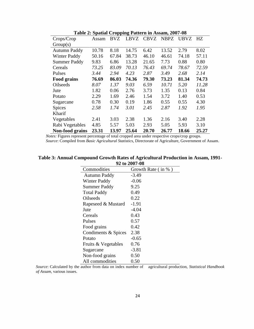
Table 2 shows the cropping pattern in Assam as well as its spatial variations across

different agro-climatic zones for the year 2007-08. As seen from Table 2, cropping

pattern in the state is largely dominated by food grains with a share of more than three

fourth of the total cropped area. Paddy, being the staple food crop of the state, has the

lion’s share of total cropped area. Of the different seasonal varieties of paddy grown in

the state, winter paddy which is grown in the kharif season has traditionally been the

most popular crop in the state because of abundance of monsoon precipitations during

8

its growing period.4 This is followed by autumn paddy and summer paddy. Among the

non-food grains, oilseeds have the largest acreage share. This is followed by rabi

vegetables (4.85%). Other crops which have more than 2 per cent of total cropped area

are kharif vegetables (2.41%), pulses (3.44%), rape & mustard (7.15%), fibres (2.02%),

potato (2.29%) and spices (2.58%).

Table 2 also shows distinct variations in the cropping pattern across the agro-

climatic zones. Like the state as a whole, the cropping pattern across the agro-climatic

zones is dominated by food grains. Being a staple food crop, paddy has traditionally

been the most popular crop among the farmers throughout the state. Moreover,

abundant monsoon precipitations in the state and mountains surrounding it have enabled

the farming communities in different agro-climatic zones to depend on paddy as the

main source of living. However, there are distinct variations in acreage shares of the

three seasonal paddy varieties across the ago-climatic zones. Notwithstanding the

cropping pattern throughout the state being dominated by winter paddy, its importance

in crop portfolio is markedly different among various zones. More than half of total

cropped area is under winter paddy in all but LBVZ, CBVZ and NBPZ. Incidentally,

agricultural sectors of the later are the worst victim of flood damages in the state (refer

to Table 5). Summer paddy is popular among the farmers in CBVZ and LBVZ whereas

less than one per cent of total cropped area in UBVZ and HZ is under this variety. The

importance of pulses in the cropping pattern is very similar across the zones. Among the

non-food grain crops, oilseeds have the largest acreage share in all except BVZ and

UBVZ. Jute is produced in a few pockets of the state and occupies more than one per

cent of total cropped area in CBVZ, LBVZ and NBPZ. Unlike other zones, sugarcane

has a considerable acreage share in HZ.

The distinct variations in cropping patterns across the state might be because of

differences in their interactions with a number of factors such as agro-climatic

4 Autumn paddy (Ahu), Winter paddy (Sali) and Summer paddy (Boro) are so named on the basis of

their harvesting periods. However, the harvesting periods of these varieties have now been pre-poned to a

great extent following the deployment of short duration high yielding varieties of seeds. Now Autumn

paddy is sown in February-March and harvested in July-August, Summer paddy is sown in around

November and harvested in March-April and Winter paddy is sown in July-August and harvested in

November-December.

9

conditions, extent of exposure to flood induced production risk, access to infrastructure

and socio-demographic factors. For example, too much dependence on food grains in

BVZ and UBVZ compared to other zones might be due to the following facts. Poor

endowment of underground water resources in the BVZ has forced its farmers to focus

on food grains, especially kharif food grains. On the other hand, small scale tea

cultivation is an important source of living for people in the UBVZ that might be

accountable for its low acreage share of non-food grains crops.

2.4 Growth of Agricultural Production in Assam

The average annual compound growth rates of agricultural production in Assam from

1991-92 to 2007-08 are shown in Table 3. The growth rate of summer paddy production

is the highest among all varieties with an annual compound growth rate of 9.25 per cent

during this period. In contrast, production of autumn paddy, rapeseed and mustard,

sugarcane, jute, winter paddy and potato has declined at a rate of 3.49%, 1.91%, 3.81%,

4.04%, 0.06% and 0.65% respectively. Another crop registering a positive growth rate

during the period is condiments and spices (2.38% per annum). The most discouraging

aspect in this regard is that the growth rate of agricultural production in case of cereals,

food grains, non-food grains and all commodities taken together is less than 1%.

[Insert Table 3]

3. Flood and Agriculture in Assam

Any analysis of agriculture in Assam would be incomplete without reference to flood.

This is because of the fact that flood is a major source of risk and uncertainty in

agricultural production that the farmers frequently face in the state.5 It is a major source

of instability of agricultural production in the state (Mandal, 2010). In the plain districts

5In this paper the terms ‘risk’ and ‘uncertainty’ have been used interchangeably. The term ‘risk’ has been

used more in Neumann-Morgenstern sense rather than that of Knight.

10

of the state (covering around 80% of its geographical area), flood is a chronic problem

that occurs in several rounds in a year. Every year large areas come under the grip of

floods that cause extensive damages to crops, lives and properties. However, the extent

of damage by flood to the crop growing sector varies from year to year depending on

the timing, frequency and intensity of flood. Table 4 shows the extent of damage by

flood to the crop growing sector in the state in some recent years.

[Insert Table 4]

It is obvious from Table 4 that the crop growing sector of Assam is faced with a

great deal of risk and uncertainty as indicated by large variability in the extent of

damage by flood from year to year. Such damages and risk have important implications

for the overall development of the agricultural sector of the state. Apart from causing

instability in production, occurrence of frequent floods is one of the factors responsible

for low rate of adoption of modern techniques of production. In many cases the farmers

are found to be skeptical of using costly inputs like chemical fertilizers and high

yielding varieties (HYVs) of seeds because of the fear of being washed away by flood.

Moreover, frequent floods every year destroy standing crops, create water logging, soil

erosion and affect large crop areas. All this is accountable, to a great extent, for low

yield and dismal growth of the agricultural sector in the state (Mandal, 2010).

[Insert Table 5]

However, this flood damage and associated risk is quite uneven across the state as

evident from Table 5. Table 5 shows that the impact of flood (captured by average

damage), and its risk and uncertainty (captured by standard deviation of damage)

concerning the crop growing sector is the highest in the North Bank plain Zone,

followed by Lower Brahmaputra Valley Zone, Central Brahmaputra Valley Zone,

Upper Brahmaputra Valley Zone and Barak Valley Zone.

In a normal year floods occur during the months of June to August when the

monsoon rainfall precipitations are the highest in the state. However, early floods in

May and late floods in September and sometimes even in the month of October occur

11

occasionally. Floods in the early part of the season mainly damage the ‘Ahu’ variety of

rice. But floods occurring late in the season are most devastating as they damage the

standing ‘Sali’ rice, which happens to be the main kharif crop of the state.

4. Data and Methodology

4.1 Data Source and the Sample

The main analysis in this paper is based on primary data collected from four non

contiguous districts of the Brahmaputra and the Barak valleys of Assam with the help of

multi-stage sampling. They are Dhubri, Morigaon, Dibrugarh and Cachar that fall in

four different agro-climatic zones: Lower Brahmaputra Valley Zone, Central

Brahmaputra Valley Zone, Upper Brahmaputra Valley Zone and Barak Valley Zone

respectively (Fig. 1). In the first stage, three Agricultural Development Officer’s (ADO)

circles have been selected from each district, with one that is frequently flood prone,

one occasionally flood prone and one flood free. 6 In frequently flood prone areas floods

occur almost every year, even several times in a year with variations in timing and

intensity. In occasionally flood prone areas, floods do occur but not every year while the

flood free areas are by and large free from floods. This selection in relation to

differences in the extent of flood proneness has been done after consultation with

officials of district Agriculture Offices and other informed sources. In the second stage,

two villages have been selected purposively from each ADO circle.7 In the final stage, a

representative number of the farm (cultivator) households have been selected at random

from each village. A total of 342 farm households, thus selected, were surveyed using a

pre-tested question schedule.

[Insert Table 6]

The nature of cropping patterns across different categories of flood proneness in the

four field study locations can be seen from Table 6. An interesting observation is that

6 An ADO circle is an agricultural unit of area for delivery of extension and other services by government

agencies. 7Villages had to be taken purposively because of the fact that an ADO being frequently flood prone, for

example, does not imply each and every village under it is exposed to the same degree of flood

proneness.

12

the cropping patterns are relatively less cereal centric and more diverse in frequently

flood-prone conditions compared to other two conditions of flood proneness. Moreover,

the farmers in frequently flood prone areas allocate a lower acreage to winter paddy

compared to other two seasonal varieties. This might be because of the fact that winter

paddy, grown in the rainy season, is very much susceptible to flood damage, and hence

in order to cope with this farmers in such areas allocate relatively a lower acreage to it

compared to that in flood free and occasionally flood prone conditions. For example, it

has been found during field survey that prolonged water logging from floods renders

cultivation of winter paddy quite impossible in the frequently flood prone areas of

Dhubri. Hence the farmers in these areas allocate a considerable proportion of total

cropped area to summer paddy, which is grown in flood free seasons. In fact, summer

paddy in the concerned location has the highest individual acreage share in total

cropped area. Likewise, winter vegetable has the highest acreage share in frequently

flood prone areas in all district level field study locations. In short, Table 6 reveals

variations in the cropping pattern not only among field study locations but also across

areas with differing exposure to flood proneness within the same location. While the

cropping patterns in some areas are concentrated around a few crops, they are spread

over a relatively larger number of crops in others. Such differences in the nature of

cropping pattern can be quantified and compared with the help of suitable

concentration/diversification measures as discussed in section 4.2.

4.2 Cropping Pattern Diversification and its Measurement

Cropping pattern diversification or crop diversification in short, may be defined as

allocation of resources, mainly cultivable land, at the disposal of farmers to

accommodate a more diverse cropping pattern. It may take place either by a change in

acreage distribution of total cropped area or a change in value-wise contribution of each

crop to total agricultural production. In the present study, therefore, crop diversification

has been measured in terms of both acreage share and value contribution of each crop in

the total crop portfolio. This is because of the fact that some crops, especially high

13

value crops, may have a relatively smaller share in total cropped area, but they may

contribute a relatively larger share to the total value of output.

Some researchers view crop diversification as adding more crops in the crop

portfolio. It is to be noted, however, that a mere increase in the number of crops does

not necessarily lead to a higher level of crop diversification. A crop portfolio with a

large number of crops but with one or two of them dominating area/value share is likely

to lead to specialization. On the other hand, a cropping pattern with the same number of

crops but with a relatively equal area/ value shares can be said to be more diversified

than one with relatively unequal shares. Therefore, suitable measures should be used to

capture variations in the extent of crop diversification.

There are several measures of crop diversification that have been used in the

literature (Shiyani and Pandya 1998; Gupta and Tewari 1985). They are Herfindahl

Index, Ogive Index, Entropy Index, Modified Entropy Index and Composite Entropy

Index. Each of these measures has its merits and limitations. In the context of the

present study Composite Entropy Index (CEI) appears to be the most suitable.8 The

index, denoted by Y, is computed using the following formula.

NPPY

N

i

iNi

11log

1

(1)

where iP represents acreage proportion of the thi crop in total cropped area and

N stands for the number of crops grown. The CEI increases with the increase in

8The CEI has its root in Entropy Index (EI) put forward by Theil (1971, p. 640) which is given

byi

N

ii

PPEI log.1

, where Pi represents proportion of total cropped area under crop i and N is total

number of crops grown. The major limitation of EI is that it does not give standard scale for measuring

the degree of diversification as the upper bound of EI depends on N and the base chosen for taking

natural logarithm (Shiyani and Pandya, 1998). Although this shortcoming is sought to be overcome

through some modification in EI by taking N as the base of the logarithm (also known as modified

entropy index) it is not sensitive to changes in the number of crops. The usefulness of modified entropy

index gets limited in comparing degrees of diversification when different number of crops is grown

across time, space and households. Hence further adjustments have been made in EI with a product of (1

– 1/N) which yields the CEI as follows ----

N

PPCEIN

iiNi

11log

1 .

14

diversification and vice versa. Its value ranges between zero and one. It takes into

account the shares of each crop in total cropped area as well as number of crops grown.

[Insert Table 7]

A preliminary investigation of sample data shows that the farmers in frequently

flood prone areas choose more diversified cropping patterns than do farmers in flood

free and occasionally flood prone areas (see Table 7). The figures, however, do not take

into account the influences of other factors like access to irrigation, farm size, access to

institutional credit etc. To ascertain if diversification of cropping patterns across

different categories of flood proneness show significant difference even after

controlling for such factors, we now turn to a multiple regression analysis.

4.3 Econometric Modeling

To examine the influence of exposure to flood induced risk, along with other factors, on

cropping pattern choice of farmers a multiple regression model has been used. As

discussed in section 4.2 the Composite Entropy Index (CEI) of diversification has been

used to measure the extent of diversification of cropping patterns and is taken as the

dependent variable Y. Here the dependent variable, crop diversification index, being

bounded between 0 and 1 a linear regression model is unsuitable as the predicted value

from a linear regression will not necessarily be contained within the interval of 0 and 1.

In a similar context, Pope and Prescott (1980), Mishra et al (2004), and Weiss and

Briglauer (2002) have used logit transformation to address the problem. 9 Even a logit

transformation may not be appropriate in the present context because the dependent

variable takes the value 0 in case of around 20 per cent of the observations. Moreover, a

9 Let Xe

Y

1

1, where Y is the diversification index such that 0 1Y . Then Logit

transformation is done in the following manner ----

XY

Y

1log .

This transformation is possible only for 10 Y . For 0Y and 1Y values, some authors have

made arbitrary manipulation by adding and subtracting respectively a negligible fraction before making

the logit transformation. But this approach may not be acceptable in situations where the number of zeros

and ones of Y are relatively large.

15

classical linear regression model is based on the assumption of normality that is not

satisfied in the present case. Therefore, to address the issues of bounded nature of the

dependent variable with a cluster of zeros and its non-normality, generalized linear

model (GLM) is used that does not depend on distributional assumption about the

dependent variable. The GLMs, first proposed by Nelder and Wedderburn (1972),

consist of a broad class of models that predict the outcome of a response variable as a

linear function of a set of predictors, with linear regression as a special case. The GLMs

extend the usual linear regression framework to cater models with non-normal

distributions. In fact, the GLMs allow us to select the appropriate distributions of the

dependent variable from a comprehensive class of density functions belonging to the

exponential family and to derive maximum likelihood estimators thereof. This can be

outlined as follows.

Let ),...,2,1( niYi be the value of the response variable for the ith out of the n

number of independent observations that belong to the family of exponential

distributions.10 Given a set of explanatory variables the linear predictor for the ith

observation can be written as follows.

kikii XX .....110 (2)

The next step is to relate the linear predictor to the predicted mean of the response

variable. The relationship between linear predictor and the predicted mean of the ith

observation is specified by a link function (.)ig that is monotonic and differentiable.

kikiiii XXg .....)( 110 (3)

Since the link function is invertible, we can also write

).....()( 11011

kikiiiii XXgg

(4)

The choice of link function depends on the distribution of the response variable. In

the classical linear regression, where the response variable is assumed to follow a

normal distribution, the link function is the identity function such that , and hence

predicted mean is simply the linear combination of the explanatory variables. In the

10 The exponential family encompasses a broader class of distributions such as Gaussian (normal),

binomial, poisson, gamma of inverse Gaussian.

16

present empirical context the response variable is bounded between 0 and 1, and hence

it may be assumed to follow binomial distribution. The next task is to choose a link

function. The identity link as in classical linear regression would not be appropriate here

because can potentially be any real number whereas the predicted mean can only

be between 0 and 1. For binomial distributions, an appropriate link function could be

the logit link, and hence the maximum likelihood estimates of the parameters are

obtained using logit link function.

The explanatory variables of the model are described as follows. Since the main

focus of the present paper is whether a diversified cropping pattern has been practiced

for mitigating flood induced production risk, hence flood proneness naturally arises as

the principal independent variable for regression analysis. However, available data do

not permit us to construct a differentiated measure of flood proneness at the farm level.

Hence the flood proneness factor is captured by categorizing the farm locations into

frequently flood prone, occasionally flood prone and flood free, which represent

different levels of exposure to flood proneness and risk thereof. As mentioned in section

4.1, in frequently flood prone areas, floods occur almost every year, even several times

in a year with variations in timing and intensity. However, though occurrence of floods

is almost certain in these areas, varying timing, frequency and intensity entail lots of

uncertainty in agricultural production. Taking flood free areas as the reference category,

two dummies - F1 and F2 – have been taken, where F1 = 1 for occasionally flood prone

areas, 0 otherwise; and F2 = 1 for frequently flood prone areas, 0 otherwise.

The available theoretical and empirical literature also suggests some other factors

such as farm size, share cropping, household size, experience of head of the farm

household, irrigation, access to institutional credit, access to extension services etc. that

influence the nature and extent of crop diversification (Joshi et al, 2004; Vyas, 1996;

Gupta and Tewari, 1985; Anosike and Coughenour, 1990; Pope and Prescott, 1980). To

ascertain relation between flood proneness and extent of crop diversification more

rigorously, these factors have been included in the regression model in the form of

17

control variables.11 Definitions of the explanatory variables (both independent and

control) along with their expected impact on cropping pattern diversification are shown

in Table 8.7

[Insert Table 8]

Summary statistics of the non-categorical variables are shown in Table 9. As the

sample observations come from four different agro-climatic zones of the state, location

dummies are also necessary to account for the impact of specific agro-climatic

conditions on farmers’ ability to diversify cropping patterns. Hence taking Dhubri as the

base category, three location dummies, denoted by L1, L2 and L3 in Table 8, have been

included as the remaining explanatory variables. Finally the Maximum Likelihood

estimates of the parameters have been obtained using STATA.

[Insert Table 9]

While choosing a particular cropping pattern a farm household is usually guided by

the twin objectives of minimization of risk and maximization of returns. Apart from

being a risk mitigation strategy a move towards diversifying the cropping pattern,

especially to high value crops, may be conducive to enhancement of income generation

in the farms. Thus it is quite pertinent to look into whether crop diversification has such

contribution to farm income in the study area.12 The gross amount of income generated

in the farms in the reference year has been obtained by value added method whereby the

costs of intermediate inputs have been subtracted from total value of output. While

doing so, the amount of non-marketed output and non-purchased intermediate inputs

have been valued at their existing market prices. The impact of crop diversification on

11 Here a notable omission from the factors influencing a farmer’s decision regarding crop diversification

is the relative expected returns from different crop choices that may be available. The relative returns will

be influenced, among other things, by the relative price movements of the crops. However, the present

study being based on data from a cross section survey is not equipped to take account of the relative price

movements, which are better observed in a time series or panel data set. Unfortunately time series data on

the prices of all the crops investigated were not available. 12The entire income generated in the farms, however, does not necessarily accrue to the farmers. It may

entirely accrue to a farmer who cultivates own land using family labour without hiring any agricultural

capital goods like tractor or power-tiller. But for a farmer using hired labour, hired capital and/or leased-

in land apart from its own inputs of land and labour, income generated in the farm will partly go out in

the form of wages and rents paid.

18

farm income generation has been investigated in a multiple regression framework as

specified in equation (5).

jjjjjjjjjjjj LLLCREXTSCIRFSFSZFI 31029187654

2

3210ln (5)

Here, FIj represents gross income generated in the jth farm. Z measures extent of

crop diversification and is captured by multiplying crop diversification index (Y) by

100. Other explanatory variables that appear as controls are farm size (FS), irrigation

(IR), share cropping (SC), access to extension services (EXT), access to institutional

credit (CR) and location specific characteristics captured by dummies (L1, L2, L3).

Equation (5) has been estimated by ordinary least square method assuming that the error

terms j s are independently normally distributed with zero mean.

5. Results and Discussion

The estimation results of the GLM regression are presented in Table 10. The prime

focus of the paper being the connection of flood risk and crop diversification, it is of

interest to note that the coefficient of F2 has turned out to be positive and significant.

This implies that after controlling for other explanatory variables, crop diversification is

significantly higher in frequently flood prone areas than in the control category of flood

free areas that are by and large free from flood induced production risk. Farmers in the

frequently flood prone areas face a great deal of production risk because of varying

timing, frequency and intensity of floods from year to year. Moreover, because of the

possibility of recurrent floods felling the standing crops and damaging crop areas with

water logging for a prolonged period, the annual cropping season in these areas gets

limited to flood-free months. In other words, farmers in such areas are affected by

floods not only in terms of production risk but also reduced time availability for

cropping. This has led the farmers to diversify their cropping pattern to hedge against

flood induced risk and limitations, and to obtain the most out of their land resources. It

is also quite possible that alluvial depositions as the floods recede replenish soil fertility

that makes such intensive use of cultivable land possible.

19

[Insert Table 10]

The coefficients of IR are statistically significant and expectedly positive. This

implies that access to irrigation enables farmers to diversify their cropping pattern to a

greater extent. This is intuitive for a region like Assam where agriculture is by and large

rain-fed. Due to a lack of assured irrigation for the majority of the farmers in the state,

agricultural production gets confined to kharif crops, mainly to winter paddy for

subsistence purpose, and the cultivable land remains fallow during rabi season. As the

farmer has more and more access to irrigation, he can diversify to a larger number of

crops including the commercial ones, and also across seasons.

That the estimated coefficients of CR are significant and positive implies that access

to institutional credit capacitates farmers to practice crop diversification to a greater

extent. Most of the farmers in the state are dependent on borrowings to carry on

agricultural operations, mostly from informal sources that charge exorbitant rates of

interest either in cash or kind. This puts excessive burdens on farmers that may limit

their capacity to move towards a diversified cropping pattern. On many occasions

(during field survey) it has been found that the indebted farmers get stuck into an

informal contract with the trader-money lender whereby they are required to pay

interest in terms of a predetermined amount of paddy and/or selling jute at a cheaper

rate to the lender. This severely limits their choice over cropping pattern. Access to

institutional credit reduces the cost of borrowing, both monetary and otherwise, and

enables them to pursue a more diverse cropping pattern.

Farm size (FS) is found to be positively impacting the extent of crop diversification

in one of the two models. Thus, larger farms are perhaps more diversified with respect

to their cropping pattern. This might be because of the fact that diversification,

especially towards high value commodities, requires more capital, improved

technologies, quality inputs and better support services. Lack of access to these facilities

may constrain diversification for small farms (Birthal et al, 2006).

Dummies (L1, L2 and L3) for capturing variations in broad agro-climatic conditions

have also been found to be statistically significant with negative coefficients. Thus crop

20

diversification tends to be lower in other agro-climatic zones compared to the control

category of Lower Brahmaputra Valley Zone. Moreover, it is worth noting that the three

coefficients are markedly different from one another which implies that within these

three agro-climatic zones too, differences in agro-climatic conditions have an impact on

farmers’ ability to diversify their cropping pattern. Thus, crop diversification seems to

be significantly influenced by agro-climatic conditions. Finally, the models gives

reasonably good fits as evident from a low value of AIC.

[Insert Table 11]

The regression results of income generation in the farms (FI) are shown in Table 11.

The point to be noted is that in both the models the coefficients of Z have turned out

significant and positive. This suggests that crop diversification has a positive impact on

income generation in the farms. More precisely, 1 per cent increase in crop

diversification causes farm income to increase by around 0.01 per cent. This is intuitive

because of the fact that as a farmer diversifies his cropping pattern across crops and

seasons he can recover the decline in output (or price) of one or two crops by others that

do not suffer such losses.

The coefficients of FS are found to be significant and positive while that of FS2

have turned out significant and negative in both the models. This implies that farm

income increases at a decreasing rate with size of farm. More specifically, farm income

falls as size of the farm increases beyond 4.7 hectares (approximately).

That the estimated coefficients of IR are positive and significant implies that as

access to irrigation increases the farms can generate more income, other things

remaining same. Our results indicate that 1 per cent increase in area under irrigation

leads to an increase in farm income by 0.003 per cent. This is quite justified because

irrigation not only facilitates farming throughout the year but also use of high yielding

variety of seeds and chemical fertilizers that, in turn, contributes towards increase in

productivity of crops.

As regards location dummies, the coefficients of L3 are found significant and

positive in the models. This implies that the farms in Cachar district have been able to

21

generate a higher income compared to the reference category of Dhubri district. But no

such comment can be made for the other two districts due to their inconsistent and/or

insignificant results in the two models. The reasonably high adjusted R2 values coupled

with highly significant F statistics indicate a good fit of the models.

The analysis of results that emanates from our study provides important insights of

farmers’ co-existence with floods while carrying out agricultural operations. Farmers

located in the areas that are exposed to regular flooding along with its varying timing,

frequency and intensity during a year tend to diversify their cropping pattern more.

Access to irrigation and institutional credit are found to help them towards this end.

Moreover, a diversified cropping pattern increases income generation in the farms. This

has important policy implications as regards capacitating farmers to cope with flood

induced production risk and making cultivation a remunerative profession in the state.

5. Conclusion and Policy Implications

This paper makes an attempt to explore how the farmers in the flood plains of Assam

cope with flood induced production risks in terms of cropping pattern choice. The

analysis of our results reveals that a diversified cropping pattern has been adopted quite

extensively by the farmers in frequently flood prone areas of Assam plains who are

regularly haunted by a great deal of production risk arising out of varying timing,

intensity and frequency of floods. In addition to statistically significant regression

results, interaction with the sample farm households lead us to conclude that the farmers

who are exposed to greater risk arising from floods tend to adopt a cropping pattern that

is more diversified across crops and seasons to hedge against flood induced risks and

limitations in agriculture. This diversified cropping pattern may be ascribed to their

compulsion of extracting maximum possible utilization of land in the flood free season.

Moreover, replenishment of soil nutrients from alluvial deposition left behind by floods

probably enables farmers to make intensive use of land with a diversified cropping

pattern. This apart, a diversified cropping pattern helps generate more income in the

farms.

22

Realizing the potentials of a diversified cropping pattern in minimizing flood

damage to agricultural production and raising farm income generation, such a strategy

is to be encouraged. Since, among the other factors, access to irrigation and institutional

credit favorably influence crop diversification, policy interventions may be required for

enhancing farmers’ access to both these facilities. It is worth mentioning that in both

irrigation coverage and credit dispersal to agriculture, Assam lags behind most of the

other states of India (CMIE, 2009). The Reserve Bank of India, India’s central bank, has

initiated action plan for enhancing financial inclusion, and the northeast part of India

including Assam has received special reference in that scheme (RBI, 2006). But these

initiatives are yet to make significant inroads into Assam’s agriculture. Moreover,

available statistics show that irrigation coverage in Assam is abysmally low.13

However, the issue here is not only of creating more irrigation capacity but also of

putting institutions in place for fuller and sustainable utilization of the created potential.

The relatively larger scale irrigation projects developed under public sector are

notorious for low utilization of capacity owing to poor management of maintenance and

delivery. But effective organization among farmers in command areas has been found to

extract better delivery even from these projects (Dutta and Bezbaruah, 2003). On the

other hand, small scale shallow tube well-based privately owned systems (irrigating

capacity up to 2 hectares) have shown greater efficiency in utilization. However,

creating and maintaining irrigation facilities in flood prone areas pose additional

challenges because of likely damages to the irrigation infrastructure by flood. Hence,

innovation in irrigation engineering to meet the challenge will go a long way in

addressing these issues.

13 Gross irrigation potential was only 18.9% of total cropped area in 2009-10 as per Economic Survey of

Assam, 2010-11.

23

Table 1: Some Characteristics of the Agro-climatic Zones of Assam

Agro-climatic

Zones

Total

Geographical

Area€

(in Hectare)

Net Area Sown*

(in hectare),

2003-04

Cropping

Intensity,

2003-04

Irrigation

IntensityΦ

(in %),

2007-08

Average Annual

Rainfall (normal

in mm),

2006

HYV area¥,

2006-07

Fertilizer

Consumptionε

(in kg/hectare),

2006-07

Barak Valley

Zone

692200

(8.82)

229811

(33.20) 137.24 0.05 3336.26 50.10 58.18

Lower

Brahmaputra

Valley Zone

2014800

(25.69)

907598

(45.05)

147.38 2.17 2483.51 65.29 85.81

Central

Brahmaputra

Valley Zone

553500

(7.06)

325880

(58.88)

149.63

5.09 1884.8 68.61 123.50

North Bank

Plain Zone

1431900

(18.26)

525933

(36.73)

154.04

2.76 2400.23 58.22 29.90

Upper

Brahmaputra

Valley Zone

1619200

(20.64)

608571

(37.58)

126.41

0.15 2304.76 57.09 49.09

Hill Zone

1532200

(19.53)

154808

(10.10)

152.98

11 1122.2 67.31 7.66

Assam 7843800

2752601

(35.09)

143.75

2.72 2217.8 61.41 64.45

Notes: €Figures in the parenthesis represent percentage share of different zones in total geographical area of the state; *Figures in the parentheses

represent Net Sown Area as percentage of total geographical area; Irrigation potential utilized through government irrigation schemes as percentage

of estimated total cropped area. Data on non-government schemes are not available; ¥HYV paddy area as percentage of total paddy area; εFertilizer

consumption in kg per hectare of estimated total cropped area.

Source: Statistical Handbook of Assam, different years.

24

Table 2: Spatial Cropping Pattern in Assam, 2007-08

Crops/Crop

Group(s)

Assam BVZ LBVZ CBVZ NBPZ UBVZ HZ

Autumn Paddy 10.78 8.18 14.75 6.42 13.52 2.79 8.02

Winter Paddy 50.16 67.84 38.73 46.10 46.61 74.18 57.11

Summer Paddy 9.83 6.86 13.28 21.65 7.73 0.88 0.80

Cereals 73.25 83.09 70.13 76.43 69.74 78.67 72.59

Pulses 3.44 2.94 4.23 2.87 3.49 2.68 2.14

Food grains 76.69 86.03 74.36 79.30 73.23 81.34 74.73

Oilseeds 8.07 1.37 9.03 6.59 10.71 5.20 11.28

Jute 1.82 0.06 2.76 3.73 1.35 0.13 0.84

Potato 2.29 1.69 2.46 1.54 3.72 1.40 0.53

Sugarcane 0.78 0.30 0.19 1.86 0.55 0.55 4.30

Spices 2.58 1.74 3.01 2.45 2.87 1.92 1.95

Kharif

Vegetables 2.41 3.03 2.38 1.36 2.16 3.40 2.28

Rabi Vegetables 4.85 5.57 5.03 2.93 5.05 5.93 3.10

Non-food grains 23.31 13.97 25.64 20.70 26.77 18.66 25.27 Notes: Figures represent percentage of total cropped area under respective crops/crop groups.

Source: Compiled from Basic Agricultural Statistics, Directorate of Agriculture, Government of Assam.

Table 3: Annual Compound Growth Rates of Agricultural Production in Assam, 1991-

92 to 2007-08

Commodities Growth Rate ( in % )

Autumn Paddy -3.49

Winter Paddy -0.06

Summer Paddy 9.25

Total Paddy 0.49

Oilseeds 0.22

Rapeseed & Mustard -1.91

Jute -4.04

Cereals 0.43

Pulses 0.57

Food grains 0.42

Condiments & Spices 2.38

Potato -0.65

Fruits & Vegetables 0.76

Sugarcane -3.81

Non-food grains 0.50

All commodities 0.50 Source: Calculated by the author from data on index number of agricultural production, Statistical Handbook

of Assam, various issues.

25

Table 4: Damage by Floods in Assam during 2000 to 2006

Year Area Affected

(% of Total

area)

Crop Area Affected

(% of Gross Cropped

Area)

Value of Crops Lost

(Rs. in million)

2000 12.32 9.48 1735.16

2001 2.59 1.07 83.58

2002 15.14 8.40 1456

2003 11.88 8.34 1470

2004 30.14 15.15 3747.06

2005 2.84 2.95 234.73

2006 0.74 0.33 11.10 Notes:

a) Flood damage is in calendar year (January-December) and Gross Cropped Area (GCA)

in financial year (April to March).

b) GCA used here is sum over all crop acreages except fruits reported in Basic Agricultural

Statistics, Directorate of Agriculture, Government of Assam, different issues and not the

officially reported GCA.

Source: Mandal (2010).

Table 5: Estimates of Flood-prone Areas of Assam

Agro-climatic Zones14 Cropped Area Damaged by

Flood15 (in '000 hectares)

Average Std.

Deviation

Barak Valley Zone (BVZ) 6.49 7.16

Lower Brahmaputra Valley Zone

(LBVZ) 77.67 69.69

Central Brahmaputra Valley Zone

(CBVZ) 32.59 37.64

Upper Brahmaputra Valley Zone

(UBVZ) 27.18 27.56

North Bank Plain Zone (NBPZ) 84.79 92.14 Source: Mandal (2010).

14 Since the focus is on flood risk and cropping pattern choice Hill Zone is omitted from this analysis. 15 Average and standard deviation for the period of 1991 to 2006.

26

Table 7: Extent of Crop Diversification in relation to Flood Proneness in the

Sample Locations

District Area Based Value Based

FF OFP FFP FF OFP FFP

Dhubri 0.64 0.60 0.71 0.69 0.72 0.73

Morigaon 0.37 0.42 0.48 0.47 0.33 0.52

Dibrugarh 0.08 0.40 0.51 0.16 0.51 0.63

Cachar 0.20 0.17 0.62 0.18 0.10 0.66 Note: FF – Flood Free areas; OFP – Occasionally Flood Prone areas; FFP – Frequently Flood Prone

areas.

Source: Field Survey.

Table 6: Cropping Patterns across Categories of Flood Proneness in Field Study Locations

Crops/Crop

Groups

Dhubri Morigaon Dibrugarh Cachar

FF OFP FFP FF OFP FFP FF OFP FFP FF OFP FFP

Winter Paddy 44.86 49.19 0.00 70.25 43.37 30.33 96.98 76.46 66.58 88.68 91.33 53.92

Summer Paddy 14.33 12.37 26.99 3.88 56.63 49.89 0.00 0.00 5.05 0.00 0.37 0.00

Autumn Paddy 2.52 0.47 5.42 0.00 0.00 0.00 0.00 0.00 1.12 9.91 8.12 1.43

Non-paddy

Cereals 5.03 0.78 0.00 0.22 0.00 0.66 0.00 0.00 0.00 0.00 0.00 0.00

Cereals 66.74 62.81 32.42 74.35 100.00 80.88 96.98 76.46 72.75 98.59 99.82 55.34

Oilseeds 17.33 15.90 23.46 0.22 0.00 12.85 0.00 12.47 7.85 0.00 0.00 4.07

Pulses 3.28 3.68 14.15 0.89 0.00 0.05 0.27 6.59 2.80 0.00 0.00 3.13

Jute 6.15 11.28 17.98 18.84 0.00 2.27 0.00 0.00 0.00 0.00 0.00 0.00

Sugarcane 0.42 0.00 0.00 0.22 0.00 0.01 0.00 0.00 0.00 0.00 0.00 0.00

Potato 1.50 1.10 0.38 0.17 0.00 1.85 0.00 2.37 2.24 0.28 0.18 8.34

Chilli 0.65 1.13 4.84 0.44 0.00 0.05 0.00 0.00 3.24 0.09 0.00 12.70

Winter

Vegetables 2.93 2.60 6.39 0.86 0.00 1.21 2.61 2.12 11.12 1.03 0.00 16.41

Summer

Vegetables 1.01 1.50 0.39 4.01 0.00 0.84 0.14 0.00 0.00 0.00 0.00 0.00

Notes:

a) The figures represent acreage share of different crops in total cropped area (in %).

b) FF – Flood Free areas; OFP – Occasionally Flood Prone areas; FFP – Frequently Flood Prone areas.

Source: Field Survey.

27

Table 8: Definition of the Explanatory Variables and their Likely Impact on Crop

Diversification

Variable Definition Expected Sign

of coefficients

Occasionally Flood Prone Area

(F1)

= 1 for occasionally flood prone area, 0

otherwise. -

Frequently Flood Prone Area

(F2)

= 1 for frequently flood prone area, 0

otherwise. -

Farm Size (FS) Size of farm in hectare. +/-

Share Cropping (SC) Area under share cropping without cost

sharing as percentage of net sown area. -

Household Size (HS) Number of members in the household. +/-

Experience (AGE) Age of the head of farm household in

years. +

Irrigation (IR) Gross irrigated area as percentage of

total cropped area. +

Access to Institutional Credit

(CR)

= 1 with access to institutional credit, 0

otherwise. +

Extension Services (EXT)16 Total Score on access to extension

services. +

Morigaon (L1) =1 for Morigaon, 0 otherwise. +/-

Dibrugarh (L2) =1 for Dibrugarh, 0 otherwise. +/-

Cachar (L3) =1 for Cachar, 0 otherwise. +/-

Table 9: Summary Statistics of the Variables (non-categorical)

Variables Unit Minimum Maximum Mean Standard

Deviation

Y (area based) ------ 0 0.828 0.393 0.26

Y (value based) ------ 0 0.840 0.419 0.28

FS Hectare 0.11 6.56 1.32 0.89

IR % 0 100 28.89 31.60

EXT Score 0 5 0.31 0.81

AGE Years 18 80 46.32 11.59

SC % 0 100 9.38 22.44

HS Number 2 16 6 1.99 Note: Number of Observations = 342

16

In the household schedule used for collecting primary data six questions related to the farmers’ interaction with

the extension agency were included. The farmers’ responses to these queries were codified into scores. The total

score for farming household on these questions could vary from 0 to 6, depending on the level of its interactions

with the extension agencies. This total score is used as a measure of access to extension services.

28

Table 10: Results of the GLM Regressions

Explanatory Variables/Particulars Model 1 Model 2

Estimated

Coefficient/Values

Estimated

Coefficient/Values

Occasionally Flood Prone Area (F1) .0586

(.123)

.0525

(.129)

Frequently Flood Prone Area (F2) .8245***

(.106)

.990***

(.121)

Farm Size (FS) .092*

(.0546)

.057

(.059)

Share Cropping (SC) -.0016

(.0017)

-.0026

(.0017)

Household Size (HS) -.0243

(.0239)

-.0167

(.026)

Experience (AGE) .0009

(.004)

.001

(.005)

Access to Irrigation (IR) .0076***

(.002)

.0057***

(.002)

Access to Institutional Credit (CR) .2327**

(.1067)

.2438**

(.116)

Extension Services (EXT) .004

(.055)

-.0108

(.057)

Morigaon (L1) -.887***

(.1136)

-.867***

(.122)

Dibrugarh (L2) -1.474***

(.133)

-1.345***

(.148)

Cachar (L3) -1.427***

(.132)

-1.68***

(.139)

Constant .0026

(.2125)

.152

(.228)

Deviance 58.279 65.438

AIC .927 .937 Notes:

a) In Model 1 and Model 2 the dependent variable crop diversification index is measured based on

acreage and value shares of crops respectively.

b) Figures in the parenthesis represent White’s heteroscedasticity corrected standard errors.

c) *, ** and *** represent significant at 10%, 5% and 1% levels respectively.

29

Table 11: Regression Results of Income Generation in Farms

Variables/Particulars Model 1 Model 2

Estimated

Coefficients/Values

Estimated

Coefficients/Values

Crop diversification (Z) 0.012***

(0.001)

0.011***

(0.001)

Farm Size (FS) 1.154***

(0.071)

1.165***

(0.072)

Farm Size squared (FS2) -0.124***

(0.013)

-0.124***

(0.014)

Irrigation (IR) 0.003***

(0.001)

0.003***

(0.001)

Share Cropping (SC) -0.001

(0.001)

-0.001

(0.001)

Extension Services (EXT) 0.030

(0.029)

0.035

(0.025)

Access to Institutional Credit (CR) -0.011

(0.053)

-0.011

(0.049)

Morigaon (L1) 0.053

(0.062)

0.021

(0.062)

Dibrugarh (L2) -0.104

(0.075)

-0.177**

(0.070)

Cachar (L3) 0.475***

(0.082)

0.484***

(0.079)

Constant 8.808***

(0.102)

8.827***

(0.102)

Adjusted R2 77.19% 77.08%

F (10, 332) 103.88*** 96.07*** Notes:

a) In Model 1 and Model 2 extent of crop diversification is measured on the basis of acreage

and value shares of crops respectively.

b) Figures in the parenthesis represent White’s heteroscedasticity corrected standard errors.

c) ***, ** and * represent significant at 1%, 5% and 10% respectively.

30

Fig. 1: Map of Agro-climatic Zones of Assam

31

REFERENCES:

Anosike, N., C. M. Coughenour (1990). The Socioeconomic Basis of Farm Enterprise

Diversification Decisions. Rural Sociology, 55(1), 1-24.

Barghouti, S., S. Kane, K. Sorby, Mubarik Ali (2004). Agricultural Diversification for the Poor:

Guidelines for Practitioners. Agriculture and Rural Development Discussion Paper 1,

The World Bank, Washington, D.C., U.S.A.

Blade, S. F., A. E. Slinkard (2002). New Crop Development: The Canadian Experience. In:

Janick, J., Whipkey, A. (Eds), Trends in New Crops and New Uses. ASHS Press,

Alexandria, VA, pp. 62-75.

Birthal, P.S., A.K Jha, P.K. Joshi, D.K. Singh (2006). Agricultural Diversification in North

Eastern Region of India: Implications for Growth and Equity. Indian Journal of

Agricultural Economics. 61(3).

CMIE (2009). Agriculture. January, Centre for Monitoring Indian Economy, Mumbai.

Dutta, M.K., M.P. Bezbaruah (2003). An Analysis of Utilisation Efficiency across Types of

Irrigation Projects in Assam and Emerging Policy Implications. Paper presented in 63rd

Annual Conference of Indian Society of Agricultural Economics held in Bhubaneswar on

19-20 December (Summary available in the Indian Journal of Agricultural Economics,

July-September 2003).

Goyari, P. (2005). Flood Damages and Sustainability of Agriculture in Assam. Economic and

Political Weekly, 40(26).

Gupta, R.P., S.K. Tewari (1985). Factors Affecting Crop Diversification: An Empirical Analysis.

Indian Journal of Agricultural Economics, 50(3), 304-309.

Joshi, P.K., A. Gulati, P.S. Birthal, L. Tewari (2004). Agricultural Diversification in South Asia:

Patterns, Determinants and Policy Implications. Economic and Political Weekly, 39(24).

Kurukulasuriya, P., R. Mendelsohn, (2008). Crop Switching as a Strategy for Adapting to

Climate Change. African Journal of Agriculture and Resource Economics. 2(1), 105-126.

Mahesh, R. (1999). Causes and Consequences of Change in Cropping Pattern: A Location

Specific Study. Discussion Paper No. 11, Kerala Research Programme on Local Level

Development, Centre for Development Studies, Thiruvananthapuram.

32

Mandal, R. (2010). Cropping Patterns and Risk Management in the Flood Plains of Assam.

Economic and Political Weekly, 45(33), 78-81.

Mishra, A. K., H. S. El-Osta, C. L. Sandretto (2004). Factors Affecting Farm Enterprise

Diversification. Agricultural Finance Review, Fall, 151-166.

Nelder, J.A., R.W.M. Wedderburn, (1972). Generalized linear models. Journal of the Royal

Statistical Society A135, 370-384.

Pandey, S., H. Bhandari (2009). Drought, Coping Mechanisms and Poverty ---- Insights from

Rainfed Rice Farming in Asia. Occasional Papers, 7. International Fund for Agricultural

Development (IFAD).

Purkayastha, G. (2005). Benegati – A Model Agricultural Village. Kurukshetra. 53(4), 44-47.

Pope, R. D., R. Prescott (1980). Diversification in Relation to Farm Size and other

Socioeconomic Characteristics. American Journal of Agricultural Economics, 62(3),

554-559.

Rathore, J. S. (2004). Drought and Household Coping Strategies: A Case of Rajasthan. Indian

Journal of Agricultural Economics. 59(4), 689-708.

RBI (2006). Report of Committee on Financial Sector Plan for North Eastern Region. Reserve

Bank of India.

Shiyani, R. L., H. R. Pandya (1998). Diversification of Agriculture in Gujarat: A Spatio-

Temporal Analysis. Indian Journal of Agricultural Economics, 53(4).

Theil, H. (1971). Principles of Econometrics, North Holland Publishing Company.

Vyas, V. S (1996). Diversification in Agriculture: Concept, Rationale and Approaches. Indian

Journal of Agricultural Economics, 51(4).

Weiss, C., W. Briglauer (2002). Determinants and Dynamics of Farm Diversification. Paper

presented at the 10th European Association of Agricultural Economists (EAAE) Congress

on ‘Exploring Diversity in the European Agri-Food System’, Zaragoza, Spain, 28-31

August.