CREDITS AND DEDUCTIONS:

AN EXPERIMENTAL TEST OF THE RELATIVE STRENGTH OF ECONOMIC

INCENTIVES1

John Scott

University of North Carolina at Chapel Hill

Jeffrey Diebold

North Carolina State University

Abstract: Does the type of tax incentive matter in terms of encouraging behavior? Social

policies often use tax incentives to encourage behavior, but little research has been on how the

structure or type of tax incentive might influence behavior. Using experimental methods, we test

the effects of incentives structured as tax deductions and credits with respect to the policy

problem of how best to encourage people to purchase annuities at retirement. We hypothesize

that tax credits may be more effective than tax deductions at increasing the rate at which

individuals would engage in socially desirable behavior because credits appear to have

immediate value. Adult subjects played a financial decision making game in which they were

offered different incentives to purchase annuities. We found that incentives in the form of tax

credits not only encouraged more annuity purchases relative to actuarially equivalent deductions

but also relative to deductions that were greater in value than the credit-based tax incentives.

1 We want to acknowledge the funding from the University of North Carolina at Chapel Hill that supported this

research. We want to thank the Wake County Court System for their cooperation. Most importantly, our thanks go

to Charlotte Lloyd, Mathew Gunnett, Amanda Shomper, Melanie Baucom, Daisy Arizpe, and Juliana Bradley for

their excellent assistance in data collection.

1

1. Introduction

The adequacy of social policies benefiting older Americans is a growing concern. Even

if abject poverty is avoided via Social Security and Medicare, many older Americans face a

decline in their standard of living in old age precisely because they now fully bear the risk of

retirement income provision. For example, half of single elderly and one-third of elderly in

relationships die with less than $10,000 in assets (Poterba, Venti and Wise 2012). Part of the

problem is that retiring Americans do not adequately insure against longevity risk. According to

the standard life-cycle model, individuals would realize significant welfare gains were they to

annuitize some, or all of their retirement savings (Yaari 1965; Mitchell 2001; Dushi and Webb

2004; Davidoff, Brown, and Diamond 2005). Despite the gains from annuitization that economic

theory and research suggest, very few individuals elect to annuitize their assets (Investment

Company Institute 2011; Mottola and Utkus 2007).

Can public policy encourage more people to annuitize their retirement savings? It is the

type of economic behavior that policymakers may have an interest in subsidizing. In fact,

legislation was introduced before Congress in 2009 that would have modified the tax code and

established a new tax expenditure that would have allowed individuals to exclude 50 percent of

any income from an annuity contract.2 But would such incentives work?

The government does use incentives for a range of behaviors including personal

retirement savings by subsidizing participation in, and contributions to, retirement saving plans

through tax provisions. These provisions, or “tax expenditures,” refer to the credits, deductions,

and exclusions in the tax code that are typically designed to promote a broad range of socially

desirable behaviors, including saving for retirement. Indeed, among the largest of the tax

2 See H.R. 2748, The Retirement Security Needs Lifetime Pay Act of 2009.

2

expenditures in the tax code is the exclusion of income contributed to individual pension plans,

which amounted to a total revenue loss from individual households in 2012 of $112 billion

Despite the substantial resources devoted to tax expenditures, empirical estimates of the effect of

different tax expenditures on their respective outcomes suggest are decidedly mixed.

There are a number of dimensions that contribute to the success of an incentive like a tax

expenditure. Contrary to standard economic theory, experimental evidence indicates that

individuals respond differently to alternative, yet economically equivalent, incentives. In this

paper, we ask whether the annuity decision is conditional of the structure of an incentive. That is,

we analyze whether the strength of the incentive depends on how the benefits are distributed. We

analyze this question by comparing the effects of different yet economically equivalent

incentives designed to resemble different types of tax expenditures in a controlled experimental

setting. Our computer-based experiment simulates asset allocation decisions made at retirement

and looks, specifically, at whether incentives structured as tax credits are more effective than

those structured as tax deductions. Determining the varying effects of incentives is important

for understanding how lawmakers can best apply the limited resources available to them in order

to encourage the use of beneficial financial products and achieve specific policy aims.

Our paper is organized as follows: We first discuss the use of tax-based incentives in

encouraging socially desirable behavior. In particular, the government uses different types of

incentives in the tax code with different outcomes. We then review the growing literature on

experimental tests of incentives and what they tell us about the effectiveness of one type of

incentive versus another. This review provides the basis for our hypotheses, which compare the

effectiveness of immediate versus delayed incentives in the annuity decision. These hypotheses

are tested by using experimental methods on a sample of adults with the different incentive

3

structures acting as treatments. A strength of this paper is that the participants in the experiment

are from a broad sample of adults rather than a particular segment of the population such as

undergraduate students. After presenting the results of the analysis, we conclude the paper by

discussing possible policy lessons as well as avenues for future work.

1.1 Tax Expenditures, Social Policy, and Behavioral Models

Policy makers often use tax credits, deductions, and exclusions to achieve policy goals,

and as an introduction we first compare the three largest: the Earned Income Tax Credit (EITC),

the mortgage interest rate deduction (MID), and exclusions for pension plan contributions (EPC).

The EITC provided $59 billion to 26.8 million working families with low-income in 2009 (Joint

Committee on Taxation 2013). This provision within the tax code is currently the largest source

of cash-assistance for the working poor and is the nation’s primary antipoverty program

(Gitterman 2010). Research has demonstrated that this program has been successful at increasing

workforce participation among single mothers and reducing US poverty rates among the working

poor (Eissa and Liebman 1996; Meyer and Rosenbaum 2001; Sherman 2009; Ben-Shalom,

Moffit, and Scholz 2011; Hotz and Scholz 2006).

The MID provided more than 34 million households with more than $68 billion worth of

tax benefits in 2012 (Joint Committee on Taxation 2013). This subsidy is intended to promote

homeownership, which is usually associated with a number of socially beneficial outcomes. But,

despite being larger in terms of total benefit than the EITC, the empirical evidence indicates that

this subsidy has had little to no effect on the rates of homeownership within the US. Glaeser and

Shapiro (2004) estimate that a one percent increase in the subsidy rate is associated with only a

0.0009 percent increase in the rate of homeownership. In other words, the subsidy is going to

people who would have engaged in the desired behavior even in the absence of the subsidy.

4

The federal government also allows for deductions and exclusions for income contributed

to defined contribution plans and individual retirement accounts. The EPC is intended to

incentivize retirement savings and thereby improve financial security in retirement for those

covered under qualifying plans. According to estimates from the Joint Committee on Taxation

(2013), US workers were able to save $112 billion in tax liabilities through contributions to their

pension plan in 2012. Contributions to these plans are typically tax deferred, meaning that

individuals are allowed to exclude them from their taxable income throughout their working

lives, but eventually they pay taxes on these contributions and any investment earnings when

they take a distribution. Here again, the empirical evidence indicates that the incentives

embedded within the tax code fail to encourage new retirement savings (Engen, Gale, and Scholz

1996; Gale and Scholz 1994).

Unequal Responses to Equivalent Incentives?

While there is little literature on this issue, research suggests that individuals may

respond differently to similar incentives depending on how the incentives are structured (Gale

2011). According to economic theory, individuals should be indifferent between two options

with equal expected values, but individual economic behavior frequently deviates from the

expectations of these models. In a field experiment comparing the relative strength of offering a

credit (cash rebate) or economically equivalent matching contributions, Saez (2009) found that

the matching contributions were more effective at increasing enrollment in and contributions to

an individual retirement account (IRA). The credit and match were set at rates such that the out-

of-pocket costs associated with any contributions were identical for individuals in each group.

Those offered a match were more likely to enroll in an IRA by roughly 4 percentage points and

contributed $153 more to their accounts after enrolling than those offered a credit. In a related

5

study, Davis and Millner (2006) compared the effect of matches and credits as price-reduction

strategies on consumer decisions. In this study, the researchers offered participants either a

rebate or a matching incentive to purchase chocolate bars. Those participants who were offered a

matching incentive purchased significantly more candy bars than those offered an economically

equivalent rebate.

There are a number of reasons to doubt that equal incentives would produce equivalent

responses. First, compliance costs of specific incentives may cause different outcomes.

Deductions and exclusions such as the MID and EPC may have a higher compliance cost than

tax credits like the EITC (Bertrand, Mullainathan, and Shafir 2006). The complexity of the tax

code may prevent individuals from being able to incorporate any expected benefit from specific

subsidies into their economic decisions. A recent article in the USA Today, based on information

from tax professionals about the difference between the marginal and effective tax rate,

incorrectly claimed that workers receiving a pay raise may actually end up with less take-home

pay after being “bump[ed] into the next tax bracket.” 3

Further, a study by Fuiji and Hawley

(1988) found that a large portion of the population could not guess or correctly identify their

marginal tax rate, which may explain why wage earners and those with positive taxable income

do not bunch into kink points at the various income tax brackets (Saez 2010; Chetty and Saez

2009). This finding is true over time as well, even when the increase in the marginal rates have

been large and stable (Saez 2010). Survey results indicate that workers are aware of the existence

of the EITC but are not knowledgeable with respect to the structure of the EITC (Phillips 2001;

Romich and Weisner 2002; Smeeding, Phillips, and O’Conner 2000; Maag 2005). This might

explain why wage earners fail to bunch around the kink points at the phase-in and phase-out

ranges of the EITC benefit schedule (Saez 2010; Chetty and Saez 2009).

3 The article was written by Gregory Connelly (2011) and the USA Today has since issued a correction.

6

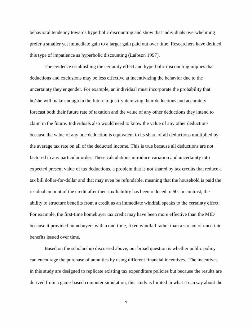
The differing behavioral responses to the different forms of tax subsidies may also be a

function of household type. Deductions and exclusions reduce the amount of income that falls

under an individual’s marginal rate of taxation and, therefore, provide a larger benefit to higher

income households that, typically, face higher marginal rates. As a result, these provisions

provide little benefit to the vast majority of income earners.4 Moreover, a household can only

claim benefits like the mortgage interest deduction if they itemize their deductions on their

income tax returns, and only a small minority of taxpayers itemizes their deductions (Prante

2007). In 2012, 77 percent of all the benefits from the MID went to the 19 percent of US

households making more than $100,000 (Joint Committee on Taxation 2013). Higher income

households may be predisposed to the types of behavior the government is attempting to

encourage through these types of tax expenditures, and these programs are functioning more as

an unexpected reward for high-income households than as an incentive for these behaviors for

those at lower points along the income distribution.

In addition, responses to these tax subsidies may vary due to psychological biases such as

those explained by prospect theory (Kahneman and Tversky 1979). One of the central tenets of

this theory is that individuals tend to prefer a benefit that is certain over a larger benefit that is

not certain. This “certainty effect” helps explain why individuals tend to heavily discount future

benefits (Laibson 1997). Indeed, research has shown that when given the choice between a larger

benefit paid out over time and a smaller but immediate lump sum benefit, individuals tend to

prefer the lump sum (Pleeter and Warner 2001; Loewenstein and Prelec 1992). In a natural

experiment involving substantial sums of money, for example, Warner and Pleeter (2001)

demonstrate that individuals place a large premium on present gains. They illustrate the

4 In 2009, 80 percent of tax payers faced a marginal rate of taxation of 15 percent, the rate applied to income below

$67,900 for a married couple filing jointly (Tax Policy Center 2011).

7

behavioral tendency towards hyperbolic discounting and show that individuals overwhelming

prefer a smaller yet immediate gain to a larger gain paid out over time. Researchers have defined

this type of impatience as hyperbolic discounting (Laibson 1997).

The evidence establishing the certainty effect and hyperbolic discounting implies that

deductions and exclusions may be less effective at incentivizing the behavior due to the

uncertainty they engender. For example, an individual must incorporate the probability that

he/she will make enough in the future to justify itemizing their deductions and accurately

forecast both their future rate of taxation and the value of any other deductions they intend to

claim in the future. Individuals also would need to know the value of any other deductions

because the value of any one deduction is equivalent to its share of all deductions multiplied by

the average tax rate on all of the deducted income. This is true because all deductions are not

factored in any particular order. These calculations introduce variation and uncertainty into

expected present value of tax deductions, a problem that is not shared by tax credits that reduce a

tax bill dollar-for-dollar and that may even be refundable, meaning that the household is paid the

residual amount of the credit after their tax liability has been reduced to $0. In contrast, the

ability to structure benefits from a credit as an immediate windfall speaks to the certainty effect.

For example, the first-time homebuyer tax credit may have been more effective than the MID

because it provided homebuyers with a one-time, fixed windfall rather than a stream of uncertain

benefits issued over time.

Based on the scholarship discussed above, our broad question is whether public policy

can encourage the purchase of annuities by using different financial incentives. The incentives

in this study are designed to replicate existing tax expenditure policies but because the results are

derived from a game-based computer simulation, this study is limited in what it can say about the

8

effect that these incentives might have on actual annuitization behavior. We analyze our

research question within the context of a game simulating the annutization decision for a number

of reasons. This study expects to find that an immediate financial incentive, which resembles a

tax credit, is a more powerful incentive for encouraging annuitization than an actuarially

equivalent delayed incentive, which resembles a tax deduction.

Hypothesis 1: Participants will be more likely to select an annuity when receiving a credit

versus a deduction with an equal expected value.

But how strong is the immediate windfall effect of the credit? Actuarially equivalent

incentives may not capture the full effects of how the incentives are structured. To test the

underlying theory even more, we also expect that people are more likely to select an annuity

when offered a credit as compared to a deduction that is worth substantially more than the credit.

Hypothesis 2: Participants will be more likely to select an annuity when receiving a credit

even when the expected value of the deduction exceeds that of the credit.

2. Data and Methods

We use an experimental design to test our hypotheses. A growing number of researchers

have used within an experimental setting to study various dimensions of the annuitization

decision as well as various behavioral biases. Two such studies were conducted recently by

Agnew, Anderson, Gerlach, and Szykman (2008) and Gazzale and Walker (2009). Agnew et al.

(2008) found that the annuitization decision is sensitive to positive and negative framing.

Gazzale and Walker (2009) found that individuals were more likely to purchase an annuity when

their benefits were specified as a stream of payments rather than a lump-sum prior to playing the

game, implying that individuals anchor themselves to a specific way of thinking about their

benefits and are more likely to annuitize because an annuity reinforces their original

9

conceptualization of their benefits. They also found evidence indicating that the annuitization

decision is negatively affected by the sequential nature of the risk associated with survival

(survival to period 15 requires survival to period 14, which requires survival to period 13, and so

forth) to which the stream of benefits from an annuity are linked. This study borrows the relevant

game design of these previous studies in an effort to determine whether individual behavior

deviates from the expectations of common economic models and whether policy might be better

designed to exploit these tendencies.

Our game simulates one of the many economic decisions confronting those entering

retirement: whether to insure against the risk of “outliving” their assets (longevity risk) by

purchasing an annuity with a portion of the account balance each player was given at the start of

the game. In our game, the rates of annuitization are compared between three mutually exclusive

treatment groups to determine whether those offered an immediate incentive, what we call a ‘tax

credit,’ were more likely to annuitize than those offered the delayed incentive or ‘tax deduction.’

The three treatment groups were Credit, Equal Deduction, or Larger Deduction. Other than the

type of incentive offered, the game was identical across treatments. We used the larger deduction

treatment to see if the credit would still be more attractive despite the financial benefit of the

actuarially larger deduction. A control group of participants were offered the annuity but

without any incentive.

The participants made their decisions related to their account before the game began, and

once made these decisions would be binding throughout the game. They were binding because

we wanted to make sure that the annuitization decision was affected only by the incentive

offered and not by the changes in the account balance due to, say, market losses. They began the

game with a fictional $20,000 in an account that they were to “live off” throughout the game.

10

They were then told that their compensation for participating would be determined by the

balance in their account when they exit the game. Individuals received $2 for exiting the game

with a negative balance, $5 for exiting the game with a positive balance but below starting

amount, and $10 for exiting the game with more than their the starting balance, which was equal

to the initial $20,000 less the cost of the annuity if purchased. The game would take place over

multiple periods, and in each period, $3,000 would be deducted from their accounts as a cost of

living expense.

Parameters determining survival were determined randomly. After each period, the

computer generated a random number between 1 and 18. Individuals with a value larger than the

specified number survived to the next period. The value necessary to survive increased with each

period, so the likelihood of survival declined over time. For example, an individual needed a

value of four or higher to survive to the second stage and then a value of five or higher to survive

to the third stage, a value of six in order to survive to the fourth stage, and so forth. Individuals

were able to see the conditional probabilities of their survival to a given period in a life table

provided to them at the beginning of the game. The game would end if they ran out of money in

their account or if they failed to “survive” to the next period.

Participants could invest their funds in three different investment options at the start of

the game. They had the option of (1) investing some or all of their money in a fictional stock

market, (2) purchasing an annuity to help offset their $3,000 per-period costs of living expenses,

or (3) leaving their money in their account balance. The cost of the annuity was $13,110 and the

amount of the per-period annuity payment was $2,000 applied to the account balance. Returns in

the stock market would be due entirely to chance and any remaining amount they chose not to

11

invest from their account balance would not gain or lose value except for the automatic

deduction of the cost of living.

Individuals assigned to the Credit group would receive an immediate one-time credit of

$3,277 applied towards their account balance if they purchased an annuity. Participants assigned

to the Credit group saw the following message on the computer screen: “As a part of a new

program, however, you will receive a credit of $3,277 that will be immediately added to your

savings account should you decide to purchase the annuity.”

Those that were assigned to the Equal Deduction group would see their cost of living

reduced by $500 to $2,500 in each period if they purchased an annuity (Equation 1). The

message for the Equal Deduction group was the following: “As a part of a new program,

however, you will be able to reduce your cost of living by $500 in each period should you decide

to purchase the annuity.” Those that were assigned to the Larger Deduction group were told that

their cost of living would be reduced by $875 in each period if they purchased the annuity

(Equation 2). The expected value of the deduction is given by the following equation:

( ) ∑ ( ) Eq. 1

( ) ∑ ( ) Eq. 2

where p is equal to the conditional probability of surviving to time period t. The values of the

equivalent and larger deductions were set to equal roughly

and

, respectively, of the per-period

cost of living. These values are, admittedly, arbitrary but are an unavoidable simplification in a

game simulation.5 The total value of the deduction for the game was set to equal that of the credit

after being weighted by the survival probabilities.

5 The value was selected primarily because it was the mid-point for acceptable range of possible values. The value

had to be less than $1,000 and more than $0. This restriction ensures that individuals that purchase an annuity will

still lose money from their account over time (Cost of Living = 3000 – 2000 – 500 = 500). This was to ensure that

the project remained within the budget by not paying out too much too often to the participants.

12

The deduction is designed to reduce the per-period “cost of living” of the participant just

as tax deductions reduce the annual costs associated with the behaviors they subsidize. In the real

world, the value of a deduction is determined by the tax rate paid by the household and the

amount of income devoted to the subsidized activity over the course of the year. When claiming

a deduction, the household never actually receives a transfer payment from the federal

government; instead they receive a reduction in their total tax liability. When considering their

total annual and monthly mortgage payments households could, conceivably, amortize their

expected mortgage interest deduction along with all other income and expenses over the course

of the year for the purpose of smoothing their month-to-month levels of consumption. Indeed,

economic theory suggests that individuals should seek to smooth their consumption over time

and, under this framework, would be expected to amortize their household income and expenses

over time.

Our simulation reflects that assumption by reducing the per-period cost-of-living

adjustment made to account balances of those participants in the deduction group. While we

acknowledge that this simplification may complicate our ability to extrapolate our results to the

real world, we have sided with a research design that emphasizes internal over external validity.

Once they have made their annuitization and investment decisions, nothing more is

required of the participant as the game proceeds automatically from period to period until the

individual either runs out of money or they fail to survive to the next period. We considered

designing the simulation to allow participants to purchase the annuity at any point during the

game. However, in doing so, we would potentially bias our estimates of the effect of the

incentive as, over time, individuals may choose to annuitize their assets due to excessive losses

or gains in the market rather than their group-specific incentive. Therefore, we restrict the

13

annuitization decision to the first period of the game. This restriction represents an additional

simplification that is not representative of real-world. In reality, individuals can choose to

annuitize their assets at any point in time; however, it is plausible that most annuitization

decisions take place at retirement from career or long-term employment, a single point in time.

However, without the necessary data to validate this assumption, we are unable to evaluate the

extent to which our model deviates from real-world annuitization decisions.

After the participants finished playing the game, they filled out a brief survey that

collected demographic information and other data relevant to this study. Individuals are asked

about their gender, age, race, marital status, employment status, education, and household size.

They were also asked to provide information with respect to their primary pension plan and a

question intended to elicit their level of risk aversion. The risk aversion question was a modified

version of the same measure taken from the Health and Retirement Study: “Suppose that you are

the only income earner in the family. Your doctor recommends that you move because of

allergies, and you have to choose between two possible jobs. The first would guarantee your

current total family income for life. The second is possibly better paying, but the income is also

less certain. There is a 50-50 chance the second job would double your total lifetime income and

a 50-50 chance that it would cut it by a third. Which job would you take - the first job or the

second job?” The risk aversion metric was measured after the participant finished playing the

game so as not to prime the participant and influence their annuitization decision. After the

individual finished filling out the survey information, they had concluded the study and they

were given their compensation.

Participants consisted of 301 individuals from a jury pool in a large metropolitan court

system in North Carolina. The jury pool consists of randomly selected county residents who

14

were either licensed drivers, registered voters, or both. County residents excluded from jury duty

included those individuals who were less than 18 years old, who served as a juror in the previous

two years, who did not speak English, who were felons who did not have their citizenship

restored, and those who were not physically or medically competent. Individuals called for jury

duty in the months between August 2011 and April 2012 were solicited to participate in this

game as they waited in the jury lounge. Participants played the game on computers set up in the

jury lounge.

2.1 Estimation Methods

This analysis relies on two types of analysis: a two sample t-test and ordinary least-

squares regression (OLS). The outcome in each of these analyses is a dichotomous variable

indicating whether or not individuals made the decision to annuitize. The variables of interest are

the dichotomous variables indicating whether the individual was assigned to the group offered a

credit or an economically equivalent deduction and the dichotomous variable indicating whether

the individual offered a credit or the group offered an economically larger deduction. We also

compare each of these groups to a control group that was offered no incentive to purchase an

annuity.

T-tests are common with randomized designs, but randomization creates only the

expectation of equivalence between groups to which participants are assigned. Ordinary least-

squares regression is used to control for differences that may exist between the groups across the

demographic and control measures collected in the survey portion of the study. Because the

outcome is dichotomous, the regression analysis is a linear probability model. A linear

15

probability model with robust standard errors was used as opposed to a non-linear model to ease

the comparison of the t-test and regression results.6

3. Descriptive Statistics

The summary statistics in Exhibit 1 highlight some important aspects of the sample of

game participants. What stands out most among the characteristics of the participants in this

study is that an overwhelming majority of the sample had completed college. The highly

educated sample reflects, in part, the population of the metropolitan population from which we

drew our sample. According to the Census Bureau, 47 percent of residents in the county have a

bachelor’s degree compared with 26 percent of the North Carolina population statewide.7 Having

a college education may also be associated with being a licensed driver or a registered voter, the

pre-requisites for jury duty selection in the state. Finally, those that attended college may have

been more willing to participate in a study linked with a local university. The relatively large

number of college graduates in the study may limit the generalizability of these findings but jury

pools are the easiest way to get access to a variety of potential participants. However, the more

highly educated are more likely to have access to and participate in defined contribution plans

(Engen, Gale, Scholz, Bernheim, and Slemrod 1994; Benjamin 2003). Therefore, the

annuitization framework of this analysis may be more relevant to this segment of the population

than to the general public. In sum, the benefit of having access to a broad range of individuals

randomly sampled from the local population is strongly preferable to sampling undergraduates or

employees of a particular firm, practices common among this type of experimental work but

there are important differences between the sample and general population.

6 Robust standard errors were used to account for heteroscedasticity in residuals.

7 U.S. Census Bureau, State & County Quick Facts, Wake County, North Carolina. Available at

http://quickfacts.census.gov/qfd/states/37/37183.html

16

[Exhibit 1]

A majority of our sample is white, married, over the age of 30, and risk averse. For the

most part, the differences across treatment and control groups with respect to these measures are

not statistically significant; however, statistical tests of equivalence indicate that we should

control for these observables in our regression models estimating the differences in annuitization

rate across groups.

4. Results

Exhibit 2 displays the levels of annuitization for each of the groups in this analysis.

Clearly, annuitization was a popular option within the game. The high rates of annuitization

across each of the groups stand in stark contrast to the low levels of demand in the actual annuity

market in the United States. However, according to data from the American Council of Life

Insurers (2011), the amount Americans invest in individual annuity contracts has increased over

the past few years, but the current demand is still well below what economic theory would

predict (Yaari 1965; Mitchell 2001; Dushi and Webb 2004; Mitchell, Poterba, Warshawsky, and

Brown 1999; Davidoff, Brown, and Diamond 2005). While this is an interesting and unexpected

finding, the absolute levels of annuitization are not as relevant as are the relative rates of

annuitization between the credit, deduction, and control conditions.

[Exhibit 2 about here]

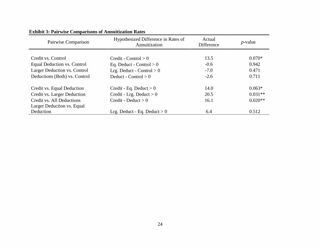
The results from the pairwise comparisons are displayed in Exhibit 3. Roughly 64 percent

of those assigned to the Credit treatment group annuitized their assets compared with a combined

47 percent of those assigned to the two deduction conditions and 51 percent in the control group.

Annuitization rates for the Credit group were also higher than those in either of the two types of

deduction groups as 50 percent of the Equal Deduction and 43 percent of the Larger Deduction

selected an annuity. In other words, being offered a credit increased the likelihood that an

17

individual purchased an annuity by 14 percentage points (p = .063) over an actuarially equivalent

deduction and 20 percentage points (p = .031) over a deduction with a larger expected value.

There was no statistically significant difference between the rate of annuitization between those

assigned to the two deduction conditions (p = .512). Interestingly, the rate of annuitization was

higher in the control group than it was in either of the deduction groups, but these differences

were not statistically significant. The rate of annuitization in the credit group was 13.5

percentage points higher than of the control group and was statistically significant.

[Exhibit 3 about here]

Because individuals were randomly assigned to their respective conditions, we can

attribute the differences in the rates of annuitization to the type of incentive each group received.

However, randomization provides only the expectation of equivalence across the credit and

deduction groups, but it does not guarantee that there will be no measurable differences between

the groups, especially in smaller sample sizes like those used in this analysis. According to

summary statistics in Exhibit 1 there appear to be some important differences across the

treatment and control groups. To control for the effect these differences may have, these

measures were included as control variables in a regression analysis comparing the rates of

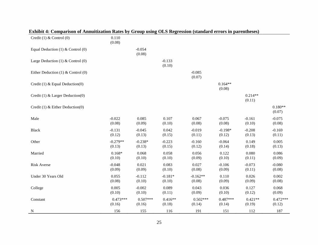
annuitization across the different groups. The results of this analysis are provided in Exhibit 4.

[Exhibit 4 about here]

The coefficients from the regression analysis indicate that the difference in the estimated

effect of the credit relative to the deduction remains even after controlling for the observable

differences between the two groups. The results from the first column compare the effect of

being assigned to the credit condition on the likelihood of annuitization relative to those assigned

to the actuarially equivalent deduction condition. The parameter of interest is on the variable

18

Credit & Equal Deduction, a dichotomous variable indicating treatment assignment. The

coefficient on this variable, 16.4, indicates that being assigned to the credit condition increases

the rate of annuitization by 16.4 percentage points over being assigned to the Equal Deduction

condition. This estimate is statistically significant at the .05 level. The second parameter of

interest is the variable Credit & Larger Deduction which indicates whether an individual was

assigned to the group offered the Credit condition or the group offered the deduction with an

actuarially larger value than the credit. Here again, the statistically significant effect is positive

and in the expected direction. Compared to the Larger Deduction group, the rate of annuitization

was 21.4 percentage points higher among those assigned to the Credit condition. Finally, when

the two groups offered deductions are combined, the rate of annuitization among those offered a

credit was 18 percentage points higher and the difference was significant at the .05 level.

The Credit group was the only group to have higher annuitization rates than the control

group, but when we add our control variables to the model, this difference is slightly attenuated

and is no longer statistically significant. It is possible that the difference in the annuitization rates

between these groups is no longer statistically significant because we have inflated our standard

errors through the inclusion of irrelevant variables to our regression model. Also, when we use a

more parsimonious model—remove all those variables that do not have a significant relationship

with annuitization—the difference between the Credit group and the control group remains

significant.

5. Discussion and Conclusion

Our findings demonstrate that individuals respond differently to economically equivalent

incentives. The immediate incentive structured to resemble a credit proved more effective at

encouraging a specific type of economic behavior than one designed as a deduction. This result

19

held true even when the expected value of the deduction was larger than the credit. The results

from this study comport with the stylized facts about the measureable effects of other tax-based

incentives such as the EITC on labor force participation and the lack of an empirical relationship

between tax incentives and homeownership and retirement savings. However, it is unclear why

the difference in the rate of annuitization was larger between the credit group and the larger

deduction group than it was between the credit group and the equal deduction group. One would

expect the annuitization rate to be higher among those offered the larger of the two deduction

incentives although the observed difference between the two deduction groups is not significant.

The variation in the observed differences across the credit and two deduction groups may be

attributable to random error in the data.

It also remains unclear why the deduction incentive appeared to have no effect on the

decision of game participants to annuitize a portion of their assets. The annuitization rates in this

group were no larger than those found in the control group.

The types of tax subsidies analyzed in this experiment are important vehicles by which

policymakers implement social welfare policies. In fact, spending on federal tax expenditures has

grown at a rate comparable to direct spending programs over the past few decades (Howard

1997). At a point in time when policymakers are looking to trim budget deficits, understanding

how these incentives can be structured to maximize their effectiveness and make the most

efficient use of public resources is paramount can lead to more efficient policy outcomes.

The overall growth of tax expenditures implies that the behavioral responses to the

various incentive structures are relevant to a wider range of activities. The tax code is replete

with rules granting favorable and unfavorable tax treatment to specific behaviors that the

Congress intends to foster or discourage. If the purpose of tax expenditure subsidies is to

20

increase the rate at which individuals engage in a specified behavior, then the evidence from this

analysis would suggest that the focus should shift away from deductions and exclusions and

towards refundable tax credits as the results suggest that the government could get a larger

behavioral response from a credit than it could with a higher valued, and more expensive,

deduction. But the other side of the coin is that credits also have more “upfront” budgetary costs

for politicians, which may reduce the appeal of immediate incentives like credits. In the end,

policy makers might consider non-financial incentives or behavioral ‘cues’ that structure

consumer choices toward annuitization. A possible example of a natural experiment in this

regard may be recently proposed Department of Labor regulations that would require defined

contribution retirement plan statements to provide a standard lifetime income equivalent of the

person’s account balance.8 While the immediate effect might encourage more savings, the

proposed rule might condition retiring workers to think of their accounts as generating an income

stream.

Future studies looking at the issue of incentives should determine whether these results

are robust under different conditions with respect to both annuitization and other types of

economic behavior. For example, would the effect of a credit-based incentive be moderated by

whether the credit is refundable or non-refundable? In their review a tax credit designed to

encourage retirement saving (the Saver’s Credit), Duflo et al. (2006) conclude that complex

design combined with non-refundability may explain the limited success of this incentive. Their

work establishes that simply providing a credit as opposed to a deduction or exclusion will not

ensure the success of the incentive, but that the structure of the credit matters. Future work might

also explore how deductions and credits are framed to individuals. For example, in the context

8 On May 8, 2013, the Department of Labor issued an Advance Notice of Proposed Rulemaking (ANPRM)

concerning lifetime income illustrations on pension benefit statements. The ANPRM follows a Request for

Information issued jointly by the DOL and Department of Treasury in 2010 (75 FR 5253, February 2, 2010).

21

of our financial decision making game credits could be framed as reductions in the cost of the

annuity or as an increase in the starting; deductions could be reductions in the cost of living or

increases in the after-tax income in each period.

22

Exhibit 1. Variable Means by Group

Full Sample Credit

Group

Deduction

Group

(Actuarially

Equivalent)

Deduction

Group

(More

Valuable)

Deduction

Group

Control

Group

Fraction Male 0.51 0.42 0.48 0.56 0.50 0.60

Fraction White 0.74 0.70 0.76 0.79 0.77 0.73

Fraction Married 0.72 0.80 0.70 0.67 0.69 0.69

Under 30 Years Old 0.36 0.28 0.25 0.46 0.31 0.50

College or More 0.75 0.79 0.70 0.74 0.72 0.75

Fraction with Risk Averse 0.69 0.78 0.63 0.78 0.68 0.64

N = 301 89 84 39 123 89

23

Exhibit 2: Rates of Annuitization by Group

0

10

20

30

40

50

60

70

Control Credit Deduction(Combined)

DeductionEqual

DeductionHigher

Pe

rce

nt

Rates of Annuitization by Group

24

Exhibit 3: Pairwise Comparisons of Annuitization Rates

Pairwise Comparison Hypothesized Difference in Rates of

Annuitization

Actual

Difference p-value

Credit vs. Control Credit - Control > 0 13.5 0.070*

Equal Deduction vs. Control Eq. Deduct - Control > 0 -0.6 0.942

Larger Deduction vs. Control Lrg. Deduct - Control > 0 -7.0 0.471

Deductions (Both) vs. Control Deduct - Control > 0 -2.6 0.711

Credit vs. Equal Deduction Credit - Eq. Deduct > 0 14.0 0.063*

Credit vs. Larger Deduction Credit - Lrg. Deduct > 0 20.5 0.031**

Credit vs. All Deductions Credit - Deduct > 0 16.1 0.020**

Larger Deduction vs. Equal

Deduction Lrg. Deduct - Eq. Deduct > 0 6.4 0.512

25

Exhibit 4: Comparison of Annuitization Rates by Group using OLS Regression (standard errors in parentheses)

Credit (1) & Control (0) 0.110

(0.08)

Equal Deduction (1) & Control (0) -0.054

(0.08)

Large Deduction (1) & Control (0) -0.133

(0.10)

Either Deduction (1) & Control (0) -0.085

(0.07)

Credit (1) & Equal Deduction(0) 0.164**

(0.08)

Credit (1) & Larger Deduction(0) 0.214**

(0.11)

Credit (1) & Either Deduction(0) 0.180**

(0.07)

Male -0.022 0.085 0.107 0.067 -0.075 -0.161 -0.075

(0.08) (0.09) (0.10) (0.08) (0.08) (0.10) (0.08)

Black -0.131 -0.045 0.042 -0.019 -0.198* -0.208 -0.169

(0.12) (0.13) (0.15) (0.11) (0.12) (0.13) (0.11)

Other -0.279** -0.238* -0.223 -0.160 -0.064 0.149 0.005

(0.13) (0.13) (0.15) (0.12) (0.14) (0.18) (0.13)

Married 0.168* 0.068 0.058 0.056 0.122 0.080 0.086

(0.10) (0.10) (0.10) (0.09) (0.10) (0.11) (0.09)

Risk Averse -0.048 0.021 0.083 0.027 -0.106 -0.073 -0.080

(0.09) (0.09) (0.10) (0.08) (0.09) (0.11) (0.08)

Under 30 Years Old 0.055 -0.112 -0.181* -0.162** 0.110 0.026 0.002

(0.08) (0.10) (0.10) (0.08) (0.09) (0.09) (0.08)

College 0.005 -0.002 0.089 0.043 0.036 0.127 0.068

(0.10) (0.10) (0.11) (0.09) (0.10) (0.12) (0.09)

Constant 0.473*** 0.507*** 0.416** 0.502*** 0.487*** 0.421** 0.472***

(0.16) (0.16) (0.18) (0.14) (0.14) (0.19) (0.12)

N 156 155 116 191 151 112 187

26

* p<.10, ** p<.05, *** p<.01

27

References

Agnew, J., Anderson, L., Gerlach, J., & Szykman, L. (2008). Who chooses annuities? An

experimental investigation of the role of gender, framing, and defaults. American Economic

Review, 98(2): 418-422.

American Council of Life Insurers. (2011). ACLI Life Insurers Fact Book 2011 (Washington,

D.C.: ACLI, November 18, 2011). Available at

http://www.acli.com/Tools/Industry%20Facts/Life%20Insurers%20Fact%20Book/Pages/GR

11-198.aspx.

Benartzi, S., & Thaler, R. (2007). Heuristics and biases in retirement savings behavior. Journal

of Economic Perspectives, 21(3): 81-104.

Benjamin, D. (2003). Does 401(k) Eligibility increase saving? Evidence from propensity score

subclassification. Journal of Public Economics, 87(5-6): 1259-90.

Ben-Shalom, Y., Moffitt, R., & Scholz, J. (2011). An assessment of the effectiveness of anti-

poverty programs in the United States. National Bureau of Economic Research Working

Papers no. 17042, available at http://www.nber.org/papers/w17042.

Bertrand, M., Mullainathan, S., & Shafir, E. (2006). Behavioral economics and marketing in aid

of decision making among the poor. Journal of Public Policy & Marketing 25(1): 8-23.

Butrica, B., & Mermin, G. (2006). Annuitized wealth and consumption at older ages. Center for

Retirement Research, Working Paper no. 2006-26, available at

http://crr.bc.edu/images/stories/Working_Papers/wp_2006-26.pdf.

Chetty, R., & Saez, E. (2009). Teaching the tax code: Earnings responses to an experiment with

EITC recipients. National Bureau of Economic Research Working Paper no. 14836, available

at http://www.nber.org/papers/w14836.

Connelly, G. (2011). Math tips for the rest of us. USA Today, (September 2, 2011), available at

http://www.usaweekend.com/article/20110902/MONEY/309020007/Math-tips-rest-us.

Davidoff, T., Brown, J., & Diamond, P. (2005). Annuities and individual welfare. American

Economic Review, 95(5): 1573-90.

Davis, D. & Millner, E. (2005). Rebates, matches, and consumer behavior. Southern Economic

Journal 72(2): 410-21.

Duflo, E., Orszag, P., Gale, W., Saez, E., & Liebman, J. (2006). Saving incentives for low- and

middle-income families: Evidence from a field experiment with H&R Block. Quarterly

Journal of Economics, 121(4): 1311-46.

Duflo, E., Orszag, P., Gale, W., Saez, E., & Liebman, J. (2007). Savings incentives for low- and

moderate-income families in the United States: Why is the Saver's Credit not more effective?

Journal of the European Economic Association, 5(2-3): 647-61.

Dushi, I. & Webb, A. (2004). Household annuitization decisions: Simulations and empirical

analyses. Journal of Pension Economics and Finance, 3(2): 109-43.

Eissa, N. & Liebman, J. (1996). Labor supply response to the Earned Income Tax Credit.

Quarterly Journal of Economics, 111(2): 605-37.

28

Engen, E., Gale, W., & Scholz, J. (1996). The illusory effects of saving incentives on saving.

Journal of Economic Perspectives, 10(4): 113-38.

Fujii, E., & Hawley, C. (1998). On the accuracy of tax perceptions. Review of Economics and

Statistics, 70(2): 344-7.

Gale, W. & Scholz, J. (1994). IRAs and household saving. American Economic Review, 84(5):

1233-60.

Gale, W. (2011). Tax reform options: Promoting retirement security. Testimony to the United

States Senate Committee on Finance, (September 15, 2011), available at

http://www.brookings.edu/research/testimony/2011/09/15-retirement-savings-gale.

Gazzale, R. & Walker, L. (2009). Behavioral biases in annuity choice: An experiment. SSRN

Working Paper (March 25, 2009), available at

http://papers.ssrn.com/sol3/papers.cfm?abstract_id=1370535.

General Accounting Office. (2011). Retirement income: Ensuring income throughout retirement

requires difficult choices. GAO-11-400 (Washington, D.C.: U.S. General Accounting

Office).

Gitterman, D. (2010). Boosting Paychecks : The Politics of Supporting America's Working Poor

(Washington, D.C.: Brookings Institution Press).

Glaeser, E., & Shapiro, J. (2003). The benefits of the home mortgage interest deduction. In J.M.

Poterba (ed.), Tax Policy and the Economy. Volume 17 (Cambridge, MA: MIT Press), pp. 37-

82.

Goldman Sachs. (2010). Q&A on housing policies in 2010. US Economics Analyst,

10(2)(January 15, 2010), available at http://www.scribd.com/doc/25316702/Goldman-Sachs-

Research-QA-on-Housing-Policies-in-2010.

Hewitt Associates. (2009). Trends and experience in 401(k) plans. Available at

http://www.retirementmadesimpler.org/Library/Hewitt_Research_Trends_in_401k_Highlight

s.pdf.

Hotz, J., & Scholz, J. (2006). Examining the effect of the Earned Income Tax Credit on the labor

market participation of families on welfare. National Bureau of Economic Research Working

Paper no. 11968, available at http://www.nber.org/papers/w11968.

Howard, C. (1997). The Hidden Welfare State : Tax Expenditures and Social Policy in the

United States (Princeton, N.J.: Princeton University Press).

Howard, C. (2007). The Welfare State Nobody Knows: Debunking Myths about U.S. Social

Policy (Princeton, N.J.: Princeton University Press).

Investment Company Institute. (2011). 2011 Investment Company Fact Book (Washington, D.C.:

Investment Company Institute), available at http://www.ici.org/pdf/2011_factbook.pdf.

Joint Committee on Taxation. 2010. Estimates of Federal Expenditures for Fiscal Years 2010-

2014, JCS-3-10 (Washington, D.C.: Joint Committee on Taxation), available at

https://www.jct.gov/publications.html?func=startdown&id=3718.

Johnson, R., Burman, L., & Kobes, D. (2004). Annuitized wealth at older ages: Evidence from

the Health and Retirement Study. Final Report to the Employee Benefits Security

29

Administration, U.S. Department of Labor (May 2004), available at

http://www.urban.org/uploadedPDF/411000_annuitized_wealth.pdf.

Kahneman, D., and Tversky, A. (1979). Prospect theory: An analysis of decision under risk.

Econometrica, 47(2): 263-91.

Laibson, D. (1997). Golden eggs and hyperbolic discounting. Quarterly Journal of Economics,

112(2): 443-77.

Loewenstein, G., & Prelec, D. (1991). Negative time preference. The American Economic

Review, 81(2): 347-352.

Maag, E. (2005). Disparities in knowledge of the EITC. Tax Notes, (Tax Policy Center, March

15, 2005), available at http://www.urban.org/UploadedPDF/1000752_Tax_Facts_3-14-

05.pdf.

Meyer, B., & Rosenbaum, D. (2001). Welfare, the Earned Income Tax Credit, and the labor

supply of single mothers. Quarterly Journal of Economics, 116(3): 1063-114.

Mitchell, O., Poterba, J., Warshawsky, M., & Brown, J. (1999). New evidence on the money's

worth of individual annuities. The American Economic Review, 89(5): 1299-318.

Mitchell, O. (2001). Developments in decumulation: The role of annuity products in financing

retirement. National Bureau of Economic Research Working Papers no. 8567,

http://www.nber.org/papers/w8567.

Mottola, G., & Utkis, S. (2007). Lump Sum or Annuity? An analysis of choice in DB pension

payouts. Vanguard Center for Retirement Research. available at

http://www.retirementplanblog.com/CRRLSA.pdf.

Phillips, K. (2001). The Earned Income Tax Credit: Knowledge is money. Political Science

Quarterly, 116(3): 413-424.

Poterba, J. M., S. F. Venti, and D. A. Wise, “Were They Prepared for Retirement? Financial

Status at Advanced Ages in the HRS and AHEAD Cohorts,” NBER Working Paper No.

17824, National Bureau of Economic Research (February 2012),

http://www.nber.org/papers/w17824.

Prante, G. (2007). Most Americans don't itemize on their tax returns. Fiscal Fact, no. 95, The

Tax Foundation (July 23, 2007), available at http://taxfoundation.org/article/most-americans-

dont-itemize-their-tax-returns.

Romich, J. & Weisner, T. (2000). How families view and use the EITC: Advance payment

versus lump sum delivery. National Tax Journal, 53(4): 1245-65.

Saez, E. (2009). Details matter: The impact of presentation and information on the take-up of

financial incentives for retirement saving. American Economic Journal, 1(1): 204-228.

Saez, E. (2010). Do taxpayers bunch at kink points? American Economic Journal: Economic

Policy, 2(3): 180-212.

Sherman, A. (2009). Safety net effective at fighting poverty but has weakened for the very

poorest. Center on Budget and Policy Priorities (July 6, 2009), available at

http://www.cbpp.org/files/7-6-09pov.pdf.

30

Smeeding, T., Philips K., & O’Connor M. (2000). The EITC: Expectation, knowledge, use, and

social and economic mobility. National Tax Journal, 53 (December): 1187-1210.

Tax Policy Center. (2011). Percent of tax filers by marginal tax rate, selected years, 1985-2009.

Tax Policy Center, Washington, D.C., available at

http://www.taxpolicycenter.org/taxfacts/displayafact.cfm?Docid=262.

U.S. Department of Labor. (2007). National Compensation Survey: Employee Benefits in Private

Industry in the United States, 2005 (Washington D.C.: U.S. Department of Labor, Bureau of

Labor Statistics). Available at http://www.bls.gov/ncs/ebs/sp/ebbl0022.pdf.

U.S. Department of Labor. (2012). Private Pension Plan Bulletin Historical Tables and Graphs.

Washington D.C.: U.S. Department of Labor, Employee Benefits Security Administration).

Available at http://www.dol.gov/ebsa/pdf/historicaltables.pdf.

Warner, J., & Pleeter, S. (2001). The personal discount rate: Evidence from military downsizing

programs. American Economic Review, 91(1): 33-53.

Yaari, M. (1965). Uncertain lifetime, life insurance, and the theory of the consumer. The Review

of Economic Studies, 32(2): 137-50.

31

Appendix

Data Source

The data was obtained from the selections made by participants in a computer-based

experiment. Participants consisted of 301 individuals from a jury pool in a large metropolitan

court system in North Carolina. The jury pool consists of randomly selected county residents

who were either licensed drivers, registered voters, or both. County residents excluded from jury

duty included those individuals who were less than 18 years old, who served as a juror in the

previous two years, who did not speak English, who were felons who did not have their

citizenship restored, and those who were not physically or medically competent. Individuals

called for jury duty in the months between August 2011 and April 2012 were solicited to

participate in this game as they waited in the jury lounge. Game monitors would make an

announcement advertising the game over the jury room audio system to the entire jury pool, and

a sign-up sheet would be provided. Participants who signed up were called in order and played

the game on laptop computers set up in the jury lounge. Not infrequently, participants would be

called for jury duty or dismissed while in the middle of the game. In such cases, no information

was collected unless the participant was able to complete the entire game before leaving.

Instructions for Computer-based Annuity Game

The following is the text taken from the computer program that collected the data for this paper.

We used the Z-Tree program to develop the game. In brackets, we indicate what the program

would do or what the participant would be asked to do or input. In general, participants were

recruited from a jury pool lounge at a large, metropolitan court system. Volunteers would sign

32

up following an announcement then proceed to a laptop computer in turn. Monitors would

ensure that hardcopy consent forms were signed and then start the program, making sure that

participants knew how to advance through the program.

"Introduction"

Welcome to the Game of Managing Your Money!

In this game you will need to need to manage a pot of money over time.

The higher your account balance when you exit from the game, the higher your compensation

will be for playing."

[Next Screen]

"Study Overview"

Basic Information

IRB Study [omitted]

Title of Study: [omitted]

Principal Investigator: [omitted]

[University information omitted]

Email Address: [omitted]

Funding Source and/or Sponsor: [omitted]

Study Contact telephone number: [omitted]

Study Contact email: [omitted]

33

[Next Screen]

"Consent"

To proceed to the game, you will need to indicate that you consent to participating.

You can do this by signing one of the hardcopy forms.

[Next Screen]

"Overview"

There are 3 parts to this study:

First, there are some introductory screens that provide information about the game and how to

play it. The second phase is when you play the game: You will make some one-time decisions,

and then the game will play out automatically. When the game ends, the third phase will be a

series of questions about yourself. You can expect to spend about 5-10 minutes total

participating in this study.

[Next Screen]

"Rules of the Game"

How to Play the Game

1. You start the game with a "savings" account of $20,000. Your goal is to live off this account

and not run out of money before the game ends.

2. In each period, you will need $3,000 to live on.

3. Before the game begins you will have the opportunity to invest your money in three separate

investments. The details of these investment options will be explained in next section.

34

4. The game is played over different periods, and it may end at any time. The likelihood of

surviving declines with each additional period of time and is determined by "throwing" dice.

The computer will do this for you automatically by generating a random number between 1

and 6, for each face of a normal die. The results of your "throw" will appear on the screen

and will determine whether you survive to the next period.

5. If you run out of money, your game will immediately end, and you will receive the lowest

compensation for playing the game.

6. The larger your account balance when you exit, the larger your compensation. Therefore,

your goal should be to maintain as much of your original account balance as possible

throughout the game

7. Payment: You will earn the following amounts for managing your money:

$10 if your ending account exceeds your starting balance (less any annuity you buy - see

next section)

$5 if your ending account is more than 0 but less than your starting balance

$2 if you run out of money"

[Next Screen]

"Investment Options"

Investment Options:

You can put your money in 3 places

Stock market: You can put some or all of your savings account in a stock market account

that can earn or lose money in each period. Gains and losses are determined by chance. This

35

option does not cost you anything but you will not be able to add or remove funds from this

account once they have been placed in the market.

Annuity. The purchase of the annuity will provide you with a $2,000 payment for each

period that you survive beginning in first period. This amount will partially offset the $3,000

living expenses that will be deducted from your account in each period. The cost associated

with the annuity will be described in the next section.

Do nothing! Let you money sit in your account, but it will not earn interest or lose money.

[Next Screen – Which option the participant gets depends on which group – treatments or

controls – the program has assigned to him or her. There are four possible branches: credit,

equal deduction, larger deduction, or control.]

"Annuity Credit"

Your starting savings account balance is $20,000.

If you want to buy the annuity, it will cost you $13,110.

As a part of a new program, however, you will receive a credit of $3,277 that will be

immediately added to your savings account should you decide to purchase the annuity.

As a result of this program, your initial account balance would increase from $6,890 to $11,665.

($20,000 - $13,110 + $3,277 = $10,167). If you buy the annuity, your available balance will be

equal to $10,167.

Would you like to purchase the annuity? [participants clicks "YES" or “No"]

You can also put some or all of your money into the stock market. If you have decided to buy an

annuity the maximum amount that you may invest is $10,167.

36

If you did not buy the annuity, the maximum you may put into the stock market is $20,000.

If you would like to invest in the stock market, enter the amount you wish to invest in the space

provided. [participants enters dollar amount]

"Annuity Equal Deduction"

Your starting savings account balance is $20,000.

The cost of the annuity is $13,110.

As a part of a new program, however, you will be able to reduce your cost of living by $500 in

each period should you decide to purchase the annuity.

As a result of this program, your per-period cost of living would be reduced from $3,000 to

$2,500 after purchasing this annuity. ($3,000 - $500 = $2,500)

If you buy the annuity, your available balance will be $6,890.

Would you like to purchase the annuity? [participants clicks "YES" or “No"]

You can also put some or all of your money into the stock market. If you have decided to buy an

annuity the maximum amount that you may invest is $6,890.

If you did not buy the annuity, the maximum you may put into the stock market is $20,000.

If you would like to invest in the stock market, enter the amount you wish to invest in the space

provided. [participants enters dollar amount]

"Annuity Larger Deduction"

Your starting savings account balance is $20,000.

The cost of the annuity is $13,110.

37

As a part of a new program, however, you will be able to reduce your cost of living by $874 in

each period should you decide to purchase the annuity.

As a result of this program, your per-period cost of living would be reduced from $3,000 to

$2,126 after purchasing this annuity. ($3,000 - $874 = $2,126)

If you buy the annuity, your available balance will be $6,890.

Would you like to purchase the annuity? [participants clicks "YES" or “No"]

You can also put some or all of your money into the stock market. If you have decided to buy an

annuity the maximum amount that you may invest is $6,890.

If you did not buy the annuity, the maximum you may put into the stock market is $20,000.

If you would like to invest in the stock market, enter the amount you wish to invest in the space

provided. [participants enters dollar amount]

"Annuity Control"

Your starting savings account balance is $20,000.

The cost of the annuity is $13,110.

If you buy the annuity, your available balance will be $6,890.

Would you like to purchase the annuity? [participants clicks "YES" or “No"]

You can also put some or all of your money into the stock market. If you have decided to buy an

annuity the maximum amount that you may invest is $6,890.

If you did not buy the annuity, the maximum you may put into the stock market is $20,000.

38

If you would like to invest in the stock market, enter the amount you wish to invest in the space

provided. [participants enters dollar amount]

[Next screen – Once the participant inputs his or her selections, the game runs without further

input from the participant. The game progresses through each stage if the participant ‘survives’

via the random number draw as described above. In each stage, changes to the participant’s

account are calculated using random ‘stock market returns’ that range from 0.5 to -0.5, if

applicable; the annuity income, if applicable; and the cost of living expense. After each stage,

the participant sees a breakdown of the starting balance, market returns if any, annuity income if

any, cost of living expense, and ending balance. Then the screen indicates whether the

participant ‘survives’ to the next stage.]

At the end of Period __:

Market Earnings ___

Amount invested in the stock market ___

Amount you received from an annuity ___

Your Cost of Living for the period was ___

Your Ending Balance is ___

Your balance at the beginning of the game was ___

To advance to the next round you, the sum of the "dice" must be greater than ___.

If you survive you will be advancing to the next round, otherwise thank you for playing.

39

[Eventually, the game ends because the participant did not survive, the participant ran out of

money in their account, or they completed the maximum number of 18 stages. When the game

ends, the survey begins.]

"Transition"

You have reached the end of the game.

You will now be prompted to answer a few questions about yourself.

[Next Screen]

Finally, we need to ask a couple of questions about you:

Are you male or female? [Participant indicates “Male”/”Female”]

Looking at the ranges of ages below, where does your age fall?

[Participant indicates the applicable age bracket, which are: "18-24”; "25-29"; "30-34"; "35-39";

"40-44"; "45-49"; "50-54"; "55-59"; "60-64"; "65-69"; "70-74"; "75+"]

[Next Screen]

Which of the following best describes your level of education?

[Participant indicates one of the following: “Some High School"; "High School Graduate";

“Some College"; "College Graduate"; "Graduate or Professional Degree"]

40

[Next Screen]

These questions ask about any retirement plans you currently may be a part of. One question

asks about types of plans. These types are: 401(k): You contribute an amount from your

paycheck on a pre-tax basis.

Other defined contribution: An amount is contributed to an account for you. Defined benefit:

You are promised a benefit that will begin when you retire, and the amount of the benefit is

based on different factors such as how long you work and how much you make in salary

Are you currently participating in a pension or retirement plan? [Participant indicates “Yes/No”]

If you are in a retirement or pension plan, what kind of plan is it?

[Participant indicates: "401(k)"; "Defined Benefit Pension"; "Other Type Not Listed"; "Profit

Sharing/Other Defined Contribution"; "Don't Know"; "Not Applicable"; "IRA"]

Do you have a second pension plan? If so, what kind?

[Participant indicates: "401(k)"; "Defined Benefit Pension"; "Other Type Not Listed"; "Profit

Sharing/Other Defined Contribution"; "Don't Know"; "Not Applicable"; "IRA"]

41

[Next Screen]

What is your marital status?

[Participant indicates: "Single"; “Married/Partnered/Coupled"; "Divorced"; "Widowed"]

How many persons are in your household currently? [Participant enters a number from 0 to 50]

[Next Screen]

"Risk"

Here is another kind of question. Suppose that you are the only income earner in the family.

Your doctor recommends that you move because of allergies, and you have to choose between

two possible jobs.

The first would guarantee your current total family income for life.

The second is possibly better paying, but the income is also less certain.

There is a 50-50 chance the second job would double your total lifetime income and a 50-50

chance that it would cut it by a third.

Which job would you take - the first job or the second job?

[Participant indicates: "First Job\"; "Second Job"; "Don't Know"]

[Next Screen]

Do you consider yourself to be Hispanic or Latino? ["Yes”/"No”]

Of the following categories, which race do you consider yourself to be?

[Participant indicates: "African-American"; "Asian"; "White"; "Other"]

42

[Next Screen]

What is your current work status?

[Participant indicates: "Employed Full Time\"; "Part-Time Employed"; "Retired";

"Unemployed"; "Not in the labor force"; "Disabled"; "Other"]

[Next Screen]

"End of questionnaire"

You have finished the question section and are at the end of the study. Thank you!