Credit Ratings, Economic Performance and Transition to

Default: Evidence on Firm Selection at Work∗

Giulio Bottazzi� Marco Grazzi Angelo Secchi Federico TamagniScuola Superiore Sant’Anna

July 28, 2007

Abstract

The study of firms’ default has attracted wide interest among both practitionersand scholars. However, attention has often been limited to a relatively small set offinancial variables. In this work, we try to increase the scope of analysis extendingour investigation to other possible determinants of default. In particular, we rely oncredit rating as a way to summarize firms’ financial conditions, and we address thepotential predictive power of a set of economic dimensions – size, growth, profitabilityand productivity – which industrial economics suggest to be meaningfull determinants ofsurvival. We present novel results based on a large Italian dataset reporting credit ratingsfor all the firms in the sample. As far as financial conditions and default are concerned, wefind that the firms dislaying the worst credit ratings are quite turbulent, but also exhibitnon-negligible chances to recover. Moreover, the analysis of the distribution of firms’economic performance reveals that profitability stands up as the only relevant economicvariable telling apart defaulting firms from ‘surviving’ ones, at different time distanceto default. Finally, probit and logit estimation of default probabilities, simultaneouslycontrolling for economic and financial dimensions, suggests that growth, in addition tocredit ratings, significantly affects the likelihood of default, albeit in a positive (and assuch unexpected) way among manufacturing firms.

JEL codes: C14, C25, D20, G30, L11

Keywords: Default probability, Credit ratings, Firm growth dynamics, selec-tion

∗The authors gratefully acknowledge the financial support for this research by Unicredit-Banca d’Impresaand the precious help received by the members of the Research Office “Pianificazione, Strategie e Studi” atUnicredit itself.�Corresponding author: LEM, Scuola Superiore Sant’Anna, Piazza Martiri della Liberta, 33, 56127, Pisa,Italy. Tel+39+050-883365. E-mail: bottazzi@sssup.it

1 Introduction

Credit rating agencies have been playing an increasingly important role within the debt market,publishing credit ranking especially for large bonds’ issuers. Ratings are employed both byprivate and institutional investors to get a concise picture of the financial soundness of thecovered firms, and as such they play a relevant role under many respects. In particular, theyaffect the cost and the extent of credit access of firms also contributing to shape their financialstructure (Sengupta, 1998). More recently banks are even more concerned with ratings, andcredit risk in general, due to the need to cope with the capital-risk requirements of BaselII Accord (Altman and Sabato, 2005). As a result, a large body of academic literature hasflourished within financial economics relating firms’ default probability to financial indicatorsand credit rating. Drawing from the classical works by Beaver (1966) and Altman (1968),particular attention has been devoted to bankruptcy prediction based on financial variablessuch as leverage, liquidity or financial ratios, and, more recently to the estimation of creditmigration matrices (see Crouhy et al. (2000), Jafry and Schuermann (2004), Schuermann(2007)).

In this paper, exploiting a confidential information on credit ratings and default eventsoccurring in a large panel of Italian firms, we present an analysis of firm default taking atwofold perspective.

On the one hand, we exploit the ‘ready to use’ information content of credit ratings asa synthetic measure of firms’ financial soundness. Whereas rating agencies usually producetheir rankings only for big and listed firms, we have access to a database reporting credit riskassignment irrespective of their size and of their being publicly-traded or not. As such, ourstudy offers an unprecedented - for breadth - account of the overall financial soundness of abroadly defined (Italian) ‘economic system’.

On the other hand, one should be aware that financial conditions alone are not able toadequately account for a comprehensive picture of firms’ performance. It is indeed unques-tioned that economic variables also contribute to shape the financial health of business firms,thereby affecting their chances of survival. In spite of this consideration, we don’t know of anyattempt to address the simultaneous effect of economic and financial performance on defaultprobability. A second fundamental contribution pursued in this article will be to attempt andbridge the aforementioned bankruptcy prediction studies, mainly focused on relating firms’default with financial indicators and credit ratings, with the large body of – both theoreticaland applied – research on the dynamics of firm growth originated in the domain of industrialeconomics.

From the theoretical side, although various and competing views are coexisting, most of themodern conceptualizations of firm dynamics share a common tenet whereby it is the action ofsome sort of selection mechanism, operating on the economic characteristics of heterogeneousfirms, which ultimately determines firms’ exit or, alternatively, growth and survival on the mar-ket. In Jovanovic (1982)’s model, selection operates on heterogeneous efficiency/productivitylevels and through a process of passive learning by doing which enables firms to uncover theirspecific level of efficiency, randomly assigned to them from the beginning and assumed con-stant along the discovery process. Over time, those firms who realize to be efficient enoughsurvive and grow, whereas the others exit. In Ericson and Pakes (1995), instead, the dynamicsare driven by the active efforts of the firms themselves, who are allowed to ‘choose’ their ownefficiency level through R&D investments. Then, selection operates on the resulting level ofrelative profitability which, in turn, is affected by the uncertainty inherently characterizingthe exploration of different technological opportunities. In both the models, however, the

2

decision to exit is conceived as an equilibrium solution for rational, profit maximizing firms.The models presented in Nelson and Winter (1982) and, to some extent, the whole stream ofevolutionary flavored research (see Winter, 1971; Nelson and Winter, 1982; Dosi and Nelson,1994; Metcalfe, 1998; Dosi, 2000; Bottazzi and Secchi, 2006) start from completely differentpremises. In this tradition, growth and exit events continuously occur in the course of a dy-namic disequilibrium process where firm choose a satisficing, rather than an optimal, efficiencylevel. The latter, in turn, depends on asymmetries in the distribution of the basic buildingblocks of firm idiosyncratic characteristics (knowledge, capabilities, routines) and, similarlyto Ericson and Pakes (1995), on the firms’ effort to perform innovative (or imitative) activ-ity. Then, competition forces create a powerful market selection mechanism whose complexinterplay with efficiency and uncertainty of R&D investment determines an associated level of(satisficing) profitability and, ultimately, the relative balance between exit and growth.

Whatever the specific model one might discuss, the implications in terms of the suggestedkey determinants of survival are rather similar. Size and growth, together with age, havebeen those variables receiving greatest attention in the empirical literature, and there is wideagreement that they positively relate with the probability of persisting in the market (see,among the many examples, the evidence reported in Evans, 1987; Hall, 1987; Dunne et al.,1988; Geroski, 1995; Agarwal, 1997; Sutton, 1997; and Caves, 1998). The same has beenrepeatedly found also with respect to technological characteristics, in terms of either innovativeinputs such as R&D (Hall, 1987; and Doms et al., 1995) or innovative output, such as patents(Cefis and Marsili, 2005). Remarkably, less work has been done to test for the existence of theselection mechanism itself, through a direct exploration of the relationship between survival,on the one hand, and efficiency or profitability, on the other.

For that matters in the context of our analysis, the message one can draw, at a rathergeneral level, is that the likelihood of default is expected to be lower for firms displaying rel-atively sounder economic performance. Within such a perspective, we explore whether thisis indeed the case, but from a slightly different viewpoint as compared to the aforementionedempirical studies. We indeed identify four basic relevant economic dimensions - namely size,growth, profitability and productivity - and relate them with a rather peculiar form of trueexit from the market, that is a formal declaration of default. Two interrelated research ques-tions concern the heterogeneities possibly existing both within and across defaulting vis a viscontinuing firms, as well as the intertemporal patterns experienced by the two groups alongthe various economic dimensions considered. To take a fresh look on these issues, we will adopta non parametric approach to estimate the empirical distribution of size, growth, profitabilityand productivity, and compare their characteristics during the transition to default for thetwo groups of firms.

In addition, we will work on the availability of credit ratings to provide novel evidence onthe way credit rationing types of mechanisms interact with the role which economic variablesare predicted to play on survival. This will allow us to improve on a serious weakness affectingthe empirical studies which are concerned with the identification of liquidity constraints ininvestment and growth dynamics. Indeed, starting from the seminal work of Fazzari et al.

(1988), there has been a pervasive reliance on cash flow as a proxy for financial constraints(for reviews, see Hubbard, 1998; Fagiolo and Luzzi, 2006; and Whited, 2006), in spite ofthe many reasons suggesting that such a variable may well be a wrong indicator for thatkind of mechanisms (Kaplan and Zingales, 1997 and 2000). In the end, it just representsa measure of the ability to generate ready to spend, merely internal, resources and, in thisrespect, it possesses only indirect informative content on the existence of non-neutralities inthe workings of financial markets. Credit ratings, instead, embody a forecast of firms’ ability

3

to pay back loans and, therefore, are much likely to represent a direct indicator of investors’(banks) propensity to bet on each firm. Noticeably, some peculiar characteristics of the creditratings included in our database makes this attempt particularly promising.

The work is organized as follows. In Section 2 we present a short description of thedataset. Section 3 focuses on default and credit rating transition probabilities. Then, Section 4investigates the interplay between economic variables and default. A formal (probit and logit)model estimating the impact of both economic and financial variables on default probabilityis presented in Section 5, while in Section 6 we sum up the results and suggest some possibleinterpretations.

2 Data sources and sample selection

The data we employ in the following come from the Centrale dei Bilanci (CeBi) database.Together with the information collected by the Italian national statistical office (ISTAT), thisdatabase represents the most detailed source of firm level information on Italy. This fact is dueto the peculiar nature and history of CeBi. Nowadays a private company involved in servicesfor financial analysis, it was instituted in 1983 by the Bank of Italy as a public agency withthe assigned task of providing financial analyses to support the Bank of Italy itself within itsactivity of supervision of the banking system. It is in this perspective that CeBi is engagedin data collection, harmonization and cleaning since its foundation, in close relationship withleading Italian commercial banks.

The database contains the time series of balance sheets data starting from the early 80’s,with the only limitation of focusing on limited liability firms, since they are the entities whichface a legal obligation to make their annual accounting publicly available at the Chambers ofCommerce. Initial reliability checks are performed by CeBi, and only balance sheets complyingwith the principles laid down by the IV EEC directive are considered to enter the dataset.As a result, included firms operates in all the sector of activity and, contrary to what it oftenhappens with other firm level panels (not only Italian ones) there are no thresholds imposedon firm size, in terms of number of employees. As such, the dataset is rich and detailed, andseems particularly suitable for the analysis of both large and small-medium sized firms.

Thanks to a collaboration between the Research Office “Strategie e Studi” of UnicreditBank Group and the Laboratory of Economics and Management at Scuola Superiore Sant’Anna,we had access to a sub-sample of the CeBi database which covers about 50.000 firms operatingin all economic sectors from 1996 to 2003.

The way we have obtained the data is particularly important, since it contributed to shapesome limitations of the analysis, but also opened up unique opportunities to exploit novelpieces of information which were never explored before by other studies making use of thesame dataset.

On the one hand, the major limitation lies in the fact that we had access to a subsetof variables, rather than to the entire accounting book. Available items are: Total Sales(TS), Value Added (VA), Gross Operating Margins (GOM), Number of Employees (L), GrossTangible Assets (K), Return on Investment (ROI), Leverage (Total Debt over Shareholders’Equity), Interest Expenses (IE), and the Debt over Revenues ratio. We sometimes had to facesome problems in terms of freedom to choose the theoretically best proxy for the economicdimensions one is willing to study. Still, the list is sufficiently rich and enabled us to check the

4

Number of firms

Class Rating Definition 1998 2000 2002

Low

1 high reliability 1114 1396 1531

2 reliability 1293 1602 16643 ample solvency 1483 1698 1671

Mid

4 solvency 4170 4549 43105 vulnerability 2360 2621 24056 high vulnerability 1969 2016 20837 risk 2249 2691 2311

Hig

h 8 high risk 350 433 4579 extremely high risk 93 121 130

Total 15081 17127 16562

Table 1: Number of firms, total and by rating classes in 1998, 2000 and 2002 - Manufacturing.

results across some alternative way of capturing most of the economic dimensions consideredin this work, such as size, efficiency, profitability, financial structure, and so on and so forth.

On the other hand, the collaboration with Unicredit Group is responsible for the two mostlyremarkable features of our data, those which ultimately allow us to bridge the dynamics offirms’ economic structure and performance with considerations about the financial side oftheir operations. First, we have been provided with a dummy variable telling whether a groupof firms, which were Unicredit customer during the period under analysis, incurred formaldefault at the end of the sample time window, in 2003. These firms (henceforth defaulting

firms) were 155 in Manufacturing and 104 in Service, respectively.Most importantly, Unicredit specific rights to access the database gave us the chance to

exploit the credit rating produced by CeBi.1 This is an index having the same function of thecredit ratings issued by internationally well known agencies such as Moody’s or Standard andPoor’s, but a clarification is needed about the kind of information which it is able to convey.With this regard, we must recognize that, unfortunately, the actual methodology employedin computing the index has not been disclosed to us, as it is proprietary of CeBi. Though, alarge body of literature on credit rating construction suggests that the CeBi index should offera summary of the financial side of firms operations, including variables such as liquidity, debtstructure and the associated maturity, leverage, and so on and so forth. In close similaritywith the aim of the credit ratings issued by international agencies, one can argue that CeBiratings should be concerned with yielding a picture of the current financial conditions as wellas a concise forecast of future sustainability. From a technical viewpoint the CeBi rating isissued once per year and is allowed to change over time. Accordingly, the firms present in thedatabase are ranked with a score ranging from 1 to 9, in increasing order of financial fragility:1 is attributed to highly solvable firms, while 9 identifies firms displaying a serious risk ofdefault. Table 1 reports the definitions given by CeBi itself to the the 9 classes.

There are however some specific characteristics, which we do know and make the CeBi

1This information, as well as the rest of the dataset, was provided to us thanks to a collaboration withthe Research Office “Pianificazione, Strategie e Studi” of Unicredit Group, a large Italian bank. They arestrictly confidential and have been provided under the mandatory condition of censorship of any individualinformation.

5

index particularly interesting. A first point concerns the fact that, remarkably, it is assignedto each firm, rather than to single debt issues. This justifies an interpretation as a proxyfor firms’ overall ability to pay back debt positions on due time, or, alternatively, to default.In addition to that, there is also a second characteristics which makes CeBi’s credit ratingrather peculiar. Indeed, due to the role played by CeBi as an institutional actor, the indexhas been for long a confidential information only available to the Bank of Italy and to theItalian banking system. This is the reason why one can claim that (Italian) banks have along experience in using CeBi credit ratings as a synthetic indicator when deciding to opencredit lines up. Therefore, the index does not only represent a valuable assessment of firms’financial conditions, but it also, and more interestingly, constitutes a very reliable proxy of(Italian) banks’ future propensity to invest in each firm, to be exploited as a measure of accessto external financing. Finally, a third difference with respect to the issued by Moody’s orStandard & Poor’s is that the latter usually apply to firms listed on the stock exchange. TheCeBi index, on the contrary, is assigned to all the business firms present in the database,which might be either listed or not, with no particular limitations in terms of their size, sectorof activity, and so on and so forth.

Let us now describe the cleaning procedures implemented in order to obtain an homoge-neous dataset. We pursued two strategies. On the one hand, we noted that the the first twoyears of the sample recorded a substantially lower number of non-missing observations, forreasons out of our control. We prefer working with similar sample sizes for the different yearsunder analysis and, accordingly, we limit the analysis to the period 1998−2003. On the otherhand, even if the raw data do not impose any threshold on the size of the firms considered, wetried to identify business units characterized by a minimum level of organizational structureand operation. We therefore discarded all those firms with only one employee, and all thosereporting less than one million of euro of Total Sales in each year.

The specific cut imposed on the number of employees is chosen on the basis of preliminaryinvestigations conducted on the properties of the original database. Indeed, explorative exer-cises soon revealed that firms with one employee and firms with more than one employee fallinto two categories representative of two different worlds, characterized by different propertieswhich, from a statistical point of view, it would be safer to analyse separately.2 Noticeably,we do not know of any other study highlighting a similar result on other datasets, despite thefact that our findings should come with not much surprise. Indeed, there is a simple economicexplanation for them: firms with only one employee capture all the phenomena connectedto self-employment, a quite peculiar universe of economic activities/organizations, which wewant to ignore here. The threshold imposed on annual revenues works along the same di-rection of working with ’true’ firms, but it also accomplishes the specific need of enhancingcomparability between the overall sample and the sub-sample of defaulting firms. Informalevidence emerged during discussions with Unicredit suggested that a threshold of one millionof euro on Total Sales was a reasonable proxy for average Unicredit customers’ size.

At the end of the day, we are left with around 15000 firms active in Manufacturing and10000 operating in the Services, depending on the year. Table 1 shows, by way of example,the precise number of Manufacturing firms in three different years of the sample period. Thenumber of observations in Services where substantially comparable.3 The small number of

2See Bottazzi et al. (2006a) and Bottazzi et al. (2006b) for some more detail and an example on this point.3In the CeBi database firms are classified in terms of the Ateco industrial classification, which is the

standard adopted by the Italian statistical office, and substantially corresponding to the European NACE 1.1taxonomy. Codes 15-36 define the Manufacturing industry, whereas codes 50-74 defines the Service sector.

6

0

10

20

30

40

50

60

70

1 2 3 4 5 6 7 8 9Rating Classes

Manufacturing 19982002

0

5

10

15

20

25

30

35

40

45

1 2 3 4 5 6 7 8 9Rating Classes

Service19982002

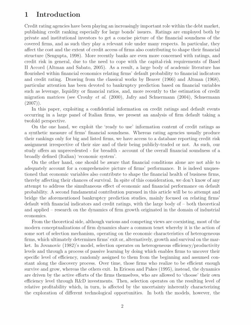
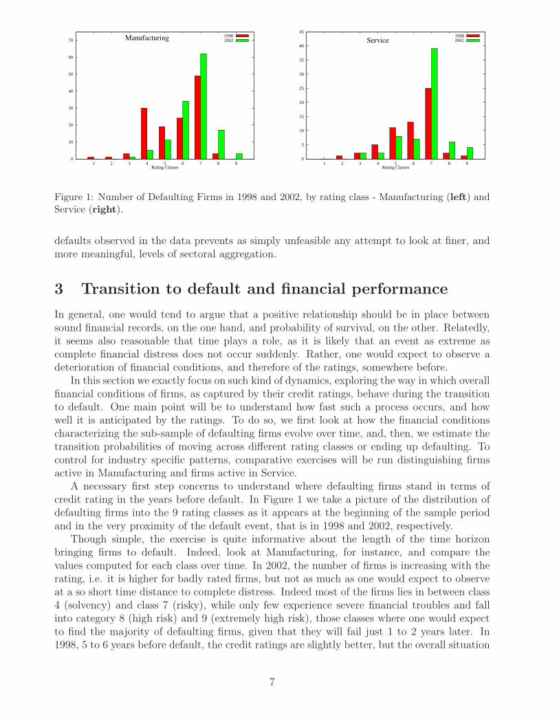
Figure 1: Number of Defaulting Firms in 1998 and 2002, by rating class - Manufacturing (left) andService (right).

defaults observed in the data prevents as simply unfeasible any attempt to look at finer, andmore meaningful, levels of sectoral aggregation.

3 Transition to default and financial performance

In general, one would tend to argue that a positive relationship should be in place betweensound financial records, on the one hand, and probability of survival, on the other. Relatedly,it seems also reasonable that time plays a role, as it is likely that an event as extreme ascomplete financial distress does not occur suddenly. Rather, one would expect to observe adeterioration of financial conditions, and therefore of the ratings, somewhere before.

In this section we exactly focus on such kind of dynamics, exploring the way in which overallfinancial conditions of firms, as captured by their credit ratings, behave during the transitionto default. One main point will be to understand how fast such a process occurs, and howwell it is anticipated by the ratings. To do so, we first look at how the financial conditionscharacterizing the sub-sample of defaulting firms evolve over time, and, then, we estimate thetransition probabilities of moving across different rating classes or ending up defaulting. Tocontrol for industry specific patterns, comparative exercises will be run distinguishing firmsactive in Manufacturing and firms active in Service.

A necessary first step concerns to understand where defaulting firms stand in terms ofcredit rating in the years before default. In Figure 1 we take a picture of the distribution ofdefaulting firms into the 9 rating classes as it appears at the beginning of the sample periodand in the very proximity of the default event, that is in 1998 and 2002, respectively.

Though simple, the exercise is quite informative about the length of the time horizonbringing firms to default. Indeed, look at Manufacturing, for instance, and compare thevalues computed for each class over time. In 2002, the number of firms is increasing with therating, i.e. it is higher for badly rated firms, but not as much as one would expect to observeat a so short time distance to complete distress. Indeed most of the firms lies in between class4 (solvency) and class 7 (risky), while only few experience severe financial troubles and fallinto category 8 (high risk) and 9 (extremely high risk), those classes where one would expectto find the majority of defaulting firms, given that they will fail just 1 to 2 years later. In1998, 5 to 6 years before default, the credit ratings are slightly better, but the overall situation

7

0

1

2

3

4

5

1 2 3 4 5 6 7 8 9Rating Classes

Manufacturing19982002

0

1

2

3

4

5

6

1 2 3 4 5 6 7 8 9Rating Classes

Service19982002

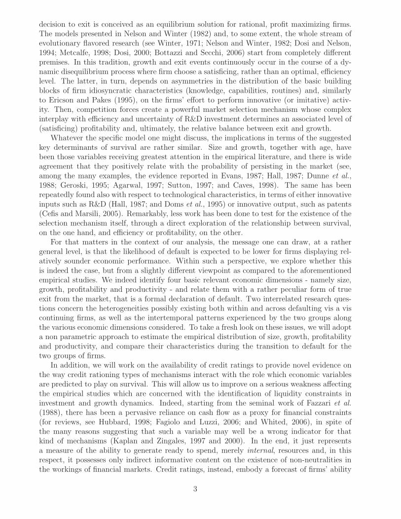
Figure 2: Percentage of Defaulting Firms in 1998 and 2002, by rating class - Manufacturing (left)and Service (right).

does not differ much: classes from 1 to 5 are more crowded than in 2002, but most of thefirms still fall in between classes 4 and class 7, and none of them is receiving a 9. Lookingat Services yields quite the same conclusion: the ratings do deteriorate as the default eventapproaches, but jumps from solvency to default are not much less frequent than jumps fromvery bad financial conditions to complete distress.

A second interesting issue regards a comparison between defaulting firms and the rest ofthe sample. In Figure 2 we look again at the number of defaulting firms broken down byrating classes in 1998 and 2002, but we now consider them in percentage of the overall numberof firms (defaulting plus non-defaulting) active in each class in the same years. The pictureemerging here is much more similar to the story one would guess a priori, that is to observe(i) an increase in the percentage of defaulting firms when moving from class 1 to class 9, ineach year; and (ii) an intertemporal shift of probability mass toward the worst rating classes,as the time of default approaches. Consistently with such conjectures, we find that, in bothsectors, the percentage of defaulting firms is much higher in classes from 6 (or 7) to 9 than inthe other categories, and a clear increasing trend does appear over time.

To improve the statistical reliance of the exercises performed so far, we estimate the tran-sition probabilities of observing firms moving across the different rating classes, and from eachof them into default. For ease of presentation of the results, we assign the firms included inthe sample to three classes only, which we name Low Risk (with credit rating 1-3), Mid Risk(rated 4-7) and High Risk (rated 8-9). Notice that the term ’Risk’ is just a shortcut for ’risk ofdefault’ and should not mislead the reader towards interpretations in terms of other definitionsof risk which are more conventional to mean-variance frameworks of financial economics, suchas, for instance, variability of prices, growth rates or stock returns. Rather, the choice of theparticular grouping employed in this work was intended to gather firms with similar financialprofiles according to their original rating. In particular, we took explicitly into account thelower discriminatory power of the class 7, emerged during our discussions at Unicredit, andwe decided to cautiously include it into our Mid Risk class. Yet, we performed a number ofrobustness checks, but the results were never significantly affected by including class 7 intothe High Risk category.

Table 2 shows the long-medium run (5 to 6 years) transition matrix for Manufacturing. Onthe main diagonal one can read the estimated probability that a firm belonging to a specificrating class in 1998 ends up into the same class at the end of the sample period, whereas off-

8

2003

Low Mid High Default

1998 Low 0.6969 0.2974 0.0048 0.0009

Mid 0.1327 0.8247 0.0330 0.0096High 0.0909 0.6970 0.1991 0.0130

Table 2: Long-medium run transition to default - Manufacturing.

2003

Low Mid High Default2002 Low 0.8219 0.1768 0.0013 0.0000

Mid 0.0567 0.9064 0.0291 0.0078High 0.0064 0.4957 0.4742 0.0236

Table 3: Short run transition to default - Manufacturing.

diagonal values capture the frequency of jumping from one class to another one, or to default.So, for instance, the first row tells that a firm classified as Low Risk at the beginning of theperiod has a probability of around 0.7 of remaining Low Risk five years later, an approximate0.3 probability of becoming a Mid Risk firm, and negligible probabilities of either moving intothe High Risk group or defaulting. Mid Risk firms, on the second row, display an even morestable pattern. The estimated probability of remaining in the same class is around 0.8, whilethey display an approximate 0.13 probability of improving their initial financial conditions andending up into the Low Risk class, but a probability of only 0.03 and 0.01 to either move intothe High Risk group or to default, respectively. However, the most interesting result emergefor those firms which were classified as High Risk in 1998. Indeed, we obtain that with aprobability of around 0.7 and 0.09 they become Mid Risk and Low Risk firms, respectively,whereas the probability of either remaining High Risk or incurring default is much lower,0.2 and 0.01 respectively. As a result, the estimated probability of recovering from a riskysituation of bad financial conditions is much higher than the estimated probability of eitherremaining in the same bad situation or defaulting.

Even more surprisingly it is the fact that we face a quite similar result also when we lookat the estimates of the short run (1 to 2 years) transition matrix, reported in Table 3. Here,given the quite short time span between the initial and the final instant of time considered, onewould expect to observe a high degree of stability, with very few jumps across rating classes.Moreover, it would be hard to imagine bad firms to recover in only one or two years: ourex-ante conjecture is that, if jumps happened to occur for the High Risk firms, they shouldlead to default. Though, the results only partially meet such an hypothesis. On the one hand,the probabilities on the main diagonal are all higher than they were for the long-medium runtransition: not surprisingly, the probability of changing rating class is lower than what observeabove. On the other hand, however, we still observe that, exactly as before, High Risk firmsdisplay a probability of switching to better financial conditions which is not much different(roughly 0.5) than that of either remaining in the same group or defaulting.

Note that such a turbulence does not prevent to identify a clearcut pattern about howfinancial conditions impact on default probabilities. On the contrary, the estimates reported

9

2003

Low Mid High Default

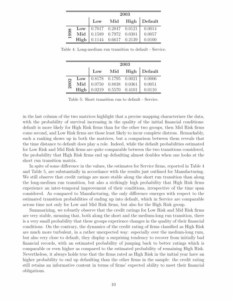
1998 Low 0.7017 0.2847 0.0121 0.0014

Mid 0.1589 0.7972 0.0381 0.0057High 0.1144 0.6617 0.2139 0.0100

Table 4: Long-medium run transition to default - Service.

2003

Low Mid High Default2002 Low 0.8178 0.1795 0.0021 0.0006

Mid 0.0750 0.8838 0.0361 0.0051High 0.0219 0.5570 0.4101 0.0110

Table 5: Short transition run to default - Service.

in the last column of the two matrices highlight that a precise mapping characterizes the data,with the probability of survival increasing in the quality of the initial financial conditions:default is more likely for High Risk firms than for the other two groups, then Mid Risk firmscome second, and Low Risk firms are those least likely to incur complete distress. Remarkably,such a ranking shows up in both the matrices, but a comparison between them reveals thatthe time distance to default does play a role. Indeed, while the default probabilities estimatedfor Low Risk and Mid Risk firms are quite comparable between the two transitions considered,the probability that High Risk firms end up defaulting almost doubles when one looks at theshort run transition matrix.

In spite of some difference in the values, the estimates for Service firms, reported in Table 4and Table 5, are substantially in accordance with the results just outlined for Manufacturing.We still observe that credit ratings are more stable along the short run transition than alongthe long-medium run transition, but also a strikingly high probability that High Risk firmsexperience an inter-temporal improvement of their conditions, irrespective of the time spanconsidered. As compared to Manufacturing, the only difference emerges with respect to theestimated transition probabilities of ending up into default, which in Service are comparableacross time not only for Low and Mid Risk firms, but also for the High Risk group.

Summarizing, we robustly observe that the credit ratings for Low Risk and Mid Risk firmsare very stable, meaning that, both along the short and the medium-long run transition, thereis a very small probability that these groups experience changes in the quality of their financialconditions. On the contrary, the dynamics of the credit rating of firms classified as High Riskare much more turbulent, in a rather unexpected way: especially over the medium-long rum,but also very close to default, they display a surprising tendency to recover from initially badfinancial records, with an estimated probability of jumping back to better ratings which iscomparable or even higher as compared to the estimated probability of remaining High Risk.Nevertheless, it always holds true that the firms rated as High Risk in the initial year have anhigher probability to end up defaulting than the other firms in the sample: the credit ratingstill retains an informative content in terms of firms’ expected ability to meet their financialobligations.

10

Mean V.C.

Variable Sample 1998 2002 1998 2002

Total SalesDefaulting 24681 34482 2.26 2.18

Aggregate 23882 27314 3.94 6.29

GrowthDefaulting 0.11 -0.17 4.02 -1.80

Aggregate 0.03 -0.01 6.87 -17.11

ProfitabilityDefaulting 0.07 0.02 1.64 5.67

Aggregate 0.10 0.09 0.95 1.16

ProductivityDefaulting 46.68 44.58 0.55 1.29

Aggregate 55.80 59.00 0.66 0.80

Table 6: Mean and Variation Coefficient (VC) of Total Sales, Growth, Profitability and LabourProductivity, in 1998 and 2002. Defaulting firms and entire sample, Manufacturing.

4 Transition to default and economic performance

Looking at the credit rating allowed to carry on a concise analysis of how the diverse financialconditions of firms are related with default. In this section we pursue a different, real ratherfinancial, perspective. We now ask how the event of default correlates with, and to someextent is determined by, some dimensions of firms’ economic operation and performance ascrucial as size-growth dynamics, profitability and productive efficiency.

In parallel with the perspective adopted above in exploring the linkages between financialconditions and default probabilities, we will be addressing two specific research questions.On the one hand, we follow the intertemporal patterns experienced along such economicdimensions by the defaulting firms, in the years before default. The issue will be tackledcomparing the statistical properties of the empirical distribution of size, growth, productivityand profitability measured at the beginning of the sample period (in1998) with those emerging1 to 2 years before the default event (in2002). On the other hand, a second point concernswhether, and to what extent, defaulting firms differ from the other firms present in the sample.For this purpose, we will estimate the empirical distribution of the same economic variablesfor all the firms present in the database in 1998 and 2002, and we will try to identify howdefaulting firms rank within the entire sample.

From a methodological point of view, a common characteristic with respect to both theresearch questions resides in the choice of adopting non parametric (kernel) techniques whichfocus on the entire distribution of the different economic dimensions, rather than more tradi-tional, parametric approaches which are mainly concerned with estimating average behavior.Such a decision avoids to impose any structure to the data, allowing to take a fresh look on theheterogeneities possibly existing both within and across defaulting vis a vis surviving firms.

A note is also due on measurement issues. Indeed, for all of the relevant economic variableswe will be discussing, several different proxies have been proposed in the literature. Thefindings presented in Bottazzi et al. (2006a) and Bottazzi et al. (2006b) on the very samedataset which is used in the present work, however, suggest that the use of alternative measuresis not very likely to significantly affect the results. Therefore, we consider here one single proxyfor each of the economic dimensions. Firm size is measured in terms of Total Sales (TS), and,accordingly, the simple log-difference of Total Sales, gTS, is used to measure firm growth.

11

0.001

0.01

0.1

1

7 8 9 10 11 12 13 14

log(Pr)

log(TS)

Aggregate - 1998Default - 1998

0.001

0.01

0.1

1

7 8 9 10 11 12 13 14

log(Pr)

log(TS)

Aggregate - 2002Default - 2002

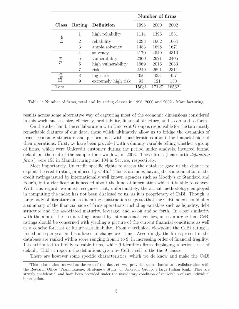
Figure 3: Empirical density of Total Sales (TS) in 1998 (left) and 2002 (right): Defaulting Firmsand entire sample - Manufacturing.

Then, we proxy profitability with the Returns on Sales (ROS), that is the ratio betweenoperating margins and revenues. Finally, efficiency in production is captured by a standardproxy of Labour Productivity, i.e. in terms of value added per employee. Descriptive statisticson these variables are shown in Table 6 for defaulting firms vis a vis the entire sample of firms.Note that here, as well as in the rest of the section, we show results only for Manufacturing,since the evidence from Service firms, which we did explore, was supportive of very similarconclusions.

Let us start with the analysis of firm size distributions. In the two panels of Figure 3 weplot, on a double logarithmic scale, the kernel density of TS estimated for defaulting firms andfor the overall sample in 1998 and in 2002. To help comparability between the two groups, inthe bottom part of each figure we also depict the actual values of TS for each defaulting firm.

First look at 1998. The most apparent feature is that the two distributions are very similarin both the supports spanned and in the shapes, which is remarkably right-skewed, a propertyrepeatedly found in the literature of firm size distribution. Together, these two characteristicstell us that, somewhat contrary to what one might conjecture on the basis of theory andempirical research on firm survival, defaulting firms are neither less heterogeneous nor smallerwith respect to the entire sample. Actually, we find that default events could even be morefrequent among medium-big sized firms, rather than at small sizes: consistently with thefigures in Table 6, the mean seems even higher for defaulting firms, and their density turnsout to be even more concentrated in the right part of the support, as compared to the others.This kind of story is robust across time: if anything, the right tail of the defaulting firms’distribution is even heavier in 2002, when it takes only 1 to 2 years to the default event, ascompared to 1998, 5 to 6 years before default. The actual values of TS attained by defaultingfirms clarify that the sort of second modes appearing in the right tails are essentially due to alimited number of very big firms. Still, the overlap in the central part of the densities, wheremost of the observations are placed, is almost perfect, so that, if not bigger, defaulting firmsare for sure not smaller than the others, at least on average. This is enough to conclude thatthere is a lack of a clearcut relationship between size and the event of default: operating abovea certain size threshold does not seem to be a relevant warranty in preventing default.

Next we focus on firms’ growth rates. Figure 4 shows the kernel density of gTS estimatedin deviation from the annual sectoral (Manufacturing) average, that is in terms of market

12

0.001

0.01

0.1

1

-2 -1.5 -1 -0.5 0 0.5 1 1.5 2

log(Pr)

gTS

Aggregate - 1998Default - 1998

0.001

0.01

0.1

1

-2 -1.5 -1 -0.5 0 0.5 1 1.5

log(Pr)

gTS

Aggregate - 2002Default - 2002

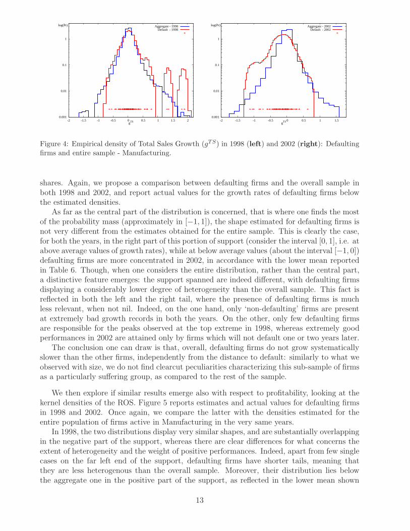
Figure 4: Empirical density of Total Sales Growth (gTS) in 1998 (left) and 2002 (right): Defaultingfirms and entire sample - Manufacturing.

shares. Again, we propose a comparison between defaulting firms and the overall sample inboth 1998 and 2002, and report actual values for the growth rates of defaulting firms belowthe estimated densities.

As far as the central part of the distribution is concerned, that is where one finds the mostof the probability mass (approximately in [−1, 1]), the shape estimated for defaulting firms isnot very different from the estimates obtained for the entire sample. This is clearly the case,for both the years, in the right part of this portion of support (consider the interval [0, 1], i.e. atabove average values of growth rates), while at below average values (about the interval [−1, 0])defaulting firms are more concentrated in 2002, in accordance with the lower mean reportedin Table 6. Though, when one considers the entire distribution, rather than the central part,a distinctive feature emerges: the support spanned are indeed different, with defaulting firmsdisplaying a considerably lower degree of heterogeneity than the overall sample. This fact isreflected in both the left and the right tail, where the presence of defaulting firms is muchless relevant, when not nil. Indeed, on the one hand, only ‘non-defaulting’ firms are presentat extremely bad growth records in both the years. On the other, only few defaulting firmsare responsible for the peaks observed at the top extreme in 1998, whereas extremely goodperformances in 2002 are attained only by firms which will not default one or two years later.

The conclusion one can draw is that, overall, defaulting firms do not grow systematicallyslower than the other firms, independently from the distance to default: similarly to what weobserved with size, we do not find clearcut peculiarities characterizing this sub-sample of firmsas a particularly suffering group, as compared to the rest of the sample.

We then explore if similar results emerge also with respect to profitability, looking at thekernel densities of the ROS. Figure 5 reports estimates and actual values for defaulting firmsin 1998 and 2002. Once again, we compare the latter with the densities estimated for theentire population of firms active in Manufacturing in the very same years.

In 1998, the two distributions display very similar shapes, and are substantially overlappingin the negative part of the support, whereas there are clear differences for what concerns theextent of heterogeneity and the weight of positive performances. Indeed, apart from few singlecases on the far left end of the support, defaulting firms have shorter tails, meaning thatthey are less heterogenous than the overall sample. Moreover, their distribution lies belowthe aggregate one in the positive part of the support, as reflected in the lower mean shown

13

0.01

0.1

1

10

-0.6 -0.4 -0.2 0 0.2 0.4 0.6

log(Pr)

ROS

Aggregate - 1998Default - 1998

0.01

0.1

1

10

-0.6 -0.4 -0.2 0 0.2 0.4 0.6

log(Pr)

ROS

Aggregate - 2002Default - 2002

Figure 5: Empirical density of Profitability (ROS) in 1998 (left) and 2002 (right): Defaulting Firmsand entire sample - Manufacturing.

in Table 6. The same differences are present, and somewhat reinforced, in the estimates for2002. The profitability density of defaulting firms turns out to be clearly shifted towards theleft of the density estimated for the overall sample: the latter is more symmetric, whereasmuch of the probability mass of defaulting firms is concentrated at negative values. As aresult, the distance between the two distributions in the right part of the support is even moreapparent than in 1998, and a significantly heavier left tail for defaulting firms also emerges.Despite negative performance is experienced also by non-defaulting firms, there is neverthelesssufficiently robust evidence to conclude that defaulting firms are, on average, less profitablethan the rest of the sample.

In this respect, the conjectures put forward by the theories of firm dynamics are confirmedby the analysis: some sort of selection on profitability seems to be at work. Interestingly, timeplays an important role in the story, as defaulting firms are not different from surviving firmsfive years before default, but, rather, their performances seem to worsen over time until theybecome quite weak in the very short run (1-2 years) before default.

As a final step, we ask whether selection operates also on productive efficiency. The densi-ties of Labour Productivity, estimated in (log) deviations from sectoral average, suggest thatthis might not be the case: efficiency does not act as a sharp discriminatory factor tellingapart defaulting firms from surviving ones. Indeed, as Figure 6 shows, we observe somethingsimilar to what we noted above for size and growth. That is, defaulting firms are substan-tially identical to the entire sample in the most relevant part of the support (approximatelyin [−1.5, 1.5]), where one nets out the effect of some outliers possibly present among bothextremely inefficient and extremely efficient firms. Again, the time distance to default doesnot play any role: the same picture is emerging both in 1998 and in 2002.

5 Estimation of default probabilities

The analysis conducted in the previous section on the distribution of economic performancehas suggested that profitability stands up as the only relevant economic variable which isable to definitely discriminate between defaulting firms and surviving ones. Size, growth andproductive efficiency, on the contrary, do not display any clearcut relationship with default,

14

0.01

0.1

1

-2 -1 0 1 2

log(Pr)

log(VA/L)

Aggregate - 1998Default - 1998

0.001

0.01

0.1

1

-3 -2 -1 0 1 2 3

log(Pr)

log(VA/L)

Aggregate - 2002Default - 2002

Figure 6: Empirical density of Labour Productivity (VA/L) in 1998 (left) and 2002 (right): De-faulting firms and entire sample - Manufacturing.

in spite of the major role attributed to these dimensions in theoretical and applied research.To gain in statistical precision about how economic performance affect firm distress, we

now turn to a more standard parametric analysis of default probabilities. This exercise, atthe same time, will allow to control for the way the economic and financial dimensions of firmdynamics interact in explaining, or determining, firm default.

Given the dichotomous nature of the event which we are focusing on, namely the occurrenceof default, binary choice models must be chosen in order to study the response probability ofobserving the outcome, conditional upon a set X of k explanatory variables. Let y be a binaryindex so that y = 1 when a certain event (default, in our case) occurs, and 0 otherwise. Then,a binary choice model reads

P (X) = P (y = 1 | X) = P (y = 1 | x1, x2, . . . , xk) . (1)

The interest lies primarily in estimating the partial (or marginal) effect of each xj on theresponse probability, that is the approximate change in P (y = 1 | X) when xj increases,holding all the other variables constant. For continuous variables, this is given by

∂P (X)

∂xj

=∂P (y = 1 | X)

∂xj

. (2)

If, instead, xj is a discrete variable (for instance, a 0-1 covariate), one is interested into

P (x1, x2, . . . , xj−1, 1, xj+1, . . . , xk) − P (x1, x2, . . . , xj−1, 0, xj+1, . . . , xk) . (3)

which tells us the difference in the response probability computed when xj switches from 0 to1, keeping all the other variables fixed.

Traditionally, binary choice response models have been estimated via two alternative ways,namely probit and logit models. They both specify (1) as

P (X) = P (y = 1 | X) = F (Xβ) , (4)

that is, they assume P (X) is a function of the covariates X only through a linear combinationof the latter, Xβ, which, in turn, is mapped into the response probability via a certain function

15

F . Then, the probit model is a special case of (4) with F given by

F (z) = Φ(z)

=∫ x

−∞

φ(v)dv , (5)

where Φ(z) is the cumulative distribution function of a standard normal variable, and φ(z)the associated density. The logit model, on the other hand, assumes F to follow a logisticdistribution

F (z) = Λ(z)

=exp(z)

1 + exp(z). (6)

In practical applications, however, it is very uncommon to observe that the two alternativemodels yield contrasting results in terms of estimated partial effect of the covariates on theresponse probabilities. This indeed holds true for all the analyses we will be performing inthis section and, accordingly, we limit the discussion to probit estimation. For completeness,the results of logit regressions are reported in the Appendix at the end of the work.

In order to understand what binary choice actually estimate, a crucial point concernsa proper interpretation of the coefficients βj and, more importantly, their relationship withthe ultimate object of interest, that is the partial (or marginal) effect of each covariate on theresponse probability P (X). For the probit model, when the explanatory variable is continuous,one can compute

∂P (X)

∂xj

= φ(Xβ)βj , (7)

which clarifies that the partial effect of xj depends on all the other covariates through φ(Xβ).Therefore, if one is interested into the magnitudes of the effects, a choice is required in orderto evaluate the latter expression at some meaningful value of X, for instance at the sampleaverage of the covariates, φ(Xβ). On the contrary, if the interest only lies in the sign ofthe effects, the estimates of the βj ’s alone are able to tell what is needed. Indeed, since thestandard normal distribution has a strictly increasing cumulative distribution function, onehas that φ(z) > 0 for all z and, thus, the sign of the partial effect is just the same as the signof βj .

4

To see how this framework can apply in the context of our exercise, it is essential, recallthat we have information about default only for 2003, the last year in the sample. This meansthat, unfortunately, we are not able to apply panel data versions of the probit model, whereone would exploit the time dimension of the data to control for firms unobserved heterogeneity.Rather, we will focus on a model of the form

P (X) = P (Default03 = 1 | X) = F (Xβ) , (8)

and attempt several specifications with X including different sets of explanatory variables.The time dimension will be used to explore the possible lagged effect of the explanatory

variables on default. Specifically, in order to facilitate comparison with the evidence presentedso far, we will pay attention to the predictive ability of variables measured in 2002, 1 to 2 yearsbefore default, and at the beginning of the sample period, that is in 1998, 5 to 6 years before

4Something similar holds also true when xj is a discrete variable.

16

default. In the same spirit of reproducing what done in the previous sections, we will also keepthe distinction between Manufacturing and Service firms, running separate estimation withineach of these two ‘macro-sectors’. In addition, all the specifications we will be presentinginclude a full set of 2-digit sectoral dummies, intended to capture sector specific effects at afiner level of aggregation.5

The first two columns of Table 7 present our first specification of equation (8), wherethe effect of the economic variables alone is investigated. In this case the set of explanatoryvariables X includes, for 1998 and 2002, the values of size (measured in terms of Total Sales,TS in the Table), efficiency (Labour Productivity, PROD in the Table), profitability (PROF,measured through the ROS), and growth (in terms of gTS, GROWTH in the Table). To givea figure of the magnitudes, we report partial effects computed at the average values of thecovariates, together with the associated p-value derived applying heteroskedasticity-robuststandard errors.6

As already argued, theoretical models, supported by the extant empirical studies, tend topredict that all of the variables should reduce the probability of default. Though, the analysisof the empirical distribution of economic variables performed so far has suggested that suchan interpretation might not be so obvious when looking at the data. Indeed, drawing upon theresults obtained in Section 4, one would expect that, on average, only Profitability presents aclear inverse relationship with default.

The picture emerging from the present probit analysis partially corroborates such a con-jecture, but also offers some novel insights. These mainly concern the role played by timeto default, and the comparison between the different patterns characterizing Manufacturing(second column of Table 7) and Services (third column). In the latter we observe that Pro-ductivity and Growth, as of 2002, are the only significant variables, whereas Profitability isnot. The sign of the effects are coherent to what one might expect, as an increase in boththese variables entail a reduction (very small one for Productivity) in the probability of de-fault. Conversely, the estimates for Manufacturing suggest something very different. Here theeffect of profitability in the short run (PROF02) is significant, with the expected negative sign,but a long-medium run role of growth (GROWTH98) also shows up, with a positive effect onthe probability of default. Two are the puzzles. A first one has to do with the sign, as onewould expect higher growth rates to be a signal of good performance in firms’ core operationalactivities and, therefore, to observe a negative effect on default probabilities. Of course, animportant caveat applies at the present stage of the analysis. We are indeed neglecting thepossible impact of variability of growth rates, which might be related to another importantissue, namely firm age, unfortunately not measured in our data. Secondly, there is a matterabout the timing of the effect, since growth records at the beginning of the sample period arethe only significantly affecting default, whereas short run growth seems not enough to helpfirms to recover.

Looking for additional insights, we propose a second specification wherein the CeBi ratingindex is added to the covariates. This allows to apply a robustness check for the previousresults and, at the same time, provides a first attempt to see how the economic and financialdimensions interact in explaining default. Since the index is purposedly built as a measure of

5Due to consideration of space and to enhance readability, we will not present the corresponding estimates inthe reported tables. Obviously, for some industries it was not possible to estimate the corresponding coefficientdue to a relatively small, or null, number of default, and to collinearity problems. Though, when we were ableto get an estimate, some of the dummies were indeed found to be statistically significant, suggesting industryeffects might play a role.

6The same will apply throughout all the section.

17

Economic Variables Economic Variables,

Independent and Lags Lags and Rating

Variables Manufacturing Services Manufacturing Services

TS02 0.000 0.000 0.000 0.000

(0.865) (0.722) (0.854) (0.849)

TS98 0.000 0.000 0.000 0.000

(0.988) (0.301) (0.678) (0.280)

PROD02 0.000 -0.00002 0.000 0.000

(0.931) (0.027) (0.212) (0.941)

PROD98 -0.0001 0.000 0.000 0.000

(0.053) (0.693) (0.525) (0.388)

PROF02 -0.0246 0.0011 -0.0008 0.00105

(0.000) (0.368) (0.696) (0.275)

PROF98 0.0080 -0.0014 0.0017 -0.0004

(0.380) (0.532) (0.712) (0.616)

GROWTH02 -0.0023 -0.0111 -0.0002 -0.0023

(0.480) (0.003) (0.684) (0.029)

GROWTH98 0.0029 0.000 0.0010 0.000

(0.000) (0.848) (0.001) (0.597)

RATING02 0.0024 0.00114

(0.000) (0.000)

RATING98 -0.0001 0.00027

(0.673) (0.101)

Pseudo R2 0.076 0.065 0.194 0.192

Obs. 12266 7840 12199 7786

Table 7: Probit estimates of default probabilities, marginal effects. Coefficients significant at 5%level are in bold. P-value for each coefficient in parenthesis.

default risk, what we expect to observe is that it should take much of the explanatory powerof the model.

The estimation results, shown in the fourth and fifth column of Table 7 for Manufacturingand Services respectively, tell us that this is indeed the case. The negative and significant effectof PROF02 observed for Manufacturing in the first specification actually vanishes, as well as thesmall effect of PROD02 observed for Services disappears. In addition, the partial effect of therating index turns out to be highly significant in the short run (RATING02), and a considerableincrease in the goodness of fit of the model (Pseudo R2 increases) is achieved with respectto the first specification. The more interesting result, however, is represented by the factthat growth keeps on playing a statistically significant role on default probability, in the samedirections estimated above. Indeed, we still obtain a negative short term effect (GROWTH02)in Services, but a puzzling positive impact of GROWTH98 among Manufacturing firms.

The relevance of the result is reinforced by its survival through the additional specificationspresented in Table 8. Here, we broaden the scope of our analysis to include a set of financialindicators. As explained during the presentation of the dataset, we had the chance to access

18

Economic & Fin. Economic, Fin. &,

Independent Variables Rating

Variables Manufacturing Services Manufacturing Services

TS02 0.000 0.000 0.000 0.000

(0.168) (0.150) (0.239) (0.517)

TS98 0.000 0.000 0.000 0.000

(0.875) (0.115) (0.654) (0.394)

PROD02 0.000 -0.0001 0.000 0.000

(0.963) (0.046) (0.482) (0.944)

PROD98 -0.0001 0.000 0.000 0.000

(0.018) (0.170) (0.391) (0.333)

PROF02 -0.017 0.002 -0.001 0.000

(0.001) (0.839) (0.910) (0.370)

PROF98 0.006 0.001 0.001 0.000

(0.391) (0.862) (0.825) (0.906)

GROWTH02 -0.008 -0.009 0.000 -0.002

(0.534) (0.005) (0.698) (0.041)

GROWTH98 0.003 -0.001 0.001 0.000

(0.000) (0.213) (0.002) (0.247)

IE02 1.80e-06 8.24e-07 6.00e-07 0.000

(0.001) (0.049) (0.001) (0.074)

IE98 -9.06e-07 0.000 -3.00e-07 0.000

(0.046) (0.199) (0.034) (0.555)

TD/SE02 0.000 0.000 -5.5e-06 0.000

(0.094) (0.149) (0.020) (0.815)

TD/SE98 0.000 0.000 3.36e-06 0.000

(0.320) (0.485) (0.016) (0.999)

TD/TS02 0.0001 0.000 0.0001 0.000

(0.000) (0.386) (0.003) (0.943)

TD/TS98 0.000 0.000 0.000 0.000

(0.403) (0.120) (0.483) (0.167)

RATING02 0.002 0.001

(0.000) (0.000)

RATING98 0.000 0.000

(0.888) (0.148)

Pseudo R2 0.116 0.083 0.209 0.200

Obs. 12264 7836 12197 7782

Table 8: Probit estimates of default probabilities, marginal effects. Coefficients significant at 5%level are in bold. P-value for each coefficient in parenthesis.

yearly figures about Interest Expenses (IE), leverage (in terms of Total Debt/Shareholders’Equity ratio, TD/SE), and Total Debt/Total Sales ratio (TD/TS). These are unfortunatelynot enough to fully describe financial structures, and quite less numerous than the wide numberof financial variables or ratios traditionally used in bankruptcy prediction models. Theirinclusion here is essentially meant to integrate the information content of the CeBi creditrating and, thus, to provide a wider account of the financial status of firms.

In the first specification presented (second and third columns of Table 8) the financial

19

indicators enter together with the economic variables, but without the credit ratings. Thisshould substantially mimic the exercise performed in our first specification (column 2 and 3of Table 7 above) and, indeed, the results are quite the same. In Manufacturing, GROWTH98

displays again a strikingly positive sign and, in addition, we also get an expected negativeeffect of short run profitability, while in Services an equally expected negative sign is found forboth short run efficiency and short run growth. The magnitudes are also very similar to thefindings emerged from our first specification. Moreover, none of the financial variables seemto play a role, with the minor exception of IE, whose effect is anyway fairly small.

Lastly, we perform probit estimates of a fourth specification, where we consider the widerpossible set of regressors, including both economic and financial variables, together with creditrating.

As shown in the last two columns of the same Table 8, the basic conclusions are not affected.Indeed, even if some of the financial variables turn significant in Manufacturing, their effectis very small, so that the single major result concerns the fact that short run credit ratingsand growth are the only variables playing a role in predicting default. Once again, however,the estimates obtained for growth in Manufacturing are quite intriguing, with respect to boththe negative sign and the medium-long run timing of the effect. Noticeably, nothing changesif one tries to improve the modeling of growth dynamics: both the sign and the timing of theeffect of growth were preserved when we tried and re-estimate the last column of Table 8 withall the possible additional lags of growth.

6 Conclusion

Models of firm dynamics put the greatest attention on selection mechanisms trough which therelative balance of exit and growth events results from the interactions of market pressureswith heterogeneities in firms’ economic characteristics such as size, growth, productivity andprofitability. The effect of these variables on survival, instead, is much less explored in standardframeworks of bankruptcy prediction originated within financial economics. The ultimategoal of this paper has been to try and bridge the predictions coming from both the strandof research, focusing on the relative role played by financial and economic dimensions of firmoperations, in view of a multidimensional and empirically driven description about the possibledeterminants of default. We address important questions like: is it true that default is mainly afinancial phenomenon, as suggested by standard financial literature, or rather, some economicvariable turns out to be important? And, if it is so, are there economic dimensions where thisis the case and other which contradict such conjectures? How does time distance to defaultinterplay with all of these issues?

Some of the analyses have certainly brought about pieces of evidence well in line with whatfound in previous empirical studies and with what theory suggests. At the same time, someother results, although still at a preliminary stage, are less expected and opens up space forfurther research.

We proceeded in three steps. We first focused on how default relates with a credit ratingindex associated to all the firms present in the database, which we use as a synthetic measureof financial conditions. The estimates of the transition probabilities of moving across differentrating classes or defaulting, confirmed that the probability of default increases with the qualityof firms’ initial financial conditions. The findings are robust across Manufacturing and Servicefirms, as well as the fact that time distance to default is important. Indeed, and consistentlywith what one might conjecture a priori, we observed that the probability of default increases

20

as the default time approaches. More surprisingly, we also found that the firms characterizedby the worst financial situation display a transition probability of improving their credit wor-thiness which is higher than the probability of either remaining in the same bad situation ordefaulting.

Secondly, we turned the attention to economic variables, and compare the kernel densities ofsize, growth, productivity and profitability estimated for a sub-sample of firms defaulting at theend of the sample period, with the characteristics of those obtained for the entire sample. Theresults were particularly intriguing, since the existing empirical evidence, based on traditionalregression approaches, tend to support the idea that, at least on average, the likelihood ofsurvival should be increasing in all the dimensions considered. Instead, our analysis based ontechniques concerned with the entire distribution of performances, rather than with averageeffects, shows that selection operates more tightly on profitability than on the other relevantdimensions, at least for the Italian case. Indeed, we found that only the empirical distributionof profitability is much more concentrated around very poor performances for the subsampleof defaulting firms, as compared to the estimates obtained for the entire sample. At the sametime, defaulting firms were not found to display any distinctive characteristic in terms ofsystematically smaller sizes, slower rates of growth, or lower productivity. Interestingly, timedistance to default, as well as the sector of activity, did not add any remarkable insight onthese points.

Finally, to gain in statistical precision, and also to recompose the picture about the si-

multaneous effect of both economic and financial indicators on firm default, we tackle a morestandard, parametric approach and estimate default probabilities via binary choice models. Aseries of alternative specifications of probit and logit regressions, also controlling for 2-digitindustry effects, showed robust evidence supportive of the following conclusions. On the onehand, as predicted by many studies in financial economics, we found that credit ratings and,relatedly, financial conditions, are confirmed to significantly affect the probability of default.Remarkably, their effect is relevant only in the very short run, that is 1 to 2 years before de-fault occurs. On the other hand, the analyses revealed that growth, rather than profitability,turns out as the only economic variable significantly affecting default, once financial fragilityare controlled for. Though, the way growth impinges on default might be more complex thanexpected: the effect differs across sector of activity and over time, and presents a puzzling signin some instances. Indeed, short run growth (occurring 1 to 2 years before default) negativelyaffects default probabilities in Services, but it is medium-long run growth (measured 5 to 6years before default) which significantly impacts on default in Manufacturing, with a puzzlingpositive sign.

21

7 Appendix: logit analysis

For completeness, we report here the results obtained with logit estimation. Table 9 reportsthe first and second specification of the model, that is including economic variables aloneand economic variables plus CeBi rating, respectively. In Table 10, instead, we show the twoalternative specifications which also include the financial indicators among the covariates.In the logit specification the probability of the outcome y = 1 is modeled as

P (X) = P (y = 1 | X) = Λ(Xβ)

=exp(Xβ)

1 + exp(Xβ), (9)

with corresponding marginal effect of the each covariate xj given by

∂P (X)

∂xj

= Λ (Xβ) [1 − Λ (Xβ)] βj . (10)

Therefore, as we already noted for the probit model, the sign of the effects is directly givenby the sign of the estimated βj ’s, whereas their magnitudes depend on the values of all theexplanatory variables. As for the case of probit estimation, a choice is required in order toevaluate expression 10 at some meaningful value of X, for instance at the sample averageX. The logit model, however, offers an alternative and convenient way to present the resultsbased on the odds of the outcome y = 1. Define the latter as

O(y = 1 | X) =P (X)

1 − P (X)= eXβ . (11)

Then, given two realizations of X, say X0 and X1, one can define the odds ratio

O(y = 1 | X1)

O(y = 1 | X0)= e(X1−X0)β , (12)

which captures a change in the odds of observing the outcome y = 1 induced by a change ofX from X0 to X1. Therefore, for each covariate xj , one has that eβj tells us how the odds ofy = 1 changes when xj changes by one unit� if eβj > 1 the variable xj increases the odds of y = 1� if eβj < 1 the variable xj decreases the odds of y = 1.

All the results in the Tables are reported in this format and must be read accordingly.

22

Economic Variables Economic Variables,

Independent and Lags Lags and Rating

Variables Manufacturing Services Manufacturing Services

TS02 0.9999 0.9999 0.9999 0.9999

(0.967) (0.665) (0.608) (0.569)

TS98 1.0000 0.9999 1.0000 0.9999

(0.850) (0.387) (0.435) (0.516)

PROD02 0.9974 0.9969 1.0016 0.9998

(0.705) (0.066) (0.171) (0.924)

PROD98 0.9935 0.9998 0.9982 1.0003

(0.158) (0.959) (0.626) (0.555)

PROF02 0.1196 1.3025 1.2167 2.6028

(0.016) (0.135) (0.740) (0.198)

PROF98 2.2805 0.7187 1.7028 0.7219

(0.428) (0.296) (0.782) (0.468)

GROWTH02 0.7003 0.1001 0.9363 0.2791

(0.453) (0.003) (0.698) (0.069)

GROWTH98 1.3876 0.9768 1.3492 0.9693

(0.000) (0.795) (0.004) (0.732)

RATING02 2.2715 2.1771

(0.000) (0.000)

RATING98 0.9936 1.2051

(0.939) (0.091)

Pseudo R2 0.068 0.063 0.186 0.187

Obs. 12266 7840 12199 7786

Table 9: Logit estimates of default probabilities, odds ratios. Coefficients significant at 5% level arein bold. P-value for each coefficient in parenthesis.

23

Economic & Fin. Economic, Fin. &,

Independent Variables Rating

Variables Manufacturing Services Manufacturing Services

TS02 0.9999 0.9999 0.9999 0.9999

(0.165) (0.410) (0.210) (0.517)

TS98 1.0001 0.9999 1.0000 0.9999

(0.671) (0.385) (0.484) (0.394)

PROD02 0.9989 0.9969 1.0009 0.9996

(0.852) (0.014) (0.394) (0.944)

PROD98 0.9929 0.9991 0.9974 0.9994

(0.085) (0.330) (0.500) (0.333)

PROF02 0.1505 1.1138 1.4377 2.2228

(0.017) (0.761) (0.530) (0.370)

PROF98 2.1097 1.1271 1.2597 1.0530

(0.451) (0.899) (0.894) (0.906)

GROWTH02 0.8518 0.1086 0.9552 0.2843

(0.574) (0.004) (0.676) (0.041)

GROWTH98 1.4202 0.8155 1.3798 0.8183

(0.002) (0.491) (0.014) (0.247)

IE02 1.0002 1.0001 1.0002 1.0001

(0.001) (0.108) (0.000) (0.074)

IE98 0.9999 1.0001 0.9999 1.0000

(0.052) (0.148) (0.011) (0.555)

TD/SE02 0.9985 1.0004 0.9998 1.0000

(0.284) (0.140) (0.007) (0.815)

TD/SE98 1.0013 1.0001 1.0013 1.0000

(0.095) (0.396) (0.009) (0.999)

TD/TS02 1.0083 1.0005 1.0050 0.9998

(0.001) (0.443) (0.006) (0.943)

TD/TS98 0.9987 1.0017 0.9986 1.0015

(0.582) (0.126) (0.569) (0.167)

RATING02 2.1324 2.1593

(0.000) (0.000)

RATING98 1.0122 1.1868

(0.894) (0.148)

Pseudo R2 0.102 0.078 0.199 0.194

Obs. 12264 7836 12197 7782

Table 10: Logit estimates of default probabilities, odds ratios. Coefficients significant at 5% level arein bold. P-value for each coefficient in parenthesis.

24

References

Agarwal, R., 1997, “Survival of firms over the Product Life Cycle”, Southern Economic Jour-

nal, 63, 571-584.

Altman, E. I., 1968, “Financial Ratios, Discriminant Analysis and the Prediction of CorporateBankruptcy”, Journal of Finance, Sept., 589-609.

Altman, E. I. and G. Sabato 2005, “Effects of the New Basel Capital Accord on Bank CapitalRequirements for SMEs”, Journal of Financial Services Research, 28, 15-42.

Baldwin, J. R., 1995, “The Dynamics of Industrial Competition”. Cambridge University Press:Cambridge.

Beaver, W.H., 1966, “Financial Ratios as Predictor of Failure”, Journal of Accounting Re-

search, Vol 4, Empirical Research in Accounting: Selected Studies 1966, 71-111.

Bottazzi, G., A. Secchi, 2006, “Explaining the Distribution of Firms Growth Rates”, Rand

Journal of Economics, 37, 234-263.

Bottazzi, G., A. Secchi and F. Tamagni, 2006, “Financial Fragility and Growth Dynamicsof Italian Business Firms”, LEM Working Paper 2006/7, Sant’Anna School of AdvancedStudies, Pisa, Italy.

Bottazzi, G., A. Secchi and F. Tamagni, 2006, “Productivity, Profitability and FinancialFragility: Empirical Evidence from Italian Business Firms”, LEM Working Paper 2006/8,Sant’Anna School of Advanced Studies, Pisa, Italy.

Caves, R. E., 1998, “Industrial organization and new findings on the turnover and mobility offirms”, Journal of Economic Literature, 36, 1947-82.

Cefis, E., and O. Marsili, 2005, “A Matter of Life and Death: innovation and Firm Survival”,Industrial and Corporate Change, 14, 1167-92.

Crouhy, M., D. Galai and R. Mark, 2000, “A Comparative Analysis of Current Credit RiskModels”, Journal of Banking and Finance, 24, 59-117.

Doms, M., T. Dunne and M. J. Roberts, 1995, “The role of technology use in the survivaland growth of manufacturing plants”, International Journal of Industrial Organization, 13,523- 542.

Dosi, G., 2000, Innovation, organization and economic dynamics: Selected essays. Chel-tenham, UK/Northampton, MA: Edward Elgar Publishing.

Dosi, G. and R.R. Nelson, 1994, “An Introduction to Evolutionary Theories in Economics”,Journal of Evolutionary Economics, 4(3), 153-72.

Dunne, T., Roberts, M.J. and Samuelson, L., 1988, “ The Growth and Failure of U.S. Manu-facturing Plants”, Quarterly Journal of Economics, 104, 671-698.

Ericson, R. and A. Pakes, 1995, “Markov-perfect industry dynamics: A framework for empir-ical work”, Review of Economic Studies, 62, 53-82.

25

Evans, D.S., 1987, “The Relationship between Firm Growth, Size and Age: Estimates for 100Manufacturing Industries”, Journal of Industrial Economics, 35, 567-581.

Fagiolo, G. and A. Luzzi, 2006, “Do liquidity constraints matter in explaining firm size andgrowth? Some evidence from the Italian manufacturing industry”, Industrial and Corporate

Change, 15(1), 1-39.

Fazzari, S., R. Hubbard and B. Petersen, 1988, “Financing Constraints and Corporate Invest-ment”, Brookings Papers on Economic Activity, 1, 141-195.

Foster, L., J. Haltiwanger and C. Syverson, 2005, “Reallocation, Firm Turnover, and Effi-ciency: selection on Productivity or profitability”, Center for Economic Studies Discussion

Papers, No. 11/2005, Bureau of Census, Washington, DC.

Geroski, P. A. , 1995, “What do we know about entry?” International Journal of Industrial

Organization, 13, 421-440.

Jafry Y. and T. Schuermann, 2004, “Measurement, Estimation and Comparison of CreditMigration Matrices”, Journal of Banking and Finance, 28, 2603-39.

Jovanovic, B., 1982, “Selection and the evolution of industry”, Econometrica, 50, 649-670.

Kaplan, S.N., and L. Zingales, 1997, “Do Investment-Cash Flow Sensitivities Provide UsefulMeasures of Financing Constraints?”, The Quarterly Journal of Economics, 112, 169-215.

Kaplan, S.N., and L. Zingales, 2000, “Investment-Cash Flow Sensitivities are not Valid Mea-sures of Financing Constraints”, The Quarterly Journal of Economics, 115, 707-712.

Hall, B. H., 1987, “The Relationship Between Firm Size and Firm Growth in the US Manu-facturing Sector”, Journal of Industrial Economics, 35, 583-606.

Hubbard, R.G., 1998, “Capital-Market Imperfections and Investment”, Journal of Economic

Literature, 36, 193-225.

Ijiri, Y., H.A. Simon, 1967, “A Model of Business Firm Growth”, Econometrica, 35, 348-355.

Metcalfe, J.S., 1998, Evolutionary Economics and Creative Destruction. London, UK: Rout-ledge.

Nelson, R.R., and S.G. Winter, 1982. An Evolutionary Theory of Economic Change. Cam-bridge, Mass: The Belknap Press of Harvard University Press.

Schuermann, T., 2007, “Credit Migration Matrices”, forthcoming in Encyclopedia of Quanti-

tative Risk Assessment, Melnick E. and B. Everitt (eds). New York: John Wiley & Sons.

Sengupta, P., 1998, “Corporate Disclosure Quality and the Cost of Debt”, The Accounting

Review, 73, 459-474.

Silverman, B.W., 1986 Density Estimation for Statistics and Data Analysis. London: Chap-man and Hall.

Stanley, M.H.R., L.A.N. Amaral, S.V. Buldyrev, S. Havlin, H. Leschhorn, P. Maass, M.A.Salinger and H.E. Stanley, 1996, “Scaling behaviour in the growth of companies”, Nature,379, 804-806.

26

Sutton, J., 1997, “Gibrat’s Legacy”, Journal of Economic Literature, 35, 40-59.

Whited, T.M., 2006, “External finance constraints and the intertemporal pattern of intermit-tent investment”, Journal of Financial Economics,81, 467-502.

Winter, S.G., 1971, “ Satisficing, Selection, and the Innovating Remnant”, The Quarterly

Journal of Economics, 85, 237-261.

27