Course Material Principles of Compiler Design Unit I Lexical ...

Course Material

Principles of Compiler Design

Unit I

Lexical Analyzer

Objectives: a. To realize and accompanying materials based on lexical rather than grammatical

principles. b. To cover the most frequent words together with their patterns and uses.

Outcomes: Separation of Tokens (Constants, Keywords, Punctuation symbol, Operator symbol, Identifier and Labels) Pre-requisites: Knowledge of Automata Theory, Context Free languages, Computer architecture, data structures and simple graph algorithms, logic or algebra. The pre-requisite for studying compiler theory is usually discrete mathematics. Knowledge of certain topics in theory of computation can also help.

The compiler frontend makes heavy use of Automata and Context Free Grammars. These topics are usually covered in theory of computation. Knowledge of sets, equivalence classes etc from discrete mathematics can help in understanding this.

Most compiler optimization work is based on processing graphs, so knowledge of graph theory is essential. For eg. register allocation uses graph coloring techniques. Many optimization problems (like constant propagation, live variable analysis) can be modeled as problems on lattices.

Along with compiler theory if you also develop skills in compiler implementation then that is a good way to secure a job. Most processor or hardware companies hire compiler engineers to develop and maintain compilers for their processors. These skills are also useful in allied areas such as Software Engineering, Embedded Design Automation etc. Introduction Why Translators?

Computer only understands Machine language For computer every code must be in 0 or 1 form called Binary Computer understands Machine code, Not Human Readable

Goals of translation • Good compile time performance • Good performance for the generated code • Correctness

– A very important issue. –Can compilers be proven to be correct?

• Tedious even for toy compilers! Undecidable in general. –However, the correctness has an implication on the development cost How to translate? • Direct translation is difficult. Why? • Source code and machine code mismatch in level of abstraction – Variables vs Memory locations/registers – Functions vs jump/return

– Parameter passing – structs • Some languages are farther from machine code than others – For example, languages supporting Object Oriented Paradigm How to translate easily? • Translate in steps. Each step handles a reasonably simple, logical, and well defined task • Design a series of program representations • Intermediate representations should be amenable to program manipulation of various kinds (type checking, optimization, code generation etc.) • Representations become more machines specific and less language specific as the translation proceeds Translator definition:

A convertor which converts source language to destination language Provides an interface to computer, to read high level language code. Translators are Compiler, Intrepreter and Assembler

Compiler

A compiler is a program that can read a program in one language (source language) and translate it into an equivalent program in another language (target language). If the target program is an executable machine-language program, it can then be called by the user to process inputs and produce outputs. As an important part of this translation process, the compiler reports to its user the presence of errors in the source program.

• Translates from one representation of the program to another • Typically from high level source code to low level machine code or object code • Source code is normally optimized for human readability

– Expressive: matches our notion of languages (and application?!) – Redundant to help avoid programming errors

• Machine code is optimized for hardware

– Redundancy is reduced – Information about the intent is lost

How humans comprehend compiler

• The first few steps can be understood by analogies to how humans comprehend a natural language • The first step is recognizing/knowing alphabets of a language. For example

–English text consists of lower and upper case alphabets, digits, punctuations and white spaces –Written programs consist of characters from the ASCII characters set (normally 9-13, 32-126)

• The next step to understand the sentence is recognizing words –How to recognize English words? –Words found in standard dictionaries –Dictionaries are updated regularly

•How to recognize words in a programming language? –a dictionary (of keywords etc.) –rules for constructing words (identifiers, numbers etc.)

• This is called lexical analysis • Recognizing words is not completely trivial. For example: w hat ist his se nte nce? Lexical Analysis: Challenges • We must know what the word separators are • The language must define rules for breaking a sentence into a sequence of words. • Normally white spaces and punctuations are word separators in languages. • In programming languages a character from a different class may also be treated as word separator. • The lexical analyzer breaks a sentence into a sequence of words or tokens:

–If a == b then a = 1 ; else a = 2 ; –Sequence of words (total 14 words) if a == b then a = 1 ; else a = 2 ; 10

Types of translators

1. An interpreter is another common kind of language processor. Instead of producing a target program as a translation, an interpreter appears to directly execute the operations specified in the source program on inputs supplied by the user. The machine-language target program produced by a compiler is usually much faster than an interpreter at mapping inputs to outputs. An interpreter, however, can usually give better error diagnostics than a compiler, because it executes the source program statement by statement.

2. Assembler- The assembly language(source) is translated into the machine language (target) 3. Preprocessor-The source program is in one high level and target language is in another high

level language Eg., Structural Fortran translated into conventional Fortran

Differences between interpreter and compiler

Why use a Compiler?

Compiler verifies entire program, so there are no syntax or semantic errors

The executable file is optimized by the compiler, so it is executes faster

Allows you to create internal structure in memory

There is no need to execute the program on the same machine it was built

Translate entire program in other language

Generate files on disk

Link the files into an executable format

Check for syntax errors and data types

Helps you to enhance your understanding of language semantics

Helps to handle language performance issues

Opportunity for a non-trivial programming project

The techniques used for constructing a compiler can be useful for other purposes as well Important tasks of compiler

Translating source program into an equivalent machine language Providing diagnostic messages wherever specific of source language are violated by

programmer

Building a compiler requires

o Programming language o Theory of computation o Algorithm and data structure o Computer architecture o Software engineering

Features or qualities of compiler

Compiler itself must be bug free It must generate correct machine code Generated machine code must run fast ie. Speed of compilation Compilation time is fast and memory size of program should be minimized. Compiler should be portable It must provide good diagnostics and display error messages Generated code must work well with existing debuggers It must be consistent and predictable optimized

A language-processing system typically involves – preprocessor, compiler, assembler and linker/loader – in translating source program to target machine code.

• Compilers are sometimes classified as:

– single-pass

– Two pass

– multi-pass

– load-and-go

– Debugging

Single Pass Compiler

In single pass Compiler source code directly transforms into machine code. For example, Pascal language.

Two Pass Compiler

Two pass Compiler is divided into two sections, viz.

1. Front end: It maps legal code into Intermediate Representation (IR).

2. Back end: It maps IR onto the target machine

The Two pass compiler method also simplifies the retargeting process. It also allows multiple front ends.

Multipass Compilers

The multipass compiler processes the source code or syntax tree of a program several times. It divided a large program into multiple small programs and processes them. It develops multiple

intermediate codes. All of these multipass take the output of the previous phase as an input. So it requires less memory. It is also known as 'Wide Compiler'.

History of Compiler

Important Landmark of Compiler's history is as follows:

The "compiler" word was first used in the early 1950s by Grace Murray Hopper The first compiler was build by John Backum and his group between 1954 and 1957 at IBM COBOL was the first programming language which was compiled on multiple platforms in

1960 The study of the scanning and parsing issues was pursued in the 1960s and 1970s to provide

a complete solution. The first FORTRAN compiler, for example, took 18 staff-years to implement. Good implementation languages, programming environments and software tools have also

been developed. Software tools that manipulate the source program first perform some kind of analysis: 1. Structure Editors: takes input a sequence of commands to build a source program.

• Performs text creation and modification, analyzes the program text – hierarchical structure (check the i/p is correctly formed). 2. Pretty Printers: analyzes the program and prints the structure of the program becomes clearly visible. 3. Static Checkers: reads a program, analyzes it, and attempts to discover potential bugs without running the program. 4. Interpreters: Instead of producing a target program as a translation, it performs the operations implied by the source program. Some examples where the analysis portion is similar to conventional compiler: 1. Text Formatters: takes input that is a stream of characters and indicates commands to indicate paragraphs, figures, or mathematical structures like subscripts and superscripts. 2. Silicon Compilers: has a source language similar to a conventional programming language.

However, the variables of the language represent, not locations in memory, but logical signals (0 or 1) or groups of signals in a switching circuit. 3. Query Interpreters: translates a predicate containing relational and Boolean operators into commands to search database for records satisfying that predicate.

Steps for Language processing systems Cousins of the Compiler:

• Preprocessors: It produces input to compilers. They may perform the following functions:

– Macro Processing: A preprocessor may allow a user to define macros that are shorthand’s for longer constructs.

– File inclusion: A preprocessor may include header files into the program text.

– For example, the C preprocessor causes the contents of the file <global.h> to replace the statement #include <global.h> when it processes a file containing this statement.

– “Rational” Preprocessors: These processors augment older languages with more modern flow-of-control and data-structuring facilities.

– Language extensions: These processors attempt to add capabilities to the language by what amounts to built-in macros.

– For example, the language Equal is a database query language embedded in C. Statements beginning with ## are taken by the preprocessor to be database-access statements, unrelated to C, and are translated into procedure calls on routines that perform the database access.

Compiler is a translator program that translates a program written in (HLL) the source program and translates it into an equivalent program in (MLL) the target program. As an important part of a compiler is error showing to the programmer.

Source program Target Program

Error Messages

Compiler

Executing a program written n HLL programming language is basically of two parts. the source program must first be compiled translated into a object program. Then the results object program is loaded into a memory executed. Source program Object program

Object program input Object program output

Assemblers:

Programmers found it difficult to write or read programs in machine language. They begin to use a mnemonic (symbols) for each machine instruction, which they would subsequently translate into machine language. Such a mnemonic machine language is now called an assembly language. Programs known as assembler were written to automate the translation of assembly language in to machine language.

The input to an assembler program is called source program, the output is a machine language translation (object program).

(Source program) (Object program)

Assembler program Machine language

• Some compilers produce assembly code that is passed to an assembler for further processing.

• Other compilers perform the job of the assembler, producing relocatable machine code that can be passed directly to the loader/link-editor.

• Assembly code is a mnemonic version of machine code.

• In which names are used instead of binary codes for operations, and names are also given to memory addresses.

• A typical sequence of assembly instructions might be

MOV a , R1

ADD #2 , R1

MOV R1 , b

• This code moves the contents of the address a into register 1, then adds the constant 2 to it, reading the contents of register 1 as a fixed-point number, and finally stores the result in the location named by b.Thus, it computes b:=a+2.

Two-Pass Compiler: • The simplest form of assembler makes two passes over the input.

• In the first pass, all the identifiers that denote storage locations are found and stored in a symbol table

Compiler

Object program

Assembler

• Identifiers are assigned storage locations as they are encountered for the first time, so after reading for example, the symbol table might contain the entries shown in given below.

• In the second pass, the assembler scans the input again.

• This time, it translates each operation code into the sequence of bits representing that operation in machine language.

• The output of the 2nd pass is usually relocatable machine code.

INTERPRETER: An interpreter is a program that appears to execute a source program as if it were machine language.

Languages such as BASIC, SNOBOL, LISP can be translated using interpreters. JAVA also uses interpreter. The process of interpretation can be carried out in following phases. 1. Lexical analysis 2. Syntax analysis 3. Semantic analysis 4. Direct Execution Advantages:

o Modification of user program can be easily made and implemented as execution proceeds.

o Type of object that denotes various may change dynamically. o Debugging a program and finding errors is simplified task for a program

used for interpretation. o The interpreter for the language makes it machine independent.

Disadvantages:

The execution of the program is slower. Memory consumption is more.

Loaders and Link-Editors:

MOV a , R1

ADD #2 , R1

MOV R1 , b

Identifiers Address

a 0

b 4

• Loader performs the two functions :

• loading

• link-editing

• Once the assembler procedures an object program, that program must be placed into memory and executed. The assembler could place the object program directly in memory and transfer control to it, thereby causing the machine language program to be execute. This would waste core by leaving the assembler in memory while the user’s program was being executed. Also the programmer would have to retranslate his program with each execution, thus wasting translation time. To overcome this problems of wasted translation time and memory. System programmers developed another component called loader.

• “A loader is a program that places programs into memory and prepares them for execution.” It would be more efficient if subroutines could be translated into object form the loader could “relocate” directly behind the user’s program. The task of adjusting programs o they may be placed in arbitrary core locations is called relocation. Relocation loaders perform four functions.

LIST OF COMPILERS

1. Ada compilers 2 .ALGOL compilers 3 .BASIC compilers 4 .C# compilers 5 .C compilers 6 .C++ compilers 7 .COBOL compilers 8 .D compilers 9 .Common Lisp compilers 10. ECMAScript interpreters 11. Eiffel compilers 12. Felix compilers 13. Fortran compilers 14. Haskell compilers 15 .Java compilers 16. Pascal compilers 17. PL/I compilers 18. Python compilers 19. Scheme compilers 20. Smalltalk compilers 21. CIL compilers

The structure of a Compiler Phases of a compiler: A compiler operates in phases. Definition: A phase is a logically interrelated operation that takes source program in one representation and produces output in another representation. The phases of a compiler are shown in below

There are two phases of compilation.

a. Analysis (Machine Independent/Language Dependent) b. Synthesis(Machine Dependent/Language independent)

Compilation process is partitioned into no-of-sub processes called ‘phases’. Pass: In implementation of a compiler ,portion of one or more phases are combined into a module called a pass. Definition: A pass reads the source program or the output of the previous pass, makes the transformations specified by its phases and written output into an intermediate file, which may then be read by a subsequent pass The Analysis-Synthesis Model of Compilation:

• There are two parts of compilation:

Analysis: Source program to intermediate representation (front end) • The analysis part breaks up the source program into constituent pieces

• Creates an intermediate representation of the source program.

• Analysis phase consists of three phases:

Linear Analysis Hierarchical Analysis Semantic Analysis

Synthesis: Intermediate representation to target program (back end) • The synthesis part constructs the desired target program from the

intermediate representation.

• Synthesis phase consists of three phases:

Intermediate code generation Code Optimization Code generation

1. Lexical analysis (Scanner or Linear Analysis) It reads the source program character by character and returns the tokens of the

source program The lexical phase reads the characters from left to right in the source program and

groups them into a stream of tokens in which each token represents a logically cohesive sequence of characters such as, an identifier, a keyword, a punctuation character.

The character sequence forming a token is called the lexeme for the token.

The tokens are

o Identifiers – position, initial, rate. o Operators symbols -- + , * ,<, = o Punctuation symbol -- &,@,$,{ o Constants (For eg. value assign to identifier,x=10) o Labels – goto L1 o Keywords – do, if, while

The tasks performed by lexical analyzer are o Remove blank spaces and comment lines o Update symbol table o Report lexical errors

Spelling error. Exceeding length of identifier or numeric constants. Appearance of illegal characters. To remove the character that should be present. Eg., whiele- while To replace a character with an incorrect character. Eg., ef - if Transposition of two characters. Eg., fi - if

Scanner may produce error messages

It store information in symbol table Input program representation Character sequence Output program representation Token sequence Analysis specification Regular expression(used to describe tokens) Recognizing machine Finite automata Implementation Finite automata Example : position : = initial + rate * 60

Identifiers – position, initial, rate. Assignment symbol - : = Operators - + , * Constant - 60

Lexical Analysis in Compiler Design with Natural Language Processing Example

LEXICAL ANALYSIS is the very first phase in the compiler designing. A Lexer takes the modified source code which is written in the form of sentences. In other words, it helps you to convert a sequence of characters into a sequence of tokens. The lexical analyzer breaks this syntax into a series of tokens. It removes any extra space or comment written in the source code.

Programs that perform lexical analysis are called lexical analyzers or lexers. A lexer contains tokenizer or scanner. If the lexical analyzer detects that the token is invalid, it generates an error. It reads character streams from the source code, checks for legal tokens, and passes the data to the syntax analyzer when it demands.

Example How Pleasant Is The Weather?

See this example; Here, we can easily recognize that there are five words How Pleasant, The, Weather, Is. This is very natural for us as we can recognize the separators, blanks, and the punctuation symbol

HowPl easantIs Th ewe ather?

Now, check this example, we can also read this. However, it will take some time because separators are put in the Odd Places. It is not something which comes to you immediately.

2. Syntax analysis (Parser or Hierarchical Analysis) It involves grouping the tokens of the source program into grammatical phases that are

used by the compiler to synthesize output. Input the parser is scanned from left to right, one symbol at a time.

Every programming language has rules that prescribe the syntactic structure of programs.

The syntax of programming language can be described by context-free grammars. A grammar gives precise, easy-to-understand, syntactic specification of a programming

language.

We can automatically construct an efficient parser and also determine undetected errors, syntactic ambiguities in the initial design phase.

The grammatical phrases of the source program are represented by a parse tree. Parse tree pictorially shows how the start symbol of a grammar derives a string in the

language o If non terminal A has a production A->XYZ, then a parse tree may have an interior

node labeled A with three children labeled X,Y,Z from left to right A

X Y Z

The hierarchical structure of a program is usually expressed by recursive rules. For example, we might have the following rules, as part of the definition of expression:

o Rule (1) --> Any identifier is an expression. o Rule(2) Any number is an expression o Rule(3) -> If expression1 and expression2 are expressions, then they are o Expression1 + expression2 o Expression1 * expression2 o (Expression1 )

Eg., 1) Position=initial+rate*60 By rule (1) initial and rate are expression and by rule (2) 60 is an expression while by rule(3) we can first infer that rate*60 is an expression and initial+rate*60 is an expression Eg ., 2)(a*b+c) ->(exp) ->(exp1+exp2) ->(exp1*exp2+exp3) exp2 becomes as exp3 here ->(id1(a)*id2(b)+id3(c))

Example of grammar for arithmetic expression exp->exp+term/exp-term/term term->term*factor/term/factor/factor factor->(exp)/id/num Eg., (a*b) Exp ->term ->factor ->(exp) ->(term) ->(term*factor) ->factor* factor) ->(id(a)*id(b)) Types of parsers for grammar are:

o Top-down: build parse tree from root to the leaves (LL) o Bottom-up: build parse tree from leaves to the root. (LR)

exp

term

exp

term

factor term

factor id

id

(b) (a)

( )

*

facto

Given a CFG, a parse tree is a tree with following properties 1) The root is labeled by the start symbol 2) Each leaf is labeled by a token or by ε 3) Each interior node is labeled by a nonterminal

Semantic analyzer

It checks the source program for semantic errors and collects the type information for the code generation

Type checking is important task Context Free Grammar(CFG) used in syntax analyzer are integrated with attributes(semantic

rules) which is done in semantic analyzer Type checking is checking for

o Variables defined before use o Operands are compatible o Real can’t be used to index arrays o Right number and type of function arguments

Input program representation Token sequence Output program representation Syntax tree or Parse tree Analysis specification Context Free Grammar(CFG) Recognizing machine Finite automata Implementation Finite automata

Input program representation Parse tree Output program representation Type checked Parse tree Analysis specification Attributes associated with CFG Implementation Syntax Directed Translation

Eg., id1(Position)=id2(initial)+id3(rate)*60.0 Here 60 is converted into 60.0 where id1,id2 and id3 are real

Intermediate Code Generation

It transforms parse tree into an intermediate language representation of the source program It has two properties

o It should be easy to produce target program o It should be easy to translate target program

One popular type of intermediate language called “Three address code”. It consists of a sequence of instructions each of which has almost three operands Three address code statements is A=B op C Where A,B and C are operands and op is operator

Compiler has to decide on the order in which operations are to be done o Multiplication precedes the addition in the source program o Compiler must generate a temporary name to hold the value computed by each

instruction o Three address instructions has fewer operands like first and last in given example

Eg: id1(Position)=id2(initial)+id3(rate)*60.0 Three address code for given expression is T1= inttoreal(60) T2=id3*T1 T3=id2+T2 Id1=T3

Input program representation Type checked Parse tree Output program representation Three address code Analysis specification Attributes associated with CFG Implementation Syntax Directed Translation

Code Optimization (or) Improvement (or)Minimization

Object programs has the criteria of size and speed o Execution should be fast and memory size is small

Improvement of intermediate code, machine code will be faster Quality of program depends on size or its running speed It has two techniques

1. Local Optimization a)It can be applied to a program to attempt an improvement if a>b goto L2

goto L3 L2: In this sequence we have two jump over jump in the intermediate code.It could be replaced

by single statement If a<=b goto L3

b) Elimination of common sub expression a=b+c+d e= b+c+f This can be replaced by t1= b+c a=t1+d e=t1+f

2. Loop Optimization It concerns with speedup of loops. Loops are good targets for optimization because

programs spend most of their time in inner loops Loop invariant problem when some logical errors in loops. That time it produces same result

for each time when loop is entered Input program representation Three address code Output program representation Optimized Three address code Analysis specification Global data flow analysis Implementation Data Flow Engines

Code generation

It converts intermediate code into a sequence of machine instructions It produces target program that contains many redundant loads and stores and utilizes the

resources of the target machine inefficiently To avoid these redundant loads and stores code generators keep track of runtime contents

of registers A good code generator utilize registers as efficiently as possible The functions of code generator is

o Generate machine

o Instruction selection o Register allocation

Eg: a=b+c Load b Add c Store a

Input program representation Optimized Three address code Output program representation Assembly or machine code Analysis specification Code generator Implementation Mnemonics code

Book keeping or symbol table management

A compiler needs to know whether a variable represents an int or real no, what size of an array has, how many arguments a function and so on.

The information about data objects is collected by lexical and syntactic analysis and entered into symbol table

A data structure with a record for each identifier used in the program Attributes may include

o Storage size o Type o Number and types of arguments o Scope

When lexical analyzer sees an identifier, it may enter in symbol table if it is not already there and produce an output as token

When syntax analyzer recognizes the token, the action of syntax analyzer will be to note n the symbol table has which type it belongs to

Eg., if (5= = max) goto 100 If([const,341) = =[id(max), 729]) goto [label,554]

Error Handling Functions of error handler in detection and reporting of errors in source program Error messages should allow the programmer to determine exactly where the errors

have occurred Errors can be encountered by virtually all the phases of compiler

o The lexical analyzer may be unable to proceed because the next token in the source program is misspelled

o The syntax analyzer may be unable to infer a structure for its input because of syntactic error such as a missing parenthesis has occurred.

o The intermediate code generation may detect an operator whose operands have incompatible types

o The code optimization doing control flow analysis may detect that certain statements can never be reached.

o The code generation may find a compiler created constant that is too large to fit in a word of the target machine

o While entering information into the symbol table, the book keeping routine may

discover an identifier that has been multiply declared with contradictory attributes.

Compiler Construction tools Different compiler construction tools are:

• The compiler writer, like any programmer, can profitably use tools such as

– Debuggers,

– Version managers,

– Profilers and so on.

– In addition to these software-development tools, other more specialized tools have been developed for helping implement various phases of a compiler.

• These systems have often been referred to as

– Compiler-compilers,

– Compiler-generators,

– Or Translator-writing systems.

• Some general tools have been created for the automatic design of specific compiler components.

• These tools use specialized languages for specifying and implementing the component, and many use algorithms that are quite sophisticated.

• The most successful tools are those that hide the details of the generation algorithm and produce components that can be easily integrated into the remainder of a compiler.

Parser generators:

– These produce syntax analyzers, normally from input that is based on a context-free grammar.

– In early compilers, syntax analysis consumed not only a large fraction of the running time of a compiler, but a large fraction of the intellectual effort of writing a compiler.

– This phase is considered one of the easiest to implement.

– Parser generators utilize powerful parsing algorithms are too complex to carried out.

Scanner generators: – These tools automatically generate lexical analyzers, normally from a specification

based on regular expressions.

– The basic organization of the resulting lexical analyzer is in effect a finite automaton.

Syntax-directed translation engines:

– These produce collections of routines that walk the parse tree, generating intermediate code.

– The basic idea is that one or more “translations” are associated with each node of the parse tree, and each translation is defined in terms of translations at its neighbor nodes in the tree.

Automatic Code generators

– Such a tool takes a collection of rules that define the translation of each operation of the intermediate language into the machine language for the target machine.

– Basic technique is ‘Template matching’

– Intermediate code statements are replaced by templates that represent sequences of machine instructions in such a way about storage of variables match from template to template

– The rule must include sufficient detail that we can handle the different access methods for data

– Variables may be in register

– Fixed location in memory

Data-flow analysis engines – Much of the information needed to perform good code optimization involves “data-

flow analysis,” the gathering of information how values are transmitted from one part of a program to each other part.

– It is used to perform good code optimization

Applications of Compiler Technology Implementation of high-level programming languages A high-level programming language defines a programming abstraction: the programmer expresses an algorithm using the language, and the compiler must translate that program to the target language. Generally, higher-level programming languages are easier to program in, but are less efficient, that is, the target programs run more slowly. Programmers using a low-level language have more control over a computation and can, in principle, produce more efficient code. Unfortunately, lower-level programs are harder to write and — worse still — less portable, more prone to errors, and harder to maintain. Optimizing compilers include techniques to improve the performance of generated code, thus offsetting the inefficiency introduced by high-level abstractions. Optimizations for computer architectures The rapid evolution of computer architectures has also led to an insatiable demand for new compiler technology. Almost all high-performance systems take advantage of the same two basic techniques: parallelism and memory hierarchies. Parallelism can be found at several levels: at the instruction level, where multiple operations are executed simultaneously and at the processor level, where different threads of the same application are run on different processors. Memory hierarchies are a response to the basic limitation that we can build very fast storage or very large storage, but not storage that is both fast and large. Parallelism-All modern microprocessors exploit instruction-level parallelism. However, this parallelism can be hidden from the programmer. Programs are written as if all instructions were executed in sequence; the hardware dynamically checks for dependencies in the sequential instruction stream and issues them in parallel when possible. In some cases, the machine includes a hardware scheduler that can change the instruction ordering to increase the parallelism in the program. Whether the hardware reorders the instructions or not, compilers can rearrange the instructions to make instruction-level parallelism more effective. Memory Hierarchies- A memory hierarchy consists of several levels of storage with different speeds and sizes, with the level closest to the processor being the fastest but smallest. The average memory-access time of a program is reduced if most of its accesses are satisfied by the faster levels of the hierarchy. Both parallelism and the existence of a memory hierarchy improve the potential performance of a machine, but they must be harnessed effectively by the compiler to deliver real performance on an application. Design of new computer architectures In the early days of computer architecture design, compilers were developed after the machines were built. That has changed. Since programming in highlevel languages is the norm, the

performance of a computer system is determined not by its raw speed but also by how well compilers can exploit its features. Thus, in modern computer architecture development, compilers are developed in the processor-design stage, and compiled code, running on simulators, is used to evaluate the proposed architectural features. Program translations While we normally think of compiling as a translation from a high-level language to the machine level, the same technology can be applied to translate between different kinds of languages

Software productivity tools Programs are arguably the most complicated engineering artifacts ever produced; they consist of many details, every one of which must be correct before the program will work completely. As a result, errors are rampant in programs; errors may crash a system, produce wrong results, render a system vulnerable to security attacks, or even lead to catastrophic failures in critical systems. Testing is the primary technique for locating errors in programs. An interesting and promising complementary approach is to use data-flow analysis to locate errors statically (that is, before the program is run). Dataflow analysis can find errors along all the possible execution paths, and not just those exercised by the input data sets, as in the case of program testing. Many of the data-flow-analysis techniques, originally developed for compiler optimizations, can be used to create tools that assist programmers in their software engineering tasks. The Grouping of phases

1. Front and Back Ends:

Front End:

• The phases are collected into a front end and a back end.

• The front end consists of those phases that depend primarily on the source language and are largely independent of the target machine.

• These normally include lexical and syntactic analysis, the creating of the symbol table, semantic analysis, and the generation of intermediate code.

• A certain among of code optimization can be done by the front end as well.

• The front end also includes the error handling that goes along with each of these phases.

Back End:

• The back end includes code optimization and code generation, symbol table and error handling portions of the compiler that depend on the target machine.

• And generally, these portions do not depend on the source language, depend on just the intermediate language.

• In the back end, we find aspects of the code optimization phase, and we find code generation, along with the necessary error handling and symbol table operations.

2. Passes

• Single pass consisting of reading an input file and writing an output file.

• LA,SA,SemA,ICG might be grouped into one pass

• CO,CG grouped into another pass

3. Reducing the number of passes

• We group several phases into one pass, we may be forced to keep the entire program in memory, because one phase may need information in a different order than previous pass produces it.

• Grouping presents few problems For example ., Interface between lexical and syntactic analyzers can often a limited a single token. At the same time it is very hard to perform code generation until the intermediate representation has been completely generated.

• To leave a blank slot for missing information and fill in the slot then the information

becomes available. Intermediate and target code generation can be merged into one pass using a technique called ‘backpatching’.

• Using backpatching concept we discussed later where first pass discovered all the identifiers that represent memory location and deduced their addresses. Than a second pass substituted address for identifiers. Ie., This backpatching approach is easy to implement if the instructions can be kept in memory until all target addressed can be determined.

Lexical Analysis Lexical analysis reads characters from left to right and groups into tokens. A simple way to build lexical analyzer is to construct a diagram to illustrate the structure of tokens of the source program. We can also produce a lexical analyzer automatically by specifying the lexeme patterns to a lexical-analyzer generator and compiling those patterns into code that functions as a lexical analyzer. This approach makes it easier to modify a lexical analyzer, since we have only to rewrite the affected patterns, not the entire program. Three general approaches for implementing lexical analyzer are:

i. Use lexical analyzer generator (LEX) from a regular expression based specification that provides routines for reading and buffering the input.

ii. Write lexical analyzer in conventional language using I/O facilities to read input. iii. Write lexical analyzer in assembly language and explicitly manage the reading of input.

The speed of lexical analysis is a concern in compiler design, since only this phase reads the source program character-by character. Lexical Analysis vs. Parsing

Simplicity of design

◦Separation of lexical from syntactical analysis ->simplify at least one of the tasks ◦e.g. parser dealing with white spaces -> complex ◦Cleaner overall language design

Improved compiler efficiency ◦Liberty to apply specialized techniques that serves only lexical tasks, not the whole parsing ◦Speedup reading input characters using specialized buffering techniques

Enhanced compiler portability ◦Input device peculiarities are restricted to the lexical analyzer

The role of the lexical analyzer

Since the lexical analyzer is the part of the compiler that reads the source text, it may perform certain other tasks besides identification of lexemes.

• One such task is stripping out comments and whitespace (blank, newline, tab, and perhaps other characters that are used to separate tokens in the input).

• Another task is correlating error messages generated by the compiler with the source program.

• For instance, the lexical analyzer may keep track of the number of newline characters seen, so it can associate a line number with each error message. In some compilers, the lexical analyzer makes a copy of the source program with the error messages inserted at the appropriate positions.

• If the source program uses a macro-preprocessor, the expansion of macros may also be performed by the lexical analyzer.

• It doesn’t return a list of tokens at one shot, it returns a token when the parser asks a token from it.

• It reads source code as input and sequence of tokens as output. This will be used as input by the parser in syntax analysis. Upon receiving ‘getNextToken’ from parser, lexical analyzer searches for the next token.

• Some additional tasks are: eliminating comments, blanks, tab and newline characters, providing line numbers associated with error messages and making a copy of the source program with error messages.

Issues in lexical analysis Reasons for separating the analysis phase of compiling into lexical analysis and parsing

• Simpler design-Eliminate white space and comments • Compiler efficiency is improved. Specialized buffering techniques for reading input

characters o Speed up execution o Minimum memory size

Some of the issues are: simpler design, compiler efficiency is improved and compiler portability is enhanced. Tokens, patterns and lexemes Token Token is a terminal symbol in the grammar for the source language. When the character sequence ‘pi’ appears in the source program, a token representing identifier is returned to the parser. A token is a pair consisting of a token name and an optional attribute value. The token name is an abstract symbol representing a kind of lexical unit, e.g., a particular keyword, or a sequence of input characters denoting an identifier. The token names are the input symbols that the parser processes.

• It represents a set of strings described by a pattern o Identifier represents a set of strings which start with a letter continuous with letter

and digits o Actual string is called a lexeme.

• It can represent more than one lexeme, additional information should be held for that specific lexeme. This additional information is called as the attribute of the token.

• Token type and its attribute uniquely identifies a lexeme • Regular expressions are used to specify patterns.

Pattern Pattern is a rule describing the set of lexemes that can represent a particular token in source programs. A pattern is a description of the form that the lexemes of a token may take. In the case of a keyword as a token, the pattern is just the sequence of characters that form the keyword. For identifiers and some other tokens, the pattern is a more complex structure that is matched by many strings. Lexeme Lexeme is a sequence of characters in the source program that is matched by the pattern for a token. A lexeme is a sequence of characters in the source program that matches the pattern for a token and is identified by the lexical analyzer as an instance of that token. Token Sample lexeme Informal description of pattern

Const Const Const

Relop <,<=,=,<>,>,>= < or <=

if If if

Id Pi,Count,d2 Letter followed by letter and digit

Num 3.14,0,6.02E3 Any numeric constant

In many programming languages, the following classes cover most or all of the tokens: 1. One token for each keyword. The pattern for a keyword is the same as the keyword itself. 2. Tokens for the1 operators, either individually or in classes such as the token comparison. One token representing all identifiers.

3. One or more tokens representing constants, such as numbers and literal 4. Tokens for each punctuation symbol, such as left and right parentheses, comma, and semicolon. Attributes for tokens A token has only a single attribute – a pointer to the symbol-table entry in which the information about the token is kept. The token names and associated attribute values for the statement E = M * C **2 are written below as a sequence of pairs. <id, pointer to symbol-table entry for E> <assign_op> <id, pointer to symbol-table entry for M> <mult_op> <id, pointer to symbol-table entry for C> <exp_op> <number, integer value 2> Lexical errors For instance, if the string f i is encountered for the first time in a C program in the context:

f i ( a == f ( x ) ) . ..

a lexical analyzer cannot tell whether f i is a misspelling of the keyword if or an undeclared function identifier. Since fi is a valid lexeme for the token id, the lexical analyzer must return the token id to the parser and let some other phase of the compiler — probably the parser in this case — handle an error due to transposition of the letters. However, suppose a situation arises in which the lexical analyzer is unable to proceed because none of the patterns for tokens matches any prefix of the remaining input. The simplest recovery strategy is "panic mode" recovery. We delete successive characters from the remaining input, until the lexical analyzer can find a well-formed token at the beginning of what input is left. This recovery technique may confuse the parser, but in an interactive computing environment it may be quite adequate. Other possible error-recovery actions are: 1. Delete one character from the remaining input. 2. Insert a missing character into the remaining input. 3. Replace a character by another character. 4. Transpose two adjacent characters. Input Buffering Before discussing the problem of recognizing lexemes in the input, let us examine some ways that the simple but important task of reading the source program can be speeded. This task is made difficult by the fact that we often have to look one or more characters beyond the next lexeme before we can be sure we have the right lexeme.

• For this two buffer input scheme is useful when lookahead on the input is necessary to identify tokens.

• Useful technique for speed up lexical analyzer , such as ‘Sentinels’ to mark the buffer end. • Lexical analyzer reads source program character by character spend more amount of time in

lexical analyzer phase so compiler introduce new technique is “Two buffer input scheme”. Buffer Pairs

Each buffer is of the same size N, and N is usually the size of a disk block, e.g., 4096 bytes.

Using one system read command we can read N characters into a buffer.

If fewer than N characters remain in the input file, then a special character, represented by eof, marks the end of the source file.

Two pointers to the input are maintained:

1. Pointer lexeme_beginning, marks the beginning of the current lexeme, whose extent we are attempting to determine.

2. Pointer forward scans ahead until a pattern match is found.

Once the next lexeme is determined, forward is set to the character at its right end.

Then, after the lexeme is recorded as an attribute value of a token returned to the parser, lexeme_beginning is set to the character immediately after the lexeme just found.

Code to advance forward pointer

if forward at end of first half then begin

reload second half;

forward := forward + 1

end

else if forward at end of second half then begin

reload second half;

move forward to beginning of first half

end

else forward := forward + 1;

Sentinels

For each character read, we make two tests: one for the end of the buffer, and one to determine what character is read .

We can combine the buffer-end test with the test for the current character if we extend each buffer to hold a sentinel character at the end.

The sentinel is a special character that cannot be part of the source program, and a natural choice is the character eof.

Note that eof retains its use as a marker for the end of the entire input.

Any eof that appears other than at the end of a buffer means that the input is at an end.

Lookahead code with sentinels

forward : = forward + 1;

if forward ↑ = eof then begin

if forward at end of first half then begin

reload second half;

forward := forward + 1

end

else if forward at end of second half then begin

reload first half;

move forward to beginning of first half

end

else /* eof within a buffer signifying end of input */

terminate lexical analysis

end

Specification of tokens

Regular expressions are an important notation for specifying lexeme patterns.

Strings and Languages

An alphabet is a finite set of symbols.

A string over an alphabet is a finite sequence of symbols drawn from that alphabet.

A language is any countable set of strings over some fixed alphabet.

In language theory, the terms "sentence" and "word" are often used as synonyms for "string." The length of a string s, usually written |s|, is the number of occurrences of symbols in s.

For example, banana is a string of length six. The empty string, denoted ε, is the string of length zero.

Terms for Parts of Strings

The following string-related terms are commonly used:

1. A prefix of string s is any string obtained by removing zero or more symbols from the end of s.

For example, ban, banana, and e are prefixes of banana.

3. A suffix of string s is any string obtained by removing zero or more symbols from the beginning of s.

For example, nana, banana, and e are suffixes of banana.

3. A substring of s is obtained by deleting any prefix and any suffix from s.

For example, banana, nan, and e are substrings of banana.

4. The proper prefixes, suffixes, and substrings of a string s are those,prefixes, suffixes, and substrings, respectively, of s that are not ε or not equal to s itself.

4. A subsequence of s is any string formed by deleting zero or more not necessarily consecutive positions of s.

For example, baan is a subsequence of banana.

Regular Expressions

Each regular expression r denotes a language L(r).

Here are the rules that define the regular expressions over some alphabet Σ and the languages that those expressions denote.

ε is a regular expression, and L(ε) is { ε }, that is, the language whose sole member is the empty string.

If a is a symbol in Σ, then a is a regular expression, and L(a) = {a}, that is, the language with one string, of length one, with a in its one position.

Suppose r and s are regular expressions denoting languages L(r) and L(s), respectively.

1. (r)|(s) is a regular expression denoting the language L(r) U L(s).

2. (r)(s) is a regular expression denoting the language L(r)L(s).

3. (r)* is a regular expression denoting (L(r))*.

4. (r) is a regular expression denoting L(r).

The unary operator * has highest precedence and is left associative.

Concatenation has second highest precedence and is left associative.

| has lowest precedence and is left associative.

A language that can be defined by a regular expression is called a regular set.

If two regular expressions r and s denote the same regular set, we say they are equivalent and write r = s.

For instance, (a|b) = (b|a).

There are a number of algebraic laws for regular expressions

Unnecessary parenthesis can be avoided in regular expressions using the following conventions:

The unary operator * (kleene closure) has the highest precedence and is left associative.

Concatenation has a second highest precedence and is left associative.

Union has lowest precedence and is left associative.

Algebraic laws for regular expressions

Regular Definitions

Giving names to regular expressions is referred a Regular definition. If Σ is an alphabet of basic symbols, then a regular definition is a sequence of definitions of the form:

where:

dl → r 1

d2 → r2

………

dn → rn

1. Each di is a distinct name

2. Each ri is a regular expression over the alphabet Σ U {dl, d2,. . . , di-l).

E.g: Identifiers is the set of strings of letters and digits beginning with a letter. Regular definition for this set:

letter → A | B | …. | Z | a | b | …. | z |

digit → 0 | 1 | …. | 9

id → le er ( le er | digit ) *

The regular expression id is the pattern for the Pascal identifier token and defines letter and digit. Where letter is a regular expression for the set of all upper-case and lower case letters in the alphabet and digit is the regular for the set of all decimal digits.

The pattern for the Pascal unsigned token can be specified as follows:

digit → 0 | 1 | 2 | . . . | 9 digit → digit digit*

Optimal-fraction → . digits | ε Optimal-exponent → (E (+ | - | ) digits) | ε num → digits op mal-fraction optimal-exponent.

This regular definition says that

An optimal-fraction is either a decimal point followed by one or more digits or it is missing (i.e., an empty string).

An optimal-exponent is either an empty string or it is the letter E followed by an ' optimal + or - sign, followed by one or more digits.

Notational Shorthands

Certain constructs occur so frequently in regular expressions that it is convenient to introduce notational shorthand’s for them.

1. One or more instances (+)

- The unary postfix operator + means “ one or more instances of” .

- If r is a regular expression that denotes the language L(r), then ( r )+ is a regular expression that denotes the language ( L (r ) )+

(r)+ = rr*

- Thus the regular expression a+ denotes the set of all strings of one or more a’s.

- The operator + has the same precedence and associativity as the operator *.

2. Zero or one instance ( ?)

- The unary postfix operator ? means “zero or one instance of”.

- The notation r? is a shorthand for r | ε.

r? = (r | ε)

- If ‘r’ is a regular expression, then ( r )? Is a regular expression that denotes the language L( r ) U { ε }.

Using these shorthand notation, Pascal unsigned number token can be written as:

digit → 0 | 1 | 2 | . . . | 9 digits →digit+ optimal-fraction → (. digits)? optimal-exponent → (E (+ | -)?digits)? num → digits op mal-fraction optimal-exponent

3. Character Classes.

- The notation [abc] where a, b and c are alphabet symbols denotes the regular expression a | b | c.

- Character class such as [a – z] denotes the regular expression a | b | c | d | ….|z.

- Identifiers as being strings generated by the regular expression,

[ A – Z a – z ] [ A – Z a – z 0 – 9 ] *

4. Regular Set

- A language denoted by a regular expression is said to be a regular set.

5. Non-regular Set

- A language which cannot be described by any regular expression.

Eg. The set of all strings of balanced parentheses and repeating strings cannot be described by a regular expression. This set can be specified by a context-free grammar.

EXPERIMENTS

OBJECTIVE: Design a lexical analyzer for given language and the lexical analyzer should ignore redundant spaces, tabs and new lines. It should also ignore comments. Although the syntax specification states that identifiers can be arbitrarily long, you may restrict the length to some reasonable value. Simulate the same in C language.

RESOURCE: Turbo C ++

PROGRAM LOGIC: 1. Read the input Expression 2. Check whether input is alphabet or digits then store it as identifier 3. If the input is operator store it as symbol 4. Check the input for keywords

PROCEDURE: Go to debug -> run or press CTRL + F9 to run the program

PROGRAM: scan.l %option noyywrap %{ int comment = 0; %} identifier [a-zA-Z][a-zA-z0-9]* %% #.* {printf("\n %s is a preprocessor directive", yytext);} int | float | double | char | void | main {printf("\n %s is a keyword", yytext);} "{" | "}" | "(" | ")" | "," | "&" |

";" {printf("\n %s is a special character", yytext);} "+" | "-" | "*" | "/" | "%" {printf("\n%s is a operator", yytext);} "<=" | ">=" |

"<" | ">" | "==" {printf("\n%s is a Relational operator", yytext);}

{identifier} {printf("\n %s is a identifier", yytext);} {identifier}+")".*"(" {printf("\n %s is a function", yytext);} %% int main() { FILE *fp; fp = fopen("ex.c","r"); yyin = fp; yylex(); return 0; }

ex.c #include<stdio.h> void main() { int a,b,c; a=1; b=2; if(a<=b)

c=a+b; }

administrator@administrator:~$ lex scan.l administrator@administrator:~$ gcc lex.yy.c -ll administrator@administrator:~$ ./a.out / is a operator / is a operator

ex is a identifier. c is a identifier #include<stdio.h> is a preprocessor directive void is a keyword main is a keyword ( is a special character ) is a special character { is a special character int is a keyword a is a identifier , is a special character b is a identifier , is a special character c is a identifier ; is a special character a is a identifier=1 ; is a special character

b is a identifier=2 ; is a special character if is a identifier ( is a special character a is a identifier <= is a Relational operator b is a identifier ) is a special character c is a identifier= a is a identifier + is a operator b is a identifier ; is a special character } is a special character

PROGRAM TO FIND WHETHER GIVEN STRING IS KEYWORD OR NOT #include<stdio.h> #include<conio.h> #include<string.h> void main() { char a[5][10]={"printf","scanf","if","else","break"}; char str[10]; int i,flag; clrscr(); puts("Enter the string :: "); gets(str); for(i=0;i<strlen(str);i++) { if(strcmp(str,a[i])==0) { flag=1; break; } else flag=0; } if(flag==1) puts("Keyword"); else puts("String"); getch(); } Output Enter the string :: printf Keyword Enter the string :: HI

String PROGRAM TO COUNT BLANK SPACE AND COUNT THE NO. OF LINES #include<stdio.h> #include<conio.h> #include<string.h> void main() { int flag=1; char i,j=0,temp[100]; clrscr(); printf("Enter the Sentence (add '$' at the end) :: \n\n"); while((i=getchar())!='$') { if(i==' ') i=';'; else if(i=='\t') i='"'; else if(i=='\n') flag++; temp[j++]=i; } temp[j]=NULL; printf("\n\n\nAltered Sentence :: \n\n"); puts(temp); printf("\n\nNo. of lines = %d",flag); getch(); } Output Enter the Sentence (add '$' at the end) :: cse dept hello world welcome$ Altered Sentence :: cse;dept hello"world welcome No. of lines = 3 // Test whether a given identifier is valid or not #include<stdio.h> #include<conio.h> #include<ctype.h> void main() { char a[10]; int flag, i=1; clrscr();

printf("\n Enter an identifier:"); gets(a); if(isalpha(a[0])) flag=1; else printf("\n Not a valid identifier"); while(a[i]!='\0') { if(!isdigit(a[i])&&!isalpha(a[i])) { flag=0; break; } i++; } if(flag==1) printf("\n Valid identifier"); getch(); } //simulate lexical analyzer for validating operators #include<stdio.h> #include<conio.h> void main() { char s[5]; clrscr(); printf("\n Enter any operator:"); gets(s); switch(s[0]) { case'>': if(s[1]=='=') printf("\n Greater than or equal"); else printf("\n Greater than"); break; case'<': if(s[1]=='=') printf("\n Less than or equal"); else printf("\nLess than"); break; case'=': if(s[1]=='=') printf("\nEqual to"); else printf("\nAssignment"); break; case'!': if(s[1]=='=') printf("\nNot Equal"); else printf("\n Bit Not");

break; case'&': if(s[1]=='&') printf("\nLogical AND"); else printf("\n Bitwise AND"); break; case'|': if(s[1]=='|') printf("\nLogical OR"); else printf("\nBitwise OR"); break; case'+': printf("\n Addition"); break; case'-': printf("\nSubstraction"); break; case'*': printf("\nMultiplication"); break; case'/': printf("\nDivision"); break; case'%': printf("Modulus"); break; default: printf("\n Not a operator"); } getch(); }

PRE LAB QUESTIONS 1. What is token? 2. What is lexeme? 3. What is the difference between token and lexeme? 4. Define phase and pass? 5. What is the difference between phase and pass? 6. What is the difference between compiler and interpreter?

LAB ASSIGNMENT

1. Write a program to recognize identifiers. 2. Write a program to recognize constants. 3. Write a program to recognize keywords and identifiers. 4. Write a program to ignore the comments in the given input source program.

POST LAB QUESTIONS 1. What is lexical analyzer? 2. Which compiler is used for lexical analyzer? 3. What is the output of Lexical analyzer? 4. What is LEX source Program?

Finite Automata o Finite automata are used to recognize patterns.

o It takes the string of symbol as input and changes its state accordingly. When the desired symbol is found, then the transition occurs.

o At the time of transition, the automata can either move to the next state or stay in the same state.

o Finite automata have two states, Accept state or Reject state. When the input string is processed successfully, and the automata reached its final state, then it will accept.

Formal Definition of FA

A finite automaton is a collection of 5-tuple (Q, ∑, δ, q0, F), where:

Q: finite set of states ∑: finite set of the input symbol q0: initial state F: final state δ: Transition function

Finite Automata o Finite automata are used to recognize patterns.

o It takes the string of symbol as input and changes its state accordingly. When the desired symbol is found, then the transition occurs.

o At the time of transition, the automata can either move to the next state or stay in the same state.

o Finite automata have two states, Accept state or Reject state. When the input string is processed successfully, and the automata reached its final state, then it will accept.

Formal Definition of FA

A finite automaton is a collection of 5-tuple (Q, ∑, δ, q0, F), where:


Finite Automata Model:

Finite automata can be represented by input tape and finite control.

Input tape: It is a linear tape having some number of cells. Each input symbol is placed in each cell.

Finite control: The finite control decides the next state on receiving particular input from input tape. The tape reader reads the cells one by one from left to right, and at a time only one input symbol is read.

Types of Automata:

There are two types of finite automata:

1. DFA(deterministic finite automata)

2. NFA(non-deterministic finite automata)

1. DFA

DFA refers to deterministic finite automata. Deterministic refers to the uniqueness of the computation. In the DFA, the machine goes to one state only for a particular input character. DFA does not accept the null move.

2. NFA

NFA stands for non-deterministic finite automata. It is used to transmit any number of states for a particular input. It can accept the null move.

Some important points about DFA and NFA:

1. Every DFA is NFA, but NFA is not DFA.

2. There can be multiple final states in both NFA and DFA.

3. DFA is used in Lexical Analysis in Compiler.

4. NFA is more of a theoretical concept.

Transition Diagram

A transition diagram or state transition diagram is a directed graph which can be constructed as follows:

o There is a node for each state in Q, which is represented by the circle.

o There is a directed edge from node q to node p labeled a if δ(q, a) = p.

o In the start state, there is an arrow with no source.

o Accepting states or final states are indicating by a double circle.

Some Notations that are used in the transition diagram:

There is a description of how a DFA operates:

1. In DFA, the input to the automata can be any string. Now, put a pointer to the start state q and read the input string w from left to right and move the pointer according to the transition function, δ. We can read one symbol at a time. If the next symbol of string w is a and the pointer is on state p, move the pointer to δ(p, a). When the end of the input string w is encountered, then the pointer is on some state F.

2. The string w is said to be accepted by the DFA if r ∈ F that means the input string w is processed successfully and the automata reached its final state. The string is said to be rejected by DFA if r ∉ F.

Example 1:

DFA with ∑ = {0, 1} accepts all strings starting with 1.

Solution:

The finite automata can be represented using a transition graph. In the above diagram, the machine initially is in start state q0 then on receiving input 1 the machine changes its state to q1. From q0 on receiving 0, the machine changes its state to q2, which is the dead state. From q1 on receiving input 0, 1 the machine changes its state to q1, which is the final state. The possible input strings that can be generated are 10, 11, 110, 101, 111......., that means all string starts with 1.

Example 2:

NFA with ∑ = {0, 1} accepts all strings starting with 1.

Solution:

The NFA can be represented using a transition graph. In the above diagram, the machine initially is in start state q0 then on receiving input 1 the machine changes its state to q1. From q1 on receiving input 0, 1 the machine changes its state to q1. The possible input string that can be generated is 10, 11, 110, 101, 111......, that means all string starts with 1.

DFA (Deterministic finite automata) o DFA refers to deterministic finite automata. Deterministic refers to the uniqueness of the

computation. The finite automata are called deterministic finite automata if the machine is read an input string one symbol at a time.

o In DFA, there is only one path for specific input from the current state to the next state.

o DFA does not accept the null move, i.e., the DFA cannot change state without any input character.

o DFA can contain multiple final states. It is used in Lexical Analysis in Compiler.

In the following diagram, we can see that from state q0 for input a, there is only one path which is going to q1. Similarly, from q0, there is only one path for input b going to q2.

Formal Definition of DFA

A DFA is a collection of 5-tuples same as we described in the definition of FA.


Transition function can be defined as:

δ: Q x ∑→Q

Graphical Representation of DFA

A DFA can be represented by digraphs called state diagram. In which:

1. The state is represented by vertices.

2. The arc labeled with an input character show the transitions.

3. The initial state is marked with an arrow.

4. The final state is denoted by a double circle.

Example 1: Q = {q0, q1, q2} ∑ = {0, 1} q0 = {q0} F = {q2}

Solution:

Transition Diagram:

Transition Diagrams

As an intermediate step in the construction of a lexical analyzer, we first convert patterns into stylized flowcharts, called "transition diagrams."

Transition diagrams have a collection of nodes or circles, called states.

Each state represents a condition that could occur during the process of scanning the input looking for a lexeme that matches one of several patterns.

Edges are directed from one state of the transition diagram to another.

Each edge is labeled by a symbol or set of symbols.

Some important conventions about transition diagrams are:

1. Certain states are said to be accepting, or final. These states indicate that a lexeme has been found. We always indicate an accepting state by a double circle, and if there is an action to be taken — typically returning a token and an attribute value to the parser — we shall attach that action to the accepting state.

2. In addition, if it is necessary to retract the forward pointer one position (i.e., the lexeme does not include the symbol that got us to the accepting state), then we shall additionally place a * near that accepting state.

3. One state is designated the start state, or initial state; it is indicated by an edge, labeled "start," entering from nowhere.

4. The transition diagram always begins in the start state before any input symbols have been read.

Transition diagrams Design of Real life machines using DFA Introduction How to design a vending machine from DFA, how to design a tolling machine from DFA, how to design a traffic signal etc. Design a vending machine which accepts currency of 5,10 or 20 rupees. The price of each cold drink is 20 rupees. A person can give any coins of either 5,10 or 20 rupees. If the total money is more than 20 rupees than it returns rest money.

Explanation of DFA vending machine 6 states are used-q0,q1,q2,q3,q4,q5 set of input symbols and alphabets ∑= 5,10,20 . To understand transition from one state to other take one example for going from q0 state q1 state transition is 5, which means by accepting 5 rupees it goes to another state and returns 0 rupees. Here we keep currency of any rupees but no. of transitions and the no. of states will go on increasing. Here as soon as the transition reaches the accepting state q4 it will give the person cold drink and return the money but it still more money is left then it will go to q5. Suppose the person enters 35 rupees in terms of one coin of 5 rupees, one of 10 rupees and another of 20 rupees. First transition: Now for first transition of 5 rupees our DFA moves from state q0 to state q1 and returns 0 rupees. Second transition: Now for second transition of 10 rupees our DFA moves from state q1 to state q3 and returns 0 rupees. Third transition: At last there is transition of 20 rupees our DFA moves from state q3 to state q4 and returns 15 rupees to the person and reaches to final state q4 and gives the person the cold drink. DFA of Tolling Machine In this machine when car arrives at the toll booth then asks for 100 rupees which can be paid either notes of 50 rupees or through the notes the 100 rupees.

DFA of Traffic Signal

Here 0 indicates that same light is glowing means if red light is glowing than it will be glowing for some time till that time the input would be 0.now 1 means if red light is glowing then it will be shift to yellow light i.e. q0 to q1, again for second 1 form yellow light to green light i.e. from q1 to q2 then for next 1 from green to yellow light finally from yellow to red light. Here there is no final state because traffic signal should worked continuously it should not stop. The central idea about DFA being a real application is being before designing a new machine we have to know the response of that machine for all transaction. Hence DFA can be used to design a mathematical model of the machine by making it respond to all transitions possible. After designing the DFA only the programming part is left, hence by doing programming by taking help of the DFA model our machine can be commercialized

NFA Construction

Let L(r) be a regular language recognized by some finite automata (FA). 1) States: States of FA are represented by circles. State names are written inside circles. 2) Start states: The state from where the automata starts is known as the start state. Start

state has an arrow pointed towards it. 3) Intermediate states: All intermediate states have at least two arrows; one pointing to and

another pointing out from them. 4) Final state: If the input string is successfully parsed, the automata is expected to be in this

state. Final state is represented by double circles. It may have any odd number of arrows pointing to it and even number of arrows pointing out from it. The number of odd arrows are one greater than even, i.e. odd = even+1.

5) Transition: The transition from one state to another state happens when a desired symbol in the input is found. Upon transition, automata can either move to the next state or stay in the same state. Movement from one state to another is shown as a directed arrow, where the arrows point to the destination state. If automata stays on the same state, an arrow pointing from a state to itself is drawn.

Example 1: We assume FA accepts any three digit binary value ending in digit 1. FA = {Q(q0, qf), Σ(0,1), q0, qf, δ}

Example 2:

Regular Expression R= (a|b)*abb (FA accepts the string which is ending with abb)

The transitions of an NFA can be conveniently represented in tabular form by means of a transition table.

State Input(a) Symbol(b) 0 {0, 1} {0} 1 - {2} 2 - {3}

Example 3: R= aa* | bb*

DFA Construction A DFA is a special case of a NFA in which,

1) No state has an based { } transition on input 2) For each state S and input symbol „a‟, there is at most one edge labeled „a‟ leaving S. For an Example:

Given Regular Expression: R= (a|b)*abb NFA for given regular expression R is,

Constructing DFA from NFA:

Figure 2.4 Regular Expression to Reduced DFA

An Algorithm for converting a DFA from a NFA: Input : An NFA N. Output : A DFA D accepting the same language. Method :

Each state D is a set of state which N could be in after reading some sequence of input symbols. Thus D is able to simulate in parallel all possible moves N can make on a given input string.

Let us define the function following rules: 1) S is added to -closure(s).

closure(s) to be the set of states of N built by applying the

2) If t is in -closure(s) and there is an edge labeled from t to u, repeated until no more states can be added to -closure(s).

Example: 1

Regular Expression R = (a|b)*abb Solution: E-closure(0) = {0, 1, 2, 4, 7} = A Move(A,a) = {3, 8} 2 reads „a‟ goes to 3 & 8 Move(A, b) = {5} E-closure(Move(A,a)) = {3, 6, 1, 2, 4, 7, 8}

Ie. {3, 8} = {1, 2, 3, 4, 6, 7, 8} = B E-closure(Move(A, b)) = {5, 6, 1, 2, 4, 5, 7}

-

Ie. {5} = {1, 2, 4, 5, 6, 7} = C Move (B, a) = {3, 8} Move (B, b) = {5, 9} Move (C, a) = {3, 8} Move (C, b) = {5} E-closure (Move (B, a)) = {1, 2, 3, 4, 6, 7, 8} = B

{3, 8} E-closure (Move (B, b)) = {1, 2, 4, 5, 6, 7, 9} = D

{5, 9} E-closure (Move (C, a)) = {1, 2, 3, 4, 6, 7, 8} = B

{3, 8} E-closure (Move (C, b)) = {1, 2, 4, 5, 6, 7} = C

{5} Move (D, a) = {3, 8} Move (D, b) = {5, 10} E-closure(Move(D, a)) = {1, 2, 3, 4, 6, 7, 8} = B

{3, 8}

E-closure(Move(D, b)) = {1, 2, 4, 5, 6, 7, 10} = E {5, 10}

Move (E, a) = {3, 8} Move (E, b) = {5} E-closure(Move(E, a)) = B

{3, 8} E-closure(Move(E, b)) = C

{5} Transition table:

States Input System a b

A B C B B D C B C D B E E B C

DFA:

Minimizing DFA: = {A, B, C, D, E}

new = {A, B, C, D} {E}

= new

= {A, B, C, D} {E} new = {E} {A, B, C} {D} = = {E} {D} {A, C} {B}

Transition table:

States Input System a b

A B A B B D D B E E B A

MULTIPLE CHOICE QUESTIONS

1. A ------------ is a program that takes as input a program written in one language (source language) and produces as output a program in another language (object language). a) translator b)assembler c)compiler d)interpreter Ans:a

2. If the source language is high-level language and the object language is a low-level language(assembly or machine), then such a translator is called as a -------------- --. a) translator b)assembler c)compiler d)interpreter Ans:c

3. An interpreter is a program that directly executes an------------ code. a) source b)object c)intermediate d)subject Ans:c

4. If the source language is an assembly language and the target language is a machine language, then the translator is called an ------------------------------------- --. a) translator b)assembler c)compiler d)interpreter Ans:b

5. ------------- is used for translators that take programs in one high-level language into equivalent programs in another high-level language. a) Preprocessor b)Compiler c)Assembler d)Translator Ans:a

6. A macro is a -------------- replacement capability. a) text b)image c)language d)none Ans:a

7. The two aspects of macros are ----------- and ------------- --. a) description, definition b)description, use

c) definition, use d) definition, function Ans:c 8. A compiler takes as input a source program and produces as output an equivalent sequence of --.

a) user program b)object language c)machine instructions d)call Ans:c

9. The compilation process is partitioned into a series of sub processes called ------------- a) phases b)sub program c)module d)subsets Ans:a

10. The first phase of the compiler is also called as ----------- --. a) scanner b)parser c)tokens d)macro Ans:a

11. The output of the lexical analyzer are a stream of ----------- --. a) instructions b)tokens c)values d)inputs Ans:b

12. Tokens are grouped together into syntactic structure called as an ------------- --. a) expression b)tokens c)instructions d)syntax Ans:a

13. Syntactic structure can be regarded as a tree whose leaves are the ----------- --. a) scanner b)parser c)tokens d)macro Ans:c

14. phase designed to improve the intermediate code. a) Code optimization b) Code Generation

c) Intermediate code generator d) Syntax Analyzer Ans:a 15. Data structure used to record the information is called a ------------- table.

a) syntactic b)symbol c)value d)tokens Ans:b 16. In an implementation of a compiler, portions of one or more phases are combined into amodule

called a --. a) pass b) parser c)scanner d)set Ans:a

17 ------------------ is a special kind of notation used to define the language. a) Expression b) Proper Expression

c) Irregular Expression d) Regular Expression Ans:d 18. The --------------- phase receives optimized intermediate codes and generates the code for

execution. a) lexical analyzer b)syntax analyzer

c)code optimizer d)code generator Ans:d 19. A compiler may run on one machine and produce object code for another machine, such a compiler

is called a ---------------------------------- --. a) cross compiler b)medium compiler

c) back compiler d)mixed compiler Ans:a 20. The main function of lexical analyzer is to read a -------------- --.

a) source program b)object program c)intermediate code d)sub Ans:a

21. One character is read at a time and translated into a sequence of primitive units called -----

a) instructions b)tokens c)values d)numbers Ans:b 22. Which is not a token?

a) operator b)instructions c)keywords d)identifier Ans:b

23. To recognize the tokens in the input stream--------------------- and -------------------- are convenient ways of designing recognizers.

a) transition diagrams, finite automata b) transaction diagram, finite automata c) transition diagram, NFA d) transaction diagram, NFA Ans:a

24. When the lexical analyzer and parser are in the same pass, the lexical analyzeracts as a --. a) subroutine b)stack c)analyzer d)parser Ans:a

25. It is easy to specify the structure of tokens than the ------------ structure of the program. a) syntactic b)syntax c)both (a) and (b) d)main Ans:a

26 --------------- is used to define a language. a) Lexical Analyzer b)Parser

c)Regular Expression d)Identifier Ans:c 27. A string is a finite sequence of ---------- --.

a) symbols b)tokens c)instructions d) passes Ans:a 28. The concatenation of any string with an empty string is the ---------- --.

a) string itself b)null c)symbol d)alphabet Ans:a 29 ----------------- is used to describe tokens and identifiers.

a) Lexical Analyzer b)Parser c)Regular Expression d)Random Ans:c

30. The symbol table keeps account of the attributes of the ------------------ --. a) identifiers b)values c)numbers d)text Ans:a

31. A ------------------ or finite automata for a language is a program that takes as input a string x and answers „yes‟ if x is a sentence of the language L „no‟ otherwise. a)recognizer b)parser c)lexical analyzer d)identifier Ans:a

32. DFA stands for ------------------ a) Deterministic Finite set Automata b) Deterministic Finite Automata

c) Non Deterministic Finite Automata d) Non Deterministic Finite set Automata Ans:b

33. NFA stands for ------------------ a) Deterministic Finite set Automata b) Deterministic Finite Automata c) Non Deterministic Finite Automata d) Non Deterministic Finite set Automata Ans:c

34. A NFA should have --------------------- start state. a) 1 b)0 c)finite d)infinite Ans:a

35. The generalized transition diagram for a regular expression is called ------------- -- . a) finite automaton b)infinite automaton

c)regular automaton c)irregular automaton Ans:a 36 ------------------ is a tool that automatically generating lexical analyzer.

a) LEX b)HEX c)SLR d)CLR Ans:a 37. LEX can build from its input, a lexical analyzer that behaves roughly like a ------------ --.

a) Finite Automaton b)Deterministic Finite Automata c)Non-Deterministic Finite Automata d)Finite Set Ans:a

38 ------------------ are used by lexical analyzers to recognize tokens. a) Line Graphs b)Bar Charts

c)Transition Diagrams d)Circle Charts Ans:c 39. In CFG ,the basic symbols of the language are called -------------- --.

a) terminals b)non-terminals c)symbols d)digits Ans:a 40. Tokens are ------------ --.

a) terminals b)non-terminals c)symbols d)digits Ans:a

UNIT – 1I

Syntax Analyzer

Objectives:

a. Top-down parsing searches for a production rule to be used to construct a string. b. Bottom-up parsing searches for a production rule to be used to reduce a string to get a starting

symbol of the grammar.

Outcomes: Develop the parsers and experiment the knowledge of different parsers design without automated tools

Pre-requisites: Basic knowledge of grammars, parse trees, ambiguity. Introduction:

Syntax analysis is the second phase of the compiler. It reads the input from the tokens and generates a

syntax tree or parse tree. It is also called as Parser or Hierarchical analysis

Advantages of grammar for syntactic specification:

1. A grammar gives a precise and easy-to-understand syntactic specification of a programming language.

2. An efficient parser can be constructed automatically from a properly designed grammar. 3. A grammar imparts a structure to a source program that is useful for its translation into

object code and for the detection of errors. 4. New constructs can be added to a language more easily when there is a grammatical

description of the language. The role of parser

The parser or syntactic analyzer or hierarchical analyzer obtains a string of tokens from t

he lexical analyzer and verifies that the string can be generated by the context free grammar for the source language. It reports any syntax errors in the program. It also recovers from commonly occurring errors so that it can continue processing its input.

Figure Role of the parser Functions of the parser:

1. It verifies the structure generated by the tokens based on the context free grammar. 2. It constructs the parse tree or syntax tree. 3. It reports the syntactic errors. 4. It recovers error by error recovery strategies.

Issues:

Parser cannot detect errors such as:

1. Variable re-declaration 2. Variable initialization before use. 3. Data type mismatch for an operation.

The above issues are handled by Semantic Analysis phase.

Syntax error handling :

Programs can contain errors at many different levels. For example : 1. Lexical, such as misspelling a keyword. 2. Syntactic, such as an arithmetic expression with unbalanced parentheses. 3. Semantic, such as an operator applied to an incompatible operand. 4. Logical, such as an infinitely recursive all.

Functions of error handler :

1. It should report the presence of errors clearly and accurately. 2. It should recover from each error quickly enough to be able to detect subsequent errors. 3. It should not significantly slow down the processing of correct programs.

Errors recovery strategies:

The different strategies that a parse uses to recover from a syntactic error are:

1. Panic mode 2. Phrase level

3. Error productions 4. Global correction

Context free grammars

A Context-Free Grammar is a quadruple that consists of terminals, non-terminals, start symbol and productions.

Terminals : These are the basic symbols from which strings are formed. It consists of small letters, numbers, punctuation symbols, operator symbols and so on.

Non-Terminals : These are the syntactic variables that denote a set of strings. These help to define the language generated by the grammar.

Start Symbol : One non-terminal in the grammar is denoted as the “Start-symbol” and the set of strings it denotes is the language defined by the grammar. It is denoted by the left side of the production.

Productions : It specifies the manner in which terminals and non -terminals can be combined to form strings. Each production consists of a non-terminal, followed by an arrow, followed by a string of non-terminals and terminals.

Informally, a context–free grammar is simply a set of rewriting rules or productions. A production is of the form A → B C D … Z A is the left–hand–side (LHS) of the production. B C D … Z constitute the right–hand– side (RHS) of the production. Every production has exactly one symbol in its LHS; it can have any number of symbols (zero or more) on its RHS. A production represents the rule that any occurrence of its LHS symbol can be represented by the symbols on its RHS. Example of context-free grammar: The following grammar defines simple arithmetic expressions:

expr → expr op expr expr → (expr) expr → - expr expr → id

op → + op → - op → * op → / op → ↑

In this grammar,

id + - * / ↑ ( ) are terminals. expr , op are non-terminals. expr is the start symbol. Each line is a production.

Derivations: Two basic requirements for a grammar are: 1. To generate a valid string. 2. To recognize a valid string.

Derivation is a process that generates a valid string with the help of grammar by replacing the non-terminals on the left with the string on the right side of the production.

Example : Consider the following grammar for arithmetic expressions : E → E+E | E*E | ( E ) | - E | id

To generate the string id+id is from the following steps:

E E+E • E+E derives from E

We can replace E by E+E

To able to do this, we have to have a production rule EE+E in our grammar.

E id

Id derives from E – We can replace id by E

– To able to do this, we have to have a production rule Eid in our grammar.

E E+E id+E id+id • A sequence of replacements of non-terminal symbols is called a derivation of id+id from E.

• In general a derivation step is A if there is a production rule A in our grammar

where and are arbitrary strings of terminal and non-terminal symbols

1 2 ... n (n derives from 1 or 1 derives n )

: derives in one step

: derives in zero or more steps

: derives in one or more steps Example : Consider the following grammar for arithmetic expressions : E

→ E+E | E*E | ( E ) | - E | id

To generate a valid string - ( id+id ) from the grammar the steps are 1. E → - E 2. E → - ( E ) 3. E → - ( E+E ) 4. E → - ( id+E ) 5. E → - ( id+id )

In the above derivation, E is the start symbol. - (id+id) is the required sentence (only terminals). Strings such as E, -E, -(E), . . . are called sentinel forms.

Types of derivations:

• At each derivation step, we can choose any of the non-terminal in the sentential form of G for the replacement.

The two types of derivation are: 1. Left most derivation 2. Right most derivation.

In leftmost derivations, the leftmost non -terminal in each sentinel is always chosen first for replacement in each derivation step.

In rightmost derivations, the rightmost non -terminal in each sentinel is always chosen first for replacement in each derivation step.

Example: Given grammar G : E → E+E | E*E | ( E ) | - E | id Sentence to be derived : – (id+id)

LEFTMOST DERIVATION RIGHTMOST DERIVATION

E → - E E → - E

E → - ( E ) E → - ( E )

E → - ( E+E ) E → - (E+E )

E → - ( id+E ) E → - ( E+id )

E → - ( id+id ) E → - ( id+id )

String that appear in leftmost derivation are called left sentinel forms. String that appear in rightmost derivation are called right sentinel forms.

Sentinels:

Given a grammar G with start symbol S, if S → α , where α may contain non-terminals or terminals, then α is called the sentinel form of G.

Ambiguity:

A grammar that produces either more than one leftmost parse tree or more than one rightmost parse tree for some sentence is said to be ambiguous grammar.

Example : Given grammar G : E → E+E | E*E | ( E ) | - E | id

The sentence id+id*id has the following two distinct leftmost derivations:

E → E+ E E → E* E

E → id + E E → E + E * E

E → id + E * E E → id + E * E

E → id + id * E E → id + id * E

E → id + id * id E → id + id * id

The sentence id+id*id has the following two distinct rightmost derivations:

E → E+ E E → E* E

E → E + E * E E → E * id

E → E + E * id E → E + E * id

E → E + id * id E → E + id * id

E → id + id * id E → id + id * id

The two corresponding parse trees are :

Parse Tree: Inner nodes of a parse tree are non-terminal symbols. • The leaves of a parse tree are terminal symbols. • A parse tree can be seen as a graphical representation of a derivation.

Figure Parse tree for derivation –(id+id) WRITING A GRAMMAR

There are four categories in writing a grammar :

1. Regular Expression Vs Context Free Grammar 2. Eliminating ambiguous grammar. 3. Eliminating left-recursion 4. Left-factoring.

Each parsing method can handle grammars only of a certain form hence, the initial grammar may have to be rewritten to make it parsable.

Regular Expressions vs. Context-Free Grammars:

REGULAR EXPRESSION CONTEXT-FREE GRAMMAR

It is used to describe the tokens of programming languages.

It consists of a quadruple where S → start symbol, P → production, T → terminal, V → variable or non- terminal.

It is used to check whether the given input is valid or not using transition diagram.

It is used to check whether the given input is valid or not using derivation.

The transition diagram has set of states and edges.

The context-free grammar has set of productions.

It has no start symbol. It has start symbol.

It is useful for describing the structure of lexical constructs such as identifiers, constants, keywords, and so forth.

It is useful in describing nested structures such as balanced parentheses, matching begin-end’s and so on.

The lexical rules of a language are simple and RE is used to describe them.

Regular expressions provide a more concise and easier to understand notation for tokens than grammars.

Efficient lexical analyzers can be constructed automatically from RE than from

grammars.

Separating the syntactic structure of a language into lexical and nonlexical parts provides a convenient way of modularizing the front end into two manageable -sized components.

Eliminating ambiguity:

Ambiguity of the grammar that produces more than one parse tree for leftmost or ri ghtmost derivation can be eliminated by re-writing the grammar.

Consider this example, G: stmt → if expr then stmt | if expr then stmt else stmt | other

This grammar is ambiguous since the string if E1 then if E2 then S1 else S2 has the following two parse trees for leftmost derivation :

1. stmt

if expr then stmt

E1

if expr then stmt else stmt

E2 S1 S2 2. stmt

if expr then stmt else stmt

E1 S2

if expr then stmt

E2 S1

To eliminate ambiguity, the following grammar may be used:

stmt → matched_stmt | unmatched_stmt

matched_stmt → if expr then matched_stmt else matched_stmt | other

unmatched_stmt → if expr then stmt | if expr then matched_stmt else unmatched_stmt

Eliminating Left Recursion:

A grammar is said to be left recursive if it has a non-terminal A such that there is a

derivation A=>Aα for some string α. I e . , Left side and right side start with same Non-terminal Top-down parsing methods cannot handle left -recursive and left- factoring grammars.

Hence, left recursion can be eliminated as follows:

If there is a production A → Aα | β it can be replaced with a sequence of two productions

A → βA’

A’ → αA’ | ε without changing the set of strings derivable from A.

Example : Consider the following grammar for arithmetic e xpressions:

E → E+T | T

T → T*F | F

F → (E) | id

First eliminate the left recursion for E as

1. A→ Aα | β

2. E → E+T | T

Compare 1 and 2 we get

A= E α= +T β = T A’= E’ Substitute A, α and β by the sequence of two productions

A → βA’

A’ → αA’ | ε E → TE’

E’ → +TE’ | ε

Then eliminate for T as

3. A→ Aα | β

4. T → T*F | F

Compare 3 and 4 we get

A= T α= *F β = F A’= T’ Substitute A, α and β by the sequence of two productions

A → βA’

A’ → αA’ | ε

T → FT’

T’→ *FT’ | ε

We can’t eliminate for F → (E) | id because left and right side of the production is not start with same non-terminal.

Thus the obtained grammar after eliminating left recursion is E → TE’

E’ → +TE’ | ε

T → FT’

T’ → *FT’ | ε

F → (E) | id Algorithm to eliminate left recursion:

1. Arrange the non-terminals in some order A1, A2 . . . An. 2. for i := 1 to n do begin

for j := 1 to i-1 do begin replace each production of the form A i → Aj γ

by the productions Ai → δ1 γ | δ2γ | . . . | δk γ where Aj → δ1 | δ2 | . . . | δk are all the current Aj-productions;

end

Left-Recursion -- Problem A grammar cannot be immediately left-recursive, but it still can be left-recursive. By just eliminating the immediate left-recursion, we may not get a grammar which is not

left-recursive. Example 1: S Aa | b

A Sc | d This grammar is not immediately left-recursive, but it is still left-recursive. S Aa Sca or A Sc Aac causes to a left-recursion So, we have to eliminate all left-recursions from our grammar

Example 2:

S Aa | b

A Ac | Sd | f

- Order of non-terminals: S, A

for S:

- we do not enter the inner loop.

- there is no immediate left recursion in S.

for A:

- Replace A Sd with A Aad | bd

So, we will have A Ac | Aad | bd | f

- Eliminate the immediate left-recursion in A

A bdA’ | fA’ A’ cA’ | adA’ | So, the resulting equivalent grammar which is not left-recursive is:

S Aa | b

A bdA’ | fA’ A’ cA’ | adA’ |

Left factoring:

Left factoring is a grammar transformation that is useful for producing a grammar suitable for predictive parsing. When it is not clear which of two alternative productions to use to expand a non-terminal A, we can rewrite the A-productions to defer the decision until we have seen enough of the input to make the right choice.

If there is any production A → αβ1 | αβ2 , it can be rewritten as

A → αA’

A’ → β1 | β2

Consider the grammar , G : S → iEtS | iEtSeS | a

E → b 5. A → αβ1 | αβ2 6. S → iEtS | iEtSeS | a

Compare 5 and 6 A=S α= iEtS β1= ε β2= eS A’= S’ Substitute A, α and β by the sequence of two productions

A → αA’

A’ → β1 | β2

Left factored, this grammar becomes S → iEtSS’ | a S’ → eS | ε E → b

PARSING

It is the process of analyzing a continuous stream of input in order to determine its

grammatical structure with respect to a given formal grammar. Parse tree:

Graphical representation of a derivation or deduction is called a parse tree. Each interior

node of the parse tree is a non-terminal; the children of the node can be terminal s or non- terminals.

Types of parsing:

1. Top down parsing 2. Bottom up parsing

Top–down parsing : A parser can start with the start symbol and try to transform it to the

input string. Example : LL Parsers.

Bottom–up parsing : A parser can start with input and attempt to rewrite it into the start symbol. Example : LR Parsers.

TOP-DOWN PARSING

It can be viewed as an attempt to find a left-most derivation for an input string or an

attempt to construct a parse tree for the input starting from the root to the leaves.

Types of top-down parsing: 1. Recursive descent parsing 2. Predictive parsing

1. RECURSIVE DESCENT PARSING

Recursive descent parsing is one of the top -down parsing techniques that uses a set of

recursive procedures to scan its input .

This parsing method may involve backtracking, that is, making repeated scans of the input.

Example for backtracking :

Consider the grammar G : S → cAd A → ab | a

and the input string w=cad. The parse tree can be constructed using the following top-down approach :

Step1:

Initially create a tree with single node labeled S. An input pointer points to ‘c’, the first symbol of w. Expand the tree with the production of S.

S

c A d Step2:

The leftmost leaf ‘c’ matches the first symbol of w, so advance the input pointer to the second symbol of w ‘a’ and consider the next leaf ‘A’. Expand A using the first alternative.

S

c A d

a b

Step3: The second symbol ‘a’ of w also matches with second leaf of tree. So advance the input pointer to third symbol of w ‘d’. But the third leaf of tree is b which does not match with the input symbol d.

Hence discard the chosen production and reset the pointer to second position. This is called backtracking.

Step4:

Now try the second alternative for A.

S

c A d

a Now we can halt and announce the successful completion of parsing.

Example for recursive decent parsing:

A left-recursive grammar can cause a recursive-descent parser to go into an infinite loop. Hence, elimination of left-recursion must be done before parsing.

Consider the grammar for arithmetic expressions

E → E+T | T

T → T*F | F

F → (E) | id

After eliminating the left-recursion the grammar becomes,

E → TE’

E’ → +TE’ | ε T → FT’

T’ → *FT’ | ε

F → (E) | id

Now we can write the procedure for grammar as follows:

Recursive procedure:

Procedure E( ) begin

end

T( ); EPRIME( );

Procedure EPRIME( ) begin

end

If input_symbol=’+’ then ADVANCE(); T( ); EPRIME( );

Procedure T( ) begin

end

F(); TPRIME( );

Procedure TPRIME( ) begin

end

If input_symbol=’*’ then ADVANCE( ); F( ); TPRIME( );

Procedure F( ) begin

end

If input-symbol=’id’ then ADVANCE( ); else if input-symbol=’(‘ then ADVANCE( ); E( ); else if input-symbol=’)’ then ADVANCE( );

else ERROR( ); Stack implementation:

To recognize input id+id*id :

PROCEDURE

INPUT STRING

E( )

id+id*id

T( )

id+id*id

F( )

id+id*id

ADVANCE( )

id+id*id

a + b $

X

Y

Z

$

TPRIME( )

id+id*id

EPRIME( )

id+id*id

ADVANCE( )

id+id*id

T( )

id+id*id

F( )

id+id*id

ADVANCE( )

id+id*id

TPRIME( )

id+id*id

ADVANCE( )

id+id*id

F( )

id+id*id

ADVANCE( )

id+id*id

TPRIME( )

id+id*id

2. PREDICTIVE PARSING

Predictive parsing is a special case of recursive descent parsing where no backtracking is

required.

The key problem of predictive parsing is to determine the production to be applied for a non-terminal in case of alternatives.

Non-recursive predictive parser

INPUT

STACK

Predictive parsing program OUTPUT

Parsing Table M

The table-driven predictive parser has an input buffer, stack, a parsing table and an output stream.

Input buffer:

It consists of strings to be parsed, followed by $ to indicate the end of the input string.

Stack:

It contains a sequence of grammar symbols preceded by $ to indicate the bottom of the stack. Initially, the stack contains the start symbol on top of $.

Parsing table:

It is a two-dimensional array M[A, a], where ‘A’ is a non-terminal and ‘a’ is a terminal.

Predictive parsing program:

The parser is controlled by a program that considers X, the symbol on top of stack, and a, the current input symbol. These two symbols determine the parser action. There are three possibilities:

1. If X = a = $, the parser halts and announces successful completion of parsing. 2. If X = a ≠ $, the parser pops X off the stack and advances the input pointer to the next

input symbol. 3. If X is a non-terminal , the program consults entry M[X, a] of the parsing table M. This

entry will either be an X-production of the grammar or an error entry. If M[X, a] = {X → UVW},the parser replaces X on top of the stack by WVU. If M[X, a] = error, the parser calls an error recovery routine.

Algorithm for nonrecursive predictive parsing:

Input : A string w and a parsing table M for grammar G. Output : If w is in L(G), a leftmost derivation of w; otherwise, an error indication.

Method : Initially, the parser has $S on the stack with S, the start symbol of G on top, and w$ in the input buffer. The program that utilizes the predictive parsing table M to produce a parse for the input is as follows:

set ip to point to the first symbol of w$; repeat

let X be the top stack symbol and a the symbol pointed to by ip; if X is a terminal or $ then

if X = a then pop X from the stack and advance ip

else error() else /* X is a non-terminal */

if M[X, a] = X →Y1Y2 … Yk then begin

end

pop X from the stack; push Yk, Yk-1, … ,Y1 onto the stack, with Y1 on top; output the production X → Y1 Y2 . . . Yk

else error() until X = $ /* stack is empty */

Predictive parsing table construction:

The construction of a predictive parser is aided by two functions associated with a grammar G : 1. FIRST

2. FOLLOW

Rules for first( ):

1. If X is terminal, then FIRST(X) is {X}.

For example 1 : If id is terminal, then FIRST(id)={id} 2 : If ‘(‘ is terminal, then FIRST( ( )={( }

2. If X → ε is a production, then add ε to FIRST(X).

For example E’→ ε Then FIRST(E’)={ ε } 3. If X is non-terminal and X → aα is a production then add a to FIRST(X).

For example 1: F→(E) then FIRST(F)= { ( } 2. F → id then FIRST(F)={ id }

4. If X is non-terminal and X → Y1 Y2…Yk is a production, then place a in FIRST(X) if for

some i, a is in FIRST(Yi), and ε is in all of FIRST(Y1),…,FIRST(Yi-1); that is, Y1,….Yi-1 => ε. If ε is in FIRST(Yj) for all j=1,2,..,k, then add ε to FIRST(X). ie. X→ YZ Y→ ZX Z→ a then FIRST(X)=FIRST(Y)=FIRST(Z)={a}

For example E → TE’ T → FT’ F → (E) | id ie., E→T T→F F→( E ) | id After the right side of the production it should consider first symbol, it may either

nonterminal or terminal. Then FIRST(E)=FIRST(T)=FIRST(F)={ (, id }

Rules for follow( ): 1. If S is a start symbol, then FOLLOW(S) contains $.

For example E→ T E’ where E is a start symbol, then FOLLOW(E)={ $ } 2. If there is a production A → αBβ, then everything in FIRST(β) except ε is placed in

follow(B). ie., Follow(B)=First(β)- ε For example

FIRST(E’) ={+ , ε } E’ → +TE’ then the production is in the form of A → αBβ According to the rule FOLLOW (B)= FIRST(β) - ε

FOLLOW (T)= FIRST(E’)- ε FOLLOW (T)= { +,……}

3. If there is a production A → αB, or a production A → αBβ where FIRST(β) contains ε, then

everything in FOLLOW(A) is in FOLLOW(B). For example FOLLOW(E’) ={$ , ) } E’ → +TE’ then the production is in the form of A → αB where β = ε According to the rule

Everything in FOLLOW (A) is in FOLLOW(B) Everything in FOLLOW (E’) is in FOLLOW(T) For example already FOLLOW (T) has {+} means then add terminals which is in FOLLOW(E’) to FOLLOW(T) FOLLOW(T)={ +, $, ) }

Algorithm for construction of predictive parsing table:

Input : Grammar G

Output : Parsing table M

Method :

1. For each production A → α of the grammar, do steps 2 and 3. 2. For each terminal a in FIRST(α), add A → α to M[A, a].

3. If ε is in FIRST(α), add A → α to M[A, b] for each terminal b in FOLLOW(A). If ε is in

FIRST(α) and $ is in FOLLOW(A) , add A → α to M[A, $]. 4. Make each undefined entry of M be error.

A E’ α + B T β E’

A E’ α + B T

Example:

Consider the following grammar :

E → E+T | T T → T*F | F F → (E) | id

After eliminating left-recursion the grammar is

E → TE’ E’ → +TE’ | ε T → FT’ T’ → *FT’ | ε F → (E) | id

First( ) :

I. According to 4th rule X→ YZ Y→ ZX Z→ a then FIRST(X)=FIRST(Y)=FIRST(Z)={a}

E → TE’ T → FT’ F →(E) | id ie., E→T T→F F→( E ) | id After the right side of the production consider first symbol, it may either nonterminal or terminal.

ie., FIRST(E)=FIRST(T)=FIRST(F) According to 3rd rule If X is non-terminal and X → a α is a production then add a to FIRST(X). After the right side production consider first symbol. F → (E) | id then FIRST(F)= { (, id }

Then FIRST(E)=FIRST(T)=FIRST(F)={ (, id }

II. E’ → +TE’ | ε According to 2nd and 3rd rule 1. If X → ε is a production, then add ε to FIRST(X).

E’→ ε Then FIRST(E’)={ ε } 2. If X is non-terminal and X → a α is a production then add a to FIRST(X). After the right side

production consider first symbol. E’ → +TE’ then FIRST(E’)= { + } So FIRST(E’) ={+ , ε }

III. T’ → *FT’ | ε According to 2nd and 3rd rule 1. If X → ε is a production, then add ε to FIRST(X).

T’→ ε Then FIRST(T’)={ ε } 2. If X is non-terminal and X → a α is a production then add a to FIRST(X). After right side

production consider first symbol. T’ → *FT’ then FIRST(T’)= { * } So FIRST(E’) ={+ , ε }

FIRST(E) = { ( , id}

FIRST(E’) ={+ , ε }

FIRST(T) = { ( , id}

FIRST(T’) = {*, ε }

FIRST(F) = { ( , id }

Follow():

FOLLOW(E) = { $, ) }

FOLLOW(E’) = { $, ) }

FOLLOW(T) = { +, $, ) }

FOLLOW(T’) = { +, $, ) }

FOLLOW(F) = {+, * , $ , ) }

Predictive parsing table :

NON- TERMINAL

id + * ( ) $

E E → TE’ E → TE’ E’ E’ → +TE’ E’ → ε E’→ ε T T → FT’ T → FT’ T’ T’→ ε T’→ *FT’ T’ → ε T’ → ε F F → id F → (E)

Stack implementation:

stack Input Output $E id+id $ E → TE’

$E’T id+id $ T → FT’

$E’T’F id+id $ F → id

$E’T’id id+id $ Pop id from both stack and input

$E’T’ +id$ T’→ ε pop T’ from stack

$E’ +id$ E’ → +TE’

$E’T+ +id$ Pop + from both stack and input

$E’T id$ T → FT’

$E’T’F id$ F → id

$E’T’id id$ Pop id from both stack and input

$E’T’ $ T’→ ε pop T’ from stack

$E’ $ E’→ ε pop E’ from stack

$ $ Input is successfully parsed. Then syntax analysis created parse tree or syntax tree

LL(1) grammar:

The parsing table entries are single entries. So each location has not more than one entry. This type of grammar is called LL(1) grammar.

Consider this following grammar:

S → iEtS | iEtSeS | a E → b

After eliminating left factoring, we have

S → iEtSS’ | a S’→ eS | ε E → b

To construct a parsing table, we need FIRST() and FOLLOW() for all the non-terminals.

FIRST(S) = { i, a }

FIRST(S’) = {e, ε }

FIRST(E) = { b}

FOLLOW(S) = { $ ,e }

FOLLOW(S’) = { $ ,e }

FOLLOW(E) = {t}

Parsing table:

NON- TERMINAL

a b e i t $

S S → a S → iEtSS’

S’ S’ → eS S’ → ε

S’ → ε

E E → b

Since there are more than one production, the grammar is not LL(1) grammar.

Actions performed in predictive parsing:

1. Shift 2. Reduce 3. Accept 4. Error

Implementation of predictive parser:

1. Elimination of left recursion, left factoring and ambiguous grammar. 2. Construct FIRST() and FOLLOW() for all non-terminals. 3. Construct predictive parsing table. 4. Parse the given input string using stack and parsing table.

BOTTOM-UP PARSING

Constructing a parse tree for an input string beginning at the leaves and going towards the root is called bottom-up parsing.

A general type of bottom-up parser is a shift-reduce parser.

SHIFT-REDUCE PARSING

Shift-reduce parsing is a type of bottom-up parsing that attempts to construct a parse tree for an input string beginning at the leaves (the bottom) and working up towards the root (the top).

Example: Consider the grammar: S → aABe A → Abc | b B → d The sentence to be recognized is abbcde.

REDUCTION (LEFTMOST) RIGHTMOST DERIVATION abbcde (A → b) S → aABe aAbcde (A → Abc) → aAde aAde (B → d) → aAbcde aABe (S → aABe) → abbcde S The reductions trace out the right -most derivation in reverse.

Handles:

A handle of a string is a substring that matches the right side of a production, and whose reduction to the non-terminal on the left side of the production represents on e step along the reverse of a rightmost derivation.

Example:

Consider the grammar:

E → E+E E → E*E E → (E) E → id

And the input string id1+id2*id3

The rightmost derivation is :

E → E+E → E+E*E → E+E*id3

→ E+id2*id3

→ id1+id2*id3

In the above derivation the underlined substrings are called handles. Handle pruning:

A rightmost derivation in reverse can be obtained by “ handle pruning”. (i.e.) if w is a sentence or string of the grammar at hand, then w = γn, where γn is the nth right- sentinel form of some rightmost derivation.

Stack implementation of shift-reduce parsing :

Stack Input Action

$ id1+id2*id3 $ shift

$ id1 +id2*id3 $ reduce by E→id

$ E +id2*id3 $ shift

$ E+ id2*id3 $ shift

$ E+id2 *id3 $ reduce by E→id

$ E+E *id3 $ shift

$ E+E* id3 $ shift

$ E+E*id3 $ reduce by E→id

$ E+E*E $ reduce by E→ E *E

$ E+E $ reduce by E→ E+E

$ E $ accept

Actions in shift-reduce parser: shift – The next input symbol is shifted onto the top of the stack. reduce – The parser replaces the handle within a stack with a non -terminal. accept – The parser announces successful completion of parsing. error – The parser discovers that a syntax error has occurred and calls an error recovery

routine.

Conflicts in shift-reduce parsing:

There are two conflicts that occur in shift shift -reduce parsing: 1. Shift-reduce conflict: The parser cannot decide whether to shift or to reduce.

2. Reduce-reduce conflict: The parser cannot decide which of several reductions to make.

1. Shift-reduce conflict:

Example: Consider the grammar:

E→E+E | E*E | id and input id+id*id

Stack Input Action Stack Input Action

$ E+E *id $ Reduce by E→E+E

$E+E *id $ Shift

$ E *id $ Shift $E+E* id $ Shift

$ E* id $ Shift $E+E*id $ Reduce by E→id

$ E*id $ Reduce by E→id

$E+E*E $ Reduce by E→E*E

$ E*E $ Reduce by E→E*E

$E+E $ Reduce by E→E*E

$ E $E

2. Reduce-reduce conflict:


M → R+R | R+c | R R → c and input c+c

Stack Input Action Stack Input Action

$ c+c $ Shift $ c+c $ Shift

$ c +c $ Reduce by R→c

$ c +c $ Reduce by R→c

$ R +c $ Shift $ R +c $ Shift

$ R+ c $ Shift $ R+ c $ Shift

$ R+c $ Reduce by R→c

$ R+c $ Reduce by M→R+c

$ R+R $ Reduce by M→R+R

$ M $

$ M $

Viable prefixes: α is a viable prefix of the grammar if there is w such that αw is a right sentinel form. The set of prefixes of right sentinel form s that can appear on the stack of a shift-reduce parser

are called viable prefixes. The set of viable prefixes is a regular language.

OPERATOR-PRECEDENCE PARSING

An efficient way of constructing shift-reduce parser is called operator-precedence parsing. Operator precedence parser can be constructed from a grammar called Operator-grammar. These grammars have the property that no production on right side is ɛ or has two adjacent non - terminals.

Example:


E → EAE | (E) | -E | id A → + | - | * | / | ↑

Since the right side EAE has three consecutive non -terminals, the grammar can be written as follows:

E → E+E | E-E | E*E | E/E | E↑E | -E | id

Operator precedence relations: There are three disjoint precedence relations namely

< . - less than = - equal to . > - greater than

The relations give the following meaning: a < . b – a yields precedence to b a = b – a has the same precedence as b a . > b – a takes precedence over b

Rules for binary operations: 1. If operator θ1 has higher precedence than operator θ2, then make

θ1 . > θ2 and θ2 < . θ1

2. If operators θ1 and θ2, are of equal precedence, then make θ1

. > θ2 and θ2 . > θ1 if operators are left associative

θ1 < . θ2 and θ2 < . θ1 if right associative 3. Make the following for all operators θ:

θ < . id , id . > θ θ < . ( , ( < . θ ) . > θ , θ . > ) θ . > $ , $ < . θ

Also make ( = ) , ( < . ( , ) . > ) , ( < . id , id . > ) , $ < . id , id . > $ , $ < . ( , ) . > $

Example:

Operator-precedence relations for the grammar

E → E+E | E-E | E*E | E/E | E↑E | (E) | -E | id is given in the following table assuming

1. ↑ is of highest precedence and right-associative 2. * and / are of next higher precedence and left -associative, and 3. + and - are of lowest precedence and left-associative Note that the blanks in the table denote error entries.

TABLE : Operator-precedence relations

+ - * / ↑ id ( ) $

+ .> .> <. <. <. <. <. .> .>

- .> .> <. <. <. <. <. .> .>

* .> .> .> .> <. <. <. .> .>

/ .> .> .> .> <. <. <. .> .>

↑ .> .> .> .> <. <. <. .> .>

id .> .> .> .> ∙.> .> .>

( <. <. <. <. <. <. <. =

) .> .> .> .> .> .> .>

$ <. <. <. <. <. <. <.

Operator precedence parsing algorithm:

Input : An input string w and a table of precedence relations. Output : If w is well formed, a skeletal parse tree ,with a placeholder non-terminal E labeling all interior nodes; otherwise, an error indication. Method : Initially the stack contains $ and the input buffer the string w $. To parse, we execute the following program :

(1) Set ip to point to the first symbol of w$; (2) repeat forever (3) if $ is on top of the stack and ip points to $ then (4) return

else begin (5) let a be the topmost terminal symbol on the stack

and let b be the symbol pointed to by ip; (6) if a <. b or a = b then begin (7) push b onto the stack; (8) advance ip to the next input symbol;

end;

(9) else if a . > b then /*reduce*/ (10) repeat (11) pop the stack (12) until the top stack terminal is related by <.

to the terminal most recently popped (13) else error( )

end

Stack implementation of operator precedence parsing: Operator precedence parsing uses a stack and precedence relatio n table for its

implementation of above algorithm. It is a shift-reduce parsing containing all four actions shift, reduce, accept and error. The initial configuration of an operator precedence parsing is

STACK INPUT $ w $

where w is the input string to be parsed.

Example:

Consider the grammar E → E+E | E-E | E*E | E/E | E↑E | (E) | id. Input string is id+id*id .The implementation is as follows:

STACK INPUT COMMENT

$ <∙ id+id*id $ shift id

$ id ∙> +id*id $ pop the top of the stack id

$ <∙ +id*id $ shift +

$ + <∙ id*id $ shift id

$ +id ∙> *id $ pop id

$ + <∙ *id $ shift *

$ + * <∙ id $ shift id

$ + * id ∙> $ pop id

$ + * ∙> $ pop *

$ + ∙> $ pop +

$ $ accept

Advantages of operator precedence parsing: 1. It is easy to implement. 2. Once an operator precedence relation is made between all pair s of terminals of a grammar ,

the grammar can be ignored. The grammar is not referred anymore during implementa tion.

Disadvantages of operator precedence parsing: 1. It is hard to handle tokens like the minus sign (-) which has two different precedence. 2. Only a small class of grammar can be parsed using operator -precedence parser.

a1

…

ai

…

an

$

Sm

Xm

Sm-1

Xm-1

…

S0

LR PARSERS An efficient bottom-up syntax analysis technique that can be used to parse a large class of

CFG is called LR(k) parsing. The ‘L’ is for left-to-right scanning of the input, the ‘R’ for constructing a rightmost derivation in reverse, and the ‘k’ for the number of input symbols. When ‘k’ is omitted, it is assumed to be 1.

Advantages of LR parsing:

It recognizes virtually all programming lan guage constructs for which CFG can be written.

It is an efficient non-backtracking shift-reduce parsing method. A grammar that can be parsed using LR method is a proper superset of a grammar that

can be parsed with predictive parser. It detects a syntactic error as soon as possible.

Drawbacks of LR method:

It is too much of work to construct a LR parser by hand for a programming language grammar. A specialized tool, called a LR parser generator, is needed. Example: YACC.

Types of LR parsing method: 1. SLR- Simple LR

Easiest to implement, least powerful. 2. CLR- Canonical LR

Most powerful, most expensive. 3. LALR- Look-Ahead LR

Intermediate in size and cost between the other two methods. The LR parsing algorithm:

The schematic form of an LR parser is as follows:

INPUT

LR parsing program OUTPUT

action goto

STACK

It consists of : an input, an output, a stack, a driver program, and a parsing table that has two parts (action and goto).

The driver program is the same for all LR parser.

The parsing program reads characters from an input buffer one at a time.

The program uses a stack to store a string of the form s 0X1s1X2s2…Xmsm, where sm is on

top. Each Xi is a grammar symbol and each s i is a state. The parsing table consists of two parts : action and goto functions.

Action : The parsing program determines sm, the state currently on top of stack, and a i, the current input symbol. It then consults action[sm,ai] in the action table which can have one of four values :

1. shift s, where s is a state, 2. reduce by a grammar production A → β, 3. accept, and 4. error.

Goto : The function goto takes a state and grammar symbol as arguments and produces a state.

LR Parsing algorithm:

Input: An input string w and an LR parsing table with functions action and goto for grammar G. Output: If w is in L(G), a bottom-up-parse for w; otherwise, an error indication.

Method: Initially, the parser has s0 on its stack, where s0 is the initial state, and w$ in the input buffer. The parser then executes the following program :

set ip to point to the first input symbol of w$; repeat forever begin

let s be the state on top of the stack and a the symbol pointed to by ip;

if action[s, a] = shift s’ then begin push a then s’ on top of the stack; advance ip to the next input symbol

end else if action[s, a] = reduce A→β then begin

pop 2* | β | symbols off the stack; let s’ be the state now on top of the stack; push A then goto[s’, A] on top of the stack; output the production A→ β

end

end else if action[s, a] = accept then

return else error( )

CONSTRUCTING SLR(1) PARSING TABLE: To perform SLR parsing, take grammar as input and do the following: 1. Find LR(0) items. 2. Complute the closure. 3. Compute goto(I,X), where, I is set of items and X is grammar symbol.

LR(0) items:

An LR(0) item of a grammar G is a production of G with a dot at some position of the right side. For example, production A → XYZ yields the four items :

A → . XYZ A → X . YZ A → XY . Z A → XYZ .

Closure operation:

If I is a set of items for a grammar G, then closure(I) is the set of items constructed from I by the two rules:

1. Initially, every item in I is added to closure(I). 2. If A → α . Bβ is in closure(I) and B → γ is a production, then add the item B → . γ to I , if it

is not already there. We apply this rule until no more new items can be added to closure(I). Goto operation:

Goto(I, X) is defined to be the closure of the set of all items [A → αX . β] such that [A→ α . Xβ] is in I.

Steps to construct SLR parsing table for grammar G are:

1. Augment G and produce G’ 2. Construct the canonical collection of set of items C for G’ 3. Construct the parsing action function action and goto using the following algorithm that

requires FOLLOW(A) for each non-terminal of grammar.

Algorithm for construction of SLR parsing table :

Input : An augmented grammar G’ Output : The SLR parsing table functions action and goto for G’ Method : 1. Construct C = {I0, I1, …. In}, the collection of sets of LR(0) items for G’. 2. State i is constructed from Ii.. The parsing functions for state i are determined as follows:

(a) If [A→α∙aβ] is in Ii and goto(Ii,a) = Ij, then set action[i,a] to “shift j”. Here a must be terminal.

(b) If [A→α∙] is in Ii , then set action[i,a] to “reduce A→α” for all a in FOLLOW(A). (c) If [S’→S.] is in Ii, then set action[i,$] to “accept”.

If any conflicting actions are generated by the above rules, we say grammar is not SLR(1).

3. The goto transitions for state i are constructed for all non-terminals A using the rule: If goto(Ii,A) = Ij, then goto[i,A] = j.

4. All entries not defined by rules (2) and (3) are made “error” 5. The initial state of the parser is the one constructed from t he set of items containing

[S’→.S]. Example for SLR parsing: Construct SLR parsing for the following grammar : G : E → E + T | T

T → T * F | F F → (E) | id

The given grammar is : G : E → E + T ------ (1)

E →T ------ (2) T → T * F ------ (3) T → F ------ (4) F → (E) ------ (5) F → id ------ (6)

Step 1 : Convert given grammar into augmented grammar. Augmented grammar :

E’ → E E → E + T E → T T → T * F T → F F → (E) F → id

Step 2 : Find LR (0) items.

I0 : E’ → . E E → . E + T E → . T T → . T * F T → . F F → . (E) F → . id

GOTO ( I0 , E) GOTO ( I4 , id ) I1 : E’ → E . I5 : F → id .

E → E . + T

GOTO ( I6 , T ) GOTO ( I0 , T) I9 : E → E + T . I2 : E → T . T → T . * F

T → T . * F GOTO ( I6 , F )

GOTO ( I0 , F) I3 : T → F . I3 : T → F .

GOTO ( I6 , ( ) I4 : F → ( . E )

GOTO ( I0 , ( ) GOTO ( I6 , id) I4 : F → ( . E) I5 : F → id .

E → . E + T E → . T GOTO ( I7 , F ) T → . T * F I10 : T → T * F . T → . F F → . (E) GOTO ( I7 , ( ) F → . id I4 : F → ( . E )

E → . E + T GOTO ( I0 , id ) E → . T I5 : F → id . T → . T * F

T → . F GOTO ( I1 , + ) F → . (E) I6 : E → E + . T F → . id

T → . T * F T → . F GOTO ( I7 , id ) F → . (E) I5 : F → id . F → . id

GOTO ( I8 , ) ) GOTO ( I2 , * ) I11 : F → ( E ) . I7 : T → T * . F

F → . (E) GOTO ( I8 , + ) F → . id I6 : E → E + . T T → . T * F

GOTO ( I4 , E ) T → . F I8 : F → ( E . ) F → . ( E )

E → E . + T F → . id

GOTO ( I4 , T) GOTO ( I9 , *) I2 : E →T . I7 : T → T * . F T → T . * F F → . ( E )

F → . id GOTO ( I4 , F) I3 : T → F .

GOTO ( I4 , ( ) I4 : F → ( . E)

E → . E + T E → . T T → . T * F T → . F F → . (E) F → id

FOLLOW (E) = { $ , ) ) FOLLOW (T) = { $ , + , ) } FOOLOW (F) = { * , + , ) , $ }

SLR parsing table:

ACTION GOTO

id + * ( ) $ E T F

I0 s5 s4 1 2 3

I1 s6 ACC

I2 r2 s7 r2 r2

I3 r4 r4 r4 r4

I4 s5 s4 8 2 3

I5 r6 r6 r6 r6

I6 s5 s4 9 3

I7 s5 s4 10

I8 s6 s11

I9 r1 s7 r1 r1

I10 r3 r3 r3 r3

I11 r5 r5 r5 r5

Blank entries are error entries.

Stack implementation:

Check whether the input id + id * id is valid or not.

STACK INPUT ACTION

0 id + id * id $ GOTO ( I0 , id ) = s5 ; shift

0 id 5 + id * id $ GOTO ( I5 , + ) = r6 ; reduce by F→id

0 F 3 + id * id $ GOTO ( I0 , F ) = 3 GOTO ( I3 , + ) = r4 ; reduce by T → F

0 T 2 + id * id $ GOTO ( I0 , T ) = 2 GOTO ( I2 , + ) = r2 ; reduce by E → T

0 E 1 + id * id $ GOTO ( I0 , E ) = 1 GOTO ( I1 , + ) = s6 ; shift

0 E 1 + 6 id * id $ GOTO ( I6 , id ) = s5 ; shift

0 E 1 + 6 id 5 * id $ GOTO ( I5 , * ) = r6 ; reduce by F → id

0 E 1 + 6 F 3 * id $ GOTO ( I6 , F ) = 3 GOTO ( I3 , * ) = r4 ; reduce by T → F

0 E 1 + 6 T 9 * id $ GOTO ( I6 , T ) = 9 GOTO ( I9 , * ) = s7 ; shift

0 E 1 + 6 T 9 * 7 id $ GOTO ( I7 , id ) = s5 ; shift

0 E 1 + 6 T 9 * 7 id 5 $ GOTO ( I5 , $ ) = r6 ; reduce by F → id

0 E 1 + 6 T 9 * 7 F 10 $ GOTO ( I7 , F ) = 10 GOTO ( I10 , $ ) = r3 ; reduce by T → T * F

0 E 1 + 6 T 9 $ GOTO ( I6 , T ) = 9 GOTO ( I9 , $ ) = r1 ; reduce by E → E + T

0 E 1 $ GOTO ( I0 , E ) = 1 GOTO ( I1 , $ ) = accept

CLR (1) Parsing

CLR refers to canonical lookahead. CLR parsing use the canonical collection of LR (1) items to build the CLR (1) parsing table. CLR (1) parsing table produces the more number of states as compare to the SLR (1) parsing.

In the CLR (1), we place the reduce node only in the lookahead symbols.

Various steps involved in the CLR (1) Parsing:

o For the given input string write a context free grammar

o Check the ambiguity of the grammar

o Add Augment production in the given grammar

o Create Canonical collection of LR (0) items

o Draw a data flow diagram (DFA)

o Construct a CLR (1) parsing table

LR (1) item

LR (1) item is a collection of LR (0) items and a look ahead symbol.

LR (1) item = LR (0) item + look ahead

The look ahead is used to determine that where we place the final item.

The look ahead always add $ symbol for the argument production.

Example

CLR ( 1 ) Grammar

1. S → AA

2. A → aA

3. A → b

Add Augment Production, insert '•' symbol at the first position for every production in G and also add the lookahead.

1. S` → •S, $

2. S → •AA, $

3. A → •aA, a/b

4. A → •b, a/b

I0 State:

Add Augment production to the I0 State and Compute the Closure

I0 = Closure (S` → •S)

Add all productions starting with S in to I0 State because "." is followed by the non-terminal. So, the I0 State becomes

I0 = S` → •S, $ S → •AA, $

Add all productions starting with A in modified I0 State because "." is followed by the non-terminal. So, the I0 State becomes.

I0= S` → •S, $ S → •AA, $ A → •aA, a/b A → •b, a/b

I1= Go to (I0, S) = closure (S` → S•, $) = S` → S•, $ I2= Go to (I0, A) = closure ( S → A•A, $ )

Add all productions starting with A in I2 State because "." is followed by the non-terminal. So, the I2 State becomes

I2= S → A•A, $ A → •aA, $ A → •b, $

I3= Go to (I0, a) = Closure ( A → a•A, a/b )


I3= A → a•A, a/b A → •aA, a/b A → •b, a/b

Go to (I3, a) = Closure (A → a•A, a/b) = (same as I3) Go to (I3, b) = Closure (A → b•, a/b) = (same as I4)

I4= Go to (I0, b) = closure ( A → b•, a/b) = A → b•, a/b I5= Go to (I2, A) = Closure (S → AA•, $) =S → AA•, $ I6= Go to (I2, a) = Closure (A → a•A, $)


I6 = A → a•A, $ A → •aA, $ A → •b, $

Go to (I6, a) = Closure (A → a•A, $) = (same as I6) Go to (I6, b) = Closure (A → b•, $) = (same as I7)

I7= Go to (I2, b) = Closure (A → b•, $) = A → b•, $ I8= Go to (I3, A) = Closure (A → aA•, a/b) = A → aA•, a/b I9= Go to (I6, A) = Closure (A → aA•, $) = A → aA•, $

Drawing DFA:

CLR (1) Parsing table:

Productions are numbered as follows:

1. S → AA ... (1)

2. A → aA ....(2)

3. A → b ... (3)

The placement of shift node in CLR (1) parsing table is same as the SLR (1) parsing table. Only difference in the placement of reduce node.

I4 contains the final item which drives ( A → b•, a/b), so action {I4, a} = R3, action {I4, b} = R3. I5 contains the final item which drives ( S → AA•, $), so action {I5, $} = R1. I7 contains the final item which drives ( A → b•,$), so action {I7, $} = R3. I8 contains the final item which drives ( A → aA•, a/b), so action {I8, a} = R2, action {I8, b} = R2. I9 contains the final item which drives ( A → aA•, $), so action {I9, $} = R2.

LALR (1) Parsing:

LALR refers to the lookahead LR. To construct the LALR (1) parsing table, we use the canonical collection of LR (1) items.

In the LALR (1) parsing, the LR (1) items which have same productions but different look ahead are combined to form a single set of items

LALR (1) parsing is same as the CLR (1) parsing, only difference in the parsing table.

Example

LALR ( 1 ) Grammar 1. S → AA

2. A → aA

3. A → b

Add Augment Production, insert '•' symbol at the first position for every production in G and also add the look ahead.

1. S` → •S, $

2. S → •AA, $

3. A → •aA, a/b

4. A → •b, a/b

I0 State:

Add Augment production to the I0 State and Compute the ClosureL

I0 = Closure (S` → •S)

Add all productions starting with S in to I0 State because "•" is followed by the non-terminal. So, the I0 State becomes

I0 = S` → •S, $ S → •AA, $

Add all productions starting with A in modified I0 State because "•" is followed by the non-terminal. So, the I0 State becomes.

I0= S` → •S, $ S → •AA, $ A → •aA, a/b A → •b, a/b

I1= Go to (I0, S) = closure (S` → S•, $) = S` → S•, $ I2= Go to (I0, A) = closure ( S → A•A, $ )

Add all productions starting with A in I2 State because "•" is followed by the non-terminal. So, the I2 State becomes

I2= S → A•A, $ A → •aA, $ A → •b, $

I3= Go to (I0, a) = Closure ( A → a•A, a/b )


I3= A → a•A, a/b A → •aA, a/b A → •b, a/b

Go to (I3, a) = Closure (A → a•A, a/b) = (same as I3) Go to (I3, b) = Closure (A → b•, a/b) = (same as I4)

I4= Go to (I0, b) = closure ( A → b•, a/b) = A → b•, a/b I5= Go to (I2, A) = Closure (S → AA•, $) =S → AA•, $ I6= Go to (I2, a) = Closure (A → a•A, $)


I6 = A → a•A, $ A → •aA, $ A → •b, $

Go to (I6, a) = Closure (A → a•A, $) = (same as I6) Go to (I6, b) = Closure (A → b•, $) = (same as I7)

I7= Go to (I2, b) = Closure (A → b•, $) = A → b•, $ I8= Go to (I3, A) = Closure (A → aA•, a/b) = A → aA•, a/b I9= Go to (I6, A) = Closure (A → aA•, $) A → aA•, $

If we analyze then LR (0) items of I3 and I6 are same but they differ only in their lookahead.

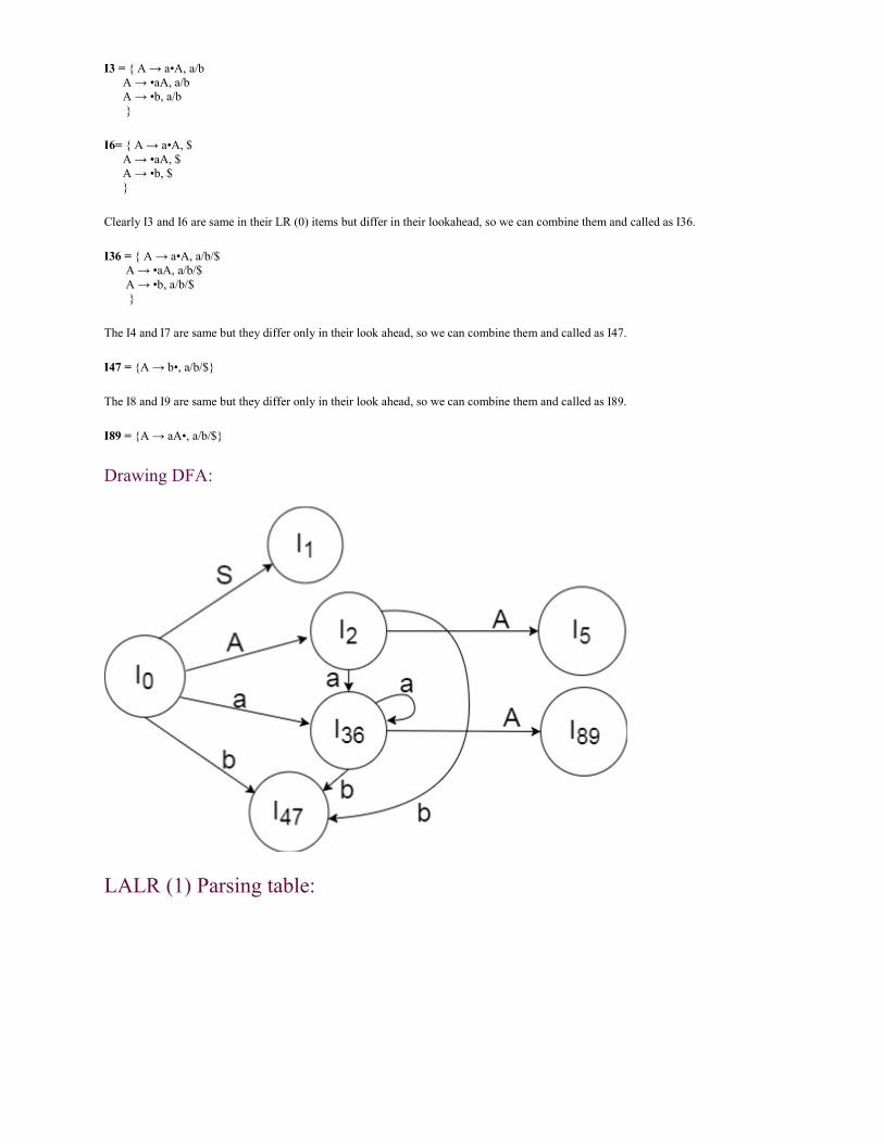
I3 = { A → a•A, a/b A → •aA, a/b A → •b, a/b }

I6= { A → a•A, $ A → •aA, $ A → •b, $ }

Clearly I3 and I6 are same in their LR (0) items but differ in their lookahead, so we can combine them and called as I36.

I36 = { A → a•A, a/b/$ A → •aA, a/b/$ A → •b, a/b/$ }

The I4 and I7 are same but they differ only in their look ahead, so we can combine them and called as I47.

I47 = {A → b•, a/b/$}

The I8 and I9 are same but they differ only in their look ahead, so we can combine them and called as I89.

I89 = {A → aA•, a/b/$}

Drawing DFA:

LALR (1) Parsing table:

SHIFT-REDUCE CONFLICT

COMPARISON OF LR (1) AND LALR:

If LR (1) has shift-reduce conflict then LALR will also have it. If LR (1) does not have shift-reduce conflict LALR will also not have it. Any shift-reduce conflict which can be removed by LR (1) can also be removed by LALR. For cases where there are no common cores SLR and LALR produce same parsing tables.

COMPARISON OF SLR AND LALR:

If SLR has shift-reduce conflict then LALR may or may not remove it. SLR and LALR tables for a grammar always have same number of states.

Hence, LALR parsing is the most suitable for parsing general programming languages.The table size is quite small as compared to LR (1) , and by carefully designing the grammar it can be made free of conflicts. For example, in a language like Pascal LALR table will have few hundred states, but a Canonical LR will have thousands of states. So it is more convenient to use an LALR parsing.

REDUCE-REDUCE CONFLICT

However, the Reduce-Reduce conflicts still might just remain .This claim may be better comprehended if we take the example of the following grammar:

S’-> S

S-> aAd

S-> bBd

S-> aBe

S-> bAe

A-> c

B-> c

Generating the LR (1) items for the above grammar,

I0 : S’-> .S , $

S-> . aAd, $

S-> . bBd, $

S-> . aBe, $

S-> . bAe, $

I1: S’-> S ., $

I2: S-> a . Ad, $

S-> a . Be, $

A-> .c, d

B->.c, e

I3: S-> b . Bd, $

S-> b . Ae, $

A->.c, e

B->.c,d

I4: S->aA.d, $

I5: S-> aB.e,$

I6: A->c. , d

B->c. , e

I7: S->bB.d, $

I8: S->bA.e, $

I9: B->c. , d

A->c. , e

I10: S->aAd. , $

I11: S->aBe., $

I12: S->bBd., $

I13: S->aBe., $

The LR (1) Parsing Table. (partly filled)

a ……………… d e

I1

I2

.

.

.

.

.

.

.

.

.

.

.

I6 ………………. r6 r7

..

.

.

.

.

.

.

.

.

.

.

I9 …………………. r7 r6

.

This table on reduction to the LALR parsing table, comes up in the forms of-

The LALR Parsing table. ( partly filled)

a ……………… d e

I1

I2

.

.

.

.

.

.

.

.

.

.

.

I69 ………………. r6/r7 r7/r6

..

.

.

.

.

.

.

.

.

.

.

I9 …………………. r7 r6

.

So, we find that the LALR gains reduce-reduce conflict whereas the corresponding LR (1) counterpart was void of it. This is a proof enough that LALR is less potent than LR (1).

But, since we have already proved that the LALR is void of shift-reduce conflicts (given that the corresponding LR(1) is devoid of the same), whereas SLR (or LR (0)) is not necessarily void of shift-reduce conflict, the LALR grammar is more potent than the SLR grammar.

SHIFT-REDUCE CONFLICT present in SLR

Some of them are solved in….

LR (1)

All those solved are preserved in…

LALR

So, we have answered all the queries on LALR that we raised intuitively.

Parsing process in NLP

Parsing is the term used to describe the process of automatically building syntactic analysis of a sentence in terms of a given grammar and lexicon. The resulting syntactic analysis may be used as input to a process of semantic interpretation. Occasionally, parsing is also used to include both syntactic and semantic analysis. The parsing process is done by the parser. The parsing performs grouping and labeling of parts of a sentence in a way that displays their relationships to each other in a proper way.

The parser is a computer program which accepts the natural language sentence as input and generates an output structure suitable for analysis. The lexicon is a dictionary of words where each word contains some syntactic, some semantic and possibly some pragmatic information. The entry in the lexicon will contain a root word and its various derivatives. The information in the lexicon is needed to help determine the function and meanings of the words in a sentence. The basic parsing technique is shown in figure .

Generally in computational linguistics the lexicon supplies paradigmatic information about words including part of speech labels, irregular plurals and sub categorization information for verbs. Traditionally, lexicons were quite small and were constructed largely by hand. The additional information being added to the lexicon increase the complexity of the lexicon. The organization and entries of a lexicon will vary from one implementation to another but they are usually made up of variable length data structures such as lists or records arranged in alphabetical order. The word order may also be given in terms of usage frequency so that frequently used words like “a”, “the” and “an” will appear at the beginning of the list facilitating the search. The entries in a lexicon could be grouped and given word category (by articles, nouns, pronouns, verbs, adjectives, adverbs and so on) and all words contained within the lexicon listed within the categories to which they belong. The entries are like a, an (determiner), be (verb), boy, stick, glass (noun), green, yellow, red (adjectives), I, we, you, he, she, they (pronouns) etc.

In most contemporary grammatical formalisms, the output of parsing is something logically equivalent to a tree, displaying dominance and precedence relations between constituents of a sentence. Parsing algorithms are usually designed for classes of grammar rather than tailored towards individual grammars.

Types of Parsing

The parsing technique can be categorized into two types such as

1. Top down Parsing

2. Bottom up Parsing

Let us discuss about these two parsing techniques and how they will work for input sentences.

1 Top down Parsing

Top down parsing starts with the starting symbol and proceeds towards the goal. We can say it is the process of construction the parse tree starting at the root and proceeds towards the leaves. It is a strategy of analyzing unknown data relationships by hypothesizing general parse tree structures and then considering whether the known fundamental structures are compatible with the hypothesis. In top down parsing words of the sentence are replaced by their categories like verb phrase (VP), Noun phrase (NP), Preposition phrase (PP), Pronoun (PRO) etc. Let us consider some examples to illustrate top down parsing. We will consider both the symbolical representation and the graphical representation. We will take the words of the sentences and reach at the complete sentence. For parsing we will consider the previous symbols like PP, NP, VP, ART, N, V and so on. Examples of top down parsing are LL (Left-to-right, left most derivation), recursive descent parser etc.

Example 1: Rahul is eating an apple.

2. Bottom up Parsing

In this parsing technique the process begins with the sentence and the words of the sentence is replaced by their relevant symbols. This process was first suggested by Yngve (1955). It is also called shift reducing parsing. In bottom up parsing the construction of parse tree starts at the leaves and proceeds towards the root. Bottom up parsing is a strategy for analyzing unknown data relationships that attempts to identify the most fundamental units first and then to infer higher order structures for them. This process occurs in the analysis of both natural languages and computer languages. It is common for bottom up parsers to take the form of general parsing engines that can wither parse or generate a parser for a specific programming language given a specific of its grammar.

A generalization of this type of algorithm is familiar from computer science LR (k) family can be seen as shift reduce algorithms with a certain amount (“K” words) of look ahead to determine for a set of possible states of the parser which action to take. The sequence of actions from a given grammar can be pre-computed to give a ‘parsing table’ saying whether a shift or reduce is to be performed and which state to go next. Generally bottom up algorithms are more efficient than top down algorithms, one particular phenomenon that they deal with only clumsily are “e mpty rules”: rules in which the right hand side is the empty string. Bottom up parsers find instances of such rules applying at every possible point in the input which can lead to much wasted effort. Let us see some examples to illustrate the bottom up parsing.

Example-2:

The small tree shades the new house by the stream

ART small tree shades the new house by the stream

ART ADJ tree shades the new house by the stream

ART ADJ N shades the new house by the stream

ART ADJ N V the new house by the stream

ART ADJ N V ART new house by the stream

ART ADJ N V ART ADJ house by the stream

ART ADJ N V ART ADJ N by the stream

ART ADJ N V ART ADJ N PREP the stream

ART ADJ N V ART ADJ N PREP ART stream

ART ADJ N V ART ADJ N PREP ART N

ART ADJ N V ART ADJ N PREP NP

ART ADJ N V ART ADJ N PP

ART ADJ N V ART ADJ NP

ART ADJ N V ART NP

ART ADJ N V NP

ART ADJ N VP

ART NP VP

NP VP

S

Deterministic Parsing

A deterministic parser is one which permits only one choice for each word category. That means there is only one replacement possibility for every word category. Thus, each word has a different test conditions. At each stage of parsing always the correct choice is to be taken. In deterministic parsing back tracking to some previous positions is not possible. Always the parser has to move forward. Suppose the parser some form of incorrect choice, then the parser will not proceed forward. This situation arises when one word satisfies more than one word categories, such as noun and verb or adjective and verb. The deterministic parsing network is shown in figure.

Non-Deterministic Parsing

The non deterministic parsing allows different arcs to be labeled with the some test. Thus, they can uniquely make the choice about the next arc to be taken. In non deterministic parsing, the back tracking procedure can be possible. Suppose at some extent of point, the parser does not find the correct word, then at that stage it may backtracks to some of its previous nodes and then start parsing. But the parser has to guess about the proper constituent and then backtrack if the guess is later proven to be wrong. So comparative to deterministic parsing, this procedure may be helpful for a number of sentences as it can backtrack at any point of state. A non deterministic parsing network is shown in figure.

XML parser is a software library or a package that provides interface for client applications to work with XML documents. It checks for proper format of the XML document and may also validate the XML documents. Modern day browsers have built-in XML parsers.

Following diagram shows how XML parser interacts with XML document −

The goal of a parser is to transform XML into a readable code.

To ease the process of parsing, some commercial products are available that facilitate the breakdown of XML document and yield more reliable results.

Some commonly used parsers are listed below −

MSXML (Microsoft Core XML Services) − This is a standard set of XML tools from Microsoft that includes a parser.

System.Xml.XmlDocument − This class is part of .NET library, which contains a number of different classes related to working with XML.

Java built-in parser − The Java library has its own parser. The library is designed such that you can replace the built-in parser with an external implementation such as Xerces from Apache or Saxon.

Saxon − Saxon offers tools for parsing, transforming, and querying XML.

Xerces − Xerces is implemented in Java and is developed by the famous open source Apache Software Foundation.

What Does Parsing a Query Mean?

A SQL statement is comprised of various inputs, i.e. different tables, functions, expressions. Thus it is possible that there are multiple ways to execute one query. Of course, the query must run in the most optimal way in order to execute in the shortest possible time. Parsing of a query is the process by which this decision making is done that for a given query, calculating how many different ways there are in which the query can run. Every query must be parsed at least once.

The parsing of a query is performed within the database using the Optimizer component. The Optimizer evaluates many different attributes of the given query i.e. number of tables involved, whether we have indexes available or not, what kind of expressions are involved, etc. Taking all of these inputs into consideration, the Optimizer decides the best possible way to execute the query. This information is stored within the SGA in the Library Cache – a sub-pool within the Shared Pool.

There are two possible states for a query’s processing information. One, that it can be found in the Library Cache and two, that it may not be found. The memory area within the Library Cache in which the information about a query’s processing is kept is called the Cursor. Thus if a reusable cursor is found within the library cache, it’s just a matter of picking it up and using it to execute the statement. This is called Soft Parsing. If it’s not possible to find a reusable cursor or if the query has never been executed before, query optimization is required. This is called Hard Parsing.

Understanding Hard Parsing

Hard parsing means that either the cursor was not found in the library cache or it was found but was invalidated for some reason. For whatever reason, Hard Parsing would mean that work needs to be done by the optimizer to ensure the most optimal execution plan for the query. The optimizer does so by looking into every possible input given to it by the user. This includes the presence (or absence) of any indexes, expressions or functions applied to the columns, whether it’s a join query or not, any hints specified etc. All of this information is of very great importance and presence or absence of any such inputs can change the execution plan.

Before the process of finding the best plan is started for the query, there are some tasks that are completed. These tasks are repeatedly executed even if the same query executes in the same session for N number of times:

1. Syntax Check 2. Semantics Check 3. Hashing the query text and generating a hash key-value pair

Free Compiler Construction Kits

JFlex

JFlex is a lexical analyzer for Java with Unicode support. It takes the regular expressions and actions you write and produces a deterministic finite automaton (DFA). The generated lexers will need JDK 7 and above and JFlex itself requires JDK 1.8 and above. It is open source.

JLex

JLex is a lexical analyzer for Java. Its input file is similar to that accepted by lex. It accepts a Unicode specification file, and you can configure it to generate a scanner that handles Unicode characters. It is open source.

Bison (parser generator)

Bison generates a parser when presented with a LALR (1) context-free grammar that is yacc compatible. The generated parser is in C. It includes extensions to yacc that make it easier to use if you want multiple parsers in your program. Bison works on Windows, MSDOS, Linux and numerous other operating systems. The link points to the source code. Although the program itself is under GPL, the generated parser (using the bison.simple skeleton) can be distributed without restriction. You can find a Windows port (one of many around) at WinFlexBison.

Flex (Lex drop-in replacement)

Flex generates a lexical analyser in C or C++ given an input program. It is designed so that it can be used together with yacc and its clones (like byacc and bison, also listed on this page). It is highly compatible with the Unix lex program. The original version of Flex, on which the above is based, can be found at ftp://ftp.ee.lbl.gov. If you are looking for a Windows port, one possibility is WinFlexBison.

RE/flex

RE/flex is a lexical analyzer generator for C++ that is compatible with flex (also listed on this page). It has integrated support for Unicode character sets (UTF-8, UTF-16, UTF-32), generates thread-safe scanners by default, can optionally use Boost Regex as a regex engine, supports lazy quantifiers, word boundary anchors (etc) in regular expressions, and

so on. When not invoked with flex compatibility, it will not use macros and globals. The generated scanner produces C++ scanner classes derived from a template. The source code is released under the BSD 3-Clause licence, and can be compiled under Windows, Mac OS X and Linux, although a Windows executable is also provided in the distribution package.

Waxeye Parser Generator

Waxeye is a parser generator that takes a Parsing Expression Grammar (PEG) as input. It supports C, Java, JavaScript, Python, Ruby and Scheme. It also supports modular grammars (where your grammar is split across multiple files) and grammar testing (to check that every component of your language is parsed the way you want it to). The program is released under the MIT licence.

peg/leg

The peg program creates a C recursive descent parser generator from a Parsing Expression Grammar (PEG). The alternative, leg, uses a slightly different syntax to make it more convenient for those who are familiar with lex and yacc. Both support unlimited backtracking, ordered choice as a means for disambiguation, and can combine lexical analysis and parsing into a single activity. The program is released under the MIT licence, and the parsers created are unencumbered by any licence.

re2c

This program, re2c, generates C/C++ lexical analyzers. It takes regular expressions that you write and produces a deterministic finite automaton (DFA), which, when run, will process input according to your rules and execute the matching code (which you write). Unlike lex and flex (see elsewhere on this page), you do not call the yylex() function to start the lexer, but have access to a variety of lower-level functions which give you greater flexibility in processing your input. According to their website, this lexer generator is used in programs like PHP and SpamAssassin. The source code is in the public domain.

AdaGOOP

AdaGOOP, which stands for Ada Generator of Object Oriented Parsers, creates a parser that generate an object oriented parse tree, and a traversal of the tree using the visitor pattern. It relies on the SCATC versions of aflex and ayacc which you can also get from their site. The source code is provided, and there are no restrictions on its use.

Quex - A Mode Oriented Directly Coded Lexical Analyzer Generator

Quex, or Queχ (depending on which part of the site you read), produces a directly coded lexical analyzer engine with pre- and post- conditions rather than the table-driven created by the Lex/Flex family (see elsewhere on this page). Features include inheritable "lexer modes" that provide transition control and indentation events, a general purpose token class, a token queue that allow tokens to be communicated without returning from the lexical analyzer function, line and column numbering, generation of transition graphs, etc. You will need to install Python before using this lexical analyser generator. It

generates C++ code. It is released under the GNU LGPL with additional restrictions; see the documentation for details. Windows, Mac OS X, Solaris and Linux are supported.

Gardens Point LEX

[Note: I'm not sure if the above link points to the official version of Gardens Point LEX, since there seems to be at least a couple of repositories around.] The Gardens Point Scanner Generator, GPLEX, accepts a lex-like input specification to create a C# lexical scanner. The scanner produced is thread-safe and all scanner state is maintained within the scanner instance. Note that the input program does not support the complete POSIX lex specifications. The scanner uses the generic types defined in C# 2.0.

Gardens Point Parser Generator

The Gardens Point Parser Generator, GPPG, accepts a yacc-like program to produce a thread-safe bottom-up C# parser. The parser uses the generic types defined in C# 2.0.

Bisonc++

Supplied with an LALR(1) context-free grammar, bisonc++ generates a C++ parser class. As its name suggests, the parser generator was originally derived from the Bison parser generator (see elsewhere on this page), and grammars used for the latter software can supposedly be adapted to bisonc++ with little or no change.

Grammatica

Grammatica is a parser generator for C# and Java. It uses LL(k) grammars with unlimited number of look-ahead tokens. It purportedly creates commented and readable source code, has automatic error recovery and detailed error messages. The generator creates the parser at runtime thus also allowing you to test and debug the parser before you even write your source code. The program is released under the GNU General Public License with an exception to facilitate its use by commercial software.

Accent Compiler Compiler

A compiler-compiler that avoids the problems of the LALR parsers (eg, when faced with shift/reduce and reduce/reduce conflicts) and LL parsers (with its restrictions due to left-recursive rules). You specify your input grammar in the Extended-Backus-Naur-Form, in which you are allowed to indicate repetition, choices and optional parts. You can insert semantic actions anywhere, and ambiguous grammars are allowed. All these features make Accent grammars easier to write than (eg) Yacc grammars. The website warns however that the generated code require significantly more system resources than code generated by Yacc. Accent is distributed under GNU GPL. I'm not sure about the generated C code.

PRECCX (Prettier Compiler-Compiler Extended)

PRECCX, or PREttier Compiler-Compiler eXtended, is "an infinite-lookahead compiler-compiler for context dependent grammars" which generates C code. You specify an input grammar in an extended BNF notation where inherited and synthetic attributes are

allowed. The parser is essentially LL(infinity) with optimisations. You can get versions for MSDOS, Linux and other Unices (including Sun, HP, etc). Source code is available and you can apparently compile it on other platforms with an ANSI C compiler if needed.

Byacc/J (Parser Generator)

This is a version of Berkeley yacc modified so that it can generate Java source code. You simply supply a "-J" option on the command line and it'll produce the Java code instead of the usual C output. You can either get the free source code and compile it yourself, or download any of the precompiled binaries for Solaris, SGI/IRIX, Windows, and Linux. Like the byacc original (see elsewhere on this page), your output is free of any restrictions, and you can freely use it for any purpose you wish.

COCO/R (Lexer and Parser Generators)

This tool generates recursive descent LL(1) parsers and their associated lexical scanners from attributed grammars. It comes with source code, and there are versions to generate Oberon, C#, F#, VB.Net, C, C++, Java, Swift, Pascal, Delphi, Ada, Python, Oberon, etc. Platforms supported appear to vary (Unix systems, Apple Macintosh, Atari, MSDOS, etc) depending on the language you want generated.

Eli

A programming environment that allows you to generate complete language implementations from application-oriented specifications. The user describes the problems that needs to be solved and Eli uses the tools and components required for that problem. It handles structural analysis, analysis of names, types, values, stores translation structures and produces the target text. It generates C code. The program is available in source form and has been tested under Linux, IRIX, HP-UX, OSF, and SunOS. Eli itself is distributed under the GNU GPL but the generated code is your property to do as you please.

ALE

This freeware system, written in Prolog, and requiring SICStus Prolog 3.7, SWI Prolog or Quintus Prolog (no longer maintained?) to run, handles phrase structure parsing, semantic-head-driven generation and constraint logic programming and includes a source level debugger.

Gentle Compiler Construction System

This compiler construction tool purports to provide a uniform framework for language recognition, definition of abstract syntax trees, construction of tree walkers based on pattern recognition, smart traversal, simple unparsing for source to source translation and optimal code selection for microprocessors. Note however that if you use it to create an application, the licensing terms require that your applications be licensed under the GNU GPL. This probably restricts your use of it in a commercial program, unless you are prepared to pay for a special license or you plan to make the sources for your program available anyway.

Bison for Eiffel (Parser generator)

This version of Bison produces Eiffel source code. Like Bison, it is released under the GNU GPL. I am uncertain whether the generated parser can be distributed freely (the current versions of Bison allow this if you do not modify the output) without restrictions.

ANTLR (Recursive Descent Parser Generator)

ANTLR generates a recursive descent parser in C, C++ or Java from predicated-LL(k>1) grammars. It is able to build ASTs automatically. If you are using C, you may have to get the PCCTS 1.XX series (the precursor to ANTLR), also available at the site. The latest version may be used for C++ and Java.

Byacc: original version and current version

[Note: the link for the original version uses the FTP protocol. If your browser does not support this, you will probably need to use an FTP client to go to that address.] Berkeley YACC ("Yet Another Compiler Compiler") is a public domain parser generator that is the precursor of the GNU BISON. The "original version" link points to the original version by Robert Corbett, released to the public domain (that is, not copyrighted). The "current version" link provides the version that is maintained by Thomas E. Dickey. Both versions are to the source code, which should compile with many compilers (including GNU's gcc). It generates C code.

BtYacc (generates parsers)

To quote from the documentation, BtYacc, or BackTracking Yacc, "is a modified version of Berkeley Yacc that supports automatic backtracking and semantic disambiguation to parse ambiguous grammars, as well as syntactic sugar for inherited attributes". The program comes with sources which are in the public domain. Although the author only mentions compilation of the program on Unix and Win32 systems, it is likely that the program can be compiled and run on DOS systems using an MSDOS port of the GNU C compiler like DJGPP, since the GNU compiler was used on the other systems. For more information about DJGPP, see the Free C and C++ compilers page.

Java Compiler Compiler (JavaCC)

This Java parser generator is written in Java and produces pure Java code. It even comes with grammars for Java 1.0.2, 1.1 as well as HTML. It generates recursive descent parsers (top-down) and allows you to specify both lexical and grammar specifications in your input grammar. In terms of syntactic and semantic lookahead, it generates an LL(1) parser with specific portions LL(k) to resolve things like shift-shift conflicts. The input grammar is in extended BNF notation. It comes with JJTree, a tree building preprocessor; a documentation generator; support for Unicode (and hence internationalization), and many examples. There are numerous other features, including debugging capabilities, error reporting, etc.

Programming Language Creator

According to the documentation, the Programming Language Creator is designed to enable you "to easily create new programming languages, or create interpreted versions of any compiled language" without the need for you to wrestle with yacc and lex. If you want your application to have a scripting language, you might want to look at this to see if it meets your requirements. The binaries, available free, are for Windows, and the source code is available for a fee.

SableCC

This is an object-oriented framework that generates DFA based lexers, LALR(1) parsers, strictly typed syntax trees, and tree walker classes from an extended BNF grammar (in other words, it's a compiler generator). The program was written in Java itself, runs on any Java 1.1 (or later) system and generates Java sources.

LEMON Parser Generator

This LALR(1) parser generator claims to generate faster parsers than Yacc or Bison. The generated parsers are also re-entrant and thread-safe. The program is written in C, and only the source code is provided, so you will need a C compiler to compile it before you can use it.

YaYacc (Generates Parsers)

[Update: this software is no longer available.] YaYacc, or Yet Another Yacc, generates C++ parsers using an LALR(1) algorithm. YaYacc itself runs on FreeBSD, but the resulting parser is not tied to any particular platform (it depends on your code, of course).

Jaccie (Java-based Compiler Compiler) and SIC (Smalltalk-based Interactive Compiler Compiler)

[Update: this software is no longer available. For the record, it used to be found at http://www2.cs.unibw.de/Tools/Syntax/english/index.html] Jaccie includes a scanner generator and a variety of parser generators that can generate LL(1), SLR(1), LALR(1) grammars. It has a debugging mode where you can operate it non-deterministically. It is based on the earlier SIC, which uses the Smalltalk programming language for evaluation rules.

TP Lex/Yacc (Lexical Analyzer and Parser Generators)

[Update: this software is no longer available.] This is a version of Lex and Yacc designed for Borland Delphi, Borland Turbo Pascal and the Free Pascal Compiler (you can find legally free versions of all the above listed on the Free Delphi Compilers and Pascal Compilers page). Like its lex and yacc predecessors, this version generates lexers and parsers, although in its case, the generated code is in the Pascal language.

https://www.thefreecountry.com/programming/compilerconstruction.shtml

Lex and Yacc programs

1. To write a LEX program for token separation using LEX tool

File name scan.l

%option noyywrap

%{

int comment = 0;

%}

identifier [a-zA-Z][a-zA-z0-9]*

%%

#.* {printf("\n %s is a preprocessor directive", yytext);}

int |

float |

double |

char |

void |

main {printf("\n %s is a keyword", yytext);}

"{" |

"}" |

"(" |

")" |

"," |

"&" |

";" {printf("\n %s is a special character", yytext);}

"+" |

"-" |

"*" |

"/" |

"%" {printf("\n%s is a operator", yytext);}

"<=" |

">=" |

"<" |

">" |

"==" {printf("\n%s is a Relational operator", yytext);}

{identifier} {printf("\n %s is a identifier", yytext);}

{identifier}+")".*"(" {printf("\n %s is a function", yytext);}

%%

int main()

{

FILE *fp;

fp = fopen("ex.c","r");

yyin = fp;

yylex();

return 0;

}

Input file name ex.c

#include<stdio.h>

void main()

{

int a,b,c;

a=1;

b=2;

if(a<=b)

c=a+b;

}

Steps to compile and run program

administrator@administrator:~$ lex scan.l

administrator@administrator:~$ gcc lex.yy.c -ll

administrator@administrator:~$ ./a.out

Output:

/ is a operator

/ is a operator

ex is a identifier.

c is a identifier

#include<stdio.h> is a preprocessor directive

void is a keyword

main is a keyword

( is a special character

) is a special character

{ is a special character

int is a keyword

a is a identifier

, is a special character

b is a identifier

, is a special character

c is a identifier

; is a special character

a is a identifier=1


b is a identifier=2


if is a identifier

( is a special character

a is a identifier

<= is a Relational operator

b is a identifier

) is a special character

c is a identifier=

a is a identifier

+ is a operator

b is a identifier


} is a special character

2. To write a program for calculator using YACC

File name cal.l

%{

#include<stdio.h>

#include "y.tab.h"

extern int yylval;

%}

%%

[0-9]+ {

yylval=atoi(yytext);

return NUMBER;

}

[\t] ;

[\n] return 0;

. return yytext[0];

%%

int yywrap()

{

return 1;

}

File name cal.y

%{

#include<stdio.h>

int flag=0;

%}

%token NUMBER

%left '+' '-'

%left '*' '/' '%'

%left '(' ')'

%%

ArithmeticExpression: E{

printf("\nResult=%d\n",$$);

return 0;

};

E:E'+'E {$$=$1+$3;}

|E'-'E {$$=$1-$3;}

|E'*'E {$$=$1*$3;}

|E'/'E {$$=$1/$3;}

|E'%'E {$$=$1%$3;}

|'('E')' {$$=$2;}

| NUMBER {$$=$1;}

;

%%

void main()

{

printf("\nEnter Any Arithmetic Expression which can have operations Addition, Subtraction, Multiplication, Divison, Modulus and Round brackets:\n");

yyparse();

if(flag==0)

printf("\nEntered arithmetic expression is Valid\n\n");

}

void yyerror()

{

printf("\nEntered arithmetic expression is Invalid\n\n");

flag=1;

}

Steps to compile and run program

administrator@administrator:~$ yacc -d cal.y

administrator@administrator:~$ lex cal.l

administrator@administrator:~$ gcc lex.yy.c y.tab.c -w

administrator@administrator:~$ ./a.out

Enter Any Arithmetic Expression which can have operations Addition, Subtraction, Multiplication, Divison, Modulus and Round brackets:

5+4/3*2

Result=7

Entered arithmetic expression is Valid

administrator@administrator:~$

3.To write a Lex program , how to count the number of lines, spaces and tabs using Lex.

File name white.l

%{

#include<stdio.h>

int lc=0, sc=0, tc=0, ch=0; /*Global variables*/

%}

/*Rule Section*/

%%

\n lc++; //line counter

([ ])+ sc++; //space counter

\t tc++; //tab counter

. ch++; //characters counter

%%

main()

{

// The function that starts the analysis

yylex();

printf("\nNo. of lines=%d, lc);

printf("\nNo. of spaces=%d, sc);

printf("\nNo. of tabs=%d, tc);

printf("\nNo. of other characters=%d, ch);

}

Input:

Geeks for Geeks

gfg gfg

Output:

No. of lines=2

No. of spaces=3

No. of tabs=1

No. of other characters=19

4. To write Lex program find the small letter, capital letter and digit from the input text

File name smcano.l

%{

#include<stdio.h>

int no;

%}

%%

[a-z] {printf("Small Letter \n");}

[A-Z] {printf("Capital Letter \n");}

[0-9] {no++;printf("No of digits=%d \n",no);}

%%

int main()

{

printf("\nEnter a combination of string(small or capital,digit):"); yylex();

return 0;

}

int yywrap()

{ return 1; }

administrator@administrator:~$ lex smcano.l administrator@administrator:~$ gcc lex.yy.c -ll administrator@administrator:~$ ./a.out

Output:

Enter a combination of string(small or capital,digit):Good Morning 786 cse

Capital Letter

Small Letter

Small Letter

Small Letter

Capital Letter

Small Letter

Small Letter

Small Letter

Small Letter

Small Letter

Small Letter

No of digits=1

No of digits=2

No of digits=3

Small Letter

Small Letter

Small Letter

vowel.l

%{

#include<stdio.h>

int vowel=0;

int cons=0;

%}

%%

"a"|"e"|"i"|"o"|"u"|"A"|"E"|"I"|"O"|"U" {printf("\nVowel\t");vowel++;}

[a-zA-z] {printf("\nConsonant\t");cons++;}

%%

int yywrap()

{

return 1;

}

int main()

{

printf("\nEnter String:");

yylex();

return 0;

}

UNIT III

Syntax-Directed Translation

Objectives:

-Intermediate code eliminates the need of a new full compiler for every unique machine by

keeping the analysis portions same for all the compilers.

-The second part of compiler, synthesis, is changed according to the target machine.

Outcomes:

Design syntax directed translation schemes for a given context free grammar. Generate intermediate code for statements in high level language.

Explain the role of a semantic analyzer and type checking; create a syntax-directed definition and an annotated parse tree; describe the purpose of a syntax tree

Pre-requisites: Basic knowledge of grammars, parse trees. Introduction:

• A SDT is a generalization of context free grammar in which each grammar symbols are

associated with attributes to associate information with the programming language constructs

that they represent.

• Values of these attributes are evaluated by the semantic rules associated with the production

rules.

• Evaluation of these semantic rules:

– may generate intermediate codes

– may put information into the symbol table

– may perform type checking

– may issue error messages

• An attribute may hold almost any thing.

– a string, a number, a memory location, a complex record.

When we associate semantic rules with productions, we use two notations:

– Syntax-Directed Definitions

– Translation Schemes

Syntax-Directed Definitions:

– give high-level specifications for translations

– hide many implementation details such as order of evaluation of semantic actions.

– We associate a production rule with a set of semantic actions

Translation Schemes:

– indicate the order of evaluation of semantic actions associated with a production rule.

– Both conceptually parse the input token stream, build the parse tree and then traverse the

tree as needed to evaluate the semantic rules at the parse tree nodes

– Evaluation of the semantic rules may generate code, save information in a symbol table,

issue error messages

Syntax-Directed Definitions

• A syntax-directed definition is a generalization of a context-free grammar in which:

– Each grammar symbol is associated with a set of attributes.

– This set of attributes for a grammar symbol is partitioned into two subsets called

synthesized and inherited attributes of that grammar symbol.

– Each production rule is associated with a set of semantic rules.

• Semantic rules set up dependencies between attributes which can be represented by a

dependency graph.

• This dependency graph determines the evaluation order of these semantic rules.

• Evaluation of a semantic rule defines the value of an attribute.

Production Semantic Rules

L → E return print(E.val)

E → E1 + T E.val = E1.val + T.val

E → T E.val = T.val

T → T1 * F T.val = T1.val * F.val

T → F T.val = F.val

F → ( E ) F.val = E.val

F → digit F.val = digit.lexval

• Symbols E, T, and F are associated with a synthesized attribute val.

• The token digit has a synthesized attribute lexval (it is assumed that it is evaluated by the lexical

analyzer).

Example : Input: 5+3*4

L->E.val(17)

->E.val(5)+T.val(12)

->T.val(5)+T.val(3) * F.val(4)

->F.val(5)+F.val(3) * digit.lexval(4)

->digit.lexval (5)+F.val(3) * digit.lexval(4)

->digit.lexval (5)+digit.lexval (3) * digit.lexval(4)

Dependency Graph

Figure Dependency graph

Annotated Parse Tree

• A parse tree showing the values of attributes at each node is called an annotated parse tree.

• The process of computing the attributes values at the nodes is called annotating (or decorating)

of the parse tree.

• The order of these computations depends on the dependency graph induced by the semantic

rules.

Annotated Parse Tree – Example

Figure Annotated parse tree

Syntax-Directed Definition

• In a syntax-directed definition, each production A→α is associated with a set of semantic rules

of the form:

b=f(c1,c2,…,cn) where f is a function,

and b can be one of the followings:

b is a synthesized attribute of A and c1,c2,…,cn are attributes of the grammar symbols in

the production ( A→α ).

OR

b is an inherited attribute one of the grammar symbols in α (on the

right side of the production), and c1,c2,…,cn are attributes of the grammar symbols in

the production ( A→α ).

Synthesized Attributes and Inherited Attributes

• Synthesized attributes are computed purely bottom-up

• A grammar with semantic actions (or syntax-directed definition) can choose to use only synthesized

attributes

• Such a grammar plus semantic actions is called an S-attributed definition

• Inherited attributes are computed at a node based on attributes from siblings or the parent

• Typically we combine synthesized attributes and inherited attributes

• It is possible to convert the grammar into a form that only uses synthesized attributes

Synthesized attribute -- Example

Inherited attribute

• Prod Semantic rule

D->TL L.in=T.type

T->int T.type=int

T->real T.type=real

L->L,id L1.in=L.in

addtype(id.entry,L.in)

L->id addtype(id.entry,L.in)

-> Nonterminal T has synthesized attribute type

-> Semantic rule L.in=T.type associated with production D->TL sets inherited attribute L.in to the type

in the declarations

Inherited attribute-Example

Intermediate Code Generation

Why Intermediate Code?

While generating machine code directly from source code is possible, it entails two problems With m languages and n target machines, we need to write m front ends, m × n optimizers, and m × n code generators The code optimizer which is one of the largest and very-difficult-to-write components of a compiler, cannot be reused By converting source code to an intermediate code, a machine-independent code optimizer may be written This means just m front ends, n code generators and 1 optimizer

• Intermediate codes are machine independent codes, but they are close to machine

instructions.

• The given program in a source language is converted to an equivalent program in an

intermediate language by the intermediate code generator.

• Intermediate language can be many different languages, and the designer of the compiler

decides this intermediate language.

– syntax trees can be used as an intermediate language.

– postfix notation can be used as an intermediate language.

– three-address code

• Quadruples

• Triples

• Indirect Triples

Three address code

• Basic idea: break down source language expressions into simple pieces that:

– translate easily into real machine code

– form a linearized representation of a syntax tree

– allow machine independent code optimizations to be performed

– increase the portability of the compiler

Three-Address Code

• A Three address code is:

x := y op z

where x, y and z are names, constants or compiler-generated temporaries; op is any operator.

But we may also the following notation for quadraples (much better notation because it looks like

a machine code instruction)

op y,z,x apply operator op to y and z, and store the result in x.We use the term “three-

address code” because each statement usually contains three addresses (two for operands, one for

the result).

Graphical Representations

• Syntax tree –depicts the hierarchical structure of a source program

• DAG-gives the same information but in a compact way because common sub expressions are

identified.

• Eg: a=b*-c+b*-c

Functions of constructing syntax for expression

• mknode(op,left,right) creates an operator node with label op and two fields containing pointers to

left and right

• mkleaf(id, entry) creates an identifier node with label id and a field containing entry, a pointer to

the symbol table entry for the identifier

• mkleaf(num, val) creates a number node with label num and a field containing val, the value of the

number

• Eg: a-4+c

1. p1=mkleaf(id,entry a);

2. p2=mkleaf(num,4);

3.p3=mknode(‘-’,p1,p2);

4. p4=mkleaf(id,entry c);

5. p5=mknode(‘+’,p3,p4);

Syntax directed translation scheme to construct syntax trees for an expression


E -> E1 + T E.nptr=mknode(‘+’,E1.nptr,T.nptr)

E -> E1 - T E.nptr=mknode(‘-’,E1.nptr,T.nptr)

E->T E.nptr=T.nptr

T -> ( E) T.nptr = E.nptr;

T-> id T.nptr= mkleaf( id,id.entry)

T->num T.nptr= mkleaf( num,num.val)

Syntax directed translation scheme to construct syntax trees for assignment statements


S -> id = E S.nptr =mknode(‘assign,mkleaf( id,id.place),E.nptr )

E -> E1 + E.nptr=mknode(‘+’,E1.nptr,E2.nptr)

E -> E1 * E2 E.nptr=mknode(‘*’,E1.nptr,E2.nptr)

E -> - E1 E.nptr=mkunode(‘uminus’,E1.nptr)

E -> ( E1) E.nptr = E1.nptr;

E-> id E.nptr= mkleaf( id,id.place)

Types of Three-Address Statements

Assignment Statements: op y,z,result or result := y op z where op is a binary arithmetic or logical

operator. This binary operator is applied to y and z, and the result of the operation is stored in

result.

Ex: add a,b,c

Assignment Instructions: op y,,result or result := op y

where op is a unary arithmetic ,shift operator and logical operator. This unary operator is applied

to y, and the result of the operation is stored in result.

Ex: uminus a,,c not a,,c inttoreal a,,c

Move Operator: mov y,,result or result := y where the content of y is copied into

result.

Ex: mov a,,c

Unconditional Jumps: jmp ,,L or goto L

We will jump to the three-address code with the label L, and the execution continues from that

statement.

Ex: jmp ,,L1 // jump to L1

jmp ,,7 // jump to the statement 7

Conditional Jumps: jmprelop y,z,L or if y relop z goto L

We will jump to the three-address code with the label L if the result of y relop z is true, and the

execution continues from that statement. If the result is false, the execution continues from the

statement following this conditional jump statement.

jmpgt y,z,L1 // jump to L1 if y>z

jmpgte y,z,L1 // jump to L1 if y>=z

jmpe y,z,L1 // jump to L1 if y==z

jmpne y,z,L1 // jump to L1 if y!=z

Our relational operator can also be a unary operator.

jmpnz y,,L1 // jump to L1 if y is not zero

jmpz y,,L1 // jump to L1 if y is zero

jmpt y,,L1 // jump to L1 if y is true

jmpf y,,L1 // jump to L1 if y is false

Procedure Parameters: param x,, or param x

Procedure Calls: call p,n, or call p,n where x is an actual parameter, we invoke the

procedure p with n parameters.

Ex: param x1,,

param x2,,

p(x1,...,xn)

param xn,, call p,n,

f(x+1,y) add x,1,t1

param t1 , ,

param y , ,

call f,2,

Indexed Assignments:

move y[i],,x or x := y[i]

move x,,y[i] or y[i] := x

Address and Pointer Assignments:

moveaddr y,,x or x := &y movecont

y,,x or x := *y

Implementations of Three Address code

1. Quadruples

• Four Fields OP,ARG1,ARG2,RESULT

Eg. A=-B*(C+D)

Three address code

T1=-B

T2=C+D

T3=T1*T2

A=T3

2.Triples

• To avoid entering temporary names into the symbol table, one can allow the statement computing

a temporary value to represent that value

• Three fields OP,ARG1,ARG2

3.Indirect Triples

•Listing pointers to triples rather than listing the triples themselves.

(0) (14)

(1) (15)

(2) (16)

(3) (17)

Syntax Translation of assignment statements

• Can be formulated as syntax-directed translation

– add new attributes where necessary, e.g. for expression E we might have

• E.place

the name that holds the value of E

• E.code the

sequence of intermediate code statements evaluating E.

– new helper functions

• newtemp() returns a new temporary variable each time it is called

• newlabel() returns a new label each time it is called

– actions that generate intermediate code formulated as semantic rules

Syntax-Directed Translation into Three-Address Code

S id := E S.code = E.code || gen(‘mov’ E.place ‘,,’ id.place)

E E1 + E2 E.place = newtemp();

E.code = E1.code || E2.code || gen(‘add’ E1.place ‘,’ E2.place ‘,’ E.place)

E E1 * E2 E.place = newtemp();

E.code = E1.code || E2.code || gen(‘mult’ E1.place ‘,’ E2.place ‘,’ E.place)

E - E1 E.place = newtemp();

E.code = E1.code || gen(‘uminus’ E1.place ‘,,’ E.place)

E ( E1 ) E.place = E1.place;

E.code = E1.code

E id E.place = id.place;

E.code = null

Eg: a=-b*(c+d) Three address code

t1=-b

t2=c+d

t3=t1*t2

a=t3

E id E.place = id.place;(For every identifier create SDT ie. b,c,d,a)

E.code = null

E - E1 E.place = newtemp()(t1);

E.code = E1.code || gen(‘uminus’ E1.place(b) ‘,,’ E.place(t1))

E ( E1 ) E.place = E1.place;

E.code = E1.code

E E1 + E2 E.place = newtemp()(t2);

E.code = E1.code || E2.code || gen(‘add’ E1.place‘,’ E2.place ‘,’ E.place()

c d t2

E E1 * E2 E.place = newtemp()(t3);

E.code = E1.code || E2.code || gen(‘mult’ E1.place ‘,’ E2.place ‘,’ E.place)

t1 t2 t3

S id := E S.code = E.code || gen(‘mov’ E.place ‘,,’ id.place)

t3 a

Assignment statements with mixed types

• Semantic action for E->E1+E2

E.place=newtemp;

If E1.type=integer and E2.type=integer then begin

emit(E.place ‘=‘ E1.place ‘int+’ E2.place);

E.type= integer

end

else If E1.type=real and E2.type=real then begin

emit(E.place ‘=‘ E1.place ‘real+’ E2.place);

E.type= real

end

else If E1.type=integer and E2.type=real then begin

u=newtemp;

emit(u ‘=‘ ‘inttoreal’ E1.place);

emit(E.place ‘=‘ u ‘real+’ E2.place);

E.type= real

end

else If E1.type=real and E2.type=integer then begin

u=newtemp;

emit(u ‘=‘ ‘inttoreal’ E2.place);

emit(E.place ‘=‘ E1.place ‘real+’ u);

E.type= real

end

else

E.type=type error

Example

x=y+i*j

where x,y declared by float and I,j declared by integer

t1= i int* j

t3= inttoreal t1

t2= y real+ t3

x=t2

1. E.place=newtemp(t1);

If E1.type=integer and E2.type=integer then begin

emit(E.place(t1) ‘=‘ E1.place(i) ‘int*’ E2.place(j));

E.type(t1)= integer

2. E.place=newtemp(t2);

If E1.type=real and E2.type=integer then begin

u=newtemp(t3);

emit(u(t3) ‘=‘ ‘inttoreal’ E2.place(t1));

emit(E.place(t2) ‘=‘ E1.place(y) ‘real+’ u(t3));

E.type(t2)= real

Boolean Expression

• In programming languages it have two primary functions

– Used to compute logical values

– Used to conditional expressions(flow of control,while,if-then)

->Boolean operators(and ,or ,not)

->Relational expression(E1 relop E2)

E->E or E/E and E/not E/(E)/id relop id/true /false

Or ,and– left associative

Or- lowest precedence than ‘and’ and ‘not’

Methods of translating boolean expressions

• First method- Encode true and false numerically and to evaluate a Boolean expression to an

arithmetic expression

False True

1 0

• Second method- Flow of control – representing value of boolean expression by position reached

in program

eg. If then

while do

• Eg

a or b and not c

the three address sequence

t1= not c

t2=b and t1

t3= a or t2

These are the two functions of translation scheme using a numerical representation for

boolean

->Emit- it places three address statement into an output file in right format and increment

nextstat after producing each three address statement

->Nextstat- the index of next three address statement in the output sequence

Translation scheme using a numerical representation for Boolean

• E-> E1 or E2 { E.place=newtemp;

emit(E.place= ‘E1.place ‘or’ E2.place)}

• E-> E1 and E2 { E.place=newtemp;

emit(E.place= ‘E1.place ‘and’ E2.place)}

• E-> not E1 { E.place=newtemp;

emit(E.place= ‘not’ E1.place )}

• E-> id1 relop id2 { E.place=newtemp;

emit(if id1.place relop id2.place ‘goto’ nextstat+3)

emit (E.place = ‘0’);

emit(‘goto’ nextstat+2);

emit(E.place = ‘1’);

E->true { E.place=newtemp;

emit(E.place=‘1’)

E->false { E.place=newtemp;

emit(E.place=‘0’)

eg. if a <b then 1 else 0

Three address code sequence

100: if a<b goto 103

101:t=0

102:goto 104

103: t=1

104:

Eg : a<b or c<d and e<f

• 100: if a<b goto 103

• 101:t1=0

• 102 :goto 104

• 103:t1=1

• 104: if c<d goto 107

• 105:t2=0

• 106 :goto 108

• 107:t2=1

• 108: if e<f goto 111

• 109:t3=0

• 110 :goto 112

• 111:t3=1

• 112: t4 = t2 and t3

• 113: t5 = t1 or t4

Syntax directed definition to produce three address code for Booleans

• E->E1 or E2 E1.true= E.true

E1.false=newlabel;

E2.true= E.true

E2.false=E.false;

E.code=E1.code|| gen(E1.false’:’) || E2.code

• E->E1 and E2 E1.true= newlabel

E1.false=E.false;

E2.true= E.true

E2.false=E.false;

E.code=E1.code|| gen(E1.true’:’) || E2.code

• E->not E1 E1.true= E.false

E1.false=E.true;

E.code=E1.code

• E->(E1) E1.true= E.true

E1.false=E.false;

E.code=E1.code

• E-> id1 relop id2 E.code=gen(if id1.place relop .op id2.place ‘goto’ E.true)||

gen(‘goto’ E.false)

• E->true E.code=gen(‘goto’E.true)

• E->false E.code=gen(‘goto’E.false)

Eg 1. a<b or c<d and e<f

Three address code

if a<b goto Ltrue

goto L1

L1: if c<d goto L2

goto Lfalse

L2: if e<f goto Ltrue

goto Lfalse

Ltrue:

L.false:

• Eg while a<b do

if c<d then

x=y+z;

else

x=y-z;

Three address code

L1: if a<b goto L2

goto Lnext

L2: if c<d goto L3

goto L4

L3: t1=y+z

x=t1

goto L1

L4: t2=y-z

x=t2

goto L1

Lnext:

Syntax-Directed Translation –Flow of control statements

• S-> if E then S1 / if E then S1 else S2 / While E do S1

S-> if E then S1 E.true=newlabel;

E.false=S.next;

S1.next=S.next

S.code=E.code || gen(E.true) || S1.code

S while E do S1 S.begin = newlabel;

E.true=newlabel;

E.false=S.next;

S1.next = S.begin;

S.code = gen(S.begin “:”) || E.code ||

gen( E.true) || S1.code ||

gen(‘goto’ S.begin)

S if E then S1 else S2 E.true = newlabel();

E.false = newlabel();

S1.next=S.next;

S2.next=S.next;

S.code = E.code ||

gen(E.true) || S1.code ||

gen(‘goto’ S.next) ||

gen(E.false) || S2.code

Backpatching

• Easiest way to implement the SDD is to use two passes.

• First construct a syntax for the input and then walk the tree in depth first order,computing the

translation given

• Problem with generating code for boolean expressions and flow of control statements in a single

pass is that during one single pass we may not know the labels that control must go to at the

time the jump statements are generated.

• Each such statement will be put on a list of goto statements whose lables will be filled in when

the proper label can be determined. We call this subsequent filling in of labels backpatching

• We show how backpatching can be used to generate code for boolean expressions and flow of

control statements in one pass

We generate quadruples into a quadruple array. Labels will be indices into this array

• To manipulate lists of labels we use three functions

1. makelist(i) creates a new list containing only i, an index into the array of quadruples

2. merge(p1,p2) concatenates the lists pointed to by p1 and p2 and returns a pointer to the

concatenated list

3. backpatch(p,i) inserts i as the target label for each of the statements on the list pointed to by p

-> Insert a marker NT M into grammar to cause a semantic action at appropriate times, the

index of the next quadruple to be generated

-> Synthesized attributes truelist and falselist of NT E are used to generate jumping code for

boolean expressions

->M.quad – records the number of the first statement of E2.code

->nextquad holds the index of the next quadruple

Syntax Directed Translation for Backpatching

• E-> E1 or M E2

{backpatch(E1.falselist,M.quad);

E.truelist=merge(E1.truelist,E2.truelist);

E.falselist=E2.falselist}

• E-> E1 and M E2

{backpatch(E1.truelist,M.quad);

E.trulist=E2.truelist

E.falselist=merge(E1.falselist,E2.falselist)}

• E->not E1

{E.trulist=E1.falselist

E.falselist=E1.falselist};

• E->(E1)

{E.trulist=E1.truelist

E.falselist=E1.falselist};

• E->id1 relop id2

{E.truelist=makelist(nextquad)

E.falselist=makelist(nextquad+1);

emit(if id1.place relop id2.place goto –’)

emit(‘goto-’)}

• E->true {E.truelist=makelist(nextquad)

emit(‘goto-’)}

• E->false {E.falselist=makelist(nextquad)

emit(‘goto-’)}

• M-> {M.quad=nextquad}

Eg: a<b or c<d and e<f

• E->id1 relop id2

{E.truelist=makelist(nextquad)

E.falselist=makelist(nextquad+1);

emit(if id1.place relop id2.place goto –’)

emit(‘goto-’)}

• 100 : if a<b goto _

• 101: goto _

• 102 : if c<d goto _

• 103: goto _

• 104 : if e<f goto _

• 105: goto _

Eg: a<b or c<d and e<f

1. a< b E.true=100 2. c<d E.true=102 3.e<f E.true=104

E.false=101 E.false=103 E.false=105

M.quad=102 M.quad=104 M.quad=106

M-> {M.quad=nextquad}

E-> E1 and M E2

{backpatch(E1.truelist,M.quad);

E.trulist=E2.truelist

E.falselist=merge(E1.falselist,E2.falselist)}

c<d and e<f

1. c<d E1.true=102 2 e<f E2.true=104 backpatch(102,104)

E1.false=103 E2.false=105 E.trulist=104

M.quad=104 M.quad=106

E.falselist=merge(103,105)

100 : if a<b goto _

101: goto _

102 : if c<d goto 104

103: goto _

104 : if e<f goto _

105: goto _

• E-> E1 or M E2

{backpatch(E1.falselist,M.quad);

E.truelist=merge(E1.truelist,E2.truelist);

E.falselist=E2.falselist}

a<b or c<d and e<f

a< b : E1true=100 c<d and e<f backpatch(101,102)

E1false=101 E2.trulist=104 E.true=merge(100,104)

M.quad=102 E2.falselist=(103,105) E.false =(103,105)

100 : if a<b goto _

101: goto 102

102 : if c<d goto 104

103: goto _

104 : if e<f goto _

105: goto _

Case statements

• Switch expression

begin

case value:statement


….


default:statement

end

Syntax directed translation of case statements

• Switch E

begin

case V1: S1

case V2: S2

…

case V n-1 S n-1

default Sn

end

Code to evaluate E into t

goto test

L1: code for S1

goto next

L2: code for S2

goto next

…..

Ln-1 code for Sn-1

goto next

Ln: code for Sn

goto next

test: if t=V1 goto L1

if t=V2 goto L2

…

if t=Vn-1 goto Ln-1

goto Ln

next:

Another translation of a case statement

Code to evaluate E into t

if t V1 goto L1

code for S1

goto next

L1: if t V1 goto L2

code for S2

goto next

…..

Ln-2 if t Vn-1 goto Ln-1

code for Sn-1

goto next

Ln-1: code for Sn

next:

Declarations

P M D

M € { offset=0 }

D D ; D

D id : T { enter(id.name,T.type,offset); offset=offset+T.width }

T int { T.type=int; T.width=4 }

T real { T.type=real; T.width=8 }

T array[num] of T1 { T.type=array(num.val,T1.type);

T.width=num.val*T1.width }

T ↑ T1 { T.type=pointer(T1.type); T.width=4 }

where enter crates a symbol table entry with given values.

Nested Procedure Declarations

• For each procedure we should create a symbol table.

mktable(previous) – create a new symbol table where previous is the parent symbol table of

this new symbol table

enter(symtable,name,type,offset) – create a new entry for a variable in the given symbol

table.

enterproc(symtable,name,newsymbtable) – create a new entry for the procedure in the

symbol table of its parent.

addwidth(symtable,width) – puts the total width of all entries in the symbol table into the

header of that table.

• We will have two stacks:

– tblptr – to hold the pointers to the symbol tables

– offset – to hold the current offsets in the symbol tables in tblptr stack.

P M D { addwidth(top(tblptr),top(offset)); pop(tblptr); pop(offset) }

M € { t=mktable(nil); push(t,tblptr); push(0,offset) }

D D ; D

D proc id N D ; S

{ t=top(tblptr); addwidth(t,top(offset));

pop(tblptr); pop(offset);

enterproc(top(tblptr),id.name,t) }

D id : T { enter(top(tblptr),id.name,T.type,top(offset));

top(offset)=top(offset)+T.width }

N € { t=mktable(top(tblptr)); push(t,tblptr); push(0,offset) }

Problem-01:

Generate three address code for the following code-

c = 0

do

{

if (a < b) then

x++;

else

x–;

c++;

} while (c < 5)

Solution-

Three address code for the given code is-

1. c = 0

2. if (a < b) goto (4)

3. goto (7)

4. T1 = x + 1

5. x = T1

6. goto (9)

7. T2 = x – 1

8. x = T2

9. T3 = c + 1

10. c = T3

11. if (c < 5) goto (2)

12.

Problem-02:


while (A < C and B > D) do

if A = 1 then C = C + 1

else

while A <= D

do A = A + B

Solution-


1. if (A < C) goto (3)

2. goto (15)

3. if (B > D) goto (5)

4. goto (15)

5. if (A = 1) goto (7)

6. goto (10)

7. T1 = c + 1

8. c = T1

9. goto (1)

10. if (A <= D) goto (12)

11. goto (1)

12. T2 = A + B

13. A = T2

14. goto (10)

15.

Problem-03:


switch (ch)

{

case 1 : c = a + b;

break;

case 2 : c = a – b;

break;

}

Solution-


if ch = 1 goto L1

if ch = 2 goto L2

L1:

T1 = a + b

c = T1

goto Last

L2:

T1 = a – b

c = T2

goto Last

Last:

Problem-04:

Construct a DAG for the following three address code-

1. a = b + c

2. t1 = a x a

3. b = t1 + a

4. c = t1 x b

5. t2 = c + b

6. a = t2 + t2

Solution-

Directed acyclic graph for the given three address code is-

Problem-05:

Consider the following code-

prod = 0 ;

i = 1 ;

do

{

prod = prod + a[ i ] x b[ i ] ;

i = i + 1 ;

} while (i <= 10) ;

1. Compute the three address code.

2. Compute the basic blocks and draw the flow graph.

Solution-

Part-01:


prod = 0

i = 1

T1 = 4 x i

T2 = a[T1]

T3 = 4 x i

T4 = b[T3]

T5 = T2 x T4

T6 = T5 + prod

prod = T6

T7 = i + 1

i = T7

if (i <= 10) goto (3)

Part-02:

Step-01:

We identify the leader statements as-

prod = 0 is a leader because first statement is a leader.

T1 = 4 x i is a leader because target of conditional or unconditional goto is a leader.

Step-02:

The above generated three address code can be partitioned into 2 basic blocks as-

Step-03:

The flow graph is-

INTERMEDIATE CODE GENERATOR FOR ARITHMETIC EXPRESSION - YACC

PROGRAM

Program:

(Lex Program : intar.l)

ALPHA [A-Za-z]

DIGIT [0-9]

%%

{ALPHA}({ALPHA}|{DIGIT})* return ID;

{DIGIT}+ {yylval=atoi(yytext); return NUM;}

[\n\t] yyterminate();

. return yytext[0];

%%

(Yacc Program : intar.y)

%token ID NUM

%right '='

%left '+' '-'

%left '*' '/'

%left UMINUS

%%

S : ID{push();} '='{push();} E{codegen_assign();}

;

E : E '+'{push();} T{codegen();}

| E '-'{push();} T{codegen();}

| T

;

T : T '*'{push();} F{codegen();}

| T '/'{push();} F{codegen();}

| F

;

F : '(' E ')'

| '-'{push();} F{codegen_umin();} %prec UMINUS

| ID{push();}

| NUM{push();}

;

%%

#include "lex.yy.c"

#include<ctype.h>

char st[100][10];

int top=0;

char i_[2]="0";

char temp[2]="t";

main()

{

printf("Enter the expression : ");

yyparse();

}

push()

{

strcpy(st[++top],yytext);

}

codegen()

{

strcpy(temp,"t");

strcat(temp,i_);

printf("%s = %s %s %s\n",temp,st[top-2],st[top-1],st[top]);

top-=2;

strcpy(st[top],temp);

i_[0]++;

}

codegen_umin()

{

strcpy(temp,"t");

strcat(temp,i_);

printf("%s = -%s\n",temp,st[top]);

top--;

strcpy(st[top],temp);

i_[0]++;

}

codegen_assign()

{

printf("%s = %s\n",st[top-2],st[top]);

top-=2;

}

Output:

nn@linuxmint ~ $ lex intar.l

nn@linuxmint ~ $ yacc intar.y

nn@linuxmint ~ $ gcc y.tab.c -ll -ly

nn@linuxmint ~ $ ./a.out

Enter the expression : a=(k+8)*(c-s)

t0 = k + 8

t1 = c - s

t2 = t0 * t1

a = t2

UNIT IV

Code Optimization

Objectives:

The optimization must be correct, it must not, in any way, change the meaning of the program. Optimization should increase the speed and performance of the program. The compilation time must be kept reasonable. The optimization process should not delay the overall compiling process.

Outcomes:

Apply optimization techniques to intermediate code Apply for various optimization techniques for dataflow analysis This makes code run faster and hence optimized code gives better performance. i.e. code optimization

allows consumption of fewer resources. (i.e. CPU, Memory), which results in faster running machine code.

Optimized code also uses memory efficiently. Pre-requisites: Basic knowledge of grammars, parse trees. Introduction:

The code optimization in the synthesis phase is a program transformation technique, which tries to improve the intermediate code by making it consume fewer resources (i.e. CPU, Memory) so that faster-running machine code will result. Compiler optimizing process should meet the following objectives :

The optimization must be correct, it must not, in any way, change the meaning of the program. Optimization should increase the speed and performance of the program. The compilation time must be kept reasonable. The optimization process should not delay the overall compiling process.

When to Optimize? Optimization of the code is often performed at the end of the development stage since it reduces readability and adds code that is used to increase the performance. Why Optimize? Optimizing an algorithm is beyond the scope of the code optimization phase. So the program is optimized. And it may involve reducing the size of the code. So optimization helps to: Reduce the space consumed and increases the speed of compilation. Manually analyzing datasets involves a lot of time. Hence we make use of software like Tableau for

data analysis. Similarly manually performing the optimization is also tedious and is better done using a code optimizer.

An optimized code often promotes re-usability. Types of Code Optimization –The optimization process can be broadly classified into two types :

1. Machine Independent Optimization – This code optimization phase attempts to improve the intermediate code to get a better target code as the output. The part of the intermediate code which is transformed here does not involve any CPU registers or absolute memory locations.

2. Machine Dependent Optimization – Machine-dependent optimization is done after the target code has been generated and when the code is transformed according to the target machine architecture.

It involves CPU registers and may have absolute memory references rather than relative references. Machine-dependent optimizers put efforts to take maximum advantage of the memory hierarchy.

Code Optimization is done in the following different ways :

Compiler Time Evaluation

1. Compile Time Evaluation :

i) A = 2*(22.0/7.0)*r Perform 2*(22.0/7.0)*r at compile time.

(ii) x = 12.4 y = x/2.3 Evaluate x/2.3 as 12.4/2.3 at compile time. 2. Variable Propagation : //Before Optimization c = a * b x = a till d = x * b + 4 //After Optimization c = a * b x = a till d = a * b + 4

Hence, after variable propagation, a*b and x*b will be identified as common sub-expression.

3.Dead code elimination : Variable propagation often leads to making assignment statement into dead code c = a * b x = a till d = a * b + 4 //After elimination : c = a * b till d = a * b + 4 4.Code Motion : • Reduce the evaluation frequency of expression. • Bring loop invariant statements out of the loop. a = 200; while(a>0) { b = x + y; if (a % b == 0} printf(“%d”, a); } //This code can be further optimized as a = 200; b = x + y;

while(a>0) { if (a % b == 0} printf(“%d”, a); } 5.Induction Variable and Strength Reduction : • An induction variable is used in loop for the following kind of assignment i = i + constant. • Strength reduction means replacing the high strength operator by the low strength. i = 1; while (i<10) { y = i * 4; } //After Reduction i = 1 t = 4 { while( t<40) y = t; t = t + 4; } Where to apply Optimization? Now that we learned the need for optimization and its two types,now let’s see where to apply these optimization. Source program

Optimizing the source program involves making changes to the algorithm or changing the loop structures. User is the actor here.

Intermediate Code Optimizing the intermediate code involves changing the address calculations and transforming the procedure calls involved. Here compiler is the actor.

Target Code Optimizing the target code is done by the compiler. Usage of registers ,select and move instructions is part of optimization involved in the target code.

Phases of Optimization There are generally two phases of optimization: Global Optimization:

Transformations are applied to large program segments that includes functions, procedures and loops. Local Optimization:

Transformations are applied to small blocks of statements. The local optimization is done prior to global optimization.

TRANSFORMATIONS ON BASIC BLOCKS

A basic block computes a set of expressions. These expressions are the values of the names live on exit from block. Two basic blocks are said to be equivalent if they compute the same set of expressions.

A number of transformations can be applied to a basic block without changing the set of expressions computed by the block. Many of these transformations are useful for improving the quality of code that will be

ultimately generated from a basic block. There are two important classes of local transformations that can be applied to basic blocks; these are the structure-preserving transformations and the algebraic transformations.

STRUCTURE-PRESERVING TRANSFORMATIONS

The primary structure-preserving transformations on basic blocks are:

1. common sub-expression elimination

2. dead-code elimination

3. renaming of temporary variables

4. interchange of two independent adjacent statements

We assume basic blocks have no arrays, pointers, or procedure calls.

1. Common sub-expression elimination

Consider the basic block

a:= b+c

b:= a-d

c:= b+c

d:= a-d

The second and fourth statements compute the same expression,

namely b+c-d, and hence this basic block may be transformed into the equivalent block

a:= b+c

b:= a-d

c:= b+c

d:= b

Although the 1st and 3rd statements in both cases appear to have the same expression on the right, the second statement redefines b. Therefore, the value of b in the 3rd statement is different from the value of b in the 1st, and the 1st and 3rd statements do not compute the same expression.

2. Dead-code elimination

Suppose x is dead, that is, never subsequently used, at the point where the statement x:= y+z appears in a basic block. Then this statement may be safely removed without changing the value of the basic block.

3. Renaming temporary variables

Suppose we have a statement t:= b+c, where t is a temporary. If we change this statement to u:= b+c, where u is a new temporary variable, and change all uses of this instance of t to u, then the value of the basic block is not changed. In fact, we can always transform a basic block into an equivalent block in which each statement that defines a temporary defines a new temporary. We call such a basic block a normal-form block.

4. Interchange of statements

Suppose we have a block with the two adjacent statements

t1:= b+c

t2:= x+y

Then we can interchange the two statements without affecting the value of the block if and only if neither x nor y is t1 and neither b nor c is t2. A normal-form basic block permits all statement interchanges that are possible.

Basic Block

Definition: A basic block B is a sequence of consecutive instructions such that:

1. control enters B only at its beginning;

2. control leaves B at its end (under normal execution); and

3. control cannot halt or branch out of B except at its end.

This implies that if any instruction in a basic block B is executed, then all instructions in B are executed.

for program analysis purposes, we can treat a basic block as a single entity.

• The following sequence of three-address statements forms a basic block:

t1 : = a * a

t2 : = a * b

t3 : = 2 * t2

t4 : = t1 + t3

t5 : = b * b

t6 : = t4 + t5

Basic Block Construction

Determine the set of leaders, i.e., the first instruction of each basic block:

• the entry point of the function is a leader;

• any instruction that is the target of a branch is a leader;

• any instruction following a (conditional or unconditional) branch is a leader.

For each leader, its basic block consists of:

• the leader itself;

• all subsequent instructions upto, but not including, the next leader.

Example: Construct Basic Block

Example:

prod :=prod+ a[i] * b[i];

i :=i+1;

end

while i <= 20

end

The three-address code for the above source program is given as :

(1) prod := 0

(2) i := 1

(3) t1 := 4* i

(4) t2 := a[t1] /*compute a[i] */

(5) t3 := 4* i

(6) t4 := b[t3] /*compute b[i] */

(7) t5 := t2*t4

(8) t6 := prod+t5

(9) prod := t6

(10) t7 := i+1

(11) i := t7

(12) if i<=20 goto (3)

Basic block 1: Statement (1) to (2)

Basic block 2: Statement (3) to (12)

Control Flow Graph

Definition: A control flow graph for a function is a directed graph G = (V, E) such that:

• each v ɛ V is a basic block; and

• there is an edge a -> b ɛ E iff control can go directly from a to b.

Construction:

1. identify the basic blocks of the function;

2. there is an edge from block a to block b if:

i. there is a (conditional or unconditional) branch from the last instruction of a to the first instruction of b; or

Basic Blocks and Flow Graphs

• For program analysis and optimization, we need to know the program’s control flow behavior.

• For this, we:

• group three-address instructions into basic blocks;

• represent control flow behavior using control flow graphs.

Example:

L1: if x > y goto L0 t1 = x+1

x = t1

L0: y = 0

goto L1

Example

int dotprod(int a[], int b[], int N)

}

return prod;

}

No. Instruction leader? Block No.

1 enter dotprod Y 1

2 prod = 0 1

3 i = 1 1

4 t1 = 4*i Y 2

5 t2 = a[t1] 2

6 t3 = 4*i 2

7 t4 = b[t3] 2

8 t5 = t2*t4 2

9 t6 = prod+t5 2

10 prod = t6 2

11 t7 = i+i 2

12 i = t7 2

13 if i N goto 4 2

14 retval prod Y 3

15 leave dotprod 3

16 return 3

• The collection has a unique entry, and the only way to reach a block in the loop is through the

entry

• Virtually every program spends most of its time in executing its loops, it is especially important

to generate good code for the loop

• Many code transformations depend upon the identification of the loops in a flow graph.

• Strongly connected components: { B2, B3}, {B4 } , There is a path of length one or more from

one node to the another to make a cycle.

• Entry are: B3 and B4 fo the loops.

• A loop that consists of no other loop is called inner loop.

Optimizing of Basic Block

• We can obtain substantial improvement in the running time of code merely by performing local

optimization within each basic block by itself.

• More thorough global optimization, which looks at how information flows among the basic

blocks of a program.

Compile time evaluation

Common sub-expression elimination

Code motion

Strength Reduction

Dead code elimination

Algebraic Transformations

Compile-Time Evaluation

• Expressions whose values can be pre-computed at the compilation time

Two ways:

• Constant folding

• Constant propagation

temp := x * 2 If(a<b) then z:= temp

area := (22.0/7.0) * r ^ 2

area := 3.14286 * r ^ 2

Compile-Time Evaluation

• Constant Propagation: Replace a variable with constant which has been assigned to it earlier.

• Example:

pi := 3.14286

area = pi * r ^ 2

area = 3.14286 * r ^ 2

Common Sub-expression Elimination

• Local common sub-expression elimination

• Performed within basic blocks.

a

…

:= b * c temp a

:=

:= b * temp c

…

… …

x := b * c + 5 x := temp + 5

z:= x * 5 else

y := x * 5 + 2

while ( i <= limit -2)

{

.......

}

X = x ^ 2

Y = y * 2

X = x * x

Y = y + y

Code Motion

• Moving code from one part of the program to other without modifying the algorithm

• Reduce size of the program

• Reduce execution frequency of the code subjected to movement

• This transformation takes an expression that yieflds the same result independent of the number of times a loop is executed ( i.e. loop invariant computation) and evaluates the expression before the loop.

• Similar to common sub-expression elimination but with the objective to reduce code size.

Strength Reduction

• Replacement of an operator with a less costly one.

Dead Code Elimination

t = limit -2 while(i<=t)

{

......

}

If(a==b)

{

b=c ;

….. return b ; c = 0 ;

}

If(a==b)

{

b=c ;

…..

return b ;

debug = FALSE;

...

if (debug) print..........

debug = FALSE

..................

.................

Algebraic Simplification

• Some statements can be deleted x := x + 0 x := x * 1

• Some statements can be simplified

x := x * 0 ⇒ x := 0 y := y ** 2 ⇒ y := y * y x := x * 8 ⇒ x := x << 3 x := x * 15 ⇒ t := x << 4; x := t – x (on some machines << is faster than *; but not on all!)

NEXT-USE INFORMATION

Next-use information is needed for dead-code elimination and register assignment (if the variable in a register is no longer needed, then the register can be assigned to some other variable).

x = y + z

z = z * 5

t7 = z + 1

y = z – t7

x = z + y

If, after computing a value X, we will soon be using the value again, we should keep it in a register. If the value has no further use in the block we can reuse the register.

Liveness of a variable

X is live at (5) because the value computed at (5) is used later in the basic block. X’s next use at (5) is (14). It is a good idea to keep X in a register between (5) and (14).

X is dead at (12) because its value has no further use in the block. Don’t keep X in a register after (12).

Computing Liveness and next-use

1. t = a - b

2. u = a – c

3. v = t + u

4. d = v + u

# u, v: live ; next-use = 4 1. t = a- b

2. u = a – c

3. v = t + u

4. d = v + u

on statement

• i : x = y op z

Add liveness/next-use info on x, y, and z to statement i (whatever in the symbol table). Assuming that symbol table initially shows all the non temporary variables in basic block as being live on exit.

Before going up to the previous statement (scan up):

Set x info to “not live” and “no next use”

Set y and z info to “live” and the next uses of y and z to i Example:

• Let us consider a basic block

Step 1: Scan the last statement (4) and update live and next-use info

Symbol Live Next-use

symbol live next-use

d T non

u T non

v T non


d No non

v No non

u Yes 3

t Yes 3

Step 2: Scan the statement ( 3 ) and update live and next-use info

1. t = a- b

2. u = a – c

3. v =t + u

# u : live ; next-use = 3

# u, v: live ; next-use = 4

4. d = v + u


d No non

v No non

# a: live; next-use = 2

# u: live ; next-use = 3


1. t = a- b

2.u = a – c

3.v =t + u

4. d = v + u

Step 3: Scan the statement ( 2 ) and update live and next-use info

Step 4: Scan the statement ( 1) and update live and next-use info

c yes 2


d No non

v No non

u No non

t No non

a yes 1

c yes 2

b yes 1

# a: live; next-use = 2

# u: live ; next-use = 3


1. t = a- b

2. u = a –

c

3. v =t + u

• Code optimizer may also take input from code generator and perform machine dependent code optimization.

• Compilers that use code optimization transformations are called as optimizing compilers.

• Code optimization does not consider target machine properties for optimization (like register allocation and memory management) if input is from intermediate code generator.

• It implies that amount of time taken for optimization should be very less when compared to the reduction of overall execution time. Generally, a fast non optimizing compilers are preferred for debugging programs.

• Local Optimization: Consider each basic block by itself. (All compilers.)

• Global Optimization: Consider each procedure by itself. (Most compilers.)

• Inter-Procedural Optimization: Consider the control flow between procedures. (A few compilers do this.)

Peephole Optimization

• Most of the compilers produce good code through careful instruction selection and register allocation.

• A few use an alternative strategy: they generate naive code and then improve the quality of the target code by applying optimizing transformations to the target program.

• This naive process of statement-by-statement code generation often produce redundant instructions that can be optimize to save time and space requirement of target program.

• A simple but effective technique for locally improving the target code is peephole optimization, which examines a short sequence of target instructions in a window (peephole) and replaces the instructions by a faster and/or shorter sequence whenever possible.

• Peephole optimization can also be applied directly after intermediate code generation to improve the IR.

• The peephole is a small, sliding window on a program.

• That is, the “peephole” is a short sequence of (usually contiguous)

instructions

– The optimizer replaces the sequence with another equivalent one (but faster)

– Algebraic simplifications

– Use of machine idioms

Eliminating Redundant Loads and Stores

Consider • MOV R0,a MOV a,R0

• The second instruction can be deleted because first ensures

value of a in R0, but only if it is not labeled with a target label

• Peephole represents sequence of instructions with at most one entry point

• The first instruction can also be deleted if live(a) = false

Eliminating unreachable code

– Code that is unreachable in the control-flow graph

– Basic blocks that are not the target of any jump or “fall through” from a conditional

– Such basic blocks can be eliminated

Using Machine Idioms

• The target machine may have hardware instructions to implement certain specific operations efficiently.

• Detecting situations that permit the use of these instructions can reduce execution time significantly.

• For example, some machines have auto-increment and auto-decrement addressing modes.

• Using these modes can greatly improve the quality of the code when pushing or popping a stack.

• These modes can also be used for implementing statements like a = a + 1.

• Eg. INC a

Algebraic Simplifications

If statements like:

a = a + 0

a =a * 1

are generated in the code, they can be eliminated, because zero is an additive identity, and one is a multiplicative identity.

Code hoisting

• Moving computations outside loops

• Saves computing time • In the following example (2.0 * PI) is an invariant expression there is no reason to

recompute it 100 times. DO I = 1, 100 ARRAY(I) = 2.0 * PI * I ENDDO

• By introducing a temporary variable 't' it can be transformed to:

t = 2.0 * PI

DO I = 1, 100

operations that compute their values.

• Dead code is code that is never executed or that does nothing useful. May appear from copy propagation:

T1 := k

...

x := x + T1 y := x - T1

...

Eliminating common sub-expressions

Optimization compilers are able to perform quite well:

X = A * LOG(Y) + (LOG(Y) ** 2)

• Introduce an explicit temporary variable t:

t = LOG(Y)

X = A * t + (t ** 2)

• Saves one 'heavy' function call, by an elimination of the common subexpression LOG(Y), the exponentiation now is: X = (A + t) * t

Induction Variable

• A basic induction variable is

– a variable X whose only definitions within the loop are assignments of the form:

X = X+c or X =X=-c, where c is either a constant or a loop-invariant variable.

int a[SIZE]; int b[SIZE]; void f (void)

{

int i1, i2, i3;

for (i1 = 0, i2 = 0, i3 = 0; i1 < SIZE; i1++) a[i2++] = b[i3++];

return;

}

The code fragment below shows the loop after induction variable elimination.

int a[SIZE]; int b[SIZE]; void f (void)

{

int i1;

for (i1 = 0; i1 < SIZE; i1++)

a[i1] = b[i1];

return;

// old loop

for(int i=0; i<3; i++)

{

color_map[n+i] = i;

}

• The loop exit checks cost CPU time.

• Loop unrolling tries to get rid of the checks completely or to reduce the number of checks.

• If you know a loop is only performed a certain number of times, or if you know the number of times it will be repeated is a multiple of a constant you can unroll this loop.

• Example:

// unrolled version int i = 0;

colormap[n+i] = i; i++;

colormap[n+i] = i; i++;

colormap[n+i] = i;

Code Motion

• Any code inside a loop that always computes the same value can be moved before

the loop.

• Example: while (i <= limit-2) do {loop code}

where the loop code doesn't change the limit variable. The subtraction, limit-2, will be inside the loop. Code motion would substitute:

t = limit-2; while (i <= t) do {loop code}

UNIT V

Code Generation

Objectives:

Execution efficiency — Configure code generation settings to achieve fast execution time.

Debugging — Configure code generation settings to debug the code generation build process.

Outcomes:

Generate machine code for high level language program.

Develop algorithms to generate code for a target machine

Pre-requisites:

Basic knowledge of assembly code

Run-time Environment

• Compiler must cooperate with OS and other system software to support implementation of different abstractions (names, scopes, bindings, data types, operators, procedures, parameters, flow-of-control) on the target machine

• Compiler does this by Run-Time Environment in which it assumes its target programs are being executed

• Run-Time Environment deals with – Layout and allocation of storage – Access to variable and data – Linkage between procedures – Parameter passing – Interface to OS, I/O devices etc

Storage Organization

• Compiler deals with logical address space

• OS maps the logical addresses to physical addresses

Memory locations for code are determined at compile time. Usually placed in the low end of memory

Size of some program data are known at compile time – can be placed another statically determined area

Dynamic space areas – size changes during program execution. • Heap

• Grows towards higher address • Stores data allocated under program control

• Stack • Grows towards lower address • Stores activation records

Typical subdivision of run-time memory

Code

Static

Heap

Free Memory

Stack

Run-Time Environments

• How do we allocate the space for the generated target code and the data object of our source programs?

• The places of the data objects that can be determined at

compile time will be allocated statically.

• But the places for the some of data objects will be allocated at run-time.

• The allocation and de-allocation of the data objects is

managed by the run-time support package. – run-time support package is loaded together with the

generated target code.

– the structure of the run-time support package depends on the semantics of the programming language (especially the semantics of procedures in that language).

Procedure Activations

• Each execution of a procedure is called as activation of that procedure.

• An execution of a procedure P starts at the beginning of the procedure body;

• When a procedure P is completed, it returns control to the point immediately after the place where P was called.

• Lifetime of an activation of a procedure P is the sequence of steps between the first and the last steps in execution of P

(including the other procedures called by P).

• If A and B are procedure activations, then their lifetimes are either non-overlapping or are nested.

• If a procedure is recursive, a new activation can begin before an earlier activation of the same procedure has ended.

Call Graph

A call graph is a directed multi-graph where:

• the nodes are the procedures of the program and

• the edges represent calls between these procedures.

Used in optimization phase. Acyclic € no recursion in the program Can

be computed statically.

Example: Call Graph

var a: array [0 .. 10] of integer;

procedure main

begin readarray(); quicksort(1,9); end

Main readarray

quicksort partition

procedure readarray

var i: integer

begin … a[i] … end

function partition(y,z: integer): integer var i,j,x,v: integer

begin … end

procedure quicksort(m,n: integer)

var i: integer

begin i := partition(m,n); quicksort(m,i-1); quicksort(i+1,n) end

Activation Tree/ Call Tree

• We can use a tree (called activation tree) to show the way control enters and leaves activations.

• In an activation tree:

– Each node represents an activation of a procedure.

– The root represents the activation of the main program.

– The node A is a parent of the node B iff the control flows from A to B.

– The node A is left to to the node B iff the lifetime of A occurs before the lifetime of B.

Activation Tree (cont.)

program main; procedure s; begin ... end;

procedure p; procedure q; begin ... end; begin

q; s; end; begin p; s; end;

enter main enter p enter q exit q enter s exit s exit p enter s exit s exit main

A Nested Structure

Activation Tree (cont.)

main

p s

q s

Activation Tree

• Activation Tree - cannot be computed statically

• Dynamic – may be different every time the program is run

main

r() q (1,9)

p (1,9) q(1,3) q (5,9)

p (1,3) q(1,0) q (2,3) p (5,9) q(5,5) q (7,9)

p (2,3) q(2,1) q (3,3) p (7,9) q(7,7) q (9,9)

Run-time Control Flow

Paths in the activation tree from root to some node represent a sequence of active calls at runtime

main

r() q (1,9)

p (1,9) q(1,3) q (5,9)

p (1,3) q(1,0) q (2,3) p (5,9) q(5,5) q (7,9)

p (2,3) q(2,1) q (3,3) p (7,9) q(7,7) q (9,9)

Implementing Run-time control flow

• Procedure call/return – when a procedure activation terminates, control returns to the caller of this procedure.

• Parameter/return value – values are passed into a procedure activation upon call. For a function, a value may be returned to the caller.

• Variable addressing – when using an identifier, language scope rules dictate the binding.

Static Allocation

• Historically, the first approach to solve the run- time control flow problem (Fortran)

• All space allocated at compile time

– Code area – machine instructions for each procedure

– Static area / procedure call frame/ activation record

• single data area allocated for each procedure. – local vars, parameters, return value, saved registers

• return address for each procedure.

Static Allocation

Code area Data area for procedure A

Data area for procedure B

Local data, parameters, return value, registers for B

return addr

Local data, parameters, return value, registers for A

return addr

Code generated for B

Code generated for A

Call/Return processing in Static Allocation

• When A calls B: – in A: evaluate actual parameters and place into B’s data

area, place RA in B’s data area, save any registers or status data needed, update the program counter (PC) to B’s code

• When the call returns – in B: move return value to known place in data area,

update PC to value in RA – in A: get return value, restore any saved registers or

status data

Static Allocation

Call tree:

B: … return

call B L1:

A:

Code area Activation

for procedure A

PC

A

Activation for procedure B

Local data, parameters, return value, registers for A

Local data, parameters, return value, registers for B

Static Allocation

Call tree:

B: … return

call B L1:

A:


for procedure A

PC

A

Activation for procedure B B

Local data for A

Local data for B

L1

Static Allocation

Call tree:

A

Code area Activation Activation A: for procedure for procedure

A B

PC call B L1:

B: … return

L1

Local data for B

Local data for A

Static Allocation: Recursion?

Code area Activation for procedure A


What happens???

Local data for A

return addr

B: call B

L2:

A: call B

Local data for B

return addr

Static Allocation: Recursion

Call tree:

A: call B

L1:


for procedure A

PC

A


B: call B

L2: return

Local data for A

Local data for B


Call tree:

B: call B

L2: return

A: call B

L1:


for procedure A

PC

A


Local data for A

Local data for B

L1


Call tree:

B: call B

L2: return

A: call B

L1:

Local data for B

L2


for procedure A

PC

A


B

Local data for A


Call tree:

B: call B

L2: return

A: call B

L1:


for procedure A

PC

A


Local data for A

Local data for B

L2


Call tree:

B: call B

L2: return

A: call B

L1:


for procedure A

PC


A

B

We’ve lost the L1 label so we can’t get back to A

Local data for A

Local data for B

L2

Runtime Addressing in Static Allocation

• Variable addresses hard-coded, usually as offset from data area where variable is declared. addr(x) = start of x's local scope + x's offset

Stack Allocation

Need a different approach to handle recursion.

• Code area – machine code for procedures

• Static data – often not associated with procedures

• Stack (Control Stack) – runtime information

Control Stack

• The flow of the control in a program corresponds to a depth-first traversal of the activation tree that: – starts at the root,

– visits a node before its children, and

– recursively visits children at each node an a left-to-right order.

• A stack (called control stack) can be used to keep track of live procedure activations. – An activation record is pushed onto the control stack as the

activation starts.

– That activation record is popped when that activation ends.

– Dynamic – grows and shrinks

• When node n is at the top of the control stack, the stack contains the nodes along the path from n to the root.

Variable Scopes

• The same variable name can be used in the different parts of the program.

• The scope rules of the language determine which declaration of a name applies when the name appears in the program.

• An occurrence of a variable (a name) is:

– local: If that occurrence is in the same procedure in which that name is declared.

– non-local: Otherwise (ie. it is declared outside of that procedure)

procedure p; var b:real; procedure q;

var a: integer; begin a := 1; b := 2; end; begin ...

end;

a is local b is non-local

Activation Records

• Information needed by a single execution of a procedure is managed using a contiguous block of storage called activation record.

• An activation record is allocated when a procedure is entered, and it is de-allocated when that procedure exited.

• Size of each field can be determined at compile time (Although actual location of the activation record is determined at run-time).

– Except that if the procedure has a local variable and its size depends on a parameter, its size is determined at the run time.

Activation Records (cont.)

The returned value of the called procedure is returned in this field to the calling procedure. In practice, we may use a machine register for the return value.

The field for actual parameters is used by the calling procedure to supply parameters to the called procedure.

The optional control link points to the activation record of the caller.

The optional access link is used to refer to nonlocal data held in other activation records.

The field for saved machine status holds information about the state of the machine before the procedure is called.

The field of local data holds data that local to an execution of a procedure..

Temporary variables is stored in the field of temporaries.

return value

actual parameters

optional control link

optional access link

saved machine status

local data

temporaries

Activation Records (Ex1)

program main; procedure p; var

a:real; procedure q;

var b:integer; begin ... end;

begin q; end; procedure s;

var c:integer; begin ... end; begin p; s; end;

p

main

s

stack

q

main

p

a:

q

b:

Activation Records for Recursive Procedures

program main; procedure p;

function q(a:integer):integer; begin

else q:=a+q(a-1); end; begin q(3); end;

begin p; end;

if (a=1) then q:=1;

main

p

a: 3

q(3)

a:2

q(2)

a:1

q(1)

Stack Allocation for quicksort 1

Call Tree

Main

readarray

Stack (growing downward)

Main a: array

readarray

i: integer


Call Tree

Main

readarray quick(1,9)


Main a: array

quick(1,9)

i: integer


Call Tree

Main

readarray quick(1,9)


p(1,9)

p(1,9)

quick(1,3)

quick(1,0)

Main a: array

quick(1,9)

i: integer

quick(1,3)

i: integer

quick(1,0) i: integer

Layout of the stack frame

Frame pointer $fp: points to the first word of the frame, Stack pointer ($sp): points to the last word of the frame. The frame consists of the memory between locations pointed by $fp and $sp

Creation of An Activation Record

• Who allocates an activation record of a procedure?

– Some part of the activation record of a procedure is created by that procedure immediately after that procedure is entered.

– Some part is created by the caller of that procedure before that procedure is entered.

• Who deallocates?

– Callee de-allocates the part allocated by Callee.

– Caller de-allocates the part allocated by Caller.

Creation of An Activation Record (cont.)

Caller’s Activation Record

Caller’s Responsibility

Callee’s Activation Record

Callee’s Responsibility

return value

actual parameters




local data

temporaries

return value

actual parameters




local data

temporaries

Callee’s responsibilities before running

• Allocate memory for the activation record/frame by subtracting the frame’s size from $sp

• Save callee-saved registers in the frame. A callee must save the

values in these registers ($s0–$s7, $fp, and $ra) before altering them [since the caller expects to find these registers unchanged after the call.] – Register $fp is saved by every procedure that allocates a new

stack frame. – $ra only needs to be saved if the callee itself makes a call. – The other callee-saved registers that are used also must be saved.

• Establish the frame pointer by adding the stack frame’s size

minus four to $sp and storing the sum in $fp.

Caller’s Responsibility

• Pass arguments: By convention, the first four arguments are passed in registers $a0–$a3. Any remaining arguments are pushed on the stack and appear at the beginning of the called procedure’s stack frame.

• Save caller-saved registers: The called procedure can use

these registers ($a0–$a3 and $t0–$t9) without first saving their value. If the caller expects to use one of these registers after a call, it must save its value before the call.

• Execute a jal instructionwhich jumps to the callee’s first

instruction and saves the return address in register $ra.

Call Processing: Callee

• Initializes local data, calculate the offset of each variable from the start of the frame

• The executing procedure uses the frame pointer to

quickly access values in its stack frame.

For example, an argument in the stack frame can be loaded into register $v0 with the instruction

lw $v0, 0($fp)

• Begins local execution

Callee’s responsibilities on returning

• If the callee is a function that returns a value, place the returned value in a special register e.g. $v0.

• Restore all callee-saved registers that were saved upon procedure entry.

• Pop the stack frame by adding the frame size to $sp.

• Return by jumping to the address in register $ra.

Added at the ‘return’ point(s) of the function

• Restore registers and status

• Copy the return value (if any) from activation

• Continue local execution

Added after the point of the call

. XLS Transformation templates

eXtensible Stylesheet Language (XSL) is a styling language for XML documents. eXtensible Stylesheet Language Transformation (XSLT) is a part of this language that’s responsible for converting XML files to other formats. This solution for template creation is part of the W3C XLS standard. The key advantage of XSLT compared with other similar tools is its flexibility.

XSLT is designed to convert the hierarchical structure of an XML document to HTML, PDF, text, source code, etc. The XSLT language is a powerful tool for manipulating data and information in a hierarchical structure.

XSLT is optimized for creating conversion rules. It consists of a set of rules marked with template tags. A rule consists of static text and a number of tags, reminiscent of the constructions of logical languages: display value, cycle, condition, etc.

Unlike classical programming languages, XSLT describes transformation not as a set of actions but as a set of rules applicable to nodes of incoming XML. Each rule contains a logic function (a predicate). You can determine if a function is relevant to a current node by calculating this function.

In XSLT, such functions are described with the XPath language. If a predicate is true, the rule is executed.

The XSLT model includes:

XML document — Input data to be converted to other types of documents

XSLT stylesheet — A well-formed XML document that contains a set of conversion rules and that’s used as a template for conversion

XSLT processor — An application that receives XML documents and XSLT styles as input data and performs a conversion by applying rules from XSLT styles to XML documents

Output document — The result of a conversion

2. UML-based tools

It’s possible to convert code to a target language using tools based on Unified Modeling Language (UML) models. They generate source code in a particular language from UML classes and enable a UML model to display any changes in the source code.

Double-sided integration helps to synchronize source code and UML. This means every time you generate a piece of code or update a UML model, these changes will be merged.

Code generation with UML models is embedded in Microsoft Visual Studio. It generates code written in C# from UML class diagrams. This allows you to concentrate on the business logic and project architecture instead of writing low-level infrastructure code. It also helps you avoid mistakes in code that inevitably occur during manual coding and take a lot of time to debug.

In order to generate C# code out of UML class diagrams, use the Generate Code command. By default, it creates C# code for each selected UML diagram. You can change or scale up this behavior by editing or copying text templates that generate code. You can also choose any other behavior for types included in various model packages.

There are also independent instruments for code generation with UML models: UModel, Visual Paradigm, Modeliosoft, Enterprise Architect, erwin Data Modeler, etc. These tools support code generation in various programming languages including Java, C++, and Python. Most of these modeling environments can be integrated with such development

environments as Eclipse, NetBeans, IntelliJ IDEA, Visual Studio, and Android Studio.

If you want to learn more about code generation with UML models in Microsoft Visual Studio, investigate the official website.

Related services

Custom Web Application Development Services & Solutions

3. Razor Generator

Razor Generator (note that it has no connection to the Razor engine) is an open-source tool written in C# that supports Visual Studio 2019. It allows a developer to process Razor files at design time instead of at run time. Due to this, you can integrate Razor files to your build in order to make it easier to reuse and distribute them.

This tool provides a developer with more time to launch and allows for testing of Razor views.

4. Metadrone

Metadrone is a free tool that uses a simple template syntax to output text based on a database scheme. It allows a developer to reduce manual

coding of interface screens, persistence layers, ORM mappings in frameworks, stored procedures, API classes, etc. Metadrone supports SQL Server, MySQL, Oracle, and PostgreSQL databases.

There’s detailed documentation of its functionality.

5. Reegenerator

Reegenerator is a free code generation tool integrated into Microsoft Visual Studio. It can use any type of file as an input and generate any type of file as an output:

Data files: XML, JSON Code files: CS, .VB Databases

Reegenerator uses several generators in a single file. The generators are regular C#/VB.NET classes in a regular .NET Class Library. To find out more about Reegenerator, visit its official website.

6. Т4 templates

Text Template Transformation Toolkit (T4) is a code generator embedded in Microsoft Visual Studio since 2008. Text Template is the element of T4

that generates output data in a Visual Studio project for every build. Template logic can be written in C# or VB.NET. The transformation of design-time T4 templates happens during compilation. These templates are generally used for code generation during current project compilation. After generation, T4 provides a user with templates. These templates can be reused by inheritance or inclusion.

Text templates consist of:

Directives — Elements that manage template processing Text blocks — Content to be copied to the output Control units — Program code that inserts variable values to the text

and manages conditional and repetitive parts of the text

Figure 2 represents an example of T4 operation, where steps 1 and 2 show the command transformation and step 3 shows the final output of the application.

T4 interacts with Microsoft SQL Server. Also, it allows for generating custom database entities. The official documentation provides basic tutorials on how to generate code. There are also a lot of user recommendations on third-party websites.

7. Radzen

Radzen is a tool for web application development that generates code for the Angular framework. You can work with Radzen files in Visual Studio

Code. This tool is especially useful for small projects due to its limited functionality.

The backend of Radzen is written in C#. When you add a data source from Microsoft SQL Server, MySQL, or PostgreSQL, Radzen creates an ASP.NET Core server application. Its pages are presented by the Model–View–Controller design pattern. You can edit such pages using C# partial classes and methods.

Radzen supports several databases:

MS SQL Server MySQL PostgreSQL OData Swagger

There’s extensive and informative official documentation as well as the Radzen blog, webinars, and official community support.

Related services

Custom .NET Development Services

8. CodeSmith Generator

СodeSmith Generator is a part of CodeSmith Tools. This is a source code generator based on templates. It automates code generation for any text language. CodeSmith Generator contains a set of useful templates, including templates for dealing with verified architectures (netTiers, SLA, NHibernate, PLINQO, Entity Framework, Kinetic Framework, etc.). You can easily change the default template or create your own. When generation is finished, CodeSmith Generator provides the results.

CodeSmith Generator supports C#, Java, VB, PHP, ASP.NET, SQL, and other languages. Templates can generate code in any language based on ASCII.

CodeSmith Generator interacts with databases using SchemaExplorer. This tool provides the generator with types of interactions with SQL server or ADO data and design tools for accessing those types from CodeSmith Generator.

Also, CodeSmith Generator includes a lot of database templates.

The official documentation isn’t extensive, especially compared to other generators. But there are also several video tutorials.

Besides the generator, the CodeSmith tool set includes:

Exceptionless — Creates reports on errors, functions, and logs in real-time and works with applications written in ASP.NET, Web API, WebForms, WPF, Console, and MVC

CodeSmith Frameworks — Provides a developer with the PLINQO framework, a set of CodeSmith templates that generate Object Relational Mapping skeletons using conformed design templates. PLINQO frameworks include an extended feature set to simplify and optimize data access.

9. ASP.Net Zero

ASP.NET Zero is a solution for Visual Studio. It’s based on the multilayered architecture, while its code structure is based on SOLID. It’s also equipped with Metronic UI, which provides a comfortable interface.

ASP.NET Zero ensures a highly capable and scalable architecture and pre-spawned pages. It also supports multi-tenancy, subscriptions, and payment systems. This generator has an admin panel with all functionality for system and user administration, including for adding log records to the database. Dynamic localization makes it possible to launch your project in

several countries, and the dynamic interface allows for adapting it to various user classes.

ASP.NET Zero provides us with various framework options:

ASP.NET Core 2.x and Angular 7.x-based Single-Page Application (SPA) solution

ASP.NET Core 2.x and jQuery-based MVC solution ASP.NET MVC 5.x, ASP.NET Web API, and AngularJS 1.x-based

Single-Page Application (SPA) solution ASP.NET MVC 5.x, ASP.NET Web API, and jQuery-based solution Xamarin mobile application integrated with a backend solution (only

for ASP.NET Core (MVC or Angular UI) versions; supports iOS & Android)

ASP.NET MVC-based application

ASP.NET Zero launch templates work with SQL Server by default. You can adapt them for other data repositories manually. Also, if you use the integrated EntityFramework, you can adapt MySQL templates. There’s a manual for this process in the official documentation. If you use Entity Framework Core, you can integrate it with MySQL, PostgreSQL,

or SQLite. It’s also possible to integrate it with other database types, but there are no instructions on how to do it.

ASP.NET Zero provides us with the source code after purchasing a license. There are two exceptions:

1. The tool contains a lot of free and open-source libraries as NuGet components. They are not included in the code you get after purchase because it would take too much space and would be hard to update those libraries.

2. There’s a NuGet component with closed source code included in ASP.NET Zero. It protects the license regulations.

The documentation for each ASP.NET Zero version is available on the official website. It’s not extensive compared to the documentation for other tools, and there are no additional webinars, blogs, or video tutorials. But there’s an officially supported community.

These features are especially useful for developers working for small and medium-sized businesses who have limited time and resources for creating software. They’re also useful for SaaS application development.

“Compiler- Design at end of

Machine Dependent Phase”

Introduction to Compiler Phases of Compiler Front and Back end of the compiler Machine dependent phase

Code Optimization

OUTLINE

Code Generation Issues in design of a Code Generator The Target Language DAG Representation of Basic Block Simple Code Generator Algorithm Optimization of Basic Block

Phases of Compiler

Introduction to Code Generation

Functions of

Code

● Instruction Selection

Choose a appropriate machine instructions to implement Intermediate Representation

● Register Allocation

Decide what value to place in Code generator

Decide what value to place in which register

● Evaluation Order

Decide in which order to execute the instruction

INSTRUCTION SELECTION

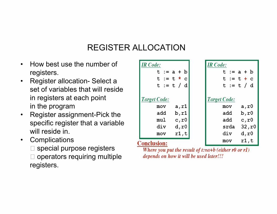
REGISTER ALLOCATION

• How best use the number of registers.

• Register allocation- Select a set of variables that will reside in registers at each pointin the programin the program

• Register assignment-Pick the specific register that a variable will reside in.

• Complications special purpose registers operators requiring multiple registers.

EVALUATION ORDER Choosing the order of instructions

to best utilize resources Picking the optimal order Simplest Approach

Target code will perform all operations in the same order as the IR code

Trickier Approach Consider re-ordering operations May produce better code... Get operands into registers just before they areneeded... May use registers more efficiently

● Input to the Code Generator● The Target Program● Instruction Selection● Register Allocation

Evaluation Order

Issues in the Design of

Code ● Evaluation OrderCode

generator

Input to Code Generator & Target Program

ST a,R0LD R0,a Produces redundant instruction

Output may be in the forms

-Absolute machine language(Executable code)- It can placed in a fixed location in memory and immediately executed-Relocatable machine language(Object files for linker)- It -Relocatable machine language(Object files for linker)- It allows subprograms to be compiled separately-Assembly language(Facilitates debugging)- It produces assembly code

The Target Language• Familiarity with the target machine and its instruction set is

a prerequisite for designing a good code generator.The target language is assembly code for a simplecomputer that is representative of many register machinesi.e. A Simple Target Machine Modeli.e. A Simple Target Machine Model

• Our target computer models a three-address machine withload and store operations, computation operations, jumpoperations, and conditional jumps.

• The underlying computer is a byte-addressable machinewith n general purpose registers.

Assume the following kinds of instructions are available:• Load operations : LD r, x loads value in location x in register r.• Store operations: ST x, r stores value in register r in location x.• Computation operations: SUB r1, r2, r3 computes r1 = r2 – r3• Unconditional jumps: BR L causes control to branch to machine instruction with label L.• Conditional jumps: BLTZ r, L causes to jump to label L if the value in • Conditional jumps: BLTZ r, L causes to jump to label L if the value in register r is less than zero.

EXAMPLE TARGET MACHINE

Program and Instruction Costs

• For simplicity, take the cost of an instruction to be one plus the costs associated with the addressing modes of the operands.• Addressing modes involving registers have zero additional cost, while those involving a memory location or constant in cost, while those involving a memory location or constant in them have an additional cost of one, because such operands have to be stored in the words following the instruction.

cost of instruction = 1 + cost(source mode) + cost(destination mode)

Properties:

A DAG for basic block is a directedacyclic graph with the followinglabels on nodes:1.The leaves of graph are labeledby unique identifier and that

DAG representation for basic blocksDefinition:Directed Acyclic Graph is a special kind ofAbstract syntax tree. Each node of it containsa unique value. It does not contain any cyclesin it, hence called Acyclic

by unique identifier and thatidentifier can be variable names orconstants.2.Interior nodes of the graph islabeled by an operator symbol.3.Nodes are also given a sequenceof identifiers for labels to store thecomputed value.

Applications:•DAGs are a type of data structure. It is used toimplement transformations on basic blocks.•Renaming temporaries•DAG provides a good way to determine the commonsub-expression.•It gives a picture representation of how the valuecomputed by the statement is used in subsequentstatements.

Algorithm for construction of DAGInput: It contains a basic blockOutput: It contains the following information:Each node contains a label. For leaves, the label is an identifier.Each node contains a list of attached identifiers to hold the computed values.

Case (i) x:= y OP zCase (ii) x:= OP yCase (iii) x:= y yy ZZ

OPOP

Method:Step 1:If y operand is undefined then create node(y).If z operand is undefined then for case(i) create node(z).Step 2:For case(i), create node(OP) whose right child is node(z) and left child is node(y).For case(ii), check whether there is node(OP) with one child node(y).For case(iii), node n will be node(y).

Problem 1:Consider the following expression and construct a DAG for it-

( a + b ) x ( a + b + c )Solution-

Three Address Code for the given expression is-

T1 = a + bT2 = T1 + c

*,T3T2 = T1 + cT3 = T1 x T2

DAG is ---------------- +,T1

ba

c

+,T2*,T3

Problem-02:

Consider the following block and construct a DAG for it-

(1) a = b x c(2) d = b(3) e = d x c

Now, the optimized block can be generated by traversing the DAG.•The common sub-expression e = d x c which is actually b x c (since d = b) is eliminated.•The dead code b = e is eliminated.

The optimized block is-

(1) a = b x c(3) e = d x c(4) b = e(5) f = b + c(6) g = f + d

(1) a = b x c(2) d = b(3) f = a + c(4) g = f + d

Problem-03:

Consider the following three address statement:1.S1:= 4 * i2.S2:= a[S1]3.S3:= 4 * i4.S4:= b[S3]4.S4:= b[S3]5.S5:= s2 * S46.S6:= prod + S57.Prod:= s68.S7:= i+19.i := S710.if i<= 20 goto (1)

Consider the following three address statement:1.S1:= 4 * i2.S2:= a[S1]3.S3:= 4 * i4.S4:= b[S3]5.S5:= s2 * S46.S6:= prod + S57.Prod:= s67.Prod:= s68.S7:= i+19.i := S710.if i<= 20 goto (1)

Consider the following three address statement:1.S1:= 4 * i2.S2:= a[S1]3.S3:= 4 * i4.S4:= b[S3]5.S5:= s2 * S46.S6:= prod + S57.Prod:= s68.S7:= i+18.S7:= i+19.i := S710.if i<= 20 goto (1)

Consider the following three address statement:1.S1:= 4 * i2.S2:= a[S1]3.S3:= 4 * i4.S4:= b[S3]5.S5:= s2 * S46.S6:= prod + S57.Prod:= s67.Prod:= s68.S7:= i+19.i := S710.if i<= 20 goto (1)

Consider the following three address statement:1.S1:= 4 * i2.S2:= a[S1]3.S3:= 4 * i4.S4:= b[S3]5.S5:= s2 * S46.S6:= prod + S57.Prod:= s68.S7:= i+19.i := S79.i := S710.if i<= 20 goto (1)

Consider the following three address statement:1.S1:= 4 * i2.S2:= a[S1]3.S3:= 4 * i4.S4:= b[S3]5.S5:= s2 * S46.S6:= prod + S57.Prod:= s68.S7:= i+18.S7:= i+19.i := S710.if i<= 20 goto (1)

A Simple Code Generator

● Introduction● Two Data structures

Register descriptor Address or variable

descriptorGenerator descriptor● Code Generation algorithm● Getreg()● Cost of an instruction

Introduction

This code generator algorithm generates code for a single basic block.

It considers each three address instructions in turn, and keeps track of what values are in what registers so it can avoid unnecessary load and stores.

Uses new function getreg to assign registers to variables getreg has access to registers and address descriptors for

all the variables of basic block and may also have access to

Example Three address statement

consider the three-addressstatement t := b+d.It can have the followingsequence of codes:

certain data flow information such as the variables that are live on exit from the block.

Computed results are kept in registers as long as possible, which means:

– Result is needed in another computation– Register is kept up to a procedure call or end of

block Checks if operands to three-address code are available in

registers

ADD Rj(d), Ri(b) Cost = 1(or)ADD d, Ri(b) Cost = 2(or)MOV d, Rj Cost = 3ADD Rj(d), Ri(b)

Data structures used in CG

Register descriptor-A register descriptor keepstrack of what is currently stored in a register at aparticular point in the code, e.g. a local variable,argument, global variable, etc.

Eg., MOV a,R0 “R0 contains a”‘a variable stored in register R0’

Address descriptor- An address descriptor keepstrack of the location where the current value of thename can be found at run time, e.g. a register,stack location, memory address, etc.

Eg., MOV a,R0MOV R0, R1 “a in R0 and R1”Address descriptor(a)={1000,R0}Register descriptor(R0)={a}

Examplet = a - bx = y op z

1. t=getreg(a,b) So t is register descriptor

t = a - b

x = y op z

is register descriptor that contains the value of t. update address descriptor of t which is stored in R0’getreg()- a stored in R0 and R0 hold the value of a.

Op z’, L Where b’ is one of the locations of b

Sub b,R0 Update register/address descriptor of t to include R0Sub b,R0 Update register/address descriptor of t to include R0

Target code

Mov b,R0ADD c,R0

IR instructions

t1=b+c R0Example

Target codeMov b,R0 Mov b,R1ADD c,R0 ADD d,R1

IR instructionst1=b+c R0t2=b*d R1

Target codeMov b,R0 Mov b,R1ADD c,R0 ADD d,R1

Mul R1(t2),R0(t1) R0(t3)

IR instructionst1=b+c R0t2=b*d R1t3=t1*t2 R0

Target code

Mul R1(t2), R0(t1) R0(t3)Sub R1(t2), R0(t3) R0(a)

IR instructionst1=b+c R0t2=b*d R1t3=t1*t2 R0a=t3-t2 R0

Cost=12

Mov a,R0 cost=1+1+0=2Sub b,R0 cost=1+1+0-2

Mov a,R1 cost=1+1+0=2Sub c,R1 cost=1+1+0-2

Add R1,R0 cost=1+0+0=1

Add R1,R0 cost=1+0+0=1Mov R0,d cost=1+0+1-2

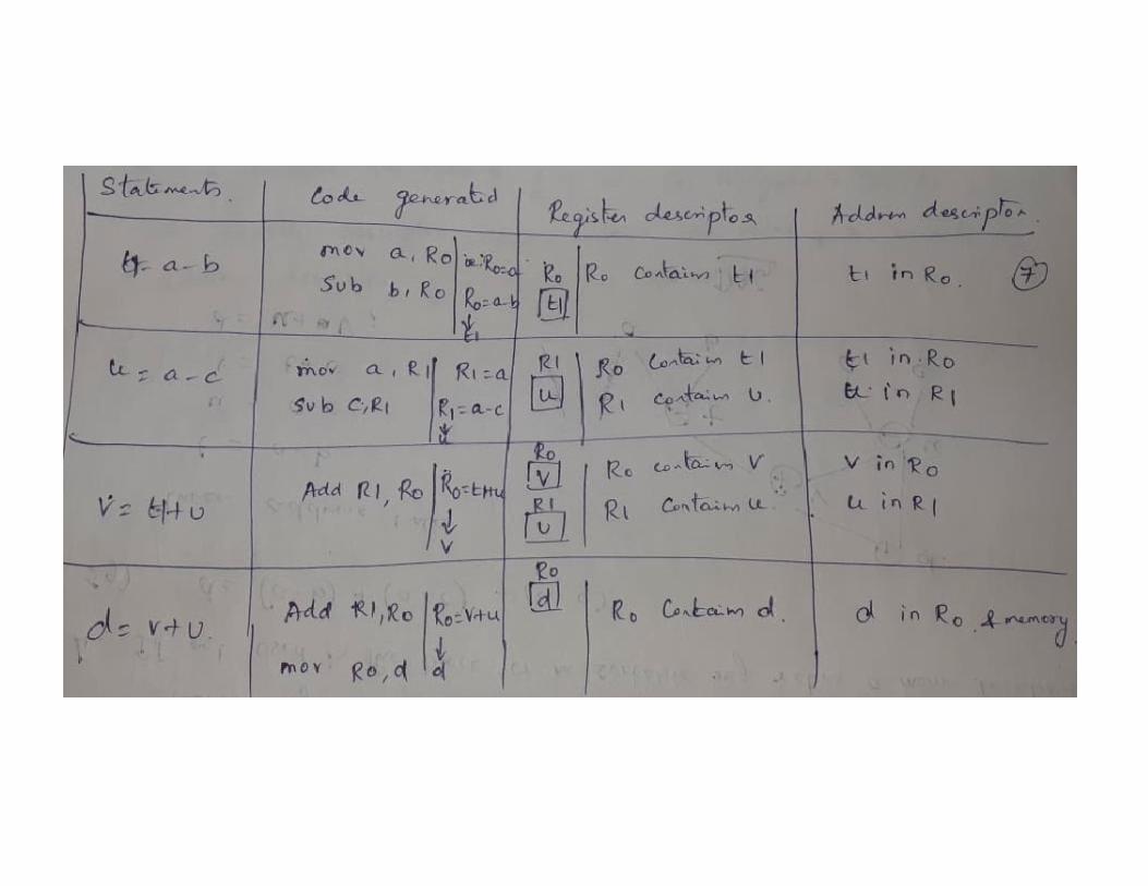
Optimization of

Basic BlockBasic Block

Course Material Principles of Compiler Design Unit I Lexical ...

Documents

Transcript of Course Material Principles of Compiler Design Unit I Lexical ...