Horne R - Modern Well Test Analysis, A Computer Aided Aproach (1)
Upload
imsciencesCategory
view
7download
0
Fundamentals of
Financial ManagementJames C. Van HorneJohn M. Wachowicz, Jr.
13th EditionDo you want to understand how fi nancial decisions impact the value of a company? If you are new to fi nancial management or studying for a professional qualifi cation, this user-friendly textbook makes the challenges facing today’s rapidly changing business world easier to understand.
Now in its 13th edition, Fundamentals of Financial Management maintains its dedication to the fi nancial decision-making process and the analysis of value creation, but develops a more international scope and introduces new topics into the debate. Current discussions on corporate governance, ethical dilemmas, globalization of fi nance, strategic alliances and the growth of outsourcing have been added with examples and boxed features to aid understanding and provide a more global perspective of fi nancial management.
What’s New?
Chapter 1 - Expanded coverage of Corporate Social Responsibility • including the concept of Sustainability.
Chapter 6 – The discussion of fi nancial statement analysis includes • the push for convergence of accounting standards around the world.
Chapter 9 – Cash and marketable securities management material • expanded and updated.
Chapter 24 - The updated chapter on International Financial • Management includes discussion of Islamic sukuk bonds.
an imprint of www.pearson-books.comFront cover image: © Getty Images
“The book provides the reader with information about the current ‘hot-topics’ in fi nance and has a clear emphasis on the basic principles of fi nancial management without repetition. Furthermore, as simple language is used, the book can be easily understood by students that are not native speakers of English.”Axel-Adam Müller, Lancaster
“This is the best book I have found so far.”Jean Bellemans, Free University of Brussels
Authors:
James C. Van Horne, Professor of Banking and Finance at Stanford University is also the author of Financial Management and Policy, a Pearson Education text.
John M. Wachowicz, Jr., Professor of Finance at The University of Tennessee.
“…a useful text either as preparation for a second year course, or as a text for a fi rst year fi nancial management course that provides a ‘fi rst sweep’ of the major fi nancial management topics. Not many texts cover this ground well.” Brian Wright, Exeter
Ideal for introductory courses in fi nancial management, for a professional qualifi cation and as a reference for practitioners.
On the reading list for Association of Chartered Certifi ed Accountants (ACCA) Qualifi cation Paper (F9) Financial Management.
Suggested reading for Certifi ed Management Accountant (CMA) examination.
Translated into over ten languages and received fi rst place among business academic texts in Pearson’s top 50 best seller’s translation list.
Visit www.pearsoned.co.uk/wachowicz to access free student resources including:
Self-test multiple-choice, true/false and essay • questions.Link to author’s award-winning website for even more • online testing material, along with exercises and regularly updated links to additional support material. Online glossary to explain key terms. • Excel templates for spread-sheet approach to • end-of-chapter problem solving.New for this edition! Link to PowerPoint slides on • key chapters and learn how to use Excel to solve problems.
Fundamentals of Financial M
anagement
13thEdition
Van Horne
Wachow
icz
CVR_VANH3630_13_SE_CVR.indd 1 23/9/08 10:35:34

••
Fundamentals of
Financial Management
Visit the Van Horne and Wachowicz: Fundamentals of Financial Managementthirteenth edition Companion Website at www.pearsoned.co.uk/wachowiczto find valuable student learning material including:
l Learning objectives for each chapterl Multiple choice, true/false and essay questions to test your understanding l PowerPoint presentations for each chapter to remind you of key concepts l An online glossary to explain key terms and flash cards to test your knowledge
of key terms and definitions in each chapter l Excel templates for end of chapter problems to help you model a spread sheet
approach to solving the probleml Link to author’s own award-winning website with even more multiple choice and
true/false questions, as well as web-based exercises and regularly updated linksto additional support material
l New to this edition, PowerPoint presentations for key chapters integrating anddemonstrating how Excel can be used to solve calculations.
FUNO_A01.qxd 9/19/08 13:56 Page i

••
We work with leading authors to develop thestrongest educational materials in business andfinance, bringing cutting-edge thinking and bestlearning practice to a global market.
Under a range of well-known imprints, includingFinancial Times Prentice Hall, we craft high qualityprint and electronic publications which help readersto understand and apply their content, whetherstudying or at work.
To find out more about the complete range of ourpublishing, please visit us on the World Wide Web at:www.pearsoned.co.uk
FUNO_A01.qxd 9/19/08 13:56 Page ii

••
Fundamentals of
Financial Managementthirteenth edition
James C. Van HorneStanford University
John M. Wachowicz, Jr.The University of Tennessee
FUNO_A01.qxd 9/19/08 13:56 Page iii

••
Pearson Education LimitedEdinburgh GateHarlowEssex CM20 2JEEngland
and Associated Companies throughout the world
Visit us on the World Wide Web at:www.pearsoned.co.uk
Previous editions published under the Prentice Hall imprintThirteenth edition published 2008
© Pearson Education Limited 2009, 2005© 2001, 1998 by Prentice-Hall, Inc.
The rights of James C. Van Horne and John M. Wachowicz, Jr. to be identified as authors of this work have been asserted by them in accordance with the Copyright, Designs and Patents Act 1988.
All rights reserved. No part of this publication may be reproduced, stored in a retrieval system, or transmitted in any form or by any means, electronic, mechanical, photocopying, recording or otherwise, without either the prior written permission of the publisher or a licence permitting restricted copying in the United Kingdom issued by the Copyright Licensing Agency Ltd, Saffron House, 6–10 Kirby Street, London EC1N 8TS.
All trademarks used herein are the property of their respective owners. The use of any trademark in this text does not vest in the author or publisher any trademark ownership rights in such trademarks, nor does the use of such trademarks imply any affiliation with or endorsement of this book by such owners.
ISBN: 978-0-273-71363-0
British Library Cataloguing-in-Publication DataA catalogue record for this book is available from the British Library
Library of Congress Cataloguing-in-Publication DataVan Horne, James C.
Fundamentals of financial management / James C. Van Horne, John M. Wachowicz. – 13th ed.p. cm.
Includes bibliographical references and index.ISBN 978-0-273-71363-0 (pbk. : alk. paper) 1. Corporations–Finance. 2. Business
enterprises–Finance. I. Wachowicz, John Martin. II. Title.HG4026.V36 2008658.15—dc22
200802736510 9 8 7 6 5 4 312 11 10 09
Typeset in 10/12pt Minion by 35Printed and bound by Ashford Colour Press Ltd., Gosport
The publisher’s policy is to use paper manufactured from sustainable forests.
FUNO_A01.qxd 4/18/09 10:23 AM Page iv

••
To Mimi, Drew, Stuart, and StephenJames C. Van Horne
To Emerson, John, June, Lien, and PatriciaJohn M. Wachowicz, Jr.
FUNO_A01.qxd 9/19/08 13:56 Page v

••
FUNO_A01.qxd 9/19/08 13:56 Page vi

••
vii
Brief Contents
l l l Part 1 Introduction to Financial Management
1 The Role of Financial Management 12 The Business, Tax and Financial Environments 17
l l l Part 2 Valuation
3 The Time Value of Money 414 The Valuation of Long-Term Securities 735 Risk and Return 97Appendix A Measuring Portfolio Risk 117Appendix B Arbitrage Pricing Theory 119
l l l Part 3 Tools of Financial Analysis and Planning
6 Financial Statement Analysis 127Appendix Deferred Taxes and Financial Analysis 1587 Funds Analysis, Cash-Flow Analysis, and Financial Planning 169Appendix Sustainable Growth Modeling 190
l l l Part 4 Working Capital Management
8 Overview of Working Capital Management 2059 Cash and Marketable Securities Management 221
10 Accounts Receivable and Inventory Management 24911 Short-Term Financing 281
l l l Part 5 Investment in Capital Assets
12 Capital Budgeting and Estimating Cash Flows 30713 Capital Budgeting Techniques 323Appendix A Multiple Internal Rates of Return 341Appendix B Replacement Chain Analysis 34314 Risk and Managerial (Real) Options in Capital Budgeting 353
FUNO_A01.qxd 9/19/08 13:56 Page vii

••
l l l Part 6 The Cost of Capital, Capital Structure, and Dividend Policy
15 Required Returns and the Cost of Capital 381Appendix A Adjusting the Beta for Financial Leverage 407Appendix B Adjusted Present Value 40816 Operating and Financial Leverage 41917 Capital Structure Determination 45118 Dividend Policy 475
l l l Part 7 Intermediate and Long-Term Financing
19 The Capital Market 50520 Long-Term Debt, Preferred Stock, and Common Stock 527Appendix Refunding a Bond Issue 54421 Term Loans and Leases 553Appendix Accounting Treatment of Leases 567
l l l Part 8 Special Areas of Financial Management
22 Convertibles, Exchangeables, and Warrants 577Appendix Option Pricing 58923 Mergers and Other Forms of Corporate Restructuring 603Appendix Remedies for a Failing Company 63024 International Financial Management 647
Appendix 679
Glossary 689
Commonly Used Symbols 705
Index 707
Brief Contents
viii
FUNO_A01.qxd 9/19/08 13:56 Page viii

••
ix
Contents
Acknowledgements xixPreface xxi
l l l Part 1 Introduction to Financial Management
1 The Role of Financial Management 1Objectives 1Introduction 2What Is Financial Management? 2The Goal of the Firm 3Corporate Governance 8Organization of the Financial Management Function 8Organization of the Book 10Key Learning Points 13Questions 14Selected References 14
2 The Business, Tax, and Financial Environments 17Objectives 17The Business Environment 18The Tax Environment 20The Financial Environment 27Key Learning Points 35Questions 36Self-Correction Problems 37Problems 37Solutions to Self-Correction Problems 38Selected References 39
l l l Part 2 Valuation
3 The Time Value of Money 41Objectives 41The Interest Rate 42Simple Interest 43Compound Interest 43Compounding More Than Once a Year 59Amortizing a Loan 62Summary Table of Key Compound Interest Formulas 63Key Learning Points 63
FUNO_A01.qxd 9/19/08 13:56 Page ix

Questions 64Self-Correction Problems 64Problems 65Solutions to Self-Correction Problems 69Selected References 71
4 The Valuation of Long-Term Securities 73Objectives 73Distinctions Among Valuation Concepts 74Bond Valuation 75Preferred Stock Valuation 78Common Stock Valuation 79Rates of Return (or Yields) 83Summary Table of Key Present Value Formulas for Valuing Long-Term
Securities 88Key Learning Points 88Questions 89Self-Correction Problems 90Problems 91Solutions to Self-Correction Problems 93Selected References 95
5 Risk and Return 97Objectives 97Defining Risk and Return 98Using Probability Distributions to Measure Risk 99Attitudes Toward Risk 101Risk and Return in a Portfolio Context 103Diversification 104The Capital-Asset Pricing Model (CAPM) 106Efficient Financial Markets 114Key Learning Points 116Appendix A: Measuring Portfolio Risk 117Appendix B: Arbitrage Pricing Theory 119Questions 121Self-Correction Problems 122Problems 122Solutions to Self-Correction Problems 125Selected References 126
l l l Part 3 Tools of Financial Analysis and Planning
6 Financial Statement Analysis 127Objectives 127
Contents
x
••
FUNO_A01.qxd 9/19/08 13:56 Page x

Financial Statements 128A Possible Framework for Analysis 134Balance Sheet Ratios 138Income Statement and Income Statement/Balance Sheet Ratios 141Trend Analysis 152Common-Size and Index Analysis 153Key Learning Points 156Summary of Key Ratios 156Appendix: Deferred Taxes and Financial Analysis 158Questions 159Self-Correction Problems 160Problems 161Solutions to Self-Correction Problems 165Selected References 167
7 Funds Analysis, Cash-Flow Analysis, and Financial Planning 169Objectives 169Flow of Funds (Sources and Uses) Statement 170Accounting Statement of Cash Flows 176Cash-Flow Forecasting 180Range of Cash-Flow Estimates 184Forecasting Financial Statements 186Key Learning Points 190Appendix: Sustainable Growth Modeling 190Questions 194Self-Correction Problems 195Problems 197Solutions to Self-Correction Problems 200Selected References 203
l l l Part 4 Working Capital Management
8 Overview of Working Capital Management 205Objectives 205Introduction 206Working Capital Issues 208Financing Current Assets: Short-Term and Long-Term Mix 210Combining Liability Structure and Current Asset Decisions 215Key Learning Points 216Questions 216Self-Correction Problem 217Problems 217Solutions to Self-Correction Problem 218Selected References 219
Contents
xi
••
FUNO_A01.qxd 9/19/08 13:56 Page xi

9 Cash and Marketable Securities Management 221Objectives 221Motives for Holding Cash 222Speeding Up Cash Receipts 223S-l-o-w-i-n-g D-o-w-n Cash Payouts 228Electronic Commerce 231Outsourcing 233Cash Balances to Maintain 234Investment in Marketable Securities 235Key Learning Points 244Questions 245Self-Correction Problems 245Problems 246Solutions to Self-Correction Problems 247Selected References 248
10 Accounts Receivable and Inventory Management 249Objectives 249Credit and Collection Policies 250Analyzing the Credit Applicant 258Inventory Management and Control 263Key Learning Points 273Questions 274Self-Correction Problems 274Problems 275Solutions to Self-Correction Problems 278Selected References 279
11 Short-Term Financing 281Objectives 281Spontaneous Financing 282Negotiated Financing 287Factoring Accounts Receivable 298Composition of Short-Term Financing 300Key Learning Points 301Questions 302Self-Correction Problems 302Problems 303Solutions to Self-Correction Problems 305Selected References 306
l l l Part 5 Investment in Capital Assets
12 Capital Budgeting and Estimating Cash Flows 307Objectives 307The Capital Budgeting Process: An Overview 308
Contents
xii
••
FUNO_A01.qxd 9/19/08 13:56 Page xii

Generating Investment Project Proposals 308Estimating Project “After-Tax Incremental Operating Cash Flows” 309Key Learning Points 318Questions 318Self-Correction Problems 319Problems 319Solutions to Self-Correction Problems 321Selected References 322
13 Capital Budgeting Techniques 323Objectives 323Project Evaluation and Selection: Alternative Methods 324Potential Difficulties 330Project Monitoring: Progress Reviews and Post-Completion Audits 340Key Learning Points 340Appendix A: Multiple Internal Rates of Return 341Appendix B: Replacement Chain Analysis 343Questions 345Self-Correction Problems 346Problems 347Solutions to Self-Correction Problems 349Selected References 350
14 Risk and Managerial (Real) Options in Capital Budgeting 353Objectives 353The Problem of Project Risk 354Total Project Risk 357Contribution to Total Firm Risk: Firm-Portfolio Approach 364Managerial (Real) Options 368Key Learning Points 373Questions 373Self-Correction Problems 374Problems 375Solutions to Self-Correction Problems 377Selected References 379
l l l Part 6 The Cost of Capital, Capital Structure, and Dividend Policy
15 Required Returns and the Cost of Capital 381Objectives 381Creation of Value 382Overall Cost of Capital of the Firm 383The CAPM: Project-Specific and Group-Specific Required Rates of Return 396Evaluation of Projects on the Basis of Their Total Risk 401Key Learning Points 406
Contents
xiii
••
FUNO_A01.qxd 9/19/08 13:56 Page xiii

Appendix A: Adjusting the Beta for Financial Leverage 407Appendix B: Adjusted Present Value 408Questions 410Self-Correction Problems 411Problems 412Solutions to Self-Correction Problems 415Selected References 417
16 Operating and Financial Leverage 419Objectives 419Operating Leverage 420Financial Leverage 427Total Leverage 435Cash-Flow Ability to Service Debt 436Other Methods of Analysis 439Combination of Methods 440Key Learning Points 441Questions 442Self-Correction Problems 443Problems 444Solutions to Self-Correction Problems 446Selected References 449
17 Capital Structure Determination 451Objectives 451A Conceptual Look 452The Total-Value Principle 456Presence of Market Imperfections and Incentive Issues 458The Effect of Taxes 461Taxes and Market Imperfections Combined 463Financial Signaling 465Timing and Financial Flexibility 465Financing Checklist 466Key Learning Points 467Questions 468Self-Correction Problems 468Problems 469Solutions to Self-Correction Problems 471Selected References 473
18 Dividend Policy 475Objectives 475Passive versus Active Dividend Policies 476Factors Influencing Dividend Policy 481Dividend Stability 484
Contents
xiv
••
FUNO_A01.qxd 9/19/08 13:56 Page xiv

Stock Dividends and Stock Splits 486Stock Repurchase 491Administrative Considerations 495Key Learning Points 496Questions 497Self-Correction Problems 498Problems 499Solutions to Self-Correction Problems 501Selected References 502
l l l Part 7 Intermediate and Long-Term Financing
19 The Capital Market 505Objectives 505Déjà Vu All Over Again 506Public Issue 507Privileged Subscription 509Regulation of Security Offerings 512Private Placement 516Initial Financing 519Signaling Effects 520The Secondary Market 522Key Learning Points 522Questions 523Self-Correction Problems 524Problems 524Solutions to Self-Correction Problems 525Selected References 526
20 Long-Term Debt, Preferred Stock, and Common Stock 527Objectives 527Bonds and Their Features 528Types of Long-Term Debt Instruments 529Retirement of Bonds 532Preferred Stock and Its Features 534Common Stock and Its Features 538Rights of Common Shareholders 539Dual-Class Common Stock 542Key Learning Points 543Appendix: Refunding a Bond Issue 544Questions 546Self-Correction Problems 547Problems 548Solutions to Self-Correction Problems 550Selected References 551
Contents
xv
••
FUNO_A01.qxd 9/19/08 13:56 Page xv

21 Term Loans and Leases 553Objectives 553Term Loans 554Provisions of Loan Agreements 556Equipment Financing 558Lease Financing 559Evaluating Lease Financing in Relation to Debt Financing 562Key Learning Points 567Appendix: Accounting Treatment of Leases 567Questions 570Self-Correction Problems 571Problems 572Solutions to Self-Correction Problems 573Selected References 575
l l l Part 8 Special Areas of Financial Management
22 Convertibles, Exchangeables, and Warrants 577Objectives 577Convertible Securities 578Value of Convertible Securities 581Exchangeable Bonds 584Warrants 585Key Learning Points 589Appendix: Option Pricing 589Questions 595Self-Correction Problems 596Problems 597Solutions to Self-Correction Problems 599Selected References 600
23 Mergers and Other Forms of Corporate Restructuring 603Objectives 603Sources of Value 604Strategic Acquisitions Involving Common Stock 608Acquisitions and Capital Budgeting 615Closing the Deal 617Takeovers, Tender Offers, and Defenses 620Strategic Alliances 622Divestiture 623Ownership Restructuring 626Leveraged Buyouts 627Key Learning Points 629Appendix: Remedies for a Failing Company 630Questions 635Self-Correction Problems 636Problems 638
Contents
xvi
••
FUNO_A01.qxd 9/19/08 13:56 Page xvi

Solutions to Self-Correction Problems 641Selected References 643
24 International Financial Management 647Objectives 647Some Background 648Types of Exchange-Rate Risk Exposure 652Management of Exchange-Rate Risk Exposure 656Structuring International Trade Transactions 668Key Learning Points 671Questions 672Self-Correction Problems 673Problems 674Solutions to Self-Correction Problems 676Selected References 677
Appendix 679Table I: Future value interest factor 680Table II: Present value interest factor 682Table III: Future value interest factor of an (ordinary) annuity 684Table IV: Present value interest factor of an (ordinary) annuity 686Table V: Area of normal distribution that is Z standard deviations
to the left or right of the mean 688
Glossary 689Commonly Used Symbols 705Index 707
Contents
xvii
••
FUNO_A01.qxd 9/19/08 13:56 Page xvii

••
Supporting resourcesVisit www.pearsoned.co.uk/wachowicz to find valuable online resources
Companion Website for studentsl Learning objectives for each chapterl Multiple choice, true/false and essay questions to test your understanding l PowerPoint presentations for each chapter to remind you of key concepts l An online glossary to explain key terms and flash cards to test your knowledge of key terms and
definitions in each chapter l Excel templates for end of chapter problems to help you model a spread sheet approach to solving
the probleml Link to author’s own award-winning website with even more multiple choice and true/false
questions, as well as web-based exercises and regularly updated links to additional supportmaterial
l New to this edition, PowerPoint presentations for each chapter integrating and demonstrating howExcel can be used to help solve calculations.
For instructorsl Extensive Instructor’s Manual including answers to questions, solutions to problems and solutions
to self-correction problemsl PowerPoint slides plus PDF’s of all figures and tables from the bookl Testbank of additional question material.
Also: The Companion Website provides the following features:l Search tool to help locate specific items of contentl E-mail results and profile tools to send results of quizzes to instructorsl Online help and support to assist with website usage and troubleshooting.
For more information please contact your local Pearson Education representative or visit www.pearsoned.co.uk/wachowicz
FUNO_A01.qxd 9/19/08 13:56 Page xviii

Acknowledgements
We would like to express our gratitude to the following academics, as well as additionalanonymous reviewers, who provided invaluable feedback on this book during the develop-ment of the thirteenth edition:
Dr Brian Wright, at Exeter UniversityDr Axel F.A. Adam-Muller, at Lancaster UniversityDr Graham Sadler, at Aston University
We are grateful to the following for permission to reproduce copyright material:Figure 10.3 D&B Composite Rating from a Reference Book and a Key to Ratings, 2003.
Reprinted by permission, Dun & Bradstreet, 2007; Cartoon on page 272 from “What isneeded to make a ‘just-in-time’ system work,” Iron Age Magazine, June 7, 1982. Reprinted bypermission, Iron Age.
Anheuser-Busch Companies, Inc., for permission to reproduce their logo and an extractfrom the 2006 Annual Report, p. 36. Copyright © 2006 Anheuser-Busch Companies Inc. Usedby permission. All rights reserved; BP p. l.c, for permission to reproduce an extract from theBP Annual Report 2006, p. 27. Copyright © 2006 BP p. l.c. Used by permission. All rightsreserved; Cameco Corporation, for permission to reproduce their logo and an extract fromthe Cameco Corporation Annual Report 2006 (www.cameco.com/investor_relations/annual/2006/html/mda/fuel_services.php). Copyright © 2006 Cameco Corporation. Used by permis-sion. All rights reserved; CCH Incorporated for permission to reproduce their logo andextracts adapted from “Ask Alice about Ethics” and “Ask Alice about Accountants”, repro-duced from www.toolkit.cch.com. Reproduced with permission from CCH Business Owner’sToolkit, published and copyrighted by CCH Incorporated; CFO Publishing Corporation forpermission to reproduce the CFO Asia logo and extracts reproduced from “Virtue Rewarded,”CFO Asia, O’Sullivan K., (November 2006), pp. 58–63 and “One Continent, One PaymentSystem,” CFO Asia (April 2007), p. 41, www.cfoasia.com. Copyright © 2007 CFO PublishingCorporation. Used by permission. All rights reserved; CFO Publishing Corporation for per-mission to reproduce the CFO logo and extracts adapted from “A Trade Secret Comes toLight, Again,” CFO, by Leone M., November 2005, pp. 97–99. “Four Eyes are Better,” CFO, byO’Sullivan K., June 2006, p. 21; “More Rules, Higher Profits,” CFO, Durfee D., August 2006,p. 24 and “Buy it Back, And Then?” CFO, Durfee D., September 2006, p. 22, www.cfo.com.Copyright © 2006 CFO Publishing Corporation. Used by permission. All rights reserved; TheCoca-Cola Company for extracts from their Annual Report, 2006 (Form 10-k) pp. 59 and 65,and permission to reproduce their registered trademarks: Coca-Cola and the Contour Bottle.Coca-Cola and the Contour Bottle are registered trademarks of The Coca-Cola Company;Crain Communications Inc., for permission to reproduce the Financial Week logo and adaptextracts from: “Shell Game Grows as an Exit Strategy,” Financial Week, by Byrt F., January 152007, pp. 3 and 18; “New Leasing Rules Could Hammer Corporate Returns,” Financial Week,by Scott M., April 2 2007; “Spin-Off Frenzy Sets New Record,” Financial Week, by Byrt F.,April 9 2007, pp. 3 and 21 and “A Bent for Cash. Literally,” Financial Week, by Johnston M.,July 23 2007, p. 10, www.financialweek.com. Copyright © 2007 by Crain CommunicationsInc. Used by permission. All rights reserved; Cygnus Business Media for permission to repro-duce its Supply & Demand Chain Executive logo and an extract from “More than $1 TrillionSeen Unnecessarily Tied Up in Working Capital,” Supply & Demand Chain Executive,June/July 2006, p. 10, www.sdcexec.com Copyright © 2006 Cygnus Business Media. Used bypermission. All rights reserved; Debra Yergen for permission to adapt an extract from “TheCheck’s in the Box,” Canadian National Treasurer, by Yergen D., December 2005/January
xix
••
FUNO_A01.qxd 9/19/08 13:56 Page xix

2006, pp. 14–15, www.tmac.ca. Copyright © 2006 Debra Yergen. Used by permission. Allrights reserved; Dell Inc. for extracts from their quarterly and annual reports. Copyright ©2004 Dell Inc. All rights reserved; The Economist Newspaper Limited for permission to repro-duce their logo and extracts in Chapter 6, p. 127, “Speaking in tongues” adapted from Speakingin Tongues, The Economist, pp. 77–78, www.economist.com © The Economist NewspaperLimited, London (19–25 May 2007), Used with permission; Chapter 23, p. 603, TextboxFeature from The Economist, p. 90, www.economist.com © The Economist Newspaper Limited,London (13 January 2007), Used with permission; Chapter 24, p. 654, “Big Mac Purchasing –Power Parity”, Based on data in “Cash and carry – The hamburger standard” table at www.economist.com/finance/displaystory.cfm?story_id=9448015 in The Economist © The EconomistNewspaper Limited, London (2007), Used with permission; Financial Executives InternationalIncorporated for permission to reproduce their logo and extracts from “Bridging the Finance-Marketing Divide,” Financial Executive, by See, E., July/August 2006, pp. 50–53; “Sarbanes-Oxley Helps Cost of Capital: Study,” Financial Executive, by Marshall J. and Heffes E.M., October2006, p. 8; “Soul-Searching over U.S. Competitiveness,” Financial Executive, by Cheny G.A.,June 2007, pp. 18–21; “BPO: Developing Market, Evolving Strategies,” Financial Executive, June2007, pp. 38–44, www.financialexecutives.org. Copyright © 2006/2007 Financial ExecutivesInternational Incorporated. Used by permission. All rights reserved; FRBNY for data from“The Basics of Trade and Exchange,” www.newyorkfed.org/education/fx/foreign.html;Hermes Pensions Management Ltd for extracts reproduced from “The Hermes Principles:What Shareholders Expect of Public Companies – and What Companies Should Expect of their Investors,” p. 11, www.hermes.co.uk/pdf/corporate_governance/Hermes_Principles.pdf. Copyright © Hermes Pensions Management Ltd; James Hartshorn for an extract reproducedfrom “Sustainability: Why CFOs Need to Pay Attention,” Canadian Treasurer, by Hartshorn J.,22 June/July 2006, p. 15. Used by permission. All rights reserved; The Motley Fool for per-mission to reproduce their logo and extracts from www.fool.com; Nasdaq Stock Market Inc.for permission to reproduce an extract from “Market Mechanics: A Guide to US StockMarkets, release 1.2,” The NASDAQ Stock Market Educational Foundation Inc., by Angel J.J.,2002, p. 7. Copyright © 2002 by the Nasdaq Stock Market Inc. Used by permission. All rightsreserved; Penton Media Inc. for permission to reproduce the Business Finance logo andextracts from “Asset-based Lending Goes Mainstream,” Business Finance, by Kroll K.M., May2006, pp. 39–42, “M&A Synergies/Don’t Count On It,” Business Finance, by Cummings J.,October 2006, p. 14, “Payment Processing: The Sea Change Continues,” Business Finance, byKroll K.M., December 2006, “7 Steps to Optimize A/R Management,” Business Finance,by Salek J., April 2007, p. 45, www.bfmag.com. Copyright © 2006/2007 Penton Media, Inc.Used by permission. All rights reserved; Treasury Management Association of Canada for per-mission to reproduce the TMAC logo, www.tmac.ca. Copyright © 2008 TMAC. Reproducedwith permission. All rights reserved; Volkswagen AG for permission to reproduce their logoand an extract from their Annual Report 2006, p. 77. Copyright © 2006 by Volkswagen AG.Used by permission. All rights reserved.
We are grateful to the Financial Times Limited for permission to reprint the followingmaterial:
Chapter 20 “It’s a question of the right packaging” © Financial Times, 25 July 2007;Chapter 20 “One share, one-vote hopes dashed” © Financial Times, 5 June 2007; Chapter 22“Warrants win over the bulls” © Financial Times, 13 March 2007; Chapter 23 “Chapter 11 isoften lost in translation” © Financial Times, 25 July 2007; Chapter 24 “Islamic bonds recruitedout for purchase of 007’s favorite car” © Financial Times, 17/18 March 2007; Chapter 24“European bond market puts US in the shade” © Financial Times, 15 January 2007.
We are grateful to the following for permission to use copyright material:Chapter 18 “Debating Point: Are Share Buybacks a Good Thing?” from The Financial
Times Limited, 28 June 2006, © Richard Dobbs and Werner Rehm.In some instances we have been unable to trace the owners of copyright material, and we
would appreciate any information that would enable us to do so.
Acknowledgements
xx
••
FUNO_A01.qxd 9/19/08 13:56 Page xx

••
xxi
Preface
Financial management continues to change at a rapid pace. Advancements are occurring notonly in the theory of financial management but also in its real-world practice. One result hasbeen for financial management to take on a greater strategic focus, as managers struggle tocreate value within a corporate setting. In the process of value creation, financial managers areincreasingly supplementing the traditional metrics of performance with new methods thatencourage a greater role for uncertainty and multiple assumptions. Corporate governanceissues, ethical dilemmas, conflicting stakeholder claims, a downsized corporate environment,the globalization of finance, e-commerce, strategic alliances, the growth of outsourcing, anda host of other issues and considerations now permeate the landscape of financial decisionmaking. It is indeed a time of both challenge and opportunity.
The purpose of the thirteenth edition of Fundamentals of Financial Management is toenable you to understand the financial decision-making process and to interpret the impactthat financial decisions will have on value creation. The book, therefore, introduces you to thethree major decision-making areas in financial management: the investment, financing, andasset management decisions.
We explore finance, including its frontiers, in an easy-to-understand, user-friendly man-ner. Although the book is designed for an introductory course in financial management, it can be used as a reference tool as well. For example, participants in management develop-ment programs, candidates preparing for various professional certifications (e.g., CertifiedManagement Accountant and Chartered Certified Accountant), and practicing finance andaccounting professionals will find it useful. And, because of the extensive material availablethrough the text’s website (which we will discuss shortly), the book is ideal for web-basedtraining and distance learning.
There are many important changes in this new edition. Rather than list them all, we willexplain some essential themes that governed our revisions and, in the process, highlight someof the changes. The institutional material – necessary for understanding the environment inwhich financial decisions are made – was updated. The book continues to grow more inter-national in scope. New sections, examples, and boxed features have been added throughoutthe book that focus on the international dimensions of financial management. Attention wasalso given to streamlining coverage and better expressing fundamental ideas in every chapter.
Chapter 1, The Role of Financial Management, has benefitted from an expanded discus-sion of corporate social responsibility to include sustainability. A discussion of how “bonusdepreciation” works under the Economic Stimulus Act (ESA) of 2008 has been incorporatedinto Chapter 2, The Business, Tax, and Financial Environments. (Note: While bonus depreciation is a “temporary” situation in the US, it has been a recurring phenomenon.)Chapter 6, Financial Statement Analysis, has benefitted from the addition of a discussion ofthe push for “convergence” of accounting standards around the world. Accounts receivableconversion (ARC), the Check Clearing for the 21st Century Act (Check 21), remote deposit capture (RDC), and business process outsourcing (BPO) are all introduced in Chapter 9, Cashand Marketable Securities Management.
Chapter 13, Capital Budgeting Techniques, has its discussion devoted to sensitivity analysisexpanded to address possible uncertainty surrounding a project’s initial cash outlay (ICO),while Chapter 19, The Capital Market, introduces a host of new terms and concepts resultingfrom recent SEC Securities Offering Reform.
In Chapter 20, Long-Term Debt, Preferred Stock, and Common Stock, an expanded dis-cussion of “Proxies, e-Proxies, and Proxy Contests” is followed by new material devoted toplurality voting, majority voting, and “modified” plurality voting procedures. In Chapter 21,
FUNO_A01.qxd 9/19/08 13:56 Page xxi

••
Preface
xxii
Term Loans and Leases, the reader is alerted to impending, and perhaps dramatic, changes inlease accounting. Revisions to the recent changes in accounting treatment for mergers andacquisitions are noted in Chapter 23, Mergers and Other Forms of Corporate Restructuring.The last chapter of the book, which is devoted to International Financial Management, hasbeen updated and a number of new items have been added, including a discussion of Islamicbonds (Sukuk).
Finally, we continued our efforts to make the book more “user friendly.” Many new boxeditems and special features appear to capture the reader’s interest and illustrate underlyingconcepts. Many of these boxed features come from new, first-time contributors to the text –Canadian Treasurer, Financial Executive, and Supply & Demand Chain Executive magazines;Financial Week newspaper; and BP p.l.c., Cameco Corporation, and Hermes PensionsManagement Limited.
Take Note
The order of the chapters reflects one common sequence for teaching the course, but theinstructor may reorder many chapters without causing the students any difficulty. For example, some instructors prefer covering Part 3, Tools of Financial Analysis and Planning,before Part 2, Valuation. Extensive selected references at the ends of chapters give the readerdirect access to relevant literature utilized in preparing the chapters. The appendices at theends of some chapters invite the reader to go into certain topics in greater depth, but thebook’s continuity is maintained if this material is not covered.
A number of materials supplement the text. For the teacher, a comprehensive Instructor’sManual contains suggestions for organizing the course, answers to chapter questions, andsolutions to chapter problems. Another aid is a Test-Item File of extensive questions andproblems, prepared by Professor Gregory A. Kuhlemeyer, Carroll College. This supplement is available as a custom computerized test bank (for Windows) through your Pearson orPrentice Hall sales representative. In addition, Professor Kuhlemeyer has done a wonderfuljob preparing an extensive collection of more than 1,000 Microsoft PowerPoint slides as outlines (with examples) to go along with this text. The PowerPoint presentation graphics are available for downloading off the following Pearson Education Companion Website:www.pearsoned.co.uk/wachowicz. All text figures and tables are available as transparency masters through the same web site listed above. Computer application software prepared by Professor Al Fagan, University of Richmond, that can be used in conjunction with end-of-chapter problems identified with a PC icon (shown in the margin), is available in Microsoft Excel format on the same web site. The Companion Website also contains anOnline Study Guide by Professor Kuhlemeyer. Designed to help students familiarize them-selves with chapter material, each chapter of the Online Study Guide contains a set of chapterobjectives, multiple-choice, true/false, and short answer questions, PowerPoint slides, andExcel templates.
For the student, “self-correction problems” (i.e., problems for which step-by-step solutionsare found a few pages later) appear at the end of each chapter in the textbook. These are inaddition to the regular questions and problems. The self-correction problems allow studentsto self-test their understanding of the material and thus provide immediate feedback on theirunderstanding of the chapter. Alternatively, the self-correction problems coupled with thedetailed solutions can be used simply as additional problem-solving examples.
Learning finance is like learning a foreign language. Part of the difficulty is simply learningthe vocabulary. Therefore, we provide an extensive glossary of more than 400 business termsin two formats – a running glossary (appears alongside the textual material in the margins) and
FUNO_A01.qxd 9/19/08 13:56 Page xxii
an end-of-book cumulative glossary. In addition, the Pearson Education Companion Website:www.pearsoned.co.uk/wachowicz contains an online version of our glossary plus interactiveflashcards to test your knowledge of key terms and definitions in each chapter.
Take Note
We purposely have made limited use of Internet addresses (i.e., the address you type intoyour browser window that usually begins “http://www.”) in the body of this text. Websitesare extremely transient – any website that we mention in print could change substantially,alter its address, or even disappear entirely by the time you read this. Therefore, we use our website to flag websites that should be of interest to you. We then constantly update ourweb listings and check for any broken or dead links. We strongly encourage you to make useof our text’s website as you read each chapter. Although the text’s website was created withstudents uppermost in mind, we are pleased to report that it has found quite a followingamong business professionals. In fact, the website has received favorable reviews in a number of business publications, including the Financial Times newspaper, The Journal ofAccountancy, Corporate Finance, CFO Asia, and Strategic Finance magazines.
To help harness the power of the Internet as a financial management learning device, students (and instructors) are invited to visit the text’s award-winning website, Wachowicz’s Web World, web.utk.edu/~jwachowi/wacho_world.html. (Note: The Pearson website – www.pearsoned.co.uk/wachowicz – also has a link to Wachowicz’s Web World.) This web-site provides links to hundreds of financial management web sites grouped to correspond withthe major headings in the text (e.g., Valuation, Tools of Financial Analysis and Planning, andso on). In addition, the website contains interactive true/false and multiple-choice quizzes (inaddition to those found on the Companion Website), and interactive web-based exercises.Finally, PowerPoint slides and Microsoft Excel spreadsheet templates can be downloadedfrom the website as well.
The authors are grateful for the comments, suggestions, and assistance given by a numberof business professionals in preparing this edition. In particular, we would like to thankJennifer Banner, Schaad Companies; Rebecca Flick, The Home Depot; Alice Magos, CCH,Inc.; and Selena Maranjian, The Motley Fool. We further want to thank Ellen Morgan,Pauline Gillett, Michelle Morgan, Angela Hawksbee and Flick Williams at Pearson and HeleneBellofatto, Mary Dalton, Jane Ashley, and Sasmita Sinha, who helped with the production ofthis edition. Finally, we would like to thank Jean Bellmans, Free University of Brussels for hisendorsement on the cover of this book.
We hope that Fundamentals of Financial Management, thirteenth edition, contributes toyour understanding of finance and imparts a sense of excitement in the process. You, thereader, are the final judge. We thank you for choosing our textbook, and welcome your com-ments and suggestions (please e-mail: [email protected]).
JAMES C. VAN HORNE Palo Alto, CaliforniaJOHN M. WACHOWICZ, JR. Knoxville, Tennessee
Preface
xxiii
••
FUNO_A01.qxd 9/19/08 13:56 Page xxiii

••
FUNO_A01.qxd 9/19/08 13:56 Page xxiv

••
1
Par
t 1 Introduction to Financial
Management
Contents
l Introduction
l What Is Financial Management?Investment Decision • Financing Decision •Asset Management Decision
l The Goal of the FirmValue Creation • Agency Problems • CorporateSocial Responsibility (CSR)
l Corporate GovernanceThe Role of the Board of Directors • Sarbanes-Oxley Act of 2002
l Organization of the Financial ManagementFunction
l Organization of the BookThe Underpinnings • Managing and AcquiringAssets • Financing Assets • A Mixed Bag
l Key Learning Points
l Questions
l Selected References
Increasing shareholder value over time is the bottom line of everymove we make.
—ROBERTO GOIZUETAFormer CEO, The Coca-Cola Company
Objectives
After studying Chapter 1, you should be able to:
l Explain why the role of the financial managertoday is so important.
l Describe “financial management” in terms of the three major decision areas that confront thefinancial manager.
l Identify the goal of the firm and understand whyshareholders’ wealth maximization is preferredover other goals.
l Understand the potential problems arising whenmanagement of the corporation and ownershipare separated (i.e., agency problems).
l Demonstrate an understanding of corporategovernance.
l Discuss the issues underlying social responsibil-ity of the firm.
l Understand the basic responsibilities of financialmanagers and the differences between a “trea-surer” and a “controller.”
1The Role of FinancialManagement
FUNO_C01.qxd 9/19/08 13:57 Page 1

IntroductionThe financial manager plays a dynamic role in a modern company’s development. This hasnot always been the case. Until around the first half of the 1900s financial managers pri-marily raised funds and managed their firms’ cash positions – and that was pretty much it. Inthe 1950s, the increasing acceptance of present value concepts encouraged financial managersto expand their responsibilities and to become concerned with the selection of capital invest-ment projects.
Today, external factors have an increasing impact on the financial manager. Heightenedcorporate competition, technological change, volatility in inflation and interest rates, world-wide economic uncertainty, fluctuating exchange rates, tax law changes, environmentalissues, and ethical concerns over certain financial dealings must be dealt with almost daily. Asa result, finance is required to play an ever more vital strategic role within the corporation.The financial manager has emerged as a team player in the overall effort of a company to create value. The “old ways of doing things” simply are not good enough in a world where old ways quickly become obsolete. Thus today’s financial manager must have the flexibility to adapt to the changing external environment if his or her firm is to survive.
The successful financial manager of tomorrow will need to supplement the traditional metrics of performance with new methods that encourage a greater role for uncertainty and multiple assumptions. These new methods will seek to value the flexibility inherent in initiatives – that is, the way in which taking one step offers you the option to stop or continue down one or more paths. In short, a correct decision may involve doing something today that in itself has small value, but gives you the option to do something of greater value in the future.
If you become a financial manager, your ability to adapt to change, raise funds, invest inassets, and manage wisely will affect the success of your firm and, ultimately, the overall economy as well. To the extent that funds are misallocated, the growth of the economy will beslowed. When economic wants are unfulfilled, this misallocation of funds may work to thedetriment of society. In an economy, efficient allocation of resources is vital to optimal growthin that economy; it is also vital to ensuring that individuals obtain satisfaction of their highestlevels of personal wants. Thus, through efficiently acquiring, financing, and managing assets,the financial manager contributes to the firm and to the vitality and growth of the economyas a whole.
What Is Financial Management?Financial management is concerned with the acquisition, financing, and management ofassets with some overall goal in mind. Thus the decision function of financial managementcan be broken down into three major areas: the investment, financing, and asset managementdecisions.
l l l Investment Decision
The investment decision is the most important of the firm’s three major decisions when itcomes to value creation. It begins with a determination of the total amount of assets neededto be held by the firm. Picture the firm’s balance sheet in your mind for a moment. Imagineliabilities and owners’ equity being listed on the right side of the balance sheet and its assetson the left. The financial manager needs to determine the dollar amount that appears abovethe double lines on the left-hand side of the balance sheet – that is, the size of the firm. Evenwhen this number is known, the composition of the assets must still be decided. For example,how much of the firm’s total assets should be devoted to cash or to inventory? Also, the flip
Part 1 Introduction to Financial Management
2
••
FinancialmanagementConcerns theacquisition, financing,and management ofassets with someoverall goal in mind.
FUNO_C01.qxd 9/19/08 13:57 Page 2

side of investment – disinvestment – must not be ignored. Assets that can no longer be economically justified may need to be reduced, eliminated, or replaced.
l l l Financing DecisionThe second major decision of the firm is the financing decision. Here the financial manager is concerned with the makeup of the right-hand side of the balance sheet. If you look at themix of financing for firms across industries, you will see marked differences. Some firms have relatively large amounts of debt, whereas others are almost debt free. Does the type offinancing employed make a difference? If so, why? And, in some sense, can a certain mix of financing be thought of as best?
In addition, dividend policy must be viewed as an integral part of the firm’s financing decision. The dividend-payout ratio determines the amount of earnings that can be retainedin the firm. Retaining a greater amount of current earnings in the firm means that fewer dollars will be available for current dividend payments. The value of the dividends paid tostockholders must therefore be balanced against the opportunity cost of retained earnings lostas a means of equity financing.
Once the mix of financing has been decided, the financial manager must still determinehow best to physically acquire the needed funds. The mechanics of getting a short-term loan,entering into a long-term lease arrangement, or negotiating a sale of bonds or stock must beunderstood.
l l l Asset Management DecisionThe third important decision of the firm is the asset management decision. Once assets have been acquired and appropriate financing provided, these assets must still be managedefficiently. The financial manager is charged with varying degrees of operating responsibilityover existing assets. These responsibilities require that the financial manager be more con-cerned with the management of current assets than with that of fixed assets. A large share of the responsibility for the management of fixed assets would reside with the operating managers who employ these assets.
The Goal of the FirmEfficient financial management requires the existence of some objective or goal, because judgment as to whether or not a financial decision is efficient must be made in light of somestandard. Although various objectives are possible, we assume in this book that the goal of the firm is to maximize the wealth of the firm’s present owners.
Shares of common stock give evidence of ownership in a corporation. Shareholder wealthis represented by the market price per share of the firm’s common stock, which, in turn, is areflection of the firm’s investment, financing, and asset management decisions. The idea isthat the success of a business decision should be judged by the effect that it ultimately has onshare price.
l l l Value CreationFrequently, profit maximization is offered as the proper objective of the firm. However,under this goal a manager could continue to show profit increases by merely issuing stock andusing the proceeds to invest in Treasury bills. For most firms, this would result in a decreasein each owner’s share of profits – that is, earnings per share would fall. Maximizing earningsper share, therefore, is often advocated as an improved version of profit maximization.However, maximization of earnings per share is not a fully appropriate goal because it does
1 The Role of Financial Management
3
••
Dividend-payout ratioAnnual cash dividendsdivided by annualearnings; or,alternatively,dividends per share divided byearnings per share.The ratio indicatesthe percentage of acompany’s earningsthat is paid out toshareholders in cash.
Profit maximizationMaximizing a firm’searnings after taxes (EAT).
Earnings per share(EPS) Earnings aftertaxes (EAT) divided by the number ofcommon sharesoutstanding.
FUNO_C01.qxd 9/19/08 13:57 Page 3

not specify the timing or duration of expected returns. Is the investment project that will pro-duce a $100,000 return five years from now more valuable than the project that will produceannual returns of $15,000 in each of the next five years? An answer to this question dependson the time value of money to the firm and to investors at the margin. Few existing stock-holders would think favorably of a project that promised its first return in 100 years, no matter how large this return. Therefore our analysis must take into account the time patternof returns.
Another shortcoming of the objective of maximizing earnings per share – a shortcomingshared by other traditional return measures, such as return on investment – is that risk is notconsidered. Some investment projects are far more risky than others. As a result, the prospec-tive stream of earnings per share would be more risky if these projects were undertaken. Inaddition, a company will be more or less risky depending on the amount of debt in relationto equity in its capital structure. This financial risk also contributes to the overall risk to theinvestor. Two companies may have the same expected earnings per share, but if the earningsstream of one is subject to considerably more risk than the earnings stream of the other, themarket price per share of its stock may well be less.
Finally, this objective does not allow for the effect of dividend policy on the market priceof the stock. If the only objective were to maximize earnings per share, the firm would neverpay a dividend. It could always improve earnings per share by retaining earnings and invest-ing them at any positive rate of return, however small. To the extent that the payment of dividends can affect the value of the stock, the maximization of earnings per share will not bea satisfactory objective by itself.
For the reasons just given, an objective of maximizing earnings per share may not be thesame as maximizing market price per share. The market price of a firm’s stock represents thefocal judgment of all market participants as to the value of the particular firm. It takes intoaccount present and expected future earnings per share; the timing, duration, and risk of theseearnings; the dividend policy of the firm; and other factors that bear on the market price ofthe stock. The market price serves as a barometer for business performance; it indicates howwell management is doing on behalf of its shareholders.
Management is under continuous review. Shareholders who are dissatisfied with manage-ment performance may sell their shares and invest in another company. This action, if takenby other dissatisfied shareholders, will put downward pressure on market price per share.Thus management must focus on creating value for shareholders. This requires managementto judge alternative investment, financing, and asset management strategies in terms of theireffect on shareholder value (share price). In addition, management should pursue product-market strategies, such as building market share or increasing customer satisfaction, only ifthey too will increase shareholder value.
Part 1 Introduction to Financial Management
4
••
“Creating superior shareholder value is our top priority.”Source: Associated Banc-Corp 2006 Annual Report.
“The Board and Senior Management recognize theirresponsibility to represent the interests of all share-holders and to maximize shareholder value.”Source: CLP Holdings Limited, the parent company of the ChinaLight & Power Group, Annual Report 2006.
“FedEx’s main responsibility is to create shareholdervalue.”Source: FedEx Corporation, SEC Form Def 14A for the period ending 9/25/2006.
“. . . we [the Board of Directors] are united in our goal toensure McDonald’s strives to enhance shareholder value.”Source: McDonald’s Corporation 2006 Annual Report.
“The desire to increase shareholder value is what drivesour actions.”Source: Philips Annual Report 2006.
“. . . the Board of Directors plays a central role in theCompany’s corporate governance system; it has thepower (and the duty) to direct Company business, pur-suing and fulfilling its primary and ultimate objective ofcreating shareholder value.”Source: Pirelli & C. SpA. Milan Annual Report 2006.
What Companies Say About Their Corporate Goal
FUNO_C01.qxd 9/19/08 13:57 Page 4

l l l Agency ProblemsIt has long been recognized that the separation of ownership and control in the modern corporation results in potential conflicts between owners and managers. In particular, theobjectives of management may differ from those of the firm’s shareholders. In a large cor-poration, stock may be so widely held that shareholders cannot even make known their objectives, much less control or influence management. Thus this separation of ownershipfrom management creates a situation in which management may act in its own best interestsrather than those of the shareholders.
We may think of management as the agents of the owners. Shareholders, hoping that theagents will act in the shareholders’ best interests, delegate decision-making authority to them.Jensen and Meckling were the first to develop a comprehensive theory of the firm underagency arrangements.1 They showed that the principals, in our case the shareholders, canassure themselves that the agents (management) will make optimal decisions only if appro-priate incentives are given and only if the agents are monitored. Incentives include stockoptions, bonuses, and perquisites (“perks,” such as company automobiles and expensiveoffices), and these must be directly related to how close management decisions come to the interests of the shareholders. Monitoring is done by bonding the agent, systematicallyreviewing management perquisites, auditing financial statements, and limiting managementdecisions. These monitoring activities necessarily involve costs, an inevitable result of the separation of ownership and control of a corporation. The less the ownership percentage of the managers, the less the likelihood that they will behave in a manner consistent with maximizing shareholder wealth and the greater the need for outside shareholders to monitortheir activities.
Some people suggest that the primary monitoring of managers comes not from the owners but from the managerial labor market. They argue that efficient capital markets provide signals about the value of a company’s securities, and thus about the performance of its managers. Managers with good performance records should have an easier time findingother employment (if they need to) than managers with poor performance records. Thus, ifthe managerial labor market is competitive both within and outside the firm, it will tend todiscipline managers. In that situation, the signals given by changes in the total market valueof the firm’s securities become very important.
l l l Corporate Social Responsibility (CSR)Maximizing shareholder wealth does not mean that management should ignore corporatesocial responsibility (CSR), such as protecting the consumer, paying fair wages to employees,maintaining fair hiring practices and safe working conditions, supporting education, andbecoming involved in such environmental issues as clean air and water. It is appropriate formanagement to consider the interests of stakeholders other than shareholders. These stake-holders include creditors, employees, customers, suppliers, communities in which a companyoperates, and others. Only through attention to the legitimate concerns of the firm’s variousstakeholders can the firm attain its ultimate goal of maximizing shareholder wealth.
Over the last few decades sustainability has become a growing focus of many corporatesocial responsibility efforts. In a sense, corporations have always been concerned with theirability to be productive, or sustainable, in the long term. However, the concept of sustain-ability has evolved to such an extent that it is now viewed by many businesses to mean meeting the needs of the present without compromising the ability of future generations tomeet their own needs. Therefore, more and more companies are being proactive and takingsteps to address issues such as climate change, oil depletion, and energy usage.
1 The Role of Financial Management
5
••
Agent(s) Individual(s)authorized by anotherperson, called theprincipal, to act onthe latter’s behalf.
Agency (theory)A branch ofeconomics relating to the behavior ofprincipals (such asowners) and theiragents (such asmanagers).
Corporate socialresponsibility (CSR) Abusiness outlook thatacknowledges a firm’sresponsibilities to itsstakeholders and thenatural environment.
Stakeholders Allconstituencies with astake in the fortunesof the company. Theyinclude shareholders,creditors, customers,employees, suppliers,and local andinternationalcommunities in whichthe firm operates.
SustainabilityMeeting the needs ofthe present withoutcompromising theability of futuregenerations to meettheir own needs.
1Michael C. Jensen and William H. Meckling, “Theory of the Firm: Managerial Behavior, Agency Costs andOwnership Structure,” Journal of Financial Economics 3 (October 1976), 305–360.
FUNO_C01.qxd 9/19/08 13:57 Page 5
Many people feel that a firm has no choice but to act in socially responsible ways. Theyargue that shareholder wealth and, perhaps, the corporation’s very existence depend on itsbeing socially responsible. Because the criteria for social responsibility are not clearly defined,however, formulating consistent policies is difficult. When society, acting through various
Part 1 Introduction to Financial Management
6
••
Companies are suddenly discovering the profit poten-tial of social responsibility.
When Al Gore, the former US vice president, showsup at Wal-Mart headquarters, you have to wonder
what’s going on. As it turns out, Gore was invited to visitthe retailer in July to introduce a screening of his docu-mentary about global warming, An Inconvenient Truth.An odd-couple pairing – Gore and a company known for its giant parking lots? Certainly. But also one of themany recent signs that “corporate social responsibility”,once seen as the purview of the hippie fringe, has gonemainstream.
In the 1970s and 1980s, companies like Ben & Jerry’sand The Body Shop pushed fair-labor practices and environmental awareness as avidly and effectively asCherry Garcia ice cream and cocoa-butter hand cream.They were widely admired but rarely imitated.
Today, more than 1,000 companies in 60 countrieshave published sustainability reports proclaiming theirconcern for the environment, their employees, and theirlocal communities. Giant corporations from BP toGeneral Electric have launched marketing campaignsemphasizing their focus on alternative energy. Wal-Mart,too, has announced new environmental goals – hencethe Gore visit. The retailer has pledged to increase theefficiency of its vehicle fleet by 25% over the next threeyears, cut the amount of energy used in its stores by atleast 25%, and reduce solid waste from US stores by thesame amount.
Changing expectationsThe sudden burst of idealism can be traced to severalsources. First among them: the wave of corporate scan-dals. “Enron was sort of the tipping point for manyCEOs and boards. They realized that they were going to
continue to be the subject of activist, consumer, andshareholder focus for a long time,” says Andrew Savitz,author of The Triple Bottom Line and a former partner inPricewaterhouseCoopers’s sustainability practice. “Peopleare now very interested in corporate behavior of all kinds.”
Second, thanks to the internet, everyone has rapidaccess to information about that behavior. Word of anoil spill or a discrimination lawsuit can spread worldwidenearly instantly. “If you had a supplier using child labor or dumping waste into a local river, that used to bepretty well hidden,” says Andrew Winston, director ofthe Corporate Environmental Strategy project at YaleUniversity and co-author of Green to Gold. “Now, some-one walks by with a camera and blogs about it.”
Real concerns about resource constraints, driven bythe rising costs of such crucial commodities as steel and oil, are a third factor spurring executives to action.Wal-Mart chief Lee Scott has said he discovered that bypackaging just one of the company’s own products insmaller boxes, he could dramatically cut down its dis-tribution and shipping costs, reducing energy use at thesame time. Such realizations have driven the company’sre-examination of its packaging and fleet efficiency.
Critics of corporate social responsibility, or CSR, havelong held that the business of business is strictly toincrease profits, a view set forth most famously by theeconomist Milton Friedman. Indeed, in a recent surveyof senior executives about the role of business in society,most respondents “still fall closer to Milton Friedmanthan to Ben & Jerry,” says Bradley Googins, executivedirector of Boston College’s Center for CorporateCitizenship, which conducted the survey. “But they seethe Milton Friedman school as less and less viable today,”due to the change in expectations of business from nearlyevery stakeholder group. In a study conducted by thecenter in 2005, more than 80% of executives said socialand environmental issues were becoming more impor-tant to their businesses.
“This debate is over,” says Winston. “The discussionnow is about how to build these intangibles into thebusiness.”
Virtue Rewarded
Source: Adapted from Kate O’Sullivan, “Virtue Rewarded,” CFO Asia (November 2006), pp. 58–63. (www.cfoasia.com) © 2007 by CFOPublishing Corporation. Used by permission. All rights reserved.
FUNO_C01.qxd 9/19/08 13:57 Page 6

representative bodies, establishes the rules governing the trade-offs between social goals, envi-ronmental sustainability, and economic efficiency, the task for the corporation is clearer. Wecan then view the company as producing both private and social goods, and the maximiza-tion of shareholder wealth remains a viable corporate objective.
1 The Role of Financial Management
7
••
No longer just the right thing to do, sustainability canaffect an organization’s reputation, brand and long-term profitability.
The surging interest in sustainable developments isdriven by the recognition that corporations, more
than any other organizations (including national govern-ments), have the power, the influence over financial,human and natural resources, the means and arguablythe responsibility to promote a corporate agenda thatconsiders not only the economics of growth but also thehealth of the environment and society at large.
Most early sustainability efforts fell under theumbrella of corporate social responsibility, which cor-porations practiced with a sense that it was the rightthing to do. The concept has changed since then, and its evolution has serious implications for the way financialprofessionals do their work. Sustainability has emergedas a business strategy for maintaining long-term growthand performance and to satisfy corporate obligations to a range of stakeholders including shareholders.
As they should, profit-oriented corporations priori-tize their fiduciary responsibilities and consider mainlythe effects of their decisions on their direct shareholders.The interests and values of other stakeholders and thewider society affected by their actions often take lower orno priority.
Under the principles of sustainability, a negativeimpact on stakeholder values becomes a cost to a cor-poration. The cost is usually defined as the expenditure of resources that could be used to achieve something elseof equal or greater value. Customarily, these costs have remained external to the organization and nevermake their way onto an income statement. They mayinclude the discharge of contaminants and pollutantsinto the environment and other abuses of the publicgood.
Now these costs have begun to appear in corporatefinancial statements through so-called triple-bottom-line accounting. This accounting approach promotes theincorporation into the income statement of not only tangible financial costs but also traditionally less tan-gible environmental and social costs of doing business.Organizations have practiced such green accountingsince the mid-1980s, as they recognize that financialindicators alone no longer adequately identify and com-municate the opportunities and risks that confront them.These organizations understand that failure in non-financial areas can have a substantial impact on share-holder value. Non-financial controversy has doggedcompanies such as Royal Dutch/Shell (Brent Spar sink-ing and Niger River delta operations), Talisman EnergyInc. (previous Sudan investments) and Wal-Mart StoresInc. (labor practices).
To corporations, sustainability presents both a stickand a carrot. The stick of sustainability takes the form ofa threat to attracting financing. Investors, particularlyinstitutions, now ask more penetrating questions aboutthe long-term viability of the elements in their portfolios.If a company cannot demonstrate that it has taken adequate steps to protect itself against long-term non-financial risks, including risks to its reputation andbrand, it may become a much less attractive asset toinvestors. Lenders, too, increasingly look at sustainabilityin their assessment of their debt portfolios.
The carrot of sustainability comes in a variety offorms. Carbon-management credits are becoming asource of income for some companies. Younger con-sumers are increasingly green-minded, screening theirinvestment and consumption choices by filtering out lesssocially and environmentally responsibly organizations.
Organizations can learn how to account more com-pletely for environmental and social issues and thendefine, capture and report on these non-financial indica-tors as part of their performance measurement. In theprocess, they can uncover new ways to safeguard theirreputation, build trust among stakeholders, consolidatetheir license to operate and ultimately enhance theirgrowth and profitability.
Sustainability: Why CFOs Need to Pay Attention
Source: James Hartshorn, “Sustainability: Why CFOs Need to Pay Attention,” Canadian Treasurer (22 June/July 2006), p. 15. (www.tmac.ca)Used by permission. All rights reserved.
FUNO_C01.qxd 9/19/08 13:57 Page 7
Part 1 Introduction to Financial Management
8
••
Corporate Governance
Corporate governance refers to the system by which corporations are managed and con-trolled. It encompasses the relationships among a company’s shareholders, board of directors,and senior management. These relationships provide the framework within which corporateobjectives are set and performance is monitored. Three categories of individuals are, thus, key to corporate governance success: first, the common shareholders, who elect the board ofdirectors; second, the company’s board of directors themselves; and, third, the top executiveofficers led by the chief executive officer (CEO).
The board of directors – the critical link between shareholders and managers – is poten-tially the most effective instrument of good governance. The oversight of the company is ultimately their responsibility. The board, when operating properly, is also an independentcheck on corporate management to ensure that management acts in the shareholders’ bestinterests.
l l l The Role of the Board of Directors
The board of directors sets company-wide policy and advises the CEO and other senior executives, who manage the company’s day-to-day activities. In fact, one of the board’s mostimportant tasks is hiring, firing, and setting of compensation for the CEO.
Boards review and approve strategy, significant investments, and acquisitions. The boardalso oversees operating plans, capital budgets, and the company’s financial reports to com-mon shareholders.
In the United States, boards typically have 10 or 11 members, with the company’s CEOoften serving as chairman of the board. In Britain, it is common for the roles of chairman and CEO to be kept separate, and this idea is gaining support in the United States.
l l l Sarbanes-Oxley Act of 2002
There has been renewed interest in corporate governance in this last decade caused by majorgovernance breakdowns, which led to failures to prevent a series of recent corporate scandalsinvolving Enron, WorldCom, Global Crossing, Tyco, and numerous others. Governmentsand regulatory bodies around the world continue to focus on the issue of corporate gover-nance reform. In the United States, one sign of the seriousness of this concern was thatCongress enacted the Sarbanes-Oxley Act of 2002 (SOX).
Sarbanes-Oxley mandates reforms to combat corporate and accounting fraud, and imposesnew penalties for violations of securities laws. It also calls for a variety of higher standards for corporate governance, and establishes the Public Company Accounting Oversight Board(PCAOB). The Securities and Exchange Commission (SEC) appoints the chairman and themembers of the PCAOB. The PCAOB has been given the power to adopt auditing, qualitycontrol, ethics, and disclosure standards for public companies and their auditors as well asinvestigate and discipline those involved.
Organization of the Financial Management FunctionWhether your business career takes you in the direction of manufacturing, marketing,finance, or accounting, it is important for you to understand the role that financial manage-ment plays in the operations of the firm. Figure 1.1 is an organization chart for a typical manufacturing firm that gives special attention to the finance function.
As the head of one of the three major functional areas of the firm, the vice president offinance, or chief financial officer (CFO), generally reports directly to the president, or chief
Corporategovernance Thesystem by whichcorporations aremanaged andcontrolled. Itencompasses the relationshipsamong a company’sshareholders, boardof directors, andsenior management.
Sarbanes-Oxley Act of 2002 (SOX)Addresses, amongother issues,corporate governance,auditing andaccounting, executivecompensation, andenhanced and timelydisclosure ofcorporate information.
Public CompanyAccounting OversightBoard (PCAOB)Private-sector,nonprofit corporation,created by theSarbanes-Oxley Act of 2002 to overseethe auditors of publiccompanies in order toprotect the interestsof investors andfurther the publicinterest in thepreparation ofinformative, fair, and independent audit reports.
FUNO_C01.qxd 9/19/08 13:57 Page 8

1 The Role of Financial Management
9
••
New research shows that good governance practicesmay reduce your cost of capital.
All too often, the drive for corporate-governancereform feels like a costly exercise in wishful thinking.
After all, can you really find a strong correlation betweena mandatory retirement age for directors and a bigger netprofit margin?
You can, as it happens. A growing body of researchsuggests that the governance practices promoted by suchproxy groups as Institutional Shareholder Services (ISS)and the Investor Responsibility Research Center areindeed associated with better corporate performance anda lower cost of capital. One 2003 study by researchers atHarvard University and the Wharton School found thatcompanies with greater protections for shareholders hadsignificantly better equity returns, profits, and salesgrowth than others. A more recent study, by ISS, foundthat companies that closely follow its governance advicehave higher price–earnings ratios.
More Rules, Higher Profits
Source: Adapted from Don Durfee, “More Rules, Higher Profits,” CFO (August 2006), p. 24. (www.cfo.com) Copyright © 2006 by CFOPublishing Corporation. Used by permission. All rights reserved.
Figure 1.1Financial managementon the organizationchart
FUNO_C01.qxd 9/19/08 13:57 Page 9

Part 1 Introduction to Financial Management
10
••
executive officer (CEO). In large firms, the financial operations overseen by the CFO will besplit into two branches, with one headed by a treasurer and the other by a controller.
The controller’s responsibilities are primarily accounting in nature. Cost accounting, aswell as budgets and forecasts, concerns internal consumption. External financial reporting isprovided to the IRS, the Securities and Exchange Commission (SEC), and the stockholders.
The treasurer’s responsibilities fall into the decision areas most commonly associated with financial management: investment (capital budgeting, pension management), financing(commercial banking and investment banking relationships, investor relations, dividend disbursement), and asset management (cash management, credit management). The organ-ization chart may give you the false impression that a clear split exists between treasurer andcontroller responsibilities. In a well-functioning firm, information will flow easily back andforth between both branches. In small firms the treasurer and controller functions may becombined into one position, with a resulting commingling of activities.
Organization of the BookWe began this chapter by offering the warning that today’s financial manager must have theflexibility to adapt to the changing external environment if his or her firm is to survive. Therecent past has witnessed the production of sophisticated new technology-driven techniquesfor raising and investing money that offer only a hint of things to come. But take heart.Although the techniques of financial management change, the principles do not.
As we introduce you to the most current techniques of financial management, our focuswill be on the underlying principles or fundamentals. In this way, we feel that we can best prepare you to adapt to change over your entire business career.
Could a different reporting structure have preventedthe WorldCom fraud? Harry Volande thinks so.
The Siemens Energy & Automation CFO reports tothe board of directors, rather than to the CEO. He saysthe structure, which Siemens refers to as the “four-eyeprinciple,” makes it easier for finance chiefs to stay honest. “The advantage is that you have a CFO who doesnot depend on the CEO for reviews or a remunerationpackage,” says Volande. “That gives him the freedom tovoice an independent opinion.” The reporting structure,which is more common in Germany, applies throughoutthe German electronics conglomerate. In the United States,such a reporting practice is rare, in part because at manycompanies the CEO also chairs the board. “Most CEOswould resist such a change in the hierarchy,” says JamesOwers, professor of finance at Georgia State University.
With a change in the reporting model unlikely, governance watchdogs are advocating frequent and independent meetings between the CFO and the board.Many CFOs have access to the board only when the CEO requests a finance presentation, says Owers.
Espen Eckbo, director of the Center for CorporateGovernance at Dartmouth’s Tuck School of Business,says boards should consider taking more responsibilityfor evaluating the CFO and determining his or her com-pensation, rather than relying solely on the CEO’s opin-ion. Such a practice would provide more independencefor the finance chief, he says.
Of course, there are drawbacks when the CFO reportsdirectly to the board. Volande admits that it can slow the decision-making process. For example, if there aredisagreements about a possible merger, the board ultimately has to make the decision. “You require additional communication, which can be useful, but ittakes longer,” says Volande. He acknowledges that thestructure is not for everyone, as conflicts can arise whensenior executives share power: “It takes a CEO and CFOwith a certain amount of humility and flexibility.”
Four Eyes Are Better
Source: Kate O’Sullivan, “Four Eyes Are Better,” CFO (June 2006), p. 21. (www.cfo.com) Copyright © 2006 by CFO Publishing Corporation.Used by permission. All rights reserved.
FUNO_C01.qxd 9/19/08 13:57 Page 10

1 The Role of Financial Management
11
••
l l l The UnderpinningsIn Part 1, Chapter 1, we define financial management, advocate maximization of shareholderwealth as the goal of the firm, and look at the position that financial management holds onthe firm’s organization chart. Our next aim is to arm you with certain background materialand some of the basic tools of financial analysis. Therefore, in Chapter 2 we examine the legal setting for financial management as it relates to organizational form and to taxes. Thefunction of financial markets and institutions, as well as of interest rates, is also included
Dear Alice,
With all the sound and fury going on about our nationalmoral crisis, do you have any words of wisdom and encour-agement on the subject of business ethics?
Hopeful in Hawaii
Dear Hopeful,Glad to hear someone out there still has some faith in theimmortality of morality in these troubled times. I don’tknow why business ethics should be a subset of general,run-of-the-mill ethics, but I’m willing to make a stab atdefining how one’s ethics can impact one’s business.
The way I see it, a business person needs several funda-mental ingredients to succeed. These might include skillsspecific to the trade he or she is in, sufficient capital, awillingness to apply a generous amount of elbow grease,and a whole lot of luck. But even given all of the above, if the ingredient of integrity is absent, true success willelude the enterprise – for what kind of a business cansurvive without a good reputation? And what is reputa-tion, after all, but ethics and integrity?
To be sure, much morality is imposed externally thesedays. Laws and regulations tend to make individuals,corporations, and even countries more virtuous thanthey might otherwise be. Good intentions are fine, but alittle external incentive never hurts to get the job done.Yet the true hope for the future of ethics in society stems from the fact that the vast majority of folks have aninternal moral compass and would do the right thingeven without extraordinary external pressure.
And while these times may indeed appear to be troubled, they are no more so than times gone by.Consider the virtual caste system declaimed by Aristotle,the rampant corruption of the late Roman Empire, theblood and guts of the Middle Ages, not to mention theexploitation of colonialism in more recent times.
If you’d like to see a wonderful example of how the ethical dilemmas of ancient times apply even today, take a look at this very pithy essay on honest business dealings. Here you will find a journal article by Randy Richards of St. Ambrose University titled “Cicero and the Ethics of Honest Business Dealings.” (www.stthom.edu/Public/getFile.asp?isDownload=1&File_Content_ID=518) It tells about how Cicero came to write his treatise On Duties, in which he addresses whatwe ought to do when what is right and ethical conflictswith what seems advantageous.
Cicero sent his son off to school in Athens, whereJunior proved to be a less-than-stellar pupil. Word got back to Rome about excessive partying and lack of attention to scholarship, and Dad was inspired towrite a long letter to his offspring on the subject of doingone’s duty. Cicero’s examples of problems in doing one’s duty, as described by the article’s author, are ascontemporary as any of the business ethics cases youread about in your daily newspaper. Manipulating earn-ings and stock values à la Enron and Andersen! Coveringup a defect in a product or property à la Firestone! Samerace, different rats!
So keep the faith and remain hopeful. Mankind hasbeen struggling with ethical challenges fairly successfullyfor the two millennia since that wise old Roman fired off a letter to his kid. And as long as the struggle to do the right thing continues, civilization will continue toimprove – despite our temporary epidemic of sex, liesand media hype.
Ask Alice About Ethics
Source: Adapted from Alice Magos, “Ask Alice About Ethics.” Retrieved from www.toolkit.cch.com/advice/096askalice.asp. Reproducedwith permission from CCH Business Owner’s Toolkit, published and copyrighted by: CCH Incorporated2700 Lake Cook RoadRiverwoods, Illinois 60015(www.toolkit.cch.com)
FUNO_C01.qxd 9/19/08 13:57 Page 11

as pertinent background information. In particular, we will focus on how business firms interact with financial markets. The time value of money, valuation, and the twin concepts ofrisk and return are explored in Part 2, Chapters 3, 4, and 5, because an understanding of thesefundamentals is essential to sound financial decisions. Indeed, the foundation for maximizingshareholder wealth lies in valuation and in an understanding of the trade-offs between riskand return. As a result, we explore these topics early on.
Question If I have no intention of becoming a financial manager, why do I need to understandfinancial management?
Answer One good reason is “to prepare yourself for the workplace of the future.” More andmore businesses are reducing management jobs and squeezing together the variouslayers of the corporate pyramid. This is being done to reduce costs and boostproductivity. As a result, the responsibilities of the remaining management positionsare being broadened. The successful manager will need to be much more of a teamplayer who has the knowledge and ability to move not just vertically within anorganization but horizontally as well. Developing cross-functional capabilities will be the rule, not the exception. Thus a mastery of basic financial management skills is a key ingredient that will be required in the workplace of your not-too-distant future.
To invest in, finance, and manage assets efficiently, financial managers must plan carefully.For one thing, they must project future cash flows and then assess the likely effect of theseflows on the financial condition of the firm. On the basis of these projections, they also mustplan for adequate liquidity to pay bills and other debts as they come due. These obligationsmay make it necessary to raise additional funds. In order to control performance, the finan-cial manager needs to establish certain norms. These norms are then used to compare actualperformance with planned performance. Because financial analysis, planning, and controlunderlie a good deal of the discussion in this book, we examine these topics in Part 3,Chapters 6 and 7.
l l l Managing and Acquiring AssetsDecisions regarding the management of assets must be made in accordance with the under-lying objective of the firm: to maximize shareholder wealth. In Part 4, we examine cash,marketable securities, accounts receivable, and inventories. We shall explore ways of efficientlymanaging these current assets in order to maximize profitability relative to the amount offunds tied up in the assets. Determining a proper level of liquidity is very much a part of this asset management. The optimal level of a current asset depends on the profitability andflexibility associated with that level in relation to the cost involved in maintaining it. In thepast, the management of working capital (current assets and their supporting financing)dominated the role of financial managers. Although this traditional function continues to be vital, expanded attention is now being paid to the management of longer-term assets andliabilities.
In Part 5, under capital budgeting, we consider the acquisition of fixed assets. Capital bud-geting involves selecting investment proposals whose benefits are expected to extend beyondone year. When a proposal requires an increase or decrease in working capital, this change istreated as part of the capital budgeting decision and not as a separate working capital decision.Because the expected future benefits from an investment proposal are uncertain, risk is
Part 1 Introduction to Financial Management
12
••
FUNO_C01.qxd 9/19/08 13:57 Page 12
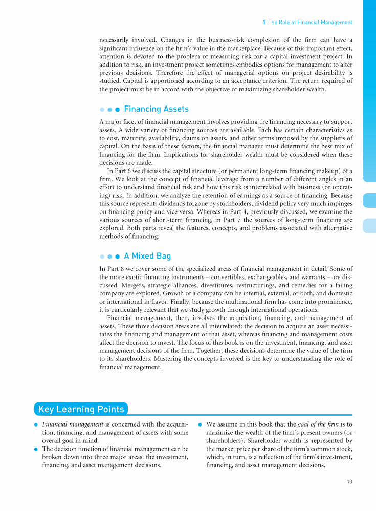
1 The Role of Financial Management
13
••
necessarily involved. Changes in the business-risk complexion of the firm can have asignificant influence on the firm’s value in the marketplace. Because of this important effect,attention is devoted to the problem of measuring risk for a capital investment project. In addition to risk, an investment project sometimes embodies options for management to alterprevious decisions. Therefore the effect of managerial options on project desirability is studied. Capital is apportioned according to an acceptance criterion. The return required ofthe project must be in accord with the objective of maximizing shareholder wealth.
l l l Financing AssetsA major facet of financial management involves providing the financing necessary to supportassets. A wide variety of financing sources are available. Each has certain characteristics as to cost, maturity, availability, claims on assets, and other terms imposed by the suppliers ofcapital. On the basis of these factors, the financial manager must determine the best mix offinancing for the firm. Implications for shareholder wealth must be considered when thesedecisions are made.
In Part 6 we discuss the capital structure (or permanent long-term financing makeup) of afirm. We look at the concept of financial leverage from a number of different angles in aneffort to understand financial risk and how this risk is interrelated with business (or operat-ing) risk. In addition, we analyze the retention of earnings as a source of financing. Becausethis source represents dividends forgone by stockholders, dividend policy very much impingeson financing policy and vice versa. Whereas in Part 4, previously discussed, we examine thevarious sources of short-term financing, in Part 7 the sources of long-term financing areexplored. Both parts reveal the features, concepts, and problems associated with alternativemethods of financing.
l l l A Mixed BagIn Part 8 we cover some of the specialized areas of financial management in detail. Some ofthe more exotic financing instruments – convertibles, exchangeables, and warrants – are dis-cussed. Mergers, strategic alliances, divestitures, restructurings, and remedies for a failingcompany are explored. Growth of a company can be internal, external, or both, and domesticor international in flavor. Finally, because the multinational firm has come into prominence,it is particularly relevant that we study growth through international operations.
Financial management, then, involves the acquisition, financing, and management ofassets. These three decision areas are all interrelated: the decision to acquire an asset necessi-tates the financing and management of that asset, whereas financing and management costsaffect the decision to invest. The focus of this book is on the investment, financing, and assetmanagement decisions of the firm. Together, these decisions determine the value of the firmto its shareholders. Mastering the concepts involved is the key to understanding the role offinancial management.
Key Learning Points l Financial management is concerned with the acquisi-
tion, financing, and management of assets with someoverall goal in mind.
l The decision function of financial management can bebroken down into three major areas: the investment,financing, and asset management decisions.
l We assume in this book that the goal of the firm is tomaximize the wealth of the firm’s present owners (orshareholders). Shareholder wealth is represented bythe market price per share of the firm’s common stock,which, in turn, is a reflection of the firm’s investment,financing, and asset management decisions.
FUNO_C01.qxd 9/19/08 13:57 Page 13

Part 1 Introduction to Financial Management
14
l The market price of a firm’s stock represents the focaljudgment of all market participants as to the value of the particular firm. It takes into account presentand prospective future earnings per share; the timing,duration, and risk of these earnings; the dividend policy of the firm; and other factors that bear on themarket price of the stock.
l Agency theory suggests that managers (the agents),particularly those of large, publicly owned firms, may have different objectives from those of the shareholders (the principals). The shareholders canassure themselves that the managers will make share-holder wealth-maximizing decisions only if manage-ment receives appropriate incentives and only ifmanagement is monitored.
l Maximizing shareholder wealth does not relieve the firmof the responsibility to act in socially responsible ways.
l Corporate governance is the system by which corpora-tions are managed and controlled. It encompasses therelationships among a company’s shareholders, boardof directors, and senior management.
l In large firms, the finance function is the responsibil-ity of the vice president of finance, or chief financialofficer (CFO), who generally reports directly to thepresident, or chief executive officer (CEO). The finan-cial operations overseen by the CFO will be split intotwo branches, with one headed by a treasurer and theother by a controller. The controller’s responsibilitiesare primarily accounting in nature, whereas the trea-surer’s responsibilities fall into the decision areas mostcommonly associated with financial management.
Questions
1. If all companies had an objective of maximizing shareholder wealth, would people over-all tend to be better or worse off?
2. Contrast the objective of maximizing earnings with that of maximizing wealth.3. What is financial management all about?4. Is the goal of zero profits for some finite period (three to five years, for example) ever
consistent with the maximization-of-wealth objective?5. Explain why judging the efficiency of any financial decision requires the existence of a goal.6. What are the three major functions of the financial manager? How are they related?7. Should the managers of a company own sizable amounts of common stock in the com-
pany? What are the pros and cons?8. During the last few decades, a number of environmental, hiring, and other regulations
have been imposed on businesses. In view of these regulatory changes, is maximization ofshareholder wealth any longer a realistic objective?
9. As an investor, do you think that some managers are paid too much? Do their rewardscome at your expense?
10. How does the notion of risk and reward govern the behavior of financial managers?11. What is corporate governance? What role does a corporation’s board of directors play in
corporate governance?12. Compare and contrast the roles that a firm’s treasurer and controller have in the opera-
tion of the firm.
Selected References
Ang, James S., Rebel A. Cole, and James Wuh Lin. “AgencyCosts and Ownership Structure.” Journal of Finance 55(February 2000), 81–106.
Barnea, Amir, Robert A. Haugen, and Lemma W. Senbet.“Management of Corporate Risk,” in Advances in Finan-cial Planning and Forecasting. New York: JAI Press, 1985.
—— . Agency Problems and Financial Contracting.Englewood Cliffs, NJ: Prentice Hall, 1985.
Bauer, Christopher. “A Preventive Maintenance Approach to Ethics.” Financial Executive 21 (May 2005), 18–20.
Bernstein, Peter L. Capital Ideas. New York: Free Press, 1992.
Brennan, Michael. “Corporate Finance Over the Past 25Years.” Financial Management 24 (Summer 1995), 9–22.
Brickley, James A., Clifford W. Smith, Jr., and Jerold L.Zimmerman. “Corporate Governance, Ethics, and
FUNO_C01.qxd 4/18/09 9:47 AM Page 14

1 The Role of Financial Management
15
Organizational Architecture.” Journal of Applied Cor-porate Finance 15 (Spring 2003), 34–45.
Brounen, Dirk, Abe de Jong, and Kees Koedijk. “CorporateFinance in Europe: Confronting Theory with Practice.”Financial Management 33 (Winter 2004), 71–101.
Chambers, Donald R., and Nelson J. Lacey. “CorporateEthics and Shareholder Wealth Maximization.” FinancialPractice and Education 6 (Spring–Summer 1996), 93–96.
Chen, Andrew H., James A. Conover, and John W.Kensinger. “Proven Ways to Increase Share Value.” Journal of Applied Finance 12 (Spring/Summer 2002),89–97.
Dore, Lucia. “Corporate Governance in Europe.” Share-holder Value 3 (January/February 2003), 54–59.
Felo, Andrew J., and Steven A. Solieri. “New Laws, NewChallenges: Implications of Sarbanes-Oxley.” StrategicFinance (February 2003), 31–34.
Friedman, Milton. “The Social Responsibility of Business Is to Increase Its Profits.” New York Times Magazine(September 13, 1970).
Haywood, M. Elizabeth, and Donald E. Wygal. “CorporateGreed vs. IMA’s Ethics Code.” Strategic Finance 86(November 2004), 45–49.
Holmstrom, Bengt, and Steven N. Kaplan. “The State of US Corporate Governance: What is Right and What’sWrong?” Journal of Applied Corporate Finance 15 (Spring2003), 8–20.
Howell, Robert A. “The CFO: From Controller to GlobalStrategic Partner.” Financial Executive 22 (April 2006),20–25.
Jensen, Michael C., and William H. Meckling. “Theory of the Firm: Managerial Behavior, Agency Costs andOwnership Structure.” Journal of Financial Economics 3(October 1976), 305–360.
Jensen, Michael C., and Clifford W. Smith Jr. “Stockholder,Manager, and Creditor Interests: Applications of AgencyTheory.” In Recent Advances in Corporate Finance, ed.Edward I. Altman and Marti G. Subrahmanyam, 93–132.Homewood, IL: Richard D. Irwin, 1985.
Koller, Tim, Marc Goedhart, and David Wessels. Valuation:Measuring and Managing the Value of Companies, 4th ed.Hoboken, NJ: John Wiley, 2005.
Megginson, William L. “Outside Equity.” Journal of Finance55 (June 2000), 1005–1038.
Millman, Gregory J. “New Scandals, Old Lessons: FinancialEthics After Enron.” Financial Executive 18 (July/August2002), 16–19.
Persaud, Avinosh, and John Plender. All You Need to KnowAbout Ethics and Finance: Finding a Moral Compass inBusiness Today. London: Longtail Publishing, 2006.
Porter, Michael E., and Mark R. Kramer. “Strategy &Society: The Link Between Competitive Advantage andCorporate Responsibility.” Harvard Business Review 36(December 2006), 78–92.
Rappaport, Alfred. Creating Shareholder Value: A Guide forManagers and Investors, rev. ed. New York: Free Press,1997.
Seitz, Neil. “Shareholder Goals, Firm Goals and FirmFinancing Decisions.” Financial Management 11 (Autumn1982), 20–26.
Shivdasani, Anil, and Marc Zenner. “Best Practices inCorporate Governance: What Two Decades of ResearchReveals.” Journal of Applied Corporate Finance 16(Spring/Summer 2004), 29–41.
Special Issue on International Corporate Governance.Journal of Financial and Quantitative Analysis 38 (March2003). Entire issue (ten articles) devoted to recent empir-ical and theoretical research in the area of internationalcorporate governance.
Statement on Management Accounting No. 1C (revised),Standards of Ethical Conduct for Practitioners of Manage-ment Accounting and Financial Management. Montvale,NJ: Institute of Management Accountants, April 30, 1997.
Stewart, G. Bennett. The Quest for Value. New York: HarperBusiness, 1991.
Sundaram, Anant K. “Tending to Shareholders,” in FTMastering Financial Management, Part 1. Financial Times(May 26, 2006), 4–5.
Treynor, Jack L. “The Financial Objective in the WidelyHeld Corporation.” Financial Analysts Journal 37(March–April 1981), 68–71.
Vershoor, Curtis C. “Do the Right Thing: IMA Issues NewEthics Guidelines.” Strategic Finance 87 (November2005), 42–46.
Part I of the text’s website, Wachowicz’s Web World, contains links to many finance websites and online articles related to topics covered in this chapter.(web.utk.edu/~jwachowi/wacho_world.html)
FUNO_C01.qxd 4/18/09 9:47 AM Page 15

••
FUNO_C01.qxd 9/19/08 13:57 Page 16

••
17
2The Business, Tax, andFinancial Environments
Contents
l The Business EnvironmentSole Proprietorships • Partnerships •Corporations • Limited Liability Companies(LLCs)
l The Tax EnvironmentCorporate Income Taxes • Personal IncomeTaxes
l The Financial EnvironmentThe Purpose of Financial Markets • FinancialMarkets • Financial Intermediaries • FinancialBrokers • The Secondary Market • Allocation ofFunds and Interest Rates
l Key Learning Points
l Questions
l Self-Correction Problems
l Problems
l Solutions to Self-Correction Problems
l Selected References
Corporation, n. An ingenious device for obtaining individual profitwithout individual responsibility.
—AMBROSE BIERCEThe Devil’s Dictionary
Objectives
After studying Chapter 2, you should be able to:
l Describe the four basic forms of business organ-ization in the United States – and the advantagesand disadvantages of each.
l Understand how to find a corporation’s taxableincome and how to determine the corporate taxrate – both average and marginal.
l Understand various methods of depreciation.
l Explain why acquiring assets through the use ofdebt financing offers a tax advantage over bothcommon and preferred stock financing.
l Describe the purpose and makeup of financialmarkets.
l Demonstrate an understanding of how letter ratings of the major rating agencies help you to judge a security’s default risk.
l Understand what is meant by the “term struc-ture of interest rates” and relate it to a “yieldcurve.”
FUNO_C02.qxd 9/19/08 16:47 Page 17

To understand better the role of financial managers, you must be familiar with the environ-ments in which they operate. The form of business organization that a firm chooses is oneaspect of the business setting in which it must function. We will explore the advantages anddisadvantages of the various alternative forms of business organization. Next, we will look at the tax environment in order to gain a basic understanding of how tax implications mayimpact various financial decisions. Finally, we investigate the financial system and the ever-changing environment in which capital is raised.
The Business EnvironmentIn the United States there are four basic forms of business organization: sole proprietor-ships (one owner), partnerships (general and limited), corporations, and limited liabilitycompanies (LLCs). Sole proprietorships outnumber the others combined by over 2 to 1, but corporations rank first by far when measured by sales, assets, profits, and contribution tonational income. As this section unfolds, you will discover some of the pluses and minuses ofeach alternative form of business organization.
l l l Sole Proprietorships
The sole proprietorship is the oldest form of business organization. As the title suggests, asingle person owns the business, holds title to all its assets, and is personally responsible forall of its debts. A proprietorship pays no separate income taxes. The owner merely adds anyprofits or subtracts any losses from the business when determining personal taxable income.This business form is widely used in service industries. Because of its simplicity, a sole pro-prietorship can be established with few complications and little expense. Simplicity is itsgreatest virtue.
Its principal shortcoming is that the owner is personally liable for all business obligations.If the organization is sued, the proprietor as an individual is sued and has unlimited liability,which means that much of his or her personal property, as well as the assets of the business,may be seized to settle claims. Another problem with a sole proprietorship is the difficulty in raising capital. Because the life and success of the business is so dependent on a single individual, a sole proprietorship may not be as attractive to lenders as another form of organ-ization. Moreover, the proprietorship has certain tax disadvantages. Fringe benefits, such asmedical coverage and group insurance, are not regarded by the Internal Revenue Service asexpenses of the firm and therefore are not fully deductible for tax purposes. A corporationoften deducts these benefits, but the proprietor must pay for a major portion of them fromincome left over after paying taxes. In addition to these drawbacks, the proprietorship formmakes the transfer of ownership more difficult than does the corporate form. In estate plan-ning, no portion of the enterprise can be transferred to members of the family during the pro-prietor’s lifetime. For these reasons, this form of organization does not afford the flexibilitythat other forms do.
l l l Partnerships
A partnership is similar to a proprietorship, except there is more than one owner. A partnership, like a proprietorship, pays no income taxes. Instead, individual partners includetheir share of profits or losses from the business as part of their personal taxable income. One potential advantage of this business form is that, relative to a proprietorship, a greateramount of capital can often be raised. More than one owner may now be providing personalcapital, and lenders may be more agreeable to providing funds given a larger owner invest-ment base.
Part 1 Introduction to Financial Management
18
••
Sole proprietorshipA business form forwhich there is oneowner. This singleowner has unlimitedliability for all debts of the firm.
Partnership Abusiness form inwhich two or moreindividuals act asowners. In a generalpartnership allpartners haveunlimited liability for the debts of thefirm; in a limitedpartnership one ormore partners mayhave limited liability.
FUNO_C02.qxd 9/19/08 16:47 Page 18

1The Trustees of Dartmouth College v. Woodward, 4 Wheaton 636 (1819).
In a general partnership all partners have unlimited liability; they are jointly liable for theobligations of the partnership. Because each partner can bind the partnership with obligations,general partners should be selected with care. In most cases a formal arrangement, or part-nership agreement, sets forth the powers of each partner, the distribution of profits, theamounts of capital to be invested by the partners, procedures for admitting new partners, and procedures for reconstituting the partnership in the case of the death or withdrawal of a partner. Legally, the partnership is dissolved if one of the partners dies or withdraws. In such cases, settlements are invariably “sticky,” and reconstitution of the partnership can be a difficult matter.
In a limited partnership, limited partners contribute capital and have liability confined tothat amount of capital; they cannot lose more than they put in. There must, however, be atleast one general partner in the partnership, whose liability is unlimited. Limited partners do not participate in the operation of the business; this is left to the general partner(s). Thelimited partners are strictly investors, and they share in the profits or losses of the partnershipaccording to the terms of the partnership agreement. This type of arrangement is frequentlyused in financing real estate ventures.
l l l Corporations
Because of the importance of the corporate form in the United States, the focus of this bookis on corporations. A corporation is an “artificial entity” created by law. It can own assets and incur liabilities. In the famous Dartmouth College decision in 1819, Justice Marshall concluded that
a corporation is an artificial being, invisible, intangible, and existing only in contemplationof the law. Being a mere creature of law, it possesses only those properties which the charter of its creation confers upon it, either expressly or as incidental to its very existence.1
The principal feature of this form of business organization is that the corporation exists legallyseparate and apart from its owners. An owner’s liability is limited to his or her investment.Limited liability represents an important advantage over the proprietorship and general partnership. Capital can be raised in the corporation’s name without exposing the owners to unlimited liability. Therefore, personal assets cannot be seized in the settlement of claims.Ownership itself is evidenced by shares of stock, with each stockholder owning that pro-portion of the enterprise represented by his or her shares in relation to the total number ofshares outstanding. These shares are easily transferable, representing another importantadvantage of the corporate form. Moreover, corporations have found what the explorer Poncede Leon could only dream of finding – unlimited life. Because the corporation exists apartfrom its owners, its life is not limited by the lives of the owners (unlike proprietorships andpartnerships). The corporation can continue even though individual owners may die or selltheir stock.
Because of the advantages associated with limited liability, easy transfer of ownershipthrough the sale of common stock, unlimited life, and the ability of the corporation to raisecapital apart from its owners, the corporate form of business organization has grown enormously in the twentieth century. With the large demands for capital that accompany anadvanced economy, the proprietorship and partnership have proven unsatisfactory, and thecorporation has emerged as the most important organizational form.
A possible disadvantage of the corporation is tax related. Corporate profits are subject to double taxation. The company pays tax on the income it earns, and the stockholder is also taxed when he or she receives income in the form of a cash dividend. (We will take a
2 The Business, Tax, and Financial Environments
19
••
Limited partnerMember of a limitedpartnership notpersonally liable for the debts of the partnership.
General partnerMember of apartnership withunlimited liability forthe debts of thepartnership.
Corporation Abusiness form legally separate from its owners. Its distinguishingfeatures includelimited liability, easytransfer of ownership,unlimited life, and anability to raise largesums of capital.
Double taxationTaxation of the sameincome twice. Aclassic example istaxation of income atthe corporate leveland again as dividendincome when receivedby the shareholder.
FUNO_C02.qxd 9/19/08 16:47 Page 19

closer look at taxes in the next section.2) Minor disadvantages include the length of time toincorporate and the red tape involved, as well as the incorporation fee that must be paid tothe state in which the firm is incorporated. Thus, a corporation is more difficult to establishthan either a proprietorship or a partnership.
l l l Limited Liability Companies (LLCs)
A limited liability company (LLC) is a hybrid form of business organization that combinesthe best aspects of both a corporation and a partnership. It provides its owners (called “members”) with corporate-style limited personal liability and the federal-tax treatment of apartnership.3 Especially well suited for small and medium-sized firms, it has fewer restrictionsand greater flexibility than an older hybrid business form – the S corporation (which we dis-cuss in the section on taxes).
Until 1990 only two states, Wyoming and Florida, allowed the formation of LLCs. A 1988Internal Revenue Service (IRS) ruling that any Wyoming LLC would be treated as a partner-ship for federal-tax purposes opened the floodgates for the remaining states to start enactingLLC statutes. Though new to the United States, LLCs have been a long-accepted form of busi-ness organization in Europe and Latin America.
Limited liability companies generally possess no more than two of the following four(desirable) standard corporate characteristics: (1) limited liability, (2) centralized manage-ment, (3) unlimited life, and (4) the ability to transfer ownership interest without prior consent of the other owners. LLCs (by definition) have limited liability. Thus members arenot personally liable for any debts that may be incurred by the LLC. Most LLCs choose tomaintain some type of centralized management structure. One drawback to an LLC, however,is that it generally lacks the corporate feature of “unlimited life,” although most states doallow an LLC to continue if a member’s ownership interest is transferred or terminated.Another drawback is that complete transfer of an ownership interest is usually subject to theapproval of at least a majority of the other LLC members.
Although the LLC structure is applicable to most businesses, service-providing profes-sionals in many states who want to form an LLC must resort to a parallel structure. In thosestates, accountants, lawyers, doctors, and other professionals are allowed to form a profes-sional LLC (PLLC) or limited liability partnership (LLP), a PLLC look-alike. One indication ofthe popularity of the PLLC/LLP structure among professionals can be found in the fact thatall of the “Big Four” accounting firms in the United States are LLPs.
The Tax EnvironmentMost business decisions are affected either directly or indirectly by taxes. Through their taxing power, federal, state, and local governments have a profound influence on the beha-vior of businesses and their owners. What might prove to be an outstanding business deci-sion in the absence of taxes may prove to be very inferior with taxes (and sometimes, viceversa). In this section we introduce you to some of the fundamentals of taxation. A basicunderstanding of this material will be needed for later chapters when we consider specificfinancial decisions.
We begin with the corporate income tax. Then we briefly consider personal income taxes.We must be mindful that tax laws frequently change.
2An S corporation, named for a subchapter of the Internal Revenue Code, is a special type of corporate structure openonly to qualifying “small corporations.” Since its reason for being is entirely tax motivated, we defer its discussionuntil the section on taxes.3Many states permit single-member LLCs. Qualified single-member LLCs are taxed as sole proprietorships.
Part 1 Introduction to Financial Management
20
••
Limited liabilitycompany (LLC) Abusiness form thatprovides its owners(called “members”)with corporate-stylelimited personalliability and thefederal-tax treatmentof a partnership.
FUNO_C02.qxd 9/19/08 16:47 Page 20

l l l Corporate Income Taxes
A corporation’s taxable income is found by deducting all allowable expenses, including depre-ciation and interest, from revenues. This taxable income is then subjected to the followinggraduated tax structure:
CORPORATE TAXABLE INCOME
AT LEAST BUT LESS THAN TAX RATE (%) TAX CALCULATION
$ 0 $ 50,000 15 0.15 × (income over $0)50,000 75,000 25 $ 7,500 + 0.25 × (income over 50,000)75,000 100,000 34 13,750 + 0.34 × (income over 75,000)
100,000 335,000 39a 22,250 + 0.39 × (income over 100,000)335,000 10,000,000 34 113,900 + 0.34 × (income over 335,000)
10,000,000 15,000,000 35 3,400,000 + 0.35 × (income over 10,000,000)15,000,000 18,333,333 38b 5,150,000 + 0.38 × (income over 15,000,000)18,333,333 – 35 6,416,667 + 0.35 × (income over 18,333,333)
aBetween $100,000 and $335,000 there is a built-in surtax of 5 percent over the 34 percent rate. This resultsin corporations with taxable income between $335,000 and $10,000,000 “effectively” paying a flat 34 percentrate on all of their taxable income.bBetween $15,000,000 and $18,333,333 there is a built-in surtax of 3 percent over the 35 percent rate. Thisresults in corporations with taxable income over $18,333,333 “effectively” paying a flat 35 percent rate on allof their taxable income.
The tax rate – the percentage of taxable income that must be paid in taxes – that is applied toeach income bracket is referred to as a marginal rate. For example, each additional dollar oftaxable income above $50,000 is taxed at the marginal rate of 25 percent until taxable incomereaches $75,000. At that point, the new marginal rate becomes 34 percent. The average tax ratefor a firm is measured by dividing taxes actually paid by taxable income. For example, a firmwith $100,000 of taxable income pays $22,250 in taxes, and therefore has an average tax rateof $22,250/$100,000, or 22.25 percent. For small firms (i.e., firms with less than $335,000 of taxable income), the distinction between the average and marginal tax rates may proveimportant. However, the average and marginal rates converge at 34 percent for firms with taxable income between $335,000 and $10 million and, finally, converge again, this time to the35 percent rate, for firms with taxable income above $18,333,333.
Alternative Minimum Tax. Companies dislike paying taxes and will take advantage of allthe deductions and credits that the law allows. Therefore, the Internal Revenue Service hasdevised a special tax to ensure that large firms that benefit from the tax laws pay at least a minimum amount of tax. This special tax is called the alternative minimum tax (AMT). Thetax – 20 percent of alternative minimum taxable income (AMTI) – applies only when the AMTwould be greater than the firm’s normally computed tax. To broaden the base of taxableincome, AMTI is calculated by applying adjustments to items that had previously receivedsome tax preference.
Quarterly Tax Payments. Corporations of any significant size are required to make quar-terly tax payments. Specifically, calendar-year corporations are required to pay 25 percent oftheir estimated taxes in any given year on or before April 15, June 15, September 15, andDecember 15. When actual income differs from that which has been estimated, adjustmentsare made. A company that is on a calendar-year basis of accounting must make final settle-ment by March 15 of the subsequent year.
Depreciation. Depreciation is the systematic allocation of the cost of a capital asset over aperiod of time for financial reporting purposes, tax purposes, or both. Depreciation deduc-tions taken on a firm’s tax return are treated as expense items. Thus depreciation lowers tax-able income. Everything else being equal, the greater the depreciation charges, the lower the
2 The Business, Tax, and Financial Environments
21
••
Depreciation Thesystematic allocationof the cost of acapital asset over a period of time forfinancial reportingpurposes, taxpurposes, or both.
FUNO_C02.qxd 9/19/08 16:47 Page 21

tax. There are a number of alternative procedures for depreciating capital assets, includingstraight-line depreciation and various accelerated depreciation methods. The depreciationmethods chosen may differ for tax reporting versus financial reporting. Most firms with taxable income prefer to use an accelerated depreciation method for tax reporting purposes –one that allows for a more rapid write-off and, hence, a lower taxable income figure.
The Tax Reform Act of 1986 allows companies to use a particular type of accelerated depre-ciation for tax purposes; it is known as the Modified Accelerated Cost Recovery System(MACRS, pronounced “makers”).4 Under MACRS, machinery, equipment, and real estate areassigned to one of eight classes for purposes of determining a prescribed life, called a costrecovery period, and a depreciation method. The property class in which an asset falls deter-mines its cost recovery period or prescribed life for tax purposes – a life that may differ fromthe asset’s useful or economic life. A general description of the property classes is provided inTable 2.1. (The reader should refer to the Internal Revenue Code for more detail.)
To illustrate some of the various methods of depreciation, let’s first consider straight-linedepreciation. If the fully installed acquisition cost of a five-year property class asset is $10,000,annual depreciation charges using straight-line depreciation would be $10,000/5, or $2,000.(For tax purposes, expected salvage value does not affect depreciation charges.)
Declining-balance depreciation, on the other hand, calls for an annual charge that is a“fixed percentage” of the asset’s net book value (acquisition cost minus accumulated deprecia-tion) at the beginning of the year to which the depreciation charge applies. For example, whenusing the double-declining-balance (DDB) method, we compute a rate by dividing 1 by thenumber of years of depreciable life for the asset. Then we double that rate. (Other declining-balance methods use other multiples.) Under the declining-balance methods the general formula for determining the depreciation charge in any period is
m (1/n)NBV (2.1)
where m is the multiple, n is the depreciable life of the asset, and NBV is the asset’s net bookvalue at the start of the year. For a $10,000 asset, with a five-year life, the depreciation chargein the first year using the DDB method would be
2(1/5)$10,000 = $4,000
4The term “Modified Accelerated Cost Recovery System” (MACRS) is used to distinguish the deductions computed underpost-1986 rules from deductions prescribed under pre-1987 rules of the Accelerated Cost Recovery System (ACRS).
Part 1 Introduction to Financial Management
22
••
Table 2.1Property classesunder MACRS
l 3-Year 200% Class. Includes property with a midpoint life of 4 years or less, except automobilesand light trucks. Under the Asset Depreciation Range (ADR) system, assets are grouped withinclasses and a guideline (midpoint) life is determined by the Treasury Department.
l 5-Year 200% Class. Includes property with an ADR midpoint life of more than 4 to less than 10 years. Also included are automobiles, light trucks, most technological and semiconductormanufacturing equipment, switching equipment, small power production facilities, research andexperimental equipment, high technology medical equipment, computers, and certain officeequipment.
l 7-Year 200% Class. Includes property with ADR midpoints of 10 to less than 16 years and single-purpose agricultural structures. Also includes office furniture and any other property for which noclass life is specified by law.
l 10-Year 200% Class. Includes property with ADR midpoints of 16 to less than 20 years.
l 15-Year 150% Class. Includes property with ADR midpoints of 20 to less than 25 years, sewagetreatment plants, and telephone distribution plants.
l 20-Year 150% Class. Includes property with ADR midpoints of 25 years or more, other than realproperty described below.
l 27.5-Year Straight-Line Class. Includes residential rental property.
l 39-Year Straight-Line Class. Includes other real estate.
Declining-balancedepreciation Methodsof depreciation callingfor an annual chargebased on a fixedpercentage of theasset’s depreciatedbook value at thebeginning of the year for which thedepreciation chargeapplies.
Straight-linedepreciationA method of depreciation thatallocates expensesevenly over thedepreciable life of the asset.
Accelerateddepreciation Methodsof depreciation thatwrite off the cost of a capital asset fasterthan under straight-line depreciation.
FUNO_C02.qxd 9/19/08 16:47 Page 22

For our example, 2(1/5) determines the “fixed percentage,” or 40 percent, that is appliedagainst the declining net book value each year. The depreciation charge in the second year isbased on the depreciated net book value of $6,000. We arrive at the $6,000 by subtracting thefirst year’s depreciation charge, $4,000, from the asset’s original acquisition cost. The depre-ciation charge in the second year would be
2(1/5)$6,000 = $2,400
The third year’s charge would be
2(1/5)$3,600 = $1,440
and so on.
Modified Accelerated Cost Recovery System. For the 3-, 5-, 7-, and 10-year propertyclasses, the double declining balance (also called 200% declining balance) depreciation method is used. This method then switches to straight-line depreciation for the remainingundepreciated book value in the first year that the straight-line method yields an equal orgreater deduction than the declining-balance method. Assets in the 15- and 20-year classes aredepreciated using the 150 percent declining balance method, again switching to straight-lineat the optimal time. The straight-line method must be used for all real estate.
Normally, the half-year convention must be applied to all declining-balance methods. Thiscalls for a half year of depreciation in the year an asset is acquired, regardless of the date ofpurchase. There is also a half year of depreciation in the year an asset is sold or retired fromservice. If property is held for longer than its recovery period, a half year of depreciation isallowed for the year following the end of the recovery period. Thus 5-year property class assetsheld for 6 years or longer have depreciation spread over 6 years.
To illustrate for the 5-year 200 percent property class, assume that an asset costing $10,000is acquired in February. For our example, the declining-balance formula yields 2(1/5) = 40%as the fixed percentage annual depreciation. However, in the first year the half-year conven-tion is employed, so first-year depreciation is 20 percent, or $2,000. In the fourth year it is favorable to switch to straight-line depreciation. Thus the depreciation schedule is as follows:
DEPRECIATION DEPRECIATION NET BOOK VALUE YEAR CALCULATION CHARGE (end of year)
0 – – $10,0001 (0.2)$10,000 $2,000 8,0002 (0.4)$8,000 3,200 4,8003 (0.4)$4,800 1,920 2,8804 $2,880/2.5 years 1,152 1,7285 $2,880/2.5 years 1,152 5766 (0.5)$2,880/2.5 years 576 0
At the beginning of the fourth year, the net book value at the end of the third year is dividedby the remaining life to get straight-line depreciation. The remaining life is 2.5 years, owingto the half-year convention in the sixth year. Finally, in the sixth year the remaining balanceis $576, or one-half the yearly straight-line amount.
Take Note
Instead of making such calculations (which as you can see can be quite a chore), one can usedepreciation percentages of original cost for each property class (see Table 2.1) published bythe Treasury. The first four property categories are seen in the following table.
2 The Business, Tax, and Financial Environments
23
••
FUNO_C02.qxd 9/19/08 16:47 Page 23

PROPERTY CLASS
RECOVERY YEAR 3-YEAR 5-YEAR 7-YEAR 10-YEAR
1 33.33% 20.00% 14.29% 10.00%2 44.45 32.00 24.49 18.003 14.81 19.20 17.49 14.404 7.41 11.52 12.49 11.525 11.52 8.93 9.226 5.76 8.92 7.377 8.93 6.558 4.46 6.559 6.56
10 6.5511 3.28
Totals 100.00% 100.00% 100.00% 100.00%
These percentages correspond to the principles on which our previous calculations are based,and they are used for determining depreciation deductions.
“Temporary” Tax Relief Provision(s). In May 2008 President Bush signed an economic-stimulus bill – Economic Stimulus Act (ESA) of 2008 – into law. The Act has a number of pro-visions that are supposed to be only “temporary.” For students of finance, one provision isespecially important because it can dramatically affect a company’s federal tax payments andcapital budgeting decisions. The critical provision involves “bonus depreciation.”
Under the 2008 Act businesses are allowed to take an additional first-year depreciationdeduction, commonly known as “bonus depreciation,” equal to 50 percent of the original“adjusted (depreciable) basis” – usually the fully installed cost – of qualified property.Property eligible for this treatment includes property to which MACRS depreciation applieswith a recovery period of 20 years or less. Certain types of water utility property, software, andleasehold improvements also qualify for bonus depreciation. Property must generally be pur-chased and placed in service in 2008. The bonus depreciation is allowed for both the regulartax and the alternative minimum tax (AMT).
In addition, the business is entitled to “normal” first-year depreciation. However, thedepreciable basis of the property and the regular depreciation allowances are adjusted toreflect the additional first-year depreciation deduction. And, finally, a taxpayer may elect outof the 50 percent bonus depreciation by asset class and be subject to “normal” tax deprecia-tion on the original “adjusted (depreciable) basis.”
EXAMPLE (with 50 percent bonus depreciation and assuming the half-year convention):On September 8, 2008, a calendar-year reporting business, bought and placed in service, a $100,000 five-year property class piece of equipment. The business may claim a first-year (2008) depreciation allowance of $60,000 – i.e., a $50,000 bonus depreciation ($100,000 times 50%) plus a $10,000 normal first-year MACRS depreciation calculated onthe new adjusted basis ([$100,000 minus $50,000] times 20%). In the second year (2009),the MACRS depreciation would be $16,000 ([$100,000 minus $50,000] times 32%). And so on.
In the above example, the “effective” depreciation percentage for the first year is a whop-ping 60 percent [($50,000 bonus depreciation plus $10,000 normal first-year depreciation)divided by the $100,000 original adjusted basis]. In the second year, the “effective” deprecia-tion is 16 percent [$16,000 divided by $100,000]. And so on.
Part 1 Introduction to Financial Management
24
••
FUNO_C02.qxd 9/19/08 16:47 Page 24
5For any dividend income to be tax exempt, however, the corporation must have owned the stock for at least 45 days.If a corporation owns 20 percent or more of another corporation’s stock, however, 80 percent of any dividendreceived is tax exempt. Also, if a corporation owns 80 percent or more of the stock of another firm, it can file a consolidated tax return. In this way, any funds transferred between the two entities are generally not considered dividends for tax purposes, and no tax is paid on such transfers.6A corporation has the option, however, of forgoing the carryback and simply carrying the loss forward up to 20 years.For example, a corporation might elect to forgo the loss carryback if it anticipated a significant increase in tax ratesin future years.
Take Note
Since the 50 percent “bonus depreciation” deduction is “temporary” and currently sched-uled to expire by the end of 2008, you will probably not have to make any EconomicStimulus Act of 2008 “bonus depreciation” choices in a real job situation. Therefore, all ourexamples and problems involving MACRS depreciation will ignore “bonus depreciation”provisions.
It is important to note, however, that “temporary” bonus depreciation may very wellreturn again during your professional future – so be prepared. A little historical backgroundmay help to convince you of that. Under the Job Creation and Worker Assistance Act of 2002(JCWAA), businesses were allowed to take a 30 percent bonus depreciation on a “temporary”basis. The following year the Jobs and Growth Tax Relief Reconciliation Act of 2003 (JGTRRA)increased bonus depreciation from 30 to 50 percent also on a “temporary” basis (expiring atthe end of 2004). To learn more about JCWAA, visit web.utk.edu/~jwachowi/hr3090.html.And, for more information on JGTRRA, see web.utk.edu/~jwachowi/hr2.html. And, finally,for additional information on ESA, see web.utk.edu/~jwachowi/hr5140.html.
Interest Expense versus Dividends Paid. Interest paid on outstanding corporate debt istreated as an expense and is tax deductible. However, dividends paid to preferred or commonstockholders are not tax deductible. Thus, for a profitable, tax-paying company, the use ofdebt (e.g., bonds) in its financing mix results in a significant tax advantage relative to the useof preferred or common stock. Given a marginal tax rate of 35 percent, a firm that pays out$1 in interest lowers its tax bill by 35 cents because of its ability to deduct the $1 of interestfrom taxable income. The after-tax cost of $1 of interest for this firm is really only 65 cents –$1 × (1 − tax rate). On the other hand, the after-tax cost of $1 of dividends paid by the firm is still $1 – there is no tax advantage here. Therefore there are tax advantages associated with using debt financing that are simply not present with either preferred or common stockfinancing.
Dividend Income. A corporation may own stock in another company. If it receives a cash dividend on this stock, normally 70 percent of the dividend is tax exempt.5 The tax lawsallow this tax break for corporations (not individuals) to help reduce the effects of multipletaxation of the same earnings. The remaining 30 percent is taxed at the corporate income tax rate. A firm that receives $10,000 in dividend income pays taxes on only $3,000 of thisincome. At a marginal tax rate of 35 percent, taxes would amount to $1,050, as opposed to$3,500 if the entire dividend income were treated as taxable income.
Carryback and Carryforward. If a corporation sustains a net operating loss, this loss maygenerally be carried back 2 years and forward up to 20 years to offset taxable income in thoseyears.6 Any loss carried back must first be applied to the earliest preceding year. If a firm sus-tained an operating loss of $400,000 in 2008 it would first carry this loss back to 2006. If the
2 The Business, Tax, and Financial Environments
25
••
Cash dividendCash distribution of earnings tostockholders, usuallyon a quarterly basis.
FUNO_C02.qxd 9/19/08 16:47 Page 25

company had net profits of $400,000 in that year and paid taxes of $136,000, it would recom-pute its taxes for 2006 to show zero profit for tax purposes. Consequently, the company wouldbe eligible for a tax refund of $136,000. If the 2008 operating loss was greater than operatingprofits in 2006, the residual would be carried back to 2007 and taxes recomputed for that year.However, if the net operating loss was greater than the net operating income in both years, theresidual would be carried forward in sequence to future profits in 2009 to 2028. Profits in eachof these years would be reduced for tax purposes by the amount of the unused loss carried forward. This feature of the tax laws is designed to avoid penalizing companies that havesharply fluctuating net operating income.
Capital Gains and Losses. When a capital asset (as defined by the Internal RevenueService) is sold, a capital gain or loss is generally incurred. Often in the history of our tax lawsthere has been a differential tax treatment of capital gains income and operating income, withcapital gains being treated more favorably. Under the Revenue Reconciliation Act of 1993,however, capital gains are taxed at the ordinary income tax rates for corporations, or a max-imum of 35 percent. Capital losses are deductible only against capital gains.
l l l Personal Income Taxes
The subject of personal taxes is extremely complex, but our main concern here is with the per-sonal taxes of individuals who own businesses – proprietors, partners, members (of LLCs),and shareholders. Any income reported by a sole proprietorship, partnership, or properlystructured LLC becomes income of the owner(s) and is taxed at the personal rate. For indi-viduals there are currently six progressive tax brackets: 10, 15, 25, 28, 33, and 35 percent. Themarginal tax rates apply up to certain levels of taxable income, which vary depending on theindividual’s filing status – that is, single, married filing a joint return, married filing separately,or head of household. Even within a filing category, however, the taxable income levels thattrigger the marginal tax rate will generally vary from year to year because they are indexed to account for inflation. There are also standard deductions and personal exemptions thatenable those with very low income to pay no taxes.
Interest, Dividends, and Capital Gains. For the individual, interest received on corporateand Treasury securities is fully taxable at the federal level. (Interest on Treasury securities is not taxable at the state level.) However, interest received on most municipal securities isexempt from federal taxation. Taxable interest is subject to the ordinary income tax rates. Thecurrent maximum dividend and capital gains tax rates for most (but not all) cash dividendsreceived and realized net capital gains are both 15 percent for qualifying taxpayers.
Subchapter S. Subchapter S of the Internal Revenue Code allows the owners of small cor-porations to elect to be taxed as an S corporation. In making this election, the company gets touse the corporate organization form but is taxed as though the firm were a partnership. Thusthe owners are able to avail themselves of the legal advantages extended to corporations, butare able to avoid any tax disadvantages that might result. They simply declare any corporateprofits as personal income on a pro rata basis and pay the appropriate tax on this income. Thistreatment eliminates the double taxation normally associated with dividend income – that is,the corporation paying dividends from after-tax income, and shareholders paying taxes on thedividend income they receive. In addition, stockholders active in the business may deduct anyoperating losses on a pro rata basis against their personal income.
As discussed earlier, a limited liability company (LLC) provides benefits similar to those of an S corporation, but with fewer limitations (e.g., no restriction as to the number and typeof owners). Many predict that the LLC form of business will grow in numbers to surpass theS corporation form.
Part 1 Introduction to Financial Management
26
••
Capital gain (loss)The amount by whichthe proceeds from thesale of a capital assetexceeds (is less than)the asset’s originalcost.
FUNO_C02.qxd 9/19/08 16:47 Page 26

The Financial EnvironmentIn varying degrees, all businesses operate within the financial system, which consists of a number of institutions and markets serving business firms, individuals, and governments.When a firm invests temporarily idle funds in marketable securities, it has direct contact withfinancial markets. More important, most firms use financial markets to help finance theirinvestment in assets. In the final analysis, the market price of a company’s securities is the test of whether the company is a success or a failure. While business firms compete with eachother in the product markets, they must continually interact with the financial markets.Because of the importance of this environment to the financial manager, as well as to the indi-vidual as a consumer of financial services, this section is devoted to exploring the financial system and the ever-changing environment in which capital is raised.
l l l The Purpose of Financial Markets
Financial assets exist in an economy because the savings of various individuals, corpora-tions, and governments during a period of time differ from their investment in real assets. By real assets, we mean such things as houses, buildings, equipment, inventories, and durablegoods. If savings equaled investment in real assets for all economic units in an economy over all periods of time, there would be no external financing, no financial assets, and nomoney or capital markets. Each economic unit would be self-sufficient. Current expendituresand investment in real assets would be paid for out of current income. A financial asset is created only when the investment of an economic unit in real assets exceeds its savings, and it finances this excess by borrowing or issuing stock. Of course, another economic unitmust be willing to lend. This interaction of borrowers with lenders determines interest rates. In the economy as a whole, savings-surplus units (those whose savings exceed theirinvestment in real assets) provide funds to savings-deficit units (those whose investments in real assets exceed their savings). This exchange of funds is evidenced by investment instruments, or securities, representing financial assets to the holders and financial liabilitiesto the issuers.
The purpose of financial markets in an economy is to allocate savings efficiently to ulti-mate users. If those economic units that saved were the same as those that engaged in capital formation, an economy could prosper without financial markets. In modern economies,however, most nonfinancial corporations use more than their total savings for investing inreal assets. Most households, on the other hand, have total savings in excess of total invest-ment. Efficiency entails bringing the ultimate investor in real assets and the ultimate savertogether at the least possible cost and inconvenience.
l l l Financial Markets
Financial markets are not so much physical places as they are mechanisms for channeling savings to the ultimate investors in real assets. Figure 2.1 illustrates the role of financial markets and financial institutions in moving funds from the savings sector (savings-surplusunits) to the investment sector (savings-deficit units). From the figure we can also note theprominent position held by certain financial institutions in channeling the flow of funds inthe economy. The secondary market, financial intermediaries, and financial brokers are the keyinstitutions that enhance funds flows. We will study their unique roles as this section unfolds.
Money and Capital Markets. Financial markets can be broken into two classes – the moneymarket and the capital market. The money market is concerned with the buying and selling of short-term (less than one year original maturity) government and corporate debt
2 The Business, Tax, and Financial Environments
27
••
Financial marketsAll institutions andprocedures forbringing buyers andsellers of financialinstruments together.
Money market Themarket for short-term(less than one yearoriginal maturity)government andcorporate debtsecurities. It alsoincludes governmentsecurities originallyissued with maturitiesof more than one yearbut that now have a year or less untilmaturity.
FUNO_C02.qxd 9/19/08 16:47 Page 27

securities. The capital market, on the other hand, deals with relatively long-term (greaterthan one year original maturity) debt and equity instruments (e.g., bonds and stocks). This section gives special attention to the market for long-term securities – the capital market. The money market and the securities that form its lifeblood are covered in Part 4 of this book.
Primary and Secondary Markets. Within money and capital markets there exist both primary and secondary markets. A primary market is a “new issues” market. Here, fundsraised through the sale of new securities flow from the ultimate savers to the ultimate investorsin real assets. In a secondary market, existing securities are bought and sold. Transactions in these already existing securities do not provide additional funds to finance capital invest-ment. (Note: On Figure 2.1 there is no line directly connecting the secondary market with theinvestment sector.) An analogy can be made with the market for automobiles. The sale of new cars provides cash to the auto manufacturers; the sale of used cars in the used-car marketdoes not. In a real sense, a secondary market is a “used-car lot” for securities.
The existence of used-car lots makes it easier for you to consider buying a new car becauseyou have a mechanism at hand to sell the car when you no longer want it. In a similar fashion,
Part 1 Introduction to Financial Management
28
••
Capital market Themarket for relativelylong-term (greaterthan one year originalmaturity) financialinstruments (e.g.,bonds and stocks).
Primary marketA market where newsecurities are boughtand sold for the firsttime (a “new issues”market).
Secondary marketA market for existing(used) securitiesrather than newissues.
Figure 2.1Flow of funds in theeconomy and themechanism thatfinancial marketsprovide for channelingsavings to theultimate investors in real assets
FUNO_C02.qxd 9/19/08 16:47 Page 28

the existence of a secondary market encourages the purchase of new securities by indi-viduals and institutions. With a viable secondary market, a purchaser of financial securitiesachieves marketability. If the buyer needs to sell a security in the future, he or she will be able to do so. Thus, the existence of a strong secondary market enhances the efficiency of theprimary market.
l l l Financial Intermediaries
The flow of funds from savers to investors in real assets can be direct; if there are financialintermediaries in an economy, the flow can also be indirect. Financial intermediaries consistof financial institutions, such as commercial banks, savings institutions, insurance companies,pension funds, finance companies, and mutual funds. These intermediaries come betweenultimate borrowers and lenders by transforming direct claims into indirect claims. Financialintermediaries purchase direct (or primary) securities and, in turn, issue their own indirect(or secondary) securities to the public. For example, the direct security that a savings and loan association purchases is a mortgage; the indirect claim issued is a savings account or acertificate of deposit. A life insurance company, on the other hand, purchases corporatebonds, among other things, and issues life insurance policies.
Financial intermediation is the process of savers depositing funds with financial intermedi-aries (rather than directly buying stocks and bonds) and letting the intermediaries do thelending to the ultimate investors. We usually think of financial intermediation making themarkets more efficient by lowering the cost and/or inconvenience to consumers of financialservices.
Among the various financial intermediaries, some institutions invest much more heavily in the securities of business firms than others. In what follows, we concentrate on those institutions involved in buying and selling corporate securities.
Deposit Institutions. Commercial banks are the most important source of funds for businessfirms in the aggregate. Banks acquire demand (checking) and time (savings) deposits fromindividuals, companies, and governments and, in turn, make loans and investments. Amongthe loans made to business firms are seasonal and other short-term loans, intermediate-termloans of up to five years, and mortgage loans. Besides performing a banking function, com-mercial banks affect business firms through their trust departments, which invest in corporatebonds and stocks. They also make mortgage loans available to companies and manage pen-sion funds.
Other deposit institutions include savings and loan associations, mutual savings banks, and credit unions. These institutions are primarily involved with individuals, acquiring their savings and making home and consumer loans.
Insurance Companies. There are two types of insurance companies: property and casualtycompanies and life insurance companies. These are in the business of collecting periodic payments from those they insure in exchange for providing payouts should events, usuallyadverse, occur. With the funds received in premium payments, insurance companies buildreserves. These reserves and a portion of the insurance companies’ capital are invested infinancial assets.
Property and casualty companies insure against fires, thefts, car accidents, and similarunpleasantness. Because these companies pay taxes at the full corporate income tax rate, theyinvest heavily in municipal bonds, which offer tax-exempt interest income. To a lesser extentthey also invest in corporate stocks and bonds.
Life insurance companies insure against the loss of life. Because the mortality of a largegroup of individuals is highly predictable, these companies are able to invest in long-termsecurities. Also, the income of these institutions is partially exempt from taxes owing to thebuildup of reserves over time. They therefore seek taxable investments with yields higher
2 The Business, Tax, and Financial Environments
29
••
FinancialintermediariesFinancial institutionsthat accept moneyfrom savers and usethose funds to makeloans and otherfinancial investmentsin their own name.They includecommercial banks,savings institutions,insurance companies,pension funds,finance companies,and mutual funds.
FUNO_C02.qxd 9/19/08 16:47 Page 29

than those of tax-exempt municipal bonds. As a result, life insurance companies invest heavily in corporate bonds. Also important are mortgages, some of which are granted to business firms.
Other Financial Intermediaries. Pension funds and other retirement funds are establishedto provide income to individuals when they retire. During their working lives, employees usually contribute to these funds, as do employers. Funds invest these contributions andeither pay out the cumulative amounts periodically to retired workers or arrange annuities. In the accumulation phase, monies paid into a fund are not taxed. When the benefits are paidout in retirement, taxes are paid by the recipient. Commercial banks, through their trustdepartments, and insurance companies offer pension funds, as do the federal government,local governments, and certain other noninsurance organizations. Because of the long-termnature of their liabilities, pension funds are able to invest in longer-term securities. As a result,they invest heavily in corporate stocks and bonds. In fact, pension funds are the largest singleinstitutional investors in corporate stocks.
Mutual investment funds also invest heavily in corporate stocks and bonds. These fundsaccept monies contributed by individuals and invest them in specific types of financial assets.The mutual fund is connected with a management company, to which the fund pays a fee(frequently 0.5 percent of total assets per annum) for professional investment management.Each individual owns a specified percentage of the mutual fund, which depends on that person’s original investment. Individuals can sell their shares at any time, as the mutual fund is required to redeem them. Though many mutual funds invest only in common stocks,others specialize in corporate bonds; in money market instruments, including commercialpaper issued by corporations; or in municipal securities. Various stock funds have differentinvestment philosophies, ranging from investing for income and safety to a highly aggressive pursuit of growth. In all cases, the individual obtains a diversified portfolio managed by pro-fessionals. Unfortunately, there is no evidence that such management results in consistentlysuperior performance.
Finance companies make consumer installment loans, personal loans, and secured loans tobusiness enterprises. These companies raise capital through stock issues as well as throughborrowings, some of which are long term but most of which come from commercial banks.In turn, the finance company makes loans.
l l l Financial Brokers
Certain financial institutions perform a necessary brokerage function. When brokers bringtogether parties who need funds with those who have savings, they are not performing a directlending function but rather are acting as matchmakers, or middlemen.
Investment bankers are middlemen involved in the sale of corporate stocks and bonds.When a company decides to raise funds, an investment banker will often buy the issue (atwholesale) and then turn around and sell it to investors (at retail). Because investmentbankers are continually in the business of matching users of funds with suppliers, they can sellissues more efficiently than can the issuing companies. For this service investment bankersreceive fees in the form of the difference between the amounts received from the sale of thesecurities to the public and the amounts paid to the companies. Much more will be said aboutthe role of investment bankers in Part 7, when we consider long-term financing.
Mortgage bankers are involved in acquiring and placing mortgages. These mortgagescome either directly from individuals and businesses or, more typically, through builders and real estate agents. In turn, the mortgage banker locates institutional and other investorsfor the mortgages. Although mortgage bankers do not typically hold mortgages in their own portfolios for very long, they usually service mortgages for the ultimate investors. Thisinvolves receiving payments and following through on delinquencies. For this service theyreceive fees.
Part 1 Introduction to Financial Management
30
••
Investment bankerA financial institutionthat underwrites(purchases at a fixedprice on a fixed date)new securities forresale.
Mortgage bankerA financial institutionthat originates (buys)mortgages primarilyfor resale.
FUNO_C02.qxd 9/19/08 16:47 Page 30

l l l The Secondary MarketVarious security exchanges and markets facilitate the smooth functioning of the financial system. Purchases and sales of existing financial assets occur in the secondary market.Transactions in this market do not increase the total amount of financial assets outstanding,but the presence of a viable secondary market increases the liquidity of financial assets andtherefore enhances the primary or direct market for securities. In this regard, organizedexchanges, such as the New York Stock Exchange, the American Stock Exchange, and the New York Bond Exchange, provide a means by which buy and sell orders can be efficientlymatched. In this matching, the forces of supply and demand determine price.
In addition, the over-the-counter (OTC) market serves as part of the secondary market forstocks and bonds not listed on an exchange as well as for certain listed securities. It is com-posed of brokers and dealers who stand ready to buy and sell securities at quoted prices. Mostcorporate bonds, and a growing number of stocks, are traded OTC as opposed to being tradedon an organized exchange. The OTC market has become highly mechanized, with market participants linked together by a telecommunications network. They do not come together ina single place as they would on an organized exchange. The National Association of SecuritiesDealers Automated Quotation Service (NASDAQ, pronounced “nas-dac”) maintains this network, and price quotations are instantaneous. Whereas once it was considered a matter of prestige, as well as a necessity in many cases, for a company to list its shares on a majorexchange, the electronic age has changed that. Many companies now prefer to have theirshares traded OTC, despite the fact that they qualify for listing, because they feel that they getas good or sometimes better execution of buy and sell orders.
Although there are a number of other financial institutions, we have looked only at thoseinteracting with business firms. As the book continues, we will become better acquainted withmany of those discussed. Our purpose here was only to introduce you briefly to them; furtherexplanation will come later.
2 The Business, Tax, and Financial Environments
31
••
QWhat are OTC-issued stocks?
AOTC officially stands for “over the counter,” but“over the computer” is more apt today. Long ago, to
buy or sell a stock that didn’t trade on an exchange, youwould call your broker. He would call another brokerand make the trade over the phone – not a terriblyefficient system. Then, in 1971, Nasdaq was established,offering an automated system. Suddenly, it was mucheasier to get the best price on your transaction, and trading activity could be monitored.
Stocks that are listed on exchanges are traded face toface at one location, in “pits.” All others are OTC stocks,traded electronically via a network of dealers across thecountry. The Nasdaq market is the main OTC system inthe US, listing over 5,500 companies. It encompasses a range of firms, from young, relatively unknown enterprises to behemoths such as Microsoft and Intel.Thousands of more obscure OTC companies that don’tmeet Nasdaq’s requirements trade separately, often withtheir prices listed only once daily, on “pink sheets.” Littleinformation is often available about these companies,and they’re frequently penny stocks, shunned by Fools.
Ask the Fool
The Motley Fool, at www.fool.com, is the world’s premier online investmenteducation site. Its mission is “To educate, amuse and enrich.” Co-founder brothersDavid and Tom Gardner have written several best-selling books, and the Foolalso has a weekly nationally syndicated newspaper feature (running in morethan 150 papers) and radio show (airing in more than 100 regions).
From time to time, The Motley Fool will be sharing some questions they’veanswered in their newspaper feature or at their website. Here’s one now . . .
Source: The Motley Fool (www.fool.com). Reproduced with the permission of The Motley Fool.
FUNO_C02.qxd 9/19/08 16:47 Page 31

l l l Allocation of Funds and Interest RatesThe allocation of funds in an economy occurs primarily on the basis of price, expressed interms of expected return. Economic units in need of funds must outbid others for their use.Although the allocation process is affected by capital rationing, government restrictions, and institutional constraints, expected return constitutes the primary mechanism by whichsupply and demand are brought into balance for a particular financial instrument acrossfinancial markets. If risk is held constant, economic units willing to pay the highest expectedreturn are the ones entitled to the use of funds. If people are rational, the economic units bidding the highest prices will have the most promising investment opportunities. As a result,savings will tend to be allocated to the most efficient uses.
It is important to recognize that the process by which savings are allocated in an economyoccurs not only on the basis of expected return but on the basis of risk as well. Different finan-cial instruments have different degrees of risk. In order for them to compete for funds, theseinstruments must provide different expected returns, or yields. Figure 2.2 illustrates the ideaof the market-imposed “trade-off ” between risk and return for securities – that is, the higherthe risk of a security, the higher the expected return that must be offered to the investor. If allsecurities had exactly the same risk characteristics, they would provide the same expectedreturns if markets were in balance. Because of differences in default risk, marketability, maturity, taxability, and embedded options, however, different instruments pose differentdegrees of risk and provide different expected returns to the investor.
Default Risk. When we speak of default risk, we mean the danger that the borrower maynot meet payments due on principal or interest. Investors demand a risk premium (or extraexpected return) to invest in securities that are not default free. The greater the possibility that the borrower will default, the greater the default risk and the premium demanded by themarketplace. Because Treasury securities are usually regarded as default free, risk and returnare judged in relation to them. The greater the default risk of a security issuer, the greater theexpected return or yield of the security, all other things the same.7
For the typical investor, default risk is not judged directly but rather in terms of quality ratings assigned by the principal rating agencies, Moody’s Investors Service and Standard &
7For an extended discussion of the influence of default risk on yields, as well as a review of the various empirical studies, see Van Horne, Financial Market Rates and Flows, Chapter 8. This book also presents a detailed examinationof the other major security attributes that affect expected return.
Part 1 Introduction to Financial Management
32
••
Default The failure to meet the terms of a contract, such as failure to makeinterest or principalpayments when dueon a loan.
Figure 2.2Risk–expected returnprofile for securitiesshowing the greaterthe risk of a givensecurity, the higherthe expected return
FUNO_C02.qxd 9/19/08 16:47 Page 32

Poor’s. These investment agencies assign and publish letter grades for the use of investors. In their ratings, the agencies attempt to rank issues in order of the perceived probability of default. The ratings used by the two agencies are shown in Table 2.2. The highest-gradesecurities, judged to have negligible default risk, are rated triple-A.
Credit ratings in the top four categories (for Moody’s, Aaa to Baa; for Standard and Poor’s,AAA to BBB) are considered “investment grade quality.” This term is used by regulatory agencies to identify securities that are eligible for investment by financial institutions such ascommercial banks and insurance companies. Securities rated below the top four categories are referred to as “speculative grade.” Because of the limited institutional demand for thesesecurities and their higher default risk, they must offer considerably higher expected returnsthan investment-grade securities.
Marketability. The marketability (or liquidity) of a security relates to the owner’s ability toconvert it into cash. There are two dimensions to marketability: the price realized and theamount of time required to sell the asset. The two are interrelated in that it is often possibleto sell an asset in a short period if enough price concession is given. For financial instruments,marketability is judged in relation to the ability to sell a significant volume of securities in ashort period of time without significant price concession. The more marketable the security,the greater the ability to execute a large transaction near the quoted price. In general, thelower the marketability of a security, the greater the yield necessary to attract investors. Thusthe yield differential between different securities of the same maturity is caused not by differ-ences in default risk alone, but also by differences in marketability.
Maturity. Securities with about the same default risk, having similar marketability, and notfaced with different tax implications can still trade at different yields. Why? “Time” is theanswer. The maturity of a security can often have a powerful effect on expected return, oryield. The relationship between yield and maturity for securities differing only in the length oftime (or term) to maturity is called the term structure of interest rates. The graphical repre-sentation of this relationship at a moment in time is called a yield curve. An example of theyield-maturity relationship for default-free Treasury securities on a particular date is shownin Figure 2.3. Maturity is plotted on the horizontal axis and yield on the vertical. What resultsis a line, or yield curve, fitted to the observations.
The most commonly observed yield pattern is the positive (i.e., upward-sloping) yield curve– where short-term yields are lower than long-term yields. Most economists attribute the tendency for positive yield curves to the presence of risk for those who invest in long-termsecurities as opposed to short-term securities. In general, the longer the maturity, the greater
2 The Business, Tax, and Financial Environments
33
••
Marketability(or liquidity) Theability to sell asignificant volume ofsecurities in a shortperiod of time in thesecondary marketwithout significantprice concession.
Maturity The life of asecurity; the amountof time before theprincipal amount of asecurity becomes due.
Term structure ofinterest rates Therelationship betweenyield and maturity forsecurities differingonly in the length oftime (or term) tomaturity.
Yield curve A graph of the relationshipbetween yields andterm to maturity forparticular securities.
Table 2.2Ratings by investmentagencies
MOODY’S INVESTORS SERVICE STANDARD & POOR’S
Aaa Best quality AAA Highest gradeAa High quality AA High gradeA Upper medium grade A Higher medium gradeBaa Medium grade BBB Medium grade
Ba Possess speculative elements BB SpeculativeB Generally lack characteristics of B Very speculative
desirable investmentCaa Poor standing; may be in default CCC–CC Outright speculationCa Highly speculative; often in default C Bankruptcy petition filedC Lowest grade D In payment default
Note: The top four categories indicate “investment grade quality” securities; the categories below thedashed line are reserved for securities below investment grade.
FUNO_C02.qxd 9/19/08 16:47 Page 33

the risk of fluctuation in the market value of the security. Consequently, investors need to beoffered risk premiums to induce them to invest in long-term securities. Only when interestrates are expected to fall significantly are they willing to invest in long-term securities yieldingless than short- and intermediate-term securities.
Taxability. Another factor affecting the observed differences in market yields is the differ-ential impact of taxes. The most important tax, and the only one that we will consider here, isincome tax. The interest income on all but one category of securities is taxable to taxableinvestors. Interest income from state and local government securities is tax exempt. Thereforestate and local issues sell in the market at lower yields to maturity than Treasury and cor-porate securities of the same maturity. For corporations located in states with income taxes,interest income on Treasury securities is exempt from state income taxes. Therefore suchinstruments may hold an advantage over the debt instruments issued by corporations orbanks because the interest they pay is fully taxable at the state level. Under present law, capital gains arising from the sale of any security at a profit are taxed at the ordinary tax ratesfor corporations, or at a maximum of 35 percent.
Option Features. Another consideration is whether a security contains any option features,such as a conversion privilege or warrants, which upon exercise allow the investor to obtaincommon stock. Other options include the call feature, which enables a company to prepay itsdebt, and a sinking-fund provision, which allows a company to retire bonds periodically withcash payments or by buying bonds in the secondary market. If the investors receive options,the issuing company should be able to borrow at a lower interest cost. Conversely, if the issuing company receives an option, such as a call feature, the investors must be compensatedwith a higher yield. The valuation principles behind options are complex. Chapter 22 coversthese principles in detail.
Inflation. In addition to the preceding factors, which affect the yield of one security relativeto that of another, inflation expectations have a substantial influence on interest rates over-all. It is generally agreed that the nominal (observed) rate of interest on a security embodies apremium for inflation. The higher the expected inflation, the higher the nominal yield on thesecurity; and the lower the expected inflation, the lower the nominal yield. Many years agoIrving Fisher expressed the nominal rate of interest on a bond as the sum of the real rate ofinterest (i.e., the interest rate in the absence of price level changes) and the rate of price changeexpected to occur over the life of the instrument.8 If the annual real rate of interest in the
8Appreciation and Interest (New York: Macmillan, 1896).
Part 1 Introduction to Financial Management
34
••
Figure 2.3Example of Treasurypositive yield curve
Inflation A rise in the average level ofprices of goods andservices.
FUNO_C02.qxd 9/19/08 16:47 Page 34

2 The Business, Tax, and Financial Environments
35
••
economy was 4 percent for low-risk securities and inflation of 6 percent per annum wasexpected over the next 10 years, this would imply a yield of 10 percent for 10-year, high-gradebonds. (Note: It is the expected rate of inflation, not the observed or reported rate of inflation,that is added to the real rate of interest.) This states merely that lenders require a nominal rateof interest high enough for them to earn the real rate of interest after being compensated forthe expected decrease in the buying power of money caused by inflation.
Behavior of Yields on Corporate Securities. Differences in default risk, marketability,maturity, taxability, and option features affect the yield of one security relative to another at a point in time. In addition, the security yields themselves (and hence the cost of funds tobusiness firms) will vary over time. Fluctuations in supply and demand pressures in financialmarkets, as well as changing inflation expectations, help explain this variability in yields.
Key Learning Pointsl The four basic forms of business organization are
the sole proprietorship, the partnership, the corporation,and the limited liability company (LLC).
l The corporation has emerged as the most importantorganizational form owing to certain advantages that it has over the other organizational forms. Theseadvantages include limited liability, easy transfer ofownership, unlimited life, and an ability to raise largesums of capital.
l Most firms with taxable income prefer to use an accelerated depreciation method for tax reporting purposes in order to lower their taxes. A firm that is profitable for financial reporting purposes may, infact, show losses for tax purposes.
l Interest paid by corporations is considered a tax-deductible expense; however, dividends paid are nottax deductible.
l Financial assets (securities) exist in an economybecause an economic unit’s investment in real assets(such as buildings and equipment) frequently differsfrom its savings. In the economy as a whole, savings-surplus units (those whose savings exceed their invest-ment in real assets) provide funds to savings-deficitunits (those whose investments in real assets exceedtheir savings). This exchange of funds is evidenced by investment instruments, or securities, representingfinancial assets to the holders and financial liabilitiesto the issuers.
l The purpose of financial markets in an economy is toallocate savings efficiently to ultimate users.
l Financial intermediaries help make the financial markets more efficient. Intermediaries come betweenultimate borrowers and lenders by transforming
direct claims into indirect claims. Financial interme-diaries purchase direct (or primary) securities and, inturn, issue their own indirect (or secondary) securitiesto the public.
l Financial brokers, such as investment bankers andmortgage bankers, bring together parties who needfunds with those who have savings. These brokers arenot performing a direct lending function but ratherare acting as matchmakers, or middlemen.
l Financial markets can be broken into two classes – themoney market and the capital market. The moneymarket is concerned with the buying and selling ofshort-term government and corporate debt securities.The capital market deals with relatively long-termdebt and equity instruments.
l Within the money and capital markets there exist bothprimary and secondary markets. A primary market is a“new issues” market, and a secondary market is a “usedissues” market.
l The secondary market for long-term securities, com-prising the organized exchanges and the OTC market,increases the liquidity (marketability) of financialassets, and therefore enhances the primary market forlong-term securities.
l The allocation of savings in an economy occurs primarily on the basis of expected return and risk.
l Differences in default risk, marketability, maturity,taxability, and option features affect the yield of one security relative to another at a point in time.Fluctuations in supply and demand pressures infinancial markets, as well as changing inflation expectations, help explain variability in yields overtime.
FUNO_C02.qxd 9/19/08 16:47 Page 35

Questions
1. What is the principal advantage of the corporate form of business organization? Discussthe importance of this advantage to the owner of a small family restaurant. Discuss theimportance of this advantage to a wealthy entrepreneur who owns several businesses.
2. How does being a limited partner in a business enterprise differ from being a stockholder,assuming the same percentage of ownership?
3. What are some of the disadvantages of (a) a sole proprietorship? (b) a partnership? (c) alimited liability company (LLC)?
4. What kind of corporation benefits from the graduated income tax?5. In general, what are the principles on which the Modified Accelerated Cost Recovery
System (MACRS) is based?6. Interest on Treasury securities is not taxable at the state level, whereas interest on
municipal securities is not taxable at the federal level. What is the reason for this feature?7. Are individual tax rates progressive or regressive in the sense of increasing or decreasing
with income levels?8. If capital gains were to be taxed at a lower rate than ordinary income, as has been the case
in the past, what types of investments would be favored?9. The method of depreciation does not alter the total amount deducted from income
during the life of an asset. What does it alter and why is that important?10. If the owners of a new corporation are very few in number, does becoming an S corpora-
tion make sense for tax purposes? Explain.11. Tax laws have become extremely complex. In addition, there is little theoretical or moral
justification for a substantial number of tax incentives (loopholes). Why and how arethese incentives created? In your opinion, is there any indication that these incentives willbe eliminated?
12. What is the purpose of the carryback and the carryforward provisions in the tax laws?13. What is the purpose of financial markets? How can this purpose be accomplished
efficiently?14. Discuss the functions of financial intermediaries.15. A number of factors give rise to different interest rates or yields being observed for dif-
ferent types of debt instruments. What are these factors?16. What is meant by making the financial markets more efficient? More complete?17. What is the purpose of stock market exchanges such as the New York Stock Exchange?18. In general, what would be the likely effect of the following occurrences on the money and
capital markets?a. The savings rate of individuals in the country declines.b. Individuals increase their savings at savings and loan associations and decrease their
savings at banks.c. The government taxes capital gains at the ordinary income tax rate.d. Unanticipated inflation of substantial magnitude occurs, and price levels rise
rapidly.e. Savings institutions and lenders increase transaction charges for savings and for
making loans.19. Pick a financial intermediary with which you are familiar and explain its economic role.
Does it make the financial markets more efficient?20. What is the distinction between the money market and the capital market? Is the distinc-
tion real or artificial?21. How do transaction costs affect the flow of funds and the efficiency of financial markets?22. What are the major sources of external financing for business firms?23. In addition to financial intermediaries, what other institutions and arrangements
facilitate the flow of funds to and from business firms?
Part 1 Introduction to Financial Management
36
••
FUNO_C02.qxd 9/19/08 16:47 Page 36

••
2 The Business, Tax, and Financial Environments
37
Self-Correction Problems
1. John Henry has a small housecleaning business that currently is a sole proprietorship. Thebusiness has nine employees, annual sales of $480,000, total liabilities of $90,000, and totalassets of $263,000. Including the business, Henry has a personal net worth of $467,000 andnonbusiness liabilities of $42,000, represented by a mortgage on his home. He would liketo give one of his employees, Tori Kobayashi, an equity interest in the business. Henry isconsidering either the partnership form or the corporate form, where Kobayashi would begiven some stock. Kobayashi has a personal net worth of $36,000.a. What is the extent of Henry’s exposure under the sole proprietorship in the case of a
large lawsuit (say, $600,000)?b. What is his exposure under a partnership form? Do the partners share the risk?c. What is his exposure under the corporate form?
2. Bernstein Tractor Company has just invested in new equipment costing $16,000. Theequipment falls in the five-year property class for cost recovery (depreciation) purposes.What depreciation charges can it claim on the asset for each of the next six years?
3. Wallopalooza Financial, Inc., believes that it can successfully “intermediate” in the mortgage market. At present, borrowers pay 7 percent on adjustable rate mortgages. Thedeposit interest rate necessary to attract funds to lend is 3 percent, also adjustable withmarket conditions. Wallopalooza’s administrative expenses, including information costs,are $2 million per annum on a base business of $100 million in loans.a. What interest rates on mortgage loans and on deposits would you recommend to
obtain business?b. If $100 million in loans and an equal amount of deposits are attracted with a mort-
gage rate of 6.5 percent and a deposit interest rate of 3.5 percent, what would beWallopalooza’s annual before-tax profit on the new business? (Assume that interestrates do not change.)
4. Suppose that 91-day Treasury bills currently yield 6 percent to maturity and that 25-yearTreasury bonds yield 7.25 percent. Lopez Pharmaceutical Company recently has issuedlong-term, 25-year bonds that yield 9 percent to maturity.a. If the yield on Treasury bills is taken to be the short-term, risk-free rate, what premium
in yield is required for the default risk and lower marketability associated with theLopez bonds?
b. What premium in yield above the short-term, risk-free rate is attributable to maturity?
Problems
1. Zaharias-Liras Wholesalers, a partnership, owes $418,000 to various shipping companies.Armand Zaharias has a personal net worth of $1,346,000, including a $140,000 equityinterest in the partnership. Nick Liras has a personal net worth of $893,000, including the same equity interest in the business as his partner. The partners have kept only a moderate equity base of $280,000 in the business, with earnings being taken out as partnerwithdrawals. They wish to limit their risk exposure and are considering the corporateform.a. What is their liability now for the business? What would it be under the corporate form?b. Will creditors be more or less willing to extend credit with a change in organization
form?2. The Loann Le Milling Company is going to purchase a new piece of testing equipment for
$28,000 and a new machine for $53,000. The equipment falls in the three-year propertyclass, and the machine is in the five-year class. What annual depreciation will the companybe able to take on the two assets?
FUNO_C02.qxd 9/19/08 16:47 Page 37

3. Tripex Consolidated Industries owns $1.5 million in 12 percent bonds of SolowElectronics Company. It also owns 100,000 shares of preferred stock of Solow, which constitutes 10 percent of all outstanding Solow preferred shares. In the past year, Solowpaid the stipulated interest on its bonds and dividends of $3 per share on its preferredstock. The marginal tax rate of Tripex is 34 percent. What taxes must Tripex pay on thisinterest and dividend income?
4. The Castle Cork Company was founded in 20X1 and had the following taxable incomethrough 20X5:
20X1 20X2 20X3 20X4 20X5
$0 $35,000 $68,000 −$120,000 $52,000
Compute the corporate income tax or tax refund in each year, assuming the graduated taxrates discussed in the chapter.
5. Loquat Foods Company is able to borrow at an interest rate of 9 percent for one year. Forthe year, market participants expect 4 percent inflation.a. What approximate real rate of return does the lender expect? What is the inflation
premium embodied in the nominal interest rate?b. If inflation proves to be 2 percent for the year, does the lender suffer? Does the borrower
suffer? Why?c. If inflation proves to be 6 percent, who gains and who loses?
6. From a recent Monday Wall Street Journal, collect yield information on yields for a long-term Treasury bond, a public utility bond (probably AA in quality), municipal bonds as described by the municipal bond index, Treasury bills, and commercial paper. (Thisinformation appears at the back of the paper under the Bond Market section, the MoneyMarket Rates section, and the Treasury Issues section.) What reasons can you give for thedifferences in yield on these various instruments?
Solutions to Self-Correction Problems
1. a. Henry is responsible for all liabilities, book as well as contingent. If the lawsuit were lost,he would lose all his net assets, as represented by a net worth of $467,000. Without thelawsuit, he still is responsible for $90,000 in liabilities if for some reason the business isunable to pay them.
b. He still could lose all his net assets because Kobayashi’s net worth is insufficient to makea major dent in the lawsuit: $600,000 − $36,000 = $564,000. As the two partners havesubstantially different net worths, they do not share equally in the risk. Henry has muchmore to lose.
c. Under the corporate form, he could lose the business, but that is all. The net worth ofthe business is $263,000 − $90,000 = $173,000, and this represents Henry’s personalfinancial stake in the business. The remainder of his net worth, $467,000 − $173,000 =$294,000, would be protected under the corporate form.
2. Depreciation charges for the equipment:
YEAR PERCENT AMOUNT
1 20.00% $ 3,200.002 32.00 5,120.003 19.20 3,072.004 11.52 1,843.205 11.52 1,843.206 5.76 921.60Total $16,000.00
Part 1 Introduction to Financial Management
38
••
FUNO_C02.qxd 9/19/08 16:47 Page 38

••
2 The Business, Tax, and Financial Environments
39
3. a. At $2 million in expenses per $100 million in loans, administrative costs come to 2 per-cent. Therefore, just to break even, the firm must set rates so that (at least) a 2 percentdifference exists between the deposit interest rate and the mortgage rate. In addition,market conditions dictate that 3 percent is the floor for the deposit rate, and 7 percentis the ceiling for the mortgage rate. Suppose that Wallopalooza wished to increase thecurrent deposit rate and lower the current mortgage rate by equal amounts while earning a before-tax return spread of 1 percent. It would then offer a deposit rate of 3.5 percent and a mortgage rate of 6.5 percent. Of course, other answers are possible,depending on your profit assumptions.
b. Before-tax profit of 1 percent on $100 million in loans equals $1 million.4. a. The premium attributable to default risk and to lower marketability is 9% − 7.25% =
1.75%.b. The premium attributable to maturity is 7.25% − 6% = 1.25%. In this case, default risk
is held constant, and marketability, for the most part, is also held constant.
Selected References
Fabozzi, Frank J., and Franco Modigliani. Capital Markets:Institutions and Instruments, 2nd ed. Upper Saddle River,NJ: Prentice Hall, 1995.
Fleischman, Gary M., and Jeffrey J. Bryant. “C Corporation,LLC, or Sole Proprietorship: What Form is Best for YourBusiness?” Management Accounting Quarterly 1 (Spring2000), 14–21.
Kidwell, David S., David Blackwell, David Whidbee, andRichard Peterson. Financial Institutions, Markets, andMoney, 9th ed. Hoboken, NJ: Wiley, 2006.
Rose, Peter, and Milton Marquis. Money and CapitalMarkets: Financial Institutions in a Global Marketplace,9th ed. New York: McGraw-Hill/Irwin, 2006.
Van Horne, James C. “Of Financial Innovations andExcesses,” Journal of Finance 40 (July 1985).
—— . Financial Market Rates and Flows, 6th ed. UpperSaddle River, NJ: Prentice Hall, 2001.
Part I of the text’s website, Wachowicz’s Web World, contains links to many finance websites and online articles related to topics covered in this chapter.(web.utk.edu/~jwachowi/wacho_world.html)
FUNO_C02.qxd 9/19/08 16:47 Page 39

••
FUNO_C02.qxd 9/19/08 16:47 Page 40

••
41
Par
t 2 Valuation
Contents
l The Interest Rate
l Simple Interest
l Compound InterestSingle Amounts • Annuities • Mixed Flows
l Compounding More Than Once a YearSemiannual and Other Compounding Periods •Continuous Compounding • Effective AnnualInterest Rate
l Amortizing a Loan
l Summary Table of Key Compound InterestFormulas
l Key Learning Points
l Questions
l Self-Correction Problems
l Problems
l Solutions to Self-Correction Problems
l Selected References
Objectives
After studying Chapter 3, you should be able to:
l Understand what is meant by “the time value ofmoney.”
l Understand the relationship between presentand future value.
l Describe how the interest rate can be used toadjust the value of cash flows – both forward andbackward – to a single point in time.
l Calculate both the future and present value of:(a) an amount invested today; (b) a stream ofequal cash flows (an annuity); and (c) a streamof mixed cash flows.
l Distinguish between an “ordinary annuity” andan “annuity due.”
l Use interest factor tables and understand howthey provide a shortcut to calculating presentand future values.
l Use interest factor tables to find an unknowninterest rate or growth rate when the number oftime periods and future and present values areknown.
l Build an “amortization schedule” for an installment-style loan.
3 The Time Value of Money
FUNO_C03.qxd 9/19/08 16:49 Page 41

The Interest RateWhich would you prefer – $1,000 today or $1,000 ten years from today? Common sense tellsus to take the $1,000 today because we recognize that there is a time value to money. Theimmediate receipt of $1,000 provides us with the opportunity to put our money to work andearn interest. In a world in which all cash flows are certain, the rate of interest can be used toexpress the time value of money. As we will soon discover, the rate of interest will allow us toadjust the value of cash flows, whenever they occur, to a particular point in time. Given thisability, we will be able to answer more difficult questions, such as: which should you prefer –$1,000 today or $2,000 ten years from today? To answer this question, it will be necessary toposition time-adjusted cash flows at a single point in time so that a fair comparison can be made.
If we allow for uncertainty surrounding cash flows to enter into our analysis, it will be necessary to add a risk premium to the interest rate as compensation for uncertainty. In later chapters we will study how to deal with uncertainty (risk). But for now, our focus is onthe time value of money and the ways in which the rate of interest can be used to adjust thevalue of cash flows to a single point in time.
Most financial decisions, personal as well as business, involve time value of money consid-erations. In Chapter 1, we learned that the objective of management should be to maximizeshareholder wealth, and that this depends, in part, on the timing of cash flows. Not surpris-ingly, one important application of the concepts stressed in this chapter will be to value astream of cash flows. Indeed, much of the development of this book depends on your under-standing of this chapter. You will never really understand finance until you understand thetime value of money. Although the discussion that follows cannot avoid being mathematicalin nature, we focus on only a handful of formulas so that you can more easily grasp the fundamentals. We start with a discussion of simple interest and use this as a springboard todevelop the concept of compound interest. Also, to observe more easily the effect of compoundinterest, most of the examples in this chapter assume an 8 percent annual interest rate.
Take Note
Before we begin, it is important to sound a few notes of caution. The examples in the chap-ter frequently involve numbers that must be raised to the nth power – for example, (1.05) tothe third power equals (1.05)3 equals [(1.05) × (1.05) × (1.05)]. However, this operation iseasy to do with a calculator, and tables are provided in which this calculation has alreadybeen done for you. Although the tables provided are a useful aid, you cannot rely on themfor solving every problem. Not every interest rate or time period can possibly be representedin each table. Therefore you will need to become familiar with the operational formulas onwhich the tables are based. (As a reminder, the appropriate formula is included at the top ofevery table.) Those of you possessing a business calculator may feel the urge to bypass boththe tables and formulas and head straight for the various function keys designed to deal withtime value of money problems. However, we urge you to master first the logic behind theprocedures outlined in this chapter. Even the best of calculators cannot overcome a faultysequence of steps programmed in by the user.
Part 2 Valuation
42
••
Interest Money paid(earned) for the useof money.
The chief value of money lies in the fact that one lives in a world inwhich it is overestimated.
—H. L. MENCKENA Mencken Chrestomathy
FUNO_C03.qxd 9/19/08 16:49 Page 42

Simple InterestSimple interest is interest that is paid (earned) on only the original amount, or principal, borrowed (lent). The dollar amount of simple interest is a function of three variables: theoriginal amount borrowed (lent), or principal; the interest rate per time period; and the num-ber of time periods for which the principal is borrowed (lent). The formula for calculatingsimple interest is
SI = P0(i )(n) (3.1)
where SI = simple interest in dollarsP0 = principal, or original amount borrowed (lent) at time period 0
i = interest rate per time periodn = number of time periods
For example, assume that you deposit $100 in a savings account paying 8 percent simpleinterest and keep it there for 10 years. At the end of 10 years, the amount of interest accumu-lated is determined as follows:
$80 = $100(0.08)(10)
To solve for the future value (also known as the terminal value) of the account at the end of 10 years (FV10), we add the interest earned on the principal only to the original amountinvested. Therefore
FV10 = $100 + [$100(0.08)(10)] = $180
For any simple interest rate, the future value of an account at the end of n periods is
FVn = P0 + SI = P0 + P0(i )(n)
or, equivalently,
FVn = P0[1 + (i )(n)] (3.2)
Sometimes we need to proceed in the opposite direction. That is, we know the future valueof a deposit at i percent for n years, but we don’t know the principal originally invested – the account’s present value (PV0 = P0). A rearrangement of Eq. (3.2), however, is all that is needed.
PV0 = P0 = FVn / [1 + (i )(n)] (3.3)
Now that you are familiar with the mechanics of simple interest, it is perhaps a bit cruel to point out that most situations in finance involving the time value of money do not rely on simple interest at all. Instead, compound interest is the norm; however, an understand-ing of simple interest will help you appreciate (and understand) compound interest all themore.
Compound Interest
The distinction between simple and compound interest can best be seen by example. Table 3.1illustrates the rather dramatic effect that compound interest has on an investment’s value overtime when compared with the effect of simple interest. From the table it is clear to see whysome people have called compound interest the greatest of human inventions.
The notion of compound interest is crucial to understanding the mathematics of fin-ance. The term itself merely implies that interest paid (earned) on a loan (an investment) is
3 The Time Value of Money
43
••
Simple interestInterest paid (earned)on only the originalamount, or principal,borrowed (lent).
Future value(terminal value) Thevalue at some futuretime of a presentamount of money, ora series of payments,evaluated at a giveninterest rate.
Present value Thecurrent value of afuture amount ofmoney, or a series ofpayments, evaluatedat a given interestrate.
Compound interestInterest paid (earned)on any previousinterest earned, aswell as on theprincipal borrowed(lent).
FUNO_C03.qxd 9/19/08 16:49 Page 43

periodically added to the principal. As a result, interest is earned on interest as well as the initial principal. It is this interest-on-interest, or compounding, effect that accounts for thedramatic difference between simple and compound interest. As we will see, the concept ofcompound interest can be used to solve a wide variety of problems in finance.
l l l Single AmountsFuture (or Compound) Value. To begin with, consider a person who deposits $100 into asavings account. If the interest rate is 8 percent, compounded annually, how much will the$100 be worth at the end of a year? Setting up the problem, we solve for the future value(which in this case is also referred to as the compound value) of the account at the end of theyear (FV1).
FV1 = P0(1 + i )= $100(1.08) = $108
Interestingly, this first-year value is the same number that we would get if simple interest wereemployed. But this is where the similarity ends.
What if we leave $100 on deposit for two years? The $100 initial deposit will have grown to$108 at the end of the first year at 8 percent compound annual interest. Going to the end ofthe second year, $108 becomes $116.64, as $8 in interest is earned on the initial $100, and$0.64 is earned on the $8 in interest credited to our account at the end of the first year. Inother words, interest is earned on previously earned interest – hence the name compoundinterest. Therefore, the future value at the end of the second year is
FV2 = FV1(1 + i ) = P0(1 + i )(1 + i ) = P0(1 + i )2
= $108(1.08) = $100(1.08)(1.08) = $100(1.08)2
= $116.64
At the end of three years, the account would be worth
FV3 = FV2(1 + i ) = FV1(1 + i )(1 + i ) = P0(1 + i )3
= $116.64(1.08) = $108(1.08)(1.08) = $100(1.08)3
= $125.97
In general, FVn, the future (compound) value of a deposit at the end of n periods, is
FVn = P0(1 + i )n (3.4)
or
FVn = P0(FVIFi,n) (3.5)
where we let FVIFi,n (i.e., the future value interest factor at i% for n periods) equal (1 + i)n. Table 3.2, showing the future values for our example problem at the end of years 1 to 3 (andbeyond), illustrates the concept of interest being earned on interest.
A calculator makes Eq. (3.4) very simple to use. In addition, tables have been constructedfor values of (1 + i)n – FVIFi,n – for wide ranges of i and n. These tables, called (appropriately)
Part 2 Valuation
44
••
Table 3.1Future value of $1invested for varioustime periods at an 8%annual interest rate
YEARS AT SIMPLE INTEREST AT COMPOUND INTEREST
2 $ 1.16 $ 1.1720 2.60 4.66
200 17.00 4,838,949.59
FUNO_C03.qxd 9/19/08 16:49 Page 44

future value interest factor (or terminal value interest factor) tables, are designed to be used with Eq. (3.5). Table 3.3 is one example covering various interest rates ranging from 1 to 15 percent. The Interest Rate (i) headings and Period (n) designations on the table are sim-ilar to map coordinates. They help us locate the appropriate interest factor. For example, the future value interest factor at 8 percent for nine years (FVIF8%,9) is located at the inter-section of the 8% column with the 9-period row and equals 1.999. This 1.999 figure means that $1 invested at 8 percent compound interest for nine years will return roughly $2 – con-sisting of initial principal plus accumulated interest. (For a more complete table, see Table Iin the Appendix at the end of this book.)
If we take the FVIFs for $1 in the 8% column and multiply them by $100, we get figures(aside from some rounding) that correspond to our calculations for $100 in the final columnof Table 3.2. Notice, too, that in rows corresponding to two or more years, the proportionalincrease in future value becomes greater as the interest rate rises. A picture may help make thispoint a little clearer. Therefore, in Figure 3.1 we graph the growth in future value for a $100initial deposit with interest rates of 5, 10, and 15 percent. As can be seen from the graph, thegreater the interest rate, the steeper the growth curve by which future value increases. Also,the greater the number of years during which compound interest can be earned, obviously thegreater the future value.
3 The Time Value of Money
45
••
Table 3.2Illustration ofcompound interestwith $100 initialdeposit and 8%annual interest rate
Table 3.3Future value interestfactor of $1 at i % atthe end of n periods(FVIFi,n)
(FVIFi,n) = (1 + i )n
INTEREST RATE (i )
PERIOD (n) 1% 3% 5% 8% 10% 15%
1 1.010 1.030 1.050 1.080 1.100 1.1502 1.020 1.061 1.102 1.166 1.210 1.3223 1.030 1.093 1.158 1.260 1.331 1.5214 1.041 1.126 1.216 1.360 1.464 1.7495 1.051 1.159 1.276 1.469 1.611 2.0116 1.062 1.194 1.340 1.587 1.772 2.3137 1.072 1.230 1.407 1.714 1.949 2.6608 1.083 1.267 1.477 1.851 2.144 3.0599 1.094 1.305 1.551 1.999 2.358 3.518
10 1.105 1.344 1.629 2.159 2.594 4.04625 1.282 2.094 3.386 6.848 10.835 32.91950 1.645 4.384 11.467 46.902 117.391 1,083.657
INTEREST EARNEDBEGINNING DURING PERIOD ENDING
YEAR AMOUNT (8% of beginning amount) AMOUNT (FVn )
1 $100.00 $ 8.00 $108.002 108.00 8.64 116.643 116.64 9.33 125.974 125.97 10.08 136.055 136.05 10.88 146.936 146.93 11.76 158.697 158.69 12.69 171.388 171.38 13.71 185.099 185.09 14.81 199.90
10 199.90 15.99 215.89
FUNO_C03.qxd 9/19/08 16:49 Page 45

••
Part 2 Valuation
46
Figure 3.1Future values with$100 initial depositand 5%, 10%, and15% compoundannual interest rates
TIP•TIP
On a number of business professional (certification) exams you will be provided with inter-est factor tables and be limited to using only basic, non-programmable, hand-held calcula-tors. So, for some of you, it makes added sense to get familiar with interest factor tables now.
Compound Growth. Although our concern so far has been with interest rates, it is impor-tant to realize that the concept involved applies to compound growth of any sort – for example,in gas prices, tuition fees, corporate earnings, or dividends. Suppose that a corporation’s mostrecent dividend was $10 per share but that we expect this dividend to grow at a 10 percentcompound annual rate. For the next five years we would expect dividends to look as shown inthe table.
YEAR GROWTH FACTOR EXPECTED DIVIDEND/SHARE
1 (1.10)1 $11.002 (1.10)2 12.103 (1.10)3 13.314 (1.10)4 14.645 (1.10)5 16.11
Question In 1790 John Jacob Astor bought approximately an acre of land on the east side ofManhattan Island for $58. Astor, who was considered a shrewd investor, made manysuch purchases. How much would his descendants have in 2009, if instead of buyingthe land, Astor had invested the $58 at 5 percent compound annual interest?
FUNO_C03.qxd 9/19/08 16:49 Page 46

Answer In Table I, in the Appendix at the end of the book, we won’t find the FVIF of $1 in 219 years at 5 percent. But notice that we can find the FVIF of #1 in 50 years – 11.467 –and the FVIF of $1 in 19 years – 2.527. So what, you might ask. Being a little creative,we can express our problem as follows:1
FV219 = P0 × (1 + i)219
= P0 × (1 + i)50 × (1 + i)50 × (1 + i)50 × (1 + i)50 × (1 + i)19
= $58 × 11.467 × 11.467 × 11.467 × 11.467 × 2.527= $58 × 43,692.26 = $2,534,151.08
Given the current price of land in New York City, Astor’s one-acre purchase seemsto have passed the test of time as a wise investment. It is also interesting to note thatwith a little reasoning we can get quite a bit of mileage out of even a basic table.
Similarly, we can determine the future levels of other variables that are subject to compoundgrowth. This principle will prove especially important when we consider certain valuationmodels for common stock, which we do in the next chapter.
Present (or Discounted) Value. We all realize that a dollar today is worth more than a dollar to be received one, two, or three years from now. Calculating the present value of future cash flows allows us to place all cash flows on a current footing so that comparisons can be made in terms of today’s dollars.
An understanding of the present value concept should enable us to answer a question thatwas posed at the very beginning of this chapter: which should you prefer – $1,000 today or$2,000 ten years from today?2 Assume that both sums are completely certain and your oppor-tunity cost of funds is 8 percent per annum (i.e., you could borrow or lend at 8 percent). Thepresent worth of $1,000 received today is easy – it is worth $1,000. However, what is $2,000received at the end of 10 years worth to you today? We might begin by asking what amount(today) would grow to be $2,000 at the end of 10 years at 8 percent compound interest. Thisamount is called the present value of $2,000 payable in 10 years, discounted at 8 percent. In present value problems such as this, the interest rate is also known as the discount rate(or capitalization rate).
Finding the present value (or discounting) is simply the reverse of compounding. Therefore,let’s first retrieve Eq. (3.4):
FVn = P0(1 + i )n
Rearranging terms, we solve for present value:
PV0 = P0 = FVn /(1 + i )n
= FVn[1/(1 + i )n] (3.6)
Note that the term [1/(1 + i)n] is simply the reciprocal of the future value interest factor at i%for n periods (FVIFi,n). This reciprocal has its own name – the present value interest factor at i%for n periods (PVIFi,n ) – and allows us to rewrite Eq. (3.6) as
PV0 = FVn(PVIFi,n) (3.7)
A present value table containing PVIFs for a wide range of interest rates and time periodsrelieves us of making the calculations implied by Eq. (3.6) every time we have a present valueproblem to solve. Table 3.4 is an abbreviated version of one such table. (Table II in theAppendix found at the end of the book is a more complete version.)
1We make use of one of the rules governing exponents. Specifically, Am+n = Am × An
2Alternatively, we could treat this as a future value problem. To do this, we would compare the future value of $1,000,compounded at 8 percent annual interest for 10 years, to a future $2,000.
47
Discount rate(capitalization rate)Interest rate used toconvert future valuesto present values.
3 The Time Value of Money
FUNO_C03.qxd 4/18/09 11:44 AM Page 47

Part 2 Valuation
48
••
(PVIFi,n) = 1/(1 + i )n
INTEREST RATE (i)
PERIOD (n) 1% 3% 5% 8% 10% 15%
1 0.990 0.971 0.952 0.926 0.909 0.8702 0.980 0.943 0.907 0.857 0.826 0.7563 0.971 0.915 0.864 0.794 0.751 0.6584 0.961 0.888 0.823 0.735 0.683 0.5725 0.951 0.863 0.784 0.681 0.621 0.4976 0.942 0.837 0.746 0.630 0.564 0.4327 0.933 0.813 0.711 0.583 0.513 0.3768 0.923 0.789 0.677 0.540 0.467 0.3279 0.914 0.766 0.645 0.500 0.424 0.284
10 0.905 0.744 0.614 0.463 0.386 0.247
Table 3.4Present value interestfactor of $1 at i % forn periods (PVIFi,n)
We can now make use of Eq. (3.7) and Table 3.4 to solve for the present value of $2,000 tobe received at the end of 10 years, discounted at 8 percent. In Table 3.4, the intersection of the8% column with the 10-period row pinpoints PVIF8%,10 – 0.463. This tells us that $1 received10 years from now is worth roughly 46 cents to us today. Armed with this information, we get
PV0 = FV10(PVIF8%,10)= $2,000(0.463) = $926
Finally, if we compare this present value amount ($926) with the promise of $1,000 to bereceived today, we should prefer to take the $1,000. In present value terms we would be better off by $74 ($1,000 − $926).
Discounting future cash flows turns out to be very much like the process of handicapping.That is, we put future cash flows at a mathematically determined disadvantage relative to cur-rent dollars. For example, in the problem just addressed, every future dollar was handicappedto such an extent that each was worth only about 46 cents. The greater the disadvantageassigned to a future cash flow, the smaller the corresponding present value interest factor(PVIF). Figure 3.2 illustrates how both time and discount rate combine to affect present value;the present value of $100 received from 1 to 10 years in the future is graphed for discount ratesof 5, 10, and 15 percent. The graph shows that the present value of $100 decreases by adecreasing rate the further in the future that it is to be received. The greater the interest rate,of course, the lower the present value but also the more pronounced the curve. At a 15 per-cent discount rate, $100 to be received 10 years hence is worth only $24.70 today – or roughly25 cents on the (future) dollar.
Question How do you determine the future value (present value) of an investment over a timespan that contains a fractional period (e.g., 11/4 years)?
Answer Simple. All you do is alter the future value (present value) formula to include thefraction in decimal form. Let’s say that you invest $1,000 in a savings account thatcompounds annually at 6 percent and want to withdraw your savings in 15 months (i.e.,1.25 years). Since FVn = P0(1 + i)n, you could withdraw the following amount 15 monthsfrom now:
FV1.25 = $1,000(1 + 0.06)1.25 = $1,075.55
FUNO_C03.qxd 9/19/08 16:49 Page 48

Unknown Interest (or Discount) Rate. Sometimes we are faced with a time-value-of-money situation in which we know both the future and present values, as well as the number of time periods involved. What is unknown, however, is the compound interest rate (i) implicit in the situation.
Let’s assume that, if you invest $1,000 today, you will receive $3,000 in exactly 8 years. Thecompound interest (or discount) rate implicit in this situation can be found by rearrangingeither a basic future value or present value equation. For example, making use of future valueEq. (3.5), we have
FV8 = P0(FVIFi,8)
$3,000 = $1,000(FVIFi,8)
FVIFi,8 = $3,000/$1,000 = 3
Reading across the 8-period row in Table 3.3, we look for the future value interest factor(FVIF) that comes closest to our calculated value of 3. In our table, that interest factor is 3.059and is found in the 15% column. Because 3.059 is slightly larger than 3, we conclude that theinterest rate implicit in the example situation is actually slightly less than 15 percent.
For a more accurate answer, we simply recognize that FVIFi ,8 can also be written as (1 + i)8,and solve directly for i as follows:
(1 + i )8 = 3(1 + i ) = 31/8 = 30.125 = 1.1472
i = 0.1472
(Note: Solving for i, we first have to raise both sides of the equation to the 1/8 or 0.125 power.To raise “3” to the “0.125” power, we use the [y x] key on a handheld calculator – entering “3,”pressing the [y x] key, entering “0.125,” and finally pressing the [==] key.)
3 The Time Value of Money
49
••
Figure 3.2Present values with$100 cash flow and5%, 10%, and 15%compound annualinterest rates
FUNO_C03.qxd 9/19/08 16:49 Page 49

Unknown Number of Compounding (or Discounting) Periods. At times we may need toknow how long it will take for a dollar amount invested today to grow to a certain future valuegiven a particular compound rate of interest. For example, how long would it take for aninvestment of $1,000 to grow to $1,900 if we invested it at a compound annual interest rate of10 percent? Because we know both the investment’s future and present value, the number ofcompounding (or discounting) periods (n) involved in this investment situation can be deter-mined by rearranging either a basic future value or present value equation. Using future valueEq. (3.5), we get
FVn = P0(FVIF10%,n)
$1,900 = $1,000(FVIF10%,n)
FVIF10%,n = $1,900/$1,000 = 1.9
Reading down the 10% column in Table 3.3, we look for the future value interest factor(FVIF) in that column that is closest to our calculated value. We find that 1.949 comes closest to 1.9, and that this number corresponds to the 7-period row. Because 1.949 is a littlelarger than 1.9, we conclude that there are slightly less than 7 annual compounding periodsimplicit in the example situation.
For greater accuracy, simply rewrite FVIF10%,n as (1 + 0.10)n, and solve for n as follows:
(1 + 0.10)n = 1.9n (ln 1.1) = ln 1.9
n = (ln 1.9)/(ln 1.1) = 6.73 years
To solve for n, which appeared in our rewritten equation as an exponent, we employed a little trick. We took the natural logarithm (ln) of both sides of our equation. This allowed us to solve explicitly for n. (Note: To divide (ln 1.9) by (ln 1.1), we use the [LN] key on a handheld calculator as follows: enter “1.9”; press the [LN] key; then press the [÷÷] key; nowenter “1.1”; press the [LN] key one more time; and finally, press the [==] key.)
l l l AnnuitiesOrdinary Annuity. An annuity is a series of equal payments or receipts occurring over aspecified number of periods. In an ordinary annuity, payments or receipts occur at the end ofeach period. Figure 3.3 shows the cash-flow sequence for an ordinary annuity on a time line.
Assume that Figure 3.3 represents your receiving $1,000 a year for three years. Now let’sfurther assume that you deposit each annual receipt in a savings account earning 8 percent com-pound annual interest. How much money will you have at the end of three years? Figure 3.4provides the answer (the long way) – using only the tools that we have discussed so far.
Expressed algebraically, with FVAn defined as the future (compound) value of an annuity,R the periodic receipt (or payment), and n the length of the annuity, the formula for FVAn is
FVAn = R(1 + i )n −1 + R (1 + i )n −2 + . . . + R (1 + i )1 + R (1 + i )0
= R [FVIFi,n −1 + FVIFi,n −2 + . . . + FVIFi,1 + FVIFi,0]
As you can see, FVAn is simply equal to the periodic receipt (R) times the “sum of the futurevalue interest factors at i percent for time periods 0 to n − 1.” Luckily, we have two shorthandways of stating this mathematically:
(3.8)
or equivalently,
FVAn = R(FVIFAi,n) (3.9)
where FVIFAi,n stands for the future value interest factor of an annuity at i% for n periods.
FVA R i R i inn t
t
nn ( ([( ) )= +
⎡
⎣⎢⎢
⎤
⎦⎥⎥
= + −−
=∑ 1 ) 1 1]/
1
Part 2 Valuation
50
••
Annuity A series ofequal payments orreceipts occurringover a specifiednumber of periods. In an ordinary annuity,payments or receiptsoccur at the end of each period; in an annuity due,payments or receiptsoccur at the beginningof each period.
FUNO_C03.qxd 9/19/08 16:49 Page 50

Bill Veeck once bought the Chicago White Sox baseballteam franchise for $10 million and then sold it 5 yearslater for $20 million. In short, he doubled his money in 5 years. What compound rate of return did Veeck earnon his investment?
A quick way to handle compound interest problemsinvolving doubling your money makes use of the “Ruleof 72.” This rule states that if the number of years, n, forwhich an investment will be held is divided into the value72, we will get the approximate interest rate, i, requiredfor the investment to double in value. In Veeck’s case,the rule gives
72/n = ior
72/5 = 14.4%
Alternatively, if Veeck had taken his initial investmentand placed it in a savings account earning 6 percent com-
pound interest, he would have had to wait approximately12 years for his money to have doubled:
72/i = nor
72/6 = 12 years
Indeed, for most interest rates we encounter, the“Rule of 72” gives a good approximation of the interestrate – or the number of years – required to double yourmoney. But the answer is not exact. For example, moneydoubling in 5 years would have to earn at a 14.87 percentcompound annual rate [(1 + 0.1487)5 = 2]; the “Rule of72” says 14.4 percent. Also, money invested at 6 percentinterest would actually require only 11.9 years to double[(1 + 0.06)11.9 = 2]; the “Rule of 72” suggests 12. However, for ballpark-close money-doubling approxima-tions that can be done in your head, the “Rule of 72”comes in pretty handy.
Psst! Want to Double Your Money? The “Rule of 72” Tells You How
TIP•TIP
It is very helpful to begin solving time value of money problems by first drawing a time lineon which you position the relevant cash flows. The time line helps you focus on the prob-lem and reduces the chance for error. When we get to mixed cash flows, this will becomeeven more apparent.
3 The Time Value of Money
51
••
Figure 3.3Time line showing thecash-flow sequencefor an ordinary annuityof $1,000 per year for3 years
Figure 3.4Time line forcalculating the future(compound) value ofan (ordinary) annuity[periodic receipt =R = $1,000; i = 8%;and n = 3 years]
FUNO_C03.qxd 9/19/08 16:49 Page 51

An abbreviated listing of FVIFAs appears in Table 3.5. A more complete listing appears inTable III in the Appendix at the end of this book.
Making use of Table 3.5 to solve the problem described in Figure 3.4, we get
FVA3 = $1,000(FVIFA 8%,3)= $1,000(3.246) = $3,246
This answer is identical to that shown in Figure 3.4. (Note: Use of a table rather than a for-mula subjects us to some slight rounding error. Had we used Eq. (3.8), our answer would have been 40 cents more. Therefore, when extreme accuracy is called for, use formulas ratherthan tables.)
Return for the moment to Figure 3.3. Only now let’s assume the cash flows of $1,000 a yearfor three years represent withdrawals from a savings account earning 8 percent compoundannual interest. How much money would you have to place in the account right now (timeperiod 0) such that you would end up with a zero balance after the last $1,000 withdrawal?Figure 3.5 shows the long way to find the answer.
As can be seen from Figure 3.5, solving for the present value of an annuity boils down todetermining the sum of a series of individual present values. Therefore, we can write the general formula for the present value of an (ordinary) annuity for n periods (PVAn) as
PVAn = R [1/(1 + i )1] + R [1/(1 + i )2] + . . . + R [1/(1 + i )n]= R [PVIFi,1 + PVIFi,2 + . . . + PVIFi,n]
Part 2 Valuation
52
••
Table 3.5Future value interestfactor of an (ordinary)annuity of $1 perperiod at i% for nperiods (FVIFAi,n)
INTEREST RATE (i )
PERIOD (n) 1% 3% 5% 8% 10% 15%
1 1.000 1.000 1.000 1.000 1.000 1.0002 2.010 2.030 2.050 2.080 2.100 2.1503 3.030 3.091 3.153 3.246 3.310 3.4734 4.060 4.184 4.310 4.506 4.641 4.9935 5.101 5.309 5.526 5.867 6.105 6.7426 6.152 6.468 6.802 7.336 7.716 8.7547 7.214 7.662 8.142 8.923 9.487 11.0678 8.286 8.892 9.549 10.637 11.436 13.7279 9.369 10.159 11.027 12.488 13.579 16.786
10 10.462 11.464 12.578 14.487 15.937 20.304
(FVIFA i i ii nn t
t
nn
,1
1 ) 1 1) ( [( ) ]/= + = + −−
=∑
Figure 3.5Time line forcalculating thepresent (discounted)value of an (ordinary)annuity [periodicreceipt = R = $1,000;i = 8%; and n = 3years]
FUNO_C03.qxd 9/19/08 16:49 Page 52

Notice that our formula reduces to PVA n being equal to the periodic receipt (R) times the“sum of the present value interest factors at i percent for time periods 1 to n.” Mathematically,this is equivalent to
(3.10)
and can be expressed even more simply as
PVAn = R (PVIFAi,n) (3.11)
where PVIFAi,n stands for the present value interest factor of an (ordinary) annuity at i percentfor n periods. Table IV in the Appendix at the end of this book holds PVIFAs for a wide rangeof values for i and n, and Table 3.6 contains excerpts from it.
We can make use of Table 3.6 to solve for the present value of the $1,000 annuity for threeyears at 8 percent shown in Figure 3.5. The PVIFA8%,3 is found from the table to be 2.577.(Notice this figure is nothing more than the sum of the first three numbers under the 8% column in Table 3.4, which gives PVIFs.) Employing Eq. (3.11), we get
PVA3 = $1,000(PVIFA8%,3)= $1,000(2.577) = $2,577
Unknown Interest (or Discount) Rate. A rearrangement of the basic future value (presentvalue) of an annuity equation can be used to solve for the compound interest (discount) rateimplicit in an annuity if we know: (1) the annuity’s future (present) value, (2) the periodicpayment or receipt, and (3) the number of periods involved. Suppose that you need to haveat least $9,500 at the end of 8 years in order to send your parents on a luxury cruise. To accu-mulate this sum, you have decided to deposit $1,000 at the end of each of the next 8 years ina bank savings account. If the bank compounds interest annually, what minimum compoundannual interest rate must the bank offer for your savings plan to work?
To solve for the compound annual interest rate (i) implicit in this annuity problem, wemake use of future value of an annuity Eq. (3.9) as follows:
FVA8 = R (FVIFAi,8)$9,500 = $1,000(FVIFAi,8)
FVIFAi,8 = $9,500/$1,000 = 9.5
Reading across the 8-period row in Table 3.5, we look for the future value interest factor ofan annuity (FVIFA) that comes closest to our calculated value of 9.5. In our table, that interestfactor is 9.549 and is found in the 5% column. Because 9.549 is slightly larger than 9.5, we
PVA R i R i int
t
nn /( [( [ ) ]= +
⎡
⎣⎢⎢
⎤
⎦⎥⎥
= − +=
∑1 1 ) 1 1/(1 ])/1
3 The Time Value of Money
53
••
Table 3.6Present value interestfactor of an (ordinary)annuity of $1 perperiod at i% for nperiods (PVIFAi,n)
INTEREST RATE (i)
PERIOD (n) 1% 3% 5% 8% 10% 15%
1 0.990 0.971 0.952 0.926 0.909 0.8702 1.970 1.913 1.859 1.783 1.736 1.6263 2.941 2.829 2.723 2.577 2.487 2.2834 3.902 3.717 3.546 3.312 3.170 2.8555 4.853 4.580 4.329 3.993 3.791 3.3526 5.795 5.417 5.076 4.623 4.355 3.7847 6.728 6.230 5.786 5.206 4.868 4.1608 7.652 7.020 6.463 5.747 5.335 4.4879 8.566 7.786 7.108 6.247 5.759 4.772
10 9.471 8.530 7.722 6.710 6.145 5.019
(PVIFA i i ii nt
t
nn
,1
1/ 1 ) 1 1 1) ( ( [ /( ) ])/= + = − +=
∑
FUNO_C03.qxd 9/19/08 16:49 Page 53

conclude that the interest rate implicit in the example situation is actually slightly less than 5 percent. (For a more accurate answer, you would need to rely on trial-and-error testing ofdifferent interest rates, interpolation, or a financial calculator.)
Unknown Periodic Payment (or Receipt). When dealing with annuities, one frequentlyencounters situations in which either the future (or present) value of the annuity, the interestrate, and the number of periodic payments (or receipts) are known. What needs to be deter-mined, however, is the size of each equal payment or receipt. In a business setting, we mostfrequently encounter the need to determine periodic annuity payments in sinking fund (i.e.,building up a fund through equal-dollar payments) and loan amortization (i.e., extinguishinga loan through equal-dollar payments) problems.
Rearrangement of either the basic present or future value annuity equation is necessary tosolve for the periodic payment or receipt implicit in an annuity. Because we devote an entiresection at the end of this chapter to the important topic of loan amortization, we will illus-trate how to calculate the periodic payment with a sinking fund problem.
How much must one deposit each year end in a savings account earning 5 percent com-pound annual interest to accumulate $10,000 at the end of 8 years? We compute the payment(R) going into the savings account each year with the help of future value of an annuity Eq. (3.9). In addition, we use Table 3.5 to find the value corresponding to FVIFA5%,8 and proceed as follows:
FVA8 = R (FVIFA5%,8)$10,000 = R(9.549)
R = $10,000/9.549 = $1,047.23
Therefore, by making eight year-end deposits of $1,047.23 each into a savings account earn-ing 5 percent compound annual interest, we will build up a sum totaling $10,000 at the endof 8 years.
Perpetuity. A perpetuity is an ordinary annuity whose payments or receipts continue for-ever. The ability to determine the present value of this special type of annuity will be requiredwhen we value perpetual bonds and preferred stock in the next chapter. A look back to PVAn
in Eq. (3.10) should help us to make short work of this type of task. Replacing n in Eq. (3.10)with the value infinity (∞) gives us
PVA∞ = R [(1 − [1/(1 + i )∞])/i ] (3.12)
Because the bracketed term – [1/(1 + i)∞] – approaches zero, we can rewrite Eq. (3.12) as
PVA∞ = R [(1 − 0)/i] = R (1/i)
or simply
PVA∞ = R /i (3.13)
Thus the present value of a perpetuity is simply the periodic receipt (payment) divided bythe interest rate per period. For example, if $100 is received each year forever and the interestrate is 8 percent, the present value of this perpetuity is $1,250 (that is, $100/0.08).
Annuity Due. In contrast to an ordinary annuity, where payments or receipts occur at theend of each period, an annuity due calls for a series of equal payments occurring at the begin-ning of each period. Luckily, only a slight modification to the procedures already outlined forthe treatment of ordinary annuities will allow us to solve annuity due problems.
Figure 3.6 compares and contrasts the calculation for the future value of a $1,000 ordinaryannuity for three years at 8 percent (FVA3) with that of the future value of a $1,000 annuitydue for three years at 8 percent (FVAD3). Notice that the cash flows for the ordinary annuityare perceived to occur at the end of periods 1, 2, and 3, and those for the annuity due are per-ceived to occur at the beginning of periods 2, 3, and 4.
Part 2 Valuation
54
••
Perpetuity An ordinaryannuity whosepayments or receiptscontinue forever.
FUNO_C03.qxd 9/19/08 16:49 Page 54

Notice that the future value of the three-year annuity due is simply equal to the futurevalue of a comparable three-year ordinary annuity compounded for one more period. Thusthe future value of an annuity due at i percent for n periods (FVADn) is determined as
FVADn = R (FVIFAi,n)(1 + i ) (3.14)
Take Note
Whether a cash flow appears to occur at the beginning or end of a period often depends onyour perspective, however. (In a similar vein, is midnight the end of one day or the begin-ning of the next?) Therefore, the real key to distinguishing between the future value of anordinary annuity and an annuity due is the point at which the future value is calculated. Foran ordinary annuity, future value is calculated as of the last cash flow. For an annuity due,future value is calculated as of one period after the last cash flow.
The determination of the present value of an annuity due at i percent for n periods(PVADn) is best understood by example. Figure 3.7 illustrates the calculations necessary todetermine both the present value of a $1,000 ordinary annuity at 8 percent for three years(PVA3) and the present value of a $1,000 annuity due at 8 percent for three years (PVAD3).
As can be seen in Figure 3.7, the present value of a three-year annuity due is equal to thepresent value of a two-year ordinary annuity plus one nondiscounted periodic receipt or payment. This can be generalized as follows:
PVADn = R(PVIFAi,n−1) + R= R(PVIFAi,n−1 + 1) (3.15)
3 The Time Value of Money
55
••
Figure 3.6Time lines forcalculating the future(compound) value ofan (ordinary) annuityand an annuity due[periodic receipt =R = $1,000; i = 8%;and n = 3 years]
FUNO_C03.qxd 9/19/08 16:49 Page 55
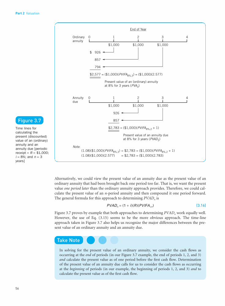
Alternatively, we could view the present value of an annuity due as the present value of anordinary annuity that had been brought back one period too far. That is, we want the presentvalue one period later than the ordinary annuity approach provides. Therefore, we could cal-culate the present value of an n-period annuity and then compound it one period forward.The general formula for this approach to determining PVADn is
PVADn = (1 + i )(R )(PVIFAi,n) (3.16)
Figure 3.7 proves by example that both approaches to determining PVADn work equally well.However, the use of Eq. (3.15) seems to be the more obvious approach. The time-lineapproach taken in Figure 3.7 also helps us recognize the major differences between the pre-sent value of an ordinary annuity and an annuity due.
Take Note
In solving for the present value of an ordinary annuity, we consider the cash flows as occurring at the end of periods (in our Figure 3.7 example, the end of periods 1, 2, and 3)and calculate the present value as of one period before the first cash flow. Determination of the present value of an annuity due calls for us to consider the cash flows as occurring at the beginning of periods (in our example, the beginning of periods 1, 2, and 3) and to calculate the present value as of the first cash flow.
Part 2 Valuation
56
••
Figure 3.7Time lines forcalculating thepresent (discounted)value of an (ordinary)annuity and anannuity due [periodicreceipt = R = $1,000;i = 8%; and n = 3years]
FUNO_C03.qxd 9/19/08 16:49 Page 56

3 The Time Value of Money
57
••
Each year, on your birthday, you invest $2,000 in a tax-free retirement investment account. By age 65 you will haveaccumulated:
COMPOUND ANNUAL STARTING AGE
INTEREST RATE (i) 21 31 41 51
6% $ 425,487 $222,870 $109,730 $46,5528 773,011 344,634 146,212 54,304
10 1,437,810 542,048 196,694 63,54412 2,716,460 863,326 266,668 74,560
From the table, it looks like the time to start saving is now!
The Magic of Compound Interest
l l l Mixed FlowsMany time value of money problems that we face involve neither a single cash flow nor a single annuity. Instead, we may encounter a mixed (or uneven) pattern of cash flows.
Question Assume that you are faced with the following problem – on an exam (arghh!),perhaps. What is the present value of $5,000 to be received annually at the end ofyears 1 and 2, followed by $6,000 annually at the end of years 3 and 4, and concludingwith a final payment of $1,000 at the end of year 5, all discounted at 5 percent?
The first step in solving the question above, or any similar problem, is to draw a time line, position the cash flows, and draw arrows indicating the direction and position to whichyou are going to adjust the flows. Second, make the necessary calculations as indicated by your diagram. (You may think that drawing a picture of what needs to be done is somewhat“childlike.” However, consider that most successful home builders work from blueprints –why shouldn’t you?)
Figure 3.8 illustrates that mixed flow problems can always be solved by adjusting each flowindividually and then summing the results. This is time-consuming, but it works.
Often we can recognize certain patterns within mixed cash flows that allow us to take somecalculation shortcuts. Thus the problem that we have been working on could be solved in anumber of alternative ways. One such alternative is shown in Figure 3.9. Notice how our two-step procedure continues to lead us to the correct solution:
Take Note
l Step 1: Draw a time line, position cash flows, and draw arrows to indicate direction andposition of adjustments.
l Step 2: Perform calculations as indicated by your diagram.
A wide variety of mixed (uneven) cash-flow problems could be illustrated. To appreciatethis variety and to master the skills necessary to determine solutions, be sure to do the prob-lems at the end of this chapter. Don’t be too bothered if you make some mistakes at first. Timevalue of money problems can be tricky. Mastering this material is a little bit like learning toride a bicycle. You expect to fall and get bruised a bit until you pick up the necessary skills.But practice makes perfect.
FUNO_C03.qxd 9/19/08 16:49 Page 57

••
Part 2 Valuation
58
Figure 3.8(Alternative 1) Timeline for calculating the present(discounted) value of mixed cash flows[FV1 = FV2 = $5,000;FV3 = FV4 = $6,000;FV5 = $1,000; i = 5%;and n = 5 years]
Figure 3.9(Alternative 2) Timeline for calculating the present(discounted) value of mixed cash flows[FV1 = FV2 = $5,000;FV3 = FV4 = $6,000;FV5 = $1,000; i = 5%;and n = 5 years]
FUNO_C03.qxd 9/19/08 16:49 Page 58

Compounding More Than Once a Year
l l l Semiannual and Other Compounding PeriodsFuture (or Compound) Value. Up to now, we have assumed that interest is paid annually.It is easiest to get a basic understanding of the time value of money with this assumption.Now, however, it is time to consider the relationship between future value and interest ratesfor different compounding periods. To begin, suppose that interest is paid semiannually. Ifyou then deposit $100 in a savings account at a nominal, or stated, 8 percent annual interestrate, the future value at the end of six months would be
FV0.5 = $100(1 + [0.08/2]) = $104
In other words, at the end of one half-year you would receive 4 percent in interest, not 8 per-cent. At the end of a year the future value of the deposit would be
FV1 = $100(1 + [0.08/2])2 = $108.16
This amount compares with $108 if interest is paid only once a year. The $0.16 differenceis caused by interest being earned in the second six months on the $4 in interest paid at theend of the first six months. The more times during the year that interest is paid, the greaterthe future value at the end of a given year.
The general formula for solving for the future value at the end of n years where interest ispaid m times a year is
FVn = PV0(1 + [i /m])mn (3.17)
To illustrate, suppose that now interest is paid quarterly and that you wish to know the futurevalue of $100 at the end of one year where the stated annual rate is 8 percent. The future valuewould be
FV1 = $100(1 + [0.08/4])(4)(1)
= $100(1 + 0.02)4 = $108.24
which, of course, is higher than it would be with either semiannual or annual compounding.The future value at the end of three years for the example with quarterly compound-
ing is
FV3 = $100(1 + [0.08/4])(4)(3)
= $100(1 + 0.02)12 = $126.82
compared with a future value with semiannual compounding of
FV3 = $100(1 + [0.08/2])(2)(3)
= $100(1 + 0.04)6 = $126.53
and with annual compounding of
FV3 = $100(1 + [0.08/1])(1)(3)
= $100(1 + 0.08)3 = $125.97
Thus, the more frequently interest is paid each year, the greater the future value. When m inEq. (3.17) approaches infinity, we achieve continuous compounding. Shortly, we will take aspecial look at continuous compounding and discounting.
Present (or Discounted) Value. When interest is compounded more than once a year, theformula for calculating present value must be revised along the same lines as for the calcula-tion of future value. Instead of dividing the future cash flow by (1 + i)n as we do when annualcompounding is involved, we determine the present value by
3 The Time Value of Money
59
••
Nominal (stated)interest rateA rate of interestquoted for a year that has not beenadjusted for frequencyof compounding. If interest iscompounded morethan once a year, the effective interestrate will be higherthan the nominal rate.
FUNO_C03.qxd 9/19/08 16:49 Page 59

PV0 = FVn /(1 + [i /m])mn (3.18)
where, as before, FVn is the future cash flow to be received at the end of year n, m is the num-ber of times a year interest is compounded, and i is the discount rate. We can use Eq. (3.18),for example, to calculate the present value of $100 to be received at the end of year 3 for anominal discount rate of 8 percent compounded quarterly:
PV0 = $100/(1 + [0.08/4])(4)(3)
= $100/(1 + 0.02)12 = $78.85
If the discount rate is compounded only annually, we have
PV0 = $100/(1 + 0.08)3 = $79.38
Thus, the fewer times a year that the nominal discount rate is compounded, the greater thepresent value. This relationship is just the opposite of that for future values.
l l l Continuous CompoundingIn practice, interest is sometimes compounded continuously. Therefore it is useful to considerhow this works. Recall that the general formula for solving for the future value at the end ofyear n, Eq. (3.17), is
FVn = PV0(1 + [i /m])mn
As m, the number of times a year that interest is compounded, approaches infinity (∞), we getcontinuous compounding, and the term (1 + [i/m])mn approaches ein, where e is approxim-ately 2.71828. Therefore the future value at the end of n years of an initial deposit of PV0
where interest is compounded continuously at a rate of i percent is
FVn = PV0(e )in (3.19)
For our earlier example problem, the future value of a $100 deposit at the end of three yearswith continuous compounding at 8 percent would be
FV3 = $100(e)(0.08)(3)
= $100(2.71828)(0.24) = $127.12
This compares with a future value with annual compounding of
FV3 = $100(1 + 0.08)3 = $125.97
Continuous compounding results in the maximum possible future value at the end of nperiods for a given nominal rate of interest.
By the same token, when interest is compounded continuously, the formula for the presentvalue of a cash flow received at the end of year n is
PV0 = FVn /(e)in (3.20)
Thus the present value of $1,000 to be received at the end of 10 years with a discount rate of20 percent, compounded continuously, is
PV0 = $1,000/(e)(0.20)(10)
= $1,000/(2.71828)2 = $135.34
We see then that present value calculations involving continuous compounding are merely the reciprocals of future value calculations. Also, although continuous compound-ing results in the maximum possible future value, it results in the minimum possible presentvalue.
Part 2 Valuation
60
••
FUNO_C03.qxd 9/19/08 16:49 Page 60

3The “special case” formula for effective annual interest rate when there is continuous compounding is as follows:
effective annual interest rate = (e)i − 1
61
••
Effective annualinterest rate Theactual rate of interestearned (paid) afteradjusting the nominalrate for factors suchas the number ofcompounding periodsper year.
Question When a bank quotes you an annual percentage yield (APY) on a savings account orcertificate of deposit, what does that mean?
Answer Based on a congressional act, the Federal Reserve requires that banks and thrifts adopta standardized method of calculating the effective interest rates they pay on consumeraccounts. It is called the annual percentage yield (APY). The APY is meant to eliminateconfusion caused when savings institutions apply different methods of compoundingand use various terms, such as effective yield, annual yield, and effective rate. The APY issimilar to the effective annual interest rate. The APY calculation, however, is based onthe actual number of days for which the money is deposited in an account in a 365-dayyear (366 days in a leap year).
In a similar vein, the Truth-in-Lending Act mandates that all financial institutionsreport the effective interest rate on any loan. This rate is called the annual percentagerate (APR). However, the financial institutions are not required to report the “true”effective annual interest rate as the APR. Instead, they may report a noncompoundedversion of the effective annual interest rate. For example, assume that a bank makes aloan for less than a year, or interest is to be compounded more frequently than annually.The bank would determine an effective periodic interest rate – based on usable funds (i.e.,the amount of funds the borrower can actually use) – and then simply multiply this rateby the number of such periods in a year. The result is the APR.
l l l Effective Annual Interest RateDifferent investments may provide returns based on various compounding periods. If we wantto compare alternative investments that have different compounding periods, we need to statetheir interest on some common, or standardized, basis. This leads us to make a distinctionbetween nominal, or stated, interest and the effective annual interest rate. The effectiveannual interest rate is the interest rate compounded annually that provides the same annualinterest as the nominal rate does when compounded m times per year.
By definition then,
(1 + effective annual interest rate) = (1 + [i /m])(m)(1)
Therefore, given the nominal rate i and the number of compounding periods per year m, wecan solve for the effective annual interest rate as follows:3
effective annual interest rate = (1 + [i /m])m − 1 (3.21)
For example, if a savings plan offered a nominal interest rate of 8 percent compounded quarterly on a one-year investment, the effective annual interest rate would be
(1 + [0.08/4])4 − 1 = (1 + 0.02)4 − 1 = 0.08243
Only if interest had been compounded annually would the effective annual interest rate haveequaled the nominal rate of 8 percent.
Table 3.7 contains a number of future values at the end of one year for $1,000 earning a nominal rate of 8 percent for several different compounding periods. The table illustrates that the more numerous the compounding periods, the greater the future value of (and interest earned on) the deposit, and the greater the effective annual interest rate.
3 The Time Value of Money
FUNO_C03.qxd 9/19/08 16:49 Page 61

Amortizing a Loan
An important use of present value concepts is in determining the payments required for an installment-type loan. The distinguishing feature of this loan is that it is repaid in equalperiodic payments that include both interest and principal. These payments can be mademonthly, quarterly, semiannually, or annually. Installment payments are prevalent in mort-gage loans, auto loans, consumer loans, and certain business loans.
To illustrate with the simplest case of annual payments, suppose you borrow $22,000 at 12 percent compound annual interest to be repaid over the next six years. Equal installmentpayments are required at the end of each year. In addition, these payments must be sufficientin amount to repay the $22,000 together with providing the lender with a 12 percent return.To determine the annual payment, R, we set up the problem as follows:
= R (PVIFA12%,6)
In Table IV in the Appendix at the end of the book, we find that the discount factor for a six-year annuity with a 12 percent interest rate is 4.111. Solving for R in the problem above, we have
$22,000 = R (4.111)R = $22,000/4.111 = $5,351
Thus annual payments of $5,351 will completely amortize (extinguish) a $22,000 loan insix years. Each payment consists partly of interest and partly of principal repayment. Theamortization schedule is shown in Table 3.8. We see that annual interest is determined by
$22,000 1/ 1 0.12)1
6
(= +⎡
⎣⎢⎢
⎤
⎦⎥⎥=
∑R t
t
Part 2 Valuation
62
••
Table 3.7Effects of differentcompounding periodson future values of$1,000 invested atan 8% nominalinterest rate
INITIAL COMPOUNDING FUTURE VALUE AT EFFECTIVE ANNUAL AMOUNT PERIODS END OF 1 YEAR INTEREST RATE*
$1,000 Annually $1,080.00 8.000%1,000 Semiannually 1,081.60 8.1601,000 Quarterly 1,082.43 8.2431,000 Monthly 1,083.00 8.3001,000 Daily (365 days) 1,083.28 8.3281,000 Continuously 1,083.29 8.329
*Note: $1,000 invested for a year at these rates compounded annually would provide the same futurevalues as those found in Column 3.
Amortizationschedule A table showing therepayment scheduleof interest andprincipal necessary to pay off a loan bymaturity.
(1) (2) (3) (4)END ANNUAL PRINCIPAL PRINCIPAL AMOUNTOF INSTALLMENT INTEREST PAYMENT OWING AT YEAR ENDYEAR PAYMENT (4)t −1 × 0.12 (1) − (2) (4)t−1 − (3)
0 – – – $22,0001 $ 5,351 $ 2,640 $ 2,711 19,2892 5,351 2,315 3,036 16,2533 5,351 1,951 3,400 12,8534 5,351 1,542 3,809 9,0445 5,351 1,085 4,266 4,7786 5,351 573 4,778 0
$32,106 $10,106 $22,000
Table 3.8Amortization schedulefor illustrated loan
FUNO_C03.qxd 9/19/08 16:49 Page 62

multiplying the principal amount outstanding at the beginning of the year by 12 percent. Theamount of principal payment is simply the total installment payment minus the interest pay-ment. Notice that the proportion of the installment payment composed of interest declinesover time, whereas the proportion composed of principal increases. At the end of six years, atotal of $22,000 in principal payments will have been made and the loan will be completelyamortized. The breakdown between interest and principal is important because on a businessloan only interest is deductible as an expense for tax purposes.
Summary Table of Key Compound Interest FormulasFLOW(S) EQUATION END OF BOOK TABLE
Single Amounts:FVn = P0(1 + i)n (3.4)
= P0(FVIFi,n) (3.5) I
PV0 = FVn[1/(1 + i)n] (3.6)= FVn(PVIFi,n) (3.7) II
Annuities:FVAn = R([(1 + i)n − 1]/i) (3.8)
= R(FVIFAi,n) (3.9) III
PVAn = R[(1 − [1/(1 + i)n])/i] (3.10)= R(PVIFAi,n) (3.11) IV
FVADn = R(FVIFAi,n)(1 + i) (3.14) III (adjusted)
PVADn = R(PVIFAi,n−1 + 1) (3.15)= (1 + i)(R)(PVIFAi,n) (3.16) IV (adjusted)
Key Learning Points
l Most financial decisions, personal as well as business,involve the time value of money. We use the rate ofinterest to express the time value of money.
l Simple interest is interest paid (earned) on only theoriginal amount, or principal, borrowed (lent).
l Compound interest is interest paid (earned) on anyprevious interest earned, as well as on the principalborrowed (lent). The concept of compound interestcan be used to solve a wide variety of problems infinance.
l Two key concepts – future value and present value –underlie all compound interest problems. Futurevalue is the value at some future time of a presentamount of money, or a series of payments, evaluatedat a given interest rate. Present value is the currentvalue of a future amount of money, or a series of pay-ments, evaluated at a given interest rate.
l It is very helpful to begin solving time value of moneyproblems by first drawing a time line on which youposition the relevant cash flows.
l An annuity is a series of equal payments or receiptsoccurring over a specified number of periods.
l There are some characteristics that should help you to identify and solve the various types of annuityproblems:1. Present value of an ordinary annuity – cash flows
occur at the end of each period, and present value iscalculated as of one period before the first cash flow.
2. Present value of an annuity due – cash flows occurat the beginning of each period, and present value iscalculated as of the first cash flow.
3. Future value of an ordinary annuity – cash flowsoccur at the end of each period, and future value iscalculated as of the last cash flow.
4. Future value of an annuity due – cash flows occurat the beginning of each period, and future value iscalculated as of one period after the last cash flow.
l Various formulas were presented for solving forfuture values and present values of single amountsand of annuities. Mixed (uneven) cash-flow problemscan always be solved by adjusting each flow indi-vidually and then summing the results. The ability torecognize certain patterns within mixed cash flowswill allow you to take calculation shortcuts.
3 The Time Value of Money
63
••
FUNO_C03.qxd 9/19/08 16:49 Page 63

Questions
1. What is simple interest?2. What is compound interest? Why is it important?3. What kinds of personal financial decisions have you made that involve compound interest?4. What is an annuity? Is an annuity worth more or less than a lump sum payment received
now that would be equal to the sum of all the future annuity payments?5. What type of compounding would you prefer in your savings account? Why?6. Contrast the calculation of future (terminal) value with the calculation of present value.
What is the difference?7. What is the advantage of using present value tables rather than formulas?8. If you are scheduled to receive a certain sum of money five years from now but wish to
sell your contract for its present value, which type of compounding would you prefer tobe used in the calculation? Why?
9. The “Rule of 72” suggests that an amount will double in 12 years at a 6 percent compoundannual rate or double in 6 years at a 12 percent annual rate. Is this a useful rule, and is itan accurate one?
10. Does present value decrease at a linear rate, at an increasing rate, or at a decreasing ratewith the discount rate? Why?
11. Does present value decrease at a linear rate, at an increasing rate, or at a decreasing ratewith the length of time in the future the payment is to be received? Why?
12. Sven Smorgasbord is 35 years old and is presently experiencing the “good” life. As aresult, he anticipates that he will increase his weight at a rate of 3 percent a year. At present he weighs 200 pounds. What will he weigh at age 60?
Self-Correction Problems
1. The following cash-flow streams need to be analyzed:
CASH-FLOW END OF YEAR
STREAM 1 2 3 4 5
W $100 $200 $200 $300 1,$300X $600 – – – –Y – – – – 11,200Z $200 – $500 – $0,300
a. Calculate the future (terminal) value of each stream at the end of year 5 with a com-pound annual interest rate of 10 percent.
b. Compute the present value of each stream if the discount rate is 14 percent.2. Muffin Megabucks is considering two different savings plans. The first plan would have her
deposit $500 every six months, and she would receive interest at a 7 percent annual rate,compounded semiannually. Under the second plan she would deposit $1,000 every yearwith a rate of interest of 7.5 percent, compounded annually. The initial deposit with Plan 1 would be made six months from now and, with Plan 2, one year hence.a. What is the future (terminal) value of the first plan at the end of 10 years?b. What is the future (terminal) value of the second plan at the end of 10 years?
Part 2 Valuation
64
••
l To compare alternative investments having differentcompounding periods, it is often necessary to calculatetheir effective annual interest rates. The effective annualinterest rate is the interest rate compounded annuallythat provides the same annual interest as the nominalrate does when compounded m times per year.
l Amortizing a loan involves determining the periodicpayment necessary to reduce the principal amount tozero at maturity, while providing interest payments onthe unpaid principal balance. The principal amountowed decreases at an increasing rate as payments aremade.
FUNO_C03.qxd 9/19/08 16:49 Page 64

c. Which plan should Muffin use, assuming that her only concern is with the value of hersavings at the end of 10 years?
d. Would your answer change if the rate of interest on the second plan were 7 percent?3. On a contract you have a choice of receiving $25,000 six years from now or $50,000 twelve
years from now. At what implied compound annual interest rate should you be indifferentbetween the two contracts?
4. Emerson Cammack wishes to purchase an annuity contract that will pay him $7,000 a yearfor the rest of his life. The Philo Life Insurance Company figures that his life expectancy is20 years, based on its actuary tables. The company imputes a compound annual interestrate of 6 percent in its annuity contracts.a. How much will Cammack have to pay for the annuity?b. How much would he have to pay if the interest rate were 8 percent?
5. You borrow $10,000 at 14 percent compound annual interest for four years. The loan isrepayable in four equal annual installments payable at the end of each year.a. What is the annual payment that will completely amortize the loan over four years?
(You may wish to round to the nearest dollar.)b. Of each equal payment, what is the amount of interest? The amount of loan principal?
(Hint: In early years, the payment is composed largely of interest, whereas at the end itis mainly principal.)
6. Your late Uncle Vern’s will entitles you to receive $1,000 at the end of every other year forthe next two decades. The first cash flow is two years from now. At a 10 percent compoundannual interest rate, what is the present value of this unusual cash-flow pattern? (Try tosolve this problem in as few steps as you can.)
7. A bank offers you a seven-month certificate of deposit (CD) at a 7.06 percent annual ratethat would provide a 7.25 percent effective annual yield. For the seven-month CD, is inter-est being compounded daily, weekly, monthly, or quarterly? And, by the way, havinginvested $10,000 in this CD, how much money would you receive when your CD maturesin seven months? That is, what size check would the bank give you if you closed youraccount at the end of seven months?
8. A Dillonvale, Ohio, man saved pennies for 65 years. When he finally decided to cash themin, he had roughly 8 million of them (or $80,000 worth), filling 40 trash cans. On average,the man saved $1,230 worth of pennies a year. If he had deposited the pennies saved each year, at each year’s end, into a savings account earning 5 percent compound annualinterest, how much would he have had in this account after 65 years of saving? How muchmore “cents” (sense) would this have meant for our “penny saver” compared with simplyputting his pennies into trash cans?
9. Xu Lin recently obtained a 10-year, $50,000 loan. The loan carries an 8 percent compoundannual interest rate and calls for annual installment payments of $7,451.47 at the end ofeach of the next 10 years.a. How much (in dollars) of the first year’s payment is principal?b. How much total interest will be paid over the life of the loan? (Hint: You do not need
to construct a loan amortization table to answer this question. Some simple math is allyou need.)
Problems
1. The following are exercises in future (terminal) values:a. At the end of three years, how much is an initial deposit of $100 worth, assuming a
compound annual interest rate of (i) 100 percent? (ii) 10 percent? (iii) 0 percent?b. At the end of five years, how much is an initial $500 deposit followed by five year-end,
annual $100 payments worth, assuming a compound annual interest rate of (i) 10 per-cent? (ii) 5 percent? (iii) 0 percent?
3 The Time Value of Money
65
••
FUNO_C03.qxd 9/19/08 16:49 Page 65

c. At the end of six years, how much is an initial $500 deposit followed by five year-end,annual $100 payments worth, assuming a compound annual interest rate of (i) 10 per-cent? (ii) 5 percent? (iii) 0 percent?
d. At the end of three years, how much is an initial $100 deposit worth, assuming a quar-terly compounded annual interest rate of (i) 100 percent? (ii) 10 percent?
e. Why do your answers to Part (d) differ from those to Part (a)?f. At the end of 10 years, how much is a $100 initial deposit worth, assuming an annual
interest rate of 10 percent compounded (i) annually? (ii) semiannually? (iii) quarterly?(iv) continuously?
2. The following are exercises in present values:a. $100 at the end of three years is worth how much today, assuming a discount rate of
(i) 100 percent? (ii) 10 percent? (iii) 0 percent?b. What is the aggregate present value of $500 received at the end of each of the next
three years, assuming a discount rate of (i) 4 percent? (ii) 25 percent?c. $100 is received at the end of one year, $500 at the end of two years, and $1,000 at the
end of three years. What is the aggregate present value of these receipts, assuming adiscount rate of (i) 4 percent? (ii) 25 percent?
d. $1,000 is to be received at the end of one year, $500 at the end of two years, and $100at the end of three years. What is the aggregate present value of these receipts assum-ing a discount rate of (i) 4 percent? (ii) 25 percent?
e. Compare your solutions in Part (c) with those in Part (d) and explain the reason forthe differences.
3. Joe Hernandez has inherited $25,000 and wishes to purchase an annuity that will providehim with a steady income over the next 12 years. He has heard that the local savings andloan association is currently paying 6 percent compound interest on an annual basis. If he were to deposit his funds, what year-end equal-dollar amount (to the nearest dollar)would he be able to withdraw annually such that he would have a zero balance after hislast withdrawal 12 years from now?
4. You need to have $50,000 at the end of 10 years. To accumulate this sum, you havedecided to save a certain amount at the end of each of the next 10 years and deposit it inthe bank. The bank pays 8 percent interest compounded annually for long-term deposits.How much will you have to save each year (to the nearest dollar)?
5. Same as Problem 4 above, except that you deposit a certain amount at the beginning ofeach of the next 10 years. Now, how much will you have to save each year (to the nearestdollar)?
6. Vernal Equinox wishes to borrow $10,000 for three years. A group of individuals agreesto lend him this amount if he contracts to pay them $16,000 at the end of the three years.What is the implicit compound annual interest rate implied by this contract (to the nearest whole percent)?
7. You have been offered a note with four years to maturity, which will pay $3,000 at the endof each of the four years. The price of the note to you is $10,200. What is the implicit compound annual interest rate you will receive (to the nearest whole percent)?
8. Sales of the P.J. Cramer Company were $500,000 this year, and they are expected to growat a compound rate of 20 percent for the next six years. What will be the sales figure at the end of each of the next six years?
9. The H & L Bark Company is considering the purchase of a debarking machine that isexpected to provide cash flows as follows:
END OF YEAR
1 2 3 4 5
Cash flow $1,200 $2,000 $2,400 $1,900 $1,600
Part 2 Valuation
66
••
FUNO_C03.qxd 9/19/08 16:49 Page 66

END OF YEAR
6 7 8 9 10
Cash flow $1,400 $1,400 $1,400 $1,400 $1,400
If the appropriate annual discount rate is 14 percent, what is the present value of thiscash-flow stream?
10. Suppose you were to receive $1,000 at the end of 10 years. If your opportunity rate is 10 percent, what is the present value of this amount if interest is compounded (a) annu-ally? (b) quarterly? (c) continuously?
11. In connection with the United States Bicentennial, the Treasury once contemplated offer-ing a savings bond for $1,000 that would be worth $1 million in 100 years. Approximatelywhat compound annual interest rate is implied by these terms?
12. Selyn Cohen is 63 years old and recently retired. He wishes to provide retirement incomefor himself and is considering an annuity contract with the Philo Life InsuranceCompany. Such a contract pays him an equal-dollar amount each year that he lives. Forthis cash-flow stream, he must put up a specific amount of money at the beginning.According to actuary tables, his life expectancy is 15 years, and that is the duration onwhich the insurance company bases its calculations regardless of how long he actuallylives.a. If Philo Life uses a compound annual interest rate of 5 percent in its calculations,
what must Cohen pay at the outset for an annuity to provide him with $10,000 peryear? (Assume that the expected annual payments are at the end of each of the 15 years.)
b. What would be the purchase price if the compound annual interest rate is 10 percent?c. Cohen had $30,000 to put into an annuity. How much would he receive each year if
the insurance company uses a 5 percent compound annual interest rate in its calcula-tions? A 10 percent compound annual interest rate?
13. The Happy Hang Glide Company is purchasing a building and has obtained a $190,000mortgage loan for 20 years. The loan bears a compound annual interest rate of 17 percentand calls for equal annual installment payments at the end of each of the 20 years. Whatis the amount of the annual payment?
14. Establish loan amortization schedules for the following loans to the nearest cent (seeTable 3.8 for an example):a. A 36-month loan of $8,000 with equal installment payments at the end of each month.
The interest rate is 1 percent per month.b. A 25-year mortgage loan of $184,000 at a 10 percent compound annual interest rate
with equal installment payments at the end of each year.15. You have borrowed $14,300 at a compound annual interest rate of 15 percent. You feel
that you will be able to make annual payments of $3,000 per year on your loan. (Paymentsinclude both principal and interest.) How long will it be before the loan is entirely paidoff (to the nearest year)?
16. Lost Dutchman Mines, Inc., is considering investing in Peru. It makes a bid to the gov-ernment to participate in the development of a mine, the profits of which will be realizedat the end of five years. The mine is expected to produce $5 million in cash to LostDutchman Mines at that time. Other than the bid at the outset, no other cash flows willoccur, as the government will reimburse the company for all costs. If Lost Dutchmanrequires a nominal annual return of 20 percent (ignoring any tax consequences), what is the maximum bid it should make for the participation right if interest is compounded(a) annually? (b) semiannually? (c) quarterly? (d) continuously?
17. Earl E. Bird has decided to start saving for his retirement. Beginning on his twenty-firstbirthday, Earl plans to invest $2,000 each birthday into a savings investment earning a
3 The Time Value of Money
67
••
FUNO_C03.qxd 9/19/08 16:49 Page 67

7 percent compound annual rate of interest. He will continue this savings program for atotal of 10 years and then stop making payments. But his savings will continue to com-pound at 7 percent for 35 more years, until Earl retires at age 65. Ivana Waite also plansto invest $2,000 a year, on each birthday, at 7 percent, and will do so for a total of 35 years.However, she will not begin her contributions until her thirty-first birthday. How muchwill Earl’s and Ivana’s savings programs be worth at the retirement age of 65? Who is better off financially at retirement, and by how much?
18. When you were born, your dear old Aunt Minnie promised to deposit $1,000 in a savingsaccount for you on each and every one of your birthdays, beginning with your first. Thesavings account bears a 5 percent compound annual rate of interest. You have just turned25 and want all the cash. However, it turns out that dear old (forgetful) Aunt Minniemade no deposits on your fifth, seventh, and eleventh birthdays. How much is in theaccount now – on your twenty-fifth birthday?
19. Assume that you will be opening a savings account today by depositing $100,000. Thesavings account pays 5 percent compound annual interest, and this rate is assumed toremain in effect for all future periods. Four years from today you will withdraw Rdollars. You will continue to make additional annual withdrawals of R dollars for a while longer – making your last withdrawal at the end of year 9 – to achieve the fol-lowing pattern of cash flows over time. (Note: Today is time period zero; one year fromtoday is the end of time period 1; etc.)
How large must R be to leave you with exactly a zero balance after your final R withdrawalis made at the end of year 9? (Tip: Making use of an annuity table or formula will makeyour work a lot easier!)
20. Suppose that an investment promises to pay a nominal 9.6 percent annual rate of inter-est. What is the effective annual interest rate on this investment assuming that interest iscompounded (a) annually? (b) semiannually? (c) quarterly? (d) monthly? (e) daily (365days)? (f ) continuously? (Note: Report your answers accurate to four decimal places –e.g., 0.0987 or 9.87%.)
21. “Want to win a million dollars? Here’s how. . . . One winner, chosen at random from allentries, will win a $1,000,000 annuity.” That was the statement announcing a contest onthe World Wide Web. The contest rules described the “million-dollar prize” in greaterdetail: “40 annual payments of $25,000 each, which will result in a total payment of$1,000,000. The first payment will be made January 1; subsequent payments will be made each January thereafter.” Using a compound annual interest rate of 8 percent, what is the present value of this “million-dollar prize” as of the first installment onJanuary 1?
22. It took roughly 14 years for the Dow Jones Average of 30 Industrial Stocks to go from1,000 to 2,000. To double from 2,000 to 4,000 took only 8 years, and to go from 4,000 to8,000 required roughly 2 years. To the nearest whole percent, what compound annualgrowth rates are implicit in these three index-doubling milestones?
Part 2 Valuation
68
••
FUNO_C03.qxd 9/19/08 16:49 Page 68

Solutions to Self-Correction Problems
1. a. Future (terminal) value of each cash flow and total future value of each stream are asfollows (using Table I in the end-of-book Appendix):
FV5 FOR INDIVIDUAL CASH FLOWS RECEIVED TOTALCASH-FLOW AT END OF YEAR FUTURESTREAM 1 2 3 4 5 VALUE
W $146.40 $266.20 $242.00 $330.00 $ 300.00 $1,284.60X 878.40 – – – – 878.40Y – – – – 1,200.00 1,200.00Z 292.80 – 605.00 – 300.00 1,197.80
b. Present value of each cash flow and total present value of each stream (using Table II inthe end-of-book Appendix):
PV0 FOR INDIVIDUAL CASH FLOWS RECEIVED TOTALCASH-FLOW AT END OF YEAR PRESENTSTREAM 1 2 3 4 5 VALUE
W $ 87.70 $153.80 $135.00 $177.60 $155.70 $709.80X 526.20 – – – – 526.20Y – – – – 622.80 622.80Z 175.40 – 337.50 – 155.70 668.60
2. a. FV10 Plan 1 = $500(FVIFA3.5%,20)= $500{[(1 + 0.035)20 − 1]/[0.035]}= $14,139.84
b. FV10 Plan 2 = $1,000(FVIFA7.5%,10)= $1,000{[(1 + 0.075)10 − 1]/[0.075]}= $14,147.09
c. Plan 2 would be preferred by a slight margin – $7.25.d. FV10 Plan 2 = $1,000(FVIFA7%,10)
= $1,000{[(1 + 0.07)10 − 1]/[0.07]}= $13,816.45
Now, Plan 1 would be preferred by a nontrivial $323.37 margin.3. Indifference implies that you could reinvest the $25,000 receipt for 6 years at X% to
provide an equivalent $50,000 cash flow in year 12. In short, $25,000 would double in 6 years. Using the “Rule of 72,” 72/6 = 12%.
Alternatively, note that $50,000 = $25,000(FVIFX%,6). Therefore (FVIFX%,6) =$50,000/$25,000 = 2. In Table I in the Appendix at the end of the book, the interest factorfor 6 years at 12 percent is 1.974 and that for 13 percent is 2.082. Interpolating, we have
as the interest rate implied in the contract.For an even more accurate answer, recognize that FVIFX%,6 can also be written as
(1 + i)6. Then, we can solve directly for i (and X% = i[100]) as follows:
(1 + i )6 = 2(1 + i ) = 21/6 = 20.1667 = 1.1225
i = 0.1225 or X% = 12.25%
4. a. PV0 = $7,000(PVIFA 6%,20) = $7,000(11.470) = $80,290b. PV0 = $7,000(PVIFA 8%,20) = $7,000(9.818) = $68,726
5. a. PV0 = $10,000 = R(PVIFA14%,4) = R(2.914)Therefore R = $10,000/2.914 = $3,432 (to the nearest dollar).
X % = +−−
=12%2.000 1.9742.082 1.974
12.24%
3 The Time Value of Money
69
••
FUNO_C03.qxd 9/19/08 16:49 Page 69

b.(1) (2) (3) (4)
ANNUAL PRINCIPAL PRINCIPAL AMOUNTEND OF INSTALLMENT INTEREST PAYMENT OWING AT YEAR ENDYEAR PAYMENT (4)t −1 × 0.14 (1) − (2) (4)t −1 − (3)
0 – – – $10,0001 $ 3,432 $1,400 $ 2,032 7,9682 3,432 1,116 2,316 5,6523 3,432 791 2,641 3,0114 3,432 421 3,011 0
$13,728 $3,728 $10,000
6. When we draw a picture of the problem, we get $1,000 at the end of every even-numberedyear for years 1 through 20:
Tip: Convert $1,000 every 2 years into an equivalent annual annuity (i.e., an annuity thatwould provide an equivalent present or future value to the actual cash flows) pattern.Solving for a 2-year annuity that is equivalent to a future $1,000 to be received at the endof year 2, we get
FVA2 = $1,000 = R (FVIFA 10%,2) = R (2.100)
Therefore R = $1,000/2.100 = $476.19. Replacing every $1,000 with an equivalent two-year annuity gives us $476.19 for 20 years.
PVA20 = $476.19(PVIFA10%,20) = $476.19(8.514) = $4,054.28
7. Effective annual interest rate = (1 + [i/m])m − 1= (1 + [0.0706/4])4 − 1= 0.07249 (approximately 7.25%)
Therefore, we have quarterly compounding. And, investing $10,000 at 7.06 percent compounded quarterly for seven months (Note: Seven months equals 21⁄3 quarter periods),we get
$10,000(1 + [0.0706/4])2.33–
= $10,000(1.041669) = $10,416.69
8. FVA 65 = $1,230(FVIFA5%,65)= $1,230[([1 + 0.05]65 − 1)/(0.05)]= $1,230(456.798) = $561,861.54
Our “penny saver” would have been better off by ($561,861.54 − $80,000) = $481,861.54– or 48,186,154 pennies – by depositing the pennies saved each year into a savings accountearning 5 percent compound annual interest.
9. a. $50,000(0.08) = $4,000 interest payment$7,451.47 − $4,000 = $3,451.47 principal payment
b. Total installment payments − total principal payments = total interest payments$74,514.70 − $50,000 = $24,514.70
Part 2 Valuation
70
••
FUNO_C03.qxd 9/19/08 16:49 Page 70

Rich, Steven P., and John T. Rose. “Interest Rate Conceptsand Terminology in Introductory Finance Textbooks.”Financial Practice and Education 7 (Spring–Summer1997), 113–121.
Shao, Stephen P., and Lawrence P. Shao. Mathematics forManagement and Finance, 8th ed. Cincinnati, OH: South-Western, 1998.
Part II of the text’s website, Wachowicz’s Web World, con-tains links to many finance websites and online articlesrelated to topics covered in this chapter.(web.utk.edu/~jwachowi/part2.html) See, especially,Annuities: Ordinary? Due? What do I do?(web.utk.edu/~jwachowi/annuity1.html) and AnnuityProblems(web.utk.edu/~jwachowi/annuity_prob.pdf )
Selected References
3 The Time Value of Money
71
••
FUNO_C03.qxd 9/19/08 16:49 Page 71

••
FUNO_C03.qxd 9/19/08 16:49 Page 72

••
73
4The Valuation of Long-TermSecurities
Contents
l Distinctions Among Valuation ConceptsLiquidation Value versus Going-Concern Value •Book Value versus Market Value • Market Valueversus Intrinsic Value
l Bond ValuationPerpetual Bonds • Bonds with a Finite Maturity
l Preferred Stock Valuation
l Common Stock ValuationAre Dividends the Foundation? • DividendDiscount Models
l Rates of Return (or Yields)Yield to Maturity (YTM) on Bonds • Yield onPreferred Stock • Yield on Common Stock
l Summary Table of Key Present ValueFormulas for Valuing Long-TermSecurities
l Key Learning Points
l Questions
l Self-Correction Problems
l Problems
l Solutions to Self-Correction Problems
l Selected References
Objectives
After studying Chapter 4, you should be able to:
l Distinguish among the various terms used toexpress value, including liquidation value,going-concern value, book value, market value,and intrinsic value.
l Value bonds, preferred stocks, and commonstocks.
l Calculate the rates of return (or yields) of differ-ent types of long-term securities.
l List and explain a number of observationsregarding the behavior of bond prices.
FUNO_C04.qxd 9/19/08 17:14 Page 73

What is a cynic? A man who knows the price of everything and the value of nothing.
—OSCAR WILDE
In the last chapter we discussed the time value of money and explored the wonders of com-pound interest. We are now able to apply these concepts to determining the value of differentsecurities. In particular, we are concerned with the valuation of the firm’s long-term secur-ities – bonds, preferred stock, and common stock (though the principles discussed apply toother securities as well). Valuation will, in fact, underlie much of the later development of thebook. Because the major decisions of a company are all interrelated in their effect on valua-tion, we must understand how investors value the financial instruments of a company.
Distinctions Among Valuation ConceptsThe term value can mean different things to different people. Therefore we need to be precisein how we both use and interpret this term. Let’s look briefly at the differences that existamong some of the major concepts of value.
l l l Liquidation Value versus Going-Concern ValueLiquidation value is the amount of money that could be realized if an asset or a group ofassets (e.g., a firm) is sold separately from its operating organization. This value is in markedcontrast to the going-concern value of a firm, which is the amount the firm could be sold foras a continuing operating business. These two values are rarely equal, and sometimes a com-pany is actually worth more dead than alive.
The security valuation models that we will discuss in this chapter will generally assume thatwe are dealing with going concerns – operating firms able to generate positive cash flows tosecurity investors. In instances where this assumption is not appropriate (e.g., impendingbankruptcy), the firm’s liquidation value will have a major role in determining the value ofthe firm’s financial securities.
l l l Book Value versus Market ValueThe book value of an asset is the accounting value of the asset – the asset’s cost minus its accumulated depreciation. The book value of a firm, on the other hand, is equal to the dollardifference between the firm’s total assets and its liabilities and preferred stock as listed on itsbalance sheet. Because book value is based on historical values, it may bear little relationshipto an asset’s or firm’s market value.
In general, the market value of an asset is simply the market price at which the asset (or asimilar asset) trades in an open marketplace. For a firm, market value is often viewed as beingthe higher of the firm’s liquidation or going-concern value.
l l l Market Value versus Intrinsic ValueBased on our general definition for market value, the market value of a security is the marketprice of the security. For an actively traded security, it would be the last reported price atwhich the security was sold. For an inactively traded security, an estimated market pricewould be needed.
The intrinsic value of a security, on the other hand, is what the price of a security shouldbe if properly priced based on all factors bearing on valuation – assets, earnings, future
Part 2 Valuation
74
••
Liquidation valueThe amount of moneythat could be realizedif an asset or a groupof assets (e.g., a firm)is sold separatelyfrom its operatingorganization.
Going-concern valueThe amount a firmcould be sold for as acontinuing operatingbusiness.
Book value(1) An asset: theaccounting value of an asset – theasset’s cost minus its accumulateddepreciation; (2) afirm: total assetsminus liabilities andpreferred stock aslisted on the balancesheet.
Market value Themarket price at whichan asset trades.
Intrinsic valueThe price a security“ought to have”based on all factorsbearing on valuation.
FUNO_C04.qxd 9/19/08 17:14 Page 74

prospects, management, and so on. In short, the intrinsic value of a security is its economicvalue. If markets are reasonably efficient and informed, the current market price of a securityshould fluctuate closely around its intrinsic value.
The valuation approach taken in this chapter is one of determining a security’s intrinsicvalue – what the security ought to be worth based on hard facts. This value is the present value of the cash-flow stream provided to the investor, discounted at a required rate of return appropriate for the risk involved. With this general valuation concept in mind, we are now able to explore in more detail the valuation of specific types of securities.
Bond ValuationA bond is a security that pays a stated amount of interest to the investor, period after period,until it is finally retired by the issuing company. Before we can fully understand the valuationof such a security, certain terms must be discussed. For one thing, a bond has a face value.1
This value is usually $1,000 per bond in the United States. The bond almost always has a statedmaturity, which is the time when the company is obligated to pay the bondholder the facevalue of the instrument. Finally, the coupon rate, or nominal annual rate of interest, is statedon the bond’s face.2 If, for example, the coupon rate is 12 percent on a $1,000-face-valuebond, the company pays the holder $120 each year until the bond matures.
In valuing a bond, or any security for that matter, we are primarily concerned with dis-counting, or capitalizing, the cash-flow stream that the security holder would receive over thelife of the instrument. The terms of a bond establish a legally binding payment pattern at thetime the bond is originally issued. This pattern consists of the payment of a stated amount ofinterest over a given number of years coupled with a final payment, when the bond matures,equal to the bond’s face value. The discount, or capitalization, rate applied to the cash-flowstream will differ among bonds depending on the risk structure of the bond issue. In gen-eral, however, this rate can be thought of as being composed of the risk-free rate plus a premium for risk. (You may remember that we introduced the idea of a market-imposed“trade-off ” between risk and return in Chapter 2. We will have more to say about risk andrequired rates of return in the next chapter.)
l l l Perpetual Bonds
The first (and easiest) place to start determining the value of bonds is with a unique class of bonds that never matures. These are indeed rare, but they help illustrate the valuation technique in its simplest form. Originally issued by Great Britain after the Napoleonic Wars to consolidate debt issues, the British consol (short for consolidated annuities) is one suchexample. This bond carries the obligation of the British government to pay a fixed interestpayment in perpetuity.
The present value of a perpetual bond would simply be equal to the capitalized value of an infinite stream of interest payments. If a bond promises a fixed annual payment of Iforever, its present (intrinsic) value, V, at the investor’s required rate of return for this debtissue, kd, is
1Much like criminals, many of the terms used in finance are also known under a number of different aliases. Thus abond’s face value is also known as its par value, or principal. Like a good detective, you need to become familiar withthe basic terms used in finance as well as their aliases.2The term coupon rate comes from the detachable coupons that are affixed to bearer bond certificates, which, whenpresented to a paying agent or the issuer, entitle the holder to receive the interest due on that date. Nowadays, registered bonds, whose ownership is registered with the issuer, allow the registered owner to receive interest by checkthrough the mail.
4 The Valuation of Long-Term Securities
75
••
Bond A long-term debtinstrument issued bya corporation orgovernment.
Face value The statedvalue of an asset. Inthe case of a bond,the face value isusually $1,000.
Coupon rate Thestated rate of intereston a bond; the annualinterest paymentdivided by the bond’sface value.
Consol A bond thatnever matures; aperpetuity in the formof a bond.
FUNO_C04.qxd 9/19/08 17:14 Page 75

(4.1)
= I (PVIFAkd,∞) (4.2)
which, from Chapter 3’s discussion of perpetuities, we know should reduce to
V = I /k d (4.3)
Thus the present value of a perpetual bond is simply the periodic interest payment divided by the appropriate discount rate per period. Suppose you could buy a bond that paid $50 ayear forever. Assuming that your required rate of return for this type of bond is 12 percent,the present value of this security would be
V = $50/0.12 = $416.67
This is the maximum amount that you would be willing to pay for this bond. If the marketprice is greater than this amount, however, you would not want to buy it.
Bonds with a Finite Maturity
Nonzero Coupon Bonds. If a bond has a finite maturity, then we must consider not onlythe interest stream but also the terminal or maturity value (face value) in valuing the bond.The valuation equation for such a bond that pays interest at the end of each year is
(4.4)
= I (PVIFAkd,n) + MV (PVIFkd,n) (4.5)
where n is the number of years until final maturity and MV is the maturity value of the bond.We might wish to determine the value of a $1,000-par-value bond with a 10 percent
coupon and nine years to maturity. The coupon rate corresponds to interest payments of $100 a year. If our required rate of return on the bond is 12 percent, then
= $100(PVIFA12%,9) + $1,000(PVIF12%,9)
Referring to Table IV in the Appendix at the back of the book, we find that the present valueinterest factor of an annuity at 12 percent for nine periods is 5.328. Table II in the Appendixreveals under the 12 percent column that the present value interest factor for a single paymentnine periods in the future is 0.361. Therefore the value, V, of the bond is
V = $100(5.328) + $1,000(0.361)= $532.80 + $361.00 = $893.80
The interest payments have a present value of $532.80, whereas the principal payment atmaturity has a present value of $360.00. (Note: All of these figures are approximate because thepresent value tables used are rounded to the third decimal place; the true present value of thebond is $893.44.)
V = + + + + . . . $100
(1.12)$100
(1.12)$100
(1.12)$1,000(1.12)1 2 9 9
VIk
Ik
Ik
MVk
Ik
MVk
n n
tt
n
n
=+
++
+ ++
++
=+
++=
∑
( )
( )
. . . ( )
( )
( )
( )
1 1 1 1
1 1
d1
d2
d d
d1 d
VIk
Ik
Ik
Ik t
t
=+
++
+ ++
=+
∞
=
∞
∑
( )
( )
. . . ( )
( )
1 1 1
1
d1
d2
d
d1
Part 2 Valuation
76
••
FUNO_C04.qxd 9/19/08 17:14 Page 76
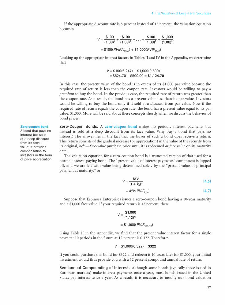
If the appropriate discount rate is 8 percent instead of 12 percent, the valuation equationbecomes
= $100(PVIFA 8%,9) + $1,000(PVIF8%,9)
Looking up the appropriate interest factors in Tables II and IV in the Appendix, we determinethat
V = $100(6.247) + $1,000(0.500)= $624.70 + $500.00 = $1,124.70
In this case, the present value of the bond is in excess of its $1,000 par value because therequired rate of return is less than the coupon rate. Investors would be willing to pay a premium to buy the bond. In the previous case, the required rate of return was greater thanthe coupon rate. As a result, the bond has a present value less than its par value. Investorswould be willing to buy the bond only if it sold at a discount from par value. Now if therequired rate of return equals the coupon rate, the bond has a present value equal to its parvalue, $1,000. More will be said about these concepts shortly when we discuss the behavior ofbond prices.
Zero-Coupon Bonds. A zero-coupon bond makes no periodic interest payments butinstead is sold at a deep discount from its face value. Why buy a bond that pays no interest? The answer lies in the fact that the buyer of such a bond does receive a return. This return consists of the gradual increase (or appreciation) in the value of the security fromits original, below-face-value purchase price until it is redeemed at face value on its maturitydate.
The valuation equation for a zero-coupon bond is a truncated version of that used for anormal interest-paying bond. The “present value of interest payments” component is loppedoff, and we are left with value being determined solely by the “present value of principal payment at maturity,” or
(4.6)
= MV (PVIFkd,n) (4.7)
Suppose that Espinosa Enterprises issues a zero-coupon bond having a 10-year maturityand a $1,000 face value. If your required return is 12 percent, then
= $1,000(PVIF12%,10)
Using Table II in the Appendix, we find that the present value interest factor for a single payment 10 periods in the future at 12 percent is 0.322. Therefore:
V = $1,000(0.322) = $322
If you could purchase this bond for $322 and redeem it 10 years later for $1,000, your initialinvestment would thus provide you with a 12 percent compound annual rate of return.
Semiannual Compounding of Interest. Although some bonds (typically those issued inEuropean markets) make interest payments once a year, most bonds issued in the UnitedStates pay interest twice a year. As a result, it is necessary to modify our bond valuation
V = $1,000(1.12)10
VMV
k n=
+ ( )1 d
V = + + + + . . . $100
(1.08)$100
(1.08)$100
(1.08)$1,000(1.08)1 2 9 9
4 The Valuation of Long-Term Securities
77
••
Zero-coupon bondA bond that pays nointerest but sells at a deep discountfrom its face value; it providescompensation toinvestors in the formof price appreciation.
FUNO_C04.qxd 9/19/08 17:14 Page 77

equations to account for compounding twice a year.3 For example, Eqs. (4.4) and (4.5) wouldbe changed as follows
(4.8)
= (I /2)(PVIFAkd /2,2n) + MV (PVIFkd /2,2n) (4.9)
where kd is the nominal annual required rate of interest, I/2 is the semiannual coupon pay-ment, and 2n is the number of semiannual periods until maturity.
Take Note
Notice that semiannual discounting is applied to both the semiannual interest payments and the lump-sum maturity value payment. Though it may seem inappropriate to use semiannual discounting on the maturity value, it isn’t. The assumption of semiannual discounting, once taken, applies to all inflows.
To illustrate, if the 10 percent coupon bonds of US Blivet Corporation have 12 years tomaturity and our nominal annual required rate of return is 14 percent, the value of one$1,000-par-value bond is
V = ($50)(PVIFA 7%,24) + $1,000(PVIF 7%,24)= ($50)(11.469) + $1,000(0.197) = $770.45
Rather than having to solve for value by hand, professional bond traders often turn to bondvalue tables. Given the maturity, coupon rate, and required return, one can look up the pre-sent value. Similarly, given any three of the four factors, one can look up the fourth. Also,some specialized calculators are programmed to compute bond values and yields, given theinputs mentioned. In your professional life you may very well end up using these tools whenworking with bonds.
TIP•TIP
Remember, when you use bond Eqs. (4.4), (4.5), (4.6), (4.7), (4.8), and (4.9), the variableMV is equal to the bond’s maturity value, not its current market value.
Preferred Stock ValuationMost preferred stock pays a fixed dividend at regular intervals. The features of this financialinstrument are discussed in Chapter 20. Preferred stock has no stated maturity date and, giventhe fixed nature of its payments, is similar to a perpetual bond. It is not surprising, then, thatwe use the same general approach as applied to valuing a perpetual bond to the valuation ofpreferred stock.4 Thus the present value of preferred stock is
V = Dp /kp (4.10)
VIk
MVkt
t
n
n=
++
+=∑ /
/ )
/ )2
(1 2 (1 2d1
2
d2
3Even with a zero-coupon bond, the pricing convention among bond professionals is to use semiannual rather thanannual compounding. This provides consistent comparisons with interest-bearing bonds.4Virtually all preferred stock issues have a call feature (a provision that allows the company to force retirement), andmany are eventually retired. When valuing a preferred stock that is expected to be called, we can apply a modifiedversion of the formula used for valuing a bond with a finite maturity; the periodic preferred dividends replace theperiodic interest payments and the “call price” replaces the bond maturity value in Eqs. (4.4) and (4.5), and all thepayments are discounted at a rate appropriate to the preferred stock in question.
Part 2 Valuation
78
••
Preferred stockA type of stock thatpromises a (usually)fixed dividend, but atthe discretion of theboard of directors. Ithas preference overcommon stock in thepayment of dividendsand claims on assets.
FUNO_C04.qxd 9/19/08 17:14 Page 78

••
4 The Valuation of Long-Term Securities
79
where Dp is the stated annual dividend per share of preferred stock and k p is the appropriatediscount rate. If Margana Cipher Corporation had a 9 percent, $100-par-value preferred stockissue outstanding and your required return was 14 percent on this investment, its value pershare to you would be
V = $9/0.14 = $64.29
Common Stock ValuationThe theory surrounding the valuation of common stock has undergone profound changeduring the last few decades. It is a subject of considerable controversy, and no one method forvaluation is universally accepted. Still, in recent years there has emerged growing acceptanceof the idea that individual common stocks should be analyzed as part of a total portfolio ofcommon stocks that the investor might hold. In other words, investors are not as concernedwith whether a particular stock goes up or down as they are with what happens to the overallvalue of their portfolios. This concept has important implications for determining therequired rate of return on a security. We shall explore this issue in the next chapter. First,however, we need to focus on the size and pattern of the returns to the common stockinvestor. Unlike bond and preferred stock cash flows, which are contractually stated, muchmore uncertainty surrounds the future stream of returns connected with common stock.
l l l Are Dividends the Foundation?When valuing bonds and preferred stock, we determined the discounted value of all the cashdistributions made by the firm to the investor. In a similar fashion, the value of a share ofcommon stock can be viewed as the discounted value of all expected cash dividends providedby the issuing firm until the end of time.5 In other words,
5This model was first developed by John B. Williams, The Theory of Investment Value (Cambridge, MA: HarvardUniversity Press, 1938). And, as Williams so aptly put it in poem form, “A cow for her milk/A hen for her eggs/Anda stock, by heck/For her dividends.”
Common stockSecurities thatrepresent the ultimate ownership(and risk) position ina corporation.
QWhat’s preferred stock?
AWe generally avoid investing in preferred stocks, butwe’re happy to explain them. Like common stock,
a share of preferred stock confers partial ownership of a company to its holder. But unlike common stock,holders of preferred stock usually have no voting privi-leges. Shares of preferred stock often pay a guaranteed
fixed dividend that is higher than the common stock dividend.
Preferred stock isn’t really for individual investors,though. The shares are usually purchased by other cor-porations, which are attracted by the dividends that givethem income taxed at a lower rate. Corporations also likethe fact that preferred stockholders’ claims on companyearnings and assets have a higher priority than that of common stockholders. Imagine that the One-LeggedChair Co. (ticker: WOOPS) goes out of business. Manypeople or firms with claims on the company will wanttheir due. Creditors will be paid before preferred stock-holders, but preferred stockholders have a higher prioritythan common stockholders.
Ask the Fool
Source: The Motley Fool (www.fool.com). Reproduced with the permission of The Motley Fool.
FUNO_C04.qxd 9/19/08 17:14 Page 79

(4.11)
(4.12)
where Dt is the cash dividend at the end of time period t and ke is the investor’s requiredreturn, or capitalization rate, for this equity investment. This seems consistent with what wehave been doing so far.
But what if we plan to own the stock for only two years? In this case, our model becomes
where P2 is the expected sales price of our stock at the end of two years. This assumes thatinvestors will be willing to buy our stock two years from now. In turn, these future investorswill base their judgments of what the stock is worth on expectations of future dividends and a future selling price (or terminal value). And so the process goes through successiveinvestors.
Note that it is the expectation of future dividends and a future selling price, which itself isbased on expected future dividends, that gives value to the stock. Cash dividends are all thatstockholders, as a whole, receive from the issuing company. Consequently, the foundation forthe valuation of common stock must be dividends. These are construed broadly to mean anycash distribution to shareholders, including share repurchases. (See Chapter 18 for a discus-sion of share repurchase as part of the overall dividend decision.)
The logical question to raise at this time is: Why do the stocks of companies that pay no dividends have positive, often quite high, values? The answer is that investors expect to sell the stock in the future at a price higher than they paid for it. Instead of dividend incomeplus a terminal value, they rely only on the terminal value. In turn, terminal value depends onthe expectations of the marketplace viewed from this terminal point. The ultimate expecta-tion is that the firm will eventually pay dividends, either regular or liquidating, and that future investors will receive a company-provided cash return on their investment. In theinterim, investors are content with the expectation that they will be able to sell their stock at a subsequent time, because there will be a market for it. In the meantime, the company isreinvesting earnings and, everyone hopes, enhancing its future earning power and ultimatedividends.
l l l Dividend Discount ModelsDividend discount models are designed to compute the intrinsic value of a share of commonstock under specific assumptions as to the expected growth pattern of future dividends and the appropriate discount rate to employ. Merrill Lynch, CS First Boston, and a numberof other investment banks routinely make such calculations based on their own particularmodels and estimates. What follows is an examination of such models, beginning with thesimplest one.
Constant Growth. Future dividends of a company could jump all over the place; but, if dividends are expected to grow at a constant rate, what implications does this hold for ourbasic stock valuation approach? If this constant rate is g, then Eq. (4.11) becomes
(4.13)
where D0 is the present dividend per share. Thus the dividend expected at the end of period nis equal to the most recent dividend times the compound growth factor, (1 + g)n. This maynot look like much of an improvement over Eq. (4.11). However, assuming that ke is greater
VD g
kD g
kD g
k=
++
++
++ +
++
∞
∞ ( )
( )
( )( )
. . . ( )
( )0
e1
02
e2
e
1 1
1 1
1 1 0
VD
kD
kP
k=
++
++
+ ( )
( )
( )
1
e1
2
e2
2
e21 1 1
=+=
∞
∑ )D
kt
tt (1 e1
VD
kD
kD
k=
++
++ +
+∞
∞ ( )
( )
. . . ( )
1
e1
2
e2
e1 1 1
Part 2 Valuation
80
••
FUNO_C04.qxd 9/19/08 17:14 Page 80

than g (a reasonable assumption because a dividend growth rate that is always greater than thecapitalization rate would imply an infinite stock value), Eq. (4.13) can be reduced to6
V = D1 /(ke − g) (4.14)
Rearranging, the investor’s required return can be expressed as
ke = (D1 /V ) + g (4.15)
The critical assumption in this valuation model is that dividends per share are expected togrow perpetually at a compound rate of g. For many companies this assumption may be a fairapproximation of reality. To illustrate the use of Eq. (4.14), suppose that LKN, Inc.’s dividendper share at t = 1 is expected to be $4, that it is expected to grow at a 6 percent rate forever, andthat the appropriate discount rate is 14 percent. The value of one share of LKN stock would be
V = $4/(0.14 − 0.06) = $50
For companies in the mature stage of their life cycle, the perpetual growth model is often reasonable.
TIP•TIP
A common mistake made in using Eqs. (4.14) and (4.15) is to use, incorrectly, the firm’smost recent annual dividend for the variable D1 instead of the annual dividend expected bythe end of the coming year.
Conversion to an Earnings Multiplier Approach With the constant growth model, wecan easily convert from dividend valuation, Eq. (4.14), to valuation based on an earnings multiplier approach. The idea is that investors often think in terms of how many dollars theyare willing to pay for a dollar of future expected earnings. Assume that a company retains aconstant proportion of its earnings each year; call it b. The dividend-payout ratio (dividendsper share divided by earnings per share) would also be constant. Therefore,
(1 − b) = D1 /E1 (4.16)
and
(1 − b)E1 = D1
where E1 is expected earnings per share in period 1. Equation (4.14) can then be expressed as
V = [(1 − b)E1] /(ke − g) (4.17)
6If we multiply both sides of Eq. (4.13) by (1 + ke)/(1 + g) and subtract Eq. (4.13) from the product, we get
Because we assume that ke is greater than g, the second term on the right-hand side approaches zero. Consequently,
V(ke − g) = D0(1 + g) = D1
V = D1 /(ke − g)
This model is sometimes called the “Gordon Dividend Valuation Model” after Myron J. Gordon, who developed itfrom the pioneering work done by John Williams. See Myron J. Gordon, The Investment, Financing, and Valuation ofthe Corporation (Homewood, IL: Richard D. Irwin, 1962).
4 The Valuation of Long-Term Securities
81
••
FUNO_C04.qxd 9/19/08 17:14 Page 81

where value is now based on expected earnings in period 1. In our earlier example, supposethat LKN, Inc., has a retention rate of 40 percent and earnings per share for period 1 areexpected to be $6.67. Therefore,
V = [(0.60)$6.67]/(0.14 − 0.06) = $50
Rearranging Eq. (4.17), we get
Earnings multiplier = V /E1 = (1 − b)/(ke − g) (4.18)
Equation (4.18) thus gives us the highest multiple of expected earnings that the investorwould be willing to pay for the security. In our example,
Earnings multiplier = (1 − 0.40)/(0.14 − 0.06) = 7.5 times
Thus expected earnings of $6.67 coupled with an earnings multiplier of 7.5 values our common stock at $50 a share ($6.67 × 7.5 = $50). But remember, the foundation for this alternative approach to common stock valuation was nevertheless our constant growth dividend discount model.
No Growth. A special case of the constant growth dividend model calls for an expected dividend growth rate, g, of zero. Here the assumption is that dividends will be maintained attheir current level forever. In this case, Eq. (4.14) reduces to
V = D1 /ke (4.19)
Not many stocks can be expected simply to maintain a constant dividend forever. However,when a stable dividend is expected to be maintained for a long period of time, Eq. (4.19) canprovide a good approximation of value.7
Growth Phases. When the pattern of expected dividend growth is such that a constantgrowth model is not appropriate, modifications of Eq. (4.13) can be used. A number of valua-tion models are based on the premise that firms may exhibit above-normal growth for a num-ber of years (g may even be larger than ke during this phase), but eventually the growth ratewill taper off. Thus the transition might well be from a currently above-normal growth rate toone that is considered normal. If dividends per share are expected to grow at a 10 percentcompound rate for five years and thereafter at a 6 percent rate, Eq. (4.13) becomes
(4.20)
Note that the growth in dividends in the second phase uses the expected dividend in period 5as its foundation. Therefore the growth-term exponent is t − 5, which means that the expon-ent in period 6 equals 1, in period 7 it equals 2, and so forth. This second phase is nothingmore than a constant-growth model following a period of above-normal growth. We canmake use of that fact to rewrite Eq. (4.20) as follows:
(4.21)
If the current dividend, D0, is $2 per share and the required rate of return, ke, is 14 percent,we could solve for V. (See Table 4.1 for specifics.)
= $8.99 + $22.13 = $31.12
Vt
tt
= + ⎡⎣⎢
⎤⎦⎥ −
⎡⎣⎢
⎤⎦⎥=
∑ $ ( )( )
( ) ( . )
2 1.101.14
11.14
$3.410.14 0 061
5
5
VD
k kD
k
t
tt
=+
++
⎡
⎣⎢
⎤
⎦⎥ −
⎡
⎣⎢
⎤
⎦⎥
=∑ ( )
( )
( ) ( . )0
e1
5
e5
6
e
1.101
11 0 06
VD
kD
k
t
tt
t
tt
=+
++=
−
=
∞
∑ ∑ ( )
( )
( )( )
0
e1
55
5
e6
1.101
1.061
7AT&T is one example of a firm that maintained a stable dividend for an extended period of time. For 36 years, from1922 until December 1958, AT&T paid $9 a year in dividends.
Part 2 Valuation
82
••
FUNO_C04.qxd 9/19/08 17:14 Page 82

The transition from an above-normal rate of dividend growth could be specified as moregradual than the two-phase approach just illustrated. We might expect dividends to grow at a10 percent rate for five years, followed by an 8 percent rate for the next five years and a 6 per-cent growth rate thereafter. The more growth segments that are added, the more closely thegrowth in dividends will approach a curvilinear function. But no firm can grow at an above-normal rate forever. Typically, companies tend to grow at a very high rate initially, after whichtheir growth opportunities slow down to a rate that is normal for companies in general. Ifmaturity is reached, the growth rate may stop altogether.
Rates of Return (or Yields)So far, this chapter has illustrated how the valuation of any long-term financial instrumentinvolves a capitalization of that security’s income stream by a discount rate (or required rateof return) appropriate for that security’s risk. If we replace intrinsic value (V) in our valuationequations with the market price (P0) of the security, we can then solve for the market requiredrate of return. This rate, which sets the discounted value of the expected cash inflows equal tothe security’s current market price, is also referred to as the security’s (market) yield. Depend-ing on the security being analyzed, the expected cash inflows may be interest payments, repay-ment of principal, or dividend payments. It is important to recognize that only when theintrinsic value of a security to an investor equals the security’s market value (price) would theinvestor’s required rate of return equal the security’s (market) yield.
Market yields serve an essential function by allowing us to compare, on a uniform basis,securities that differ in cash flows provided, maturities, and current prices. In future chapterswe will see how security yields are related to the firm’s future financing costs and overall costof capital.
l l l Yield to Maturity (YTM) on BondsThe market required rate of return on a bond (kd) is more commonly referred to as the bond’syield to maturity. Yield to maturity (YTM) is the expected rate of return on a bond if boughtat its current market price and held to maturity; it is also known as the bond’s internal rate
4 The Valuation of Long-Term Securities
83
••
Table 4.1Two-phase growth andcommon stockvaluation calculations
Yield to maturity(YTM) The expectedrate of return on abond if bought at itscurrent market priceand held to maturity.
PHASE 1: PRESENT VALUE OF DIVIDENDS TO BE RECEIVED OVER FIRST 5 YEARS
END OF PRESENT VALUE CALCULATION PRESENT VALUEYEAR (DIVIDEND × PVIF14%,t ) OF DIVIDEND
1 $2(1.10)1 = $2.20 × 0.877 = $1.932 2(1.10)2 = 2.42 × 0.769 = 1.863 2(1.10)3 = 2.66 × 0.675 = 1.804 2(1.10)4 = 2.93 × 0.592 = 1.735 2(1.10)5 = 3.22 × 0.519 = 1.67
= $8.99
PHASE 2: PRESENT VALUE OF CONSTANT GROWTH COMPONENT
Dividend at the end of year 6 = $3.22(1.06) = $3.41Value of stock at the end of year 5 = D6 /(ke − g) = $3.41/(0.14 − 0.06) = $42.63Present value of $42.63 at end of year 5 = ($42.63)(PVIF14%,5)
= ($42.63)(0.519) = $22.13
PRESENT VALUE OF STOCK
V = $8.99 + $22.13 = $31.12
or =
$ ( . )
( . )
2 1 10
1 141
5 t
tt∑
⎡
⎣⎢⎢
⎤
⎦⎥⎥
FUNO_C04.qxd 9/19/08 17:14 Page 83

of return (IRR). Mathematically, it is the discount rate that equates the present value of allexpected interest payments and the payment of principal (face value) at maturity with thebond’s current market price. For an example, let’s return to Eq. (4.4), the valuation equationfor an interest-bearing bond with a finite maturity. Replacing intrinsic value (V) with currentmarket price (P0) gives us
(4.22)
If we now substitute actual values for I, MV, and P0, we can solve for kd, which in this casewould be the bond’s yield to maturity. However, the precise calculation for yield to maturityis rather complex and requires bond value tables, or a sophisticated handheld calculator, or acomputer.
Interpolation. If all we have to work with are present value tables, we can still determine an approximation of the yield to maturity by making use of a trial-and-error procedure. To illustrate, consider a $1,000-par-value bond with the following characteristics: a currentmarket price of $761, 12 years until maturity, and an 8 percent coupon rate (with interest paidannually). We want to determine the discount rate that sets the present value of the bond’sexpected future cash-flow stream equal to the bond’s current market price. Suppose that westart with a 10 percent discount rate and calculate the present value of the bond’s expectedfuture cash flows. For the appropriate present value interest factors, we make use of Tables IIand IV in the Appendix at the end of the book.
V = $80(PVIFA10%,12) + $1,000(PVIF10%,12)= $80(6.814) + $1,000(0.319) = $864.12
A 10 percent discount rate produces a resulting present value for the bond that is greaterthan the current market price of $761. Therefore we need to try a higher discount rate tohandicap the future cash flows further and drive their present value down to $761. Let’s try a15 percent discount rate:
V = $80(PVIFA15%,12) + $1,000(PVIF15%,12)= $80(5.421) + $1,000(0.187) = $620.68
This time the chosen discount rate was too large. The resulting present value is less thanthe current market price of $761. The rate necessary to discount the bond’s expected cashflows to $761 must fall somewhere between 10 and 15 percent.
To approximate this discount rate, we interpolate between 10 and 15 percent as follows:8
XX
0.05$103.12$243.44
Therefore,(0.05) ($103.12)
$243.44 = =
×= 0.0212
0.050.10 $864.12
$761.00$103.12
0.15 $620.68
XYTM⎡⎣⎢
⎤⎦⎥
⎡
⎣
⎢⎢⎢
⎤
⎦
⎥⎥⎥$ .243 44
PIk
MVkt
t
n
n0d1 d(1 (1
)
)
=+
++=
∑
8Mathematically, we can generalize our discount-rate interpolation as follows:
where iL = discount rate that is somewhat lower than the investment’s YTM (or IRR), iH = discount rate that is somewhat higher than the investment’s YTM, PVL = present value of the investment at a discount rate equal to iL,PVH = present value of the investment at a discount rate equal to i H, PVYTM = present value of the investment at a discount rate equal to the investment’s YTM, which (by definition) must equal the investment’s current price.
Part 2 Valuation
84
••
Interpolate Estimatean unknown numberthat lies somewherebetween two knownnumbers.
FUNO_C04.qxd 9/19/08 17:14 Page 84
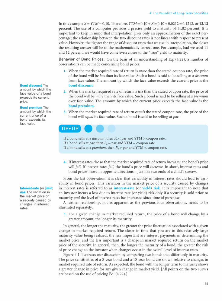
In this example X = YTM − 0.10. Therefore, YTM = 0.10 + X = 0.10 + 0.0212 = 0.1212, or 12.12percent. The use of a computer provides a precise yield to maturity of 11.82 percent. It isimportant to keep in mind that interpolation gives only an approximation of the exact per-centage; the relationship between the two discount rates is not linear with respect to presentvalue. However, the tighter the range of discount rates that we use in interpolation, the closerthe resulting answer will be to the mathematically correct one. For example, had we used 11and 12 percent, we would have come even closer to the “true” yield to maturity.
Behavior of Bond Prices. On the basis of an understanding of Eq. (4.22), a number ofobservations can be made concerning bond prices:
1. When the market required rate of return is more than the stated coupon rate, the priceof the bond will be less than its face value. Such a bond is said to be selling at a discountfrom face value. The amount by which the face value exceeds the current price is thebond discount.
2. When the market required rate of return is less than the stated coupon rate, the price ofthe bond will be more than its face value. Such a bond is said to be selling at a premiumover face value. The amount by which the current price exceeds the face value is thebond premium.
3. When the market required rate of return equals the stated coupon rate, the price of thebond will equal its face value. Such a bond is said to be selling at par.
TIP•TIP
If a bond sells at a discount, then P0 < par and YTM > coupon rate.If a bond sells at par, then P0 = par and YTM = coupon rate.If a bond sells at a premium, then P0 > par and YTM < coupon rate.
4. If interest rates rise so that the market required rate of return increases, the bond’s pricewill fall. If interest rates fall, the bond’s price will increase. In short, interest rates andbond prices move in opposite directions – just like two ends of a child’s seesaw.
From the last observation, it is clear that variability in interest rates should lead to vari-ability in bond prices. This variation in the market price of a security caused by changes in interest rates is referred to as interest-rate (or yield) risk. It is important to note that an investor incurs a loss due to interest-rate (or yield) risk only if a security is sold prior tomaturity and the level of interest rates has increased since time of purchase.
A further relationship, not as apparent as the previous four observations, needs to be illustrated separately.
5. For a given change in market required return, the price of a bond will change by agreater amount, the longer its maturity.
In general, the longer the maturity, the greater the price fluctuation associated with a givenchange in market required return. The closer in time that you are to this relatively large maturity value being realized, the less important are interest payments in determining themarket price, and the less important is a change in market required return on the market price of the security. In general, then, the longer the maturity of a bond, the greater the riskof price change to the investor when changes occur in the overall level of interest rates.
Figure 4.1 illustrates our discussion by comparing two bonds that differ only in maturity.The price sensitivities of a 5-year bond and a 15-year bond are shown relative to changes inmarket required rate of return. As expected, the bond with the longer term to maturity showsa greater change in price for any given change in market yield. [All points on the two curvesare based on the use of pricing Eq. (4.22).]
4 The Valuation of Long-Term Securities
85
••
Bond discount Theamount by which theface value of a bondexceeds its currentprice.
Bond premium Theamount by which thecurrent price of abond exceeds its face value.
Interest-rate (or yield)risk The variation inthe market price of a security caused bychanges in interestrates.
FUNO_C04.qxd 9/19/08 17:14 Page 85

••
Part 2 Valuation
86
One last relationship also needs to be addressed separately, and it is known as the couponeffect.
6. For a given change in market required rate of return, the price of a bond will change byproportionally more, the lower the coupon rate. In other words, bond price volatility isinversely related to coupon rate.
The reason for this effect is that the lower the coupon rate, the more return to the investoris reflected in the principal payment at maturity as opposed to interim interest payments. Putanother way, investors realize their returns later with a low-coupon-rate bond than with ahigh-coupon-rate bond. In general, the further in the future the bulk of the payment stream,the greater the present value effect caused by a change in required return.9 Even if high- andlow-coupon-rate bonds have the same maturity, the price of the low-coupon-rate bond tendsto be more volatile.
YTM and Semiannual Compounding. As previously mentioned, most domestic bonds payinterest twice a year, not once. This real-world complication is often ignored in an attempt tosimplify discussion. We can take semiannual interest payments into account, however, whendetermining yield to maturity by replacing intrinsic value (V) with current market price (P0)in bond valuation Eq. (4.8). The result is
(4.23)
Solving for kd/2 in this equation would give us the semiannual yield to maturity.The practice of doubling the semiannual YTM has been adopted by convention in bond
circles to provide the “annualized” (nominal annual) YTM or what bond traders would callthe bond-equivalent yield. The appropriate procedure, however, would be to square “1 plus thesemiannual YTM” and then subtract 1: that is,
(1 + semiannual YTM)2 − 1 = (effective annual) YTM
PIk
MVkt
t
n
n0d1
2
d2
2(1 2 (1 2
/
/ )
/ )=
++
+=∑
9The interested reader is referred to James C. Van Horne, Financial Market Rates and Flows, 6th ed. (Upper SaddleRiver, NJ: Prentice Hall, 2001), Chap. 7.
Figure 4.1Price–yieldrelationship for twobonds where eachprice–yield curverepresents a set of prices for that bond for differentassumed marketrequired rates ofreturn (market yields)
FUNO_C04.qxd 9/19/08 17:14 Page 86

As you may remember from Chapter 3, the (effective annual) YTM just calculated is the effective annual interest rate.
l l l Yield on Preferred Stock
Substituting current market price (P0) for intrinsic value (V) in preferred stock valuation Eq. (4.10), we have
P0 = Dp /kp (4.24)
where Dp is still the stated annual dividend per share of preferred stock, but kp is now the market required return for this stock, or simply the yield on preferred stock. Rearrangingterms allows us to solve directly for the yield on preferred stock:
kp = Dp /P0 (4.25)
To illustrate, assume that the current market price per share of Acme Zarf Company’s 10 percent, $100-par-value preferred stock is $91.25. Acme’s preferred stock is thereforepriced to provide a yield of
kp = $10/$91.25 = 10.96%
l l l Yield on Common Stock
The rate of return that sets the discounted value of the expected cash dividends from a shareof common stock equal to the share’s current market price is the yield on that common stock.If, for example, the constant dividend growth model was appropriate to apply to the commonstock of a particular company, the current market price (P0) could be said to be
P0 = D1 /(ke − g) (4.26)
Solving for ke, which in this case is the market-determined yield on a company’s commonstock, we get
ke = D1/P0 + g (4.27)
From this last expression, it becomes clear that the yield on common stock comes from two sources. The first source is the expected dividend yield, D1/P0; whereas the second source,g, is the expected capital gains yield. Yes, g wears a number of hats. It is the expected com-pound annual growth rate in dividends. But, given this model, it is also the expected annualpercent change in stock price (that is, P1/P0 − 1 = g) and, as such, is referred to as the capitalgains yield.
Question What market yield is implied by a share of common stock currently selling for $40whose dividends are expected to grow at a rate of 9 percent per year and whosedividend next year is expected to be $2.40?
Answer The market yield, ke, is equal to the dividend yield, D1/P0, plus the capital gains yield, g,as follows:
ke = $2.40/$40 + 0.09 = 0.06 + 0.09 = 15%
4 The Valuation of Long-Term Securities
87
••
FUNO_C04.qxd 9/19/08 17:14 Page 87

Part 2 Valuation
88
••
Summary Table of Key Present Value Formulas for Valuing Long-Term Securities (Annual Cash Flows Assumed)
SECURITIES EQUATION
BONDS
1. Perpetual
(4.1), (4.3)
2. Finite maturity, nonzero coupon
(4.4)
= I(PVIFAkd,n) + MV(PVIFkd,n) (4.5)
3. Zero coupon
(4.6)
= MV(PVIFkd,n) (4.7)
PREFERRED STOCK
1. No call expected
(4.10)
2. Call expected at n
(see footnote 4)
= Dp(PVIFAkp,n) + (call price)(PVIFkp,n)
COMMON STOCK
Constant growth
(4.14)
Key Learning Points
VD g
k
D
k g
t
tt
( )
)
( )=
++
=−=
∞
∑ 0
e1
1
e(1
1
VD
k ktt
n
n
)
)=
++
+=∑ p
p1 p(1
call price
(1
VD
k
D
ktt
)
=+
==
∞
∑ p
p1
p
p(1
VMV
k n
)=
+(1 d
VI
k
MV
ktt
n
n
)
)=
++
+=∑
(1 (1d1 d
VI
k
I
ktt
)
=+
==
∞
∑(1 d1 d
l The concept of value includes liquidation value, going-concern value, book value, market value, and intrinsicvalue.
l The valuation approach taken in this chapter is one ofdetermining a security’s intrinsic value – what thesecurity ought to be worth based on hard facts. Thisvalue is the present value of the cash-flow stream pro-vided to the investor, discounted at a required rate ofreturn appropriate for the risk involved.
l The intrinsic value of a perpetual bond is simply thecapitalized value of an infinite stream of interest payments. This present value is the periodic interestpayment divided by the investor’s required rate ofreturn.
l The intrinsic value of an interest-bearing bond with afinite maturity is equal to the present value of theinterest payments plus the present value of principalpayment at maturity, all discounted at the investor’srequired rate of return.
l The intrinsic value of a zero-coupon bond (a bond thatmakes no periodic interest payments) is the presentvalue of the principal payment at maturity, dis-counted at the investor’s required rate of return.
l The intrinsic value of preferred stock is equal to thestated annual dividend per share divided by theinvestor’s required rate of return.
l Unlike bonds and preferred stock, for which thefuture cash flows are contractually stated, much more
FUNO_C04.qxd 9/19/08 17:14 Page 88

••
4 The Valuation of Long-Term Securities
89
Questions
1. What connection, if any, does a firm’s market value have with its liquidation and/or going-concern value?
2. Could a security’s intrinsic value to an investor ever differ from the security’s marketvalue? If so, under what circumstances?
3. In what sense is the treatment of bonds and preferred stock the same when it comes tovaluation?
4. Why do bonds with long maturities fluctuate more in price than do bonds with shortmaturities, given the same change in yield to maturity?
5. A 20-year bond has a coupon rate of 8 percent, and another bond of the same maturityhas a coupon rate of 15 percent. If the bonds are alike in all other respects, which will havethe greater relative market price decline if interest rates increase sharply? Why?
6. Why are dividends the basis for the valuation of common stock?7. Suppose that the controlling stock of IBM Corporation was placed in a perpetual trust
with an irrevocable clause that cash or liquidating dividends would never be paid out of this trust. Earnings per share continued to grow. What would be the value of the company to the stockholders? Why?
8. Why is the growth rate in earnings and dividends of a company likely to taper off in thefuture? Could the growth rate increase as well? If it did, what would be the effect on stockprice?
9. Using the constant perpetual growth dividend valuation model, could you have a situa-tion in which a company grows at 30 percent per year (after subtracting out inflation) forever? Explain.
10. Tammy Whynot, a classmate of yours, suggests that when the constant growth dividendvaluation model is used to explain a stock’s current price, the quantity (ke − g) representsthe expected dividend yield. Is she right or wrong? Explain.
uncertainty surrounds the future stream of returnsconnected with common stock.
l The intrinsic value of a share of common stock can beviewed as the discounted value of all the cash divi-dends provided by the issuing firm.
l Dividend discount models are designed to computethe intrinsic value of a share of stock under specificassumptions as to the expected growth pattern offuture dividends and the appropriate discount rate toemploy.
l If dividends are expected to grow at a constant rate,the formula used to calculate the intrinsic value of ashare of common stock is
V = D1/(ke − g) (4.14)
l In the case of no expected dividend growth, the equa-tion above reduces to
V = D1/ke (4.19)
l Finally, when dividend growth is expected to differduring various phases of a firm’s development, thepresent value of dividends for various growth phases
can be determined and summed to produce thestock’s intrinsic value.
l If intrinsic value (V) in our valuation equations isreplaced by the security’s market price (P0), we canthen solve for the market required rate of return. Thisrate, which sets the discounted value of the expectedcash inflows equal to the security’s market price, isalso referred to as the security’s (market) yield.
l Yield to maturity (YTM) is the expected rate of returnon a bond if bought at its current market price andheld to maturity. It is also known as the bond’s internal rate of return.
l Interest rates and bond prices move in opposite directions.
l In general, the longer the maturity for a bond, thegreater the bond’s price fluctuation associated with agiven change in market required return.
l The lower the coupon rate, the more sensitive that relative bond price changes are to changes in marketyields.
l The yield on common stock comes from two sources.The first source is the expected dividend yield, and thesecond source is the expected capital gains yield.
FUNO_C04.qxd 9/19/08 17:14 Page 89

••
Part 2 Valuation
90
11. “$1,000 US Government Treasury BondFREE! with any $999 Purchase” shouted theheadline of an ad from a local furniture company. “Wow! Like, for sure, this is likegetting the furniture like free,” said yourfriend Heather Dawn Tiffany. What Heatheroverlooked was the fine print in the ad whereyou learned that the “free” bond was a zero-coupon issue with a 30-year maturity. Explainto Heather why the “free” $1,000 bond ismore in the nature of an advertising “come-on” rather than something of large value.
Self-Correction Problems
1. Fast and Loose Company has outstanding an 8 percent, four-year, $1,000-par-value bondon which interest is paid annually.a. If the market required rate of return is 15 percent, what is the market value of the bond?b. What would be its market value if the market required return dropped to 12 percent?
To 8 percent?c. If the coupon rate were 15 percent instead of 8 percent, what would be the market
value [under Part (a)]? If the required rate of return dropped to 8 percent, what wouldhappen to the market price of the bond?
2. James Consol Company currently pays a dividend of $1.60 per share on its common stock.The company expects to increase the dividend at a 20 percent annual rate for the first fouryears and at a 13 percent rate for the next four years, and then grow the dividend at a 7 per-cent rate thereafter. This phased-growth pattern is in keeping with the expected life cycleof earnings. You require a 16 percent return to invest in this stock. What value should youplace on a share of this stock?
3. A $1,000-face-value bond has a current market price of $935, an 8 percent coupon rate,and 10 years remaining until maturity. Interest payments are made semiannually. Beforeyou do any calculations, decide whether the yield to maturity is above or below the couponrate. Why?a. What is the implied market-determined semiannual discount rate (i.e., semiannual
yield to maturity) on this bond?b. Using your answer to Part (a), what is the bond’s (i) (nominal annual) yield to matur-
ity? (ii) (effective annual) yield to maturity?4. A zero-coupon, $1,000-par-value bond is currently selling for $312 and matures in exactly
10 years.a. What is the implied market-determined semiannual discount rate (i.e., semiannual
yield to maturity) on this bond? (Remember, the bond pricing convention in theUnited States is to use semiannual compounding – even with a zero-coupon bond.)
b. Using your answer to Part (a), what is the bond’s (i) (nominal annual) yield to matur-ity? (ii) (effective annual) yield to maturity?
5. Just today, Acme Rocket, Inc.’s common stock paid a $1 annual dividend per share andhad a closing price of $20. Assume that the market expects this company’s annual dividendto grow at a constant 6 percent rate forever.a. Determine the implied yield on this common stock.b. What is the expected dividend yield?c. What is the expected capital gains yield?
$1000U.S. GOVERNMENTTREASURY BOND
FREE!WITH ANY $999 PURCHASE
ANY COMBINATION OF ANY ITEMS TOTALING$999 OR MORE AND YOU
GET A $1000 U.S. GOVERNMENT BOND FREE.
FUNO_C04.qxd 9/19/08 17:14 Page 90

••
4 The Valuation of Long-Term Securities
91
6. Peking Duct Tape Company has outstanding a $1,000-face-value bond with a 14 percentcoupon rate and 3 years remaining until final maturity. Interest payments are made semiannually.a. What value should you place on this bond if your nominal annual required rate of
return is (i) 12 percent? (ii) 14 percent? (iii) 16 percent?b. Assume that we are faced with a bond similar to the one described above, except that
it is a zero-coupon, pure discount bond. What value should you place on this bond if your nominal annual required rate of return is (i) 12 percent? (ii) 14 percent? (iii) 16 percent? (Assume semiannual discounting.)
Problems
1. Gonzalez Electric Company has outstanding a 10 percent bond issue with a face value of$1,000 per bond and three years to maturity. Interest is payable annually. The bonds areprivately held by Suresafe Fire Insurance Company. Suresafe wishes to sell the bonds, and is negotiating with another party. It estimates that, in current market conditions, the bonds should provide a (nominal annual) return of 14 percent. What price per bondshould Suresafe be able to realize on the sale?
2. What would be the price per bond in Problem 1 if interest payments were made semiannually?
3. Superior Cement Company has an 8 percent preferred stock issue outstanding, with eachshare having a $100 face value. Currently, the yield is 10 percent. What is the market priceper share? If interest rates in general should rise so that the required return becomes 12 percent, what will happen to the market price per share?
4. The stock of the Health Corporation is currently selling for $20 a share and is expected to pay a $1 dividend at the end of the year. If you bought the stock now and sold it for$23 after receiving the dividend, what rate of return would you earn?
5. Delphi Products Corporation currently pays a dividend of $2 per share, and this dividendis expected to grow at a 15 percent annual rate for three years, and then at a 10 percentrate for the next three years, after which it is expected to grow at a 5 percent rate forever.What value would you place on the stock if an 18 percent rate of return was required?
6. North Great Timber Company will pay a dividend of $1.50 a share next year. After this,earnings and dividends are expected to grow at a 9 percent annual rate indefinitely.Investors currently require a rate of return of 13 percent. The company is considering several business strategies and wishes to determine the effect of these strategies on themarket price per share of its stock.a. Continuing the present strategy will result in the expected growth rate and required
rate of return stated above.b. Expanding timber holdings and sales will increase the expected dividend growth rate
to 11 percent but will increase the risk of the company. As a result, the rate of returnrequired by investors will increase to 16 percent.
c. Integrating into retail stores will increase the dividend growth rate to 10 percent andincrease the required rate of return to 14 percent.
From the standpoint of market price per share, which strategy is best?7. A share of preferred stock for the Buford Pusser Baseball Bat Company just sold for $100
and carries an $8 annual dividend.a. What is the yield on this stock?b. Now assume that this stock has a call price of $110 in five years, when the company
intends to call the issue. (Note: The preferred stock in this case should not be treatedas a perpetual – it will be bought back in five years for $110.) What is this preferredstock’s yield to call?
FUNO_C04.qxd 9/19/08 17:14 Page 91

8. Wayne’s Steaks, Inc., has a 9 percent, noncallable, $100-par-value preferred stock issueoutstanding. On January 1 the market price per share is $73. Dividends are paid annuallyon December 31. If you require a 12 percent annual return on this investment, what isthis stock’s intrinsic value to you (on a per share basis) on January 1?
9. The 9-percent-coupon-rate bonds of the Melbourne Mining Company have exactly 15 years remaining to maturity. The current market value of one of these $1,000-par-value bonds is $700. Interest is paid semiannually. Melanie Gibson places a nominalannual required rate of return of 14 percent on these bonds. What dollar intrinsic valueshould Melanie place on one of these bonds (assuming semiannual discounting)?
10. Just today, Fawlty Foods, Inc.’s common stock paid a $1.40 annual dividend per shareand had a closing price of $21. Assume that the market’s required return, or capitaliza-tion rate, for this investment is 12 percent and that dividends are expected to grow at aconstant rate forever.a. Calculate the implied growth rate in dividends.b. What is the expected dividend yield?c. What is the expected capital gains yield?
11. The Great Northern Specific Railway has noncallable, perpetual bonds outstanding.When originally issued, the perpetual bonds sold for $955 per bond; today (January 1)their current market price is $1,120 per bond. The company pays a semiannual interestpayment of $45 per bond on June 30 and December 31 each year.a. As of today (January 1), what is the implied semiannual yield on these bonds?b. Using your answer to Part (a), what is the (nominal annual) yield on these bonds? the
(effective annual) yield on these bonds?12. Assume that everything stated in Problem 11 remains the same except that the bonds are
not perpetual. Instead, they have a $1,000 par value and mature in 10 years.a. Determine the implied semiannual yield to maturity (YTM) on these bonds. (Tip: If
all you have to work with are present value tables, you can still determine an approx-imation of the semiannual YTM by making use of a trial-and-error procedure coupledwith interpolation. In fact, the answer to Problem 11, Part (a) – rounded to the near-est percent – gives you a good starting point for a trial-and-error approach.)
b. Using your answer to Part (a), what is the (nominal annual) YTM on these bonds? the(effective annual) YTM on these bonds?
13. Red Frog Brewery has $1,000-par-value bonds outstanding with the following character-istics: currently selling at par; 5 years until final maturity; and a 9 percent coupon rate(with interest paid semiannually). Interestingly, Old Chicago Brewery has a very similarbond issue outstanding. In fact, every bond feature is the same as for the Red Frog bonds, except that Old Chicago’s bonds mature in exactly 15 years. Now, assume that the market’s nominal annual required rate of return for both bond issues suddenly fellfrom 9 percent to 8 percent.a. Which brewery’s bonds would show the greatest price change? Why?b. At the market’s new, lower required rate of return for these bonds, determine the per
bond price for each brewery’s bonds. Which bond’s price increased the most, and byhow much?
14. Burp-Cola Company just finished making an annual dividend payment of $2 per shareon its common stock. Its common stock dividend has been growing at an annual rate of10 percent. Kelly Scott requires a 16 percent annual return on this stock. What intrinsicvalue should Kelly place on one share of Burp-Cola common stock under the followingthree situations?a. Dividends are expected to continue growing at a constant 10 percent annual rate.b. The annual dividend growth rate is expected to decrease to 9 percent and to remain
constant at that level.c. The annual dividend growth rate is expected to increase to 11 percent and to remain
constant at the level.
Part 2 Valuation
92
••
FUNO_C04.qxd 9/19/08 17:14 Page 92

••
4 The Valuation of Long-Term Securities
93
Solutions to Self-Correction Problems
1. a, b.
END OF DISCOUNT PRESENT DISCOUNT PRESENT YEAR PAYMENT FACTOR, 15% VALUE, 15% FACTOR, 12% VALUE, 12%
1–3 $ 80 2.283 $182.64 2.402 $192.164 1,080 0.572 617.76 0.636 686.88
Market value $800.40 $879.04
Note: Rounding error incurred by use of tables may sometimes cause slight differences in answers whenalternative solution methods are applied to the same cash flows.
The market value of an 8 percent bond yielding 8 percent is its face value, of $1,000.c. The market value would be $1,000 if the required return were 15 percent.
END OF DISCOUNT PRESENT YEAR PAYMENT FACTOR, 8% VALUE, 8%
1–3 $0,150 2.577 $ 386.554 1,150 0.735 845.25
Market value $1,231.80
2.
PHASES 1 and 2: PRESENT VALUE OF DIVIDENDS TO BE RECEIVED OVER FIRST 8 YEARS
END OF PRESENT VALUE CALCULATION PRESENT VALUEYEAR (Dividend × PVIF16%,t ) OF DIVIDEND
1 $1.60(1.20)1 = $1.92 × 0.862 = $ 1.66
Phase 12 1.60(1.20)2 = 2.30 × 0.743 = 1.713 1.60(1.20)3 = 2.76 × 0.641 = 1.774 1.60(1.20)4 = 3.32 × 0.552 = 1.83
5 3.32(1.13)1 = 3.75 × 0.476 = 1.79
Phase 26 3.32(1.13)2 = 4.24 × 0.410 = 1.747 3.32(1.13)3 = 4.79 × 0.354 = 1.708 3.32(1.13)4 = 5.41 × 0.305 = 1.65
= $13.85
PHASE 3: PRESENT VALUE OF CONSTANT GROWTH COMPONENT
Dividend at the end of year 9 = $5.41(1.07) = $5.79
Value of stock at the end of year 8
Present value of $64.33 at end of year 8 = ($64.33)(PVIF16%,8)
= ($64.33)(0.305) = $19.62
PRESENT VALUE OF STOCK
V = $13.85 + $19.62 = $33.47
=−
=−
= ( )
)
D
k g9
e
$5.79
(0.16 0.07$64.33
or(1.161
)
Dt
tt =∑
⎡
⎣⎢⎢
⎤
⎦⎥⎥
8
123
123
FUNO_C04.qxd 9/19/08 17:14 Page 93

••
Part 2 Valuation
94
3. The yield to maturity is higher than the coupon rate of 8 percent because the bond sells at a discount from its face value. The (nominal annual) yield to maturity as reported inbond circles is equal to (2 × semiannual YTM). The (effective annual) YTM is equal to (1 + semiannual YTM)2 − 1. The problem is set up as follows:
= ($40)(PVIFAkd /2,20) + MV (PVIFkd /2,20)
a. Solving for kd/2 (the semiannual YTM) in this expression using a calculator, a computerroutine, or present value tables yields 4.5 percent.
b. (i) The (nominal annual) YTM is then 2 × 4.5 percent = 9 percent.(ii) The (effective annual) YTM is (1 + 0.045)2 − 1 = 9.2025 percent.
4. a. P0 = FV20(PVIFkd/2,20)
(PVIFkd/2,20) = P0/FV20 = $312/$1,000 = 0.312From Table II in the end-of-book Appendix, the interest factor for 20 periods at 6 percentis 0.312: therefore the bond’s semiannual yield to maturity (YTM) is 6 percent..b. (i) (nominal annual) YTM = 2 × (semiannual YTM)
= 2 × (0.06)= 12 percent
(ii) (effective annual) YTM = (1 + semiannual YTM)2 − 1= (1 + 0.06)2 − 1= 12.36 percent
5. a. ke = (D1/P0 + g) = ([D0(1 + g)]/P0) + g= ([$1(1 + 0.06)]/$20) + 0.06= 0.053 + 0.06 = 0.113
b. Expected dividend yield = D1/P0 = $1(1 + 0.06)/$20 = 0.053c. Expected capital gains yield = g = 0.06
6. a. (i) V = ($140/2)(PVIFA0.06,6) + $1,000(PVIF0.06,6)= $70(4.917) + $1,000(0.705)= $344.19 + $705= $1,049.19
(ii) V = ($140/2)(PVIFA0.07,6) + $1,000(PVIF0.07,6)= $70(4.767) + $1,000(0.666)= $333.69 + $666= $999.69 or $1,000
(Value should equal $1,000 when the nominal annual required return equals thecoupon rate; our answer differs from $1,000 only because of rounding in the Table values used.)(iii) V = ($140/2)(PVIFA0.08,6) + $1,000(PVIF0.08,6)
= $70(4.623) + $1,000(0.630)= $323.61 + $630= $953.61
b. The value of this type of bond is based on simply discounting to the present the maturity value of each bond. We have already done that in answering Part (a) and thosevalues are: (i) $705; (ii) $666; and (iii) $630.
$935$40
(1 2$1,000
(1 2d1
20
d20
/ )
/ )
=+
++=
∑ k ktt
FUNO_C04.qxd 9/19/08 17:14 Page 94

••
4 The Valuation of Long-Term Securities
95
Selected References
Alexander, Gordon J., William F. Sharpe, and Jeffrey V.Bailey. Fundamentals of Investment, 3rd ed. Upper SaddleRiver, NJ: Prentice Hall, 2001.
Chew, I. Keong, and Ronnie J. Clayton. “Bond Valuation: A Clarification.” The Financial Review 18 (May 1983),234–236.
Gordon, Myron J. The Investment, Financing, and Valuationof the Corporation. Homewood, IL: Richard D. Irwin, 1962.
Haugen, Robert A. Modern Investment Theory, 5th ed.Upper Saddle River, NJ: Prentice Hall, 2001.
Reilly, Frank K., and Keith C. Brown. Investment Analysisand Portfolio Management, 8th ed. Cincinnati, OH: South-Western, 2006.
Rusbarsky, Mark, and David B. Vicknair. “Accounting forBonds with Accrued Interest in Conformity with Brokers’Valuation Formulas.” Issues in Accounting Education 14(May 1999), 233–253.
Taggart, Robert A. “Using Excel Spreadsheet Functions to Understand and Analyze Fixed Income SecurityPrices.” Journal of Financial Education 25 (Spring 1999),46–63.
Van Horne, James C. Financial Market Rates and Flows, 6thed. Upper Saddle River, NJ: Prentice Hall, 2001.
White, Mark A., and Janet M. Todd. “Bond Pricing betweenCoupon Payment Dates Using a ‘No-Frills’ FinancialCalculator.” Financial Practice and Education 5 (Spring–Summer, 1995), 148–151.
Williams, John B. The Theory of Investment Value.Cambridge, MA: Harvard University Press, 1938.
Part II of the text’s website, Wachowicz’s Web World, contains links to many finance websites and online articles related to topics covered in this chapter.(web.utk.edu/~jwachowi/part2.html)
FUNO_C04.qxd 9/19/08 17:14 Page 95

••
FUNO_C04.qxd 9/19/08 17:14 Page 96

••
97
5Risk and Return
Contents
l Defining Risk and ReturnReturn • Risk
l Using Probability Distributions to MeasureRiskExpected Return and Standard Deviation •Coefficient of Variation
l Attitudes Toward Riskl Risk and Return in a Portfolio Context
Portfolio Return • Portfolio Risk and theImportance of Covariance
l DiversificationSystematic and Unsystematic Risk
l The Capital-Asset Pricing Model (CAPM)The Characteristic Line • Beta: An Index ofSystematic Risk • Unsystematic (Diversifiable)Risk Revisited • Required Rates of Return andthe Security Market Line (SML) • Returns andStock Prices • Challenges to the CAPM
l Efficient Financial MarketsThree Forms of Market Efficiency • DoesMarket Efficiency Always Hold?
l Key Learning Pointsl Appendix A: Measuring Portfolio Riskl Appendix B: Arbitrage Pricing Theoryl Questionsl Self-Correction Problemsl Problems l Solutions to Self-Correction Problemsl Selected References
Objectives
After studying Chapter 5, you should be able to:
l Understand the relationship (or “trade-off ”)between risk and return.
l Define risk and return and show how to measurethem by calculating expected return, standarddeviation, and coefficient of variation.
l Discuss the different types of investor attitudestoward risk.
l Explain risk and return in a portfolio context,and distinguish between individual security andportfolio risk.
l Distinguish between avoidable (unsystematic)risk and unavoidable (systematic) risk; andexplain how proper diversification can eliminateone of these risks.
l Define and explain the capital-asset pricingmodel (CAPM), beta, and the characteristic line.
l Calculate a required rate of return using the capital-asset pricing model (CAPM).
l Demonstrate how the Security Market Line(SML) can be used to describe the relationshipbetween expected rate of return and systematicrisk.
l Explain what is meant by an “efficient financialmarket,” and describe the three levels (or forms)to market efficiency.
FUNO_C05.qxd 9/19/08 17:15 Page 97

Take calculated risks. That is quite different from being rash.
—GENERAL GEORGE S. PATTON
In Chapter 2 we briefly introduced the concept of a market-imposed “trade-off ” between riskand return for securities – that is, the higher the risk of a security, the higher the expectedreturn that must be offered the investor. We made use of this concept in Chapter 3. There weviewed the value of a security as the present value of the cash-flow stream provided to theinvestor, discounted at a required rate of return appropriate for the risk involved. We have,however, purposely postponed until now a more detailed treatment of risk and return. Wewanted you first to have an understanding of certain valuation fundamentals before tacklingthis more difficult topic.
Almost everyone recognizes that risk must be considered in determining value and makinginvestment choices. In fact, valuation and an understanding of the trade-off between risk andreturn form the foundation for maximizing shareholder wealth. And yet, there is controversyover what risk is and how it should be measured.
In this chapter we will focus our discussion on risk and return for common stock for anindividual investor. The results, however, can be extended to other assets and classes ofinvestors. In fact, in later chapters we will take a close look at the firm as an investor in assets(projects) when we take up the topic of capital budgeting.
Defining Risk and Return
l l l ReturnThe return from holding an investment over some period – say, a year – is simply any cashpayments received due to ownership, plus the change in market price, divided by the begin-ning price.1 You might, for example, buy for $100 a security that would pay $7 in cash to youand be worth $106 one year later. The return would be ($7 + $6)/$100 = 13%. Thus returncomes to you from two sources: income plus any price appreciation (or loss in price).
For common stock we can define one-period return as
(5.1)
where R is the actual (expected) return when t refers to a particular time period in the past(future); Dt is the cash dividend at the end of time period t; Pt is the stock’s price at time periodt ; and Pt −1 is the stock’s price at time period t − 1. Notice that this formula can be used to deter-mine both actual one-period returns (when based on historical figures) and expected one-period returns (when based on future expected dividends and prices). Also note that the term inparentheses in the numerator of Eq. (5.1) represents the capital gain or loss during the period.
l l l RiskMost people would be willing to accept our definition of return without much difficulty. Noteveryone, however, would agree on how to define risk, let alone how to measure it.
To begin to get a handle on risk, let’s first consider a couple of examples. Assume that youbuy a US Treasury note (T-note), with exactly one year remaining until final maturity, to yield8 percent. If you hold it for the full year, you will realize a government-guaranteed 8 percent
RD P P
Pt t t
t
( )
=+ − −
−
1
1
1This holding period return measure is useful with an investment horizon of one year or less. For longer periods, itis better to calculate rate of return as an investment’s yield (or internal rate of return), as we did in the last chapter.The yield calculation is present-value-based and thus considers the time value of money.
Part 2 Valuation
98
••
Return Incomereceived on aninvestment plus anychange in marketprice, usuallyexpressed as apercentage of thebeginning marketprice of theinvestment.
FUNO_C05.qxd 9/19/08 17:15 Page 98
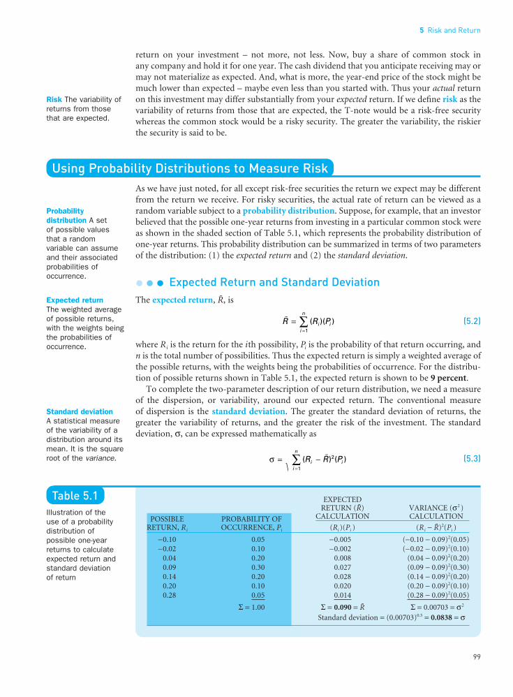
return on your investment – not more, not less. Now, buy a share of common stock in any company and hold it for one year. The cash dividend that you anticipate receiving may ormay not materialize as expected. And, what is more, the year-end price of the stock might bemuch lower than expected – maybe even less than you started with. Thus your actual returnon this investment may differ substantially from your expected return. If we define risk as thevariability of returns from those that are expected, the T-note would be a risk-free securitywhereas the common stock would be a risky security. The greater the variability, the riskierthe security is said to be.
Using Probability Distributions to Measure RiskAs we have just noted, for all except risk-free securities the return we expect may be differentfrom the return we receive. For risky securities, the actual rate of return can be viewed as arandom variable subject to a probability distribution. Suppose, for example, that an investorbelieved that the possible one-year returns from investing in a particular common stock wereas shown in the shaded section of Table 5.1, which represents the probability distribution ofone-year returns. This probability distribution can be summarized in terms of two parametersof the distribution: (1) the expected return and (2) the standard deviation.
l l l Expected Return and Standard DeviationThe expected return, b, is
(5.2)
where Ri is the return for the ith possibility, Pi is the probability of that return occurring, andn is the total number of possibilities. Thus the expected return is simply a weighted average ofthe possible returns, with the weights being the probabilities of occurrence. For the distribu-tion of possible returns shown in Table 5.1, the expected return is shown to be 9 percent.
To complete the two-parameter description of our return distribution, we need a measureof the dispersion, or variability, around our expected return. The conventional measure of dispersion is the standard deviation. The greater the standard deviation of returns, thegreater the variability of returns, and the greater the risk of the investment. The standard deviation, σ, can be expressed mathematically as
(5.3)σ ( ) ( )= −=∑ R Pi ii
n
B 2
1
B ( )( )==∑ R Pi ii
n
1
5 Risk and Return
99
••
Risk The variability ofreturns from thosethat are expected.
Expected returnThe weighted averageof possible returns,with the weights beingthe probabilities ofoccurrence.
Standard deviationA statistical measureof the variability of adistribution around itsmean. It is the squareroot of the variance.
Probabilitydistribution A set of possible valuesthat a randomvariable can assumeand their associatedprobabilities ofoccurrence.
Table 5.1Illustration of the use of a probabilitydistribution ofpossible one-yearreturns to calculateexpected return andstandard deviation of return
EXPECTEDRETURN (b) VARIANCE (σ2 )
POSSIBLE PROBABILITY OF CALCULATION CALCULATION
RETURN, Ri OCCURRENCE, Pi (Ri )(Pi ) (Ri − b)2(Pi )
−0.10 0.05 −0.005 (−0.10 − 0.09)2(0.05)−0.02 0.10 −0.002 (−0.02 − 0.09)2(0.10)
0.04 0.20 0.008 (0.04 − 0.09)2(0.20)0.09 0.30 0.027 (0.09 − 0.09)2(0.30)0.14 0.20 0.028 (0.14 − 0.09)2(0.20)0.20 0.10 0.020 (0.20 − 0.09)2(0.10)0.28 0.05 0.014 (0.28 − 0.09)2(0.05)
Σ = 1.00 Σ = 0.090 = b Σ = 0.00703 = σ2
Standard deviation = (0.00703)0.5 = 0.0838 = σ
FUNO_C05.qxd 9/19/08 17:15 Page 99
where √ represents the square root. The square of the standard deviation, σ 2, is known as the variance of the distribution. Operationally, we generally first calculate a distribution’s variance, or the weighted average of squared deviations of possible occurrences from themean value of the distribution, with the weights being the probabilities of occurrence. Thenthe square root of this figure provides us with the standard deviation. Table 5.1 reveals ourexample distribution’s variance to be 0.00703. Taking the square root of this value, we findthat the distribution’s standard deviation is 8.38 percent.
Use of Standard Deviation Information. So far we have been working with a discrete(noncontinuous) probability distribution, one where a random variable, like return, can takeon only certain values within an interval. In such cases we do not have to calculate the standarddeviation in order to determine the probability of specific outcomes. To determine the prob-ability of the actual return in our example being less than zero, we look at the shaded sectionof Table 5.1 and see that the probability is 0.05 + 0.10 = 15%. The procedure is slightly morecomplex when we deal with a continuous distribution, one where a random variable can takeon any value within an interval. And, for common stock returns, a continuous distribution isa more realistic assumption, as any number of possible outcomes ranging from a large loss toa large gain are possible.
Assume that we are facing a normal (continuous) probability distribution of returns. It issymmetrical and bell-shaped, and 68 percent of the distribution falls within one standarddeviation (right or left) of the expected return; 95 percent falls within two standard deviations;and over 99 percent falls within three standard deviations. By expressing differences from theexpected return in terms of standard deviations, we are able to determine the probability thatthe actual return will be greater or less than any particular amount.
We can illustrate this process with a numerical example. Suppose that our return distribu-tion had been approximately normal with an expected return equal to 9 percent and a standard deviation of 8.38 percent. Let’s say that we wish to find the probability that the actual future return will be less than zero. We first determine how many standard deviations0 percent is from the mean (9 percent). To do this we take the difference between these twovalues, which happens to be −9 percent, and divide it by the standard deviation. In this casethe result is −0.09/0.0838 = −1.07 standard deviations. (The negative sign reminds us that weare looking to the left of the mean.) In general, we can make use of the formula
(5.4)
where R is the return range limit of interest and where Z (the Z-score) tells us how many standard deviations R is from the mean.
Table V in the Appendix at the back of the book can be used to determine the proportionof the area under the normal curve that is Z standard deviations to the left or right of themean. This proportion corresponds to the probability that our return outcome would be Zstandard deviations away from the mean.
Turning to (Appendix) Table V, we find that there is approximately a 14 percent prob-ability that the actual future return will be zero or less. The probability distribution is illus-trated in Figure 5.1. The shaded area is located 1.07 standard deviations left of the mean, and,as indicated, this area represents approximately 14 percent of the total distribution.
As we have just seen, a return distribution’s standard deviation turns out to be a rather versatile risk measure. It can serve as an absolute measure of return variability – the higher thestandard deviation, the greater the uncertainty concerning the actual outcome. In addition,we can use it to determine the likelihood that an actual outcome will be greater or less than aparticular amount. However, there are those who suggest that our concern should be with“downside” risk – occurrences less than expected – rather than with variability both above and
ZR
=−
=−
=
B
σ
0 0.090.0838
−−1.07
Part 2 Valuation
100
••
FUNO_C05.qxd 9/19/08 17:15 Page 100

below the mean. Those people have a good point. But, as long as the return distribution is relatively symmetric – a mirror image above and below the mean – standard deviation stillworks. The greater the standard deviation, the greater the possibility for large disappointments.
l l l Coefficient of VariationThe standard deviation can sometimes be misleading in comparing the risk, or uncertainty,surrounding alternatives if they differ in size. Consider two investment opportunities, A and B, whose normal probability distributions of one-year returns have the following characteristics:
INVESTMENT A INVESTMENT B
Expected return, b 0.08 0.24Standard deviation, σ 0.06 0.08Coefficient of variation, CV 0.75 0.33
Can we conclude that because the standard deviation of B is larger than that of A, it is theriskier investment? With standard deviation as our risk measure, we would have to. However,relative to the size of expected return, investment A has greater variation. This is similar torecognizing that a $10,000 standard deviation of annual income to a multimillionaire is reallyless significant than an $8,000 standard deviation in annual income would be to you. Toadjust for the size, or scale, problem, the standard deviation can be divided by the expectedreturn to compute the coefficient of variation (CV):
Coefficient of variation (CV) = σ/B (5.5)
Thus the coefficient of variation is a measure of relative dispersion (risk) – a measure of risk“per unit of expected return.” The larger the CV, the larger the relative risk of the investment.Using the CV as our risk measure, investment A with a return distribution CV of 0.75 isviewed as being more risky than investment B, whose CV equals only 0.33.
Attitudes Toward RiskJust when you thought that you were safely immersed in the middle of a finance chapter, youfind yourself caught up in a time warp, and you are a contestant on the television game showLet’s Make a Deal. The host, Monty Hall, explains that you get to keep whatever you find
5 Risk and Return
101
••
Figure 5.1Normal probabilitydistribution of possible returns forexample highlightingarea 1.07 standarddeviations left of the mean
Coefficient ofvariation (CV)The ratio of thestandard deviation of a distribution to the mean of thatdistribution. It is a measure of relative risk.
FUNO_C05.qxd 9/19/08 17:15 Page 101

behind either door #1 or door #2. He tells you that behind onedoor is $10,000 in cash, but behind the other door is a “zonk,”a used tire with a current market value of zero. You choose toopen door #1 and claim your prize. But before you can makea move, Monty says that he will offer you a sum of money tocall off the whole deal.
(Before reading any further, decide for yourself what dollaramount would make you indifferent between taking what isbehind the door or taking the money. That is, determine anamount such that one dollar more would prompt you to takethe money; one dollar less and you would keep the door.Write this number down on a sheet of paper. In a moment,we will predict what that number will look like.)
Let’s assume that you decide that if Monty offers you $2,999 or less, you will keep the door.At $3,000 you can’t quite make up your mind. But at $3,001, or more, you would take the cashoffered and give up the door. Monty offers you $3,500, so you take the cash and give up thedoor. (By the way, the $10,000 was behind door #1, so you blew it.)
What does any of this have to do with this chapter on risk and return? Everything. We have just illustrated the fact that the average investor is averse to risk. Let’s see why. You had a 50/50 chance of getting $10,000 or nothing by keeping a door. The expected value of keeping a door is $5,000 (0.50 × $10,000 plus 0.50 × $0). In our example, you found your-self indifferent between a risky (uncertain) $5,000 expected return and a certain return of$3,000. In other words, this certain or riskless amount, your certainty equivalent (CE) to therisky gamble, provided you with the same utility or satisfaction as the risky expected value of $5,000.
It would be amazing if your actual certainty equivalent in this situation was exactly $3,000,the number that we used in the example. But take a look at the number that we asked you to write down. It is probably less than $5,000. Studies have shown that the vast majority ofindividuals, if placed in a similar situation, would have a certainty equivalent less than theexpected value (i.e., less than $5,000). We can, in fact, use the relationship of an individual’scertainty equivalent to the expected monetary value of a risky investment (or opportunity) todefine their attitude toward risk. In general, if the
l Certainty equivalent < expected value, risk aversion is present.
l Certainty equivalent = expected value, risk indifference is present.
l Certainty equivalent > expected value, risk preference is present.
Thus, in our Let’s Make a Deal example, any certainty equivalent less than $5,000 indicatesrisk aversion. For risk-averse individuals, the difference between the certainty equivalent andthe expected value of an investment constitutes a risk premium; this is additional expectedreturn that the risky investment must offer to the investor for this individual to accept therisky investment. Notice that in our example the risky investment’s expected value had toexceed the sure-thing offer of $3,000 by $2,000 or more for you to be willing to accept it.
In this book we will take the generally accepted view that investors are, by and large, risk averse. This implies that risky investments must offer higher expected returns than lessrisky investments in order for people to buy and hold them. (Keep in mind, however, that weare talking about expected returns; the actual return on a risky investment could be much lessthan the actual return on a less risky alternative.) And, to have low risk, you must be willingto accept investments having lower expected returns. In short, there is no free lunch when itcomes to investments. Any claims for high returns produced by low-risk investments shouldbe viewed skeptically.
Part 2 Valuation
102
••
Certainty equivalent(CE) The amount ofcash someone wouldrequire with certaintyat a point in time tomake the individualindifferent betweenthat certain amountand an amountexpected to bereceived with risk at the same point in time.
Risk averse Termapplied to an investorwho demands ahigher expectedreturn, the higher the risk.
FUNO_C05.qxd 9/19/08 17:15 Page 102

Risk and Return in a Portfolio ContextSo far, we have focused on the risk and return of single investments held in isolation. Investorsrarely place their entire wealth into a single asset or investment. Rather, they construct a portfolio or group of investments. Therefore we need to extend our analysis of risk and returnto include portfolios.
l l l Portfolio ReturnThe expected return of a portfolio is simply a weighted average of the expected returns of thesecurities constituting that portfolio. The weights are equal to the proportion of total fundsinvested in each security (the weights must sum to 100 percent). The general formula for theexpected return of a portfolio, bp, is as follows:
(5.6)
where Wj is the proportion, or weight, of total funds invested in security j ; b j is the expectedreturn for security j ; and m is the total number of different securities in the portfolio.
The expected return and standard deviation of the probability distribution of possiblereturns for two securities are shown below.
SECURITY A SECURITY B
Expected return, b j 14.0% 11.5%Standard deviation, σj 10.7 1.5
If equal amounts of money are invested in the two securities, the expected return of the port-folio is (0.5)14.0% + (0.5)11.5% = 12.75%.
l l l Portfolio Risk and the Importance of CovarianceAlthough the portfolio expected return is a straightforward, weighted average of returns onthe individual securities, the portfolio standard deviation is not the simple, weighted averageof individual security standard deviations. To take a weighted average of individual securitystandard deviations would be to ignore the relationship, or covariance, between the returnson securities. This covariance, however, does not affect the portfolio’s expected return.
Covariance is a statistical measure of the degree to which two variables (e.g., securities’returns) move together. Positive covariance shows that, on average, the two variables movetogether. Negative covariance suggests that, on average, the two variables move in oppositedirections. Zero covariance means that the two variables show no tendency to vary togetherin either a positive or negative linear fashion. Covariance between security returns complicatesour calculation of portfolio standard deviation. Still, this dark cloud of mathematical com-plexity contains a silver lining – covariance between securities provides for the possibility ofeliminating some risk without reducing potential return.
The calculation of a portfolio’s standard deviation, σp, is complicated and requires illustration.2 We therefore address it in detail in Appendix A at the end of this chapter. As
B Bp1
==
∑Wj jj
m
2The standard deviation of a probability distribution of possible portfolio returns, σp, is
where m is the total number of different securities in the portfolio, Wj is the proportion of total funds invested insecurity j , Wk is the proportion of total funds invested in security k, and σj,k is the covariance between possible returnsfor securities j and k.
5 Risk and Return
103
••
Portfolio Acombination of two or more securities or assets.
CovarianceA statistical measureof the degree to whichtwo variables (e.g.,securities’ returns)move together. Apositive value meansthat, on average, they move in thesame direction.
FUNO_C05.qxd 9/19/08 17:15 Page 103

explained in Appendix A, for a large portfolio the standard deviation depends primarily onthe “weighted” covariances among securities. The “weights” refer to the proportion of fundsinvested in each security, and the covariances are those determined between security returnsfor all pairwise combinations of securities.
An understanding of what goes into the determination of a portfolio’s standard deviationleads to a startling conclusion. The riskiness of a portfolio depends much more on the pairedsecurity covariances than on the riskiness (standard deviations) of the separate security hold-ings. This means that a combination of individually risky securities could still constitute amoderate- to low-risk portfolio as long as securities do not move in lockstep with each other.In short, low covariances lead to low portfolio risk.
DiversificationThe concept of diversification makes such common sense that our language even containseveryday expressions that exhort us to diversify (“Don’t put all your eggs in one basket”). The idea is to spread your risk across a number of assets or investments. While pointing us in the right direction, this is a rather naive approach to diversification. It would seem to imply that investing $10,000 evenly across 10 different securities makes you morediversified than the same amount of money invested evenly across 5 securities. The catch is that naive diversification ignores the covariance (or correlation) between security returns.The portfolio containing 10 securities could represent stocks from only one industry and have returns that are highly correlated. The 5-stock portfolio might represent various industries whose security returns might show low correlation and, hence, low portfolio return variability.
Meaningful diversification, combining securities in a way that will reduce risk, is illustratedin Figure 5.2. Here the returns over time for security A are cyclical in that they move with theeconomy in general. Returns for security B, however, are mildly countercyclical. Thus thereturns for these two securities are negatively correlated. Equal amounts invested in bothsecurities will reduce the dispersion of return, σp, on the portfolio of investments. This isbecause some of each individual security’s variability is offsetting. Benefits of diversification,in the form of risk reduction, occur as long as the securities are not perfectly, positively correlated.
Investing in world financial markets can achieve greater diversification than investing insecurities from a single country. As we will discuss in Chapter 24, the economic cycles of dif-ferent countries are not completely synchronized, and a weak economy in one country maybe offset by a strong economy in another. Moreover, exchange-rate risk and other risks dis-cussed in Chapter 24 add to the diversification effect.
Part 2 Valuation
104
••
Figure 5.2Effect ofdiversification onportfolio risk
FUNO_C05.qxd 9/19/08 17:15 Page 104

l l l Systematic and Unsystematic RiskWe have stated that combining securities that are not perfectly, positively correlated helps to lessen the risk of a portfolio. How much risk reduction is reasonable to expect, and howmany different security holdings in a portfolio would be required? Figure 5.3 helps provideanswers.
Research studies have looked at what happens to portfolio risk as randomly selected stocksare combined to form equally weighted portfolios. When we begin with a single stock, the riskof the portfolio is the standard deviation of that one stock. As the number of randomlyselected stocks held in the portfolio is increased, the total risk of the portfolio is reduced. Sucha reduction is at a decreasing rate, however. Thus a substantial proportion of the portfolio risk can be eliminated with a relatively moderate amount of diversification – say, 20 to 25 ran-domly selected stocks in equal-dollar amounts. Conceptually, this is illustrated in Figure 5.3.
As the figure shows, total portfolio risk comprises two components:
Systematic risk Unsystematic risk Total risk = (nondiversifiable + (diversifiable (5.7)
or unavoidable) or avoidable)
The first part, systematic risk, is due to risk factors that affect the overall market – such aschanges in the nation’s economy, tax reform by Congress, or a change in the world energy situation. These are risks that affect securities overall and, consequently, cannot be diver-sified away. In other words, even an investor who holds a well-diversified portfolio will beexposed to this type of risk.
The second risk component, unsystematic risk, is risk unique to a particular company orindustry; it is independent of economic, political, and other factors that affect all securities ina systematic manner. A wildcat strike may affect only one company; a new competitor maybegin to produce essentially the same product; or a technological breakthrough may make anexisting product obsolete. For most stocks, unsystematic risk accounts for around 50 percentof the stock’s total risk or standard deviation. However, by diversification this kind of risk
5 Risk and Return
105
••
Figure 5.3Relationship of total,systematic, andunsystematic risk to portfolio size
Systematic riskThe variability ofreturn on stocks orportfolios associatedwith changes in return on the marketas a whole.
Unsystematic riskThe variability ofreturn on stocks or portfolios notexplained by generalmarket movements. It is avoidable throughdiversification.
FUNO_C05.qxd 9/19/08 17:15 Page 105

can be reduced and even eliminated if diversification is efficient. Therefore not all of the riskinvolved in holding a stock is relevant, because part of this risk can be diversified away. Theimportant risk of a stock is its unavoidable or systematic risk. Investors can expect to be compensated for bearing this systematic risk. They should not, however, expect the market toprovide any extra compensation for bearing avoidable risk. It is this logic that lies behind thecapital-asset pricing model.
The Capital-Asset Pricing Model (CAPM)Based on the behavior of risk-averse investors, there is an implied equilibrium relationshipbetween risk and expected return for each security. In market equilibrium, a security is supposed to provide an expected return commensurate with its systematic risk – the risk thatcannot be avoided by diversification. The greater the systematic risk of a security, the greaterthe return that investors will expect from the security. The relationship between expectedreturn and systematic risk, and the valuation of securities that follows, is the essence of Nobellaureate William Sharpe’s capital-asset pricing model (CAPM). This model was developed inthe 1960s, and it has had important implications for finance ever since. Though other modelsalso attempt to capture market behavior, the CAPM is simple in concept and has real-worldapplicability.
Like any model, this one is a simplification of reality. Nevertheless, it allows us to draw certain inferences about risk and the size of the risk premium necessary to compensate forbearing risk. We shall concentrate on the general aspects of the model and its importantimplications. Certain corners have been cut in the interest of simplicity.
As with any model, there are assumptions to be made. First, we assume that capital marketsare efficient in that investors are well informed, transactions costs are low, there are negligiblerestrictions on investment, and no investor is large enough to affect the market price of astock. We also assume that investors are in general agreement about the likely performance ofindividual securities and that their expectations are based on a common holding period, sayone year. There are two types of investment opportunities with which we will be concerned.The first is a risk-free security whose return over the holding period is known with certainty.Frequently, the rate on short- to intermediate-term Treasury securities is used as a surrogatefor the risk-free rate. The second is the market portfolio of common stocks. It is representedby all available common stocks and weighted according to their total aggregate market valuesoutstanding. As the market portfolio is a somewhat unwieldy thing with which to work, most
Part 2 Valuation
106
••
Capital-asset pricingmodel (CAPM) Amodel that describesthe relationshipbetween risk andexpected (required)return; in this model,a security’s expected(required) return isthe risk-free rate plusa premium based onthe systematic risk ofthe security.
QWhat is an “index”?
AAn index is a group of stocks, the performance of which is measured as a whole. Some are large,
containing hundreds or thousands of companies. These
are often used to gauge the performance of the overallmarket, as with an index such as the S&P 500. Otherindexes are smaller, or more focused, perhaps containingjust small companies or pharmaceutical companies orLatin American companies.
Indexes aren’t things you invest in, though. To meetthe needs of people interested in investing in variousindexes, index mutual funds were created. If you want toinvest in a certain index, for example, you would investin an index fund based on it.
Ask the Fool
Source: The Motley Fool (www.fool.com). Reproduced with the permission of The Motley Fool.
FUNO_C05.qxd 9/19/08 17:15 Page 106

people use a surrogate, such as the Standard & Poor’s 500 Stock Price Index (S&P 500 Index).This broad-based, market-value-weighted index reflects the performance of 500 major common stocks.
Earlier we discussed the idea of unavoidable risk – risk that cannot be avoided by efficientdiversification. Because one cannot hold a more diversified portfolio than the market port-folio, it represents the limit to attainable diversification. Thus all the risk associated with themarket portfolio is unavoidable, or systematic.
l l l The Characteristic LineWe are now in a position to compare the expected return for an individual stock with theexpected return for the market portfolio. In our comparison, it is useful to deal with returnsin excess of the risk-free rate, which acts as a benchmark against which the risky asset returnsare contrasted. The excess return is simply the expected return less the risk-free return. Figure 5.4 shows an example of a comparison of expected excess returns for a specific stockwith those for the market portfolio. The solid blue line is known as the security’s character-istic line; it depicts the expected relationship between excess returns for the stock and excessreturns for the market portfolio. The expected relationship may be based on past experience,in which case actual excess returns for the stock and for the market portfolio would be plot-ted on the graph, and a regression line best characterizing the historical relationship would bedrawn. Such a situation is illustrated by the scatter diagram shown in the figure. Each pointrepresents the excess return of the stock and that of the S&P 500 Index for a given month inthe past (60 months in total). The monthly returns are calculated as
From these returns the monthly risk-free rate is subtracted to obtain excess returns.For our example stock, we see that, when returns on the market portfolio are high, returns
on the stock tend to be high as well. Instead of using historical return relationships, one might obtain future return estimates from security analysts who follow the stock. Because
(Dividends paid) (Ending price Beginning price)Beginning price
+ −
5 Risk and Return
107
••
Characteristic lineA line that describesthe relationshipbetween an individualsecurity’s returns andreturns on the marketportfolio. The slope ofthis line is beta.
Standard & Poor’s500 Stock Index(S&P 500 Index) Amarket-value-weightedindex of 500 large-capitalization commonstocks selected froma broad cross-sectionof industry groups. Itis used as a measureof overall marketperformance.
Figure 5.4Relationship betweenexcess returns for astock and excessreturns for the marketportfolio based on 60 pairs of excessmonthly return data
FUNO_C05.qxd 9/19/08 17:15 Page 107

this approach is usually restricted to investment organizations with a number of security analysts, we illustrate the relationship assuming the use of historical data.
l l l Beta: An Index of Systematic Risk
A measure that stands out in Figure 5.4, and the most important one for our purposes, is beta.Beta is simply the slope (i.e., the change in the excess return on the stock over the change inexcess return on the market portfolio) of the characteristic line. If the slope is 1.0, it meansthat excess returns for the stock vary proportionally with excess returns for the market port-folio. In other words, the stock has the same systematic risk as the market as a whole. If themarket goes up and provides an excess return of 5 percent for a month, we would expect, onaverage, the stock’s excess return to be 5 percent as well. A slope steeper than 1.0 means thatthe stock’s excess return varies more than proportionally with the excess return of the marketportfolio. Put another way, it has more unavoidable risk than the market as a whole. This typeof stock is often called an “aggressive” investment. A slope less than 1.0 means that the stock’sexcess return varies less than proportionally with the excess return of the market portfolio.This type of stock is often called a “defensive” investment. Examples of the three types of relationship are shown in Figure 5.5.
The greater the slope of the characteristic line for a stock, as depicted by its beta, the greaterits systematic risk. This means that, for both upward and downward movements in marketexcess returns, movements in excess returns for the individual stock are greater or lessdepending on its beta. With the beta of the market portfolio equal to 1.0 by definition, beta is thus an index of a stock’s systematic or unavoidable risk relative to that of the market portfolio. This risk cannot be diversified away by investing in more stocks, because it dependson such things as changes in the economy and in the political atmosphere, which affect all stocks.
Part 2 Valuation
108
••
Beta An index ofsystematic risk. It measures thesensitivity of astock’s returns tochanges in returns onthe market portfolio.The beta of a portfoliois simply a weightedaverage of theindividual stock betasin the portfolio.
Figure 5.5Examples ofcharacteristic lineswith different betas
FUNO_C05.qxd 9/19/08 17:15 Page 108

Take Note
In addition, a portfolio’s beta is simply a weighted average of the individual stock betas inthe portfolio, with the weights being the proportion of total portfolio market value repre-sented by each stock. Thus the beta of a stock represents its contribution to the risk of ahighly diversified portfolio of stocks.
l l l Unsystematic (Diversifiable) Risk RevisitedBefore moving on, we need to mention an additional feature of Figure 5.4. The dispersion ofthe data points about the characteristic line is a measure of the unsystematic risk of the stock.The wider the relative distance of the points from the line, the greater the unsystematic risk ofthe stocks: this is to say that the stock’s return has increasingly lower correlation with thereturn on the market portfolio. The narrower the dispersion, the higher the correlation andthe lower the unsystematic risk. From before, we know that unsystematic risk can be reducedor even eliminated through efficient diversification. For a portfolio of 20 carefully selectedstocks, the data points would hover closely around the characteristic line for the portfolio.
l l l Required Rates of Return and the Security Market Line (SML)If we assume that financial markets are efficient and that investors as a whole are efficientlydiversified, unsystematic risk is a minor matter. The major risk associated with a stockbecomes its systematic risk. The greater the beta of a stock, the greater the relevant risk of thatstock, and the greater the return required. If we assume that unsystematic risk is diversifiedaway, the required rate of return for stock j is
Bj = Rf + (Bm − Rf)βj (5.8)
where R f is the risk-free rate, bm is the expected return for the market portfolio, and β j is thebeta coefficient for stock j as defined earlier.
Put another way, the required rate of return for a stock is equal to the return required by themarket for a riskless investment plus a risk premium. In turn, the risk premium is a functionof: (1) the expected market return less the risk-free rate, which represents the risk premiumrequired for the typical stock in the market; and (2) the beta coefficient. Suppose that theexpected return on Treasury securities is 8 percent, the expected return on the market port-folio is 13 percent, and the beta of Savance Corporation is 1.3. The beta indicates that Savancehas more systematic risk than the typical stock (i.e., a stock with a beta of 1.0). Given thisinformation, and using Eq. (5.8), we find that the required return on Savance stock would be
Bj = 0.08 + (0.13 − 0.08)(1.3) = 14.5%
What this tells us is that on average the market expects Savance to show a 14.5 percent annualreturn. Because Savance has more systematic risk, this return is higher than that expected ofthe typical stock in the marketplace. For the typical stock, the expected return would be
Bj = 0.08 + (0.13 − 0.08)(1.0) = 13.0%
Suppose now that we are interested in a defensive stock whose beta coefficient is only 0.7. Itsexpected return is
Bj = 0.08 + (0.13 − 0.08)(0.7) = 11.5%
The Security Market Line. Equation (5.8) describes the relationship between an individualsecurity’s expected return and its systematic risk, as measured by beta. This linear relationshipis known as the security market line (SML) and is illustrated in Figure 5.6. The expected one-year return is shown on the vertical axis. Beta, our index of systematic risk, is on the
5 Risk and Return
109
••
Security market line(SML) A line thatdescribes the linearrelationship betweenexpected rates ofreturn for individualsecurities (andportfolios) andsystematic risk, asmeasured by beta.
FUNO_C05.qxd 9/19/08 17:15 Page 109

horizontal axis. At zero risk, the security market line has an intercept on the vertical axis equalto the risk-free rate. Even when no risk is involved, investors still expect to be compensatedfor the time value of money. As risk increases, the required rate of return increases in the manner depicted.
Obtaining Betas. If the past is thought to be a good surrogate for the future, one can usepast data on excess returns for the stock and for the market to calculate beta. Several servicesprovide betas on companies whose stocks are actively traded; these betas are usually based onweekly or monthly returns for the past three to five years. Services providing beta informa-tion include Merrill Lynch, Value Line, Reuters (www.reuters.com/finance/stocks), andIbbotson Associates. The obvious advantage is that one can obtain the historical beta for astock without having to calculate it. See Table 5.2 for a sample of companies, their identifyingticker symbols, and their stock betas. The betas of most stocks range from 0.4 to 1.4. If onefeels that the past systematic risk of a stock is likely to prevail in the future, the historical betacan be used as a proxy for the expected beta coefficient.
Adjusting Historical Betas. There appears to be a tendency for measured betas of indi-vidual securities to revert toward the beta of the market portfolio, 1.0, or toward the beta of
Part 2 Valuation
110
••
Figure 5.6The security marketline (SML)
Ticker symbolA unique, letter-character code nameassigned to securitiesand mutual funds. It is often used innewspapers and price-quotationservices. Thisshorthand method of identification wasoriginally developed in the nineteenthcentury by telegraphoperators.
Security market line
Risk premium
Risk-free return
1.0
SYSTEMATIC RISK (beta)
EXP
EC
TED
RE
TUR
N Rm
Rf
Table 5.2Betas for selectedstocks (January 13,2008)
COMMON STOCK (Ticker Symbol) BETA
Amazon.com (AMZN) 2.63Apple Computer (AAPL) 1.75Boeing (BA) 1.25Bristol-Myers Squibb (BMY) 1.15The Coca-Cola Company (KO) 0.68Dow Chemical (DOW) 1.39The Gap (GPS) 1.29General Electric (GE) 0.76Google (GOOG) 1.36Hewlett-Packard (HPQ) 1.54The Limited (LTD) 1.31Microsoft (MSFT) 0.73Nike (NKE) 0.69Yahoo! (YHOO) 1.20
Source: Reuters (www.reuters.com/finance/stocks).
FUNO_C05.qxd 9/19/08 17:15 Page 110

the industry of which the company is a part. This tendency may be due to economic factorsaffecting the operations and financing of the firm and perhaps to statistical factors as well. Toadjust for this tendency, Merrill Lynch, Value Line, and certain others calculate an adjustedbeta. To illustrate, suppose that the reversion process was toward the market beta of 1.0. If themeasured beta was 1.4 and a weight of 0.67 was attached to it and a weight of 0.33 applied tothe market beta, the adjusted beta would be 1.4(0.67) + 1.0(0.33) = 1.27. The same procedurecould be used if the reversion process was toward an industry average beta of, say, 1.2. As one is concerned with the beta of a security in the future, it may be appropriate to adjust themeasured beta if the reversion process just described is clear and consistent.
Obtaining Other Information for the Model. In addition to beta, the numbers used for themarket return and the risk-free rate must be the best possible estimates of the future. The pastmay or may not be a good proxy. If the past was represented by a period of relative economicstability, but considerable inflation is expected in the future, averages of past market returnsand past risk-free rates would be biased, low estimates of the future. In this case it would be amistake to use historical average returns in the calculation of the required return for a secur-ity. In another situation, realized market returns in the recent past might be very high and notexpected to continue. As a result, the use of the historical past would result in an estimate ofthe future market return that was too high.
In situations of this sort, direct estimates of the risk-free rate and of the market return must be made. The risk-free rate is easy; one simply looks up the current rate of return on anappropriate Treasury security. The market return is more difficult, but even here forecasts are available. These forecasts might be consensus estimates of security analysts, economists,and others who regularly predict such returns. Estimates in recent years of the return on common stocks overall have been in the 12 to 17 percent range.
Use of the Risk Premium. The excess return of the market portfolio (over the risk-free rate)is known as the market risk premium. It is represented by (bm − Rf) in Eq. (5.8). The expectedexcess return for the S&P 500 Index has generally ranged from 5 to 8 percent. Instead of esti-mating the market portfolio return directly, one might simply add a risk premium to the prevail-ing risk-free rate. To illustrate, suppose that we feel we are in a period of uncertainty, and thereis considerable risk aversion in the market. Therefore our estimated market return is bm = 0.08+ 0.07 = 15%, where 0.08 is the risk-free rate and 0.07 is our market risk premium estimate.If, on the other hand, we feel that there is substantially less risk aversion in the market, wemight use a risk premium of 5 percent, in which case the estimated market return is 13 percent.
5 Risk and Return
111
••
Adjusted betaAn estimate of asecurity’s future beta that involvesmodifying thesecurity’s historical(measured) betaowing to theassumption that thesecurity’s beta has a tendency to moveover time toward the average beta forthe market or thecompany’s industry.
QWhat can you tell me about ticker symbols?
AA ticker symbol is a short identifier for a company’sstock. Companies that trade on the old, respected
“big board,” the New York Stock Exchange, have three or fewer letters in their tickers. Those trading on the
smaller American Stock Exchange also have three letters.Tickers of stocks trading on the NASDAQ have four letters. Sometimes you’ll see a fifth. If so, it’s not tech-nically part of the ticker – it’s tacked on to reflect some-thing about the company. For example, an F means it’s a foreign company, and a Q means it’s in bankruptcyproceedings.
Many companies have chosen amusing ticker symbolsfor themselves. For example: Southwest Airlines (LUV),Tricon Global Restaurants (YUM), explosives specialistDynamic Materials (BOOM), religious Internet companyCrosswalk.com (AMEN), and Anheuser Busch (BUD).
Ask the Fool
Source: The Motley Fool (www.fool.com). Reproduced with the permission of The Motley Fool.
FUNO_C05.qxd 9/19/08 17:15 Page 111

The important thing is that the expected market return on common stocks and the risk-freerate employed in Eq. (5.8) must be current market estimates. Blind adherence to historical ratesof return may result in faulty estimates of these data inputs to the capital-asset pricing model.
l l l Returns and Stock PricesThe capital-asset pricing model provides us a means by which to estimate the required rate ofreturn on a security. This return can then be used as the discount rate in a dividend valuationmodel. You will recall that the intrinsic value of a share of stock can be expressed as the present value of the stream of expected future dividends. That is
(5.9)
where Dt is the expected dividend in period t, ke is the required rate of return for the stock,and Σ is the sum of the present value of future dividends going from period 1 to infinity.
Suppose that we wish to determine the value of the stock of Savance Corporation and thatthe perpetual dividend growth model is appropriate. This model is
(5.10)
where g is the expected annual future growth rate in dividends per share. Furthermore,assume that Savance Corporation’s expected dividend in period 1 is $2 per share and that theexpected annual growth rate in dividends per share is 10 percent. On page 109, we determinedthat the required rate of return for Savance was 14.5 percent. On the basis of these expecta-tions, the value of the stock is
If this value equaled the current market price, the expected return on the stock and the requiredreturn would be equal. The $44.44 figure would represent the equilibrium price of the stock,based on investor expectations about the company, about the market as a whole, and aboutthe return available on the riskless asset.
These expectations can change, and when they do, the value (and price) of the stockchanges. Suppose that inflation in the economy has diminished and we enter a period of relatively stable growth. As a result, interest rates decline, and investor risk aversion lessens.Moreover, the growth rate of the company’s dividends also declines somewhat. The variables,both before and after these changes, are as listed below.
BEFORE AFTER
Risk-free rate, Rf 0.08 0.07Expected market return, bm 0.13 0.11Savance beta, βj 1.30 1.20Savance dividend growth rate, g 0.10 0.09
The required rate of return for Savance stock, based on systematic risk, becomes
Bj = 0.07 + (0.11 − 0.07)(1.20) = 11.8%
Using this rate as ke, the new value of the stock is
Thus the combination of these events causes the value of the stock to increase from $44.44 to$71.43 per share. If the expectation of these events represented the market consensus, $71.43would also be the equilibrium price. Thus the equilibrium price of a stock can change veryquickly as expectations in the marketplace change.
V =−
= .
$2.00
0.118 0 09$71.43
V =−
= .
$2.00
(0.145 0 10)$44.44
VD
k g=
−
1
e
VD
kt
tt
=+=
∞
∑ ( )1 e1
Part 2 Valuation
112
••
FUNO_C05.qxd 9/19/08 17:15 Page 112

Underpriced and Overpriced Stocks. We just finished saying that in market equilibriumthe required rate of return on a stock equals its expected return. That is, all stocks will lie onthe security market line. What happens when this is not so? Suppose that in Figure 5.7 thesecurity market line is drawn on the basis of what investors as a whole know to be the approx-imate relationship between the required rate of return and systematic or unavoidable risk. Forsome reason, two stocks – call them X and Y – are improperly priced. Stock X is underpricedrelative to the security market line, whereas stock Y is overpriced.
As a result, stock X is expected to provide a rate of return greater than that required, basedon its systematic risk. In contrast, stock Y is expected to provide a lower return than thatrequired to compensate for its systematic risk. Investors, seeing the opportunity for superiorreturns by investing in stock X, should rush to buy it. This action would drive the price upand the expected return down. How long would this continue? It would continue until themarket price was such that the expected return would now lie on the security market line. In the case of stock Y, investors holding this stock would sell it, recognizing that they couldobtain a higher return for the same amount of systematic risk with other stocks. This sellingpressure would drive Y’s market price down and its expected return up until the expectedreturn was on the security market line.
When the expected returns for these two stocks return to the security market line, marketequilibrium will again prevail. As a result, the expected returns for the two stocks will thenequal their required returns. Available evidence suggests that disequilibrium situations instock prices do not long persist and that stock prices adjust rapidly to new information. Withthe vast amount of evidence indicating market efficiency, the security market line conceptbecomes a useful means for determining the expected and required rate of return for a stock.3
This rate can then be used as the discount rate in the valuation procedures described earlier.
l l l Challenges to the CAPMThe CAPM has not gone unchallenged. As we know, the key ingredient in the model is the useof beta as a measure of risk. Early empirical studies showed beta to have reasonable predictivepower about return, particularly the return on a portfolio of common stocks. No one claimedthe model was perfect; as if anything were! However, it is fairly easy to understand and apply. Such market imperfections as bankruptcy costs, taxes, and institutional restraints havebeen recognized, and refinements can be made to account for their effects. Some of theserefinements are explored in subsequent chapters when we deal with applications of the CAPM.
3It is difficult in practice to derive satisfactory beta information for fixed-income securities. Therefore, most of thework on the CAPM has involved common stocks. The concept of the relationship between systematic risk and therequired return is important, however, for both fixed-income securities and common stocks.
5 Risk and Return
113
••
Figure 5.7Underpriced andoverpriced stocksduring temporarymarket disequilibrium
FUNO_C05.qxd 9/19/08 17:15 Page 113

Anomalies. When scholars have tried to explain actual security returns, several anomalies(i.e., deviations from what is considered normal) have become evident. One is a small-firm, orsize, effect. It has been found that common stocks of firms with small market capitalizations(price per share times the number of shares outstanding) provide higher returns than com-mon stocks of firms with high capitalizations, holding other things constant. Another irregu-larity is that common stocks with low price/earnings and market-to-book-value ratios do betterthan common stocks with high ratios. Still other anomalies exist. For example, holding a common stock from December to January often produces a higher return than is possible for other similar-length periods. This anomaly is known as the January effect. Although theseJanuary effects have been found for many years, they do not occur every year.
Fama and French Study. In a provocative article, Eugene Fama and Kenneth Frenchlooked empirically at the relationship among common stock returns and a firm’s market capitalization (size), market-to-book-value ratio, and beta.4 Testing stock returns over the1963–1990 period, they found that the size and market-to-book-value variables are powerfulpredictors of average stock returns. When these variables were used first in a regression ana-lysis, the added beta variable was found to have little additional explanatory power. This ledProfessor Fama, a highly respected researcher, to claim that beta – as sole variable explainingreturns – is “dead.” Thus Fama and French launched a powerful attack on the ability of theCAPM to explain common stock returns, suggesting that a firm’s market value (size) andmarket-to-book-value ratio are the appropriate proxies for risk.
However, the authors tried to explain market value returns with two variables that arebased on market value. The fact that the correlation between the explained variable and theexplaining variables is high is not surprising. Fama and French did not focus on risk, butrather on realized returns. No theoretical foundation is offered for the findings they dis-covered. Though beta may not be a good indicator of the returns to be realized from invest-ing in common stocks, it remains a reasonable measure of risk. To the extent that investorsare risk averse, beta gives information about the underlying minimum return that one shouldexpect to earn. This return may or may not be realized by investors. However, for the pur-poses of corporate finance it is a helpful guide for allocating capital to investment projects.
The CAPM and Multifactor Models. Although the CAPM remains useful for our purposes,it does not give a precise measurement of the market equilibration process or of the requiredreturn for a particular stock. Multifactor models – that is, models which claim that the returnon a security is sensitive to movements of multiple factors, or indices, and not just to overallmarket movements – give added dimension to risk and certainly have more explanatorypower than a single-factor model like the CAPM. In Appendix B to this chapter we take upmultifactor models and a specific model called the arbitrage pricing theory. Our view is thatthe CAPM remains a practical way to look at risk and returns that might be required in cap-ital markets. It also serves as a general framework for understanding unavoidable (systematic)risk, diversification, and the risk premium above the risk-free rate that is necessary in order toattract capital. This framework is applicable to all valuation models in finance.
Efficient Financial MarketsThroughout this chapter we have implicitly considered the efficiency of financial markets. Anefficient financial market exists when security prices reflect all available public informationabout the economy, about financial markets, and about the specific company involved. Theimplication is that market prices of individual securities adjust very rapidly to new information.
4Eugene F. Fama and Kenneth R. French, “The Cross-Section of Expected Stock Returns,” Journal of Finance 47 (June 1992), 427–465. See also Eugene F. Fama and Kenneth R. French, “Common Risk Factors in the Returns onStocks and Bonds,” Journal of Financial Economics 33 (February 1993), 3–56.
Part 2 Valuation
114
••
Efficient financialmarket A financialmarket in whichcurrent prices fullyreflect all availablerelevant information.
FUNO_C05.qxd 9/19/08 17:15 Page 114

As a result, security prices are said to fluctuate randomly about their “intrinsic” values. Thedriving force behind market efficiency is self-interest, as investors seek under- and overvaluedsecurities either to buy or to sell. The more market participants and the more rapid the releaseof information, the more efficient a market should be.
New information can result in a change in the intrinsic value of a security, but subsequentsecurity price movements will not follow any predictable pattern, so that one cannot use pastsecurity prices to predict future prices in such a way as to profit on average. Moreover, closeattention to news releases will be for naught. Alas, by the time you are able to take action,security price adjustments already will have occurred, according to the efficient marketnotion. Unless they are lucky, investors will on average earn a “normal” or “expected” rate ofreturn given the level of risk assumed.
l l l Three Forms of Market Efficiency
Eugene Fama, a pioneer in efficient markets research, has described three levels of marketefficiency:
l Weak-form efficiency: Current prices fully reflect the historical sequence of prices. In short,knowing past price patterns will not help you improve your forecast of future prices.
l Semistrong-form efficiency: Current prices fully reflect all publicly available information,including such things as annual reports and news items.
l Strong-form efficiency: Current prices fully reflect all information, both public and private (i.e., information known only to insiders).
On balance, the evidence indicates that the market for common stocks, particularly thoselisted on the New York Stock Exchange (NYSE), is reasonably efficient. Security prices appear to be a good reflection of available information, and market prices adjust quickly tonew information. About the only way one can consistently profit is to have insider informa-tion – that is, information about a company known to officers and directors but not to thepublic. And, even here, SEC regulations act to limit attempts by insiders to profit unduly frominformation not generally available to the public. If security prices impound all available public information, they tell us a good deal about the future. In efficient markets, one canhope to do no better.
Stock market efficiency presents us with a curious paradox: The hypothesis that stock markets are efficient will be true only if a sufficiently large number of investors disbelieve itsefficiency and behave accordingly. In other words, the theory requires that there be a suffi-ciently large number of market participants who, in their attempts to earn profits, promptlyreceive and analyze all information that is publicly available concerning companies whosesecurities they follow. Should this considerable effort devoted to data accumulation and evaluation cease, financial markets would become markedly less efficient.
l l l Does Market Efficiency Always Hold?
Anyone who remembers the stock market crash on October 19, 1987 – when it went into afree fall, losing 20 percent in a few hours – is inclined to question the efficiency of financialmarkets. We know that stock market levels tend to increase over time in relatively small incre-ments, but when they decline it is often with a vengeance. Still, the 1987 crash was huge by anystandard. A number of explanations have been offered, but none is particularly compelling.
We are left with the uneasy feeling that although market efficiency is a good explainer ofmarket behavior most of the time and securities seem to be efficiently priced relative to eachother, there are exceptions. These exceptions call into question market prices embodying allavailable information and, therefore, whether they can be completely trusted. Not only arethere some extreme events, such as the 1987 stock market crash, but there are also some
5 Risk and Return
115
••
FUNO_C05.qxd 9/19/08 17:15 Page 115

••
Part 2 Valuation
116
seemingly persistent anomalies. Perhaps these anomalies, some of which we discussed earlier, are merely the result of an inadequate measurement of risk. But perhaps they are due to things that we really do not understand. Although the concept of financial marketefficiency underlies a good deal of our thinking, we must be mindful of the evidence that suggests exceptions.
Key Learning Points
l The (holding period) return from an investment is the change in market price, plus any cash paymentsreceived due to ownership, divided by the beginningprice.
l The risk of a security can be viewed as the variabilityof returns from those that are expected.
l The expected return is simply a weighted average of thepossible returns, with the weights being the probabil-ities of occurrence.
l The conventional measure of dispersion, or variability,around an expected value is the standard deviation, σ.The square of the standard deviation, σ 2, is known asthe variance.
l The standard deviation can sometimes be misleadingin comparing the risk, or uncertainty, surroundingalternative investments if they differ in size. To adjustfor the size, or scale, problem, the standard deviationcan be divided by the expected return to compute thecoefficient of variation (CV) – a measure of “risk perunit of expected return.”
l Investors are, by and large, risk averse. This impliesthat they demand a higher expected return, the higherthe risk.
l The expected return from a portfolio (or group) ofinvestments is simply a weighted average of theexpected returns of the securities comprising thatportfolio. The weights are equal to the proportion oftotal funds invested in each security. (The weightsmust sum to 100 percent.)
l The covariance of the possible returns of two securitiesis a measure of the extent to which they are expectedto vary together rather than independently of eachother.
l For a large portfolio, total variance and, hence, standard deviation depend primarily on the weightedcovariances among securities.
l Meaningful diversification involves combining secur-ities in a way that will reduce risk. Risk reductionoccurs as long as the securities combined are not perfectly, positively correlated.
l Total security (or portfolio) risk is composed of twocomponents – systematic risk and unsystematic risk.The first component, sometimes known as unavoidable
or nondiversifiable risk, is systematic in the sense that itaffects all securities, although to different degrees.
l Unsystematic risk is company specific in that it doesnot depend on general market movements. This risk is avoidable through proper diversification of one’sportfolio.
l In market equilibrium, a security is supposed to provide an expected return commensurate with itssystematic risk, the risk that cannot be avoided with diversification. The capital-asset pricing model(CAPM) formally describes this relationship betweenrisk and return.
l The degree of systematic risk that a security possessescan be determined by drawing a characteristic line.This line depicts the relationship between a stock’sexcess expected returns (returns in excess of the risk-free rate) and the market’s excess expected returns.The slope (rise over run) of this line, known as beta, isan index of systematic risk. The greater the beta, thegreater the unavoidable risk of the security involved.
l The relationship between the required rate of returnfor a security and its beta is known as the security market line. This line reflects the linear, positive relationship between the return investors require andsystematic risk. The required return is the risk-freerate plus a risk premium for systematic risk that isproportional to beta.
l Although the CAPM has proved useful in estimatingrates of return in capital markets, it has been seri-ously challenged in recent years. Anomalies such asthe small-firm effect, price/earnings ratio effect, and theJanuary effect have detracted from it. Professors Famaand French claim that a firm’s market capitalization(size) and market-to-book-value ratio are better predictors of average stock returns than is beta. Still,the CAPM serves as a useful theoretical framework forunderstanding risk and leads naturally to multiple-factor models and the arbitrage pricing theorydescribed in Appendix B to this chapter.
l Financial markets are said to be efficient when securityprices fully reflect all available information. In such a market, security prices adjust very rapidly to newinformation.
FUNO_C05.qxd 9/19/08 17:15 Page 116

••
5 Risk and Return
117
Appendix A Measuring Portfolio Risk
The total risk of a portfolio is measured by the standard deviation of the probability distribu-tion of possible security returns, σp. The portfolio standard deviation, σp, is
(5A.1)
where m is the total number of different securities in the portfolio, Wj is the proportion oftotal funds invested in security j, Wk is the proportion of total funds invested in security k, andσj,k is the covariance between possible returns for securities j and k. (The covariance term willbe explained shortly.)
This rather intimidating formula needs some further explanation. The double summa-tion signs, ΣΣ , mean that we sum across rows and columns all the elements within a square(m by m) matrix – in short, we sum m2 items. The matrix consists of weighted covariancesbetween every possible pairwise combination of securities, with the weights consisting of theproduct of the proportion of funds invested in each of the two securities forming each pair. For example, suppose that m equals 4. The matrix of weighted covariances for possiblepairwise combinations would be
Column 1 Column 2 Column 3 Column 4Row 1 W1W1σσ1,1 W1W2σ1,2 W1W3σ1,3 W1W4σ1,4
Row 2 W2W1σ2,1 W2W2σσ2,2 W2W3σ2,3 W2W4σ2,4
Row 3 W3W1σ3,1 W3W2σ3,2 W3W3σσ3,3 W3W4σ3,4
Row 4 W4W1σ4,1 W4W2σ4,2 W4W3σ4,3 W4W4σσ4,4
The combination in the upper left-hand corner is 1,1, which means that j = k and our con-cern is with the weighted covariance of security 1 with itself, or simply security 1’s weightedvariance. That is because σ1,1 = σ1σ1 = σ 2
1 in Eq. (5A.1) or the standard deviation squared. Aswe trace down the main diagonal from upper left to lower right, there are four situations inall where j = k, and we would be concerned with the weighted variances in all four. The second combination in row 1 is W1W2σ1,2, which signifies the weighted covariance betweenreturns for securities 1 and 2. Note, however, that the first combination in row 2 is W2W1σ2,1,which signifies the weighted covariance between possible returns for securities 2 and 1. Inother words, we count the weighted covariance between securities 1 and 2 twice. Similarly, wecount the weighted covariances between all other combinations not on the diagonal twice.This is because all elements above the diagonal have a mirror image, or twin, below the diagonal. In short, we sum all of the weighted variances and covariances in our matrix of possible pairwise combinations. In our example matrix, we have 16 elements, represented by4 weighted variances and 6 weighted covariances counted twice. The matrix, itself, is appro-priately referred to as a variance-covariance matrix.
Equation (5A.1) makes a very fundamental point. The standard deviation for a portfoliodepends not only on the variance of the individual securities but also on the covariancesbetween various securities that have been paired. As the number of securities in a portfolioincreases, the covariance terms become more important relative to the variance terms. Thiscan be seen by examining the variance-covariance matrix. In a two-security portfolio there aretwo weighted variance terms and two weighted covariance terms. For a large portfolio, how-ever, total variance depends primarily on the covariances among securities. For example, witha 30-security portfolio, there are 30 weighted variance terms in the matrix and 870 weightedcovariance terms. As a portfolio expands further to include all securities, covariance clearlybecomes the dominant factor.
JKKLGHHI
σ σp11
===
∑∑ ,W Wj k j kk
m
j
m
FUNO_C05.qxd 9/19/08 17:15 Page 117

••
Part 2 Valuation
118
The covariance of the possible returns of two securities is a measure of the extent to whichthey are expected to vary together rather than independently of each other.5 More formally,the covariance term in Eq. (5A.1) is
σj,k = rj,kσj σk (5A.2)
where rj,k is the expected correlation coefficient between possible returns for securities j andk, σj is the standard deviation for security j, and σk is the standard deviation for security k.When j = k in Eq. (5A.1), the correlation coefficient is 1.0 as a variable’s movements correlateperfectly with itself, and rj , jσjσj becomes σ 2
j . Once again, we see that our concern along thediagonal of the matrix is with each security’s own variance.
The correlation coefficient always lies in the range from −1.0 to +1.0. A positive correlationcoefficient indicates that the returns from two securities generally move in the same direction,whereas a negative correlation coefficient implies that they generally move in opposite direc-tions. The stronger the relationship, the closer the correlation coefficient is to one of the twoextreme values. A zero correlation coefficient implies that the returns from two securities areuncorrelated; they show no tendency to vary together in either a positive or negative linearfashion. Most stock returns tend to move together, but not perfectly. Therefore the correla-tion coefficient between two stocks is generally positive, but less than 1.0.
Illustration of Calculations. To illustrate the determination of the standard deviation fora portfolio using Eq. (5A.1), consider a stock for which the expected value of annual return is16 percent, with a standard deviation of 15 percent. Suppose further that another stock has anexpected value of annual return of 14 percent and a standard deviation of 12 percent, and thatthe expected correlation coefficient between the two stocks is 0.40. By investing equal-dollaramounts in each of the two stocks, the expected return for the portfolio would be
Bp = (0.5)16% + (0.5)14% = 15%
In this case, the expected return is an equally weighted average of the two stocks comprisingthe portfolio. As we will see next, the standard deviation for the probability distribution ofpossible returns for the new portfolio will not be an equally weighted average of the standarddeviations for two stocks in our portfolio; in fact, it will be less.
The standard deviation for the portfolio is found by summing up all the elements in thefollowing variance-covariance matrix and then taking the sum’s square root.
Stock 1 Stock 2
Stock 1 (0.5)2(1.0)(0.15)2 (0.5)(0.5)(0.4)(0.15)(0.12)Stock 2 (0.5)(0.5)(0.4)(0.12)(0.15) (0.5)2(1.0)(0.12)2
Therefore,
σp = [(0.5)2(1.0)(0.15)2 + 2(0.5)(0.5)(0.4)(0.15)(0.12) + (0.5)2(1.0)(0.12)2]0.5
= [0.012825]0.5 = 11.3%
From Eq. (5A.1) we know that the covariance between the two stocks must be countedtwice. Therefore we multiply the covariance by 2. When j = 1 and k = 1 for stock 1, the proportion invested (0.5) must be squared, as must the standard deviation (0.15). The
GI
GI
5The covariance between the returns on two securities can also be measured directly by taking the probability-weighted average of the deviations from the mean for one return distribution times the deviations from the mean ofanother return distribution. That is,
σj ,k = (Rj , i − b j)(Rk , i − bk)(Pi)
where Rj,i and Rk,i are the returns for securities j and k for the ith possibility, bj and bk are the expected returns forsecurities j and k, Pi is the probability of the ith possibility occurring, and n is the total number of possibilities.
Correlationcoefficient Astandardizedstatistical measure ofthe linear relationshipbetween twovariables. Its range is from –1.0 (perfectnegative correlation),through 0 (nocorrelation), to +1.0(perfect positivecorrelation).
FUNO_C05.qxd 9/19/08 17:15 Page 118

••
5 Risk and Return
119
correlation coefficient, of course, is 1.0. The same thing applies to stock 2 when j = 2 and k = 2.
The important principle to grasp is that, as long as the correlation coefficient between twosecurities is less than 1.0, the standard deviation of the portfolio will be less than the weightedaverage of the two individual standard deviations. [Try changing the correlation coefficient inthis example to 1.0, and see what standard deviation you get by applying Eq. (5A.1) – itshould, in this special case, be equal to a weighted average of the two standard deviations(0.5)15% + (0.5)12% = 13.5%.] In fact, for any size portfolio, as long as the correlationcoefficient for even one pair of securities is less than 1.0, the portfolio’s standard deviation willbe less than the weighted average of the individual standard deviations.
The example suggests that, everything else being equal, risk-averse investors may want todiversify their holdings to include securities that have less-than-perfect, positive correlation(rj,k < 1.0) among themselves. To do otherwise would be to expose oneself to needless risk.
Appendix B Arbitrage Pricing Theory
Perhaps the most important challenge to the capital-asset pricing model (CAPM) is the arbitrage pricing theory (APT). Originally developed by Stephen A. Ross, this theory is basedon the idea that in competitive financial markets arbitrage will assure equilibrium pricingaccording to risk and return.6 Arbitrage simply means finding two things that are essentiallythe same and buying the cheaper and selling the more expensive. How do you know whichsecurity is cheap and which is dear? According to the APT, you look at a small number ofcommon risk factors.
Two-Factor Model
To illustrate with a simple two-factor model, suppose that the actual return on a security, Rj,can be explained by the following:
Rj = a + b1jF1 + b2jF2 + ej (5B.1)
where a is the return when the two factors have zero values, F1 and F2 are the (uncertain) values of factors 1 and 2, b1j and b2 j are the reaction coefficients depicting the change in thesecurity’s return to a one-unit change in a factor, and ej is the error term.
For the model, the factors represent systematic, or unavoidable, risk. The constant term,denoted by a, corresponds to the risk-free rate. The error term is security specific and repre-sents unsystematic risk. This risk can be diversified away by holding a broad-based portfolioof securities. These notions are the same as we discussed for the capital-asset pricing model,with the exception that there now are two risk factors as opposed to only one, the stock’s beta.Risk is represented by an unanticipated change in a factor.
The expected return on a security, in contrast to the actual return in Eq. (5B.1), is
Bj = λ0 + b1j(λ1) + b2j(λ2) (5B.2)
The λ0 parameter corresponds to the return on a risk-free asset. The other λ (lambda) param-eters represent risk premiums for the types of risk associated with particular factors. Forexample, λ1 is the expected excess return (above the risk-free rate) when b1j = 1 and b2 j = 0.The parameters can be positive or negative. A positive λ reflects risk aversion by the marketto the factor involved. A negative parameter indicates value being associated with the factor,in the sense of a lesser return being required.
6Stephen A. Ross, “The Arbitrage Theory of Capital Asset Pricing.” Journal of Economic Theory 13 (December 1976),341–360.
Arbitrage pricingtheory (APT) A theoryin which the price ofan asset depends onmultiple factors andarbitrage efficiencyprevails.
FUNO_C05.qxd 9/19/08 17:15 Page 119

••
Part 2 Valuation
120
Suppose Torquay Resorts Limited’s common stock is related to two factors where the reac-tion coefficients, b1j and b2j, are 1.4 and 0.8, respectively. If the risk-free rate is 8 percent, λ1 is6 percent, and λ 2 is −2 percent, the stock’s expected return is
B = λ0 + b1j(λ1) + b2j(λ2)= 0.08 + 1.4(0.06) − 0.8(0.02) = 14.8%
The first factor reflects risk aversion and must be compensated for with a higher expectedreturn, whereas the second is a thing of value to investors and lowers the expected return.Thus the lambdas represent market prices associated with factor risks.
Thus Eq. (5B.2) simply tells us that a security’s expected return is the risk-free rate, λ0, plusrisk premiums for each of the factors. To determine the expected return, we simply multiplythe market prices of the various factor risks, the lambdas, by the reaction coefficients for a particular security, the bs, and sum them. This weighted product represents the total risk pre-mium for the security, to which we add the risk-free rate to obtain its expected return.
Multifactor ModelThe same principles hold when we go to more than two factors. We simply extend Eq. (5B.1)by adding factors and their reaction coefficients. Factor models are based on the idea thatsecurity prices move together or apart in reaction to common forces as well as by chance (theerror term). The idea is to isolate the chance element in order to get at the common forces(factors.) One way to do so is with a statistical technique called factor analysis, which, unfor-tunately, is beyond the scope of this book.
Another approach is to specify various factors on the basis of theory and then proceed totest them. For example, Richard Roll and Stephen A. Ross believe that there are five factors ofimportance.7 These factors are: (1) changes in expected inflation; (2) unanticipated changesin inflation; (3) unanticipated changes in industrial production; (4) unanticipated changes inthe yield differential between low-grade and high-grade bonds (the default-risk premium);and (5) unanticipated changes in the yield differential between long-term and short-termbonds (the term structure of interest rates). The first three factors primarily affect the cashflow of the company, and hence its dividends and growth in dividends. The last two factorsaffect the market capitalization, or discount, rate.
Different investors may have different risk attitudes. For example, some may want littleinflation risk but be willing to tolerate considerable default risk and productivity risk. Severalstocks may have the same beta, but greatly different factor risks. If investors are, in fact, con-cerned with these factor risks the CAPM beta would not be a good predictor of the expectedreturn for a stock.
The Means to Producing Equilibrium – ArbitrageHow does a factor model of the Roll-Ross (or some other) type produce equilibrium securityprices? The answer is, it produces them through individuals arbitraging across multiple fac-tors, as mentioned at the outset. According to the APT, two securities with the same reactioncoefficients (the bs in Eq. (5B.2)) should provide the same expected return. What happens ifthis is not the case? Investors rush in to buy the security with the higher expected return andsell the security with the lower expected return.
Suppose that returns required in the markets by investors are a function of two factorswhere the risk-free rate is 7 percent, as in
Bj = 0.07 + b1j(0.04) − b2j(0.01)
7Richard Roll and Stephen A. Ross, “The Arbitrage Pricing Theory Approach to Strategic Portfolio Planning.”Financial Analysis Journal 40 (May–June 1984), 14–26. For testing of the five factors, see Nai-Fu Chen, Richard Roll,and Stephen A. Ross, “Economic Forces and the Stock Market.” Journal of Business 59 (July 1986), 383–403.
FUNO_C05.qxd 9/19/08 17:15 Page 120

••
5 Risk and Return
121
Quigley Manufacturing Company and Zolotny Basic Products Corporation both have thesame reaction coefficients to the factors, such that b1j = 1.3 and b2 j = 0.9. Therefore therequired return for both securities is
Bj = 0.07 + 1.3(0.04) − 0.9(0.01) = 11.3%
However, Quigley’s stock is depressed, so its expected return is 12.8 percent. Zolotny’s shareprice, on the other hand, is relatively high and has an expected return of only 10.6 percent. Aclever arbitrager should buy Quigley and sell Zolotny (or sell Zolotny short). If the arbitragerhas things right and the only risks of importance are captured by factors 1 and 2, the two securities have the same overall risk. Yet because of mispricing, one security provides a higherexpected return than its risk would dictate, and the other provides a lower expected returnthan the facts would imply. This is a money game, and our clever arbitrager will want toexploit the opportunity as long as possible.
Price adjustments will occur as arbitragers recognize the mispricing and engage in thetransactions suggested. The price of Quigley stock will rise, and its expected return will fall.Conversely, the price of Zolotny stock will fall, and its expected return will rise. This will continue until both securities have an expected return of 11.3 percent.
According to the APT, rational market participants will exhaust all opportunities for arbitrage profits. Market equilibrium will occur when expected returns for all securities bear a linear relationship to the various reaction coefficients, the bs. Thus the foundation for equilibrium pricing is arbitrage. The APT implies that market participants act in a manner consistent with general agreement as to what are the relevant risk factors that movesecurity prices.
Whether this assumption is a reasonable approximation of reality is a subject of muchdebate. There is disagreement as to which factors are important, and empirical testing has not produced parameter stability and consistency from test to test and over time. Becausemultiple risks are considered, the APT is intuitively appealing. We know that different stocksmay be affected differently by different risks. Despite its appeal, the APT has not displaced theCAPM in use. However, it holds considerable future promise for corporate finance, and forthis reason we have presented it to you.
Questions
1. If investors were not risk averse on average, but rather were either risk indifferent (neutral)or even liked risk, would the risk-return concepts presented in this chapter be valid?
2. Define the characteristic line and its beta.3. Why is beta a measure of systematic risk? What is its meaning?4. What is the required rate of return of a stock? How can it be measured?5. Is the security market line constant over time? Why or why not?6. What would be the effect of the following changes on the market price of a company’s
stock, all other things the same?a. Investors demand a higher required rate of return for stocks in general.b. The covariance between the company’s rate of return and that for the market decreases.c. The standard deviation of the probability distribution of rates of return for the com-
pany’s stock increases.d. Market expectations of the growth of future earnings (and dividends) of the company
are revised downward.7. Suppose that you are highly risk averse but that you still invest in common stocks. Will the
betas of the stocks in which you invest be more or less than 1.0? Why?8. If a security is undervalued in terms of the capital-asset pricing model, what will happen if
investors come to recognize this undervaluation?
FUNO_C05.qxd 9/19/08 17:15 Page 121

Self-Correction Problems
1. Suppose that your estimates of the possible one-year returns from investing in the com-mon stock of the A. A. Eye-Eye Corporation were as follows:
Probability of occurrence 0.1 0.2 0.4 0.2 0.1
Possible return −10% 5% 20% 35% 50%
a. What are the expected return and standard deviation?b. Assume that the parameters that you just determined [under Part (a)] pertain to a
normal probability distribution. What is the probability that return will be zero or less?Less than 10 percent? More than 40 percent? (Assume a normal distribution.)
2. Sorbond Industries has a beta of 1.45. The risk-free rate is 8 percent and the expectedreturn on the market portfolio is 13 percent. The company currently pays a dividend of $2 a share, and investors expect it to experience a growth in dividends of 10 percent perannum for many years to come.a. What is the stock’s required rate of return according to the CAPM?b. What is the stock’s present market price per share, assuming this required return?c. What would happen to the required return and to market price per share if the beta
were 0.80? (Assume that all else stays the same.)
Appendix A Self-Correction Problem3. The common stocks of companies A and B have the expected returns and standard devia-
tions given below; the expected correlation coefficient between the two stocks is −0.35.
b j σj
Common stock A 0.10 0.05Common stock B 0.06 0.04
Compute the risk and return for a portfolio comprising 60 percent invested in the stock ofcompany A and 40 percent invested in the stock of company B.
Problems
1. Jerome J. Jerome is considering investing in a security that has the following distributionof possible one-year returns:
Probability of occurrence 0.10 0.20 0.30 0.30 0.10
Possible return −0.10 0.00 0.10 0.20 0.30
a. What is the expected return and standard deviation associated with the investment?b. Is there much “downside” risk? How can you tell?
2. Summer Storme is analyzing an investment. The expected one-year return on the invest-ment is 20 percent. The probability distribution of possible returns is approximately normal with a standard deviation of 15 percent.a. What are the chances that the investment will result in a negative return?b. What is the probability that the return will be greater than 10 percent? 20 percent?
30 percent? 40 percent? 50 percent?3. Suppose that you were given the following data for past excess quarterly returns for
Markese Imports, Inc., and for the market portfolio:
Part 2 Valuation
122
••
FUNO_C05.qxd 9/19/08 17:15 Page 122

EXCESS RETURNS EXCESS RETURNSQUARTER MARKESE MARKET PORTFOLIO
1 0.04 0.052 0.05 0.103 −0.04 −0.064 −0.05 −0.105 0.02 0.026 0.00 −0.037 0.02 0.078 −0.01 −0.019 −0.02 −0.08
10 0.04 0.0011 0.07 0.1312 −0.01 0.0413 0.01 −0.0114 −0.06 −0.0915 −0.06 −0.1416 −0.02 −0.0417 0.07 0.1518 0.02 0.0619 0.04 0.1120 0.03 0.0521 0.01 0.0322 −0.01 0.0123 −0.01 −0.0324 0.02 0.04
On the basis of this information, graph the relationship between the two sets of excessreturns and draw a characteristic line. What is the approximate beta? What can you sayabout the systematic risk of the stock, based on past experience?
4. Assuming that the CAPM approach is appropriate, compute the required rate of returnfor each of the following stocks, given a risk-free rate of 0.07 and an expected return forthe market portfolio of 0.13:
Stock A B C D E
Beta 1.5 1.0 0.6 2.0 1.3
What implications can you draw?5. On the basis of an analysis of past returns and of inflationary expectations, Marta Gomez
feels that the expected return on stocks in general is 12 percent. The risk-free rate onshort-term Treasury securities is now 7 percent. Gomez is particularly interested in thereturn prospects for Kessler Electronics Corporation. Based on monthly data for the pastfive years, she has fitted a characteristic line to the responsiveness of excess returns of thestock to excess returns of the S&P 500 Index and has found the slope of the line to be 1.67.If financial markets are believed to be efficient, what return can she expect from investingin Kessler Electronics Corporation?
6. Currently, the risk-free rate is 10 percent and the expected return on the market port-folio is 15 percent. Market analysts’ return expectations for four stocks are listed here,together with each stock’s expected beta.
STOCK EXPECTED RETURN EXPECTED BETA
1. Stillman Zinc Corporation 17.0% 1.32. Union Paint Company 14.5 0.83. National Automobile Company 15.5 1.14. Parker Electronics, Inc. 18.0 1.7
a. If the analysts’ expectations are correct, which stocks (if any) are overvalued? Which(if any) are undervalued?
5 Risk and Return
123
••
FUNO_C05.qxd 9/19/08 17:15 Page 123

b. If the risk-free rate were suddenly to rise to 12 percent and the expected return on themarket portfolio to 16 percent, which stocks (if any) would be overvalued? Which (ifany) undervalued? (Assume that the market analysts’ return and beta expectations forour four stocks stay the same.)
7. Selena Maranjian invests the following sums of money in common stocks havingexpected returns as follows:
AMOUNT EXPECTEDCOMMON STOCK (Ticker Symbol) INVESTED RETURN
One-Legged Chair Company (WOOPS) $ 6,000 0.14Acme Explosives Company (KBOOM) 11,000 0.16Ames-to-Please, Inc. (JUDY) 9,000 0.17Sisyphus Transport Corporation (UPDWN) 7,000 0.13Excelsior Hair Growth, Inc. (SPROUT) 5,000 0.20In-Your-Face Telemarketing, Inc. (RINGG) 13,000 0.15McDonald Farms, Ltd. (EIEIO) 9,000 0.18
a. What is the expected return (percentage) on her portfolio?b. What would be her expected return if she quadrupled her investment in Excelsior Hair
Growth, Inc., while leaving everything else the same?8. Salt Lake City Services, Inc., provides maintenance services for commercial buildings.
Currently, the beta on its common stock is 1.08. The risk-free rate is now 10 percent, andthe expected return on the market portfolio is 15 percent. It is January 1, and the com-pany is expected to pay a $2 per share dividend at the end of the year, and the dividend isexpected to grow at a compound annual rate of 11 percent for many years to come. Basedon the CAPM and other assumptions you might make, what dollar value would you placeon one share of this common stock?
9. The following common stocks are available for investment:
COMMON STOCK (Ticker Symbol) BETA
Nanyang Business Systems (NBS) 1.40Yunnan Garden Supply, Inc. (YUWHO) 0.80Bird Nest Soups Company (SLURP) 0.60Wacho.com! (WACHO) 1.80Park City Cola Company (BURP) 1.05Oldies Records, Ltd. (SHABOOM) 0.90
a. If you invest 20 percent of your funds in each of the first four securities, and 10 per-cent in each of the last two, what is the beta of your portfolio?
b. If the risk-free rate is 8 percent and the expected return on the market portfolio is 14 percent, what will be the portfolio’s expected return?
10. Schmendiman, Inc., is the sole manufacturer of schmedimite (an inflexible, brittle buildingmaterial made of radium and asbestos). Assume that the company’s common stock canbe valued using the constant dividend growth model (also sometimes known as the“Gordon Dividend Growth Model”). You expect that the return on the market will be 14percent and the risk-free rate is 6 percent. You have estimated that the dividend one yearfrom now will be $3.40, the dividend will grow at a constant 6 percent, and the stock’s betais 1.50. The common stock is currently selling for $30.00 per share in the marketplace.a. What value would you place on one share of this company’s common stock (based on
a thorough understanding of Chapter 5 in the book)?b. Is the company’s common stock overpriced, underpriced, or fairly priced? Why?
Appendix A Problem11. Common stocks D, E, and F have the following characteristics with respect to expected
return, standard deviation, and correlation between them:
Part 2 Valuation
124
••
FUNO_C05.qxd 9/19/08 17:15 Page 124
b j σj rj,k
Common stock D 0.08 0.02 between D and E 0.40Common stock E 0.15 0.16 between D and F 0.60Common stock F 0.12 0.08 between E and F 0.80
What is the expected return and standard deviation of a portfolio composed of 20 percent offunds invested in stock D, 30 percent of funds in stock E, and 50 percent of funds in stock F?
Solutions to Self-Correction Problems
1. a.
POSSIBLE PROBABILITY OFRETURN, Ri OCCURRENCE, Pi (Ri)(Pi ) (Ri − b)2(Pi )
−0.10 0.10 −0.010 (−0.10 − 0.20)2(0.10)0.05 0.20 0.010 (0.05 − 0.20)2(0.20)0.20 0.40 0.080 (0.20 − 0.20)2(0.40)0.35 0.20 0.070 (0.35 − 0.20)2(0.20)0.50 0.10 0.050 (0.50 − 0.20)2(0.10)
Σ = 1.00 Σ = 0.200 = b Σ = 0.027 = σ2
(0.027)0.5 = 16.43% = σ2
b. For a return that will be zero or less, standardizing the deviation from the expected return,we obtain (0% − 20%)/16.43% = −1.217 standard deviations. Turning to Table V in theAppendix at the back of the book, 1.217 falls between standard deviations of 1.20 and1.25. These standard deviations correspond to areas under the curve of 0.1151 and0.1056, respectively. This means that there is approximately an 11 percent probabilitythat actual return will be zero or less.
For a return that will be 10 percent or less, standardizing the deviation we obtain (10% − 20%)/16.43% = −0.609 standard deviations. Referring to Table V, we see thatthis corresponds to approximately 27 percent.
For a return of 40 percent or more, standardizing the deviation we obtain (40% − 20%)/16.43% = 1.217 standard deviations. This is the same as in our first instance involvinga zero return or less, except that it is to the right, as opposed to the left, of the mean.Therefore, the probability of a return of 40 percent or more is approximately 11 percent.
2. a. b = 8% + (13% − 8%)1.45 = 15.25%b. If we use the perpetual dividend growth model, we would have
c. b = 8% + (13% − 8%)0.80 = 12%
Solution to Appendix A Self-Correction Problem3. bp = (0.60)(0.10) + (0.40)(0.06) = 8.4%
σp = [(0.6)2(1.0)(0.05)2 + 2(0.6)(0.4)(−0.35)(0.05)(0.04) + (0.4)2(1.0)(0.04)2]0.5
In the above expression, the middle term denotes the covariance (−0.35)(0.05)(0.04) timesthe weights of 0.6 and 0.4, all of which is counted twice – hence, the two in front. For thefirst and last terms, the correlation coefficients for these weighted variance terms are 1.0.This expression reduces to
σp = [0.00082]0.5 = 2.86%
P0$2(1.10)
0.12 0.10
=
−= $110
PD
k g01
e
$2(1.10)0.1525 0.10
=−
=−
$41.90==
5 Risk and Return
125
••
FUNO_C05.qxd 9/19/08 17:15 Page 125

Alexander, Gordon J., William F. Sharpe, and Jeffrey V.Bailey. Fundamentals of Investment, 3rd ed. Upper SaddleRiver, NJ: Prentice Hall, 2001.
Campbell, John Y., Martin Lettau, Burton G. Malkiel, and Yexiao Xu. “Have Individual Stocks Become MoreVolatile? An Empirical Exploration of IdiosyncraticRisk.” Journal of Finance 56 (February 2001), 1–43.
Evans, Jack, and Stephen H. Archer. “Diversification andthe Reduction of Dispersion: An Empirical Analysis.”Journal of Finance 23 (December 1968), 761–767.
Fama, Eugene F. “Efficient Capital Markets: A Review ofTheory and Empirical Work.” Journal of Finance 25 (May1970), 384–387.
—— . “Components of Investment Performance.” Journalof Finance 27 (June 1972), 551–567.
—— , and Kenneth R. French. “The Cross-Section ofExpected Stock Returns.” Journal of Finance 47 (June1992), 427–465.
—— , and Kenneth R. French. “Common Risk Factors inthe Returns on Stocks and Bonds.” Journal of FinancialEconomics 33 (February 1993), 3–56.
—— , and Kenneth R. French. “Multifactor Explanations ofAsset Pricing Anomalies.” Journal of Finance 51 (March1996), 55–84.
Ferson, Wayne, and Robert A. Korajczyk. “Do ArbitragePricing Models Explain the Predictability of StockReturns?” Journal of Business 68 (1995), 309–349.
Grundy, Kevin, and Burton G. Malkiel. “Reports of Beta’sDeath Have Been Greatly Exaggerated.” Journal ofPortfolio Management 22 (Spring 1996), 36–44.
Haugen, Robert A. Modern Investment Theory, 5th ed.Upper Saddle River, NJ: Prentice Hall, 2001.
Horim, M. Ben, and H. Levy. “Total Risk, Diversifiable Riskand Nondiversifiable Risk: A Pedagogic Note.” Journal ofFinancial and Quantitative Analysis 15 (June 1980),289–297.
Kothari, S. P., and Jay Shanken. “In Defense of Beta.” Journalof Applied Corporate Finance 8 (Spring 1995), 53–58.
Levy, Haim, Deborah Gunthorpe, and John Wachowicz Jr.“Beta and an Investor’s Holding Period.” Review ofBusiness 15 (Spring 1994), 32–35.
Lindahl, Mary, and John Wachowicz Jr. “Judging YourPortfolio’s Return, Given its Risk.” Review of Business22 (Summer 2001), 59–61.
Modigliani, Franco, and Gerald A. Pogue. “An Introductionto Risk and Return.” Financial Analysts Journal 30(March–April 1974), 68–80, and (May–June 1974),69–86.
Mullins, David W., Jr. “Does the Capital Asset PricingModel Work?” Harvard Business Review 60 (January–February 1982), 105–114.
Reilly, Frank K., and Keith C. Brown. Investment Analysisand Portfolio Management, 8th ed. Cincinnati, OH:South-Western, 2006.
Roll, Richard. “Performance Evaluation and BenchmarkErrors.” Journal of Portfolio Management 6 (Summer1980), 5–12.
—— , and Stephen A. Ross. “The Arbitrage Pricing TheoryApproach to Strategic Portfolio Planning.” FinancialAnalysts Journal 40 (May–June 1984), 14–26.
—— , and Stephen A. Ross. “On the Cross-SectionalRelation Between Expected Returns and Betas.” Journal ofFinance 49 (March 1994), 101–121.
Rosenberg, Barr. “The Capital Asset Pricing Model and theMarket Model.” Journal of Portfolio Management 7(Winter 1981), 5–16.
Ross, Stephen A. “The Arbitrage Theory of Capital AssetPricing.” Journal of Economic Theory 13 (December1976), 341–360.
Sharpe, William. “Capital Asset Prices: A Theory of MarketEquilibrium Under Conditions of Risk.” Journal ofFinance 19 (September 1964), 425–442.
Shrieves, Ronald E., and John M. Wachowicz Jr. “A Utility Theoretic Basis for ‘Generalized’ Mean-Coefficient of Variation (MCV) Analysis.” Journal ofFinancial and Quantitative Analysis 16 (December 1981),671–683.
Siegel, Jeremy J. “The Application of the DCF Methodologyfor Determining the Cost of Equity Capital.” FinancialManagement 14 (Spring 1985), 46–53.
Wachowicz, John M., Jr., and Ronald E. Shrieves. “AnArgument for ‘Generalized’ Mean-Coefficient ofVariation Analysis.” Financial Management 9 (Winter1980), 51–58.
Part II of the text’s web site, Wachowicz’s Web World, contains links to many finance websites and online articles related to topics covered in this chapter.(web.utk.edu/~jwachowi/part2.html)
Selected References
Part 2 Valuation
126
••
FUNO_C05.qxd 9/19/08 17:15 Page 126

••
127
Par
t 3 Tools of Financial Analysis and
Planning
Contents
l Financial StatementsBalance Sheet Information • Income StatementInformation
l A Possible Framework for AnalysisUse of Financial Ratios • Types of Ratios
l Balance Sheet RatiosLiquidity Ratios • Financial Leverage (Debt) Ratios
l Income Statement and Income Statement/Balance Sheet RatiosCoverage Ratios • Activity Ratios • ProfitabilityRatios
l Trend Analysis
l Common-Size and Index AnalysisFinancial Statement Items as Percentages ofTotals • Financial Statement Items as IndexesRelative to a Base Year
l Key Learning Points
l Summary of Key Ratios
l Appendix: Deferred Taxes and FinancialAnalysis
l Questions
l Self-Correction Problems
l Problems
l Solutions to Self-Correction Problems
l Selected References
Objectives
After studying Chapter 6, you should be able to:
l Understand the purpose of basic financial state-ments and their contents.
l Understand what is meant by “convergence” inaccounting standards.
l Explain why financial statement analysis isimportant to the firm and to outside suppliers ofcapital.
l Define, calculate, and categorize (according toliquidity, financial leverage, coverage, activity,and profitability) the major financial ratios andunderstand what they can tell us about the firm.
l Define, calculate, and discuss a firm’s operatingcycle and cash cycle.
l Use ratios to analyze a firm’s health and thenrecommend reasonable alternative courses ofaction to improve the health of the firm.
l Analyze a firm’s return on investment (i.e.,“earning power”) and return on equity using aDu Pont approach.
l Understand the limitations of financial ratioanalysis.
l Use trend analysis, common-size analysis, andindex analysis to gain additional insights into afirm’s performance.
6Financial Statement Analysis
FUNO_C06.qxd 9/19/08 16:55 Page 127
To make rational decisions in keeping with the objectives of the firm, the financial managermust have analytical tools. Some of the more useful tools of financial analysis and planningare the subjects of this and the next chapter.
The firm itself and outside providers of capital – creditors and investors – all undertakefinancial statement analysis. The type of analysis varies according to the specific interests ofthe party involved. Trade creditors (suppliers owed money for goods and services) are pri-marily interested in the liquidity of a firm. Their claims are short term, and the ability of thefirm to pay these claims quickly is best judged by an analysis of the firm’s liquidity. The claimsof bondholders, on the other hand, are long term. Accordingly, bondholders are more inter-ested in the cash-flow ability of the firm to service debt over a long period of time. They mayevaluate this ability by analyzing the capital structure of the firm, the major sources and usesof funds, the firm’s profitability over time, and projections of future profitability.
Investors in a company’s common stock are principally concerned with present andexpected future earnings as well as with the stability of these earnings about a trend line. As aresult, investors usually focus on analyzing profitability. They would also be concerned withthe firm’s financial condition insofar as it affects the ability of the firm to pay dividends andavoid bankruptcy.
Internally, management also employs financial analysis for the purpose of internal controland to better provide what capital suppliers seek in financial condition and performance fromthe firm. From an internal control standpoint, management needs to undertake financialanalysis in order to plan and control effectively. To plan for the future, the financial managermust assess the firm’s present financial position and evaluate opportunities in relation to this current position. With respect to internal control, the financial manager is particularlyconcerned with the return on investment provided by the various assets of the company, and with the efficiency of asset management. Finally, to bargain effectively for outside funds,the financial manager needs to be attuned to all aspects of financial analysis that outside suppliers of capital use in evaluating the firm. We see, then, that the type of financial analysisundertaken varies according to the particular interests of the analyst.
Financial StatementsFinancial analysis involves the use of various financial statements. These statements do sev-eral things. First, the balance sheet summarizes the assets, liabilities, and owners’ equity of abusiness at a moment in time, usually the end of a year or a quarter. Next, the income state-ment summarizes the revenues and expenses of the firm over a particular period of time,again usually a year or a quarter. Though the balance sheet represents a snapshot of the firm’sfinancial position at a moment in time, the income statement depicts a summary of the firm’sprofitability over time. From these two statements (plus, in some cases, a little additionalinformation), certain derivative statements can be produced, such as a statement of retainedearnings, a sources and uses of funds statement, and a statement of cash flows. (We considerthe latter two in the next chapter.)
In analyzing financial statements, you may want to use a computer spreadsheet program.For repetitive analyses, such a program permits changes in assumptions and simulations to bedone with ease. Analyzing various scenarios allows richer insight than otherwise would be thecase. In fact, financial statements are an ideal application for these powerful programs, andtheir use for financial statement analysis (both external and internal) is quite common.
Part 3 Tools of Financial Analysis and Planning
128
••
Financial statements are like a fine perfume – to be sniffed but not swallowed.
—ABRAHAM BRILLOFF
Financial (statement)analysis The art oftransforming datafrom financialstatements intoinformation that isuseful for informeddecision making.
Balance sheet Asummary of a firm’sfinancial position on agiven date that showstotal assets = totalliabilities + owners’equity.
FUNO_C06.qxd 9/19/08 16:55 Page 128

In the US, the Financial Accounting Standards Board (FASB) determines the accountingstandards used to prepare, present, and report a corporation’s financial statements by issuingStatements of Financial Accounting Standards (SFAS). Collectively, these statements make upwhat is known as the US Generally Accepted Accounting Principles (US GAAP, or simply GAAP).
Global capital markets demand global accounting standards and global regulatory cooper-ation. With a goal of developing global accounting standards, the International AccountingStandards Board (IASB) has the responsibility for developing International FinancialReporting Standards (IFRS). In 2005, all European Union (EU) countries adopted IFRS. Inaddition, many countries outside of Europe, including Japan, rely on accounting standardslargely equivalent to IFRS. The IASB works closely with the FASB, and other nationalaccounting standard setters, toward “convergence” in accounting standards around theworld. Convergence is a process of getting closer. Convergence of accounting standards aimsto narrow or remove differences so that investors can better understand financial statementsprepared under different accounting frameworks.
6 Financial Statement Analysis
129
••
Income statementA summary of a firm’s revenues andexpenses over aspecified period,ending with netincome or loss for the period.
Dragging America down the rocky road to a set ofglobal accounting rules
FORGET Esperanto. Too straightforward. The linguafranca that is increasingly spanning the globe is a
tongue-twisting accounting-speak that is forcing evenAmericans to rethink some precious notions of financialsovereignty.
International Financial Reporting Standards (IFRS),which aim to harmonise financial reporting in a world of cross-border trade and investment, have made greatstrides since they were adopted by 7,000 or so listed companies in the European Union in 2005. To date, over100 countries, from Canada to China, have adopted therules, or said that they plan to adopt them. The London-based International Accounting Standards Board (IASB)expects that to swell to 150 in the next four years.
Even America, no ardent internationalist, is workingwith the IASB to narrow the gap between its ownaccounting standards and IFRS, which foreign compan-ies listed in America could choose by 2009, or possiblysooner. Today such companies must “reconcile” theiraccounts with American rules – a costly exercise thatsome believe is driving foreign listings away from theUnited States.
But even the EU’s embrace of IFRS has been less thaneffusive. It chose a version of the rules endorsed by the
European Parliament, rather than one issued by theIASB. There is only one difference, but it is a big one –the rule on how to account for financial instruments(derivatives and the like).
Kuwait and other countries in the Middle East, too,are said to be adopting IFRS with certain peculiarities.The worry is that if enough countries seek to tailor stan-dards to their liking, there could be “hundreds of differ-ent versions of IFRS instead of one set of internationalrules, which is the whole point,” says Sir David Tweedie,the head of the IASB. “We have to nip this in the bud.”
So far, nipping means working with internationalstandard setters to compel companies to disclose exactlywhat set of rules they are using. The hope is thatinvestors would press companies not to use country-specific, bespoke versions of IFRS, or charge them higherrisk premiums if they do. Today, an investor in Europecould not tell from reading a company’s financial reportwhether it is using full-blown IFRS or the EU version.
Whether pure IFRS or not, all countries are prone tointerpret the rules in ways that reflect their old nationalaccounting standards, according to KPMG, an accoun-tancy firm. Regulators are working through IOSCO, aninternational body of securities regulators, to attempt towhittle down these differences.
The task is further complicated by the fact that inter-national accounting rules tend to be “principles based,”which means there are no hard-and-fast codes to follow.This is different from America, where accounting principles are accompanied by thousands of pages ofprescriptive regulatory guidance and interpretationsfrom auditors and accounting groups, some of it gleanedfrom SEC speeches. IFRS have no such baggage, leavingmore room for judgment.
Speaking In Tongues
Source: Adapted from “Speaking in Tongues,” The Economist (May 19–25, 2007), pp. 77–78. (www.economist.com) Copyright © 2007 TheEconomist Newspaper Limited. Used by permission. All rights reserved.
FUNO_C06.qxd 9/19/08 16:55 Page 129

l l l Balance Sheet InformationTable 6.1 shows the balance sheets of Aldine Manufacturing Company for the fiscal years ending March 31, 20X2, and March 31, 20X1. The assets are listed in the upper panel accord-ing to their relative degree of liquidity (i.e., their closeness to cash). Cash is the ultimate in liquidity, and appears first.
Take Note
For many years in the US and other countries, cash was combined with cash equivalentsunder the heading “cash and cash equivalents” on a company’s balance sheet and statementof cash flows. In an attempt to simplify accounting standards the US Financial AccountingStandards Board voted approval in early 2007 to change this heading to simply “cash.” Itemspreviously classified as cash equivalents would now be classified in the same way as othershort-term investments. An implementation date has yet to be set, but in anticipation of thischange, we will use the new terminology in the financial statements presented in this text.However, unless there is official implementation and guidance on this issue, “cash and cashequivalents” must be used in actual practice.
Part 3 Tools of Financial Analysis and Planning
130
••
Table 6.1Aldine ManufacturingCompany balancesheets (inthousands)1
MARCH 31ASSETS2 20X2 20X1
Cash $ 178 $ 175Accounts receivable3 678 740Inventories, at lower of cost
or market4 1,329 1,235Prepaid expenses5 21 17Accumulated tax prepayments 35 29
Current assets6 $2,241 $2,196Fixed assets at cost7 1,596 1,538Less: Accumulated depreciation8 (857) (791)
Net fixed assets $ 739 $ 747Investment, long term 65 —Other assets, long term 205 205
Total assets9 $3,250 $3,148
LIABILITIES AND MARCH 31SHAREHOLDERS’ EQUITY10,11 20X2 20X1
Bank loans and notes payable $ 448 $ 356Accounts payable12 148 136Accrued taxes13 36 127Other accrued liabilities14 191 164
Current liabilities15 $ 823 $ 783Long-term debt16 631 627Shareholders’ equity
Common stock, $1 par value17 421 421Additional paid-in capital 361 361Retained earnings18 1,014 956Total shareholders’ equity $1,796 $1,738Total liabilities and
shareholders’ equity19 $3,250 $3,148
EXPLANATIONS
1. Shows how company stands atclose of business on a given date.
2. What Aldine owned.3. Amounts owed to company by
customers.4. Raw materials, work-in-process,
and finished goods.5. Future expense items (e.g.,
insurance premiums) that havealready been paid.
6. Cash and items likely convertibleto cash within 1 year.
7. Original amount paid for land,buildings, and equipment.
8. Accumulated deductions for wearand tear on fixed assets.
9. Assets = liabilities + shareholders’equity.
10. What Aldine owed.11. Ownership interest of shareholders.12. Due to suppliers for goods and
services.13. “Accrued” refers to an obligation
incurred but payment not yetmade.
14. Unpaid wages, salaries, etc.15. Debts payable within 1 year.16. Debt that need not be paid until
after 1 year (e.g., bonds).17. Amount originally invested in the
business by the shareholders.18. Earnings retained (i.e., re-
invested) in the business.19. Liabilities + shareholders’ equity
= assets.
Cash equivalentsHighly liquid, short-term marketablesecurities that arereadily convertible toknown amounts ofcash and generallyhave remainingmaturities of threemonths or less at thetime of acquisition.
FUNO_C06.qxd 9/19/08 16:55 Page 130

••
The further an asset is removed from cash, the less liquid it is. Accounts receivable are one step from cash, and inventories are two steps. Accounts receivable represent IOUs from customers, which should convert into cash within a given billing period, usually 30 to60 days. Inventories are used in the production of a product. The product must first be sold and a receivable generated before it can go the next step and be converted into cash.Because fixed assets, long-term investment, and other long-term assets are the least liquid,they appear last.
The bottom panel of the table shows the liabilities and shareholders’ equity of the com-pany. These items are ordered according to the nearness with which they are likely to be paid.All current liabilities are payable within one year, whereas the long-term debt is payablebeyond one year. Shareholders’ equity will be “paid” only through regular cash dividends,common stock repurchases, and, perhaps, a final liquidation dividend. Shareholders’ equity,or net worth as it is sometimes called, consists of several subcategories. Common stock (at par)and additional paid-in capital together represent the total amount of money paid into thecompany in exchange for shares of common stock. As we discuss in Chapter 20, a par value isusually assigned to the stock. In this case the par value is $1 per share, which means that onMarch 31, 20X2, there were roughly 421,000 shares of common stock outstanding. The addi-tional paid-in capital section represents money paid in excess of par value for shares sold. Forexample, if the company were to sell an additional share of stock for $6, there would be a $1 increase in the common stock section and a $5 increase in the additional paid-in capitalsection. Retained earnings represent a company’s cumulative profits after dividends since thefirm’s inception: thus these are earnings that have been retained (or reinvested) in the firm.
Take Note
It is common to hear people say that a company pays dividends “out of retained earnings.”Wrong. A company pays dividends out of “cash,” while incurring a corresponding reductionin the retained earnings account. Retained earnings are not a pile of cash (or any other asset)but merely an accounting entry used to describe one source of financing for the firm’s assets.
We see in the table that total assets equal – or balance – total liabilities plus shareholders’equity. Indeed, that is an accounting identity. Also, it follows that assets minus liabilities equalshareholders’ equity. For the most part, the liabilities of the firm are known with certainty.Most accounting questions concerning the balance sheet have to do with the numbersattached to the assets. We must remember that the figures are accounting numbers as opposedto estimates of the economic value of the assets. The accounting value of fixed assets (land,buildings, equipment) is based on their actual (historical) costs, not on what they would costtoday (the replacement value). Inventories are stated at the lower of cost or market value. Thereceivable figure implies that all of these receivables will be collected. This may or may not be the case. Often it is necessary to go beyond the reported figures to analyze the financial condition of the firm properly. Depending on the analysis, the shareholders’ equity figureshown on the balance sheet, which is a residual amount, may or may not be a reasonableapproximation of the true value of the firm to the shareholders.
l l l Income Statement InformationThe income (earnings, or profit and loss) statement in Table 6.2 shows Aldine’s revenues,expenses, and net profits for the two fiscal years under discussion. The cost of goods soldrepresents the cost of actually producing the products that were sold during the period.Included here are the cost of raw materials, labor costs associated with production, and manu-facturing overhead related to products sold. Selling, general, and administrative expenses as
6 Financial Statement Analysis
131
Cost of goods soldProduct costs(inventoriable costs)that become periodexpenses only whenthe products are sold;equals beginninginventory plus cost ofgoods purchased ormanufactured minusending inventory.
Shareholders’ equityTotal assets minustotal liabilities.Alternatively, the bookvalue of a company’scommon stock (atpar) plus additionalpaid-in capital andretained earnings.
FUNO_C06.qxd 9/19/08 16:55 Page 131

well as interest expense are shown separately from the cost of goods sold because they areviewed as period expenses rather than product costs.
For a manufacturing company, as in this case, depreciation expense is generally consideredone component of the cost of goods manufactured and thus becomes part of the cost of goods sold. For a merchandising firm (wholesaler or retailer), depreciation is generally listedseparately as another period expense (like interest expense) below the gross profit figure.Depreciation was discussed in Chapter 2, but remember that it is based on historical costs,which in a period of inflation may not correspond with economic costs.
Part 3 Tools of Financial Analysis and Planning
132
••
Dear Alice,In light of the Enron debacle, should we believe anythingany accountant says from now on?
Skeptical in Skokie
Dear Skeptical,My fellow Illinoisan, Abe Lincoln, was fond of posingthis riddle: “How many legs does a dog have if you callhis tail a leg?” His answer was four. He observed that call-ing a tail a leg doesn’t make it a leg! We, the consumersof accounting data, need to keep this type of criticalthinking in mind when reading annual reports, auditedfinancial statements, or even our own bookkeeper’s (ordare I say spouse’s) monthly scribblings.
Being a lifelong bean-counter myself, I may be a bitbiased, but I think the accounting profession is gettingmore of a bad rap lately than it perhaps deserves. A fewbad apples shouldn’t discourage us from keeping thefaith with the vast majority of professionals who havealways acted in the public interest as a matter of traditionand pride.
Furthermore, it seems to me that we should all takesome responsibility for being too easily duped, much and often, on a host of issues including, but certainly not limited to, financial reports.
Cooking the books to pacify or please investorsand/or lenders is an age-old practice generally perpe-trated by business owners or managers, not accountants.Booking revenue you hope or expect to receive soon, ordeferring reporting expenses already incurred (or doingthe reverse of one or both) is the first part of the recipe.
Misstating inventories, failing to disclose contingent liabilities such as possible lawsuits or questionable insurance claims, and a host of other practices are oftenemployed to get a firm over a rough patch . . . with everygood intention of amending the books at a later point in time.
In a small business, this is a dangerous exercise in self-deception. In a large business, this would be appro-priately known as fraud.
The problem with this kind of wishful-thinkingaccounting is compounded when the professionalaccountant comes along and quite rightly questions theincorrect statements, and the owner/manager presents a forceful and convincing argument for allowing the misdirection to remain. Since the accountant wouldseem to be employed by the owner/manager, and thecompetition for clients is fierce, one can see how theseproblems and conflicts of interest persist.
Times have changed and accounting has become somuch more complex due to technology, governmentregulation, global commerce and the sheer speed andvolume of transactions taking place 24/7 in most busi-nesses. The role of the accountant in the culture also haschanged. These factors require that we, you and I, theconsumers of this critical product, use our own brains,experience, and plain old-fashioned common sensewhen interpreting the results of an accountant’s work.
Had the Wall Street analysts done a little more inde-pendent thinking and analysis, Enron might not havecrashed and burned.
Don’t be afraid to dig into reports that might appearto be perfection personified just because they’re printedin four dazzling colors on expensive parchment. Infinancial statements as in life, appearances often differfrom reality. If you think you see a five-legged dog, per-severe and be an ad hoc independent auditor.
Ask Alice About Accountants
Source: Adapted from Alice Magos, “Ask Alice About Accountants.” Retrieved from (www.toolkit.cch.com/advice/02-256askalice.asp)Reproduced with permission from CCH Business Owner’s Toolkit, published and copyrighted by: CCH INCORPORATED2700 Lake Cook RoadRiverwoods, Illinois 60015, USA(www.toolkit.cch.com)
FUNO_C06.qxd 9/19/08 16:55 Page 132
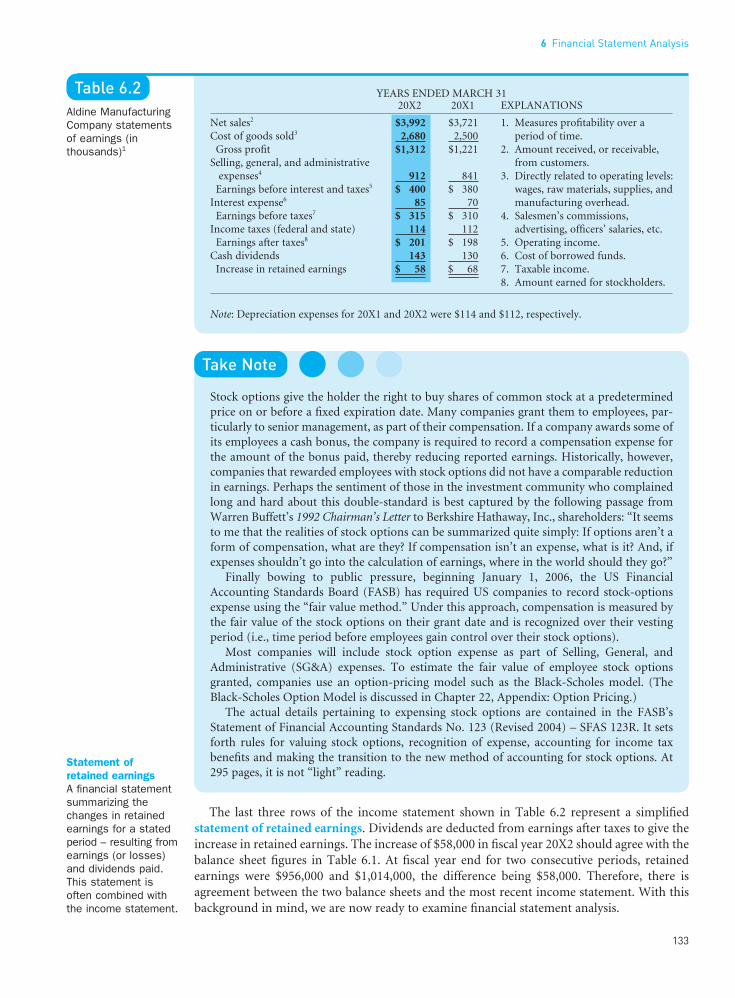
6 Financial Statement Analysis
133
••
Take Note
Stock options give the holder the right to buy shares of common stock at a predeterminedprice on or before a fixed expiration date. Many companies grant them to employees, par-ticularly to senior management, as part of their compensation. If a company awards some ofits employees a cash bonus, the company is required to record a compensation expense forthe amount of the bonus paid, thereby reducing reported earnings. Historically, however,companies that rewarded employees with stock options did not have a comparable reductionin earnings. Perhaps the sentiment of those in the investment community who complainedlong and hard about this double-standard is best captured by the following passage fromWarren Buffett’s 1992 Chairman’s Letter to Berkshire Hathaway, Inc., shareholders: “It seemsto me that the realities of stock options can be summarized quite simply: If options aren’t aform of compensation, what are they? If compensation isn’t an expense, what is it? And, ifexpenses shouldn’t go into the calculation of earnings, where in the world should they go?”
Finally bowing to public pressure, beginning January 1, 2006, the US FinancialAccounting Standards Board (FASB) has required US companies to record stock-optionsexpense using the “fair value method.” Under this approach, compensation is measured bythe fair value of the stock options on their grant date and is recognized over their vestingperiod (i.e., time period before employees gain control over their stock options).
Most companies will include stock option expense as part of Selling, General, andAdministrative (SG&A) expenses. To estimate the fair value of employee stock optionsgranted, companies use an option-pricing model such as the Black-Scholes model. (TheBlack-Scholes Option Model is discussed in Chapter 22, Appendix: Option Pricing.)
The actual details pertaining to expensing stock options are contained in the FASB’sStatement of Financial Accounting Standards No. 123 (Revised 2004) – SFAS 123R. It setsforth rules for valuing stock options, recognition of expense, accounting for income taxbenefits and making the transition to the new method of accounting for stock options. At295 pages, it is not “light” reading.
The last three rows of the income statement shown in Table 6.2 represent a simplifiedstatement of retained earnings. Dividends are deducted from earnings after taxes to give theincrease in retained earnings. The increase of $58,000 in fiscal year 20X2 should agree with thebalance sheet figures in Table 6.1. At fiscal year end for two consecutive periods, retainedearnings were $956,000 and $1,014,000, the difference being $58,000. Therefore, there isagreement between the two balance sheets and the most recent income statement. With thisbackground in mind, we are now ready to examine financial statement analysis.
Table 6.2Aldine ManufacturingCompany statementsof earnings (inthousands)1
EXPLANATIONS
1. Measures profitability over aperiod of time.
2. Amount received, or receivable,from customers.
3. Directly related to operating levels:wages, raw materials, supplies, andmanufacturing overhead.
4. Salesmen’s commissions,advertising, officers’ salaries, etc.
5. Operating income.6. Cost of borrowed funds.7. Taxable income.8. Amount earned for stockholders.
YEARS ENDED MARCH 3120X2 20X1
Net sales2 $3,992 $3,721Cost of goods sold3 2,680 2,500
Gross profit $1,312 $1,221Selling, general, and administrative
expenses4 912 841Earnings before interest and taxes5 $ 400 $ 380
Interest expense6 85 70Earnings before taxes7 $ 315 $ 310
Income taxes (federal and state) 114 112Earnings after taxes8 $ 201 $ 198
Cash dividends 143 130Increase in retained earnings $ 58 $ 68
Note: Depreciation expenses for 20X1 and 20X2 were $114 and $112, respectively.
Statement ofretained earningsA financial statementsummarizing thechanges in retainedearnings for a statedperiod – resulting fromearnings (or losses)and dividends paid.This statement isoften combined withthe income statement.
FUNO_C06.qxd 9/19/08 16:55 Page 133

Part 3 Tools of Financial Analysis and Planning
134
••
Figure 6.1Framework forfinancial analysis
A Possible Framework for AnalysisA number of different approaches might be used in analyzing a firm. Many analysts have afavorite procedure for coming to some generalizations about the firm being analyzed. At therisk of treading on some rather sacred ground, we present a conceptual framework that lendsitself to situations in which external financing is contemplated. The factors to be consideredare shown in Figure 6.1.
Taking them in order, our concern in the first case is with the trend and seasonal com-ponent of a firm’s funds requirements. How much funding will be required in the future, and what is the nature of these needs? Is there a seasonal component to the needs? Analyticaltools used to answer these questions include sources and uses of funds statements, statementsof cash flow, and cash budgets, all of which are considered in Chapter 7. The tools used toassess the financial condition and performance of the firm are financial ratios, a topic taken
QCan you explain the “accrual” method of recog-nizing sales?
AWith pleasure. It’s an important concept to under-stand because, under this system, the “revenues” on
a company’s income statement may not have actuallybeen received by the company.
Revenues, sometimes reported as “sales,” don’t neces-sarily represent the receipt of cash in a sale. Many firms
“accrue” revenues, booking sales when goods areshipped, when services are rendered, or as a long-termcontract proceeds through stages of completion.
Imagine the Beehive Wig Co. (ticker: WHOAA). Withthe accrual method, if it has shipped off a thousandcrates of wigs but hasn’t yet received payment for them,those sales still appear on the income statement. Thechecks “in the mail” get reported as “accounts receiv-able” on the balance sheet.
Keep an eye on receivables, to make sure the companyisn’t booking as sales that which it cannot collect. Also,make sure it’s not packing sales into this quarter thatreally belong in the next quarter.
Ask the Fool
Source: The Motley Fool (www.fool.com). Reproduced with the permission of The Motley Fool.
FUNO_C06.qxd 9/19/08 16:55 Page 134

6 Financial Statement Analysis
135
••
up in this chapter. The financial analyst uses these ratios much like a skilled physician useslab-test results. In combination, and over time, these data offer valuable insight into the health of a firm – its financial condition and profitability. Completing our first set of three factors is an analysis of the business risk of the firm. Business risk relates to the risk inherentin the operations of the firm. Some companies are in highly volatile lines of business and/ormay be operating close to their break-even point. Other companies are in very stable lines ofbusiness and/or find themselves operating far from their break-even point. A machine toolcompany might fall in the first category, whereas a profitable electric utility would probablyfall in the latter. The analyst needs to estimate the degree of business risk of the firm beinganalyzed.
All three of these factors should be used in determining the financial needs of the firm.Moreover, they should be considered jointly. The greater the funds requirements, of course,the greater the total financing that will be necessary. The nature of the needs for fundsinfluences the type of financing that should be used. If there is a seasonal component to thebusiness, this component lends itself to short-term financing, bank loans in particular. Thefirm’s level of business risk also strongly affects the type of financing that should be used. The greater the business risk, the less desirable debt financing usually becomes relative tocommon stock financing. In other words, equity financing is safer in that there is no contrac-tual obligation to pay interest and principal, as there is with debt. A firm with a high degreeof business risk is generally ill advised to take on considerable financial risk as well.1 The financial condition and performance of the firm also influence the type of financing that shouldbe used. The greater the firm’s liquidity, the stronger the overall financial condition; and thegreater the profitability of the firm, the more risky the type of financing that can be incurred.That is, debt financing becomes more attractive with improvements in liquidity, financialcondition, and profitability. The circled item in Figure 6.1 indicates that it is not sufficient todetermine the best financing plan from the viewpoint of the firm and simply assume that itcan be achieved. The plan needs to be sold to outside suppliers of capital. The firm may deter-mine that it needs $1 million in short-term financing, but lenders may not go along witheither the amount or the type of financing requested by management. In the end, the firm mayhave to compromise its plan to meet the realities of the marketplace. The interaction of thefirm with these suppliers of capital determines the amount, terms, and price of financing.These negotiations are often not too far removed from the type of haggling one may witnessin an oriental bazaar – although usually at a lower decibel level. In any event, the fact that the firm must negotiate with outside suppliers of capital serves as a feedback mechanism tothe other factors in Figure 6.1. Analysis cannot be undertaken in isolation from the fact that ultimately an appeal will have to be made to suppliers of capital. Similarly, suppliers ofcapital must keep an open mind to a company’s approach to financing, even if it is differentfrom their own.
As we have just seen, there are a number of facets to financial analysis. Presumably, analysis will be in relation to some structural framework similar to that presented here. Other-wise, the analysis is likely to be loose and not lend itself to answering the questions for whichit was intended. As we shall see, an integral part of financial analysis is the analysis of financialratios – a topic that fills most of the remainder of this chapter.
l l l Use of Financial RatiosTo evaluate a firm’s financial condition and performance, the financial analyst needs to per-form “checkups” on various aspects of a firm’s financial health. A tool frequently used duringthese checkups is a financial ratio, or index, which relates two pieces of financial data bydividing one quantity by the other.
1In Chapter 16 we discuss business risk in some detail, especially as it relates to the firm’s willingness to take on finan-cial risk.
Financial ratio Anindex that relates twoaccounting numbersand is obtained bydividing one numberby the other.
FUNO_C06.qxd 9/19/08 16:55 Page 135

Part 3 Tools of Financial Analysis and Planning
136
••
Why bother with a ratio? Why not simply look at the raw numbers themselves? We calcu-late ratios because in this way we get a comparison that may prove more useful than the rawnumbers by themselves. For example, suppose that a firm had a net profit figure this year of$1 million. That looks pretty profitable. But what if the firm has $200 million invested in totalassets? Dividing net profit by total assets, we get $1M/$200M = 0.005, the firm’s return ontotal assets. The 0.005 figure means that each dollar of assets invested in the firm earned a one-half percent return. A savings account provides a better return on investment than this,and with less risk. In this example, the ratio proved quite informative. But be careful. Youneed to be cautious in your choice and interpretation of ratios. Take inventory and divide itby additional paid-in capital. You have a ratio, but we challenge you to come up with anymeaningful interpretation of the resulting figure.
Internal Comparisons. The analysis of financial ratios involves two types of comparison.First, the analyst can compare a present ratio with past and expected future ratios for the samecompany. The current ratio (the ratio of current assets to current liabilities) for the presentyear could be compared with the current ratio for the previous year end. When financial ratiosare arrayed over a period of years (on a spreadsheet, perhaps), the analyst can study the com-position of change and determine whether there has been an improvement or deteriorationin the firm’s financial condition and performance over time. In short, we are concerned notso much with one ratio at one point in time, but rather with that ratio over time. Financialratios can also be computed for projected, or pro forma, statements and compared with present and past ratios.
External Comparisons and Sources of Industry Ratios. The second method of com-parison involves comparing the ratios of one firm with those of similar firms or with indus-try averages at the same point in time. Such a comparison gives insight into the relativefinancial condition and performance of the firm. It also helps us identify any significant devi-ations from any applicable industry average (or standard). Financial ratios are published forvarious industries by The Risk Management Association, Dun & Bradstreet, Prentice Hall(Almanac of Business and Industrial Financial Ratios), the Federal Trade Commission/theSecurities and Exchange Commission, and by various credit agencies and trade associations.2
Industry-average ratios should not, however, be treated as targets or goals. Rather, they pro-vide general guidelines.
The analyst should also avoid using “rules of thumb” indiscriminately for all industries.The criterion that all companies have at least a 1.5 to 1 current ratio is inappropriate. Theanalysis must be in relation to the type of business in which the firm is engaged and to the firmitself. The true test of liquidity is whether a company has the ability to pay its bills on time.Many sound companies, including electric utilities, have this ability despite current ratiossubstantially below 1.5 to 1. It depends on the nature of the business. Failure to consider the nature of the business (and the firm) may lead one to misinterpret ratios. We might endup with a situation similar to one in which a student with a 3.5 grade point average fromRalph’s Home Correspondence School of Cosmetology is perceived as being a better scholarthan a student with a 3.4 grade point average from Harvard Law School just because one index
2The Risk Management Association (formerly Robert Morris Associates), an association of financial servicesproviders, publishes industry averages based on financial statements supplied to banks by borrowers. Sixteen ratiosare computed annually for over 640 industries. In addition, each industry is divided into asset-size and sales-volumecategories. Dun & Bradstreet annually calculates 14 important ratios for more than 800 industries. The Almanac ofBusiness and Industrial Financial Ratios (Upper Saddle River, NJ: Prentice Hall, annual) shows industry averages forsome 22 financial ratios. Approximately 180 businesses and industries are listed, covering the complete spectrum.The data for this publication come from United States corporate tax filings with the Internal Revenue Service. TheQuarterly Financial Report for Manufacturing Corporations is published jointly by the Federal Trade Commission andthe Securities and Exchange Commission. This publication contains balance sheet and income statement informa-tion by industry groupings and by asset-size categories.
FUNO_C06.qxd 9/19/08 16:55 Page 136

6 Financial Statement Analysis
137
••
number is higher than the other. Only by comparing the financial ratios of one firm withthose of similar firms can one make a realistic judgment.
To the extent possible, accounting data from different companies should be standardized(i.e., adjusted to achieve comparability).3 Apples cannot be compared with oranges. Even withstandardized figures, the analyst should use caution in interpreting the comparisons.
l l l Types of RatiosThe commonly used financial ratios are of essentially two kinds. The first kind summarizessome aspect of the firm’s “financial condition” at a point in time – the point at which a bal-ance sheet has been prepared. We call these balance sheet ratios, quite appropriately, becauseboth the numerator and denominator in each ratio come directly from the balance sheet. Thesecond kind of ratio summarizes some aspect of a firm’s performance over a period of time,usually a year. These ratios are called either income statement or income statement/balancesheet ratios. Income statement ratios compare one “flow” item from the income statementwith another flow item from the income statement. Income statement/balance sheet ratioscompare a flow (income statement) item in the numerator with a “stock” (balance sheet) itemin the denominator. Comparing a flow item with a stock item poses a potential problem forthe analyst. We run the risk of a possible mismatch of variables. The stock item, being a snap-shot taken from the balance sheet, may not be representative of how this variable looked overthe period during which the flow occurred. (Would a photograph of you taken at midnighton New Year’s Eve be representative of how you look, on average?) Therefore, where appro-priate, we may need to use an “average” balance sheet figure in the denominator of an incomestatement/balance sheet ratio to make the denominator more representative of the entireperiod. (We will have more to say on this later.)
TIP•TIP
Benchmarking – measuring a company’s operations and performance against those ofworld-class firms – can be applied to ratio analysis. Therefore, in addition to comparing afirm’s ratios to industry averages over time, you may also want to compare the firm’s ratiosto those of a “benchmark,” or world-class, competitor in the firm’s industry.
Additionally, we can further subdivide our financial ratios into five distinct types: liquid-ity, financial leverage (or debt), coverage, activity, and profitability ratios. (See Figure 6.2.) Noone ratio gives us sufficient information by which to judge the financial condition and per-formance of the firm. Only when we analyze a group of ratios are we able to make reasonablejudgments. We must be sure to take into account any seasonal character of a business.Underlying trends may be assessed only through a comparison of raw figures and ratios at the same time of year. We should not compare a December 31 balance sheet with a May 31balance sheet but rather compare December 31 with December 31.
Although the number of financial ratios that might be compared increases geometricallywith the amount of financial data, only the more important ratios are considered in this chapter. Actually, the ratios needed to assess the financial condition and performance of acompany are relatively few.
3Firms, even within the same industry, may apply different accounting procedures, thus contributing to a confusionbetween perceived and real differences among firms. For example, one firm may use FIFO inventory valuation, whileanother firm uses LIFO, and still a third firm uses average cost.
FUNO_C06.qxd 9/19/08 16:55 Page 137

Part 3 Tools of Financial Analysis and Planning
138
••
Balance Sheet Ratios
l l l Liquidity RatiosLiquidity ratios are used to measure a firm’s ability to meet short-term obligations. Theycompare short-term obligations with short-term (or current) resources available to meetthese obligations. From these ratios, much insight can be obtained into the present cash solvency of the firm and the firm’s ability to remain solvent in the event of adversity.
Current Ratio. One of the most general and frequently used of these liquidity ratios is thecurrent ratio:
(6.1)
For Aldine Manufacturing Company, this ratio for year-end 20X2 is
Aldine is engaged in making household electrical appliances. Its current ratio is somewhatabove the median ratio for the industry of 2.1. (The median – or middle value – for the industryis taken from the Risk Management Association, Statement Studies.4) Although comparisonswith industry averages do not always reveal financial strength or weakness, they are meaningfulin identifying companies that are out of line. Where a significant deviation occurs, the analystwill want to determine the reasons. Perhaps the industry itself is overly liquid, and the
$2,241,000$823,000
= 2.72
Current assetsCurrent liabilities
4The use of a median average eliminates the influence that extreme values from “unusual” statements would have ona simple arithmetic average.
Figure 6.2Types of ratios
Liquidity ratios Ratiosthat measure a firm’sability to meet short-term obligations.
Current ratio Currentassets divided bycurrent liabilities. Itshows a firm’s abilityto cover its currentliabilities with itscurrent assets.
FUNO_C06.qxd 9/19/08 16:55 Page 138
6 Financial Statement Analysis
139
••
company being examined is basically sound despite a lower current ratio. In another situa-tion, the company being analyzed may be too liquid, relative to the industry, with the resultthat it forgoes additional profitability. Whenever a financial “red flag” is raised, the analystmust search out the reasons behind it.
Supposedly, the higher the current ratio, the greater the ability of the firm to pay its bills;however, this ratio must be regarded as a crude measure because it does not take into accountthe liquidity of the individual components of the current assets. A firm having current assetscomposed principally of cash and nonoverdue receivables is generally regarded as more liquid than a firm whose current assets consist primarily of inventories.5 Consequently, weturn to a more critical, or severe, test of the firm’s liquidity – the acid-test ratio.
Acid-Test (or Quick) Ratio. A more conservative measure of liquidity is the acid-test, orquick, ratio:
(6.2)
For Aldine, this ratio for 20X2 year end is
This ratio serves as a supplement to the current ratio in analyzing liquidity. This ratio is the same as the current ratio except that it excludes inventories – presumably the least liquidportion of current assets – from the numerator. The ratio concentrates primarily on the more
$2,241,000 $1,329,000$823,000
−= 1.11
Current assets InventoriesCurrent liabilities
−
5Liquidity has two dimensions: (1) the time required to convert the asset into cash, and (2) the certainty of the pricerealized. Even if the price realized on receivables were as predictable as that realized on inventories, receivables wouldbe a more liquid asset than inventories, owing to the shorter time required to convert the asset into cash. If the pricerealized on receivables were more certain than that on inventories, receivables would be regarded as being even moreliquid.
Liquidity The ability of an asset to beconverted into cashwithout a significantprice concession.
Acid-test (quick)ratio Current assetsless inventoriesdivided by currentliabilities. It shows afirm’s ability to meetcurrent liabilities withits most liquid (quick)assets.
To illustrate, assume that it is March 30, the auditors aresoon to arrive, we hope to make a short-term loan nextweek, and the bank will be very concerned with our cur-rent position as a sign of our short-term solvency.
We could postpone some purchases and use availablecash (or sell marketable securities) to pay some currentcreditors. The current and quick ratios might thus betemporarily improved.
Let’s see how Aldine Manufacturing Company mighthave tried this gambit. Assume, on March 30, 20X2, wefind:
Current Assets Current Liabilities Current Ratio$2,918,000 $1,500,000 1.95
If we pay off $677,000 worth of accounts payable fromcash and marketable securities, we get
$2,241,000 $823,000 2.72
The current ratio has shown a healthy improvement.However, if we go back to business as usual, has our
liquidity position really been improved by this one-timeearly payment to creditors?
It should be noted that year-end financial statementsmay paint a more rosy financial-condition picture than those at any other time in the year, even when nodeliberate steps have been taken to artificially enhancefinancial position. For example, a firm that has adopteda fiscal year ending in a seasonal low point (Red flag: noteAldine’s March 31 fiscal-year closing date) may havedone so not to deceive but to make inventory count-ing easier. However, cash may also be at a yearly high in anticipation of inventory purchases while accountspayable may be at a yearly low; the result may be higherthan normal current and quick ratios.
Therefore, as a manager you may want to look at anaverage of monthly or quarterly liquidity ratios. Thiswould give you a feel for the firm’s average liquidity posi-tion. The idea here is that even if others who look at yourannual data get fooled – don’t fool yourself.
Window Dressing: Taking steps, just before financial statements are prepared, to create a more favorable-looking situation than really exists
FUNO_C06.qxd 9/19/08 16:55 Page 139
Part 3 Tools of Financial Analysis and Planning
140
••
liquid current assets – cash, marketable securities, and receivables – in relation to current obligations. Thus this ratio provides a more penetrating measure of liquidity than does thecurrent ratio. Aldine’s acid-test ratio is slightly above the industry median average of 1.1, indicating that it is in line with the industry.
Summary of Aldine’s Liquidity (So Far). Comparisons of Aldine’s current and acid-testratios with medians for the industry are favorable. However, these ratios don’t tell us whetheraccounts receivable and/or inventory might actually be too high. If they are, this should affectour initial favorable impression of the firm’s liquidity. Thus we need to go behind the ratiosand examine the size, composition, and quality of these two important current assets. We willlook more closely at accounts receivable and inventory when we discuss activity ratios. Wewill reserve a final opinion on liquidity until then.
l l l Financial Leverage (Debt) RatiosDebt-to-Equity Ratio. To assess the extent to which the firm is using borrowed money, wemay use several different debt ratios. The debt-to-equity ratio is computed by simply dividingthe total debt of the firm (including current liabilities) by its shareholders’ equity:
(6.3)
For Aldine, at year-end 20X2 this ratio is
The ratio tells us that creditors are providing 81 cents of financing for each $1 being pro-vided by shareholders. Creditors would generally like this ratio to be low. The lower the ratio,the higher the level of the firm’s financing that is being provided by shareholders, and thelarger the creditor cushion (margin of protection) in the event of shrinking asset values oroutright losses. The median debt-to-equity ratio for the electrical appliance industry is 0.80,so Aldine is right in line with the industry. Presumably, it would not experience difficulty withcreditors because of an excessive debt ratio.
Depending on the purpose for which the ratio is used, preferred stock is sometimesincluded as debt rather than as equity when debt ratios are calculated. Preferred stock repre-sents a prior claim from the standpoint of the investors in common stock; consequently,investors might include preferred stock as debt when analyzing a firm. The ratio of debt toequity will vary according to the nature of the business and the variability of cash flows. An electric utility, with very stable cash flows, will usually have a higher debt-to-equity ratiothan will a machine tool company, whose cash flows are far less stable. A comparison of the debt-to-equity ratio for a given company with those of similar firms gives us a generalindication of the creditworthiness and financial risk of the firm.
Debt-to-Total-Assets Ratio. The debt-to-total-assets ratio is derived by dividing a firm’stotal debt by its total assets:
(6.4)
For Aldine, at the end of 20X2 this ratio is
This ratio serves a similar purpose to the debt-to-equity ratio. It highlights the relative impor-tance of debt financing to the firm by showing the percentage of the firm’s assets that is supported by debt financing. Thus 45 percent of the firm’s assets are financed with debt
$1,454,000$3,250,000
= 0.45
Total debtTotal assets
$1,454,000$1,796,000
= 0.81
Total debtShareholders’ equity
Debt ratios Ratiosthat show the extentto which the firm isfinanced by debt.
FUNO_C06.qxd 9/19/08 16:55 Page 140

6 Financial Statement Analysis
141
••
(of various types), and the remaining 55 percent of the financing comes from shareholders’equity. Theoretically, if the firm were liquidated right now, assets could be sold to net as littleas 45 cents on the dollar before creditors would face a loss. Once again, this points out thatthe greater the percentage of financing provided by shareholders’ equity, the larger the cush-ion of protection afforded the firm’s creditors. In short, the higher the debt-to-total-assetsratio, the greater the financial risk; the lower this ratio, the lower the financial risk.
In addition to the two previous debt ratios, we may wish to compute the following ratio,which deals with only the long-term capitalization of the firm:
(6.5)
where total capitalization represents all long-term debt and shareholders’ equity. For Aldine,the most recent year-end long-term-debt-to-total-capitalization ratio is
This measure tells us the relative importance of long-term debt to the capital structure (long-term financing) of the firm. Again, this ratio is in line with the median ratio of 0.24 for theindustry. The debt ratios just computed have been based on accounting, book value, figures;it is sometimes useful to calculate these ratios using market values. In summary, debt ratiostell us the relative proportions of capital contribution by creditors and by owners.
Income Statement and Income Statement/Balance Sheet RatiosWe now turn our attention to three new types of ratio – coverage, activity, and profitabilityratios – that are derived from either income statement or income statement/balance sheetdata. The significance is that we are no longer talking about just stock (balance sheet) rela-tionships. Now, each ratio relates a flow (income statement) item to another flow item or amixture of a flow to a stock item. (And, to compare a flow with a stock item correctly, we mayneed to make some minor adjustments.)
l l l Coverage RatiosCoverage ratios are designed to relate the financial charges of a firm to its ability to service,or cover, them. Bond rating services, such as Moody’s Investors Service and Standard &Poor’s, make extensive use of these ratios. One of the most traditional of the coverage ratiosis the interest coverage ratio, or times interest earned. This ratio is simply the ratio of earningsbefore interest and taxes for a particular reporting period to the amount of interest chargesfor the period; that is,
(6.6)
For Aldine, in fiscal-year 20X2 this ratio is
This ratio serves as one measure of the firm’s ability to meet its interest payments and thusavoid bankruptcy. In general, the higher the ratio, the greater the likelihood that the companycould cover its interest payments without difficulty. It also sheds some light on the firm’scapacity to take on new debt. With an industry median average of 4.0, Aldine’s ability to cover annual interest 4.71 times with operating income (EBIT) appears to provide a goodmargin of safety.
$400,000$85,000
= 4.71
Earnings before interest and taxes (EBIT)Interest expense
$631,000$2,427,000
= 0.26
Long-term debtTotal capitalization
Coverage ratiosRatios that relate thefinancial charges of a firm to its ability to service, or cover,them.
Interest coverageratio Earnings beforeinterest and taxesdivided by interestcharges. It indicates afirm’s ability to coverinterest charges. It isalso called timesinterest earned.
FUNO_C06.qxd 9/19/08 16:55 Page 141

Part 3 Tools of Financial Analysis and Planning
142
••
A broader type of analysis would evaluate the ability of the firm to cover all charges of afixed nature. In addition to interest payments, we could include principal payments on debtobligations, preferred stock dividends, lease payments, and possibly even certain essential cap-ital expenditures. As we will see in Chapter 16, an analysis of this type is a far more realisticgauge than a simple interest coverage ratio in determining whether a firm has the ability tomeet its long-term obligations.
In assessing the financial risk of a firm, then, the financial analyst should first compute debtratios as a rough measure of financial risk. Depending on the payment schedule of the debtand the average interest rate, debt ratios may or may not give an accurate picture of the firm’sability to meet its financial obligations. Therefore we augment debt ratios with an analysis ofcoverage ratios. Additionally, we realize that interest and principal payments are not reallymet out of earnings per se, but out of cash. Therefore it is also necessary to analyze the cash-flow ability of the firm to service debt (and other financial charges as well). The topicsaddressed in the following chapter, as well as Chapter 16, will aid us in that task.
l l l Activity RatiosActivity ratios, also known as efficiency or turnover ratios, measure how effectively the firm is using its assets. As we will see, some aspects of activity analysis are closely related to liquidity analysis. In this section, we will focus our attention primarily on how effectively the firm is managing two specific asset groups – receivables and inventories – and its totalassets in general.
In computing activity ratios for the Aldine Company, we will use year-end asset levels fromthe balance sheet. However, an average of monthly, quarterly, or beginning and year-end assetlevels is often employed with these income statement/balance sheet ratios. As we mentionedearlier in the chapter, the use of an average balance sheet figure is an attempt to better matchthe income statement flow item with a balance sheet stock figure more representative of theentire period, not just year end.
Receivables Activity. The receivable turnover (RT) ratio provides insight into the quality ofthe firm’s receivables and how successful the firm is in its collections. This ratio is calculatedby dividing receivables into annual net credit sales:
(6.7)
If we assume that all 20X2 sales for Aldine are credit sales, this ratio is
This ratio tells us the number of times accounts receivable have been turned over (turned intocash) during the year. The higher the turnover, the shorter the time between the typical saleand cash collection. For Aldine, receivables turned over 5.89 times during 20X2.
When credit sales figures for a period are not available, we must resort to using total salesfigures. When sales are seasonal or have grown considerably over the year, using the year-endreceivable balance may not be appropriate. With seasonality, an average of the monthly clos-ing balances may be the most appropriate to use. With growth, the receivable balance at theend of the year will be deceptively high in relation to sales. The result is that the receivableturnover calculated is a biased and low estimate of the number of times receivables turnedover during the course of the year. In this case, an average of receivables at the beginning andend of the year might be appropriate if the growth in sales was steady throughout the year.
The median industry receivable turnover ratio is 8.1, which tells us that Aldine’s receivablesare considerably slower in turning over than is typical for the industry. This might be an indication of a lax collection policy and a number of past-due accounts still on the books.
$3,992,000$678,000
= 5.89
Annual net credit salesReceivables
Activity ratios Ratiosthat measure howeffectively the firm isusing its assets.
FUNO_C06.qxd 9/19/08 16:55 Page 142

6 Financial Statement Analysis
143
••
In addition, if receivables are far from being current, we may have to reassess the firm’s liquidity. To regard all receivables as liquid, when in fact a sizable portion may be past due,overstates the liquidity of the firm being analyzed. Receivables are liquid only insofar as theycan be collected in a reasonable amount of time. In an attempt to determine whether there iscause for concern, the analyst may reformulate the receivable turnover ratio to producereceivable turnover in days (RTD), or average collection period.
Receivable turnover in days (RTD), or average collection period, is calculated as
(6.8)
or equivalently
(6.9)
For Aldine, whose receivable turnover we calculated to be 5.89, the average collection period is
This figure tells us the average number of days for which receivables are outstanding before being collected. Since the median industry receivable turnover ratio is 8.1, the averagecollection period for the industry is 365/8.1 = 45 days. The disparity between the industry’sreceivable collection performance and Aldine’s is once again highlighted.
However, before concluding that a collections problem exists, we should check the creditterms offered by Aldine to its customers. If the average collection period is 62 days and thecredit terms are “2/10, net 30,”6 a sizable proportion of the receivables are past the final duedate of 30 days. On the other hand, if the terms are “net 60,” the typical receivable is beingcollected only two days after the final due date.
Although too high an average collection period is usually bad, a very low average collectionperiod may not necessarily be good. A very low average collection period may be a symptomof a credit policy that is excessively restrictive. The few receivables on the books may be ofprime quality, yet sales may be curtailed unduly – and profits less than they might be –because of the restrictive issuance of credit to customers. In this situation, perhaps credit standards used to determine an acceptable credit account should be relaxed somewhat.
Aging Accounts Receivable. Another means by which we can obtain insight into the liquidity of receivables and management’s ability to enforce its credit policy is through aging accounts receivable. With this method we categorize the receivables on a given dateaccording to the percentages billed in previous months. We might have the following hypo-thetical aging schedule of accounts receivable at December 31:
Aging schedule for accounts receivable as of December 31
MONTH OF AUG ANDCREDIT SALE DEC NOV OCT SEPT BEFORE
MONTHS PAST DUE CURRENT 0–1 1–2 2–3 3 OR MORE TOTAL
Percent of total accounts receivable balance outstanding 67 19 7 2 5 100
If the credit terms are “2/10, net 30,” this aging schedule tells us that 67 percent of thereceivables outstanding at December 31 are current, 19 percent are up to one month past due,
3655.89
= 62 days
Receivables Days in the yearAnnual credit sales
×
Days in the yearReceivable turnover
6The notation means that the supplier gives a 2 percent discount if the receivable invoice is paid within 10 days andtotal payment is due within 30 days if the discount is not taken.
Aging accountsreceivableThe process ofclassifying accountsreceivable by theirage outstanding as of a given date.
FUNO_C06.qxd 9/19/08 16:55 Page 143

Part 3 Tools of Financial Analysis and Planning
144
••
7 percent are one to two months past due, and so on. Depending on the conclusions drawnfrom our analysis of the aging schedule, we may want to examine more closely the company’scredit and collection policies. In this example, we might be prompted to investigate the individual receivables that were billed in August and before to determine whether any shouldbe charged off as bad debts. The receivables shown on the books are only as good as the like-lihood that they will be collected. An aging of accounts receivable gives us considerably moreinformation than does the calculation of the average collection period, because it pinpointsthe trouble spots more specifically.
Payables Activity. There may be occasions when a firm wants to study its own prompt-ness of payment to suppliers or that of a potential credit customer. In such cases, it may bedesirable to obtain an aging of accounts payable, much like that just illustrated for accountsreceivable. This method of analysis, combined with the less exact payable turnover (PT) ratio (annual credit purchases divided by accounts payable), allows us to analyze payables inmuch the same manner as we analyze receivables. Also, we can compute the payable turnoverin days (PTD) or average payable period as
(6.10)
or, equivalently,
(6.11)
where accounts payable is the ending (or perhaps, average) balance outstanding for the yearand annual credit purchases are the external purchases during the year. This figure yields theaverage age of a firm’s accounts payable.
Take Note
When information on purchases is not available, one can occasionally use instead the “costof goods sold plus (minus) any increase (decrease) in inventory” in determining these ratios.A department store chain, for example, typically does no manufacturing. As a result, the“cost of goods sold plus the change in inventory” consists primarily of purchases.7 However,in situations where sizable value is added, as with a manufacturer, the “cost of goods soldplus the change in inventory” is an inappropriate proxy for purchases. One must have theactual dollar amount of purchases if the ratio is to be used. Another caveat relates to growth.As with receivables, the use of a year-end payable balance will result in a biased and high estimate of the time it will take a company to make payment on its payables if there is strong underlying growth. In this situation, it may be better to use an average of payables at the beginning and end of the year.
The average payable period is valuable information in evaluating the probability that acredit applicant will pay on time. If the average age of payables is 48 days and the terms in the industry are “net 30,” we know that a portion of the applicant’s payables is not being paidon time. A credit check of the applicant’s other suppliers will give insight into the severity ofthe problem.
Accounts payable Days in the yearAnnual credit purchases
×
Days in the yearPayable turnover
7Typically, for a retail firm we have
(Beginning inventory) + (Purchases) − (Cost of goods sold) = Ending inventory
Therefore
(Cost of goods sold) + [(Ending inventory) − (Beginning inventory)] = Purchases
FUNO_C06.qxd 9/19/08 16:55 Page 144

6 Financial Statement Analysis
145
••
Inventory Activity. To help determine how effectively the firm is managing inventory (andalso to gain an indication of the liquidity of inventory), we compute the inventory turnover(IT) ratio:
(6.12)
For Aldine, this ratio for 20X2 is
The figure for cost of goods sold used in the numerator is for the period being studied – usually a year; the inventory figure used in the denominator, though a year-end figure in our example, might represent an average value. For a situation involving simple growth, anaverage of beginning and ending inventories for the period might be used. As is true withreceivables, however, it may be necessary to compute a more sophisticated average when thereis a strong seasonal element. The inventory turnover ratio tells us how many times inventoryis turned over into receivables through sales during the year. This ratio, like other ratios, mustbe judged in relation to past and expected future ratios of the firm and in relation to ratios ofsimilar firms, the industry average, or both.
Generally, the higher the inventory turnover, the more efficient the inventory managementof the firm and the “fresher,” more liquid, the inventory. However, sometimes a high inven-tory turnover indicates a hand-to-mouth existence. It therefore might actually be a symptomof maintaining too low a level of inventory and incurring frequent stockouts. Relatively lowinventory turnover is often a sign of excessive, slow-moving, or obsolete items in inventory.Obsolete items may require substantial write-downs, which, in turn, would tend to negate the treatment of at least a portion of the inventory as a liquid asset. Because the inventoryturnover ratio is a somewhat crude measure, we would want to investigate further any per-ceived inefficiency in inventory management. In this regard, it is helpful to compute theturnover of the major categories of inventory to see whether there are imbalances, which mayindicate excessive investment in specific components of the inventory.
Aldine’s inventory turnover of 2.02 is in marked contrast to an industry median turnoverratio of 3.3. This unfavorable comparison suggests that the company is less efficient in inventorymanagement than is average for the industry, and that Aldine holds excessive inventory stock.A question also arises as to whether the inventory on the books is worth its stated value. If not,the liquidity of the firm is less than the current ratio or quick ratio alone suggests. Once we havea hint of an inventory problem, we must investigate it more specifically to determine its cause.
An alternative measure of inventory activity is inventory turnover in days (ITD):
(6.13)
or, equivalently,
(6.14)
For Aldine, whose inventory turnover we calculated to be 2.02, the inventory turnover in days(ITD) is
This figure tells us how many days, on average, before inventory is turned into accountsreceivable through sales. Transforming the industry’s median inventory turnover of 3.3 intoan inventory turnover in days figure, we get 365/3.3 = 111 days. Thus Aldine is, on average,70 days slower in “turning” its inventory than is typical for the industry.
3652.02
= 181 days
Inventory Days in the yearCost of goods sold
×
Days in the yearInventory turnover
$2,680,000$1,329,000
= 2.02
Cost of goods soldInventory
Stockout Not havingenough items ininventory to fill anorder.
FUNO_C06.qxd 9/19/08 16:55 Page 145

Part 3 Tools of Financial Analysis and Planning
146
••
Operating Cycle versus Cash Cycle. A direct result of our interest in both liquidity andactivity ratios is the concept of a firm’s operating cycle. A firm’s operating cycle is the lengthof time from the commitment of cash for purchases until the collection of receivables result-ing from the sale of goods or services. It is as if we start a stopwatch when we purchase rawmaterials and stop the watch only when we receive cash after the finished goods have beensold. The time appearing on our watch (usually in days) is the firm’s operating cycle.Mathematically, a firm’s operating cycle is equal to
(6.15)
We stress the fact that our stopwatch starts at the commitment of cash for purchases ratherthan from the actual cash outlay itself. The reason for this subtle distinction is that most firmsdo not pay for raw materials immediately but rather buy on credit and incur an accountpayable. However, if we want to measure the length of time from the actual outlay of cash for purchases until the collection of cash resulting from sales, it is a simple matter. We wouldsubtract the firm’s payable turnover in days (PTD) from its operating cycle and thus producethe firm’s cash cycle:
(6.16)
Figure 6.3 illustrates the operating cycle and cash cycle for the firm – and highlights their differences.8
Why even worry about the firm’s operating cycle? The length of the operating cycle is animportant factor in determining a firm’s current asset needs. A firm with a very short operat-ing cycle can operate effectively with a relatively small amount of current assets and relatively
Operating cycle(ITD RTD)
Payable turnoverin days (PTD)+
−
Inventory turnoverin days (ITD)
Receivable turnoverin days (RTD)
+
8For more information on the firm’s operating and cash cycles, see Verlyn D. Richards and Eugene J. Laughlin, “ACash Conversion Cycle Approach to Liquidity Analysis.” Financial Management 9 (Spring 1980), 32–38.
Operating cycle Thelength of time fromthe commitment ofcash for purchasesuntil the collection ofreceivables resultingfrom the sale ofgoods or services.
Cash cycle The lengthof time from theactual outlay of cashfor purchases untilthe collection ofreceivables resultingfrom the sale ofgoods or services;also called cashconversion cycle.
Figure 6.3Operating cycleversus cash cycle
FUNO_C06.qxd 9/19/08 16:55 Page 146

6 Financial Statement Analysis
147
••
low current and acid-test ratios. This firm is relatively liquid in a “dynamic” sense – it can produce a product, sell it, and collect cash for it, all in a relatively short period of time. It doesnot have to rely so heavily on high “static” levels of liquidity as measured by the current oracid-test ratio. This is very similar to judging the “liquidity” of a garden hose. This liquiditydepends not only on the “static” amount of water in the hose at any one time but also thevelocity with which the water moves through the hose.
The operating cycle, by focusing on ITD and RTD, provides a summary activity measure.For example, a relatively short operating cycle generally indicates effectively managed receiv-ables and inventory. But, as we have just discussed, this measure provides supplementaryinformation on a firm’s liquidity as well. A relatively short operating cycle would thus alsoreflect favorably on a firm’s liquidity. In contrast, a relatively long operating cycle might be awarning sign of excessive receivables and/or inventory, and would reflect negatively on thefirm’s true liquidity.
Comparing Aldine’s operating cycle with that of the median industry average, we have:
Aldine Median Industry AverageOperating cycle 243 days 156 days
The cumulative effect of both a sluggish inventory turnover and receivable turnover forAldine is clearly apparent; relative to the typical firm in the industry, it takes Aldine an extra87 days to manufacture a product, sell it, and collect cash from sales. The length of the firm’soperating cycle should also cause us to to have second thoughts about the firm’s liquidity.
We have not said very much, so far, about the firm’s cash cycle. One reason is that one mustbe extremely careful in trying to analyze this measure. On the surface, it would seem that a relatively short cash cycle would be a sign of good management. Such a firm is quick to collect cash from sales once it pays for purchases. The catch is that this measure reflects bothoperating and financing decisions of the firm, and mismanagement in one or both of thesedecision areas might be overlooked. For example, one way to arrive at a short cash cycle issimply never to pay your bills on time (a poor financing decision). Your payable turnover in days figure will become large, and subtracted from your operating cycle, it will produce alow (perhaps even negative!) cash cycle. The operating cycle, by focusing strictly on the effectsof operating decisions on inventory and receivables, provides clearer signals for the analyst to consider.
Dell, Inc.’s Negative 42-Day Cash Cycle
Some firms have proven successful at aggressivelymanaging their cash cycle. Dell, Inc. (DELL) – com-
puter hardware manufacturer – is one of the few com-panies that have even been able to produce a negativecash cycle while still paying its bills on time.
KEY ACTIVITY MEASURES Q4 1996 Q4 2007
1. Inventory turnover in days 31 52. Receivable turnover in days 42 313. Operating cycle: Line (1) + Line (2) 73 364. Payable turnover in days 33 785. Cash cycle: Line (3) − Line (4) 40 (42)
Source: Dell, Inc., quarterly and annual reports. © 2007 DellInc. All Rights Reserved.
Since implementing a program late in fiscal year 1996aimed at shortening its cash cycle, Dell’s cash cycle wentfrom an acceptable 40 days to an astounding negative 42 days in the fourth quarter of fiscal year 2007. (See thetable below for details.)
A primarily build-to-order manufacturing modelcoupled with reliance on standard parts, available frommany sources, allowed Dell to carry only a 5-day supplyof inventory. Improvements in sales processing and collections helped drive receivable turnover in days downto 31 days. And, by negotiating generous credit termsand ensuring that bills are not paid before the negotiatedterms, Dell has pushed payables out to 78 days. The endresult – a negative 42-day cash cycle – means that Dell isable to collect cash from a typical customer well before itpays its bills related to that customer.
FUNO_C06.qxd 9/19/08 16:55 Page 147

Part 3 Tools of Financial Analysis and Planning
148
••
Few companies can claim negative cash cycles without resort to poor operating and/orpayables decisions. However, there are a few firms that can do it – and do it well. They gener-ally use a “just-in-time” approach to inventory (a topic we take up in Chapter 10), managereceivables tightly, and, because of strong purchasing power, secure generous credit termsfrom suppliers.
A Second Look at Aldine’s Liquidity. As you may remember, Aldine’s current and acid-test ratios compared favorably with industry median ratios. However, we decided to reserve afinal opinion on liquidity until we had performed a more detailed examination of the firm’sreceivables and inventory. The turnover ratios for both of these assets, and the resulting operating cycle, are significantly worse than the industry median values for these same measures. These findings suggest that the two assets are not entirely current, and this factordetracts from the favorable current and quick ratios. A sizable portion of receivables is slow, and there appear to be inefficiencies in inventory management. On the basis of our analysis, we conclude that these assets are not particularly liquid in the sense of turning overinto cash in a reasonable period of time (see the boxed feature opposite).
Total Asset (or Capital) Turnover. The relationship of net sales to total assets is known asthe total asset turnover, or capital turnover, ratio:
(6.17)
Aldine’s total asset turnover for fiscal-year 20X2 is
The median total asset turnover for the industry is 1.66, so it is clear that Aldine generates less sales revenue per dollar of asset investment than does the industry, on average. The totalasset turnover ratio tells us the relative efficiency with which a firm utilizes its total assets togenerate sales. Aldine is less efficient than the industry in this regard. From our previous analysis of Aldine’s receivables and inventory activity, we suspect that excessive investmentsin receivables and inventories may be responsible for a large part of the problem. If Aldine couldgenerate the same sales revenue with fewer dollars invested in receivables and inventories,total asset turnover would improve.
l l l Profitability RatiosProfitability ratios are of two types – those showing profitability in relation to sales and thoseshowing profitability in relation to investment. Together, these ratios indicate the firm’s overall effectiveness of operation.
Profitability in Relation to Sales. The first ratio we consider is the gross profit margin:
(6.18)
or simply gross profit divided by net sales. For Aldine, the gross profit margin for fiscal-year20X2 is
This ratio tells us the profit of the firm relative to sales, after we deduct the cost of producingthe goods. It is a measure of the efficiency of the firm’s operations, as well as an indication ofhow products are priced. Aldine’s gross profit margin is significantly above the median of23.8 percent for the industry, indicating that it is relatively more effective at producing andselling products above cost.
$1,312,000$3,992,000
= 32.9%
Net sales Cost of goods soldNet sales
−
$3,992,000$3,250,000
= 1.23
Net salesTotal assets
Profitability ratiosRatios that relateprofits to sales andinvestment.
FUNO_C06.qxd 9/19/08 16:55 Page 148

6 Financial Statement Analysis
149
••
A more specific measure of sales profitability is the net profit margin:
(6.19)
For Aldine, this ratio for fiscal-year 20X2 is
$201,000$3,992,000
= 5.04%
Net profit after taxesNet sales
FUNO_C06.qxd 9/19/08 16:55 Page 149

The net profit margin is a measure of the firm’s profitability of sales after taking account of allexpenses and income taxes. It tells us a firm’s net income per dollar of sales. For Aldine,roughly 5 cents out of every sales dollar constitutes after-tax profits. Aldine’s net profit margin is above the median net profit margin (4.7 percent) for the industry, which indicatesthat it has a higher relative level of “sales profitability” than most other firms in the industry.
By considering both ratios jointly, we are able to gain considerable insight into the opera-tions of the firm. If the gross profit margin is essentially unchanged over a period of severalyears but the net profit margin has declined over the same period, we know that the cause is either higher selling, general, and administrative (SG&A) expenses relative to sales, or ahigher tax rate. On the other hand, if the gross profit margin falls, we know that the cost of producing goods relative to sales has increased. This occurrence, in turn, may be due tolower prices or to lower operating efficiency in relation to volume.
Profitability in Relation to Investment. The second group of profitability ratios relatesprofits to investment. One of these measures is the rate of return on investment (ROI), orreturn on assets:
(6.20)
For Aldine, ROI for fiscal-year 20X2 is
This ratio compares unfavorably with a median value of 7.8 percent for the industry. Higherprofitability per dollar of sales but a slightly lower return on investment confirms that Aldineemploys more assets to generate a dollar of sales than does the typical firm in the industry.
ROI and the Du Pont Approach. In about 1919 the Du Pont Company began to use a particular approach to ratio analysis to evaluate the firm’s effectiveness. One variation of thisDu Pont approach has special relevance to understanding a firm’s return on investment. Asshown in Figure 6.4, when we multiply the net profit margin of the firm by the total assetturnover, we obtain the return on investment, or earning power on total assets.
For Aldine, we have
Earning power = Sales profitability × Asset efficiencyROI = Net profit margin × Total asset turnover
6.20% = 5.04% × 1.23
Neither the net profit margin nor the total asset turnover ratio by itself provides an ad-equate measure of overall effectiveness. The net profit margin ignores the utilization of assets,and the total asset turnover ratio ignores profitability on sales. The return on investment ratio,or earning power, resolves these shortcomings. An improvement in the earning power of thefirm will result if there is an increase in turnover on assets, an increase in the net profit margin, or both. Two firms with different net profit margins and total asset turnovers mayhave the same earning power. Geraldine Lim’s Oriental Grocery, with a net profit margin ofonly 2 percent and a total asset turnover of 10, has the same earning power – 20 percent – as the Megawatt Power Supply Company, with a net profit margin of 20 percent and a totalasset turnover of 1. For each firm, every dollar invested in assets returns 20 cents in after-taxprofit per year.
Return on Equity (ROE). Another summary measure of overall firm performance is returnon equity. Return on equity (ROE) compares net profit after taxes (minus preferred stock dividends, if any) with the equity that shareholders have invested in the firm:
(6.21)Net profit after taxesShareholders’ equity
$201,000$3,250,000
= 6.18%
Net profit after taxesTotal assets
Part 3 Tools of Financial Analysis and Planning
150
••
FUNO_C06.qxd 9/19/08 16:55 Page 150

6 Financial Statement Analysis
151
••
For Aldine, ROE is
This ratio tells us the earning power on shareholders’ book value investment, and is frequentlyused in comparing two or more firms in an industry. A high return on equity often reflectsthe firm’s acceptance of strong investment opportunities and effective expense management.However, if the firm has chosen to employ a level of debt that is high by industry standards,a high ROE might simply be the result of assuming excessive financial risk. Aldine’s ROE isbelow the median return (14.04 percent) for the industry.
To investigate this return more fully, we can utilize a Du Pont approach – that is, break thisreturn measure into its components:
Net TotalEquity
ROE = profit × asset ×multiplier
margin turnover
For, Aldine, we have
11.2% = 5.04% × 1.23 × 1.81
This Du Pont approach to ROE helps to explain “why” Aldine’s ROE is less than the indus-try’s median ROE. Although Aldine’s net profit margin is higher than average and its equitymultiplier is about at the industry norm,9 its lower-than-average total asset turnover pulls itsROE down below that of the typical firm in the industry. This suggests that Aldine’s use of arelatively greater proportion of assets to produce sales than most other firms in the industryis the root cause of its below-average ROE.
With all of the profitability ratios discussed, comparing one company with similar com-panies and industry standards is extremely valuable. Only by comparisons are we able to judge whether the profitability of a particular company is good or bad, and why. Absolutefigures provide some insight, but it is relative performance that is most revealing.
Net profit after taxes
Shareholders’equity
Net profit after taxesNet sales
Net salesTotal assets
Total assetsShareholders’
equity
= × ×
$201,000$1,796,000
= 11.19%
9The “equity multiplier” is yet another measure of financial leverage. Since it is equivalent to (1 + debt-to-equity ratio), the higher the debt-to-equity ratio, the higher the multiplier. For Aldine, the multiplier is 1 + 0.81 =1.81, whereas for the industry we have 1 + 0.80 = 1.80.
Figure 6.4Earning power and theDu Pont approach
FUNO_C06.qxd 9/19/08 16:55 Page 151

Part 3 Tools of Financial Analysis and Planning
152
••
Trend AnalysisUntil now, our concern has been with introducing the various financial ratios, explainingtheir uses in analysis, and comparing the ratios computed for our sample company withindustry averages. As we pointed out earlier, it is important to compare the financial ratios for a given company over time. In this way, the analyst is able to detect any improvement or deterioration in a firm’s financial condition and performance.
To illustrate, Table 6.3 shows selected financial ratios for Aldine Manufacturing Companyover the 20X0–20X2 period along with industry median figures for 20X2. As can be seen, thecurrent and acid-test ratios have fallen off somewhat over time but still exceed industry normsin 20X2. The figures for average collection period and inventory turnover in days have grownsince 20X0 and exceed the current industry median levels. The trends here tell us that there hasbeen a relative buildup in receivables and inventories. The turnover of each has slowed, whichraises questions as to the quality and liquidity of these assets. When a trend analysis of receiv-ables and inventory is coupled with a comparison with median ratios for the industry, the onlyconclusion possible is that a problem exists. The analyst would want to investigate the creditpolicies of Aldine, the company’s collection experience, and its bad-debt losses. Moreover, oneshould investigate inventory management, obsolescence of inventory, and any imbalances inthe makeup of inventory (i.e., raw material versus work-in-process versus finished goods).Thus, despite above average levels of current and acid-test ratios, the apparent deteriorationin receivables and inventory is a matter of concern and needs to be investigated in depth.
The stability of the firm’s leverage (debt) ratios coupled with a present relative debt leveltypical of the industry would be viewed favorably by creditors. The gross profit margin andnet profit margin have generally shown improvement over the recent past, and current levelsare stronger than for the typical firm in the industry. Return on investment has been relativelystable over time, but at a level below the industry standard. Sluggish asset turnover over timehas dampened any positive effects of above-average sales profitability. From our analysis of activity ratios, we know that the primary cause has been the large and growing relativeamounts of receivables and inventory.
We see, then, that the analysis of the trend of financial ratios over time, coupled with a com-parison with industry averages, can give the analyst valuable insight into changes that have
Table 6.3Selected financialratios of AldineManufacturingCompany for fiscalyears 20X0–20X2
INDUSTRY MEDIAN20X0 20X1 20X2 20X2
LiquidityCurrent ratio 2.95 2.80 2.72 2.10Acid-test ratio 1.30 1.23 1.11 1.10
LeverageDebt-to-equity ratio 0.76 0.81 0.81 0.80Total-debt-to-total-assets ratio 0.43 0.45 0.45 0.44
CoverageInterest coverage ratio 5.95 5.43 4.71 4.00
ActivityAverage collection perioda 55 days 73 days 62 days 45 daysInventory turnover in daysa 136 days 180 days 181 days 111 daysTotal asset turnovera 1.25 1.18 1.23 1.66
ProfitabilityGross profit margin 30.6% 32.8% 32.9% 23.8%Net profit margin 4.90% 5.32% 5.04% 4.70%Return on investmenta 6.13% 6.29% 6.19% 7.80%Return on equitya 10.78% 11.36% 11.19% 14.04%
aIn computing “income statement/balance sheet”-type ratios, year-end balance sheet figures were used.
FUNO_C06.qxd 9/19/08 16:55 Page 152

6 Financial Statement Analysis
153
••
occurred in a firm’s financial condition and performance. Additional insight can be providedif we extend our analysis to include comparisons with similar competitors in the industry.
Common-Size and Index AnalysisIn addition to financial ratio analysis over time, it is often useful to express balance sheet andincome statement items as percentages. The percentages can be related to totals, such as totalassets or total net sales, or to some base year. Called common-size analysis and index analysisrespectively, the evaluation of levels and trends in financial statement percentages over timeaffords the analyst insight into the underlying improvement or deterioration in financial condition and performance. Though a good portion of this insight is revealed in the analysisof financial ratios, a broader understanding of the trends is possible when the analysis isextended to include the foregoing considerations. Also, these two new types of analysis areextremely helpful in comparing firms whose data differ significantly in size, because everyitem on the financial statements gets placed on a relative, or standardized, basis.
l l l Financial Statement Items as Percentages of TotalsIn common-size analysis, we express the various components of a balance sheet as percent-ages of the total assets of the company. In addition, this can be done for the income statement,but here items are related to net sales. The gross and net profit margins, taken up earlier, areexamples of this type of expression, and the procedure can be extended to include all the itemson the income statement. The expression of individual financial statement items as percent-ages of total helps the analyst spot trends with respect to the relative importance of these itemsover time. To illustrate, common-size balance sheets and income statements are shown along-side regular statements in Tables 6.4 and 6.5 for R. B. Harvey Electronics Company for 20X0through 20X2. In Table 6.4 we see that, over the three-year span, the percentage of current
Common-size analysisAn analysis ofpercentage financialstatements where allbalance sheet itemsare divided by totalassets and all incomestatement items aredivided by net salesor revenues.
Index analysisAn analysis ofpercentage financialstatements where all balance sheet orincome statementfigures for a baseyear equal 100.0(percent) andsubsequent financialstatement items are expressed aspercentages of theirvalues in the baseyear.
Table 6.4R. B. HarveyElectronics Companybalance sheets (atDecember 31)
REGULAR (in thousands) COMMON-SIZE (%)
ASSETS 20X0 20X1 20X2 20X0 20X1 20X2
Cash $ 2,507 $ 11,310 $ 19,648 1.0 3.8 5.1Accounts receivable 70,360 85,147 118,415 29.3 28.9 30.9Inventory 77,380 91,378 118,563 32.2 31.0 31.0Other current assets 6,316 6,082 5,891 2.6 2.1 1.5
Current assets $156,563 $193,917 $262,517 65.1 65.8 68.5Fixed assets, net 79,187 94,652 115,461 32.9 32.2 30.1Other long-term assets 4,695 5,899 5,491 2.0 2.0 1.4
Total assets $240,445 $294,468 $383,469 100.0 100.0 100.0
LIABILITIES AND SHAREHOLDERS’ EQUITY
Accounts payable $ 35,661 $ 37,460 $ 62,725 14.8 12.7 16.4Notes payable 20,501 14,680 17,298 8.5 5.0 4.5Other current liabilities 11,054 8,132 15,741 4.6 2.8 4.1
Current liabilities $ 67,216 $ 60,272 $ 95,764 27.9 20.5 25.0Long-term debt 888 1,276 4,005 0.4 0.4 1.0
Total liabilities $ 68,104 $ 61,548 $ 99,769 28.3 20.9 26.0Common stock 12,650 20,750 24,150 5.3 7.0 6.3Additional paid-in capital 37,950 70,350 87,730 15.8 23.9 22.9Retained earnings 121,741 141,820 171,820 50.6 48.2 44.8
Total shareholders’equity $172,341 $232,920 $283,700 71.7 79.1 74.0
Total liabilities and shareholders’ equity $240,445 $294,468 $383,469 100.0 100.0 100.0
FUNO_C06.qxd 9/19/08 16:55 Page 153

Part 3 Tools of Financial Analysis and Planning
154
••
assets increased, and that this was particularly true for cash. In addition, we see that accountsreceivable showed a relative increase from 20X1 to 20X2. On the liability and equity portionof the balance sheet, the total debt of the company declined on a relative (and absolute) basisfrom 20X0 to 20X1, primarily because of a decline in notes payable. However, with the largeabsolute increase in assets that occurred in 20X1 and 20X2, the debt ratio increased from20X1 to 20X2. The rebound in the importance of debt financing is particularly apparent inaccounts payable, which increased substantially in both absolute and relative terms in 20X2.
The common-size income statements shown in Table 6.5 show the gross profit marginfluctuating from year to year. An improved 20X2 gross profit margin, coupled with better relative control over selling, general, and administrative expenses, caused 20X2 profitability to improve sharply over 20X0 and 20X1.
l l l Financial Statement Items as Indexes Relative to a Base YearThe common-size balance sheets and income statements can be supplemented by the expres-sion of items relative to a base year. For Harvey Electronics, the base year is 20X0, and allfinancial statement items are 100.0 (percent) for that year. Items for subsequent years areexpressed as an index relative to that year. For example, comparing Harvey Electronics’accounts receivable in 20X1 ($85,147,000) with its receivables in the base year, 20X0($70,360,000), the index would be 121.0 (i.e., [$85,147,000/$70,360,000] × 100). Tables 6.6and 6.7 show indexed balance sheets and income statements alongside regular statements.
Take Note
We should expect that changes in a number of the firm’s current assets and liabilitiesaccounts (e.g., cash, accounts receivable, inventory, and accounts payable – which all sup-port sales activity) would move roughly together with sales for a normal, well-run company.Therefore, remember for future reference that Harvey Electronics’ indexed net sales figurefor 20X2 is 148.0, which indicates a 48 percent (148.0 minus 100.0 percent) increase in salesover the base period two years ago.
In Table 6.6 the buildup in cash from the base year is particularly apparent over the pasttwo years, and agrees with our previous assessment. Also, the 683.7 percent (783.7 minus 100 percent) increase in cash over two years seems way out of proportion when comparedwith only a 48 percent increase in net sales over the same period.
Also, note the large increase in accounts receivable and inventory from 20X1 to 20X2. Thislatter change was not apparent in the common-size analysis. When we compare the accountsreceivable and inventory figures with those for net sales, however, the increases do not seem
Table 6.5R. B. HarveyElectronics Companyincome statements(for years endingDecember 31)
REGULAR (in thousands) COMMON-SIZE (%)
20X0 20X1 20X2 20X0 20X1 20X2
Net sales $323,780 $375,088 $479,077 100.0 100.0 100.0Cost of goods sold 148,127 184,507 223,690 45.8 49.2 46.7
Gross profit $175,653 $190,581 $255,387 54.2 50.8 53.3Selling, general, and
administrative expenses 131,809 140,913 180,610 40.7 37.6 37.7Depreciation 7,700 9,595 11,257 2.4 2.5 2.3Interest expense 1,711 1,356 1,704 0.5 0.4 0.4
Earnings before taxes $ 34,433 $ 38,717 $ 61,816 10.6 10.3 12.9Taxes 12,740 14,712 23,490 3.9 3.9 4.9
Earning after taxes $ 21,693 $ 24,005 $ 38,326 6.7 6.4 8.0
FUNO_C06.qxd 9/19/08 16:55 Page 154

6 Financial Statement Analysis
155
••
too much out of line. (We would probably want to follow up on this information, nonethe-less, by checking the firm’s receivable turnover and inventory turnover to see how well thefirm is managing these growing asset accounts.) To a lesser extent, there was a noticeableincrease in fixed assets, but the change was accompanied by a somewhat favorable, more thanproportionate, change in sales over the past two years.
On the liability portion of the balance sheet, we note the large increase in accounts payableand in other current liabilities that occurred. Only the payables increase, however, seems largerelative to the increase in sales, as well as the increases in receivables and inventories. Basedon this insight, we would want to take a look at the firm’s payable turnover to see whether thefirm might not be paying its suppliers in a timely fashion. Finally, increases in long-term debt,common stock, and retained earnings also helped finance the large increase in assets thatoccurred over the last two years.
The indexed income statements in Table 6.7 give much the same picture as the common-size income statements – namely, fluctuating behavior. The sharp improvement in 20X2
Table 6.7R. B. HarveyElectronics Companyincome statements(for years endingDecember 31)
Table 6.6R. B. HarveyElectronics Companybalance sheets (atDecember 31)
REGULAR (in thousands) INDEXED (%)
ASSETS 20X0 20X1 20X2 20X0 20X1 20X2
Cash $ 2,507 $ 11,310 $ 19,648 100.0 451.1 783.7Accounts receivable 70,360 85,147 118,415 100.0 121.0 168.3Inventory 77,380 91,378 118,563 100.0 118.1 153.2Other current assets 6,316 6,082 5,891 100.0 96.3 93.3
Current assets $156,563 $193,917 $262,517 100.0 123.9 167.7Fixed assets, net 79,187 94,652 115,461 100.0 119.5 145.8Other long-term assets 4,695 5,899 5,491 100.0 125.6 117.0
Total assets $240,445 $294,468 $383,469 100.0 122.5 159.5
LIABILITIES AND SHAREHOLDERS’ EQUITY
Accounts payable $ 35,661 $ 37,460 $ 62,725 100.0 105.0 175.9Notes payable 20,501 14,680 17,298 100.0 71.6 84.4Other current liabilities 11,054 8,132 15,741 100.0 73.6 142.4
Current liabilities $ 67,216 $ 60,272 $ 95,764 100.0 89.7 142.5Long-term debt 888 1,276 4,005 100.0 143.7 451.0
Total liabilities $ 68,104 $ 61,548 $ 99,769 100.0 90.4 146.5Common stock 12,650 20,750 24,150 100.0 164.0 190.9Additional paid-in capital 37,950 70,350 87,730 100.0 185.4 231.2Retained earnings 121,741 141,820 171,820 100.0 116.5 141.1
Total shareholders’ equity $172,341 $232,920 $283,700 100.0 135.2 164.6
Total liabilities and shareholders’ equity $240,445 $294,468 $383,469 100.0 122.5 159.5
REGULAR (in thousands) INDEXED (%)
20X0 20X1 20X2 20X0 20X1 20X2
Net sales $323,780 $375,088 $479,077 100.0 115.8 148.0Cost of goods sold 148,127 184,507 223,690 100.0 124.6 151.0
Gross profit $175,653 $190,581 $255,387 100.0 108.5 145.4Selling, general, and
administrative expenses 131,809 140,913 180,610 100.0 106.9 137.0Depreciation 7,700 9,595 11,257 100.0 124.6 146.2Interest expense 1,711 1,356 1,704 100.0 79.3 99.6
Earnings before taxes $ 34,433 $ 38,717 $ 61,816 100.0 112.4 179.5Taxes 12,740 14,712 23,490 100.0 115.5 184.4
Earnings after taxes $ 21,693 $ 24,005 $ 38,326 100.0 110.7 176.7
FUNO_C06.qxd 9/19/08 16:55 Page 155
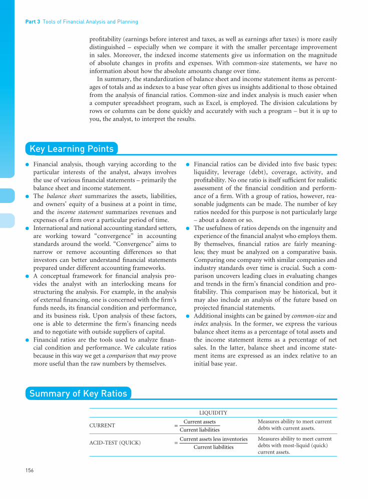
Part 3 Tools of Financial Analysis and Planning
156
••
profitability (earnings before interest and taxes, as well as earnings after taxes) is more easilydistinguished – especially when we compare it with the smaller percentage improvement in sales. Moreover, the indexed income statements give us information on the magnitude of absolute changes in profits and expenses. With common-size statements, we have no information about how the absolute amounts change over time.
In summary, the standardization of balance sheet and income statement items as percent-ages of totals and as indexes to a base year often gives us insights additional to those obtainedfrom the analysis of financial ratios. Common-size and index analysis is much easier when a computer spreadsheet program, such as Excel, is employed. The division calculations byrows or columns can be done quickly and accurately with such a program – but it is up to you, the analyst, to interpret the results.
Key Learning Points
l Financial analysis, though varying according to theparticular interests of the analyst, always involves the use of various financial statements – primarily thebalance sheet and income statement.
l The balance sheet summarizes the assets, liabilities,and owners’ equity of a business at a point in time,and the income statement summarizes revenues andexpenses of a firm over a particular period of time.
l International and national accounting standard setters,are working toward “convergence” in accountingstandards around the world. “Convergence” aims tonarrow or remove accounting differences so thatinvestors can better understand financial statementsprepared under different accounting frameworks.
l A conceptual framework for financial analysis pro-vides the analyst with an interlocking means for structuring the analysis. For example, in the analysisof external financing, one is concerned with the firm’sfunds needs, its financial condition and performance,and its business risk. Upon analysis of these factors,one is able to determine the firm’s financing needsand to negotiate with outside suppliers of capital.
l Financial ratios are the tools used to analyze finan-cial condition and performance. We calculate ratiosbecause in this way we get a comparison that may provemore useful than the raw numbers by themselves.
l Financial ratios can be divided into five basic types:liquidity, leverage (debt), coverage, activity, and profitability. No one ratio is itself sufficient for realisticassessment of the financial condition and perform-ance of a firm. With a group of ratios, however, rea-sonable judgments can be made. The number of keyratios needed for this purpose is not particularly large– about a dozen or so.
l The usefulness of ratios depends on the ingenuity andexperience of the financial analyst who employs them.By themselves, financial ratios are fairly meaning-less; they must be analyzed on a comparative basis.Comparing one company with similar companies andindustry standards over time is crucial. Such a com-parison uncovers leading clues in evaluating changesand trends in the firm’s financial condition and pro-fitability. This comparison may be historical, but itmay also include an analysis of the future based onprojected financial statements.
l Additional insights can be gained by common-size andindex analysis. In the former, we express the variousbalance sheet items as a percentage of total assets andthe income statement items as a percentage of netsales. In the latter, balance sheet and income state-ment items are expressed as an index relative to an initial base year.
Summary of Key Ratios
LIQUIDITY
CURRENTMeasures ability to meet currentdebts with current assets.
ACID-TEST (QUICK)Measures ability to meet currentdebts with most-liquid (quick)current assets.
= Current assets less inventories
Current liabilities
= Current assets
Current liabilities
FUNO_C06.qxd 9/19/08 16:55 Page 156

6 Financial Statement Analysis
157
••
LEVERAGE
DEBT-TO-EQUITYIndicates the extent to which debtfinancing is used relative to equityfinancing.
DEBT-TO-TOTAL-ASSETSShows the relative extent to whichthe firm is using borrowed money.
COVERAGE
INTEREST COVERAGEIndicates ability to cover interestcharges; tells number of timesinterest is earned.
ACTIVITY
RECEIVABLE TURNOVER (RT)Measures how many times thereceivables have been turned over(into cash) during the year;provides insight into quality of the receivables.
RECEIVABLE TURNOVER Average number of days IN DAYS (RTD) receivables are outstanding(Average collection period) before being collected.
INVENTORY TURNOVER (IT)Measures how many times theinventory has been turned over(sold) during the year; providesinsight into liquidity of inventoryand tendency to overstock.
INVENTORY TURNOVER Average number of days the IN DAYS (ITD) inventory is held before it is
turned into accounts receivablethrough sales.
TOTAL ASSET TURNOVER Measures relative efficiency of(Capital turnover) total assets to generate sales.
PROFITABILITY
NET PROFIT MARGINMeasures profitability with respectto sales generated; net income perdollar of sales.
RETURN ON INVESTMENT Measures overall effectiveness in(ROI) generating profits with available(Return on assets) assets; earning power of invested
capital.
= NET PROFIT MARGIN × TOTAL ASSET TURNOVER
×
RETURN ON EQUITY (ROE)Measures earning power onshareholders’ book-valueinvestment.
NET PROFIT TOTAL ASSET EQUITY=MARGIN
×TURNOVER
×MULTIPLIER
= × ×
*Earnings before interest and taxes.**An average, rather than an ending, balance may be needed.
Total assets**
Shareholders’ equity**
Net sales
Total assets**
Net profit after taxes
Net sales
= Net profit after taxes
Shareholders’ equity**
Net sales
Total assets**=
Net profit after taxes
Net sales
= Net profit after taxes
Total assets**
= Net profit after taxes
Net sales
= Net sales
Total assets**
= 365
IT
= Cost of goods sold
Inventory**
= 365
RT
= Annual net credit sales
Receivables**
= EBIT*
Interest expense
= Total debt
Total assets
= Total debt
Shareholders’ equity
FUNO_C06.qxd 9/19/08 16:55 Page 157

Part 3 Tools of Financial Analysis and Planning
158
••
10Deferred taxes are not the same thing as taxes payable. Taxes payable are tax payments due within the year, whereasdeferred taxes are “due” at some indefinite long-term date.
Appendix Deferred Taxes and Financial Analysis
Deferred taxes10 – an item that often appears in the long-term liability portion of a firm’s balance sheet – pose some real problems for the financial analyst attempting to do ratio analysis. Though its position on the balance sheet would make it appear to be a long-termdebt item, analysts (and especially accountants) can’t agree on whether to treat the deferredtaxes account as debt or equity, or neither, in ratio and other analyses. Why the confusion?
Where Do Deferred Taxes Come From?Deferred taxes most commonly arise when a firm determines depreciation expense in its published financial statements on a different basis from that in its tax returns. Most likely, a company chooses straight-line depreciation for its published income statement but uses atype of accelerated depreciation (MACRS) for tax purposes. (See Table 6A.1 for an example.)This action “temporarily” defers the payment of taxes by making tax-return profits less thanbook profits. When a higher tax expense is reported on the firm’s books than is actually paid,the firm’s books won’t balance. To solve this problem, accountants create a deferred taxaccount in the long-term liability section of the balance sheet to maintain a running total ofthese differences between taxes reported and taxes actually due. If the firm slows or ceasesbuying new assets, there will eventually be a reversal – reported taxes will be less than actualtaxes due – and the deferred taxes account will need to be reduced to keep the balance sheetin balance. In this particular situation, our deferred tax liability item is truly a “debt” thateventually comes due. On the other hand, if the firm continues to invest in depreciable assets,payment of the deferred tax may continue to be delayed indefinitely.
So What’s the Problem?The catch is that for stable or growing firms there is no foreseeable reversal, and the deferredtaxes account balance continues to grow. For many firms, a growing, never-reversing,deferred taxes account is the norm. Faced with this reality, the analyst may decide to modifythe financial statements for purposes of analysis.
Depending on the situation (for example, the nature and magnitude of the tax deferrals,whether the account has been growing, and the likelihood of a reversal), the analyst maydecide to make one or both of the following adjustments to the firm’s financial statements:
Deferred taxes A “liability” thatrepresents theaccumulateddifference betweenthe income taxexpense reported onthe firm’s books andthe income taxactually paid. It arisesprincipally becausedepreciation iscalculated differentlyfor financial reportingthan for tax reporting.
Table 6A.1Income statementshighlighting deferredtaxes for year endingDecember 31, 20X2(in millions)
FINANCIAL REPORTING TAX REPORTING
Net sales $100.0 $100.0Costs and expenses, except for depreciation 45.0 45.0Depreciation
Straight-line 15.0Accelerated (MACRS) 20.0Earnings before taxes $ 40.0 $ 35.0
Taxes (40%) 16.0* 14.0Earnings after taxes $ 24.0 $ 21.0
*TaxesCurrent (involves cash payment) $14.0Deferred (noncash charge added to
deferred taxes account on balance sheet) 2.0Total tax shown $16.0
FUNO_C06.qxd 9/19/08 16:55 Page 158

6 Financial Statement Analysis
159
••
l The current period’s deferred tax expense (a noncash charge) is added back to netincome – the argument is that profits were understated because taxes were, in effect,overstated.
l The deferred taxes reported on the firm’s balance sheet are added to equity – here theargument is that because this amount is not a definite, legal obligation requiring pay-ment in the foreseeable future, it overstates the debt position of the firm. In short, it ismore like equity than debt.
Such adjustment will, of course, affect the calculation of the firm’s debt and profitabilityratios.
Still another school of thought rejects both of the previous adjustments. Called the “net-of-tax” approach, this viewpoint calls for most deferred taxes to be treated as adjustments tothe amounts at which the related assets are carried on the firm’s books. An analyst subscrib-ing to this approach would make the following financial statement adjustment:
l The deferred taxes on the firm’s balance sheet are subtracted from net fixed assets – thereason is that when there is an excess of tax depreciation over book depreciation, anasset’s value is decreased, rather than a liability created. Accelerated depreciation, ineffect, uses up an additional part of an asset’s tax-reducing capacity relative to straight-line depreciation. The immediate loss of the future tax-reducing (i.e., tax-shield) benefitshould be deducted from the related asset account.
This adjustment will affect the calculation of various leverage, activity, and profitabilityratios.
Questions
1. What is the purpose of a balance sheet? An income statement?2. Why is the analysis of trends in financial ratios important?3. Auxier Manufacturing Company has a current ratio of 4 to 1 but is unable to pay its bills.
Why?4. Can a firm generate a 25 percent return on assets and still be technically insolvent (unable
to pay its bills)? Explain.5. The traditional definitions of collection period and inventory turnover are criticized
because in both cases balance sheet figures that are a result of approximately the lastmonth of sales are related to annual sales (in the former case) or annual cost of goods sold(in the latter case). Why do these definitions present problems? Suggest a solution.
6. Explain why a long-term creditor should be interested in liquidity ratios.7. Which financial ratios would you be most likely to consult if you were the following?
Why?a. A banker considering the financing of seasonal inventoryb. A wealthy equity investorc. The manager of a pension fund considering the purchase of a firm’s bondsd. The president of a consumer products firm
8. In trying to judge whether a company has too much debt, what financial ratios would youuse and for what purpose?
9. Why might it be possible for a company to make large operating profits, yet still be unableto meet debt payments when due? What financial ratios might be employed to detect sucha condition?
10. Does increasing a firm’s inventory turnover ratio increase its profitability? Why shouldthis ratio be computed using cost of goods sold (rather than sales, as is done by somecompilers of financial statistics)?
FUNO_C06.qxd 9/19/08 16:55 Page 159

Part 3 Tools of Financial Analysis and Planning
160
••
11. Is it appropriate to insist that a financial ratio, such as the current ratio, exceed a certainabsolute standard (e.g., 2:1)? Why?
12. Which firm is more profitable – Firm A with a total asset turnover of 10.0 and a net profitmargin of 2 percent, or Firm B with a total asset turnover of 2.0 and a net profit marginof 10 percent? Provide examples of both types of firm.
13. Why do short-term creditors, such as banks, emphasize balance sheet analysis when con-sidering loan requests? Should they also analyze projected income statements? Why?
14. How can index analysis be used to reinforce the insight gained from a trend analysis offinancial ratios?
Self-Correction Problems
1. Barnaby Cartage Company has current assets of $800,000 and current liabilities of$500,000. What effect would the following transactions have on the firm’s current ratio(and state the resulting figures)?a. Two new trucks are purchased for a total of $100,000 in cash.b. The company borrows $100,000 short term to carry an increase in receivables of the
same amount.c. Additional common stock of $200,000 is sold and the proceeds invested in the expan-
sion of several terminals.d. The company increases its accounts payable to pay a cash dividend of $40,000 out of
cash.2. Acme Plumbing Company sells plumbing fixtures on terms of 2/10, net 30. Its financial
statements over the last three years are as follows:
20X1 20X2 20X3
Cash $ 30,000 $ 20,000 $ 5,000Accounts receivable 200,000 260,000 290,000Inventory 400,000 480,000 600,000Net fixed assets 800,000 800,000 800,000
$1,430,000 $1,560,000 $1,695,000
Accounts payable $ 230,000 $ 300,000 $ 380,000Accruals 200,000 210,000 225,000Bank loan, short term 100,000 100,000 140,000Long-term debt 300,000 300,000 300,000Common stock 100,000 100,000 100,000Retained earnings 500,000 550,000 550,000
$1,430,000 $1,560,000 $1,695,000
Sales $4,000,000 $4,300,000 $3,800,000Cost of goods sold 3,200,000 3,600,000 3,300,000Net profit 300,000 200,000 100,000
Using the ratios discussed in the chapter, analyze the company’s financial condition andperformance over the last three years. Are there any problems?
3. Using the following information, complete the balance sheet found on the next page:
Long-term debt to equity 0.5 to 1Total asset turnover 2.5 timesAverage collection period* 18 daysInventory turnover 9 timesGross profit margin 10%Acid-test ratio 1 to 1
*Assume a 360-day year and all sales on credit.
FUNO_C06.qxd 9/19/08 16:55 Page 160

6 Financial Statement Analysis
161
••
Cash $ Notes and payables $100,000Accounts receivable Long-term debtInventory Common stock $100,000Plant and equipment Retained earnings $100,000Total assets Total liabilities and
$ shareholders’ equity $
4. Kedzie Kord Company had the following balance sheets and income statements over thelast three years (in thousands):
20X1 20X2 20X3
Cash $ 561 $ 387 $ 202Receivables 1,963 2,870 4,051Inventories 2,031 2,613 3,287
Current assets $ 4,555 $ 5,870 $ 7,540Net fixed assets 2,581 4,430 4,364
Total assets $ 7,136 $10,300 $11,904
Payables $ 1,862 $ 2,944 $ 3,613Accruals 301 516 587Bank loan 250 900 1,050
Current liabilities $ 2,413 $ 4,360 $ 5,250Long-term debt 500 1,000 950Shareholder’s equity 4,223 4,940 5,704
Total liabilities andshareholder’s equity $ 7,136 $10,300 $11,904
Sales $11,863 $14,952 $16,349Cost of goods sold 8,537 11,124 12,016Selling, general, and
administrative expenses 2,276 2,471 2,793Interest 73 188 200
Profit before taxes $ 977 $ 1,169 $ 1,340Taxes 390 452 576
Profit after taxes $ 587 $ 717 $ 764
Using common-size and index analysis, evaluate trends in the company’s financial condi-tion and performance.
Problems
1. The data for various companies in the same industry are as follows:
COMPANY
A B C D E F
Sales (in millions) $10 $20 $8 $5 $12 $17Total assets (in millions) 8 10 6 2.5 4 8Net income (in millions) 0.7 2 0.8 0.5 1.5 1
Determine the total asset turnover, net profit margin, and earning power for each of thecompanies.
2. Cordillera Carson Company has the following balance sheet and income statement for20X2 (in thousands):
FUNO_C06.qxd 9/19/08 16:55 Page 161

Part 3 Tools of Financial Analysis and Planning
162
••
BALANCE SHEET INCOME STATEMENT
Cash $ 400 Net sales (all credit) $12,680Accounts receivable 1,300 Cost of goods sold 8,930Inventories 2,100 Gross profit $ 3,750
Current assets $3,800 Selling, general, andNet fixed assets 3,320 administration expenses 2,230
Total assets $7,120 Interest expense 460Profit before taxes $ 1,060
Accounts payable $ 320 Taxes 390Accruals 260 Profit after taxes $ 670Short-term loans 1,100
Current liabilities $1,680Long-term debt 2,000Net worth 3,440
Total liabilities and net worth $7,120
Notes: (i) current period’s depreciation is $480; (ii) ending inventory for 20X1 was $1,800.
On the basis of this information, compute (a) the current ratio, (b) the acid-test ratio, (c) the average collection period, (d) the inventory turnover ratio, (e) the debt-to-net-worthratio, (f ) the long-term debt-to-total-capitalization ratio, (g) the gross profit margin, (h) the net profit margin, and (i) the return on equity.
3. Selected financial ratios for RMN, Incorporated, are as follows:
20X1 20X2 20X3
Current ratio 4.2 2.6 1.8Acid-test ratio 2.1 1.0 0.6Debt-to-total-assets 23% 33% 47%Inventory turnover 8.7× 5.4× 3.5×Average collection period 33 days 36 days 49 daysTotal asset turnover 3.2× 2.6× 1.9×Net profit margin 3.8% 2.5% 1.4%Return on investment (ROI) 12.1% 6.5% 2.8%Return on equity (ROE) 15.7% 9.7% 5.4%
a. Why did return on investment decline?b. Was the increase in debt a result of greater current liabilities or of greater long-term
debt? Explain.4. The following information is available on the Vanier Corporation:
BALANCE SHEET AS OF DECEMBER 31, 20X6 (in thousands)
Cash and marketable securities $500 Accounts payable $ 400Accounts receivable ? Bank loan ?Inventories ? Accruals 200
Current assets ? Current liabilities ?Long-term debt 2,650
Net fixed assets ? Common stock and retained earnings 3,750Total assets ? Total liabilities and equity ?
INCOME STATEMENT FOR 20X6 (in thousands)
Credit sales $8,000Cost of goods sold ?
Gross profit ?Selling and administrative expenses ?Interest expense 400
Profit before taxes ?Taxes (44% rate) ?
Profit after taxes ?
FUNO_C06.qxd 9/19/08 16:55 Page 162

6 Financial Statement Analysis
163
••
OTHER INFORMATION
Current ratio 3 to 1Depreciation $500Net profit margin 7%Total liabilities/shareholders’ equity 1 to 1Average collection period 45 daysInventory turnover ratio 3 to 1
Assuming that sales and production are steady throughout a 360-day year, complete thebalance sheet and income statement for Vanier Corporation.
5. A company has total annual sales (all credit) of $400,000 and a gross profit margin of 20 percent. Its current assets are $80,000; current liabilities, $60,000; inventories, $30,000;and cash, $10,000.a. How much average inventory should be carried if management wants the inventory
turnover to be 4?b. How rapidly (in how many days) must accounts receivable be collected if management
wants to have an average of $50,000 invested in receivables? (Assume a 360-day year.)6. Stoney Mason, Inc., has sales of $6 million, a total asset turnover ratio of 6 for the year, and
net profits of $120,000.a. What is the company’s return on assets or earning power?b. The company is considering the installation of new point-of-sales cash registers
throughout its stores. This equipment is expected to increase efficiency in inventorycontrol, reduce clerical errors, and improve record keeping throughout the system. Thenew equipment will increase the investment in assets by 20 percent and is expected toincrease the net profit margin from 2 to 3 percent. No change in sales is expected. Whatis the effect of the new equipment on the return on assets ratio or earning power?
7. The long-term debt section of the balance sheet of the Queen Anne’s Lace Corporationappears as follows:
91/4% mortgage bonds $2,500,000123/8% second mortgage bonds 1,500,000101/4% debentures 1,000,000141/2% subordinated debentures 1,000,000
$6,000,000
If the average earnings before interest and taxes of the company is $1.5 million and all debtis long term, what is the overall interest coverage?
8. Tic-Tac Homes has had the following balance sheet statements the past four years (inthousands):
20X1 20X2 20X3 20X4
Cash $ 214 $ 93 $ 42 $ 38Receivables 1,213 1,569 1,846 2,562Inventories 2,102 2,893 3,678 4,261Net fixed assets 2,219 2,346 2,388 2,692
Total assets $5,748 $6,901 $7,954 $9,553
Accounts payable $1,131 $1,578 $1,848 $2,968Notes payable 500 650 750 750Accruals 656 861 1,289 1,743Long-term debt 500 800 800 800Common stock 200 200 200 200Retained earnings 2,761 2,812 3,067 3,092
Total liabilities andshareholders’ equity $5,748 $6,901 $7,954 $9,553
Using index analysis, what are the major problems in the company’s financial condition?
FUNO_C06.qxd 9/19/08 16:55 Page 163

9. US Republic Corporation balance sheet, December 31, 20X3
ASSETS LIABILITIES AND SHAREHOLDERS’ EQUITY
Cash $ 1,000,000 Notes payable, bank $ 4,000,000Accounts receivable 5,000,000 Accounts payable 2,000,000Inventory 7,000,000 Accrued wages and taxes 2,000,000Fixed assets, net 17,000,000 Long-term debt 12,000,000
Preferred stock 4,000,000Common stock 2,000,000Retained earnings 4,000,000
Total liabilities andTotal assets $30,000,000 shareholders’ equity $30,000,000
US Republic Corporation statement of income and retained earnings, year ended December 31, 20X3
Net salesCredit $16,000,000Cash 4,000,000
Total $20,000,000Cost and Expenses
Cost of goods sold $12,000,000Selling, general, and administrative expenses 2,200,000Depreciation 1,400,000Interest 1,200,000 $16,800,000
Net income before taxes $ 3,200,000Taxes on income 1,200,000
Net income after taxes $ 2,000,000Less: Dividends on preferred stock 240,000
Net income available to common shareholders $ 1,760,000Add: Retained earnings at 1/1/X3 2,600,000
Subtotal $ 4,360,000Less: Dividends paid on common stock 360,000
Retained earnings 12/31/X3 $ 4,000,000
a. Fill in the 20X3 column in the table that follows.
US Republic Corporation
INDUSTRYRATIO 20X1 20X2 20X3 NORMS
1. Current ratio 250% 200% 225%2. Acid-test ratio 100% 90% 110%3. Receivable turnover 5.0× 4.5× 6.0×4. Inventory turnover 4.0× 3.0× 4.0×5. Long-term debt/total capitalization 35% 40% 33%6. Gross profit margin 39% 41% 40%7. Net profit margin 17% 15% 15%8. Return on equity 15% 20% 20%9. Return on investment 15% 12% 12%
10. Total asset turnover 0.9× 0.8× 1.0×11. Interest coverage ratio 5.5× 4.5× 5.0×
b. Evaluate the position of the company using information from the table. Cite specificratio levels and trends as evidence.
c. Indicate which ratios would be of most interest to you and what your decision wouldbe in each of the following situations:(i) US Republic wants to buy $500,000 worth of merchandise inventory from you,
with payment due in 90 days.(ii) US Republic wants you, a large insurance company, to pay off its note at the bank
and assume it on a 10-year maturity basis at a current rate of 14 percent.
Part 3 Tools of Financial Analysis and Planning
164
••
FUNO_C06.qxd 9/19/08 16:55 Page 164

6 Financial Statement Analysis
165
••
(iii) There are 100,000 shares outstanding, and the stock is selling for $80 a share. Thecompany offers you 50,000 additional shares at this price.
Solutions to Self-Correction Problems
1. Present current ratio = $800/$500 = 1.60.a. $700/$500 = 1.40. Current assets decline, and there is no change in current liabilities.b. $900/$600 = 1.50. Current assets and current liabilities each increase by the same
amount.c. $800/$500 = 1.60. Neither current assets nor current liabilities are affected.d. $760/$540 = 1.41. Current assets decline, and current liabilities increase by the same
amount.
2. 20X1 20X2 20X3
Current ratio 1.19 1.25 1.20Acid-test ratio 0.43 0.46 0.40Average collection period 18 22 27Inventory turnover 8.0 7.5 5.5Total debt/equity 1.38 1.40 1.61Long-term debt/total capitalization 0.33 0.32 0.32Gross profit margin 0.200 0.163 0.132Net profit margin 0.075 0.047 0.026Total asset turnover 2.80 2.76 2.24Return on assets 0.21 0.13 0.06
The company’s profitability has declined steadily over the period. As only $50,000 is addedto retained earnings, the company must be paying substantial dividends. Receivables aregrowing at a slower rate, although the average collection period is still very reasonable rela-tive to the terms given. Inventory turnover is slowing as well, indicating a relative buildupin inventories. The increase in receivables and inventories, coupled with the fact thatshareholders’ equity has increased very little, has resulted in the total-debt-to-equity ratioincreasing to what would have to be regarded on an absolute basis as quite a high level.
The current and acid-test ratios have fluctuated, but the current ratio is not particularlyinspiring. The lack of deterioration in these ratios is clouded by the relative buildup in bothreceivables and inventories, evidencing a deterioration in the liquidity of these two assets.Both the gross profit and net profit margins have declined substantially. The relationshipbetween the two suggests that the company has reduced relative expenses in 20X3 in par-ticular. The buildup in inventories and receivables has resulted in a decline in the assetturnover ratio and this, coupled with the decline in profitability, has resulted in a sharpdecrease in the return on assets ratio.
3. Long-term debt = $100,000
Total liabilities and shareholders’ equity = $400,000
Total assets = $400,000
Sales = $1,000,000
Cost of goods sold = (1 − Gross profit margin)(Sales)= (0.9)($1,000,000) = $900,000
Inventory = $100,000Cost of goods sold
Inventory$900,000 Inventory
9 = =
SalesTotal assets
2.5 Sales
$400,000 = =
Long-term debtEquity
0.5 Long-term debt
$200,000 = =
FUNO_C06.qxd 9/19/08 16:55 Page 165

Part 3 Tools of Financial Analysis and Planning
166
••
Receivables = $50,000
Cash = $50,000
Plant and equipment (plug figure on left-hand side of the balance sheet) = $200,000
BALANCE SHEET
Cash $ 50,000 Notes and payables $100,000Accounts receivable 50,000 Long-term debt 100,000Inventory 100,000 Common stock 100,000Plant and equipment 200,000 Retained earnings 100,000
Total $400,000 Total $400,000
4. COMMON-SIZE ANALYSIS (%) 20X1 20X2 20X3
Cash 7.9 3.8 1.7Receivables 27.5 27.8 34.0Inventories 28.4 25.4 27.6
Current assets 63.8 57.0 63.3Net fixed assets 36.2 43.0 36.7
Total assets 100.0 100.0 100.0
Payables 26.1 28.6 30.4Accruals 4.2 5.0 4.9Bank loan 3.5 8.7 8.8
Current liabilities 33.8 42.3 44.1Long-term debt 7.0 9.7 8.0Shareholders’ equity 59.2 48.0 47.9
Total liabilities and shareholders’ equity 100.0 100.0 100.0
Sales 100.0 100.0 100.0Cost of goods sold 72.0 74.4 73.5Selling, general, and administrative expenses 19.2 16.5 17.1Interest 0.6 1.3 1.2
Profit before taxes 8.2 7.8 8.2Taxes 3.3 3.0 3.5
Profit after taxes 4.9 4.8 4.7
INDEX ANALYSIS (%) 20X1 20X2 20X3
Cash 100.0 69.0 36.0Receivables 100.0 146.2 206.4Inventories 100.0 128.7 161.8
Current assets 100.0 128.9 165.5Net fixed assets 100.0 171.6 169.1
Total assets 100.0 144.3 166.8
Payables 100.0 158.1 194.0Accruals 100.0 171.4 195.0Bank loan 100.0 360.0 420.0
Current liabilities 100.0 180.7 217.6Long-term debt 100.0 200.0 190.0Shareholders’ equity 100.0 117.0 135.1
Total liabilities and shareholders’ equity 100.0 144.3 166.8
Sales 100.0 126.0 137.8Cost of goods sold 100.0 130.3 140.8Selling, general, and administrative expenses 100.0 108.6 122.7Interest 100.0 257.5 273.9
Profit before taxes 100.0 119.7 137.2Taxes 100.0 115.9 147.7
Profit after taxes 100.0 122.2 130.2
Cash $50,000$100,000
1+
=
Receivables 360 days$1,000,000
18 days×
=
FUNO_C06.qxd 9/19/08 16:55 Page 166

6 Financial Statement Analysis
167
••
The common-size analysis shows that cash declined dramatically relative to other currentassets and total assets in general. Net fixed assets surged in 20X2 but then fell back as a per-centage of the total to almost the 20X1 percentage. The absolute amounts suggest that thecompany spent less than its depreciation on fixed assets in 20X3. With respect to financ-ing, shareholders’ equity has not kept up, so the company has had to use somewhat moredebt percentage-wise. It appears to be leaning more on trade credit as a financing sourceas payables increased percentage-wise. Bank loans and long-term debt also increasedsharply in 20X2, no doubt to finance the bulge in net fixed assets. The bank loan remainedabout the same in 20X3 as a percentage of total liabilities and shareholders’ equity, whilelong-term debt declined as a percentage. Profit after taxes slipped slightly as a percentageof sales over the three years. In 20X2 this decline was a result of the cost of goods sold andinterest expense, as other expenses and taxes declined as a percentage of sales. In 20X3 costof goods sold declined as a percentage of sales, but this was more than offset by increasesin other expenses and taxes as percentages of sales.
Index analysis shows much the same picture. Cash declined faster than total assets andcurrent assets, and receivables increased faster than these two benchmarks. Inventoriesfluctuated but were about the same percentage-wise relative to total assets in 20X3 as theywere in 20X1. Net fixed assets increased more sharply than total assets in 20X2 and thenfell back into line in 20X3. The sharp increase in bank loans in 20X2 and 20X3 and thesharp increase in long-term debt in 20X2, along with the accompanying increases in inter-est expenses, are evident. The percentage increases in shareholders’ equity were less thanthose for total assets, so debt increased by larger percentages than for either of the othertwo items. With respect to profitability, net profits increased less than sales, for the reasonsindicated earlier.
Selected References
Almanac of Business and Industrial Ratios. Upper SaddleRiver, NJ: Prentice Hall, annual.
Altman, Edward I. “Financial Ratios, Discriminant Analysisand the Prediction of Corporate Bankruptcy.” Journal ofFinance 23 (September 1968), 589–609.
—— , Robert G. Haldeman, and P. Naraynan. “ZetaAnalysis: A New Model to Identify Bankruptcy Risk ofCorporations.” Journal of Banking and Finance 1 (June1977), 29–54.
Chen, Kung H., and Thomas A. Shimerda. “An EmpiricalAnalysis of Useful Financial Ratios.” FinancialManagement 10 (Spring 1991), 51–69.
Cunningham, Donald F., and John T. Rose. “IndustryNorms in Financial Statement Analysis: A Comparison of RMA and D&B Benchmark Data.” The Credit andFinancial Management Review (1995), 42–48.
Fraser, Lyn M., and Aileen Ormiston. UnderstandingFinancial Statements, 8th ed. Upper Saddle River, NJ:Prentice Hall, 2007.
Gombola, Michael J., and J. Edward Ketz. “Financial RatioPatterns in Retail and Manufacturing Organizations.”Financial Management 12 (Summer 1983), 45–56.
Harrington, Diana R. Corporate Financial Analysis in aGlobal Environment, 7th ed. Mason, OH: South-Western,2004.
Helfert, Erich A. Techniques of Financial Analysis, 11th ed.New York, NY: McGraw-Hill/Irwin, 2003.
Higgins, Robert C. Analysis for Financial Management, 8th ed. New York, NY: McGraw-Hill/Irwin, 2007.
Lewellen, W. G., and R. O. Edmister. “A General Model for Accounts Receivable Analysis and Control.” Journal of Financial and Quantitative Analysis 8 (March 1973),195–206.
Matsumoto, Keishiro, Melkote Shivaswamy, and James P.Hoban Jr. “Security Analysts’ Views of the FinancialRatios of Manufacturers and Retailers.” Financial Practiceand Education 5 (Fall/Winter 1995), 44–55.
Richards, Verlyn D., and Eugene J. Laughlin. “A CashConversion Cycle Approach to Liquidity Analysis.”Financial Management 9 (Spring 1980), 32–38.
Statement of Financial Accounting Standard No. 95.Stamford, CT: Financial Accounting Standards Board,1987.
Stone, Bernell K. “The Payments-Pattern Approach to theForecasting of Accounts Receivable.” Financial Manage-ment 5 (Autumn 1976), 65–82.
Part III of the text’s website, Wachowicz’s Web World, contains links to many finance websites and online articles related to topics covered in this chapter.(http://web.utk.edu/~jwachowi/part3.html)
FUNO_C06.qxd 9/19/08 16:55 Page 167

••
FUNO_C06.qxd 9/19/08 16:55 Page 168

••
169
7Funds Analysis, Cash-FlowAnalysis, and Financial Planning
Contents
l Flow of Funds (Sources and Uses)StatementAlternative “Funds” Definitions • What AreSources? Uses? • Adjustments • Analyzing theSources and Uses of Funds Statement
l Accounting Statement of Cash FlowsContent and Alternative Forms of the Statement• Analyzing the Statement of Cash Flows
l Cash-Flow ForecastingThe Sales Forecast• Collections and Other CashReceipts • Cash Disbursements • Net CashFlow and Cash Balance
l Range of Cash-Flow EstimatesDeviations from Expected Cash Flows • Use ofProbabilistic Information
l Forecasting Financial StatementsForecast Income Statement • Forecast BalanceSheet • Use of Ratios and Implications
l Key Learning Points
l Appendix: Sustainable Growth Modeling
l Questions
l Self-Correction Problems
l Problems
l Solutions to Self-Correction Problems
l Selected References
Objectives
After studying Chapter 7, you should be able to:
l Explain the difference between the flow of funds(sources and uses of funds) statement and thestatement of cash flows – and understand thebenefits of using each.
l Define “funds,” and identify sources and uses of funds.
l Create a sources and uses of funds statement,make adjustments, and analyze the final results.
l Describe the purpose and content of the state-ment of cash flows as well as implications thatcan be drawn from it.
l Prepare a cash budget from forecasts of sales,receipts, and disbursements – and know whysuch a budget should be flexible.
l Develop forecasted balance sheets and incomestatements.
l Understand the importance of using prob-abilistic information in forecasting financialstatements and evaluating a firm’s condition.
FUNO_C07.qxd 9/19/08 16:56 Page 169

The second portion of our examination of the tools of financial analysis and planning dealswith the analysis of funds flows and cash flows and with financial forecasting. A flow of fundsstatement (also known as a sources and uses of funds statement or a statement of changes infinancial position) is a valuable aid to a financial manager or a creditor in evaluating the usesof funds by a firm and in determining how the firm finances those uses. In addition to study-ing past flows, the financial manager can evaluate future flows by means of a funds statementbased on forecasts. Until 1989, all US corporate annual reports were required to present a flow of funds statement in addition to a balance sheet and income statement. The cash flowstatement now officially replaces the flow of funds statement in annual reports. The purposeof the cash flow statement is to report a firm’s cash inflows and outflows – not its flow of funds– segregated into three categories: operating, investing, and financing activities. Although thisstatement certainly serves as an aid for analyzing cash receipts and disbursements, importantcurrent period investing and financing noncash transactions are omitted. Therefore the analyst will still want to prepare a flow of funds statement in order to more fully understandthe firm’s funds flows.
Another major tool, the cash budget, is indispensable to the financial manager in deter-mining the short-term cash needs of the firm and, accordingly, in planning its short-termfinancing. When cash budgeting is extended to include a range of possible outcomes, thefinancial manager can evaluate the business risk and liquidity of the firm and plan for a real-istic margin of safety. The financial manager can adjust the firm’s liquidity cushion, rearrangethe maturity structure of its debt, arrange a line of credit with a bank, or do some combina-tion of the three.
The preparation of forecast balance sheets and income statements enables the financialmanager to analyze the effects of various policy decisions on the future financial conditionand performance of the firm. Such statements may derive from the cash budget or be basedon past or projected financial ratios and/or other assumptions. We examine each of thesetools in turn.
The final method of analysis, contained in an Appendix to this chapter, involves sustain-able growth modeling. Here we determine whether the sales growth objectives of the companyare consistent with its operating efficiency and with its financial ratios. This powerful tool ofanalysis allows us to simulate the likely effects of changes in target ratios when we move froma steady-state environment.
Cash budgeting, the preparation of forecast statements, and even sustainable growth modeling are made easier through use of a computer spreadsheet program. Such programsare readily available for financial analysis and planning.
Flow of Funds (Sources and Uses) StatementThe financial manager makes decisions to ensure that the firm has sufficient funds to meetfinancial obligations when they are due and to take advantage of investment opportunities. Tohelp the analyst appraise these decisions (made over a period of time), we need to study thefirm’s flow of funds. By arranging a company’s flow of funds in a systematic fashion, the analyst can better determine whether the decisions made for the firm resulted in a reasonableflow of funds or in questionable flows, which warrant further inspection.
Part 3 Tools of Financial Analysis and Planning
170
••
Forecasting is very difficult, especially if it is about the future.
—ANONYMOUS
FUNO_C07.qxd 9/19/08 16:56 Page 170

l l l Alternative “Funds” DefinitionsJust what do we mean by “funds”? The first definition that comes to mind is that funds arecash (and cash equivalents). So defined, we should be concerned with transactions that affectthe cash accounts. These transactions, affecting inflows and outflows of cash, are extremelyimportant (and, in fact, help to explain the prominence afforded the statement of cash flows).But defining funds as cash is somewhat limiting. A flow of funds analysis in which funds aredefined strictly as cash would fail to consider transactions that did not directly affect “cash,”and these transactions could be critical to a complete evaluation of a business. Major end-of-period purchases and sales on credit, the acquisition of property in exchange for stock orbonds, and the exchange of one piece of property for another are just a few examples of transactions that would not be reported on a totally cash-based flow of funds statement.Broadening our conception of funds to include all of the firm’s investments and claims (against those investments) allows us to capture all of these transactions as both sources anduses of funds.
Accepting “investments and claims” as our definition of funds, we turn our attention to thefirm’s balance sheet. The balance sheet is a statement of financial position (or “funds posi-tion”). On it we have arrayed all of the firm’s investments (assets) and claims (liabilities andshareholders’ equity) against these investments by creditors and by the owners. The firm’sflow of funds therefore comprises the individual changes in balance sheet items between twopoints in time. These points conform to beginning and ending balance sheet dates for what-ever period of examination is relevant – a quarter, a year, or five years. The differences in theindividual balance sheet account items represent the various “net” funds flows resulting fromdecisions made by management during the period.
Take Note
Balance sheet = Stock of fundsChanges in balance sheet items = “Net” flow of funds
We must emphasize that the flow of funds statement portrays net rather than gross changesbetween two comparable balance sheets at different dates. For example, gross changes mightbe thought to include all changes that occur between two statement dates, rather than the sum of these changes – the net change as defined. Although an analysis of the gross funds flowof a firm over time would be much more revealing than an analysis of net funds flow, we areusually constrained by the financial information available – namely, the basic financial state-ments. Though generally taking a broad view of funds, resulting funds statements will oftenfocus on the firm’s change in cash position over a period of time or its change in net workingcapital (current assets minus current liabilities). As you will see, our funds flow statement willultimately focus on the firm’s change in cash.
l l l What Are Sources? Uses?We prepare a basic, bare-bones funds statement by (1) determining the amount and directionof net balance sheet changes that occur between two balance sheet dates, (2) classifying netbalance sheet changes as either sources or uses of funds, and (3) consolidating this informa-tion in a sources and uses of funds statement format. In the first of these steps, we simply placeone balance sheet beside the other, compute the changes in the various accounts, and note thedirection of change – an increase (+) or decrease (−) in amount. In step 2, each balance sheetitem change is classified as either a source or use of funds, as follows:
7 Funds Analysis, Cash-Flow Analysis, and Financial Planning
171
••
Flow of fundsstatement A summaryof a firm’s changes infinancial position fromone period to another;it is also called asources and uses offunds statement or astatement of changesin financial position.
FUNO_C07.qxd 9/19/08 16:56 Page 171

Take Note
Sources of Funds Uses of Funds
l Any decrease (−) in an asset item l Any increase (+) in an asset iteml Any increase (+) in a claim item (i.e., a l Any decrease (−) in a claim item (i.e., a
liability or shareholders’ equity item) liability or shareholders’ equity item)
For example, a reduction in inventory (an asset) would be a source of funds, as would anincrease in short-term loans (a claim). An increase in accounts receivable (assets) would be ause of funds, and a reduction in shareholders’ equity (claims) – through, for example, a sharerepurchase – would also be a use of funds.
Table 7.1 walks us through the first two steps necessary to produce a funds statement forthe Aldine Manufacturing Company, our example in the preceding chapter. The amount and direction of balance sheet changes are determined. Notice that total sources of funds($263,000) equals total uses of funds ($263,000). Because total sources must always equal total uses, it provides a check on our work.
Part 3 Tools of Financial Analysis and Planning
172
••
Table 7.1Aldine ManufacturingCompany balancesheets (in thousands)
MARCH 31 DIRECTION CHANGES
ASSETS 20X2 20X1 OF CHANGE Sources Uses
Cash $ 178 $ 175 + $ 3Accounts receivable 678 740 − $ 62Inventories, at lower of cost or
market 1,329 1,235 + 94Prepaid expenses 21 17 + 4Accumulated tax prepayments 35 29 + 6
Current assets $2,241 $2,196 N/AFixed assets at cost 1,596 1,538 N/ALess: Accumulated depreciation (857) (791) N/A
Net fixed assets $ 739 $ 747 − 8Investment, long term 65 – + 65Other assets, long term 205 205 – –
Total assets $3,250 $3,148
LIABILITIES AND SHAREHOLDERS’ EQUITY
Bank loans and notes payable $ 448 $ 356 + 92Accounts payable 148 136 + 12Accrued taxes 36 127 − 91Other accrued liabilities 191 164 + 27
Current liabilities $ 823 $ 783 N/ALong-term debt 631 627 + 4Shareholders’ equity
Common stock, $1 par value 421 421 – –Additional paid-in capital 361 361 – –Retained earnings 1,014 956 + 58Total shareholders’ equity $1,796 $1,738 N/ATotal liabilities and
shareholders’ equity $3,250 $3,148 $263 $263
Note: N/A = not applicable; we do not focus here on changes in subtotals or the components of “netfixed assets.”
FUNO_C07.qxd 9/19/08 16:56 Page 172

TIP•TIP
The following device should help you to remember what constitutes a source or use of funds:
The letters labeling the box stand for Uses, Sources, Assets, and Liabilities(broadly defined). The pluses (minuses) indicate increases (decreases) inassets or liabilities. You might find it easier to remember the order of the letters by thinking – United States of America, Lucille.
Once all sources and uses are computed, they may be arranged in statement form so thatwe can analyze them better. Table 7.2 shows a “basic” sources and uses of funds statement forthe Aldine Manufacturing Company for the fiscal year ended March 31, 20X2.
Question Is an increase in cash a source or use of funds?
Answer One’s first inclination is to answer, “a source.” But, if you did, you would be wrong.Remember, because cash is an asset, if it increases, it is (by definition) a use. The realsource might have been increased borrowing that could have gone to increase inventorybut instead went to increase the cash account.
l l l AdjustmentsAlthough we could begin to analyze our “basic” sources and uses statement right now, a fewminor adjustments will provide us with an even more useful statement with which to work.We will want to better explain the change in retained earnings and that in net fixed assets. Wepurposely separated these two items from all the rest in Table 7.2. Once we give a moredetailed explanation of these two net changes, the rest of Table 7.2 will remain virtuallyuntouched.
7 Funds Analysis, Cash-Flow Analysis, and Financial Planning
173
••
A L
S
U
− +
+ −
Table 7.2Aldine ManufacturingCompany “basic”sources and uses offunds statement forMarch 31, 20X1 toMarch 31, 20X2 (inthousands)
SOURCES USES
Increase, retained earnings $ 58Decrease, net fixed assets 8
Decrease, accounts receivable 62 Increase, inventories $ 94Increase, bank loans 92 Increase, prepaid expenses 4Increase, accounts payable 12 Increase, tax prepayments 6Increase, other accruals 27 Increase, long-term investment 65Increase, long-term debt 4 Decrease, accrued taxes 91
Increase, cash 3$263 $263
FUNO_C07.qxd 9/19/08 16:56 Page 173

Take Note
But to adjust these two items, we will have to go beyond the firm’s balance sheets and get someadditional information from the firm’s statement of earnings, see Table 6.2 in Chapter 6.
Recognize Profits and Dividends. So far our funds statement reflects only the net changein the retained earnings account. Profits earned and dividends paid have netted out to pro-duce this figure. The individual components are important funds flows and need to be shownseparately, however. Making use of the firm’s earnings statement to get the needed figures, wesimply delete the net change in retained earnings and substitute its components in our fundsstatement – net profit as a source of funds and cash dividends as a use of funds.
Source: Net profit $201Less Use: Cash dividends 143(Net) Source: Increase, retained earnings $ 58
Giving individual recognition to profits (or losses) and dividends paid provides importantadded funds detail with a minimum of effort.
Recognize Depreciation and Gross Change in Fixed Assets. Depreciation is a book-keeping entry that allocates the cost of assets against income but does not involve any move-ment of capital. This noncash expense actually helps conceal the full operating funds flowfrom us. What we really want to know is something called funds provided by operations –something usually not expressed directly on the income statement. To find it, we must addback depreciation to net profit.1 We should keep in mind that depreciation does not really create funds; funds are generated from operations. But we need to add it back to net incometo reverse the effect of the accounting entry that originally removed it. So although we will listdepreciation as a source under net income, it is there more as a reversing entry than as a realsource of funds in its own right.
Besides helping us derive funds provided by operations, adding back depreciation as a sourceof funds allows us to explain the gross additions (or reductions) to fixed assets as opposed tomerely the change in net fixed assets. First, we need the change in net fixed assets from the“basic” sources and uses statement (Table 7.2). Then we need to retrieve the depreciationfigure found on Aldine’s earnings statement (Table 6.2 in Chapter 6). From this data we compute gross additions (or reductions) to fixed assets in the following manner:
(7.1)
Therefore, for Aldine we have (in thousands)
Gross additions to fixed assets = −$8 + $112 = $104
So we conclude:
Source: Depreciation $112Less Use: Additions to fixed assets 104(Net) Source: Decrease, net fixed assets $ 8
Once depreciation is added to the funds statement as a source and additions to fixed assetsis shown as a use, we can remove the change in net fixed assets because it is no longer needed.The decrease in net fixed assets of $8,000 has been more fully explained as being the net resultof the addition of $104,000 in new assets and depreciation charges of $112,000.
Gross additionsto fixed assets
Increase (decrease)in net fixed assets
Depreciationduring period
= +
1Amortization expense and any change in deferred taxes would also be added back to net profit in order to establishfunds provided by operations. However, Aldine does not have these accounts.
Part 3 Tools of Financial Analysis and Planning
174
••
FUNO_C07.qxd 9/19/08 16:56 Page 174

Table 7.3 shows a finalized sources and uses of funds statement for the Aldine Company.
When we compare it with Table 7.2, the funds statement based solely on balance sheet changes,we see that changes in two balance sheet items – retained earnings and net fixed assets – havebeen replaced by their earnings-statement-derived components. And, as a result of this fullexplanation, the sources and uses totals, though still in balance, have increased to $510,000.
l l l Analyzing the Sources and Uses of Funds StatementIn Table 7.3 we see that the principal uses of funds for the 20X2 fiscal year were dividends,additions to fixed assets, increases in inventories and long-term investment, and a sizabledecrease in taxes payable. These were financed primarily by funds provided by operations, a decrease in accounts receivable, and an increase in bank loans. Also of note is the fact thatthe firm has increased its cash balance by $3,000. In a sources and uses of funds analysis, it is useful to place cash dividends opposite net profits and additions to fixed assets oppositedepreciation. Doing this allows the analyst to easily evaluate both the amount of the dividendpayout and the net increase (decrease) in fixed assets.
In Aldine’s case, having the source of dividend payment being net profit rather than anincrease in debt or a decrease in fixed assets is a healthy sign. However, having more of thefirm’s assets worn away (depreciated) rather than replaced (through additions) may not besuch a good sign. The difference for now is small, but this could pose a problem if allowed tocontinue and grow.
Implications of Funds Statement Analysis. The analysis of funds statements gives usinsight into the financial operations of a firm that will be especially valuable to you if youassume the role of a financial manager examining past and future expansion plans of the firmand their impact on liquidity. Imbalances in the uses of funds can be detected and appropri-ate actions taken. For example, an analysis spanning the past several years might reveal agrowth in inventories out of proportion to the growth of other assets or with sales. Upon analysis, you might find that the problem was due to inefficiencies in inventory manage-ment. Thus a funds statement alerts you to problems that you can analyze in detail and takeproper actions to correct.
Another use of funds statements is in the evaluation of the firm’s financing. An analysis ofthe major sources of funds in the past reveals what portions of the firm’s growth were financedinternally and externally. In evaluating the firm’s financing, you will want to evaluate the ratioof dividends to earnings relative to the firm’s total need for funds.
Funds statements are also useful in judging whether the firm has expanded at too fast a rateand whether the firm’s financing capability is strained. You can determine whether tradecredit from suppliers (accounts payable) has increased out of proportion to increases in cur-rent assets and to sales. If trade credit has increased at a significantly faster rate, you would
7 Funds Analysis, Cash-Flow Analysis, and Financial Planning
175
••
Table 7.3Aldine ManufacturingCompany sources anduses of fundsstatement for March31, 20X1 to March31, 20X2 (inthousands)
SOURCES USES
Funds provided by operationsNet profit $201 Dividends $143Depreciation 112 Additions to fixed assets 104
Decrease, accounts receivable 62 Increase, inventories 94Increase, bank loans 92 Increase, prepaid expenses 4Increase, accounts payable 12 Increase, tax prepayments 6Increase, other accruals 27 Increase, long-term investment 65Increase, long-term debt 4 Decrease, accrued taxes 91
Increase, cash 3$510 $510
FUNO_C07.qxd 9/19/08 16:56 Page 175

wish to evaluate the consequences of increased slowness in trade payments on the creditstanding of the firm and its ability to finance in the future. It is also revealing to analyze themix of short- and long-term financing in relation to the funds needs of the firm. If these needsare primarily for fixed assets and permanent increases in current assets, you might be dis-turbed if a significant portion of total financing came from short-term sources.
An analysis of a funds statement for the future will be extremely valuable to you as thefinancial manager in planning intermediate- and long-term financing of the firm. It revealsthe firm’s total prospective need for funds, the expected timing of these needs, and theirnature – that is,whether the increased investment is primarily for inventories, fixed assets, andso forth. Given this information, along with the expected changes in trade payables and thevarious accruals, you can arrange the firm’s financing more effectively. In addition, you candetermine the expected closing cash position of the firm simply by adjusting the beginningcash balance for the change in cash reflected on the projected sources and uses statement. In essence, the projected change in cash is a residual. Alternatively, you can forecast futurecash positions of the firm through a cash budget, where direct estimates of the future cashflows are made.
Accounting Statement of Cash FlowsThe purpose of the statement of cash flows is to report a firm’s cash inflows and outflows,during a period of time, segregated into three categories: operating, investing, and financingactivities. This statement is required under Statement of Financial Accounting Standards(SFAS) No. 95. When used with the information contained in the other two basic financialstatements and their related disclosures, it should help the financial manager to assess andidentify
l a company’s ability to generate future net cash inflows from operations to pay debts,interest, and dividends
l a company’s need for external financing
l the reasons for differences between net income and net cash flow from operating activities
l the effects of cash and noncash investing and financing transactions.2
l l l Content and Alternative Forms of the StatementThe statement of cash flows explains changes in cash (and cash equivalents, such as Treasurybills) by listing the activities that increased cash and those that decreased cash. Each activity’scash inflow or outflow is segregated according to one of three broad category types: operat-ing, investing, or financing activity. Table 7.4 lists the activities found most often in a typicalstatement of cash flows grouped according to the three required major categories.
The cash flow statement may be presented using either a “direct method” (which is encour-aged by the Financial Accounting Standards Board because it is easier to understand) or an“indirect method” (which is likely to be the method followed by a good majority of firmsbecause it is easier to prepare). Making use of both methods, alternative cash flow statementsfor the Aldine Manufacturing Company are presented in Table 7.5. (In addition, we sharewith you a worksheet – Table 7.6 – that we used to determine some of the operating activity
2The cash flow statement’s biggest shortcoming is that important current period noncash transactions that may affectcash flow in future periods are omitted from the statement itself. For example, obtaining an asset by entering a cap-ital lease would not be reported on a cash flow statement but would appear on a sources and uses statement. Onlythrough disclosures (notes) to the financial statements and the preparation of a funds statement will users be able toround out the cash flow statement to get an understanding of the full scope of a company’s investing and financingtransactions.
Part 3 Tools of Financial Analysis and Planning
176
••
Statement of cashflows A summary of a firm’s cash receiptsand cash paymentsduring a period oftime.
FUNO_C07.qxd 9/19/08 16:56 Page 176

cash flows required under the direct method. Hopefully, this will help remove any confusionconcerning where those particular cash-flow figures originated.)
The only difference between the direct and indirect methods of presentation concerns the reporting of operating activities; the investing and financing activity sections would beidentical under either method. Under the direct method, operating cash flows are reported(directly) by major classes of operating cash receipts (from customers) and payments (to suppliers and employees). A separate (indirect) reconciliation of net income to net cash flowfrom operating activities must be provided. (For the Aldine Company, this reconciliationappears in Table 7.5 as the last section of the statement of cash flows in Frame A.) This reconciliation starts with reported net income and adjusts this figure for noncash incomestatement items and related changes in balance sheet items to determine cash provided byoperating activities.
Do the figures used in the reconciliation in Frame A of Table 7.5 look familiar? Theyshould. They consist of the firm’s “funds provided by operations” plus all of Aldine’s balance
7 Funds Analysis, Cash-Flow Analysis, and Financial Planning
177
••
Table 7.4Operating, investing,and financingactivities
CASH INFLOWS AND OUTFLOWS*
Operating ActivitiesCash Inflows
From sales of goods or servicesFrom returns on loans (interest income) and
equity securities (dividend income)**Cash Outflows
To pay suppliers for inventoryTo pay employees for servicesTo pay lenders (interest)**To pay government for taxesTo pay other suppliers for other operating
expenses
Investing ActivitiesCash Inflows
From sale of fixed assets (property, plant,equipment)
From sale of debt or equity securities (otherthan cash equivalents) of other entities
Cash OutflowsTo acquire fixed assets (property, plant,
equipment)To purchase debt or equity securities of
other entities
Financing ActivitiesCash Inflows
From borrowingFrom the sale of the firm’s own equity securities
Cash OutflowsTo repay amounts borrowed (principal)To repurchase the firm’s own equity securitiesTo pay shareholders dividends
*These inflows and outflows are typical for a nonfinancial firm and are classified according to theoperating, investing, and financing activity definitions of SFAS No. 95.
**It would seem logical to classify interest and dividends “received” as investing inflows, whereasinterest “paid” certainly looks like a financing outflow. In fact, three out of seven FinancialAccounting Standards Board members dissented from classifying interest and dividends received andinterest paid as cash flows from operating activities – but the majority ruled.
EXPLANATION
Shows impact of transactions not defined as investing or financing activities. Thesecash flows are generally the cash effects of transactions that enter into thedetermination of net income. Thus, we seeitems that not all statement users might thinkof as “operating” flows – items such asdividends and interest received, as well asinterest paid.
Shows impact of buying and selling fixedassets and debt or equity securities of otherentities.
Shows impact of all cash transactions withshareholders and the borrowing and repayingtransactions with lenders.
FUNO_C07.qxd 9/19/08 16:56 Page 177

sheet changes in current assets and current liabilities except for the changes in cash and bankloans. All of these figures can be found on the finalized sources and uses statement for Aldine,Table 7.3. The need for the figures used in the reconciliation provides another reason why wecannot simply forget about the “replaced” sources and uses statement.
Under the indirect method shown in Frame B of Table 7.5, the reconciliation of net incometo net cash flow from operating activities moves up to replace the direct method’s operatingactivity cash-flow section. In effect, then, the indirect method is just a reduced version of thedirect method of presentation.
Part 3 Tools of Financial Analysis and Planning
178
Table 7.5 Alternative cash flow statements showing direct versus indirect methods
DIRECT METHOD
ALDINE MANUFACTURING COMPANYSTATEMENT OF CASH FLOWS
FOR THE YEAR ENDED MARCH 31, 20X2(in thousands)
CASH FLOW FROM OPERATING ACTIVITIESCash received from customersa $4,054Cash paid to suppliers and employeesb (3,539)Interest paid (85)Taxes paidc (211)
Net cash provided (used) by operating activities $ 219
CASH FLOW FROM INVESTING ACTIVITIESAdditions to fixed assets $ (104)Payment for long-term investment (65)
Net cash provided (used) by investing activities $ (169)
CASH FLOW FROM FINANCING ACTIVITIESIncrease in short-term borrowings $ 92Additions to long-term borrowing 4Dividends paid (143)
Net cash provided (used) by financing activities $ (47)
Increase (decrease) in cash $ 3Cash, March 31, 20X1 175Cash, March 31, 20X2 $ 178
Supplementary Schedule: A reconciliation ofnet income to net cash provided by operating activities
Net income $ 201Depreciation 112Cash provided (used) by current assets and
operating-related current liabilitiesDecrease, accounts receivable 62Increase, inventories (94)Increase, prepaid expenses (4)Increase, tax prepayments (6)Increase, accounts payable 12Decrease, accrued taxes (91)Increase, other accrued liabilities 27
Net cash provided (used) by operatingactivities $ 219
a,b,c See Table 7.6 (Worksheet for preparing statement of cash flows) for details.
INDIRECT METHOD
ALDINE MANUFACTURING COMPANYSTATEMENT OF CASH FLOWS
FOR THE YEAR ENDED MARCH 31, 20X2(in thousands)
CASH FLOW FROM OPERATING ACTIVITIESNet income $ 201Depreciation 112Cash provided (used) by current assets and
operating-related liabilitiesDecrease, accounts receivable 62Increase, inventories (94)Increase, prepaid expenses (4)Increase, tax prepayments (6)Increase, accounts payable 12Decrease, accrued taxes (91)Increase, other accrued liabilities 27
Net cash provided (used) by operatingactivities $ 219
CASH FLOW FROM INVESTING ACTIVITIESAdditions to fixed assets $(104)Payment for long-term investment (65)
Net cash provided (used) by investing activities $(169)
CASH FLOW FROM FINANCING ACTIVITIESIncrease in short-term borrowings $ 92Additions to long-term borrowing 4Dividends paid $(143)
Net cash provided (used) by financing activities $ (47)
Increase (decrease) in cash $ 3Cash, March 31, 20X1 175Cash, March 31, 20X2 $ 178
Supplemental cash-flow disclosuresInterest paid $ 85Taxes paidc 211
FrameA
FrameB
FUNO_C07.qxd 4/18/09 11:47 AM Page 178

l l l Analyzing the Statement of Cash FlowsIn Table 7.5 we see that while Aldine’s reported net income for 20X2 was $201,000, its cashflow from operating activities was $219,000. Interestingly, the company spent $169,000 –slightly more than 75 percent of its entire operating cash flow – on new fixed assets and long-term investments. (Only the additions to fixed assets, however, would seem to be a recurringannual expenditure.) This left only $50,000 of operating cash flow to cover dividend paymentsof $143,000. Increased borrowings, mostly short term, provided the additional financing tocover dividend payments and provide for a small increase in cash and cash equivalents. Whenwe consider that about half of Aldine’s operating cash flow goes to replace depreciating assets,the firm’s ability to maintain its current dividend seems to depend on its ability to continueto borrow funds. We may, therefore, be witnessing a signal that the firm will be encounteringdifficulty in maintaining its current dividend into the future.
From the reconciliation (net income to net cash provided by operating activities) sectionin Frame A of Table 7.5, we see that a decrease in receivables helped increase cash providedby operating activities, while an increase in inventories and a large decrease in taxes payablehelped use up cash from operations. You may have noticed by now that the cash flow state-ment gives you much of the same information as gathered from an analysis of the sources and uses of funds statement. However, with the direct method of cash-flow presentation, you do get some added details not necessarily derivable from an analysis of simple balancesheet changes.
Implications of Cash Flow Statement Analysis. A major benefit of the statement of cashflows (especially under the direct method) is that the user gets a reasonably detailed pictureof a company’s operating, investing, and financing transactions involving cash. This three-part breakdown of cash flow aids the user in assessing the company’s current and potentialfuture strengths and weaknesses. Strong internal generation of operating cash, over time,would be considered a positive sign. Poor operating cash flow should prompt the analyst tocheck for unhealthy growth in receivables and/or inventory. Even strong operating cash flow,however, is not enough to ensure success. Statement users need to see the extent to whichoperating cash is funding needed investments, debt reductions, and dividends. Too muchreliance on external financing sources to meet recurring needs may be a danger signal. Inshort, the cash flow statement is a rich source of information. The difficulty with this state-ment (as with the other financial statements) is that it must be used in conjunction with otherstatements and disclosures in order to attain any real depth of understanding.
7 Funds Analysis, Cash-Flow Analysis, and Financial Planning
179
••
Table 7.6Aldine ManufacturingCompany worksheetfor preparingstatement of cashflows (in thousands)
Sales $3,992+(−) Decrease (increase) in accounts receivable 62= Cash received from customersa $4,054
Cost of goods sold (minus depreciation for the year) $2,568+(−) Increase (decrease) in inventory 94+(−) Decrease (increase) in accounts payable (12)+(−) Increase (decrease) in prepaid expenses 4+ Selling, general, and administrative expenses 912+(−) Decrease (increase) in other accrued liabilities (27)= Cash paid to suppliers and employeesb $3,539
Income taxes (federal and state) $ 114+(−) Increase (decrease) in accumulated tax prepayments 6+(−) Decrease (increase) in accrued taxes 91= Taxes paidc $ 211
a,b,c See Statement of Cash Flows for the year ended March 31, 20X2.
FUNO_C07.qxd 9/19/08 16:56 Page 179

Question The signs (positive or negative) of a firm’s net cash provided (used) by operating,investing, and financing activities form a particular cash-flow pattern. What type ofpattern(s) should we “generally” expect to find?
Answer For a healthy, growing firm “generally” expect:
l Positive cash flow from operating activities;
l Negative cash flow from investing activities;
l Positive or negative cash flow from financing activities (which may move back andforth over time).
Cash-Flow ForecastingCash-flow forecasting can take on critical importance for a firm. Many dot-com start-upsfound out to their dismay that their business venture was over when their cash was unex-pectedly used up. Even for firms with lots of cash coming in, a missed cash-flow forecast maymean that money sits idle not earning a return.
At the core of any good cash-flow forecasting system, you find the cash budget. A cashbudget is arrived at through a projection of future cash receipts and cash disbursements of thefirm over various intervals of time. It reveals the timing and amount of expected cash inflowsand outflows over the period studied. With this information, the financial manager is betterable to determine the future cash needs of the firm, plan for the financing of these needs, andexercise control over the cash and liquidity of the firm. Though cash budgets may be preparedfor almost any interval of time, monthly projections for a year are most common. This enablesanalysis of seasonal variations in cash flows. When cash flows are volatile, however, weeklyprojections may be necessary.
l l l The Sales ForecastThe key to the accuracy of most cash budgets is the sales forecast. This forecast can be basedon an internal analysis, an external one, or both. With an internal approach, sales representa-tives are asked to project sales for the forthcoming period. The product sales managers screenthese estimates and consolidate them into sales estimates for product lines. The estimates forthe various product lines are then combined into an overall sales estimate for the firm. Thebasic problem with an internal approach is that it can be too myopic. Often, significant trendsin the economy and in the industry are overlooked.
For this reason, many companies use an external analysis as well. With an externalapproach, economic analysts make forecasts of the economy and of industry sales for severalyears to come. They may use regression analysis to estimate the association between industrysales and the economy in general. After these basic predictions of business conditions andindustry sales, the next step is to estimate market share by individual products, prices that arelikely to prevail, and the expected reception of new products. Usually, these estimates aremade in conjunction with marketing managers, even though the ultimate responsibilityshould lie with the economic forecasting department. From this information, an external salesforecast can be prepared.
When the internal sales forecast differs from the external one, as it is likely to do, a com-promise must be reached. Past experience will show which of the two forecasts is likely to be
Part 3 Tools of Financial Analysis and Planning
180
••
Dot-com A companywith a strong Internetpresence thatconducts much or all of its businessthrough its website.The name itself refersto the period (dot)followed by theabbreviation of thecommercial domain(.com) at the end ofan e-mail or webaddress; also calleddotcom or dot.com.
Cash budget Aforecast of a firm’sfuture cash flowsarising fromcollections anddisbursements,usually on a monthlybasis.
FUNO_C07.qxd 9/19/08 16:56 Page 180
more accurate. In general, the external forecast should serve as a foundation for the final sales forecast, often modified by the internal forecast. A final sales forecast based on bothinternal and external analyses is usually more accurate than either an internal or an externalforecast by itself. The final sales forecast should be based on prospective demand, notmodified initially by internal constraints, such as physical capacity. The decision to removethese constraints will depend on the forecast. The value of accurate sales forecasts cannot be overestimated because most of the other forecasts, in some measure, are based on ex-pected sales.
l l l Collections and Other Cash ReceiptsThe sales forecast out of the way, the next job is to determine the cash receipts from thesesales. For cash sales, cash is received at the time of the sale; for credit sales, the receipts come later. How much later depends on the billing terms, the type of customer, and the creditand collection policies of the firm. Pacific Jams Company offers terms of “net 30,” meaningthat payment is due within 30 days after the invoice date. Also assume that, in the company’sexperience, an average of 90 percent of receivables are collected one month from the date ofsale and the remaining 10 percent are collected two months from sale date if no bad-debtlosses occur. Moreover, on the average, 10 percent of total sales are cash sales.
If the sales forecasts are those shown in Frame A of Table 7.7, we can compute a scheduleof the expected sales receipts based on the foregoing assumptions. This schedule appears as
7 Funds Analysis, Cash-Flow Analysis, and Financial Planning
181
••
QHow do I make sense of the Statement of CashFlows?
ALet’s say that Otis the postal carrier has just deliveredthe investor’s package you requested from Coca-
Cola. You’ve been thinking of buying stock in Coke but,good Fool that you are, you want to research it first. Youflip through the glossy photos of happy people drinkingCoke. Then you bear down and scrutinize the three mainfinancial statements. The easiest of the three statementsis the income statement, which shows how much moneythe company made over the last year. Next up is the balance sheet, revealing how much cash, inventories and debt Coke has. The third and most complex of allfinancial statements is the statement of cash flows.
The cash flow statement shows how much moneyCoke is really making, as it works through operations,makes investments, and borrows money. It breaks cashinflows and outflows into three categories: operations,investments, and financing. Some operating activities
include purchases or sales of supplies and changes inpayments expected and payments due. Investing activ-ities include the purchase or sale of equipment, plants,property, companies, and securities like stocks or bonds.Financing activities include issuing or repurchasing stockand issuing or reducing debt.
If the bottom-line number is positive, the company is“cash flow positive.” That’s a good thing. But it’s not theonly thing you should look at on this statement. Check tosee where most of the moolah is coming from. You’drather see more greenbacks generated from operationsthan financing. Examine the various line items and seehow they have changed over past years.
For example, under financing activities, Coke’s “pay-ments of debt” jump from $212 million in 1995 to $751million in 1997. This shows the firm increasingly payingoff debt. In each of the last few years, Coke has repur-chased more than $1 billion dollars’ worth of its ownstock. Coke is actively increasing its stock share value by reducing the number of shares outstanding. “Net cash provided by operating activities” in 1997 is a hefty$4.03 billion, about eight times more than was neededfor investing activities. This is where the money to paydown debt and buy back stock came from.
Scouring the cash flow statement can be profitable.
Ask the Fool
Source: The Motley Fool (www.fool.com). Reproduced with the permission of The Motley Fool.
FUNO_C07.qxd 9/19/08 16:56 Page 181

Frame B in Table 7.7. For January, we see that total sales are estimated to be $250,000, ofwhich $25,000 are cash sales. Of the $225,000 in credit sales, 90 percent, or $202,500, isexpected to be collected in February, and the remaining 10 percent, or $22,500, is expected tobe collected in March. Similarly, collections in other months are estimated according to thesame percentages. The firm should be ready, however, to change its assumptions with respectto collections when there is an underlying shift in the payment habits of its customers.
From this example, it is easy to see the effect of a variation in sales on the magnitude andtiming of cash receipts, all other things held constant. For most firms there is a degree of correlation between sales and collection experience. In times of recession and sales decline theaverage collection period is likely to lengthen, and bad-debt losses are likely to increase. Thusthe collection experience of a firm may reinforce a decline in sales, magnifying the downwardimpact on total sales receipts.
Cash receipts may arise from the sale of assets, as well as from product sales. If Pacific Jamsintends to sell $40,000 of fixed assets in February, total cash receipts that month would be$294,000. For the most part, the sale of assets is planned in advance and easily predicted forpurposes of cash budgeting. In addition, cash receipts may arise from external financing aswell as investment income.
l l l Cash DisbursementsNext comes a forecast of cash disbursements. Given the sales forecast, management maychoose to gear production closely to seasonal sales, to produce at a relatively constant rateover time, or to have mixed production strategy.
Production Outlays. Once a production schedule has been established, estimates can bemade of the needs for materials, labor, and additional fixed assets. As with receivables, thereis a lag between the time a purchase is made and the time of actual cash payment. If suppliersgive average billing terms of “net 30” and the firm’s policy is to pay its bills at the end of thisperiod, there is approximately a one-month lag between a purchase and the payment. If theproduction program of Pacific Jams calls for the manufacture of goods in the month preced-ing forecasted sales, we might have a schedule of disbursements for purchases and operat-ing expenses like that in Table 7.8. As we see, there is a one-month lag between the time ofpurchase and the payment for the purchase. As with the collection of receivables, payment for purchases can be lagged for other average payable periods. The setup is similar to thatillustrated for collections. With a computer-based spreadsheet program, it is an easy matterto set up a lagged disbursement schedule (and a lagged collections schedule as well).
Wages are assumed to vary with the amount of production – but not perfectly. Generally,wages are more stable over time than are purchases. When production dips slightly, workers
Part 3 Tools of Financial Analysis and Planning
182
••
Table 7.7Schedules ofprojected sales andcollections for Januaryto June (in thousands)
NOV. DEC. JAN. FEB. MAR. APR. MAY JUNE
Frame A: SalesCredit sales, 90% $270.0 $315.0 $225.0 $180.0 $225.0 $270.0 $315.0 $342.0Cash sales, 10% 30.0 35.0 25.0 20.0 25.0 30.0 35.0 38.0Total sales, 100% $300.0 $350.0 $250.0 $200.0 $250.0 $300.0 $350.0 $380.0
Frame B: Cash CollectionsCash sales, this month $ 25.0 $ 20.0 $ 25.0 $ 30.0 $ 35.0 $ 38.090% of last month’s
credit sales 283.5 202.5 162.0 202.5 243.0 283.510% of 2-month-old
credit sales 27.0 31.5 22.5 18.0 22.5 27.0Total sales receipts $355.5 $254.0 $209.5 $250.5 $300.5 $348.5
FUNO_C07.qxd 9/19/08 16:56 Page 182

are usually not laid off. When production picks up, labor becomes more efficient with relatively little increase in total wages. Only after a certain point is overtime work required orare new workers needed to meet the increased production schedule. Other expenses includegeneral, administrative, and selling costs; property taxes; interest; power, light, and heat;maintenance; and indirect labor and material. All of these expenses tend to be reasonably predictable over the short run.
Other Disbursements. In addition to cash operating expenses, we must take into accountcapital expenditures, dividends, federal income taxes, and any other cash outflows not alreadyaccounted for. Because capital expenditures are planned in advance, they are usually predict-able for the short-term cash budget. As the forecast becomes more distant, however, predictionof these expenditures becomes less certain. Dividend payments for most companies are stableand are paid on specific dates. Federal income tax estimates must be based on projected profitsfor the period under review. Other cash outlays might consist of the repurchase of commonstock or payment of long-term debt. These outlays are combined with total disbursements forpurchases and operating expenses to obtain the schedule of total cash disbursements shownin Table 7.9.
l l l Net Cash Flow and Cash BalanceOnce we are satisfied that we have taken all foreseeable cash inflows and outflows intoaccount, we combine the cash receipts and disbursements schedules to obtain the net cashinflow or outflow for each month. The net cash flow may then be added to beginning cash inJanuary, which is assumed to be $100,000, and the projected cash position computed monthby month for the period under review. This final schedule is shown in Table 7.10.
The cash budget shown there indicates that the firm is expected to have a cash deficit inApril and May. These deficits are caused by a decline in collections through March, capitalexpenditures totaling $200,000 spread over February and March, and cash dividends of
7 Funds Analysis, Cash-Flow Analysis, and Financial Planning
183
••
Table 7.8Schedule of projecteddisbursements forpurchases andoperating expensesfor January to June (in thousands)
DEC. JAN. FEB. MAR. APR. MAY JUNE
Frame A: Purchases $100 $ 80 $100 $120 $140 $150 $150
Frame B: Cash Disbursements for Purchases and Operating Expenses100% of last month’s purchases $100 $ 80 $100 $120 $140 $150Wages paid 80 80 90 90 95 100Other expenses paid 50 50 50 50 50 50
Total disbursements for purchases and operating expenses $230 $210 $240 $260 $285 $300
Table 7.9Schedule of projected total cash disbursements forJanuary to June (in thousands)
JAN. FEB. MAR. APR. MAY JUNE
Total disbursements for purchasesand operating expenses $230 $210 $240 $260 $285 $300
Capital expenditures 150 50Dividend payments 20 20Income taxes 30 30
Total cash disbursements $260 $360 $310 $290 $285 $320
FUNO_C07.qxd 9/19/08 16:56 Page 183

$20,000 in March and June. With the increase in collections in May and June, the cash bal-ance without additional financing rises to $13,500 in June. The cash budget indicates thatpeak cash requirements occur in April. If the firm has a policy of maintaining a minimumcash balance of $75,000 and of borrowing from its bank to maintain this minimum, it willneed to borrow an additional $66,000 in March. Additional borrowings will peak at $105,500in April, after which they will decline to $61,500 in June, if all goes according to prediction.
Alternative means of meeting the cash deficits are available. The firm may be able to delayits capital expenditures or its payments for purchases. Indeed, one of the principal purposesof a cash budget is to determine the timing and magnitude of prospective financing needs sothat the most appropriate method of financing can be arranged. A decision to obtain long-term financing should be based on long-range funds requirements and on considerationsapart from a cash forecast. In addition to helping the financial manager plan for short-termfinancing, the cash budget is valuable in managing the firm’s cash position. On the basis of acash budget, the manager can plan to invest excess funds in marketable securities. The resultis an efficient transfer of funds from cash to marketable securities and back.
Range of Cash-Flow EstimatesOften there is a tendency to place considerable faith in the cash budget simply because it isexpressed in impressive-looking figures – perhaps even on a computer printout. We stressagain that a cash budget merely represents an estimate of future cash flows. Depending on thecare devoted to preparing the budget and the volatility of cash flows resulting from the natureof the business, actual cash flows will deviate more or less widely from those that are expected.In the face of uncertainty, we must provide information about the range of possible outcomes.Analyzing cash flows under only one set of assumptions, as is the case with conventional cashbudgeting, can result in a faulty perspective of the future.
l l l Deviations from Expected Cash FlowsTo take into account deviations from expected cash flows, it is desirable to work out additionalcash budgets. At the very least, we might want to base one cash forecast on the assumption ofa maximum probable decline in business and another on the assumption of the maximumprobable increase in business. With a spreadsheet program, it is a simple matter to changeassumptions and display a new cash budget in seconds.
The final product might be a series of distributions of end-of-month cash without addi-tional financing. Figure 7.1 shows relative frequency distributions for the months of Januarythrough June, using bar graphs. The most likely values of ending cash balances are depictedby the highest bar; these conform with the values shown in Table 7.10. We note that while
Part 3 Tools of Financial Analysis and Planning
184
••
Table 7.10Schedule of projectednet cash flows andcash balances forJanuary to June (inthousands)
JAN. FEB. MAR. APR. MAY JUNE
Beginning cash balance, withoutadditional financing $100.0 $175.5 $ 109.5 $ 9.0 $(30.5) $(15.0)Total cash receipts 335.5 294.0* 209.5 250.5 300.5 348.5Total cash disbursements 260.0 360.0 310.0 290.0 285.0 320.0Net cash flow $ 75.5 $ (66.0) $(100.5) $(39.5) $ 15.5 $ 28.5
Ending cash balance, withoutadditional financing $175.5 $109.5 $ 9.0 $(30.5) $(15.0) $ 13.5
*Includes sales receipts of $254,000 and cash sale of fixed assets of $40,000.
FUNO_C07.qxd 9/19/08 16:56 Page 184

several of the distributions are reasonably symmetrical, others are skewed. In particular, thedistributions for March and April are skewed to the left. As a result, the need for cash duringthese months might be considerably greater than that depicted in Table 7.10. It is clear thatthe type of information portrayed in Figure 7.1 better enables management to plan for con-tingencies than does information giving only single-point estimates of monthly cash flows.
l l l Use of Probabilistic InformationThe expected cash position plus the distribution of possible outcomes give us a considerableamount of information. We can see the additional funds required or the funds released undervarious possible outcomes. This information enables us to determine more accurately theminimum cash balance, maturity structure of debt, and borrowing levels necessary to give thefirm a margin of safety.
We can also analyze the firm’s ability to adjust to deviations from the expected outcomes.If sales should fall off, how flexible are our expenses? What can be cut? By how much? Howquickly? How much effort should be devoted to the collection of receivables? If there is anunexpected increase in business, what additional purchases will be required, and when? Canlabor be expanded? Can the present plant handle the additional demand? How much in fundswill be needed to finance the buildup? Answers to these questions provide valuable insightinto the efficiency and flexibility of the firm under a variety of conditions.
From the standpoint of internal planning, it is far better to allow for a range of possibleoutcomes than to rely solely on the expected outcome. This allowance is particularly neces-sary for firms whose business is relatively unstable in character. If the firm bases its plans onexpected cash flows only, it is likely to be caught flat-footed if there is a significant deviationfrom the expected outcome. An unforeseen deficit in cash may be difficult to finance on shortnotice. Therefore it is essential for the firm to be honest with itself and attempt to minimize
7 Funds Analysis, Cash-Flow Analysis, and Financial Planning
185
••
Figure 7.1 Distributions of ending cash balances for January through June
FUNO_C07.qxd 9/19/08 16:56 Page 185

the costs associated with deviations from expected outcomes. It may do this by taking thesteps necessary to ensure accuracy, and by preparing additional cash budgets to take intoaccount the range of possible outcomes.
TIP•TIP
It is a good idea to compare each month’s forecasted cash-flow figures with actual perform-ance figures. Significant discrepancies between forecasted and actual numbers are a signal to revise assumptions and estimates. One may also need to make some operating and/orfinancing adjustments in response to these discrepancies (e.g., delay a capital expenditure orincrease a bank line of credit).
Forecasting Financial StatementsIn addition to forecasting the cash flow of a firm over time, it is often useful to prepareprospective, or forecast, financial statements for selected future dates. A cash budget gives usinformation about only the prospective future cash positions of the firm, whereas forecaststatements embody expected estimates of all assets and liabilities as well as of income state-ment items. Much of the information that goes into the preparation of the cash budget can beused to derive a forecast income statement. In fact, the forecast income statement usually precedes the cash budget. In this way the financial manager is able to use the tax estimatesfrom the forecast income statement when preparing the cash budget.
l l l Forecast Income StatementThe forecast income statement is a summary of a firm’s expected revenues and expenses oversome future period, ending with the net income (loss) for the period. As was true with ourcash budget, the sales forecast is the key to scheduling production and estimating productioncosts. The analyst may wish to evaluate each component of the cost of goods sold. A detailedanalysis of purchases, production-based wages, and overhead costs is likely to produce themost accurate forecasts. Often, however, costs of goods sold are estimated on the basis of pastratios of cost of goods sold to sales.
Selling, general, and administrative expenses are estimated next. Because these expenses areusually budgeted in advance, estimates of them are fairly accurate. Typically, these expensesare not overly sensitive to changes in sales, particularly to reductions in sales in the very shortrun. Next, we estimate other income and expenses as well as interest expenses to obtain netincome before taxes. Income taxes are then computed – based on the applicable tax rate(s) –and deducted to arrive at estimated net income after taxes. All of these estimates are thencombined into an income statement. To illustrate, suppose that estimated sales for Januarythrough June for Pacific Jams Company total $1,730,000, as reflected in Frame A of our cash budget in Table 7.7. In the cash budget, the cost of goods sold is not depicted directly.Rather than construct a detailed analysis of estimated components of cost of goods sold, wedecide instead to rely on the recent historical relationship of the cost of goods sold to sales.Multiplying a three-year average of cost-of-goods-sold-to-sales ratios of 75.4 percent timesour six-month net sales estimate of $1,730,000 yields a forecast figure for cost of goods soldof $1,305,000. Other expenses (selling, general, and administrative) are expected to be $50,000a month and are shown in Table 7.8. For the six-month period they total $300,000. Finally, let us assume an income tax rate (federal plus state) of 48 percent. Given this information, wecan derive a forecast income statement for the January-to-June period (in thousands):
Part 3 Tools of Financial Analysis and Planning
186
••
Forecast financialstatements Expectedfuture financialstatements based onconditions thatmanagement expectsto exist and actions itexpects to take.
FUNO_C07.qxd 9/19/08 16:56 Page 186
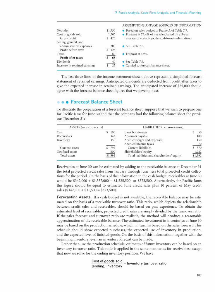
ASSUMPTIONS AND/OR SOURCES OF INFORMATION
Net sales $1,730 l Based on sales budget in Frame A of Table 7.7.Cost of goods sold 1,305 l Forecast at 75.4% of net sales; based on a 3-year
Gross profit $ 425 average of cost-of-goods-sold-to-net-sales ratios.Selling, general, and
administrative expenses 300 l See Table 7.8.Profit before taxes $ 125
Taxes 60 l Forecast at 48%.Profit after taxes $ 65
Dividends 40 l See Table 7.9.Increase in retained earnings $ 25 l Carried to forecast balance sheet.
The last three lines of the income statement shown above represent a simplified forecaststatement of retained earnings. Anticipated dividends are deducted from profit after taxes togive the expected increase in retained earnings. The anticipated increase of $25,000 shouldagree with the forecast balance sheet figures that we develop next.
l l l Forecast Balance SheetTo illustrate the preparation of a forecast balance sheet, suppose that we wish to prepare onefor Pacific Jams for June 30 and that the company had the following balance sheet the previ-ous December 31:
ASSETS (in thousands) LIABILITIES (in thousands)
Cash $ 100 Bank borrowings $ 50Receivables 342 Accounts payable 100Inventory 350 Accrued wages and expenses 150
Accrued income taxes 70Current assets $ 792 Current liabilities $ 370
Net fixed assets 800 Shareholders’ equity 1,222Total assets $1,592 Total liabilities and shareholders’ equity $1,592
Receivables at June 30 can be estimated by adding to the receivable balance at December 31the total projected credit sales from January through June, less total projected credit collec-tions for the period. On the basis of the information in the cash budget, receivables at June 30would be $342,000 + $1,557,000 − $1,525,500, or $373,500. Alternatively, for Pacific Jams this figure should be equal to estimated June credit sales plus 10 percent of May credit sales ($342,000 + $31,500 = $373,500).
Forecasting Assets. If a cash budget is not available, the receivable balance may be esti-mated on the basis of a receivable turnover ratio. This ratio, which depicts the relationshipbetween credit sales and receivables, should be based on past experience. To obtain the estimated level of receivables, projected credit sales are simply divided by the turnover ratio.If the sales forecast and turnover ratio are realistic, the method will produce a reasonableapproximation of the receivable balance. The estimated investment in inventories at June 30may be based on the production schedule, which, in turn, is based on the sales forecast. Thisschedule should show expected purchases, the expected use of inventory in production, and the expected level of finished goods. On the basis of this information, together with thebeginning inventory level, an inventory forecast can be made.
Rather than use the production schedule, estimates of future inventory can be based on aninventory turnover ratio. This ratio is applied in the same manner as for receivables, exceptthat now we solve for the ending inventory position. We have
Cost of goods sold(ending) Inventory
Inventory turnover ratio =
7 Funds Analysis, Cash-Flow Analysis, and Financial Planning
187
••
FUNO_C07.qxd 9/19/08 16:56 Page 187

Given an assumed annual turnover ratio and an assumed six-month figure for cost of goods sold and knowing the beginning inventory, we rearrange the equation to solve for the unknown ending inventory figure:
If the estimated inventory turnover ratio in our example is 6.2143 for a 12-month period and the estimated cost of goods sold for the upcoming 6-month period is $1,305,000, we have
In keeping with the buildup in sales, our estimate of inventory on June 30 would be $420,000,a figure that represents a moderate increase over the inventory level of December 31.
Future net fixed assets are estimated by adding planned expenditures to existing net fixed assets and subtracting from this sum the book value of any fixed assets sold along with depreciation during the period. From the cash budget, we note that capital expendituresare estimated at $200,000 over the period and that $40,000 in fixed assets will be sold at what we assume to be their depreciated book values. If depreciation for the period is expectedto be $110,000, the expected net additions to fixed assets would be $50,000 ($200,000 −$40,000 − $110,000). Projected net fixed assets at June 30 would be $850,000. Because capitalexpenditures are planned in advance, fixed assets are fairly easy to forecast.
Forecasting Liabilities and Shareholders’ Equity. Turning now to the liabilities,accounts payable are estimated by adding projected purchases for January through June, lesstotal projected cash payments for purchases for the period, to the December 31 balance. Ourestimate of accounts payable, therefore, is $740,000 − $690,000 + $100,000, or $150,000 –which, as we would expect with a one-month lag between the time of purchase and the pay-ment, is equal to the June purchases amount. The calculation of accrued wages and expensesis based on the production schedule and the historical relationship between these accruals andproduction. We assume the estimate of accrued wages and expenses to be $140,000. Accruedincome taxes are estimated by adding the taxes due on forecasted income for the six-monthperiod to the December 31 balance and subtracting the actual payment of taxes. With aDecember 31 balance of $70,000, income taxes for the period forecast at $60,000 (as shown inthe forecast income statement), and the firm scheduled to make $60,000 in actual payments(as shown in Table 7.9), estimated accrued income taxes at June 30 would be $70,000.
Shareholders’ equity at June 30 would be equity at December 31 plus profits after taxes forthe period, less the amount of dividends paid. If profits after taxes are estimated at $65,000 in the forecast income statement, shareholders’ equity at June 30 would be $1,222,000 plus$65,000 minus dividends of $40,000, or $1,247,000. Two items remain: cash and bank loans.We see from the cash budget that estimated cash at June 30 would be $13,500 without addi-tional financing. If the firm has the policy of maintaining a minimum cash balance of $75,000and borrowing from its bank to maintain this balance, cash at June 30 would be $75,000; bankborrowings would therefore increase by $61,500 to produce an ending balance of $111,500. Ingeneral, cash and notes payable (short-term bank borrowings) serve as balancing factors inthe preparation of forecast balance sheets, whereby assets and liabilities plus shareholders’equity are brought into balance.
Once we have estimated all the components of the forecast balance sheet, they are com-bined into a balance sheet format. Table 7.11 contains the forecast balance sheet for PacificJams at June 30. Notice that we provide some additional detail so that the reader might havesome confidence in our estimates.
(ending) Inventory = 2 ($1,305,000)
6.2143×
= $420,000
(ending) Inventory = 2 (6-month cost of goods sold)
Inventory turnover ratio×
Part 3 Tools of Financial Analysis and Planning
188
••
FUNO_C07.qxd 9/19/08 16:56 Page 188

l l l Use of Ratios and ImplicationsAs we have seen, the information that goes into a cash budget can be used to prepare forecastfinancial statements. Instead, ratios could be used to produce these forecast statements. Forexample, one would make direct estimates of all the items on the balance sheet by project-ing financial ratios into the future and then making estimates on the basis of these ratios.Receivables, inventories, accounts payable, and accrued wages and expenses are frequentlybased on historical relationships to sales and production when a cash budget is not available.For example, if the average collection period is 45 days, receivable turnover would be eighttimes a year. If receivables were $500,000 but the firm was predicting a $2 million increase insales for the coming year, receivables would increase by $2 million/8 = $250,000. Thus thelevel of receivables one year from now might be forecast at $750,000.
Forecast statements allow us to study the composition of expected future balance sheetsand income statements. Financial ratios may be computed for analysis of the statements; theseratios and the raw figures may be compared with those for present and past financial state-ments. Using this information, the financial manager can analyze the direction of change inthe financial condition and performance of the firm over the past, the present, and the future.If the firm is accustomed to making accurate estimates, the preparation of a cash budget, fore-cast statements, or both literally forces it to plan ahead and to coordinate policy in the vari-ous areas of operation. Continual revision of these forecasts keeps the firm alert to changingconditions in its environment and in its internal operations. In addition, forecast statementscan even be constructed with selected items taking on a range of probable values rather thansingle-point estimates.
7 Funds Analysis, Cash-Flow Analysis, and Financial Planning
189
••
Table 7.11Pacific Jams Companyforecast balancesheet at June 30,20X2 (in thousands)
ACTUAL FORECASTASSETS 12-31-X1 CHANGE 6-30-X2 ASSUMPTIONS
Cash $ 100 −025.0 $ 75.0 l Set at estimated minimum balance.Receivables 342 +031.5 373.5 l 100% June credit sales plus 10%
May credit sales.Inventory 350 +070.0 420.0 l Based on inventory turnover
Current assets $ 792 +076.5 $ 868.5 ratio of 6.2143 and cost of goodssold of $1,305.
Net fixed assets 800 +050.0 850.0 l Capital expenditures of $200, Total assets $1,592 +126.5 $1,718.5 sale of fixed assets with book value
of $40, and depreciation of $110.
LIABILITIES
Bank borrowings $ 50 +061.5 $ 111.5 l Previous balance plus additionalfinancing needed.
Accounts payable 100 +050.0 150.0 l 100% June purchases.Accrued wages
and expenses 150 −010.0 140.0 l Based on the production scheduleand past experience.
Accrued income taxes 70 – 70.0 l Change equals new accruals lesspayments ($60–$60).
Current liabilities $ 370 +101.5 $ 471.5Shareholders’ equity 1,222 +025.0 1,247.0 l Change in retained earnings per
forecast income statement.Total liabilities and
shareholders’equity $1,592 +126.5 $1,718.5
FUNO_C07.qxd 9/19/08 16:56 Page 189

Key Learning Points
l The sources and uses of funds statement is a summaryof a firm’s changes in financial position from oneperiod to another. An understanding of this statementgives the analyst considerable insight into the uses offunds and how these uses are financed over a specificperiod of time. Flow of funds analysis is valuable inanalyzing the commitments of funds to assets and in planning the firm’s intermediate- and long-termfinancing. The flow of funds studied, however, repre-sents net rather than gross transactions between twopoints in time.
l The statement of cash flows has replaced the flow offunds statement when the firm is required to presenta complete set of financial statements. However,unlike the cash flow statement, the flow of funds state-ment does not omit the net effects of important noncash transactions. In addition, the flow of fundsstatement is easy to prepare and is often preferred bymanagers over the more complex cash flow statement.
l An accounting statement of cash flows reports a firm’scash inflows and outflows during a period of time seg-regated into three categories: operating, investing, andfinancing activities. When used with other financial
statements and disclosures, the statement of cashflows should help the analyst to assess a firm’s abilityto generate cash for dividends and investments, iden-tify a firm’s needs for external financing, and under-stand the differences between net income and net cashflow from operating activities.
l A cash budget is a forecast of a firm’s future cashreceipts and disbursements. This forecast is particu-larly useful to the financial manager in determiningthe probable cash balances of the firm over the nearfuture and in planning prospective cash needs. Inaddition to analyzing expected cash flows, the finan-cial manager should take into account possible devia-tions from the expected outcome. An analysis of therange of possible outcomes enables management tobetter assess the efficiency and flexibility of the firmand to determine the appropriate margin of safety.
l Forecast financial statements are expected future finan-cial statements based on conditions that managementexpects to exist and actions it expects to take. Thesestatements offer financial managers insight into theprospective future financial condition and perform-ance of their firms.
Part 3 Tools of Financial Analysis and Planning
190
••
Appendix Sustainable Growth Modeling
The management of growth requires careful balancing of the sales objectives of the firm withits operating efficiency and financial resources. Many a company overreaches itself financiallyat the altar of growth; the bankruptcy courts are filled with such cases. The trick is to deter-mine what sales growth rate is consistent with the realities of the company and of the finan-cial marketplace. In this regard, sustainable growth modeling is a powerful planning tool thathas found enthusiastic use in companies like Hewlett-Packard. In the way of definition, thesustainable growth rate (SGR) is the maximum annual percentage increase in sales that can be achieved based on target operating, debt, and dividend-payout ratios. If actual growthexceeds the sustainable growth rate, something must give, and frequently it is the debt ratio.By modeling the process of growth, we are able to plan for intelligent trade-offs.
A Steady-State ModelTo illustrate the calculation of a sustainable growth rate, we begin with a steady-state modelwhere the future is exactly like the past with respect to balance sheet and performance ratios.We also assume that the firm engages in no external equity financing; the equity accountbuilds only through retaining earnings. Both of these assumptions will be relaxed later whenwe consider sustainable growth modeling under changing assumptions.
Variables Employed. In a steady-state environment, the variables necessary to determinethe sustainable growth rate are
FUNO_C07.qxd 9/19/08 16:56 Page 190

3If this is not the case, it may be better to use an operating-assets-to-sales ratio.
A /S = total-assets-to-sales ratioNP /S = net profit margin (net profits divided by sales)
b = retention rate of earnings (1 − b is the dividend – payout ratio)D /Eq = debt-to-equity ratio
S0 = most recent annual sales (beginning sales)ΔS = absolute change in sales from the most recent annual sales
The first four variables are target variables. The total-assets-to-sales ratio, the reciprocal ofthe traditional total asset turnover ratio, is a measure of operating efficiency. The lower theratio, the more efficient the utilization of assets. In turn, this ratio is a composite of: (1) receiv-able management, as depicted by the average collection period; (2) inventory management, asindicated by the inventory turnover ratio; (3) fixed assets management, as reflected by thethroughput of product through the plant; and (4) liquidity management, as suggested by theproportion of and return on liquid assets. For purposes of illustration, we assume liquid assetsare kept at moderate levels.3
The net profit margin is a relative measure of operating efficiency, after taking account of all expenses and income taxes. Although both the total-assets-to-sales ratio and the netprofit margin are affected by the external product markets, they largely capture internal management efficiency. The earnings retention rate and the debt-to-equity ratio should bedetermined in keeping with dividend and capital structure theory and practice. They areimportantly influenced by the external financial markets. Our purpose is not to touch on howthey are established, because that is done elsewhere in this book, but to incorporate them inthe planning model presented.
Sustainable Growth Rate (SGR). With these six variables we can derive the sustainablegrowth rate (SGR). The idea is that an increase in assets (a use of funds) must equal theincrease in liabilities and shareholders’ equity (a source of funds). The increase in assets can be expressed as ΔS(A/S), the change in sales times the total-assets-to-sales ratio. Theincrease in shareholders’ equity (through retaining earnings) is b(NP/S)(S0 + ΔS), or theretention rate times the net profit margin times total sales. Finally, the increase in total debtis simply the shareholders’ equity increase multiplied by the target debt-to-equity ratio, or[b(NP/S)(S0 + ΔS)]D/Eq. Putting these things together, we have
AssetsRetained
Debt= earnings +
increaseincrease
increase
(7A.1)
By rearrangement, this equation can be expressed as
(7A.2)
This is the maximum rate of growth in sales that is consistent with the target ratios.Whether or not this growth rate can be achieved, of course, depends on the external productmarkets and on the firm’s marketing efforts. A particular growth rate may be financially feasible, but the product demand may simply not be there. Implicit in the formulations presented is that depreciation charges are sufficient to maintain the value of operating assets.A final caveat has to do with interest on new borrowings. The implicit assumption is that allinterest expenses are incorporated in the target net profit margin.
ΔSS
SGRb
NPS
DEq
AS
bNPS
DEq
0
or 1
1
=
⎛⎝⎜
⎞⎠⎟
+⎛⎝⎜
⎞⎠⎟
⎛⎝⎜
⎞⎠⎟
− ⎛⎝⎜
⎞⎠⎟
+⎛⎝⎜
⎞⎠⎟
⎡
⎣⎢
⎤
⎦⎥
Δ Δ ΔSAS
bNPS
S S bNPS
S SDEq
⎛⎝⎜
⎞⎠⎟
= ⎛⎝⎜
⎞⎠⎟
+ + ⎛⎝⎜
⎞⎠⎟
+⎡
⎣⎢
⎤
⎦⎥ ( ) ( )0 0
7 Funds Analysis, Cash-Flow Analysis, and Financial Planning
191
••
FUNO_C07.qxd 9/19/08 16:56 Page 191

An Illustration. Suppose that a company is characterized by the data shown in Table 7A.1.The sustainable growth rate would be computed as follows and is consistent with the steady-state variables shown in Table 7A.1.
It can be demonstrated that initial equity increases by 9.17 percent to $109.17 million andthat debt grows by 9.17 percent to $87.34 million, as everything increases in stable equilib-rium. If the actual growth rate is other than 9.17 percent, however, one or more of the vari-ables must change. In other words, operating efficiency, leverage, or earnings retention mustchange, or there must be the sale or repurchase of common stock.
TIP•TIP
Multiplying both the numerator and denominator in Eq. (7A.2) by the quantity (S/A), andrearranging terms slightly, produces a much shortened, alternative SGR formula:
This formula spotlights the fact that – reduced to its most basic elements – a firm’s SGR ispositively related to its target earnings retention rate (b) and its target return on equity(NP/Eq).
Modeling Under Changing AssumptionsTo see what happens when we move from a steady state and variables change from year toyear, we must model sustainable growth in a different way. In effect, the growth in equity base and the growth in sales are unbalanced over time. More specifically, we must bring inbeginning sales, S0, and beginning equity capital, Eq0, as foundations on which to build.Additionally, we express dividend policy in terms of the absolute amount of dividends a com-pany wishes to pay, as opposed to a payout ratio. Finally, we allow for the sale of commonstock in a given year, although this can be specified as zero.
With these variables, the sustainable growth rate in sales for the next year, SGR in decimalform, becomes
(7A.3)SGREq New Eq Div
DEq
SA
NPS
DEq
SA
S
( )
=+ − +⎛
⎝⎜⎞⎠⎟
⎛⎝⎜
⎞⎠⎟
− ⎛⎝⎜
⎞⎠⎟
+⎛⎝⎜
⎞⎠⎟
⎛⎝⎜
⎞⎠⎟
⎡
⎣⎢
⎤
⎦⎥
⎡
⎣
⎢⎢⎢⎢⎢
⎤
⎦
⎥⎥⎥⎥⎥
⎡
⎣⎢
⎤
⎦⎥ −
0
0
1
1 1
11
SGRb NP Eq
b NP Eq
( / ) [ ( / )]
=−1
SGR [
=−
=0.70(0.04)(1.8)
0.60 0.70(0.04)(1.80)]9.17%
Part 3 Tools of Financial Analysis and Planning
192
••
Table 7A.1Initial inputs and variables used to illustrate sustainable growth rates
SYMBOL INITIAL INPUT AND/OR VARIABLE
Eq0 Beginning equity capital (in millions) $100Debt0 Beginning debt (in millions) $ 80Sales0 Sales the previous year (in millions) $300b Target earnings retention rate 0.70NP/S Target net profit margin 0.04D/Eq Target debt-to-equity ratio 0.80A/S Target assets-to-sales ratio 0.60
FUNO_C07.qxd 9/19/08 16:56 Page 192

where New Eq is the amount of new equity capital raised, Div is the absolute amount of annualdividend, and S/A is the sales-to-total-assets ratio. The latter is simply the reciprocal of thetotal-assets-to-sales ratio that we used before. Intuitively, the numerator in the first bracket inEq. (7A.3) represents the sales that could occur on the basis of existing capital plus any changeoccasioned by sale of new common stock or dividends. The equity base is expanded by thedebt employed and then multiplied by the sales-to-assets ratio. The denominator in the firstbracket is one minus the target earning power of the company, (NP/S)(S/A), as magnified bythe proportion of debt employed. When the numerator is divided by the denominator, weobtain the new level of sales that can be achieved. In the last bracket we divided this new levelby beginning sales to determine the change in sales that is sustainable for the next year.
To illustrate, suppose that the target dividend were $3.93 million, that no new equityissuance was planned, and that the other variables in Table 7A.1 held. The sustainable growthrate, using Eq. (7A.3), is
This is exactly the same as that computed with the steady-state model because a dividend of$3.93 million corresponds to an earnings retention rate of 0.70. Note also that a total-assets-to-sales ratio of 0.60 corresponds to a sales-to-total-assets ratio of 1.6667.
Suppose now that the target total-assets-to-sales ratio is 0.55 (a sales-to-assets ratio of1.8182) instead of 0.60. Moreover, the target net profit margin is also better, 0.05 instead of 0.04. Finally, the target debt-to-equity ratio is moved up from 0.80 to 1.00. Assuming a dividend of $4 million, the sustainable growth rate for next year becomes
This substantial increase in SGR is due to improved operating efficiency, which generatesmore retained earnings, and a higher debt ratio. It is important to recognize that the salesgrowth rate possible is for one year only. Even if operating efficiency continues on animproved basis, the debt ratio would have to increase continually in order to generate a SGRof 42.22 percent. The change in debt ratio affects all assets, not just the growth component.
To illustrate, suppose the debt-to-equity ratio were to remain at 1.00 and the other ratiosalso stayed the same. At the end of the year, we would be building from higher equity and sales bases:
S1 = $300(1.4222) = $426.66
Eq1 = $300(1.4222)0.05 − $4 + 100 = $117.333
The sustainable growth rate for year 2 becomes
Thus the model produces the sustainable growth rate year by year in a changing environment.Just because a high SGR is possible one year does not mean that this growth rate is sustain-able in the future. In fact, it will not be sustainable unless further variable changes in the samedirection occur. In this sense it represents a one-time occurrence.
Solving for Other Variables and Implications
With any five of the original six variables, together with beginning equity and beginning sales,it is possible to solve for the sixth. In Table 7A.2 we present certain simulations, where themissing variables for which we solve are shown in the shaded boxes.
SGR2(117.333 4)(2.00)(1.8182)1 [(0.05)(2.00)(1.8182)]
1426.66
1 =
=−
−⎡⎣⎢
⎤⎦⎥
⎡⎣⎢
⎤⎦⎥
− 18.06%
SGR =−
−⎡⎣⎢
⎤⎦⎥
⎡⎣⎢
⎤⎦⎥
−
(100 4)(2.00)(1.8182)
1 [(0.05)(2.00)(1.8182)]1
3001 = 42.22%
SGR =−
−⎡⎣⎢
⎤⎦⎥
⎡⎣⎢
⎤⎦⎥
−
(100 3.93)(1.80)(1.6667)1 [(0.04)(1.80)(1.6667)]
1300
1 = 9.17%
7 Funds Analysis, Cash-Flow Analysis, and Financial Planning
193
••
FUNO_C07.qxd 9/19/08 16:56 Page 193

By putting things into a sustainable growth model, we are able to check the consistency of
various growth plans. Often in corporate planning the company wants a number of goodthings: high sales growth, manufacturing flexibility, moderate use of debt, and high dividends.However, these things may be inconsistent with one another.
Sustainable growth modeling enables one to check for such inconsistency. In this way,more informed and wiser marketing, finance, and manufacturing decisions can be reached.Sustainable growth modeling provides an integrative tool for helping the decision-makingprocess. With the current emphasis in corporations on return on assets and on asset manage-ment, such modeling can play an integral part.
Questions
1. Contrast flow of funds (sources and uses) statements with cash budgets as planning tools.2. What is the purpose of a statement of cash flows?3. In constructing a cash budget, which variable is most important in order to arrive at
accurate projections? Explain.4. Discuss the benefits that can be derived by the firm from cash budgeting.5. Explain why a decrease in cash constitutes a source of funds while an increase in cash is a
use of funds in the sources and uses of funds statement.6. Explain why selling inventory to credit customers is considered a source of funds when in
fact no “funds” were generated.7. Why do most audited financial reports to the shareholders include a statement of cash
flows in addition to the balance sheet and income statement?8. Why might some managers actually prefer to work with a flow of funds statement rather
than the cash flow statement?9. Is depreciation a source of funds? Under what conditions might the “source” dry up?
10. Why do bankers closely analyze cash flow statements and/or sources and uses of fundsstatements in considering credit applications?
11. Which of the following are sources of funds and which are uses of funds?a. Sale of landb. Dividend paymentsc. Decrease in accrued taxesd. Decrease in raw materials inventorye. Depreciation chargesf. Sale of government bondsNow, go back and identify which items would appear under either the operating, invest-ing, or financing activities sections of a cash flow statement prepared using the indirectmethod.
Part 3 Tools of Financial Analysis and Planning
194
••
Table 7A.2 Thirteen different simulations using sustainable growth modeling
VARIABLE 1 2 3 4 5 6 7 8 9 10 11 12 13
A/S 0.60 0.60 0.55 0.50 0.65 0.70 0.50 0.4292 0.5263 0.60 0.5882 0.60 0.60NP/S 0.04 0.04 0.05 0.05 0.035 0.03 0.05 0.04 0.0623 0.0538 0.05 0.04 0.04D/E 0.80 0.80 1.00 0.50 0.80 0.80 0.50 0.50 0.60 1.00 0.7682 1.0272 1.1659Div 4.00 4.00 4.00 4.00 4.00 4.00 4.00 4.00 4.00 4.00 4.00 4.00 4.00New Eq 0 10.00 0 0 5.00 0 10.00 10.00 0 0 10.00 0 0SGR 0.0909 0.2046 0.4222 0.1294 0.0325 −0.1083 0.25 0.30 0.20 0.30 0.25 0.25 0.35
Note: Beginning sales = $300; beginning equity = $100.
FUNO_C07.qxd 9/19/08 16:56 Page 194

12. What are the major points of difference between a cash budget and the sources and usesof funds statement?
13. On what items should the financial manager concentrate in order to improve the accur-acy of the cash budget? Explain your reasoning.
14. Is the cash budget a better measure of liquidity than traditional measures, such as the current ratio and quick ratio?
15. Why is the sales forecast so important in preparing the cash budget?16. What is the principal purpose of forecast statements? Being a projection of the future,
how do they differ from the cash budget?17. What are the two principal ways by which one can prepare forecast financial
statements?
Appendix Questions18. What is a sustainable growth rate for a company? Of what value is sustainable growth
modeling?19. Explain the differences between steady-state sustainable growth modeling and year-by-
year modeling.20. List the variables used in sustainable growth modeling. Which variables usually have the
most effect on the growth rate in sales?
Self-Correction Problems
1. a. Dana-Stallings, Inc., had the following financial statements for 20X1 and 20X2. Preparea sources and uses of funds statement, and evaluate your findings.
ASSETS 20X1 20X2
Cash $ 53,000 $ 31,000Marketable securities 87,000 0Accounts receivable 346,000 528,000Inventories 432,000 683,000
Current assets $ 918,000 $1,242,000Net fixed assets 1,113,000 1,398,000
Total $2,031,000 $2,640,000
LIABILITIES AND EQUITY
Accounts payable $ 413,000 $ 627,000Accrued expenses 226,000 314,000Bank borrowings 100,000 235,000
Current liabilities $ 739,000 $1,176,000Common stock 100,000 100,000Retained earnings 1,192,000 1,364,000
Total $2,031,000 $2,640,000
Note: For 20X2, depreciation was $189,000; interest paid was $21,000;taxes paid amounted to $114,000; and no dividends were paid.
b. Using the information provided plus your sources and uses of funds statement fromPart (a), prepare a statement of cash flows using the indirect method and evaluate yourfindings. (Was your analysis based on the cash flow statement much different from thatbased on the flow of funds statement?)
2. At December 31, the balance sheet of Rodriguez Malting Company was the following (inthousands):
7 Funds Analysis, Cash-Flow Analysis, and Financial Planning
195
••
FUNO_C07.qxd 9/19/08 16:56 Page 195

Cash $ 50 Accounts payable $ 360Accounts receivable 530 Accrued expenses 212Inventories 545 Bank loan 400
Current assets $1,125 Current liabilities $ 972Net fixed assets 1,836 Long-term debt 450
Common stock 100Retained earnings 1,439
Total liabilities andTotal assets $2,961 shareholders’ equity $2,961
The company has received a large order and anticipates the need to go to its bank toincrease its borrowings. As a result, it needs to forecast its cash requirements for January,February, and March.
Typically, the company collects 20 percent of its sales in the month of sale, 70 percentin the subsequent month, and 10 percent in the second month after the sale. All sales arecredit sales.
Purchases of raw materials to produce malt are made in the month prior to the sale andamount to 60 percent of sales in the subsequent month. Payments for these purchasesoccur in the month after the purchase. Labor costs, including overtime, are expected to be$150,000 in January, $200,000 in February, and $160,000 in March. Selling, administrative,tax, and other cash expenses are expected to be $100,000 per month for January throughMarch. Actual sales in November and December and projected sales for January throughApril are as follows (in thousands):
November $500 February $1,000December 600 March 650January 600 April 750
On the basis of this information:a. Prepare a cash budget for the months of January, February, and March.b. Determine the amount of additional bank borrowings necessary to maintain a cash
balance of $50,000 at all times. (Ignore interest on such borrowings.)c. Prepare a forecast balance sheet for March 31. (It should be noted that the company
maintains a safety stock of inventory and that depreciation for the three-month periodis expected to be $24,000.)
3. Margaritaville Nautical Company expects sales of $2.4 million next year and the sameamount the following year. Sales are spread evenly throughout the year. On the basis of the following information, prepare a forecast income statement and balance sheet foryear end:l Cash: Minimum of 4 percent of annual sales.l Accounts receivable: 60-day average collection period based on annual sales.l Inventories: Turnover of eight times a year.l Net fixed assets: $500,000 now. Capital expenditures equal to depreciation.l Accounts payable: One month’s purchases.l Accrued expenses: 3 percent of sales.l Bank borrowings: $50,000 now. Can borrow up to $250,000.l Long-term debt: $300,000 now, payable $75,000 at year end.l Common stock: $100,000. No additions planned.l Retained earnings: $500,000 now.l Net profit margin: 8 percent of sales.l Dividends: None.l Cost of goods sold: 60 percent of sales.l Purchases: 50 percent of cost of goods sold.l Income taxes: 50 percent of before-tax profits.
Part 3 Tools of Financial Analysis and Planning
196
••
FUNO_C07.qxd 9/19/08 16:56 Page 196

Appendix Self-Correction Problem4. Kidwell Industries has equity capital of $12 million, total debt of $8 million, and sales last
year of $30 million.a. It has a target assets-to-sales ratio of 0.6667, a target net profit margin of 0.04, a target
debt-to-equity ratio of 0.6667, and a target earnings retention rate of 0.75. In steadystate, what is its sustainable growth rate?
b. Suppose the company has established for next year a target assets-to-sales ratio of 0.62,a target net profit margin of 0.05, and a target debt-to-equity ratio of 0.80. It wishes topay an annual dividend of $0.3 million and raise $1 million in equity capital next year.What is its sustainable growth rate for next year? Why does it differ from that in Part (a)?
Problems
1. Shmenge Brothers Accordion Company reports the following changes from the previousyear end. Categorize these items as either a source of funds or a use of funds.
ITEM ITEM
Cash −$ 100 Accounts payable +$300Accounts receivable + 700 Accrued expenses − 100Inventory − 300 Long-term debt − 200Dividends paid + 400 Net profit + 600Depreciation +1,000 Additions to fixed assets + 900
2. Svoboda Corporation comparative balance sheets at December 31 (in millions)
LIABILITIES ANDASSETS 20X1 20X2 SHAREHOLDERS’ EQUITY 20X1 20X2
Cash $ 5 $ 3 Notes payable $20 $ 0Accounts receivable 15 22 Accounts payable 5 8Inventories 12 15 Accrued wages 2 2Fixed assets, net 50 55 Accrued taxes 3 5Other assets 8 5 Long-term debt 0 15
Common stock 20 26Retained earnings 40 44
Total liabilities andTotal assets $90 $100 shareholders’ equity $90 $100
Svoboda Corporation statement of income and retained earnings, yearended December 31, 20X2 (in millions)
Net sales $48Expenses
Cost of goods sold $25Selling, general, and administrative expenses 5Depreciation 5Interest 2 37
Net income before taxes $11Less: Taxes 4
Net income $ 7Add: Retained earnings at 12/31/X1 40
Subtotal $47Less: Dividends 3
Retained earnings at 12/31/X2 $44
a. Prepare a flow of funds (sources and uses of funds) statement for 20X2 for the SvobodaCorporation.
7 Funds Analysis, Cash-Flow Analysis, and Financial Planning
197
••
FUNO_C07.qxd 9/19/08 16:56 Page 197

b. Prepare a statement of cash flows for 20X2 using the indirect method for the SvobodaCorporation.
3. Financial statements for the Begalla Corporation follow.
Begalla Corporation comparative balance sheets at December 31 (in millions)
ASSETS 20X1 20X2 LIABILITIES 20X1 20X2
Cash $ 4 $ 5 Accounts payable $ 8 $10Accounts receivable 7 10 Notes payable 5 5Inventory 12 15 Accrued wages 2 3
Accrued taxes 3 2Total current assets $23 $30 Total current liabilities $18 $20
Net fixed assets 40 40 Long-term debt 20 20Common stock 10 10Retained earnings 15 20
Total $63 $70 Total $63 $70
Begalla Corporation income statement 20X2 (in millions)
Sales $95Cost of goods sold $50Selling, general, and administrative expenses 15Depreciation 3Interest 2 70
Net income before taxes $25Taxes 10
Net income $15
a. Prepare a sources and uses of funds statement for Begalla Corporation.b. Prepare a cash flow statement using the indirect method for Begalla Corporation.
4. Prepare a cash budget for the Ace Manufacturing Company, indicating receipts and dis-bursements for May, June, and July. The firm wishes to maintain at all times a minimumcash balance of $20,000. Determine whether or not borrowing will be necessary during the period, and if it is, when and for how much. As of April 30, the firm had a balance of $20,000 in cash.
ACTUAL SALES FORECASTED SALES
January $50,000 May $ 70,000February 50,000 June 80,000March 60,000 July 100,000April 60,000 August 100,000
l Accounts receivable: 50 percent of total sales are for cash. The remaining 50 percent will be collected equally during the following two months (the firm incurs a negligiblebad-debt loss).
l Cost of goods manufactured: 70 percent of sales: 90 percent of this cost is paid the fol-lowing month and the remaining 10 percent one more month later.
l Selling, general, and administrative expenses: $10,000 per month plus 10 percent of sales.All of these expenses are paid during the month of incurrence.
l Interest payments: A semiannual interest payment on $150,000 of bonds outstanding (12 percent coupon) is paid during July. An annual $50,000 sinking-fund payment isalso made at that time.
l Dividends: A $10,000 dividend payment will be declared and made in July.l Capital expenditures: $40,000 will be invested in plant and equipment in June.l Taxes: Income tax payments of $1,000 will be made in July.
5. Given the information that follows, prepare a cash budget for the Central City DepartmentStore for the first six months of 20X2.a. All prices and costs remain constant.
Part 3 Tools of Financial Analysis and Planning
198
••
FUNO_C07.qxd 9/19/08 16:56 Page 198
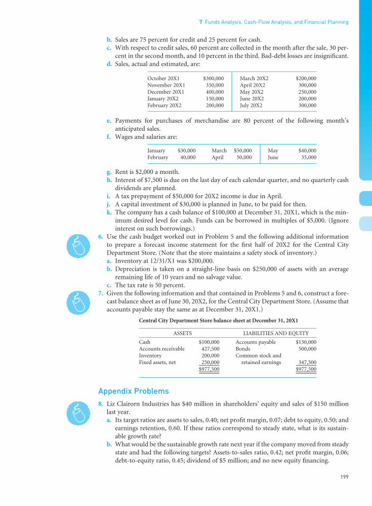
b. Sales are 75 percent for credit and 25 percent for cash.c. With respect to credit sales, 60 percent are collected in the month after the sale, 30 per-
cent in the second month, and 10 percent in the third. Bad-debt losses are insignificant.d. Sales, actual and estimated, are:
October 20X1 $300,000 March 20X2 $200,000November 20X1 350,000 April 20X2 300,000December 20X1 400,000 May 20X2 250,000January 20X2 150,000 June 20X2 200,000February 20X2 200,000 July 20X2 300,000
e. Payments for purchases of merchandise are 80 percent of the following month’s anticipated sales.
f. Wages and salaries are:
January $30,000 March $50,000 May $40,000February 40,000 April 50,000 June 35,000
g. Rent is $2,000 a month.h. Interest of $7,500 is due on the last day of each calendar quarter, and no quarterly cash
dividends are planned.i. A tax prepayment of $50,000 for 20X2 income is due in April.j. A capital investment of $30,000 is planned in June, to be paid for then.k. The company has a cash balance of $100,000 at December 31, 20X1, which is the min-
imum desired level for cash. Funds can be borrowed in multiples of $5,000. (Ignoreinterest on such borrowings.)
6. Use the cash budget worked out in Problem 5 and the following additional information to prepare a forecast income statement for the first half of 20X2 for the Central CityDepartment Store. (Note that the store maintains a safety stock of inventory.)a. Inventory at 12/31/X1 was $200,000.b. Depreciation is taken on a straight-line basis on $250,000 of assets with an average
remaining life of 10 years and no salvage value.c. The tax rate is 50 percent.
7. Given the following information and that contained in Problems 5 and 6, construct a fore-cast balance sheet as of June 30, 20X2, for the Central City Department Store. (Assume thataccounts payable stay the same as at December 31, 20X1.)
Central City Department Store balance sheet at December 31, 20X1
ASSETS LIABILITIES AND EQUITY
Cash $100,000 Accounts payable $130,000Accounts receivable 427,500 Bonds 500,000Inventory 200,000 Common stock and Fixed assets, net 250,000 retained earnings 347,500
$977,500 $977,500
Appendix Problems8. Liz Clairorn Industries has $40 million in shareholders’ equity and sales of $150 million
last year.a. Its target ratios are assets to sales, 0.40; net profit margin, 0.07; debt to equity, 0.50; and
earnings retention, 0.60. If these ratios correspond to steady state, what is its sustain-able growth rate?
b. What would be the sustainable growth rate next year if the company moved from steadystate and had the following targets? Assets-to-sales ratio, 0.42; net profit margin, 0.06;debt-to-equity ratio, 0.45; dividend of $5 million; and no new equity financing.
7 Funds Analysis, Cash-Flow Analysis, and Financial Planning
199
••
FUNO_C07.qxd 9/19/08 16:56 Page 199

9. Herb I. Vore Hydroponics Corporation wishes to achieve a 35 percent increase in salesnext year. Sales last year were $30 million, and the company has equity capital of $12 mil-lion. It intends to raise $0.5 million in new equity by the sale of common stock to officers.No dividend is planned. Tentatively, the company has set the following target ratios: assetsto sales, 0.67; net profit margin, 0.08; and debt to equity, 0.60. The company has deter-mined that these ratios are not sufficient to produce a growth in sales of 35 percent.a. Holding the other two target ratios constant, what assets-to-sales ratio would be neces-
sary to attain the 35 percent sales increase?b. Holding the other two ratios constant, what net profit margin would be necessary?c. Holding the other two ratios constant, what debt-to-equity ratio would be necessary?
Solutions to Self-Correction Problems
1. a. Sources and uses of funds statement for Dana-Stallings, Inc. (in thousands)
SOURCES USES
Funds provided by operationsNet profit $172Depreciation 189 Additions to fixed assets $474
$361Decrease, marketable securities 87 Increase, accounts receivable 182Increase, accounts payable 214 Increase, inventories 251Increase, accrued expenses 88Increase, bank borrowings 135Decrease, cash 22
$907 $907
The company has had substantial capital expenditures and increases in current assets.This growth has far outstripped the growth in retained earnings. To finance this growth,the company has reduced its marketable securities to zero, has leaned heavily on tradecredit (accounts payable), and has increased its accrued expenses and bank borrowings.All of this is short-term financing of mostly long-term buildups in assets.
b. Statement of cash flows for Dana-Stallings, Inc. (in thousands)
CASH FLOW FROM OPERATING ACTIVITIESNet income $ 172Depreciation 189Cash provided (used) by current assets and operating-related current liabilities
Increase, accounts payable 214Increase, accrued expenses 88Increase, accounts receivable (182)Increase, inventories (251)
Net cash provided (used) by operating activities $ 230
CASH FLOW FROM INVESTING ACTIVITIESAdditions to fixed assets $(474)Decrease, marketable securities 87
Net cash provided (used) by investing activities $(387)
CASH FLOW FROM FINANCING ACTIVITIESIncrease in short-term bank borrowings $ 135
Net cash provided (used) by financing activities $ 135Increase (decrease) in cash $ (22)Cash, December 31, 20X1 53Cash, December 31, 20X2 $ 31
Supplemental cash flow disclosuresInterest paid $ 21Taxes paid 114
Part 3 Tools of Financial Analysis and Planning
200
••
FUNO_C07.qxd 9/19/08 16:56 Page 200

In addition to the same points raised by an analysis of the sources and uses of fundsstatement, we see that all of the firm’s cash flow from operating activities (and thensome) went toward additions to fixed assets. By and large, the cash flow statement pre-pared using the indirect method gives you much the same information gathered froman analysis of the sources and uses of funds statement.
2. a. Cash budget (in thousands)
NOV. DEC. JAN. FEB. MAR. APR.
Sales $500 $600 $600 $1,000 $650 $750Cash collections
20% of current month sales $120 $ 200 $13070% of last month’s sales 420 420 70010% of 2-month-old sales 50 60 60
Total cash receipts $590 $ 680 $890
Purchases $360 $600 $ 390 $450
NOV. DEC. JAN. FEB. MAR. APR.
Cash disbursements for purchasesand operating expenses100% of last month’s purchases $360 $ 600 $390Labor costs 150 200 160Other expenses paid 100 100 100
Total cash disbursements $610 $ 900 $650
Cash receipts less cash disbursements $ (20) $ (220) $240
b. DEC. JAN. FEB. MAR.
Beginning bank borrowings $400 $420 $640Additional borrowings 20 220 (240)Ending bank borrowings $400 $420 $640 $400
The amount of financing peaks in February owing to the need to pay for purchasesmade the previous month and higher labor costs. In March, substantial collections aremade on the prior month’s billings, causing a large net cash inflow sufficient to pay offthe additional borrowings.
c. Forecast balance sheet at March 31 (in thousands)
ACTUAL FORECASTASSETS 12–31 CHANGE 3–31 ASSUMPTIONS
Cash $ 50 0 $ 50 l Set at estimated minimum balance.Receivables 530 +090 620 l 80% Mar sales plus 10% Feb sales.Inventory 545 +090 635 l Based on $545 plus $1,985 in
purchases (Jan–Mar) minus 0.6 times$2,250 in sales (Jan–Mar).
Current assets $1,125 +180 $1,305Net fixed assets 1,836 −024 1,812 l Depreciation expected to be $24.
Total assets $2,961 +156 $3,117
ACTUAL FORECASTLIABILITIES 12–31 CHANGE 3–31 ASSUMPTIONS
Bank borrowings $ 400 0 $ 400 l Previous balance plus zeroadditional financing needed.
Accounts payable 360 +090 450 l 100% Mar purchases.Accrued expenses 212 0 212 l No change expected.
Current liabilities $ 972 +090 $1,062Long-term debt 450 0 450 l No change expected.Common stock 100 0 100 l No change expected.Retained earnings 1,439 +066 1,505 l Change in retained earnings equals
sales, minus payment for purchases,Total liabilities and minus labor costs, depreciation,shareholders’ equity $2,961 +156 $3,117 and other expenses, for Jan–Mar.
7 Funds Analysis, Cash-Flow Analysis, and Financial Planning
201
••
FUNO_C07.qxd 9/19/08 16:56 Page 201

3. Forecast income statement (in thousands)
ASSUMPTIONS
Net sales $2,400 l Based on sales forecast.Cost of goods sold 1,440 l Forecast at 60% of net sales.
Gross profit $ 960Expenses 576 l 24% of net sales; required to produce
16% before-tax profit margin (see below).Profit before taxes $ 384 l 16% of net sales; based on an 8% net profit
margin and 50% tax rate.Taxes 192 l Forecast at 50%.
Profit after taxes $ 192 l Forecast at 8% of net sales.Dividends 0 l None expected.Increase in retained earnings $ 192 l Carried to forecast balance sheet.
Forecast balance sheet (in thousands)
END OFASSETS YEAR ASSUMPTIONS
Cash $ 96 l Set at estimated minimum balance; 4% ofannual sales of $2.4M.
Receivables 400 l Based on 60-day average collection period; (net sales of $2.4M)/(360/60).
Inventory 180 l Based on an annual turnover of 8; (cost ofgoods sold of $1.44M)/8.
Current assets $ 676Net fixed assets 500 l $500,000 at beginning of year and capital
expenditures expected to equal depreciationcharge for the year.
Total assets $1,176
END OFLIABILITIES YEAR ASSUMPTIONS
Bank borrowings $ 27 l Plug figure equal to total assets minus all theindividual items listed below.
Accounts payable 60 l 1 month’s purchases; (0.5)(cost of goodssold of $1.44M)/12.
Accrued expenses 72 l Estimated at 3% of sales of $2.4M.Current liabilities $ 159
Long-term debt 225 l $300,000 minus year-end $75,000 principalpayment.
Common stock 100 l No change expected.Retained earnings 692 l $500,000 plus $192,000 change in retained
Total liabilities and earnings per forecast income statement.shareholders’ equity $1,176
Solution to Appendix Self-Correction Problem
4. a.
b.
The company has moved from steady state with higher target operating efficiency, ahigher debt ratio, and the sale of common stock. All of these things permit a high rateof growth in sales next year. Unless further changes in these directions occur, the SGRwill decline.
SGR
=+ −
−⎡⎣⎢
⎤⎦⎥
⎡⎣⎢
⎤⎦⎥
−(12 1 0.3)(1.80)(1.6129)
1 [(0.05)(1.80)(1.6129)]1
301 = 43.77%
SGR .
=−
0.75(0.04)(1.6667)0 6667 [0.75(0.04)(1.6667)]
= 8.11%
Part 3 Tools of Financial Analysis and Planning
202
••
FUNO_C07.qxd 9/19/08 16:56 Page 202

Selected References
Bhandari, Shyan B. “Pedagogical Issues ConcerningAnalysis of the Cash Flow Statement.” Journal of FinancialEducation 29 (Spring 2003), 1–11.
Gahlon, James M., and Robert L. Vigeland. “AnIntroduction to Corporate Cash Flow Statements.” AAIIJournal 11 (January 1989), 14–18.
Gup, Benton E., William D. Samson, Michael T. Dugan,Myung J. Kim, and Thawatchai Jittrapanun. “An Analysisof Patterns from the Statement of Cash Flows.” FinancialPractice and Education 3 (Fall 1993), 73–79.
Helfert, Erich A. Techniques of Financial Analysis, 11th ed.New York, NY: McGraw-Hill/Irwin, 2004.
Higgins, Robert C. “How Much Growth Can a FirmAfford?” Financial Management 6 (Fall 1977), 7–16.
—— . “Sustainable Growth under Inflation.” FinancialManagement 10 (Autumn 1981), 36–40.
—— . Analysis for Financial Management, 8th ed. NewYork, NY: McGraw-Hill/Irwin, 2007.
Moore, Marty. “Cash Flow Management in a LeveragedEnvironment.” Strategic Finance (January 2002), 31–33.
Mulford, Charles W., and Eugene E. Comiskey. CreativeCash Flow Reporting: Uncovering Sustainable FinancialPerformance. Hoboken, NJ: John Wiley & Sons, 2005.
Nurnberg, Hugo. “Inconsistencies and Ambiguities in CashFlow Statements under FASB Statement No. 95.”Accounting Horizons 7 (June 1993), 60–75.
Plewa, Franklin J., and G. Thomas Friedlob. “New Ways to Analyze Cash Flows.” National Public Accountant 47(February/March 2002), 25–30, 43.
Statement of Cash Flows: Understanding and ImplementingFASB Statement No. 95. Ernst & Whinney, January 1988.
Van Horne, James C. “Sustainable Growth Modeling.”Journal of Corporate Finance 1 (Winter 1988), 19–25.
Part III of the text’s website, Wachowicz’s Web World, contains links to many finance websites and online articles related to topics covered in this chapter.(web.utk.edu/~jwachowi/part3.html)
7 Funds Analysis, Cash-Flow Analysis, and Financial Planning
203
••
FUNO_C07.qxd 9/19/08 16:56 Page 203

••
204
FUNO_C07.qxd 9/19/08 16:56 Page 204

••
205
Par
t 4 Working Capital
Management
Contents
l IntroductionWorking Capital Concepts • Significance ofWorking Capital Management • Profitability and Risk
l Working Capital IssuesOptimal Amount (or Level) of Current Assets •Detour: Classification of Working Capital
l Financing Current Assets: Short-Term andLong-Term MixHedging (Maturity Matching) Approach • Short-Term versus Long-Term Financing
l Combining Liability Structure and CurrentAsset DecisionsUncertainty and the Margin of Safety • Risk andProfitability
l Key Learning Points
l Questions
l Self-Correction Problem
l Problems
l Solutions to Self-Correction Problem
l Selected References
Every noble acquisition is attended with risks; he who fears to encounter the one must not expect to obtain the other.
—PIETRO METASTASIO
Objectives
After studying Chapter 8, you should be able to:
l Explain how the definition of “working capital” differs between financial analysts andaccountants.
l Understand the two fundamental decision issuesin working capital management – and thetrade-offs involved in making these decisions.
l Discuss how to determine the optimal level ofcurrent assets.
l Describe the relationship between profitability,liquidity, and risk in the management of working capital.
l Explain how to classify working capital according to its “components” and according to “time” (i.e., either permanent or temporary).
l Describe the hedging (maturity matching)approach to financing and the advantages/dis-advantages of short- versus long-term financing.
l Explain how the financial manager combines thecurrent asset decision with the liability structuredecision.
8Overview of Working Capital Management
FUNO_C08.qxd 9/19/08 16:57 Page 205

Introduction
l l l Working Capital ConceptsThere are two major concepts of working capital – net working capital and gross working capital. When accountants use the term working capital, they are generally referring to networking capital, which is the dollar difference between current assets and current liabilities.This is one measure of the extent to which the firm is protected from liquidity problems.From a management viewpoint, however, it makes little sense to talk about trying to activelymanage a net difference between current assets and current liabilities, particularly when thatdifference is continually changing.
Financial analysts, on the other hand, mean current assets when they speak of working capital. Therefore, their focus is on gross working capital. Because it does make sense for the financial manager to be involved with providing the correct amount of current assets forthe firm at all times, we will adopt the concept of gross working capital. As the discussion ofworking capital management unfolds, our concern will be to consider the administration ofthe firm’s current assets – namely, cash and marketable securities, receivables, and inventory– and the financing (especially current liabilities) needed to support current assets.
l l l Significance of Working Capital Management
The management of working capital, which is taken up in this and the subsequent three chapters, is important for several reasons. For one thing, the current assets of a typical manu-facturing firm account for over half of its total assets. For a distribution company, theyaccount for even more. Excessive levels of current assets can easily result in a firm realizing a substandard return on investment. However, firms with too few current assets may incurshortages and difficulties in maintaining smooth operations.
For small companies, current liabilities are the principal source of external financing. Thesefirms do not have access to the longer-term capital markets, other than to acquire a mortgageon a building. The fast-growing but larger company also makes use of current liability financ-ing. For these reasons, the financial manager and staff devote a considerable portion of theirtime to working capital matters. The management of cash, marketable securities, accountsreceivable, accounts payable, accruals, and other means of short-term financing is the directresponsibility of the financial manager; only the management of inventories is not. More-over, these management responsibilities require continuous, day-to-day supervision. Unlikedividend and capital structure decisions, you cannot study the issue, reach a decision, and set the matter aside for many months to come. Thus working capital management is import-ant, if for no other reason than the proportion of the financial manager’s time that must bedevoted to it. More fundamental, however, is the effect that working capital decisions have onthe company’s risk, return, and share price.
l l l Profitability and Risk
Underlying sound working capital management lie two fundamental decision issues for thefirm. They are the determination of
l the optimal level of investment in current assets
l the appropriate mix of short-term and long-term financing used to support this invest-ment in current assets.
In turn, these decisions are influenced by the trade-off that must be made between profitabilityand risk. Lowering the level of investment in current assets, while still being able to support
Part 4 Working Capital Management
206
••
Net working capitalCurrent assets minuscurrent liabilities.
Gross working capitalThe firm’s investmentin current assets (like cash andmarketable securities,receivables, andinventory).
Working capitalmanagement Theadministration of thefirm’s current assetsand the financingneeded to supportcurrent assets.
FUNO_C08.qxd 9/19/08 16:57 Page 206
sales, would lead to an increase in the firm’s return on total assets. To the extent that theexplicit costs of short-term financing are less than those of intermediate- and long-termfinancing, the greater the proportion of short-term debt to total debt, the higher is theprofitability of the firm.
Although short-term interest rates sometimes exceed long-term rates, generally they areless. Even when short-term rates are higher, the situation is likely to be only temporary. Overan extended period of time, we would expect to pay more in interest cost with long-term debtthan we would with short-term borrowings, which are continually rolled over (refinanced) atmaturity. Moreover, the use of short-term debt as opposed to longer-term debt is likely toresult in higher profits because debt will be paid off during periods when it is not needed.
These profitability assumptions suggest maintaining a low level of current assets and a high proportion of current liabilities to total liabilities. This strategy will result in a low, orconceivably negative, level of net working capital. Offsetting the profitability of this strategy,however, is the increased risk to the firm. Here, risk means jeopardy to the firm for not maintaining sufficient current assets to
l meet its cash obligations as they occur
l support the proper level of sales (e.g., running out of inventory).
In this chapter we study the trade-off between risk and profitability as it relates to the level andfinancing of current assets.
8 Overview of Working Capital Management
207
••
More than $1 trillion seen unnecessarily tied up inworking capital.
The 2,000 largest companies in the United States andEurope have more than $1 trillion in cash unneces-
sarily tied up in working capital in the form of invoicespaid late by customers, suppliers paid too early andinventory moving too slowly through the supply chain,according to research from business advisory firm TheHackett Group.
By implementing best practices and achieving work-ing capital levels seen by leaders in this study, companieswould also reduce annual operating costs by up to $42billion, Hackett reported.
Taken together, these working capital improve-ments could enable companies to boost net profits by up to 11 percent. Hackett’s research also shows a strongcorrelation between companies that consistently grow
shareholder value and those that excel at working capitalmanagement.
The research highlights a range of best practices that leading companies use to enhance their workingcapital performance, such as better understanding theircustomers and focusing proactive efforts on those thathave the greatest material impact on working capital performance.
Hackett also sees next-generation opportunities forcompanies willing to take an extended view of supply chainoperations, collaborating with customers, channel partnersand vendors to enable better demand visibility, inventoryoptimization and other operational improvements.
“Working capital optimization is inherently complex,as it touches many business processes and people withinan organization,” said Hackett-REL President StephenPayne. “It’s a balancing act, and companies must manageit carefully to ensure that they keep working capital lowand also have the critical resources they need to do thingslike fund product development, produce and delivertheir products, and provide high levels of customer ser-vice. But the ability to impact the bottom line throughworking capital optimization is tremendous.”
Working Capital Management, Supply Chain Visibility
Source: “More than $1 Trillion Seen Unnecessarily Tied Up in Working Capital,” Supply & Demand Chain Executive (June/July 2006), p. 10.(www.sdcexec.com) © Copyright 2006 by Cygnus Business Media. Used by permission. All rights reserved.
FUNO_C08.qxd 9/19/08 16:57 Page 207

Working Capital Issues
l l l Optimal Amount (or Level) of Current AssetsIn determining the appropriate amount, or level, of current assets, management must con-sider the trade-off between profitability and risk. To illustrate this trade-off, suppose that,with existing fixed assets, a firm can produce up to 100,000 units of output a year.1 Productionis continuous throughout the period under consideration, in which there is a particular levelof output. For each level of output, the firm can have a number of different levels of currentassets. Let’s assume, initially, three different current asset policy alternatives. The relationshipbetween output and current asset level for these alternatives is illustrated in Figure 8.1. We seefrom the figure that the greater the output, the greater the need for investment in currentassets to support that output (and sales). However, the relationship is not linear; currentassets increase at a decreasing rate with output. This relationship is based on the notion thatit takes a greater proportional investment in current assets when only a few units of outputare produced than it does later on, when the firm can use its current assets more efficiently.
If we equate liquidity with “conservativeness,” Policy A is the most conservative of thethree alternatives. At all levels of output, Policy A provides for more current assets than anyother policy. The greater the level of current assets, the greater the liquidity of the firm, allother things equal. Policy A is seen as preparing the firm for almost any conceivable currentasset need; it is the financial equivalent to wearing a belt and suspenders. Policy C is least liquid and can be labeled “aggressive.” This “lean and mean” policy calls for low levels of cashand marketable securities, receivables, and inventories. We should keep in mind that for everyoutput level there is a minimum level of current assets that the firm needs just to get by. Thereis a limit to how “lean and mean” a firm can get. We can now summarize the rankings of thealternative working capital policies in respect to liquidity as follows:
HIGH LOW
Liquidity Policy A Policy B Policy C
1This illustration holds constant the amount of the firm’s fixed assets. This is actually a rather fair assumption. Afirm’s fixed assets are generally determined by its scale of production. Once established, the fixed assets remaininvested (at least in the short run) regardless of production levels.
Part 4 Working Capital Management
208
••
Figure 8.1Current asset levelsfor three alternativeworking capitalpolicies
FUNO_C08.qxd 9/19/08 16:57 Page 208

Though policy A clearly provides the highest liquidity, how do the three alternative policies rank when we shift our attention to expected profitability? To answer this question,we need to recast the familiar return on investment (ROI) equation as follows:
From the equation above we can see that decreasing the amounts of current assets held (forexample, a movement from Policy A toward Policy C) will increase our potential profitabil-ity. If we can reduce the firm’s investment in current assets while still being able to properlysupport output and sales, ROI will increase. Lower levels of cash, receivables, and inventorywould reduce the denominator in the equation; and net profits, our numerator, would remainroughly the same or perhaps even increase. Policy C, then, provides the highest profitabilitypotential as measured by ROI.
However, a movement from Policy A toward Policy C results in other effects besidesincreased profitability. Decreasing cash reduces the firm’s ability to meet financial obligationsas they come due. Decreasing receivables, by adopting stricter credit terms and a tougherenforcement policy, may result in some lost customers and sales. Decreasing inventory mayalso result in lost sales due to products being out of stock. Therefore more aggressive work-ing capital policies lead to increased risk. Clearly, Policy C is the most risky working capitalpolicy. It is also a policy that emphasizes profitability over liquidity. In short, we can nowmake the following generalizations:
HIGH LOW
Liquidity Policy A Policy B Policy CProfitability Policy C Policy B Policy ARisk Policy C Policy B Policy A
Interestingly, our discussion of working capital policies has just illustrated the two mostbasic principles in finance:
1. Profitability varies inversely with liquidity. Notice that for our three alternative workingcapital policies, the liquidity rankings are the exact opposite of those for profitability.Increased liquidity generally comes at the expense of reduced profitability.
2. Profitability moves together with risk (i.e., there is a trade-off between risk and return). Insearch of higher profitability, we must expect to take greater risks. Notice how theprofitability and risk rankings for our alternative working capital policies are identical.You might say that risk and return walk hand in hand.
Ultimately, the optimal level of each current asset (cash, marketable securities, receivables,and inventory) will be determined by management’s attitude to the trade-off betweenprofitability and risk. For now, we continue to restrict ourselves to some broad generalities.In subsequent chapters, we will deal more specifically with the optimal levels of these assets,taking into consideration both profitability and risk.
l l l Detour: Classification of Working CapitalBefore turning our attention to the way working capital should be financed, we need to takea slight detour and classify working capital. Having defined working capital as current assets,it can now be classified according to
l Components, such as cash, marketable securities, receivables, and inventory (subsequentchapters will focus on these components), or
l Time, as either permanent or temporary.
Though the components of working capital are self-explanatory, classification by timerequires some explanation. A firm’s permanent working capital is the amount of current
ROINet profit
Total assetsNet profit
(Cash Receivables Inventory) Fixed assets
= =
+ + +
8 Overview of Working Capital Management
209
••
Permanent workingcapital The amount of current assetsrequired to meet afirm’s long-termminimum needs.
FUNO_C08.qxd 9/19/08 16:57 Page 209
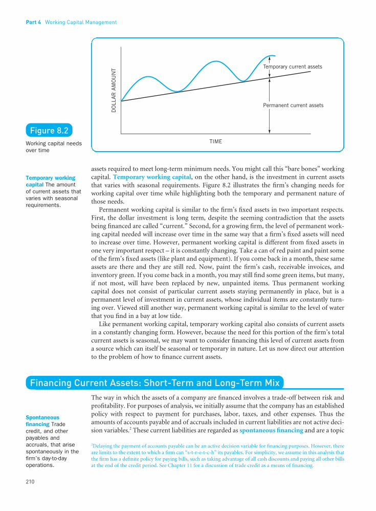
assets required to meet long-term minimum needs. You might call this “bare bones” workingcapital. Temporary working capital, on the other hand, is the investment in current assetsthat varies with seasonal requirements. Figure 8.2 illustrates the firm’s changing needs forworking capital over time while highlighting both the temporary and permanent nature ofthose needs.
Permanent working capital is similar to the firm’s fixed assets in two important respects.First, the dollar investment is long term, despite the seeming contradiction that the assetsbeing financed are called “current.” Second, for a growing firm, the level of permanent work-ing capital needed will increase over time in the same way that a firm’s fixed assets will needto increase over time. However, permanent working capital is different from fixed assets inone very important respect – it is constantly changing. Take a can of red paint and paint someof the firm’s fixed assets (like plant and equipment). If you come back in a month, these sameassets are there and they are still red. Now, paint the firm’s cash, receivable invoices, andinventory green. If you come back in a month, you may still find some green items, but many,if not most, will have been replaced by new, unpainted items. Thus permanent working capital does not consist of particular current assets staying permanently in place, but is a permanent level of investment in current assets, whose individual items are constantly turn-ing over. Viewed still another way, permanent working capital is similar to the level of waterthat you find in a bay at low tide.
Like permanent working capital, temporary working capital also consists of current assetsin a constantly changing form. However, because the need for this portion of the firm’s totalcurrent assets is seasonal, we may want to consider financing this level of current assets froma source which can itself be seasonal or temporary in nature. Let us now direct our attentionto the problem of how to finance current assets.
Financing Current Assets: Short-Term and Long-Term MixThe way in which the assets of a company are financed involves a trade-off between risk andprofitability. For purposes of analysis, we initially assume that the company has an establishedpolicy with respect to payment for purchases, labor, taxes, and other expenses. Thus theamounts of accounts payable and of accruals included in current liabilities are not active deci-sion variables.2 These current liabilities are regarded as spontaneous financing and are a topic
Part 4 Working Capital Management
210
••
2Delaying the payment of accounts payable can be an active decision variable for financing purposes. However, thereare limits to the extent to which a firm can “s-t-r-e-t-c-h” its payables. For simplicity, we assume in this analysis thatthe firm has a definite policy for paying bills, such as taking advantage of all cash discounts and paying all other billsat the end of the credit period. See Chapter 11 for a discussion of trade credit as a means of financing.
Temporary workingcapital The amount of current assets thatvaries with seasonalrequirements.
Spontaneousfinancing Tradecredit, and otherpayables andaccruals, that arisespontaneously in thefirm’s day-to-dayoperations.
Figure 8.2Working capital needsover time
FUNO_C08.qxd 9/19/08 16:57 Page 210

••
in Chapter 11. They finance a portion of the current assets of the firm and tend to fluctuatewith the production schedule and, in the case of accrued taxes, with profits. As the underlyinginvestment in current assets grows, accounts payable and accruals also tend to grow, in partfinancing the buildup in assets. Our concern is the way in which assets not supported by spontaneous financing are handled. This residual financing requirement pertains to the netinvestment in assets after spontaneous financing is deducted.
l l l Hedging (Maturity Matching) ApproachIf the firm adopts a hedging (maturity matching) approach to financing, each asset would beoffset with a financing instrument of the same approximate maturity. Short-term or seasonalvariations in current assets would be financed with short-term debt; the permanent com-ponent of current assets and all fixed assets would be financed with long-term debt or withequity. This policy is illustrated in Figure 8.3. If total funds requirements behave in the man-ner shown, only the short-term fluctuations shown at the top of the figure would be financedwith short-term debt. The rationale for this is that if long-term debt is used to finance short-term needs, the firm will be paying interest for the use of funds during times when thesefunds are not needed. This occurrence can be illustrated by drawing a straight line across the seasonal humps in Figure 8.3 to represent the total amount of long-term financing. It is apparent that financing would be employed in periods of seasonal lulls – when it is notneeded. With a hedging approach to financing, the borrowing and payment schedule forshort-term financing would be arranged to correspond to the expected swings in currentassets, less spontaneous financing. (Note again that some of the current assets are financed by payables and accruals, but that we deduct such spontaneous financing, and equivalentamounts of current assets in creating Figure 8.3.)
A hedging (maturity matching) approach to financing suggests that apart from currentinstallments on long-term debt, a firm would show no current borrowings at the seasonaltroughs for asset needs shown in Figure 8.3. As the firm moved into a period of seasonal assetneeds, it would borrow on a short-term basis, paying off the borrowings with the cash releasedas the recently financed temporary assets were eventually reduced. For example, a seasonal
8 Overview of Working Capital Management
211
Hedging (maturitymatching) approachA method of financingwhere each assetwould be offset with a financinginstrument of thesame approximatematurity.
Figure 8.3Financing (and asset)needs over time:hedging (maturitymatching) financingpolicy
FUNO_C08.qxd 9/19/08 16:57 Page 211

expansion in inventory (and receivables) for the Christmas selling season would be financedwith a short-term loan. As the inventory was reduced through sales, receivables would be builtup. The cash needed to repay the loan would come from the collection of these receivables.All of this would occur within a matter of a few months. In this way, financing would beemployed only when it was needed. This loan to support a seasonal need would be follow-ing a self-liquidating principle. That is, the loan is for a purpose that will generate the funds necessary for repayment in the normal course of operations. (In fact, we have just describedthe “ideal bank loan” – short-term, inherently self-liquidating, referred to as “STISL.”)Permanent asset requirements would be financed with long-term debt and equity. In this situation, it would be the long-term profitability of the financed assets that would be countedon to cover the long-term financing costs. In a growth situation, permanent financing wouldbe increased in keeping with increases in permanent asset requirements.
l l l Short-Term versus Long-Term FinancingAlthough an exact matching of the firm’s schedule of future net cash flows and the debt payment schedule is appropriate under conditions of certainty, it is usually not appropriatewhen uncertainty exists. Net cash flows will deviate from expected flows in keeping with thefirm’s business risk. As a result, the schedule of maturities of the debt is very significant inassessing the risk-profitability trade-off. The question is: What margin of safety should bebuilt into the maturity schedule to allow for adverse fluctuations in cash flows? This dependson management’s attitude to the trade-off between risk and profitability.
The Relative Risks Involved. In general, the shorter the maturity schedule of a firm’s debtobligations, the greater the risk that the firm will be unable to meet principal and interest payments. Suppose a company borrows on a short-term basis in order to build a new plant.The cash flows from the plant would not be sufficient in the short run to pay off the loan. Asa result, the company bears the risk that the lender may not roll over (renew) the loan atmaturity. This refinancing risk could be reduced in the first place by financing the plant on along-term basis – the expected long-term future cash flows being sufficient to retire the debtin an orderly manner. Thus committing funds to a long-term asset and borrowing short termcarries the risk that the firm may not be able to renew its borrowings. If the company shouldfall on hard times, creditors might regard renewal as too risky and demand immediate pay-ment. In turn, this would cause the firm either to retrench, perhaps by selling off assets to getcash, or to declare bankruptcy.
In addition to refinancing risk, there is also the uncertainty associated with interest costs.When the firm finances with long-term debt, it knows precisely its interest costs over theperiod of time for which it needs the funds. If it finances with short-term debt, it is uncertainof interest costs on refinancing. In a real sense, then, the uncertainty of interest costs repre-sents risk to the borrower. We know that short-term interest rates fluctuate far more thanlong-term rates. A firm forced to refinance its short-term debt in a period of rising interestrates may pay an overall interest cost on short-term debt that is higher than it would havebeen originally on long-term debt. Therefore not knowing the cost of future short-term borrowing represents risk to a company.
The Risks versus Costs Trade-Off. Differences in risk between short- and long-termfinancing must be balanced against differences in interest costs. The longer the maturityschedule of a firm’s debt, the more costly the financing is likely to be. In addition to the gen-erally higher costs of long-term borrowings, the firm may well end up paying interest on debtover periods of time when the funds are not needed. Thus there are cost inducements tofinance funds requirements on a short-term basis.
Consequently, we have a trade-off between risk and profitability. We have seen that, ingeneral, short-term debt has greater risk than long-term debt but also less cost. The margin ofsafety provided by the firm can be thought of as the lag between the firm’s expected net cash
Part 4 Working Capital Management
212
••
FUNO_C08.qxd 9/19/08 16:57 Page 212

flow and the contractual payments on its debt. This margin of safety will depend on the riskpreferences of management. In turn, management’s decision on the maturity composition ofthe firm’s debt will determine the portion of current assets financed by current liabilities andthe portion financed on a long-term basis.
To allow for a margin of safety, management might decide on the proportion of short-termand long-term financing shown in Figure 8.4. Here we see that the firm finances a portion ofits expected seasonal funds requirement, less payables and accruals, on a long-term basis. If the expected net cash flows do occur as forecast, it will pay interest on excess debt (theshaded area in Figure 8.4) during seasonal troughs when these particular funds are notneeded. In the extreme, peak requirements might be financed entirely on a long-term basis,as would be the case if we drew the long-term financing line across the seasonal humps at thetop of Figure 8.4. The higher the long-term financing line, the more conservative the financ-ing policy of the firm, and the higher the cost.
In contrast to a conservative (longer maturity schedule) financing policy, an aggressive policy might look like that shown in Figure 8.5. Here we see that there is a negative margin ofsafety. The firm has financed part of its permanent current assets with short-term debt.3 As aresult, it must refinance this debt at maturity, and this involves an element of risk. The greaterthe portion of the permanent asset needs financed with short-term debt, the more aggressivethe financing is said to be. Therefore the expected margin of safety associated with a firm’spolicy regarding its short- and long-term financing mix can be positive, or negative, or zero.Zero would be the case in a hedging policy, illustrated in Figure 8.3.
As we have already seen in the earlier section, the firm can also create a margin of safety byincreasing its liquid assets. Thus the firm can reduce the risk of cash insolvency either byincreasing the maturity schedule of its debt or by carrying greater amounts of short-lived(current) assets. Shortly, we will explore the interdependence of these two facets. But beforewe do, we need to take a look at Table 8.1.
3Smaller companies are often forced to finance a portion of their permanent asset needs with short-term debt becauseof their difficulties in attracting long-term debt financing. Often this takes the form of a bank line of credit, rolled overagain and again. For an informative, readable article on the special financing problems of the small but growing firm,see Jerry A. Viscione, “How Long Should You Borrow Short Term?” Harvard Business Review (March–April 1986), 20–24.
8 Overview of Working Capital Management
213
••
Figure 8.4Financing (and asset)needs over time:conservative financing policy
FUNO_C08.qxd 9/19/08 16:57 Page 213

Table 8.1 summarizes our discussion of short- versus long-term financing as it relates tothe trade-off between risk and profitability. Notice that maintaining a policy of short-termfinancing for short-term, or temporary, asset needs (Box 1) and long-term financing for long-term, or permanent, asset needs (Box 3) would comprise a set of moderate risk-profitabilitystrategies – what we have been calling a hedging (maturity matching) approach to financing.Other strategies are possible, however, and should not necessarily be considered wrong. But
Part 4 Working Capital Management
214
••
Figure 8.5Financing (and asset)needs over time:aggressive financingpolicy
Table 8.1Short- versus long-term financing
FUNO_C08.qxd 9/19/08 16:57 Page 214

what you gain by following alternative strategies (like those represented by Box 2 or Box 4)needs to be weighed against what you give up. For example, the low-risk strategy of usinglong-term financing to support short-term asset needs comes at the expense of curtailedprofits. How management answers questions like those posed in the bottom panel of Table 8.1will help them determine which strategies are best to employ (and when).
Combining Liability Structure and Current Asset DecisionsIn the preceding sections, we examined two broad aspects of working capital management:what level of current assets to maintain and how to finance current assets. These two facetsare interdependent. All other things equal, a firm that follows a conservative policy of main-taining high levels of current assets should be in a better position to successfully utilize short-term borrowing than a firm that maintains aggressively low levels of current assets. On theother hand, a firm that finances its current assets entirely with equity will be in a better riskposition to take a more aggressive stance when it comes to maintaining low (“lean and mean”)levels of current assets. Because of their interdependence, these two aspects of working cap-ital management must be considered jointly.
l l l Uncertainty and the Margin of SafetyIf the firm knows with certainty its future sales demand, resulting receivable collections, and production schedule, it will be able to arrange its debt maturity schedule to correspondexactly to the schedule of future net cash flows. As a result, profits will be maximized, for therewill be no need to hold excessive (and relatively low-yielding) levels of current assets nor tohave more long-term financing than is absolutely necessary. When sales and resulting cashflows are subject to uncertainty, however, the situation is changed. The greater the dispersionof the probability distribution of possible net cash flows, the greater the margin of safety thatmanagement will wish to provide.
Assume initially that the firm cannot borrow on short notice to meet unexpected cashdrains. As a result, it can provide a margin of safety only by (1) increasing the level of currentassets (especially cash and marketable securities), or (2) lengthening the maturity schedule of financing. Both of these actions affect profitability. In the first choice, funds are committedto relatively low-yielding assets. In the second, the firm may pay interest on borrowings overperiods of time when the funds are not needed. In addition, long-term debt has a higherexpected interest cost than does short-term debt.
l l l Risk and ProfitabilityA decision on the appropriate margin of safety will be governed by considerations of risk and pro-fitability and by management’s attitude toward bearing risk. Each solution (increasing liquidity,lengthening the maturity schedule, or a combination of the two) will cost the firm somethingin profit-making ability. For a given risk tolerance, management may determine which solu-tion is least costly and then implement that solution. On the other hand, management mightdetermine the least costly solution for various levels of risk. Then management could formulaterisk tolerances on the basis of the cost involved in providing a margin of safety. Presumably,these tolerances would be in keeping with an objective of maximizing shareholder wealth.
If the firm can borrow in times of emergency, the foregoing analysis needs to be modified.The greater the ability of the firm to borrow on short notice, the less it needs to provide for amargin of safety by the means previously discussed. Certain companies can arrange for linesof credit or revolving credits that enable them to borrow on short notice.4 When a company
8 Overview of Working Capital Management
215
••
4For a discussion of these methods see Chapter 11.
FUNO_C08.qxd 9/19/08 16:57 Page 215

••
Part 4 Working Capital Management
216
has access to such credit, it must compare the cost of these arrangements with the cost of othersolutions. There are, of course, limits on how much a firm may borrow on short notice.Consequently, it must provide for some margin of safety on the basis of the considerationsdiscussed in this chapter.
Key Learning Pointsl There are two major concepts of working capital –
net working capital (current assets minus current liabilities) and gross working capital (current assets).
l In finance, working capital is synonymous with current assets. Working capital management concernsthe administration of the firm’s current assets alongwith the financing (especially current liabilities)needed to support current assets.
l In determining the appropriate amount, or level, ofcurrent assets, management must consider the trade-off between profitability and risk. The greater the levelof current assets, the greater the liquidity of the firm,all other things equal. With greater liquidity comesless risk, but also less profitability. In the managementof working capital, we see the two most basic prin-ciples of finance in operation:1. Profitability varies inversely with liquidity.2. Profitability moves together with risk.
l We can classify working capital by components – cash,marketable securities, receivables, and inventory. Inaddition, working capital can be classified by time, aseither permanent or temporary. Permanent working
capital is the amount of current assets required tomeet a firm’s long-term minimum needs. Temporaryworking capital, on the other hand, is the amount ofcurrent assets that varies with seasonal needs.
l If the firm adopts a hedging (maturity matching)approach to financing, each asset would be offset witha financing instrument of the same approximatematurity. Short-term or seasonal variations in currentassets would be financed with short-term debt. Thepermanent component of current assets and all fixedassets would be financed with long-term debt or equity.
l In general, the longer the composite maturity schedule of the financing used by the firm, the lessrisky is that financing. However, the longer this maturity schedule, the more costly the financing islikely to be. Consequently, we have yet another trade-off between risk and profitability.
l The two key facets of working capital management –what level of current assets to maintain and how tofinance current assets – are interdependent. Becauseof their interdependence, these two facets must beconsidered jointly.
Questions
1. What does working capital management encompass? What functional decisions areinvolved, and what underlying principle or trade-off influences the decision process?
2. A firm is currently employing an “aggressive” working capital policy with regard to thelevel of current assets it maintains (relatively low levels of current assets for each pos-sible level of output). The firm has decided to switch to a more “conservative” working capital policy. What effect will this decision probably have on the firm’s profitability and risk?
3. Utilities hold 10 percent of total assets in current assets; retail trade industries hold 60 percent of total assets in current assets. Explain how industry characteristics accountfor this difference.
4. Distinguish between “temporary” and “permanent” working capital.5. If the firm adopts a hedging (maturity matching) approach to financing, how would it
finance its current assets?6. Some firms finance their permanent working capital with short-term liabilities
(commercial paper and short-term notes). Explain the impact of this decision on theprofitability and risk of these firms.
FUNO_C08.qxd 9/19/08 16:57 Page 216

••
8 Overview of Working Capital Management
217
7. Suppose that a firm finances its seasonal (temporary) current assets with long-term funds.What is the impact of this decision on the profitability and risk of this firm?
8. Risk associated with the amount of current assets is generally assumed to decrease withincreased levels of current assets. Is this assumption always correct for all levels of currentassets – in particular, for an excessively high level of current assets relative to the firm’sneeds? Explain.
9. At times, long-term interest rates are lower than short-term rates, yet the discussion in thechapter suggests that long-term financing is more expensive. If long-term rates are lower,should the firm finance itself entirely with long-term debt?
10. How does shortening the maturity composition of outstanding debt increase the firm’srisk? Why does increasing the liquidity of the firm’s assets reduce the risk?
11. What are the costs of maintaining too large a level of working capital? Too small a levelof working capital?
12. How is a margin of safety provided for in working capital management?
Self-Correction Problem
1. Zzzz Worst Company currently has total assets of $3.2 million, of which current assetscomprise $0.2 million. Sales are $10 million annually, and the before-tax net profit margin (the firm currently has no interest-bearing debt) is 12 percent. Given renewed fears of potential cash insolvency, an overly strict credit policy, and imminent stockouts,the company is considering higher levels of current assets as a buffer against adversity.Specifically, levels of $0.5 million and $0.8 million are being considered instead of the $0.2 million presently held. Any additions to current assets would be financed with newequity capital.a. Determine the total asset turnover, before-tax return on investment, and before-tax net
profit margin under the three alternative levels of current assets.b. If the new additions to current assets were financed with long-term debt at 15 percent
interest, what would be the before-tax interest “cost” of the two new policies?
Problems
1. The Anderson Corporation (an all-equity-financed firm) has a sales level of $280,000 witha 10 percent profit margin before interest and taxes. To generate this sales volume, the firmmaintains a fixed-asset investment of $100,000. Currently, the firm maintains $50,000 incurrent assets.a. Determine the total asset turnover for the firm and compute the rate of return on total
assets before taxes.b. Compute the before-tax rate of return on assets at different levels of current assets
starting with $10,000 and increasing in $15,000 increments to $100,000.c. What implicit assumption is being made about sales in Part (b)? Appraise the
significance of this assumption along with the policy to choose the level of current assetsthat will maximize the return on total assets as computed in Part (b).
2. The Malkiel Corporation has made the three-year projection of its asset investment given in the following table. It has found that payables and accruals tend to equal one-third of current assets. It currently has $50 million in equity, and the remainder of its financing is provided by long-term debt. The earnings retained amount to $1 millionper quarter.
FUNO_C08.qxd 9/19/08 16:57 Page 217

••
Part 4 Working Capital Management
218
FIXED ASSETS CURRENT ASSETSDATE (in millions) (in millions)
3/31/X1 (now) $50 $216/30/X1 51 309/30/X1 52 25
12/31/X1 53 213/31/X2 54 226/30/X2 55 319/30/X2 56 26
12/31/X2 57 223/31/X3 58 236/30/X3 59 329/30/X3 60 27
12/31/X3 61 23
a. Graph the time path of (i) fixed assets and (ii) total assets (less amount financed spont-aneously by payables and accruals).
b. Devise a financing plan, assuming that your objective is to use a hedging (maturitymatching) approach.
3. Mendez Metal Specialties, Inc., has a seasonal pattern to its business. It borrows under aline of credit from Central Bank at 1 percent over prime. Its total asset requirements now(at year end) and estimated requirements for the coming year are (in millions):
1ST 2ND 3RD 4THNOW QUARTER QUARTER QUARTER QUARTER
Total asset requirements $4.5 $4.8 $5.5 $5.9 $5.0
Assume that these requirements are level throughout the quarter. At present the companyhas $4.5 million in equity capital plus long-term debt plus the permanent component ofcurrent liabilities, and this amount will remain constant throughout the year.
The prime rate currently is 11 percent, and the company expects no change in this ratefor the next year. Mendez Metal Specialties is also considering issuing intermediate-termdebt at an interest rate of 13.5 percent. In this regard, three alternative amounts are underconsideration: zero, $500,000, and $1 million. All additional funds requirements will beborrowed under the company’s bank line of credit.a. Determine the total dollar borrowing costs for short- and intermediate-term debt under
each of the three alternatives for the coming year. (Assume that there are no changes incurrent liabilities other than borrowings.) Which alternative is lowest in cost?
b. Is there a consideration other than expected cost that deserves our attention?
Solutions to Self-Correction Problem
1. a. POLICY
EXISTING 2 3
Sales (millions) $10.0 $10.0 $10.0EBIT (millions) 1.2 1.2 1.2Total assets (millions) 3.2 3.5 3.8
Total asset turnover 3.125 2.857 2.632Before-tax return on assets 37.5% 34.3% 32.6%Before-tax net profit margin 12.0% 12.0% 12.0%
The before-tax net profit margin is unchanged, as sales and earnings before interest andtaxes (EBIT) are the same regardless of the liquidity policy employed.
FUNO_C08.qxd 9/19/08 16:57 Page 218

••
8 Overview of Working Capital Management
219
b. POLICY
2 3
Additional debt $300,000 $600,000Additional interest 45,000 90,000
The “cost” of financing additional current assets could be reduced by the amount thatcould be earned on any additional investment of cash in marketable securities. Also,more lenient credit terms may lead to increased sales and profits. A hidden cost is thatpart of the debt capacity of the firm is used up by virtue of financing increased levels ofcurrent assets with debt.
Selected References
Gamble, Richard H. “The Long and Short of Debt.” BusinessFinance 8 (October 2002), 25–28.
Maness, Terry S., and John T. Zietlow. Short-Term FinancialManagement, 3rd ed. Cincinnati, OH: South-Western, 2005.
Morris, James R. “The Role of Cash Balances in FirmValuation.” Journal of Financial and Quantitative Analysis18 (December 1983), 533–546.
Petty, J. William, and David F. Scott. “The Analysis ofCorporate Liquidity.” Journal of Economics and Business32 (Spring–Summer 1980), 206–218.
Sartoris, William L., and Ned C. Hill. “A Generalized CashFlow Approach to Short-Term Financial Decisions.”Journal of Finance 38 (May 1983), 349–360.
Van Horne, James C. “A Risk-Return Analysis of a Firm’sWorking-Capital Position.” Engineering Economist 14(Winter 1969), 71–89.
Viscione, Jerry A. “How Long Should You Borrow ShortTerm?” Harvard Business Review (March–April 1986),20–24.
Walker, Ernest W. “Towards a Theory of Working Capital.”Engineering Economist 9 (January–February 1964), 21–35.
Part IV of the text’s website, Wachowicz’s Web World, contains links to many finance websites and online articles related to topics covered in this chapter.(http://web.utk.edu/~jwachowi/part4.html)
FUNO_C08.qxd 9/19/08 16:57 Page 219

••
FUNO_C08.qxd 9/19/08 16:57 Page 220

••
221
9Cash and Marketable Securities Management
Contents
l Motives for Holding Cash
l Speeding Up Cash ReceiptsCollections • Collections Improvements • Concentration Banking
l S-l-o-w-i-n-g D-o-w-n Cash Payouts“Playing the Float” • Control of Disbursements• Remote and Controlled Disbursing
l Electronic CommerceElectronic Data Interchange • Costs andBenefits of Electronic Data Interchange
l Outsourcing
l Cash Balances to MaintainCompensating Balances and Fees
l Investment in Marketable SecuritiesThe Marketable Securities Portfolio: ThreeSegments • Variables in Marketable SecuritiesSelection • Common Money Market Instruments• Selecting Securities for the Portfolio Segments
l Key Learning Points
l Questions
l Self-Correction Problems
l Problems
l Solutions to Self-Correction Problems
l Selected References
Objectives
After studying Chapter 9, you should be able to:
l List and explain the motives for holding cash.
l Understand the purpose of efficient cash management.
l Describe methods for speeding up the collectionof accounts receivable and methods for con-trolling cash disbursements.
l Differentiate between remote and controlleddisbursement, and discuss any ethical concernsraised by either of these two methods.
l Discuss how electronic data interchange (EDI)and outsourcing each relates to a company’scash collections and disbursements.
l Identify the key variables that should be considered before purchasing any marketablesecurities.
l Define the most common money-market instru-ments that a marketable securities portfoliomanager would consider for investment.
l Describe the three segments of the marketablesecurities portfolio and note which securities aremost appropriate for each segment and why.
FUNO_C09.qxd 9/19/08 16:58 Page 221

Money is like muck, not good except it be spread.
—FRANCIS BACON
In the previous chapter, we were occupied with questions concerning the optimal level of current assets for the firm. By examining the trade-off between profitability and risk, we wereable to determine, generally, the proper level of current assets that the firm should carry. Oncethe overall level of current assets is determined, other questions remain. How much should becarried in cash? How much should be carried in marketable securities? We are going to findout how to answer these questions. We will also find out how to improve the efficiency of cashmanagement and how to invest funds in marketable securities.
Motives for Holding CashJohn Maynard Keynes suggested three reasons for individuals to hold cash.1 Keynes labeledthese motives as follows: transactions, speculative, and precautionary. Shifting the emphasisaway from individuals, we can use these three categories to describe the motives for corpora-tions to hold cash.
l Transactions motive: to meet payments, such as purchases, wages, taxes, and dividends,arising in the ordinary course of business.
l Speculative motive: to take advantage of temporary opportunities, such as a suddendecline in the price of a raw material.
l Precautionary motive: to maintain a safety cushion or buffer to meet unexpected cashneeds. The more predictable the inflows and outflows of cash for a firm, the less cashthat needs to be held for precautionary needs. Ready borrowing power to meet emer-gency cash drains also reduces the need for this type of cash balance.
It is important to point out that not all of the firm’s needs for cash call for holding cash balances exclusively. Indeed, a portion of these needs may be met by holding marketable securities (cash-equivalent assets) and by maintaining unused borrowing capacity (e.g., banklines of credit). For the most part, firms do not hold cash for the purpose of speculation.Consequently, we concentrate only on the transactions and precautionary motives of the firm, with these needs being met with balances held both in cash and in marketable securities.
Cash management involves the efficient collection, disbursement, and temporary invest-ment of cash. The treasurer’s department of a company is usually responsible for the firm’scash management system. A cash budget, instrumental in the process (see Chapter 7), tells ushow much cash we are likely to have, when we are likely to have it, and for how long. Thus it serves as a foundation for cash forecasting and control. In addition to the cash budget, the firm needs systematic information on cash as well as some kind of control system. (See Figure 9.1.) For a large firm, the information is usually computer based. It is necessary toobtain frequent reports, generally daily, on cash balances in each of the company’s bankaccounts, on cash disbursements, on average daily balances, and on the marketable securityposition of the firm as well as a detailed report on changes in this position. It is also useful to have information on major anticipated cash receipts and cash disbursements. All of thisinformation is essential if a firm is to manage its cash in an efficient manner – one that provides for safe and convenient cash availability and for reasonable investment income ontemporary investments of cash.
1John Maynard Keynes, The General Theory of Employment, Interest, and Money (New York: Harcourt BraceJovanovich, 1936), pp. 170–174.
Part 4 Working Capital Management
222
••
FUNO_C09.qxd 9/19/08 16:58 Page 222

Speeding Up Cash ReceiptsThe various collection and disbursement methods that a firm employs to improve its cashmanagement efficiency constitute two sides of the same coin. They exercise a joint impact on the overall efficiency of cash management. The general idea is that the firm will benefit by “speeding up” cash receipts and “s-l-o-w-i-n-g d-o-w-n” cash payouts. The firm wants tospeed up the collection of accounts receivable so that it can have the use of money sooner.Conversely, it wants to pay accounts payable as late as is consistent with maintaining thefirm’s credit standing with suppliers so that it can make the most use of the money it alreadyhas. Today, most companies of reasonable size use sophisticated techniques to speed up collections and tightly control disbursements. Let’s see how they do it.
l l l CollectionsWe consider first the acceleration of collections, which includes the steps taken by the firmfrom the time a product or service is sold until the customers’ checks are collected andbecome usable funds for the firm. A number of methods are designed to speed up this collec-tion process by doing one or more of the following: (1) expedite preparing and mailing theinvoice; (2) accelerate the mailing of payments from customers to the firm; and (3) reduce thetime during which payments received by the firm remain uncollected funds.
Collection Float. The second and third items in the preceding list collectively represent collection float, the total time between the mailing of a check by a customer and the availabil-ity of cash to the receiving firm. (See Figure 9.2.) The second item, by itself, refers to mail float,
9 Cash and Marketable Securities Management
223
••
Figure 9.1Cash managementsystem
Invoice Bill preparedby a seller of goodsor services andsubmitted to thepurchaser. It lists theitems bought, prices,and terms of sale.
FUNO_C09.qxd 9/19/08 16:58 Page 223

or the time for which the check is in the mail. The third item, representing deposit float, has two aspects. The first, processing float, is the time it takes a company to process checks internally. This interval extends from the moment a check is received until the moment it isdeposited with a bank for credit to the company’s account. The second aspect of deposit floatis availability float; it involves the time consumed in clearing the check through the bank-ing system. A check becomes collected funds when it is presented to the payor’s bank and is actually paid by that bank. To streamline the availability of credit, the Federal Reserve Systemhas established a schedule specifying availability for all checks deposited with it for collection.This schedule is based on the average time required for a check deposited with a particularFederal Reserve Bank to be collected in a particular geographic area of the country. For busi-ness accounts, the maximum period for which credit is deferred is two days. This means thateven if a check is not actually collected through the Federal Reserve System in two days, itbecomes collected funds because the Federal Reserve carries the remaining float in the system.
Collection float is important to the financial manager because a company usually must waituntil a check mailed by a customer finally clears the banking system before the cash becomesavailable to the firm. Because the name of the game is to turn mailed checks into cash morequickly, the financial manager wants to reduce collection float as much as possible. In whatfollows, we examine various ways to speed up the collection process to have more usable funds.
Earlier Billing. An obvious but easily overlooked way to speed up the collection of receiv-ables is to get invoices to customers earlier. Customers have different payment habits. Somepay their bills on the discount date or the final due date (or later), and others pay immediatelyon receipt of an invoice. In any event, accelerated preparation and mailing of invoices willresult in faster payment because of the earlier invoice receipt and resulting earlier discountand due dates. Computerized billing could be used to accomplish this. In addition, somecompanies find it advantageous to enclose invoices with shipped merchandise, send invoicesby fax, or even request advance payment.
Billing can be eliminated entirely through the use of a preauthorized debit. A customersigns an agreement with a firm allowing the firm to automatically debit the customer’s bankaccount on a specified date and transfer funds from the customer’s bank to the firm’s bank.Insurance and mortgage payments are often handled this way, as they both involve recurringpayments of a fixed amount.
Part 4 Working Capital Management
224
••
Figure 9.2A time-lineexplanation ofcollection float and its components
Preauthorized debitThe transfer of funds from a payor’sbank account on aspecified date to the payee’s bankaccount; the transferis initiated by thepayee with thepayor’s advanceauthorization.
FUNO_C09.qxd 9/19/08 16:58 Page 224

Lockbox System. The single most important tool for accelerating the collection of remit-tances in the United States is the lockbox. A company rents a local post office box and authorizes its bank to pick up remittances in the box. Customers are billed with instructionsto mail their remittances to the lockbox. The bank picks up the mail several times a day anddeposits the checks directly into the company’s account. The checks are recorded and clearedfor collection. The company receives a deposit slip and a list of payments, together with anymaterial in the envelopes. Often, the remittance material and checks are first scanned andconverted into digital images. These images can then be transmitted to the company or supplied on a CD-ROM. The benefit of this system is that checks are deposited before, ratherthan after, any processing and accounting work is done. In short, the lockbox arrangementeliminates processing float (the time between the receipt of remittances by the company andtheir deposit in the bank). Today, because of modern technology, lockbox system users alsobenefit from improvements in data entry efficiency and the automation of information flows.
Many businesses have multiple collection locations in the form of a lockbox network. Witha lockbox network, mail float and availability float are reduced by locating lockboxes close tocustomers’ mailing points. This type of lockbox arrangement is usually on a regional basis,with the company choosing regional banks according to its billing patterns. Before determin-ing the regions to be used and the number of collection points, a feasibility study is made ofthe availability of checks that would be deposited under alternative plans. Generally, the bestcollection points are cities that have a high volume of air traffic, since most mail travels by air.
The main advantage of a lockbox arrangement, once again, is that checks are deposited at a bank sooner and become collected balances sooner than if they were processed by thecompany prior to deposit. The principal disadvantage of a lockbox arrangement is the cost.Because the bank is providing a number of services in addition to the usual clearing of checks,it requires compensation for them. Because the cost is almost directly proportional to thenumber of checks deposited, lockbox arrangements are usually not profitable for the firm ifthe average remittance is small.
In addition to a traditional lockbox arrangement, banks also offer to provide a firm withan electronic lockbox to receive electronic payments. The banks will consolidate (if desired)the reports from both paper-based and electronic lockboxes.
The customary rule for deciding whether or not to use a lockbox system is simply to compare the added cost of the more efficient system with the marginal income that can begenerated from the accelerated funds availability. If costs are less than income, the system isprofitable; if not, the system is not worth implementing. The degree of profitability dependsprimarily on the geographic dispersion of customers, the size of the typical remittance, andthe earnings rate on the released funds.
Collections Improvements
As the collections landscape continues to evolve, the search for faster and cheaper collectionsmethods has led to an interest in alternatives to physically moving original paper checks alongthe entire collection process. While the endgame may be to eliminate paper checks com-pletely, the current focus in the US is on making the paper-based system more efficient andcost effective.
Accounts Receivable Conversion (ARC). Available since 2002, accounts receivable con-version (ARC) technology enables check payments sent to a lockbox or other collection siteto be converted in Automated Clearing House (ACH) debits. Payments converted to ACHdebits cease to be checks. They clear electronically through the ACH infrastructure and arereported as ACH items. The original paper checks, once converted, are destroyed. This prac-tice speeds up the collection of funds by eliminating the costly and time-consuming physicalmovement of checks between financial institutions that occurs during the regular paper-checkclearing process.
9 Cash and Marketable Securities Management
225
••
Lockbox A post officebox maintained by afirm’s bank that isused as a receivingpoint for customerremittances. Retaillockbox systems caterfor the receipt andprocessing of low- tomoderate-dollar, high-volume remittances,whereas wholesalelock-box systems aredesigned to handlehigh-dollar, low-volumeremittances.
Electronic lockboxA collection serviceprovided by a firm’sbank that receiveselectronic paymentsand accompanyingremittance data andcommunicates thisinformation to thecompany in aspecified format.
Accounts receivableconversion (ARC)A process by whichpaper checks areconverted intoAutomated ClearingHouse (ACH) debits at lockboxes or othercollection sites. Itreduces availabilityfloat associated withcheck clearing.
Automated ClearingHouse (ACH) Anationwide electronicfunds transfersystem. Payroll directdeposit and directpayment of mortgagebills are examples oftypical ACH payments.
FUNO_C09.qxd 9/19/08 16:58 Page 225

CChheecckk 2211 aanndd BBeeyyoonndd.. The interruption of air travel – and check transportation – in thedays after the September 11, 2001 attacks in the US highlighted a serious weakness in the USpaper-based check processing system. Since checks could not move by air, the system prettymuch ground to a halt for a few days. This situation added momentum to the already ongo-ing interest of businesses in electronic payments and image-based processing. All of this culminated in Congress ultimately enacting the Check Clearing for the 21st Century Act(Check 21), which became effective October 28, 2004.
Check 21 is meant to foster innovation in the US payments system and encourage checktruncation (removing original paper checks from the payment processing stream). The lawfacilitates check truncation by permitting banks to archive digital images of original checks,
Part 4 Working Capital Management
226
••
The largest US banks provide lockbox services as partof a broader cash-management strategy.
Only a small percentage of Canadian companiesoperate exclusively through domestic sales and
business. Of the Canadian companies that export theirgoods and services, many deal more in US dollars thanCanadian dollars on a daily basis. They may report inCanadian dollars, but their functional currency is the USdollar.
This has prompted more Canadian companies towork with multinational banks for US cash-managementsolutions, particularly lockbox services for processingincoming checks. These companies need to be aware of the differences between the check-clearing system here and in the US. Unlike the Canadian system, whichprovides same-day clearance, the complexity of the US system – with more than 15,000 financial institutions in 12 federal reserve districts – means that checks havevariable clearing schedules. Depending on the bank andthe jurisdiction, funds may become available immedi-ately or only after a delay of as long as three days.
Successful lockbox strategies have two main com-ponents: geography and cost-efficiency.
“It’s important for the bank’s lockbox locations to be close to the company’s customers so that, when a customer puts a check in the mail, it gets to the lockboxsite as quickly as possible,” says Nathaniel Orens, Headof Global Receivables for Citigroup Corporate andInvestment Banking. “A large US bank with multiplelockbox processing facilities can provide a mail floatanalysis that maps the locations where checks are mailed
from compared to where the lockbox sites are located, toidentify potential mail-float savings.”
Although checks have historically been the dominantpayment method in the US, recent initiatives in the bank-ing industry aim to convert paper-based to electronic-based payments during clearing to speed processing and reduce expenses. Under NACHA rules for AccountsReceivable Entries (ARC), for example, a consumer checksubmitted to an accounts receivable location such as alockbox or dropbox can be converted into an ACH debitwhen prior notice has been provided to the consumer.The ARC application is used for consumer bill payments.Check 21 is a Congressional amendment that makes apaper substitute check the legal equivalent of the originalpaper check. (See “The cheque stops here”, CanadianTreasurer, April 2005.) Both ARC and Check 21 aredesigned to accelerate check-clearing schedules andreduce the costs of physically exchanging checks amongbanks.
New services taking advantage of these initiatives arebecoming available from banks. For example, with theadvent of the Check 21 Act, companies in Canada canscan their US checks on desktop scanners in their ownoffices and transmit an electronic file to the US bank,which will then clear the transactions electronically. Thecheck received by the Canadian company in Canadanever has to be physically sent to the US to be cleared,which eliminates the front-end mail float issue.
Once companies have a lockbox in place as the foun-dation for their receivables processing, the next step is tomake sure that all other methods of payments such asincoming wires or ACH are handled efficiently. The finalstep is to make certain that the information about thereceived items is consolidated and delivered to themeither on paper or in electronic files so that they admin-ister a single receivables stream regardless of how theircustomers choose to pay them.
The Check’s in the Box
Source: Adapted from Debra Yergen, “The Check’s in the Box,” Canadian Treasurer 21 (December 2005/January 2006), pp. 14–15.(www.tmac.ca) Used by permission. All rights reserved.
FUNO_C09.qxd 9/19/08 16:58 Page 226

process check information electronically, and deliver “substitute checks” to banks that wantto continue receiving paper checks. A substitute check is legally the same as the original check.It is a paper copy of an electronic image of the original check, both front and back, includingall endorsements.
Check 21 does not require banks to convert checks into an electronic image, but it doesrequire them to accept substitute checks as the legal equivalent of the original paper check. Inshort, checks can now be cleared (converted into cash at a payee’s account) in the US by pro-cessing original paper checks, electronic image files of the checks, or substitute checks. Onlywith the processing of original paper checks would the paper check need to physically moveamong multiple financial institutions by truck, rail, and/or air. Thus, Check 21 creates theopportunity for banks to save both time and money by trimming the transportation costs theyincur by moving original paper checks among financial institutions.
Interestingly, Check 21 cleared the legal pathway for checks to be truncated even beforethey reach a bank. With early truncation in mind, remote deposit capture (RDC) was bornin 2004. Remote deposit capture allows a user to scan checks and transmit the scanned digital check images to a bank for posting and clearing. The point of check truncation is now moved up to a business’s location or lockbox provider rather than at a bank. Thus, this service allows for checks to be truncated quickly and then cleared electronically. Once again,if there is a need for a paper check, a “substitute check” can always be produced.
l l l Concentration BankingThe firm that uses a lockbox network as well as the one having numerous sales outlets thatreceive funds over the counter have something in common. Both firms will find themselveswith deposit balances at a number of regional banks. Each firm may find it advantageous tomove part or all of these deposits to one central location, which is known as a concentrationbank. This process of cash concentration has several effects:
l It improves control over inflows and outflows of corporate cash. The idea is to put all ofyour eggs (or in this case, cash) into one basket and then to watch the basket.
l It reduces idle balances – that is, keeps deposit balances at regional banks no higher thannecessary to meet transactions needs (or alternatively, minimum compensating balancerequirements). Any excess funds would be moved to the concentration bank.
l It allows for more effective investments. Pooling excess balances provides the larger cashamounts needed for some of the higher yielding, short-term investment opportunitiesthat require a larger minimum purchase. For example, some marketable securities aresold in blocks of $100,000 or more.
Concentration Services for Transferring Funds. The concentration process is depend-ent on the timely transfer of funds between financial institutions. There are three principalmethods employed to move funds between banks: (1) depository transfer checks; (2) elec-tronic transfer checks through automated clearinghouses; and (3) wire transfers.
The depository transfer check (DTC) arrangement moves funds through the use of a pre-printed depository check drawn on a local bank and payable to a single company account at aconcentration bank. Funds are not immediately available on receipt of the DTC, however, becausethe check must still be collected through the usual channels. Today, more and more compan-ies are transmitting deposit information via telephone to their concentration banks, whichprepare and deposit the DTCs into the firms’ accounts. Of course, any savings that result fromthe use of the DTCs must be measured and compared with the costs of using this arrangement.
Another alternative is the automated clearinghouse (ACH) electronic transfer. This itemis an electronic check image version of the depository transfer check, which can be usedbetween banks that are members of the automated clearing house system. Transferred fundsbecome available one business day later. As the cost is not significant, ACH electronic trans-fers have been replacing many mail-based DTC transfers.
9 Cash and Marketable Securities Management
227
••
Check Clearing forthe 21st Century Act (Check 21)US, federal law thatfacilitates electroniccheck exchange byenabling banks toexchange checkimage fileselectronically and,where necessary, to create legallyequivalent paper“substitute checks”from images forpresentment to banksthat have not agreedto accept checkselectronically.
Remote depositcapture (RDC)Technology thatallows a user to scanchecks and transmitthe scanned digitalcheck images to abank for posting andclearing.
Cash concentrationThe movement ofcash from lockbox orfield banks into thefirm’s central cashpool residing in aconcentration bank.
Compensatingbalance Demanddeposits maintainedby a firm tocompensate a bankfor services provided,credit lines, or loans.
Depository transfercheck (DTC) A non-negotiable checkpayable to a singlecompany account at a concentration bank.
Automated clearinghouse (ACH)electronic transferThis is essentially an electronic versionof the depositorytransfer check.
FUNO_C09.qxd 9/19/08 16:58 Page 227

The fastest way to move money between banks is with a wire transfer. A wire transfer issimply a telephone-like communication, which, via bookkeeping entries, removes funds froma payor bank account and deposits them in an account of a payee bank. Wire transfers maybe made through the Federal Reserve Wire System (Fedwire) or through a private wire system. Funds are considered available upon receipt of the wire transfer. Though a DTC costs only 50 cents or so for processing, sending, and receiving, charges for a wire transfer typically range around $15. As a result of their relatively high cost, wire transfers are generallyreserved for moving only large sums of money or when speed is of the essence.
S-l-o-w-i-n-g D-o-w-n Cash PayoutsWhereas one of the underlying objectives of cash management is to accelerate collections, stillanother objective is to slow down cash disbursements as much as possible. The combinationof fast collections and slow disbursements will result in increased availability of cash.
l l l “Playing the Float”The cash figure shown on a firm’s books seldom represents the available amount of cash thatthe firm has in the bank. In fact, the funds available in the bank are generally greater than the
Part 4 Working Capital Management
228
••
“The times, they are a-changin.”
Admittedly, Bob Dylan didn’t have payment processesin mind when he penned those words, but they aptly
describe the ongoing evolution of these key corporatefunctions, driven by shifts in legislation and technology aswell as an ever-increasing focus on efficiency and control.
Changing regulations have facilitated the conversionof many paper payments to electronic ones. Case inpoint: Check 21. The law allows the use of substitutechecks – as long as they meet certain requirements – asthe legal equivalent of the original paper. Today, just twoyears after the law went into effect, 6.2 million payments,accounting for more than $20 million, are processed inthis way on an average day, according to the FederalReserve.
Those numbers are expected to rise, although growthestimates vary. Industry analysts predict that the propor-tion of checks processed as image exchanges, currentlybetween 10 percent and 30 percent, will grow to some-where between 60 percent and 90 percent by 2010.
On March 16 of next year [2007], back-office conver-sion goes into effect. This will allow retailers and other
businesses that accept checks at point-of-sale or bill-payment locations to convert eligible checks to ACHdebits in their back offices.
In 2008, the provisions of the single euro paymentsarea (SEPA) start to phase in. SEPA will replace Europe’smultiple national payment infrastructures with a singleplatform. Organizations will be able to use that resourceto process payments that cross national boundaries at acost similar to that charged for domestic payments.
Improved technical tools are also impacting paymentprocesses. For example, new software packages can helptreasuries automate exception processing. In the past,businesses had to manually research checks that arrivedwithout the payer’s account number. Now software cancapture and retain the check writer’s name so that futurepayments can be applied to the correct account even ifthe account number is not on the check.
Companies that use lockbox services are finding thattheir bank or financial institution can electronically cap-ture not only checks but also the supporting documents,such as invoices, that accompany them. That makesresearching exceptions more efficient and reduces theneed to store paper payment documents.
In addition, treasury information systems increasinglyprovide greater visibility into the monies companiesreceive. For example, some tools provide daily records of the payments coming in to an organization’s bankaccounts around the globe.
Payment Processing: The Sea Change Continues
Source: Adapted from Karen M. Kroll, “Payment Processing: The Sea Change Continues,” Business Finance (December 2006), Innovations inFinance: CFOs Best Solutions Supplement. (www.bfmag.com) Copyright © 2006 by Penton Media, Inc. Used by permission. All rights reserved.
Wire transfer Ageneric term forelectronic fundstransfer using a two-way communicationssystem, such as Fedwire.
FUNO_C09.qxd 9/19/08 16:58 Page 228

2In many instances, shortly after a creditor puts a check in the mail, an invoice is considered paid. The “mailbox rule,”a custom since 1818, sets the postmark on the envelope as the date of payment. However, not everyone adheres tothe “mailbox rule.” Many firms consider the payment date to be the date of receipt of a check at their lockbox (orother designated remittance center). Therefore creditors need to familiarize themselves with the specific credit andpayment terms of each supplier.
balance shown on the company’s books. The dollar difference between the company’s bankbalance and its book balance of cash is called net float (or sometimes, just plain float). Netfloat is the result of delays between the time checks are written and their eventual clearing bythe bank. It is very possible for a company to have a negative cash balance on its books and apositive bank balance, because checks just written by the company may still be outstanding.If the size of net float can be estimated accurately, bank balances can be reduced and the fundsinvested to earn a positive return. This activity has been referred to by corporate treasurers as“playing the float.”
l l l Control of DisbursementsEssential to good cash management is a company’s control of disbursements that will slow down cash outflows and minimize the time that cash deposits are idle. A company withmultiple banks should be able to shift funds quickly to banks from which disbursements aremade to prevent excess balances from temporarily building up in a particular bank. The ideais to have adequate cash at the various banks, but not to let excess balances build up. Thisrequires daily information on collected balances. Excess funds may then be transferred to disbursement banks, either to pay bills or to invest in marketable securities. Many companieshave developed sophisticated computer systems to provide the necessary information and totransfer excess funds automatically. Instead of developing one’s own system, a firm can hireoutside computer services to provide the described functions.
One procedure for tightly controlling disbursements is to centralize payables into a singleaccount (or a small number of accounts), presumably at the company’s headquarters. In thisway, disbursements can be made at the precise time they are desired. Operating proceduresfor disbursements should be well established. If cash discounts are taken on accounts payable,the firm should send payment at the end of the cash discount period.2 But, if a discount is nottaken, the firm should not pay until the final due date in order to have maximum use of cash.(We will have more to say on whether or not to take a cash discount for prompt payment inChapter 11.)
Payable Through Draft (PTD). A means for delaying disbursements is through the use ofpayable through drafts (PTDs). Unlike an ordinary check, the payable through draft is notpayable on demand. When it is presented to the issuer’s bank for collection, the bank mustpresent it to the issuer for acceptance. The funds are then deposited by the issuing firm tocover payment of the draft. The advantage of the draft arrangement is that it delays the timethe firm actually has to have funds on deposit to cover the draft. Consequently, it allows thefirm to maintain smaller balances at its banks. A disadvantage of a draft system is that certainsuppliers may prefer checks. Also, banks do not like to process drafts because they oftenrequire special manual attention. As a result, banks typically impose a higher service charge toprocess drafts than they do to process checks.
Payroll and Dividend Disbursements. Many companies maintain a separate account forpayroll disbursements. To minimize the balance in this account, the firm must predict whenthe payroll checks issued will be presented for payment. If payday falls on a Friday, not all ofthe checks will be cashed on that day. Consequently, the firm does not need to have funds ondeposit to cover its entire payroll. Even on Monday, some checks will not be presentedbecause of delays in their deposit. Based on its experience, the firm should be able to constructa distribution of when, on the average, checks are presented for collection. An example isshown in Figure 9.3. With this information, the firm can approximate the funds it needs
9 Cash and Marketable Securities Management
229
••
Payable through draft(PTD) A check-likeinstrument that isdrawn against thepayor and not againsta bank as is a check.After a PTD ispresented to a bank,the payor gets todecide whether tohonor or refusepayment.
Net float The dollardifference betweenthe balance shown in a firm’s (orindividual’s)checkbook balanceand the balance onthe bank’s books.
FUNO_C09.qxd 9/19/08 16:58 Page 229

to have on deposit to cover payroll checks. Many firms also establish a separate account fordividend payments, similar to the one used for payroll. Here, too, the idea is to predict whendividend checks will be presented for payment so that the firm can minimize the cash balancein the account.
Zero Balance Account (ZBA). The use of a zero balance account (ZBA) system, which isoffered by many major banks, eliminates the need to accurately estimate and fund each indi-vidual disbursement account. Under such a system, one master disbursing account services allother subsidiary accounts. When checks are cleared at the end of each day, the bank auto-matically transfers just enough funds from the master account to each disbursement account(e.g., one for payroll, one for payables, etc.) to just cover checks presented.3 Thus a zero ending balance is maintained each day in all but the master account. Besides improving con-trol over disbursements, a zero balance account system eliminates idle cash balances from all subsidiary accounts. The firm’s cash manager still needs to forecast anticipated check-clearing times so that the master account will have sufficient cash to service the subsidiary disbursement accounts. But, by the law of large numbers, multiple errors tend to cancel eachother out, and a fair approximation of the cash needed to be maintained in the master accountcan be made.
l l l Remote and Controlled DisbursingTaking advantage of inefficiencies in the check-clearing processes of the Federal ReserveSystem and of certain commercial banks, as well as inefficiencies in the postal system, a firmmay maximize the time the checks it writes remain outstanding. Various models have beenproposed to maximize disbursement float through the selection of geographically optimaldisbursing banks. The idea is to locate disbursing banks and to draw checks on them in a waythat will maximize the time a check will remain outstanding. A firm using remote disburse-ment might, for example, mail a check to a supplier in Maine that was drawn on a bank inHelena, Montana.
By maximizing disbursement float, the firm can reduce the amount of cash it holds andemploy these unused funds in more profitable ways. One firm’s gain, however, is another’sloss. Maximizing disbursement float means that suppliers will not have collectible funds asearly as would otherwise be the case. To the extent that suppliers look with disfavor on suchpayment habits, supplier relations may be hurt by remote disbursing.
Part 4 Working Capital Management
230
••
Figure 9.3Percentage of payrollchecks collected
3Alternatively, zero balance accounts at one or more banks could be funded through wire transfers from a centralaccount at another bank (often a concentration bank).
Zero balance account(ZBA) A corporatechecking account inwhich a zero balanceis maintained. Theaccount requires a master (parent)account from whichfunds are drawn to cover negativebalances or to whichexcess balances are sent.
Disbursement floatTotal time betweenthe mailing of a checkby a firm and thecheck’s clearing thefirm’s checkingaccount.
Remote disbursementA system in which thefirm directs checks tobe drawn on a bankthat is geographicallyremote from itscustomer so as tomaximize check-clearing time.
FUNO_C09.qxd 9/19/08 16:58 Page 230

9 Cash and Marketable Securities Management
231
••
On May 2, 1985, E. F. Hutton, the nation’s fifth largest brokerage firm at that time, pleadedguilty to 2,000 felony counts of mail and wire fraud. Hutton had been engaging in “extreme”float-creating practices – a number involving remote disbursing. This case prompted manycompanies to review all of their cash management practices. In many cases these reviews ledcompanies to adopt formal cash management policies and codes of conduct. In some cases,remote disbursing was considered to be unethical in that it was a cash management techniquedesigned expressly to delay normal check clearing.
A practice related to remote disbursement, but having fewer negative connotations, iscalled controlled disbursement. It too may make use of small, out-of-the-way disbursementbanks (or branches of large banks). However, the primary reason for choosing these par-ticular disbursement banks is that late presentments (checks received after the initial dailyshipment of checks from the Federal Reserve) are minimal. This fact allows the firm to better predict disbursements on a day-to-day basis.
Electronic CommerceCurrently, most business documents and payments in the United States are in paper form and exchange generally takes place through the US mail. Electronic commerce (EC) – theexchange of business information in an electronic format – offers an alternative to this paper-based system. At one end of the electronic commerce spectrum, we find unstructuredelectronic messaging such as facsimile transmission (fax) and electronic mail (e-mail). At theother end, the highly structured messaging known as electronic data interchange (EDI) isfound. Our focus in this section is on EDI, especially how EDI relates to a company’s collec-tions and disbursements.
l l l Electronic Data InterchangeElectronic data interchange (EDI) involves the transfer of business information (e.g.,invoices, purchase orders, and shipping information) in a computer-readable format. EDI notonly involves direct, computer-to-computer data movement via communication links but
ControlleddisbursementA system in which thefirm directs checks tobe drawn on a bank(or branch bank) thatis able to give early or mid-morningnotification of thetotal dollar amount ofchecks that will bepresented against itsaccount that day.
Electronic commerce(EC) The exchange ofbusiness informationin an electronic(nonpaper) format,including over theInternet.
Electronic datainterchange (EDI)The movement ofbusiness dataelectronically in astructured, computer-readable format.
The payments systems for various countries differ. Forexample, the lockbox system so widely used in the
United States is not as well developed in other countries.A foreign lockbox arrangement is generally more costlythan is a US arrangement. As lockbox networks aredeveloped in Europe and Asia, however, the cost shouldcome down. Now the cost/benefit ratio is not as favor-able as typically occurs in the United States.
Many payments in Europe are through a postal clear-ing service. In this regard, the giro system permits auto-matic payments through the postal service. The service is instructed by the payer to transfer funds to a payee’saccount, and advices are sent to both parties. No phys-ical check is used. This service is apart from the bankingsystem.
Checks on the banking system are also used for pay-ments, and their use is growing. However, for recurring
payments the giro payments system is the most widelyused. Payments also can be through wire transfers, usu-ally with a one-day lag in availability of funds if domesticcurrency is involved and two-day if the currency is foreign.
For multinational companies, cash and marketablesecurities may be kept in multiple currencies. Manycompanies maintain liquidity in the country whereinvestment takes place and/or where the sourcing of the product occurs. The marketable securities position of such a company is part of a broader management of currency risk exposure, which we address in Chapter 24.
It is important that the financial manager understandthe many differences in institutional aspects of over-seas payment and investment of excess funds. We havetouched on only a few, but the globalization of businessand finance dictates a familiarity if the company is tocompete in the world arena.
International Cash Management
FUNO_C09.qxd 9/19/08 16:58 Page 231

Part 4 Working Capital Management
232
••
also the physical delivery among businesses of electronic data storage items such as computertapes, disks, and CD-ROMs.
Electronic funds transfer (EFT) forms an important subset of EDI. The distinguishing feature of EFT is that a transfer of value (money) occurs in which depository institutions (primarily banks) send and receive electronic payments. Examples of domestic EFT includeautomated clearing house (ACH) transfers and wire transfers. Internationally, EFT mayinvolve instructions and transfers by way of the Society for Worldwide Interbank FinancialTelecommunication (SWIFT) and the Clearing House Interbank Payments System(CHIPS).
A major boost to EFT in the United States came in January 1999, when a new regulationwent into effect requiring that all federal government payments – except for tax refunds andsituations where waivers are granted – be made electronically. Direct deposit of paymentsthrough EFT should prove more secure than paper checks and, typically, be more convenient.EFT payments are also expected to provide cost savings for the government.
A second major subset of EDI is known as financial EDI (FEDI). FEDI involves theexchange of electronic business information (nonvalue transfer) between a firm and its bank or between banks. Examples include lockbox remittance information and bank balanceinformation.
Even for businesses that have implemented electronic data interchange and funds transfertechniques, many of their transactions will still be at least partially paper-based. For example,a company could transact all of its business activities using EDI and yet make some paymentswith paper checks. Alternatively, some of a firm’s data interchange may be paper-based,whereas ACH and wire transfers might handle all of its payments.
The main benefit to companies is that SEPA will allowcheaper and ultimately faster payments to be made ineuros.
When the euro was first introduced in 1999, it wassimply the first step toward a pan-European
payments system. Now the finishing touches on theinfrastructure necessary to achieve that vision are beingput in place. SEPA, or the Single Euro Payments Area, is scheduled to be introduced in January of 2008 andfully implemented by 2010.
Mandated by the European Union, SEPA will requirebanks to price all cross-border settlements in euros at the same level as comparable domestic products. For the first time, treasurers will have access to a fluid cross-border payment framework at the low-value, or ACH,level.
The main benefit is that SEPA will allow cheaper andultimately faster payments to be made in euros. Why? Forstarters, fees will become more transparent, says MichaelWagner, a director in the London office of consultancyMercer Oliver Wyman, and that will create “pressure tomove to parity.” Moreover, SEPA will allow companiesto reduce their banking relationships and rethink theirtreasury-center locations. “What treasurer would not liketo see [his] accounts consolidated from 30 to five?” asksAlan Koenigsberg of JPMorgan Chase’s Treasury Services.
For the banks, however, the conversion will not becheap. A 2006 Boston Consulting Group study estimatesthat the cost to make national banking systems in the EUinteroperable by 2008 could run to US$650m. The nextstep – eliminating or converting all domestic schemes by2010 – will take another US$6.5 bn. In addition, Wagnerpredicts a “10% to 30% erosion in fees” once SEPA isunder way. The result could be more consolidation orthe outsourcing of initiatives by smaller banks. Therecould still be roadblocks, particularly political ones. Butif all goes according to plan, by 2011 the global paymentslandscape could be a much more level place.
SEPA: One Continent, One Payment System
Source: “One Continent, One Payment System,” CFO Asia (April 2007), p. 41. (www.cfoasia.com) © 2007 by CFO Publishing Corporation.Used by permission. All rights reserved.
Electronic fundstransfer (EFT) Theelectronic movementsof informationbetween twodepository institutionsresulting in a value(money) transfer.
Society for WorldwideInterbank FinancialTelecommunication(SWIFT) The majorinternational financialtelecommunications network that transmitsinternational paymentinstructions as well as other financialmessages.
Clearing HouseInterbank PaymentsSystem (CHIPS) Anautomated clearingsystem used primarilyfor internationalpayments. The Britishcounterpart is knownas CHAPS.
FUNO_C09.qxd 9/19/08 16:58 Page 232

OutsourcingSubcontracting acertain businessoperation to anoutside firm – whetherabroad or at home –instead of doing it “in-house.”
9 Cash and Marketable Securities Management
233
••
l l l Costs and Benefits of Electronic Data Interchange
A host of benefits have been attributed to the application of electronic data interchange in its various forms. For example, information and payments move faster and with greater reliability. This benefit, in turn, leads to improved cash forecasting and cash management.The company’s customers also benefit from faster and more reliable service. In addition, thecompany is able to reduce mail, paper, and document storage costs.
These benefits, however, come with a cost. The movement of electronic data requires com-puter hardware and software. The company must train personnel to utilize the EDI system. In addition, time, money, and effort are often expended convincing suppliers and customersto do business electronically with the company. Of course, the speed of an electronic fundstransfer eliminates float. For some corporations, the loss of the favorable float in disburse-ments is a high price to pay.
Whether the benefits of adopting an electronic business document and payment systemoutweigh the costs must be decided on a company-by-company basis. However, even forthose firms that embrace such an electronic system, it may be necessary (for legal, marketing,and other reasons) to maintain a dual system – both electronic and paper-based – for sometime to come.
OutsourcingIn recent years, firms have increasingly focused on the core processes of their businesses –those core competencies they possess to create and sustain a competitive advantage. All otheressential, but noncore areas of business are candidates for outsourcing.
Outsourcing – shifting an ordinarily “in-house” operation to an outside firm – is not a“new” idea when it comes to cash management. Think back to our earlier discussion of lock-boxes. Next to a firm’s checking account, a lockbox service is the oldest corporate cash man-agement service. The use of a lockbox is but one example of the outsourcing of a critical butnoncore financial process. In fact, all the major areas of cash management – collections, dis-bursements, and marketable-securities investment – are ripe for outsourcing consideration.
Outsourcing has the potential to reduce a company’s costs. The outsourcer (subcontrac-tor) can use economies of scale and their specialized expertise to perform an outsourced busi-ness operation. As a result, the firm may get the service it needs at both a lower cost and ahigher quality than it could have provided by itself. In addition, outsourcing may free up timeand personnel so that the company can focus more on its core business. So, although cuttingcosts is an important consideration in the outsourcing decision, it is not the only one. Indeed,when The Outsourcing Institute (www.outsourcing.com) asked outsourcing end-users in a2005 survey to list the reasons why they had outsourced, “reduce and control operating costs”ranked first, “improve company focus” ranked a close second, and “free resources for otherpurposes” came in third.
We have already seen outsourcing applied to collections (i.e., a lockbox system). The growing interest shown by firms in electronic commerce makes the area of disbursementsespecially well suited for outsourcing. Most likely, a bank would manage this outsourcedoperation. For example, a firm might deliver a single file of all payment instructions to a bankin EDI format. The bank would then separate the payments by type (check, ACH, or wire) andmake the payments. This service would be especially helpful to a firm needing to make inter-national payments. A major, money-center bank would have the technical expertise necessaryto handle the many currencies and clearing systems involved.
Business process outsourcing (BPO) is a more specialized form of outsourcing in whichan entire business process, such as finance and accounting, is handed over to a third-party ser-vice provider. These outsourcing deals often involve multi-year contracts that can run intohundreds of millions of dollars. Interestingly, while BPO companies are often located in
Business processoutsourcing (BPO)A form of outsourcingin which an entirebusiness process is handed over to a third-party serviceprovider.
Financial EDI (FEDI)The movement offinancially relatedelectronic informationbetween a companyand its bank orbetween banks.
FUNO_C09.qxd 9/19/08 16:58 Page 233

Part 4 Working Capital Management
234
••
lower-cost countries such as India, Mexico, or China, many of these companies are actuallyowned by multinationals such as IBM, Accenture, or Convergys.
Cash Balances to MaintainMost business firms establish a target level of cash balances to maintain. They do not want to maintain excess cash balances because interest can be earned when these funds are investedin marketable securities. The greater the interest rate available on marketable securities, ofcourse, the greater the opportunity cost to maintaining idle cash balances. The optimal levelof cash should be the larger of (1) the transactions balances required when cash managementis efficient, or (2) the compensating balance requirements of commercial banks with whichthe firm has deposit accounts.
Transactions balances are determined in keeping with considerations taken up earlier inthe chapter. Also, the higher the interest rate, the greater the opportunity cost of holding cash,and the greater the corresponding desire to reduce the firm’s cash holdings, all other thingsthe same. A number of cash management models have been developed for determining anoptimal split between cash and marketable securities.
Business process outsourcing, or BPO, continues togain customers, and much of it is being done offshore.Human resources is still the biggest area, with financeand accounting and procurement trying to find moretraction.
Business process outsourcing (BPO) has been growingsteadily in recent years and could be a $500 billion
market globally by next year, according to McKinsey &Co. It’s a market both for smaller multinationals, likeChurch’s, and larger ones, like Kimberly-Clark. As such,it’s not one-size-fits all; it’s customized, and it can bedone in one location or several.
What is BPO, and why has it taken off ? “At this point,virtually every standard business process – humanresources, procurement, finance and accounting, projectmanagement, legal, research and development, customercare and acquisition – has been outsourced to someextent as Global 100 enterprises search for new ways toreduce costs, improve processes and remain competi-tive,” write John K. Halvey and Barbara Murphy Melby inthe second edition of Business Process Outsourcing: Process,Strategies and Contracts (John Wiley & Sons, 2007).
BPO really is an evolution from the major informa-tion technology (IT) outsourcing contracts that startedto blossom in the 1990s. It’s less of a cost play – usingcheaper overseas labor to do the same work – than aneffort to let a third party undertake best-practices functions (often reengineered) that aren’t core to thecorporation’s profit-making abilities. And, yes, the workshould be delivered more cheaply, after the startup costsare absorbed, sometimes far more so.
To be sure, some BPO contracts still are beingjustified on the labor arbitrage model. But that advan-tage has been shrinking in many instances, and is wellbelow the 50 to 60 percent or even more first trumpetedabout IT outsourcing. Halvey, a partner with Milbank,Tweed, Hadley & McCloy in New York and a noted outsourcing expert, says the savings on BPO often runfrom 30 percent down to the single digits.
Yet, BPO is clearly central to the outsourcing move-ment for US multinationals, which has morphed from acontroversial focus on offshoring a few years ago – wherejobs were essentially moved to lower-cost locations like India or the Philippines – to a more complex“nearshoring” model that might make use of a multi-plicity of locations, some domestic. India remains theforemost location for BPO, followed by countries like thePhilippines, Brazil and Eastern European nations likeHungary.
Business Process Outsourcing (BPO)
Source: Adapted from Jeffrey Marshall, “BPO: Developing Market, Evolving Strategies,” Financial Executive (June 2007), pp. 38–44.(www.financialexecutives.org) © Copyright 2007 by Financial Executives International Incorporated. Used by permission. All rightsreserved.
FUNO_C09.qxd 9/19/08 16:58 Page 234

9 Cash and Marketable Securities Management
235
••
l l l Compensating Balances and FeesEstablishing a minimum level of cash balances depends, in part, on the compensating balancerequirements of banks. The requirements for the firm to maintain a certain amount ofdemand deposits to compensate a bank for services provided are based on the profitability of the account.
Because banks differ in the method of account analysis they use, the determination of compensating balances varies. The firm therefore may be wise to shop around and find thebank that requires the lowest compensating balances for a given level of activity. If a firm hasa lending arrangement with a bank, the firm may well be required to maintain balances inexcess of those required to compensate the bank for the activity in its account. Because weconsider compensation for a lending arrangement in Chapter 11, no discussion of this formof compensation will be undertaken at this time.
In recent years there has been a marked trend toward paying cash for services rendered bya bank instead of maintaining compensating balances. The advantage to the firm is that it maybe able to earn more on funds used for compensating balances than the fee for the services.The higher the interest rate in the money market, the greater the opportunity cost of com-pensating balances, and the greater the advantage of service charges. It is an easy matter todetermine whether the firm would be better off with service charges as opposed to maintain-ing compensating balances. One simply compares the charges with the earnings on the fundsreleased. Where a service offered can better be paid for by a fee, the firm should be alert totake advantage of the situation and to reduce its compensating balances.
Investment in Marketable SecuritiesIn general, firms try to maintain some target level of cash to meet their needs for transactionsand/or compensating balances requirements. But beyond that we often find firms investing in short-term marketable securities. In this section we explore the firm’s use of marketablesecurities as near-cash investments. Before we begin, we should mention that, for accountingpurposes, short-term marketable securities are often shown on the balance sheet as “short-term investments.”
l l l The Marketable Securities Portfolio: Three SegmentsIt is useful to think of the firm’s portfolio of short-term marketable securities as if it were a pie cut into three (not necessarily equal) pieces.4 (See Figure 9.4.) One portion of the piewould consist of marketable securities acting as a reserve for the company’s cash account.That is, if the firm found that its daily opening cash balance was less than desired, some ofthese particular securities could be sold quickly to build up cash. Unless a firm’s cash inflowswere always greater than or equal to its cash outflows each day, the firm would probably needto cash in some securities from time to time – but exactly when and in what amount wouldbe difficult to forecast with certainty. In this segment, a major requirement is instant liquid-ity. Because these securities are intended to provide the first line of defense against unforeseenoperating needs of the firm, these securities may have to be liquidated on very short notice.We could label that portion of the firm’s total marketable securities portfolio held to meetthese needs as the ready cash segment (R$).
In addition to holding marketable securities to meet some unforeseen cash needs, secur-ities are also held to meet “controllable” (or knowable) outflows as well. The firm knows in advance, and has quite a bit of control over, its quarterly dividend and tax payments, for
4We base this discussion on an approach suggested by James M. Stancill, The Management of Working Capital(Scranton, PA: Intext Educational Publishers, 1971), Chapters 2 and 3.
FUNO_C09.qxd 9/19/08 16:58 Page 235

Part 4 Working Capital Management
236
••
example. Still other controllable outflows would be loans coming due and interest payments.The firm can prepare for these controllable outflows by gradually accumulating funds. Thisgradual accumulation could remain in the cash account but could just as easily be earninginterest if invested temporarily in marketable securities instead. Thus another portion of thefirm’s securities portfolio, the controllable cash segment (C$), could be earmarked for meetingcontrollable (knowable) outflows, such as taxes and dividends.
Finally, we have the free cash segment (F$). This is an amount of marketable securities thatis set aside to service neither the cash account nor the firm’s controllable outlays. It is basicallyextra cash that the firm has simply invested short term. Because the firm has no immediateuse for these funds, it is better to keep these funds invested than to have them lie idle in thecash account.
Before deciding which marketable securities are most appropriate for the three portfoliosegments, we need to become acquainted with the variables that must be considered in theprocess of selecting marketable securities. We also need to become familiar with the alterna-tive securities themselves.
l l l Variables in Marketable Securities SelectionWhen considering the purchase of marketable securities, the firm’s portfolio manager mustfirst understand how each potential security purchase relates to certain key variables. Amongthe most important of these variables are safety, marketability, yield, and maturity.
Safety. The most basic test that marketable securities must pass concerns safety of principal.This refers to the likelihood of getting back the same number of dollars originally invested.Safety is judged relative to US Treasury securities, which are considered certain if held tomaturity. For securities other than Treasury issues, the safety of these securities will varydepending on the issuer and the type of security issued. A relatively high degree of safety is amust for a security to be seriously considered for inclusion in the firm’s short-term market-able securities portfolio.
Marketability. The marketability (or liquidity) of a security relates to the owner’s ability toconvert it into cash on short notice. Although it is possible that a security could be quite “safe”if held to maturity, this does not necessarily mean that it is always possible to easily sell the
Figure 9.4The firm’s portfolio ofshort-term marketablesecurities can bethought of as a piecut into three (notnecessarily equal)pieces
Safety (of principal)Refers to thelikelihood of gettingback the samenumber of dollars youoriginally invested(principal).
Marketability (orliquidity) The ability to sell a significantvolume of securitiesin a short period oftime in the secondarymarket withoutsignificant priceconcession.
FUNO_C09.qxd 9/19/08 16:58 Page 236

9 Cash and Marketable Securities Management
237
••
security before maturity without incurring a loss. If your instructor (a very honest person, wemight add) gave you a personal, one-week IOU in exchange for your providing a $10 loan,rest assured that you would get your money back at the end of a week. However, try to sellthat IOU in your local shopping mall, and see how well you do. It would be a difficult, time-consuming task. Even if successful, you might have to accept a substantial price concession.In general, a large, active secondary market – that is, a secondhand market where a securitycan be traded after issuance – is necessary for a security to have high marketability.
Yield. The yield, or return, on a security is related to the interest and/or appreciation of prin-cipal provided by the security. Some securities, notably Treasury bills, do not pay interest.Instead, they are sold at a discount and redeemed at face value.
Take Note
Examples
A $1,000, 26-week Treasury bill might be purchased for $956. In this case, the yield (orappreciation) of $44 can be expressed in several ways.
Bond Equivalent Yield (BEY) Method
This method produces a nominal yield, quoted on a 365-day basis, and is commonly used inreporting yields on T-bills of various maturities.
BEY = [(FA − PP )/(PP )](365/DM )
where BEY = bond equivalent yieldFA = face amountPP = purchase price
DM = days to maturity
For the T-bill described above, we would calculate the bond equivalent yield as follows:
BEY = [($1,000 − $956)/($956)](365/182) = 0.0923 = 9.23%
Effective Annual Yield (EAY) Method
This method assumes compounding and is calculated on a 365-day basis. (It is based on theeffective annual interest rate calculation – Eq. (3.21) in Chapter 3.)
EAY = (1 + [BEY /(365/DM )])365/DM − 1 = (FA /PP )365/DM − 1
where EAY = effective annual yield, and the other variables are as previously defined.For the T-bill in our example, the effective annual yield calculation gives us:
EAY = (1 + [0.0923/(365/182)])365/182 − 1 = ($1,000/$956)365/182 − 1 = 0.0944 = 9.44%
You may remember that in Chapter 2 we discussed how the price of a debt security variesinversely with the interest rate or yield. The firm’s marketable securities portfolio manager,therefore, needs to be alert to interest-rate (or yield) risk. The fact is that a loss can beincurred if a marketable security is sold prior to maturity and the level of interest rates hasincreased.
Interest-rate (oryield) risk Thevariability in themarket price of asecurity caused bychanges in interestrates.
FUNO_C09.qxd 9/19/08 16:58 Page 237

Part 4 Working Capital Management
238
••
Take Note
Example
Assume that we have just purchased the 26-week Treasury bill described in the previousexample. Further assume that we suddenly have a need to cash in this investment and thatfor some reason interest rates have risen such that investors now demand a 10 percent bondequivalent yield before they will purchase a 26-week Treasury bill.
Market price Face amount Bond equivalent yieldThis morning $956.00 $1,000 [($1,000 − $956.00)/($956.00)](365/182) = 0.0923Later the same day $952.50 $1,000 [($1,000 − $952.50)/($952.50)](365/182) = 0.1000
If we sold our Treasury bill later that same day – after interest rates had risen – we wouldexperience a loss of $3.50 ($956.00 − $952.50). Now you should better understand that whensecurity prices are volatile (owing to changing interest rates), the firms’s marketable secur-ities portfolio manager may try to avoid having to sell securities before they mature.
Maturity. Maturity simply refers to the life of the security. Some marketable securities havea specific life. Treasury bills, for example, have original lives of 4, 13, or 26 weeks. Other secur-ities, such as commercial paper and negotiable certificates of deposit, can have lives tailoredto meet specific needs. Usually, the longer the maturity, the greater the yield, but also themore exposure to yield risk.
l l l Common Money Market InstrumentsThe firm’s marketable securities portfolio manager usually restricts securities purchases tomoney market instruments. These instruments are generally short-term (original maturity ofless than one year), high-quality government and corporate debt issues. In addition, govern-ment securities originally issued with maturities of more than one year but now having a yearor less until maturity would also qualify as money market instruments. In what follows we willexplore the most common types of money market instruments available to the company asnear-cash investments.
Treasury Securities. Treasury securities are direct obligations of the US government andcarry its full faith and credit. Bills, notes, and bonds are the principal securities issued.Treasury bills (T-bills) with maturities of 4, 13, 26, and 52 weeks are auctioned weekly by theTreasury. (All sales by the Treasury are by auction.) Smaller investors can enter a “non-competitive” bid, which is filled at the market-clearing price. Treasury bills carry no couponbut are sold on a discount basis. Bills are now sold in minimum amounts of $100 and multiplesof $100 above the minimum. These securities are very popular with companies, in partbecause of the large and active market in them. In addition, transactions costs involved in thesale of Treasury bills in the secondary market are small.
The original maturity on Treasury notes is 2 to 10 years, whereas the original maturity on Treasury bonds is over 10 years. With the passage of time, of course, a number of thesesecurities have maturities of less than one year and serve the needs of short-term investors.Notes and bonds are coupon issues, and there is an active market for them. Overall, Treasurysecurities are the safest and most marketable money market investments. Therefore they pro-vide the lowest yield for a given maturity of the various instruments that we consider. (Onceagain, we see the trade-off between risk and return.) The interest income on these securitiesis taxed at the federal level, but it is exempt from state and local income taxes.
Repurchase Agreements. In an effort to finance their inventories of securities, govern-ment security dealers offer repurchase agreements (RPs; repos) to corporations. The repur-chase agreement, or repo, is the sale of short-term securities by the dealer to the investor
Maturity The life of asecurity; the amountof time before theprincipal amount of a security becomesdue.
Money marketinstruments(broadly defined). Allgovernment securitiesand short-termcorporate obligations.
Treasury bills (T-bills)Short-term, non-interest-bearingobligations of the US Treasury issued at a discount andredeemed at maturityfor full face value.
Treasury notesMedium-term (2–10 years’ originalmaturity) obligationsof the US Treasury.
Treasury bondsLong-term (more than10 years’ originalmaturity) obligationsof the US Treasury.
Repurchaseagreements (RPs;repos) Agreements to buy securities(usually Treasury bills)and to resell them ata specified higherprice at a later date.
FUNO_C09.qxd 4/18/09 9:53 AM Page 238

9 Cash and Marketable Securities Management
239
••
whereby the dealer agrees to repurchase the securities at an established higher price at aspecified future time. The investor thereby receives a given yield while holding the securities.The length of the holding period itself is tailored to the needs of the investor. Thus repurchaseagreements give the investor a great deal of flexibility with respect to maturity. Rates on repur-chase agreements are related to rates on Treasury bills, federal funds, and loans to governmentsecurity dealers by commercial banks. There is limited marketability to repurchase agree-ments, but the most common maturities run from overnight to only a few days. Because theunderlying instruments involved are generally Treasury securities, the safety of the arrange-ment depends solely on the reliability and financial condition of the dealer.
Federal Agency Securities. Federal agencies issue securities directly, or indirectly throughthe Federal Financing Bank. Principal agencies include the Federal Housing Administration,the Government National Mortgage Association (GNMA, “Ginnie Mae”), and the TennesseeValley Authority (TVA). In addition, a number of government-sponsored enterprises (GSEs),which are privately owned, publicly chartered entities, issue their own securities. Major GSEsinclude the Federal Farm Credit Banks (FFCBs), Federal National Mortgage Association(FNMA, “Fannie Mae”), and Federal Home Loan Mortgage Corporation (FHLMC, “FreddieMac”). Debt securities issued by federal agencies and GSEs are collectively referred to as federal agency securities.
Obligations of the various agencies of the federal government are guaranteed by the agencyissuing the security and sometimes by the US government. The federal government does notguarantee GSE securities; nor is there any stated “moral” obligation, but there is an impliedbacking. It would be hard to imagine the federal government allowing them to fail. Agencyand GSE securities typically provide a fairly high degree of marketability and are sold in thesecondary market through the same dealers that sell Treasury securities. Although interestincome on these securities is subject to federal income taxes, for many issues it is not subjectto state and local income taxes. About half of the outstanding securities mature in less than a year.
Bankers’ Acceptances. Bankers’ acceptances (BAs) are time drafts (short-term promis-sory notes) drawn on a bank by a firm to help finance foreign and domestic trade.5 By “accept-ing” the draft, a bank promises to pay the holder of the draft a stated amount of money atmaturity. The bank ends up substituting its own credit for that of a borrower. Therefore thecreditworthiness of bankers’ acceptances is primarily judged relative to the bank accepting the draft. However, the drawer of the draft remains secondarily liable to the holder in case thebank defaults. Accepted drafts are negotiable instruments that generally have maturities of less than six months and are of very high quality. They are traded in an over-the-counter market. The rates on bankers’ acceptances tend to be slightly higher than rates on Treasurybills of like maturity, and both are sold on a discount basis. Bankers’ acceptances can be ondomestic banks and on large foreign banks, where the yield tends to be higher.
Commercial Paper. Commercial paper consists of short-term, unsecured promissory notesissued by finance companies and certain industrial firms. It constitutes the largest dollar-volume instrument in the money market. Commercial paper can be sold by the issuing firm directly or through dealers acting as intermediaries.6 Because of the volume, a number of large finance companies have found it cheaper to sell their paper directly to investors, thus bypassing dealers. Among companies selling paper on this basis are General ElectricCapital Corporation, Ford Motor Credit Company, General Motors Acceptance Corpora-tion (GMAC), and Sears, Roebuck Acceptance Corporation. Paper sold through dealers is issued by industrial companies and smaller finance companies. Dealers carefully screen the
5For an example, showing how a banker’s acceptance can be used to help finance foreign trade, see the further dis-cussion of bankers’ acceptances in the “Money Market Credit” section of Chapter 11.6For a discussion of commercial paper from the viewpoint of the corporate issuer, see Chapter 11.
Bankers’acceptances (BAs)Short-term promissorytrade notes for whicha bank (by having“accepted” them)promises to pay theholder the faceamount at maturity.
Commercial paperShort-term, unsecuredpromissory notes,generally issued bylarge corporations(unsecured corporateIOUs).
Federal agency An executive department,an independentfederal establishment,a corporation, or otherentity established by Congress that is owned in whole or in part by theUnited States.
FUNO_C09.qxd 9/19/08 16:58 Page 239

creditworthiness of potential issuers. In a sense, dealers stand behind the paper they place with investors.
Usually, commercial paper is sold on a discount basis. Maturities in the US generally runup to 270 days, and, when directly placed, commercial paper is often tailored to mature on a specific date specified by the purchaser.7 Most paper is held to maturity, and there is no formal secondary market. However, direct sellers of commercial paper will often repurchasethe paper on request. Arrangements may also be made through dealers for repurchase ofpaper sold through them. Because of the absence of an active secondary market and the slight(but present) credit risk involved in corporate issuers, commercial paper has a somewhathigher yield than Treasury issues of similar maturity – or about the same yield as available on similar maturity bankers’ acceptances. Paper sold directly generally commands a loweryield than does paper sold through dealers. Commercial paper is sold only in fairly largedenominations, usually at least $100,000.
Commercial paper issued in the United States by foreign corporations is called Yankeecommercial paper. For instance, Mercedes-Benz AG might issue commercial paper in theUnited States to help finance working capital needs for its US assembly plant. Commercialpaper issued and sold outside the country in whose currency the security is denominated iscalled Euro-commercial paper (Euro CP). Swiss-franc denominated commercial paper issuedby General Motors in Switzerland would be an example. Euro-commercial paper gives theissuer the added flexibility to borrow in a variety of currencies. Though Euro-commercialpaper is similar to domestic (US) commercial paper, there are some differences. For instance,although US commercial paper usually matures in less than 270 days, the maturity of Euro-commercial paper can be considerably longer owing to its freedom from certain US secur-ities regulations. Also, because of the generally longer maturity of Euro-commercial papercompared with US commercial paper, a more active secondary market has developed forEuro-commercial paper than for US commercial paper.
Negotiable Certificates of Deposit. A short-term investment that originated in 1961, thenegotiable certificate of deposit (CD) is a large-denomination, negotiable time deposit at acommercial bank or savings institution paying a fixed or variable rate of interest for a specifiedtime. Original maturities usually range from 30 days to 12 months. For it to be negotiable(able to be sold in the secondary market), most money-center banks require a minimumdenomination of $100,000. A secondary market for CDs issued by large money-center banksdoes exist. However, this market is not as liquid as that for Treasury issues, because CDs are more heterogeneous than Treasury issues. For example, CDs differ widely with respect to the quality of the issuing bank, the maturity of the instrument, and the stated interest rate. Because of less liquidity and slightly higher risk, yields on CDs are greater than those on Treasury bills of similar maturity, but about the same as those on bankers’ acceptances and commercial paper.
So far, our discussion of CDs has focused primarily on domestic CDs – those issued bydomestic US banks. There are, however, three other types of large CD:
l Eurodollar CDs (or Euro CDs) – dollar-denominated CDs issued by foreign branches of US banks and foreign banks, primarily in London (see the Eurodollar discussion that follows)
l Yankee CDs – CDs issued by US branches of foreign banks
l Thrift CDs – CDs issued by savings and loan associations, savings banks, and credit unions.
Thus the firm’s securities portfolio manager has quite a selection of CDs to choose from whenit comes to making a short-term investment.
Part 4 Working Capital Management
240
••
Negotiable certificateof deposit (CD)A large-denominationinvestment in anegotiable timedeposit at acommercial bank orsavings institutionpaying a fixed orvariable rate ofinterest for aspecified time period.
7US companies rarely issue commercial paper with maturities longer than 270 days because these securities wouldthen have to be registered with the Securities and Exchange Commission, which entails added time and expense.European commercial paper (ECP) maturities may extend up to one year.
FUNO_C09.qxd 9/19/08 16:58 Page 240

9 Cash and Marketable Securities Management
241
••
Eurodollars. Eurodollars are bank deposits, denominated in US dollars, not subject to US bank regulations. Although most Eurodollars are deposited in banks in Europe, the termapplies to any dollar deposit in foreign banks or in foreign branches of US banks. Eurodollarsgenerally take the form of either Eurodollar time deposits (Euro TDs) or Eurodollar certificatesof deposit (Euro CDs). Although Euro TDs are non-negotiable, most have relatively short maturities ranging from overnight to a few months. The Euro CD, on the other hand, is anegotiable instrument like its domestic counterpart. For the large corporation having readyaccess to international money centers, the Eurodollar deposit is usually an important invest-ment option.
Short-Term Municipals. Increasingly, state and local governments are providing securitiestailored to the short-term investor. One is a commercial paper type of instrument, where the interest rate is reset every week. That is, the security has a floating rate, and the weeklyreset ensures that market price will scarcely vary. Some corporations invest in longer-termmunicipal securities, but the maturity is usually kept within one or two years. A problem withlonger-term instruments is that they are not highly marketable. Shorter-term instrumentsdesigned for the corporate treasurer and for municipal money market mutual funds havemuch better marketability and greater price stability.
Money Market Preferred Stock. Beginning in 1982, a special type of preferred stock began to be issued, and it found considerable favor in the marketable securities portfolios ofcorporations. As we shall see in Chapter 20, straight preferred stock is a perpetual securitypaying a fixed dividend. However, the dividend can be omitted by the issuing firm if its financial condition deteriorates. For these reasons, we do not usually think of preferred stock as being suitable for the marketable security portfolio of a corporation. However, thecorporate investor gains a considerable tax advantage, in that generally 70 percent of the preferred stock dividend is exempt from federal taxation. (The full dividend is subject to state income taxes.)
This tax advantage, together with regulatory changes, prompted the innovation of variousfloating-rate preferred stock products. One of the largest in use today is money market preferred stock (MMP). With MMP, an auction is held every 49 days, a period that is beyondthe minimum holding period required for a corporate investor to benefit from the federal corporate dividend tax exclusion. The auction process provides the investor with liquidity andrelative price stability. It does not protect the investor against default risk. The new auctionrate is set by the forces of supply and demand in keeping with interest rates in the money market. Corporations already holding MMPs on auction day have three options. They can (1)rebid, (2) enter a sell order, or (3) enter a hold order, in which case they retain their shares,which yield the new rate.
In a failed auction where there is an insufficient number of bidders, a default dividend ratefor one period at 110 percent of the commercial paper rate, together with an option to theholder to have the instrument redeemed at its face value, usually applies. These provisionsprotect the investor only so long as the issuing corporation is solvent and can provide therequired cash flows to the investor.
l l l Selecting Securities for the Portfolio SegmentsThe decision to invest cash in marketable securities involves not only the amount to invest but also the type of security in which to invest. Our earlier partitioning of the firm’s marketable securities portfolio into three segments helps us in making these determinations.An evaluation of the firm’s expected future cash-flow patterns and the degree of uncertaintyassociated with them is needed to help determine the size of the securities balances to befound in each segment. For securities constituting the firm’s ready cash segment (R$), safetyand an ability to convert quickly into cash are primary concerns. Because they are both thesafest and the most marketable of all money market instruments, Treasury bills make an
Money marketpreferred stock(MMP) Preferredstock having adividend rate that is reset at auctionevery 49 days.
Eurodollars A USdollar-denominateddeposit – generally in a bank locatedoutside the UnitedStates – not subjectto US bankingregulations.
FUNO_C09.qxd 9/19/08 16:58 Page 241

Part 4 Working Capital Management
242
••
ideal choice to meet the firm’s unexpected needs for ready cash. Short-term, high-qualityrepos and certain highly liquid, short-term municipals can also play a role. If, for example,overnight repos are secured by Treasury securities and continually rolled over (reinvested intoother repos), funds can remain invested while providing continuing liquidity and safety ofprincipal.
The second segment of the firm’s securities portfolio, the controllable cash segment (C$),holds securities earmarked for meeting controllable (knowable) outflows, such as payroll,payables, taxes, and dividends. Here the presumption is that the required conversion date tocash is known (or, at least, can be forecast to fall within very narrow limits). Thus securitiesin this segment would not necessarily have to meet the same strict requirement for imme-diate marketability as those in the ready cash segment. The portfolio manager may attempt to choose securities whose maturities more accurately coincide with particular known cashneeds – like a quarterly dividend payment or a large bill due on the 15th of the month. Forthis segment, federal agency issues, CDs, commercial paper, repos, bankers’ acceptances,Eurodollar deposits, and MMPs would warrant consideration. Also, though safety and marketability would still be important issues of concern, the portfolio manager would placemore emphasis on the yield of the securities in this segment than would be placed on secur-ities in the ready cash segment.
Finally, for securities forming the firm’s free cash segment (F$) of its securities portfolio, the date of needed conversion into cash is not known in advance – just like for the ready cashsegment – but there is no overriding need for quick conversion. The portfolio manager mayfeel that yield is the most important characteristic of securities to be considered for this segment. Higher yields can generally be achieved by investing in longer-term, less market-able securities with greater default risk. Although the firm should always be concerned withmarketability, some possibility of loss of principal is tolerable, provided the expected returnis high enough. Thus, in this segment (as in the other two), the firm faces the familiar trade-off between risk and return. (See Figure 9.5 for a summary of our approach to determiningthe firm’s portfolio of short-term marketable securities.)
Portfolio Management. The larger the firm’s short-term marketable securities portfolio,the more chance there is for specialization and economies of scale in its operation. A largesecurity portfolio may justify a staff solely responsible for managing it. Such a staff can under-take research, plan diversification, keep abreast of market conditions, and continually analyzeand improve the firm’s portfolio position. When portfolio management is a specialized function in a firm, it is likely that a large number of diverse securities will be considered for
Figure 9.5Determination of thefirm’s portfolio ofshort-term marketablesecurities
FUNO_C09.qxd 9/19/08 16:58 Page 242

9 Cash and Marketable Securities Management
243
••
investment. Moreover, continual effort can be devoted to achieving the highest yield possiblein keeping with the cash needs and the safety, marketability, and maturity requirements of thefirm. For companies with modest security positions, there may be no economic justificationfor a separate staff. Indeed, a single individual may handle investments on a part-time basis.Alternatively, part or all of the portfolio management function may be outsourced.
Money Market Mutual Funds. Because of transactions costs and the large minimum cashamounts needed to purchase some of the higher-yielding marketable securities, the small firm has often felt that holding a short-term marketable securities portfolio was out of the
When Bruce Bent created the first money-marketfund in 1970, most corporate treasurers weren’t
interested. Managing cash was what their job was allabout. “It gave a little sex appeal to their jobs,” herecalled. “It was fun.”
Today, however, savvy treasurers know there are manyother ways for them to add value to their companies.“The level of sophistication of corporate treasurers is awhole different world today,” said Mr. Bent, founder andchairman of the Reserve in New York City. “They have to do the things that most impact the bottom line.Generally speaking, that’s not managing cash.”
Retail investors these days are increasingly attracted tomoney-market funds as yields have pushed past 5%(they currently hover around the intended federal fundsrate of 5.25%). But institutional assets are growing morequickly. Over the past 52 weeks, institutional assets inmoney-market funds have grown by 22.4%, while retailassets have grown by 15.6%. At last count, according tothe Investment Company Institute, total money fundassets stood at $2.58 trillion, an all-time high.
That’s been good news for Mr. Bent’s firm. The Reservehas $66 billion in assets under management, up 600%over the past few years. Mr. Bent attributes the rapid riseto its unleashing an array of new products, includingenhanced cash, and those that are FDIC-insured. It has also helped that the Reserve has always stuck to itsknitting. “We do one thing: We manage cash,” he said.
Peter G. Crane, founder of money-market fund information supplier Crane Data, says that money-market funds are one of the most underrated develop-ments in the financial markets in the last 50 years. “Cashisn’t sexy, but money-market mutual funds have beeninstrumental in the development of the overall mutual
fund market,” said Mr. Crane, adding that money-market funds have had no greater cheerleader than Mr. Bent. “His official symbol should be the bulldog.”
Prior to founding the Reserve in 1970, Mr. Bent workedfor the investment banking and brokerage firm L. F.Rothschild & Co., then moved to TIAA-CREF, where hewas responsible for cash management. At the time, Treasurybills were paying 8%, but most individual investors werelimited by Regulation Q to a yield of 5.25% on bankmoney-market accounts. Mr. Bent wanted to figure outa way for individual investors to capture more yield witha relatively safe investment. He had an epiphany: Createa mutual fund that invests in short-term instrumentspreviously inaccessible to individual investors.
In the beginning, it was difficult to get investors to sign on. “We targeted anybody I could think of,” Mr. Bent remembered. Companies weren’t all that inter-ested either. Mr. Bent recounts one lunch meeting in theearly 1970s with the chairman of Borden, which was also attended by Borden’s treasurer. “The treasurer is notgoing to want to do anything about it because he wantsto manage the cash himself,” he remembers being told.
That notion certainly has changed. In addition, corporations have allocated more to cash in recent yearsin a desire to keep more assets liquid. According to theInvestment Company Institute, money-market mutualfunds managed 27% of US companies’ short-term assetsin 2006, up from 22% in 2005. Corporations increasedtheir money fund holdings 18% in 2006, to $392 billion,up from $331 billion in 2005.
And as cash products have gotten more complicated,companies need more help managing them. For instance,money-market funds now invest heavily in products like asset-backed commercial paper and structured securities. “You can’t just invest in T-bills anymore andexpect to get yield,” said Mr. Crane.
Only the largest companies still have cash manage-ment departments, Mr. Bent said, and even when theydo, they still invest in money-market funds.
Money-Market Funds Continue to Grow
Source: Adapted from Megan Johnston, “A Bent for Cash. Literally,” Financial Week (July 23, 2007), p. 10. (www.financialweek.com)Copyright © 2007 by Crain Communications, Inc. Used by permission. All rights reserved.
FUNO_C09.qxd 9/19/08 16:58 Page 243

Part 4 Working Capital Management
244
••
Key Learning Pointsl Firms, as well as individuals, hold cash to meet trans-
actions, as well as for speculative and precautionarymotives.
l Cash management involves the efficient collectionand disbursement of cash and any temporary invest-ment of cash while it resides with the firm.
l The firm will generally benefit by “speeding up” cashreceipts and “s-l-o-w-i-n-g d-o-w-n” cash payouts.The firm wants to speed up the collection of accountsreceivable so that it can have the use of money sooner.It wants to pay accounts payable as late as is consistentwith maintaining the firm’s credit standing with sup-pliers so that it can make the most use of the money italready has.
l To accelerate collections, the firm may utilize a number of methods, including computerized billing,preauthorized debits, and lockboxes.
l Large firms are likely to engage in the process of cashconcentration to improve control over corporate cash,reduce idle cash balances, and provide for more effective short-term investing.
l Check 21 enables US banks to truncate checks,exchange check-image files electronically and, wherenecessary, create legally equivalent substitute checksfrom images.
l The concentration process depends on three principalmethods to move funds between banks: (1) depositorytransfer checks (DTCs), (2) automated clearing house(ACH) transfers, and (3) wire transfers.
l Methods used by corporations to control disburse-ments include the use of payable through drafts(PTDs), the maintenance of separate disbursementaccounts, zero balance accounts (ZBAs), and controlled(or possibly remote) disbursing.
l Electronic data interchange (EDI), and two of its subsets,electronic funds transfer (EFT) and financial EDI (FEDI),are all key elements of electronic commerce (EC).
l All the major areas of cash management – collections,disbursements, and marketable-securities manage-ment – are candidates for outsourcing.
l In business process outsourcing (BPO), an entire business process, such as finance and accounting, ishanded over to a third-party service provider.
l The optimal level of cash should be the larger of (1) the transactions balances required when cashmanagement is efficient or (2) the compensating balance requirements of commercial banks withwhich the firm has deposit accounts.
l It is useful to think of the firm’s portfolio of short-term marketable securities as if it were a pie cut intothree (not necessarily equal) pieces:1. Ready cash segment (R$): optimal balance of
marketable securities held to take care of probabledeficiencies in the firm’s cash account.
2. Controllable cash segment (C$): marketable secur-ities held for meeting controllable (knowable)outflows, such as taxes and dividends.
3. Free cash segment (F$): “free” marketable securities(i.e., available for as yet unassigned purposes).
l When considering the purchase of marketable secur-ities, the firm’s portfolio manager must understandhow each potential security relates to safety of prin-cipal, marketability, yield, and maturity.
l The firm’s marketable securities portfolio managerusually restricts purchases to money market instru-ments. Common money market instruments includeTreasury securities, repurchase agreements, federal agencysecurities, bankers’ acceptances (BAs), commercial
Money marketmutual funds (MMFs)Mutual funds thatutilize pools ofinvestors’ funds toinvest in large-denomination moneymarket instruments.
question. In the early 1970s the creation of money market mutual funds (MMFs) made it possible for even small firms (and individuals) to hold a well-diversified portfolio of marketable securities. Money market funds sell shares to raise cash, and by pooling the fundsof a large number of small investors they can invest in large-denomination money marketinstruments. Unlike other mutual funds, money market funds declare daily dividends (whichfor tax purposes are treated like interest income), which may be reinvested automatically orwithdrawn in cash. Many of these funds allow an account to be started with as little as a $500initial investment. Most of these funds have a check-writing privilege, usually with a statedcheck minimum. Money market funds thus provide many small firms with greater liquidity,diversification, and yield (net of expenses) than they could possibly obtain by managing theirown marketable securities portfolio.
Large firms are also increasingly drawn to money market mutual funds for at least some of their marketable securities portfolio needs. The reason is a combination of strong safety,liquidity, and yield plus the opportunity to reduce workloads and operational costs withintheir own treasury departments.
FUNO_C09.qxd 9/19/08 16:58 Page 244

9 Cash and Marketable Securities Management
245
••
Questions
1. Define the function of cash management.2. Explain the concept of concentration banking.3. Explain how the lockbox system can improve the efficiency of cash management.4. Money market instruments are used as investment vehicles for otherwise idle cash.
Discuss the most important criterion for asset selection in investing temporarily idle cash.5. Discuss the impact of lockbox banking on corporate cash balances.6. A firm desires to maintain a certain portion of its marketable securities portfolio to meet
unforeseen cash needs. Would commercial paper or Treasury bills be better suited as short-term investments in this ready cash segment? Why?
7. What are compensating bank balances, and why are they not the same for all depositors?8. What is net float? How might a company “play the float” in its disbursements?9. Assuming that the return on real assets of a company exceeds the return on marketable
securities, why should a company hold any marketable securities?10. Under what conditions would it be possible for a company to hold no cash or marketable
securities? Are these conditions realistic?11. What are the three motives for holding cash?12. Compare and contrast bankers’ acceptances and Treasury bills as marketable security
investments for the corporation.13. Compare and contrast electronic commerce (EC), electronic data interchange (EDI), elec-
tronic funds transfer (EFT), and financial EDI (FEDI).14. What is outsourcing? Why might a company outsource some or all of its cash management
processes? What is business processing outsourcing (BPO)?15. How did “Check 21” in the US create the opportunity for banks to save both time and money?
Self-Correction Problems
1. The Zindler Company currently has a centralized billing system. Payments are made by allcustomers to the central billing location. It requires, on average, four days for customers’mailed payments to reach the central location. An additional day and a half is required toprocess payments before a deposit can be made. The firm has a daily average collection of $500,000. The company has recently investigated the possibility of initiating a lockboxsystem. It has estimated that with such a system customers’ mailed payments would reachthe receipt location two and one-half days sooner. Further, the processing time could bereduced by an additional day because each lockbox bank would pick up mailed depositstwice daily.a. Determine how much cash would be freed up (released) through the use of a lockbox
system.b. Determine the annual gross dollar benefit of the lockbox system, assuming the firm
could earn a 5 percent return on the released funds in Part (a) by investing in short-term instruments.
paper, negotiable certificates of deposit (CDs), Euro-dollars, short-term municipals, and money market preferred stock (MMP).
l In selecting securities for the various marketable securities portfolio segments (R$, C$, and F$), theportfolio manager tries to match alternative moneymarket instruments with the specific needs relating to each segment, after taking into account such
considerations as safety, marketability, yield, andmaturity. In short, the composition of the firm’sshort-term marketable securities account is deter-mined while keeping in mind the trade-off that existsbetween risk and return.
l Money market mutual funds (MMFs) make it possiblefor even small firms (and individuals) to hold a well-diversified portfolio of marketable securities.
FUNO_C09.qxd 9/19/08 16:58 Page 245
Part 4 Working Capital Management
246
••
c. If the annual cost of the lockbox system will be $75,000, should such a system be initiated?
2. Over the next year, El Pedro Steel Company, a California corporation, expects the follow-ing returns on continual investment in the following marketable securities:
Treasury bills 8.00%Commercial paper 8.50%Money market preferred stock 7.00%
The company’s marginal tax rate for federal income tax purposes is 30 percent (afterallowance for the payment of state income taxes), and its marginal, incremental tax ratewith respect to California income taxes is 7 percent. On the basis of after-tax returns,which is the most attractive investment? Are there other considerations?
Problems
1. Speedway Owl Company franchises “Gas and Go” stations in North Carolina and Virginia.All payments by franchisees for gasoline and oil products, which average $420,000 a day,are by check. At present, the overall time between the mailing of the check by the fran-chisee to Speedway Owl and the time the company has collected or available funds at itsbank is six days.a. How much money is tied up in this interval of time?b. To reduce this delay, the company is considering daily pickups from the stations. In all,
three cars would be needed and three additional people hired. This daily pickup wouldcost $93,000 on an annual basis, and it would reduce the overall delay by two days.Currently, the opportunity cost of funds is 9 percent, that being the interest rate onmarketable securities. Should the company inaugurate the pickup plan? Why?
c. Rather than mail checks to its bank, the company could deliver them by messenger service. This procedure would reduce the overall delay by one day and cost $10,300annually. Should the company undertake this plan? Why?
2. The List Company, which can earn 7 percent on money market instruments, currently hasa lockbox arrangement with a New Orleans bank for its Southern customers. The bankhandles $3 million a day in return for a compensating balance of $2 million.a. The List Company has discovered that it could divide the Southern region into a south-
western region (with $1 million a day in collections, which could be handled by a Dallasbank for a $1 million compensating balance) and a southeastern region (with $2 mil-lion a day in collections, which could be handled by an Atlanta bank by a $2 millioncompensating balance). In each case, collections would be one-half day quicker thanwith the New Orleans arrangement. What would be the annual savings (or cost) ofdividing the Southern region?
b. In an effort to retain the business, the New Orleans bank has offered to handle the collections strictly on a fee basis (no compensating balance). What would be the maximum fee the New Orleans bank could charge and still retain List’s business?
3. The Franzini Food Company has a weekly payroll of $150,000 paid on Friday. On average,its employees cash their checks in the following manner:
DAY CHECK CLEARED ON PERCENTAGE OF COMPANY’S ACCOUNT CHECKS CASHED
Friday 20Monday 40Tuesday 25Wednesday 10Thursday 5
FUNO_C09.qxd 9/19/08 16:58 Page 246

9 Cash and Marketable Securities Management
247
••
As treasurer of the company, how would you arrange your payroll account? Are there anyproblems?
4. Sitmore and Dolittle, Inc., has 41 retail clothing outlets scattered throughout the country.Each outlet sends an average of $5,000 daily to the head office in South Bend, Indiana,through checks drawn on local banks. On average, it takes six days before the company’sSouth Bend bank collects the checks. Sitmore and Dolittle is considering an electronicfunds transfer arrangement that would completely eliminate the float.a. What amount of funds will be released?b. What amount will be released on a net basis if each local bank requires an increase in
compensating balances of $15,000 to offset the loss of float?c. Suppose that the company could earn 10 percent interest on the net released funds in
Part (b). If the cost per electronic transfer were $7 and each store averaged 250 trans-fers per year, would the proposed arrangement be worthwhile? (Assume that the cost ofissuing checks on local banks is negligible.)
5. In the Wall Street Journal, or some other financial paper, determine in the money-rate section the rate of interest on Treasury bills, commercial paper, certificates of deposit, andbankers’ acceptances. Do the differentials in return have to do with marketability anddefault risk? If you were a corporate treasurer of a company with considerable business risk,in what security or securities would you invest? How would you arrange the maturities?
Solutions to Self-Correction Problems
1. a. Total time savings = 2.5 + 1 = 3.5 days
Time savings × daily average collection = cash released3.5 × $500,000 = $1,750,000
b. 5% × $1,750,000 = $87,500c. Since the dollar gross benefit of the lockbox system ($87,500) exceeds the annual cost
of the lockbox system ($75,000), the system should be initiated.
2. FEDERAL STATE COMBINED AFTER-TAX SECURITY TAX RATE TAX RATE EFFECT EXPECTED RETURN
Treasury bills 0.30 0.00 0.30 (1 − 0.30)8.00% = 5.60%Commercial paper 0.30 0.07 0.37 (1 − 0.37)8.50% = 5.36%Money market preferred stock 0.09* 0.07 0.16 (1 − 0.16)7.00% = 5.88%
*(1 − 0.70)(0.30) = 0.09.
The money market preferred is the most attractive after taxes, owing to the 70 percentexemption for federal income tax purposes. Commercial paper is less attractive thanTreasury bills because of the state income tax from which Treasury bills are exempt. (Instates with no income taxes, the after-tax yield on commercial paper would be higher.)
Preferred stock may not be the most attractive investment when risk is taken intoaccount. There is the danger that interest rates will rise above the ceiling and the marketvalue will fall. There also is default risk with respect to dividend payment, whereasTreasury bills have no default risk.
FUNO_C09.qxd 9/19/08 16:58 Page 247

Part 4 Working Capital Management
248
••
Bort, Richard. “Lockboxes: The Original Outsource.” TheSmall Business Controller 8 (Fall 1995), 44–47.
—— . “What Every Financial Manager Needs to KnowAbout Controlled Disbursing.” The Small BusinessController 9 (Winter 1996), 47–50.
Gamble, Richard H. “Cash-Management Milestones.”Business Finance 5 (December 1999), 50–56.
—— . “When the Lockbox Meets the Net.” Business Finance7 (February 2001), 51–56.
Gitman, Lawrence J., D. Keith Forrester, and John R.Forrester Jr. “Maximizing Cash Disbursement Float.”Financial Management 5 (Summer 1976), 15–24.
Higgins, David P. Essentials of Treasury Management, 2nd ed. Bethesda, MD: Association for FinancialProfessionals, 2007.
Kim, Chang-Soo, David C. Mauer, and Ann E. Sherman.“The Determinants of Corporate Liquidity: Theory andEvidence.” Journal of Financial and Quantitative Analysis33 (September 1998), 335–359.
Lacker, Jeffrey M. “The Check Float Puzzle.” EconomicQuarterly of the Federal Reserve Bank of Richmond 83(Summer 1997), 1–25.
Maier, Steven F., and James H. Vander Weide. “WhatLockbox and Disbursement Models Really Do.” Journalof Finance 38 (May 1983), 361–371.
Maness, Terry S., and John T. Zietlow. Short-Term FinancialManagement, 3rd ed. Cincinnati, OH: South-Western, 2005.
Miller, Merton H., and Daniel Orr. “The Demand forMoney by Firms: Extension of Analytic Results.” Journalof Finance 23 (December 1968), 735–759.
Stancill, James M. The Management of Working Capital.Scranton, PA: Intext Educational Publishers, 1971.
Stone, Bernell K. “Design of a Receivable Collection System.”Management Science 27 (August 1981), 866–880.
—— . “The Design of a Company’s Banking System.”Journal of Finance 38 (May 1983), 373–385.
—— . “Corporate Trade Payments: Hard Lessons inProduct Design.” Economic Review of Fed of Atlanta 71(April 1986), 9–21.
—— , and Ned C. Hill. “Cash Transfer Scheduling forEfficient Cash Concentration.” Financial Management 9(Autumn 1980), 35–43.
US Treasury Securities Cash Market. Chicago: ChicagoBoard of Trade, 1998.
Van Horne, James C. Financial Market Rates and Flows,6th ed. Upper Saddle River, NJ: Prentice Hall, 2001.
Part IV of the text’s website, Wachowicz’s Web World, contains links to many finance websites and online articles related to topics covered in this chapter.(http://web.utk.edu/~jwachowi/part4.html)
Selected References
FUNO_C09.qxd 9/19/08 16:58 Page 248

••
249
10Accounts Receivable andInventory Management
Contents
l Credit and Collection PoliciesCredit Standards • Credit Terms • Default Risk• Collection Policy and Procedures • Credit andCollection Policies – Summary
l Analyzing the Credit ApplicantSources of Information • Credit Analysis •Credit Decision and Line of Credit • OutsourcingCredit and Collections
l Inventory Management and ControlClassification: What to Control? • EconomicOrder Quantity: How Much to Order? • OrderPoint: When to Order? • Safety Stock • Just-in-Time • Inventory and the FinancialManager
l Key Learning Points
l Questions
l Self-Correction Problems
l Problems
l Solutions to Self-Correction Problems
l Selected References
IN GOD WE TRUST. All others must pay cash.
—ANONYMOUS
Objectives
After studying Chapter 10, you should be able to:
l List the key factors that can be varied in a firm’scredit policy, and understand the trade-offbetween profitability and costs involved.
l Explain how the level of investment in accountsreceivable is affected by the firm’s credit policies.
l Critically evaluate proposed changes in creditpolicy, including changes in credit standards,credit period, and cash discount.
l Describe possible sources of information oncredit applicants and how you might use theinformation to analyze a credit applicant.
l Identify the various types of inventories and discuss the advantages and disadvantages toincreasing/decreasing inventories.
l Define, explain, and illustrate the key conceptsand calculations necessary for effective invent-ory management and control, including clas-sification, economic order quantity (EOQ),order point, safety stock, and just-in-time (JIT).
FUNO_C10.qxd 9/19/08 17:16 Page 249

In Chapter 8 we saw that the investment of funds in accounts receivable involves a trade-off between profitability and risk. The optimum investment is determined by comparingbenefits to be derived from a particular level of investment with the costs of maintaining that level. This chapter will reveal the key variables involved in managing receivables effi-ciently, and it will show how these variables can be changed to obtain the optimal investment.We consider first the credit and collection policies of the firm as a whole, and then discusscredit and collection procedures for the individual account. The last part of the chapter investigates techniques for efficiently managing the final major current asset account for thetypical firm – inventories.
Credit and Collection PoliciesEconomic conditions, product pricing, product quality, and the firm’s credit policies are thechief influences on the level of a firm’s accounts receivable. All but the last of these influencesare largely beyond the control of the financial manager. As with other current assets, however,the manager can vary the level of receivables in keeping with the trade-off between profitabil-ity and risk. Lowering credit standards may stimulate demand, which, in turn, should lead tohigher sales and profits. But there is a cost to carrying the additional receivables, as well as agreater risk of bad-debt losses. It is this trade-off that we wish to examine.
The policy variables we consider include the quality of the trade accounts accepted, thelength of the credit period, the cash discount (if any) for early payment, and the collectionprogram of the firm. Together, these elements largely determine the average collection periodand the proportion of credit sales that result in bad-debt losses. We analyze each element inturn, holding constant certain of the others as well as all external variables that affect the average collection period and the ratio of bad debts to credit sales. In addition, we assume thatthe evaluation of risk is sufficiently standardized so that degrees of risk for different accountscan be compared objectively.
l l l Credit StandardsCredit policy can have a significant influence on sales. If our competitors extend credit liber-ally and we do not, our policy may have a dampening effect on our firm’s marketing effort.Credit is one of the many factors that influence the demand for a firm’s product. Con-sequently, the degree to which credit can promote demand depends on what other factors arebeing employed. In theory, the firm should lower its quality standard for accounts acceptedas long as the profitability of sales generated exceeds the added costs of the receivables. Whatare the costs of relaxing credit standards? Some arise from an enlarged credit department, theclerical work involved in checking additional accounts, and servicing the added volume ofreceivables. We assume that these costs are deducted from the profitability of additional sales
Part 4 Working Capital Management
250
••
Accounts receivableAmounts of moneyowed to a firm bycustomers who havebought goods orservices on credit. A current asset, theaccounts receivableaccount is also calledreceivables.
Credit standardThe minimum qualityof creditworthiness of a credit applicantthat is acceptable tothe firm.
Credit and collection policies share a relationship withmarketing (sales and customer service) policies. For ex-ample, processing credit orders efficiently affects salesand customer satisfaction. In fact, it is useful to think ofa company’s credit and collection policies as part of theproduct or service that a business is selling. Therefore the marketing manager and financial manager should
actively cooperate in developing credit and collectionpolicies. Usually, the financial manager is subsequentlyresponsible for carrying out these policies. However, permanent, cross-functional teams involving financeand marketing personnel are becoming quite common – especially when it comes to implementing collectionpolicies.
Credit and Collection Policy Formulation – Done Right – Helps Break Down Barriers Between Marketing and Finance
FUNO_C10.qxd 9/19/08 17:16 Page 250

to give a net profitability figure for computational purposes. Another cost comes from theincreased probability of bad-debt losses. We postpone consideration of this cost to a sub-sequent section and assume, for now, that there are no bad-debt losses.
Finally, there is the opportunity cost of committing funds to the investment in additionalreceivables instead of to some other investment. The additional receivables result from (1)increased sales and (2) a longer average collection period. If new customers are attracted bythe relaxed credit standards, collecting from these less-creditworthy customers is likely to beslower than collecting from existing customers. In addition, a more liberal extension of creditmay cause certain existing customers to be less conscientious about paying their bills on time.
An Example of the Trade-off. To assess the profitability of a more liberal extension ofcredit, we must know the profitability of additional sales, the added demand for products arising from the relaxed credit standards, the increased length of the average collection period,and the required return on investment. Suppose that a firm’s product sells for $10 a unit, ofwhich $8 represents variable costs before taxes, including credit department costs. The firm is operating at less than full capacity, and an increase in sales can be accommodated withoutany increase in fixed costs. Therefore the contribution margin per unit for each additional unit sold is the selling price less variable costs involved in producing an additional unit, or $10 − $8 = $2.
Currently, annual credit sales are running at a level of $2.4 million, and there is no under-lying growth trend in such credit sales. The firm may liberalize credit, which will result in an average collection period of two months for new customers. Existing customers are notexpected to alter their payment habits. The relaxation in credit standards is expected to pro-duce a 25 percent increase in sales, to $3 million annually. The $600,000 increase represents60,000 additional units if we assume that the price per unit stays the same. Finally, assume thatthe firm’s opportunity cost of carrying the additional receivables is 20 percent before taxes.
This information reduces our evaluation to a trade-off between the added expectedprofitability on the additional sales and the opportunity cost of the increased investment inreceivables. The increased investment arises solely from new, slower-paying customers. Wehave assumed that existing customers continue to pay in 1 month. With additional sales of$600,000 and a receivable turnover of six times a year for new customers (12 months dividedby the average collection period of 2 months), the additional receivables are $600,000/6 =$100,000. For these additional receivables, the firm invests the variable costs tied up in them.For our example, $0.80 of every $1 in sales represents variable costs. Therefore the addedinvestment in receivables is 0.80 × $100,000 = $80,000. With these inputs, we are able to make the calculations shown in Table 10.1. Inasmuch as the profitability on additional sales,$2 × 60,000 = $120,000, far exceeds the required return on the additional investment inreceivables, 0.20 × $80,000 = $16,000, the firm would be well advised to relax its credit standards. An optimal policy would involve extending credit more liberally until the marginal
10 Accounts Receivable and Inventory Management
251
••
Profitability of additional sales = (Contribution margin per unit) × (Additional units sold)$2 × 60,000 units = $120,000
Additional receivables = (Additional sales revenue)/(Receivable turnover for new customers)$600,000/6 = $100,000
Investment in additional receivables = (Variable cost per unit/Sales price per unit) × (Additional receivables)
0.80 × $100,000 = $80,000
Required before-tax return on additional investment = (Opportunity cost) × (Investment in additional receivables)
0.20 × $80,000 = $16,000
Table 10.1Profitability versusrequired return inevaluating a creditstandard change
FUNO_C10.qxd 9/19/08 17:16 Page 251
profitability on additional sales equals the required return on the additional investment inreceivables necessary to generate those sales. However, as we take on poorer credit risks, wealso increase the risk of the firm, as reflected in the variance of the firm’s expected cash-flowstream. This increase in risk also manifests itself in additional bad-debt losses, a subject wedeal with shortly.
l l l Credit Terms
Credit Period. Credit terms specify the length of time over which credit is extended to a cus-tomer and the discount, if any, given for early payment. For example, one firm’s credit termsmight be expressed as “2/10, net 30.” The term “2/10” means that a 2 percent discount is givenif the bill is paid within 10 days of the invoice date. The term “net 30” implies that if a discount is not taken, the full payment is due by the 30th day from invoice date. Thus thecredit period is 30 days. Although the customs of the industry frequently dictate the creditterms given, the credit period is another means by which a firm may be able to increase product demand. As before, the trade-off is between the profitability of additional sales and the required return on the additional investment in receivables.
Let us say that the firm in our example changes its credit terms from “net 30” to “net 60”– thus increasing its credit period from 30 to 60 days. The average collection period for existing customers goes from one month to two months. The more liberal credit periodresults in increased sales of $360,000, and these new customers also pay, on average, in twomonths. The total additional receivables are composed of two parts. The first part representsthe receivables associated with the increased sales. In our example, there are $360,000 in additional sales. With a new receivable turnover of six times a year, the additional receivablesassociated with the new sales are $360,000/6 = $60,000. For these additional receivables, theinvestment by the firm consists of the variable costs tied up in them. For our example, we have($8/$10) × ($60,000) = $48,000.
The second part of the total additional receivables is caused by the slowing in collectionsassociated with sales to original customers. Receivables due from original customers are nowcollected in a slower manner resulting in a higher receivable level. With $2.4 million in originalsales, the level of receivables with a turnover of 12 times a year is $2,400,000/12 = $200,000.The new level with a turnover of 6 times a year is $2,400,000/6 = $400,000. Thus there are$200,000 in additional receivables associated with sales to original customers. For this addi-tion, the relevant investment using marginal analysis is the full $200,000. In other words, theuse of variable costs tied up in receivables pertains only to new sales. The incremental $200,000in receivables related to sales to original customers would have been collected in cash had itnot been for the change in credit period. Therefore the firm must increase its investment inreceivables by $200,000.1
Based on these inputs, our calculations are shown in Table 10.2. The appropriate com-parison is the profitability of additional sales with the opportunity cost of the additionalinvestment in receivables. Inasmuch as the profitability on additional sales, $72,000, exceedsthe required return on the investment in additional receivables, $49,600, the change in creditperiod from 30 to 60 days is worthwhile. The profitability of the additional sales more thanoffsets the opportunity cost associated with the added investment in receivables. The bulk ofthis added investment in receivables comes from existing customers slowing their payments.
1For the first 30 days after the credit period change, original customers will be paying bills incurred before the changein credit policy. Since sales to original customers remain unchanged, the level of receivables related to original cus-tomers remains unchanged. During the next 30 days, however, no payments from these customers will be received,as they will now wait to pay until 60 days have passed. Receivables will build up until, at the end of 60 days from thepolicy change, we have double the level of receivables that we began with. Thus the firm is left without one month’sworth of receipts from original customers ($200,000 less cash than would have flowed in without the change in policy) and with $200,000 more in receivables on the books.
Part 4 Working Capital Management
252
••
Credit period Thetotal length of timeover which credit isextended to acustomer to pay a bill.
FUNO_C10.qxd 9/19/08 17:16 Page 252

Cash Discount Period and Cash Discount. The cash discount period represents theperiod of time during which a cash discount can be taken for early payment. Though tech-nically a credit policy variable, like the credit period, it usually stays at some standard length.For many firms, 10 days is about the minimum time they could expect between when aninvoice is mailed to the customer and when the customer could put a check in the mail.
Varying the cash discount involves an attempt to speed up the payment of receivables.Here we must determine whether a speedup in collections would more than offset the cost of an increase in the discount. If it would, the present discount policy should be changed.Suppose that the firm has annual credit sales of $3 million and an average collection period of two months. Also, assume that sales terms are “net 45,” with no cash discount given.Consequently, the average receivables balance is $3,000,000/6 = $500,000. By initiating termsof “2/10, net 45,” the average collection period can be reduced to one month, as 60 percent ofthe customers (in dollar volume) take advantage of the 2 percent discount. The opportunitycost of the discount to the firm is 0.02 × 0.6 × $3 million, or $36,000 annually. The turnoverof receivables has improved to 12 times a year, so that average receivables are reduced from$500,000 to $250,000 (i.e., $3,000,000/12 = $250,000).
Thus the firm realizes $250,000 from accelerated collections. The value of the funds releasedis their opportunity cost. If we assume a 20 percent before-tax rate of return, the opportunitysaving is $50,000. (See Table 10.3 for step-by-step calculations.) In this case the opportunitysaving arising from a speedup in collections is greater than the cost of the discount. The firmshould adopt a 2 percent discount. If the speedup in collections had not resulted in sufficientopportunity savings to offset the cost of the cash discount, the discount policy would not bechanged. It is possible, of course, that discounts other than 2 percent may result in an evengreater difference between the opportunity saving and the cost of the discount.
Seasonal Datings. During periods of slack sales, firms will sometimes sell to customerswithout requiring payment for some time to come. This seasonal dating can be tailored to the
10 Accounts Receivable and Inventory Management
253
••
Cash discount periodThe period of timeduring which a cashdiscount can be takenfor early payment.
Cash discountA percent (%)reduction in sales orpurchase priceallowed for earlypayment of invoices.It is an incentive forcredit customers topay invoices in atimely fashion.
Seasonal datingCredit terms thatencourage the buyerof seasonal productsto take delivery beforethe peak sales periodand to defer paymentuntil after the peaksales period.
Profitability of additional sales = (Contribution margin per unit) × (Additional units sold)$2 × 36,000 units = $72,000
Additional receivables associated with new sales = (New sales revenue)/(New receivable turnover)
$360,000/6 = $60,000
Investment in additional receivables associated with new sales = (Variable cost per unit/Sales price per unit) × (Additional receivables)
0.80 × $60,000 = $48,000
Level of receivables before credit period change = (Annual credit sales)/(Old receivable turnover)
$2,400,000/12 = $200,000New level of receivables asso-
ciated with original sales = (Annual credit sales)/(New receivable turnover)$2,400,000/6 = $400,000
Investment in additional receivables associated with original sales = $400,000 − $200,000 = $200,000
Total investment in additional receivables = $48,000 + $200,000 = $248,000
Required before-tax return on additional investment = (Opportunity cost) × (Total investment in additional receivables)
0.20 × $248,000 = $49,600
Table 10.2Profitability versusrequired return inevaluating a creditperiod change
FUNO_C10.qxd 9/19/08 17:16 Page 253

cash flow of the customer, and may stimulate demand from customers who cannot pay untillater in the season. Again, we should compare the profitability of additional sales with therequired return on the additional investment in receivables to determine whether datings areappropriate terms by which to stimulate demand.
Seasonal datings can also be used to avoid inventory-carrying costs. If sales are seasonal andproduction is steady throughout the year, there will be buildups in finished-goods inventoryduring certain times of the year. Storage involves warehousing costs that might be avoided by giving datings. If warehousing costs plus the required return on investment in inventoryexceed the required return on the additional receivables, datings are worthwhile.
l l l Default RiskIn the foregoing examples we assumed no bad-debt losses. Our concern in this section is notonly with the slowness of collection but also with the portion of the receivables in default.Different credit standard policies will involve both of these factors. The optimum credit stan-dard policy, as we shall see, will not necessarily be the one that minimizes bad-debt losses.
Suppose that we are considering the present credit standard policy (resulting in sales of $2.4 million) together with two, increasingly more liberal, new ones. These alternative policies are expected to produce the following results:
PRESENT POLICY POLICY A POLICY B
Demand (credit sales) $2,400,000 $3,000,000 $3,300,000Incremental sales $ 600,000 $ 300,000Default losses
Original sales 2%Incremental sales 10% 18%
Average collection periodOriginal sales 1 monthIncremental sales 2 months 3 months
We assume that after six months an account is turned over to a collection agency, and, onaverage, 2 percent of the original sales of $2.4 million is never received by the firm, 10 percentis never received on the $600,000 in additional sales under Policy A, and 18 percent on the$300,000 in additional sales under Policy B is never received. Similarly, the one-month average
Part 4 Working Capital Management
254
••
Level of receivables before cash discount change = (Annual credit sales) / (Old receivable turnover)
$3,000,000/6 = $500,000
New level of receivables associated with cash discount change = (Annual credit sales) / (New receivable turnover)
$3,000,000/12 = $250,000
Reduction of investment inaccounts receivable = (Old receivable level) − (New receivable level)
$500,000 − $250,000 = $250,000
Before-tax cost of cash discount change = (Cash discount) × (Percentage taking discount) × (Annual credit sales)
= 0.02 × 0.60 × $3,000,000 = $36,000
Before-tax opportunity savings on reduction in receivables = (Opportunity cost) × (Reduction in receivables)
= 0.20 × $250,000 = $50,000
Table 10.3Cost versus savingsin evaluating a cashdiscount change
FUNO_C10.qxd 9/19/08 17:16 Page 254

collection period pertains to the original sales, two months to the $600,000 in additional salesunder Policy A, and three months to the $300,000 in additional sales under Policy B. Thesenumbers of months correspond to annual receivable turnovers of 12 times, 6 times, and 4 times, respectively.
The incremental profitability calculations associated with these two new credit standardpolicies are shown in Table 10.4. We would want to adopt Policy A but would not want to goas far as Policy B in relaxing our credit standards. The marginal benefit is positive in movingfrom the present policy to Policy A but negative in going from Policy A to Policy B. It is possible, of course, that a relaxation of credit standards that fell on one side or the other ofPolicy A would provide an even greater marginal benefit. The optimal policy is the one thatprovides the greatest incremental benefit.
l l l Collection Policy and ProceduresThe firm determines its overall collection policy by the combination of collection proceduresit undertakes. These procedures include such things as letters, faxes, phone calls, personal visits, and legal action. One of the principal policy variables is the amount of money spent oncollection procedures. Within a range, the greater the relative amount expended, the lower theproportion of bad-debt losses, and the shorter the average collection period, all other thingsbeing the same.
The relationships are not linear, however. Initial collection expenditures are likely to causelittle reduction in bad-debt losses. Additional expenditures begin to have a significant effectup to a point – then they tend to have little effect in further reducing these losses. The hypothesized relationship between collection expenditures and bad-debt losses is shown inFigure 10.1. The relationship between the average collection period and the level of collectionexpenditure is likely to be similar to that shown in the figure.
If sales are independent of the collection effort, the appropriate level of collection expendi-tures again involves a trade-off – this time between the level of expenditure on the one handand the reduction in the cost of bad-debt losses and savings due to the reduction in invest-ment in receivables on the other. Calculations are the same as for the cash discount given andfor default losses illustrated earlier. The reader can easily verify the trade-off.
Because a receivable is only as good as the likelihood that it will be paid, a firm cannotafford to wait too long before initiating collection procedures. On the other hand, if it initiatesprocedures too soon, it may anger reasonably good customers who, for some reason, fail tomake payments by the due date. Whatever they are, procedures should be firmly established.
10 Accounts Receivable and Inventory Management
255
••
POLICY A POLICY B
1. Additional sales $600,000 $300,000
2. Profitability of additional sales:(20% contribution margin) × (Additional sales) 120,000 60,000
3. Additional bad-debt losses: (Additional sales) × (Bad-debt percentage) 60,000 54,000
4. Additional receivables: (Additional sales/New receivable turnover) 100,000 75,000
5. Investment in additional receivables: (0.80) × (Additional receivables) 80,000 60,000
6. Required before-tax return on additional investment: (20%) 16,000 12,000
7. Additional bad-debt losses plus additional required return: Line (3) + Line (6) 76,000 66,000
8. Incremental profitability: Line (2) −− Line (7) 44,000 (6,000)
Table 10.4Profitability versusrequired return inevaluating creditpolicy changes
FUNO_C10.qxd 9/19/08 17:16 Page 255

Initially, a telephone call is usually made to ask why payment has not been made. Next, a letteris often sent and followed, perhaps, by additional letters that become more serious in tone. A phone call or letter from the company’s attorney may then prove necessary. Some com-panies have collection personnel who make visits to a customer about an overdue account.
If all else fails, the account may be turned over to a collection agency. The agency’s fees arequite substantial – frequently one-half the amount of the receivable – but such a proceduremay be the only feasible alternative, particularly for a small account. Direct legal action iscostly, sometimes serves no real purpose, and may only force the account into bankruptcy.When payments cannot be collected, compromise settlements may provide a higher percent-age of collection.
l l l Credit and Collection Policies – SummaryWe see that the credit and collection policies of a firm involve several decisions: (1) the quality of the account accepted; (2) the length of the credit period; (3) the size of the cash dis-count given; (4) any special terms, such as seasonal datings; and (5) the level of collectionexpenditures. In each case, the decision should involve a comparison of possible gains from achange in policy with the cost of the change. Optimal credit and collection policies would bethose that resulted in the marginal gains equaling the marginal costs.
To maximize profits arising from credit and collection policies, the firm should vary thesepolicies jointly until it achieves an optimal solution. That solution will determine the bestcombination of credit standards, credit period, cash discount policy, special terms, and levelof collection expenditures. For most policy variables, profits increase at a decreasing rate up to a point and then decrease as the policy is varied from no effort to an extreme effort.Figure 10.2 depicts this relationship with the quality of accounts rejected. When there are nocredit standards (that is, when all credit applicants are accepted), sales are maximized, butthey are offset by large bad-debt losses as well as by the opportunity cost of carrying a verylarge receivables position. The latter is due to a long average collection period. As credit stan-dards are initiated and applicants rejected, revenues from sales decline, but so do the averagecollection period and bad-debt losses. Because the last two decline initially at a faster rate thansales, profits increase. As credit standards are increasingly tightened, sales revenue declines at an increasing rate. At the same time, the average collection period and bad-debt losses
Part 4 Working Capital Management
256
••
Figure 10.1Relationship betweenamount of bad-debtlosses and collectionexpenditures
FUNO_C10.qxd 9/19/08 17:16 Page 256

10 Accounts Receivable and Inventory Management
257
••
decrease at a decreasing rate. Fewer and fewer bad credit risks are eliminated. Because of thecombination of these influences, total profits of the firm increase at a diminishing rate withstricter credit standards up to a point, after which they decline. The optimal policy withrespect to credit standards is represented by point X in the figure. In turn, this policy deter-mines the level of accounts receivable held by the firm.
A$1.5 billion heavy manufacturer delivered big cashand profit benefits by improving its management of
accounts receivable.The company had numerous divisions making heavy-
duty construction materials and engineered products. Itsclient base was broad and varied, including contractors(which are often undercapitalized and slow to pay), government agencies and Fortune 100 companies. Thecompany’s DSO was in the mid-40s-to-50 range – decent,but not at the level where management wanted it to be.
In addition, each division was decentralized, with itsown receivables management, metrics and practices. Inmany divisions, management didn’t see an urgent reasonto change and was invested in maintaining the statusquo.
How did the company manage the change? First, itconducted an assessment, which found that collectionprocesses in the divisions were inconsistent and creditcontrols were lenient – sometimes so lenient that a clientcompany would go bankrupt before it had paid long-overdue bills. Dispute resolution, where it existed, was adhoc. Metrics often measured the wrong data.
After reviewing the assessment, the company imple-mented the following initiatives:
A redesigned, rigorous collection process withincreased customer contact to enforce agreed paymentterms. Before, clients were given 30 days to pay but notcontacted until day 45 of non-payment. With the newprocess, clients were contacted on day 35. As well, allclients – not just a few problem ones – received follow-up calls.
A formal, documented, dispute-management process to replace the ad hoc process. Processes were tailored to each division, and everyone understood theirresponsibilities within each process.
Redesigned reports to enable management to monitor progress of receivables management and identify
serious risks. Rather than receiving an itemized breakdownof every outstanding bill, management received a regularreport of the exceptions – the biggest problems – andfocused on cash collection.
An incentive plan for collection staff to spur per-formance. While targets varied among divisions, theresult was the same: Employees were spurred to collec-tion by the promise of a quarterly payout.
Technological enhancements to automate the collection and dispute-management processes. Instead of tapping the potential of the ERP system they already had, employees were still using Excel spreadsheets. Oncethey were trained on the system, they began to use it consistently.
The results? In one group of about a dozen divisions,the following results were obtained:
l Cash released from receivables totaled $45 million.Valued at a 10 percent cost of capital, this reducedfunding costs by $4.5 million per year.
l DSO decreased from 47 days to 36 days over thecourse of 14 months.
l Bad debt expense was reduced by $1 million.
l Total profit improvement in the first year totaled $5.5 million.
Case Study: The A/R Management Payoff
Source: Adapted from John Salek, “7 Steps to Optimize A/R Management,” Business Finance (April 2007), p. 45. (www.bfmag.com)Copyright © 2007 by Penton Media, Inc. Used by permission. All rights reserved.
FUNO_C10.qxd 9/19/08 17:16 Page 257
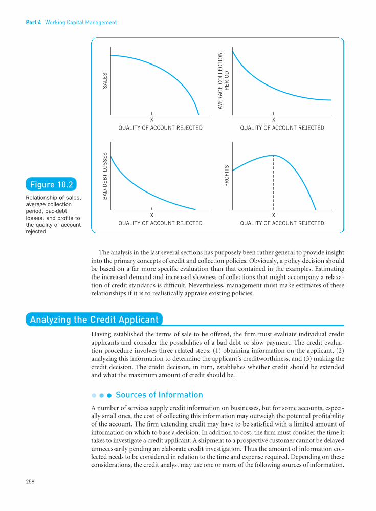
Part 4 Working Capital Management
258
••
The analysis in the last several sections has purposely been rather general to provide insightinto the primary concepts of credit and collection policies. Obviously, a policy decision shouldbe based on a far more specific evaluation than that contained in the examples. Estimating the increased demand and increased slowness of collections that might accompany a relaxa-tion of credit standards is difficult. Nevertheless, management must make estimates of theserelationships if it is to realistically appraise existing policies.
Analyzing the Credit ApplicantHaving established the terms of sale to be offered, the firm must evaluate individual creditapplicants and consider the possibilities of a bad debt or slow payment. The credit evalua-tion procedure involves three related steps: (1) obtaining information on the applicant, (2)analyzing this information to determine the applicant’s creditworthiness, and (3) making thecredit decision. The credit decision, in turn, establishes whether credit should be extendedand what the maximum amount of credit should be.
l l l Sources of InformationA number of services supply credit information on businesses, but for some accounts, especi-ally small ones, the cost of collecting this information may outweigh the potential profitabilityof the account. The firm extending credit may have to be satisfied with a limited amount ofinformation on which to base a decision. In addition to cost, the firm must consider the time ittakes to investigate a credit applicant. A shipment to a prospective customer cannot be delayedunnecessarily pending an elaborate credit investigation. Thus the amount of information col-lected needs to be considered in relation to the time and expense required. Depending on theseconsiderations, the credit analyst may use one or more of the following sources of information.
Figure 10.2Relationship of sales,average collectionperiod, bad-debtlosses, and profits tothe quality of accountrejected
FUNO_C10.qxd 9/19/08 17:16 Page 258

2The two letters, BB, in Beaumont & Hunt’s “BB1” rating indicate that the company’s net worth falls between$200,000 and $300,000. The number 1 following BB indicates that the firm has a “high” composite credit appraisalrelative to other firms with a similar level of net worth.
Financial Statements. At the time of the prospective sale, the seller may request financialstatements, one of the most desirable sources of information for credit analysis. Frequently,there is a correlation between a company’s refusal to provide statements and a weak financialposition. Audited statements are preferable. When possible, it is helpful to obtain interimstatements in addition to year-end ones, particularly for companies having seasonal patternsof sales.
Credit Ratings and Reports. In addition to financial statements, credit ratings are availablefrom various credit reporting agencies. Dun & Bradstreet (D&B) is perhaps the best knownand most comprehensive of these agencies. It provides credit ratings to subscribers for a vastnumber of business firms. Figure 10.3 shows a D&B reference book’s composite rating of“BB1” for Beaumont & Hunt, Inc., and provides a key to D&B’s individual ratings. As we cansee from the key to ratings, D&B ratings give the credit analyst an indication of the estimatedsize of net worth (a rough guide to financial capacity) and a credit appraisal for companies of a particular size, ranging from “high = 1” to “limited = 4.”2 D&B also indicates when theinformation available is insufficient to provide a rating for a given business. In addition to itsrating service, D&B provides credit reports containing a brief history of a company and itsprincipal officers; the nature of the business; certain financial information; and a trade checkof suppliers, including the length of their experience with the company and whether paymentsare discount, prompt, or past due. The quality of the D&B report varies with the informationavailable externally and the willingness of the company being checked to cooperate with theD&B reporter. The report itself can be accessed via a computer terminal if so desired.
Bank Checking. Another source of credit information for the credit analyst checking on a particular firm is the firm’s bank. Most banks have credit departments that will provideinformation on their commercial customers as a service to those customers seeking to acquiretrade credit (credit granted from one business to another). By calling or writing to a bank inwhich the credit applicant has an account, the analyst can obtain information, such as aver-age cash balance carried, loan accommodations, experience, and sometimes more extensivefinancial information. What is provided is determined by the extent of the permission givenby the bank’s customer. In exchanging credit information, most banks follow guidelinesadopted by the Risk Management Association (RMA), the national association for the finan-cial services industry. The RMA Principles for the Exchange of Commercial Credit Informationdescribes how to respond to requests for commercial credit information, whether they arereceived in writing, by telephone, or by fax.
Trade Checking. Credit information is frequently exchanged among companies selling tothe same customer. Through various credit organizations, credit people in a particular areabecome a closely knit group. A company can ask other suppliers about their experiences withan account.
The Company’s Own Experience. A study of the promptness of past payments, includ-ing any seasonal patterns, is very useful. Frequently, the credit department will make writtenassessments of the quality of the management of a company to whom credit may be extended.These assessments are very important, for they pertain to the original “three Cs” of creditanalysis: character (creditor’s willingness to honor obligations), capacity (creditor’s ability togenerate cash to meet obligations), and capital (creditor’s net worth and the relationship ofnet worth to debt). The person who made the sale to a prospective customer can frequentlyoffer useful impressions of management and operations. Caution is necessary in interpretingthis information because a salesperson has a natural bias toward granting credit and makingthe sale.
10 Accounts Receivable and Inventory Management
259
••
FUNO_C10.qxd 9/19/08 17:16 Page 259

l l l Credit AnalysisHaving collected credit information, the firm must make a credit analysis of the applicant. In practice, the collection of information and its analysis are closely related. If, on the basis of initial credit information, a large account appears to be relatively risky, the credit analyst
Part 4 Working Capital Management
260
••
Figure 10.3D&B composite rating from a reference book and a key to ratings. Reprinted with permission from Dun &Bradstreet, Inc., 2007.
FUNO_C10.qxd 9/19/08 17:16 Page 260

will want to obtain further information. Presumably, the expected value of the additionalinformation will exceed the cost of acquiring it. Given the financial statements of a creditapplicant, the credit analyst should undertake a ratio analysis, as described in Chapter 6. Theanalyst will be particularly interested in the applicant’s liquidity and ability to pay bills ontime. Such ratios as the quick ratio, receivable and inventory turnovers, the average payableperiod, and debt-to-equity ratio are particularly relevant.
In addition to analyzing financial statements, the credit analyst will consider the characterof the company and its management, the financial strength of the firm, and various other matters. Then the analyst attempts to determine the ability of the applicant to service creditand the probability of an applicant’s not paying on time and of a bad-debt loss. On the basisof this information, together with information about the profit margin on the product or service being sold, a decision is reached on whether or not to extend credit.
Sequential Investigation Process. The amount of information collected should be deter-mined in relation to the expected profit from an order and the cost of investigation. Moresophisticated analysis should be undertaken only when there is a chance that a credit decisionbased on the previous stage of investigation will be changed. If an analysis of a Dun &Bradstreet report resulted in an extremely unfavorable picture of the applicant, an investiga-tion of the applicant’s bank and trade suppliers might have little prospect of changing thereject decision. Therefore, the added cost associated with this stage of investigation would notbe worthwhile. Each incremental stage of investigation has a cost, which can be justified onlyif the information obtained has value in changing a prior decision.3
Figure 10.4 is a flowchart example of a sequential approach to credit analysis. The first stage consists of simply consulting past experience to see whether the firm has sold previouslyto the account and, if it has, whether that experience has been satisfactory. Stage two mightinvolve ordering a Dun & Bradstreet report on the applicant and evaluating it. The third andlast stage could be credit checks of the applicant’s bank and creditors – coupled, perhaps, with a financial statement analysis. Each stage adds to the cost. The expected profit fromaccepting an order will depend on the size of the order, as will the opportunity cost associatedwith its rejection. Rather than perform all stages of investigation regardless of the size of theorder and the firm’s past experience, the firm should investigate in stages and go to a newstage only when the expected net benefits of the additional information exceed the cost ofacquiring it. When past experience has been favorable, there may be little need for furtherinvestigation. In general, the riskier the applicant, the greater the desire for more information.By balancing the costs of information with the likely profitability of the order, as well as with information from the next stage of investigation, added sophistication is introduced onlywhen it is beneficial.
Credit-Scoring Systems. Quantitative approaches have been developed to estimate theability of businesses to service credit granted to them; however, the final decision for mostcompanies extending trade credit (credit granted from one business to another) rests on thecredit analyst’s judgment in evaluating available information. Strictly numerical evaluationshave been successful in determining the granting of credit to retail customers (consumercredit), where various characteristics of an individual are quantitatively rated, and a creditdecision is made on the basis of the total score. The plastic credit cards many of us hold areoften given out on the basis of a credit-scoring system in which such things as occupation,duration of employment, home ownership, years of residence, and annual income are takeninto account. Numerical rating systems are also being used by some companies extendingtrade credit. With the overall growth of trade credit, a number of companies are finding itworthwhile to use numerical credit-scoring systems to identify clearly unacceptable and accept-able applicants. Credit analysts can then devote their energies to evaluating marginal applicants.
10 Accounts Receivable and Inventory Management
261
••
3For such an analysis, see Dileep Mehta, “The Formulation of Credit Policy Models,” Management Science 15(October 1968), 35–50.
Credit-scoring systemA system used todecide whether togrant credit byassigning numericalscores to variouscharacteristics relatedto creditworthiness.
FUNO_C10.qxd 9/19/08 17:16 Page 261

l l l Credit Decision and Line of CreditOnce the credit analyst has marshaled the necessary evidence and analyzed it, a decision mustbe reached about the disposition of the account. In an initial sale, the first decision to be madeis whether or not to ship the goods and extend credit. If repeat sales are likely, the companywill probably want to establish procedures so that it does not have to fully evaluate the exten-sion of credit each time an order is received. One means of streamlining the procedure is toestablish a line of credit for an account. A line of credit is a maximum limit on the amountthe firm will permit to be owed at any one time. In essence, it represents the maximum riskexposure that the firm will allow itself to undergo for an account.4 The establishment of a
4One credit agency offers the following “rule of thumb” for setting the dollar limit to the amount of credit extended– pick the lesser of (a) 10 percent of the applicant’s net worth, or (b) 20 percent of the applicant’s net working capital.
Part 4 Working Capital Management
262
Line of credit A limitto the amount ofcredit extended to anaccount. Purchasercan buy on credit upto that limit.
••
Figure 10.4Sequentialinvestigation process:who should we acceptas a credit customer?
FUNO_C10.qxd 9/19/08 17:16 Page 262

credit line streamlines the procedure for shipping goods, but the line must be reevaluated ona regular basis to keep abreast of developments in the account. What was a satisfactory riskexposure today may be more or less satisfactory a year from today. Despite comprehensivecredit procedures, there will always be special cases that must be dealt with individually. Here,too, a firm can streamline the operation by defining responsibilities clearly.
l l l Outsourcing Credit and CollectionsThe entire credit/collection function can be outsourced (i.e., subcontracted to an outside firm).A number of third-party companies, such as Dun & Bradstreet, offer complete or partial services to corporations. Credit scoring systems, together with other information, are used in deciding whether credit will be granted. Ledger accounts are maintained, payments are processed, and collection efforts on tardy accounts are initiated. As with the outsourcing ofany business function, it often comes down to a question of core competence. Where suchinternal competence does not exist or is inefficient, the decision – even for large companies –may be to buy the service on the outside. For small- and medium-sized companies, credit andcollections may simply prove too costly to do on one’s own.
Inventory Management and ControlInventories form a link between the production and sale of a product. A manufacturing company must maintain a certain amount of inventory, known as work-in-process, duringproduction. Although other types of inventory – in-transit, raw-materials, and finished-goodsinventories – are not necessary in the strictest sense, they allow the firm to be flexible.Inventory in transit – that is, inventory between various stages of production or storage – permits efficient production scheduling and utilization of resources. Without this type ofinventory, each stage of production would have to wait for the preceding stage to complete aunit. The possibility of resultant delays and idle time gives the firm an incentive to maintainin-transit inventory.
Raw-materials inventory gives the firm flexibility in its purchasing. Without it, the firmmust exist on a hand-to-mouth basis, buying raw materials strictly in keeping with its production schedule. Finished-goods inventory allows the firm flexibility in its productionscheduling and in its marketing. Production does not need to be geared directly to sales. Large inventories allow efficient servicing of customer demands. If a certain product is temporarily out of stock, present as well as future sales to the customer may be lost. Thusthere is an incentive to maintain stocks of all types of inventory.
The traditionally extolled advantages of increased inventories, then, are several. The firmcan effect economies of production and purchasing and can fill orders more quickly. In short,the firm is said to be more flexible. The obvious disadvantages are the total cost of holding theinventory, including storage and handling costs, and the required return on capital tied up ininventory. An additional disadvantage is the danger of obsolescence. Because of the benefits,however, the sales manager and production manager are often biased toward relatively largeinventories. Moreover, the purchasing manager can often achieve quantity discounts withlarge orders, and there may be a bias here as well. It falls on the financial manager to dampenthe temptation for large inventories. This is done by forcing consideration of the cost of fundsnecessary to carry inventories as well as perhaps of the handling and storage costs.
In recent years, additional support for the financial manager’s questioning of the mainten-ance of large inventories has come from an understanding of a Japanese-inspired inventorycontrol system called Just-in-Time, or JIT for short. JIT breaks with the conventional wisdomof maintaining large inventory stocks as buffers against uncertainties. The basic objective ofJIT is to produce (or receive) a required item at the exact time needed, or “just in time.”Inventories of all types would thus be reduced to a bare minimum (in some cases, zero).
10 Accounts Receivable and Inventory Management
263
••
FUNO_C10.qxd 9/19/08 17:16 Page 263

Reductions in inventory-carrying costs are one of the more obvious results of the JIT system.However, additional hoped-for results include improvements in productivity, product quality,and flexibility.
Like accounts receivable, inventories should be increased as long as the resulting savingsexceed the total cost of holding the added inventory. The balance finally reached depends on the estimates of actual savings, the cost of carrying additional inventory, and the effici-ency of inventory control. Obviously, this balance requires coordination of the production,marketing, and finance areas of the firm in keeping with an overall objective. Our purpose is to examine various principles of inventory control by which an appropriate balance mightbe achieved.
l l l Classification: What to Control?We have already noted the different types of inventory that exist for a typical manufacturingfirm – raw-materials, work-in-process, in-transit, and finished-goods inventories. Anotherway to classify inventory is by the dollar value of the firm’s investment. If a firm were to rankinventory items by decreasing value per item, we might get a cumulative distribution thatlooks like Figure 10.5. For the firm described by Figure 10.5, we find that, as a group, “A”items reflect the fact that roughly 15 percent of the items in inventory account for 70 percentof inventory value. The next 30 percent of the items, group “B,” account for 20 percent ofinventory value. And more than half, or 55 percent, of the items explain only 10 percent oftotal inventory value.
Based on this typical breakdown, in which a relatively small proportion of items accountfor most of the total inventory value, it seems reasonable for the firm to devote more care andattention to controlling the more valuable items. This can be accomplished by assigning theman “A” classification and reviewing these items more frequently. “B” and “C” items mightwarrant increasingly less rigorous, less timely reviews. This system is often referred to, appro-priately enough, as the ABC method of inventory control. Factors other than dollar valuemay also need to be considered when developing a classification plan – for example, whether
Part 4 Working Capital Management
264
••
Figure 10.5Distribution ofinventory by inventory value
ABC method ofinventory controlMethod that controlsexpensive inventoryitems more closelythan less expensiveitems.
FUNO_C10.qxd 9/19/08 17:16 Page 264

something is a critical, or bottleneck, item or may soon become obsolete. The bottom line,however, is to classify inventory items in such a fashion that we ensure that the most impor-tant inventory items are reviewed most often.5 Thus a valid method of inventory classificationforms the first leg in the construction of a solid inventory control system.
l l l Economic Order Quantity: How Much to Order?To be a successful contestant on the television quiz show Jeopardy, you must be able to pro-vide the questions to answers that are given in various categories. Thus, if the category wasinventory theory, you might run across the following answer: the EOQ amount. Hopefully, bythe time you finish reading this section you will understand why the correct “question” to this“answer” is: How much should we order?
The economic order quantity (EOQ) is an important concept in the purchase of raw materials and in the storage of finished-goods and in-transit inventories. In our analysis, wedetermine the optimal order quantity for a particular item of inventory, given its forecastusage, ordering cost, and carrying cost. Ordering can mean either the purchase of the item or itsproduction. Assume for the moment that the usage of a particular item of inventory is knownwith certainty. This usage is at a steady rate throughout the period of time being analyzed. Inother words, if usage is 2,600 items for a six-month period, 100 items are used each week.
We assume that ordering costs per order, O, are constant regardless of the size of the order. In the purchase of raw materials or other items, these costs represent the clerical costsinvolved in placing an order together with certain costs of receiving and checking the goodsonce they arrive. For finished-goods inventories, ordering costs involve scheduling a produc-tion run. When setup costs are large – as they are in producing a machined piece of metal, for example – ordering costs can be quite significant. For in-transit inventories, ordering costsare likely to involve nothing more than record keeping. The total ordering cost for a period issimply the cost per order times the number of orders for that period.
Carrying costs per unit, C, represent the cost of inventory storage, handling, and insurance,together with the required return on the investment in inventory over the period. These costsare assumed to be constant per unit of inventory, per period of time. Thus the total carryingcost for a period is the carrying cost per unit times the average number of units of inventoryfor the period. In addition, we assume that inventory orders are filled when needed, withoutdelay. Because out-of-stock items can be replaced immediately, there is no need to maintaina buffer or safety stock. Though the assumptions made up to now may seem overly restrictive,they are necessary for an initial understanding of the conceptual framework that follows.Subsequently, we will relax some of them, and you may be surprised at how robust our original approach will prove itself to be.
If usage of an inventory item is at a steady rate over a period of time and there is no safetystock, average inventory (in units) can be expressed as
Average inventory = Q /2 (10.1)
where Q is the quantity ordered and is assumed to be constant for the planning period. Thissituation is illustrated in Figure 10.6. Although the quantity demanded is a step function, weassume for analytical purposes that it can be approximated by a straight line. We see thatwhen a zero level of inventory is reached, a new order of Q items arrives.
Once again, the carrying cost of inventory is the average number of units of inventory timesthe carrying cost per unit, or C(Q/2). The total number of orders over a period of time is simply the total usage (in units) of an item of inventory for that period, S, divided by Q, the
5Those of you familiar with the classic television series M*A*S*H may remember the doctors and nurses performingtriage on arriving groups of wounded soldiers – that is, classifying the wounded according to who warrants moreimmediate attention. The firm, in essence, is performing a type of triage on its inventory as it classifies it into “A,”“B,” and “C” categories.
10 Accounts Receivable and Inventory Management
265
••
Economic orderquantity (EOQ)The quantity of aninventory item toorder so that totalinventory costs areminimized over thefirm’s planning period.
FUNO_C10.qxd 9/19/08 17:16 Page 265

quantity ordered. Consequently, total ordering costs are represented by the ordering cost perorder times the number of orders, or O(S/Q). Total inventory costs, then, are the sum of thetotal carrying costs plus total ordering costs, or
Total inventory cost (T ) = C(Q /2) + O(S/Q) (10.2)
We see from Eq. (10.2) that the higher the order quantity, Q, the higher the total carryingcosts, but the lower the total ordering costs. The lower the order quantity, the lower the totalcarrying costs, but the higher the total ordering costs. We are, therefore, concerned with thetrade-off between the economies of increased order size and the added cost of carrying additional inventory.
Optimal Order Quantity. The optimal quantity of an inventory item to order at any onetime is that quantity, Q*, that minimizes total inventory costs over our planning period. Wecan use calculus to find the lowest point on the total inventory cost curve described by Eq. (10.2) and then solve for Q.6 The resulting optimal quantity, or EOQ, is
To illustrate the use of this EOQ equation, suppose that usage of an inventory item is 2,000during a 100-day planning period, ordering costs are $100 per order, and carrying costs are$10 per unit per 100 days. The EOQ amount, then, is
(10.3)Q* = =2($100)(2,000)
$10200 units
QO SC
* =2( )( )
6Taking the first derivative of Eq. (10.2) with respect to Q and setting the result equal to zero, we obtain
dT/dQ = (C/2) − O(S/Q2) = 0
Now, solving for Q, we get
O(S/Q2) = C/2
Part 4 Working Capital Management
266
••
Figure 10.6Order quantityexample with certain,steady demand andno safety stock
FUNO_C10.qxd 9/19/08 17:16 Page 266

With an order quantity of 200 units, the firm would order (2,000/200) = 10 times during theperiod under consideration or, in other words, every 10 days. We see from Eq. (10.3) that Q*varies directly with usage, S, and order cost, O, and inversely with carrying cost, C. However,the relationship is dampened by the square-root sign in both cases. As usage increases, then,the optimal order size and the average level of inventory increase by a lesser percentage. Inother words, economies of scale are possible. For example, if we double usage in our exampleto 4,000 units, we get a new optimal order quantity that is only 40 percent higher than the oldone – that is, 280 units. This new order quantity results in a new average inventory level (Q/2)that is likewise only 40 percent higher – 140 units versus 100 units.
The EOQ function is shown in Figure 10.7. In the figure, we plot total ordering costs; total carrying costs; and total inventory costs, which are the sum of the first two costs. We see that whereas total carrying costs vary directly with the size of the order, total ordering costs vary inversely with order size. The total inventory costs line declines at first as the fixedcosts of ordering are incurred less often as fewer but larger orders are placed. However, thetotal inventory costs line then begins to rise when the decrease in total ordering costs is more than offset by the additional carrying costs caused by maintaining a larger averageinventory. Point Q*, then, represents the economic order quantity, which minimizes the totalcost of inventory.7 The EOQ formula taken up in this section is a useful tool for inventorycontrol. In purchasing raw materials or other items of inventory, it tells us the amount to
7As shown in Figure 10.7, the total carrying costs and total ordering costs lines intersect at the order-size level wherethe total inventory costs curve has its minimum, point Q*. To see why this always holds true for our model, set totalcarrying costs (TCC) equal to total ordering costs (TOC) and solve for order quantity Q:
TCC = TOC
C(Q/2) = O(S/Q)
C(Q2) = 2(O)(S)
10 Accounts Receivable and Inventory Management
267
••
Figure 10.7Economic orderquantity relationships
FUNO_C10.qxd 9/19/08 17:16 Page 267

order. For finished goods, it enables us to exercise better control over the size of produc-tion runs. In general, the EOQ model gives us a rule for deciding the amount of inventory to replenish.
l l l Order Point: When to Order?
In addition to knowing how much to order, the firm also needs to know when to order.“When,” in this case, means the quantity to which inventory must fall in order to signal areorder of the EOQ amount. In our previous example, we have assumed that inventory canbe ordered and received without delay. Usually there is a time lapse between placement of apurchase order and receipt of the inventory, or in the time it takes to manufacture an itemafter an order is placed. This lead time must be considered.
Suppose that demand for inventory is known with certainty, but that it takes 5 daysbetween the placement and receipt of an order. In our previous illustration of the EOQ formula, we found that the EOQ for our example firm was 200 units, resulting in an order being placed (and filled) every 10 days. This firm thus had a zero lead time and a daily usage of 20 units. If usage remains at a steady rate, the firm would now need to order 5 days before it ran out of stock, or at 100 units of stock on hand. The order point may beexpressed as
Order point (OP) = Lead time × Daily usage (10.4)
Thus the order point is now
5 days × 20 units per day = 100 units
When the new order is received 5 days later, the firm will just have exhausted its existing stock.This example, involving an order point, is illustrated in Figure 10.8.
l l l Safety Stock
In practice, the demand or usage of inventory is generally not known with certainty; usu-ally, it fluctuates during a given period of time. Typically, the demand for finished-goods
Part 4 Working Capital Management
268
••
Lead time The lengthof time between theplacement of an orderfor an inventory itemand when the item isreceived in inventory.
Order point Thequantity to whichinventory must fall inorder to signal that anorder must be placedto replenish an item.
Figure 10.8Order point when lead time is non-zeroand certain
FUNO_C10.qxd 9/19/08 17:16 Page 268

inventory is subject to the greatest uncertainty. In general, the usage of raw-materials inven-tory and in-transit inventory, both of which depend on the production scheduling, is morepredictable. In addition to demand, the lead time required to receive delivery of inventoryonce an order is placed is usually subject to some variation. Owing to these fluctuations, it is not usually feasible to allow expected inventory to fall to zero before a new order is anticipated, as the firm could do when usage and lead time were known with certainty.
Therefore, when we allow for uncertainty in demand for inventory as well as in lead time,a safety stock becomes advisable. The concept of a safety stock is illustrated in Figure 10.9.Frame A of the figure shows what would happen if the firm had a safety stock of 100 units andif expected demand of 200 units every 10 days and expected lead time of 5 days were to occur.However, treating lead time and daily usage as average, or expected, values, rather than asconstants, causes us to modify our original order point equation as follows:
Order point (OP) = (Average lead time × Average daily usage) + Safety stock (10.5)
10 Accounts Receivable and Inventory Management
269
••
Safety stockInventory stock heldin reserve as acushion againstuncertain demand (or usage) andreplenishment lead time.
Figure 10.9Safety stock andorder point whendemand and leadtime are uncertain
FUNO_C10.qxd 9/19/08 17:16 Page 269

••
Part 4 Working Capital Management
270
Note that with a safety stock of 100 units, the order point must be set at (5 days × 20 units) +100 units = 200 units of inventory on hand as opposed to the previous 100 units. In otherwords, the order point determines the amount of safety stock held. Thus, by varying the orderpoint, one can vary the safety stock that is held.
Frame B of the figure shows the actual experience for our hypothetical firm. In the first segment of demand, we see that actual usage is somewhat less than expected. (The slope of theline is less than that for the expected demand line in frame A.) At the order point of 200remaining units, an order is placed for 200 units of additional inventory. Instead of taking the expected 5 days for the inventory to be replenished, we see that it takes only 4 days. Thesecond segment of usage is much greater than expected, and, as a result, inventory is rapidlyused up. At 200 units of remaining inventory, a 200-unit order is again placed, but here ittakes 6 days for the inventory to be received. As a result of both of these factors, heavy inroadsare made into the safety stock.
In the third segment of demand, usage is about the same as expected: that is, the slopes of the expected and actual usage lines are about the same. Because inventory was so low at the end of the previous segment of usage, an order is placed almost immediately. The leadtime turns out to be 5 days. In the last segment of demand, usage is slightly greater thanexpected. The lead time necessary to receive an order is 7 days – much longer than expected.The combination of these two factors again causes the firm to go into its safety stock. Theexample illustrates the importance of safety stock in absorbing random fluctuations in usageand lead times. Without such a buffer stock, the firm would have run out of inventory on two occasions.
The Amount of Safety Stock. The proper amount of safety stock to maintain depends onseveral factors. The greater the uncertainty associated with forecasted demand for inven-tory, the greater the safety stock the firm will wish to carry, all other things being the same. Put another way, the greater the risk of running out of stock, the larger the unforeseen fluc-tuations in usage. Similarly, the greater the uncertainty of lead time to replenish stock, the greater the risk of running out of stock, and the more safety stock the firm will wish tomaintain, all other things being equal. Another factor influencing the safety stock decision is the cost of running out of inventory. The cost of being out of raw-materials and in-transit inventories is a delay in production. How much does it cost when production closesdown temporarily? Where fixed costs are high, this cost will be quite high, as, for example, inthe case of an aluminum extrusion plant. The cost of running out of finished goods comesfrom lost sales and customer dissatisfaction. Not only will the immediate sale be lost butfuture sales will be endangered if customers take their business elsewhere. Although thisopportunity cost is difficult to measure, it must be recognized by management and incor-porated into the safety stock decision. The greater the costs of running out of stock, of course,the greater the safety stock that management will wish to maintain, all other things staying the same.
The final factor is the cost of carrying additional inventory. If it were not for this cost, afirm could maintain whatever safety stock was necessary to avoid all possibility of running outof inventory. The greater the cost of carrying inventory, the more costly it is to maintain asafety stock, all other things being equal. Determination of the proper amount of safety stockinvolves balancing the probability and cost of a stockout against the cost of carrying enoughsafety stock to avoid this possibility. Ultimately, the question reduces to the probability ofinventory stockout that management is willing to tolerate. In a typical situation, this prob-ability is reduced at a decreasing rate as more safety stock is added. A firm may be able toreduce the probability of inventory stockout by 20 percent if it adds 100 units of safety stock,but only by an additional 10 percent if it adds another 100 units. There comes a point whenit becomes very expensive to further reduce the probability of stockout. Management will not wish to add safety stock beyond the point at which incremental carrying costs exceed the incremental benefits to be derived from avoiding a stockout.
FUNO_C10.qxd 9/19/08 17:16 Page 270

l l l Just-in-TimeThe management of inventory has become very sophisticated in recent years. In certain industries, the production process lends itself to just-in-time (JIT) inventory control. As thename implies, the idea is that inventories are acquired and inserted in production at the exacttimes they are needed. The JIT management philosophy thus focuses on pulling inventorythrough the production process on an “as-needed” basis, rather than pushing inventorythrough the process on an “as-produced” basis. This requires a very accurate production and inventory information system, highly efficient purchasing, very reliable suppliers, and an efficient inventory-handling system. Although raw-materials inventory and in-transitinventory can never be reduced to zero, the notion of “just in time” is one of extremely tight control so as to cut back on inventories. The goal of a JIT system, however, is not only to reduce inventories but also to continuously improve productivity, product quality, and manufacturing flexibility.
EOQ in a JIT World. At first glance, it might seem that a JIT system – in which inventorieswould be reduced to a bare minimum and the EOQ for a particular item might approach oneunit – would be in direct conflict with our EOQ model. However, it is not. A JIT system, onthe other hand, rejects the notion that ordering costs (clerical, receiving, inspecting, schedul-ing, and/or setup costs) are necessarily fixed at their current levels. As part of a JIT system,steps are continuously taken to drive these costs down. For example:
l Small-sized delivery trucks, with predetermined unloading sequences, are used to facil-itate economies in receiving time and costs.
l Pressure is placed on suppliers to produce raw materials with “no defects,” thus reduc-ing (or eliminating) inspection costs.
l Products, equipment, and procedures are modified to reduce setup time and costs.
By successfully reducing these ordering-related costs, the firm is able to flatten the total order-ing cost curve in Figure 10.7. This causes the optimal order quantity, Q*, to shift to the left,thus approaching the JIT ideal of one unit. Additionally, continuous efforts to reduce supplierdelays, production inefficiencies, and sales forecasting errors allow safety stocks to be cut back or eliminated. How close a company comes to the JIT ideal depends on the type of production process and the nature of the supplier industries, but it is a worthy objective for most companies.
JIT Inventory Control, Supply Chain Management, and the Internet. JIT inventorycontrol can be viewed as one link in the chain of activities associated with moving goods fromthe raw material stage through to the end user or customer. These activities are collectivelyreferred to as supply chain management (SCM). The advent of instant information throughsophisticated computer networks has greatly facilitated this process.
For standard inventory items, the use of the Internet has enhanced supply chain management.A number of exchanges have developed for business-to-business (B2B) types of transactions.If you need to purchase a certain type of chemical for use in your production process, you canspecify your exact need on a chemical B2B exchange. Various suppliers will then bid for thecontract. This auction technique significantly reduces the paperwork and other costs involvedin searching for the best price. This, together with competition among suppliers, maysignificantly reduce your costs. A number of B2B exchanges already exist for a wide variety ofproducts, and new ones are developing all the time. Again, the raw material in question mustbe relatively standardized for an Internet exchange to work well for you.
l l l Inventory and the Financial ManagerAlthough inventory management is usually not the direct operating responsibility of thefinancial manager, the investment of funds in inventory is a very important aspect of financial
10 Accounts Receivable and Inventory Management
271
••
Just-in-time (JIT) Anapproach to inventorymanagement andcontrol in whichinventories areacquired and insertedin production at theexact times they are needed.
Supply chainmanagement (SCM)Managing the processof moving goods,services, andinformation fromsuppliers to endcustomers.
Business-to-business(B2B)Communications and transactionsconducted betweenbusinesses, asopposed to betweenbusinesses and endcustomers. Expressedin alphanumeric form(i.e., B2B), it refers to such transactionsconducted over theInternet.
B2B exchangeBusiness-to-businessInternet marketplacethat matches supplyand demand by real-time auction bidding.
FUNO_C10.qxd 9/19/08 17:16 Page 271

••
Part 4 Working Capital Management
272
Source: “What is needed to make a ‘just-in-time’ system work,” Iron Age Magazine (June 7 1982)p. 45. Reprinted with permission.
FUNO_C10.qxd 9/19/08 17:16 Page 272

10 Accounts Receivable and Inventory Management
273
••
management. Consequently, the financial manager must be familiar with ways to controlinventories effectively so that capital may be allocated efficiently. The greater the opportunitycost of funds invested in inventory, the lower the optimal level of average inventory, and thelower the optimal order quantity, all other things held constant. This statement can be verifiedby increasing the carrying costs, C, in Eq. (10.3). The EOQ model can also be used by thefinancial manager in planning for inventory financing.
When demand or usage of inventory is uncertain, the financial manager may try to effectpolicies that will reduce the average lead time required to receive inventory once an order is placed. The lower the average lead time, the lower the safety stock needed, and the lower the total investment in inventory, all other things held constant. The greater the opportunitycost of funds invested in inventory, the greater the incentive to reduce this lead time. The purchasing department may try to find new vendors that promise quicker delivery, or it maypressure existing vendors to deliver faster. The production department may be able to deliverfinished goods faster by producing a smaller run. In either case, there is a trade-off betweenthe added cost involved in reducing the lead time and the opportunity cost of funds tied upin inventory. This discussion serves to point out the value of inventory management to thefinancial manager.
Key Learning Pointsl Credit and collection policies encompass several
decisions: (1) the quality of accounts accepted; (2) thelength of the credit period; (3) the size of the cash discount (if any) for early payment; (4) any specialterms, such as seasonal datings; and (5) the level ofcollection expenditures. In each case, the decisioninvolves a comparison of the possible gains from achange in policy with the cost of the change. To maximize profits arising from credit and collectionpolicies, the firm should vary these policies jointlyuntil it achieves an optimal solution.
l The firm’s credit and collection policies, together withits credit and collection procedures, determine themagnitude and quality of its receivable position.
l In evaluating a credit applicant, the credit analyst (1)obtains information on the applicant, (2) analyzes thisinformation to determine the applicant’s credit-worthiness, and (3) makes the credit decision. Thecredit decision, in turn, establishes whether creditshould be extended and what the maximum amountof credit, or line of credit, should be.
l Inventories form a link between the production andsale of a product. Inventories give the firm flexibilityin its purchasing, production scheduling, and servic-ing of customer demands.
l In evaluating the level of inventories, management mustbalance the benefits of economies of production, pur-chasing, and marketing against the cost of carrying theadditional inventory. Of particular concern to the finan-cial manager is the cost of funds invested in inventory.
l Firms often classify inventory items into groups insuch a fashion as to ensure that the most importantitems are reviewed most often. One such approach iscalled the ABC method of inventory control.
l The optimal order quantity for a particular item ofinventory depends on the item’s forecasted usage,ordering cost, and carrying cost. Ordering can meaneither the purchase of the item or its production.Ordering costs include the costs of placing, receiving,and checking an order. Carrying costs represent thecost of inventory storage, handling, and insurance and the required return on the investment in inventory.
l The economic order quantity (EOQ) model affirms thatthe optimal quantity of an inventory item to order atany one time is that quantity that minimizes totalinventory costs over our planning period.
l An inventory item’s order point is that quantity towhich inventory must fall to signal a reorder of theEOQ amount.
l Under conditions of uncertainty, the firm must usu-ally provide for a safety stock, owing to fluctuations in demand for inventory and in lead times. By varyingthe point at which orders are placed, one varies thesafety stock that is held.
l Just-in-time (JIT) inventory control is the result of anew emphasis by firms on continuous process im-provement. The idea is that inventories are acquiredand inserted in production at the exact times they are needed.
FUNO_C10.qxd 9/19/08 17:16 Page 273

Questions
1. Is it always good policy to reduce the firm’s bad debts by “getting rid of the deadbeats”?2. What are the probable effects on sales and profits of each of the following credit policies?
a. A high percentage of bad-debt loss but normal receivable turnover and credit rejectionrate.
b. A high percentage of past-due accounts and a low credit rejection rate.c. A low percentage of past-due accounts but high credit rejection and receivable
turnover rates.d. A low percentage of past-due accounts and a low credit rejection rate but a high
receivable turnover rate.3. Is an increase in the collection period necessarily bad? Explain.4. What are the various sources of information you might use to analyze a credit applicant?5. What are the principal factors that can be varied in setting credit policy?6. If credit standards for the quality of accounts accepted are changed, what things are
affected?7. Why is the saturation point reached in spending money on collections?8. What is the purpose of establishing a line of credit for an account? What are the benefits
of this arrangement?9. The analysis of inventory policy is analogous to the analysis of credit policy. Propose a
measure to analyze inventory policy that is analogous to the aging of accounts receivable.10. What are the principal implications to the financial manager of ordering costs, storage
costs, and cost of capital as they relate to inventory?11. Explain how efficient inventory management affects the liquidity and profitability of the
firm.12. How can the firm reduce its investment in inventories? What costs might the firm incur
from a policy of very low inventory investment?13. Explain how a large seasonal demand complicates inventory management and produc-
tion scheduling.14. Do inventories represent an investment in the same sense as fixed assets?15. Should the required rate of return for investment in inventories of raw materials be the
same as that for finished goods?
Self-Correction Problems
1. Kari-Kidd Corporation currently gives credit terms of “net 30 days.” It has $60 million incredit sales, and its average collection period is 45 days. To stimulate demand, the com-pany may give credit terms of “net 60 days.” If it does instigate these terms, sales areexpected to increase by 15 percent. After the change, the average collection period isexpected to be 75 days, with no difference in payment habits between old and new cus-tomers. Variable costs are $0.80 for every $1.00 of sales, and the company’s before-taxrequired rate of return on investment in receivables is 20 percent. Should the companyextend its credit period? (Assume a 360-day year.)
2. Matlock Gauge Company makes wind and current gauges for pleasure boats. The gaugesare sold throughout the Southeast to boat dealers, and the average order size is $50. Thecompany sells to all registered dealers without a credit analysis. Terms are “net 45 days,”and the average collection period is 60 days, which is regarded as satisfactory. Sue Ford,vice president of finance, is now uneasy about the increasing number of bad-debt losses on new orders. With credit ratings from local and regional credit agencies, she feels shewould be able to classify new orders into one of three risk categories. Past experience showsthe following:
Part 4 Working Capital Management
274
••
FUNO_C10.qxd 9/19/08 17:16 Page 274

••
10 Accounts Receivable and Inventory Management
275
ORDER CATEGORY
LOW MEDIUM HIGHRISK RISK RISK
Bad-debt loss 3% 7% 24%Category orders to total orders 30% 50% 20%
The cost of producing and shipping the gauges and of carrying the receivables is 78 per-cent of sales. The cost of obtaining credit information and of evaluating it is $4 per order.Surprisingly, there does not appear to be any association between the risk category and thecollection period; the average for each of the three risk categories is around 60 days. Basedon this information, should the company obtain credit information on new orders insteadof selling to all new accounts without credit analysis? Why?
3. Vostick Filter Company is a distributor of air filters to retail stores. It buys its filters fromseveral manufacturers. Filters are ordered in lot sizes of 1,000, and each order costs $40 toplace. Demand from retail stores is 20,000 filters per month, and carrying cost is $0.10 afilter per month.a. What is the optimal order quantity with respect to so many lot sizes (that is, what
multiple of 1,000 units should be ordered)?b. What would be the optimal order quantity if the carrying cost were cut in half to $0.05
a filter per month?c. What would be the optimal order quantity if ordering costs were reduced to $10 per
order?4. To reduce production start-up costs, Bodden Truck Company may manufacture longer
runs of the same truck. Estimated savings from the increase in efficiency are $260,000 peryear. However, inventory turnover will decrease from eight times a year to six times a year.Cost of goods sold is $48 million on an annual basis. If the required before-tax rate ofreturn on investment in inventories is 15 percent, should the company instigate the newproduction plan?
Problems
1. To increase sales from their present annual $24 million, Kim Chi Company, a wholesaler,may try more liberal credit standards. Currently, the firm has an average collection periodof 30 days. It believes that, with increasingly liberal credit standards, the following willresult:
CREDIT POLICY
A B C D
Increase in sales from previous level (in millions) $2.8 $1.8 $1.2 $.6Average collection period for incremental sales (days) 45 60 90 144
The prices of its products average $20 per unit, and variable costs average $18 per unit.No bad-debt losses are expected. If the company has a pre-tax opportunity cost of fundsof 30 percent, which credit policy should be pursued? Why? (Assume a 360-day year.)
2. Upon reflection, Kim Chi Company has estimated that the following pattern of bad-debtlosses will prevail if it initiates more liberal credit terms:
CREDIT POLICY
A B C D
Bad-debt losses on incremental sales 3% 6% 10% 15%
Given the other assumptions in Problem 1, which credit policy should be pursued? Why?
FUNO_C10.qxd 9/19/08 17:16 Page 275

3. Recalculate Problem 2, assuming the following pattern of bad-debt losses:
CREDIT POLICY
A B C D
Bad-debt losses on incremental sales 1.5% 3.0% 5.0% 7.5%
Which policy now would be best? Why?4. The Acme Aglet Corporation has a 12 percent opportunity cost of funds and currently
sells on terms of “net/10, EOM.” (This means that goods shipped before the end of themonth must be paid for by the tenth of the following month.) The firm has sales of $10 million a year, which are 80 percent on credit and spread evenly over the year. Theaverage collection period is currently 60 days. If Acme offered terms of “2/10, net 30,”customers representing 60 percent of its credit sales would take the discount, and theaverage collection period would be reduced to 40 days. Should Acme change its termsfrom “net/10, EOM” to “2/10, net 30”? Why?
5. Porras Pottery Products, Inc., spends $220,000 per annum on its collection department.The company has $12 million in credit sales, its average collection period is 2.5 months,and the percentage of bad-debt losses is 4 percent. The company believes that, if it wereto double its collection personnel, it could bring down the average collection period to 2 months and bad-debt losses to 3 percent. The added cost is $180,000, bringing total collection expenditures to $400,000 annually. Is the increased effort worthwhile if thebefore-tax opportunity cost of funds is 20 percent? If it is 10 percent?
6. The Pottsville Manufacturing Corporation is considering extending trade credit to theSan Jose Company. Examination of the records of San Jose has produced the followingfinancial statements:
San Jose Company balance sheets (in millions)
ASSETS 20X1 20X2 20X3
Current assetsCash $ 1.5 $ 1.6 $ 1.6Receivables 1.3 1.8 2.5Inventories (at lower of cost or market) 1.3 2.6 4.0Other 0.4 0.5 0.4
Total current assets $ 4.5 $ 6.5 $ 8.5Fixed assets
Building (net) 2.0 1.9 1.8Machinery and equipment (net) 7.0 6.5 6.0
Total fixed assets $ 9.0 $ 8.4 $ 7.8Other assets 1.0 0.8 0.6
Total assets $14.5 $15.7 $16.9
LIABILITIES
Current liabilitiesNotes payable (8.5%) $ 2.1 $ 3.1 $ 3.8Trade payables 0.2 0.4 0.9Other payables 0.2 0.2 0.2
Total current liabilities $ 2.5 $ 3.7 $ 4.9Term loan (8.5%) 4.0 3.0 2.0
Total liabilities $ 6.5 $ 6.7 $ 6.9Net worth
Preferred stock (6.5%) 1.0 1.0 1.0Common stock 5.0 5.0 5.0Retained earnings 2.0 3.0 4.0
Total liabilities and net worth $14.5 $15.7 $16.9
Part 4 Working Capital Management
276
••
FUNO_C10.qxd 9/19/08 17:16 Page 276

San Jose Company income statements (in millions)
20X1 20X2 20X3
Net credit sales $15.0 $15.8 $16.2Cost of goods sold 11.3 12.1 13.0
Gross profit $ 3.7 $ 3.7 $ 3.2Operating expenses 1.1 1.2 1.0
Net profit before taxes $ 2.6 $ 2.5 $ 2.2Tax 1.3 1.2 1.2
Profit after taxes $ 1.3 $ 1.3 $ 1.0Dividends 0.3 0.3 0.0
To retained earnings $ 1.0 $ 1.0 $ 1.0
The San Jose Company has a Dun & Bradstreet rating of 4A2. Inquiries into its bankingdisclosed balances generally in the low millions. Five suppliers to San Jose revealed thatthe firm takes its discounts from the three suppliers offering “2/10, net 30” terms, thoughit is about 15 days slow in paying the two firms offering terms of “net 30.”
Analyze the San Jose Company’s application for credit. What positive factors are present? What negative factors are present?
7. A college bookstore is attempting to determine the optimal order quantity for a popularbook on psychology. The store sells 5,000 copies of this book a year at a retail price of$12.50, and the cost to the store is 20 percent less, which represents the discount from thepublisher. The store figures that it costs $1 per year to carry a book in inventory and $100to prepare an order for new books.a. Determine the total inventory costs associated with ordering 1, 2, 5, 10, and 20 times
a year.b. Determine the economic order quantity.c. What implicit assumptions are being made about the annual sales rate?
8. The Hedge Corporation manufactures only one product: planks. The single raw materialused in making planks is the dint. For each plank manufactured, 12 dints are required.Assume that the company manufactures 150,000 planks per year, that demand for planksis perfectly steady throughout the year, that it costs $200 each time dints are ordered, andthat carrying costs are $8 per dint per year.a. Determine the economic order quantity of dints.b. What are total inventory costs for Hedge (total carrying costs plus total ordering costs)?c. How many times per year would inventory be ordered?
9. A firm that sells 5,000 blivets per month is trying to determine how many blivets to keepin inventory. The financial manager has determined that it costs $200 to place an order.The cost of holding inventory is 4 cents per month per average blivet in inventory. A five-day lead time is required for delivery of goods ordered. (This lead time is known withcertainty.)a. Develop the algebraic expression for determining the total cost of holding and order-
ing inventory.b. Plot the total holding costs and the total ordering costs on a graph where the hori-
zontal axis represents size of order and the vertical axis represents costs.c. Determine the EOQ from the graph.
10. Common Scents, Inc., makes various scents for use in the manufacture of food products.Although the company does maintain a safety stock, it has a policy of maintaining “lean”inventories, with the result that customers sometimes must be turned away. In an analysisof the situation, the company has estimated the cost of being out of stock associated withvarious levels of safety stock:
10 Accounts Receivable and Inventory Management
277
••
FUNO_C10.qxd 9/19/08 17:16 Page 277
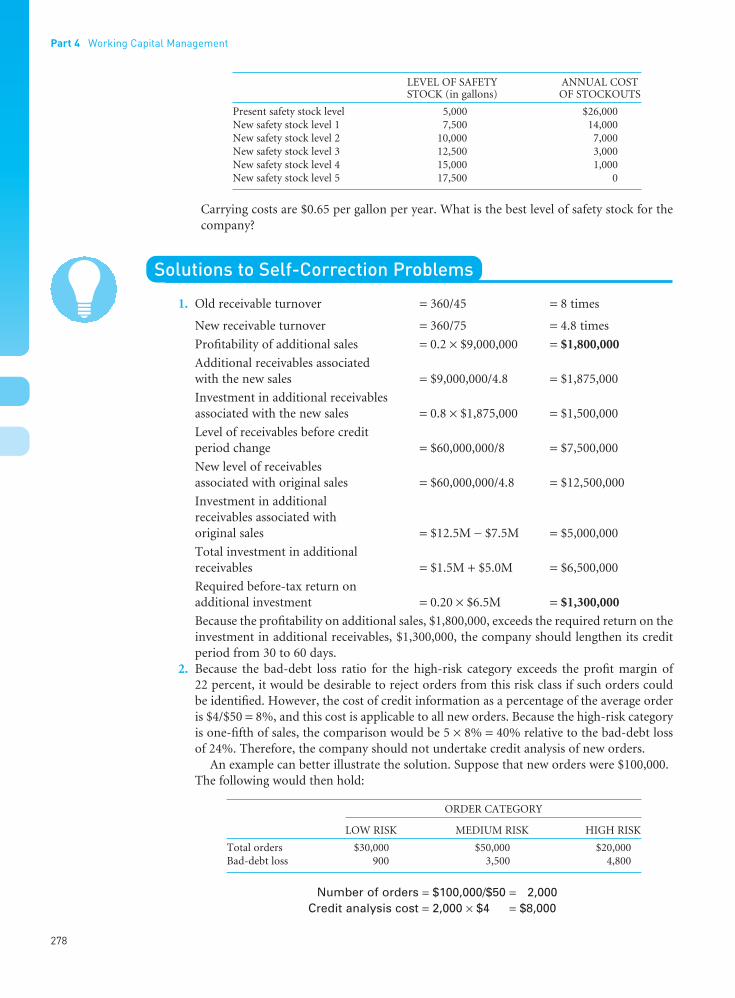
LEVEL OF SAFETY ANNUAL COSTSTOCK (in gallons) OF STOCKOUTS
Present safety stock level 5,000 $26,000New safety stock level 1 7,500 14,000New safety stock level 2 10,000 7,000New safety stock level 3 12,500 3,000New safety stock level 4 15,000 1,000New safety stock level 5 17,500 0
Carrying costs are $0.65 per gallon per year. What is the best level of safety stock for thecompany?
Solutions to Self-Correction Problems
1. Old receivable turnover = 360/45 = 8 times
New receivable turnover = 360/75 = 4.8 times
Profitability of additional sales = 0.2 × $9,000,000 = $1,800,000
Additional receivables associated with the new sales = $9,000,000/4.8 = $1,875,000
Investment in additional receivables associated with the new sales = 0.8 × $1,875,000 = $1,500,000
Level of receivables before credit period change = $60,000,000/8 = $7,500,000
New level of receivables associated with original sales = $60,000,000/4.8 = $12,500,000
Investment in additional receivables associated with original sales = $12.5M − $7.5M = $5,000,000
Total investment in additional receivables = $1.5M + $5.0M = $6,500,000
Required before-tax return on additional investment = 0.20 × $6.5M = $1,300,000
Because the profitability on additional sales, $1,800,000, exceeds the required return on theinvestment in additional receivables, $1,300,000, the company should lengthen its creditperiod from 30 to 60 days.
2. Because the bad-debt loss ratio for the high-risk category exceeds the profit margin of 22 percent, it would be desirable to reject orders from this risk class if such orders could be identified. However, the cost of credit information as a percentage of the average orderis $4/$50 = 8%, and this cost is applicable to all new orders. Because the high-risk categoryis one-fifth of sales, the comparison would be 5 × 8% = 40% relative to the bad-debt lossof 24%. Therefore, the company should not undertake credit analysis of new orders.
An example can better illustrate the solution. Suppose that new orders were $100,000.The following would then hold:
ORDER CATEGORY
LOW RISK MEDIUM RISK HIGH RISK
Total orders $30,000 $50,000 $20,000Bad-debt loss 900 3,500 4,800
Number of orders = $100,000/$50 = 2,000Credit analysis cost = 2,000 × $4 = $8,000
Part 4 Working Capital Management
278
••
FUNO_C10.qxd 9/19/08 17:16 Page 278

To save $4,800 in bad-debt losses by identifying the high-risk category of new orders,the company must spend $8,000. Therefore, it should not undertake the credit analysis ofnew orders. This is a case where the size of order is too small to justify credit analysis. Aftera new order is accepted, the company will gain experience and can reject subsequent ordersif its experience is bad.
3. a.
The optimal order size would be 4,000 filters, which represents five orders a month.(Note: Carrying costs (C) per 1,000-unit lot = $0.10 × 1,000 = $100)
b.
Since the lot size is 1,000 filters, the company would order 6,000 filters each time. Thelower the carrying cost, the more important ordering costs become relatively, and thelarger the optimal order size.
c.
The lower the order cost, the more important carrying costs become relatively, and thesmaller the optimal order size.
4. Inventories after change = $48 million/6 = $8 millionPresent inventories = $48 million/8 = $6 million
Additional inventories = $2 millionOpportunity cost = $2 million × 0.15 = $300,000
The opportunity cost, $300,000, is greater than the potential savings of $260,000.Therefore, the new production plan should not be undertaken.
Selected References
QO SC
* = = =2( )( ) 2($10)(20)
$1002 (thousand-unit) lots
QO SC
* = = =2( )( ) 2($40)(20)
$505.66 (thousand-unit) lots
QO SC
* = = =2( )( ) 2($40)(20)
$1004 (thousand-unit) lots
10 Accounts Receivable and Inventory Management
279
••
Bendor-Samuel, Peter. Turning Lead into Gold: TheDemystification of Outsourcing. Provo, UT: ExcellencePublishing, 2000.
Cloud, Randall J. “Supply Chain Management: New Role forFinance Professionals.” Strategic Finance (August 2000),29–32.
Dyl, Edward A. “Another Look at the Evaluation of Invest-ment in Accounts Receivable.” Financial Management 6(Winter 1977), 67–70.
Hadley, Scott W. “Safety Inventory Analysis: Why andHow?” Strategic Finance 86 (September 2004), 27–33.
Hill, Ned C., and Kenneth D. Riener. “Determining theCash Discount in the Firm’s Credit Policy.” FinancialManagement 8 (Spring 1979), 68–73.
Johnson, Gene H., and James D. Stice. “Not Quite Just InTime Inventories.” The National Public Accountant 38(March 1993), 26–29.
Magee, John F. “Guides to Inventory Policy,” I–III, HarvardBusiness Review 34 (January–February 1956), 49–60; 34(March–April 1956), 103–116; and 34 (May–June 1956),57–70.
Maness, Terry S., and John T. Zietlow. Short-Term FinancialManagement, 3rd ed. Cincinnati, OH: South-Western,2005.
Mehta, Dileep. “The Formulation of Credit Policy Models.”Management Science 15 (October 1968), 30–50.
Mester, Loretta J. “What’s the Point of Credit Scoring?”Business Review, Federal Reserve Bank of Philadelphia(September–October 1997), 3–16.
Mian, Shehzad L., and Clifford W. Smith Jr. “ExtendingTrade Credit and Financing Receivables.” Journal ofApplied Corporate Finance 7 (Spring 1994), 75–84.
Ng, Chee K., Janet Kiholm Smith, and Richard L. Smith.“Evidence on the Determinants of Credit Terms Used in Interfirm Trade.” Journal of Finance 54 (June 1999),1109–1129.
Oh, John S. “Opportunity Cost in the Evaluation of Invest-ment in Accounts Receivable.” Financial Management 5(Summer 1976), 32–36.
Parkinson, Kenneth L., and Joyce R. Ochs. “Using CreditScreening to Manage Credit Risk.” Business Credit 100(March 1998), 22–27.
FUNO_C10.qxd 9/19/08 17:16 Page 279

Sartoris, William L., and Ned C. Hill. “A Generalized CashFlow Approach to Short-Term Financial Decisions.”Journal of Finance 38 (May 1983), 349–360.
Scherr, Frederick C. “Optimal Trade Credit Limits.”Financial Management 25 (Spring 1996), 71–85.
Wrightsman, D. W. “Optimal Credit Terms for AccountsReceivable.” Quarterly Review of Economics and Business9 (Summer 1969), 59–66.
Part IV of the text’s website, Wachowicz’s Web World, contains links to many finance websites and online articles related to topics covered in this chapter.(http://web.utk.edu/~jwachowi/part4.html)
Part 4 Working Capital Management
280
••
FUNO_C10.qxd 9/19/08 17:16 Page 280

••
281
11Short-Term Financing
Contents
l Spontaneous FinancingAccounts Payable (Trade Credit from Suppliers) • Accrued Expenses
l Negotiated FinancingMoney Market Credit • Unsecured Loans •Detour: Cost of Borrowing • Secured (or Asset-Based) Loans
l Factoring Accounts ReceivableFactoring Costs • Flexibility
l Composition of Short-Term Financing
l Key Learning Points
l Questions
l Self-Correction Problems
l Problems
l Solutions to Self-Correction Problems
l Selected References
Creditors have better memories than debtors, and creditors are asuperstitious sect – great observers of set days and times.
—BENJAMIN FRANKLIN
Objectives
After studying Chapter 11, you should be able to:
l Understand the sources and types of spontane-ous financing.
l Calculate the annual cost of trade credit whentrade discounts are forgone.
l Explain what is meant by “stretching payables”and understand its potential drawbacks.
l Describe the various types of negotiated (orexternal) short-term financing.
l Identify the factors that affect the cost of short-term borrowing.
l Calculate the effective annual interest rate on short-term borrowing with or without acompensating balance requirement and/or acommitment fee.
l Understand what is meant by factoring accountsreceivable.
FUNO_C11.qxd 9/19/08 17:17 Page 281

Short-term financing can be categorized according to whether or not the source is spontaneous.Accounts payable and accrued expenses are classified as spontaneous because they arise naturally from the firm’s day-to-day transactions. Their magnitude is primarily a function ofa company’s level of operations. As operations expand, these liabilities typically increase andfinance a part of the buildup in assets. Though all spontaneous sources of financing behave inthis manner, there still remains a degree of discretion on the part of a company as to the exactmagnitude of this financing. In this chapter, we consider the methods of spontaneous financ-ing and how such discretion might be used.
In addition, we examine negotiated (or external) sources of short-term financing – con-sisting of certain money market credit and both unsecured and secured (or asset-based) loans.Such financing is not spontaneous or automatic. It must be arranged on a formal basis.
Spontaneous Financing
l l l Accounts Payable (Trade Credit from Suppliers)Trade liabilities are a form of short-term financing common to almost all businesses. In fact,they are collectively the largest source of short-term funds for business firms. In an advancedeconomy, most buyers are not required to pay for goods on delivery but are allowed a shortdeferment period before payment is due. During this period the seller of goods extends creditto the buyer. Because suppliers are more liberal in the extension of credit than are financialinstitutions, companies – especially small ones – rely heavily on this trade credit.
Of the three types of trade credit – open accounts, notes payable, and trade acceptances –the open-account arrangement is by far the most common kind. With this arrangement theseller ships goods to the buyer and sends an invoice that specifies the goods shipped, the totalamount due, and the terms of the sale. Open-account credit derives its name from the fact thatthe buyer does not sign a formal debt instrument evidencing the amount owed the seller. Theseller generally extends credit based on a credit investigation of the buyer (see Chapter 10).Open-account credit appears on the buyer’s balance sheet as accounts payable.
In some situations promissory notes are employed instead of open-account credit. Thebuyer signs a note that evidences a debt to the seller. The note calls for the payment of theobligation at some specified future date. This arrangement is employed when the seller wantsthe buyer to acknowledge the debt formally. For example, a seller might request a promissorynote from a buyer if the buyer’s open account became past due.
A trade acceptance is another arrangement by which the indebtedness of the buyer is form-ally recognized. Under this arrangement, the seller draws a draft on the buyer, ordering thebuyer to pay the draft at some future date. The seller will not release the goods until the buyeraccepts the time draft.1 Accepting the draft, the buyer designates a bank at which the draft willbe paid when it comes due. At that time, the draft becomes a trade acceptance, and, depend-ing on the creditworthiness of the buyer, it may possess some degree of marketability. If the trade acceptance is marketable, the seller of the goods can sell it at a discount and receiveimmediate payment for the goods. At final maturity, the holder of the acceptance presents itto the designated bank for collection.
Terms of Sale. Because the use of promissory notes and trade acceptances is rather limited,the subsequent discussion will be confined to open-account trade credit. The terms of the salemake a great deal of difference in this type of credit. These terms, specified in the invoice, maybe placed in several broad categories according to the “net period” within which payment isexpected and according to the terms of the cash discount, if any.
1If the instrument is a sight draft, the buyer is ordered to pay the draft on presentation. Under this arrangement, tradecredit is not extended.
Part 4 Working Capital Management
282
••
Trade liabilitiesMoney owed tosuppliers.
Trade credit Creditgranted from onebusiness to another.
Draft A signed,written order by whichthe first party (drawer)instructs a secondparty (drawee) to paya specified amount ofmoney to a third party(payee). The drawerand payee are oftenone and the same.
FUNO_C11.qxd 9/19/08 17:17 Page 282

1. COD and CBD – No Trade Credit. COD means cash on delivery of goods. The only riskthe seller undertakes is that the buyer may refuse the shipment. Under such circum-stances, the seller will be stuck with the shipping costs. Occasionally a seller might askfor cash before delivery (CBD) to avoid all risk. Under either COD or CBD terms, theseller does not extend credit.
2. Net Period – No Cash Discount. When credit is extended, the seller specifies the periodof time allowed for payment. For example, the terms “net 30” indicate that the invoiceor bill must be paid within 30 days. If the seller bills on a monthly basis, it might requiresuch terms as “net 15, EOM,” which means that all goods shipped before the end of themonth must be paid for by the 15th of the following month.
3. Net Period – Cash Discount. In addition to extending credit, the seller may offer a cashdiscount if the bill is paid during the early part of the net period. The terms “2/10, net 30” indicate that the seller offers a 2 percent discount if the bill is paid within 10 days; otherwise, the buyer must pay the full amount within 30 days. Usually, a cashdiscount is offered as an incentive to the buyer to pay early. In Chapter 10, we dis-cussed the optimal cash discount the seller might offer. A cash discount differs from atrade discount and from a quantity discount. A trade discount is greater for one class of customers (wholesalers) than for others (retailers). A quantity discount is offered on large shipments.
4. Seasonal Dating. In a seasonal business, sellers frequently use datings to encourage customers to place their orders before a heavy selling period. A manufacturer of lawnmowers, for example, may give seasonal datings specifying that any shipment to a dealerin the winter or spring does not have to be paid for until summer. Earlier orders benefitthe seller, who can now gauge demand more realistically and schedule production moreefficiently. Also, the seller can reduce or avoid the carrying costs associated with main-taining a finished goods inventory. The buyer has the advantage of knowing that stockwill be on hand when the selling season begins, and of not having to pay for the goodsuntil well into the selling period. Under this arrangement, credit is extended for a longerthan normal period of time. (This topic is discussed in more detail in Chapter 10.)
Trade Credit as a Means of Financing. We have seen that trade credit is a source of fundsto the buyer because the buyer does not have to pay for goods until after they are delivered. Ifthe firm automatically pays its bills a certain number of days after the invoice date, trade creditbecomes a spontaneous (or built-in) source of financing that varies with the production cycle.As the firm increases its production and corresponding purchases, accounts payable increaseand provide part of the funding needed to finance the increase in production. For example,suppose that, on average, a firm purchases $5,000 worth of goods a day from its suppliers onterms of “net 30.” The firm will thus be provided with $150,000 worth of financing fromaccounts payable (30 days × $5,000 per day = $150,000) if it always pays at the end of the netperiod. Now, if purchases from suppliers should increase to $6,000 per day, $30,000 of addi-tional financing will be provided as the level of accounts payable ultimately rises to $180,000(30 days × $6,000 per day). Similarly, as production decreases, accounts payable tend todecrease. Under these circumstances, trade credit is not a discretionary source of financing. It is entirely dependent on the purchasing plans of the firm, which, in turn, are dependent on the firm’s production cycle. In examining trade credit as a discretionary form of financing,we want to specifically consider situations in which (1) a firm does not take a cash discountbut pays on the last day of the net period, and (2) a firm pays its bills beyond the net period.
Payment on the Final Due Date. In this section we assume that the firm forgoes a cash dis-count but does pay its bill on the final due date of the net period. If no cash discount is offered,there is no cost for the use of credit during the net period. On the other hand, if a firm takesa discount, there is no cost for the use of trade credit during the discount period. If a cash dis-count is offered but not taken, however, there is a definite opportunity cost. If the terms of
11 Short-Term Financing
283
••
FUNO_C11.qxd 9/19/08 17:17 Page 283

sale are “2/10, net 30,” the firm has the use of funds for an additional 20 days if it does nottake the cash discount but pays on the final day of the net period. For a $100 invoice, it wouldhave the use of $98 for 20 days, and for this privilege it pays $2. (This is the result of paying$100 thirty days after the sale, rather than $98 ten days after the sale.) Treating this situationas equivalent to a loan of $98 for 20 days at a $2 interest cost, we can solve for the approx-imate annual interest rate (X%) as follows:
$2 = $98 × X % × (20 days/365 days)
Therefore,
X % = (2/98) × (365/20) = 37.2%
Thus we see that trade credit can be a very expensive form of short-term financing when acash discount is offered but not accepted.
The cost, on an annual percentage basis, of not taking a cash discount can be generalizedas2
Approximate annual interest (11.1)
cost
Making use of Eq. (11.1), we can see that the cost of not taking a discount declines as the pay-ment date becomes longer in relation to the discount period. Had the terms in our examplebeen “2/10, net 60,” the approximate annual percentage cost of not taking the discount, butrather paying at the end of the credit period, would have been
(2/98) × (365/50) = 14.9%
The relationship between the annualized implicit interest cost of trade credit and the numberof days between the end of the discount period and the end of the net period is shown inFigure 11.1. We assume “2/10” discount terms. For situations in which payment is made onthe final due date, we see that the cost of trade credit decreases at a decreasing rate as the netperiod increases. The point is that, if a firm does not take a cash discount, its cost of tradecredit declines with the length of time it is able to postpone payment.
S-t-r-e-t-c-h-i-n-g Accounts Payable. In the preceding section we assumed that pay-ment was made at the end of the net period; however, a firm may postpone payment beyondthis period. We call this postponement “s-t-r-e-t-c-h-i-n-g” accounts payable or “leaning onthe trade.” Stretching accounts payable generates additional short-term financing for thefirm by way of the additional buildup in a liability account. However, this “benefit” must beweighed against the associated costs. The possible costs of stretching accounts payable include
l The cost of the cash discount (if any) forgone.
l Late payment penalties or interest that “may” be charged, depending on the industrypractice.
l The possible deterioration in credit rating, along with the firm’s ability to obtain futurecredit.
In Chapter 10 we discussed the rating system of credit agencies such as Dun & Bradstreet.If a firm stretches its payables excessively, so that payables are significantly delinquent, itscredit rating will suffer. Suppliers will view the firm with apprehension and may insist onrather strict terms of sale if, indeed, they sell at all. In assessing a company, banks and other lenders do not favorably regard patterns of excessively slow payment. Although it isdifficult to quantify, there is certainly an opportunity cost to a deterioration in a firm’s credit reputation.
=−
×−
% discount
(100% % discount)365 days
(payment date discount period)
2The simple formula presented does not take account of compound interest.
Part 4 Working Capital Management
284
••
Stretching accountspayable Postponingpayment of theamount due tosuppliers beyond theend of the net (credit)period; also calledleaning on the trade.
FUNO_C11.qxd 9/19/08 17:17 Page 284

Notwithstanding the possibility of a deteriorating credit rating, it may be possible to post-pone certain payables beyond the net period without severe consequences. Suppliers are inbusiness to sell goods, and trade credit may increase sales. A supplier may be willing to goalong with stretching payables, particularly if the risk of bad-debt loss is negligible. If thefunds requirement of the firm is seasonal, suppliers may not view the stretching of payablesin an unfavorable light during periods of peak requirements, provided that the firm is currentin the trade during the rest of the year. There may be an indirect charge for this extension of credit, in the form of higher prices, a possibility that the firm should carefully consider inevaluating the cost of stretching accounts payable.
Periodic and reasonable stretching of payables is not necessarily bad, per se. It should beevaluated objectively in relation to alternative sources of short-term credit. When a firm doesstretch its payables, it should make efforts to keep suppliers fully informed of its situation. Alarge number of suppliers will allow a firm to stretch payables if the firm is honest with thesupplier and consistent in its payments.
Advantages of Trade Credit. The firm must balance the advantages of trade credit againstthe cost of forgoing a possible cash discount, any possible late payment penalties, the oppor-tunity cost associated with a possible deterioration in credit reputation, and the possibleincrease in selling price the seller imposes on the buyer. There are several advantages of tradecredit as a form of short-term financing. Probably the major advantage is its ready availabil-ity. The accounts payable of most firms represent a continuous form of credit. There is no need to formally arrange financing – it is already there. As old bills are paid and new creditpurchases made, new accounts payable replace old, and the amount of trade credit financingfluctuates accordingly. If the firm is now taking cash discounts, additional credit is readilyavailable by not paying existing accounts payable until the end of the net period. There is no need to negotiate with the supplier; the decision is entirely up to the firm. In stretching
11 Short-Term Financing
285
••
Figure 11.1Annual rate of intereston accounts payablewith credit terms of“2/10, net ”
FUNO_C11.qxd 9/19/08 17:17 Page 285

accounts payable, the firm will find it necessary, after a certain degree of postponement, tonegotiate with the supplier.
In most other types of short-term financing, it is necessary to negotiate formally with thelender over the terms of a loan. The lender may impose restrictions on the firm and seek asecured position. Restrictions are possible with trade credit, but they are not nearly as likely.With other sources of short-term financing, there may be a lead time between the time theneed for funds is recognized and the time the firm is able to borrow. Trade credit is a moreflexible means of financing. The firm does not have to sign a note, pledge collateral, or adhereto a strict payment schedule on a note. A supplier views an occasional delinquent paymentwith a far less critical eye than does a banker or other lender.
The advantages of using trade credit must be weighed against the cost. As we have seen, thecost may be high when all factors are considered. Many firms utilize other sources of short-term financing to be able to take advantage of cash discounts. The savings in cost over otherforms of short-term financing, however, must offset the loss of flexibility and convenienceassociated with trade credit. For certain firms, there are no alternative sources of short-termcredit.
Who Bears the Cost? We should recognize that trade credit involves a cost for the use offunds over time. This use is not free. The burden may fall on the supplier, the buyer, or bothparties. The supplier may be able to pass the cost on to the buyer in the form of higher prices.
The supplier of a product for which demand may slow dramatically if prices are raised maybe reluctant to increase prices. This supplier may, therefore, end up absorbing most of the costof trade credit. Under other circumstances the supplier is able to pass the cost on to the buyer.The buyer should determine who is bearing the cost of trade credit. A buyer who is bearingthe cost may shop around for a better deal. The buyer should recognize that the cost of tradecredit changes over time. In periods of rising interest rates and tight money, suppliers mayraise the price of their products to take account of the rising cost of carrying receivables. Thisrise in price should not be confused with other rises caused by changing supply and demandconditions in the product markets.
l l l Accrued Expenses
Perhaps even more than accounts payable, accrued expenses represent a spontaneous sourceof financing. The most common accrued expenses are for wages and taxes. For both accounts,the expense is incurred, or accrued, but not yet paid. Usually a date is specified when theaccrued expense must be paid. Income taxes are paid quarterly; property taxes are paid semi-annually. Wages are typically paid weekly, every other week, semimonthly, or monthly. Likeaccounts payable, accrued expenses tend to rise and fall with the level of the firm’s operations.For example, as sales increase, labor costs usually increase and, with them, accrued wages alsoincrease. And as profits increase, accrued taxes increase.
In a sense, accrued expenses represent costless financing. Services are rendered for wages,but employees are not paid and do not expect to be paid until the end of the pay period.Similarly, taxes are not expected to be paid until their due date. Thus accrued expenses represent an interest-free source of financing.
Unfortunately for the company, they do not represent truly discretionary financing. Fortaxes, the government is the creditor, and it likes to be paid on time. A company in extremefinancial difficulty can postpone a tax payment for a short while, but there are penalties andinterest charges. It may postpone the payment of wages only at the expense of employees andmorale. Employees may respond with absenteeism or reduced efficiency, or they may evenseek employment elsewhere. A company must be extremely careful in postponing wages. Itmust inform employees and set a firm date for payment. Such a measure is one of last resort,but, nevertheless, many a company on the brink of cash-flow disaster finds itself having topostpone wages as well as all other payments.
Part 4 Working Capital Management
286
Accrued expensesAmounts owed butnot yet paid forwages, taxes,interest, anddividends. Theaccrued expensesaccount is a short-term liability.
••
FUNO_C11.qxd 9/19/08 17:17 Page 286

Negotiated FinancingFrom two of the main sources of short-term financing, trade credit from suppliers andaccrued expenses, we turn to methods of negotiated (or external) short-term financing in thepublic or private market. In the public market, certain money market instruments providecorporations with financing when they are sold to investors, either directly by the issuer orindirectly through dealers. The principal sources of short-term loans are commercial banksand finance companies. With both money market credit and short-term loans, financing mustbe arranged on a formal basis.
l l l Money Market Credit
Commercial Paper. Large, well-established companies sometimes borrow on a short-termbasis through commercial paper and other money market instruments. Commercial paperrepresents an unsecured, short-term, negotiable promissory note sold in the money market.Because these notes are a money market instrument, only the most creditworthy companiesare able to use commercial paper as a source of short-term financing.
The commercial paper market is composed of two parts: the dealer market and the direct-placement market.3 Industrial firms, utilities, and medium-sized finance companies sell com-mercial paper through dealers. The dealer organization is composed of a half-dozen majordealers who purchase commercial paper from the issuer and, in turn, sell it to investors. The typical commission a dealer earns is 1/8 percent, and maturities on dealer-placed papergenerally range from 30 to 90 days. The market is highly organized and sophisticated; paper is generally sold in minimum denominations of $100,000. Although the dealer market has been characterized in the past by the significant number of issuers who borrowed on a seasonal basis, the trend is definitely toward financing on a revolving or more permanentbasis.
A number of large finance companies, such as General Motors Acceptance Corporation(GMAC), bypass the dealer organization in favor of selling their paper directly to investors.These issuers tailor both the maturity and the amount of the notes to the needs of investors,mostly large corporations with excess cash. Maturities on directly placed domestic paper canrange from as little as a few days up to 270 days. Unlike many industrial issuers, finance com-panies use the commercial paper market as a permanent source of funds. Both dealer-placedand directly placed paper is rated according to its quality by one or more of the independentrating agencies – Moody’s, Standard & Poor’s, Duff & Phelps, and Fitch’s. The top ratings areP-1, A-1, D-1, and F-1 for the four agencies, respectively. Only grade-1 and grade-2 paper findfavor in the market.
The principal advantage of commercial paper as a source of short-term financing is that itis generally cheaper than a short-term business loan from a commercial bank. Depending onthe interest-rate cycle, the rate on commercial paper may be as much as several percent lowerthan the prime rate for bank loans to the highest-quality borrowers. For most companies,commercial paper is a supplement to bank credit. In fact, commercial paper dealers requireborrowers to maintain lines of credit at banks in order to backstop the use of commercialpaper. This provides added assurance that commercial paper borrowings can be paid off. Onthe whole, however, the growth of the commercial paper and other money markets has beenat the expense of bank borrowings. The market share of total corporate financing enjoyed bybanks has declined over time.
Instead of issuing “stand-alone” paper, some corporations issue what is known as “bank-supported” commercial paper. For a fee, a bank provides a letter of credit (L/C) guaranteeingthe investor that the company’s obligation will be paid. The quality of the investment then
3For a discussion of commercial paper from the standpoint of a short-term investor, see Chapter 9.
11 Short-Term Financing
287
••
Commercial paperShort-term, unsecuredpromissory notes,generally issued bylarge corporations(unsecured corporate IOUs).
Letter of credit (L/C)A promise from a thirdparty (usually a bank)for payment in theevent that certainconditions are met. It is frequently usedto guarantee paymentof an obligation.
FUNO_C11.qxd 9/19/08 17:17 Page 287

depends on the creditworthiness of the bank, and the paper is rated accordingly by the ratingagencies. A bank-supported arrangement makes sense for companies that are not well known,such as those which are privately held, as well as for companies that would be rated somewhatless than prime quality if they were to issue stand-alone paper. It affords access to the com-mercial paper market at times when the cost is less than direct borrowings at the bank.
Bankers’ Acceptances. For a company engaged in foreign trade or the domestic shipmentof certain marketable goods, bankers’ acceptances can be a meaningful source of financing.When an American company wishes to import $100,000 worth of electronic componentsfrom a company in Japan, the two companies agree that a 90-day time draft will be used insettlement of the trade. The American company arranges a letter of credit with its bank,whereby the bank agrees to honor drafts drawn on the company as presented through aJapanese bank. The Japanese company ships the goods and at the same time draws a draftordering the American company to pay in 90 days. It then takes the draft to its Japanese bank.By prearrangement, the draft is sent to the American bank and is “accepted” by that bank. At that time it becomes a bankers’ acceptance. In essence, the bank accepts responsibility for payment, thereby substituting its creditworthiness for that of the drawee, the Americancompany.
If the bank is large and well known – and most banks accepting drafts are – the instrumentbecomes highly marketable upon acceptance. As a result, the drawer (the Japanese company)does not have to hold the draft until the final due date; it can sell the draft in the market forless than its face value. The discount involved represents the interest payment to the investor.At the end of 90 days the investor presents the acceptance to the accepting bank for paymentand receives $100,000. At this time the American company is obligated to have funds ondeposit to cover the draft. Thus it has financed its import for a 90-day period. Presumably, theJapanese exporter would have charged a lower price if payment were to be made on shipment.In this sense the American company is the “borrower.”
The presence of an active and viable bankers’ acceptance market makes possible the financ-ing of foreign trade at interest rates approximating those on commercial paper. Although theprinciples by which the acceptance is created are the same for foreign and domestic trade, a smaller portion of the total bankers’ acceptances outstanding is domestic. In addition totrade, domestic acceptance financing is used in connection with the storage of such things as grain.
l l l Unsecured LoansFor explanatory purposes it is useful to separate business loans into two categories: unsecured loans and secured loans. Almost without exception, finance companies do notoffer unsecured loans, simply because a borrower who deserves unsecured credit can borrowat a lower cost from a commercial bank. Consequently, our discussion of unsecured loans will involve only commercial banks.
Short-term, unsecured bank loans are typically regarded as “self-liquidating” in that theassets purchased with the proceeds generate sufficient cash flows to pay off the loan. At onetime, banks confined their lending almost exclusively to this type of loan, but they now provide a wide variety of business loans tailored to the specific needs of the borrower. Still, the short-term, self-liquidating loan is a popular source of business financing, particularly infinancing seasonal buildups in accounts receivable and inventories. Unsecured short-termloans may be extended under a line of credit, under a revolving credit agreement, or on atransaction basis. (Note: Secured versions of these three loan types also exist.) The debt itselfis formally evidenced by a promissory note signed by the borrower, stating the interest to bepaid along with how and when the loan will be repaid.
Line of Credit. A line of credit is an informal arrangement between a bank and its customerspecifying the maximum amount of credit the bank will permit the firm to owe at any one
Part 4 Working Capital Management
288
••
Bankers’acceptances (BAs)Short-term promissorytrade notes for whicha bank (by having“accepted” them)promises to pay the holder the faceamount at maturity.
Unsecured loansA form of debt formoney borrowed thatis not backed by thepledge of specificassets.
Secured loans A formof debt for moneyborrowed in whichspecific assets havebeen pledged toguarantee payment.
Line of credit (with abank) An informalarrangement betweena bank and itscustomer specifyingthe maximum amountof credit the bank willpermit the firm to oweat any one time.
FUNO_C11.qxd 9/19/08 17:17 Page 288

time. Usually, credit lines are established for a one-year period and are set for renewal afterthe bank receives the latest annual report and has had a chance to review the progress of theborrower. If the borrower’s year-end statement date is December 31, a bank may set its lineto expire sometime in March. At that time, the bank and the company would meet to discussthe credit needs of the firm for the coming year in light of its past year’s performance. Theamount of the line is based on the bank’s assessment of the creditworthiness and the creditneeds of the borrower. Depending on changes in these conditions, a line of credit may beadjusted at the renewal date or before, if conditions necessitate a change.
The cash budget often gives the best insight into the borrower’s short-term credit needs. Ifmaximum or peak borrowing needs over the forthcoming year are estimated at $800,000, acompany might seek a line of credit of $1 million to give it a margin of safety. Whether thebank will go along with the request will depend, of course, on its evaluation of the credit-worthiness of the firm. If the bank agrees, the firm then may borrow on a short-term basis – usually through a series of specific promissory notes whose average maturity is around 90 days– up to the full $1 million line. Because certain banks regard borrowing under lines of creditas seasonal or temporary financing, they may impose a “cleanup” provision. Under a cleanupprovision, the borrower would be required to clean up bank debt – that is, to owe the banknothing – for a period of time during the year. The cleanup period is usually one to twomonths. The cleanup itself is evidence to the bank that the loan is truly seasonal in nature and not part of the permanent financing of the firm. (Otherwise, the bank might end up providing, in essence, long-term financing at short-term rates.) If the interval during which a profitable firm were out of bank debt decreased from four months two years ago, to twomonths last year, and to no cleanup this year, the trend would suggest the use of bank creditto finance permanent funds requirements.
Despite its many advantages to the borrower, it is important to note that a line of creditdoes not constitute a legal commitment on the part of the bank to extend credit. The borrower is usually informed of the line by means of a letter indicating that the bank is willing to extend credit up to a certain amount. An example of such a letter (containing acleanup provision) is shown in Figure 11.2. This letter is not a legal obligation of the bank to extend credit. If the creditworthiness of the borrower should deteriorate over the year, the bank might not want to extend credit and would not be required to do so. Under mostcircumstances, however, a bank feels bound to honor a line of credit.
Revolving Credit Agreement. A revolving credit agreement is a formal, legal commit-ment by a bank to extend credit up to a maximum amount. While the commitment is in force,the bank must extend credit whenever the borrower wishes to borrow, provided that totalborrowings do not exceed the maximum amount specified. If the revolving credit is for $1 million and $700,000 is already owing, the borrower can borrow up to an additional$300,000 at any time. For the privilege of having this formal commitment, the borrower isusually required to pay a commitment fee on the unused portion of the revolving credit, inaddition to interest on any loaned amount. If the revolving credit is for $1 million and bor-rowing for the year averages $400,000, the borrower could be required to pay a commitmentfee on the $600,000 unused (but available) portion. If the commitment fee is 0.5 percent, thecost of this privilege will be $3,000 for the year.
Revolving credit agreements frequently extend beyond one year. Because lending agree-ments of more than a year must be regarded as intermediate- rather than short-term credit,we will examine revolving credits more extensively in Chapter 21.
Transaction Loan. Borrowing under a line of credit or under a revolving credit agreementis not appropriate when the firm needs short-term funds for only one specific purpose. A con-tractor may borrow from a bank in order to complete a job. When the contractor receivespayment for the job, the loan is paid off. For this type of loan, a bank evaluates each requestby the borrower as a separate transaction. In these evaluations, the cash-flow ability of theborrower to pay the loan is usually of paramount importance.
11 Short-Term Financing
289
••
Revolving creditagreement A formal,legal commitment toextend credit up tosome maximumamount over a statedperiod of time.
Commitment feeA fee charged by thelender for agreeing tohold credit available.
FUNO_C11.qxd 9/19/08 17:17 Page 289

l l l Detour: Cost of BorrowingBefore turning our attention to secured loans, we need to take a slight detour and discuss anumber of important factors that affect the cost of borrowing on a short-term basis. Thesefactors – which include “stated” interest rates, compensating balances, and commitment fees– help determine the “effective” rate of interest on short-term borrowing.
Interest Rates. The stated (nominal) interest rates on most business loans are determinedthrough negotiation between the borrower and the lender. In some measure, banks try to varythe interest rate charged according to the creditworthiness of the borrower – the lower thecreditworthiness, the higher the interest rate. Interest rates charged also vary in keeping withmoney market conditions. One measure that changes with underlying market conditions, forexample, is the prime rate. The prime rate is the rate charged on short-term business loans tofinancially sound companies. The rate itself is usually set by large money market banks and isrelatively uniform throughout the country.
Although the term prime rate would seem to imply the rate of interest a bank charges itsmost creditworthy customers, this has not been the recent practice. With banks becoming morecompetitive for corporate customers and facing extreme competition from the commercialpaper market, the well-established, financially sound company often is able to borrow at a rate
Part 4 Working Capital Management
290
Prime rate Short-terminterest rate chargedby banks to large,creditworthycustomers. It is alsocalled simply prime.
••
Figure 11.2Sample letterextending a line of credit
FUNO_C11.qxd 9/19/08 17:17 Page 290

of interest below prime. The rate charged is based on the bank’s marginal cost of funds, as typically reflected by the London interbank offered rate (LIBOR), or the rate paid on moneymarket certificates of deposit. An interest-rate margin is added to the cost of funds, and thissum becomes the rate charged the customer. This rate is changed daily with changes in moneymarket rates. The margin over the cost of funds depends on competitive conditions and onthe relative bargaining power of the borrower, but it will usually be in excess of 1 percent.
Other borrowers will pay either the prime rate or a rate above prime, the bank’s pricing ofthe loan being stated relative to the prime rate. Thus the prime often serves as a benchmarkrate. For example, with “prime-plus” pricing, a bank might extend a line of credit to a com-pany at the prime rate plus 0.5 percent – “prime plus 0.5.” If the prime rate is 10 percent, theborrower is charged an interest rate of 10.5 percent. If the prime rate changes to 8 percent, theborrower will pay 8.5 percent. Among the various bank customers, interest-rate differentialsfrom prime supposedly should reflect only differences in creditworthiness.
Other factors, however, also influence the differential. Among them are the cash balancesmaintained and other business the borrower has with a bank (such as trust business). Also,the cost of servicing a loan is a factor determining the differential from prime. Certain col-lateralized loans are costly to administer, and this cost must be passed on to the borrower,either in the form of the interest rate charged or in a special fee.
Thus the interest rate charged on a short-term loan will depend on the prevailing cost offunds to banks, the existing benchmark rate (often the prime rate), the creditworthiness of theborrower, the present and prospective relationships of the borrower with the bank, and some-times other considerations as well. In addition, because of the fixed costs involved in creditinvestigation and in the processing of a loan, we would expect the interest rate on small loansto be higher than the rate on large loans.
Methods of Computing Interest Rates. Two common ways in which interest on a short-term business loan may be paid are on a collect basis and on a discount basis. When paid on acollect basis, the interest is paid at the maturity of the note; when paid on a discount basis,interest is deducted from the initial loan. On a $10,000 loan at 12 percent stated interest forone year, the effective rate of interest on a collect note is simply the stated rate:4
On a discount basis, however, the effective rate of interest is higher than 12 percent:
When we pay on a discount basis, we have the “use” of only $8,800 for the year but must payback $10,000 at the end of that time. Thus the effective rate of interest is higher on a discountnote than on a collect note. We should point out that most bank loans are paid on a collect basis.
Compensating Balances. In addition to charging interest on loans, commercial banks mayrequire the borrower to maintain demand deposit balances at the bank in direct proportionto either the amount of funds borrowed or the amount of the commitment. These minimumbalances are known as compensating balances. The amount required in the compensatingbalance varies according to competitive conditions in the market for loans and specific negotiations between the borrower and the lender. Banks generally would like to obtain bal-ances equal to at least 10 percent of a line of credit. If the line is $2 million, the borrowerwould be required to maintain average balances of at least $200,000 during the year. Anotherarrangement might be for the bank to require average balances of 5 percent on the line and
$1,200 in interest8,800 in usable funds$
= 13.64%
$1,200 in interest10,000 in usable funds$
= 12.00%
4The general formula for calculating the effective annual rate of interest on a short-term loan is:
11 Short-Term Financing
291
••
London interbankoffered rate (LIBOR)The interest rate thatworld-class banks inLondon pay eachother for Eurodollars.
Compensatingbalance Demanddeposits maintainedby a firm tocompensate a bankfor services provided,credit lines, or loans.
FUNO_C11.qxd 9/19/08 17:17 Page 291

5 percent more on the amount owing when the line is in use. If a firm’s line were $2 millionand its borrowings averaged $600,000, it would be required to maintain $130,000 in com-pensating balances.
The result of compensating balance requirements is to raise the effective cost of borrow-ing if the borrower is required to maintain cash balances above the amount the firm wouldordinarily maintain. If we borrow $1 million at 12 percent and are required to maintain$100,000 more in balances than we would ordinarily, we will then have the use of only$900,000 of the $1 million loan. The effective annual interest cost is then not equal to thestated rate of 12 percent, but rather:
The notion of compensating balances for loans may be weakening. Increasingly, banks are becoming oriented toward “profits” as opposed to “deposits.” Accordingly, they are fine-tuning profitability analyses of customer relationships. With the rapid and significantfluctuations in the cost of funds to banks in recent years, as well as the accelerated competi-tion among financial institutions, banks are increasingly making loans without compensating balance requirements. The interest rate charged, however, is more in line with the bank’sincremental cost of obtaining funds. The movement toward sophisticated profitability analyses has driven banks to direct compensation for loans through interest rates and fees as opposed to indirect compensation through deposit balances.
Commitment Fees. We have already discussed why a commitment fee is usually requiredunder the terms of a revolving credit agreement. Now, let’s see how the presence of this feecan affect the cost of borrowing. Assume that Acme Aglet Company has a revolving creditagreement with a bank. It can borrow up to $1 million at 12 percent interest but is requiredto maintain a 10 percent compensating balance on any funds borrowed under the agreement.In addition, it must pay a 0.5 percent commitment fee on the unused portion of the formalcredit line. If the firm borrows $400,000 for an entire year under this agreement, makes allpayments at note maturity, and would not otherwise maintain cash deposits at this particularbank, the effective cost of borrowing is
l l l Secured (or Asset-Based) Loans
Question Two firms each seek a $100,000, three-month, short-term loan from the samefinancial institution. One firm walks away with an unsecured loan, and the otherleaves with a secured loan. Which firm’s loan is probably more expensive?
Answer The secured loan will probably be more expensive. There are two reasons for this. First,short-term, unsecured loans generally carry a lower interest rate because only borrowerswith high creditworthiness can acquire funds on an unsecured basis. Secondly, thelender will pass the administrative costs of monitoring collateral on to the securedborrower in the form of higher interest payments. In fact, the secured borrower’s goalshould be to eventually become an unsecured borrower. In this way the borrower maybe able to save from 1 to 5 percent in short-term borrowing costs.
$48,000 in interest 3 000 in commitment fees360,000 in usable funds
$ ,$
+
= 14.17%
$120,000 in interest900,000 in usable funds$
= 13.33%
Part 4 Working Capital Management
292
••
FUNO_C11.qxd 9/19/08 17:17 Page 292

Many firms cannot obtain credit on an unsecured basis, either because they are new andunproven or because bankers do not have high regard for the firm’s ability to service theamount of debt sought. To make loans to such firms, lenders may require security (collateral)that will reduce their risk of loss. With security, lenders have two sources of loan repayment:the cash-flow ability of the firm to service the debt and, if that source fails for some reason,the collateral value of the security. Most lenders will not make a loan unless the firm hassufficient expected cash flows to make proper servicing of debt highly probable. To reducetheir risk, however, they may require security.
Collateral. The excess of the market value of the security pledged over the amount of theloan determines the lender’s margin of safety. If the borrower is unable to meet an obliga-tion, the lender can sell the security to satisfy the claim. If the security is sold for an amountexceeding the amount of the loan and interest owed, the difference is remitted to the bor-rower. If the security is sold for less, the lender becomes a general, or unsecured, creditor for the amount of the difference. Because secured lenders do not wish to become general creditors, they usually seek security with a market value sufficiently above the amount of theloan to minimize the likelihood of their not being able to sell the security in full satisfactionof the loan. The degree of security protection a lender seeks varies with the creditworthinessof the borrower, the security the borrower has available, and the financial institution makingthe loan.
The value of the collateral to the lender varies according to several factors. Perhaps themost important is marketability. If the collateral can be sold quickly in an active market with-out depressing the price, the lender is likely to be willing to lend an amount that represents afairly high percentage of the collateral’s stated value. On the other hand, if the collateral is aspecial-purpose machine designed specifically for a company and has no viable secondarymarket, the lender may choose to lend nothing at all. The life of the collateral also matters. If the collateral has a cash-flow life that closely parallels the life of the loan, it will be morevaluable to the lender than collateral that has a much longer cash-flow life. As the collateral’seconomic use generates cash flow, these proceeds may be used to pay down the loan. Stillanother important factor is the basic riskiness associated with the collateral. The greater thefluctuation in its market value or the more uncertain the lender is concerning market value,the less desirable the collateral from the standpoint of the lender. Thus marketability, life, andriskiness determine the attractiveness of various types of collateral to a lender and, in turn, theamount of potential financing available to a company. Before taking up specific, short-term,secured lending arrangements, we take a brief look at how lenders protect themselves underthe Uniform Commercial Code.
Article 9 of the Code deals with security interests of lenders, the specific aspect with whichwe are concerned. A lender who requires collateral of a borrower obtains a security interest inthe collateral. The collateral may be accounts receivable, inventory, equipment, or other assetsof the borrower. The security interest in the collateral is created by a security agreement, alsoknown as a security device. This agreement is signed by the borrower and lender and containsa description of the collateral. To “perfect” a security interest in the collateral, the lender mustfile a copy of the security agreement, or a financing statement, with a public office of the statein which the collateral is located. Frequently, this office is that of the secretary of state. Thefiling gives public notice to other parties that the lender has a security interest in the collateraldescribed. Before accepting collateral as security for a loan, a lender will search the publicnotices to see whether the collateral has been pledged previously in connection with anotherloan. Only the lender with a valid security interest in the collateral has a prior claim on theassets and can sell the collateral in settlement of the loan.
Technically, a secured (or asset-based) loan is any loan secured by any of the borrower’sassets. However, when the loan involved is “short-term,” the assets most commonly used assecurity are accounts receivable and inventories.
11 Short-Term Financing
293
••
Security (collateral)Asset(s) pledged by a borrower to ensurerepayment of a loan.If the borrowerdefaults, the lendermay sell the securityto pay off the loan.
Uniform CommercialCode Model statelegislation related to many aspects of commercialtransactions that went into effect inPennsylvania in 1954.It has been adoptedwith limited changesby most statelegislatures.
FUNO_C11.qxd 9/19/08 17:17 Page 293

Accounts-Receivable-Backed Loans. Accounts receivable are one of the most liquidassets of the firm. Consequently, they make desirable security for a short-term loan. From thestandpoint of the lender, the major difficulties with this type of security are the cost of pro-cessing the collateral and the risk of fraud due to the borrower pledging nonexistent accounts.A company may seek a receivable loan from either a commercial bank or a finance company.Because a bank usually charges a lower interest rate than a finance company does, the firm willgenerally try to first borrow from a bank.
In evaluating the loan request, the lender will analyze the quality of the firm’s receiv-ables to determine how much to lend against them. The higher the quality of the accounts the firm maintains, the higher the percentage the lender is willing to advance against the face value of the receivables pledged. A lender does not have to accept all of the borrower’saccounts receivable. Usually, accounts from creditors who have a low credit rating or who are unrated will be rejected. Based on an aging schedule analysis (see Chapter 6), accountsmore than, say, one month overdue may be rejected. Also, government and foreign accountsare usually ineligible unless special arrangements are made. Depending on the quality of the receivables accepted, a lender typically advances between 50 and 80 percent of their face value.
The lender is concerned not only with the quality of receivables but also with their size. The lender must keep records on each account receivable that is pledged. Therefore, thesmaller the average size of the accounts, the more it costs per dollar of loan to process them.Consequently, a firm that sells low-priced items on open account will generally be unable toobtain a receivable loan regardless of the quality of the accounts – the cost of processing theloan is simply too high. Sometimes a pledge of receivables “in general,” also known as a “bulk”or “blanket” pledge, will be used to circumvent the cost involved with examining eachaccount separately to determine acceptability. With such an arrangement, the lender does notkeep track of the individual accounts but records only the total amounts of the pledgedaccounts and the payments received. Because preventing fraud is difficult with a “blanket”pledge of receivables, the percentage advance against face value of receivables is likely to bequite low, perhaps 25 percent.
Suppose a lender has decided to extend credit to a firm on the basis of a 75 percent advanceagainst the face of specifically pledged accounts receivable. The borrower then sends thelender a schedule of accounts showing the names of the accounts, the dates of billing, and theamounts owed. The lender will sometimes require evidence of shipment, such as an invoice.Having received the schedule of accounts, the lender has the borrower sign a promissory noteand a security agreement. The borrowing firm then receives 75 percent of the face value of thereceivables shown on the schedule of accounts.
A receivable loan can be on either a nonnotification or a notification basis. Under the former arrangement, customers of the firm are not notified that their accounts have beenpledged to the lender. When the firm receives payment on an account, it forwards this pay-ment, together with other payments, to the lender. The lender checks the payments against its record of accounts outstanding and reduces the amount the borrower owes by 75 percentof the total payment. The other 25 percent is credited against the borrower’s account. With a nonnotification arrangement, the lender must take precautions to make sure that the borrower does not withhold a payment check. With a notification arrangement, the accountis notified of the assignment, and remittances are made directly to the lender. Under thisarrangement, the borrower cannot withhold payments. Most firms naturally prefer to borrowon a nonnotification basis; however, the lender reserves the right to place the arrangement ona notification basis.
An accounts receivable loan is a more or less “continuous financing arrangement.” As thefirm generates new receivables that are acceptable to the lender, they are pledged, adding to the security base against which the firm is able to borrow. New receivables replace the old, and the security base and the amount of the loan fluctuate accordingly. A receivable loan is a very flexible means of securing financing. As receivables build up, the firm is able
Part 4 Working Capital Management
294
••
FUNO_C11.qxd 9/19/08 17:17 Page 294

to borrow additional funds against them to help finance this buildup. Thus the firm has accessto “built-in” financing.
Inventory-Backed Loans. Basic raw-material and finished-goods inventories representreasonably liquid assets and are therefore suitable as security for short-term loans. As with a receivable loan, the lender determines a percentage advance against the market value of the collateral. This percentage varies according to the quality and type of inventory. Certaininventories, such as grains, are very marketable and, when properly stored, resist physicaldeterioration. The margin of safety required by the lender on a loan of this sort is fairly small, and the advance may be as high as 90 percent. (However, even this type of inventory issubject to misrepresentation, as you will soon see when we highlight “The Great Salad OilSwindle.”) On the other hand, the market for a highly specialized piece of equipment may beso narrow that a lender is unwilling to make any advance against its reported market value.Thus not every kind of inventory can be pledged as security for a loan. The best collateral is inventory that is relatively standard and for which a ready market exists apart from the marketing organization of the borrower.
Lenders determine the percentage that they are willing to advance by considering market-ability, perishability, market price stability, and the difficulty and expense of selling the inven-tory to satisfy the loan. The cost of selling some inventory may be very high. Lenders do notwant to be in the business of liquidating collateral, but they do want to assure themselves thatcollateral has adequate value in case the borrower defaults in the payment of principal or
11 Short-Term Financing
295
••
A growing number of companies in search of inexpen-sive capital are leveraging various types of assets.
If you’ve assumed that asset-based lending is used onlyby companies in financial trouble, think again.
Consider Chicago-based Hartmarx Corp., the manu-facturer and marketer of 40-plus brands of men’s andwomen’s apparel, including such iconic names as HartSchaffner Marx and Hickey-Freeman. For the past fouryears, the company has made a $200 million asset-basedrevolving line of credit its primary credit facility. Theloan, from Wachovia Capital Finance, is secured byHartmarx’s accounts receivable and inventory. “It makessense because we’re borrowing based on a specific need,”says Glenn Morgan, executive vice president and CFOwith the $600 million company. Hartmarx’s inventoryand receivables balances peak toward the end of summeras retailers begin stocking their shelves for the holidayseason. Because the loan amount available is tied to thelevel of these assets, the company can adjust its borrow-ings as its inventory and receivables increase anddecrease. Although Hartmarx probably could switch to a
more traditional cash-flow loan, Morgan isn’t planningto move. “We’re satisfied with this facility. It’s competi-tive in terms of the interest rate and terms,” he says.
Asset-based loans are lines of credit that typically aresecured by working-capital assets, including accountsreceivable and inventory. Some also are backed bymachinery and equipment. “Five to 10 years ago, asset-based financing was considered rescue financing and thelender of last resort,” says Joyce White, the New YorkCity-based president of Bank of America BusinessCapital. It was seen as a financing vehicle used only by companies whose financial performance couldn’tsupport a cash-flow loan.
Asset-based financing also provides flexibility forbusinesses in a growth spurt, because the loan amountcan increase along with the borrower’s inventory andreceivables. “An asset-backed loan can track the businessgrowth,” says Jim Occhiogrosso, senior vice president incharge of the asset-based lending division of Rosenthal &Rosenthal Inc. in New York City.
As Hartmarx’s experience shows, asset-based loanscan work very well for companies in cyclical industries,because the loan amount can fluctuate with the com-pany’s accounts receivable and inventory base. They alsowork well for businesses that are newer or in a turn-around phase and don’t have a strong track record offinancial performance on which to base a cash-flow loan.
Asset-Based Lending Goes Mainstream
Source: Adapted from Karen M. Kroll, “Asset-Based Lending Goes Mainstream,” Business Finance (May 2006), pp. 39–42. (www.bfmag.com)Copyright © 2006 by Penton Media, Inc. Used by permission. All rights reserved.
FUNO_C11.qxd 9/19/08 17:17 Page 295

interest. As is true with most secured, short-term loans, however, the actual decision to makethe loan will primarily depend on the cash-flow ability of the borrower to service debt. Thereare a number of different ways in which a lender can obtain a secured interest in inventories,and we consider each in turn. In the first three methods (floating lien, chattel mortgage, and trust receipt), the inventory remains in the possession of the borrower. In the last twomethods (terminal warehouse and field warehouse receipts), the inventory is in the possessionof a third party.
1. Floating lien. Under the Uniform Commercial Code the borrower may pledge inven-tories “in general” without specifying the specific property involved. Under this arrange-ment the lender obtains a floating lien on all of the borrower’s inventory. This lienallows for the legal seizure of the pledged assets in the event of loan default. By its verynature, the floating lien is a loose arrangement, and the lender may find it difficult topolice. Frequently, a floating lien is requested only as additional protection and doesnot play a major role in determining whether or not the loan will be made. Even if thecollateral is valuable, the lender is usually willing to make only a moderate advancebecause of the difficulty in exercising tight control over the collateral. The floating liencan be made to cover both receivables and inventories, as well as the collection ofreceivables. This modification gives the lender a lien on a major portion of a firm’s current assets. In addition, the lien can be made to encompass almost any length of timeso that it includes future as well as present inventory as security.
2. Chattel mortgage. With a chattel mortgage, inventories are identified by serial numberor some other means. While the borrower holds title to the goods, the lender has a lienon inventory. This inventory cannot be sold unless the lender consents. Because of therigorous identification requirements, chattel mortgages are ill-suited for inventory withrapid turnover or inventory that is not easy to identify specifically. Chattel mortgagesare well suited, however, for certain finished-goods inventories of capital goods such asmachine tools.
3. Trust receipt. Under a trust receipt arrangement, the borrower holds the inventory andthe proceeds from its sale in trust for the lender. This type of lending arrangement, alsoknown as floor planning, has been used extensively by automobile dealers, equipmentdealers, and consumer durable goods dealers. An automobile manufacturer will shipcars to a dealer, who, in turn, may finance the payment for these cars through a financecompany. The finance company pays the manufacturer for the cars shipped. The dealersigns a trust receipt security agreement, which specifies what can be done with theinventory. The car dealer is allowed to sell the cars but must turn the proceeds of thesale over to the lender in payment of the loan. Inventory in trust, unlike inventoryunder a floating lien, is specifically identified by serial number or other means. In ourexample, the finance company periodically audits the cars the dealer has on hand. Theserial numbers of these cars are checked against those shown in the security agreement.The purpose of the audit is to see whether the dealer has sold cars without remitting theproceeds of the sale to the finance company.
As the dealer buys new cars from the automobile manufacturer, a new trust receiptsecurity agreement is signed, reflecting the new inventory. The dealer then borrowsagainst this new collateral, holding it in trust. Although there is tighter control over collateral with a trust receipt agreement than with a floating lien, there is still the risk of inventory being sold without the proceeds being turned over to the lender. Con-sequently, the lender must exercise judgment in deciding to lend under this arrange-ment. A dishonest dealer can devise numerous ways to fool the lender.
Many durable goods manufacturers finance the inventories of their distributors or dealers. Their purpose is to encourage dealers or distributors to carry reasonablestocks of goods. It is reasoned that the greater the stock, the more likely the dealer or distributor is to make a sale. Because the manufacturer is interested in selling
Part 4 Working Capital Management
296
••
Floating lienA general, or blanket,lien against a groupof assets, such as inventory orreceivables, withoutthe assets beingspecifically identified.
Chattel mortgageA lien on specificallyidentified personalproperty (assets otherthan real estate)backing a loan.
Trust receiptA security deviceacknowledging thatthe borrower holdsspecifically identifiedinventory andproceeds from its sale in trust for the lender.
FUNO_C11.qxd 9/19/08 17:17 Page 296

its product, financing terms are often more attractive than they would be with an “outside” lender.
4. Terminal warehouse receipt. A borrower secures a terminal warehouse receipt loan bystoring inventory with a public, or terminal, warehousing company. The warehousecompany issues a warehouse receipt, which evidences title to specific goods that arelocated in the warehouse. The warehouse receipt gives the lender a security interest inthe goods, against which a loan can be made to the borrower. Under such an arrange-ment, the warehouse can release the collateral to the borrower only when authorized todo so by the lender. Consequently, the lender is able to maintain strict control over the collateral and will release collateral only when the borrower pays a portion of theloan. For protection, the lender usually requires the borrower to take out an insurancepolicy with a “loss-payable” clause in favor of the lender.
Warehouse receipts may be either nonnegotiable or negotiable. A nonnegotiablewarehouse receipt is issued in favor of a specific party – in this case, the lender – who isgiven title to the goods and has sole authority to release them. A negotiable warehousereceipt can be transferred by endorsement. Before goods can be released, the negotiablereceipt must be presented to the warehouse operator. A negotiable receipt is usefulwhen title to the goods is transferred from one party to another while the goods are instorage. With a nonnegotiable receipt, the release of goods can be authorized only inwriting. Most lending arrangements are based on nonnegotiable receipts.
5. Field warehouse receipt. In a terminal warehouse receipt loan, the pledged goods arelocated in a public warehouse. In a field warehouse receipt loan, the pledged inventoryis located on the borrower’s premises. Under this arrangement, a field warehousingcompany (an independent company that operates a borrower’s warehouse) reserves adesignated area on the borrower’s premises for the inventory pledged as collateral. Thefield warehousing company has sole access to this area and is supposed to maintainstrict control over it. (The goods that serve as collateral are segregated from the bor-rower’s other inventory.) The field warehouse company issues a warehouse receipt asdescribed in the previous section, and the lender extends a loan based on the collateralvalue of the inventory. The field warehouse arrangement is a useful means of financingwhen it is not desirable to place the inventory in a public warehouse – either because of the expense or because of the inconvenience. Field warehouse receipt lending is par-ticularly appropriate when a borrower must make frequent use of inventory. Because of the need to pay the field warehouse company’s expenses, the cost of this method offinancing can be relatively high.
11 Short-Term Financing
297
••
Terminal warehousereceipt A receipt forthe deposit of goodsin a public warehousethat a lender holds ascollateral for a loan.
Field warehousereceipt A receipt forgoods segregated and stored on theborrower’s premises(but under the controlof an independentwarehousingcompany) that alender holds ascollateral for a loan.
The most famous case of warehouse receipt fraud cameto light in the early 1960s. Over 50 banks and otherlenders made loans of roughly $200 million to the AlliedCrude Vegetable Refining Corporation. These loans weresecured by warehouse receipts for close to 2 billionpounds of vegetable oil. At first, cursory inspectionsfailed to uncover the fact that a network of interconnect-ing pipes could move the same oil from tank to tank and that a thin layer of oil often covered a tankful of seawater or sludge.
A shortfall of 1.85 billion pounds of oil was eventuallyuncovered. The end result was that the field warehousingcompany went bankrupt, the lenders lost most of their$200 million in loans, and the president of Allied Crude,Antonio “Tino” DeAngelis, entered the Guinness Book of World Records. (What world record did “Tino” set? At the time, the highest amount ever demanded as bail was the $46,500,000 million against DeAngelis in a civil-damaged suit stemming from the Great Salad OilSwindle.*)
The Great Salad Oil Swindle
*For a more detailed account, see N. C. Miller, The Great Salad Oil Swindle (Baltimore: Penguin Books, 1965). For more on this and otherfrauds that have taken place against secured lenders, see Monroe R. Lazere, “Swinging Swindles and Creepy Frauds,” Journal of CommercialBank Lending 60 (September 1977), 44–52.
FUNO_C11.qxd 9/19/08 17:17 Page 297

The warehouse receipt, as evidence of collateral, is only as good as the issuing warehousing company. When administered properly, a warehouse receipt loan affordsthe lender a high degree of control over the collateral. However, sufficient examples of fraud show that the warehouse receipt does not always provide concrete evidence of value.
Factoring Accounts ReceivableAs we saw earlier, accounts receivable can be pledged to a lender as security against a loan.Instead of pledging receivables, however, a firm may engage in factoring receivables toacquire cash. In pledging accounts receivable, the firm still retains title to the receivables.When a firm factors its receivables, it transfers title to the receivables by actually selling themto a factor (often a subsidiary of a bank holding company). The sale is usually “withoutrecourse,” meaning that the selling firm would not be liable for any receivables not collectedby the factor. The factor maintains a credit department and makes credit checks on accounts.Based on its credit investigation, the factor may refuse to buy certain accounts that it deemstoo risky. By factoring, a firm frequently relieves itself of the expense of maintaining a creditdepartment and making collections. Thus factoring can serve as a vehicle for outsourcingcredit and collection responsibilities. Any account that the factor is unwilling to buy is anunacceptable credit risk unless, of course, the firm wants to assume this risk on its own andship the goods.
Factoring arrangements are governed by a contract between the factor and the client. The contract is frequently for one year with an automatic provision for renewal and can becanceled only with prior notice of 30 to 60 days. Although it is customary in a factoringarrangement to notify customers that their accounts have been sold and that payments on theaccount should be sent directly to the factor, in many instances notification is not made.Customers continue to remit payments to the firm, which, in turn, endorses them to the factor.These endorsements are frequently camouflaged to prevent customers from learning thattheir accounts have been sold.
For many of you, factoring may still seem to be a rather foreign concept. You may, there-fore, be surprised to learn that you have probably been a party to numerous factoring trans-actions without even realizing it. Every time that you make a purchase using a bank credit cardyou are involved in a factoring arrangement. The account receivable created by your creditpurchase is being sold to a bank.
l l l Factoring Costs
For bearing credit risk and servicing the receivables, the factor receives a commission, which for trade accounts is typically somewhat less than 1 percent of the face value of thereceivables, but can run to as much as 3 percent of the amount due. The commission variesaccording to the size of the individual accounts, the volume of receivables sold, and the quality of the accounts. The factor generally does not pay the firm immediately on the pur-chase of accounts receivable. Rather, cash payment is usually made on the actual or averagedue date of the accounts receivable involved. If the factor advances money before it is duefrom customers, the firm must pay the factor interest on the advance. Advancing payment is a lending function of the factor in addition to risk bearing and servicing the receivables. For this additional function, the factor requires compensation. If the factored receivables total $10,000 and the factoring fee is 2 percent, the factor will credit the firm’s account with$9,800. If the firm wants to draw on this account before the receivables become due, it willhave to pay an interest charge – say, 1.5 percent a month – for the use of funds. If it wishes a cash advance and the receivables are due, on the average, in one month, the interest cost
Part 4 Working Capital Management
298
••
Factoring The sellingof receivables to afinancial institution,the factor, usually“without recourse.”
FUNO_C11.qxd 9/19/08 17:17 Page 298

5The actual cash advance would be $9,800 less the $147 interest cost, or $9,653.
will be approximately 0.015 × $9,800 = $147.5 Thus the total cost of factoring is composed of a factoring fee plus an interest charge if the firm takes a cash advance. If the firm does nottake a cash advance, there is no interest charge. In a third alternative, the firm may leave itsfunds with the factor beyond the receivables’ due date and receive interest on the accountfrom the factor.
11 Short-Term Financing
299
••
Globalization and customer consolidation are spurringrenewed interest in trade-credit insurance.
Three years ago, Skyworks Solutions Inc. was in aquandary. Sales of its semiconductors were soaring
and the company was eager to increase capacity andboost research and development. To finance the expan-sion, Skyworks wanted to tap a key asset – $60 million inreceivables – to use as collateral for a line of credit, but its bankers balked. For one thing, the chipmaker wasoperating in the red, with a heavy burden of debt from a merger. For another, 70 percent of its receivables were from customers in China and Korea. Spooked bythe unfamiliar political and economic risks in Asia,Skyworks’s American bankers were reluctant to extendcredit.
Skyworks found a solution in a long forgotten and little-understood finance tool: trade-credit insurance.The Woburn, Massachusetts, company bought a policyto insure its receivables, which effectively guaranteed itsmoney if a customer failed to pay its bill or significantlydelayed payment. A few months later, Wachovia Bankapproved a new $50 million line of credit. Today, thanksin part to its timely financing deal, Skyworks is asignificant player in specialty chips for cell phones andother handheld devices whose customers include wire-less giants Nokia, Motorola, Samsung, and Siemens.Revenues have nearly doubled in the last three years, to$785 million in 2004. And Skyworks is profitable, earn-ing $22.4 million last year. “The trade-credit insuranceallowed us to unleash cash at a time when we needed tofeed growth,” says Paul Vincent, vice president of finance.
Trade-credit insurance has been around since theCivil War, but it never really caught on in the UnitedStates. Now, as a result of globalization and other
economic factors, CFOs are rediscovering this antiquefinance tool – and putting it to good use. Some use itsimply to expand their available collateral base. Otherswant to insure receivables from far-flung customers inunstable or economically immature regions, or to reducethe risk of rapid expansion into new and untested salesterritories. Still others buy it as a measure of protectionin situations in which a single, large customer accountsfor the bulk of their sales. Trade-credit insurance helpsreduce the risk of financial catastrophe if a big customerdeclares bankruptcy. With more industries undergoingconsolidation – think retail and telecom, to name justtwo – customer-concentration risk is a growing concernfor many companies.
Bankers favor trade-credit insurance because itenables them to write more asset-backed loans. CFOs say trade-credit insurance is appealing in part because it buys them peace of mind at a relatively low cost.Skyworks’s premium was less than 1 percent of the totalamount of the receivables it used for security. (They wereplaced in a special-purpose entity that was fully consoli-dated for accounting purposes.) Skyworks’s new policyenabled the company to negotiate a better interest ratethan it would have gotten on an unsecured line of credit.Vincent says he has renewed the company’s policy everyyear for the past three years, and intends to maintain thepolicy for years to come.
Skyworks is one of the few companies to rediscovertrade-credit insurance. In the United States, fewer than 5 percent of companies buy it, according to the CreditResearch Foundation, a nonprofit research group inBaltimore. In contrast, 40 percent of European compan-ies do. Tradition and culture are key in explaining thedisparity. Cross-border trade has been a fact of businesslife for centuries in Europe, yet many executives thereharbor a deep mistrust of foreign receivables. Europeansalso tend to have a lower tolerance for risk thanAmericans, says Neil Leary, CEO of Atradius TradeCredit Insurance Inc., the US unit of Amsterdam-basedAtradius NV.
A Trade Secret Comes to Light, Again
Source: Adapted from Marie Leone, “A Trade Secret Comes to Light, Again,” CFO (November 2005), pp. 97–99. (www.cfo.com) © 2005 byCFO Publishing Corporation. Used by permission. All rights reserved.
FUNO_C11.qxd 9/19/08 17:17 Page 299

l l l Flexibility
The typical factoring arrangement is continuous. As new receivables are acquired, they aresold to the factor, and the firm’s account is credited. The firm then draws on this account as it needs funds. Sometimes the factor will allow the firm to overdraw its account duringperiods of seasonal needs and thereby borrow on an unsecured basis. Under other arrange-ments, the factor may withhold a reserve from the firm’s account as a protection against possible returns and allowances. The principal sources of factoring are commercial banks, factoring subsidiaries of bank holding companies, and certain old-line factors. Although somepeople attach a stigma to the company that factors its receivables, many others regard factor-ing as a perfectly acceptable method of financing. Its principal shortcoming is that it can beexpensive. We must bear in mind, however, that the factor often relieves the firm of creditchecking, the cost of processing receivables, collection expenses, and bad-debt expenses. Fora small firm especially, the savings may be quite substantial.
Composition of Short-Term FinancingIn this chapter we considered various sources of short-term financing. Because the totalamount of short-term financing needed was assumed to have been determined according to the framework presented in Chapter 8, only the determination of the best combination ofshort-term financing need be considered in this chapter. The appropriate mix, or weighting,of alternative sources depends on considerations of cost, availability, timing, flexibility, andthe degree to which the assets of the firm are encumbered (burdened with legal claims).Central to any meaningful analysis of alternative sources of funds is a comparison of theircosts and the problem of timing. Cost differentials among the various short-term financingalternatives are not necessarily constant over time. Indeed, they fluctuate in keeping withchanging market conditions. Thus timing bears heavily on the question of the most appro-priate mix of short-term financing.
Naturally, the availability of financing is important. If a firm cannot borrow through commercial paper or through a bank loan because of its low credit standing, it must turn toalternative sources. The lower the credit standing of the firm, of course, the fewer the sourcesof short-term financing available to it. Flexibility with respect to short-term financing pertainsto the firm’s ability to pay off a loan as well as to its ability to renew or even increase it. Withshort-term loans, the firm can pay off the debt when it has surplus funds and thereby reduceits overall interest costs. With factoring, advances can be taken only when needed, and inter-est costs incurred only as necessary. For commercial paper, the firm must wait until finalmaturity before paying off the loan.
Flexibility also relates to how easily the firm can increase its borrowing on short notice.With a line of credit or revolving credit at a bank, it is an easy matter to increase borrowings,assuming the maximum limit has not been reached. With other forms of short-term financ-ing, the firm is less flexible. Finally, the degree to which assets are encumbered impacts on the decision. With secured loans, lenders obtain a lien on the various assets of the firm. Thissecured position puts constraints on the firm’s future financing possibilities. When receiv-ables are actually sold under a factoring arrangement, the principle remains the same. In thiscase, the firm is selling one of its most liquid assets, thus reducing its creditworthiness in theminds of many creditors.
All of these factors influence the firm in deciding on the appropriate mix of short-termfinancing. Because cost is perhaps the key factor, differences in other factors should be com-pared with differences in cost. The cheapest source of financing from the standpoint ofexplicit costs may not be the cheapest source when flexibility, timing, and the degree to whichassets are encumbered are considered. Although it would be desirable to express sources of short-term financing in terms of both explicit and implicit costs, the latter are hard to
Part 4 Working Capital Management
300
••
FUNO_C11.qxd 9/19/08 17:17 Page 300

••
11 Short-Term Financing
301
quantify. A more practical approach is to rank sources according to their explicit costs andthen consider the other factors to see whether they change the rankings as they relate to totaldesirability. Because the financing needs of the firm change over time, multiple sources ofshort-term financing should be explored on a continuous basis.
Key Learning Pointsl Trade credit from suppliers can be a significant source
of short-term financing for the firm. If the firm has a strict policy regarding its promptness in paying bills, trade credit becomes a spontaneous (or built-in)source of financing that varies with the productioncycle.
l When a cash discount for prompt payment is offeredbut not taken, the cash discount forgone becomes acost of trade credit. The longer the period between theend of the discount period and the time the bill ispaid, the less the annualized percentage opportunitycost incurred.
l “S-t-r-e-t-c-h-i-n-g” accounts payable involves post-ponement of payment beyond the due date. Althoughstretching payables generates additional short-termfinancing, this “benefit” must be weighed againstassociated costs, such as (1) the cost of the cash dis-count (if any) forgone, (2) any possible late paymentpenalties or interest charges, and (3) the possible deterioration in credit rating, along with the firm’sability to obtain future credit.
l Like accounts payable (trade credit from suppliers),accrued expenses represent a spontaneous source offinancing. The principal accrued expenses are wagesand taxes, and both are expected to be paid on estab-lished dates.
l Until accrued expenses are paid, interest-free financ-ing is being provided to the company. For an ongoingfirm, this financing is continuous. As old accruedexpenses are paid, new expenses are incurred, and theamount of accrued expenses fluctuates accordingly. Acompany in dire financial straits will sometimes post-pone tax and wage payments, but the consequences ofsuch postponement can be severe.
l Money market credit and short-term loans are formsof negotiated (or external) short-term financing in thepublic or private market.
l Large, well-established, high-quality companiessometimes borrow on a short-term basis throughcommercial paper. Commercial paper represents anunsecured, short-term promissory note that is sold in the money market. Commercial paper is sold either through dealers or directly to investors. Ratherthan issue “stand-alone” paper, a firm may issue
“bank-supported” paper, in which case a bank guar-antees that the obligation will be paid. The principaladvantage of commercial paper is that it is generallycheaper than a short-term business loan from a com-mercial bank.
l Bankers’ acceptance financing is another type ofmoney market credit. Usually associated with a foreigntrade transaction, the acceptance is highly market-able and can be a very desirable source of short-termfunds.
l Short-term loans can be divided into two types: unsecured and secured.
l Unsecured, short-term lending is generally confinedto commercial bank loans under a line of credit, arevolving credit agreement, or a transaction basis.Secured versions of these three types of loans alsoexist.
l Often, banks require firms to maintain cash balancesto compensate for a lending arrangement. If the bor-rowing firm is required to maintain balances abovethose that it would ordinarily maintain, the effectivecost of borrowing is increased. Interest rates on short-term business loans are a function of the cost of fundsto banks, the existing prime rate, the creditworthinessof the borrower, and the profitability of the relation-ship for the bank.
l Many firms unable to obtain unsecured credit arerequired by the lender to pledge security. In giving a secured loan, the lender has two sources of loanrepayment: the cash-flow ability of the firm to service the debt and, if that source fails for some reason, the collateral value of the security. To provide a margin of safety, a lender will usuallyadvance somewhat less than the market value of thecollateral.
l Accounts receivable and inventory are the principalassets used to secure short-term business loans.
l There are a number of ways in which a lender canobtain a secured interest in inventories. With a float-ing lien, chattel mortgage, or trust receipt arrange-ment, the inventory remains in the possession of theborrower. Under a terminal warehouse receipt or a field warehouse receipt method, the inventory is in the possession of an independent third party.
FUNO_C11.qxd 9/19/08 17:17 Page 301

••
Part 4 Working Capital Management
302
Questions
1. Explain why trade credit from suppliers is a “spontaneous source of funds.”2. Trade credit from suppliers is a very costly source of funds when discounts are lost. Ex-
plain why many firms rely on this source of funds to finance their temporary working capital.3. Stretching payables provides “free” funds to customers for a short period. The sup-
plier, however, can face serious financial problems if all of its customers stretch their accounts. Discuss the nature of the problems the supplier may face, and suggest differentapproaches to cope with stretching.
4. Suppose that a firm elected to tighten its trade credit policy from “2/10, net 90” to “2/10,net 30.” What effect could the firm expect this change to have on its liquidity?
5. Why are accrued expenses a more spontaneous source of financing than trade credit fromsuppliers?
6. Why is the rate on commercial paper usually less than the prime rate charged by bankersand more than the Treasury bill rate?
7. Why would a firm borrow bank funds at higher rates instead of issuing commercial paper?8. Who is able to issue commercial paper and for what purpose?9. How do bankers’ acceptances differ from commercial paper as a means of financing?
10. Compare and contrast a line of credit and a revolving credit agreement.11. Would you rather have your loan on a “collect basis” or a “discount basis” if you were a
borrower, all other things being the same? If you were a lender?12. What determines whether a lending arrangement is unsecured or secured?13. As a lender, how would you determine the percentage you are willing to advance against
a particular type of collateral?14. As a financial consultant to a company, how would you go about recommending whether
to use an assignment of accounts receivable or a factoring arrangement?15. List assets that you would accept as collateral on a short-term loan in your order of
preference. Justify your priorities.16. Which of the methods of short-term financing considered in this chapter would be most
likely to be used by the following? Explain your reasoning.a. A raw-materials processor, such as a mining or lumber companyb. A retail sales concern, such as an appliance retailer or stereo equipment dealerc. An international companyd. A dealer in consumer durable goods, such as an automobile sales agency
17. In choosing the composition of short-term financing, what factors should be considered?
Self-Correction Problems
1. In Parts (a)–(h), determine the effective annualized cost of financing for the followingcredit terms, assuming that (i) discounts are not taken, (ii) accounts are paid at the end ofthe credit period, and (iii) a year has 365 days.a. 1/10, net/30 e. 3/10, net/60b. 2/10, net/30 f. 2/10, net/90c. 3/10, net/30 g. 3/10, net/90d. 10/30, net/60 h. 5/10, net/100
l Instead of pledging receivables, a firm may engage in factoring (selling) receivables to acquire cash.Factoring often relieves the firm of credit checking,the cost of processing receivables, collection expenses,and bad-debt expenses.
l The best combination of alternative sources of short-term financing depends on considerations of cost,availability, timing, flexibility, and the degree to whichthe assets of the firm are encumbered (burdened withlegal claims).
FUNO_C11.qxd 9/19/08 17:17 Page 302

11 Short-Term Financing
303
••
2. The Pawlowski Supply Company needs to increase its working capital by $4.4 million. Thefollowing three financing alternatives are available (assume a 365-day year):a. Forgo cash discounts (granted on a basis of “3/10, net 30”) and pay on the final due date.b. Borrow $5 million from a bank at 15 percent interest. This alternative would necessitate
maintaining a 12 percent compensating balance.c. Issue $4.7 million of six-month commercial paper to net $4.4 million. Assume that new
paper would be issued every six months. (Note: Commercial paper has no stipulatedinterest rate. It is sold at a discount, and the amount of the discount determines theinterest cost to the issuer.)
Assuming that the firm would prefer the flexibility of bank financing, provided the addi-tional cost of this flexibility was no more than 2 percent per annum, which alternativeshould Pawlowski select? Why?
3. The Barnes Corporation has just acquired a large account. As a result, it will soon need anadditional $95,000 in working capital. It has been determined that there are three feasiblesources of funds:a. Trade credit : The Barnes company buys about $50,000 of materials per month on terms
of “3/30, net 90.” Discounts currently are taken.b. Bank loan: The firm’s bank will loan $106,000 at 13 percent. A 10 percent compensat-
ing balance will be required.c. Factoring : A factor will buy the company’s receivables ($150,000 per month), which
have an average collection period of 30 days. The factor will advance up to 75 percentof the face value of the receivables at 12 percent on an annual basis. The factor also will charge a 2 percent fee on all receivables purchased. It has been estimated that thefactor’s services will save the company $2,500 per month – consisting of both creditdepartment expenses and bad-debts expenses.
Which alternative should Barnes select on the basis of annualized percentage cost?4. The Kedzie Cordage Company needs to finance a seasonal bulge in inventories of
$400,000. The funds are needed for six months. The company is considering the follow-ing possibilities:a. A terminal warehouse receipt loan is obtained from a finance company. Terms are
12 percent annualized with an 80 percent advance against the value of the inventory.The warehousing costs are $7,000 for the six-month period. The residual financingrequirement ($80,000), which is $400,000 less the amount advanced, will need to befinanced by forgoing some cash discounts on its payables. Standard terms are “2/10, net 30”; however, the company feels that it can postpone payment until the 40th daywithout adverse effect.
b. A floating lien arrangement is obtained from the supplier of the inventory at an effect-ive interest rate of 20 percent. The supplier will advance the full value of the inventory.
c. A field warehouse loan is obtained from another finance company at an interest rate of10 percent annualized. The advance is 70 percent, and field warehousing costs amountto $10,000 for the six-month period. The residual financing requirement will need to befinanced by forgoing cash discounts on payables as in the first alternative.
What is the least costly method of financing the inventory needs of the firm? (Tip:Compare the total six-month financing costs under each alternative.)
Problems
1. The Dud Company purchases raw materials on terms of “2/10, net 30.” A review of the company’s records by the owner, Ms. Dud, revealed that payments are usually made 15 days after purchases are received. When asked why the firm did not take advantage of its discounts, the bookkeeper, Mr. Blunder, replied that it costs only 2 percent for thesefunds, whereas a bank loan would cost the firm 12 percent.
FUNO_C11.qxd 9/19/08 17:17 Page 303

a. What mistakes is Mr. Blunder making?b. What is the real cost of not taking advantage of the discount?c. If the firm could not borrow from the bank and were forced to resort to the use of trade
credit funds, what suggestion might be made to Mr. Blunder that would reduce theannual interest cost?
2. Determine the annual percentage interest cost for each of the following terms of sale,assuming that the firm does not take the cash discount but pays on the final day of the netperiod (assume a 365-day year):a. 1/20, net 30 ($500 invoice) c. 2/5, net 10 ($100 invoice)b. 2/30, net 60 ($1,000 invoice) d. 3/10, net 30 ($250 invoice)
3. Does the dollar size of the invoice affect the percentage annual interest cost of not takingdiscounts? Illustrate with an example.
4. Recompute Problem 2, assuming a 10-day stretching of the payment date.5. Hayleigh Mills Company has a $5 million revolving credit agreement with First State Bank
of Arkansas. Being a favored customer, the rate is set at 1 percent over the bank’s cost of funds, where the cost of funds is approximated as the rate on negotiable certificates ofdeposit (CDs). In addition, there is a 1⁄2 percent commitment fee on the unused portion of the revolving credit. If the CD rate is expected to average 9 percent for the coming yearand if the company expects to utilize, on average, 60 percent of the total commitment,what is the expected annual dollar cost of this credit arrangement? What is the percentagecost when both the interest rate and the commitment fee paid are considered? What happens to the percentage cost if, on average, only 20 percent of the total commitment isutilized?
6. Bork Corporation wishes to borrow $100,000 for one year. It has the following alternativesavailable to it.a. An 8 percent loan on a discount basis with 20 percent compensating balances required.b. A 9 percent loan on a discount basis with 10 percent compensating balances required.c. A 10.5 percent loan on a collect basis with no compensating balance requirement.Which alternative should the Bork Corporation choose if it is concerned with the effectiveinterest rate?
7. The Shelby Gaming Manufacturing Company has experienced a severe cash squeeze andneeds $200,000 over the next 90 days. The company has already pledged its receivables in support of a loan. However, it does have $570,000 in unencumbered inventories.Determine the best financing alternative from the following two that are available.a. The Cody National Bank of Reno will lend against finished goods provided that they are
placed in a public warehouse under its control. As the finished goods are released forsale, the loan will be reduced by the proceeds of the sale. The company currently has$300,000 in finished-goods inventory and would expect to replace finished goods thatare sold out of the warehouse with new finished goods, so that it could borrow the full $200,000 for 90 days. The interest rate will be 10 percent, and the company will pay quarterly warehousing costs of $3,000. Finally, it will experience a reduction in efficiency as a result of this arrangement. Management estimates that the lowerefficiency will reduce quarterly before-tax profits by $4,000.
b. The Vigorish Finance Company will lend the company the money under a floating lienon all of its inventories. The rate will be 23 percent, but no additional expenses will be incurred.
8. The Bone Company has been factoring its accounts receivable for the past 5 years. The factor charges a fee of 2 percent and will lend up to 80 percent of the volume of receiv-ables purchased for an additional 1.5 percent per month. The firm typically has sales of$500,000 per month, 70 percent of which are on credit. By using the factor, two savingswould be effected:a. $2,000 per month that would be required to support a credit departmentb. A bad-debt expense of 1 percent on credit sales
Part 4 Working Capital Management
304
••
FUNO_C11.qxd 9/19/08 17:17 Page 304

11 Short-Term Financing
305
••
The firm’s bank has recently offered to lend the firm up to 80 percent of the face value of the receivables shown on the schedule of accounts. The bank would charge 15 percentper annum interest plus a 2 percent monthly processing charge per dollar of receivableslending. The firm extends terms of “net 30,” and all customers who pay their bills do so bythe 30th day. Should the firm discontinue its factoring arrangement in favor of the bank’soffer if the firm borrows, on the average, $100,000 per month on its receivables?
9. Solid-Arity Corporation is a chain of appliance stores in Chicago. It needs to finance all ofits inventories, which average the following during the four quarters of the year:
QUARTER
1 2 3 4
Inventory level (in thousands) $1,600 $2,100 $1,500 $3,200
Solid-Arity currently utilizes a loan from a finance company secured by a floating lien. Theinterest rate is the prime rate plus 7.5 percent, but no additional expenses are incurred. The Boundary Illinois National Bank of Chicago is bidding for the Solid-Arity business. It has proposed a trust receipt financing arrangement. The interest rate will be 2.5 percentabove the prime rate, with servicing costs of $20,000 each quarter. Should the companyswitch financing arrangements? Why?
Solutions to Self-Correction Problems
1. a. 1/10, net/30 (1/99)(365/20) = 18.4%b. 2/10, net/30 (2/98)(365/20) = 37.2%c. 3/10, net/30 (3/97)(365/20) = 56.4%d. 10/30, net/60 (10/90)(365/30) = 135.2%e. 3/10, net/60 (3/97)(365/50) = 22.6%f. 2/10, net/90 (2/98)(365/80) = 9.3%g. 3/10, net/90 (3/97)(365/80) = 14.1%h. 5/10, net/100 (5/95)(365/90) = 21.3%
2. Annualized costs are as follows:a. Trade credit:
(3/97)(365/20) = 56.44%
b. Bank financing:
($5,000,000 × 0.15)/($4,400,000) = 17.05%
c. Commercial paper:
($300,000/$4,400,000) × 2 = 13.64%
The bank financing is approximately 3.4 percent more expensive than the commercialpaper: therefore commercial paper should be issued.
3. Annualized costs are as follows:a. Trade credit: If discounts are not taken, up to $97,000 (97% × $50,000 per month × 2
months) can be raised after the second month. The cost would be
(3/97)(365/60) = 18.8%
b. Bank loan: Assuming that the compensating balance would not otherwise be main-tained, the cost would be
($106,000 × 0.13)/($106,000 × 0.90) = 14.4%
c. Factoring : Factor fee for the year would be
2% × ($150,000 × 12) = $36,000
FUNO_C11.qxd 9/19/08 17:17 Page 305

The savings effected, however, would be $30,000, giving a net factoring cost of $6,000.Borrowing $95,000 on the receivables would thus cost approximately
[(0.12 × $95,000) + $6,000]/$95,000 = 18.3%
Bank borrowing would thus be the cheapest source of funds.4. a. 12% of 80% of $400,000 for 6 months $19,200
Terminal warehousing cost for 6 months 7,0006-month cost of cash discount forgone to extendpayables from 10 days to 40 days:(2/98)(365/30)($80,000)(1/2 year) = 0.2483 × $80,000 × 0.5 9,932
Total 6-month cost $36,132b. $400,000 × 20% × 1/2 year $40,000c. 10% of 70% of $400,000 for 6 months $14,000
Field warehousing cost for 6 months 10,0006-month cost of cash discount forgone to extend payables from 10 days to 40 days:(2/98)(365/30)($120,000)(1/2 year) = 0.2483 × $120,000 × 0.5 14,898
Total 6-month cost $38,898The terminal warehouse receipt loan results in the lowest cost.
Selected References
ABCs of Figuring Interest. Chicago, IL: Federal Reserve Bankof Chicago, 1994.
Berlin, Mitchell. “Trade Credit: Why Do Production FirmsAct as Financial Intermediaries?” Federal Reserve Bank of Philadelphia Business Review (Third Quarter 2003),21–28 (available online at www.phil.frb.org/files/br/brq303mb.pdf).
Edwards, Mace. “Factoring for Cash Flow: An Option.” TheSmall Business Controller 7 (Fall 1994), 12–16.
Farragher, Edward J. “Factoring Accounts Receivable.”Journal of Cash Management (March–April 1986), 38–42.
GE Capital: Guide to Asset Based Lending. Stamford, CT: GECapital Corporation, 1999 (available online at www.gelending.com/Clg/Resources/PDF/guide/asset_guide.pdf).
Hahn, Thomas K. “Commercial Paper.” Federal ReserveBank of Richmond Economic Quarterly 79 (Spring 1993),45–67.
Lazere, Monroe R. “Swinging Swindles and Creepy Frauds.”Journal of Commercial Bank Lending 60 (September 1977),44–52.
Maness, Terry S., and John T. Zietlow. Short-Term FinancialManagement, 3rd ed. Cincinnati, OH: South-Western,2005.
McDougall, Bruce. “The Ins and Outs of StructuredFinance.” Canadian Treasurer 21 (August/September2005), 33–35.
Mian, Shehzad L., and Clifford W. Smith Jr. “ExtendingTrade Credit and Financing Receivables.” Journal ofApplied Corporate Finance 7 (Spring 1994), 75–84.
Miller, N. C. The Great Salad Oil Swindle. Baltimore:Penguin Books, 1965.
Shaw, Michael J., and James A. Gentry. “Using an ExpertSystem with Inductive Learning to Evaluate BusinessLoans.” Financial Management 17 (Autumn 1988), 45–56.
Shockley, Richard L., and Anjan V. Thakor. “Bank LoanCommitment Contracts.” Journal of Money, Credit andBanking 33 (November 1997), 515–534.
Part IV of the text’s website, Wachowicz’s Web World, contains links to many finance websites and online articles related to topics covered in this chapter.(http://web.utk.edu/~jwachowi/part4.html)
Part 4 Working Capital Management
306
••
FUNO_C11.qxd 9/19/08 17:17 Page 306

••
307
Par
t 5 Investment in Capital Assets
Contents
l The Capital Budgeting Process: AnOverview
l Generating Investment Project Proposals
l Estimating Project “After-Tax IncrementalOperating Cash Flows”Cash-Flow Checklist • Tax Considerations •Calculating the Incremental Cash Flows •Example of Asset Expansion • Example of AssetReplacement • End of the Beginning
l Key Learning Points
l Questions
l Self-Correction Problems
l Problems
l Solutions to Self-Correction Problems
l Selected References
“Data! data! data!” he cried impatiently.“I can’t make bricks without clay.”
—SHERLOCK HOLMESThe Copper Beeches
Objectives
After studying Chapter 12, you should be able to:
l Define “capital budgeting” and identify the stepsinvolved in the capital budgeting process.
l Explain the procedure used to generate long-term project proposals within the firm.
l Justify why cash, not income, flows are the mostrelevant to capital budgeting decisions.
l Summarize in a “checklist” the major concernsto keep in mind as one prepares to determinerelevant capital budgeting cash flows.
l Define the terms “sunk cost” and “opportunitycost” and explain why sunk costs must beignored, whereas opportunity costs must beincluded, in capital budgeting analysis.
l Explain how tax considerations, as well as depre-ciation for tax purposes, affect capital budgetingcash flows.
l Determine initial, interim, and terminal period“after-tax, incremental, operating cash flows”associated with a capital investment project.
12Capital Budgeting andEstimating Cash Flows
FUNO_C12.qxd 9/19/08 14:03 Page 307

The Capital Budgeting Process: An OverviewHaving just explored ways to efficiently manage working capital (current assets and their supporting financing), we now turn our attention to decisions that involve long-lived assets.These decisions involve both investment and financing choices, the first of which takes up thenext three chapters.
When a business makes a capital investment, it incurs a current cash outlay in the expecta-tion of future benefits. Usually, these benefits extend beyond one year in the future. Examplesinclude investment in assets, such as equipment, buildings, and land, as well as the introduc-tion of a new product, a new distribution system, or a new program for research and develop-ment. In short, the firm’s future success and profitability depend on long-term decisions currently made.
An investment proposal should be judged in relation to whether or not it provides a returnequal to, or greater than, that required by investors.1 To simplify our investigation of themethods of capital budgeting in this and the following chapter, we assume that the requiredreturn is given and is the same for all investment projects. This assumption implies that theselection of any investment project does not alter the operating, or business-risk, complexionof the firm as perceived by financing suppliers. In Chapter 15 we investigate how to determinethe required rate of return, and in Chapter 14 we allow for the fact that different investmentprojects have different degrees of business risk. As a result, the selection of an investment project may affect the business-risk complexion of the firm, which, in turn, may affect the rateof return required by investors. For purposes of introducing capital budgeting in this and thenext chapter, however, we hold risk constant.
Take Note
Capital budgeting involves
l Generating investment project proposals consistent with the firm’s strategic objectives
l Estimating after-tax incremental operating cash flows for investment projects
l Evaluating project incremental cash flows
l Selecting projects based on a value-maximizing acceptance criterion
l Reevaluating implemented investment projects continually and performing postauditsfor completed projects
In this chapter, we restrict ourselves to a discussion of the first two items on this list.
Generating Investment Project ProposalsInvestment project proposals can stem from a variety of sources. For purposes of analysis,projects may be classified into one of five categories:
1. New products or expansion of existing products
2. Replacement of equipment or buildings
3. Research and development
4. Exploration
5. Other (for example, safety-related or pollution-control devices)
1The development of the material on capital budgeting assumes that the reader understands the concepts covered inChapter 3 on the time value of money.
Part 5 Investment in Capital Assets
308
••
Capital budgetingThe process ofidentifying, analyzing,and selectinginvestment projectswhose returns (cashflows) are expected to extend beyond one year.
FUNO_C12.qxd 9/19/08 14:03 Page 308
For a new product, the proposal usually originates in the marketing department. A proposalto replace a piece of equipment with a more sophisticated model, however, usually arises from the production area of the firm. In each case, efficient administrative procedures areneeded for channeling investment requests. All investment requests should be consistent withcorporate strategy to avoid needless analysis of projects incompatible with this strategy.(McDonald’s probably would not want to sell cigarettes in its restaurants, for example.)
Most firms screen proposals at multiple levels of authority. For a proposal originating inthe production area, the hierarchy of authority might run (1) from section chiefs, (2) to plantmanagers, (3) to the vice president for operations, (4) to a capital expenditures committeeunder the financial manager, (5) to the president, and (6) to the board of directors. How higha proposal must go before it is finally approved usually depends on its cost. The greater thecapital outlay, the greater the number of “screens” usually required. Plant managers may be able to approve moderate-sized projects on their own, but only higher levels of authorityapprove larger ones. Because the administrative procedures for screening investment pro-posals vary from firm to firm, it is not possible to generalize. The best procedure will dependon the circumstances. It is clear, however, that companies are becoming increasingly sophis-ticated in their approach to capital budgeting.
Estimating Project “After-Tax Incremental Operating Cash Flows”
l l l Cash-Flow ChecklistOne of the most important tasks in capital budgeting is estimating future cash flows for a project. The final results we obtain from our analysis are no better than the accuracy of ourcash-flow estimates. Because cash, not accounting income, is central to all decisions of thefirm, we express whatever benefits we expect from a project in terms of cash flows rather thanincome flows. The firm invests cash now in the hope of receiving even greater cash returns in the future. Only cash can be reinvested in the firm or paid to shareholders in the form ofdividends. In capital budgeting, good guys may get credit, but effective managers get cash. Insetting up the cash flows for analysis, a computer spreadsheet program is invaluable. It allowsone to change assumptions and quickly produce a new cash-flow stream.
Take Note
For each investment proposal we need to provide information on operating, as opposed tofinancing, cash flows. Financing flows, such as interest payments, principal payments, andcash dividends, are excluded from our cash-flow analysis. However, the need for an invest-ment’s return to cover capital costs is not ignored. The use of a discount (or hurdle) rateequal to the required rate of return of capital suppliers will capture the financing cost dimen-sion. We will discuss the mechanics of this type of analysis in the next chapter.
Cash flows should be determined on an after-tax basis. The initial investment outlay, aswell as the appropriate discount rate, will be expressed in after-tax terms. Therefore all fore-casted flows need to be stated on an equivalent, after-tax basis.
In addition, the information must be presented on an incremental basis, so that we analyzeonly the difference between the cash flows of the firm with and without the project. For example, if a firm contemplates a new product that is likely to compete with existing products, it is not appropriate to express cash flows in terms of estimated total sales of the new product. We must take into account the probable “cannibalization” of existing products and make our cash-flow estimates on the basis of incremental sales. When continuation of the
12 Capital Budgeting and Estimating Cash Flows
309
••
FUNO_C12.qxd 9/19/08 14:03 Page 309

status quo results in loss of market share, we must take this into account when analyzing whathappens if we do not make a new investment. That is, if cash flows will erode if we do notinvest, we must factor this into our analysis. The key is to analyze the situation with and with-out the new investment and where all relevant costs and benefits are brought into play. Onlyincremental cash flows matter.
In this regard, sunk costs must be ignored. Our concern lies with incremental costs andbenefits. Unrecoverable past costs are irrelevant and should not enter into the decision pro-cess. Also, we must be mindful that certain relevant costs do not necessarily involve an actualdollar outlay. If we have allocated plant space to a project and this space can be used for some-thing else, its opportunity cost must be included in the project’s evaluation. If a currentlyunused building needed for a project can be sold for $300,000, that amount (net of any taxes)should be treated as if it were a cash outlay at the outset of the project. Thus, in deriving cashflows, we need to consider any appropriate opportunity costs.
When a capital investment contains a current asset component, this component (net of anyspontaneous changes in current liabilities) is treated as part of the capital investment and notas a separate working capital decision. For example, with the acceptance of a new project it issometimes necessary to carry additional cash, receivables, or inventories. This investment in working capital should be treated as a cash outflow at the time it occurs. At the end of aproject’s life, the working capital investment is presumably returned in the form of an addi-tional cash inflow.
In estimating cash flows, anticipated inflation must be taken into account. Often there is atendency to assume erroneously that price levels will remain unchanged throughout the lifeof a project. If the required rate of return for a project to be accepted embodies a premiumfor inflation (as it usually does), then estimated cash flows must also reflect inflation. Suchcash flows are affected in several ways. If cash inflows ultimately arise from the sale of a product, expected future prices affect these inflows. As for cash outflows, inflation affects both expected future wages and material costs.
Table 12.1 summarizes the major concerns to keep in mind as we prepare to actually deter-mine project “after-tax incremental operating cash flows.” It provides us with a “checklist” fordetermining cash-flow estimates.
l l l Tax Considerations
Method of Depreciation. As you may remember from Chapter 2, depreciation is the sys-tematic allocation of the cost of a capital asset over a period of time for financial reportingpurposes, tax purposes, or both. Because depreciation deductions taken on a firm’s tax return
Part 5 Investment in Capital Assets
310
••
Sunk costsUnrecoverable pastoutlays that, as theycannot be recovered,should not affectpresent actions orfuture decisions.
Opportunity costWhat is lost by nottaking the next-bestinvestmentalternative.
Table 12.1Cash-flow checklist
BASIC CHARACTERISTICS OF RELEVANT PROJECT FLOWS
o3 Cash (not accounting income) flows
o3 Operating (not financing) flows
o3 After-tax flows
o3 Incremental flows
BASIC PRINCIPLES THAT MUST BE ADHERED TOIN ESTIMATING “AFTER-TAX INCREMENTAL OPERATING CASH FLOWS”
o3 Ignore sunk costs
o3 Include opportunity costs
o3 Include project-driven changes in working capital net of spontaneous changes in current liabilities
o3 Include effects of inflation
FUNO_C12.qxd 9/19/08 14:03 Page 310

are treated as expense items, depreciation lowers taxable income. Everything else being equal,the greater the depreciation charges, the lower the taxes paid. Although depreciation itself isa noncash expense, it does affect the firm’s cash flow by directly influencing the cash outflowof taxes paid.
There are a number of alternative procedures that may be used to depreciate capital assets.These include straight-line and various accelerated depreciation methods. Most profitablefirms prefer to use an accelerated depreciation method for tax purposes – one that allows for amore rapid write-off and, therefore, a lower tax bill.
The Tax Reform Act of 1986 allows companies to use a particular type of accelerated depre-ciation for tax purposes known as the Modified Accelerated Cost Recovery System (MACRS).Under MACRS, machinery, equipment, and real estate are assigned to one of eight classes forcost recovery (depreciation) purposes. As described in Chapter 2, the property category inwhich an asset falls determines its depreciable life for tax purposes. As also described in thatchapter, the half-year convention must generally be applied to all machinery and equipment.There is a half-year of depreciation in the year an asset is acquired and in the final year that depreciation is taken on the asset. The Treasury publishes depreciation percentages oforiginal cost for each property class, which incorporate the half-year conventions. Table 12.2presents the depreciation percentages for the first four property classes. These percentagescorrespond to the principles taken up in Chapter 2, and they should be used for determiningdepreciation.
Take Note
In Chapter 2, we noted that the “temporary” first-year 50 percent “bonus depreciation” provision allowed under the recently enacted US Economic Stimulus Act (ESA) of 2008would affect a company’s federal tax payments and capital budgeting decisions. However,this “bonus depreciation” provision is scheduled to expire by the end of 2008. Therefore, all of our examples and problems involving MACRS depreciation will ignore the “bonusdepreciation” provision.
But remember, a “temporary” bonus depreciation provision may very well return againin your professional future – so be prepared. To learn more about the first-year 50 percent“bonus depreciation” provision under ESA visit: (web.utk.edu/~jwachowi/hr5140.html).And, to learn more about earlier “bonus depreciation” provisions visit the following web-sites: Job Creation and Worker Assistance Act of 2002 (web.utk.edu/~jwachowi/hr3090.html)and Jobs and Growth Tax Relief Reconciliation Act of 2003 (web.utk.edu/~jwachowi/hr2.html).
12 Capital Budgeting and Estimating Cash Flows
311
••
Table 12.2MACRS depreciationpercentages
RECOVERY PROPERTY CLASS
YEAR 3-YEAR 5-YEAR 7-YEAR 10-YEAR
1 33.33% 20.00% 14.29% 10.00%2 44.45 32.00 24.49 18.003 14.81 19.20 17.49 14.404 7.41 11.52 12.49 11.525 11.52 8.93 9.226 5.76 8.92 7.377 8.93 6.558 4.46 6.559 6.56
10 6.5511 3.28
Totals 100.00% 100.00% 100.00% 100.00%
FUNO_C12.qxd 9/19/08 14:03 Page 311

Question Can MACRS depreciation be utilized by US companies on equipment used outsidethe United States?
Answer No. Generally, MACRS depreciation is not allowed for equipment that is used pre-dominantly outside the United States during the taxable year. For such equipment, theAlternative Depreciation System (ADS) is required. ADS is a straight-line method ofdepreciation (determined without regard to estimated future salvage value).
Take Note
Depreciable Basis. Computing depreciation for an asset requires a determination of theasset’s depreciable basis. This is the amount that taxing authorities allow to be written offfor tax purposes over a period of years. The cost of the asset, including any other capitalizedexpenditures – such as shipping and installation – that are incurred to prepare the asset forits intended use, constitutes the asset’s depreciable basis under MACRS. Notice that underMACRS the asset’s depreciable basis is not reduced by the estimated salvage value of the asset.
Sale or Disposal of a Depreciable Asset. In general, if a depreciable asset used in busi-ness is sold for more than its depreciated (tax) book value, any amount realized in excess ofbook value but less than the asset’s depreciable basis is considered a “recapture of deprecia-tion” and is taxed at the firm’s ordinary income tax rate. This effectively reverses any positivetax benefits of having taken “too much” depreciation in earlier years – that is, reducing (tax)book value below market value. If the asset happens to sell for more than its depreciable basis(which, by the way, is not too likely), the portion of the total amount in excess of the depre-ciable basis is taxed at the capital gains tax rate (which currently is equal to the firm’s ordinaryincome tax rate, or a maximum of 35 percent).
If the asset sells for less than (tax) book value, a loss is incurred equal to the differencebetween sales price and (tax) book value. In general, this loss is deducted from the firm’s ordin-ary income. In effect, an amount of taxable income equal to the loss is “shielded” from beingtaxed. The net result is a tax-shield savings equal to the firm’s ordinary tax rate multiplied bythe loss on the sale of the depreciable asset. Thus a “paper” loss is cause for a “cash” savings.
Our discussion on the tax consequences of the sale of a depreciable asset has assumed noadditional complicating factors. In actuality, a number of complications can and often dooccur. Therefore the reader is cautioned to refer to the tax code and/or a tax specialist when faced with the tax treatment of a sale of an asset. In examples and problems, for ease ofcalculation we will generally use a 40 percent marginal ordinary income tax rate.
l l l Calculating the Incremental Cash FlowsWe now face the task of identifying the specific components that determine a project’s rele-vant cash flows. We need to keep in mind both the concerns enumerated in our “cash-flowchecklist” (Table 12.1) as well as the various tax considerations just discussed. It is helpful toplace project cash flows into three categories based on timing:
1. Initial cash outflow: the initial net cash investment.
2. Interim incremental net cash flows: those net cash flows occurring after the initial cashinvestment but not including the final period’s cash flow.
Part 5 Investment in Capital Assets
312
••
Depreciable basisIn tax accounting, thefully installed cost ofan asset. This is theamount that, by law,may be written offover time for taxpurposes.
CapitalizedexpendituresExpenditures that may provide benefitsinto the future andtherefore are treatedas capital outlays andnot as expenses ofthe period in whichthey were incurred.
FUNO_C12.qxd 9/19/08 14:03 Page 312

3. Terminal-year incremental net cash flow: the final period’s net cash flow. (This period’scash flow is singled out for special attention because a particular set of cash flows oftenoccurs at project termination.)
Initial Cash Outflow. In general, the initial cash outflow for a project is determined as follows in Table 12.3. As seen, the cost of the asset is subject to adjustments to reflect the totality of cash flows associated with its acquisition. These cash flows include installationcosts, changes in net working capital, sale proceeds from the disposition of any assets replaced,and tax adjustments.
Interim Incremental Net Cash Flows. After making the initial cash outflow that is neces-sary to begin implementing a project, the firm hopes to benefit from the future cash inflowsgenerated by the project. Generally, these future cash flows can be determined by followingthe step-by-step procedure outlined in Table 12.4.
Notice that we first deduct any increase (add any decrease) in incremental tax deprecia-tion related to project acceptance – see step (b) – in determining the “net change in incomebefore taxes.” However, a few steps later we add back any increase (deduct any decrease) in tax depreciation – see step (f) – in determining “incremental net cash flow for the period.”What is going on here? Well, tax depreciation itself, as you may remember, is a noncashcharge against operating income that lowers taxable income. So we need to consider it as we determine the incremental effect that project acceptance has on the firm’s taxes. However,we ultimately need to add back any increase (subtract any decrease) in tax depreciation to our resulting “net change in income after taxes” figure so as not to understate the project’seffect on cash flow.
12 Capital Budgeting and Estimating Cash Flows
313
••
(a) Cost of “new” asset(s)
(b) + Capitalized expenditures (for example, installation costs, shipping expenses, etc.)*
(c) +(−) Increased (decreased) level of “net” working capital**
(d) − Net proceeds from sale of “old” asset(s) if the investment is a replacement decision
(e) +(−) Taxes (tax savings) due to the sale of “old” asset(s) if the investment is a replacementdecision
(f) = Initial cash outflow
*Asset cost plus capitalized expenditures form the basis on which tax depreciation is computed.**Any change in working capital should be considered “net” of any spontaneous changes in currentliabilities that occur because the project is implemented.
Table 12.3Basic format fordetermining initialcash outflow
Table 12.4Basic format fordetermining interimincremental net cashflow (per period)
(a) Net increase (decrease) in operating revenue less (plus) any net increase (decrease) inoperating expenses, excluding depreciation
(b) −(+) Net increase (decrease) in tax depreciation charges
(c) = Net change in income before taxes
(d) −(+) Net increase (decrease) in taxes
(e) = Net change in income after taxes
(f) +(−) Net increase (decrease) in tax depreciation charges
(g) = Incremental net cash flow for the period
FUNO_C12.qxd 9/19/08 14:03 Page 313

Take Note
Project-related changes in working capital are more likely to occur at project inception and termination. Therefore Table 12.4 does not show a separate, recurring adjustment forworking capital changes. However, for any interim period in which a material change inworking capital occurs, we would need to adjust our basic calculation. We should thereforeinclude an additional step in the “interim incremental net cash flow” determination. Thefollowing line item would then appear right after step (f ): + (−) Decreased (increased) level of “net” working capital – with any change in working capital being considered “net” of anyspontaneous changes in current liabilities caused by the project in this period.
Terminal-Year Incremental Net Cash Flow. Finally, we turn our attention to determin-ing the project’s incremental cash flow in its final, or terminal, year of existence. We apply thesame step-by-step procedure for this period’s cash flow as we did to those in all the interimperiods. In addition, we give special recognition to a few cash flows that are often connectedonly with project termination. These potential project windup cash flows are (1) the salvagevalue (disposal/reclamation costs) of any sold or disposed assets, (2) taxes (tax savings) relatedto asset sale or disposal, and (3) any project-termination-related change in working capital –generally, any initial working capital investment is now returned as an additional cash inflow.Table 12.5 summarizes all the necessary steps and highlights those steps that are reserved especially for project termination.
l l l Example of Asset ExpansionTo illustrate the information needed for a capital budgeting decision, we examine the follow-ing situation. The Faversham Fish Farm is considering the introduction of a new fish-flakingfacility. To launch the facility, it will need to spend $90,000 for special equipment. The equip-ment has a useful life of four years and is in the three-year property class for tax purposes.Shipping and installation expenditures equal $10,000, and the machinery has an expectedfinal salvage value, four years from now, of $16,500. The machinery is to be housed in anabandoned warehouse next to the main processing plant. The old warehouse has no alterna-tive economic use. No additional “net” working capital is needed. The marketing department
Part 5 Investment in Capital Assets
314
••
(a) Net increase (decrease) in operating revenue less (plus) any net increase (decrease) inoperating expenses, excluding depreciation
(b) −(+) Net increase (decrease) in tax depreciation charges
(c) = Net change in income before taxes
(d) −(+) Net increase (decrease) in taxes
(e) = Net change in income after taxes
(f) +(−) Net increase (decrease) in tax depreciation charges
(g) = Incremental cash flow for the terminal year before project windup considerations
(h) +(−) Final salvage value (disposal/reclamation costs) of “new” asset(s)
(i) −(+) Taxes (tax savings) due to sale or disposal of “new” asset(s)
(j) +(−) Decreased (increased) level of “net” working capital*
(k) = Terminal year incremental net cash flow
*Any change in working capital should be considered “net” of any spontaneous changes in currentliabilities that occur because the project is terminated.
Table 12.5Basic format fordetermining terminalyear incremental netcash flow
FUNO_C12.qxd 9/19/08 14:03 Page 314

envisions that use of the new facility will generate additional net operating revenue cash flows,before consideration of depreciation and taxes, as follows:
END OF YEAR
1 2 3 4
Net cash flows $35,167 $36,250 $55,725 $32,258
Assuming that the marginal tax rate equals 40 percent, we now need to estimate the project’srelevant incremental cash flows.
The first step is to estimate the project’s initial cash outflow:
Step A: Estimating initial cash outflowCost of “new” asset(s) $ 90,000
+ Capitalized expenditures(shipping and installation) 10,000
= Initial cash outflow $100,000
The next steps involve calculating the incremental future cash flows.
END OF YEAR
1 2 3 4
Step B: Calculating interim incremental net cash flows (years 1 to 3)Net change in operating revenue,
excluding depreciation $35,167 $36,250 $55,725 $32,258− Net increase in tax
depreciation chargesa (33,330) (44,450) (14,810) (7,410)= Net change in income before taxes $ 1,837 $ (8,200) $40,915 $24,848−(+) Net increase (decrease) in
taxes (40% rate) (735) 3,280b (16,366) (9,939)= Net change in income after taxes $ 1,102 $ (4,920) $24,549 $14,909+ Net increase in tax
depreciation charges 33,330 44,450 14,810 7,410= Incremental net cash flow for
years 1 to 3 $34,432 $39,530 $39,359
Step C: Calculating terminal-year incremental net cash flow= Incremental cash flow for the terminal year before project windup considerations $22,319+ Final salvage value of “new” asset(s) 16,500− Taxes due to sale or disposal of “new” asset(s) (6,600)c
= Terminal-year incremental net cash flow $32,219
aMACRS depreciation percentages for 3-year property class asset applied against asset with a depreciablebasis of $100,000.bAssumes that tax loss shields other income of the firm.cAssumes salvage value is recapture of depreciation and taxed at ordinary income rate of 40 percent –$16,500(0.40) = $6,600.
The expected incremental net cash flows from the project are
END OF YEAR
0 1 2 3 4
Net cash flows ($100,000) $34,432 $39,530 $39,359 $32,219
Thus, for an initial cash outflow of $100,000, the firm expects to generate net cash flows of $34,432, $39,530, $39,359, and $32,219 over the next four years. This data represents therelevant cash-flow information that we need to judge the attractiveness of the project.
12 Capital Budgeting and Estimating Cash Flows
315
••
FUNO_C12.qxd 9/19/08 14:03 Page 315

By now, you are probably dying to know whether the Faversham Fish Farm should favorthe fish-flaking facility. However, we will leave the analysis of these cash flows until the nextchapter. Our concern here has been simply to determine the relevant cash-flow informationneeded. For the time being then, this expansion example must remain “to be continued inChapter 13.”
l l l Example of Asset ReplacementTo go to a somewhat more complicated example, we suppose that we are considering the purchase of a new automotive-glass mold to replace an old mold and that we need to obtaincash-flow information to evaluate the attractiveness of this project. The purchase price of thenew mold is $18,500, and it will require an additional $1,500 to install, bringing the total costto $20,000. The old mold, which has a remaining useful life of four years, can be sold for itsdepreciated (tax) book value of $2,000. The old mold would have no salvage value if held tothe end of its useful life. Notice that, as salvage value equals tax book value, taxes due to thesale of the old asset are zero. The initial cash outflow for the investment project, therefore, is$18,000 as follows:
Cost of “new” asset $18,500+ Capitalized expenditures (shipping and installation) 1,500− Net proceeds from sale of “old” asset (2,000)+ Taxes (tax savings) due to sale of “old” asset 0= Initial cash outflow $18,000
The new machine should cut labor and maintenance costs and produce other cash savingstotaling $7,100 a year before taxes for each of the next four years, after which it will probablynot provide any savings nor have a salvage value. These savings represent the net operatingrevenue savings to the firm if it replaces the old mold with the new one. Remember, we areconcerned with the differences in the cash flows resulting from continuing to use the old moldversus replacing it with a new one.
Suppose that the new mold we are considering falls into the three-year property categoryfor MACRS depreciation. Moreover, assume the following in regards to the old mold:
1. The original depreciable basis was $9,000.
2. The mold fell into the three-year property class.
3. The remaining depreciable life is two years.
Because we are interested in the incremental impact of the project, we must subtract depre-ciation charges on the old mold from depreciation charges on the new one to obtain the incre-mental depreciation charges associated with the project. Given the information provided plusthe appropriate MACRS depreciation percentages, we are able to calculate the difference indepreciation charges resulting from the acceptance of the project. The necessary calculationsare as follows:
YEAR
1 2 3 4
(a) New mold’s depreciable basis $20,000 $20,000 $20,000 $20,000(b) × MACRS depreciation (%) × 0.3333 × 0.4445 × 0.1481 × 0.0741(c) = New mold’s periodic depreciation $ 6,666 $ 8,890 $ 2,962 $ 1,482(d) Old mold’s depreciable basis $ 9,000 $ 9,000 $ 9,000 $ 9,000(e) × MACRS depreciation (%) × 0.1481 × 0.0741 × 0 × 0(f) = Old mold’s remaining periodic
depreciation $ 1,333 $ 667 $ 0 $ 0(g) Net increase in tax depreciation
charges Line (c) − Line (f) $ 5,333 $ 8,223 $ 2,962 $ 1,482
Part 5 Investment in Capital Assets
316
••
FUNO_C12.qxd 9/19/08 14:03 Page 316

12 Capital Budgeting and Estimating Cash Flows
317
••
We can now calculate the future incremental cash flows as follows:
END OF YEAR
1 2 3 4
Interim incremental net cash flows (years 1 to 3)Net change in operating revenue,
excluding depreciation $7,100 $ 7,100 $7,100 $7,100− Net increase in tax
depreciation charges (5,333) (8,223) (2,962) (1,482)= Net change in income before taxes $1,767 $(1,123) $4,138 $5,618−(+) Net increase (decrease) in
taxes (40% rate) (707) 449a (1,655) (2,247)= Net change in income after taxes $1,060 $ (674) $2,483 $3,371+ Net increase in tax
depreciation charges 5,333 8,223 2,962 1,482= Incremental net cash flow
for years 1 to 3 $6,393 $ 7,549 $5,445
Terminal-year incremental net cash flow= Incremental cash flow for the terminal year before project windup considerations $4,853+ Final salvage value of “new” asset 0− Taxes (tax savings) due to sale or disposal of “new”asset 0= Terminal-year incremental net cash flow $4,853
aAssumes that tax loss shields other income of the firm.
The expected incremental net cash flows from the replacement project are:
END OF YEAR
0 1 2 3 4
Net cash flows ($18,000) $6,393 $7,549 $5,445 $4,853
For an initial cash outflow of $18,000, then, we are able to replace an old glass mold with anew one that is expected to result in net cash flows of $6,393, $7,549, $5,445, and $4,853 overthe next four years. As in the previous example, the relevant cash-flow information for capital budgeting purposes is expressed on an incremental, after-tax basis.
l l l End of the Beginning
In this chapter we considered how to generate investment project proposals and how to estimate the relevant cash-flow information needed to evaluate investment proposals. In thenext chapter we continue our discussion of the capital budgeting process. There you will learnhow to evaluate project incremental cash flows and how to determine which projects shouldbe accepted.
FUNO_C12.qxd 9/19/08 14:03 Page 317

••
Part 5 Investment in Capital Assets
318
Key Learning Points
Questions
1. When relevant project cash flows are examined, why is an increase in tax depreciation atfirst deducted and then later added back in determining incremental net cash flow for aperiod?
2. In capital budgeting, should the following be ignored, or rather added or subtracted fromthe new machine’s purchase price when estimating initial cash outflow? When estimatingthe machine’s depreciable basis?a. The market value of the old machine is $500, the old machine has a remaining useful
life, and the investment is a replacement decision.b. An additional investment in inventory of $2,000 is required.c. $200 is required to ship the new machine to the plant site.d. A concrete foundation for the new machine will cost $250.e. Training of the machine operator will cost $300.
3. In determining the expected cash flows from a new investment project, why should pastsunk costs be ignored in the estimates?
4. Discuss the adjustments in the capital budgeting process that should be made to com-pensate for expected inflation.
5. What is the purpose of requiring more levels of management approval, the larger the proposed capital expenditure? Is more information also required in support of the request?
6. What is the difference between a product expansion and an equipment replacementinvestment?
l Capital budgeting is the process of identifying, analyzing, and selecting investment projects whosereturns (cash flows) are expected to extend beyondone year.
l Specifically, capital budgeting involves (1) generat-ing investment project proposals consistent with the firm’s strategic objectives; (2) estimating after-tax incremental operating cash flows for the investment projects; (3) evaluating project incre-mental cash flows; (4) selecting projects based on a value-maximizing acceptance criterion; and (5) continually reevaluating implemented investmentprojects and performing postaudits for completedprojects.
l Because cash, not accounting income, is central to all decisions of the firm, we express the benefits we
expect to receive from a project in terms of cash flowsrather than income flows.
l Cash flows should be measured on an incremental,after-tax basis. In addition, our concern is with operating, not financing, flows.
l Tax depreciation under the Modified AcceleratedCost Recovery System (1986 Tax Reform Act) has asignificant effect on the size and pattern of cash flows.Also affecting the size and pattern of cash flows is the presence of salvage value (disposal/reclamationcosts) and project-driven changes in working capitalrequirements.
l It is helpful to place project cash flows into three categories based on timing: (1) the initial cash out-flow, (2) interim incremental net cash flows, and (3)the terminal-year incremental net cash flow.
FUNO_C12.qxd 9/19/08 14:03 Page 318

••
12 Capital Budgeting and Estimating Cash Flows
319
Self-Correction Problems
1. Pilsudski Coal Company is considering the replacement of two machines that are threeyears old with a new, more efficient machine. The two old machines could be sold cur-rently for a total of $70,000 in the secondary market, but they would have a zero final salvage value if held to the end of their remaining useful life. Their original depreciablebasis totaled $300,000. They have a depreciated tax book value of $86,400, and a remain-ing useful life of eight years. MACRS depreciation is used on these machines, and they arefive-year property class assets. The new machine can be purchased and installed for$480,000. It has a useful life of eight years, at the end of which a salvage value of $40,000 isexpected. The machine falls into the five-year property class for accelerated cost recovery(depreciation) purposes. Owing to its greater efficiency, the new machine is expected toresult in incremental annual operating savings of $100,000. The company’s corporate tax rate is 40 percent, and if a loss occurs in any year on the project, it is assumed that thecompany can offset the loss against other company income.
What are the incremental cash inflows over the eight years, and what is the incrementalcash outflow at time 0?
2. The Fresno Finial Fabricating Works is considering automating its existing finial cast-ing and assembly department. The plant manager, Mel Content, has accumulated the following information for you:l The automation proposal would result in reduced labor costs of $150,000 per year.l The cost of defects is expected to remain at $5,000 even if the new automation proposal
is accepted.l New equipment costing $500,000 would need to be purchased. For financial reporting
purposes, the equipment will be depreciated on a straight-line basis over its useful four-year life. For tax purposes, however, the equipment falls into the three-year propertyclass and will be depreciated using the MACRS depreciation percentages. The estimatedfinal salvage value of the new equipment is $50,000.
l Annual maintenance costs will increase from $2,000 to $8,000 if the new equipment ispurchased.
l The company is subject to a marginal tax rate of 40 percent.What are the relevant incremental cash inflows over the proposal’s useful life, and whatis the incremental cash outflow at time 0?
Problems
1. Thoma Pharmaceutical Company may buy DNA-testing equipment costing $60,000. Thisequipment is expected to reduce labor costs of the clinical staff by $20,000 annually. Theequipment has a useful life of five years but falls in the three-year property class for costrecovery (depreciation) purposes. No salvage value is expected at the end. The corporatetax rate for Thoma (combined federal and state) is 38 percent, and its required rate ofreturn is 15 percent. (If profits after taxes on the project are negative in any year, the firmwill offset the loss against other firm income for that year.) On the basis of this informa-tion, what are the relevant cash flows?
2. In Problem 1, suppose that 6 percent inflation in savings from labor costs is expected overthe last four years, so that savings in the first year are $20,000, savings in the second yearare $21,200, and so forth.a. On the basis of this information, what are the relevant cash flows?b. If working capital of $10,000 were required in addition to the cost of the equipment and
this additional investment were needed over the life of the project, what would be theeffect on the relevant cash flows? (All other things are the same as in Problem 2, Part (a).)
FUNO_C12.qxd 9/19/08 14:03 Page 319

••
Part 5 Investment in Capital Assets
320
3. The City of San Jose must replace a number of its concrete-mixer trucks with new trucks.It has received two bids and has evaluated closely the performance characteristics of thevarious trucks. The Rockbuilt truck, which costs $74,000, is top-of-the-line equipment.The truck has a life of eight years, assuming that the engine is rebuilt in the fifth year.Maintenance costs of $2,000 a year are expected in the first four years, followed by totalmaintenance and rebuilding costs of $13,000 in the fifth year. During the last three years,maintenance costs are expected to be $4,000 a year. At the end of eight years the truck willhave an estimated scrap value of $9,000.
A bid from Bulldog Trucks, Inc., is for $59,000 a truck. Maintenance costs for the truckwill be higher. In the first year they are expected to be $3,000, and this amount is expectedto increase by $1,500 a year through the eighth year. In the fourth year the engine will needto be rebuilt, and this will cost the company $15,000 in addition to maintenance costs inthat year. At the end of eight years the Bulldog truck will have an estimated scrap value of$5,000.a. What are the relevant cash flows related to the trucks of each bidder? Ignore tax con-
siderations because the City of San Jose pays no taxes.b. Using the figures determined in Part (a), what are the cash-flow savings each year that
can be obtained by going with the more expensive truck rather than the less expensiveone? (That is, calculate the periodic cash-flow differences between the two cash-flowstreams – assume that any net cost savings are positive benefits.)
4. US Blivet is contemplating the purchase of a more advanced blivet-extrusion machine toreplace the machine currently being used in its production process. The firm’s productionengineers contend that the newer machine will turn out the current volume of outputmore efficiently. They note the following facts in support of their contention.l The old machine can be used for four more years. It has a current salvage value of
$8,000, but if held to the end of its useful life, the old machine would have an estimatedfinal salvage value of $2,000. This is the final year that tax depreciation will be taken onthe machine, and the amount of depreciation is equal to the machine’s remainingdepreciated (tax) book value of $4,520.
l The new, advanced blivet-extrusion machine costs $60,000. Its final salvage value isprojected to be $15,000 at the end of its four-year useful life. The new machine falls intothe three-year property category for MACRS depreciation.
l The new machine will reduce labor and maintenance usage by $12,000 annually.l Income taxes on incremental profits are paid at a 40 percent rate.
Calculate the expected annual incremental cash flows for years 1 through 4, as well asthe estimated initial cash outflow.
5. In Problem 4, suppose that you just discovered that the production engineers had slippedup twice in their statement of the relevant facts concerning the potential purchase of thenew machine:l The engineers failed to note that in addition to the $60,000 invoice price for the new
machine, $2,000 must be paid for installation.l The current salvage value of the old machine is not $8,000, but rather only $3,000.
On the basis of this new information, what are the relevant cash flows for this replace-ment problem?
FUNO_C12.qxd 9/19/08 14:03 Page 320

••
12 Capital Budgeting and Estimating Cash Flows
321
Solutions to Self-Correction Problems
1. Incremental cash inflows:
END OF YEAR
1 2 3 4
1. Savings $100,000 $100,000 $100,000 $100,000 2. Depreciation, new 96,000 153,600 92,160 55,2963. Depreciation, old 34,560 34,560 17,280 04. Incremental depreciation
Line (2) − Line (3) 61,440 119,040 74,880 55,2965. Profit change before tax
Line (1) − Line (4) 38,560 (19,040) 25,120 44,7046. Taxes
Line (5) × (40%) 15,424 (7,616) 10,048 17,8827. Profit change after tax
Line (5) − Line (6) 23,136 (11,424) 15,072 26,822
END OF YEAR
1 2 3 4
8. Operating cash-flow change Line (7) + Line (4) orLine (1) − Line (6) 84,576 107,616 89,952 82,118
9. Salvage value × (1 − 0.40) 0 0 0 0
10. Net cash flow Line (8) + Line (9) $ 84,576 $107,616 $ 89,952 $ 82,118
END OF YEAR
5 6 7 8
1. Savings $100,000 $100,000 $100,000 $100,0002. Depreciation, new 55,296 27,648 0 03. Depreciation, old 0 0 0 04. Incremental depreciation
Line (2) − Line (3) 55,296 27,648 0 05. Profit change before tax
Line (1) − Line (4) 44,704 72,352 100,000 100,0006. Taxes
Line (5) × (40%) 17,882 28,941 40,000 40,0007. Profit change after tax
Line (5) − Line (6) 26,822 43,411 60,000 60,0008. Operating cash-flow change
Line (7) + Line (4) orLine (1) − Line (6) 82,118 71,059 60,000 60,000
9. Salvage value × (1 − 0.40) 0 0 0 24,000
10. Net cash flow Line (8) + Line (9) $ 82,118 $ 71,059 $ 60,000 $ 84,000
Incremental cash outflow at time 0 (initial cash outflow)
Cost − Sale of old machines − Tax savings on book loss$480,000 − $70,000 − (0.40)($86,400 − $70,000) = $403,440
FUNO_C12.qxd 9/19/08 14:03 Page 321

••
Part 5 Investment in Capital Assets
322
2. Incremental cash inflows:
END OF YEAR
1 2 3 4
1. Labor savings $150,000 $150,000 $150,000 $150,0002. Incremental maintenance 6,000 6,000 6,000 6,0003. Depreciation 166,650 222,250 74,050 37,0504. Profit change before tax
Line (1) − Line (2) − Line (3) (22,650) (78,250) 69,950 106,9505. Taxes
Line (4) × (40%) (9,060) (31,300) 27,980 42,7806. Profit change after tax
Line (4) − Line (5) (13,590) (46,950) 41,970 64,1707. Operating cash-flow change
Line (6) + Line (3) orLine (1) − Line (2) − Line (5) 153,060 175,300 116,020 101,220
8. Salvage value × (1 − 0.40) 0 0 0 30,000
9. Net cash flow Line (7) + Line (8) $153,060 $175,300 $116,020 $131,220
Incremental cash outflow at time 0 (initial cash outflow) = $500,000 (in this case, simplythe cost of the project).
Selected References
Barwise, Patrick, Paul R. Marsh, and Robin Wensley. “MustFinance and Strategy Clash?” Harvard Business Review 67(September–October 1989), 85–90.
Bierman, Harold, Jr., and Seymour Smidt. The Capital Budgeting Decision: Economic Analysis of InvestmentProjects, 8th ed. New York: Macmillan, 1993.
Levy, Haim, and Marshall Sarnat. Capital Investment andFinancial Decisions, 5th ed. Englewood Cliffs, NJ: PrenticeHall, 1994.
Rappaport, Alfred, and Robert A. Taggart, Jr. “Evaluation of Capital Expenditure Proposals Under Inflation.”Financial Management 11 (Spring 1982), 5–13.
Seitz, Neil, and Mitch Ellison. Capital Budgeting and Long-Term Financing Decisions, 4th ed. Mason, OH: South-Western, 2004.
Shapiro, Alan C. “Corporate Strategy and the CapitalBudgeting Decision.” Midland Corporate Finance Journal3 (Spring 1985), 22–36.
Van Horne, James C. “A Note on Biases in CapitalBudgeting Introduced by Inflation.” Journal of Financialand Quantitative Analysis 6 (January 1971), 653–658.
Part V of the text’s website, Wachowicz’s Web World, contains links to many finance websites and online articles related to topics covered in this chapter.(http://web.utk.edu/~jwachowi/part5.html)
FUNO_C12.qxd 9/19/08 14:03 Page 322

••
323
13Capital Budgeting Techniques
Contents
l Project Evaluation and Selection:Alternative MethodsPayback Period • Internal Rate of Return • Net Present Value • Profitability Index
l Potential DifficultiesDependency and Mutual Exclusion • RankingProblems • Multiple Internal Rates of Return •Capital Rationing • Single-Point Estimates
l Project Monitoring: Progress Reviews andPost-Completion Audits
l Key Learning Points
l Appendix A: Multiple Internal Rates ofReturn
l Appendix B: Replacement Chain Analysis
l Questions
l Self-Correction Problems
l Problems
l Solutions to Self-Correction Problems
l Selected References
Objectives
After studying Chapter 13, you should be able to:
l Understand the payback period (PBP) methodof project evaluation and selection, including its:(a) calculation; (b) acceptance criterion; (c)advantages and disadvantages; and (d) focus onliquidity rather than profitability.
l Understand the three major discounted cashflow (DCF) methods of project evaluation andselection – internal rate of return (IRR), net present value (NPV), and profitability index (PI).
l Explain the calculation, acceptance criterion,and advantages (over the PBP method) for eachof the three major DCF methods.
l Define, construct, and interpret a graph calledan “NPV profile.”
l Understand why ranking project proposals onthe basis of the IRR, NPV, and PI methods“may” lead to conflicts in rankings.
l Describe the situations where ranking projectsmay be necessary and justify when to use eitherIRR, NPV, or PI rankings.
l Understand how “sensitivity analysis” allows us to challenge the single-point input estimatesused in traditional capital budgeting analysis.
l Explain the role and process of project monitor-ing, including “progress reviews” and “post-completion audits.”
FUNO_C13.qxd 9/19/08 17:03 Page 323

Once we have determined the relevant cash-flow information necessary to make capital bud-geting decisions, we need to evaluate the attractiveness of the various investment proposalsunder consideration. The investment decision will be to either accept or reject each proposal. Inthis chapter we study alternative methods of project evaluation and selection. In addition, weaddress some of the potential difficulties encountered in trying to implement these methods.
Project Evaluation and Selection: Alternative MethodsIn this section, we evaluate four alternative methods of project evaluation and selection usedin capital budgeting:
1. Payback period
2. Internal rate of return
3. Net present value
4. Profitability index
The first is a simple additive method for assessing the worth of a project. The remaining methods are more complicated discounted cash flow (DCF) techniques. For simplicity, weassume throughout that the expected cash flows are realized at the end of each year. In addi-tion, we carry over our assumption from Chapter 12 that the acceptance of any investmentproposal would not change the total business-risk complexion of the firm. This assumptionallows us to use a single required rate of return in judging whether or not to accept a projectunder the various discounted cash flow techniques. In Chapter 14 we allow for the possibilitythat different investment projects may have different degrees of business risk.
l l l Payback PeriodThe payback period (PBP) of an investment project tells us the number of years required to recover our initial cash investment based on the project’s expected cash flows. Suppose that we wish to determine the payback period for the new fish-flaking facility discussed in the last chapter. We determined, at that time, that for an initial cash outflow of $100,000, the Faversham Fish Farm expected to generate net cash flows of $34,432, $39,530, $39,359,and $32,219 over the next 4 years. Recording the cash flows in a column, and following a few simple steps, will help you calculate the paypack period.
YEAR CASH FLOWS CUMULATIVE INFLOWS
0 ($100,000)(−b)1 34,432 $ 34,4322(a) 39,530 73,962(c)3 39,359(d) 113,3214 32,219 145,540
Note: PBP = a + (b − c)/d = 2.66 years.
“These hieroglyphics have evidently a meaning. If it is a purelyarbitrary one, it may be impossible for us to solve it. If, on the otherhand, it is systematic, I have no doubt that we shall yet get to the
bottom of it.”
—SHERLOCK HOLMESThe Adventure of the Dancing Men
Part 5 Investment in Capital Assets
324
••
Discounted cash flow(DCF) Any method ofinvestment projectevaluation andselection that adjustscash flows over timefor the time value of money.
Payback period(PBP) The period oftime required for thecumulative expectedcash flows from aninvestment project to equal the initialcash outflow.
FUNO_C13.qxd 9/19/08 17:03 Page 324

Steps:
1. Accumulate the cash flows occurring after the initial outlay in a “cumulative inflows”column.
2. Look at the “cumulative inflows” column and note the last year (a whole figure) forwhich the cumulative total does not exceed the initial outlay. (In our example, thatwould be year 2.)
3. Compute the fraction of the following year’s cash inflow needed to “payback” the initial cash outlay as follows: Take the initial outlay minus the cumulative total fromstep 2, then divide this amount by the following year’s cash inflow. [For our example,we have ($100,000 − $73,962)/$39,359 = 0.66.]
4. To get the payback period in years, take the whole figure determined in step 2, and addto it the fraction of a year determined in step 3. (Thus our payback period is 2 plus 0.66,or 2.66 years.)
Acceptance Criterion. If the payback period calculated is less than some maximum accept-able payback period, the proposal is accepted; if not, it is rejected. If the required paybackperiod were three years, our project would be accepted.
Problems. A major shortcoming of the payback method is that it fails to consider cash flowsoccurring after the expiration of the payback period; consequently, it cannot be regarded as ameasure of profitability. Two proposals costing $10,000 each would have the same paybackperiod if they both had annual net cash inflows of $5,000 in the first two years. But one project might be expected to provide no cash flows after two years, whereas the other mightbe expected to provide cash flows of $5,000 in each of the next three years. Thus the paybackmethod can be deceptive as a yardstick of profitability.
In addition to this shortcoming, the method ignores the time value of money. It simplyadds cash flows without regard to the timing of these flows.1 Finally, the maximum acceptablepayback period, which serves as the cutoff standard, is a purely subjective choice.
Although a poor gauge of profitability, the payback period does give a rough indication ofthe liquidity of a project. Many managers also use it as a crude measure of project risk; but, as we shall see in the next chapter, other analytical approaches do a much better job of capturing risk. The payback period may provide useful insights, but it is best employed as asupplement to discounted cash flow methods.
l l l Internal Rate of Return
Because of the various shortcomings in the payback method, it is generally felt that discountedcash flow methods provide a more objective basis for evaluating and selecting investment projects. These methods take account of both the magnitude and the timing of expected cashflows in each period of a project’s life. Stockholders, for example, place a higher value on aninvestment project that promises cash returns over the next five years than on a project thatpromises identical cash flows for years 6 through 10. Consequently, the timing of expectedcash flows is extremely important in the investment decision.
Discounted cash flow methods enable us to capture differences in the timing of cash flowsfor various projects through the discounting process. In addition, through our choice of thediscount (or hurdle rate), we can also account for project risk. The three major discountedcash flow methods are the internal rate of return (IRR), the net present value (NPV), and the profitability index (PI). We consider each method in turn. This presentation builds on
1See end-of-chapter Question 10, which deals with the concept of a “discounted” payback period (DPBP).
13 Capital Budgeting Techniques
325
••
FUNO_C13.qxd 9/19/08 17:03 Page 325

the foundations established in Chapter 3 when we covered the time value of money and inChapter 4 when we took up security returns.
The internal rate of return (IRR) for an investment proposal is the discount rate thatequates the present value of the expected net cash flows (CFs) with the initial cash outflow(ICO). If the initial cash outflow or cost occurs at time 0, it is represented by that rate, IRR,such that
(13.1)
Thus IRR is the interest rate that discounts the stream of future net cash flows – CF1 throughCFn – to equal in present value the initial cash outflow (ICO) at time 0. For our fish-flakingfacility, the problem can be expressed as
Interpolation. Solving for the internal rate of return, IRR, sometimes involves a trial-and-error procedure using present value tables. Fortunately, there are computer programs andprogrammed calculators for solving for the internal rate of return. These aids eliminate thearduous computations involved in the trial-and-error procedure. Still, there are times when,by necessity, one must resort to the trial-and-error method. To illustrate, again consider ourexample. We want to determine the discount rate that sets the present value of the future net cash-flow stream equal to the initial cash outflow. Suppose that we start with a 15 percentdiscount rate and calculate the present value of the cash-flow stream. For the appropriate present value interest factors, we use Table II in the Appendix at the end of the book.(Alternatively, we could make repeated use of the equation PVIFi,n = 1/(1 + i)n.)
YEAR NET CASH FLOWS PVIF AT 15% PRESENT VALUES
1 $34,432 × 0.870 = $ 29,955.842 39,530 × 0.756 = 29,884.683 39,359 × 0.658 = 25,898.224 32,219 × 0.572 = 18,429.27
$104,168.01
A 15 percent discount rate produces a resulting present value for the project that is greaterthan the initial cash outflow of $100,000. Therefore, we need to try a higher discount rate tofurther handicap the future cash flows and force their present value down to $100,000. Howabout a 20 percent discount rate?
YEAR NET CASH FLOWS PVIF AT 20% PRESENT VALUES
1 $34,432 × 0.833 = $28,681.862 39,530 × 0.694 = 27,433.823 39,359 × 0.579 = 22,788.864 32,219 × 0.482 = 15,529.56
$94,434.10
This time the discount rate chosen was too large. The resulting present value is less thanthe hoped-for $100,000 figure. The discount rate necessary to discount the cash-flow streamto $100,000 must, therefore, fall somewhere between 15 and 20 percent.
Present value at 15% > ICO > Present value at 20%$104,168.01 > $100,000 > $94,434.10
$ $ )
$ )
$ )
$ )
100,00034,432
(139,530
(139,359
(132,219
(11 2 3 4=
++
++
++
+IRR IRR IRR IRR
ICOCF
IRRCF
IRRCF
IRRn
n )
)
. . . )
=+
++
+ ++
11
22(1 (1 (1
Part 5 Investment in Capital Assets
326
••
Internal rate of return(IRR) The discountrate that equates thepresent value of thefuture net cash flowsfrom an investmentproject with theproject’s initial cash outflow.
FUNO_C13.qxd 9/19/08 17:03 Page 326

To approximate the actual rate, we interpolate between 15 and 20 percent as follows:
and IRR = 0.15 + X = 0.15 + 0.0214 = 0.1714, or 17.14 percent. (Solving for IRR by computeryields 17.04 percent, which in this case is very close to our approximate answer.)
If the cash-flow stream is a uniform series of inflows (an annuity) and the initial outflowoccurs at time 0, there is no need for a trial-and-error approach. We simply divide the initialcash outflow by the periodic receipt and search for the nearest discount factor in a table ofpresent value interest factors of an annuity (PVIFAs). This is because for a net cash-flowstream that is an annuity, we have
ICO = (PVIFAIRR,n) × (periodic cash flow) (13.2)
And rearranging terms reveals
(PVIFAIRR,n) = ICO/(periodic cash flow) (13.3)
Modifying our example, let’s assume that the initial cash outflow of $100,000 was followedby four annual receipts of $36,000. We divide $100,000 by $36,000, obtaining 2.778. The near-est discount factor on the four-period row in Table IV in the Appendix at the end of the bookis 2.798, and this figure corresponds to a discount rate of 16 percent. Inasmuch as 2.778 is less than 2.798, we know that the actual rate lies between 16 and 17 percent, and we wouldinterpolate accordingly if a more precise answer were required. As we have seen, when thecash-flow stream is an uneven series the task is more difficult. In such a case we must resortto trial and error. With practice, a person can become surprisingly close in selecting discountrates from which to start.
Acceptance Criterion. The acceptance criterion generally employed with the internal rateof return method is to compare the internal rate of return to a required rate of return, knownas the cutoff or hurdle rate. We assume for now that the required rate of return is given. Ifthe internal rate of return exceeds the required rate, the project is accepted; if not, the projectis rejected. If the required rate of return is 12 percent in our example problem and the internal rate of return method is employed, the investment proposal will be accepted. If therequired rate of return is the return investors expect the firm to earn on the project, accept-ing a project with an internal rate of return in excess of the required rate of return shouldresult in an increase in the market price of the stock. This is because the firm accepts a project with a return greater than that required to maintain the present market price per share.An example is Anheuser-Busch’s acceptance criterion for investments. (See Anheuser-Buschfeature on the next page.)
l l l Net Present ValueLike the internal rate of return method, the net present value method is a discounted cash flow approach to capital budgeting. The net present value (NPV) of an investment proposalis the present value of the proposal’s net cash flows less the proposal’s initial cash outflow. Informula form we have
(13.4)
where k is the required rate of return and all the other variables remain as previously defined.
NPVCF
kCF
kCF
kICOn
n=
++
++ +
+−
)
) . . .
) 1
12
2(1 (1 (1
XX
0 05$4,168.01$9,733.91
Therefore (0.05) ($4,168.01)
$9,733.910.0214
. = =
×=
0.050.15 104,168.01
100,000.004,168.01
0.20 94,434.10
XIRR
⎡⎣⎢
⎤⎦⎥
⎡
⎣
⎢⎢⎢
⎤
⎦
⎥⎥⎥
$$
$
$$ , .9 733 91
13 Capital Budgeting Techniques
327
••
Interpolate Estimatean unknown numberthat lies somewherebetween two knownnumbers.
Hurdle rate Theminimum requiredrate of return on an investment in adiscounted cash flowanalysis; the rate atwhich a project isacceptable.
Net present value(NPV) The presentvalue of aninvestment project’snet cash flows minusthe project’s initialcash outflow.
FUNO_C13.qxd 9/19/08 17:03 Page 327

The company has a formal and intensive review procedure for the authorization of capital expenditures, with the most important financial measure of acceptability for a
discretionary capital project being the degree to which its projected discounted cash flowreturn on investment exceeds the company’s cost of capital.
Source: Anheuser-Busch Companies, Inc., 2006 Annual Report, p. 36. © 2006 Anheuser-Busch Companies,Inc. Used by permission. All rights reserved.
Anheuser-Busch and Its Capital Investments
Acceptance Criterion. If an investment project’s net present value is zero or more, the proj-ect is accepted; if not, it is rejected. Another way to express the acceptance criterion is to saythat the project will be accepted if the present value of cash inflows exceeds the present valueof cash outflows. The rationale behind the acceptance criterion is the same as that behind theinternal rate of return method. If the required rate of return is the return investors expect thefirm to earn on the investment proposal and the firm accepts a proposal with a net presentvalue greater than zero, the market value of the stock should rise. In fact, if the required rateof return, or discount rate, is chosen correctly, the total market price of the firm’s stock shouldchange by an amount equal to the net present value of the project. Thus taking a project witha net present value equal to zero should leave the market price of the firm’s stock unchanged.
If we assume a required rate of return of 12 percent after taxes, the net present value of ourprevious example is
or, alternatively,
NPV = $34,432(PVIF12%,1) + $39,530(PVIF12%,2) + $39,359(PVIF12%,3) + $32,219(PVIF12%,4) − $100,000
= $30,748 + $31,505+ $28,024 + $20,491 − $100,000= $10,768
Once again, the problem can be solved by computer, by calculator, or by reference to theappropriate present value table in the Appendix at the end of the book. Inasmuch as the netpresent value of this proposal is greater than zero, the proposal should be accepted, based onthe net present value method.
NPV Profile. In general, the net present value and internal rate of return methods lead to the same acceptance or rejection decision. In Figure 13.1 we illustrate graphically the twomethods applied to our example project. The graph, called an NPV profile, shows the curvilinear relationship between the net present value for a project and the discount rateemployed. When the discount rate is zero, net present value is simply the total cash inflowsless the total cash outflows of the project. Assuming a conventional project – one where totalinflows exceed total outflows and where the initial outflow(s) is (are) followed by inflows –the highest net present value will occur when the discount rate is zero. As the discount rateincreases, the net present value profile slopes downward to the right. At the point where theNPV curve intersects the horizontal axis on the graph, the net present value of the project iszero. By definition, the discount rate at that point represents the internal rate of return – the
NPV =+
++
++
++
− . )
. )
. )
. )
$34,432
(1 0 12$39,530
(1 0 12$39,359
(1 0 12$32,219
(1 0 12$100,000
1 2 3 4
Part 5 Investment in Capital Assets
328
NPV profileA graph showing the relationshipbetween a project’snet present value and the discount rate employed.
••
FUNO_C13.qxd 9/19/08 17:03 Page 328

discount rate at which the project’s net present value equals zero. For discount rates greaterthan the internal rate of return, the net present value of the project is negative.
If the required rate of return is less than the internal rate of return, we would accept theproject using either method. Suppose that the required rate of return was 12 percent. As seenin Figure 13.1, the net present value of the project is somewhat over $10,000. (From our previous net present value calculations, we know it to be $10,768.) Inasmuch as the net present value of the project is greater than zero, we would accept the project using the net present value method. Similarly, we would accept the project using the internal rate ofreturn method because the internal rate of return (roughly 17 percent) exceeds the requiredrate of return (12 percent). For required rates greater than the internal rate of return, wewould reject the project under either method. Thus we see that the internal rate of return andthe net present value methods give us identical answers with respect to the acceptance orrejection of an investment project.
TIP•TIP
The greater the number of data points plotted, the more accurate the resulting NPV profile.However, a useful rough approximation of a conventional project’s NPV profile can oftenresult from plotting and connecting as few as three data points – NPV at a 0 percent discountrate, NPV at the required rate of return, and NPV at the project’s IRR.
l l l Profitability IndexThe profitability index (PI), or benefit-cost ratio, of a project is the ratio of the present valueof future net cash flows to the initial cash outflow. It can be expressed as
(13.5)PICF
kCF
kCF
kICOn
n )
)
. . . )
=+
++
+ ++
⎡
⎣⎢
⎤
⎦⎥1
12
2(1 (1 (1
13 Capital Budgeting Techniques
329
••
Figure 13.1NPV profile for fish-flaking facilityexample showing theproject’s net presentvalue calculated for a wide range ofdiscount rates
Profitability index(PI) The ratio of thepresent value of aproject’s future netcash flows to theproject’s initial cash outflow.
FUNO_C13.qxd 9/19/08 17:03 Page 329

For our example problem,
PI = ($30,748 + $31,505 + $28,024 + $20,491)/$100,000= $110,768/$100,000 = 1.11
Acceptance Criterion. As long as the profitability index is 1.00 or greater, the investmentproposal is acceptable. For any given project, the net present value and the profitability indexmethods give the same accept-reject signals. (A profitability index greater than 1.00 impliesthat a project’s present value is greater than its initial cash outflow which, in turn, implies that net present value is greater than zero.) The net present value method, however, is oftenpreferred over the profitability index method. The reason for this is that the net present valuetells you whether to accept a project or not and also expresses the absolute dollar economiccontribution that the project makes to shareholder wealth. In contrast, the profitability indexexpresses only the relative profitability.
Potential Difficulties
l l l Dependency and Mutual Exclusion
So far our analysis has shown that for a single, conventional, independent project, the IRR,NPV, and PI methods would lead us to make the same accept-reject decision. We must be aware, however, that several different types of project pose potential difficulties for the capital budgeting analyst.
A dependent (or contingent) project – one whose acceptance depends on the accept-ance of one or more other projects – deserves special attention. The addition of a largemachine, for example, may necessitate construction of a new factory wing to house it. Anycontingent proposals must be part of our thinking when we consider the original, dependentproposal.
In evaluating a group of investment proposals, some of them may be mutually exclusive. A mutually exclusive project is one whose acceptance precludes the acceptance of one ormore alternative proposals. For example, if the firm is considering investment in one of twocomputer systems, acceptance of one system will rule out the acceptance of the other. Twomutually exclusive proposals cannot both be accepted. When faced with mutually exclusiveprojects, merely knowing whether each project is good or bad is not enough. We must be ableto determine which one is best.
l l l Ranking Problems
When two or more investment proposals are mutually exclusive, so that we can select onlyone, ranking proposals on the basis of the IRR, NPV, and PI methods may give contradictoryresults. If projects are ranked differently using these methods, the conflict in rankings will bedue to one or a combination of the following three project differences:
1. Scale of investment: Costs of projects differ.
2. Cash flow pattern: Timing of cash flows differs. For example, the cash flows of one project increase over time whereas those of another decrease.
3. Project life: Projects have unequal useful lives.
It is important to remember that one or more of these project differences constitutes a neces-sary, but not sufficient, condition for a conflict in rankings. Thus it is possible that mutuallyexclusive projects could differ on all these dimensions (scale, pattern, and life) and still notshow any conflict between rankings under the IRR, NPV, and PI methods.
Part 5 Investment in Capital Assets
330
Independent projectA project whoseacceptance (orrejection) does not prevent theacceptance of otherprojects under consideration.
Dependent(or contingent)project A projectwhose acceptancedepends on theacceptance of one ormore other projects.
Mutually exclusiveproject A projectwhose acceptanceprecludes theacceptance of one or more alternativeprojects.
••
FUNO_C13.qxd 9/19/08 17:03 Page 330

Scale Differences. A problem sometimes arises if the initial cash outflows are different formutually exclusive investment projects. Suppose a firm had two mutually exclusive investmentproposals that were expected to generate the following net cash flows:
NET CASH FLOWS
END OF YEAR PROJECT S PROJECT L
0 −$100 −$100,0001 0 02 400 156,250
Internal rates of return for projects S (the small project) and L (the large project) are 100 per-cent and 25 percent, respectively. If the required rate of return is 10 percent, the net presentvalue of project S is $231, and its profitability index is 3.31. For project L the net present valueis $29,132 with a corresponding profitability index of 1.29. Summarizing our results, we have
IRR NPV AT 10% PI AT 10%
Project S 100% $ 231 3.31Project L 25% $29,132 1.29
Ranking the projects based on our results reveals
RANKINGS IRR NPV AT 10% PI AT 10%
1st place project S L S2nd place project L S L
Project S is preferred if we use either the internal rate of return or profitability indexmethod. However, project L is preferred if we use the net present value method. If we canchoose only one of these proposals, we obviously have a conflict.
Because the results of the internal rate of return method are expressed as a percentage, thescale of investment is ignored. Likewise, because the profitability index method looks at relative profitability, scale of investment is ignored once again. Without allowance for this factor, a 100 percent return on a $100 investment would always be preferred to a 25 percentreturn on a $100,000 investment. In contrast, the results of the net present value method areexpressed in terms of absolute dollar increase in value to the firm. With respect to absolutedollar returns, project L is clearly superior, despite the fact that its internal rate of return andprofitability index are less than those for project S. The reason is that the scale of investmentis greater, affording a greater net present value in this case.
Differences in Cash-Flow Patterns. To illustrate the nature of the problem that may be caused by differences in cash-flow patterns, assume that a firm is facing two mutuallyexclusive investment proposals with the following cash-flow patterns:
NET CASH FLOWS
END OF YEAR PROJECT D PROJECT I
0 −$1,200 −$1,2001 1,000 1002 500 6003 100 1,080
Notice that both projects, D and I, require the same initial cash outflow and have the sameuseful life. Their cash-flow patterns, however, are different. Project D’s cash flows decreaseover time, whereas project I’s cash flows increase.
13 Capital Budgeting Techniques
331
••
FUNO_C13.qxd 9/19/08 17:03 Page 331
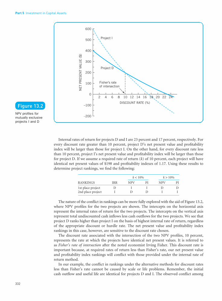
Internal rates of return for projects D and I are 23 percent and 17 percent, respectively. Forevery discount rate greater than 10 percent, project D’s net present value and profitabilityindex will be larger than those for project I. On the other hand, for every discount rate lessthan 10 percent, project I’s net present value and profitability index will be larger than thosefor project D. If we assume a required rate of return (k) of 10 percent, each project will haveidentical net present values of $198 and profitability indexes of 1.17. Using these results todetermine project rankings, we find the following:
k < 10% k > 10%
RANKINGS IRR NPV PI NPV PI
1st place project D I I D D2nd place project I D D I I
The nature of the conflict in rankings can be more fully explored with the aid of Figure 13.2,where NPV profiles for the two projects are shown. The intercepts on the horizontal axis represent the internal rates of return for the two projects. The intercepts on the vertical axisrepresent total undiscounted cash inflows less cash outflows for the two projects. We see thatproject D ranks higher than project I on the basis of highest internal rate of return, regardlessof the appropriate discount or hurdle rate. The net present value and profitability index rankings in this case, however, are sensitive to the discount rate chosen.
The discount rate associated with the intersection of the two NPV profiles, 10 percent, represents the rate at which the projects have identical net present values. It is referred to as Fisher’s rate of intersection after the noted economist Irving Fisher. This discount rate isimportant because, at required rates of return less than Fisher’s rate, our net present value and profitability index rankings will conflict with those provided under the internal rate ofreturn method.
In our example, the conflict in rankings under the alternative methods for discount ratesless than Fisher’s rate cannot be caused by scale or life problems. Remember, the initial cash outflow and useful life are identical for projects D and I. The observed conflict among
Part 5 Investment in Capital Assets
332
••
Figure 13.2NPV profiles formutually exclusiveprojects I and D
FUNO_C13.qxd 9/19/08 17:03 Page 332

methods is due to different implicit assumptions with respect to the reinvestment rate onintermediate cash flows released from the projects. Each of the discounted cash flow methodsimplicitly assumes that the project’s cash inflows can be reinvested at the rate employed bythat method to discount cash flows. Thus the internal rate of return method implicitlyassumes that funds can be reinvested at the internal rate of return over the remaining life ofthe project. The net present value and profitability index methods, however, implicitly assumereinvestment at a rate equivalent to the required rate of return used as the discount rate.
With the internal rate of return method, then, the implicit reinvestment rate will differfrom project to project depending on the pattern of the cash-flow stream for each proposalunder consideration. For a project with a high internal rate of return, a high reinvestment rateis assumed. For a project with a low internal rate of return, a low reinvestment rate is inferred.Only if two projects had the same internal rate of return would the reinvestment rates be identical. With the net present value method, however, the implicit reinvestment rate –namely, the required rate of return – is the same for each project. In essence, this reinvestmentrate represents the minimum return on opportunities available to the firm. This single ratemore accurately reflects the marginal rate of return that the firm can expect to earn on anymarginal funds available to it. Thus, when mutually exclusive projects rank differently becauseof cash-flow-pattern differences, the net present value rankings should be used. In this fashionwe can identify the project that adds most to shareholder wealth.
Differences in Project Lives. A final project difference that might lead to a conflict in project rankings concerns mutually exclusive projects with unequal useful lives. The key question here is: What happens at the end of the shorter-lived project? Most likely, the firmwill either (1) replace the investment with an identical (or similar) project, or (2) reinvest in some other project or projects. We will explore the former situation in Appendix B at the end of this chapter. There we will view the choice as one involving a series of project replications – or a “replacement chain” – of the respective alternatives over some commoninvestment horizon. The second situation, where alternative projects would not be replacedat the end of their useful lives, is considered here.
As an example, suppose that you are faced with choosing between two mutually exclusiveinvestment projects, X and Y, that have the following patterns of cash flows:
NET CASH FLOWS
END OF YEAR PROJECT X PROJECT Y
0 −$1,000 −$1,0001 0 2,0002 0 03 3,375 0
Internal rates of return for projects X and Y are 50 percent and 100 percent, respectively. Ifthe required rate of return is 10 percent, the net present value of project X is $1,536, and itsprofitability index is 2.54. For project Y the net present value is $818 with a correspondingprofitability index of 1.82. Summarizing our results, we have
IRR NPV AT 10% PI AT 10%
Project X 50% $1,536 2.54Project Y 100% $ 818 1.82
Ranking the projects based on our results reveals
RANKINGS IRR NPV AT 10% PI AT 10%
1st place project Y X X2nd place project X Y Y
13 Capital Budgeting Techniques
333
••
FUNO_C13.qxd 9/19/08 17:03 Page 333

Once again we see a conflict in project rankings among the alternative methods. By now wehope that your inclination is to base your choice on the net present value method – that is, tochoose the project that adds the greatest absolute increment in value to the firm. In that caseyou would choose project X. However, you may be bothered by the following facts: (1) project Y’s IRR is twice that of project X, and yet it costs the same amount, namely, $1,000;(2) you have to wait three years to get any positive cash flow from project X, whereas projectY provides all of its cash flow after just one year; and (3) you could put project Y’s positivecash flow to work for you all the while project X produced nothing.
To see that the net present value method will lead to the proper rankings even when facedwith mutually exclusive projects possessing unequal lives, we can compare the projects as of a common termination date. To do so, we assume that the shorter-lived project’s cash flowsare reinvested up to the termination date of the longer-lived project at the firm’s required rate of return (i.e., its opportunity cost of capital). We use this reinvestment rate, as opposedto some higher rate, because this is the rate we assume that the firm would be able to earn onthe next-best (marginal) project when additional funds are made available.
Because projects X and Y each require the same initial cash outlay, we can compare thesetwo projects on the basis of terminal values. Notice that on this basis project X, the projectwith higher NPV, is preferred because its terminal value of $3,375 is higher than the $2,420terminal value for project Y. Also, whether the projects had equivalent initial cash outlays ornot, we could always rank the projects by net present values based on terminal values and ini-tial cash outflows. Notice that project Y’s net present value does not change when we switchfrom actual cash flows to imputed flows. This is because we have used the same required rateof return for both compounding and discounting. Thus net present values based on actualcash flows for mutually exclusive projects with unequal lives will still produce correct projectrankings. In this case, project X is preferred over project Y because it has a positive net present value and adds $718/($1,536 − $818) more in present value to the firm.
l l l Multiple Internal Rates of ReturnA potential problem with the internal rate of return method that we have yet to mention isthat multiple internal rates of return are possible. A necessary, but not sufficient, conditionfor this occurrence is that the cash-flow stream changes sign more than once. For example,the pattern −, +, +, − reveals two changes in sign – from minus to plus and from plus to minus.All of our examples so far depicted conventional cash-flow patterns, where a cash outflow wasfollowed by one or more cash inflows. In other words, there was but one change in sign (fromminus to plus), which ensured a unique internal rate of return. However, some projects,which we could label as nonconventional, involve multiple changes in sign. For example, at the end of a project there may be a requirement to restore the environment. This often happens in an extractive industry like strip mining, where land must be reclaimed at the endof the project. Additionally, with a chemical plant there are often sizable dismantling costs.Whatever the cause, these costs result in a cash outflow at the end of the project, and hence in more than one change in sign in the cash-flow stream.
Part 5 Investment in Capital Assets
334
••
FUNO_C13.qxd 9/19/08 17:03 Page 334

Whether these changes in sign cause more than one internal rate of return also depends on the magnitudes of the cash flows. Because the relationship is complicated and requiresillustration, we address the problem in detail in Appendix A at the end of the chapter. Mostprojects have only one change in sign in the cash-flow stream, but some have more. When thisoccurs, the financial manager must be alert to the possibility of multiple internal rates ofreturn. As shown in Appendix A, no one internal rate of return makes sense economicallywhen there are multiple internal rates of return. Therefore an alternative method of analysismust be used.
When multiple IRR situations are analyzed, calculators and computer programs are oftenfooled and produce only one IRR. Perhaps the best way to determine whether a problem existsis to calculate the net present value of a project at various discount rates. If the discount rate were increased from zero in small increments up to 1,000 percent, for instance, an NPVprofile similar to that shown in Figure 13.2 could be plotted. If the NPV profile line connect-ing the dots crosses the horizontal axis more than once, you have a multiple IRR problem.
Summary of Shortcomings of the IRR Method. We have seen that the net present valuemethod always provides correct rankings of mutually exclusive investment projects, whereasthe internal rate of return method sometimes does not. With the IRR method, the implicitreinvestment rate will differ depending on the cash-flow stream for each investment proposalunder consideration. With the net present value method, however, the implicit reinvestmentrate – namely, the required rate of return – is the same for each investment.
In addition, the net present value method takes into account differences in the scale andlife of each investment. If our objective is truly value maximization, the only theoretically
13 Capital Budgeting Techniques
335
••
The two disciplines have often worked at cross-purposes or have simply failed to understand each other’s needs.
How are leading companies restructuring themselvesto better align marketing with finance? For one,
they are changing the very way they talk to one another.Traditionally, marketing talked about brand-building,awareness and customer satisfaction. Obviously, that terminology had little to do with the language financewas comfortable with – hard numbers like sales figures,shareholder value and return on investment (ROI).
Conversations between the two disciplines could takeon an “Alice in Wonderland” quality. Marketing mightsay that the objective of a program was to drive brandawareness. Meanwhile, finance would want to knowwhat moving brand awareness 10 points would do toshareholder value. Marketers didn’t have the answer.Marketers not only didn’t think in those terms; theylacked the tools to address the questions.
Pioneering companies are developing the capabilitiesto make marketing accountable as they shift their organizational mindset regarding marketing. At many of the author’s firm’s Fortune 500 clients, for example,marketing has moved from being viewed as an expenseto an investment. To that end, these leading companiesare building formal organizational and informal humanconnections between the two disciplines.
In some cases, a dedicated finance person is being placedwithin marketing; in others, marketing has added afinance person. Whatever the structure, however, a con-structive dialogue is now taking place between financeand marketing. Now, when marketing presents a budget,it understands that it needs to deliver a set amount of salesas determined by the CFO. And if the CFO later decidesto cut the budget, marketing has the knowledge to tellthe CFO what sales will be under the smaller budget.
“Marketing and corporate strategy are now our keypartners, because we need to be aligned to achieve ourcorporate objectives,” says the vice president of financeat the Fortune 500 cosmetics company. “Another reasonfor the partnership is the need to get the buy-in for ourgrowth strategy, and ensure that marketing activities aretreated as an investment and not just as an expense.”
Bridging the Finance-Marketing Divide
Source: Adapted from Ed See, “Bridging the Finance-Marketing Divide,” Financial Executive (July/August 2006), pp. 50–53. (www.financialexecutives.org) © Copyright 2006 by Financial Executives International Incorporated. Used by permission. All rights reserved.
FUNO_C13.qxd 9/19/08 17:03 Page 335

correct opportunity cost of funds is the required rate of return. It is consistently applied withthe net present value method, thereby avoiding the reinvestment rate problem. Finally, thepossibility of multiple rates of return hurts the case for the internal rate of return method.
With all these criticisms, why is the IRR method used at all? The reason is that many managers find the internal rate of return easier to visualize and interpret than they do the net present value measure. One does not have to initially specify a required rate of return inthe calculations. To the extent that the required rate of return is but a rough estimate, theinternal rate of return method may permit a more satisfying comparison of projects for the typical manager. Put another way, managers feel comfortable with a return measure asopposed to an absolute net present value figure. As long as the company is not confrontedwith many mutually exclusive projects or with unusual projects having multiple sign changesin the cash-flow stream, the internal rate of return method may be used with reasonableconfidence. When this is not the case, the shortcomings just discussed must be borne in mind.Either modifications in the internal rate of return method (see Appendix A to this chapter for a discussion) or a switch to the net present value method (perhaps augmented by an NPVprofile) needs to occur.
l l l Capital RationingThe final potential difficulty related to implementing the alternative methods of project evaluation and selection that we will discuss concerns capital rationing. Capital rationingoccurs any time there is a budget ceiling, or constraint, on the amount of funds that can beinvested during a specific period, such as a year. Such constraints are prevalent in a numberof firms, particularly in those that have a policy of internally financing all capital expenditures.Another example of capital rationing occurs when a division of a large company is allowed to make capital expenditures only up to a specified budget ceiling, over which the divisionusually has no control. With a capital rationing constraint, the firm attempts to select thecombination of investment proposals that will provide the greatest increase in the value of thefirm subject to not exceeding the budget ceiling constraint.
When capital is rationed over multiple periods, several alternative (and rather compli-cated) methods of handling constrained maximization can be applied to the capital rationingproblem. These methods make use of linear, integer, or goal programming.
If capital is to be rationed for only the current period, the problem is reduced to selectingthose projects that add the greatest increment in value per dollar of investment without sur-passing the budget ceiling. Assume, for example, that your firm faces the following investmentopportunities:
PROJECT INITIAL CASH OUTFLOW IRR NPV PI
A $50,000 15% $12,000 1.24B 35,000 19 15,000 1.43C 30,000 28 42,000 2.40D 25,000 26 1,000 1.04E 15,000 20 10,000 1.67F 10,000 37 11,000 2.10G 10,000 25 13,000 2.30H 1,000 18 100 1.10
If the budget ceiling for initial cash outflows during the present period is $65,000 and the pro-posals are independent of each other, you would want to select the combination of proposalsthat provides the greatest increase in firm value that $65,000 (or less) can provide. Selectingprojects in descending order of profitability according to the various discounted cash flowmethods until the $65,000 budget is exhausted reveals the following:
Part 5 Investment in Capital Assets
336
••
Capital rationingA situation where aconstraint (or budgetceiling) is placed on the total size ofcapital expendituresduring a particularperiod.
FUNO_C13.qxd 9/19/08 17:03 Page 336

INITIALPROJECT IRR NPV OUTFLOW
F 37% $11,000 $10,000C 28 42,000 30,000D 26 1,000 25,000
$54,000 $65,000
With capital rationing, you would accept projects C, E, F, and G, totaling $65,000 in initialoutflows. No other mix of available projects will provide a greater total net present value thanthe $76,000 that these projects provide. Because of the budget constraint, you cannot neces-sarily invest in all proposals that increase the net present value of the firm; you invest in anacceptable proposal only if the budget constraint allows such an investment. As you can see,selecting projects by descending order of profitability index (the ratio of the present value offuture net cash flows over the initial cash outflow) allows you to select the mix of projects thatadds most to firm value when operating under a single-period budget ceiling. This is becausethe problem boils down to selecting that mix of projects that gives you “the biggest bang forthe buck” – exactly what ranking projects by profitability index reveals.2
A budget ceiling carries a real cost when it bars us from taking advantage of any additionalprofitable opportunities. In our example, a number of opportunities were forgone by theimposition of the $65,000 budget ceiling. We were prohibited from taking projects A, B, D,and H even though they would have added $28,100 ($12,000 + $15,000 + $1,000 + $100) invalue to the firm.
It should come as no surprise, then, that capital rationing usually results in an investmentpolicy that is less than optimal. From a theoretical standpoint, a firm should accept all projects yielding more than the required rate of return. By doing so, it will increase the marketprice per share of its common stock because it is taking on projects that will provide a returnhigher than necessary to maintain the present market price per share. This propositionassumes that the firm actually can raise capital, within reasonable limits, at the required rateof return. Certainly, unlimited amounts of capital are not available at any one cost. However,most firms are involved in a more or less continuous process of making decisions to under-take capital expenditures and to finance these expenditures. Given these assumptions the firmshould accept all proposals yielding more than the required rate of return and raise capital tofinance these proposals at that approximate real cost. Without doubt, there are circumstancesthat complicate the use of this rule. In general, however, this policy should tend to maximizethe market price of the firm’s stock over the long run. If the firm rations capital and rejectsprojects that yield more than the required return, the firm’s investment policy is, by defini-tion, less than optimal. Management could increase the value of the firm to the shareholdersby accepting these rejected value-creating projects.
13 Capital Budgeting Techniques
337
••
INITIALPROJECT NPV OUTFLOW
C $42,000 $30,000B 15,000 35,000
$57,000 $65,000
INITIALPROJECT PI NPV OUTFLOW
C 2.40 $42,000 $30,000G 2.30 13,000 10,000F 2.10 11,000 10,000E 1.67 10,000 15,000
$76,000 $65,000
2Sometimes a firm may not be able to utilize its full capital budget by selecting projects on the basis of descendingorder of profitability index because the next best acceptable project is too large. When this situation occurs the firmmay be better off searching for another combination of projects (perhaps including some smaller ones in place of alarger one) that will use up more of the capital budget while still increasing the net present value of the total groupof projects accepted. (See end-of-chapter Problem 8 for an example.)
FUNO_C13.qxd 9/19/08 17:03 Page 337

l l l Single-Point EstimatesTraditional capital budgeting analysis, as we have seen, places an emphasis on a series of single-point estimates for inputs like the “yearly change in net operating revenue,” “installa-tion cost,” “final salvage value,” etc. Sensitivity analysis allows us to challenge those single-point estimates and ask a series of “what if ” questions. “What if ” a particular input estimateshould actually be higher or lower than we originally thought? As input variable estimates arechanged from an original set of estimates (called the base case), their impact on a project’smeasured results, such as net present value (NPV), can be determined.
Knowing the sensitivity of a project’s value to capital budgeting input variables makes youbetter informed. Armed with this information, you can then decide whether any estimatesneed refining or reviewing, and whether any are not worth investigating further before decid-ing on project acceptance/rejection. Also, for accepted projects, sensitivity analysis can helpyou identify which variables may warrant monitoring.
Sensitivity analysis can be especially helpful in addressing uncertainties surrounding a project’s “initial cash outlay (ICO).”3 In a typical capital budgeting analysis, a project’s ICO isgenerally treated as a single, certain cash outflow. However, upon closer inspection, the ICOmay have several cash outflow components – e.g., land, buildings, machinery and equipment.Some of the ICO components may be certain cash flows and some may be uncertain/riskycash flows. Some ICO components may not be subject to tax depreciation (e.g., land). OtherICO components may be subject to tax depreciation (e.g., equipment, capitalized shippingand installation costs) and these outflows will have multi-year spillover effects on operatingcash flows because of their depreciation tax shield.
Example of Sensitivity Analysis. To illustrate the use of sensitivity analysis as it applies tocapital budgeting decisions, let’s revisit the Faversham Fish Farm fish-flaking facility project.In Chapter 12, we calculated the incremental net cash flows for the project. And, earlier in thischapter, we saw how those same cash flows led to a net present value, at the firm’s 12 percentcost of capital, of $10,768.
Sensitivity analysis can be applied to our fish-flaking project to answer a series of “what if ”questions. What if, for example, our Chapter 12 estimates for net operating revenue cash flowsin years 1 through 4 – $35,167, $36,250, $55,725, and $33,258, respectively – should really behigher/lower? What if our final salvage value estimate of $16,500 should be higher/lower? Andwhat if shipping and installation is higher/lower than the $10,000 we originally thought?
To answer those “what if ” questions, we first perform new NPV calculations in which wechange our three variables of concern (shipping and installation, final salvage value, andyearly net operating revenue cash flows) individually by, for example, −15%, −10%, −5%,+5%, +10%, and +15%. (Note that changes in these variables can have spillover effects onother variables such as depreciation and taxes.) The results are then compared with the resultswith the unchanged (base case) data and shown in Table 13.1.
Part 5 Investment in Capital Assets
338
••
Table 13.1Sensitivity analysis for fish-flaking facilityshowing the impact ofindividual changes inthree input variableson the project’s netpresent value (NPV)
CHANGE IN ORIGINAL VARIABLE VALUE
VARIABLE −15% −10% −5% Base +5% +10% +15%
Shipping and installation $11,785 $11,447 $11,107 $10,768 $10,429 $10,089 $ 9,751Final salvage value 9,824 10,139 10,453 10,768 11,083 11,398 11,713Yearly net operating
revenue cash flows (78) 3,539 7,154 10,768 14,382 17,997 21,614
Sensitivity analysisType of “what if”uncertainty analysis in which variables or assumptions arechanged from a basecase in order todetermine theirimpact on a project’smeasured results,such as net presentvalue (NPV) or internalrate of return (IRR).
3For a full discussion of a proper capital budgeting analysis that incorporates the additional risk due to ICO un-certainties see Michael C. Ehrhardt and John M. Wachowicz, Jr., “Capital Budgeting and Initial Cash Outlay (ICO)Uncertainty,” Financial Decisions 18 (Summer 2006, Article 2: 1–16). (www.financialdecisionsonline.org/current/EhrhardtWachowicz.pdf).
FUNO_C13.qxd 9/19/08 17:03 Page 338

From Table 13.1 we can see that −15 to +15 percent changes in estimates for shipping andinstallation, as well as final salvage value, do not change the resulting net present values verymuch from the base case value of $10,768. However, if estimated yearly net operating revenuecash flows drop by roughly 15 percent or more from the base case, our project’s net presentvalue turns negative.
The data contained in Table 13.1 can also be presented graphically in an NPV sensitivitygraph – see Figure 13.3. Notice the three “sensitivity lines” in the NPV sensitivity graph. The “yearly net operating revenue cash flows” line has the steepest slope. Therefore NPV ismore sensitive to equal percentage changes in that variable than in “final salvage value” or“shipping and installation.” Based on this information, management may want to concen-trate more forecasting and/or monitoring efforts on the seemingly more critical “yearly net operating revenue cash flows” variable.
TIP•TIP
Take another look at the NPV profile contained in Figure 13.1. Notice how this graph canalso be viewed as a type of “sensitivity line,” showing the sensitivity of NPV to changes in the cost of capital assumption.
One potential problem with our sensitivity analysis, so far, is that it has looked at sensitiv-ity “one variable at a time.” It has ignored relationships among variables. That is a drawbackto the method. However, one way to judge the sensitivity of our results to simultaneouschanges in two variables, at least, is to construct an NPV sensitivity matrix. Table 13.2 is onesuch sensitivity matrix that depicts NPV results for combinations of changes in two inputestimates – “final salvage value” and “yearly net operating revenue cash flows.”
Sensitivity analysis, as we have seen, provides simple to understand, useful knowledge aboutthe sensitivity of a project’s NPV to a change in one (or more) input variables. However, noticethat our approach has said nothing about the “likelihood” of a change in any input variable.A steep slope to a sensitivity line for a particular variable, for example, may not be a problemif that variable’s estimate is not likely to change. Even more insights are possible when the
13 Capital Budgeting Techniques
339
••
Figure 13.3NPV sensitivity graphfor the FavershamFish Farm fish-flakingfacility project
FUNO_C13.qxd 9/19/08 17:03 Page 339

••
Part 5 Investment in Capital Assets
340
range of likely values that our variables could take on, as reflected in their probability distribu-tions, is considered. In Chapter 14, therefore, we will take a more rigorous, quantitative lookat the “riskiness” of an investment project and consider probability distribution information.
Project Monitoring: Progress Reviews and Post-Completion AuditsThe capital budgeting process should not end with the decision to accept a project. Continualmonitoring of the project is the necessary next step to help ensure project success. Therefore,companies should perform progress reviews followed by post-completion audits for all largeprojects; strategically important projects, regardless of size; and a sample of smaller projects.Progress reviews, or status reports, can provide, especially during the implementation phaseof a project, early warnings of potential cost overruns, revenue shortfalls, invalid assump-tions, and outright project failure. Information revealed through progress reviews may lead to revised forecasts, remedial actions to improve performance, or project abandonment.
Post-completion audits allow management to determine how close the actual results of an implemented project have come to its original estimates. When they are used properly,progress reviews and post-completion audits can help identify forecasting weaknesses and any important factors that were omitted. With a good feedback system, any lessons learnedcan be used to improve the quality of future capital budgeting decision making.
Monitoring of a project can also have important psychological effects on managers. Forexample, if managers know in advance that their capital investment decisions will be mon-itored, they will be more likely to make realistic forecasts and to see that original estimates aremet. In addition, managers may find it easier to abandon a failing project within the contextof a formal review process. Finally, it is useful for managers to set milestones for a project andto agree in advance to abandon it if these milestones are not met.
Key Learning Pointsl We began our discussion of capital budgeting in
Chapter 12 with the assumption that the acceptanceof any investment proposal would not change the totalbusiness-risk complexion of the firm. This assump-tion allowed us to use a single required rate of returnin judging whether or not to accept a project.
l Four alternative methods of project evaluation andselection were discussed. The first was a simple addi-tive method for assessing the worth of a project called
the payback period. The remaining three methods(internal rate of return, net present value, and profit-ability index) were all discounted cash flow techniques.
l The payback period (PBP) of an investment tells us thenumber of years required to recover our initial cashinvestment. Although this measure provides a roughguide to the liquidity of a project, it is a poor gauge ofprofitability. It falls short as a measure of profitabilitybecause it (1) ignores cash flows occurring after the
Post-completion auditA formal comparisonof the actual costsand benefits of aproject with originalestimates. A keyelement of the auditis feedback: that is,results of the auditare given to relevantpersonnel so thatfuture decisionmaking can beimproved.
Table 13.2Sensitivity matrix forfish-flaking facilityshowing the impact of simultaneouschanges in two inputvariables on theproject’s net presentvalue (NPV)
CH
AN
GE
IN
YE
AR
LY
NE
T O
PE
RA
TIN
G
RE
VE
NU
E C
ASH
FLO
WS
CHANGE IN FINAL SALVAGE VALUE
−15% −10% −5% Base +5% +10% +15%
−15% ($ 1,022) ($ 707) ($ 393) ($ 78) $ 237 $ 552 $ 867
−10% 2,595 2,910 3,224 3,539 3,854 4,169 4,484
−5% 6,218 6,525 6,839 7,154 7,469 7,784 8,099
Base 9,824 10,139 10,453 10,768 11,083 11,398 11,713
+5% 13,438 13,753 14,067 14,382 14,697 15,012 15,327
+10% 17,053 17,368 17,682 17,997 18,312 18,627 18,942
+15% 20,670 20,985 21,299 21,614 21,929 22,244 22,559
FUNO_C13.qxd 9/19/08 17:03 Page 340

••
341
13 Capital Budgeting Techniques
expiration of the payback period, (2) ignores the time value of money, and (3) makes use of a crudeacceptance criterion, namely, a subjectively determined cutoff point.
l The internal rate of return (IRR) for an investmentproposal is the discount rate that equates the presentvalue of the expected net cash flows with the initial cashoutflow. If a project’s IRR is greater than or equal to arequired rate of return, the project should be accepted.
l The net present value (NPV) of an investment pro-posal is the present value of the proposal’s net cashflows less the proposal’s initial cash outflow. If a project’s NPV is greater than or equal to zero, the project should be accepted.
l The profitability index (PI), or benefit-cost ratio, of aproject is the ratio of the present value of future netcash flows to the initial cash outflow. If a project’s PIis greater than or equal to 1.00, the project should beaccepted.
l When two or more investment proposals are mutuallyexclusive, so that we can select only one, ranking pro-posals on the basis of the IRR, NPV, and PI methodsmay give contradictory results. If a conflict in rank-ings occurs, it will be due to one or a combination of the following three project differences: (1) scale ofinvestment, (2) cash-flow pattern and (3) project life.In every case, the net present value rankings can beshown to lead to the correct project selection. In
short, if net present value rankings are used, projectsthat are expected to add the greatest increment in dollar value to the firm will be chosen.
l A potential problem with the internal rate of returnmethod is that multiple internal rates of return mightoccur for nonconventional projects – projects whosecash-flow streams show multiple changes in sign.When there are multiple rates of return, an alternativemethod of analysis must be used.
l Capital rationing occurs any time there is a budgetceiling, or constraint, on the amount of funds that canbe invested during a specific period, such as a year.When capital is rationed over multiple periods, sev-eral alternative (and rather complicated) methods canbe applied to the capital rationing problem. If capitalis to be rationed for only the current period, select-ing projects by descending order of profitability indexgenerally leads to a selection of a project mix that addsmost to firm value.
l Sensitivity analysis allows us to change input variableestimates from an original set of estimates (called thebase case) and determine their impact on a project’smeasured results, such as net present value (NPV) orinternal rate of return (IRR).
l It is important to monitor projects continually to helpensure project success. Therefore companies shouldperform progress reviews followed by post-completionaudits.
Appendix A Multiple Internal Rates of Return
Certain nonconventional cash-flow streams may have more than one internal rate of return.To illustrate the problem, suppose that we are considering an investment proposal consistingof a new, more effective, oil pump that will remove a fixed quantity of oil out of the groundmore quickly than our existing pump.4 This investment would require an initial cash outflowof $1,600 for the new pump. Our older, slower pump would provide cash flows of $10,000 ineach of the next two years. However, our new pump would produce a cash flow of $20,000 inone year, after which our oil supply is exhausted. Salvage value for both pumps is negligible.The calculations necessary to determine the appropriate incremental net cash flows due to thepump replacement are as follows:
END OF YEAR
0 1 2
(a) New pump’s cash flows −$1,600 $20,000 0(b) Old pump’s cash flows 0 $10,000 $10,000(c) Net cash flows due to
pump replacement Line (a) – Line (b) −$1,600 $10,000 −$10,000
4This problem is adapted from James H. Lorie and Leonard J. Savage, “Three Problems in Rationing Capital.” Journalof Business 28 (October 1955), 229–239.
FUNO_C13.qxd 9/19/08 17:03 Page 341

••
Part 5 Investment in Capital Assets
342
On an incremental basis, then, the net cash flows resulting from the increased efficiency of the new pump are −$1,600, + $10,000, and −$10,000. When we solve for the internal rateof return for the cash-flow stream, we find that it is not one rate but two: 25 percent and 400 percent.
Take Note
when IRR = 0.25 or 4.0
This unusual situation is illustrated in Figure 13A.1, which consists of this nonconven-tional proposal’s NPV profile. At a 0 percent discount rate, the net present value of the project is simply the sum of all the cash flows. It is −$1,600 because total cash outflows exceedtotal cash inflows. As the discount rate increases, the present value of the second-year outflowdiminishes with respect to the first-year inflow, and the net present value of the proposalbecomes positive when the discount rate exceeds 25 percent. As the discount rate increasesbeyond 100 percent, the present value of all future cash flows (years 1 and 2) diminishes rela-tive to the initial outflow of −$1,600. At 400 percent, the net present value again becomes zero.
This type of proposal differs from the usual case, shown previously in Figure 13.1, in whichnet present value is a decreasing function of the discount rate and in which there is but oneinternal rate of return that equates the present value of the future net cash flows with the initial cash outflow. A nonconventional proposal may have any number of internal rates ofreturn depending on the cash-flow pattern. Consider the following series of cash flows:
END OF YEAR
0 1 2 3
Cash flows −$1,000 $6,000 −$11,000 $6,000
In this example, discount rates of 0, 100, and 200 percent result in the net present value of all cash flows equaling zero.
$ $ )
$ )
1,60010,000
(110,000
(11 2=
+−
+IRR IRR
Figure 13A.1NPV profile for pumpreplacement proposalshowing two internalrates of return
FUNO_C13.qxd 9/19/08 17:03 Page 342

••
343
13 Capital Budgeting Techniques
The number of possible internal rates of return has an upper limit equal to the number ofreversals of sign in the cash-flow stream. In the example, we have three reversals and, it justso happens, three internal rates of return. Although a multiple reversal in signs is a necessarycondition for multiple internal rates of return, it is not sufficient for such an occurrence. Theoccurrence of multiple internal rates of return also depends on the magnitude of cash flows.For the following series of cash flows, there is but one internal rate of return (32.5 percent),despite two reversals of sign:
END OF YEAR
0 1 2
Cash flows −$1,000 $1,400 −$100
When confronted with a proposal having multiple rates of return, how does one decidewhich is the correct rate? In our first example, is the correct rate 25 percent or 400 percent?Actually, neither rate is correct, because neither is a measure of investment worth. If the firm’s required rate of return is 20 percent, should the investment be accepted? Despite thefact that both internal rates of return are greater than the required rate of return, a glance atFigure 13A.1 is enough to reveal that at a 20 percent discount rate the project has a negativenet present value (−$211) and, therefore, should not be accepted.
= $8,333 − $6,944 − $1,600 = −$211
An alternative way to view the pump problem is that the firm is being offered the chanceto accelerate the receipt of the cash flow of the second year by one year in exchange for payinga $1,600 fee. The relevant question then becomes: What is it worth to the firm to have the useof $10,000 for one year? This question, in turn, depends on the rate of return on investmentopportunities available to the firm for that period of time. If the firm could earn 20 percenton the use of these funds and realize these earnings at the end of the period, the value of thisopportunity would be $2,000, to be received at the end of the second year. The present valueof this $2,000 at a 20 percent discount rate is $1,389 ($2,000/(1 + 0.20)2) – which, when addedto the $1,600 outflow, yields, once again, a net present value of −$211. Similarly, other projects having multiple rates of return are best evaluated using a net present value approach.
Appendix B Replacement Chain Analysis
In this chapter we noted that it was possible to encounter a conflict in project rankings formutually exclusive projects with unequal useful lives. The key question is: What happens atthe end of the shorter-lived project? Most likely, the firm will either (1) replace the investmentwith an identical (or similar) project, or (2) reinvest in some other projects. We saw that,where alternative projects would not be replaced at the end of their useful lives (the latter situation), we do not need to take future investment decisions into account. In these cases wesimply choose the project with the highest net present value.
We now turn our attention to the former situation. Here we are faced with a choicebetween mutually exclusive investments having unequal lives that will require replacements.For example, we may need to purchase one of two alternative machines – with one machinebeing more durable and, therefore, having a longer useful life than the other. Because sub-sequent decisions are affected by the initial investment, the sequence of decisions associatedwith each alternative must be evaluated. This evaluation generally views the choice as oneinvolving a series of replications – or “replacement chain” – of respective alternatives oversome common investment horizon.
NPV =+
−+
− $ )
$ )
10,000
(1 0.2010,000
(1 0.20$1,600
1 2
FUNO_C13.qxd 9/19/08 17:03 Page 343

••
Part 5 Investment in Capital Assets
344
Replacement Chain (Common Life) Approach
Repeating each project until the earliest date that we can terminate each project in the sameyear results in multiple like-for-like replacement chains covering the shortest common life. Atthe conclusion of each chain, the firm thus has identical options regardless of which choicewas made initially.
Then, we solve for the net present value of each replacement chain, NPVchain, according tothe following formula:
(13B.1)
where n = single-replication project life, in yearsNPVn = single-replication net present value for a project with an n-year useful life
R = number of replications needed to provide the shortest common life, (R) × (n), forall mutually exclusive alternatives under consideration
k = appropriate project-specific discount rateIn effect, the firm realizes a net present value at the beginning of each replacement. The valueof each replacement chain, therefore, is simply the present value of the sequence of NPVs generated by that replacement chain.
An IllustrationAssume the following regarding mutually exclusive investment alternatives A and B, both ofwhich require future replacements:
PROJECT A PROJECT B
Single-replication life (n) 5 years 10 yearsSingle-replication net present value calculated at
project-specific required rate of return (NPVn) $5,328 $8,000Number of replications needed to provide the
shortest common life (R) 2 1Project-specific discount rate (k)a 10% 10%
aDiscount rates for alternative projects could differ.
At first glance, project B looks better. Its single-replication net present value of $8,000 is certainly higher than the $5,328 net present value provided by project A. However, the need to make future replacements dictates that we consider the value provided by both alternatives over the same common life – in this case, 10 years. Figure 13B.1 shows how to find the net present value for two replications of project A – a replacement chain 10 years inlength.
NPVNPV
kn
n tt
R
chain 11 1
( ) ( )
=+ −
=∑
Figure 13B.1Time line forcalculating thereplacement chainNPV for project A(NPV5 = $5,328; k = 10%; and R = 2)
FUNO_C13.qxd 9/19/08 17:03 Page 344

345
13 Capital Budgeting Techniques
••
5Notice that we have just discounted the second single-replication NPV of project A at a “risky” 10 percent rate. Theuse of a risky project-specific rate is the procedure most commonly discussed. There may be instances, however, whendiscounting NPVs of future replications to the present at the risk-free rate will be more appropriate. The choice of the discount rate to be used in calculating the net present value of a chain of project replications should dependon the nature of uncertainty (risk) between replications. For a full discussion of this issue and alternative capital budgeting procedures that correctly reflect the nature of risk between replications, see Ronald E. Shrieves and John M. Wachowicz Jr., “Proper Risk Resolution in Replacement Chain Analysis,” The Engineering Economist 34(Winter 1989), 91–114.
The net present value of the replacement chain for project B involves but a single replica-tion and is, therefore, already known; that is, project B’s NPVchain = $8,000. Since
Project A’s NPVchain = $8,636 > Project B’s NPVchain = $8,000
we prefer project A.5
Questions
1. Explain what is meant by the time value of money. Why is a bird in the hand worth two (or so) in the bush? Which capital budgeting approach ignores this concept? Is itoptimal?
2. Why does the payback period bias the process of asset selection toward short-lived assets?
3. Why does the net present value method favor larger projects over smaller ones when usedto choose between mutually exclusive projects? Is this a problem?
4. Contrast the internal rate of return method of project evaluation and selection with thenet present value method. Why might these two discounted cash flow techniques lead toconflicts in project rankings?
5. Although it is conceptually unsound, the payback period is very popular in business as a criterion for assigning priorities to investment projects. Why is it unsound, and why isit popular?
6. What are mutually exclusive investment projects? What is a dependent project?7. Is the economic efficiency of a country enhanced by the use of modern capital budgeting
techniques? Why?8. If capital rationing is not optimal, why would any company use it?9. The internal rate of return method implies that intermediate cash flows are reinvested at
the internal rate of return. Under what circumstances is this assumption likely to lead toa seriously biased measure of the economic return from the project?
10. Some people have suggested combining the payback period (PBP) method with presentvalue analysis to calculate a “discounted” payback period (DPBP). Instead of using cumu-lative inflows, cumulative present values of inflows (discounted at the cost of capital) are used to see how long it takes to “pay” for a project with discounted cash flows. For afirm not subject to a capital rationing restraint, if an independent project’s “discounted”payback period is less than some maximum acceptable “discounted” payback period, theproject would be accepted; if not, it would be rejected. Assume that an independent project’s “discounted” payback period is greater than a company’s maximum acceptable“discounted” payback period but less than the project’s useful life; would rejection of thisproject cause you any concern? Why? Does the “discounted” payback period methodovercome all the problems encountered when using the “traditional” payback periodmethod? What advantages (if any) do you see the net present value method holding overa “discounted” payback period method?
FUNO_C13.qxd 9/19/08 17:03 Page 345

Self-Correction Problems
1. Briarcliff Stove Company is considering a new product line to supplement its range line. It is anticipated that the new product line will involve cash investment of $700,000 at time 0 and $1.0 million in year 1. After-tax cash inflows of $250,000 are expected in year 2, $300,000 in year 3, $350,000 in year 4, and $400,000 each year thereafter throughyear 10. Though the product line might be viable after year 10, the company prefers to be conservative and end all calculations at that time.a. If the required rate of return is 15 percent, what is the net present value of the project?
Is it acceptable?b. What is its internal rate of return?c. What would be the case if the required rate of return was 10 percent?d. What is the project’s payback period?
2. Carbide Chemical Company is considering the replacement of two old machines with anew, more efficient machine. It has determined that the relevant after-tax incrementaloperating cash flows of this replacement proposal are as follows:
END OF YEAR
0 1 2 3
Cash flows −$404,424 $86,890 $106,474 $91,612
END OF YEAR
4 5 6 7 8
Cash flows $84,801 $84,801 $75,400 $66,000 $92,400
What is the project’s net present value if the required rate of return is 14 percent? Is theproject acceptable?
3. The Acme Blivet Company is evaluating three investment situations: (1) produce a newline of aluminum blivets, (2) expand its existing blivet line to include several new sizes, and (3) develop a new, higher-quality line of blivet. If only the project in question is undertaken, the expected present values and the amounts of investment required are asfollows:
INVESTMENT PRESENT VALUE OF PROJECT REQUIRED FUTURE CASH FLOWS
1 $200,000 $290,0002 115,000 185,0003 270,000 400,000
If projects 1 and 2 are jointly undertaken, there will be no economies; the investmentrequired and present values will simply be the sum of the parts. With projects 1 and 3,economies are possible in investment because one of the machines acquired can be used inboth production processes. The total investment required for projects 1 and 3 combined is$440,000. If projects 2 and 3 are undertaken, there are economies to be achieved in mar-keting and producing the products but not in investment. The expected present value offuture cash flows for projects 2 and 3 combined is $620,000. If all three projects are under-taken simultaneously, the economies noted above will still hold. However, a $125,000extension on the plant will be necessary, as space is not available for all three projects.Which project or projects should be chosen?
Part 5 Investment in Capital Assets
346
••
FUNO_C13.qxd 9/19/08 17:03 Page 346
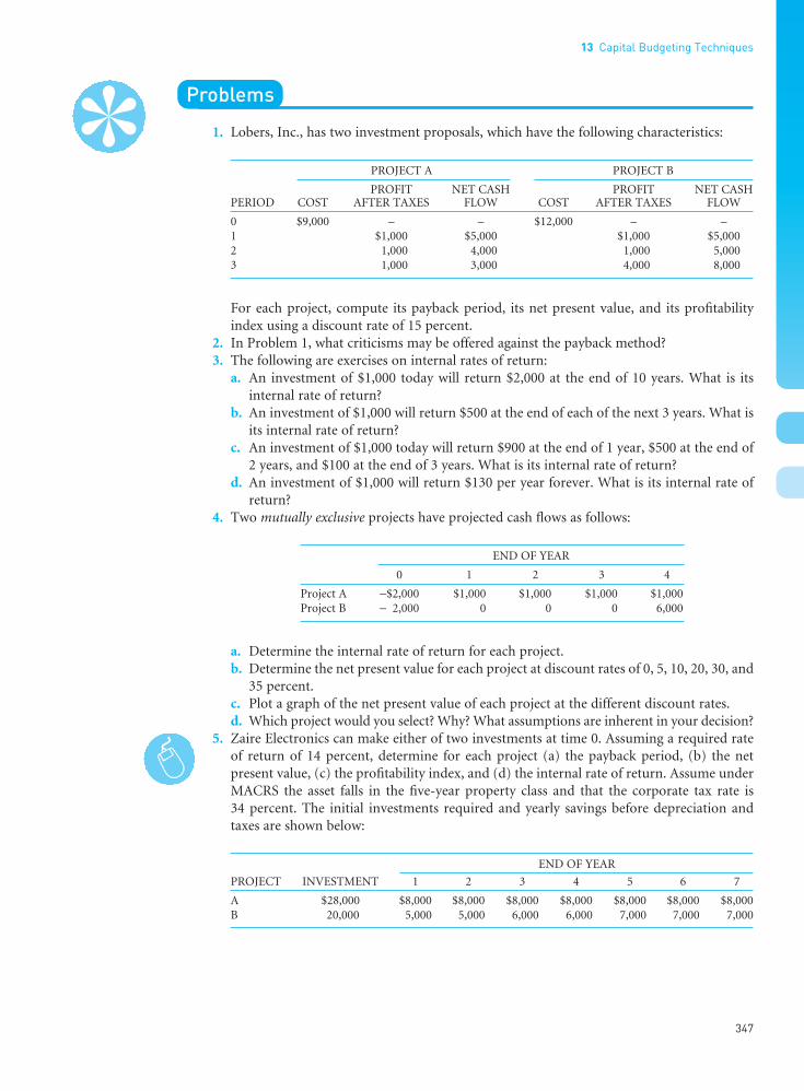
347
13 Capital Budgeting Techniques
••
Problems
1. Lobers, Inc., has two investment proposals, which have the following characteristics:
PROJECT A PROJECT B
PROFIT NET CASH PROFIT NET CASHPERIOD COST AFTER TAXES FLOW COST AFTER TAXES FLOW
0 $9,000 – – $12,000 – –1 $1,000 $5,000 $1,000 $5,0002 1,000 4,000 1,000 5,0003 1,000 3,000 4,000 8,000
For each project, compute its payback period, its net present value, and its profitabilityindex using a discount rate of 15 percent.
2. In Problem 1, what criticisms may be offered against the payback method?3. The following are exercises on internal rates of return:
a. An investment of $1,000 today will return $2,000 at the end of 10 years. What is itsinternal rate of return?
b. An investment of $1,000 will return $500 at the end of each of the next 3 years. What isits internal rate of return?
c. An investment of $1,000 today will return $900 at the end of 1 year, $500 at the end of2 years, and $100 at the end of 3 years. What is its internal rate of return?
d. An investment of $1,000 will return $130 per year forever. What is its internal rate ofreturn?
4. Two mutually exclusive projects have projected cash flows as follows:
END OF YEAR
0 1 2 3 4
Project A −$2,000 $1,000 $1,000 $1,000 $1,000Project B −$2,000 0 0 0 6,000
a. Determine the internal rate of return for each project.b. Determine the net present value for each project at discount rates of 0, 5, 10, 20, 30, and
35 percent.c. Plot a graph of the net present value of each project at the different discount rates.d. Which project would you select? Why? What assumptions are inherent in your decision?
5. Zaire Electronics can make either of two investments at time 0. Assuming a required rateof return of 14 percent, determine for each project (a) the payback period, (b) the net present value, (c) the profitability index, and (d) the internal rate of return. Assume underMACRS the asset falls in the five-year property class and that the corporate tax rate is 34 percent. The initial investments required and yearly savings before depreciation andtaxes are shown below:
END OF YEAR
PROJECT INVESTMENT 1 2 3 4 5 6 7
A $28,000 $8,000 $8,000 $8,000 $8,000 $8,000 $8,000 $8,000B 20,000 5,000 5,000 6,000 6,000 7,000 7,000 7,000
FUNO_C13.qxd 9/19/08 17:03 Page 347

••
Part 5 Investment in Capital Assets
348
6. Thoma Pharmaceutical Company may buy DNA testing equipment costing $60,000. Thisequipment is expected to reduce labor costs of clinical staff by $20,000 annually. Theequipment has a useful life of five years but falls in the three-year property class for costrecovery (depreciation) purposes. No salvage value is expected at the end. The corporatetax rate for Thoma is 38 percent (combined federal and state), and its required rate ofreturn is 15 percent. (If profits after taxes on the project are negative in any year, the firmwill offset the loss against other firm income for that year.) On the basis of this informa-tion, what is the net present value of the project? Is it acceptable?
7. In Problem 6, suppose that 6 percent inflation in cost savings from labor is expected overthe last four years, so that savings in the first year are $20,000, savings in the second yearare $21,200, and so forth.a. If the required rate of return is still 15 percent, what is the net present value of the
project? Is it acceptable?b. If a working capital requirement of $10,000 were required in addition to the cost of
the equipment and this additional investment were needed over the life of the project,what would be the effect on net present value? (All other things are the same as inProblem 7, Part (a).)
8. The Lake Tahow Ski Resort is comparing a half dozen capital improvement projects. It hasallocated $1 million for capital budgeting purposes. The following proposals and associatedprofitability indexes have been determined. The projects themselves are independent ofone another.
PROFITABILITY PROJECT AMOUNT INDEX
1. Extend ski lift 3 $500,000 1.222. Build a new sports shop 150,000 0.953. Extend ski lift 4 350,000 1.204. Build a new restaurant 450,000 1.185. Build addition to housing complex 200,000 1.196. Build an indoor skating rink 400,000 1.05
a. If strict capital rationing for only the current period is assumed, which of the invest-ments should be undertaken? (Tip: If you didn’t use up the entire capital budget, trysome other combinations of projects, and determine the total net present value for each combination.)
b. Is this an optimal strategy?9. The City of San Jose must replace a number of its concrete mixer trucks with new trucks.
It has received two bids and has evaluated closely the performance characteristics of thevarious trucks. The Rockbuilt truck, which costs $74,000, is top-of-the-line equipment.The truck has a life of eight years, assuming that the engine is rebuilt in the fifth year.Maintenance costs of $2,000 a year are expected in the first four years, followed by totalmaintenance and rebuilding costs of $13,000 in the fifth year. During the last three years,maintenance costs are expected to be $4,000 a year. At the end of eight years the truck will have an estimated scrap value of $9,000.
A bid from Bulldog Trucks, Inc., is for $59,000 a truck. Maintenance costs for the truckwill be higher. In the first year they are expected to be $3,000, and this amount is expectedto increase by $1,500 a year through the eighth year. In the fourth year the engine will needto be rebuilt, and this will cost the company $15,000 in addition to maintenance costs inthat year. At the end of eight years the Bulldog truck will have an estimated scrap value of $5,000.a. If the City of San Jose’s opportunity cost of funds is 8 percent, which bid should it
accept? Ignore tax considerations, because the city pays no taxes.b. If its opportunity cost were 15 percent, would your answer change?
FUNO_C13.qxd 9/19/08 17:03 Page 348

349
13 Capital Budgeting Techniques
••
Solutions to Self-Correction Problems
1. a. PRESENT VALUEYEAR CASH FLOW DISCOUNT FACTOR (15%) PRESENT VALUE
0 $ (700,000) 1.000 $(700,000)1 (1,000,000) 0.870 (870,000)2 250,000 0.756 189,0003 300,000 0.658 197,4004 350,000 0.572 200,2005–10 400,000 2.164* 865,600**
Net present value = $(117,800)
*PVIFA of 5.019 for 10 years minus PVIFA of 2.855 for 4 years.**Total for years 5–10.
Because the net present value is negative, the project is unacceptable.b. The internal rate of return is 13.21 percent. If the trial-and-error method were used,
we would have the following:
14% 14% 13% 13% DISCOUNT PRESENT DISCOUNT PRESENT
YEAR CASH FLOW FACTOR VALUE FACTOR VALUE
0 $ (700,000) 1.000 $(700,000) 1.000 $(700,000)1 (1,000,000) 0.877 (877,000) 0.885 (885,000)2 250,000 0.769 192,250 0.783 195,7503 300,000 0.675 202,500 0.693 207,9004 350,000 0.592 207,200 0.613 214,5505–10 400,000 2.302* 920,800** 2.452* 980,800**
Net present value $ (54,250) $ 14,000
*PVIFA for 10 years minus PVIFA for 4 years.**Total for years 5–10.
To approximate the actual rate, we interpolate between 13 and 14 percent as follows:
and IRR = 0.13 + X = 0.13 + 0.0021 = 0.1321, or 13.21 percent. Because the internal rateof return is less than the required rate of return, the project would not be acceptable.
c. The project would be acceptable.d. Payback period = 6 years. (−$700,000 − $1,000,000 + $250,000 + $300,000 + $350,000
+ $400,000 + $400,000 = 0)
XX
0.01$14,000$68,250
Therefore, (0.01) ($14,000)
$68,2500.0021 = =
×=
0.010.13 14,000
04,000
0.14 54,25068,250X
IRR⎡⎣⎢
⎤⎦⎥
⎡
⎣
⎢⎢⎢
⎤
⎦
⎥⎥⎥
$$
$( )$1
FUNO_C13.qxd 9/19/08 17:03 Page 349

••
Part 5 Investment in Capital Assets
350
Aggarwal, Raj. Capital Budgeting Under Uncertainty.Englewood Cliffs, NJ: Prentice Hall, 1993.
Bacon, Peter W. “The Evaluation of Mutually ExclusiveInvestments.” Financial Management 6 (Summer 1977),55–58.
Barwise, Patrick, Paul R. Marsh, and Robin Wensley. “MustFinance and Strategy Clash?” Harvard Business Review 67(September–October 1989), 85–90.
Bierman, Harold, Jr., and Seymour Smidt. The CapitalBudgeting Decision, 8th ed. New York: Macmillan, 1993.
Block, Stanley. “Are There Differences in Capital BudgetingProcedures Between Industries? An Empirical Study.” TheEngineering Economist 50 (January–March 2005), 55–67.
Brounen, Dirk, Abe de Jong, and Kees Koedijk. “CorporateFinance in Europe: Confronting Theory with Practice.”Financial Executive 33 (Winter 2004), 71–101.
Ehrhardt, Michael C., and John M. Wachowicz, Jr. “CapitalBudgeting and Initial Cash Outlay (ICO) Uncertainty.”Financial Decisions 18 (Summer 2006), Article 2: 1–16(available online at www.financialdecisionsonline.org/current/EhrhardtWachowicz.pdf).
Gitman, Lawrence J., and Pieter A. Vandenberg. “Cost ofCapital Techniques Used by Major US Firms: 1997 vs.1980.” Financial Practice and Education 10 (Fall/Winter2000), 53–68.
Gordon, Lawrence A., and Mary D. Myers. “PostauditingCapital Projects: Are You in Step with the Competition?”Management Accounting 72 (January 1991), 39–42.
Graham, John, and Campbell Harvey. “How Do CFOs MakeCapital Budgeting and Capital Structure Decisions?” Journalof Applied Corporate Finance 15 (Spring 2002), 8–23(available online at faculty.fuqua.duke.edu/~jgraham/website/surveyJACF.pdf).
Harris, Milton, and Arthur Raviv. “The Capital BudgetingProcess: Incentives and Information.” Journal of Finance51 (September 1996), 1139–1174.
_____ . “Capital Budgeting and Delegation.” Journal ofFinancial Economics 50 (December 1998), 259–289.
Herbst, Anthony. “The Unique, Real Internal Rate ofReturn: Caveat Emptor!” Journal of Financial and Quan-titative Analysis 13 (June 1978), 363–370.
Kelleher, John C., and Justin J. MacCormack. “Internal Rateof Return: A Cautionary Tale.” McKinsey on Finance(Summer 2006), 16–19.
Levy, Haim, and Marshall Sarnat. Capital Investment andFinancial Decisions, 5th ed. Englewood Cliffs, NJ: PrenticeHall, 1994.
Logue, Dennis E., and T. Craig Tapley. “PerformanceMonitoring and the Timing of Cash Flows.” FinancialManagement 14 (Autumn 1985), 34–39.
2. PRESENT VALUE YEAR CASH FLOW DISCOUNT FACTOR (14%) PRESENT VALUE
0 $(404,424) 1.000 $(404,424)1 86,890 0.877 76,2032 106,474 0.769 81,8793 91,612 0.675 61,8384 84,801 0.592 50,2025 84,801 0.519 44,0126 75,400 0.456 34,3827 66,000 0.400 26,4008 92,400 0.351 32,432
Net present value = $ 2,924
Because the net present value is positive, the project is acceptable.
3. INVESTMENT PRESENT VALUE OF NETPROJECT(S) REQUIRED FUTURE CASH FLOWS PRESENT VALUE
1 $200,000 $290,000 $ 90,0002 115,000 185,000 70,0003 270,000 400,000 130,0001, 2 315,000 475,000 160,0001, 3 440,000 690,000 250,0002, 3 385,000 620,000 235,0001, 2, 3 680,000 910,000 230,000
Projects 1 and 3 should be chosen because they provide the highest net present value.
Selected References
FUNO_C13.qxd 9/19/08 17:03 Page 350

351
13 Capital Budgeting Techniques
••
Lorie, James H., and Leonard J. Savage. “Three Problems in Rationing Capital.” Journal of Business 28 (October1955), 229–239.
McConnell, John J., and Chris J. Muscarella. “CorporateCapital Expenditure Decisions and the Market Value ofthe Firm.” Journal of Financial Economics 14 (September1985), 399–422.
Pinches, George E. “Myopia, Capital Budgeting and DecisionMaking.” Financial Management 11 (Autumn 1982), 6–19.
Schwab, Bernhard, and Peter Lusztig. “A ComparativeAnalysis of the Net Present Value and the Benefit-CostRatios as Measures of the Economic Desirability of Invest-ments.” Journal of Finance 24 (June 1969), 507–516.
Seitz, Neil, and Mitch Ellison. Capital Budgeting and Long-Term Financing Decisions, 4th ed. Mason, OH: South-Western, 2004.
Shrieves, Ronald E., and John M. Wachowicz Jr. “ProperRisk Resolution in Replacement Chain Analysis.”Engineering Economist 34 (Winter 1989), 91–114.
_____ . “Free Cash Flow (FCF), Economic Value Added(EVA), and Net Present Value (NPV): A Reconciliation ofVariations in Discounted-Cash-Flow (DCF) Valuation.”Engineering Economist 46 (No. 1, 2001), 33–52.
Smith, Kimberly J., “Postauditing Capital Investments.” Financial Practice and Education 4 (Spring–Summer1994), 129–137.
Smyth, David. “Keeping Control with Post CompletionAudits.” Accountancy 106 (August 1990), 163–164.
Van Horne, James C. “The Variation of Project Life as aMeans for Adjusting for Risk.” Engineering Economist21 (Spring 1976), 151–158.
Weingartner, H. Martin. “Capital Rationing: Authors inSearch of a Plot.” Journal of Finance 32 (December 1977),1403–1431.
Part V of the text’s website, Wachowicz’s Web World, contains links to many finance websites and online articles related to topics covered in this chapter.(http://web.utk.edu/~jwachowi/part5.html)
FUNO_C13.qxd 9/19/08 17:03 Page 351

••
FUNO_C13.qxd 9/19/08 17:03 Page 352

••
353
14Risk and Managerial (Real)Options in Capital Budgeting
Contents
l The Problem of Project RiskAn Illustration • Expectation and Measurementof Dispersion: A Cash-Flow Example
l Total Project RiskProbability Tree Approach • Simulation Approach• Use of Probability Distribution Information
l Contribution to Total Firm Risk: Firm-Portfolio ApproachExpectation and Measurement of Portfolio Risk • An Illustration • Correlation BetweenProjects • Combinations of Risky Investments
l Managerial (Real) OptionsValuation Implications • The Option to Expand(or Contract) • The Option to Abandon • TheOption to Postpone • Some Final Observations
l Key Learning Pointsl Questionsl Self-Correction Problemsl Problems l Solutions to Self-Correction Problemsl Selected References
“Risk? Risk is our business. That’s what this starship is all about.That’s why we’re aboard her!”
—JAMES T. KIRKcaptain of the starship Enterprise
Objectives
After studying Chapter 14, you should be able to:
l Define the “riskiness” of a capital investmentproject.
l Understand how cash-flow riskiness for a particular period is measured, including the con-cepts of expected value, standard deviation, andcoefficient of variation.
l Describe methods for assessing total project risk,including a probability approach and a simula-tion approach.
l Judge projects with respect to their contributionto total firm risk (a firm-portfolio approach).
l Understand how the presence of managerial(real) options enhances the worth of an invest-ment project.
l List, discuss, and value different types of mana-gerial (real) options.
FUNO_C14.qxd 9/19/08 17:04 Page 353

In the preceding chapter, we assumed that the acceptance of any investment proposal wouldnot alter the business-risk complexion of the firm as perceived by the suppliers of capital. Thisassumption allowed us to use a single required rate of return in determining which capitalbudgeting projects a firm should select. We know, however, that different investment projectsoften have different degrees of risk. The project that is expected to provide a high return maybe so risky that it causes a significant increase in the perceived risk of the firm. In turn, thismay cause a decrease in the firm’s value, despite the project’s considerable potential. In thischapter we consider various ways by which management can gauge the risk of a project or agroup of projects. Our ultimate objective is to come to a better understanding of how riskaffects value. However, to do so, we must first be able to measure project risk under a varietyof circumstances.
Given information about the expected risk of an investment proposal or proposals,together with information about the expected return, management must evaluate this information and reach a decision. The decision to accept or reject an investment proposal will depend on the risk-adjusted return required by suppliers of capital. Because we considerrequired rates of return in the next chapter, we defer the actual evaluation of risky invest-ments until that time.
In this chapter we develop the information necessary to evaluate risky investments. Inaddition to risk, investment projects sometimes embody options for management to makedecisions at a later date. Once a project is accepted, management may have flexibility to makechanges that will affect subsequent cash flows and/or the project’s life. This flexibility is calleda managerial, or real, option. This chapter begins with a general introduction to project riskand follows with the consideration of its specific measurement. Next, an investment project is examined with respect to its firm-portfolio risk – that is, the marginal risk of a project to the firm as a whole. Finally, the effect of managerial (real) options on project desirability is studied.
The Problem of Project RiskFor now, we will define the “riskiness” of an investment project as the variability of its cashflows from those that are expected. The greater the variability, the riskier the project is said tobe. For each project under consideration, we can make estimates of the future cash flows.Rather than estimate only the most likely cash-flow outcome for each year in the future as wedid in Chapter 12, we estimate a number of possible outcomes. In this way we are able to consider the range of possible cash flows for a particular future period rather than just themost likely cash flow.
l l l An IllustrationTo illustrate the formulation of multiple cash-flow forecasts for a future period, suppose thatwe have two investment proposals under consideration. Suppose further that we are inter-ested in making forecasts for the following alternative states of the economy: deep recession,mild recession, normal, minor boom, and major boom. After assessing the future under eachof these possible states, we estimate the following net cash flows for the next year:
ANNUAL CASH FLOWS: YEAR 1
STATE OF THE ECONOMY PROPOSAL A PROPOSAL B
Deep recession $3,000 $2,000Mild recession 3,500 3,000Normal 4,000 4,000Minor boom 4,500 5,000Major boom 5,000 6,000
Part 5 Investment in Capital Assets
354
••
FUNO_C14.qxd 9/19/08 17:04 Page 354

We see that the dispersion of possible cash flows for proposal B is greater than that for pro-posal A. Therefore, we might say that it is riskier. To quantify our analysis of risk, however,we need additional information. More specifically, we need to know the likelihood of theoccurrence of various states of the economy. Assume that our estimate of the probability of adeep recession occurring next year is 10 percent, of a mild recession 20 percent, of a normaleconomy 40 percent, of a minor boom 20 percent, and of a major economic boom 10 percent.Given this information, we are now able to formulate a probability distribution of possiblecash flows for proposals A and B, as follows:
PROPOSAL A PROPOSAL B
STATE OF THE ECONOMY PROBABILITY CASH FLOW PROBABILITY CASH FLOW
Deep recession 0.10 $3,000 0.10 $2,000Mild recession 0.20 3,500 0.20 3,000Normal 0.40 4,000 0.40 4,000Minor boom 0.20 4,500 0.20 5,000Major boom 0.10 5,000 0.10 6,000
1.00 1.00
We can graph the probability distributions, and the results are shown in Figure 14.1. As we see, the dispersion of cash flows is greater for proposal B than it is for proposal A, despitethe fact that the most likely outcome is the same for both investment proposals – namely,$4,000. According to the discussion in Chapter 13 (and assuming equal initial outlays andone-year project lives), the firm would rank the proposals equally. The critical question iswhether dispersion of cash flows should be considered. If risk is associated with the probabil-ity distribution of possible cash flows, such that the greater the dispersion, the greater the risk,proposal B would be the riskier investment. If management, stockholders, and creditors areaverse to risk, proposal A would then be preferred to proposal B.
14 Risk and Managerial (Real) Options in Capital Budgeting
355
••
Figure 14.1Comparison of two proposals using probabilitydistributions ofpossible cash flows
FUNO_C14.qxd 9/19/08 17:04 Page 355

l l l Expectation and Measurement of Dispersion: A Cash-Flow Example
The probability distributions shown in Figure 14.1 can be summarized in terms of two param-eters of the distribution: (1) the expected value and (2) the standard deviation. You mayremember that we discussed both of these parameters – as related to security returns – inChapter 5. This time our focus is on cash flows as opposed to percentage returns. We will present the mathematical calculation of expected value and standard deviation, once again, as a review. Then we will illustrate these calculations with the previous cash-flow example.
The expected value of a cash-flow probability distribution for time period t, ct , is defined as
(14.1)
where CFxt is the cash flow for the xth possibility at time period t, Pxt is the probability of thatcash flow occurring, and n is the total number of cash-flow possibilities occurring at timeperiod t. Thus the expected value of cash flow is simply a weighted average of the possible cashflows, with the weights being the probabilities of occurrence.
The conventional measure of dispersion is the standard deviation, which completes ourtwo-parameter description of a cash-flow distribution. The tighter the distribution, the lowerthis measure will be; the wider the distribution, the greater it will be. The cash-flow standarddeviation at time period t, σt, can be expressed mathematically as
(14.2)
where √ represents the square-root sign. The square of the standard deviation, σt2, is known
as the variance of the distribution. Though all of this looks rather formidable, in fact the standard deviation can be computed easily with the aid of a calculator.
The standard deviation is simply a measure of the tightness of a probability distribution.For a normal, bell-shaped distribution, approximately 68 percent of the total area of the distribution falls within one standard deviation on either side of the expected value. Thismeans that there is only a 32 percent chance that the actual outcome will be more than onestandard deviation from the mean. The probability that the actual outcome will fall withintwo standard deviations of the expected value of the distribution is approximately 95 percent,and the probability that it will fall within three standard deviations is over 99 percent. TableV showing the area of a normal distribution that is so many standard deviations to the left or right of the expected value is given in the Appendix at the end of the book. As we shallreview later in the chapter, the standard deviation can be used to assess the likelihood of anevent’s occurring.
An Illustration. To illustrate the derivation of the expected value and standard deviation ofa probability distribution of possible cash flows, consider again our previous two-proposalexample.
Proposal A
POSSIBLE CASH PROBABILITY OFFLOW, CFX1 OCCURRENCE, PX1 (CFX1)(PX1) (CFX1 − c1)
2(PX1)
$3,000 0.10 $ 300 ($3,000 − $4,000)2(0.10)$3,500 0.20 700 ( 3,500 − 4,000)2(0.20)$4,000 0.40 1,600 ( 4,000 − 4,000)2(0.40)$4,500 0.20 900 ( 4,500 − 4,000)2(0.20)$5,000 0.10 500 ( 5,000 − 4,000)2(0.10)
Σ = 1.00 Σ = $4,000 = c1 Σ = $300,000 = σ21
($300,000)0.5 = $548 = σ1
σt x t t x tx
n
CF P= −=
∑ ( ) ( )C 2
1
Ct xt xtx
n
CF P==
∑ ( )( )1
Part 5 Investment in Capital Assets
356
••
Expected value Theweighted average ofpossible outcomes,with the weights beingthe probabilities ofoccurrence.
Standard deviation Astatistical measure ofthe variability of adistribution around itsmean. It is the squareroot of the variance.
FUNO_C14.qxd 9/19/08 17:04 Page 356

Proposal B
POSSIBLE CASH PROBABILITY OFFLOW, CFX1 OCCURRENCE, PX1 (CFX1)(PX1) (CFX1 − c1)
2(PX1)
$2,000 0.10 $ 200 ($2,000 − $4,000)2(0.10)$3,000 0.20 600 ($3,000 − $4,000)2(0.20)$4,000 0.40 1,600 ($4,000 − $4,000)2(0.40)$5,000 0.20 1,000 ($5,000 − $4,000)2(0.20)$6,000 0.10 600 ($6,000 − $4,000)2(0.10)
Σ = 1.00 Σ = $4,000 = c1 Σ = $1,200,000 = σ21
($1,200,000)0.5 = $1,095 = σ1
The expected value of the cash-flow distribution for proposal A is $4,000, the same as for pro-posal B. However, the standard deviation for proposal A is $548, whereas the standard devia-tion for proposal B is $1,095. Thus proposal B has a higher standard deviation, indicating agreater dispersion of possible outcomes – so we would say that it has greater risk.
Coefficient of Variation. A measure of the relative dispersion of a distribution is thecoefficient of variation (CV). Mathematically it is defined as the ratio of the standard devia-tion of a distribution to the expected value of the distribution. Thus it is simply a measure ofrisk per unit of expected value. For proposal A, the coefficient of variation is
CVA = $548/$4,000 = 0.14
and that for proposal B is
CVB = $1,095/$4,000 = 0.27
Because the coefficient of variation for proposal B exceeds that for proposal A, it has a greaterdegree of relative risk. Frequent reference to the expected value, the standard deviation, andthe coefficient of variation will be made in the remainder of this chapter.1
Total Project RiskIf investors and creditors are risk averse – and all available evidence suggests that they are – itis necessary for management to incorporate the risk of an investment proposal into its analy-sis of the proposal’s worth. Otherwise, capital budgeting decisions are unlikely to be in accordwith the objective of maximizing share price. Having established the need for taking risk intoaccount, we proceed to measure it for individual investment proposals. But remember thatthe riskiness of a stream of cash flows for a project can, and often does, change with the lengthof time in the future that the flows occur. In other words, the probability distributions are notnecessarily the same from one period to the next.
This notion is illustrated in Figure 14.2 for a hypothetical investment project. The dis-tributions are like those shown in Figure 14.1 except that they are continuous instead of discrete. This means that the cash-flow outcome for each period can take on any value withina given interval as opposed to taking on only certain values within an interval. Thus a continu-ous line is drawn for each graph in Figure 14.2 instead of a series of bars like those appear-ing in Figure 14.1. As before, the tighter and more peaked the distribution, the less risk. Theexpected value of each of the distributions is depicted by the horizontal dashed line. We seethat both the expected value of cash flow and the dispersion of the probability distributionchange over time. We must come to grips with this factor so that we can quantify the risk ofa prospective investment proposal.
1We assume that risk can be judged solely in relation to the expected value and standard deviation of a probabilitydistribution. Implied is that the shape of the distribution is unimportant. This holds when the distribution is relatively symmetric, or “bell-shaped.” However, if it is significantly skewed to the left or right, management maywish to take account of this fact as well. Although it is possible to incorporate a skewness measure into our analysisof risk, it is difficult to do so mathematically. For simplicity, we shall deal with only the expected value and standarddeviation of a normal probability distribution.
14 Risk and Managerial (Real) Options in Capital Budgeting
357
••
Coefficient ofvariation (CV)The ratio of thestandard deviation of a distribution to the mean of thatdistribution. It is ameasure of relativerisk.
FUNO_C14.qxd 9/19/08 17:04 Page 357

l l l Probability Tree ApproachOne way of approaching the problem is with a probability tree. A probability tree is a graphicor tabular approach for organizing the possible cash-flow streams generated by an investment.Here we specify the likely future cash flows of a project as they relate to the outcomes in previous periods. In this way we can build into our analysis how the cash flows are correlatedover time. For example, if a project happens to have a good (high) cash flow in the first period,it may well have good cash flows in subsequent periods. Although there frequently is a linkbetween what happens in one period and what happens in the next, this is not always the case. If cash flows are believed to be independent from period to period, we simply specify aprobability distribution of cash-flow outcomes for each period. If there is a link, we shouldtake this dependence into account.
With a probability tree we attempt to unfold future events as they might occur. Figure 14.3shows a probability tree for a two-period project. Each complete branch represents one
Part 5 Investment in Capital Assets
358
••
Figure 14.2Probabilitydistributions ofpossible cash flowsshowing changingexpected value andrisk over time
Figure 14.3Graphic illustration of a probability treeshowing how flows inthe second year aremoderately correlatedwith those in the first year: e.g., it ismore likely (but notguaranteed) that youwill have a good cashflow in year 2 if year1’s cash flow is good
Probability treeA graphic or tabularapproach fororganizing thepossible cash-flowstreams generated by an investment. The presentationresembles thebranches of a tree.Each complete branch representsone possible cash-flow sequence.
FUNO_C14.qxd 9/19/08 17:04 Page 358

possible cash-flow sequence. For each of the nine branches in the figure, cash flows as well asprobabilities are enumerated. Here we see that if the outcome in period 1 is very good (plac-ing you on the $500 limb), it results in a different set of possible outcomes in period 2 ($800,$500, or $200) than if you had done very poorly in period 1 (placing you on the −$100 limb).Therefore, at time 0 the probability tree represents our best estimate of what is likely to occurin the future, contingent on what occurs before (in previous periods).
For the first period, the cash-flow outcome does not depend on what happened before.Therefore the probability associated with the initial portion of each complete branch is saidto be an initial probability. For the second period, however, cash-flow outcomes depend onwhat happened before. Therefore the probabilities involved in succeeding periods are said to be conditional probabilities. Finally, the joint probability is the probability that a particularsequence of cash flows might occur. To illustrate, let us refer to our two-period example.
Suppose that we are considering the investment project described in Figure 14.3, whichrequires an initial investment outflow of $240. Given a resulting cash flow of $500 in year 1,the conditional probability is 40 percent that an $800 inflow will occur in year 2, 40 percentthat the cash flow will be $500, and 20 percent that it will be $200. The joint probability thata $500 inflow in year 1 will be followed by an $800 cash flow in period 2 (that is, the prob-ability of completing the path indicated by boldfaced branch 1) is simply the product of theinitial probability and the conditional probability, or 0.25 × 0.40 = 0.10. (See Table 14.1.)
Similarly, the joint probability that a cash flow of $500 in year 1 will be followed by a cashflow of $500 in year 2 is 0.25 × 0.40 = 0.10, and the probability that a $500 cash flow in year1 will be followed by a $200 cash flow in year 2 is 0.25 × 0.20 = 0.05. If the cash flow in year 1turns out to be $200, there is a 0.20 probability that year 2’s cash flow will be $500, 0.60 thatit will be $200, and 0.20 that it will be −$100. In the same manner as before, we can calculatethe joint probabilities for the three complete branches represented by these figures. They arefound to be 0.10, 0.30, and 0.10, respectively. Likewise, the joint probabilities for the last setof three complete branches, where a −$100 net cash flow occurs in year 1, can be determined.
Discounting to Present Value at the Risk-Free Rate. In the last chapter we calculated asingle net present value for each project by discounting cash flows at a required rate of returnthat “adjusted” future cash flows for both the time value of money and risk. Using a prob-ability tree approach, however, we attempt to gather information on an entire probability distribution of net present values. We do not want to “adjust” for risk at this point, but ratherto study it. Therefore we discount the various cash flows to their present value at the risk-free
14 Risk and Managerial (Real) Options in Capital Budgeting
359
••
Table 14.1Tabular illustration ofa probability tree*
YEAR 1 YEAR 2
INITIAL NET CONDITIONAL NET JOINTPROBABILITY CASH PROBABILITY CASH PROBABILITY
P(1) FLOW P(2 | 1) FLOW P(1,2)
0.40 $800 0.100.25 $500 0.40 500 0.10
0.20 200 0.051.000.20 500 0.10
0.50 200 0.60 200 0.300.20 −100 0.101.000.20 200 0.05
0.25 −100 0.40 −100 0.100.40 −400 0.10
1.00 1.00 1.00
*Initial investment at time 0 = $240.
FUNO_C14.qxd 9/19/08 17:04 Page 359

rate. This rate is used because in this approach we attempt to isolate the time value of moneyby discounting and then analyze risk separately. To include a premium for risk in the discountrate would result in double counting risk with regard to this method. We would be compen-sating for risk in the discounting process and then again in our analysis of the dispersion of the probability distribution of possible net present values. For this reason, we use the risk-freerate for discounting purposes.
For our example problem, the expected value of the probability distribution of possible netpresent values is
(14.3)
where NPVi is the net present value calculated at the risk-free rate for cash-flow series i (com-plete cash-flow branch i), Pi is the joint probability of that cash-flow series occurring, and zis the total number of complete cash-flow series (or branches). For our example, there arenine possible series of net cash flows, so z = 9. The first series (branch) is represented by a net cash flow of −$240 at time 0, $500 in year 1, and $800 in year 2. The joint probability ofthat particular cash-flow sequence is 0.10. If the risk-free rate used as the discount rate is 8 percent, the net present value of this particular series is
The second cash-flow series is represented by a net cash flow of −$240 at time 0, $500 in year 1, and $500 in year 2. The net present value of this series is
In the same manner, the net present values for the seven other cash-flow series can bedetermined. When these values are multiplied by their respective joint probabilities of occurrence (the last column in Table 14.1) and summed, we obtain the expected value of net present value of the probability distribution of possible net present values (rounded to the nearest dollar). The calculations are shown in Table 14.2, and we see that the expectedvalue of net present value is $116.
It is important to note that a positive expected value of net present value (d ) cannot beused as a clear-cut accept signal for the project. This is because we have not yet consideredrisk. By the same token, the expected value of net present value does not represent the increasein value of the firm if the project were to be accepted. The correct NPV to use for such a pur-pose would require that expected cash flows for each period be discounted at a risk-adjustedrequired rate of return.
NPV2 1 2
$5001 0.08)
$5001 0.08)
$240 =+
++
− = (
(
$652
NPV1 =+
++
− = (
(
$500
1 0.08)$800
1 0.08)$240
1 2$909
D ( )( )==∑ NPV Pi ii
z
1
Part 5 Investment in Capital Assets
360
••
Table 14.2Calculation ofexpected value of netpresent value forexample problem
(1) (2) (3) (4)CASH NET PRESENT JOINT PROBABILITY
FLOW SERIES VALUE OF OCCURRENCE (2) × (3)
1 $−909 0.10 $−912 652 0.10 653 394 0.05 204 374 0.10 375 117 0.30 356 −141 0.10 −147 −161 0.05 − 88 −418 0.10 −429 −676 0.10 −68
Weighted average = $116 = 1
FUNO_C14.qxd 9/19/08 17:04 Page 360

Calculating the Standard Deviation. The standard deviation of the probability distribu-tion of possible net present values, σNPV, can be determined by
(14.4)
where our variables remain as previously defined. The standard deviation for our exampleproblem is
σNPV = [ ($909 − $116)2(0.10) + (−$652 − $116)2(0.10)+ ( 394 − 116)2(0.05) + (−$374 − $116)2(0.10)+ ( 117 − 116)2(0.30) + ($−141 − $116)2(0.10)+ (−161 − 116)2(0.05) + ($−418 − $116)2(0.10)+ (−676 − 116)2(0.10)]0.5 = [$197.277]0.5 = $444
Rounding to the nearest dollar, the project has an expected value of net present value of $116and a standard deviation of $444. Although the mathematical calculation of the standarddeviation is feasible for simple cases, it is not for complex situations. Here one should resortto simulation to approximate the standard deviation.
l l l Simulation ApproachIn considering risky investments, we can also use simulation to approximate the expectedvalue of net present value, the expected value of internal rate of return, or the expected valueof profitability index and the dispersion about the expected value. By simulation, we meantesting the possible results of an investment proposal before it is accepted. The testing itself is based on a model coupled with probabilistic information. Making use of a simulationmodel first proposed by David Hertz, we might consider, for example, the following factorsin deriving a project’s cash-flow stream:2
Market analysis
1. Market size
2. Selling price
3. Market growth rate
4. Share of market (which controls physical sales volume)
Investment cost analysis
5. Investment required
6. Useful life of facilities
7. Residual value of investment
Operating and fixed costs
8. Operating costs
9. Fixed costs
Probability distributions are assigned to each of these factors based on management’sassessment of the probable outcomes. Thus the possible outcomes are charted for each factoraccording to their probability of occurrence. Once the probability distributions are deter-mined, the next step is to determine the internal rate of return (or net present value calculatedat the risk-free rate) that will result from a random combination of the nine factors just listed.
σNPV i ii
z
NPV P= −=∑ ( ) ( )D 2
1
2David B. Hertz, “Risk Analysis in Capital Investment,” Harvard Business Review 42 (January–February 1964), 95–106.
14 Risk and Managerial (Real) Options in Capital Budgeting
361
••
FUNO_C14.qxd 9/19/08 17:04 Page 361

To illustrate the simulation process, assume that the market-size factor has the followingprobability distribution:
Market size (in thousands of units) 450 500 550 600 650 700 750
Probability of occurrence 0.05 0.10 0.20 0.30 0.20 0.10 0.05
Now suppose that we have a roulette wheel with 100 numbered slots, on which numbers 1through 5 represent a market size of 450,000 units, 6 through 15 represent a market size of500,000 units, 16 through 35 represent a market size of 550,000 units, and so on through 100.As in roulette, we spin the wheel, and the ball falls in one of the 100 numbered slots. Assumethat the ball lands on number 26. For this trial, then, we simulate a market size of 550,000units. Fortunately, we do not need a roulette wheel to undertake a simulation. The same typeof operation can be carried out on a computer in a much more efficient manner.
Simulation trials are undertaken for each of the other eight factors. Jointly, the first fourfactors (market analysis) give us the annual sales per year. Factors 8 and 9 give us the operat-ing and fixed costs per year. Together, these six factors enable us to calculate the annual incremental revenues. When trial values for these six factors are combined with trial valuesfor the required investment, the useful life, and the residual value of the project, we havesufficient information to calculate the internal rate of return (or net present value) for thattrial run. Thus the computer simulates trial values for each of the nine factors and then cal-culates the internal rate of return based on the values simulated. The process is repeated manytimes. Each time we obtain a combination of values for the nine factors and the internal rateof return for that combination. When the process is repeated often enough, the internal ratesof return can be plotted in a frequency distribution like that shown in Figure 14.4. From thisfrequency distribution we are able to identify the expected value of internal rate of return andthe dispersion about this expected return.
l l l Use of Probability Distribution InformationThe expected value and standard deviation of the probability distribution of possible net present values (or alternatively, internal rates of return), whether derived by a probability tree,simulation, or some other means, give us a considerable amount of information by which toevaluate the risk of the investment proposal. For example, if the probability distribution of net
Part 5 Investment in Capital Assets
362
••
Figure 14.4Probability distributionfor internal rate ofreturn
FUNO_C14.qxd 9/19/08 17:04 Page 362

present values is approximately normal, we are able to calculate the probability of the proposalproviding a net present value of less than (greater than) a specified amount. The probabilityis found by determining the area under the probability distribution curve to the left (to theright) of a particular point of interest.
Building on our previous probability tree results (but assuming a normal distribution),suppose that we wish to determine the probability that the net present value will be zero orless. To determine this probability, we first determine how many standard deviations zero isfrom the expected value of net present value for the project, $116. To do this we first take the difference between zero and $116, and standardize this difference by dividing it by thestandard deviation of possible net present values. The general formula is
(14.5)
where Z (the Z-score) tells us how many standard deviations NPV*, the outcome in which weare interested, is from the expected value; d is the expected value of net present value; andσNPV is the standard deviation of the probability distribution. In our case
This figure tells us that a net present value of zero lies 0.26 standard deviations to the left ofthe expected value of the probability distribution of possible net present values. (The negativeZ-score value reminds us that we are looking to the left of the mean.)
To determine the probability that the net present value of the project will be zero or less,we consult a normal probability distribution table found in Table V in the Appendix at theend of this book. We find that for a normal distribution there is a 0.4013 probability that anobservation will be more than 0.25 standard deviations left of the expected value of that dis-tribution. There is a 0.3821 probability that it will be more than 0.30 standard deviations fromthe expected value. Interpolating, we find that there is “approximately” a 40 percent prob-ability that the net present value of the proposal will be zero or less. Thus we also know thatthere is a 60 percent probability that the net present value of the project will be greater thanzero. By expressing differences from the expected value in terms of standard deviations, weare able to determine the probability that the net present value for an investment will begreater or less than a particular amount.3
Problems with Interpretation. Although the foregoing procedures allow us to calculatethe probability that net present value might be less than some specific value (such as zero), theresults may be difficult to interpret. This is because net present value, you should remember,is now being calculated at the risk-free rate and not the project’s required rate of return.Therefore, what does it really mean when we say, for example, that the probability of net present value being negative is 40 percent?
A key to answering this question lies in noting that the probability that a project’s internalrate of return will be less than the risk-free rate is equal to the probability that the project’snet present value will be less than zero, where the risk-free rate is used in discounting.4 If we view an opportunity loss as any return less than the risk-free return, then the 40 percentlikelihood of an NPV less than zero can be interpreted as a 40 percent chance at incurring an opportunity loss – earning a rate of return less than the risk-free rate – if the project isaccepted. In short, there is a 40 percent chance that the firm would be better off by simply
Z =−
= − $
0 116
$4440.26
ZNPV
NPV
=−
* Dσ
3In these examples we have assumed normal distributions. Although this property is very desirable for purposes ofcalculation, it is not necessary for use of the above approach. Even when the distribution is not normal, we are usually able to make relatively strong probability statements by using Chebyshev’s inequality, which places an upperlimit on the proportion of values falling in the tails of any distribution.4Frederick S. Hillier, “The Derivation of Probabilistic Information for the Evaluation of Risky Investments.”Management Science 9 (April 1963), 450.
14 Risk and Managerial (Real) Options in Capital Budgeting
363
••
FUNO_C14.qxd 9/19/08 17:04 Page 363

investing in Treasury securities than investing in this project. However, even with this addedperspective on risk, namely, the likelihood of an opportunity loss, we still do not have a clear-cut accept-reject signal. Whether a 40 percent chance of an opportunity loss should rule outthe project’s acceptance remains a subjective management decision.
Probability Distribution Comparisons. Knowledge of NPV or IRR probability distribu-tions may prove especially useful in the assessment of risk for competing projects. Supposethat the firm is considering another investment proposal, called project Y. The probability dis-tribution for this proposal is shown in Figure 14.5, as well as our probability tree proposal,which we call project X. We see that the expected value of net present value for project Y is$200, which is higher than the $116 figure for project X. Moreover, there is less dispersionwith project Y than there is with project X. Therefore we would say that project Y dominatesproject X on the basis of both total project risk and return. Whether project Y should beaccepted depends on the risk tolerance of management. We address ourselves to that issue inthe next chapter. In this chapter we focus on learning how to measure risk.
Contribution to Total Firm Risk: Firm-Portfolio ApproachIn the last section we measured risk for a single, stand-alone investment proposal. When multiple investment projects are involved, we may want to study their combined risk. In thatcase, we need to use a measurement procedure that differs from that for a single project. Theapproach we take corresponds to the portfolio approach in security analysis discussed inChapter 5. Now, however, we apply that approach to capital investment projects. The limitedcircumstances under which the approach is feasible are covered in Chapter 15, when weexamine the acceptance criteria for risky investments. Our purpose here is only to show how to measure risk for combinations of risky investments, assuming that such a measure is desired.
If a firm adds a project whose future cash flows are likely to be highly correlated with thoseof existing assets, the total risk of the firm will increase more than if it adds a project that hasa low degree of correlation with existing assets. Given this reality, a firm might wish to seekout projects that could be combined to reduce relative firm risk.
Figure 14.6 shows the expected cash-flow patterns for two projects over time. Proposal Ais cyclical, whereas proposal B is mildly countercyclical. By combining the two projects, we see that total cash-flow dispersion is reduced. The combining of projects in a way that will
Part 5 Investment in Capital Assets
364
••
Figure 14.5Probabilitydistributions of netpresent values for two projects
FUNO_C14.qxd 9/19/08 17:04 Page 364

reduce risk is known as diversification, and the principle is the same as for diversification ofsecurities. We attempt to reduce deviations in return from the expected value of return.
l l l Expectation and Measurement of Portfolio RiskThe expected value of the net present value for a combination (portfolio) of investment projects, dp , is simply the sum of the separate expected values of net present value, wherediscounting takes place at the risk-free rate. The standard deviation of the probability dis-tribution of the portfolio’s net present values (σp), however, is not merely the summation ofthe standard deviations of the individual projects making up the portfolio. Instead, it is
(14.6)
where m is the total number of projects in the portfolio, and σj,k is the covariance betweenpossible net present values for projects j and k. (This rather formidable expression will beillustrated shortly.)
The covariance term in Eq. (14.6) is
σj,k = rj,kσjσk (14.7)
where rj,k is the expected correlation coefficient between possible net present values for projects j and k, σj is the standard deviation for project j, and σk is the standard deviation forproject k. The standard deviations of the probability distributions of possible net present values for projects j and k are determined by the methods taken up in the previous section.When j = k in Eq. (14.7), the correlation coefficient is 1, and σjσk becomes σ2
j (that is, thecovariance of project j’s net present value with itself is its variance).
l l l An IllustrationTo illustrate these concepts, suppose that a firm has a single existing investment project, 1,and that it is considering investing in an additional project, 2. Assume further that the projects have the following expected values of net present value, standard deviations, and correlation coefficient:
EXPECTED VALUE OF STANDARD CORRELATIONNET PRESENT VALUE DEVIATION COEFFICIENT
Project 1 $12,000 $14,000 between 1 and 2 0.40Project 2 8,000 6,000
σ σp ,11
===
∑∑ j kk
m
j
m
14 Risk and Managerial (Real) Options in Capital Budgeting
365
••
Figure 14.6Effect ofdiversification on cash flows
FUNO_C14.qxd 9/19/08 17:04 Page 365

The expected value of the net present value of the combination of projects is the sum of thetwo separate expected values of net present value:
Dp = $12,000 + $8,000 = $20,000
The standard deviation for the combination, using Eqs. (14.6) and (14.7), is
σp
= $17,297
Thus the expected value of net present value of the firm increases from $12,000 to $20,000,and the standard deviation of possible net present values increases from $14,000 to $17,297with the acceptance of project 2. The firm’s coefficient of variation – standard deviation over expected value of net present value – is $14,000/$12,000 = 1.17 without project 2 and $17,297/$20,000 = 0.86 with the project. If we employ the coefficient of variation as ameasure of relative firm risk, we conclude that acceptance of project 2 would lower the risk of the firm.
By accepting projects with relatively low degrees of correlation with existing projects, a firmdiversifies and, in so doing, may be able to lower its overall risk. Note, the lower the degree ofpositive correlation between possible net present values for projects, the lower the standarddeviation of possible net present values, all other things being equal. Whether the coefficientof variation declines when an investment project is added also depends on the expected valueof net present value for the project.
l l l Correlation Between ProjectsEstimating the correlation between possible net present values for pairs of projects is called forin Eq. (14.7). These correlations prove to be the key ingredients in analyzing risk in a firm-portfolio context. When prospective projects are similar to projects with which the companyhas had experience, it may be feasible to compute the correlation coefficients using histor-ical data. For other investments, estimates of the correlation coefficients must be based solelyon an assessment of the future.
Management might have reason to expect only slight correlation between investment projects involving research and development for an electronic tester and a new food product.On the other hand, it might expect high positive correlation between investments in a millingmachine and a turret lathe if both machines are used in the production of industrial lift trucks.The profit from a machine to be used in a production line will be highly, if not perfectly, correlated with the profit for the production line itself.
The correlation between expected net present values of various investments may be posi-tive, negative, or 0, depending on the nature of the association. A correlation of 1 indicates that the net present values of two investments vary directly in the same proportional manner.A correlation coefficient of −1 indicates that they vary inversely in exactly the same propor-tional manner. And a correlation of 0 indicates that they are independent or unrelated. Formost pairs of investments, the correlation coefficient lies between 0 and 1. The reason for the lack of negatively correlated investment projects is that most investments are correlatedpositively with the economy, and thus with each other.
Estimates of the correlation coefficients must be as objective as possible if the total standard deviation obtained in Eq. (14.6) is to be realistic. It is not unreasonable to expectmanagement to make fairly accurate estimates of these coefficients. When actual correlation
= + + (1)($14,000) (2)(0.40)($14,000)($6,000) (1)($6,000)2 2
= + + ( ) r r r1,1 12
1,2 1 2 2,2 222σ σ σ σ
===
∑∑ rj k j kkj
,1
2
1
2
σ σ
Part 5 Investment in Capital Assets
366
••
CorrelationcoefficientA standardizedstatistical measure of the linearrelationship betweentwo variables. Itsrange is from −1.0(perfect negativecorrelation), through 0 (no correlation), to+1.0 (perfect positivecorrelation).
FUNO_C14.qxd 9/19/08 17:04 Page 366

differs from expected correlation, the situation can be a learning process, and estimates onother projects can be revised.
l l l Combinations of Risky InvestmentsWe now have a procedure for determining the total expected value and the standard devia-tion of a probability distribution of possible net present values for a combination of invest-ments. For our purposes, we define a combination as including all of the firm’s existinginvestment projects plus one or more projects under consideration. We assume, then, that the firm has existing investment projects and that these projects are expected to generatefuture cash flows. Thus existing projects constitute a subset that is included in all potentialfuture combinations. We denote the portfolio of existing projects by the letter E.
Assume further that a firm is considering four new investment projects that are independentof one another. If these proposals are labeled 1, 2, 3, and 4, we have the following possiblecombinations of risky investments:
E E + 1 E + 1 + 2 E + 1 + 2 + 3 E + 1 + 2 + 3 + 4E + 2 E + 1 + 3 E + 1 + 2 + 4E + 3 E + 1 + 4 E + 1 + 3 + 4E + 4 E + 2 + 3 E + 2 + 3 + 4
E + 2 + 4E + 3 + 4
Thus 16 project combinations are possible. One of these possibilities consists of the rejectionof all of the new projects under consideration, so that the firm is left with only its existing projects – combination E. The expected value of net present value, standard deviation, andcoefficient of variation for each of these combinations can be computed in the mannerdescribed previously. The results can then be graphed.
Figure 14.7 is a scatter diagram of the 16 possible combinations. Here the expected valueof net present value is measured along the vertical axis, and risk (standard deviation or, alternatively, coefficient of variation) is measured on the horizontal axis. Each dot repre-sents a combination of projects. Collectively, these dots constitute the total set of feasiblecombinations of investment opportunities available to the firm.
We see that certain dots dominate others in the sense that they represent (1) a higherexpected value of net present value and the same level of risk, or (2) a lower level of risk and
14 Risk and Managerial (Real) Options in Capital Budgeting
367
••
Figure 14.7Scatter diagramshowing the set offeasible combinations(portfolios) of projects
FUNO_C14.qxd 9/19/08 17:04 Page 367

the same expected value of net present value, or (3) both a higher expected value of net present value and a lower level of risk. The dominating combinations have been specificallyidentified in Figure 14.7 as dots A, B, and C. (The dot E represents a portfolio consisting of allexisting projects.)
Although the selection process itself is deferred until Chapter 15, we observe here that the combination ultimately chosen determines the new investment project(s) that will be accepted. If combination B were selected and it consisted of E plus projects 1 and 4, investment projects 1 and 4 would be accepted. Those investment proposals not in the combination finally selected would be rejected. In our example, projects 2 and 3 would berejected. If the combination finally selected consisted of only existing investment projects (E), all new investment proposals under consideration would be rejected. The selection of any other combination implies acceptance of one or more of the investment proposals under consideration.
The incremental expected value of net present value and level of risk can be determined by measuring the horizontal and vertical distances from dot E to the dot representing thecombination finally selected. These distances can be thought of as the incremental con-tribution of expected value of net present value and level of risk to the firm as a whole. InChapter 15 we explore how the actual selection can be made and under what circumstancesthis approach is appropriate. Our purpose here has been to measure risk for combinations of risky investments in order to provide management with such information.
Managerial (Real) OptionsUp to now, we have assumed that cash flows in a capital budgeting project occurred out tosome horizon and then were discounted to obtain their present value. However, investmentprojects are not necessarily set in stone once they are accepted. Managers can, and often do,make changes that affect subsequent cash flows and/or the life of the project. Slavish devo-tion to traditional discounted cash flow (DCF) methods often ignores future managerial flexibility – that is, the flexibility to alter old decisions when conditions change.
l l l Valuation Implications
The presence of managerial, or real, options enhances the worth of an investment project.The worth of a project can be viewed as its net present value, calculated in the traditional way,together with the value of any option(s):
Project worth = NPV + Option(s) value (14.8)
The greater the number of options and the uncertainty surrounding their use, the greater thesecond term in Eq. (14.8), and the greater the project’s worth. In Chapter 22 and its Appendixwe consider option valuation more formally. For now, it is sufficient to say that the greater the uncertainty, the greater the chance that an option will be exercised, and hence, the greaterthe option’s value.
The types of managerial option available include
1. Option to expand (or contract) – An important option is one that allows the firm toexpand production if conditions become favorable and to contract production if con-ditions become unfavorable.
2. Option to abandon – If a project has abandonment value, this effectively represents a put option to the project’s owner.
3. Option to postpone – For some projects there is the option to wait and thereby to obtainnew information.
Part 5 Investment in Capital Assets
368
••
Managerial (real)option Managementflexibility to makefuture decisions thataffect a project’sexpected cash flows,life, or futureacceptance.
FUNO_C14.qxd 9/19/08 17:04 Page 368

Sometimes these options are treated informally as qualitative factors when judging the worthof a project. The treatment given to these options may consist of no more than the recogni-tion that “if such and such occurs, we will have the opportunity to do this and that.”
Managerial options are more difficult to value than are financial options; you will find thatthe formulas for financial options taken up in the Appendix to Chapter 22 often do not workwhen applied to managerial options. Rather, we must resort to less precise approaches suchas decision trees (i.e., diagrams of decision problems) and simulations.
l l l The Option to Expand (or Contract)In a project such as establishing a manufacturing plant, management often has the option tomake a follow-up investment. For example, Gummy Glue Company is evaluating a new, revolu-tionary glue. The company can build a plant that is capable of producing 25,000 gallons of gluea month. That level of production is not economical, however, either from a manufacturingor from a marketing standpoint. As a result, the project’s net present value is expected to bea negative $3 million. According to traditional DCF analysis, the project should be rejected.
However, the new glue could prove to be a winner. If sales were to increase dramatically,Gummy Glue Company could expand the new plant, say, in two years. With the expansion,output would triple, and the plant would be operating at a highly efficient scale. However, theopportunity to accommodate this higher level of demand will not be available unless a first-stage investment is made now. If Gummy Glue does not make the initial investment, the company will not have what business strategists refer to as the first-mover (i.e., first into a market) advantage.
Let’s assume there is a fifty-fifty chance that the market will be much larger in two years. Ifit is, the net present value of the second-stage investment (expansion) at the end of year 2 willbe $15 million. When this value is discounted to the present at the required rate of return, thenet present value at time 0 is $11 million. If the market falters over the next two years, thecompany will not invest further, and the incremental net present value at the end of year 2, bydefinition, is zero. The situation is depicted in a decision tree in Figure 14.8.
The mean of the distribution of possible net present values associated with the option is(0.5)($11 million) + (0.5)($0) = $5.5 million. Using Eq. (14.8), we determine the project’sworth as follows:
14 Risk and Managerial (Real) Options in Capital Budgeting
369
••
Figure 14.8Decision tree showing Gummy Glue Company’soption to expand
FUNO_C14.qxd 9/19/08 17:04 Page 369

Project worth = −$3.0 million + $5.5 million= $2.5 million
Although our initial view of the project revealed a negative net present value, we find theoption to expand more than offsets the negative NPV. Because the project embraces a valu-able option, it should be accepted. For sequential decisions of this sort, a decision treeapproach allows us to analyze subsequent chance events.
l l l The Option to AbandonA second option is that of abandoning a project after it has been undertaken. This may con-sist of selling the project’s assets or employing them in another area of the enterprise. In eithercase, an abandonment value can be estimated. Certain projects, however, have no externalmarket value or alternative use, and for them abandonment value is zero.
The rationale used to determine whether to abandon a project is the same as that used forcapital budgeting. Funds should be removed or divested from a project whenever the projectdoes not economically justify their continued use. In general, an investment project should be abandoned when (1) its abandonment value exceeds the present value of the project’s subsequent future cash flows, and (2) it is better to abandon the project at that time than it is to abandon it at some future date. When the ability to abandon exists, the worth of aninvestment project may be enhanced. Thus we can say that
(14.9)
The recognition of an abandonment option may have a significant effect on project selection.To illustrate, we suppose Acme Tractor Company is considering establishing a new facility
to produce the Acme Mulchmaster III lawn tractor. This tractor will be produced for only oneor two years because the Acme Mulchmaster IV, now on the drawing boards, will replace it.The proposal will cost $3 million, and the cash flows and their probabilities of occurrence areshown as a series of conditional probabilities in Table 14.3. For simplicity of illustration, weassume that, after the second year, the proposal is not expected to provide any cash flow orresidual value. We also assume an expected abandonment value of $1.5 million at the end ofthe first year. There are nine possible series of cash flows over the two-year horizon. The firstseries (indicated by the boldfaced path) represents a cash flow of $1 million in the first yearfollowed by a cash flow of zero in year 2. The joint probability of each series of cash flows isshown in the last column of the table. For the first series, the joint probability is the productof the initial probability and the conditional probability, or 0.25 × 0.25 = 0.0625.
If we assume a required rate of return of 10 percent and use this rate in discounting, we areable to determine the expected net present value of the proposal without the abandonmentoption.5 We do this by (1) computing the net present value for each possible cash-flow series,(2) weighting each series by multiplying the computed net present value by the (joint) prob-ability of occurrence of that series, and (3) adding the probability-weighted net present valuesof all the possible sequences. Carrying out these computations for our example problem, wefind the expected net present value to be $445,246.
When we allow for the possibility of abandoning the project at a later date, however, theresults change dramatically. Following the abandonment rationale specified earlier, AcmeTractor would divest itself of the project if its abandonment value at the end of year 1 were toexceed the present value of the subsequent expected cash flows discounted at 10 percent.
Project worthNPV without
abandonmentoption
Value ofabandonment
option = +
5Earlier in this chapter we used a similar probability tree approach. There we discounted the various cash flows totheir present value at the risk-free rate. We chose that rate because we wanted to isolate the time value of money bydiscounting and then analyze risk separately. Here we are discounting cash flows at a required rate of return that“adjusts” future cash flows for both the time value of money and risk.
Part 5 Investment in Capital Assets
370
••
Abandonment valueThe value of a projectif the project’s assetswere sold externally;or alternatively, itsopportunity value if the assets wereemployed elsewherein the firm.
FUNO_C14.qxd 9/19/08 17:04 Page 370

Because cash flows are expected for only two periods, the possibility of abandoning the project beyond year 1 does not exist. Consequently, we do not need to determine whether itmight be better to abandon the project at some date farther in the future. Referring again toTable 14.3, we find that we should abandon the project at the end of the first year if the cashflow in that year turns out to be $1 million. The reason is that if the first-year cash flow is $1 million, the expected value of possible second-year cash flows is also $1 million (i.e.,(0.25)($0.0) + (0.50)($1.0) + (0.25)($2.0) = $1 million). And when this second-year $1 mil-lion expected value is discounted to the end of year 1, the present value is only $909,091,which is less than the $1.5 million abandonment value at the end of year 1. If the cash flow inyear 1 turns out to be either $2 million or $3 million, however, abandonment would not beworthwhile because in both instances the expected values of possible cash flows in the secondyear discounted to the end of year 1 exceed $1.5 million.
When we allow for abandonment, we must revise the projected cash flows shown in Table 14.3. The revised figures are shown in Table 14.4. When we recalculate the expected netpresent value for the proposal based on the revised information, we find it to be $579,544.This significant improvement in expected net present value occurs relative to that in the basecase because a portion of the base case’s worst possible future cash-flow outcomes is elim-inated if the project is abandoned when market conditions become unfavorable.
The greater the variability of possible cash flows for a project, the more valuable is theoption to abandon. The abandonment option, like other managerial options, lets a firmbenefit from good times, while it can mitigate the effect of bad times by exercising its option.To the extent that the option has value, recognizing its existence may change a signal to rejecta project into a signal to accept.
In addition to being used to evaluate new investment proposals, the procedure outlinedabove can be used to evaluate existing investment projects on a continuing basis – that is, to decide whether it is better to continue with the project, or modify it to reflect changing conditions, or abandon it and employ released funds elsewhere. Thus, even though a projectis profitable, it may make sense to abandon it if its abandonment value is sufficiently high. The optimal time to abandon is found by determining which combination of expectedremaining future cash flows and future abandonment values has the highest present value.
14 Risk and Managerial (Real) Options in Capital Budgeting
371
••
Table 14.3Probability distribution series for abandonmentexample – base casea
YEAR 1 YEAR 2
INITIAL CONDITIONAL JOINT PROBABILITY CASH FLOW PROBABILITY CASH FLOW PROBABILITY
P(1) (in millions) P(2 | 1) (in millions) P(1,2)
0.25 $0.0 0.06250.25 $1.0 0.50 1.0 0.1250
0.25 2.0 0.06251.000.25 1.0 0.1250
0.50 2.0 0.50 2.0 0.25000.25 3.0 0.12501.000.25 2.0 0.0625
0.25 3.0 0.50 3.0 0.12500.25 3.5 0.0625
1.00 1.00 1.0000
Abandonment Valueb 1.5
aInitial investment at time 0 is $3 million.bIf the project were to be abandoned, there would be an additional cash inflow at the end of year 1 of$1.5 million.
FUNO_C14.qxd 9/19/08 17:04 Page 371

Through the continual assessment of projects, a company is able to weed out those that areno longer economically viable.
In the context of our discussion of risk in the first part of this chapter, more uncertaintywas viewed as something negative. In the context of managerial (real) options, however, more uncertainty is considered positive. Volatility makes the option more valuable as long asthe option remains open. Thus we have two distinctly different considerations of risk in thischapter. Which viewpoint dominates depends on the situation.
l l l The Option to PostponeFor some investment projects, an option exists to wait: that is, the project does not have to be undertaken immediately. By waiting, a firm can obtain new information on the market,prices, costs, and perhaps other things as well. However, waiting causes a firm to give up the early cash flows and, possibly, a first-mover advantage as well. When it makes a deci-sion regarding a new product, management has the option to launch the product now or todefer its introduction. If the product is launched now, the company will realize cash flows earlier than if it waits. But if it waits, the company may be able to execute the launch moreadvantageously. As with other managerial options, the greater the volatility of possible out-comes, the greater the value of the option to postpone.
One must, however, make sure that the option remains open. It is generally not good towait for the last piece of information. By then, others will have exploited the opportunity, andprofit margins will be unsatisfactory.
l l l Some Final ObservationsThe managerial options discussed – expansion (or contraction), abandonment, and postponement – have a common thread. Because they limit the downside outcomes, thegreater the uncertainty associated with the future, the more valuable these options become.Recognition of management flexibility can alter an initial decision to accept or reject a project. A decision to reject arrived at using traditional DCF analysis can be reversed if theoption value is high enough. A decision to accept can be turned into a decision to postpone ifthe option value more than offsets that of missing out on the early cash flows. Though a DCFapproach to determining net present value is an appropriate starting point, in many cases thisapproach needs to be modified to allow for managerial options.
Part 5 Investment in Capital Assets
372
••
Table 14.4Probability distribution series for abandonmentexample – revisedcasea
YEAR 1 YEAR 2
INITIAL CONDITIONAL JOINT PROBABILITY CASH FLOW PROBABILITY CASH FLOW PROBABILITY
P(1) (in millions) P(2 | 1) (in millions) P(1,2)
0.25 $2.5b 1.00 $0.0 0.25000.25 1.0 0.1250
0.50 2.0 0.50 2.0 0.25000.25 3.0 0.12501.000.25 2.0 0.0625
0.25 3.0 0.50 3.0 0.12500.25 3.5 0.0625
1.00 1.00 1.0000
aInitial investment at time 0 is $3 million.bIf the project is abandoned after year 1, the cash flow in year 1 of $1 million increases to $2.5 millionwhen the $1.5 million abandonment cash flow is added. Note also that the cash flow in year 2 falls to zero.
FUNO_C14.qxd 9/19/08 17:04 Page 372

14 Risk and Managerial (Real) Options in Capital Budgeting
373
••
Key Learning Points
Questions
1. Why should we be concerned with risk in capital budgeting? Why not just work with theexpected cash flows as we did in Chapter 13?
2. Is the standard deviation an adequate measure of risk? Can you think of a better measure?3. How do you go about “standardizing” the dispersion of a probability distribution to
make generalizations about the risk of a project?4. Risk in capital budgeting can be judged by analyzing the probability distribution of pos-
sible returns. What shape distribution would you expect to find for a safe project whosereturns were absolutely certain? For a very risky project?
5. If project A has an expected value of net present value of $200 and a standard deviationof $400, is it more risky than project B, whose expected value is $140 and standard deviation is $300? Explain.
6. In a probability tree approach to project risk analysis, what are initial, conditional, andjoint probabilities?
7. Why should the risk-free rate be used for discounting cash flows to their present valuewhen evaluating the risk of capital investments?
8. What are the benefits of using simulation to evaluate capital investment projects?9. What role does the correlation between net present values play in the risk of a portfolio
of investment projects?
l The risk of an investment project can be viewed as the variability of its cash flows from those that areexpected.
l The possible outcomes for an investment project canbe expressed in the form of probability distributionsof possible cash flows. Given a cash-flow probabilitydistribution, we can express risk quantitatively as thestandard deviation of the distribution.
l A measure of the relative risk of a distribution is thecoefficient of variation (CV). Mathematically, it isdefined as the ratio of the standard deviation of a distribution to the expected value of the distribution.
l One approach to the evaluation of risky investments is the direct analysis of the probability distribution of possible net present values of a project calculated at the risk-free rate. A probability tree or simulationmethod may be used to estimate the expected valueand standard deviation of the distribution. Manage-ment can then use this information to determine theprobability that the actual net present value will belower than some amount, such as zero.
l The probability that a project’s internal rate of returnwill be less than the risk-free rate is equal to the prob-ability that the project’s net present value will be lessthan zero, where the risk-free rate is used in discount-ing. If we view an opportunity loss as any return lessthan the risk-free return, then the likelihood of anNPV less than zero can be interpreted as the chance
of incurring an opportunity loss if the project isaccepted.
l Investment projects can also be judged with respect totheir contribution to total firm risk, which implies afirm-portfolio approach to risk assessment.
l By diversifying into projects not having high degreesof correlation with existing assets, a firm is able toreduce the standard deviation of its probability dis-tribution of possible net present values relative to theexpected value of the distribution. The correlationsbetween pairs of projects prove to be the key ingredi-ents in analyzing risk in a firm-portfolio context.
l Often managerial options are important considera-tions in capital budgeting. The term simply means theflexibility that management has to alter a previouslymade decision.
l An investment project’s worth can be viewed as its traditionally calculated net present value togetherwith the value of any managerial option(s). The greaterthe uncertainty surrounding the use of an option, thegreater its value.
l Managerial options include the option to expand(contract), the option to abandon, and the option to postpone. Consideration of these various optionscan sometimes turn a reject decision otherwise made in evaluating a capital budgeting project into an accept decision and an accept decision into a decision topostpone.
FUNO_C14.qxd 9/19/08 17:04 Page 373

10. What is meant by “dominance” in a portfolio sense?11. Under a portfolio approach how would we know whether particular projects were
accepted or rejected?12. What are managerial options and why are they important?13. In general terms, what determines the value of a managerial option?14. Name the various types of managerial option, and describe how they differ from one
another.
Self-Correction Problems
1. Naughty Pine Lumber Company is evaluating a new saw with a life of two years. The sawcosts $3,000, and future after-tax cash flows depend on demand for the company’s pro-ducts. The tabular illustration of a probability tree of possible future cash flows associatedwith the new saw is as follows:
YEAR 1 YEAR 2
INITIAL NET CONDITIONAL NETPROBABILITY CASH PROBABILITY CASH
P(1) FLOW P(2 | 1) FLOW BRANCH
0.30 $1,000 10.40 $1,500 0.40 $1,500 2
0.30 $2,000 31.000.40 $2,000 4
0.60 $2,500 0.40 $2,500 50.20 $3,000 6
1.00 1.00
a. What are the joint probabilities of occurrence of the various branches?b. If the risk-free rate is 10 percent, what is (i) the net present value of each of the six com-
plete branches, and (ii) the expected value and standard deviation of the probabilitydistribution of possible net present values?
c. Assuming a normal distribution, what is the probability that the actual net presentvalue will be less than zero? What is the significance of this probability?
2. Zello Creamery Company would like to develop a new product line – puddings. Theexpected value and standard deviation of the probability distribution of possible net present values for the product line are $12,000 and $9,000, respectively. The company’sexisting lines include ice cream, cottage cheese, and yogurt. The expected values of net present value and standard deviation for these product lines are as follows:
EXPECTED NET PRESENT VALUE σNPV
Ice cream $16,000 $8,000Cottage cheese $20,000 $7,000Yogurt $10,000 $4,000
The correlation coefficients between products are
ICE CREAM COTTAGE CHEESE YOGURT PUDDING
Ice cream 1.00Cottage cheese 0.90 1.00Yogurt 0.80 0.84 1.00Pudding 0.40 0.20 0.30 1.00
a. Compute the expected value and the standard deviation of the probability distributionof possible net present values for a combination consisting of the three existing products.
Part 5 Investment in Capital Assets
374
••
FUNO_C14.qxd 9/19/08 17:04 Page 374

b. Compute the expected value and standard deviation for a combination consisting ofexisting products plus pudding. Compare your results in Parts (a) and (b). What canyou say about the pudding line?
3. Zydeco Enterprises is considering undertaking a special project requiring an initial outlayof $90,000. The project would have a two-year life, after which there will be no expectedsalvage or terminal value. The possible incremental after-tax cash flows and associatedprobabilities of occurrence are as follows:
YEAR 1 YEAR 2
INITIAL NET CONDITIONAL NET PROBABILITY CASH PROBABILITY CASH
P(1) FLOW P(2 | 1) FLOW BRANCH
0.30 $20,000 10.30 $60,000 0.50 $30,000 2
0.20 $40,000 31.000.30 $40,000 4
0.40 $70,000 0.40 $50,000 50.30 $60,000 61.000.20 $60,000 7
0.30 $80,000 0.50 $70,000 80.30 $80,000 9
1.00 1.00
The company’s required rate of return for this investment is 8 percent.a. Calculate the expected net present value of this project.b. Suppose that the possibility of abandonment exists and that the abandonment value of
the project at the end of the first year is $45,000 after taxes. For this project, wouldabandonment after one year ever be the right choice? Calculate the new expected netpresent value, assuming that the company would abandon the project if it is worthwhileto do so. Compare your calculations with those in Part (a). What are the implicationsfor you as a manager?
Problems
1. George Gau, Inc., can invest in one of two mutually exclusive, one-year projects requiringequal initial outlays. The two proposals have the following discrete probability distribu-tions of net cash inflows for the first year:
PROJECT A PROJECT B
PROBABILITY CASH FLOW PROBABILITY CASH FLOW
0.20 $2,000 0.10 $2,0000.30 $4,000 0.40 $4,0000.30 $6,000 0.40 $6,0000.20 $8,000 0.10 $8,0001.00 1.00
a. Without calculating a mean and a coefficient of variation, can you select the better pro-posal, assuming a risk-averse management?
b. Verify your intuitive determination.2. Smith, Jones, and Nguyen, Inc., is faced with several possible investment projects. For
each, the total cash outflow required will occur in the initial period. The cash outflows,expected net present values, and standard deviations are given in the following table. Allprojects have been discounted at the risk-free rate, and it is assumed that the distributionsof their possible net present values are normal.
14 Risk and Managerial (Real) Options in Capital Budgeting
375
••
FUNO_C14.qxd 9/19/08 17:04 Page 375

EXPECTED NETPROJECT COST PRESENT VALUE STANDARD DEVIATION
A $100,000 $10,000 $20,000B $050,000 $10,000 $30,000C $200,000 $25,000 $10,000D $010,000 $05,000 $10,000E $500,000 $75,000 $75,000
a. Are there some projects that are clearly dominated by others with respect to expectedvalue and standard deviation? With respect to expected value and coefficient of variation?
b. What is the probability that each of the projects will have a net present value less thanzero?
3. The probability distribution of possible net present values for project X has an expectedvalue of $20,000 and a standard deviation of $10,000. Assuming a normal distribution, cal-culate the probability that the net present value will be zero or less, that it will be greaterthan $30,000, and that it will be less than $5,000.
4. Xonics Graphics, Inc., is evaluating a new technology for its reproduction equipment. Thetechnology will have a three-year life, will cost $1,000, and will have an impact on cashflows that is subject to risk. Management estimates that there is a fifty-fifty chance that thetechnology will either save the company $1,000 in the first year or save it nothing at all. Ifnothing at all, savings in the last two years would be zero as well. Even here there is somepossibility that in the second year an additional outlay of $300 would be required to convert back to the original process, for the new technology may decrease efficiency.Management attaches a 40 percent probability to this occurrence if the new technology“bombs out” in the first year. If the technology proves itself in the first year, it is felt thatsecond-year cash flows will be $1,800, $1,400, and $1,000, with probabilities of 0.20, 0.60,and 0.20, respectively. In the third year, cash flows are expected to be either $200 greateror $200 less than the cash flow in period 2, with an equal chance of occurrence. (Again,these cash flows depend on the cash flow in period 1 being $1,000.)a. Set up a tabular version of a probability tree to depict the cash-flow possibilities, and
the initial, conditional, and joint probabilities.b. Calculate a net present value for each of the three-year possibilities (that is, for each of
the eight complete branches in the probability tree) using a risk-free rate of 5 percent.c. Calculate the expected value of net present value for the project represented in the
probability tree.d. What is the risk of the project?
5. The Flotsam and Jetsam Wreckage Company will invest in two of three possible proposals,the cash flows of which are normally distributed. The expected net present value (discountedat the risk-free rate) and the standard deviation for each proposal are given as follows:
PROPOSAL
1 2 3
Expected net present value $10,000 $8,000 $6,000Standard deviation $04,000 $3,000 $4,000
Assuming the following correlation coefficients for each possible two-project combina-tion, which combination dominates the others?
PROPOSAL CORRELATIONCOMBINATIONS COEFFICIENTS
1 with 2 0.601 with 3 0.402 with 3 0.50
Part 5 Investment in Capital Assets
376
••
FUNO_C14.qxd 9/19/08 17:04 Page 376

6. The Plaza Corporation is confronted with various combinations of risky investments.
EXPECTED NET STANDARDCOMBINATION PRESENT VALUE DEVIATION
A $100,000 $200,000B 20,000 80,000C 75,000 100,000D 60,000 150,000E 50,000 20,000F 40,000 60,000G 120,000 170,000H 90,000 70,000I 50,000 100,000J 75,000 30,000
a. Plot the above portfolios.b. Which combinations dominate the others?
7. The Bertz Merchandising Company uses a simulation approach to judge investment projects. Three factors are employed: market demand, in units; price per unit minus costper unit (on an after-tax basis); and investment required at time 0. These factors are felt to be independent of one another. In analyzing a new “fad” consumer product with a one-year product life, Bertz estimates the following probability distributions:
PRICE MINUS COSTMARKET DEMAND PER UNIT (after-tax) INVESTMENT REQUIRED
PROBABILITY UNITS PROBABILITY DOLLARS PROBABILITY DOLLARS
0.15 26,000 0.30 $6.00 0.30 $160,0000.20 27,000 0.40 $6.50 0.40 $165,0000.30 28,000 0.30 $7.00 0.30 $170,0000.20 29,000 1.00 1.000.15 30,0001.00
a. Using a table of random numbers or some other random process, simulate 20 or moretrials of these three factors, and compute the internal rate of return on this one-yearinvestment for each trial.
b. Approximately, what is the most likely return? How risky is the project?8. The Bates Pet Motel Company is considering opening a new branch location. If it con-
structs an office and 100 pet cages at its new location, the initial outlay will be $100,000,and the project is likely to produce net cash flows of $17,000 per year for fifteen years, afterwhich the leasehold on the land expires and the project is left with no residual or salvagevalue. The company’s required rate of return is 18 percent. If the location proves favorable,Bates Pet Motel will be able to expand by another 100 cages at the end of four years. Thissecond-stage expansion would require a $20,000 outlay. With the additional 100 cagesinstalled, incremental net cash flows of $17,000 per year for years 5 through 15 would beexpected. The company believes there is a fifty-fifty chance that the location will prove tobe a favorable one.a. Is the initial project acceptable? Why?b. What is the value of the option to expand? What is the project worth with this option?
Is the project now acceptable? Why?
Solutions to Self-Correction Problems
1. a. BRANCH
1 2 3 4 5 6 TOTAL
Joint probability 0.12 0.16 0.12 0.24 0.24 0.12 1.00
14 Risk and Managerial (Real) Options in Capital Budgeting
377
••
FUNO_C14.qxd 9/19/08 17:04 Page 377

b. At a risk-free rate of 10 percent (i) the net present value of each of the six completebranches, and (ii) the expected value and standard deviation of the probability dis-tribution of possible net present values are as follows (with rounding):
YEAR 0 YEAR 1 YEAR 2 BRANCH NPV
$0,826 1 $ −810$1,364 $1,240 2 −396
$1,653 3 17−$3,000
$1,653 4 926$2,273 $2,066 5 $1,339
$2,479 6 1,752
d = 0.12(−$810) + 0.16(−$396) + 0.12($17) + 0.24($926) + 0.24($1,339) + 0.12($1,752) = $595
σNPV = [0.12(−$810 − $595)2 + 0.16(−$396 − $595)2 + 0.12($17 − $595)2
+ 0.24($926 − $595)2 + 0.24($1,339 − $595)2 + 0.12($1,752 − $595)2]0.5
= $868
c. Standardizing the difference from zero, we have −$595/$868 = −0.685. Looking in Table V in the Appendix at the end of the book, we find that −0.685 corresponds to anarea of approximately 0.25. Therefore there is approximately one chance out of fourthat the net present value will be zero or less.
2. a. Expected net present value = $16,000 + $20,000 + $10,000 = $46,000
Standard deviation = [($8,000)2 + (2)(0.9)($8,000)($7,000)+ (2)(0.8)($8,000)($4,000) + ($7,000)2
+ (2)(0.84)($7,000)($4,000) + ($4,000)2]1/2
= [$328,040,000]0.5 = $18,112
b. Expected net present value = $46,000 + $12,000 = $58,000
Standard deviation = [$328,040,000 + ($9,000)2
+ (2)(0.4)($9,000)($8,000) + (2)(0.2)($9,000)($7,000) + (2)(0.3)($9,000)($4,000)]1/2
= [$513,440,000]0.5 = $22,659
The coefficient of variation for existing projects (σ/d ) = $18,112/$46,000 = 0.39.The coefficient of variation for existing projects plus puddings = $22,659/$58,000 =0.39. Though the pudding line has a higher coefficient of variation ($9,000/$12,000 =0.75) than existing projects, indicating a higher degree of risk, the correlation of thisproduct line with existing lines is sufficiently low as to bring the coefficient of variationfor all products, including puddings, in line with that for only existing products.
3. a. YEAR 0 YEAR 1 YEAR 2 BRANCH NPV
$20,000 1 −$17,298$60,000 30,000 2 −$08,724
40,000 3 −$00,15140,000 4 −$09,108
−$90,000 70,000 50,000 5 −$17,68260,000 6 −$26,25560,000 7 −$35,514
80,000 70,000 8 −$44,08880,000 9 −$52,661
Expected NPV = (0.30)(0.30)(−$17,298) + (0.30)(0.50)(−$8,724) + (0.30)(0.20)(−$151) + (0.40)(0.30)($9,108) + (0.40)(0.40)($17,682) + (0.40)(0.30)($26,255) + (0.30)(0.20)($35,514) + (0.30)(0.50)($44,088) + (0.30)(0.30)($52,661)
= $17,682
Part 5 Investment in Capital Assets
378
••
FUNO_C14.qxd 9/19/08 17:04 Page 378

Amram, Martha, and Nalin Kulatilaka. Real Options:Strategic Investments in an Uncertain World. Boston, MA:Harvard Business School Press, 1999.
Bailes, Jack C., and James F. Nielsen. “Using Decision Treesto Manage Capital Budgeting Risk.” ManagementAccounting Quarterly 2 (Winter 2001), 14–17.
Berger, Philip G., Eli Ofek, and Itzhak Swarg. “InvestorValuation of the Abandonment Option.” Journal ofFinancial Economics 42 (October 1996), 257–287.
Bey, Roger P. “Capital Budgeting Decisions When CashFlows and Project Lives Are Stochastic and Dependent.”Journal of Financial Research 6 (Fall 1983), 175–187.
Black, Stanley. “Are ‘Real Options’ Actually Used in the RealWorld?” The Engineering Economist 52 (No. 3, 2007),255–267.
Brennen, Michael J., and Eduardo S. Schwartz. “A NewApproach to Evaluating Natural Resource Investments.”Midland Corporate Finance Journal 3 (Spring 1985), 37–47.
Butler, J. S., and Barry Schachter. “The Investment Decision:Estimation Risk and Risk Adjusted Discount Rates.”Financial Management 18 (Winter 1989), 13–22.
Copeland, Tom, and Vladimir Antikarov. Real Options(Revised Edition): A Practitioner’s Guide. New York, NY:Texere, 2003.
Cromwell, Nancy O., and Charles W. Hodges. “TeachingReal Options in Corporate Finance.” Journal of FinancialEducation 24 (Spring 1998), 33–48.
Dixit, Avinash. “Entry and Exit Decisions Under Uncertainty.”Journal of Political Economy 97 (June 1989), 620–638.
—— , and Robert S. Pindyck. “The Options Approach to Capital Investment.” Harvard Business Review 73(May–June 1995), 105–115.
Hertz, David B. “Risk Analysis in Capital Investment.”Harvard Business Review 42 (January–February 1964),95–106.
—— . “Investment Policies That Pay Off.” Harvard BusinessReview 46 (January–February 1968), 96–108.
Hillier, Frederick S. “The Derivation of ProbabilisticInformation for the Evaluation of Risky Investments.”Management Science 9 (April 1963), 443–457.
Ingersoll, Jonathan E., Jr., and Stephen A. Ross. “Waiting to Invest: Investment Under Uncertainty.” Journal ofBusiness 65 (1992), 1–29.
Journal of Applied Corporate Finance 17 (Spring 2005).Entire issue (12 articles) highlighting real options andcorporate strategy.
Kulatilaka, Nalin, and Alan J. Marcus. “Project ValuationUnder Uncertainty: When Does DCF Fail?” Journal ofApplied Corporate Finance 5 (Fall 1992), 92–100.
Kwan, Clarence C. Y., and Yufei Yuan. “Optimal SequentialSelection in Capital Budgeting: A Shortcut.” FinancialManagement 17 (Spring 1988), 54–59.
Luehrman, Timothy A. “Investment Opportunities as RealOptions: Getting Started on the Numbers.” HarvardBusiness Review 76 (July–August 1998), 51–67.
Magee, J. F. “How to Use Decision Trees in CapitalInvestment.” Harvard Business Review 42 (September–October 1964), 79–96.
b. We should abandon the project at the end of the first year if the cash flow in that yearturns out to be $60,000. The reason is that given a $60,000 first-year cash flow, the$29,000 expected value of possible second-year cash flows (i.e., (0.30)($20,000) +(0.50)($30,000) + (0.20)($40,000) = $29,000), when discounted to the end of year 1 isonly $26,854, and this value is less than the $45,000 abandonment value at the end ofyear 1. If the cash flow in year 1 turns out to be either $70,000 or $80,000, however,abandonment would not be worthwhile because in both instances the expected valuesof possible cash flows in year 2 discounted to the end of year 1 exceed $45,000.
When we allow for abandonment, the original projected cash flows for branches 1,2, and 3 are replaced by a single branch having a cash flow of $105,000 ($60,000 plus$45,000, the abandonment value) in year 1 and resulting NPV of $7,230. Recalculatingthe expected net present value for the proposal based upon revised information, we findit to be
(0.30)($7,230) + (0.40)(0.30)($9,108) + (0.40)(0.40)($17,682) + (0.40)(0.30)($26,255)+ (0.30)(0.20)($35,514) + (0.30)(0.50)($44,088) + (0.30)(0.30)($52,661) = $22,725.
Thus the expected net present value is increased when the possibility of abandonmentis considered in the evaluation. Part of the downside risk is eliminated because of theabandonment option.
Selected References
14 Risk and Managerial (Real) Options in Capital Budgeting
379
••
FUNO_C14.qxd 9/19/08 17:04 Page 379

Miller, Luke T., and Chan S. Park. “Decision Making Under Uncertainty: Real Options to the Rescue?” TheEngineering Economist 47 (No. 2, 2002), 105–150.
Mun, Johnathan. Real Options Analysis: Tools and Tech-niques for Valuing Strategic Investments and Decisions, 2nd ed. Hoboken, NJ: John Wiley & Sons, 2006.
Park, Chan S., and Hemantha S. B. Herath. “ExploitingUncertainty – Investment Opportunities as Real Options:A New Way of Thinking in Engineering Economics.” The Engineering Economist 45 (No. 1, 2000), 1–36.Winner of the 2001 Eugene L. Grant Award for the best paper published in The Engineering Economist in2000.
Robichek, Alexander A. “Interpreting the Results of RiskAnalysis.” Journal of Finance 30 (December 1975),1384–1386.
—— , and James Van Horne. “Abandonment Value andCapital Budgeting.” Journal of Finance 22 (December1967), 557–589; Edward A. Dyl and Hugh W. Long,“Comment,” Journal of Finance 24 (March 1969), 88–95;and Robichek and Van Horne, “Reply,” ibid., 96–97.
Ross, Stephen A. “Uses, Abuses, and Alternatives to the NetPresent Value Rule.” Financial Management 24 (Autumn1995), 96–101.
Shrieves, Ronald E., and John M. Wachowicz, Jr. “A UtilityTheoretic Basis for ‘Generalized’ Mean-Coefficient ofVariation (MCV) Analysis.” Journal of Financial andQuantitative Analysis 16 (December 1981), 671–683.
Special Issue – Parts I, II, and III: “Real Options: StrategicPlanning Under Uncertainty.” The Engineering Economist47 (Nos. 2, 3, and 4, 2002). Three issues featuring a totalof 12 articles related to “Real Options.”
Triantis, Alex, and Adam Borison. “Real Options: State ofthe Practice.” Journal of Applied Corporate Finance 14(Summer 2001), 8–24.
Trigeorgis, Lenos. “Real Options and Interactions withFinancial Flexibility.” Financial Management 22 (Autumn1993), 202–224.
—— . “Making Use of Real Options Simple: An Overviewand Applications in Flexible/Modular Decision Making.”The Engineering Economist 50 (January–March 2005),25–53.
—— , and Scott P. Mason. “Valuing Managerial Flexibility.”Midland Corporate Finance Journal 5 (Spring 1987), 14–21.
Van Horne, James. “Capital-Budgeting Decisions InvolvingCombinations of Risky Investments.” ManagementScience 13 (October 1966), 84–92.
—— . “The Analysis of Uncertainty Resolution in CapitalBudgeting for New Products.” Management Science 15(April 1969), 376–386.
—— . “Capital Budgeting Under Conditions of Uncertaintyas to Project Life.” The Engineering Economist 17 (Spring1972), 189–199.
—— . “Variation of Project Life as a Means of Adjusting for Risk.” The Engineering Economist 21 (Summer 1976),151–158.
Wachowicz, John M., Jr., and Ronald E. Shrieves. “AnArgument for ‘Generalized’ Mean-Coefficient ofVariation Analysis.” Financial Management 9 (Winter1980), 51–58.
Part V of the text’s website, Wachowicz’s Web World, contains links to many finance websites and online articles related to topics covered in this chapter.(http://web.utk.edu/~jwachowi/part5.html)
Part 5 Investment in Capital Assets
380
••
FUNO_C14.qxd 9/19/08 17:04 Page 380

••
381
Par
t 6 The Cost of Capital, Capital
Structure, and Dividend Policy
Contents
l Creation of ValueIndustry Attractiveness • Competitive Advantage
l Overall Cost of Capital of the FirmCost of Debt • Cost of Preferred Stock • Cost ofEquity: Dividend Discount Model Approach • Cost ofEquity: Capital-Asset Pricing Model Approach • Costof Equity: Before-Tax Cost of Debt Plus Risk PremiumApproach • Weighted Average Cost of Capital • SomeLimitations • Rationale for a Weighted Average Cost •Economic Value Added (EVA)
l The CAPM: Project-Specific and Group-SpecificRequired Rates of ReturnCapital-Asset Pricing Model Approach to ProjectSelection • Group-Specific Required Return • SomeQualifications • Ascribing Debt Funds to Groups
l Evaluation of Projects on the Basis of TheirTotal RiskRisk-Adjusted Discount Rate Approach • ProbabilityDistribution Approach • Contribution to Total FirmRisk: Firm-Portfolio Approach • ConceptualImplications
l Key Learning Points
l Appendix A: Adjusting the Beta for Financial Leverage
l Appendix B: Adjusted Present Value
l Questions
l Self-Correction Problems
l Problems
l Solutions to Self-Correction Problems
l Selected References
Objectives
After studying Chapter 15, you should be able to:
l Explain how a firm creates value, and identifythe key sources of value creation.
l Define the overall “cost of capital” of the firm.
l Calculate the costs of the individual com-ponents of a firm’s overall cost of capital: cost of debt, cost of preferred stock, and cost ofequity.
l Explain and use alternative models to determinethe cost of equity, including the dividend dis-count approach, the capital-asset pricing model(CAPM) approach, and the before-tax cost ofdebt plus risk premium approach.
l Calculate the firm’s weighted average cost ofcapital (WACC) and understand its rationale,use, and limitations.
l Explain how the concept of Economic ValueAdded (EVA) is related to value creation and afirm’s cost of capital.
l Understand the capital-asset pricing model’srole in computing project-specific and group-specific required rates of return.
15Required Returns and the Cost of Capital
FUNO_C15.qxd 9/19/08 17:18 Page 381

Having just considered risk in the capital budgeting process, we need to understand how risk affects the valuation of the enterprise. Its effect on value is shown through the returns that financial markets expect the corporation to provide on debt, equity, and other financialinstruments. In general, the greater the risk, the higher the returns the financial marketsexpect from a capital investment. Thus the link from a capital investment to valuation is therequired return used to determine whether or not a capital budgeting project will be accepted.
The acceptance criterion for capital investments is perhaps the most difficult and con-troversial topic in finance. We know that in theory the minimum acceptable rate of return ona project should be the rate that will leave the market price of the company’s common stockunchanged. The difficulty lies in determining this rate in practice. Because predicting theeffect of capital investment decisions on stock prices is an inexact science (some would call itan art form), estimating the appropriate required rate of return is inexact as well. Rather thanskirt the issue, we address it head on and propose a general framework for measuring therequired rate of return. The idea is a simple one. We try to determine the opportunity cost ofa capital investment project by relating it to a financial market investment with the same risk.
Creation of ValueIf the return on a project exceeds what the financial markets require, it is said to earn an excessreturn. This excess return, as we define it, represents the creation of value. Simply put, the project earns more than its economic keep. Finding and undertaking these value-creating(positive NPV) projects increases a company’s common stock share price.
Value creation has several sources, but perhaps the most important are industry attrac-tiveness and competitive advantage. These are the things that give rise to projects with posi-tive net present values – ones that provide expected returns in excess of what the financial markets require.
l l l Industry AttractivenessFavorable industry characteristics include positioning in the growth phase of a product cycle, barriers to competitive entry, and other protective devices, such as patents, temporarymonopoly power, and/or oligopoly pricing where nearly all competitors are profitable. Inshort, industry attractiveness has to do with the relative position of an industry in the spec-trum of value-creating investment opportunities.
l l l Competitive AdvantageCompetitive advantage involves a company’s relative position within an industry. The com-pany could be multidivisional, in which case competitive advantage needs to be judged indus-try by industry. The avenues to competitive advantage are several: cost advantage, marketingand price advantage, perceived quality advantage, and superior organizational capability (corporate culture). Competitive advantage is eroded with competition. Relative cost, quality,or marketing superiority, for example, are conspicuous and will be attacked. A successfulcompany is one that continually identifies and exploits opportunities for excess returns. Onlywith a sequence of short-run advantages can any overall competitive advantage be sustained.
Thus industry attractiveness and competitive advantage are principal sources of value crea-tion. The more favorable these are, the more likely the company is to have expected returns
Part 6 The Cost of Capital, Capital Structure, and Dividend Policy
382
••
To guess is cheap. To guess wrong is expensive.
—CHINESE PROVERB
FUNO_C15.qxd 9/19/08 17:18 Page 382

in excess of what the financial markets require for the risk involved. These notions are illus-trated in Figure 15.1.
Overall Cost of Capital of the FirmA company can be viewed as a collection of projects. As a result, the use of an overall cost ofcapital as the acceptance criterion (hurdle rate) for investment decisions is appropriate onlyunder certain circumstances. These circumstances are that the current projects of the firm areof similar risk and that investment proposals under consideration are of the same character.If investment proposals vary widely with respect to risk, the required rate of return for thecompany as a whole is not appropriate as the sole acceptance criterion. The advantage of usingthe firm’s overall required rate of return is, of course, its simplicity. Once it is computed, projects can be evaluated using a single rate that does not change unless underlying businessand financial market conditions change. Using a single hurdle rate avoids the problem ofcomputing individual required rates of return for each investment proposal. It is importantto note, however, that if the firm’s overall required rate of return is used as an acceptance criterion, projects should generally correspond to the foregoing conditions. Otherwise, oneshould determine an individual acceptance criterion for each project, a topic that we take upin the latter part of this chapter.
The overall cost of capital of a firm is a proportionate average of the costs of the variouscomponents of the firm’s financing. The cost of equity capital is the most difficult to mea-sure, and it will occupy most of our attention. We also consider the component costs of debtand preferred stock. We will rely on return (yield) calculations to determine cost figuresbecause “cost” and “return” are essentially two sides of the same coin.1 Our concern through-out will be with the marginal cost of a specific source of financing. The use of marginal costsfollows from the fact that we use the cost of capital to decide whether to invest in newprojects. Past costs of financing have no bearing on this decision. All costs will be expressedon an after-tax basis, to conform to the expression of investment project cash flows on an
1For example, if we give you $10, you have just experienced a $10 return while we have experienced a $10 cost.
15 Required Returns and the Cost of Capital
383
••
Figure 15.1Key sources of valuecreation
Cost of capital Therequired rate of returnon the various typesof financing. Theoverall cost of capitalis a weighted averageof the individualrequired rates ofreturn (costs).
Cost of equity capitalThe required rate ofreturn on investmentof the commonshareholders of the company.
Cost of debt (capital)The required rate ofreturn on investmentof the lenders of acompany.
Cost of preferredstock (capital)The required rate ofreturn on investmentof the preferredshareholders of thecompany.
FUNO_C15.qxd 9/19/08 17:18 Page 383

after-tax basis. Once we have examined the explicit costs of the various sources of financing,we will assign weights to each source. Finally, we will compute a weighted average of the component costs of financing to obtain an overall cost of capital to the firm. We assume inthe development of this chapter that the reader has covered the foundation materials inChapters 3 and 4 on the mathematics of finance and on valuation.
Question The cost of capital – what is it, really?
Answer It is the firm’s required rate of return that will just satisfy all capital providers. To getsome feel for what this cost of capital figure really means, let’s look at a simple, personalexample. Assume that you borrow some money from two friends (at two differentcosts), add some of your own money with the expectation of at least a certain minimumreturn, and seek out an investment. What is the minimum return you can earn that willjust satisfy the return expectations of all capital providers (as listed in column number2 of the table below)?
(1) (2) (3) (2) × (3) (1) × (2)
PERCENTAGE DOLLARANNUAL COST PROPORTION ANNUAL COST
CAPITAL INVESTED (INVESTOR OF TOTAL WEIGHTED (INVESTORPROVIDERS CAPITAL RETURN) FINANCING COST RETURN)
Bubba $ 2,000 5% 20% 1.0% $ 100Dolly 3,000 10 30 3.0 300You 5,000 15 50 7.5 750
$10,000 100% 11.5% $1,150
Assume that your “firm” earns a yearly 11.5 percent return (the weighted averagecost of capital employed) on the $10,000 of invested capital. The $1,150 so provided will just satisfy the return requirements of all the capital providers. Now, replace “Bubba,”“Dolly,” and “You” with the terms “Debt,” “Preferred Stock,” and “Common Stock”(and yes, we still need to consider tax implications; but let’s assume no taxes for themoment). With these new terms in place you should begin to understand the directionthat we will be taking in finding the firm’s required rate of return – the cost of capital –that will just satisfy all capital providers.
l l l Cost of DebtAlthough the liabilities of a company are varied, our focus is only on nonseasonal debt thatbears an explicit interest cost. We ignore accounts payable, accrued expenses, and other obligations not having an explicit interest cost. For the most part, our concern is with long-term debt. However, continuous short-term debt, such as an accounts-receivable-backed loan,also qualifies. (A bank loan to finance seasonal inventory requirements would not qualify.)The assumption is that the firm is following a hedging (maturity matching) approach to project financing. That is, the firm will finance a capital project, whose benefits extend over anumber of years, with financing that is generally long term in nature.
The explicit cost of debt can be derived by solving for the discount rate, kd, that equates themarket price of the debt issue with the present value of interest plus principal payments andby then adjusting the explicit cost obtained for the tax deductibility of interest payments. Thediscount rate, kd, known as the yield to maturity, is solved for by making use of the formula
Part 6 The Cost of Capital, Capital Structure, and Dividend Policy
384
••
Hedging (maturitymatching) approachA method of financingwhere each assetwould be offset with a financing instrumentof the sameapproximate maturity.
FUNO_C15.qxd 9/19/08 17:18 Page 384

(15.1)
where P0 is the current market price of the debt issue; Σ denotes the summation for periods 1 through n, the final maturity; It is the interest payment in period t; and Pt is the payment ofprincipal in period t. If principal payments occur only at final maturity, only Pn will occur. Bysolving for kd, the discount rate that equates the present value of cash flows to the suppliers ofdebt capital with the current market price of the new debt issue, we obtain the required rateof return of the lenders to the company. This required return to lenders can be viewed as theissuing company’s before-tax cost of debt. (Most of this should already be familiar to youfrom our discussion of yield to maturity (YTM) on bonds in Chapter 4.)
The after-tax cost of debt, which we denote by k i, can be approximated by
k i = kd(1 − t ) (15.2)
where kd remains as previously stated and t is now defined as the company’s marginal tax rate. Because interest charges are tax deductible to the issuer, the after-tax cost of debt is substantially less than the before-tax cost. If the before-tax cost, kd, in Eq. (15.1) was found tobe 11 percent and the marginal tax rate (federal plus state) was 40 percent, the after-tax costof debt would be
k i = 11.00(1 − 0.40) = 6.60%
You should note that the 6.60 percent after-tax cost in our example represents the marginal,or incremental, cost of additional debt. It does not represent the cost of debt funds alreadyemployed.
Implied in the calculation of an after-tax cost of debt is the fact that the firm has taxableincome. Otherwise, it does not gain the tax benefit associated with interest payments. Theexplicit cost of debt for a firm without taxable income is the before-tax cost, kd.
l l l Cost of Preferred StockThe cost of preferred stock is a function of its stated dividend. As we discuss in Chapter 20,this dividend is not a contractual obligation of the firm but, rather, is payable at the discretionof the firm’s board of directors. Consequently, unlike debt, it does not create a risk of legalbankruptcy. To the holders of common stock, however, preferred stock is a security that takespriority over their securities when it comes to the payment of dividends and to the distribu-tion of assets if the company is dissolved. Most corporations that issue preferred stock fullyintend to pay the stated dividend. The market-required return for this stock, or simply theyield on preferred stock, serves as our estimate of the cost of preferred stock. Because pre-ferred stock has no maturity date, its cost, kp, may be represented as
kp = Dp /P0 (15.3)
where Dp is the stated annual dividend and P0 is the current market price of the preferredstock.2 If a company were able to sell a 10 percent preferred stock issue ($50 par value) at acurrent market price of $49 a share, the cost of preferred stock would be $5/$49 = 10.20%.Note that this cost is not adjusted for taxes because the preferred stock dividend used in Eq. (15.3) is already an after-tax figure – preferred stock dividends being paid after taxes. Thusthe explicit cost of preferred stock is greater than that for debt.
Pl P
kt t
tt
n
01 1
=+
+=∑
( )d
2Virtually all preferred stock issues have a call feature (a provision that allows the company to force retirement). If theissuer anticipates retiring (calling) preferred stock at a particular date, we can apply a modified version of the formulaused to solve for the yield on debt, Eq. (15.1), to find the yield (cost) of preferred stock that will be called. In Eq. (15.1)the periodic preferred dividend replaces the periodic interest payment, and the “call price” replaces the principal pay-ment at final maturity (call date). The discount rate that equates all payments to the price of the preferred stock is thecost of the preferred stock.
15 Required Returns and the Cost of Capital
385
••
FUNO_C15.qxd 9/19/08 17:18 Page 385

However, the preferred stock offers a desirable feature to the corporate investor. The taxlaw provides that generally 70 percent of the dividends received by one corporation fromanother are exempt from federal taxation. This attraction on the demand side usually resultsin yields on preferred stock being slightly below those on bonds issued by the same com-pany. It is only after taxes, then, that debt financing generally looks more attractive to the issuing firm.
l l l Cost of Equity: Dividend Discount Model Approach
Take Note
The cost of equity capital is by far the most difficult cost to measure. Equity capital can beraised either internally by retaining earnings or externally by selling common stock. In theory, the cost of both may be thought of as the minimum rate of return that the companymust earn on the equity-financed portion of an investment project in order to leave the market price of the firm’s common stock unchanged. If the firm invests in projects havingan expected return less than this required return, the market price of the stock will sufferover the long run.
In the context of the dividend discount valuation models presented in Chapter 4, the costof equity capital, ke, can be thought of as the discount rate that equates the present value of allexpected future dividends per share, as perceived by investors at the margin, with the currentmarket price per share. Recall from Chapter 4 that
(15.4)
where P0 is the market price of a share of stock at time 0, Dt is the dividend per share expectedto be paid at the end of time period t, ke is the appropriate discount rate, and Σ represents the sum of the discounted future dividends from period 1 through infinity, depicted by thesymbol ∞.
Estimating Future Dividends. If we accurately estimate the stream of future dividends thatthe market expects, it is an easy matter to solve for the discount rate that equates this cashstream with the current market price of the stock. Because expected future dividends are notdirectly observable, they must be estimated. Herein lies the major difficulty in estimating the cost of equity capital. Given reasonably stable patterns of past growth, one might projectthis trend into the future. However, we must temper our projection with current market sentiment. Insight into such sentiment can come from reviewing various analyses about thecompany in financial newspapers and magazines.
For example, if dividends are expected to grow at an 8 percent annual rate into the fore-seeable future, the constant growth model presented in Chapter 4 might be used to determinethe required rate of return. If the expected dividend in the first year were $2 and the presentmarket price were $27, we would have
ke = (D1/P0) + g (15.5)= ($2/$27) + 0.08 = 15.4%
This rate would then be used as an estimate of the firm’s required return on equity capital.The key element in Eq. (15.5) is an accurate measurement of the growth in dividends pershare, g, as perceived by investors at the margin.
PD
kD
kD
k
Dkt
tt
01
12
2
1
1 1 1
1
=+
++
+ ++
=+
∞∞
=
∞
∑
( )
( )
. . . ( )
( )
e e e
e
Part 6 The Cost of Capital, Capital Structure, and Dividend Policy
386
••
FUNO_C15.qxd 9/19/08 17:18 Page 386

Growth Phases. If the growth in dividends is expected to taper off in the future, the con-stant growth model will not do. As explained in Chapter 4, a modification of Eq. (15.4) is then in order. Frequently, the transition in dividend growth is from an above-normal growthrate to one that is considered normal. If dividends were expected to grow at a 15 percent compound rate for five years, at a 10 percent rate for the next five years, and then grow at a 5 percent rate, we would have
(15.6)
We see that the current dividend, D0, is the base on which the expected growth in future dividends is built. By solving for ke, we obtain the cost of equity capital. One would use themethod illustrated in Chapter 4 to solve for ke. For example, if the current dividend, D0, were$2 a share and the market price per share, P0, were $70, ke in Eq. (15.6) would be 10.42 per-cent. For other patterns of expected future growth, Eq. (15.4) can easily be modified to dealwith the particular situation.
The more growth segments that we specify, of course, the more the growth pattern willapproximate a curvilinear relationship. From Chapter 4, we learned how to determine thepresent value of the last growth phase in Eq. (15.6). This last phase is nothing more than aconstant growth model following periods of above-normal growth.
l l l Cost of Equity: Capital-Asset Pricing Model Approach
Rather than estimating the future dividend stream of the firm and then solving for the cost ofequity capital, we may approach the problem directly by estimating the required rate of returnon the company’s common stock. From our discussion of the capital-asset pricing model(CAPM) in Chapter 5, we know that the CAPM implies the following required rate of return,Rj, for a share of common stock:
Rj = Rf + (Bm − R f)βj (15.7)
where Rf is the risk-free rate, bm is the expected return for the market portfolio, and βj is thebeta coefficient for stock j. From Chapter 5, we know that because of the market’s aversion tosystematic risk, the greater the beta of a stock, the greater its required return. The risk-returnrelationship is described by Eq. (15.7) and is known as the security market line (see Fig. 5.6 inChapter 5). It implies that in market equilibrium, security prices will be such that there is alinear trade-off between the required rate of return and systematic risk, as measured by beta.
Beta. Beta is a measure of the responsiveness of the excess returns for a security (in excess of the risk-free rate) to those of the market, using some broad-based index, such as the S&P 500 Index as a surrogate for the market portfolio. If the historical relationship betweensecurity returns and those for the market portfolio is believed to be a reasonable proxy for the future, one can use past returns to compute beta for a stock. This was illustrated inChapter 5, where a characteristic line was fitted to the relationship between returns in excessof the risk-free rate for a stock and those for the market index. Beta is defined as the slope ofthis line. To free us of the need to calculate beta information directly, several services (forexample, Value Line Investment Survey, Standard & Poor’s Stock Reports, and Reuters[www.reuters.com/finance/stocks]) provide historical beta information on a large number ofpublicly traded stocks. These services allow us to obtain the beta for a stock with ease, therebygreatly facilitating the calculation of the cost of equity capital.
If the past is thought to be a good proxy for the future, we can use Eq. (15.7) to computethe cost of equity capital for a company. To illustrate, suppose that the beta for Schlosky’sPaint Company was found to be 1.20, based on monthly excess return data over the last fiveyears. This beta value tells us that the stock’s excess return goes up or down by a somewhatgreater percentage than does the excess return for the market. (A beta of 1.00 means that
PD
kD
kD
k
t
tt
t
tt
t
tt
00
1
55
5
6
1010
10
11
1 151
1 101
1 051
=+
++
++=
−
=
−
=
∞
∑ ∑ ∑ ( . )
( )
( . )( )
( . )
( )e e e
15 Required Returns and the Cost of Capital
387
••
FUNO_C15.qxd 9/19/08 17:18 Page 387

excess returns for the stock vary proportionally with excess returns for the market portfolio.)Thus the stock of Schlosky’s Paint Company has more unavoidable, or systematic, risk thandoes the market as a whole. Management believes that this past relationship is likely to holdin the future. Furthermore, assume that a rate of return of about 13 percent on stocks in general is expected to prevail and that a risk-free rate of 8 percent is expected.
This is all the information that we need to compute the required rate of return on equityfor Schlosky’s Paint Company. Using Eq. (15.7), the cost of equity capital would be
Rj = 0.08 + (0.13 − 0.08)(1.20) = 14%
Thus the estimated required rate of return for Schlosky’s Paint Company is approximately 14 percent. In essence, we are saying that this is the rate of return that investors expect thecompany to earn on its equity.
Risk-Free Rate and Market Return. In addition to beta, it is important that the numbersused for the risk-free rate and the expected market return in Eq. (15.7) be the best possibleestimates of the future. The risk-free return estimate is controversial – not as to the type ofsecurity return that should be used but as to the security’s relevant maturity. Most agree thata Treasury security, which is backed by the full faith and credit of the US government, is theproper instrument to use in making a “risk-free” return estimate. But the choice of a propermaturity is another matter. As the CAPM is a one-period model, some contend that a short-term rate, such as that for three-month Treasury bills, is in order. Others argue that, becausecapital investment projects are long-lived, a long-term Treasury bond rate should be used.Still others, the authors included, feel more comfortable with an intermediate-term rate, suchas that on three-year Treasury securities. This is a middle position in a rather murky area.With an upward-sloping yield curve (graph of the relationship between yields and maturity),the longer the maturity, the higher the risk-free rate.
For the expected return on the market portfolio of stock, as usually depicted by the S&P500 Index, one can use consensus estimates of security analysts, economists, and others whoregularly predict such returns. Goldman Sachs, Merrill Lynch, and other investment banksmake these predictions, often on a monthly basis. These estimated annual returns are for theimmediate future. The expected return on the market portfolio has exceeded the risk-free rateby anywhere from 5 to 8 percent in recent years. Expressed differently, the “before-hand” or ex ante market risk premium has ranged from 5 to 8 percent. This is not the range of riskpremiums actually realized over some holding period but rather the expected risk premiumfor investing in the market portfolio as opposed to the risk-free security. Owing to changes in expected inflation, interest rates, and the degree of investor risk aversion in society, boththe risk-free rate and the expected market return change over time. Therefore the 14 per-cent figure that we computed earlier would be an estimate of the required return on equity atonly a particular moment in time.
If measurements were exact and the assumption of a perfect capital market held,3 the costof equity determined by this method would be the same as that provided by a dividend dis-count model. Recall that the latter estimate is the discount rate that equates the present valueof the stream of expected future dividends with the current market price of the stock. By nowit should be apparent that we can only hope to approximate the cost of equity capital. We
3As discussed in Chapter 5, the capital-asset pricing model assumes the presence of perfect capital markets. When thisassumption is relaxed to take account of real-world conditions, the unsystematic risk of a stock may take on a degreeof importance. We know that the total risk of a security is composed of its systematic as well as its unsystematic risk.The assumption of the capital-asset pricing model is that unsystematic risk can be completely diversified away, leaving us with only systematic risk.
If imperfections exist in the capital markets, these may impede efficient diversification by investors. (One exampleof an imperfection is the presence of significant bankruptcy costs.) The greater the imperfections that are believed toexist, the greater the allowance that must be made for the return on common stock to also provide compensation forunsystematic risk. As a result, it would be necessary to adjust upward the required rate of return on equity.
Part 6 The Cost of Capital, Capital Structure, and Dividend Policy
388
••
FUNO_C15.qxd 9/19/08 17:18 Page 388

believe that the methods suggested enable such an approximation to be made more or lessaccurately, depending on the situation. For a large company whose stock is actively traded onthe New York Stock Exchange and whose systematic risk is close to that of the market as awhole, we can usually estimate more confidently than we can for a moderate-sized companywhose stock is inactively traded in the over-the-counter market and whose systematic risk isvery large. We must live with the inexactness involved in the measurement process and try todo as good a job as possible.
l l l Cost of Equity: Before-Tax Cost of Debt Plus Risk Premium Approach
Rather than estimate the required return on equity capital using the sophisticated methodspreviously described, some people use a relatively simple, “quick and dirty,” approach. Herethe company’s before-tax cost of debt forms the basis for estimating the firm’s cost of equity.The firm’s before-tax cost of debt will exceed the risk-free rate by a risk premium. The greaterthe risk of the firm, the greater this premium, and the more interest the firm must pay in orderto borrow. The relationship is illustrated in Figure 15.2. On the horizontal axis, the firm’s debtis shown to have systematic risk equal to βd. As a result, its required return is kd, which exceedsthe risk-free rate of Rf .
In addition to this risk premium, the common stock of a company must provide a higherexpected return than the debt of the same company. The reason is that there is more system-atic risk involved. This phenomenon is also illustrated in Figure 15.2. We see that for an equitybeta of βe, an expected return of ke is required and that this percentage exceeds the company’sbefore-tax cost of debt, kd. The historical (modern era) risk premium in expected return forstocks over corporate bonds has been around 5 percent. If this seemed reasonable for a particular company, one could use the firm’s before-tax cost of debt as a base and add to it apremium of around 5 percent to estimate its cost of equity capital.
To illustrate, suppose that Schlosky’s Paint Company’s bonds sell in the market to yield 9 percent. Using the approach just outlined, we find the company’s approximate cost ofequity would be
Before-tax Risk premium inke = cost of + expected return for (15.8)
debt (kd) stock over debt= 9% + 5% = 14%
15 Required Returns and the Cost of Capital
389
••
Figure 15.2The security marketline (SML) with debtand stock illustrated
FUNO_C15.qxd 9/19/08 17:18 Page 389

This percentage would then be used as an estimate of the cost of equity capital. The advantageof this approach is that one does not have to use beta information and make the calculationinvolved in Eq. (15.7). One disadvantage is that it does not allow for changing risk premiumsover time. Also, because the 5 percent risk premium is based on an average for companiesoverall, the approach is not as accurate as either of the other methods discussed for estimat-ing the required return on equity capital for a specific company. It does, however, offer analternative method of estimating the cost of equity capital that falls within the overall frame-work of the capital-asset pricing model. It also provides a ready check on the reasonablenessof the answers we get from applying the more complicated estimation techniques.
l l l Weighted Average Cost of CapitalOnce we have computed the costs of the individual components of the firm’s financing,4 wewould assign weights to each financing source according to some standard and then calculatea weighted average cost of capital (WACC). Thus the firm’s overall cost of capital can beexpressed as
(15.9)
where kx is the after-tax cost of the xth method of financing, Wx is the weight given to thatmethod of financing as a percentage of the firm’s total financing, and Σ denotes the summa-tion for financing methods 1 through n. To illustrate the calculations involved, suppose thata firm had the following financing at the latest balance sheet statement date, where theamounts shown in the table below represent market values.
AMOUNT OF PROPORTION OF FINANCING TOTAL FINANCING
Debt $ 30 million 30%Preferred stock 10 million 10Common stock equity 60 million 60
$100 million 100%
Take Note
Remember, common stock equity on our books is the sum total of common stock at par,additional paid-in capital, and retained earnings. For market value purposes, however, it isrepresented by the current market price per share of common stock times the number ofshares outstanding. In calculating proportions, it is important that we use market value asopposed to book value weights. Because we are trying to maximize the value of the firm to itsshareholders, only market value weights are consistent with our objective. Market values are used in the calculation of costs of the various components of financing, so market value weights should be used in determining the weighted average cost of capital. (Also, weare implicitly assuming that the current financing proportions will be maintained into thefuture. We will have more to say on this issue a little later in the chapter.)
Cost of capital ( )==
∑ k Wx xx
n
1
4Debt, preferred stock, and equity are the major types of financing. So, generally we have
Cost of capital = k i(Wi) + kp(Wp) + ke(We)
However, there are other types of financing, such as leasing and convertible securities. Because determining the costsof these other financing sources involves some special and rather complex issues, we treat them in individual chap-ters, where we are able to give such issues proper attention. For our purposes in this chapter, knowing the costs ofdebt, preferred stock, and equity financing is sufficient for illustrating the overall cost of capital for a company. Whencosts are determined for other types of financing, they can be inserted in the weighting scheme to be discussed now.
Part 6 The Cost of Capital, Capital Structure, and Dividend Policy
390
••
FUNO_C15.qxd 9/19/08 17:18 Page 390

To continue with our illustration, suppose that the firm computed the following after-taxcosts for the component sources of financing:
COST
Debt 6.6%Preferred stock 10.2Common stock equity 14.0
TIP•TIP
As explained earlier, the common stock of a company must provide a higher expected returnthan the debt of the same company. Therefore, distrust any calculation of cost of equity thatproduces a cost estimate lower than the before-tax cost of the firm’s debt.
Again we emphasize that these costs must be present-day costs based on current financialmarket conditions. Past embedded costs of financing have no bearing on the required rate of return to be applied to new projects. Given the costs shown, the weighted average cost ofcapital for this example problem is determined as follows:
(1) (2) (1) × (2)
PROPORTION OF WEIGHTEDCOST TOTAL FINANCING COST
Debt 6.6% 30% 1.98%Preferred stock 10.2 10 1.02Common stock equity 14.0 60 8.40
100% 11.40%
Thus, given the assumptions of this example, 11.4 percent represents the weighted averagecost of the component sources of financing, where each component is weighted according tomarket value proportions.
l l l Some LimitationsWith the calculation of a weighted average cost of capital, the critical question is whether thefigure represents the firm’s real cost of capital. The answer depends on how accurately we have measured the individual marginal costs, on the weighting system, and on certain otherassumptions. Assume for now that we are able to accurately measure the marginal costs of theindividual sources of financing, and let us examine the importance of the weighting system.
Weighting System. The critical assumption in any weighting system is that the firm will infact raise capital in the proportions specified. Because the firm raises capital marginally tomake marginal investments in new projects, we need to work with the marginal cost of capitalfor the firm as a whole. This rate depends on the package of funds employed to finance invest-ment projects. In other words, our concern is with new or incremental capital, not with cap-ital raised in the past. For the weighted average cost of capital to represent a marginal cost, theweights employed must be marginal. That is, the weights must correspond to the proportionsof financing inputs the firm intends to employ. If they do not, capital is raised on a marginalbasis in proportions other than those used to calculate this cost. As a result, the real weightedaverage cost of capital will differ from that calculated and used for capital investment deci-sions. If the real cost is greater than that which is measured, certain investment projects thatwill leave investors worse off than before will be accepted. On the other hand, if the real cost
15 Required Returns and the Cost of Capital
391
••
FUNO_C15.qxd 9/19/08 17:18 Page 391

is less than the measured cost, projects that could increase shareholder wealth will be rejected.Therefore the 11.4 percent weighted average cost of capital computed in our example is real-istic only if the firm intends to finance in the future in the same proportions as its existing capital structure would imply.
Raising capital is “lumpy,” and strict proportions cannot be maintained. For example, afirm would have difficulty financing each project with exactly 30 percent debt, 10 percent pre-ferred stock, and 60 percent equity. In practice, it may finance with debt in one instance andwith preferred stock or equity in another. Over time, however, most firms are able to financein a roughly proportional manner. It is in this sense that we try to measure the marginal costof capital for the package of financing employed.
Flotation Costs. Flotation costs involved in the sale of debt instruments, preferred stock, orcommon stock affect the profitability of a firm’s investments. In many cases, the new issuemust be priced below the market price of existing financing. In addition, there are out-of-pocket flotation costs. Owing to flotation costs, the amount of funds the firm receives is lessthan the price at which the issue is sold. The presence of flotation costs in financing requiresthat an adjustment be made in the evaluation of investment proposals.
One approach, which we refer to as the adjustment to initial outlay (AIO) method, treats the flotation costs of financing as an addition to the initial cash outlay for the project.According to this procedure, the net present value of a project is computed according to:5
(15.10)
where CFt is the project cash flow at time t, ICO is the initial cash outlay required for the project, and k is the firm’s cost of capital.
Suppose that an investment proposal costs $100,000 and that to finance the project thecompany must raise $60,000 externally. Both debt and common stock are involved, and after-tax flotation costs (in present value terms) come to $4,000.6 Therefore $4,000 should be addedto $100,000, bringing the total initial outlay to $104,000. In this way, the proposal is properly“penalized” for the flotation costs associated with its financing. The expected future cash flowsassociated with the project are then discounted at the weighted average cost of capital. If theproject were expected to provide annual after-tax cash inflows of $24,000 for 20 years and theweighted average cost of capital were 20 percent, the project’s net present value would be
= $24,000(PVIFA20%,20) − $104,000
= $116,870 − $104,000 = $12,870
This amount contrasts with a net present value of $116,870 − $100,000 = $16,870 if no adjust-ment is made for flotation costs.
A second, more traditional approach calls for an upward adjustment of the cost of capitalwhen flotation costs are present. This method, which we refer to as the adjustment to discount
NPVt
t
=+
− +=
∑ $ ,( . )
($ , ,24 000
1 0 20100 000 4 000
1
20
$ )
NPVCF
kICOt
tt
n
=+
− +=
∑ ( ) (
11
Flotation costs)
5Alternatively, expressing flotation costs as a percentage of the initial investment, f = flotation costs/ICO, we canrewrite Eq. (15.10) as follows:
This alternative formula may come in handy when trying to estimate actual future flotation costs proves difficult. Onecould use instead a flotation cost percentage based on past experience.6Equity flotation costs are not tax deductible. Debt flotation costs, however, are a tax-deductible expense amortizedover the life of the debt issue. Therefore we reduce out-of-pocket total flotation costs by the present value of the debtflotation cost tax-shield benefits provided over the life of the debt issue.
Part 6 The Cost of Capital, Capital Structure, and Dividend Policy
392
••
Flotation costs Thecosts associated withissuing securities,such as underwriting,legal, listing, andprinting fees.
FUNO_C15.qxd 9/19/08 17:18 Page 392

rate (ADR) procedure, thus adjusts a project’s discount rate for flotation costs and not theproject’s cash flows. Under this procedure each component cost of capital would be recalcu-lated by finding the discount rate that equates the present value of cash flows to the suppliersof capital with the net proceeds of a security issue, rather than with the security’s market price.7
The resulting “adjusted” component costs would then be weighted and combined to producean overall “adjusted” cost of capital for the firm.
The “adjusted” cost of capital figure thus calculated will always be greater than the “unadjusted” cost of capital figure, which we have described in this chapter. However, NPVscalculated under the AIO and ADR methods will (with rare exceptions) have different numer-ical values and may, in fact, have opposite signs. Thus the question of which method is “correct” is not a matter of indifference.
Advocates of the AIO method argue that it is superior to the ADR method because (1) it issimpler and/or (2) the discount rate derived under the ADR approach is not the “true” costof capital and therefore does not give the “true” market value of a project’s cash flows.8 Wetend to agree with both arguments and therefore favor the AIO method. We suggest that aflotation cost adjustment be made to the project’s initial cash outlay and that the weightedaverage “unadjusted” cost of capital be used as the discount rate. However, we should pointout that in many circumstances (for example, where external financing is a small propor-tion of total project financing) the differences in resulting NPVs under the two alternativemethods will be small. In such cases, the ADR method is acceptable.
Question Some projects that a firm accepts will undoubtedly result in zero or negative returns.Therefore, shouldn’t the firm adjust its hurdle rate upward to ensure that theweighted average return on its total new investments meets or exceeds the firm’s costof capital?
Answer No. Arbitrarily raising the firm’s hurdle rate means that the firm will be rejecting someprojects with otherwise positive net present values. Only by accepting all positive netpresent value projects does the firm maximize its ability to offset any nonearninginvestments.
l l l Rationale for a Weighted Average CostThe rationale behind the use of a weighted average cost of capital is that, by financing in theproportions specified and accepting projects yielding more than the weighted averagerequired return, the firm is able to increase the market price of its stock. This increase occursbecause investment projects are expected to return more on their equity-financed portionsthan the required return on equity capital, ke. Once these expectations are apparent to themarketplace, the market price of the firm’s stock should rise, all other things remaining equal.The firm has accepted projects that are expected to provide a return greater than that requiredby investors at the margin, based on the risk involved.
We must return to the critical assumption that over time the firm finances projects in the proportions specified. If it does so, the financial risk of the company remains roughly
7Computationally, in Equations (15.1), (15.3), and (15.5), the current market price of every security (P0) would bereplaced with the current net proceeds for each new issued security (NP0). For example, consider Eq. (15.3), whichstates that kp = Dp /P0. Using the ADR procedure, a modified Eq. (15.3) would give kp = Dp /NP0.8For a defense of the AIO procedure, see John R. Ezzell and R. Burr Porter, “Flotation Costs and the WeightedAverage Cost of Capital,” Journal of Financial and Quantitative Analysis 11 (September 1976), 403–413.
15 Required Returns and the Cost of Capital
393
••
FUNO_C15.qxd 9/19/08 17:18 Page 393

unchanged. As we shall see in Chapter 17, the “implicit” costs of financing are embodied inthe weighted average cost of capital by virtue of the fact that a firm has to supplement non-equity financing with equity financing. It does not continually raise capital with supposedlycheaper debt funds without increasing its equity base. The firm’s financing mix need not be optimal for the firm to employ the weighted average cost of capital for capital budgetingpurposes. The important consideration is that the weights be based on the future financingplans of the company. If they are not, the weighted average cost of capital calculated does notcorrespond to the actual cost of funds obtained. As a result, capital budgeting decisions arelikely to be suboptimal.
Question Felsham Industries plans on financing all of its new capital budgeting projects thisyear with long-term debt. Therefore, its cost of capital this year should be the after-tax cost of its new debt – right?
Answer Wrong. Firms frequently finance new projects with long-term debt one year and equitythe next. The firm’s capital structure will thus vary somewhat year to year from itsoptimal level. It is the firm’s long-term, target capital structure along with its associatedcomponent costs and market value weights that should be used to determine the firm’scost of capital. To do otherwise would cause the firm’s cost of capital (hurdle rate) to beoverly generous (low) in years when debt financing is primarily employed and undulysevere (high) in years when equity capital is primarily used to finance new projects.
The use of a weighted average cost of capital figure must also be qualified for the pointsraised earlier. It assumes that the investment proposals being considered do not differ in systematic, or unavoidable, risk from that of the firm and that the unsystematic risk of theproposals does not provide any diversification benefits to the firm. Only under these circum-stances is the cost of capital figure obtained appropriate as an acceptance criterion. Theseassumptions are extremely limiting. They imply that the projects of a firm are completely alikewith respect to risk and that only projects of the same risk will be considered.
In actual practice, however, the issue is one of degree. If the conditions noted are approx-imately met, then the company’s weighted average cost of capital may be used as the accept-ance criterion. If a firm produced only one product and all proposals considered were in conjunction with the marketing and production of the product, the use of the firm’s over-all cost of capital as the acceptance criterion would probably be appropriate. (Even here, however, there may be significant enough differences in risk among investment proposals to warrant separate consideration.) For a multiproduct firm with investment proposals of vary-ing risk, the use of an overall required return is inappropriate. Here a required rate of returnbased on the risk characteristics of the specific proposal should be used. We will determinethese project-specific required rates of return with the methods proposed in the next section.The key, then, to using the overall cost of capital as a project’s required rate of return is thesimilarity of the project with respect to the risk of existing projects and investment proposalsunder consideration.
l l l Economic Value Added (EVA)Another way of expressing the fact that to create value a company must earn returns oninvested capital greater than its cost of capital is through the concept of Economic ValueAdded (EVA). EVA is the trademarked name for a specific approach to calculating economic
Part 6 The Cost of Capital, Capital Structure, and Dividend Policy
394
Economic valueadded (EVA) Ameasure of businessperformance. It is a type of economicprofit, which is equalto a company’s after-tax net operatingprofit minus a dollarcost of capital charge(and possiblyincluding someadjustments).
••
FUNO_C15.qxd 9/19/08 17:18 Page 394

profit developed by the consulting firm of Stern Stewart & Co. The concept of economic profit(or residual income) has been discussed in the economic literature for more than 100 years.EVA, however, was introduced in the late 1980s. Basically, EVA is the economic profit a company earns after all capital costs are deducted. More specifically, it is a firm’s net oper-ating profit after tax (NOPAT) minus a dollar-amount cost of capital charge for the capitalemployed. Although the basic EVA calculation appears quite simple, Stern Stewart’s specificmethod of calculating EVA includes a long list of possible adjustments to the accountingfigures. Adjustments are suggested to NOPAT to reflect more of a cash rather than accrualaccounting approach to performance. And adjustments are suggested to the accounting bookvalue of capital employed, such as capitalizing research and development (R&D) expendituresto better reflect the investment nature of these expenditures.
Infosys Technologies Limited, one of India’s largest Information Technology companies,follows a Stern Stewart & Co. style approach to EVA. Based on figures reported in InfosysTechnologies 2007 annual report, here is a condensed version of their EVA calculation forfiscal year 2007:
(In millions of Indian Rupees – Rs.)
Net (adjusted) operating profit after taxes Rs. 34,910Less: Average capital employed × Cost of capital
Rs. 94,170 × 14.97% 13,690Economic value added Rs. 21,220
This says that Infosys Technologies earned roughly Rs. 21,220 million more in profit than isrequired to cover all costs, including the cost of capital.
15 Required Returns and the Cost of Capital
395
••
Net operating profitafter tax (NOPAT)A company’s potentialafter-tax net profit if itwas all-equity-financedor “unlevered.”
Despite current calls in Congress to ease the impact of the Sarbanes-Oxley Act, an MIT Sloan School
of Management professor and co-authors find that theAct’s reporting and disclosure standards have broughtsignificant financial benefits for businesses, includingsmaller firms that some have been seeking to exemptfrom the law.
Far from just adding to corporate costs, says MITSloan Assistant Professor Ryan LaFond, “our findings tella very different but consistent story about Sarbanes-Oxley. Firms with strong internal controls already inplace and firms that remediate prior control weaknessesare rewarded with a significantly lower cost of capital,”which falls by as much as 150 basis points [1.5 percent]for firms that can demonstrate such compliance.
LaFond compared unaudited financial disclosures bycompanies prior to Sarbanes-Oxley to audit opinionsissued after the law was enacted. “Our results indicate
that the market was adding higher costs of capital bor-rowing even before the formal internal control reportingrequired by [the law],” he says. “Companies with poorinternal controls tend to have poorer quality financialinformation, which indicates problems to investors, whichcauses the market to assess a higher cost of capital.”
But that market penalty is reversed – and capital costsare lower – after Sarbanes-Oxley compliance enablescompanies to prove to investors they have maintained orestablished solid financial systems. “A subset of the firmsthat we reviewed had poor internal controls,” says LaFond.“The real test of our study is whether their cost of capitalgoes down once the Sarbanes-Oxley audit demonstratesto the market that the internal control problems arefixed. And those costs do consistently go down.”
LaFond agrees that Sarbanes-Oxley does add costs forbusinesses, but predicts that burden will most likely easeover time. “Most audit firms will tell you that there wasa large, one-time cost to get companies up to speed tomeet SOX requirements, but going forward, things won’tbe so costly. There is already some evidence that auditfees are going down.”
Sarbanes-Oxley Helps Cost of Capital
Source: Jeffrey Marshall and Ellen M. Heffes, “Sarbanes-Oxley Helps Cost of Capital: Study,” Financial Executive (October 2006), p. 8.(www.financialexecutives.org) © Copyright 2006 by Financial Executives International Incorporated. Used by permission. All rights reserved.
FUNO_C15.qxd 9/19/08 17:18 Page 395

EVA’s strength comes from its explicit recognition that a firm is not really creating share-holder value until it is able to cover all of its capital costs. Accounting profit calculations ex-plicitly consider debt financing charges but exclude the costs related to equity financing.Economic profit, and hence EVA, differs from accounting profit in that it includes a charge for all the company’s capital – both debt and equity. In short, a firm showing a positiveaccounting profit could actually be destroying value because shareholders might not be earning their required return. Thus a positive EVA value generally indicates that shareholdervalue is being created, whereas a negative EVA value suggests value destruction.9
EVA enjoys growing popularity because it serves as a constant reminder to managers thatthey have not really done a good job unless and until they have earned a return that coverstheir cost of capital. To the extent a company finds that the EVA concept better links corporatestrategy and investments with shareholder value, it is a useful device. It also helps underscorewhy it is so important for all managers to understand the concept of the cost of capital.
The CAPM: Project-Specific and Group-Specific Required Rates of Return
When the existing investment projects of the firm and investment proposals under considera-tion are not alike with respect to risk, the use of the firm’s cost of capital as the sole acceptancecriterion will not do. In such cases, we must formulate a specific acceptance criterion for theparticular project involved. One means for so doing relies on the capital-asset pricing model(CAPM). This CAPM approach is described in this section.
l l l Capital-Asset Pricing Model Approach to Project SelectionWe assume initially that projects will be financed entirely by equity, that the firm consideringprojects is entirely equity financed, and that all beta information pertains to all-equity situa-tions. Later we modify the approach for financial leverage, but our understanding of the basicsis made much easier if we first ignore this consideration. This simplifying assumption resultsin the firm’s overall cost of capital being simply its cost of equity. For such a firm, the CAPMapproach to determining a required return is equivalent to determining the cost of equity capital of a firm. However, instead of the expected relationship between excess returns forcommon stock (returns in excess of the risk-free rate) and those for the market portfolio, oneis concerned with the expected relationship of excess returns for a project and those for themarket portfolio. The required return for an equity-financed project, therefore, would be
Rk = Rf + (Bm − Rf)βk (15.11)
where βk is the slope of the characteristic line that describes the relationship between excessreturns for project k and those for the market portfolio. As can be seen, the right-hand side ofthis equation is identical to that of Eq. (15.7) except for the substitution of the project’s betafor that of the stock. Rk, then, becomes the required return for the project, which compensatesfor the project’s systematic risk.
Assuming that the firm intends to finance a project entirely with equity, the acceptance criterion would then be to invest in the project if its expected return met or exceeded therequired return, Rk, as determined by Eq. (15.11).10 To illustrate the acceptance criterion for
9Conceptually, free cash flow, economic value added, and net present value approaches to valuation and decision-making are equivalent. See Ronald E. Shrieves and John M. Wachowicz, Jr., “Free Cash Flow (FCF), Economic Value Added (EVA), and Net Present Value (NPV): A Reconciliation of Discounted-Cash-Flow (DCF) Valuation,”The Engineering Economist 46 (No. 1, 2001), 33–52.10Alternatively, the required rate of return, Rk, could be used as the appropriate discount rate for calculating the project’s net present value, in which case the acceptance criterion would be to invest in the project if its net presentvalue was greater than or equal to zero.
Part 6 The Cost of Capital, Capital Structure, and Dividend Policy
396
••
FUNO_C15.qxd 9/19/08 17:18 Page 396

projects using this concept, see Figure 15.3. The line in the figure represents the security mar-ket line – the market-determined relationship between required rate of return and systematicrisk. All projects with internal rates of return lying on or above the line should be accepted,because they are expected to provide returns greater than or equal to their respective requiredreturns. Acceptable projects are depicted by x’s. All projects lying below the line, shown by theo’s, would be rejected. Note that the greater the systematic risk of a project, the greater thereturn that is required. If a project had no systematic risk, only the risk-free rate would berequired. For projects with more risk, however, a risk premium is demanded, and it increaseswith the degree of systematic risk of the project. The goal of the firm, in this context, is tosearch for investment opportunities lying above the line.
Application of the Model – the Use of Proxy Companies. The difficulty in applying the CAPM approach to project selection is in estimating the beta for a project. Recall fromChapter 5 that derivation of the characteristic line (whose slope equals beta) is based on a seriesof period returns for a stock and those for the market portfolio. It is therefore necessary toestimate a project’s period returns in terms of its periodic cash flows and its change in valuefrom the beginning of each period to the end of that period. The difficulty is in estimating the value of the project from period to period. Unfortunately, the values of assets that are not publicly traded are not directly observable, so we cannot calculate beta in the manner presented earlier for a publicly traded stock.
However, in many cases a project is sufficiently similar to a company whose stock is publicly held so that we can use that company’s beta in deriving the required rate of return on equity for the project. For large projects one can frequently identify publicly traded companies that are engaged entirely, or almost entirely, in the same type of operation. Theimportant thing is to identify a company or companies with systematic risk characteristicssimilar to those of the project in question.
Suppose that a chemical company is considering the formation of a real estate division.Because there are a number of real estate companies with publicly traded stock, one couldsimply determine the beta for one of those companies, or a group of them, and use it in Eq. (15.11) to derive the required rate of return for the project. Note that the relevant required rate of return is not that for the chemical company but that for other real estatefirms. Stated differently, the market views the chemical company’s potential real estate ven-ture in the same way that it views other firms engaged solely in real estate. By concentratingon companies in the same line of business as the firm desires to enter, we can find surrogates
15 Required Returns and the Cost of Capital
397
••
Figure 15.3Creating value byaccepting projectsexpected to providereturns greater thantheir respectiverequired returns
FUNO_C15.qxd 9/19/08 17:18 Page 397

that approximate the systematic risk of the project. An exact duplication of the project’s riskis unlikely, but reasonable approximations are frequently possible.
To illustrate the calculations, suppose that the median beta for a sample of real estate companies whose stocks were publicly traded and whose basic businesses were similar to theventure contemplated by the chemical company was 1.6. We can use this beta as a surrogatefor the beta of the project.11 If we expect the average return on the market portfolio of stocksto be 13 percent and the risk-free rate to be 8 percent, the required return on equity for theproject would be
Rk = 0.08 + (0.13 − 0.08)1.6 = 16%
Therefore 16 percent would be used as the required equity return for the project.
Finding Proxy Companies. One should try to identify companies of a similar nature to the project in question. The search for these companies is usually industry based. One optionis to turn to the North American Industry Classification System (NAICS, pronounced“nakes”) Codes to determine an initial sample.12 When a project falls into a single industryclassification, the job is relatively easy. The betas of the proxy companies should be rankordered. Rather than computing an arithmetic average of the sample betas, we suggest takinga median or modal value from the rank-ordered array. This choice helps minimize the effectsof any outliers in the group. The idea is to come up with a beta that broadly portrays the business risk of the investment project.
Unless one is able to find a company or companies whose stock is publicly traded to use as a proxy for the project, the derivation of a beta for a specific project is a difficult matter. For this reason, we will restrict our discussion to the use of proxy company information.Sometimes a mutual fund specializes in common stocks in a specific industry. In such a case, one might use the fund’s beta and industry leverage ratio to measure the project’s systematic risk.
The Required Return with Leverage. If the firm consistently finances its projects onlywith equity, we would use the required return on equity, Rk, as the required rate of return forthe project. If some debt financing is employed, however, we need to determine a weightedaverage required return. Here the weighting system is the same as that illustrated earlier forthe firm’s overall cost of capital. Rather than vary the proportion of debt financing project byproject, a more consistent approach is to apply the same weights to all projects. Presumablythese weights will correspond to the proportions with which the firm intends to finance overtime. If, for example, the firm intends to finance with one part debt for every three partsequity, and the after-tax cost of debt is 6.60 percent and the required return on equity is 16 percent, the overall (weighted average) required return for the project is
= (0.066)(0.25) + (0.16)(0.75) = 13.65%
If the project were expected to provide an internal rate of return greater than or equal to thisrate, the project would be accepted. If not, it would be rejected. Thus, even for a leveragedfirm, the acceptance criterion remains specifically related to the systematic risk of the projectthrough the cost of equity capital.
Weighted averagerequired return
Cost ofdebt
Proportionof debt
Cost ofequity
Proportionof equity
= ⎡⎣⎢
⎤⎦⎥
⎡⎣⎢
⎤⎦⎥ + ⎡
⎣⎢
⎤⎦⎥
⎡⎣⎢
⎤⎦⎥
Part 6 The Cost of Capital, Capital Structure, and Dividend Policy
398
••
11If the proxy company did not have financing similar to our firm, we would need to adjust this company’s beta forthe difference in relative financial risk. We will have more to say on this later in the chapter.12NAICS replaces the older Standard Industrial Classification (SIC) System.
North AmericanIndustryClassification System (NAICS,pronounced “nakes”)Codes A standardizedclassification ofbusinesses by typesof economic activitydeveloped jointly byCanada, Mexico, andthe United States. Afive- or six-digit codenumber is assigneddepending on how abusiness is defined.
FUNO_C15.qxd 9/19/08 17:18 Page 398

l l l Group-Specific Required ReturnRather than determine project-specific required returns, some companies categorize projectsinto roughly risk-equivalent groups and then apply the same CAPM-determined requiredreturn to all projects included within that group. One advantage of this procedure is that it isnot as time-consuming as computing required returns for each project. Another advantage isthat it is often easier to find proxy companies for a group than it is for individual projects. By“group,” we mean some subunit of the company that carries on a set of activities that can bedifferentiated from the other activities of the firm. Usually these activities are differentiatedalong product or service lines as well as along management lines. Frequently the subunits aredivisions or subsidiaries of the company.
If the products or services of the group are similar with respect to risk and new proposalsare of the same sort, a group-specific required return is an appropriate acceptance criterion.It represents the rate charged by the company against a group for capital employed. Stated differently, it is the rate of return the company expects the group to earn on its capital invest-ments. The greater the systematic risk of the group, the greater its required return.
The computation of the required rate of return is the same as that for the specific project.For each group, proxy companies whose stocks are publicly traded are identified. Based onthese surrogates, a beta is derived for each group, and a required return on equity capital iscalculated from this. If debt is used, a weighted average required return for the group isderived in the same manner as in the previous section. Once group-specific required returnsare computed, capital is allocated, or transferred, throughout the firm on the basis of eachgroup’s ability to earn its required rate of return. This approach provides a consistent frame-work for allocating capital among groups with greatly different risks.
The “group-specific required return approach” to project selection is illustrated in Figure 15.4.Here, the horizontal bars represent the required returns, or hurdles, for four different groups.The cost of capital for the firm as a whole is depicted by the dashed line. Projects from a groupthat provide expected returns above their group-specific bar should be accepted. Those belowtheir respective bars should be rejected. This criterion means that for the two “lower-risk”groups, some accepted projects may provide expected returns below the firm’s overall cost ofcapital but above the required return for the group. For the two “riskier” groups, rejected projects may have provided expected returns greater than the overall cost of capital but lessthan the group’s required return. In short, capital is allocated on a risk-return basis specific to the systematic risk of the group. Otherwise, accept/reject decisions will be biased in favorof bad, high-risk projects and against good, low-risk projects.
15 Required Returns and the Cost of Capital
399
••
Subsidiary A companywhich has more thanhalf of its votingshares owned byanother company (the parent company).
Figure 15.4Comparison of acompany’s cost of capital and group-specific required returns
FUNO_C15.qxd 9/19/08 17:18 Page 399

l l l Some QualificationsWhether the required returns are project specific or group specific, there are certain problemsin the application of the CAPM approach. For one thing, the amount of nonequity financingthat is attributed to a project is an important consideration. For the procedure to hold, nonequity financing should approximate the same relative amount as that used by the proxycompany. In other words, the proportion of nonequity financing allocated to a project shouldnot be significantly out of line with that for the proxy company being used. Otherwise, one willnot get a reasonable proxy for the systematic risk of the project. Where the proportions are notnearly the same, the proxy company’s beta should be adjusted before it is used in determiningthe cost of equity capital for the project. A procedure for adjusting the beta is presented inAppendix A to this chapter. Using this procedure, one can derive an adjusted beta for the proxycompany – a beta that assumes that the proxy company had the same relative proportion ofnonequity financing as that contemplated for the project. Armed with this adjusted beta, thecost of equity capital for the project can then be determined in the same manner as before.
In addition to any practical problems encountered, there is an underlying assumption inthe CAPM approach that must be questioned. As we know, the capital-asset pricing modelassumes that only the systematic risk of the firm is important. However, the probability of afirm becoming insolvent depends on its total risk, not just its systematic risk. When insolvencyor bankruptcy costs are significant, investors may be served by the firm paying attention tothe impact of a project on the firm’s total risk. The total risk is composed of both systematicand unsystematic risk. The variability of cash flows determines the possibility of a companybecoming insolvent, and this variability depends on the firm’s total risk, not just its system-atic risk.13 For this reason, a company may wish to estimate the impact of a new project onboth systematic and total risk.
13When there are significant bankruptcy costs, these costs work to the detriment of stockholders as the residual owners of the company. It therefore may be important for the firm to keep the probability of becoming bankruptwithin reasonable bounds. To do so, the company must consider the impact of the project on the firm’s total risk(systematic plus unsystematic). This approach is taken up in the last section of the chapter.
Part 6 The Cost of Capital, Capital Structure, and Dividend Policy
400
••
Volkswagen AG’s Annual Report 2006 provides anexcellent example of calculating a division’s cost of
capital (see below). Note especially how Volkswagen usesthe capital-asset pricing model (CAPM) to determine its divisional cost of equity. In determining the marketrisk premium (i.e., the expected return for the marketportfolio minus the risk-free rate) input, the company,however, does not use the S&P 500 Index as its surrogate
for the market portfolio. Instead, it uses the DAX Indexof the Frankfurt Stock Exchange.
COST OF CAPITALAUTOMOTIVE DIVISION
2006 2005
Risk-free interest rate 3.8% 3.3%DAX market risk premium 6.0 6.0Volkswagen-specific risk premium 0.2 –
(Volkswagen beta factor) (1.03) (1.00)Cost of equity after tax 10.0 9.3Cost of debt 4.3 3.7Tax (average rate 35%) −1.5 −1.3Cost of debt after tax 2.8 2.4Proportion of equity 66.7 66.7Proportion of debt 33.3 33.3Cost of capital after tax 7.6 7.0
Volkswagen AG and the Cost of Capital for Its Automotive Division
Source: Volkswagen AG Annual Report 2006, p. 77. © 2006 Volkswagen AG. Used by permission. All rights reserved.
FUNO_C15.qxd 9/19/08 17:18 Page 400

l l l Ascribing Debt Funds to GroupsWhen determining the weighted average required return for a group, most analysts use thecompany’s overall after-tax borrowing cost as the cost of debt component. However, thenotion that equity costs differ according to a group’s underlying risk also applies to the costof debt funds. Both types of costs are determined in capital markets according to a risk-returntrade-off. The greater the risk, the greater the interest rate that will be required on debt funds.Although a case can be made for differentiating debt costs among groups according to theirsystematic risks, few companies do it. For one thing, there are mechanical difficulties in computing the beta, because the market index must include debt instruments. Also, concep-tually, the group itself is not ultimately responsible for its debt. The company as a whole isresponsible. Because of the diversification of cash flows among groups, the probability of payment for the whole (the firm) may be greater than the sum of the parts (the groups). Forthese reasons, few companies have tried to apply the capital-asset pricing model to group debt costs as they have to equity costs. Still, it may be appropriate to vary debt costs for groupsdepending on their risk, even though the adjustment is partly subjective.
If a much higher than average proportion of debt is ascribed to one group, it will have a lower overall required return assigned to it than would otherwise be the case. But is thatfigure the “true” required return for that group? Should one group be allowed to significantlylower its required return simply by taking on more leverage? Is it fair to other groups? Apart from the incentive issue, what problems are created for the company as a whole by such a policy?
First, high leverage for one group may cause the cost of debt funds for the overall companyto rise. This marginal increase should not be allocated across groups, but rather it should bepinpointed to the group responsible. Second, the high leverage incurred by one group mayincrease the uncertainty of the tax shield associated with debt for the company as a whole.Finally, high leverage for one group increases the volatility of returns to stockholders of thecompany, together with the possibility of insolvency and bankruptcy costs being incurred. Inturn, this will cause investors to increase the required return on equity to compensate for theincreased risk. (The way this comes about will be taken up in Chapter 17.)
For these reasons, the “true” cost of debt for the high-leverage group may be considerablygreater than originally imagined. If this is the case, some type of premium should be added tothe group’s required return to reflect more accurately the “true” cost of capital for the group.The difficulty lies in deciding on what premium is appropriate to assign as an adjustment factor. Any adjustments are usually at least partly subjective. While only an approximation, itis best to make some adjustment in overall group required returns when significantly differ-ent debt costs and/or proportions of debt financing are involved.
Evaluation of Projects on the Basis of Their Total RiskWhen, for either theoretical or practical reasons, it is not appropriate to compute a requiredrate of return for a project or group using a CAPM approach, or when we simply want to supplement that approach for the reasons just mentioned, we turn to more subjective meansfor evaluating risky investments. Many firms deal with the problem in very informal ways.Decision makers simply try to incorporate risk into their judgment on the basis of their “feel”for the projects being evaluated. This “feel” can be improved on by discussions with othersfamiliar with the proposals and the risks inherent in them. Often, such discussions result in a“risk-adjusted discount rate” being applied to the project or group.
l l l Risk-Adjusted Discount Rate ApproachFor investment proposals having risk similar to that of an “average” project for the firm, wehave already seen that the firm’s overall cost of capital can serve as the required rate of return.
15 Required Returns and the Cost of Capital
401
••
FUNO_C15.qxd 9/19/08 17:18 Page 401

The risk-adjusted discount rate (RADR) approach to investment proposal selection pertainsto projects or groups whose outcomes are considered to have greater or less risk than the“average” undertaking of the firm.
Take Note
The RADR approach calls for
l Adjusting the required return (discount rate) upward from the firm’s overall cost of capital for projects or groups showing greater than “average” risk and
l Adjusting the required return (discount rate) downward from the firm’s overall cost ofcapital for projects or groups showing less than “average” risk.
Thus, in the RADR method, the discount rate is “adjusted” for risk by increasing it relative to theoverall cost of capital to compensate for greater risk and lowering it to account for less risk.The project- or group-specific required return then becomes the risk-adjusted discount rate.
One way to visualize the RADR approach is to make use of an “old friend,” the NPV profile.In Chapter 13, we used an NPV profile (Figure 13.1) to illustrate the NPV and IRR methodsas applied to the Faversham Fish Farm fish-flaking facility project. With an IRR of approx-imately 17 percent and an NPV of $10,768 at the firm’s cost of capital of 12 percent, we recommended that the project be accepted. That acceptance, however, was based on theassumption that the project was of “average” risk and using the firm’s cost of capital was,therefore, the appropriate discount/hurdle rate.
In Figure 15.5, we modify Chapter 13’s NPV profile slightly to highlight not only the use ofthe “average” risk RADR (or cost of capital of 12 percent), but also what would happen to our
Part 6 The Cost of Capital, Capital Structure, and Dividend Policy
402
••
Figure 15.5NPV profile for fish-flaking facilityexample from Chapter 13,highlighting theproject’s NPV at three alternative risk-adjusted discount rates
Risk-adjusteddiscount rate (RADR)A required return(discount rate) that is increased relativeto the firm’s overallcost of capital forprojects or groupsshowing greater than “average” riskand decreased forprojects or groupsshowing less than“average” risk.
FUNO_C15.qxd 9/19/08 17:18 Page 402

analysis under two other possible situations. What if, for example, relative to the firm’s otherprojects, the fish-flaking project is really of “below average” risk (calling for, say, a 10 percentRADR)? Or, alternatively, what if the project is of “above average” risk (requiring, let’sassume, a 20 percent RADR)?
Notice, in Figure 15.5, that at a 10 percent discount rate the project is still clearly accept-able. The project’s NPV is $15,516 and the project’s IRR is higher than the 10 percent RADR.However, assuming that an “above average” risk discount rate is appropriate, the projectwould not be acceptable. The project’s NPV at a 20 percent RADR is negative and the project’s IRR of 17 is less than the appropriate risk-adjusted hurdle rate.
Also, if the RADR approach sounds familiar, it should. A CAPM-determined requiredreturn could be considered as simply a special type of risk-adjusted rate, but with any adjust-ment taking place relative to a risk-free return base. However, the RADR approach, unlike the CAPM approach, generally relies on relatively informal, subjective ways of determin-ing the required risk adjustment. The problems with this approach, of course, are that theinformation used to make risk adjustments is often sketchy and the treatment applied to this information may not be consistent from project to project or over time.
Other project selection approaches try to make better, more consistent use of proposalinformation. We know from our discussion in Chapter 14 that expected return and risk canbe quantified in a consistent manner. Given this information, the question becomes whethera project should be accepted or rejected. We begin to answer this question by examining howmanagement might evaluate a single investment proposal, and then move on to combinationsof risky investments. The methods that we will employ are firm-risk-oriented in the sense that management does not explicitly consider the effect of the firm’s project selection oninvestors’ portfolios. The focus is on total risk, the sum of systematic and unsystematic risk.Management assesses the likely effect of project selection on the variability of cash flows andearnings of the firm. From this assessment, management can then estimate the likely effect on share price. The critical factor from the standpoint of stock valuation is how accuratelymanagement is able to link share price with risk-return information for an investment pro-posal. As we shall see, the linkage tends to be subjective, which detracts from the accuracy ofthese approaches.
l l l Probability Distribution ApproachYou will recall from Chapter 14 that one set of information that can be generated for aninvestment proposal is the probability distribution of possible net present values. (Remember,in a probability distribution approach we do not initially “adjust” for risk, but rather study it.Therefore the various cash flows are discounted to their present value at the risk-free rate.)We also saw that by standardizing the dispersion in terms of so many standard deviationsfrom the expected value of the distribution, we can determine the probability that the net present value of the project will be zero or less. In the evaluation of a single proposal, it isunlikely that management would accept an investment proposal having an expected value of net present value of zero unless the probability distribution had no dispersion. In this special case, we would have, by definition, a risk-free proposal providing a risk-free return.For risky investments, the expected net present value would have to exceed zero. How muchit would have to exceed zero before acceptance were warranted depends on the amount of dispersion of the probability distribution and the utility preferences of management withrespect to risk.
A real problem with this approach is that we cannot relate it directly with the effect of project selection on share price. Management is simply presented with information about theexpected return and risk of a project. On the basis of this information it reaches a decision.However, there is no “direct” link between a decision based on this information and the likely reaction of well-diversified stockholders in the company. Thus any success in using
15 Required Returns and the Cost of Capital
403
••
FUNO_C15.qxd 9/19/08 17:18 Page 403

this method depends entirely on the perceptiveness of management in judging investors’trade-off between profitability and risk. Moreover, there is no analysis of the impact of the project on the overall risk of the firm. In essence, the project is evaluated in isolation – separate from the portfolios of the firm’s shareholders and separate from the firm’s alreadyexisting projects.
l l l Contribution to Total Firm Risk: Firm-Portfolio Approach
From Chapter 14 we know that the marginal risk of an individual proposal to the firm as awhole depends on its correlation with existing projects as well as its correlation with propo-sals under consideration that might be accepted. The appropriate information is the expectedvalue and standard deviation of the probability distribution of possible net present values forall feasible combinations of existing projects and investment proposals under consideration.Assume for now that management is interested only in the marginal impact of an investmentproposal on the risk complexion of the firm as a whole.
The selection of the most desirable combination of investments will depend on manage-ment’s risk preferences with respect to expected net present value and standard deviation.Figure 15.6 shows various combinations of risky investments available to the firm. This figure is the same as Figure 14.7 in Chapter 14 except that here we also superimpose a seriesof management’s indifference curves. Management is indifferent to any combination ofexpected value of net present value and standard deviation on a particular curve. As we moveto the left in Figure 15.6, each successive curve represents a greater level of satisfaction. Eachdot represents a combination of all of the firm’s existing investment projects plus one or moreproposals under consideration. We see that certain dots dominate others in the sense that they represent a higher expected value of net present value and the same standard deviation,a lower standard deviation and the same expected value of net present value, or both a higherexpected value and a lower standard deviation. The dots that dominate others are those thatare located on the leftmost outer edge of the figure. With information of this sort before it,management can eliminate most combinations of risky investments simply because they aredominated by other combinations.
In this case, management would probably consider only three combinations of risky investments – A, B, and C. From these it would choose the one that it felt offered the bestcombination of expected return and risk. If it were moderately averse to risk, as represented
Part 6 The Cost of Capital, Capital Structure, and Dividend Policy
404
••
Figure 15.6Scatter diagramshowing the set offeasible combinations(portfolios) of projectswith management’sindifference mapsuperimposed on this scatter diagram
Indifference curveA line representing all combinations ofexpected return andrisk that provide aninvestor with an equal amount ofsatisfaction.
FUNO_C15.qxd 9/19/08 17:18 Page 404

15 Required Returns and the Cost of Capital
405
••
by the indifference map shown in Figure 15.6, it would probably choose combination B. This combination is determined by the intersection of a dot in the figure – point B – with thehighest attainable indifference curve. Point B represents the portfolio of existing projects andproposals under consideration that possesses the most desirable combination of expectedvalue of net present value and standard deviation. Though combination C provides a some-what higher expected value of net present value, it also has a higher standard deviation.Combination A has lower risk but also lower expected value of net present value.
As discussed in Chapter 14, the final selection determines the new investment proposal or proposals that will be accepted. An exception would occur only when the combinationselected was composed solely of existing projects. In this situation, no investment proposalsunder consideration would be accepted. If the portfolio of existing projects were representedby combination E in the figure, the selection of any of the three outlying combinations would imply the acceptance of one or more new investment proposals. Investment proposalsunder consideration that were not in the combination finally selected would, of course, berejected.
l l l Conceptual Implications
On the basis of the information just presented, management determines which investmentproposals under consideration offer the best marginal contribution of expected value of netpresent value and standard deviation to the firm as a whole. In determining the standard deviation for a combination, management must consider the correlation between an invest-ment proposal and the set of existing investments and other new proposed investments. Thisevaluation suggests that the total risk of the firm is what is important. Investment decisionswould then be made in light of their marginal impact on total risk.
This approach implies that from the standpoint of stockholders, management should beconcerned with the firm’s solvency. As discussed, such solvency depends on the total risk ofthe firm. Owing to less than perfect correlation with each other, certain projects have diver-sification properties. As a result, the total risk of the firm will be less than the sum of the parts.Management will presumably endeavor to accept investment proposals in a way that will keepthe probability of insolvency within reasonable bounds while providing the best combinationof expected return and risk.
As indicated before, the problem with this approach is that it ignores the fact that investorscan diversify the portfolios of common stocks that they hold. They are not dependent on thefirm to diversify away risk. Therefore diversification by the firm may not be a thing of valuein the sense of doing something for investors that they cannot do for themselves. To the extentthat investors are concerned only with the unavoidable or systematic risk of a project, theCAPM approach illustrated earlier should be used.
Dual Approach. It may be reasonable to use both approaches. The CAPM approach mightserve as the foundation for judging the valuation implications of an investment project. Tothe extent that the possibility of insolvency exists and the bankruptcy costs that result are con-siderable, the project would also be judged in a total firm-risk context. If both approaches giveclear accept or reject signals, those signals should be followed. An obvious problem occurs ifone approach gives an accept signal but the other gives a reject signal. In this case, manage-ment should place more weight on one or the other signal, depending on which approach ismore applicable.
If the stock of a large company is publicly held, and if the possibility of insolvency is remote,a strong case can be made for using the signal given by the capital-asset pricing model. If thestock is traded in a market with high transactions and information costs, if the possibility ofinsolvency is significant, and if the expression of project returns in terms of market-basedreturns is crude, greater reliance should be placed on the total firm-risk approach. Even here,one should recognize that a portion of unsystematic risk can be diversified away.
FUNO_C15.qxd 9/19/08 17:18 Page 405

••
Part 6 The Cost of Capital, Capital Structure, and Dividend Policy
406
l In theory, the required rate of return for an invest-ment project should be the rate that leaves the marketprice of the stock unchanged. If an investment projectearns more than what financial markets require it toearn for the risk involved, value is created. The keysources of value creation are industry attractivenessand competitive advantage.
l If existing investment projects and investment pro-posals under consideration are similar with respect torisk, it is appropriate to use the overall cost of capitalas the acceptance criterion.
l The overall cost of capital is a weighted average of the individual required rates of return (costs) for thevarious instruments with which the firm intends tofinance.
l By far the most difficult component cost to measure is the cost of equity capital. Using a dividend discountmodel, this cost is the discount rate that equates thepresent value of the stream of expected future divid-ends with the market price of the common stock.Alternatively, we can estimate the cost of equity withthe capital-asset pricing model or add a risk premiumto the before-tax cost of the firm’s debt.
l Once we have computed the marginal costs of theindividual components of the firm’s financing, weassign weights to each financing source and calculatea weighted average cost of capital. The weightsemployed should correspond to the proportions withwhich the firm intends to finance long-term.
l The presence of flotation costs in financing requires anadjustment in the evaluation of investment proposals.One approach treats the flotation costs of financing as an addition to the initial cash outlay for the project.A second approach calls for an upward adjustment of the cost capital when flotation costs are present.Theoretically, it is more appropriate to make a flota-tion cost adjustment to the project’s initial cash outlayand then use the weighted average “unadjusted” costof capital as the discount rate.
l The key to using the overall cost of capital as a project’s required rate of return is the similarity of theproject with respect to the risk of existing projects andinvestments under consideration.
l When investment projects, both existing and new,vary widely with respect to risk, use of the company’soverall cost of capital as an acceptance criterion is notappropriate. In such cases, we should determine an
acceptance criterion for each investment project orgroup of projects under consideration.
l One means for computing a project-specific required rateof return for a proposal is with the capital-asset pricingmodel. Here the idea is to identify publicly tradedcompanies whose line of business and systematic riskclosely parallel the project in question. These compan-ies serve as proxies for developing beta information,which may be adjusted for financial leverage. (SeeAppendix A to this chapter.) Once a representativebeta is computed, the required return on equity can bedetermined. If debt financing is employed, a weightedaverage required return for the project is calculated,based on the proportions the firm uses in its financing.
l A group-specific required rate of return may also bedetermined for a division, a subsidiary, or some othersubunit of the firm with the capital-asset pricingmodel. Certain problems may arise, however, owingto the differential utilization of non-equity financingamong various groups of a company.
l The risk-adjusted discount rate (RADR) method ofinvestment selection calls for “adjusting” the requiredreturn, or discount rate, upward (downward) fromthe firm’s overall cost of capital for projects or groupsshowing greater (less) than “average” risk. The RADRapproach, unlike the CAPM approach, generally relieson relatively informal, subjective ways of determiningthe required risk adjustment.
l A practical means for evaluating risky investments isto analyze the expected value and standard deviationof the probability distribution of possible returns foran investment proposal and, on the basis of this infor-mation, reach a decision. The greater the dispersion ofthe distribution, the greater the expected value thatwould presumably be required by management. Theproblem with this approach is that the link betweenthe investment decision and anticipated share pricereaction is not direct.
l Solvency depends on the total risk of the firm. Whenthe possibility of firm insolvency is real and poten-tially costly, management may be concerned with themarginal impact of an investment project on the totalrisk of the firm. By analyzing the expected return and risk of various possible combinations of existing projects and investment proposals under consideration,management is able to select the best combination –often relying on dominance.
Key Learning Points
FUNO_C15.qxd 9/19/08 17:18 Page 406

Appendix A Adjusting the Beta for Financial Leverage
The common stock beta for a firm with financial leverage reflects both the business risk andthe financial risk of the company. In attempting to indirectly calculate a project’s (or group’s)cost of equity capital, we need to use a proxy company that has business risk similar to that of our project. Unfortunately, the proxy firm may use a significantly different proportion ofdebt than that used by our firm. Therefore it may be necessary to adjust the beta of the proxycompany for this difference in capital structure.
In what follows, we present a way to adjust betas for capital structure differences. Thisadjustment is made under the assumptions of the capital-asset pricing model with taxes. Atthe end, we qualify the results somewhat owing to considerations to be taken up in Chapter 17.
The required rate of return for common stock in a firm with financial leverage (a “levered”firm) is
Rj = Rf + (Bm − Rf)βj (15A.1)
where Rf = risk-free ratebm = expected return on the market portfolioβj = beta measuring the systematic risk of the equity of the levered firm
Equation (15A.1) can also be expressed as14
Rj = Rf + (Bm − Rf)βju[1 + (B/S)(1 − Tc)] (15A.2)
where βju = beta measuring the systematic risk of the equity of the firm in the absence of finan-cial leverage (the beta if the firm were all-equity-financed or “unlevered”)
B/S = debt-to-equity ratio in market value termsTc = corporate tax rate
Rewriting Eq. (15A.2), we can clearly see that the required rate of return on equity is com-posed of the risk-free rate, plus a premium for business risk and a premium for financial risk:
Required Risk-free Business-risk Financial-riskreturn
=rate
+premium
+premium
Rj = Rf + (Bm − Rf)βju + (Bm − Rf)βju(B/S)(1 − Tc)
The measured beta for the stock, βj, embodies both risks and is simply
βj = βju[1 + (B/S)(1 − Tc)] (15A.3)
Rearranging Eq. (15A.3), the unlevered beta for the stock can be expressed as follows:
βju = (15A.4)
Given these expressions, we can derive the unlevered beta for a particular stock. Supposethat the measured (levered) beta, βj, for security j is 1.4; the debt-to-equity ratio, B/S, is 0.70;and the tax rate is 40 percent. The unlevered beta would be
βju =
If we now wish to determine the beta with a different amount of financial leverageemployed, we would use Eq. (15A.3). Using security j as a proxy for the systematic businessrisk of our project, we require a debt-to-equity ratio of 0.30 instead of the 0.70 for adjustedsecurity j. Therefore the adjusted beta would be
Adjusted βj = βju[1 + (B /S)(1 − Tc)]
= (0.99)[1 + (0.30)(0.60)] = 1.17
1 41 0 70 0 60
. ( . )( . )
+
= 0.99
βj
B S T1 1 ( / )( )+ − c
15 Required Returns and the Cost of Capital
407
••
14See Robert S. Hamada, “Portfolio Analysis, Market Equilibrium and Corporation Finance,” Journal of Finance 24(March 1969), 19–30.
FUNO_C15.qxd 9/19/08 17:18 Page 407

This beta is higher than the 0.99 figure for an unlevered security j, but lower than the 1.40figure for the actual, more highly levered, security j.
In summary, we are able to derive an adjusted beta for a security when the proxy firm uses a different proportion of debt than our own. We first estimate the beta for the stock inthe absence of leverage and then adjust this figure for the proportion of leverage we wish to employ. The final result is an approximation of the beta that would prevail if the proxycompany were to employ the desired proportion of debt.
Note that the adjustment procedure assumes that all the tenets of the capital-asset pricingmodel, except for the presence of corporate taxes, hold. With corporate taxes, value isassumed to increase in a linear manner with leverage. Chapter 17 introduces additionalimperfections in an overall assessment of the impact of capital structure on valuation.Therefore, the adjustment procedure presented provides an approximate beta when the proportion of debt is varied, but it is only an approximation. For large beta adjustments, theprocedure is crude.
Appendix B Adjusted Present Value
In much of our discussion in Chapter 15, we have focused on the weighted average cost ofcapital (WACC) as an acceptance criterion. This, of course, is a blended cost of capital whereall component costs are embraced. An alternative acceptance criterion is the adjusted presentvalue (APV) method, first proposed by Stewart C. Myers.15 With an APV approach, projectcash flows are broken down into two components: operating cash flows and certain cash flowsassociated with financing the project. These components then are valued so that
APV =Unlevered
+Value of project
(15B.1)project value financing
The decomposition of cash flows is undertaken so that different discount rates may be usedon the components. As operating cash flows are more risky than the financing-related cashflows, they are discounted at a higher rate.
More formally, the adjusted present value is
(15B.2)
where CFt is the after-tax operating cash flow at time t ; ICO is the initial cash outlay requiredfor the project; keu is the required rate of return in the absence of financial leverage (therequired rate of return if the firm were all-equity-financed or “unlevered”); It is the interestpayment on debt at time t; Tc is the corporate tax rate; kd is the before-tax cost of debt financ-ing; and F is the after-tax flotation cost (in present value terms) associated with financing(debt or equity, or both). The first bracketed term on the right-hand side of Eq. (15B.2) represents the net present value of operating cash flows discounted at the unlevered cost ofequity capital. The first component within the second bracketed term is the present value ofthe tax-shield benefits of interest on any debt employed to finance the project. The discountrate used on this component is the before-tax corporate cost of borrowing. This rate is usedbecause the realization of the tax-shield benefits bears a risk comparable to that embraced in the cost of debt funds. Finally, any flotation costs are subtracted to arrive at the project’sadjusted present value.
APVCF
kICO
I Tk
Ftt
t
nt
tt
n
=+
−⎡
⎣⎢⎢
⎤
⎦⎥⎥
++
−⎡
⎣⎢⎢
⎤
⎦⎥⎥= =
∑ ∑ ( )
( )( )
( )
1 11 1eu
c
d
Part 6 The Cost of Capital, Capital Structure, and Dividend Policy
408
••
Tax shield A tax-deductible expense.The expense protects (shields) an equivalent dollar amount ofrevenue from beingtaxed by reducingtaxable income.
15Stewart C. Meyers, “Interactions of Corporate Financing and Investment Decisions – Implications for CapitalBudgeting,” Journal of Finance 29 (March 1974), 1–25.
Adjusted presentvalue (APV) The sumof the discountedvalue of a project’soperating cash flows(assuming equityfinancing) plus thevalue of any tax-shieldbenefits of interestassociated with theproject’s financingminus any flotationcosts.
FUNO_C15.qxd 9/19/08 17:18 Page 408

An Illustration
Tennessee-Atlantic Paper Company is considering a new linerboard machine costing $2 mil-lion. It is expected to produce after-tax savings of $400,000 per year for eight years. Therequired rate of return on unlevered equity is 13 percent. To an all-equity-financed firm, thenet present value of the project would be
Under these circumstances the project would be rejected. Wally Bord, plant manager at thelinerboard mill, is heartbroken, because he really wanted the new machine.
But, all is not lost! After all, it is the policy of the company to finance capital investmentprojects with 50 percent debt, because that is the target debt to total capitalization of the com-pany. Tennessee-Atlantic Paper Company is able to borrow $1 million at 10 percent interestto finance part of the new machine. (The balance will come from equity funds.) The principalamount of the loan will be repaid in equal year-end installments of $125,000 through the endof the eighth year. (In this way the amount borrowed declines over time along with, we wouldassume, the value of the depreciating asset.) If the company’s tax rate (federal plus state)equals 40 percent, we now have enough information to compute the tax-shield benefits ofinterest and their present value. Our results are shown in Table 15B.1. We see in column (4)that the present value of the tax-shield benefits of interest totals $132,000.
The adjusted present value of the project is now
APV = −$80,400 + $132,000 = $51,600
Wally Bord is happy because the project now appears to be acceptable and he can look for-ward to soon hearing the roar of the shiny, new linerboard machine.
But what about flotation costs? These are the legal, underwriting, printing, and other feesinvolved in issuing securities. These costs pertain both to new debt and equity, with thosebelonging to issuance of new equity usually being higher. Suppose in our example thatTennessee-Atlantic incurs after-tax flotation costs (in present value terms) of $40,000. Thesecosts reduce the company’s cash flows such that the adjusted present value becomes
APV = −$80,400 + $132,000 − $40,000 = $11,600
The project is still acceptable but provides less benefit than it did when flotation costs wereabsent.
NPVt
t
=+
− ==
∑ $ ,( . )
$ , , 400 000
1 0 132 000 000
1
8
−−$80,400
15 Required Returns and the Cost of Capital
409
••
Table 15B.1Schedule fordetermining thepresent value of the tax-shield benefits of interestrelated to the newlinerboard machine (in thousands)
(1) (2) (3) (4)DEBT OWED ANNUAL TAX-SHIELD PV OF
END OF AT YEAR END INTEREST BENEFITS BENEFITS YEAR (1)t −1 − $125 (1)t −1 × 0.10 (2) × 0.40 AT 10%
0 $1,000 – – –1 875 $100 $40 $ 362 750 88 35 293 625 75 30 234 500 62 25 175 375 50 20 126 250 38 15 87 125 25 10 58 0 12 5 2
$132
FUNO_C15.qxd 9/19/08 17:18 Page 409

WACC Versus APV Method
We have examined two ways of determining the value of a project. One method makes use of the firm’s weighted average cost of capital (WACC), and the other relies on finding theproject’s adjusted present value (APV). The APV is actually a general theoretical rule that can be shown to contain the WACC method as a subcase. In his original article advocating the APV method, Myers pointed to certain biases involved in the WACC method. His articlehas been followed by a number of challenges and counterchallenges.16
Whenever a capital investment occurs, there is an interaction of investment and financing.As a general rule, as long as the firm maintains a relatively constant debt ratio over time andit invests in projects like those it already owns, the WACC method gives a relatively accurateportrayal of a project’s worth. This is merely to say that financial risk and business risk are relatively unchanging over time. If a company should depart radically from its previousfinancing patterns and/or invest in an entirely new line of business (such as production ofmotion pictures by a soft-drink company), then the APV approach could theoretically provide a more accurate answer.
A major advantage of the WACC method is that it is easy to understand and widely used.The APV method is pleasing to many academics, but it is not widely used in business. Also,the APV method is not without its own difficulties. Implied is the assumption that there areno market imperfections other than corporate taxes and flotation costs. In other words, con-sideration of the tax-shield benefits of interest and flotation costs is all that matters when itcomes to financing decisions. We explore other market imperfections in Chapter 17, when we evaluate capital structure decisions from a broader perspective. For now it is enough torecognize the differences in approach and that for most situations the two approaches (ifproperly applied) lead to identical accept or reject decisions.
Questions
1. Why is it important to use marginal weights in calculating a weighted average cost of capital?
2. Under what circumstances is it appropriate to use the weighted average cost of capital asan acceptance criterion?
3. Do the funds provided by sources such as accounts payable and accruals have a cost ofcapital? Explain.
4. What will happen to the cost of debt funds for cost of capital purposes if a companyshould go into a period when it has negligible profits and pays no taxes?
5. With a dividend discount model, how do you estimate the cost of equity capital? What isthe critical variable in this model?
6. What is the critical assumption inherent in the capital-asset pricing model (CAPM) as itrelates to the acceptance criterion for risky investments?
7. Instead of using the expected return on the market portfolio and the risk-free rate in aCAPM approach to estimating the required return on equity, how would one use the firm’sdebt cost in a CAPM-type approach to estimate the firm’s required return on equity?
8. What is the purpose of proxy companies in the application of the capital-asset pricingmodel to estimating required returns?
9. Distinguish a project-specific required return from a group-specific required return.
Part 6 The Cost of Capital, Capital Structure, and Dividend Policy
410
••
16See James Miles and John R. Ezzell, “The Weighted Average Cost of Capital, Perfect Capital Markets, and ProjectLife: A Clarification,” Journal of Financial and Quantitative Analysis 15 (September 1980), 719–730; Donald R. Chambers, Robert S. Harris, and John J. Pringle, “Treatment of Financing Mix in Analyzing InvestmentOpportunities,” Financial Management 11 (Summer 1982), 24–41; and Robert A. Taggart, Jr., “Consistent Valuationand Cost of Capital Expressions with Corporate and Personal Taxes,” Working Paper, National Bureau of EconomicResearch (August 1989).
FUNO_C15.qxd 9/19/08 17:18 Page 410

10. When a project is evaluated on the basis of its total risk, who determines whether the project is acceptable? How? Is share price likely to be maximized?
11. What is the risk-adjusted discount rate (RADR) approach to project selection? How is itsimilar to the CAPM approach? How is it different from the CAPM approach?
12. What is the distinction between evaluating the expected value of net present value andstandard deviation for an individual investment project and those for a group or com-bination of projects?
13. Should companies in the same industry have approximately the same required rates ofreturn on investment projects? Why or why not?
14. If you use debt funds to finance a project, is the after-tax cost of debt the required returnfor the project? As long as the project earns more than enough to pay interest and servicethe principal, does it not benefit the firm?
15. If the cost of bankruptcy proceedings (attorney fees, trustee fees, delays, inefficiencies,and so on) were to rise substantially, would this occurrence have an effect on a company’srequired rate of return and on the way the firm looks at investment opportunities?
16. Should a company with multiple divisions establish separate required rates of return, or costs of capital, for each division as opposed to using the company’s overall cost of capital? Explain.
17. For a corporation investing in capital projects, how is value created by using requiredreturn calculations?
18. What are the sources of value creation through capital investment decisions?
Self-Correction Problems
1. Silicon Wafer Company currently pays a dividend of $1 per share and has a share price of $20.a. If this dividend was expected to grow at a 12 percent rate forever, what is the firm’s
expected, or required, return on equity using a dividend discount model approach?b. Instead of the situation in Part (a), suppose that the dividend was expected to grow at
a 20 percent rate for five years and at 10 percent per year thereafter. Now what is thefirm’s expected, or required, return on equity?
2. Using the capital-asset pricing model, determine the required return on equity for the following situations:
EXPECTED RETURN RISK-FREE SITUATION ON MARKET PORTFOLIO RATE BETA
1 15% 10% 1.002 18 14 0.703 15 8 1.204 17 11 0.805 16 10 1.90
What generalizations can you make?3. The Sprouts-N-Steel Company has two divisions: health foods and specialty metals. Each
division employs debt equal to 30 percent and preferred stock equal to 10 percent of itstotal requirements, with equity capital used for the remainder. The current borrowing rateis 15 percent, and the company’s tax rate is 40 percent. At present, preferred stock can besold yielding 13 percent.
Sprouts-N-Steel wishes to establish a minimum return standard for each division basedon the risk of that division. This standard then would serve as the transfer price of capital tothe division. The company has thought about using the capital-asset pricing model in thisregard. It has identified two samples of companies, with modal value betas of 0.90 for healthfoods and 1.30 for specialty metals. (Assume that the sample companies had similar capital
15 Required Returns and the Cost of Capital
411
••
FUNO_C15.qxd 9/19/08 17:18 Page 411

structures to that of Sprouts-N-Steel.) The risk-free rate is currently 12 percent and theexpected return on the market portfolio 17 percent. Using the CAPM approach, what weightedaverage required returns on investment would you recommend for these two divisions?
4. You are evaluating two independent projects as to their effect on the total risk and returnof your corporation. The projects are expected to result in the following:
EXPECTED VALUE OF NET STANDARD DEVIATION PRESENT VALUE OF COMPANY OF NET PRESENT VALUE
(in millions) (in millions)
Existing projects only $6.00 $3.00Plus project 1 7.50 4.50Plus project 2 8.20 3.50Plus projects 1 and 2 9.70 4.80
a. In which of the new projects (if any) would you invest? Explain.b. What would you do if a CAPM approach to the problem suggested a different decision?
Problems
1. Zapata Enterprises is financed by two sources of funds: bonds and common stock. Thecost of capital for funds provided by bonds is k i, and ke is the cost of capital for equityfunds. The capital structure consists of B dollars’ worth of bonds and S dollars’ worth ofstock, where the amounts represent market values. Compute the overall weighted averageof cost of capital, ko.
2. Assume that B (in Problem 1) is $3 million and S is $7 million. The bonds have a 14 per-cent yield to maturity, and the stock is expected to pay $500,000 in dividends this year.The growth rate of dividends has been 11 percent and is expected to continue at the samerate. Find the cost of capital if the corporation tax rate on income is 40 percent.
3. On January 1, 20X1, International Copy Machines (ICOM), one of the favorites of thestock market, was priced at $300 per share. This price was based on an expected dividendat the end of the year of $3 per share and an expected annual growth rate in dividends of20 percent into the future. By January 20X2, economic indicators have turned down, andinvestors have revised their estimate for future dividend growth of ICOM downward to15 percent. What should be the price of the firm’s common stock in January 20X2?Assume the following:a. A constant dividend growth valuation model is a reasonable representation of the way
the market values ICOM.b. The firm does not change the risk complexion of its assets nor its financial leverage.c. The expected dividend at the end of 20X2 is $3.45 per share.
4. K-Far Stores has launched an expansion program that should result in the saturation ofthe Bay Area marketing region of California in six years. As a result, the company is predicting a growth in earnings of 12 percent for three years and 6 percent for the fourththrough sixth years, after which it expects constant earnings forever. The company expectsto increase its annual dividend per share, most recently $2, in keeping with this growthpattern. Currently, the market price of the stock is $25 per share. Estimate the company’scost of equity capital.
5. The Manx Company was recently formed to manufacture a new product. It has the following capital structure in market value terms:
Debentures $ 6,000,000Preferred stock 2,000,000Common stock (320,000 shares) 8,000,000
$16,000,000
Part 6 The Cost of Capital, Capital Structure, and Dividend Policy
412
••
FUNO_C15.qxd 9/19/08 17:18 Page 412
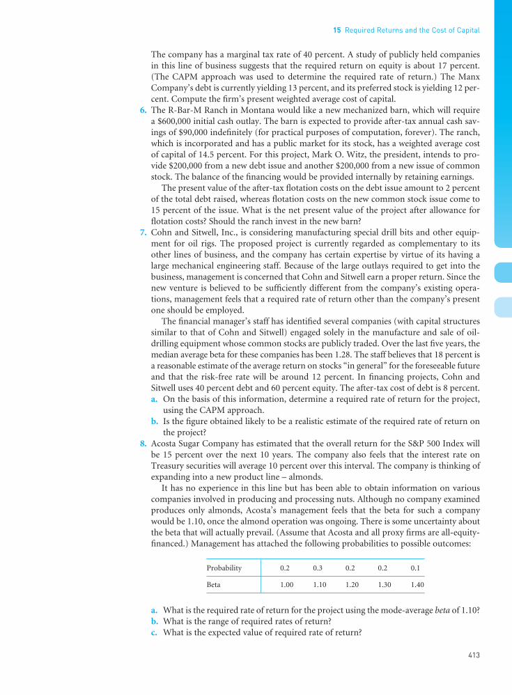
The company has a marginal tax rate of 40 percent. A study of publicly held companiesin this line of business suggests that the required return on equity is about 17 percent.(The CAPM approach was used to determine the required rate of return.) The ManxCompany’s debt is currently yielding 13 percent, and its preferred stock is yielding 12 per-cent. Compute the firm’s present weighted average cost of capital.
6. The R-Bar-M Ranch in Montana would like a new mechanized barn, which will requirea $600,000 initial cash outlay. The barn is expected to provide after-tax annual cash sav-ings of $90,000 indefinitely (for practical purposes of computation, forever). The ranch,which is incorporated and has a public market for its stock, has a weighted average costof capital of 14.5 percent. For this project, Mark O. Witz, the president, intends to pro-vide $200,000 from a new debt issue and another $200,000 from a new issue of commonstock. The balance of the financing would be provided internally by retaining earnings.
The present value of the after-tax flotation costs on the debt issue amount to 2 percentof the total debt raised, whereas flotation costs on the new common stock issue come to15 percent of the issue. What is the net present value of the project after allowance forflotation costs? Should the ranch invest in the new barn?
7. Cohn and Sitwell, Inc., is considering manufacturing special drill bits and other equip-ment for oil rigs. The proposed project is currently regarded as complementary to itsother lines of business, and the company has certain expertise by virtue of its having alarge mechanical engineering staff. Because of the large outlays required to get into thebusiness, management is concerned that Cohn and Sitwell earn a proper return. Since thenew venture is believed to be sufficiently different from the company’s existing opera-tions, management feels that a required rate of return other than the company’s presentone should be employed.
The financial manager’s staff has identified several companies (with capital structuressimilar to that of Cohn and Sitwell) engaged solely in the manufacture and sale of oil-drilling equipment whose common stocks are publicly traded. Over the last five years, themedian average beta for these companies has been 1.28. The staff believes that 18 percent isa reasonable estimate of the average return on stocks “in general” for the foreseeable futureand that the risk-free rate will be around 12 percent. In financing projects, Cohn andSitwell uses 40 percent debt and 60 percent equity. The after-tax cost of debt is 8 percent.a. On the basis of this information, determine a required rate of return for the project,
using the CAPM approach.b. Is the figure obtained likely to be a realistic estimate of the required rate of return on
the project?8. Acosta Sugar Company has estimated that the overall return for the S&P 500 Index will
be 15 percent over the next 10 years. The company also feels that the interest rate onTreasury securities will average 10 percent over this interval. The company is thinking ofexpanding into a new product line – almonds.
It has no experience in this line but has been able to obtain information on variouscompanies involved in producing and processing nuts. Although no company examinedproduces only almonds, Acosta’s management feels that the beta for such a companywould be 1.10, once the almond operation was ongoing. There is some uncertainty aboutthe beta that will actually prevail. (Assume that Acosta and all proxy firms are all-equity-financed.) Management has attached the following probabilities to possible outcomes:
Probability 0.2 0.3 0.2 0.2 0.1
Beta 1.00 1.10 1.20 1.30 1.40
a. What is the required rate of return for the project using the mode-average beta of 1.10?b. What is the range of required rates of return?c. What is the expected value of required rate of return?
15 Required Returns and the Cost of Capital
413
••
FUNO_C15.qxd 9/19/08 17:18 Page 413

9. Able Elba Palindrome, Inc., is evaluating a capital investment project. The after-tax cashflows for the project are listed as follows:
YEAR EXPECTED CASH FLOW
0 $−400,0001 50,0002 50,0003 150,0004 350,000
The risk-free rate is 8 percent, the firm’s weighted average cost of capital is 10 percent,and the management-determined risk-adjusted discount rate appropriate to this projectis 15 percent. Should the project be accepted? Explain.
10. The Totally Tubular Tube Company wishes to evaluate three new investment proposals.The firm is concerned with the impact of the proposals on its total risk. Consequently, ithas determined expected values and standard deviations of the probability distributionsof possible net present values for the possible combinations of existing projects, E, andinvestment proposals under consideration:
EXPECTED VALUE OF STANDARDNET PRESENT VALUE DEVIATION
COMBINATION (in millions) (in millions)
E $6.50 $5.25E + 1 6.80 5.00E + 2 7.60 8.00E + 3 7.20 6.50E + 1 + 2 7.90 7.50E + 1 + 3 7.50 5.60E + 2 + 3 8.30 8.50E + 1 + 2 + 3 8.60 9.00
Which combination do you feel is most desirable? Which proposals should be accepted?Which should be rejected?
Appendix A Problem
11. Willie Sutton Bank Vault Company has a debt-to-equity ratio (in market value terms) of0.75. Its present cost of debt funds is 15 percent, and it has a marginal tax rate of 40 per-cent. Willie Sutton Bank Vault is eyeing the automated bank teller business, a field thatinvolves electronics and is considerably different from its own line of business, so thecompany is looking for a benchmark or proxy company. The Peerless Machine Company,whose stock is publicly traded, produces only automated teller equipment. Peerless has adebt-to-equity ratio (in market value terms) of 0.25, a beta of 1.15, and an effective taxrate of 0.40.a. If Willie Sutton Bank Vault Company wishes to enter the automated bank teller
business, what systematic risk (beta) is involved if it intends to employ the sameamount of leverage in the new venture as it presently employs?
b. If the risk-free rate currently is 13 percent and the expected return on the market port-folio is 17 percent, what return should the company require for the project if it uses aCAPM approach?
Appendix B Problem
12. Aspen Plowing, Inc., is considering investing in a new snowplow truck costing $30,000.The truck is likely to provide after-tax incremental operating cash flows of $10,000 per
Part 6 The Cost of Capital, Capital Structure, and Dividend Policy
414
••
FUNO_C15.qxd 9/19/08 17:18 Page 414

year for six years. The unlevered cost of equity capital for the firm is 16 percent. The com-pany intends to finance the project with 60 percent debt, bearing an interest rate of 12 percent. The loan will be repaid in equal annual principal payments at the end of eachof the six years. Flotation costs (in present value terms) on financing amount to $1,000,and the company is in a 30 percent tax bracket.a. What is the adjusted present value (APV) of the project? Is the project acceptable?b. What would happen if expected after-tax incremental operating cash flows were
$8,000 per year instead of $10,000?
Solutions to Self-Correction Problems
1. a. ke = D1/P0 + g D1 = D0(1.12) = $1(1.12) = $1.12
ke = $1.12/$20 + 12% = 17.6%b. Through the trial-and-error approach illustrated in Chapters 3 and 4, one ends up
determining that the discount rate necessary to discount the cash-dividend stream to$20 must fall somewhere between 18 and 19 percent as follows:
DIVIDEND PRESENT VALUE PRESENT VALUE END OF YEAR PER SHARE AT 18% AT 19%
1 $1.20 $1.02 $1.012 1.44 1.03 1.023 1.73 1.05 1.034 2.07 1.07 1.035 2.49 1.09 1.04Present value, years 1–5 $5.26 $5.13
Year 6 dividend = $2.49 (1.10) = $2.74Market prices at the end of year 5 using a constant growth dividend valuation model:P5 = D6/(ke − g)
P5 = $2.74/(0.18 − 0.10) = $34.25, P5 = $2.74/(0.19 − 0.10) = $30.44
Present value at time 0 for amounts received at end of year 5:
$34.25 at 18% = $14.97, $30.44 at 19% = $12.76
18% 19%
Present value of years 1–5 $ 5.26 $ 5.13Present value of years 6–∞ 14.97 12.76Present value of all dividends $20.23 $17.89
Therefore, the discount rate is closer to 18 percent than it is to 19 percent.Interpolating, we get
and ke = 0.18 + X = 0.18 + 0.0010 = 18.10%, which is the estimated return on equity thatthe market requires.
XX
0.01$0.23$2.34
Therefore, (0.01) ($0.23)
$2.340.0010 = =
×=
0 010 19
0 230 00
23
17 892 34.
.
$ .$ .
$ .
$ .$ .
Xk
0.18 22
0e
⎡⎣⎢
⎤⎦⎥
⎡
⎣
⎢⎢⎢
⎤
⎦
⎥⎥⎥
15 Required Returns and the Cost of Capital
415
••
FUNO_C15.qxd 9/19/08 17:18 Page 415

2. SITUATION EQUATION: Rf + (b m − Rf)β REQUIRED RETURN
1 10% + (15% − 10%)1.00 15.0%2 14% + (18% − 14%)0.70 16.83 8% + (15% − 8%)1.20 16.44 11% + (17% − 11%)0.80 15.85 10% + (16% − 10%)1.90 21.4
The greater the risk-free rate, the greater the expected return on the market portfolio; and the greater the beta, the greater will be the required return on equity, all other thingsbeing the same. In addition, the greater the market risk premium (bm − Rf), the greater therequired return, all other things being the same.
3. Cost of debt = 15%(1 − 0.4) = 9%Cost of preferred stock = 13%Cost of equity for health foods division = 0.12 + (0.17 − 0.12)0.90 = 16.5%Cost of equity for specialty metals division = 0.12 + (0.17 − 0.12)1.30 = 18.5%Weighted average required return for health foods division
= 9%(0.3) + 13%(0.1) + 16.5%(0.6) = 13.9%Weighted average required return for specialty metals division
= 9%(0.3) + 13%(0.1) + 18.5%(0.6) = 15.1%As mentioned in the text, a conceptual case can be made for adjusting the non-equity costsof financing of the two divisions for differences in systematic risks. However, we have notdone so.
4. a. The coefficients of variation (standard deviation/d ) and the graphs of risk versusreturn for the alternatives are as follows:
Existing projects (E) 0.50Plus project 1 (E1) 0.60Plus project 2 (E2) 0.43Plus projects 1 and 2 (E12) 0.49
Part 6 The Cost of Capital, Capital Structure, and Dividend Policy
416
••
FUNO_C15.qxd 9/19/08 17:18 Page 416

Amihud, Yakov, and Haim Mendelson. “The Liquidity
Route to a Lower Cost of Capital.” Journal of AppliedCorporate Finance 12 (Winter 2000), 8–25.
Arditti, Fred D., and Haim Levy. “The Weighted AverageCost of Capital as a Cutoff Rate: A Critical Analysis of theClassical Textbook Weighted Average.” FinancialManagement 6 (Fall 1977), 24–34.
Ariel, Robert. “Risk Adjusted Discount Rates and the Present Value of Risky Costs.” The Financial Review 33(February 1998), 17–29.
Block, Stanley. “Divisional Cost of Capital: A Study of ItsUse by Major US Firms.” The Engineering Economist48 (No. 4, 2003), 345–362.
Booth, Laurence. “Finding Value Where None Exists:Pitfalls in Using Adjusted Present Value.” Journal ofApplied Corporate Finance 15 (Spring 2002), 95–104.
Brounen, Dirk, Abe de Long, and Kees Koedijk. “Corpor-ate Finance in Europe: Confronting Theory withPractice.” Financial Management 33 (Winter 2004),71–101.
Bruner, Robert F., Kenneth M. Eades, Robert S. Harris, andRobert C. Higgins. “Best Practices in Estimating the Costof Capital: Survey and Synthesis.” Financial Practice andEducation 8 (Spring/Summer 1998), 13–28.
Chambers, Donald R., Robert S. Harris, and John J. Pringle.“Treatment of Financing Mix in Analyzing InvestmentOpportunities.” Financial Management 11 (Summer1982), 24–41.
Conine, Thomas E., Jr., and Maurry Tamarkin. “DivisionCost of Capital Estimation: Adjusting for Leverage.”Financial Management 14 (Spring 1985), 54–58.
Ehrhardt, Michael C., and Yatin N. Bhagwat. “A Full-Information Approach for Estimating Divisional Betas.”Financial Management 20 (Summer 1991), 60–69.
Ezzell, John R., and R. Burr Porter. “Flotation Costs and the Weighted Average Cost of Capital.” Journal ofFinancial and Quantitative Analysis 11 (September 1976),403–413.
Fama, Eugene F., and Kenneth French. “The Corporate Costof Capital and the Return on Corporate Investment.”Journal of Finance 54 (December 1995), 1939–1968.
Fuller, Russell J., and Halbert S. Kerr. “Estimating theDivisional Cost of Capital: An Analysis of the Pure-PlayTechnique.” Journal of Finance 36 (December 1981),997–1009.
Gitman, Lawrence J., and Pieter A. Vandenberg. “Cost ofCapital Techniques Used by Major US Firms: 1997 vs.1980.” Financial Practice and Education 10 (Fall/Winter2000), 53–68.
Greenfield, Robert L., Maury R. Randall, and John C.Woods. “Financial Leverage and Use of the Net PresentValue Investment Criterion.” Financial Management 12(Autumn 1983), 40–44.
Gup, Benton E., and Samuel W. Norwood III. “DivisionalCost of Capital: A Practical Approach.” FinancialManagement 11 (Spring 1982), 20–24.
Hamada, Robert S. “Portfolio Analysis, Market Equilibriumand Corporation Finance.” Journal of Finance 24 (March1969), 19–30.
Harrington, Diana R. “Stock Prices, Beta and StrategicPlanning.” Harvard Business Review 61 (May–June 1983),157–164.
Harris, Robert S., Thomas J. O’Brien, and Doug Wakeman.“Divisional Cost-of-Capital Estimation for Multi Industry Firms.” Financial Management 18 (Summer 1989), 74–84.
Harris, Robert S., and John J. Pringle. “Risk-Adjusted Dis-count Rate – Extensions from the Average-Risk Case.”Journal of Financial Research 8 (Fall 1985), 237–244.
Krueger, Mark K., and Charles M. Linke. “A SpanningApproach for Estimating Divisional Cost of Capital.”Financial Management 23 (Spring 1994), 64–70.
Lessard, Donald R., and Richard S. Bower. “An OperationalApproach to Risk Screening.” Journal of Finance 27 (May1973), 321–338.
Lewellen, Wilbur G., and Douglas R. Emery. “CorporateDebt Management and the Value of the Firm.” Journal of
15 Required Returns and the Cost of Capital
417
••
A moderately risk-averse decision maker will probably prefer the existing projects plusboth new projects to any of the other three possible combinations. If this is the case,both new projects will be accepted. The actual decision will depend on your risk prefer-ences. A very risk-averse individual might prefer the existing projects plus only project2. Presumably, these preferences will be influenced by the presence of bankruptcy costs.
b. If the CAPM approach leads to a different decision, the key to deciding would be theimportance of market imperfections. As indicated earlier, if a company’s stock is tradedin imperfect markets, if the possibility of insolvency is substantive, and if bankruptcycosts are significant, more reliance should be placed on a total variability approachbecause it recognizes unsystematic plus systematic risk. If things point to minimal market imperfections, more reliance should be placed on the CAPM results.
Selected References
FUNO_C15.qxd 9/19/08 17:18 Page 417

Financial and Quantitative Analysis 21 (December 1986),415–425.
Miles, James A., and John R. Ezzell. “The Weighted AverageCost of Capital, Perfect Capital Markets, and Project Life:A Clarification.” Journal of Financial and QuantitativeAnalysis 15 (September 1980), 719–730.
—— . “Reforming Tax Shield Valuation: A Note.” Journalof Financial Economics 40 (December 1985), 1485–1492.
Myers, Stewart C. “Interactions of Corporate Financing and Investment Decisions – Implications for CapitalBudgeting.” Journal of Finance 29 (March 1974), 1–25.
—— . “Determinants of Corporate Borrowing.” Journal ofFinancial Economics 5 (November 1977), 147–175.
Pagano, Michael S., and David E. Stout. “Calculating aFirm’s Cost of Capital.” Management AccountingQuarterly 5 (Spring 2004), 13–20.
Parasuraman, N. R. “Ascertaining the Divisional Beta forProject Evaluation – the Pure Play Method – a Discussion.”The Chartered Accountant 31 (November 2002), 546–549(available online at www.icai.org/pdf/p546-549.pdf).
Porter, Michael E. Competitive Advantage. New York: FreePress, 1999.
Pratt, Shannon P. Cost of Capital: Estimation and Applica-tions, 2nd ed. New York: John Wiley & Sons, 2002.
Rosenburg, Barr, and Andrew Rudd. “The Corporate Use of Beta.” Issues in Corporate Finance. New York: Stern,Stewart, Putnam & Macklis, Inc., 1983.
Shapiro, Alan C. “Corporate Strategy and the CapitalBudgeting Decision.” Midland Corporate Finance Journal3 (Spring 1985), 22–36.
—— , and Sheridan Titman. “An Integrated Approach to Corporate Risk Management.” Midland Corporate Finance Journal 3 (Summer 1985), 41–56.
Shrieves, Ronald E., and John M. Wachowicz, Jr. “Free Cash Flow (FCF), Economic Value Added (EVA), andNet Present Value (NPV): A Reconciliation of Variations of Discounted-Cash-Flow (DCF) Valuation.” TheEngineering Economist 46 (No. 1, 2001), 33–52.
Stein, Jeremy C. “Rational Capital Budgeting in anIrrational World.” Journal of Business 69 (1996),429–455.
Stewart, G. Bennett. The Quest for Value. New York: HarperCollins, 1991.
Van Horne, James C. “An Application of the Capital AssetPricing Model to Divisional Required Returns.” FinancialManagement 9 (Spring 1980), 14–19.
Weaver, Samuel C. “Using Value Line to Estimate the Costof Capital and Industry Capital Structure.” Journal ofFinancial Education 29 (Fall 2003), 55–71.
Part VI of the text’s website, Wachowicz’s Web World, contains links to many finance websites and online articles related to topics covered in this chapter.(http://web.utk.edu/~jwachowi/part6.html)
Part 6 The Cost of Capital, Capital Structure, and Dividend Policy
418
••
FUNO_C15.qxd 9/19/08 17:18 Page 418

••
419
16Operating and Financial Leverage
Contents
l Operating LeverageBreak-Even Analysis • Degree of OperatingLeverage (DOL) • DOL and the Break-EvenPoint • DOL and Business Risk
l Financial LeverageEBIT-EPS Break-Even, or Indifference, Analysis• Degree of Financial Leverage (DFL) • DFL andFinancial Risk
l Total LeverageDegree of Total Leverage (DTL) • DTL and TotalFirm Risk
l Cash-Flow Ability to Service DebtCoverage Ratios • Probability of Cash Insolvency
l Other Methods of AnalysisComparison of Capital Structure Ratios •Surveying Investment Analysts and Lenders •Security Ratings
l Combination of Methods
l Key Learning Points
l Questions
l Self-Correction Problems
l Problems
l Solutions to Self-Correction Problems
l Selected References
Objectives
After studying Chapter 16, you should be able to:
l Define operating and financial leverage andidentify causes of both.
l Calculate a firm’s operating break-even (quan-tity) point and break-even (sales) point.
l Define, calculate, and interpret a firm’s degree ofoperating, financial, and total leverage.
l Understand EBIT-EPS break-even, or indiffer-ence, analysis, and construct and interpret anEBIT-EPS chart.
l Define, discuss, and quantify “total firm risk”and its two components, “business risk” and“financial risk.”
l Understand what is involved in determining the appropriate amount of financial leverage for a firm.
FUNO_C16.qxd 9/19/08 17:19 Page 419

When a lever is used properly, a force applied at one point is transformed, or magnified, intoanother, larger force or motion at some other point. This comes most readily to mind whenconsidering mechanical leverage, such as that which occurs when using a crowbar. In a busi-ness context, however, leverage refers to the use of fixed costs in an attempt to increase (orlever up) profitability. In this chapter we explore the principles of both operating leverageand financial leverage. The former is due to fixed operating costs associated with the pro-duction of goods or services, whereas the latter is due to the existence of fixed financing costs – in particular, interest on debt. Both types of leverage affect the level and variability ofthe firm’s after-tax earnings, and hence the firm’s overall risk and return.
Operating LeverageOperating leverage is present any time a firm has fixed operating costs – regardless of volume.In the long run, of course, all costs are variable. Consequently, our analysis necessarilyinvolves the short run. We incur fixed operating costs in the hope that sales volume will produce revenues more than sufficient to cover all fixed and variable operating costs. One ofthe more dramatic examples of an effect of operating leverage is the airline industry, where alarge proportion of total operating costs is fixed. Beyond a certain break-even load factor, eachadditional passenger essentially represents straight operating profit (earnings before interestand taxes, or EBIT) to the airline.
It is essential to note that fixed operating costs do not vary as volume changes. These costs include such things as depreciation of buildings and equipment, insurance, part of theoverall utility bills, and part of the cost of management. On the other hand, variable operat-ing costs vary directly with the level of output. These costs include raw materials, direct laborcosts, part of the overall utility bills, direct selling commissions, and certain parts of generaland administrative expenses.
One interesting potential effect caused by the presence of fixed operating costs (operatingleverage) is that a change in the volume of sales results in a more than proportional change inoperating profit (or loss). Thus, like a lever used to magnify a force applied at one point intoa larger force at some other point, the presence of fixed operating costs causes a percentagechange in sales volume to produce a magnified percentage change in operating profit (or loss).(A note of caution: remember, leverage is a two-edged sword – just as a company’s profits canbe magnified, so too can the company’s losses.)
This magnification effect is illustrated in Table 16.1. In Frame A we find three differentfirms possessing various amounts of operating leverage. Firm F has a heavy amount of fixedoperating costs (FC) relative to variable costs (VC). Firm V has a greater dollar amount ofvariable operating costs than of fixed operating costs. Finally, Firm 2F has twice the amountof fixed operating costs as does Firm F. Notice that, of the three firms shown, Firm 2F has (1)the largest absolute dollar amount of fixed costs and (2) the largest relative amount of fixedcosts as measured by both the (FC/total costs) and (FC/sales) ratios.
Each firm is then subjected to an anticipated 50 percent increase in sales for next year.Which firm do you think will be more sensitive to the change in sales: that is, for a given percentage change in sales, which firm will show the largest percentage change in operatingprofit (EBIT)? (Most people would pick Firm 2F – because it has either the largest absolute orthe largest relative amount of fixed costs. Most people would be wrong.)
Part 6 The Cost of Capital, Capital Structure, and Dividend Policy
420
••
It does not do to leave a live dragon out of your calculations, if youlive near him.
—J. R. R. TOLKIENThe Hobbit
Leverage The use of fixed costs in anattempt to increase(or lever up)profitability.
Operating leverageThe use of fixedoperating costs by the firm.
Financial leverageThe use of fixedfinancing costs by the firm. The Britishexpression is gearing.
FUNO_C16.qxd 9/19/08 17:19 Page 420

The results are shown in Frame B of Table 16.1. For each firm, sales and variable costsincrease by 50 percent. Fixed costs do not change. All firms show the effects of operating lever-age (that is, changes in sales result in more than proportional changes in operating profits).But Firm F proves to be the most sensitive firm, with a 50 percent increase in sales leading toa 400 percent increase in operating profit. As we have just seen, it would be an error to assumethat the firm with the largest absolute or relative amount of fixed costs automatically showsthe most dramatic effects of operating leverage. Later, we will come up with an easy way todetermine which firm is most sensitive to the presence of operating leverage. But, before wecan do so, we need to learn how to study operating leverage by means of break-even analysis.
l l l Break-Even AnalysisTo illustrate break-even analysis as applied to the study of operating leverage, consider a firmthat produces a high-quality child’s bicycle helmet that sells for $50 a unit. The company hasannual fixed operating costs of $100,000, and variable operating costs are $25 a unit regard-less of the volume sold. We wish to study the relationship between total operating costs andtotal revenues. One means for doing so is with the break-even chart in Figure 16.1, whichshows the relationship among total revenues, total operating costs, and profits for various levels of production and sales. As we are concerned only with operating costs at this point, wedefine profits here to mean operating profits before taxes. This definition purposely excludesinterest on debt and preferred stock dividends. These costs are not part of the total fixed oper-ating costs of the firm and have no relevance when it comes to analyzing operating leverage.They are taken into account, however, when we analyze financial leverage in the next section.
Break-Even (Quantity) Point. The intersection of the total costs line with the total revenuesline determines the break-even point. The break-even point is the sales volume required fortotal revenues to equal total operating costs or for operating profit to equal zero. In Figure16.1 this break-even point is 4,000 units of output (or $200,000 in sales). Mathematically, wefind this point (in units) by first noting that operating profit (EBIT) equals total revenuesminus variable and fixed operating costs:
16 Operating and Financial Leverage
421
••
Break-even analysis Atechnique for studyingthe relationshipamong fixed costs,variable costs, salesvolume, and profits. It is also calledcost/volume/profit(C/V/P) analysis.
Break-even chart Agraphic representationof the relationshipbetween totalrevenues and totalcosts for variouslevels of productionand sales, indicatingareas of profit andloss.
Break-even pointThe sales volumerequired so that totalrevenues and totalcosts are equal; maybe expressed in unitsor in sales dollars.
Table 16.1Effect of operatingleverage showing thatchanges in salesresult in more thanproportional changesin operating profit(EBIT)
Frame A: Three firms before changes in sales
Firm F Firm V Firm 2FSales $10,000 $11,000 $19,500Operating costs
Fixed (FC) 7,000 2,000 14,000Variable (VC) 2,000 7,000 3,000
Operating profit (EBIT) $ 1,000 $ 2,000 $ 2,500Operating leverage ratios
FC/total costs 0.78 0.22 0.82FC/sales 0.70 0.18 0.72
Frame B: Three firms after 50 percent increases in sales in following year
Firm F Firm V Firm 2FSales $15,000 $16,500 $29,250Operating costs:
Fixed (FC) 7,000 2,000 14,000Variable (VC) 3,000 10,500 4,500
Operating profit (EBIT) $ 5,000 $ 4,000 $10,750
Percent change in EBIT(EBITt − EBITt −1)/EBITt −1 400% 100% 330%
FUNO_C16.qxd 9/19/08 17:19 Page 421
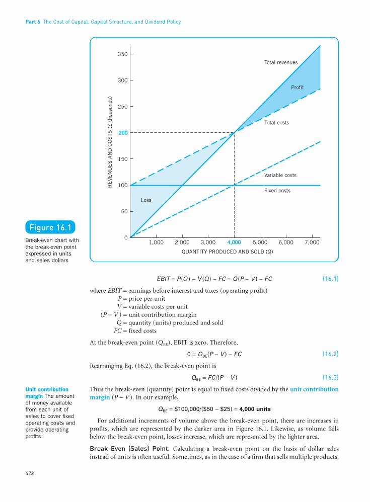
EBIT = P (Q ) − V (Q ) − FC = Q (P − V ) − FC (16.1)
where EBIT = earnings before interest and taxes (operating profit)P = price per unitV = variable costs per unit
(P − V ) = unit contribution marginQ = quantity (units) produced and sold
FC = fixed costs
At the break-even point (QBE), EBIT is zero. Therefore,
0 = QBE(P − V ) − FC (16.2)
Rearranging Eq. (16.2), the break-even point is
QBE = FC /(P − V ) (16.3)
Thus the break-even (quantity) point is equal to fixed costs divided by the unit contributionmargin (P − V). In our example,
QBE = $100,000/($50 − $25) = 4,000 units
For additional increments of volume above the break-even point, there are increases inprofits, which are represented by the darker area in Figure 16.1. Likewise, as volume fallsbelow the break-even point, losses increase, which are represented by the lighter area.
Break-Even (Sales) Point. Calculating a break-even point on the basis of dollar salesinstead of units is often useful. Sometimes, as in the case of a firm that sells multiple products,
Part 6 The Cost of Capital, Capital Structure, and Dividend Policy
422
••
Figure 16.1Break-even chart withthe break-even pointexpressed in unitsand sales dollars
Unit contributionmargin The amount of money availablefrom each unit ofsales to cover fixedoperating costs andprovide operatingprofits.
FUNO_C16.qxd 9/19/08 17:19 Page 422

it is a necessity. It would be impossible, for example, to come up with a meaningful break-even point in total units for a firm such as General Electric, but a break-even point based onsales revenues could easily be imagined. When determining a general break-even point for amultiproduct firm, we assume that sales of each product are a constant proportion of thefirm’s total sales.
Recognizing that at the break-even (sales) point the firm is just able to cover its fixed andvariable operating costs, we turn to the following formula:
SBE = FC + VCBE (16.4)
where SBE = break-even sales revenuesFC = fixed costs
VCBE = total variable costs at the break-even point
Unfortunately, we are now faced with a single equation containing two unknowns – SBE andVCBE. Such an equation is insolvable. Luckily, there is a trick that we can use in order to turnEq. (16.4) into a single equation with a single unknown. First, we need to rewrite Eq. (16.4)as follows:
SBE = FC + (VCBE /SBE)SBE (16.5)
Because the relationship between total variable costs and sales is assumed constant in linearbreak-even analysis, we can replace the ratio (VCBE/SBE) with the ratio of total variable coststo sales (VC/S) for any level of sales. For example, we can use the total variable costs and salesfigures from the firm’s most recent income statement to produce a suitable (VC/S) ratio. Inshort, after replacing the ratio (VCBE /SBE) with the “generic” ratio (VC/S) in Eq. (16.5), we get
SBE = FC + (VC /S )SBE
SBE[1 − (VC /S )] = FCSBE = FC / [1 − (VC /S )] (16.6)
For our example bicycle-helmet manufacturing firm, the ratio of total variable costs to salesis 0.50 regardless of sales volume. Therefore, using Eq. (16.6) to solve for the break-even(sales) point, we get
SBE = $100,000/[1 − 0.50] = $200,000
At $50 a unit, this $200,000 break-even (sales) point is consistent with the 4,000 unit break-even (quantity) point determined earlier [i.e., (4,000)($50) = $200,000].
TIP•TIP
You can easily modify break-even (quantity) Eq. (16.3) and break-even (sales) point Eq. (16.6)to calculate the sales volume (in units or dollars) required to produce a “target” operatingincome (EBIT) figure. Simply add your target or minimum desired operating income figureto fixed costs (FC) in each equation. The resulting answers will be your target sales volume– in units and dollars, respectively – needed to produce your target operating income figure.
l l l Degree of Operating Leverage (DOL)Earlier, we said that one potential effect of operating leverage is that a change in the volumeof sales results in a more than proportional change in operating profit (or loss). A quantitativemeasure of this sensitivity of a firm’s operating profit to a change in the firm’s sales is calledthe degree of operating leverage (DOL). The degree of operating leverage of a firm at a particular level of output (or sales) is simply the percentage change in operating profit overthe percentage change in output (or sales) that causes the change in profits. Thus,
16 Operating and Financial Leverage
423
••
Degree of operatingleverage (DOL) Thepercentage change in a firm’s operatingprofit (EBIT) resultingfrom a 1 percentchange in output(sales).
FUNO_C16.qxd 9/19/08 17:19 Page 423

(16.7)
The sensitivity of the firm to a change in sales as measured by DOL will be different at eachlevel of output (or sales). Therefore, we always need to indicate the level of output (or sales)at which DOL is measured – as in DOL at Q units.
TIP•TIP
When you use Eq. (16.7) to describe DOL at the firm’s current level of sales, remember thatyou are dealing with future percentage changes in EBIT and sales as opposed to pastpercentage changes. Using last period’s percentage changes in the equation would give uswhat the firm’s DOL used to be as opposed to what it is currently.
It is often difficult to work directly with Eq. (16.7) to solve for the DOL at a particular levelof sales because an anticipated percentage change in EBIT (the numerator in the equation)will not be observable from historical data. Thus, although Eq. (16.7) is crucial for definingand understanding DOL, a few simple alternative formulas derived from Eq. (16.7) are moreuseful for actually computing DOL values:
(16.8)
(16.9)
Equation (16.8) is especially well suited for calculating the degree of operating leverage for asingle product or a single-product firm.1 It requires only two pieces of information, Q andQBE, both of which are stated in terms of units. Equation (16.9), on the other hand, comes invery handy for finding the degree of operating leverage for a multiproduct firm. It too requiresonly two pieces of information, EBIT and FC, both of which are stated in dollar terms.
Suppose that we wish to determine the degree of operating leverage at 5,000 units of out-put and sales for our hypothetical example firm. Making use of Eq. (16.8), we have
For 6,000 units of output and sales, we have
Take Note
Notice that when output was increased from 5,000 to 6,000 units, the degree of operatingleverage decreased from a value of 5 to a value of 3. Thus, the further the level of output isfrom the break-even point, the lower the degree of operating leverage. How close a firmoperates to its break-even point – not its absolute or relative amount of fixed operating costs – determines how sensitive its operating profits will be to a change in output or sales.
DOL6 units, ,
( , , ) 000
6 0006 000 4 000
=−
= 3
DOL5 units, ,
( , , ) 000
5 0005 000 4 000
=−
= 5
DOLS VC
S VC FCEBIT FC
EBITS
dollars of sales =
−− −
=+
DOLQ P V
Q P V FCQ
Q QQ ( )
( )
( )unitsBE
=−
− −=
−
Degree of operatingleverage (DOL) at units
of output (or sales)
Percentage change inoperating profit (EBIT)Percentage change in
output (or sales)
Q =
1Self-correction Problem 4 at the end of this chapter asks you to mathematically derive Eq. (16.8) from Eq. (16.7).
Part 6 The Cost of Capital, Capital Structure, and Dividend Policy
424
••
FUNO_C16.qxd 9/19/08 17:19 Page 424

Question What does “DOL5,000 units = 5” really mean?
Answer It means that a 1 percent change in sales from the 5,000-unit sales position causes a 5 percent change in EBIT. In fact, any percentage change in sales from the 5,000-unitposition causes a percentage change in EBIT that is five times as large. For example, a 3 percent decrease in sales causes a 15 percent decrease in EBIT, and a 4 percent increasein sales causes a 20 percent increase in EBIT.
l l l DOL and the Break-Even PointTable 16.2 shows us the operating profit and degree of operating leverage for various levels of output (sales). We see that the further we move from the firm’s break-even point, thegreater is the absolute value of the firm’s operating profit or loss and the lower is the relativesensitivity of operating profit to changes in output (sales) as measured by DOL. The linearrelationship between operating profits and output (sales) has previously been revealed withthe break-even chart in Figure 16.1. In Figure 16.2 we plot the distinctly nonlinear relation-ship between DOL and output (sales).
Given the stable, linear cost and revenue functions of our example firm, we see that DOL approaches positive (or negative) infinity as sales approach the break-even point fromabove (or below) that point. DOL approaches 1 as sales grow beyond the break-even point.This implies that the magnification effect on operating profits caused by the presence of fixed costs diminishes toward a simple 1-to-1 relationship as sales continue to grow beyondthe break-even point. Figure 16.2 demonstrates that even firms with large fixed costs will have a low DOL if they operate well above their break-even point. By the same token, a firm with very low fixed costs will have an enormous DOL if it operates close to its break-even point.2
2The graph in Figure 16.2 is a rectangular hyperbola with asymptotes Q = QBE and DOL = 1. All firms having stable,linear cost structures will have similar-looking graphs – but each firm’s graph will be centered above its own respec-tive break-even point. Plotting DOL versus dollar sales instead of unit sales would produce a similar-looking result.
Interestingly, one can produce a standardized graph that could serve for all firms if we plot DOL versus Q/QBE orS/SBE – that is, DOL versus relative proximity to the break-even point. (The authors thank Professor James Gahlonfor sharing this insight as well as other helpful leverage observations.) The interpretation here would be that a firm’srelative proximity to its break-even point determines its DOL. Further, all firms operating at the same relative dis-tance from their break-even points (1.5 times QBE or SBE, for example) will have the same DOL.
16 Operating and Financial Leverage
425
••
Table 16.2Operating profit anddegree of operatingleverage at variouslevels of output(sales) for ourexample firm
QUANTITY PRODUCED OPERATING DEGREE OF OPERATINGAND SOLD (Q) PROFIT (EBIT) LEVERAGE (DOL)
0 $−100,000 0.001,000 −75,000 −0.332,000 −50,000 −1.003,000 −25,000 −3.00
QBE = 4,000 0 Infinite5,000 25,000 5.006,000 50,000 3.007,000 75,000 2.338,000 100,000 2.00
FUNO_C16.qxd 9/19/08 17:19 Page 425

Question How would knowledge of a firm’s DOL be of use to a financial manager?
Answer The manager would know in advance what impact a potential change in sales wouldhave on operating profit. Sometimes, in response to this advance knowledge, the firmmay decide to make some changes in its sales policy and/or cost structure. As a generalrule, firms do not like to operate under conditions of a high degree of operating leveragebecause, in that situation, a small drop in sales may lead to an operating loss.
l l l DOL and Business RiskIt is important to recognize that the degree of operating leverage is only one component of the overall business risk of the firm. The other principal factors giving rise to business risk are variability or uncertainty of sales and production costs. The firm’s degree of operatingleverage magnifies the impact of these other factors on the variability of operating profits.However, the degree of operating leverage itself is not the source of the variability. A highDOL means nothing if the firm maintains constant sales and a constant cost structure.Likewise, it would be a mistake to treat the degree of operating leverage of the firm as a synonym for its business risk. Because of the underlying variability of sales and productioncosts, however, the degree of operating leverage will magnify the variability of operatingprofits, and hence the company’s business risk. The degree of operating leverage should thus
Part 6 The Cost of Capital, Capital Structure, and Dividend Policy
426
••
Figure 16.2Plot of DOL versusquantity produced and sold, showing that closeness to the break-even point means highersensitivity ofoperating profits tochanges in quantityproduced and sold
Business risk Theinherent uncertainty in the physicaloperations of the firm.Its impact is shown in the variability of the firm’s operatingincome (EBIT).
FUNO_C16.qxd 9/19/08 17:19 Page 426

16 Operating and Financial Leverage
427
••
Indifference point(EBIT-EPS indifferencepoint) The level ofEBIT that producesthe same level of EPSfor two (or more)alternative capitalstructures.
be viewed as a measure of “potential risk” which becomes “active” only in the presence of salesand production cost variability.
Question Now that you have a better understanding of DOL, how can you tell from only theinformation in Frame A of Table 16.1 which firm – F, V, or 2F – will be more sensitiveto the anticipated 50 percent increase in sales for the next year?
Answer Simple. Calculate the DOL – using [(EBIT + FC)/EBIT] – for each firm, and then pickthe firm with the largest DOL.
Firm F: DOL$10,000 of sales = = 8
Firm V: DOL$11,000 of sales = = 2
Firm 2F: DOL$19,500 of sales = = 6.6
In short, Firm F – with a DOL of 8 – is most sensitive to the presence of operatingleverage. That is why a 50 percent increase in sales in the following year causes a 400 percent (8 × 50%) increase in operating profit.
Financial LeverageFinancial leverage involves the use of fixed cost financing. Interestingly, financial leverage isacquired by choice, but operating leverage sometimes is not. The amount of operating lever-age (the amount of fixed operating costs) employed by a firm is sometimes dictated by thephysical requirements of the firm’s operations. For example, a steel mill by way of its heavyinvestment in plant and equipment will have a large fixed operating cost component consist-ing of depreciation. Financial leverage, on the other hand, is always a choice item. No firm isrequired to have any long-term debt or preferred stock financing. Firms can, instead, financeoperations and capital expenditures from internal sources and the issuance of common stock.Nevertheless, it is a rare firm that has no financial leverage. Why, then, do we see such relianceon financial leverage?
Financial leverage is employed in the hope of increasing the return to common share-holders. Favorable or positive leverage is said to occur when the firm uses funds obtained at afixed cost (funds obtained by issuing debt with a fixed interest rate or preferred stock with aconstant dividend rate) to earn more than the fixed financing costs paid. Any profits left aftermeeting fixed financing costs then belong to common shareholders. Unfavorable or negativeleverage occurs when the firm does not earn as much as the fixed financing costs. The favor-ability of financial leverage, or “trading on the equity” as it is sometimes called, is judged interms of the effect that it has on earnings per share to the common shareholders. In effect,financial leverage is the second step in a two-step profit-magnification process. In step one,operating leverage magnifies the effect of changes in sales on changes in operating profit. Instep two, the financial manager has the option of using financial leverage to further magnifythe effect of any resulting changes in operating profit on changes in earnings per share. In thenext section we are interested in determining the relationship between earnings per share(EPS) and operating profit (EBIT) under various financing alternatives and the indifferencepoints between these alternatives.
$ , $ ,$ ,
2 500 14 0002 500+
$ , $ ,$ ,
2 000 2 0002 000
+
$ , $ ,$ ,
1000 7 0001000
+
FUNO_C16.qxd 9/19/08 17:19 Page 427

l l l EBIT-EPS Break-Even, or Indifference, AnalysisCalculation of Earnings per Share. To illustrate an EBIT-EPS break-even analysisof financial leverage, suppose that Cherokee Tire Company with long-term financing of $10 million, consisting entirely of common stock equity, wishes to raise another $5 millionfor expansion through one of three possible financing plans. The company may gain addi-tional financing with a new issue of (1) all common stock, (2) all debt at 12 percent interest,or (3) all preferred stock with an 11 percent dividend. Present annual earnings before inter-est and taxes (EBIT) are $1.5 million but with expansion are expected to rise to $2.7 million.The income tax rate is 40 percent, and 200,000 shares of common stock are now outstand-ing. Common stock can be sold at $50 per share under the first financing option, which translates into 100,000 additional shares of stock.
To determine the EBIT-EPS break-even, or indifference, points among the various financ-ing alternatives, we begin by calculating earnings per share, EPS, for some hypothetical levelof EBIT using the following formula:
(16.10)
where I = annual interest paidPD = annual preferred dividend paid
t = corporate tax rateNS = number of shares of common stock outstanding
Suppose we wish to know what earnings per share would be under the three alternativeadditional-financing plans if EBIT were $2.7 million. The calculations are shown in Table 16.3.Note that interest on debt is deducted before taxes, whereas preferred stock dividends arededucted after taxes. As a result, earnings available to common shareholders (EACS) arehigher under the debt alternative than they are under the preferred stock alternative, despitethe fact that the interest rate on debt is higher than the preferred stock dividend rate.
EBIT-EPS Chart. Given the information in Table 16.3, we are able to construct an EBIT-EPS break-even chart similar to the one for operating leverage. On the horizontal axis we plotearnings before interest and taxes, and on the vertical axis we plot earnings per share. For eachfinancing alternative, we must draw a straight line to reflect EPS for all possible levels of EBIT.Because two points determine a straight line, we need two data points for each financing alter-native. The first is the EPS calculated for some hypothetical level of EBIT. For the expected $2.7 million level of EBIT, we see in Table 16.3 that earnings per share are $5.40, $6.30, and$5.35 for the common stock, debt, and preferred stock financing alternatives. We simply plot
EPSEBIT I t PD
NS=
− − − ( )( ) 1
Part 6 The Cost of Capital, Capital Structure, and Dividend Policy
428
••
EBIT-EPS break-evenanalysis Analysis ofthe effect of financingalternatives onearnings per share.The break-even pointis the EBIT levelwhere EPS is thesame for two (ormore) alternatives.
Table 16.3Calculations ofearnings per shareunder threeadditional-financingalternatives
COMMON PREFERREDSTOCK DEBT STOCK
Earnings before interest and taxes (EBIT) $2,700,000 $2,700,000 $2,700,000Interest (I) – 600,000 –
Earnings before taxes (EBT) $2,700,000 $2,100,000 $2,700,000Income taxes (EBT × t) 1,080,000 840,000 1,080,000
Earnings after taxes (EAT) $1,620,000 $1,260,000 $1,620,000Preferred stock dividends (PD) – – 550,000
Earnings available to commonshareholders (EACS) $1,620,000 $1,260,000 $1,070,000
Number of shares of commonstock outstanding (NS) 300,000 200,000 200,000
Earnings per share (EPS) $5.40 $6.30 $5.35
FUNO_C16.qxd 9/19/08 17:19 Page 428

these earnings per share levels to correspond with the $2.7 million level of EBIT. Technically,it does not matter which hypothetical level of EBIT we choose for calculating EPS. On goodgraph paper one EBIT level is as good as the next. However, it does seem to make commonsense to choose the most likely, or expected, EBIT level rather than some level not too likelyto occur.
The second data point – chosen chiefly because of its ease of calculation – is where EPS iszero. This is simply the EBIT necessary to cover all fixed financial costs for a particular financ-ing plan, and it is plotted on the horizontal axis. We can make use of Eq. (16.10) to determinethe horizontal axis intercept under each alternative. We simply set the numerator in the equa-tion equal to zero and solve for EBIT. For the common stock alternative we have
0 = (EBIT − I )(1 − t ) − PD (16.11)= (EBIT − 0)(1 − 0.40) − 0= (EBIT )(0.60)
EBIT = 0/(0.60) = 0
Notice that there are no fixed financing costs whatsoever (on either old or new financing).Therefore, EPS equals zero at zero EBIT.3 For the debt alternative we have
0 = (EBIT − I )(1 − t ) − PD= (EBIT − $600,000)(1 − 0.40) − 0= (EBIT )(0.60) − $360,000
EBIT = $360,000/(0.60) = $600,000
Thus the after-tax interest charge divided by 1 minus the tax rate gives us the EBIT necessaryto cover these interest payments. In short, we must have $600,000 to cover interest charges,so $600,000 becomes the horizontal axis intercept. Finally, for the preferred stock alternativewe have
0 = (EBIT − I )(1 − t ) − PD= (EBIT − 0)(1 − 0.40) − $550,000= (EBIT )(0.60) − $550,000
EBIT = $550,000/(0.60) = $916,667
We divide total annual preferred dividends by 1 minus the tax rate to obtain the EBIT neces-sary to cover these dividends. Thus we need $916,667 in EBIT to cover $550,000 in preferredstock dividends, assuming a 40 percent tax rate. Again, preferred dividends are deducted aftertaxes, so it takes more in before-tax earnings to cover them than it does to cover interest.Given the horizontal axis intercepts and earnings per share for some hypothetical level ofEBIT (like the “expected” EBIT), we draw a straight line through each set of data points. Thebreak-even, or indifference, chart for Cherokee Tire Company is shown in Figure 16.3.
We see from Figure 16.3 that the earnings per share indifference point between the debtand common stock additional-financing alternatives is $1.8 million in EBIT.4 If EBIT is below that point, the common stock alternative will provide higher earnings per share. Abovethat point the debt alternative produces higher earnings per share. The indifference pointbetween the preferred stock and the common stock alternative is $2.75 million in EBIT.Above that point, the preferred stock alternative produces more favorable earnings per share.Below that point, the common stock alternative leads to higher earnings per share. Note that
3If some of the firm’s pre-expansion financing had involved fixed costs, the horizontal intercept for the commonstock financing alternative would not have been zero. It is only because I and PD are both zero in Eq. (16.11) that weget a zero value for EBIT.4Actually, $1.8 million in EBIT is more accurately referred to as a “break-even point” rather than an “indifferencepoint.” The financial manager will probably not be truly indifferent between the two alternative financing plans at thatlevel of EBIT. Though both plans do produce the same level of EPS at $1.8 million in EBIT, they do not do so byincurring the same level of financial risk – an issue that we will take up shortly. However, “indifference point” is partof the terminology common to EBIT-EPS analysis, so we need to be familiar with it.
16 Operating and Financial Leverage
429
••
FUNO_C16.qxd 9/19/08 17:19 Page 429

there is no indifference point between the debt and preferred stock alternatives. The debtalternative dominates for all levels of EBIT and by a constant amount of earnings per share,namely 95 cents.
Indifference Point Determined Mathematically. The indifference point between twoalternative financing methods can be determined mathematically by first using Eq. (16.10) to express EPS for each alternative and then setting these expressions equal to each other asfollows:
(16.12)
where EBIT1,2 = EBIT indifference point between the two alternative financing methods thatwe are concerned with – in this case, methods 1 and 2
I1, I2 = annual interest paid under financing methods 1 and 2PD1, PD2 = annual preferred stock dividend paid under financing methods 1 and 2
t = corporate tax rateNS1, NS2 = number of shares of common stock to be outstanding under financing
methods 1 and 2
Suppose that we wish to determine the indifference point between the common stock anddebt-financing alternatives in our example. We would have
Cross multiplying and rearranging, we obtain
(EBIT1,2)(0.60)(200,000) = (EBIT1,2)(0.60)(300,000) − (0.60)($600,000)(300,000)(EBIT1,2)(60,000) = $108,000,000,000
EBIT1,2 = $1,800,000
The EBIT-EPS indifference point, where earnings per share for the two methods of financingare the same, is $1.8 million. This amount can be verified graphically in Figure 16.3. Thusindifference points can be determined both graphically and mathematically.
Common Stock
EBIT
Debt
EBIT
( )( . ) ,
( $ , )( . )
,, ,1 2 1 20 1 0 40 0
300 000600 000 1 0 40 0
200 000− − −
=− − −
( )( )
( )( ) , ,EBIT I t PDNS
EBIT I t PDNS
1 2 1 1
1
1 2 2 2
2
1 1− − −=
− − −
Part 6 The Cost of Capital, Capital Structure, and Dividend Policy
430
••
Figure 16.3EBIT-EPS break-even,or indifference, chartfor three additional-financing alternatives
FUNO_C16.qxd 9/19/08 17:19 Page 430

Effect on Risk. So far our concern with EBIT-EPS analysis has been only with what happensto the return to common shareholders as measured by earnings per share. We have seen inour example that, if EBIT is above $1.8 million, debt financing is the preferred alternativefrom the standpoint of earnings per share. We know from our earlier discussion, however,that the impact on expected return is only one side of the coin. The other side is the effect thatfinancial leverage has on risk. An EBIT-EPS chart does not permit a precise analysis of risk.Nevertheless, certain generalizations are possible. For one thing, the financial manager shouldcompare the indifference point between two alternatives, such as debt financing versus com-mon stock financing, with the most likely level of EBIT. The higher the expected level of EBIT,assuming that it exceeds the indifference point, the stronger the case that can be made for debtfinancing, all other things the same.
In addition, the financial manager should assess the likelihood of future EBITs actuallyfalling below the indifference point. As before, our estimate of expected EBIT is $2.7 million.Given the business risk of the company and the resulting possible fluctuations in EBIT, thefinancial manager should assess the probability of EBITs falling below $1.8 million. If theprobability is negligible, the use of the debt alternative will be supported. On the other hand,if EBIT is presently only slightly above the indifference point and the probability of EBITsfalling below this point is high, the financial manager may conclude that the debt alternativeis too risky.
This notion is illustrated in Figure 16.4, where two probability distributions of possibleEBITs are superimposed on the indifference chart first shown in Figure 16.3. In Figure 16.4,however, we focus on only the debt and common stock alternatives. For the safe (peaked) dis-tribution, there is virtually no probability that EBIT will fall below the indifference point.Therefore we might conclude that debt should be used, because the effect on shareholderreturn is substantial, whereas risk is negligible. For the risky (flat) distribution, there is asignificant probability that EBIT will fall below the indifference point. In this case, the finan-cial manager may conclude that the debt alternative is too risky.
In summary, the greater the level of expected EBIT above the indifference point and thelower the probability of downside fluctuation, the stronger the case that can be made for the
16 Operating and Financial Leverage
431
••
Figure 16.4EBIT-EPS break-even,or indifference, chartand EBIT probabilitydistributions for debtand common stockadditional-financingalternatives
FUNO_C16.qxd 9/19/08 17:19 Page 431

use of debt financing. EBIT-EPS break-even analysis is but one of several methods used fordetermining the appropriate amount of debt a firm might carry. No one method of analysisis satisfactory by itself. When several methods of analysis are undertaken simultaneously,however, generalizations are possible.
l l l Degree of Financial Leverage (DFL)
A quantitative measure of the sensitivity of a firm’s earnings per share to a change in the firm’soperating profit is called the degree of financial leverage (DFL). The degree of financial lever-age at a particular level of operating profit is simply the percentage change in earnings pershare over the percentage change in operating profit that causes the change in earnings per share. Thus,
(16.13)
Whereas Eq. (16.13) is useful for defining DFL, a simple alternative formula derived fromEq. (16.13) is more useful for actually computing DFL values:
(16.14)
Equation (16.14) states that DFL at a particular level of operating profit is calculated by divid-ing operating profit by the dollar difference between operating profit and the amount ofbefore-tax operating profit necessary to cover total fixed financing costs. (Remember, it takesmore in before-tax earnings to cover preferred dividends than it does to cover interest: hencewe need to divide preferred dividends by 1 minus the tax rate in our formula.)
For our example firm, using the debt-financing alternative at $2.7 million in EBIT, we have
For the preferred stock financing alternative, the degree of financial leverage is
Interestingly, although the stated fixed cost involved with the preferred stock financing alter-native is lower than that for the debt alternative ($550,000 versus $600,000), the DFL is greaterunder the preferred stock option than under the debt option. This is because of the taxdeductibility of interest and the nondeductibility of preferred dividends. It is often argued thatpreferred stock financing is of less risk than debt financing for the issuing firm. With regardto the risk of cash insolvency, this is probably true. But the DFL tells us that the relative vari-ability of EPS will be greater under the preferred stock financing arrangement, everything elsebeing equal. This discussion naturally leads us to the topic of financial risk and its relation-ship to the degree of financial leverage.
l l l DFL and Financial Risk
Financial Risk. Broadly speaking, financial risk encompasses both the risk of possible insol-vency and the added variability in earnings per share that is induced by the use of financialleverage. As a firm increases the proportion of fixed cost financing in its capital structure,fixed cash outflows increase. As a result, the probability of cash insolvency increases. To illustrate this aspect of financial risk, suppose that two firms differ with respect to financial
DFLEBIT of $2.7 million =−
= $ , ,
$ , , [$ , /( . )]
2 700 0002 700 000 550 000 0 60
1.51
DFLEBIT of $2.7 million =−
= $ , ,
$ , , $ ,
2 700 0002 700 000 600 000
1.29
DFLEBIT
EBIT I PD tEBIT X of dollars =− − −
[ /( )]1
Degree of financialleverage (DFL) at EBIT of
dollars
Percentage change inearnings per share (EPS)
Percentage change inoperating profit (EBIT)
X =
Part 6 The Cost of Capital, Capital Structure, and Dividend Policy
432
••
Degree of financialleverage (DFL) Thepercentage change in a firm’s earningsper share (EPS)resulting from a 1percent change inoperating profit (EBIT).
Cash insolvencyInability to payobligations as they fall due.
Financial risk Theadded variability inearnings per share(EPS) – plus the riskof possible insolvency– that is induced bythe use of financialleverage.
FUNO_C16.qxd 9/19/08 17:19 Page 432

leverage but are identical in every other respect. Each has expected annual cash earningsbefore interest and taxes of $80,000. Firm A has no debt. Firm B has $200,000 worth of 15 per-cent perpetual bonds outstanding. Thus the total annual fixed financial charges for Firm B are$30,000, whereas Firm A has no fixed financial charges. If cash earnings for both firms hap-pen to be 75 percent lower than expected, namely $20,000, firm B will be unable to cover itsfinancial charges with cash earnings. We see, then, that the probability of cash insolvencyincreases with the financial charges incurred by the firm.
The second aspect of financial risk involves the relative dispersion of earnings per share. Toillustrate, suppose that the expected future EBITs for firm A and firm B are random variableswhere the expected values of the probability distributions are each $80,000 and the standarddeviations $40,000. As before, firm A has no debt but rather 4,000 shares of $10-par-valuecommon stock outstanding. Firm B has $200,000 in 15 percent bonds and 2,000 shares of $10-par-value common stock outstanding.
Frame A in Table 16.4 shows that the expected earnings available to common shareholdersfor firm A equals $48,000, while for firm B this figure equals only $30,000. Dividing expectedearnings available to common shareholders by the number of shares of common stock out-standing, however, reveals that firm B has a higher expected earnings per share than firm A:that is, $15 and $12, respectively. The standard deviation of earnings per share is determinedto be $6 for firm A and $12 for firm B.
Total Firm Risk Equals Business Risk Plus Financial Risk. The coefficient of variationof earnings per share, which is simply the standard deviation divided by the expected value,gives us a measure of the relative dispersion of earnings per share. We use this statistic as a measure of total firm risk. In frame B of Table 16.4 we see that for firm A, the 100-percent-equity situation, the coefficient of variation of earnings per share is 0.50. Notice that this figure is exactly equal to the firm’s coefficient of variation of earnings before interestand taxes. What this says is that even in the absence of financial leverage, the firm’s share-holders are still exposed to risk – business risk. A good quantitative measure of a firm’s relative amount of business risk is thus the coefficient of variation of EBIT. For firm B, the
16 Operating and Financial Leverage
433
••
Table 16.4Effect of financialleverage exampleshowing that financialleverage affects boththe level andvariability of earningsper share
FIRM A FIRM B(100% EQUITY) (50% EQUITY)
Frame A: Forecast income statement informationExpected earnings before interest and taxes [E(EBIT)] $80,000 $80,000Interest (I) – 30,000
Expected earnings before taxes [E(EBT)] $80,000 $50,000Expected taxes [E(EBT) × t] 32,000 20,000
Expected earnings available to commonshareholders [E(EACS)] $48,000 $30,000
Number of shares of common stock outstanding (NS) 4,000 2,000Expected earnings per share [E(EPS)] $12.00 $15.00
Frame B: Risk componentsStandard deviation of earnings per share (σEPS)* $6.00 $12.00Coefficient of variation of earnings before interest
and taxes [σEBIT /E(EBIT)] 0.50 0.50DFLexpected EBIT of $800,000
[E(EBIT)]/[E(EBIT) − I − PD/(1 − t)] 1.00 1.60Coefficient of variation of earnings per share
[σEPS/E(EPS)] or [σEBIT/E(EBIT)] × [DFLE(EBIT)] 0.50 0.80
*For any random variable X, the σ(a+bx) = (b)(σx): therefore σEPS = (1/number of shares of commonstock outstanding) (1 − t)(σEBIT). Example for 50% debt: (1/2,000)(1 − 0.40)($40,000) = $12.00.
Total firm risk Thevariability in earningsper share (EPS). It isthe sum of businessplus financial risk.
FUNO_C16.qxd 9/19/08 17:19 Page 433

50-percent-debt situation, the coefficient of variation of earnings per share is 0.80. Becausefirm B is exactly like firm A except for the use of financial leverage, we can use the differencebetween the coefficients of variation of earnings per share for firm B and firm A: that is, 0.80 − 0.50 = 0.30, as a measure of the added variability in earnings per share for firm B that is induced by the use of leverage; in short, this difference is a measure of financial risk.Equivalently, this measure of financial risk equals the difference between firm B’s coefficientof variation of earnings per share and its coefficient of variation of earnings before interestand taxes.
Take Note
In summary, then
l Total firm risk = business risk + financial risk.
l The coefficient of variation of earnings per share, CVEPS, is a measure of relative total firmrisk : CVEPS = σEPS /E(EPS).
l The coefficient of variation of earnings before interest and taxes, CVEBIT, is a measure ofrelative business risk: CVEBIT = σEBIT /E(EBIT).
l The difference, therefore, between the coefficient of variation of earnings per share(CVEPS) and the coefficient of variation of earnings before interest and taxes (CVEBIT) is ameasure of relative financial risk: (CVEPS − CVEBIT).
We have seen from Table 16.4 that total firm risk in our example, as measured by thecoefficient of variation of earnings per share, is higher under the 50-percent-bond financingthan it is under the 100-percent-equity financing. However, the expected level of earnings pershare is also higher. We witness, once again, the kind of risk-return trade-off that character-izes most financial leverage decisions.
DFL Magnifies Risk. Our measure of relative total firm risk, the coefficient of variation ofearnings per share, can be calculated directly by dividing the standard deviation of earningsper share by the expected earnings per share. However, given the assumptions behind ourexample, it can be shown that this measure is also equal to the coefficient of variation of earn-ings before interest and taxes times the degree of financial leverage at the expected EBIT level.5
Firm A, in our example, has no financial leverage and a resulting DFL equal to 1: in short,there is no magnification of business risk as measured by the CVEBIT. For firm A, then, CVEPS
equals CVEBIT, and thus its total firm risk is equal to its business risk. Firm B’s CVEPS, on theother hand, is equal to its CVEBIT (its measure of business risk) times 1.6 (its DFL at theexpected EBIT). Thus, for firms employing financial leverage, their DFL will act to magnifythe impact of business risk on the variability of earnings per share. So, although DFL is notsynonymous with financial risk, its magnitude does determine the relative amount of addi-tional risk induced by the use of financial leverage. As a result, firms with high business riskwill often employ a financing mix that entails a limited DFL, and vice versa.
5Proof:
Part 6 The Cost of Capital, Capital Structure, and Dividend Policy
434
••
FUNO_C16.qxd 9/19/08 17:19 Page 434

Total LeverageWhen financial leverage is combined with operating leverage, the result is referred to as total(or combined) leverage. The effect of combining financial and operating leverage is a two-step magnification of any change in sales into a larger relative change in earnings per share. Aquantitative measure of this total sensitivity of a firm’s earnings per share to a change in thefirm’s sales is called the degree of total leverage (DTL).
l l l Degree of Total Leverage (DTL)
The degree of total leverage of a firm at a particular level of output (or sales) is equal to thepercentage change in earnings per share over the percentage change in output (or sales) thatcauses the change in earnings per share. Thus,
(16.15)
Computationally, we can make use of the fact that the degree of total leverage is simply theproduct of the degree of operating leverage and the degree of financial leverage as follows:
DTLQ units (or S dollars) = DOLQ units (or S dollars) × DFLEBIT of X dollars (16.16)
In addition, multiplying alternative DOLs, Eqs. (16.8) and (16.9), by DFL, Eq. (16.14), gives us
(16.17)
(16.18)
These alternative equations tell us that for a particular firm the greater the before-tax financialcosts, the greater the degree of total leverage over what it would be in the absence of financialleverage.
Suppose that our bicycle-helmet manufacturing firm used to illustrate operating leveragehas $200,000 in debt at 8 percent interest. Recall that the selling price is $50 a unit, variableoperating costs are $25 a unit, and annual fixed operating costs are $100,000. Assume that thetax rate is 40 percent, and that we wish to determine the degree of total leverage at 8,000 unitsof production and sales. Therefore, using Eq. (16.17), we have
Thus a 10 percent increase in the number of units produced and sold would result in a 23.8percent increase in earnings per share.
Stating the degree of total leverage for our example firm in terms of the product of itsdegree of operating leverage times its degree of financial leverage, we get
In the absence of financial leverage, our firm’s degree of total leverage would have been equal to its degree of operating leverage for a value of 2 (remember, DFL for a firm with no
DOL DFL DTL8,000 units EBIT of $100,000 8,000 units
8 000 50 258 000 50 25 100 000
100 000100 000 16 000
, ($ $ ), ($ $ ) $ ,
$ ,
$ , $ ,
−− −
×
×
×
−
=
=
=2.00 1.19
2.38
2.38
DTL8,000 units =−
− − −=
, ($ $ ), ($ $ ) $ , $ ,
8 000 50 25
8 000 50 25 100 000 16 0002.38
DTLEBIT FC
EBIT I PD tS dollars of sales =+
− − −
[ /( )]1
DTLQ P V
Q P V FC I PD tQ ( )
( ) [ /( )]units =−
− − − − −1
Degree of total leverage (DTL)at units (or dollars)
of output (or sales)
Percentage change inearnings per share (EPS)
Percentage change inoutput (or sales)
Q S =
16 Operating and Financial Leverage
435
••
Total (or combined)leverage The use ofboth fixed operatingand financing costs bythe firm.
Degree of totalleverage (DTL) Thepercentage change ina firm’s earnings pershare (EPS) resultingfrom a 1 percentchange in output(sales). This is alsoequal to a firm’sdegree of operatingleverage (DOL) timesits degree of financialleverage (DFL) at aparticular level ofoutput (sales).
FUNO_C16.qxd 9/19/08 17:19 Page 435

financial leverage equals 1). We see, however, that the firm’s financial leverage magnifies itsDOL figure by a factor of 1.19 to produce a degree of total leverage equal to 2.38.
l l l DTL and Total Firm RiskOperating leverage and financial leverage can be combined in a number of different ways toobtain a desirable degree of total leverage and level of total firm risk. High business risk canbe offset with low financial risk and vice versa. The proper overall level of firm risk involves atrade-off between total firm risk and expected return. This trade-off must be made in keepingwith the objective of maximizing shareholder value. The discussion, so far, is meant to showhow certain tools can be employed to provide information on the two types of leverage –operating and financial – and their combined effect.
Cash-Flow Ability to Service DebtWhen trying to determine the appropriate financial leverage for a firm, we would also analyzethe cash-flow ability of the firm to service fixed financial charges. The greater the dollaramount of senior securities that the firm issues and the shorter their maturity, the greater thefixed financial charges of the firm. These charges include principal and interest payments ondebt, financial lease payments, and preferred stock dividends. Before taking on additionalfixed financial charges, the firm should analyze its expected future cash flows, because fixedfinancial charges must be met with cash. The inability to meet these charges, with the excep-tion of preferred stock dividends, may result in financial insolvency. The greater and morestable the expected future cash flows of the firm, the greater the debt capacity of the company.
l l l Coverage RatiosAmong the ways in which we can gain knowledge about the debt capacity of a firm is throughan analysis of coverage ratios. These ratios, as you may remember from Chapter 6, aredesigned to relate the financial charges of a firm to the firm’s ability to service, or cover, them.In the computation of these ratios, one typically uses earnings before interest and taxes as arough measure of the cash flow available to cover fixed financial charges. Perhaps the mostwidely used coverage ratio is the interest coverage ratio, or times interest earned. This ratio issimply earnings before interest and taxes for a particular period divided by interest charges forthe period:
(16.19)
Suppose, for example, that the most recent annual earnings before interest and taxes for acompany were $6 million and annual interest payments on all debt obligations were $1.5 million.Then EBIT would “cover” interest charges four times. This tells us that EBIT can drop by asmuch as 75 percent and the firm will still be able to cover interest payments out of earnings.
An interest coverage ratio of only 1 indicates that earnings are just sufficient to satisfy theinterest burden. Generalizations about what is a proper interest coverage ratio are inappro-priate unless reference is made to the type of business in which the firm is engaged. In a highlystable business, a relatively low interest coverage ratio may be appropriate, whereas it may notbe appropriate in a highly cyclical business.
Note that the interest coverage ratio tells us nothing about the firm’s ability to meet prin-cipal payments on its debts. The inability to meet a principal payment constitutes the samelegal default as failure to meet an interest payment. Therefore it is useful to compute the coverage ratio for the full debt-service burden. This ratio is
Interest coverage ratio(or times interest earned)
Earnings before interestand taxes (EBIT)Interest expense
=
Part 6 The Cost of Capital, Capital Structure, and Dividend Policy
436
••
Debt capacity Themaximum amount ofdebt (and other fixed-charge financing) thata firm can adequatelyservice.
Coverage ratiosRatios that relate thefinancial charges of afirm to its ability toservice, or cover,them.
Interest coverageratio Earnings beforeinterest and taxesdivided by interestcharges. It indicates afirm’s ability to coverinterest charges. It isalso called timesinterest earned.
Debt-service burdenCash required duringa specific period,usually a year, tomeet interestexpenses andprincipal payments.Also called simplydebt service.
FUNO_C16.qxd 9/19/08 17:19 Page 436

(16.20)
Here principal payments are adjusted upward for the tax effect. The reason is that EBIT rep-resents earnings before tax. Because principal payments are not deductible for tax purposes,they must be paid out of after-tax earnings. Therefore we must adjust principal payments sothat they are consistent with EBIT. If principal payments in our previous example were $1million per annum and the tax rate were 40 percent, the debt-service coverage ratio would be
A coverage ratio of 1.89 means that EBIT can fall by only 47 percent before earnings coverageis insufficient to service the debt.6 Obviously, the closer the debt-service coverage ratio is to 1,the worse things are, all other things the same. However, even with this coverage ratio beingless than 1, a company may still be able to meet its obligations if it can renew some of its debtwhen principal comes due or if assets are sold.
Part of the overall analysis of the financial risk associated with financial leverage shouldfocus on the firm’s ability to service total fixed charges. Lease financing is not debt per se, butits impact on cash flows is exactly the same as the payment of interest and principal on a debtobligation. (See Chapter 21 for an analysis of lease financing.) Annual financial lease pay-ments, therefore, should be added to the numerator and denominator of Eq. (16.20) in orderto properly reflect the total cash-flow burden associated with financing.
As with the interest coverage ratio, “rules of thumb” generalizations about what constitutesa good or bad debt-service ratio are often inappropriate. What constitutes a good or bad ratiovaries according to the business risk of the firm. This fact is illustrated in Figure 16.5, whichshows the probability distributions of EBIT for two hypothetical companies. The expectedvalue of EBIT is the same for both companies, as is the debt-service burden as described bythe denominator in Eq. (16.20). Therefore the debt-service coverage ratios are also the same,namely $100,000/$60,000 = 1.67. Company A, however, has much more business risk, as
Debt-servicecoverage
$6 million
$1.5 million $1 million
0
.
=+
−
=
1 40
1.89
Debt-servicecoverage
Earnings before interest and taxes (EBIT)
Interest expense Principal payments
Tax rate
=+
−1
6This percentage is determined by 1 − (1/1.89) = 0.47.
16 Operating and Financial Leverage
437
••
Figure 16.5Possible EBITs inrelation to debt-service burdens forcompanies A and B
FUNO_C16.qxd 9/19/08 17:19 Page 437

shown in the greater variability of its EBIT. The probability that EBIT will fall below the debt-service burden is depicted by the shaded areas in the figure. We see that this probabilityis much greater for company A than it is for company B. Though a debt-service coverage ratio of 1.67 may be appropriate for company B, it may not be appropriate for company A.Simply put, a company with stable cash flows is better able to take on relatively more fixedcharges.
Ultimately, one wants to make generalizations about the appropriate amount of debt (andleases) for a firm to have in its financing mix. It is clear that the ability of a going-concern firmto service debt over the long run is tied to earnings. Therefore coverage ratios are an import-ant tool of analysis. However, they are but one tool by which a person is able to reach con-clusions with respect to determining an appropriate financing mix for the firm. Coverageratios, like all ratios, are subject to certain limitations and, consequently, cannot be used as asole means for determining a firm’s financing. The fact that EBIT falls below the debt-serviceburden does not spell immediate doom for the company. Often alternative sources of funds,including renewal of the loan, are available, and these sources must be considered.
l l l Probability of Cash InsolvencyThe vital question for the firm is not so much whether a coverage ratio will fall below 1 butrather, what are the chances of cash insolvency? Fixed-charge financing adds to the firm’s danger of cash insolvency. Therefore the answer depends on whether all sources of payment– earnings, cash, a new financing arrangement, or the sale of assets – are collectively deficient.A coverage ratio tells only part of the story. To address the broad question of cash insolvency,we must obtain information on the possible deviation of actual cash flows from those that areexpected. As we discussed in Chapter 7, cash budgets can be prepared for a range of possibleoutcomes, with a probability attached to each outcome. This information is extremely valu-able to the financial manager in evaluating the ability of the firm to meet fixed obligations.Not only are expected earnings taken into account in determining this ability, but other cash-flow factors as well – the purchase or sale of assets, the liquidity of the firm, dividendpayments, and seasonal patterns. Given the probabilities of particular cash-flow sequences,the financial manager is able to determine the amount of fixed financing charges the companycan undertake while still remaining within insolvency limits tolerable to management.
Management may feel that a 5 percent probability of being out of cash is the maximum that it can tolerate and that this probability corresponds to a cash budget prepared under pessimistic assumptions. In this case, debt might be undertaken up to the point where thecash balance under the pessimistic cash budget is just sufficient to cover the fixed chargesassociated with the debt. In other words, debt would be increased to the point at which theadditional cash drain would cause the probability of cash insolvency to equal the risk toler-ance specified by management. Note that the method of analysis simply provides a means forassessing the effect of increases in debt on the risk of cash insolvency. On the basis of thisinformation, management would arrive at the most appropriate level of debt.
The analysis of the cash-flow ability of the firm to service fixed financial charges is perhapsthe best way to analyze financial risk, but there is a real question as to whether all (or most)of the participants in the financial markets analyze a company in this manner. Sophisticatedlenders and institutional investors certainly analyze the amount of fixed financial charges andevaluate financial risk in keeping with the ability of the firm to service these charges. However,individual investors may judge financial risk more by book value proportions of debt andequity. There may or may not be a reasonable correspondence between the ratio of debt toequity and the amount of fixed charges relative to the firm’s cash-flow ability to service thesecharges. Some firms may have relatively high ratios of debt to equity but substantial cash-flowability to service debt. Consequently, the analysis of debt-to-equity ratios alone can be deceiv-ing, and an analysis of the magnitude and stability of cash flows relative to fixed financialcharges is extremely important in determining the appropriate financing mix for the firm.
Part 6 The Cost of Capital, Capital Structure, and Dividend Policy
438
••
FUNO_C16.qxd 9/19/08 17:19 Page 438

Other Methods of Analysis
l l l Comparison of Capital Structure RatiosAnother method of analyzing the appropriate financing mix for a company is to evaluate thecapital structure of other companies having similar business risk. Companies used in thiscomparison are most often those in the same industry. If the firm is contemplating a capitalstructure significantly out of line with that of similar companies, it is conspicuous in the marketplace. This is not to say that the firm is wrong. Other companies in the industry maybe too conservative in their use of debt. The optimal capital structure for all companies in theindustry might call for a higher proportion of debt to equity than the industry average. As aresult, the firm may be able to justify more debt than the industry average. If the firm’s finan-cial leverage is noticeably out of line in either direction, it should be prepared to justify itsposition, because investment analysts and creditors tend to evaluate companies by industry.
There are wide variations in the use of financial leverage across business firms. A good dealof the variation is removed, however, if one groups firms by industry classification, becausethere is a tendency for the firms in an industry to cluster when it comes to debt ratios. Forselected industries, the debt-to-net-worth ratios for a recent period looked as follows:
INDUSTRY DEBT TO NET WORTH
Optical instruments and lenses (manufacturing) 1.2Pharmaceutical preparations (manufacturing) 1.2Meat packing plants (manufacturing) 1.8Electronic components (manufacturing) 1.8Carpets and rugs (manufacturing) 1.9Wood kitchen cabinets (manufacturing) 2.9Gasoline service stations (retail) 3.2General contractors (single-family houses) 5.0
Whereas optical instruments manufacturers and pharmaceutical companies do not employmuch financial leverage, general contractors make extensive use of debt in financing projects.So when making capital structure comparisons, look at other companies in the same indus-try. In short, compare apples with apples as opposed to apples with oranges.
l l l Surveying Investment Analysts and LendersThe firm may profit by also talking with investment analysts, institutional investors, andinvestment bankers to obtain their views on appropriate amounts of financial leverage. Theseanalysts examine many companies and are in the business of recommending stocks. Theytherefore have an influence on the financial market. Their judgments with respect to how themarket evaluates financial leverage may be very worthwhile. Similarly, a firm may wish tointerview lenders to see how much debt it can undertake before the cost of borrowing is likelyto rise. Finally, the management of a company may develop a “feel” for what has happened tothe market price of the company’s stock when it has issued debt in the past.
l l l Security RatingsThe financial manager must consider the effect of a financing alternative on its security rat-ing. Whenever a company sells a debt or preferred stock issue to public investors, as opposedto private lenders such as banks, it must have the issue rated by one or more rating services.The principal rating agencies are Moody’s Investors Service and Standard & Poor’s. The issuerof a new corporate security issue contracts with the agency to evaluate the issue as to quality,as well as to update the rating throughout the issue’s life. For this service, the issuer pays a fee. In addition, the rating agency charges subscribers to its rating publications. Whereas the
16 Operating and Financial Leverage
439
••
Capital structure Themix (or proportion) ofa firm’s permanentlong-term financingrepresented by debt,preferred stock, andcommon stock equity.
FUNO_C16.qxd 9/19/08 17:19 Page 439
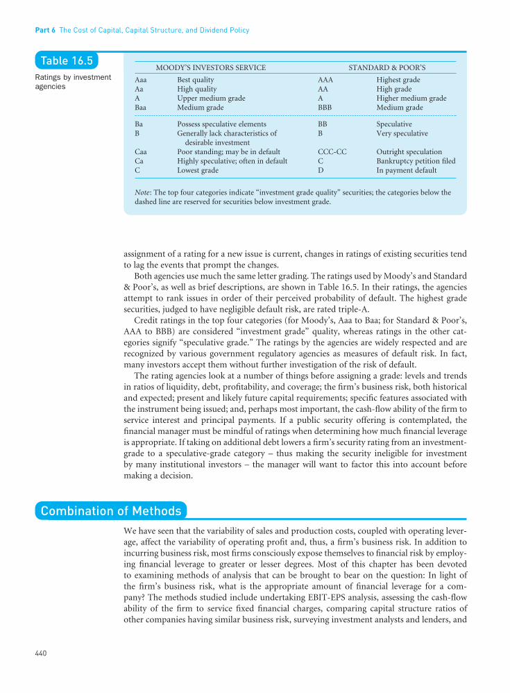
assignment of a rating for a new issue is current, changes in ratings of existing securities tendto lag the events that prompt the changes.
Both agencies use much the same letter grading. The ratings used by Moody’s and Standard& Poor’s, as well as brief descriptions, are shown in Table 16.5. In their ratings, the agenciesattempt to rank issues in order of their perceived probability of default. The highest gradesecurities, judged to have negligible default risk, are rated triple-A.
Credit ratings in the top four categories (for Moody’s, Aaa to Baa; for Standard & Poor’s,AAA to BBB) are considered “investment grade” quality, whereas ratings in the other cat-egories signify “speculative grade.” The ratings by the agencies are widely respected and arerecognized by various government regulatory agencies as measures of default risk. In fact,many investors accept them without further investigation of the risk of default.
The rating agencies look at a number of things before assigning a grade: levels and trendsin ratios of liquidity, debt, profitability, and coverage; the firm’s business risk, both historicaland expected; present and likely future capital requirements; specific features associated withthe instrument being issued; and, perhaps most important, the cash-flow ability of the firm toservice interest and principal payments. If a public security offering is contemplated, thefinancial manager must be mindful of ratings when determining how much financial leverageis appropriate. If taking on additional debt lowers a firm’s security rating from an investment-grade to a speculative-grade category – thus making the security ineligible for investment by many institutional investors – the manager will want to factor this into account beforemaking a decision.
Combination of MethodsWe have seen that the variability of sales and production costs, coupled with operating lever-age, affect the variability of operating profit and, thus, a firm’s business risk. In addition toincurring business risk, most firms consciously expose themselves to financial risk by employ-ing financial leverage to greater or lesser degrees. Most of this chapter has been devoted to examining methods of analysis that can be brought to bear on the question: In light of the firm’s business risk, what is the appropriate amount of financial leverage for a com-pany? The methods studied include undertaking EBIT-EPS analysis, assessing the cash-flowability of the firm to service fixed financial charges, comparing capital structure ratios of other companies having similar business risk, surveying investment analysts and lenders, and
Part 6 The Cost of Capital, Capital Structure, and Dividend Policy
440
••
Table 16.5Ratings by investmentagencies
MOODY’S INVESTORS SERVICE STANDARD & POOR’S
Aaa Best quality AAA Highest gradeAa High quality AA High gradeA Upper medium grade A Higher medium gradeBaa Medium grade BBB Medium grade
Ba Possess speculative elements BB SpeculativeB Generally lack characteristics of B Very speculative
desirable investmentCaa Poor standing; may be in default CCC-CC Outright speculationCa Highly speculative; often in default C Bankruptcy petition filedC Lowest grade D In payment default
Note: The top four categories indicate “investment grade quality” securities; the categories below thedashed line are reserved for securities below investment grade.
FUNO_C16.qxd 9/19/08 17:19 Page 440

evaluating the effect of a financial leverage decision on a firm’s security rating. In addition tothe information provided by using these techniques, the financial manager will want to knowthe changing interest costs for various levels of debt. The maturity structure of debt is impor-tant as well, but we take this up later in the book. We focus here only on the broad issue of theamount of financial leverage to employ. All of the analyses should be guided by the concep-tual framework presented in the next chapter.
The implicit cost of financial leverage – that is, the effect that financial leverage has on thevalue of the firm’s common stock – is not easy to isolate and determine. Nevertheless, byundertaking a variety of analyses, the financial manager should be able to determine, withinsome range, the appropriate capital structure for the firm. By necessity, the final decision hasto be somewhat subjective, but it should be based on the best information available. In thisway, the firm is able to obtain the capital structure most appropriate for its situation – the oneit hopes will maximize the market price of the firm’s common stock.
Key Learning Points
l Leverage refers to the use of fixed costs in an attemptto increase (or lever up) profitability. Operating lever-age is due to fixed operating costs associated with theproduction of goods or services, whereas financialleverage is due to the existence of fixed financing costs– in particular, interest on debt. Both types of leverageaffect the level and variability of the firm’s after-taxearnings, and hence the firm’s overall risk and return.
l We can study the relationship between total operatingcosts and total revenues by using a break-even chart,which shows the relationship among total revenues,total operating costs, and operating profits for variouslevels of production and sales.
l The break-even point is the sales volume required sothat total revenues and total costs are equal. It may beexpressed in units or in sales dollars.
l A quantitative measure of the sensitivity of a firm’soperating profit to a change in the firm’s sales is calledthe degree of operating leverage (DOL). The DOL of afirm at a particular level of output (or sales) is the per-centage change in operating profit over the percentagechange in output (or sales) that causes the change inprofits. The closer a firm operates to its break-evenpoint, the higher is the absolute value of its DOL.
l The degree of operating leverage contributes but onecomponent of the overall business risk of the firm.The other principal factors giving rise to business riskare variability or uncertainty of sales and produc-tion costs. The firm’s degree of operating leveragemagnifies the impact of these other factors on thevariability of operating profits.
l Financial leverage is the second step in a two-step profit-magnification process. In step one, operating leveragemagnifies the effect of changes in sales on changes inoperating profit. In step two, financial leverage can be
used to further magnify the effect of any resulting changesin operating profit on changes in earnings per share.
l EBIT-EPS break-even, or indifference, analysis is usedto study the effect of financing alternatives on earn-ings per share. The break-even point is the EBIT levelwhere EPS is the same for two (or more) alternatives.The higher the expected level of EBIT, assuming thatit exceeds the indifference point, the stronger the casethat can be made for debt financing, all other thingsthe same. In addition, the financial manager shouldassess the likelihood of future EBITs actually fallingbelow the indifference point.
l A quantitative measure of the sensitivity of a firm’searnings per share to a change in the firm’s operatingprofit is called the degree of financial leverage (DFL).The DFL at a particular level of operating profit is the percentage change in earnings per share over thepercentage change in operating profit that causes thechange in earnings per share.
l Financial risk encompasses both the risk of possibleinsolvency and the “added” variability in earnings pershare that is induced by the use of financial leverage.
l When financial leverage is combined with operatingleverage, the result is referred to as total (or combined)leverage. A quantitative measure of the total sensitivityof a firm’s earnings per share to a change in the firm’ssales is called the degree of total leverage (DTL). TheDTL of a firm at a particular level of output (or sales)is equal to the percentage change in earnings per shareover the percentage change in output (or sales) thatcauses the change in earnings per share.
l When trying to determine the appropriate financialleverage for a firm, the cash-flow ability of the firm to service debt should be evaluated. The firm’s debtcapacity can be assessed by analyzing coverage ratios
16 Operating and Financial Leverage
441
••
FUNO_C16.qxd 9/19/08 17:19 Page 441

Questions
1. Define operating leverage and the degree of operating leverage (DOL). How are the tworelated?
2. Classify the following short-run manufacturing costs as either typically fixed or typicallyvariable. Which costs are variable at management’s discretion? Are any of these costs fixedin the long run?a. Insurance d. R&D g. Depletionb. Direct labor e. Advertising h. Depreciationc. Bad-debt loss f. Raw materials i. Maintenance
3. What would be the effect on the firm’s operating break-even point of the following individual changes?a. An increase in selling priceb. An increase in the minimum wage paid to the firm’s employeesc. A change from straight-line to accelerated depreciationd. Increased salese. A liberalized credit policy to customers
4. Are there any businesses that are risk free?5. Your friend, Jacques Fauxpas, suggests, “Firms with high fixed operating costs show
extremely dramatic fluctuations in operating profits for any given change in sales volume.” Do you agree with Jacques? Why or why not?
6. You can have a high degree of operating leverage (DOL) and still have low business risk.Why? By the same token, you can have a low DOL and still have high business risk. Why?
7. Define financial leverage and the degree of financial leverage (DFL). How are the tworelated?
8. Discuss the similarities and differences between financial leverage and operating leverage.9. Can the concept of financial leverage be analyzed quantitatively? Explain.
10. The EBIT-EPS chart suggests that the higher the debt ratio, the higher are the earningsper share for any level of EBIT above the indifference point. Why do firms sometimeschoose financing alternatives that do not maximize EPS?
11. Why is the percentage of debt for an electric utility higher than that for the typical manu-facturing company?
12. Is the debt-to-equity ratio a good proxy for financial risk as represented by the cash-flowability of a company to service debt? Why or why not?
13. How can a company determine in practice whether it has too much debt? Too little debt?14. How can coverage ratios be used to determine an appropriate amount of debt to employ?
Are there any shortcomings to the use of these ratios?15. In financial leverage, why not simply increase leverage as long as the firm is able to earn
more on the employment of the funds thus provided than they cost? Would not earningsper share increase?
16. Describe how a company could determine its debt capacity by increasing its debt hypo-thetically until the probability of running out of cash reached some degree of tolerance.
17. How might a company’s bond rating influence a capital structure decision?
Part 6 The Cost of Capital, Capital Structure, and Dividend Policy
442
••
and the probability of cash insolvency under variouslevels of debt.
l Other methods of analyzing the appropriate financ-ing mix for a company include comparing capitalstructure ratios of other companies having similarbusiness risk, surveying investment analysts and
lenders, and evaluating the effect of a financial lever-age decision on a firm’s security rating. In deciding on an appropriate capital structure, all these factorsshould be considered. In addition, certain conceptsinvolving valuation should guide the decision. Theseconcepts are discussed in the next chapter.
FUNO_C16.qxd 9/19/08 17:19 Page 442

Self-Correction Problems
1. Stallings Specialty Paint Company has fixed operating costs of $3 million a year. Variableoperating costs are $1.75 per half pint of paint produced, and the average selling price is $2 per half pint.a. What is the annual operating break-even point in half pints (QBE)? In dollars of sales
(SBE)?b. If variable operating costs decline to $1.68 per half pint, what would happen to the
operating break-even point (QBE)?c. If fixed costs increase to $3.75 million per year, what would be the effect on the operat-
ing break-even point (QBE)?d. Compute the degree of operating leverage (DOL) at the current sales level of 16 million
half pints.e. If sales are expected to increase by 15 percent from the current sales position of
16 million half pints, what would be the resulting percentage change in operating profit (EBIT) from its current position?
2. Gahlon Gearing, Ltd., has a DOL of 2 at its current production and sales level of 10,000units. The resulting operating income figure is $1,000.a. If sales are expected to increase by 20 percent from the current 10,000-unit sales posi-
tion, what would be the resulting operating profit figure?b. At the company’s new sales position of 12,000 units, what is the firm’s “new” DOL
figure?3. David Ding Baseball Bat Company currently has $3 million in debt outstanding, bearing
an interest rate of 12 percent. It wishes to finance a $4 million expansion program and isconsidering three alternatives: additional debt at 14 percent interest (option 1), preferredstock with a 12 percent dividend (option 2), and the sale of common stock at $16 per share(option 3). The company currently has 800,000 shares of common stock outstanding andis in a 40 percent tax bracket.a. If earnings before interest and taxes are currently $1.5 million, what would be earnings
per share for the three alternatives, assuming no immediate increase in operating profit?b. Develop a break-even, or indifference, chart for these alternatives. What are the approx-
imate indifference points? To check one of these points, mathematically determine theindifference point between the debt plan and the common stock plan. What are thehorizontal axis intercepts?
c. Compute the degree of financial leverage (DFL) for each alternative at the expectedEBIT level of $1.5 million.
d. Which alternative do you prefer? How much would EBIT need to increase before thenext alternative would be “better” (in terms of EPS)?
4. Show how to derive Eq. (16.8),
from Eq. (16.7),
5. Archimedes Torque and Gear Company has $7.4 million in long-term debt having the following payment schedule:
Degree of operatingleverage (DOL) at units
of output (or sales)
Percentage change inoperating profit (EBIT)Percentage change in
output (or sales)
Q =
DOLQ P V
Q P V FCQ
Q QQ unitsBE
( )=
−− −
=−
( )
16 Operating and Financial Leverage
443
••
FUNO_C16.qxd 9/19/08 17:19 Page 443

AMOUNT
15% serial bonds, $100,000 payable annually in principal $2,400,00013% first-mortgage bonds, $150,000 payable annually in principal 3,000,00018% subordinated debentures, interest only until maturity in 10 years 2,000,000
$7,400,000
Archimedes’ common stock has a book value of $8.3 million and a market value of $6 mil-lion. The corporate tax rate, federal plus state, is 50 percent. Archimedes is in a cyclicalbusiness; its expected EBIT is $2 million, with a standard deviation of $1.5 million. Theaverage debt-to-equity ratio of other companies in the industry is 0.47.a. Determine the interest coverage and the debt-service coverage ratios for the company.b. What are the probabilities that these two ratios will go below 1:1?c. Does Archimedes have too much debt?
6. Aberez Company and Vorlas Vactor, Inc., have the following financial characteristics:
ABEREZ VORLAS VACTOR
Company Industry Norm Company Industry Norm
Debt to equity 1.10 1.43 0.78 0.47Bond rating Aa A Ba BaaInterest coverage 6.10 5.70 7.30 7.10Cash and marketable
securities to total assets 0.08 0.07 0.10 0.13
On the basis of these data, which company has the greater degree of financial risk? Why?
Problems
1. The Andrea S. Fault Seismometer Company is an all-equity-financed firm. It earnsmonthly, after taxes, $24,000 on sales of $880,000. The tax rate of the company is 40 per-cent. The company’s only product, “The Desktop Seismometer,” sells for $200, of which$150 is variable cost.a. What is the company’s monthly fixed operating cost?b. What is the monthly operating break-even point in units? In dollars?c. Compute and plot the degree of operating leverage (DOL) versus quantity produced
and sold for the following possible monthly sales levels: 4,000 units; 4,400 units; 4,800 units; 5,200 units; 5,600 units; and 6,000 units.
d. What does the graph that you drew (see Part (c)) – and especially the company’s DOLat its current sales figure – tell you about the sensitivity of the company’s operatingprofit to changes in sales?
2. What would be the effect of the following on the break-even point of the Andrea S. FaultCompany (Problem 1)?a. An increase in selling price of $50 per unit (assume that sales volume remains constant)b. A decrease in fixed operating costs of $20,000 per monthc. A decrease in variable costs of $10 per unit and an increase in fixed costs of $60,000
per month3. The Crazy Horse Hotel has a capacity to stable 50 horses. The fee for stabling a horse
is $100 per month. Maintenance, depreciation, and other fixed operating costs total $1,200 per month. Variable operating costs per horse are $12 per month for hay and bedding and $8 per month for grain.a. Determine the monthly operating break-even point (in horses stabled).b. Compute the monthly operating profit if an average of 40 horses are stabled.
4. Cybernauts, Ltd., is a new firm that wishes to determine an appropriate capital structure.It can issue 16 percent debt or 15 percent preferred stock. The total capitalization of thecompany will be $5 million, and common stock can be sold at $20 per share. The company
Part 6 The Cost of Capital, Capital Structure, and Dividend Policy
444
••
FUNO_C16.qxd 9/19/08 17:19 Page 444

is expected to have a 50 percent tax rate (federal plus state). Four possible capital structuresbeing considered are as follows:
PLAN DEBT PREFERRED EQUITY
1 0% 0% 100%2 30 0 703 50 0 504 50 20 30
a. Construct an EBIT-EPS chart for the four plans. (EBIT is expected to be $1 million.) Be sure to identify the relevant indifference points and determine the horizontal-axisintercepts.
b. Using Eq. (16.12), verify the indifference point on your graph between plans 1 and 3and between plans 3 and 4.
c. Compute the degree of financial leverage (DFL) for each alternative at an expectedEBIT level of $1 million.
d. Which plan is best? Why?5. Hi-Grade Regulator Company currently has 100,000 shares of common stock outstanding
with a market price of $60 per share. It also has $2 million in 6 percent bonds. The com-pany is considering a $3 million expansion program that it can finance with all commonstock at $60 a share (option 1), straight bonds at 8 percent interest (option 2), preferredstock at 7 percent (option 3), and half common stock at $60 per share and half 8 percentbonds (option 4).a. For an expected EBIT level of $1 million after the expansion program, calculate the
earnings per share for each of the alternative methods of financing. Assume a tax rateof 50 percent.
b. Construct an EBIT-EPS chart. Calculate the indifference points between alternatives.What is your interpretation of them?
6. Hi-Grade Regulator Company (see Problem 5) expects the EBIT level after the expansionprogram to be $1 million, with a two-thirds probability that it will be between $600,000and $1,400,000.a. Which financing alternative do you prefer? Why?b. Suppose that the expected EBIT level were $1.5 million and that there is a two-thirds
probability that it would be between $1.3 million and $1.7 million. Which financingalternative would you prefer? Why?
7. Fazio Pump Corporation currently has 1.1 million shares of common stock outstandingand $8 million in debt bearing an interest rate of 10 percent on average. It is considering a$5 million expansion program financed with common stock at $20 per share being realized(option 1), or debt at an interest rate of 11 percent (option 2), or preferred stock with a 10 percent dividend rate (option 3). Earnings before interest and taxes (EBIT) after the newfunds are raised are expected to be $6 million, and the company’s tax rate is 35 percent.a. Determine likely earnings per share after financing for each of the three alternatives.b. What would happen if EBIT were $3 million? $4 million? $8 million?c. What would happen under the original conditions if the tax rate were 46 percent? If the
interest rate on new debt were 8 percent and the preferred stock dividend rate were 7 percent? If the common could be sold for $40 per share?
8. Boehm-Gau Real Estate Speculators, Inc., and the Northern California Electric UtilityCompany have the following EBIT and debt-servicing burden:
NORTHERNBOEHM-GAU CALIFORNIA
Expected EBIT $5,000,000 $100,000,000Annual interest 1,600,000 45,000,000Annual principal payments on debt 2,000,000 35,000,000
16 Operating and Financial Leverage
445
••
FUNO_C16.qxd 9/19/08 17:19 Page 445

The tax rate for Boehm-Gau is 40 percent, and for Northern California Electric Utility is36 percent. Compute the interest coverage and the debt-service coverage ratios for the twocompanies. With which company would you feel more comfortable if you were a lender? Why?
9. The debt ratios of four companies are
TOTAL DEBT/ LONG-TERM DEBT/COMPANY TOTAL ASSETS TOTAL CAPITALIZATION*
A 0.56 0.43B 0.64 0.66C 0.47 0.08D 0.42 0.26
*Total capitalization represents all long-term debt plus shareholders’ equity.
The companies are part of the following industries: supermarket, chemical, apparel mak-ing, and airline (not in order). Match the company with the industry.
Solutions to Self-Correction Problems
1. a.
b.
c.
d.
e. (15 percent) × 4 = 60% increase in EBIT2. a. (Percentage change in sales) × DOL = Percentage change in EBIT
(20 percent) × 2 = 40% change in EBITTherefore, $1,000 × (1 + 0.40) = $1,400
b.
Therefore QBE must equal 5,000 units.
3. a. (000s omitted)
PREFERRED COMMONDEBT STOCK STOCK
Operating profit (EBIT) $1,500 $1,500 $1,500Interest on existing debt 360 360 360Interest on new debt 560 – –
Profit before taxes $ 580 $1,140 $1,140Taxes 232 456 456
Profit after taxes $ 348 $ 684 $ 684Preferred stock dividend – 480 –
Earnings available to common shareholders $ 348 $ 204 $ 684Number of shares 800 800 1,050Earnings per share $0.435 $0.255 $0.651
DOL1 units12,000
2 000 12 000 5 000, , ,
=−
= 1.7
DOLQ1 units
BE
10,0000 000 10 000,
, =
−= 2
DOL16 million units16M
(16M 12M)=
−= 4
QBE$3.75M
($2.00 $1.75)=
−= 15 million half pints
QBE$3M
($2.00 $1.68)=
−= 9.375 million half pints
SBE$3M
1 ($1.75 $2.00)=
−=
/ $24 million in annual sales
QBE$3M
($2.00 $1.75)=
−= 12 million half pints
Part 6 The Cost of Capital, Capital Structure, and Dividend Policy
446
••
FUNO_C16.qxd 9/19/08 17:19 Page 446

b.
Approximate indifference points:
Debt (1) and common (3): $2.7 million in EBIT
Preferred (2) and common (3): $3.7 million in EBIT
Debt dominates preferred by the same margin throughout. There is no indifferencepoint between these two alternative financing methods.
Mathematically, the indifference point between debt (1) and common (3), with 000somitted, is
Cross multiplying and rearranging, we obtain
(EBIT1,3)(0.60)(1,050) − ($920)(0.60)(1,050) = (EBIT1,3)(0.60)(800) − ($360)(0.60)(800)(EBIT1,3)(630) − ($579,600) = (EBIT1,3)(480) − ($172,800)
(EBIT1,3)(150) = $406,800EBIT1,3 = $2,712
Note that, for the debt alternative, the total before-tax interest is $920, and this is theintercept on the horizontal axis. For the preferred stock alternative, we divide $480 by (1 − 0.4) to get $800. When this is added to $360 in interest on existing debt, theintercept becomes $1,160.
c. Debt (1):
Preferred (2):
DFLEBIT of $1.5 million$1,500,000
$1,500,000=
− − −=
$ , [$ , /( . )]
360 000 480 000 1 0 404.41
DFLEBIT of $1.5 million$1,500,000
$1,500,000=
−=
$ ,
920 0002.59
Debt (1)
EBIT
Common Stock (3)
EBIT( $ )( . ) ( $ )( . )
,, ,1 3 1 3920 1 0 40 0
800
360 1 0 40 0
1050− − −
=− − −
16 Operating and Financial Leverage
447
••
FUNO_C16.qxd 9/19/08 17:19 Page 447

Common (3):
d. For the present EBIT level, common is clearly preferable. EBIT would need to increaseby $2,712,000 − $1,500,000 = $1,212,000 before an indifference point with debt isreached. One would want to be comfortably above this indifference point before astrong case for debt should be made. The lower the probability that actual EBIT will fallbelow the indifference point, the stronger the case that can be made for debt, all otherthings the same.
4.
which reduces to
Dividing both the numerator and denominator by (P − V) produces
5. a. Total annual interest is determined as follows:
15% of $2.4 million = $ 360,00013% of $3.0 million = 390,00018% of $2.0 million = 360,000
$1,110,000
Interest coverage ratio = $2,000,000/$1,110,000 = 1.80
Total annual principal payments = $100,000 + $150,000 = $250,000
b. Required deviation of EBIT from its mean value before ratio in question becomes 1:1:
Interest coverage: $1,110,000 − $2,000,000 = −$890,000
Debt-service coverage: $1,610,000 − $2,000,000 = −$390,000
Standardizing each deviation from the mean produces the following Z-scores:
Table V in the Appendix at the end of the book can be used to determine the proportionof the area under the normal curve that is Z standard deviations left of the mean. Thisproportion corresponds to the probability that an EBIT figure will occur that producescoverage ratios lower than 1:1. For interest coverage and debt-service coverage ratiosless than 1:1, these probabilities are approximately 28 percent and 40 percent, respec-tively. These probabilities assume that the distribution of possible EBITs is normal.
c. There is a substantial probability, 40 percent, that the company will fail to cover itsinterest and principal payments. Its debt ratio (using either book or market values) ismuch higher than the industry norm of 0.47. Although the information is limited,
Debt-service coverage standard deviations (left of the mean): $ ,
$ , , .
−= −
390 0001500 000
0 260
Interest coverage 93 standard deviations (left of the mean): $ ,
$ , , .
−= −
890 0001500 000
0 5
Debt-servicecoverage ratio
$ , ,
$ , , [$ , /( . )] =
+ −=
2 000 0001110 000 250 000 1 0 50
1.24
DOLQ
Q FC P VQ
Q QQ unitsBE
=− −
=−
[ /( )]
DOLQ P V
Q P V FCQ units =−
− −
( )( )
DOL
Q P VQ P V FC
Q QQ units
Percentage change inoperating profit (EBIT)Percentage change in
output (or sales)
= =
−− −
⎡⎣⎢
⎤⎦⎥
( )( )
/
Δ
Δ
DFLEBIT of $1.5 million$1,500,000
$1,500,000=
−=
$ ,
360 0001.32
Part 6 The Cost of Capital, Capital Structure, and Dividend Policy
448
••
FUNO_C16.qxd 9/19/08 17:19 Page 448

Donaldson, Gordon. Corporate Debt Capacity. Boston:Division of Research, Harvard Business School, 1961.
—— . “Strategy for Financial Emergencies.” HarvardBusiness Review 47 (November–December 1969), 67–79.
Gahlon, James. “Operating Leverage as a Determinant of Systematic Risk.” Journal of Business Research 9(September 1981), 297–308.
—— , and James Gentry. “On the Relationship BetweenSystematic Risk and the Degrees of Operating andFinancial Leverage.” Financial Management 11 (Summer1982), 15–23.
Harvey, Campbell R., and John R. Graham. “The Theoryand Practice of Corporate Finance: Evidence from theField.” Journal of Financial Economics 60 (May/June2001), 187–243.
Hong, Hai, and Alfred Rappaport. “Debt Capacity, OptimalCapital Structure, and Capital Budgeting.” FinancialManagement 7 (Autumn 1978), 7–11.
Levy, Haim, and Robert Brooks. “Financial Break-EvenAnalysis and the Value of the Firm.” FinancialManagement 15 (Autumn 1986), 22–26.
Myers, Stewart C. “Capital Structure Puzzle.” Journal ofFinance 39 (July 1984), 575–592.
Piper, Thomas R., and Wolf A. Weinhold. “How MuchDebt Is Right for Your Company?” Harvard BusinessReview 60 (July–August 1982), 106–114.
Zivney, Terry L. “Alternative Formulations of Degrees ofLeverage.” Journal of Financial Education 26 (Spring2000), 77–81.
Part VI of the text’s website, Wachowicz’s Web World, contains links to many finance websites and online articles related to topics covered in this chapter.(http://web.utk.edu/~jwachowi/part6.html)
based on what we have, it would appear that Archimedes has too much debt. However,other factors, such as liquidity, may mitigate this conclusion.
6. Aberez has a lower debt ratio than its industry norm. Vorlas has a higher ratio relative toits industry. Both companies exceed modestly their industry norms with respect to inter-est coverage. The lower debt-to-equity ratio and higher interest coverage for Vorlas’sindustry suggests that its industry might have more business risk than the industry ofwhich Aberez is a part. The liquidity ratio of Aberez is higher than the industry norm,whereas that for Vorlas is lower than the industry norm. Although all three financial ratiosfor Vorlas are better than are those for Aberez, they are lower relative to the industry norm.Finally, the bond rating of Aberez is much better than is that of Vorlas, being an Aa gradeand higher than the industry norm. The bond rating of Vorlas is one grade below the verylowest grade for investment-grade bonds. It is also lower than the typical company’s bondrating in the industry. If the industry norms are reasonable representations of underlyingbusiness and financial risk, we would say that Vorlas had the greater degree of risk.
Selected References
16 Operating and Financial Leverage
449
••
FUNO_C16.qxd 9/19/08 17:19 Page 449

••
FUNO_C16.qxd 9/19/08 17:19 Page 450

••
451
17Capital StructureDetermination
Contents
l A Conceptual LookNet Operating Income Approach • TraditionalApproach
l The Total-Value PrincipleArbitrage Support Illustrated
l Presence of Market Imperfections andIncentive IssuesBankruptcy Costs • Agency Costs • Debt andthe Incentive to Manage Efficiently •Institutional Restrictions • Transactions Costs
l The Effect of TaxesCorporate Taxes • Uncertainty of Tax-ShieldBenefits • Corporate Plus Personal Taxes
l Taxes and Market Imperfections CombinedBankruptcy Costs, Agency Costs, and Taxes •Impact of Additional Imperfections
l Financial Signaling
l Timing and Financial Flexibility
l Financing Checklist
l Key Learning Points
l Questions
l Self-Correction Problems
l Problems
l Solutions to Self-Correction Problems
l Selected References
Objectives
After studying Chapter 17, you should be able to:
l Define “capital structure.”
l Explain the net operating income (NOI)approach to capital structure and the valuationof a firm, and calculate a firm’s value using thisapproach.
l Explain the traditional approach to capital struc-ture and the valuation of a firm.
l Discuss the relationship between financial leverage and the cost of capital as originally set forth by Modigliani and Miller (M&M), andevaluate their arguments.
l Describe various market imperfections andother “real world” factors that tend to diluteM&M’s original position.
l Present a number of reasonable arguments forbelieving that an optimal capital structure existsin theory.
l Explain how financial structure changes can beused for financial signaling purposes, and givesome examples.
FUNO_C17.qxd 9/19/08 17:08 Page 451

In the last chapter we approached the question of how much debt a company should have inits capital structure. The incremental expected return and risk to common shareholders arevery much a part of the answer. Now we explore the valuation underpinnings to the ques-tion of capital structure. As we shall see, much controversy surrounds the issue. Despite theunsettled nature of the matter, we hope that this presentation will provide the conceptualbackdrop necessary to guide the financial manager in capital structure decisions.
Throughout our discussion, we assume that the investment and asset management deci-sions of the firm are held constant. We do this in an attempt to isolate the effect of a changein financing mix on share price. The focus is different from before in that we are concernedwith how security prices are determined in the financial markets. That is, how do suppliers of capital value a company in relation to other firms when the company changes its capitalstructure? We shall see that financial market imperfections play a major role in this valuationprocess. For simplicity, we consider only debt-versus-equity financing, though the principlesdiscussed apply to preferred stock financing as well.
A Conceptual LookThe key question with which we are concerned is whether a firm can affect its total valuation(debt plus equity) and its cost of capital by changing its financing mix. We must be careful notto confuse any effects of a change in the financing mix with the results of investment or assetmanagement decisions made by the firm. Therefore changes in the financing mix are assumedto occur by issuing debt and repurchasing common stock or by issuing common stock andretiring debt. In what follows, our attention is directed to what happens to the total valuationof the firm and to its overall required return when the ratio of debt to equity, or the relativeamount of financial leverage, is varied.
For ease of illustration, let us assume that we are concerned with a company whose earnings are not expected to grow and which pays out all of its earnings to shareholders in theform of dividends. Moreover, suppose that we live in a world where there are no income taxes.Later, this assumption will be relaxed to consider the very real-world issue of taxes. For now,the matter of capital structure can best be understood if we assume no taxes and later treattaxes as a financial market imperfection.
In the subsequent discussion we are concerned with three different rates of return. The first is
(17.1)
In this equation, k i is the yield on the company’s debt, assuming this debt to be perpetual.1
The second rate of return with which we are concerned is
(17.2)kESe
Earnings available to common shareholdersMarket value of common stock outstanding
= =
kIBi
Annual interest on debtMarket value of debt outstanding
= =
1In Chapter 4 we saw that the price of a security expected to provide a fixed periodic receipt of R forever is P = R/k,where k is the yield on a perpetual investment. Rearranging, we have k = R/P, which is equivalent to Eq. (17.1).
Part 6 The Cost of Capital, Capital Structure, and Dividend Policy
452
••
When you have eliminated the impossible, whatever remains, howeverimprobable, must be the truth.
—SHERLOCK HOLMESThe Sign of the Four
Capital structure Themix (or proportion) ofa firm’s permanentlong-term financingrepresented by debt,preferred stock, andcommon stock equity.
FUNO_C17.qxd 9/19/08 17:08 Page 452

With our assumptions of a firm whose earnings are not expected to grow and which has a 100 percent dividend payout, the firm’s earnings/price ratio represents the market rate of discount that equates the present value of the perpetual stream of expected constant futuredividends with the current market price of the common stock.2 This is not to say that this particular equation should be used as a general rule to depict the required return on equity.(See Chapter 15.) We use it here only because it works for our example situation of zerogrowth – a situation chosen specifically for its simplicity in illustrating the theory of capitalstructure. The final rate we consider is
(17.3)
where V = B + S (i.e., the total market value of the firm is the sum of the market value of itsdebt and equity), and O = I + E (i.e., the firm’s net operating income is equal to interest paidplus earnings available to common shareholders). Here ko is an overall capitalization ratefor the firm. It is defined as the weighted average cost of capital, and may also be expressed as
(17.4)
We want to know what happens to k i, ke, and ko when the amount of financial leverage, asdenoted by the ratio B/S, increases.
l l l Net Operating Income Approach
One approach to the valuation of the earnings of a company is known as the net operatingincome (NOI) approach. To illustrate it, assume that a firm has $1,000 in debt at 10 percentinterest, that the expected annual net operating income (NOI or EBIT) figure is $1,000, andthat the overall capitalization rate, ko, is 15 percent. Given this information, we may calculatethe value of the firm as follows:
O Net operating income $1,000ko Overall capitalization rate ÷0.15V Total value of the firm (O/ko) $6,667B Market value of debt 1,000S Market value of stock (V − B) $5,667
The earnings available to common shareholders, E, is simply net operating income minusinterest payments, O − I, or $1,000 − $100 = $900. The implied required return on equity is
With this approach, net operating income is capitalized (discounted) at the firm’s overall capitalization rate to obtain the total market value of the firm. The market value of the debtis then deducted from the total market value to obtain the market value of the common stock.Note that with this approach the overall capitalization rate, ko, as well as the cost of debt funds,k i, stays the same regardless of the financial leverage employed. However, the required returnon equity, ke, increases linearly with financial leverage measured as B/S.
kESe = = =
$$ ,
900
5 66715.88%
k kB
B Sk
SB So i e=
+⎡⎣⎢
⎤⎦⎥
++
⎡⎣⎢
⎤⎦⎥
kOVo
Net operating incomeTotal market value of the firm
= =
2Dividing both the numerator and denominator in Eq. (17.2) by the number of shares outstanding reveals that themarket rate of discount, in this case, is equivalent to the earnings/price ratio.
17 Capital Structure Determination
453
••
Capitalization rateThe discount rateused to determine the present value of a stream of expectedfuture cash flows.
Net operating income(NOI) approach (tocapital structure)A theory of capitalstructure in which theweighted average costof capital and thetotal value of the firmremain constant asfinancial leverage ischanged.
FUNO_C17.qxd 9/19/08 17:08 Page 453

To illustrate, suppose that the firm increases the amount of debt from $1,000 to $3,000 anduses the proceeds of the debt issue to repurchase common stock. The valuation of the firmwould then proceed as follows:
O Net operating income $1,000ko Overall capitalization rate ÷0.15V Total value of the firm (O/ko) $6,667B Market value of debt 3,000S Market value of stock (V − B) $3,667
The earnings available to common shareholders, E, is equal to net operating income minusthe now higher interest payments, or $1,000 − $300 = $700. The implied required return onequity is
We see that the required return on equity, ke, rises with increasing leverage. This approachimplies that the total valuation of the firm is unaffected by its capital structure. The reason is that both net operating income and the capitalization rate applied to that income remainconstant in the face of changing capital structure. Figure 17.1 shows the NOI approach graphically.
Importantly, not only is the total value of the firm unaffected by changes in financial leverage but so is share price. To illustrate, assume in our example that the firm with $1,000in debt has 100 shares of common stock outstanding. Thus the market price per share is$5,667/100 = $56.67. The firm then issues $2,000 in additional debt and at the same timerepurchases $2,000 of stock at $56.67 per share, or 35.29 shares if we permit fractional shares.It now has 100 − 35.29 = 64.71 shares outstanding. We saw that the total market value of thefirm’s stock after the change in capital structure is $3,667. Therefore the market price pershare is $3,667/64.71 = $56.67, the same as before the increase in financial leverage resultingfrom recapitalization.
kESe = = =
$$ ,
700
3 66719.09%
Part 6 The Cost of Capital, Capital Structure, and Dividend Policy
454
••
Recapitalization Analteration of a firm’scapital structure. Forexample, a firm maysell bonds to acquirethe cash necessary to repurchase someof its outstandingcommon stock.
Figure 17.1Capital costs and thenet operating income(NOI) approach tocapital structure
FUNO_C17.qxd 9/19/08 17:08 Page 454

The critical assumption with this approach is that ko is constant regardless of the amount
of financial leverage. The market capitalizes the net operating income of the firm and therebydetermines the value of the firm as a whole. As a result, the mix of debt and equity financingis unimportant. An increase in the supposedly “cheaper” debt funds is exactly offset by theincrease in the required rate of return on equity, ke. Thus the weighted average of ke and k i
remains constant as financial leverage is changed. As a firm increases its use of financial lever-age, it becomes increasingly more risky. Investors penalize the stock by raising the requiredequity return directly in keeping with the increase in the debt-to-equity ratio. As long as k i
remains constant, ke is a constant linear function of the debt-to-equity ratio (measured inmarket value terms). Because the cost of capital of the firm, ko, cannot be altered throughfinancial leverage, the net operating income approach implies that there is no one optimalcapital structure.
So far, our discussion of the net operating income approach has been purely definitional.It lacks behavioral significance. Two Nobel Prize-winning finance theorists, Modigliani andMiller, offered behavioral support for the independence of the total valuation and cost of capital of the firm from its capital structure.3 Before taking up the implications of their posi-tion, however, we examine what is called the traditional approach to capital structure andvaluation.
l l l Traditional ApproachThe traditional approach to capital structure and valuation assumes that there is an optimalcapital structure and that management can increase the total value of the firm through thejudicious use of financial leverage. This approach suggests that the firm can initially lower itscost of capital and raise its total value through increasing leverage. Although investors raisethe required rate of return on equity, the increase in ke does not entirely offset the benefit ofusing “cheaper” debt funds. As more and more financial leverage occurs, investors increas-ingly penalize the firm’s required equity return until eventually this effect more than offsetsthe benefits of “cheaper” debt funds.
In one variation of the traditional approach, shown in Figure 17.2, ke is assumed to rise atan increasing rate with financial leverage, whereas k i is assumed to rise only after a significantincrease in financial leverage has occurred. At first, the weighted average cost of capitaldeclines with leverage because the rise in ke does not entirely offset the use of cheaper debtfunds. As a result, the weighted average cost of capital, ko, declines with the moderate use of
3Franco Modigliani and Merton Miller, “The Cost of Capital, Corporation Finance and the Theory of Investment,”American Economic Review 48 (June 1958), 261–297.
17 Capital Structure Determination
455
••
Traditional approach(to capital structure)A theory of capitalstructure in whichthere exists anoptimal capitalstructure and wheremanagement canincrease the totalvalue of the firmthrough the judicioususe of financialleverage.
Optimal capitalstructure The capital structure thatminimizes the firm’scost of capital andthereby maximizes the value of the firm.
Debt Financing
Our Company maintains debt levels we consider prudentbased on our cash flows, interest coverage ratio and
percentage of debt to capital. We use debt financing to lowerour overall cost of capital, which increases our return onshareowners’ equity.
Source: The Coca-Cola Company 2006 Annual Report (Form 10-K), p. 59.Reproduced with permission of The Coca-Cola Company.“Coca-Cola”, the Contour Bottle, and the Dynamic Ribbon are registered trademarks of The Coca-Cola Company.
The Coca-Cola Company Comments on Its Use of Debt Financing
FUNO_C17.qxd 9/19/08 17:08 Page 455

financial leverage. After a point, however, the increase in ke more than offsets the use ofcheaper debt funds in the capital structure, and ko begins to rise. The rise in ko is supportedfurther, once k i begins to rise. The optimal capital structure is the point at which ko bottomsout. In the figure, this optimal capital structure is represented by point X. At the optimal capital structure position represented by point X, not only will the firm’s weighted averagecost of capital be at its lowest point but the firm’s total value will be at its highest point. Thisis because the lower the capitalization rate, ko, applied to the firm’s net operating incomestream, the higher the present value of that stream. Thus the traditional approach to capitalstructure implies that (1) the cost of capital is dependent on the capital structure of the firm,and (2) there is an optimal capital structure.
The Total-Value PrincipleModigliani and Miller (M&M) in their original position advocate that the relationshipbetween financial leverage and the cost of capital is explained by the net operating incomeapproach. They make a formidable attack on the traditional position by offering behavioraljustification for having the firm’s overall capitalization rate, ko, remain constant throughoutthe entire range of financial leverage possibilities.
M&M argue that the total risk for all security holders of a firm is not altered by changes inthe firm’s capital structure. Therefore the total value of the firm must be the same, regardlessof the firm’s financing mix. Simply put, the M&M position is based on the idea that no matter how you divide up the capital structure of a firm among debt, equity, and other claims,there is a conservation of investment value. That is, because the total investment value of acorporation depends on its underlying profitability and risk, firm value is unchanging withrespect to changes in the firm’s capital structure. Thus, in the absence of taxes and other mar-ket imperfections, the value of the total pie does not change as it is divided into debt, equity,and other securities. This idea is illustrated with the two pie graphs in Figure 17.3. Differentmixes of debt and equity do not alter the overall size of the pie; in other words, the total valueof the firm stays the same.
Part 6 The Cost of Capital, Capital Structure, and Dividend Policy
456
••
Figure 17.2Capital costs and thetraditional approachto capital structure
FUNO_C17.qxd 9/19/08 17:08 Page 456
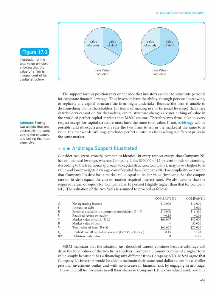
The support for this position rests on the idea that investors are able to substitute personal
for corporate financial leverage. Thus investors have the ability, through personal borrowing,to replicate any capital structure the firm might undertake. Because the firm is unable to do something for its shareholders (in terms of making use of financial leverage) that theseshareholders cannot do for themselves, capital structure changes are not a thing of value inthe world of perfect capital markets that M&M assume. Therefore two firms alike in everyrespect except for capital structure must have the same total value. If not, arbitrage will bepossible, and its occurrence will cause the two firms to sell in the market at the same totalvalue. In other words, arbitrage precludes perfect substitutes from selling at different prices inthe same market.
l l l Arbitrage Support IllustratedConsider two (zero-growth) companies identical in every respect except that Company NLhas no financial leverage, whereas Company L has $30,000 of 12 percent bonds outstanding.According to the traditional approach to capital structure, Company L may have a higher totalvalue and lower weighted average cost of capital than Company NL. For simplicity, we assumethat Company L’s debt has a market value equal to its par value (implying that the couponrate on its debt equals the current market-required interest rate). We also assume that therequired return on equity for Company L is 16 percent (slightly higher than that for companyNL). The valuation of the two firms is assumed to proceed as follows:
COMPANY NL COMPANY L
O Net operating income $10,000 $10,000I Interest on debt – 3,600E Earnings available to common shareholders (O − I) $10,000 $ 6,400ke Required return on equity ÷0.15 ÷0.16S Market value of stock (E/ke) $66,667 $40,000B Market value of debt – 30,000V Total value of firm (B + S) $66,667 $70,000
ko Implied overall capitalization rate [k i(B/V ) + ke(S/V )] 0.15 0.143B/S Debt-to-equity ratio 0 0.75
M&M maintain that the situation just described cannot continue because arbitrage willdrive the total values of the two firms together. Company L cannot command a higher totalvalue simply because it has a financing mix different from Company NL’s. M&M argue thatCompany L’s investors would be able to maintain their same total dollar return for a smallerpersonal investment outlay and with no increase in financial risk by engaging in arbitrage.This would call for investors to sell their shares in Company L (the overvalued asset) and buy
17 Capital Structure Determination
457
••
Arbitrage Finding two assets that areessentially the same,buying the cheaper,and selling the moreexpensive.
Figure 17.3Illustration of thetotal-value principleshowing that thevalue of a firm isindependent of itscapital structure
FUNO_C17.qxd 9/19/08 17:08 Page 457

shares in Company NL (the undervalued asset). These arbitrage transactions would continueuntil Company L’s shares declined in price and Company NL’s shares increased in priceenough to make the total value of the two firms identical.
For example, assume that you are a rational investor who owns 1 percent of the stock ofCompany L, the levered firm, with a market value of $40,000 × 0.01 = $400. You should
1. Sell the stock in Company L for $400.
2. Borrow $300 at 12 percent interest. This personal debt is equal to 1 percent of the debtof Company L – the same percentage as your previous ownership interest in CompanyL. (Your total capital available for investment is now $400 + $300 = $700.)
3. Buy 1 percent of the shares of Company NL, the unlevered firm, for $666.67 and stillhave $700 − $666.67 = $33.33 left over for other investments.
Prior to this series of transactions, your expected return on investment in Company L’scommon stock was 16 percent on an investment of $400, or $64. Your return on investmentin Company NL is 15 percent on a $666.67 investment, or $100. From this return, you mustdeduct the interest charges on your personal borrowings, so your net dollar return is deter-mined as follows:
Return on investment in Company NL $100Less: Interest paid ($300 × 0.12) 36
Net return $ 64
Your net dollar return, $64, is the same as it was for your investment in Company L. However,your personal cash outlay of $366.67 ($666.67 less personal borrowings of $300) is $33.33 less than the previous $400 investment in Company L, the levered firm. Because of the lowerpersonal investment, you would prefer to invest in Company NL under the conditions wedescribed. In essence, you “lever” the common stock of the unlevered firm by taking on personal debt.
The action of a number of investors undertaking similar arbitrage transactions will tend to(1) drive up Company NL’s share price while lowering its required return on equity, and (2)drive down Company L’s share price while increasing its required return on equity. This arbitrage process will continue until there is no further opportunity for reducing one’s invest-ment outlay and achieving the same dollar return. At this equilibrium, the total value of thetwo firms must be the same. As a result, the weighted average costs of capital for the two firms,the kos, must also be the same.
The important element in this process is the presence of rational investors in the market whoare willing to substitute personal, or “homemade,” financial leverage for corporate financialleverage. On the basis of the arbitrage process illustrated, M&M conclude that a firm cannotchange its total value or its weighted average cost of capital by using financial leverage. Fromour earlier discussion of the NOI approach – the approach advocated by M&M – we saw thatnot only is the total value of the firm unaffected by changes in financial leverage but so is share price. Consequently, the financing decision does not matter from the standpoint of ourobjective of maximizing market price per share. One capital structure is as good as the next.
Presence of Market Imperfections and Incentive IssuesWith perfect capital markets, the arbitrage argument ensures the validity of M&M’s con-tention that the cost of capital and total valuation of a firm are independent of its capitalstructure. To dispute the M&M position, we need to look for reasons why the arbitrage process may not work perfectly. The following are the major arguments against the M&Marbitrage process.
Part 6 The Cost of Capital, Capital Structure, and Dividend Policy
458
••
FUNO_C17.qxd 9/19/08 17:08 Page 458

l l l Bankruptcy CostsIf there is a possibility of bankruptcy, and if administrative and other costs associated with bankruptcy are significant, the levered firm may be less attractive to investors than theunlevered one. With perfect capital markets, zero bankruptcy costs are assumed. If the firmgoes bankrupt, assets presumably can be sold at their economic values with no liquidating orlegal costs involved. Proceeds from the sale are distributed according to the priority of claimson assets as described in the Appendix to Chapter 23. If capital markets are less than perfect,however, there may be administrative costs, and assets may have to be liquidated at less thantheir economic values. These administrative costs and the “shortfall” in liquidating value fromeconomic value represent a drain on the system from the viewpoint of the debt and equityholders. (See the Appendix to Chapter 23 for a discussion of the administrative aspects ofbankruptcy.)
In the event of bankruptcy, security holders as a whole receive less than they would have in the absence of bankruptcy costs. To the extent that the levered firm has a greater pos-sibility of bankruptcy than the unlevered one, it would be a less attractive investment, all other things being the same. The possibility of bankruptcy is not a linear function of the debt-to-equity ratio but rather increases at an increasing rate beyond some threshold. As a result, the expected cost of bankruptcy also increases in this accelerating manner and wouldbe expected to have a corresponding negative effect on the value of the firm.
Put another way, investors are likely to penalize the price of the stock as leverage increases.The nature of the penalty is illustrated in Figure 17.4 for the case of a no-tax world. Here the required rate of return for equity investors, ke, is broken down into its component parts. There is the risk-free rate, Rf, plus a premium for business risk. The premium is depicted on the vertical axis by the difference between the required rate of return for an all-equity capital structure and the risk-free rate. As debt is added, the required rate of return rises, and this increment represents a financial-risk premium. In the absence ofbankruptcy costs, the required return would rise in a linear manner according to M&M, and this relationship is shown. However, allowing for bankruptcy costs and an increasingprobability of bankruptcy with increasing financial leverage, the required rate of return onequity would be expected to rise at an increasing rate beyond some point. At first there might
17 Capital Structure Determination
459
••
Figure 17.4Required rate ofreturn for equitycapital whenbankruptcy costs exist
FUNO_C17.qxd 9/19/08 17:08 Page 459

be a negligible probability of bankruptcy, so there would be little or no penalty. As financialleverage increases, so too does the penalty. For extreme leverage, the penalty becomes verysubstantial indeed.
l l l Agency Costs
Closely related to bankruptcy costs with respect to impact on capital structure and value areagency costs. We may think of management as agents of the owners of the company, theshareholders. These shareholders, hoping that the agents will act in the shareholders’ bestinterests, delegate decision-making authority to them. For management to make optimaldecisions on the shareholders’ behalf, it is important that management not only have the correct incentives (salary, bonuses, stock options, and “perks”) but that they be monitored as well. Monitoring can be done through such methods as bonding the agents, auditing financial statements, and explicitly restricting management decisions. Creditors monitor thebehavior of management and shareholders by imposing protective covenants in loan agree-ments between the borrower and lenders. (See Chapter 20.) The monitoring activities men-tioned necessarily involve costs.
Jensen and Meckling have developed a sophisticated theory of agency costs.4 Among other things, they show that, regardless of who makes the monitoring expenditures, the costis ultimately borne by shareholders. For example, debt holders, anticipating monitoringexpenditures, charge higher interest. The greater the probable monitoring costs, the higherthe interest rate, and the lower the value of the firm to its shareholders, all other things stay-ing the same. The presence of monitoring costs acts as a disincentive to the issuance of debt,particularly beyond a prudent amount. It is likely that the amount of monitoring required bydebt holders increases with the amount of debt outstanding. When there is little or no debt,lenders may engage in only limited monitoring, whereas with a great deal of debt, they mayinsist on extensive monitoring. Monitoring costs, like bankruptcy costs, tend to rise at anincreasing rate with financial leverage, as illustrated in Figure 17.4.
l l l Debt and the Incentive to Manage Efficiently
Working in the opposite direction from bankruptcy and agency costs is the notion that highdebt levels create incentives for management to be more efficient.5 By taking on the cash-flowobligation to service debt, it is claimed that management’s “feet are held close to the fire.” Asa result there is said to be an incentive not to squander funds in wasteful expenditures,whether it be for an investment, a “perk,” a company plane, or whatever. The idea is that levered companies may be leaner because management cuts the fat. In contrast, the companywith little debt and significant free cash flow (cash left over after investing in all worthwhileprojects) may have a tendency to squander money. In the absence of other incentives, “running scared” to make debt payments may have a salutary effect on efficiency.
l l l Institutional Restrictions
Restrictions on investment behavior may retard the arbitrage process. Many institutionalinvestors, such as pension funds and life insurance companies, are not allowed to engage inthe “homemade” leverage that was described earlier. Regulatory bodies often restrict stockand bond investments to a list of companies meeting certain quality standards such as
4Michael C. Jensen and William H. Meckling, “Theory of the Firm: Managerial Behavior, Agency Costs andOwnership Structure,” Journal of Financial Economics 3 (October 1976), 305–360.5A number of people have made this argument, but it is perhaps articulated best in Michael C. Jensen, “The TakeoverControversy: Analysis and Evidence,” Midland Corporate Finance Journal 4 (Summer 1986), 12–21.
Part 6 The Cost of Capital, Capital Structure, and Dividend Policy
460
••
Agency costsCosts associated with monitoringmanagement toensure that itbehaves in waysconsistent with thefirm’s contractualagreements withcreditors andshareholders.
FUNO_C17.qxd 9/19/08 17:08 Page 460

exhibiting only a “safe” amount of financial leverage. If a company exceeds that amount, itssecurities may be removed from the approved list, thereby preventing certain institutions frominvesting in them. This reduction in institutional investor demand can have an adverse effecton the market value of the company’s financial instruments.
l l l Transactions Costs
Transactions costs tend to restrict the arbitrage process. Arbitrage will take place only up to the limits imposed by transactions costs, after which it is no longer profitable. As a result,the levered firm could have a slightly higher or slightly lower total value than theory might dictate. The direction of the net effect of this imperfection is not predictable.
With the exception of the incentive to manage efficiently and of transactions costs, the factors discussed above limit the amount of debt that the firm will want to issue. In particular,extreme financial leverage will be burdened by a number of costs and restrictions. If marketimperfections systematically affect the arbitrage process, then capital structure decisions maymatter. To develop a complete picture, we must include the important role of taxes, to whichwe now turn.
The Effect of TaxesWhen we allow for taxes, most financial experts agree that the judicious use of financial leverage can have a favorable impact on a company’s total valuation. We must consider twotaxes – corporate and personal. Because their effects are different, we take them up sepa-rately. In the end, we will draw together their separate effects along with those of the marketimperfections previously considered. For now, we assume that there are no market imper-fections other than the presence of corporate taxes.
l l l Corporate Taxes
The advantage of debt in a world of corporate taxes is that interest payments are a tax-deductible expense to the debt-issuing firm. However, dividends paid are not a tax-deductibleexpense to the dividend-paying corporation. Consequently, the total amount of funds avail-able to pay both debt holders and shareholders is greater if debt is employed.
To illustrate, suppose that net operating income is $2,000 for Companies ND and D. Thesetwo companies are alike in every respect except for their use of financial leverage. CompanyD has $5,000 in debt at 12 percent interest, whereas Company ND has no debt. If the tax rate(federal plus state) is 40 percent for each company, we have
COMPANY ND COMPANY D
Net operating income $2,000 $2,000Interest on debt (also, income to debt holders) – 600
Income before taxes $2,000 $1,400Taxes (at 0.40 rate) 800 560
Income available to common shareholders $1,200 $ 840Total income available to all (debt plus equity) security holders $1,200 $1,440Difference in income available to all (debt plus equity) security holders $240
Thus total income available to both debt holders and shareholders is larger for the leveredCompany D than it is for unlevered Company ND. The reason is that debt holders receiveinterest payments before the deduction of taxes at the corporate level, whereas income toshareholders is available only after corporate taxes have been paid. In essence, the government
17 Capital Structure Determination
461
••
FUNO_C17.qxd 9/19/08 17:08 Page 461

pays a subsidy to the levered firm for the firm’s use of debt. Because interest on debt reducestaxable income, it is called a tax shield. Total income available to all investors increases by an amount equal to the interest tax shield times the corporate tax rate. In our example, thisamounts to $600 × 0.40 = $240. This figure represents a tax-shield benefit that the governmentprovides the levered company. If the debt employed by a company is permanent, the presentvalue of the annual tax-shield benefit using the perpetual cash-flow formula is
(17.5)
where r is the interest rate on the debt, B is the market value of the debt, and tc is the corpor-ate tax rate. For Company D in our example, we have
The “bottom line” is that the interest tax shield is a thing of value and that the overall valueof Company D is $2,000 higher because the company employed debt than it would be if thecompany had no debt. This increased valuation occurs because the stream of income to allinvestors is $240 per year greater than in the absence of debt. The present value of $240 peryear discounted at 12 percent is $240/0.12 = $2,000. Implied is that the risk associated withthe tax-shield benefits is that of the stream of interest payments, so the appropriate discountrate is the interest rate on the debt. Thus we have
(17.6)
For our example situation, suppose that the equity capitalization rate for company ND, whichhas no debt, is 16 percent. Assuming zero growth and a 100 percent earnings payout, the valueof the (unlevered) firm is $1,200/0.16 = $7,500. The value of the tax-shield benefits is $2,000,so the total value of Company D, the levered firm, is $7,500 + $2,000 = $9,500.
We see in Eqs. (17.5) and (17.6) that the greater the amount of debt, the greater the tax-shield benefits and the greater the value of the firm, all other things staying the same. Bythe same token, the greater the financial leverage, the lower the cost of capital of the firm.Thus the original M&M proposition as subsequently adjusted for corporate taxes suggests that an optimal strategy is to take on a maximum amount of financial leverage.6 This implies a capital structure consisting almost entirely of debt. Because this is not consistent with theobserved behavior of corporations, we must seek alternative explanations.
l l l Uncertainty of Tax-Shield Benefits
The tax savings associated with the use of debt are not usually certain, as implied in the treat-ment above. If taxable income should be low or turn negative, the tax-shield benefits fromdebt are reduced or even eliminated. Moreover, if the firm should go bankrupt and liquidate,the future tax savings associated with debt would stop altogether. There is uncertainty notonly as to the tax-shield benefits associated with debt but also concerning those associatedwith other tax shields (e.g., lease payments). This only compounds the overall uncertainty.Finally, there is uncertainty that Congress will change the corporate tax rate.
Value oflevered
firm
Value offirm if
unlevered
Present value oftax-shield benefits
of debt = +
Present value oftax-shield benefits
of debt ($ , )( . ) = =5 000 0 40 $2,000
Present value oftax-shield benefits
of debt
cc
( )( )( ) ( )( )= =
r B tr
B t
6Franco Modigliani and Merton H. Miller, “Corporate Income Taxes and the Cost of Capital: A Correction,”American Economic Review 64 (June 1963), 433–442.
Part 6 The Cost of Capital, Capital Structure, and Dividend Policy
462
••
Tax shield A tax-deductible expense.The expense protects(shields) anequivalent dollaramount of revenuefrom being taxed byreducing taxableincome.
FUNO_C17.qxd 9/19/08 17:08 Page 462

All of these things make the tax-shield benefits associated with debt financing less than certain. As financial leverage increases, the uncertainty associated with the interest tax-shieldbenefits becomes a more and more important issue. As a result, this uncertainty may reducethe value of the corporate tax-shield benefits shown in Eq. (17.6). With extreme financialleverage, the lessening in value of the corporate tax-shield benefits may be rather significant.
l l l Corporate Plus Personal Taxes
With the combination of corporate taxes and personal taxes on both debt and stock income,the present value of the interest tax-shield benefits shown in Eq. (17.5) will likely be lowered.The magnitude of the resulting tax-shield benefits is an empirical question subject to muchdebate. However, the general consensus is that personal taxes act to reduce but not eliminatethe corporate tax advantage associated with debt. As a result, an optimal leverage strategywould still call for the corporation to have a large proportion of debt. This is despite the factthat tax-shield benefits uncertainty may lessen the “net” tax effect with extreme leverage. Ascorporations overall are not highly levered, we must search for other factors affecting the valuation of the corporation when it alters the proportion of debt in its capital structure.
Taxes and Market Imperfections CombinedOur last statement brings us back to the influence of various market imperfections consideredearlier. Only if they in some way restrict the use of debt financing can the observed capitalstructure behavior of corporations be explained.
l l l Bankruptcy Costs, Agency Costs, and Taxes
If one allows for bankruptcy costs, and if the probability of bankruptcy increases at an increasing rate with the use of financial leverage, extreme leverage is likely to be penalized bylenders and investors. (As discussed earlier, bankruptcy costs represent a drain on the systemto security holders.) In a world of both bankruptcy costs and taxes, an optimal capital struc-ture would exist even if all of the other behavioral tenets of the M&M position held. The costof capital of a firm would decline as financial leverage was first employed because of the nettax advantage of debt. Gradually, however, the prospect of bankruptcy would become increas-ingly important, causing the cost of capital to decrease at a decreasing rate as financial lever-age increased. As financial leverage became extreme, the bankruptcy effect might more thanoffset the tax effect, causing the cost of capital of the firm to rise.
The presence of agency, or monitoring, costs accentuates this rise in the cost of capital.Again, with increases in financial leverage beyond some threshold, agency costs increase at an increasing rate. The combined influence of bankruptcy and agency costs serves to limit therange over which the net tax-shield benefits have a positive effect on share price. In short, we have
(17.7)
As financial leverage is increased, the second term on the right increases so that the value ofthe firm also increases. With more and more financial leverage, the growing uncertainty sur-rounding tax-shield benefits gradually reduces the increment in value that occurs. Despite thisoccurrence, if we look only at the net tax effect, a high proportion of debt would be optimal.
This effect is illustrated in Figure 17.5 by the solid line. We see that tax-shield benefituncertainty causes the cost of capital line to curve up slightly as more and more financial
Value oflevered
firm
Value offirm if
unlevered
Present value ofnet tax-shield
benefits of debt
Present value ofbankruptcy and
agency costs = + −
17 Capital Structure Determination
463
••
FUNO_C17.qxd 9/19/08 17:08 Page 463

leverage occurs. Still, the net tax effect (corporate plus personal) has a favorable impact on thecost of capital and on share value. When the firm has little debt, bankruptcy and agency costsare seen to be insignificant. As more debt is employed, these costs eventually become signifi-cant, as reflected by the dashed line. Increasingly, these costs offset the net tax-shield benefits.At the point where marginal bankruptcy/agency costs equal the marginal tax-shield benefits,the cost of capital is minimized and share price is maximized. By definition, this representsthe optimal capital structure, as denoted by the mark along the horizontal axis in Figure 17.5.To visualize the effect of financial leverage on share price, substitute share value for cost ofcapital on the vertical axis and turn the figure upside down.
l l l Impact of Additional Imperfections
If other imperfections and behavioral factors further dilute the M&M position, the point atwhich the cost of capital line turns up would be earlier than that depicted in the figure.Consider now the cost of borrowing. After some point of financial leverage, the interest ratecharged by creditors usually rises. The greater the financial leverage, of course, the higher theinterest rate charged. As a result, the cost of debt would turn up after a point. This phe-nomenon was illustrated earlier in Figure 17.2. In turn, this factor exerts upward influence onthe overall cost of capital line. Institutional restrictions on lenders might also cause the cost of capital line to turn up sooner than it does in Figure 17.5. Because of extreme financial leverage a company may no longer be able to sell debt securities to institutions. In such a case, the company must seek out unrestricted investors, and these investors will demand even higher interest rates. If institutional imperfections are serious enough, debt funds maynot be available beyond a particular point of financial leverage. In that case there would be a discontinuity in Figure 17.5.
Other capital market imperfections work to hamper the arbitrage process so that “home-made” financial leverage is not a perfect substitute for corporate financial leverage. Recall thatthese imperfections include institutional restrictions and transaction costs. The greater theimportance attached to market imperfections, the less effective the arbitrage process becomes,and the stronger the case that can be made for an optimal capital structure.
There are a number of reasons for believing that an optimal capital structure exists in theory. Depending on one’s view as to the strengths of the various capital market and be-havioral imperfections, the expected optimal capital structure may occur earlier or later alongthe scale of possible debt-to-equity ratios.
Part 6 The Cost of Capital, Capital Structure, and Dividend Policy
464
Figure 17.5Cost of capital withtaxes, bankruptcy,and agency costscombined
FUNO_C17.qxd 4/18/09 9:59 AM Page 464

Financial SignalingClosely related to monitoring costs and agency relationships is the notion of signaling. Becausestrict managerial contracts are difficult to enforce, a manager may use capital structurechanges to convey information about the profitability and risk of the firm. The implication is that insiders (managers) know something about the firm that outsiders (security holders)do not. As a manager, your pay and benefits may depend on the firm’s market value, whichgives you an incentive to let investors know when the firm is undervalued. You could makean announcement, “Our firm is undervalued,” but you know that investors would probablybe as convinced as if you were boasting about your child’s intelligence. So, instead, you alter your firm’s capital structure by issuing more debt. Increased leverage implies a higherprobability of bankruptcy. Because you would be penalized contractually if bankruptcyoccurred, investors conclude that you have good reason to believe that things are really betterthan the stock price reflects. Your actions speak louder than words. Increased leverage is apositive sign.
More formally, a signaling effect assumes that information asymmetry (unequalness) existsbetween management and shareholders. Assume that management is considering additionallong-term financing and will issue either bonds or common stock. Management will want tochoose the overvalued security if it is acting in the interests of current shareholders. That is, it will issue common stock if it believes the existing common stock is overvalued and debt if it believes the stock is undervalued. However, investors are aware of this phenomenon, sothey regard debt issues as “good news” and common stock issues as “bad news.”
This is not to say that capital structure changes necessarily cause changes in valuation.Rather, it is the signal conveyed by the change that is significant. This signal pertains to theunderlying profitability and risk of the firm, because that is what is important when it comesto valuation. Financial signaling is a topic of considerable interest in finance research, but the various models that have been built around this topic are difficult to evaluate. Unless themanagerial contract is very precise, the manager is tempted to give false signals. Moreover,there may simply be more effective and less costly ways to convey information than by alter-ing the firm’s capital structure. We will have more to say about financial signaling when weconsider dividend policy in Chapter 18 and new security issues in Chapter 19.
Timing and Financial FlexibilityOnce a company has determined an appropriate capital structure, it still has the problem of timing security issues. When external financing is required, a company often faces the question of how to time an issue appropriately and whether to use debt or common stock.Because financing is “lumpy,” it is difficult for a company to maintain strict proportions in itscapital structure. Frequently, it must decide whether to finance now with a stock issue andlater with a debt issue, or vice versa. Consequently, it is forced to evaluate the alternativemethods of financing in light of general market conditions and expectations for the com-pany itself.
If the future were certain, it would be an easy matter to determine today an optimal financ-ing sequence for many years to come. The sequence would be timed to take advantage ofknown future changes in the stock market and in the market for fixed-income securities.Unfortunately, prices in financial markets, particularly in the equity market, are unstable.Instead of making decisions based on a sure thing, decisions must be based on manage-ment’s best estimate of the future. In addition, there are the financial signaling and incentiveissues mentioned earlier. Usually, the announcement of a debt issue has a favorable impact onshare price, as we know from that discussion.
If a firm chooses the debt alternative, however, it may sacrifice a certain amount of flex-ibility. By flexibility, we simply mean the extent to which today’s financing decision will keep
17 Capital Structure Determination
465
••
FUNO_C17.qxd 9/19/08 17:08 Page 465

open future financing options. Remember that a company cannot issue debt continuouslywithout building its equity base. Sooner or later, default risk becomes too great. Therefore theequity base must be increased over time, and this is where flexibility becomes important. If acompany undertakes a substantial debt issue and things take a turn for the worse, it may beforced to issue common stock on unfavorable terms in the future. To preserve its flexibility in drawing from the capital markets, it may be better for a firm to issue common stock nowso that it will have unused debt capacity for future needs. The preservation of unused debt capacity can be a significant consideration for the company whose funds requirements aresudden and unpredictable. It gives the company financial maneuverability by virtue of leav-ing its financing options open.
We must keep in mind that if the financial markets are efficient, all available informationis reflected in the price of the security. Under these circumstances, the market price of thesecurity is the market’s best estimate of the value of that security. If management is no betterthan the average investor at forecasting future market prices, efforts by a company to timesecurity offerings will be for naught. In other words, management will be wrong about as often as it is right. If timing is to be of value, management’s expectations must be more correct than those of the market. In Part 7, we examine specific methods of long-term financ-ing, the timing of a specific security issue, and the flexibility afforded by the instrument.
Financing ChecklistWe have discovered a number of methods of analysis that can be brought to bear on the question: What is the appropriate capital structure for our company? In particular, we areconcerned with the mix of debt and equity, saving for later chapters the specific features oftypical long-term financial instruments as well as the more exotic instruments. It is useful now to provide a practical checklist of things that should be considered, drawing both from Chapter 16 and from this chapter.
˛ Taxes – The degree to which a company is subject to taxation is very important. Muchof the advantage of debt is tax related. If, because of marginal profitability, a companypays little or no tax, debt is less attractive than it is for the company subject to the fullcorporate tax rate.
˛ Explicit cost – The higher the interest rate on debt, and the higher the preferred stockdividend rate, the less attractive that method of financing, all other things being the same.
˛ Cash-flow ability to service debt – The analysis here focuses on both the business and the financial risk of a company. Answers to questions posed here are critical to
Part 6 The Cost of Capital, Capital Structure, and Dividend Policy
466
••
Ready Access to Capital
Cameco has an ambitious plan to grow in the nuclear energyindustry. Opportunities to invest are unpredictable and
often capital intensive. We intend to maintain financial flexibil-ity to pursue opportunities as they arise. For that reason, wemaintain a conservative financial structure with a target of nomore than 25% net debt to total capital.
Source: Cameco Corporation, Annual Report – 2006, (www.cameco.com/investor_relations/annual/2006/html/mda/fuel_services.php). Copyright © 2006 Cameco Corporation. Used by permission. All rights reserved.
Cameco Corporation and Financial Flexibility
FUNO_C17.qxd 9/19/08 17:08 Page 466

••
17 Capital Structure Determination
467
determining the debt capacity of a firm. How large and stable are the expected futurecash flows of the firm? What do the firm’s interest coverage and debt-service coverageratios look like, and how do they compare with other firms’ ratios in the same industry?What is the probability that EBIT will fall below the firm’s debt-service burden? What arethe chances of cash insolvency?
˛ Agency costs and incentive issues – Are shareholders willing to bear the increasedmonitoring costs required by debt holders as the amount of debt is increased? Willmanagement be more efficient if saddled with the obligation to service debt? These andother questions of this sort need to be addressed.
˛ Financial signaling – What is likely to be the stock market reaction to a particularfinancing decision, and why? An effect, if any, is based on asymmetric informationbetween management and security holders.
˛ EBIT-EPS analysis – At what point in earnings before interest and taxes (EBIT) areearnings per share (EPS) of a company the same under alternative methods of financ-ing? How does this relate to the existing level of EBIT, and what is the probability offalling below the EBIT-EPS indifference point?
˛ Capital structure ratios – What effect does a method of financing have on the com-pany’s capital structure ratios (e.g., debt to equity, debt to total assets, and debt to networth)? How do these ratios compare with other companies’ ratios in the same indus-try? What is the likely effect of a change in these ratios on investment analysts andlenders?
˛ Security rating – Is a particular method of financing likely to result in a downgrade or an upgrade of a company’s security rating? No financial manager can ignore this consideration, though it should not necessarily be a binding constraint.
˛ Timing – Is it a good time to issue debt? Is it a good time to issue equity? Wheneversecurities are to be issued, the vitality of the debt and stock markets must be addressed.
˛ Flexibility – If a company needs to finance on a continuing basis over time, how doesthe method chosen this time affect future financing? How important is it that a com-pany has flexibility to draw on the debt markets in the future?
These important issues and questions must be addressed when considering the appropriatedegree of financial leverage for a company. By undertaking a variety of analyses, the financialmanager should be able to determine, within some range, the appropriate capital structure for his or her company. The final decision is somewhat subjective, but it can be based on thebest information available. Hopefully, this decision will be consistent with maximizing share-holder wealth.
Key Learning Pointsl Much controversy has developed over whether a firm
can affect its total valuation (debt plus equity) and itscost of capital by changing its financing mix.
l The traditional approach to capital structure and valu-ation assumes that there is an optimal capital structureand that management can increase the total value ofthe firm (and market value per share) through thejudicious use of financial leverage.
l Modigliani and Miller (M&M), on the other hand,argue that in the absence of taxes and other marketimperfections, the total value of the firm and its costof capital are independent of capital structure.
l M&M’s position, which is the same as the net operat-ing income (NOI) approach, is based on the notionthat there is a conservation of investment value. Nomatter how you divide the investment value piebetween debt and equity claims, the total pie (orinvestment value of the firm) stays the same. There-fore leverage is said to be irrelevant. Behavioral sup-port for the M&M position is based on the arbitrageprocess.
l Bankruptcy and agency costs work to the disadvan-tage of financial leverage, particularly extreme finan-cial leverage.
FUNO_C17.qxd 9/19/08 17:08 Page 467

••
Part 6 The Cost of Capital, Capital Structure, and Dividend Policy
468
Questions
1. Contrast the net operating income (NOI) approach with the Modigliani and Miller(M&M) approach to the theory of capital structure.
2. Why might you suspect that the optimal capital structure would differ significantly fromone industry to another? Would the same factors produce differing optimal capital struc-tures within all industry groupings?
3. What factors determine the interest rate a firm must pay for debt funds? Is it reasonableto expect this rate to rise with an increasing debt-to-equity ratio? Why?
4. What is the total-value principle as it applies to capital structure?5. Define the notion of arbitrage. How does it affect the issue of capital structure?6. If there were no imperfections in financial markets, what capital structure should the firm
seek? Why are market imperfections important considerations in finance? Which imper-fections are most important?
7. What are bankruptcy costs? What are agency costs? How do they affect the valuation ofthe firm when it comes to financial leverage?
8. Why do institutional lenders no longer lend money to a corporation when it takes on toomuch debt?
9. Suppose that a company were to earn negligible profits and pay no taxes. How would thisaffect the firm’s optimal capital structure?
10. If the corporate tax rate were cut in half, what would be the effect on debt financing?11. Dividends are currently taxed twice. The corporation must pay taxes on its earnings,
and then shareholders must pay taxes on the dividends paid. What would be the effect oncorporate financing if this double taxation were eliminated by permitting companies todeduct dividend payments as an expense?
12. Why might capital structure changes speak louder than words if management believed itsstock were undervalued? What is the likely direction of the financial signal?
Self-Correction Problems
1. Qwert Typewriter Company and Yuiop Typewriters, Inc., are identical except for capitalstructures. Qwert has 50 percent debt and 50 percent equity financing, whereas Yuiop has 20 percent debt and 80 percent equity financing. (All percentages are in market valueterms.) The borrowing rate for both companies is 13 percent in a no-tax world, and cap-ital markets are assumed to be perfect. The earnings of both companies are not expectedto grow, and all earnings are paid out to shareholders in the form of dividends.
l In a world of corporate income taxes, there is a substantial advantage to the use of debt, and we canmeasure the present value of the tax-shield benefits of debt. This advantage is lessened with tax-shieldbenefits uncertainty, particularly if financial leverageis high.
l When we allow for personal income taxes, we find thetax advantage of debt to be further reduced.
l A combination of the net tax effect with bankruptcyand agency costs will result in an optimal capitalstructure. Other market imperfections impede theequilibrium of security prices based on expectedreturn and risk. As a result, financial leverage mayaffect the value of the firm.
l Financial signaling occurs when capital structurechanges convey information to security holders.Management behavior results in new debt issues being regarded as “good news” by investors, whereasnew stock issues are regarded as “bad news.”
l Once a company has determined an appropriate capital structure, it still has the problem of timing a debt or equity security issue. And when sequentialfinancing is involved, the choice of debt or equityinfluences the future financial flexibility of the firm.
l A checklist of practical and conceptual considera-tions, drawn from this chapter and the preceding one, can help guide you in determining a firm’s capitalstructure.
FUNO_C17.qxd 9/19/08 17:08 Page 468
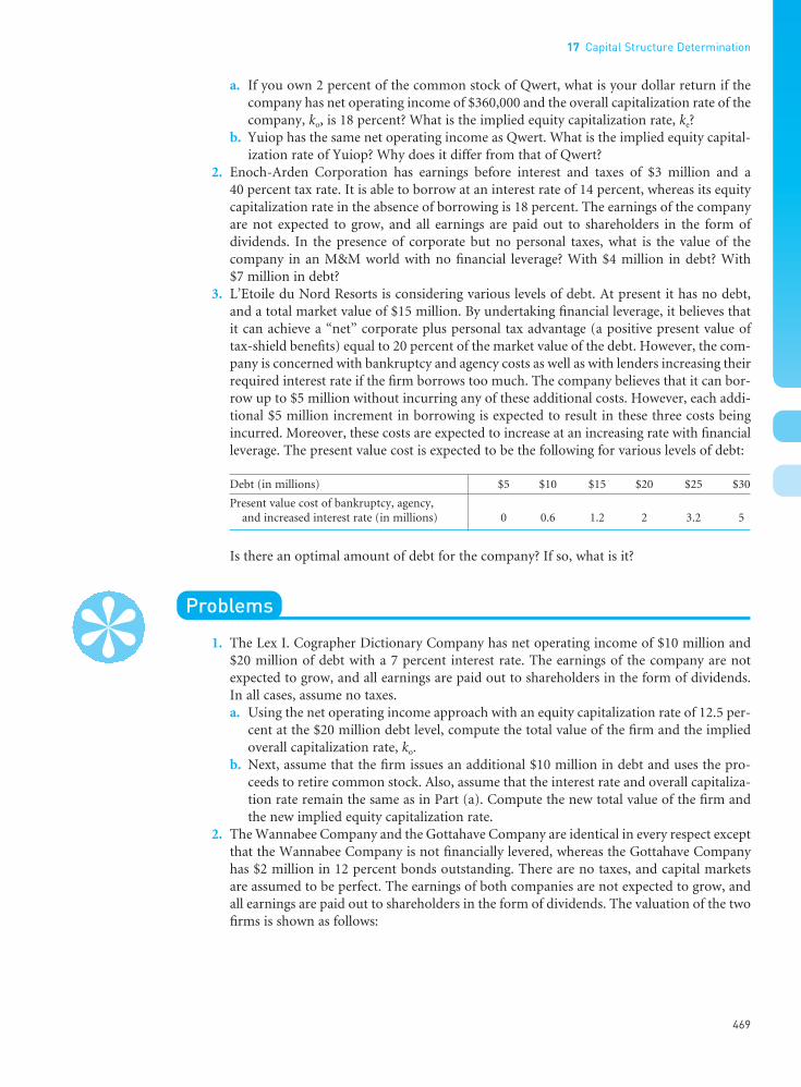
••
17 Capital Structure Determination
469
a. If you own 2 percent of the common stock of Qwert, what is your dollar return if thecompany has net operating income of $360,000 and the overall capitalization rate of thecompany, ko, is 18 percent? What is the implied equity capitalization rate, ke?
b. Yuiop has the same net operating income as Qwert. What is the implied equity capital-ization rate of Yuiop? Why does it differ from that of Qwert?
2. Enoch-Arden Corporation has earnings before interest and taxes of $3 million and a 40 percent tax rate. It is able to borrow at an interest rate of 14 percent, whereas its equitycapitalization rate in the absence of borrowing is 18 percent. The earnings of the companyare not expected to grow, and all earnings are paid out to shareholders in the form of dividends. In the presence of corporate but no personal taxes, what is the value of the company in an M&M world with no financial leverage? With $4 million in debt? With $7 million in debt?
3. L’Etoile du Nord Resorts is considering various levels of debt. At present it has no debt,and a total market value of $15 million. By undertaking financial leverage, it believes thatit can achieve a “net” corporate plus personal tax advantage (a positive present value oftax-shield benefits) equal to 20 percent of the market value of the debt. However, the com-pany is concerned with bankruptcy and agency costs as well as with lenders increasing theirrequired interest rate if the firm borrows too much. The company believes that it can bor-row up to $5 million without incurring any of these additional costs. However, each addi-tional $5 million increment in borrowing is expected to result in these three costs beingincurred. Moreover, these costs are expected to increase at an increasing rate with financialleverage. The present value cost is expected to be the following for various levels of debt:
Debt (in millions) $5 $10 $15 $20 $25 $30
Present value cost of bankruptcy, agency, and increased interest rate (in millions) 0 0.6 1.2 2 3.2 5
Is there an optimal amount of debt for the company? If so, what is it?
Problems
1. The Lex I. Cographer Dictionary Company has net operating income of $10 million and$20 million of debt with a 7 percent interest rate. The earnings of the company are notexpected to grow, and all earnings are paid out to shareholders in the form of dividends.In all cases, assume no taxes.a. Using the net operating income approach with an equity capitalization rate of 12.5 per-
cent at the $20 million debt level, compute the total value of the firm and the impliedoverall capitalization rate, ko.
b. Next, assume that the firm issues an additional $10 million in debt and uses the pro-ceeds to retire common stock. Also, assume that the interest rate and overall capitaliza-tion rate remain the same as in Part (a). Compute the new total value of the firm andthe new implied equity capitalization rate.
2. The Wannabee Company and the Gottahave Company are identical in every respect exceptthat the Wannabee Company is not financially levered, whereas the Gottahave Companyhas $2 million in 12 percent bonds outstanding. There are no taxes, and capital marketsare assumed to be perfect. The earnings of both companies are not expected to grow, andall earnings are paid out to shareholders in the form of dividends. The valuation of the twofirms is shown as follows:
FUNO_C17.qxd 9/19/08 17:08 Page 469

WANNABEE GOTTAHAVE
O Net operating income $ 600,000 $ 600,000I Interest on debt 0 240,000E Earnings available to common shareholders (O − I) $ 600,000 $ 360,000ke Equity capitalization rate ÷0.15 ÷0.16S Market value of stock (E/ke) $4,000,000 $2,250,000B Market value of debt 0 2,000,000V Total value of firm (B + S) $4,000,000 $4,250,000ko Implied overall capitalization rate [k i(B/V) + ke(S/V)] 0.15 0.1412B/S Debt-to-equity ratio 0 0.89
a. You own $22,500 worth of Gottahave stock. Show the process and the amount by whichyou could reduce your outlay through the use of arbitrage.
b. When will this arbitrage process cease?3. The T. Boom Pickens Corporation has a $1 million capital structure and always maintains
this book value amount. Pickens currently earns $250,000 per year before taxes of 50 per-cent, has an all-equity capital structure of 100,000 shares, and pays out all earnings in dividends. The company is considering issuing debt in order to retire common stock. Thecost of the debt and the resulting price per share of the common stock at various levels ofdebt are given in the following table. It is assumed that the new capital structure would bereached all at once by purchasing common stock at the current price of $10 per share. Inother words, the table below is a schedule of alternative conditions at a single point in time.
AVERAGE PRE-TAX RESULTING PRICE PER SHAREAMOUNT OF DEBT COST OF DEBT OF COMMON STOCK
$ 0 – $10.00100,000 10.0% 10.00200,000 10.0 10.50300,000 10.5 10.75400,000 11.0 11.00500,000 12.0 10.50600,000 14.0 9.50
a. By observation, what do you think is the optimal capital structure (the capital structurethat minimizes the firm’s overall cost of capital)? Why?
b. Construct a graph that relates after-tax capital costs (ke, k i, and ko) to financial leverageratios (B/S) based on the data given above.
c. Are your feelings in Part (a) confirmed?4. Gioanni Chantel Truffles, Inc., has $1 million in earnings before interest and taxes. Currently
it is all-equity-financed. It may issue $3 million in perpetual debt at 15 percent interest inorder to repurchase stock, thereby recapitalizing the corporation. There are no personal taxes.a. If the corporate tax rate is 40 percent, what is the income available to all security
holders if the company remains all-equity-financed? If it is recapitalized?b. What is the present value of the debt tax-shield benefits?c. The equity capitalization rate for the company’s common stock is 20 percent while
it remains all-equity-financed. What is the value of the firm if it remains all-equity-financed? What is the firm’s value if it is recapitalized?
5. Stinton Vintage Wine Company is currently family owned and has no debt. The Stintonfamily is considering going public by selling some of their stock in the company. Invest-ment bankers tell them the total market value of the company is $10 million if no debt isemployed. In addition to selling stock, the family wishes to consider issuing debt that, forcomputational purposes, would be perpetual. The debt would then be used to purchaseand retire common stock, so that the size of the company would stay the same. Based on various valuation studies, the present value of the tax-shield benefits is estimated at 22 percent of the amount borrowed when both corporate and personal taxes are taken into
Part 6 The Cost of Capital, Capital Structure, and Dividend Policy
470
••
FUNO_C17.qxd 9/19/08 17:08 Page 470

••
17 Capital Structure Determination
471
account. The company’s investment banker has estimated the following present values forbankruptcy costs associated with various levels of debt:
DEBT PRESENT VALUE OF BANKRUPTCY COSTS
$1,000,000 $ 02,000,000 50,0003,000,000 100,0004,000,000 200,0005,000,000 400,0006,000,000 700,0007,000,000 1,100,0008,000,000 1,600,000
Given this information, what amount of debt should the family choose?6. Rebecca Isbell Optical Corporation is trying to determine an appropriate capital structure.
It knows that, as its financial leverage increases, its cost of borrowing will eventuallyincrease as will the required rate of return on its common stock. The company has madethe following estimates for various financial leverage ratios.
DEBT INTEREST REQUIRED RATE OF RETURN ON EQUITY
DIVIDED BY RATE ON Without Bankruptcy With Bankruptcy (DEBT + EQUITY) BORROWINGS Costs Costs
0 – 10.00% 10.00%0.10 8.0% 10.50 10.500.20 8.0 11.00 11.250.30 8.5 11.50 12.000.40 9.0 12.25 13.000.50 10.0 13.25 14.500.60 11.0 14.50 16.250.70 12.5 16.00 18.500.80 15.0 18.00 21.00
a. At a tax rate of 50 percent, what is the weighted average cost of capital of the companyat various leverage ratios in the absence of bankruptcy costs?
b. With bankruptcy costs, what is the optimal capital structure?7. Art Wyatt Pool Company wishes to finance a $15 million expansion program and is trying
to decide between debt and external equity. Management believes that the market does not appreciate the company’s profit potential and that the common stock is undervalued.What type of security (debt or common stock) do you suppose that the company will issueto provide financing, and what will be the market’s reaction? What type of security do youthink would be issued if management felt the stock were overvalued? Explain.
Solutions to Self-Correction Problems
1. a. Qwert Typewriter Company:
O Net operating income $ 360,000ko Overall capitalization rate ÷0.18V Total value of the firm (B + S) $2,000,000B Market value of debt (50%) 1,000,000S Market value of stock (50%) $1,000,000O Net operating income $ 360,000I Interest on debt (13%) 130,000E Earnings available to common shareholders (O − I) $ 230,000
2% of $230,000 = $4,600
Implied equity capitalization rate, ke = E/S = $230,000/$1,000,000 = 23%.
FUNO_C17.qxd 9/19/08 17:08 Page 471

••
Part 6 The Cost of Capital, Capital Structure, and Dividend Policy
472
b. Yuiop Typewriters, Inc.:
O Net operating income $ 360,000ko Overall capitalization rate ÷0.18V Total value of the firm (B + S) $2,000,000B Market value of debt (20%) 400,000S Market value of stock (80%) $1,600,000O Net operating income $ 360,000I Interest on debt (13%) 52,000E Earnings available to common shareholders (O − I) $ 308,000
Implied equity capitalization rate, ke = E/S = $308,000/$1,600,000 = 19.25%. Yuiop hasa lower equity capitalization rate than Qwert because Yuiop uses less debt in its capitalstructure. As the equity capitalization rate is a linear function of the debt-to-equity ratiowhen we use the net operating income approach, the decline in the equity capitalizationrate exactly offsets the disadvantage of not employing so much in the way of cheaperdebt funds.
2. Value of firm if unlevered:
Earnings before interest and taxes $ 3,000,000Interest 0Earnings before taxes $ 3,000,000Taxes (40 percent) 1,200,000Earnings after taxes $ 1,800,000Equity capitalization rate, ke ÷0.18Value of the firm (unlevered) $10,000,000
Value with $4 million in debt:
Value of Value of firm Present value oflevered firm
=if unlevered
+tax-shield benefits of debt
= $10,000,000 + ($4,000,000)(0.40)= $11,600,000
Value with $7 million in debt:
= $10,000,000 + ($7,000,000)(0.40)= $12,800,000
Owing to the tax subsidy, the firm is able to increase its value in a linear manner with more debt.
3. (In millions):
(1) (2) (3) (4) LEVEL FIRM PV OF TAX-SHIELD PV OF BANKRUPTCY, VALUE OF
OF VALUE BENEFITS OF DEBT AGENCY & INCREASED FIRM DEBT UNLEVERED (1) × 0.20 INTEREST COSTS (2) + (3) − (4)
$ 0 $15 $0 $0.0 $15.05 15 1 0.0 16.0
10 15 2 0.6 16.415 15 3 1.2 16.820* 15 4 2.0 17.025 15 5 3.2 16.830 15 6 5.0 16.0
*The market value of the firm is maximized with $20 million in debt.
FUNO_C17.qxd 9/19/08 17:08 Page 472

Arditti, Fred D. “The Weighted Average Cost of Capital:Some Questions on Its Definition, Interpretation, andUse.” Journal of Finance 28 (September 1973), 1001–1009.
Barclay, Michael J., and Clifford W. Smith, Jr. “The CapitalStructure Puzzle: The Evidence Revisited.” Journal ofApplied Corporate Finance 17 (Winter 2005), 8–17.
Baxter, Nevins D. “Leverage, Risk of Ruin, and the Cost ofCapital.” Journal of Finance 22 (September 1967), 395–404.
Berlin, Mitchell. “Debt Maturity: What Do Economists Say?What Do CFOs Say?” Federal Reserve Bank of PhiladelphiaBusiness Review (First Quarter 2006), 3–9 (available onlineat www.phil.frb.org/files/br/Q1_06_DebtMaturity.pdf).
Brounen, Dirk, Abe de Long, and Kees Koedijk. “CorporateFinance in Europe: Confronting Theory with Practice.”Financial Management 33 (Winter 2004), 71–101.
Davis, Henry A., and William W. Sihler. Building Value withCapital-Structure Strategies. Morristown, NJ: FinancialExecutives Research Foundation, 1998.
Deangelo, Harry, and Ronald W. Masulis. “Optimal CapitalStructure Under Corporate and Personal Taxation.”Journal of Financial Economics 8 (March 1980), 3–29.
Graham, John, and Campbell Harvey. “How Do CFOs MakeCapital Budgeting and Capital Structure Decisions?” Jour-nal of Applied Corporate Finance 15 (Spring 2002), 8–23.
Groth, John C., and Ronald C. Anderson. “CapitalStructure: Perspectives for Managers.” ManagementDecision 35 (No. 7, 1997), 522–561.
Harris, Milton, and Arthur Raviv. “The Theory of CapitalStructure.” Journal of Finance 46 (March 1991), 297–355.
Haugen, Robert A., and Lemma W. Senbet. “The Irrelevanceof Bankruptcy Costs to the Theory of Optimal CapitalStructure.” Journal of Finance 33 (June 1978), 383–394.
—— . “Corporate Finance and Taxes: A Review.” FinancialManagement 15 (Autumn 1986), 5–21.
Hovakimian, Armen, Tim Opler, and Sheridan Titman.“The Debt-Equity Choice.” Journal of Financial andQuantitative Analysis 36 (March 2001), 1–24.
Jensen, Michael C. “The Takeover Controversy: Analysisand Evidence.” Midland Corporate Finance Journal 4(Summer 1986), 12–21.
—— , and William E. Meckling. “Theory of the Firm: Man-agerial Behavior, Agency Cost and Ownership Structure.”Journal of Financial Economics 3 (October 1976), 305–360.
Leary, Mark T., and Michael R. Roberts. “Do FirmsRebalance Their Capital Structures?” Journal of Finance60 (December 2005), 2575–2619.
Litzenberger, Robert H. “Some Observations on CapitalStructure and the Impact of Recent Recapitalizations on Share Prices.” Journal of Financial and QuantitativeAnalysis 21 (March 1986), 47–58.
—— , and James C. Van Horne. “Elimination of the DoubleTaxation of Dividends and Corporate Financial Policy.”Journal of Finance 33 (June 1978), 737–749.
Maloney, Michael T., Robert E. McCormick, and Mark L.Mitchell. “Managerial Decision Making and CapitalStructure.” Journal of Business 66, No. 2 (1993), 189–217.
Mello, Antonio S., and John E. Parsons. “Measuring theAgency Costs of Debt.” Journal of Finance 47 (December1992), 1887–1904.
Miller, Merton H. “Debt and Taxes.” Journal of Finance 32(May 1977), 266–268.
—— . “The Modigliani–Miller Propositions After ThirtyYears.” Journal of Applied Corporate Finance 2 (Spring1989), 6–18.
Modigliani, Franco, and M. H. Miller. “The Cost of Capital,Corporate Finance, and the Theory of Investment.”American Economic Review 48 (June 1958), 261–297.
—— . “The Cost of Capital Corporation Finance, and theTheory of Investment: Reply.” American Economic Review51 (September 1959), 655–669; “Taxes and the Cost ofCapital: A Correction.” American Economic Review 53(June 1963), 433–443; “Reply.” American Economic Review55 (June 1965), 524–527; “Reply to Heins and Sprenkle.”American Economic Review 59 (September 1969), 592–595.
Myers, Stewart C. “Capital Structure Puzzle.” Journal ofFinance 39 (July 1984), 575–592.
—— , and Nicholas S. Mujluf. “Corporate Financing and Investment Decisions When Firms Have Informa-tion That Investors Do Not Have.” Journal of FinancialEconomics 13 (June 1984), 187–222.
Opler, Tim C., and Sheridan Titman. “Financial Distressand Corporate Performance.” Journal of Finance 49 (July1994), 1015–1040.
Rajan, Raghuram G., and Luigi Zingales. “What Do WeKnow about Capital Structure: Some Evidence fromInternational Data.” Journal of Finance 50 (December1995), 1421–1460.
Ross, Stephen A. “The Determination of FinancialStructure: The Incentive-Signalling Approach.” BellJournal of Economics 8 (Spring 1977), 23–40.
Van Horne, James C. “Optimal Initiation of BankruptcyProceedings by Debt Holders.” Journal of Finance 31(1976), 897–910.
Zuberi, Azmat, and Chris Hui. “Optimizing Your CapitalStructure.” Finance Asia 8 (December 2003/January2004), 91–93.
Part VI of the text’s website, Wachowicz’s Web World, contains links to many finance websites and online articles related to topics covered in this chapter.(http://web.utk.edu/~jwachowi/part6.html)
17 Capital Structure Determination
473
••
Selected References
FUNO_C17.qxd 9/19/08 17:08 Page 473

••
474
FUNO_C17.qxd 9/19/08 17:08 Page 474
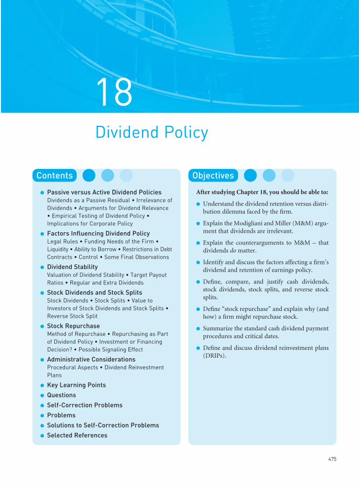
••
475
18Dividend Policy
Contents
l Passive versus Active Dividend PoliciesDividends as a Passive Residual • Irrelevance ofDividends • Arguments for Dividend Relevance• Empirical Testing of Dividend Policy •Implications for Corporate Policy
l Factors Influencing Dividend PolicyLegal Rules • Funding Needs of the Firm •Liquidity • Ability to Borrow • Restrictions in DebtContracts • Control • Some Final Observations
l Dividend StabilityValuation of Dividend Stability • Target PayoutRatios • Regular and Extra Dividends
l Stock Dividends and Stock SplitsStock Dividends • Stock Splits • Value toInvestors of Stock Dividends and Stock Splits •Reverse Stock Split
l Stock RepurchaseMethod of Repurchase • Repurchasing as Partof Dividend Policy • Investment or FinancingDecision? • Possible Signaling Effect
l Administrative ConsiderationsProcedural Aspects • Dividend ReinvestmentPlans
l Key Learning Points
l Questions
l Self-Correction Problems
l Problems
l Solutions to Self-Correction Problems
l Selected References
Objectives
After studying Chapter 18, you should be able to:
l Understand the dividend retention versus distri-bution dilemma faced by the firm.
l Explain the Modigliani and Miller (M&M) argu-ment that dividends are irrelevant.
l Explain the counterarguments to M&M – thatdividends do matter.
l Identify and discuss the factors affecting a firm’sdividend and retention of earnings policy.
l Define, compare, and justify cash dividends,stock dividends, stock splits, and reverse stocksplits.
l Define “stock repurchase” and explain why (andhow) a firm might repurchase stock.
l Summarize the standard cash dividend paymentprocedures and critical dates.
l Define and discuss dividend reinvestment plans(DRIPs).
FUNO_C18.qxd 9/19/08 17:09 Page 475

Dividend policy is an integral part of the firm’s financing decision. The dividend-payout ratiodetermines the amount of earnings that can be retained in the firm as a source of financing.However, retaining a greater amount of current earnings in the firm means that fewer dollarswill be available for current dividend payments. A major aspect, then, of the dividend policyof the firm is to determine the appropriate allocation of profits between dividend paymentsand additions to the firm’s retained earnings. But also important are other issues pertainingto a firm’s overall dividend policy: legal, liquidity, and control issues; stability of dividends;stock dividends and splits; stock repurchase; and administrative considerations.
Passive versus Active Dividend Policies
l l l Dividends as a Passive ResidualWe focus first on a two-part question. Can the payment of cash dividends affect shareholderwealth and, if so, what dividend-payout ratio will maximize shareholder wealth? As we didwhen studying the effects of financial leverage, we again assume that business risk is held constant. To evaluate the question of whether the dividend-payout ratio affects shareholderwealth, it is necessary to first examine the firm’s dividend policy as solely a financing decisioninvolving the retention of earnings. Each period, the firm must decide whether to retain itsearnings or distribute part or all of them to shareholders as cash dividends. (We rule out sharerepurchase for now.) As long as the firm is faced with investment projects having returnsexceeding those that are required (i.e., positive-NPV projects), the firm will use earnings, plusthe amount of senior securities the increase in the equity base will support, to finance theseprojects. If the firm has earnings left after financing all acceptable investment opportunities,these earnings would then be distributed to shareholders in the form of cash dividends. If not, there would be no dividends. If the number of acceptable investment opportunitiesinvolves a total dollar amount that exceeds the amount of retained earnings plus the seniorsecurities these retained earnings will support, the firm would finance the excess needs with acombination of a new equity issue and senior securities.
When we treat dividend policy as strictly a financing decision, the payment of cash dividends is a passive residual. The percentage of earnings paid out as dividends will fluctu-ate from period to period in keeping with fluctuations in the amount of acceptable invest-ment opportunities available to the firm. If these opportunities abound, the percentage ofearnings paid out is likely to be zero. On the other hand, if the firm is unable to find profitable investment opportunities, dividends paid out will be 100 percent of earnings. Forsituations between these two extremes, the dividend-payout ratio will be a fraction betweenzero and one.
The treatment of dividend policy as a passive residual, determined solely by the availabil-ity of acceptable investment proposals, implies that dividends are irrelevant. Are dividendsreally just a means of distributing unused funds? Instead, should dividend payments be anactive decision variable with earnings retentions as a residual? To answer these questions, we must examine the argument that dividends are irrelevant, which means that changes in the dividend-payout ratio (holding investment opportunities constant) do not affect share-holder wealth.
Part 6 The Cost of Capital, Capital Structure, and Dividend Policy
476
••
“Contrariwise,” continued Tweedledee, “if it was so, it might be; and if it were so, it would be; but as it isn’t, it ain’t. That’s logic.”
—LEWIS CARROLLThrough the Looking Glass
Dividend-payout ratioAnnual cash dividends divided byannual earnings;alternatively,dividends per sharedivided by earningsper share. The ratio indicates thepercentage of acompany’s earningsthat is paid out toshareholders in cash.
FUNO_C18.qxd 9/19/08 17:09 Page 476

l l l Irrelevance of DividendsMiller and Modigliani (M&M) provide the most comprehensive argument for the irrelevanceof dividends.1 They assert that, given the investment decision of the firm, the dividend-payout ratio is a mere detail and that it does not affect the wealth of shareholders. M&M arguethat the value of the firm is determined solely by the earning power of the firm’s assets or its investment policy, and that the manner in which the earnings stream is split between dividends and retained earnings does not affect this value. As we pointed out in the previouschapter, when we considered the capital structure decision, M&M assume perfect capital markets where there are no transactions costs, no flotation costs to companies issuing secur-ities, and no taxes. Moreover, the future profits of the firm are assumed to be known with certainty. (Later this last assumption will be removed.)
Current Dividends versus Retention of Earnings. The crux of M&M’s position is thatthe effect of dividend payments on shareholder wealth is exactly offset by other means offinancing. Let us first consider selling additional common stock to raise equity capital insteadof simply retaining earnings. After the firm has made its investment decision, it must decidewhether (1) to retain earnings or (2) to pay dividends and sell new stock in the amount ofthese dividends in order to finance the investments. M&M suggest that the sum of the dis-counted value per share of common stock after financing plus current dividends paid isexactly equal to the market value per share of common stock before the payment of currentdividends. In other words, the common stock’s decline in market price because of the dilution caused by external equity financing is exactly offset by the payment of the dividend.Thus the shareholder is said to be indifferent between receiving dividends and having earn-ings retained by the firm.
Take Note
At this point, one might rightfully ask: How does all of this relate to our earlier chapters, whenwe said that dividends are the foundation for the valuation of common stock? Is there somecontradiction? Although it is still true that the market value of a share of common stock isthe present value of all expected future dividends, the timing and magnitude of the divi-dends can vary. It is still true that a company that is expected never to pay a dividend – noteven a liquidation dividend – should be worthless to an investor. The dividend-irrelevanceposition simply argues that the present value of future dividends remains unchanged eventhough dividend policy may change the timing and magnitude of dividends. It does notargue that dividends, including a liquidating dividend, are never paid. On the contrary, itargues only that dividend postponement (but where the future dividend magnitude is allowedto grow) is a matter of indifference when it comes to the market price of common stock.
Conservation of Value. Given M&M’s assumptions of certainty and perfect capital mar-kets, the irrelevance of dividends naturally follows. As with our example for corporate finan-cial leverage in the previous chapter, the total-value principle ensures that the sum of marketvalue plus current dividends of two firms identical in all respects other than dividend-payoutratios will be the same.
Investors are able to replicate any dividend stream the corporation might be able to pay butcurrently is not. If dividends are lower than desired, investors can sell some shares of stock toobtain their desired cash distribution. If dividends are higher than desired, investors can usedividends to purchase additional shares of stock in the company. Thus investors are able to
1Merton H. Miller and Franco Modigliani, “Dividend Policy, Growth, and the Valuation of Shares,” Journal ofBusiness 34 (October 1961), 411–433.
18 Dividend Policy
477
••
Dilution A decrease in the proportionalclaim on earnings and assets of a share of commonstock because of theissuance of additionalshares.
FUNO_C18.qxd 9/19/08 17:09 Page 477

manufacture “homemade” dividends in the same way that they could devise “homemade”financial leverage if they were unhappy with a firm’s current capital structure. For a corporatedecision to have value, the company must be able to do something for shareholders that theycannot do for themselves. Because investors can manufacture homemade dividends, whichare perfect substitutes for corporate dividends under the preceding assumptions, dividendpolicy is irrelevant. As a result, one dividend policy is as good as the next. The firm is unableto create value simply by altering the mix of dividends and retained earnings. As in capitalstructure theory, there is a conservation of value so that the sum of the parts is always thesame. The total size of the pie is not changed by the slicing.
l l l Arguments for Dividend RelevanceA number of arguments have been advanced in support of the contrary position, namely, that dividends are relevant under conditions of uncertainty. In other words, investors are not indifferent as to whether they receive returns in the form of dividend income or shareprice appreciation. We shall examine these arguments under conditions of uncertainty.
Preference for Dividends. Certain investors may have a preference for dividends over capital gains. The payment of dividends may resolve uncertainty in their minds concerningcompany profitability. Dividends are received on a current, ongoing basis, whereas the prospectof realizing capital gains is in the future. Therefore investors in a dividend-paying companyresolve their uncertainty earlier than those investing in a non-dividend-paying company. Tothe extent that investors prefer the early resolution of uncertainty, they may be willing to paya higher price for the stock that offers the greater dividend, all other things held constant. If,in fact, investors can manufacture “homemade” dividends, such a preference is irrational.Nonetheless, sufficient statements from investors make it difficult to dismiss this argument.Perhaps, for either psychological reasons or reasons of inconvenience, investors prefer not tomanufacture “homemade” dividends but to get the “real thing” directly from the company.
Taxes on the Investor. When we allow for taxes, there are a variety of effects. To the extentthat the personal tax rate on capital gains is less than that on dividend income, there may bean advantage to the retention of earnings. (Only recently in the US have these rates been thesame for individuals.) In addition, the capital gains tax is deferred until the actual sale of stock(when any gain is then realized). Effectively, the shareholder is given a valuable timing optionwhen the firm retains earnings as opposed to paying dividends. Also, the capital gains tax may be avoided altogether if appreciated securities are given as gifts to charitable causes or ifthe security owner dies. For these reasons, the effective tax on capital gains (in present valueterms) is less than that on dividend income, even when the federal tax rate on the two typesof income is the same. This would suggest that a dividend-paying stock will need to providea higher expected before-tax return than a non-dividend-paying stock of the same risk.According to this notion, the greater the dividend yield on a stock, the higher the requiredbefore-tax return, all other things being the same.
However, all investors do not experience the same taxation on the two types of income justdiscussed. Certain institutional investors, such as retirement and pension funds, pay no tax on either dividend income or realized capital gains. Such investors would be indifferent froma tax standpoint between a dollar of dividend income and a dollar of capital gains. For cor-porate investors intercompany dividends are taxed at an effective rate below that applicable to capital gains. For example, if Alpha Corporation owns 100 shares of Omega Corporation,which pays a $1 per share annual dividend, 70 percent of the dividend income to AlphaCorporation is tax exempt. In other words, Alpha Corporation would pay taxes on $30 of dividend income at the corporate tax rate. The overall tax effect will be less than if OmegaCorporation had share appreciation of $100 and all of this were taxed at the capital gains rate. Accordingly, there may be a preference for current dividends on the part of corporateinvestors. Also, there are a growing number of institutional investors.
Part 6 The Cost of Capital, Capital Structure, and Dividend Policy
478
••
Dividend yieldAnticipated annualdividend divided bythe market price ofthe stock.
FUNO_C18.qxd 9/19/08 17:09 Page 478

If there are clienteles of investors having different dividend preferences, corporations couldadjust their dividend-payout ratio to take advantage of the situation. Suppose that two-fifthsof all investors prefer a zero dividend-payout ratio, one-fifth prefer a 25 percent payout ratio,and the remaining two-fifths prefer a 50 percent payout ratio. If most companies pay out 25 percent of their earnings in dividends, there will be excess demand for the shares of com-panies paying zero dividends and for the shares of companies whose dividend-payout ratio is 50 percent. Presumably, a number of companies will recognize this excess demand andadjust their payout ratios to increase share price. The action of these companies will eliminatethe excess demand. In equilibrium, the dividend-payout ratios of corporations will match the desires of investor groups. At this point, no company would be able to affect its share price by altering its dividend. As a result, even with taxes, the dividend-payout ratio would be irrelevant.
In actuality, we are left with an unsettled situation in which the effect of taxes on dividendsis not clear. Before considering some of the empirical evidence on the effect that dividends haveon share price, we must look at other factors that may influence the payment of dividends.
Flotation Costs. The irrelevance of the dividend payout is based on the idea that, whenfavorable investment opportunities exist and yet dividends are paid, the funds paid out of thefirm must be replaced by funds acquired through external financing. The introduction offlotation costs involved with external financing favors the retention of earnings in the firm.For each dollar paid out in dividends, the firm nets less than a dollar after flotation costs perdollar of external financing.
Transactions Costs and Divisibility of Securities. Transactions costs involved in the saleof securities tend to restrict the arbitrage process in the same manner as that described fordebt. Shareholders who desire current income must pay brokerage fees on the sale of portionsof their stock ownership if the dividend paid is not sufficient to satisfy their current desire forincome. This fee, per dollar of shares sold, varies inversely with the size of the sale. For a smallsale, the brokerage fee can be a rather significant percentage of the total sale. As a result of thisfee, shareholders with consumption desires in excess of current dividends will prefer that thecompany pay additional dividends. Perfect capital markets also assume that securities areinfinitely divisible. The fact that the smallest equity-security unit is one share may result in“lumpiness” with respect to selling shares for current income. This, too, acts as a deterrent tothe sale of stock in lieu of dividends. On the other hand, shareholders not desiring dividendsfor current consumption purposes will need to reinvest their dividends. Here, again, transac-tions costs and divisibility problems work to the disadvantage of the shareholder, althoughthis time as a deterrent to the purchase of stock. Thus transactions costs and divisibility problems cut both ways, and one is not able to draw directional inferences regarding payingdividends versus retaining earnings.
Institutional Restrictions. Certain institutional investors are restricted in the types of com-mon stock they can buy or in the portfolio percentages they can hold in various types of com-mon stock. The prescribed list of eligible securities for these investors is determined in part bythe length of time over which dividends have been paid. If a company does not pay dividends,or has not paid them over a sufficiently long period, certain institutional investors are not permitted to invest in the stock of that company.
Universities, on the other hand, sometimes have restrictions on the expenditure of capitalgains from their endowments. Also, a number of trusts have a prohibition against the liquida-tion of principal. In the case of common stocks, the trust beneficiary is entitled to dividendincome but not to the proceeds from the sale of common stock. As a result of this stipulation,the trustee who manages the investments may feel constrained to pay particular attention to dividend yield and seek stocks paying reasonable dividends. Though the two influencesdescribed are small in aggregate, they work in the direction of a preference for dividends asopposed to earnings retention and capital gains.
18 Dividend Policy
479
••
Flotation costs Thecosts associated withissuing securities,such as underwriting,legal, listing, andprinting fees.
FUNO_C18.qxd 9/19/08 17:09 Page 479

Financial Signaling. Financial signaling is different from the other arguments presented in this section in that it depends on imperfections in the market for financial information. Itsuggests that dividends have an impact on share price because they communicate informa-tion, or signals, about the firm’s profitability. Presumably, firms with good news about theirfuture profitability will want to tell investors. Rather than make a simple announcement, dividends may be increased to add conviction to the statement. When a firm has a target dividend-payout ratio that has been stable over time, and the firm increases this ratio,investors may believe that management is announcing a positive change in the expectedfuture profitability of the firm. The signal to investors is that management and the board ofdirectors truly believe that things are better than the stock price reflects.
Accordingly, the price of the stock may react favorably to this increase in dividends. Theidea here is that the reported accounting earnings of a company may not be a properreflection of the company’s economic earnings. To the extent that dividends provide informa-tion on economic earnings not provided by reported earnings, share price will respond. Putanother way, cash dividends speak louder than words. Thus dividends are said to be used byinvestors as predictors of the firm’s future performance. Dividends convey management’sexpectations of the future.
l l l Empirical Testing of Dividend Policy
Although there are a number of factors that may explain dividends’ impact on valuation,many are difficult to test. Most empirical testing has concentrated on the tax effect and onfinancial signaling. This is not to say that such things as preference for dividends, flotationcosts, transactions costs, and institutional restrictions have no effect. Rather, whatever resultthese factors may have is swamped by tax and financial signaling effects.
With a tax effect, where dividends are taxed more heavily (in present value terms) than arecapital gains, stock prices and before-tax returns should reflect this differential taxation.Empirical results have been mixed as to whether high-dividend stocks provide higher expectedbefore-tax returns than low-dividend stocks to offset the tax effect. In recent years, however,the evidence is largely consistent with dividend neutrality.
In contrast to the mixed results for a tax effect, the evidence on financial signaling is con-sistent in support of a dividend announcement effect: Increases in dividends lead to positiveexcess stock returns, whereas decreases in dividends lead to negative excess returns. Thereforedividends would appear to convey information. Where does all this leave us with respect todirections for a corporation’s dividend policy?
l l l Implications for Corporate Policy
A company should endeavor to establish a dividend policy that will maximize shareholderwealth. Most everyone agrees that if a company does not have sufficiently profitable invest-ment opportunities, it should distribute any excess funds to its shareholders. The firm need not pay out the exact unused portion of earnings each period. Indeed, it may wish to stabilize the absolute amount of dividends paid from period to period. But over the longer run the total earnings retained, plus the additional senior securities the increasing equity basewill support, will correspond to the amount of new profitable investment opportunities.Dividend policy would still be a passive residual determined by the amount of investmentopportunities.
For the firm to be justified in paying a dividend larger than that dictated by the amount ofearnings left over after making all acceptable investment opportunities, there must be a netpreference for dividends in the market. It is difficult to “net out” the arguments just discussedto arrive at the bottom line. Only institutional restrictions and some investors’ preferences
Part 6 The Cost of Capital, Capital Structure, and Dividend Policy
480
••
FUNO_C18.qxd 9/19/08 17:09 Page 480

for dividends argue for dividends. The other arguments suggest either a neutral effect or a bias favoring earnings retention. There does appear to be some positive value associated witha modest dividend as opposed to none at all. This occurrence may be due to institutionalrestrictions and a signaling effect. Beyond that, the picture is cloudy, and some argue that evena modest dividend has no effect on valuation. Few academic scholars argue that dividendssignificantly in excess of what a passive policy would dictate will lead to share price improve-ment. With personal taxes and flotation costs, shareholders are “money behind” when a com-pany issues stock to pay dividends. Before making a final observation, let us look at somepractical things to consider in approaching a dividend policy decision.
Factors Influencing Dividend PolicySo far we have discussed only the theoretical aspects of dividend policy. Yet when a companyestablishes a dividend policy, it looks at a number of other matters. These additional consid-erations should be related to the theoretical concepts surrounding dividend payout and thevaluation of the firm. In what follows, we take up various practical factors that firms actuallydo (and should) analyze when approaching a dividend policy decision.
l l l Legal Rules
The laws of a firm’s state of incorporation decide the legality of any distribution to commonshareholders. The legal rules that we discuss below are important in establishing the legalboundaries within which a firm’s finalized dividend policy can operate. These legal rules haveto do with capital impairment, insolvency, and undue retention of earnings.
Capital Impairment Rule. Although state laws vary considerably, many states prohibit the payment of dividends if these dividends impair capital. Some states define capital as thetotal par value of the common stock. If a firm’s shareholders’ equity consists of $4 million incommon stock (at par), $3 million in additional paid-in capital, and $2 million in retainedearnings, total capital would be $4 million. This company could not pay a cash dividend totaling more than $5 million without impairing capital (i.e., reducing shareholders’ equitybelow $4 million).
Other states define capital to include not only the total par value of the common stock butalso the additional paid-in capital. Under such state statutes, dividends can be paid only “tothe extent of retained earnings.” Notice, we did not say that dividends can be paid “out ofretained earnings.” A company pays dividends “out of cash,” while incurring a correspondingreduction in the retained earnings account.
Interestingly, in some states dividends to common shareholders can exceed not only thebook value of a firm’s retained earnings but also the total book value of shareholders’ equity.For example, Holiday Corporation (the parent company of Holiday Inns of America) paid a one-time, $65-per-share dividend in 1987 as part of an antitakeover strategy. This $1.55 billion dividend created a $770 million negative book balance for Holiday’s total commonshareholders’ equity. Under “traditional” capital impairment laws, this would not have beenpossible because the book value of capital was now negative. Holiday, a Delaware corporation,could make this huge dividend payment (legally, according to Delaware law) only if the dividend came from surplus. In Delaware, capital means the “par value” of a firm’s commonstock, and surplus is equal to the “fair value” (i.e., market value) of its assets minus the totalof its debts plus capital. In short, in Delaware – and other like-minded states – the “fair value,”rather than “book value,” of a firm’s assets can be used to judge whether a dividend paymentimpairs capital. By the way, we chose to highlight a Delaware company in our example for animportant reason. Delaware is the state of incorporation for roughly 60 percent of the Fortune500 firms and 50 percent of all companies listed on the New York Stock Exchange.
18 Dividend Policy
481
••
FUNO_C18.qxd 9/19/08 17:09 Page 481

Insolvency Rule. Some states prohibit the payment of cash dividends if the company isinsolvent. Insolvency is defined either in a legal sense as total liabilities of a company exceed-ing its assets “at a fair valuation,” or in an “equitable” (technical) sense as the firm’s inabilityto pay its creditors as obligations come due. Because the firm’s ability to pay its obligations is dependent on its liquidity rather than on its capital, the equitable (technical) insolvencyrestriction gives creditors a good deal of protection. When cash is limited, a company isrestricted from favoring shareholders to the detriment of creditors.
Undue Retention of Earnings Rule. The Internal Revenue Code prohibits the undueretention of earnings. Although undue retention is vaguely defined, it is usually thought to mean retention significantly in excess of the present and future investment needs of thecompany. The purpose of the law is to prevent companies from retaining earnings for the sakeof avoiding taxes. For example, a company might retain all of its earnings and build up a sub-stantial cash and marketable securities position. The entire company could then be sold, andshareholders would be subject to only a capital gains tax, which is postponed relative to whatwould occur if dividends were paid. If the Internal Revenue Service can prove unjustifiedretention, it can impose penalty tax rates on the earnings accumulation. Whenever a companydoes build up a substantial liquid position, it has to be sure that it can justify the retention ofthese funds to the IRS. Otherwise, it may be more prudent to pay the excess funds as dividendsto shareholders.
l l l Funding Needs of the Firm
Once the legal boundaries for the firm’s dividend policy have been established, the next step involves an assessment of the funding needs of the firm. In this regard, cash budgets, projected sources and uses of funds statements, and projected cash flow statements (topicstaken up in Chapter 7) are of particular use. The key is to determine the likely cash flows and cash position of the company in the absence of a change in dividend policy. In additionto looking at expected outcomes, we should factor in business risk, so that we may obtain a range of possible cash-flow outcomes, a procedure spelled out in Chapter 7.
In keeping with our earlier discussion of the theoretical aspects of dividend policy, the firm would wish to determine whether anything is left over after servicing its funding needs,including funding acceptable investment projects. In this regard, the firm should look at itssituation over a reasonable number of future years to iron out fluctuations. The likely abilityof the firm to sustain a dividend should be analyzed relative to the probability distributions of possible future cash flows and cash balances. On the basis of this analysis, a company candetermine its likely future residual funds.
l l l Liquidity
The liquidity of a company is a prime consideration in many dividend decisions. Because dividends represent a cash outflow, the greater the cash position and overall liquidity of acompany, the greater its ability to pay a dividend. A company that is growing and profitablemay not be liquid because its funds may go into fixed assets and permanent working capital.Because the management of such a company usually desires to maintain some liquidity cushion to give it financial flexibility and protection against uncertainty, it may be reluctantto jeopardize this position to pay a large dividend.
l l l Ability to Borrow
A liquid position is not the only way to provide for financial flexibility and thereby protectagainst uncertainty. If a firm has the ability to borrow on comparatively short notice, it may
Part 6 The Cost of Capital, Capital Structure, and Dividend Policy
482
••
FUNO_C18.qxd 9/19/08 17:09 Page 482

be relatively financially flexible. This ability to borrow can be in the form of a line of credit ora revolving credit agreement from a bank, or simply the informal willingness of a financialinstitution to extend credit. In addition, financial flexibility can come from the ability of afirm to go to the capital market with a bond issue. The larger and more established a com-pany, the better its access to the capital market. The greater the ability of the firm to borrow,the greater its financial flexibility, and the greater its ability to pay a cash dividend. With ready access to debt funds, management should be less concerned with the effect that a cashdividend has on its liquidity.
l l l Restrictions in Debt ContractsThe protective covenants in a bond indenture or loan agreement often include a restrictionon the payment of dividends. The restriction is employed by the lenders to preserve the com-pany’s ability to service debt. Usually it is expressed as a maximum percentage of cumulativeearnings retained (reinvested) in the firm. When such a restriction is in force, it naturallyinfluences the firm’s dividend policy. Sometimes the management of a company welcomes adividend restriction imposed by lenders, because then it does not have to justify the retentionof earnings to its shareholders. It needs only to point to the restriction.
l l l ControlIf a company pays substantial dividends, it may need to raise capital at a later time throughthe sale of stock in order to finance profitable investment opportunities. Under such circum-stances, the controlling interest of the company may be diluted if controlling shareholders donot or cannot subscribe for additional shares. These shareholders may prefer a low dividendpayout and the financing of investment needs by retaining earnings. Such a dividend policymay not maximize overall shareholder wealth, but it still may be in the best interests of thosein control.
Control can operate in another, very different, way. When a company is being sought foracquisition by another company or by individuals, a low dividend payout may work to theadvantage of the “outsiders” seeking control. The outsiders may be able to convince share-holders that the company is not maximizing shareholder wealth and that they (the outsiders)can do a better job. Consequently, companies in danger of being acquired may establish a highdividend payout to please shareholders.
l l l Some Final ObservationsIn determining a dividend payout, the typical company will analyze a number of the factorsjust described. These factors largely dictate the legal and other boundaries within which a dividend can be paid. When a company pays a dividend in excess of its residual funds, itimplies that management and the board of directors believe that the payment has a favorableeffect on shareholder wealth. The frustrating thing is that we have so little in the way of cleargeneralizations from the empirical evidence. The lack of a firm footing for predicting thelong-run effect of a specific dividend policy on valuation makes the dividend choice a mostdifficult policy decision.
Considerations taken up in this section allow a company to determine with reasonableaccuracy what would be an appropriate passive dividend strategy. An active dividend policyinvolves an act of faith, because it demands that a portion of the cumulative dividends paidout ultimately be replaced with common stock financing. Such a strategy is undertaken in afoggy area, but one in which most academics have difficulty believing that shareholder wealthwill be enhanced. Notwithstanding, many companies profess a belief that dividend payoutaffects share price and behave in a manner consistent with dividend importance.
18 Dividend Policy
483
••
Covenant A restrictionon a borrowerimposed by a lender:for example, theborrower mustmaintain a minimumamount of workingcapital.
FUNO_C18.qxd 9/19/08 17:09 Page 483

Dividend StabilityStability of dividend payments is an attractive feature to many investors. By stability we meanmaintaining the position of the firm’s dividend payments in relation to a trend line, prefer-ably one that is upward sloping. All other things being the same, a share of stock may com-mand a higher price if it pays a stable dividend over time than if it pays out a fixed percentageof earnings. Suppose that Company A has a long-run dividend-payout ratio of 50 percent ofearnings. It pays out this percentage every year, despite the fact that its earnings are cyclical.The earnings and dividends per share of Company A are shown in Figure 18.1. Company B,on the other hand, has exactly the same earnings and a long-run dividend-payout ratio of 50 percent, but it maintains a relatively stable dividend over time. It changes the absoluteamount of dividend payment only in keeping with the underlying trend of earnings. The earnings and dividends per share of Company B are shown in Figure 18.2.
Part 6 The Cost of Capital, Capital Structure, and Dividend Policy
484
••
Figure 18.1Dividend policy ofcompany A showingstrict adherence to aconstant 50 percentdividend-payout ratio
Figure 18.2Dividend policy ofcompany B showing along-run 50 percentdividend-payout ratio but dividendincreases only whensupported by growthin earnings
FUNO_C18.qxd 9/19/08 17:09 Page 484

Over the long run, the total amount of dividends paid by these two firms is the same.However, the market price per share of Company B may be higher than that of Company A,all other things being the same. Investors may well place a positive utility on dividend stabil-ity and pay a premium for the company that offers it. To the extent that investors value dividend stability, the overall dividend policy of Company B would be better than that ofCompany A. This policy encompasses not only the percentage of dividend payout in relationto earnings but also the manner in which the actual dividends are paid. Rather than vary dividends directly with changes in earnings per share, Company B raises the dividend onlywhen reasonably confident a higher dividend can be maintained.
l l l Valuation of Dividend Stability
Investors may be willing to pay a premium for stable dividends because of the informationalcontent of dividends, the desire of investors for current income, and certain institutional considerations.
Informational Content. When earnings drop and a company does not cut its dividend, themarket may have more confidence in the stock than it would have if the dividend were cut.The stable dividend may convey management’s view that the future of the company is betterthan the drop in earnings suggests. Thus management may be able to affect the expectationsof investors through the informational content of dividends. Management will not be able tofool the market permanently. If there is a downward trend in earnings, a stable dividend willnot convey forever an impression of a promising future. Moreover, if a firm is in an unstablebusiness with wide swings in earnings, a stable dividend cannot give the illusion of underly-ing stability.
Current Income Desires. A second factor may favor stable dividends. Investors who desirea specific periodic income will prefer a company with stable dividends to one with unstabledividends, even though both companies may have the same pattern of earnings and long-run dividend payout. Although investors can always sell a portion of their common stock for income when the dividend is not sufficient to meet their current needs, many investors have an aversion to dipping into principal. Moreover, when a company reduces its dividend,earnings are usually down and the market price of the common stock is depressed. Overall,income-conscious investors place a positive utility on stable dividends, even though they canalways sell a few shares of stock for income.
Institutional Considerations. A stable dividend may be advantageous from the legal stand-point of permitting certain institutional investors to buy the common stock. Various govern-mental bodies prepare approved (or legal) lists of securities in which pension funds, savingsbanks, trustees, insurance companies, and certain other institutions may invest. To qualify, acompany often must have an uninterrupted pattern of dividends. A cut in dividends mayresult in the removal of a company from these approved lists.
The arguments presented in support of the notion that stable dividends have a positiveeffect on the market price of the stock are only suggestive. Little empirical evidence sheds light on the question. Although studies of individual stocks often suggest that stable dividendsbuffer the market price of the stock when earnings are down, there have been no compre-hensive studies of a large sample of stocks dealing with the relationship between dividend stability and valuation. Nevertheless, most companies strive for stability in their dividend pay-ments. This is consistent with a belief that stable dividends have a positive effect on value.
l l l Target Payout Ratios
A number of companies appear to follow the policy of a target dividend-payout ratio over the long run. John Lintner contends that dividends are adjusted to changes in earnings, but
18 Dividend Policy
485
••
FUNO_C18.qxd 9/19/08 17:09 Page 485

only with a lag.2 When earnings increase to a new level, a company increases dividends onlywhen it feels it can maintain the increase in earnings. Companies are also reluctant to cut theabsolute amount of their cash dividend. Both of these factors help explain why dividendchanges often lag behind changes in earnings. In an economic upturn, the lag relationshipbecomes visible when retained earnings increase in relation to dividends. In a contraction,retained earnings will decrease relative to dividends.
l l l Regular and Extra DividendsOne way for a company to increase its cash distribution to shareholders in periods of prosperity is to declare an extra dividend in addition to the regular dividend that is generallypaid on a quarterly or semiannual basis. By declaring an extra dividend, the company warnsinvestors that the dividend is not an increase in the established dividend rate. The declarationof an extra dividend is particularly suitable for companies with fluctuating earnings. The useof extra dividends enables the company to maintain a stable record of regular dividends and also to distribute some of the rewards of prosperity. If a company pays extra dividendscontinuously, it defeats its purpose. The extra dividend becomes expected. When properlylabeled, however, an extra, or special, dividend still conveys positive information to the market concerning the firm’s present and future performance.
Stock Dividends and Stock SplitsStock dividends and stock splits are often used for different purposes. In an economic sense,there is little difference between the two. Only from an accounting standpoint is there asignificant difference.
l l l Stock DividendsA stock dividend is simply the payment of additional shares of common stock to share-holders. It represents nothing more than a bookkeeping shift within the shareholders’ equityaccount on the firm’s balance sheet. A shareholder’s proportional ownership in the firmremains unchanged. Accounting authorities make a distinction between small-percentagestock dividends and large-percentage stock dividends.3
Small-Percentage Stock Dividends. If a stock dividend represents an increase of less than(typically) 25 percent of the previously outstanding common stock, it is referred to as a small-percentage stock dividend. Accounting for this type of stock dividend entails transferring anamount from retained earnings to common stock and additional paid-in capital.
Suppose that Chen Industries had a total shareholders’ equity account – before issuing a stock dividend – as shown on the left-hand side of Table 18.1. Chen Industries then pays a5 percent stock dividend, amounting to 20,000 additional shares (400,000 × 0.05) of stock.The fair market value of the stock is $40 per share. For each 20 shares of common stockowned, the shareholder receives an additional share. The total shareholders’ equity accountafter the stock dividend is pictured on the right-hand side of Table 18.1.
With a 5 percent stock dividend, $800,000 ($40 × 20,000 shares) in market value of theadditional shares is transferred (on paper) from retained earnings to the common stock andadditional paid-in capital accounts. Because the par value per share stays the same, the increase
2See John Lintner, “Distribution of Income of Corporations,” American Economic Review 46 (May 1956), 97–113.3The suggested accounting treatments that we discuss for stock dividends are sometimes modified to reflect state lawsin which a firm is incorporated. This is especially true in situations involving a “transitional range” that is centeredon the gray area where a small-percentage stock dividend changes to a large-percentage stock dividend.
Part 6 The Cost of Capital, Capital Structure, and Dividend Policy
486
••
Extra dividendA nonrecurringdividend paid toshareholders inaddition to the regular dividend. It is brought about by specialcircumstances.
Regular dividendThe dividend that isnormally expected tobe paid by the firm.
Stock dividend Apayment of additionalshares of stock toshareholders. Oftenused in place of or in addition to a cashdividend.
FUNO_C18.qxd 9/19/08 17:09 Page 486

in number of shares is reflected in a $100,000 ($5 × 20,000 shares) increase in the commonstock account. The residual of $700,000 is entered into the additional paid-in capital account.The total shareholders’ equity of the company remains the same, namely $10 million.
Because the number of shares of common stock outstanding is increased by 5 percent,earnings per share of the company are reduced proportionately. Assume that net profit aftertaxes for the period just ended is $1 million. Before the stock dividend, earnings per sharewere $2.50 ($1,000,000/400,000 shares). After the stock dividend, earnings per share would be$2.38 ($1,000,000/420,000 shares). Shareholders have more shares of stock but lower earningsper share. However, each shareholder’s proportionate ownership claim against total earningsavailable to common shareholders remains unchanged.
Large-Percentage Stock Dividends. Large-percentage stock dividends (typically 25 per-cent or higher of previously outstanding common stock) must be accounted for differently.Though small-percentage stock dividends are not expected to have much effect on the marketvalue per share of stock, large-percentage stock dividends are expected to materially reducethe market price per share of stock. In the case of large-percentage stock dividends, therefore,conservatism argues for reclassifying an amount limited to the par value of additional sharesrather than an amount related to the pre-stock-dividend market value of the stock.
Suppose that Chen Industries decided to issue a 100 percent stock dividend instead of the5 percent stock dividend originally discussed. In Table 18.2 we see what the total share-holders’ equity section of Chen Industries’ balance sheet looks like both before and after the100 percent stock dividend.
Because of the 100 percent stock dividend, $2,000,000 ($5 × 400,000 shares) in par value ofthe additional 400,000 shares is transferred from retained earnings to the common stock (at par)account. The total shareholders’ equity of the company remains unchanged at $10 million.
l l l Stock SplitsWith a stock split the number of shares is increased through a proportional reduction in thepar value of the stock. In our last example, Chen Industries issued a 100 percent stock divi-dend. A 2-for-1 stock split would have similar economic consequences to a 100 percent stock
18 Dividend Policy
487
••
Table 18.15% stock dividend forChen Industries
Before After
Common stock Common stock($5 par; 400,000 shares) $ 2,000,000 ($5 par; 420,000 shares) $ 2,100,000
Additional paid-in capital 1,000,000 Additional paid-in capital 1,700,000Retained earnings 7,000,000 Retained earnings 6,200,000
Total shareholders’ equity $10,000,000 Total shareholders’ equity $10,000,000
Note: Current market price per share = $40.
Table 18.2100% stock dividendfor Chen Industries
Before After
Common stock Common stock($5 par; 400,000 shares) $ 2,000,000 ($5 par; 800,000 shares) $ 4,000,000
Additional paid-in capital 1,000,000 Additional paid-in capital 1,000,000Retained earnings 7,000,000 Retained earnings 5,000,000
Total shareholders’ equity $10,000,000 Total shareholders’ equity $10,000,000
Stock split Anincrease in thenumber of sharesoutstanding byreducing the par valueof the stock: forexample, a 2-for-1stock split where parvalue per share isreduced by one-half.
FUNO_C18.qxd 9/19/08 17:09 Page 487

dividend but would require different accounting treatment. Table 18.3 shows us the totalshareholders’ equity account for Chen Industries both before and after a 2-for-1 stock split.
With a stock dividend, the par value of common stock is not reduced, whereas with a stocksplit, it is. As a result, the common stock, additional paid-in capital, and retained earningsaccounts remain unchanged with a stock split. The total shareholders’ equity, of course, alsostays the same. The only change is in the par value of the common stock, which, on a per-sharebasis, is now half of what it once was. Except in accounting treatment, then, the stock divid-end and stock split are very similar. A stock split (or alternatively, a large-percentage stockdividend) is usually reserved for occasions when a company wishes to achieve a substantialreduction in the market price per share of common stock. A principal purpose of a split is toplace the stock in a more popular trading range, thereby (hopefully) attracting more buyers.
A company will seldom maintain the same cash dividend per share before and after a stocksplit. But it might increase the effective dividend to shareholders. For example, a companymay split its common stock 2 for 1 and establish an annual dividend rate of $1.20 a share,whereas before the rate might have been $2 a share. A shareholder owning 100 shares beforethe stock split would receive $200 in cash dividends per year. After the stock split, the share-holder would own 200 shares and would receive $240 in dividends per year.
l l l Value to Investors of Stock Dividends and Stock SplitsTheoretically, a stock dividend or stock split is not a thing of value to investors. They receiveownership of additional shares of common stock, but their proportionate ownership of the company is unchanged. The market price of the stock should decline proportionately, so that the total value of each shareholder’s holdings stays the same. To illustrate with a stock dividend, suppose that you held 100 shares of common stock worth $40 per share or$4,000 in total. After a 5 percent stock dividend, share price should drop to $38.10 ($40/1.05).The total value of your holdings, however, would still be worth $4,000 ($38.10 × 10⁵ shares).Under these conditions, the stock dividend does not represent a thing of value to you. Youmerely have a greater number of shares of stock evidencing the same ownership interest. Intheory, the stock dividend or split is a purely cosmetic change.
To the extent that an investor wishes to sell a few shares of stock for income, the stock dividend/split may make it easier to do so. Without the stock dividend/split, of course, shareholders could also sell a few shares of their original holdings for income. In either case,the sale of stock represents the sale of principal and is subject to the capital gains tax. It isprobable that certain investors do not look at the sale of additional stock resulting from a stock dividend/split as a sale of principal. To them, the stock dividend/split represents a windfall gain. They can sell the additional shares and still retain their original holdings. Thestock dividend/split may have a favorable psychological effect on these shareholders.
Effect on Cash Dividends. The stock dividend or stock split may be accompanied by anincreased cash dividend. For the former, suppose that an investor owns 100 shares of a com-pany paying a $1 annual dividend. The company declares a 10 percent stock dividend and, atthe same time, announces that the cash dividend per share will remain unchanged. The
Part 6 The Cost of Capital, Capital Structure, and Dividend Policy
488
••
Table 18.32-for-1 stock split forChen Industries
Before After
Common stock Common stock($5 par; 400,000 shares) $ 2,000,000 ($2.50 par; 800,000 shares) $ 2,000,000
Additional paid-in capital 1,000,000 Additional paid-in capital 1,000,000Retained earnings 7,000,000 Retained earnings 7,000,000
Total shareholders’ equity $10,000,000 Total shareholders’ equity $10,000,000
FUNO_C18.qxd 9/19/08 17:09 Page 488

QWhat are “stock splits?”
AWondering whether to buy a stock before or after a split is like asking, “Should I eat this peanut-
butter-and-jelly sandwich before or after Mom cuts it in half ?”
Stocks don’t become more inexpensive when theysplit. True, you get more shares. But each is worth less.Imagine you own 100 shares of Sisyphus TransportCorp. (ticker: UPDWN). They’re trading at $60 each andtotal $6,000. When Sisyphus splits 2-for-1, you’ll own200 shares, worth about $30 each. Total value: (drumroll, please) $6,000. Yawn.
Some people drool over stocks about to split, thinkingthe price will surge. Stock prices sometimes do pop a littleon news of splits. But these are artificial moves, sus-tainable only if the businesses grow to justify them. The real reason to smile at a split announcement is because it
signals that management is bullish. They’re not likely tosplit their stock if they expect the price to go down.
Splits come in many varieties, such as 3-for-2 or 4-for-1. There’s even a “reverse split,” when you end upwith fewer shares, with each worth more. Reverse splitsare usually employed by companies in trouble, to avoidlooking like the penny stocks they are. If a stock is trad-ing at a red-flag-raising $2 per share and it does a reverse1-for-10 split, the price will rise to $20 and those whoheld 100 shares will then own 10.
Companies often split their stock so that the price willremain psychologically appealing. Sometimes, not splittingwould mean that few people could afford even a singleshare. If Microsoft hadn’t split seven times in the lastdecade, each share would be worth more than $6,500.
With stocks, just as with any purchase, examine whatyou’re getting for the price. Study the company andcompare the stock price to other numbers, such as earn-ings. A low price might be inviting, but a $200 stock canbe much more of a bargain than a $20 one. If your fundsare limited, you can just buy fewer shares.
It’s always fun to suddenly own more shares, butsplits are like getting change for a dollar. They’re notcause for celebration.
Ask the Fool
Source: The Motley Fool (www.fool.com). Reproduced with the permission of The Motley Fool.
investor will then have 110 shares, and total cash dividends will be $110 rather than $100, asbefore. In this case, a stock dividend increases the total cash dividends. Whether this increasein cash dividend has a positive effect on shareholder wealth will depend on the trade-offbetween current dividends and the retention of earnings, which we discussed earlier. Clearly,the stock dividend in this case represents a decision by the firm to moderately increase theamount of cash dividends. However, the firm does not need the stock dividend to do so. Thefirm could merely increase its cash dividend per share from $1 to $1.10.
Sometimes a stock dividend is employed to conserve cash. Instead of increasing the cashdividend as earnings rise, a company may desire to retain a greater portion of its earnings anddeclare a modest stock dividend. This decision effectively amounts to lowering the dividend-payout ratio: as earnings rise and the dividend remains approximately the same, the dividend-payout ratio will decline. Whether shareholder wealth is increased by this action will dependon considerations previously discussed. The decision to retain a higher proportion of earn-ings, of course, could be accomplished without a stock dividend. Although the stock dividendmay tend to please certain investors by virtue of its psychological impact, the substitution ofcommon stock for cash dividends involves a sizable administrative cost. Stock dividends aresimply much more costly to administer than are cash dividends. This out-of-pocket expenseworks to the disadvantage of stock dividends.
More Popular Trading Range. A stock split and, to a lesser extent, a stock dividend areused to place a stock in a lower, more popular trading range that may attract more buyers andmay also affect the mix of stockholders as individual holdings are increased and institutionalholdings are decreased.
18 Dividend Policy
489
••
FUNO_C18.qxd 9/19/08 17:09 Page 489

Informational Content. The declaration of a stock dividend or a stock split may conveyinformation to investors. As taken up earlier, there may be a situation in which managementpossesses more favorable information about the company than investors. Instead of simplyissuing an announcement to the press, management may use a stock dividend or stock splitto more convincingly state its belief about the favorable prospects of the company. Whethersuch a signal has a positive share price effect is an empirical question. Here the evidence isoverwhelming. There is a statistically significant, positive stock price reaction around theannouncement of a stock dividend or a stock split.4 The information effect is that the stock isundervalued and should be higher priced. But we must be careful in how we interpret theseresults. As it turns out, stock dividends and stock splits generally precede cash dividend and earnings increases. The market appears to be viewing stock dividends and stock splits as leading indicators of greater cash dividends and earning power. Thus it is not the stock dividend or stock split itself that causes a positive share price reaction, but rather it is the positive information that these signals convey. Also, the company must eventually deliverimproved dividends and earnings if the stock price is to remain higher.
l l l Reverse Stock SplitRather than increase the number of shares of common stock outstanding, a company maywant to reduce the number. It can accomplish this with a reverse stock split. If the firm in our previous examples, Chen Industries, had engaged in a 1-for-4 reverse stock split, for eachfour shares held the shareholder would receive one new share in exchange. The new par value per share would become $20 ($5 × 4), and there would be 100,000 shares outstand-ing (400,000 shares/4) rather than 400,000. Reverse stock splits are employed to increase themarket price per share when the stock is considered to be selling at too low a price. In somecases, a reverse stock split is an attempt to stay listed on a major security exchange because the stock’s price may have fallen so low that it risks being delisted.
As with stock dividends and straight stock splits, there is likely to be an information or signaling effect associated with the announcement of a reverse stock split. Usually the signalis negative, such as would accompany the admission by a company that it is in financialdifficulty. However, financial difficulty need not be the underlying motivating factor for thereverse split. The company may simply want to move the stock price into a higher tradingrange where total trading costs and servicing expenses are lower. Nevertheless, the empiricalevidence is consistent with a statistically significant decline in share price around the reversestock split announcement date, holding other things constant.5 The decline is tempered by thecompany’s past earnings performance, but a healthy company should think twice beforeundertaking a reverse stock split. There are too many bad apples in the barrel to not be taintedby association.
4See Guy Charest, “Split Information, Stock Returns and Market Efficiency,” Journal of Financial Economics 6 (June–September 1978), 265–296; Eugene F. Fama, Lawrence Fisher, Michael Jensen, and Richard Roll, “The Adjustmentof Stock Prices to New Information,” International Economic Review 10 (February 1969), 1–21; Mark S. Grinblatt,Ronald W. Masulis, and Sheridan Titman, “The Valuation Effects of Stock Splits and Stock Dividends,” Journal ofFinancial Economics 13 (December 1984), 461–490; and J. Randall Woolridge, “Stock Dividends as Signals,” Journalof Financial Research 6 (Spring 1983), 1–12.5See J. Randall Woolridge and Donald R. Chambers, “Reverse Splits and Shareholder Wealth,” Financial Management12 (Autumn 1983), 5–15; and R. C. Radcliffe and W. Gillespie, “The Price Impact of Reverse Splits,” FinancialAnalysts Journal 35 (January–February 1979), 63–67.
Part 6 The Cost of Capital, Capital Structure, and Dividend Policy
490
••
Reverse stock splitA stock split in whichthe number of sharesoutstanding isdecreased: forexample, a 1-for-2reverse stock split where eachshareholder receivesone new share inexchange for everytwo old shares held.
FUNO_C18.qxd 9/19/08 17:09 Page 490

6Outside the United States, common stock repurchases are less common. In some countries share buybacks are noteven legal. In other countries, the tax consequences for investors make them unpopular.
Stock RepurchaseIn recent years, the repurchase of common stock by corporations has grown dramatically.6
Some companies repurchase their common stock to have it available for management stock-option plans. In this way, the total number of shares is not increased with the exercise of theoptions. Another reason for stock repurchase is to have shares available for the acquisition of other companies. In certain cases, companies no longer wishing to be publicly owned “goprivate” by purchasing all of the stock of outside shareholders. In still other situations, stockis repurchased with the full intention of retiring it. When you look at the total cash distributedto shareholders by corporations – cash dividends, share repurchases, and cash tender offers in connection with acquisitions – dividends are simply one (and not always the primary)mechanism for cash distribution.
l l l Method of RepurchaseThe three most common methods of stock repurchase are through a fixed-price self-tenderoffer, a Dutch-auction self-tender offer, and an open-market purchase. With a fixed-price self-tender offer, the company makes a formal offer to shareholders to purchase a certain numberof shares, typically at a set price. This bid price is above the current market price. Shareholderscan elect either to sell their shares at the specified price or to continue to hold them. Usually,the tender-offer period is between two and three weeks. If shareholders tender more sharesthan originally sought by the company, the company may elect to purchase all or part of theexcess. However, it is under no obligation to do so. In general, the transaction costs to the firmin making a self-tender offer are higher than those incurred in the purchase of stock in theopen market.
With a Dutch-auction self-tender offer, the company specifies the number of shares itwishes to repurchase plus a minimum and maximum price it is willing to pay. Typically, theminimum price is slightly above the current market price. Shareholders then have the oppor-tunity to submit to the company the number of shares each is willing to sell and their min-imum acceptable selling price within the company’s stated price range. Upon receipt of thetenders, the company arrays them from low to high. It then determines the lowest price thatwill result in the full repurchase of the shares specified. This price is paid to all shareholderswho tendered shares at or below that price. If more shares than specified are tendered at orbelow the purchase price, the company will make purchases on a pro rata basis. If too fewshares are tendered, the firm either cancels the offer or buys back all tendered shares at thestated maximum price.
Unlike a fixed-price self-tender offer, the company does not know in advance the eventualpurchase price. In both types of self-tender offers, the firm is initially uncertain as to the number of shares that will be tendered. The Dutch-auction self-tender offer has become apopular means of repurchase, sometimes exceeding the number of fixed-price self-tenderoffers in a given year. Larger companies tend to use the Dutch-auction, versus the fixed-price,self-tender offer more than smaller companies do.
In open-market purchases, a company buys its stock as any other investor does – througha brokerage house. Usually, the brokerage fee is negotiated. Certain Securities and ExchangeCommission rules restrict the manner in which a company bids for its own shares. As a result,it takes an extended period of time for a company to accumulate a relatively large block ofstock. For this reason, the self-tender offer is more suitable when the company seeks a largeamount of stock.
Before the company repurchases its stock, shareholders must be informed of the com-pany’s intentions. In a self-tender offer, these intentions are announced by the offer itself.
18 Dividend Policy
491
••
Stock repurchaseThe repurchase(buyback) of stock by the issuing firm,either in the open(secondary) market or by self-tender offer.
Self-tender offerAn offer by a firm torepurchase some of its own shares.
Dutch auctionA procedure for buying(selling) securities,named for a systemused for flowerauctions in Holland. A buyer (seller) seeksbids within a specifiedprice range, usuallyfor a large block ofstock or bonds. Afterevaluating the rangeof bid prices received,the buyer (seller)accepts the lowestprice that will allow itto acquire (disposeof) the entire block.
FUNO_C18.qxd 9/19/08 17:09 Page 491

Even here, the company must not withhold other information. It would be unethical for amining company, for example, to withhold information of a substantial ore discovery whilemaking a self-tender offer to repurchase shares. In open-market purchases, especially, it isnecessary to disclose the company’s repurchase intentions. Otherwise, shareholders may selltheir stock not knowing about a repurchase program that will increase earnings per share.Given full information about the amount of repurchase and the objective of the company, theshareholders can sell their shares if they so choose. Without proper disclosure, the sellingshareholder may be penalized. When the amount of the stock repurchase is substantial, a self-tender offer is particularly suitable, for it gives all shareholders equal treatment.
l l l Repurchasing as Part of Dividend PolicyIf a firm has excess cash and insufficient profitable investment opportunities to justify the useof these funds, it may be in the shareholders’ interests to distribute the funds. The distribu-tion can be accomplished either by the repurchase of stock or by paying the funds out inincreased dividends. In the absence of personal income taxes and transactions costs, the twoalternatives should theoretically make no difference to shareholders. With repurchase, fewershares remain outstanding, and earnings per share and, ultimately, dividends per share rise.As a result, the market price per share should rise as well. In theory, the capital gain arisingfrom repurchase should equal the dividend that otherwise would have been paid.
Suppose Deuce Hardware Company is considering the distribution of $1.5 million, eitherin cash dividends or in the repurchase of its own stock. Key company figures just prior to the$1.5 million distribution are as follows:
Earnings after taxes $2,000,000Number of common shares outstanding ÷500,000Earnings per share (EPS) $ 4Current market price per share $ 63Expected dividend per share $ 3
Because investors are expecting a $3-per-share cash dividend ($1,500,000/500,000 shares),the $63 value of a share of stock before the dividend is paid consists of the $3-per-shareexpected dividend plus the $60 market price expected to occur after the cash dividend distribution.
Alternatively, the firm could choose to repurchase some of its stock and make a self-tenderoffer to shareholders at $63 a share. It then would be able to repurchase 23,810 shares($1,500,000/$63). Earnings per share after repurchase would be
EPS = $2,000,000/(500,000 − 23,810) = $4.20
If the firm chooses to pay a cash dividend, its price/earnings ratio after the dividend would be 15 ($60/$4). If this price/earnings ratio stays at 15 after a stock repurchase, the total market price per share will be $63 ($4.20 × 15). The firm’s shareholders are equally well offwith either a cash dividend or stock repurchase. Under the cash dividend option, currentshareholders end up with $3 in dividends per share plus stock worth $60 a share, while underthe repurchase option, current shareholders have stock worth $63 a share. Thus the amountof distribution to shareholders is $3 per share – in the form either of dividends or of shareprice appreciation (and resulting capital gain).
To the extent that the personal tax rate on capital gains is less than that on dividendincome, the repurchase of stock offers a tax advantage over the payment of dividends to the taxable investor. In addition, the capital gains tax is postponed until the stock is sold,whereas with dividends the tax must be paid on a current basis.
The repurchase of stock seems particularly appropriate when the firm has a large amountof excess cash to distribute. To pay these funds out through an extra dividend would result in
Part 6 The Cost of Capital, Capital Structure, and Dividend Policy
492
••
FUNO_C18.qxd 9/19/08 17:09 Page 492

a nonpostponable tax to shareholders. The tax effect could be alleviated somewhat by payingthe funds out as extra dividends over a period of time, but this action might result in investors’counting on the extra dividend to be maintained continuously into the future. Also, the firm must be careful not to undertake a steady program of stock repurchase in lieu of payingdividends. The Internal Revenue Service may regard regularly occurring repurchases as theequivalent of cash dividends and not allow shareholders redeeming their shares any capitalgains tax advantages.
l l l Investment or Financing Decision?Some regard the repurchase of stock as an investment decision instead of a financing decision.Indeed, in a strict sense, it is, even though shares held as treasury stock do not provide anexpected return as do other investments. No company can exist by “investing” only in its ownstock. The decision to repurchase stock should involve distribution of excess funds when thefirm’s investment opportunities are not sufficiently attractive to warrant employing thosefunds, either now or in the foreseeable future. Thus the repurchase of stock cannot really betreated as an investment decision as we define the term.
Stock repurchase is best regarded as a type of financing decision possessing capital structure or dividend policy motivations. For example, sometimes the purpose of a stockrepurchase is to alter the capital structure of the firm. By issuing debt and repurchasing stock,a firm can immediately change its debt-to-equity ratio toward a greater proportion of debt.At other times, when there is excess cash, the repurchase of stock can be viewed as part of thefirm’s overall dividend policy.
l l l Possible Signaling EffectStock repurchases may also have a positive signaling effect. For example, suppose manage-ment believed that the firm’s common stock was undervalued and that they were personallyconstrained in not being able to respond to a self-tender offer with shares that they ownedindividually. In such a case, the self-tender offer “premium” (amount by which the repurchase
18 Dividend Policy
493
••
The total dividend paid in 2006 was $7,686 million,compared with $7,359 million for 2005. The divi-
dend paid per share was 38.40 cents, an increase of 10%compared with 2005. In sterling terms, the dividend wasalso 10% higher.
Our dividend policy is to grow the dividend per shareprogressively. In pursuing this policy and in setting thelevels of dividends, the board is guided by several con-siderations, including the prevailing circumstances of thegroup, the future investment patterns and sustainabilityof the group and the trading environment. We deter-mine the dividend in US dollars, the economic currencyof BP.
BP intends to continue the operation of the DividendReinvestment Plan (DRIP) for shareholders who wish toreceive their dividend in the form of shares rather thancash. The BP Direct Access Plan for US and Canadian
shareholders also includes a dividend reinvestment feature.
We remain committed to returning all free cash flowsin excess of investment and dividend needs to our share-holders, circumstances permitting.
During 2006, the company repurchased 1,334 millionof its own shares at a cost of $15,481 million. Of these,358 million were for cancellation and the remainder areheld in treasury. The repurchased shares had a nominalvalue of $333 million and represented 6.5% of ordinaryshares in issue, net of treasury shares, at the end of 2005.Since the inception of the share repurchase programmein 2000, we have repurchased 3,996 million shares at a cost of $40.7 billion. BP intends to continue its pro-gramme of share buybacks, subject to market conditionsand constraints and to renewed authority at the April2007 AGM [Annual General Meeting].
Dividends and Share Repurchases at BP
Source: BP Annual Review 2006, p. 27. Copyright © 2007 BP p.l.c. Used by permission. All rights reserved.
Treasury stockCommon stock thathas been repurchasedand is held by theissuing company.
FUNO_C18.qxd 9/19/08 17:09 Page 493

Part 6 The Cost of Capital, Capital Structure, and Dividend Policy
494
7A number of empirical studies find evidence supporting the positive signaling effect of stock repurchases, particu-larly for self-tender offers as opposed to open-market purchases. See Larry Y. Dann, “Common Stock Repurchases:An Analysis of Returns to Bondholders and Stockholders,” Journal of Financial Economics 9 (June 1981), 113–138;Theo Vermaelen, “Common Stock Repurchases and Market Signaling,” Journal of Financial Economics 9 (June 1981),139–183; and Theo Vermaelen, “Repurchase Tender Offers, Signaling, and Managerial Incentives,” Journal ofFinancial and Quantitative Analysis, 19 (June 1984), 163–182.8Robert Comment and Gregg A. Jarrell, “The Relative Signalling Power of Dutch-Auction and Fixed-Price Self-Tender Offers and Open-Market Share Repurchases,” Journal of Finance 46 (September 1991), 1243–1271. See alsoLaurie Simon Bagwell, “Dutch Auction Repurchases: An Analysis of Shareholder Heterogeneity,” Journal of Finance47 (March 1992), 71–105.
••
price exceeds the existing share price) would reflect management’s belief about the degree ofundervaluation. The idea is that concrete actions speak louder than words.7
Interestingly, Dutch-auction self-tender offers appear to have a somewhat smaller positivesignaling effect than fixed-price self-tender offers. One reason is that a Dutch auction usuallyresults in a lower “premium” than does a fixed-price self-tender offer. Open-market purchaseprograms generally provide only a modest positive signaling effect. One explanation is thatsuch programs often are instigated only after a period of share price decline, in contrast to thetwo types of self-tender offer.8
Although cash dividends and stock repurchases are similar in informational content in thatthey both use cash to send a positive signal, they also provide some dissimilar information.The regular cash dividend provides ongoing reinforcement of the underlying ability of thefirm to generate cash. It is like a quarterly news release, and can be habit-forming. In contrast,
Markets respond positively to share buy-back announcements because they offer new informa-
tion, or “signals,” about a company’s future.One signal might be that management believes the
stock to be undervalued, an interpretation generallyconfirmed if executives also purchase significant num-bers of shares on their own account.
Another signal might be that management is confidentit will not need the cash to cover future commitmentssuch as interest payments and capital expenditures – perhaps because underlying operations are doing betterthan the market realizes.
Yet, in many cases, the most significant reason whyinvestors respond positively is because they are relievedthat managers are not going to spend a company’s casheither on a rash or ill thought-out merger or acquisi-tion or some other project with negative net presentvalue.
Such scepticism can be well-founded. In many indus-tries, chief executives and their management teams have
allocated cash reserves poorly and destroyed shareholdervalue.
For instance, from the mid-1960s to the mid-1990s,the spread between the return on invested capital and thecost of capital in the oil industry was mostly negative – aconsequence of poor capital discipline and diversifica-tion into unrelated activities such as retailing, miningand office automation.
Investors (and executives) nevertheless need to bearin mind that a buy-back announcement may send nega-tive signals too.
Rather than feeling relieved that their cash will not bewasted, some investors may feel disappointed that a com-pany’s executives seem to be admitting that it is unable tofind worthwhile investment opportunities – one explana-tion perhaps of why the share prices of a few companiesdecline in the wake of an announcement. And, in busi-nesses where boards link compensation to EPS, the markets may suspect that managers are promoting theshort-term effects of a share buy-back for their own endsrather than investing the company’s funds with a view totending its long-term health. Value-minded executivesshould therefore resist pressure to conduct share buy-backs, if it means forgoing value-creating investments.
They will be better placed to do so if they understandthe real value of buy-backs to their shareholders.
Debating Point: Are Share Buybacks a Good Thing?
Source: Adapted from Richard Dobbs and Werner Rehm, “Debating Point: Are Share Buybacks a Good Thing?,” Financial Times – SpecialReport: Corporate Finance (June 28, 2006), p. 6. (www.ft.com) © The Financial Times Limited 2006. Used by permission. All rights reserved.
FUNO_C18.qxd 9/19/08 17:09 Page 494

share repurchase is not a regular event. It may be viewed more as an “extra” news bulletinused on occasions when management believes that the firm’s common stock is greatly under-valued.9 Because both cash dividends and stock repurchases are done with money, manage-ment has a disincentive to give false signals and implicitly pledges itself to provide cash-flowresults consistent with the signal.
Administrative Considerations
l l l Procedural AspectsWhen the board of directors of a corporation declares a cash dividend, it specifies a recorddate. At the close of business on that date, a list of shareholders is drawn up by the companyfrom its stock-transfer books. Shareholders on the list are entitled to the dividend, whereasshareholders who come on the books after the record date are not entitled to the dividend.For example, suppose that when the board of directors of United Chemical Company met onMay 8, it declared a dividend of $1 per share payable June 15 to shareholders of record on May 31. Beth Broach owns some United Chemical stock purchased well before May 31, so she is entitled to the dividend even though she might sell her stock prior to the dividend actually being paid on June 15.
A problem can develop in the sale of stock in the days immediately prior to the record date.The buyer and the seller of the stock have several days to settle: that is, to pay for the stock orto deliver it, in the case of the seller. To avoid confusion about which investors are entitled todividends when shares are sold just prior to the record date, the brokerage community has a rule whereby new shareholders are entitled to dividends only if they purchase the stock atleast two business days prior to the record date. If the stock is purchased after that time, theshareholder is not entitled to the dividend. The date itself is known as the ex-dividend date.
Figure 18.3 shows the important dividend dates in our example on a time line. May 8 wasthe date on which the board of directors declared a dividend (the declaration date), payableJune 15 (the payment date) to shareholders of record as of May 31 (the record date). If May 31 were a Friday, two business days before would be May 29 (the ex-dividend date). Toreceive the dividend, a new shareholder must purchase the stock on May 28 or before. If purchased on May 29 or after, the stock is said to be ex-dividend. That is, it trades without the right to the declared dividend.
l l l Dividend Reinvestment PlansA number of large companies have established dividend reinvestment plans (DRIPs). Underthese plans, shareholders have the option to reinvest their cash dividends in additional sharesof the company’s stock. There are two basic types of DRIP, characterized by whether the additional shares come from already existing common stock or from newly issued common
18 Dividend Policy
495
••
Figure 18.3Important dividenddates for UnitedChemical Company
Record date Thedate, set by the board of directorswhen a dividend isdeclared, on which an investor must be ashareholder of recordto be entitled to theupcoming dividend.
Ex-dividend dateThe first date onwhich a stockpurchaser is no longer entitled to the recently declareddividend.
Declaration dateThe date when theboard of directorsannounces theamount and date ofthe next dividend.
Payment dateThe date when thecorporation actuallypays the declareddividend.
Dividendreinvestment plan(DRIP) An optionalplan allowingshareholders toautomatically reinvestdividend payments inadditional shares ofthe company’s stock.
9See Paul Asquith and David W. Mullins, Jr., “Signalling with Dividends, Stock Repurchases, and Equity Issues,”Financial Management 15 (Autumn 1986), 27–44.
FUNO_C18.qxd 9/19/08 17:09 Page 495

Part 6 The Cost of Capital, Capital Structure, and Dividend Policy
496
stock. If existing common stock is used, the company transfers the cash dividends from allshareholders wishing to reinvest to a bank, which acts as a trustee. The bank then purchasesshares of the company’s common stock in the open market. Some companies even absorb anybrokerage costs involved with purchasing the common stock required for reinvestment. ForDRIPs in which the shareholder must bear the brokerage costs, these costs are relatively low,however, because the trustee buys stock in volume.
The other type of reinvestment plan involves having the firm issue new common stock.Only under this method can the firm actually raise new funds. This type of plan has provenespecially popular with companies in need of new capital for construction and improvements.Effectively, such a plan reduces a firm’s cash dividend payout. For example, suppose that afirm using a “new-stock” DRIP currently reports a 60 percent dividend-payout ratio. But aftersubtracting all cash dividends that are reinvested in new common stock, the “actual” payoutmay drop to only 40 percent. The cash savings to a large firm could easily amount to millionsof dollars. With a new-stock DRIP the shares come directly from the company, so there are no brokerage costs involved. Some of these new-stock plans even allow participants to buy additional shares at a discount from the current market price of the stock. Commonly the discount is 3 to 5 percent, and it serves as an inducement for reinvestment. Even though reinvested, the dividend is taxable to the shareholder, and this is a major dis-advantage to the taxable shareholder. Companies offering DRIPs range from utilities to banksto industrial concerns.
Key Learning Pointsl The critical question in dividend policy is, given the
investment decision of the firm, do dividends have an influence on the value of the firm?
l If dividends are irrelevant, as argued by Modiglianiand Miller (M&M), the firm should retain earningsonly in keeping with the availability of acceptableinvestment proposals. If there are not sufficientinvestment opportunities to provide returns in excessof those that are required, the unused funds should be paid out as dividends.
l With perfect capital markets and an absence of taxes,shareholders can manufacture “homemade” divi-dends, making the firm’s dividend payout irrelevant.With differential taxes (in present value terms) oncash dividends and capital gains, there seemingly is abias in favor of earnings retention.
l The market imperfection of flotation costs biasesthings in favor of earnings retention because this“internal” equity financing is less expensive than“external” equity financing (issuance of new commonstock) used to replace the funds lost to the cash dividend. On the other hand, restrictions on theinvestment behavior of financial institutions work in the direction of a preference for dividends. Othermarket imperfections are also part of the picture.
l Empirical testing of dividend policy has focused onwhether there is a tax effect and whether dividendsserve as a signal in conveying information. The evidence is conflicting with respect to the tax effect,
ranging from a neutral effect to a negative (anti-dividend-paying) effect. However, there seems to be agreement that dividends provide financial signals.
l In the final analysis, finance experts are unable to stateunequivocally whether the dividend payout of thefirm should be more than a passive decision variable.Most academics think not. Admittedly, many com-panies behave as if dividend policy is relevant, but the case for it is not conclusive.
l When a company is faced with a dividend decision,managerial considerations include legal rules, the fund-ing needs of the firm, business risk, liquidity, ability to borrow, assessment of any valuation information,control, and restrictions in debt contracts.
l Many people feel that the stability of dividends has a positive effect on the market price of the stock.Stable dividends may tend to resolve uncertainty inthe minds of investors, particularly when earnings pershare drop. Stable dividends may also have a positiveutility to investors interested in current periodicincome. Many companies appear to follow the policyof a target dividend-payout ratio, increasing divi-dends only when they feel that an increase in earningscan be maintained. The use of an extra dividendpermits a cyclical company to maintain a stable recordof regular dividends while paying additional dividendswhenever earnings are unusually high.
l A stock dividend pays additional common stock toshareholders. It is frequently used to conserve cash
FUNO_C18.qxd 4/18/09 11:50 AM Page 496

and to reduce the cash-dividend-payout ratio of thefirm. Theoretically, a stock dividend/split per se is nota thing of value to the shareholder unless total cashdividends paid increase.
l When the intent is to materially reduce the marketprice per share of stock, either a stock split or large-percentage stock dividend is used. With a split, thenumber of shares is increased by the terms of the split.For example, a 3-for-1 split means that the number ofshares outstanding is tripled.
l Both stock dividends and stock splits appear to havean informational or signaling effect. Share price tendsto rise around the time of a stock dividend/splitannouncement, consistent with a positive signal. Themarket appears to view the stock dividend/split as a leading indicator of greater cash dividends and earning power. In a reverse stock split, the number ofshares outstanding is reduced, and the signal to themarket usually is negative.
l A company’s repurchase of its own stock should betreated as part of the firm’s dividend policy when the
firm has funds in excess of present and foreseeablefuture investment needs. The use of these excess fundsto repurchase stock is an alternative to distributingthem in the form of cash dividends.
l With a tax differential (in present value terms)between cash dividends and capital gains, there is a tax advantage to the repurchase of common stock.Because of objections by the Internal Revenue Service,regularly occurring repurchases of common stockcannot be used in lieu of regular dividends.
l The dividend payment process begins with the firm’sboard of directors, which on a particular date (the declaration date) declares a dividend, payable on alater date (the payment date) to shareholders of recordas of a particular date (the record date). On the secondbusiness date before the record date (the ex-dividenddate), the stock goes “ex-dividend” – meaning that thestock trades without the right to the declared dividend.
l Dividend reinvestment plans (DRIPs) allow share-holders to automatically reinvest dividend paymentsin additional shares of the company’s stock.
18 Dividend Policy
497
••
Questions
1. Contrast a passive dividend policy with an active one.2. How does an investor manufacture “homemade” dividends? What is the effect of the
actions of a number of investors doing so, all other things held constant?3. How do taxes affect the return to different investors? Are taxes a consideration in the
dividend policy decision?4. Why do companies with high growth rates tend to have low dividend-payout ratios and
companies with low growth rates tend to have high dividend-payout ratios?5. What is financial signaling as it relates to cash dividends, stock dividends/splits, and stock
repurchase?6. From a managerial standpoint, how do a firm’s liquidity and ability to borrow affect its
dividend-payout ratio?7. As the firm’s financial manager, would you recommend to the board of directors that the
firm adopt as policy a stable dividend payment per share or a stable dividend-payout ratio?What are the disadvantages of each? Would the firm’s industry influence your decision? Why?
8. What is a target dividend-payout ratio? An extra cash dividend?9. Define a stock dividend and a stock split. What is the impact of each on share value?
10. Are stock dividends valuable to investors? Why or why not?11. If we wish to raise share price, is it a good idea to have a reverse stock split? Explain.12. As an investor, would you prefer the firm to repurchase its common stock by means of a
self-tender offer or through open-market operations? Why?13. If repurchase of stock has a favorable tax effect, why would a company ever want to pay
a cash dividend?14. When earnings falter, why are boards of directors of companies reluctant to reduce the
dividend?15. Why do lenders frequently place a formal restriction in the debt contract on the amount
of dividends that can be paid?16. What is a dividend reinvestment plan (DRIP) and how might it help shareholders?17. Is dividend policy a type of financing decision or is it a type of investment decision? Explain.
FUNO_C18.qxd 9/19/08 17:09 Page 497

Part 6 The Cost of Capital, Capital Structure, and Dividend Policy
498
••
Self-Correction Problems
1. The Borowiak Rose Water Company expects with some degree of certainty to generate the following net income and to have the following capital expenditures during the nextfive years (in thousands of dollars):
YEAR
1 2 3 4 5
Net income $2,000 $1,500 $2,500 $2,300 $1,800Capital expenditures $1,000 $1,500 $2,000 $1,500 $2,000
The company currently has 1 million shares of common stock outstanding and paysannual dividends of $1 per share.a. Determine dividends per share and external financing required in each year if dividend
policy is treated as a residual decision.b. Determine the amounts of external financing that will be necessary in each year if the
present annual dividend per share is maintained.c. Determine dividends per share and the amounts of external financing that will be
necessary if a dividend-payout ratio of 50 percent is maintained.d. Under which of the three dividend policies are aggregate dividends (total dividends
over five years) maximized? External required financing (total financing over five years)minimized?
2. Dew Drop Inn, Inc.’s earnings per share over the last 10 years were the following:
YEAR
1 2 3 4 5 6 7 8 9 10
EPS $1.70 $1.82 $1.44 $1.88 $2.18 $2.32 $1.84 $2.23 $2.50 $2.73
a. Determine annual dividends per share under the following policies:i A constant dividend-payout ratio of 40 percent (to the nearest cent).ii A regular dividend of 80 cents and an extra dividend to bring the payout ratio to
40 percent if it otherwise would fall below.iii A stable dividend that is occasionally raised. The payout ratio may range between
30 percent and 50 percent in any given year, but it should average approximately 40 percent.
b. What are the valuation implications of each of these policies?3. The Klingon Fastener Company has the following shareholders’ equity account:
Common stock ($8 par value) $ 2,000,000Additional paid-in capital 1,600,000Retained earnings 8,400,000
Total shareholders’ equity $12,000,000
The current market price of the stock is $60 per share.a. What will happen to this account and to the number of shares outstanding with (1) a
10 percent stock dividend? (2) a 2-for-1 stock split? (3) a 1-for-2 reverse stock split?b. In the absence of an informational or signaling effect, at what share price should the
common stock sell after the 10 percent stock dividend? What might happen to stockprice if there were a signaling effect?
FUNO_C18.qxd 9/19/08 17:09 Page 498

Problems
1. The DeWitt Company’s shareholders’ equity account (book value) as of December 31,20X1, is as follows:
Common stock ($5 par value; 1,000,000 shares) $ 5,000,000Additional paid-in capital 5,000,000Retained earnings 15,000,000
Total shareholders’ equity $25,000,000
Currently, DeWitt is under pressure from shareholders to pay some dividends. DeWitt’scash balance is $500,000, all of which is needed for transactions purposes. The stock istrading for $7 a share.a. Reformulate the shareholders’ equity account if the company pays a 15 percent stock
dividend.b. Reformulate the shareholders’ equity account if the company pays a 25 percent stock
dividend.c. Reformulate the shareholders’ equity account if the company declares a 5-for-4 stock split.
2. Tijuana Brass Instruments Company treats dividends as a residual decision. It expects to generate $2 million in net earnings after taxes in the coming year. The company has anall-equity capital structure, and its cost of equity capital is 15 percent. The company treatsthis cost as the opportunity cost of “internal” equity financing (retained earnings). Becauseof flotation costs and underpricing, “external” equity financing (new common stock) isnot relied on until internal equity financing is exhausted.a. How much in dividends (out of the $2 million in earnings) should be paid if the com-
pany has $1.5 million in projects whose expected returns exceed 15 percent?b. How much in dividends should be paid if it has $2 million in projects whose expected
returns exceed 15 percent?c. How much in dividends should be paid if it has $3 million in projects whose expected
returns exceed 16 percent? What else should be done?3. For each of the companies described here, would you expect it to have a low, medium, or
high dividend-payout ratio? Explain why.a. A company with a large proportion of inside ownership, all of whom are high-income
individualsb. A growth company with an abundance of good investment opportunitiesc. A company that has high liquidity and much unused borrowing capacity and is experi-
encing ordinary growthd. A dividend-paying company that experiences an unexpected drop in earnings from an
upward-sloping trend linee. A company with volatile earnings and high business risk
4. Jumbo Shrimp Corporation and Giant Shrimp Company are in the same industry; both arepublicly held with a large number of shareholders; and they have the following characteristics:
JUMBO GIANT
Expected annual cash flow (in thousands) $ 50,000 $35,000Standard deviation of cash flow (in thousands) 30,000 25,000Annual capital expenditures (in thousands) 42,000 40,000Cash and marketable securities (in thousands) 5,000 7,000Existing long-term debt (in thousands) 100,000 85,000Unused short-term line of credit (in thousands) 25,000 10,000Flotation costs on common stock issues
as a percent of proceeds 5 8
On the basis of this information, which company is likely to have the higher dividend–payout ratio? Why?
18 Dividend Policy
499
••
FUNO_C18.qxd 9/19/08 17:09 Page 499

5. The Oprah Corporation and the Harpo Corporation have had remarkably similar earningspatterns over the last five years. In fact, both firms have had identical earnings per share.Further, both firms are in the same industry, produce the same product, and face the same business and financial risks. In short, these firms are carbon copies of each other inevery respect but one: Oprah paid out a constant percentage of its earnings (50 percent) individends, whereas Harpo has paid a constant cash dividend. The financial manager of theOprah Corporation has been puzzled by the fact that the price of her firm’s stock has been generally lower than the price of Harpo’s stock, even though in some years Oprah’sdividend was substantially larger than Harpo’s.a. What might account for the condition that has been puzzling the financial manager of
Oprah?b. What might be done by both companies to increase the market prices of their
stock?
OPRAH HARPO
MARKET MARKETYEARS EPS DIVIDEND PRICE EPS DIVIDEND PRICE
1 $1.00 $0.50 $6.00 $1.00 $0.23 $4.752 0.50 0.25 4.00 0.50 0.23 4.003 −0.25 nil 2.00 −0.25 0.23 4.254 0.50 0.25 3.50 0.50 0.23 4.50
6. The Chris Clapper Copper Company declared a 25 percent stock dividend on March 10 toshareholders of record on April 1. The market price of the stock is $50 per share. You own160 shares of the stock.a. If you sold your stock on March 20, what would be the price per share, all other things
the same (no signaling effect)?b. After the stock dividend is paid, how many shares of stock will you own?c. At what price would you expect the stock to sell on April 2, all other things the same
(no signaling effect)?d. What will be the total value of your holdings before and after the stock dividend, all
other things the same?e. If there were an informational or signaling effect, what would be the effect on share
price?
7. SHERILL CORPORATION SHAREHOLDERS’ EQUITY AS OF DECEMBER 30, 20X3
Common stock ($1 par value; 1,000,000 shares) $1,000,000Additional paid-in capital 300,000Retained earnings 1,700,000
Total shareholders’ equity $3,000,000
The firm earned $300,000 after taxes in 20X3 and paid out 50 percent of these earnings ascash dividends. The price on the firm’s stock on December 30 was $5.a. If the firm declared a stock dividend of 3 percent on December 31, what would be the
reformulated shareholders’ equity account?b. Assuming the firm paid no stock dividend, how much would earnings per share be for
20X3? Dividends per share?c. Assuming a 3 percent stock dividend, what would happen to earnings per share (EPS)
and dividends per share (DPS) for 20X3?d. What would the price of the stock be after the 3 percent stock dividend if there were
no signaling or other effects?8. Johore Trading Company has 2.4 million shares of common stock outstanding, and the
present market price per share is $36. Its equity capitalization is as follows:
Part 6 The Cost of Capital, Capital Structure, and Dividend Policy
500
••
FUNO_C18.qxd 9/19/08 17:09 Page 500

Common stock ($2.00 par; 2,400,000 shares) $ 4,800,000Additional paid-in capital 5,900,000Retained earnings 87,300,000
Total shareholders’ equity $98,000,000
a. If the company were to declare a 12 percent stock dividend, what would happen to theseaccounts? A 25 percent stock dividend? A 5 percent stock dividend?
b. If, instead, the company declared a 3-for-2 stock split, what would happen to theaccounts? A 2-for-1 stock split? A 3-for-1 split?
c. What would happen if there were a reverse stock split of 1 for 4? 1 for 6?9. The H. M. Hornes Company is primarily owned by several wealthy Texans. The firm
earned $3,500,000 after taxes this year. With 1 million shares outstanding, earnings pershare were $3.50. The stock recently has traded at $72 per share, among the current shareholders. Two dollars of this value is accounted for by investor anticipation of a cashdividend. As financial manager of H. M. Hornes, you have contemplated the alternative ofrepurchasing some company common stock by means of a tender offer at $72 per share.a. How much common stock could the firm repurchase if this alternative were selected?b. Ignoring taxes, which alternative should be selected?c. Considering taxes, which alternative should be selected?
Solutions to Self-Correction Problems
1. a. INCOME AVAILABLE EXTERNAL FINANCING FOR DIVIDENDS DIVIDENDS REQUIRED
YEAR (in thousands) PER SHARE (in thousands)
1 $1,000 $1.00 $ 02 0 0 03 500 0.50 04 800 0.80 05 0 0 200
$2,300 $200
b. (in thousands)
(1) (2) (3) (4)EXTERNAL FINANCING
CAPITAL REQUIREDYEAR NET INCOME DIVIDENDS EXPENDITURES (2) + (3) − (1)
1 $2,000 $1,000 $1,000 $ 02 1,500 1,000 1,500 1,0003 2,500 1,000 2,000 5004 2,300 1,000 1,500 2005 1,800 1,000 2,000 1,200
$5,000 $2,900
c. (1) (2) (3) (4) (5)EXTERNAL
FINANCING NET DIVIDENDS CAPITAL REQUIRED
INCOME DIVIDENDS PER EXPENDITURES (2) + (4) − (1) YEAR (in thousands) (in thousands) SHARE (in thousands) (in thousands)
1 $2,000 $1,000 $1.00 $1,000 $ 02 1,500 750 0.75 1,500 7503 2,500 1,250 1.25 2,000 7504 2,300 1,150 1.15 1,500 3505 1,800 900 0.90 2,000 1,100
$5,050 $2,950
18 Dividend Policy
501
••
FUNO_C18.qxd 9/19/08 17:09 Page 501

d. Aggregate dividends are highest under Alternative C, which involves a 50 percent dividend-payout ratio. However, they are only slightly higher than that which occursunder Alternative B. External financing is minimized under Alternative A, the residualdividend policy.
2. a. YEAR POLICY 1 POLICY 2 POLICY 3
1 $0.68 $0.80 $0.682 0.73 0.80 0.683 0.58 0.80 0.684 0.75 0.80 0.805 0.87 0.87 0.806 0.93 0.93 0.807 0.74 0.80 0.808 0.89 0.89 1.009 1.00 1.00 1.00
10 1.09 1.09 1.00
Other dividend streams are possible under Policy 3. This solution is but one.b. Policy 1 and, to a much lesser degree, Policy 2 result in fluctuating dividends over time,
as the company is cyclical. Because of the $0.80 minimum regular dividend, Policy 2results in an average payout ratio in excess of 40 percent. Shareholders may come tocount on the extra dividend and be disappointed when it is not paid, such as in year 7.To the extent that investors value stable dividends and periodic rising dividends overtime and that 40 percent is an optimal average payout ratio, dividend Policy 3 would bepreferred and would likely maximize share price.
3. a. Present number of shares = $2,000,000/$8 par value = 250,000.
(1) (2) (3)STOCK DIVIDEND STOCK SPLIT REVERSE SPLIT
Common stock (par) $02,200,000 ($8) $02,000,000 ($4) $02,000,000 ($16)Additional paid-in capital 2,900,000 1,600,000 1,600,000Retained earnings 6,900,000 8,400,000 8,400,000
Total shareholders’ equity $12,000,000 $12,000,000 $12,000,000Number of shares 275,000 500,000 125,000
b. The total market value of the firm before the stock dividend is $60 × 250,000 shares =$15 million. With no change in the total value of the firm, market price per share afterthe stock dividend should be $15,000,000/275,000 shares = $54.55 per share. If there isa signaling effect, the total value of the firm might rise and share price be somewhathigher than $54.55 per share. The magnitude of the effect would probably be no morethan several dollars a share, based on empirical findings.
Selected References
Part 6 The Cost of Capital, Capital Structure, and Dividend Policy
502
••
Asquith, Paul, and David W. Mullins, Jr. “The Impact ofInitiating Dividend Payments on Shareholders’ Wealth.”Journal of Business 56 (January 1983), 77–96.
—— . “Signalling with Dividends, Stock Repurchases, andEquity Issues.” Financial Management 15 (Autumn 1986),27–44.
Bagwell, Laurie Simon. “Dutch Auction Repurchases: AnAnalysis of Shareholder Heterogeneity.” Journal ofFinance 47 (March 1992), 71–105.
—— , and John B. Shoven. “Cash Distributions to Share-holders.” Journal of Economic Perspectives 3 (Summer1989), 129–140.
Baker, H. Kent, Aaron L. Phillips, and Gary E. Powell. “TheStock Distribution Puzzle: A Synthesis of the Literatureon Stock Splits and Stock Dividends.” Financial Practiceand Education 5 (Spring/Summer 1995), 24–37.
Baker, H. Kent, and Gary E. Powell. “Determinants ofCorporate Dividend Policy: A Survey of NYSE Firms.”
FUNO_C18.qxd 9/19/08 17:09 Page 502

18 Dividend Policy
503
••
Financial Practice and Education 10 (Spring/Summer2000), 29–40.
Baker, H. Kent, and David M. Smith. “In Search of aResidual Dividend Policy.” Review of Financial Economics15 (Issue 1, 2006), 1–18.
Benartzi, Shlomo, Roni Michaely, and Richard Thaler. “Do Changes in Dividends Signal the Future or the Past?” Journal of Finance 52 (July 1997), 1007–1034.
Black, Fischer. “The Dividend Puzzle.” Journal of PortfolioManagement 2 (Winter 1976), 5–8.
—— , and Myron Scholes. “The Effects of Dividend Yieldand Dividend Policy on Common Stock Prices andReturns.” Journal of Financial Economics 1 (May 1974),1–22.
Bline, Dennis M., and Charles P. Cullinan. “Distributions to Stockholders: Legal Distinctions and AccountingImplications for Classroom Discussion.” Issues inAccounting Education 10 (Fall 1995), 307–316.
Brennan, Michael J., and Thomas E. Copeland. “StockSplits, Stock Prices, and Transaction Costs.” Journal ofFinancial Economics 22 (October 1988), 83–101.
Charest, Guy. “Split Information, Stock Returns and MarketEfficiency.” Journal of Financial Economics 6 (June–September 1978), 265–296.
Comment, Robert, and Gregg A. Jarrell. “The RelativeSignalling Power of Dutch-Auction and Fixed-Price Self-Tender Offers and Open-Market Share Repur-chases.” Journal of Finance 46 (September 1991),1243–1271.
Ehrbar, Al. “When to Do a Stock Buyback.” Corporate BoardMember 9 (May/June 2006), 60–70.
Fama, Eugene F., Lawrence Fisher, Michael Jensen, and Richard Roll. “The Adjustment of Stock Prices toNew Information.” International Economic Review 10(February 1969), 1–21.
Grinblatt, Mark S., Ronald W. Masulis, and SheridanTitman. “The Valuation Effects of Stock Splits and StockDividends.” Journal of Financial Economics 13 (December1984), 461–490.
Hansell, Gerry, and Eric E. Olsen. “The Case forReconsidering Dividends.” Shareholder Value 3 (May/June 2003), 32–35.
Healy, Paul M., and Krishna G. Palepu. “EarningsInformation Conveyed by Dividend Initiations andOmissions.” Journal of Financial Economics 21(September 1988), 149–175.
Ikenberry, David L., Graeme Rankin, and Earl K. Stice.“What Do Stock Splits Really Signal?” Journal of Financialand Quantitative Analysis 31 (September 1996), 357–375.
Judd, Elizabeth. “Demystifying Share Buybacks.” Share-holder Value 2 (July/August 2002), 28–33.
Julio, Brandon, and David L. Ikenberry. “ReappearingDividends.” Journal of Applied Corporate Finance 16 (Fall2004), 89–100.
Lakonishok, Josef, and Theo Vermaelen. “Anomalous PriceBehavior Around Repurchase Tender Offers.” Journal ofFinance 45 (June 1990), 455–478.
Lease, Ronald C., Kose John, Avner Kalay, Uri Loewenstein,and Oded H. Sarig. Dividend Policy: Its Impact on FirmValue. Boston, MA: Harvard Business School Press, 2000.
Lintner, John. “Distribution of Income of Corpora-tions Among Dividends, Retained Earnings, and Taxes.” American Economic Review 46 (May 1956),97–113.
Litzenberger, Robert H., and Krishna Ramiswamy.“Dividends, Short Selling Restrictions, Tax InducedInvestor Clienteles and Market Equilibrium.” Journal ofFinance 35 (May 1980), 469–482.
—— . “The Effects of Dividends on Common Stock Prices:Tax Effects or Information Effects?” Journal of Finance 37(May 1982), 429–444.
Litzenberger, Robert H., and James C. Van Horne.“Elimination of the Double Taxation of Dividends andCorporate Financial Policy.” Journal of Finance 33 (June1978), 737–749.
Markese, John. “Common Stock Dividends: What Are TheyWorth?” AAII Journal 11 (July 1989), 29–33.
McNichols, Maureen, and Ajay Dravid. “Stock Dividends,Stock Splits, and Signaling.” Journal of Finance 45 (July1990), 857–879.
Miller, Merton H. “Behavioral Rationality in Finance: TheCase of Dividends.” Midland Corporate Finance Journal 4(Winter 1987), 6–15.
—— , and Franco Modigliani. “Dividend Policy, Growth,and the Valuation of Shares.” Journal of Business 34(October 1961), 411–433.
—— , Merton H., and Kevin Rock. “Dividend Policy under Asymmetric Information.” Journal of Finance 40(September 1985), 1031–1051.
O’Byrne, Stephen F., and Justin Pettit. “Stock Splits: WhatGood Are They?” Shareholder Value 2 (May/June 2002),34–39.
Roberts, Michael, William D. Samson, and Michael T.Dugan. “The Stockholders’ Equity Section: FormWithout Substance?” Accounting Horizons 4 (December1990), 35–46.
Szewczyk, Samuel H., and George P. Tsetsekos. “The Effectof Managerial Ownership on Stock Split-InducedAbnormal Returns.” Financial Review 28 (August 1993),351–370.
Van Horne, James C., and John G. McDonald. “DividendPolicy and New Equity Financing.” Journal of Finance 26(May 1971), 507–519.
FUNO_C18.qxd 9/19/08 17:09 Page 503

Part 6 The Cost of Capital, Capital Structure, and Dividend Policy
504
••
Vermaelen, Theo. “Common Stock Repurchases andMarket Signaling.” Journal of Financial Economics 9 (June 1981), 139–183.
—— . “Repurchase Tender Offers, Signaling, and Mana-gerial Incentives.” Journal of Financial and QuantitativeAnalysis, 19 (June 1984), 163–182.
Woolridge, J. Randall. “Stock Dividends as Signals.” Journalof Financial Research 6 (Spring 1983), 1–12.
—— , and Donald R. Chambers. “Reverse Splits and Shareholder Wealth.” Financial Management 12(Autumn 1983), 5–15.
Part VI of the text’s website, Wachowicz’s Web World, contains links to many finance websites and online articles related to topics covered in this chapter.(http://web.utk.edu/~jwachowi/part6.html)
FUNO_C18.qxd 9/19/08 17:09 Page 504
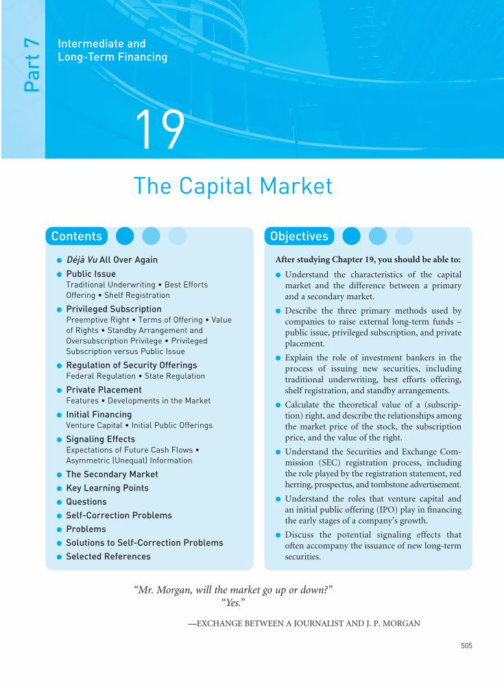
••
505
Par
t 7 Intermediate and
Long-Term Financing
Contents
l Déjà Vu All Over Again
l Public IssueTraditional Underwriting • Best Efforts Offering • Shelf Registration
l Privileged SubscriptionPreemptive Right • Terms of Offering • Value of Rights • Standby Arrangement andOversubscription Privilege • PrivilegedSubscription versus Public Issue
l Regulation of Security OfferingsFederal Regulation • State Regulation
l Private PlacementFeatures • Developments in the Market
l Initial FinancingVenture Capital • Initial Public Offerings
l Signaling EffectsExpectations of Future Cash Flows •Asymmetric (Unequal) Information
l The Secondary Marketl Key Learning Pointsl Questionsl Self-Correction Problemsl Problems l Solutions to Self-Correction Problemsl Selected References
Objectives
After studying Chapter 19, you should be able to:
l Understand the characteristics of the capitalmarket and the difference between a primaryand a secondary market.
l Describe the three primary methods used bycompanies to raise external long-term funds –public issue, privileged subscription, and privateplacement.
l Explain the role of investment bankers in theprocess of issuing new securities, including traditional underwriting, best efforts offering,shelf registration, and standby arrangements.
l Calculate the theoretical value of a (subscrip-tion) right, and describe the relationships amongthe market price of the stock, the subscriptionprice, and the value of the right.
l Understand the Securities and Exchange Com-mission (SEC) registration process, includingthe role played by the registration statement, redherring, prospectus, and tombstone advertisement.
l Understand the roles that venture capital and an initial public offering (IPO) play in financingthe early stages of a company’s growth.
l Discuss the potential signaling effects that often accompany the issuance of new long-termsecurities.
19The Capital Market
“Mr. Morgan, will the market go up or down?”“Yes.”
—EXCHANGE BETWEEN A JOURNALIST AND J. P. MORGAN
FUNO_C19.qxd 9/19/08 17:09 Page 505

••
Part 7 Intermediate and Long-Term Financing
506
Financial marketsAll institutions andprocedures forbringing buyers andsellers of financialinstruments together.
Capital market Themarket for relativelylong-term (greaterthan one year originalmaturity) financialinstruments (e.g.,bonds and stocks).
Primary marketA market where new securities arebought and sold forthe first time (a “newissues” market).
Secondary marketA market for existing(used) securitiesrather than newissues.
Figure 19.1Capital market forcorporate securities
In Chapters 17 and 18 we studied how business firms determine their mix of permanent long-term financing and how they finance “internally” by retaining earnings. We now need to findout how firms raise long-term financing “externally.” More specifically, the purpose of thischapter is to observe the ways in which bond and stock issues are initially sold in the capitalmarket. We shall get to know public issues of securities placed through investment bankers,privileged subscriptions to the company’s own shareholders, and private placements by thefirm to institutional investors. The presentation here draws on “The Financial Environment”section of Chapter 2. It was there that we first discussed financial markets in general.
Déjà Vu All Over AgainThe capital market, you may remember, deals with bonds and stocks. Within the capital market there exist both a primary and a secondary market. A primary market is a “newissues” market. It is here that funds raised through the sale of new securities flow from thebuyers of securities (the savings sector) to the issuers of securities (the investment sector). Ina secondary market, existing securities are bought and sold. Transactions in these alreadyexisting securities do not provide additional funds to finance capital investment. In this chapter, we will focus chiefly on primary market activities within the capital market.
Figure 19.1 illustrates the capital market for corporate securities. From the figure, we cannote the prominent position held by certain financial institutions in moving funds from thesavings sector to the investment sector via three main avenues: a public issue, a privileged subscription, and a private placement. Investment bankers, financial intermediaries, and the
FUNO_C19.qxd 9/19/08 17:09 Page 506

secondary market are the key institutions that enhance the movement of funds. You may wantto use Figure 19.1 as a “road map” for the unfolding discussion in this chapter.
Public IssueA large company typically raises funds both publicly and privately. With a public issue, securities are sold to hundreds, and often thousands, of investors under a formal contractoverseen by federal and state regulatory authorities. A private placement, on the other hand, is made to a limited number of investors, sometimes only one, and with considerably less regulation. An example of a private placement might be a loan by a small group of insurancecompanies to a corporation. Thus the two types of security issue differ primarily in the number of investors involved and in the regulations governing issuance.
When a company issues securities to the general public, it usually uses the services of aninvestment banker. The investment banker acts as a middleman in bringing together partieswho need funds with those who have savings. The principal function of the investment bankeris to buy the new securities from the issuing company (at wholesale) and then resell them to investors (at retail). For this service, investment bankers receive the difference, or under-writing spread, between the price they pay for the security and the price at which the securityis resold to the public. Because most companies make only occasional trips to the capital market, they are not specialists in the distribution of securities. On the other hand, investmentbanking firms have the expertise, the contacts, and the sales organization necessary to do anefficient job of marketing securities to investors. Because they are continually in the businessof buying securities from companies and selling them to investors, investment bankers canperform this service at a lower cost than can the individual firm.
There are three primary means by which companies offer securities to the general public:a traditional (or firm commitment) underwriting, a best efforts offering, and a shelf registra-tion. In recent years, the shelf registration has come to dominate, at least for larger corpora-tions. Let us explore these three methods for offering bonds and stock to investors.
l l l Traditional Underwriting
An investment banker or group of investment bankers buying a security issue underwritesthe sale of the issue by giving the company a check for the purchase price. At that time, theissuing company is relieved of the risk of not being able to sell the issue to the general publicat the established price. If the issue does not sell well, either because of an adverse turn in themarket or because it is overpriced, the underwriter, not the company, takes the loss. Thus the investment banker insures, or underwrites, the risk of adverse price fluctuations duringthe period of distribution.
Often, the investment banking institution with which a company discusses the offeringdoes not handle the underwriting alone. To spread the risk and obtain better distribution,other investment bankers are invited to participate in the offering. The originating investmentbanker is usually the manager and has the largest participation. Other investment bankers areinvited into the underwriting syndicate, and their participation is determined primarily onthe basis of their ability to sell securities.
Competitive Bid versus Negotiated Offerings. A traditional underwriting can be oneither a competitive-bid or a negotiated basis. With a competitive bid, the issuing companyspecifies the date that sealed bids will be received, and competing syndicates submit bids at the specified time and place. The syndicate with the highest bid wins the security issue. Witha negotiated offering, the issuing company selects an investment banking firm and worksdirectly with that firm in determining the essential features of the issue. Together they discussand negotiate a price for the security and the timing of the issue. Depending on the size of
19 The Capital Market
507
••
Public issue Sale ofbonds or stock to thegeneral public.
Investment bankerA financial institutionthat underwrites(purchases at a fixed price on a fixeddate) new securitiesfor resale.
Underwriting Bearingthe risk of not beingable to sell a securityat the establishedprice by virtue ofpurchasing thesecurity for resale to the public; alsoknown as firmcommitmentunderwriting.
UnderwritingsyndicateA temporarycombination ofinvestment bankingfirms formed to sell a new security issue.
FUNO_C19.qxd 9/19/08 17:09 Page 507

the issue, the investment banker may invite other firms to join in sharing the risk and sellingthe issue. In either case, the investment bankers are compensated for the risk-bearing func-tion through the underwriting spread. The competitive-bid method frequently is used bymunicipalities and public utilities (often because required by law), whereas the negotiatedmethod generally is used in corporate stock and most corporate bond issues.
Making a Market. On occasion, the underwriter will make a market for a security after it isissued. In a company’s first public offering of common stock, making a market is especiallyimportant to investors. In making a market, the underwriter maintains an inventory in thestock, quotes a price at which the stock will be purchased (a bid price) and a price at whichthe stock will be sold (an ask price), and stands ready to buy and sell at those prices. With thissecondary market activity provided by the investment banker, the stock has greater liquidityto investors. This added liquidity enhances the chances for success of the original offering.
l l l Best Efforts OfferingInstead of underwriting a security issue, investment bankers may sell the issue on a best effortsoffering basis. Under this arrangement, the investment bankers agree to sell only as manysecurities as they can at an established price. They have no responsibility for securities that remainunsold. In other words, they bear no risk. Investment bankers are often unwilling to underwritesecurity issues of small, nontechnological companies. For these companies, the only feasiblemeans by which to place securities with the general public may be through a best efforts offering.
There are also a number of variations to the basic best-efforts offering. For example, underan “all or none” agreement, the underwriters will complete the offering only if the entire issueis sold. Otherwise, the entire issue is canceled and any money received is returned to thoseinvestors who paid for part of the issue.
l l l Shelf RegistrationA distinguishing feature of public issues is that the registration process with the Securities andExchange Commission (SEC) generally takes at least several weeks to complete. (The processitself is described later in the chapter.) Often two or more months elapse between the time acompany decides to finance and the time the security offering actually takes place. As a resultof this time lapse, as well as the fixed costs associated with a registration, there is an incentivefor having a large, as opposed to a small, public offering.
Large, high-quality, well-known corporations, as well as qualified medium sized compan-ies, are able to shortcut the registration process by filing only a brief registration form underSEC Rule 415. This rule permits what is known as shelf registration. Shelf registration allows a company to register securities the company may want to offer from time to time andessentially put that registration “on the shelf” until it makes a sales offering. By using a shelfregistration, a company is able to go to the market with a new issue very quickly as opposedto having to wait weeks or months for approval. As a result, the firm has the flexibility to timeissues to market conditions, and the individual issues themselves need not be large. (We will have more to say about shelf registration later in this chapter when we discuss recent“Securities Offering Reform.”)
Flotation Costs and Other Advantages. The firm with securities sitting “on the shelf ” canrequire that investment banking firms competitively bid for its underwriting business. Obviously,the company will either select the low-cost bidder or simply refuse to sell at all if the bidsprove unacceptable. In this regard, large corporations are able to play investment bankers offagainst each other, and the resulting competition leads to reduced underwriting spreads. Inaddition, the total fixed costs (legal and administrative) of successive public debt issues are lowerwhen accomplished with a single shelf registration than with a series of traditional registra-tions. Therefore it is not surprising that large corporations have turned to shelf registrations.
Part 7 Intermediate and Long-Term Financing
508
Best efforts offeringA security offering inwhich the investmentbankers agree to useonly their best effortsto sell the issuer’ssecurities. Theinvestment bankersdo not commit topurchase any unsoldsecurities.
Shelf registration Aprocedure that allowsa company to registersecurities in advancethat it may want tosell and essentiallyput that registration“on the shelf” until it makes a salesoffering; also calledSEC Rule 415. Thesesecurities can then be sold piecemealwhenever thecompany chooses.
••
FUNO_C19.qxd 9/19/08 17:09 Page 508

Privileged Subscription
Instead of selling a security issue to new investors, a number of firms offer the security first to existing shareholders on a privileged subscription basis. This method of issuance is alsoknown as a rights offering. Frequently, the firm’s corporate charter or state stature requiresthat a new issue of common stock or an issue of securities convertible into common stock beoffered first to existing shareholders because of their preemptive right.
l l l Preemptive RightUnder a preemptive right, existing common shareholders have the right to preserve theirproportionate ownership in the corporation; if the corporation issues common stock, shareholders must be given the right to subscribe to the new stock so that they can maintaintheir pro rata interest in the company. Suppose that you own 100 shares of stock in a corpora-tion that decides to make a new common stock offering that would increase outstandingshares by 10 percent. If you have a preemptive right, you must be given the option to buy 10additional shares so that you can maintain your proportionate ownership in the company.Various states have different laws regarding preemptive rights. For example, some states provide that a shareholder has a preemptive right unless the corporate charter otherwisedenies it, while other states deny that the preemptive right exists unless it is specified in thecorporate charter.
l l l Terms of OfferingWhen a company offers its securities for sale by privileged subscription (either because it “hasto” under a preemptive right or because it simply “wants to”), it mails its shareholders oneright for each share of common stock that they hold. With a common stock offering, therights give shareholders the option to purchase additional shares according to the terms of theoffering. The terms specify the number of rights required to subscribe for an additional shareof stock, the subscription (purchase) price per share, and the expiration date of the offering.The holder of rights has three choices: (1) exercise the rights and subscribe for additionalshares; (2) sell the rights, because they are transferable; or (3) do nothing and let the rightsexpire. With rational investors, the last option usually occurs only if the value of a right is negligible or if the shareholder owns only a few shares of stock. Generally, the subscriptionperiod is three weeks or less. A shareholder who wishes to buy a share of additional stock but does not have the necessary number of rights may purchase additional rights in the openmarket. If you now own 85 shares of stock in a company and the number of rights required
Privilegedsubscription The sale of new securitiesin which existingshareholders aregiven a preference in purchasing thesesecurities up to the proportion ofcommon shares that they already own; also known as a rights offering.
Preemptive rightThe privilege ofshareholders tomaintain theirproportional companyownership bypurchasing aproportionate share of any new issue ofcommon stock, orsecurities convertibleinto common stock.
Right A short-termoption to buy acertain number (or fraction) ofsecurities from theissuing corporation;also called asubscription right.
19 The Capital Market
509
••
A growing number of companies are looking to foreigncapital markets to sell new issues of common stocks and bonds. Foreign sales may be for strategic as well asfinancial reasons. International equity sales can broadena company’s shareholder base. Raising capital abroad can also give a company greater visibility with foreignsuppliers and customers.
The foreign sale of new, long-term securities takes theform of either an international or a global securities offer-ing. An international offering consists of the sale of new
securities outside the issuer’s home country. A properlystructured international offering by a US firm would not be subject to the registration requirement of the 1933Securities Act. A global offering consists of an interna-tional offering combined with an offering in the issuer’shome country. For a US firm making a global offeringthis would involve registration with the SEC, unless theUS “tranche” (French word for “slice”) is structured as aprivate placement.
Selling New Securities No Longer Is a Strictly Domestic Affair
FUNO_C19.qxd 9/19/08 17:09 Page 509

to purchase 1 additional share is 10, your 85 rights would allow you to purchase only 8 fullshares of stock. If you would like to buy the 9th share, you may do so by purchasing an additional 5 rights.
Companies follow a procedure for distributing rights that looks very much like thatdesigned for cash dividends. The board of directors declares a record date and an ex-rightsdate. An investor who purchases the firm’s stock prior to the ex-rights date receives the rightto subscribe to additional stock. The stock is therefore said to trade “rights-on” prior to theex-rights date. On or after the ex-rights date, the stock is said to trade “ex-rights.” That is, thestock is traded without the rights attached.
l l l Value of Rights
What gives a right its value is that it allows you to buy new stock at a discount from the current market price. The discount is given to ensure the successful sale of the new issue. For most rights offerings, the subscription price discount from the current market priceranges between 10 and 20 percent. Technically, the market value of a right is a function of the present market price of the stock, the subscription price, and the number of rightsrequired to purchase an additional share of stock.
Suppose that a rights offering has been announced and that the stock is still selling “rights-on.” An investor wishing to be sure of owning one share of stock trading “ex-rights” couldbuy one share of stock just before the stock went “ex-rights” for the “rights-on” market priceof the stock and simply hold the stock. Alternatively, the investor could purchase the numberof rights necessary to purchase one share, set aside an amount of money equal to the sub-scription price, and wait until the subscription date to purchase the stock. The differencebetween the two options is that the former gives the investor one right in addition to one share of stock. Therefore the dollar difference between the two alternatives must equal thevalue of the right. Mathematically, then, the theoretical market value of one right after theoffering is announced but while the stock is still selling “rights-on” is
Ro = Po − [(Ro)(N) + S ] (19.1)
where Ro = market value of one right when the stock is selling “rights-on”Po = market price of a share of stock selling “rights-on”S = subscription price per share
N = number of rights required to purchase one share of stock
Rearranging Eq. (19.1), we get
(19.2)
If the market price of a stock “rights-on” is $100 a share, the subscription price is $90 a share,and it takes four rights to buy an additional share of stock, the theoretical value of a rightwhen the stock is selling “rights-on” is
Note that the market value of the stock “rights-on” contains the value of one right.When the stock goes “ex-rights,” the market price theoretically declines, because investors
no longer receive the right to subscribe to additional shares. The theoretical value of one shareof stock when it goes “ex-rights,” Px, is
(19.3)PP N S
Nxo
1=
++
( )( )
Ro$100 $90
4 1=
−+
=
$2
RP SNoo
1=
−+
Part 7 Intermediate and Long-Term Financing
510
••
Ex-rights date Thefirst date on which astock purchaser nolonger receives theright to subscribe toadditional sharesthrough the recentlyannounced rightsoffering.
FUNO_C19.qxd 9/19/08 17:09 Page 510

For our example,
From this example, we see that, theoretically, the right does not provide additional value tothe shareholder who either exercises the right or sells it. Notice, the shareholder’s stock wasworth $100 before the ex-rights date. After that date, it is worth $98 a share. The decline in market price is exactly offset by the value of the right. Thus, theoretically, the shareholderdoes not receive additional benefit from a rights offering. The right merely represents a returnof capital.
The theoretical value of a right when the stock sells “ex-rights,” Rx, is
(19.4)
If, in our example, the market price of the stock is $98 a share when it goes “ex-rights,” then
or the same value as before.We should be aware that the actual value of a right may differ somewhat from its theoret-
ical value because of transactions costs, speculation, and the irregular exercise and sale ofrights over the subscription period. However, arbitrage acts to limit the deviation of the actualvalue from the theoretical value. If the price of a right is significantly higher than its theoret-ical value, shareholders will sell their rights and purchase the stock in the market. Such actionwill exert downward pressure on the market price of the right and upward pressure on its theoretical value. The latter occurs because of the upward pressure on the market price of thestock. If the price of the right is significantly lower than its theoretical value, arbitragers willbuy the rights, exercise their option to buy stock, and then sell the stock in the market. Thisoccurrence will exert upward pressure on the market price of the right and downward pressureon its theoretical value. These arbitrage actions will continue as long as they are profitable.
l l l Standby Arrangement and Oversubscription Privilege
A company can ensure the complete success of a rights offering by having an investmentbanker or group of investment bankers “stand by” to underwrite any unsold portion of the issue. In fact, most companies use a standby arrangement in a rights offering. For thisstandby commitment, the underwriter charges a fee that varies with the risk involved in theoffering. Often the fee consists of two parts: a flat fee, and an additional fee for each unsoldshare of stock that the underwriter has to buy. From the standpoint of the company issuingthe stock, the greater the risk of an unsuccessful rights offering, the more desirable a standbyarrangement. However, the added cost must also be considered.
Another, less used means to increase the probability that the entire issue will be sold isthrough the use of an oversubscription privilege. This device gives shareholders not only theright to subscribe for their proportional share of the total rights offering but also the right to oversubscribe for any unsold shares. Oversubscriptions are then awarded on a pro ratabasis relative to the number of unsold shares. For example, shareholders might subscribe to 460,000 shares of a 500,000-share rights offering. Perhaps some of them would like to purchase more shares, and their oversubscriptions total 100,000 shares. As a result, eachshareholder oversubscribing is awarded four-tenths (40,000/100,000) of a share for each shareoversubscribed. This results in the entire issue being sold. Although the use of oversubscrip-tions increases the chances that the issue will be entirely sold, it does not completely ensurethis occurrence, as does the standby arrangement. It is always possible that the combination
Rx$98 $90
4
=
−= $2
RP S
Nxx
=−
Px($100)(4) $90
4 1=
++
=
$98
19 The Capital Market
511
••
Standby arrangementA measure taken toensure the completesuccess of a rightsoffering in which aninvestment banker orgroup of investmentbankers agrees to “stand by” tounderwrite anyunsubscribed (unsold)portion of the issue.
Oversubscriptionprivilege The right to purchase, on a pro rata basis, anyunsubscribed sharesin a rights offering.
FUNO_C19.qxd 9/19/08 17:09 Page 511

of subscriptions and oversubscriptions will still fall short of the amount of stock that the company desires to sell.
l l l Privileged Subscription versus Public Issue
By offering new common stock first to existing shareholders, the company taps investors who are familiar with its operations. The principal sales tool is the discount from the currentmarket price, whereas, with a public issue, the major selling tool is the investment bankingorganization. Because the issue is not underwritten, the flotation costs of a rights offering are lower than the costs of an offering to the general public. Moreover, many shareholders feel that they should be given the first opportunity to buy new common shares.
Offsetting these advantages in the minds of some is that a rights offering will have to be sold at a lower price than will an issue to the general public. If a company goes to the equitymarket with reasonable frequency, this means that there will be somewhat more dilution withrights offerings than there will be with public issues. Even though this consideration is not relevant theoretically, many companies wish to minimize dilution. Also, a public offering willtend to result in a wider distribution of shares, which may be desirable to the company.
Although these factors may have an effect on shareholder wealth, we would expect theireffect to be slight. The question remains as to why so many companies incur the costs associated with a public issue when they could sell securities through a privileged subscrip-tion (without a standby arrangement) at less cost. Several explanations have been offered.These include the concentration of stock ownership affecting the merchandising cost of asecurity and greater decline in share price associated with a rights offering.
Regulation of Security OfferingsBoth the federal and state governments regulate the sale of new securities to the public, butfederal authority is far more encompassing in its influence.
l l l Federal Regulation
With the collapse of the stock market in 1929 and the subsequent Great Depression, therecame a cry to protect investors from misinformation and fraud. Congress undertook exten-sive investigations and proposed federal regulation of the securities industry. The SecuritiesAct of 1933 (1933 Act) deals with the sale of new securities to the public and requires full dis-closure of material information to investors. The Securities Exchange Act of 1934 (1934 Act)deals with the regulation of securities already outstanding. It also established the Securitiesand Exchange Commission (SEC) to enforce the two Acts.
Registration of Securities. Because of the 1933 Act most corporations selling securities to the public must register with the SEC. There are some exemptions, and certain qualified“small business issuers” are required to file only a limited amount of information. Most security-issuing corporations, however, must file a registration statement.
The registration statement generally consists of two parts: Part I is the prospectus (see Figure 19.2), which will also be available as a separate communication to underwriters andinvestors, and Part II is additional information required by the SEC. Part I (the prospectus)contains the more essential information, such as the nature and history of the company, theuse of the proceeds of the security issue, certified financial statements, the names of manage-ment and directors and their security holdings, competitive conditions, risk factors, legalopinions, and a description of the security being registered. Part II contains miscellaneousinformation that, although available for public inspection, is not part of the final prospectusthat will be made available to investors once the registration statement is approved.
Part 7 Intermediate and Long-Term Financing
512
Securities Act of1933 (1933 Act)Generally requiresthat public offeringsbe registered with thefederal governmentbefore they may besold; also known as the Truth inSecurities Act.
Securities ExchangeAct of 1934 (1934Act) Regulates thesecondary market forlong-term securities – the securitiesexchanges and theover-the-countermarket.
••
Securities andExchangeCommission (SEC)The US governmentagency responsiblefor administration of federal securitieslaws, including the1933 and 1934 Acts.
Registrationstatement Thedisclosure documentfiled with the SEC to register a newsecurities issue. The registrationstatement includesthe prospectus andother informationrequired by the SEC.
Prospectus Part I of the registrationstatement filed withthe SEC. It disclosesinformation about theissuing company andits new offering, and isavailable as a separatecommunication toinvestors.
FUNO_C19.qxd 9/19/08 17:09 Page 512

Because one of the basic purposes of the 1933 Act is that investors be provided with material information concerning securities offered for public sale, the SEC allows distributionof a preliminary prospectus, called a red herring, while it studies the registration statement.The preliminary prospectus is known as a “red herring” because it includes a statement in red on the front page stating that, although the prospectus has been filed with the SEC, the registration statement is not yet effective and is therefore subject to change.
The SEC reviews the registration statement to see that all the required information is pres-ented and that it is not misleading. Any deficiencies are communicated to the issuing firm inthe form of a comment letter, in response to which the firm may file an amended statement.Once the SEC is satisfied with the information, it approves the registration, and the companyis then able to issue a final prospectus and sell the securities. If not, the SEC issues a stop order, which prevents the sale of the securities. Most deficiencies can be corrected by the com-pany, and approval will usually be given eventually, except in discovered cases of fraud or
19 The Capital Market
513
••
Red herringThe preliminaryprospectus. It includesa legend in red on the front page statingthat the registrationstatement has not yetbecome effective.
Figure 19.2Sample of outsidefront cover of aprospectus showingkey facts about thesecurity offering,including members of the underwritingsyndicate at thebottom
FUNO_C19.qxd 9/19/08 17:09 Page 513

misrepresentation. For serious violations of the 1933 Act, the SEC is empowered to go tocourt and seek an injunction.
It should be pointed out that the SEC is not concerned with the investment value of thesecurities being issued, only with the presentation of complete and accurate information of all material facts regarding the security. Investors must make their own decisions based on thefacts. A security undergoing registration may very well be issued by a risky, poorly managed,or unprofitable company. As long as the information in the registration statement is correct,the SEC will not prevent its sale. In short, the saying caveat emptor – let the buyer beware –definitely applies to registered securities.
The 1933 Act provides that most registration statements become effective on the 20th dayafter filing (or on the 20th day after filing the last amendment). The SEC, at its discretion, mayadvance the effective date if it wishes. As a practical matter, the usual time lapse from filing toapproval (the “waiting period”) is around 40 days. As we discussed earlier, large corporationsare able to use shelf registrations. Once a statement is pre-approved covering a block of securities, the company is able to sell “off the shelf ” by filing a simple amendment and havingthe SEC accelerate the “normal” 20-day waiting period.
Once the registration statement becomes effective, final prospectuses are made available to interested investors. Also, the SEC allows the issuing firm to publish in the press a limitednotice of the offering, including the company’s name, a brief description of the security, the offering price, and the names of the investment bankers in the underwriting syndicate. These notices are known as tombstone advertisements (see Figure 19.3) because of their stark,black-bordered appearance.
Secondary Market Regulation. The SEC regulates the sale of securities in the secondarymarket in addition to the sale of new issues. In this regard, it regulates the activities of the security exchanges, the over-the-counter market, investment bankers and brokers, theNational Association of Securities Dealers, and investment companies. It requires monthlyreports on inside stock transactions by officers, directors, and large shareholders. Wheneveran investor group obtains 5 percent or more of a company’s stock, it must file Form 13D,which alerts all to the accumulation and to possible subsequent changes in effective owner-ship. In its regulatory capacity, the SEC seeks to prevent manipulative practices by investmentdealers and by officers and directors of companies, abuses by insiders (officers and directors)in transactions involving a company’s stock, fraud by any party, and other abuses affecting theinvesting public.
Sarbanes-Oxley Act of 2002. As a response to a series of recent corporate and accountingfrauds involving Enron, Arthur Andersen, WorldCom, and numerous other firms, Congresspassed the Sarbanes-Oxley Act of 2002 (SOX). Running to well over 100 pages, this is themost wide-ranging security law reform legislation enacted since the mid-1930s.
The provisions of the Act are directed primarily at public companies, but also at companyinsiders, auditors, and lawyers. Some of the key features of the Act include the establishmentof an oversight board to regulate the public accounting firms that audit public companies,new audit and audit committee independence standards, a requirement that executive officersof public companies certify the company’s SEC reports, and increased liability for violationsof federal securities laws.
Securities Offering Reform. The SEC recently adopted a series of new rules that are meantto significantly improve the registration, communications, and offering processes under theSecurities Act of 1933. These rules (collectively referred to as the “Securities OfferingReform”) took effect December 1, 2005. With the SEC’s final report running to more than 450 pages and containing more than 650 footnotes, this reform package clearly represents asignificant development in securities offering regulation.
Motivation for securities reform was provided by advances in technology that haveincreased the amount and timeliness of information available about public companies.
Part 7 Intermediate and Long-Term Financing
514
••
Tombstoneadvertisement Anannouncement placedin newspapers andmagazines giving justthe most basic detailsof a security offering.The term reflects thestark, black-borderedlook of the ad.
Sarbanes-Oxley Actof 2002 (SOX)Addresses, amongother issues,corporate governance,auditing andaccounting, executivecompensation, and enhanced andtimely disclosure ofcorporate information.
FUNO_C19.qxd 9/19/08 17:09 Page 514

Another motivation was the greater detail and reliability of public company reporting inresponse to stronger government regulations – some of which can be directly attributable tothe Sarbanes-Oxley Act.
A key change brought about by the recent reforms involves the SEC dividing the world ofpublic company issuers into tiered groups, and applying different rules deemed appropriatefor each group. The bottom group consists of “ineligible issuers,” followed up by “non-reporting issuers,” “unseasoned issuers,” “seasoned issuers,” and at the very top well-knownseasoned issuers (WKSIs, pronounced “wick-sees”). The biggest winners in the new SECreview process are the WKSIs because the SEC gives them the least oversight and the greatestamount of flexibility. WKSIs are essentially the most widely followed issuers because of theirsize and activity in the capital market. They represent approximately 30 percent of all publiclytraded companies.
In addition to the new categorization system for issuers, other key changes worth notinginclude: (1) improving the “shelf registration” process for both “seasoned issuers” and WKSIs;(2) creating “automatic shelf registration” for WKSIs; (3) liberalizing permitted communications
19 The Capital Market
515
••
Figure 19.3Sample tombstoneadvertisement
Well-known seasonedissuers (WKSIs,pronounced “wick-sees”) Essentiallylarge, actively tradedcompanies withestablished US publictrack records.
FUNO_C19.qxd 4/20/09 2:26 PM Page 515

during registered offerings; and (4) establishing an “access equals delivery” model for finalprospectuses. Under the prior rules, certain qualified issuers could use a shelf registration toregister a specified amount of securities that they might offer to sell within a two-year period.Under the new requirements, both “seasoned issuers” and WKSIs can shelf register an un-limited amount of securities. A new registration statement (in effect, “refreshing the shelf”),however, would be required every three years. In addition, only WKSIs would be permitted to use a new form of shelf registration, the automatic shelf registration. This registrationbecomes automatically effective, so that sales can take place immediately after filing – in other words, there is no need to wait for any SEC review or approval. Companies other thanWKSIs are still required to wait for the SEC to declare their registration statements effective.
In the area of communications, a major innovation under the new rules allows companiesto issue certain written and electronic communications other than preliminary and finalprospectuses, called free-writing prospectuses (FWPs), during an offering. Thus, issuers andunderwriters will be able to use additional offering material that previously might not havebeen permitted. The ability to use a free-writing prospectus is based on an issuer’s SEC category, with WKSIs having the most flexibility. Free-writing prospectuses will have to con-tain a legend in a prescribed format, and in some cases must be filed with the SEC. Additionally,the information permitted to be included in “tombstone advertisements” was substantiallyexpanded, and one can expect to see tombstone ads used more as a marketing tool.
Finally, the Securities Act of 1933 requires a delivery of a final prospectus to each investorin a registered offering. Under the new rules, timely “access” to a final prospectus is deemedequivalent to “delivery,” or “access equals delivery.” For example, electronic access to the finalprospectus – as through the SEC’s Electronic Data Gathering, Analysis, and Retrieval(EDGAR) web site (www.sec.gov/edgar.shtml) – is equivalent to physical delivery.
The changes brought about by the “Securities Offering Reform” send a signal that the SECseems to be moving to the idea of continuous dissemination of information concerning publiccompanies. The “end game” would be that public companies could issue securities at any time,without delay, and with minimal filing requirements. However, because of the perceived dif-ferences in disclosure between smaller and larger companies, the most latitude is likely to begiven – for some time to come – only to the largest and most sophisticated issuers, the WKSIs.For links to more information about “Securities Offering Reform” see (http://web.utk.edu/~jwachowi/part7.html#SOR).
l l l State RegulationIndividual states have security commissions that regulate the offering and sale of new secur-ities in their states. Like the SEC, these commissions seek to prevent the fraudulent sale ofsecurities. The laws providing for state regulation are known as blue sky laws, in reference tovarious schemes common in the early 1900s promoting the sale of securities representingnothing more than a “piece of the blue sky.” State regulations are particularly important whena security issue is sold entirely to people within the state and may therefore not be subject toSEC scrutiny. In addition, it can be important in other instances where the issue may be sub-ject to only limited SEC review. Unfortunately, the laws of the individual states vary greatly in their effectiveness. Some states are strict, but others are fairly permissive. The result is that misrepresentative security promotions can sometimes occur.
Private PlacementRather than sell new securities to the general public or existing shareholders, a corporationcan sell the entire issue to a single purchaser (generally a financial institution or wealthy indi-vidual) or a group of such purchasers. This type of sale is known as a private (or direct) place-ment, for the company negotiates directly with the investor(s) over the terms of the offering,
Part 7 Intermediate and Long-Term Financing
516
••
Blue sky laws USstate laws regulatingthe offering and saleof securities.
Private (or direct)placement The saleof an entire issue ofunregisteredsecurities (usuallybonds) directly to onepurchaser or a groupof purchasers (usually financial intermediaries).
Automatic shelfregistration A moreflexible form of shelfregistration onlyavailable to “well-known seasonedissuers (WKSIs)” that becomesautomatically effectiveupon filing with theSEC.
Free-writingprospectuses (FWPs)Written or electroniccommunications,other than preliminaryor final prospectuses,that constitute anoffer of securitiesrelated to a registeredoffering.
FUNO_C19.qxd 9/19/08 17:09 Page 516
eliminating the underwriting function of the investment banker. Financial intermediaries isthe term that might best describe the many types of financial institutions that invest in privateplacements. Dominant private placement investors in this group include insurance companies,bank trust departments, and pension funds. In what immediately follows, we focus on the private placement of debt issues. Equity placements involving venture capitalists will be discussed shortly.
l l l FeaturesOne of the more frequently mentioned advantages of a private placement is the speed with which the private deal is transacted. A public issue must be registered with the SEC, redherrings and final prospectuses prepared and printed, and extensive negotiations undertaken.All this requires time. In addition, public issues always involve risks with respect to timing.Private placements, on the other hand, are not subject to SEC registration requirements,because it is felt that persons or institutions with enough capital to buy an entire security issueshould be able to acquire on their own the kind of information that registration would dis-close. Also, with private placements the terms can be tailored to the borrower’s needs, andfinancing can be consummated quickly. However, we need to remember that the qualifiedlarge corporation can also tap the public market quickly, and with limited paperwork, througha shelf registration.
Because the private placement of debt is negotiated, the exact timing in the market is not a critical problem. The fact that there is most often only a single investor or small group of investors is attractive if it later becomes necessary to change any of the terms of the issue.It is much easier to deal with one investor (or a small group) than with a large number ofsecurity holders.
Another advantage of a privately placed debt issue is that the actual borrowing does notnecessarily have to take place all at once. The company can enter an arrangement whereby it can borrow up to a fixed amount over a period of time. For this credit arrangement, the borrower will pay a commitment fee. This type of arrangement gives the company flexibility,allowing it to borrow only when it needs the funds. Also, because the private placement doesnot have to be registered with the SEC, the company avoids making public certain informa-tion that it may deem better left confidential, such as sources of raw materials, a unique manufacturing process, or executive compensation.
l l l Developments in the MarketBy selling new bonds to the general public, the issuing corporation can dramatically changeits capital structure and thereby end up with much higher debt. Any bonds previously out-standing become less creditworthy and drop in price. Generally, this event risk – decline increditworthiness brought on by increased financial leverage – cannot legally be prevented bythe holders of the company’s previously issued bonds. With a private placement, however,such event risk can be avoided with tightly written protective covenants. Under such cove-nants, should the corporation undergo a substantial change in capital structure, the bondswould become immediately payable at their face value. Thus, starting in the 1980s, privateplacements gained renewed importance as lenders sought to protect themselves from some ofthe adverse effects caused by prevalent corporate restructurings.
Another advantage to institutional investors is that the SEC (through Rule 144a) now permitsthem to resell securities generated in the private placement market to other large institutions.Thus US companies, as well as foreign companies, can issue bonds and stocks in the marketwithout having to go through public market registration procedures. Then qualified institu-tional buyers (QIBs) can sell the securities to other qualified institutional buyers without waiting out any holding period and without subjecting the issuer or security holder to addi-tional regulation by the SEC. As a result, the market becomes broader and more liquid.
19 The Capital Market
517
••
Event risk The riskthat existing debt willsuffer a decline increditworthinessbecause of theissuance of additionaldebt securities,usually in connectionwith corporaterestructurings.
FinancialintermediariesFinancial institutionsthat accept moneyfrom savers and usethose funds to makeloans and otherfinancial investmentsin their own name.They includecommercial banks,savings institutions,insurance companies,pension funds,finance companies,and mutual funds.
FUNO_C19.qxd 9/19/08 17:09 Page 517

Private Placement with Registration Rights. A private placement with registration rightsis a novel twist on the familiar private placement of securities. It combines a standard privateplacement with a contract requiring the issuer to register the securities with the SEC for possible resale in the public market. Thirty days is the typical time frame, although someissuers have up to six months or a year before having to register. With registration rightspurchasers are virtually guaranteed that they will have a publicly issued, more marketablesecurity, usually within months. Penalty interest must be paid by the issuer for failing to meetregistration deadlines. Another variation on this approach calls for the issuer to agree toexchange the privately placed securities for registered securities to be issued in the near future.The registered securities would have identical terms and features as the securities initially sold. What is the benefit to the issuer in all this? The issuer gets security sale proceeds rightaway, receives additional time to work out registration details, and has a lower interest costthan would be the case without registration.
Underwritten Rule 144a Private Placement. The so-called underwritten Rule 144a trans-action is another variation on the traditional private placement. In this arrangement, theissuer sells its securities initially to an investment bank. The investment bank then resells thesesecurities to the same institutional buyers that are candidates for a regular private placement.In this way the issuer outsources the marketing and distribution of the securities. This methodof sale is often combined with registration rights – thus providing the ultimate purchasers withthe promise, once again, of greater marketability for their securities.
Part 7 Intermediate and Long-Term Financing
518
••
Hal Scott, director of the CCMR [Committee on CapitalMarket Regulation] and a professor of international
financial systems at Harvard Law School, says that com-panies outside the US are seeking investment in threemain places: the public markets in London and HongKong and the private market in the US, the so-called144a market that works outside the SEC’s jurisdiction.
The 144a market is strictly for big players, companiesthat can navigate in that less regulated realm and institu-tional investors savvy enough to know what they’re deal-ing with.
In the 144a market, the cost of raising capital is higherbecause the market is smaller and secondary trading ofstock is less liquid. Nonetheless, raising capital on theprivate market can be more cost effective – and often justplain easier – than the effort needed to qualify for listingon a public exchange.
“You have to ask yourself ,” says Scott, “Why are for-eign companies raising money in the United States [inthe 144a private market], with its higher cost of capital?”He says, “The answer is, they don’t want to be subject toSarbanes-Oxley, and they don’t want the litigation riskthey would have as a public company.”
At the same time, companies that go public on foreignmarkets are obviously finding support from investorsnot scared off by markets unprotected by Sarbanes-Oxleyand the SEC. Those markets have apparently found acomfortable balance that satisfies investors and issuers.That balance, Scott says, is what seems to be missing inthe US, and aggravating the imbalance is what he calls “adeficit in shareholder rights.”
“If you go to the UK, you have much less regulationand almost no litigation, but more shareholder rights,”Scott says. “That’s who we’re competing with.” Indeed,shareholders in the US have fewer rights than those inthe UK with respect to voting on takeovers, makingshareholder proposals and advisory votes on such thingsas executive compensation.
The Lure of the 144a Market
Source: Adapted from Glenn Alan Cheney, “Soul-Searching Over U.S. Competitiveness,” Financial Executive (June 2007), pp. 18–21.(www.financialexecutives.org) © 2007 by Financial Executives International Incorporated. Used by permission. All rights reserved.
FUNO_C19.qxd 9/19/08 17:09 Page 518

Initial FinancingWhen a company is formed, it obviously must be financed. Often the seed money (i.e., initialfinancing) comes from the founders and their families and friends. For some companies this is sufficient to get things launched, and by retaining future earnings they need no moreexternal equity financing. For others, infusions of additional external equity are necessary. Inthis section, we look at venture capital and initial public offerings.
l l l Venture CapitalVenture capital represents funds invested in a new enterprise. Wealthy investors and financialinstitutions are the major sources of venture capital. Debt funds are sometimes provided, but it is mostly common stock that is involved. This stock is almost always initially placed privately. Rule 144 of the 1933 Act currently requires that newly issued, privately placed securities be held for at least two years or be registered before they can be resold withoutrestriction. (Limited quantities of privately placed securities can be resold beginning one yearafter issuance.) The aim of this rule is to protect “unsophisticated” investors from beingoffered unproven securities. As a result, however, investors in these securities have no liquidityfor a period of time. The hope of investors in privately placed stock (known as letter stock) isthat the company will thrive and, after five years or so, be large and profitable enough to havethe stock registered and sold in the public market. (Note: Under SEC Rule 144a, however, letter stock could be resold to qualified institutional buyers without a waiting period.)
l l l Initial Public OfferingsIf the new enterprise is successful, the owners may want to “take the company public” with a sale of common stock to outsiders. Often this desire is prompted by venture capitalists, who want to realize a cash return on their investment. In another situation, the founders may simply want to establish a value, and liquidity, for their common stock. Whatever theirmotivations, the owners may decide to turn their firm into a public corporation. There areexceptions to this pattern of events: some large, successful companies choose to remain privately held. For example, Bechtel Corporation is one of the largest construction and engineering companies in the world, but its common stock is privately held.
Most initial public offerings (IPOs) are accomplished through underwriters. In an IPO,because the common stock has not been previously traded in the public market, there is no stock price benchmark to use. Consequently, there is more price uncertainty than there is when a public company sells additional common stock. Empirical studies suggest that, on average, IPOs are sold at a significant discount (over 15 percent) from the prices that
19 The Capital Market
519
••
Letter stock Privatelyplaced common stockthat cannot beimmediately resold.
Investors can buy shares in hundreds of leading for-eign companies just as easily as they can buy stocks
in US companies through American Depositary Receipts(ADRs). Normally, it is difficult and expensive for USinvestors to trade foreign shares because they would haveto deal with foreign markets that are open at differenttimes, and then deal with the problems of settling tradesin other countries in different currencies. An ADR pro-
gram simplifies the process dramatically. An ADR is a USsecurity issued by a bank that represents an owner-ship interest in the foreign security. Unlike the foreignsecurity, the ADR trades in the US just like a regular USstock. ADR trades can be executed easily through regularbrokerage channels and are denominated in dollars.Furthermore, shareholders receive their annual reportsin English and receive their dividends in US dollars.
Foreign Stocks in the US
Source: James J. Angel, Market Mechanics: A Guide to US Stock Markets (release 1.2), The NASDAQ Stock Market Educational Foundation, Inc.,p. 7. Copyright 2002, The Nasdaq Stock Market, Inc. Used by permission. All rights reserved. (www.nasdaq.com/about/market_mechanics.pdf)
Initial public offering(IPO) A company’sfirst offering ofcommon stock to the general public.
FUNO_C19.qxd 9/19/08 17:09 Page 519

ultimately prevail in the after-issued market.1 For the corporation, the implication is that theinitial public stock offering will need to be priced significantly below what managementbelieves it should be, based on its true value. This difference is the price of admission to thepublic market. Any subsequent public offering will not need to be underpriced by as much,because a benchmark price will exist, and thus there will be less price uncertainty.
Signaling EffectsWhen a public company announces a security issue, there may be an information effect thatcauses a stock market reaction. In studies where other factors causing market movementshave been held constant, scholars have found negative stock price reactions (or “abnormalreturns”) to common stock or convertible security issues.2 Announcements regarding straight
Part 7 Intermediate and Long-Term Financing
520
••
Reverse takeovers big for small firms.
Pssst! Want to go public and avoid the hassle of an initial public offering? Buy a publicly traded shell
company and do a reverse takeover merger.That may sound like one of Hulk Hogan’s wrestling
moves, but it has become an increasingly popular way forsmaller companies to become public without the hassleof an IPO.
In a reverse merger, a private company buys all ormost of the stock of an already publicly traded one that is not actively involved in another business, called ashell company, and takes it over, thereby acquiring itslisting.
“It’s really been replacing IPOs for small companies,”over the past five years or so, said David Feldman of theNew York law firm Feldman Weinstein and an expert onreverse mergers. “They’re cheaper, faster, simpler andless dilutive, and they involve virtually no regulatoryinterference prior to closing the deal.”
According to Reverse Merger Report, an industrypublication, there were 186 reverse mergers year to datethrough Dec. 8, putting this year close to the pace of lastyear’s 218.
However, the dollar value of the transactions is up,especially in the third quarter, when the average marketcapitalization per deal was $90 million, which only takesinto account reverse mergers that resulted in a companythat could be actively traded, the publication said.
Among the factors driving the newfound popularityof reverse mergers is that investment bankers are nolonger interested in helping small companies – thosewith sales under $100 million – through an IPO since it’snot as profitable as it used to be for them. In fact, tougherregulations and auditing requirements have made small-company IPOs more expensive for all involved.
But being publicly traded gives a company increasedpublic recognition and prestige and the ability to sellstock, ideally to big institutional investors like mutualfunds or pension funds, to raise money without addingdebt. Hence, the allure.
Helping to burnish the image of reverse takeovers wasthe New York Stock Exchange’s deal to acquire ArchipelagoHoldings earlier this year. Through the acquisition, theBig Board, which was a non-profit organization, scrappedits membership structure to become a public company,NYSE Group Inc. At the same time, it acquired the elec-tronic trading systems of the much smaller Archipelago.
While Archipelago was no shell company, other bigname firms, such as video-rental chain Blockbuster andTurner Broadcasting, which is now part of Time Warner,have gone public using the traditional reverse takeover ofa shell.
Shell Game Grows As An Exit Strategy
Source: Adapted from Frank Byrt, “Shell Game Grows as an Exit Strategy,” Financial Week (January 15, 2007), pp. 3 and 18. (www.financialweek.com) Copyright © 2007 by Crain Communications, Inc. Used by permission. All rights reserved.
1For a synthesis of these studies, see Clifford W. Smith, Jr., “Investment Banking and the Capital Acquisition Process,”Journal of Financial Economics 15 (January–February 1986), 19–22.2For an excellent synthesis of the empirical evidence, see Clifford W. Smith, Jr., “Investment Banking and the CapitalAcquisition Process,” Journal of Financial Economics 15 (January–February 1986), 3–29. See also Paul Asquith andDavid W. Mullins, Jr., “Signalling with Dividends, Stock Repurchases, and Equity Issues,” Financial Management 15(Autumn 1986), 27–44.
FUNO_C19.qxd 9/19/08 17:09 Page 520

3See Stewart C. Myers and Nicholas S. Majluf, “Corporate Financing and Investment Decisions When Firms HaveInformation That Investors Do Not Have,” Journal of Financial Economics 13 (June 1984), 187–221.
debt and preferred stock do not tend to show statistically significant effects. The typical reac-tion of returns to an announcement of a stock issue is shown in Figure 19.4. Time around theannouncement event is shown on the horizontal axis, and the cumulative average abnormalreturn, after isolating overall market-movement effects, is along the vertical axis. As seen, areduction in stock price occurs around the announcement date (day 0), and tends to averageabout 3 percent.
l l l Expectations of Future Cash FlowsSeveral explanations have been offered for this phenomenon. For one thing, the announce-ment may tell investors something about cash flows expected in the future. When a companyannounces a security issue, it implies that the funds raised will go to one or more purposes,such as investment in assets, reduction of debt, stock repurchase or increased dividends, oroffsetting of lower than expected operating cash flows. To the extent that an unexpected saleof securities is associated with the last situation, the event may be interpreted as bad news, and the stock price may suffer accordingly.
l l l Asymmetric (Unequal) Information
A second effect relates to “asymmetric” (unequal) information possessed by investors andmanagement. The idea is that potential investors in securities have less information thanmanagement, and management tends to issue securities when the market’s assessment of thecompany’s value is higher than management’s.3 This would be particularly true for commonstock, where investors have only a residual claim to income and assets. Because cash flows areaffected when a new security is offered, the effect of asymmetric information is difficult to sort out using data about new issues.
When one security is exchanged for another, however, operating cash flows are not affected.When empirical studies on exchange offers are categorized into those that increase financialleverage and those that decrease financial leverage, the results are striking. Leverage-increasing
19 The Capital Market
521
••
Figure 19.4Relative abnormalstock returns(calculated as the differencebetween actual andpredicted returns) in connection with theannouncement of anew equity issue
FUNO_C19.qxd 9/19/08 17:09 Page 521

••
Part 7 Intermediate and Long-Term Financing
522
transactions are accompanied by positive abnormal stock returns in the two days prior to the exchange announcement. Leverage-reducing transactions are accompanied by negativeabnormal returns. The effects are greatest for debt-for-common-stock exchanges (positivereturn) and common-stock-for-debt exchanges (negative return). Thus the evidence supportsan asymmetric information effect. In other words, managers are more likely to issue debtwhen they believe the common stock is underpriced in the market and to issue common stock when they believe it is overpriced.
In summary, the issuance of new securities, as well as exchange offerings, appears to causeinformation effects that impact stock prices. The financial manager must be mindful of thesepotential effects before reaching a decision to issue securities.
The Secondary MarketPurchases and sales of existing stocks and bonds occur in the secondary market. Transactionsin this market do not provide firms with additional funds to buy new plants or buy new equip-ment. However, the presence of a viable secondary market increases the liquidity of securitiesalready outstanding. Without this liquidity, firms issuing new securities would have to payhigher returns because investors would have trouble finding a resale market for their stocksand bonds. Thus the ongoing trading of existing securities is crucial to the efficient operationof the primary or new-issues market for long-term securities.
The secondary market for long-term securities consists of the organized exchanges, such as the New York Stock Exchange, the American Stock Exchange, and the New York BondExchange. In addition, the over-the-counter (OTC) market serves as part of the secondarymarket for stocks and bonds not listed on an exchange as well as for a number of listed secur-ities. It is composed of brokers and dealers who stand ready to buy and sell securities at quoted prices. Most corporate bonds and a growing number of stocks are traded OTC. Also, as we saw earlier, the advent of SEC Rule 144a allows qualified institutional buyers totrade privately placed securities among themselves.
Key Learning Pointsl When companies finance their long-term needs
externally, they may use three primary methods: apublic issue of securities placed through investmentbankers; a privileged subscription to the company’sown shareholders; and a private placement to institu-tional investors.
l When a company issues securities to the general pub-lic, it usually uses the services of an investment banker.The investment banker’s principal functions are riskbearing, or underwriting, and selling the securities.For performing these functions, investment bankersare compensated by the spread between the price theypay for the securities and the price at which they resellthe securities to investors.
l A public issue can be a traditional (firm commitment)underwriting, or a best efforts offering, or, in the case ofa large corporation, a shelf registration. With a shelfregistration, a company sells securities “off the shelf ”without the delays associated with a lengthy registra-tion process. Not only is the shelf registration faster,
but the cost of the issue is a good deal less than otherwise.
l A company may give its existing shareholders the firstopportunity to purchase a new security issue on aprivileged subscription basis. This type of issue is also known as a rights offering, because existing share-holders receive one (subscription) right for each shareof stock that they hold. A right represents a short-termoption to buy the new security at the subscriptionprice. It takes a certain number of rights to purchasethe security.
l Security offerings to the general public and offeringson a privileged subscription basis must comply with federal and state regulations. The enforcementagency for the federal government is the Securities andExchange Commission (SEC), whose authority encom-passes both the sale of new securities and the tradingof existing securities in the secondary market.
l Recent rules adopted by the SEC permit well-knownseasoned issuers (WKSIs) to use a new form of shelf
FUNO_C19.qxd 9/19/08 17:09 Page 522

Questions
1. What is the difference between a public and a private issue of securities?2. How does a traditional (firm commitment) underwriting differ from a shelf registration?3. As a best efforts offering is “cheaper” than a traditional (firm commitment) under-
writing, why don’t more companies make use of it?4. In offering a new bond issue, the firm may decide to sell the bonds through a private
placement or through a public issue. Evaluate these two alternatives.5. An inverse relationship exists between flotation costs and the size of the issue being sold.
Explain the economic forces that cause this relationship.6. Should the preemptive right be required of all companies that issue common stock or
securities convertible into common stock?7. Many major US corporations have extensively used rights offerings in the past. Why do
you feel these corporations have chosen to raise funds with a rights offering rather than apublic equity issue, especially when a fair percentage of the rights (2 to 5 percent) is neverexercised?
8. What role does the subscription price play in a rights offering?9. Define a standby arrangement and an oversubscription privilege. Why are they used? Which
do you think is used more often?10. What is the principal regulatory authority when it comes to security offerings? What is its
function?11. Which of the following companies would you expect to use a private placement of long-
term debt as opposed to a public offering?a. An electric utility serving Chicagob. A $13-million-annual-volume maker of electronic componentsc. A consortium of oil companies to finance an oil discovery in the Arcticd. A tennis-shoe-retreading company serving northern California
12. In general, how do the costs of a private placement of a debt issue differ from those of atraditional (firm commitment) underwriting?
13. Has the availability of shelf registrations reduced the importance of private placements?Why?
19 The Capital Market
523
••
registration, the automatic shelf registration. The SECalso now permits a new type of company communica-tion during a security offering, called a free-writingprospectus (FWP).
l Rather than sell new securities to the general public orto existing shareholders, a corporation can place themprivately with an institutional investor or a group ofsuch investors. With a private placement, the com-pany negotiates directly with the investor(s). There is no underwriting and no registration of the issuewith the SEC. The private placement has the virtue offlexibility, and it affords the medium-sized and eventhe small company the opportunity to sell its secur-ities. As a result of large institutional investors beingable to sell private placements to one another in the secondary market, such offerings have grown in importance in recent years.
l In its early stages, a company needs financing. Onesource is the venture capitalist, who specializes in
financing new enterprises. If the company is success-ful, it often will “go public” with an initial public offering of common stock.
l The announcement of a debt or stock issue may be accompanied by a stock market reaction. Theannouncement may connote information about thefuture cash flows of the company or informationabout whether management believes the commonstock is under- or overvalued. Empirical evidence isconsistent with both of these ideas, so the financialmanager must be aware of information effects whenissuing securities.
l Purchases and sales of existing stocks and bonds occur in the secondary market. The presence of a viablesecondary market increases the liquidity of secur-ities already outstanding. Without this liquidity, firmsissuing new securities would have to pay higherreturns because investors would have trouble findinga resale market for their stocks and bonds.
FUNO_C19.qxd 9/19/08 17:09 Page 523

14. What does a venture capitalist hope to gain from an investment in a new enterprise? How liquid is the investment?
15. Why is a security offering of new common stock often accompanied by a stock price reaction around the time of the announcement?
16. Define a shelf registration and an automatic shelf registration. What types of public com-panies can use a shelf registration and/or an automatic shelf registration?
Self-Correction Problems
1. The stock of the Ocean Specific Company is selling for $150 per share. The company issuesrights that allow the holders to subscribe for one additional share of stock at a subscriptionprice of $125 a share for each nine rights held. Compute the theoretical value of the following:a. A right when the stock is selling “rights-on”b. One share of stock when it goes “ex-rights”c. A right when the stock sells “ex-rights” and the actual market price goes to $143 per share
2. Dim-Sum Restaurants, Inc., must decide between a public issue of intermediate-term notesand the private placement of this debt with an insurance company. In both cases, the fundsneeded are $6 million for 6 years with no principal repayment until the final maturity ofthe notes. With a public issue, the interest rate will be 15 percent, the underwriting spreadwill be $10 per note, and the notes will be priced to the public at $1,000 apiece. To realize$6 million in proceeds, the company will need to issue some additional notes to offset thespread. Legal, printing, and other initial costs come to $195,000 with the public issue. For theprivate issue, the interest rate will be 15.5 percent, and initial costs will come to only $20,000.a. Ignoring the time value of money, which method has the higher total costs over the 6 years?
In words, which method would be helped if we considered the time value of money?b. What if the maturity were 12 years and all other things stayed the same?
Problems
1. Tex Turner Telecommunications Company needs to raise $1.8 billion (face value) of debtfunds over the next two years. If it were to use traditional (firm commitment) under-writings, the company would expect to have six underwritings over the two-year span. Theunderwriter spread would likely be $7.50 per bond, and out-of-pocket expenses paid bythe company would total $350,000 per underwriting. With shelf registrations, the averagesize of offering would probably be $75 million. Here the estimated spread is $3 per bond,and out-of-pocket expenses of $40,000 per issue are expected.a. Ignoring interest costs and the time value of money, what are the total absolute costs of
flotation over the two years for (1) the traditional underwriting method of offeringsecurities? (2) the shelf registration method?
b. Which method results in lower total costs?2. The Cliff Claven Artists School will issue 200,000 shares of common stock at $40 per share
through a privileged subscription. The 800,000 shares of stock currently outstanding havea “rights-on” market price of $50 per share.a. Compute the number of rights required to buy a share of stock at $40.b. Compute the value of a right.c. Compute the value of the stock “ex-rights.”
3. The stock of the HAL Computer Corporation is selling for $50 per share. The company thenissues rights which allow holders to subscribe for one new share at $40 for each five rights held.a. What is the theoretical value of a right if the stock is selling “rights-on”?b. What is the theoretical value of one share of stock when it goes “ex-rights”?c. What is the theoretical value of a right if the stock sells “ex-rights” at $50?
Part 7 Intermediate and Long-Term Financing
524
••
FUNO_C19.qxd 9/19/08 17:09 Page 524

4. Two different companies are considering rights offerings. The current market price pershare is $48 in both cases. To allow for fluctuations in market price, company X wants toset a subscription price of $42, whereas company Y feels a subscription price of $41.50 isin order. The number of rights necessary to purchase an additional share is 14 in the caseof company X and 4 in the case of company Y.a. Which company (potentially) will have the greatest percentage increase in shares out-
standing? Is it the larger stock issue in absolute terms?b. In which case is there less risk that the market price will fall below the subscription
price?5. Obtain a prospectus on a recent security issue of a corporation. Analyze it according to the
following:a. The type of security being offered. Are there any special features? If a bond, is it secured?
How is it secured?b. The size of the issue and the type of company involved. How financially sound is the com-
pany? How stable are its earnings? What is the growth potential? Is the size of the issueappropriate?
c. The flotation cost. What is the underwriter spread? Is it too high a percentage of grossproceeds? What portion of the spread is in support of underwriting? What portion ofthe spread is in support of selling? What is the dealer concession? Under which condi-tions may it be earned?
d. The underwriting syndicate. How many underwriters are there? What is the maximumparticipation? What is the minimum participation? Who is the manager? Are there provisions made for support of the price during the distribution period?
e. The pricing. Is the issue priced properly from the standpoint of (1) the company? (2) theinvestor? (3) the underwriter? How successful was the issue?
Solutions to Self-Correction Problems
1. a.
b.
c.
2. a. Public issue:Number of $1,000-face-value notes to be issued to raise $6 million (to nearest note) =$6,000,000/$990 = 6,061 or $6,061,000 in notes.
Total interest cost = $6,061,000 × 15% × 6 years = $5,454,900Total costs = $5,454,900 + $195,000 = $5,649,900
Private placement:
Total interest cost = $6,000,000 × 15.5% × 6 years = $5,580,000Total costs = $5,580,000 + $20,000 = $5,600,000
The public issue has the higher total costs. As the interest payments are spread out over the 6 years, the time value of money effect would act to enhance the private place-ment. The differential in out-of-pocket expense occurs at the beginning.
b. Public issue:
Total interest cost = $6,061,000 × 15% × 12 years = $10,909,800Total costs = $10,909,800 + $195,000 = $11,104,800
RP S
Nxx $143 $125
9$18
9=
+=
−= =
$2
PP N S
Nxo
1($150)(9) $125
9 1$1,475
10=
++
=+
+= =
( )( )
$147.50
RP SNoo
1$150 $125
9 1$2510
=−+
=−+
= =
$2.50
19 The Capital Market
525
••
FUNO_C19.qxd 9/19/08 17:09 Page 525

Allen, David S., Robert E. Lamy, and G. Rodney Thompson.“The Shelf Registration and Self Selection Bias.” Journalof Finance 45 (March 1990), 275–287.
Asquith, Paul, and David Mullins, Jr. “Equity Issues andOffering Dilution.” Journal of Financial Economics 15(January–February 1986), 61–90.
—— . “Signalling with Dividends, Stock Repurchases, andEquity Issues.” Financial Management 15 (Autumn 1986),27–44.
Berlin, Mitchell. “That Thing Venture Capitalists Do.”Business Review of the Federal Reserve Bank of Philadelphia(January/February 1998), 15–26 (available online atwww.phil.frb.org/econ/br/brjf98mb.pdf).
Fung, W. K. H., and Andrew Rudd. “Pricing New CorporateBond Issues: An Analysis of Issue Cost and SeasoningEffects.” Journal of Finance 41 (July 1986), 633–642.
Gompers, Paul A. “Optimal Investment, Monitoring, andStaging of Venture Capital.” Journal of Finance 50(December 1995), 1461–1489.
Hansen, Robert S. “The Demise of the Rights Issue.” Reviewof Financial Studies 1 (Fall 1988), 289–309.
—— , and John M. Pinkerton. “Direct Equity Financing: AResolution of a Paradox.” Journal of Finance 37 (June1982), 651–665.
Hess, Alan C., and Peter A. Frost. “Tests for Price Effects of New Issues of Seasoned Securities.” Journal of Finance37 (March 1982), 11–26.
Ibbotson, Roger G., Jody L. Sindelar, and Jay R. Ritter. “The Market’s Problems with the Pricing of Initial PublicOfferings.” Journal of Applied Corporate Finance 7 (Spring1994), 66–74.
Johnson, Greg, Thomas Funkhouser, and RobertsonStephens. “Yankee Bonds and Cross-Border PrivatePlacement.” Journal of Applied Corporate Finance 10 (Fall1997), 34–45.
Keane, Simon M. “The Significance of the Issue Price inRights Issues.” Journal of Business Finance 4 (1972), 40–45.
Loughran, Tim, and Jay R. Ritter. “The New Issues Puzzle.”Journal of Finance 50 (March 1995), 23–51.
Myers, Stewart C., and Nicholas S. Majluf. “CorporateFinancing and Investment Decisions When Firms HaveInformation That Investors Do Not Have.” Journal ofFinancial Economics 13 (June 1984), 187–221.
Q&A: Small Business & the SEC. Washington, DC: USSecurities and Exchange Commission, 1997 (updatedversion available online at www.sec.gov/smbus/qasbsec.htm).
Ritter, Jay R. “The Costs of Going Public.” Journal ofFinancial Economics 19 (June 1987), 269–282.
Schultheis, Patrick J., Christian E. Montegut, Robert G.O’Conner, Shawn Linquist, and J. Randall Lewis. TheInitial Public Offering: A Guidebook for Executives andBoards of Directors, 2nd ed. (available for free download atwww.bowne.com/securitiesconnect/pubs_download.asp?pubs=IPO&src=BSC).
Smith, Clifford W., Jr. “Investment Banking and the CapitalAcquisition Process.” Journal of Financial Economics 15(January–February 1986), 3–29.
Ursel, Nancy D. “Rights Offerings and Corporate FinancialCondition.” Financial Management 35 (Spring 2006),31–52.
Wilhelm, William J., Jr. “Internet Investment Banking: The Impact of Information Technology on RelationshipBanking.” Journal of Applied Corporate Finance 12(Spring 1999), 21–27.
The Work of the SEC. Washington, DC: US Securities andExchange Commission, 1997.
Wruck, Karen Hopper. “Equity Ownership Concentra-tion and Firm Value: Evidence from Private EquityFinancings.” Journal of Financial Economics 23 (June1989), 3–28.
Wu, Congsheng, and Chuck C. Y. Kwok. “Why Do USFirms Choose Global Equity Offerings?” Financial Man-agement 31 (Summer 2002), 47–65.
Part VII of the text’s website, Wachowicz’s Web World, contains links to many finance websites and online articles related to topics covered in this chapter.(http://web.utk.edu/~jwachowi/part7.html)
Part 7 Intermediate and Long-Term Financing
526
••
Private placement:
Total interest cost = $6,000,000 × 15.5% × 12 years = $11,160,000Total costs = $11,160,000 + $20,000 = $11,180,000
The private placement has the higher total costs. With a longer-term loan, the differen-tial in interest rate becomes more important.
Selected References
FUNO_C19.qxd 9/19/08 17:09 Page 526

••
527
20Long-Term Debt, PreferredStock, and Common Stock
Contents
l Bonds and Their FeaturesBasic Terms • Trustee and Indenture • BondRatings
l Types of Long-Term Debt InstrumentsDebentures • Subordinated Debentures • IncomeBonds • Junk Bonds • Mortgage Bonds •Equipment Trust Certificates • Asset Securitization
l Retirement of BondsSinking Funds • Serial Payments • Call Provision
l Preferred Stock and Its FeaturesCumulative Dividends Feature • ParticipatingFeature • Voting Rights (in Special Situations) •Retirement of Preferred Stock • Use in Financing
l Common Stock and Its FeaturesAuthorized, Issued, and Outstanding Shares • Par Value • Book Value and Liquidating Value •Market Value
l Rights of Common ShareholdersRight to Income • Voting Rights • Rights toPurchase New Shares (Maybe)
l Dual-Class Common Stock
l Key Learning Points
l Appendix: Refunding a Bond Issue
l Questions
l Self-Correction Problems
l Problems
l Solutions to Self-Correction Problems
l Selected References
Objectives
After studying Chapter 20, you should be able to:
l Understand the terminology and characteristicsof bonds, preferred stock, and common stock.
l Explain how the retirement (repayment) ofbonds and preferred stock may be accomplishedin a number of different ways.
l Explain the differences between various types of long-term securities in terms of claims onincome and assets, maturities, security holders’rights, and the tax treatment of income from thesecurities.
l Discuss the advantages and disadvantages ofissuing/buying the three different types of long-term securities from the perspective of both theissuer and the investor.
FUNO_C20.qxd 9/19/08 14:08 Page 527

In Chapter 19 we explored the capital market for corporate securities – the market for rela-tively long-term financial instruments. In this chapter, we examine the major long-term secur-ities issued by firms to provide for their long-term financing needs – long-term debt (bonds),preferred stock, and common stock – and evaluate their features. Also, in the Appendix to thischapter we analyze the potential profitability of a company refunding (replacing) an existingbond issue with a new one.
Bonds and Their FeaturesA bond is a long-term debt instrument with a final maturity generally being 10 years or more.If the security has a final maturity shorter than 10 years, it is usually called a note. To fullyunderstand bonds, we must be familiar with certain basic terms and common features.
l l l Basic TermsPar Value. Par value for a bond represents the amount to be paid to the lender at the bond’smaturity. It is also called face value or principal. Par value is usually $1,000 per bond (or some multiple of $1,000). With the major exception of a zero-coupon bond, most bonds payinterest that is calculated on the basis of the bond’s par value.
Coupon Rate. The stated rate of interest on a bond is referred to as the coupon rate. Forexample, a 13 percent coupon rate indicates that the issuer will pay bondholders $130 perannum for every $1,000-par-value bond that they hold.
Maturity. Bonds almost always have a stated maturity. This is the time when the company isobligated to pay the bondholder the par value of the bond.
l l l Trustee and IndentureA company issuing bonds to the public designates a qualified trustee to represent the inter-ests of the bondholders. The obligations of a trustee are specified in the Trust Indenture Actof 1939, administered by the Securities and Exchange Commission. The trustee’s responsi-bilities are to authenticate the bond issue’s legality at the time of issuance, to watch over thefinancial condition and behavior of the borrower, to make sure that all contractual obligationsare carried out, and to initiate appropriate actions if the borrower does not meet any of theseobligations. The trustee is compensated directly by the corporation, a compensation that addsto the effective costs of borrowing.
The legal agreement between the corporation issuing the bonds and the trustee, who rep-resents the bondholders, is defined in the bond indenture. The indenture contains the termsof the bond issue as well as any restrictions placed on the company. These restrictions, knownas protective covenants, are very similar to those contained in a term loan agreement. (Becausewe analyze protective covenants extensively in the next chapter, when we deal with term loans,we will not describe them here.) The terms contained in the indenture are established jointlyby the borrower and the underwriter along with the trustee. If the corporation defaults underany of the provisions of the indenture, the trustee, on the behalf of the bondholders, can takeaction to correct the situation. If not satisfied, the trustee can then call for the immediaterepayment of all outstanding bonds.
Part 7 Intermediate and Long-Term Financing
528
••
An investment in knowledge always pays the best interest.
—BENJAMIN FRANKLIN
Bond A long-term debtinstrument issued bya corporation orgovernment.
Coupon rate Thestated rate of intereston a bond; the annualinterest paymentdivided by the bond’s face value.
Trustee A person or institutiondesignated by a bond issuer as theofficial representativeof the bondholders.Typically, a bankserves as trustee.
Indenture The legalagreement, alsocalled the deed oftrust, between thecorporation issuingbonds and thebondholders,establishing the termsof the bond issue andnaming the trustee.
FUNO_C20.qxd 9/19/08 14:08 Page 528

l l l Bond RatingsThe creditworthiness of a publicly traded debt instrument is often judged in terms of thecredit ratings assigned to it by investment rating agencies. The principal rating agencies areMoody’s Investors Service (Moody’s) and Standard & Poor’s (S&P). The issuer of a new cor-porate bond contracts with the agency to evaluate and rate the bond, and to update the ratingthroughout the bond’s life. For this service, the issuer pays a fee. In addition, the rating agencycharges subscribers to its rating publications.
Based on their evaluations of a bond issue, the agencies give their opinion in the form of letter grades, which are published for use by investors. In their ratings, the agencies attempt to rank issues according to the perceived probability of default. The highest gradeissues, whose risk of default is felt to be negligible, are rated triple-A, followed by double-A,single-A, B-double-A (Moody’s) or triple-B (S&P), and so forth through C and D, which are the lowest grades of Moody’s and S&P, respectively. The first four grades mentioned are considered to represent investment-quality issues, whereas the other rated bonds are considered speculative. (The ratings used by Moody’s and S&P, as well as brief descriptions,are shown in Table 16.5 in Chapter 16.) The ratings by the two agencies are widely respectedas measures of default risk. In fact, many investors do not separately analyze the default risk of a company.
Types of Long-Term Debt InstrumentsBonds can be issued on either an unsecured or a secured (asset-backed) basis. Debentures, subordinated debentures, and income bonds form the major categories of unsecured bonds, whereas mortgage bonds represent the most common type of secured long-term debt instrument.
l l l Debentures
The word debenture usually applies to the unsecured bonds of a corporation. Because debentures are not secured by any specific company property, the debenture holder becomesa general creditor of the firm in the event of company liquidation. Therefore investors look tothe earning power of the firm as their primary security. Although the bonds are unsecured,debenture holders are afforded some protection by the restrictions imposed in the bondindenture, particularly any negative-pledge clause, which precludes the corporation frompledging any of its assets (not already pledged) to other creditors. This provision safe-guards the investor in that the borrower’s assets will not be additionally restricted. Becausedebenture holders must look to the general credit of the borrower to meet principal and interest payments, typically only well-established and creditworthy companies are able toissue debentures.
l l l Subordinated Debentures
Subordinated debentures represent unsecured debt with a claim to assets that ranks behindall debt senior to these debentures. In the event of liquidation, subordinated debenture holders usually receive settlement only if all senior creditors are paid the full amount owedthem. These subordinated debenture holders would still rank ahead of preferred and commonstockholders in the event of liquidation. The existence of subordinated debt may work to theadvantage of senior bondholders because senior holders are able to assume the claims of thesubordinated holders. To illustrate, suppose that a corporation is liquidated for $600,000. Ithad $400,000 in straight debentures outstanding, $400,000 in subordinated debentures out-standing, and $400,000 in obligations owed to general creditors. One might suppose that the
20 Long-Term Debt, Preferred Stock, and Common Stock
529
••
Debenture A long-term, unsecured debt instrument.
Subordinateddebenture A long-term, unsecured debtinstrument with alower claim on assetsand income thanother classes of debt;known as junior debt.
FUNO_C20.qxd 9/19/08 14:08 Page 529

straight debenture holders and the general creditors would have an equal and prior claim inliquidation – that each would receive $300,000. The fact (of law) is that the straight deben-ture holders are entitled to use the subordinated debenture holders’ claims, giving them$800,000 in total claims for purposes of determining a partial repayment. As a result they areentitled to two-thirds ($800,000/$1,200,000) of the liquidating value, or $400,000, whereasthe general creditors are entitled to only one-third ($400,000/$1,200,000) of the liquidatingvalue, or $200,000.
Because of the nature of the claim, a subordinated debenture issue has to provide a yieldsignificantly higher than does a regular debenture issue in order to be attractive to investors.Frequently, subordinated debentures are convertible into common stock. Therefore thisadded option feature may allow the convertible subordinated debenture to sell at a yield that is actually less than what the company would have to pay on an ordinary debenture.
l l l Income Bonds
A company is obligated to pay interest on an income bond only when the interest is earned.There may be a cumulative feature where unpaid interest in a particular year accumulates. Ifthe company does generate earnings in the future, it will have to pay the cumulative interestto the extent that earnings permit. However, the cumulative obligation is usually limited tono more than three years. As should be evident, this type of security offers the investor a rather weak promise of a fixed return. Nevertheless, the income bond is still senior to preferred and common stock, as well as to any subordinated debt. Unlike preferred stock dividends, the interest payment is deductible for tax purposes. Because income bonds are not popular with investors, their issuance has been primarily limited to situations involvingreorganizations.
l l l Junk Bonds
During the 1980s an active market developed for non-investment-grade bonds. These arebonds with a rating of Ba (Moody’s) or less, and they are called “junk” or “high-yield” bonds.The market for junk bonds was fostered by the investment banking firm of Drexel BurnhamLambert, which dominated this market until Drexel’s demise in 1990. A number of com-panies used the market to raise billions of dollars, displacing what was previously bank andprivate placement financing. In addition, junk bonds were used in acquisitions and leveragedbuyouts (topics taken up in Chapter 23).
Principal investors in junk bonds include pension funds, high-yield bond mutual funds,and some individuals who invest directly. A secondary market of sorts exists, but in any kindof financial panic or “flight to quality” by investors in the bond markets, such liquidity driesup. In the late 1980s, bonds issued in connection with highly levered transactions (leveragedbuyouts) began to experience difficulty, and many issues defaulted. Investors lost confidence,and there was a sharp drop in new issues. The market recovered after the early 1990s, par-ticularly for higher-quality issues. Although junk bonds are a viable means of financing forsome companies, it must be recognized that there are windows of opportunity. In an unstablemarket, few investors are to be found.
l l l Mortgage Bonds
A mortgage bond issue is secured by a lien (creditor claim) on specific assets of the corpora-tion – usually fixed assets. The specific property securing the bonds is described in detail inthe mortgage, which is the legal document giving the bondholder a lien on a property. As withother secured lending arrangements, the market value of the collateral should exceed theamount of the bond issue by a reasonable margin of safety. If the corporation defaults on any
Part 7 Intermediate and Long-Term Financing
530
••
Income bond A bondwhere the payment ofinterest is contingenton sufficient earningsof the firm.
Junk bond A high-risk,high-yield (oftenunsecured) bondrated belowinvestment grade.
Mortgage bondA bond issue securedby a mortgage on theissuer’s property.
FUNO_C20.qxd 9/19/08 14:08 Page 530

of the provisions in the bond indenture, the trustee, on behalf of the bondholders, has thepower to foreclose. In a foreclosure, the trustee takes over the property and sells it, using theproceeds to pay the bondholders. If the proceeds are less than the amount of the bond issueoutstanding, the bondholders become general creditors for the residual amount.
A company may have more than one bond issue secured by the same property. A bondissue may be secured by a second mortgage on property already used to secure another bondissue under a first mortgage. In the event of foreclosure, the first-mortgage bondholders must be paid the full amount owed them before there can be any distribution to the second-mortgage bondholders.
l l l Equipment Trust CertificatesAlthough equipment trust financing is a form of lease financing, the equipment trustcertificates themselves represent an intermediate- to long-term investment. This method offinancing is used by railroads to finance the acquisition of rolling stock. Under this method,a railroad arranges with a trustee to purchase equipment from a manufacturer. The railroadsigns a contract with the manufacturer for the construction of specific equipment. When theequipment is delivered, equipment trust certificates are sold to investors. The proceeds of thissale, together with the down payment by the railroad, are used to pay the manufacturer. Titleto the equipment is held by the trustee, which in turn leases the equipment to the railroad.Lease payments are used by the trustee to pay a fixed return on the certificates outstanding –actually a dividend – and to retire a specified portion of the certificates at regular intervals.Upon the final lease payment by the railroad, the last of the certificates is retired, and title tothe equipment passes to the railroad.
The life of the lease varies according to the equipment involved, but 15 years is rather com-mon. Because rolling stock is essential to the operation of a railroad and has a ready marketvalue, equipment trust certificates enjoy a very high standing as fixed-income investments. As a result, railroads are able to acquire cars and locomotives on favorable financing terms.Airlines, too, use a form of equipment trust certificate to finance aircraft. Although thesecertificates are usually sold to institutional investors, some issues are sold to the public.
l l l Asset SecuritizationAsset securitization is the process of taking a cash-flow-producing asset, packaging it into apool of similar assets, and then issuing securities backed by the asset pool. The purpose is toreduce financing costs. For example, the Acme Aglet Company needs cash but doesn’t have a high enough credit rating to make a bond issue economical. So it picks assets to package,removes them from its balance sheet, and sells them to a special-purpose, bankruptcy-remoteentity (called a special-purpose vehicle). In this way, if Acme ever went bankrupt, its creditorscould not seize the packaged assets. The special-purpose vehicle (SPV), in turn, raises moneyby selling asset-backed securities (ABS) – securities backed by the assets just purchased fromAcme Aglet Company.
Interest and principal payments on the asset-backed securities are dependent on the cashflow coming from the specific package of assets. Thus asset-backed securities can be issuedthat are not tied to the Acme Aglet Company’s low general credit rating. Instead, the securities’ rating is now a function of the cash flow from the underlying assets. In this way,asset-backed securities are able to get a higher credit rating – and a lower interest rate – thancould the Acme Aglet Company by itself.
A wide range of assets has been successfully securitized in the past, including trade receiv-ables, car loans, credit card receivables, and leases. Ever more exotic assets have been recentlyshowing up as securitized – royalty streams from films and music, electric utility bill receiv-ables, health spa memberships, and security alarm contracts. What all these assets have incommon is that they generate predictable cash flows.
20 Long-Term Debt, Preferred Stock, and Common Stock
531
••
Equipment trustcertificate Anintermediate- to long-term security,usually issued by a transportationcompany, such as a railroad or airline,that is used tofinance newequipment.
Asset securitizationThe process ofpackaging a pool of assets and thenselling interests in the pool in the formof asset-backedsecurities (ABS).
Asset-backedsecurities (ABS)Debt securities whose interest andprincipal paymentsare provided by thecash flows comingfrom a discrete poolof assets.
FUNO_C20.qxd 9/19/08 14:08 Page 531

Retirement of Bonds
The retirement (repayment) of bonds may be accomplished in a number of different ways. Forexample, bonds may be retired by making a single-sum payment at final maturity, by conver-sion (an exchange for common stock) if the bonds are convertible, by calling the bonds if thereis a call feature, or by periodic repayment. Periodic repayment of the debt is possible if eithera sinking-fund or serial bond issue is involved. Conversion is taken up in Chapter 22, and thecalling of bonds will be taken up shortly. But first we turn our attention to sinking-fund andserial bonds.
Part 7 Intermediate and Long-Term Financing
532
••
In a corporate securitisation, assets and related cashflows are carved out from a business into special pur-
pose entities (SPEs) and repackaged. Debt is then raisedagainst the SPEs alone.
“Securitisation isolates a cash flow and insulates itfrom extraneous events,” says Ted Yarbrough, head ofglobal securitised products at Citigroup.
Depending on the credit quality and the quantum ofborrowing, part or all the debt may be highly rated, andthere is sometimes a low-rated or unrated subordinatedslice of debt as well. This is not, however, an off-balance-sheet financing method – the assets and debt within the SPEs are consolidated in the company’s financialstatements.
A financing structured this way can achieve highercredit ratings than the business on its own. This partlyreflects the structural aspects – for example, the fact that the SPEs can survive a bankruptcy of the umbrellagroup – and partly the fact that the securities issued areoften “wrapped,” or guaranteed, by highly-rated bondinsurers such as Ambac, Figic or MBIA in return for afee.
This is a complex and costly exercise, but can result inmuch cheaper debt. Once established, a securitisationcan be tapped again later if a business grows.
“Securitisation techniques can result in incrementalleverage, but the real advantage is the cost savings andefficiency,” says Mr Yarbrough.
Sometimes securitisation is best suited to part of abusiness rather than the whole. When applied to an
entire business, as with Dunkin’ Brands or Domino’s, thenew financing typically replaces all traditional debt.
Rob Krugel, head of the esoteric asset-backed secur-ities business at Lehman Brothers, says: “Generally, theconstituencies – rating agencies and bond insurers –require that all pre-existing debt is refinanced. There isflexibility on a go-forward basis to issue debt outside thesecuritisation as well as additional securitisation debt.We generally find that securitisation is so efficient there’sno reason to issue debt outside the structure.”
While a securitisation does involve financial constraints,they can be fewer and less onerous than with traditionalbank and bond debt. Managers would, for example, havegreater flexibility to pay dividends or buy back stock.
This reflects the fact that financiers in a securitisationlook only to the specific assets and cash flows held withinthe SPEs.
With the help of bond insurers, corporate securitisationscan achieve triple-A or at least investment grade ratings,even if the company concerned could not have done so.
This attracts the broadest possible range of investors,including pension funds and fund managers at the most highly rated end, and hedge funds lower down thecapital structure.
Mr Krugel says the magic is in the legal separation of the assets and the creation of a tailored package forsecuritised investors. “You’re not fundamentally chang-ing the operational risk of the business, but you’reputting in place a lot of protections in downside cases.”
He says it is also crucial that the SPEs are bankruptcy-remote. He points to the test case of US car rental groupAlamo National.
A securitised financing put in place before the groupwent bankrupt in 2001 survived the bankruptcy process,and was used for acquisition finance when the companywas acquired by private equity firm Cerberus in 2003.
Securitisation: It’s All a Question of the Right Packaging
Source: Adapted from Richard Beales, “It’s all a question of the right packaging,” Financial Times Special Report (July 25, 2007), p. 2.(www.ft.com) Copyright © The Financial Times Limited 2007. Used by permission. All rights reserved.
FUNO_C20.qxd 9/19/08 14:08 Page 532

l l l Sinking FundsThe majority of corporate bond issues carry a provision for a sinking fund that requires thecorporation to make periodic sinking-fund payments to a trustee in order to retire a specifiedface amount of bonds each period. The sinking-fund retirement of a bond issue can take twoforms. The corporation can make a cash payment to the trustee, which in turn calls the bondsfor redemption at the sinking-fund call price. (This is usually lower than the regular call priceof a bond, which we discuss shortly.) The bonds themselves are called on a lottery basis bytheir serial numbers, which are published in the Wall Street Journal and other newspapers.The second option available to the issuing firm is to purchase bonds in the open market andto deliver a given number of bonds to the trustee.
The corporation should purchase the bonds in the open market as long as the market priceis less than the sinking-fund call price. When the market price exceeds the call price, it shouldmake cash payments to the trustee. If interest rates increase and/or credit quality deteriorates,the bond’s price will decline in relation to the sinking-fund call price. As a result, the optionof the corporation to deliver either cash or bonds to the trustee can have significant value. Aswith any option, the option feature works to the advantage of the holder – in this case the cor-poration – and to the disadvantage of the bondholders. The greater the volatility of interestrates and/or the volatility of the firm’s value, the more valuable the option to the corporation.
On the other hand, the sinking-fund provision may benefit the bondholder. By deliver-ing bonds whose cost is lower than the call price, the company conserves cash, which maylower the probability of default. Because of the orderly retirement of sinking-fund debt,known as the amortization effect, some feel that this type of debt has less default risk than non-sinking-fund debt. In addition, steady repurchase activity adds liquidity to the market,which may be beneficial to the firm’s bondholders.
The two factors discussed work in opposite directions. The “delivery” option works to thedisadvantage of bondholders, but debt amortization and other things that reduce risk and/orincrease liquidity work to the bondholders’ advantage. The limited empirical evidence avail-able supports both effects but the amortization effect somewhat more so. Also, sinking-fundpayments do not necessarily retire the entire bond issue. There can be a balloon payment atfinal maturity.
l l l Serial PaymentsAll sinking-fund bonds in an issue mature on the same date, although specific bonds areretired before that date. Serial bonds, however, mature periodically until final maturity. Forexample, a $20 million issue of serial bonds might have $1 million of predetermined bondsmaturing each year for 20 years. With a serial bond issue, the investor is able to choose thematurity that best suits his or her needs. Thus a bond issue of this type might appeal to a widergroup of investors than an issue in which all the bonds have the same maturity.
l l l Call ProvisionCorporate bond issues often provide for a call provision, which gives the corporation theoption to buy back its bonds at a stated price (or series of stated prices) before their maturity.However, not all bond issues are callable. Particularly in times of low interest rates some corporations issue noncallable bonds. When a bond is callable, the call price is usually abovethe par value of the bond and often decreases over time. Frequently, the call price in the firstyear is established at 1 year’s interest above the face value of the bond. If the coupon rate is 14 percent, the initial call price may be 114 ($1,140 per $1,000 face value).1
1Among professionals (and in the newspaper bond quotations) bonds are always quoted as a percentage of their facevalue. For example, a bond callable at 105 would actually be callable at 105 percent of $1,000, or $1,050 per $1,000face value.
20 Long-Term Debt, Preferred Stock, and Common Stock
533
••
Balloon paymentA payment on debtthat is much largerthan other payments.The ultimate balloonpayment is the entireprincipal at maturity.
Serial bonds An issue of bonds withdifferent maturities,as distinguished froman issue where all the bonds haveidentical maturities(term bonds).
Call provisionA feature in anindenture that permits the issuer torepurchase securitiesat a fixed price (or aseries of fixed prices)before maturity; alsocalled call feature.
Call price The price atwhich a security witha call provision canbe repurchased by theissuer prior to thesecurity’s maturity.
Sinking fundFund established toperiodically retire aportion of a securityissue before maturity.The corporation isrequired to makeperiodic sinking-fundpayments to atrustee.
FUNO_C20.qxd 9/19/08 14:08 Page 533

There are two types of call provision, according to when they can be exercised. The security may be immediately callable, which simply means that the instrument may be boughtback by the issuer at the call price at any time. Alternatively, the call provision may be deferredfor a period of time. The most widely used deferred call periods are 5 years for public utilitybonds and 10 years for industrial bonds. During this deferment period, the investor is pro-tected from a call by the issuer. In recent years, virtually all issues of corporate bonds haveinvolved a deferred call as opposed to an immediate call feature.
The call provision gives the company flexibility in its financing. If interest rates shoulddecline significantly, it can call the bonds and refinance the issue at a lower interest cost. Thusthe company does not have to wait until the final maturity to refinance. In addition, the pro-vision may be advantageous to the company if it finds any of the protective covenants in thebond indenture to be unduly restrictive.
Value of Call Privilege. Although the call privilege is beneficial to the issuing corporation,it works to the detriment of investors. If interest rates fall and the bond issue is called, theinvestors can invest in other bonds only at a sacrifice in yield to maturity. Consequently, thecall privilege usually does not come free to the borrower. Its cost, or value, is measured at the time of bond issuance by the difference in yield on the callable bond and the yield thatwould be necessary if the security were noncallable. This value is determined by supply anddemand forces in the market for callable securities.
One can think of the value of a callable bond as
Callable-bond =
Noncallable-bond −
Call-option (20.1)value value value
where the noncallable bond is identical to the callable bond in all respects except for the call feature. The greater the value of the call feature, the lower the value of the callable bondrelative to that of the noncallable one. The level and volatility of interest rates are key factorsgiving value to the call feature.
If interest rates are high and expected to fall, the call feature is likely to have significantvalue. Because the call price limits the upside potential in price movement, bondholders donot realize the full benefit of a significant interest-rate decline. Just as the bondholders’ partygets going, the bonds are called, and they can invest in other bonds only at a lower couponrate than the rate they currently enjoy. As a result, investors demand a significantly higheryield (and lower price) on the callable bond than they do on the noncallable one. In contrast,when interest rates are low and expected to rise, the threat of a call is negligible. As a result,the yields on the two bonds (callable and noncallable) may be nearly the same. The volatilityof interest rates determines the magnitude of bond price movement. The greater the volatil-ity, the greater the magnitude of possible interest-rate decline. As with any option, the greaterthe volatility of the associated asset, the more valuable the option. (See Chapter 21 and itsAppendix for elaboration on this principle.)
In the Appendix to this chapter, we explore how a company decides whether or not call-ing its bonds will be a profitable undertaking. By refunding (replacing) the bonds with a bond issue with a lower coupon, certain costs may be more than offset, and the call would be worthwhile.
Preferred Stock and Its FeaturesPreferred stock is a hybrid form of financing, combining features of debt and common stock.In the event of liquidation, a preferred stockholder’s claim on assets comes after that of cred-itors but before that of common stockholders. Usually, this claim is restricted to the par valueof the stock. If the par value of a share of preferred stock is $100, the investor will be entitledto a maximum of $100 in settlement of the principal amount. Although preferred stock
Part 7 Intermediate and Long-Term Financing
534
Preferred stockA type of stock thatpromises a (usually)fixed dividend but atthe discretion of theboard of directors. Ithas preference overcommon stock in thepayment of dividendsand claims on assets.
••
FUNO_C20.qxd 9/19/08 14:08 Page 534

carries a stipulated dividend, the actual payment of a dividend is a discretionary rather than a fixed obligation of the company. The omission of a dividend will not result in a default ofthe obligation or insolvency of the company. The board of directors has full power to omit apreferred stock dividend if it so chooses.
The maximum return to preferred stockholders is usually limited to the specified dividend,and these stockholders do not share in the residual earnings of the company. Thus, if you own100 shares of 101⁄2 percent preferred stock, $50 par value, the maximum return you can expectin any year is $525, and this return is at the discretion of the board of directors. The corpora-tion cannot deduct this dividend on its tax return. This fact is the principal shortcoming of preferred stock as a means of financing. In view of the fact that interest payments on debtare deductible for tax purposes, the company that treats a preferred stock dividend as a fixedobligation finds the explicit cost to be rather high.
l l l Cumulative Dividends FeatureAlmost all preferred stocks have a cumulative dividends feature, providing for unpaid divid-ends in any single year to be carried forward. Before the company can pay a dividend on itscommon stock, it must pay dividends in arrears on its preferred stock. Suppose that a boardof directors omits the preferred stock dividend on the company’s 8 percent cumulative pre-ferred stock for three consecutive years. If the stock has a $100 par value, the company is $24 per share in arrears on its preferred stock. Before it can pay a dividend to its commonstockholders, it must pay preferred stockholders $24 for each share of preferred stock held. It should be emphasized that, just because preferred stock dividends are in arrears, there is no guarantee that they will ever be paid. If the corporation has no intention of paying a common stock dividend, there is no need to clear up the arrearage on the preferred stock. The preferred stock dividend is typically omitted for lack of earnings, but the corporationdoes not have to pay a dividend even if earnings are restored.
l l l Participating FeatureA participating feature allows preferred stockholders to participate in the residual earnings of the corporation according to some specified formula. The preferred stockholders might be entitled to share equally with common stockholders in any common stock dividendbeyond a certain amount. Suppose that a 6 percent preferred issue ($100 par value) was participating preferred stock, so that the holders were entitled to share equally in any com-mon stock dividends in excess of $6 a share. If the common stock dividend is $7, the pre-ferred stockholders will receive $1 in extra dividends for each share of stock owned. The formula for participation can vary greatly. The essential feature is that preferred stockholdershave a prior claim on income and an opportunity for additional return if the dividends tocommon stockholders exceed a certain amount. Unfortunately for the investor, practically allpreferred stock issues are nonparticipating, with the maximum return limited to the specifieddividend rate.
l l l Voting Rights (in Special Situations)Because of their “preferred” (prior) claim on assets and income, preferred stockholders arenot normally given a voice in management unless the company is unable to pay preferredstock dividends during a specified period. Arrearages on four quarterly dividend paymentsmight constitute such a default. Under such circumstances, preferred stockholders as a classwould be entitled to elect a specific number of directors. Usually, the number of directors israther small in relation to the total. Also, by the time the preferred stockholders obtain a voicein management, the company is probably in considerable financial difficulty. Consequently,the voting power that preferred stockholders are granted may be virtually meaningless.
20 Long-Term Debt, Preferred Stock, and Common Stock
535
••
Participatingpreferred stockPreferred stock wherethe holder is allowedto participate inincreasing dividends if the commonstockholders receiveincreasing dividends.
Cumulative dividendsfeature A requirementthat all cumulativeunpaid dividends onthe preferred stock bepaid before a dividendmay be paid on thecommon stock.
Arrearage A late oroverdue payment,which may becumulative.
FUNO_C20.qxd 9/19/08 14:08 Page 535

Depending on the agreement between the preferred stockholders and the company, thepreferred stockholders may obtain voting power under other conditions as well. The com-pany may default under restrictions in the agreement that are similar to those found in a loan agreement or a bond indenture. One of the more frequently imposed restrictions is that dividends on common stock are prohibited if the company does not satisfy certain financial ratios. We note, however, that default under any of the provisions of the agreementbetween the corporation and its preferred stockholders does not result in the obligation’sbecoming immediately payable, as does default under a loan agreement or bond indenture.The preferred stockholders are merely given a voice in management and assurance that common stock dividends will not be paid during the period of default. Thus preferred stock-holders do not have nearly the same legal power in default as do debt holders.
l l l Retirement of Preferred StockThe fact that preferred stock, like common stock, has no maturity does not, however, meanthat most preferred stock issues will remain outstanding forever. Provision for retirement ofthe preferred stock invariably is made.
Call Provision. Almost all preferred stock issues have a stated call price, which is above theoriginal issuance price and may decrease over time. Like the call provision on bonds, the callprovision on preferred stock affords the company flexibility. Long-term debt, unlike pre-ferred stock, has a final maturity that ensures the eventual retirement of the issue. Without a call feature on preferred stock, the corporation would be able to retire the issue only by the more expensive and less efficient methods of purchasing the stock in the open market,inviting tenders of the stock from preferred stockholders at a price above the market price, or offering the preferred stockholders another security in its place.
Sinking Fund. Many preferred stock issues provide for a sinking fund, which partiallyensures the orderly retirement of the stock. Like bond issues, a preferred stock sinking fundmay be advantageous to investors because the retirement process exerts upward pressure onthe market price of the remaining shares.
Conversion. Certain preferred stock issues are convertible into common stock at the optionof the holder. Upon conversion, of course, the preferred stock is retired. Because virtually all convertible securities have a call feature, the company can force conversion by calling the preferred stock if the market price of the preferred is significantly above the call price.Convertible preferred stock is used frequently in the acquisition of other companies. In part, its use in acquisitions stems from the fact that the transaction is not taxable for the companythat is acquired or its stockholders at the time of the acquisition. It becomes a taxable trans-action only when the preferred stock is sold. We shall examine convertible securities in muchmore detail in Chapter 22.
l l l Use in FinancingNonconvertible preferred stock is not used extensively as a means of long-term financing. Oneof its drawbacks is the fact that the preferred dividend is not tax deductible by the issuer.Public utilities, however, employ it with a certain degree of regularity. Why? Public utilitiesare allowed to take preferred dividends into account when they set their rates. Thus these regulated monopolies can pass through the higher cost of preferred stock to their customers.
For the corporate investor, however, preferred stock may be more attractive than debt instru-ments because generally 70 percent of the dividends received by the corporation is not subjectto taxation.2 It is not surprising, then, that most preferred stock is held by corporate investors.
2 Corporate investors receiving dividends from less-than-20-percent-owned corporations are allowed the 70 percentdeduction. Dividends from 20-percent-or-more-owned corporations are subject to an 80 percent deduction.
Part 7 Intermediate and Long-Term Financing
536
••
Convertible securityA bond or preferredstock that isconvertible into aspecified number ofshares of commonstock at the option of the holder.
FUNO_C20.qxd 9/19/08 14:08 Page 536

This attraction for corporate investors has given rise to floating-rate preferred stock. In onevariation, money market preferred stock (MMP), the dividend rate is set by auction every 49 days. Put another way, the dividend rate is established by the forces of supply and demand inkeeping with money market rates in general. A typical rate might be 0.75 times the commercialpaper rate, and more creditworthy issuers may command an even greater discount. As long asenough investors bid at each auction, the security’s effective maturity date is 49 days. As aresult, there is little variation in the market price of the investment over time. For the issuer,the relevant cost comparison is with the after-tax cost of other methods of short-term financing.
Apart from such short-term financing considerations, one advantage of regular (long-term) preferred stock financing is that it is a flexible financing arrangement. The dividend isnot a legal obligation of the corporation issuing the securities. If earnings falter and the finan-cial condition of the company deteriorates, the dividend can be omitted. With debt financing,interest must be paid regardless of whether earnings are good or bad. To be sure, companiesthat are accustomed to paying dividends on their common stock certainly regard the pre-ferred dividend as a fixed obligation. Nevertheless, under dire circumstances, a company thatomits its common stock dividend can also omit its preferred dividend.
Another advantage of a straight (nonconvertible) preferred stock issue is that it has no finalmaturity. In essence, it is a perpetual loan. From the standpoint of creditors, preferred stockadds to the equity base of the company and thereby strengthens its financial condition. Theadditional equity base enhances the ability of the company to borrow in the future. Althoughthe explicit, after-tax cost of preferred stock is considerably higher than that of bonds, theimplied benefits just discussed may offset this cost. In addition, the implicit cost of preferredstock financing, from the standpoint of penalizing the price/earnings (P/E) ratio of the com-mon stock, may be somewhat less than that of debt financing. To the extent that investors areapprehensive over legal bankruptcy, they would regard debt as a riskier form of leverage.Unlike creditors, preferred stockholders cannot force a company into legal bankruptcy.
20 Long-Term Debt, Preferred Stock, and Common Stock
537
••
Money marketpreferred stock(MMP) Preferredstock having adividend rate that is reset at auctionevery 49 days.
Price/earnings (P/E)ratio The market priceper share of a firm’scommon stock dividedby the most recent 12 months of earningsper share; also knownas a trailing P/E ratio.
Wall Street investment bankers have been workingovertime since the early 1990s to come up with
dozens of exotic new securities that inhabit a gray areasomewhere between long-term debt and equity. Some ofthe most innovative financing instruments are known astrust-preferred securities (TPS).
The first step in issuing TPS calls for the creation of aspecial-purpose vehicle (SPV). The SPV is a wholly ownedsubsidiary (usually a business trust or limited partner-ship) of the parent company. The SPV is simply a con-duit. The SPV issues preferred securities (stock) to publicinvestors. The proceeds are then lent to the parent company. The interest paid on the loan is deductible bythe parent as an expense for tax purposes. The interestreceived by the SPV is used to pay preferred cash dividends to the outside investors. The loan itself is subordinated to the parent’s other debt, and usually islong term (e.g., 30 years is common).
One other wrinkle is that payment of interest on thedebt can be deferred for up to some maximum length,say, five years – thus providing the parent company withfinancial flexibility not common to conventional debt.Up to the end of the possible interest deferral period,
then, the SPV cannot force the parent into bankruptcyfor failure to pay interest. In addition, if interest pay-ments are not made on the debt, the parent may notmake common stock dividend payments – a traditionalfeature of cumulative preferred stock.
The SPV is viewed as a nontaxable entity (or “shellcompany”) under US tax law. The par value of trust-preferred securities is often set at only $25, which findsfavor with individual investors. The dividend paid doesnot qualify for the normal 70 percent dividend deduc-tion if received by another corporation.
Investment banks have developed a number of varia-tions of TPS. Perhaps the most widely used TPS are MIPS,QUIPS, and TOPRS. The first, MIPS, stands for MonthlyIncome Preferred Securities. The Goldman Sachs invest-ment banking firm invented MIPS in 1993. As the nameimplies, dividends are paid monthly. Quarterly IncomePreferred Securities, QUIPS, provide quarterly dividends.TOPRS stands for Trust-Originated Preferred RedeemableSecurities, a Merrill Lynch product. Here too, the dividendsare paid quarterly. The popularity of TPS, in general, isdue not only to the tax advantage to the issuing firm butalso to the financial flexibility it affords.
Trust-Preferred Securities (TPS): An Example of Long-Term Securities Innovation
FUNO_C20.qxd 9/19/08 14:08 Page 537

Common Stock and Its FeaturesThe common stockholders of a company are its ultimate owners. Collectively, they own thecompany and assume the ultimate risk associated with ownership. Their liability, however, isrestricted to the amount of their investment. In the event of liquidation, these stockholdershave a residual claim on the assets of the company after the claims of all creditors and pre-ferred stockholders are settled in full. Common stock, like preferred stock, has no maturitydate. However, shareholders can still liquidate their investments by selling their stocks in thesecondary market.
l l l Authorized, Issued, and Outstanding SharesThe corporate charter of a company specifies the number of authorized shares of commonstock, the maximum that the company can issue without amending its charter. Althoughamending the charter is not a difficult procedure, it does require the approval of existingshareholders, which takes time. For this reason, a company usually likes to have a certainnumber of shares that are authorized but unissued. These unissued shares allow flexibility ingranting stock options, pursuing merger targets, and splitting the stock. When authorizedshares of common stock are sold, they become issued shares. Outstanding shares refers to thenumber of shares issued and actually held by the public. The corporation can buy back partof its issued stock and hold it as treasury stock.
l l l Par ValueA share of common stock can be authorized either with or without par value. The par valueof a share of stock is merely a recorded figure in the corporate charter and is of little economicsignificance. A company should not, however, issue common stock at a price less than parvalue, because any discount from par value (amount by which the issuing price is less than thepar value) is considered a contingent liability of the owners to the creditors of the company.In the event of liquidation, the shareholders would be legally liable to the creditors for any discount from par value. Consequently, the par values of most stocks (if they have any par values at all) are set at fairly low figures relative to their market values. Suppose that Fawlty Pacemakers, Inc., is ready to start business for the first time after just having sold10,000 shares of $5-par-value common stock at $45 a share. The shareholders’ equity portionof the balance sheet would be
Common stock ($5 par value; 10,000 shares issued and outstanding) $ 50,000Additional paid-in capital 400,000
Total shareholders’ equity $450,000
Common stock that is authorized without par value (no-par stock) is carried on the books at the original market price or at some assigned (or stated) value. The difference between the issuing price and the par or stated value is reflected as additional paid-in capital.
l l l Book Value and Liquidating ValueThe book value per share of common stock is the shareholders’ equity – total assets minus liabilities and preferred stock as listed on the balance sheet – divided by the number of shares outstanding. Suppose that Fawlty Pacemakers is now one year old, has generated$80,000 in after-tax profit, but pays no dividend. Thus retained earnings are $80,000; theshareholders’ equity is now $450,000 + $80,000 = $530,000; and the book value per share is$530,000/10,000 shares = $53.
Part 7 Intermediate and Long-Term Financing
538
••
Assigned (or stated)value A nominal valueassigned to a shareof no-par commonstock that is usuallyfar below the actualissuing price.
Additional paid-incapital Fundsreceived by acompany in a sale ofcommon stock thatare in excess of thepar or stated value ofthe stock.
Par value The facevalue of a stock orbond.
Common stockSecurities thatrepresent the ultimateownership (and risk)position in acorporation.
Treasury stockCommon stock thathas been repurchasedand is held by theissuing company.
FUNO_C20.qxd 9/19/08 14:08 Page 538

Although one might expect the book value per share of stock to correspond to the liquid-ating value (per share) of the company, most frequently it does not. Often assets are sold forless than their book values, particularly when liquidating costs are involved. In some cases,certain assets – notably land and mineral rights – have book values that are modest in relationto their market values. For the company involved, liquidating value may be higher than bookvalue. Thus book value may not correspond to liquidating value, and, as we shall see, it oftendoes not correspond to market value.
l l l Market ValueMarket value per share is the current price at which the stock is traded. For actively tradedstocks, market price quotations are readily available. For the many inactive stocks that havethin markets, prices are difficult to obtain. Even when obtainable, the information may reflectonly the sale of a few shares of stock and not typify the market value of the firm as a whole.For companies of this sort, care must be taken in interpreting market price information.
The market value of a share of common stock will usually differ from its book value and itsliquidating value. Market value per share of common stock is a function of the current andexpected future dividends of the company and the perceived risk of the stock on the part ofinvestors. Because these factors bear only a partial relationship to the book value and liquidat-ing value of the company, the market value per share may not be tied closely to these values.
Typically, the shares of a newer company are traded in the over-the-counter (OTC) market,where one or more security dealers maintain an inventory in the common stock and buy and sell it at the bid and ask prices that they quote. As a company grows in financial stature,number of shareholders, and volume of transactions, it may qualify for listing on a stockexchange, such as the New York Stock Exchange. However, many firms prefer to remain apart of the OTC marketplace. The National Association of Securities Dealers AutomatedQuotations (NASDAQ) system for many of these OTC stocks provides significant market-ability to the investor.
Rights of Common Shareholders
l l l Right to IncomeCommon shareholders are entitled to share in the earnings of the company only if cash divi-dends are paid. Shareholders also prosper from the market value appreciation of their shares,but they are entirely dependent on the board of directors for the declaration of dividends thatgive them income from the company. Thus we see that the position of a common shareholderdiffers markedly from that of a creditor. If the company fails to pay contractual interest and principal payments to creditors, the creditors are able to take legal action to ensure thatpayment is made or the company is liquidated. Common shareholders, on the other hand,have no legal recourse to a company for not distributing profits.
l l l Voting RightsBecause the common shareholders of a company are its owners, they are entitled to elect aboard of directors. In a large corporation, shareholders usually exercise only indirect con-trol through the board of directors they elect. The board, in turn, selects the management, and management actually controls the operations of the company. In a sole proprietorship,partnership, or small corporation, the owners usually control the operation of the businessdirectly. In a large corporation, there may be times when the goals of management differ fromthose of the common shareholders. One of the few recourses of a shareholder who wishes toaffect management is through the board of directors.
20 Long-Term Debt, Preferred Stock, and Common Stock
539
••
Listing Admission ofa security for tradingon an organizedexchange. A securityso admitted isreferred to as a listedsecurity.
FUNO_C20.qxd 9/19/08 14:08 Page 539

Because common shareholders are often geographically widely dispersed and thus opera-tively disorganized, management can often exercise effective control of a large corporation if it controls only a small percentage of the outstanding common stock. By proposing a slate ofdirectors that is favorable to its own interests, management is able to maintain control.
Proxies, e-Proxies, and Proxy Contests. Voting can be done either in person at theshareholders’ annual meeting or by proxy. A proxy form or card allows a shareholder to givehis or her right to vote to another person or persons. Because most shareholders do not attendthe annual meeting, voting by proxy is the mechanism by which most votes are cast. The USSecurities and Exchange Commission (SEC) regulates the solicitation of proxies and alsorequires companies to disseminate proxy statements and information to their shareholders.The SEC amended its proxy rules effective July 2007 to permit companies and other personsto furnish proxy material to shareholders through the Internet (so-called “e-proxy”), whileallowing shareholders who so desire to elect to receive paper copies. The SEC has stated thatthe purpose of e-proxies is to both improve shareholder communication and lower the costsof proxy solicitations.
Prior to the annual meeting, management solicits proxies from shareholders to vote for therecommended slate of directors and for any other proposals requiring shareholder approval.If shareholders are satisfied with the company, they generally submit the proxy form in favorof management, giving authorization to management to vote their shares. Because of theproxy system and the fact that management is able to send information to shareholders at thecompany’s expense, management has a distinct advantage in the voting process.
But the fortress is vulnerable. Outsiders can seize control of a company through a proxycontest. When an outside group undertakes a proxy raid, it is required to register its proxy statement with the SEC to prevent presentation of misleading or false information. In a proxy contest, the odds favor existing management to win. Management has both theorganization and the use of the company’s resources to carry on the proxy fight. Insurgentsare likely to be successful only when the performance of the company has been bad and man-agement obviously ineffective. Interestingly, the new e-proxy rules may lead to more proxycontests because dissident/activist shareholder groups can now use e-proxies to more cost-effectively pitch their own board of directors candidates or bring other matters to a vote.
Plurality and Cumulative Voting Procedures. Depending on the corporate charter, corporate bylaws, and state corporation law, the board of directors can be elected under anumber of different methods, with variations within methods. Typically, shareholders haveone vote for each share of common stock that they own, and they may vote for each directorposition that is open. A shareholder who owns 100 shares will be able to cast 100 votes foreach position open.
In the US, the plurality voting system has historically been the predominant standard.(But, it is rapidly being replaced with majority voting, a topic that we will take up shortly.)With plurality voting, directors are elected by a plurality of the votes cast. A “plurality” is gen-erally understood to mean the receipt of the most “for” votes for a candidate or candidateswithout regard to votes “withheld,” “against,” or not cast. Thus, all open positions are filledby those candidates with the highest “for” vote tallies. Interestingly, with plurality voting in“uncontested elections” (i.e., elections where the number of candidates equals the number ofdirectors to be elected), a candidate could be elected with as little as a single “for” vote eventhough all other votes are “withheld” or “against.” Therefore, in uncontested elections, allcandidates are virtually guaranteed to be elected.
A cumulative voting system elects the highest vote-getters, just like with plurality voting.Under a cumulative voting system, a stockholder is able to accumulate votes and cast them for less than the total number of directors being elected. The total number of votes for each stockholder is equal to the number of shares the stockholder owns times the numberof directors being elected. If you are a stockholder who owns 100 shares and 12 directors are to be elected, you may cast 100 × 12 = 1,200 votes. All 1,200 of your votes may be cast
Part 7 Intermediate and Long-Term Financing
540
••
Plurality voting Amethod of electingcorporate directors,where each commonshare held carriesone vote for eachdirector position thatis open and thehighest “for” vote-getters for the openpositions win.
Cumulative votingA method of electingcorporate directors,where each commonshare held carries asmany votes as thereare directors to beelected, and eachshareholder mayaccumulate thesevotes and cast themin any fashion for oneor more particulardirectors.
Proxy A legaldocument giving one person theauthority to act foranother. In business,it generally refers tothe instructions givenby a shareholder with regards to voting shares ofcommon stock.
FUNO_C20.qxd 9/19/08 14:08 Page 540

3This formula assumes that the minority votes are cast evenly for only the specific number of directors sought, andthat the majority votes are cast evenly for the majority’s entire slate of directors.
for one director, or these votes may be spread over whatever other number of directors you choose.
A cumulative voting system, in contrast to a majority-rule system, allows minority inter-ests a greater chance to elect a certain number of directors. The minimum number of sharesnecessary to elect a specific number of directors is determined by the following equation:3
(20.2)
If there are 3 million voting shares, if the total number of directors to be elected is 15, and if a minority group wishes to elect 2 directors, it will need at least the following number ofshares:
In this example, 375,001/3,000,000 = 12.5% of the voting shares has been sufficient to elect2/15 = 13.3% of the board of directors.
As you can see, cumulative voting gives minority interests a better opportunity to be rep-resented on the board of directors of a corporation. Because this system is more democratic,a number of states require that companies chartered in their states elect directors in this way. Even with cumulative voting, however, management is able to take steps that may effec-tively preclude minority interests from obtaining a seat on the board. One method involvesreducing the number of directors on the board. Suppose that the minority group actuallyowns the 375,001 shares mentioned earlier. With 15 directors to be elected the group can elect2 directors. If the board is reduced to 6 members, however, the minority group can elect nodirectors because the minimum number of shares needed to elect a single director is
Another method of thwarting a minority interest from obtaining representation is to stagger the terms of the directors so that only a portion of the board is elected each year. If afirm has 15 directors and the term is for 5 years, it is possible to have only 3 directors electedeach year. As a result, a minority group needs considerably more shares voted in its favor –750,001 shares to be exact – to elect a director than it would if all 15 directors came up forelection each year.
Majority and Modified Plurality Voting Procedures – A Growing Trend. Recently in theUS, there has been a growing momentum, primarily driven by institutional investors andshareholder advocacy groups, for public companies to at least consider some form of major-ity voting. While relatively new to US corporations, majority voting is standard practice in anumber of European countries (e.g., the UK, Germany, and France). Under majority voting,a candidate in an uncontested election would be elected only if they received an affirmativemajority of total votes cast (i.e., more than 50 percent of “for” votes plus “withhold” or“against” votes) for a position. Thus, with majority voting “withhold” or “against” votes carryreal significance.
It is important to note that majority voting policies generally carry a “carve out” provisionfor dealing with contested elections (i.e., elections where the number of candidates exceedsthe number of directors to be elected). In contested elections, plurality voting would thenapply. Also, cumulative voting is generally viewed as incompatible with majority voting.
3,000,000 16 1
1
×+
+ = 428,572
3,000,000 215 1
1
×+
+ = 375,001
Total number ofvoting shares
Specific number ofdirectors sought
Total number of directors to be elected 11
×
++
20 Long-Term Debt, Preferred Stock, and Common Stock
541
••
Majority voting Amethod of electingcorporate directors,where each commonshare held carriesone vote for eachdirector position that is open, and in uncontestedelections, a candidatemust receive anaffirmative majority of all votes cast for aposition to be electedto the board.
FUNO_C20.qxd 9/19/08 14:08 Page 541
Part 7 Intermediate and Long-Term Financing
542
••
Recently, a number of well-known firms such as Dell, Intel, and Motorola have switchedfrom plurality voting to majority voting. And, a number of other companies have made modi-fications to plurality voting that mimic certain aspects of majority voting. One modificationto plurality voting is to attach a “director resignation policy.” For example, if an elected director does not receive a majority of the votes cast for that position, he or she must submittheir resignation for the other board members’ consideration.
To underscore the fact that majority voting is quickly becoming the norm, one merelyneeds to look at the results of a recent survey of majority voting done by the Chicago-basedlaw firm Neal, Gerber & Eisenberg LLP. Their survey revealed that as of November 2007, 66 percent of the companies in the S&P 500 had adopted some form of majority voting, versus just 16 in February 2006.
l l l Right to Purchase New Shares (Maybe)As discussed in Chapter 19, a firm’s corporate charter or state statute may require that a newissue of common stock or an issue of securities convertible into common stock be offered firstto existing common shareholders because of their preemptive right. If the preemptive rightapplies to a particular firm, existing common shareholders would have the right to preservetheir proportionate ownership in the corporation. Thus, if the corporation issues commonstock, the common shareholders must be given the right to subscribe to the new stock so thatthey can maintain their pro rata interest in the company.
Dual-Class Common StockTo retain control for management, for company founders, or for some other group, a com-pany may have more than one class of common stock. For example, common stock might be classified according to voting power and to the claim on income. Class A common stock of a company may have inferior voting privileges but may be entitled to a prior claim to dividends, whereas Class B common stock may have superior voting rights but a lower claimto dividends. Dual classes of common stock are common in new ventures where promotionalcommon stock usually goes to the founders. Usually, the promoters of a corporation and its management hold the Class B common stock, while the Class A common stock is sold tothe public.
Suppose that the Class A and Class B common shareholders of a company are entitled toone vote per share but that the Class A stock is issued at an initial price of $20 a share. If $2 million is raised in the original offering through the issuance of 80,000 shares of Class Acommon stock for $1.6 million and 200,000 shares of Class B common stock for $400,000, the Class B shareholders will have over twice as many votes as Class A holders have, althoughtheir original investment is only one-fourth as large. Thus the Class B holders have effectivecontrol of the company. Indeed, this is the purpose of dual-class common stock.
For this control, the Class B holders must be willing to give up something in order to make Class A common stock attractive to investors. Usually, they take a lower claim both todividends and assets. An appropriate balance must be struck between voting power and theclaim to dividends and assets if the company is to bargain effectively for Class A equity funds.Sometimes, the Class B common stock is simply given to the promoters of a corporation with-out any cash investment on their part. Perhaps the most famous example of a company withdual-class common stock is the Ford Motor Company. The Class B common stock is ownedby members of the Ford family, and the Class A common stock is held by the general public.Regardless of the number of shares of Class A common stock issued, the Class B commonstock constitutes 40 percent of the voting power of the Ford Motor Company. Thus membersof the Ford family retain substantial voting power in the company, despite the fact that theyhold far fewer shares than does the general public.
Dual-class commonstock Two classes of common stock,usually designatedClass A and Class B.Class A is usually the weaker voting ornonvoting class, andClass B is usually the stronger.
FUNO_C20.qxd 9/19/08 14:08 Page 542

••
20 Long-Term Debt, Preferred Stock, and Common Stock
543
Key Learning Points
Brussels report is setback for activists – “Control-enhancing” measures backed
There is no evidence that multiple voting shares, voting rights ceilings and similar “control enhancing”
mechanisms destroy value or undermine efficient control of management, according to an influentialEuropean Commission report that will dash the hopes of activist investors.
The keenly awaited study, published on Monday, willplay a crucial role in shaping Commission policy on corporate governance.
The study reflects a change of stance by CharlieMcCreevy, EU internal market commissioner, who has in the past come out in favour of the one-share, one-vote principle, and floated the possibility of intro-ducing a formal EU recommendation backing theregime.
But on Monday he took a markedly more cautiousline, saying that “previously we did not have a clear pic-ture of how this issue affects European listed companiesand whether it has an impact on their performance.”
Brussels would now approach the issue with an “openmind,” he said.
Though the Commission will pursue the matter withan impact assessment of its own, the subtle shift in posi-
tion will disappoint corporate governance activists andinvestor groups.
They have long battled against so-called control-enhancing mechanisms such as priority shares, arguingthat such schemes protect privileged insiders and shieldinefficient managers against shareholder pressure.
But the exhaustive study by Institutional ShareholderServices Europe, the European Corporate GovernanceInstitute and Shearman & Sterling, a law firm, fails toback them up on this point.
It finds there is “no satisfactory answer to the questionof whether disproportional ownership creates socialcosts by destroying value” and states that “enough evidence casts doubts on the alleged negative effects ofdisproportional ownership.”
The study notes that 44 percent of the 464 Europeancompanies examined featured a device that favours onegroup of shareholders over others.
France, Sweden, Spain, Hungary and Belgium had thehighest proportion of companies departing from theone-share, one-vote principle.
The study also includes a poll of 445 institutionalinvestors representing 13 percent of European assetsunder management.
It finds that investors perceive the presence of control-enhancing mechanisms as negative – with priority shares, golden shares, multiple voting shares andvoting rights ceilings being especially unpopular.
Peter Montagnon, head of investment affairs at the Association of British Insurers, said the Commissionshould now work to ensure “greater transparency and moreexplanation as to how and why these devices are used.”
Source: Tobias Buck, “One-share, one-vote hopes dashed,” Financial Times (June 5, 2007), p. 4. (www.ft.com) Copyright © The FinancialTimes Limited 2007. Used by permission. All rights reserved.
l A bond is a long-term debt instrument with a finalmaturity generally being 10 years or more. Basic termsrelated to bonds include par value, coupon rate, andmaturity.
l A trustee is a person or institution designated by a bond issuer as the official representative of the bondholder, and an indenture is the legal agreementbetween the corporation issuing bonds and the bond-holders establishing the terms of the bond issue andnaming the trustee.
l Bonds can be issued on either an unsecured or asecured (asset-backed) basis. Debentures, subordinateddebentures, and income bonds form the major cate-gories of unsecured bonds; mortgage bonds representthe most common type of secured long-term debtinstrument.
l The retirement (repayment) of bonds may be accom-plished in a number of different ways. For example,bonds may be retired by making a single-sum pay-ment at final maturity, by conversion if the bonds
One-Share, One-Vote Hopes Dashed
FUNO_C20.qxd 9/19/08 14:08 Page 543

••
Part 7 Intermediate and Long-Term Financing
544
Appendix Refunding a Bond Issue
In this Appendix, we analyze the profitability of a company’s refunding a bond issue beforeits maturity. By refunding, we mean calling the issue and replacing it with a new issue ofbonds. In this regard, we focus our attention on only one reason for refunding – profitability– which, in turn, is due to interest rates having declined since the bonds were issued.
A Refunding ExampleThe refunding decision can be regarded as a form of capital budgeting. There is an initial cashoutlay followed by future interest savings. These savings are represented by the differencebetween the annual net cash outflow required under the old bonds and the net cash outflowrequired on the new, or refunding, bonds. Calculating the initial cash outlay is more complex.Consequently, it is best to show an example of this method of evaluation.4
A company currently has a $20 million, 12 percent debenture issue outstanding, and theissue still has 20 years to final maturity. Because current interest rates are significantly lowerthan at the time of the original offering, the company can now sell a $20 million issue of 20-year bonds at a coupon rate of 10 percent that will net it $19,600,000 after the under-writing spread.
For federal income tax purposes, the unamortized (not-yet-written-off ) issuing expense ofthe old bonds, the call premium, and the unamortized discount of the old bonds, if they weresold at a discount, are deductible as expenses in the year of the refunding. The old bonds weresold 5 years ago at a $250,000 discount from par value, so the unamortized portion now is$200,000. Moreover, the legal fees and other issuing expenses involved with the old bondshave an unamortized balance of $100,000. The call price on the old bonds is 109 ($1,090 per
4This section draws upon Oswald D. Bowlin, “The Refunding Decision: Another Special Case in Capital Budgeting,”Journal of Finance 21 (March 1966), 55–68. The development in this section assumes that the reader has coveredChapters 12 and 13.
Refunding Replacingan old debt issue witha new one, usually to lower the interestcost.
Call premium Theexcess of the callprice of a securityover its par value.
are convertible, by calling the bonds, if there is a callfeature, or by periodic repayment. Periodic repay-ment of the debt is possible if either a sinking-fund orserial bond issue is involved.
l Preferred stock is a hybrid form of security havingcharacteristics of both debt and common stock. The payment of dividends is not a legal but rather adiscretionary obligation, although many companiesregard the obligation as fixed. Preferred stockholders’claims on assets and income come after those of creditors but before those of common shareholders.
l Preferred stock, like common stock, has no maturity.However, retirement of the preferred stock can occurthrough the use of a call provision, a sinking fund, or aconversion.
l Because of the generally 70 percent exemption of dividends to the corporate investor, preferred stocktypically has a lower yield than corporate bonds.Particularly popular for marketable security portfoliosof corporations is money market preferred stock(MMP). The principal disadvantage of preferred stock
to the issuer is the nondeductibility for tax purposesof preferred dividends paid.
l The common stockholders of a company are its ultimate owners. As such they are entitled to share in the residual earnings of the company if cash divi-dends are paid. As owners, however, they have only aresidual claim on assets in the event of liquidation.
l Common stockholders are also entitled to a voice inmanagement through the board of directors that theyelect. Many shareholders vote by means of a proxy.The directors can be elected under a number of different methods, with variations within methods.Standard methods include plurality voting and cumu-lative voting. In the US, there is growing momentumfor public companies to at least consider some form ofmajority voting, a method that is standard practice ina number of European countries.
l The use of different classes of common stock allowsthe promoters and management of a corporation toretain voting control without having to make a largecapital contribution.
FUNO_C20.qxd 9/19/08 14:08 Page 544

••
20 Long-Term Debt, Preferred Stock, and Common Stock
545
$1,000-face-value bond); issuing expenses on the new bonds are $150,000; the income tax rateis 40 percent; and there is a 30-day period of overlap. The period of overlap is the lag betweenthe time the new bonds are sold and the time the old bonds are called. This lag occurs becausemost companies wish to have the proceeds from the new issue in hand before they call the oldissue. Otherwise, there is a certain amount of risk associated with calling the old issue andbeing at the “mercy” of the bond market in raising new funds. During the period of overlap,the company pays interest on both bond issues.
Framework for Analysis. With this rather involved background information in mind, wecan calculate the initial cash outflow and the future cash benefits. The net cash outflow at thetime of the refunding is as follows:
Cost of calling old bonds (call price, 109) $21,800,000Net proceeds of new bond issue 19,600,000
Difference $ 2,200,000Expenses
Issuing expense of new bonds $ 150,000Interest expense on old bonds during overlap period 200,000 350,000
Gross cash outlay $ 2,550,000Less: Tax savings
Interest expense on old bonds during overlap period $ 200,000Call premium 1,800,000Unamortized discount on old bonds 200,000Unamortized issuing expenses on old bonds 100,000
Total $2,300,000Tax savings (40% of $2,300,000) 920,000
Net cash outflow $ 1,630,000
For ease of presentation, we ignore any interest that might be earned by investing the refund-ing bond proceeds in marketable securities during the 30-day period of overlap. The annualnet cash benefits may be determined by calculating the difference between the net cashoutflow required on the old bonds and the net cash outflow required on the new or refund-ing bonds. We assume for simplicity that interest is paid but once a year, at year end. Theannual net cash outflow on the old bonds is
Interest expense, 12% coupon rate $ 2,400,000Less: Tax savings
Interest expense $2,400,000Amortization of bond discount ($200,000/20) 10,000Amortization of issuing costs ($100,000/20) 5,000
Total $2,415,000Tax savings (40% of $2,415,000) 966,000
Annual net cash outflow, old bonds $ 1,434,000
For the new bonds, the bond discount as well as the issuing costs may be amortized for taxpurposes in the same manner as were the old bonds. The annual net cash outflow on the newbonds is as follows:
Interest expense, 10% coupon rate $2,000,000Less: Tax savings
Interest expense $2,000,000Amortization of bond discount ($400,000/20) 20,000Amortization of issuing costs ($150,000/20) 7,500Total $2,027,500
Tax savings (40% of $2,027,500) 811,000Annual net cash outflow, new bonds $1,189,000
Difference between annual net cash outflows($1,434,000 − $1,189,000) $ 245,000
FUNO_C20.qxd 9/19/08 14:08 Page 545

Discounting. Thus, for an initial net cash outflow of $1,630,000, the company can achieveannual net cash benefits of $1,434,000 − $1,189,000 = $245,000 over the next 20 years.Because the net cash benefits occur in the future, they must be discounted back to presentvalue. But what discount rate should be used? Certain individuals advocate the use of the costof capital. However, a refunding operation differs from other investment proposals. Once thenew bonds are sold, the net cash benefits are known with certainty. From the standpoint ofthe corporation, the refunding operation is essentially a riskless investment project. The onlyrisk associated with the cash flows is that of the firm’s defaulting in the payment of principalor interest. Because a premium for default risk is embodied in the market rate of interest thefirm pays, a more appropriate discount might be the after-tax cost of borrowing on therefunding bonds. Using this cost, (0.10) × (1 − 0.40) = 6%, as our discount factor, the refund-ing operation would be worthwhile if the net present value were positive.5 For our example,the net present value is $1,180,131, indicating that the refunding operation is worthwhile. Theinternal rate of return is 13.92 percent, indicating again that the refunding is worthwhile,because the internal rate of return exceeds the required rate of 6 percent.6
Other ConsiderationsJust because a refunding operation is found to be worthwhile, it should not necessarily beundertaken right away. If interest rates are declining and this decline is expected to continue,management may prefer to delay the refunding. At a later date, the refunding bonds can besold at an even lower rate of interest, making the refunding operation even more worthwhile.The decision concerning timing must be based on expectations of future interest rates.
Several points should be raised with respect to the calculations in our example. First, mostfirms refund an existing issue with a new bond issue of a longer maturity. In our example, weassumed that the new bond issue had the same final maturity date as that of the old bondissue. Our analysis needs to be modified slightly when the maturity dates are different. Theusual procedure is to consider only the net cash benefits up to the maturity of the old bonds.A second assumption in our example was that neither issue involved sinking-fund bonds or serial bonds. If either issue calls for periodic reduction of the debt, we must adjust our procedure for determining future net cash benefits. Finally, the annual cash outflows associated with the refunded bonds are usually less than those associated with the originalbond issue. As a result, there is a decrease in the degree of financial leverage of the firm.Though this effect is likely to be small, on occasion it can be a significant consideration.
Questions
1. Contrast serial bonds and bonds requiring a sinking fund.2. How does an income bond differ from a mortgage bond issue?3. Explain why a commercial bank loan officer would be particularly concerned that debt
owed by a corporate borrower to the principal stockholders or officers of the company besubordinated debt.
4. What are “junk bonds”? How might they be used in financing a corporation?5. In issuing long-term debt, which types of debt instruments would most likely be used by
(a) railroads? (b) public utilities? (c) strong industrial firms?
Part 7 Intermediate and Long-Term Financing
546
••
5Recall from Chapter 13 that the net present value is the present value of net cash benefits less the initial cash outflow.6An alternative method of analysis is to replicate the cash outflows of the old bond issue and then determine the present value of this stream using as the discount rate the interest rate at which new bonds could be sold in the currentmarket. If this present value exceeds the call price of the old bonds, the refunding would be worthwhile. Among others using this approach are Jess B. Yawitz and James A. Anderson, “The Effect of Bond Refunding on ShareholderWealth,” Journal of Finance 32 (December 1979), 1738–1746.
FUNO_C20.qxd 9/19/08 14:08 Page 546
••
20 Long-Term Debt, Preferred Stock, and Common Stock
547
6. Why do callable bonds typically have a higher yield to maturity than noncallable bonds,holding all other things constant? Is the yield differential between callable and noncallablebonds likely to be constant over time? Why?
7. Because the dividend payments on preferred stock are not a tax-deductible expense, theexplicit cost of this form of financing is high. What are some of the offsetting advantagesto the issuing firm and to the investor that enable this type of security to be sold?
8. From the standpoint of the preferred stock issuer, why is it desirable to have a call feature?9. How does a money market preferred (MMP) stock differ from regular preferred stock?
10. Why do most preferred stock issues have a cumulative feature? Would the company bebetter off with a noncumulative feature?
11. If not otherwise stated, what would you “typically” expect to find with respect to the following features for a preferred stock: cumulative feature, participation, voting rights,call feature, and claim on assets?
12. Why would a company ever wish to use dual-class common stock in its financing insteadof straight common stock?
13. Why does most common stock have a low par value in relation to its market value?14. The common stockholder is considered the residual owner of a corporation. What does
this mean in terms of risk and return?15. In any proxy attempt by an outside group to gain control of a company, the advantage
lies with management. What are the reasons for this advantage?16. If Congress were to eliminate the double taxation of dividends so that a company could
deduct dividend payments in the same way it does interest payments for tax purposes,what would be the effect on preferred stock and common stock financing?
Appendix Questions
17. In the refunding decision, differential cash flows are discounted at the after-tax cost ofdebt. Explain why these cash flows are not discounted at the average cost of capital.
18. Are refundings by corporations likely to occur steadily over time? If not, when are wavesof refundings likely to occur?
Self-Correction Problems
1. The Phelps Corporation has $8 million of 10 percent mortgage bonds outstanding underan open-end indenture. The indenture allows additional bonds to be issued as long as allof the following conditions are met:a. Pretax interest coverage [(income before taxes + bond interest)/bond interest] remains
greater than 4.b. Net depreciated value of mortgage assets remains twice the amount of mortgage debt.c. Debt-to-equity ratio remains below 0.5.The Phelps Corporation has net income after taxes of $2 million and a 40 percent tax rate,$40 million in equity, and $30 million in depreciated assets, covered by the mortgage.Assuming that 50 percent of the proceeds of a new issue would be added to the base ofmortgaged assets and that the company has no sinking-fund payments until next year, how much more 10 percent debt could be sold under each of the three conditions? Whichprotective covenant is binding?
2. Alvarez Apparel, Inc., could sell preferred stock with a dividend cost of 12 percent. If itwere to sell bonds in the current market, the interest rate cost would be 14 percent. Thecompany is in a 40 percent tax bracket.a. What is the after-tax cost of each of these methods of financing?b. Powder Milk Biscuits, Inc., holds a limited number of preferred stocks as investments.
It is in a 40 percent tax bracket. If it were to invest in the preferred stock of Alvarez
FUNO_C20.qxd 9/19/08 14:08 Page 547

••
Part 7 Intermediate and Long-Term Financing
548
Apparel, what would be its after-tax return? What would be its after-tax return if it wereto invest in the bonds?
3. Thousand Islands Resorts has 1,750,000 shares of authorized common stock, each havinga $1 par value. Over the years, it has issued 1,532,000 shares, but currently 63,000 are heldas treasury stock. The additional paid-in capital of the company is presently $5,314,000.a. How many shares are now outstanding?b. If the company were able to sell stock at $19 per share, what is the maximum amount
it could raise under its existing authorization, including treasury shares?c. What would be its common stock and additional paid-in capital accounts after the
financing?4. Roy’s Orbs & Sons, Inc., has a nine-person board and 2 million shares of common stock
outstanding. It is chartered with a cumulative voting rule. Tammy Whynot, a grand-daughter of the founder, directly or indirectly controls 482,000 shares. Because she dis-agrees with present management, she wants a slate of her own directors on the board.a. If all directors are elected once a year, how many directors can she elect?b. If directors’ terms are staggered so that only three are elected each year, how many can
she elect?
Problems
1. Gillis Manufacturing Company has in its capital structure $20 million of 13.5 percent sinking-fund debentures. The sinking-fund call price is $1,000 per bond, and sinking-fundpayments of $1 million in face amount of bonds are required annually. At present, theyield to maturity on the debentures in the market is 12.21 percent. To satisfy the sinking-fund payment, should the company deliver cash to the trustee or bonds? What if the yieldto maturity were 14.60 percent?
2. Five years ago, Zapada International issued $50 million of 10 percent, 25-year debenturesat a price of $990 per bond to the public. The call price was originally $1,100 per bond thefirst year after issuance, and this price declined by $10 each subsequent year. Zapada is now“calling” the bonds in order to refund them at a lower interest rate.a. Ignoring taxes, what is a bondholder’s return on investment for the 5 years? (Assume
that interest is paid once a year and that the investor owns one bond.)b. If the bondholder can now invest $1,000 in a 20-year security of equivalent risk that
provides 8 percent interest, what is the overall return over the 25-year holding period?How does this compare with the return on the Zapada bonds had they not been called? (Assume again that interest is paid once a year. Both rates of return can beapproximated using the present value tables at the end of the book.)
3. Crakow Machine Company wishes to borrow $10 million for 10 years. It can issue either a noncallable bond at 11.40 percent interest or a bond callable at the end of 5 years for 12 percent. For simplicity, we assume that the bond will be called only at the end of year5. The interest rate that is likely to prevail 5 years hence for a 5-year straight bond can bedescribed by the following probability distribution:
Interest rate 9% 10% 11% 12% 13%
Probability 0.1 0.2 0.4 0.2 0.1
Issuing and other costs involved in selling a bond issue 5 years hence will total $200,000.The call price is assumed to be par.a. What is the total absolute amount of interest payments for the noncallable issue over
the 10 years? (Do not discount.) What is the expected value of total interest paymentsand other costs if the company issues callable bonds? (Assume that the company calls
FUNO_C20.qxd 9/19/08 14:08 Page 548

••
20 Long-Term Debt, Preferred Stock, and Common Stock
549
the bonds and issues new ones only if there is a savings in interest costs after issuingexpenses.) On the basis of total costs, should the company issue noncallable or callablebonds?
b. What would be the outcome if the probability distribution of interest rates 5 yearshence were the following?
Interest rate 7% 9% 11% 13% 15%
Probability 0.2 0.2 0.2 0.2 0.2
Assume that all other conditions stay the same.4. Research Project: Obtain copies of several bond indentures. Pay particular attention to the
restrictive covenants concerning such things as dividends, working capital, additional debt,and nature of the business. Try to relate the cost of debt to the firm to the relative restric-tiveness of these provisions. How would you go about finding a measure of the degree ofrestriction so that trade-offs with interest cost could be made?
5. The O.K. Railroad needs to raise $9.5 million for capital improvements. One possibility isa new preferred stock issue – 8 percent dividend, $100 par value – stock that would yield 9 percent to investors. Flotation costs for an issue this size amount to 5 percent of the total amount of preferred stock sold. These costs are deducted from gross proceeds indetermining the net proceeds to the company. (Ignore any tax considerations.)a. At what price per share will the preferred stock be offered to investors? (Assume that
the issue will never be called.)b. How many shares must be issued to raise $9.5 million for the O.K. Railroad?
6. Lost Dutchman Silver Mining Company has 200,000 shares of $7 cumulative preferredstock outstanding, $100 par value. The preferred stock has a participating feature. If dividends on the common stock exceed $1 per share, preferred stockholders receive additional dividends per share equal to one-half of the excess. In other words, if the common stock dividend were $2, preferred stockholders would receive an additional dividend of $0.50. The company has 1 million shares of common stock outstanding. Whatwould dividends per share be on the preferred stock and on the common stock if earningsavailable for dividends in three successive years were (a) $1,000,000, $600,000, and$3,000,000? (b) $2,000,000, $2,400,000, and $4,600,000? (c) $1,000,000, $2,500,000, and$5,700,000? (Assume that all of the available earnings are paid in dividends, but nothingmore is paid.)
7. Mel Content, a disgruntled stockholder of the Penultimate Corporation, desires repre-sentation on the board. The Penultimate Corporation, which has 10 directors, has 1 millionshares outstanding.a. How many shares would Mel have to control to be assured of 1 directorship under a
plurality voting system?b. Recompute Part (a), assuming a cumulative voting system.c. Recompute Parts (a) and (b), assuming that the number of directors was reduced to 5.
Appendix Problem8. The US Zither Corporation has $50 million of 14 percent debentures outstanding, which
are due in 25 years. USZ could refund these bonds in the current market with new 25-yearbonds, sold to the public at par ($1,000 per bond) with a 12 percent coupon rate. Thespread to the underwriter is 1 percent, leaving $990 per bond in proceeds to the company.The old bonds have an unamortized discount of $1 million, unamortized legal fees andother expenses of $100,000, and a call price of $1,140 per bond. The tax rate is 40 percent.There is a one-month overlap during which both issues are outstanding, and issuingexpenses are $200,000. Compute the present value of the refunding, using the after-tax rateon the new bonds as the discount rate. Is the refunding worthwhile?
FUNO_C20.qxd 9/19/08 14:08 Page 549

••
Part 7 Intermediate and Long-Term Financing
550
Solutions to Self-Correction Problems
1. (dollars in millions) Let X = the number of millions of dollars of new debt that can be issued.
a.
4($0.80) + (4)(0.10)X = $4.13
(0.40)X = $0.93
X = $0.93/0.40 = $2.325
b.
2($8) = 2(X) = $30 + (0.5)X
(1.5)X = $14
X = $14/(1.5) = $9.33
c.
$8 + X = (0.5)($40)
X = $20 − $8 = $12
Condition (a) is binding, and it limits the amount of new debt to $2.325 million.2. a. After-tax cost:
Preferred stock = 12%Bonds = 14%(1 − 0.40) = 8.40%
b. The dividend income to a corporate investor is generally either 70 or 80 percent exemptfrom taxation. With a corporate tax rate of 40 percent, we have for the preferred stock either
after-tax return = 12%(1 − [(0.30)(0.40)]) = 10.56% or12%(1 − [(0.20)(0.40)]) = 11.04%
For the bonds,
after-tax return = 14%(1 − 0.40) = 8.40%
3. a.Issued shares 1,532,000Treasury shares 63,000Outstanding shares 1,469,000
b.Authorized shares 1,750,000Outstanding shares 1,469,000
Available shares 281,000281,000 shares × $19 = $5,339,000
c.Common stock ($1 par) $ 1,750,000Additional paid-in capital* 10,372,000
*Consists of $18 × 281,000 shares plus $5,314,000
$8 $40
0 5+
=X
.
$30 (0.5)$8
2+
+=
XX
$3.33 $0.80$0.80 (0.10)
$4.13$0.80 (0.10)
4+
+=
+=
X X
[$2/(1 0.40)] [$8(0.10)][$8(0.10)] [(0.10)
4− +
+=
]
X
FUNO_C20.qxd 9/19/08 14:08 Page 550

4. a. Number of shares necessary to elect one director =
Therefore she can elect two directors.b. Number of shares necessary to elect one director =
She can elect no directors.
Selected References
2,000,000 1(3 1)
500,001×
++ = 1
2,000,000 1(9 1)
200,001×
++ = 1
20 Long-Term Debt, Preferred Stock, and Common Stock
551
••
Anderson, James S. “Asset Securitization: An Overview for Issuers and Investors.” TMA Journal 15 (November/December 1995), 38–42.
Ang, James S. “The Two Faces of Bond Refunding.” Journalof Finance 30 (June 1975), 869–874.
Bowlin, Oswald D. “The Refunding Decision: AnotherSpecial Case in Capital Budgeting.” Journal of Finance 21(March 1966), 55–68.
Crabbe, Leland E., and Jean Helwege. “Alternative Tests ofAgency Theories of Callable Corporate Bonds.” FinancialManagement 23 (Winter 1994), 3–20.
DeAngelo, Harry, and Linda DeAngelo. “ManagerialOwnership of Voting Rights: A Study of Public Corpora-tions with Dual Classes of Common Stock.” Journal ofFinancial Economics 14 (March 1985), 33–70.
—— . “Proxy Contests and the Governance of PubliclyHeld Corporations.” Journal of Financial Economics 23(June 1989), 29–59.
Donaldson, Gordon. “In Defense of Preferred Stock.”Harvard Business Review 40 (July–August 1962), 123–136.
—— . “Financial Goals: Management vs. Stockholders.”Harvard Business Review 41 (May–June 1963), 116–129.
Dyl, Edward A., and Michael D. Joehnk. “Sinking Funds and the Cost of Corporate Debt.” Journal of Finance 34(September 1979), 887–894.
Emerick, Dennis, and William White. “The Case for PrivatePlacements: How Sophisticated Investors Add Value toCorporate Debt Issuers.” Journal of Applied CorporateFinance 5 (Fall 1992), 83–91.
Finnerty, John D., and Douglas R. Emery. “CorporateSecurities Innovation: An Update.” Journal of AppliedFinance 12 (Spring/Summer 2002), 21–47.
Fooladi, Iraj, and Gordon S. Roberts. “On Preferred Stock.”Journal of Financial Research 9 (Winter 1986), 319–324.
Gilman, Lois. “Majority Voting Now Has the Majority.”Corporate Board Member 11 (March/April 2008), 26.
Ho, Andrew, and Michael Zaretsky. “Valuation of SinkingFund Bonds.” Journal of Fixed Income 48 (March–April1992), 59–67.
Kalotay, Andrew J. “On the Management of Sinking Funds.”Financial Management 10 (Summer 1981), 34–40.
—— , George O. Williams, and Frank J. Fabozzi. “A Modelfor Valuing Bonds and Embedded Options.” FinancialAnalysts Journal 49 (May–June 1993), 35–46.
Khanna, Arun, and John J. McConnell. “MIPS, QUIPS, andTOPrS: Old Wine in New Bottles.” Journal of AppliedCorporate Finance 11 (Spring 1998), 39–44.
Markese, John. “Shareholder Voting Rights: DifferencesAmong Classes.” AAII Journal 11 (February 1989), 35–37.
Mitchell, Karlyn. “The Call, Sinking Fund, and Term-to-Maturity Features of Corporate Bonds: An EmpiricalInvestigation.” Journal of Financial and QuantitativeAnalysis 26 (June 1991), 201–222.
Ofer, Aharon R., and Robert A. Taggart Jr. “BondRefunding: A Clarifying Analysis.” Journal of Finance 32(March 1977), 21–30.
Pound, John. “Proxy Contests and the Efficiency ofShareholder Oversight.” Journal of Financial Economics20 (January–March 1988), 237–265.
Van Horne, James C. “Implied Fixed Costs in Long-TermDebt Issues.” Journal of Financial and QuantitativeAnalysis 8 (December 1973), 821–833.
———. Financial Market Rates and Flows, 6th ed. UpperSaddle River, NJ: Prentice Hall, 2001, Chapters 7 and 11.
Part VII of the text’s website, Wachowicz’s Web World, contains links to many finance websites and online articles related to topics covered in this chapter.(http://web.utk.edu/~jwachowi/part7.html)
FUNO_C20.qxd 9/19/08 14:08 Page 551

••
FUNO_C20.qxd 9/19/08 14:08 Page 552
••
553
21Term Loans and Leases
Contents
l Term LoansCosts and Benefits • Revolving CreditAgreements • Insurance Company Term Loans • Medium-Term Notes
l Provisions of Loan AgreementsFormulation of Provisions • Negotiation ofRestrictions
l Equipment FinancingSources and Types of Equipment Financing
l Lease FinancingForms of Lease Financing • AccountingTreatment • Tax Treatment • EconomicRationale for Leasing
l Evaluating Lease Financing in Relation toDebt FinancingExample for Analysis • Present Value for LeaseAlternative • Present Value for BorrowingAlternative • Other Considerations • TheImportance of the Tax Rate
l Key Learning Points
l Appendix: Accounting Treatment of Leases
l Questions
l Self-Correction Problems
l Problems
l Solutions to Self-Correction Problems
l Selected References
Objectives
After studying Chapter 21, you should be able to:
l Describe various types of term loans and discussthe costs and benefits of each.
l Explain the nature and the content of loanagreements, including protective (restrictive)covenants.
l Discuss the sources and types of equipmentfinancing.
l Understand and explain lease financing in itsvarious forms.
l Compare lease financing with debt financing viaa numerical evaluation of the present value ofcash outflows.
FUNO_C21.qxd 9/19/08 14:09 Page 553

The principal characteristic of short-term loans is that they are self-liquidating in less than ayear. Frequently, they finance seasonal or temporary funds requirements. Term financingfinances more permanent funds requirements, such as those for fixed assets and underlyingbuildups in receivables and inventories. The loan is usually paid with the generation of cashflows over a period of years. As a result, most of these loans are paid in regular, periodic installments. We regard term financing as involving final maturities between 1 and 10 years.Although the 1-year boundary is rather commonly accepted, the 10-year upper limit is some-what arbitrary. In this chapter we examine various types of term debt as well as lease financing.
Term LoansCommercial banks are a primary source of term financing. Two features of a bank term loandistinguish it from other types of business loan. First, a term loan has a final maturity of morethan 1 year. Second, it most often represents credit extended under a formal loan agreement.For the most part, these loans are repayable in periodic installments – quarterly, semiannual,or annual – that cover both interest and principal. The payment schedule of the loan is usually geared to the borrower’s cash-flow ability to service the debt. Typically, the repay-ment schedule calls for equal periodic installments, but it may specify irregular amounts orrepayment in one lump sum at final maturity. Sometimes the loan is amortized (graduallyextinguished) in equal periodic installments except for a final balloon payment (a paymentmuch larger than any of the others). Most bank term loans are written with original maturitiesin the 3- to 5-year range.
l l l Costs and BenefitsGenerally, the interest rate on a term loan is higher than the rate on a short-term loan to thesame borrower. If a firm could borrow at the prime rate on a short-term basis, it might pay0.25 to 0.50 percent more on a term loan. The higher interest rate helps to compensate for themore prolonged risk exposure of the lender. The interest rate on a term loan is generally setin two ways: (1) a fixed rate established at the outset that remains effective over the life of theloan, or (2) a variable rate adjusted in keeping with changes in market rates. Sometimes a flooror a ceiling rate is established, limiting the range within which a variable rate may fluctuate.
In addition to interest costs, the borrower is required to pay the legal expenses that thebank incurs in drawing up the loan agreement. Also, a commitment fee may be charged forthe time during the commitment period when the loan is not “taken down.” For an ordinaryterm loan, these additional costs are usually rather small in relation to the total interest costof the loan. Typically fees on the unused portion of a commitment range between 0.25 per-cent and 0.75 percent. Suppose, for example, that the commitment fee was 0.50 percent on acommitment of $1 million and a company took down all of the loan 3 months after the com-mitment. The firm would owe the bank a ($1 million) × (0.005) × (3 months/12 months) =$1,250 commitment fee.
The principal advantage of an ordinary bank term loan is flexibility. The borrower dealsdirectly with the lender, and the loan can be tailored to the borrower’s needs through directnegotiation. Should the firm’s requirements change, the terms and conditions of the loan maybe revised. In many instances, bank term loans are made to small businesses that do not have
Part 7 Intermediate and Long-Term Financing
554
••
Rough winds do shake the darling buds of May,And summer’s lease hath all too short a date. . . .
—WILLIAM SHAKESPEARESonnet XVIII
Term loan Debtoriginally scheduledfor repayment in more than 1 year, but generally in lessthan 10 years.
Commitment feeA fee charged by thelender for agreeing tohold credit available.
FUNO_C21.qxd 9/19/08 14:09 Page 554

access to the capital markets and cannot readily float a public issue. The ability to float a public issue varies over time in keeping with the tone of the capital markets, whereas access to term loan financing is more dependable. Even large companies that are able to go to thepublic market may occasionally find it more convenient to seek a bank term loan than to floata public issue.
l l l Revolving Credit AgreementsAs we said in Chapter 11, a revolving credit agreement is a formal commitment by a bank tolend up to a certain amount of money to a company over a specified period of time. The actualnotes evidencing debt are short term (usually 90 days), but the company may renew them orborrow additionally, up to the specified maximum, throughout the duration of the commit-ment. Many revolving credit commitments are for three years, although it is possible for a firmto obtain a shorter commitment. As with a term loan, the interest rate is usually 0.25 to 0.50percent higher than the rate at which the firm could borrow on a short-term basis under a lineof credit. When a bank makes a revolving credit commitment, it is legally bound under the loanagreement to have funds available whenever the company wants to borrow. The borrowerusually must pay for this availability in the form of a commitment fee, perhaps 0.50 percentper annum, on the difference between the amount borrowed and the specified maximum.
This borrowing arrangement is particularly useful at times when the firm is uncertainabout its funds requirements. The borrower has flexible access to funds over a period ofuncertainty and can make more definite credit arrangements when the uncertainty is resolved.Revolving credit agreements can be set up so that, at the maturity of the commitment, bor-rowings then owing can be converted into a term loan at the option of the borrower. Supposethat the company you work for is introducing a new product and is facing a period of uncertainty over the next several years. To provide maximum financial flexibility, you mightarrange a three-year revolving credit agreement that is convertible into a five-year term loanat the expiration of the revolving credit commitment. At the end of three years, the companyshould know its funds requirements better. If these requirements are permanent, or nearly so,the firm might wish to exercise its option and take down the term loan.
l l l Insurance Company Term LoansIn addition to banks, life insurance companies and certain other institutional investors lendmoney on a term basis but with differences in the maturity of the loan extended and in theinterest rate charged. In general, life insurance companies are interested in term loans withfinal maturities in excess of seven years. Because these companies do not have the benefit ofcompensating balances or other business from the borrower, and because their loans usuallyhave a longer maturity than bank term loans, the rate of interest is typically higher than a bankwould charge. To the insurance company, the term loan represents an investment and mustyield a return commensurate with the costs involved in making the loan, as well as the riskand the maturity of the loan and the prevailing yields on alternative investments. Because an insurance company is interested in keeping its funds employed without interruption, itnormally has a prepayment penalty, whereas the bank usually does not. Insurance companyterm loans are generally not competitive with bank term loans. Indeed, they are comple-mentary, for they serve different maturity ranges.
l l l Medium-Term NotesMedium-term notes (MTNs) are a type of continuously offered debt obligation originallydesigned in the 1970s to fill the maturity gap between commercial paper and long-term bonds.Initially, MTNs were issued with maturities in the nine-month to two-year range. But now,maturities of up to 30 years or more are common (thus making “medium-term” a misnomer).
21 Term Loans and Leases
555
••
Revolving creditagreement A formal,legal commitment to extend credit up to some maximumamount over a statedperiod of time.
Medium-term note(MTN) A corporate or government debtinstrument that isoffered to investorson a continuousbasis. Maturitiesrange from ninemonths to 30 years(or more).
FUNO_C21.qxd 9/19/08 14:09 Page 555

The coming of shelf registration gave MTNs their real start. SEC Rule 415 made it practicalfor corporate issuers to offer small amounts of medium-term debt to the public continuouslywithout having to refile with the Securities and Exchange Commission after each sale.
Merrill Lynch pioneered the dealer-sponsored MTN market in the early 1980s. Today, several competitors – notably Goldman Sachs, Lehman Brothers, and CS First Boston – arealso quite active and help support a secondary market. Issuers of MTNs include finance companies, banks or bank holding companies, and industrial companies.
MTNs were introduced internationally in the mid-1980s. Euro medium-term notes (EuroMTNs) are issued in a variety of currencies, amounts, maturities, and at fixed or floating ratesof interest. Thus, from humble beginnings in the 1970s, the public MTN market has growninto a multibillion-dollar international funding vehicle.
Provisions of Loan AgreementsWhen a lender makes a term loan or revolving credit commitment, it provides the borrowerwith available funds for an extended period. Much can happen to the financial condition of the borrower during that period. To safeguard itself, the lender requires the borrower tomaintain its financial condition and, in particular, its current position at a level at least asfavorable as when the commitment was made. The provisions for protection contained in aloan agreement are known as protective covenants.
The loan agreement itself simply gives the lender legal authority to step in should the borrower default under any of the loan provisions. Otherwise, the lender would be locked intoa commitment and would have to wait until maturity before being able to take correctiveactions. The borrower who suffers losses or other adverse developments will default under a well-written loan agreement – thus giving an “early warning” of potentially more seriousproblems ahead. The lender will then be able to act. The action usually takes the form of work-ing with the company to straighten out its problems. Seldom will a lender demand immedi-ate repayment, despite the legal right to do so in cases of default. More typically, the conditionunder which the borrower defaults is waived, or the loan agreement is amended. The point isthat the lender has the authority to act.
l l l Formulation of Provisions
The formulation of the different restrictive provisions should be tailored to the specific loansituation. The lender fashions these provisions for the overall protection of the loan. No oneprovision is able by itself to provide the necessary safeguard. Collectively, however, these provisions act to ensure the firm’s overall liquidity and ability to repay a loan. The importantprotective covenants of a loan agreement may be classified as follows: (1) general provisionsused in most loan agreements, which are usually variable to fit the situation; (2) routine provi-sions used in most agreements, which are usually not variable; and (3) specific provisions that are used according to the situation. Although we focus on a loan agreement, the protectivecovenants used and the philosophy underlying their use are the same for a bond indenture,which we described in Chapter 20.
General Provisions. The working capital requirement is probably the most commonly usedand most comprehensive provision in a loan agreement. Its purpose is to preserve the com-pany’s current position and ability to repay the loan. Frequently, a straight dollar amount,such as $6 million, is set as the minimum working capital the company must maintain dur-ing the duration of the commitment. When the lender feels that it is desirable for a specificcompany to build working capital, it may increase the minimum working capital requirementthroughout the duration of the loan. The establishment of a working capital minimum is normally based on the amount of present working capital and projected working capital,
Part 7 Intermediate and Long-Term Financing
556
••
Euro medium-termnote (Euro MTN)An MTN issue soldinternationally outsidethe country in whosecurrency the MTN isdenominated.
Covenant A restrictionon a borrowerimposed by a lender:for example, theborrower mustmaintain a minimumamount of workingcapital.
Loan agreementA legal agreementspecifying the termsof a loan and theobligations of theborrower.
FUNO_C21.qxd 9/19/08 14:09 Page 556

allowing for seasonal fluctuations. The requirement should not unduly restrict the companyin the ordinary generation of profit. Should the borrower incur sharp losses or spend toomuch for fixed assets, common stock repurchases, dividends, redemption of long-term debt,and so forth, it would probably breach the working capital requirement.
The cash dividend and repurchase of common stock restriction is another major provision in this category. Its purpose is to limit cash going outside the business, thus preserving the liquidity of the company. Most often, cash dividends and repurchases of common stock arelimited to a percentage of net profits on a cumulative basis after a certain base date, frequentlythe last fiscal year end prior to the date of the term loan agreement. A less flexible method isto restrict dividends and repurchases of common stock to an absolute dollar amount eachyear. In most cases the prospective borrower must be willing to restrict cash dividends andrepurchases of common stock. If tied to earnings, this restriction will still allow adequate dividends as long as the company is able to generate satisfactory profits.
The capital expenditures limitation is third in the category of general provisions. Capitalexpenditures may be limited to a yearly fixed dollar amount or, more commonly, to anamount equal to current depreciation charges or to a certain percentage of current deprecia-tion charges. The capital expenditures limitation is another tool the lender uses to ensure themaintenance of the borrower’s current position. By directly limiting capital expenditures, thebank can be more sure that it will not have to look to liquidation of fixed assets for repay-ment of its loan. Again, the provision should not be so restrictive that it prevents adequatemaintenance and improvement of facilities.
A limitation on other indebtedness is the last general provision. This limitation may take anumber of forms, depending on the circumstances. Frequently, a loan agreement will prohibita company from incurring any other long-term debt. This provision protects the lender, inasmuch as it prevents future lenders from obtaining a prior claim on the borrower’s assets.Usually a company is permitted to borrow within reasonable limits for seasonal and othershort-term purposes arising in the ordinary course of business.
Routine Provisions. The second category of restrictions includes routine, usually inflexible,provisions found in most loan agreements. Ordinarily, the loan agreement requires the borrower to furnish the bank with financial statements and to maintain adequate insurance.Additionally, the borrower normally must not sell a significant portion of its assets and mustpay, when due, all taxes and other liabilities, except those it contests in good faith. A provisionforbidding the future pledging or mortgaging of any of the borrower’s assets is almost alwaysincluded in a loan agreement. This important provision is known as a negative pledge clause.
Ordinarily, the company is required not to discount or sell its receivables. Moreover, theborrower generally is prohibited from entering into any leasing arrangement of property,except up to a certain dollar amount of annual rental. The purpose of this provision is to prevent the borrower from taking on a substantial lease liability, which might endanger its ability to repay the loan. A lease restriction also prevents the firm from leasing propertyinstead of purchasing it and thereby getting around the limitations on capital expendituresand debt. Usually there is a restriction on other contingent liabilities. In addition, there is typically a restriction on the acquisition of other companies. This restriction often takes theform of a prohibition on acquisitions unless specifically approved by the lender. The provisionsin this category appear as a matter of routine in most loan agreements. Although somewhatmechanical, they close many loopholes and provide a tight, comprehensive loan agreement.
Special Provisions. In specific loan agreements, the lender uses special provisions to achievea desired protection of its loan. A loan agreement may contain a definite understandingregarding the use of the loan proceeds, so that there will be no diversion of funds to purposesother than those contemplated when the loan was negotiated. If one or more key executivesare essential to a firm’s effective operation, a lender may insist that the company carry lifeinsurance on them. Proceeds of the insurance may be payable to the company or directly tothe lender, to be applied to the loan. An agreement may also contain a management clause,
21 Term Loans and Leases
557
••
Negative pledgeclause A protectivecovenant whereby theborrower agrees notto allow a lien on anyof its assets.
FUNO_C21.qxd 9/19/08 14:09 Page 557

under which certain key individuals must remain actively employed in the company duringthe time the loan is outstanding. Aggregate executive salaries and bonuses are sometimes limited in the loan agreement to prevent excessive compensation of executives, which mightreduce profits. This provision also closes another loophole. It prevents large shareholders who are officers of the company from increasing their own salaries in lieu of paying higherdividends, which are limited under the agreement.
l l l Negotiation of Restrictions
The provisions just described represent the most frequently used protective covenants in aloan agreement. From the standpoint of the lender, the aggregate impact of these provisionsshould be to safeguard the financial position of the borrower and its ability to repay the loan.Under a well-written agreement, a borrower cannot get into serious financial difficulty with-out defaulting under an agreement, thereby giving the lender legal authority to take action.Although the lender is instrumental in establishing the restrictions, the restrictiveness of protective covenants is subject to negotiation between borrower and lender. The final resultwill depend on the bargaining power of each of the parties involved.
Equipment FinancingEquipment represents another asset that may be pledged to secure a loan. If the firm eitherhas equipment that is marketable or is purchasing such equipment, it is usually able to obtainsome sort of secured financing. Because the terms of such loans are usually more than a year,we take them up in this chapter rather than under short-term secured loans. As with othersecured loans, the lender evaluates the marketability of the collateral and will advance a percentage of the market value, depending on the quality of the equipment. Frequently, therepayment schedule for the loan is set in keeping with the economic depreciation schedule of the equipment. In setting the repayment schedule, the lender wants to be sure that the market value of the equipment always exceeds the balance of the loan.
The excess of the expected market value of the equipment over the amount of the loan isthe margin of safety, which will vary according to the specific situation. For example, therolling stock of a trucking company is movable collateral and reasonably marketable. As aresult, the advance may be as high as 80 percent. Less marketable equipment, such as that witha limited use, will not command as high an advance. A certain type of lathe may have a thinmarket, and a lender might not be willing to advance more than 40 percent of its reportedmarket value. Some equipment is so specialized that it has no value as collateral.
l l l Sources and Types of Equipment Financing
Commercial banks, finance companies, and the sellers of equipment are among the sources ofequipment financing. The seller of the equipment may finance the purchase either by holdinga secured note or by selling the note to its captive finance subsidiary or some third party. Theinterest charge will depend on the extent to which the seller uses financing as a sales tool. Theseller who uses financing extensively may charge only a moderate interest rate but may makeup for part of the cost of carrying the notes by charging higher prices for the equipment. Theborrower must consider this possibility in judging the true cost of financing. Equipment loansmay be secured either by a chattel mortgage or by a conditional sales contract arrangement.
Chattel Mortgage. A chattel mortgage is a lien on property other than real estate. The borrower signs a security agreement that gives the lender a lien on the equipment specified inthe agreement. To perfect (make legally valid) the lien, the lender files a copy of the securityagreement or a financing statement with a public office of the state in which the equipment is
Part 7 Intermediate and Long-Term Financing
558
Lien A legal claim on certain assets. A lien can be used to secure a loan.
••
FUNO_C21.qxd 9/19/08 14:09 Page 558

located. Given a valid lien, the lender can sell the equipment if the borrower defaults in thepayment of principal or interest on the loan.
Conditional Sales Contract. With a conditional sales contract arrangement, the seller ofthe equipment retains the title to it until the purchaser has satisfied all the terms of the con-tract. The buyer signs a conditional sales contract security agreement to make periodic install-ment payments to the seller over a specified period of time. These payments are usuallymonthly or quarterly. Until the terms of the contract are completely satisfied, the seller retainstitle to the equipment. Thus the seller receives a down payment and a promissory note for thebalance of the purchase price on the sale of the equipment. The note is secured by the con-tract, which gives the seller the authority to repossess the equipment if the buyer does notmeet all of the terms of the contract. The seller may either hold the contract or sell it, simplyby endorsing it, to a commercial bank or finance company. The bank or finance companythen becomes the lender and assumes the security interest in the equipment.
Lease FinancingA lease is a contract. By its terms the owner of an asset (the lessor) gives another party (thelessee) the exclusive right to use the asset, usually for a specified period of time, in return for the payment of rent. Most of us are familiar with leases of houses, apartments, offices, orautomobiles. Recent decades have seen an enormous growth in the leasing of business assets,such as cars and trucks, computers, machinery, and even manufacturing plants. An obviousadvantage to the lessee is the use of an asset without having to buy it. For this advantage, thelessee incurs several obligations. First and foremost is the obligation to make periodic leasepayments, usually monthly or quarterly. Also, the lease contract specifies who is to maintainthe asset. Under a full-service (or maintenance) lease, the lessor pays for maintenance, repairs,taxes, and insurance. Under a net lease, the lessee pays these costs.
The lease may be cancellable or noncancellable. When cancellable, there sometimes is apenalty. An operating lease for office space, for example, is relatively short term and is oftencancellable at the option of the lessee with proper notice. The term of this type of lease isshorter than the asset’s economic life. It is only in leasing the space over and over, either tothe same party or to others, that the lessor recovers its costs. Other examples of operatingleases include the leasing of copying machines, certain computer hardware, word processors,and automobiles. In contrast, a financial lease is longer term in nature and is noncancellable.The lessee is obligated to make lease payments until the lease’s expiration, which generallycorresponds to the useful life of the asset. These payments not only amortize the cost of theasset but also provide the lessor an interest return.
Finally, the lease contract typically specifies one or more options to the lessee at expiration.One option is to simply return the leased asset to the lessor. Another option may involverenewal, where the lessee has the right to renew the lease for another lease period, either at thesame rent or at a different, usually lower, rent. A final option would be to purchase the assetat expiration. For tax reasons, the asset’s purchase price must not be significantly lower thanits fair market value. If the lessee does not exercise its option, the lessor takes possession of the asset and is entitled to any residual value associated with it. As we will see, the deter-mination of the cost of lease financing and the return to the lessor depend importantly on theasset’s assumed residual value. This is particularly true for operating leases.
l l l Forms of Lease FinancingVirtually all financial lease arrangements fall into one of three main types of lease financing: asale and leaseback arrangement, direct leasing, and leveraged leasing. In this section we brieflydescribe these categories. In the subsequent section we present a framework for the analysisof lease financing.
21 Term Loans and Leases
559
••
Conditional salescontract A means of financing providedby the seller ofequipment, who holdstitle to it until thefinancing is paid off.
Promissory noteA legal promise to pay a sum of moneyto a lender.
Lease A contractunder which oneparty, the lessor(owner) of an asset,agrees to grant theuse of that asset toanother, the lessee,in exchange forperiodic rentalpayments.
Net lease A leasewhere the lesseemaintains and insuresthe leased asset.
Operating lease Ashort-term lease thatis often cancellable.
Financial lease Along-term lease thatis not cancellable.
Fair market valueThe price at whichproperty can be soldin an arm’s lengthtransaction.
Residual valueThe value of a leasedasset at the end ofthe lease period.
FUNO_C21.qxd 9/19/08 14:09 Page 559

Sale and Leaseback. Under a sale and leaseback arrangement a firm sells an asset toanother party, and this party leases it back to the firm. Usually the asset is sold at approxi-mately its market value. The firm receives the sales price in cash and the economic use of theasset during the basic lease period. In turn, it contracts to make periodic lease payments andgive up title to the asset. As a result, the lessor realizes any residual value the asset might have at the end of the lease period, whereas before, this value would have been realized by the firm. The firm may realize an income tax advantage if the asset involves a building onowned land. Land is not depreciable if owned outright. However, because lease payments are tax deductible, the lessee is able to indirectly “depreciate” (or expense) the cost of the land. Lessors engaged in sale and leaseback arrangements include insurance companies, other institutional investors, finance companies, and independent leasing companies.
Direct Leasing. Under direct leasing, a company acquires the use of an asset it did not ownpreviously. A firm may lease an asset from the manufacturer. IBM leases computers. Xerox Cor-poration leases copiers. Indeed, many capital goods are available today on a lease-financed basis.The major lessors are manufacturers, finance companies, banks, independent leasing companies,special-purpose leasing companies, and partnerships. For leasing arrangements involving allbut manufacturers, the vendor sells the asset to the lessor, who, in turn, leases it to the lessee.
Leveraged Leasing. A special form of leasing has become popular in the financing of big-ticket assets, such as aircraft, oil rigs, and railway equipment. This device is known asleveraged leasing. In contrast to the two parties involved in a sale and leaseback or direct leasing, there are three parties involved in leveraged leasing: (1) the lessee, (2) the lessor (orequity participant), and (3) the lender.
From the standpoint of the lessee, there is no difference between a leveraged lease and anyother type of lease. The lessee contracts to make periodic payments over the basic lease periodand, in return, is entitled to the use of the asset over that period of time. The role of the lessor,however, is changed. The lessor acquires the asset in keeping with the terms of the leasearrangement and finances the acquisition in part by an equity investment of, say, 20 percent(hence the term “equity participant”). The remaining 80 percent of the financing is providedby a long-term lender or lenders. Usually the loan is secured by a mortgage on the asset, aswell as by the assignment of the lease and lease payments. The lessor, then, is itself a borrower.
As owner of the asset, the lessor is entitled to deduct all depreciation charges associated withthe asset. The cash-flow pattern for the lessor typically involves: (1) a cash outflow at the timethe asset is acquired, which represents the lessor’s equity participation; (2) a period of cashinflows represented by lease payments and tax benefits, less payments on the debt (interest andprincipal); and (3) a period of net cash outflows during which, because of declining tax benefits,the sum of lease payments and tax benefits falls below the debt payments due. If there is anyresidual value at the end of the lease period, this of course represents a cash inflow to the lessor.Although the leveraged lease may seem the most complicated of the three forms of lease financ-ing we have described, it reduces to certain basic concepts. From the standpoint of the lessee,which is our stance, the leveraged lease can be analyzed in the same manner as any other lease.
l l l Accounting TreatmentAccounting for leases has changed dramatically over time. A number of years ago lease financ-ing was attractive to some because the lease obligation did not appear on the company’s finan-cial statements. As a result, leasing was regarded as a “hidden” or “off-balance-sheet” methodof financing. However, accounting requirements have changed so that now many long-termleases must be shown on the balance sheet as a “capitalized” asset with an associated liabilitybeing shown as well. For these leases, the reporting of earnings is affected. Other leases mustbe fully disclosed in footnotes to the financial statements. Because the accounting treatmentof leases is involved, we discuss it separately in the Appendix to this chapter to maintain thechapter’s continuity.
Part 7 Intermediate and Long-Term Financing
560
••
Sale and leasebackThe sale of an assetwith the agreement toimmediately lease itback for an extendedperiod of time.
Leveraged leasingA lease arrangementin which the lessorprovides an equityportion (usually 20 to 40 percent) of theleased asset’s cost,and third-party lendersprovide the balance ofthe financing.
FUNO_C21.qxd 9/19/08 14:09 Page 560

Take Note
The US Financial Standards Board (FASB) and the International Accounting StandardsBoard (IASB) established an international working group in late 2006 to reconsider theirstandards on lease accounting. While it is too early to tell what lease-accounting frameworkwould result from the deliberations, the underlying goal is to ensure useful, transparent, andcomplete information about leasing transactions in financial statements. With that said, anynew methodologies for recording assets and liabilities involved in leasing arrangements willlikely call for moving many transactions that are currently treated as operating leases out ofthe footnotes to the financial statements and onto the lessee’s balance sheet. So, be preparedfor eventual, and perhaps dramatic, changes in lease accounting before too long.
For the latest information – from a variety of sources – on lease accounting, visit the Equipment Leasing and Finance Association’s “Accounting Home” website atwww.elfaonline.org/accounting/.
l l l Tax TreatmentFor tax purposes, the lessee can deduct the full amount of the lease payment in a properlystructured (tax-oriented) lease. The Internal Revenue Service (IRS) wants to be sure that the leasecontract truly represents a lease and not an installment purchase of the asset. To assure itselfthat a “true lease” is in fact involved, the IRS has established some guidelines. The most impor-tant is that the lessor have a minimum “at-risk” investment, both at lease inception and through-out the lease period, of 20 percent or more of the acquisition cost of the asset. This means thatthe asset must also have a residual value of at least 20 percent of initial cost. Another guidelineis that the remaining life of the asset at the end of the lease period must be at least the longer ofone year or 20 percent of the asset’s original estimated life. There can be no bargain purchaseoption given to the lessee, nor can there be a loan from the lessee to the lessor. Last, there mustbe an expected profit to the lessor from the lease contract, apart from any tax benefits.
The IRS wants to assure itself that the lease contract is not, in effect, a purchase of the asset,for which the lease payments are much more rapid than would be allowed with depreciationunder an outright purchase. Because lease payments are deductible for tax purposes, such acontract would allow the lessor effectively to “depreciate” the asset more quickly than allowedunder a straight purchase. If the lease contract meets the conditions described, the full leasepayment is deductible for tax purposes. If not, the lease is regarded as a conditional sales contract and the tax rules governing a depreciable asset hold.
With leasing, the cost of any land is amortized in the lease payments. By deducting the leasepayments as an expense for federal income tax purposes, the lessee is able to effectively writeoff the original cost of the land. If, instead, the land is purchased, the firm cannot depreciateit for tax purposes. When the value of land represents a significant portion of the assetacquired, lease financing can offer a tax advantage to the firm. Offsetting this tax advantage isthe likely residual value of land at the end of the basic lease period. The firm may also gaincertain tax advantages in a sale and leaseback arrangement when the assets are sold for lessthan their depreciated value.
l l l Economic Rationale for LeasingThe principal reason for the existence of leasing is that companies, financial institutions, and individuals derive different tax benefits from owning assets. The marginally profitablecompany may not be able to reap the full benefit of accelerated depreciation, whereas thehigh-income taxable corporation or individual is able to realize such. The former may be ableto obtain a greater portion of the overall tax benefits by leasing the asset from the latter partyas opposed to buying it. Because of competition among lessors, part of the tax benefits
21 Term Loans and Leases
561
••
FUNO_C21.qxd 9/19/08 14:09 Page 561

may be passed on to the lessee in the form of lower lease payments than would otherwise bethe case.
Another tax disparity has to do with the alternative minimum tax (AMT). For a companysubject to the AMT, accelerated depreciation is a “tax preference item,” whereas a lease payment is not. Such a company may prefer to lease, particularly from another party that pays taxes at a higher effective rate. The greater the divergence in abilities of various parties to realize the tax benefits associated with owning an asset, the greater the attraction of leasefinancing overall. It is not the existence of taxes per se that gives rise to leasing, but divergencesin the abilities of various parties to realize the tax benefits.
Another consideration, albeit a minor one, is that lessors enjoy a somewhat superior posi-tion in bankruptcy proceedings over what would be the case if they were secured lenders. Theriskier the firm that seeks financing, the greater the incentive for the supplier of capital tomake the arrangement a lease rather than a loan.
In addition to these reasons, there may be others that explain the existence of lease financ-ing. For one thing, the lessor may enjoy economies of scale in the purchase of assets that arenot available to individual lessees. This is particularly true for the purchase of autos andtrucks. Also, the lessor may have a different estimate of the life of the asset, its salvage value,or the opportunity cost of funds. Finally, the lessor may be able to provide expertise to its customers in equipment selection and maintenance. Though all of these factors may give riseto leasing, we would not expect them to be nearly as important as the tax reason.
Evaluating Lease Financing in Relation to Debt FinancingTo evaluate whether or not a proposal for lease financing makes economic sense, one shouldcompare the proposal with financing the asset with debt. Whether leasing or borrowing is bestwill depend on the patterns of cash flows for each financing method and on the opportunitycost of funds. To illustrate a method of analysis, we compare lease financing with debt financ-ing using a hypothetical example.
Take Note
We assume that the firm has decided to invest in a project on the basis of discounted-cash-flow and required rate of return considerations that were discussed in Part 5: Investment in Capital Assets. In other words, the investment worthiness of the project is evaluated separately from the specific method of financing to be employed. We also assume that thefirm has determined an appropriate capital structure and has decided to finance the projectwith a fixed-cost type of instrument – either debt or lease financing. For our purposes, therelevant comparison is the after-tax cost of debt financing versus that of lease financing. Thecompany will want to use the least costly alternative.
We turn now to examining the two alternatives.
l l l Example for AnalysisSuppose that McNabb Electronics, Inc., wants to acquire a piece of equipment costing$148,000 for use in the fabrication of microprocessors. A leasing company is willing to financethe equipment with a 7-year “true” lease. The terms of the lease call for an annual payment of $26,000. The lease payments are made in advance – that is, at the beginning of each of theseven years. At the end of seven years, the equipment is expected to have a residual value of$30,000. The lessee is responsible for maintenance of the equipment, insurance, and taxes; inshort, it is a net lease.
Part 7 Intermediate and Long-Term Financing
562
••
Alternative minimumtax (AMT) Analternative, separatetax calculation basedon the taxpayer’sregular taxableincome, increased bycertain tax benefits,collectively referred to as “tax preferenceitems.” The taxpayerpays the larger of theregularly determinedtax or the AMT.
FUNO_C21.qxd 9/19/08 14:09 Page 562

Embodied in the lease payments is an implied interest rate to the lessor. The before-taxreturn to the lessor can be found by solving the following for R:
(21.1)
= $26,000 + $26,000(PVIFAR,6) + $30,000(PVIFR,7) (21.2)
Because these lease payments are made in advance, we solve for the internal rate of return, R,that equates the cost of the asset with one lease payment at time 0, plus the present value ofan annuity consisting of six lease payments at the end of each of the next six years, plus thepresent value of the residual value at the end of year 7. When we solve for R, we find it to be11.61 percent. If, instead of this return, the lessor wishes a before-tax return of 13 percent, itwould need to obtain annual lease payments of X in the following equation:
$148,000 = X + X(PVIFA13%,6) + $30,000(PVIF13%,7)
$148,000 = X + X(3.998) + $30,000(0.425)
$148,000 = X(4.998) + $12,750
X = ($148,000 − $12,750)/4.998
X = $27,061
Therefore the annual lease payment would be $27,061.If the asset is purchased, McNabb Electronics would finance it with a seven-year term
loan at 12 percent. The company is in a 40 percent tax bracket. The asset falls in the five-yearproperty class for modified accelerated cost recovery (depreciation) purposes. Accordingly,the depreciation schedule discussed in Chapter 2 is used:
YEAR
1 2 3 4 5 6Depreciation 20.00% 32.00% 19.20% 11.52% 11.52% 5.76%
The cost of the asset is then depreciated at these rates, so that first-year depreciation is 0.20 × $148,000 = $29,600 and so forth. At the end of the seven years, the equipment isexpected to have a salvage value of $30,000. McNabb Electronics is entitled to this residualvalue, as it would be the owner of the asset under the purchase alternative.
A potential lessee will find it useful to first calculate the before-tax return to the lessor, as we did earlier. This allows you to make a quick comparison with interest rates for othermethods of financing. Only if the before-tax return to the lessor is lower than the before-taxcost of borrowing is it usually worthwhile to go on to after-tax calculations. In our example,because the imputed return to the lessor is less than the lessee’s borrowing rate (11.61 versus12 percent), it is appropriate to bring in tax effects and consider alternative discounted after-tax cash flows.
l l l Present Value for Lease AlternativeBy comparing the present values of cash outflows for leasing and borrowing, we are able totell which method of financing should be used. It is simply the one with the lowest presentvalue of cash outflows less inflows. Remember that the company will make annual lease payments of $26,000 if the asset is leased. Because these “true” lease payments are an expense,they are deductible for tax purposes, but only in the year for which the payment applies. The$26,000 payment at the end of year 0 represents a prepaid expense and is not deductible for
$148,0001 0.13
$30,0001 0.130
6
7
( )
( )=
++
+=∑ X
tt
$148,000$26,0001
$30,00010
6
7
( )
( )=
++
+=∑ R Rtt
21 Term Loans and Leases
563
••
FUNO_C21.qxd 9/19/08 14:09 Page 563

tax purposes until the end of year 1. Similarly, the other six payments are not deductible untilthe end of the following year.
Take Note
As leasing is analogous to borrowing, an appropriate discount rate for discounting the after-tax cash flows might be the after-tax cost of borrowing. For our example, the after-tax costof borrowing is 12 percent times (1 − 0.40), or 7.2 percent. The reason for using this rate asour discount rate is that the difference in cash flows between lease financing and debt financ-ing involves little risk. Therefore, it is not appropriate to use the company’s overall cost ofcapital, which embodies a risk premium for the firm as a whole, as the discount rate.
Given the foregoing information, we are able to compute the present value of cash flows.The computed figures are shown in the last column of Table 21.1. We see that the presentvalue of the total cash flows under the leasing alternative is $93,509. This figure must then becompared with the present value of cash flows under the borrowing alternative.
l l l Present Value for Borrowing AlternativeIf the asset is purchased, McNabb Electronics is assumed to finance it entirely with a 12 per-cent term loan with a payment schedule being of the same general configuration as the leasepayment schedule. In other words, loan payments are assumed to be payable at the beginning,not the end, of each year. This assumption places the loan on a basis roughly equivalent withthe lease in terms of the time pattern of cash flows. A loan of $148,000 is taken out at time 0and is payable over seven years with annual payments of $28,955 at the beginning of each year.The proportion of interest in each payment depends on the unpaid principal amount owingduring the year. The principal amount owing during the first year is $148,000 minus the payment at the very start of the year of $28,955, or $119,045. The annual interest for the firstyear is $119,045 × 0.12 = $14,285.1 As subsequent payments are made, the interest componentdecreases. Table 21.2 shows these components over time.
To compute the cash outflows after taxes for the debt alternative, we must determine thetax effect.2 This requires knowing the amounts of annual interest and annual depreciation.Using the modified accelerated cost recovery schedule for the five-year property class listedearlier, we show the annual depreciation charges in column (c) of Table 21.3. Because both
1For ease of illustration, we round to the nearest dollar throughout. This results in the final debt payment in Table 21.2 being slightly less than would otherwise be the case.2We assume for ease of illustration that the firm’s regularly determined tax is higher than its AMT. Therefore the tax-shield benefits of depreciation (a “tax preference item”) are not lost (or lowered) through a debt-financed purchase.
Part 7 Intermediate and Long-Term Financing
564
••
Table 21.1Schedule of cashflows for the leasingalternative
(a) (b) (c) (d)TAX-SHIELD CASH OUTFLOW PRESENT VALUE
END OF LEASE BENEFITS AFTER TAXES OF CASH OUTFLOWSYEAR PAYMENT (a)t−1 × (0.40) (a) − (b) (at 7.2%)
0 $26,000 – $26,000 $26,0001–6 26,000 $10,400 15,600 73,901*7 – 10,400 (10,400) (6,392)
$93,509
*Total for years 1–6.
FUNO_C21.qxd 9/19/08 14:09 Page 564

depreciation and interest are deductible expenses for tax purposes, they provide tax-shieldbenefits equal to their sum times the assumed tax rate of 40 percent. This is shown in column(d) of the table. When these benefits are deducted from the debt payment, we obtain the cashoutflow after taxes at the end of each year, shown in column (e). At the end of the seventhyear, the asset is expected to have a salvage value of $30,000. This recapture of depreciation issubject to the corporate tax rate of 40 percent for the company, which leaves an expectedafter-tax cash inflow of $18,000. Finally we compute the present value of all of these cash flowsat a 7.2 percent discount rate and find that they total $87,952.
This present value of cash outflow for the debt alternative, $87,952, is less than that for thelease alternative, which is $93,509. Therefore the analysis suggests that the company use debtas opposed to lease financing in acquiring the use of the asset. This conclusion arises despitethe fact that the implicit interest rate embodied in the lease payments, 11.61 percent, is lessthan the explicit cost of debt financing, 12 percent. However, if the asset is bought, the com-pany is able to avail itself of modified accelerated cost recovery depreciation, and this helpsthe situation from a present value standpoint. Moreover, the residual value at the end of theproject is a favorable factor, whereas this value goes to the lessor with lease financing.
Another factor that favors the debt alternative is the deductibility of interest payments fortax purposes. Because the amount of interest embodied in a “mortgage-type” debt payment is
21 Term Loans and Leases
565
••
Table 21.3 Schedule of cash flows for the debt alternative
(a) (b) (c) (d) (e) (f )PRESENT
TAX-SHIELD CASH OUTFLOWS VALUE OFEND OF LOAN ANNUAL ANNUAL BENEFITS AFTER TAXES CASH OUTFLOWS YEAR PAYMENT INTEREST DEPRECIATION [(b) + (c)] × (0.40) (a) − (d) (at 7.2%)
0 $28,955 $ 0 $ 0 $ 0 $28,955 $28,9551 28,955 14,285 29,600 17,554 11,401 10,6352 28,955 12,525 47,360 23,954 5,001 4,3523 28,955 10,553 28,416 15,588 13,367 10,8514 28,955 8,345 17,050 10,158 18,797 14,2335 28,955 5,872 17,050 9,169 19,786 13,9766 28,952 3,102 8,524 4,650 24,303 16,0137 (30,000)* 0 0 (12,000)** (18,000) (11,064)
$148,000 $87,952
*Salvage value.**Tax due to recapture of depreciation, $30,000 × 0.40 = $12,000.
Table 21.2Schedule of debtpayments
(a) (b) (c)PRINCIPAL AMOUNT OWING ANNUAL
END OF LOAN AT END OF YEAR INTERESTYEAR PAYMENT (b)t −1 − (a) + (c) (b)t −1 × (0.12)
0 $28,955 $119,045 –1 28,955 104,375 $14,2852 28,955 87,945 12,5253 28,955 69,543 10,5534 28,955 48,933 8,3455 28,955 25,850 5,8726 28,952* 0 3,102
*The last payment is slightly lower owing to rounding throughout.
FUNO_C21.qxd 9/19/08 14:09 Page 565

higher at first and declines with successive payments, the tax benefits associated with thesepayments follow the same pattern over time. From a present value standpoint, this patternbenefits the firm relative to the pattern of lease payments, which are typically constant over time.
l l l Other ConsiderationsThe decision to borrow rests on the relative timing and magnitude of cash flows under the twofinancing alternatives, as well as on the discount rate employed. We have assumed that thecash flows are known with relative certainty. This is reasonable for the most part, but there issome uncertainty that, on occasion, can be important. The estimated salvage (residual) valueof an asset is usually subject to considerable uncertainty, for example.
Take Note
Because of the uncertainty surrounding an asset’s salvage value, one can make an argumentfor discounting the net salvage value at a rate higher than the firm’s after-tax cost of debt.For example, some leasing experts suggest using the firm’s cost of capital as a more appro-priate discount rate for salvage value flows under the buy/borrow alternative.
In our example (see Table 21.3), applying a discount rate higher than the firm’s after-taxcost of debt (i.e., 7.2 percent) to the net salvage value would increase the present value of the net cash outflows for the debt alternative, making buy/borrow less attractive. However,we would prefer lease financing to debt financing in our example only if the discount ratechosen for the net salvage value exceeded roughly 18.4 percent.
As we can see, deciding between leasing and borrowing can involve some rather extensivecalculations. Each situation requires a separate analysis. The analysis is complicated if the two alternatives involve different amounts of financing. If we finance less than the total costof the asset by borrowing but finance 100 percent of the cost by leasing, we must consider the difference in the amount of financing, both from the standpoint of explicit as well asimplicit costs. These considerations and the others mentioned throughout this chapter canmake the evaluation of lease financing rather detailed.
l l l The Importance of the Tax RateLease-versus-borrow analyses are very sensitive to the tax rate of the potential lessee. If theeffective tax rate is 20 percent instead of the 40 percent in our previous example, the presentvalue comparison changes. The tax-shield benefits are lower and the discount rate – the after-tax cost of borrowing – higher, that is, 12% (1 − 0.20) = 9.6%. By reworking the figures inTables 21.1 and 21.3, we can determine that these two changes result in the present value ofcash outflows for the lease alternative being $114,924 and for the debt alternative $112,261.The debt alternative still dominates but by a lesser margin than before. At a zero tax rate andusing the full 12 percent as the discount rate, the present value of cash outflows for the leasealternative is $132,897 versus $134,430 for the debt alternative. The lease alternative nowdominates by a slight margin.
The important lesson of these examples is that the tax rate of the lessee matters a lot. In general, as the effective tax rate declines, the relative advantage of debt versus lease financing declines. This explains why lease financing usually is attractive only to those in lowor zero tax brackets who are unable to enjoy the full tax benefits associated with owning anasset. By leasing from a party in a high tax bracket, the lessee may be able to get part of the tax benefits of ownership because lease payments are lower than they otherwise would be.How much lower depends on the supply and demand conditions in the leasing industry. The
Part 7 Intermediate and Long-Term Financing
566
••
FUNO_C21.qxd 9/19/08 14:09 Page 566

••
21 Term Loans and Leases
567
exact sharing of the tax benefits is negotiable, and it depends on the competitive situation at the time.
For all practical purposes, the leasing industry in the United States is an artifact of the tax laws. As these laws change, the industry is affected, often in dramatic ways. Parties that financed via the leasing route may no longer do so, while others may find it attractive.Previous lessors may step out of the business, whereas others may be able to serve this role toadvantage. The greater the change in laws affecting asset write-offs, tax rates, and alternativeminimum taxes, the greater the disequilibrium, and the longer the equilibration process asparties exit or enter the market as either lessors or lessees. One thing is clear: taxes have adominant influence on the leasing industry.
Key Learning Pointsl A term loan represents debt originally scheduled for
repayment in more than 1 year but generally in lessthan 10 years.
l Commercial banks, insurance companies, and otherinstitutional investors make term loans to businessfirms. Banks also provide financing under a revolvingcredit agreement, which represents a formal commit-ment on the part of the bank to lend up to a certainamount of money over a specified period of time.
l Lenders who offer unsecured credit usually imposerestrictions on the borrower. These restrictions arecalled protective covenants and are contained in a loan agreement. If the borrower defaults under any ofthe provisions of the loan agreement, the lender mayinitiate immediate corrective measures.
l On a secured basis, firms can obtain intermediate-term financing by pledging equipment that they ownor are purchasing. Banks, finance companies, and sellers of the equipment are active in providing thistype of secured financing.
l In lease financing, the lessee (the renter) agrees to pay the lessor (the owner), periodically, for economic
use of the lessor’s asset. Because of this contractualobligation, leasing is regarded as a method of financ-ing similar to borrowing.
l An operating lease is a short-term lease that is oftencancellable; a financial lease is a long-term lease that is not cancellable.
l A financial lease can involve the acquisition of an assetunder a direct lease, a sale and leaseback arrangement,or a leveraged lease.
l One of the principal economic reasons for leasing is the inability of a firm to utilize all the tax benefitsassociated with the ownership of an asset. This canarise because of (1) unprofitable operations, (2) theprovisions of the alternative minimum tax (AMT), or(3) insufficient earnings to effectively utilize all of thepossible tax benefits.
l A common means used for analyzing lease financ-ing in relation to debt financing is to discount to present value the after-tax net cash flows under eachalternative. The preferred financing alternative is theone that provides the lower present value of cashoutflows.
Appendix Accounting Treatment of Leases
The accounting treatment of leases has undergone sweeping change over the past threedecades. At one time leases were not disclosed in financial statements at all. Gradually leasedisclosure was required, and appeared first in the footnotes to the financial statements. Withonly minimal disclosure, leasing was attractive to certain firms as an “off-balance-sheet”method of financing. There is, however, no evidence that such financing had a favorable effecton company valuation, all other things being the same. Nevertheless, many companies proceeded on the assumption that “off-balance-sheet” financing was a good thing. Then camethe Financial Accounting Standards Board Statement No. 13 (called FASB 13) in 1976 with anexplicit ruling that called for the capitalization on the balance sheet of certain types of lease.3
In essence, this statement says that if the lessee acquires essentially all of the economic benefits
3Statement of Financial Accounting Standards No. 13, Accounting for Leases (Stamford, CT: Financial AccountingStandards Board, November 1976).
FASB 13 Statementissued by theFinancial AccountingStandards Board(FASB) establishingfinancial accountingstandards for lesseesand lessors.
FUNO_C21.qxd 9/19/08 14:09 Page 567

••
Part 7 Intermediate and Long-Term Financing
568
and risks of the leased property, then the value of the asset along with the corresponding leaseliability must be shown on the lessee’s balance sheet.
Capital and Operating LeasesLeases that conform in principle to this definition are called capital leases. More specifically, a lease is regarded as a capital lease if it meets one or more of the following conditions:
1. The lease transfers ownership of the asset to the lessee by the end of the lease period.
2. The lease contains an option to purchase the asset at a bargain price (i.e., less than thefair market value of the asset at the end of the lease term).
3. The lease period equals 75 percent or more of the estimated economic life of the asset.
4. At the beginning of the lease, the present value of the minimum lease payments equals90 percent or more of the fair market value of the leased asset.4
If any of these conditions is met, the lessee is said to have acquired most of the economicbenefits and risks associated with the leased property. Therefore a capital lease is involved. Ifa lease does not meet any of these conditions, it is classified (for accounting purposes) as anoperating lease.5 Essentially, operating leases give the lessee the right to use the leased propertyover a period of time, but they do not give the lessee all of the benefits and risks that are associated with the asset.
Recording the Value of a Capital Lease. With a capital lease, the lessee must report thevalue of the leased property on the asset side of the balance sheet. The amount reflected is thepresent value of the minimum lease payments over the lease period. If executory costs, suchas insurance, maintenance, and taxes, are a part of the total lease payment, these are deducted,and only the remainder is used for purposes of calculating the present value. As required bythe accounting rules, the discount rate employed is the lower of (1) the lessee’s incrementalborrowing rate, or (2) the rate of interest implicit in the lease if, in fact, that rate can be determined.
The present value of the lease payments should be recorded as an asset on the lessee’s bal-ance sheet. (If the fair market value of the leased property is lower than the present value ofthe minimum lease payments, then the fair market value would be shown.) A correspondingliability is also recorded on the balance sheet, with the present value of payments due withinone year being reflected as current liabilities and the present value of payments due after oneyear being shown as noncurrent liabilities. Information on leased property may be combinedwith similar information on assets that are owned, but there must be a disclosure in a foot-note with respect to the value of the leased property and its amortization. The capital-lease-related portions of a hypothetical balance sheet might look like the following:
ASSETS LIABILITIES
Gross fixed assetsa $3,000,000 CurrentLess: accumulated Obligations under
depreciation and capital leases $ 90,000amortization 1,000,000 Noncurrent
Net fixed assets $2,000,000 Obligations under capital leases $270,000
aGross fixed assets include leased property of $500,000. Accumulated depreciation and amortization includes$140,000 in amortization associated with such property.
4The discount rate used to determine the present value is generally the lessee’s incremental borrowing rate. The FASBdefines this as the before-tax interest rate that the lessee would have incurred to borrow the funds necessary to buythe leased asset using a secured loan with repayment terms similar to the payment schedule called for in the lease.5Earlier in this chapter, we used the term operating lease to describe a short-term lease. Accountants, however, wouldalso apply this term to any (long-term) financial lease that did not technically qualify to be considered a capital lease.
FUNO_C21.qxd 9/19/08 14:09 Page 568

21 Term Loans and Leases
569
••
Analyst: Whole Foods and Walgreen would see ROAhalved by huge jump in reported liabilities.
Domestic and international accounting regulators are at least two years away from changing the rules
for leasing, but a new study has found that some majorcompanies with extensive leaseholdings could see theirliabilities jump by more than 100% and their assets climbby 70% if leases move to balance sheets.
“Those are big numbers,” said Matt Magilke, an assistant professor of accounting at the University ofUtah who authored the study. “Who knows what’s goingto happen if a firm actually has to start booking thesekinds of liabilities?”
The study, commissioned by Grant Thornton, lookedat the impact of such an accounting change for the 50companies that have a market capitalization of at least $1 billion and the greatest number of leases off balancesheet as of 2005, the most recent year for which completedata are available. Lease accounting changes are on the agenda at both the Financial Accounting StandardsBoard and the International Accounting StandardsBoard.
Topping the list of affected companies is Whole FoodsMarket, whose liabilities would increase by 666% if itsleases were brought onto its balance sheet. The next threeon the list include Walgreen (liabilities up 421%), PaneraBread (up 420%) and AirTran (up 413%). The fourcompanies’ assets would rise by anywhere from 116% to288%, according to the study.
That, of course, could also mean a big reduction inreturn on assets and an increase in leverage for thesefirms – outcomes that might be received negatively byanalysts, investors and creditors, who use these metricsto evaluate companies.
Mr. Magilke estimated that Whole Foods would seeits ROA fall by more than half, to 3.7% from the current7.2%, and its debt-to-equity percentage would morethan quintuple, to 169% from 38%. Walgreen’s ROAwould also fall by more than half, to 5.3% from 10.7%,
while its debt-to-equity would more than triple, from64% to 229%.
The financial health of the companies would not beaffected by placing additional assets and liabilities on the books, Mr. Magilke noted, but their balance sheetswould provide a truer picture of their obligations. Hewasn’t sure whether share prices would change as aresult.
“We assume the sophisticated investor should alreadyknow [about the obligation] because it’s footnoted,” he said.
Yet that raises a question about why the leases are offbalance sheets in the first place. “Most companies wouldrather not have the debt on their balance sheet,” saidEdward Nusbaum, CEO of Grant Thornton. “They don’tlike what it does to their debt-to-equity ratio or the waytheir balance sheet would look to potential lenders andpotential investors. It looks bad.”
While US GAAP currently allows leases to be kept offbalance sheets if companies structure them as operatingleases instead of capital leases, Mr. Nusbaum said he favorseliminating that option. Treating all leases as capitalleases, he said, would “do a better job of approximatingand better reflecting the economics of the transaction.”
It may take FASB and the IASB at least two yearsbefore recommendations on rule changes are voted on.Mr. Nusbaum suggested that companies revisit the issuesoon.
New Leasing Rules Could Hammer Corporate Returns
Source: Adapted from Matthew Scott, “New Leasing Rules Could Hammer Corporate Returns,” Financial Week (April 2, 2007), pp. 1 and19. (www.financialweek.com) Copyright © 2007 by Crain Communications, Inc. Used by permission. All rights reserved.
FUNO_C21.qxd 4/20/09 2:43 PM Page 569

Part 7 Intermediate and Long-Term Financing
570
••
Here we see in the footnote to the balance sheet information that the capitalized value of leases of the company is $500,000 less $140,000 in amortization, or $360,000 in total. Theliability is split between $90,000 in current liabilities and $270,000 due beyond one year. Inaddition to this information, more details are required in footnotes. Relevant informationhere includes the gross amounts of leased property by major property categories (these can be combined with categories of owned assets); the total future minimum lease payments; a schedule, by years, of future lease payments required over the next five years; the total min-imum sublease rentals to be received; the existence and terms of purchase or renewal optionsand escalation clauses; rentals that are contingent on some factor other than the passage oftime; and any restrictions imposed in the lease agreements.
Disclosure of Operating Leases. For operating leases, as for capital leases, some of thesame disclosure is required, but it can be in footnotes. For noncancellable leases havingremaining terms in excess of one year, the lessee must disclose total future minimum leasepayments; a schedule, by year, for the next five years plus a total figure for all years there-after; the total sublease rentals to be received; the basis for contingent rental payments; theexistence and terms of purchase and renewal options and escalation clauses; and any leaseagreement restrictions. The last two categories are included in a general description of theleasing arrangement.
Amortizing the Capital Lease and Reducing the ObligationA capital lease must be amortized and the liability reduced over the lease period. The methodof amortization can be the lessee’s usual depreciation method for assets that are owned. Itshould be pointed out that the period of amortization is always the lease term even if the economic life of the asset is longer. If the economic life is longer, the asset would have anexpected residual value, which would go to the lessor. FASB 13 also requires that the capitallease obligation be reduced and expensed over the lease period by the “interest method.”Under this method, each lease payment is separated into two components – the payment ofprincipal and the payment of interest. The obligation is reduced by just the amount of theprincipal payment.
Reporting Earnings. For income reporting purposes, FASB 13 requires that both the amortization of the leased property and the annual interest embodied in the capital lease payment be treated as an expense. This expense is then deducted in the same way that anyexpense is to obtain net income. As you can appreciate, the accounting for leases can becomequite complicated.
Questions
1. What reasons can you cite for a firm’s use of intermediate-term debt? Why isn’t (a) long-term debt substituted in its place? (b) short-term debt substituted in its place?
2. Why do insurance companies not compete more actively with banks to provide short-and intermediate-term financing?
3. What is the purpose of protective covenants in a term loan agreement?4. How does a revolving credit agreement differ from a line of credit?5. How should a lender go about setting (a) the working capital protective covenant in a
loan agreement? (b) the capital expenditure covenant in a loan agreement?6. As a borrower, how would you approach negotiating the working capital and capital
expenditure restrictions a lender wished to impose?7. What are the key financial institutions that provide intermediate-term financing to busi-
ness firms?8. How does a chattel mortgage differ from a conditional sales contract when it comes to
financing equipment?
FUNO_C21.qxd 9/19/08 14:09 Page 570

••
21 Term Loans and Leases
571
9. Chapter 1 suggests that the decision-making processes of investing in assets (buying assets)and of financing assets (raising funds) are two separate and distinct functions of thefinancial manager. This chapter suggests that, at least in the case of leasing, the decision-making processes cannot be separated. Discuss the problems raised by this sort of situation.
10. How does a financial lease differ from an operating lease? How does a full-service (or maintenance) lease differ from a net lease?
11. Contrast a sale and leaseback with direct leasing.12. In general, how is lease financing treated from an accounting standpoint versus debt
financing?13. Discuss the probable impact that a sale and leaseback arrangement will have on the
following:a. Liquidity ratiosb. Return on investmentc. Return on equityd. The risk class of the corporation’s common stocke. The price of the corporation’s common stock
14. Some business people consider that the risk of obsolescence and inflexibility is beingtransferred from the lessee to the lessor. How is the lessor induced to accept higher riskand greater inflexibility?
15. In your opinion, would the following factors tend to favor borrowing or leasing as afinancing alternative? Why?a. Increased corporate tax rateb. Faster accelerated depreciationc. Rising price leveld. Increased residual value of the leased assete. An increase in the risk-free interest rate
Self-Correction Problems
1. Burger Rex is expanding its chain of fast-food outlets. This program will require a capitalexpenditure of $3 million, which must be financed. The company has settled on a three-year revolving credit of $3 million, which may be converted into a three-year term loan at the expiration of the revolving credit commitment. The commitment fee for both credit arrangements is 0.5 percent of the unused portions. The bank has quoted Burger Rex an interest rate of 1 percent over prime for the revolving credit and 1.5 percent over prime for the term loan, if that option is taken. The company expects to borrow $1.4 million at the outset and another $1.6 million at the very end of the first year. At theexpiration of the revolving credit, the company expects to take down the full-term loan. Atthe end of each of the fourth, fifth, and sixth years, it expects to make principal paymentsof $1 million.a. For each of the next six years, what is the expected commitment fee in dollars?b. What is the expected dollar interest cost above the prime rate?
2. Assuming that annual lease payments are made in advance (an annuity due) and that thereis no residual value, solve for the unknown in each of the following situations:a. For a purchase price of $46,000, an implicit interest rate of 11 percent, and a 6-year
lease period, solve for the annual lease payment.b. For a purchase price of $210,000, a five-year lease period, and annual lease payments of
$47,030, solve for the implied interest rate.c. For an implied interest rate of 8 percent, a seven-year lease period, and annual lease
payments of $16,000, solve for the purchase price.d. For a purchase price of $165,000, an implied interest rate of 10 percent, and annual
lease payments of $24,412, solve for the lease period.
FUNO_C21.qxd 9/19/08 14:09 Page 571

••
Part 7 Intermediate and Long-Term Financing
572
3. US Blivet wishes to acquire a $100,000 blivet-degreasing machine, which it plans to use foreight years. At the end of this time, the machine’s residual value will be $24,000. The assetfalls into the five-year property class for cost recovery (depreciation) purposes. The company can use either a “true” lease or debt financing. Lease payments of $16,000 at the beginning of each of the eight years would be required. If debt financed, the interestrate would be 14 percent, and debt payments would be due at the beginning of each of theeight years. (Interest would be amortized as a mortgage-type of debt instrument.) Thecompany is in a 40 percent tax bracket. Which method of financing has the lower presentvalue of cash outflows?
Problems
1. Eva Forlines Fashions Corporation wishes to borrow $600,000 on a five-year term basis.Cattleperson’s National Bank is willing to make such a loan at a 14 percent rate, providedthe loan is completely amortized over the five-year period. Payments are due at the end ofeach of the five years. Set up an amortization schedule of equal annual loan payments thatwill satisfy these conditions. Be sure to show both the principal and interest componentsof each of the overall payments.
2. On January 1, Acme Aglet Corporation is contemplating a four-year, $3 million term loanfrom the Fidelity First National Bank. The loan is payable at the end of the fourth year andwould involve a loan agreement that would contain a number of protective covenants.Among these restrictions are that the company must maintain net working capital (currentassets minus current liabilities) of at least $3 million at all times, that it cannot take on any more long-term debt, that its total liabilities cannot be more than 0.6 of its total assets,and that capital expenditures in any year are limited to depreciation plus $3 million. The company’s balance sheet at December 31, before the term loan, is as follows (in millions):
Current assets $ 7 Current liabilities $ 3Net fixed assets 10 Long-term debt (due in 8 years) 5
Shareholders’ equity 9Total $17 Total $17
The proceeds of the term loan will be used to increase Acme Aglet’s investment in inven-tories and accounts receivables in response to introducing a new “fit-to-be-tied” metalaglet. The company anticipates a subsequent need to grow at a rate of 24 percent a year,equally divided between current assets and net fixed assets. Profits after taxes of $1.5 millionare expected this year, and these profits are expected to grow by $250,000 per year over the subsequent three years. The company pays no cash dividends and does not intend topay any over the next four years. Depreciation in the past year was $2.5 million, and this ispredicted to grow over the next four years at the same rate as the increase in net fixedassets.
Under the loan agreement, will the company be able to achieve its growth objective?Explain numerically.
3. Given the following information, compute the annual lease payment (paid in advance)that a lessor will require:a. Purchase price of $260,000, interest rate of 13 percent, 5-year lease period, and no
residual valueb. Purchase price of $138,000, interest rate of 6 percent, 9-year lease period, and a near-
certain residual value of $20,000c. Purchase price of $773,000, interest rate of 9 percent, 10-year lease period, and no
residual value
FUNO_C21.qxd 9/19/08 14:09 Page 572

••
21 Term Loans and Leases
573
4. Volt Electronics Company is considering leasing one of its products in addition to sellingit outright to customers. The product, the Volt Tester, sells for $18,600 and has an eco-nomic life of eight years.a. To earn 12 percent interest, what annual lease payment must Volt require as lessor?
(Assume that lease payments are payable in advance.)b. If the product has a salvage value (known with relative certainty) of $4,000 at the end
of eight years, what annual lease payment will be required?5. Fez Fabulous Fabrics wishes to acquire a $100,000 multifacet cutting machine. The
machine is expected to be used for eight years, after which there is a $20,000 expectedresidual value. If Fez were to finance the cutting machine by signing an eight-year “true”lease contract, annual lease payments of $16,000 would be required, payable in advance.The company could also finance the purchase of the machine with a 12 percent term loan having a payment schedule of the same general configuration as the lease paymentschedule. The asset falls in the five-year property class for cost recovery (depreciation) purposes, and the company has a 35 percent tax rate. What is the present value of cashoutflows for each of these alternatives, using the after-tax cost of debt as the discount rate?Which alternative is preferred?
6. Valesquez Ranches, Inc., wishes to use a new truck fueled by compressed natural gas thatcosts $80,000. The ranch intends to operate the truck for five years, at the end of which timeit is expected to have a $16,000 residual value. Assume that the asset falls in the three-yearproperty class for modified accelerated cost recovery (depreciation) purposes, and thatValesquez Ranches is in a 30 percent tax bracket. Two means of financing the new truck areavailable. A five-year, “net lease” arrangement calls for annual lease payments of $17,000,payable in advance. A debt alternative carries an interest cost of 10 percent. Debt paymentswill be made at the start of each of the five years using a mortgage-type of debt amortization.Using the present value of cash outflows method, determine the best financing alternative.
Appendix Problem7. The Locke Corporation has just leased a metal-bending machine that calls for annual lease
payments of $30,000 payable in advance. The lease period is six years, and the lease isclassified as a capital lease for accounting purposes. The company’s incremental borrow-ing rate is 11 percent, whereas the lessor’s implicit interest rate is 12 percent. Amortizationof the lease in the first year amounts to $16,332. On the basis of this information, computethe following:a. The accounting lease liability that will be shown on the balance sheet immediately after
the first lease payment.b. The annual lease expense (amortization plus interest) in the first year as it will appear
on the accounting income statement. [The interest expense is based on the accountingvalue determined in Part (a).]
Solutions to Self-Correction Problems
1. a. b. (in thousands)
YEAR
Revolving Credit Term Loan
1 2 3 4 5 6
Amount borrowed during year $1,400 $3,000 $3,000 $3,000 $2,000 $1,000Unused portion 1,600 0 0 0 1,000 2,000Commitment fee (0.005) 8 0 0 0 5 10Interest cost above prime
(1% first 3 years and 1.5% in last 3) 14 30 30 45 30 15
FUNO_C21.qxd 4/20/09 2:43 PM Page 573

••
Part 7 Intermediate and Long-Term Financing
574
2. A generalized version of Eq. (21.2) as the formula is used throughout.a. $46,000 = X + X(PVIFA11%,5)
$46,000 = X + X(3.696) = X(4.696)X = $46,000/4.696 = $9,796
b. $210,000 = $47,030/(1 + PVIFAX,5)$210,000/$47,030 = (1 + PVIFAX,5) = 4.465Subtracting 1 from this gives PVIFAX,5 = 3.465. Looking in Table IV (in the Appendixat the end of the book) across the 4-period row, we find that 3.465 is the figure reportedfor 6 percent. Therefore the implied interest rate, X, is 6 percent.
c. X = $16,000(1 + PVIFA8%,6)X = $16,000(1 + 4.623) = $89,968
d. $165,000 = $24,412(1 + PVIFA10%,X)$165,000/$24,412 = (1 + PVIFA10%,X) = 6.759Subtracting 1 from this gives 5.759. Looking in Table IV in the 10% column, we find that5.759 corresponds to the 9-period row. Therefore the lease period is 9 + 1, or 10 years.
3. SCHEDULE OF CASH FLOWS FOR THE LEASING ALTERNATIVE
(a) (b) (c) (d)TAX-SHIELD CASH OUTFLOW PRESENT VALUE
END OF LEASE BENEFITS AFTER TAXES OF CASH OUTFLOWS YEAR PAYMENT (a)t −1 × (0.40) (a) − (b) (at 8.4%)
0 $16,000 – $16,000 $16,0001–7 16,000 $6,400 9,600 49,305*8 – 6,400 (6,400) (3,357)
$61,948
*Total for years 1–7.
The discount rate is the before-tax cost of borrowing times 1 minus the tax rate, or (14 percent)(1 − 0.40) = 8.4%.Annual debt payment:
$100,000 = X(1 + PVIFA14%,7)$100,000 = X(1 + 4.288) = X(5.288)
X = $100,000/5.288 = $18,910
SCHEDULE OF DEBT PAYMENTS
(a) (b) (c)PRINCIPAL AMOUNT OWING ANNUAL
END OF LOAN AT END OF YEAR INTEREST YEAR PAYMENT (b)t −1 − (a) + (c) (b)t −1 × (0.14)
0 $18,910 $81,090 –1 18,910 73,533 $11,3532 18,910 64,917 10,2953 18,910 55,096 9,0884 18,910 43,899 7,7135 18,910 31,135 6,1466 18,910 16,584 4,3597 18,906* 0 2,322
*The last payment is slightly lower owing to rounding throughout.
FUNO_C21.qxd 9/19/08 14:09 Page 574

SCHEDULE OF CASH FLOWS FOR THE DEBT ALTERNATIVE
(a) (b) (c) (d) (e) (f)AFTER-TAX PV OF
TAX-SHIELD CASH CASH END OF DEBT ANNUAL ANNUAL BENEFITS FLOW FLOWS YEAR PAYMENT INTEREST DEPRECIATION (b + c) × 0.40 (a) − (d) (at 8.4%)
0 $18,910 $ 0 $ 0 $ 0 $18,910 $18,9101 18,910 11,353 20,000 12,541 6,369 5,8752 18,910 10,295 32,000 16,918 1,992 1,6953 18,910 9,088 19,200 11,315 7,595 5,9624 18,910 7,713 11,520 7,693 11,217 8,1245 18,910 6,146 11,520 7,066 11,844 7,9136 18,910 4,359 5,760 4,048 14,862 9,1607 18,906 2,322 929 17,977 10,2228 (24,000)* (9,600)** (14,400) (7,553)
$100,000 $60,308
*Salvage value.**Tax due to recapture of depreciation, ($24,000)(0.40) = $9,600.
Because the debt alternative has the lower present value of cash outflows, it is preferred.However, some would argue that we should apply a discount rate higher than the lessee’safter-tax cost of debt (i.e., 8.4 percent) to the residual value because of the greater uncer-tainty to this cash flow. A discount rate of roughly 11.8 percent6 or more – applied to theresidual value – would now make the present value of cash outflows greater for the debtalternative than for the leasing alternative. In this situation, we would prefer the leasingalternative.
21 Term Loans and Leases
575
••
6For the present value of cash outflows for the leasing alternative ($61,948) to be less than the present value of cashoutflows for the debt alternative ([$60,309 + $7,553] − [$14,400/(1 + X)8]), the discount rate (X) must be roughly11.8 percent or more.
Selected References
Bierman, Harold, Jr. “Buy Versus Lease with an AlternativeMinimum Tax.” Financial Management 20 (Autumn1991), 96–107.
Bower, Richard S. “Issues in Lease Financing.” FinancialManagement 2 (Winter 1973), 25–34.
—— , and George S. Oldfield Jr. “Of Lessees, Lessors, andDiscount Rates and Whether Pigs Have Wings.” Journalof Business Research 9 (March 1981), 29–38.
Bower, Richard S., Frank C. Herringer, and J. PeterWilliamson. “Lease Evaluation.” Accounting Review 41(April 1966), 257–265.
Cenker, William J., and Robert Bloom. “The LeasingConundrum.” Management Accounting Quarterly 1(Spring 2000), 34–41.
Crabbe, Leland. “Corporate Medium-Term Notes.” Journalof Applied Corporate Finance 4 (Winter 1992), 90–102.
—— . “Anatomy of the Medium-Term Note Market.”Federal Reserve Bulletin 79 (August 1993), 751–768.
Fisher, Omar Clark. “Unveiling Islamic Leasing.” Journal ofEquipment Lease Financing 21 (Spring 2003), 2–12.
GE Capital: Our Business Is Helping Yours Find Its WayThrough the Leasing Maze. Stamford, CT: General ElectricCapital Corporation, 1999.
Gill, Richard C. “Term Loan Agreements.” Journal ofCommercial Bank Lending 62 (February 1980), 22–27.
Hull, John C. “The Bargaining Positions of the Parties to aLease Agreement.” Financial Management 11 (Autumn1982), 71–79.
Lease, Ronald C., John J. McConnell, and James S.Shallheim. “Realized Returns and the Default andPrepayment Experience of Financial Leasing Contracts.”Financial Management 19 (Summer 1990), 11–20.
Lummer, Scott L., and John J. McConnell. “FurtherEvidence on the Bank Lending Process and the Capital-Market Response to Bank Loan Agreements.” Journal of Financial Economics 25 (November 1989), 99–122.
McConnell, John J., and James S. Schallheim. “Valuation ofAsset Leasing Contracts.” Journal of Financial Economics12 (August 1983), 237–261.
FUNO_C21.qxd 9/19/08 14:09 Page 575

Part 7 Intermediate and Long-Term Financing
576
••
McDaniel, Morey W. “Are Negative Pledge Clauses inPublic Debt Issues Obsolete?” Business Lawyer 38 (May1983), 867–881.
Miller, Merton H., and Charles W. Upton. “Leasing,Buying, and the Cost of Capital Services.” Journal ofFinance 31 (June 1976), 787–798.
Myers, Stewart C., David A. Dill, and Alberto J. Bautista.“Valuation of Financial Lease Contracts.” Journal ofFinance 31 (June 1976), 799–820.
Schallheim, James S. Lease or Buy? Principles for Sound DecisionMaking. Boston, MA: Harvard Business School Press, 1994.
Slovin, Myron B., Marie E. Sushka, and John A. Polonchek.“Corporate Sale-and-Leasebacks and Shareholder Wealth.”Journal of Finance 45 (March 1990), 289–299.
Van Horne, James. “A Linear-Programming Approach toEvaluating Restrictions under a Bond Indenture or Loan Agreement.” Journal of Financial and QuantitativeAnalysis 1 (June 1966), 68–83.
—— . “The Cost of Leasing with Capital Market Imper-fections.” The Engineering Economist 23 (Fall 1977), 1–12.
Weingartner, H. Martin. “Leasing, Asset Lives andUncertainty: Guides to Decision Making.” FinancialManagement 16 (Summer 1987), 5–12.
Part VII of the text’s website, Wachowicz’s Web World, contains links to many finance websites and online articles related to topics covered in this chapter.(http://web.utk.edu/~jwachowi/part7.html)
FUNO_C21.qxd 9/19/08 14:09 Page 576
••
577
Par
t 8 Special Areas of
Financial Management
Contents
l Convertible SecuritiesConversion Price and Conversion Ratio •Conversion Value and Premium Over ConversionValue • Other Features • Financing withConvertibles • Forcing or Stimulating Conversion
l Value of Convertible SecuritiesDebt-Plus-Option Characteristic • StraightBond Value • Premiums • Relationships AmongPremiums
l Exchangeable BondsFeatures • Use in Financing • Valuation of anExchangeable
l WarrantsFeatures • Valuation of a Warrant • PremiumOver Theoretical Value • Relationship BetweenValues
l Key Learning Points
l Appendix: Option Pricing
l Questions
l Self-Correction Problems
l Problems
l Solutions to Self-Correction Problems
l Selected References
Objectives
After studying Chapter 22, you should be able to:
l Describe the features of three common types of options that may be used by firms in theirfinancing – the convertible security, theexchangeable bond, and the warrant.
l Understand why securities with option featuresmay be attractive for a firm’s long-term finan-cing needs.
l Explain the different terms used to express value for convertible securities – conversionvalue, market value, and straight-bond value.
l Calculate the value of convertible securities,exchangeable bonds, and warrants, and explainwhy premiums over different values occur.
l Understand the relationship between an optioninstrument and its underlying security.
22Convertibles, Exchangeables,and Warrants
FUNO_C22.qxd 9/19/08 17:11 Page 577

In addition to straight debt and equity instruments, a company may finance with an option,a contract giving its holder the right to buy common stock or to exchange something for itwithin a specific period of time. As a result, the value of the option instrument is stronglyinfluenced by changes in value of the stock. Options belong to a broad category of financialinstruments known as derivative securities. In this chapter we consider three specific types of options employed by business firms in their financing – the convertible security, theexchangeable bond, and the warrant. In the Appendix to the chapter, a detailed discussion ofoption pricing theory appears.
Convertible Securities
A convertible security is a bond or share of preferred stock that can be converted at theoption of the holder into common stock of the same corporation. The convertible securitygives the investor a fixed return from a bond or a specified dividend from preferred stock. In addition, the investor receives an option on the common stock. Because of this option, the company can sell the convertible security at a lower yield than it would have to pay on a straight bond or preferred stock issue.
l l l Conversion Price and Conversion Ratio
The ratio of exchange between the convertible security and the common stock can be stated in terms of either a conversion price or a conversion ratio. Suppose McKessonCorporation’s 9.75 percent convertible subordinated debentures ($1,000 face value) have a conversion price of $43.75, meaning that each debenture is convertible into 22.86 shares of common stock. We simply divide the face value of the security ($1,000) by the conver-sion price ($43.75) to obtain the conversion ratio, 22.86 shares. This is the number of shares of common stock an investor will receive upon converting each convertible debenture.
The conversion terms are not necessarily constant over time. Some convertible issues provide for increases or “step-ups” in the conversion price at periodic intervals. For example, a $1,000-face-value bond might have a conversion price of $40 a share for the first five years, $45 a share for the second five years, $50 for the third five years, and so on. In this way, the bond converts into fewer shares of common stock as time goes by. Usually,the conversion price is adjusted for any stock splits or stock dividends that occur after thesecurities are sold. If the common stock were split 2 for 1, the conversion price would behalved. This provision protects the convertible bondholder and is known as an antidilutionclause.
l l l Conversion Value and Premium Over Conversion Value
The conversion value of a convertible security is the conversion ratio of the security times the market price per share of the common stock. If McKesson stock were selling for $50, the conversion value of one convertible subordinated debenture would be 22.86 × $50 =$1,143.
Part 8 Special Areas of Financial Management
578
••
Straight debt (or equity) Debt (or equity) that cannotbe exchanged foranother asset.
Derivative securityA financial contractwhose value derivesin part from the valueand characteristics of one or moreunderlying assets(e.g., securities,commodities), interestrates, exchange rates,or indices.
Convertible securityA bond or a preferredstock that isconvertible into aspecified number ofshares of commonstock at the option of the holder.
Conversion priceThe price per share atwhich common stockwill be exchanged fora convertible security.It is equal to the facevalue of the convertiblesecurity divided by theconversion ratio.
Conversion ratioThe number of sharesof common stock intowhich a convertiblesecurity can beconverted. It is equalto the face value of the convertiblesecurity divided by the conversion price.
Conversion valueThe value of theconvertible security interms of the commonstock into which the security can beconverted. It is equalto the conversionratio times the current market priceper share of thecommon stock.
You pays your money and you takes your choice.
—PUNCH
FUNO_C22.qxd 9/19/08 17:11 Page 578

At the time of issuance, the convertible security will be priced higher than its conversionvalue. The differential is known as the premium over conversion value. The McKesson convertible subordinated debentures were sold to the public for $1,000 a bond. The marketprice of the common stock at the time of issuance of the convertibles was approximately$38.50 per share. Therefore the conversion value of each bond was 22.86 × $38.50 = $880, and the differential of $120 between this value and the $1,000 issuing price represented thepremium over conversion value. Frequently, this premium is expressed as a percentage of the conversion value. In our example the conversion premium is $120 divided by $880, or 13.6 percent. For most issues of convertibles, the conversion premium ranges from 10 to25 percent. For a growth company, the conversion premium can be in the upper part of thisrange, or perhaps even higher in the case of “super-growth.” For companies with more moderate growth, the conversion premium may be closer to 10 percent. The range itself isestablished mainly by market tradition, in keeping with the idea that the issuer should be in aposition to force conversion within a reasonable period of time. (Forcing conversion will beillustrated shortly.)
Almost without exception, convertible securities provide for a call price. As was true with the straight bond or preferred stock, the call feature enables the corporation to call thesecurity for redemption. Few convertible securities, however, are ever redeemed. Instead, thepurpose of the call is usually to force conversion when the conversion value of the security issignificantly above its call price.
l l l Other Features
Almost all convertible bond issues are subordinated to other creditors. That fact permits thelender to treat convertible subordinated debt or convertible preferred stock as a part of theequity base when evaluating the financial condition of the issuer. In the event of liquida-tion, it makes no difference to the creditor if the issue is actually converted. In either case, the lender has a prior claim.
Investors in a company’s common stock tend to recognize the potential dilution in theirposition before actual conversion takes place. For accounting reporting purposes, a companywith convertible securities or warrants outstanding is required to report earnings per share insuch a way that the reader of the financial statement can visualize the potential dilution. Morespecifically, it must report earnings per share on two bases. The first is basic earnings per share,where earnings per share is based on only outstanding common stock. The second is dilutedearnings per share, where earnings per share is calculated “as if ” all potentially dilutive securitieswere converted or exercised. For companies with sizable financing involving potentially dilutivesecurities, the difference between the two earnings per share figures can be substantial.
l l l Financing with Convertibles
In many cases, convertible securities are employed as “deferred” common stock financing.Technically, these securities represent debt or preferred stock, but in essence they are delayedcommon stock. Companies that issue convertibles expect them to be converted in the future.
Dilution. By selling a convertible security instead of common stock, companies create lessdilution in earnings per share, both now and in the future. The reason is that the conversionprice on a convertible security is higher than the issuing price on a new issue of common stock.
The current market price of the common stock of the mythical ABC Corporation is $40 pershare. If the company raises capital with an issue of common stock, it will have to underpricethe issue to sell it in the market. The company can sell the stock through underwriters andthus realize net proceeds of $36 per share. If the company wishes to raise $18 million, the issue will involve 500,000 shares of additional stock. On the other hand, if ABC Corporationsells a convertible issue, it is able to set the conversion price above the current market price
22 Convertibles, Exchangeables, and Warrants
579
••
Premium overconversion valueThe market price of a convertible securityminus its conversionvalue; also calledconversion premium.
Dilution A decrease in the proportionalclaim on earnings and assets of a share of commonstock because of the issuance of additional shares.
FUNO_C22.qxd 9/19/08 17:11 Page 579

per share. If the conversion premium is 15 percent, the conversion price will be $46 per share.Assuming an $18 million issue of convertibles, the number of shares of additional commonstock after conversion will be
We see that potential dilution with a convertible issue is less than that with a common stockissue because 500,000 minus 391,305 leaves 108,695 fewer shares to be added.
Financing Costs. Another advantage to the company in using convertible securities is thatthe interest rate or preferred dividend rate is lower than the rate the company would have topay on a straight bond or a straight preferred stock issue. The conversion feature makes theissue more attractive to investors. The greater the value of the conversion feature to investors,the lower the yield the company will need to pay in order to sell the issue. The lower interestpayments may be particularly useful to a company in a growth phase, because lower paymentsallow the firm to keep more cash for growth. Moreover, new companies or ones with relativelylow credit ratings may find it extremely difficult to sell a straight issue of bonds or preferredstock. The market may respond favorably to convertible issues of these companies, notbecause of the quality of the convertible bonds or the convertible preferred stock per se butbecause of the quality of the underlying common stock.
Agency Problems. Finally, convertible securities may serve a useful role for the companywhen agency problems exist. Here straight debt holders are concerned about company actionsthat might result in wealth expropriation in favor of the equity holders. The convertible bondmitigates this problem by giving lenders a potential equity stake.
l l l Forcing or Stimulating ConversionCompanies usually issue convertible securities with the expectation that these securities willbe converted within a certain length of time. Investors can exercise (use) their options volun-tarily at any time and exchange the convertible security for common stock. However, they may prefer to hold the security, for its price will increase if the price of the common stockincreases. Also, during this time, they receive regular interest payments or preferred stock dividends. For the security convertible into common stock that pays no dividend, it is to theholder’s advantage never to convert voluntarily. In other words, the investor should delayconversion as long as possible. (When a company pays a common stock dividend, it may bein the interest of the convertible security holder to convert voluntarily.) On the other hand, it is in the company’s interest, on behalf of its current shareholders, to force conversion assoon as the conversion value exceeds the call price – thereby taking the option away from theoption’s holder. In doing so, the firm also eliminates the cost of paying interest on the con-vertible debentures or dividends on the convertible preferred stock. If the common dividendpaid on conversion is more than the after-tax interest expense for the convertible, the issuingcorporation has reason not to want to force conversion. It is cash flow ahead as long as thesecurity stays unconverted.
Forcing Conversion. To force conversion, companies issuing convertible securities mustusually call the issue. If the call is to succeed, the market price of the security must be signifi-cantly higher than the call price so that investors will convert rather than accept the lower callprice. Many companies regard a 15 percent premium of conversion value over call price as asufficient cushion for possible resulting declines in market price and for enticing investors toconvert their securities. The conversion price of a convertible debenture ($1,000 face value)might be $50 and the call price $1,080. For the conversion value of the bond to equal the callprice, the market price of the stock must be $1,080 divided by 20, or $54 a share. If the bondsare called when the market price is $54, many investors might choose to accept the call price
$18 million$46
= 391,305
Part 8 Special Areas of Financial Management
580
••
FUNO_C22.qxd 9/19/08 17:11 Page 580

rather than convert. The company would then have to redeem many of the bonds for cash, inpart defeating the purpose of the original financing. To ensure almost complete conversion,the company might wait to call the debentures until the conversion value of the bond was 15 percent above the call price, a value that corresponds to a common stock market price ofapproximately $62 a share. At this price, the investor who accepts the call price suffers asignificant opportunity loss. Studies show that companies tend to call their convertibles aftera period of rise in their common stock price relative to the market. As a result, the opportun-ity loss to the holder for not converting is pronounced.
Stimulating Conversion. Other means are available for a company to “stimulate,” asopposed to “force,” conversion. By establishing an acceleration or “step-up” in the conversionprice at steady intervals in the future, the company places persistent pressure on bondholdersto convert, assuming that the conversion value of the security is relatively high. If the conver-sion price is scheduled to increase from $50 to $56 at the end of next month, convertiblebondholders have an incentive to convert prior to that time, all other things being the same.If the holders wait, they receive fewer shares of common stock. The step-up provision mustbe established at the time the convertible issue is sold. It cannot be used for purposes of stimulating conversion at a particular moment.
Another means for stimulating conversion is to increase the dividend on the commonstock, thereby making the common stock more attractive. In certain cases, the dividendincome available on the common stock may exceed interest income on the convertible security. Although these two stimulants enhance conversion, invariably a portion of the convertible bondholders will not convert, owing to the downside protection of the bond, the superior legal claim on assets, and other reasons. Consequently, calling the issue may bethe only means for ensuring that the issue will be substantially converted.
Value of Convertible SecuritiesThe simplistic view that a convertible bond is the best of all possible worlds for the issuingfirm – because it offers a lower interest cost than straight debt and less dilution than equityfinancing – overlooks the option nature of the contract.
l l l Debt-Plus-Option Characteristic
The convertible bond may be viewed as straight debt plus an option to purchase commonstock in the corporation. If the expiration of the option and the maturity of the convertibleare the same, then the following relationship roughly holds
Debt value + Option value = Convertible bond value
Both the value of the debt and the value of the option components are affected by the volatility of the company’s cash flows. The greater this volatility, the lower the value of the debt component but the higher the value of the option component.
Thus risk cuts both ways when it comes to convertibles. As its operating risk increases, a firm incurs higher interest costs on new straight debt. However, with convertible debt theoption component becomes more valuable to the option holder as the firm’s operating risk increases. This suggests that when a company’s future is highly uncertain, a convertiblesecurity may be the financing method of choice. Whereas a high-risk company may be unableto sell straight debt at a reasonable price, the option characteristic in a convertible securitymakes the debt-plus-option characteristic attractive in the marketplace. Thus the convertiblesecurity serves an important role for the company faced with operating uncertainty.
In the Appendix at the end of this chapter, we explore option characteristics in more detail.Next we look at convertible security valuation in more traditional ways.
22 Convertibles, Exchangeables, and Warrants
581
••
FUNO_C22.qxd 9/19/08 17:11 Page 581

l l l Straight Bond Value
As we know, the value of a convertible security to an investor is twofold – its value as a bond or preferred stock and its potential value as common stock. (Because the principles ofvaluation of a convertible bond and of a convertible preferred stock are nearly the same, oursubsequent discussion will refer to convertible bonds.) Investors obtain a hedge when theypurchase a convertible bond. If the market price of the stock rises, the value of the convertibleis determined largely by its conversion value. If the market for the stock turns down, theinvestor still holds a bond whose value provides a floor below which the price of the convert-ible is unlikely to fall.
The straight bond value of a convertible security is the price at which a similar but non-convertible bond of the same company would sell in the open market. For semiannual compounding, it can be determined by solving the following equation for VSB:
(22.1)
= (I /2)(PVIFAi /2,2n) + MV(PVIFi /2,2n) (22.2)
where VSB = straight bond value of the convertibleI/2 = semiannual interest payments determined by the coupon rate
MV = maturity value of the bond2n = number of semiannual periods until final maturityi/2 = market semiannual yield to maturity on a similar but nonconvertible bond of the
same company
In Eqs. (22.1) and (22.2), we assume semiannual interest payments, which are typical with UScorporate bonds, so the total number of interest payments is 2 times the years to maturity.
Fawlty Food Company has outstanding a 9 percent convertible debenture with a finalmaturity 20 years hence. This corresponds to a semiannual coupon payment of 4.5 per-cent of the bond’s face value of $1,000, or $45. If the company is to sell a straight 20-year debenture in the current market, the semiannual yield will have to be 6 percent to be attractive to investors. For a 20-year bond with a 9 percent coupon to provide a 6 percentsemiannual yield to maturity, the bond has to sell at a discount. Using Eq. (22.2) and round-ing, we have
VSB = ($45)(PVIFA6%,40) + $1,000(PVIF6%,40) = $774
Thus the straight bond floor value of Fawlty Food Company’s convertible bonds would be$774. This floor value suggests that if the price of the common stock were to fall sharply, sothat the conversion feature had negligible value, the price of the convertible would fall only to$774. At that price, the security would sell as a straight bond in keeping with prevailing bondyields for that grade of security.
The straight bond value of a convertible is not constant over time. It varies with (1) interest-rate movements in the capital market and (2) changes in the financial risk of the company involved. If interest rates in general rise, the straight bond value of a convertiblebond will decline. If the semiannual yield to maturity on a straight bond in our exampleincreases from 6 to 7 percent, the straight bond value of the convertible will drop from $774to $667. Moreover, the company’s credit rating can either improve or deteriorate over time.If it improves and the company is able to sell a straight bond at a lower yield to maturity, thestraight bond value of the convertible security will increase, all other things held constant. If the company’s credit standing deteriorates and the yield on a straight bond increases, thestraight bond value will decline. Unfortunately for the investor, when the market price of thestock falls because of poor earnings and/or increased risk, the company’s credit standing maysuffer. As a result, the straight bond value of the convertible may decline along with the
VI
iMV
itt
n
nSB1
2
2
/21 /2 1 /2
=+
++=
∑ ( )
( )
Part 8 Special Areas of Financial Management
582
••
Straight bond valueThe value of aconvertible bond if theconvertible featurewere valueless; inother words, the valueof a nonconvertiblebond with the samecoupon rate, maturity,and default risk asthe convertible bond.
Hedge (noun)Something thatreduces the risk of future pricemovements.
FUNO_C22.qxd 9/19/08 17:11 Page 582

1Mathematically, the straight bond value of a convertible will rise over time, all other things being held constant, ifthe face value of the convertible is above the straight bond value at the time of issuance. At final maturity, the straightbond value will equal the face value of the convertible, assuming the company is not in default.
decline in its conversion value, giving investors less downside protection than they might haveoriginally expected.1
l l l PremiumsConvertible securities frequently sell at premiums over both their straight bond value andtheir conversion value. Recall that the conversion value of a convertible is simply the currentmarket price per share of the company’s common stock times the number of shares intowhich the security is convertible. The fact that the convertible bond provides the investor with a degree of downside protection, given the qualifications mentioned, often results in itsselling at a market price somewhat higher than its conversion value. In general, the morevolatile the price movements of the stock, the more valuable is the downside protectionafforded by the straight bond value floor. For this reason, as well as for additional reasons discussed later, the market price of a convertible security frequently is above its conversionvalue. The difference is known as the premium over conversion value.
Moreover, a convertible bond will typically sell at a premium over straight bond value,primarily because of the conversion feature. Unless the market price of the stock is very low relative to the conversion price, the conversion feature will usually have value, becauseinvestors may eventually find it profitable to convert the securities. To the extent that the conversion feature does have value, the convertible security will sell at a premium over itsstraight bond value. The higher the market price of the common stock relative to the conver-sion price, the greater this premium.
l l l Relationships Among PremiumsThe trade-off between the two premiums depicts the value of the option to investors, and isillustrated in Figure 22.1. The market price of the common stock is on the horizontal axis. Thevalue of the convertible security is on the vertical. It should be pointed out that the two axesare on different scales. The diagonal line, which starts at the origin, represents the conversionvalue of the bond. It is linear, because the conversion ratio is unchanging with respect to themarket price of the stock.
The straight bond value line, however, is related to the market price of the common stock.If a company is doing badly financially, the prices of both its common stock and its bonds are likely to be low. At the extreme, if the total value of the company were zero, both the bonds and the common stock would have a value of zero. As the company becomes sounderfinancially and the common stock increases in price, bond value increases but at a decreasingrate. After a point, the straight bond value line becomes flat, and further increases in commonstock price are unrelated to it. At this point, the straight bond value is determined by whatother similar high-grade bonds sell for in the market. The upper curved line in the figure represents the market price of the convertible security. The distance between this line and thestraight bond value line is the premium over straight bond value, and the distance betweenthe market value line and the conversion value line represents the premium over conversionvalue. Finally, if we consider the convertible bond’s floor value to be the higher of its conver-sion value or straight bond value, the shaded area in Figure 22.1 represents the “overall” premium, or premium over floor value.
We see that, at relatively high common stock price levels, the value of the convertible as abond is insignificant. Consequently, its premium over straight bond value is high, whereas itspremium over conversion value is negligible. The security sells mainly for its common stockequivalent. Investors are unwilling to pay a significant premium over conversion value for thefollowing reasons. First, the greater the premium of market price of the convertible over its
22 Convertibles, Exchangeables, and Warrants
583
••
Premium overstraight bond valueMarket price of aconvertible bondminus its straightbond value.
FUNO_C22.qxd 9/19/08 17:11 Page 583

straight bond value, the less valuable the straight bond value protection is to the investor.Second, when the conversion value is high, the convertible may be called. If it is, the investorwill want to convert rather than redeem the bond for the call price. Upon conversion, ofcourse, the bond is worth only its conversion value.
On the other hand, when the market value of the convertible is close to its straight bondvalue, the conversion feature has little value. At this level, the convertible security is valuedprimarily as a straight bond. Under these circumstances, the market price of the convertibleis likely to exceed its conversion value by a significant premium.
The principal reason for premiums in market price over both conversion value and straightbond value is the unusual appeal of a convertible as both a bond and an option on commonstock. A convertible security offers the holder partial protection on the downside togetherwith participation in upward movements in common stock price. Thus the distribution ofpossible outcomes is skewed to the right, and this characteristic finds favor with investors. Thegreater the volatility of common stock price, the greater the potential for upside gain and themore valuable the option. In Figure 22.1, this greater volatility would be expressed as a largershaded area in the figure. Lower volatility would cause the shaded area to be smaller. Optionpricing theory allows for a deeper understanding of this characteristic, and that is the subjectof the Appendix to this chapter.
Exchangeable BondsAn exchangeable bond is like a convertible bond, but the common stock involved is that of another corporation. For example, National Distillers and Chemical Corporation issued$49 million in 6 percent subordinated debentures exchangeable into common stock of Cetus Corporation, a biotechnology firm.
l l l FeaturesLike the conversion price and conversion ratio for a convertible security, the exchange ratiomust be set at the time of issuance. The National Distillers debentures had an exchange priceof $49, which translates into 20.41 shares of Cetus for each $1,000-face-value debenture. At
Part 8 Special Areas of Financial Management
584
Exchangeable bondA bond that allowsthe holder toexchange the securityfor common stock ofanother company –generally, one inwhich the bond issuerhas an ownershipinterest.
••
Figure 22.1Relationships amongthe various types ofbond values andpremiums
FUNO_C22.qxd 9/19/08 17:11 Page 584

the time of issuance, Cetus was selling for $37.50 per share. Therefore the exchange premiumwas 30.7 percent, which is very high as conversion premiums go. This reflected the nature ofCetus – lots of potential but having little revenue and much uncertainty. The more variablethe outcome, of course, the higher the option value. As with convertible bonds, there is typically a call feature with an exchangeable bond, and most issues are subordinated.
l l l Use in FinancingExchangeable bond issues usually occur only when the issuer owns common stock in the com-pany in which the bonds can be exchanged. National Distillers, for example, owned 4 percentof the outstanding stock of Cetus Corporation. Exchange requests presumably would be satisfiedfrom this holding, as opposed to acquiring stock in the open market. Therefore the decisionto go with an exchangeable bond issue may bring with it the reduction in or elimination of stockownership in another company. A conscious decision of this sort is embodied in the financing.
As with a convertible security, interest costs of exchangeable bonds are lower because of the option value of the instrument. So far, most companies issuing exchangeables have been large and would not have experienced difficulty financing with a straight debt issue. The attraction is a lower interest cost together with the possibility of disposing of a commonstock investment at a premium above the present price. Finally, some exchangeable issues ofUS companies have been placed with investors outside the United States.
l l l Valuation of an ExchangeableThe value of exchangeable debt can be viewed as
Debt value + Option value = Exchangeable debt value
where the call option is on the common stock of the company in which the debt is exchange-able. Therefore the investor must analyze and track the bond of one company and the com-mon stock of another.
One advantage with this arrangement is diversification. The straight bond value and thestock value are not directly linked. Poor earnings and financial performance in one companywill not lead to a simultaneous decline in straight bond value and in the common stock value. If the companies are in unrelated industries, the investor achieves diversification. Withmarket imperfections, this may lead to a higher valuation for an exchangeable than for a convertible, all other things the same.
Because option values are driven by the volatility of the associated asset, differences involatility may affect the choice between an exchangeable and a convertible bond issue. If thecommon stock of the company in exchange is more volatile than that of the issuer, the optionvalue will be greater with an exchangeable bond issue than it will with a convertible bondissue, all other things the same.
A relative disadvantage has to do with taxation. The difference between the market valueof the common stock at the time of exchange and the cost of the bond is treated as a capitalgain for tax purposes. In the case of a convertible, this gain goes unrecognized until the common stock is sold. The net effect of these factors is unclear.
Warrants
A warrant is an option to purchase common stock at a specified exercise price (usually higherthan the market price at the time of warrant issuance) for a specified period (often lasting foryears and, in some cases, in perpetuity). In contrast, a right is also an option to buy com-mon stock, but normally it has a subscription price lower than the market value of the common stock and a very short life (often two to four weeks).
22 Convertibles, Exchangeables, and Warrants
585
••
Warrant A relativelylong-term option topurchase commonstock at a specifiedexercise price over a specified period of time.
FUNO_C22.qxd 9/19/08 17:11 Page 585

Warrants often are employed as “sweeteners” to a public issue of bonds or debt that is priv-ately placed. As a result, the corporation should be able to obtain a lower interest rate than itwould otherwise. For companies that are marginal credit risks, the use of warrants may spell thedifference between being able and not being able to raise funds through a debt issue. Occa-sionally, warrants are sold directly to investors for cash. In addition, warrants are sometimesused in the founding of a company as compensation to underwriters and venture capitalists.Still, the origin of most warrants is in connection with a debt issue, often a private placement.
l l l FeaturesThe warrant itself contains the provisions of the option. It states the number of shares theholder can buy for each warrant. Frequently, a warrant will provide the option to purchase 1share of common stock for each warrant held, but it might be 2 shares, 3 shares, or 2.54 shares.
Part 8 Special Areas of Financial Management
586
••
When the recent bout of risk aversion sent manyinvestors fleeing the Hong Kong stock market,
Yang Liu, a long-time fund manager of Chinese equities,did exactly the opposite.
Ms Liu, chairman of Atlantis Investment Manage-ment, which has $2 bn invested in Chinese stocks, says:“I am a complete bull on Chinese equities, there isnowhere for the market to go but up from here.” But shedid not add to her existing holding of shares in ChinaLife, the company she believed would rebound sharply.
Instead, she scooped up the company’s warrants – akind of derivative that amplifies the effect of a risingshare price.
Ms Liu is just one of many investors in Hong Kongand China buying warrants, which are exchange-listedand can be bought and sold just like shares. Warrantshave long been popular in many developed markets, particularly in Europe. But they are taking on a newprominence in Asia, particularly in Hong Kong andChina, where frenetic speculative activity by mostly retailinvestors has fuelled an explosion in warrant trading.
Like options, warrants allow investors the right – butnot the obligation – to buy a security at a future time fora fixed price.
They allow investors to gain leveraged exposure toshares and share indices at a fraction of the cost of share.
Unlike call options, warrants are issued by a financialinstitution (covered warrants) or a company attempting
to raise capital (company-issued warrants) whereasoptions are exchange instruments, which are not issuedby a company or financial institution but are negotiablecontracts with standardised terms.
Also, the life of a warrant is often measured in years,and that of a typical option in months.
Michael Walker, director of Asia Pacific equity deriva-tives and head of Asia Pacific warrants at Citigroup, says:“The chief driver of the market is speculation and morethan any other region, people in Asia have more of adesire to speculate on the stock market.” He adds thatwarrants accounted for more than a quarter of HongKong market turnover last year.
Warrants are becoming increasingly popular in otherAsian markets, including South Korea and Singapore,while bankers say there is potential for growth in Taiwan.However, there are differences across markets.
In mainland China, for instance, warrants are onlyissued by listed companies predominantly for capitalmanagement purposes to issue new shares.
Volatility in Asian stock markets is unlikely to steminvestors’ appetite for warrants, bankers say. However,they also point out that warrant issuance is linked tostrong markets. In the late 1980s, for example, Japaneseborrowers, taking advantage of the strong market, issueda lot of bonds with very low coupons, with warrantsattached.
When the stock market crashed in the early 1990s, thewarrants – which were separated and traded separately –expired worthless.
“It’s not coincidence that they took off so stronglysince 2002,” says William Lee, head of equity derivativesAsia Ex-Japan at JPMorgan. “The warrant is a bull market instrument.”
Warrants Win Over the Bulls
Source: Adapted from Joanna Chung, “Warrants win over the bulls,” Financial Times (March 13, 2007), p. 27. (www.ft.com) © The FinancialTimes Limited 2007. Used by permission. All rights reserved.
FUNO_C22.qxd 9/19/08 17:11 Page 586

Another important provision is the price at which the warrant is exercisable, such as $12 ashare. This means that in order to buy 1 share, the warrant holder must put up $12 a share.This exercise price may either be fixed or “stepped up” over time. For example, the exerciseprice might increase from $12 to $13 after three years and to $14 after another three years.
The warrant must specify the date that the option expires unless it is perpetual, having noexpiration date. Because a warrant is only an option to purchase stock, warrant holders arenot entitled to any cash dividends paid on the common stock, nor do they have voting power.If the common stock is split or a stock dividend is declared, the option price of the warrant isusually adjusted to take this change into account. Some warrants are callable after a period oftime – provided that share price exceeds some minimum price.
As with convertibles, it is necessary for companies to report earnings per share on a dilutedbasis. Diluted earnings per share is calculated “as if ” all convertible securities were convertedinto common stock and all warrants or options to purchase common stock were exercised.Because of this requirement, the common stock investor is not likely to over-look the poten-tial dilution inherent in a company’s financing with convertible securities and warrants.
Exercise of Warrants. When warrants are exercised (used), the common stock of the company is increased. Moreover, the debt that was issued in conjunction with the warrantsremains outstanding. At the time of the issue of the warrants, the exercise price is usually set in excess of the market price of the common stock. The premium is often 15 percent or soabove the stock’s value. If the share price is $40, and the holder can purchase one share ofcommon stock for each warrant held, this translates into an exercise price of $46.
To see how new capital can be infused with the exercise of warrants, let us take a look at a company we will call Black Shoals, Inc. It has just raised $25 million in debt funds with warrants attached. The debentures carry a 10 percent coupon rate. With each debenture($1,000 face value) investors receive one warrant entitling them to purchase four shares ofcommon stock at $30 a share. The capitalization of the company before financing, afterfinancing, and after complete exercise of the warrant options is as follows (in millions):
BEFORE AFTER AFTERFINANCING FINANCING EXERCISE
Debentures $25 $25Common stock ($10 par value) $10 $10 $11Additional paid-in capital 2Retained earnings 40 40 40
Shareholders’ equity $50 $50 $53Total capitalization $50 $75 $78
The retained earnings of the company remain unchanged, and the debenture issue has neithermatured nor been called. Exercising their warrant options, the warrant holders purchase100,000 shares of stock at $30 a share, or $3 million in total. Consequently, the total capital-ization of the company is increased by that amount.
l l l Valuation of a WarrantThe theoretical value of a warrant can be determined by
max[(N )(Ps) − E, 0] (22.3)
where N is the number of shares that can be purchased with one warrant, Ps is the marketprice of one share of stock, E is the exercise price associated with the purchase of N shares, andmax means the maximum value of (N)(Ps) − E, or zero, whichever is greater. The theoreticalvalue of a warrant is the lowest level at which the warrant will generally sell. If, for some reason, the market price of a warrant were to go lower than its theoretical value, arbitragerswould eliminate the differential by buying the warrants, exercising them, and selling the stock.
22 Convertibles, Exchangeables, and Warrants
587
••
Exercise priceThe price at which the common stockassociated with a warrant or calloption can bepurchased over aspecified period.
FUNO_C22.qxd 9/19/08 17:11 Page 587

Part 8 Special Areas of Financial Management
588
••
When the market value of the associated stock is less than the exercise price, the theoret-ical value of the warrant is zero, and it is said to be trading “out of the money.” When thevalue of the associated common stock is greater than the exercise price, the theoretical valueof the warrant is positive, as depicted by the solid diagonal line in Figure 22.2. Under thesecircumstances, the warrant is said to be trading “in the money.”
l l l Premium Over Theoretical ValueThe primary reason that a warrant sells at a price higher than its theoretical value is the oppor-tunity for leverage. To illustrate the concept of leverage, consider the Textron warrants. Foreach warrant held, one share of common stock can be purchased, and the exercise price is $10.If the common stock were selling at $12 a share, the theoretical value of the warrant would be$2. Suppose, however, that the common stock increased by 25 percent in price to $15 a share.The theoretical value of the warrant would go from $2 to $5, a gain of 150 percent.
The opportunity for increased gain is attractive to investors when the common stock is selling near its exercise price. For a particular dollar investment, the investor can buy morewarrants than common stock. If the stock moves up in price, the investor will make moremoney on the warrants than on an equal dollar investment in common stock. Of course,leverage works both ways. The percentage change can be almost as pronounced on the down-side. However, there is a limit to how far the warrant can fall in price because it is bounded atzero. Moreover, for the market price to drop to zero, there would have to be no probabilitythat the market price of the stock would exceed the exercise price during the exercise period.Usually there is some probability.
The market prices of many warrants are in excess of their theoretical values because of thepotential for upside movements in the value of the warrant while, at the same time, downsidemovements are cushioned. In particular, this event occurs when the market price of the asso-ciated common stock is near the exercise price of the warrant.
l l l Relationship Between ValuesThe typical relationship between the market value of a warrant and the price of the associatedcommon stock is shown in Figure 22.2. The theoretical value of the warrant is represented by
Figure 22.2Relationship betweenthe theoretical valueand the market valueof a warrant
FUNO_C22.qxd 9/19/08 17:11 Page 588

the solid line in the figure and the actual market value by the dashed line. One might think ofthe theoretical value line as representing the values a warrant might take with only a momentto expiration of the warrant. When there is a reasonable amount of time to expiration of the warrant, the relationship between warrant value and stock price is better depicted by thedashed line in Figure 22.2. The greater the length of time to expiration, the more time theinvestor has in which to exercise the warrant, and the more valuable it becomes. As a result,the further in the future the expiration date of the warrant, the higher the market value linetends to be in relation to the theoretical value line.
We note in the figure that, when the market price of the associated common stock is lowin relation to the exercise price, the actual market value of a warrant exceeds its theoreticalvalue. As the market price of the associated stock rises, the market value of the warrant usu-ally approaches its theoretical value. This simply suggests that a warrant has the greatest value,relative to its theoretical value, when it has the greatest potential in terms of percentage forupside movements and where the amount of funds invested is not all that great. The valua-tion of options, of which warrants are one form, is explored in more depth in the Appendixto this chapter.
Key Learning Points
22 Convertibles, Exchangeables, and Warrants
589
••
l Convertible securities, exchangeable securities, andwarrants are options under which the holder canobtain common stock.
l A convertible security is a bond or a share of prefer-red stock that can be converted at the option of theholder into common stock of the same corporation.For the issuing corporation, convertibles often repre-sent “delayed” common stock financing. For a givenamount of financing, there will be less dilution with a convertible issue than with a common stock issue,assuming that the convertible is eventually convertedand is not simply left “overhanging.”
l As a hybrid security, a convertible bond has a straightbond value floor and a conversion, or stock, value. As a result, the distribution of possible returns to thesecurity holder is skewed to the right, and there is atrade-off between the two factors.
l An exchangeable bond may be exchanged for commonstock in another corporation. It is like the convertiblesecurity in its valuation underpinnings with a coupleof exceptions. This method of financing is applicable
to companies that have stock holdings in anothercompany.
l A warrant is an option to purchase common stock at a specified exercise price (usually higher than themarket price at the time of warrant issuance) for aspecified period (often lasting for years and, in somecases, in perpetuity).
l The conversion or exchange feature enables theinvestor to transfer a debt instrument or preferredstock into common stock, whereas a warrant attachedto a bond enables the holder to purchase a specifiednumber of shares at a specified price. With a warrant,the exercise of the option does not result in the elimination of the bonds.
l Normally, warrants are employed as a “sweetener” fora public or private issue of debt. The market price of a warrant is usually higher than its theoretical valuewhen the market price of the stock is close to the exercise price. When the market price of the stock ishigh relative to the exercise price, warrants tend to sell at about their theoretical values.
Appendix Option Pricing
An option is simply a contract that gives the holder the right to buy or sell the common stockof a company at some specified price. Among a variety of option contracts, the most preva-lent are the call option and the put option. The call option gives the holder the right to buy ashare of stock at a specified price, known as the exercise price. We might have a call option tobuy one share of ABC Corporation’s common stock at $10 through December 31, which isthe expiration date. The party that provides the option is known as the option writer. In thecase of a call option, the writer must deliver stock to the option holder when the latter exer-cises the option.
Call option A contractthat gives the holderthe right to purchasea specified quantity ofthe underlying assetat a predeterminedprice (the exerciseprice) on or before afixed expiration date.
FUNO_C22.qxd 9/19/08 17:11 Page 589

As is evident from our discussions in the chapter, a warrant is a form of call option, as is aconvertible security. Both give the holder an option on the company’s stock. In contrast to acall option, a put option gives the holder the right to sell a share of stock at a specified priceup to the expiration date. It is the mirror image of a call option. In what follows, we will focusonly on the valuation of call options.
Valuation on Expiration Date
Suppose that we are concerned with the value of a call option (hereafter simply called anoption) on its expiration date. The value of the option, Vo, is simply
Vo = max(Ps − E, 0) (22A.1)
where Ps is the market price of one share of stock, E is the exercise price of the option, andmax means the maximum value of (Ps − E), or zero, whichever is greater. To illustrate the formula, suppose that one share of Lindahl Corporation’s common stock is $25 at the expira-tion date and that the exercise price of an option is $15. The value of the option would be $25 − $15 = $10. Note that the value of the option is determined solely by the price of the common stock less the exercise price. However, the value of the option cannot have a negative value. When the exercise price exceeds the price of the common stock, the value ofthe option becomes zero.
This notion is illustrated graphically in Figure 22.2, where the theoretical value of a warrant is shown. The expiration value of the option lies along the theoretical value line. The horizontal axis represents the price of a share of common stock at the expiration date.
Valuation Prior to Expiration
Consider now the value of the option with one period to expiration. For simplicity, let usassume that it can be exercised only on the expiration date. The price of the common stock atthe expiration date is not known but rather is subject to probabilistic beliefs. As long as thereis some time to expiration, it is possible for the market value of the option to be greater thanits theoretical value. The reason is that the option may have value in the future. This idea wasexplored when we discussed warrants, so further discussion here is not necessary. The actualvalue of the option might be described by the dashed line in Figure 22.2.
The Effect of Time to Expiration. In general, the longer the time to expiration, the greaterthe value of the option relative to its theoretical value. This makes sense in that there is more time in which the option may have value. Moreover, the further in the future one pays the exercise price, the lower its present value, and this too enhances the option’s value.As the expiration date of an option approaches, the relationship between the option value and the common stock price becomes more convex (rounded outward). This is illustrated inFigure 22A.1. Market value line 1 represents an option with a shorter time to expiration thanthat for market value line 2, and market value line 2 represents an option with a shorter timeto expiration than that for market value line 3.
The Interest Rate Employed. Another feature crucial to option valuation is the time valueof money. When an investor acquires a share of common stock by means of an option, he orshe makes an initial “down payment” on the total price to be paid for the exercised option.The “final installment” (i.e., the exercise price) is not due until the option is exercised sometime in the future. The higher that interest rates are in the market, the more valuable this delay (until the time the exercise price is paid) is to the investor. Thus an option will be morevaluable the longer the time to its expiration and the higher the interest rate.
The Influence of Volatility. Usually the most important factor in the valuation of optionsis the price volatility of the associated common stock. More specifically, the greater the
Part 8 Special Areas of Financial Management
590
••
Put option A contractthat gives the holderthe right to sell aspecified quantity ofthe underlying assetat a predeterminedprice (the exerciseprice) on or before afixed expiration date.
FUNO_C22.qxd 9/19/08 17:11 Page 590

possibility of extreme outcomes, the greater the value of the option to the holder, all otherthings the same. We may, at the beginning of a period, be considering options on two common stocks that have the following probability distributions of possible values at the expiration of the option:
PROBABILITY PRICE OF PRICE OF OF OCCURRENCE COMMON STOCK A COMMON STOCK B
0.10 $30 $200.25 36 300.30 40 400.25 44 500.10 50 601.00
The expected stock price at the end of the period is the same for both common stocks, namely$40. For common stock B, however, there is a much larger dispersion of possible outcomes.Suppose that the exercise prices of options to purchase common stock A and common stockB at the end of the period are also the same, say, $38. Thus the two common stocks have the same expected values at the end of the period, and the options have the same exerciseprice. The expected value of the option, fo , for common stock A at the end of the period, however, is
(1) (2) (3) (4)PROBABILITY PRICE OF
OF OCCURRENCE COMMON STOCK A, Ps max(Ps − $38, 0) (1) × (3)
0.10 $30 $ 0 $0.000.25 36 0 0.000.30 40 2 0.600.25 44 6 1.500.10 50 12 1.201.00 fo = $3.30
22 Convertibles, Exchangeables, and Warrants
591
••
Figure 22A.1Relationship betweencommon stock priceand option value forvarious expirationdates
FUNO_C22.qxd 9/19/08 17:11 Page 591

whereas that for common stock B is
(1) (2) (3) (4)PROBABILITY PRICE OF
OF OCCURRENCE COMMON STOCK B, Ps max(Ps − $38, 0) (1) × (3)
0.10 $20 $ 0 $0.000.25 30 0 0.000.30 40 2 0.600.25 50 12 3.000.10 60 22 2.201.00 fo = $5.80
Thus the greater dispersion of possible outcomes for common stock B leads to a greaterexpected value of option price on the expiration date. The reason is that values for the optioncannot be negative. As a result, the greater the dispersion, the greater the magnitude of favor-able outcomes as measured by the common stock price minus the exercise price. Increases in the volatility of the common stock price therefore increase the magnitude of favorable outcomes for the option buyer, and hence increase the value of the option.
This effect of stock price volatility on option value is illustrated in Figure 22A.2. Two com-mon stocks with different end-of-period share price distributions are shown. The exerciseprice is the same for each stock, so the lower boundary for expiration-date option values (theoretical values) is also the same. This is shown by the hockey-stick-shaped portion of theline at the bottom of the figure. The probability distribution of end-of-period share price iswider for common stock W than it is for common stock N, reflecting greater price volatilityfor stock W. Because common stock W provides a greater chance for a big payoff (i.e., onethat is far to the right of the exercise price), its option is worth more than that for commonstock N.
To summarize where we are, we note that the value (or price) of a call option will changeas follows when the variables listed below increase:
Part 8 Special Areas of Financial Management
592
••
Figure 22A.2Stock price volatilityand option values fortwo common stocks
FUNO_C22.qxd 9/19/08 17:11 Page 592

2Fischer Black and Myron Scholes, “The Pricing of Options and Corporate Liabilities,” Journal of Political Economy81 (May–June 1973), 637–654.
RESULTING CHANGE IN INCREASE IN VARIABLE OPTION VALUE
Stock price volatility IncreaseTime to option expiration IncreaseInterest rate IncreaseExercise price DecreaseCurrent stock price Increase
Keeping these relationships in mind will help us as we probe deeper into option valuation.
Hedging with OptionsHaving two related financial assets – a common stock and an option on that common stock– we can set up a risk-free hedged position. Price movements in one of the financial assets willbe offset by opposite price movements in the other. A hedged position can be established bybuying the common stock (termed holding it long) and by writing options. If the commonstock goes up in price, we gain in our long position – that is, in the value of the common stockwe hold. We lose in the options we have written, because the price we must pay for the com-mon stock to deliver to the person exercising the option is higher than it was when the optionwas written.
Thus when one holds a combination of common stock and options written, movementsupward or downward in the price of the common stock are offset by opposite movements inthe value of the option position written. If one does this properly, one can make the overall posi-tion (long in common stock coupled with options written) approximately risk free. In marketequilibrium, one would expect to earn only the risk-free rate on a perfectly hedged position.
Black-Scholes Option ModelIn a landmark paper, Fischer Black and Nobel laureate Myron Scholes developed a precisemodel for determining the equilibrium value of an option.2 This model is based on the hedging notion just discussed. Black-Scholes assume an option that can be exercised only at maturity; no transactions costs or market imperfections; a common stock that pays no dividend; a known short-term interest rate at which market participants can both borrow and lend; and, finally, changes to common stock prices that follow a random pattern wherethe probability distribution of returns is normal and variance is constant.
Given these assumptions, we can determine the equilibrium value of an option. Should theactual price of the option differ from that given by the model, we could establish a risklesshedged position and earn a return in excess of the short-term interest rate. As arbitragers enterthe scene, the excess return would eventually be driven out, and the price of the option wouldequal that value given by the model.
To illustrate a hedged position, suppose that the appropriate relationship between theoption and the common stock of XYZ Corporation is that shown in Figure 22A.3. Supposefurther that the current market price of the common stock is $20 and the price of the option$7. At $20 a share, the slope (rise over run) of the market value line in Figure 22A.3 is one-half,or 1 to 2. The slope determines the appropriate hedged position. Therefore in this particularsituation a hedged position could be undertaken by buying one share of stock for $20 and writingtwo options at $7 each. The “net money” invested in this position would be $20 − 2($7) = $6.
The combination of holding one share of common stock long and two options short leavesus essentially hedged with respect to risk. If the common stock drops slightly in price, thevalue of the short position goes up by approximately an equal amount. We say approximatelybecause, with changes in the price of the common stock and with changes in time, the idealhedge ratio changes. With a common stock price increase, for example, the slope of the
22 Convertibles, Exchangeables, and Warrants
593
••
FUNO_C22.qxd 9/19/08 17:11 Page 593

market value line in Figure 22A.3 increases. Therefore fewer options would need to be written. If the common stock price declines, the slope decreases, and more options would need to bewritten to maintain a hedge. In addition to modifications to the slope of the line caused bystock price changes, the line itself will shift downward as time goes on and the expiration dateapproaches. This is illustrated in Figure 22A.1.
Thus one’s short position in options must be continually adjusted for changes in the com-mon stock price and for changes in time if a riskless hedged position is to be maintained. Theassumptions of the model make this possible. But in the real world, transactions costs makeit impractical to adjust one’s short position continuously. Even here, however, the risk thatwill appear as a result of moderate changes in common stock price or of the passage of timewill be small. Moreover, it can be diversified away. For practical purposes, then, it is possibleto maintain a hedged position that is approximately risk free. Arbitrage will ensure that thereturn on this position is approximately the short-term, risk-free rate.
The Exact Formula and Implications. In this context, the equilibrium value of the option,Vo , that entitles the holder to buy one share of stock is shown by Black and Scholes to be
Vo = (Ps)(N(d1)) − (E/ert)(N(d2)) (22A.2)
where Ps = current price of the underlying common stockE = exercise price of the optione = 2.71828, the base of the natural system of logarithmsr = short-term, risk-free annual interest rate, continuously compoundedt = length of time in years to the expiration of the option
N(d) = probability that a standardized, normally distributed random variable will have avalue less than d
d1 =
d2 =
ln = natural logarithmσ = standard deviation of the continuously compounded annual rate on the stock
In 0.5s2( / ) [ ( ) ]P E r t
t
+ − σσ
In 0.5s2( / ) [ ( ) ]P E r t
t
+ + σσ
Part 8 Special Areas of Financial Management
594
••
Figure 22A.3Relationship betweenthe option value andthe common stockprice for XYZCorporation
FUNO_C22.qxd 9/19/08 17:11 Page 594

The important implication of this formula is that the value of the option is a function of theshort-term, risk-free interest rate; of the time to expiration; and of the variance of the rate of return on the stock; but that it is not a function of the expected return on the stock. Thevalue of the option in Eq. (22A.2) increases with the increase of the time to expiration, t, the standard deviation, σ, and the short-term, risk-free interest rate, r. The reasons for theserelationships were discussed earlier in this Appendix.
In solving the formula, we know the current common stock price, the time to expiration,the exercise price, and the short-term interest rate. The key unknown, then, is the standarddeviation of the annual rate of return on the common stock. This must be estimated. Theusual approach is to use the past volatility of the common stock’s return as a proxy for thefuture. Black and Scholes, as well as others, have tested the model using standard deviationsestimated from past data with some degree of success. Given the valuation equation foroptions, Black and Scholes have derived the hedge ratio of shares of common stock to optionsnecessary to maintain a fully hedged position. It is shown to be N(d1), which was defined earlier. Thus the Black-Scholes model permits the quantification of the various factors thataffect the value of an option. As we saw, the key factor is estimating the future volatility of thecommon stock.
A Summing Up
In summary, it is possible to establish a riskless hedged position by buying a common stock and by writing options. The hedge ratio determines the portion of stock held long inrelation to the options that are written. In efficient financial markets, the rate of return on a perfectly hedged position would be the risk-free rate. If this is the case, it is possible to determine the appropriate value of the option at the beginning of the period. If the actualvalue is above or below this value, arbitrage should drive the price of the option toward thecorrect price.
The Black-Scholes option pricing model provides an exact formula for determining thevalue of an option based on the volatility of the common stock, the price of the commonstock, the exercise price of the option, the time to expiration of the option, and the short-term, risk-free interest rate. The model is based on the notion that investors are able to main-tain reasonably hedged positions over time and that arbitrage will drive the return on suchpositions to the risk-free rate. As a result, the option price will bear a precise relationship to the common stock price. The Black-Scholes model provides considerable insight into thevaluation of options.
Questions
1. Define the conversion price of a convertible debenture, the conversion ratio, the conversionvalue, the premium over conversion value, and the premium over straight bond value.
2. This chapter argues that convertible securities are a form of delayed equity financingallowing the sale of equity at a 10 to 20 percent premium over current market price. Yet most convertibles are finally called only if the current market price is well in excess of the conversion price. Would the firm have been better off to simply wait and sell thecommon stock later? Explain your position.
3. If convertible securities can be issued at a lower effective interest rate than long-termbonds, why would a company ever issue straight debt?
4. Some warrants have a current theoretical value of zero and yet sell for positive prices.Explain why.
5. Suppose that you are the financial manager of a closely held (owned by few shareholders)small electronics firm. You have a favorable investment opportunity and are consideringraising funds to finance it, using subordinated convertible debentures or straight bonds
22 Convertibles, Exchangeables, and Warrants
595
••
FUNO_C22.qxd 9/19/08 17:11 Page 595

with warrants attached. Equity funds are not a possibility, as you feel the current stockprice has been unnecessarily penalized for recent start-up expenses and the firm’s highdebt ratio (relative to the industry). If you expect additional large future funds require-ments, which financing alternative would you adopt? Why?
6. Why might the holder of a convertible bond elect to convert voluntarily?7. What reasons can you offer for the use of warrants by small, rapidly growing companies?8. Why does the market price of an option such as a warrant usually exceed its value as
common stock?9. When a convertible security is converted into common stock, there is dilution in earn-
ings per share. Would you expect the market price of the stock to decline as a result of this dilution? Explain.
10. If the desire of a company in selling convertible securities is delayed equity financing,would it be wise to establish at the time the security is initially sold a step-up in conver-sion price every few years?
11. Why would an investor want to invest in warrants as opposed to common stock?12. As a lender, how attractive are warrants to you as a “sweetener”? Will you give terms more
favorable than you otherwise would? Explain.13. Why is unlimited upside potential and a lower (price) boundary of zero attractive to
investors in a warrant? If the common stock were highly volatile, would this be a good ora bad thing?
14. With option financing, such as convertible securities and debt issues with warrantsattached, does the company get something (a lower interest cost) for nothing?
15. How does an exchangeable bond differ from a convertible bond? How is the bond the same?16. With respect to valuation, is the investor better off with an exchangeable bond or with a
convertible bond?
Self-Correction Problems
1. The Barnaby Boat Company has current earnings of $3 a share with 500,000 shares of common stock outstanding. The company plans to issue 40,000 shares of 7 percent, $50-par-value convertible preferred stock at par. The preferred stock is convertible intotwo shares of common for each preferred share held. The common stock has a currentmarket price of $21 per share.a. What is the preferred stock’s conversion value?b. What is its premium over conversion value?c. Assuming that total earnings stay the same, what will be the effect of the issue on basic
earnings per share (i) before conversion? (ii) on a diluted basis?d. If profits after taxes increase by $1 million, what will be basic earnings per share (i)
before conversion? (ii) on a diluted basis?2. Phlogiston Chemical Company plans to issue $10 million in 10 percent convertible
subordinated debentures. Currently, the common stock price is $36 per share, and thecompany believes it could obtain a conversion premium (issuing price in excess of con-version value) of approximately 12 percent. The call price of the debenture in the first 10 years is $1,060 per bond, after which it drops to $1,030 in the next 10 years and to$1,000 in the last 10 years. To allow for fluctuations in the market price of the stock, thecompany does not want to call the debentures until their conversion value is at least 15percent in excess of the call price. Earnings per share are expected to grow at an 8 percentcompound annual rate in the foreseeable future, and the company envisions no change inits price/earnings ratio.a. Determine the expected length of time that must elapse before the company is in a
position to force conversion.b. Is the issuance of a convertible security a good idea for the company?
Part 8 Special Areas of Financial Management
596
••
FUNO_C22.qxd 9/19/08 17:11 Page 596

3. Red Herring Pizza has outstanding warrants, where each warrant entitles the holder topurchase two shares of stock at $24 per share. The market price per share of stock and market price per warrant were the following over the last year:
OBSERVATION
1 2 3 4 5 6
Stock price $20 $18 $27 $32 $24 $38Warrant price 5 3 12 20 8 29
Determine the theoretical value per warrant for each of these observations. Then plot themarket value per warrant in relation to this theoretical value. At what price per commonshare is the warrant premium over theoretical value the greatest? Why?
Problems
1. The common stock of the Blue Sky Corporation earns $3 per share, has a 60 percent dividend payout, and sells at a P/E ratio of 8.333. Blue Sky wishes to offer $10 million of 9 percent, 20-year convertible debentures with an initial conversion premium of 20 percent and a call price of 105 ($1,050 per $1,000 face value). Blue Sky currently has 1 million common shares outstanding and has a 40 percent tax rate.a. What is the conversion price?b. What is the conversion ratio per $1,000 debenture?c. What is the initial conversion value of each debenture?d. How many new shares of common stock must be issued if all debentures are
converted?e. If Blue Sky can increase operating earnings (before taxes) by $1 million per year with
the proceeds of the debenture issue, compute the new earnings per share and earningsretained before and after conversion.
2. Assume that the Blue Sky Corporation (in Problem 1) could sell $10 million in straightdebt at 12 percent as an alternative to the convertible issue. Compute the earnings pershare and earnings retained after issuance of the straight debt under the assumption of a $1 million increase in operating earnings, and compare your answers with thoseobtained in Problem 1, Part (e).
3. Faversham Fish Farm has outstanding a 7.75 percent, 20-year convertible debenture issue.Each $1,000 debenture is convertible into 25 shares of common stock. The company alsohas a straight debt issue outstanding of the same approximate maturity, so it is an easymatter to determine the straight bond value of the convertible issue. The market price ofFaversham common stock is volatile. Over the last year, the following was observed:
OBSERVATION
1 2 3 4 5
Market price per share $ 40 $ 45 $ 32 $ 23 $ 18Straight bond value 690 700 650 600 550Market price of convertible debenture 1,065 1,140 890 740 640
a. Compute the premium over conversion value (in dollars) and the premium overstraight bond value for each of the observations.
b. Compare the two premiums either visually or by graph. What do the relationships tellyou with respect to the valuation of the convertible debenture?
4. The following year, Faversham Fish Farm (see Problem 3) flounders. Its stock price dropsto $10 per share and the market price of the convertible debentures to $440 per debenture.The straight bond value goes to $410. Determine the premium over conversion value andthe premium over straight bond value. What can you say about the bond value floor?
22 Convertibles, Exchangeables, and Warrants
597
••
FUNO_C22.qxd 9/19/08 17:11 Page 597

5. The Rambutan Fruit Company needs to raise $10 million by means of a debt issue. It has the following two alternatives: a 20-year, 8 percent convertible debenture issue with a$50 conversion price and $1,000 face value; or a 20-year, 12 percent straight debt issue.Each $1,000 bond has a detachable warrant to purchase four shares of stock for a total of$200. The company has a 40 percent tax rate, and its stock is currently selling at $40 pershare. Its net income before interest and taxes is a constant 20 percent of its total capital-ization, which currently appears as follows:
Common stock (par $5) $ 5,000,000Additional paid-in capital 10,000,000Retained earnings 15,000,000
Total capitalization $30,000,000
a. Show the capitalization from each alternative, both before and after conversion orexercise (a total of four different capitalizations).
b. Compute earnings per share currently and under each of the four capitalizationdetermined in Part (a).
c. If the price of Rambutan stock went to $75, determine the theoretical value of eachwarrant issued under the second alternative.
6. Singapore Enterprise is considering an exchangeable bond issue where each bond can beexchanged for 162⁄3 shares of Malaysian Palm Oil Company. The latter company’s stock iscurrently selling for $50 a share. At what premium over exchange value (expressed as apercentage) will the bonds be sold if they are sold for $1,000 a bond? Are there advantagesto this type of financing versus a convertible issue?
7. Using Eq. (22.3), compute the theoretical value of each of the following warrants:
WARRANT N Ps E
(a) 5 $100 $400(b) 10 10 60(c) 2.3 4 10(d) 3.54 27.125 35.40
8. Alexander Zinc Company called its 7 percent convertible subordinated debentures forredemption at the end of last month. The call price was 106 ($1,060 per $1,000 face value).A holder of a $1,000 bond was entitled to convert into 34.7 shares of stock. At the time ofthe call announcement, the common stock of Alexander Zinc was selling at $43 per share.a. What is the approximate market price at which the debentures would be selling at the
time of the announcement?b. By what percentage would market price per share need to drop before bondholders
would rationally accept the call price?9. Jenni Shover, Inc., has warrants outstanding that allow the holder to purchase three
shares of common stock for a total $60 for each warrant that is held. Currently, the market price per share of Jenni Shover common stock is $18. However, investors hold the following probabilistic beliefs about the stock six months hence.
Market price per share $16 $18 $20 $22 $24
Probability 0.15 0.20 0.30 0.20 0.15
a. What is the present theoretical value of the warrant?b. What is the expected value of stock price six months hence?c. What is the expected theoretical value of the warrant six months hence?d. Would you expect the present market price of the warrant to equal its theoretical
value? If not, why not?
Part 8 Special Areas of Financial Management
598
••
FUNO_C22.qxd 9/19/08 17:11 Page 598

10. Suppose you have just bought a warrant that entitles you to purchase two shares of com-mon stock for $45. The market price of the common stock is $26 per share, whereas themarket price of the warrant is $10 in excess of its theoretical value. One year later thecommon stock has risen in price to $50 per share. The warrant now sells for $2 more thanits theoretical value.a. If the common stock paid $1 in dividends for the year, what is the return on invest-
ment in the common stock?b. What is the return on investment in the warrant?c. Why do the two rates of return differ?
Solutions to Self-Correction Problems
1. a. Conversion value = Conversion ratio × market price per share = 2 × $21 = $42b. Premium over conversion value = $50 − $42 = $8
(or, expressed as a percentage = $8/$42 = 19.05%)c. Earnings per share:
Total after-tax earnings ($3 × 500,000 shares) $1,500,000Preferred stock dividend 140,000Earnings available to common shareholders $1,360,000Number of shares ÷500,000Basic earnings per share $2.72Total after-tax earnings $1,500,000Number of shares (500,000 + 80,000) ÷580,000Diluted earnings per share $2.59
d. Earnings per share after profit increase:
Total after-tax earnings $2,500,000Preferred stock dividend 140,000Earnings available to common shareholders $2,360,000Number of shares ÷500,000Basic earnings per share $4.72Total after-tax earnings $2,500,000Number of shares (500,000 + 80,000) ÷580,000Diluted earnings per share $4.31
2. a. Conversion price = $36 × 1.12 = $40.32Call price per share the first 10 years = $40.32 × 1.06 = $42.74Price to which the common must rise before company will be in a position to force conversion = $42.74 × 1.15 = $49.15Increase from present price = ($49.15/$36) − 1 = 36.5%At an 8 percent compound growth rate, earnings per share will grow to 36 percent in 4 years: this is simply (1.08)4 – 1. If the price/earnings ratio stays the same, it will takeapproximately four years before the company will be in a position to force conversion.
b. This period is somewhat longer than the two to three years that market participantshave come to expect for the convertible security. Still, it is not far out of line, and thecompany may wish to go ahead. However, if uncertainty as to earnings per shareincreases with the length of time in the future, there may be considerable risk of an“overhanging” issue. This may cause the company to reconsider.
3. Market price of warrant and theoretical value at various common stock prices (in ascend-ing order):
22 Convertibles, Exchangeables, and Warrants
599
••
FUNO_C22.qxd 9/19/08 17:11 Page 599

Common stock $18 $20 $24 $27 $32 $38
Warrant price 3 5 8 12 20 29
Theoretical value 0 0 0 6 16 28
When plotted, the relationship is of the same pattern as shown in Figure 22.2. The max-imum premium over theoretical value occurs when share price is $24 and the warrant hasa theoretical value of zero. Here the greatest leverage occurs, and since volatility is whatgives an option value, the premium over theoretical value tends to be greatest at this point.
Selected References
Part 8 Special Areas of Financial Management
600
••
Arditti, Fred D. Derivatives: A Comprehensive Resource forOptions, Futures, Interest Rate Swaps, and MortgageSecurities. Boston: Harvard Business School Press, 1996.
Asquith, Paul. “Convertible Bonds Are Not Called Late.”Journal of Finance 50 (September 1995), 1275–1289.
—— , and David W. Mullins, Jr. “Convertible Debt:Corporate Call Policy and Voluntary Conversion.”Journal of Finance 46 (September 1991), 1273–1289.
Barber, Brad M. “Exchangeable Debt.” Financial Manage-ment 22 (Summer 1993), 48–60.
Barth, Mary E., Wayne R. Landsman, and Richard J.Rendleman, Jr. “Implementation of an Option-PricingBased Bond Valuation Model for Corporate Debt and ItsComponents.” Accounting Horizons 14 (December 2000),455–479.
Black, Fischer. “How to Use the Holes in Black-Scholes.”Journal of Applied Corporate Finance 1 (Winter 1989),67–73.
—— , and Myron Scholes. “The Pricing of Options andCorporate Liabilities.” Journal of Political Economy 81(May–June 1973), 637–654.
Brennan, Michael J., and Eduardo S. Schwartz. “ConvertibleBonds: Valuation and Optimal Strategies for Call andConversion.” Journal of Finance 32 (December 1977),1699–1715.
—— . “The Case for Convertibles.” Journal of AppliedCorporate Finance 1 (Summer 1988), 55–64.
Burney, Robert B., and William T. Moore. “Valuation ofCallable Warrants.” Review of Quantitative Finance andAccounting 8 (January 1997), 5–18.
Byrd, Anthony K., and William T. Moore. “On theInformation Content of Calls of Convertible Securities.”Journal of Business 69 (January 1996), 89–101.
Chen, Andrew H. “Uncommon Equity.” Journal of AppliedCorporate Finance 5 (Spring 1992), 36–43.
Ederington, Louis H., Gary L. Caton, and Cynthia J.Campbell. “To Call or Not to Call Convertible Debt.”Financial Management 26 (Spring 1997), 22–31.
Finnerty, John D. “The Case for Issuing SyntheticConvertible Bonds.” Midland Corporate Finance Journal4 (Fall 1986), 73–82.
Green, Richard C. “Investment Incentives, Debt, andWarrants.” Journal of Financial Economics 13 (March1984), 115–136.
Haugen, Robert A. Modern Investment Theory, 5th ed.Upper Saddle River, NJ: Prentice Hall, 2001.
Hull, John C. Options, Futures, and Other Derivatives,6th ed. Upper Saddle River, NJ: Prentice Hall, 2006.
Jen, Frank C., Dosoung Choi, and Seong-Hyo Lee. “SomeNew Evidence on Why Companies Use ConvertibleBonds.” Journal of Applied Corporate Finance 10 (Spring1997), 44–53.
Jones, E. Philip, and Scott P. Mason. “Equity-Linked Debt.”Midland Corporate Finance Journal 3 (Winter 1986), 47–58.
Lauterbach, Beni, and Paul Schultz. “Pricing Warrants: AnEmpirical Study of the Black-Scholes Model and ItsAlternatives.” Journal of Finance (September 1990),1181–1209.
Long, Michael S., and Stephen E. Sefcik. “ParticipationFinancing: A Comparison of the Characteristics of Con-vertible Debt and Straight Bonds Issued in Conjunctionwith Warrants.” Financial Management 19 (Autumn1990), 23–34.
Marr, M. Wayne, and G. Rodney Thompson. “The Pricingof New Convertible Bond Issues.” Financial Management13 (Summer 1984), 31–37.
Mayers, David. “Why Firms Issue Convertible Bonds: TheMatching of Financial and Real Investment Options.”Journal of Financial Economics 47 (January 1998), 83–102.
Mikkelson, Wayne H. “Convertible Calls and SecurityReturns.” Journal of Financial Economics 9 (September1981), 237–264.
Stultz, Rene M. “Demystifying Financial Derivatives.” TheMilken Institute Review 7 (Third Quarter 2005), 20–31(available online at www.milkeninstitute.org/publications/review/2005_9/20_31mr27.pdf).
FUNO_C22.qxd 9/19/08 17:11 Page 600

22 Convertibles, Exchangeables, and Warrants
601
••
Tsiveriotis, Kostas, and Chris Fernandez. “Valuing Con-vertible Bonds with Credit Risk.” Journal of Fixed Income8 (September 1998), 95–102.
Van Horne, James C. “Warrant Valuation in Relation toVolatility and Opportunity Costs.” Industrial Manage-ment Review 10 (Spring 1969), 19–32.
—— . Financial Market Rates and Flows, 6th ed. UpperSaddle River, NJ: Prentice Hall, 2001.
Part VIII of the text’s website, Wachowicz’s Web World, contains links to many finance websites and online articles related to topics covered in this chapter.(http://web.utk.edu/~jwachowi/part8.html)
FUNO_C22.qxd 9/19/08 17:11 Page 601

••
FUNO_C22.qxd 9/19/08 17:11 Page 602

••
603
23Mergers and Other Forms of Corporate Restructuring
Contentsl Sources of Value
Sales Enhancement and Operating Economies •Improved Management • Information Effect • WealthTransfers • Tax Reasons • Leverage Gains • HubrisHypothesis • Management’s Personal Agenda
l Strategic Acquisitions Involving Common StockEarnings Impact • Market Value Impact • EmpiricalEvidence on Mergers • Developments in Mergers andAcquisitions
l Acquisitions and Capital BudgetingFree Cash Flows and Their Value • Noncash Paymentsand Assumption of Liabilities • Estimating Cash Flows •Cash-Flow Approach versus Earnings Per Share Approach
l Closing the DealPurchase of Assets or Common Stock • Taxable or Tax-Free Transaction • Accounting Treatment
l Takeovers, Tender Offers, and DefensesAntitakeover Amendments and Other Devices •Empirical Evidence on Antitakeover Devices
l Strategic AlliancesJoint Ventures • Virtual Corporations
l DivestitureVoluntary Corporate Liquidation • Partial Sell-offs •Corporate Spin-offs • Equity Carve-outs • EmpiricalEvidence on Divestitures
l Ownership RestructuringGoing Private • Motivations • Empirical Evidence onGoing Private
l Leveraged BuyoutsAn Illustration in Detail • Arranging Debt Financing
l Key Learning Pointsl Appendix: Remedies for a Failing Companyl Questionsl Self-Correction Problemsl Problemsl Solutions to Self-Correction Problemsl Selected References
Objectives
After studying Chapter 23, you should be able to:
l Explain why a company might decide to engagein corporate restructuring.
l Understand and calculate the impact on earn-ings and on market value of companies involvedin mergers.
l Describe what merger benefits, if any, accrue toacquiring company shareholders and to sellingcompany shareholders.
l Analyze a proposed merger as a capital budget-ing problem.
l Describe the merger process from its beginningto its conclusion.
l Describe different ways to defend against anunwanted takeover.
l Discuss strategic alliances and understand howoutsourcing has contributed to the formation ofvirtual corporations.
l Explain what “divestiture” is and how it may beaccomplished.
l Understand what “going private” means andwhat factors may motivate management to takea company private.
l Explain what a leveraged buyout is and what riskit entails.
FUNO_C23.qxd 9/19/08 17:11 Page 603

Growth is an essential ingredient to the success and vitality of many companies. Without it, acompany has difficulty generating dedication of purpose and attracting first-rate managers.Growth can be either internal or external. Up to now, we have considered only internal growth:a firm acquires specific assets and finances them by the retention of earnings or externalfinancing. External growth, on the other hand, involves the acquisition of another company. Inprinciple, growth by acquiring another company is little different from growth by acquiring aspecific asset. Each requires an initial outlay, which is expected to be followed by future benefits.
Corporate restructuring embraces many things in addition to mergers. It can be con-strued as almost any change in capital structure, operations, or ownership that is outside theordinary course of business. Such things as strategic alliances, sell-offs, spin-offs, and leveragedbuyouts (LBOs) are some examples. In mergers and in other forms of restructuring the ideais to create value.
Sources of ValueThere are various reasons why a company would wish to engage in corporate restructuring.The foundation in all cases is to create value for the shareholders, a theme that runs through-out this book. In this section, we consider various reasons for a restructuring. But remember,these reasons must be considered collectively.
l l l Sales Enhancement and Operating Economies
An important reason for some acquisitions is the enhancement of sales. By gaining market share,a firm may be able to increase sales continually and gain market dominance. Other marketingand strategic benefits may accrue as well. Perhaps the acquisition will bring technologicaladvances to the product table; or it may be that an acquisition will fill a gap in the productline, thereby enhancing sales made throughout the firm. To be a thing of value, however, suchan acquisition and corresponding enhancement of sales must be cost effective.
Operating economies can often be achieved through a combination of companies.Duplicate facilities can be eliminated. Marketing, accounting, purchasing, and other opera-tions can be consolidated. The sales force may be reduced to avoid duplication of effort in a particular territory. In a railroad merger, the principal objective is to realize economies of operation through elimination of duplicate facilities and routes. When industrial com-panies merge, a firm with a product that complements an existing product line may fill outthat line and increase the total demand for products of the acquiring company. The realiza-tion of such economies is known as synergy. The fused company is of greater value than thesum of its parts; that is, 2 + 2 = 5.
In addition to operating economies, economies of scale may be possible with a merger oftwo companies. Economies of scale occur when average cost declines as volume increases.Usually we think of economies of scale in production and overlook their possibilities in marketing, purchasing, distribution, accounting, and even finance. The idea is to concentratea greater volume of activity into a given facility, into a given number of people, into a givendistribution system, and so on. In other words, increases in volume permit a more efficientutilization of resources. Like anything else, economies of scale have limits. Beyond a point,increases in volume may cause more problems than they solve, and a company may actuallybecome less efficient. Economists speak of an “envelope curve” (i.e., U-shaped average cost curve)with economies of scale possible up to some optimal point, after which diseconomies occur.
Part 8 Special Areas of Financial Management
604
••
In the takeover business, if you want a friend, you buy a dog.
—CARL ICAHN
CorporaterestructuringAny change in acompany’s capitalstructure, operations,or ownership that isoutside its ordinarycourse of business.
Merger Thecombination of two or more companies in which only one firm survives as alegal entity.
Synergy Economiesrealized in a merger where theperformance of the combined firmexceeds that of its previouslyseparate parts.
Economies of scaleThe benefits of size in which the averageunit cost falls asvolume increases.
FUNO_C23.qxd 9/19/08 17:11 Page 604

Economies can best be realized with a horizontal merger, combining two companies in thesame line of business. The economies achieved by this means result primarily from eliminatingduplicate facilities and offering a broader product line in the hope of increasing total demand.A vertical merger, whereby a company expands either forward toward the ultimate consumer orbackward toward the source of raw material, may also bring about economies. This type of mergergives a company more control over its distribution and purchasing. There are few operatingeconomies in a conglomerate merger, combining two companies in unrelated lines of business.
With a divestiture, such as a sell-off or spin-off, reverse synergy may occur, where 4 − 2 = 3.That is, the divested operation may be more valuable to someone else in generating cash flowsand positive net present value. As a result, someone else is willing to pay a higher price for thisoperation than its present value to you. In some situations the operation may be a chronic loser,and the present owner may be unwilling to commit the necessary resources to make it profitable.
Another reason for divestiture is a desire for a strategic change by the company.Periodically, most companies review their long-range plans in an effort to answer the eternalquestion, What businesses should we be in? Strategic considerations include internal capa-bities (capital, plant, and people), the external product markets, and competitors. The market,
23 Mergers and Other Forms of Corporate Restructuring
605
••
The latest wave of mergers and acquisitions is gather-ing force, and for good reason – M&A is a key driver
of revenue growth, according to a survey of 420 corpo-rate executives in the United States and Europe con-ducted by Accenture and The Economist IntelligenceUnit. More than half of respondents say their global revenues have grown by an average of 18 percent in thelast three years thanks to M&A, and 56 percent expectcomparable gains in the next three.
Whether M&A activity translates to increased share-holder value, though, is debatable. “There is a growingbody of evidence that most large transactions fail to create shareholder value for acquirers,” notes Art Bert,partner in Accenture’s strategy practice in Wellesley, Mass.“But what makes M&A so alluring is the less common,successfully executed deal that allows an acquirer to create shareholder value far beyond what its peers andcompetitors can achieve.”
Participants were unenthusiastic about outcomesrelated to cost-saving and revenue synergies. Only 45percent of respondents reported that their most recentdeal achieved expected cost-saving synergies. And onlyabout half (51 percent) said that it achieved expectedrevenue synergies.
The research also revealed that companies are lookingfarther afield for acquisition targets. Most recent
purchases have been cross-border. Fifty-eight percent ofrespondents said that their most recent acquisition wasan international one, and 55 percent believe that com-panies in their industry will be driven to acquire overseasin the next five years to guarantee the profitability of thebusiness.
M&A Synergies? Don’t Count On It
Source: John Cummings, “M&A Synergies? Don’t Count On It,” Business Finance (October 2006), p. 14. (www.bfmag.com) Copyright ©2006 by Penton Media, Inc. Used by permission. All rights reserved.
FUNO_C23.qxd 9/19/08 17:11 Page 605
as well as the competitive advantage of a company within a market, changes over time, some-times very quickly. New markets emerge, as do new capabilities within the firm. What wasonce a good fit may no longer be a good fit. As a result, a decision may be reached to divest a particular operation. In the case of an acquisition of another company, not all of theacquired parts may fit the strategic plan of the acquiring company. As a result, a decision may be reached to divest one or more of the parts. Strategic realignment is the most cited reason chief executive officers give to justify a divestiture.
l l l Improved ManagementSome companies are inefficiently managed, with the result that profitability is lower than itmight otherwise be. To the extent that restructuring can provide better management, it maymake sense for this reason alone. Although a company can change management itself, thepractical realities of entrenchment may be such that a pronounced restructuring is requiredfor anything substantive to happen. This motivation would suggest that low-return com-panies whose earnings are poor are ripe acquisition candidates, and there appears to be someevidence in support of this contention. However, there must be the potential for significantlybetter earnings through improved management. Some products and companies simply havelittle potential, and poor performance is due to things other than inefficient management.
l l l Information EffectValue could also occur if new information is conveyed as a result of the corporate restructur-ing. This notion implies asymmetric (unequal) information possessed by management (or anacquirer) and the general market for the firm’s common stock. To the extent that a stock isbelieved to be undervalued, a positive signal may occur via the restructuring announcementthat causes share price to rise. The idea is that the merger/restructuring event provides information on underlying profitability that cannot otherwise be convincingly conveyed. This argument has been examined elsewhere in the book, and, in a nutshell, it is that specificactions speak louder than words.
In the case of a divestiture, its announcement may signal a change in investment strategyor in operating efficiency that, in turn, might have a positive effect on share price. On theother hand, if the announcement is interpreted as the sale of the most marketable subsidi-ary in order to deal with adversities elsewhere in the company, the signal will be negative.Whether a company is truly under- or overvalued is always questionable. Invariably, man-agement believes it is undervalued, and in certain cases it has information that is not properlyreflected in market price. There may be ways, however, to effectively convey value other thanby an irreversible corporate restructuring.
l l l Wealth TransfersAnother reason for shareholder wealth to change is wealth transfers from shareholders to debtholders, and vice versa. If a merger lowers the relative variability of cash flows, for example,debt holders benefit in having a more creditworthy claim. As a result, the market value of theirclaim should increase, all other things the same. If overall value does not change in other ways,their gain comes at the expense of shareholders.
In contrast, if a company divests a portion of the enterprise and distributes the proceeds to shareholders, there will be a wealth transfer from debt holders to shareholders. The trans-action, by reducing the firm’s earning assets, lowers the probability that the debt will be paid, and the debt will have a lesser value. If the value of the debt declines by virtue of moredefault risk, the value of the equity will increase, assuming the total value of the firm remainsunchanged. In essence, the shareholders have stolen away part of the enterprise, therebyreducing its collateral value to debt holders.
Part 8 Special Areas of Financial Management
606
••
FUNO_C23.qxd 9/19/08 17:11 Page 606

1A tax loss is generally carried back 2 years and forward up to 20 years to offset taxable income in those years. Anyloss carried back must first be applied to the earliest preceding year and then to the next year in order. If the loss isnot entirely offset by earnings in the 2 prior years, the residual is carried forward sequentially to reduce future profitsand taxes in each year – up to the next 20 years.2Richard Roll, “The Hubris Hypothesis of Corporate Takeovers,” Journal of Business 59 (April 1986), 197–216.
In summary, any action that reduces the riskiness of cash flows, such as a merger, mayresult in a wealth transfer from equity holders to debt holders. A restructuring that increasesthe relative riskiness, however, such as a divestiture or increased financial leverage, may resultin a wealth transfer from debt holders to equity holders.
l l l Tax ReasonsA motivation in some mergers is a lower tax bill. In the case of a tax-loss carryforward, a company with cumulative tax losses may have little prospect of earning enough in the futureto fully utilize its tax-loss carryforward.1 By merging with a profitable company, it may be possible for the surviving company to more effectively utilize the carryforward. However,there are restrictions that limit its utilization to a percentage of the fair market value of theacquired company. Still, there can be an economic gain – at the expense of the government –that cannot be realized by either company separately.
l l l Leverage GainsValue may also arise through the use of financial leverage. In many corporate restructurings,the amount of financial leverage often increases. When this occurs, value may be created for shareholders along the lines discussed in Chapter 17. There is a trade-off among the cor-porate tax effect, the personal tax effect, bankruptcy and agency costs, and incentive effects.Because the valuation implications were presented in the earlier chapter, we will not repeatthe discussion here. However, recognize that value may change simply because the restruc-turing action results in a change in financial leverage.
l l l Hubris HypothesisRichard Roll argues that takeovers are motivated by bidders who get caught up in believingthat they can do no wrong and that their foresight is perfect.2 Hubris refers to an overweeningspirit of arrogant pride and self-confidence. Individuals possessing hubris are said not to havethe rational behavior necessary to refrain from excessive bidding. They get caught up in the“heat of the hunt,” where the prey must be grabbed regardless of cost. As a result, bidders paytoo much for their targets. The hubris hypothesis suggests that the excess premium paid forthe target company benefits the acquired firm’s shareholders, but that shareholders of theacquiring company suffer a decrease in wealth.
l l l Management’s Personal AgendaRather than being the result of hubris, any overpayment made by the acquiring firm may be the result of its management pursuing personal goals rather than the goal of maximizingshareholder wealth. Sometimes management “chases growth.” For example, going from asmall company to a larger one may be viewed by management as more prestigious. Or man-agement’s goal may be diversification because, with diversification into unrelated businesses,a firm spreads out risk, and management jobs may be more secure.
When management considers selling the company, personal reasons also may come intoplay. In a privately held company, the individuals who have controlling interest may wanttheir company acquired by another company that has an established market for its stock. For estate tax purposes, it may be desirable for these individuals to hold shares of stock thatare readily marketable and for which market price quotations are available. The owners of
23 Mergers and Other Forms of Corporate Restructuring
607
••
FUNO_C23.qxd 9/19/08 17:11 Page 607

a privately held company may have too much of their wealth tied up in the company. Bymerging with a publicly held company, they obtain a marked improvement in their liquidity,enabling them to sell some of their stock and diversify their investments. All of these thingsare forms of agency costs, a concept explored in earlier chapters.
With these reasons in mind, let us consider various forms of corporate restructuring. Webegin with mergers and then go on to divestitures and changes in ownership structure.
Strategic Acquisitions Involving Common StockA strategic acquisition occurs when one company acquires another as part of its overall busi-ness strategy. Achieving a cost advantage may be the desired result. For example, a brewingcompany in need of additional capacity may purchase another brewer that is suffering fromovercapacity. Or, perhaps, the target company may be able to provide revenue enhancementthrough product extension or market dominance. The key is that a strategic reason exists forblending together two companies.
In contrast, a financial acquisition happens when a private equity (or “buyout”) firm, such as Kohlberg, Kravis, and Roberts (KKR), is the acquirer. The acquirer’s motivation in this instance is to sell off assets, cut costs, and operate whatever remains more efficientlythan before. Hopefully, these actions result in creating value in excess of the purchase price.The acquisition is not strategic, however, because the company acquired is operated as anindependent, stand-alone entity. A financial acquisition invariably involves a cash exchange,and payment to the selling shareholders is financed largely with debt. Known as a leveragedbuyout (LBO), this type of acquisition is studied more closely later in the chapter.
Our focus here is on strategic acquisitions and, more narrowly, on those that are carriedout with common stock as opposed to cash. When an acquisition is done for common stock,a “ratio of exchange,” which denotes the relative weighting of the two companies with regardto certain key variables, results. In this section we consider two ratios of exchange, one for per-share earnings and the other for market price, of the two companies that are combined.
l l l Earnings ImpactIn evaluating a possible acquisition, the acquiring firm considers the effect that the merger willhave on the earnings per share of the surviving corporation. Company A is considering theacquisition, by common stock, of Company B. The financial data on the potential acquisitionat the time it is being considered are as follows:
COMPANY A COMPANY B
Present earnings $20,000,000 $5,000,000Shares outstanding 5,000,000 2,000,000Earnings per share $4.00 $2.50Price per share $64.00 $30.00Price/earnings ratio 16 12
Company B has agreed to an offer of $35 a share to be paid in Company A’s stock. Theexchange ratio, then, is $35/$64, or about 0.547 of a share of Company A’s stock for each shareof Company’s B’s stock. In total, 1,093,750 shares of common stock in Company A will needto be issued to acquire Company B. Assuming that the earnings of the component companiesstay the same after the acquisition, earnings per share of the surviving company would be
SURVIVING COMPANY A
Total earnings $25,000,000Shares outstanding 6,093,750Earnings per share $4.10
Part 8 Special Areas of Financial Management
608
••
Agency costsCosts associated with monitoringmanagement toensure that itbehaves in waysconsistent with thefirm’s contractualagreements withcreditors andshareholders.
FUNO_C23.qxd 9/19/08 17:11 Page 608

Thus there is an immediate improvement in earnings per share for Company A as a result ofthe merger. Company B’s former shareholders experience a reduction in earnings per share,however. For each share of B’s stock they had held, they now hold 0.547 of a share of A. Thusthe post-merger earnings per share related to each share of Company B’s stock that they pre-viously held is (0.547)($4.10), or $2.24, compared with the pre-merger $2.50.
Suppose that the price agreed on for Company B’s stock is $45 instead of $35 a share. Theratio of exchange would then be $45/$64, or about 0.703 of a share of Company A for each
23 Mergers and Other Forms of Corporate Restructuring
609
••
Share repurchases could fuel a surging M&A market asbuyers use the stock to make acquisitions.
To judge from the sudden proliferation of PorscheSUVs on the streets of lower Manhattan, this has
been a good year for investment bankers. Indeed, USmerger-and-acquisition activity reached $370 billionduring the second quarter, its highest level since 1999,according to Thomson Financial. At the same time,another kind of transaction has been booming: sharebuybacks. Treasury stock, as repurchased shares areknown, now accounts for 10 percent of the total marketcapitalization of the S&P 500.
Although seemingly unrelated, these two trends maysoon intersect. After a buyback, firms don’t have to putshares back on the market, but experience shows thatthey eventually do, says Howard Silverblatt, senior indexanalyst for Standard & Poor’s. “Companies don’t have ahistory of sitting on repurchased shares for long,” he says.
When companies do start to reissue shares, addsSilverblatt, the most likely use will be for mergers, sincemany managers see stock as a cheap (and tax-deferred)way of paying for a deal. And investors are more willingto put up with dilution if shares are used for a goodacquisition.
There is a less obvious benefit. New York StockExchange rules call for shareholder approval whenever acompany wants to issue new stock that would accountfor 20 percent or more of shares outstanding. But trea-sury stock doesn’t count toward that total, according toAtilla Bodi of McDermott, Will & Emery. SovereignBancorp exploited this exception last year when it usedtreasury shares to override shareholder objections to itspurchase of Independence Community Bank.
The outcome of all of this may be that the cash that goestoward a buyback – typically perceived as an alternative
to making an acquisition – may end up fueling the M&Amachine anyway. And that will surely help the bankerskeep the fuel tanks of those new Porsches full.
Buy It Back, And Then?
Source: Don Durfee, “Buy It Back, And Then?” CFO (September 2006), p. 22. (www.cfo.com) Copyright © 2006 by CFO PublishingCorporation. Used by permission. All rights reserved.
FUNO_C23.qxd 9/19/08 17:11 Page 609

share of Company B. In total, 1,406,250 shares would have to be issued, and earnings pershare after the merger would be
SURVIVING COMPANY A
Total earnings $25,000,000Shares outstanding 6,406,250Earnings per share $3.90
In this case, there is an initial dilution in Company A’s earnings per share on account ofthe acquisition of Company B.3 Dilution in earnings per share will occur any time the price/earnings ratio paid for a company exceeds the price/earnings ratio of the company doing theacquiring. In our example, the price/earnings ratio in the first case was $35/$2.50, or 14. Inthe second case it was $45/$2.50, or 18. Because the price/earnings ratio of Company A was16, there was an increase in earnings per share in the first case and a decrease in the second.
Thus both initial increases and decreases in earnings per share are possible for the surviv-ing firm. The amount of increase or decrease is a function of (1) the ratio of pre-mergerprice/earnings multiples and (2) the relative size of the two pre-merger firms as measured bytotal earnings. The higher the pre-merger price/earnings ratio of the acquiring company inrelation to that of the company being acquired, and the larger the earnings of the acquiredcompany in relation of those of the pre-merger acquiring company, the greater the increasein earnings per share of the surviving (acquiring) company.
Future Earnings. If the decision to acquire another company were based solely on the initial impact on earnings per share, an initial dilution in earnings per share would stop anycompany from acquiring another. This type of analysis, however, does not take into accountthe possibility of a future growth in earnings owing to the merger. This growth may be due tothe expected growth in earnings of the acquired company as an independent entity and to anysynergistic effects that result from the fusion of the two companies.
It is useful to graph likely future earnings per share with and without the acquisition.Figure 23.1 shows this for the acquiring firm in a hypothetical merger. The graph tells us howlong it will take for the dilution in earnings per share to be eliminated and for an increase totake place. In this example, it is 1.5 years. Earnings per share drop $0.30 initially, but this relative dilution is eliminated by the middle of the second year. The greater the duration ofthe dilution, the less desirable the acquisition is said to be from the standpoint of the acquir-ing company. Some companies set a ceiling on the number of years for which dilution will betolerated.
l l l Market Value ImpactThe major emphasis in the acquisition bargaining process is on the ratio of exchange of market price per share. The ratio of exchange of market price is simply
(23.1)
If the market price of Acquiring Company is $60 per share and that of Bought Company is $30 and Acquiring Company offers a half share of its stock for each share of BoughtCompany, the ratio of exchange of market prices will be
$ $
60 0.5
30×
= 1.00
Market price per share of theacquiring company
Number of shares offered by
the acquiring company for eachshare of the acquired company
Market price per share of the acquired company
×
Part 8 Special Areas of Financial Management
610
••
3Company B’s former shareholders obtain an improvement in earnings per share. Post-merger earnings per share foreach share of stock they had previously held is $2.74.
FUNO_C23.qxd 9/19/08 17:11 Page 610

In other words, the common stocks for the two companies will be exchanged 1 to 1 based on market price. If the market price of the surviving company is relatively stable at $60 a share, shareholders of both companies are as well off as before with respect to market value. The company being acquired finds little enticement to accept a market value ratio ofexchange of 1 to 1, however. The acquiring company must usually offer a price in excess ofthe current market price per share of the company it wishes to acquire. Instead of a half share of stock, Acquiring Company might have to offer 0.667 of a share, or $40 a share in current market value.
“Bootstrapping” Earnings Per Share. In the absence of synergy, improved manage-ment, or the underpricing of Bought Company’s stock in an inefficient market, we would not expect it to be in the interests of Acquiring’s shareholders to offer a price in excess ofBought Company’s current market price. Acquiring Company’s shareholders could be betteroff, however, if their company’s price/earnings ratio is higher than Bought Company’s and if somehow the surviving company is able to keep that same higher price/earnings relation-ship after the merger. Suppose Bought Company has a price/earnings ratio of 10. AcquiringCompany, on the other hand, has a price/earnings ratio of 18. Assume the following financialinformation:
ACQUIRING BOUGHT COMPANY COMPANY
Present earnings $20,000,000 $6,000,000Shares outstanding 6,000,000 2,000,000Earnings per share $3.33 $3.00Market price per share $60.00 $30.00Price/earnings ratio 18 10
23 Mergers and Other Forms of Corporate Restructuring
611
••
Figure 23.1Expected earnings pershare of the acquiringfirm with and withoutthe merger
FUNO_C23.qxd 9/19/08 17:11 Page 611

With an offer of 0.667 of a share of Acquiring Company for each share of Bought Company,or (0.667) × ($60) = $40 a share in value, the market price exchange ratio for BoughtCompany is
Shareholders of Bought Company are being offered $40 worth of stock for each share ofstock that they own. Obviously, they benefit from the acquisition with respect to market price,because their stock was formerly worth only $30 a share. Altogether, 1,333,333 new SurvivingCompany shares (i.e., 0.667 × 2,000,000 Bought Company shares) would be issued to theshareholders of Bought Company. Shareholders of Acquiring Company also stand to benefitif the price/earnings ratio of the surviving company stays at 18. The market price per share ofthe surviving company after the acquisition, all other things being held constant, would be
SURVIVING COMPANY
Total earnings $26,000,000Shares outstanding 7,333,333Earnings per share $3.55Price/earnings ratio 18Market price per share $63.90
The reason for this apparent bit of magic, whereby the shareholders of both companiesbenefit, is the difference in price/earnings ratios.
Thus companies with high price/earnings ratios supposedly would be able to acquire companies with lower price/earnings ratios and obtain an immediate increase in earnings pershare, despite the fact that they pay a premium with respect to the market value exchangeratio. The key factor is what happens to the surviving company’s price/earnings ratio after the merger. If it stays the same, the market price of the stock will increase. As a result, anacquiring company would be able to show a steady growth in earnings per share if it acquireda sufficient number of companies over time in this manner. This increase is not the result of operating economies or underlying growth but is due to “bootstrapping” (pulling up as ifby the bootstraps) its earnings per share through acquisitions. If the marketplace values thisillusory growth in earnings per share, a company could presumably increase shareholderwealth through acquisitions alone.
In reasonably efficient capital markets, it is unlikely that the market will hold constant theprice/earnings ratio of a company that cannot demonstrate growth potential in ways otherthan acquiring companies with lower price/earnings ratios. The acquiring company must beable to manage the companies it acquires and show some degree of synergy if the benefit ofacquisitions is to be lasting. If the market is relatively free from imperfections and if synergyis not anticipated, we would expect the price/earnings ratio of the surviving firm to approacha weighted average of the pre-merger price/earnings ratios of the two firms. Under these circum-stances, the acquisition of companies with lower price/earnings ratios would not enhanceshareholder wealth. For the acquiring company, share price would actually decline if the market value exchange ratio were more than 1.00. If synergy and/or improved managementwere expected, however, shareholder wealth could be increased through the acquisition.
l l l Empirical Evidence on Mergers
In recent years, there have been a number of empirical studies on acquisitions, and these studies provide a wealth of information. However, differences in samples, sample periods, and research methods render some of the valuation implications ambiguous. Nonetheless,with the ever-increasing number of studies certain patterns emerge that make generalizationspossible.
$ $
60 0.667
30×
= 1.33
Part 8 Special Areas of Financial Management
612
••
FUNO_C23.qxd 9/19/08 17:11 Page 612

For the successful, or completed, takeover, all studies show that the shareholders of thetarget or selling company realize appreciable increments in wealth relative to the market valueof their holdings prior to any takeover activity. This wealth increment is due to the premiumpaid by the acquiring company, the size of which runs around 30 percent on average, thoughpremiums as high as 80 percent occur. The market price of the target company’s stock tendsto rise once information about a potential takeover becomes available or rumors of suchdevelop. Typically the stock price improvement begins prior to the takeover announcement,perhaps one month in advance. The return pattern usually observed for the target companyis shown in Figure 23.2.
For the buying, or acquiring, company, the evidence is less clear. In all cases of a successfultakeover, a premium is obviously paid, and its justification must be expected synergy and/ormore efficient management of the resources of the target company. The question is whetherlikely synergy and/or improved management will result in a wealth increment sufficient tooffset the premium. Answers from empirical studies to this question are mixed. Some stud-ies suggest that shareholders of acquiring firms obtain a small improvement in share price,and others find no effect at all. The situation of no effect is illustrated in Figure 23.2. Still others find that the shareholders of acquiring companies earn negative returns, holding con-stant other factors. In the year following a takeover, negative returns are particularly evident.
Another explanation, of course, is that acquiring companies simply pay too much. Thiswould agree with the hubris hypothesis, which predicts a decrease in the value of the acquir-ing firm. In other words, potential synergy and management improvement are not enough to offset the premium paid. In certain bidding wars, the frenzy is such that rational decisionmaking seems to disappear. In some takeover contests the quest of the prize is so importantthat the premium is bid up beyond what synergy and/or improved management will justify.This is fueled in part by investment bankers who earn ever more handsome fees, the greaterthe price paid.
One more cause for concern is that so many acquirers later divest themselves of the companies they acquired. More often than not the divestiture is of a diversifying acquisitionas opposed to one in a related line of business. The invariable reason for the divestiture is that the target company did not live up to expectations. Often, the disposition involves a loss. The question remains as to why the acquirer was so eager and paid so much in the firstplace. Equally puzzling is why companies acquire firms in unrelated lines of business. Onaverage, acquiring company shareholders experience negative returns in “conglomerate”
23 Mergers and Other Forms of Corporate Restructuring
613
••
Figure 23.2Relative abnormalstock returns(calculated as thedifference betweenactual and predictedreturns) around theannouncement dateof a successfultakeover
Takeover Theacquisition of anothercompany that may(from the viewpoint of the acquired firm’smanagement) takethe form of a“friendly” or“unfriendly” merger.
FUNO_C23.qxd 9/19/08 17:11 Page 613

types of acquisitions. The premium paid simply is not recovered, given the limited possiblesynergy. Sometimes the acquiring company will get lucky and come across a truly under-valued firm, but this is usually not the case. An acquisition in a related line of business makesmore sense.
In summary, the evidence on returns to shareholders of acquiring companies is mixed. Itis difficult to make an overall case for takeovers being a thing of value to the shareholders ofthe acquiring company. Clearly, some acquisitions are worthwhile because of synergy andmanagerial improvement, and some are bad. The key for the financial manager is to be care-ful because, on average, a case cannot be made for corporations, overall, making consistentlygood acquisitions. For the acquired and the acquiring companies collectively, there is anincrement in wealth associated with takeovers. This is primarily the result of the premiumpaid to the selling company’s shareholders.
l l l Developments in Mergers and AcquisitionsA number of industries are being transformed owing to an increasingly popular merger and acquisition strategy – a multicompany union known as a roll-up. The roll-up trend isoccurring within fragmented industries as a way to consolidate and gain economies of scale.Roll-ups have occurred for such companies as equipment rental firms, floral shops, travelagencies, and car dealerships.
Roll-up Transactions. The idea behind a roll-up is to rapidly build a larger, more valuablecompany through multiple acquisitions of small- to medium-sized firms. Roll-ups carry thehope of cost savings due to volume purchasing and a centralized, lower-cost administration.Acquisitions are structured to provide the selling companies’ owners with cash or stock. As a general rule, the owners of small independent companies that sold out stay on as managersin the new company. The new company, if privately owned, often uses roll-ups as a way to accelerate its growth and thus move more rapidly toward going public through an initialpublic offering (IPO).
The ultimate consolidation tactic in accelerating growth and progress toward going public calls for combining roll-ups with an IPO – thus producing the IPO roll-up. In an IPO
Part 8 Special Areas of Financial Management
614
••
Roll-up The combiningof multiple smallcompanies in thesame industry tocreate one largercompany.
Initial public offering(IPO) A company’sfirst offering ofcommon stock to the general public.
IPO roll-up An initialpublic offering (IPO) of independentcompanies in the sameindustry that mergeinto a single companyconcurrent with thestock offering. Thefunds from the IPOare used to financethe acquisition of thecombining companies.
For a company making an acquisition of another,shareholder value will only be created if the acquiring
company is able to add value to the acquiree which isgreater than any premium they have to pay. Acquisitionscan be a way of building businesses that would take yearsto build from scratch. Acquisitions can be beneficialwhere companies concentrate on buying activities withwhich they are familiar and which fall within their own
competence and capability. They can, for example,extend the core business’s product range or geographicalreach. However evidence from firms such as KPMG and PA Consulting has shown that as many as 80% ofacquisitions fail to deliver shareholder value. Against thisevidence we would urge management to be particularlycareful before embarking upon acquisitive growth. Thereare many pitfalls, not least the acquisition process itself. Companies should stay within the envelope oftheir proven skills and competences and should not seek acquisitions of businesses outside that boundary.Cultural compatibility between acquirer and acquiree is also essential. Executive incentive schemes should bedesigned so that acquisition for its own sake, as opposedto enhancing value, is discouraged.
Acquisitions
Source: “The Hermes Principles: What Shareholders Expect of Public Companies – and What Companies Should Expect of Their Investors,”p. 11. (www.hermes.co.uk/pdf/corporate_governance/Hermes_Principles.pdf) © Copyright 2006 Hermes Pensions Management Limited. Used by permission. All rights reserved.
FUNO_C23.qxd 9/19/08 17:11 Page 614

roll-up, privately owned companies in the same line of business simultaneously merge into anew company. At the time of the merger, the company undertakes an IPO. The newly formedcompany is sometimes called a “poof company,” as in: “The multimillion-dollar public com-pany appeared out of nowhere, as if – poof ! – by magic!”
Acquisitions and Capital BudgetingFrom the standpoint of the buying corporation, acquisitions can be treated as another aspect ofcapital budgeting. In principle, the prospective acquisition may be evaluated in much the samemanner as any capital budgeting project. There is an initial outlay and expected future benefits.Whether the outlay is in cash or in common stock, the firm should attempt to allocate capitaloptimally to increase shareholder wealth over the long run. Unlike traditional capital budgetingsituations, however, there may be more uncertainty surrounding the initial outlay with anacquisition. Indeed, this outlay is usually subject to bargaining. Also, if it can be assumed thatthe acquiring company intends to maintain its existing capital structure over the long run, it isappropriate to evaluate the prospective acquisition without reference to the way it is financed.
l l l Free Cash Flows and Their ValueIn evaluating the prospective acquisition, the buying company should estimate the future cashflows that the acquisition is expected to add after taxes. We are interested in what is known asfree cash flows. These are the cash flows that remain after we subtract from expected revenuesany expected operating costs and the investments necessary to sustain, and hopefully improve,the cash flows. Expressed differently, free cash flow is the cash flow in excess of that required
23 Mergers and Other Forms of Corporate Restructuring
615
••
All sorts of records were broken in mergers and acquisitions in 2006. According to Dealogic, a capital-
markets information-systems firm, the value ofannounced M&A topped $4 trillion for the first time.Cash-only deals were worth almost $3 trillion and share-only transactions $602 billion. The combined price tag ofEuropean targets, almost $1.6 trillion, was the highestever, and just pipped America’s total. Cross-border deals were worth $1.3 trillion, another record, of which$219 billion went on American companies – $45 billionof this from Canada – and $210 billion on British firms. Finance, telecoms and property, which togetheraccounted for 34% of the total volume, were the mostpopular targets.
Mergers and Acquisitions
Source: The Economist (January 13, 2007), p. 90. (www.economist.com) Copyright © 2007 The Economist Newspaper Limited. Used bypermission. All rights reserved.
FUNO_C23.qxd 9/19/08 17:11 Page 615

to finance all projects that have positive net present values when discounted at appropriaterequired rates of return.
The estimates of free cash flows should include consideration of any synergistic effects, forwe are interested in the marginal impact of the acquisition. Moreover, the cash-flow estimatesshould be before any financial charges. The idea is to divorce the prospective acquisition’sfinancial structure from its overall worth as an investment. Our concern is with after-tax operating cash flows that arise from operating the acquired company, not with prospectivenet income after financial changes. (Remember, these were exactly the same types of cashflows we were concerned with when we considered individual capital budgeting proposals.)On the basis of these considerations, suppose the following free cash flows are expected froma prospective acquisition:
AVERAGE FOR YEARS (in thousands)
1–5 6–10 11–15 16–20 21–25
Annual after-tax operating cash flows from acquisition $2,000 $1,800 $1,400 $800 $200
Net investment 600 300 – – –Cash flow after taxes $1,400 $1,500 $1,400 $800 $200
The appropriate discount rate would be the cost of capital for the acquired firm. We use thisrate to best reflect the riskiness of the acquired firm’s cash flows. If this rate were 15 percentafter taxes, the present value of the expected free cash flows shown would be $8,724,000. If theprospective acquisition has no debt, this figure suggests that the acquiring company can paya maximum cash price of $8,724,000 for the acquisition and still be acting in the best interestsof the company’s shareholders. The actual price paid will be subject to negotiation. However,the present value of the prospective acquisition should represent an upper boundary for theacquiring company. Any price up to this amount should result in a worthwhile investment forthe company. As a result, the market price per share of the firm’s stock should increase. If theprice paid is in excess of the acquisition’s present value, this suggests that capital is less thanoptimally allocated.
l l l Noncash Payments and Assumption of LiabilitiesNow what if the acquisition were for something of value other than cash? Payment to theacquired company’s shareholders may involve common stock, preferred stock, debt, cash, orsome combination of these items. Moreover, in many cases, the buyer assumes the liabilities ofthe company it acquires. Do these matters complicate the acquisition analysis? They do. Butwe must keep our eye on the overriding valuation principle – that is, the value of the incre-mental cash flows. The present value figure obtained in our calculations, $8,724,000, repre-sents the maximum “cash-equivalent” price to be paid. If securities other than cash are used inthe acquisition, they should be converted to their cash-equivalent market value. If the acquiringfirm assumes the liabilities of the acquired company, these too should be converted to theirmarket value and subtracted from the cash-equivalent price. Thus the present value of incre-mental cash flows (less the market value of any liabilities assumed in the acquisition) sets anupper limit on the market value of all securities, including cash, used in payment. In this way,we are able to separate the investment worth of an acquisition from the way it is financed.
l l l Estimating Cash FlowsIn an acquisition, there are the usual problems with estimating future cash flows. The processmay be somewhat easier than for a capital budgeting proposal, however, because the companybeing acquired is a going concern. The acquiring company buys more than assets. It buysexperience, an organization, and proven performance. The estimates of sales and costs are
Part 8 Special Areas of Financial Management
616
••
FUNO_C23.qxd 9/19/08 17:11 Page 616

based on past results. Consequently, they are likely to be more accurate than the estimates fora new investment proposal. Less uncertainty involved in the estimates means less dispersionof expected outcomes and lower risk, all other things held constant. An additional problem,however, is introduced when the acquisition is to be integrated into the acquiring company.Under this circumstance, the acquisition cannot be evaluated as a separate operation. Thesynergistic effects must be considered. Estimates of these effects are difficult, particularly if theorganization that results from the acquisition is complex.
l l l Cash-Flow Approach versus Earnings Per Share ApproachThe analysis of an acquisition on a free-cash-flow basis differs from that done on an earningsper share basis. With an earnings per share approach, assuming that an exchange of commonstock for common stock were involved, the question is whether there would be an improve-ment in earnings per share now or in the future. In the cash-flow approach, the question iswhether the expected net cash flows have a present value in excess of the acquisition’s cost.
In general, the cash-flow approach looks at the valuation of an acquisition over the long run, whereas the earnings per share approach focuses on the short run. If a prospective acquisition does not result in a positive increment in earnings per share within a few years, itis usually ruled out if one relies only on the earnings per share approach. In contrast, the cash-flow approach looks at incremental cash flows likely to be generated from the acquisition formany years into the future. Thus the earnings per share approach tends to bias the selec-tion process in favor of companies with immediate growth prospects, but not necessarilylong-term ones. Neither approach embodies in it a consideration for changes in business risk. However, this dimension can be incorporated into either method of analysis using thetechniques discussed in Chapter 15.
Apart from risk, the question is which method should be used – the cash-flow or the earn-ings per share method. Probably the best answer is that both methods should be employed.The cash-flow method is more comprehensive and more theoretically correct with respect to the long-term economic worth of an acquisition. In practice, it is difficult to imagine management ignoring the effect of an acquisition on earnings per share, no matter how soundthe cash-flow approach is conceptually. By the same token, an earnings per share approach by itself may be too shortsighted and may bias things away from solid long-term growthprospects. Therefore a strong case can be made for using a free-cash-flow method of analysisin addition to an earnings per share one.
Closing the DealA merger or consolidation often begins with negotiations between the management of thetwo companies. Usually, the boards of directors of the companies are kept up to date on thenegotiations. The acquirer evaluates many facets of a target company. Terms are agreed on,are ratified by the respective boards, and are then approved by the common shareholders of both companies. Depending on the corporate charter, an established majority – usuallytwo-thirds – of the total shares is required. After approval by the common shareholders, themerger or consolidation can take place once the necessary papers are filed with the states inwhich the companies are incorporated.
One hurdle remains, however. The Antitrust Division of the Department of Justice or theFederal Trade Commission could bring suit to block the combination. To block a merger orconsolidation, the government, under Section 7 of the Clayton Act, must prove that a “sub-stantial lessening of competition” might occur because of it. Usually restraint of competitionis interpreted as applying to either a geographic area, such as food stores in New Orleans, or toa line of commerce, such as aluminum ingot production. Broader interpretations are possible,and the combination of two large companies in unrelated lines of business and geographic areas is
23 Mergers and Other Forms of Corporate Restructuring
617
••
Clayton Act A 1914,US, federal antitrustlaw designed topromote competitionthat addressesseveral antitrustmatters, includinginterlockingdirectorates, racediscrimination,exclusive dealing, and mergers.
Consolidation Thecombination of two ormore firms into anentirely new firm. The old firms cease to exist.Though technicallydifferent, the termsmerger (where onefirm survives) andconsolidationtend to be usedinterchangeably.
FUNO_C23.qxd 4/18/09 10:17 AM Page 617

sometimes suspect simply because of “largeness” per se. Because the costs of executive time,legal expenses, and other expenses of waging an antitrust battle are so great, most companies wantto be reasonably sure that they will not be challenged before going ahead with a consolidation.
l l l Purchase of Assets or Common StockA company may be acquired by the purchase either of its assets or of its common stock. Thebuying company may purchase all or a portion of the assets of another company and pay forthem in cash or with its own common stock. Frequently, the buyer acquires only the assets ofthe other company and does not assume its liabilities.
When an acquiring company purchases the stock of another company, the latter is com-bined into the acquiring company. The company that is acquired ceases to exist, and the surviving company assumes all of the acquired firm’s assets and liabilities. As with a purchaseof assets, the means of payment to the shareholders of the company being acquired can beeither cash or common stock.
l l l Taxable or Tax-Free TransactionIf the acquisition is made with cash or with a debt instrument, the transaction is taxable to theselling company or to its shareholders at that time. This means that they must recognize anycapital gain or loss on the sale of the assets or the sale of the stock at the time of the sale. Ifpayment is made with voting preferred or common stock, the transaction is not taxable at thetime of the sale. The capital gain or loss is recognized only when the newly received commonstock is eventually sold. In addition to the requirement of voting stock, for a combination to be tax free it must have a business purpose. In other words, it cannot be entirely for tax reasons. Moreover, in a purchase of assets the acquisition must involve substantially all of theassets of the selling company, and no less than 80 percent of those assets must be paid for withvoting stock. In a purchase of stock, the buying company must own at least 80 percent of theselling company’s stock immediately after the transaction.
l l l Accounting TreatmentPrior to the issuance in the United States of Statement of Financial Accounting Standards (SFAS)141 in 2001, a combination of two companies was treated either as a purchase or as a poolingof interests. In a purchase, the buyer treats the acquired company as an investment. If thebuyer pays a premium above the book value of the assets, this premium must be reflected on the buyer’s balance sheet. The purchase method requires that tangible assets be reportedat fair market value. As a result, it may be possible for the buyer to write up the acquired company’s tangible assets. If such a write-up occurs, there are higher depreciation charges.
If the premium paid exceeds the write-up, however, the difference had to be reflected asgoodwill on the buyer’s balance sheet. Moreover, prior to SFAS 142 (also issued in 2001),firms had to amortize goodwill over some period of time (not to exceed 40 years). Thusaccounting earnings were reduced by the amount of the periodic charges. In addition, as aresult of 1993 tax law changes, goodwill charges are generally deductible for “tax purposes”over 15 years for acquisitions occurring after August 10, 1993. Previously, goodwill chargeswere not deductible for tax purposes, which resulted in a tax disadvantage to firms acquiringgoodwill in an asset purchase.
In a pooling of interests, the balance sheets of the two companies are combined, with theassets and liabilities simply being added together. As a result, write-ups of assets and/or good-will are not reflected in the combination, and there are no charges against future income.
Important Accounting Changes. Because reported earnings are higher with the pooling-of-interests treatment than they are with the purchase treatment, many acquiring companiespreferred it. Widespread use of the pooling-of-interests method, however, was largely a US
Part 8 Special Areas of Financial Management
618
••
Purchase (method)A method ofaccounting treatmentfor a merger based on the market pricepaid for the acquiredcompany.
Pooling of interests(method) A method ofaccounting treatmentfor a merger based on the net book value of the acquiredcompany’s assets.The balance sheets of the two companiesare simply combined.
Goodwill Theintangible assets of the acquired firmarising from theacquiring firm payingmore for them thantheir book value.Goodwill must betested at leastannually forimpairment (or decline).
FUNO_C23.qxd 9/19/08 17:11 Page 618

phenomenon. Most other major countries either ban the method outright or severely restrictits use. In the late 1990s, the Financial Accounting Standards Board (FASB) – the professionalgroup that writes accounting rules for US businesses – proposed a standard that would forcecompanies to only use purchase accounting. There was a considerable outcry from businessesagainst this proposal because accounting earnings would be reduced subsequent to a corpor-ate merger owing to the amortization of goodwill. After lengthy discussions, the FASB cre-ated a compromise set of requirements. SFAS 141 eliminates the pooling-of-interests method,allowing only the purchase method for mergers and acquisitions. SFAS 142 eliminates man-datory periodic amortization of goodwill for financial accounting purposes, but requires animpairment test (at least annually) to goodwill. If the market value of the goodwill is less thanits book value, the company must recognize this impairment by a charge to earnings and acorresponding reduction in the goodwill balance down to its market value.
In December 2007, the FASB issued a “revised” version of SFAS 141, labeled SFAS 141R,which continues to shift away from historical costs to reliance on fair value in a business com-bination. It affects accounting and reporting requirements for business acquisitions in fiscalyears beginning on or after December 15, 2008.
In January 2008, the International Accounting Standards Board (IASB) issued its own“revised” set of standards for business combinations, International Financial ReportingStandard 3R (IFRS 3R). SFAS 141R and IFRS 3R reached the same or similar conclusions onmost, but not all, business combination issues. Remaining differences may be resolved or nar-rowed as both the FASB and IASB continue working toward “convergence” in accountingstandards around the world.
Accounting Method Illustrated. To illustrate the purchase accounting method, let us takea look at a typical merger. ABC Company acquired XYZ Company in an exchange for ABCcommon stock valued at $2 million. XYZ Company had debt of $1 million and shareholders’equity of $1.2 million prior to the merger, the net book value of its assets being $2.2 million.On the other hand, ABC Company, the acquirer, has shareholders’ equity of $10 million, debt of $5 million, and assets having a net book value of $15 million prior to the merger. The effects of the merger (in thousands) under the purchase method of accounting are shownbelow:
BEFORE MERGER AFTER MERGER
ABC Company XYZ Company Purchase
Net tangible assets $15,000 $2,200 $17,200Goodwill 0 0 800
Total assets $15,000 $2,200 $18,000
Debt $ 5,000 $1,000 $ 6,000Shareholders’ equity 10,000 1,200 12,000
Total liabilities and shareholders’ equity $15,000 $2,200 $18,000
With the purchase method, the total assets of the acquired company are written up by$800,000, which is the price paid in excess of the net book value of the acquired firm’s assets.Moreover, this amount is reflected as goodwill and must be subjected to periodic impairmenttests in the future.
So far we have implicitly assumed that the fair market value of the assets of the acquiredcompany was equal to their net book value. In many situations, the fair market value of theassets of the acquired company exceeds the net book value of those assets. Under the purchasemethod of accounting, the tangible assets of the acquired company are written up to their fairmarket value. This write-up reduces the amount of goodwill. In our example, had the fairmarket value of the assets of the acquired company been $2.5 million instead of $2.2 million,the net tangible assets of the surviving company would have been $17.5 million instead of$17.2 million, and goodwill would have been $500,000 instead of $800,000. If the purchasetransaction is taxable, as defined in the previous section, the surviving company can claim
23 Mergers and Other Forms of Corporate Restructuring
619
••
FUNO_C23.qxd 9/19/08 17:11 Page 619

a larger depreciation expense for tax purposes, which, in turn, enhances cash flows. This represents an advantage for purchase over pooling if the objective of the firm is to maximizethe present value of after-tax cash flows. To the extent that the objective is maximizingaccounting earnings, however, the purchase method loses its appeal as a greater amount ofgoodwill must be recorded.
Takeovers, Tender Offers, and DefensesIn our hypothetical examples, negotiations were confined to the managements and boards of directors of the companies involved. However, the acquiring company can make a tenderoffer directly to the shareholders of the company it wishes to acquire. A tender offer is an offerto purchase shares of stock of another company at a fixed price per share from shareholderswho “tender” (surrender) their shares. The tender price is usually set significantly above thepresent market price as an incentive to tender. Use of the tender offer allows the acquiringcompany to bypass the management of the company it wishes to acquire, and therefore servesas a threat in any negotiations with that management.
The tender offer can also be used when there are no negotiations but when one companysimply wants to acquire another. It is not possible to surprise another company with its acquisition, however, because the Securities and Exchange Commission requires ratherextensive disclosure. The primary selling tool is the premium that is offered over the exist-ing market price of the stock. In addition, brokers are often given attractive commissions for shares tendered through them. The tender offer itself is usually communicated throughfinancial newspapers. Direct mailings are made to the shareholders of the company being bid for if the bidder is able to obtain a list of shareholders. Although a company is legally obligated to provide such a list, it is often able to delay delivery long enough to frustrate thebidder.
Instead of one tender offer, some bidders make a two-tier tender offer. An example of thiswas the bid by CSX Corporation for Consolidated Rail Corporation (Conrail) in the late1990s. With a two-tier offer, the first tier of stock usually represents control and, for example,might be 45 percent of the stock outstanding if the bidder already owned 5 percent. The first-tier offer is more attractive in terms of price and/or form of payment than is the second-tier offer for the remaining shares of stock. The differential is designed to increase the prob-ability of successfully gaining control, by providing an incentive to tender early. The two-tieroffer avoids the “free-rider” problem associated with a single tender offer where individualshareholders have an incentive to hold out in the hope of realizing a higher counteroffer bysomeone else.
The company being bid for may use a number of defensive tactics. Management may tryto persuade shareholders that the offer is not in their best interests. Usually, the argument isthat the bid is too low in relation to the true, long-run value of the firm. Hearing this, share-holders may look at an attractive premium and find the long run too long. Some companiesraise the cash dividend or declare a stock split in hopes of gaining shareholder support. Legalactions are often undertaken, more to delay and frustrate the bidder than with the expecta-tion of winning. When the two firms are competitors, an antitrust suit may prove a powerfuldeterrent to the bidder. As a last resort, management of the company being bid for may seeka merger with a “friendly” company, known as a white knight.
l l l Antitakeover Amendments and Other DevicesIn addition to defensive tactics, some companies use more formal methods that are put intoplace prior to an actual takeover attempt. Known as antitakeover devices or shark repellent,they are designed to make an unwanted takeover more difficult. Before describing them, it isuseful to consider their motivation. The managerial entrenchment hypothesis suggests that the
Part 8 Special Areas of Financial Management
620
••
Tender offerAn offer to buy current shareholders’stock at a specifiedprice, often with theobjective of gainingcontrol of thecompany. The offer is often made byanother company and usually for morethan the presentmarket price.
Two-tier tender offerTender offer in whichthe bidder offers asuperior first-tier price(e.g., higher or allcash) for a specifiedmaximum number (orpercentage) of sharesand simultaneouslyoffers to acquire theremaining shares at a second-tier price(e.g., lower and/orsecurities rather than cash).
White knightA friendly acquirerwho, at the invitationof a target company,purchases sharesfrom the hostilebidder(s) or launchesa friendly counterbidto frustrate the initial,unfriendly bidder(s).
Shark repellentDefenses employedby a company to ward off potentialtakeover bidders – the “sharks.”
FUNO_C23.qxd 9/19/08 17:11 Page 620

barriers erected are to protect management jobs, and that such actions work to the detrimentof shareholders. On the other hand, the shareholders’ interest hypothesis implies that contestsfor corporate control are dysfunctional and take management time away from profit-makingactivities. Antitakeover devices ensure that more attention is paid by management to produc-tive activities and are, therefore, in the interest of shareholders. Moreover, the barriers erectedare said to cause individual shareholders not to accept a low offer price but to join other shareholders in a cartel response to any offer. Therefore antitakeover devices actually enhanceshareholder wealth, according to this hypothesis.
A handful of devices exist to make it more difficult for one party to take over another. Aswe know from Chapter 20, some companies stagger the terms of their boards of directors so thatfewer directors stand for election each year and, accordingly, more votes are needed to elect amajority of directors sympathetic to a takeover. Sometimes, it is desirable to change the stateof incorporation. Charter rules differ state by state, and many companies like to incorporate in a state with few limitations, such as Delaware. By so doing, it is easier for the corpora-tion to install antitakeover amendments as well as defend itself legally if a takeover battleensues. Some companies put into place a supermajority merger approval provision. Instead of an ordinary majority being needed for approval of a merger, a higher percentage, oftentwo-thirds or three-fourths of the shareholder vote, is required.
Another antitakeover device is a fair merger price provision. Here the bidder must pay noncontrolling shareholders a price at least equal to a “fair price,” which is established in advance. Usually, this minimum price is linked to earnings per share through a price/earnings ratio, but it may simply be a stated market price. Often the fair price provision is coupled with a supermajority provision. If the stated minimum price is not satisfied, the combination can be approved only if a supermajority of shareholders vote in favor of it. The fair price provision is also frequently accompanied by a freeze-out provision, under whichthe transaction is allowed to proceed at a “fair price” only after a delay of anywhere from twoto five years.
Still another method used to thwart potential acquirers is the leveraged recapitalization.This calls for the current management to load the balance sheet with new debt and use theproceeds to pay a huge, one-time cash dividend to shareholders. Taking on all this debt actsto discourage the acquirer, who can no longer borrow against the firm’s assets to help financethe acquisition. The company continues to be publicly held, because stockholders retain their common shares, known as “stub” shares. Obviously the shares now are worth much less because of the huge cash dividend. In this type of transaction, management and otherinsiders do not participate in the cash payout; instead, they take additional shares of commonstock. As a result, their proportional ownership of the corporation increases substantially,which further discourages a potential acquirer. In effect, leveraged recapitalization allows acompany to act as its own “white knight.”
To discourage potential acquirers, some companies instigate a distribution of rights to shareholders, allowing them to purchase a new security, often convertible preferred stock.However, the security offering is triggered only if an outside party acquires some percent-age, frequently 20 percent, of the company’s stock. The idea is to have a security offeringavailable that is unpalatable to the acquirer. This can be with respect to voting rights, withrespect to a low (bargain) exercise price paid for the security, or with respect to precluding a control transaction unless a substantial premium, often several hundred percent, is paid.Known as a poison pill, the provision is meant to force the potential acquirer into negotiat-ing directly with the board of directors. The board reserves the ability to redeem the rights at any time for a token amount. Thus the poison pill puts power in the hands of the board of directors to dissuade a takeover, which may or may not be in the best interest of share-holders overall.
A lockup provision is used in conjunction with other provisions. This provision requiressupermajority shareholder approval to modify the corporate charter and any previouslypassed antitakeover provisions. In addition to these charter amendments, many companies
23 Mergers and Other Forms of Corporate Restructuring
621
••
Poison pill A deviceused by a company to make itself lessattractive as atakeover candidate.Its poison, so tospeak, is releasedwhen the buyer takesa sufficient bite of the target firm.
FUNO_C23.qxd 9/19/08 17:11 Page 621
••
Part 8 Special Areas of Financial Management
622
enter into management contracts with their top management. Typically, high compensa-tion is triggered if the company is taken over. Known as a “golden parachute,” these contracts effectively increase the price the acquiring company must pay in an unfriendly takeover.
Despite these devices, outside groups do acquire blocks of stock in a corporation prior to either a takeover attempt or the sale of their stock to someone else who poses such a threat. Indication of unusual accumulation of stock comes from watching trading volume and stock transfers. If a group acquires more than 5 percent of a company, it is required to file Form 13D with the Securities and Exchange Commission. This form describes the peopleinvolved with the group, its holdings, and its intention. The standard response to the last item is, “we bought it only as an investment,” so little information is really conveyed. Eachtime the group acquires an additional 1 percent of the stock, it must file an amendment to its Form 13D. Therefore a company can accurately track the amount of its stock that isbeing accumulated.
Sometimes the company will negotiate a standstill agreement with the outside party. Suchan agreement is a voluntary contract where, for a period of several years, the substantial shareholder group agrees not to increase its shareholdings. Often this limitation is expressedas a maximum percentage of stock the group may own. The agreement also specifies that the group will not participate in a control contest against management, and that it gives the right of first refusal to the company if it should decide to sell its stock. The standstill agreement, together with the other provisions discussed, serves to reduce competition for corporate control.
As a last resort, some companies make a premium buy-back offer to the threatening party.As the name implies, the repurchase of stock is at a premium over its market price and is usually in excess of what the accumulator paid. Moreover, the offer is not extended to othershareholders. Known as “greenmail,” the idea is to remove the threat by making it attractivefor the party to leave. Of course the premium paid to one party may work to the disadvantageof shareholders left “holding the bag.”
l l l Empirical Evidence on Antitakeover DevicesAre antitakeover devices in the best interests of shareholders? The empirical results are mixed.For the most part, the evidence does not indicate that a significant share price effect occurswhen various antitakeover amendments are adopted. However, standstill agreements appearto have a negative effect on shareholder wealth, as do stock repurchases by a company fromthe owner of a large block of stock. The latter are often associated with greenmail, where suchan owner threatens the company with a hostile takeover and the company buys the owner’slarge block of stock at a favorable price to eliminate the threat. Unfortunately there is a wealthtransfer away from nonparticipating shareholders. The use of a poison pill appears to have a negative, though modest, effect on share price, a finding consistent with the managerialentrenchment hypothesis. (See the Selected References at the end of the chapter for articlesabout actual studies.)
Strategic AlliancesSometimes individual firms lack the resources to achieve all their strategic objectives through direct investment or acquisition. Strategic alliances, or cooperative arrangementsbetween companies, offer a third option. Strategic alliances – distinct from mergers in that the members remain independent firms – can take many forms and involve a variety of partners. Collaboration can take place between suppliers and their customers (e.g., the cooperative agreements necessary to make “just-in-time” inventory systems work); between
Strategic allianceAn agreementbetween two or moreindependent firms tocooperate in order toachieve some specificcommercial objective.
FUNO_C23.qxd 4/18/09 10:17 AM Page 622

competitors in the same business (e.g., two auto firms sharing one assembly plant); orbetween noncompetitors with complementary strengths (e.g., health-care providers, hospitals,and physicians cooperating to reduce costs).
l l l Joint VenturesIn one type of strategic alliance, the joint venture, two or more firms collaborate to such anextent that they jointly establish and control a separate company to meet their specific set ofobjectives. For example, NBC and Microsoft expanded a loose strategic alliance into a 50–50joint venture. A major component of this joint venture was the creation of a global 24-hournews and information cable network called MSNBC.
l l l Virtual CorporationsIn recent years, outsourcing has become a widespread business tool. This shifting of whatmight ordinarily be an in-house operation to an outside firm has allowed firms to focus onthe core competencies they possess that give them a competitive advantage. What happenswhen you take outsourcing to its limits and strip a company to only its bare-bones core com-petencies? You end up with what has been termed a virtual corporation. For such a firm, eventhe manufacture of its branded products might be outsourced. To survive, such firms wouldneed to form alliances and/or joint ventures with suppliers and manufacturers.
Brand name recognition has become so valuable that a number of companies have out-sourced their manufacturing processes so they could devote themselves entirely to brandmanagement. Nike is a prime example. Nike manufactures no shoes – its strategic-partnersuppliers (primarily in Asia) do that. Instead, Nike focuses on product design, marketing, anddistribution; these are Nike’s core competencies, not manufacturing.
For firms like Nike, the virtual corporations, the strategic cooperative arrangements theyform with their suppliers/manufacturers are crucial. These arrangements also give virtual corporations great flexibility and allow them to better control the risk surrounding new busi-ness initiatives. This is because the virtual corporation can experiment without overinvestingin activities that might not work out.
DivestitureIn a merger, two or more enterprises are put together. With a strategic alliance, two or moreindependent firms agree to cooperate. However, sometimes value creation requires that corporate restructurings take on quite different aspects from either growth or cooperation. A company may decide to divest part of the enterprise or liquidate entirely. In this section, weconsider various methods of divestiture.
l l l Voluntary Corporate LiquidationThe decision to sell a firm in its entirety should be rooted in value creation for the share-holders. Assuming the situation does not involve financial failure, which we address in the Appendix to this chapter, the idea is that the firm’s assets may have a higher value in liquidation than the present value of the expected cash-flow stream emanating from them. By liquidating, the seller is able to sell the assets to multiple parties, which may result in a higher value being realized than if they had to be sold as a whole, as occurs in a merger. With a complete liquidation, the debt of the company must be paid off at its face value. If the market value of the debt was previously below this, debt holders realize a wealth gain,which ultimately is at the expense of equity holders.
23 Mergers and Other Forms of Corporate Restructuring
623
••
Joint ventureA business venturejointly owned andcontrolled by two ormore independentfirms. Each venturepartner continues toexist as a separatefirm, and the jointventure represents a new businessenterprise.
OutsourcingSubcontracting acertain businessoperation to anoutside firm insteadof doing it in house.
Virtual corporationA businessorganizational model that involvesthe large-scaleoutsourcing ofbusiness functions.
DivestitureThe divestment of a portion of theenterprise or the firm as a whole.
Liquidation The saleof assets of a firm,either voluntarily or in bankruptcy.
FUNO_C23.qxd 9/19/08 17:11 Page 623

l l l Partial Sell-offsIn the case of a partial sell-off, only part of the company is sold. When a business unit is sold,payment is generally in the form of cash or securities. The decision should result in some positive net present value to the selling company. The key is whether the value received ismore than the present value of the stream of expected future cash flows if the operation wereto be continued.
l l l Corporate Spin-offsSimilar to a sell-off, a spin-off involves a decision to divest a business unit, such as a stand-alone subsidiary or division. In a spin-off, the business unit is not sold for cash or securities.Rather, common stock in the unit is distributed to the shareholders of the company on a prorata basis, after which the unit operates as a completely separate company. For example, in2004 Motorola, Inc., “spun off” its semiconductor division into a $5.7 billion company calledFreescale Semiconductor, Inc. Physical assets as well as people were involved in the spin-off.There was no tax liability to the shareholders at the time of the spin-off, since taxation occursonly when the common stock is sold. After the spin-off, Freescale operated independentlyuntil 2006 when it accepted a buyout for the sum of $17.6 billion from a consortium led byBlackstone Group LP. The purchase was reportedly one of the 10 largest buyouts ever madeup to that time.
The motivations for a spin-off are similar in some ways to those for a sell-off. In the case of a spin-off, however, another company will not operate the unit. Therefore there is noopportunity for synergy in the usual sense of the term. It is possible that, as an independentcompany with different management incentives, the operation will be better run. In thissense, an economic gain may be achieved from the transaction. However, costs are involved.New shares must be issued, and there are the ongoing costs of servicing shareholders, together with new agency costs in having two public companies as opposed to one. The casefor economic net gain is not clear.
Other reasons for a spin-off would appear to have more substance. The previously cited argument of a wealth transfer from debt holders to equity holders might be applicable.Another factor from our earlier discussion is the information effect associated with the spin-off.
With a spin-off it may also be possible to obtain flexibility in contracting. With a separateoperation, one can sometimes rearrange labor contracts, get out from under tax regulations,or skirt regulatory constraints that no longer are directly applicable. Another type of contractinvolves management. With a spin-off, there is a separation of the business unit’s manage-ment from that of the parent. As a result, it may be possible to restructure incentives to gainimproved managerial productivity. Finally, the spin-off may permit greater flexibility in debtcontracts when it comes to imposed protective covenants.4 All of these things may influencethe decision to spin off a business unit and the valuation of the transaction.
l l l Equity Carve-outsAn equity carve-out is similar in some ways to the two previously described forms of divesti-ture. However, common stock in the business unit is sold to the public. The initial publicoffering usually involves only some of the subsidiary’s stock. Typically, the parent companycontinues to have an equity stake in the subsidiary and does not relinquish control. Underthese circumstances, a minority interest is sold, and the carve-out represents a form of equityfinancing. The difference when it, rather than the parent company, sells stock under its own
Part 8 Special Areas of Financial Management
624
••
Equity carve-out The public sale ofstock in a subsidiaryin which the parentusually retainsmajority control.
4For an analysis of these various reasons, see Katherine Schipper and Abbie Smith, “Effects of Recontracting onShareholder Wealth: The Case of Voluntary Spin-Offs,” Journal of Financial Economics 12 (December 1983), 437–468.
Sell-off The sale of adivision of a company,known as a partialsell-off, or of thecompany as a whole,known as a voluntaryliquidation.
Spin-off A form ofdivestiture resulting in a subsidiary ordivision becoming an independentcompany. Ordinarily,shares in the newcompany aredistributed to theparent company’sshareholders on a pro rata basis.
FUNO_C23.qxd 9/19/08 17:11 Page 624
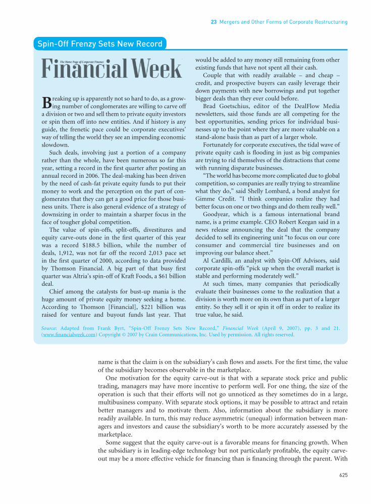
Breaking up is apparently not so hard to do, as a grow-ing number of conglomerates are willing to carve off
a division or two and sell them to private equity investorsor spin them off into new entities. And if history is anyguide, the frenetic pace could be corporate executives’way of telling the world they see an impending economicslowdown.
Such deals, involving just a portion of a companyrather than the whole, have been numerous so far thisyear, setting a record in the first quarter after posting anannual record in 2006. The deal-making has been drivenby the need of cash-fat private equity funds to put theirmoney to work and the perception on the part of con-glomerates that they can get a good price for those busi-ness units. There is also general evidence of a strategy ofdownsizing in order to maintain a sharper focus in theface of tougher global competition.
The value of spin-offs, split-offs, divestitures andequity carve-outs done in the first quarter of this yearwas a record $188.5 billion, while the number of deals, 1,912, was not far off the record 2,013 pace set in the first quarter of 2000, according to data provided by Thomson Financial. A big part of that busy first quarter was Altria’s spin-off of Kraft Foods, a $61 billiondeal.
Chief among the catalysts for bust-up mania is thehuge amount of private equity money seeking a home.According to Thomson [Financial], $221 billion wasraised for venture and buyout funds last year. That
would be added to any money still remaining from otherexisting funds that have not spent all their cash.
Couple that with readily available – and cheap –credit, and prospective buyers can easily leverage theirdown payments with new borrowings and put togetherbigger deals than they ever could before.
Brad Goetschius, editor of the DealFlow Medianewsletters, said those funds are all competing for thebest opportunities, sending prices for individual busi-nesses up to the point where they are more valuable on astand-alone basis than as part of a larger whole.
Fortunately for corporate executives, the tidal wave ofprivate equity cash is flooding in just as big companiesare trying to rid themselves of the distractions that comewith running disparate businesses.
“The world has become more complicated due to globalcompetition, so companies are really trying to streamlinewhat they do,” said Shelly Lombard, a bond analyst forGimme Credit. “I think companies realize they had better focus on one or two things and do them really well.”
Goodyear, which is a famous international brandname, is a prime example. CEO Robert Keegan said in anews release announcing the deal that the companydecided to sell its engineering unit “to focus on our coreconsumer and commercial tire businesses and onimproving our balance sheet.”
Al Cardilli, an analyst with Spin-Off Advisors, saidcorporate spin-offs “pick up when the overall market isstable and performing moderately well.”
At such times, many companies that periodically evaluate their businesses come to the realization that adivision is worth more on its own than as part of a largerentity. So they sell it or spin it off in order to realize itstrue value, he said.
Spin-Off Frenzy Sets New Record
Source: Adapted from Frank Byrt, “Spin-Off Frenzy Sets New Record,” Financial Week (April 9, 2007), pp. 3 and 21.(www.financialweek.com) Copyright © 2007 by Crain Communications, Inc. Used by permission. All rights reserved.
name is that the claim is on the subsidiary’s cash flows and assets. For the first time, the valueof the subsidiary becomes observable in the marketplace.
One motivation for the equity carve-out is that with a separate stock price and public trading, managers may have more incentive to perform well. For one thing, the size of theoperation is such that their efforts will not go unnoticed as they sometimes do in a large,multibusiness company. With separate stock options, it may be possible to attract and retainbetter managers and to motivate them. Also, information about the subsidiary is more readily available. In turn, this may reduce asymmetric (unequal) information between man-agers and investors and cause the subsidiary’s worth to be more accurately assessed by themarketplace.
Some suggest that the equity carve-out is a favorable means for financing growth. Whenthe subsidiary is in leading-edge technology but not particularly profitable, the equity carve-out may be a more effective vehicle for financing than is financing through the parent. With
23 Mergers and Other Forms of Corporate Restructuring
625
••
FUNO_C23.qxd 9/19/08 17:11 Page 625

a separate subsidiary, the market may become more complete because investors are able toobtain a pure play investment in the technology.
l l l Empirical Evidence on DivestituresAs with mergers, the principal empirical tests on divestitures have involved event studies,where daily security return behavior, after isolating out general market effects, is studiedaround the time of the announcement. For liquidation of the entire company, the results indicate large gains to shareholders of the liquidating company, in the range of 12 to 20 percent. For partial sell-offs, shareholders of the selling company seem to realize a slightpositive return (about 2 percent) around the time of the announcement. Shareholders ofthe buying company also experience small positive gains on average, consistent with the subsidiary or division sold being more valuable to the buyer in terms of economic efficiencythan it is to the seller.
For the spin-off, somewhat higher shareholder excess returns (5 percent or more) wererecorded on average than for sell-offs. The findings here are consistent with a positive information effect of the spin-off announcement. The evidence is not consistent with a wealth transfer from debt holders to equity holders. Finally, for equity carve-outs a modestgain (around 2 percent) to shareholders around the time of the announcement was found. On balance, then, divestitures seem to have a positive informational effect, with voluntary liquidations having the largest effect.
Ownership RestructuringOther corporate restructurings are designed to change the ownership structure of a company.This is often accompanied by a dramatic change in the proportion of debt employed. In thissection we explore going private and leveraged buyouts.
l l l Going PrivateA number of well-known companies, such as Levi Strauss & Company, have “gone private.”Going private simply means transforming a company whose stock is publicly held into a private one. The privately held stock is owned by a small group of investors, with incumbentmanagement usually having a large equity stake. In this ownership change, a variety of vehicles are used to buy out the public shareholders. Probably the most common involvespaying them cash and merging the company into a shell corporation owned solely by a private investor management group. Rather than being treated as a merger, the transactionmay be treated as an asset sale to the private group. There are other ways, but the result is thesame: the company ceases to exist as a publicly held entity, and the shareholders receive a valuable consideration for their shares. Though most transactions involve cash, noncashcompensation, such as notes, is sometimes employed.
l l l MotivationsA number of factors may prompt management to take a company private.5 There are costsassociated with being a publicly held company. The stock must be registered, and share-holders must be serviced. There are administrative expenses in paying dividends and sendingout materials, and legal and administrative expenses are incurred in filing reports with theSecurities and Exchange Commission and other regulators. In addition, there are annual
Part 8 Special Areas of Financial Management
626
••
5The major paper dealing with going private is by Harry DeAngelo, Linda DeAngelo, and Edward M. Rice, “GoingPrivate: Minority Freezeouts and Stockholder Wealth,” Journal of Law and Economics 27 (June 1984), 367–401, wheremost of these motivations are discussed.
Pure playAn investmentconcentrated in one line of business.The extreme oppositeof a pure play wouldbe an investment in a conglomerate.
Going private Makinga public companyprivate through therepurchase of stock by currentmanagement and/oroutside privateinvestors.
FUNO_C23.qxd 9/19/08 17:11 Page 626

shareholders’ meetings and meetings with security analysts leading to often embarrassingquestions that most chief executive officers would rather do without. All of these things canbe avoided by being a private company.
With a publicly held company, some feel there is a fixation on quarterly accounting earnings as opposed to long-run economic earnings. To the extent that decisions are directedmore toward building economic value, going private may improve resource allocation deci-sions and, thereby, enhance value.
Another motivation for going private is to realign and improve management incentives.With increased equity ownership by management, there may be an incentive to work longerand more efficiently. The money saved and the profits generated through more effective management largely benefit the company’s management as opposed to a wide group of share-holders. As a result, they may be more willing to make the tough decisions, to cut costs, toreduce management “perks,” and simply to work harder. The rewards are linked more closelyto their decisions. The greater the performance and profitability, the greater the reward. In apublicly held company, the compensation level is not so directly linked, particularly for deci-sions that produce high profitability. When compensation is high, there are always questionsfrom security analysts, shareholders, and the press.
Although there are a number of reasons for going private, there are some offsetting argu-ments. For one thing, there are transactions costs to investment bankers, lawyers, and othersthat can be quite substantial. A private company gives little liquidity to its owners with respectto their stock ownership. A large portion of their wealth may be tied up in the company.Management, for example, may create value for the company but be unable to realize thisvalue unless the company goes public in the future. If the company later goes public, transac-tions costs are repeated – wonderful for investment bankers and lawyers, but a sizable costnonetheless.
l l l Empirical Evidence on Going PrivateThere have been a few studies of the effect of going private on security holder wealth. The evidence we have suggests that shareholders realize sizable gains (about 12 to 22 percent intwo studies) around the time of the announcement. In the case of a cash offer, the gain ismuch more, similar to the premiums realized in a merger. Shareholders clearly gain, butwhether or not they are treated fairly cannot be stated.
Leveraged BuyoutsGoing private can be a straightforward transaction, where the investor group simply buys out the public shareholders, or it can be a leveraged buyout (LBO), where there are third- andsometimes fourth-party investors. As the name implies, a leveraged buyout represents anownership transfer consummated primarily with debt. Sometimes called asset-based financing,the debt is secured by the assets of the enterprise involved. As a result, most leveraged buy-outs involve capital-intensive businesses. Though some leveraged buyouts involve an entirecompany, most involve the purchase of a division of a company or some other subunit.Frequently, the sale is to the management of the division being sold, the company havingdecided that the division no longer fits its strategic objectives. This type of transaction isreferred to as a management buyout (MBO). Another distinctive feature is that leveragedbuyouts are cash purchases, as opposed to stock purchases. Finally, the business unit involvedinvariably becomes a privately held company.
Desirable LBO candidates have certain common characteristics. Frequently the com-pany in question enjoys a window of opportunity extending for several years and duringwhich major expenditures can be deferred. Often the company has gone through a pro-gram of heavy capital expenditures, and, as a result, its plant is modern. The company may
23 Mergers and Other Forms of Corporate Restructuring
627
••
Management buyout(MBO) A leveragedbuyout (LBO) in which prebuyoutmanagement ends up with a substantialequity position.
Leveraged buyout(LBO) A primarilydebt-financedpurchase of all thestock or assets of acompany, subsidiary,or division by aninvestor group.
FUNO_C23.qxd 9/19/08 17:11 Page 627

have subsidiary assets that can be sold without adversely impacting its core business, and such a sale can provide cash for debt service in the early years. In contrast, companies with high research and development (R&D) requirements, such as drug companies, are notgood candidates. For the first several years after an LBO, cash flows must be dedicated to debt service. Capital expenditures, R&D, advertising, and personnel development must take a back seat. Usually a service company, where people constitute the bulk of the franchisevalue, is not a good LBO candidate because, if the people should leave, little of valueremains.
Stable, predictable operating cash flows are prized in LBO candidates. In this regard, companies who produce consumer brands dominate “commodity-type” businesses. Provenhistorical performance, with an established market position, is also rated highly. Turn-around situations tend to be spurned. The less the products of the company or business are subject to cyclical demand, the better. As a rule, the company’s assets must be physicalassets and/or brand names. Management is also important in that the experience and qual-ity of senior management are critical elements needed for success. While the characteristicsjust described are not all-inclusive, they give a flavor of the ingredients that make for desir-able, and undesirable, LBO candidates.
l l l An Illustration in DetailTo illustrate a typical leveraged buyout, suppose that Klim-On Corporation wishes to divestitself of its dairy products division. The assets of the division consist of plants, equipment,truck fleets, inventories, and receivables. These assets have a book value of $120 million. Theirreplacement value is $170 million, but if the division were to be liquidated, the assets wouldfetch only $95 million. Klim-On has decided to sell the division if it can obtain $110 millionin cash, and it has enlisted an investment banker to assist it in the sale. After surveying themarket for such a sale, the investment banker concludes that the best prospect is to sell thedivision to existing management. The four top divisional officers are interested and eager topursue the opportunity. However, they are able to come up with only $2 million in personalcapital among them. Obviously, more capital is needed.
The investment banker agrees to try to arrange a leveraged buyout. Financial projectionsand cash budgets are prepared for the division to determine how much debt can be serviced.On the basis of these forecasts, as well as the curtailment of certain capital expenditures,research and development expenses, and advertising expenses, it is felt that the likely cashthrown off is sufficient to service approximately $100 million in debt. The reduction in expenditures is regarded as temporary, for the company to service debt during the next several years. The investment banker has lined up a limited partnership to make an addi-tional equity investment of $8 million, which will bring total equity to $10 million. For thiscash contribution, the partnership receives 60 percent of the initial common stock, and man-agement receives the remainder.
l l l Arranging Debt FinancingWith this equity capital commitment, the investment banker proceeds to arrange debt financing. In a leveraged buyout, two forms of debt are typically employed: senior debt andjunior subordinated debt. For the senior debt, a large New York bank, through its asset-basedlending subsidiary, has agreed to provide $75 million toward the cost plus an additional $8 million revolving credit for seasonal needs. The rate on both arrangements is 2 percentover the prime rate, and the loans are secured by liens on all of the assets – real estate, build-ings, equipment, rolling stock, inventories, and receivables. The term of the $75 million loan is six years, payable in equal monthly installments of principal and with interest for themonth being added on. All major banking will be done with the lending bank, and com-pany receipts will be deposited into a special account at the bank for purposes of servicing
Part 8 Special Areas of Financial Management
628
••
FUNO_C23.qxd 9/19/08 17:11 Page 628
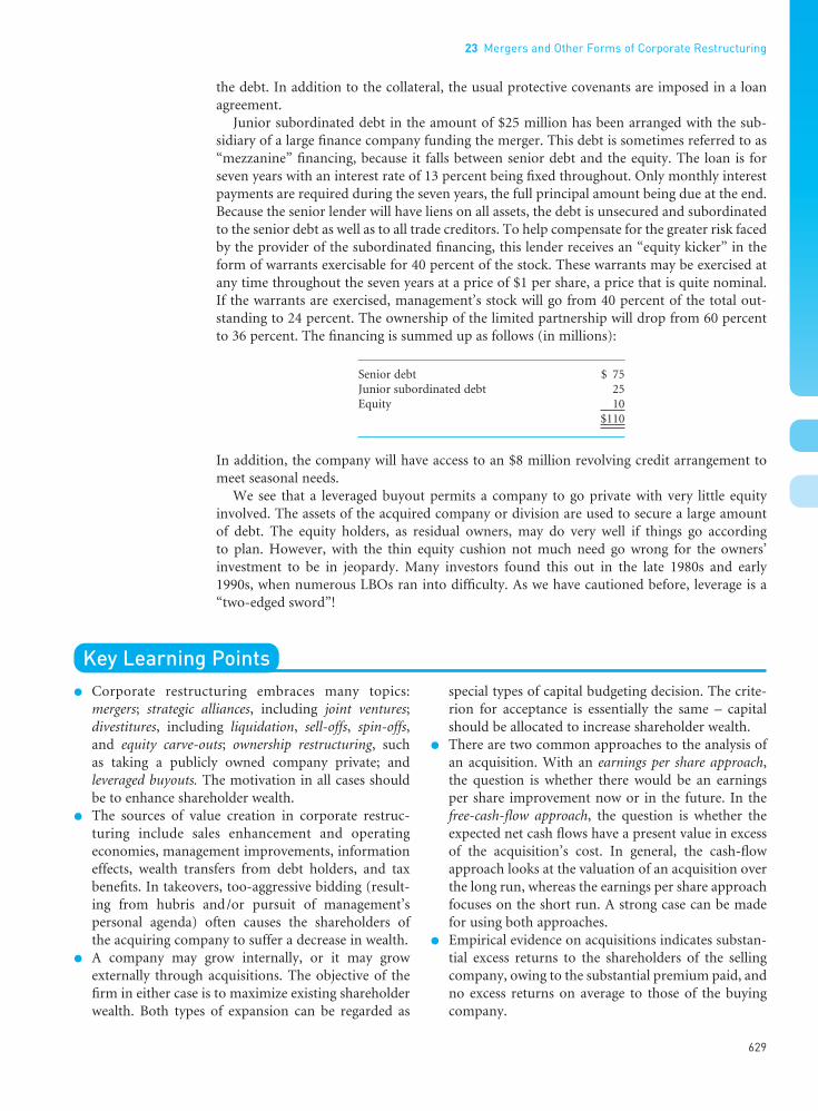
••
23 Mergers and Other Forms of Corporate Restructuring
629
the debt. In addition to the collateral, the usual protective covenants are imposed in a loan agreement.
Junior subordinated debt in the amount of $25 million has been arranged with the sub-sidiary of a large finance company funding the merger. This debt is sometimes referred to as“mezzanine” financing, because it falls between senior debt and the equity. The loan is forseven years with an interest rate of 13 percent being fixed throughout. Only monthly interestpayments are required during the seven years, the full principal amount being due at the end.Because the senior lender will have liens on all assets, the debt is unsecured and subordinatedto the senior debt as well as to all trade creditors. To help compensate for the greater risk facedby the provider of the subordinated financing, this lender receives an “equity kicker” in theform of warrants exercisable for 40 percent of the stock. These warrants may be exercised atany time throughout the seven years at a price of $1 per share, a price that is quite nominal.If the warrants are exercised, management’s stock will go from 40 percent of the total out-standing to 24 percent. The ownership of the limited partnership will drop from 60 percentto 36 percent. The financing is summed up as follows (in millions):
Senior debt $ 75Junior subordinated debt 25Equity 10
$110
In addition, the company will have access to an $8 million revolving credit arrangement tomeet seasonal needs.
We see that a leveraged buyout permits a company to go private with very little equityinvolved. The assets of the acquired company or division are used to secure a large amount of debt. The equity holders, as residual owners, may do very well if things go according to plan. However, with the thin equity cushion not much need go wrong for the owners’ investment to be in jeopardy. Many investors found this out in the late 1980s and early 1990s, when numerous LBOs ran into difficulty. As we have cautioned before, leverage is a“two-edged sword”!
Key Learning Pointsl Corporate restructuring embraces many topics:
mergers; strategic alliances, including joint ventures;divestitures, including liquidation, sell-offs, spin-offs,and equity carve-outs; ownership restructuring, such as taking a publicly owned company private; andleveraged buyouts. The motivation in all cases shouldbe to enhance shareholder wealth.
l The sources of value creation in corporate restruc-turing include sales enhancement and operatingeconomies, management improvements, informationeffects, wealth transfers from debt holders, and taxbenefits. In takeovers, too-aggressive bidding (result-ing from hubris and/or pursuit of management’s personal agenda) often causes the shareholders of the acquiring company to suffer a decrease in wealth.
l A company may grow internally, or it may grow externally through acquisitions. The objective of thefirm in either case is to maximize existing shareholderwealth. Both types of expansion can be regarded as
special types of capital budgeting decision. The crite-rion for acceptance is essentially the same – capitalshould be allocated to increase shareholder wealth.
l There are two common approaches to the analysis ofan acquisition. With an earnings per share approach,the question is whether there would be an earningsper share improvement now or in the future. In thefree-cash-flow approach, the question is whether theexpected net cash flows have a present value in excessof the acquisition’s cost. In general, the cash-flowapproach looks at the valuation of an acquisition overthe long run, whereas the earnings per share approachfocuses on the short run. A strong case can be madefor using both approaches.
l Empirical evidence on acquisitions indicates substan-tial excess returns to the shareholders of the sellingcompany, owing to the substantial premium paid, andno excess returns on average to those of the buyingcompany.
FUNO_C23.qxd 9/19/08 17:11 Page 629

Appendix Remedies for a Failing Company
So far our discussion of corporate restructuring has assumed that the firm is a going concern.Nevertheless, we must not lose sight of the fact that some firms fail. Internal managementmust keep this in mind, and so must a creditor who has amounts due from a company infinancial distress. The word “failure” is vague, partly because there are varying degrees of failure. Three terms are commonly used to give more precise meaning to the varying degreesof failure. Equitable (technical) insolvency is usually defined as a debtor’s general inability topay debts as they become due. However, such insolvency may be only temporary and subjectto remedy. Equitable insolvency, then, denotes only a lack of liquidity. Legal insolvency, on theother hand, means that the liabilities of a company exceed its assets “at a fair valuation.”Financial failure includes the entire range of situations between these two extremes.
The remedies for a failing company vary in harshness according to the degree of financialdifficulty. If the outlook is sufficiently hopeless, liquidation may be the only feasible alternative. However, some failing companies can be rehabilitated to the gain of creditors,shareholders, and society. The purpose of this Appendix is to review the remedies available, beginning with those that are voluntary, and then to move on to examine legal actions.
Voluntary SettlementsAn extension involves creditors postponing the maturity of their obligations. By not forcinglegal proceedings, creditors avoid considerable legal expense and the possible shrinkage ofvalue in liquidation. Because all creditors must agree to extend their obligations, the majorcreditors usually form a committee whose functions are to negotiate with the company andformulate a plan mutually satisfactory to all concerned.
A composition involves a pro rata settlement of creditors’ claims in cash or in cash andpromissory notes. All creditors must agree to accept this partial settlement in discharge oftheir entire claim. As with an extension, dissenting creditors must either be brought into thefold or paid in full.
Part 8 Special Areas of Financial Management
630
••
l Another company can be acquired through the purchase of either its assets or its common stock. Inturn, the means of payment can be cash or commonstock. Prior to the issuance in the US of Statement ofFinancial Accounting Standards (SFAS) 141 in 2001, acombination of two companies was treated either as apurchase or as a pooling of interests. SFAS 141 elimin-ates the pooling-of-interests method, allowing onlythe purchase method for mergers and acquisitions.And now, with a purchase, any goodwill arising fromthe combination must be tested at least annually forimpairment (or decline).
l Whether a combination is taxable or tax free is highly consequential to the selling company and its shareholders and, sometimes, to the buying company.
l The acquisition of another company can be negoti-ated with the management of the prospective acquisi-tion, or the acquiring company can make its appealdirectly to the shareholders through a tender offerto purchase their shares. These “unfriendly” takeoversare usually resisted by management. A number of
antitakeover devices exist. Some appear to have a negative effect on shareholder wealth.
l A company may decide to restructure by divestingitself of a portion of the enterprise or liquidatingentirely. Voluntary liquidations, sell-offs, spin-offs, andequity carve-outs are some of the major options opento the firm. In general, divestitures seem to have apositive informational effect, with voluntary liquida-tions having the largest.
l When a company goes private, it is transformed frompublic ownership to private ownership by a small groupof investors, including management. The empiricalevidence suggests sizable premiums, similar to thosefor mergers, being paid to the public shareholders.
l One means for going private is the leveraged buyout(LBO). Here a large amount of debt is used to financea cash purchase of a division of a company or a com-pany as a whole. Both senior debt secured by assetsand junior subordinated debt are employed. Giventhe small equity base, leveraged buyouts are risky. It does not take a very large adverse change in opera-tions or interest rates for default to occur.
FUNO_C23.qxd 9/19/08 17:11 Page 630

Voluntary liquidation represents an orderly private liquidation of a company away from thebankruptcy courts. Not only is it likely to be more efficient than a court-imposed liquidation,but creditors are likely to receive a higher settlement as many of the costs of bankruptcy are avoided. However, the company and all creditors must go along. As a result, voluntary liquidations are usually restricted to companies with a limited number of creditors.
Legal ProceedingsLegal procedures undertaken in connection with a failing company fall under bankruptcy lawas decreed through bankruptcy courts. Bankruptcy law is composed of many facets, but weare concerned with only two that pertain to business failure. Chapter 7 of the bankruptcy lawdeals with liquidation, and Chapter 11 deals with the rehabilitation of an enterprise throughits reorganization.
In both cases, proceedings begin with the debtor or creditors filing a petition in the bank-ruptcy court. When the debtor initiates the petition, it is called a voluntary proceeding. If theinitiative is taken by creditors, it is said to be involuntary. In a voluntary proceeding, merelyfiling the petition gives the debtor immediate protection from creditors. A stay restrains creditors from collecting their claims or taking actions until the court decides on the merit ofthe petition. The court can either accept the petition and order relief or dismiss it.
Three or more unsecured creditors with claims totaling $5,000 or more are required to initiate an involuntary bankruptcy. Here the petition must give evidence that the debtor firm has not paid debts on a timely basis (equitable insolvency) or has assigned possession of most of its property to someone else. The bankruptcy court then must decide whether theinvoluntary petition has merit. If the decision is negative, the petition is dismissed. If the petition is accepted, the court issues an order of relief pending a more permanent solution.The idea behind this stay of creditor action is to give the debtor breathing space to propose a solution to the problem. In what follows, we observe the solutions of liquidation and thereorganization of an enterprise.
LiquidationIf there is no hope for the successful operation of a company, liquidation is the only feasiblealternative. Upon petition of bankruptcy, the debtor obtains temporary relief from creditorsuntil a decision is reached by the bankruptcy court. After issuing the order of relief, the courtfrequently appoints an interim trustee to take over the operation of the company and to calla meeting of creditors. The interim trustee is a “disinterested” private citizen who is appointedfrom an approved list and who serves until at least the first meeting of creditors. At the first meeting, claims are proven, and the creditors may then elect a new trustee to replace theinterim trustee. Otherwise, the interim trustee serves as the regular trustee, continuing tofunction in that capacity until the case is completed. The trustee has responsibility for liquid-ating the property of the company and distributing liquidating dividends to creditors.
In distributing the proceeds of a liquidation to creditors with unsecured claims, the priority of claims must be observed. The order of distribution is as follows:
1. Administrative expenses associated with liquidating the property, including thetrustee’s fee and attorney fees
2. Creditor claims that arise in the ordinary course of the debtor’s business from the timethe case starts to the time a trustee is appointed
3. Wages earned by employees within 90 days of the bankruptcy petition (limited to$2,000 per employee)
4. Claims for contributions to employee benefit plans for services rendered within 180 days of the bankruptcy petition (limited to $2,000 per employee)
5. Claims of customers who make cash deposits for goods or services not provided by the debtor (limited to $900 per customer)
23 Mergers and Other Forms of Corporate Restructuring
631
••
FUNO_C23.qxd 9/19/08 17:11 Page 631

6. Taxes owed
7. Unsecured claims either filed on time or tardily filed if the creditor did not know ofthe bankruptcy
8. Unsecured claims filed late by creditors who had knowledge of the bankruptcy
9. Fines and punitive damages
10. Interest that accrues to claims after the date of the petition
Claims in each of these classes must be paid in full before any payment can be made toclaims in the next class. If anything is left over after all of these claims are paid in full, liquid-ating dividends can then be paid to subordinated debt holders, to preferred stockholders, and, finally, to common stockholders. It is unlikely, however, that common stockholders willreceive any distribution from a liquidation. Special provision is made in the Bankruptcy Actfor damage claims by lessors to the debtor. In general, lessors are limited to the greater of oneyear of payments or 15 percent of the total remaining payments but not to exceed those for three years. Upon the payment of all liquidating dividends, the debtor is discharged andrelieved of any further claims.
ReorganizationIt may be in the best interests of all concerned to reorganize a company rather than liquidateit. Conceptually, a firm should be reorganized if its economic worth as an operating entity is greater than its liquidation value. It should be liquidated if the converse is true: that is, if itis worth more “dead” than “alive.” Reorganization is an effort to keep a company alive bychanging its capital structure. The rehabilitation involves the reduction of fixed charges by substituting equity and limited-income securities for fixed-income securities.
Procedures. Reorganizations occur under Chapter 11 of the bankruptcy law and are initi-ated in the same general manner as liquidation in bankruptcy. Either the debtor or creditorsfile a petition, and the case begins. In most cases, the debtor will continue to run the business,although a trustee can assume operating responsibility of the company. One of the great needsin rehabilitation is interim credit. To provide inducements, Chapter 11 gives post-petitioncreditors priority over pre-petition creditors. If this inducement is not sufficient, the bank-ruptcy court is empowered to authorize new, or post-petition, creditors to obtain a lien on thedebtor’s property.
If a trustee is not appointed, the debtor has the sole right to draw up a reorganization planand to file it within 120 days. Otherwise, the trustee has the responsibility of seeing that a planis filed. It may be drawn up by the trustee, the debtor, the creditors’ committee, or individualcreditors, and more than one plan can be filed. All reorganization plans must be submitted tocreditors and stockholders for approval. The role of the court is to review the information inthe plan, to make sure disclosure is full.
In a reorganization, the plan should be fair, equitable, and feasible. This means that all parties must be treated fairly and equitably, and that the plan must be workable with respectto the earning power and financial structure of the reorganized company as well as the abilityof the company to obtain trade credit and, perhaps, short-term bank loans. Each class of claimholders must vote on a plan. More than one-half the number and two-thirds the amount of total claims in each class must vote in favor of the plan if it is to be accepted. If creditorsreject the reorganization plan, the bankruptcy judge will try to get the various parties to negotiate another plan. If creditors reject such efforts, the judge may impose a plan, known asa cram down, on all claimholders. Upon confirmation of any plan by the bankruptcy court,the debtor must then perform according to the terms of the plan. Moreover, the plan bindsall creditors and shareholders, including dissenters.
Reorganization Plan. The difficult aspect of a reorganization is the recasting of the com-pany’s capital structure to reduce the amount of fixed charges. In formulating a reorganiza-
Part 8 Special Areas of Financial Management
632
••
ReorganizationRecasting of thecapital structure of a financially troubledcompany, underChapter 11 of theBankruptcy Act, in order to reducefixed charges. Claimholders may be givensubstitute securities.
FUNO_C23.qxd 9/19/08 17:11 Page 632

tion plan, there are three steps. First, the total valuation of the reorganized company must bedetermined. This step is the most difficult and the most important. The technique favored bytrustees is a capitalization of prospective earnings. If future annual earnings of the reorganizedcompany are expected to be $2 million and the overall capitalization rate of similar com-panies averages 10 percent, a total valuation of ($2 million)/(0.10) = $20 million would be set for the company. The valuation figure is subject to considerable variation, owing to thedifficulty of estimating prospective earnings and determining an appropriate capitalizationrate. Thus the valuation figure represents nothing more than a best estimate of potentialvalue. Although the capitalization of prospective earnings is the generally accepted approachof valuing a company in reorganization, the valuation may be adjusted upward if the assetshave substantial liquidating value.
Once a valuation figure has been determined, the next step is to formulate a new capital structure for the company to reduce fixed charges, so that there will be an adequatecoverage margin. To reduce these charges, the total debt of the firm is scaled down by being partly shifted to income bonds, preferred stock, and common stock. In addition tobeing scaled down, the terms of the remaining debt may be changed. The maturity of the debt can be extended to reduce the amount of annual sinking-fund obligation. If it appears that the reorganized company will need new financing in the future, the trustee may feel that a more conservative ratio of debt to equity is in order to provide for future financial flexibility.
Once a new capital structure is established, the last step involves the valuation of the oldsecurities and their exchange for new securities. In general, all senior claims on assets must be settled in full before a junior claim can be settled. In the exchange process, bondholdersmust receive the par value of their bonds in another security before there can be any distribu-tion to preferred stockholders. The total valuation figure arrived at in step 1 sets an upperlimit on the amount of securities that can be issued. The existing capital structure of a com-pany undergoing reorganization may be as follows (in millions):
Debentures $ 9Subordinated debentures 3Preferred stock 6Common stock equity (at book value) 10
$28
If the total valuation of the reorganized company is to be $20 million, the trustee might establish the following capital structure in step 2 (in millions):
Debentures $ 3Income bonds 6Preferred stock 3Common stock equity 8
$20
Having established the “appropriate” capital structure for the reorganized company, thetrustee must then allocate the new securities. In this regard, the trustee may propose that thedebenture holders exchange their $9 million in debentures for $3 million in new debenturesand $6 million in income bonds, that the subordinated debenture holders exchange their $3 million in securities for preferred stock, and that preferred stockholders exchange theirsecurities for $6 million of common stock in the reorganized company. The common stock-holders would then be entitled to $2 million in stock in the reorganized company, or 25 per-cent of the total common stock of the reorganized company.
23 Mergers and Other Forms of Corporate Restructuring
633
••
FUNO_C23.qxd 9/19/08 17:11 Page 633

Thus each claim is settled in full before a junior claim is settled. The example represents arelatively mild reorganization. In a harsh reorganization, debt instruments may be exchangedentirely for common stock in the reorganized company, and the old common stock may be eliminated completely. Had the total valuation figure in the example been $12 million, thetrustee might have proposed a new capital structure consisting of $3 million in preferred stockand $9 million in common stock. Only the straight and subordinated debenture holderswould receive a settlement in this case. The preferred and the common stockholders of the old company would receive nothing.
These examples show that the common stockholders of a company undergoing reorgan-ization suffer under an absolute-priority rule, whereby claims must be settled in the order of their legal priority. From their standpoint, they would much prefer to see claims settled on a relative-priority basis. Under this rule, new securities are allocated on the basis of the relative market prices of the securities. The common stockholders could never obtain seniorsecurities in a reorganization, but they would be entitled to some common stock if their present stock had value. Because the company is not actually being liquidated, commonstockholders argue that a rule of relative priority is really the fairest. The Supreme Courtdecided otherwise when it upheld the absolute-priority rule (Case v. Los Angeles LumberProducts Company 1939).
Negotiated SettlementsWhile the principle of absolute priority is used in reorganization cases, the BankruptcyReform Act of 1978 provided a degree of flexibility and shifted the focus in the direction ofrelative priority. During the late 1980s and early 1990s, when many companies experiencedfinancial distress, negotiated settlements achieved even greater flexibility. The practical realityis that during often protracted reorganization proceedings, management still controls thecompany; put bluntly, management often wields a club over creditors. Parties willing to infusenew capital as equity participants have clout as well.
The problem for creditors is that bankruptcy proceedings are costly and time-consumingand that, during the time taken in proceedings, corporate value often is destroyed. Manage-ment and equity participants are able to drive hard bargains, and creditors are asked to givesignificant ground in order to make the reorganization plan workable. If the “haircut” (i.e.,reduction in the value of claims) is too severe, the creditors will rebel. So there is a delicatebalance in negotiating a compromise between what the equity participants and manage-ment would like and what the creditors will begrudgingly accept. Various classes of creditors often battle with each other over sharing the corporate pie, and this sometimes gives equityparticipants and management a wedge they can use to extract concessions.
Prepackaged bankruptcy (prepack) is a device sometimes employed to avoid the legaldelays inherent in a Chapter 11 reorganization. Here a company in financial distress devises aworkout plan prior to filing under Chapter 11. The company seeks approval from a minimumof two-thirds of each class of claimants in advance. If the court approves the plan, the termscan be imposed on dissenting debt holders. For example, Resorts International and TWA used this method. The advantage of a prepackaged bankruptcy is that it takes a short time to implement. The delays involved in Chapter 11 proceedings often add up to years, but aprepackaged bankruptcy often takes six months or so to implement.
Whether voluntary or under Chapter 11, workouts help management and employees. But they are not always in the best interests of creditors, who are asked to accept less than the book value of their claims. For creditors, the trade-off is whether keeping the companyrunning is better than “pulling the plug” and incurring the deadweight loss of bankruptcyproceedings.
Part 8 Special Areas of Financial Management
634
••
Prepackagedbankruptcy (prepack)A reorganization that a majority of acompany’s creditorshave approved prior to the beginning of a bankruptcyproceeding.
Absolute-priority ruleThe rule in bankruptcyor reorganization thatclaims of a set ofclaim holders must be paid, or settled, in full before the next,junior, set of claimholders may be paidanything.
FUNO_C23.qxd 9/19/08 17:11 Page 634

Questions
1. Explain the concept of synergy.2. Illustrate and explain how the ratio of P/E multiples for two merged firms affects the
earnings per share of the surviving firm.3. With a common-stock-for-common-stock acquisition, is it better to analyze the situation
on a cash-flow basis or to look more to the acquisition’s effect on the surviving firm’searnings per share?
4. It has been noted that the number of mergers tends to vary directly with the level of relative business activity. Why would this be?
23 Mergers and Other Forms of Corporate Restructuring
635
••
The unraveling of Italian dairy producer Parmalat in December 2003 marked a watershed in Italian
restructurings by triggering a rewrite of the country’sinsolvency law.
This brought the regime more in line with the USChapter 11 process.
Those changes allowed for faster, more flexiblerestructuring, but they omitted a crucial element: a pro-vision to facilitate “work-out loans” to fund companiesthrough their insolvencies.
Similar liquidity constraints complicate work-outs inthe UK and the rest of Europe – lender liability laws inFrance and shareholder-friendly legislation in Germany.
That means that the loan-to-own and equitizationstrategies implemented by distressed investors in the USare often “lost in translation” when applied in Europe.
When traditional restructuring formulas fail,European investors resort to more unorthodox methods:for example, soliciting white-knight investors or seizingthe shares backing their debts.
When lenders extend new financing to British orItalian debtors, they do not enjoy the same super prior-ity allowed to their US counterparts through debtor-in-possession (DIP) loans.
That puts lenders at risk of being lumped in withother claimants should the restructuring deteriorate intoa liquidation.
“There’s no sense in [bondholders] providing thefunding if they are junior to other creditors,” a source
involved in the work-out of Italian IT services providerDamovo told Debtwire.
Damovo, which began work-out negotiations withbondholders in October, is now asking them for a60 mil-lion of rescue financing, but the creditors are balking forfear of having their claim on the assets subordinated,should the restructuring slide into liquidation.
The uncertainty does not stop there, as lenders toinsolvent companies often find themselves dealing withdifferent leadership once the debtor has filed for protec-tion. British and Italian insolvency codes require anadministrator to take over the running of a companyfrom existing management after an insolvency petition.
As a result, corporations face a heavy burden of proofto secure new financing, even when they have negotiatedhaircuts [i.e., partial debt forgiveness] for existing creditors.
The result is a Catch-22, whereby the mechanism forrestructuring exists, but creditors remain reluctant toprovide the funding needed to power that process.
Germany was the first European country to reform itsinsolvency regime based on Chapter 11 in 1999.
Unlike the French and Italian regimes, the Germansystem encourages a troubled company to obtain rescuefinancing on a secured basis while it restructures its operations and balance sheet.
In theory, the super-priority protection should allowfor more balance sheet restructurings facilitated by insolvency bridge loans.
In practice, work-outs and work-out financingsremain a risky proposition because of German share-holder rights in restructuring situations.
Bankrupt companies may present an Insolvenzplan ora restructuring plan that proposes a 100 percent equitywipe-out, but this can only be implemented with theconsent of shareholders.
European Insolvency Law: Chapter 11 is Often “Lost in Translation”
Source: Adapted from Adelene Lee, “Chapter 11 is often lost in translation,” Financial Times Special Report (July 25, 2007), p. 5.(www.ft.com) Copyright © The Financial Times Limited 2007. Used by permission. All rights reserved.
FUNO_C23.qxd 9/19/08 17:11 Page 635
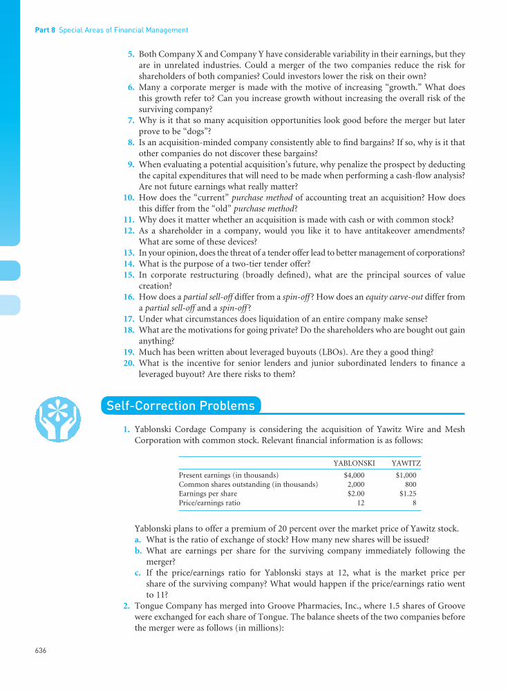
5. Both Company X and Company Y have considerable variability in their earnings, but theyare in unrelated industries. Could a merger of the two companies reduce the risk forshareholders of both companies? Could investors lower the risk on their own?
6. Many a corporate merger is made with the motive of increasing “growth.” What does this growth refer to? Can you increase growth without increasing the overall risk of thesurviving company?
7. Why is it that so many acquisition opportunities look good before the merger but laterprove to be “dogs”?
8. Is an acquisition-minded company consistently able to find bargains? If so, why is it thatother companies do not discover these bargains?
9. When evaluating a potential acquisition’s future, why penalize the prospect by deductingthe capital expenditures that will need to be made when performing a cash-flow analysis?Are not future earnings what really matter?
10. How does the “current” purchase method of accounting treat an acquisition? How doesthis differ from the “old” purchase method?
11. Why does it matter whether an acquisition is made with cash or with common stock?12. As a shareholder in a company, would you like it to have antitakeover amendments?
What are some of these devices?13. In your opinion, does the threat of a tender offer lead to better management of corporations?14. What is the purpose of a two-tier tender offer?15. In corporate restructuring (broadly defined), what are the principal sources of value
creation?16. How does a partial sell-off differ from a spin-off ? How does an equity carve-out differ from
a partial sell-off and a spin-off ?17. Under what circumstances does liquidation of an entire company make sense?18. What are the motivations for going private? Do the shareholders who are bought out gain
anything?19. Much has been written about leveraged buyouts (LBOs). Are they a good thing?20. What is the incentive for senior lenders and junior subordinated lenders to finance a
leveraged buyout? Are there risks to them?
Self-Correction Problems
1. Yablonski Cordage Company is considering the acquisition of Yawitz Wire and MeshCorporation with common stock. Relevant financial information is as follows:
YABLONSKI YAWITZ
Present earnings (in thousands) $4,000 $1,000Common shares outstanding (in thousands) 2,000 800Earnings per share $2.00 $1.25Price/earnings ratio 12 8
Yablonski plans to offer a premium of 20 percent over the market price of Yawitz stock.a. What is the ratio of exchange of stock? How many new shares will be issued?b. What are earnings per share for the surviving company immediately following the
merger?c. If the price/earnings ratio for Yablonski stays at 12, what is the market price per
share of the surviving company? What would happen if the price/earnings ratio went to 11?
2. Tongue Company has merged into Groove Pharmacies, Inc., where 1.5 shares of Groovewere exchanged for each share of Tongue. The balance sheets of the two companies beforethe merger were as follows (in millions):
Part 8 Special Areas of Financial Management
636
••
FUNO_C23.qxd 9/19/08 17:11 Page 636

23 Mergers and Other Forms of Corporate Restructuring
637
••
TONGUE GROOVE
Current assets $ 5 $20Fixed assets 7 30Goodwill – 2
Total $12 $52
Current liabilities $ 3 $ 9Long-term debt 2 15Shareholders’ equity 7 28
Total $12 $52
Number of shares (in millions) 0.2 1.4Market value per share $35 $28
The fair market value of Tongue’s fixed assets is $400,000 higher than their book value.Construct the balance sheet for the company after the merger, using the purchase methodof accounting.
3. Hi-Tec Corporation is considering the acquisition of Lo-Tec, Inc., which is in a related lineof business. Lo-Tec, an all-equity-financed firm, currently has an after-tax cash flow of $2 million per year. With a merger, synergy would be expected to result in a growth rateof this cash flow of 15 percent per year for 10 years, at the end of which time level cashflows would be expected. To sustain the cash-flow stream, Hi-Tec will need to invest $1 million annually. For purposes of analysis and to be conservative, Hi-Tec limits its calculations of cash flows to 25 years.a. What expected annual cash flows would Hi-Tec realize from this acquisition?b. If its required rate of return is 18 percent, what is the maximum price that Hi-Tec
could pay?4. Aggressive, Inc., wishes to make a tender offer for the Passive Company. Passive has 100,000
shares of common stock outstanding and earns $5.50 per share. If it were combined withAggressive, total economies (in present value terms) of $1.5 million could be realized. Atpresent, the market price per share of Passive is $55. Aggressive makes a two-tier tender offer:$65 per share for the first 50,001 shares tendered and $50 per share for the remaining shares.a. If successful, what will Aggressive end up paying for Passive? How much incrementally
will shareholders of Passive receive for the economies?b. Acting independently, what will each Passive shareholder do to maximize his or her
wealth? What might they do if they could respond collectively as a cartel?c. How can a target company increase the probability of individual shareholders resisting
too low a tender offer?d. What might happen if Aggressive offered $65 in the first tier and only $40 in the
second tier?5. McNabb Enterprises is considering going private through a leveraged buyout by man-
agement. Management currently owns 21 percent of the 5 million shares outstanding.Market price per share is $20, and it is felt that a 40 percent premium over the present price will be necessary to entice public shareholders to tender their shares in a cash offer.Management intends to keep its shares and to obtain senior debt equal to 80 percent of thefunds necessary to consummate the buyout. The remaining 20 percent will come fromjunior subordinated debentures.
Terms on the senior debt are 2 percent above the prime rate with principal reductionsof 20 percent of the initial loan at the end of each of the next five years. The junior sub-ordinated debentures bear a 13 percent interest rate and must be retired at the end of sixyears with a single balloon payment. The debentures have warrants attached that enablethe holders to purchase 30 percent of the stock at the end of the sixth year. Managementestimates that earnings before interest and taxes will be $25 million per year. Because oftax-loss carryforwards, the company expects to pay no taxes over the next five years. Thecompany will make capital expenditures in amounts equal to its depreciation.
FUNO_C23.qxd 9/19/08 17:11 Page 637

Part 8 Special Areas of Financial Management
638
••
a. If the prime rate is expected to average 10 percent over the next five years, is the lever-aged buyout feasible?
b. What if the prime rate averages only 8 percent?c. What minimal EBIT is necessary to service the debt?
Problems
1. The following data are pertinent for Companies A and B:
COMPANY A COMPANY B
Present earnings (in millions) $20 $ 4Number of shares (in millions) 10 1Price/earnings ratio 18 10
a. If the two companies were to merge and the share exchange ratio were 1 share ofCompany A for each share of Company B, what would be the initial impact on earn-ings per share of the two companies? What is the market value exchange ratio? Is amerger likely to take place?
b If the share exchange ratio were 2 shares of Company A for each share of Company B,what would happen with respect to Part (a)?
c. If the exchange ratio were 1.5 shares of Company A for each share of Company B,what would happen?
d. What exchange ratio would you suggest?
2. EXPECTED NUMBER OF MARKET PRICE TAX EARNINGS SHARES PER SHARE RATE
Schoettler Company $5,000,000 1,000,000 $100 50%Stevens Company 3,000,000 500,000 60 50%
The Schoettler Company wishes to acquire the Stevens Company. If the merger wereeffected through an exchange of stock, Schoettler would be willing to pay a 25 percent premium for the Stevens shares. If done for cash, the terms would have to be just as favor-able to the Stevens shareholders. To obtain the cash, Schoettler would have to sell its owncommon stock in the market.a. Compute the share exchange ratio and the combined expected earnings per share for
Schoettler under an exchange of common stock.b. If we assume that all Stevens shareholders have held their common stock for more
than one year, have a 28 percent marginal capital gains tax rate, and have paid an average of $14 for their shares, what cash price would have to be offered to be just asattractive as the terms in Part (a)?
3. Assume the exchange of Schoettler shares for Stevens shares as outlined in Problem 2.a. What is the share exchange ratio?b. Compare the earnings per Stevens share before and after the merger. Compare the
earnings per Schoettler share. On this basis alone, which merger group fared better? Why?c. Why do you imagine that Schoettler commanded a higher P/E ratio than Stevens?
What should be the change in P/E ratio resulting from the merger? Does this conflictwith what you previously concluded? Why?
d. If the Schoettler Company were in a high-technology growth industry and Stevensmade cement, would you revise your answers?
e. In determining the appropriate P/E ratio for Schoettler, should the increase in earn-ings resulting from this merger be added as a growth factor?
4. Copper Clapper Company currently has annual earnings of $10 million with 4 millionshares of common stock outstanding and a market price per share of $30. In the absence
FUNO_C23.qxd 9/19/08 17:11 Page 638

23 Mergers and Other Forms of Corporate Restructuring
639
••
of any mergers, Copper Clapper’s annual earnings are expected to grow at a compoundrate of 5 percent per annum. Brass Bell Company, which Copper Clapper is seeking toacquire, has present annual earnings of $2 million, 1 million shares of common stock out-standing, and a market price per share of $36. Its annual earnings are expected to grow ata compound annual rate of 10 percent per annum. Copper Clapper will offer 1.2 sharesof its stock for each share of Brass Bell Company.a. What is the immediate effect on the surviving company’s earnings per share?b. Would you want to acquire Brass Bell Company? If it is not attractive now, when will
it be attractive from the standpoint of earnings per share?5. The Byer Corporation, which has a 16 percent after-tax cost of capital, is considering the
acquisition of the Cellar Company, which has about the same degree of systematic risk. If the merger were effected, the incremental cash flows would be as follows:
AVERAGE FOR YEARS (in millions)
1–5 6–10 11–15 16–20
Annual cash income attributable to Cellar $10 $15 $20 $15Required new investment 2 5 10 10
Net after-tax cash flow $ 8 $10 $10 $ 5
What is the maximum price that Byer should pay for Cellar, assuming the business-riskcomplexion of the company remains unchanged?
6. Valdez Coffee Company is considering the cash acquisition of Mountain Creamery, Inc.,for $750,000. The acquisition is expected to result in incremental cash flows of $100,000in the first year, and this amount is expected to grow at a 6 percent compound rate. In theabsence of the acquisition, Valdez expects net cash flows (after capital expenditures) of$600,000 this year, and these are expected to grow at a 6 percent compound rate forever.At present, suppliers of capital require a 14 percent overall rate of return for ValdezCoffee Company. However, Mountain Creamery is much more risky, and the acquisitionof it will raise the company’s overall required return to 15 percent.a. Should Valdez Coffee Company acquire Mountain Creamery, Inc.?b. Would your answer be the same if the overall required rate of return stayed the same?c. Would your answer be the same if the acquisition increased the surviving company’s
growth rate to 8 percent forever?7. Bigge Stores, Inc. (BSI), has acquired the L. Grande Company (LGC) for $4 million in
stock and the assumption of $2 million in LGC liabilities. The balance sheets of the twocompanies before the merger revealed the following information (in millions):
BSI LGC
Tangible and total assets $10.0 $5.0Liabilities 4.0 2.0
Shareholders’ equity $ 6.0 $3.0
Determine the balance sheet of the combined company after the merger under the pur-chase method of accounting. (Assume that the net book value of LGC assets representstheir fair market value.)
8. Leonardo Company has three divisions, and the total market value (debt and equity) ofthe firm is $71 million. Its debt-to-market-value ratio is 0.40, and bond indentures providethe usual protective covenants. However, they do not preclude the sale of a division.Leonardo has decided to divest itself of its Raphael division for a consideration of $20million. In addition to this payment to Leonardo, the buyer will assume $5 million ofexisting debt of the division. The full $20 million will be distributed to Leonardo Companyshareholders. In words, explain whether the remaining debt holders of Leonardo Companyare better or worse off. Why? In theory, are the equity holders better or worse off? Why?
FUNO_C23.qxd 9/19/08 17:11 Page 639

9. Lorzo-Perez International has a subsidiary, the DelRay Sorter Company. The companybelieves the subsidiary on average will generate $1 million per year in annual net cashflows after necessary capital expenditures. These annual net cash flows are projected far into the future (assume infinity). The required rate of return for the subsidiary is 12 percent. If the company were to invest an additional $10 million now, it is believed that annual net cash flows could be increased from $1 to $2 million. Exson Corporationhas expressed an interest in DelRay, because it is in the sorter business and believes it can achieve some economies. Accordingly, it has made a cash offer of $10 million for the subsidiary. Should Lorzo-Pereza. Continue the business as is?b. Invest the additional $10 million?c. Sell the subsidiary to Exson? (Assume the subsidiary is entirely equity financed.)
10. Hogs Breath Inns, a chain of restaurants, is considering going private. The president,Clint Westwood, believes that with the elimination of shareholder servicing costs andother costs associated with public ownership, the company could save $800,000 per annumbefore taxes. In addition, the company believes management incentives and, hence, performance will be higher as a private company. As a result, annual profits are expectedto be 10 percent greater than present after-tax profits of $9 million. The effective tax rateis 30 percent; the price/earnings ratio of the stock is 12; and there are 10 million sharesoutstanding. What is the present market price per share? What is the maximum dollarpremium above this price that the company could pay to take the company private?
11. Donatello Industries wishes to sell its sewer pipe division for $10 million. Management ofthe division wishes to buy it and has arranged a leveraged buyout. Management will putup $1 million in cash. A senior lender will advance $7 million secured by all the assets ofthe company. The rate on the loan is 2 percent above the prime rate, which is currently12 percent. The loan is payable in equal annual principal installments over five years, with interest for the year payable at the end of each year. A junior subordinated loan of$2 million also has been arranged, and this loan is due at the end of six years. The interest rate is fixed at 15 percent, and interest payments only are due at the end of eachof the first five years. Interest and the entire principal are due at the end of the sixth year.In addition, the lender has received warrants exercisable for 50 percent of the stock.
The sewer pipe division expects earnings before interest and taxes of $3.4 million in each of the first three years and $3.7 million in the last three years. The tax rate is 331⁄3 percent, and the company expects capital expenditures and investments in receiv-ables and inventories to equal depreciation charges in each year. All debt servicing mustcome from profits. (Assume also that the warrants are not exercised and that there is nocash infusion as a result.)
If the prime rate stays at 12 percent on average throughout the six years, will the enterprise be able to service the debt properly? If the prime rate were to rise to 20 percentin the second year and average that for the second year through the sixth year, would thesituation change?
Appendix Problems
12. Merry Land Company, an amusement park in Atlanta, has experienced increased diffi-culty in paying its bills. Although the park has been marginally profitable over the years,the current outlook is not encouraging, as profits during the last two years have been negative. The park is located on reasonably valuable real estate and has an overall liquid-ating value of $5 million. After much discussion with creditors, management has agreedto a voluntary liquidation. A trustee, who is appointed by the various parties to liquidatethe properties, will charge $200,000 for her services. The Merry Land Company owes$300,000 in back property taxes. It has a $2 million mortgage on certain amusement parkequipment that can be sold for only $1 million. Creditor claims are as follows:
Part 8 Special Areas of Financial Management
640
••
FUNO_C23.qxd 9/19/08 17:11 Page 640

23 Mergers and Other Forms of Corporate Restructuring
641
••
PARTY BOOK VALUE CLAIM
General creditors $1,750,000Mortgage bonds 2,000,000Long-term subordinated debt 1,000,000Common stock 5,000,000
What amount is each party likely to receive in liquidation?13. The Fias Company is in Chapter 11. The trustee has estimated that the company can earn
$1.5 million before interest and taxes (40 percent tax rate) in the future. In the new capitalization, the trustee feels that debentures should bear a coupon of 10 percent andhave a coverage ratio of 5, income bonds (12 percent) should have an overall coverageratio of 2, preferred stock (10 percent) should have an after-tax coverage ratio of 3, andcommon stock should be issued on a price/earnings ratio basis of 12. Determine the capital structure that conforms to the trustee’s criteria.
14. Facile Fastener Company had the following liabilities and equity position when it filed forbankruptcy under Chapter 11 (in thousands):
Accounts payable $ 500Accrued wages 200Bank loan, 12% rate (secured by receivables) 600
Current liabilities $1,30013% First-mortgage bonds 50015% Subordinated debentures 1,700
Total debt $3,500Common stock and additional paid-in capital 500Retained earnings 420
Total liabilities and equity $4,420
After straightening out some operating problems, the company is expected to be able toearn $800,000 annually before interest and taxes. Based on other going-concern values, it is felt that the company as a whole is worth five times its EBIT. Court costs associatedwith the reorganization will total $200,000, and the expected tax rate is 40 percent for thereorganized company. As trustee, suppose that you have the following instruments to use for the long-term capitalization of the company: 13 percent first-mortgage bonds, 15 percent capital notes, 13 percent preferred stock, and common stock.
With the new capitalization, the capital notes should have an overall coverage ratio,after bank loan interest, of 4, and preferred stock should have a coverage ratio after interest and taxes of 2. Moreover, it is felt that common stock equity should equal at least30 percent of the total assets of the company.a. What is the total valuation of the company after reorganization?b. If the maximum amounts of debt and preferred stock are employed, what will be
the new capital structure and current liabilities of the company?c. How should these securities be allocated, assuming a rule of absolute priority?
Solutions to Self-Correction Problems
1. a. YABLONSKI YAWITZ
Earnings per share $2.00 $1.25Price/earnings ratio 12 8Market price per share $ 24 $ 10Offer to Yawitz shareholders in Yablonski stock
(including the premium) = $10 × 1.20 = $12 per share
FUNO_C23.qxd 9/19/08 17:11 Page 641

Part 8 Special Areas of Financial Management
642
••
Exchange ratio = $12/24 = 0.5, or one-half share of Yablonski stock for every share of Yawitz stock.Number of new shares issued = 800,000 shares × 0.5 = 400,000 shares.
b. Surviving company earnings (in thousands) $ 5,000Common shares outstanding (in thousands) 2,400Earnings per share $2.0833
There is an increase in earnings per share by virtue of acquiring a company with a lowerprice/earnings ratio.
c. Market price per share: $2.0833 × 12 = $25.00Market price per share: $2.0833 × 11 = $22.92In the first instance, share price rises, from $24, owing to the increase in earnings pershare. In the second case, share price falls owing to the decline in the price/earningsratio. In efficient markets, we might expect some decline in the price/earnings ratio ifthere was not likely to be synergy and/or improved management.
2. With an exchange ratio of 1.5, Groove would issue 300,000 new shares of stock with a market value of $28 × 300,000 = $8.4 million for the common stock of Tongue. This exceedsthe shareholders’ equity of Tongue by $1.4 million. With the purchase method, Tongue’sfixed assets will be written up by $400,000 and goodwill of Groove by $1 million. The balance sheet after the merger under the purchase method of accounting is (in millions):
PURCHASE
Current assets $25.0Fixed assets (net) 37.4Goodwill 3.0
Total $65.4
Current liabilities $12.0Long-term debt 17.0Shareholders’ equity 36.4
Total $65.4
3. a, b.
PRESENT VALUE OF YEAR CASH FLOW INVESTMENT NET CASH FLOW NET CASH FLOW (18%)
1 $2,300,000 $1,000,000 $1,300,000 $ 1,101,1002 2,645,000 ″ 1,645,000 1,181,1103 3,041,750 ″ 2,041,750 1,243,4264 3,498,013 ″ 2,498,013 1,288,9755 4,022,714 ″ 3,022,714 1,320,9266 4,626,122 ″ 3,626,122 1,341,6657 5,320,040 ″ 4,320,040 1,356,4938 6,118,046 ″ 5,118,046 1,361,4009 7,035,753 ″ 6,035,753 1,358,044
10–25 8,091,116 ″ 7,091,116 8,254,059*Total present value = $19,807,198
*Total for years 10–25.
The maximum price that is justified is approximately $19.81 million. It should be notedthat these calculations use present value tables. To arrive at the discount rate for cash flowsgoing from years 10 to 25, we subtract the discount factor for 9 years of annuity payments,4.303, from that for 25 years, 5.467. The difference, 5.467 − 4.303 = 1.164, is the discountfactor for cash flows for an annuity starting in year 10 and going through year 25. If a present value function of a calculator is used, a slightly different total may be given due toour having rounded to three decimal points.
FUNO_C23.qxd 9/19/08 17:11 Page 642

Betker, Brian L. “An Empirical Examination of PrepackagedBankruptcy.” Financial Management 24 (Spring 1995),3–18.
Black, Bernard S., and Joseph A. Gundfest. “ShareholderGains from Takeovers and Restructurings.” Journal ofApplied Corporate Finance 1 (Spring 1988), 5–15.
Borokhovich, Kenneth A., Kelly R. Brunarski, and Robert Parrino. “CEO Contracting and Antitakeover
Amendments.” Journal of Finance 52 (September 1997),1495–1517.
Brannen Laurie, Anand Desai, and E. Han Kim. “TheRationale Behind Interfirm Tender Offers: Informationor Synergy.” Journal of Financial Economics 11 (April1983), 183–206.
—— , “The Status of Shareholder Value in M&As.” BusinessFinance 7 (August 2001), 12.
23 Mergers and Other Forms of Corporate Restructuring
643
••
4. a. 50,001 shares × $65 = $3,250,06549,999 shares × $50 = 2,499,950
Total purchase price = $5,750,015Total value of stock before = 100,000 shares × $55 = 5,500,000
Increment to Passive shareholders = $ 250,015
The total value of the economies to be realized is $1,500,000. Therefore Passive share-holders receive only a modest portion of the total value of the economies. In contrast,Aggressive shareholders obtain a large share.
b. With a two-tier offer, there is a great incentive for individual shareholders to tenderearly, thereby ensuring success for the acquiring firm. Collectively, Passive share-holders would be better off holding out for a larger fraction of the total value of theeconomies. They can do this only if they act as a cartel in their response to the offer.
c. By instigating antitakeover amendments and devices, some incentives may be createdfor individual shareholders to hold out for a higher offer. However, in practice it isimpossible to achieve a complete cartel response.
d. 50,001 shares × $65 = $3,250,06549,999 shares × $40 = 1,999,960
Total purchase price = $5,250,025
This value is lower than the previous total market value of $5,500,000. Clearly, shareholders would fare poorly if in the rush to tender shares the offer were success-ful. However, other potential acquirers would have an incentive to offer more thanAggressive, even with no economies to be realized. Competition among potentialacquirers should ensure counterbids, so that Aggressive would be forced to bid no lessthan $5,500,000 in total, the present market value.
5. a. Shares owned by outsiders = 5 million × 0.79 = 3,950,000Price to be offered = $20 × 1.40 = $28 per shareTotal buyout amount = 3,950,000 shares × $28 = $110,600,000Senior debt = $110,600,000 × 0.80 = $88,480,000Annual principal payment = $88,480,000/5 = $17,696,000Junior debt = $110,600,000 × 0.20 = $22,120,000Annual EBIT to service debt:Senior debt interest: $88,480,000 × 0.12 = $10,617,600Senior debt principal: 17,696,000Junior debt interest: $22,120,000 × 0.13 = 2,875,600
Total EBIT necessary: $31,189,200During the first five years, EBIT of $25 million will not be sufficient to service the debt.
b. $88,480,000 × 0.10 = $8,848,000, which, with the two other amounts above, comes to$29,419,600. Expected EBIT will still not be sufficient to service the debt.
c. $31,189,200 is the minimal EBIT necessary to service the debt.
Selected References
FUNO_C23.qxd 9/19/08 17:11 Page 643

Part 8 Special Areas of Financial Management
644
••
Chan, Su Han, John W. Kensinger, Arthur J. Keown, andJohn D. Martin. “When Do Strategic Alliances CreateShareholder Value?” Journal of Applied Corporate Finance11 (Winter 1999), 82–87.
Chatterjee, Sris, Upinder S. Dhillon, and Gabriel G.Ramierez. “Resolution of Financial Distress: DebtRestructurings via Chapter 11, Prepackaged Bank-ruptcies, and Workouts.” Financial Management 24(Autumn 1995), 5–21.
Christofferson, Scott A., Robert S. McNish, and Diane L.Siss. “Where Mergers Go Wrong.” The McKinseyQuarterly (Number 2, 2004), 92–99.
Conn, Robert L. “International Mergers: Review ofLiterature and Clinical Projects.” Journal of FinancialEducation 29 (Fall 2003), 1–27.
DeAngelo, Harry, and Edward M. Rice. “AntitakeoverCharter Amendments and Stockholder Wealth.” Journalof Financial Economics 11 (April 1983), 329–360.
DeAngelo, Harry, Linda DeAngelo, and Edward M. Rice.“Going Private: Minority Freezeouts and StockholderWealth.” Journal of Law and Economics 27 (June 1984),367–401.
Dennis, Debra K., and John J. McConnell. “CorporateMergers and Security Returns.” Journal of FinancialEconomics 16 (June 1986), 143–187.
Donaldson, Gordon. Corporate Restructuring. Cambridge,MA: Harvard Business School Press, 1994.
Eberhart, Allan C., William T. Moore, and Rodney L.Roenfelt. “Security Pricing and Deviations from theAbsolute Priority Rule in Bankruptcy Proceedings.”Journal of Finance 45 (December 1990), 1457–1469.
Ehrhardt, Michael C., and John M. Wachowicz, Jr. “FormFollows Function: The Appropriate Definition of FreeCash Flow.” Journal of Financial and Economic Practice 7(Spring 2007), 18–37.
Fabozzi, Frank J., Jane Tripp Howe, Takashi Makabe, andToshihide Sudo. “Recent Evidence on the DistributionPatterns in Chapter 11 Reorganizations.” Journal of FixedIncome 2 (March 1993), 6–23.
Frank, Kimberly E. “Making Sense of Spin-Offs, TrackingStock, and Equity Carve-Outs.” Strategic Finance 83(December 2001), 39–43.
Franks, Julian R., and Robert S. Harris. “Shareholder WealthEffects of Corporate Takeovers: The UK Experience.”Journal of Financial Economics 23 (August 1989), 225–250.
Halpern, Paul. “Corporate Acquisitions: A Theory of SpecialCases? A Review of Event Studies Applied to Acquisi-tions.” Journal of Finance 38 (May 1983), 297–317.
Hite, Gailen L., and James E. Owers. “Security Price ReactionsAround Corporate Spin-Off Announcements.” Journal ofFinancial Economics 12 (December 1983), 409–436.
—— , and Ronald C. Rogers. “The Market for InterfirmAsset Sales: Partial Sell-Offs and Total Liquidations.”
Journal of Financial Economics 18 (June 1987), 229–252.
—— , and Michael R. Vetsuypens. “Management Buyoutsof Divisions and Shareholder Wealth.” Journal of Finance44 (June 1989), 953–980.
Hong, H., G. Mandelker, and R. S. Kaplan. “Pooling vs.Purchase: The Effects of Accounting for Mergers on StockPrices.” Accounting Review 53 (January 1978), 31–47.
Ikenberry, David, and Josef Lakonishok. “CorporateGovernance Through the Proxy Contest: Evidence andImplications.” Journal of Business 66 (July 1993),405–435.
Iverson, Glaydon. “Does Your Company Need a Workout?”Strategic Finance 86 (September 2004), 51–53.
Jain, Prem C. “The Effect of Voluntary Sell-off Announce-ments on Shareholder Wealth.” Journal of Finance 40(March 1985), 209–224.
Jarrell, Greg A., and Annette B. Poulsen. “The Returns toAcquiring Firms in Tender Offers: Evidence from ThreeDecades.” Financial Management 18 (Autumn 1989),12–19.
Jensen, Michael C. “The Takeover Controversy: Analysisand Evidence.” Midland Corporate Finance Journal 4(Summer 1986), 6–32.
Kaplan, Steven. “Management Buyouts: Evidence on Taxesas a Source of Value.” Journal of Finance 44 (July 1989),611–632.
—— . “The Effects of Management Buyouts on OperatingPerformance and Value.” Journal of Financial Economics24 (October 1989), 217–254.
Kelly, Shaun T. “Corporate Divestiture Gains as Value-Creator.” Financial Executive 18 (December 2002),40–42.
Krell, Eric. “The Alliance Advantage.” Business Finance 8(July 2002), 16–23.
Kuglin, Fred A. “New Realities of Alliance Partnering.”Financial Executive 18 (December 2002), 30–34.
Larson, Kermit D., and Nicholas J. Gonedes. “BusinessCombinations: An Exchange-Ratio DeterminationModel.” Accounting Review 44 (October 1969), 720–728.
Loughran, Tim, and Anand M. Vijh. “Do Long-TermShareholders Benefit from Corporate Acquisitions?”Journal of Finance 52 (December 1997), 1765–1790.
Marias, Laurentius, Katherine Schipper, and Abbie Smith.“Wealth Effects of Going Private for Senior Securities.”Journal of Financial Economics 23 (June 1989), 155–191.
Michaely, Roni, and Wayne H. Shaw. “The Choice of GoingPublic: Spin-offs vs. Carve-outs.” Financial Management24 (Autumn 1995), 5–21.
Miles, James A., and James D. Rosenfeld. “The Effect ofVoluntary Spin-off Announcements on ShareholderWealth.” Journal of Finance 38 (December 1983),1597–1606.
FUNO_C23.qxd 9/19/08 17:11 Page 644

23 Mergers and Other Forms of Corporate Restructuring
645
••
Moeller, Sara B., Frederik P. Schlingemann, and Rene M.Stulz. “Wealth Destruction on a Massive Scale? A Study ofAcquiring-Firm Returns in the Recent Merger Wave.”Journal of Finance 60 (April 2005), 757–782.
Morck, Randall, Andrei Shleifer, and Robert W. Vishny.“Management Ownership and Market Valuation: AnEmpirical Analysis.” Journal of Financial Economics 20(January–March 1988), 293–316.
Mukherjee, Tarun K., Halil Kiymaz, and H. Kent Baker.“Merger Motives and Target Valuation: A Survey ofEvidence from CEOs.” Journal of Applied Finance 14(Fall/Winter 2004), 7–24.
Nathan, Kevin S., and Terrence B. O’Keefe. “The Rise inTakeover Premiums: An Exploratory Study.” Journal ofFinancial Economics 23 (June 1989), 101–120.
Roll, Richard. “The Hubris Hypothesis of CorporateTakeovers.” Journal of Business 59 (April 1986), 197–216.
Rosenfeld, James D. “Additional Evidence on the RelationBetween Divestiture Announcements and ShareholderWealth.” Journal of Finance 39 (December 1984), 1437–1448.
Ryngaert, Michael. “The Effect of Poison Pill Securities onShareholder Wealth.” Journal of Financial Economics 20(January–March 1988), 377–417.
Sammer, Joanne. “Alliances: How to Get DesiredOutcomes.” Business Finance 12 (April 2006), 38–40.
Schipper, Katherine, and Abbie Smith. “A Comparison of Equity Carve-outs and Seasoned Equity Offerings:Share Price Effects and Corporate Restructuring.” Journalof Financial Economics 15 (January–February 1986),153–186.
—— . “Effects of Recontracting on Shareholder Wealth:The Case of Voluntary Spin-offs.” Journal of FinancialEconomics 12 (December 1983), 437–468.
Segil, Larraine. “Partnering: Metrics Matters.” FinancialExecutive 20 (December 2004), 30–35.
Shleifer, Andrei, and Robert W. Vishny. “ManagementEntrenchment: The Case of Manager-Specific Invest-ments.” Journal of Financial Economics 25 (November1989), 123–139.
Sicherman, Neil W., and Richard H. Pettway. “Acquisitionof Divested Assets and Shareholder Wealth.” Journal ofFinance 42 (December 1987), 1261–1273.
Sinnenberg, John. “The Pros and Cons of Going Private.”Financial Executive 21 (January/February 2005), 24–27.
Skantz, Terrance R., and Roberto Marchesini. “The Effect ofVoluntary Corporate Liquidation on Shareholder Wealth.”Journal of Financial Research 10 (Winter 1987), 65–76.
Stulz, Rene M., Ralph A. Walkling, and Moon H. Song.“The Distribution of Target Ownership and the Divisionof Gains in Successful Takeovers.” Journal of Finance 45(July 1990), 817–834.
Sullivan, Michael J., Marlin R. H. Jensen, and Carl D.Hudson. “The Role of Medium of Exchange in MergerOffers: Examination of Terminated Merger Proposals.”Financial Management 23 (Autumn 1994), 51–62.
Torres, Alberto, and Paul Reiner. “The Spin-off as aTransformation Event.” Corporate Finance (March 2001),35–37.
Weston, J. Fred. “Divestitures: Mistakes or Learning.” Journalof Applied Corporate Finance (Summer 1989), 68–76.
—— , Juan A. Siu, and Brian A. Johnson. Takeovers,Restructuring, and Corporate Governance, 3rd ed. UpperSaddle River, NJ: Prentice Hall, 2001.
Part VIII of the text’s website, Wachowicz’s Web World, contains links to many finance websites and online articles related to topics covered in this chapter.(http://web.utk.edu/~jwachowi/part8.html)
FUNO_C23.qxd 9/19/08 17:11 Page 645

••
FUNO_C23.qxd 9/19/08 17:11 Page 646

••
647
24International FinancialManagement
Contents
l Some BackgroundInternational Capital Budgeting • Risk Factors •Taxation • Political Risk
l Types of Exchange-Rate Risk ExposureTranslation Exposure • Transactions Exposure• Economic Exposure
l Management of Exchange-Rate RiskExposureNatural Hedges • Cash Management andAdjusting Intracompany Accounts •International Financing Hedges • CurrencyMarket Hedges • Hedging Exchange-Rate RiskExposure: A Summing Up • Macro FactorsGoverning Exchange-Rate Behavior
l Structuring International TradeTransactionsInternational Trade Draft • Bill of Lading •Letter of Credit • Countertrade • ExportFactoring • Forfaiting
l Key Learning Points
l Questions
l Self-Correction Problems
l Problems
l Solutions to Self-Correction Problems
l Selected References
Objectives
After studying Chapter 24, you should be able to:
l Explain why many firms invest in foreign operations.
l Explain why foreign investment is different fromdomestic investment.
l Describe how capital budgeting, in an inter-national environment, is similar to or dissimilarfrom that in a domestic environment.
l Understand the types of exchange-rate exposureand how to manage exchange-rate risk exposure.
l Compute domestic equivalents of foreign currencies given the spot or forward exchangerates.
l Understand and illustrate purchasing-powerparity (PPP) and interest-rate parity.
l Describe the specific instruments and docu-ments used in structuring international tradetransactions.
l Distinguish among countertrade, export factor-ing, and forfaiting.
FUNO_C24.qxd 9/19/08 17:12 Page 647
Beginning in the 1980s, there has been an explosion in international investments, throughmutual funds and other intermediaries by the individual and through direct investments by institutions. On the other side, capital raising increasingly is occurring across nationalboundaries. The financial manager must search for the “best price” in a global marketplace,sometimes while making use of currency and other hedges. To accommodate the underlyingdemands of investors and capital raisers, financial institutions and instruments have changeddramatically. Financial deregulation, first in the United States and then in Europe and in Asia, has prompted increased integration of world financial markets. As a result of the rapidly changing scene, the financial manager today must have a global perspective. Althoughthe concepts developed earlier in this book are still applicable here, the environment in which decisions are made is different. In this chapter we develop an understanding of thisenvironment and explore how a company goes about making decisions in an internationalsetting.
Some BackgroundThe motivation to invest capital in a foreign operation is, of course, to provide a return inexcess of that required. There may be gaps in foreign markets where excess returns can beearned. Domestically, competitive pressures may be such that only a normal rate of return can be earned. Although expansion into foreign markets is the reason for most investmentabroad, there are other reasons. Some firms invest in order to produce more efficiently.Another country may offer lower labor and other costs, and a company will choose to locateproduction facilities there in the quest for lower operating costs. The electronics industry hasmoved toward foreign production facilities for this saving. Finally, some companies investabroad to secure necessary raw materials. Oil companies and mining companies in particularinvest abroad for this reason. All of these pursuits – markets, production facilities, and rawmaterials – are in keeping with an objective of securing a higher rate of return than is possiblethrough domestic operations alone.
l l l International Capital BudgetingThe relevant cash inflows for a foreign investment are those that can be “repatriated”(returned) to the home-country parent. If the expected return on investment is based on nonremittable cash flows that build up in a foreign subsidiary, the investment is unlikely to be attractive. If cash flows can be freely repatriated, however, capital budgeting is straight-forward. The US firm would
1. Estimate expected cash flows in the foreign currency
2. Compute their US-dollar equivalents at the expected exchange rate (foreign currencyper dollar)
3. Determine the net present value of the project using the US required rate of return, withthe rate adjusted upward or downward for any risk premium effect associated with theforeign investment
Suppose that the Teasdale Company is considering an investment in the country ofFreedonia costing 1.5 million Freedonian marks. The project has a short life – four years – andthe required rate of return on repatriated US dollars is 18 percent. The mark, now 2.50 to the
648
Part 8 Special Areas of Financial Management
••
Exchange rateThe number of unitsof one currency thatmay be purchasedwith one unit ofanother currency.
Where profit is, loss is hidden nearby.
—JAPANESE PROVERB
FUNO_C24.qxd 9/19/08 17:12 Page 648

dollar, is expected to “depreciate” over time. That is, a dollar is expected to be worth moremarks in the future than it is now. Table 24.1 illustrates the three steps used to calculate dollar cash flows and their net present value, which we see to be approximately $64,000.
Although the calculations are straightforward, obviously much goes into the assumptionsconcerning projected cash flows, projected exchange rates, and the required rate of return.Learning about these things is the purpose of this chapter.
l l l Risk FactorsWith respect to required returns, international diversification is a consideration. Recall fromour discussion of portfolio risk in Chapters 5 and 14 that the key element is the correlationamong projects in the asset portfolio. By combining projects with low degrees of correlationwith each other, a firm is able to reduce risk in relation to expected return. Because domesticinvestment projects tend to be correlated with each other, most being highly dependent onthe state of the domestic economy, foreign investments have an advantage. The economiccycles of different countries do not tend to be completely synchronized, so it is possible toreduce risk relative to expected return by investing across countries. The idea is simply thatreturns on investment projects tend to be less correlated among countries than they are in anyone particular country. By diversifying across countries, overall risk may be reduced.1
l l l TaxationOwing to different tax laws and different treatments of foreign investment, the taxation of amultinational firm is complex. Our purpose is to discuss some of the more prominent aspectsof the problem.
Taxation by the US Government. If a US corporation carries on business abroad througha branch or division, the income from that operation is reported on the company’s US taxform and is taxed in the same way as domestic income. If business is carried on through a foreign subsidiary, the income is normally not taxed in the United States until it is distributedto the parent in the form of dividends. The advantage here, of course, is that the tax is deferred until the parent receives a cash return. In the meantime, earnings are reinvested inthe subsidiary to finance expansion. Unlike dividends received from a domestic corporation
1We need to keep in mind that what is of more importance is not so much the physical location of the asset or invest-ment but where the production of that investment is finally destined. For example, if a US company produces goodsin France that are ultimately sold in the United States and a competitive US company produces the same product forsale in the United States, both companies’ sales potential are equally affected by ups and downs in the US economy.However, many foreign investment projects are for local sales and thus may provide diversification benefits.
24 International Financial Management
649
••
Table 24.1Expected cash flows for TeasdaleCompany’sFreedonian project
(a) (b) (c) (d)EXPECTED PRESENT VALUE
EXPECTED CASH FLOW OF DOLLAR CASHEND CASH FLOW EXCHANGE (in thousands FLOWS AT 18% OF (in thousands RATE of dollars) (in thousandsYEAR of marks) (marks:dollar) (a)/(b) of dollars)
0 −1,500 2.50 −600 −6001 500 2.54 197 1672 800 2.59 309 2223 700 2.65 264 1614 600 2.72 221 114
Net present value == 64
FUNO_C24.qxd 9/19/08 17:12 Page 649

(generally 70 percent exempt to the receiving company), dividends received by a US corpora-tion from a foreign subsidiary are generally fully taxable.
Taxation by Foreign Governments. Every country taxes income of foreign companiesdoing business in that country. The type of tax imposed varies. Some of these countries differentiate between income distributed to shareholders and undistributed income, with alower tax on distributed income. Less developed countries frequently have lower taxes andprovide certain other tax incentives to encourage foreign investment.
The taxation policies of foreign governments are not only varied but also highly complex.The definition of what constitutes taxable income is different for different countries, and thetax rate varies among countries. Certain nations, such as Panama and the Bahamas, have lowtax rates on corporate profits in order to encourage foreign investment, whereas the tax ratesin most advanced industrial countries are high. The picture is further complicated by thenumerous tax treaties that the United States has with other nations. Although the US govern-ment restricts the use of a low-tax country as a tax haven, enough latitude remains so thatcompanies still devise complicated legal structures to take advantage of such havens.
To avoid double taxation (by two different countries on the same income), the UnitedStates gives a federal income tax credit for foreign taxes paid by a US corporation. If a foreigncountry has a tax rate that is lower than that applicable to the US corporation, the firm willpay combined taxes at the full US tax rate. Part of the taxes are paid to the foreign govern-ment, and the other part is paid to the US government. Suppose that a foreign branch of a UScorporation operates in a country where the income tax rate is 27 percent. The branch earns$2 million and pays $540,000 in foreign income taxes. Assume further that the $2 million in earnings is subject to a 34 percent tax rate in the United States, or $680,000 in taxes. The company receives a tax credit of $540,000 for the foreign taxes paid. Thus it pays only$140,000 in US taxes on earnings of its foreign branch. If the foreign tax rate were 50 percent,the company would pay $1 million in foreign taxes on those earnings and nothing in US taxes.Here, total taxes paid are obviously higher than they would be if only the US tax rate applied.
Moreover, the size of the foreign tax credit may be constrained. The United States taxescompanies on their worldwide income and permits a foreign tax credit only to the extent that the foreign source income would have been taxed in the United States. (Excess foreigntax credits can be carried forward, however.) Suppose that 30 percent of a multinational company’s total income is attributable to foreign sources. If its precredit US tax liability is $10 million, only $3 million in foreign tax credits may be used to offset the US tax liability. Ifthe company pays more in foreign taxes, it will be subject to double taxation on that portion.Some countries have withholding taxes on dividend distributions to foreign investors. To theextent that the investor pays little or no taxes domestically, such as occurs with institutionalinvestors, there is no ability to neutralize the withholding tax. Thus a withholding tax servesas a disincentive to foreign investment.
It is clear that tax planning for an international operation is both technical and complex.From time to time, various special tax incentives come into existence to help export indus-tries. These tax provisions, both US and foreign, are constantly changing. The advice of taxexperts and legal counsel, both foreign and domestic, should be sought at the time the foreignoperation is organized.
l l l Political Risk
A multinational company faces political risks that can range from mild interference to com-plete confiscation of all assets. Interference includes laws that specify a minimum percentageof nationals who must be employed in various positions, required investment in environ-mental and social projects, and restrictions on the convertibility of currencies. The ultimatepolitical risk is expropriation, such as that which occurred in Chile in 1971, when the coun-try took over the copper companies. Between mild interference and outright expropriation,
650
Part 8 Special Areas of Financial Management
••
Multinationalcompany A companythat does businessand has assets in twoor more countries.
FUNO_C24.qxd 9/19/08 17:12 Page 650

there may be discriminatory practices, such as higher taxes, higher utility charges, and therequirement to pay higher wages than a national company. In essence, these practices placethe foreign operation of the US company at a competitive disadvantage. However, the situa-tion is not one-directional. Certain developing countries give foreign companies concessionsto invest such that they may have more favorable costs than a domestic company.
Because political risk has a serious influence on the overall risk of an investment project, itmust be realistically assessed. Essentially, the job is one of forecasting political instability. Howstable is the host government? What are the prevailing political winds? What is likely to be a
24 International Financial Management
651
••
Foreign Exchange Market: What Is It?
Source: The Basics of Foreign Trade and Exchange, Federal Reserve Bank of New York. (Last modified: Tuesday, September 3, 2002)Retrieved from (www.newyorkfed.org/education/fx/index.html)
To buy foreign goods or services, or to invest in othercountries, companies and individuals may need to
first buy the currency of the country with which they are doing business. Generally, exporters prefer to be paidin their country’s currency or in US dollars, which areaccepted all over the world.
When Canadians buy oil from Saudi Arabia they maypay in US dollars and not in Canadian dollars or Saudidinars, even though the United States is not involved inthe transaction.
The foreign exchange market, or the “FX” market, iswhere the buying and selling of different currencies takesplace. The price of one currency in terms of another iscalled an exchange rate.
The market itself is actually a worldwide network of traders, connected by telephone lines and computerscreens – there is no central headquarters. There arethree main centers of trading, which handle the majorityof all FX transactions – United Kingdom, United States,and Japan.
Transactions in Singapore, Switzerland, Hong Kong,Germany, France and Australia account for most of theremaining transactions in the market. Trading goes on24 hours a day: at 8 a.m. the exchange market is firstopening in London, while the trading day is ending in Singapore and Hong Kong. At 1 p.m. in London, the New York market opens for business and later in the afternoon the traders in San Francisco can also
conduct business. As the market closes in San Francisco, the Singapore and Hong Kong markets are starting their day.
The FX market is fast paced, volatile and enormous –it is the largest market in the world. In 2001 on average,an estimated $1,210 billion was traded each day –roughly equivalent to every person in the world trading$195 each day.
FUNO_C24.qxd 9/19/08 18:25 Page 651

new government’s view of foreign investment? How efficient is the government in processingrequests? How much inflation and economic stability are there? How strong and equitable are the courts? Answers to these questions should give considerable insight into the politicalrisk involved in an investment. Some companies have categorized countries according to theirpolitical risk. If a country is classified in the undesirable category, probably no investment willbe permitted, no matter how high its expected return.
Once a company decides to invest in a foreign country, it should take steps to protect itself.By cooperating with the host country in hiring local nationals, making the “right” types ofinvestment, and acting responsibly in other ways, political risk can be reduced. A joint ven-ture with a company in the host country can improve the public image of the operation.Indeed, in some countries a joint venture may be the only way to do business, because directownership, particularly of manufacturing, is prohibited. The risk of expropriation also can bereduced by making the subsidiary dependent on the parent for technology, markets, and/orsupplies. A foreign government is reluctant to expropriate when the enterprise is not self-sustaining. In addition, political risk insurance may be warranted. Insurance or guaranteesagainst various political risks can be purchased from a number of private insurance com-panies, such as Lloyd’s of London, and various governmental agencies, such as the Agency forInternational Development (AID), the Export-Import Bank of the United States (Eximbank),and the Overseas Private Investment Corporation (OPIC). The political risks covered mayinclude expropriation, currency inconvertibility, war, and revolution. In any event, the timeto look hardest at political risk is before the investment is made.
Types of Exchange-Rate Risk ExposureThe company with foreign operations is at risk in various ways. Apart from political danger,risk fundamentally emanates from changes in exchange rates. In this regard, the spotexchange rate represents the number of units of one currency that can be exchanged foranother. Put differently, it is the price of one currency relative to another. The currencies ofthe major countries are traded in active markets, where rates are determined by the forces ofsupply and demand. Quotations can be in terms of the domestic currency or in terms of theforeign currency. If the US dollar is the domestic currency and the British pound the foreigncurrency, a quotation might be 0.505 pounds per dollar or $1.98 per pound. The result is thesame, for one is the reciprocal of the other (1/0.505 = 1.98, and 1/1.98 = 0.505).
Currency risk can be thought of as the volatility of the exchange rate of one currency foranother. In Figure 24.1, this risk is illustrated for the spot exchange rate of US dollars perBritish pound. As shown, the dollar fluctuated in between $1.55 and $1.95 from 1989 until the1992 European correction, when it rose in value (fewer dollars per pound). Through theremainder of the 1990s, it fluctuated in a band between $1.40 and $1.70 per pound. From2000 through 2007 the dollar has generally weakened in value (more dollars per pound).
We must distinguish a spot exchange rate from a forward exchange rate. Forward trans-actions involve an agreement today for settlement in the future. It might be the delivery of1,000 British pounds 90 days hence, where the settlement rate is 2.10 US dollars per pound.The forward exchange rate usually differs from the spot exchange rate for reasons we willexplain shortly.
With these definitions in mind, there are three types of exchange-rate risk exposure withwhich we are concerned:
l Translation exposure
l Transactions exposure
l Economic exposure
The first, translation exposure, is the change in accounting income and balance sheet statementscaused by changes in exchange rates. This will be illustrated in the next section. Transactions
652
Part 8 Special Areas of Financial Management
••
Spot exchange rateThe rate today forexchanging onecurrency for anotherfor immediatedelivery.
Forward exchangerate The rate todayfor exchanging onecurrency for anotherat a specific futuredate.
FUNO_C24.qxd 9/19/08 17:12 Page 652
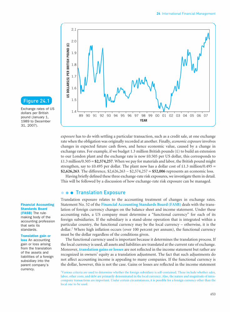
exposure has to do with settling a particular transaction, such as a credit sale, at one exchangerate when the obligation was originally recorded at another. Finally, economic exposure involveschanges in expected future cash flows, and hence economic value, caused by a change inexchange rates. For example, if we budget 1.3 million British pounds (£) to build an extensionto our London plant and the exchange rate is now £0.505 per US dollar, this corresponds to£1.3 million/0.505 = $2,574,257. When we pay for materials and labor, the British pound mightstrengthen, say to £0.495 per dollar. The plant now has a dollar cost of £1.3 million/0.495 =$2,626,263. The difference, $2,626,263 − $2,574,257 = $52,006 represents an economic loss.
Having briefly defined these three exchange-rate risk exposures, we investigate them in detail.This will be followed by a discussion of how exchange-rate risk exposure can be managed.
l l l Translation ExposureTranslation exposure relates to the accounting treatment of changes in exchange rates.Statement No. 52 of the Financial Accounting Standards Board (FASB) deals with the trans-lation of foreign currency changes on the balance sheet and income statement. Under theseaccounting rules, a US company must determine a “functional currency” for each of its foreign subsidiaries. If the subsidiary is a stand-alone operation that is integrated within a particular country, the functional currency may be the local currency – otherwise, it is the dollar.2 Where high inflation occurs (over 100 percent per annum), the functional currencymust be the dollar regardless of the conditions given.
The functional currency used is important because it determines the translation process. Ifthe local currency is used, all assets and liabilities are translated at the current rate of exchange.Moreover, translation gains or losses are not reflected in the income statement but rather arerecognized in owners’ equity as a translation adjustment. The fact that such adjustments donot affect accounting income is appealing to many companies. If the functional currency isthe dollar, however, this is not the case. Gains or losses are reflected in the income statement
24 International Financial Management
653
••
Figure 24.1Exchange rates of USdollars per Britishpound (January 1,1989 to December31, 2007).
Financial AccountingStandards Board(FASB) The rule-making body of theaccounting professionthat sets itsstandards.
Translation gain orloss An accountinggain or loss arisingfrom the translation of the assets andliabilities of a foreignsubsidiary into theparent company’scurrency.
2Various criteria are used to determine whether the foreign subsidiary is self-contained. These include whether sales,labor, other costs, and debt are primarily denominated in the local currency. Also, the nature and magnitude of intra-company transactions are important. Under certain circumstances, it is possible for a foreign currency other than thelocal one to be used.
FUNO_C24.qxd 9/19/08 17:12 Page 653

of the parent company, using what is known as the temporal method (to be described shortly).In general, the use of the dollar as the functional currency results in greater fluctuations inaccounting income but in smaller fluctuations in balance sheet items than does the use of thelocal currency. Let us examine the differences in accounting methods.
Differences in Accounting Methods. With the dollar as the functional currency, balancesheet and income statement items are categorized as to historical exchange rates or as to current exchange rates. Cash, receivables, liabilities, sales, expenses, and taxes are translatedusing current exchange rates, whereas inventories, plant and equipment, equity, cost of goodssold, and depreciation are translated at the historical exchange rates existing at the time of thetransactions. This differs from the situation where the local currency is used as the functionalcurrency; in that situation, all items are translated at current exchange rates.
To illustrate, a company we shall call Woatich Precision Instruments has a subsidiary in theKingdom of Spamany where the currency is the liso (L). At the first of the year, the exchangerate is 8 lisos to the dollar, and that rate has prevailed for many years. However, during 20X2,the liso declines steadily in value to 10 lisos to the dollar at year end. The average exchangerate during the year is 9 lisos to the dollar. Table 24.2 shows the foreign subsidiary’s balancesheet at the beginning and end of the year, the income statement for the year, and the effectof the method of translation.
Taking the balance sheet first, we see the 12/31/X1 date serves as a base, and the dollarstatement in column 3 is simply the liso amounts shown in column 1 divided by the exchangerate of 8 lisos to the dollar. For the two separate dollar statements at 12/31/X2, shown in thelast two columns, we see that cash, receivables, current liabilities, and long-term debt are the
654
Part 8 Special Areas of Financial Management
••
Table 24.2Foreign subsidiary ofWoatich PrecisionInstruments
(1) (2) (3) (4) (5)IN DOLLARS
Local DollarFunctional Functional
IN LISOS Currency Currency
12/31/X1 12/31/X2 12/31/X1 12/31/X2 12/31/X2
Balance Sheets (in thousands)Cash L 600 L 1,000 $ 75 $ 100 $ 100Receivables 2,000 2,600 250 260 260Inventories (FIFO) 4,000 4,500 500 450 500
Current Assets L 6,600 L 8,100 $ 825 $ 810 $ 860Net fixed assets 5,000 4,400 625 440 550
Total L11,600 L12,500 $1,450 $1,250 $1,410
Current liabilities L 3,000 L 3,300 $ 375 $ 330 $ 330Long-term debt 2,000 1,600 250 160 160Common stock 600 600 75 75 75Retained earnings 6,000 7,000 750 861 845Cumulative translation
adjustment −176Total L11,600 L12,500 $1,450 $1,250 $1,410
Income Statements for the Years Ending (in thousands with rounding)Sales L10,000 $1,111 $1,111Cost of goods sold 4,000 444 500Depreciation 600 67 75Expenses 3,500 389 389Taxes 900 100 100
Operating income L 1,000 $ 111 $ 47Translation 48
Net income L 1,000 $ 111 $ 95
Translation adjustment $ −176
FUNO_C24.qxd 9/19/08 17:12 Page 654

same for both methods of accounting. These amounts are determined on a current exchange-rate basis by dividing the amounts shown in column 2 by the exchange rate at year end of 10 lisos to the dollar. For the local functional currency statement, column 4, inventories andfixed assets are determined in the same manner – by use of the current exchange rate. For thedollar functional currency statement, inventories and fixed assets are valued using histor-ical exchange rates. Because the cost of goods sold figure equals beginning inventory, underthe first-in, first-out (FIFO) inventory accounting method, the ending inventory represents items purchased throughout the year. Assuming steady purchases, we divided the ending lisoamount by the average exchange rate (L9:$1) to obtain $500,000. Using historical exchangerates again, net fixed assets are determined by dividing the liso amount at year end by the earlier exchange rate of 8 lisos to the dollar. The common stock account is carried at the baseamount under both methods.
Finally, the change in retained earnings is a residual. (We defer explaining the cumulativetranslation adjustment item until the discussion of the income statement.) Because of theupward adjustment in inventories and fixed assets, total assets are higher with the dollar func-tional currency (temporal method) than they are with the local functional currency (currentmethod). The opposite would occur in our example if the liso increased in value relative tothe dollar. We see that there is substantially more change in total assets when a local func-tional currency is used than when a dollar functional currency is employed.
The opposite occurs for the income statement. Sales are adjusted by the average exchangerate that prevailed during the year (L9:$1) for both accounting methods. For the local functional currency statement, column 4, all cost and expense items are adjusted by thisexchange rate. For the dollar functional currency statement, the last column, the cost of goodssold and depreciation are translated at historical exchange rates (L8:$1), whereas the otheritems are translated at the average rate (L9:$1). We see that operating income and net incomeare larger when the local functional currency is used than when the functional currency is thedollar. For the latter method, the translation gain is factored in, so that net income agrees with the change in retained earnings from 12/31/X1 to 12/31/X2. We see that this change is$845 − $750 = $95. In contrast, when the functional currency is local, the translation adjust-ment occurs after the income figure of $111 is calculated. The adjustment is that amount,namely −$176, that, together with net income, brings the liability and shareholders’ equitypart of the balance sheet into balance. This amount is then added to the sum of past trans-lation adjustments to obtain the new cumulative translation adjustment figure that appearson the balance sheet. As we assume past adjustments total zero, this item becomes −$176.
Thus the translation adjustments for the two methods are in opposite directions. Shouldthe liso increase in value relative to the dollar, the effect would be the reverse of that illustrated. In this case, operating income would be higher if the functional currency were the dollar.
Because translation gains or losses are not reflected directly on the income statement,reported operating income tends to fluctuate less when the functional currency is local thanwhen it is the dollar. However, the variability of balance sheet items is increased, owing to the translation of all items by the current exchange rate. Because many corporate executivesare concerned with accounting income, the accounting method described in FASB No. 52 is popular as long as a subsidiary qualifies for a local functional currency. However, thisaccounting procedure also has its drawbacks. For one thing, it distorts the balance sheet andthe historical cost numbers. Moreover, it may cause calculation of return on assets and othermeasures of return to be meaningless. It is simply inconsistent with the nature of otheraccounting rules, which are based on historical costs. Most financial ratios are affected by the functional currency employed, so the financial analyst must be very careful when foreignsubsidiaries account for a sizable portion of a company’s operations.3 The method has also
24 International Financial Management
655
••
3See Thomas I. Selling and George H. Sorter, “FASB Statement No. 52 and Its Implications for Financial StatementAnalysis,” Financial Analysts Journal 39 (May–June 1983), 64–69.
FUNO_C24.qxd 9/19/08 17:12 Page 655

been criticized for not allowing proper assessment of the parent’s likely future cash flows. Insummary, there is no universally satisfactory way to treat foreign currency translations, andthe accounting profession continues to struggle with the issue.
l l l Transactions ExposureTransactions exposure involves the gain or loss that occurs when settling a specific foreigntransaction. The transaction might be the purchase or sale of a product, the lending or borrowing of funds, or some other transaction involving the acquisition of assets or theassumption of liabilities denominated in a foreign currency. While any transaction will do, the term “transactions exposure” is usually employed in connection with foreign trade, thatis, specific imports or exports on open-account credit.
Suppose a British pound receivable of £680 is booked when the exchange rate is £0.60 tothe US dollar. Payment is not due for two months. In the interim, the pound weakens (morepound per dollar), and the exchange rate goes to £0.62 per $1. As a result, there is a transac-tions loss. Before, the receivable was worth £680/0.60 = $1,133.33. When payment is received,the firm receives payment worth £680/0.62 = $1,096.77. Thus we have a transactions loss of $1,133.33 − $1,096.77 = $36.56. If instead the pound were to strengthen, for example, to £0.58 to the dollar, there would be a transactions gain. We would receive payment worth£680/0.58 = $1,172.41. With this illustration in mind, it is easy to produce examples of othertypes of transactions gains and losses.
l l l Economic ExposurePerhaps the most important of the three exchange-rate risk exposures – translation, transac-tions, and economic – is the last. Economic exposure is the change in value of a company thataccompanies an unanticipated change in exchange rates. Note that we distinguish anticipatedfrom unanticipated. Anticipated changes in exchange rates are already reflected in the marketvalue of the firm. If we do business with Japan, the anticipation might be that the yen willweaken relative to the dollar. The fact that it weakens should not affect market value. How-ever, if it weakens more or less than expected, this will affect value. Economic exposure doesnot lend itself to as precise a description and measurement as either translation or transac-tions exposure. Economic exposure depends on what happens to expected future cash flows,so subjectivity is necessarily involved.
Management of Exchange-Rate Risk ExposureThere are a number of ways by which exchange-rate risk exposure can be managed. Naturalhedges; cash management; adjusting of intracompany accounts; as well as internationalfinancing hedges and currency hedges, through forward contracts, futures contracts, currencyoptions, and currency swaps, all serve this purpose.
l l l Natural HedgesThe relationship between revenues (or pricing) and costs of a foreign subsidiary sometimesprovides a natural hedge, giving the firm ongoing protection from exchange-rate fluctua-tions. The key is the extent to which cash flows adjust naturally to currency changes. It is notthe country in which a subsidiary is located that matters, but whether the subsidiary’s revenueand cost functions are sensitive to global or domestic market conditions. At the extremesthere are four possible scenarios.4
656
Part 8 Special Areas of Financial Management
4For further categorization and explanation, see Christine R. Hekman, “Don’t Blame Currency Values for StrategicErrors,” Midland Corporate Finance Journal 4 (Fall 1986), 45–55.
••
Natural hedgeA hedge (riskreduction action) that occurs naturallyas a result of a firm’snormal operations.For example, revenuereceived in a foreigncurrency and used to pay commitmentsin the same foreigncurrency wouldconstitute a natural hedge.
FUNO_C24.qxd 9/19/08 17:12 Page 656

GLOBALLY DOMESTICALLY DETERMINED DETERMINED
Scenario 1Pricing X
]*Cost X
Scenario 2Pricing X
]*Cost X
Scenario 3Pricing XCost X
Scenario 4Pricing XCost X
*There is a natural offsetting relationship provided by pricing and costsboth occurring in similar market environments.
In the first category we might have a copper fabricator in Taiwan. Its principal cost is thatfor copper, the raw material, whose price is determined in the global market and quoted in US dollars. Moreover, the fabricated product produced is sold in markets dominated byglobal pricing. Therefore the subsidiary has little exposure to exchange-rate fluctuations. Inother words, there is a “natural hedge,” because protection of value follows from the naturalworkings of the global marketplace.
The second category might correspond to a cleaning service company in Switzerland. Thedominant cost component is labor, and both it and the pricing of the service are determineddomestically. As domestic inflation affects costs, the subsidiary is able to pass along theincrease in its pricing to customers. Margins, expressed in US dollars, are relatively insensit-ive to the combination of domestic inflation and exchange-rate changes. This situation alsoconstitutes a natural hedge.
The third situation might involve a British-based international consulting firm. Pricing isdetermined largely in the global market, whereas costs, again mostly labor, are determined inthe domestic market. If, owing to inflation, the British pound should decrease in value relativeto the dollar, costs will rise relative to prices, and margins will suffer. Here the subsidiary isexposed. Finally, the last category might correspond to a Japanese importer of foreign foods.Costs are determined globally, whereas prices are determined domestically. Here, too, thesubsidiary would be subject to much exposure.
These simple notions illustrate the nature of natural hedging. A company’s strategic posi-tioning largely determines its natural exchange-rate risk exposure. However, such exposurecan be modified. For one thing, a company can internationally diversify its operations when it is overexposed in one currency. It can also source differently in the production of aproduct. Any strategic decision that affects markets served, pricing, operations, or sourcingcan be thought of as a form of natural hedging.
A key concern for the financial manager is the degree of exchange-rate risk exposure thatremains after any natural hedging. This remaining risk exposure then can be hedged usingoperating, financing, or currency-market hedges. We explore each in turn.
l l l Cash Management and Adjusting Intracompany AccountsIf a company knew that a country’s currency, where a subsidiary was based, were going to fallin value, it would want to do a number of things. First, it should reduce its cash holdings in this currency to a minimum by purchasing inventories or other real assets. Moreover, thesubsidiary should try to avoid extended trade credit (accounts receivable). Achieving as quicka turnover as possible of receivables into cash would thus be desirable. In contrast, it should
24 International Financial Management
657
••
FUNO_C24.qxd 9/19/08 17:12 Page 657

try to obtain extended terms on its accounts payable. It may also want to borrow in the localcurrency to replace any advances made by the US parent. The last step will depend on relativeinterest rates. If the currency were going to appreciate in value, opposite steps should beundertaken. Without knowledge of the future direction of currency value movements, aggres-sive policies in either direction are inappropriate. Under most circumstances we are unable to predict the future, so the best policy may be one of balancing monetary assets against monetary liabilities to neutralize the effect of exchange-rate fluctuations.
A company with multiple foreign operations can protect itself against exchange-rate risk by adjusting its commitments to transfer funds among companies. Accelerating the timing of payments made or received in foreign currencies is called leading, and decelerating the timing is called lagging. For example, assume that your company has foreign subsidiaries inSwitzerland and the Czech Republic. You think that the Czech koruna will soon be revaluedupward, but the Swiss franc will hold steady. The Swiss subsidiary purchases approximately$100,000 worth of goods each month from the Czech subsidiary. Normal billing calls for pay-ment three months after delivery of the goods. Instead of this arrangement, you now instructthe Swiss subsidiary to lead by paying for the goods on delivery in view of the likely revalua-tion upward of the Czech koruna.
Some multinational companies establish a reinvoicing center to manage intracompanyand third-party foreign trade. The multinational’s exporting subsidiaries sell goods to thereinvoicing center, which resells (reinvoices) them to importing subsidiaries or third-partybuyers. Title to the goods initially passes to the reinvoicing center, but the goods move directlyfrom the selling unit to the buying unit or independent customer.
Tax implications form a large part of the incentive for reinvoicing. The location – espe-cially the tax jurisdiction where revenue will be booked – is strategically important. Popular(i.e., tax-friendly) locations for reinvoicing centers include Hong Kong and the British VirginIslands.
Generally, the reinvoicing center is billed in the selling unit’s home currency and, in turn,bills the purchasing unit in that unit’s home currency. In this way the reinvoicing center can then centralize and manage all intracompany transactions exposure. The reinvoicing center’s centralized position also facilitates interunit netting of obligations so as to reduce thenecessary volume of actual foreign exchange transactions. Also, this system allows for morecoordinated control over any leading or lagging arrangements between affiliates.
In addition to these arrangements, the multinational company can also adjust intra-company dividends and royalty payments. Sometimes the currency in which a sale is billed is varied in keeping with anticipated foreign exchange movements. Transfer pricing of com-ponents or of finished goods, which are exchanged between the parent and various foreignaffiliates, can be varied. (However, the tax authorities in most countries look very closely at transfer prices to ensure that taxes are not being avoided.) In all of these cases, as well as others, intracompany payments are arranged so that they fit into the company’s overallmanagement of its currency exposure.
l l l International Financing Hedges
If a company is exposed in one country’s currency and is hurt when that currency weakens invalue, it can borrow in that country to offset the exposure. In the context of the frameworkpresented earlier, asset-sensitive exposure would be balanced with borrowings. A wide varietyof sources of external financing are available to the foreign affiliate. These range from com-mercial bank loans within the host country to loans from international lending agencies. Inthis section we consider the chief sources of external financing.
Commercial Bank Loans and Trade Bills. Foreign commercial banks are one of themajor sources of financing abroad. They perform essentially the same financing function asdomestic commercial banks. One subtle difference is that banking practices in Europe allow
658
Part 8 Special Areas of Financial Management
••
Reinvoicing centerA company-ownedfinancial subsidiarythat purchasesexported goods from companyaffiliates and resells(reinvoices) them to other affiliates or independentcustomers.
Netting System inwhich cross-borderpurchases amongparticipatingsubsidiaries of thesame company arenetted so that eachparticipant pays or receives only the net amount of its intracompanypurchases and sales.
FUNO_C24.qxd 9/19/08 17:12 Page 658

longer-term loans than are available in the United States. Another difference is that loans tendto be on an overdraft basis. That is, a company writes a check that overdraws its account andis charged interest on the overdraft. Many of these lending banks are known as merchantbanks, which simply means that they offer a full menu of financial services to business firms.Corresponding to the growth in multinational companies, international banking operationsof US banks have grown accordingly. All the principal commercial cities of the world havebranches or offices of US banks.
In addition to commercial bank loans, “discounting” trade bills is a common method ofshort-term financing. Although this method of financing is not used extensively in the UnitedStates, it is widely used in Europe to finance both domestic and international trade. More willbe said about the instruments involved later in the chapter.
Eurodollar Financing. Eurodollars are bank deposits denominated in US dollars but notsubject to US banking regulations. Since the late 1950s an active market has developed forthese deposits. Foreign banks and foreign branches of US banks, mostly in Europe, activelybid for Eurodollar deposits, paying interest rates that fluctuate in keeping with supply anddemand. The deposits are in large denominations, frequently $100,000 or more, and the banksuse them to make dollar loans to quality borrowers. The loans are made at a rate in excess ofthe deposit rate. The rate differential varies according to the relative risk of the borrower.Essentially, borrowing and lending Eurodollars is a wholesale operation, with far fewer coststhan are usually associated with banking. The market itself is unregulated, so supply anddemand forces have free rein.
The Eurodollar market is a major source of short-term financing for the working capitalrequirements of the multinational company. The interest rate on loans is based on theEurodollar deposit rate and bears only an indirect relationship to the US prime rate. Typi-cally, rates on loans are quoted in terms of the London interbank offered rate (LIBOR). Thegreater the risk, the greater the spread above LIBOR. A prime borrower will pay about one-half percent over LIBOR for an intermediate-term loan. One should realize that LIBOR ismore volatile than the US prime rate, owing to the sensitive nature of supply and demand forEurodollar deposits.
We should point out that the Eurodollar market is part of a larger Eurocurrency marketwhere deposit and lending rates are quoted on the stronger currencies of the world. The prin-ciples involved in this market are the same as for the Eurodollar market, so we do not repeatthem. The development of the Eurocurrency market has greatly facilitated international borrowing and financial intermediation (the flow of funds through intermediaries such asbanks and insurance companies to ultimate borrowers).
International Bond Financing. The Eurocurrency market must be distinguished from theEurobond market. The latter market is a more traditional one, with underwriters placingsecurities. Though a bond issue is denominated in a single currency, it is placed in multiplecountries. Once issued, it is traded over the counter in multiple countries and by a number of security dealers. A Eurobond is different from a foreign bond, which is a bond issued by a foreign government or corporation in a local market. A foreign bond is sold in a single country and falls under the security regulations of that country. Foreign bonds have colorfulnicknames. For example, Yankee bonds are issued by non-Americans in the US market, and Samurai bonds are issued by non-Japanese in the Japanese market. Eurobonds, foreignbonds, and domestic bonds of different countries differ in terminology, in the way interest iscomputed, and in features. We do not address these differences, because that would require aseparate book.
Many debt issues in the international arena are floating-rate notes (FRNs). These instru-ments have a variety of features, often involving multiple currencies. Some instruments areindexed to price levels or to commodity prices. Others are linked to an interest rate, such asLIBOR. The reset interval may be annual, semiannual, quarterly, or even more frequent. Stillother instruments have option features.
24 International Financial Management
659
••
Eurodollars A USdollar-denominateddeposit – generally in a bank locatedoutside the UnitedStates – not subjectto US bankingregulations.
London interbankoffered rate (LIBOR)The interest rate thatworld-class banks in London pay eachother for Eurodollars.
EurocurrencyA currency depositedoutside its country of origin.
EurobondA bond issue soldinternationally outsidethe country in whosecurrency the bond isdenominated.
Floating-rate note(FRN) Debt issue with a variableinterest rate.
FUNO_C24.qxd 9/19/08 17:12 Page 659

Currency-Option and Multiple-Currency Bonds. Certain bonds provide the holder withthe right to choose the currency in which payment is received, usually prior to each couponor principal payment. Typically, this option is confined to two currencies, although it can bemore. For example, a company might issue $1,000-par-value bonds with an 8 percent couponrate. Each bond might carry the option to receive payment either in US dollars or in Britishpounds. The exchange rate between the currencies is fixed at the time of bond issue.
Bonds are sometimes issued with principal and interest payments being a weighted average,or “basket,” of multiple currencies. Known as currency cocktail bonds, these securities providea degree of exchange-rate stability not found in any one currency. In addition, dual-currencybonds have their purchase price and coupon payments denominated in one currency, whereasa different currency is used to make the principal payments. For example, a Swiss bond mightcall for interest payments in Swiss francs and principal payments in US dollars.
Islamic Bonds (Sukuk). Islamic banking and finance, in its contemporary form, started inthe 1960s as a movement to align personal and business investment practices with Islamic law(Sharia’h). But, the high oil prices in the 1970s and the growing accumulation of petrodollarsin Islamic nations gave the movement real momentum.
Sharia’h is based on the teachings of the Koran and prohibits paying or receiving interest(riba) and investing in “unethical/improper” business sectors, such as alcohol, tobacco, gam-bling, and defense. The ban on interest, a practice viewed as exploiting the borrower, elimi-nates pure debt securities as investments, but an obligation linked to the performance of a realasset is acceptable. Islamic bonds (or sukuk) rely on property or other assets to generateincome equivalent to interest that would be paid on conventional debt. Structuring Islamicbonds can be challenging and requires approval from recognized Sharia’h advisors/scholars toensure compliance with Islamic rules and principles.
The prohibition of interest creates a very different view of finance from that generallyfound in the West. Until recently, the sukuk market was a niche market and limited to Muslimcountries. However, it is expanding rapidly and estimates of its size at the end of 2006 rangedfrom $50 to $70 billion. It is definitely an area of growing international interest.
l l l Currency Market HedgesYet another means to hedge currency exposure is through devices of several currency markets– forward contracts, futures contracts, currency options, and currency swaps. Let us see howthese markets and vehicles work to protect the multinational company.
Forward Exchange Market. In the forward exchange market, one buys a forward contractfor the exchange of one currency for another at a specific future date and at a specificexchange ratio. A forward contract provides assurance of being able to convert into a desiredcurrency at a price set in advance.
The Fillups Electronics Company is hedging through the forward market. It sold equip-ment to a Swiss customer through its Zurich branch for 1 million francs with credit terms of“net 90.” Upon payment, Fillups intends to convert the Swiss francs into US dollars. Assumethe spot and 90-day forward rates of Swiss francs in terms of US dollars were the following:
Spot rate $0.97090-day forward rate 0.965
The spot rate is simply the current market-determined exchange rate for Swiss francs. In ourexample, 1 franc is worth $0.970, and $1 will buy 1.00/0.970 = 1.031 francs. A foreign currencysells at a forward discount if its forward price is less than its spot price. In our example, theSwiss franc sells at a discount. If the forward price exceeds the spot price, it is said to sell at aforward premium. For example, assume that the British pound sells at a forward premium. Inthat case, pounds buy more dollars for future delivery than they do for present delivery.
660
Part 8 Special Areas of Financial Management
••
Forward contractA contract for thedelivery of acommodity, foreigncurrency, or financialinstrument at a price specified now,with delivery andsettlement at aspecified future date.Although similar to afutures contract, it isnot easily transferredor canceled.
Islamic bonds (orsukuk) A type ofasset-backed security(ABS) adhering to therules and principles ofIslamic law (Sharia’h).
FUNO_C24.qxd 9/19/08 17:12 Page 660

If Fillups wishes to avoid exchange-rate risk, it should sell 1 million Swiss francs forward90 days. When it delivers the francs 90 days hence, it will receive $965,000 (1 million Swissfrancs times the 90-day futures price of $0.965). If the spot rate stays at $0.970, of course,Fillups would have been better off not having sold francs forward. It could sell 1 million francsin the spot market for $970,000. In this sense, Fillups pays $.005 per franc, or $5,000 in total,to ensure its ability to convert Swiss francs to dollars. On an annualized basis, the cost of thisprotection is
($0.005/$0.970) × (365 days/90 days) = 2.09%
For stable pairs of currencies, the discount or premium of the forward rate over the spotrate generally varies from 0 to 5 percent on an annualized basis. For somewhat less stable cur-rencies, the discount may go as high as 20 percent. Much beyond this point of instability, theforward market for the currency ceases to exist. In summary, the forward exchange marketallows a company to insure against devaluation or market-determined declines in value. Theforward market is particularly suited for hedging transactions exposure.
24 International Financial Management
661
••
The name is Bond. Islamic bond.
Or rather it should be, considering that the consor-tium which this week bought Aston Martin – makers ofJames Bond’s favourite sports car – is going to financethe purchase according to strict Islamic principles.
Ford Motor agreed to sell the company for £479 mil-lion to a leveraged buy-out consortium organised out ofLondon by Dave Richards, a motor racing entrepreneur.
Now WestLB, the German bank, has been appointedto arrange £225 million of quasi-debt finance to back the LBO – but only that which accords with the Koran’sopposition to interest and speculation.
“This will be financed in an exclusively shariah-compliant way,” said David Testa, an executive directorat WestLB, who believes that this is the first time thatIslamic finance has been used for an LBO in the UK –and probably the western world.
The Islamic financial focus has arisen partly becausetwo key financiers behind the LBO are Investment Darand Adeem Investment Company, two Kuwaiti groupsthat only invest in accordance with Islamic principles,like a growing number of Gulf investors.
However, the move comes at a time of rapid growthin the Islamic finance sector, now estimated to have
assets of well over $300 billion (£155 billion) worldwide– a reflection of growing religious sentiment in theMuslim world and high oil prices putting more financein the hands of groups such as Investment Dar.
At the same time, western investment banks such asWestLB, Deutsche Bank, Citigroup and Barclays arebecoming more involved in Islamic finance.
WestLB, for example, expects to syndicate the AstonMartin LBO finance among Islamic banks in the Gulfand London, as well as to non-Islamic groups such as European banks. “This has wide appeal,” Mr Testasaid.
The finance package will initially be structured in amanner comparable to a syndicated bank loan, with totaldebt of about 4.5 times earnings before interest, tax anddepreciation – a relatively low level compared withrecent European LBOs.
However, the LBO consortium is expected to issuesukuk – or so-called Islamic bonds – in the future to takeadvantage of planned changes in UK law that will makeit more attractive, in tax terms, for UK companies toissue these instruments.
This additional financing is expected partly becausethe company has ambitious plans.
These ambitions are likely to meet warm approvalamong Middle East financiers, given the Gulf ’s love affairwith fast cars. But it remains to be seen whether thesefinanciers will also ban other factors that might be deemednon-Koranic – such as the use of martini-swilling spiesto market the iconic brand.
Islamic Bonds Used to Buy 007’s Wheels
Source: Gillian Tett, “Islamic bonds rolled out for purchase of 007’s favourite car,” Financial Times (March 17/18, 2007), p. 1. (www.ft.com)© The Financial Times Limited 2007. Used by permission. All rights reserved.
FUNO_C24.qxd 9/19/08 17:12 Page 661

Exchange-rate quotations on selected currencies at a moment in time are shown in Table 24.3. The spot rates reported in the first column indicate the conversion rate into dollars. The exchange-rate quotations contained in newspapers such as the Wall Street Journal,the Financial Times, and the New York Times are for very large transactions. As a foreign traveler, you cannot buy or sell foreign currency at nearly as good a rate. Often you will payseveral percent more when you buy and receive several percent less when you sell. Alas, thehardships of dealing in amounts less than $1 million!
In the first numerical column of Table 24.3, for each currency the conversion rate of oneunit of a foreign currency into US dollars is shown. Near the top, we see that the Australiandollar is worth 0.9488 US dollars (US$0.9488). To determine how many Australian dollars(A$) one US dollar will buy, we take the reciprocal, 1/0.9488 = A$1.0540. Forward rates for30, 90, and 180 days are shown for the British pound, Canadian dollar, Japanese yen, andSwiss franc. Comparing the forward rates with the spot rates for these four currencies, we find that only the Japanese and Swiss currencies are at forward rate premiums relative to theUS dollar. That is, they are worth more dollars on future delivery than they are now. The reasons for premiums and discounts must await our discussion of interest-rate parity, whichis coming up shortly.
The Euro. At the bottom of Table 24.3, we find the euro. The euro is the single currency(currently) shared by the following 15 European Union (EU) countries – Austria, Belgium,Cyprus, Finland, France, Germany, Greece, Ireland, Italy, Luxemburg, Malta, the
662
Part 8 Special Areas of Financial Management
••
Euro (EUR) The namegiven to the singleEuropean currency. Itsofficial abbreviation is EUR. Like the dollar($) and the Britishpound (£), the euro(A) has a distinctivesymbol, which lookssimilar to a “C” with a “=” through it.
Table 24.3Exchange rates onFebruary 28, 2008
US DOLLARS REQUIRED UNITS REQUIRED TO BUY TO BUY ONE UNIT ONE US DOLLAR
Argentina (peso) $ .3169 3.1556Australia (dollar) .9488 1.0540Brazil (real) .5992 1.6689Britain (pound) 1.9917 .5021
30-day forward 1.9877 .503190-day forward 1.9789 .5053180-day forward 1.9654 .5088
Canada (dollar) 1.0240 .976630-day forward 1.0234 .977190-day forward 1.0222 .9783180-day forward 1.0201 .9803
Chile (peso) .002196 455.37China (renminbi) .1406 7.1125Czech Republic (koruna) .06058 16.507Hong Kong (dollar) .1285 7.7822India (rupee) .02508 39.872Japan (yen) .009489 105.39
30-day forward .009508 105.1790-day forward .009539 104.83180-day forward .009581 104.37
Malaysia (ringgit) .3123 3.2020Saudi Arabia (riyal) .2671 3.7439Singapore (dollar) .7175 1.3937Switzerland (franc) .9520 1.0504
30-day forward .9524 1.050090-day forward .9526 1.0498180-day forward .9525 1.0499
Taiwan (dollar) .03237 30.893Thailand (baht) .03384 29.551Venezuela (b.fuerte) .466287 2.1446
Euro area (euro) 1.5214 .6573
FUNO_C24.qxd 9/19/08 17:12 Page 662

Netherlands, Portugal, Slovenia, and Spain. Together these make up the “euro area.” OnJanuary 1, 1999, currency conversion rates between the “legacy currencies” (i.e., formernational currencies of the original euro area member states) and the euro were established.The euro was introduced amid much fanfare, and began trading January 1, 1999 at 1.17 USdollars to the euro, even getting as high as 1.19. However, there was a steady decline in value.It traded at less than 1.00 US dollar to the euro for most of the period 2000 through 2002. Inlate 2002 it broke over the one dollar mark. From there, the euro gained strength against theUS dollar, and is shown trading at 1.5214 in Table 24.3.
Currency Futures. Closely related to the use of a forward contract is a futures contract. A currency futures market exists for the major currencies of the world – for example, theAustralian dollar, the Canadian dollar, the British pound, the Swiss franc, and the yen. Afutures contract is a standardized agreement that calls for delivery of a currency at somespecified future date, such as the third Wednesday of March, June, September, or December.Contracts are traded on an exchange, and the clearing house of the exchange interposes itselfbetween the buyer and the seller. This means that all transactions are with the clearing house,and not made directly between two parties. Very few contracts involve actual delivery at expiration. Rather, a buyer and a seller of a contract independently take offsetting positions
24 International Financial Management
663
••
The euro has displaced the US dollar as the world’spre-eminent currency in international bond markets,
having outstripped the dollar-denominated market forthe second year in a row.
The data consolidate news last month that the valueof euro notes in circulation had overtaken the dollar forthe first time. Outstanding debt issued in the euro wasworth the equivalent of $4,836 billion at the end of 2006compared with $3,892 billion for the dollar, according toInternational Capital Market Association data.
Outstanding euro-denominated debt accounts for 45percent of the global market, compared with 37 percentfor the dollar. New issuance last year accounted for 49percent of the global total. That represents a startlingturnabout from the pattern seen in recent decades, whenthe US bond market dwarfed its European rival: asrecently as 2002, outstanding euro-denominated issuancerepresented just 27 percent of the global pie, comparedwith 51 percent for the dollar.
The rising role of the euro comes amid growingissuance by debt-laden European governments. However,the main factor is a rise in euro-denominated issuance bycompanies and financial institutions.
One factor driving this is that European companiesare moving away from their traditional reliance on bankloans – and embracing the capital markets to a greaterdegree. Another is that the creation of the single currencyin 1999 has permitted development of a deeper and moreliquid market, consolidated by a growing eurozone.
This has made it more attractive for issuers aroundthe world to raise funds in the euro market. And, morerecently, the trend among some Asian and MiddleEastern countries to diversify their assets away from thedollar has further boosted this trend.
René Karsenti, executive president of ICMA, said: “Itis the stable interest rates in Europe that have helped andthe fact that [the euro] has strengthened and shownresilience.”
Since the start of 2003, the European Central Bank’smain interest rate has fluctuated only 1.5 percentagepoints, ranging from a low of 2 percent in the middle ofthat year to 3.5 percent, its rate today. In comparison, theFed funds rate, the main US interest rate, has fluctuated4.25 percentage points, ranging from 1 percent in themiddle of 2003 to 5.25 percent, its level today. The eurohas also risen to trade around $1.30 against the dollar,from around parity three years ago. Sterling issuance hasgrown in the past three years, reinforcing its attraction as a niche currency among some investors. The yen, incomparison, has fallen out of favour.
Overall, international capital markets have doubled insize in terms of bond issuance during the past six years.
European Bond Market Puts US in the Shade
Source: David Oakley and Gillian Tett, “European bond market puts US in the shade,” Financial Times (January 15, 2007), p. 13.(www.ft.com) Copyright © The Financial Times Limited 2007. Used by permission. All rights reserved.
Futures contractA contract for the delivery of acommodity, foreigncurrency, or financialinstrument at aspecified price on astipulated future date.Futures contracts aretraded on organizedexchanges.
FUNO_C24.qxd 9/19/08 17:12 Page 663

to close out a contract. The seller cancels a contract by buying another contract, and the buyercancels a contract by selling another contract.
Each day, the futures contract is marked-to-market in the sense that it is valued at the closing price. Price movements affect the buyer and seller in opposite ways. Every day there isa winner and a loser, depending on the direction of price movement. The loser must come upwith more margin (a deposit), whereas the winner can draw off excess margin. Futures con-tracts are different from forward contracts in this regard: forward contracts need to be settledonly at expiration. Another difference is that only a set number of maturities are available forfutures contracts. Finally, futures contracts come only in multiples of standard-size contracts– for example, multiples of 12.5 million yen. Forward contracts can be for almost any size.However, the two instruments are used for the same hedging purpose.5
Currency Options. Forward and futures contracts provide a “two-sided” hedge against cur-rency movements. That is, if the currency involved moves in one direction, the forward orfutures position offsets it. Currency options, in contrast, enable the hedging of “one-sided”risk. Only adverse currency movements are hedged, either with a call option to buy the for-eign currency or with a put option to sell it. The holder has the right, but not the obligation,to buy or sell the currency over the life of the contract. If not exercised, of course, the optionexpires. For this protection, one pays a premium.
There are options both on spot market currencies and on currency futures contracts.Because currency options are traded on a number of exchanges throughout the world, one is able to trade with relative ease. The use of currency options and their valuation are largelythe same as for stock options. (Since we described option valuation in the Appendix toChapter 22 for stock options, we do not repeat that discussion.) The value of the option, andhence the premium paid, depends importantly on exchange-rate volatility.
Currency Swaps. Yet another device for shifting risk is the currency swap. In a currency swaptwo parties exchange debt obligations denominated in different currencies. Each party agreesto pay the other’s interest obligation. At maturity, principal amounts are exchanged, usuallyat a rate of exchange agreed to in advance. The exchange is notional in that only the cash-flowdifference is paid. If one party should default, there is no loss of principal per se. There is,however, the opportunity cost associated with currency movements after the swap’s initiation.
Currency swaps typically are arranged through an intermediary, such as a commercialbank. Many different arrangements are possible: a swap involving more than two currencies;a swap with option features; and a currency swap combined with an interest-rate swap, wherethe obligation to pay interest on long-term debt is swapped for that to pay interest on short-term, floating-rate, or some other type of debt. As can be imagined, things get complicatedrather quickly. The point to keep in mind, however, is that currency swaps are widely usedand serve as longer-term risk-shifting devices.
l l l Hedging Exchange-Rate Risk Exposure: A Summing Up
We have seen that there are a number of ways that exchange-rate risk exposure can be hedged.The place to begin is to determine whether your company has a natural hedge. If it does have a natural hedge, then to add a financing or a currency hedge actually increases your riskexposure. That is, you will have undone a natural hedge that your company has by virtue of the business it does abroad and the sourcing of such business. As a result, you will have created a net risk exposure where little or none existed before. Therefore you need to care-fully assess your exchange-rate risk exposure before taking any hedging actions.
The first step is to estimate your net, residual exchange-rate risk exposure after takingaccount of any natural hedges that your company may have. If you have a net exposure (a
664
Part 8 Special Areas of Financial Management
••
5See James C. Van Horne, Financial Market Rates and Flows, 6th ed. (Upper Saddle River, NJ: Prentice Hall, 2001) fora detailed discussion of futures markets.
Currency optionA contract that givesthe holder the right tobuy (call) or sell (put)a specific amount of a foreign currency at some specifiedprice until a certain(expiration) date.
FUNO_C24.qxd 9/19/08 17:12 Page 664

difference between estimated inflows and outflows of a foreign currency over a specifiedtime), then the questions are whether you wish to hedge it and how. Cash management andintracompany account adjustments are only temporary measures, and they are limited in the magnitude of their effect. Financing hedges provide a means to hedge on a longer-term basis,as do currency swaps. Currency forward contracts, futures, and options are usually availablefor up to one or two years. Though it is possible to arrange longer-term contracts through amerchant bank, the cost is usually high, and there are liquidity problems. How you hedge yournet exposure, if at all, should be a function of the suitability of the hedging device and its cost.
l l l Macro Factors Governing Exchange-Rate Behavior
Fluctuations in exchange rates are continual and often defy explanation, at least in the shortrun. In the longer run, however, there are linkages between domestic and foreign inflationand between interest rates and exchange rates.
Purchasing-Power Parity. If product and financial markets are efficient internationally,we would expect certain relationships to hold. Over the long run, markets for tradable goodsand foreign exchange should move toward purchasing-power parity (PPP). The idea is thata basket of standardized goods should sell at the same price internationally.
If it is cheaper to buy wheat from Canada than it is from a US producer, after account-ing for transportation costs and after adjusting the Canadian price for the exchange rate, a rational US buyer will purchase Canadian wheat. This action, together with commodity arbitrage, will cause the Canadian wheat price to rise relative to the US price and, perhaps, the Canadian-dollar exchange rate to strengthen. The combination of rising Canadian wheatprices and a changing Canadian-dollar value raises the US-dollar price of Canadian wheat to the US buyer. Theory would have it that these transactions would continue until the US-dollar cost of wheat is the same as the Canadian. At that point, there would be purchasing-power parity for the US buyer. That is, the buyer would be indifferent between US andCanadian wheat. For that matter, a Canadian buyer of wheat should also be indifferent forpurchasing-power parity works both ways.
How closely a country’s exchange rate corresponds to purchasing-power parity depends on the price elasticity of exports and imports. To the extent that exports are traded in worldcompetitive markets, there is usually close conformity to purchasing-power parity. Com-modities and fabricated products such as steel and clothing are highly price sensitive. In general, products in mature industries conform more closely to purchasing-power parity thanproducts with emerging technology. To the extent that a country’s inflation is dominated byservices, there tends to be less conformity to purchasing-power parity. We also know that purchasing-power parity does not work well when a country intervenes in the exchange-ratemarket, either propping up its currency or keeping it artificially low. Because of frictions,
24 International Financial Management
665
••
The Coca-Cola Company and Foreign Currency Management
We manage most of our foreign currency exposures on a consolidated basis, whichallows us to net certain exposures and take advantage of any natural offsets. In
2006, we generated approximately 72 percent of our net operating revenues from out-side of the United States; therefore, weakness in one particular currency might be offsetby strengths in other currencies over time. We use derivative financial instruments tofurther reduce our net exposure to currency fluctuations.
Source: The Coca-Cola Company 2006 Annual Report (form 10-K), p. 65.Reproduced with Permission of The Coca-Cola Company.“Coca-Cola”, the Contour Bottle, and the Dynamic Ribbon are registered trademarks of The Coca-Cola Company.
Purchasing-powerparity (PPP) The idea that a basket of goods should sellfor the same price intwo countries, afterexchange rates aretaken into account.
FUNO_C24.qxd 9/19/08 17:12 Page 665

trade barriers, government intervention in the exchange market, and other imperfections,purchasing-power parities between various tradable goods generally do not hold in the shortrun. They are a long-run equilibration phenomenon, and they help us understand the likelydirection of change.
Interest-Rate Parity. The second link in our equilibrium process concerns the interest-ratedifferential between two countries. Interest-rate parity suggests that, if interest rates are higherin one country than they are in another, the former’s currency will sell at a discount in the for-ward market. Expressed differently, interest-rate differentials and forward spot exchange-ratedifferentials are offsetting. How does it work? The starting point is the relationship betweennominal (observed) interest rates and inflation. Recall from Chapter 2 that the Fisher effectimplies that the nominal rate of interest is the sum of the real rate of interest (the interest ratein the absence of price-level changes) plus the rate of inflation expected to prevail over the lifeof the instrument.
In an international context, sometimes called the international Fisher effect, it is suggestedthat differences in interest rates between two countries serve as a proxy for differences inexpected inflation. For example, if the nominal interest rate were 7 percent in the UnitedStates but 12 percent in Australia, the expected differential in inflation would be 5 percent.That is, inflation in Australia is expected to be 5 percent higher than in the United States. Does this hold exactly? Although there is disagreement as to the precise relationship betweennominal interest rates and inflation, most people feel that expected inflation for a country has
666
Part 8 Special Areas of Financial Management
••
McDonald’s Big Mac hamburgers are sold in 120countries. Though standardized across countries,
the product is produced locally with respect to both foodmaterials and labor. If purchasing-power parity (PPP)were working perfectly, exchange rates would adjust sothat Big Macs would cost the same in all countries. Fromtime to time, The Economist publishes Big Mac price and
exchange-rate comparisons, which suggest whether acurrency is over- or undervalued relative to the US dollar. This supposes, of course, that exchange rates candeviate significantly from purchasing-power parity in theshort run. However, in the long run, economic forceswill eventually equalize the purchasing power of curren-cies. A recent comparison showed the following:
BIG MAC IMPLIED ACTUAL % OVER (+) OR PRICE IN LOCAL EXCHANGE RATE EXCHANGE RATE UNDER (−) VALUATION
COUNTRY CURRENCY (to buy $1) (to buy $1) AGAINST US DOLLAR
United States $3.41 – – –
Australia A$3.45 1.01 1.17 −14Britain £1.99 .58 .49 +18Japan ¥280 82.1 122.0 −33Malaysia Ringgit 5.50 1.61 3.43 −53Singapore S$3.95 1.16 1.52 −24Sweden SKr 33.0 9.68 6.79 +42Switzerland SFr 6.30 1.85 1.21 +53
The implied exchange rate is simply the local price of a Big Mac divided by its US dollar price. For Australia,it is A$3.45/$3.41 = 1.01. As the actual exchange rate is 1.17, the Australian dollar is undervalued by (1.01 −1.17)/1.17 = −−14%. At the time, it was cheaper to eat BigMacs in Australia than in the United States. PPP theoryimplies that eventually undervalued currencies will
appreciate (get stronger) against the US dollar, whileovervalued currencies will depreciate (get weaker) againstthe US dollar. If Big Macs are a reasonable approxima-tion of a consumption basket, equilibrium suggests thatthe European currencies in our Table will depreciateagainst the US dollar, while the Asian-Pacific currencieswill appreciate against the US dollar.
Big Mac Purchasing-Power Parity
Source: Based on data taken from www.economist.com/finance/displaystory.cfm?story_id=9448015. Copyright © 2007 The EconomistNewspaper Ltd. Used by permission. All rights reserved.
FUNO_C24.qxd 9/19/08 17:12 Page 666

an important effect on interest rates in that country. The more open the capital markets, thecloser the conformity to an international Fisher effect.
To illustrate interest-rate parity, consider the relationship between the US dollar ($) andthe British pound (£) both now and 90 days in the future. The international Fisher effect suggests that
(24.1)
where F£ = current 90-day forward exchange rate in pounds per dollarS£ = current spot exchange rate in pounds per dollarr£ = nominal British interbank Euromarket interest rate, expressed in terms of the
90-day returnr$ = nominal US interbank Euromarket interest rate, expressed in terms of the 90-day return
If the nominal interest rate in Britain were 8 percent and the nominal US rate 6 percent, theseannualized rates would translate into 90-day rates of 2 percent and 1.5 percent, respectively.If the current spot rate were 0.625 pounds per dollar, we would have
Solving for the implied forward rate, we get
(1.015)F£ = (0.625)(1.020)F£ = 0.6375/1.015 = 0.6281
Thus the implied forward rate is 0.6281 British pounds per US dollar. The British-poundforward rate is at a discount from the spot rate of 0.625 pounds to the dollar. That is, a poundis worth less in terms of dollars in the forward market, 1/0.6281 = $1.592, than it is in the spotmarket, 1/0.625 = $1.60. The discount is (0.6281 − 0.625)/0.625 = 0.005. With interest-rateparity, the discount must equal the relative difference in interest rates, and, indeed, this is thecase, for (1.020 − 1.015)/1.015 = 0.005. If the interest rate in Britain were less than that in the United States, the implied forward rate in our example would be less than the spot rate.In this case, the British-pound forward rate is at a premium above the spot rate. For example,if the US interest rate (annualized) were 8 percent and the British interest rate 6 percent, theimplied 90-day forward rate for British pounds would be
Solving for the implied forward rate, we get
(1.020)F£ = (0.625)(1.015)F£ = 0.6344/1.020 = 0.6220
Therefore the forward rate is at a premium in the sense that it is worth more in terms of dollars in the forward market than in the spot market. If interest-rate parity did not occur,presumably arbitragers would be alert to the opportunity for profit.
Does this mean that interest-rate parity prevails between each set of currencies at all times?In the market for European and other currencies, which is largely free of imperfections, interest-rate parity generally holds within the limits of transactions costs. The relationship is strong for short-term interest rates, but it weakens for rates on investments with longermaturities. For countries with restrictions on exchange and where tax and other imper-fections occur, interest-rate parity is not expected. To the extent that interest-rate parity isreasonable, however, one is able to determine the cost in dollars of a foreign sale or purchasewhere a future receipt or payment is involved.
F£ 0.625
1.0151.020
=
F£ 0.625
1.0201.015
=
FS
rr
£
£
£
$
=++
11
24 International Financial Management
667
••
FUNO_C24.qxd 9/19/08 17:12 Page 667

Structuring International Trade TransactionsForeign trade differs from domestic trade with respect to the instruments and documentsemployed. Most domestic sales are on open-account credit. The customer is billed and has somany days to pay. In international trade, sellers are seldom able to obtain as accurate or asthorough credit information on potential buyers as they are in domestic sales. Communicationis more cumbersome, and transportation of the goods slower and less certain. Moreover, thechannels for legal settlement in cases of default are more complicated and more costly to pursue.For these reasons, procedures for international trade differ from those for domestic trade. Thereare three key documents in international trade: an order to pay, or draft; a bill of lading, whichinvolves the physical movement of the goods; and a letter of credit, which guarantees the creditworthiness of the buyer. We examine each in turn. This is followed by a discussion ofother means for facilitating international trade: countertrade, export factoring, and forfaiting.
l l l International Trade DraftThe international trade draft, sometimes called a bill of exchange, is simply a written state-ment by the exporter ordering the importer to pay a specific amount of money at a specifictime. Although the word “order” may seem harsh, it is the customary way of doing businessinternationally. The draft may be either a sight draft or a time draft. A sight draft is payable on presentation to the party to whom the draft is addressed. This party is known as the drawee.If the drawee, or importer, does not pay the amount specified on presentation of the draft, he or she defaults, and redress is achieved through the letter of credit arrangement (to be discussed later in this chapter). A time draft is not payable until a specified future date.6 Forexample, a time draft might be payable “90 days after sight.” An example of such a time draftis shown in Figure 24.2.
Several features should be noted about the time draft. First, it is an unconditional order inwriting signed by the drawer, the exporter. It specifies an exact amount of money that thedrawee, the importer, must pay. Finally, it specifies the future date when this amount must be paid. Upon presentation of the time draft to the drawee, it is accepted. The acceptance canbe by either the drawee or a bank. If the drawee accepts the draft, he or she acknowledges in
668
Part 8 Special Areas of Financial Management
••
Figure 24.2A time draft
6The draft itself can be either “clean” or “documentary.” A clean draft is one to which documents of title are notattached. Documents of title are attached to a documentary draft and are delivered to the importer at the time thedraft is presented. Clean drafts are usually used when there is no trade as such and the drawer is simply collecting abill. Most drafts are documentary.
FUNO_C24.qxd 9/19/08 17:12 Page 668

7The bill of lading can be negotiable if specified at the time it is made out. It can also be used as collateral for a loan.
writing on the back of the draft the obligation to pay the amount specified 90 days hence. Thedraft is then known as a trade acceptance. If a bank accepts the draft, it is known as a banker’sacceptance. The bank accepts responsibility for payment and thereby substitutes its credit-worthiness for that of the drawee.
If the bank is large and well known – and most banks accepting drafts are – the instrumentbecomes highly marketable on acceptance. As a result, the drawer, or exporter, does not have to hold the draft until the due date. He or she can sell it (at a discount from face) in themarket. In fact, an active market exists for bankers’ acceptances of well-known banks. Forexample, a 90-day draft for $10,000 may be accepted by a well-known bank. Say that 90-dayinterest rates in the bankers’ acceptance market are 8 percent. The drawer could then sell thedraft to an investor for $10,000 − [$10,000 × 0.08(90 days/360 days)] = $9,800. At the end of90 days, the investor would present the acceptance to the accepting bank for payment andwould receive $10,000. Thus the existence of a strong secondary market for bankers’ accept-ances has facilitated international trade by providing liquidity to the exporter.
l l l Bill of LadingA bill of lading is a shipping document used in the transportation of goods from the exporterto the importer. It has several functions. First, it serves as a receipt from the transportationcompany to the exporter, showing that specified goods have been received. Second, it servesas a contract between the transportation company and the exporter to ship the goods anddeliver them to a specific party at a specific destination. Finally, the bill of lading can serve asa document of title. It gives the holder title to the goods. The importer cannot take title untilit receives the bill of lading from the transportation company or its agent. This bill will not bereleased until the importer satisfies all the conditions of the draft.7
The bill of lading accompanies the draft, and the procedures by which the two are handledare well established. Banks and other institutions that are able to efficiently handle these documents exist in virtually every country. Moreover, the procedures by which goods aretransferred internationally are well grounded in international law. These procedures allow an exporter in one country to sell goods to an unknown importer in another country and not release possession of the goods until paid if there is a sight draft or until the obligation is acknowledged if there is a time draft.
l l l Letter of CreditA commercial letter of credit is issued by a bank on behalf of the importer. In the docu-ment, the bank agrees to honor a draft drawn on the importer, provided the bill of lading and other details are in order. In essence, the bank substitutes its credit for that of theimporter. Obviously, the local bank will not issue a letter of credit unless it feels the importeris creditworthy and will pay the draft. The letter of credit arrangement almost eliminates the exporter’s risk in selling goods to an unknown importer in another country.
Illustration of a Confirmed Letter. The letter of credit arrangement is further strengthenedif a bank in the exporter’s country confirms the letter of credit. For example, a New Yorkexporter wishes to ship goods to a Brazilian importer located in Rio de Janeiro. The importer’sbank in Rio regards the importer as a sound credit risk and is willing to issue a letter of creditguaranteeing payment for the goods when they are received. Thus the Rio bank substitutes its credit for that of the importer. The contract is now between the Rio bank and thebeneficiary of the letter of credit, the New York exporter. The exporter may wish to workthrough her bank, because she has little knowledge of the Rio bank. She asks her New York
24 International Financial Management
669
••
Bill of ladingA shipping documentindicating the detailsof the shipment anddelivery of goods andtheir ownership.
Letter of credit (L/C)A promise from a thirdparty (usually a bank)for payment in theevent that certainconditions are met. It is frequently usedto guarantee paymentof an obligation.
FUNO_C24.qxd 9/19/08 17:12 Page 669

bank to confirm the Rio bank’s letter of credit. If the New York bank is satisfied with the creditworthiness of the Rio bank, it will agree to do so. When it does, it obligates itself tohonor drafts drawn in keeping with the letter of credit arrangement.
Thus, when the exporter ships the goods, she draws a draft in accordance with the terms ofthe letter of credit arrangement. She presents the draft to her New York bank, and the bankpays her the amount designated, assuming all the conditions of shipment are met. As a resultof this arrangement, the exporter has her money, with no worries about payment. The NewYork bank then forwards the draft and other documents to the Rio bank. Upon affirming thatthe goods have been shipped in a proper manner, the Rio bank honors the draft and pays theNew York bank. In turn, the Rio bank goes to the Brazilian importer and collects from himonce the goods have arrived in Rio and are delivered.
Facilitation of Trade. From the description, it is easy to see why the letter of credit facili-tates international trade. Rather than extending credit directly to an importer, the exporterrelies on one or more banks, and their creditworthiness is substituted for that of the importer.The letter itself can be either irrevocable or revocable, but drafts drawn under an irrevocableletter must be honored by the issuing bank. This obligation can be neither canceled normodified without the consent of all parties. On the other hand, a revocable letter of credit canbe canceled or amended by the issuing bank. A revocable letter specifies an arrangement forpayment but is no guarantee that the draft will be paid. Most letters of credit are irrevocable,and the process described assumes an irrevocable letter.
The three documents described – the draft, the bill of lading, and the letter of credit – arerequired in most international transactions. Established procedures exist for doing businesson this basis. Together, they afford the exporter protection in selling goods to unknownimporters in other countries. They also give the importer assurance that the goods will beshipped and delivered in a proper manner.
l l l Countertrade
In addition to the documents used to facilitate a standard transaction, more customizedmeans exist for financing international trade. One method is known as countertrade. In atypical countertrade agreement the selling party accepts payment in the form of goods insteadof currency. When exchange restrictions or other difficulties prevent payment in hard curren-cies (i.e., currencies in which there is widespread confidence, such as dollars, British pounds,and yen), it may be necessary to accept goods instead. These goods may be produced in thecountry involved, but this need not be the case. A common form of countertrading is barter-ing. For example, a US manufacturer of soft drinks may sell concentrates and syrups to aRussian bottling company in exchange for Russian vodka. One needs to be mindful that thereare risks in accepting goods in lieu of a hard currency. Quality and standardization of goodsthat are delivered and accepted may differ from what was promised. In addition, there is thenthe added problem of having to resell the accepted goods for cash. Although countertrade carries risk, an infrastructure involving countertrade associations and specialized consultantshas developed to facilitate this means of international trade.
l l l Export Factoring
Factoring export receivables is similar to factoring domestic receivables, a topic discussed in Chapter 11. It involves the outright sale of the exporting firm’s accounts receivable to a factoring institution, called a factor. The factor assumes the credit risk and services the exportreceivables. Typically, the exporter receives payment from the factor when the receivables aredue. The usual commission fee is around 2 percent of the value of the overseas shipment.Before the receivable is collected, a cash advance is often possible for up to 90 percent of the
670
Part 8 Special Areas of Financial Management
••
Countertrade Genericterm for barter andother forms of tradethat involve theinternational sale ofgoods or services thatare paid for – in wholeor in part – by thetransfer of goods orservices from aforeign country.
FUNO_C24.qxd 9/19/08 17:12 Page 670

••
24 International Financial Management
671
Forfaiting The selling“without recourse” ofmedium- to long-termexport receivables toa financial institution,the forfaiter. A thirdparty, usually a bankor governmental unit,guarantees thefinancing.
shipment’s value. For such an advance, the exporter pays interest, which is over and above thefactor’s fee. Due to the nature of the arrangement, most factors are primarily interested inexporters that generate large, recurring bases of export receivables. Also, the factor can rejectcertain accounts that it deems too risky. For accounts that are accepted, the main advantageto the exporter is the peace of mind that comes in entrusting collections to a factor with inter-national contacts and experience.
l l l ForfaitingForfaiting is a means of financing foreign trade that resembles export factoring. An exportersells “without recourse” an export receivable, generally evidenced by a promissory note or bill ofexchange from the importer, to a forfaiter at a discount. The forfaiter may be a subsidiary ofan international bank or a specialized trade finance firm. The forfaiter assumes the credit riskand collects the amount owed from the importer. Additionally, forfaiting involves a guaranteeof payment from a bank or an arm of the government of the importer’s country. Usually thenote or bill is for six months or longer and involves a large transaction. Forfaiting is especiallyuseful to an exporter in a sales transaction involving an importer in a less-developed country(LDC) or in an Eastern European nation. It is the presence of a strong, third-party guaranteethat makes the forfaiter willing to work with receivables from these countries.
Key Learning Pointsl Increasingly the financial manager is involved in
global product and financial markets. The globaliza-tion movement means that investment and financingdecisions must be made in an international arena.International capital budgeting, for example, em-braces estimates of future rates of exchange betweentwo currencies.
l Expansion abroad is undertaken to go into new markets, acquire less costly production facilities, and secure raw materials. Owing to market seg-mentation, foreign projects sometimes afford risk-reduction properties that are not available in domestic projects.
l A number of factors make foreign investment differ-ent from domestic investment. Taxation is different,and there are risks present in political conditions.
l A company faces three types of exchange-rate risk ex-posure in its foreign operations: translation exposure,transactions exposure, and economic exposure. Trans-lation exposure is the change in accounting incomeand balance sheet statements caused by account-ing treatment of a foreign subsidiary. Transactions exposure relates to settling a particular transaction,such as open-account credit, at one exchange ratewhen the obligation was originally booked at another.Economic exposure has to do with the impact of unanticipated changes in exchange rates on expectedfuture cash flows and, hence, on the economic valueof the firm.
l There are a number of ways by which exchange-raterisk exposure can be managed. Natural hedges; cashmanagement; adjusting of intracompany accounts; aswell as international financing hedges and currencyhedges, through forward contracts, futures contracts,currency options, and currency swaps, all serve thispurpose.
l Natural hedges involve offsets between revenues and costs with respect to different sensitivities toexchange-rate changes. Natural hedges depend on the degree to which prices and costs are globally ordomestically determined.
l A company can also protect itself by balancing monetary assets and liabilities and by adjusting intracompany accounts. It can hedge by financing indifferent currencies. The major sources of interna-tional financing are loans from commercial banks,discounted trade drafts, Eurodollar loans, and inter-national bonds.
l Currency hedges include forward contracts, futurescontracts, currency options, and currency swaps. For the first, one buys a forward contract for theexchange of one currency for another at a specificfuture date and at an exchange ratio set in advance.For this protection there is a cost that is determinedby the difference in the forward and spot exchangerates. Currency futures contracts are like forward contracts in function, but there are differences in settlement and other features. Currency options
FUNO_C24.qxd 9/19/08 17:12 Page 671

••
Part 8 Special Areas of Financial Management
672
Questions
1. Is the risk-reward trade-off the same with an international investment as it is with adomestic investment?
2. Why would a company want to establish a joint foreign venture when it loses partial control over its foreign operations?
3. Many countries require that nationals control more than 50 percent of the voting stockin any venture. Is this wise? Explain.
4. Do income taxes paid by a foreign branch work to the detriment of the US parent company?
5. What are the various types of exchange-rate risk exposure to the corporation with operations abroad?
6. What difference does it make whether the dollar or the local currency is the “functionalcurrency” when it comes to the accounting treatment of currency translations gains orlosses?
7. Natural hedges sometimes exist for a company with an operation abroad. What is meantby this term, and why are natural hedges important?
8. With respect to foreign currency, what is a forward discount? What is a forward premium?Illustrate with an example. What is the purpose of forward exchange markets?
9. When it comes to currency hedges, how do forward contracts, futures contracts, optionscontracts, and currency swaps differ?
10. Should purchasing-power parity always hold in international markets? Explain.11. What is meant by interest-rate parity? Does it work?12. Why should a company manage its currency-risk exposure? Can the company “self-
insure” at less cost?13. Explain the function performed by the Eurodollar market.14. What are the functions of the bill of lading?15. In a letter of credit arrangement, who is the borrower? Who is the lender?16. What is the creditworthiness of a bankers’ acceptance? How does it differ from that of the
international trade draft? What determines the face value of the acceptance?17. In general, how does financing foreign trade differ from financing domestic trade?
afford protection against adverse currency move-ments, for which one pays a premium for the right,but not the obligation, to exercise the option. They aresuited for hedging “one-sided” risk. Finally, currencyswaps are an important longer term risk-shiftingdevice. Here, two parties exchange debt obligations in different currencies.
l Two related theories provide a better understandingof the relationships among inflation, interest rates,and exchange rates. Purchasing-power parity is theidea that a basket of goods should sell at the sameprice internationally, after factoring into accountexchange rates. Interest-rate parity suggests that thedifference between forward and spot currencyexchange rates can be explained by the difference innominal interest rates between two countries.
l Three principal documents greatly facilitate interna-tional trade. The international trade draft is an orderby the exporter to the importer to pay a specified
amount of money either on presentation of the draftor a certain number of days after presentation. A billof lading is a shipping document that can serve as a receipt, as a shipping contract, and as title to thegoods involved. A letter of credit is an agreement by a bank to honor a draft drawn on the importer. Itgreatly reduces the risk to the exporter and may beconfirmed by another bank.
l Additional means of financing international tradeinclude countertrade, export factoring, and forfaiting.Countertrade involves the international trading ofgoods directly between two parties or through anintermediary. Export factoring involves the sale ofreceivables to a factor that assumes the credit risk.Forfaiting is similar to export factoring but involveshigh-value, medium- to long-term receivables (sixmonths or longer) that are sold at a discount to a forfaiter. Additionally, a third-party guarantee isinvolved.
FUNO_C24.qxd 9/19/08 17:12 Page 672

••
24 International Financial Management
673
Self-Correction Problems
1. The following exchange rates prevail in the foreign currency market:
US DOLLARS REQUIREDCURRENCY TO BUY ONE UNIT
Spamany (liso) 0.100Britland (ounce) 1.500Chilaquay (peso) 0.015Trance (franc) 0.130Shopan (ben) 0.005
Determine the number of:a. Spamany lisos that can be acquired for $1,000.b. US dollars that 30 Britland ounces will buy.c. Chilaquay pesos that $900 will acquire.d. US dollars that 100 Trance francs will purchase.e. Shopan bens that $50 will acquire.
2. Kingsborough Industries, Inc., has a subsidiary in Lolland where the currency is the guildnote. The exchange rate at the beginning of the year is 3 guildnotes to the dollar. Atthe end of the year, the exchange rate is 2.5 guildnotes to the dollar, as the guildnotestrengthens in value. The subsidiary’s balance sheets at the two points in time and theincome statement for the year are as follows (in thousands):
IN GUILDNOTES
12/31/X1 12/31/X2
Balance SheetsCash 300 400Receivables 1,800 2,200Inventories (FIFO) 1,500 2,000Net fixed assets 2,100 1,800
Total 5,700 6,400
Current liabilities 2,000 1,900Common stock 600 600Retained earnings 3,100 3,900
Total 5,700 6,400
Income StatementSales 10,400Cost of goods sold 6,000Depreciation 300Expenses 2,400Taxes 900
Operating income 800
The historical exchange rate for the fixed assets is 3 guildnotes to the dollar. The historical-cost exchange rate for inventories and cost of goods sold, using the dollar as thefunctional currency, is 2.70 guildnotes to the dollar. Using guildnotes as the functionalcurrency, it is 2.60 guildnotes to the dollar for purposes of cost of goods sold. The averageexchange rate for the year is 2.75 guildnotes to the dollar, and sales, depreciation, expenses,and taxes paid are steady throughout the year. Also assume no previous translation adjust-ments. On the basis of this information and assuming that the functional currency is theguildnote, determine the balance sheet for 12/31/X2 and income statement for the year (to the nearest thousand dollars). Now, reconstruct these statements assuming that thefunctional currency is the dollar. What differences do you observe?
FUNO_C24.qxd 9/19/08 17:12 Page 673

••
Part 8 Special Areas of Financial Management
674
3. Zike Athletic Shoe Company sells to a wholesaler in Freedonia. The purchase price of a shipment is 50,000 Freedonian marks with terms of 90 days. Upon payment Zike willconvert the marks to dollars. The present spot rate for marks per dollar is 1.71, whereas the90-day forward rate is 1.70.a. If Zike were to hedge its exchange-rate risk, what would it do? What transactions are
necessary?b. Is the mark at a forward premium or at a forward discount?c. What is the implied differential in interest rates between the two countries? (Use
interest-rate parity assumptions.)
Problems
1. The following spot rates are observed in the foreign currency markets:
UNITS REQUIRED TO CURRENCY BUY ONE US DOLLAR
Britland (ounce) 0.62Spamany (liso) 1,300.00Shopan (ben) 140.00Lolland (guildnote) 1.90Dweeden (corona) 6.40Trance (franc) 1.50
On the basis of this information, compute to the nearest second decimal the number ofa. Britland ounces that can be acquired for $100b. US dollars that 50 Lolland guildnotes will buyc. Dweedish corona that can be acquired for $40d. US dollars that 200 Trance francs can buye. Spamany lisos that can be acquired for $10f. US dollars that 1,000 Shopan bens will buy
2. The US Imports Company purchased 100,000 Freedonian marks’ worth of machineryfrom a firm in Zeppo, Freedonia. The value of the dollar in terms of the mark has beendecreasing. The firm in Zeppo offered credit terms of “2/10, net 90.” The spot rate for themark is $0.55, and the 90-day forward rate is $0.56.a. Compute the dollar cost of paying the account within the 10-day discount period.b. Compute the dollar cost of buying a forward contract to liquidate the account in
90 days.c. The differential between the correct answers to Parts (a) and (b) is the result of the
time value of money (the discount for prepayment) and protection from currency value fluctuation. Determine the magnitude of each of these components.
3. Fuel-Guzzler Vehicles, Inc., is considering a new plant in Lolland. The plant will cost 26 million guildnotes. Incremental cash flows are expected to be 3 million guildnotes peryear for the first 3 years, 4 million guildnotes for the next 3 years, 5 million guildnotes inyears 7 through 9, and 6 million guildnotes in years 10 through 19, after which the projectwill terminate with no residual value. The present exchange rate is 1.90 guildnotes per dollar. The required rate of return on repatriated dollars is 16 percent.a. If the exchange rate stays at 1.90, what is the project’s net present value?b. If the guildnote appreciates to 1.84 for years 1–3, to 1.78 for years 4–6, to 1.72 for
years 7–9, and to 1.65 for years 10–19, what happens to the net present value?4. Fleur du Lac, a Trance company, has shipped goods to an American importer under a
letter of credit arrangement, which calls for payment at the end of 90 days. The invoice is for $124,000. At present the exchange rate is 5.70 Trance francs to the dollar. If theTrance franc were to strengthen by 5 percent by the end of 90 days, what would be the
FUNO_C24.qxd 9/19/08 17:12 Page 674

••
24 International Financial Management
675
transactions gain or loss in Trance francs? If the Trance franc were to weaken by 5 percent,what would happen? (Note: Make all calculations in francs per dollar.)
5. Wheat sells for $4 a bushel in the United States. The price in Canada for a bushel of wheatis 4.56 Canadian dollars. The exchange rate is 1.2 Canadian dollars to $1 US. Does purchasing-power parity exist? If not, what changes would need to occur for it to exist?
6. At present, the US dollar is worth 140 yen in the spot market. The nominal Japanese interbank Euromarket interest rate, expressed in terms of the 90-day return, is 4 per-cent, and for the United States this interest rate is 8 percent. If the interest-rate parity theorem holds, what is the implied 90-day forward exchange rate in yen per dollar? What would be implied if the US interest rate mentioned above were 6 percent instead of 8 percent?
7. Cordova Leather Company is in a 38 percent US tax bracket. It has sales branches inAlgeria and in Switzerland, each of which generates earnings of $200,000 before taxes. Ifthe effective income tax rate is 52 percent in Algeria and 35 percent in Switzerland, whattotal US and foreign taxes will Cordova pay on the above earnings?
8. McDonnoughs Hamburger Company wishes to lend $500,000 to its Japanese subsidiary.At the same time, Tsunami Heavy Industries is interested in making a medium-term loan of approximately the same amount to its US subsidiary. The two parties are broughttogether by an investment bank for the purpose of making parallel loans (a form of currency swap). McDonnoughs will lend $500,000 to the US subsidiary of Tsunami forfour years at 13 percent. Principal and interest are payable only at the end of the fourthyear, with interest compounding annually. Tsunami will lend the Japanese subsidiary ofMcDonnoughs 70 million yen for four years at 10 percent. Again the principal and inter-est (annual compounding) are payable at the end. The current exchange rate is 140 yen tothe dollar. However, the dollar is expected to decline by 5 yen to the dollar per year overthe next four years.a. If these expectations prove to be correct, what will be the dollar equivalent of principal
and interest payments to Tsunami at the end of four years?b. What total dollars will McDonnoughs receive at the end of four years from the payment
of principal and interest on its loan by the US subsidiary of Tsunami?c. Which party is better off with the parallel loan arrangement? What would happen if the
yen did not change in value?9. The government of Zwill presently encourages investment in the country. Comstock
International Mining Corporation, a US company, is planning to open a new copper minein Zwill. The front-end investment is expected to be $25 million, after which cash flows areexpected to be more than sufficient to cover further capital needs. Preliminary explora-tion findings suggest that the project is likely to be very profitable, providing an expectedinternal rate of return of 34 percent, based on business considerations alone.
The government of Zwill, like that of many countries, is unstable. The management of Comstock, trying to assess this instability and its consequences, forecasts a 10 percentprobability that the government will be overthrown and a new government will expro-priate the property, with no compensation. The full $25 million would be lost, and theinternal rate of return would be −100 percent. There also is a 15 percent probability that the government will be overthrown but that the new government will make a partialpayment for the properties. This situation would result in an internal rate of return of −40 percent. Finally, there is a 15 percent probability that the present government will stayin power but that it will change its policy on repatriation of profits. More specifically, it willallow the corporation to repatriate its original investment, $25 million, but all other cashflows generated by the project would have to be reinvested in the host country forever.These probabilities still leave a 60 percent chance that a 34 percent internal rate of returnwill be achieved.
Given these political risks, approximate the likely return to Comstock. Should the mining venture be undertaken? Explain.
FUNO_C24.qxd 9/19/08 17:12 Page 675

Solutions to Self-Correction Problems
1. a. $1,000/0.100 = 10,000 lisosb. 30 × $1.500 = $45c. $900/0.015 = 60,000 pesosd. 100 × $0.13 = $13e. $50/0.005 = 10,000 ben
2. IN DOLLARS 12/31/X2
Guildnote Dollar Functional Functional Currency Currency
Balance SheetsCash $ 160 $ 160Receivables 880 880Inventories 800 741Net fixed assets 720 600
Total $2,560 $2,381
Current liabilities $ 760 $ 760Common stock 200 200Retained earnings
($1,033 at 12/31/X1) 1,198 1,421Cumulative translation
adjustment 402Total $2,560 $2,381
Income StatementsSales $3,782 $3,782Cost of goods sold 2,308 2,222Depreciation 109 100Expenses 873 873Taxes 327 327
Operating income $ 165 $ 260Translation gain 128
Net income $ 165 $ 388
Translation adjustment $ 402
When the guildnote is used as the functional currency, all balance sheet items exceptcommon stock and retained earnings are translated at the current exchange rate, 2.50. All income statement items are translated at the average exchange rate for the year, 2.75, except cost of goods sold, which is translated at 2.60. Net income is a residual, afterdeducting costs and expenses from sales. Retained earnings are net income, $165, plusretained earnings at the beginning of the year, $1,033, and total $1,198. The transla-tion adjustment is that amount necessary to bring about an equality in the two totals on the balance sheet. It is $402. For the dollar as the functional currency, inventories and cost of goods sold are translated at the historical exchange rate of 2.70 and fixed assetsand depreciation at the historical exchange rate of 3.00. Other items are translated in thesame manner as they were with the other method. Retained earnings are a balancing factor to bring equality between the balance sheet totals. Operating income is a residual.The translation gain is that amount necessary to make net income equal to the change in retained earnings ($1,421 − $1,033 = $388) and therefore is $388 − $260 = $128.Depending on the accounting method, income is more variable with the dollar as the functional currency, whereas balance sheet totals are more variable with the guildnote asthe functional currency.
Part 8 Special Areas of Financial Management
676
••
FUNO_C24.qxd 9/19/08 17:12 Page 676

••
24 International Financial Management
677
3. a. It would hedge by selling marks forward 90 days. Upon delivery of 50,000 marks in 90 days, it would receive M50,000/1.70 = $29,412. If it were to receive payment today,Zike would get M50,000/1.71 = $29,240.
b. The mark is at a forward premium because the 90-day forward rate of marks per dollaris less than the current spot rate. The mark is expected to strengthen (fewer marks tobuy a dollar).
c. [(1.70 − 1.71)/1.71] × [365 days/90 days] = rM − r$ = −−0.0237The differential in interest rates is −2.37 percent, which means that, if interest-rate parity holds, interest rates in the United States should be 2.37 percent higher than inFreedonia.
Selected References
Abuaf, Niso, and Philippe Jorion. “Purchasing Power Parityin the Long-Run.” Journal of Finance 45 (March 1990),157–174.
Bhagwat, Yatin, Deborah L. Gunthorpe, and John M.Wachowicz, Jr. “Creative Export Financing: Factoringand Forfaiting.” The Small Business Controller 7 (Spring1994), 51–55.
Black, Fischer. “Equilibrium Exchange Rate Hedging.”Journal of Finance 45 (July 1990), 899–908.
Errunza, Vihang R., and Lemma W. Senbet. “The Effects of International Operations on the Market Value of theFirm: Theory and Evidence.” Journal of Finance 36 (May1981), 401–418.
Hekman, Christine R. “Measuring Foreign Exchange Expo-sure: A Practical Theory and Its Application.” FinancialAnalysts Journal 39 (September–October 1983), 59–65.
—— . “Don’t Blame Currency Values for Strategic Errors.”Midland Corporate Finance Journal 4 (Fall 1986), 45–55.
Hill, Kendall P., and Murat N. Tanju. “Forfaiting: WhatFinance and Accounting Managers Should Know.” Finan-cial Practice and Education 8 (Fall/Winter 1998), 53–58.
Lessard, Donald. “International Portfolio Diversification: A Multivariate Analysis for a Group of Latin AmericanCountries.” Journal of Finance 28 (June 1973), 619–634.
Levy, Haim, and Marshall Sarnat. “International Diver-sification of Investment Portfolios.” American EconomicReview 60 (September 1970), 668–675.
Madura, Jeff. International Financial Management, 9th ed.Cincinnati, OH: South-Western, 2008.
Pakko, Michael R., and Patricia S. Pollard. “Burgernomics:A Big Mac Guide to Purchasing Power Parity.” FederalReserve Bank of St Louis Review 85 (November/December2003), 9–27 (available online at research.stlouisfed.org/publications/review/03/11/pakko.pdf).
Perold, Andre F., and Evan C. Schulman. “The Free Lunchin Currency Hedging: Implications for Investment Policyand Performance Standards.” Financial Analysts Journal44 (May–June 1988), 45–50.
Pringle, John J. “Managing Foreign Exchange Exposure.”Journal of Applied Corporate Finance 3 (Winter 1991),73–82.
Shapiro, Alan C. Foundations of Multinational FinancialManagement, 6th ed. Hoboken, NJ: John Wiley & Sons,2008.
Solnick, Bruno. “Global Asset Management.” Journal ofPortfolio Management 24 (Summer 1998), 43–51.
Stulz, Rene M. “Globalization of Capital Markets and theCost of Capital: The Case of Nestlé.” Journal of AppliedCorporate Finance 8 (Fall 1995), 30–38.
Thau, Annette. “Foreign Interest: A Closer Look at theInternational Bond.” AAII Journal 26 (May 2004), 11–16.
Van Horne, James C. Financial Market Rates and Flows, 6thed. Upper Saddle River, NJ: Prentice Hall, 2001.
Part VIII of the text’s website, Wachowicz’s Web World, contains links to many finance websites and online articles related to topics covered in this chapter.(http://web.utk.edu/~jwachowi/part8.html)
FUNO_C24.qxd 9/19/08 17:12 Page 677

••
678
FUNO_C24.qxd 9/19/08 17:12 Page 678

••
679
Appendix
Now go, write it before them in a table, and note it in a book, that itmay be for the time to come for ever and ever.
—ISAIAH 30:8
l l l Table IFuture value interest factor of $1 at i% at the end of n periods (FVIFi,n)
l l l Table IIPresent value interest factor of $1 at i% for n periods (PVIFi,n)
l l l Table IIIFuture value interest factor of an (ordinary) annuity of $1 per period at i% for n periods (FVIFAi,n)
l l l Table IVPresent value interest factor of an (ordinary) annuity of $1 per period at i% for n periods (PVIFAi,n)
l l l Table VArea of normal distribution that is Z standard deviations to the left or right of the mean
FUNO_Z01.qxd 9/19/08 17:13 Page 679

••
680
Tabl
e I
Futu
re v
alue
inte
rest
fac
tor
of $
1 a
ti%
at
the
end
of n
period
s(F
VIF i
,n)
FVIF
i,n=
(1 +
i)n
INT
ER
EST
RA
TE
(i)
PE
RIO
D (
n)1%
2%3%
4%5%
6%7%
8%9%
10%
11%
12%
PE
RIO
D (
n)
11.
010
1.02
01.
030
1.04
01.
050
1.06
01.
070
1.08
01.
090
1.10
01.
110
1.12
01
21.
020
1.04
01.
061
1.08
21.
102
1.12
41.
145
1.16
61.
188
1.21
01.
232
1.25
42
31.
030
1.06
11.
093
1.12
51.
158
1.19
11.
225
1.26
01.
295
1.33
11.
368
1.40
53
41.
041
1.08
21.
126
1.17
01.
216
1.26
21.
311
1.36
01.
412
1.46
41.
518
1.57
44
51.
051
1.10
41.
159
1.21
71.
276
1.33
81.
403
1.46
91.
539
1.61
11.
685
1.76
25
61.
062
1.12
61.
194
1.26
51.
340
1.41
91.
501
1.58
71.
677
1.77
21.
870
1.97
46
71.
072
1.14
91.
230
1.31
61.
407
1.50
41.
606
1.71
41.
828
1.94
92.
076
2.21
17
81.
083
1.17
21.
267
1.36
91.
477
1.59
41.
718
1.85
11.
993
2.14
42.
305
2.47
68
91.
094
1.19
51.
305
1.42
31.
551
1.68
91.
838
1.99
92.
172
2.35
82.
558
2.77
39
101.
105
1.21
91.
344
1.48
01.
629
1.79
11.
967
2.15
92.
367
2.59
42.
839
3.10
610
111.
116
1.24
31.
384
1.53
91.
710
1.89
82.
105
2.33
22.
580
2.85
33.
152
3.47
911
121.
127
1.26
81.
426
1.60
11.
796
2.01
22.
252
2.51
82.
813
3.13
83.
498
3.89
612
131.
138
1.29
41.
469
1.66
51.
886
2.13
32.
410
2.72
03.
066
3.45
23.
883
4.36
313
141.
149
1.31
91.
513
1.73
21.
980
2.26
12.
579
2.93
73.
342
3.79
74.
310
4.88
714
151.
161
1.34
61.
558
1.80
12.
079
2.39
72.
759
3.17
23.
642
4.17
74.
785
5.47
415
161.
173
1.37
31.
605
1.87
32.
183
2.54
02.
952
3.42
63.
970
4.59
55.
311
6.13
016
171.
184
1.40
01.
653
1.94
82.
292
2.69
33.
159
3.70
04.
328
5.05
45.
895
6.86
617
181.
196
1.42
81.
702
2.02
62.
407
2.85
43.
380
3.99
64.
717
5.56
06.
544
7.69
018
191.
208
1.45
71.
754
2.10
72.
527
3.02
63.
617
4.31
65.
142
6.11
67.
263
8.61
319
201.
220
1.48
61.
806
2.19
12.
653
3.20
73.
870
4.66
15.
604
6.72
78.
062
9.64
620
251.
282
1.64
12.
094
2.66
63.
386
4.29
25.
427
6.84
88.
623
10.8
3513
.585
17.0
0025
301.
348
1.81
12.
427
3.24
34.
322
5.74
37.
612
10.0
6313
.268
17.4
4922
.892
29.9
6030
351.
417
2.00
02.
814
3.94
65.
516
7.68
610
.677
14.7
8520
.414
28.1
0238
.575
52.8
0035
401.
489
2.20
83.
262
4.80
17.
040
10.2
8614
.974
21.7
2531
.409
45.2
5965
.001
93.0
5140
501.
645
2.69
24.
384
7.10
711
.467
18.4
2029
.457
46.9
0274
.358
117.
391
184.
565
289.
002
50
FUNO_Z01.qxd 9/19/08 17:13 Page 680

••
681
Tabl
e I
(con
t.)
FVIF
i,n=
(1 +
i)n
INT
ER
EST
RA
TE
(i)
PE
RIO
D (
n)13
%14
%15
%16
%17
%18
%19
%20
%25
%30
%40
%50
%P
ER
IOD
(n)
11.
130
1.14
01.
150
1.16
01.
170
1.18
01.
190
1.20
01.
250
1.30
01.
400
1.50
01
21.
277
1.30
01.
322
1.34
61.
369
1.39
21.
416
1.44
01.
563
1.69
01.
960
2.25
02
31.
443
1.48
21.
521
1.56
11.
602
1.64
31.
685
1.72
81.
953
2.19
72.
744
3.37
53
41.
630
1.68
91.
749
1.81
11.
874
1.93
92.
005
2.07
42.
441
2.85
63.
842
5.06
34
51.
842
1.92
52.
011
2.10
02.
192
2.28
82.
386
2.48
83.
052
3.71
35.
378
7.59
45
62.
082
2.19
52.
313
2.43
62.
565
2.70
02.
840
2.98
63.
815
4.82
77.
530
11.3
916
72.
353
2.50
22.
660
2.82
63.
001
3.18
53.
379
3.58
34.
768
6.27
510
.541
17.0
867
82.
658
2.85
33.
059
3.27
83.
511
3.75
94.
021
4.30
05.
960
8.15
714
.758
25.6
298
93.
004
3.25
23.
518
3.80
34.
108
4.43
54.
785
5.16
07.
451
10.6
0420
.661
38.4
439
103.
395
3.70
74.
046
4.41
14.
807
5.23
45.
696
6.19
29.
313
13.7
8628
.925
57.6
6510
113.
836
4.22
64.
652
5.11
75.
624
6.17
66.
777
7.43
011
.642
17.9
2240
.496
86.4
9811
124.
335
4.81
85.
350
5.93
66.
580
7.28
88.
064
8.91
614
.552
23.2
9856
.694
129.
746
12
134.
898
5.49
26.
153
6.88
67.
699
8.59
99.
596
10.6
9918
.190
30.2
8879
.372
194.
620
13
145.
535
6.26
17.
076
7.98
89.
007
10.1
4711
.420
12.8
3922
.737
39.3
7411
1.12
029
1.92
914
156.
254
7.13
88.
137
9.26
610
.539
11.9
7413
.590
15.4
0728
.422
51.1
8615
5.56
843
7.89
415
167.
067
8.13
79.
358
10.7
4812
.330
14.1
2916
.172
18.4
8835
.527
66.5
4221
7.79
565
6.84
116
177.
986
9.27
610
.761
12.4
6814
.426
16.6
7219
.244
22.1
8644
.409
86.5
0430
4.91
498
5.26
117
189.
024
10.5
7512
.375
14.4
6316
.879
19.6
7322
.901
26.6
2355
.511
112.
455
426.
879
1477
.892
18
1910
.197
12.0
5614
.232
16.7
7719
.748
23.2
1427
.252
31.9
4869
.389
146.
192
597.
630
2216
.838
19
2011
.523
13.7
4316
.367
19.4
6123
.106
27.3
9332
.429
38.3
3886
.736
190.
050
836.
683
3325
.257
20
2521
.231
26.4
6232
.919
40.8
7450
.658
62.6
6977
.388
95.3
9626
4.69
870
5.64
144
99.8
8025
251.
168
25
3039
.116
50.9
5066
.212
85.8
5011
1.06
514
3.37
118
4.67
523
7.37
680
7.79
426
20.0
0024
201.
432
1917
5130
3572
.069
98.1
0013
3.17
618
0.31
424
3.50
332
7.99
744
0.70
159
0.66
824
65.1
9097
27.8
6013
0161
1456
110
35
4013
9.78
218
8.88
426
7.86
437
8.72
153
3.86
975
0.37
810
51.6
6814
69.7
7275
23.1
6436
118.
865
7000
3811
0573
3240
5045
0.73
670
0.23
310
83.6
5716
70.7
0425
66.2
1539
27.3
5759
88.9
1491
00.4
3870
064.
923
4979
29.2
2320
2489
1663
7621
500
50
FUNO_Z01.qxd 9/19/08 17:13 Page 681

••
682
Tabl
e II
Pre
sent
val
ue in
tere
st f
acto
r of
$1 a
t i%
for
npe
riod
s (P
VIF i
,n)
PVIF
i,n=
1/(
1 +
i)n
INT
ER
EST
RA
TE
(i)
PE
RIO
D (
n)1%
2%3%
4%5%
6%7%
8%9%
10%
11%
12%
PE
RIO
D (
n)
10.
990
0.98
00.
971
0.96
20.
952
0.94
30.
935
0.92
60.
917
0.90
90.
901
0.89
31
20.
980
0.96
10.
943
0.92
50.
907
0.89
00.
873
0.85
70.
842
0.82
60.
812
0.79
72
30.
971
0.94
20.
915
0.88
90.
864
0.84
00.
816
0.79
40.
772
0.75
10.
731
0.71
23
40.
961
0.92
40.
888
0.85
50.
823
0.79
20.
763
0.73
50.
708
0.68
30.
659
0.63
64
50.
951
0.90
60.
863
0.82
20.
784
0.74
70.
713
0.68
10.
650
0.62
10.
593
0.56
75
60.
942
0.88
80.
837
0.79
00.
746
0.70
50.
666
0.63
00.
596
0.56
40.
535
0.50
76
70.
933
0.87
10.
813
0.76
00.
711
0.66
50.
623
0.58
30.
547
0.51
30.
482
0.45
27
80.
923
0.85
30.
789
0.73
10.
677
0.62
70.
582
0.54
00.
502
0.46
70.
434
0.40
48
90.
914
0.83
70.
766
0.70
30.
645
0.59
20.
544
0.50
00.
460
0.42
40.
391
0.36
19
100.
905
0.82
00.
744
0.67
60.
614
0.55
80.
508
0.46
30.
422
0.38
60.
352
0.32
210
110.
896
0.80
40.
722
0.65
00.
585
0.52
70.
475
0.42
90.
388
0.35
00.
317
0.28
711
120.
887
0.78
90.
701
0.62
50.
557
0.49
70.
444
0.39
70.
356
0.31
90.
286
0.25
712
130.
879
0.77
30.
681
0.60
10.
530
0.46
90.
415
0.36
80.
326
0.29
00.
258
0.22
913
140.
870
0.75
80.
661
0.57
70.
505
0.44
20.
388
0.34
00.
299
0.26
30.
232
0.20
514
150.
861
0.74
30.
642
0.55
50.
481
0.41
70.
362
0.31
50.
275
0.23
90.
209
0.18
315
160.
853
0.72
80.
623
0.53
40.
458
0.39
40.
339
0.29
20.
252
0.21
80.
188
0.16
316
170.
844
0.71
40.
605
0.51
30.
436
0.37
10.
317
0.27
00.
231
0.19
80.
170
0.14
617
180.
836
0.70
00.
587
0.49
40.
416
0.35
00.
296
0.25
00.
212
0.18
00.
153
0.13
018
190.
828
0.68
60.
570
0.47
50.
396
0.33
10.
277
0.23
20.
194
0.16
40.
138
0.11
619
200.
820
0.67
30.
554
0.45
60.
377
0.31
20.
258
0.21
50.
178
0.14
90.
124
0.10
420
250.
780
0.61
00.
478
0.37
50.
295
0.23
30.
184
0.14
60.
116
0.09
20.
074
0.05
925
300.
742
0.55
20.
412
0.30
80.
231
0.17
40.
131
0.09
90.
075
0.05
70.
044
0.03
330
350.
706
0.50
00.
355
0.25
30.
181
0.13
00.
094
0.06
80.
049
0.03
60.
026
0.01
935
400.
672
0.45
30.
307
0.20
80.
142
0.09
70.
067
0.04
60.
032
0.02
20.
015
0.01
140
500.
608
0.37
20.
228
0.14
10.
087
0.05
40.
034
0.02
10.
013
0.00
90.
005
0.00
350
FUNO_Z01.qxd 9/19/08 17:13 Page 682

••
683
Tabl
e II
(con
t.)
PVIF
i,n=
1/(
1 +
i)n
INT
ER
EST
RA
TE
(i)
PE
RIO
D (
n)13
%14
%15
%16
%17
%18
%19
%20
%25
%30
%40
%50
%P
ER
IOD
(n)
10.
885
0.87
70.
870
0.86
20.
855
0.84
70.
840
0.83
30.
800
0.76
90.
714
0.66
71
20.
783
0.76
90.
756
0.74
30.
731
0.71
80.
706
0.69
40.
640
0.59
20.
510
0.44
42
30.
693
0.67
50.
658
0.64
10.
624
0.60
90.
593
0.57
90.
512
0.45
50.
364
0.29
63
40.
613
0.59
20.
572
0.55
20.
534
0.51
60.
499
0.48
20.
410
0.35
00.
260
0.19
84
50.
543
0.51
90.
497
0.47
60.
456
0.43
70.
419
0.40
20.
328
0.26
90.
186
0.13
25
60.
480
0.45
60.
432
0.41
00.
390
0.37
00.
352
0.33
50.
262
0.20
70.
133
0.08
86
70.
425
0.40
00.
376
0.35
40.
333
0.31
40.
296
0.27
90.
210
0.15
90.
095
0.05
97
80.
376
0.35
10.
327
0.30
50.
285
0.26
60.
249
0.23
30.
168
0.12
30.
068
0.03
98
90.
333
0.30
80.
284
0.26
30.
243
0.22
50.
209
0.19
40.
134
0.09
40.
048
0.02
69
100.
295
0.27
00.
247
0.22
70.
208
0.19
10.
176
0.16
20.
107
0.07
30.
035
0.01
710
110.
261
0.23
70.
215
0.19
50.
178
0.16
20.
148
0.13
50.
086
0.05
60.
025
0.01
211
120.
231
0.20
80.
187
0.16
80.
152
0.13
70.
124
0.11
20.
069
0.04
30.
018
0.00
812
130.
204
0.18
20.
163
0.14
50.
130
0.11
60.
104
0.09
30.
055
0.03
30.
013
0.00
513
140.
181
0.16
00.
141
0.12
50.
111
0.09
90.
088
0.07
80.
044
0.02
50.
009
0.00
314
150.
160
0.14
00.
123
0.10
80.
095
0.08
40.
074
0.06
50.
035
0.02
00.
006
0.00
215
160.
141
0.12
30.
107
0.09
30.
081
0.07
10.
062
0.05
40.
028
0.01
50.
005
0.00
216
170.
125
0.10
80.
093
0.08
00.
069
0.06
00.
052
0.04
50.
023
0.01
20.
003
0.00
117
180.
111
0.09
50.
081
0.06
90.
059
0.05
10.
044
0.03
80.
018
0.00
90.
002
0.00
118
190.
098
0.08
30.
070
0.06
00.
051
0.04
30.
037
0.03
10.
014
0.00
70.
002
0.00
019
200.
087
0.07
30.
061
0.05
10.
043
0.03
70.
031
0.02
60.
012
0.00
50.
001
0.00
020
250.
047
0.03
80.
030
0.02
40.
020
0.01
60.
013
0.01
00.
004
0.00
10.
000
0.00
025
300.
026
0.02
00.
015
0.01
20.
009
0.00
70.
005
0.00
40.
001
0.00
00.
000
0.00
030
350.
014
0.01
00.
008
0.00
60.
004
0.00
30.
002
0.00
20.
000
0.00
00.
000
0.00
035
400.
008
0.00
50.
004
0.00
30.
002
0.00
10.
001
0.00
10.
000
0.00
00.
000
0.00
040
500.
002
0.00
10.
001
0.00
10.
000
0.00
00.
000
0.00
00.
000
0.00
00.
000
0.00
050
FUNO_Z01.qxd 9/19/08 17:13 Page 683

••
684
Tabl
e III
Futu
re v
alue
inte
rest
fac
tor
of a
n (o
rdin
ary)
ann
uity
of
$1 p
er p
erio
d at
i%
for
npe
riod
s (F
VIFA
i,n)
INT
ER
EST
RA
TE
(i)
PE
RIO
D (
n)1%
2%3%
4%5%
6%7%
8%9%
10%
11%
12%
PE
RIO
D (
n)
11.
000
1.00
01.
000
1.00
01.
000
1.00
01.
000
1.00
01.
000
1.00
01.
000
1.00
01
22.
010
2.02
02.
030
2.04
02.
050
2.06
02.
070
2.08
02.
090
2.10
02.
110
2.12
02
33.
030
3.06
03.
091
3.12
23.
153
3.18
43.
215
3.24
63.
278
3.31
03.
342
3.37
43
44.
060
4.12
24.
184
4.24
64.
310
4.37
54.
440
4.50
64.
573
4.64
14.
710
4.77
94
55.
101
5.20
45.
309
5.41
65.
526
5.63
75.
751
5.86
75.
985
6.10
56.
228
6.35
35
66.
152
6.30
86.
468
6.63
36.
802
6.97
57.
153
7.33
67.
523
7.71
67.
913
8.11
56
77.
214
7.43
47.
662
7.89
88.
142
8.39
48.
654
8.92
39.
200
9.48
79.
783
10.0
897
88.
286
8.58
38.
892
9.21
49.
549
9.89
710
.260
10.6
3711
.028
11.4
3611
.859
12.3
008
99.
369
9.75
510
.159
10.5
8311
.027
11.4
9111
.978
12.4
8813
.021
13.5
7914
.164
14.7
769
1010
.462
10.9
5011
.464
12.0
0612
.578
13.1
8113
.816
14.4
8715
.193
15.9
3716
.722
17.5
4910
1111
.567
12.1
6912
.808
13.4
8614
.207
14.9
7215
.784
16.6
4517
.560
18.5
3119
.561
20.6
5511
1212
.683
13.4
1214
.192
15.0
2615
.917
16.8
7017
.888
18.9
7720
.141
21.3
8422
.713
24.1
3312
1313
.809
14.6
8015
.618
16.6
2717
.713
18.8
8220
.141
21.4
9522
.953
24.5
2326
.212
28.0
2913
1414
.947
15.9
7417
.086
18.2
9219
.599
21.0
1522
.550
24.2
1526
.019
27.9
7530
.095
32.3
9314
1516
.097
17.2
9318
.599
20.0
2421
.579
23.2
7625
.129
27.1
5229
.361
31.7
7234
.405
37.2
8015
1617
.258
18.6
3920
.157
21.8
2523
.657
25.6
7327
.888
30.3
2433
.003
35.9
5039
.190
42.7
5316
1718
.430
20.0
1221
.762
23.6
9825
.840
28.2
1330
.840
33.7
5036
.974
40.5
4544
.501
48.8
8417
1819
.615
21.4
1223
.414
25.6
4528
.132
30.9
0633
.999
37.4
5041
.301
45.5
9950
.396
55.7
5018
1920
.811
22.8
4125
.117
27.6
7130
.539
33.7
6037
.379
41.4
4646
.018
51.1
5956
.939
63.4
4019
2022
.019
24.2
9726
.870
29.7
7833
.066
36.7
8640
.995
45.7
6251
.160
57.2
7564
.203
72.0
5220
2528
.243
32.0
3036
.459
41.6
4647
.727
54.8
6563
.249
73.1
0684
.701
98.3
4711
4.41
313
3.33
425
3034
.785
40.5
6847
.575
56.0
8566
.439
79.0
5894
.461
113.
283
136.
308
164.
494
199.
021
241.
333
30
3541
.660
49.9
9460
.462
73.6
5290
.320
111.
435
138.
237
172.
317
215.
711
271.
024
341.
590
431.
663
35
4048
.886
60.4
0275
.401
95.0
2612
0.80
015
4.76
219
9.63
525
9.05
733
7.88
244
2.59
358
1.82
676
7.09
140
5064
.463
84.5
7911
2.79
715
2.66
720
9.34
829
0.33
640
6.52
957
3.77
081
5.08
411
63.9
0916
68.7
7124
00.0
1850
FVIF
Ai
i iin
nt
tnn
,
(
)
(
)
=
+=
+−
−
=∑1
11
1
FUNO_Z01.qxd 9/19/08 17:13 Page 684

••
685
Tabl
e III
(con
t.)
INT
ER
EST
RA
TE
(i)
PE
RIO
D (
n)13
%14
%15
%16
%17
%18
%19
%20
%25
%30
%40
%50
%P
ER
IOD
(n)
11.
000
1.00
01.
000
1.00
01.
000
1.00
01.
000
1.00
01.
000
1.00
01.
000
1.00
01
22.
130
2.14
02.
150
2.16
02.
170
2.18
02.
190
2.20
02.
250
2.30
02.
400
2.50
02
33.
407
3.44
03.
473
3.50
63.
539
3.57
23.
606
3.64
03.
813
3.99
04.
360
4.75
03
44.
850
4.92
14.
993
5.06
65.
141
5.21
55.
291
5.36
85.
766
6.18
77.
104
8.12
54
56.
480
6.61
06.
742
6.87
77.
014
7.15
47.
297
7.44
28.
207
9.04
310
.946
13.1
885
68.
323
8.53
68.
754
8.97
79.
207
9.44
29.
683
9.93
011
.259
12.7
5616
.324
20.7
816
710
.405
10.7
3011
.067
11.4
1411
.772
12.1
4212
.523
12.9
1615
.073
17.5
8323
.853
32.1
727
812
.757
13.2
3313
.727
14.2
4014
.773
15.3
2715
.902
16.4
9919
.842
23.8
5834
.395
49.2
588
915
.416
16.0
8516
.786
17.5
1918
.285
19.0
8619
.923
20.7
9925
.802
32.0
1549
.153
74.8
879
1018
.420
19.3
3720
.304
21.3
2122
.393
23.5
2124
.709
25.9
5933
.253
42.6
1969
.814
113.
330
10
1121
.814
23.0
4524
.349
25.7
3327
.200
28.7
5530
.404
32.1
5042
.566
56.4
0598
.739
170.
995
11
1225
.650
27.2
7129
.002
30.8
5032
.824
34.9
3137
.180
39.5
8154
.208
74.3
2713
9.23
525
7.49
312
1329
.985
32.0
8934
.352
36.7
8639
.404
42.2
1945
.244
48.4
9768
.760
97.6
2519
5.92
938
7.23
913
1434
.883
37.5
8140
.505
43.6
7247
.103
50.8
1854
.841
59.1
9686
.949
127.
913
275.
300
581.
859
14
1540
.417
43.8
4247
.580
51.6
6056
.110
60.9
6566
.261
72.0
3510
9.68
716
7.28
638
6.42
087
3.78
815
1646
.672
50.9
8055
.717
60.9
2566
.649
72.9
3979
.850
87.4
4213
8.10
921
8.47
254
1.98
813
11.6
8216
1753
.739
59.1
1865
.075
71.6
7378
.979
87.0
6896
.022
105.
931
173.
636
285.
014
759.
784
1968
.523
17
1861
.725
68.3
9475
.836
84.1
4193
.406
103.
740
115.
266
128.
117
218.
045
371.
518
1064
.697
2953
.784
18
1970
.749
78.9
6988
.212
98.6
0311
0.28
512
3.41
413
8.16
615
4.74
027
3.55
648
3.97
314
91.5
7644
31.6
7619
2080
.947
91.0
2510
2.44
411
5.38
013
0.03
314
6.63
816
5.41
818
6.68
834
2.94
563
0.16
520
89.2
0666
48.5
1320
2515
5.62
018
1.87
121
2.79
324
9.21
429
2.10
534
2.60
340
2.04
247
1.98
110
54.7
9123
48.8
0311
247.
199
5050
025
3029
3.19
935
6.78
743
4.74
553
0.31
264
7.43
979
0.94
896
6.71
211
81.8
8232
27.1
7487
29.9
8560
501
3835
0030
3554
6.68
169
3.57
388
1.17
011
20.7
1314
26.4
9111
20.7
1323
14.2
1429
48.3
4198
56.7
6132
423
3254
0029
1221
735
4010
13.7
0413
42.0
2517
79.0
9023
60.7
5731
34.5
2241
63.2
155
29.8
2973
43.8
5830
089
1203
9317
5009
222
1146
6340
5034
59.5
0749
94.5
2172
17.7
1610
435.
649
1508
9.50
221
813.
131
515
4549
728
0256
1659
761
5062
2288
1275
2429
9850
FVIF
Ai
i iin
nt
tnn
,
(
)
(
)
=
+=
+−
−
=∑1
11
1
FUNO_Z01.qxd 9/19/08 17:13 Page 685

••
686
Tabl
e IV
Pre
sent
val
ue in
tere
st f
acto
r of
an
(ord
inar
y) a
nnui
ty o
f $1 p
er p
erio
d at
i%
for
npe
riod
s (P
VIFA
i,n)
INT
ER
EST
RA
TE
(i)
PE
RIO
D (
n)1%
2%3%
4%5%
6%7%
8%9%
10%
11%
12%
PE
RIO
D (
n)
10.
990
0.98
00.
971
0.96
20.
952
0.94
30.
935
0.92
60.
917
0.90
90.
901
0.89
31
21.
970
1.94
21.
913
1.88
61.
859
1.83
31.
808
1.78
31.
759
1.73
61.
713
1.69
02
32.
941
2.88
42.
829
2.77
52.
723
2.67
32.
624
2.57
72.
531
2.48
72.
444
2.40
23
43.
902
3.80
83.
717
3.63
03.
546
3.46
53.
387
3.31
23.
240
3.17
03.
102
3.03
74
54.
853
4.71
34.
580
4.45
24.
329
4.21
24.
100
3.99
33.
890
3.79
13.
696
3.60
55
65.
795
5.60
15.
417
5.24
25.
076
4.91
74.
767
4.62
34.
486
4.35
54.
231
4.11
16
76.
728
6.47
26.
230
6.00
25.
786
5.58
25.
389
5.20
65.
033
4.86
84.
712
4.56
47
87.
652
7.32
67.
020
6.73
36.
463
6.21
05.
971
5.74
75.
535
5.33
55.
146
4.96
88
98.
566
8.16
27.
786
7.43
57.
108
6.80
26.
515
6.24
75.
995
5.75
95.
537
5.32
89
109.
471
8.98
38.
530
8.11
17.
722
7.36
07.
024
6.71
06.
418
6.14
55.
889
5.65
010
1110
.368
9.78
79.
253
8.76
08.
306
7.88
77.
499
7.13
96.
805
6.49
56.
207
5.93
811
1211
.255
10.5
759.
954
9.38
58.
863
8.38
47.
943
7.53
67.
161
6.81
46.
492
6.19
412
1312
.134
11.3
4810
.635
9.98
69.
394
8.85
38.
358
7.90
47.
487
7.10
36.
750
6.42
413
1413
.004
12.1
0611
.296
10.5
639.
899
9.29
58.
745
8.24
47.
786
7.36
76.
982
6.62
814
1513
.865
12.8
4911
.938
11.1
1810
.380
9.71
29.
108
8.56
08.
061
7.60
67.
191
6.81
115
1614
.718
13.5
7812
.561
11.6
5210
.838
10.1
069.
447
8.85
18.
313
7.82
47.
379
6.97
416
1715
.562
14.2
9213
.166
12.1
6611
.274
10.4
779.
763
9.12
28.
544
8.02
27.
549
7.12
017
1816
.398
14.9
9213
.754
12.6
5911
.690
10.8
2810
.059
9.37
28.
756
8.20
17.
702
7.25
018
1917
.226
15.6
7914
.324
13.1
3412
.085
11.1
5810
.336
9.60
48.
950
8.36
57.
839
7.36
619
2018
.046
16.3
5214
.877
13.5
9012
.462
11.4
7010
.594
9.81
89.
129
8.51
47.
963
7.46
920
2522
.023
19.5
2417
.413
15.6
2214
.094
12.7
8411
.654
10.6
759.
823
9.07
78.
422
7.84
325
3025
.808
22.3
9619
.601
17.2
9215
.373
13.7
6512
.409
11.2
5810
.274
9.42
78.
694
8.05
530
3529
.409
24.9
9921
.487
18.6
6516
.374
14.4
9812
.948
11.6
5510
.567
9.64
48.
855
8.17
635
4032
.835
27.3
5623
.115
19.7
9317
.159
15.0
4613
.332
11.9
2510
.757
9.77
98.
951
8.24
440
5039
.196
31.4
2425
.730
21.4
8218
.256
15.7
6213
.801
12.2
3310
.962
9.91
59.
042
8.30
450
PV
IFA
ii
iin
t
tnn
,
/(
)
[/(
)]
=+
=−
+
=∑1
11
11
1
FUNO_Z01.qxd 9/19/08 17:13 Page 686

••
687
Tabl
e IV
(con
t.)
INT
ER
EST
RA
TE
(i)
PE
RIO
D (
n)13
%14
%15
%16
%17
%18
%19
%20
%25
%30
%40
%50
%P
ER
IOD
(n)
10.
885
0.87
70.
870
0.86
20.
855
0.84
70.
840
0.83
30.
800
0.76
90.
714
0.66
71
21.
668
1.64
71.
626
1.60
51.
585
1.56
61.
547
1.52
81.
440
1.36
11.
224
1.11
12
32.
361
2.32
22.
283
2.24
62.
210
2.17
42.
140
2.10
61.
952
1.81
61.
589
1.40
73
42.
974
2.91
42.
855
2.79
82.
743
2.69
02.
639
2.58
92.
362
2.16
61.
849
1.60
54
53.
517
3.43
33.
352
3.27
43.
199
3.12
73.
058
2.99
12.
689
2.43
62.
035
1.73
75
63.
998
3.88
93.
784
3.68
53.
589
3.49
83.
410
3.32
62.
951
2.64
32.
168
1.82
46
74.
423
4.28
84.
160
4.03
93.
922
3.81
23.
706
3.60
53.
161
2.80
22.
263
1.88
37
84.
799
4.63
94.
487
4.34
44.
207
4.07
83.
954
3.83
73.
329
2.92
52.
331
1.92
28
95.
132
4.94
64.
772
4.60
74.
451
4.30
34.
163
4.03
13.
463
3.01
92.
379
1.94
89
105.
426
5.21
65.
019
4.83
34.
659
4.49
44.
339
4.19
23.
571
3.09
22.
414
1.96
510
115.
687
5.45
35.
234
5.02
94.
836
4.65
64.
486
4.32
73.
656
3.14
72.
438
1.97
711
125.
918
5.66
05.
421
5.19
74.
988
4.79
34.
611
4.43
93.
725
3.19
02.
456
1.98
512
136.
122
5.84
25.
583
5.34
25.
118
4.91
04.
715
4.53
33.
780
3.22
32.
469
1.99
013
146.
302
6.00
25.
724
5.46
85.
229
5.00
84.
802
4.61
13.
824
3.24
92.
478
1.99
314
156.
462
6.14
25.
847
5.57
55.
324
5.09
24.
876
4.67
53.
859
3.26
82.
484
1.99
515
166.
604
6.26
55.
954
5.66
85.
405
5.16
24.
938
4.73
03.
887
3.28
32.
489
1.99
716
176.
729
6.37
36.
047
5.74
95.
475
5.22
24.
990
4.77
53.
910
3.29
52.
492
1.99
817
186.
840
6.46
76.
128
5.81
85.
534
5.27
35.
033
4.81
23.
928
3.30
42.
494
1.99
918
196.
938
6.55
06.
198
5.87
75.
584
5.31
65.
070
4.84
33.
942
3.31
12.
496
1.99
919
207.
025
6.62
36.
259
5.92
95.
628
5.35
35.
101
4.87
03.
954
3.31
62.
497
1.99
920
257.
330
6.87
36.
464
6.09
75.
766
5.46
75.
195
4.94
83.
985
3.32
92.
499
2.00
025
307.
496
7.00
36.
566
6.17
75.
829
5.51
75.
235
4.97
93.
995
3.33
22.
500
2.00
030
357.
586
7.07
06.
617
6.21
55.
858
5.53
95.
251
4.99
23.
998
3.33
32.
500
2.00
035
407.
634
7.10
56.
642
6.23
35.
871
5.54
85.
258
4.99
73.
999
3.33
32.
500
2.00
040
507.
675
7.13
36.
661
6.24
65.
880
5.55
45.
262
4.99
94.
000
3.33
32.
500
2.00
050
PV
IFA
ii
iin
t
tnn
,
/(
)
[/(
)]
=+
=−
+
=∑1
11
11
1
FUNO_Z01.qxd 9/19/08 17:13 Page 687

••
688
Table VArea of normaldistribution that is Zstandard deviations to the left or right ofthe mean
NUMBER OF NUMBER OFSTANDARD AREA TO THE STANDARD AREA TO THE
DEVIATIONS LEFT OR RIGHT DEVIATIONS LEFT OR RIGHTFROM MEAN (Z) (one tail) FROM MEAN (Z) (one tail)
0.00 0.5000 1.55 0.0606
0.05 0.4801 1.60 0.0548
0.10 0.4602 1.65 0.0495
0.15 0.4404 1.70 0.0446
0.20 0.4207 1.75 0.0401
0.25 0.4013 1.80 0.0359
0.30 0.3821 1.85 0.0322
0.35 0.3632 1.90 0.0287
0.40 0.3446 1.95 0.0256
0.45 0.3264 2.00 0.0228
0.50 0.3085 2.05 0.0202
0.55 0.2912 2.10 0.0179
0.60 0.2743 2.15 0.0158
0.65 0.2578 2.20 0.0139
0.70 0.2420 2.25 0.0122
0.75 0.2264 2.30 0.0107
0.80 0.2119 2.35 0.0094
0.85 0.1977 2.40 0.0082
0.90 0.1841 2.45 0.0071
0.95 0.1711 2.50 0.0062
1.00 0.1577 2.55 0.0054
1.05 0.1469 2.60 0.0047
1.10 0.1357 2.65 0.0040
1.15 0.1251 2.70 0.0035
1.20 0.1151 2.75 0.0030
1.25 0.1056 2.80 0.0026
1.30 0.0968 2.85 0.0022
1.35 0.0885 2.90 0.0019
1.40 0.0808 2.95 0.0016
1.45 0.0735 3.00 0.0013
1.50 0.0668
Table V shows the area of the normaldistribution that is Z standard deviationsto the left or to the right of the mean.The test is “one tailed” in the sense thatwe are concerned with one side of thedistribution or the other. If we wished toknow the area of the curve, or probabil-ity, that was 1.5 standard deviations ormore from the arithmetic mean on theright, it would be depicted by the colored
area in the figure to the left. In Table V we see that this corresponds to 6.68 percent of the total area ofthe normal distribution. Thus we could say that there was a 6.68 percent probability that the actual out-come would exceed the mean by 1.5 standard deviations.
FUNO_Z01.qxd 9/19/08 17:13 Page 688

••
Additional paid-in capital Funds received by a com-pany in a sale of common stock that are in excess ofthe par or stated value of the stock. [Chapter 20]
Adjusted beta An estimate of a security’s future betathat involves modifying the security’s historical (measured) beta owing to the assumption that thesecurity’s beta has a tendency to move over timetoward the average beta for the market or the com-pany’s industry. [Chapter 5]
Adjusted present value (APV) The sum of the dis-counted value of a project’s operating cash flows(assuming equity financing) plus the value of any tax-shield benefits of interest associated with the project’s financing minus any flotation costs.[Chapter 15 Appendix B]
*Agency costs Costs associated with monitoring man-agement to ensure that it behaves in ways consistentwith the firm’s contractual agreements with creditorsand shareholders. [Chapters 17 and 23]
Agency (theory) A branch of economics relating to thebehavior of principals (such as owners) and theiragents (such as managers). [Chapter 1]
Agent(s) Individual(s) authorized by another person,called the principal, to act in the latter’s behalf.[Chapter 1]
Aging accounts receivable The process of classifyingaccounts receivable by their age outstanding as of agiven date. [Chapter 6]
Alternative minimum tax (AMT) An alternative, separate tax calculation based on the taxpayer’s regular taxable income, increased by certain tax bene-fits, collectively referred to as “tax preference items.”The taxpayer pays the larger of the regularly deter-mined tax or the AMT. [Chapter 21]
Amortization schedule A table showing the repaymentschedule of interest and principal necessary to pay offa loan by maturity. [Chapter 3]
Annuity A series of equal payments or receipts occur-ring over a specified number of periods. In an ordinaryannuity, payments or receipts occur at the end of eachperiod; in an annuity due, payments or receipts occurat the beginning of each period. [Chapter 3]
Arbitrage Finding two assets that are essentially thesame, buying the cheaper, and selling the moreexpensive. [Chapter 17]
Note: Chapter numbers in brackets [ ] indicatethe chapter in which the term is introduced. Termsmarked with an asterisk are discussed in more thanone chapter.
For definitions of finance and accounting termsnot found in this glossary, visit the “Glossary Portal”section of the text’s website, Wachowicz’s Web World.(web.utk.edu/~jwachowi/glossary.html)
Abandonment value The value of a project if the project’s assets were sold externally; or alternatively,its opportunity value if the assets were employed else-where in the firm. [Chapter 14]
ABC method of inventory control Method that con-trols expensive inventory items more closely than lessexpensive items. [Chapter 10]
Absolute-priority rule The rule in bankruptcy or re-organization that claims of a set of claim holders mustbe paid, or settled, in full before the next, junior, setof claim holders may be paid anything. [Chapter 23Appendix]
Accelerated depreciation Methods of depreciation thatwrite off the cost of a capital asset faster than understraight-line depreciation. [Chapter 2]
Accounts receivable Amounts of money owed to a firm by customers who have bought goods or services on credit. A current asset, the accountsreceivable account is also called receivables. [Chapter 10]
Accounts receivable conversion (ARC) A process bywhich paper checks are converted into AutomatedClearing House (ACH) debits at lockboxes or othercollection sites. It reduces availability float associatedwith check clearing. [Chapter 9]
Accrued expenses Amounts owed but not yet paid for wages, taxes, interest, and dividends. The accrued expenses account is a short-term liability.[Chapter 11]
Acid-test (quick) ratio Current assets less inventoriesdivided by current liabilities. It shows a firm’s abilityto meet current liabilities with its most liquid (quick)assets. [Chapter 6]
Activity ratios Ratios that measure how effectively thefirm is using its assets. [Chapter 6]
689
Glossary
FUNO_Z02.qxd 9/19/08 14:11 Page 689

Arbitrage pricing theory (APT) A theory where theprice of an asset depends on multiple factors and arbitrage efficiency prevails. [Chapter 5 Appendix B]
Arrearage A late or overdue payment, which may becumulative. [Chapter 20]
Asset-backed securities (ABS) Debt securities whoseinterest and principal payments are provided by thecash flows coming from a discrete pool of assets.[Chapter 20]
Asset securitization The process of packaging a pool of assets and then selling interests in the pool in theform of asset-backed securities (ABS). [Chapter 20]
Assigned (or stated) value A nominal value assigned toa share of no-par common stock that is usually farbelow the actual issuing price. [Chapter 20]
Automated Clearing House (ACH) A nationwide elec-tronic funds transfer system. Payroll direct depositand direct payment of mortgage bills are examples oftypical ACH payments.
Automated clearing house (ACH) electronic transferThis is essentially an electronic version of the deposi-tory transfer check. [Chapter 9]
Automatic shelf registration A more flexible form ofshelf registration only available to “well-known sea-soned issuers (WKSIs)” that becomes automaticallyeffective upon filing with the SEC. [Chapter 19]
B2B exchange Business-to-business Internet market-place that matches supply and demand by real-timeauction bidding. [Chapter 10]
Balance sheet A summary of a firm’s financial positionon a given date that shows total assets = total liabilities+ owners’ equity. [Chapter 6]
Balloon payment A payment on debt that is muchlarger than other payments. The ultimate balloon pay-ment is the entire principal at maturity. [Chapter 20]
*Bankers’ acceptances (BAs) Short-term promissorytrade notes for which a bank (by having “accepted”them) promises to pay the holder the face amount atmaturity. [Chapters 9 and 11]
Best efforts offering A security offering in which theinvestment bankers agree to use only their best effortsto sell the issuer’s securities. The investment bankersdo not commit to purchase any unsold securities.[Chapter 19]
Beta An index of systematic risk. It measures the sensi-tivity of a stock’s returns to changes in returns on themarket portfolio. The beta of a portfolio is simply aweighted average of the individual stock betas in theportfolio. [Chapter 5]
Bill of lading A shipping document indicating thedetails of the shipment and delivery of goods andtheir ownership. [Chapter 24]
Blue sky laws US state laws regulating the offering andsale of securities. [Chapter 19]
*Bond A long-term debt instrument issued by a cor-poration or government [Chapters 4 and 20]
Bond discount The amount by which the face value ofa bond exceeds its current price. [Chapter 4]
Bond premium The amount by which the current priceof a bond exceeds its face value. [Chapter 4]
Book value (1) An asset: the accounting value of anasset – the asset’s cost minus its accumulated depre-ciation; (2) a firm: total assets minus liabilities and preferred stock as listed on the balance sheet.[Chapter 4]
Break-even analysis A technique for studying the relationship among fixed costs, variable costs, salesvolume, and profits. It is also called cost/volume/profit(C/V/P) analysis. [Chapter 16]
Break-even chart A graphic representation of the relationship between total revenues and total costs for various levels of production and sales, indicatingareas of profit and loss. [Chapter 16]
Break-even point The sales volume required so thattotal revenues and total costs are equal; may beexpressed in units or in sales dollars. [Chapter 16]
Business process outsourcing (BPO) A form of out-sourcing in which an entire business process is handedover to a third-party service provider. [Chapter 9]
Business risk The inherent uncertainty in the physicaloperations of the firm. Its impact is shown in the variability of the firm’s operating income (EBIT).[Chapter 16]
Business-to-business (B2B) Communications andtransactions conducted between businesses, asopposed to between businesses and end customers.Expressed in alphanumeric form (i.e., B2B), it refersto such transactions conducted over the Internet.[Chapter 10]
Call option A contract that gives the holder the right topurchase a specified quantity of the underlying asset at a predetermined price (the exercise price) on orbefore a fixed expiration date. [Chapter 22 Appendix]
Call premium The excess of the call price of a securityover its par value. [Chapter 20 Appendix]
Call price The price at which a security with a call pro-vision can be repurchased by the issuer prior to thesecurity’s maturity. [Chapter 20]
Call provision A feature in an indenture that permitsthe issuer to repurchase securities at a fixed price (ora series of fixed prices) before maturity; also called call feature. [Chapter 20]
Capital-asset pricing model (CAPM) A model thatdescribes the relationship between risk and expected
Glossary
690
FUNO_Z02.qxd 4/20/09 8:44 PM Page 690

(required) return; in this model, a security’s expected(required) return is the risk-free rate plus a pre-mium based on the systematic risk of the security.[Chapter 5]
Capital budgeting The process of identifying, analyz-ing, and selecting investment projects whose returns(cash flows) are expected to extend beyond one year.[Chapter 12]
Capital gain (loss) The amount by which the proceedsfrom the sale of a capital asset exceeds (is less than)the asset’s original cost. [Chapter 2]
Capitalization rate The discount rate used to deter-mine the present value of a stream of expected futurecash flows. [Chapter 17]
Capitalized expenditures Expenditures that may pro-vide benefits into the future and therefore are treatedas capital outlays and not as expenses of the period inwhich they were incurred. [Chapter 12]
*Capital market The market for relatively long-term(greater than one year original maturity) financialinstruments (e.g., bonds and stocks). [Chapters 2 and 19]
Capital rationing A situation where a constraint (orbudget ceiling) is placed on the total size of capitalexpenditures during a particular period. [Chapter 13]
*Capital structure The mix (or proportion) of a firm’spermanent long-term financing represented by debt,preferred stock, and common stock equity. [Chapters16 and 17]
Cash budget A forecast of a firm’s future cash flowsarising from collections and disbursements, usuallyon a monthly basis. [Chapter 7]
Cash concentration The movement of cash from lock-box or field banks into the firm’s central cash poolresiding in a concentration bank. [Chapter 9]
Cash cycle The length of time from the actual outlay ofcash for purchases until the collection of receivablesresulting from the sale of goods or services; also calledcash conversion cycle. [Chapter 6]
Cash discount A percentage (%) reduction in sales orpurchase price allowed for early payment of invoices.It is an incentive for credit customers to pay invoicesin a timely fashion. [Chapter 10]
Cash discount period The period of time during whicha cash discount can be taken for early payment.[Chapter 10]
Cash dividend Cash distribution of earnings to stock-holders, usually on a quarterly basis. [Chapter 2]
Cash equivalents Highly liquid, short-term market-able securities that are readily convertible to knownamounts of cash and generally have remaining matur-ities of three months or less at the time of acquisition.[Chapter 6]
Cash insolvency Inability to pay obligations as they falldue. [Chapter 16]
Certainty equivalent (CE) The amount of cash some-one would require with certainty at a point in time tomake the individual indifferent between that certainamount and an amount expected to be received withrisk at the same point in time. [Chapter 5]
Characteristic line A line that describes the relationshipbetween an individual security’s returns and returnson the market portfolio. The slope of this line is beta.[Chapter 5]
Chattel mortgage A lien on specifically identified per-sonal property (assets other than real estate) backing aloan. [Chapter 11]
Check Clearing for the 21st Century Act (Check 21) US,federal law that facilitates electronic check exchangeby enabling banks to exchange check image files elec-tronically and, where necessary, to create legallyequivalent paper “substitute checks” from images forpresentment to banks that have not agreed to acceptchecks electronically. [Chapter 9]
Clayton Act A 1914, US, federal, antitrust law designedto promote competition that addresses severalantitrust matters, including interlocking directorates,race discrimination, exclusive dealing, and mergers.[Chapter 23]
Clearing House Interbank Payments System (CHIPS)An automated clearing system used primarily forinternational payments. The British counterpart isknown as CHAPS. [Chapter 9]
*Coefficient of variation (CV) The ratio of the standarddeviation of a distribution to the mean of that dis-tribution. It is a measure of relative risk. [Chapters 5and 14]
*Commercial paper Short-term, unsecured promis-sory notes, generally issued by large corporations(unsecured corporate IOUs). [Chapters 9 and 11]
*Commitment fee A fee charged by the lender foragreeing to hold credit available. [Chapters 11 and21]
Common-size analysis An analysis of percentage finan-cial statements where all balance sheet items aredivided by total assets and all income statement itemsare divided by net sales or revenues. [Chapter 6]
*Common stock Securities that represent the ultimateownership (and risk) position in a corporation.[Chapters 4 and 20]
*Compensating balance Demand deposits maintainedby a firm to compensate a bank for services provided,credit lines, or loans. [Chapters 9 and 11]
Compound interest Interest paid (earned) on any pre-vious interest earned, as well as on the principal borrowed (lent). [Chapter 3]
Glossary
691
••
FUNO_Z02.qxd 9/19/08 14:11 Page 691

Conditional sales contract A means of financing pro-vided by the seller of equipment, who holds title to ituntil the financing is paid off. [Chapter 21]
Consol A bond that never matures; a perpetuity in theform of a bond. [Chapter 4]
Consolidation The combination of two or more firmsinto an entirely new firm. The old firms cease to exist.Though technically different, the terms merger (whereone firm survives) and consolidation tend to be usedinterchangeably. [Chapter 23]
Controlled disbursement A system in which the firmdirects checks to be drawn on a bank (or branch bank)that is able to give early or mid-morning notificationof the total dollar amount of checks that will be pre-sented against its account that day. [Chapter 9]
Conversion price The price per share at which com-mon stock will be exchanged for a convertible security. It is equal to the face value of the convertiblesecurity divided by the conversion ratio. [Chapter 22]
Conversion ratio The number of shares of commonstock into which a convertible security can be con-verted. It is equal to the face value of the convertiblesecurity divided by the conversion price. [Chapter 22]
Conversion value The value of the convertible securityin terms of the common stock into which the securitycan be converted. It is equal to the conversion ratiotimes the current market price per share of the com-mon stock. [Chapter 22]
*Convertible security A bond or a preferred stock thatis convertible into a specified number of shares ofcommon stock at the option of the holder. [Chap-ters 20 and 22]
Corporate governance The system by which corpora-tions are managed and controlled. It encompasses therelationships among a company’s shareholders, boardof directors, and senior management. [Chapter 1]
Corporate restructuring Any change in a company’scapital structure, operations, or ownership that isoutside its ordinary course of business. [Chapter 23]
Corporate social responsibility (CSR) A business outlook that acknowledges a firm’s responsibilities to its stakeholders and the natural environment.[Chapter 1]
Corporation A business form legally separate from itsowners. Its distinguishing features include limited liability, easy transfer of ownership, unlimited life, andan ability to raise large sums of capital. [Chapter 2]
*Correlation coefficient A standardized statistical measure of the linear relationship between two variables. Its range is from −1.0 (perfect negative cor-relation), through 0 (no correlation), to +1.0 (perfectpositive correlation). [Chapter 5 Appendix A andChapter 14]
Cost of capital The required rate of return on the vari-ous types of financing. The overall cost of capital is aweighted average of the individual required rates ofreturn (costs). [Chapter 15]
Cost of debt (capital) The required rate of return oninvestment of the lenders of a company. [Chapter 15]
Cost of equity capital The required rate of return oninvestment of the common shareholders of the com-pany. [Chapter 15]
Cost of goods sold Product costs (inventoriable costs)that become period expenses only when the productsare sold; equals beginning inventory plus cost of goodspurchased or manufactured minus ending inventory.[Chapter 6]
Cost of preferred stock (capital) The required rate ofreturn on investment of the preferred shareholders of the company. [Chapter 15]
Countertrade Generic term for barter and other formsof trade that involve the international sale of goods orservices that are paid for – in whole or in part – by thetransfer of goods or services from a foreign country.[Chapter 24]
*Coupon rate The stated rate of interest on a bond; theannual interest payment divided by the bond’s facevalue. [Chapters 4 and 20]
Covariance A statistical measure of the degree to whichtwo variables (e.g., securities’ returns) move together.A positive value means that, on average, they move inthe same direction. [Chapter 5]
*Covenant A restriction on a borrower imposed by alender: for example, the borrower must maintain a min-imum amount of working capital. [Chapters 18 and 21]
*Coverage ratios Ratios that relate the financial chargesof a firm to its ability to service, or cover, them.[Chapters 6 and 16]
Credit period The total length of time over which creditis extended to a customer to pay a bill. [Chapter 10]
Credit-scoring system A system used to decide whetherto grant credit by assigning numerical scores to variouscharacteristics related to creditworthiness. [Chapter 10]
Credit standard The minimum quality of creditworthi-ness of a credit applicant that is acceptable to the firm.[Chapter 10]
Cumulative dividends feature A requirement that allcumulative unpaid dividends on the preferred stockbe paid before a dividend may be paid on the com-mon stock. [Chapter 20]
Cumulative voting A method of electing corporatedirectors, where each common share held carries asmany votes as there are directors to be elected andeach shareholder may accumulate these votes and cast them in any fashion for one or more particulardirectors. [Chapter 20]
Glossary
692
••
FUNO_Z02.qxd 9/19/08 14:11 Page 692

Currency option A contract that gives the holder theright to buy (call) or sell (put) a specific amount of aforeign currency at some specified price until a cer-tain (expiration) date. [Chapter 24]
Current ratio Current assets divided by current liabil-ities. It shows a firm’s ability to cover its current liabilities with its current assets. [Chapter 6]
Debenture A long-term, unsecured debt instrument.[Chapter 20]
Debt capacity The maximum amount of debt (andother fixed-charge financing) that a firm can ad-equately service. [Chapter 16]
Debt ratios Ratios that show the extent to which thefirm is financed by debt. [Chapter 6]
Debt-service burden Cash required during a specificperiod, usually a year, to meet interest expenses andprincipal payments. Also called simply debt service.[Chapter 16]
Declaration date The date that the board of directorsannounces the amount and date of the next dividend.[Chapter 18]
Declining-balance depreciation Methods of deprecia-tion calling for an annual charge based on a fixed percentage of the asset’s depreciated book value at the beginning of the year for which the depreciationcharge applies. [Chapter 2]
Default The failure to meet the terms of a contract,such as failure to make interest or principal paymentswhen due on a loan. [Chapter 2]
Deferred taxes A “liability” that represents the ac-cumulated difference between the income tax expensereported on the firm’s books and the income tax actually paid. It arises principally because deprecia-tion is calculated differently for financial reportingthan for tax reporting. [Chapter 6 Appendix]
Degree of financial leverage (DFL) The percentagechange in a firm’s earnings per share (EPS) resultingfrom a 1 percent change in operating profit (EBIT).[Chapter 16]
Degree of operating leverage (DOL) The percentagechange in a firm’s operating profit (EBIT) result-ing from a 1 percent change in output (sales).[Chapter 16]
Degree of total leverage (DTL) The percentage changein a firm’s earnings per share (EPS) resulting from a 1 percent change in output (sales). This is also equalto a firm’s degree of operating leverage (DOL) timesits degree of financial leverage (DFL) at a particularlevel of output (sales). [Chapter 16]
Dependent (or contingent) project A project whoseacceptance depends on the acceptance of one or moreother projects. [Chapter 13]
Depository transfer check (DTC) A non-negotiablecheck payable to a single company account at a con-centration bank. [Chapter 9]
Depreciable basis In tax accounting, the fully installedcost of an asset. This is the amount that, by law, may be written off over time for tax purposes.[Chapter 12]
Depreciation The systematic allocation of the cost of acapital asset over a period of time for financial report-ing purposes, tax purposes, or both. [Chapter 2]
Derivative security A financial contract whose valuederives in part from the value and characteristics ofone or more underlying assets (e.g., securities, com-modities), interest rates, exchange rates, or indices.[Chapter 22]
*Dilution A decrease in the proportional claim onearnings and assets of a share of common stockbecause of the issuance of additional shares. [Chap-ters 18 and 22]
Disbursement float Total time between the mailing of a check by a firm and the check’s clearing the firm’schecking account. [Chapter 9]
Discounted cash flow (DCF) Any method of invest-ment project evaluation and selection that adjustscash flows over time for the time value of money.[Chapter 13]
Discount rate (capitalization rate) Interest rate used toconvert future values to present values. [Chapter 3]
Divestiture The divestment of a portion of the enter-prise or the firm as a whole. [Chapter 23]
*Dividend-payout ratio Annual cash dividends dividedby annual earnings; or alternatively, dividends pershare divided by earnings per share. The ratio indi-cates the percentage of a company’s earnings that ispaid out to shareholders in cash. [Chapters 2 and 18]
Dividend reinvestment plan (DRIP) An optional planallowing shareholders to automatically reinvest divid-end payments in additional shares of the company’sstock. [Chapter 18]
Dividend yield Anticipated annual dividend divided bythe market price of the stock. [Chapter 18]
Dot-com A company with a strong Internet presencethat conducts much or all of its business through itsweb site. The name itself refers to the period (dot) fol-lowed by the abbreviation of the commercial domain(.com) at the end of an e-mail or Web address; alsocalled dotcom or dot.com. [Chapter 7]
Double taxation Taxation of the same income twice. Aclassic example is taxation of income at the corporatelevel and again as dividend income when received bythe shareholder. [Chapter 2]
Draft A signed, written order by which the first party(drawer) instructs a second party (drawee) to pay a
Glossary
693
••
FUNO_Z02.qxd 9/19/08 14:11 Page 693

specified amount of money to a third party (payee).The drawer and payee are often one and the same.[Chapter 11]
Dual-class common stock Two classes of commonstock, usually designated Class A and Class B. Class Ais usually the weaker voting or nonvoting class, andClass B is usually the stronger. [Chapter 20]
Dutch auction A procedure for buying (selling) secur-ities named for a system used for flower auctions inHolland. A buyer (seller) seeks bids within a specifiedprice range, usually for a large block of stock or bonds.After evaluating the range of bid prices received, thebuyer (seller) accepts the lowest price that will allow itto acquire (dispose of) the entire block. [Chapter 18]
Earnings per share (EPS) Earnings after taxes (EAT)divided by the number of common shares outstand-ing. [Chapter 1]
EBIT-EPS break-even analysis Analysis of the effect of financing alternatives on earnings per share. Thebreak-even point is the EBIT level where EPS is thesame for two (or more) alternatives. [Chapter 16]
Economic order quantity (EOQ) The quantity of aninventory item to order so that total inventory costs are minimized over the firm’s planning period.[Chapter 10]
Economic value added (EVA) A measure of businessperformance. It is a type of economic profit that isequal to a company’s after-tax net operating profitminus a dollar cost of capital charge (and possiblyincluding some adjustments). [Chapter 15]
Economies of scale The benefits of size in which theaverage unit cost falls as volume increases. [Chapter 23]
Effective annual interest rate The actual rate of inter-est earned (paid) after adjusting the nominal rate for factors such as the number of compounding periodsper year. [Chapter 3]
Efficient financial market A financial market in whichcurrent prices fully reflect all available relevant information. [Chapter 5]
Electronic commerce (EC) The exchange of businessinformation in an electronic (nonpaper) format,including over the Internet. [Chapter 9]
Electronic data interchange (EDI) The movement ofbusiness data electronically in a structured, computer-readable format. [Chapter 9]
Electronic funds transfer (EFT) The electronic move-ments of information between two depository institutions resulting in a value (money) transfer.[Chapter 9]
Electronic lockbox A collection service provided by a firm’s bank that receives electronic payments andaccompanying remittance data and communicates
this information to the company in a specified format.[Chapter 9]
Equipment trust certificate An intermediate- to long-term security, usually issued by a transportation company, such as a railroad or airline, that is used tofinance new equipment. [Chapter 20]
Equity carve-out The public sale of stock in a subsidiaryin which the parent usually retains majority control.[Chapter 23]
Euro (EUR) The name given to the single Europeancurrency. Its official abbreviation is EUR. Like thedollar ($) and the British pound (£), the euro (a) hasa distinctive symbol, which looks similar to a “C”with a “=” through it. [Chapter 24]
Eurobond A bond issue sold internationally outside thecountry in whose currency the bond is denominated.[Chapter 24]
Eurocurrency A currency deposited outside its countryof origin. [Chapter 24]
*Eurodollars A US dollar-denominated deposit – generally in a bank located outside the United States– not subject to US banking regulations. [Chapters 9and 24]
Euro medium-term note (Euro MTN) An MTN issuesold internationally outside the country in whose currency the MTN is denominated. [Chapter 21]
Event risk The risk that existing debt will suffer adecline in creditworthiness because of the issuance ofadditional debt securities, usually in connection withcorporate restructurings. [Chapter 19]
Exchangeable bond A bond that allows the holder toexchange the security for common stock of anothercompany – generally, one in which the bond issuerhas an ownership interest. [Chapter 22]
Exchange rate The number of units of one currencythat may be purchased with one unit of another currency. [Chapter 24]
Ex-dividend date The first date on which a stock pur-chaser is no longer entitled to the recently declareddividend. [Chapter 18]
Exercise price The price at which the common stockassociated with a warrant or call option can be pur-chased over a specified period. [Chapter 22]
Expected return The weighted average of possiblereturns, with the weights being the probabilities ofoccurrence. [Chapter 5]
Expected value The weighted average of possible out-comes, with the weights being the probabilities ofoccurrence. [Chapter 14]
Ex-rights date The first date on which a stock purchaserno longer receives the right to subscribe to addi-tional shares through the recently announced rightsoffering. [Chapter 19]
Glossary
694
••
FUNO_Z02.qxd 9/19/08 14:11 Page 694

Extra dividend A nonrecurring dividend paid to shareholders in addition to the regular dividend. It is brought about by special circumstances. [Chapter 18]
Face value The stated value of an asset. In the case of abond, the face value is usually $1,000. [Chapter 4]
Factoring The selling of receivables to a financial institution, the factor, usually “without recourse.”[Chapter 11]
Fair market value The price at which property can besold in an arm’s length transaction. [Chapter 21]
FASB 13 Statement issued by the Financial Account-ing Standards Board (FASB) establishing financialaccounting standards for lessees and lessors. [Chap-ter 21 Appendix]
Federal agency An executive department, an inde-pendent federal establishment, a corporation, orother entity established by Congress that is owned inwhole or in part by the United States. [Chapter 9]
Field warehouse receipt A receipt for goods segregatedand stored on the borrower’s premises (but under thecontrol of an independent warehousing company)that a lender holds as collateral for a loan. [Chapter 11]
Financial Accounting Standards Board (FASB) Therule-making body of the accounting profession thatsets its standards. [Chapter 24]
Financial EDI (FEDI) The movement of financiallyrelated electronic information between a companyand its bank or between banks. [Chapter 9]
*Financial intermediaries Financial institutions thataccept money from savers and use those funds to makeloans and other financial investments in their ownname. They include commercial banks, savings insti-tutions, insurance companies, pension funds, financecompanies, and mutual funds. [Chapters 2 and 19]
Financial lease A long-term lease that is not cancellable.[Chapter 21]
Financial leverage The use of fixed financing costs by thefirm. The British expression is gearing. [Chapter 16]
Financial management Concerns the acquisition, financ-ing, and management of assets with some overall goalin mind. [Chapter 1]
*Financial markets All institutions and procedures forbringing buyers and sellers of financial instrumentstogether. [Chapters 2 and 19]
Financial ratio An index that relates two accountingnumbers and is obtained by dividing one number bythe other. [Chapter 6]
Financial risk The added variability in earnings pershare (EPS) – plus the risk of possible insolvency –that is induced by the use of financial leverage.[Chapter 16]
Financial (statement) analysis The art of transformingdata from financial statements into information thatis useful for informed decision making. [Chapter 6]
Floating lien A general, or blanket, lien against a groupof assets, such as inventory or receivables, without the assets being specifically identified. [Chapter 11]
Floating-rate note (FRN) Debt issue with a variableinterest rate. [Chapter 24]
*Flotation costs The costs associated with issuing securities, such as underwriting, legal, listing, andprinting fees. [Chapters 15 and 18]
Flow of funds statement A summary of a firm’schanges in financial position from one period toanother; it is also called a sources and uses of fundsstatement or a statement of changes in financial posi-tion. [Chapter 7]
Forecast financial statements Expected future financialstatements based on conditions that managementexpects to exist and actions it expects to take.[Chapter 7]
Forfaiting The selling “without recourse” of medium-to long-term export receivables to a financial institution, the forfaiter. A third party, usually a bankor governmental unit, guarantees the financing.[Chapter 24]
Forward contract A contract for the delivery of a com-modity, foreign currency, or financial instrument at aprice specified now, with delivery and settlement at a specified future date. Although similar to a futurescontract, it is not easily transferred or canceled.[Chapter 24]
Forward exchange rate The rate today for exchangingone currency for another at a specific future date.[Chapter 24]
Free-writing prospectuses (FWPs) Written or electroniccommunications, other than preliminary or finalprospectuses, that constitutes an offer of securitiesrelated to a registered offering. [Chapter 19]
Futures contract A contract for the delivery of a com-modity, foreign currency, or financial instrument at a specified price on a stipulated future date. Futurescontracts are traded on organized exchanges.[Chapter 24]
Future value (terminal value) The value at some future time of a present amount of money, or a seriesof payments, evaluated at a given interest rate.[Chapter 3]
General partner Member of a partnership with unlimited liability for the debts of the partnership.[Chapter 2]
Going-concern value The amount a firm could be soldfor as a continuing operating business. [Chapter 4]
Glossary
695
••
FUNO_Z02.qxd 9/19/08 14:11 Page 695

Going private Making a public company privatethrough the repurchase of stock by current manage-ment and/or outside private investors. [Chapter 23]
Goodwill The intangible assets of the acquired firmarising from the acquiring firm paying more for them than their book value. Goodwill must be testedat least once a year for impairment (or decline).[Chapter 23]
Gross working capital The firm’s investment in cur-rent assets (such as cash and marketable securities, receivables, and inventory). [Chapter 8]
Hedge (noun) Something that reduces the risk of futureprice movements. [Chapter 22]
*Hedging (maturity matching) approach A method of financing where each asset would be offset with a financing instrument of the same approximatematurity. [Chapters 8 and 15]
Hurdle rate The minimum required rate of return onan investment in a discounted cash flow analysis; therate at which a project is acceptable. [Chapter 13]
Income bond A bond where the payment of interest is contingent on sufficient earnings of the firm.[Chapter 20]
Income statement A summary of a firm’s revenues and expenses over a specified period, ending with net income or loss for the period. [Chapter 6]
Indenture The legal agreement, also called the deed oftrust, between the corporation issuing bonds and thebondholders, establishing the terms of the bond issueand naming the trustee. [Chapter 20]
Independent project A project whose acceptance (orrejection) does not prevent the acceptance of otherprojects under consideration. [Chapter 13]
Index analysis An analysis of percentage financial state-ments where all balance sheet or income statementfigures for a base year equal 100.0 (percent) and subsequent financial statement items are expressed as percentages of their values in the base year.[Chapter 6]
Indifference curve A line representing all combinationsof expected return and risk that provide an investorwith an equal amount of satisfaction. [Chapter 15]
Indifference point (EBIT-EPS indifference point) The level of EBIT that produces the same level of EPS for two (or more) alternative capital structures.[Chapter 16]
Inflation A rise in the average level of prices of goodsand services. [Chapter 2]
*Initial public offering (IPO) A company’s first offer-ing of common stock to the general public. [Chap-ters 19 and 23]
Interest Money paid (earned) for the use of money.[Chapter 3]
*Interest coverage ratio Earnings before interest andtaxes divided by interest charges. It indicates a firm’sability to cover interest charges. It is also called timesinterest earned. [Chapters 6 and 16]
*Interest-rate (or yield) risk The variability in the market price of a security caused by changes in interest rates. [Chapters 4 and 9]
Internal rate of return (IRR) The discount rate thatequates the present value of the future net cash flowsfrom an investment project with the project’s initialcash outflow. [Chapter 13]
*Interpolate Estimate an unknown number that liessomewhere between two known numbers. [Chap-ters 4 and 13]
Intrinsic value The price a security “ought to have”based on all factors bearing on valuation. [Chapter 4]
*Investment banker A financial institution that under-writes (purchases at a fixed price on a fixed date) newsecurities for resale. [Chapters 2 and 19]
Invoice Bill prepared by a seller of goods or services andsubmitted to the purchaser. It lists the items bought,prices, and terms of sale. [Chapter 9]
IPO roll-up An initial public offering (IPO) of inde-pendent companies in the same industry that mergeinto a single company concurrent with the stockoffering. The funds from the IPO are used to financethe acquisition of the combining companies.[Chapter 23]
Islamic bonds (or sukuk) A type of asset-backed security (ABS) adhering to the rules and principles ofIslamic law (Sharia’h). [Chapter 24]
Joint venture A business venture jointly owned andcontrolled by two or more independent firms. Eachventure partner continues to exist as a separate firm,and the joint venture represents a new business enter-prise. [Chapter 23]
Junk bond A high-risk, high-yield (often unsecured)bond rated below investment grade. [Chapter 20]
Just-in-time (JIT) An approach to inventory manage-ment and control in which inventories are acquiredand inserted in production at the exact times they areneeded. [Chapter 10]
Lead time The length of time between the placement ofan order for an inventory item and when the item isreceived in inventory. [Chapter 10]
Lease A contract under which one party, the lessor(owner) of an asset, agrees to grant the use of thatasset to another, the lessee, in exchange for periodicrental payments. [Chapter 21]
Glossary
696
••
FUNO_Z02.qxd 9/19/08 14:11 Page 696

*Letter of credit (L/C) A promise from a third party(usually a bank) for payment in the event that certainconditions are met. It is frequently used to guaranteepayment of an obligation. [Chapters 11 and 24]
Letter stock Privately placed common stock that cannotbe immediately resold. [Chapter 19]
Leverage The use of fixed costs in an attempt to increase(or lever up) profitability. [Chapter 16]
Leveraged buyout (LBO) A primarily debt-financedpurchase of all the stock or assets of a company, sub-sidiary, or division by an investor group. [Chapter 23]
Leveraged leasing A lease arrangement in which thelessor provides an equity portion (usually 20 to 40 percent) of the leased asset’s cost and third-party lenders provide the balance of the financing.[Chapter 21]
Lien A legal claim on certain assets. A lien can be usedto secure a loan. [Chapter 21]
Limited liability company (LLC) A business form that provides its owners (called “members”) with corporate-style limited personal liability and the federal-tax treatment of a partnership. [Chapter 2]
Limited partner Member of a limited partnership notpersonally liable for the debts of the partnership.[Chapter 2]
Line of credit A limit to the amount of credit extendedto an account. Purchaser can buy on credit up to thatlimit. [Chapter 10]
Line of credit (with a bank) An informal arrangementbetween a bank and its customer specifying the maximum amount of credit the bank will permit the firm to owe at any one time. [Chapter 11]
Liquidation The sale of assets of a firm, either volun-tarily or in bankruptcy. [Chapter 23]
Liquidation value The amount of money that could berealized if an asset or a group of assets (e.g., a firm) issold separately from its operating organization.[Chapter 4]
Liquidity The ability of an asset to be converted into cash without a significant price concession.[Chapter 6]
Liquidity ratios Ratios that measure a firm’s ability tomeet short-term obligations. [Chapter 6]
Listing Admission of a security for trading on an organized exchange. A security so admitted is re-ferred to as a listed security. [Chapter 20]
Loan agreement A legal agreement specifying the terms of a loan and the obligations of the borrower.[Chapter 21]
Lockbox A post office box maintained by a firm’s bankthat is used as a receiving point for customer remit-tances. Retail lockbox systems cater to the receipt andprocessing of low- to moderate-dollar, high-volume
remittances, whereas wholesale lockbox systems aredesigned to handle high-dollar, low-volume remit-tances. [Chapter 9]
*London interbank offered rate (LIBOR) The interestrate that world-class banks in London pay each otherfor Eurodollars. [Chapters 11 and 24]
Majority voting A method of electing corporate direc-tors, where each common share held carries one vote for each director position that is open, and inuncontested elections, a candidate must receive anaffirmative majority of all votes cast for a position tobe elected to the board. [Chapter 20]
Management buyout (MBO) A leveraged buyout(LBO) in which prebuyout management ends up witha substantial equity position. [Chapter 23]
Managerial (real) option Management flexibility tomake future decisions that affect a project’s expectedcash flows, life, or future acceptance. [Chapter 14]
*Marketability (or liquidity) The ability to sell asignificant volume of securities in a short period of time in the secondary market without significantprice concession. [Chapters 2 and 9]
Market value The market price at which an asset trades.[Chapter 4]
*Maturity The life of a security; the amount of timebefore the principal amount of a security becomesdue. [Chapters 2 and 9]
Medium-term note (MTN) A corporate or governmentdebt instrument that is offered to investors on a continuous basis. Maturities range from nine monthsto 30 years (or more). [Chapter 21]
Merger The combination of two or more companies in which only one firm survives as a legal entity.[Chapter 23]
Money market The market for short-term (less thanone year original maturity) government and corporatedebt securities. It also includes government securitiesoriginally issued with maturities of more than oneyear but that now have a year or less until maturity.[Chapter 2]
Money market instruments (Broadly defined). All government securities and short-term corporate obligations. [Chapter 9]
*Money market mutual funds (MMFs) Mutual fundsthat utilize pools of investors’ funds to invest in large-denomination money market instruments.[Chapters 9 and 20]
Money market preferred stock (MMP) Preferred stockhaving a dividend rate that is reset at auction every 49 days. [Chapter 9]
Mortgage banker A financial institution that originates(buys) mortgages primarily for resale. [Chapter 2]
Glossary
697
••
FUNO_Z02.qxd 9/19/08 14:11 Page 697

Mortgage bond A bond issue secured by a mortgage onthe issuer’s property. [Chapter 20]
Multinational company A company that does businessand has assets in two or more countries. [Chapter 24]
Mutually exclusive project A project whose acceptanceprecludes the acceptance of one or more alternativeprojects. [Chapter 13]
Natural hedge A hedge (risk reduction action) thatoccurs naturally as a result of a firm’s normal opera-tions. For example, revenue received in a foreign currency and used to pay commitments in the sameforeign currency would constitute a natural hedge.[Chapter 24]
Negative pledge clause A protective covenant wherebythe borrower agrees not to allow a lien on any of itsassets. [Chapter 21]
Negotiable certificate of deposit (CD) A large-denomination investment in a negotiable timedeposit at a commercial bank or savings institutionpaying a fixed or variable rate of interest for aspecified time period. [Chapter 9]
Net float The dollar difference between the balanceshown in a firm’s (or individual’s) checkbook balanceand the balance on the bank’s books. [Chapter 9]
Net lease A lease where the lessee maintains and insuresthe leased asset. [Chapter 21]
Net operating income (NOI) approach (to capitalstructure) A theory of capital structure in which theweighted average cost of capital and the total value of the firm remain constant as financial leverage ischanged. [Chapter 17]
Net operating profit after tax (NOPAT) A company’spotential after-tax net profit if it was all-equity-financed or “unlevered.” [Chapter 15]
Net present value (NPV) The present value of aninvestment project’s net cash flows minus the pro-ject’s initial cash outflow. [Chapter 13]
Netting System in which cross-border purchases amongparticipating subsidiaries of the same company arenetted so that each participant pays or receives onlythe net amount of its intracompany purchases andsales. [Chapter 24]
Net working capital Current assets minus current liabilities. [Chapter 8]
Nominal (stated) interest rate A rate of interest quotedfor a year that has not been adjusted for frequency ofcompounding. If interest is compounded more thanonce a year, the effective interest rate will be higherthan the nominal rate. [Chapter 3]
North American Industry Classification System(NAICS, pronounced “nakes”) Codes A standard-ized classification of businesses by types of economic
activity developed jointly by Canada, Mexico, and the United States. A five- or six-digit code number is assigned depending on how a business is defined.[Chapter 15]
NPV profile A graph showing the relationship betweena project’s net present value and the discount rateemployed. [Chapter 13]
Operating cycle The length of time from the commit-ment of cash for purchases until the collection ofreceivables resulting from the sale of goods or ser-vices. [Chapter 6]
Operating lease A short-term lease that is often can-cellable. [Chapter 21]
Operating leverage The use of fixed operating costs bythe firm. [Chapter 16]
Opportunity cost What is lost by not taking the next-best investment alternative. [Chapter 12]
Optimal capital structure The capital structure thatminimizes the firm’s cost of capital and thereby maximizes the value of the firm. [Chapter 17]
Order point The quantity to which inventory must fallin order to signal that an order must be placed toreplenish an item. [Chapter 10]
*Outsourcing Subcontracting a certain business operation to an outside firm – either abroad or athome – instead of doing it “in-house.” [Chapters 9and 23]
Oversubscription privilege The right to purchase, on a pro rata basis, any unsubscribed shares in a rightsoffering. [Chapter 19]
Participating preferred stock Preferred stock where theholder is allowed to participate in increasing divid-ends if the common stockholders receive increasingdividends. [Chapter 20]
Partnership A business form in which two or moreindividuals act as owners. In a general partnership allpartners have unlimited liability for the debts of thefirm; in a limited partnership one or more partnersmay have limited liability. [Chapter 2]
Par value The face value of a stock or bond. [Chapter 20]Payable through draft (PTD) A check-like instrument
that is drawn against the payor and not against abank, as is a check. After a PTD is presented to a bank,the payor gets to decide whether to honor or refusepayment. [Chapter 9]
Payback period (PBP) The period of time required forthe cumulative expected cash flows from an invest-ment project to equal the initial cash outflow.[Chapter 13]
Payment date The date when the corporation actuallypays the declared dividend. [Chapter 18]
Glossary
698
••
FUNO_Z02.qxd 9/19/08 14:11 Page 698

Permanent working capital The amount of currentassets required to meet a firm’s long-term minimumneeds. [Chapter 8]
Perpetuity An ordinary annuity whose payments orreceipts continue forever. [Chapter 3]
Plurality voting A method of electing corporate direc-tors, where each common share held carries one votefor each director position that is open and the highest“for” vote-getters for the open positions win.[Chapter 20]
Poison pill A device used by a company to make itselfless attractive as a takeover candidate. Its poison, so to speak, is released when the buyer takes a sufficientbite of the target firm. [Chapter 23]
Pooling of interests (method) A method of accountingtreatment for a merger based on the net book value ofthe acquired company’s assets. The balance sheets ofthe two companies are simply combined. [Chapter 23]
Portfolio A combination of two or more securities orassets. [Chapter 5]
Post-completion audit A formal comparison of theactual costs and benefits of a project with originalestimates. A key element of the audit is feedback: thatis, results of the audit are given to relevant personnelso that future decision making can be improved.[Chapter 13]
Preauthorized debit The transfer of funds from a payor’sbank account on a specified date to the payee’s bankaccount; the transfer is initiated by the payee with thepayor’s advance authorization. [Chapter 9]
Preemptive right The privilege of shareholders tomaintain their proportional company ownership bypurchasing a proportionate share of any new issue ofcommon stock, or securities convertible into com-mon stock. [Chapter 19]
*Preferred stock A type of stock that promises a (usually) fixed dividend but at the discretion of theboard of directors. It has preference over commonstock in the payment of dividends and claims onassets. [Chapters 4 and 20]
Premium over conversion value The market price of aconvertible security minus its conversion value; alsocalled conversion premium. [Chapter 22]
Premium over straight bond value Market price of a convertible bond minus its straight bond value.[Chapter 22]
Prepackaged bankruptcy (prepack) A reorganizationthat a majority of a company’s creditors haveapproved prior to the beginning of a bankruptcy proceeding. [Chapter 23]
Present value The current value of a future amount ofmoney, or a series of payments, evaluated at a giveninterest rate. [Chapter 3]
Price/earnings (P/E) ratio The market price per shareof a firm’s common stock divided by the most recent12 months of earnings per share; also known as atrailing P/E ratio. [Chapter 20]
*Primary market A market where new securities arebought and sold for the first time (a “new issues”market). [Chapters 2 and 19]
Prime rate Short-term interest rate charged by banks to large, creditworthy customers. It is also called simply prime. [Chapter 11]
Private (or direct) placement The sale of an entire issueof unregistered securities (usually bonds) directly to one purchaser or a group of purchasers (usuallyfinancial intermediaries). [Chapter 19]
Privileged subscription The sale of new securities inwhich existing shareholders are given a preference in purchasing these securities up to the proportion ofcommon shares that they already own; also known as a rights offering. [Chapter 19]
Probability distribution A set of possible values that a random variable can assume and their associatedprobabilities of occurrence. [Chapter 5]
Probability tree A graphic or tabular approach fororganizing the possible cash-flow streams generatedby an investment. The presentation resembles thebranches of a tree. Each complete branch representsone possible cash-flow sequence. [Chapter 14]
Profitability index (PI) The ratio of the present value of a project’s future net cash flows to the project’s initial cash outflow. [Chapter 13]
Profitability ratios Ratios that relate profits to sales andinvestment. [Chapter 6]
Profit maximization Maximizing a firm’s earnings aftertaxes (EAT). [Chapter 1]
Promissory note A legal promise to pay a sum ofmoney to a lender. [Chapter 21]
Prospectus Part I of the registration statement filed withthe SEC. It discloses information about the issuingcompany and its new offering and is available as aseparate communication to investors. [Chapter 19]
Proxy A legal document giving one person the author-ity to act for another. In business, it generally refers tothe instructions given by a shareholder with regard to voting shares of common stock. [Chapter 20]
Public Company Accounting Oversight Board(PCAOB) Private-sector, nonprofit corporation, cre-ated by the Sarbanes-Oxley Act of 2002 to oversee theauditors of public companies in order to protect theinterests of investors and further the public interest inthe preparation of informative, fair, and independentaudit reports. [Chapter 1]
Public issue Sale of bonds or stock to the general public.[Chapter 19]
Glossary
699
••
FUNO_Z02.qxd 9/19/08 14:11 Page 699

Purchase (method) A method of accounting treatmentfor a merger based on the market price paid for theacquired company. [Chapter 23]
Purchasing-power parity (PPP) The idea that a basket ofgoods should sell for the same price in two countries,after exchange rates are taken into account. [Chapter 24]
Pure play An investment concentrated in one line ofbusiness. The extreme opposite of a pure play wouldbe an investment in a conglomerate. [Chapter 23]
Put option A contract that gives the holder the right tosell a specified quantity of the underlying asset at apredetermined price (the exercise price) on or before a fixed expiration date. [Chapter 22 Appendix]
Recapitalization An alteration of a firm’s capital struc-ture. For example, a firm may sell bonds to acquirethe cash necessary to repurchase some of its out-standing common stock. [Chapter 17]
Record date The date, set by the board of directorswhen a dividend is declared, on which an investormust be a shareholder of record to be entitled to theupcoming dividend. [Chapter 18]
Red herring The preliminary prospectus. It includes a legend in red on the front page stating that the registration statement has not yet become effective.[Chapter 19]
Refunding Replacing an old debt issue with a new one,usually to lower the interest cost. [Chapter 20 Appendix]
Registration statement The disclosure document filedwith the SEC to register a new securities issue. Theregistration statement includes the prospectus andother information required by the SEC. [Chapter 19]
Regular dividend The dividend that is normallyexpected to be paid by the firm. [Chapter 18]
Reinvoicing center A company-owned financial sub-sidiary that purchases exported goods from com-pany affiliates and resells (reinvoices) them to otheraffiliates or independent customers. [Chapter 24]
Remote deposit capture (RDC) Technology that allowsa user to scan checks and transmit the scanned digitalcheck images to a bank for posting and clearing.[Chapter 9]
Remote disbursement A system in which the firmdirects checks to be drawn on a bank that is geographically remote from its customer so as tomaximize check-clearing time. [Chapter 9]
Reorganization Recasting of the capital structure of afinancially troubled company, under Chapter 11 ofthe Bankruptcy Act, to reduce fixed charges. Claimholders may be given substitute securities. [Chap-ter 23 Appendix]
Repurchase agreements (RPs; repos) Agreements tobuy securities (usually Treasury bills) and to resell
them at a specified higher price at a later date.[Chapter 9]
Residual value The value of a leased asset at the end ofthe lease period. [Chapter 21]
Return Income received on an investment plus anychange in market price, usually expressed as a per-centage of the beginning market price of the invest-ment. [Chapter 5]
Reverse stock split A stock split in which the numberof shares outstanding is decreased; for example, a 1-for-2 reverse stock split where each shareholderreceives one new share in exchange for every two oldshares held. [Chapter 18]
*Revolving credit agreement A formal, legal commit-ment to extend credit up to some maximum amountover a stated period of time. [Chapters 11 and 21]
Right A short-term option to buy a certain number (orfraction) of securities from the issuing corporation;also called a subscription right. [Chapter 19]
Risk The variability of returns from those that areexpected. [Chapter 5]
Risk-adjusted discount rate (RADR) A required return(discount rate) that is increased relative to the firm’s overall cost of capital for projects or groupsshowing greater than “average” risk and decreased forprojects or groups showing less than “average” risk.[Chapter 15]
Risk averse Term applied to an investor who demands ahigher expected return, the higher the risk. [Chapter 5]
Roll-up The combining of multiple small companies in the same industry to create one larger company.[Chapter 23]
Safety (of principal) Refers to the likelihood of gettingback the same number of dollars you originallyinvested (principal). [Chapter 9]
Safety stock Inventory stock held in reserve as a cushion against uncertain demand (or usage) andreplenishment lead time. [Chapter 10]
Sale and leaseback The sale of an asset with the agree-ment to immediately lease it back for an extendedperiod of time. [Chapter 21]
*Sarbanes-Oxley Act of 2002 (SOX) Addresses, amongother issues, corporate governance, auditing andaccounting, executive compensation, and enhancedand timely disclosure of corporate information.[Chapters 1 and 19]
Seasonal dating Credit terms that encourage the buyerof seasonal products to take delivery before the peaksales period and to defer payment until after the peaksales period. [Chapter 10]
*Secondary market A market for existing (used) secur-ities rather than new issues. [Chapters 2 and 19]
Glossary
700
••
FUNO_Z02.qxd 9/19/08 14:11 Page 700

Secured loans A form of debt for money borrowed inwhich specific assets have been pledged to guaranteepayment. [Chapter 11]
Securities Act of 1933 (1933 Act) Generally requiresthat public offerings be registered with the federalgovernment before they may be sold; also known asthe Truth in Securities Act. [Chapter 19]
Securities and Exchange Commission (SEC) The USgovernment agency responsible for administration offederal securities laws, including the 1933 and 1934Acts. [Chapter 19]
Securities Exchange Act of 1934 (1934 Act) Regulatesthe secondary market for long-term securities – thesecurities exchanges and the over-the-counter market.[Chapter 19]
Security (collateral) Asset(s) pledged by a borrower toensure repayment of a loan. If the borrower defaults,the lender may sell the security to pay off the loan.[Chapter 11]
Security market line (SML) A line that describes thelinear relationship between expected rates of returnfor individual securities (and portfolios) and system-atic risk, as measured by beta. [Chapter 5]
Self-tender offer An offer by a firm to repurchase someof its own shares. [Chapter 18]
Sell-off The sale of a division of a company, known as a partial sell-off, or the company as a whole, known as a voluntary liquidation. [Chapter 23]
Sensitivity analysis Type of “what if ” uncertainty analysis in which variables or assumptions arechanged from a base case in order to determine theirimpact on a project’s measured results, such as netpresent value (NPV) or internal rate of return (IRR).[Chapter 13]
Serial bonds An issue of bonds with different matur-ities, as distinguished from an issue where all thebonds have identical maturities (term bonds).[Chapter 20]
Shareholders’ equity Total assets minus total liabilities.Alternatively, the book value of a company’s com-mon stock (at par) plus additional paid-in capital and retained earnings. [Chapter 6]
Shark repellent Defenses employed by a company toward off potential takeover bidders – the “sharks.”[Chapter 23]
Shelf registration A procedure that allows a company toregister securities in advance that it may want to selland essentially put that registration “on the shelf”until it makes a sales offering; also called SEC Rule415. These securities can then be sold piecemealwhenever the company chooses. [Chapter 19]
Simple interest Interest paid (earned) on only the originalamount, or principal, borrowed (lent). [Chapter 3]
Sinking fund Fund established to periodically retire aportion of a security issue before maturity. The cor-poration is required to make periodic sinking-fundpayments to a trustee. [Chapter 20]
Society for Worldwide Interbank Financial Tele-communication (SWIFT) The major internationalfinancial telecommunications network that transmitsinternational payment instructions as well as otherfinancial messages. [Chapter 9]
Sole proprietorship A business form for which there isone owner. This single owner has unlimited liabilityfor all debts of the firm. [Chapter 2]
Spin-off A form of divestiture resulting in a subsidiaryor division becoming an independent company.Ordinarily, shares in the new company are distributedto the parent company’s shareholders on a pro ratabasis. [Chapter 23]
Spontaneous financing Trade credit, and other pay-ables and accruals, that arise spontaneously in thefirm’s day-to-day operations. [Chapter 8]
Spot exchange rate The rate today for exchanging one currency for another for immediate delivery.[Chapter 24]
Stakeholders All constituencies with a stake in the fortunes of the company. They include shareholders,creditors, customers, employees, suppliers, and localand international communities in which the firmoperates. [Chapter 1]
Standard & Poor’s 500 Stock Index (S&P 500 Index)A market-value-weighted index of 500 large-capitalization common stocks selected from a broadcross section of industry groups. It is used as a meas-ure of overall market performance. [Chapter 5]
*Standard deviation A statistical measure of the variability of a distribution around its mean. It is the square root of the variance. [Chapters 5 and 14]
Standby arrangement A measure taken to ensure thecomplete success of a rights offering in which aninvestment banker or group of investment bankersagrees to “stand by” to underwrite any unsubscribed(unsold) portion of the issue. [Chapter 19]
Statement of cash flows A summary of a firm’s cashreceipts and cash payments during a period of time.[Chapter 7]
Statement of retained earnings A financial statementsummarizing the changes in retained earnings for astated period – resulting from earnings (or losses) anddividends paid. This statement is often combinedwith the income statement. [Chapter 6]
Stock dividend A payment of additional shares of stockto shareholders. Often used in place of or in additionto a cash dividend. [Chapter 18]
Glossary
701
••
FUNO_Z02.qxd 9/19/08 14:11 Page 701

Stockout Not having enough items in inventory to fillan order. [Chapter 6]
Stock repurchase The repurchase (buyback) of stock by the issuing firm, either in the open (secondary)market or by self-tender offer. [Chapter 18]
Stock split An increase in the number of shares out-standing by reducing the par value of the stock; forexample, a 2-for-1 stock split where par value pershare is reduced by one-half. [Chapter 18]
Straight bond value The value of a convertible bond if the convertible feature were valueless; in otherwords, the value of a nonconvertible bond with thesame coupon rate, maturity, and default risk as theconvertible bond. [Chapter 22]
Straight debt (or equity) Debt (or equity) that cannotbe exchanged for another asset. [Chapter 22]
Straight-line depreciation A method of depreciationthat allocates expenses evenly over the depreciable life of the asset. [Chapter 2]
Strategic alliance An agreement between two or moreindependent firms to cooperate in order to achievesome specific commercial objective. [Chapter 23]
Stretching accounts payable Postponing payment ofthe amount due to suppliers beyond the end of thenet (credit) period; also called leaning on the trade.[Chapter 11]
Subordinated debenture A long-term, unsecured debtinstrument with a lower claim on assets and incomethan other classes of debt; known as junior debt.[Chapter 20]
Subsidiary A company that has more than half of itsvoting shares owned by another company (the parentcompany). [Chapter 15]
Sunk costs Unrecoverable past outlays that, becausethey cannot be recovered, should not affect presentactions or future decisions. [Chapter 12]
Supply chain management (SCM) Managing the pro-cess of moving goods, services, and information fromsuppliers to end customers. [Chapter 10]
Sustainability Meeting the needs of the present withoutcompromising the ability of future generations tomeet their own needs. [Chapter 1]
Synergy Economies realized in a merger where the performance of the combined firm exceeds that of its previously separate parts. [Chapter 23]
Systematic risk The variability of return on stocks orportfolios associated with changes in return on themarket as a whole. [Chapter 5]
Takeover The acquisition of another company that may (from the viewpoint of the acquired firm’s management) take the form of a “friendly” or“unfriendly” merger. [Chapter 23]
*Tax shield A tax-deductible expense. The expense pro-tects (shields) an equivalent dollar amount of revenuefrom being taxed by reducing taxable income.[Chapter 15 Appendix B and Chapter 17]
Temporary working capital The amount of currentassets that varies with seasonal requirements.[Chapter 8]
Tender offer An offer to buy current shareholders’stock at a specified price, often with the objective ofgaining control of the company. The offer is oftenmade by another company and usually for more thanthe present market price. [Chapter 23]
Terminal warehouse receipt A receipt for the depositof goods in a public warehouse that a lender holds ascollateral for a loan. [Chapter 11]
Term loan Debt originally scheduled for repayment inmore than 1 year, but generally in less than 10 years.[Chapter 21]
Term structure of interest rates The relationshipbetween yield and maturity for securities differingonly in the length of time (or term) to maturity.[Chapter 2]
Ticker symbol A unique, letter-character code nameassigned to securities and mutual funds. It is oftenused in newspapers and price-quotation services. Thisshorthand method of identification was originallydeveloped in the nineteenth century by telegraphoperators. [Chapter 5]
Tombstone advertisement An announcement placed innewspapers and magazines giving just the most basicdetails of a security offering. The term reflects thestark, black-bordered look of the ad. [Chapter 19]
Total firm risk The variability in earnings per share(EPS). It is the sum of business plus financial risk.[Chapter 16]
Total (or combined) leverage The use of both fixedoperating and financing costs by the firm. [Chapter 16]
Trade credit Credit granted from one business toanother. [Chapter 11]
Trade liabilities Money owed to suppliers. [Chapter 11]Traditional approach (to capital structure) A theory
of capital structure in which there exists an optimalcapital structure and where management can increasethe total value of the firm through the judicious use offinancial leverage. [Chapter 17]
Translation gain or loss An accounting gain or lossarising from the translation of the assets and liabilitiesof a foreign subsidiary into the parent company’s currency. [Chapter 24]
Treasury bills (T-bills) Short-term, non-interest-bearing obligations of the US Treasury issued at a discount and redeemed at maturity for full face value. [Chapter 9]
Glossary
702
••
FUNO_Z02.qxd 9/19/08 14:11 Page 702

Treasury bonds Long-term (more than 10 years’ original maturity) obligations of the US Treasury.[Chapter 9]
Treasury notes Medium-term (2–10 years’ originalmaturity) obligations of the US Treasury. [Chapter 9]
*Treasury stock Common stock that has been repur-chased and is held by the issuing company. [Chapters18 and 20]
Trustee A person or institution designated by a bondissuer as the official representative of the bondholders.Typically, a bank serves as trustee. [Chapter 20]
Trust receipt A security device acknowledging that the borrower holds specifically identified inventoryand proceeds from its sale in trust for the lender.[Chapter 11]
Two-tier tender offer Tender offer in which the bidderoffers a superior first-tier price (e.g., higher or allcash) for a specified maximum number (or percent)of shares and simultaneously offers to acquire theremaining shares at a second-tier price (e.g., lowerand/or securities rather than cash). [Chapter 23]
Underwriting Bearing the risk of not being able to sell asecurity at the established price by virtue of purchas-ing the security for resale to the public; also known asfirm commitment underwriting. [Chapter 19]
Underwriting syndicate A temporary combination of investment banking firms formed to sell a newsecurity issue. [Chapter 19]
Uniform Commercial Code Model state legislationrelated to many aspects of commercial transactionsthat went into effect in Pennsylvania in 1954. It hasbeen adopted with limited changes by most state legislatures. [Chapter 11]
Unit contribution margin The amount of money avail-able from each unit of sales to cover fixed operatingcosts and provide operating profits. [Chapter 16]
Unsecured loans A form of debt for money borrowedthat is not backed by the pledge of specific assets.[Chapter 11]
Unsystematic risk The variability of return on stocks or portfolios not explained by general market
movements. It is avoidable through diversification.[Chapter 5]
Virtual corporation A business organizational modelthat involves the large-scale outsourcing of businessfunctions. [Chapter 23]
Warrant A relatively long-term option to purchasecommon stock at a specified exercise price over aspecified period of time. [Chapter 22]
Well-known seasoned issuers (WKSIs, pronounced“wick-sees”) Essentially large, actively traded com-panies with established US public track records.[Chapter 19]
White knight A friendly acquirer who, at the invitationof a target company, purchases shares from the hostile bidder(s) or launches a friendly counterbid in order to frustrate the initial, unfriendly bidder(s).[Chapter 23]
Wire transfer A generic term for electronic funds trans-fer using a two-way communications system, likeFedwire. [Chapter 9]
Working capital management The administration ofthe firm’s current assets and the financing needed tosupport current assets. [Chapter 8]
Yield curve A graph of the relationship between yields and term to maturity for particular securities.[Chapter 2]
Yield to maturity (YTM) The expected rate of returnon a bond if bought at its current market price andheld to maturity. [Chapter 4]
Zero balance account (ZBA) A corporate checkingaccount in which a zero balance is maintained. Theaccount requires a master (parent) account fromwhich funds are drawn to cover negative balances orto which excess balances are sent. [Chapter 9]
Zero-coupon bond A bond that pays no interest butsells at a deep discount from its face value; it pro-vides compensation to investors in the form of price appreciation. [Chapter 4]
Glossary
703
••
FUNO_Z02.qxd 9/19/08 14:11 Page 703

••
FUNO_Z02.qxd 9/19/08 14:11 Page 704

••
FV Future valueFVA Future (compound) value of an (ordinary)
annuityFVIF Future value interest factorFVIFA Future value interest factor of an (ordinary)
annuityFWP Free-writing prospectusFX Foreign exchangeg Growth ratei Interest rate per time periodIPO Initial public offeringIRR Internal rate of returnIRS Internal Revenue ServiceJIT Just-in-timekd Before-tax cost of debtke Cost of equity capitalk i After-tax cost of debtko Overall cost of capitalkp Cost of preferred stockLBO Leveraged buyoutL/C Letter of creditLIBOR London interbank offered rateLLC Limited liability companyMACRS Modified Accelerated Cost Recovery
SystemMBO Management buyoutMMFs Money market mutual fundsMMP Money market preferred stockMTN Medium-term noten Number of periodsNAICS North American Industry Classification
SystemNOI Net operating incomeNOPAT Net operating profit after taxNPV Net present valueNWC Net working capitalOP Order pointPt Market price at time tPBP Payback periodPCAOB Public Company Accounting Oversight
BoardP/E Price/earnings ratioPI Profitability indexPPP Purchasing-power parity
ABS Asset-backed securitiesACH Automated clearing houseAMT Alternative minimum taxA/P Accounts payableAPR Annual percentage rateAPT Arbitrage pricing theoryAPV Adjusted present valueAPY Annual percentage yieldA/R Accounts receivableARC Accounts receivable conversionB2B Business-to-businessBAs Bankers’ acceptancesBPO Business process outsourcingβ BetaCAPM Capital-asset pricing modelCD Negotiable certificate of depositCE Certainty equivalentCFt Cash flow at time tCML Capital market lineCOD Cash on deliveryCSR Corporate social responsibilityC/V/P Cost/volume/profitCV Coefficient of variationDp Dividend on preferred stockDt Dividend at time tDCF Discounted cash flowDFL Degree of financial leverageDOL Degree of operating leverageDRIP Dividend reinvestment planDTC Depository transfer checkDTL Degree of total leverageEAT Earnings after taxesEBIT Earnings before interest and taxesEBT Earnings before taxEC Electronic commerceEDI Electronic data interchangeEFT Electronic funds transferEOM End of monthEOQ Economic order quantityEPS Earnings per shareEVA™ Economic value addedFASB Financial Accounting Standards BoardFEDI Financial EDIFRN Floating-rate note
705
Commonly Used Symbols
FUNO_Z03.qxd 9/19/08 14:12 Page 705

PTD Payable through draftPV Present valuePVA Present value of an (ordinary) annuityPVIF Present value interest factorPVIFA Present value interest factor of an (ordinary)
annuityQBE Break-even sales quantityr Interest rate or returnRf Risk-free rateb j Expected return on security jbm Expected return on market portfolioRADR Risk-adjusted discount rateRDC Remote deposit captureROE Return on equityROI Return on investmentRPs Repurchase agreements (repos)SBE Break-even sales revenue
SCM Supply chain managementSEC Securities and Exchange CommissionSGR Sustainable growth rateSML Security market lineSOX Sarbanes-Oxley Act of 2002S&P Standard & Poor’sSWIFT Society for Worldwide Interbank Financial
Telecommunicationσ Standard deviationσ2 VarianceΣ Summation signt Time periodUCC Uniform commercial codeWC Working capitalWKSIs Well-known seasoned issuersYTM Yield to maturityZBA Zero balance account
Commonly Used Symbols
706
••
FUNO_Z03.qxd 9/19/08 14:12 Page 706

••
A/R management payoff 257
abandonment value 370, 689
ABC method of inventory control 264–5, 689
absolute-priority rule 634, 689
acceptance criterion 325, 327, 328, 668–9
accountants 132
accounting methods, differences in 654–6
accounting profit 396
accounting statement of cash flows 176–80
analysis 179
content and alternative forms of the
statement 176–9
accounting treatment 560–1, 618–20
accounts payable 282
aging 144
accounts receivable 298–300, 689
aging 143–4, 689
-backed loans 294–5
conversion (ARC) 225–6, 689
entries 226
and inventory management 250–79
credit applicant, analysis of 258–63
see also credit and collection policies;
inventory management and control
accrual method 134
accrued expenses 286, 689
acid-test (quick) ratio 139–40, 689
acquisitions see mergers
activity 152
activity ratios 142–8, 689
aging accounts receivable 143–4
Aldine’s liquidity 148
inventory activity 145
operating cycle versus cash cycle 146–8
payables activity 144
receivables activity 142–3
total asset (capital) turnover 148
actual returns 99, 102
additional paid-in capital 131, 136, 538, 689
adjusted present value (APV) 408–10, 689
adjustment to discount rate (ADR) 392–3
adjustment to initial outlay (AIO) 392, 393
‘after-tax incremental operating cash flows’
309–17
asset expansion 314–16
asset replacement 316–17
calculation 312–14
cash flow checklist 309–10
tax considerations 310–12
agency costs 460, 463–4, 467, 608, 689
Agency for International Development (AID)
652
agency problems 5, 580
agency (theory) 5, 689
agent(s) 5, 689
aggressive financing policy 214
aging accounts payable 144
aging accounts receivable 143–4, 689
aging schedule analysis 294
Aldine’s liquidity 148
Alternative Depreciation System 312
alternative minimum tax (AMT) 21, 24, 562,
689
alternative minimum taxable income (AMTI)
21
Altria 625
American Depository Receipts (ADRs) 519
American Stock Exchange 31, 522
amortization effect 533
amortization schedule 62, 689
amortized loan 54, 62–3, 554
amortizing capital lease and reducing obligation
570
Anheuser-Busch acceptance criterion for
investments 327, 328
annual interest rate 284, 285
effective 61–2, 87, 291n, 694
annual percentage rate (APR) 61
annual percentage yield (APY) 61
annual turnover ratio 188
annuities 50–6, 689
consolidated (consol) 75, 692
due 54–6, 689
ordinary 50–3, 54, 689, 699
perpetuity 54
unknown interest (discount) rate 53–4
unknown periodic payment (receipt) 54
antitakeover amendments 620–2
antitakeover devices 622
Antitrust Division of Department of Justice 617
appreciation 666
approved (legal) list of securities 485
approved list 461
arbitrage 689
pricing theory (APT) 114, 119–21, 690
support 457–8
area of normal distribution that is Z standard
deviations to left or right of mean 688
arrearage 535, 690
Arthur Andersen 514
as-needed basis 271
as-produced basis 271
Asia 231, 663
Asquith, P. 495n, 520n
Asset Depreciation Range (ADR) system 22
Asset Depreciation Range System 22
asset/assets 172, 690
-backed securities (ABS) 531, 690, 696
-based financing 295
depreciable 312
efficiency 151
expansion 314–16
fixed, gross additions to 174
fixed, gross change in 174–5
forecasting 187–8
management decision 3
optimal amount (level) of current 208–9
purchase 618
replacement 316–17
securitization 531–2, 690
-to-sales ratio, total 191, 193
total 148, 691, 701
see also capital-asset pricing model (CAPM);
current assets
assigned (stated) value 538, 690
authorized shares 538
Automated Clearing House (ACH) 225, 689,
690
debit 226
electronic transfer 227
transfers 232
availability float 224
average collection period 149, 250, 258
average tax rate 21
aysmmetric (unequal) information 521–2
Bacon, F. 222
bad-debt losses 256, 258
Bagwell, L.S. 494n
Bahamas 650
balance 131
balance sheet 128, 153, 155, 171, 172, 690
forecast 170, 189
information 130–1
ratios 138–41
balloon payment 533, 554, 690
bank checking 259
707
Index
Note: Emboldened page references indicate items that appear in the Glossary.
FUNO_Z04.qxd 9/19/08 14:13 Page 707

bankers’ acceptances (BAs) 239, 288, 669, 690
Bankruptcy Act 632
bankruptcy costs 459–60, 463–4
Bankruptcy Reform Act 1978 634
base case 338
bearer bond certificates 75n
Bechtel Corporation 519
before-hand (ex ante) market risk premium 388
before-tax cost of debt plus risk premium
approach 389–90
beginning inventory 692
below-face-value purchase price 77
benchmarking 137
best efforts offering 508, 690
beta 110, 120, 387–8, 690, 691
adjusted 689
adjustment for financial leverage 407–8
historical 110–11
index of systematic risk 108–9
required returns and cost of capital 400
Bierce, A. 17
bill of exchange see international trade draft
bill of lading 669, 670, 690
billing, earlier 224
Black, F. 133, 593–5
Blackstone Group 624
blue sky laws 516, 690
Board of Directors, role of 8
bond/bonds 75, 690
discount 85, 690
dual currency 650
-equivalent yield 86, 237
exchangeable 584–5, 694
features 528–9
financing, international 659
finite maturity 76–8
foreign 659
income 530, 696
issue refunding 544–6
junk 530, 696
market, European 663
multiple currency 660
perpetual 75–8
premium 85, 690
prices, behavior of 85–6
ratings 529
registered 75n
retirement 532–4
secured 529
serial 701
straight 582–4, 702
Treasury 238, 703
unsecured 529
valuation 75–8
Yankee 659
book profits 158
book value 390, 538–9, 690
versus market value 74
borrow, ability to 482–3
B.P. Direct Access Plan 493
break-even analysis 421–3, 690
break-even chart 421–2, 690
break-even point 429n, 690
and degree of operating leverage (DOL)
425–6
quantity 421–2, 423
sales 422–3
Brilloff, A. 128
British Virgin Island 658
budget ceiling 337
budgeting see capital budgeting
Burr Porter, R. 393n
Bush, G.W. 24
business environment 18–20
business process outsourcing (BPO) 233–4,
690
business risk 135, 407, 433–4, 690
and degree of operating leverage (DOL)
426–7
business-to-business (B2B) 271, 690
exchange 271, 690
buyout see leveraged; management
call feature see call provision
call option 589, 590, 690
call premium 544, 690
call price 78n, 385n, 533, 579, 690
call privilege, value of 534
call provision 385n, 533–4, 690
Cameco Corporation 466
Canada 226, 493, 615, 698
capital 481
additional paid-in 131, 136, 538, 689
expenditure 183, 557
gains and losses 26, 691
gains yield 87
impairment rule 481
lease, recording value of 568–70
rationing 336–7, 691
venture 519
see also capital budgeting; capital market;
capital structure; capital-asset pricing
model (CAPM); cost of capital
capital budgeting 691
and estimating cash flows 308–22
investment project proposals 308–9
see also ‘after-tax incremental operating
cash flows’
international 648–9
techniques 324–50
capital market 27–8, 506–26, 691
initial financing 519–20
private placement 516–18
privileged subscription 509–12
public issue 507–9
secondary market 522
security offerings, regulation of 512–16
signaling effects 520–2
capital rationing 336–7
dependency and mutual exclusion 330
multiple internal rates of return 334–6,
341–3
project monitoring: progress reviews and
post-completion audits 340
ranking problems 330–4
replacement chain analysis 343–5
single-point estimates 338–40
see also project evaluation and selection
see also risk and managerial (real) options in
capital budgeting
capital structure 452–72, 691
financial signaling 465
financing checklist 466–7
market imperfections and incentive issues
458–61
net operating income approach 453–5
optimal 455, 698
ratios 439, 467
taxes, effect of 461–3
taxes and market imperfections combined
463–4
timing and financial flexibility 465–6
total-value principle 456–8
traditional approach 455–6
capital-asset pricing model (CAPM) 106–14,
387–9, 690–1
approach to project selection 396–8
beta: index of systematic risk 108–9
challenges to 113–14
characteristic line 107–8
index 106
required rates of return and security market
line 109–12
required returns and cost of capital 399, 400,
401, 403, 405, 408
returns and stock prices 112–13
risk and return 119, 120, 121
unsystematic (diversifiable) risk 109
capitalization
rate 453, 691
total 141
capitalized expenditures 312, 691
Carroll, L. 476
carryback and carryforward 25–6
Case v. Los Angeles Lumber Products Company
(1939) 634
cash
before delivery (CBD) 283
budget 170, 180, 691
commitment 698
concentration 227–8, 691
conversion cycle see cash cycle
cycle 146–8, 691
on delivery (COD) 283
disbursements 182–3
discount 253, 283, 691
dividend 25, 488–9, 557, 691
equivalents 130, 691
initial cash outflow (ICO) 312, 313, 326
initial cash outlay (ICO) 338
Index
708
••
FUNO_Z04.qxd 9/19/08 14:13 Page 708

cash (continued)
insolvency 432, 438, 691
management 223, 657–8
marginal 383
and marketable securities management
222–47
cash balances to maintain 234–5
cash handling, motives for 222–3
cash receipts 223–8
electronic commerce 231–3
outsourcing 233–4
slowing down cash payouts 228–31
see also investment in marketable securities
outlay 310
segment, controllable 236, 242
see also cash flow
cash flow 356–7
ability to service debt 436–8, 466–7
approach versus earnings per share approach
617
checklist 309–10
for debt alternative schedule 565
estimation 184–6, 616–17
expected net 326
forecasting 180–4
free 460, 615–16
future, expectations of 521
interim incremental net 312, 313–14
net, and cash balance 183–4
patterns 330, 331–3
terminal-year incremental net 313, 314
see also accounting statement; ‘after-tax
incremental operating cash flows’;
discounted
caveat emptor 514
certainty equivalent (CE) 102, 691
Chambers, D.R. 490n
changing state of incorporation 621
CHAPS 691
characteristic line 107–8, 387, 396, 397, 691
Charets, G. 490n
chattel mortgage 296, 558–9, 691
Chebyshev’s inequality 363n
check
truncation 226–7
see also depository
Check Clearing for the 21st Century Act (Check
21) 226–7, 228, 691
Chile 650–1
claims 172
Clayton Act 1914 617, 691
clean draft 668n
cleanup provision 289
Clearing House Interbank Payments System
(CHIPS) 232, 691
closing the deal 617–20
Coca-Cola 455, 665
coefficient of variation (CV) 101, 691
collateral 293
collect basis 291
collection 181–2, 223–5
float 223–4
improvement 225–7
and other cash receipts 181–2
process 257
comment letter 513
Comment, R. 494n
commercial bank loans 658–9
commercial banks 29
commercial paper 239–40, 287–8, 691
bank-supported 287–8
commitment fee 289, 292, 554, 691
common shareholders, rights of 539–42
common stock 131, 592, 594, 691
dual class 542–3, 694
and its features 538–9
price 591
purchase 618
valuation calculations 83
see also long-term debt, preferred stock and
common stock; strategic acquisitions
involving common stock
common-size analysis 153–6, 691
company’s own experience 259–60
comparison 136
compensating balance 227, 291–2, 691
competitive advantage 382–3
competitive bid versus negotiated offerings 507–8
components 209
composition 630
compound growth 46–7
compound interest 43–58, 691
annual 77–8
formulas 63
mixed flows 57
more than once a year 59–62
see also annuities; single amounts
compounding, continuous 59, 60–1
compounding periods on future values 62
compounding periods, semiannual 59–60, 77–8,
86–7
conditional sales contract 559, 692
confirmed letter 669–70
conglomerate 700
consolidated annuities (consol) 75, 692
consolidation 617, 692
consumer credit 261
contribution margin per unit 251
control 483
-enhancing measures 543
convergence 129
conversion 532
premium see premium over conversion value
price 692
ratio 692
value 692
convertible securities 536, 578–81, 590, 692
conversion price and conversion ratio 578
conversion value and premium over
conversion value 578–9
financing with convertibles 579–80
forcing conversion 580–1
stimulating conversion 581
value of 581–4
core competencies 233
corporate annual reports 170
corporate goal 4
corporate governance 8, 692
corporate income taxes 21–6
alternative minimum tax 21
capital gains and losses 26
carryback and carryforward 25–6
depreciation 21–3
dividend income 25
interest expense versus dividends paid
25
modified accelerated cost recovery system
23–4
quarterly tax payments 21
‘temporary’ tax relief provisions 24–5
corporate restructuring 692
corporate securities 506
corporate social responsibility (CSR) 5–7,
692
corporate spin-offs 624, 625
corporate taxes 461–2, 463
corporation 19–20, 692
correlation coefficient 118, 365–6, 692
cost
bankruptcy 459–60, 463–4
of borrowing 290–2
of capital 692
see also overall cost of capital; required
returns and cost of capital; weighted
average cost
of debt (capital) 383, 692
of equity capital 383, 692
explicit 466
factoring 298–9
financing 580
fixed 361
fixed operating 420
flotation 392–3, 479, 508–9, 695
of goods purchased/manufactured 692
of goods sold 131, 144, 692
operating 361
opportunity 251, 310, 698
of preferred stock (capital) 383, 692
recovery period 22
sunk 310, 702
of term loans 554–5
trade-off 212–15
transactions 461, 479
variable 420
versus savings 254
/volume/profit analysis see break-even
analysis
countertrade 670, 692
coupon effect 86
coupon rate 75, 528, 692
Index
709
••
FUNO_Z04.qxd 9/19/08 14:13 Page 709

covariance 118, 692
negative 103
and portfolio risk 103–4
weighted 104
zero 103
covenant 483, 556, 692
protective 528
coverage 152
ratios 141–2, 436–8, 692
cram down 632
credit
analysis 260–2
applicant, analysis of 258–63
and collection policies 250–8
credit standards 250
credit terms 252–4
default risk 254–5
procedures 255–6
consumer 261
continuous form of 285
decision and line of credit 262–3
extending line of 290
line of 288–9, 697
open-account 668
period 252–3, 692
ratings and reports 259
-scoring system 261–2, 692
standard 692
terms 252–4
unions 29
CS First Boston 556
cumulative dividends feature 535
cumulative feature 530
cumulative voting 540–1, 692
currency
bonds, dual 650
cocktail bonds 650
futures 663
market hedges 660–4
option 660, 664, 693
risk 652
swaps 664
current assets decisions 215–16
current assets finance: short-term and long-
term mix 210–15
hedging (maturity matching) approach
211–12
short-term versus long-term financing
212–15
current income desires 485
current ratio 136, 138–9, 149, 693
customer consolidation 299
Damovo 635
Dann, L.Y. 494n
Dartmouth College decision (1819) 19
data interchange 232
see also electronic
DeAngelo, H. 626n
DeAngelo, L. 626n
debenture 529–30, 693
subordinated 702
debt
capacity 436, 693
contracts, restrictions in 483
cost of 384–5
financing 455, 562–7, 628–9
funds, ascribing of to groups 401
and incentive to manage efficiently
460
payments schedule 565
-plus-option characteristic 581
ratio 693
-service burden 693
-service coverage 437–8, 467
-specific burden 436–7, 438
straight 578, 702
-to-equity ratio 140, 455
-to-total-assets ratio 140–1
see also long-term debt
decision trees 369
declaration date 495, 693
deed of trust see indenture
default 693
risk 32–3, 254–5
defenses 620–2
deferred taxes 158–9, 693
degree of financial leverage (DFL) 432–4, 435,
693, 693
degree of operating leverage (DOL) 423–7,
436, 693
degree of total leverage (DTL) 435–6, 693
Dell Inc. 147, 542
dependency 330
dependent (contingent) project 693
deposit float 224
deposit institutions 29
depository transfer check (DTC) 227, 228,
693
depreciable asset, sale of disposal of 312
depreciable basis 312, 693
depreciation 21–3, 174–5, 666, 693
accelerated 22, 311, 689
Alternative Depreciation System 312
Asset Depreciation Range System 22
back 174
bonus 24, 25, 311
calculation 23
charge 23
declining-balance 22, 693
financial statement analysis 132
method 310–12
recapture 565
straight-line 22, 702
derivative security 578, 693
detour: cost of borrowing 290–2
dilution 477, 579–80, 693
direct method 176–8
direct (primary) securities 29
director resignation policy 542
disbursement
cash 182–3
controlled 229–31, 692
float 230, 693
payroll 229–30
projected for purchases and operating
expenses 183
projected total cash 183
remote 230–1, 700
discount
basis 291
cash 253, 283, 691
forward 660
from par value 77
quantity 283
rate, adjustment to (ADR) 392–3
rate (capitalization rate) 47, 326, 693
discounted cash flow (DCF) 324, 325, 368, 372,
693
discounting 546
to present value at risk-free rate 359–60
trade bills 659
disperison, expectation and measurement of
356–7
dispute-management process 257
diversification 104–6, 365, 585
divestiture 623–6, 693
dividend 26, 79–80, 174, 493
cash 25, 488–9, 557, 691
cumulative 535
current 477
disbursements 229–30
discount models 80–3, 386–7
extra 695
future, estimation of 386
income 25
paid 25
payments 183
-payout ratio 3, 81, 476, 484, 693
policy 476–502
borrow, ability to 482–3
control 483
corporate policy, implications for 380–1
debt contracts, restrictions in 483
dividends as passive residual 476
empirical testing 480
funding needs of the firm 482
investment/financing decision 493
irrelevance of dividends 477–8
legal rules 481–2
liquidity 482
possible signaling effect 493–5
procedural aspects 495
regular and extra dividends 486
reinvestment plans 495–6
relevance of dividends 478–80
repurchase, method of 491–2
repurchasing as part of 492–3
reverse stock split 490
stability, valuation of 485
Index
710
••
FUNO_Z04.qxd 9/19/08 14:13 Page 710

dividend (continued)
stock dividends 486–7, 488–90
stock splits 487–90
target payout ratios 485–6
regular 700
stock 486–7, 488–90, 701
yield 478, 693
Dividend Reinvestment Plan (DRIP) 493, 693
documentary draft 668n
dot-com company 180, 693
double declining balance (DDB) method (aka
200declining balance) 22, 23
double taxation 19, 693
draft 282, 670, 693–4
clean 668n
sight 282n, 668
drawee 668
Drexel Burnham Lambert 530
Du Pont approach 150, 151
dual approach 405
Duff & Phelps 287
Dun & Bradstreet 136, 259, 260, 261, 263, 284
Dutch auction 491, 494, 694
e-proxies 540
earning power 150–1
earnings
after taxes (EAT) 3, 694
available to common shareholders (EACS) 428
before interest and taxes (EBIT) 453, 690, 693
-earnings per share (EPS) analysis 467
-earnings per share (EPS) break-even
analysis 428–32, 694
-earnings per share (EPS) break-even chart
428–30, 431–2
-earnings per share (EPS) indifference
point 427, 430, 431, 467
operating and financial leverage 420–1,
423–5, 433, 434, 436, 437–8
impact 608–10
maximization 3–4
muliplier approach, conversion to 81–2
per share (EPS) 432, 693, 694, 695
approach versus cash-flow approach 617
basic 579
‘bootstrapping’ 611–12
diluted 579
expected 611
operating and financial leverage 433–4
role of financial management 3
see also earnings before interest and taxes
(EBIT)
see also price/earnings ratio
economic exposure 653, 656
economic order quantity (EOQ) 265–8, 271,
273, 694
economic profit 394–5, 396
economic rationale for leasing 561–2
Economic Stimulus Act (ESA) 2008 24, 25, 311
economic value added (EVA) 394–6, 694
economies of scale 604, 694
E.F. Hutton (brokerage firm) 231
effective annual yield (EAY) method 237
effective rate 61
efficiency 115
ratios see activity ratios
efficient financial market 114–16, 694
Ehrhardt, M.C. 338n
electronic commerce (EC) 231–3, 694
electronic data interchange (EDI) 231–3, 694
see also financial
electronic funds transfer (EFT) 232, 694
electronic lockbox 694
electronic mail (e-mail) 231
ending inventory 692
Enron 514
envelope curve 604
equilibrium price 112
equipment financing 558–9
equipment trust certificate 531, 694
equitable (technical) insolvency 630
equity
carve-out 624–6, 694
cost of 386–7
before-tax cost of debt plus risk premium
approach 389–90
capital-asset pricing model (CAPM) 387–9
dividend discount model approach 386–7
kicker 629
multiplier 151n
estimating cash flows see capital budgeting and
estimating cash flows
Euro 662–3, 694
Euro commercial paper (Euro CP) 240
Euro medium-term note (Euro MTN) 556, 694
Eurobond 659, 694
Eurocurrency 659, 694
Eurodollar 241, 694
certificates of deposit (Euro CDs) 240, 241
financing 659
time deposits (Euro TDs) 241
Europe 20, 77, 231, 635, 659
European bond market 663
European Central Bank 663
European insolvency law 635
European Union 129, 232
event risk 517, 694
ex-dividend date 495, 694
ex-rights date 510–11, 694
exchange market
foreign 651
forward 660–2
exchange premium 585
exchange rate 648, 653, 662, 694
behavior, macro factors governing 665–8
current 654–5
forward 652, 695
historical 654–5
spot 652, 701
see also exchange rate risk exposure
exchange rate risk exposure 652–68
cash management and adjusting
intracompany accounts 657–8
currency market hedges 660–4
economic exposure 656
hedging exchange-rate risk expsosure 664–5
international financing hedges 658–60
macro factors governing exchange-rate
behavior 665–8
natural hedges 656–7
transactions exposure 656
translation exposure 653–6
exchange ratio 608
exchangeable bond 584–5, 694
exercise price 587, 690, 694, 700
expected value 356, 357n, 694
of net present value (NPV) 365–6
export factoring 670–1
Export-Import Bank of the United States
(Eximbank) 652
extension 630
Ezzell, J.R. 393n
face value 75, 77, 695
see also par value
facsimile transmission (fax) 231
factor 695
analysis 120
factoring 695
accounts receivable 298–300
costs 298–9
failing company, remedies for 630–4
Fama, E.F. 114, 115, 490n
Federal Agency 695
securities 239
Federal Financing Bank 239
Federal Housing Administration 239
Federal income tax 183
Federal regulation 512–16
Federal Reserve 228, 231
Bank 224
System 224, 230
Wire System (Fedwire) 228
Federal Trade Commission 136, 617
field warehouse receipt 297, 695
fifty percent dividend-payout ratio 484
finance companies 30
Financial Accounting Standards Board (FASB)
129, 130, 561, 569, 619, 653, 695
No. 13 567, 570, 695
No. 52 655
No. 123 133
financial acquisition 608
financial brokers 30
financial electronic data interchange (FEDI)
232, 233, 695
financial environment 27–35
financial brokers 30
financial intermediaries 29–30
financial markets 27–9
Index
711
••
FUNO_Z04.qxd 9/19/08 14:13 Page 711

financial environment (continued)
funds, allocation of and interest rates 32–5
purpose of financial markets 27
secondary market 31–2
financial failure 630
financial flexibility 465–6
financial intermediaries 29–30, 517, 659, 695
financial lease 559, 695
financial leverage 420, 427–34, 695
absence of 407
(debt) ratios 140–1
earnings before interest and taxes (EBIT)-
earnings per share (EPS) break-even or
indifference analysis 428–32
see also degree of financial leverage
financial management 695
financial markets 27–9, 506, 695
efficient 114–16, 694
financial ratio 135–7, 152, 695
financial risk 407, 432–4, 695
financial signaling 465, 467, 480
financial statement 259
analysis 128–67, 695
balance sheet information 130–1
balance sheet ratios 138–41
common-size and index analysis 153–6
deferred taxes 158–9
financial ratios 135–7
income statement information 131–4
ratios, types of 137–8
trend analysis 152–3
see also balance sheet ratios; forecasting;
income statement and income
statement/balance sheet ratios
items as indexes relative to a base year 154–6
items as percentages of tools 153–4
percentage 691
Financial Times 662
financing (and asset) needs over time 214
financing costs 580
financing decision 3
finite maturity bonds 76–8
firm 690
commitment underwriting see underwriting
goal of 3–7
-portfolio approach 364–8, 404–5
risk, total 433–4, 436, 702
first mortgage 531
first-in, first-out (FIFO) inventory 655
first-mover advantage 369, 372
Fisher effect 666
Fisher, I. 34, 490n
Fisher’s rate of intersection 332
Fitch’s 287
fixed costs 361
fixed operating costs (FC) 420
fixed price self-tender offer 491, 494
flexibility 300, 467
floating lien 296, 695
floating-rate note (FRN) 659, 695
floor planning see trust receipt
flotation costs 392–3, 479, 508–9, 695
flow of funds (sources and uses) statement
170–6, 695
adjustments 173–5
alternative ‘funds’ definitions 171
analysis of sources and uses 175–6
sources and uses, definition of 172–3
forecast balance sheet 170, 189
forecasting financial statements 186–9, 695
forecast balance sheet 187–9
forecast income statement 186–7
ratios, uses of and implications 18
foreclosure 531
foreign bond 659
foreign exchange market 651
foreign stocks in the United States 519
forfaiter 671, 695
forfaiting 671, 695
Form 13D 514, 622
forward contract 660, 695
forward discount 660
forward exchange market 660–2
forward exchange rate 652, 695
forward premium 660
forward rates 662
France 541, 635
Franklin, B. 281, 528
free cash segment 236, 242
free-writing prospectuses (FWPs) 516, 695
Freescale Semiconductor Inc. 624
freeze-out provision 621
French, K. 114
full-service (maintenance) lease 559
functional currency 653, 655
funding needs of the firm 482
funds, allocation of 32–5
funds provided by operations 174
future (compound) value 44–6, 59
of (ordinary) annuity 51, 52, 54, 55
future earnings 610
future (terminal) value 43
future value interest factor 44, 47, 50
of $1 at 1 percent at the end of n periods
680–1
of an annuity (FVIFA) 53, 54
of an (ordinary) annuity of $1 per period at
1 for n periods 684–5
future value (terminal value) 45, 46, 61, 693,
695
futures contract 663, 664, 695, 695
FVAD 54, 55
gearing 695
General Motors Acceptance Corporation
(GMAC) 287
general partner 18–19, 695
Generally Accepted Accounting Principles
(GAAP) 129
geographic concentration 272
Germany 541, 635
Gillespie, W. 490n
giro system 231
globalization 299
glossary 689–703
going concern value 74, 630, 695–6
going private 626, 696
Goizueta, R. 1
golden parachute 622
Goldman Sachs 388, 537, 556
goodwill 618, 696
Gordon Dividend Valuation Model 81n
Gordon, M.J. 81n
governance 9
Government National Mortgage Association
(GNMA) 239
government-sponsored enterprises (GSEs) 239
greenmail 622
Grinblatt, M.S. 490n
group-specific required return 399–400
growth phases 387
half-year convention 23, 24, 311
Hamada, R.S. 407n
handicapping 48
hard currencies 670
Hartmarx Corp. 295
hedge 582, 595, 696, 698
natural 656–7, 698
hedged position 593
hedging 658–60
exchange-rate risk expsosure 664–5
(maturity matching) approach 211–12, 384,
696
with options 593
Hekman, C.R. 656
Hermes 614
Hertz, D.B. 361n
Hewlett-Packard 190
high-yield bonds see junk bonds
Hillier, F.S. 363n
holding it long 593
Holiday Corporation 481
Holmes, S. 307, 324, 452
Hong Kong 518, 658
hubris hypothesis 607
hurdle rate 327, 393, 394, 696
Ibbotson Associates 110
Icahn, C. 604
impairment 696
incentive issues 458–61, 467
incentive to manage efficiently and debt 460
incentive plan for collection staff 257
income
bond 530, 696
net operating income (NOI) 453–5, 458,
698
right to 539
see also income statement; income taxes
Index
712
••
FUNO_Z04.qxd 9/19/08 14:13 Page 712

income statement 129, 138, 154, 155, 158, 170,
696
and income statement/balance sheet ratios
138, 141–51
common-size and index analysis
153–6
coverage ratios 141–2
profitability ratios 148–51
see also activity ratios
information 131–4
income taxes
Federal 183
personal 26
see also corporate
indenture 528, 696
independent project 330, 696
index 106
analysis 153–6, 696
indifference
analysis 428–32
curve 404–5, 696
map 404–5
point (EBIT-EPS indifference point) 429n,
696
indirect method 176–8
industry attractiveness 382
infinity 54
inflation 34–5, 696
anticipated 310
information
asymmetric 521–2
content 485, 490
effect 606
probabilistic 185–6
publicly available 115
sources 258–60
initial cash outflow (ICO) 312, 313, 326
initial cash outlay (ICO) 338
initial financing 519–20
initial public offering (IPO) 519–20, 614–15,
696
roll-up 614, 696
insolvency
cash 432, 438, 691
equitable (technical) 630
law 635
legal 630
rule 482
institutional considerations 485
institutional restrictions 460–1, 479
insurance company 29–30
term loans 555
Intel 542
interest 26, 696
coverage 467
coverage ratio 141, 436, 437, 696
expense versus dividends paid 25
rate, unknown 49, 53–4
simple 43, 701
see also compound interest; interest rate
interest rate 32–5, 42
cost of borrowing 290–1
effective 698
employed 590
methods of computing 291
nominal (stated) 59, 698
parity 662, 666–8
term structure 33, 702
(yield) risk 85, 237, 696
see also annual
internal rate of return 83–4, 325–7, 696, 701
capital budgeting techniques 325–6, 330, 338
multiple 334–6, 341–3
required returns and cost of capital 402–3
risk and managerial options in capital
budgeting 362, 364
Internal Revenue Code 482
see also Subchapter S
Internal Revenue Service 482, 561
International Accounting Standards Board
(IASB) 129, 561, 569
International Financial Reporting Standard
3R 619
international bond financing 659
international cash management 231
international financial management 648–77
international capital budgeting 648–9
political risk 650–2
risk factors 649
structuring international trade transactions
668–71
taxation 649–50
see also exchange-rate risk exposure
International Financial Reporting Standards
(IFRS) 129, 619
international financing hedges 658–60
international Fisher effect 666–7
international/global securities offering 509
Internet 271
interpolate 84–5, 326–7, 696
intracompany accounts, adjustment of 657–8
intrinsic value 74–5, 115, 696
inventory 136
activity 145
backed loans 295–8
beginning 692
distribution 264
ending 692
management see accounts receivable and
inventory management
turnover in days (ITD) 145, 147, 149
turnover (IT) ratio 145
see also inventory management and control
inventory management and control 263–73
classification: what to control 264–5
economic order quantity 265–8
financial manager and inventory 271–3
just-in-time 271
order point: when to order 268
safety stock 268–70
investment
aggressive 108
analysts and lenders, surveying of 439
banker 30, 507, 696
and claims (against those investments) 171
cost analysis 361
decision 2–3
defensive 108
grade quality 33, 440
in marketable securities 235–44
common money market instruments
238–41
marketable securities portfolio 235–6
selection of securities for portfolio
segments 241–4
variables in marketable securities selection
236–8
project proposals 308–9
scale 330
invoice 223, 696
IOSCO 129
Islamic bonds (Sukuki) 660, 661, 696
Italy 635
January effect 114
Japan 129, 659
Jarrell, G.A. 494n
Jensen, M.C. 5, 460, 490n
Job Creation and Worker Assistance Act
(JCWAA) 2002 25
Jobs and Growth Tax Relief Reconciliation Act
(JGTRRA) 2003 25
joint venture 623, 696
junk bond 530, 696
just-in-time (JIT) 148, 263–4, 271, 272, 622,
696
Keynes, J.M. 222
Kirk, J.T. 353
KPMG 129, 614
Kraft Foods 625
Kuwait 129
lagging 658
Latin America 20
Laughlin, E.J. 146n
lead time 268, 696
leading 658
leaning on the trade see stretching accounts
payable
lease 696
economic rationale 561–2
financial 559, 695
financing evaluation in relation to debt
financing 562–7
example for analysis 562–3
present value for borrowing alternative
564–6
present value for lease alternative 563–4
tax rate, importance of 566–7
Index
713
••
FUNO_Z04.qxd 9/19/08 14:13 Page 713

lease (continued)
full service 559
leveraged 697
net 559, 562, 698
operating 559, 570, 698
see also term loans and leases
legal insolvency 630
legal proceedings 631
Lehman Brothers 556
lessee’s incremental borrowing rate 568n
letter of credit (L/C) 287–8, 669–70, 697
letter stock 519, 697
leverage 152, 420, 697
gains 607
mechanical 420
see also financial; operating; total
leveraged buyout (LBO) 608, 627–9, 697
leveraged leasing 697
leveraged recapitalization 621
Levi Strauss & Co. 626
liability
assumption of 616
structure and current asset decisions 215–16
total 701
lien (creditor claim) 530, 558, 697
life insurance companies 29–30
limited liability company (LLC) 20, 26, 697
limited liability partnership (LLP) 20
limited partner 18–19, 697
line of credit 288–9, 697
Lintner, J. 486n
liquidation 623, 631–2, 697
value 74, 538–9, 697
voluntary 631
voluntary corporate 623
liquidity 33, 139, 152, 236–7, 482, 697
Aldine’s 148
ratios 138–40, 697
acid-test (quick) ratio 139–40
current ratio 138–9
Listing Admission 539, 697
Lloyd’s of London 652
loan
agreement 697
amortization 54, 62–3, 554
commercial bank 658–9
receivable 294
transactions 289–90
unsecured 288–90, 292, 703
see also secured; term loans and leases
lockbox 225, 226, 697
electronic 225, 694
retail 225, 697
wholesale 225, 697
lockup provision 621–2
London Interbank Offered Rate (LIBOR) 291,
659, 697
long-term debt, preferred stock and common
stock 528–51
bond issue refunding 544–6
bonds, retirement of 532–4
bonds and their features 528–9
common shareholders, rights of 539–42
common stock and its features 538–9
dual-class common stock 542–3
preferred stock and its features 534–7
see also types of long-term debt instruments
long-term financing 214
long-term-debt-to-total-capitalization ratio
141
lot sizes, small 272
McDonald’s 666
mail float 223–4
mailbox rule 229n
Majluf, N.S. 521n
majority rule system 541
majority voting 540–2, 697
management
buyout (MBO) 627, 697
commitment, strong 272
improved 606
personal agenda 607–8
managerial entrenchment hypothesis 620–1
managerial (real) option 354, 697
see also risk and managerial (real) options in
capital budgeting
manufacturing flexibility 272
margin of safety 215
marginal cost 383
marginal rate 21
marked-to-market 664
market
analysis 361
efficiency 115–16
imperfections 458–61
imperfections and taxes combined 463–4
over-the-counter 31, 522, 539
portfolio 106–7
price 700
required rate of return 83
return 111–12, 388–9
risk premium 111
-to-book-value ratio 114
value 74, 114, 390, 539, 588, 697
fair 559, 695
impact 610–12
line 593
versus intrinsic value 74–5
see also capital; financial; money; primary;
secondary
marketability (liquidity) 33, 236–7, 697
Masulis, R.W. 490n
material handling 272
maturity 33–4, 75, 238, 528, 697
Meckling, W.H. 5, 460
medium-term note (MTN) 555–6, 694, 697
Mehta, D. 261n
‘members’ 20
Mencken, H.L. 42
merchant banks 659
mergers and other forms of restructuring
604–43, 697
acquisitions and capital budgeting 615–17
acquisitions, financial 608
closing the deal 617–20
divestitures 623–6
failing company, remedies for 630–4
leveraged buyouts 627–9
ownership restructuring 626–7
price provision, fair 621
strategic alliances 622–3
takeovers, tender offers and defenses 620–2
value, sources of 604–8
see also strategic acquisitions involving
common stock
Merrill Lynch 110, 111, 388, 537, 556
Metastasio, P. 205
Mexico 698
mezzanine financing 629
Microsoft 623
Middle East 129, 663
Miller, M.H. 455–9, 462–4, 477
mixed flows 57
Modified Accelerated Cost Recovery System
(MACRS) depreciation 22, 23–4, 158,
311, 312, 316
modified plurality voting 541–2
Modigliani, F. 455–9, 462–4, 477
money market 27–8, 697
credit 287–8
instruments 238–41, 697
mutual funds (MMFs) 243–4, 697
preferred stock (MMP) 241, 537, 697
Monthly Income Preferred Securities (MIPS)
537
Moody’s Investors Service 32–3, 141, 287,
439–40, 529
Morgan, J.P. 505
mortgage
banker 30, 697
bond 530–1, 698
chattel 296, 558–9, 691
first 531
second 531
motivations 626–7
Motorola Inc. 542, 624
MSNBC (cable network) 623
Mullins Jr, D.W. 495n, 520n
multifactor model 114, 120
multinational company 650, 698
multiple-currency bonds 660
mutual exclusion 330
mutual investment funds 30
mutual savings banks 29
mutually exclusive project 698
Myers, S.C. 408, 410, 521n
NACHA rules 226
Nai-Fu Chen 120n
Index
714
••
FUNO_Z04.qxd 9/19/08 14:13 Page 714

National Association of Securities Dealers
Automated Quotation Service
(NASDAQ) 31, 514, 539
natural hedge 656–7, 698
NBC 623
Neal, Gerber & Eisenberg (law firm) 542
negative pledge clause 529, 557, 698
negotiable certificate of deposit (CD) 240, 698
negotiated financing 287–98
detour: cost of borrowing 290–2
money market credit 287–8
unsecured loans 288–90
see also secured (asset-based) loans
negotiated offerings versus competitive bid
507–8
negotiated settlements 634
net book value 23, 699
net float 229, 698
net lease 559, 562, 698
net operating income (NOI) 453–5, 458, 698
net operating profit after tax (NOPAT) 395, 698
net period – cash discount 283
net period – no cash discount 283
net present value (NPV) 698, 701
capital budgeting techniques 325, 330, 332,
334–6, 338
dividend policy 476
positive 382
project evaluation and selection 327–9
required returns and cost of capital 393,
402–3
risk and managerial options in capital
budgeting 359–60, 363, 368
sensitivity graph 339
sensitivity matrix 339
net proceeds 393
net revenues 691
net sales 691
net of tax approach 159
netting system 658, 698
New York Bond Exchange 31, 522
New York Stock Exchange 31
and Archipelago Holdings 520
capital market 522
long-term debt, preferred stock and common
stock 539
mergers and other forms of corporate
restructuring 609
required returns and cost of capital 389
risk and return 115
New York Times 662
Nike 623
no cash discount 283
no trade credit 283
nominal rate 61, 694, 698
noncash payments 616
nonnotification basis 294
nonzero coupon bonds 76–7
normal (continuous) probability distribution
100
North American Industry Classification System
(NAICS) 398, 698
note 528
notification basis 294
number of compounding (discounting) periods,
unknown 50
open-account arrangement 282
open-account credit 668
open-market purchase 491
operating costs 361
operating cycle 146–8, 698
operating, investing and financing activities 177
operating lease 559, 570, 698
operating leverage 420–7, 698
break-even analysis 421–3
see also degree of operating leverage (DOL)
opportunity cost 251, 310, 698
opportunity loss 363
option to abandon 368, 370–2
option to expand (or contract) 368, 369–70
option features 34
option to postpone 368, 372
option pricing 133, 589–95
option value 591, 592, 594
option writer 589
order point 269, 698
organization of financial management function
8–10
organized exchanges 31
outsourcing 208, 233–4, 263, 623, 698
over-the-counter (OTC) market 31, 522, 539
overall cost of capital of the firm 383–96
debt, cost of 384–5
economic value added 394–6
flotation costs: limitations 392–3
preferred stock, cost of 385–6
weighted average cost of capital 390–1
weighted average cost rationale 393–4
weighting system limitation 391–2
see also equity, cost of
overdraft basis 659
Overseas Private Investment Corporation 652
oversubscription privilege 511–12, 698
ownership restructuring 626–7
PA Consulting 614
Panama 650
par value 528, 538, 698
participating feature 535
participating preferred stock 535, 698
partnership 18–19, 698
general 698
limited 698
Patton, General G.S. 98
payable through draft (PTD) 229, 698
payables activity 144
payback period (PBP) 324–5, 698
payble turnover in days (PTD) (average payable
period) 144, 146
payble turnover (PT) ratio 144
payment 232
date 495, 698
on final due date 283–4
payroll disbursements 229–30
pension funds 30
percentage financial statements 691
periodic payment (receipt), unknown 54
permanent working capital 209–10, 699
perpetual bonds 75–8
perpetuity 54, 699
personal property 691
‘playing the float’ 228–9
pledge of receivables 294
plurality voting 540–1, 699
poison pill 621, 699
political risk 650–2
pooling of interests (method) 618, 699
portfolio 699
management 242–3
return 103
risk
and covariance, importance of 103–4
expectation and measurement 365
measurement 117–19
post-completion audit 699
preauthorized debit 224, 699
precautionary motive 222
preemptive right 509, 699
preferred stock 534–7, 699
cost 385–6
money market (MMP) 241, 537, 697
participating 535, 698
valuation 78–9
see also long-term debt, preferred stock and
common stock
premium 77, 583–4
buy-back offer 622
over conversion value 583, 699
over floor value 583
over straight bond value 583, 699
over theoretical value 588
Prentice Hall 136
prepackaged bankruptcy (prepack) 634, 699
present value 43, 47–9, 59–60, 693, 699
of an (ordinary) annuity (PVA) 55
for borrowing alternative 564–6
interest factor 47–8
of $1 at 1 percent for n periods 682–3
of an (ordinary) annuity 52, 53, 56
of an (ordinary) annuity of $1 per period
at 1for n periods 686–7
interest factors of an annuity (PVIFAs) 327
of interest payments 77
for lease alternative 563–4
of mixed cash flows 58
of (ordinary) annuity 52, 56
of principal payment at maturity 77
see also adjusted; net
price-yield relationship 86
Index
715
••
FUNO_Z04.qxd 9/19/08 14:13 Page 715

price/earnings (P/E) ratio 114, 537, 612, 699
prices, historical sequence of 115
primary market 28–9, 506, 699
prime rate (prime) 290–1, 699
principal see par value
private placement 507, 509, 516–18, 586, 699
privileged subscription 509–12, 699
probabilistic information, uses of 185–6
probability
conditional 359
distribution 403–4, 699
continuous 100
discrete (noncontinuous) 100
information, use of 362–4
for internal rate of return 362
to measure risk 99–101
risk and managerial options in capital
budgeting 355, 357n, 358
series for abandonment 371, 372
initial 359
joint 359, 360
ratios 699
tree approach 358–61, 370n
processing float 224, 225
production outlays 182–3
professional limited liability companies (PLLC)
20
profit 174, 258
accounting 396
book 158
economic 394–5, 396
margin, gross 148, 150
margin, net 149, 150, 191
maximization 3, 699
net operating profit after tax 395, 698
profitability 152
index (PI) 325, 329–30, 336
moves together with risk 209
ratios 148–51
in relation to investment 150
in relation to sales 148–50
and risk 215–16
varies with liquidity 209
versus required return 251, 253, 255
working capital management 206–8
project
conventional 328
evaluation on basis of total risk 401–5
evaluation and selection 324–30
internal rate of return 325–7
net present value (NPV) 327–9
payback period 324–5
profitability index 329–30
life 330, 333–4
monitoring: progress reviews and post-
completion audits 340
see also total project risk
projected net cash flows and cash balances 184
projected sales and collections 182
promissory note 282, 559, 630, 699
property and casualty companies 29
prospectus 512–13, 699
proxy 540, 699
companies 397–8
contests 540
Public Company Accounting Oversight Board
(PCAOB) 8, 699
public issue 507–9, 512, 699
pulling inventory 271
purchase (method) 618, 690, 700
purchasing-power parity (PPP) 665–6, 700
pure play 626, 700
purpose of financial markets 27
pushing inventory 271
put option 589–90, 700
PVAD 55, 56
qualified institutional buyers 517
quality, dependable 272
quantity discount 283
Quarterly Income Preferred Securities (QUIPS)
537
Radcliffe, R.C. 490n
ranking problems 330–4
rate above prime 291
rates of return (yields) 83–7
ratios 18, 137–8
ready cash segment 235, 236, 241–2
recapitalization 454, 621, 700
receivable loan 294
receivable turnover in days (RTD) (average
collection period) 143, 147
receivable turnover (RT) ratio 142
receivables 142–3, 689
receiving, efficient 272
reconciliation 177–9
record date 495, 700
red herring 513, 700
refunding 700
registered bonds 75n
registration statement 512, 700
reinvoicing center 658, 700
relative abnormal stock 521, 613
relative dispersion (risk) 101
relative priority basis 634
relative risk 691
remote deposit capture (RDC) 227, 700
reorganization 632–4, 700
replacement chain 333, 343–5
reporting earnings 570
reports, redesigned 257
repurchase agreements (RPs, repos) 238–9, 700
required rate of return 83, 109–12, 459
required returns and cost of capital 382–417
adjusted present value 408–10
beta adjustment for financial leverage 407–8
capital-asset pricing model (CAPM) approach
to project selection 396–8
debt funds, ascribing of to groups 401
group-specific required return 399–400
projects evaluation on basis of total risk
401–5
qualifications 400
required returns with leverage 398
value creation 382–3
see also overall cost of capital of the firm
residual value 559, 560, 700
Resorts International 634
restrictions, negotiation of 558
restructuring see mergers and other forms of
restructuring
retained earnings 131, 477
retirement 536
funds 30
return 700
actual 99, 102
on assets (ROA) 569
on equity 150–1
excess 107, 382
expected 99–101, 102, 112, 113, 694
on investment (ROI) 150, 209
required 112
and stock prices 112–13
see also internal rate of return; risk and return
Reuters Investor 110, 387
Revenue Reconciliation Act 1993 26
reverse stock split 490, 700
reverse synergy 605
reverse takeovers 520
revolving credit agreement 289, 555, 700
Richards, V.D. 146n
right 509, 585, 700
rights offering 509
see also privileged subscription
rights-on market 510–11
risk 700
-adjusted discount rate (RADR) 401–3, 700
averse 102, 700
and earnings before interest and taxes-
earnings per share break-even analysis
431–2
-expected return profile 32
-free rate 111–12, 370n, 388–9
and managerial (real) options in capital
budgeting 354–79
firm-portfolio approach 364–8
option to abandon 370–2
option to expand (or contract) 369–70
option to postpone 372
project risk, problem of 354–7
valuation implications 368–9
see also total project risk
political 650–2
portfolio 103–4, 117–19, 365
premium 102, 111–12
and profitability 215–16
and return 98–125
arbitrage pricing theory 119–21
attitudes towards risk 101–2
Index
716
••
FUNO_Z04.qxd 9/19/08 14:13 Page 716

risk (continued)
definition of return 98
definition of risk 98–9
diversification 104–6
efficient financial markets 114–16
market efficiency 115–16
in portfolio context 103–4
portfolio risk, measurement of 117–19
probability distributions to measure risk
99–101
see also capital-asset pricing model
(CAPM)
short-term versus long-term financing 212
unsystematic 105–6, 109, 703
versus costs trade-off 212–15
working capital management 206–8
see also business risk
Risk Management Association 136, 138, 259
risky investments, combinations of 367–8
role of financial management 2–14
asset management decision 3
corporate governance 8
financing decision 3
firm, goal of 3–7
investment decision 2–3
organization of financial management
function 8–10
Roll, R. 120, 490n, 607
roll-up 614–15, 700
Ross, S.A. 119, 120
Rule of 72 51
Rule 144 519
Rule 144a 517, 518, 522
Rule 415 508, 556
S corporation 20, 26
safety (of principal) 236, 700
safety stock 268–70, 700
sales 258
enhancement and operating economies 604–6
forecast 180–1
and leaseback 560, 700
profitability 151
-to-toal-assets ratio 193
Samurai bonds 659
Sarbanes-Oxley Act 2002 8, 395, 514, 515, 518,
699, 700
savings and loan associations 29
scale differences 331
Schipper, K. 624n
Scholes, M. 133, 593–5
seasonal dating 253–4, 283, 700
second mortgage 531
secondary market 28–9, 31–2, 506–7, 514, 522,
700
secured (asset-based) loans 288, 292–8, 701
accounts-receivable-backed loans 294–5
collateral 293
inventory-backed loans 295–8
secured bonds 529
Securities Act 1933 509, 512–14, 516, 701
Securities Exchange Act 1934 512, 701
Securities and Exchange Commission (SEC)
700, 701
capital market 509, 512–14, 515, 516, 518
cash and marketable securities management
240n
dividend policy 491
financial statement analysis 136
Form 13-D 622
long-term debt, preferred stock and common
stock 528, 540
mergers and other forms of corporate
restructuring 620, 626
role of financial management 8
Security Market Line (SML) 109–12, 113, 387,
389, 701
security/securities 701
agreement 293
approved (legal) list 485
asset-backed 531, 690, 696
corporate 506
derivative 578, 693
device 293
direct (primary) 29
divisibility 479
Federal Agency 239
indirect (secondary) 29
innovation, long-term 537
interest 293
international 509
listed 539, 697
marketable 231
see also cash and marketable securities
management
new, selling of 509
offerings, regulation of 512–16
rating 439–40, 467
Treasury 106, 236, 238, 388
Trust-Originated Preferred Redeemable 537
Trust-Preferred 537
trust-preferred (TPS) 537
see also convertible; valuation of long-term
securities
seed money 519
self-liquidating principle 212
self-tender offer 491, 701, 702
sell-off 701
partial 624
Selling, T.I. 655n
sensitivity analysis 338–40, 701
sensitivity matrix 339–40
sequential investigation process 261, 262
serial bonds 701
serial payments 533
Shakespeare, W. 554
shareholders
equity 131, 153, 155, 188–9, 701
interest hypothesis 621
rights 529–42, 621
shares
authorized 538
buybacks 494
issued 538
new, right to purchase 542
outstanding 538
repurchases 493, 609
stub 621
Sharia’h 660
shark repellent 620, 701
Sharpe, W. 106
shelf registration 508–9, 556, 690, 701
short-term financing 214, 282–306
composition 300–1
factoring accounts receivable 298–300
see also negotiated financing; spontaneous
financing
short-term municipals 241
Shrieves, R.E. 396n
sight draft 282n, 668
signaling effects 493–5, 520–2
simulation approach 361–2
single amounts 44–50
compound growth 46–7
future (compound) value 44–6
present (discounted) value 47–9
unknown interest (discount) rate 49
unknown number of compounding
(discounting) periods 50
single euro payments area (SEPA) 228, 232
single point estimates 338–40
sinking fund 54, 533, 701
six-month figure 188
Skyworks Solutions Inc. 299
slowing down cash payouts 228–31
small-firm (size) effect 114
Smith, A. 624n
Smith Jr, C.W. 520n
Society for Worldwide Interbank Financial
Telecommunications (SWIFT) 232,
701
sole proprietorship 18, 701
Sorter, G.H. 655n
sources and uses of funds statement see flow of
funds statement
special-purpose entities (SPEs) 532
special-purpose vehicle (SPV) 531, 537
speculative grade 33, 440
speculative motive 222
spin-off 624, 625, 701
spontaneous financing 210, 282–6, 701
accounts payable (trade credit from
suppliers) 282–6
accrued expenses 286
stagger terms of boards of directors 621
stakeholders 5, 701
Stancill, J.M. 235n
Standard & Poor’s (S&Ps) 32–3
500 stock index 107, 111, 388, 701
financial statement analysis 141
Index
717
••
FUNO_Z04.qxd 9/19/08 14:13 Page 717

Standard & Poor’s (S&Ps) (continued)
long-term debt, preferred stock and common
stock 529
operating and financial leverage 439–40
short-term financing 287
Stock Reports 387
standard deviation 701
calculation 361
and expected return 99–101
required returns and cost of capital 404
risk and managerial options in capital
budgeting 356–7, 365–6
standby arrangement 511–12, 701
standstill agreement 622
state regulation 516
statement
of cash flows 179, 181, 701
of changes in financial position see flow of
funds statement
of earnings 133
see also financial statement; flow of funds
statement; income statement
Statement of Financial Accounting Standards
(SFAS) 129
statement of retained earnings 133, 701
stay 631
steady-state model 190–2
stock
market crash 1987 115
overpriced 113
price
and returns 112–13
volatility 592
relative abnormal 521, 613
repurchase 702
safety 268–70, 700
split 487–90, 702
Treasury 493, 538, 703
underpriced 113
see also preferred stock
Stock Exchanges see American; New York
stockout 145, 702
stop order 513–14
straight bond value 582–4, 702
straight debt (or equity) 578, 702
strategic acquisitions involving common stock
608–15
earnings impact 608–10
empirical evidence on mergers 612–14
market value impact 610–12
roll-up transactions 614–15
strategic alliance 622–3, 702
stretching 702
stub shares 621
Subchapter S of Internal Revenue Code 26
subscription right see right
subsidiary 399, 702
substitute checks 227
sunk costs 310, 702
supermajority merger approval provision 621
supplier network, manageable 272
supply chain management (SCM) 271, 702
supply chain visibility 207
surplus 481
sustainability 5, 7, 702
sustainable growth modeling 170, 190–4
synergy 604, 702
systematic risk 105–6, 702
takeover 613, 620–2, 702
target payout ratios 485–6
tax 466, 649–50
alternative minimum tax (AMT) 21, 24, 562,
689
alternative minimum taxable income
(AMTI) 21
average tax rate 21
considerations 310–12
corporate 461–2, 463
deferred 158–9, 693
and dividends 478–9
double 19, 693
effect of 461–3
environment 20–6
corporate income taxes 21–6
personal income taxes 26
Federal income tax 183
-free transaction 618
and market imperfections combined 463–4
personal 463
quarterly tax payments 21
rate, importance of 566–7
reasons 607
relief provisions, temporary 24–5
-return profits 158
shield 408–9, 462–4, 702
taxability 34
taxable transaction 618
treatment 561
see also corporate income taxes
Tax Reform Act 1986 22, 311
technological enhancements 257
temporal method 654
tender offer 620–2, 702
Tennessee Valley Authority (TVA) 239
term loans and leases 554–75, 702
accounting treatment of leases 567–70
equipment financing 558–9
lease financing 559–62
loan agreements, provisions of 556–8
term loans 554–6
see also lease financing evaluation in relation
to debt financing 562–7
terminal warehouse receipt 297, 702
terms of offering 509–10
terms of sale 282–3
three Cs of credit analysis: character, capacity
and capital 259
thrift certificates of deposit 240
ticker symbol 110, 111, 702
time 209–10
-adjusted cash flows 42
draft 282, 668
effect of to expiration 590
line 51, 52, 55, 56, 58
value of money 42–77
compound interest formulas 63
interest rate 42
loan amortization 62–3
simple interest 43
see also compound interest
times interest earned see interest coverage ratio
timing 465–6, 467
Titman, S. 490n
Tolkien, J.R.R. 420
tombstone advertisement 514–15, 516, 702
total leverage 435–6, 702
see also degree of total leverage
total project risk 357–64
probability distribution information, use of
362–4
probability tree approach 358–61
simulation approach 361–2
total risk and projects evaulation 401–5
total-value principle 456–8, 477
trade
acceptance 282, 669
bills 658–9
checking 259
credit 261, 702
-credit insurance 299
discount 283
draft, international 668–9
facilitation 670
liabilities 282, 702
-off 251–2
transactions, international 668–71
traditional approach (to capital structure) 702
traditional underwriting 407–8
trailing P/E ratio see price/earnings (P/E) ratio
transactions
costs 461, 479
exposure 652–3, 656
loan 289–90
motive 222
transitional range 486n
translation exposure 652, 653–6
translation gain/loss 653, 655, 702
transportation system, controlled 272
Treasury 311
bills 238, 239, 242, 702
bonds 238, 703
notes 238, 703
securities 106, 236, 238, 388
stock 493, 538, 703
trend analysis 152–3
Trust Indenture Act 1939 528
trust receipt 296–7, 703
Trust-Originated Preferred Redeemable
Securities (TOPRS) 537
Index
718
••
FUNO_Z04.qxd 9/19/08 14:13 Page 718

trust-preferred securities (TPS) 537
trustee 528, 703
Truth in Securities Act see Securities Act 1933
turnover ratios see activity ratios
TWA 634
two-factor model 119–20
two-phase growth 83
two-tier tender offer 620, 703
types of long-term debt instruments 529–32
asset securitization 531–2
debentures 529–30
equipment trust certificates 531
income bonds 530
junk bonds 530
mortgage bonds 530–1
uncertainty and margin of safety 215
underwriting 703
spread 507
syndicate 507, 703
undue retention of earnings rule 482
Uniform Commercial Code 293, 296, 703
unit contribution margin 422, 703
United Kingdom 518, 541, 615, 635, 667
valuation on expiration date 590
valuation implications 368–9
valuation of long-term securities 74–94
bond valuation 75–8
book value versus market value 74
common stock valuation 79–83
key present value formulas 88
liquidation value versus going-concern value
74
market value versus intrinsic value 74–5
preferred stock valuation 78–9
rates of return (yields) 83–7
value 74
assigned (stated) 538, 690
conservation 477–8
creation 3–4, 382–3
Economic Value Added 394–6, 694
face 75, 77, 695
fair 133, 481
future compound 44–6, 59
going concern 74, 630, 695–6
intrinsic 74–5, 115, 696
liquidation 74, 538–9, 697
net book 23, 699
option 591, 592, 594
par 528, 538, 698
residual 559, 560, 700
of rights 510–11
sources of 604–8
hubris hypothesis 607
information effect 606
leverage gains 607
management, improved 606
management’s personal agenda 607–8
sales enhancement and operating
economies 604–6
tax reasons 607
wealth transfers 606–7
total 456–8, 477
see also book value; expected value; future
value; market value; present value; time
value
Value Line 110, 111
Investment Survey 387
values, relationship between 588–9
Van Horne, J.C. 32n, 86n, 664n
variable costs (VC) 420
variance 100, 701
-covariance matrix 117
of distribution 356
venture capital 519
Vermaelen, T. 494n
virtual corporation 623, 703
Viscione, J.A. 213n
volatility, influence of 590–1
Volkswagen AG 400
voluntary corporate liquidation 623
voluntary liquidation 631
voluntary settlements 630–1
voting
cumulative 540–1, 692
rights 535–6, 539–42
Wachowicz Jr, J.M. 338n, 396n
wages 182–3
Wall Street Journal 662
warrants 585–9, 590, 703
valuation 587–8
wealth transfers 606–7
weighted average cost of capital (WACC) 390–1,
393–4, 408, 410
weighting system limitation 391–2
well-known seasoned issues (WKSIs) 515–16,
703
white knight 620, 703
Wilde, O. 74
Williams, J.B. 79n, 81n
wire transfer 228, 231, 232, 703
Woolridge, J.R. 490n
work-in-process 263
working capital
gross 206, 696
management 206–19, 703
classification 209–10
concepts 206
current assets finance: short-term and
long-term mix 210–15
liability structure and current asset
decisions 215–16
optimal amount (level) of current assets
208–9
profitability and risk 206–8
significance 206
net 206, 698
permanent 209–10, 699
requirement 556–7
temporary 210, 702
WorldCom 514
Yankee bonds 659
Yankee certificates of deposit 240
Yankee commercial paper 240
yield 83, 98n, 237–8
annual percentage yield (APY) 61
behavior of on corporate securities 34
curve 33–4, 388, 703
effective 61
effective annual yield (EAY) method 237
to maturity (YTM) 83–7, 384–5, 703
on preferred stock 87
Z-score 363
zero balance account (ZBA) 230, 703
zero-coupon bond 77, 703
Index
719
••
FUNO_Z04.qxd 9/19/08 14:13 Page 719
Copyright © 2022 FDOKUMEN