Boundary-Layer Meteorol (2010) 137:441–457DOI 10.1007/s10546-010-9536-6

ARTICLE

Coupling Mesoscale Modelling with a Simple UrbanModel: The Lisbon Case Study

Efisio Solazzo · Silvana Di Sabatino · Noel Aquilina ·Agnes Dudek · Rex Britter

Received: 12 May 2008 / Accepted: 3 August 2010 / Published online: 29 August 2010© Springer Science+Business Media B.V. 2010

Abstract The ongoing trend of urbanisation worldwide is leading to a growing requirementfor detailed flow and transport parameterisations to be included within numerical weatherprediction (NWP) models. Such models often employ a simple roughness parameterisationfor urban areas, which is not particularly accurate in predicting or assessing the flow anddispersion at street scale. Moreover, this kind of parameterisation offers too poor a repre-sentation of the mechanical and thermal forcing exerted by urban areas on the larger scaleflow. At present, high computational costs and long simulation running times are among theconstraints for the implementation of more detailed urban sub-models within NWP mod-els. To overcome such limitations, a downscaling procedure from the atmospheric flow atthe synoptic scale to the neighbourhood scale and below, is presented in this study. This isachieved by means of a simple urban model based on a parameterised formulation of thedrag exerted by the building on the airflow. Application of the urban model for estimatingspatially-averaged mean wind speed and the urban heat island over a selected neighbourhoodarea in Lisbon, Portugal, is presented. The results show the capability of the urban model toprovide more accurate mean wind and temperature profiles. Moreover, the urban model hasthe advantage of being cost effective, as it requires small computational resources, and thus

E. SolazzoDivision of Environmental Health and Risk Management, School of Geography, Earth and EnvironmentalSciences, University of Birmingham, Birmingham, UK

S. Di SabatinoDivision of Climatology and Meteorology, Material Sciences Department, University of Salento,Lecce, Italy

N. Aquilina (B)Department of Physics, University of Malta, Msida, MSD 2080, Maltae-mail: noel.aquilina@um.edu.mt

A. DudekNorwegian Institute for Air Research, Kjeller, Norway

R. BritterMassachusetts Institute of Technology, Cambridge, MA, USA

123

442 E. Solazzo et al.

is suitable to be adopted in an operational context. The model is simple enough to be alsoused to assess how the resolving of urban surface processes may affect those at the largerscales.

Keywords Neighbourhood scale · Spatially-averaged profiles · Urban canopy ·Urban heat island

1 Introduction

The European research training network ATREUS (Advanced Tools for Rational Energy Usetowards Sustainability, with emphasis on micro-climatic issues in urban application) aimedto optimize the energy efficiency of buildings in relation to their heating, ventilation, andair-conditioning requirements, by means of building simulation models (Papadopoulos andMoussiopoulos 2004). The energy budget of buildings was studied by considering meteo-rological and micro-climatic conditions through the combination of climate models frommesoscale to the street scale. On the large scale, the numerical mesoscale model MM5 (ver-sion 3.6.1) (e.g. Dudhia and Bresch 2002) was used to provide the meteorological fieldvariables used as input for the building simulation models, for a selected neighbourhood areain the city of Lisbon, Portugal. However, study of the energy efficiency of buildings requiresdetailed information on wind speed and temperature in the urban area, which cannot be pro-vided by mesoscale models. For this reason, both computational fluid dynamics (CFD) andstatistical models were used to produce urbanised micrometeorological profiles of wind andtemperature, to be also used as input for the building simulation models. The final outputs ofthe ATREUS network, i.e. applications of the urbanised profiles for the studying of energyefficiency of buildings, are discussed in Oxizidis et al. (2007).

In the present study, an intermediate task of the ATREUS methodology is presented. Thisconsists of downscaling the results from MM5 at the synoptic scale to the smaller streetscale, achieved by means of a simple urban model. Results from MM5 were used to provideboundary conditions for the urban model well above the urban area.

Previous studies (e.g., Martilli et al. 2002; Dupont et al. 2004; Lee and Park 2008), pro-posed detailed methodologies for the so-called “urbanisation” of mesoscale models such asMM5, based on a comprehensive set of equations linking the synoptic to the street scale cir-culation, and including parameterisations for the turbulent exchange processes of momentumand mass. However, while on the one hand such methodologies allow to produce very detailedresults, on the other hand they usually require a large amount of input data, which limits theiruse in fast-response operational models (Best 2005; Oxizidis et al. 2007). A crucial questionto be addressed is to what level of detail should mesoscale models include the heterogeneitiesof urban areas. This question is directly linked to the size of the grid cells used to solve theequations in the model. Too coarse a resolution would result in a poor characterisation ofthe urban effects on the large flow and surface energy balance. By contrast, studies of theflow around individual buildings, or small portions of urban areas, using for example CFDmodels, are computationally demanding and require many input details that are site-specific(Best 2005). Such level of accuracy does not significantly improve the general understandingof flow and temperature distributions at the urban scale and below, and cannot be obtainedusing available numerical weather prediction (NWP) models.

The current challenge is to develop a cost-effective methodology to include an urbanmodel capable of dealing with the micro-climate developing within urban areas, and to linkit to the larger scales of atmospheric circulation. Such urban model should be detailed enough

123

The Lisbon Case Study 443

to capture salient modifications to the local fields due to the urban area as a whole, but shouldnot require additional computational resources.

Our study proposes a cost effective downscaling procedure for modelling (a) the spatially-averaged mean flow, and (b) the urban heat island (UHI) intensity at the neighbourhood scalefor an urban area, using boundary conditions obtained by mesoscale modelling calculations.Several velocity scales are determined and quantified (the friction velocity u�, the exchangevelocity uE , the in-canopy velocity UC ), and a new methodology for estimating the exchangeof mass between the urban canopy layer and the inertial sublayer above based on uE is pro-posed. The results achieved are of direct relevance for application to urban flow modelling,building simulation models, NWP, and other environmental applications, such as air qualityassessment.

2 Horizontal and Vertical Scales

The atmospheric boundary layer developing over an urban area is usually divided into threemajor layers: the urban canopy layer (UCL), the roughness sublayer, and the inertial sublayer(Britter and Hanna 2003). The urban canopy layer has a depth equal to that of the buildings;here the flow is directly affected by the local obstacles. The roughness sublayer is assumed tohave a depth of 3–5 times the averaged building height H (Cheng and Castro 2002; Kastner-Klein and Rotach 2004). The roughness sublayer is, when horizontally averaged, adapted tothe presence of the building canopy (if canopy properties reasonably homogeneous), but itis continually adjusting to the specific buildings it encounters. The inertial sublayer is wherethe atmospheric boundary layer has adapted to the effect of the underlying urban surface.The inertial sublayer is thus high enough to only “see” the average effect of the buildingsand so is adapted to the presence of the canopy, but is not adapted to individual buildings.Above the inertial sublayer, at larger scales, the geostrophic condition is retained, resultingin the balance between the Coriolis and the horizontal pressure gradient forces. In Fig. 1 theaforementioned layers are shown for a cross-section of an idealised urban neighbourhood.

Based on the Monin–Obukhov similarity theory, the wind-speed profile above a roughsurface is typically expressed by the logarithmic law, which, under neutral atmospheric con-ditions, can be expressed as:

u(z) =(u�

κ

)ln

(z − d

z0

)(1)

where κ = 0.40 is the von Karman constant, u� is the friction velocity, z0 and d are theaerodynamic roughness length and the zero-plane displacement height, respectively. Theadvantage of using Eq. 1 within NWP models resides in the continuity with the surround-ing rural areas, where the same profile as Eq. 1, but with different z0 and d parameters, isadopted. Moreover, it has a negligible impact on the computational costs (Martilli 2007).On the other hand, disadvantages related to the use of Eq. 1 are of major concern, since itresults in u(zt ) = 0 for zt = d + z0. Thus, at z = zt mesoscale models based on parameteri-sations similar to Eq. 1 see a flat, rough surface, drastically simplifying the features of theflow below. It is important to notice that d and z0 have meaning only if Eq. 1 is applied overa statistically homogeneous fetch (Hamlyn et al. 2007). For application over urban areas, dand z0 need to be defined based on the characteristics of the underlying roughness (Kast-ner-Klein and Rotach 2004). In Fig. 1 the dashed profile represents a typical output froma mesoscale model that relies on a simple roughness approach. The dotted profile repre-sents a spatially-averaged mean wind-speed profile from within the inertial sublayer (see, for

123

444 E. Solazzo et al.

Fig. 1 Logarithmic velocity profile (Eq. 1) (dashes) and the spatially-averaged mean wind speed profile (dots)in the vicinity of an urban area (adapted from Britter and Hanna 2003)

example, Macdonald 2000; Coceal and Belcher 2004; Di Sabatino et al. 2008). The effectof the urban roughness on the flow field is averaged over an appropriately defined horizontalarea, removing the spatial variability associated with individual buildings. One of the desiredoutcomes of our study is to obtain such a profile. To this scope the area over which the spatialaverage is computed needs to be defined.

Britter and Hanna (2003) argued that the processes driving the mixing and transport withinand above urban areas vary over a large range of spatial scales. Different applications requiredetails at a different level, depending on the spatial scale being analysed. Four horizontal spa-tial scales were introduced and the corresponding vertical depth identified, each characterisedby a different dispersion and fluid dynamics mechanisms:

– Regional scale, the larger surrounding area that is mutually influenced by the city area,extending up to several hundreds km in the horizontal, and throughout the whole depthof the troposphere.

– City scale, over which the urban area varies, i.e. up to 50 km. Its influence is extendedover the whole depth of the boundary layer, i.e. up to about 1 km.

– Neighbourhood scale, which bridges the range of scales between street and city scales,i.e. from 0.2 to 10 km in the horizontal, and from the ground up to the lowest 100 m ofthe atmospheric boundary layer.

– Street scale, up to 200 m in the horizontal, and from the ground up to about 2–3 times thebuilding height vertically.

Our study focuses on the neighbourhood and street scales, at which the meteorologicalfields are strongly influenced by the building morphology. Therefore, detailed treatment ofthe canopy structures in mesoscale models is required, as well as additional morphologicaldatabases as input (Dupont et al. 2004).

3 Methodology

A simple urban model is introduced with the aim of coupling the larger scale mesoscalecirculations with the neighbourhood and street scales, and hence to produce urbanised mete-orological vertical profiles. The proposed urban model is based on the spatially-averagedexchange of momentum and mass between the urban canopy layer and the atmosphere above.

123

The Lisbon Case Study 445

Domain 1

Domain 2

Domain 3

Domain 4

Fig. 2 Lisbon nesting configuration adopted for MM5 simulations

Spatial averaging has the advantage of removing the variability of the flow due to individualobstacles (Kastner-Klein and Rotach 2004; Coceal and Belcher 2004). Thus, buildings arenot explicitly resolved within the model, but are parameterised as sources of drag on the air-flow (Di Sabatino et al. 2008). The advantage of the proposed urban model is that it is simpleto run, needs modest computational resources, and requires a limited number of input data.

In Sect. 3.1, the geometric features of the investigated urban neighbourhood are described,and applications of MM5 simulations to this site are outlined. In Sect. 3.2 the urban modelis presented, and in Sect. 4 the results for the spatially-averaged wind speed and temperatureprofiles are then presented and discussed. In order to apply the urban model, two velocityscales are calculated: u� (discussed in Sect. 4.1), and the in-canopy velocity UC (Sect. 4.2).This latter scale is of direct relevance to urban dispersion modelling, and it is calculated bycomparing several parameterisations proposed in the literature. Main conclusions and futurework are discussed in Sect. 5.

3.1 MM5 Modelling of the Baixa Area (Lisbon)

The MM5 is a limited-area, terrain-following, high resolution, non-hydrostatic NWP, withsigma-coordinates developed by Penn State University and the National Center for Atmo-spheric Research. MM5 is designed to simulate or predict mesoscale and regional-scaleatmospheric circulations. The model is supported by several auxiliary programs, which arereferred to as MM5 (http://www.mmm.ucar.edu/mm5/). In MM5, the boundary conditionsare specified in terms of horizontal winds, temperature, pressure, and moisture fields. For thepurposes of our study, boundary conditions were obtained from the ERA-40 archive (http://data.ecmwf.int/data), which contains data with a timestep of six hours and a 0.5◦ × 0.5◦spatial resolution, covering the period from 1957 to 2001.

Within the ATREUS network, the Baixa neighbourhood in Lisbon was selected for sim-ulations (Oxizidis et al. 2007). MM5 domains over Lisbon were defined as shown in Fig. 2.Four nested domains were identified with increasing spatial resolution from 27 km (domain1) to 1 km (domain 4). The intermediate domains 2 and 3 have resolutions of 20 km and 4 km,respectively. The Baixa area was the subject of previous CFD pollutant dispersion study byBorrego et al. (2003).

123

446 E. Solazzo et al.

Fig. 3 Area of Lisbon centered on Baixa. The bold line outlines the limits of the Baixa area (adapted fromBorrego et al. 2003)

Baixa is located in the southern part of Lisbon, between the river Tagus and the Atlan-tic Ocean. The area is characterised by homogeneously distributed buildings, consisting ofwell-aligned arrays of blocks with uniform height H = 15 m. The Baixa area is aligned witha frame of reference rotated clockwise by 344◦ with respect to north (Fig. 3). The planar areaAp of Baixa is 450 × 450 m2, which falls in the neighbourhood scale defined in Sect. 2. Thecanopy planar area density λp (the ratio of the total roof area to Ap), is equal to 0.33. Thefrontal area density λ f (the ratio of the frontal area of the building affected by the wind toAp) is more important to the drag because it represents the surface facing the airflow. Conse-quently, λ f depends on the incoming wind direction θ . Eight wind directions were analysed,of equal intervals of 45◦ (with respect to the Baixa orientation). λ f (θ) was calculated usingthe methodology discussed by Ratti et al. (2002), based on digital elevation model (DEM)data. The zero-plane displacement height, d and aerodynamic roughness length, z0 (whichalso depends on θ ) were calculated according to Macdonald et al. (1998):

d = (1.0 + 4.2−λp (λp − 1.0)

)H, (2)

z0(θ) =(

1.0 − d

H

)exp

[−

(CD

κ2

(1.0 − d

H

)λ f (θ)

)−0.5]

, (3)

in which CD = 1.2 is the drag coefficient. Parameterisations (2) and (3) were obtained byMacdonald et al. (1998) for array of cubes and have the advantage of being based on readilyavailable input data. The numerical coefficient 4.2 in Eq. 2 has been obtained as an averageof the values given by Macdonald et al. (1998). Its variation, however, has little influence onthe results and it is not central to the scope of our study.

Geometrical features of the Baixa neighbourhood are summarised in Table 1. Resultsshowed that for the investigated λ f and λp , the roughness length and the displacementheight are close to the rule-of-thumb values of 0.1H and 0.66H respectively, suggested byGrimmond and Oke (1999), as well as within the range of variability suggested by Britterand Hanna (2003).

For the purposes of ATREUS, 9 July 2000 was chosen as representative of the most fre-quent circulation weather type in Lisbon, to reproduce hourly vertical profiles of wind speed

123

The Lisbon Case Study 447

Table 1 Geometrical featuresand morphological parameters ofthe Baixa area

Planar area (m2) λ f (θ) λp H (m) d (m) z0 (m)

450 × 450 0.07–0.36 0.33 15.0 8.8 0.07H–0.15H

and temperature over the Baixa area (Oxizidis et al. 2007). The selected day was characterisedby wind speeds in the range 5.0 to 13.0 m s−1 at a height of 3H , and prevailing wind direc-tion from the south. Pressure, temperature, humidity, turbulent kinetic energy and verticalprofiles of wind speed and direction, were generated from MM5 simulations over Baixa forthe selected day. MM5 simulations provided vertical profiles of the meteorological variablesstarting from zt ≈ 10 m, up to approximately 1200 m (u(z < zt ) = 0 in MM5). Shear stress,latent and sensible heat fluxes at the ground (z = 0 m) were also provided by MM5.

3.2 The Urban Model

A simple urban model was developed to derive vertical profiles of mean wind speed andtemperature within the urban canopy, from z = 3H down to the ground.

The aim of the urban model is to produce more accurate solutions for the wind profileswithin the urban canopy layer, and to offer a simple and cost-effective parameterisation forthe spatial distribution of the temperature within the urban canopy layer. The urban modeldeveloped in our study uses the mass exchange formulation based on the exchange velocityuE . The transfer of mass is the main process responsible for the scalar exchange of heat,moisture, and other scalar quantities such as pollutants, between the urban canopy layerand the urban boundary layer above. The exchange velocity formulation uE proposed byBentham and Britter (2003) was applied to obtain spatially-averaged temperature profileswithin the urban canopy layer:

uE = u2�

u3H − UC(4)

where u3H is the wind speed at the reference height z3H , u� is the friction velocity and UC

is the in-canopy wind speed. The velocity scale uE is related to the momentum flux at thetop of the urban canopy layer, and represents an exchange between two flows, that of theurban canopy layer (identified with UC ) and that of the inertial sublayer (identified with u3H ).Various formulations for UC are discussed in Sect. 4.2.

The model adopted here for the calculation of the spatially-averaged mean wind profiles isthat developed and validated by Di Sabatino et al. (2008) for the case of uniform (cube-typeof roughness) and non-uniform (buildings in urban areas) spatial distributions of roughnesselements. It is based on the momentum balance between the urban canopy layer and the atmo-sphere above. This is expressed in terms of the drag force exerted by the various land-useelements on the airflow as:

d

dz

(l(z, L)

du(z)

dz

)2

= 1

Ap

(nland−use∑i=1

CD,iλ f,i

2HiAp,i

)u(z)2 (5)

in which u(z) is the spatially-averaged wind profile. Parameters CD,i (the drag coefficient),Hi (the averaged height of the roughness elements), and λ f,i (the frontal area density affectedby the wind) are relative to the associated land-use category, each weighted with the corre-sponding portion of land-use area Ap,i . For example, if the area being analysed is composedof 70% buildings and 30% trees, the weighting factor would be 0.7 and 0.3 for buildings and

123

448 E. Solazzo et al.

trees respectively.∑

i Ap,i = Ap is the total planar area of the neighbourhood. When Eq. 5 isapplied to urban areas, only land-use categories with roughness element heights comparableto that of the buildings contribute to the drag on the mean flow. That is, only trees and otherman-made structures should be incorporated. For the Baixa area analysed here, Ap,i �= 0only for buildings. Therefore, Eq. 5 for Baixa simplifies with H, λ f , and CD the mean height,the frontal area density, and the drag coefficient of buildings, respectively.

Atmospheric stability effects in terms of the Obukhov length scale L are included in theexpression for the mixing length l to yield:

l(z, L) ={

H − d z ≤ Hκz�(z/L) z > H

, (6)

where �(z/L) reads (Businger et al. 1971; Dyer 1974):

�(z/L) ={

1 + 4.7z/L z/L ≤ 0,

(1 − 15z/L)−0.25 z/L > 0.(7)

Using MM5 data from the nearest grid point to Baixa and parameters in Table 1, Eq. 5 wasapplied to calculate the spatial-averaged wind profiles over the Baixa area. Boundary condi-tions, in terms of u, du/dz, and wind direction were specified at z3H . It is worth remarkingthat one of the main novelties introduced by Eq. 5 is that the boundary condition is not pre-scribed in terms of the no-slip condition u(z = 0) = 0 (e.g. Cionco 1965; Coceal and Belcher2004). As observed by Di Sabatino et al. (2008), such a condition is inappropriate in a modelthat does not resolve the building geometry or treat the roughness of the various constituentsurfaces (ground, building walls, etc.) By contrast, by specifying u and du/dz at the top of theinvestigated area, the shape of the mean flow profile is solely controlled by the drag throughλ f .

Equation (5) assumes that the wind is representative of the investigated neighbourhoodarea. Consequently, the mean wind speed is equivalent to the spatially-averaged wind speedover the area available for the flow. The roughness elements within the urban canopy layerexert a drag force on the local airflow, whose effects are represented as a body force. Thisapproach avoids the unnecessary detail and the large computational costs to resolve the flowaround individual buildings. Moreover, the simple model based on Eq. 5 has the advantage ofbeing easily extended to an operational context, as it requires few input parameters, namelyH and the morphological parameter λ f . The use of Eq. 5 may require that the investigatedarea is statistically homogeneous. This can be achieved by fulfilling some morphologicalconditions, e.g. that the standard deviation of the building height σH in the investigated areais small. Such model requirements are extensively discussed by Di Sabatino et al. (2008).For the case analysed herein, the selected area does not differ substantially from a regulararray of cubes, being characterised by well aligned buildings of the same height, for whichσH ≈ 0.0. For this particular scenario the model based on Eq. 5 was successfully validatedby Di Sabatino et al. (2008).

The exchange velocity uE (Eq. 4) has been applied for calculating the sensible heat fluxdensity Q H (W m−2) between the urban canopy layer and the inertial sublayer, which canbe approximated as (Solazzo and Britter 2007):

Q H = ρC puE (Tcan − T3H ) (8)

where ρ (kg m−3) is the density of the air, C p (J K−1 kg−1) is the specific heat capacity atconstant pressure of the air, and T3H (K) is the air temperature at the reference height z3H .uE (m s−1) is the exchange velocity calculated as in Eq. 4, using u� from MM5 calculations.

123

The Lisbon Case Study 449

According to Solazzo and Britter (2007), the temperature distribution at street scale andwithin the urban canopy layer, Tcan , is considered as well mixed, and thus spatially homoge-neous (in a spatially-averaged sense). In this study the spatially-averaged temperature of thewhole urban canopy layer, Tcan , has been evaluated using Eq. 8 and assuming that the heatflux was known:

Tcan = T3H + Q H

ρC puE(9)

In Eq. 9, Q H and T3H were provided by the MM5 simulations. To each land-use category,MM5 associates the thermal properties of albedo, heat capacity, and heat conductivity. Basedon these features and meteorological conditions, the heat flux density is evaluated. Detail ofthese calculations are given in Oxizidis et al. (2007).

The set of equations (4), (5), and (9) forms the core of the urban model proposed in ourstudy, which has been tested for the selected day, 9 July 2000, over the Baixa neighbourhood.

4 Results and Discussion

4.1 Friction Velocity

Friction velocity values were estimated from Eq. 1, with u = u3H and z = 3H :

u�

u3H= κ

ln(z3H − d) − ln(z0(θ))(10)

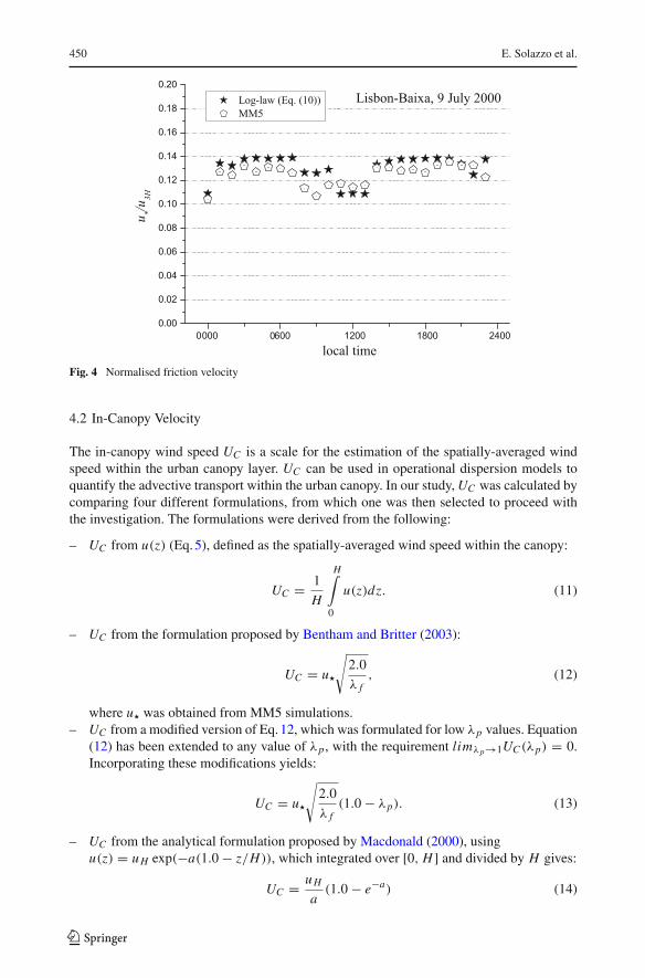
Results shown in Fig. 4 highlight some important aspects. Hourly variations of u�/u3H

derived from Eq. 10 are determined by the wind direction. Oscillations of the MM5 data forthe normalised u� are due to the hourly variation of the wind direction and of the stability,whereas the values of d and z0(θ) in Eq. 10 were calculated using Eqs. 2 and 3 for intervalsof 45◦ (see Sect. 3.1). Within MM5, z0 and d do not depend “directly” on wind direction,in the sense that there is not an explicit relationship expressing them as a function of winddirection. There is, though, an “indirect” effect of the wind direction on the mean flow, whichis due to the different z0 values associated with each land-use category surrounding the Baixaarea. Because the oncoming flow approaching Baixa is affected by the underlying roughness,depending on wind direction, departure from equilibrium is expected, which translates intoa u�/u3H variation.

In our approach, the normalised friction velocity from Eq. 10 is calculated by assumingthat the flow is in equilibrium with the Baixa area, and in this respect is a function of the localmorphology. The value calculated by MM5 provides an independent calculation of frictionvelocity. In this latter case it depends on the upstream fetch and atmospheric stability. Figure 4shows that the two approaches give comparable values of the friction velocity. Some featuresof the inertial sublayer are discussed in more detail in Sect. 4.3. To explain the similar trend(i.e. the hourly variation) of the two sets of data in Fig. 4, however, the data available do notallow general conclusions to be drawn at this stage, and further investigations are required.

Results in Fig. 4 show that u� is in the range of 10 to 14% of the reference wind speed,u3H . These values agree well with the local friction velocity at z = 3H (based on an aver-age over a large number of full-scale observations) reported by Roth (2000), who foundu�/u3H ≈ 0.11.

123

450 E. Solazzo et al.

Fig. 4 Normalised friction velocity

4.2 In-Canopy Velocity

The in-canopy wind speed UC is a scale for the estimation of the spatially-averaged windspeed within the urban canopy layer. UC can be used in operational dispersion models toquantify the advective transport within the urban canopy. In our study, UC was calculated bycomparing four different formulations, from which one was then selected to proceed withthe investigation. The formulations were derived from the following:

– UC from u(z) (Eq. 5), defined as the spatially-averaged wind speed within the canopy:

UC = 1

H

H∫

0

u(z)dz. (11)

– UC from the formulation proposed by Bentham and Britter (2003):

UC = u�

√2.0

λ f, (12)

where u� was obtained from MM5 simulations.– UC from a modified version of Eq. 12, which was formulated for low λp values. Equation

(12) has been extended to any value of λp , with the requirement limλp→1UC (λp) = 0.Incorporating these modifications yields:

UC = u�

√2.0

λ f(1.0 − λp). (13)

– UC from the analytical formulation proposed by Macdonald (2000), usingu(z) = u H exp(−a(1.0 − z/H)), which integrated over [0, H ] and divided by H gives:

UC = u H

a(1.0 − e−a) (14)

123

The Lisbon Case Study 451

Fig. 5 Comparison between several formulations of UC for the Baixa area

where a is the attenuation coefficient (a = 9.6λ f , Macdonald 2000) and u H is the horizontalwind speed at z = H obtained from Eq. 5.

Results in Fig. 5 show that Eqs. 11 and 13 predict very similar values, with UC in the range20 to 40% of u3H , depending on the wind direction. Results from Eq. 12 are about 30% larger,whereas results from Eq. 14 are lower than those of the previous two formulations. Equation(14) depends on a larger number of additional parameters, such as the attenuation coefficientand the roof top wind speed, which are usually difficult to measure. For consistency withthe downscaling approach based on Eq. 5, UC derived from Eq. 11 has been adopted in ourstudy. It is worth observing that λp is introduced in Eq. 11 through the mixing length (Eq. 6),which is l = H − d for z ≤ H . Since limλp→1d = H , it follows limλp→1l = 0, and thusUC (λp = 1) = 0.

Results in Fig. 5 also show a sharp increase between 0800 and 1400 local time (LT), whichcorresponds to a trend similar to that already observed for the normalised u� shown in Fig. 4.This clearly shows the dependence of λ f on wind direction. All formulations for UC com-pared in Fig. 5 depend on λ f and are derived from Eq. 5, which explains the trend in the figure.The only exception are Eqs. 12 and 13 that use u� from MM5 and depend on λ f explicitely.

4.3 Spatially-Averaged Mean Wind-Speed Profiles

Two examples of the solution of Eq. 5 are displayed in Fig. 6, which resemble the schematicprofiles shown in Fig. 1. The two cases refer to two different hours, and were selected forthe value of λ f , which is low in the first case (λ f = 0.07, Fig. 6a) and high in the secondcase (λ f = 0.36, Fig. 6b). Both, the spatially-averaged mean wind speed u(z) and the wind-speed profile computed by MM5 are normalised with the reference wind speed, u3H . Forcomparison, Eq. 5 was also solved above z3H , by using u3H as boundary condition at thebottom. In this case the right-hand side of Eq. 5 is zero, and the derivative du3H /dz was alsoprovided as a boundary condition. From the two graphs in Fig. 6, MM5 and Eq. 5 predict thesame wind-speed profile within the inertial sublayer, above z3H . Below z3H , Eq. 5 predictslower values. In fact, the mean wind speed here is strongly influenced by the drag exerted

123

452 E. Solazzo et al.

a

b

Fig. 6 Spatially-averaged mean wind speed profile for a 0000 LT, and b 0100 LT of the selected day 9 July2000 for the Baixa neighbourhood in Lisbon. Outputs from Eq. 5 and MM5 are compared, for different λ f

by the buildings below z = H , which is felt throughout the roughness sublayer. Wind-speedprofiles predicted by MM5 clearly show that the model does not represent the effect of theunderlying buildings on the airflow.

Effects of the frontal area density λ f are also evident by comparing the two curves in Fig. 6.For λ f = 0.36, the inflexion of the mean wind speed for z ≤ H indicates a wind-speed reduc-tion. For λ f = 0.06, the spatially-averaged wind-speed profile is well approximated by astraight line (Fig. 6a), indicating the poor resistance of the buildings on the airflow. A lineartrend of the mean wind-speed profile for z ≤ H has been also found in the computationalstudy by Martilli and Santiago (2007) for an array of cubes with λ f = 0.25, and in the

123

The Lisbon Case Study 453

water flume experiment by Macdonald (2000), for λ f = 0.16. Thus, it may be argued thata trend does exist for λ f ≤ 0.25 (at least), for which the spatially-averaged wind speedprofile within the urban canopy layer obeys a linear law. For λ f = 0.44, experimental databy Macdonald (2000), and the theoretical study by Di Sabatino et al. (2008), showed that anexponential-based function provides a better accuracy than a straight line as far as replicatingthe mean wind speed within the urban canopy layer. Similar conclusions were also drawnwith the simple model developed by Cionco (1965) for the spatially-averaged mean windspeed within a vegetative canopy. In the case of Fig. 6b, it can also be observed that forλ f = 0.36 a simple straight line would not provide a good estimation of u(z) for z < H .

It is also worth to notice that different wind-speed profiles below z = H imply differentUC values. In fact, results from Eqs. 11 and 13 in Fig. 5 show that the spatially-averaged UC isabout 20% larger at 0000 LT (corresponding to λ f = 0.06), than at 0100 LT (correspondingto λ f = 0.36).

Results based on Eq. 5 give more detailed wind-speed profiles. Moreover, the simple modelbased on Eq. 5 is fast to run because it does not require large computational costs. Thus, itcould be implemented within MM5 (or other similar models) to give an initial estimationof the urban effect on the airflow within the urban canopy layer, which would allow for theimprovement of the simple parameterisation given by Eq. 1 within the roughness sublayer.

4.4 Urban Heat Island Effect

Spatially-averaged temperature profiles remove the sensitivity associated with individualmeasurement points within the urban area. Kanda et al. (2005) argued that temperature pro-files within the urban canopy layer are strongly related to the location where measurementsare collected, due to the diversity of surface materials and geometries. One of the advantagesof using Tcan from Eq. 9 is that it provides an initial estimation of the canopy temperature asa whole, regardless of the specific location within the urban canopy layer.

Results for Tcan and T3H are shown in Fig. 7, where the crosses indicate the normalisedexchange velocity uE , which is controlled by the friction velocity in Eq. 4. It can be observedthat uE is within the range 2.0 to 2.5% of u3H . Such a result is in good agreement with otherCFD-based studies, where uE was estimated from the transfer of scalar tracers, such as heat(Solazzo and Britter 2007), and mass release (Hamlyn et al. 2007).

From Fig. 7 it can be observed that the maximum difference between Tcan and T3H cor-responds to a minimum of uE , as expected from Eq. 9. The maximum difference for theinvestigated day was detected at 1200 LT, with a temperature difference of about 3 K. Sim-ilarly, between 1000 LT and 1300 LT the temperature difference was approximately 2.5 K.During the time periods 0000 LT to 0700 LT, and 2000 LT to 2300 LT, the simple modelbased on Eqs. 4 and 9 predicted a smaller difference between the temperature within theurban canopy layer and that at z3H (of approximately 1 K).

The canopy temperature Tcan is also compared with Tout , which was measured at a heightof 2 m above the ground at the Cacem meteorological station, located in the outskirts ofLisbon. The determination of the air temperature in the urban canopy allows the calculationof TU H I , defined as:

TU H I = Tcan − Tout , (15)

which represents the difference between the air temperature in the urban canopy layer andthe air temperature recorded at a close meteorological station, in the surrounding rural partof the city. Calculation of TU H I provides an estimation of the UHI in Lisbon during theselected day (Oke 1992). Peak differences between Tcan and Tout of about 5.5 K were found

123

454 E. Solazzo et al.

Fig. 7 Temperatures (left hand side axis) and normalised exchange velocity (right hand side axis) time series.Tout : temperature measured at the Cacem meteorological station; TM M5z=3H : reference temperature pro-vided by MM5; TM M5z=0: temperature at the ground predicted by MM5; Tcan : temperature of the urbancanopy layer from Eq. 9

between 1300 LT and 1600 LT. A large UHI effect is also evident during the night, between0000 LT and 0700 LT, with TU H I ≈ 4.5 K. Between 0800 LT and 1000 LT the UHI is at theminimum, with TU H I ≈ 1.5 K. Finally, TU H I is almost constant after 1700 LT, equal toapproximately 3 K. Alcoforado and Andrade (2006) reported a mean nocturnal UHI in Lisbonof approximately 2.5 K, with a peak of 4 K, based on field measurements. Results obtained inour study are not far from those findings, although based on the calculation of a single day.It is worth pointing out that unbiased models are assumed in estimating the UHI in Eq. 15,given that “modelled” urban temperature and “measured” rural temperature are compared.

In Fig. 7 the ground level temperature predicted by MM5, TM M5z=0 is also reported. Thistemperature is estimated by the model by considering the thermal properties of the Baixa areaand it does not include any “canopy effect”. Therefore, the difference between TM M5z=0 andTcan are due to the urban model developed in our study. TM M5z=0 and T3H exhibit a similartrend during nighttime hours. Between 0900 LT and 1400 LT the difference is more pro-nounced due to the larger heat flux density Q H . During this time lag the difference betweenTcan and TM M5z=0 is more evident, with peak differences of approximately 2 K at 1200 LT,but much smaller than the values predicted by means of Eq. 15.

Finally, it should be noticed that for the case of sensible heat fluxes, field data or moredetailed models could be used to estimate Q H , (for example, see the radiative model pro-posed by Lee and Park (2008) and by Kusuka and Kimura (2004)). Nevertheless, this wouldnot change the simplicity of the methodology based on Eq. 9.

5 Conclusions and Future Work

Accurate modelling of the flow field and temperature patterns inside the roughness sublayeris one of the key aspects for assessing the energy consumption of buildings as well as for

123

The Lisbon Case Study 455

investigating pollutant dispersion at neighbourhood scales and below. The assumption of asimple roughness parameterisation may result in poorly detailed results at such scales. On theother hand, very detailed formulations accounting for the effects of the city area within NWPmodels may require large computational resources and numerous input data. Therefore, asimple urban parameterisation has been developed to be coupled with mesoscale models, suchas MM5, to output meteorological profiles within the urban canopy layer. Furthermore, themodel proposed is simple to run and requires few input parameters, requiring no additionalcomputational costs.

The urban model is based on the spatially-averaged mean profiles of wind speed andtemperature. A drag-force approach is used to represent the dynamic and turbulent effects ofthe buildings on the flow, and a mass transfer parameterisation is used to take into accounturban thermal effects on the flow. The urban model was used for a real application for thecity of Lisbon (Portugal) where the Baixa neighbourhood was selected for analyses. Hourlyvariations of several meteorological variables over 24 hours were analysed. Three velocityscales were quantified, each of direct usefulness for dealing with the flow, the dispersion, andthe exchange processes in urban areas. The following results were obtained:

– The friction velocity u� was found to be between 10 and 14% of the reference wind speedu3H .

– The spatially-averaged in-canopy wind speed UC was found to be highly sensitive tothe formulation applied for its calculation. Results obtained in our study suggest thatUC ≈ 0.3u3H offers a valid estimation, calculated as an integral velocity averaged overthe height of the canopy layer.

– The exchange velocity uE was found to vary within the range 2.0 to 2.5% of u3H . Wenote that uE is the main parameter controlling the transfer of mass between the urbancanopy layer and the atmospheric layer above.

– The variations with time of the aforementioned variables indicate that the flow field andthe turbulence within the urban canopy layer are mainly controlled by the wind direction,which, in our model is accounted for by λ f and z0.

– Results derived from the mass exchange analyses showed a canopy effect (differentialtemperature between the canopy and the reference height of 3H above the canopy), witha maximum of 3 K between 1200 and 1400 local time, and negligible during the nighttimehours. Moreover, a urban heat island effect (differential temperature between the canopyand a location outside the urban area) of an average of 3 K was calculated for the selectedday.

The results presented herein provide the basis for future research. The limitations of thedeveloped model will be the starting point of further investigations. For example, it is impor-tant to test the model sensitivity to other formulations of the parameters d, z0, CD , and l.Analyses on the urban heat island and u� should also be extended to other days and possiblyto other urban areas for which more accurate information on heat flux density and shearstress are available. The model for momentum balance between the urban canopy and theinertial sublayer assumes that all momentum sources derive from the pressure and viscousdrag forces from the vertical building surfaces. Considering additional sources, such as fromhorizontal building surfaces (e.g. Dupont et al. 2004), can also contribute to improve ourmodel.

The model developed in our study can be extended to any scalar whose transfer is drivenby the mass exchange at the urban canopy layer interface. Therefore, the exchange of latentheat flux, pollutants, heat, and others, could be analysed based on the hypothesis that anyscalar is homogeneously mixed within the urban canopy layer.

123

456 E. Solazzo et al.

Acknowledgments This study was partially conducted within the Research Training Network ATREUS(Contract No. HPRN-CT-2002-00207), funded by the European Commission, Training and Mobility ofResearchers Programme. The authors wish to thanks all the participants in the project. Rex Britter was funded inpart by the Singapore National Research Foundation (NRF) through the Singapore-MIT Alliance for Researchand Technology (SMART) Center for Environmental Sensing and Modeling (CENSAM).

References

Alcoforado M-J, Andrade H (2006) Nocturnal urban heat island in Lisbon (Portugal): main features and mod-elling attempts. Theor Appl Climatol 84:151–159

Bentham T, Britter RE (2003) Spatially averaged flow within obstacle arrays. Atmos Environ 37:2037–2043

Best MJ (2005) Representing urban areas within operational numerical weather prediction models. Boundary-Layer Meteorol 114:91–109

Borrego C, Tchepel O, Costa AM, Amorim JH, Miranda AL (2003) Emission and dispersion modelling ofLisbon air quality at local scale. Atmos Environ 37:5197–5205

Britter RE, Hanna SR (2003) Flow and dispersion in urban areas. Annu Rev Fluid Mech 35:469–496Businger JA, Wyngaard JC, Izumi Y, Bradley EF (1971) Flux-profile relationships in the atmospheric surface

layer. J Atmos Sci 28:181–189Cheng H, Castro IP (2002) Near wall flow over urban-like roughness. Boundary-Layer Meteorol 104:

229–259Cionco R (1965) A mathematical model for air flow in a vegetative canopy. J Appl Meteorol 4:517–522Coceal O, Belcher SE (2004) A canopy model of mean winds through urban areas. Q J Roy Meteorol Soc

130:1349–1372Di Sabatino S, Solazzo E, Paradisi P, Britter R (2008) A simple model for spatially-averaged wind profiles

within and above an urban canopy. Boundary-Layer Meteorol 127:131–151Dudhia J, Bresch JF (2002) A global version of the PSU-NCAR mesoscale model. Mon Weather Rev

130:2989–3007Dupont S, Otte TL, Ching JKS (2004) Simulation of meteorological fields within and above urban and rural

canopies with a mesoscale model (MM5). Boundary Layer Meteorol 113:111–158Dyer AJ (1974) A review of flux-profile relationships. Boundary-Layer Meteorol 7:363–372Grimmond S, Oke T (1999) Aerodynamic properties of urban areas derived form analysis of surface form.

J Appl Meteorol 38:1261–1292Hamlyn D, Hilderman T, Britter RE (2007) A simple network approach to modelling dispersion among large

groups of obstacles. Atmos Environ 41:5848–5862Kanda M, Moriwaki R, Kimoto Y (2005) Temperature profiles within and above an urban canopy. Boundary-

Layer Meteorol 115:499–506Kastner-Klein P, Rotach MW (2004) Mean flow and turbulence characteristics in an urban roughness sublayer.

Boundary-Layer Meteorol 111:55–84Kusaka H, Kimura F (2004) Coupling a single-layer urban canopy model with a simple atmospheric model:

impact on urban heat island simulation for an idealized case. J Meteorol Soc Jpn 82:67–80Lee S-H, Park S-U (2008) A vegetated urban canopy model for meteorological and environmental modelling.

Boundary-Layer Meteorol 126:73–102Macdonald RW (2000) Modelling the mean velocity profile in the urban canopy layer. Boundary-Layer Mete-

orol 97:25–45Macdonald R, Griffiths RF, Hall DJ (1998) A comparison of results from scaled field and wind tunnel mod-

elling of dispersion in arrays of obstacles. Atmos Environ 32:3845–3862Martilli A (2007) Current research and future challenges in urban mesoscale modelling. Int J Climatol

27:1909–1918Martilli A, Santiago JL (2007) CFD simulation of airflow over a regular array of cubes. Part II: analysis of

spatial average properties. Boundary-Layer Meteorol 122:635–654Martilli A, Cappier A, Rotach MW (2002) An urban surface exchange parameterisation for mesoscale models.

Boundary-Layer Meteorol 104:261–304Oke TR (1992) Boundary layer climates. Methuen, LondonOxizidis S, Dudek A, Papadopoulos AM (2007) A computational method to assess the impact of urban climate

on buildings using modelled climatic data. Energy Build 40:215–223

123

The Lisbon Case Study 457

Papadopoulos AM, Moussiopoulos N (2004) Towards an holistic approach for the urban environment and itsimpact on energy utilization in buildings: the ATREUS project. J Environ Monit 6:841–848

Ratti C, Di Sabatino S, Britter RE, Brown M, Caton F, Burian S (2002) Analysis of 3-D urban database withrespect to pollution dispersion for a number of European and American cities. Water Air Soil Pollut2:459–469

Roth M (2000) Review of atmospheric turbulence over cities. Q J Roy Meteorol Soc 126:941–990Solazzo E, Britter RE (2007) Transfer processes in a simulated urban street canyon. Boundary-Layer Meteorol

124:43–60

123