Correspondence Free Registration through aPoint-to-Model Distance Minimization

Mohammad RouhaniComputer Vision CenterEdifici O, Campus UAB

08193 Bellaterra, Barcelona, Spainrouhani@cvc.uab.es

Angel D. SappaComputer Vision CenterEdifici O, Campus UAB

08193 Bellaterra, Barcelona, Spainasappa@cvc.uab.es

Abstract

This paper presents a novel formulation, which derivesin a smooth minimization problem, to tackle the rigid reg-istration between a given point set and a model set. Unlikemost of the existing works, which are based on minimizinga point-wise correspondence term, we propose to describethe model set by means of an implicit representation. It al-lows a new definition of the registration error, which worksbeyond the point level representation. Moreover, it couldbe used in a gradient-based optimization framework. Theproposed approach consists of two stages. Firstly, a novelformulation is proposed that relates the registration param-eters with the distance between the model and data set. Sec-ondly, the registration parameters are obtained by means ofthe Levengberg-Marquardt algorithm. Experimental resultsand comparisons with state of the art show the validity ofthe proposed framework.

1. Introduction

Registration problem has been largely studied in thecomputer vision community since the last two decades (e.g.,[5], [8], [16], [22], [7]). It aims at finding the best trans-formation that places both the given data set and its corre-sponding model set into the same reference system as closeas possible. The different approaches proposed in the lit-erature can be broadly classified into two categories, de-pending on whether an initial information is required (fineregistration) or not (coarse registration); see [18] for a de-tailed survey. The proposed approach lies within the finerigid registration category.

Typically, the fine registration process consists of iterat-ing the following two stages. Firstly, the correspondencebetween every point from the current data set and the modelset should be found. These correspondences are used to de-fine the residual error of the registration. Secondly, the best

set of parameters that minimizes the sum of these residu-als should be found. These two stages are iteratively ap-plied till convergence is reached. The Iterative Closest Point(ICP)—originally introduced by [5] and [8]—is one of themost widely used registration techniques using this two-stage scheme. Since then, several variations and improve-ments have been proposed in order to increase the efficiencyand robustness of the method (e.g., [12], [19], [26], [13]).It should be noticed that the correspondence search in theseapproaches makes the whole scheme as a discrete evolution.

In order to avoid the correspondence search in the firststage, different techniques have been proposed in the lit-erature: i) Implicit polynomials have been used in [20] torepresent both the data set and model set. Then an accuratepose estimation is computed through constructing two co-variants. ii) Probabilistic representations have been used todescribe both data set and model set (e.g. [23], [14], [7]).iii) In [10] the point-wise problem is avoided by using adistance field of the model set; the value and behavior ofthis distance field is computed in a discrete domain. iv) In[15] the behavior of the distance field is approximated ana-lytically based on the curvature information. v) An implicitpolynomial is used in [24] to fit the distance field, whichlater defines a gradient field leading the data set towardsthat model set.

The current paper proposes a novel formulation differ-ent to the point-wise based correspondence approaches. Itis based on an implicit representation of the model set thatallows to define a continuous and smooth distance functionfor the registration. Hence, it is independent of point den-sities and robust to noise and missing data. The main con-tribution of the proposed approach is the novel way of dis-tance definition, which avoids correspondence search of theclassical registration algorithms. Moreover it is differen-tiable with respect to the registration parameters and allowssolving the registration problem through a gradient basedoptimization algorithm.

1

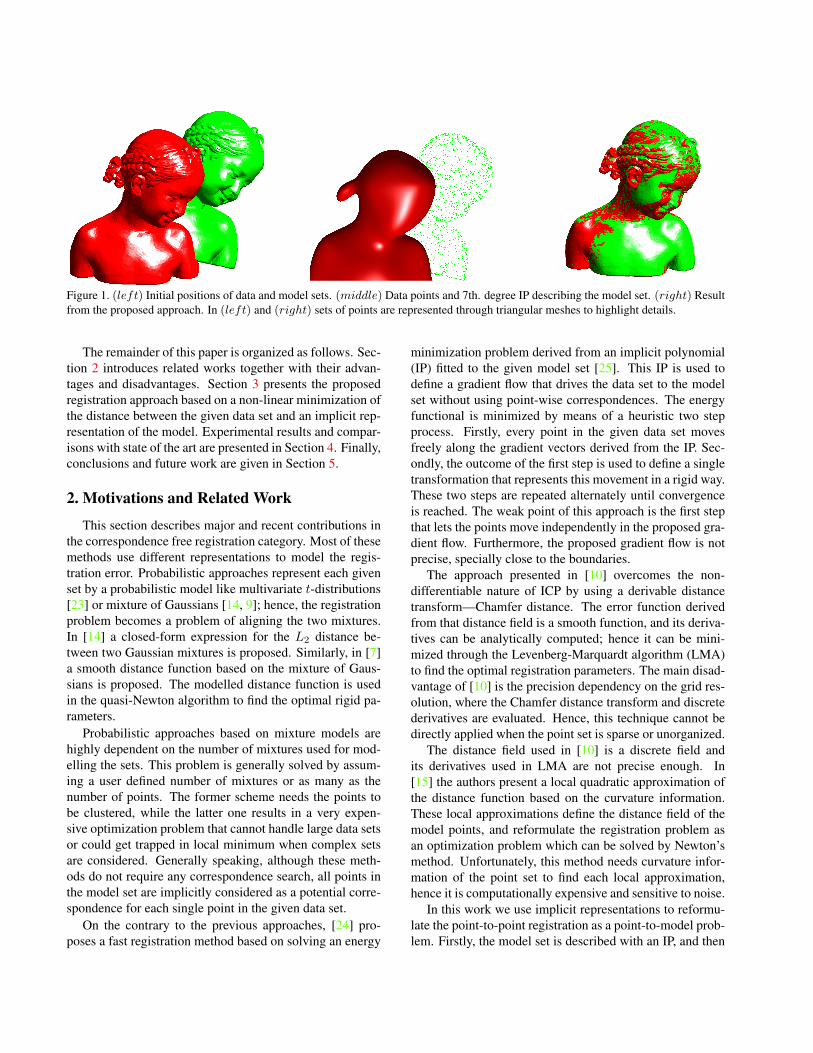
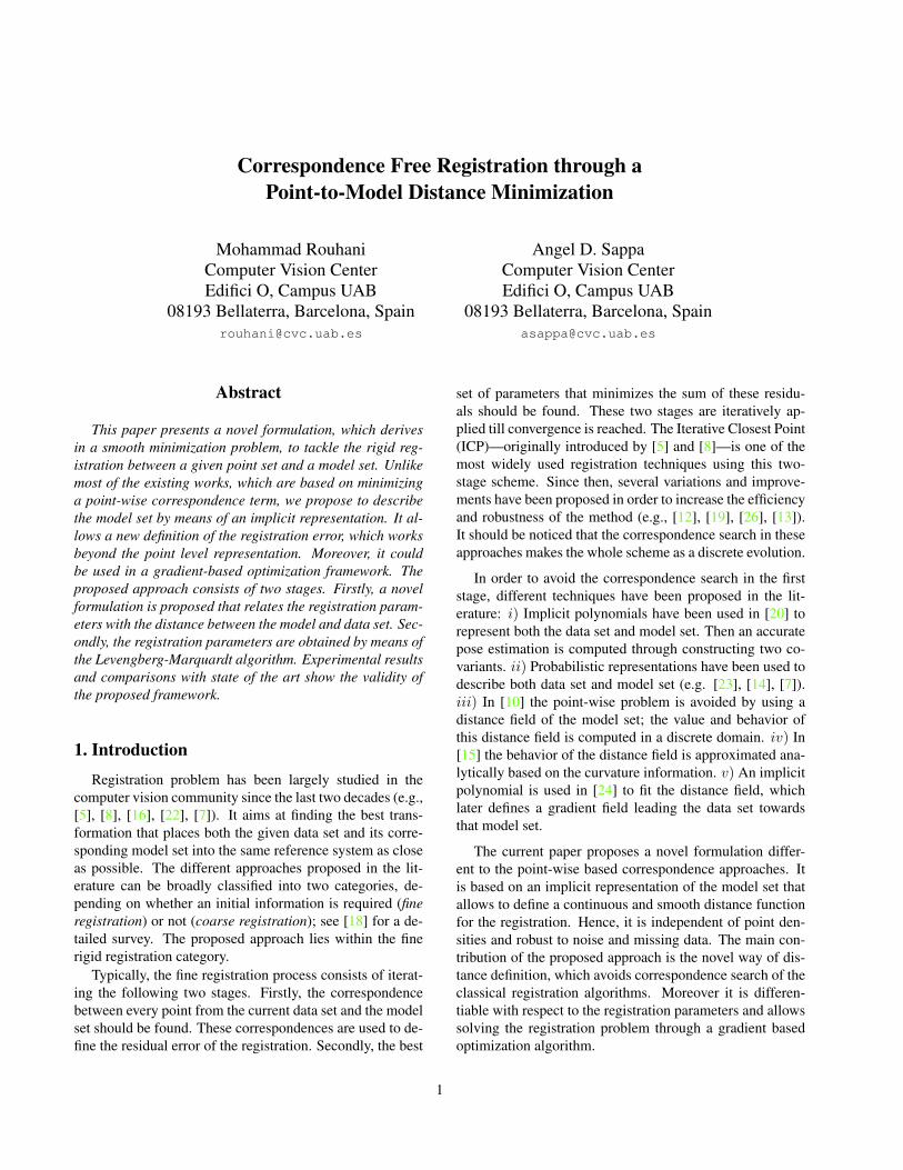
Figure 1. (left) Initial positions of data and model sets. (middle) Data points and 7th. degree IP describing the model set. (right) Resultfrom the proposed approach. In (left) and (right) sets of points are represented through triangular meshes to highlight details.

The remainder of this paper is organized as follows. Sec-tion 2 introduces related works together with their advan-tages and disadvantages. Section 3 presents the proposedregistration approach based on a non-linear minimization ofthe distance between the given data set and an implicit rep-resentation of the model. Experimental results and compar-isons with state of the art are presented in Section 4. Finally,conclusions and future work are given in Section 5.

2. Motivations and Related Work

This section describes major and recent contributions inthe correspondence free registration category. Most of thesemethods use different representations to model the regis-tration error. Probabilistic approaches represent each givenset by a probabilistic model like multivariate t-distributions[23] or mixture of Gaussians [14, 9]; hence, the registrationproblem becomes a problem of aligning the two mixtures.In [14] a closed-form expression for the L2 distance be-tween two Gaussian mixtures is proposed. Similarly, in [7]a smooth distance function based on the mixture of Gaus-sians is proposed. The modelled distance function is usedin the quasi-Newton algorithm to find the optimal rigid pa-rameters.

Probabilistic approaches based on mixture models arehighly dependent on the number of mixtures used for mod-elling the sets. This problem is generally solved by assum-ing a user defined number of mixtures or as many as thenumber of points. The former scheme needs the points tobe clustered, while the latter one results in a very expen-sive optimization problem that cannot handle large data setsor could get trapped in local minimum when complex setsare considered. Generally speaking, although these meth-ods do not require any correspondence search, all points inthe model set are implicitly considered as a potential corre-spondence for each single point in the given data set.

On the contrary to the previous approaches, [24] pro-poses a fast registration method based on solving an energy

minimization problem derived from an implicit polynomial(IP) fitted to the given model set [25]. This IP is used todefine a gradient flow that drives the data set to the modelset without using point-wise correspondences. The energyfunctional is minimized by means of a heuristic two stepprocess. Firstly, every point in the given data set movesfreely along the gradient vectors derived from the IP. Sec-ondly, the outcome of the first step is used to define a singletransformation that represents this movement in a rigid way.These two steps are repeated alternately until convergenceis reached. The weak point of this approach is the first stepthat lets the points move independently in the proposed gra-dient flow. Furthermore, the proposed gradient flow is notprecise, specially close to the boundaries.

The approach presented in [10] overcomes the non-differentiable nature of ICP by using a derivable distancetransform—Chamfer distance. The error function derivedfrom that distance field is a smooth function, and its deriva-tives can be analytically computed; hence it can be mini-mized through the Levenberg-Marquardt algorithm (LMA)to find the optimal registration parameters. The main disad-vantage of [10] is the precision dependency on the grid res-olution, where the Chamfer distance transform and discretederivatives are evaluated. Hence, this technique cannot bedirectly applied when the point set is sparse or unorganized.

The distance field used in [10] is a discrete field andits derivatives used in LMA are not precise enough. In[15] the authors present a local quadratic approximation ofthe distance function based on the curvature information.These local approximations define the distance field of themodel points, and reformulate the registration problem asan optimization problem which can be solved by Newton’smethod. Unfortunately, this method needs curvature infor-mation of the point set to find each local approximation,hence it is computationally expensive and sensitive to noise.

In this work we use implicit representations to reformu-late the point-to-point registration as a point-to-model prob-lem. Firstly, the model set is described with an IP, and then

the approximated distance between the data set and the fit-ted polynomial is minimized to find the best rigid transfor-mation. Figure 1(middle) shows a seventh degree IP that isconsidered instead of the model set. It should be mentionedthat the IP is just used as an interface to tackle the registra-tion problem. For instance, in the extreme case, when thedata set P is a rigid transformation of the model set Q andfc is the best polynomial fitting the model set, then it couldbe proved that:

minR,tDist(RP+ t, fc) = Dist(Q, fc),

where Dist refers to the orthogonal distance of a set ofpoints to the implicit polynomial; and [R, t] refers to therotation and translation of the rigid transform.

3. Proposed ApproachThe proposed approach consists of two main steps. The

first step formulates the registration error based on the ap-proximated distance between the current data set and theimplicit function used for representing the model set. Thisformulation relates the error function with the registrationparameters. The second step finds the optimal rigid parame-ters that minimize the proposed registration error through itsgradient information. Before detailing the aforementionedtwo steps IP fitting is introduced, which is used to describethe model set. It should be noticed that the proposed formu-lation is valid for any implicit representation (e.g. implicitRBF and B-Splines).

3.1. Model Representation

This section briefly describes the algorithm used for find-ing the implicit polynomial that fits the model set. The 3Lalgorithm [6] has been chosen due to its simplicity and ro-bustness; other algebraic or geometric fitting approachescould be adopted since the proposed distance formulationis independent of the algorithm used for fitting the model.Finding the best IP representation is out of the scope of thecurrent paper and several approaches can be found in theliterature (e.g., [3], [4], [6], [17], [21], [25]).

Without loss of generality, lets consider the 2D case,where an implicit polynomial describes a set of points inthe plane fulfilling this equation:

fc(x, y) =∑

(i+j)5d

{i,j}=0

ci,jxiyj = 0, (1)

which could be represented in the vector form:

fc(x) = mTc = 0, (2)

where m is the column vector of monomials and c is thepolynomial coefficient vector; the fitting problem consists

in first defining a criterion—or residual error—to measurethe distance between the zero set and the given data set, andthen minimizing this criterion to find the best coefficientvector c.

The simplest and straightforward criterion could be thesum of squared IP values at the given data points (i.e.∑

i fc(xi, yi)2). The parameters can be easily obtained by

minimizing this criterion, but there is not a clear geometricinterpretation and the least square solution for this problemcould be very unstable.

To address the two problems mentioned above, the au-thors in [6] have proposed the 3L algorithm, which consistsin generating two additional level sets: Γ−δ and Γ+δ fromthe original data set Γ0. These two additional data sets aregenerated so that one is internal and the other is external.These sets are placed at a distance ±δ from the original dataalong a direction that is locally perpendicular to the givendata set. In the current implementation a principal com-ponents analysis (PCA) based approach, in a local neigh-borhood for every point, has been used for estimating thisdirection. Hence, the 3L algorithm incorporates a controlfor a local continuity resulting in a more stable solution.

The 3L fitting algorithm is then formalized as a linearleast squares explicit polynomial fitting problem. Consid-ering the three level sets: {Γ−δ,Γ0,Γ+δ} the equation (2)is now defined by using a block matrix M3L and a blockcolumn vector b:

M3L =

MΓ−δ

MΓ0

MΓ+δ

,b =

−ϵ0+ϵ

, (3)

where MΓ0 , MΓ+δ, MΓ−δ

are matrices of monomials cal-culated in the original, inner and outer set respectively; ±ϵare the corresponding expected values in the inner and outerlevel sets. Then, the least squares solution for c is obtained:

c = M†3Lb = (MT

3LM3L)−1MT

3Lb, (4)

where M†3L denotes the pseudoinverse of M3L.

3.2. Distance Formulation

The registration process seeks for the best transformationparameter Θ which contains rotation R = Rθ and transla-tion t = [tx, ty]

T in rigid case. The optimal parametermoves the data set P = {pi}N1 , in a rigid way, as close aspossible to the model fc(x):

Θ̂ = argminΘ

(N∑i=1

Dist2(Rpi + t, fc)

), (5)

for this purpose, the distance function, Dist, between thedata set and the model should be approximated. In the cur-rent work, the estimation of the orthogonal distance pro-posed in [21] is used. This approximation is based on the

first order Taylor expansion of the distance function. It hassome interesting properties including: i) independence ofthe zero set representation; and ii) invariance to rigid bodytransformation. It is computed through normalizing the al-gebraic distance by the gradient norm:

Dist(p, fc) ≈|fc(p)|

||∇fc(p)||, (6)

using this approximation in (5) the registration parameterscan be found by minimizing the following function:

DistΘ =N∑i=1

(fc(Rpi + t)

∥ ∇fc(Rpi + t) ∥

)2

(7)

=

N∑i=1

(wifc(Rpi + t))2 =

N∑i=1

d2i ,

where:di = wifc(Rpi + t), (8)

wi = 1/∥ ∇fc(Rpi + t) ∥,

show the distance of each item and the weight to approxi-mate this distance. Thus the point-to-point registration willbe done in a higher level using a curve or surface as an in-terface. It will provide a rich structure as well as many ad-vantages like robustness to noise and missing data.

3.3. Distance Optimization

The distance presented above provides a correspondencefree formulation for the registration problem, which is di-rectly related to rigid parameters. This relation couldbe exploited in many optimization algorithms. Here weuse gradient based algorithms like gradient descent andLevenberg−Marquardt algorithm (LMA). The gradient in-formation shows the sensitivity of distance with respect torigid parameters as illustrated in Fig. 2.

LMA is a well-known technique in non-linear optimiza-tion [11], which is particularly proposed for functions inthe form of sum of squared residuals as the case in (7).This method proposes a tradeoff between two well knownmethods in nonlinear optimization: the Gauss−Newton al-gorithm and the gradient descent algorithm. In order to han-dle LMA, the value of the function (7) and its partial deriva-tives, which are expressed in a Jacobian matrix J , should beprovided. Since LMA uses the gradient information of theobjective function, the first order distance approximation in(7) captures this information; hence, better approximationswould not benefit the result of LMA. It should be mentionedthat the derivatives of (7) must be calculated with respectto the parameters Θ = [θ tx ty]

T, where θ, tx and tycapture the three degrees of freedom of the rigid registra-tion. Hence, the first column of the Jacobian matrix can becomputed as follow:

� �

�

�����

���

� �

�

�����

���

Figure 2. (left) Sensitivity of the distance with respect to smallchanges in rotation. (right) Sensitivity of the distance with re-spect to the translation along y axis.

J(i, 1) =∂di∂θ

= (∂wi/∂θ)fc(Rpi+t)+wi∂fc(Rpi + t)

∂θ,

(9)since the implicit function fc is a smooth function, wi couldbe considered as a constant weight, then the first term couldbe ignored:

J(i, 1) = wi(R′θpi.∇fc(Rpi + t)), (10)

where R′θ is the derivative of the rotation matrix w.r.t. the

rotation angle, and ∇fc is the gradient with respect to (x, y)components. Similarly, other columns of the Jacobian ma-trix can be calculated as:

J(i, 2) =∂di∂tx

= wi∂

∂xfc(Rpi + t), (11)

J(i, 3) =∂di∂ty

= wi∂

∂yfc(Rpi + t).

For the 3D case the Jacobian matrix includes six columnscorresponding to three rotation and three translation param-eters. As a general formula each entry of this matrix couldbe computed as:

J(i, j) = wi

(∂

∂Θj(Rpi + t)

).∇f(Rpi + t), (12)

where Θj is the jth parameter of Θ = [θ, ϕ, ψ, tx, ty, tz].Having estimated the proposed distance (7) and its Jaco-

bian matrix through (9), (10) and (11) it is easy to performLMA in order to refine the rigid parameters Θ:

Θk+1 = Θk + β△Θ,

(JTJ + λdiag(JTJ))△Θ = JTD, (13)

where β is the refinement step; diag(JTJ) is the diago-nal matrix containing the elements of (JTJ); △Θ repre-sents the refinement vector for the rigid parameters; λ isthe damping parameter in LMA; and the vector D is a col-umn vector containing Dist(Rpi + t, fc), R and t are thecurrent rotation and translation respectively. In the currentimplementation they are initialized as θ = 0, tx = 0 andty = 0; more evolved initializations, such as using simpleSVD based techniques, could be used since we are tacklingthe rigid registration case. Parameter refinement (13) mustbe repeated till convergence is reached.

Model Set: 40 points Data Set: 40 points

Model Set: 44 pointsData Set: 44 points

Data Set: 46 pointsModel Set: 67 points

Data Set: 20 pointsModel Set: 44 points

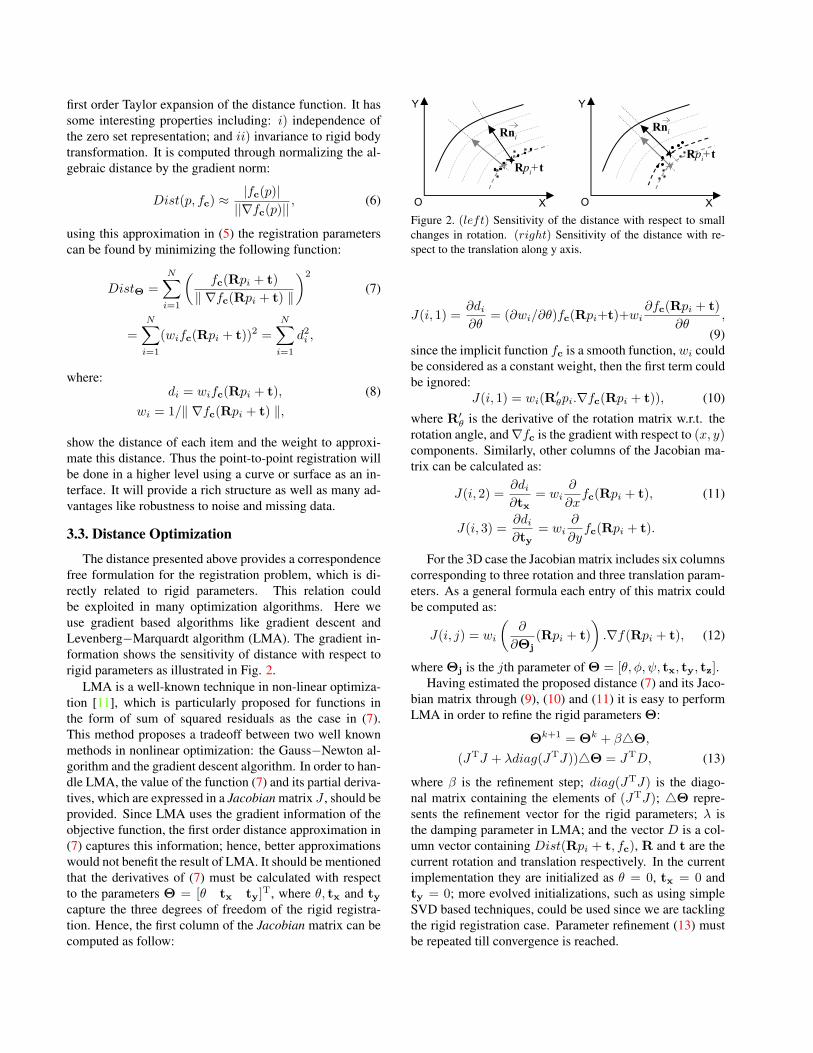
Figure 3. Initial positions of data sets and model sets for noisy(top) and partial overlap (bottom) examples registered with thedifferent approaches.

4. Experimental Results and ComparisonsThe proposed approach has been evaluated using differ-

ent data sets and model sets. Additionally four techniques(i.e., [14], [10], [24] and [15]) from the state of the art, to-gether with the classical ICP [5], have been implementedfor a comparative study in the 2D and 3D cases. Each tech-niques iterates till one of the stopping criteria is reached:maximum number of iterations (#Iter=30) or relative reg-istration error smaller than a given threshold. The relativeregistration error is defined as: ϵ = |Et −Et−1|/Et, whereEt refers to the error between the model and data set at iter-ation t. In our implementation (ϵ < 0.001) has been used.

On the contrary to the relative registration error, which isan internal measure, an Accumulated Residual Error (ARE)is used during the comparisons. It is computed by measur-ing the accumulated error, in a point-wise manner, from thedata set to a reference set. This reference set correspondsto a highly detailed description of the model set. It containsthe model set and on average is defined by a set of points tentimes larger than the model set. Each residual error is com-puted by finding the nearest point in between the registereddata set and the reference set.

Figure 3 shows initial configurations for four differentdata and model sets. The first row corresponds to closedcontours with a full overlap. Data sets have been obtainedby rotating and translating the corresponding model set, andby adding Gaussian noise to study the robustness of all thetechniques. Accuracy and number of iterations are providedin Table 1. It should be highlighted that the proposed ap-proach converges in all the cases and most of the time withthe smallest error and lowest number of iterations, in spite

Model Set: 39 pointsData Set: 45 points

Model Set: 39 pointsData Set: 45 points

Model Set: 58 pointsData Set: 67 points

Model Set: 58 pointsData Set: 67 points

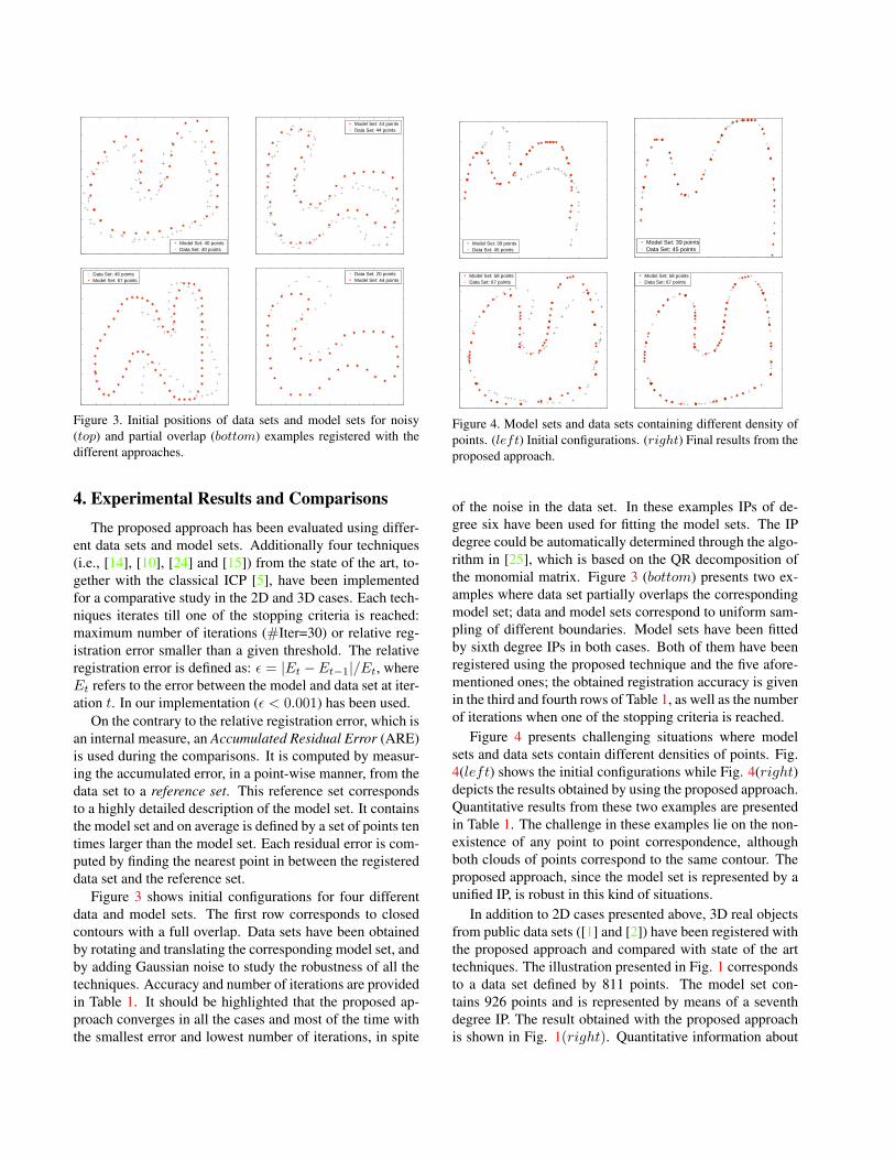
Figure 4. Model sets and data sets containing different density ofpoints. (left) Initial configurations. (right) Final results from theproposed approach.

of the noise in the data set. In these examples IPs of de-gree six have been used for fitting the model sets. The IPdegree could be automatically determined through the algo-rithm in [25], which is based on the QR decomposition ofthe monomial matrix. Figure 3 (bottom) presents two ex-amples where data set partially overlaps the correspondingmodel set; data and model sets correspond to uniform sam-pling of different boundaries. Model sets have been fittedby sixth degree IPs in both cases. Both of them have beenregistered using the proposed technique and the five afore-mentioned ones; the obtained registration accuracy is givenin the third and fourth rows of Table 1, as well as the numberof iterations when one of the stopping criteria is reached.

Figure 4 presents challenging situations where modelsets and data sets contain different densities of points. Fig.4(left) shows the initial configurations while Fig. 4(right)depicts the results obtained by using the proposed approach.Quantitative results from these two examples are presentedin Table 1. The challenge in these examples lie on the non-existence of any point to point correspondence, althoughboth clouds of points correspond to the same contour. Theproposed approach, since the model set is represented by aunified IP, is robust in this kind of situations.

In addition to 2D cases presented above, 3D real objectsfrom public data sets ([1] and [2]) have been registered withthe proposed approach and compared with state of the arttechniques. The illustration presented in Fig. 1 correspondsto a data set defined by 811 points. The model set con-tains 926 points and is represented by means of a seventhdegree IP. The result obtained with the proposed approachis shown in Fig. 1(right). Quantitative information about

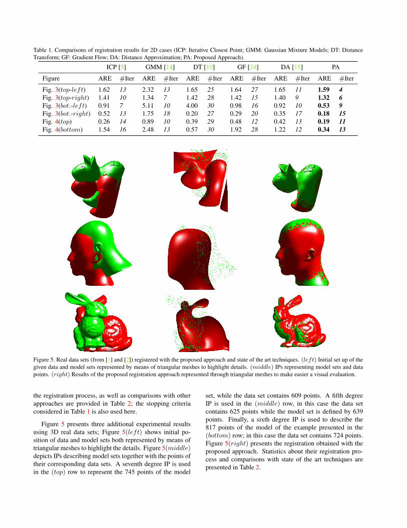
Table 1. Comparisons of registration results for 2D cases (ICP: Iterative Closest Point; GMM: Gaussian Mixture Models; DT: DistanceTransform; GF: Gradient Flow; DA: Distance Approximation; PA: Proposed Approach).

ICP [5] GMM [14] DT [10] GF [24] DA [15] PA

Figure ARE #Iter ARE #Iter ARE #Iter ARE #Iter ARE #Iter ARE #Iter

Fig. 3(top-left) 1.62 13 2.32 13 1.65 25 1.64 27 1.65 11 1.59 4Fig. 3(top-right) 1.41 10 1.34 7 1.42 28 1.42 15 1.40 9 1.32 6Fig. 3(bot.-left) 0.91 7 5.11 10 4.00 30 0.98 16 0.92 10 0.53 9Fig. 3(bot.-right) 0.52 13 1.75 18 0.20 27 0.29 20 0.35 17 0.18 15Fig. 4(top) 0.26 14 0.89 10 0.39 29 0.48 12 0.42 13 0.19 11Fig. 4(bottom) 1.54 16 2.48 13 0.57 30 1.92 28 1.22 12 0.34 13

Figure 5. Real data sets (from [1] and [2]) registered with the proposed approach and state of the art techniques. (left) Initial set up of thegiven data and model sets represented by means of triangular meshes to highlight details. (middle) IPs representing model sets and datapoints. (right) Results of the proposed registration approach represented through triangular meshes to make easier a visual evaluation.

the registration process, as well as comparisons with otherapproaches are provided in Table 2; the stopping criteriaconsidered in Table 1 is also used here.

Figure 5 presents three additional experimental resultsusing 3D real data sets; Figure 5(left) shows initial po-sition of data and model sets both represented by means oftriangular meshes to highlight the details. Figure 5(middle)depicts IPs describing model sets together with the points oftheir corresponding data sets. A seventh degree IP is usedin the (top) row to represent the 745 points of the model

set, while the data set contains 609 points. A fifth degreeIP is used in the (middle) row, in this case the data setcontains 625 points while the model set is defined by 639points. Finally, a sixth degree IP is used to describe the817 points of the model of the example presented in the(bottom) row; in this case the data set contains 724 points.Figure 5(right) presents the registration obtained with theproposed approach. Statistics about their registration pro-cess and comparisons with state of the art techniques arepresented in Table 2.

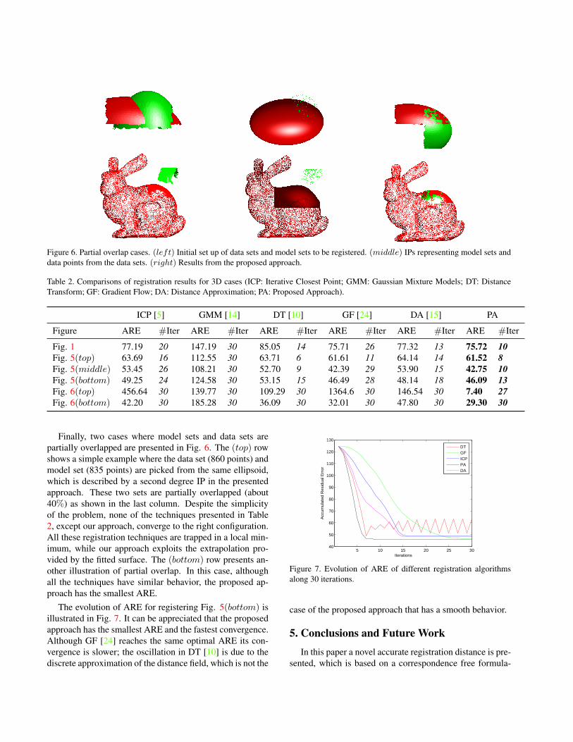
Figure 6. Partial overlap cases. (left) Initial set up of data sets and model sets to be registered. (middle) IPs representing model sets anddata points from the data sets. (right) Results from the proposed approach.

Table 2. Comparisons of registration results for 3D cases (ICP: Iterative Closest Point; GMM: Gaussian Mixture Models; DT: DistanceTransform; GF: Gradient Flow; DA: Distance Approximation; PA: Proposed Approach).

ICP [5] GMM [14] DT [10] GF [24] DA [15] PA

Figure ARE #Iter ARE #Iter ARE #Iter ARE #Iter ARE #Iter ARE #Iter

Fig. 1 77.19 20 147.19 30 85.05 14 75.71 26 77.32 13 75.72 10Fig. 5(top) 63.69 16 112.55 30 63.71 6 61.61 11 64.14 14 61.52 8Fig. 5(middle) 53.45 26 108.21 30 52.70 9 42.39 29 53.90 15 42.75 10Fig. 5(bottom) 49.25 24 124.58 30 53.15 15 46.49 28 48.14 18 46.09 13Fig. 6(top) 456.64 30 139.77 30 109.29 30 1364.6 30 146.54 30 7.40 27Fig. 6(bottom) 42.20 30 185.28 30 36.09 30 32.01 30 47.80 30 29.30 30

Finally, two cases where model sets and data sets arepartially overlapped are presented in Fig. 6. The (top) rowshows a simple example where the data set (860 points) andmodel set (835 points) are picked from the same ellipsoid,which is described by a second degree IP in the presentedapproach. These two sets are partially overlapped (about40%) as shown in the last column. Despite the simplicityof the problem, none of the techniques presented in Table2, except our approach, converge to the right configuration.All these registration techniques are trapped in a local min-imum, while our approach exploits the extrapolation pro-vided by the fitted surface. The (bottom) row presents an-other illustration of partial overlap. In this case, althoughall the techniques have similar behavior, the proposed ap-proach has the smallest ARE.

The evolution of ARE for registering Fig. 5(bottom) isillustrated in Fig. 7. It can be appreciated that the proposedapproach has the smallest ARE and the fastest convergence.Although GF [24] reaches the same optimal ARE its con-vergence is slower; the oscillation in DT [10] is due to thediscrete approximation of the distance field, which is not the

5 10 15 20 25 3040

50

60

70

80

90

100

110

120

130

Iterations

Acc

umul

ated

Res

idua

l Err

or

DTGFICPPADA

Figure 7. Evolution of ARE of different registration algorithmsalong 30 iterations.

case of the proposed approach that has a smooth behavior.

5. Conclusions and Future Work

In this paper a novel accurate registration distance is pre-sented, which is based on a correspondence free formula-

tion. Additionally, its continuous nature allows the use ofgradient based optimization frameworks. Experimental re-sults and comparisons show both fast convergence and ro-bustness in challenging situations (e.g., noisy data; partialoverlap between data set and its corresponding model set;different densities). As a future work the proposed registra-tion error will be extended for more general implicit repre-sentations in a non-rigid deformation space. Furthermore,since the proposed formulation is independent of the fitting,a coarse to fine representation would be explored to avoidlocal minima.

AcknowledgmentsThis work has been partially supported by the Spanish

Government under project TRA2010-21371-C03-01 andresearch programme Consolider-Ingenio 2010: MIPRCV(CSD2007-00018).

References[1] AIM@SHAPE, Digital Shape WorkBench,

http://shapes.aimatshape.net/. 5, 6[2] The Stanford 3D Scanning Repository,

http://graphics.stanford.edu/data/3Dscanrep/. 5, 6[3] S. Ahn, W. Rauh, H. Cho, and H. Warnecke. Orthogonal

distance fitting of implicit curves and surfaces. IEEE Trans.on Pattern Analysis and Machine Intelligence, 24(5):620–638, May 2002. 3

[4] M. Aigner and B. Jutler. Gauss-Newton-type technique forrobustly fitting implicit defined curves and surfaces to unor-ganized data points. Proc. IEEE International Conferenceon Shape Modeling and Applications, pages 121–130, 2008.3

[5] P. Besl and N. McKay. A method for registration of 3-dshapes. IEEE Trans. on Pattern Analysis and Machine In-telligence, 14(2):239–256, 1992. 1, 5, 6, 7

[6] M. Blane, Z. Lei, H. Civil, and D. Cooper. The 3L algorithmfor fitting implicit polynomials curves and surface to data.IEEE Trans. on Pattern Analysis and Machine Intelligence,22(3):298–313, March 2000. 3

[7] F. Boughorbel, M. Mercimek, A. Koschan, and M. Abidi. Anew method for the registration of three-dimensional point-sets: The Gaussian fields framework. Image and Vision Com-puting , 28(1):124–137, 2010. 1, 2

[8] Y. Chen and G. Medioni. Object modelling by registrationof multiple range images. Image and Vision Computing ,10(3):145–155, 1992. 1

[9] H. Chui and A. Rangarajan. A feature registration frame-work using mixture models. In MMBIA ’00: Proceedings ofthe IEEE Workshop on Mathematical Methods in BiomedicalImage Analysis, pages 190–197, 2000. 2

[10] A. Fitzgibbon. Robust registration of 2D and 3D point sets.Image and Vision Computing , 21(13-14):1145–1153, 2003.1, 2, 5, 6, 7

[11] R. Fletcher. Practical Methods of Optimization. New York:Wiley, 1990. 4

[12] M. Greenspan and G. Godin. A nearest neighbor method forefficient ICP. In Proc. IEEE International Conference on on3-D Digital Imaging and Modeling, pages 161–170, 2001. 1

[13] J. Ho, A. Peter, A. Rangarajan, and M. Yang. An algebraicapproach to affine registration of point sets, 2009. Proc. In-ternational Conference on Computer Vision. 1

[14] B. Jian and B. Vemuri. A robust algorithm for point set reg-istration using mixture of Gaussians. In Proc. InternationalConference on Computer Vision, pages 1246–1251, 2005. 1,2, 5, 6, 7

[15] H. Pottmann, S. Leopoldseder, and M. Hofer. Registrationwithout ICP. Computer Vision and Image Understanding ,95(1):54–71, 2004. 1, 2, 5, 6, 7

[16] A. Restrepo-Specht, A. Sappa, and M. Devy. Edge registra-tion versus triangular mesh registration, a comparative study.Signal Processing: Image Communication, 20(9-10):853–868, October-November 2005. 1

[17] M. Rouhani and A. Sappa. Relaxing the 3L algorithm foran accurate implicit polynomial fitting. In Proc. IEEE Con-ference on Computer Vision and Pattern Recognition, SanFrancisco, USA, 2010. 3

[18] J. Salvi, C. Matabosch, D. Fofi, and J. Forest. A review ofrecent range image registration methods with accuracy eval-uation. Image and Vision Computing , 25(5):578–596, 2007.1

[19] G. Sharp, S. Lee, and D. Wehe. ICP registration using invari-ant features. IEEE Trans. on Pattern Analysis and MachineIntelligence, 24(1):90–102, 2002. 1

[20] J.-P. Tarel, H. Civi, and D. B. Cooper. Pose estimation offree-form 3D objects without point matching using algebraicsurface models. In Proc. IEEE Worshop Model Based 3DImage Analysis, pages 13–21, Mumbai, India, 1998. 1

[21] G. Taubin. Estimation of planar curves, surfaces, and non-planar space curves defined by implicit equations with appli-cations to edge and range image segmentation. IEEE Trans.on Pattern Analysis and Machine Intelligence, 13(11):1115–1138, Nov. 1991. 3

[22] Y. Tsin and T. Kanade. A correlation-based approach to ro-bust point set registration. In Proc. the European Conferenceon Computer Vision, pages 558–569, 2004. 1

[23] H. Wang, Q. Zhang, B. Luo, and S. Wei. Robust mix-ture modelling using multivariate t-distribution with missinginformation. Pattern Recognition Letters , 25(6):701–710,2004. 1, 2

[24] B. Zheng, R. Ishikawa, T. Oishi, J. Takamatsu, andK. Ikeuchi. A fast registration method using IP and its ap-plication to ultrasound image registration. IPSJ Transactionson Computer Vision and Applications, 1:209–219, 2009. 1,2, 5, 6, 7

[25] B. Zheng, J. Takamatsu, and K. Ikeuchi. An adaptive andstable method for fitting implicit polynomial curves and sur-faces. IEEE Trans. on Pattern Analysis and Machine Intelli-gence, 32(3):561–568, 2010. 2, 3, 5

[26] T. Zinßer, J. Schmidt, and H. Niemann. A refined ICP al-gorithm for robust 3D correspondence estimation. In Proc.IEEE International Conference on Image Processing, pages695–698, 2003. 1